Consulting Process Engineers for the Natural Gas Industries

PITFALLS OF CO2 FREEZING PREDICTION

Presented at the 82nd Annual Convention

of the

Gas Processors Association

March 10, 2003

San Antonio, Texas

Tim Eggeman, Ph.D, P.E. Steve Chafin

River City Engineering, Inc.

Lawrence, Kansas www.rivercityeng.com

PITFALLS OF CO2 FREEZING PREDICTION

Tim Eggeman and Steve ChafinRiver City Engineering, Inc.

Lawrence, Kansas USA

ABSTRACT

Carbon dioxide (CO2) and its potential for freezing can be a limiting factor in gas plant designand operation. Feed CO2 levels can dramatically affect project economics and risk as it may dictate thetype of recovery process utilized, the maximum achievable NGL recovery, and/or the amount of aminetreating required. The usual approach for avoiding CO2 freezing conditions uses thermodynamics tomake predictions of freezing temperatures at key locations within a given processing scheme. Aminimum temperature safety margin is then employed to ensure that CO2 freezing conditions areavoided.

We have found that unreliable CO2 freezing temperature predictions are being made by severalof the commercial process simulators typically used by gas processors. This sparked the literaturereview presented here. In general, we found the existing experimental data were adequate and thatthermodynamic models, both equation of state and activity coefficient based, can be used to makeaccurate predictions of CO2 freezing temperatures. However, previous work has not adequatelyaddressed how to properly apply these models within a process simulation. Improper formulation ofthe CO2 freezing calculations was the cause of the unreliable predictions made by the commercialprocess simulators.

In this paper, we will show how to properly formulate the thermodynamic calculations used topredict CO2 solids formation. Procedures for heat exchangers, expanders and columns will bediscussed. Common pitfalls (convergence to spurious roots, convergence to physically meaningful butuseless solutions, non-convergence of numerical algorithms, improper formulation of temperaturesafety margins, etc.) can be avoided by using these procedures.

PITFALLS OF CO2 FREEZING PREDICTION

BACKGROUND

River City Engineering was recently contracted to provide process engineering services duringthe revamp of an existing gas plant to recover additional ethane. For this particular revamp, the overallproject economics were extremely sensitive to achievable ethane recovery levels. Moreover, thepotential addition of inlet gas amine treating to remove CO2 would have seriously jeopardized theentire project’s viability. Thus our goal was to achieve high ethane recovery despite possibleconstraints posed by CO2 freezing in the process equipment.

The gas processed at the facility in question is a lean gas with a fairly high CO2/ethane ratio.The subcooled reflux process considered for the plant is shown in Figure 1. This process is well knownand widely utilized throughout the gas processing industry for economically recovering ethane from awide range of gas compositions. Figure 1 also indicates the typical locations where, depending upongas composition, CO2 content, and operating conditions, CO2 freezing may occur. Generally, theselocations are checked by a design engineer for an approach to CO2 freezing using built-in processsimulator utilities and data published in the GPSA Engineering Data Book [1] as well as other sources.

DE

ME

TH

AN

IZE

REXPANDER

SUBCOOLER

RESIDUE

INLET

EPBC

POTENTIALFREEZING

COLD SEPARATOR

Figure 1 – Ethane Recovery Process Flow Scheme

When the initial revamp design simulation was checked for CO2 freezing, it was unclearwhether our base process simulation package was providing accurate predictions for conditions in theoverhead section of the demethanizer tower (Table I). When other process simulation packages wereused to provide a comparison, a lack of prediction consistency was observed. Notice the discrepanciesbetween the prediction of the three process simulators as well as to the data commonly referred to in

the GPSA Engineering Data Book, Figure 13-64 [1]. Suspect results were noted for vapor streams inalternate, off-design simulation cases as well (Table I).

Table I: Liquid and Vapor CO2 Freeze Comparison

Components (mole%) Tray 1Liquid

Tray 2Liquid

Tray 3Liquid

Off-DesignVapor

N2 0.38 0.31 0.29 1.42CO2 3.44 5.49 6.82 1.13Methane 90.35 85.64 80.29 96.38Ethane 5.03 7.65 11.54 1.03Propane 0.69 0.79 0.92 0.04C4+ 0.11 0.12 0.14 Trace

Simulated Temperature -152.5°F -149.2°F -145.4°F -137.3°F

Freeze Prediction-Simulator A -133.5°F -123.4°F -123.8°F -190.3°FFreeze Prediction-Simulator B -158.3°F -121.0°F -120.9°F -190.2°FFreeze Prediction-Simulator C -159.3°F -123.4°F -123.8°F -190.3°FGPSA: Figure 13-64 -157°F -142°F -134°F -155°F

These discrepancies led us to examine a simpler case; freeze point prediction for the methane-CO2 binary system. These predictions can be directly compared with experimental data in GPAResearch Report RR-10 [2]. The results for the liquid-solid equilibrium (LSE) comparison are shownin Table II and graphically in Figure 2.

Table II: Methane-CO2 Binary Freezing Comparison (LSE)

Temperature (°F)Mole

FractionMethane

MoleFraction

CO2

GPARR-10

SimulatorA

SimulatorB

SimulatorC

0.9984 0.0016 -226.3 -196.3 -239.2 -236.40.9975 0.0025 -216.3 -186.9 -229.3 -227.00.9963 0.0037 -208.7 -178.8 -220.1 -218.10.9942 0.0058 -199.5 -169.0 -208.8 -207.10.9907 0.0093 -189.0 -158.1 -195.9 -158.00.9817 0.0183 -168.0 -140.0 -175.5 -140.00.9706 0.0294 -153.9 -127.3 -159.9 -160.90.9415 0.0585 -131.8 -108.1 -135.1 -108.10.8992 0.1008 -119.0 -92.9 -90.8 -92.90.8461 0.1539 -105.2 -88.1 -82.1 -88.00.7950 0.2050 -97.4 -99.4 -83.6 -99.4

Maximum Absolute Deviation 31 28 31

-250

-230

-210

-190

-170

-150

-130

-110

-90

-70

0.001 0.01 0.1 1

Mole Fraction CO2

Tem

per

atu

re, F

GPA RR-10

Simulator A

-250

-230

-210

-190

-170

-150

-130

-110

-90

-70

0.001 0.01 0.1 1

Mole Fraction CO2

Tem

per

atu

re, F

GPA RR-10

Simulator B

-250

-230

-210

-190

-170

-150

-130

-110

-90

-70

0.001 0.01 0.1 1

Mole Fraction CO2

Tem

per

atu

re, F

GPA RR-10

Simulator C

Figure 2 – Comparison of Liquid Phase Methane-CO2 Freezing Predictions

It is clearly evident that the three process simulators are not reliably matching experimentalLSE data for even this simple system. The results were unexpectedly poor. Our need for dependableliquid-solid and vapor-solid prediction sparked the review of existing experimental data, a review ofthe thermodynamics of solid formation, and the development of the calculation procedures presented inthis paper.

LITERATURE REVIEW

There are actually two modes for formation of solid CO2 in gas processing systems. In one, theCO2 content of a liquid can exceed its solubility limit, in which case carbon dioxide precipitates orcrystallizes from the liquid solution. In the other, the CO2 content of a vapor can exceed the solubilitylimit, in which case solid CO2 is formed by desublimation or frosting.

Liquid-Solid SystemsThe GPA Research Report RR-10 [2] and Knapp et. al. [3] are good sources for finding many

of the original papers containing experimental data for liquid-solid systems. We were able to obtain theoriginal source papers for most of the data sets, which allowed for critical evaluation. Sources that onlycontained graphical information were rejected from further consideration because of the limitedaccuracy of interpolation. We also judged the degree of care used in the experimental methods andtraced the sometimes twisted lineage of the data sets to ensure all of the data were independentlydetermined.

We decided to only include the data presented in GPA RR-10 for the regressions discussedlater. The data reported in GPA RR-10 are actually a compilation from several sources [4-7]. Thesedata are of high quality. The measurements are based on three phase experiments (vapor-liquid-solid),so the pressure at which the data were collected was recorded. In general, data sets from other sourcesdid not record system pressure. System pressure is needed to correlate the data when using theequation of state approach, as discussed later.

Figure 3 is a plot of experimental data for the solubility of CO2 in methane. Also shown areexperimental data from sources outside [3, 8-10] of those given in GPA RR-10. There is some scatterin the data around -150°F, which is the region of interest for the distillation problem at hand.Unfortunately, we have not been able to devise a meaningful thermodynamic consistency test, similarto those used to examine VLE data, to justify throwing away certain data sets or specific data points.

Experimental data for the ethane-CO2 binary system [8,11,12], propane-CO2 binary system[8,11], methane-ethane-CO2 ternary system [11], methane-propane-CO2 ternary system [13], ethane-propane-CO2 ternary system [13], and the methane-ethane-propane-CO2 quaternary system [13] areavailable. Many of these data sets were collected by Dr. Fred Kurata and his graduate students at theUniversity of Kansas. The scatter in the data for these systems was lower than that shown in Figure 3since there are fewer independent sets.

Vapor-Solid SystemsThe experimental data for frosting of CO2 are meager. The Pikaar [14] data set for the CO2-

methane binary is frequently displayed in the literature, for example in Figure 25-6 of the GPSAEngineering Data Book [1], but unfortunately the data were never published outside of Pikaar’sdissertation. We could not critically review this work since we have not been able to obtain a copy ofhis dissertation. No other relevant experimental data sets were found.

-300

-250

-200

-150

-100

-50

0.0001 0.001 0.01 0.1 1

Mole Fraction CO2

Tem

per

atu

re, F

GPA RR-10 [2,4-7]Boyle [3]Cheung and Zander [8]Mraw et. al. [9]Sterner [10]Voss [3]NRTL FitPR Fit

Figure 3 - Solubility of CO2 in Liquid Methane

THERMODYNAMICS OF SOLID FORMATION

Most of the experimental data were collected in the 1950’s-1970’s. Computer software andthermodynamic models have advanced since that time. Much of the thermodynamic analysis in thepapers containing the original experimental data is dated. This section briefly reviews some modernapproaches to correlating the data.

Liquid-Solid Equilibria (LSE)The starting point in deriving any phase equilibrium relationship is equating partial fugacities

for each component in each phase. Only one meaningful equation results if one makes the normalassumption of a pure CO2 solid phase. Then one has to decide whether to use an activity coefficient oran equation of state approach.

The following equation holds at equilibrium when using an activity coefficient model:

))(1()ln()1()1(ln 22

)()())()(()(

22 T

T

Rbb

TT

Raa

T

T

RTbbaa

T

T

R

SS

COCOTpSL

Tp

SLTpSLSLTpTpSTpL Tx −−+−−−= −−−−−−γ (1)

where2COγ = Activity coefficient for CO2 in the liquid phase, dimensionless

2COx = Mole fraction of CO2 in the liquid phase, dimensionless

TpLS = Entropy of liquid CO2 at the triple point, 27.76 cal/(gmol K) [15]

TpSS = Entropy of solid CO2 at the triple point, 18.10 cal/(gmol K) [15]

R = Gas constant, 1.9872 cal/(gmol K)

TpT = Triple point temperature for CO2, 216.55 K [15]

T = Temperature, KaL, bL = Liquid CO2 heat capacity = aL+bLT = 3.0447+0.0714T, T in K, cp in cal/(gmol K) [16]aS, bS = Solid CO2 heat capacity = aS + bST = 5.0745+0.0379T, T in K, cp in cal/(gmol K) [16]

One interesting feature of Eq. 1 is that the right hand side is independent of composition, so theproduct

22 COCO xγ is constant at any given temperature. At -150°F (172 K), 22 COCO xγ = 0.3036.

Assuming 2COx = 0.05, then

2COγ = 6.07, which indicates a fairly high level of liquid phase non-

ideality in the region of interest.We chose the NRTL equation [17] to model the activity coefficient since it is applicable to

multi-component mixtures and is capable of handling the expected level of non-ideality. The binaryinteraction parameters between methane and CO2 were regressed using the GPA RR-10 data in Figure3. The resulting fit, also shown in Figure 3, gives good agreement over the entire range. The absolutevalue of the maximum deviation from the GPA RR-10 data was 2.6°F, a much closer fit than any ofthe simulator predictions shown previously in Table II/Figure 2. The absolute value of the maximumdeviation from the additional data sets shown in Figure 3 was 9.4°F, reflective of the higher degree ofscatter.

We have regressed NRTL parameters to predict CO2 freezing of liquid mixtures containingmethane, ethane and propane. Non-key interaction parameters (e.g. methane/ethane binary) were set byconverting Wilson parameters from VLE regressions given in Im [16] into an NRTL format byequating the two models at infinite dilution. The resulting fits are comparable to that shown in Figure3.

These four components (CO2, methane, ethane, propane) are responsible for over 99% of thespecies present in the original demethanizer problem summarized earlier in Table I. The remainingspecies were mapped into either methane or propane according to boiling point. The error caused bythis approximation should be quite small, but it does point to some of the limitations of the activitymodel approach: 1) limited accuracy of predictive modes for generating key interaction parametersthrough UNIFAC or similar means, 2) difficulties in handling supercritical components via Henry’slaw, and 3) the need to generate a large number of non-key interaction parameters.

Switching to an equation of state model, the following equation holds at equilibrium:

)(2

2

2222

ˆSat

SolidCORT

SolidCOVPPSat

COSat

SolidCOLCOCO ePPx

−= φφ (2)

where2COx = Mole fraction of CO2 in liquid phase, dimensionless

LCO2

φ̂ = Liquid phase partial fugacity coefficient for CO2, dimensionless

P = System Pressure, kPaSat

SolidCOP2

= Vapor pressure of solid CO2 at system temperature, kPaSatCO2

φ = Fugacity of pure CO2 vapor at SatSolidCOP

2, dimensionless

SolidCOV2

= Molar volume of solid CO2, cm3/gmol

R = Gas constant, 8314 (kPa cm3)/(gmol K)T = Temperature, K

The vapor pressure and molar volume of solid CO2 were regressed from the data in [15]. Anyequation of state could be used to calculate the required fugacities. We chose a standard form of thePeng-Robinson equation [18,19] since it is widely used to model natural gas processing systems.Binary interaction parameters for all of the non-key pairs were set to their values derived from VLEregressions. VLE based interaction parameters can also be used with CO2 pairs, resulting in surprisingaccuracy. We have found, though, slightly better performance when the interaction parameters for theCO2 pairs are regressed from experimental data.

Figure 3 compares the fitted Peng-Robinson (PR) model predictions for the CO2-methanebinary system with the experimental data and the NRTL model predictions. The Peng-Robinson modelhas accuracy comparable to that of the NRTL model in the -150°F region, but the accuracy falls off inother areas. The CO2-methane binary interaction parameter only had to be changed by ~13% from thevalue used for VLE calculations. Frankly, we were quite surprised by the ability of the Peng-Robinsonequation of state to accurately model this system given the high degree of non-ideality.

While the equation of state approach has the advantage of providing a consistent theoreticalframework that is more easily extended to new situations, the details of the numerical proceduresrequired are more complex. For example, when the Peng-Robinson cubic equation of state is used, oneneeds to find roots of:

0)()23()1( 32223 =−−−−−+−− BBABzBBAzBz (3)

where z is the unknown compressibility, and A and B are real constants that are constructed from themixing rules. The resulting compressibility is then inserted into the appropriate fugacity equation andthen Eq. 2 is root solved to find the conditions (T, P, and composition) where solid CO2 begins toform.

There are up to three real roots for Eq. 3. One is tempted to solve Eq. 3 analytically usingCardan’s rule. However, Cardan’s rule can produce meaningless results since it is sensitive to round-off errors under certain conditions [20]. Press et. al. [21] discuss numerical methods to find the roots ofpolynomials. We have found that eigenvalue based methods work well and accurately provide all threeroots, whether real or complex.

It is important to initialize the root finding calculation for Eq. 2 with a reasonably good guess.Eq. 3 may only have one real root and if the initial guess is far off target, the resulting compressibilitymight correspond to that of a vapor rather than a liquid phase, in which case the root findingcalculation will converge to a meaningless answer. Unfortunately empirical root discriminationmethods for VLE flashes, such as the method by Poling [22], do not always work well with the liquid-solid and vapor-solid flashes considered here. We have found the best way to avoid this pitfall is to usea conservative numerical root solving method, such as false position, in which the root is alwaysbracketed and to initialize the calculation with the result of a converged solution to the NRTLformulation.

Vapor-Solid Equilibria (VSE)Equation of state models are best used for this type of system since they readily provide the

required terms. The relevant equilibrium relationships are:

)(2

2

2222

ˆSat

SolidCORT

SolidCOVPPSat

COSat

SolidCOVCOCO ePPy

−= φφ (4)

and

TpTT ≤ (5)

where2COy = Mole fraction of CO2 in vapor phase, dimensionless

VCO2

φ̂ = Vapor phase partial fugacity coefficient for CO2, dimensionless

P = System Pressure, kPaSat

SolidCOP2

= Vapor pressure of solid CO2 at system temperature, kPaSatCO2

φ = Fugacity of pure CO2 vapor at SatSolidCOP

2, dimensionless

SolidCOV2

= Molar volume of solid CO2, cm3/gmol

R = Gas constant, 8314 (kPa cm3)/(gmol K)T = Temperature, K

TpT = Triple point temperature for CO2, 216.55 K [15]

Eq. 4 is derived from equating partial fugacities; Eq. 5 merely states the solid must be stable ifformed. Quite often thermodynamic textbooks forget to mention Eq. 5. We have found several caseswhere solids were predicted from Eq. 4 but the temperature was too high for a stable solid.

As in the liquid-solid case, any equation of state can be used to evaluate the fugacities. Weagain chose a standard version of the Peng-Robinson equation. This time, due to the lack of data, thebinary interaction parameters were defaulted to the values used for VLE calculations. Figure 4 showsthe predictions agree quite well with the experimental methane-CO2 binary data derived from Pikaar[14]. Further improvement by regressing the data was not pursued since the experimental values wouldhave to be interpolated from a second generation graph rather than the original data.

The numerical methods used to solve Eq. 4 for the conditions (T, P, composition) at whichfrosting occurs are basically the same as those used to solve the LSE relation given in Eq. 2. To avoidthe pitfall of an improperly evaluated fugacity, we again recommend using a conservative root findingmethod, such as false position, but this time the calculation can be initialized with the result of aconverged solution to Eq. 4 under the assumption of ideality (i.e. the fugacities and exponentialPoynting factor terms of Eq. 4 are set to unity).

0

100

200

300

400

500

600

700

800

900

1000

0.76 0.78 0.80 0.82 0.84 0.86 0.88 0.90 0.92 0.94 0.96 0.98 1.00

yCH4

Pre

ssu

re, p

sia

-81.4 F-94 F-112 F-130 F-148 F-184 FPR w/ VLE kij

Figure 4 - Frost Point Isotherms for Methane+CO2 System

CALCULATION PROCEDURES

The usual approach for avoiding CO2 freezing conditions uses thermodynamics to makepredictions of freezing temperatures at key locations within a given processing scheme. A minimumtemperature safety margin is then employed to ensure that CO2 freezing conditions are avoided byallowing for adequate operating flexibility and to account for the uncertainty in the freeze pointprediction. We define the temperature safety margin as the temperature difference between theoperating temperature and the temperature at which freezing would occur at that phase compositionand system pressure. The mechanism for freezing can either be crystallization from a liquid or frostingfrom a vapor depending upon the type of unit operation. Since understanding the mechanism forfreezing is useful information, it is good practice to report whether crystallization or frosting is thelimiting factor.

Notice that our definition of the temperature safety margin depends on the phase compositionbeing constant. The CO2 freeze utility in at least one commercial process simulator is provided in theform of a general purpose stream checker. The problem here is that the utility will perform VLE flashcalculations while searching for the nearest freeze point, which changes the phase composition if onehappens to be in or near a two phase (i.e. vapor + liquid) region. This not only confuses the issue onhow to define the temperature safety margin, but as we will see, introduces the possibility of multiplefreeze points and is the source of much of the inconsistent results for that particular simulator.

The next few subsections details how to tailor the thermodynamic calculations to thecharacteristics of specific unit operations. Our analysis uses thermodynamics with the bulk fluid

properties to predict CO2 freezing. There are several limitations inherent to this approach. For instance,temperature profiles that occur in the boundary layer when fluids pass over heat exchange surfaces areignored. It is possible that freezing could occur in the boundary layer but not in the bulk fluid. Asecond limitation is that thermodynamics does not address the kinetics of nucleation and growth forsolid CO2. It may be possible to operate equipment in regimes where CO2 freezing isthermodynamically possible, but kinetics inhibit CO2 freezing. As a third class of example limitations,the actual conditions within a unit operation may not be accurately described by equilibriumthermodynamics. Two cases, one for expanders and one for columns, are discussed later. A moredetailed analysis, beyond the scope of this paper, is required if these issues are of concern.

ExchangersAll exchangers, whether a plate-fin or other type of construction, have at least one hot side pass

and one cold side pass. To simplify the discussion, we illustrate a CO2 freezing calculation for a fluidbeing cooled in the hot side of an exchanger. A cold side analysis follows by analogy.

If the hot side feed is a vapor that does not condense inside the exchanger, then one only has todo a VSE calculation to check the outlet vapor for freezing. Likewise, if the hot side feed is a liquid,then one only has to do a LSE calculation to check the outlet liquid for freezing. The situation becomesmore complicated if the hot side feed condenses within the exchanger. In this case, one has to stepthrough the temperature/composition path of the condensing fluid, performing a LSE freezingcalculation at each increment.

To see why this is so, consider the hypothetical example shown in Figure 5. The hot feed entersas a saturated vapor (Point A). As it cools, the heavier components preferentially condense, creating avarying liquid phase composition along the exchanger pass. Since CO2 is heavier than methane, ittends to concentrate in the liquid phase and it is possible to reach a point at which the liquid solubilityis exceeded and the CO2 could freeze and potentially plug the exchanger, shown as Point B in Figure 5.Forget for a moment that the CO2 could freeze and continue cooling the stream. Eventually enoughmethane will condense and the CO2 solubility in the liquid will increase to the point where all of theCO2 can be held in the liquid phase again without freezing, shown as Point C in Figure 5. If onecontinues to cool this stream, the vapor phase will completely condense (Point D). Further cooling willeventually cause the liquid solubility to be exceeded again (Point E), where CO2 could freeze again.

This example shows that multiple freeze points can occur inside an exchanger pass when theprocess fluid is undergoing a vapor-liquid phase change. In this particular case, just looking at theoutlet conditions would lead to the correct conclusion of a freezing problem. However, if the examplewas modified so that hot side outlet occurred between Points C and E, one would miss the potentialfreezing problem by looking only at the outlet condition. This pitfall is avoided by the incrementalmethod discussed here.

The example in Figure 5 also explains the inconsistent results from the commercial processsimulator that provides CO2 freeze predictions with a general purpose checker. This simulator doesVLE flash calculations on the entire stream while searching for the nearest freeze point. In this case, allthree freeze points (Points B, C and E of Figure 5) are thermodynamically valid predictions for theCO2 freezing temperature. The solution given by this simulator depends upon the internal details of theinitial guess and root finding method used by the simulator. As discussed earlier, this pitfall can beavoided by using freeze prediction routines that are customized to a specific unit operation and do notconduct VLE flash calculations while searching for a freeze point.

-170

-160

-150

-140

-130

-120

-110

-100

-90

0 500,000 1,000,000 1,500,000 2,000,000 2,500,000 3,000,000 3,500,000 4,000,000

Heat Flow, Btu/hr

Tem

per

atu

re, F

Hot Composite Curve

LSE Freeze Curve

A

B

CDE

Hot In

Cold In

Hot In Conditions T = -96 F, P = 300 psia Flow = 1000 lbmol/hr yCO2 = 0.04 yMethane = 0.85 yEthane = 0.11

Figure 5 - An Exchanger Profile with Multiple Freeze Points

ExpandersThe procedures for prediction of CO2 freeze points within expanders are similar to those used

for exchangers. If there is no phase change within the expander, then one can just do a VSE calculationat the outlet conditions to check for freezing. If condensing occurs within the expander, then anincremental pressure analysis can be performed, checking for freezing with an LSE calculation at eachpoint where liquid exists.

Caveat: In actual operation, when liquid condensation is expected, expanders do not(internally) obey equilibrium thermodynamics. Velocities can sometimes be quite high. There may notbe sufficient residence time to truly establish vapor-liquid equilibrium at any given point other than atthe outlet. Solid CO2 formation may also be kinetically limited under these conditions. A more detailedanalysis and consultation with the expander vendors should be pursued if this issue is of concern.

ColumnsThe methodology for CO2 freezing prediction within columns remains the same as that for any

other equipment handling mixed liquid and vapor phases. The evaluation of the approach to CO2

freezing requires careful analysis and depends upon the type of column under consideration (i.e.packed versus trayed).

General Simulation IssuesA quick review of column simulation is in order before discussing the more specific CO2

freezing issues. Column operations in the general process simulation packages are tailored specificallyto performing stage-wise material and energy balance calculations. These calculations are based upontheoretical column stages. Usually, the design engineer applies a tray efficiency to the actual numberof trays to determine the number of theoretical simulation stages for a new or existing column. Theactual tray efficiency of a column in operation can be impacted by a number of design, operational,and/or mechanical factors. A similar analogy (via packing HETP) may be applied to packed columnsalthough they are not inherently stage-wise since the vapor and liquid phases are in continuous contactwith each other as they proceed upwards and downwards, respectively, through the packing.

Sensitivity studies characterizing column performance (i.e. temperature, component loadings,etc.) versus varying plant operating parameters (e.g. number of theoretical simulation trays, off-designflow/pressure/temperature/composition, etc.) are of paramount importance. This is especially trueconsidering that CO2 freezing (and approach to freezing) calculations are pressure, temperature, andcomposition dependent. These sensitivity studies can be used to explore and evaluate the widestoperating regions to identify the most critical point(s) of concern.

Caveat: Column operations in most process simulators will allow the user to specify trayefficiencies so that an actual number of trays can be simulated. The simulators also allow the user tospecify efficiencies for specific components for a particular column. The use of tray or componentefficiencies in the column simulation can sometimes result in 1) non-equilibrium conditions (non-dewpoint tray vapors/non-bubble point tray liquids) or 2) dew point tray vapor/bubble point tray liquidstreams where the individual, calculated phase temperatures do not match their respective stagetemperatures. Since this introduces error, use of either of these efficiencies is not recommended whenanalyzing column CO2 freezing. Simulation of theoretical trays is highly recommended for theprediction methods introduced here.

Tray Liquid PredictionLiquid phase CO2 freezing calculation procedures are the same for either packed or trayed

columns. For each stage in the column, the temperature safety margin is calculated by comparing thestage temperature to the CO2 freezing temperature predicted by an LSE calculation using either Eq. 1or 2.

Tray Vapor PredictionVapor phase CO2 freezing calculation procedures differ slightly depending upon whether a

packed or a trayed column is being considered. For each stage in a packed column, the temperaturesafety margin is calculated by comparing the stage temperature to the CO2 freezing temperaturepredicted by a VSE calculation using Eq. 4 and 5.

Vapor phase freezing in a packed column may be mitigated by washing of the solid CO2 withthe downflowing liquid. Determining the ultimate fate for this solid CO2, once formed, is beyond thescope of this paper. The methods of this paper only show how to avoid situations in which solid willform in the first place.

The procedure for a trayed column follows in an analogous manner, however, the temperaturesafety margin for each stage is calculated by comparing the temperature of the tray above with the CO2

freezing temperature predicted by a VSE calculation. Recall, that while the vapor is in equilibriumwith its tray liquid, the vapor will contact the colder tray above. Any cooling of the vapor past itsvapor-solid equilibrium point may result in desublimation of solid CO2 onto the cold underside surfaceof the tray above. Weeping, frothing, entrainment, etc. may wash the solid CO2 off of the bottom of the

tray above, but again analysis of the ultimate fate of the CO2 and evaluating the potential for pluggingin this situation is beyond the scope of this paper.

THE PROBLEM AT HAND

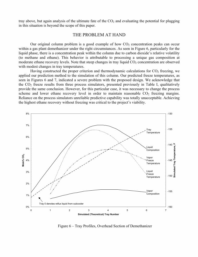
Our original column problem is a good example of how CO2 concentration peaks can occurwithin a gas plant demethanizer under the right circumstances. As seen in Figure 6, particularly for theliquid phase, there is a concentration peak within the column due to carbon dioxide’s relative volatility(to methane and ethane). This behavior is attributable to processing a unique gas composition atmoderate ethane recovery levels. Note that steep changes in tray liquid CO2 concentration are observedwith modest changes in tray temperatures.

Having constructed the proper criterion and thermodynamic calculations for CO2 freezing, weapplied our prediction method to the simulation of this column. Our predicted freeze temperatures, asseen in Figures 6 and 7, indicated a severe problem with the proposed design. We acknowledge thatthe CO2 freeze results from three process simulators, presented previously in Table I, qualitativelyprovide the same conclusion. However, for this particular case, it was necessary to change the processscheme and lower ethane recovery level in order to maintain reasonable CO2 freezing margins.Reliance on the process simulators unreliable predictive capability was totally unacceptable. Achievingthe highest ethane recovery without freezing was critical to the project’s viability.

0%

1%

2%

3%

4%

5%

6%

7%

8%

0 1 2 3 4 5 6 7

Simulated (Theoretical) Tray Number

Mo

le%

CO

2

-160

-155

-150

-145

-140

-135

-130

Sim

ula

ted

Tra

y T

emp

erat

ure

, F

LiquidComposition

VaporComposition

TrayTemperature

Tray 0 denotes reflux liquid from subcooler

VaporFreezeTemperature

LiquidFreezeTemperature

Figure 6 – Tray Profiles, Overhead Section of Demethanizer

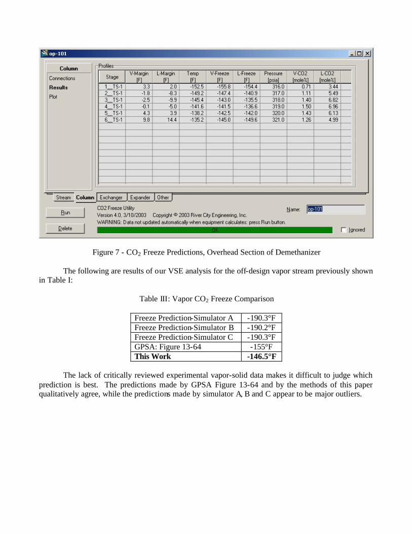
Figure 7 - CO2 Freeze Predictions, Overhead Section of Demethanizer

The following are results of our VSE analysis for the off-design vapor stream previously shown in Table I:

Table III: Vapor CO2 Freeze Comparison

Freeze Prediction-Simulator A -190.3°F Freeze Prediction-Simulator B -190.2°F Freeze Prediction-Simulator C -190.3°F GPSA: Figure 13-64 -155°F This Work -146.5°F

The lack of critically reviewed experimental vapor-solid data makes it difficult to judge which

prediction is best. The predictions made by GPSA Figure 13-64 and by the methods of this paper qualitatively agree, while the predictions made by simulator A, B and C appear to be major outliers.

EXTENDING THE MODEL

To help verify our freezing predictions, we back-checked them against actual data from variousoperating plants. From these operating data, we have built simulation models for several differentplants which have operated very near (or unfortunately at) their known CO2 freezing points. Theseplants operate with widely varying gas richness and have ethane recovery levels in the range of 70-98%. The results of the comparison are shown in Table IV. The predicted freeze temperatures agreequite well with the observed plant freeze temperatures for all four facilities.

Table IV: Comparison of Actual Plant Freezing versus This Work

Plant #

Observed PlantFreeze

Temperature*

Predicted FreezeTemperature(this work)

Absolute∆

LimitingFreezingCriteria

1 -150.2°F -145.7°F 4.5°F LSE2 -142.2°F -141.0°F 1.2°F VSE3 -137.5°F -137.1°F 0.4°F VSE4 -117.0°F -116.2°F 0.8°F LSE

* Simulated values reported

CONCLUSIONS

Unreliable predictions for the temperature of CO2 freezing are being made by several of thecommercial process simulators typically used by gas processors. Our need for dependable predictionsparked the review of existing experimental data, a review of the thermodynamics of solid formation,and the development of the calculation procedures presented in this paper.

Our thermodynamic models are capable of predicting the liquid-solid CO2 freezing point forthe methane-CO2 binary data in GPA RR-10 [2] to within ± 2.6 °F, but the uncertainty increases to ±9.4 °F when considering data from additional sources. The accuracy of our models is far better than theaccuracy of the commercial process simulators tested.

For the column problem presented here, it should be noted that Figure 13-64 of the GPSAEngineering Data Book [1] provides adequate liquid-solid CO2 freezing prediction for the system inquestion. Tray liquid compositions closely approximate a methane-CO2 binary system. Each are almostentirely comprised of methane, a small amount of ethane, and CO2. Of course, this figure is built uponthe underlying binary methane-CO2 freeze data which it represents. Its accuracy for other liquidsystems with higher levels of non-methane and non-CO2 components is expected to diminish.

The vapor-solid CO2 freezing predictions made by GPSA Figure 13-64 and by the methods ofthis paper qualitatively agree. However, the lack of critically reviewed experimental vapor-solid datamakes it difficult to judge which prediction is best. The accuracy of either appears far better than theaccuracy of the commercial process simulators tested.

We have also presented procedures for analyzing CO2 freezing in several common unitoperations. Common pitfalls are avoided by carefully defining the temperature safety margin and bytailoring the thermodynamic calculations to the needs of the specific unit operation. We haveincorporated these procedures into customized add-in extensions for commercial process simulators.

ACKNOWLEDGEMENTS

The authors would like to thank ConocoPhillips, without whom this work would not have beenpossible. We would also like to thank our colleagues at River City Engineering for comments,suggestions, data gathering, and data compilation during the development of this paper. Additionalassistance was provided by Dan Hubbard of HPT, Inc. and Julie Howat of the University of Kansas(Kurata Thermodynamics Laboratory).

REFERENCES CITED

1. Engineering Data Book, Eleventh Edition, Gas Processors Suppliers Association, Tulsa, 1998.

2. Kurata, F., “Solubility of Solid Carbon Dioxide in Pure Light Hydrocarbons and Mixtures of LightHydrocarbons”, Research Report RR-10, Gas Processors Association, Tulsa, Feb. 1974.

3. Knapp, H., Teller, M., Langhorst, R., Solid-Liquid Equilibrium Data Collection: Binary Systems,Chemistry Data Series Vol. VIII, Part I, DECHEMA, 1987.

4. Davis, J.A., Rodewald, N., Kurata, F., “Solid-Liquid-Vapor Phase Behavior of the Methane-CarbonDioxide System”, AIChE J., Vol. 8, No. 4, p.537-539, 1962.

5. Brewer, J., Kurata, F., “Freezing Points of Binary Mixtures of Methane”, AIChE J., Vol. 4, No. 3, p.317-318, 1958.

6. Donnelly, H.G., Katz, D.L., "Phase Equilibria in the Carbon Dioxide-Methane System", ResearchConference, Phase Behavior of the Hydrocarbons, University of Michigan, July 1&2, 1953.

7. Donnelly, H.G., Katz, D. L., “Phase Equilibria in the Carbon Dioxide-Methane System”, Ind. Eng.Chem., Vol. 46, No. 3, p. 511-517, 1954.

8. Cheung, H., Zander, E.H., “Solubility of Carbon Dioxide and Hydrogen Sulfide in LiquidHydrocarbons at Cryogenic Temperatures”, Chem. Eng. Progr. Symp. Ser., Vol. 64, p. 34-43, 1968.

9. Mraw, S.C., Hwang, S.C.., Kobayashi, R., "Vapor-Liquid Equilibrium of the CH4-CO2 System atLow Temperatures", Jour. Chem. Eng. Data, Vol. 23, No. 2, p. 135-139, 1978.

10. Sterner, C.J., “Phase Equilibria in CO2-Methane Systems”, Adv. Cryog. Eng., Vol. 6, p. 467-474,1961.

11. Jensen, R.H., Kurata, F., “Heterogeneous Phase Behavior of Solid Carbon Dioxide in LightHydrocarbons at Cryogenic Temperatures”, AIChE J., Vol. 17, No. 2, p. 357-364, March, 1971.

12. Clark, A.M., Din, F., “Equilibria Between Solid, Liquid and Gaseous Phases at Low Temperatures:The System Carbon Dioxide+Ethane+Ethylene”, Disc. Faraday Society, Vol. 15, p. 202-207, 1953.

13. Im, U.K., Kurata, F., “Solubility of Carbon Dioxide in Mixed Paraffinic Hydrocarbon Solvents atCryogenic Temperatures”, Jour. Chem. Eng. Data, Vol. 17, No. 1, p. 68-71, 1972.

14. Pikaar, M.J., “A Study of Phase Equilibria in Hydrocarbon-CO2 System”, Ph.D. Thesis, Universityof London, London, England, October, 1959.

15. Din, F., Thermodynamic Functions of Gases, Vol. 1, Butterworths, London, 1962.

16. Im, U.K., “Solubility of Solid Carbon Dioxide in Certain Paraffinic Hydrocarbons: Binary, Ternaryand Quaternary Systems”, Ph.D. Thesis, University of Kansas, May, 1970.

17. Renon, H., Prausnitz, J.M., AIChE J. Vol. 14, No. 1, p. 135-144, January, 1968.

18. Peng, D.Y., Robinson, D.B., “A New Two-Constant Equation of State”, Ind. Eng. Chem. Fund.,Vol. 15, No. 1, 1976.

19. Peng, D.Y., Robinson, D.B., “Calculation of Three-Phase Solid-Liquid-Vapor Equilibrium Usingan Equation of State”, p. 185-195, in Chao, K.C., Robinson, R.L., (editors), “Equations of State inEngineering and Research”, Advances in Chemistry Series 182, American Chemical Society,Washington, DC., 1979

20. Zhi, Y., Lee, H., “Fallibility of Analytical Roots of Cubic Equations of State in Low TemperatureRegion”, Fluid Phase Equilibria, Vol. 201, p. 287-294, 2002.

21. Press, W.H., Vetterling, W.T., Teukolsky, S.A., Flannery, B.P., Numerical Recipes in FORTRAN77: The Art of Scientific Computing, 2nd Ed., Vol. 1, Cambridge University Press, 1992.

22. Poling, B.E., Grens II, E.A., Prausnitz, J.M., “Thermodynamic Properties from a Cubic Equation ofState: Avoiding Trivial Roots and Spurious Derivatives”, Ind. Eng. Chem. Proc. Des. Dev., Vol. 20, p.127-130, 1981.