Embed Size (px)
Citation preview

IMPORTANT NOTICE
For Users of TSUPREM-4 Version 6.6
Enhancements to the TSUPREM-4 version 6.6 program with respect to ver-sion 6.5 are noted in Appendix C. To make efficient use of the program, readAppendix C before using version 6.6, as there were extensive changes insome modules.


this, or faxitional
____
r.
Reader Comments: TSUPREM-4 Version 6.6 User’s Manual
Avant!TCAD welcomes your comments and suggestions concerning this manual. Please mailform (Attn.: Technical Publications Department) to the address on the reverse side of this sheeta copy to (510) 413-7766, or e-mail your comments to [email protected]. Attach addpages if needed
What model of computer are you using?________________Operating system?____________
Did you find any errors in this manual? If so, please list the page number and describe the erro
Have you encountered program features that need to be better described in this manual?
What additional information should be included?
How can we improve this document?
Other comments and suggestions:

_______________________________Fold here and tape_________________________________________
To:Avant! CorporationTCAD Business Unit, Technical Publications46871 Bayside ParkwayFremont, CA 94538USA
______________________________Fold here and tape________________________________
From:(Optional Information)
Name, Position: ..........................................................................................
Company....................................................................................................
Address: .....................................................................................................
.....................................................................................................
......................................................................................................Phone, fax, or e-mail ..................................................................................

Avant! Corporation, TCAD Business Unit Fremont, California
TSUPREM-4
Two-Dimensional ProcessSimulation Program
Version 6.6
User’s Manual
June 1998
Copyright Notice TSUPREM-4 User’s Manual
ii Confidential and Proprietary S4 6.6
TSUPREM-4™ User’s Manual, Release 6.6 First Printing: June 1998Copyright 1998 Avant! Corporation and Avant! subsidiary. All rights reserved.Unpublished—rights reserved under the copyright laws of the United States.
Avant! softwareTSUPREM-4™ v6.6 Copyright 1998 Avant! Corporation and Avant! subsidiary.All rights reserved.Unpublished—rights reserved under the copyright laws of the United States.
Use of copyright notices is precautionary and does not imply publication or disclosure. Use, duplication,or disclosure by the Government is subject to restrictions as set forth in subparagraph (c) (1) (ii) of theRights in Technical Data and Computer Software clause at DFARS 252.227-7013
DisclaimerAVANT! CORPORATION RESERVES THE RIGHT TO MAKE CHANGES WITHOUT FURTHERNOTICE TO ANY PRODUCTS DESCRIBED HEREIN. AVANT! CORPORATION MAKES NOWARRANTY, REPRESENTATION, OR GUARANTEE REGARDING THE SUITABILITY OF ITSPRODUCTS FOR ANY PARTICULAR PURPOSE, NOR DOES AVANT! CORPORATIONASSUME ANY LIABILITY ARISING OUT OF THE APPLICATION OR USE OF ANY PRODUCT,AND SPECIFICALLY DISCLAIMS ANY AND ALL LIABILITY, INCLUDING WITHOUTLIMITATION, CONSEQUENTIAL OR INCIDENTAL DAMAGES.
Proprietary Rights NoticeThis document contains information of a proprietary nature. No part of this manual may be copied ordistributed without the prior written consent of Avant! corporation. This document and the softwaredescribed herein is only provided under a written license agreement or a type of written non-disclosureagreement with Avant! corporation or its subsidiaries. ALL INFORMATION CONTAINED HEREINSHALL BE KEPT IN CONFIDENCE AND USED STRICTLY IN ACCORDANCE WITH THETERMS OF THE WRITTEN NON-DISCLOSURE AGREEMENT OR WRITTEN LICENSEAGREEMENT WITH AVANT! CORPORATION OR ITS SUBSIDIARIES.
Trademark/Service-Mark NoticeADM, Apollo, ApolloGA, Aquarius, AquariusBV, AquariusDP, AquariusGA, AquariusXO, ArcCell,ArcChip, ArcUtil, ATEM, Aurora, Avan Testchip, AvanWaves, Baseline, Baseline Software Acceler-ator, Cyclelink, Davinci, Depict, Device Model Builder, DFM WorkBench, DriveLine, DynamicModel Switcher, EVaccess, Explorer, Hercules, HSPICE, HSPICE-Link, Liquid, LTL, Mars-Rail,Master Toolbox, Medici, Milkyway, Planet, PlanetPL, PlanetRTL, Polaris, Polaris-CBS, Polaris-MT,ProGen, Prospector, Proteus, PureSpeed, Raphael, Raphael NES, SimLine, Sirius, Smart Extraction,Solar, SolarII, Star-DC, Star-Hspice, Star-HspiceLink, Star-Hspice-XO, Star-MTB, Star-Power, Star-RC, Star-Sim, Star-Time, VeriCheck, VeriView, Taurus, Tech Composer, Terrain, TMA Layout,TMA SUPREM-3, TSUPREM-4, TMA Visual, TMA WorkBench, YChips, YCrunch, and YTime aretrademarks of Avant! Corporation and its subsidiaries. Avant! Corporation, Avant! logo, and Avan-Labs are trademarks and service-marks of Avant! Corporation. All other trademarks are the property oftheir respective owners.
TSUPREM-4 incorporates Galaxy Run Time Components, which are copyright © 1993-1998, VisixSoftware Inc. All rights reserved.
SubsidiariesAnagram, Inc., ArcSys, Inc., Frontline Design Automation, Inc., Galax!, ISS, Inc., Meta-Software, Inc.,NexSyn, Inc., and Technology Modeling Associates, Inc. are subsidiaries of Avant! Corporation.
Contacting Avant! Corporation :
Telephone: (510) 413-8000(800) 369-0080
FAX: (510) 413-7766e-mail [email protected]: http://www.avanticorp.com/
Avant! CorporationTCAD Business Unit46871 Bayside ParkwayFremont, CA 94538
Table of Contents
CONTENTS
xxixxxix
xxix. xxx. xxxxxxixxxixxxixxxi
. 1-1. 1-1-1
. 1-21-21-2
. 1-3
. 1-3. 1-3. 1-3
1-3. 1-4. 1-4. 1-4
List of Figures xxiii
Introduction to TSUPREM-4 xxix
Program Overview . . . . . . . . . . . . . . . . . . . . . . . . . . . . . . . . . . . . . . . .Processing Steps. . . . . . . . . . . . . . . . . . . . . . . . . . . . . . . . . . . . . . . .Simulation Structure . . . . . . . . . . . . . . . . . . . . . . . . . . . . . . . . . . . .Additional Features . . . . . . . . . . . . . . . . . . . . . . . . . . . . . . . . . . . . .
Manual Overview . . . . . . . . . . . . . . . . . . . . . . . . . . . . . . . . . . . . . . . . . Typeface Conventions . . . . . . . . . . . . . . . . . . . . . . . . . . . . . . . . . . . . .Related Publications . . . . . . . . . . . . . . . . . . . . . . . . . . . . . . . . . . . . . . .
Reference Materials . . . . . . . . . . . . . . . . . . . . . . . . . . . . . . . . . . . . .Problems and Troubleshooting . . . . . . . . . . . . . . . . . . . . . . . . . . . . . . .
Chapter 1 Using TSUPREM-4 1-1
Introduction. . . . . . . . . . . . . . . . . . . . . . . . . . . . . . . . . . . . . . . . . . . . . . Program Execution and Output. . . . . . . . . . . . . . . . . . . . . . . . . . . . . . .
StartingTSUPREM-4 . . . . . . . . . . . . . . . . . . . . . . . . . . . . . . . . . . . . 1Program Output . . . . . . . . . . . . . . . . . . . . . . . . . . . . . . . . . . . . . . . .
Printed Output . . . . . . . . . . . . . . . . . . . . . . . . . . . . . . . . . . . . . . . .Graphical Output . . . . . . . . . . . . . . . . . . . . . . . . . . . . . . . . . . . . . .
Errors, Warnings, and Syntax . . . . . . . . . . . . . . . . . . . . . . . . . . . . . File Specification . . . . . . . . . . . . . . . . . . . . . . . . . . . . . . . . . . . . . . . . .
File Types. . . . . . . . . . . . . . . . . . . . . . . . . . . . . . . . . . . . . . . . . . . . . Default File Names . . . . . . . . . . . . . . . . . . . . . . . . . . . . . . . . . . . . . Environment Variables . . . . . . . . . . . . . . . . . . . . . . . . . . . . . . . . . . .
Input Files . . . . . . . . . . . . . . . . . . . . . . . . . . . . . . . . . . . . . . . . . . . . . . . Command Input Files. . . . . . . . . . . . . . . . . . . . . . . . . . . . . . . . . . . . Mask Data Files . . . . . . . . . . . . . . . . . . . . . . . . . . . . . . . . . . . . . . . .
S4 6.6 Confidential and Proprietary iii

Table of Contents TSUPREM-4 User’s Guide
1-5. 1-5. 1-51-51-6
-66-6. 1-61-61-7-71-71-7. 1-7. 1-7
1-81-8
. 1-8-9-99-910
. 2-1
. 2-1. 2-12-2
. 2-2
. 2-2
. 2-22-3
2-32-3
. 2-32-42-5-5-5-5
2-6-6
Profile Files . . . . . . . . . . . . . . . . . . . . . . . . . . . . . . . . . . . . . . . . . . . .Other Input Files . . . . . . . . . . . . . . . . . . . . . . . . . . . . . . . . . . . . . . .
Output Files. . . . . . . . . . . . . . . . . . . . . . . . . . . . . . . . . . . . . . . . . . . . . . Terminal Output . . . . . . . . . . . . . . . . . . . . . . . . . . . . . . . . . . . . . . . . .Output Listing Files . . . . . . . . . . . . . . . . . . . . . . . . . . . . . . . . . . . . . .
Standard Output File—s4out . . . . . . . . . . . . . . . . . . . . . . . . . . . . . 1Informational Output File—s4inf. . . . . . . . . . . . . . . . . . . . . . . . . . 1-Diagnostic Output File—s4dia. . . . . . . . . . . . . . . . . . . . . . . . . . . . 1
Saved Structure Files . . . . . . . . . . . . . . . . . . . . . . . . . . . . . . . . . . . . TSUPREM-4 . . . . . . . . . . . . . . . . . . . . . . . . . . . . . . . . . . . . . . . . .TIF . . . . . . . . . . . . . . . . . . . . . . . . . . . . . . . . . . . . . . . . . . . . . . . . .Depict andDonatello . . . . . . . . . . . . . . . . . . . . . . . . . . . . . . . . . . 1Medici. . . . . . . . . . . . . . . . . . . . . . . . . . . . . . . . . . . . . . . . . . . . . . .MINIMOS 5 . . . . . . . . . . . . . . . . . . . . . . . . . . . . . . . . . . . . . . . . . .Wave. . . . . . . . . . . . . . . . . . . . . . . . . . . . . . . . . . . . . . . . . . . . . . .
Graphical Output . . . . . . . . . . . . . . . . . . . . . . . . . . . . . . . . . . . . . . . Extract Output Files . . . . . . . . . . . . . . . . . . . . . . . . . . . . . . . . . . . . . .Electrical Data Output Files. . . . . . . . . . . . . . . . . . . . . . . . . . . . . . . .
Library Files . . . . . . . . . . . . . . . . . . . . . . . . . . . . . . . . . . . . . . . . . . . . . Initialization Input File—s4init . . . . . . . . . . . . . . . . . . . . . . . . . . . . . 1Ion Implant Data File—s4imp0 . . . . . . . . . . . . . . . . . . . . . . . . . . . . . 1Plot Device Definition File—s4pcap. . . . . . . . . . . . . . . . . . . . . . . . . 1-Key Files—s4fky0 ands4uky0. . . . . . . . . . . . . . . . . . . . . . . . . . . . . . 1Authorization File—s4auth . . . . . . . . . . . . . . . . . . . . . . . . . . . . . . . 1-
Chapter 2 TSUPREM-4 Models 2-1
Introduction. . . . . . . . . . . . . . . . . . . . . . . . . . . . . . . . . . . . . . . . . . . . . . Simulation Structure . . . . . . . . . . . . . . . . . . . . . . . . . . . . . . . . . . . . . . .
Coordinates . . . . . . . . . . . . . . . . . . . . . . . . . . . . . . . . . . . . . . . . . . . Initial Structure . . . . . . . . . . . . . . . . . . . . . . . . . . . . . . . . . . . . . . . . .Regions and Materials . . . . . . . . . . . . . . . . . . . . . . . . . . . . . . . . . . .
Grid Structure . . . . . . . . . . . . . . . . . . . . . . . . . . . . . . . . . . . . . . . . . . . . Mesh, Triangular Elements, and Nodes . . . . . . . . . . . . . . . . . . . . . . Defining Grid Structure . . . . . . . . . . . . . . . . . . . . . . . . . . . . . . . . . . .Explicit Specification of Grid Structure. . . . . . . . . . . . . . . . . . . . . . .
TheLINE Statement . . . . . . . . . . . . . . . . . . . . . . . . . . . . . . . . . . .Generated Grid Lines . . . . . . . . . . . . . . . . . . . . . . . . . . . . . . . . . . Eliminating Grid Lines . . . . . . . . . . . . . . . . . . . . . . . . . . . . . . . . . .
Automatic Grid Generation . . . . . . . . . . . . . . . . . . . . . . . . . . . . . . . .Automatic Grid Generation in the X Direction . . . . . . . . . . . . . . . 2
X Grid fromWIDTH Parameter . . . . . . . . . . . . . . . . . . . . . . . . . 2X Grid fromMASK Statement. . . . . . . . . . . . . . . . . . . . . . . . . . . 2Column Elimination . . . . . . . . . . . . . . . . . . . . . . . . . . . . . . . . . .
Automatic Grid Generation in the Y Direction . . . . . . . . . . . . . . . 2
iv Confidential and Proprietary S4 6.6

TSUPREM-4 User’s Guide Table of Contents
. 2-7-7. 2-7-82-82-8-82-92-92-9-10-10-102-12-122-122-122-13-13-14
2-142-14-14
2-14-15-15-16-16-17-182-192-19-199
2-212-21-23-23-23-24-24
2-242-24-25-25
-25-25
Changes to the Mesh During Processing . . . . . . . . . . . . . . . . . . . . .DEPOSITION andEPITAXY . . . . . . . . . . . . . . . . . . . . . . . . . . . . 2Structure Extension . . . . . . . . . . . . . . . . . . . . . . . . . . . . . . . . . . . ETCH andDEVELOP . . . . . . . . . . . . . . . . . . . . . . . . . . . . . . . . . . . 2Oxidation and Silicidation . . . . . . . . . . . . . . . . . . . . . . . . . . . . . . .
Removal of Nodes in Consumed Silicon . . . . . . . . . . . . . . . . . .Addition of Nodes in Growing Oxide. . . . . . . . . . . . . . . . . . . . . 2Nodes in Regions Where Oxide is Deforming . . . . . . . . . . . . . .Numerical Integrity. . . . . . . . . . . . . . . . . . . . . . . . . . . . . . . . . . .
Adaptive Gridding . . . . . . . . . . . . . . . . . . . . . . . . . . . . . . . . . . . . . . .Enabling and Disabling . . . . . . . . . . . . . . . . . . . . . . . . . . . . . . . . 2
One-Dimensional Simulation of Simple Structures. . . . . . . . . . . . . 2Initial Impurity Concentration . . . . . . . . . . . . . . . . . . . . . . . . . . . . . 2
Diffusion . . . . . . . . . . . . . . . . . . . . . . . . . . . . . . . . . . . . . . . . . . . . . . . .DIFFUSION Statement . . . . . . . . . . . . . . . . . . . . . . . . . . . . . . . . . . 2
Temperature . . . . . . . . . . . . . . . . . . . . . . . . . . . . . . . . . . . . . . . . .Ambient Gas Pressure . . . . . . . . . . . . . . . . . . . . . . . . . . . . . . . . .Ambient Gas Characteristics . . . . . . . . . . . . . . . . . . . . . . . . . . . .Ambients and Oxidation of Materials . . . . . . . . . . . . . . . . . . . . . 2Default Ambients . . . . . . . . . . . . . . . . . . . . . . . . . . . . . . . . . . . . . 2Chlorine . . . . . . . . . . . . . . . . . . . . . . . . . . . . . . . . . . . . . . . . . . . .
Example . . . . . . . . . . . . . . . . . . . . . . . . . . . . . . . . . . . . . . . . . .Coefficient Tables. . . . . . . . . . . . . . . . . . . . . . . . . . . . . . . . . . . 2
Chemical Predeposition . . . . . . . . . . . . . . . . . . . . . . . . . . . . . . . .Solution of Diffusion Equations. . . . . . . . . . . . . . . . . . . . . . . . . . 2
Diffusion of Impurities. . . . . . . . . . . . . . . . . . . . . . . . . . . . . . . . . . . 2Impurity Fluxes . . . . . . . . . . . . . . . . . . . . . . . . . . . . . . . . . . . . . . 2Mobile Impurities and Ion Pairing . . . . . . . . . . . . . . . . . . . . . . . . 2Electric Field . . . . . . . . . . . . . . . . . . . . . . . . . . . . . . . . . . . . . . . . 2Diffusivities . . . . . . . . . . . . . . . . . . . . . . . . . . . . . . . . . . . . . . . . . 2Polysilicon Enhancement . . . . . . . . . . . . . . . . . . . . . . . . . . . . . . .Point Defect Enhancement . . . . . . . . . . . . . . . . . . . . . . . . . . . . . .PD.FERMI Model . . . . . . . . . . . . . . . . . . . . . . . . . . . . . . . . . . . . 2PD.TRANS andPD.FULL Models . . . . . . . . . . . . . . . . . . . . . . . 2-1Paired Fractions of Dopant Atoms . . . . . . . . . . . . . . . . . . . . . . . .Reaction Rate Constants. . . . . . . . . . . . . . . . . . . . . . . . . . . . . . . .
Activation of Impurities . . . . . . . . . . . . . . . . . . . . . . . . . . . . . . . . . . 2Solid Solubility Model . . . . . . . . . . . . . . . . . . . . . . . . . . . . . . . . . 2
Solid Solubility Tables . . . . . . . . . . . . . . . . . . . . . . . . . . . . . . . 2Clustering Model . . . . . . . . . . . . . . . . . . . . . . . . . . . . . . . . . . . . . 2Combining the Models . . . . . . . . . . . . . . . . . . . . . . . . . . . . . . . . . 2
Segregation of Impurities. . . . . . . . . . . . . . . . . . . . . . . . . . . . . . . . .Segregation Flux. . . . . . . . . . . . . . . . . . . . . . . . . . . . . . . . . . . . . .
Transport Coefficient . . . . . . . . . . . . . . . . . . . . . . . . . . . . . . . . 2Segregation Coefficient . . . . . . . . . . . . . . . . . . . . . . . . . . . . . . 2Moving-Boundary Flux . . . . . . . . . . . . . . . . . . . . . . . . . . . . . . 2Interface Trap Model . . . . . . . . . . . . . . . . . . . . . . . . . . . . . . . . 2
S4 6.6 Confidential and Proprietary v

Table of Contents TSUPREM-4 User’s Guide
2-28-28-282-29-29
-30-30-31-32-32-32-33-33-342-34-352-35-36-362-372-38
2-392-39-39
-412-41-41
2-422-422-432-44-442-4452-45-45-45-46-462-46-47
2-472-482-492-49492-50
Using the Interface Trap Model . . . . . . . . . . . . . . . . . . . . . . . . . . . .Diffusion of Point Defects . . . . . . . . . . . . . . . . . . . . . . . . . . . . . . . . 2
Equilibrium Concentrations . . . . . . . . . . . . . . . . . . . . . . . . . . . . . 2Charge State Fractions . . . . . . . . . . . . . . . . . . . . . . . . . . . . . . . . .Point Defect Diffusion Equations. . . . . . . . . . . . . . . . . . . . . . . . . 2Interstitial and Vacancy Diffusivities. . . . . . . . . . . . . . . . . . . . . . 2Reaction of Pairs with Point Defects . . . . . . . . . . . . . . . . . . . . . . 2Net Recombination Rate of Interstitials . . . . . . . . . . . . . . . . . . . . 2Absorption by Traps, Clusters, and Dislocation Loops . . . . . . . . 2
Injection and Recombination of Point Defects at Interfaces . . . . . . 2Surface Recombination Velocity Models. . . . . . . . . . . . . . . . . . . 2
V.MAXOX Model . . . . . . . . . . . . . . . . . . . . . . . . . . . . . . . . . . . 2V.INITOX Model . . . . . . . . . . . . . . . . . . . . . . . . . . . . . . . . . . 2V.NORM Model . . . . . . . . . . . . . . . . . . . . . . . . . . . . . . . . . . . . 2
Injection Rate . . . . . . . . . . . . . . . . . . . . . . . . . . . . . . . . . . . . . . . .Moving-Boundary Flux . . . . . . . . . . . . . . . . . . . . . . . . . . . . . . . . 2
Interstitial Traps . . . . . . . . . . . . . . . . . . . . . . . . . . . . . . . . . . . . . . . .Enabling, Disabling, and Initialization. . . . . . . . . . . . . . . . . . . . . 2
Interstitial Clustering Model . . . . . . . . . . . . . . . . . . . . . . . . . . . . . . 2Model Equations. . . . . . . . . . . . . . . . . . . . . . . . . . . . . . . . . . . . . .Choosing Model Parameters. . . . . . . . . . . . . . . . . . . . . . . . . . . . .Using the Model . . . . . . . . . . . . . . . . . . . . . . . . . . . . . . . . . . . . . .
Oxidation. . . . . . . . . . . . . . . . . . . . . . . . . . . . . . . . . . . . . . . . . . . . . . . .Theory of Oxidation. . . . . . . . . . . . . . . . . . . . . . . . . . . . . . . . . . . . . 2Analytical Oxidation Models . . . . . . . . . . . . . . . . . . . . . . . . . . . . . . 2
Overview . . . . . . . . . . . . . . . . . . . . . . . . . . . . . . . . . . . . . . . . . . .Oxide Growth Rate . . . . . . . . . . . . . . . . . . . . . . . . . . . . . . . . . . 2Thin Regime . . . . . . . . . . . . . . . . . . . . . . . . . . . . . . . . . . . . . . .Linear Rate . . . . . . . . . . . . . . . . . . . . . . . . . . . . . . . . . . . . . . . .Parabolic Rate . . . . . . . . . . . . . . . . . . . . . . . . . . . . . . . . . . . . . .
Usage . . . . . . . . . . . . . . . . . . . . . . . . . . . . . . . . . . . . . . . . . . . . . .TheERFC Model . . . . . . . . . . . . . . . . . . . . . . . . . . . . . . . . . . . . . 2
Recommended Usage . . . . . . . . . . . . . . . . . . . . . . . . . . . . . . . .TheERF1, ERF2, andERFG Models . . . . . . . . . . . . . . . . . . . . . 2-4
Parameters. . . . . . . . . . . . . . . . . . . . . . . . . . . . . . . . . . . . . . . . .Initial Structure . . . . . . . . . . . . . . . . . . . . . . . . . . . . . . . . . . . . . 2ERF1 Model . . . . . . . . . . . . . . . . . . . . . . . . . . . . . . . . . . . . . . . 2ERF2 Model . . . . . . . . . . . . . . . . . . . . . . . . . . . . . . . . . . . . . . . 2ERFG Model . . . . . . . . . . . . . . . . . . . . . . . . . . . . . . . . . . . . . . . 2Recommended Usage . . . . . . . . . . . . . . . . . . . . . . . . . . . . . . . .
Numerical Oxidation Models. . . . . . . . . . . . . . . . . . . . . . . . . . . . . . 2Oxide Growth Rate. . . . . . . . . . . . . . . . . . . . . . . . . . . . . . . . . . . .
Concentration Dependence . . . . . . . . . . . . . . . . . . . . . . . . . . . .Thin Regime . . . . . . . . . . . . . . . . . . . . . . . . . . . . . . . . . . . . . . .Usage. . . . . . . . . . . . . . . . . . . . . . . . . . . . . . . . . . . . . . . . . . . . .
TheVERTICAL Model . . . . . . . . . . . . . . . . . . . . . . . . . . . . . . . . 2-Recommended Usage . . . . . . . . . . . . . . . . . . . . . . . . . . . . . . . .
vi Confidential and Proprietary S4 6.6

TSUPREM-4 User’s Guide Table of Contents
-50-50-512-51-51-51-512-522-53
-53-542-552-56-562-562-57-5757-5757-58-58
2-582-582-592-592-59
2-61-61
2-612-61
2-612-622-62-622-622-63-63-644
2-652-65-66-66-67
2-692-69
COMPRESS Model . . . . . . . . . . . . . . . . . . . . . . . . . . . . . . . . . . . . 2Compressible Viscous Flow . . . . . . . . . . . . . . . . . . . . . . . . . . . 2Boundary Conditions . . . . . . . . . . . . . . . . . . . . . . . . . . . . . . . . 2Model Parameters . . . . . . . . . . . . . . . . . . . . . . . . . . . . . . . . . . .COMPRESS Model: Recommended Usage. . . . . . . . . . . . . . . . 2
VISCOUS Model . . . . . . . . . . . . . . . . . . . . . . . . . . . . . . . . . . . . . 2Incompressible Viscous Flow. . . . . . . . . . . . . . . . . . . . . . . . . . 2Stress Dependence . . . . . . . . . . . . . . . . . . . . . . . . . . . . . . . . . .Recommended Usage . . . . . . . . . . . . . . . . . . . . . . . . . . . . . . . .
VISCOELA Model . . . . . . . . . . . . . . . . . . . . . . . . . . . . . . . . . . . . 2Viscoelastic Flow . . . . . . . . . . . . . . . . . . . . . . . . . . . . . . . . . . . 2Model Parameters . . . . . . . . . . . . . . . . . . . . . . . . . . . . . . . . . . .Recommended Usage . . . . . . . . . . . . . . . . . . . . . . . . . . . . . . . .
Polysilicon Oxidation. . . . . . . . . . . . . . . . . . . . . . . . . . . . . . . . . . . . 2Surface Tension and Reflow . . . . . . . . . . . . . . . . . . . . . . . . . . . . . .
Silicide Models . . . . . . . . . . . . . . . . . . . . . . . . . . . . . . . . . . . . . . . . . .TiSi2 Growth Kinetics . . . . . . . . . . . . . . . . . . . . . . . . . . . . . . . . . . . 2
Reaction at TiSi2/Si Interface . . . . . . . . . . . . . . . . . . . . . . . . . . . . 2-Diffusion of Silicon . . . . . . . . . . . . . . . . . . . . . . . . . . . . . . . . . . . 2Reaction at TiSi2/Si Interface . . . . . . . . . . . . . . . . . . . . . . . . . . . . 2-Initialization . . . . . . . . . . . . . . . . . . . . . . . . . . . . . . . . . . . . . . . . . 2Material Flow . . . . . . . . . . . . . . . . . . . . . . . . . . . . . . . . . . . . . . . . 2
Impurities and Point Defects . . . . . . . . . . . . . . . . . . . . . . . . . . . . . .Specifying Silicide Models and Parameters. . . . . . . . . . . . . . . . . . .
Materials . . . . . . . . . . . . . . . . . . . . . . . . . . . . . . . . . . . . . . . . . . . .Impurities . . . . . . . . . . . . . . . . . . . . . . . . . . . . . . . . . . . . . . . . . . .Reactions . . . . . . . . . . . . . . . . . . . . . . . . . . . . . . . . . . . . . . . . . . .Impurities . . . . . . . . . . . . . . . . . . . . . . . . . . . . . . . . . . . . . . . . . . .
Tungsten Silicide Model . . . . . . . . . . . . . . . . . . . . . . . . . . . . . . . . . 2Other Silicides . . . . . . . . . . . . . . . . . . . . . . . . . . . . . . . . . . . . . . . . .
Stress Models . . . . . . . . . . . . . . . . . . . . . . . . . . . . . . . . . . . . . . . . . . . .Stress History Model . . . . . . . . . . . . . . . . . . . . . . . . . . . . . . . . . . . .Thermal Stress Model Equations . . . . . . . . . . . . . . . . . . . . . . . . . . .
Boundary Conditions . . . . . . . . . . . . . . . . . . . . . . . . . . . . . . . . . .Initial Conditions . . . . . . . . . . . . . . . . . . . . . . . . . . . . . . . . . . . . . 2Intrinsic Stress in Deposited Layers . . . . . . . . . . . . . . . . . . . . . . .Effect of Etching on Stress . . . . . . . . . . . . . . . . . . . . . . . . . . . . . .Using the Stress History Model . . . . . . . . . . . . . . . . . . . . . . . . . . 2Limitations . . . . . . . . . . . . . . . . . . . . . . . . . . . . . . . . . . . . . . . . . . 2
Modeling Stress with theSTRESS Statement . . . . . . . . . . . . . . . . . 2-6Boundary Conditions . . . . . . . . . . . . . . . . . . . . . . . . . . . . . . . . . .
Ion Implantation . . . . . . . . . . . . . . . . . . . . . . . . . . . . . . . . . . . . . . . . . .Analytic Ion Implant Models . . . . . . . . . . . . . . . . . . . . . . . . . . . . . . 2
Implanted Impurity Distributions . . . . . . . . . . . . . . . . . . . . . . . . . 2Implant Moment Tables . . . . . . . . . . . . . . . . . . . . . . . . . . . . . . . . 2Gaussian Distribution . . . . . . . . . . . . . . . . . . . . . . . . . . . . . . . . . .Pearson Distribution . . . . . . . . . . . . . . . . . . . . . . . . . . . . . . . . . . .
S4 6.6 Confidential and Proprietary vii

Table of Contents TSUPREM-4 User’s Guide
-702-70-72-72-72
2-72-73-73-73-742-74-74-75
2-752-762-76-77-77-78
2-79-80-81-81-81-812-822-832-832-842-84-85-852-852-852-86-87-872-882-89-89-892-892-89-902-902-902-91
Dual Pearson Distribution . . . . . . . . . . . . . . . . . . . . . . . . . . . . . . 2Dose-dependent Implant Profiles . . . . . . . . . . . . . . . . . . . . . . . . .Tilt and Rotation Tables . . . . . . . . . . . . . . . . . . . . . . . . . . . . . . . . 2Multilayer Implants . . . . . . . . . . . . . . . . . . . . . . . . . . . . . . . . . . . 2
Effective Range Model . . . . . . . . . . . . . . . . . . . . . . . . . . . . . . . 2Dose Matching . . . . . . . . . . . . . . . . . . . . . . . . . . . . . . . . . . . . .
Lateral Distribution . . . . . . . . . . . . . . . . . . . . . . . . . . . . . . . . . . . 2Wafer Tilt and Rotation . . . . . . . . . . . . . . . . . . . . . . . . . . . . . . . . 2Analytic Damage Model. . . . . . . . . . . . . . . . . . . . . . . . . . . . . . . . 2
Damage Distribution Calculations . . . . . . . . . . . . . . . . . . . . . . 2Recommended Usage and Limitations . . . . . . . . . . . . . . . . . . .
Monte Carlo Ion Implant Model . . . . . . . . . . . . . . . . . . . . . . . . . . . 2Binary Scattering Theory . . . . . . . . . . . . . . . . . . . . . . . . . . . . . . . 2
Energy Loss . . . . . . . . . . . . . . . . . . . . . . . . . . . . . . . . . . . . . . .Scattering Angle . . . . . . . . . . . . . . . . . . . . . . . . . . . . . . . . . . . .Dimensionless Form . . . . . . . . . . . . . . . . . . . . . . . . . . . . . . . . .Coulomb Potential . . . . . . . . . . . . . . . . . . . . . . . . . . . . . . . . . . 2Universal Potential . . . . . . . . . . . . . . . . . . . . . . . . . . . . . . . . . . 2
Amorphous Implant Calculation . . . . . . . . . . . . . . . . . . . . . . . . . 2Nuclear Stopping . . . . . . . . . . . . . . . . . . . . . . . . . . . . . . . . . . .Electronic Stopping. . . . . . . . . . . . . . . . . . . . . . . . . . . . . . . . . . 2Electronic Stopping at High Energies. . . . . . . . . . . . . . . . . . . . 2Total Energy Loss and Ion Deflection . . . . . . . . . . . . . . . . . . . 2Ion Beam Width . . . . . . . . . . . . . . . . . . . . . . . . . . . . . . . . . . . . 2
Crystalline Implant Model . . . . . . . . . . . . . . . . . . . . . . . . . . . . . . 2Channeling . . . . . . . . . . . . . . . . . . . . . . . . . . . . . . . . . . . . . . . .Lattice Temperature . . . . . . . . . . . . . . . . . . . . . . . . . . . . . . . . .Lattice Damage . . . . . . . . . . . . . . . . . . . . . . . . . . . . . . . . . . . . .
Damage Dechanneling . . . . . . . . . . . . . . . . . . . . . . . . . . . . . . . . .Damage Annealing . . . . . . . . . . . . . . . . . . . . . . . . . . . . . . . . . .Number of Ions . . . . . . . . . . . . . . . . . . . . . . . . . . . . . . . . . . . . . 2BF2 Implantation. . . . . . . . . . . . . . . . . . . . . . . . . . . . . . . . . . . . 2
Implant Damage Model . . . . . . . . . . . . . . . . . . . . . . . . . . . . . . . . . .Net Damage Calculation. . . . . . . . . . . . . . . . . . . . . . . . . . . . . . . .
Frenkel Pair Component . . . . . . . . . . . . . . . . . . . . . . . . . . . . . .Using the Implant Damage Model . . . . . . . . . . . . . . . . . . . . . . . . 2
Boundary Conditions for Ion Implantation . . . . . . . . . . . . . . . . . . . 2Epitaxial Growth. . . . . . . . . . . . . . . . . . . . . . . . . . . . . . . . . . . . . . . . . .
Layer Thickness . . . . . . . . . . . . . . . . . . . . . . . . . . . . . . . . . . . . . . . .Incorporation of Impurities . . . . . . . . . . . . . . . . . . . . . . . . . . . . . . . 2Diffusion of Impurities. . . . . . . . . . . . . . . . . . . . . . . . . . . . . . . . . . . 2
Deposition. . . . . . . . . . . . . . . . . . . . . . . . . . . . . . . . . . . . . . . . . . . . . . .Layer Thickness . . . . . . . . . . . . . . . . . . . . . . . . . . . . . . . . . . . . . . . .Incorporation of Impurities . . . . . . . . . . . . . . . . . . . . . . . . . . . . . . . 2
Photoresist Type . . . . . . . . . . . . . . . . . . . . . . . . . . . . . . . . . . . . . .Masking, Exposure and Development of Photoresist . . . . . . . . . . . . . .Etching . . . . . . . . . . . . . . . . . . . . . . . . . . . . . . . . . . . . . . . . . . . . . . . . .
viii Confidential and Proprietary S4 6.6

TSUPREM-4 User’s Guide Table of Contents
2-91-92
2-922-922-922-932-932-942-95-96-96
-962-97-97-972-982-99-99
-100-100-101-101101-101102103-104-104-104105105-106106-1070708
108-110110111111-1122-113
Defining the Etch Region. . . . . . . . . . . . . . . . . . . . . . . . . . . . . . . . .Removal of Material . . . . . . . . . . . . . . . . . . . . . . . . . . . . . . . . . . . . 2The Trapezoidal Etch Model . . . . . . . . . . . . . . . . . . . . . . . . . . . . . .
Parameters . . . . . . . . . . . . . . . . . . . . . . . . . . . . . . . . . . . . . . . . . .Etch Steps . . . . . . . . . . . . . . . . . . . . . . . . . . . . . . . . . . . . . . . . . . .Etch Examples . . . . . . . . . . . . . . . . . . . . . . . . . . . . . . . . . . . . . . .
Simple Structure . . . . . . . . . . . . . . . . . . . . . . . . . . . . . . . . . . . .Structure with Overhangs . . . . . . . . . . . . . . . . . . . . . . . . . . . . .Complex Structures. . . . . . . . . . . . . . . . . . . . . . . . . . . . . . . . . .
Modeling Polycrystalline Materials . . . . . . . . . . . . . . . . . . . . . . . . . . . 2Diffusion . . . . . . . . . . . . . . . . . . . . . . . . . . . . . . . . . . . . . . . . . . . . . 2
Diffusion in Grain Interiors . . . . . . . . . . . . . . . . . . . . . . . . . . . . . 2Grain Boundary Structure. . . . . . . . . . . . . . . . . . . . . . . . . . . . . . .Diffusion Along Grain Boundaries . . . . . . . . . . . . . . . . . . . . . . . 2
Anisotropic Diffusion . . . . . . . . . . . . . . . . . . . . . . . . . . . . . . . . 2Segregation Between Grain Interior and Boundaries . . . . . . . . . . .Grain Size Model . . . . . . . . . . . . . . . . . . . . . . . . . . . . . . . . . . . . . . .
Initial Grain Size. . . . . . . . . . . . . . . . . . . . . . . . . . . . . . . . . . . . . . 2Grain Growth . . . . . . . . . . . . . . . . . . . . . . . . . . . . . . . . . . . . . . . 2
Concentration Dependence . . . . . . . . . . . . . . . . . . . . . . . . . . . 2Grain Surface Energy . . . . . . . . . . . . . . . . . . . . . . . . . . . . . . . 2Segregation Drag . . . . . . . . . . . . . . . . . . . . . . . . . . . . . . . . . . 2
Interface Oxide Break-up and Epitaxial Regrowth . . . . . . . . . . . . 2-Oxide Break-Up . . . . . . . . . . . . . . . . . . . . . . . . . . . . . . . . . . . . . 2Epitaxial Regrowth. . . . . . . . . . . . . . . . . . . . . . . . . . . . . . . . . . . 2-
Using the Polycrystalline Model . . . . . . . . . . . . . . . . . . . . . . . . . . 2-Electrical Calculations . . . . . . . . . . . . . . . . . . . . . . . . . . . . . . . . . . . . 2
Automatic Regrid. . . . . . . . . . . . . . . . . . . . . . . . . . . . . . . . . . . . . . 2Poisson’s Equation. . . . . . . . . . . . . . . . . . . . . . . . . . . . . . . . . . . . . 2
Boltzmann and Fermi-Dirac Statistics . . . . . . . . . . . . . . . . . . . . 2-Ionization of Impurities . . . . . . . . . . . . . . . . . . . . . . . . . . . . . . . 2-Solution Methods . . . . . . . . . . . . . . . . . . . . . . . . . . . . . . . . . . . . 2
Carrier Mobility . . . . . . . . . . . . . . . . . . . . . . . . . . . . . . . . . . . . . . . 2-Tabular Form . . . . . . . . . . . . . . . . . . . . . . . . . . . . . . . . . . . . . . . 2Arora Mobility Model . . . . . . . . . . . . . . . . . . . . . . . . . . . . . . . . 2-1Caughey Mobility Model . . . . . . . . . . . . . . . . . . . . . . . . . . . . . . 2-1
Quantum Mechanical Model for MOSFET . . . . . . . . . . . . . . . . . . 2-Extended Defects AAM . . . . . . . . . . . . . . . . . . . . . . . . . . . . . . . . . . . 2
Dislocation Loop Model . . . . . . . . . . . . . . . . . . . . . . . . . . . . . . . . 2-Creation of Dislocation Loops . . . . . . . . . . . . . . . . . . . . . . . . . . 2-Effects of Dislocation Loops . . . . . . . . . . . . . . . . . . . . . . . . . . . 2-
Transient Clustering Model . . . . . . . . . . . . . . . . . . . . . . . . . . . . . . 2References. . . . . . . . . . . . . . . . . . . . . . . . . . . . . . . . . . . . . . . . . . . . . .
S4 6.6 Confidential and Proprietary ix

Table of Contents TSUPREM-4 User’s Guide
. 3-1 . 3-2. 3-2. 3-23-2
. . 3-33-3
. 3-3 . 3-4. 3-43-4
. 3-4
. 3-5 . 3-5. 3-53-53-5-73-8
. 3-8. 3-8. 3-83-9
. 3-9. 3-9. 3-9. 3-93-103-10-10-103-11-123-123-123-133-143-143-143-153-153-15-163-16
Chapter 3 Input Statement Descriptions 3-1
Introduction. . . . . . . . . . . . . . . . . . . . . . . . . . . . . . . . . . . . . . . . . . . . . . Input Statements . . . . . . . . . . . . . . . . . . . . . . . . . . . . . . . . . . . . . . . . . .
Format . . . . . . . . . . . . . . . . . . . . . . . . . . . . . . . . . . . . . . . . . . . . . . . Syntax. . . . . . . . . . . . . . . . . . . . . . . . . . . . . . . . . . . . . . . . . . . . . . . . Specifying Materials and Impurities . . . . . . . . . . . . . . . . . . . . . . . . .
Parameters. . . . . . . . . . . . . . . . . . . . . . . . . . . . . . . . . . . . . . . . . . . . . . Logical . . . . . . . . . . . . . . . . . . . . . . . . . . . . . . . . . . . . . . . . . . . . . . . .Numerical. . . . . . . . . . . . . . . . . . . . . . . . . . . . . . . . . . . . . . . . . . . . . Character . . . . . . . . . . . . . . . . . . . . . . . . . . . . . . . . . . . . . . . . . . . . .
Statement Description Format . . . . . . . . . . . . . . . . . . . . . . . . . . . . . . . Parameter Definition Table . . . . . . . . . . . . . . . . . . . . . . . . . . . . . . . .Syntax of Parameter Lists . . . . . . . . . . . . . . . . . . . . . . . . . . . . . . . .
Parameter Types < >. . . . . . . . . . . . . . . . . . . . . . . . . . . . . . . . . . . Parameter Groups . . . . . . . . . . . . . . . . . . . . . . . . . . . . . . . . . . . . .Optional Parameters [ ]. . . . . . . . . . . . . . . . . . . . . . . . . . . . . . . . . Choices , |. . . . . . . . . . . . . . . . . . . . . . . . . . . . . . . . . . . . . . . . . .Group Hierarchy ( ) . . . . . . . . . . . . . . . . . . . . . . . . . . . . . . . . . . . .
3.1 Documentation and Control. . . . . . . . . . . . . . . . . . . . . . . . . . . . . . 3COMMENT . . . . . . . . . . . . . . . . . . . . . . . . . . . . . . . . . . . . . . . . . . . . . . . .
Description . . . . . . . . . . . . . . . . . . . . . . . . . . . . . . . . . . . . . . . . . . . . Examples . . . . . . . . . . . . . . . . . . . . . . . . . . . . . . . . . . . . . . . . . . . . . Notes . . . . . . . . . . . . . . . . . . . . . . . . . . . . . . . . . . . . . . . . . . . . . . . .
SOURCE . . . . . . . . . . . . . . . . . . . . . . . . . . . . . . . . . . . . . . . . . . . . . . . . .Description . . . . . . . . . . . . . . . . . . . . . . . . . . . . . . . . . . . . . . . . . . . . Reusing Combinations of Statements . . . . . . . . . . . . . . . . . . . . . . . Generating Templates . . . . . . . . . . . . . . . . . . . . . . . . . . . . . . . . . . . Examples . . . . . . . . . . . . . . . . . . . . . . . . . . . . . . . . . . . . . . . . . . . . .
RETURN . . . . . . . . . . . . . . . . . . . . . . . . . . . . . . . . . . . . . . . . . . . . . . . .Description . . . . . . . . . . . . . . . . . . . . . . . . . . . . . . . . . . . . . . . . . . . .Returning from Batch Mode . . . . . . . . . . . . . . . . . . . . . . . . . . . . . . 3Exiting Interactive Input Mode . . . . . . . . . . . . . . . . . . . . . . . . . . . . 3Example . . . . . . . . . . . . . . . . . . . . . . . . . . . . . . . . . . . . . . . . . . . . . .
INTERACTIVE . . . . . . . . . . . . . . . . . . . . . . . . . . . . . . . . . . . . . . . . . . 3Description . . . . . . . . . . . . . . . . . . . . . . . . . . . . . . . . . . . . . . . . . . . .Interactive Input Mode. . . . . . . . . . . . . . . . . . . . . . . . . . . . . . . . . . .Example . . . . . . . . . . . . . . . . . . . . . . . . . . . . . . . . . . . . . . . . . . . . . .
PAUSE. . . . . . . . . . . . . . . . . . . . . . . . . . . . . . . . . . . . . . . . . . . . . . . . . .Description . . . . . . . . . . . . . . . . . . . . . . . . . . . . . . . . . . . . . . . . . . . .Example . . . . . . . . . . . . . . . . . . . . . . . . . . . . . . . . . . . . . . . . . . . . . .
STOP. . . . . . . . . . . . . . . . . . . . . . . . . . . . . . . . . . . . . . . . . . . . . . . . . . .Description . . . . . . . . . . . . . . . . . . . . . . . . . . . . . . . . . . . . . . . . . . . .Example . . . . . . . . . . . . . . . . . . . . . . . . . . . . . . . . . . . . . . . . . . . . . .
FOREACH/END . . . . . . . . . . . . . . . . . . . . . . . . . . . . . . . . . . . . . . . . . . 3Description . . . . . . . . . . . . . . . . . . . . . . . . . . . . . . . . . . . . . . . . . . . .
x Confidential and Proprietary S4 6.6

TSUPREM-4 User’s Guide Table of Contents
3-163-17-183-19-193-193-203-203-21-22
3-223
3-233-243-243-253-28-29-29-30303-313-313-323-323-32
3-333-343-343-34-343-34-353-35
3-363-363-363-363-37-39
3-393-393-39
3-403-403-40
3-40
Examples . . . . . . . . . . . . . . . . . . . . . . . . . . . . . . . . . . . . . . . . . . . . .Notes . . . . . . . . . . . . . . . . . . . . . . . . . . . . . . . . . . . . . . . . . . . . . . . .
LOOP/L.END. . . . . . . . . . . . . . . . . . . . . . . . . . . . . . . . . . . . . . . . . . . . 3Description . . . . . . . . . . . . . . . . . . . . . . . . . . . . . . . . . . . . . . . . . . . .Termination of Optimization Looping. . . . . . . . . . . . . . . . . . . . . . . 3Parameter Sensitivity . . . . . . . . . . . . . . . . . . . . . . . . . . . . . . . . . . . .Dependence and Variability. . . . . . . . . . . . . . . . . . . . . . . . . . . . . . .Example . . . . . . . . . . . . . . . . . . . . . . . . . . . . . . . . . . . . . . . . . . . . . .Advantages. . . . . . . . . . . . . . . . . . . . . . . . . . . . . . . . . . . . . . . . . . . .
L.MODIFY . . . . . . . . . . . . . . . . . . . . . . . . . . . . . . . . . . . . . . . . . . . . . . 3Description . . . . . . . . . . . . . . . . . . . . . . . . . . . . . . . . . . . . . . . . . . . .
IF/ELSEIF/ELSE/IF.END . . . . . . . . . . . . . . . . . . . . . . . . . . . . . . 3-2Description . . . . . . . . . . . . . . . . . . . . . . . . . . . . . . . . . . . . . . . . . . . .Conditional Operators . . . . . . . . . . . . . . . . . . . . . . . . . . . . . . . . . . .Expression for Condition . . . . . . . . . . . . . . . . . . . . . . . . . . . . . . . . .
ASSIGN . . . . . . . . . . . . . . . . . . . . . . . . . . . . . . . . . . . . . . . . . . . . . . . .Description . . . . . . . . . . . . . . . . . . . . . . . . . . . . . . . . . . . . . . . . . . . .Varying During Statement Looping. . . . . . . . . . . . . . . . . . . . . . . . . 3ASSIGN with Mathematical Expressions . . . . . . . . . . . . . . . . . . . . 3ASSIGN and Optimization . . . . . . . . . . . . . . . . . . . . . . . . . . . . . . . 3Expansion ofASSIGNed Variable. . . . . . . . . . . . . . . . . . . . . . . . . . 3-Reading the External Data File . . . . . . . . . . . . . . . . . . . . . . . . . . . .Reading the Array from a String . . . . . . . . . . . . . . . . . . . . . . . . . . .
ECHO. . . . . . . . . . . . . . . . . . . . . . . . . . . . . . . . . . . . . . . . . . . . . . . . . . .Description . . . . . . . . . . . . . . . . . . . . . . . . . . . . . . . . . . . . . . . . . . . .Examples . . . . . . . . . . . . . . . . . . . . . . . . . . . . . . . . . . . . . . . . . . . . .
OPTION . . . . . . . . . . . . . . . . . . . . . . . . . . . . . . . . . . . . . . . . . . . . . . . .Selecting a Graphics Device . . . . . . . . . . . . . . . . . . . . . . . . . . . . . .Redirecting Graphics Output . . . . . . . . . . . . . . . . . . . . . . . . . . . . . .Printed Output . . . . . . . . . . . . . . . . . . . . . . . . . . . . . . . . . . . . . . . . .Informational and Diagnostic Output . . . . . . . . . . . . . . . . . . . . . . . 3Echoing and Execution of Input Statements . . . . . . . . . . . . . . . . . .Version Compatibility . . . . . . . . . . . . . . . . . . . . . . . . . . . . . . . . . . . 3Examples . . . . . . . . . . . . . . . . . . . . . . . . . . . . . . . . . . . . . . . . . . . . .
DEFINE . . . . . . . . . . . . . . . . . . . . . . . . . . . . . . . . . . . . . . . . . . . . . . . .Description . . . . . . . . . . . . . . . . . . . . . . . . . . . . . . . . . . . . . . . . . . . .Format and Syntax . . . . . . . . . . . . . . . . . . . . . . . . . . . . . . . . . . . . . .Examples . . . . . . . . . . . . . . . . . . . . . . . . . . . . . . . . . . . . . . . . . . . . .Usage Notes . . . . . . . . . . . . . . . . . . . . . . . . . . . . . . . . . . . . . . . . . . .
UNDEFINE. . . . . . . . . . . . . . . . . . . . . . . . . . . . . . . . . . . . . . . . . . . . . . 3Description . . . . . . . . . . . . . . . . . . . . . . . . . . . . . . . . . . . . . . . . . . . .Example . . . . . . . . . . . . . . . . . . . . . . . . . . . . . . . . . . . . . . . . . . . . . .Redefined Parameter Names . . . . . . . . . . . . . . . . . . . . . . . . . . . . . .
CPULOG . . . . . . . . . . . . . . . . . . . . . . . . . . . . . . . . . . . . . . . . . . . . . . . .Description . . . . . . . . . . . . . . . . . . . . . . . . . . . . . . . . . . . . . . . . . . . .Examples . . . . . . . . . . . . . . . . . . . . . . . . . . . . . . . . . . . . . . . . . . . . .Limitations . . . . . . . . . . . . . . . . . . . . . . . . . . . . . . . . . . . . . . . . . . . .
S4 6.6 Confidential and Proprietary xi

Table of Contents TSUPREM-4 User’s Guide
3-413-413-413-41
-433-443-453-45-46-46
3-473-473-483-493-493-493-503-503-50-503-50-513-513-523-523-52-54
3-543-553-553-563-573-57-583-603-603-60-60
-613-61-62
3-62-623-63-63633-63
HELP. . . . . . . . . . . . . . . . . . . . . . . . . . . . . . . . . . . . . . . . . . . . . . . . . . .Description . . . . . . . . . . . . . . . . . . . . . . . . . . . . . . . . . . . . . . . . . . . .Example . . . . . . . . . . . . . . . . . . . . . . . . . . . . . . . . . . . . . . . . . . . . . .Notes . . . . . . . . . . . . . . . . . . . . . . . . . . . . . . . . . . . . . . . . . . . . . . . .
3.2 Device Structure Specification. . . . . . . . . . . . . . . . . . . . . . . . . . . 3MESH. . . . . . . . . . . . . . . . . . . . . . . . . . . . . . . . . . . . . . . . . . . . . . . . . . .
Description . . . . . . . . . . . . . . . . . . . . . . . . . . . . . . . . . . . . . . . . . . . .Grid Creation Methods. . . . . . . . . . . . . . . . . . . . . . . . . . . . . . . . . . .Horizontal Grid Generation . . . . . . . . . . . . . . . . . . . . . . . . . . . . . . . 3Vertical Grid Generation . . . . . . . . . . . . . . . . . . . . . . . . . . . . . . . . . 3Scaling the Grid Spacing . . . . . . . . . . . . . . . . . . . . . . . . . . . . . . . . .1D Mode . . . . . . . . . . . . . . . . . . . . . . . . . . . . . . . . . . . . . . . . . . . . .Examples . . . . . . . . . . . . . . . . . . . . . . . . . . . . . . . . . . . . . . . . . . . . .
LINE . . . . . . . . . . . . . . . . . . . . . . . . . . . . . . . . . . . . . . . . . . . . . . . . . . .Description . . . . . . . . . . . . . . . . . . . . . . . . . . . . . . . . . . . . . . . . . . . .Placing Grid Lines . . . . . . . . . . . . . . . . . . . . . . . . . . . . . . . . . . . . . .Example . . . . . . . . . . . . . . . . . . . . . . . . . . . . . . . . . . . . . . . . . . . . . .Additional Notes . . . . . . . . . . . . . . . . . . . . . . . . . . . . . . . . . . . . . . .
Structure Depth and Point Defect Models . . . . . . . . . . . . . . . . . .Maximum Number of Nodes and Grid Lines. . . . . . . . . . . . . . . . 3Default Regions and Boundaries . . . . . . . . . . . . . . . . . . . . . . . . .
ELIMINATE . . . . . . . . . . . . . . . . . . . . . . . . . . . . . . . . . . . . . . . . . . . . . 3Description . . . . . . . . . . . . . . . . . . . . . . . . . . . . . . . . . . . . . . . . . . . .Reducing Grid Nodes. . . . . . . . . . . . . . . . . . . . . . . . . . . . . . . . . . . .Overlapping Regions . . . . . . . . . . . . . . . . . . . . . . . . . . . . . . . . . . . .Examples . . . . . . . . . . . . . . . . . . . . . . . . . . . . . . . . . . . . . . . . . . . . .
BOUNDARY. . . . . . . . . . . . . . . . . . . . . . . . . . . . . . . . . . . . . . . . . . . . . . 3Description . . . . . . . . . . . . . . . . . . . . . . . . . . . . . . . . . . . . . . . . . . . .Limitations . . . . . . . . . . . . . . . . . . . . . . . . . . . . . . . . . . . . . . . . . . . .Example . . . . . . . . . . . . . . . . . . . . . . . . . . . . . . . . . . . . . . . . . . . . . .
REGION . . . . . . . . . . . . . . . . . . . . . . . . . . . . . . . . . . . . . . . . . . . . . . . .Description . . . . . . . . . . . . . . . . . . . . . . . . . . . . . . . . . . . . . . . . . . . .Example . . . . . . . . . . . . . . . . . . . . . . . . . . . . . . . . . . . . . . . . . . . . . .
INITIALIZE . . . . . . . . . . . . . . . . . . . . . . . . . . . . . . . . . . . . . . . . . . . . 3Description . . . . . . . . . . . . . . . . . . . . . . . . . . . . . . . . . . . . . . . . . . . .Mesh Generation . . . . . . . . . . . . . . . . . . . . . . . . . . . . . . . . . . . . . . .Previously Saved Structure Files . . . . . . . . . . . . . . . . . . . . . . . . . . .Crystalline Orientation. . . . . . . . . . . . . . . . . . . . . . . . . . . . . . . . . . . 3Specifying Initial Doping. . . . . . . . . . . . . . . . . . . . . . . . . . . . . . . . . 3Examples . . . . . . . . . . . . . . . . . . . . . . . . . . . . . . . . . . . . . . . . . . . . .
LOADFILE . . . . . . . . . . . . . . . . . . . . . . . . . . . . . . . . . . . . . . . . . . . . . . 3Description . . . . . . . . . . . . . . . . . . . . . . . . . . . . . . . . . . . . . . . . . . . .TSUPREM-4 Files . . . . . . . . . . . . . . . . . . . . . . . . . . . . . . . . . . . . . 3
Older Versions . . . . . . . . . . . . . . . . . . . . . . . . . . . . . . . . . . . . . . .User-Defined Materials and Impurities . . . . . . . . . . . . . . . . . . . . . . 3Depict andDonatello Files. . . . . . . . . . . . . . . . . . . . . . . . . . . . . . . 3-Examples . . . . . . . . . . . . . . . . . . . . . . . . . . . . . . . . . . . . . . . . . . . . .
xii Confidential and Proprietary S4 6.6

TSUPREM-4 User’s Guide Table of Contents
-653-68-683-683-68-69
69-703-703-70-713-723-733-73733-743-753-753-76
3-773-773-783-78-793-79-803-803-81813-83-843-86-863-873-87
873-883-883-893-903-903-903-913-933-933-94
3-95
SAVEFILE . . . . . . . . . . . . . . . . . . . . . . . . . . . . . . . . . . . . . . . . . . . . . . 3Description . . . . . . . . . . . . . . . . . . . . . . . . . . . . . . . . . . . . . . . . . . . .TSUPREM-4 Files . . . . . . . . . . . . . . . . . . . . . . . . . . . . . . . . . . . . . 3
Older Versions . . . . . . . . . . . . . . . . . . . . . . . . . . . . . . . . . . . . . . .TIF Files. . . . . . . . . . . . . . . . . . . . . . . . . . . . . . . . . . . . . . . . . . . . . .Medici Files . . . . . . . . . . . . . . . . . . . . . . . . . . . . . . . . . . . . . . . . . . . 3Depict andDonatello Files. . . . . . . . . . . . . . . . . . . . . . . . . . . . . . . 3-MINIMOS . . . . . . . . . . . . . . . . . . . . . . . . . . . . . . . . . . . . . . . . . . . . 3Temperature . . . . . . . . . . . . . . . . . . . . . . . . . . . . . . . . . . . . . . . . . . .Examples . . . . . . . . . . . . . . . . . . . . . . . . . . . . . . . . . . . . . . . . . . . . .
STRUCTURE. . . . . . . . . . . . . . . . . . . . . . . . . . . . . . . . . . . . . . . . . . . . . 3Description . . . . . . . . . . . . . . . . . . . . . . . . . . . . . . . . . . . . . . . . . . . .
Order of Operations . . . . . . . . . . . . . . . . . . . . . . . . . . . . . . . . . . .Truncation Cautions. . . . . . . . . . . . . . . . . . . . . . . . . . . . . . . . . . . . .TSUPREM-4 Version Compatibility . . . . . . . . . . . . . . . . . . . . . . . 3-Examples . . . . . . . . . . . . . . . . . . . . . . . . . . . . . . . . . . . . . . . . . . . . .
MASK. . . . . . . . . . . . . . . . . . . . . . . . . . . . . . . . . . . . . . . . . . . . . . . . . . .Description . . . . . . . . . . . . . . . . . . . . . . . . . . . . . . . . . . . . . . . . . . . .Examples . . . . . . . . . . . . . . . . . . . . . . . . . . . . . . . . . . . . . . . . . . . . .
PROFILE . . . . . . . . . . . . . . . . . . . . . . . . . . . . . . . . . . . . . . . . . . . . . . .Description . . . . . . . . . . . . . . . . . . . . . . . . . . . . . . . . . . . . . . . . . . . .OFFSET Parameter . . . . . . . . . . . . . . . . . . . . . . . . . . . . . . . . . . . . .Interpolation . . . . . . . . . . . . . . . . . . . . . . . . . . . . . . . . . . . . . . . . . . .IMPURITY Parameter . . . . . . . . . . . . . . . . . . . . . . . . . . . . . . . . . . . 3Example . . . . . . . . . . . . . . . . . . . . . . . . . . . . . . . . . . . . . . . . . . . . . .
ELECTRODE. . . . . . . . . . . . . . . . . . . . . . . . . . . . . . . . . . . . . . . . . . . . . 3Description . . . . . . . . . . . . . . . . . . . . . . . . . . . . . . . . . . . . . . . . . . . .Examples . . . . . . . . . . . . . . . . . . . . . . . . . . . . . . . . . . . . . . . . . . . . .AdditionalELECTRODE Notes . . . . . . . . . . . . . . . . . . . . . . . . . . . . 3-
3.3 Process Steps . . . . . . . . . . . . . . . . . . . . . . . . . . . . . . . . . . . . . . . . .DEPOSITION. . . . . . . . . . . . . . . . . . . . . . . . . . . . . . . . . . . . . . . . . . . . 3
Description . . . . . . . . . . . . . . . . . . . . . . . . . . . . . . . . . . . . . . . . . . . .Polycrystalline Materials . . . . . . . . . . . . . . . . . . . . . . . . . . . . . . . . . 3Photoresist . . . . . . . . . . . . . . . . . . . . . . . . . . . . . . . . . . . . . . . . . . . .Examples . . . . . . . . . . . . . . . . . . . . . . . . . . . . . . . . . . . . . . . . . . . . .AdditionalDEPOSITION Notes . . . . . . . . . . . . . . . . . . . . . . . . . . . 3-
EXPOSE . . . . . . . . . . . . . . . . . . . . . . . . . . . . . . . . . . . . . . . . . . . . . . . .Description . . . . . . . . . . . . . . . . . . . . . . . . . . . . . . . . . . . . . . . . . . . .Example . . . . . . . . . . . . . . . . . . . . . . . . . . . . . . . . . . . . . . . . . . . . . .
DEVELOP . . . . . . . . . . . . . . . . . . . . . . . . . . . . . . . . . . . . . . . . . . . . . . .Description . . . . . . . . . . . . . . . . . . . . . . . . . . . . . . . . . . . . . . . . . . . .Example . . . . . . . . . . . . . . . . . . . . . . . . . . . . . . . . . . . . . . . . . . . . . .
ETC. . . . . . . . . . . . . . . . . . . . . . . . . . . . . . . . . . . . . . . . . . . . . . . . . . . .Description . . . . . . . . . . . . . . . . . . . . . . . . . . . . . . . . . . . . . . . . . . . .Removing Regions. . . . . . . . . . . . . . . . . . . . . . . . . . . . . . . . . . . . . .Examples . . . . . . . . . . . . . . . . . . . . . . . . . . . . . . . . . . . . . . . . . . . . .
IMPLANT . . . . . . . . . . . . . . . . . . . . . . . . . . . . . . . . . . . . . . . . . . . . . . .
S4 6.6 Confidential and Proprietary xiii

Table of Contents TSUPREM-4 User’s Guide
3-993-99-100101-101-102-102-10203-103105-108-108-108109-109-110
-111-112-113-114-114-114
115-115-117-118-118-118-119-120122-124-124-124-124
-126-131-132-132-133
-134-136-137-137
-139-140
Description . . . . . . . . . . . . . . . . . . . . . . . . . . . . . . . . . . . . . . . . . . . .Gaussian and Pearson Distributions. . . . . . . . . . . . . . . . . . . . . . . . .Table of Range Statistics . . . . . . . . . . . . . . . . . . . . . . . . . . . . . . . . 3Monte Carlo Implant Model . . . . . . . . . . . . . . . . . . . . . . . . . . . . . 3-Point Defect Generation. . . . . . . . . . . . . . . . . . . . . . . . . . . . . . . . . 3Extended Defects . . . . . . . . . . . . . . . . . . . . . . . . . . . . . . . . . . . . . . 3Channeling Effects. . . . . . . . . . . . . . . . . . . . . . . . . . . . . . . . . . . . . 3Boundary Conditions . . . . . . . . . . . . . . . . . . . . . . . . . . . . . . . . . . . 3TSUPREM-4 Version Considerations . . . . . . . . . . . . . . . . . . . . . 3-1Examples . . . . . . . . . . . . . . . . . . . . . . . . . . . . . . . . . . . . . . . . . . . . 3
DIFFUSION . . . . . . . . . . . . . . . . . . . . . . . . . . . . . . . . . . . . . . . . . . . . 3-Description . . . . . . . . . . . . . . . . . . . . . . . . . . . . . . . . . . . . . . . . . . . 3Ambient Gas . . . . . . . . . . . . . . . . . . . . . . . . . . . . . . . . . . . . . . . . . 3
Ambient Gas Parameters . . . . . . . . . . . . . . . . . . . . . . . . . . . . . . 3Oxidation Limitations . . . . . . . . . . . . . . . . . . . . . . . . . . . . . . . . . . 3-Reflow . . . . . . . . . . . . . . . . . . . . . . . . . . . . . . . . . . . . . . . . . . . . . . 3Examples . . . . . . . . . . . . . . . . . . . . . . . . . . . . . . . . . . . . . . . . . . . . 3
EPITAXY . . . . . . . . . . . . . . . . . . . . . . . . . . . . . . . . . . . . . . . . . . . . . . 3Description . . . . . . . . . . . . . . . . . . . . . . . . . . . . . . . . . . . . . . . . . . . 3Example . . . . . . . . . . . . . . . . . . . . . . . . . . . . . . . . . . . . . . . . . . . . . 3
STRESS . . . . . . . . . . . . . . . . . . . . . . . . . . . . . . . . . . . . . . . . . . . . . . . 3Description . . . . . . . . . . . . . . . . . . . . . . . . . . . . . . . . . . . . . . . . . . . 3Printing and Plotting of Stresses and Displacements. . . . . . . . . . . 3Reflecting Boundary Limitations. . . . . . . . . . . . . . . . . . . . . . . . . . 3-Example . . . . . . . . . . . . . . . . . . . . . . . . . . . . . . . . . . . . . . . . . . . . . 3
3.4 Output . . . . . . . . . . . . . . . . . . . . . . . . . . . . . . . . . . . . . . . . . . . . . 3SELECT . . . . . . . . . . . . . . . . . . . . . . . . . . . . . . . . . . . . . . . . . . . . . . . 3
Description . . . . . . . . . . . . . . . . . . . . . . . . . . . . . . . . . . . . . . . . . . . 3Solution Values . . . . . . . . . . . . . . . . . . . . . . . . . . . . . . . . . . . . . . . 3Mathematical Operations and Functions . . . . . . . . . . . . . . . . . . . . 3Examples . . . . . . . . . . . . . . . . . . . . . . . . . . . . . . . . . . . . . . . . . . . . 3
PRINT.1D . . . . . . . . . . . . . . . . . . . . . . . . . . . . . . . . . . . . . . . . . . . . . 3-Description . . . . . . . . . . . . . . . . . . . . . . . . . . . . . . . . . . . . . . . . . . . 3Layers. . . . . . . . . . . . . . . . . . . . . . . . . . . . . . . . . . . . . . . . . . . . . . . 3Interface Values . . . . . . . . . . . . . . . . . . . . . . . . . . . . . . . . . . . . . . . 3Examples . . . . . . . . . . . . . . . . . . . . . . . . . . . . . . . . . . . . . . . . . . . . 3
PLOT.1D . . . . . . . . . . . . . . . . . . . . . . . . . . . . . . . . . . . . . . . . . . . . . . 3Description . . . . . . . . . . . . . . . . . . . . . . . . . . . . . . . . . . . . . . . . . . . 3Line Type and Color . . . . . . . . . . . . . . . . . . . . . . . . . . . . . . . . . . . 3IN.FILE Parameter . . . . . . . . . . . . . . . . . . . . . . . . . . . . . . . . . . . 3Examples . . . . . . . . . . . . . . . . . . . . . . . . . . . . . . . . . . . . . . . . . . . . 3
PLOT.2D . . . . . . . . . . . . . . . . . . . . . . . . . . . . . . . . . . . . . . . . . . . . . . 3Description . . . . . . . . . . . . . . . . . . . . . . . . . . . . . . . . . . . . . . . . . . . 3Line Type and Color . . . . . . . . . . . . . . . . . . . . . . . . . . . . . . . . . . . 3Examples . . . . . . . . . . . . . . . . . . . . . . . . . . . . . . . . . . . . . . . . . . . . 3
CONTOUR . . . . . . . . . . . . . . . . . . . . . . . . . . . . . . . . . . . . . . . . . . . . . . 3Description . . . . . . . . . . . . . . . . . . . . . . . . . . . . . . . . . . . . . . . . . . . 3
xiv Confidential and Proprietary S4 6.6

TSUPREM-4 User’s Guide Table of Contents
-140-14040-141-142-142-142
-143-144-145-14545-146-149-149-149-150-150
-151-156-157-157159-159159-160162165-170-170-17117217274175-175-175-176
177-178-186-186187-1871888888
Line Type and Color . . . . . . . . . . . . . . . . . . . . . . . . . . . . . . . . . . . 3Example . . . . . . . . . . . . . . . . . . . . . . . . . . . . . . . . . . . . . . . . . . . . . 3AdditionalCONTOUR Notes . . . . . . . . . . . . . . . . . . . . . . . . . . . . . 3-1
COLOR. . . . . . . . . . . . . . . . . . . . . . . . . . . . . . . . . . . . . . . . . . . . . . . . . 3Description . . . . . . . . . . . . . . . . . . . . . . . . . . . . . . . . . . . . . . . . . . . 3Plot Device Selection . . . . . . . . . . . . . . . . . . . . . . . . . . . . . . . . . . . 3Examples . . . . . . . . . . . . . . . . . . . . . . . . . . . . . . . . . . . . . . . . . . . . 3
PLOT.3D . . . . . . . . . . . . . . . . . . . . . . . . . . . . . . . . . . . . . . . . . . . . . . 3Description . . . . . . . . . . . . . . . . . . . . . . . . . . . . . . . . . . . . . . . . . . . 3Line Type and Color . . . . . . . . . . . . . . . . . . . . . . . . . . . . . . . . . . . 3Examples . . . . . . . . . . . . . . . . . . . . . . . . . . . . . . . . . . . . . . . . . . . . 3AdditionalPLOT.3D Notes . . . . . . . . . . . . . . . . . . . . . . . . . . . . . 3-1
LABEL. . . . . . . . . . . . . . . . . . . . . . . . . . . . . . . . . . . . . . . . . . . . . . . . . 3Description . . . . . . . . . . . . . . . . . . . . . . . . . . . . . . . . . . . . . . . . . . . 3Label Placement . . . . . . . . . . . . . . . . . . . . . . . . . . . . . . . . . . . . . . . 3Line, Symbol, and Rectangle . . . . . . . . . . . . . . . . . . . . . . . . . . . . . 3Color. . . . . . . . . . . . . . . . . . . . . . . . . . . . . . . . . . . . . . . . . . . . . . . . 3Examples . . . . . . . . . . . . . . . . . . . . . . . . . . . . . . . . . . . . . . . . . . . . 3
EXTRACT . . . . . . . . . . . . . . . . . . . . . . . . . . . . . . . . . . . . . . . . . . . . . . 3Description . . . . . . . . . . . . . . . . . . . . . . . . . . . . . . . . . . . . . . . . . . . 3Solution Variables . . . . . . . . . . . . . . . . . . . . . . . . . . . . . . . . . . . . . 3Extraction Procedure . . . . . . . . . . . . . . . . . . . . . . . . . . . . . . . . . . . 3Targets for Optimization . . . . . . . . . . . . . . . . . . . . . . . . . . . . . . . . 3-
File Formats . . . . . . . . . . . . . . . . . . . . . . . . . . . . . . . . . . . . . . . . 3Error Calculation . . . . . . . . . . . . . . . . . . . . . . . . . . . . . . . . . . . . 3-
Examples . . . . . . . . . . . . . . . . . . . . . . . . . . . . . . . . . . . . . . . . . . . . 3Optimization Examples . . . . . . . . . . . . . . . . . . . . . . . . . . . . . . . 3-
ELECTRICAL. . . . . . . . . . . . . . . . . . . . . . . . . . . . . . . . . . . . . . . . . . . 3-Description . . . . . . . . . . . . . . . . . . . . . . . . . . . . . . . . . . . . . . . . . . . 3Files and Plotting . . . . . . . . . . . . . . . . . . . . . . . . . . . . . . . . . . . . . . 3Examples . . . . . . . . . . . . . . . . . . . . . . . . . . . . . . . . . . . . . . . . . . . . 3
Optimization Examples . . . . . . . . . . . . . . . . . . . . . . . . . . . . . . . 3-Quantum Effect in CV Plot . . . . . . . . . . . . . . . . . . . . . . . . . . . . 3-
AdditionalELECTRICAL Notes . . . . . . . . . . . . . . . . . . . . . . . . . . 3-1VIEWPORT. . . . . . . . . . . . . . . . . . . . . . . . . . . . . . . . . . . . . . . . . . . . . 3-
Description . . . . . . . . . . . . . . . . . . . . . . . . . . . . . . . . . . . . . . . . . . . 3Scaling Plot Size . . . . . . . . . . . . . . . . . . . . . . . . . . . . . . . . . . . . . . 3Examples . . . . . . . . . . . . . . . . . . . . . . . . . . . . . . . . . . . . . . . . . . . . 3
3.5 Models and Coefficients . . . . . . . . . . . . . . . . . . . . . . . . . . . . . . . 3-METHOD . . . . . . . . . . . . . . . . . . . . . . . . . . . . . . . . . . . . . . . . . . . . . . . 3
Description . . . . . . . . . . . . . . . . . . . . . . . . . . . . . . . . . . . . . . . . . . . 3Oxidation Models. . . . . . . . . . . . . . . . . . . . . . . . . . . . . . . . . . . . . . 3
Grid Spacing in Oxide . . . . . . . . . . . . . . . . . . . . . . . . . . . . . . . . 3-Rigid vs. Viscous Substrate . . . . . . . . . . . . . . . . . . . . . . . . . . . . 3
Point Defect Modeling . . . . . . . . . . . . . . . . . . . . . . . . . . . . . . . . . . 3-PD.FERMI Model . . . . . . . . . . . . . . . . . . . . . . . . . . . . . . . . . . . 3-1PD.TRANS Model . . . . . . . . . . . . . . . . . . . . . . . . . . . . . . . . . . . 3-1
S4 6.6 Confidential and Proprietary xv

Table of Contents TSUPREM-4 User’s Guide
88188189-190-190-190190-19091191191191191-192-192
-193-202-20220220303030303-204
-205-205-2053-206-206-206206-206-20707-208-209-21010-210211212-2192193-219-220221
PD.FULL Model . . . . . . . . . . . . . . . . . . . . . . . . . . . . . . . . . . . . 3-1Customizing the Point Defect Models . . . . . . . . . . . . . . . . . . . . 3-
Adaptive Gridding . . . . . . . . . . . . . . . . . . . . . . . . . . . . . . . . . . . . . 3-Fine Control . . . . . . . . . . . . . . . . . . . . . . . . . . . . . . . . . . . . . . . . 3
Initial Time Step. . . . . . . . . . . . . . . . . . . . . . . . . . . . . . . . . . . . . . . 3Internal Solution Methods . . . . . . . . . . . . . . . . . . . . . . . . . . . . . . . 3
Time Integration . . . . . . . . . . . . . . . . . . . . . . . . . . . . . . . . . . . . . 3-System Solutions . . . . . . . . . . . . . . . . . . . . . . . . . . . . . . . . . . . . 3Minimum-Fill Reordering . . . . . . . . . . . . . . . . . . . . . . . . . . . . . 3-1Block Solution . . . . . . . . . . . . . . . . . . . . . . . . . . . . . . . . . . . . . . 3-
Solution Method . . . . . . . . . . . . . . . . . . . . . . . . . . . . . . . . . . . 3-Matrix Structure . . . . . . . . . . . . . . . . . . . . . . . . . . . . . . . . . . . 3-
Matrix Refactoring . . . . . . . . . . . . . . . . . . . . . . . . . . . . . . . . . . . 3-Error Tolerances . . . . . . . . . . . . . . . . . . . . . . . . . . . . . . . . . . . . . 3
Examples . . . . . . . . . . . . . . . . . . . . . . . . . . . . . . . . . . . . . . . . . . . . 3AMBIENT . . . . . . . . . . . . . . . . . . . . . . . . . . . . . . . . . . . . . . . . . . . . . . 3
Description . . . . . . . . . . . . . . . . . . . . . . . . . . . . . . . . . . . . . . . . . . . 3Oxidation Models. . . . . . . . . . . . . . . . . . . . . . . . . . . . . . . . . . . . . . 3
ERFC Model . . . . . . . . . . . . . . . . . . . . . . . . . . . . . . . . . . . . . . . . 3-ERFG Model . . . . . . . . . . . . . . . . . . . . . . . . . . . . . . . . . . . . . . . . 3-VERTICAL Model . . . . . . . . . . . . . . . . . . . . . . . . . . . . . . . . . . . 3-2COMPRESS Model . . . . . . . . . . . . . . . . . . . . . . . . . . . . . . . . . . . 3-2VISCOELA Model . . . . . . . . . . . . . . . . . . . . . . . . . . . . . . . . . . . 3-2VISCOUS Model . . . . . . . . . . . . . . . . . . . . . . . . . . . . . . . . . . . . 3-2
Stress Dependence . . . . . . . . . . . . . . . . . . . . . . . . . . . . . . . . . 3Coefficients . . . . . . . . . . . . . . . . . . . . . . . . . . . . . . . . . . . . . . . . . . 3
Chlorine . . . . . . . . . . . . . . . . . . . . . . . . . . . . . . . . . . . . . . . . . . . 3Examples. . . . . . . . . . . . . . . . . . . . . . . . . . . . . . . . . . . . . . . . . 3
Parameter Dependencies . . . . . . . . . . . . . . . . . . . . . . . . . . . . . . . .Orientation . . . . . . . . . . . . . . . . . . . . . . . . . . . . . . . . . . . . . . . . . 3Oxidizing Species. . . . . . . . . . . . . . . . . . . . . . . . . . . . . . . . . . . . 3Specified Material . . . . . . . . . . . . . . . . . . . . . . . . . . . . . . . . . . . 3-Specified Units . . . . . . . . . . . . . . . . . . . . . . . . . . . . . . . . . . . . . . 3
Examples . . . . . . . . . . . . . . . . . . . . . . . . . . . . . . . . . . . . . . . . . . . . 3AdditionalAMBIENT Notes . . . . . . . . . . . . . . . . . . . . . . . . . . . . . 3-2
MOMENT . . . . . . . . . . . . . . . . . . . . . . . . . . . . . . . . . . . . . . . . . . . . . . . 3Description . . . . . . . . . . . . . . . . . . . . . . . . . . . . . . . . . . . . . . . . . . . 3Optional and Required Model Parameters . . . . . . . . . . . . . . . . . . . 3Using theMOMENT Statement . . . . . . . . . . . . . . . . . . . . . . . . . . . . 3-2Examples . . . . . . . . . . . . . . . . . . . . . . . . . . . . . . . . . . . . . . . . . . . . 3Additional Note . . . . . . . . . . . . . . . . . . . . . . . . . . . . . . . . . . . . . . . 3-
MATERIAL. . . . . . . . . . . . . . . . . . . . . . . . . . . . . . . . . . . . . . . . . . . . . 3-Description . . . . . . . . . . . . . . . . . . . . . . . . . . . . . . . . . . . . . . . . . . . 3Viscosity and Compressibility . . . . . . . . . . . . . . . . . . . . . . . . . . . . 3-
Stress Dependence . . . . . . . . . . . . . . . . . . . . . . . . . . . . . . . . . . .Examples . . . . . . . . . . . . . . . . . . . . . . . . . . . . . . . . . . . . . . . . . . . . 3
IMPURITY . . . . . . . . . . . . . . . . . . . . . . . . . . . . . . . . . . . . . . . . . . . . . 3-
xvi Confidential and Proprietary S4 6.6

TSUPREM-4 User’s Guide Table of Contents
-231231-231-231-232-232233-235235
-235-235-236
-237238-241-241241-242-242244-251-251-2522
-253-258-258-25959260-264-26565-266-270-27171-272-276-27777278-282-283
83-285
Description . . . . . . . . . . . . . . . . . . . . . . . . . . . . . . . . . . . . . . . . . . . 3Impurity Type . . . . . . . . . . . . . . . . . . . . . . . . . . . . . . . . . . . . . . . . 3-Solution Options . . . . . . . . . . . . . . . . . . . . . . . . . . . . . . . . . . . . . . 3
Other Parameters . . . . . . . . . . . . . . . . . . . . . . . . . . . . . . . . . . . . 3Further Reading . . . . . . . . . . . . . . . . . . . . . . . . . . . . . . . . . . . . . . . 3Examples . . . . . . . . . . . . . . . . . . . . . . . . . . . . . . . . . . . . . . . . . . . . 3
REACTION. . . . . . . . . . . . . . . . . . . . . . . . . . . . . . . . . . . . . . . . . . . . . 3-Description . . . . . . . . . . . . . . . . . . . . . . . . . . . . . . . . . . . . . . . . . . . 3Defining and Deleting . . . . . . . . . . . . . . . . . . . . . . . . . . . . . . . . . . 3-Insertion of Native Layers . . . . . . . . . . . . . . . . . . . . . . . . . . . . . . . 3Reaction Equation . . . . . . . . . . . . . . . . . . . . . . . . . . . . . . . . . . . . . 3
Parameters . . . . . . . . . . . . . . . . . . . . . . . . . . . . . . . . . . . . . . . . . 3Effects. . . . . . . . . . . . . . . . . . . . . . . . . . . . . . . . . . . . . . . . . . . . . 3
MOBILITY . . . . . . . . . . . . . . . . . . . . . . . . . . . . . . . . . . . . . . . . . . . . . 3-Description . . . . . . . . . . . . . . . . . . . . . . . . . . . . . . . . . . . . . . . . . . . 3Tables and Analytic Models . . . . . . . . . . . . . . . . . . . . . . . . . . . . . 3
Analytic Models . . . . . . . . . . . . . . . . . . . . . . . . . . . . . . . . . . . . . 3-Tables or Model Selection . . . . . . . . . . . . . . . . . . . . . . . . . . . . . 3
Example . . . . . . . . . . . . . . . . . . . . . . . . . . . . . . . . . . . . . . . . . . . . . 3INTERSTITIAL . . . . . . . . . . . . . . . . . . . . . . . . . . . . . . . . . . . . . . . . 3-
Description . . . . . . . . . . . . . . . . . . . . . . . . . . . . . . . . . . . . . . . . . . . 3Bulk and Interface Parameters . . . . . . . . . . . . . . . . . . . . . . . . . . . . 3Examples . . . . . . . . . . . . . . . . . . . . . . . . . . . . . . . . . . . . . . . . . . . . 3Additional INTERSTITIAL Notes . . . . . . . . . . . . . . . . . . . . . . . 3-25
VACANCY . . . . . . . . . . . . . . . . . . . . . . . . . . . . . . . . . . . . . . . . . . . . . . 3Description . . . . . . . . . . . . . . . . . . . . . . . . . . . . . . . . . . . . . . . . . . . 3Bulk and Interface Parameters . . . . . . . . . . . . . . . . . . . . . . . . . . . . 3Examples . . . . . . . . . . . . . . . . . . . . . . . . . . . . . . . . . . . . . . . . . . . . 3AdditionalVACANCY Notes . . . . . . . . . . . . . . . . . . . . . . . . . . . . . 3-2
ANTIMONY. . . . . . . . . . . . . . . . . . . . . . . . . . . . . . . . . . . . . . . . . . . . . 3-Description . . . . . . . . . . . . . . . . . . . . . . . . . . . . . . . . . . . . . . . . . . . 3Examples . . . . . . . . . . . . . . . . . . . . . . . . . . . . . . . . . . . . . . . . . . . . 3AdditionalANTIMONY Notes . . . . . . . . . . . . . . . . . . . . . . . . . . . . 3-2
ARSENIC . . . . . . . . . . . . . . . . . . . . . . . . . . . . . . . . . . . . . . . . . . . . . . 3Description . . . . . . . . . . . . . . . . . . . . . . . . . . . . . . . . . . . . . . . . . . . 3Examples . . . . . . . . . . . . . . . . . . . . . . . . . . . . . . . . . . . . . . . . . . . . 3AdditionalARSENIC Notes . . . . . . . . . . . . . . . . . . . . . . . . . . . . . 3-2
BORON. . . . . . . . . . . . . . . . . . . . . . . . . . . . . . . . . . . . . . . . . . . . . . . . . 3Description . . . . . . . . . . . . . . . . . . . . . . . . . . . . . . . . . . . . . . . . . . . 3Examples . . . . . . . . . . . . . . . . . . . . . . . . . . . . . . . . . . . . . . . . . . . . 3AdditionalBORON Notes . . . . . . . . . . . . . . . . . . . . . . . . . . . . . . . . 3-2
PHOSPHORUS. . . . . . . . . . . . . . . . . . . . . . . . . . . . . . . . . . . . . . . . . . . 3-Description . . . . . . . . . . . . . . . . . . . . . . . . . . . . . . . . . . . . . . . . . . . 3Examples . . . . . . . . . . . . . . . . . . . . . . . . . . . . . . . . . . . . . . . . . . . . 3AdditionalPHOSPHORUS Notes . . . . . . . . . . . . . . . . . . . . . . . . . . 3-2
3.6 Summary . . . . . . . . . . . . . . . . . . . . . . . . . . . . . . . . . . . . . . . . . . . 3
S4 6.6 Confidential and Proprietary xvii

Table of Contents TSUPREM-4 User’s Guide
. 4-14-14-2
4-24-2. 4-24-34-4
. 4-44-44-4
. 4-54-54-54-54-6
. 4-6. 4-64-64-64-7. 4-74-84-8-84-9 . 4-94-94-114-124-124-134-144-144-144-154-16
4-1719-19-19
4-194-21-21
Chapter 4 Tutorial Examples 4-1
Overview. . . . . . . . . . . . . . . . . . . . . . . . . . . . . . . . . . . . . . . . . . . . . . . . Input File Syntax and Format. . . . . . . . . . . . . . . . . . . . . . . . . . . . . . .
One-Dimensional Bipolar Example . . . . . . . . . . . . . . . . . . . . . . . . . . . .TSUPREM-4 Input File Sequence . . . . . . . . . . . . . . . . . . . . . . . . . .Initial Active Region Simulation . . . . . . . . . . . . . . . . . . . . . . . . . . . .Mesh Generation . . . . . . . . . . . . . . . . . . . . . . . . . . . . . . . . . . . . . . .
Automatic Mesh Generation. . . . . . . . . . . . . . . . . . . . . . . . . . . . . .Adaptive Gridding . . . . . . . . . . . . . . . . . . . . . . . . . . . . . . . . . . . . .
Model Selection . . . . . . . . . . . . . . . . . . . . . . . . . . . . . . . . . . . . . . . . Oxidation Model. . . . . . . . . . . . . . . . . . . . . . . . . . . . . . . . . . . . . . .Point Defect Model. . . . . . . . . . . . . . . . . . . . . . . . . . . . . . . . . . . . .
Processing Steps. . . . . . . . . . . . . . . . . . . . . . . . . . . . . . . . . . . . . . . .Buried Layer Masking Oxide . . . . . . . . . . . . . . . . . . . . . . . . . . . . .Buried Layer. . . . . . . . . . . . . . . . . . . . . . . . . . . . . . . . . . . . . . . . . .Epitaxial Layer . . . . . . . . . . . . . . . . . . . . . . . . . . . . . . . . . . . . . . . .Pad Oxide and Nitride Mask . . . . . . . . . . . . . . . . . . . . . . . . . . . . .
Saving the Structure . . . . . . . . . . . . . . . . . . . . . . . . . . . . . . . . . . . . . Plotting the Results . . . . . . . . . . . . . . . . . . . . . . . . . . . . . . . . . . . . .
Specifying a Graphics Device . . . . . . . . . . . . . . . . . . . . . . . . . . . .TheSELECT Statement . . . . . . . . . . . . . . . . . . . . . . . . . . . . . . . . .ThePLOT.1D Statement . . . . . . . . . . . . . . . . . . . . . . . . . . . . . . . .Labels . . . . . . . . . . . . . . . . . . . . . . . . . . . . . . . . . . . . . . . . . . . . . .
Printing Layer Information . . . . . . . . . . . . . . . . . . . . . . . . . . . . . . . .ThePRINT.1D Statement. . . . . . . . . . . . . . . . . . . . . . . . . . . . . . .UsingPRINT.1D Layers . . . . . . . . . . . . . . . . . . . . . . . . . . . . . . . 4
Completing the Active Region Simulation . . . . . . . . . . . . . . . . . . . .Reading a Saved Structure . . . . . . . . . . . . . . . . . . . . . . . . . . . . . .Field Oxidation. . . . . . . . . . . . . . . . . . . . . . . . . . . . . . . . . . . . . . . .
Final Structure . . . . . . . . . . . . . . . . . . . . . . . . . . . . . . . . . . . . . . . . .Local Oxidation . . . . . . . . . . . . . . . . . . . . . . . . . . . . . . . . . . . . . . . . . .
Calculation of Oxide Shape . . . . . . . . . . . . . . . . . . . . . . . . . . . . . . .Mesh Generation . . . . . . . . . . . . . . . . . . . . . . . . . . . . . . . . . . . . .Pad Oxide and Nitride Layers . . . . . . . . . . . . . . . . . . . . . . . . . . .Plotting the Mesh . . . . . . . . . . . . . . . . . . . . . . . . . . . . . . . . . . . . .Model Selection . . . . . . . . . . . . . . . . . . . . . . . . . . . . . . . . . . . . . .Plotting the Results. . . . . . . . . . . . . . . . . . . . . . . . . . . . . . . . . . . .Plotting Stresses . . . . . . . . . . . . . . . . . . . . . . . . . . . . . . . . . . . . . .
Contour Plots . . . . . . . . . . . . . . . . . . . . . . . . . . . . . . . . . . . . . .Two-Dimensional Diffusion with Point Defects . . . . . . . . . . . . . . . 4-
Automatic Grid Generation . . . . . . . . . . . . . . . . . . . . . . . . . . . . . 4Field Implant . . . . . . . . . . . . . . . . . . . . . . . . . . . . . . . . . . . . . . . . 4Oxidation . . . . . . . . . . . . . . . . . . . . . . . . . . . . . . . . . . . . . . . . . . .Grid Plot . . . . . . . . . . . . . . . . . . . . . . . . . . . . . . . . . . . . . . . . . . . .Contour of Boron Concentration . . . . . . . . . . . . . . . . . . . . . . . . . 4
xviii Confidential and Proprietary S4 6.6

TSUPREM-4 User’s Guide Table of Contents
-23-24-25-25-264-274-29-29-29
-294-299-30-30-314-314-32-32
. 5-1
. 5-25-25-35-45-45-45-55-75-75-85-9
. 5-95-10-12-14
5-145-155-16-175-185-18-19-20
Using theFOREACH Statement . . . . . . . . . . . . . . . . . . . . . . . . . . 4Vertical Distribution of Point Defects . . . . . . . . . . . . . . . . . . . . . 4Lateral Distribution of Point Defects . . . . . . . . . . . . . . . . . . . . . . 4Shaded Contours of Interstitial Concentration . . . . . . . . . . . . . . . 4
Local Oxidation Summation . . . . . . . . . . . . . . . . . . . . . . . . . . . . . . 4Point Defect Models . . . . . . . . . . . . . . . . . . . . . . . . . . . . . . . . . . . . . . .
Creating the Test Structure . . . . . . . . . . . . . . . . . . . . . . . . . . . . . . .Automatic Grid Generation . . . . . . . . . . . . . . . . . . . . . . . . . . . . . 4Outline of Example. . . . . . . . . . . . . . . . . . . . . . . . . . . . . . . . . . . . 4
Oxidation and Plotting of Impurity Profiles . . . . . . . . . . . . . . . . . . 4Simulation Procedure . . . . . . . . . . . . . . . . . . . . . . . . . . . . . . . . . .PD.FERMI andPD.TRANS Models. . . . . . . . . . . . . . . . . . . . . . 4-2PD.FULL Model . . . . . . . . . . . . . . . . . . . . . . . . . . . . . . . . . . . . . 4Printing Junction Depth . . . . . . . . . . . . . . . . . . . . . . . . . . . . . . . . 4Doping and Layer Information. . . . . . . . . . . . . . . . . . . . . . . . . . . 4
Point Defect Profiles . . . . . . . . . . . . . . . . . . . . . . . . . . . . . . . . . . . .Commentary. . . . . . . . . . . . . . . . . . . . . . . . . . . . . . . . . . . . . . . . . . .
Choosing a Point Defect Model . . . . . . . . . . . . . . . . . . . . . . . . . . 4
Chapter 5 Advanced Examples 5-1
Overview. . . . . . . . . . . . . . . . . . . . . . . . . . . . . . . . . . . . . . . . . . . . . . . . NMOS LDD Process. . . . . . . . . . . . . . . . . . . . . . . . . . . . . . . . . . . . . . .
Creating the Initial Structure . . . . . . . . . . . . . . . . . . . . . . . . . . . . . . .Setting the Grid Density . . . . . . . . . . . . . . . . . . . . . . . . . . . . . . . . .Adaptive Gridding . . . . . . . . . . . . . . . . . . . . . . . . . . . . . . . . . . . . .Masking Information . . . . . . . . . . . . . . . . . . . . . . . . . . . . . . . . . . .
Field Isolation Simulation . . . . . . . . . . . . . . . . . . . . . . . . . . . . . . . . .Displaying the Plot . . . . . . . . . . . . . . . . . . . . . . . . . . . . . . . . . . . . .
Active Region Simulation . . . . . . . . . . . . . . . . . . . . . . . . . . . . . . . . .Modeling Polysilicon . . . . . . . . . . . . . . . . . . . . . . . . . . . . . . . . . . .LDD Implant . . . . . . . . . . . . . . . . . . . . . . . . . . . . . . . . . . . . . . . . .Oxide Spacer and Source/Drain Implant . . . . . . . . . . . . . . . . . . . .Source/Drain Contacts . . . . . . . . . . . . . . . . . . . . . . . . . . . . . . . . . Plots . . . . . . . . . . . . . . . . . . . . . . . . . . . . . . . . . . . . . . . . . . . . . . .
Formation of the Complete NMOS Transistor . . . . . . . . . . . . . . . . 5Electrical Extraction. . . . . . . . . . . . . . . . . . . . . . . . . . . . . . . . . . . . . 5
Threshold Voltage . . . . . . . . . . . . . . . . . . . . . . . . . . . . . . . . . . . .MOS Capacitance. . . . . . . . . . . . . . . . . . . . . . . . . . . . . . . . . . . . .Source/Drain Junction Capacitance . . . . . . . . . . . . . . . . . . . . . . .Plotting Results of Electrical Extraction . . . . . . . . . . . . . . . . . . . 5
Trench Implant Simulation . . . . . . . . . . . . . . . . . . . . . . . . . . . . . . . . . .Structure Generation . . . . . . . . . . . . . . . . . . . . . . . . . . . . . . . . . . . .Analytic Implant . . . . . . . . . . . . . . . . . . . . . . . . . . . . . . . . . . . . . . . 5Plotting the Results of the Analytic Method . . . . . . . . . . . . . . . . . . 5
S4 6.6 Confidential and Proprietary xix

Table of Contents TSUPREM-4 User’s Guide
-235-23-23-23
5-23-24-265-265-275-27285-285-30
5-325-325-345-345-34-345-345-35-355-35-37
5-375-37-385-395-405-405-425-425-445-455-45465-48-50-50
5-515-545-545-545-545-56-56
5-57
Monte Carlo Implant . . . . . . . . . . . . . . . . . . . . . . . . . . . . . . . . . . . . 5Overview . . . . . . . . . . . . . . . . . . . . . . . . . . . . . . . . . . . . . . . . . . .Using the Monte Carlo Model . . . . . . . . . . . . . . . . . . . . . . . . . . . 5
Plotting the Results of the Monte Carlo Method . . . . . . . . . . . . . . . 5Boron Contours . . . . . . . . . . . . . . . . . . . . . . . . . . . . . . . . . . . . . .Vertical Profiles . . . . . . . . . . . . . . . . . . . . . . . . . . . . . . . . . . . . . . 5Sidewall Profiles. . . . . . . . . . . . . . . . . . . . . . . . . . . . . . . . . . . . . . 5
Summary . . . . . . . . . . . . . . . . . . . . . . . . . . . . . . . . . . . . . . . . . . . . .Poly-Buffered LOCOS . . . . . . . . . . . . . . . . . . . . . . . . . . . . . . . . . . . . .
Structure Generation . . . . . . . . . . . . . . . . . . . . . . . . . . . . . . . . . . . .Using theVISCOEL Model . . . . . . . . . . . . . . . . . . . . . . . . . . . . . . . 5-Plotting the Results . . . . . . . . . . . . . . . . . . . . . . . . . . . . . . . . . . . . .
CMOS Process . . . . . . . . . . . . . . . . . . . . . . . . . . . . . . . . . . . . . . . . . . .Main Loop . . . . . . . . . . . . . . . . . . . . . . . . . . . . . . . . . . . . . . . . . . . .Mesh Generation . . . . . . . . . . . . . . . . . . . . . . . . . . . . . . . . . . . . . . .CMOS Processing . . . . . . . . . . . . . . . . . . . . . . . . . . . . . . . . . . . . . .
Models . . . . . . . . . . . . . . . . . . . . . . . . . . . . . . . . . . . . . . . . . . . . .Channel Doping Plot . . . . . . . . . . . . . . . . . . . . . . . . . . . . . . . . . .Lightly Doped Drain Structure. . . . . . . . . . . . . . . . . . . . . . . . . . . 5Contacts . . . . . . . . . . . . . . . . . . . . . . . . . . . . . . . . . . . . . . . . . . . .Saving the Structure . . . . . . . . . . . . . . . . . . . . . . . . . . . . . . . . . . .End of Main Loop . . . . . . . . . . . . . . . . . . . . . . . . . . . . . . . . . . . . 5
Plotting the Results . . . . . . . . . . . . . . . . . . . . . . . . . . . . . . . . . . . . .0.8 Micron Device . . . . . . . . . . . . . . . . . . . . . . . . . . . . . . . . . . . . 5Final Mesh . . . . . . . . . . . . . . . . . . . . . . . . . . . . . . . . . . . . . . . . . .Arsenic Profiles in Gate . . . . . . . . . . . . . . . . . . . . . . . . . . . . . . . .1.2 Micron Device . . . . . . . . . . . . . . . . . . . . . . . . . . . . . . . . . . . . 5
DMOS Power Transistor. . . . . . . . . . . . . . . . . . . . . . . . . . . . . . . . . . . .Mesh Generation . . . . . . . . . . . . . . . . . . . . . . . . . . . . . . . . . . . . . . .Processing the DMOS Power Transistor . . . . . . . . . . . . . . . . . . . . .
Gate Processing . . . . . . . . . . . . . . . . . . . . . . . . . . . . . . . . . . . . . .Source Processing. . . . . . . . . . . . . . . . . . . . . . . . . . . . . . . . . . . . .
Summary . . . . . . . . . . . . . . . . . . . . . . . . . . . . . . . . . . . . . . . . . . . . .SOI MOSFET . . . . . . . . . . . . . . . . . . . . . . . . . . . . . . . . . . . . . . . . . . . .
Mesh Generation . . . . . . . . . . . . . . . . . . . . . . . . . . . . . . . . . . . . . . .Depositing a Layer with Nonuniform Grid Spacing . . . . . . . . . . 5-
Process Simulation. . . . . . . . . . . . . . . . . . . . . . . . . . . . . . . . . . . . . .MOSFET with Self-Aligned Silicides . . . . . . . . . . . . . . . . . . . . . . . . . 5
Preparation for Silicidation . . . . . . . . . . . . . . . . . . . . . . . . . . . . . . . 5Silicidation . . . . . . . . . . . . . . . . . . . . . . . . . . . . . . . . . . . . . . . . . . . .
Polysilicon Emitter Study . . . . . . . . . . . . . . . . . . . . . . . . . . . . . . . . . . .Process Simulation. . . . . . . . . . . . . . . . . . . . . . . . . . . . . . . . . . . . . .
Models . . . . . . . . . . . . . . . . . . . . . . . . . . . . . . . . . . . . . . . . . . . . .Processing. . . . . . . . . . . . . . . . . . . . . . . . . . . . . . . . . . . . . . . . . . .
Plotting the Results . . . . . . . . . . . . . . . . . . . . . . . . . . . . . . . . . . . . .After Implant . . . . . . . . . . . . . . . . . . . . . . . . . . . . . . . . . . . . . . . . 5Doping and Grain Size . . . . . . . . . . . . . . . . . . . . . . . . . . . . . . . . .
xx Confidential and Proprietary S4 6.6

TSUPREM-4 User’s Guide Table of Contents
-58
A-1. A-2-2
. A-4A-6
A-6 . A-7. A-9-12A-13-15-18-19-20
A-21A-22-26
. B-1. B-1. B-2B-2B-3B-3. B-3B-3B-3
. B-3B-3B-3B-3
. B-4
. B-4B-4B-4B-4B-4B-4
Doping vs. Stripe Width . . . . . . . . . . . . . . . . . . . . . . . . . . . . . . . . 5
Appendix A:Default Coefficients A-1
Default Coefficient Values . . . . . . . . . . . . . . . . . . . . . . . . . . . . . . . . . . .Impurity Parameters. . . . . . . . . . . . . . . . . . . . . . . . . . . . . . . . . . . . . Impurity Diffusion Coefficients. . . . . . . . . . . . . . . . . . . . . . . . . . . . . ASegregation and Transport Coefficients. . . . . . . . . . . . . . . . . . . . . . Polysilicon Grain Segregation . . . . . . . . . . . . . . . . . . . . . . . . . . . . . .Clustering and Solid Solubility . . . . . . . . . . . . . . . . . . . . . . . . . . . . .Point Defect Parameters. . . . . . . . . . . . . . . . . . . . . . . . . . . . . . . . . .Oxidation . . . . . . . . . . . . . . . . . . . . . . . . . . . . . . . . . . . . . . . . . . . . . Silicidation . . . . . . . . . . . . . . . . . . . . . . . . . . . . . . . . . . . . . . . . . . . . AElectrical Parameters . . . . . . . . . . . . . . . . . . . . . . . . . . . . . . . . . . . .Material Coefficients . . . . . . . . . . . . . . . . . . . . . . . . . . . . . . . . . . . . AMonte Carlo Implant . . . . . . . . . . . . . . . . . . . . . . . . . . . . . . . . . . . . ANumerical Methods . . . . . . . . . . . . . . . . . . . . . . . . . . . . . . . . . . . . . AAutomatic Grid Generation Parameters. . . . . . . . . . . . . . . . . . . . . . AAdaptive Grid Parameters . . . . . . . . . . . . . . . . . . . . . . . . . . . . . . . .
Default Coefficient References. . . . . . . . . . . . . . . . . . . . . . . . . . . . . . .Default Coefficient Notes . . . . . . . . . . . . . . . . . . . . . . . . . . . . . . . . . . . A
Appendix B:Graphics Devices B-1
Determining the Device . . . . . . . . . . . . . . . . . . . . . . . . . . . . . . . . . . . . Output . . . . . . . . . . . . . . . . . . . . . . . . . . . . . . . . . . . . . . . . . . . . . . . . . .
Supported Devices . . . . . . . . . . . . . . . . . . . . . . . . . . . . . . . . . . . . . . X (Window) . . . . . . . . . . . . . . . . . . . . . . . . . . . . . . . . . . . . . . . . . .I/X. . . . . . . . . . . . . . . . . . . . . . . . . . . . . . . . . . . . . . . . . . . . . . . . . .X/BW . . . . . . . . . . . . . . . . . . . . . . . . . . . . . . . . . . . . . . . . . . . . . . .POSTSCRIPT (PS,PS-P) . . . . . . . . . . . . . . . . . . . . . . . . . . . . . . . L/POSTSCRIPT (PS-L) . . . . . . . . . . . . . . . . . . . . . . . . . . . . . . . . .PS-INSERT . . . . . . . . . . . . . . . . . . . . . . . . . . . . . . . . . . . . . . . . . .C/POSTSCRIPT (PS-C,PS-CP) . . . . . . . . . . . . . . . . . . . . . . . . . . CL/POSTSCRIPT (PS-CL) . . . . . . . . . . . . . . . . . . . . . . . . . . . . . .C/PS-INSERT. . . . . . . . . . . . . . . . . . . . . . . . . . . . . . . . . . . . . . . . .REPLOT. . . . . . . . . . . . . . . . . . . . . . . . . . . . . . . . . . . . . . . . . . . . .HP2648 (2648) . . . . . . . . . . . . . . . . . . . . . . . . . . . . . . . . . . . . . . . HP2623 (2623) . . . . . . . . . . . . . . . . . . . . . . . . . . . . . . . . . . . . . . . TEK4100 (4100). . . . . . . . . . . . . . . . . . . . . . . . . . . . . . . . . . . . . . .TEKBW . . . . . . . . . . . . . . . . . . . . . . . . . . . . . . . . . . . . . . . . . . . . .TEK4010 (4010). . . . . . . . . . . . . . . . . . . . . . . . . . . . . . . . . . . . . . .XTERM . . . . . . . . . . . . . . . . . . . . . . . . . . . . . . . . . . . . . . . . . . . . .REGIS (VT240, VT241) . . . . . . . . . . . . . . . . . . . . . . . . . . . . . . . .
S4 6.6 Confidential and Proprietary xxi

Table of Contents TSUPREM-4 User’s Guide
. B-4
. B-4B-4B-4B-4B-5B-5B-5 . B-5B-6
B-6B-6B-6B-6B-6B-6B-6
. B-6B-6B-7B-7B-7B-7B-7B-7
. B-8
. C-1
. C-4. C-4C-4C-4. C-5. C-5C-6C-6C-6C-7 . C-7-7
. C-7
. C-8C-8
HP7550 (7550) . . . . . . . . . . . . . . . . . . . . . . . . . . . . . . . . . . . . . . . HP7550-P (7550-P) . . . . . . . . . . . . . . . . . . . . . . . . . . . . . . . . . . . PRINTRONIX . . . . . . . . . . . . . . . . . . . . . . . . . . . . . . . . . . . . . . . .SELANAR . . . . . . . . . . . . . . . . . . . . . . . . . . . . . . . . . . . . . . . . . . .SUN (SUNVIEW) . . . . . . . . . . . . . . . . . . . . . . . . . . . . . . . . . . . . .I/SUN . . . . . . . . . . . . . . . . . . . . . . . . . . . . . . . . . . . . . . . . . . . . . . .APOLLO . . . . . . . . . . . . . . . . . . . . . . . . . . . . . . . . . . . . . . . . . . . .I/APOLLO . . . . . . . . . . . . . . . . . . . . . . . . . . . . . . . . . . . . . . . . . . .
Unsupported Devices . . . . . . . . . . . . . . . . . . . . . . . . . . . . . . . . . . . . . .TEK4510 (4510). . . . . . . . . . . . . . . . . . . . . . . . . . . . . . . . . . . . . . .HPJET (THINKJET) . . . . . . . . . . . . . . . . . . . . . . . . . . . . . . . . . . .HPDESK (HP2671G, HP2673) . . . . . . . . . . . . . . . . . . . . . . . . . . .HPLP (LP2563) . . . . . . . . . . . . . . . . . . . . . . . . . . . . . . . . . . . . . . .IMAGEN . . . . . . . . . . . . . . . . . . . . . . . . . . . . . . . . . . . . . . . . . . . .DITROFF . . . . . . . . . . . . . . . . . . . . . . . . . . . . . . . . . . . . . . . . . . . .TGPLOT. . . . . . . . . . . . . . . . . . . . . . . . . . . . . . . . . . . . . . . . . . . . .TGPLOT-P . . . . . . . . . . . . . . . . . . . . . . . . . . . . . . . . . . . . . . . . . . .
The Default Device. . . . . . . . . . . . . . . . . . . . . . . . . . . . . . . . . . . . . . . . DEFAULT . . . . . . . . . . . . . . . . . . . . . . . . . . . . . . . . . . . . . . . . . . .
Modifying s4pcap. . . . . . . . . . . . . . . . . . . . . . . . . . . . . . . . . . . . . . . . . .PIXX and PIXY . . . . . . . . . . . . . . . . . . . . . . . . . . . . . . . . . . . . . . .PUNX and PUNY. . . . . . . . . . . . . . . . . . . . . . . . . . . . . . . . . . . . . .FILE . . . . . . . . . . . . . . . . . . . . . . . . . . . . . . . . . . . . . . . . . . . . . . . .LIKE. . . . . . . . . . . . . . . . . . . . . . . . . . . . . . . . . . . . . . . . . . . . . . . .PEN and AREA . . . . . . . . . . . . . . . . . . . . . . . . . . . . . . . . . . . . . . .BFSZ. . . . . . . . . . . . . . . . . . . . . . . . . . . . . . . . . . . . . . . . . . . . . . .
Appendix C:Version 6.6 Enhancements C-1
Interface Trap Model . . . . . . . . . . . . . . . . . . . . . . . . . . . . . . . . . . . . . . Simulation of Stress History . . . . . . . . . . . . . . . . . . . . . . . . . . . . . . . . .
Thermal Stress Model Equations . . . . . . . . . . . . . . . . . . . . . . . . . . . Boundary Conditions . . . . . . . . . . . . . . . . . . . . . . . . . . . . . . . . . . .Initial Conditions . . . . . . . . . . . . . . . . . . . . . . . . . . . . . . . . . . . . . .
Intrinsic Stress in Deposited Layers. . . . . . . . . . . . . . . . . . . . . . . . . Effect of Etching on Stress. . . . . . . . . . . . . . . . . . . . . . . . . . . . . . . . Using the Stress History Model . . . . . . . . . . . . . . . . . . . . . . . . . . . . .
Limitations . . . . . . . . . . . . . . . . . . . . . . . . . . . . . . . . . . . . . . . . . . .Enhanced Viscoelastic Oxidation Model . . . . . . . . . . . . . . . . . . . . . . . .
Stress Calculation in Silicon . . . . . . . . . . . . . . . . . . . . . . . . . . . . . . .Dependence on Tangential Stress . . . . . . . . . . . . . . . . . . . . . . . . . .Vc, Vd, Vr, and Vt Functions of Temperature and Ambient. . . . . . . CSurface Tension . . . . . . . . . . . . . . . . . . . . . . . . . . . . . . . . . . . . . . . .
Other Improvements . . . . . . . . . . . . . . . . . . . . . . . . . . . . . . . . . . . . . . . More Accurate Modeling of Dopant-Defect Pairs . . . . . . . . . . . . . . .
xxii Confidential and Proprietary S4 6.6

TSUPREM-4 User’s Guide Table of Contents
-8C-9C-9
. C-9C-9100-10-111-11
C-1112-12-12-12
C-13-134C-14C-15
. D-1 . D-1
. E-1E-1. E-2E-2. E-2. E-2. E-2. E-3. E-3E-5
. E-5. E-5-6. E-7. E-7
Default Value for Viscosity and Young’s Modulus. . . . . . . . . . . . . . CIon Implantation into Silicon Carbide . . . . . . . . . . . . . . . . . . . . . . . .Depth-Dependent Lateral Spread of Implant Profile . . . . . . . . . . . . .Lateral Spread of Gaussian Implant Profiles . . . . . . . . . . . . . . . . . . Improved Implant Damage Profiles. . . . . . . . . . . . . . . . . . . . . . . . . .More Flexibility in Loop and Clustering Models . . . . . . . . . . . . . . C-Last Temperature Set bySAVEFILE Statement . . . . . . . . . . . . . . . C-1More Flexible Plotting of Data . . . . . . . . . . . . . . . . . . . . . . . . . . . . CCompatibility of Saved Structure Files . . . . . . . . . . . . . . . . . . . . . . CEnhancements toLOOP andASSIGN Statements. . . . . . . . . . . . . . C-1Improved Parsing of Mathematical Expressions . . . . . . . . . . . . . . . CFaster Simulation . . . . . . . . . . . . . . . . . . . . . . . . . . . . . . . . . . . . . . .
Changes inTSUPREM-4 Version 6.5.2 . . . . . . . . . . . . . . . . . . . . . . . C-Improved Monte Carlo Implant Model . . . . . . . . . . . . . . . . . . . . . . CSupport for Technology Composer . . . . . . . . . . . . . . . . . . . . . . . . . CMiscellaneous Improvements (Version 6.5.2) . . . . . . . . . . . . . . . . . C
Error Corrections . . . . . . . . . . . . . . . . . . . . . . . . . . . . . . . . . . . . . . . . .Error Corrections (Version 6.5.2) . . . . . . . . . . . . . . . . . . . . . . . . . . C
Compatibility withTSUPREM-4 Version 6.5 . . . . . . . . . . . . . . . . . . C-1Accuracy Issues . . . . . . . . . . . . . . . . . . . . . . . . . . . . . . . . . . . . . . . .Performance Issues . . . . . . . . . . . . . . . . . . . . . . . . . . . . . . . . . . . . .
Appendix D:Format of Mask Data Files D-1
Introduction. . . . . . . . . . . . . . . . . . . . . . . . . . . . . . . . . . . . . . . . . . . . . . Format . . . . . . . . . . . . . . . . . . . . . . . . . . . . . . . . . . . . . . . . . . . . . . . . . .
Appendix E:Data Format of Saved Structure Files E-1
Introduction. . . . . . . . . . . . . . . . . . . . . . . . . . . . . . . . . . . . . . . . . . . . . . TSUPREM-4 Structure File Format . . . . . . . . . . . . . . . . . . . . . . . . . . .
Current Version . . . . . . . . . . . . . . . . . . . . . . . . . . . . . . . . . . . . . . . . Program Identification . . . . . . . . . . . . . . . . . . . . . . . . . . . . . . . . . .Coordinates. . . . . . . . . . . . . . . . . . . . . . . . . . . . . . . . . . . . . . . . . . Edges . . . . . . . . . . . . . . . . . . . . . . . . . . . . . . . . . . . . . . . . . . . . . . Regions . . . . . . . . . . . . . . . . . . . . . . . . . . . . . . . . . . . . . . . . . . . . . Triangles . . . . . . . . . . . . . . . . . . . . . . . . . . . . . . . . . . . . . . . . . . . . Model Parameters. . . . . . . . . . . . . . . . . . . . . . . . . . . . . . . . . . . . . Solution Values . . . . . . . . . . . . . . . . . . . . . . . . . . . . . . . . . . . . . . .Nodes . . . . . . . . . . . . . . . . . . . . . . . . . . . . . . . . . . . . . . . . . . . . . . Example . . . . . . . . . . . . . . . . . . . . . . . . . . . . . . . . . . . . . . . . . . . .
Older Versions ofTSUPREM-4 . . . . . . . . . . . . . . . . . . . . . . . . . . . . ERegions . . . . . . . . . . . . . . . . . . . . . . . . . . . . . . . . . . . . . . . . . . . . . Model Parameters. . . . . . . . . . . . . . . . . . . . . . . . . . . . . . . . . . . . .
S4 6.6 Confidential and Proprietary xxiii

Table of Contents TSUPREM-4 User’s Guide
E-7. E-8E-8
. E-9
-2-2
F-5F-5F-6F-6F-8 . F-8
Solution Values . . . . . . . . . . . . . . . . . . . . . . . . . . . . . . . . . . . . . . .Nodes . . . . . . . . . . . . . . . . . . . . . . . . . . . . . . . . . . . . . . . . . . . . . .
Medici Structure File Format . . . . . . . . . . . . . . . . . . . . . . . . . . . . . . . . .Example . . . . . . . . . . . . . . . . . . . . . . . . . . . . . . . . . . . . . . . . . . . .
Appendix F:Using the MINIMOS 5 Interface F-1
Overview of theTSUPREM-4 Interface to MINIMOS 5 . . . . . . . . . . . F-1Step 1: DirectingTSUPREM-4 to Generate a Formatted File . . . . . . . F
Defining the MINIMOS 5 Simulation Region. . . . . . . . . . . . . . . . . . FNotes on the Size of the MINIMOS 5 Simulation Region . . . . . . . .Nonplanar Oxide Regions in MINIMOS 5 . . . . . . . . . . . . . . . . . . . .
Step 2: Converting the Formatted File to FORTRAN Binary . . . . . . . .Step 3: Running MINIMOS 5. . . . . . . . . . . . . . . . . . . . . . . . . . . . . . . . .
Notes on Using MINIMOS 5 . . . . . . . . . . . . . . . . . . . . . . . . . . . . . . .Interpreting Error Messages . . . . . . . . . . . . . . . . . . . . . . . . . . . . . . . . .
Index Index-1
xxiv Confidential and Proprietary S4 6.6
FIGURES
Figures
2-1-712-94
-1
-21-173
4-1
4-3
-8
-9
-10
11
-12
-15
List of Figures
TSUPREM-4 Models . . . . . . . . . . . . . . . . . . . . . . . . . . . . . . . . . . . . . .Figure 2-1 BF2 implant profile. . . . . . . . . . . . . . . . . . . . . . . . . . . . 2Figure 2-2 Examples of the trapezoidal etch model . . . . . . . . . . . .
Input Statement Descriptions . . . . . . . . . . . . . . . . . . . . . . . . . . . . . . . 3Figure 3-1 Example of sensitivity plot for target with
multiple data . . . . . . . . . . . . . . . . . . . . . . . . . . . . . . . . . 3Figure 3-2 Quantum effect in MOS capacitance . . . . . . . . . . . . . 3
Tutorial Examples. . . . . . . . . . . . . . . . . . . . . . . . . . . . . . . . . . . . . . . . .Figure 4-1 Input files4ex1a.inp, for simulating the buried
layer and epitaxial deposition for a bipolar transistorstructure. . . . . . . . . . . . . . . . . . . . . . . . . . . . . . . . . . . . . .
Figure 4-2 Impurity distributions in bipolar structure at end of input files4ex1a.inp. . . . . . . . . . . . . . . . . . . . . . . . . . . . 4
Figure 4-3 Output listing fromPRINT.1D command in files4ex1a.inp. . . . . . . . . . . . . . . . . . . . . . . . . . . . . . . . . . . . 4
Figure 4-4 Listing of input files4ex1b.inp, showing statements forsimulating the field oxide, base, and emitter regionprocessing for a bipolar transistor. . . . . . . . . . . . . . . . . 4
Figure 4-5 Final profiles produced by input files4ex1b.inp . . . . . 4-11Figure 4-6 Output listing fromPRINT.1D command in file
s4ex1b.inp. . . . . . . . . . . . . . . . . . . . . . . . . . . . . . . . . . . 4-Figure 4-7 First part of input files4ex2a.inp, for determining
LOCOS shape . . . . . . . . . . . . . . . . . . . . . . . . . . . . . . . . 4Figure 4-8 Mesh used for oxidation simulation. Produced by
PLOT.2D GRID statement in input files4ex2a.inp. . . 4-13Figure 4-9 Second part of statement input files4ex2a.inp,
showing statements for plotting results ofLOCOS process . . . . . . . . . . . . . . . . . . . . . . . . . . . . . . 4
S4 6.6 Confidential and Proprietary xxiii

List of Figures TSUPREM-4 User’s Guide
6
7
4-20
1
22
23
4
5
6
-27
28
30
1
5-1
5-3
-4
5-6
-6
-7
-8
Figure 4-10 Plot produced by the PLOT.2D FLOW statementin input files4ex2a.inp . . . . . . . . . . . . . . . . . . . . . . . . . 4-1
Figure 4-11 Plot produced by thePLOT.2D STRESS statementin input files4ex2a.inp . . . . . . . . . . . . . . . . . . . . . . . . . 4-1
Figure 4-12 Contours of hydrostatic pressure plotted bystatements in input files4ex2a.inp . . . . . . . . . . . . . . . . 4-18
Figure 4-13 First part of input files4ex2b.inp, showing processingsteps. . . . . . . . . . . . . . . . . . . . . . . . . . . . . . . . . . . . . . . .
Figure 4-14 Grid plot produced by firstPLOT.2D statement ininput file s4ex2b.inp . . . . . . . . . . . . . . . . . . . . . . . . . . . 4-2
Figure 4-15 Second part of input files4ex2b.inp, showingstatements for plotting the results of thediffusion simulation . . . . . . . . . . . . . . . . . . . . . . . . . . . 4-
Figure 4-16 Contours of boron concentration produced by inputfile s4ex2b.inp. . . . . . . . . . . . . . . . . . . . . . . . . . . . . . . . 4-
Figure 4-17 Concentration of point defects vs. depth, as plottedby input files4ex2b.inp. . . . . . . . . . . . . . . . . . . . . . . . . 4-2
Figure 4-18 Concentration of point defects vs. width, as plottedby input files4ex2b.inp. . . . . . . . . . . . . . . . . . . . . . . . . 4-2
Figure 4-19 Contours of interstitial concentration, as plotted byinput file s4ex2b.inp . . . . . . . . . . . . . . . . . . . . . . . . . . . 4-2
Figure 4-20 First part of input files4ex3.inp, showing processingand plotting using thePD.FERMI pointdefect model . . . . . . . . . . . . . . . . . . . . . . . . . . . . . . . . . 4
Figure 4-21 Second part of input fileS4EX3.INP, using the fulltwo-dimensional point defect model. . . . . . . . . . . . . . . 4-
Figure 4-22 Profiles withPD.FERMI andPD.FULL models,from s4ex3.inp. . . . . . . . . . . . . . . . . . . . . . . . . . . . . . . . 4-
Figure 4-23 Output produced byPRINT.1D statement ininput file s4ex3.inp . . . . . . . . . . . . . . . . . . . . . . . . . . . . 4-3
Figure 4-24 Point defect profiles plotted bys4ex3.inp. . . . . . . . . . . 4-32
Advanced Examples . . . . . . . . . . . . . . . . . . . . . . . . . . . . . . . . . . . . . . .Figure 5-1 First part of input files4ex4a.inp: Setting up the grid
for simulating an NMOS process . . . . . . . . . . . . . . . . . .Figure 5-2 Listing of mask information read from file
s4ex4m.tl1. . . . . . . . . . . . . . . . . . . . . . . . . . . . . . . . . . . . 5Figure 5-3 Second part of input files4ex4a.inp, for simulating an
NMOS process . . . . . . . . . . . . . . . . . . . . . . . . . . . . . . . .Figure 5-4 Grid after formation of isolation region, plotted
by s4ex4a.inp . . . . . . . . . . . . . . . . . . . . . . . . . . . . . . . . . 5Figure 5-5 Structure with contours of boron concentration, after
formation of isolation region, as plotted byfile s4ex4a.inp. . . . . . . . . . . . . . . . . . . . . . . . . . . . . . . . . 5
Figure 5-6 First part of input files4ex4b.inp, showingpolysilicon gate formation . . . . . . . . . . . . . . . . . . . . . . . 5
xxiv Confidential and Proprietary S4 6.6

TSUPREM-4 User’s Guide List of Figures
Figures
Figures
Figures
-9
-10
-13
13
-15
-16
-17
17
-19
20-21-22-22
-24-2525-26
-2728
-29
-29
-30
-31
-32
3-35
Figure 5-7 NMOS structure after LDD implant, as plotted byfile s4ex4b.inp. . . . . . . . . . . . . . . . . . . . . . . . . . . . . . . . . 5
Figure 5-8 Second part of input files4ex4b.inp, showingsource/drain processing and metallization . . . . . . . . . . 5
Figure 5-9 Final grid for LDD NMOS example, produced byinput filess4ex4a.inp ands4ex4b.inp. . . . . . . . . . . . . . 5-11
Figure 5-10 Final NMOS structure, as plotted by files4ex4b.inp . . 5-12Figure 5-11 Input file s4ex4c.inp, for plotting the final LDD
NMOS structure . . . . . . . . . . . . . . . . . . . . . . . . . . . . . . 5Figure 5-12 Complete NMOS structure, plotted by input file
s4ex4c.inp . . . . . . . . . . . . . . . . . . . . . . . . . . . . . . . . . . . 5-Figure 5-13 First part of input files4ex4d.inp, showing the
threshold voltage extraction . . . . . . . . . . . . . . . . . . . . . 5Figure 5-14 Second part of input files4ex4d.inp, showing the
MOS capacitance extraction . . . . . . . . . . . . . . . . . . . . . 5Figure 5-15 Third part of input files4ex4d.inp, showing the
junction capacitance extraction. . . . . . . . . . . . . . . . . . . 5Figure 5-16 Electrical characteristics, plotted by input file
s4ex4d.inp. . . . . . . . . . . . . . . . . . . . . . . . . . . . . . . . . . . 5-Figure 5-17 First part of input files4ex5.inp, showing grid setup . . 5-18Figure 5-18 Grid for trench implant example. . . . . . . . . . . . . . . . . . 5Figure 5-19 Second part of input files4ex5.inp, showing tilted
implantation using analytic implant model. . . . . . . . . . 5-Figure 5-20 Contours of boron after analytic implant . . . . . . . . . . . 5Figure 5-21 Vertical profiles produced by analytic implant. . . . . . . 5Figure 5-22 Sidewall profiles produced by analytic implant . . . . . . 5Figure 5-23 Third part of files4ex5.inp, using the Monte Carlo
implantation model . . . . . . . . . . . . . . . . . . . . . . . . . . . . 5Figure 5-24 Contours of boron after Monte Carlo implant . . . . . . . 5Figure 5-25 Vertical profiles after Monte Carlo implant . . . . . . . . . 5-Figure 5-26 Sidewall profiles after Monte Carlo implant . . . . . . . . 5Figure 5-27 First part of input files4ex6.inp: Poly-buffered
LOCOS process . . . . . . . . . . . . . . . . . . . . . . . . . . . . . . 5Figure 5-28 Grid for poly-buffered LOCOS application . . . . . . . . . 5-Figure 5-29 Second part ofs4ex6.inp: Plotting final poly-buffered
LOCOS structure . . . . . . . . . . . . . . . . . . . . . . . . . . . . . 5Figure 5-30 Contours of hydrostatic pressure in final poly-buffered
LOCOS structure . . . . . . . . . . . . . . . . . . . . . . . . . . . . . 5Figure 5-31 First part of input files4ex7a.inp, to set up grid for
simulating a CMOS process . . . . . . . . . . . . . . . . . . . . . 5Figure 5-32 Second part of input files4ex7a.inp, showing
statements for simulating a CMOS process . . . . . . . . . 5Figure 5-33 Third part of input files4ex7a.inp, for simulating
a CMOS process . . . . . . . . . . . . . . . . . . . . . . . . . . . . . . 5Figure 5-34 Initial grid for the 0.8 micron NMOS transistor,
produced bys4ex7a.inp . . . . . . . . . . . . . . . . . . . . . . . . 5-3Figure 5-35 Channel doping profile for NMOS transistor . . . . . . . . 5
S4 6.6 Confidential and Proprietary xxv
List of Figures TSUPREM-4 User’s Guide
6
37
-38
38
940
41
1-42
-43
4
4546
47
48
-49
-50
2-52-53
-53
-55
-57
-58
Figure 5-36 Input files4ex7b.inp, for plotting results . . . . . . . . . . . 5-3Figure 5-37 Final 0.8 micron structure, NMOS structure, plotted
by s4ex7b.inp (left) and final mesh for 0.8 micronNMOS structure (right). . . . . . . . . . . . . . . . . . . . . . . . . 5-
Figure 5-38 Profiles of active and total arsenic concentrationthrough the poly gate . . . . . . . . . . . . . . . . . . . . . . . . . . 5
Figure 5-39 Final 1.2 micron NMOS structure, plotted by inputfile s4ex7c.inp. . . . . . . . . . . . . . . . . . . . . . . . . . . . . . . . 5-
Figure 5-40 Mesh generation for DMOS power transistor, frominput file s4ex8.inp . . . . . . . . . . . . . . . . . . . . . . . . . . . . 5-3
Figure 5-41 Initial grid for simulating DMOS power transistor. . . . 5-Figure 5-42 Second part of files4ex8.inp: Processing of DMOS
power transistor, through body diffusion . . . . . . . . . . . 5-Figure 5-43 Structure with contours of boron concentration,
after first p-well diffusion . . . . . . . . . . . . . . . . . . . . . . . 5-4Figure 5-44 DMOS power transistor after p-type body diffusion . . 5Figure 5-45 Third part ofs4ex8.inp: Final processing
and plotting . . . . . . . . . . . . . . . . . . . . . . . . . . . . . . . . . . 5Figure 5-46 Final mesh for DMOS simulation (left), showing
the result of adaptive gridding, and Final DMOSpower transistor structure (right), produced byinput file s4ex8.inp . . . . . . . . . . . . . . . . . . . . . . . . . . . . 5-4
Figure 5-47 Mesh generation for SOI MOSFET, from input files4ex9.inp. . . . . . . . . . . . . . . . . . . . . . . . . . . . . . . . . . . . 5-
Figure 5-48 Initial grid for simulating SOI MOSFET . . . . . . . . . . . 5-Figure 5-49 Processing of SOI MOSFET, from input file
s4ex9.inp. . . . . . . . . . . . . . . . . . . . . . . . . . . . . . . . . . . . 5-Figure 5-50 Final structure, showing contours of net doping
for SOI MOSFET (left) and final grid for SOIMOSFET (right) . . . . . . . . . . . . . . . . . . . . . . . . . . . . . . 5-
Figure 5-51 Channel and source/drain doping profiles forSOI MOSFET . . . . . . . . . . . . . . . . . . . . . . . . . . . . . . . . 5
Figure 5-52 First part of input files4ex10.inp: NMOS transistorprocessing . . . . . . . . . . . . . . . . . . . . . . . . . . . . . . . . . . . 5
Figure 5-53 Second part of input files4ex10.inp: Silicide growth. . 5-51Figure 5-54 Input filese4ex10p.inp: Plotting results . . . . . . . . . . . . 5-5Figure 5-55 Structure immediately before silicide growth step . . . . 5Figure 5-56 Structure after silicide growth step . . . . . . . . . . . . . . . . 5Figure 5-57 Final structure, after removal of remaining titanium . . 5Figure 5-58 Listing of input files4ex11a.inp for simulating
the bipolar emitter structure . . . . . . . . . . . . . . . . . . . . . 5Figure 5-59 Bipolar emitter structure and as-implanted arsenic
profiles, as plotted usings4ex11c.inp. . . . . . . . . . . . . . 5-56Figure 5-60 First part ofs4ex11c.inp, for plotting the structure and
contours of as-implanted arsenic concentration . . . . . . 5Figure 5-61 Contours of total arsenic concentration and poly
grain size after RTA . . . . . . . . . . . . . . . . . . . . . . . . . . . 5
xxvi Confidential and Proprietary S4 6.6

TSUPREM-4 User’s Guide List of Figures
Figures
Figures
Figures
-58
-1D-2
-1-610
-1-3
-7
Figure 5-62 Contours of net doping for 1-micron and 2-micronemitter stripes . . . . . . . . . . . . . . . . . . . . . . . . . . . . . . . . 5
Appendix D:Format of Mask Data Files. . . . . . . . . . . . . . . . . . . . . . . . . . . . . . . . . . DFigure D-1 Example of a mask data file . . . . . . . . . . . . . . . . . . . . . .
Appendix E:Data Format of Saved Structure Files . . . . . . . . . . . . . . . . . . . . . . . . EFigure E-1 TSUPREM-4 structure file . . . . . . . . . . . . . . . . . . . . . . EFigure E-2 Medici structure file. . . . . . . . . . . . . . . . . . . . . . . . . . . E-
Appendix F:Using the MINIMOS 5 Interface. . . . . . . . . . . . . . . . . . . . . . . . . . . . . FFigure F-1 NMOS structure to be transferred to MINIMOS 5. . . . . FFigure F-2 Listing of MINIMOS 5 command fileEX2D.INP . . . . . F-7Figure F-3 Listing of MINIMOS 5 command fileEX2D.INP,
modified to read doping profiles produced byTSUPREM-4 . . . . . . . . . . . . . . . . . . . . . . . . . . . . . . . . . F
S4 6.6 Confidential and Proprietary xxvii

List of Figures TSUPREM-4 User’s Guide
xxviii Confidential and Proprietary S4 6.6

INTRODUCTION
d in
naltput
ped
Introduction toTSUPREM-41
Program OverviewTSUPREM-4 is a computer program for simulating the processing steps usethe manufacture of silicon integrated circuits and discrete devices.TSUPREM-4simulates the incorporation and redistribution of impurities in a two-dimensiodevice cross-section perpendicular to the surface of the silicon wafer. The ouinformation provided by the program includes:
• Boundaries of the various layers of materials in the structure
• Distribution of impurities within each layer
• Stresses produced by oxidation, thermal cycling, or film deposition
Processing Steps
The types of processing steps modeled by the current version of the programinclude:
• Ion implantation
• Inert ambient drive-in
• Silicon and polysilicon oxidation and silicidation
• Epitaxial growth
• Low temperature deposition and etching of various materials
Simulation Structure
A TSUPREM-4 simulated structure consists of a number of regions, each ofwhich is composed of one of a number of materials. Each material can be dowith multiple impurities. The materials available inTSUPREM-4 are single-crys-tal silicon, polycrystalline silicon, silicon dioxide, silicon nitride, silicon oxyni-
S4 6.6 Confidential and Proprietary xxix
Draft 6/26/98

Introduction to TSUPREM-4 TSUPREM-4 User’s Manual
os-
elcu-
u-
thete-
.
e
e
t
test
tride, titanium, titanium silicide, tungsten, tungsten silicide, photoresist,aluminum, and user-defined materials. The available impurities are boron, phphorus, arsenic, antimony, and user-defined impurities.
Additional Features
TSUPREM-4 also simulates the distribution of point defects (interstitials andvacancies) in silicon layers and their effects on the diffusion of impurities. Thdistribution of the oxidizing species in silicon dioxide layers is simulated to calate oxidation rates.
Manual OverviewThis manual is organized as follows:
Chapter 1 Discusses the execution ofTSUPREM-4, the required inputfiles, the output files generated, and other files required to runthe program.
Chapter 2 Describes the physical models for the physical processes simlated byTSUPREM-4 and discusses some of the numericalmethods used during the simulation.
Chapter 3 Contains detailed descriptions of the input statements recog-nized byTSUPREM-4. The description of each statementincludes a summary of the statement syntax, descriptions of statement parameters, and a discussion of the use of the stament, with examples.
Chapter 4 Presents simple examples illustrating the use of the program
Chapter 5 Presents more complicated examples illustrating the use of thprogram for simulating complete processes.
Appendix A Lists the default simulation coefficient values and the literaturreferences from which they were derived.
Appendix B Describes the plot device definition files4pcap. This file con-tains information that describes the available graphical outpudevices.
Appendix C Describes the program enhancements implemented in the laversion ofTSUPREM-4.
Appendix D Describes the data format used by mask data files.
Appendix E Describes the data formats files created with theSAVEFILEstatement.
Appendix F Contains a detailed description of the interface to theMINIMOS 5 device simulation program.
xxx Confidential and Proprietary S4 6.6
DRAFT 6/26/98

TSUPREM-4 User’s Manual Typeface Conventions
ture.ded in
in-
this
rs
Typeface ConventionsThe following typeface conventions are used in this manual:
Related PublicationsThis manual covers all aspects of theTSUPREM-4 2D process simulation pro-gram. For information onTSUPREM-4 installation procedures, see theTCADProducts and Utilities Installation Manual.
Reference Materials
This manual uses many references from the changing body of industry literaWhere appropriate, you are directed to source material. References are incluChapter 2, beginning onpage 2-113, and inAppendix A, beginning onpage A-22.
Problems and TroubleshootingIf you have problems or questions regardingTSUPREM-4 operation, first checkthe UNIX window from which you startedTSUPREM-4 for warning or errormessages:
• For help in resolving UNIX system errors (cannot create <file> :Permission denied , and others), please see your UNIX systems admistrator.
• ForTSUPREM-4-specific problems, please see the person who installed product or associatedAvant! TCAD product in your company. Usually this isyour UNIX systems administrator or the CAD manager.
For further help, please contactAvant! TCAD orAvanti!TCAD’s representative inyour area.
Typeface Used for
STATEMENT Commands or keyboard information that you type appeain this bold, fixed width typeface.SILICON is an exampleof a parameter in this typeface.
output text Text output byTSUPREM-4 or your system appears inthis typeface. Listings of output file contents are shown inthis typeface.
<pathname> Variable information you type, which must be replacedwith specific text, is indicated in italics enclosed by anglebrackets (< >). The plot device definition file <mdpdev > isan example of this convention. Do not type the anglebrackets when entering your text.
S4 6.6 Confidential and Proprietary xxxi
Draft 6/26/98

Introduction to TSUPREM-4 TSUPREM-4 User’s Manual
xxxii Confidential and Proprietary S4 6.6
DRAFT 6/26/98

CHAPTER 1
pter
dtinghen
Using TSUPREM-41
IntroductionThis chapter discusses startingTSUPREM-4, required input files, output filesgenerated, and miscellaneous files required to execute the program. The chaincludes discussions of the following:
• StartingTSUPREM-4
• Program output
• File specification
• Output files generated
• Miscellaneous files required to execute the program
Program Execution and OutputThis section describes execution ofTSUPREM-4 and program output.
Starting TSUPREM-4
The execution ofTSUPREM-4 is initiated with the command
tsuprem4 <input filename>
where the optional command line argument,<input filename>, specifies the nameof aTSUPREM-4 command input file.
If <input filename> is specified,TSUPREM-4 executes the statements containein the input file. If the file specification is blank, the program responds by prina header identifying the program version on the user’s terminal. The user is tprompted for the file specification of a command input file.
Note:The file specification must conform to conventions in the operating sys-tem; it may not contain more than eighty characters.
S4 6.6 Confidential and Proprietary 1-1
Draft 6/26/98

Using TSUPREM-4 TSUPREM-4 User’s Manual
e
iden-d as
sim-tion
in
on-
e
on
rial
ula-
-
ce vs.
pro-
pro-
If no file is specified in response to the prompt, the program enters interactivinput mode, described in“3.1 Documentation and Control” on page 3-7. In thiscase, the input statements must be entered from the user’s terminal.
Program Output
Commands entered from the user’s terminal or from an input file are treated tically. In either case, the command is executed, and the results are displayesoon as the command is read. (See also,“Errors, Warnings, and Syntax” on page1-3.)
TSUPREM-4 generates both printed and graphical outputs that describe theulation results. All outputs generated before the termination of program execuare made available to the user. The locations of these outputs are described“Output Files” on page 1-5.
Printed Output The following printed output can be obtained:
• Solution information (e.g., impurity concentrations) along vertical or horiztal lines through the structure or along material interfaces (PRINT.1D state-ment)
• Results produced by theEXTRACT statement
• Extracted electrical characteristics (e.g., sheet resistance) produced by thELECTRICAL statement
• Summary of the mask information for each mask level (MASK statement)
• Summary of ion implantation parameters (IMPLANT statement)
• Informational and error messages to indicate the progress of the simulati
Graphical Output The following graphical output can be obtained:
• Plots of solution values along a line through the structure or along a mateinterface (PLOT.1D statement)
• Two-dimensional plots of the structure, showing material boundaries, simtion grid, contours of impurity or point defect concentrations, or growthvelocity and stress vectors (PLOT.2D statement)
• Three-dimensional (“bird’s-eye view” or “surface projection”) plots of solution values (PLOT.3D statement)
• Plots of electrical parameters such as capacitance or channel conductanbias voltage (PLOT.1D statement)
• Plots of user-specified data (e.g., for comparing measured and simulatedfiles)
Solutions can also be saved for later analysis with graphical post-processinggrams.
1-2 Confidential and Proprietary S4 6.6
Draft 6/26/98

TSUPREM-4 User’s Manual File Specification
- of the
onlys
case
ocuted.
y con-
m-
ut-ow-et
le
Errors, Warnings, and Syntax
If an error is detected in processing a command, a message is printed; if commands are being read from a file, no-execute mode is set and the remainderstatements in the input file are checked for syntax but not executed.
The program also prints warning messages. Warnings are not fatal and serveto indicate potential problems that you should be aware of. Warning messagenormally indicate any corrective action taken automatically by the program.
File SpecificationIn this manual, file names are highlighted by printing them in anitalic font. Low-ercase names are used for input files, library files, and plot files, while uppernames are used for saved structure files.
File Types
Files used byTSUPREM-4 can be grouped into two categories:
• Files known to the program (library files)
• Files specified by the user
Files known to the program (e.g., s4init, ands4pcap) have names assigned byAvant! TCAD. These names can be changed by the system administrator whinstalls the program at a user’s site and by the user when the program is exe
Files specified by the user include command input files, plot output files, andsaved solution files. Any names can be used for these files, provided that theform to the file naming conventions of the operating system.
Default File Names
The default names for output listing files are derived from the name of the comand input file, if one was specified on thetsuprem4 command line or inresponse to the file name prompt. This allows multiple copies ofTSUPREM-4 tobe executed simultaneously (using different command input files) in a singledirectory without encountering naming conflicts among the output files. The oput file names are derived by removing the extension (the last “.” and any folling characters in the file name), if any, from the input file name and adding thextensions.out, .inf,and.dia for the output, informational, and diagnostic outpufiles, respectively. If no input file name was specified (i.e.,TSUPREM-4 is beingrun in interactive mode), the default namess4out, s4inf, ands4dia are used.
Environment Variables
Environment variables can be used to override the default values for library finames, standard file identifiers, and graphics output device names (see
S4 6.6 Confidential and Proprietary 1-3
Draft 6/26/98

Using TSUPREM-4 TSUPREM-4 User’s Manual
se
ne gen-
inter- file,
spe-te-
ext
Appendix B). A unique environment variable is associated with each file. Theenvironment variables are described in the remainder of this chapter in thedescriptions of the file identifiers they control.
The following environment variables are used inTSUPREM-4:
Input FilesTSUPREM-4 requires several types of input files. The user usually supplies oor more command input files. In addition, the program can read solution fileserated by previousTSUPREM-4, Depict, orDonatello simulations, mask datafiles, and library files.TSUPREM-4 can also read TIF (Technology InterchangeFormat) files for use withTMA WorkBench, Michelangelo, andTerrain.
Command Input Files
Command input files contain statements that direct theTSUPREM-4 simulation.These are text files that can be created and modified using any text editor. Inactive applications, the user’s terminal serves as the primary command inputwhile secondary command input files are specified with theSOURCE statement.
Descriptive names can be used for specialized command input files—processdescription files, coefficient files, and simulation control files are examples ofcial-purpose command input files. A detailed description of the valid input staments and their proper format is provided inChapter 3.
For convenience when using theSTUDIO visualization program, end commandinput file names with the extension.inp.
Mask Data Files
Mask data files are created byTMA Layout. These files contain the mask infor-mation from a cross section of a mask layout. Mask data files are formatted t
S4OUT standard output file identifieron page 1-6
S4INF informational output file identifieron page 1-6
S4DIA diagnostic output file identifieron page 1-6
S4FKY0 formatted key file identifieron page 1-9
S4UKY0 unformatted key file identifieron page 1-9
S4INIT initialization input file identifieron page 1-9
S4IMP0 ion implant data file identifieron page 1-9
S4PCAP plot device definition file identifieron page 1-9
S4AUTH authorization file identifieron page 1-10
DEFPDEV graphics output device nameon page 1-7 andAppendix B
1-4 Confidential and Proprietary S4 6.6
Draft 6/26/98

TSUPREM-4 User’s Manual Output Files
s
o
ut-
sn the
l, butoth atuts-
tput.
rorde,
files; the format of these files is described inAppendix D. By convention, theextension.tl1 is used for the mask layout files used byTSUPREM-4.
Profile Files
Profile files contain doping profile information to be read by thePROFILE state-ment. Profile data can also be plotted with thePLOT.1D statement or used as atarget for optimization. The format of these files is described in“PROFILE” onpage 3-77.
Other Input Files
The following files are also read byTSUPREM-4; they are described elsewherein this chapter:
• TSUPREM-4, Depict, andTerrain (formerly,Donatello) structure files con-tain saved solution information. See“Program Output” on page 1-2.
• Thes4init library file contains commands to initialize the model coefficientused byTSUPREM-4. SeeAppendix A.
• Thes4compat64 file contains commands to modify the model coefficients tmakeTSUPREM-4 version 6.5 give the same results as version 6.4.
• Thes4imp0 library file contains ion implant range statistics for use by theIMPLANT statement. See “Ion Implant Data File—s4imp0” on page 1-9.
• Thes4pcap library file defines the characteristics of the various graphical oput devices available toTSUPREM-4. See “Plot Device Definition File—s4pcap”on page 1-9 andAppendix B.
• Thes4auth library file contains information on the computer systems forwhichTSUPREM-4 has been licensed. See “Authorization File—s4auth”onpage 1-10.
Output FilesTSUPREM-4 produces a variety of printed and graphical output and data filedescribing the simulation results. The various types of output are described iremainder of this section.
Terminal Output
The standard and error output streams normally appear at the user’s terminain some computing environments they can be redirected to a file, or appear bthe user’s terminal and in an output file. The standard output consists of outpfrom thePRINT.1D command as well as informational, error, and warning mesages generated by many commands. IfECHO is set with theOPTION command(it is set by default), the input statements are also printed on the standard ou
The error output usually will be interspersed with the standard output. The eroutput receives error messages generated by the program. In interactive mo
S4 6.6 Confidential and Proprietary 1-5
Draft 6/26/98

Using TSUPREM-4 TSUPREM-4 User’s Manual
thee-
e
t isbled
file,ro-
ro-can
The
-ead
or
input prompts are also sent to the error output. (See also“Errors, Warnings, andSyntax” on page 1-3.)
Output Listing Files
This section describes the various output listing files.
Standard OutputFile—s4out
A record of eachTSUPREM-4 execution is sent to the output listing file. Thedefault name for this file is derived from the name of the input file, but use ofenvironment variableS4OUToverrides this name during program execution (se“File Specification” on page 1-3). This text file includes a listing of all input statements, error messages, and printed output produced by the program.
InformationalOutput File—
s4inf
Additional information produced byTSUPREM-4 can be sent to the informa-tional output file. The default name for this file is derived from the name of thinput file, but the environment variableS4INFcan be used to override this nameduring program execution (see“File Specification” on page 1-3).
This text file can be useful in understanding the operation of the program, bunot normally of interest to the user. Output to the informational file can be enaor disabled using theINFORMAT keyword on theOPTION statement; by default,it is disabled.
DiagnosticOutput File—
s4dia
Diagnostic information produced byTSUPREM-4 can be sent to the diagnosticoutput file. The default name for this file is derived from the name of the input but the environment variableS4DIA can be used to override this name during pgram execution (see“File Specification” on page 1-3).
This text file receives diagnostic information on the internal operation of the pgram, and is not normally of interest to the user. Output to the diagnostic file be enabled or disabled using theDIAGNOST keyword on theOPTION statement;by default, it is disabled.
Saved Structure Files
The structure and impurity distributions can be saved in a number of formats.name of a saved structure file is specified by theOUT.FILE parameter on theSAVEFILE statement. All files are written in text format, so they can be transferred easily between hardware platforms. Some structure files can both be rand written byTSUPREM-4. The structure file formats used byTSUPREM-4are described in the following sections.
TSUPREM-4 This is the primary file format for saving structures and solution information flater use inTSUPREM-4. This is the default format produced by theSAVEFILEstatement.TSUPREM-4 structure files contain complete structure and solutioninformation plus some model specifications. They can be read with the
1-6 Confidential and Proprietary S4 6.6
Draft 6/26/98

TSUPREM-4 User’s Manual Output Files
la-
l
an
nd-
a.S 5.
-
t
INITIALIZE andLOADFILE statements and used as a basis for further simutions. The format ofTSUPREM-4 structure files is described inAppendix E.
TIF TIF (Technology Interchange Format) files are used to communicate withTMAWorkBench (formerlyCaesar), Michelangelo, Terrain, andTMA Visual. TIFfiles are produced by specifying theTIF parameter on theSAVEFILE statement.TIF files contain complete structure and solution information plus some modespecifications. They can be read byTSUPREM-4 with theINITIALIZE andLOADFILE statements and used as a basis for further simulations. TIF files calso be used to pass structures toMedici.
Depict andDonatello
Depict structure files are used for communication withAvant! TCAD’s DepictandDonatello programs. There are twoDepict structure file formats:
• Written byTSUPREM-4 and read byDepict or Donatello
• Written byDepict or Donatello and read byTSUPREM-4
Unlike TSUPREM-4 and TIF structure files,Depict structure files only containstructure boundary information. Thus, it is necessary to save a file inTSUPREM-4 format in addition to theDepict file to capture the doping profiles.When reading aDepict-format file, theTSUPREM-4 file should be read first.
Depict structure files are written or read with theDEPICT parameter on theSAVEFILE or LOADFILE statements.
Medici Medici structure files are used to communicate withAvant! TCAD’s Medicidevice simulation program. They contain the full physical structure plus net atotal doping concentrations.Medici structure files can also be read by many versions of PISCES. The format ofMedici structure files is described inAppendix E.TIF files can also be used to pass structures toMedici.
MINIMOS 5 Structure files can also be created with a format that can be read into theMINIMOS 5 device simulation program from the Technical University of ViennThese files contain the structure and doping information needed by MINIMOUse of MINIMOS 5 structure files is described inAppendix F.
Wave Solution data can be saved inwave format for later graphical display using Wavefront Technologies’ Data Visualizer program. The format of these files isdescribed inThe Data Visualizer Version 2.0 Programming Guide from WavefrontTechnologies.
Graphical Output
Graphical output is sent to the device determined by theDEVICE parameter ontheOPTION statement or to a default output device (see“OPTION” on page 3-33). This is typically the user’s terminal, but some graphics devices use outpufiles specified in thes4pcap file (see “Plot Device Definition File—s4pcap”on
S4 6.6 Confidential and Proprietary 1-7
Draft 6/26/98

Using TSUPREM-4 TSUPREM-4 User’s Manual
n
e is
con-
file
hesement
heir
page 1-9). The device names that can be specified are defined in thes4pcap file.Drivers are available for a variety of devices, including graphics terminals, peplotters, and laser printers. A list of available devices is given inAppendix B.
TSUPREM-4 selects a graphics output device by the following process:
1. If a validDEVICE parameter has been specified on anOPTION statement, itsvalue is used as the device name.
2. If theDEFPDEVenvironment variable specifies a valid device name, thatdevice is used.
3. If theTERMenvironment variable specifies a valid device name, that devicused.
4. If none of the above steps produces a valid device name, thedefault device inthes4pcap file is used. Thedefault device can be linked to any device ins4pcap; in thes4pcap file shipped byAvant! TCAD, thedefault device isequivalent tops, which produces files in PostScript format.
This selection process occurs the first time that plotting is requested in a job.
Extract Output Files
TheEXTRACT statement (see“EXTRACT” on page 3-151) allows printing ofarbitrary device structure information such as layer thicknesses and impuritycentrations. Extracted information is sent to the file specified by theOUT.FILEparameter on theEXTRACT statement. The formatting features of theEXTRACTstatement allows the flexible combination of text and data in the output file.
Electrical Data Output Files
TheELECTRICAL statement saves extracted electrical characteristics in the specified by theOUT.FILE parameter. (See“ELECTRICAL” on page 3-165.)
Library FilesThe following files are used for specific purposes byTSUPREM-4 and mostusers will not need to reference or modify these files directly. The names of tfiles are predefined, but can be overridden by specifying appropriate environvariables (see“Environment Variables” on page 1-3). These files are typicallyinstalled in a library common to all users of the program, but users can use town customized version if they wish.
CAUTIONTSUPREM-4 will not run correctly if these files are missing or inaccessible.
1-8 Confidential and Proprietary S4 6.6
Draft 6/26/98

TSUPREM-4 User’s Manual Library Files
e
ofs a
f
t edi-ngeerial,ence
use
m edi-is
d
ehe
Initialization Input File— s4init
The initialization input file contains simulation input statements that specify thdefault coefficients for the materials, impurities, and numerical models inTSUPREM-4. This file is read automatically each timeTSUPREM-4 is exe-cuted. The default name for this file iss4init,but the environment variableS4INITcan be used to override this name during program execution. Default values coefficients and model parameters can be changed by modifying this file. It itext file and can be modified with any text editor or with theStudioTSUPREM-4 Command Editor.
Note:Normally, all files read byTSUPREM-4 must be accessible by the userwho runs the program. An exception is made for s4init: If the set-user-ID (or set-group-ID) mode is set for theTSUPREM-4 executable file(and set-user-ID execution is allowed by the file system containing theexecutable), then s4init may be owned by the user (or group) that ownstheTSUPREM-4 executable. Thus, it is possible forTSUPREM-4 touse an s4init file that cannot otherwise be read by the user.
Ion Implant Data File— s4imp0
The ion implant data file defines the range statistics for the ion implantation oimpurities in various materials. The default name for this file iss4imp0,but theenvironment variableS4IMP0 can be used to override this name during programexecution. This file is in text format and can be modified by any standard textor. The data in the file is formatted in a manner that is defined in the file. Rastatistics data for any number of materials can be represented. For each matdata for several impurity ions is present, with range statistics listed for a sequof implantation energies for each ion.
Plot Device Definition File— s4pcap
The plot device definition file contains the information required to set up and various graphics output devices. The default name for this file iss4pcap,but theenvironment variableS4PCAP can be used to override this name during prograexecution. The file is in standard text format and can be modified by any texttor. The format is not intended to be self-explanatory. More information on thfile is included inAppendix B.
Key Files— s4fky0 and s4uky0
The filess4fky0 ands4uky0 define the statement names, parameter names, andefault values used byTSUPREM-4, and are used to check the syntax of thecommand input file. They contain identical information in different formats: Thfile s4fky0 is in text format and can be modified by any standard text editor. Tfile s4uky0 is in binary format, and can be used more efficiently thans4fky0 duringthe syntax check.s4uky0 is generated froms4fky0 during the initial installation of
S4 6.6 Confidential and Proprietary 1-9
Draft 6/26/98

Using TSUPREM-4 TSUPREM-4 User’s Manual
reeodi-
u-
n
-
TSUPREM-4. Only the unformatted key files4uky0 needs to be available whenthe program is executed. Note that statement and parameter names must agwith names coded in the program source and cannot be changed simply by mfying the key files. The environment variablesS4FKY0 andS4UKY0can be usedto override the default names of these files during program execution.
Authorization File— s4auth
The authorization files4authcontains authorization values that enable the exection of TSUPREM-4. If this file contains invalid authorization values, an errorwill be displayed indicating that the program is not authorized for execution othe machine.Avant! TCAD must be contacted for assistance in correcting thisproblem. The files4auth is a text file. The environment variableS4AUTHcan beused to override the default name of this file during program execution. Thes4auth file is not required by versions ofTSUPREM-4 that use a license management program.
1-10 Confidential and Proprietary S4 6.6
Draft 6/26/98

CHAPTER 2
usedf the
ical
or-
afer,ture,
ving
lthe
TSUPREM-4 Models2
IntroductionThis chapter describes the modeling capabilities ofTSUPREM-4 for the analysisof fabrication processing steps. Discussions include the following:
• Simulation structure and numerical discretization grid
• Processing capabilities that can be simulated by the program. Equationsto model the physical processes. The equations are discussed in terms ostatement parameters documented inChapter 3.
For a more detailed discussion of the physical basis of many of the modelsdescribed in this chapter, refer to the Stanford University SUPREM-III TechnReport[1].
Simulation StructureA TSUPREM-4 simulation represents a two-dimensional cross-section of a ption of a semiconductor wafer.
Coordinates
Usually, the coordinate represents distance parallel to the surface of the wand the coordinate corresponds to depth into the wafer. In plots of the struc
increases from left to right, andy increases from top to bottom. In specializedapplications, the coordinate also lies parallel to the surface of the wafer, gia simulation space in the plane of the wafer surface.
The coordinate system is defined by the user and is fixed relative to the initiastructure, meaning that the coordinate system is tied to the substrate, not to wafer surface.
xy
xy
S4 6.6 Confidential and Proprietary 2-1
Draf Draft 6/26/98t 6/

TSUPREM-4 Models TSUPREM-4 User’s Manual
ed)ge
atays
chns
be
lar
ents.s
tra-
of
thates
Initial Structure
The initial structure is defined as a rectangular region of arbitrary (user-definwidth and depth. By default, the top of the structure is exposed, and reflectinboundary conditions are applied to the sides and bottom. However, this can bchanged using theBOUNDARY statement (seepage 3-54). Deposition, etching,impurity predeposition, oxidation, silicidation, reflow, and out-diffusion occur exposed surfaces, while photolithographic exposure and ion implantation alwoccur at the top surface.
Note:There are restrictions on these processes when surfaces other than thetop surface are exposed; see the description of theBOUNDARYstatement(page 3-54) for details.
Regions and Materials
The structure is composed of from one to forty regions of arbitrary shape. Earegion consists of a single material. By definition, adjacent regions (i.e., regiothat meet along an edge) contain different materials. The same material canpresent in multiple (non-adjacent) regions.
Grid StructureThe continuous physical processes modeled byTSUPREM-4 are approximatednumerically using finite difference (for diffusion) and finite element (for oxideflow) solution techniques.
Mesh, Triangular Elements, and Nodes
Each region of the structure is divided into a mesh of nonoverlapping trianguelements. There can be up to 80,000 triangles in aTSUPREM-4 mesh. Solutionvalues are calculated at the mesh nodes at the corners of the triangular elemAt points where two or more materials meet, there are multiple solution value(multiple nodes), one for each material at the meeting point. On an exposedboundary, there is also an extra node at each point, which represents concentions in the ambient gas.
The total number of nodes in a structure is calculated by adding the number mesh points in each material, plus the number of mesh points along exposedboundaries. There can be up to 40,000 nodes in aTSUPREM-4 mesh. Additionalnodes may be required on a temporary basis when simulating process stepsmodify the structure. The total of the user-defined nodes plus temporary nodmust not exceed the maximum of 40,000.
2-2 Confidential and Proprietary S4 6.6
D Draft 6/26/98

TSUPREM-4 User’s Manual Grid Structure
ne an
e auto-
l the
or-trian-by
ach
ing
and
Defining Grid Structure
A grid structure must be defined before process simulation can start. You defiinitial grid structure by explicitly specifying the locations and spacing of gridlines or, automatically, by generating a grid given the width and (optionally) thlocations of mask edges. Once an initial grid has been defined, it is adjustedmatically as various process steps are simulated.
The statements that generate and modify the grid have parameters to controgrid spacing. All grid spacing specifications are multiplied by the value of theGRID.FAC parameter on theMESH statement.
Explicit Specification of Grid Structure
You can specify a nonuniform rectangular grid that is modified by removing ptions of some grid lines. The modified rectangular grid is then converted to a gular grid by adding diagonals. The nonuniform rectangular grid is specified means of theLINE , BOUNDARY, andREGION statements and modified with theELIMINATE statement. The triangular grid is produced by theINITIALIZEstatement (seeChapter 3, 3.2 Device Structure Specification on page 3-43 forcomplete descriptions of these statements.)
The LINEStatement
TheLINE statement is used to specify a series of grid lines. The location of eline is given by theLOCATION parameter, and the spacing is specified with theoptionalSPACING parameter. Grid lines must be specified in order of increasLOCATION. The result is a set of locations
Equation 2-1
and spacings
Equation 2-2
for the user-specified grid lines. If aSPACING is specified for line on theLINEstatement, then is given by
Equation 2-3
otherwise, is taken as
Equation 2-4
Generated GridLines
Grid lines are added between the user-specified lines based on the locationsspacings of the user-specified lines and on the value of theRATIO parameter ontheINITIALIZE statement. The goal is to choose a ratio and number ofspaces that satisfy the equations
x1 x2 ... , xm,
h1 h2 ... , hm,
ihi
hi SPACING= GRID.FAC×
hi
hi min xi 1+ xi ,– xi xi 1+–( ) GRID.FAC×=
rn
S4 6.6 Confidential and Proprietary 2-3
Draft Draft 6/26/98 6/

TSUPREM-4 Models TSUPREM-4 User’s Manual
nded. theteger
thanr.
qualand
egion
in
e as,
Equation 2-5
Equation 2-6
subject to the constraints
Equation 2-7
Equation 2-8
A total of grid lines is added with spacings
Equation 2-9
To satisfy the constraints, it is usually necessary to modify the values of a. Equation 2-8 is satisfied by reducing the larger of and , as need
Equation 2-7 is then satisfied by increasing or decreasing both and bysame factor. The factor is chosen so that the final value of is the nearest into the value obtained by solvingEquations 2-5 and2-6 exactly, with the constraintEquation 2-8 on . Note that the final spacings and may be slightlygreater than their user-specified values, and the ratio may be slightly largerRATIO or smaller than to satisfy the constraint that be an intege
Two special cases should be noted: If and are both greater than or eto the distance , then no grid lines are added between and ; if and are equal, then uniformly spaced lines are added.
The and grids are generated independently, using the same algorithms.
Eliminating GridLines
TheELIMINATE statement (seepage 3-51) can be used to thin out the grid inuser-specified portions of the structure. The user specifies a rectangular subrof the structure and whether vertical grid lines (COLUMNS) or horizontal grid lines(ROWS) are to be eliminated. The program then removes every other grid linethe specified direction within the specified region. Each additionalELIMINATEstatement that specifies the region removes half of the remaining grid lines.
In some instances, it is not possible to eliminate grid lines when the specifiedregion overlaps the region specified on a previousELIMINATE statement. Inthese cases, a warning is printed and the elimination is not performed. TheELIM-INATE statement is guaranteed to work when the specified region is the samtotally included in, or totally separate from the regions specified on previousELIMINATE statements.
xi 1+ xir
n1–
r 1–-------------hi=–
hi 1+ hirn 1–
=
n is an integer
1RATIO---------------- r RATIO≤ ≤
n 1–
hi hir hir2
... , hirn 2–,,,
hihi 1+ hi hi 1+
hi hi 1+n
r hi hi 1+r
1 RATIO⁄ n
hi hi 1+xi 1+ xi– xi xi 1+
hi hi 1+
x y
2-4 Confidential and Proprietary S4 6.6
D Draft 6/26/98

TSUPREM-4 User’s Manual Grid Structure
dbe
on-
r
rs.
lly
ation
acing
d
Automatic Grid Generation
If no LINE X statements are specified, grid lines in thex direction are generatedautomatically. Similarly, if noLINE Y statements are specified, the vertical griis generated automatically. Automatic grid generation in either direction can combined with manual grid generation in the other direction.
Automatic grid generation is controlled by parameters on theMESH statement andby theWIDTH andDX parameters on theINITIALIZE statement. Automaticgrid generation in thex direction also depends on the location of mask edgesobtained from mask information read with theMASK statement.
Automatic grid generation is intended for applications in which fine manual ctrol over the grid is not needed. It is especially useful when mask informationfrom TMA Layout—IC Layout Interface is available. Note that specifications foautomatic grid generation can be put in thes4init file, allowing advanced users ofTSUPREM-4 to set process-specific defaults for use by less experienced use
Automatic GridGeneration in
the X Direction
A grid in thex direction (i.e., a set of vertical grid lines) is generated automaticaif an INITIALIZE statement without anIN.FILE is processed and noLINE Xstatements have been specified since the lastINITIALIZE statement.
Placement of grid lines in thex direction is controlled by theDX.MIN , DX.MAX,andDX.RATIO parameters on theMESH statement and theWIDTH andDXparameters on theINITIALIZE statement. Automatic elimination of verticalgrid lines is controlled by theLY.SURF andLY.ACTIV parameters on theMESHstatement.
X Grid fromWIDTH Parameter
TheWIDTH parameter on theINITIALIZE statement specifies the width of thedevice. The grid spacing in thex direction is specified by theDX parameter on theINITIALIZE statement or byDX.MAX on theMASK statement ifDX is not spec-ified.
X Grid from MASKStatement
If the WIDTH parameter is not specified, but aMASK statement has been used toread mask information, the locations of mask edges are used to guide generof the grid. A line is placed at each mask edge, with spacing given by
Equation 2-10
To either side of the mask edge, the grid spacing increases by a factor ofDX.RATIO until a spacing of
Equation 2-11
is reached, or until a point halfway between two mask edges is reached. A spof is used far from mask edges.
If the GRID parameter is used on theMASK statement, only edges on the specifiemask levels are used for grid generation. If theG.EXTENT parameter is used, the
hmin DX.MIN GRID.FAC×=
hmax DX.MAX GRID.FAC×=
hmax
S4 6.6 Confidential and Proprietary 2-5
Draft Draft 6/26/98 6/

TSUPREM-4 Models TSUPREM-4 User’s Manual
reas-
te
ll but
read
ati-
t
ccu-
spacing is used for the specified distance under the mask line before incing towards .
ColumnElimination
If no ELIMINATE COLUMNS statements are specified, a default set of eliminaoperations is performed on the vertical grid lines. One elimination is donebetween
Equation 2-12
and the bottom of the structure. Eight eliminations are done betweenLY.ACTIVand the bottom of the structure. These eliminations are intended to remove atwo grid lines belowLY.ACTIV .
If the WIDTH parameter is not specified and if no mask information has been with aMASK statement, vertical grid lines are placed atx=0 andx=1 micron pro-ducing a grid for one-dimensional simulations.
Automatic GridGeneration in
the Y Direction
A grid in they direction (i.e., a set of horizontal grid lines) is generated automcally if anINITIALIZE statement without anIN.FILE is processed and if noLINE Y statements have been specified since the lastINITIALIZE statement.
Automatic grid generation in they direction is controlled by theLY.SURF,DY.SURF, LY.ACTIV , DY.ACTIV, LY.BOT, DY.BOT, andDY.RATIO param-eters on theMESH statement.
For grid generation, the structure is divided into three regions.
• The surface region extends fromy=0 down toLY.SURF, and has grid spacing. The surface region has the finest grid spacing. It
normally contains shallow implants and the channels of MOS transistors.
• The active region extends fromLY.SURF down toLY.ACTIV and has a gridspacing that varies smoothly from to
. The active region extends to below the deepesjunctions in the structure.
• The substrate region extends fromLY.ACTIV to LY.BOT and has a gridspacing that starts at . It increases by factors ofDY.RATIO until it reaches a spacing of . The sub-strate region is very deep, but has few vertical grid lines. It provides for arate modeling of point defect recombination.
Note:The default values for the automatic grid generation parameters are typ-ical of those required for simulating small-geometry MOS processes.Especially when using bipolar or power processes, you are encouragedto customize the default values for your needs.
hminhmax
y12--- LY.SURF LY.ACTIV+( )=
DY.SURF GRID.FAC×
DY.USRF GRID.FAC×DY.ACTIV GRID.FAC×
DY.ACTIV GRID.FAC×DY.BOT GRID.FAC×
2-6 Confidential and Proprietary S4 6.6
D Draft 6/26/98
TSUPREM-4 User’s Manual Grid Structure
re.angeposi-
e
r
a-
in the
ith
ed
es.
spac- to
rs on arcs
-
Changes to the Mesh During Processing
The initial grid applies to the structure, not to the space containing the structuThus, processing steps that change the device structure must necessarily chthe mesh structure as well. The processing steps that change the grid are detion, epitaxy, etching, photoresist development, oxidation, and silicidation. Inaddition, if adaptive gridding is enabled, the grid may be modified during ionimplantation and diffusion. The structure can also be truncated, reflected, orextended using theSTRUCTURE statement.
DEPOSITIONand EPITAXY
TheDEPOSITION andEPITAXY statements deposit a conformal layer on theexposed surface of the structure (see“DEPOSITION” on page 3-84 and“EPITAXY” on page 3-111). The grid distribution normal to the exposed surfacis controlled by four parameters:
• Layer thickness (THICKNES)
• Nominal grid spacing (DY)
• Location of the nominal grid spacing relative to the top surface of the laye(YDY)
• Number of grid spaces in the layer (SPACES)
The thickness must always be specified. Effects produced by various combintions of parameters are as follows:
• If none of the other parameters is specified, a single grid space is placed layer.
• If SPACES or DY (but not both) is specified, a uniform grid spacing ofTHICKNES/SPACES or DY (multiplied byGRID.FAC) is used.
• If bothSPACES andDY are specified, a nonuniform grid spacing is used, wa spacing of at a depthYDY below the surface and spacingthat increases or decreases by a constant ratio for a total of
grid spaces. The algorithm is similar to that describin “Explicit Specification of Grid Structure” on page 2-3, except that the num-ber of grid spaces is fixed instead of the ratio between adjacent grid spac
Normally, the grid spacing parallel to the exposed surface is the same as theing along the original surface. However, when the grid spacing perpendicularthe surface is large compared to the parallel spacing, the parallel spacing isincreased to approximately half of the perpendicular spacing. Exposed cornethe original surface produce arcs at the surface of the deposited layer. Theseare approximated by straight segments of length orsmaller.
StructureExtension
TheSTRUCTURE statement with theEXTEND parameter works similarly to deposition, except that grid is added horizontally to one edge of the structure; theparametersWIDTH, DX, andXDX are used in place ofTHICKNES, DY, andYDY.Note thatXDX in this case is the absolutex coordinate at which the grid spacingspecified byDX applies.
DY GRID.FAC×
SPACES GRID.FAC⁄
ARC.SPAC GRID.FAC×
S4 6.6 Confidential and Proprietary 2-7
Draft Draft 6/26/98 6/

TSUPREM-4 Models TSUPREM-4 User’s Manual
re.
here.t tond
ngs of
leide)xed,ce
ed to
g. Toxi-odes
acing
equal
num-
e
innly
ETCH andDEVELOP
TheETCH andDEVELOP statements remove a specified portion of the structuThe grid is modified in two steps:
1. Nodes are added along the etch boundary. Nodes are placed at points wthe etch boundary intersects the boundary of the material to be removedWithin the material being removed, the spacing of the added nodes is sethe smaller of the grid spacing of the points defining the etch boundary athe grid spacing in the material being removed.
2. Mesh elements inside the etch boundary are removed
Oxidation andSilicidation
The moving silicon/oxide interface and the material expansion produced durioxidation require continuous modifications to the simulation mesh. Three kindgrid manipulation are required:
• Removal of nodes in consumed silicon
• Addition of nodes in growing oxide
• Removal or rearrangement of nodes in regions where oxide is deforming
Similar adjustments may be required during silicidation processes.
Removal of Nodesin Consumed
Silicon
As oxidation occurs, the silicon/oxide interface advances into the silicon, whithe growing oxide expands away from the silicon. Nodes (both silicon and oxon the interface move with the interface; nodes in the silicon interior remain fiwhile nodes in the oxide move with the oxide flow. As a consequence, interfanodes are continuously moving towards silicon nodes, which must be removallow the interface to advance.
Addition of Nodesin Growing Oxide
On the oxide side of the interface, the triangular mesh elements are expandinmaintain solution accuracy in the oxide (e.g., for calculating the diffusion of odant in the oxide), it is necessary to add nodes to the oxide. The addition of nto the oxide is controlled by theDY.OXIDE andGRID.OXI parameters on theMETHOD statement (seepage 3-178).
An extra grid node is added to the oxide near an interface node when the spin the oxide becomes greater than . IfDY.OXIDE iszero, an extra node is added when the spacing in the oxide is approximately to the spacing in the silicon multiplied by the value ofGRID.OXI . Oxide growththen occurs between the interface node and the new oxide node.
For (the silicon to silicon/dioxide volumetric expansionratio) you might expect the number of nodes added to the oxide to equal theber of nodes removed from the silicon. Actually, more nodes are added to theoxide, because the apparent spacing of nodes in the silicon is reduced by thmovement of the interface.
TheDY.OXIDE parameter is the preferred means of controlling grid spacing the oxide. TheGRID.OXI parameter is considered obsolete, and is retained ofor compatibility with older versions of the program.
DY.OXIDE GRID.FAC×
GRID.OXI 2.2=
2-8 Confidential and Proprietary S4 6.6
D Draft 6/26/98

TSUPREM-4 User’s Manual Grid Structure
e mayby canriate
in
ivide
terial, the
eadossi-ing
callity.
n,
t the
on
Nodes in RegionsWhere Oxide is
Deforming
The flow of oxide may not be uniform when masking layers are present. At thedge of a nitride layer, for example, two corners of a triangular mesh elementbe constrained by the presence of the nitride, while the third is being carried the flow of oxide out from under the mask. In such situations, mesh trianglesbecome severely distorted, and could prevent further oxidation unless appropremedies are applied, such asflipping triangles and removing nodes or triangles congested portions of the mesh. (In flipping triangles, the line common to twoadjacent triangles is removed to form a quadrilateral, then a line is added to dthe quadrilateral into two triangles using the opposite two corners.)
In some cases, it may be necessary to eliminate a very thin triangle of one mathat protrudes into another material. To avoid creating a hole in the structurematerial type of the triangle is changed to that of the surrounding structure.
NumericalIntegrity
After any modification to the mesh, a check is made for triangles that might lto numerical difficulties (i.e., loss of accuracy or poor convergence). Where pble, these triangles are eliminated by adjusting the triangularization or by addnodes. Where such adjustment is not possible or would lead to large numerierrors, the discretization of the triangle is modified to avoid numerical instabi
Adaptive Gridding
To reduce the effort required to set up an initial grid and to improve simulatioaccuracy,TSUPREM-4 can perform adaptive gridding during ion implantationdiffusion, and oxidation. Adaptive gridding inTSUPREM-4 consists of splittingan edge of a triangle by adding a node at its midpoint if the estimated error amidpoint is less than the user-specified limit:
Equation 2-13
whereREL.ADAP, ABS.ADAP, andERR.FAC are parameters on theMETHODstatement and is the value of a solution variable.
For adaptive grid during ion implantation:
• is the concentration of the impurity being implanted
• is calculated directly from the ion implantation model
For adaptive gridding during diffusion:
• The calculation is done for each mobile impurity species, using values ofbased on estimates of the curvature of the impurity profile.
For adaptive gridding during oxidation:
• The calculation is done for the oxidizing species, using values of basedestimates of the curvature of the profile of the oxidant.
Separate values ofREL.ADAP andABS.ADAP are specified for each solutionvalue in each material.ERR.FAC is a single value that scales the relative errorsspecified byREL.ADAP. The minimum grid spacing produced during adaptive
ε REL.ADAP ERR.FAC C ABS.ADAP+××<
C
C
ε
ε
ε
S4 6.6 Confidential and Proprietary 2-9
Draft Draft 6/26/98 6/

TSUPREM-4 Models TSUPREM-4 User’s Manual
ve
sider-
truc-re inionssing.
t areey-
be
tiv-
gridding is specified for each solution value and material by theMIN.SPACparameter on theMETHOD statement.
Enabling andDisabling
TheIMP.ADAP parameter on theMETHOD statement enables or disables adaptigridding during ion implantation. TheDIF.ADAP parameter enables or disablesadaptive gridding during diffusion. TheOX.ADAP parameter enables or disablesadaptive gridding in oxide based on oxidant concentration.
Note:Adaptive gridding during ion implantation takes place only when theanalytical implant model is used; it is not available when the MonteCarlo model is used.
Note:Adaptive gridding during diffusion following a Monte Carlo implantmay cause an unnecessarily large number of nodes to be added inresponse to statistical variations in the implanted profile. It is often agood idea to disable adaptive gridding during the first few minutes of dif-fusion following a Monte Carlo implant.
One-Dimensional Simulation of Simple Structures
In many simulations, the geometry and doping vary in they direction only. Suchstructures are represented internally as one-dimensional structures, with conable savings in simulation time and memory requirements.
One-dimensional structures are automatically converted to two-dimensional stures whenever an etch or expose step destroys the uniformity of the structuthex direction. One-dimensional structures are also converted to two dimensfor display (using thePLOT.2D statement) or saving to a file. Such conversionare temporary, and one-dimensional simulation resumes after plotting or sav
All saved structures are stored as two-dimensional structures; structures thauniform in thex direction are converted to one-dimensional structures when thare read from a file. Full two-dimensional simulation of one-dimensional structures can be forced by specifying^FAST on theMESH statement.
Initial Impurity Concentration
The initial impurity concentration in a structure can be specified directly or byspecifying the resistivity of the material. In either case, one of two styles can used:
• In the old-style specification,ANTIMONY, ARSENIC, BORON, andPHOSPHOR parameters are used to set the impurity concentration or resisity of antimony, arsenic, boron, and phosphorus, respectively;CONCENTR or
2-10 Confidential and Proprietary S4 6.6
D Draft 6/26/98

TSUPREM-4 User’s Manual Grid Structure
rity
ther
n-
RESISTIV is used to determine whether the concentration or resistivity isspecified.
• In the new-style specification, impurity is specified by name with theIMPURITY parameter and the concentration or resistivity is specified withtheI.CONC or I.RESIST parameters.
The old-style and new-style specifications can be mixed when specifying impuconcentrations directly, i.e., theIMPURITY andI.CONC parameters can be usedon the same statement with theANTIMONY, ARSENIC, BORON, andPHOSPHORparameters. Only one impurity can be specified whenRESISTIV or I.RESISTis specified.
When the resistivity is specified, the concentration is given by
Equation 2-14
where and are the electron and hole mobilities, respectively, and isresistivity. The carrier mobilities are contained in three internal tables—one fohole mobility in p-type silicon, one for electron mobility in arsenic- and anti-mony-doped silicon, and one for electron mobility in silicon doped with otherdonor impurities. The tables are from Masetti, et al. [2].
Note:The mobility tables used for determining the initial concentration arenot the same as those used for calculating sheet resistance with theELECTRICAL statement. Thus, the extracted sheet resistance is notidentical to the specified resistivity of the starting material.
The same calculation is used for all materials, even though it is only meaingful for silicon and polysilicon; a warning is printed if the resistivity isspecified for other materials.
Specification of the initial impurity concentration is the same for theINITIALIZE , DEPOSITION, andEPITAXY statements.
C
1qµnρ------------ donor impurity
1qµpρ------------- acceptor impurity
=
µn µp ρ
S4 6.6 Confidential and Proprietary 2-11
Draft Draft 6/26/98 6/

TSUPREM-4 Models TSUPREM-4 User’s Manual
fu-
s
ffu-
s
ture
the
nd is
. If
DiffusionThe most fundamental process simulated byTSUPREM-4 is diffusion, which,when performed in an oxidizing ambient or in the presence of an appropriatemetal, also produces oxidation or silicidation. In addition to simulating the difsion of the dopant atoms,TSUPREM-4 models the diffusion of point defects(i.e., self-interstitials and vacancies) and, in some cases, an oxidizing specie(assumed to be O2 or H2O). For silicidation, diffusion of metal and/or siliconatoms through silicide is modeled. The models used by theDIFFUSION state-ment are described in the following sections.
DIFFUSION Statement
TheDIFFUSION statement (seepage 3-105) is used to model the diffusion ofimpurities under oxidizing and nonoxidizing conditions. The duration of the dision step (in minutes) is specified with theTIME parameter.
Temperature The initial temperature of the step (in°C) is given by theTEMPERAT parameter.Linear variation of the temperature over the step can be specified with theT.RATE orT.FINAL parameters. IfT.RATE is specified, the temperature varieas
Equation 2-15
where is the time since the start of the step and is the diffusion tempera(in °C) at time . IfT.FINAL is specified, the temperature varies as
Equation 2-16
If neitherT.RATE norT.FINAL is specified, the temperature is constant. Thephysical coefficients that depend on temperature are presumed to be valid inrange 800 to 1250°C, but temperatures outside this range are allowed.
Ambient GasPressure
The pressure of the ambient gas during the step can vary linearly with time aspecified with thePRESSURE parameter and either theP.RATE or P.FINALparameter. ThePRESSURE parameter specifies the initial pressure. If neitherP.RATE norP.FINAL is specified, the pressure is constant. IfP.RATE is speci-fied, the pressure varies as
Equation 2-17
where is the time since the start of the step and is the pressure at timeP.FINAL is specified, the pressure varies as
Equation 2-18
Tc TEMPERAT T.RATE t×+=
t Tct
Tc TEMPERATT.FINAL TEMPERAT–( )
TIME-----------------------------------------------------------t+=
P PRESSURE P.RATE t×+=
t P t
P PRESSUREP.FINAL PRESSURE–( )
TIME-----------------------------------------------------------t+=
2-12 Confidential and Proprietary S4 6.6
D Draft 6/26/98

TSUPREM-4 User’s Manual Diffusion
t the
d
ing
ed
hewith
d to
e
These values must be chosen to yield positive, nonzero pressures throughoustep.
Ambient GasCharacteristics
The characteristics of the ambient gas can be specified in one of two ways:
1. Specify a previously defined ambient with one of the parametersDRYO2,WETO2, STEAM, INERT, AMB.1, AMB.2, AMB.3, AMB.4, orAMB.5.
2. Define the ambient gas directly by specifying the flows of the oxidizing annonoxidizing species with the parametersF.O2 , F.H2O, F.H2 , F.N2 , andF.HCL or HCL.
Ambients andOxidation of
Materials
The characteristics of defined ambients and the physical coefficients describthe oxidation of materials are specified with theAMBIENT statement(seepage 3-193). The flows of the oxidizing and nonoxidizing species associatwith the ambient are specified with theF.O2 , F.H2O, F.H2 , F.N2 , andF.HCLparameters. The default gas pressure can be specified for the ambient with tPRESSURE parameter, and the default chlorine percentage can be specified HCL.
If flows of both O2 and H2 are present in the ambient, these gases are assumeundergo a complete pyrogenic reaction to form H2O as given by
Equation 2-19
The final flows of O2, H2, and H2O after the pyrogenic reaction are given by
Equation 2-20
Equation 2-21
Equation 2-22
The partial pressures of the oxidizing species are given by
Equation 2-23
Equation 2-24
If the resulting ambient contains both O2 and H2, the oxidation rate is based on thpartial pressure of H2O.
H212---O2 H2O→+
FO2 F.O2 min F.O2 ,F.H22
------------- –=
FH2 F.H2 min 2 F.O2 ,F.H2×( )–=
FH2O F.H2O min 2 F.O2 ,F.H2×( )+=
PO2
FO2
FO2 FH2O FH2 F.N2 F.HCL+ + + +---------------------------------------------------------------------------------P=
H20
FH2O
FO2 FH2O FH2 F.N2 F.HCL+ + + +---------------------------------------------------------------------------------P=
S4 6.6 Confidential and Proprietary 2-13
Draft Draft 6/26/98 6/

TSUPREM-4 Models TSUPREM-4 User’s Manual
rine
bient.
rep-bles
nsluesaturesin theients
The
lting
Default Ambients The following default ambients are defined:
• DRYO2: The dry oxygen ambient contains 100% O2.
• WETO2: The wet oxygen ambient contains 92% H2O and 8% N2. This reflectsevidence that wet O2 (oxygen bubbled through H2O at 95°C) is equivalent topyrogenic steam with O2 and H2 flow rates of 1.175 and 2.0 liters/minute,respectively[3]. (The actual ambient contains 8% O2, but becauseTSUPREM-4 cannot model simultaneous oxidation by H2O and O2, nitrogenis substituted for the oxygen in the simulation.)
• STEAM: The steam ambient contains 100% H2O. This represents formation ofH2O by a complete pyrogenic reaction of O2 and H2, without excess O2 or H2.
• INERT: The inert ambient contains 100% N2 (or other inert gasses).
The defaultPRESSURE for each of these ambients is 1 atmosphere.
Chlorine The inclusion of chlorine in the ambient is specified with either theHCL orF.HCL parameter. These parameters are related by
Equation 2-25
where , , and are the final flows of O2, H2, and H2O, respectively,after the pyrogenic reaction of O2 and H2 to form H2O. The chlorine percentage isdefined as 100 times the mole fraction of atomic chlorine relative to the totalambient gas.
Example For example, in dry oxygen 1% chlorine represents the presence of one chloatom for every 99 O2 molecules. EitherHCL orF.HCL can be used when definingan ambient on theAMBIENT orDIFFUSION statement. IfHCL is specified alongwith a predefined ambient on theDIFFUSION statement, the specified chlorinepercentage is used instead of the percentage or flow rate defined for the am
Coefficient Tables The effects of chlorine in the ambient gas on the oxidation rate of silicon are resented by tables of coefficients that modify the linear oxidation rate. The taare specified with theAMBIENT statement (seepage 3-193). The tables are two-dimensional, with the rows representing chlorine percentages and the columrepresenting diffusion temperatures. Linear interpolation is used to obtain vafor temperatures or percentages between the values in the table. For temperor percentages outside the range of values present in the tables, the values first or last rows or columns, as appropriate, are used. The use of the coefficin these tables is described in“Analytical Oxidation Models” on page 2-41.
ChemicalPredeposition
A chemical predeposition step can be modeled with theDIFFUSION statementby specifying the concentrations of one or more impurities in the ambient gas.impurity concentrations are specified explicitly with the parametersANTIMONY,ARSENIC, BORON, andPHOSPHOR or with theIMPURITY andI.CONC param-eters. Impurities can also be included in a thermal oxidation step, but the resu
HCL 100 F.HCLFO2 FH2O FH2 F.N2 F.HCL+ + + +---------------------------------------------------------------------------------=
FO2 FH2 FH20
2-14 Confidential and Proprietary S4 6.6
D Draft 6/26/98

TSUPREM-4 User’s Manual Diffusion
pu-
siontra-andd by
e esti-osen
h
es,
ffi-
s in
oxide is always modeled as a high-quality thermal oxide; the effects of high imrity concentrations on the oxide characteristics are not simulated.
Solution ofDiffusion
Equations
The diffusion equations are nonlinear because of the dependence of the diffucoefficients and electric field on the impurity, point defect, and carrier concentions. These dependencies also couple the equations for multiple impurities point defects. An accurate solution to this coupled nonlinear system is obtainedividing the total diffusion time specified by theTIME parameter into a series ofsmaller time steps represented by . The initial time step is set by theINIT.TIM parameter on theMETHOD statement (seepage 3-178). For each timestep thereafter, the value of is made as large as possible while holding thmated error in the solution to acceptably small values. The time step is chto satisfy[10]
Equation 2-26
where
• is the number of nodes in the structure
• is the number of diffusing species (impurities and point defects) at eacnode
• is the concentration of species at node
• is the estimated error in
• REL.ERR andABS.ERR are the relative and absolute error for each specispecified with theMETHOD statement
The time step may be also be reduced during oxidation to avoid numerical diculties or to prevent mesh tangling.
Diffusion of Impurities
This section describes the equations that model the diffusion of dopant atomthe device structure. Diffusion of dopants is simulated in all materials.
The diffusion equation solved for each impurity present in the structure is
Equation 2-27
where
• is the chemical impurity concentration
• is the divergence operator
∆t
∆t∆t
1n--- ∆Cij
REL.ERRj Cij ABS.ERRj+⋅------------------------------------------------------------------
j 1=
m
∑
2
i 1=
n
∑ 1≤
n
m
Cij j i
∆Cij Cij
∂C∂t------- ∇ Jm Jn+( )⋅–=
C
∇ .
S4 6.6 Confidential and Proprietary 2-15
Draft Draft 6/26/98 6/

TSUPREM-4 Models TSUPREM-4 User’s Manual
s
to
f
he
nega-
df
Impurity Fluxes The impurity fluxes in the interior of a material region are given by
Equation 2-28
Equation 2-29
where
• and are the flux and diffusivity of impurities diffusing with (or as)interstitials
• and are the flux and diffusivity of impurities diffusing with vacancie
• is the charge of the ionized impurity (+1 for donors and–1 for acceptors)
• is the electronic charge
• is Boltzmann’s constant
• is the absolute temperature
• is the mobile impurity concentration
• is the gradient operator
• and model the enhancement (or retardation) of diffusion duenonequilibrium point defect concentrations
MobileImpurities and
Ion Pairing
TSUPREM-4 includes a model for the pairing of positively and negativelycharged dopant ions, see[4], [5], and[6]. This model reduces the concentration omobile dopant atoms according to:
Equation 2-30
Equation 2-31
where is the electrically active dopant concentration (“Activation of Impuri-ties” on page 2-23) and and are the ion pairing factors for donors andacceptors, respectively. Ion pairing reduces the diffusivity of dopants where tconcentration of dopants of the opposite type is large.
The ion pairing model assumes that positively charged donors can bind with tively charged acceptors to form neutral pairs:
Equation 2-32
The forward reaction rate is proportional to the number of unpaired donor anacceptor ions, while the reverse reaction rate is proportional to the number opairs. In equilibrium:
Jm Dm ∇ CmMM′------
zs CmMM′------
qEkT-------––=
Jn Dn ∇ CmNN′-----
zs CmNN′-----
qEkT-------––=
Jm Dm
Jn Dn
zs
q
k
T
Cm
∇M M′⁄ N N′⁄
Cm
Cm Fpd Ca donors( )=
Cm Fpa Ca= acceptors( )
CaFpa Fpd
D+
A-
P→←+
2-16 Confidential and Proprietary S4 6.6
D Draft 6/26/98

TSUPREM-4 User’s Manual Diffusion
ndr-
:
d
ri-
mpu-, it
i-
he
Equation 2-33
Where and are the total concentrations of electrically active donors aacceptors, respectively, is the concentration of ion pairs, and is a propotionality factor.Equation 2-33 can be solved for the number of ion pairs, giving
Equation 2-34
The pairing factors are then given by
Equation 2-35
Equation 2-36
The parameter is given by
Equation 2-37
whereIP.OMEGA is a parameter on theMATERIAL statement; the default valuefor silicon and polysilicon is 6.0[5]. The ion pairing model is enabled or disablefor each material by theION.PAIR parameter on theMATERIAL statement; bydefault, it is enabled for silicon and polysilicon, but disabled for all other mateals, including new user-defined materials.
The ion pairing model is significant because it allows the dependence of the irity diffusivity to be modeled in both n-type and p-type materials. In particularmay reduce the diffusivity of boron in n-type materials without introducing astrong increase in diffusivity at high p-type concentrations.
Electric Field In insulator and conductor materials, the electric field vector is zero. In semconductor materials, the electric field is given by
Equation 2-38
where is the electron concentration. By assuming local charge neutrality, telectron concentration is written as
Nd( Np ) Na Np–( ) ΩNp=–
Nd NaNp Ω
Np12--- Nd( Na Ω ) Nd( Na Ω )2
4Nd Na–+ +–+ +=
Fpd 1NpNd-------–
= donors( )
Fpa 1NpNa-------–
= acceptors( )
Ω
Ω IP .OMEGAni=
E
E ∇ψ–=
kTq
------1n---∇n–=
n
S4 6.6 Confidential and Proprietary 2-17
Draft Draft 6/26/98 6/

TSUPREM-4 Models TSUPREM-4 User’s Manual
pu-
ons
c-s
fecties
dif-
Equation 2-39
where
• and are the sums of the electrically active donor and acceptor imrity concentrations, respectively
• is the intrinsic carrier concentration given by
Equation 2-40
whereNI.0 , NI.E , andNI.F are specified in theMATERIAL statement. Pres-ence of the electric field term produces couplings among the diffusion equatifor the different impurities.
The electrically active and mobile impurity concentrations ( and , respetively) are assumed to be the same. The model for calculating these values idescribed in“Activation of Impurities” on page 2-23.
Diffusivities It is assumed that impurities diffuse in semiconductor materials as dopant-depairs. The diffusion coefficients and are sums of the effective diffusivitof impurities due to pairing with defects in various charge states:
Equation 2-41
where is the normalized electron concentration. The components offusivity are given by
Equation 2-42
Equation 2-43
Equation 2-44
nNd Na–
2-------------------
Nd Na–
2-------------------
2
ni2
++=
Nd Na
ni
ni NI.0 exp NI.E–kT
---------------- TNI.F⋅=
Ca Cm
Dm Dn
Dm FGB Dmkηk–
k 6–=
6
∑×= Dn FGB Dnkηk–
k 6–=
6
∑×=
η n ni⁄≡
Dm0 DIX.0 exp DIX.E–kT
------------------- ⋅= Dn0 DVX.0 exp DVX.E–
kT-------------------
⋅=
Dm1 DIP.0 exp DIP.E–kT
------------------- ⋅= Dn1 DVP.0 exp DVP.E–
kT-------------------
⋅=
Dm 1–( ) DIM.0 exp DIM.E–kT
------------------- ⋅= Dn 1–( ) DVM.0 exp DVM.E–
kT-------------------
⋅=
2-18 Confidential and Proprietary S4 6.6
D Draft 6/26/98

TSUPREM-4 User’s Manual Diffusion
lomis-
nds
s are
Equation 2-45
where the parametersDIX.0 , DIX.E , DIP.0 , DIP.E , DIM.0 , DIM.E ,DIMM.0 , DIMM.E, DVX.0 , DVX.E, DVP.0 , DVP.E, DVM.0, DVM.E,DVMM.0, andDVMM.E are specified in theANTIMONY, ARSENIC, BORON, andPHOSPHORUS statements (see“3.5 Models and Coefficients” on page 3-177).Diffusivities for arbitrary charge states are given by
Equation 2-46
where the parametersDIC.0 , DIC.E , DVC.0, andDVC.E for the charge state are specified on theIMPURITY statement (seepage 3-221).
PolysiliconEnhancement
The factorFGB is applied only for materials for which the polycrystalline modeis disabled, and only if the value specified is nonzero. It compensates for the sion of the grain-boundary diffusion flux in polycrystalline materials when thepolycrystalline diffusion models are not used.
Point DefectEnhancement
The definition of the point defect enhancement factors and depeon theNSTREAMS, PAIR.SAT , andPAIR.REC parameters specified on theMETHOD statement. ForNSTREAMS =1 (e.g., ifPD.FERMI is set on theMETHODstatement) and in materials other than silicon, the point defect concentrationassumed to be at their thermal equilibrium values so that
PD.FERMIModel
Equation 2-47
andEquations 2-27, 2-28 and2-29 reduce to
Equation 2-48
PD.TRANS andPD.FULL
Models
ForNSTREAMS =3 (e.g., ifPD.TRANS or PD.FULL is set on theMETHOD state-ment), use the full equations for the enhancement factors:
Dm 2–( ) DIMM.0 exp DIMM.E–kT
----------------------- ⋅= Dn 2–( ) DVMM.0 exp DVMM.E–
kT-----------------------
⋅=
Dmk DIC.0 expDIC.E–kT
------------------- ⋅= Dnk DVC.0 exp
DVC.E–kT
------------------- ⋅=
k C.STATE=
M M'⁄ N N'⁄
MM′------ N
N′----- 1= =
∂C∂t------- ∇ Dm Dn+( ) ∇Cm zsCa
qEkT-------–
–⋅–=
S4 6.6 Confidential and Proprietary 2-19
Draft Draft 6/26/98 6/

TSUPREM-4 Models TSUPREM-4 User’s Manual
stitu-fine
Equation 2-49
Equation 2-50
and are the ratios of the dopant-defect pair concentrations to the subtional dopant concentration under equilibrium conditions. They are used to de
and :
Equation 2-51
Equation 2-52
The values of and are calculated from
Equation 2-53
where
Equation 2-54
Equation 2-55
andDIPAIR.0 , DIPAIR.E , DVPAIR.0 , andDVPAIR.E are parameters on theIMPURITY, ANTIMONY, ARSENIC, BORON, andPHOSPHORUS statements.Physically, and are the diffusivities (assumed to be independent of
MM′------
I
I*
----Km Kmv
I*
I----+
Km KmvV
V*
------+------------------------------
1 αmI
I*
----Km Kmv
I*
I----+
Km KmvV
V*
------+------------------------------
αnV
V*
------Kn Kni
V*
V------+
Kn KniI
I*
----+---------------------------
+ +
-------------------------------------------------------------------------------------------------------------=
NN′-----
V
V*
------Kn Kni
V*
V------+
Kn KniI
I*
----+---------------------------
1 αmI
I*
----Km Kmv
I*
I----+
Km KmvV
V*
------+------------------------------
αnV
V*
------Kn Kni
V*
V------+
Kn KniI
I*
----+---------------------------
+ +
-------------------------------------------------------------------------------------------------------------=
αm αn
M′ N′
M′ αmC≡
N′ αnC≡
αm αn
αm
Dm
DM--------= and αn
Dn
DN-------=
DM DIPAIR.0 exp DIPAIR.EkT
--------------------------– ⋅=
DN DVPAIR.0 exp DVPAIR.EkT
--------------------------– ⋅=
DM DN
2-20 Confidential and Proprietary S4 6.6
D Draft 6/26/98

TSUPREM-4 User’s Manual Diffusion
mpara-
endns of
ntra-
sti-
rsti-
bina-re
charge state) of the dopant-defect pairs; they are expected to have values coble to the diffusivities of interstitials and vacancies, respectively.
Paired Fractionsof Dopant Atoms
The values of and vary with the Fermi level, but do not otherwise depon the dopant or defect concentrations. Physically, they represent the fractiodopant atoms that are coupled with interstitials and vacancies. The andterms prevent the pair concentrations from exceeding the total dopant concetions when the concentrations of point defects are very high[8]. These terms arecalculated only ifPAIR.SAT is true (set on theMETHOD statement, directly or byspecifyingPD.FULL); otherwise, they are set to 0.
Reaction RateConstants
The and terms arise from the competition between the kick-out andFrank-Turnable mechanisms of pair formation[9].
• and are the reaction rate constants for generation of dopant-intertial and dopant-vacancy pairs
• is the rate constant for the reaction of dopant-interstitial pairs withvacancies
• is the rate constant for the reaction of dopant-vacancy pairs with intetials
Thus, and are the reaction rate constants for dopant-assisted recomtion of interstitials and vacancies. The values of the reaction rate constants acomputed from
Equation 2-56
Equation 2-57
Equation 2-58
Equation 2-59
where , , , and are given by
Equation 2-60
αm αn
αm αn
Km Kn
Km Kn
Kmv
Kni
Kmv Kni
Km gmφIkη k–
k 2–=
1
∑=
Kn gnφVkηk
k 2–=
1
∑=
Kmv rmv
Dmk
DM---------- φV k–( )
k 2–=
1
∑=
Kni rni
Dnk
DN--------- φI k–( )
k 2–=
1
∑=
gm gn rmv rni
gm R.I.S 4πDI I i*
exp E.I.SkT
----------------– ⋅=
S4 6.6 Confidential and Proprietary 2-21
Draft Draft 6/26/98 6/

TSUPREM-4 Models TSUPREM-4 User’s Manual
e
Equation 2-61
Equation 2-62
Equation 2-63
The capture radiiR.I.S , R.V.S , R.IP.V , andR.VP.I and barrier energiesE.I.S , E.V.S , E.IP.V , andE.VP.I are specified by parameters on theANTIMONY, ARSENIC, BORON, andPHOSPHORUS statements. The interstitialand vacancy diffusivities ( and ) and charge fractions ( and ) ardescribed in“Diffusion of Point Defects” on page 2-28.
The dopant-assisted recombination factors are calculated only ifPAIR.REC istrue (set on theMETHOD statement, directly or by specifyingPD.FULL); other-wise, they are set to 1.
If neitherPAIR.SAT norPAIR.REC is set,Equations 2-49 and2-50 reduce to
Equation 2-64
Equation 2-65
This is the approximation used in many other process simulators.
If the spatial variation of and is small, you can approximateEqua-tions 2-27, 2-28, and2-29 by
Equation 2-66
This form of the equation (with the approximation ofEquations 2-64 and2-65) isused for theTWO.DIM model inTSUPREM-4 prior to version 6.0. It is used inversions 6.0 and later (without the approximation ofEquations 2-64 and2-65) ifPAIR.GRA andPD.PFLUX are false (reset on theMETHOD statement, directly orby specifyingPD.TRANS). (Equations 2-27, 2-28, and2-29 are always used ifPD.PFLUX is true to avoid numerical difficulties.)
gn R.V.S 4πDVVi*
exp E.V.SkT
----------------– ⋅=
rmv R.IP.V 4π DM D+ V( )Vi*
exp E.IP.VkT
-------------------– ⋅=
rni R.VP.I 4π DN D+ I( )I i*
exp E.VP.IkT
-------------------– ⋅=
DI DV φIk φVk
MM′------ I
I*
----=
NN′----- V
V*
------=
M M′⁄ N N′⁄
∂C∂t------- ∇ Dm
MM′------ Dn
NN′-----+
∇Cm zsCaqEkT-------–
–⋅–=
2-22 Confidential and Proprietary S4 6.6
D Draft 6/26/98
TSUPREM-4 User’s Manual Diffusion
icalre
-ny.
lsoe
bil-
e
s of
e
d
ra-luesluesme,w thee the
Activation of Impurities
The electrically active concentration of an impurity may be less than its chemconcentration for large chemical concentrations. Two different mechanisms aconsidered in calculating the active concentration:
• Solid Solubility—Limits the solid solubility of a dopant species. Solid solubility (precipitation) is used by default for boron, phosphorus, and antimo
• Clustering of Impurities—Used by default for arsenic.
Either or both can be applied to any impurity. A transient activation model is aavailable as part of the Extended Defects Advanced Applications Module (se“Transient Clustering Model” on page 2-112).
Solid SolubilityModel
In high doping concentrations, the active concentration is limited by solid soluity to:
Equation 2-67
whereCss is the solid solubility andC is the total chemical impurity concentra-tion. In version 6.4 and earlier, the active concentration is simply
;
this form is still used ifV.COMPAT=6.4 is specified on theOPTION statement.
Solid SolubilityTables
The solid solubilities of impurities are represented by tables of values that arspecified with theIMPURITY statement (page 3-221). Each table is one dimen-sional, with up to 100 rows corresponding to the diffusion temperatures. Pairtemperatures and concentrations are specified using theSS.TEMP andSS.CONCparameters. The table can be cleared by specifying theSS.CLEAR parameter.
The material to which the table applies is specified with theMATERIAL parame-ter. (The solid solubility data for boron, phosphorus, and antimony can also bspecified on theBORON, PHOSPHORUS, andANTIMONY statements, respec-tively.) The solubility data for silicon and polysilicon is obtained from publishepolynomial approximations[10].
Logarithmic interpolation is used to obtain values of solid solubility for tempetures between the values in a table. For temperatures outside the range of vapresent in the table, the value is extrapolated using the first two or last two vain the table. (In the default tables, the first two values in each table are the saso the extrapolation results in the first value being used at temperatures belolowest temperature in the table. Similarly, the last two values of each table ar
Cas
C C 0.9Css≤,
Cas
C 1.1Css–( )2
0.4Css-----------------------------------– , 0.9Css C 1.1≤ ≤ Css
Css , C 1.1Css≥
=
Css min C Css,( )=
S4 6.6 Confidential and Proprietary 2-23
Draft Draft 6/26/98 6/

TSUPREM-4 Models TSUPREM-4 User’s Manual
erature
ed
cen-
rium
to
cesrfaces
l
same, so that the last value is used for temperatures above the highest tempin the table.)
Clustering Model In the clustering model, the electrically active impurity concentration is obtainby solving
Equation 2-68
where the parametersCTN.0 , CTN.E, andCTN.F are specified in theIMPURITY statement (seepage 3-221). (The clustering parameters for arseniccan also be specified on theARSENIC statement.)
Combining theModels
The solid solubility and clustering models are combined to give the active contration :
Equation 2-69
Segregation of Impurities
The segregation of impurities at material interfaces is treated as a nonequilibprocess byTSUPREM-4.
Segregation Flux At an interface between materials and , the impurity flux from materialmaterial (normal to the interface) is given by
Equation 2-70
where
• and are the concentrations in materials and , respectively
• is the interface transport coefficient
• is the equilibrium interface segregation coefficient
This expression represents the impurity flux in the diffusion equation at interfabetween different materials and between the ambient gas and the exposed suof the simulation structure.
The segregation is based on the chemical impurity concentrations when theACT.EQUI model is used and the active concentrations whenACT.TRAN isused. (When , the chemical concentrations are used in allcases.) For materials using the polycrystalline model, segregation at materiainterfaces is based on the concentration in the grain interior.
C Cac CTN.0 expCTN.E–kT
--------------------- Cac⋅
CTN.F
+=
Ca
Ca min Cas Cac,( )=
i j J ij
J hCi
m----- Cj–
=
Ci Cj i j
h
m
V.COMPAT 6.4≤
2-24 Confidential and Proprietary S4 6.6
D Draft 6/26/98

TSUPREM-4 User’s Manual Diffusion
ili-
f
erials,he
eri-
gard-e
TransportCoefficient
The transport coefficient is given by
Equation 2-71
SegregationCoefficient
The segregation coefficient defines the ratio in equilibrium, when theinterface impurity flux vanishes. The segregation coefficient is given by
Equation 2-72
The coefficientsTRANS.0, TRANS.E, SEG.0, andSEG.E for each impurityand pair of materials are defined on the coefficient statements for impurities(“ IMPURITY” on page 3-221, “ANTIMONY” on page 3-260, “ARSENIC” onpage 3-266, “BORON” on page 3-272, and“PHOSPHORUS” on page 3-278). Foran interface between materials and , material is specified by theMATERIALparameter and material is specified with/MATERIA.
Moving-BoundaryFlux
There is an additional flux at oxidizing interfaces due to the consumption of scon containing impurities. The flux is from the silicon into the oxide and is ofmagnitude , where is the impurity concentration on the silicon side othe interface and is the velocity of the interface.
Interface TrapModel
Assuming that there are trap sites at the interface between two adjacient matthe dopant diffusing through the interface can be trapped into the trap site. Tmodel is activated by specifying theITRAP parameter on theMETHOD statement.
Equation 2-73
whereσ is the areal density of occupied trap sites andl is the length along theboundary and,Fi andFj are the dopant flux to the interface trap sites from matals i andj, respectively.
Equation 2-74
Equation 2-75
whereCi andCj are the concentrations in materialsi andj, respectively. The activeconcentration is used for the surface concentrations of silicon and polysiliconmaterials unless theIT.ACT parameter on theMETHOD statement is turned off. Ifthe transient clustering model is turned on, the active concentration is used reless of the specification of theIT.ACT parameter. The interface trap exists on thboundry of either materiali or materialj. The material that contains the traps isspecified by theMATERIAL parameter, while the adjacient material is specified
h TRANS.0 expTRANS.E–
kT----------------------------
⋅=
Ci Cj⁄
m SEG.0 expSEG.E–kT
--------------------- ⋅=
i j ij
vCSi CSiv
σ∂t∂
------l∂
∂D
σ∂l∂
------ – Fi F j+ +=
Fi hi Ci f r iσ
σmax-----------+
κiσ– =
F j hj Cj f r jσ
σmax-----------+
κ jσ– =
S4 6.6 Confidential and Proprietary 2-25
Draft Draft 6/26/98 6/

TSUPREM-4 Models TSUPREM-4 User’s Manual
rface.
e for
n-
e
by the/MATERIA parameter on theIMPURITY statement.f is the fraction ofunfilled trap sites. If theIT.CPL parameter on theMETHOD statement is speci-fied,
Equation 2-76
where the sum is taken over all the trapped dopant species present in the inteOtherwise, as default,f is given by
Equation 2-77
D is the diffusivity of trapped dopant moving along the interface, andσmaxdenotes the maximum trap density dependent on the property of the interfaceach dopant species.
Equation 2-78
Equation 2-79
When the interface is formed by deposition, epitaxy or oxidation, the initial desity, σini, of trapped dopant is set as one of following:
Equation 2-80
Equation 2-81
Equation 2-82
The initial density of trapped dopant is set by specifying one of parameters,IT.ZERO (Equation 2-80), IT.THERM (Equation 2-81) or IT.STEAD (Equa-tion 2-82) on theMETHOD statement.Equation 2-82 satisfies the steady state,Fi+Fj=0.
Note:If the impurity is first introduced by implantation, the initial value of theoccupied trap density of the impurity is set to zero regardless of the abovspecification.
Assuming that the interface trap exists on the boundary of materiali, hereinafter,the transport coefficientshi andhj are given by
f 1 σσmax-----------∑–=
f 1 σσmax-----------–=
σmax Q.MAX.0 expQ.MAX.E–
kT----------------------------
⋅=
D DIX.0 expDIX.E–kT
--------------------- ⋅=
σini 0=
σini Q.INI.0 expQ.INI.E–
kT----------------------------
⋅=
σini
σmaxf hiCi hjCj+( )hiCi 1 r i–( ) hjCj 1 r j–( ) σmax hiκi hjκ j+( )+ +---------------------------------------------------------------------------------------------------------------=
2-26 Confidential and Proprietary S4 6.6
D Draft 6/26/98

TSUPREM-4 User’s Manual Diffusion
e
nyd
ping
ad
eri-ed.
Equation 2-83
Equation 2-84
Theri andrj denote the ratio of detrapping rate to trapping rate at the interfacwith materialsi andj, respectively, which are given by
Equation 2-85
Equation 2-86
The detrapping of trapped dopant from an interface is determined by how mamore dopants can be accepted into the material, as well as how many trappedopants exist. For concentrations over critical concentration, no more detrapoccurs.SEG.SS and/SEG.SS specify that the critical concentrations are thesame as the solid solubilities of dopant in materials i and j, respectively.SEG.SSand/SEG.SS may be applied only to the silicon or polysilicon material. Theκiandκj are then given by
Equation 2-87
Note:For a dopant for which solid solubility is not known, solid solubility is cal-culated from the clustering model by setting the total concentration to theconcentration of atoms in the material.
Also, theκi andκj can be explicitly given by
Equation 2-88
Equation 2-89
The specification of eitherSEG.EQ2 or /SEG.EQ2 makes the segregation inequilibrium equal to the 2-phase segregation in equilibrium.SEG.EQ2 specifiesthat theκi is calculated withκj and the segregation in the 2-phase system insteof with Equation 2-88. For/SEG.EQ2 , κj is calculated in the same manner.
The interface trap model is applied only when the impurity and adjacient matals are well defined. Otherwise, the normal 2-phase segregation model is us
hi TRANS.0 expTRANS.E–
kT----------------------------
⋅=
hj /TRANS.0 exp/TRANS.E–
kT------------------------------
⋅=
r i RATIO.0 expRATIO.E–
kT----------------------------
⋅=
r j /RATIO.0 exp/RATIO.E–
kT------------------------------
⋅=
κi r i
Css,i
σmax-----------, κ j r j
Css,j
σmax-----------==
κi SEG.0 expSEG.E–kT
--------------------- ⋅=
κ j /SEG.0 exp/SEG.E–
kT-----------------------
⋅=
S4 6.6 Confidential and Proprietary 2-27
Draft Draft 6/26/98 6/
TSUPREM-4 Models TSUPREM-4 User’s Manual
luded
pped
mate-
nd
rmi
iffu-
n.
When the interface trap model is applied, the 2-phase segregation flux is excunless theTWO.PHAS parameter is specified.
The parameters,TRANS.0, TRANS.E, TRANS.0,TRANS.E, RATIO.0 ,RATIO.E , /RATIO.0 , /RATIO.E , SEG.0, SEG.E, /SEG.0 , /SEG.E ,SEG.SEG.SS, SEG.EQ2, /SEG.EQ2 , Q.MAX.0 , Q.MAX.E, Q.INI.0 ,Q.INI.E , DIX.0 , DIX.E andTWO.PHAS, are specified on theIMPURITYstatement.
Using the Interface Trap Model
The trapped component is stored as a separate impurity. The name of the traimpurity is created from the name of the base impurity by prependingI_ to thename. Thus, you set the diffusivities of the trapped component of boron with
The interface trap model for the specified trapped impurity works only at theinterface between the materials specified with theMATERIAL and/MATERIAparameters. Note that the trapped impurity exists on the surface node of the rial specified byMATERIAL. Thus, you get the occupied trap density with
Diffusion of Point Defects
This section describes the equations that model the diffusion of interstitials avacancies in silicon. The modeling of point defects depends on theNSTREAMS,PD.PFLUX, PD.PTIME, andPD.PREC parameters on theMETHOD statement(seepage 3-178). ForNSTREAMS =1 (e.g., ifPD.FERMI is set on theMETHODstatement), the interstitial and vacancy concentrations depend only on the Felevel:
Equation 2-90
The point defect enhancement factors and in the equation for dsion of impurities are unity (see“Diffusion of Impurities” on page 2-15), andthere is no enhancement (or retardation) of impurity diffusion due to oxidatio
EquilibriumConcentrations
The equilibrium concentrations and are given by
Equation 2-91
Equation 2-92
IMPURITY IMP=I_BORON MAT=OXIDE /MAT=SILICON DIX.0=...
SELECT Z=I_BORONEXTRACT OXIDE /SILICON X=0
I I*
= and V V*
=
M M′⁄ N N′⁄
I*
V*
I*
I i* φIkη k–
k 2–=
2
∑= V*
Vi* φVkη
k–
k 2–=
2
∑=
I i*
and Vi*
CEQUIL.0 expCEQUIL.E–
kT-------------------------------
⋅=
2-28 Confidential and Proprietary S4 6.6
D Draft 6/26/98

TSUPREM-4 User’s Manual Diffusion
ram-
are
whereCEQUIL.0 andCEQUIL.E are parameters on theINTERSTITIAL andVACANCY statements.
Charge StateFractions
The charge state fractions and are given by
Equation 2-93
Equation 2-94
Equation 2-95
Equation 2-96
Equation 2-97
Equation 2-98
Equation 2-99
The last form gives the fractions for arbitrary charge states . The paeters for interstitials are specified on theINTERSTITIAL statement (seepage 3-244), while the parameters for vacancies are specified on theVACANCY statement(seepage 3-253); the charge state is specified by theC.STATE parameter. Notethat the defect concentrations are not actually calculated whenNSTREAMS=1; thevalues and are used when the interstitial and vacancy concentrations printed or plotted.
Point DefectDiffusion
Equations
ForNSTREAMS =3 (e.g., ifPD.TRANS or PD.FULL is set on theMETHOD state-ment), the equations for point defect diffusion are solved:
Equation 2-100
φIk φVk
φIk
φ′Ik
φ′Ikk 6–=
6
∑---------------------= and φVk
φ′Vk
φ′Vkk 6–=
6
∑----------------------=
φ′I 2–( ) and φ′V 2–( ) DNEG.0 expDNEG.E–
kT------------------------
⋅=
φ′I 1–( ) and φ′V 1–( ) NEG.0 expNEG.E–kT
--------------------- ⋅=
φ′I 0 and φ′V0 NEU.0 expNEU.E–kT
--------------------- ⋅=
φ′I 1 and φ′V1 POS.0 expPOS.E–kT
--------------------- ⋅=
φ′I 2 and φ′V2 DPOS.0 expDPOS.E–
kT------------------------
⋅=
φ′Ik and φ′Vk FRAC.0 expFRAC.E–
kT------------------------
⋅=
6– k 6≤ ≤
k
I*
V*
∂I∂t----- ∂M
∂t--------∑+ ∇ DI I
* ∇ I
I*
----
Jm∑+– Gp Rb Rti Rc– Rl–––+⋅–=
S4 6.6 Confidential and Proprietary 2-29
Draft Draft 6/26/98 6/

TSUPREM-4 Models TSUPREM-4 User’s Manual
y
nd
en
r-h is
-
Equation 2-101
Equation 2-102
where
• and are the concentrations of dopant-interstitial and dopant-vacancpairs defined in“Diffusion of Impurities” on page 2-15
• and are the corresponding fluxes
The sums are taken over all dopant species present in the structure. The aterms are included only ifPD.PTIME is true (set on theMETHOD statement,directly or by specifyingPD.FULL); otherwise, they are set to 0. Likewise, the
and terms are included only ifPD.PFLUX is true (set on theMETHOD
statement, directly or by specifyingPD.FULL).
Interstitial andVacancy
Diffusivities
and are the diffusivities of interstitials and vacancies, respectively, givby
Equation 2-103
whereD.0 andD.E are parameters on theINTERSTITIAL (page 3-244) andVACANCY (page 3-253) statements.
Reaction ofPairs with Point
Defects
The terms are the result of dopant-defect pairs reacting with dopants. Nomally, when dopant-interstitial pairs break up they produce an interstitial, whicaccounted for by the and terms inEquation 2-100. However, when dopant-assisted recombination is dominant, dopant-interstitial pairs are destroyed byabsorbing a vacancy rather than producing an interstitial. Under these circumstances, the term cancels the and terms inEquation 2-100 and sub-tracts them fromEquation 2-101 instead. Similarly, dopant-vacancy pairs caneither produce a vacancy or absorb an interstitial when they dissolve.
∂V∂t------- ∂N
∂t-------∑+ ∇ DVV
* ∇ V
V*
------
Jn∑+– Gp Rb–+⋅–=
Gp
KmvV
V*
------
Km KmvV
V*
------+------------------------------ ∂M
∂t-------- ∇ Jm⋅+
Kni
I
I*
----
Kn KniI
I*
----+-------------------------- ∂N
∂t------- ∇ Jn⋅+
+∑=
M N
Jm Jn
M N
Jm Jn
DI DV
DI and DV D.0 expD.E–kT
-------------- ⋅=
Gp
M Jm
Gp M Jm
2-30 Confidential and Proprietary S4 6.6
D Draft 6/26/98

TSUPREM-4 User’s Manual Diffusion
odel
reac-
itely
yodel
NetRecombination
Rate ofInterstitials
The net recombination rate of interstitials with vacancies in the bulk silicon isgiven by
Equation 2-104
where
• is the substitutional dopant concentration
• , , and are described in"Diffusion of Impurities"on page 2-15
Again, the sums are taken over all dopant species. The and terms mdopant-assisted recombination; they are included only ifPD.PREC is true (set ontheMETHOD statement, directly or by specifyingPD.FULL); otherwise, they areset to zero.
The bulk recombination factor is specified by
Equation 2-105
whereKB.0 andKB.E are parameters on theINTERSTITIAL statement.
The factorFIV depends on which bulk recombination model is active:
Equation 2-106
The three bulk recombination models reflect differing assumptions about the tion rates between interstitials and vacancies in various charge states. TheKB.LOW model assumes that charged interstitials recombine only with opposcharged vacancies. This is the model used in older versions ofTSUPREM-4 andis the default. TheKB.HIGH model assumes that any interstitial is equally likelto recombine with any vacancy, regardless of their charge states. This is the mused in many other process simulators:
Rb KbFIVI
I*
---- V
V*
------ 1–
KmKmv
Km KmvV
V*
------+------------------------------
KnKni
Kn KniI
I*
----+--------------------------+
S∑ I
I*
---- V
V*
------ 1– +
=
S C M– N–=
Km Kn Kmv Kni
Kmv Kni
Kb
Kb KB.0 expKB.E–kT
------------------ ⋅=
FIV
I i*
Vi*
, ppooppppppp( ) KB.LOW
φV0Vi*
I* φI 0I i
*V
*I i*
+ Vi* φIkφVk 2φI 0φV0–
k∑
, KB.MED+
I*
V*
pppppppoopp KB.HIGH,
=
S4 6.6 Confidential and Proprietary 2-31
Draft Draft 6/26/98 6/

TSUPREM-4 Models TSUPREM-4 User’s Manual
ecthilelomb
on of
eden
er-.
s;
s is
e
on the
Equation 2-107
TheKB.MED model assumes that reactions involving an uncharged point defand reactions involving oppositely charged point defects are equally likely, wreactions between point defects of like charge do not occur (because of Courepulsion).
It is expected that for a given value of theKB.LOW model underestimates therecombination rate at high doping levels because it neglects the recombinatineutral defects with charged defects. Similarly, theKB.HIGH model overesti-mates the recombination because it includes recombination of similarly chargdefects. TheKB.MED should work the best, although it ignores reactions betwedefects having opposite charge of different magnitudes (e.g., doubly negativevacancies and singly positive interstitials). Note that the values of and (phaps) other parameters may need to be recalibrated if the model is changed
Absorption byTraps, Clusters,and Dislocation
Loops
is the rate of absorption of interstitials at stationary interstitial trapping site is given byEquation 2-127 in “Interstitial Traps” on page 2-35. is the rate
of absorption by interstitial clusters (see“Interstitial Clustering Model” on page2-36). is the rate of absorption of interstitials by dislocation loops (see“Dislo-cation Loop Model” on page 2-110).
Injection and Recombination of Point Defects at Interfaces
Recombination of interstitials and vacancies at interfaces with other materialmodeled as[13]
Equation 2-108
where
• is the local concentration of interstitials or vacancies
• is the equilibrium concentration of interstitials or vacancies
• is the surface recombination rate
SurfaceRecombination
Velocity Models
There are three models for the surface recombination velocity, specified by thV.MAXOX, V.INITOX , andV.NORM parameters on theINTERSTITIAL andVACANCY statements. In each case, the surface recombination rate depends motion of the interface due to oxidation:
Equation 2-109
Rb Kb= IV I*
V*
–( )
Kb
Kb
RtRt Rc
Rl
Rs Ks C C*
–( )=
C
C*
Ks
Ks Ksurf Ksvel Ksurf–( ) vvmax----------
K pow
+= V.MAXOXmodel( )
2-32 Confidential and Proprietary S4 6.6
D Draft 6/26/98

TSUPREM-4 User’s Manual Diffusion
loc-an-
-ithot
aliza-
-face
Equation 2-110
Equation 2-111
where is the local velocity of the interface and , and arespecified by
Equation 2-112
Equation 2-113
Equation 2-114
Equation 2-115
whereKSURF.0, KSURF.E, KSVEL.0 , KSVEL.E, KSRAT.0, KSRAT.E,KPOW.0, andKPOW.E are parameters on theINTERSTITIAL andVACANCYstatements.
The three models differ primarily in the normalizing factor for the interface veity. This section describes the differences between the models, and their advtages and disadvantages.
V.MAXOX Model TheV.MAXOX model (the model used in releases ofTSUPREM-4 prior to ver-sion 6.0) uses , the maximumy component of interface velocity in the structure. The disadvantage of this model is that the normalization factor varies wtime and oxidation conditions so that the peak recombination velocity does ndepend on the oxidation rate.
V.INITOX Model TheV.INITOX model (the model used inSUPREM-IV from Stanford Universityand the University of Florida) corrects the time dependence by using a normtion factor
Equation 2-116
where and are the linear and thin regime oxidation rates defined in“Oxi-dation” on page 2-39. Thus is the initial oxidation rate of a bare silicon surface. This normalizing factor gives a good time dependence, but the initial sur
Ks Ksurf 1 Ksrat+v
vinit---------
K pow
= V.INITOX model( )
Ks Ksurf Ksvelv
vnorm------------
K pow
+= V.NORMmodel( )
v Ksurf Ksvel Ksrat
Ksurf KSURF.0 expKSURF.E–
kT----------------------------
⋅=
Ksvel KSVEL.0 expKSVEL.E–
kT----------------------------
⋅=
Ksrat KSRAT.0 expKSRAT.E–
kT----------------------------
⋅=
K pow KPOW.0 expKPOW.E–
kT------------------------
⋅=
vmax
vinitBA--- r thin+=
BA--- r thin
vinit
S4 6.6 Confidential and Proprietary 2-33
Draft Draft 6/26/98 6/

TSUPREM-4 Models TSUPREM-4 User’s Manual
wet
onou:
tocity
ce
recombination velocity is still independent of the oxidation conditions such asor dry ambient, pressure, or presence of HCl.
V.NORM Model TheV.NORM model provides both the time dependence and the dependencethe oxidation conditions by using a constant normalizing factor specified by y
Equation 2-117
whereVNORM.0 andVNORM.E are parameters on theINTERSTITIAL andVACANCY statements.
Injection Rate At moving interfaces there can be injection of interstitials and/or vacancies inthe silicon. The injection rate is given either as a function of the interface veloor by an analytical function of time, depending on whether theGROWTH parame-ter has been specified on theINTERSTITIAL or VACANCY statement. The injec-tion rate also depends on which of the injection/recombination models(V.MAXOX, V.INITOX , orV.NORM) is specified.
WhenGROWTH is true, the injection is calculated based on the local interfavelocity:
Equation 2-118
Equation 2-119
Equation 2-120
where
• VMOLE is the number of silicon atoms per cubic centimeter
• is the fraction of silicon atoms injected
• is the local interface velocity
• , , and are given byEquations 2-115, 2-116, and2-117,respectively
The values of and are specified as
Equation 2-121
Equation 2-122
vnorm VNORM.0 expVNORM.E–
kT----------------------------
⋅=
Gs
Gs VMOLE θvK pow⋅= V.MAXOXmodel( )
Gs VMOLE θvv
vinit---------
Gpow
⋅= V.INITOX model( )
Gs VMOLE θvv
vnorm------------
Gpow
⋅= V.NORMmodel( )
θv
K pow vinit vnorm
θ Gpow
θ THETA.0 expTHETA.E–
kT----------------------------
⋅=
Gpow GPOW.0 expGPOW.E–
kT------------------------
⋅=
2-34 Confidential and Proprietary S4 6.6
D Draft 6/26/98

TSUPREM-4 User’s Manual Diffusion
r
li- of
ili-ag-n
alsfect
whereTHETA.0 , THETA.E, GPOW.0 andGPOW.E are parameters on theINTERSTITIAL andVACANCY statements.
If GROWTH is false, the analytical model is used:
Equation 2-123
Equation 2-124
where is the time into the oxidation step and and are given by
Equation 2-125
Equation 2-126
whereA.0 , A.E , T0.0 , andT0.E are parameters on theINTERSTITIAL andVACANCY statements. Note that this model must be calibrated for a particulastarting structure and growth conditions.
TheGROWTH model is normally used for injection of interstitials at an oxide/sicon interface. The analytical model is used with to disable injectioninterstitials at other interfaces and injection of vacancies at all interfaces.
Moving-Boundary Flux
There is an additional flux at oxidizing interfaces due to the consumption of scon containing point defects. The flux is directed out of the silicon and is of mnitude , where is the interstitial or vacancy concentration in the silicoand is the velocity of the interface. Point defects are not modeled in materiother than silicon, so point defects removed in this fashion have no further efon the simulation.
Interstitial Traps
The rate of absorption of interstitials at stationary trapping sites is given by[15]and[17],
Equation 2-127
where
• is the concentration of filled interstitial traps
• is the concentration of empty traps
• and are the forward and reverse rates for the trap-filling reaction
GsA
T0 t+( )K pow
---------------------------= V.MAXOXmodel( )
Gs A T0 t+( )Gpow=( ) V.INITOX andV.NORMmodels( )
t A T0
A A.0 expA.E–kT
-------------- ⋅=
T0 T0.0 expT0.E–kT
------------------ ⋅=
A.0 0=
vCSi CSiv
Rt
∂TF
∂t---------- kf TEI krTF–= =
TF
TE
kf kr
S4 6.6 Confidential and Proprietary 2-35
Draft Draft 6/26/98 6/

TSUPREM-4 Models TSUPREM-4 User’s Manual
g
s,
value to
al
-
d toates
In equilibrium, the forward and reverse reactions proceed at equal rates givin
Equation 2-128
where and are the equilibrium concentrations of filled and empty traprespectively. ThusEquation 2-127 becomes
Equation 2-129
The total number of traps is given by
Equation 2-130
whereTRAP.CON is a parameter on theINTERSTITIAL statement. The reac-tion rate and equilibrium concentration of empty traps are given by
Equation 2-131
Equation 2-132
whereK.TRAP.0 , K.TRAP.E , F.TRAP.0 , andF.TRAP.E are parameters ontheINTERSTITIAL statement.
Enabling,Disabling, and
Initialization
The interstitial trap model is enabled by settingTRAP.CON to a nonzero valueand disabled by settingTRAP.CON to zero. The empty trap concentration isinitialized to its equilibrium value at the start of the first diffusion step(DIFFUSION or EPITAXY statement) after the trap model is first enabled. Insome cases it may be desirable to initialize the empty trap concentration to a smaller than its equilibrium value. This can be accomplished by first settingthe desired initial concentration of empty traps, doing a short diffusion (withTRAP.CON set nonzero to enable the trap model), then setting to the actuequilibrium concentration of empty traps.
Interstitial Clustering Model
TSUPREM-4 includes a model for the formation and dissolution of interstitialclusters (311 or 113 defects). These clusters play an important part in transient-enhanced diffusion (TED) of impurities following ion implantation. Themain effect of the model is to delay the onset of TED at low temperatures andistribute the diffusion enhancement over a longer period of time. This elimin
kr
k f TE*I*
TF*
-----------------=
TF*
TE*
Rt
∂TF
∂t---------- kf TEI
TE*I*
TF*
-----------TF–= =
TT TF TE+ TF*
TE*
+ TRAP.CON= = =
kf K.TRAP.0 exp K.TRAP.EkT
--------------------------– ⋅=
TE*
F.TRAP.0 exp F.TRAP.EkT
--------------------------– TRAP.CON×⋅=
TETE
*
TE*
TE*
2-36 Confidential and Proprietary S4 6.6
D Draft 6/26/98

TSUPREM-4 User’s Manual Diffusion
s of
sev--
and
ofs.
husters
or.
the excessive diffusion at low temperatures that is predicted by older versionTSUPREM-4.
Model Equations The kinetics of 311 formation and dissolution are not well understood, and eral models have been proposed (e.g.,[11]). TSUPREM-4 therefore uses a generalized model that includes many of the proposed models as subsets. This isaccomplished by including two terms describing the clustering of interstitials one describing the declustering:
Equation 2-133
where is the concentration of clustered interstitials, is the concentration unclustered interstitials, and is the equilibrium concentration of interstitialThe reactions constants are given by
Equation 2-134
Equation 2-135
Equation 2-136
CL.IFI , CL.ISFI , CL.IFC , CL.ISFC , CL.CF, CL.CR, CL.KFI.0 ,CL.KFI.E , CL.KFC.0 , CL.KFC.E , CL.KR.0 , andCL.KR.E are parametersspecified on theINTERSTITIAL statement.
All changes in are accompanied by corresponding inverse changes in . Tclustering reduces the number of free interstitials, while the dissolution of clusreleases interstitials.
The clustered interstitial concentration is initialized to the value specified fABS.ERR (109/cm3 in silicon) when the point defect models are first activatedAfter that, the concentration is determined byEquation 2-133.
RcC∂t∂
------- KfiICL.IFI
I∗CL.ISFI-------------------------- Kfc
ICL.IFC
I∗CL.ISFC-------------------------- C I+( )CL.CF
KrCCL.CR
–+= =
C II∗
Kfi CL.KFI.0CL.KFI.E
kT--------------------------–
exp⋅=
Kfc CL.KFC.0CL.KFC.E
kT--------------------------–
exp⋅=
Kr CL.KR.0CL.KR.E
kT-----------------------–
exp⋅=
C I
C
S4 6.6 Confidential and Proprietary 2-37
Draft Draft 6/26/98 6/

TSUPREM-4 Models TSUPREM-4 User’s Manual
ectdel are
fol-
.
uilib- the
a-on-
,
. Usea-
erm. (aolu-n the
e
h-sses.
nsntra-. Inable
n cho-
Choosing ModelParameters
The interstitial clustering model is designed to work automatically, but for corroperation suitable parameter values must be chosen. Parameters for the moset on theINTERSTITIAL statement specifyingMATERIAL=SILICON as thematerial. Parameters should be chosen so that:
1. Clusters form rapidly when the interstitial concentration is very high (i.e., lowing an implant).
2. Clusters decay at a suitable rate when the interstitial concentration is low
3. There is a small but nonzero concentration of clustered interstitials at eqrium. This is required for numerical reasons, and may be needed to startclustering process following a subsequent implant.
4. The clustering model does not interfere with simulations of high-concentrtion diffusion, oxidation-enhanced diffusion, or other situations in which nequilibrium interstitial concentrations may be present.
5. The clustering model is numerically well behaved.
To obtain clustering following an implant, either the or term (or both)must be nonzero. For rapid clustering in response to an excess of interstitialsCL.IFI , CL.IFC , and/orCL.CF must be set appropriately; larger valuesincrease the dependence of the clustering rate on the interstitial concentrationCL.ISFI andCL.ISFC to modify the clustering rate at high doping concentrtions.
Dissolution of clusters and the release of interstitials requires a nonzero tThe parameterCL.CR must be greater than zero to avoid numerical difficultiesvalue of 1.0 is typical). The forward reaction terms are also active during disstion, so the net dissolution rate depends on the and terms as well as o
term.
The equilibrium concentration of clustered interstitials depends on the balancbetween the and terms and the term. It can be found by setting
in Equation 2-133 and solving for .
The clustering model should also be examined to determine its impact on higconcentration diffusion (withPD.FULL) or OED. In either of these cases, exceinterstitials could produce clustering, which can affect the diffusion of impuriti
The interstitial clustering model has been designed to be numerically wellbehaved when used with “reasonable” parameter values. In general this meathat the clustering and dissolution rates must not be too large and the concetion of clustered interstitials must approach a reasonable value in equilibriumpractice, it has been found that parameter values that give physically reasonresults are numerically well behaved.
The default parameter values use only the and terms. They have beesen to fit the clustering data of Poate, et al.[12] when used with the default valuesof the point defect parameters.
Kfi Kfc
Kr
Kfi KfcKr
Kfi Kfc KrC∂ t∂⁄ 0= C
Kfc Kr
2-38 Confidential and Proprietary S4 6.6
D Draft 6/26/98

TSUPREM-4 User’s Manual Oxidation
i-iconng
to asili-
eory
Using the Model The model is enabled by using the L.MODEL parameter on theINTERSTITIALstatement:
INTERST MAT=SILICON CL.MODEL
The model is enabled by default. To disable the model use:
INTERST MAT=SILICON ^CL.MODEL
The concentration of clustered interstitials is obtained by specifying the namecl_interst in theSELECT statement:
SELECT Z=LOG10(CL_INTERST)
In Avant! TCAD’s graphical post-processing programs and inTIF files, the nameclInterst is used.
OxidationOxidation occurs whenever aDIFFUSION statement specifies an oxidizing ambent and either exposed silicon or polysilicon or exposed oxide adjacent to silor polysilicon is present in the structure. An oxidizing ambient is one containiO2 or H2O. The flows of O2 or H2O can be specified directly on theDIFFUSIONstatement or a predefined ambient containing O2 or H2O (i.e.,DRYO2, WETO2, orSTEAM) can be specified (see“Diffusion” on page 2-12, andon page 3-105, and“AMBIENT” on page 3-193). If an ambient contains both O2 and H2O, the oxida-tion rate is based on the partial pressure of H2O.
Oxidation occurs at points in the structure where an oxide region is adjacentsilicon or polysilicon region. If a structure contains an exposed silicon or polycon surface at the start of an oxidation step, a native oxide of thicknessINITIAL(specified on theAMBIENT statement) is deposited on this surface before pro-ceeding with the oxidation.
Five oxidation models are available. All are based on the one-dimensional thof Deal and Grove[16]. The differences are in the way they extend the Deal-Grove model to two dimensions.“Theory of Oxidation” on page 2-39 outlines thebasic theory of oxidation, while the sections“Analytical Oxidation Models” onpage 2-41 through“VISCOELA Model” on page 2-53 describe how the theory isapplied by the models available inTSUPREM-4.
Theory of Oxidation
Oxidation inTSUPREM-4 is based on the theory of Deal and Grove[16], whichis briefly outlined. The flux of oxidant (assumed to be O2 or H2O) entering theoxide from the ambient gas is given by
Equation 2-137F h C*
Co–( )ns=
S4 6.6 Confidential and Proprietary 2-39
Draft Draft 6/26/98 6/

TSUPREM-4 Models TSUPREM-4 User’s Manual
de
eter
fmer-
where
• is the gas-phase mass-transfer coefficient
• is the concentration of oxidant in the oxide at the surface
• where
is the Henry’s law coefficient for the oxidant in oxide and is the partial pressure of oxidant in the ambient
• is the unit vector normal to the oxide surface, pointing towards the oxi
The flux of oxidant in the oxide is
Equation 2-138
where
• is the diffusivity of oxidant in the oxide
• is the local concentration of oxidant
• is the gradient operator
The rate of oxidant consumption at the oxidizing interface is
Equation 2-139
where
• is the surface reaction rate
• is the oxidant concentration at the interface
• is the unit vector normal to the interface pointing away from the oxide
In steady state, the divergence of the fluxes is zero:
Equation 2-140
The oxide growth rate is given by
Equation 2-141
where
• represents the interface velocity relative to the oxide
• is the number of oxidant molecules needed to form each cubic centimof oxide
The term models the rapid growth that is seen during the initial stages ooxidation; the calculation of this term depends on whether an analytical or nuical model is used.
In one dimension,Equations 2-137 through2-141 can be solved to give
h
Co
C*
HPox=
HPox
ns
F D∇C=
D
C
∇
F ksCni=
ks
C
ni
∇ F⋅ 0=
dYdt------- F
N1------ r thin+=
dY dt⁄N1
r thin
2-40 Confidential and Proprietary S4 6.6
D Draft 6/26/98

TSUPREM-4 User’s Manual Oxidation
te
s
ar
onxideifiedc-e
e
Equation 2-142
where is the oxide thickness and and are given by
Equation 2-143
Equation 2-144
In TSUPREM-4, and are specified in terms of the linear and parabolic raconstants and , respectively.
The analytical models are based onEquation 2-142, while the numerical modelsuseEquations 2-137 through2-141. Values of and for the numerical modelare derived fromEquations 2-143 and2-144, using the user-specified linear andparabolic rate constants.
Analytical Oxidation Models
There are two analytical models,ERFC andERFG (ERF1 andERF2 are subsetsof ERFG). They differ in how the growth rate depends on the coordinate nethe mask edge.
Overview The analytical oxidation models inTSUPREM-4 are designed for fast simulationof simple structures. They are limited to structures consisting of a planar silicsubstrate covered by an optional initial oxide layer; masking layers over the oare ignored. Oxidation occurs to the right of an assumed mask location specby MASK.EDG on theAMBIENT statement. Any actual mask layers on the struture move vertically with the surface of the growing oxide, but do not affect thoxide shape. Furthermore, theERF1, ERF2, andERFG models assume that theinitial silicon surface is planar, at .
Oxide Growth Rate The analytical oxidation models are based onEquation 2-142, with an added termto model thin oxide growth. Far to the right ofMASK.EDG the oxidation rate is
Equation 2-145
where
• is the unmasked (one-dimensional) oxide thickness
• , , and are the linear, parabolic, and thin regime oxidation ratconstants, respectively, described below.
dydt----- B
A 2y+---------------=
y A B
A 2D1ks---- 1
h---+
=
B2DC
*
N1--------------=
A BB A⁄ B
D ks
x
y 0=
dy∞dt
--------- BA 2y∞+------------------- r thin+=
y∞B A⁄ B rthin
S4 6.6 Confidential and Proprietary 2-41
Draft Draft 6/26/98 6/

TSUPREM-4 Models TSUPREM-4 User’s Manual
g
re- con-
-
tingon
Thin Regime The thin regime oxidation rate constant is given by[17]
Equation 2-146
where the parametersTHINOX.0 , THINOX.E, andTHINOX.L are specified intheAMBIENT statement (seepage 3-193) for each of the oxidizing species. Dif-ferent values ofTHINOX.0 , THINOX.E, andTHINOX.L can be defined foreach of the three available silicon orientations and for polysilicon by specifyinthe<111> , <110> , <100> , orPOLYSILI parameters in theAMBIENT state-ment.
Linear Rate The linear oxidation rate constant is given by[3], [18], [19], [20]
Equation 2-147
where represents the intrinsic linear oxidation rate and , , and repsent the dependence on partial pressure, carrier concentration, and chlorinecentration, respectively. The intrinsic linear oxidation rate is given by
Equation 2-148
where is the diffusion temperature in°C, and the parametersL.LIN.0 ,L.LIN.E , H.LIN.0 , H.LIN.E , andLIN.BREA are specified in theAMBIENTstatement for each of the oxidizing species. Different values ofL.LIN.0 ,L.LIN.E , H.LIN.0 , andH.LIN.E can be defined for each of the three available silicon orientations and for polysilicon by specifying the<111> , <110> ,<100> , orPOLYSILI parameters in theAMBIENT statement.
The partial pressure dependence of the linear oxidation rate is given by
Equation 2-149
where the parameterLIN.PDEP is specified in theAMBIENT statement for eachof the oxidizing species.
The concentration dependence is only used with the numeric models; it isdescribed in“Numerical Oxidation Models” on page 2-47.
The chlorine dependence of the linear oxidation rate is obtained by interpolawithin a table of values depending on the chlorine percentage and the diffusitemperature (see “DIFFUSION Statement”on page 2-12). The values in the tableare specified with theLIN.CLDE , COLUMN, TEMPERAT, LIN.PCT , andTABLE
r thin THINOX.0 expTHINOX.E–
kT-------------------------------
expy∞–
THINOX.L--------------------------
⋅=
B A⁄ l0lPlClCl=
l0 lP lC lCl
l0
L.LIN.0 expL.LIN.E–
kT----------------------------
⋅ Tc LIN.BREA<
H.LIN.0 expH.LIN.E–
kT----------------------------
⋅ Tc LIN.BREA≥
=
Tc
lPP
1 atmosphere---------------------------------
LIN.PDEP
=
lC
2-42 Confidential and Proprietary S4 6.6
D Draft 6/26/98

TSUPREM-4 User’s Manual Oxidation
of
ed
pre-ively.
olat-fu-
-
th themn
parameters in theAMBIENT statement for each of the oxidizing species. Values are specified with theLIN.CLDE andTABLE parameters for the column of
the table defined by theCOLUMN parameter. The chlorine percentages associatwith the rows of the table are defined with theLIN.PCT andTABLE parameters.The temperature associated with each column of the table is defined with theTEMPERAT parameter.
Parabolic Rate The parabolic oxidation rate constant is given by[3], [18], [19], [20]
Equation 2-150
where represents the intrinsic parabolic oxidation rate and and resent the dependence on partial pressure and chlorine concentration, respectThe intrinsic parabolic oxidation rate is given by
Equation 2-151
where is the diffusion temperature in°C, and the parametersL.PAR.0 ,L.PAR.E , H.PAR.0 , H.PAR.E , andPAR.BREA are specified in theAMBIENTstatement for each of the oxidizing species.
The partial pressure dependence of the parabolic oxidation rate is given by
Equation 2-152
where the parameterPAR.PDEP is specified in theAMBIENT statement for eachof the oxidizing species.
The chlorine dependence of the parabolic oxidation rate is obtained by interping within a table of values depending on the chlorine percentage and the difsion temperature (see “DIFFUSION Statement”on page 2-12).
The values in the table are specified with thePAR.CLDE, COLUMN, TEMPERAT,PAR.PCT, andTABLE parameters in theAMBIENT statement for each of the oxidizing species. Values of are specified with thePAR.CLDE andTABLEparameters for the column of the table defined by theCOLUMN parameter.
The chlorine percentages associated with the rows of the table are defined wiPAR.PCT andTABLE parameters. The temperature associated with each coluof the table is defined with theTEMPERAT parameter.
lCl
B p0pPpCl=
p0 pP pCl
p0
L.PAR.0 expL.PAR.E–
kT----------------------------
⋅ Tc PAR.BREA<
H.PAR.0 expH.PAR.E–
kT----------------------------
⋅ Tc PAR.BREA≥
=
Tc
pPP
1 atmosphere---------------------------------
PAR.PDEP
=
pCl
S4 6.6 Confidential and Proprietary 2-43
Draft Draft 6/26/98 6/

TSUPREM-4 Models TSUPREM-4 User’s Manual
t
the
ur-ntain-
tion
e
derate
he
e
e
la-xida-
g
Usage Oxide growth is vertical, with the oxide interface moving in the +y direction andeverything above it moving in the -y direction. (Actually, all silicon nodes, excepfor those at the oxide interface, remain stationary, while all nonsilicon nodes,except for oxide nodes at the interface, move with the oxide surface. This is origin of the restrictions on the device structure for the analytical models.)
The analytical models are appropriate for oxidation of planar or near-planar sfaces; they are not appropriate for very nonplanar structures, or structures coing non-silicon layers below the top layer of oxide (e.g., silicon-on-insulatorstructures). Likewise, the analytical models cannot be used to simulate oxidaof polysilicon.
The unmasked thickness is calculated by numerically integratingEquation 2-145, starting with the initial value specified by theINITIAL parame-ter on theAMBIENT statement. The analytical models are only correct when thvalue of theINITIAL parameter is equal to the actual initial oxide thickness.Because theINITIAL parameter also specifies the thickness of the native oxideposited on exposed silicon surfaces prior to oxidation, the results are accuwhen oxidizing bare silicon.
The ERFC Model TheERFC model is the simplest oxidation model available inTSUPREM-4. It isselected by specifying theERFC parameter on theMETHOD statement (seepage 3-178). TheERFC model uses one parameter,SPREAD, in addition to theINITIAL andMASK.EDG parameters. All three parameters are specified on tAMBIENT statement (seepage 3-193).
The oxidation rate as a function of is given by
Equation 2-153
where
• is the position of the mask edge
• is the unmasked oxide thickness
TheSPREAD parameter controls the width of the “bird’s beak” relative to theunmasked oxide thickness. FromEquation 2-153, you can see that the growth ratat is half the unmasked growth rate; thusMASK.EDG actually represents thehalf-thickness point, not necessarily the true location of the mask edge.
RecommendedUsage
TheERFC model is accurate for one-dimensional simulations, provided that thcoefficients are accurate,INITIAL is correctly set or a bare silicon surface isbeing oxidized, and the dependence of the oxidation rate on doping can beneglected. TheERFC model can also be used for simulating local oxidation of pnar or near-planar structures, if accurately calibrated. It is the fastest of the otion models, but this speed advantage is rarely significant. TheERFC model doesnot simulate the oxidation of polysilicon, nor does it take into account maskinlayers. Because of its limitations, theERFC is not often used.
y∞
x
dy x( )dt
-------------12--- erfc
2SPREAD-------------------
xo x–
y∞ INITIAL–----------------------------------⋅
dy∞dt
---------=
xo MASK.EDG=
y∞
xo
2-44 Confidential and Proprietary S4 6.6
D Draft 6/26/98

TSUPREM-4 User’s Manual Oxidation
f a
-
,lt
The ERF1,ERF2, and
ERFG Models
TheERFG model is a more complex analytical model for oxidation of siliconunder a nitride mask. It is based on the work of Guillemot, et al. [21] and containstwo models, selected by theERF1 andERF2 parameters on theMETHOD state-ment (seepage 3-178). If ERFG is specified,ERF1 or ERF2 is selected by theprogram based on the initial pad oxide and nitride mask thicknesses.
Parameters TheERF1 model uses three parameters,NIT.THIC , ERF.H, andERF.LBB inaddition to theINITIAL andMASK.EDG parameters. TheERF2 model uses twoadditional parameters,ERF.Q andERF.DELT. All seven parameters are speci-fied on theAMBIENT statement (seepage 3-193).
Initial Structure TheERF1, ERF2, andERFG models assume that the initial structure consists oplanar silicon surface at , with a pad oxide of thicknessINITIAL and anitride mask of thicknessNIT.THIC to the left ofMASK.EDG. The nitride maskneed not be present in the simulated structure.
ERF1 Model TheERF1 model is used when the thickness of the nitride mask is small compared to the pad oxide thickness. The oxidation rate as a function of for theERF1 model is given by
Equation 2-154
where
Equation 2-155
and is the position of the mask edge,andERF.LBB andERF.H are user-supplied empirical expressions. The defauvalues ofERF.LBB andERF.H are
Equation 2-156
Equation 2-157
where
• is the oxidation temperature (in degrees Kelvin)
y 0=
x
dy x( )dt
-------------12--- erfc
xo x–
ERF.LBB----------------------- c
2ln 10( )+ c–
c+dy∞dt
---------=
cπ
2------- 1 2H′
1 0.44–------------------–
=
xo MASK.EDG= H′ ERF.H 1 0.44–( )⁄=
ERF.LBB 8.25 103–
1580.3 Tox–( ) y∞0.67
INITIAL0.3
expNIT.THIC 0.08–( )2
0.06-------------------------------------------------–
×
×=
ERF.H 402 0.445 1.75 NIT.THIC×–( )eTox 200⁄–
×=
Tox
S4 6.6 Confidential and Proprietary 2-45
Draft Draft 6/26/98 6/

TSUPREM-4 Models TSUPREM-4 User’s Manual
,
er-
arese
ilea
• is the unmasked oxide thickness
• INITIAL andNIT.THIC are the pad oxide and nitride mask thicknessesrespectively
ERF2 Model TheERF2 model is used when the nitride is thick compared to the pad oxidethickness. The oxidation rate as a function of for theERF2 model is given by
Equation 2-158
where
• ERF.LBB is a parameter on theAMBIENT statement (with a default value of0.05 microns)
• , , andERF.LBB have the same meanings and values as for theERF1model
The value used for depends on the coordinate of the point under considation:
Equation 2-159
whereERF.DELT is a parameter on theAMBIENT statement (with a defaultvalue of 0.04 microns). Thus the breakpoint inEquation 2-158 occurs atMASK.EDG when calculating the position of the top surface of the oxide( microns), but is offset byERF.DELT when calculating the position ofthe silicon/oxide interface ( microns).
ERFG Model TheERFG model selects eitherERF1 or ERF2 depending on the values ofINITIAL , andNIT.THIC . ERF1 is used if
, andERF2 is used otherwise.
RecommendedUsage
TheERFG models provide a fast, analytical simulation of local oxidation of plansurfaces. The accuracy of this model has not been determined. (Note that thmodels differ slightly from those proposed by Guillemot et al. Guillemot com-putes the final oxide shape as a function of the final field oxide thickness, whTSUPREM-4 uses the same equations to calculate the oxide growth rate as function of the field oxide thickness at each time point in the simulation.)
y∞
x
dy x( )dt
-------------
H′ erfcxo δ– x–
ERF.LBB----------------------- ln10
x xo δ–<
x xo δ–( ) H′ERF.Q
1 H′–----------------------+–
x xo δ–( ) ERF.Q1 H′–----------------+–
------------------------------------------------------- x xo δ–≥
=
H′ xo
δ y
δ0 y 10
5–microns–≤
ERF.DELT y 105–
microns–>
=
y 105–
–≤y 10
5––>
NIT.THIC 2.5≤ INITIAL 0.035µm+×
2-46 Confidential and Proprietary S4 6.6
D Draft 6/26/98

TSUPREM-4 User’s Manual Oxidation
to be
n the
The is
ec-
bi-
TheERFG shares all the limitations of theERFC model. In addition, it placesmore restrictions on the initial structure and has more parameters that need determined. TheERFC model is rarely used in practical simulations.
Numerical Oxidation Models
There are four numerical models of oxidation,VERTICAL, COMPRESS,VISCOUS, andVISCOELA in TSUPREM-4. These models are designed foraccurate simulation of arbitrary structures, using the masking layers present isimulated structure. They work by solvingEquations 2-137 through2-141directly to obtain the growth rate at each point on the oxide/silicon interface. models differ in the way in which the oxide flow caused by volume expansioncalculated. This section describes the calculation of the oxide growth rate. Stions“The VERTICAL Model” on page 2-49, “COMPRESS Model” on page 2-50,“The VISCOUS Model” on page 2-51 and“VISCOELA Model” on page 2-53 dis-cuss how the four models simulate the oxide flow.
Oxide GrowthRate
The oxide growth rate is calculated usingEquations 2-137 through2-141. Equa-tions 2-137 gives the flux of oxidant molecules entering the oxide from the ament gas. The gas-phase mass transfer coefficient is given by
Equation 2-160
whereTRANS.0 andTRANS.E are specified on theAMBIENT statement withtheOXIDE and/AMBIENT parameters (seepage 3-193). Henry’s law coefficient
is specified for each oxidizing species (O2 or H2O) with theHENRY.COparameter on theAMBIENT statement.
Diffusion of oxidant through the oxide is modeled byEquation 2-138. The diffu-sivity is calculated from the parabolic oxidation rate usingEquations 2-143 and2-144:
Equation 2-161
where is given by
Equation 2-162
andTHETA is a parameter on theAMBIENT statement. The parabolic oxidationrate is given byEquation 2-150 in “Analytical Oxidation Models” on page 2-41. The diffusivity in other materials is given by
h
h TRANS.0 expTRANS.E–
kT----------------------------
⋅=
H
B
D BN1
2C*
---------=
N1
N1THETA for O2
2 THETA× for H2O
=
B
S4 6.6 Confidential and Proprietary 2-47
Draft Draft 6/26/98 6/

TSUPREM-4 Models TSUPREM-4 User’s Manual
en
n by
sili-
Equation 2-163
whereD.0 andD.E are parameters on theAMBIENT statement.
The rate at which the oxidant molecules react with silicon at the oxide/siliconinterface is given byEquation 2-139. The reaction rate is derived fromEqua-tion 2-143:
Equation 2-164
where it is assumed that . The value of is the linear growth rate givby Equation 2-147 in “Analytical Oxidation Models” on page 2-41.
ConcentrationDependence
The electron concentration dependence of the linear oxidation rate is give[22], [23], [24]
Equation 2-165
where
Equation 2-166
Equation 2-167
The parametersGAMMA.0 andGAMMA.E are specified in theAMBIENT state-ment for each of the oxidizing species; is the electron concentration in the con at the oxidizing interface. The terms , , and are the normalizedintrinsic concentrations of positive, negative, and double negative vacancies,respectively, given by
Equation 2-168
Equation 2-169
D D.0 expD.E–kT
-------------- ⋅=
ks
ksBA---
N1
C*
------=
k h« B A⁄
lC
lC1 analytical oxidation models
1 γV CV 1–( )+ numerical oxidation models
=
γV GAMMA.0 expGAMMA.E–
kT----------------------------
⋅=
CV
1 C+ni
n----
C_ n
ni----
C = nni----
2+ + +
1 C+ C_
C =+ + +-----------------------------------------------------------------------------=
nC+ C
_C =
C+ expE+ Ei–
kT-----------------
=
C_
expEi E -–
kT-----------------
=
2-48 Confidential and Proprietary S4 6.6
D Draft 6/26/98

TSUPREM-4 User’s Manual Oxidation
hee,
g
al-
he
on
in
ithand
Equation 2-170
Equation 2-171
Equation 2-172
Equation 2-173
Equation 2-174
Equation 2-175
The dependence on carrier concentration is a function of the location along toxidizing interface, and is only used with the numerical oxidation models. Thsurface reaction rate depends on the local crystal orientation of the interfacewhich is derived from the user-specified substrate orientation and rotation.
Thin Regime The thin regime oxidation rate constant inEquation 2-141 is given by[17]
Equation 2-176
where the parametersTHINOX.0 , THINOX.E, andTHINOX.L are specified intheAMBIENT statement (seepage 3-193) for each of the oxidizing species. Dif-ferent values ofTHINOX.0 , THINOX.E, andTHINOX.L can be defined foreach of the three available silicon orientations and for polysilicon by specifyinthe<111> , <110> , <100> , orPOLYSILI parameters in theAMBIENT state-ment. The effective thickness at each point on the oxidizing interface is cculated as the oxide thickness required to produce the observed oxidantconcentration in a one-dimensional solution to the Deal-Grove equations.
Usage The numerical models have no restrictions regarding initial oxide thickness. Tvalue ofINITIAL need not correspond to the oxide thickness in the startingstructure, but is still used for the thickness of the native oxide to be depositedbare silicon or polysilicon surfaces prior to oxidation.
The VERTICALModel
TheVERTICAL model is the simplest of the numerical oxidation models inTSUPREM-4. In this model, the oxide/silicon interface is constrained to movethe +y direction while the expansion of the oxide occurs in the -y direction. Theimplementation assumes that there is a single active oxide/silicon interface, wthe oxide on top. All layers above the interface move with the oxide surface,
C = exp2Ei E
_– E =–
kT---------------------------------
=
E+ 0.35 eV=
E_
Eg 0.57 eV–=
E = Eg 0.12 eV–=
Ei
Eg
2------ 0.75ln 0.719( )kT eV+=
Eg 1.174.73 10
4–T
2×T 636+
--------------------------------- eV–=
r thin THINOX.0= expTHINOX.E–
kT-------------------------------
expyeff–
THINOX.L--------------------------
⋅
yeff
S4 6.6 Confidential and Proprietary 2-49
Draft Draft 6/26/98 6/

TSUPREM-4 Models TSUPREM-4 User’s Manual
te
se-
pla-ar
ere
hepen-e ise
ity.ity,ot
ition
all layers below the interface remain fixed. Because the growth is only in they di-rection, the growth rate depends only on the orientation of the silicon substra(and not on the orientation of the interface).
RecommendedUsage
TheVERTICAL model is the fastest of the numerical oxidation models. It is uful for uniform oxidation with arbitrary initial oxide thickness (INITIAL neednot be set), and for local oxidation when the initial structure is approximatelynar. It is not appropriate for fully recessed oxides, trenches, or other nonplanstructures. TheVERTICAL model can be used to model silicon-on-insulatorstructures, provided that only one silicon/oxide interface is being oxidized. Thmust be no path for oxidant to diffuse to underlying oxide layers. TheVERTICALmodel does not simulate oxidation of polysilicon.
COMPRESSModel
TheCOMPRESS model simulates viscous flow of the oxide during oxidation. Tmovement of the oxide/silicon interface is two dimensional (movement is perdicular to the interface), and variation of crystal orientation along the interfactaken into account when calculating the oxidation rate. The viscous flow of thoxide is calculated in two dimensions using linear (3-node) finite elements.
The nameCOMPRESS comes from the fact that a small amount of compressibilmust be allowed to ensure that the model remains numerically well-behavedBecause of the simplicity of the model and the small amount of compressibilthe model cannot be used to calculate accurate values of stress, and does ninclude the effects of stress on the oxidation process.
CompressibleViscous Flow
The equations governing oxide flow were derived by Chin, et al. [25]. The oxideflow is described by a creeping-flow equation:
Equation 2-177
where
• is the shear viscosity of oxide
• is the local velocity
• is the hydrostatic pressure
The incompressibility condition can be written
Equation 2-178
To solve these equations with the 3-node element, the incompressibility condis modified to relate the divergence of velocity to the pressure:
Equation 2-179
µ∇2V ∇P=
µV
P
∇ V⋅ 0=
∇ V⋅ 1 2v–µ
-------------- P–=
2-50 Confidential and Proprietary S4 6.6
D Draft 6/26/98

TSUPREM-4 User’s Manual Oxidation
to an
thege
tringateri-
lla-e oxi-f
epen-e ise
ow
s for
where , specified byPOISS.R on theMATERIAL statement (page 3-212), is aparameter analogous to Poisson’s ratio. The viscosity is specified by analogyelastic model:
Equation 2-180
where is specified by theYOUNG.M parameter on theMATERIAL statement.Equations 2-177, 2-179, and2-180 are applied to all materials except single-crystal silicon, which remains fixed.
BoundaryConditions
The stress in the direction normal to a material interface is continuous acrossinterface, while the stress normal to a free surface is zero. There is no slippabetween materials at an interface.
ModelParameters
Default values ofYOUNG.M andPOISS.R are provided for each material, excepfor aluminum and photoresist, which should not be present in the structure duoxidation; users must provide values for these parameters for user-defined mals that are present in the structure during oxidation with theCOMPRESS model.
COMPRESSModel:
RecommendedUsage
TheCOMPRESS model is recommended for simulating the oxidation of generanonplanar structures and structures containing polysilicon when stress calcutions are not required. Because it does not include the effects of stress on thdation process, theCOMPRESS model should be used only when one or more othe following conditions is satisfied:
• structure is planar
• amount of oxide grown is small
• exact details of the shape of the oxide are not critical
When none of these conditions is satisfied, theVISCOELA or VISCOUS modelshould be used. TheCOMPRESS mode is slower than theVERTICAL model andhas somewhat larger memory requirements.
VISCOUS Model TheVISCOUS model simulates viscous flow of the oxide during oxidation. Thmovement of the oxide/silicon interface is two-dimensional (movement is perdicular to the interface), and variation of crystal orientation along the interfactaken into account when calculating the oxidation rate. The viscous flow of thoxide is calculated in two dimensions using 7-node finite elements, which allaccurate values of stress to be computed[26].
IncompressibleViscous Flow
The equations and boundary conditions governing oxide flow are the same atheCOMPRESS model (Equations 2-177 through2-180), except that surface ten-sion is included (refer to“Surface Tension and Reflow” on page 2-56) and a differ-ent set of parameters is used. The viscosity is specified for each material by
v
µ E2 1 v+( )-------------------=
E
S4 6.6 Confidential and Proprietary 2-51
Draft Draft 6/26/98 6/

TSUPREM-4 Models TSUPREM-4 User’s Manual
y, islgibles forthe
:
del areThe
ed byu-
e
Equation 2-181
whereVISC.0 andVISC.E are parameters on theMATERIAL statement (seepage 3-212). The parameter , which determines the degree of compressibilitspecified asVISC.X on theMATERIAL statement. The default value of for almaterials (except aluminum and photoresist) is 0.499, which produces a negliamount of compressibility; the user must provide values for these parameteruser-defined materials that are present in the structure during oxidation with VISCOUS model.
The stresses are calculated from the constitutive equations for each material
Equation 2-182
Equation 2-183
Equation 2-184
where and are the and components of velocity, and , , andare the components of the stress tensor. The stresses in a purely viscous moproportional to the flow velocities, and thus fall to zero when oxidation stops. stresses reported byTSUPREM-4 after an oxidation step are the values calcu-lated at the end of the step, before the flow is stopped. The stresses calculattheVISCOUS model replace any stresses that may have been previously calclated using theST.HISTO model or theSTRESS statement.
StressDependence
WhenSTRESS.D is set true on theAMBIENT statement, the surface reaction rat, diffusivity of oxidant in oxide , and the oxide viscosity are modified to
reflect their dependence on the stresses in the oxide:
Equation 2-185
Equation 2-186
Equation 2-187
µo VISC.0 expVISC.E–
kT------------------------
⋅=
vv
σxx σyy+µ
12--- v–-----------
∂ux
∂x--------
∂uy
∂y--------+
=
σxx σyy– 2µ∂ux
∂x--------
∂uy
∂y--------–
=
σxy µ∂ux
∂y--------
∂uy
∂x--------+
=
ux uy x y σxx σyy σxy
ks D µ
k′s ksexpσnVR
kT------------–
expσtVT
kT------------–
=
D′ D exppVD
kT----------–
=
µ µo
σsVC 2kT⁄sinh σsVC 2kT⁄( )----------------------------------------=
2-52 Confidential and Proprietary S4 6.6
D Draft 6/26/98

TSUPREM-4 User’s Manual Oxidation
vis-
reac-
e.
bye, and sim-
the
r It is
duech.
n.
nter-tice-ss to
where , , and are the stress-dependent reaction rate, diffusivity, and cosity, respectively, andVR, VT, VD, andVC are parameters on theAMBIENTstatement. The exponential inEquation 2-186 is limited for positive arguments(i.e., negative values of ) to the value ofVDLIM (a parameter on theAMBIENTstatement) to prevent unrealistic enhancement of the diffusivity. The surface tion rate depends both on the stress normal to the interface
Equation 2-188
and on the stress in the plane perpendicular to the interface
Equation 2-189
where and are the components of the unit vector normal to the interfacThe oxidant diffusivity depends on the hydrostatic pressure defined by
Equation 2-190
while the oxide viscosity depends on the total shear stress :
Equation 2-191
Newton-Raphson iteration is used to solve the nonlinear equations producedthe stress dependences. Many iterations are usually required for convergencin some cases full convergence is not be obtained. Thus, the time required toulate stress-dependent oxidation may be 20-200 times that required without stress dependences.
RecommendedUsage
TheVISCOUS model has been made largely obsolete by theVISCOELA model.It is more accurate than theVISCOELA model when the viscosity is much smallethan Young’s modulus, but is much slower when stress dependence is used.occasionally useful in verifying the results of theVISCOELA model, but it isoften difficult to determine whether the difference between the two models isto the differences in the physical model or to differences in numerical approa
VISCOELAModel
TheVISCOELA model simulates viscoelastic flow of the oxide during oxidatioThe movement of the oxide/silicon interface is two-dimensional (movement isperpendicular to the interface), and variation of crystal orientation along the iface is taken into account when calculating the oxidation rate. The viscoelasflow of the oxide is calculated in two dimensions by using three-node finite elments, which use numerical techniques that allow approximate values of strebe computed. The model is similar to that developed by Senez, et al.,[27] and inReference [36] in Appendix A.
k′s D′ µ
p
σn σxxnx2 σyyny
22σxynxny+ +( )–=
σt σxxny2 σyynx
22σxynxny+ +( )–=
nx nyp
p12--- σxx σyy+( )–=
σs
σs14--- σxx σyy–( )2 σxy
2+=
S4 6.6 Confidential and Proprietary 2-53
Draft Draft 6/26/98 6/

TSUPREM-4 Models TSUPREM-4 User’s Manual
e
inus aa-o-
at
Viscoelastic Flow TheVISCOELA model adds an elastic component to the equations used by thCOMPRESS andVISCOUS models. In one dimension, the stress is related tothe strain by
Equation 2-192
where
• is the modulus of elasticity in shear and
• is the stress relaxation time ( is the viscosity)
This states that the change in stress is proportional to the change in strain, mrelaxation term that is proportional to the stress. In three dimensions, the equtions are written most simply in terms of volumetric (dilatory) and shear compnents:
Equation 2-193
where
Equation 2-194
are the volumetric components of the stress and strain, respectively, and
Equation 2-195
are the shear components.
The strains are defined by
Equation 2-196
where , , and are the components of the flow displacements. Note th and are zero for the two-dimensional case analyzed inTSUPREM-4.
The stresses must satisfy the force balance equations
σε
∂σ∂t------ 2G
∂ε∂t----- σ
τ---–=
G
τ µ G⁄= µ
∂σv
∂t--------- 3K
∂εv
∂t--------
σv
τv-----–= , τv
µv
K-----=
∂σ′∂t
-------- 2G∂ε′∂t------- σ′
τ′-----–= , τ′ µ
G----=
σv13--- σxx σyy σzz+ +( )≡ and εv
13--- εxx εyy εzz+ +( )≡
σ′
σxx σv–
σyy σv–
σzz σv–
σxy
≡ and ε′
εxx εv–
εyy εv–
εzz εv–
εxy
≡
εxx
∂ux
∂x--------≡ εyy
∂uy
∂y--------≡ εzz
∂uz
∂y--------≡ εxy
12---
∂ux
∂y--------
∂uy
∂x--------+
≡
ux uy uzuz εzz
2-54 Confidential and Proprietary S4 6.6
D Draft 6/26/98

TSUPREM-4 User’s Manual Oxidation
ous sur-
olved
ax-
d on
-calcu-d. The
.0urs detail
Equation 2-197
These equations can be combined withEquation 2-193 and solved for the flowvelocities. The stress in the direction normal to a material interface is continuacross the interface, while the stress normal to a free surface is zero (unlessface tension is included). (See“Surface Tension and Reflow” on page 2-56.)There is no slippage between mat.erials at an interface. The equations are sin silicon only if^SKIP.SIL has been specified on theMETHOD statement.
Model Parameters TheVISCOELA model uses the same elasticity parameters as theCOMPRESSmodel and the same viscosity and stress dependence parameters as theVISCOUSmodel. The bulk modulus and shear modulus are given by
Equation 2-198
where and are specified on theMATERIALstatement.
The bulk viscosity and shear viscosity are given by
Equation 2-199
whereVISC.0 , VISC.E , and are specified on theMATERIALstatement. Note that is normally very slightly less than 0.5, so is muchlarger than and is much larger than typical oxidation times. Thus the relation in volumetric stress is negligible.
The oxidant diffusivity, interface reaction rate, and material viscosities depenstress in the same way as in theVISCOUS model. Stress dependence is enabledby default; it can be disabled by specifying^STRESS.D on theAMBIENT state-ment.
The linear elements used in theVISCOELA model produce stresses that are constant across each element and discontinuous between elements. In order to late the stress dependences, these discontinuous stresses must be smootheamount of smoothing is controlled by theVE.SMOOT parameter on theMETHODstatement.VE.SMOOT can be varied between 0.0 (minimum smoothing) and 1(maximum smoothing). With smaller amounts of smoothing, the stress contobecome rougher; larger amounts give smoother contours, but may lose somein the solution.
∂σxx
∂x-----------
∂σxy
∂y----------- 0=+
∂σyy
∂y-----------
∂σxy
∂x----------- 0=+
K G
KE
3 1 2ν–( )----------------------= , G
E2 1 ν+( )-------------------=
E YOUNG.M= ν POISS.R=
µv µ
µv
2µ 1 νv+( )3 1 2νv–( )-------------------------= , µ VISC.0 exp VISC.E–
kT-----------------------
⋅=
νv VISC.X=νv µv
K τv
S4 6.6 Confidential and Proprietary 2-55
Draft Draft 6/26/98 6/
TSUPREM-4 Models TSUPREM-4 User’s Manual
ails. It is
It ison-f there
el-
abled
li-
he speci-
ettureg
oth
RecommendedUsage
TheVISCOELA model is recommended for simulating 2D structures when detof the resulting oxide shape are important or when stress values are requireddesigned to be used withSTRESS.D enabled. (It is slower than theCOMPRESSmodel, and without stress dependence it is not significantly more accurate.) much faster than theVISCOUS model, especially when stress dependence is csidered. The model is designed to give a good approximation to the shape ooxide in a minimum simulation time. While stress and flow rate information aavailable, these quantities are provided only as rough estimates.
TheVISCOELA model must be used when comprehensive stress history moding (usingST.HISTO ) is required; see“Stress History Model” on page 2-61.WhenST.HISTO is used with theVISCOELA model, intrinsic and thermal mis-match stresses are included in the oxidation model and the stress model is enduring inert anneals to model relaxation of stresses in the structure.
Polysilicon Oxidation
The oxidation of polysilicon is treated using the models for the oxidation of sicon. Only theCOMPRESS, VISCOUS, andVISCOELA models allow oxidation ofpolysilicon. Values ofTHINOX.0 , THINOX.E, THINOX.L , L.LIN.0 ,L.LIN.E , H.LIN.0 , andH.LIN.E may be defined for polysilicon by specify-ing thePOLYSILI parameter on theAMBIENT statement. The ratio of polysili-con thickness consumed to oxide thickness grown can be defined with theALPHAparameter on theAMBIENT statement.
Surface Tension and Reflow
TheVISCOUS andVISCOELA models include the effects of surface tension. Tsurface tension is modeled as a tensile force along the surface of magnitudefied by theSURF.TEN parameter on theMATERIAL statement. On planar sur-faces, the forces on either side of any point of the surface cancel, giving no nforce. But on curved surfaces there is a net force in the direction of the curvawith magnitude inversely proportional to the radius of curvature. The resultinforce tends to round off corners and smooth irregularities in the surface. Withappropriate values ofSURF.TEN and material viscosities, the surface tensionmodel can be used to simulate reflow processes.
The surface tension model is active during oxidation with theVISCOUS andVISCOELA model and whenever stress history modeling is active (i.e., when bVISCOELA andST.HISTO are used).
2-56 Confidential and Proprietary S4 6.6
D Draft 6/26/98

TSUPREM-4 User’s Manual Silicide Models
hisn sili-
ther
ithtosion
thef theon
e
d by
ly,
ity.
Silicide ModelsTSUPREM-4 allows you to define models for new materials and reactions. Tability has been used to define models for the growth of titanium and tungstecides. The following sections describe the kinetics of TiSi2 growth, the specifica-tion of the model and parameters, and suggestions for how you can model osilicides.
TiSi2 Growth Kinetics
Titanium silicide is assumed to form when silicon atoms react in the silicide wtitanium at the TiSi2/Ti interface. The consumption of silicon and titanium lead deformation of the material layers in the structure. Note that while the discusthat follows describes the growth of TiSi2 on silicon, it also applies to growth ofTiSi2 on polycrystalline silicon.
Reaction atTiSi2/Si Interface
At the TiSi2/Si interface you have the reaction
Equation 2-200
Thus silicon (on the Si side of the interface) reacts to form silicon atoms (on TiSi2 side of the interface) plus some number of vacancies (on the Si side ointerface). The reaction is reversible, allowing the reformation of silicon (if silicis released by nitridation of TiSi2, for example). The forward rate of this reactiondepends only on temperature, while the reverse rate is also proportional to thconcentration of diffusing silicon atoms in the TiSi2. For each silicon atomremoved from the silicon side of the interface, the volume of silicon is reduce
Equation 2-201
whereMOL.WT andDENSITY are the molecular weight and density, respectiveof silicon, as specified on theMATERIAL statement.
Diffusion ofSilicon
Silicon is transported across the TiSi2 layer by simple diffusion:
Equation 2-202
where is the concentration of diffusion silicon atoms and is their diffusiv
Reaction at TiSi 2/Si Interface
At the TiSi2/Ti interface you have the reaction
Equation 2-203
Si(Si) →← Si(TiSi2) + aV(Si)
a
∆V MOL.WT
6.022 1023× DENSITY×----------------------------------------------------------=
∂C∂t------- ∇ D∇C–( )⋅–=
C D
2Si TiSi2( ) Ti Ti( )+ →← TiSi2 TiSi2( )
S4 6.6 Confidential and Proprietary 2-57
Draft Draft 6/26/98 6/

TSUPREM-4 Models TSUPREM-4 User’s Manual
or-
etoited.
cal-
uctorlec-
nttion-
.
nter-
This reaction is assumed to be irreversible. The forward reaction rate is proptional to the concentration of diffusing silicon at the TiSi2 side of the interface.The volumes of Ti and TiSi2 change according toEquation 2-201.
Initialization The TiSi2 growth model is initialized by inserting a thin layer of titanium silicidbetween layers of titanium and silicon (or polysilicon) wherever they come incontact. This layer is added automatically as needed when titanium is depos
Material Flow Consumption of silicon and titanium and growth of TiSi2 cause distortion of thelayers making up the structure. The flow of material caused by silicidation is culated using theVERTICAL, COMPRESS, orVISCOELA growth modelsdescribed in“The VERTICAL Model” on page 2-49, the“COMPRESS Model” onpage 2-50, and the“VISCOELA Model” on page 2-53; silicide growth occurs onlyif one of these models has been specified.
Impurities and Point Defects
Impurities in silicides are modeled in the same way as in other nonsemicondmaterials. Transport within a silicide is governed by simple diffusion (i.e., no etric field effects). Segregation at material interfaces is as described in“Segregationof Impurities” on page 2-24.
Point defects can participate in reactions at interfaces with silicon. The curretitanium silicide model specifies the generation of vacancies by the consumpof silicon (Equation 2-200). The reaction rate has not yet been adequately calibrated to experimental data, however; it is suggested that thePD.FERMI modelbe used for silicide growth processes.
Specifying Silicide Models and Parameters
The specification of the titanium silicide model requires the following:
1. The new materials (titanium and TiSi2 in this case) must be defined.
2. Any diffusing species that participates in the growth reactions must bedefined.
3. The growth reactions themselves (one at each interface) must be defined
4. The deposition of initial layers (e.g., the initial TiSi2 layer between titaniumand silicon) must be specified.
5. The diffusion and segregations of impurities in the new materials and at ifaces must be specified.
All of these are accomplished withTSUPREM-4 input statements. Thus no newcode is required to implement new silicide models.
2-58 Confidential and Proprietary S4 6.6
D Draft 6/26/98

TSUPREM-4 User’s Manual Silicide Models
e ther
l is
edand
y arerface
Materials The required materials are specified with theMATERIAL statement:
For purposes of defining a silicide growth model, the important parameters arnames of the material (theMATERIAL parameter) and the density and moleculaweight (DENSITY andMOL.WT, respectively). The atomic number and atomicweight (AT.NUM andAT.WT) are used when implanting into the material withthe Monte Carlo implant model. The default grid spacing in a growing materiagiven by . A full description of theMATERIAL state-ment is given in“MATERIAL” on page 3-212.
Impurities For the titanium silicide model, you define silicon as a diffusing impurity:
The important parameters here are the pre-exponential factor and activationenergy (DIX.0 andDIX.E , respectively) for the diffusivity of silicon in TiSi2.TheSTEADY parameter specifies that the equation for silicon diffusion is solvunder steady-state conditions; this is appropriate for fast-diffusing impurities is recommended for impurities that produce material growth. For a completedescription of theIMPURITY statement seepage 3-221.
Reactions Two reactions are needed to model the growth of titanium silicide. The firstdescribes the solution of silicon atoms in TiSi2:
This statement implements the reverse of the reaction ofEquation 2-200:
Equation 2-204
Parameters ending in “.L ” denote reactants (silicon atoms in TiSi2 and vacanciesin silicon) while parameters ending in “.R ” denote products (bulk silicon).Parameters can also be classified by which side of the material interface theassociated with. In this case, the vacancies are on the silicon side of the inte(no “/ ” in the parameter name), while silicon (as an impurity) is on the TiSi2 sideof the interface (with “/ ” in the parameter name).
MATERIAL NEW MAT=TITANIUM TIF.NAME=TI + MD.INDEX=-5 DENSITY=4.5 AT.NUM=22.0 + AT.WT=47.90 MOL.WT=47.90
MATERIAL NEW MAT=TISI2 TIF.NAME=TISI2 + MD.INDEX=-5 DENSITY=4.043 AT.NUM=16.67 + AT.WT=34.68 MOL.WT=104.038 DY.DEFAU=0.025
DY.DEFAU GRID.FAC×
IMPURITY NEW IMP=SILICON TIF.NAME=SI STEADYIMPURITY IMP=SILICON MAT=TISI2 DIX.0=2.0 DIX.E=1.86 + CM.SEC
REACTION /MAT.L=TISI2 MAT.R=SILICON NM.R=1.0 + /IMP.L=SILICON IMP.L=VACANCY NI.L=1E-3 EI.L=0 + RATE.0=1E-3 EQUIL.0=1E20
Si TiSi2( ) + 103–V Si( ) →← Si Si( )
S4 6.6 Confidential and Proprietary 2-59
Draft Draft 6/26/98 6/
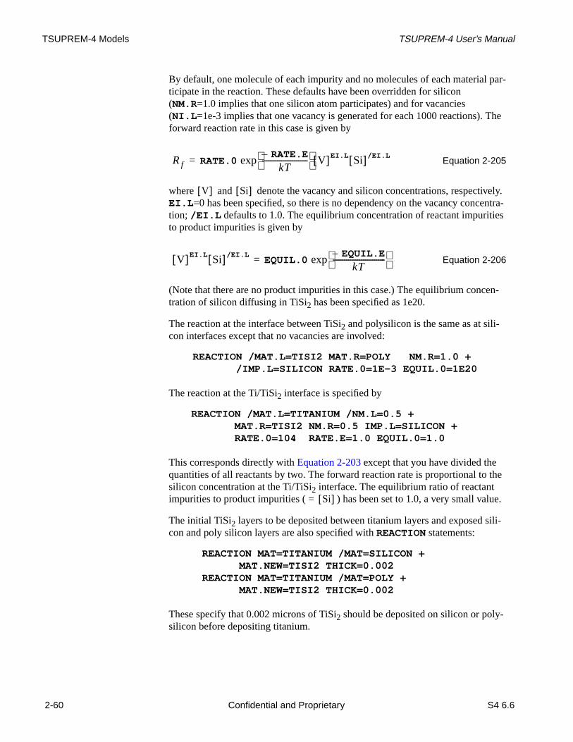
TSUPREM-4 Models TSUPREM-4 User’s Manual
l par-
The
vely.entra-ies
en-
the
ue.
sili-
-
By default, one molecule of each impurity and no molecules of each materiaticipate in the reaction. These defaults have been overridden for silicon(NM.R=1.0 implies that one silicon atom participates) and for vacancies(NI.L =1e-3 implies that one vacancy is generated for each 1000 reactions).forward reaction rate in this case is given by
Equation 2-205
where and denote the vacancy and silicon concentrations, respectiEI.L =0 has been specified, so there is no dependency on the vacancy conction; /EI.L defaults to 1.0. The equilibrium concentration of reactant impuritto product impurities is given by
Equation 2-206
(Note that there are no product impurities in this case.) The equilibrium conctration of silicon diffusing in TiSi2 has been specified as 1e20.
The reaction at the interface between TiSi2 and polysilicon is the same as at sili-con interfaces except that no vacancies are involved:
The reaction at the Ti/TiSi2 interface is specified by
This corresponds directly withEquation 2-203 except that you have divided thequantities of all reactants by two. The forward reaction rate is proportional tosilicon concentration at the Ti/TiSi2 interface. The equilibrium ratio of reactantimpurities to product impurities ( ) has been set to 1.0, a very small val
The initial TiSi2 layers to be deposited between titanium layers and exposed con and poly silicon layers are also specified withREACTION statements:
These specify that 0.002 microns of TiSi2 should be deposited on silicon or polysilicon before depositing titanium.
REACTION /MAT.L=TISI2 MAT.R=POLY NM.R=1.0 + /IMP.L=SILICON RATE.0=1E-3 EQUIL.0=1E20
REACTION /MAT.L=TITANIUM /NM.L=0.5 + MAT.R=TISI2 NM.R=0.5 IMP.L=SILICON + RATE.0=104 RATE.E=1.0 EQUIL.0=1.0
REACTION MAT=TITANIUM /MAT=SILICON + MAT.NEW=TISI2 THICK=0.002REACTION MAT=TITANIUM /MAT=POLY + MAT.NEW=TISI2 THICK=0.002
Rf RATE.0 expRATE.E–
kT------------------------
V[ ]EI.L Si[ ]/EI.L=
V[ ] Si[ ]
V[ ]EI.L Si[ ]/EI.LEQUIL.0 exp
EQUIL.E–kT
---------------------------- =
Si[ ]=
2-60 Confidential and Proprietary S4 6.6
D Draft 6/26/98

TSUPREM-4 User’s Manual Stress Models
ay:
wse
heween
for
the
rica-eennom-
Impurities Diffusion and segregation of impurities in silicides are specified in the usual w
TheMATERIAL and/MATERIA parameters must be used when specifying nematerial names; they are optional when specifying old built-in materials. Theparameters could also be specified with theIMPURITY statement:
Tungsten Silicide Model
The tungsten silicide model is identical in form to the titanium silicide model. Tparameters of the model are different, however, reflecting the differences betthe materials[28]-[34]. The names of the relevant materials aretungsten andWSi2.
Other Silicides
Models for other silicides can be defined following the example given above titanium silicide. The diffusing impurity in the silicide can be metal rather thansilicon.
Stress ModelsTSUPREM-4 has several models for calculating the stresses produced duringfabrication model. The most complete is the stress history (ST.HISTO ) model.Older and more limited capabilities are provided by theSTRESS statement andtheVISCOUS oxidation model.
Stress History Model
A number of physical phenomena give rise to stress in a structure during fabtion. These include volume changes during oxidation, thermal mismatch betwmaterials, intrinsic strain in deposited layers, and surface tension. These pheena are simulated by the stress history (ST.HISTO ) model inTSUPREM-4.
BORON MAT=TISI2 CM.SEC DIX.0=6.0E-7 DIX.E=2.0BORON SILICON /MAT=TISI2 SEG.0=0.3 + TRANS.0=1E-6 TRANS.E=2.0BORON MAT=POLY /MAT=TISI2 SEG.0=0.3 + TRANS.0=1E-6 TRANS.E=2.0
IMPURITY IMP=BORON MAT=TISI2 CM.SEC DIX.0=6.0E-7 + DIX.E=2.0IMPURITY IMP=BORON MAT=SILICON /MAT=TISI2 + SEG.0=0.3 . . .
S4 6.6 Confidential and Proprietary 2-61
Draft Draft 6/26/98 6/

TSUPREM-4 Models TSUPREM-4 User’s Manual
dd-
y aesro-in
artingnd theo- Theion;step
tch-
alues.
h the
is fol-turee
Thermal Stress Model Equations
The effect of thermal expansion during temperature ramping is modeled by aing an additional term toEquation 2-193 in Chapter 2 for the volumetric stress:
Equation 2-207
whereLCTE is the linear coefficient of thermal expansion specified on theMATERIAL statement and is the temperature.
BoundaryConditions
The boundary conditions assume that the thermal expansion is dominated bthick silicon substrate with equivalent conditions on the front and back surfac(so there is no curvature of the wafer). Thermal expansion of the substrate pduces a constant strain in the direction. The displacement thex direction at vertical reflecting boundaries and in silicon whenSKIP.SIL isset is proportional tox, ux = xLCTE∆T, while the displacement in they directionat horizontal reflecting boundaries and in silicon whenSKIP.SIL is set is pro-portional toy, uy = yLCTE∆T. The value ofLCTE for silicon is used for theseboundary conditions.
Surface tension acts on the surface of the structure; see“Surface Tension andReflow” on page 2-56 for details.
Initial Conditions The final stress from one high-temperature processing step is used as the ststress for the next; if the temperature changes between the end of one step astart of the next, a very short ramping step is inserted automatically by the prgram to compute the change in stress caused by the change in temperature.stress is set to zero at the first temperature specified after structure initializatthis temperature may be specified as part of a high-temperature processing (i.e.,DIFFUSION, DEPOSITION, orEPITAXY) or on aSELECT orSAVEFILE statement. The stresses may be modified during deposition and eing, as described below. TheSTRESS statement and oxidation with theVISCOUSmodel compute new stresses, ignoring and replacing previously calculated v
Intrinsic Stressin Deposited
Layers
The intrinsic stress in deposited layers can be specified for each material witINTRIN.S parameter on theMATERIAL statement. This intrinsic stress isincluded whenever stress history modeling is enabled. Each deposition step lowed by a stress relaxation calculation to determine the stresses in the strucfollowing the deposition. The model includes the effects of surface tension; thstress is only calculated whenST.HISTO andVISCOELA models are active.
Note:The interpretation of theINTRIN.S parameter by the stress historymodel is different from that used by theSTRESS statement. Both work byplacing an initial stress in the deposited layer then allowing the layer torelax to conform to the boundary conditions (e.g., zero stress normal to
∂σv∂t
--------- 3K∂εv∂t
-------- LCTEdTdt-------–
σvτv------–=
T
εzz LCTE T∆= z
2-62 Confidential and Proprietary S4 6.6
D Draft 6/26/98

TSUPREM-4 User’s Manual Stress Models
ctingture.mine sur-
re
pera-
free surfaces). TheSTRESS statement usesINTRIN.S as the initialstress, while the stress history model uses an initial stress that givesINTRIN.S as the x (and z) component of stress in a uniform, planar layerafter relaxation. The difference is summarized byTable 2-1. For theST.HISTO model to generate the same results as theSTRESS statement,you must multiplyINTRIN.S by , where is the value ofPOISS.R .
Effect of Etchingon Stress
When stressed material is removed from a structure, the balance of forces aon the remaining material changes, as do the stresses in the remaining strucThus, each etching step is followed by a stress relaxation calculation to deterthe stresses in the structure after the etch. The model includes the effects offace tension; the stress is only calculated when theST.HISTO andVISCOELAmodels are active.
Using the StressHistory Model
The stress history in a structure is simulated when the following conditions asatisfied:
• Stress history simulation has been enabled by theST.HISTO parame-ter on theMETHOD statement:
METHOD ST.HISTO
• TheVISCOELA oxidation model has been selected
Stresses in silicon are simulated only if^SKIP.SIL has been specified on theMETHOD statement. Thermal mismatch stresses are simulated whenever temture ramping is specified on theDIFFUSION statement. Intrinsic stresses areincluded during deposition wheneverINTRIN.S for the deposited material isnonzero. Surface tension is included wheneverSURF.TEN for an exposed mate-rial is nonzero.
1 2ν–( ) 1 ν–( )⁄ ν
Table 2-1. Model Comparisons After Relaxation
Model Initial After Relaxation
ST.HISTO
STRESS
σxx σyy σzz INTRIN.S1 ν–1 2ν–--------------= = = σyy 0
σxx
,σzz INTRIN.S
== =
σxx σyy σzz INTRIN.S= = = σyy 0
σxx
,
σzz INTRIN.S1 2ν–1 ν–--------------
=
= =
S4 6.6 Confidential and Proprietary 2-63
Draft Draft 6/26/98 6/

TSUPREM-4 Models TSUPREM-4 User’s Manual
nfer
dif-
otthe
s. Itls
and theyefer-
Limitations The thermal stress model has the following limitations:
1. The model assumes that thermal expansion is dominated by a thick silicosubstrate with equivalent conditions on the front and back sides of the wa(i.e., no bending of the wafer).
2. The model is active only when theVISCOELA oxidation model is active.Stresses in silicon are calculated only if^SKIP.SIL has been specified. Thestress history is lost and replaced with newly calculated stresses by theSTRESS statement and during oxidation with theVISCOUS model.
3. While the thermal mismatch model works down to room temperature, thefusion models do not. At temperatures below about 50°C they may producearithmetic exceptions or cause the program to hang; below about 600°C theymay produce inaccurate results.
4. The stresses caused by phase changes during temperature cycling are nmodeled. It may be possible to approximate these stresses by changing thermal expansion coefficients as a function of time and temperature.
Modeling Stress with the STRESS Statement
TheSTRESS statement (seepage 3-114) allows calculation of stresses due tothermal mismatch between materials or due to intrinsic stress in deposited filmuses a finite-element analysis based on a linear elastic model for the materiainvolved. The equations that are solved are
Equation 2-208
Equation 2-209
Equation 2-210
Equation 2-211
Equation 2-212
Equations 2-208 and2-209 are the equations of motion for the structure, whileEquations 2-210 through2-212 are the constitutive relations for the materials.Here , , and are the calculated stresses and and are the
displacements; and are stored as the and velocities (even thoughare actually displacements), and can be accessed for printing or plotting by r
∂σxx
∂x-----------
∂σxy
∂y-----------+ 0=
∂σyy
∂y-----------
∂σxy
∂x-----------+ 0=
σxx σyy+E
1 v+( ) 1 2v–( )-----------------------------------
∂ux
∂x--------
∂uy
∂y--------+
2E1 2v–-------------- LCTE dT 2σi+
T1
T2
∫–=
σxx σyyE
1 v+-----------=–
∂ux
∂x--------
∂uy
∂y--------–
σxyE
2 1 v+( )-------------------
∂ux
∂y--------
∂uy
∂x--------+
=
σxx σyy σxy ux uy xy ux uy x y
2-64 Confidential and Proprietary S4 6.6
D Draft 6/26/98
TSUPREM-4 User’s Manual Ion Implantation
the
are
ro. cal-idesn
o.sion
tressy the
-able
ained
encing thex.vel andy.vel functions on theSELECT statement. The values ofYoung’s modulus and Poisson’s ratio for each material are specified on MATERIAL statement byYOUNG.M andPOISS.R , respectively (seepage 3-212).
The linear coefficient of thermal expansion for each material,LCTE, can be speci-fied as a function of (absolute temperature) on theMATERIAL statement. Thisfunction is integrated between temperatures and , specified by theTEMP1andTEMP2 parameters on theSTRESS statement. IfTEMP1 andTEMP2 are notgiven, then theLCTE term is omitted from the analysis.
BoundaryConditions
The following boundary conditions are used:
• Exposed surfaces: stress normal to the surface is zero.
• Material interfaces: stress normal to the interface and the displacements continuous across the interface.
• Reflecting boundaries: displacement perpendicular to the boundary is zeThis displacement value produces incorrect results for thermal expansionculations when there are reflecting boundaries on both the left and right sof the structure and theLCTE of the substrate is nonzero. This is one reasothat the stress history model should be used instead of theSTRESS statement.
• direction: displacement and stress in the direction are taken to be zer(The strain in the direction should be determined by the thermal expanof the substrate, as it is in the stress history model.)
Thin film intrinsic stresses are accounted for by the terms[75], [76]. The valueof for each material is given by theINTRIN.S parameter on theMATERIALstatement.
The calculated values of stresses and displacements replace any values of sand velocity that may have been calculated by a previous oxidation step or bstress history model.
TheSTRESS statement has been made obsolete by the stress history(ST.HISTO ) model.
Ion ImplantationTheIMPLANT statement (seepage 3-95) is used to model the implantation of ionized impurities into the simulation structure. Two distinct approaches are availfor modeling ion implantation.
• The analytic approach models the impurity and point defect distributionsusing Gaussian or Pearson functions based on distribution moments contin a data file.
• The Monte Carlo approach calculates the trajectories of implanted ionsthrough the two-dimensional target structure, based on physical models.
E v
TT1 T2
z zz
σiσi
S4 6.6 Confidential and Proprietary 2-65
Draft Draft 6/26/98 6/

TSUPREM-4 Models TSUPREM-4 User’s Manual
lThe
inu- at theion
men-u-
yede.n
ble
der
These two approaches are described in the following sections.
Analytic Ion Implant Models
The impurity being implanted is selected with one of the parametersANTIMONY,ARSENIC, BORON, PHOSPHOR, orBF2. TheDOSE parameter specifies the totanumber of impurity ions per square centimeter provided by the ion implanter. acceleration energy of the ions is specified with theENERGY parameter. Only theportion of the distribution within the simulation region contributes to the dosethe structure. If theBACKSCAT parameter is specified, the portion of the distribtion above the top of the simulation structure is assumed to be backscatteredsurface. Any portion of the distribution below the bottom of the simulation regis assumed to have passed through the structure.
ImplantedImpurity
Distributions
Implanted impurity distributions in a two-dimensional structure are derived frodistributions calculated along vertical lines through the structure. The one-dimsional procedures described below are used to find the vertical implant distribtion along each line.
Each one-dimensional profile is converted to a two-dimensional distribution bmultiplying by a function of . The final profile is determined by integrating thcontributions of all the two-dimensional distributions to the doping at each noIf the TILT parameter is nonzero, the lines for the one-dimensional calculatioare taken at the specified angle from the vertical. The variableu in the discussionthat follows then represents the distance along the angled line, while the variaxcorresponds to distance perpendicular to the slices.
The vertical distribution along each line is given by
Equation 2-213
where occurs at the surface of the top material layer along the line, anis a normalized Gaussian or Pearson distribution, depending on wheth
GAUSSIAN or PEARSON is selected on theIMPLANT statement. The equationsfor are described below.
The vertical distribution function is calculated from its spatial distributionmoments. The first four moments are defined as
Equation 2-214
Equation 2-215
x
I u( ) DOSE f u( )×=
u 0=f u( )
f u( )
f u( )
Rp uf u( ) ud∞–
∞
∫=
σ u Rp–( )2f u( ) ud
∞–
∞
∫=
2-66 Confidential and Proprietary S4 6.6
D Draft 6/26/98

TSUPREM-4 User’s Manual Ion Implantation
esr of
rialthe
with
The
his
ults
Equation 2-216
Equation 2-217
The values of , , , and are obtained from the implant data files4imp0 orfrom an alternate implant data file specified with theIN.FILE parameter in theIMPLANT statement. For each combination of impurity and material, these filcontain the distribution moments for a series of acceleration energies in ordeincreasing energy.
Implant MomentTables
The implant data file associates distribution moments with each ion and mateby using ion and material names present in the file. The material names are same as those used elsewhere in the program (i.e.,SILICON , OXIDE, NITRIDE ,POLYSILI , PHOTORES, andALUMINUM). The data for silicon dioxide is alsoused for silicon oxynitride.
The data table to be used for an implantation step can be specified explicitlytheIMPL.TAB parameter in theIMPLANT statement. This allows the implantdata file to contain several sets of distribution moments for the same impurity.implant data file defines the following table names:
• ANTIMONY: Original antimony data with extended energy ranges fitted toresults of amorphous Monte Carlo calculations (energies: 5–1000 keV). Tis the default for antimony implantation.
• ARSENIC: Original arsenic data with extended energy ranges fitted to resof amorphous Monte Carlo calculations (energies: 5–11,000 keV).
• DUAL.ARS: Dual-Pearson data for arsenic with channeling in silicon(energies: 10-1000 keV)[35]. This is the default for arsenic implantation.
• TR.ARSENIC: Dual-Pearson data for arsenic in <100> silicon with fullenergy, dose, tilt, and rotation dependence (energy: 0.5–180 keV;dose: 1013–8 ×10¹⁵ atoms/cm2; tilt: 0°–10°; rotation: 0°–45°) [36] and[87].
• BF2: Data for boron from a BF2 source (energies: 5–120 keV)[38].
• DUAL.BF2: Dual-Pearson data for boron from a BF2 source with channelingin silicon (energies: 10–200 keV)[35]. This is the default for BF2 implanta-tion.
• UT.BF2 : Dual-Pearson data for boron from a BF2 source with channeling insilicon (energies: 15–120 keV)[36].
• TR.BF2 : Dual-Pearson data for BF2 in <100> silicon with full energy, dose,tilt, and rotation dependence (energy: 0.5–65 keV;dose: 1013–8 ×10¹⁵ atoms/cm2; tilt: 0°–10°; rotation: 0°–45°) [36] and[87].
γ
u Rp–( )3f u( ) ud
∞–
∞
∫σ3
-----------------------------------------------------=
β
u Rp–( )4f u( ) ud
∞–
∞
∫σ4
-----------------------------------------------------=
Rp σ γ β
S4 6.6 Confidential and Proprietary 2-67
Draft Draft 6/26/98 6/

TSUPREM-4 Models TSUPREM-4 User’s Manual
of
V)
,
ed).
.
li-
nt inthee forinted near-y areis
t
ach
d in
at a
• BORON: Original boron data with extended energy ranges fitted to resultsamorphous Monte Carlo calculations (energies: 5–4000 keV).
• LEBORON: Data for low-energy boron with channeling in silicon(energies: 10–30 keV)[38].
• CHBORON: Data for boron with channeling in silicon (energies: 5–2000 ke[35]. This is the default for boron implantation.
• UT.BORON: Dual-Pearson data for boron with channeling in silicon(energies: 15–100 keV)[36].
• TR.BORON: Dual-Pearson data for boron in <100> silicon with full energydose, tilt, and rotation dependence (energy: 0.5–80 keV;dose: 1013–8×10¹⁵ atoms/cm2; tilt: 0°–10°; rotation: 0°–45°) [39] and[87].
• PHOSPHORUS: Original phosphorus data with extended energy ranges fittto results of amorphous Monte Carlo calculations (energies: 5–7000 keV
• DUAL.PHO: Dual-Pearson data for phosphorus with channeling in silicon(energies: 10–200 keV)[35]. This is the default for phosphorus implantation
• TR.PHOSPHORUS: Dual-Pearson data for phosphorus into bare <100> sicon with full energy, dose, tilt, and rotation dependence (energy: 15—180keV; dose: 1013–8×10¹⁵ atoms/cm2; tilt: 0°–10°; rotation: 0°–45°)[37].
The energy ranges shown are for implantation into silicon. If no data is presethe implant data file for the specified energy, linear interpolation is used with available data to determine the distribution moments. No extrapolation is donenergies outside the range of the table. For implants into silicon, an error is prand the program terminates; for other materials, a warning is printed and theest available energy is used. If the first three moments for the specified energpresent in the implant data file, but the value of is missing or zero, then calculated using the expression[40]
Equation 2-218
which yields a reasonable value for and requires knowledge of only the firsthree distribution moments.
Moments for up to 20 materials can be included in the implant moments file. Ematerial in the file has an unique name. Usually,TSUPREM-4 searches themoments file for a material with a name that matches the material name useTSUPREM-4. For example, data for the material calledphotoresist in themoments file is used for implantation into photoresist. But you can request thdifferent set of data be used with theIMPL.TAB parameter on theMATERIALstatement. Thus the statement
MATERIAL MAT=PHOTORESIST IMPL.TAB=AZ-7500
requests that data for the material namedaz-7500 in the implant moments file beused for implantation into photoresist.
β β
β 2.91 1.56γ20.59γ4
+ +=
β
2-68 Confidential and Proprietary S4 6.6
D Draft 6/26/98

TSUPREM-4 User’s Manual Ion Implantation
as
by
of
sat-ur
eal
pe Ie
GaussianDistribution
A Gaussian distribution requires only the moments and and is defined
Equation 2-219
where and are defined above.
PearsonDistribution
A Pearson distribution requires the moments , , , and , and is definedthe differential equation[41]
Equation 2-220
where
Equation 2-221
Equation 2-222
Equation 2-223
Equation 2-224
Equation 2-225
Not all combinations of and produce useful profiles. The characteristics the profile can be determined by examining the denominator ofEquation 2-220:
Equation 2-226
For the profile to have a maximum at , must be negative; for themean of the profile to be at requires that .
TSUPREM-4 checks these conditions and produces an error unless both areisfied. The fourth moment is equal to only if , which can only occwhen . However, the program produces profiles forwithout printing a warning (provided that ).
The nature of the profile depends on the value of and whether there are rsolutions to the equation . In the following, it is assumed thatand the solutions to (if they exist) are and , with . For
, the profile is nonzero for ; this corresponds to a Pearson tyor II distribution. If and has no real solutions, then the profil
Rp σ
f u( ) 1
2π σ----------------exp
u Rp–( )2–
2σ2---------------------------=
Rp σ
Rp σ γ β
df v( )dv
------------- v a–( ) f v( )b0 av b2v
2+ +--------------------------------=
v u Rp–=
aσγ β 3+( )–
A----------------------------=
b0σ2
– 4β 3γ2–( )
A------------------------------------=
b22β– 3γ2
6+ +A
---------------------------------=
A 10β 12γ2– 18–=
β γ
p ν( ) b0 aν b2ν2+ +=
v a= p a( )Rp b2 1 2⁄–>
β b2 1 5⁄–>A 0> 1 2⁄– b2 1 5⁄–< <
p a( ) 0<
b2p ν( ) 0= p a( ) 0<
p ν( ) 0= ν1 ν2 ν1 ν2≤b2 0> ν1 ν ν2< <
b2 0≤ p ν( ) 0=
S4 6.6 Confidential and Proprietary 2-69
Draft Draft 6/26/98 6/

TSUPREM-4 Models TSUPREM-4 User’s Manual
rson
atr
ose.plant
tch
ment
antlyg
lantsed.
f thertion-n-s areas:
d
ely
rre-dose.aseodel
ve tohly
is nonzero for all , but approaches zero as approaches ; this is a Peatype IV or VII distribution for and a Gaussian for .
If and has real solutions, then the profile either goes to zero and (for ) or at and (for ); this is Pearson type V o
VI distribution for and a type III distribution for .
Dual PearsonDistribution
In the case of implantation into crystalline silicon, for low to medium doseimplants the shape of the resultant profile is relatively insensitive to implant dIn this range, a single Pearson function can be used to model the range of imdoses at a given energy by simply scaling the magnitude of the profile to mathe implant dose. This is the method used when thePEARSON distribution isselected and data for a single Pearson function is included in the implant modata file for the specified impurity name.
Dose-dependentImplant Profiles
At higher doses, substrate damage causes the implant profile to vary significwith dose. A dual-Pearson approach has been found to work well for modelinsuch dose-dependent implant profiles[35], [36], [39]. When thePEARSON distri-bution is selected and data for a dual-Pearson function is included in the impmoment data file for the specified impurity name, a dual-Pearson function is u
Following this approach, one Pearson profile models the channeled portion oimplant profile, while the second Pearson profile models the nonchanneled poresulting from implantation into partially amorphized silicon. The dose dependence is modeled by varying the relative magnitude of the channeled and nochanneled Pearson functions. The moments of each of the Pearson functionindependent of dose. The composite dual-Pearson profile can be described
Equation 2-227
where
• and are the normalized amorphous and channelePearson profiles, respectively
• is the ratio of the dose of the amorphous profile to the total dose
• subscripts and refer to amorphous and channeled profiles, respectiv
• is the depth coordinate along the line
The implant data file for dual-Pearson data has two sets of four moments, cosponding to both Pearson profiles, and a table of ratio values as a function of Figure 2-1 shows the variation of profile shape with implantation dose, in the cof an initially crystalline silicon substrate, and compares the dual-Pearson mwith data taken from[36]. In Figure 2-1(a)-(d), the composite profile is plotted(solid line), along with the channeled and amorphous profile contributions(dashed lines). The ratio of the dose allocated to the amorphous profile relatithe channeled dose is indicated in each figure. A ratio of unity indicates a hig
ν ν ∞±b2 0< b2 0=
b2 0≤ p ν( ) 0=ν1 ∞– a ν1< ν2 ∞ a ν2>
b2 0< b2 0=
I compositeu( ) rI amorphousu RPa σa γa βa, , , ,( ) 1 r–( )I channeledu RPc σc γc βc, , , ,( )+=
I amorphous I channeled
r
a c
u
2-70 Confidential and Proprietary S4 6.6
D Draft 6/26/98

TSUPREM-4 User’s Manual Ion Implantation
edr theblese is withdary
damaged substrate with little channeling, whereas a ratio of zero indicates ahighly channeled profile with little or no implant damage.
When theGAUSSIAN distribution is selected and dual-Pearson data is containin the implant data file, the first set of moments is used as described above focalculation of the distribution. If the dose is outside the range of values availain the implant data file, the fraction corresponding to the nearest available doused. The dual-Pearson functions are useful for modeling channeling effects,the primary Pearson function modeling the bulk of the implant and the seconPearson function modeling the distribution of channeled ions.
Figure 2-1 BF2 implant profile
BF2energy=65 keVdose=5e15ratio=0.969
BF2energy=65 keVdose=1.5e15ratio=0.957
BF2energy=65 keVdose=5e14ratio=0.767
BF2energy=65 keVdose=2e13ratio=0.0
(a) (b)
(c)(d)
channeledprofile
amorphousprofile
S4 6.6 Confidential and Proprietary 2-71
Draft Draft 6/26/98 6/

TSUPREM-4 Models TSUPREM-4 User’s Manual
d, lin-eci-ge is
g byate-
e,ter-
tedtion
This
se
match-ith
Tilt and RotationTables
Thetr.arsenic, tr.bf2, andtr.boron tables contain dual-Pearson distributions for arange of energies, doses, wafer tilts, and rotations for implantation into bare,<100> silicon. When one of these tables is specified with theIMPL.TAB parame-ter, the distribution for the specified energy, dose, tilt and rotation are obtainefrom the table. If the specified implant parameters do not appear in the tableear interpolation (in four dimensions) between table entries is used. If the spfied implant parameters lie outside of the range of the table, a warning messaprinted and the nearest available values are used.
Note:The tilt and rotation tables give accurate results after implantation intobare, <100> silicon, but may not be appropriate under other implantconditions.
MultilayerImplants
A multilayer implant is represented by treating each layer sequentially, startinwith the top layer in the structure. The impurity distribution is determinedfirst obtaining the moments from the implant data file for the impurity in the mrial comprising the layer. The distribution is used for the impuritydistribution within the layer, where
Equation 2-228
The summation is performed over all previously treated layers of the structurand is the thickness of layer . Either of two approaches can be used to demine : effective range model or dose matching.
Effective RangeModel
By default, is given by[42]
Equation 2-229
where is the first moment of in layer , is the first moment ofin the present layer, and the summation is performed over all previously trealayers of the structure. For layers below the first, the magnitude of the distribuis scaled so that the integral of from to plus the total doseplaced in all previously treated layers is equal to the specified implant dose. method is referred to as theeffective range or effective thicknessapproach.
Dose Matching If the parameterRP.EFF is set as false on theIMPLANT statement, is deter-mined such that the integral of from to equals the total doplaced in all previously treated layers[43]. For the top layer, . This methodis referred to as thedose matching approach.
The effective range approach has proved to be more accurate than the dose ing approach; the dose matching approach is retained only for compatibility wolder revisions (8926 and older) of the program.
I u( )
I u ul– us+( )
ul tii
∑=
ti ius
us
us
tiRp
Rpi
----------i
∑=
Rpif u( ) i Rp f x( )
I u( ) u us= u ∞=
usI u( ) u 0= u us=
us 0=
2-72 Confidential and Proprietary S4 6.6
D Draft 6/26/98
TSUPREM-4 User’s Manual Ion Implantation
y a
al
by
re
reon—
nt.
dthe
er
ithn oft onis tiltnn of
eleds a
he anyanta-ced
LateralDistribution
Each one-dimensional profile is expanded to two dimensions by multiplying bGaussian distribution in the direction perpendicular to the line[44]:
Equation 2-230
where is the distance perpendicular to the line. The quantity is the laterstandard deviation of the implant profile in the given material and is found byinterpolation in the implant data file. The complete implant profile is obtainedsumming together the two-dimensional profiles produced by all of the lines.
Wafer Tilt andRotation
Tilt and rotation of the wafer during implantation are specified by theTILT andROTATION parameters, respectively. The various effects of tilting the wafer asimulated as follows:
1. When a nonplanar structure is tilted, shadowing of portions of the structucan occur. The amount of shadowing for a given tilt depends on the rotatifrom full shadowing at zero rotation to no shadowing at 90° rotation. Shadow-ing is simulated by tilting the simulated structure by an appropriate amou
2. The number of incident ions per square centimeter of the wafer is reducewhen the wafer is tilted. This dose reduction is simulated naturally when simulation structure is tilted, but an analytical adjustment to the dose isrequired if the tilt of the simulation structure is less than the specified waftilt because of rotation.
3. Tilting the wafer causes the implanted profiles to be foreshortened. As wdose reduction, foreshortening of the profiles is simulated by a combinatiotilting the simulation structure and by analytical adjustments to the implanparameters. If the implantation data is derived from measurements basedtilted wafer samples, the tilt of the data also affects foreshortening. For threason, each table of data in the implantation data file has an associatedand rotation value that reflects the conditions under which the implantatiodata were measured. The tilt value for each table is used in the calculatioforeshortening effects.
4. The tilt and rotation of the wafer affect the number of ions that are channalong crystal planes in silicon. Channeling effects in bare <100> silicon afunction of tilt and rotation are included in thetr.arsenic, tr.bf2, andtr.boronimplant tables.
Analytic DamageModel
When theDAMAGE parameter on theIMPLANT statement is set true, an analyticmodel for the production of point defects during ion implantation is invoked. Tinterstitial and vacancy distributions created by the implantation are added tointerstitials and vacancies that may have existed in the structure prior to impltion. For more information on how damage is used to model transient-enhandiscussion, see“Implant Damage Model” on page 2-85.
I u v,( ) I u( ) 1
2π σx
------------------ expv
2
2σx2
---------–
×=
v σx
S4 6.6 Confidential and Proprietary 2-73
Draft Draft 6/26/98 6/

TSUPREM-4 Models TSUPREM-4 User’s Manual
rherrbye
a-lete
esianram-u- by
orus.
l forhewith
suf- the
iconmod-odelform
eseepen-te
n
o
DamageDistribution
Calculations
The damage distributions are calculated using the model of Hobler and Selbein its one-dimensional form[45]. This model approximates the damage profiles combinations of Gaussian and exponential functions. The parameters of thesfunctions were chosen to fit damage profiles predicted by Monte Carlo simultions over the range of implant energies between 1 and 300 keV. For a compdescription of the equations and parameter values, seeReference [45]. The imple-mentation inTSUPREM-4 differs from that in[45] in that both the Gaussian andexponential components are used when implanting arsenic at energies abov170 keV. The model is extended to two dimensions by multiplying by a Gauswith a standard deviation equal to the value of Hobler and Selberherr’s paeter (the standard deviation of the Gaussian component of the vertical distribtion). For BF2 implants, the model for boron is used and the damage is scaled49/11. (The scaling is omitted ifV.COMPAT=6.4 is specified on theOPTIONstatement.)
RecommendedUsage andLimitations
The damage model is designed only for antimony, arsenic, boron, and phosphIf DAMAGE is specified on a BF2 implantation, the model for boron is used, withenergy reduced by a factor of 0.2215. For other impurities, the damage modeone of the ions listed above (the one having atomic weight closest to that of timplanted ion) is used. There are no user-accessible coefficients associated the damage model. If the damage calculation is followed by aDIFFUSION step, care should be used to ensure that a simulation region withficient depth is used to accommodate the rapid diffusion of point defects intostructure.
Monte Carlo Ion Implant Model
You can select a Monte Carlo model for ion implantation by specifying theMONTECAR parameter on theIMPLANT statement.TSUPREM-4 contains acomprehensive Monte Carlo model that incorporates models for crystalline silas well as amorphous models for silicon and other materials. The calculation els the crystal to amorphous transition that occurs during implantation. The mincludes the effect of reflected ions and produces damage information in the of vacancy and interstitial profiles. In addition,TSUPREM-4 contains models forcalculating damage self-annealing of silicon substrates.
The Monte Carlo calculation is useful for examining a number of dependencifor which the empirical models are imperfect or incompletely calibrated. Somexamples of these are: profile dependence on tilt and rotation angles, dose ddence, implant temperature dependence, and low energy implants. The MonCarlo model is the only implant model inTSUPREM-4 that can simulate theeffects of reflected ions.
The capabilities contained inTSUPREM-4 are a superset of the Monte Carlo ioimplant functionality of the one-dimensional process simulator, PEPPER[46].The calculation used inTSUPREM-4 assumes that ions lose energy through twprocesses.
a3
2-74 Confidential and Proprietary S4 6.6
D Draft 6/26/98

TSUPREM-4 User’s Manual Ion Implantation
eion
ism
re
loss
ics
ary
ow
nd
e
e, and
• Nuclear scattering, where the nucleus of the ion elastically scatters off thnucleus of an atom in the target. This interaction is based on binary collistheory and is described in the following section.
• Interaction of the ion with the electrons of the target atoms. This mechanis inelastic and does not alter the direction of the ion’s motion. This isdescribed in“Amorphous Implant Calculation” on page 2-78.
The calculation of damage and damage self-annealing of silicon substrates adescribed in“Crystalline Implant Model” on page 2-81.
Binary ScatteringTheory
TSUPREM-4 models the nuclear collision energy loss according to classicalbinary scattering theory. The basic assumption of the nuclear collision energymechanism is that the ion interacts with only one target atom at a time. Thisassumption allows the use of binary scattering theory from classical mechan[47]. This section briefly outlines the pertinent results of this theory.
Consider a particle of mass and kinetic energy approaching a stationparticle with mass . The impact parameter, , is the distance of closestapproach if the particle is not deflected and gives a convenient measure of hclose the collision is. After collision, the first particle deviates from its originalcourse by an angle .
Energy Loss It can be shown that the first particle loses kinetic energy
Equation 2-231
where is the energy lost by particle 1, is its energy before collision, a is the integral
Equation 2-232
where is the inverse separation between the two particles, is thpotential between the two particles (assumed to be repulsive), and
Equation 2-233
is the reduced energy in the center of mass coordinates. The upper limit of thintegral, , is the inverse distance of closest approach of the two particlesis given by the solution to the equation
Equation 2-234
M1 E0M2 b
θ
∆En
E0----------
4M1M2
M1 M2+( )2----------------------------cos
2bI( )=
∆En E0I
Isd
1 V s( )Er
-----------– b2s
2–
----------------------------------------0
smax
∫=
s 1 r⁄= V s( )
Er
E0
1 M1 M2⁄+---------------------------=
smax
1V smax( )
Er-------------------– b
2smax
2– 0=
S4 6.6 Confidential and Proprietary 2-75
Draft Draft 6/26/98 6/

TSUPREM-4 Models TSUPREM-4 User’s Manual
con-
t
Scattering Angle The angle by which particle 1 is deflected is given by
Equation 2-235
DimensionlessForm
Equations 2-231 through2-235 are the basic equations for classical two-bodyscattering. The scattering integral,Equation 2-232, can be cast into a dimension-less form by assuming the potential has the form
Equation 2-236
where is the charge on particle 1, is the charge on particle 2, is thestant
Equation 2-237
is an arbitrary function of , to be defined later, and is a unit oflength.TSUPREM-4 uses
Equation 2-238
which is the so-called Universal screening length[48] and a dimensionless impacparameter
Equation 2-239
and a dimensionless energy
Equation 2-240
UsingEquations 2-238, 2-239, and2-240 in the scattering integralEquation 2-232, and making the substitution gives
Equation 2-241
FromEquation 2-231, the quantity of interest is , which becomes
θ
cosθ1 0.5 1
M2
M1-------+ ∆E E0⁄–
1 ∆E E0⁄–-------------------------------------------------------=
V s( ) Z1Z2k1sg aus( )=
Z1 Z2 k1
k1q2
4πε0------------ 14.39495 10
7–× keVµm= =
g aus( ) aus au
au 0.8854 104– 0.529
Z10.23
Z20.23
+ --------------------------------------- µm×=
bn b au⁄=
εauEr
Z1Z2k1-----------------=
s′ aus=
I1au-----= s′d
1 s′g s′( ) ε bn2s′2–⁄–
----------------------------------------------------0
s′max
∫cos
2bI( )
2-76 Confidential and Proprietary S4 6.6
D Draft 6/26/98

TSUPREM-4 User’s Manual Ion Implantation
n-
een
iv-
by
scat-n-
Equation 2-242
Thus usingEquation 2-242, can be evaluated in terms of the dimensioless variables and , without reference to a particular particle’s charge ormass.
Coulomb Potential As an example of the above procedure, consider the Coulomb potential betwtwo particles,
Equation 2-243
or . In this case, . Then fromEquation 2-242
Equation 2-244
with
Equation 2-245
from a solution ofEquation 2-234. Then the integral can be evaluated exactly, ging
Equation 2-246
For a given impact parameter and incident energy , the dimensionlessand can be obtained fromEquations 2-239 and2-240, giving fromEquation 2-246. Then the energy loss due to the collision is given byEquation 2-231, and the angle at which particle 1 leaves the collision is given Equation 2-235.
Universal Potential For the simple form of the Coulomb potential used in the example above, thetering integral can be solved analytically. For more realistic inter-atomic potetials, however, the scattering integral cannot be evaluated analytically. Forexample, the Universal potential[48] that is used inTSUPREM-4 is
cos2
bI( ) cos2
bns′d
1 s′g s′( ) ε bn2s′2–⁄–
----------------------------------------------------0
s′max
∫=
cos2
bl( )bn ε
V r( )Z1Z2k1
r-----------------=
V s( ) Z1Z2k1s= g aus( ) 1=
cos2
bI( ) cos2
bns′d
1 s′ ε bn2s′2–⁄–
----------------------------------------0
s′max
∫=
s′max
1 4bn2ε2
+ 1–
2εbn2
----------------------------------------=
cos2
bI( ) 1
1 4bn2ε2
+----------------------=
b E0 bnε cos
2bI( )
S4 6.6 Confidential and Proprietary 2-77
Draft Draft 6/26/98 6/

TSUPREM-4 Models TSUPREM-4 User’s Manual
ith
o-
the
los-
flision,nd
gieses of
n is
nd
mal.
Equation 2-247
An analytic solution does not exist since the upper limit of the integral inEquation2-232 is given byEquation 2-234, which becomes a transcendental equation wthis potential.
All Monte Carlo ion implantation codes use a formalism similar toEquations 2-231 through2-235 to treat the nuclear scattering; the differencebetween codes is in the method of evaluating the scattering integral,Equation 2-232. The code MARLOWE[49] numerically integrates the scatteringintegral, providing accurate solutions at great computational expense. The prgram TRIM[50] fits an analytic function of five parameters to the values of thescattering integral obtained by numerical integration. This technique retainedaccuracy of MARLOWE while improving efficiency by an order of magnitude.However, TRIM still requires the evaluation of , the inverse distance of cest approach at each collision. This requires solving the nonlinearEquation 2-234. With an initial guess of , Newton’s method con-verges to an answer in about 3 to 5 iterations. If the Universal potential[48] isused, this requires 18 to 30 exponentials to be evaluated at each collision.
A different algorithm is used inTSUPREM-4 [51]. The quantity , in itsdimensionless form,Equation 2-242, is numerically integrated for a wide range oits parameters and . These results are stored in tables. Then at each col
is obtained from these tables. This scheme eliminates the need to fi for each collision, minimizing the amount of arithmetic performed during
the calculation of an ion’s trajectory, while retaining accuracy.
Tables for the Universal potential over a wide range of energies and impactparameters are provided for immediate use inTSUPREM-4. They span the nor-malized energy range of and the normalized impact parameterrange . For , the Coulomb formEquation 2-247 is used. Valuesof are not encountered for ion-atom combinations of interest at enerabove the energy at which the ion is assumed to be stopped (10 eV). For valu
, the ion is assumed to be undeflected.
AmorphousImplant
Calculation
This section describes how the binary scattering theory of the previous sectioused to calculate ion trajectories in an amorphous solid.TSUPREM-4 calculatesa number of ion trajectories that can be specified using theN.ION parameter ontheIMPLANT statement. The implant species can be any impurity (includinguser-defined impurities) for which the required information (atomic number aweight, electronic stopping powers, and so on) has been specified.
The calculation of ion trajectories proceeds as follows. Assume an ion withkinetic energy hits a target with an angle with respect to the target nor
V r( )Z1Z2k
r--------------- 0.18175e
3.1998r au⁄–0.50986e
0.94229r– au⁄
0.28022e0.4029r au⁄–
0.028171e0.20162r au⁄–
+
+ +
=
smax
smax 1 b⁄=
cos2
bI( )
bn εcos
2bI( )
smax
105– ε 100≤ ≤
0 bn 30≤ ≤ ε 100>ε 10
5–<
bn 30>
E0 θ0
2-78 Confidential and Proprietary S4 6.6
D Draft 6/26/98

TSUPREM-4 User’s Manual Ion Implantation
lly
ra-l a
s thee
n
ugh
The surface of the target is assumed to be at , with increasing verticainto the target. The incident energy can be set on theIMPLANT statementusing theENERGY parameter. The incident angle can be specified on theIMPLANT statement using theTILT parameter.
Given the atomic density for the target material, the mean atomic sepation between atoms in the target is . The ion is assumed to travedistance
Equation 2-248
between scattering events. As the ion enters the target material, it approachefirst target atom with impact parameter , defined in the previous section. Thprobability of finding a target atom between and is given by
Equation 2-249
for . If is a uniformly distributed random number betwee0 and 1, then the probability distribution gives
Equation 2-250
as described in[50].
Nuclear Stopping Given the above definitions, the algorithm for calculating the energy loss thronuclear collisions experienced by the ion proceeds as follows:
1. A random number between 0 and 1 is chosen.
2. The normalized impact parameter for this collision is calculated fromEquations 2-239 and2-250
Equation 2-251
3. The ion energy, , is normalized to
Equation 2-252
from Equations 2-233 and2-240.
4. Now the value of can be obtained from the tables, andEquation 2-231 gives the energy loss due to nuclear scattering
y 0= yE0
θ0
Ndens1 Ndens( )⁄ 1 3⁄
L 1 Ndens( )⁄ 1 3⁄=
bb b δb+
w b( )δb 2πNdens2 3⁄
b δb=
b 1 πNdens2 3⁄⁄< Rrand
bRrand
πNdens2 3⁄-----------------=
b1au-----
Rrand
πNdens2 3⁄-----------------=
E0
εauE0
1 M1 M2⁄+( )Z1Z2k1--------------------------------------------------=
cos2
bI( )
S4 6.6 Confidential and Proprietary 2-79
Draft Draft 6/26/98 6/

TSUPREM-4 Models TSUPREM-4 User’s Manual
th
t file.
m-
Equation 2-253
This procedure is repeated for each collision event.
ElectronicStopping
The ion also loses energy by inelastic electronic processes, which include bononlocal and local stopping power. At low energies this is modeled by
Equation 2-254
Equation 2-255
Equation 2-256
Equation 2-257
Equation 2-258
Equation 2-259
Equation 2-260
where L is the free flight path between collisions, p is the impact parameter,ε isthe scaled dimensionless energy, E0 is the ion energy, and aU is the universalscreening length.NLOC.PREN, NLOC.EXP, NLOC.MAX, NLOC. K, ES.RAND,ES.F.RAN , andLOC.FAC can be defined on theIMPURITY statement.
In the absence of a specification using anIMPURITY statement, or if the specifiedvalues are zero, values for these parameters are obtained from the coefficienIf no value or a value of zero is specified in the coefficient file for parametersES.RAND andES.F.RAN , the default values are given by[52]
Equation 2-261
Equation 2-262
where is the ion atomic number and is the composite target atomic nuber. For boron and phosphorus in silicon, the default values ofES.RAND havebeen set to 2.079 and 2.5, respectively[50]. For light ions ( ) and -parti-cles, the value for electronic stopping given byEquation 2-261 is very crude.
∆E0 E0
4M1M2
M1 M2+( )2----------------------------cos
2bI( )=
∆Ee xnl ∆E
nle x
loc ∆Eloce⋅+⋅=
∆Enle
L Ndens Se⋅ ⋅=
x∆Eloce
Se
2πa2
------------ p– a⁄( )exp⋅=
xnl
min NLOC.PRE εNLOC.EXPNLOC.MAX,⋅( )=
xnl
xloc
+ 1=
Se NLOC.K ES.RAND E0ES.F.RAN⋅ ⋅=
a LOC.FACaU
0.3-------⋅=
ES.RAND1.212Z1
7 6⁄Z2
Z12 3⁄
Z22 3⁄
+3 2⁄
M11 2⁄
----------------------------------------------------=
ES.F.RAN 0.5=
Z1 Z2
Z1 5≤ α
2-80 Confidential and Proprietary S4 6.6
D Draft 6/26/98

TSUPREM-4 User’s Manual Ion Implantation
ear
ch
-
henili- thean-xes.
elect-f thearam-tice.actle
Experimental values should be specified wherever possible[48], [53], [54], [56],usingES.RAND andES.F.RAN on the impurity statements.
ElectronicStopping at High
Energies
At energies aboveES.BREAK, Equation 2-262 is replaced by
Equation 2-263
whereES.BREAK andES.F.H are parameters on theIMPURITY statement.Note that the high energy stopping model is used only whenES.BREAK is non-zero, i.e., the model can be disabled by settingES.BREAK=0.
Total Energy Lossand Ion Deflection
The total change in energy of the ion after the collision is the sum of nuclenergy loss,Equation 2-253, and electronic energy loss,Equation 2-254
Equation 2-264
The corresponding angle through which the ion is scattered is given by
Equation 2-265
Note that for , approaches zero.
Ion Beam Width The incident angle used in the Monte Carlo calculation given byTILT can be var-ied about its nominal value by specifying theBEAMWIDT parameter. For a non-zero value ofBEAMWIDT, the angle used to calculate the incident velocity of eaion is varied about its nominal value,TILT , by the addition of(BEAMWIDT) where is selected from a uniform distribution of random numbers from -1/2 to 1/2.
CrystallineImplant Model
The calculation described in the previous section is for amorphous layers. WtheCRYSTAL parameter is set during a Monte Carlo ion implant calculation, scon layers are treated with a more sophisticated calculation that incorporatescrystal structure of the silicon lattice. This calculation is intended to model chneling, which is the preferential penetration of implanted ions along crystal a
The calculation proceeds as in the amorphous case except that rather than sing the collision of the implanted ion with target atoms based on the density otarget material and a random number, the simulation determines an impact peter based on the implanted ion’s position relative to sites on an idealized latThis is accomplished by discretizing the silicon lattice and calculating the impparameter for each of eight lattice sites within each discretization cell. A sing
∆Ee LNdensES.RAND ES.BREAKES.F.RAND E0
ES.BREAK--------------------------
ES.F.H
⋅=
ith
Ei Ei 1– ∆En– ∆Ee–=
θ cos1–
112--- 1 M2 M1⁄+( )∆En E0⁄–
1 ∆En E0⁄–----------------------------------------------------------------=
∆En E0⁄ 1« θ
Rrand Rrand
S4 6.6 Confidential and Proprietary 2-81
Draft Draft 6/26/98 6/

TSUPREM-4 Models TSUPREM-4 User’s Manual
mor-
t-
lat-le ofn-ical
n
onicng in
op- par-
cified
site is then selected for collision, and the energy loss is calculated as in the aphous case.
Channeling The effect of theTILT parameter is much more pronounced for implants intocrystalline silicon than into amorphous silicon. Axial implants (obtained by seting TILT to zero) show an enhanced penetration due to channeling.
Channeling occurs naturally due to the inclusion of the structure of the silicontice. For a given incident ion energy, the critical angle is a measure of the angdeviation from a crystal axis that is required to prevent an ion from being chaneled along that axis. For channeling along the <100> axial direction, the critangle is given by
Equation 2-266
where
Equation 2-267
is the conventional cell dimension of 5.431Å for silicon andCRIT.F is aparameter on theIMPLANT statement. The critical angle for the <110> directiois given by[57]
Equation 2-268
whereCRIT.110 is a parameter on theIMPLANT statement.
Due to the lower electron density in the center of an axial channel, the electrstopping of ions that are channeled is generally less than that for ions travellirandom directions.TSUPREM-4 allows explicit specification of the electronicstopping along the <100> and <110> directions. The channeled electronic stping is selected whenever the ion is traveling within an angle with respect to aticular crystal axis given by
Equation 2-269
and
Equation 2-270
for the <100> and <110> directions, respectively. The factorCRIT.PRE is a frac-tion of the critical angle that can be specified on theIMPLANT statement.
The electronic stopping along the <100> and <110> crystal axes can be spewith the parametersES.100 , ES.F.100 , ES.110 , andES.F.110 . When theimplanted ion is determined to be travelling along a <100> crystal axis, asdescribed above, the values ofES.100 andES.F.100 are substituted for
ψ100 ψ0E CRIT.F–=
ψ0 2.314 a0Z1Z2aconv3–
×CRIT.F
=
aconv
ψ110 CRIT.110 ψ100×=
ψ′ 100 CRIT.PRE ψ100⋅=
ψ′ 110 CRIT.PRE ψ100⋅=
2-82 Confidential and Proprietary S4 6.6
D Draft 6/26/98

TSUPREM-4 User’s Manual Ion Implantation
e on
ergyfi-
ch, arther
the
icong the
ctedof
g the
rys-.
r-from
a dam-t
s-
s
ES.RAND andES.F.RAN , respectively, inEquations 2-261 and2-263 to deter-mine the energy loss of the ion through electronic stopping.
For nonzero values ofTILT , the penetration of implanted ions through silicondepends on the crystalline orientation of thex axis of the simulation space and thvalue ofROTATION because of planar channeling. The orientation can be settheINITIALIZE statement with theX.ORIENT or ROT.SUB parameters.
For the Monte Carlo code, the multiple collision should be handled carefully,because the traditional multiple collision algorithm does not conserve both enand momentum simultaneously[49], yet increases the computational time signicantly due to the calculation of multiple collision partners. InTSUPREM-4, anovel approach is used to simulate the channeling effect. In this new approasmall scattering angle is identified to be that of channel ions. This angle is fureduced to reflect the nature of multiple collision. So, if the scattering angle isθ < CHAN.CRI , it is replaced by an effective scattering angle,θeff = θ/CHAN.FAC. The default parameters areCHAN.CRI = 11.54, andCHAN.FAC = 2.0 for all species. These parameters can also be changed on IMPURITY statement. IncreasingCHAN.CRI and/orCHAN.FAC causes morechanneling.
LatticeTemperature
The temperature of the lattice can be specified using theTEMPERAT parameter.When theVIBRATIO parameter is set, the temperature specified byTEMPERATis used in a Debye calculation to determine the rms vibration amplitude of sillattice atoms from their sites. This calculation can be superseded by specifyinrms vibration amplitude explicitly using theX.RMS parameter. At each collisionsite, the displacement of silicon lattice atoms from their idealized sites is seleas (X.RMS) where is a value selected from a normal distribution random numbers with unity standard deviation.
Empirical observations of implant profiles produced byTSUPREM-4 haveshown that better agreement with measured profiles is achieved by neglectindechanneling effect of lattice vibrations for each collision at which the ion’senergy is above some limit. This limit can be specified using theE.LIMITparameter. If no value forE.LIMIT is specified,TSUPREM-4 neglects latticevibrations if the ion’s energy is greater than 5 keV for boron or 40 species.
Lattice Damage TSUPREM-4 contains a damage calculation that models the transition from ctalline to amorphous material which occurs in silicon as an implant proceedsOther workers have modeled the crystal-to-amorphous transition by a criticalenergy model[58]. When theDAMAGE parameter is specified, a calculation is peformed to determine the trajectories of silicon lattice atoms that are knocked their sites in the lattice by collisions with implanted ions. A silicon atom isassumed to be knocked from its site when it absorbs an energy greater than age threshold from a collision. The value of this damage threshold can be seusing theTHRESHOL parameter on theIMPLANT statement. The silicon atomsfreed from the lattice can in turn knock other atoms from their sites so that cacades of damage result[35]. TSUPREM-4 calculates the trajectories of theseknock-ions with the same detail as the implanted ions. The program maintain
Rnorm Rnorm
S4 6.6 Confidential and Proprietary 2-83
Draft Draft 6/26/98 6/

TSUPREM-4 Models TSUPREM-4 User’s Manual
rac-al gen-
med rest. con-
se-n as
ulatedpro-on
ri-
dor-em-
ndent
efficiency by calculating only a weighted fraction of these secondaries. The ftion can be specified using theREC.FRAC parameter; setting this parameter equto unity results in the calculation of trajectories for all secondaries as they areerated.
The output from the damage calculation produces information in the form ofvacancy and interstitial profiles[59]. A vacancy is assumed to be formed when-ever a lattice atom is knocked from its site. An interstitial is assumed to be forwhenever a silicon lattice atom that has been knocked from its site comes toThe profiles of interstitials and vacancies that result are retained as an initialdition for subsequent diffusion steps if theDAMAGE parameter is specified.
DamageDechanneling
The accumulated damage has significant effect on the destination of the subquent ions, thus altering the shape of the impurity profiles. This effect is knowdamage dechanneling. TSUPREM-4 handles this problem by switching from thecrystal model to the amorphous model based on the damage that has accumin the substrate. The probability for the selection of the amorphous model is portional to the local interstitial concentration and a random number call. Silicis treated as amorphous when
Equation 2-271
whereCI(x) is the local interstitial concentration, andMAX.DAMA is the maxi-mum damage allowed.MAX.DAMA can be specified on theIMPLANT statement,while DISP.FAC can be specified on theIMPURITY statement. IncreasingDISP.FAC makes the profiles more like those implants into amorphous mateals.
Note:The amorphization process is not explicitly simulated byTSUPREM-4.However, for the Monte Carlo model, by common practice, when a criti-cal amount of damage is accumulated in a certain region, a crystal/amorphous phase transition is assumed to occur in this region. For sili-con implants, this critical damage is approximately 10% of the latticedensity. Thus, if the interstitial concentration reaches more than5e21 /cm-3 for silicon, this region is considered to be amorphized. Usingthis criteria,TSUPREM-4 can reasonably predict the onset of amor-phization and the thicknesses of the amorphous layers for high doseimplants.
Damage Annealing TSUPREM-4 contains a model for the self-annealing of the damage produceduring implantation. Experimental measurements of the dose required to amphize silicon as a function of temperature show an increase with increasing tperature[60]. This is modeled inTSUPREM-4 by assuming that a temperature-dependent fraction of the point defects is self-annealing. A temperature-depevalue forTHRESHOL has been empirically determined. This compensates for
Rrand
CI x( )DISP.FAC MAX.DAMA⋅--------------------------------------------------------<
2-84 Confidential and Proprietary S4 6.6
D Draft 6/26/98

TSUPREM-4 User’s Manual Ion Implantation
tem-plant
uee in
isl vari-
eci-e
are
tenta-
fhe
recombination by eliminating calculation of trajectories of ions that eventuallyrecombine[61].
Besides the in situ annealing that occurs during ion implantation, the damagewhich accumulates in the silicon material is annealed during subsequent highperature processing steps. Until such a step, the damage produced by an imstep serves as an initial condition for subsequent implantations.
Number of Ions The results of the Monte Carlo calculation are subject to statistical variation dto the finite number of particles that make up the solution. The resulting noisthe solution can be reduced by increasing the value of theN.ION parameterabove its default value of 1000. The solution time is directly proportional to thvalue. The solution time can be reduced at the expense of a higher statisticaation in the results by reducing the value ofN.ION .
BF2 Implantation The Monte Carlo model does not model the dissociation of BF2 ions. IfBF2 isspecified withMONTECAR on theIMPLANT statement, the BF2 implant isapproximated by a boron implant with an energy of 0.2215 times the user-spfied implant energy. The damage is scaled by 49/11 to account for the fluorinions. (The scaling is omitted ifV.COMPAT=6.4 is specified on theOPTION state-ment.)
Implant Damage Model
The implant damage model inTSUPREM-4 accounts both for the silicon atomsknocked out of lattice sites and for interstitials produced when silicon atoms displaced by implanted ions (the “plus one” model). In addition, the effects ofamorphization are taken into account, and an analytical model of point defecrecombination has been included to speed up subsequent diffusion steps. Thimplant damage model works with both the analytical and Monte Carlo implation models.
Net DamageCalculation
The model is described by the following equations, where is the number oFrenkel pairs generated according to the model of Hobler and Selberher or tMonte Carlo model, is the concentration of implanted ions, andD.SCALE,D.PLUS, MAX.DAMA, andD.RECOMB are parameters on theIMPLANT state-ment:
Equation 2-272
Equation 2-273
Equation 2-274
Equation 2-275
If D.RECOMB is true,
F
C
I 1 I 0 D.SCALE F D.PLUS C×+×+=
V1 V0 D.SCALE F×+=
I 2 min I 1,MAX.DAMA I*
+( )=
V2 min V1,MAX.DAMA V*
+( )=
S4 6.6 Confidential and Proprietary 2-85
Draft Draft 6/26/98 6/
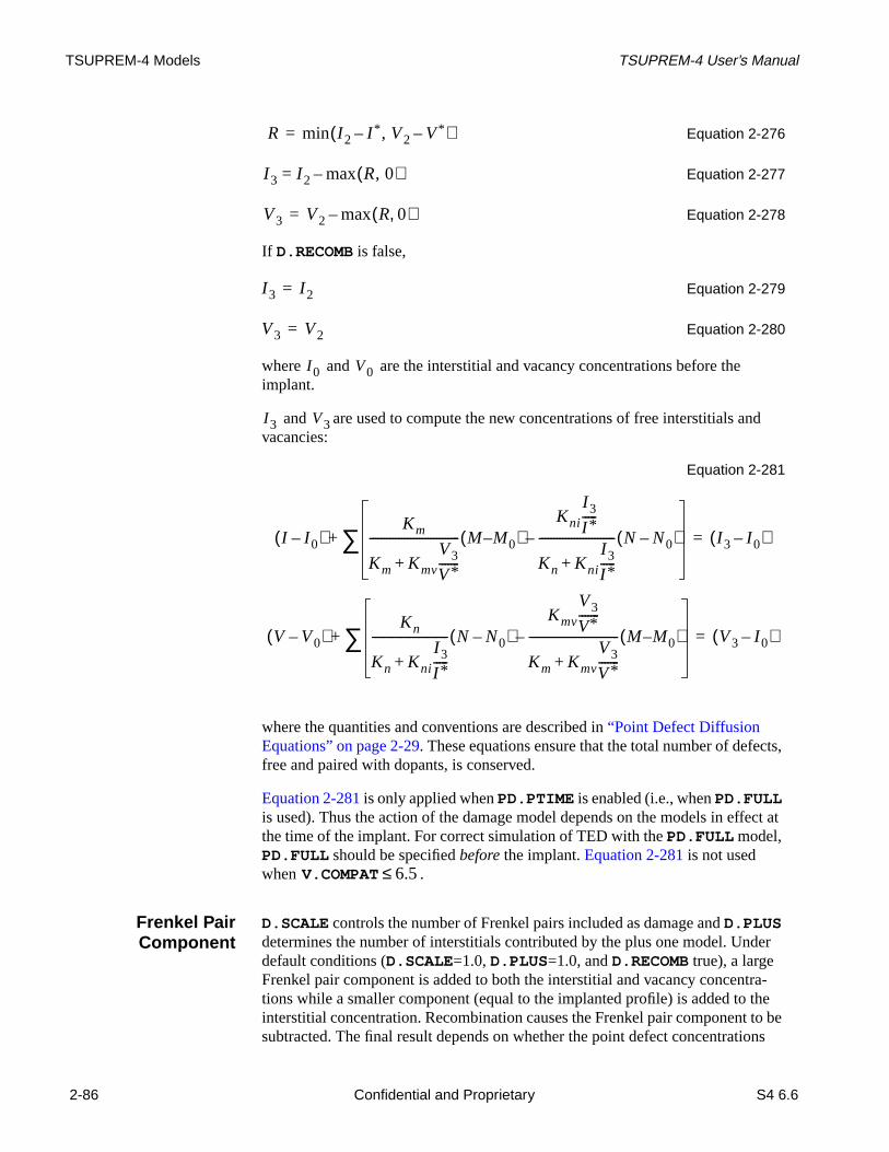
TSUPREM-4 Models TSUPREM-4 User’s Manual
d
cts,
ect at
er
ra-heto bens
Equation 2-276
Equation 2-277
Equation 2-278
If D.RECOMB is false,
Equation 2-279
Equation 2-280
where and are the interstitial and vacancy concentrations before theimplant.
and are used to compute the new concentrations of free interstitials anvacancies:
Equation 2-281
where the quantities and conventions are described in“Point Defect DiffusionEquations” on page 2-29. These equations ensure that the total number of defefree and paired with dopants, is conserved.
Equation 2-281 is only applied whenPD.PTIME is enabled (i.e., whenPD.FULLis used). Thus the action of the damage model depends on the models in effthe time of the implant. For correct simulation of TED with thePD.FULL model,PD.FULL should be specifiedbefore the implant.Equation 2-281 is not usedwhen .
Frenkel PairComponent
D.SCALE controls the number of Frenkel pairs included as damage andD.PLUSdetermines the number of interstitials contributed by the plus one model. Unddefault conditions (D.SCALE=1.0,D.PLUS=1.0, andD.RECOMB true), a largeFrenkel pair component is added to both the interstitial and vacancy concenttions while a smaller component (equal to the implanted profile) is added to tinterstitial concentration. Recombination causes the Frenkel pair component subtracted. The final result depends on whether the point defect concentratio
R min I 2 I * , V2– V*–( )=
I 3 I 2= max R, 0( )–
V3 V2 max R 0,( )–=
I 3 I 2=
V3 V2=
I 0 V0
I 3 V3
I I 0–( )Km
Km Kmv
V3
V*-------+
------------------------------- M M0–( )Kni
I 3
I *-----
Kn Kni
I 3
I *-----+
-------------------------- N N0–( )–∑+ I 3 I 0–( )=
V V0–( )Kn
Kn Kni
I 3
I *-----+
-------------------------- N N0–( )Kmv
V3
V*-------
Km Kmv
V3
V*-------+
------------------------------- M M0–( )–∑+ V3 I 0–( )=
V.COMPAT 6.5≤
2-86 Confidential and Proprietary S4 6.6
D Draft 6/26/98
TSUPREM-4 User’s Manual Ion Implantation
ti-ove
elim-po-
t
phiza-
fu-are
ld-
ng
ch the
es of
reimu-ens
uallyation
ame-
mask
before recombination ( and ) exceed the threshold for amorphization(MAX.DAMA). Below amorphization, the Frenkel pair components of the interstial and vacancy profiles cancel exactly, leaving the plus one component. Abamorphization, the interstitial and vacancy components are limited toMAX.DAMA; the excess interstitials produced by the plus one component are inated. Note that the amorphization is calculated locally, so the plus one comnent of damage remains in portions of the structure that are not amorphized.
Using theImplant Damage
Model
The default parameter values are expected to give reasonable results in moscases. However, you might consider the following modifications:
• You can simplify the calculation by settingD.SCALE=0.0. The result is thescaled plus one model as used at Stanford. Note that the effects of amortion are lost when this is done.
• You can modify the amorphization threshold by reducingMAX.DAMA. Thiscauses amorphization effects to appear at lower doses.
• D.SCALE can be reduced to model the effects of self-annealing duringimplantation.
• D.PLUS can be adjusted to change the amount of transient-enhanced difsion. This may be necessary for modeling situations in which interstitials bound in clusters after an implantation.
• To model the accumulation of damage in consecutive implants, you shouspecify^D.RECOMB in all implants except the last. This allows the full damage produced by each implant to accumulate, with recombination occurrionly after the last one.
The damage model can produce concentrations of point defects that are mugreater than those produced by oxidation. Accurate simulation of diffusion inpresence of such high defect concentrations requires that thePD.FULL diffusionmodel be used. Note that very small time steps are required in the initial stagdiffusion following an implant with damage. It is suggested that an initial timestep on the order of 10-6 minutes be used. If a larger initial time step is used, theis a delay during the first step while the start of the post-implant transient is slated. Use ofD.RECOMB reduces the peak point defect concentration and lessthe need for small time steps and thePD.FULL model. If thePD.FERMI modelis in effect when an implant withDAMAGE is specified, thePD.TRANS model isautomatically enabled.
Boundary Conditions for Ion Implantation
Ion implantation does not obey the reflecting boundary conditions that are usused at the left and right edges of the structure. Instead, the analytic implantextends the structure at a reflecting boundary out to infinity, while the MonteCarlo model uses the boundary condition specified by your choice of the parters,VACUUM, PERIODIC, orREFLECT. Thus there a loss of accuracy in theimplanted profile unless the lateral spread of the implant distribution is smallcompared to the distance between the edge of the structure and the nearest
I 1 V1
S4 6.6 Confidential and Proprietary 2-87
Draft Draft 6/26/98 6/

TSUPREM-4 Models TSUPREM-4 User’s Manual
n and
.
re
d fore left
t.
lys the
y neede the
e
pe
edge. In some cases, you may need to reflect the structure before implantatiotruncate it afterwards to ensure the accuracy of the implanted profile.
For Monte Carlo implants, three choices of boundary conditions are available
1. The default,PERIODIC, specifies that ions leaving one side of the structure-enter on the other side, with the same velocity.
This condition gives accurate answers for one-dimensional structures anstructures where the sequence and thickness of layers are the same at thand right edges.
2. REFLECT specifies that ions hitting the edge of the structure are reflectedback into the structure.
This condition is accurate forTILT=0 implants and for pairs of implants withopposite tilts.
3. VACUUM specifies that ions leaving the structure through the sides are los
This boundary condition is a poor approximation for most structures.
There are many situations (particularly single-tilted implants into two-dimen-sional structures) where none of the available boundary conditions is perfectaccurate. As with the analytical implant model, you lose some accuracy unleslateral spread of the implant distribution is small compared to the distancebetween the edge of the structure and the nearest mask edge. Again, you mato reflect the structure before implantation and truncate it afterwards to ensuraccuracy of the implanted profile.
Epitaxial GrowthTheEPITAXY statement (seepage 3-111) is used to model the epitaxial growthof silicon layers. An epitaxial layer can only be grown when the top layer of thstructure consists of single crystal silicon. The duration of the epitaxy step (inminutes) is specified with theTIME parameter. The initial temperature of the ste(in °C) is given by theTEMPERAT parameter. Linear variation of the temperaturover the step can be specified with theT.RATE or T.FINAL parameters. IfT.RATE is specified, the temperature varies as
Equation 2-282
where
• is the time since the start of the step
• is the diffusion temperature (in°C) at time
If T.FINAL is specified, the temperature varies as
Equation 2-283
Tc TEMPERAT T.RATE t×+=
t
Tc t
Tc TEMPERATT.FINAL TEMPERAT–( )
TIME-------------------------------------------------------------t+=
2-88 Confidential and Proprietary S4 6.6
D Draft 6/26/98
TSUPREM-4 User’s Manual Deposition
the
-
the
ulti-
truc-
gs
d
tion
If neitherT.RATE norT.FINAL is specified, the temperature is constant. Thephysical coefficients that depend on temperature are presumed to be valid inrange 800 to 1250°C, but temperatures outside this range may be specified.
Layer Thickness
The thickness of the epitaxial layer must be specified with theTHICKNES param-eter. The grid distribution within the epitaxial layer can be controlled with theDY,YDY, andSPACES parameters, as described in“Changes to the Mesh During Processing” on page 2-7.
Incorporation of Impurities
One or more impurities may be incorporated into the growing layer by using parametersANTIMONY, ARSENIC, BORON, andPHOSPHOR to indicate the con-centrations of impurities present in the ambient gas. The concentrations of mple impurities can be specified with these parameters. Impurities can also bespecified using theIMPURITY andI.CONC parameters. For a single impurity,the resistivity may be specified in place of the impurity concentration.
Diffusion of Impurities
The diffusion equations are solved for all the mobile species present in the sture during the epitaxial growth step (see“Diffusion of Impurities” on page 2-15and“Diffusion of Point Defects” on page 2-28).The epitaxial growth is dividedinto diffusion steps proportional in length to the thicknesses of the grid spacinin the deposited layer. An epitaxial step that specifies five grid spaces in thedeposited layer is simulated by five diffusion steps.
DepositionTSUPREM-4 models the deposition of material layers at temperatures lowenough that impurity diffusion can be ignored during the deposition. TheDEPOSITION statement specifies the deposition of a material on the exposesurfaces of the existing structure (seepage 3-84). The material to be deposited isspecified by one of the seven logical parameters for identifying a material:SILICON , OXIDE, OXYNITRI, NITRIDE , POLYSILI , ALUMINUM, orPHOTORES; or by specifying the name of the material with theMATERIAL state-ment.
Layer Thickness
The thickness of the deposited layer must be specified with theTHICKNESparameter. The deposition is conformal, i.e., all points within a distance ofTHICKNES of the exposed surface are included in the new layer. The generaof the mesh in the new layer and the use of theDY, YDY, SPACES andARC.SPAC
S4 6.6 Confidential and Proprietary 2-89
Draft Draft 6/26/98 6/

TSUPREM-4 Models TSUPREM-4 User’s Manual
2-
con-
inien-
or
magead
d. The
n
linescu- such
parameters are described in“Changes to the Mesh During Processing” on page7.
Incorporation of Impurities
The deposited layer can be doped with one or more impurities. The impurity centrations are specified with theANTIMONY, ARSENIC, BORON, andPHOSPHOR parameters. Impurities can also be specified using theIMPURITYandI.CONC parameters. For a single impurity, the resistivity may be specifiedplace of the impurity concentration. If single crystal silicon is deposited, its ortation the same as the substrate orientation specified by theINITIALIZE state-ment.
Photoresist Type The type of deposited photoresist can be specified as eitherPOSITIVE orNEGATIVE. All photoresist in the structure is assumed to be of this type. Thistype of resist is used by theDEVELOP statement to determine whether exposed unexposed resist should be removed (see“Masking, Exposure and Developmentof Photoresist” on page 2-90).
Note:The implementation of the deposition capability assumes that the topsurface is exposed, and allows the right side of the structure to either beexposed or on a reflecting boundary. Deposition should not be attemptedwhen the left or bottom sides of the structure are exposed, or when thetop surface is not exposed.
Masking, Exposure and Development of PhotoresistMasking, exposure, and development of photoresist are used to transfer an ion a mask to a structure on a semiconductor wafer. Masking information is refrom a mask file created byTMA Layout—IC Layout Interface. For each masklevel, the starting and ending coordinates of each opaque region are recordeEXPOSE statement uses thesex coordinates to determine which portions of thephotoresist in a structure should be marked as exposed (in the photographicsense). TheDEVELOP statement removes all positive photoresist that has beemarked as exposed, or all negative photoresist that has not been marked asexposed.
TSUPREM-4 uses idealized exposure and development models: photoresist always have vertical sidewalls, positioned directly beneath mask edges. If acrate physical models of photolithographic processes are needed, a simulatorasDepict should be used.
2-90 Confidential and Proprietary S4 6.6
D Draft 6/26/98

TSUPREM-4 User’s Manual Etching
-
e
-
one
e
st
l. It
of
EtchingTSUPREM-4 allows the removal of material layers or portions of layers usingtheETCH statement (seepage 3-91). The material to be removed is specified byone of the seven logical parameters for identifying a material:SILICON , OXIDE,OXYNITRI, NITRIDE , POLYSILI , ALUMINUM, orPHOTORES; or by specify-ing the name of the material with theMATERIAL parameter. If a material is specified, only regions of that material are subject to removal; if no material isspecified, the entire structure is subject to removal.
Defining the Etch Region
The region to be removed (theetch region) can be defined in one of six ways:
1. TheTRAPEZOI parameter specifies that removal occurs where etchablematerial appears at the exposed surface of the structure. The shape of thregion is specified with theTHICKNES, ANGLE, andUNDERCUT parameters.In a planar substrate, the region to be removed is trapezoidal in shape.“TheTrapezoidal Etch Model” on page 2-92 describes theTRAPEZOI model.
2. TheISOTROPI parameter specifies that removal occurs in a region withinthe givenTHICKNES of the exposed surface.
3. TheLEFT or RIGHT parameter specifies that removal occurs to the left orright of a line defined by the coordinatesP1.X , P1.Y , P2.X , andP2.Y .
4. TheSTART, CONTINUE, andDONE parameters are used to specify an arbitrary region to be removed. A series ofETCH statements are given, each oneusing theX andY parameters to specify the location of one point on a polygthat defines the etch boundary. The firstETCH statement in the series uses thSTART parameter, the last uses theDONE parameter, and the statements inbetween use theCONTINUE parameter. The polygon defining the region to bremoved is closed automatically by connecting the last point to the first. Amaterial specification can appear on any of theETCH statements; if more thanone of theETCH statements contains a material specification, all but the laare ignored.
5. TheALL parameter specifies that the entire structure is subject to removais only useful with a material specification.
6. TheOLD.DRY parameter specifies that the region to be removed consistsall points within a vertical distanceTHICKNES of the top surface. This model(called theDRY model inTSUPREM-4 versions 5.0 and older) has beensuperseded by theTRAPEZOI model.
If no region is specified,TRAPEZOI is assumed.
S4 6.6 Confidential and Proprietary 2-91
Draft Draft 6/26/98 6/

TSUPREM-4 Models TSUPREM-4 User’s Manual
pe.di-
d).
etch
mask-sk-
ficu-
e
esses,
oowedrface
Step
h ofus a
Removal of Material
Etching proceeds from exposed surfaces through material of the specified tyThus a point within the structure is removed if it meets all of the following contions:
• The material at the point is of the specified type (or no material is specifie
• The point lies within the etch region.
• There is a continuous path, through the specified material and within the region, from the point to an exposed surface.
Note:It is not possible to etch holes in a structure, but it is possible to cut astructure into two or more pieces with theETCH statement. All piecesexcept the one with the largest area are discarded. A warning is printedfor each detached piece of the structure that is removed.
The Trapezoidal Etch Model
TheTRAPEZOI etch model provides a simple but flexible approximation to anumber of real etching processes. The location of the etch is determined by ing layers (i.e., layers of nonetchable material), and thus does not require madependent coordinates to be specified. This means theTRAPEZOI model can beused with the photoresist masking, exposure, and development capabilities oTSUPREM-4 to create process descriptions that are independent of any partlar mask layout.
Parameters TheTRAPEZOI model uses the three parametersTHICKNES, ANGLE, andUNDERCUT to specify the shape of the region to be removed.THICKNES speci-fies the vertical depth (in microns),ANGLE specifies the angle (in degrees) of thresulting sidewalls, andUNDERCUT specifies the horizontal penetration (inmicrons) of the etch under the edges of the masking layer.
These parameters can be used to approximate a number of real etching procincluding combinations of vertical and isotropic etches, V-groove etches, andetches that produce retrograde sidewall profiles.
Etch Steps An etch with theTRAPEZOI model is done in three steps:
1. A vertical etch to depthTHICKNES is performed. This etch does not apply tportions of the surface that are masked by nonetchable materials or shadby etchable or nonetchable materials, nor is it used on segments of the suthat form an angle greater thanANGLE to the horizontal.
2. A horizontal etch is performed. Surfaces that were exposed at the start of1 are etched horizontally by the distanceUNDERCUT. Surfaces that wereexposed during Step 1 are etched by a distance proportional to the lengttime between when they first became exposed and the end of Step 1. Th
2-92 Confidential and Proprietary S4 6.6
D Draft 6/26/98

TSUPREM-4 User’s Manual Etching
of
verti-
ofstepnt of
etch-
case
us
sidewall exposed 3/4 of the way into Step 1 is etched horizontally by 1/4 UNDERCUT. (An exception is made when anANGLE greater than 90° is spec-ified; this case is described below.)
3. Where overhangs of etchable material are present at the end of Step 2, acalupwards etch (i.e., in the direction) is performed. On surfaces thatwere exposed at the start of Step 2, this etch is to a distanceUNDERCUT; onsurfaces that were first exposed during the course of Step 2, the distancethis etch is reduced in proportion to the time from the start of Step 2. This approximates the undercutting of the mask due to the isotropic componethe etch.
Etch Examples Figure 2-2 shows a number of examples of theTRAPEZOI etch model. In eachcase, an etchable layer (light and medium gray) is partially masked by a nonable layer (dark gray).
Simple Structure When theTHICKNES, ANGLE, andUNDERCUT parameters satisfy the relation-ship
Equation 2-284
the etch approximates a vertical etch with an isotropic component. This is thewhenever two or fewer of the parametersTHICKNES, ANGLE, andUNDERCUTare specified.Figure 2-2 (a) and (b) show the effect of this type of etch on variostarting structures.
y–
THICKNESUNDERCUT-------------------------- tan ANGLE( )=
S4 6.6 Confidential and Proprietary 2-93
Draft Draft 6/26/98 6/

TSUPREM-4 Models TSUPREM-4 User’s Manual
the
1 of
cing has
ch. side-
eft sup-
etchhel-
rti-
The left half ofFigure 2-2(a) shows the result when etching a planar substrate:etch region is a trapezoid of depthTHICKNES, extending a distanceUNDERCUTbeneath the mask edge, and with a sidewall slope ofANGLE degrees. The righthalf of Figure 2-2(a) shows the result when etching a nonplanar surface: Step the etch sequence etches the exposed surface vertically to a depth ofTHICKNESmicrons. Step 2 etches the resulting sidewall in the horizontal direction, produan undercutting of the mask and the sloped sidewall. In this case Step 3 alsoan effect, etching upwards from the undercut region. Thus, thehook in the finalsilicon profile is the result of approximating the isotropic component of the etIn every case, the intersection between the bottom of the etch region and thewall occurs directly under the edge of the mask.
Structure withOverhangs
Figure 2-2 (b) shows the result of etching a more complicated structure. The lside of the figure shows the effects of overhangs. The vertical etch (Step 1) ispressed where the silicon is shadowed by the masking layer. The horizontal (Step 2) applies to the entire structure, including the near-vertical sidewalls stered under the overhang. The right half of the figure shows what happens toexposed near-vertical sidewalls: Again the horizontal surfaces are etched ve
Figure 2-2 Examples of the trapezoidal etch model
2-94 Confidential and Proprietary S4 6.6
D Draft 6/26/98

TSUPREM-4 User’s Manual Etching
ginaleriale
nter-
, the pro-pth of
on,d of
ang-e- 1
e sur-all”
cally in Step 1, then both the sidewalls created by the vertical etch and the orinear-vertical sidewalls are etched horizontally in Step 2. The effect is that matis removed if it can be etched byeither the vertical (anisotropic) component or thhorizontal (isotropic) component of the etch.
ComplexStructures
Figure 2-2 (c) and (d) show what happens whenEquation 2-284 is not satisfied. InFigure 2-2 (c) you haveTHICKNESS/UNDERCUT < tan(ANGLE). In this case thesloped sidewall of the etch extends out under the opening in the mask. The isection between the bottom of the etch region and the sidewall is no longerdirectly beneath the edge of the mask. If the mask opening is narrow enoughbottom of the etch region disappears entirely, resulting in a V-groove etch. Toduce this etch shape, Step 1 of the etch process is modified to reduce the dethe vertical etch near the edges of the mask opening. Note that in this situatieven the tiniest speck of nonetchable material can produce a triangular moununetched material in the final structure.
Figure 2-2 (d) shows the case whereANGLE > 90. In this case, the bottom of theetched region is wider than the opening in the masking layer, producing overhing sidewalls. This etch is accomplished by modifying Step 2 of the etch procdure to etch further horizontally at the bottom of the sidewalls formed by Stepthan at the top. The apparent etch depth of 0.5 microns at the right side of thmask opening is the result of a 0.3 micron vertical etch of the original slopedface (Step 1) followed by a 0.4 micron horizontal etch of the sloped “bottom wthat results from Step 1.
S4 6.6 Confidential and Proprietary 2-95
Draft Draft 6/26/98 6/

TSUPREM-4 Models TSUPREM-4 User’s Manual
the thehe
diffu-ound-for
of
To
cess-n
ninthis
rys-
iffu- the
s are
n for
Modeling Polycrystalline MaterialsThe behavior of dopants in polycrystalline materials is strongly influenced byboundaries between crystalline grains. Dopant atoms tend to segregate frominterior of a grain to the boundaries, which provide paths for rapid diffusion. Trate of segregation depends on the rate of grain growth, while the number of sion paths along the boundaries depends on the grain size. In addition, the baries of the polycrystalline material act like grain boundaries, providing sites electrically inactive dopant atoms and paths for diffusion.
The diffusion equations for the grain-interior and grain-boundary componentsthe doping profile are solved separately. The equations are coupled by termsdescribing the segregation between the grain interiors and grain boundaries.determine the rate of segregation and the density of grain-boundary diffusionpaths, you also solve for the growth in grain size during high-temperature proing. The boundaries of the polycrystalline region are included as explicit graiboundaries in the diffusion and segregation equations.
The poly model has been implemented inTSUPREM-4 in collaboration withGEC Plessey Semiconductors (GPS) in the UK. The physical model has beedeveloped at GPS and GEC-Marconi Materials Technology, Caswell, UK withthe collaborative European ESPRIT project STORM. The key contributors to work were S. K. Jones, C. Hill, and A. G. O’Neill[62]-[65]. Although the modelwas developed and optimized for polysilicon, it can be applied to other polyctalline materials (e.g., silicides).
Diffusion
Diffusion inGrain Interiors
Redistribution of dopants in polycrystalline materials occurs by the parallel dsion of dopants through the interiors of grains and along grain boundaries. Ingrain interiors diffusion of the active dopant is given by
Equation 2-285
where is the active concentration in the grain interior and the other symboldescribed in“Diffusion of Impurities” on page 2-15. The diffusivity and elec-tric field in the grain interior are calculated from the electron concentratio
, which is in turn calculated from the doping concentrations . accountsthe segregation of dopant to grain boundaries, as described in“SegregationBetween Grain Interior and Boundaries” on page 2-98. (The calculation of theactive concentration is described in“Activation of Impurities” on page 2-23, andthe calculation of the electron concentration is described in“Diffusion of Impuri-ties” on page 2-15.)
∂cg
∂t-------- ∇ Dg– ∇cg zscg
qEg
kT---------–
G–⋅–=
cgDg
Egng cg G
2-96 Confidential and Proprietary S4 6.6
D Draft 6/26/98

TSUPREM-4 User’s Manual Modeling Polycrystalline Materials
ation per
f theher
is
erial
u-
,nd-
inthe is
e
Grain BoundaryStructure
Diffusion along grain boundaries is described in terms of the dopant concentrper unit area of grain boundary and the average area of grain boundariesunit volume
Equation 2-286
where is the average area of grain boundaries per unit volume in the bulk opoly layer and accounts for the dopant at interfaces between poly and otmaterials (or ambient). is inversely proportional to the average grain size
Equation 2-287
whereG.DENS is a geometrical factor specified on theMATERIAL statement. is a function of position defined by the fact that its integral over any area
equal to the length of the polysilicon interface passing through that area:
Equation 2-288
The concentration of dopants in the grain boundaries per unit volume of matis then given by
Equation 2-289
Diffusion AlongGrain
Boundaries
The diffusion of dopant in the grain boundaries is given by
Equation 2-290
The diffusivity and electric field along the grain boundaries are calclated from the electron concentration ; is calculated as inEquation 2-39except that the net donor and acceptor concentrations are calculated fromthe equilibrium dopant concentrations in the grain interior near the grain bouary.
AnisotropicDiffusion
is a tensor that describes the diffusion paths available to dopant in the graboundaries. It is composed of two parts: . describes available paths within the bulk of the poly layer. For a horizontal poly layer, itgiven by
Equation 2-291
whereF11 andF22 are parameters on theMATERIAL statement. Because of thecolumnar grain structure,F22 is larger thanF11, which implies that diffusionthrough the layer is faster than diffusion parallel to the layer. describes th
cgb
ρ′ ρ δif+=
ρδif
ρ Lg
ρ G.DENSLg
-------------------=
δifLif
δif Ad∫ Lif=
wgb ρ′cgb=
∂wgb
∂t------------ ∇ FDgb– ∇cgb zscgb
qEgb
kT------------–
G+⋅–=
DgbEgbngb ngb
cgb K⁄
FF Fb 1 Fbu–( )Fif+= Fb
Fb diag F11Lg
--------- F22Lg
---------, =
Fif
S4 6.6 Confidential and Proprietary 2-97
Draft Draft 6/26/98 6/

TSUPREM-4 Models TSUPREM-4 User’s Manual
on-
ial
thatce,
grain
theionlan-
es onion is
terial
available paths for diffusion along material interfaces. In the vicinity of a horiztal interface it has the value
Equation 2-292
For the interface between polysilicon and silicon, the phenomenon of interfacbreak-up accompanied by epitaxial realignment can occur, as described in“Inter-face Oxide Break-up and Epitaxial Regrowth” on page 2-101. is the fractionof the polysilicon/silicon interface that has broken up. For layers or interfacesare not horizontal, and are rotated by the angle of the layer or interfarespectively, with respect to thex axis.
Segregation Between Grain Interior and Boundaries
When dopant is initially introduced into a polycrystalline material, some of thedopant occupies sites in the interior of a grain and some occupies sites on aboundary. The initial segregation of dopant is given by
Equation 2-293
Q.SITES , CG.MAX, andGSEG.INI are parameters on theIMPURITY state-ment; they represent the density of available sites on grain boundaries and ingrain interiors and the initial segregation entropy, respectively. In the case of implantation and describe the additional dopant introduced by the imptation; dopant that is present before the implantation is not redistributed.)
Dopant atoms are free to move between sites in the interior of a grain and sitthe grain boundary during high-temperature processing. The rate of segregatgiven by
Equation 2-294
The segregation coefficient is given by[66]
Equation 2-295
whereGSEG.0 andE.SEG are parameters on theIMPURITY statement. Thesegregation velocities associated with the bulk of the poly region and the mainterfaces are given by
Equation 2-296
Equation 2-297
Fif diag δif 0,( )=
Fbu
Fb Fif
cgbQ.SITESCG.MAX-----------------------GSEG.INI cg=
cg cgb
G ρqb 1 Fbu–( )δif qif+( ) fgbcg fg
cgb
K-------–
=
K
KQ.SITESCG.MAX-----------------------GSEG.0 exp
GSEG.EkT
------------------- =
qb1
ALPHA----------------
∂Lg
∂t--------- e
4Lg-----Dg+=
qif VELIF.0 exp VELIF.EkT
-----------------------– =
2-98 Confidential and Proprietary S4 6.6
D Draft 6/26/98

TSUPREM-4 User’s Manual Modeling Polycrystalline Materials
-
isd in
altra-
mnsagetorined
heres by
pro-
ci-
thero-s
whereALPHA is a parameter on theMATERIAL statement,VELIF.0 andVELIF.E are parameters on theIMPURITY statement. and are the fractions of unfilled interior and boundary sites:
Equation 2-298
Equation 2-299
where the sum is taken over all the dopant species present in the structure.the fraction of the polysilicon/silicon interface that has broken up, as describe“Interface Oxide Break-up and Epitaxial Regrowth” on page 2-101.
When calculating the segregation between poly and another material, the tot(active plus inactive) concentration in the grain interior is used for the concention in poly inEquation 2-70.
Grain Size Model
The grains in the polycrystalline material are assumed to be oriented as coluthat extend through the wafer. The structure is characterized by , the avergrain size in the lateral direction (i.e., in the plane of the layer), and , a vecdescribing the orientation of the columnar grains. The grain size can be examby specifying thelgrain solution variable on theSELECT statement:
This returns the average grain size in microns or a negative value at nodes wthe material is amorphous. (Note that the grain size is reported in centimeterMichelangelo andTMA Visual.)
Initial Grain Size The initial grain size is determined by the temperature of the poly deposition cess and the value of theGSZ.LIN parameter on theDEPOSITION statement. IfGSZ.LIN is false, the grain size in the layer is constant[67]:
Equation 2-300
whereFRAC.TA, MIN.GRAI , GRASZ.0, GRASZ.E, andTEMP.BRE areparameters on theMATERIAL statement, is the deposition temperature (spefied on theDEPOSITION statement) in°C, and is the deposition temperaturein Kelvins.THICKNES is the thickness of the deposited layer, as specified onDEPOSITION statement. is the thickness of the amorphous silicon layer pduced by low-temperature deposition. IfGSZ.LIN is true, the grain size increaselinearly from the bottom of the layer to the top:
fg fgb
fg 1cg
CG.MAX-------------------–=
fgb 1cgb
Q.SITES-----------------------∑–=
Fbu
SELECT Z=LGRAIN
Lgξ
Lg
max FRAC.TA ta MIN.GRAI,×( ) Tc TEMP.BRE≤
GRASZ.0 expGRASZ.E–
kT----------------------------
THICKNES Tc TEMP.BRE>
=
TcT
ta
S4 6.6 Confidential and Proprietary 2-99
Draft Draft 6/26/98 6/

TSUPREM-4 Models TSUPREM-4 User’s Manual
ed oni-i-rted inlp. size.
isls the(see
and are
Equation 2-301
where is the distance from the bottom of the layer.
For high-temperature depositions, grain size depends on the thickness specifitheDEPOSITION statement. Dividing a deposition into multiple smaller depostions produces different results for the grain size. For low-temperature depostions, the material is assumed to be amorphous (a negative grain size is repoprinting or plotting). The initial grain size (above) is calculated from the actuathickness of the amorphous layer at the beginning of the next diffusion steThus, successive amorphous depositions are merged in computing the grain
Grain Growth The growth of the grains during high-temperature processing is given by[67]
Equation 2-302
whereGEOM, GAMMA.0, andGAMMA.E are parameters on theMATERIAL state-ment, is the silicon self-diffusivity in the vicinity of a grain boundary, the surface energy per atom associated with the grain boundary, modesegregation drag effect, and models epitaxial regrowth of the poly layer “Interface Oxide Break-up and Epitaxial Regrowth” on page 2-101).
ConcentrationDependence
The silicon self-diffusivity is given by
Equation 2-303
where is the intrinsic carrier concentration at the processing temperature is the electron concentration in the grain interior. The components of
given by
Equation 2-304
Equation 2-305
Equation 2-306
Lg
max FRAC.TA ta MIN.GRAI,×( ) Tc TEMP.BRE≤
MIN.GRAI 2GRASZ.0+ expGRASZ.E–
kT----------------------------
z Tc TEMP.BRE>
=
z
ta
∂Lg
∂t---------
1Lg-----GEOM GAMMA.0exp
GAMMA.E–kT
---------------------------- DSi
Egb
kT-------- Fseg GEA×××××=
DSi EgbFseg
GEA
DSi DSix
DSi+ ni
ng-----
DSi
_ ng
ni-----
DSi= ng
ni-----
2+ + +=
ning DSi
DSix
DSIX.0 exp DSIX.EkT
-------------------– =
DSi+
DSIP.0 exp DSIP.EkT
-------------------– =
DSi_
DSIM.0 exp DSIM.EkT
-------------------– =
2-100 Confidential and Proprietary S4 6.6
D Draft 6/26/98

TSUPREM-4 User’s Manual Modeling Polycrystalline Materials
sent
on aurewing
de
ion
Equation 2-307
whereDSIX.0 , DSIX.E , DSIP.0 , DSIP.E , DSIM.0 , DSIM.E , DSIMM.0,andDSIMM.E are parameters on theMATERIAL statement.
Grain SurfaceEnergy
The grain boundary energy is given by[67]-[69]
Equation 2-308
Equation 2-309
whereGBE.0, GBE.H, andGBE.1 are parameters on theMATERIAL statement,and is the thickness of the polycrystalline layer. Note thatGBE.0 andGBE.1 are in units of electron volts per atom; to convert from values given ineV/µm2 you must multiply by 6.25 × 10⁻⁸ µm2/atom.
Segregation Drag The segregation drag effect reduces the grain growth rate[70]:
Equation 2-310
Q.SITES is a parameter on theIMPURITY statement,NSEG is a parameter ontheMATERIAL statement, and the summation is taken over the impurities prein the structure.
Interface Oxide Break-up and Epitaxial Regrowth
A thin interfacial oxide layer is typically present between a deposited polysiliclayer and any underlying single-crystal silicon. This interfacial oxide presentsbarrier to epitaxial realignment of the poly layer. With sufficient high-temperatprocessing, the oxide layer breaks up into a discrete set of small spheres, alloepitaxial regrowth of the poly to proceed.
Oxide Break-Up The oxide break-up is modeled by the formation of voids in the interfacial oxilayer[71]-[74]. The radius of the voids increases as
Equation 2-311
where is a constant, is the initial oxide thickness, and is the activatenergy of the break-up process. is initialized to zero whenever poly is
DSi=
DSIMM.0 exp DSIMM.EkT
-----------------------– =
EgbGBE.0
1 GBE.H f n+------------------------------- GBE.1
Lg
tpoly----------+=
f n
Lg
2t poly Lg–------------------------- Lg tpoly<
Lg
tpoly---------- Lg tpoly≥
=
t poly
Fseg 1cgb
Q.SITES-----------------------∑+
NSEG–
=
Rvoid
dRvoid
dt---------------
βtox3
------ expEbu
kT--------–
×=
β tox EbuRvoid
S4 6.6 Confidential and Proprietary 2-101
Draft Draft 6/26/98 6/

TSUPREM-4 Models TSUPREM-4 User’s Manual
s
recial
ces
ch
ce)s for
deposited on exposed silicon. The fraction of the interface that is broken up igiven by
Equation 2-312
where is the areal density of the voids. The parameters for the model aspecified in terms of a characteristic break-up time for the thinnest (5Å) interfaoxide layers
Equation 2-313
whereTBU.0 andTBU.E are parameters on theMATERIAL statement.Equation2-311 can be then written
Equation 2-314
In the present implementation, you assume that all poly/single-crystal interfashare a common oxide thickness given by
Equation 2-315
whereTOXIDE is a parameter on theMATERIAL statement.
EpitaxialRegrowth
Epitaxial regrowth is modeled by increasing the poly grain size to a value mularger than the thickness of the poly layer. This grain growth is described byin Equation 2-292 for the grain size:
Equation 2-316
The first term models the propagation of the regrowth through the poly layer,while the second term (which is nonzero only at the silicon/polysilicon interfaserves as a driving force for epitaxial regrowth from the interface. Parameterthis model are given by
Equation 2-317
Equation 2-318
whereDLGX.0, DLGX.E, EAVEL.0 , andEAVEL.E are parameters on theMATERIAL statement.
Fbu 1 exp πNEARvoid2
–( )–=
NEA
tbu5Å
3
πNEAβ--------------------- exp
Ebu
kT-------- TBU.0 exp TBU.E
kT----------------–
⋅=×≡
dRvoid
dt---------------
1tbu------ 5Å
tox-------
3 1
πNEA
------------------=
tox TOXIDE=
GEA
GEA DLg∇2
Lg FbuvEAδif+=
DLgDLGX.0 exp DLGX.E
kT-------------------–
⋅=
vEA EAVEL.0 exp EAVEL.EkT
-----------------------– ⋅=
2-102 Confidential and Proprietary S4 6.6
D Draft 6/26/98
TSUPREM-4 User’s Manual Modeling Polycrystalline Materials
e foron-me of
f thesdesnehile itt the
total
f the
ary
r in
but.
is-revitydary
Using the Polycrystalline Model
For each dopant in a polycrystalline material there are two solution values: onthe total doping concentration at each node in the structure and one for the ccentration in grain boundaries. The total concentration is accessed by the nathe impurity, e.g.
The grain-boundary component is accessed with thegb() function on theSELECTstatement:
The grain-boundary component includes the dopant stored at the boundary opolycrystalline material. Although this dopant is confined to the boundary, it ireported as if it were evenly distributed over the areas associated with the noon the boundary. Thus, the concentration at the boundary of the polycrystalliregion is discontinuous and depends on the grid spacing at the boundary. Wis not possible to resolve the profile at the boundary, care has been taken thatotal dose at and near the boundary is correct.
The grain-interior component can be computed as the difference between theconcentration and the grain-boundary concentration:
The grain-boundary component is stored as a separate impurity. The name ograin-boundary impurity is created from the name of the base impurity byprependingGB_ to the name. Thus, you set the diffusivities of the grain-boundcomponent of boron with
The grain size can be examined by specifying thelgrain solution variable on theSELECT statement:
This returns the average grain size in microns; a negative value is returned fonodes where the material is amorphous. (Note that the grain size is reportedcentimeters byMichelangelo andTMA Visual.)
The polycrystalline models address the need to model polycrystalline silicon,the implementation allows them to be used for other polycrystalline materialsThe polycrystalline model is enabled or disabled for a material by thePOLYCRYSparameter on theMATERIAL statement. When the polycrystalline models are dabled with^POLYCRYS, the impurity concentrations in the grain boundaries aset to zero and the corresponding equations are not solved. Thus, the diffusireduces to that of the grain interiors. To compensate for the lack of grain bounsolutions, the grain interior diffusivity is multiplied byFGB in materials for whichthe polycrystalline models are disabled.FGB is a parameter on theIMPURITYstatement.
SELECT Z=LOG10(BORON)
SELECT Z=LOG10(GB(BORON))
SELECT Z=LOG10(BORON-GB(BORON))
IMPURITY IMP=GB_BORON MAT=POLY DIX.0= . . .
SELECT Z=LGRAIN
S4 6.6 Confidential and Proprietary 2-103
Draft Draft 6/26/98 6/

TSUPREM-4 Models TSUPREM-4 User’s Manual
lne-for-ndsis-.
therto-re
c-
tion
id
s is
the-he
Electrical CalculationsTSUPREM-4 calculates a limited set of electrical characteristics along verticacut-lines through a simulation structure. This is accomplished by saving the odimensional Poisson’s equation for specified bias conditions. The electrical inmation consists of the threshold voltage, the low-frequency, high-frequency, adeep-depletion MOS capacitances, spreading resistance profile and sheet retances for all diffused regions in all semiconductor layers within the structureThis information can be saved in a file for later plotting by using theOUT.FILEparameter in theELECTRICAL statement (seepage 3-165).
TSUPREM-4 extends the structure automatically if the bias voltage expandsdepletion region beyond the bottom of a simulation structure. Also, the grid fosimulation may not be adequate for solving Poisson’s equation; the grid is aumatically extended if necessary. The extended structure and the added grid atemporary and are used only for the electrical extraction.
Automatic Regrid
TheE.REGRID in theMETHOD statement specifies the automatic regrid for eletrical extraction. The automatic regrid follows the two steps.
1. The first step regrids the region in the estimated maximum depth of depleregion. The minimum and maximum grid spacing are determined by theincremental depletion depth calculated for given bias conditions.
2. The second step generates more dense grids near the surface. This regrresults in the accurate calculation specially for the quantum effect.
Placement of grid near the surface is controlled by the thickness of the regridregion (E.TSURF), the first grid spacing at the surface (E.DSURF) and the incre-mental ratio of grid spacing (E.RSURF) in theMETHOD statement.
Poisson’s Equation
The form of Poisson’s equation solved in semiconductor and insulator region
Equation 2-319
where is the dielectric constant in vacuum, is the potential,p is the holeconcentration,n is the electron concentration, and and are the sums ofionized electrically active donor and acceptor impurity concentrations, respectively. TheEPSILON parameter is the relative dielectric constant specified in tMATERIAL statement (seepage 3-212). The potential in a semiconductor regionis defined as the potential of the edge of the conduction band.
∂∂x----- EPSILON ε0
∂ψ∂x-------
q p n– Nd+
Na
_–+( )– semiconductor
0 insulator
=
ε0 ψNd
+Na
_
2-104 Confidential and Proprietary S4 6.6
D Draft 6/26/98

TSUPREM-4 User’s Manual Electrical Calculations
trond in a
con-
ions
entions.ith
cen-
Boltzmann andFermi-Dirac
Statistics
Either Boltzmann or Fermi-Dirac statistics may be used to represent the elecand hole concentrations in semiconductor regions. The type of statistics usesemiconductor material is specified with theBOLTZMAN parameter in theMATERIAL statement. If Boltzmann statistics are used, the electron and holecentrations are given by
Equation 2-320
Equation 2-321
where is the electron quasi-Fermi potential and is the hole quasi-Fermpotential. If Fermi-Dirac statistics are used, the electron and hole concentratiare given by
Equation 2-322
Equation 2-323
where is the Fermi-Dirac integral of one-half order. The parametersN.CONDUC, N.VALENC, andBANDGAP are specified in theMATERIAL state-ment. The temperatureT used for the device simulation is specified with theTEMPERAT parameter in theELECTRICAL statement.
Ionization ofImpurities
Either complete or incomplete ionization of impurities may be used to represthe ionized donor and acceptor impurity concentrations in semiconductor regThe type of impurity ionization used in a semiconductor material is specified wtheIONIZATI parameter in theMATERIAL statement. If complete ionization isused, the ionized donor and acceptor impurity concentrations are given by
Equation 2-324
Equation 2-325
If incomplete ionization is used, the ionized donor and acceptor impurity contrations are given by[77]
n N.CONDUCexpq ψ φn–( )
kT-----------------------=
p N.VALENCexpq φp ψ–( ) BANDGAP–
kT----------------------------------------------------=
φn φp
n N.CONDUCF1 2⁄q ψ φn–( )
kT-----------------------=
p N.VALENCF1 2⁄q φp ψ–( ) BANDGAP–
kT----------------------------------------------------=
F1 2⁄
Nd+
Nd=
Na
_Na=
S4 6.6 Confidential and Proprietary 2-105
Draft Draft 6/26/98 6/

TSUPREM-4 Models TSUPREM-4 User’s Manual
tion the
ro.
n byolvee
atedd. Ater-m-
lec-
Equation 2-326
Equation 2-327
where and are the sums of the electrically active donor and acceptorimpurity concentrations, respectively. The parametersG.DONOR, E.DONOR,G.ACCEP andE.ACCEP are specified in theMATERIAL statement.
The potential in a conductor region is constant with a value given by
Equation 2-328
where is the conductor bias and theWORKFUNC parameter is specified in theMATERIAL statement. If any semiconductor regions are present in the simulastructure, is the electron affinity for the bottommost semiconductor layer instructure. The value of is specified with theAFFINITY parameter in theMATERIAL statement. If no semiconductor regions are present, is set to ze
SolutionMethods
Poisson’s equation is solved numerically using a three-point finite differenceapproach. Newton’s method is used to iteratively solve the nonlinear equatiolinearizing the equation at each iteration and using Gaussian elimination to sthe resulting tridiagonal system. The iteration is normally terminated when threlative change in the potential between successive iterations is less than theallowed error at each node in the structure. The iteration may also be terminwhen the maximum number of allowed Newton iterations has been performeminimum number of required iterations are performed before the iteration is minated. The allowed error, maximum number of iterations, and minimum nuber of iterations may be specified with theE.RELERR, E.ITMAX , andE.ITMINparameters, respectively, in theMETHOD statement.
Carrier Mobility
The mobilities of electrons and holes depend on the impurity concentration, etric field, and temperature. The mobility is given by[78], [79]
Equation 2-329
Nd+ Nd
1 G.DONORexpq ψ φn–( ) E.DONOR+
kT----------------------------------------------------+
---------------------------------------------------------------------------------------------------=
Na
_ Na
1 G.ACCEP1– exp
q φ ψ–( ) BANDGAP E.ACCEP+–kT
------------------------------------------------------------------------------+
----------------------------------------------------------------------------------------------------------------------------------=
Nd Na
ψ Vc WORKFUNCχ+–=
Vc
χχ
χ
µn GSURFNµ0n
1E
ECN.MU-------------------
+
-------------------------------------=
2-106 Confidential and Proprietary S4 6.6
D Draft 6/26/98

TSUPREM-4 User’s Manual Electrical Calculations
ntada-
hould
theent
d by
ra-umedlin-
Equation 2-330
where is the low-field mobility,E is the electric field, andECN.MU andECP.MU are the critical electric fields. The mobility used for calculating currealong semiconductor-insulator interfaces may be reduced by specifying degrtion factorsGSURFN andGSURFP which multiply the low field mobility. It isimportant to note that the factorsGSURFN andGSURFP are only applied at inter-faces between semiconductor and insulator. Everywhere else, these factors sbe considered to have values of unity.ECN.MU, ECP.MU, GSURFN, andGSURFPcan be specified on theMOBILITY statement (seepage 3-238).
TSUPREM-4 provides three alternatives—tabular form, the Arora model, andCaughey model—for specifying low field electron and hole mobilities dependon impurity concentration and temperature.
Tabular Form The low-field mobilities for the tabular form depend on the electrically activeimpurity concentration and device temperature. The mobilities are representethe table of values specified with theMOBILITY statement. Two-dimensionalinterpolation is used to obtain values of low-field mobility for impurity concenttion and temperature between the values in a table. The concentration is assto vary exponentially and the temperature and mobility are assumed to vary early.TSUPREM-4 uses this method by default. The mobility using this tablecan be selected with theMOB.TABL on theMETHOD statement. The table valuesmay be modified using theMOBILITY statement.
Note:The default mobility tables are the same as those used inMedici. Theydiffer slightly from the tables used for calculating initial impurity con-centrations from resistivity.
Arora MobilityModel
Also available is the analytic model based on work by Arora, et al., [80] whichtakes into account total impurity concentration and temperature. The mobilityexpressions are
Equation 2-331
µp GSURFPµ0p
1E
ECP.MU-------------------
+
-------------------------------------=
µ0
µ0n MUN1T
300---------
EXN1MUN2
T300---------
EXN2
1Ntotal
CNT
300---------
EXN3------------------------------
αn
+
------------------------------------------------+=
S4 6.6 Confidential and Proprietary 2-107
Draft Draft 6/26/98 6/

TSUPREM-4 Models TSUPREM-4 User’s Manual
inal
or the with
Equation 2-332
where
Equation 2-333
Equation 2-334
whereNtotal is the local total impurity concentration in atoms/cm3, andT is thetemperature in Kelvins. The Arora mobility model is selected with theMOB.AROR parameter on theMETHOD statement. The default parameter valuesused by the Arora model may be modified with theMOBILITY statement.
CaugheyMobility Model
The Caughey mobility model[81] is given by the expressions
Equation 2-335
Equation 2-336
whereNtotal is the local total impurity concentration in atoms/cm3, andT is thetemperature in Kelvins. The Caughey mobility model is selected with theMOB.CAUG parameter on theMETHOD statement. The default parameter valuesused by the Caughey model can be modified with theMOBILITY statement.
Quantum Mechanical Model for MOSFET
The high electric fields caused by thin gate oxides and high substrate dopingquantize electron motion perpendicular to semiconductor/insulator interfacesMOSFET inversion layers. This affects threshold voltages, inversion layer arecharge densities, and capacitance-voltage characteristics. A robust solution fquantum effect can be achieved by solving the Schrödinger equation coupled
µ0p MUP1T
300---------
EXP1MUP2
T300---------
EXP2
1Ntotal
CPT
300---------
EXP3------------------------------
αp
+
-------------------------------------------------+=
αn ANT
300---------
EXN4
=
αp APT
300---------
EXP4
=
µ0n MUN.MIN
MUN.MAXT
300---------
NUN
MUN.MIN–
1T
300---------
XIN Ntotal
NREFN----------------
ALPHAN
+
-------------------------------------------------------------------------+=
µ0p MUP.MIN
MUP.MAXT
300---------
NUP
MUP.MIN–
1T
300---------
XIP Ntotal
NREFP----------------
ALPHAP
+
-------------------------------------------------------------------------+=
2-108 Confidential and Proprietary S4 6.6
D Draft 6/26/98

TSUPREM-4 User’s Manual Electrical Calculations
t
.
tiza-
ntra-
-ned
Poisson’s equation. However, it takes considerable CPU time to solve theSchrödinger equation. InTSUPREM-4, the quantum effect is taken into accounin an approximate manner by using a method suggested by van Dort, et al[82].This approach provides a reasonable solution in spite of very short CPU time
The approximate bandgap-widening effect in the inversion layer due to quantion is:
Equation 2-337
whereEn(0) is the electric field at the interface.
The bandgap-widening effect causes a decrease in the intrinsic carrier concetion in the inversion layer.
Equation 2-338
in whichni,CL is the classical model for the intrinsic carrier concentration. However, this model should be applied to the region where the electrons are confito a layer near the interface. The smoothing functions(a) is used to describe thetransition:
Equation 2-339
in whicha = y/QM.YCRIT, wherey is the distance from the surface of an inver-sion layer. Thus, the intrinsic carrier concentration becomes:
Equation 2-340
QM.BETAandQM.YCRIT are parameters on theMATERIAL statement. Thequantum mechanical model is used whenQM is specified on theELECTRICALstatement.
∆Eg139------QM.BETA
εSi
4kT----------
1 3⁄
En 0( ) 2 3⁄=
ni QM, ni CL, expEg∆–
2kT------------
=
s a( ) 2a
2–( )exp
1 2a2
–( )exp+( )---------------------------------------=
ni ni CL, 1 s a( )–( ) s a( )ni QM,+=
S4 6.6 Confidential and Proprietary 2-109
Draft Draft 6/26/98 6/

TSUPREM-4 Models TSUPREM-4 User’s Manual
of ofare
atpszingrved
ge
Extended Defects AAMThe Extended Defects Advanced Applications Module is an optional feature TSUPREM-4. It includes models for dislocation loops and transient clusteringimpurities during ion implantation and subsequent annealing. These models described in the following sections.
Dislocation Loop Model
It has been observed that amorphizing implants give rise to dislocation loopsthe edge of the amorphized region following annealing. The size of these loohas been observed to grow (presumably by absorption of interstitials) in oxidiambients and shrink (by emission of interstitials) in inert ambients. The obsereduction in the amount of oxidation-enhanced diffusion (OED) in underlyingdopant distributions is consistent with the presumption of growth and shrinkaby absorption and emission of interstitials.
The Extended Defects AAM inTSUPREM-4 implements the model of Huangand Dutton for the interaction between interstitials and dislocation loops[83]. Therate of absorption of interstitials by dislocation loops is given by
Equation 2-341
Equation 2-342
Equation 2-343
where is the volume density (number/cm3), is the loop radius (in cm), andKLOOP.0 andKLOOP.E are parameters on theINTERSTITIAL statement. Thedefault forKLOOP.0 (29.8047) is the value fit by Huang and Dutton[83]; theactivation energy in the expression forKLOOP.E (0.4) and the expression for
are from Hu[84].
The other quantities in the equation above are:
• , diffusivity of interstitials
• , interstitial concentration
• , Boltzmann’s constant
• , temperature (Kelvins)
• , internal energy associated with a stacking fault in silicon (70 × 10-5 N/cm)
• , volume per silicon atom (2 × 10-23 cm3)
• , magnitude of the Burger’s vector for the dislocation loop (3.14 × 10⁻⁸ cm)
• , shear modulus of silicon (6.6406 × 10⁶ N/cm2)
Rl
Rl KLDI ρvr I I loop*–( )=
KL KLOOP.0 expKLOOP.E
kT----------------------–
=
I loop* I * exp
γΩbkT----------
exp µbΩ4πrkT 1 v–( )--------------------------------ln
8rb-----
=
ρv r
I loop*
DI
I
k
T
γΩb
µ
2-110 Confidential and Proprietary S4 6.6
D Draft 6/26/98
TSUPREM-4 User’s Manual Extended Defects AAM
lo-
mesdif-
vol-
tm-
s aretycen-nposi-for
s.
ter-s-
f oxi-t.
• , Poisson’s ratio for silicon (0.28)
The evolution of the loop radius is given by
Equation 2-344
where
• is the 111 planar density of silicon (1.57 × 10¹⁵/cm2)
• is the equilibrium concentration of interstitials in the presence of discation loops
decreases from about 10 times for 100Å loops down to one or two ti for loops of 1000Å or more. Loops of 100Å or less dissolve quickly during
fusion in an inert ambient; to save simulation time, such loops are discarded.
Creation ofDislocation
Loops
Dislocation loops are created during the ion implantation process. The initial ume density and radius are specified by theL.DENS andL.RADIUSparameters, respectively, on theIMPLANT statement. Loops are produced in thaportion of the structure where the interstitial concentration (due to implant daage, before recombination) is in the range
Equation 2-345
whereL.DMIN andL.DMAX are parameters on theIMPLANT statement (defaultvalues of 1020/cm3 and 1.15x10²²/cm3). The concentration of interstitials corre-sponding to the edge of the amorphous region is from the work of Cerva andHobler[4]. Pre-existing dislocation loops in the region where arepresumed to be destroyed by the implant. Note that the loop density and radiutaken to be constant for a particular implant. Following the implant, the densiremains constant, but the change in radius is a function of the interstitial contration and thus depends on position. When the radius decreases to less tha100Å, both the radius and density are set to zero. The density can vary with tion as a result of multiple implants. The density and radius can be selected printing or plotting by specifyingdloop or rloop, respectively, as values of theZparameter on theSELECT statement. The loop radius is reported in centimeter
Effects ofDislocation
Loops
Dislocation loops affect the diffusion of impurities by absorbing or emitting institials. They tend to reduce the impact of transient-enhanced diffusion effectimmediately after an implant, but can produce a long-term diffusivity enhancement as they dissolve. Similarly, they tend to reduce the immediate impact odation on impurity diffusion while producing a smaller long-term enhancemen
v
r
drdt-----
πNo------
KlDI I I loop*–( )=
No
I loop*
I loop* I *
I *
ρv r
L.DMIN I L.DMAX≤<
I L.DMIN>
S4 6.6 Confidential and Proprietary 2-111
Draft Draft 6/26/98 6/

TSUPREM-4 Models TSUPREM-4 User’s Manual
ingon-
is
.e.,; in
s
tan-
ant
Transient Clustering Model
The transient clustering model simulates the activation of dopant atoms followion implantation. It does this by solving the transient equation for the active ccentration :
Equation 2-346
where is the chemical concentration of the dopant andthe equilibrium active concentration defined in“Activation of Impurities” on page2-23. The time constant for the activation of dopants is given by
Equation 2-347
whereT.ACT.0 andT.ACT.E are parameters on theIMPURITY statement.
After an implant, it is assumed that all implanted dopant atoms are inactive, iion implantation increases the value of but does not change the value ofamorphized regions, the implanted dopants are assumed to be inactive unles^CL.INI.A has been specified for the dopant and material on theMATERIALstatement. This assumption is modified by the constraint
Equation 2-348
where is the intrinsic carrier concentration andACT.MIN is a parameter on theIMPURITY statement. Thus activation to a level comparable to occurs instaneously, after whichEquation 2-347 takes over. The result is that transient-enhanced diffusion can occur in the tail of an implanted profile without significdiffusion near the peak.
The transient clustering model is activated by specifying theACT.TRAN parame-ter on theMETHOD statement; it is disabled by specifying theACT.EQUI param-eter.
Ca
∂ C Ca–( )∂t
------------------------Ca Ca
*–
τa------------------=
C Ca* min Cas Cac,( )=
τa
τa T.ACT.0 expT.ACT.E–
kT----------------------------
×=
C Ca
Ca min Ca* ACT.MIN ni×,( )≥
nini
2-112 Confidential and Proprietary S4 6.6
D Draft 6/26/98

TSUPREM-4 User’s Manual References
,
t
n-
nctorhop Los
on
and
g
ann,n,”
z, C.n,”
jec-
References[1] C. P. Ho, S. E. Hansen, and P. M. Fahey. “SUPREM III—A Program forIntegrated Circuit Process Modeling and Simulation,” Technical Report No.SEL84-001, Stanford Electronics Laboratories, Stanford University, StanfordCalifornia, July 1984.
[2] G. Masetti, M. Severi, and S. Solmi. “Modeling of Carrier Mobility AgainsCarrier Concentration in Arsenic-, Phosphorus-, and Boron-Doped Silicon,”IEEETrans. Electron Devices, Vol. ED-30, No. 7, pp. 764-769, July 1983.
[3] B. E. Deal. “Thermal Oxidation Kinetics of Silicon in Pyrogenic H2O and5% HCl/H2O Mixtures,”J. Electrochem. Soc., Vol. 125, No. 4, pp. 576-579, April1978.
[4] R. B. Fair and P. N. Pappas. “Diffusion of Ion-Implanted B in High Concetration P- and As-Doped Silicon,”J. Electrochem. Soc., Vol. 122, No. 9, pp. 1241-4, Sept. 1975.
[5] N. E. B. Cowern and D. J. Godfrey. “A Model for Coupled Dopant Diffusioin Silicon,” Fundamental Research on the Numerical Modelling of SemiconduDevices and Processes (Papers from NUMOS I, the First International Workson the Numerical Modelling of Semiconductors, 11th - 12th December 1986,Angeles, USA), edited by J. J. H. Miller, Dublin, Ireland: Boole Press, 1987.
[6] F. Wittel and S. T. Dunham. “Diffusion of Phosphorus in Arsenic and BorDoped Silicon,”Appl. Phys. Lett., Vol. 66, p. 1415, 1995.
[7] R. E. Bank, W. M. Coughran Jr., W. Fichtner, E. H. Grosse, D. J. Rose, R. K. Smith. “Transient Simulation of Silicon Devices and Circuits,”IEEE Trans.Elec. Dev., Vol. ED-32, No. 10, pp. 1992-2007, Oct. 1985.
[8] M. E. Law, H. Park, and P. Novell. “Theory of Dopant Diffusion AssuminNondilute Concentrations of Dopant-Defect Pairs,”Appl. Phys. Lett., Vol. 59, No.26, pp. 3488-3489, Dec. 1991.
[9] N. E. B. Cowern. “General Model for Intrinsic Dopant Diffusion in SiliconUnder Nonequilibrium Point-Defect Conditions,”J. Appl. Phys.,Vol. 64, No. 9,pp. 4484-4490, Nov. 1988.
[10] F. A. Trumbore. “Solid Solubilities of Impurity Elements in Germaniumand Silicon,”Bell Sys. Tech. J., pp. 205-233, Jan. 1960.
[11] C. S. Rafferty, G. H. Gilmer, J. Jaraiz, D. Eaglesham, and H.-J. Gossm“Simulation of Cluster Evaporation and Transient Enhanced Diffusion in SilicoAppl. Phys. Lett., Vol. 68, No. 17, pp. 2395-7, 22 April 1996.
[12] J. M. Poate, D. J. Eaglesham, G. H. Gilmer, H.-J. Gossmann, M. JaraiS. Rafferty, and P. A. Stolk, “Ion Implantation and Transient Enhanced Diffusio1995 IEDMTech. Dig., pp. 77-80, 1995.
[13] S. M. Hu. “On Interstitial and Vacancy Concentrations in Presence of Intion,” J. Appl. Phys., Vol. 57, p. 1069, 1985.
S4 6.6 Confidential and Proprietary 2-113
Draft Draft 6/26/98 6/

TSUPREM-4 Models TSUPREM-4 User’s Manual
u-
,
da-
une
n
da-
ili-.
el
”
ri-
ily
er-.
[14] P. B. Griffin and J. D. Plummer. “Process Physics Determining 2-D Imprity Profiles in VLSI Devices,”IEDM Technical Digest,pp. 522-525, 1986.
[15] P. B. Griffin. “Physics and Modeling of Two-Dimensional Diffusion inSUPREM-IV,” Doctoral dissertation, Stanford University, Palo Alto, California1989.
[16] B. E. Deal and A. S. Grove. “General Relationship for the Thermal Oxition of Silicon,”J. Appl. Phys., Vol. 36, p. 3770, 1965.
[17] H. Z. Massoud. “Thermal Oxidation of Silicon in Dry Oxygen—GrowthKinetics and Charge Characterization in the Thin Regime,” Technical Report,Stanford Electronics Laboratories, Stanford University, Stanford, California, J1983.
[18] D. W. Hess and B. E. Deal. “Kinetics of the Thermal Oxidation of Silicoin O2/HCl Mixtures,”J. Electrochem. Soc., Vol. 124, No. 5, pp. 735-739, May1977.
[19] R. R. Razouk, L. N. Lie, and B. E. Deal. “Kinetics of High Pressure Oxition of Silicon in Pyrogenic Steam,”J. Electrochem. Soc., Vol. 128, No. 10, pp.2214-2220, Oct. 1981.
[20] L. N. Lie, R. R. Razouk, and B. E. Deal. “High Pressure Oxidation of Scon in Dry Oxygen,”J. Electrochem. Soc., Vol. 129, No. 12, pp. 2828-2834, Dec1982.
[21] N. Guillemot, G. Pananakakis, and P. Chenevier. “A New Analytical Modof the “Bird’s Beak,”IEEE Trans. Elec. Dev., Vol. ED-34, No. 5, pp. 1033-1038,May 1987.
[22] C. P. Ho and J. D. Plummer. “Si/SiO2 Interface Oxidation Kinetics: APhysical Model for the Influence of High Substrate Doping Levels—I. Theory,J.Electrochem. Soc., Vol. 126, No. 9, pp. 1516-1522, Sept. 1979.
[23] C. P. Ho and J. D. Plummer. “Si/SiO2 Interface Oxidation Kinetics: APhysical Model for the Influence of High Substrate Doping Levels—II. Compason with Experiment and Discussion,”J. Electrochem. Soc., Vol. 126, No. 9, pp.1523-1530, Sept. 1979.
[24] C. P. Ho, J. D. Plummer, and J. D. Meindl. “Thermal Oxidation of HeavPhosphorus-Doped Silicon,”J. Electrochem. Soc., Vol. 125, No. 4, pp. 665-671,April 1978.
[25] D. Chin, S. Y. Oh, S. M. Hu, R. W. Dutton, and J. L. Moll. “Two-Dimen-sional Oxidation,”IEEE Trans. Elec. Dev., Vol. ED-30, No. 7, pp. 744-749, July1983.
[26] C. S. Rafferty. “Stress Effects in Silicon Oxidation—Simulation and Expiments,” Doctoral dissertation, Stanford University, Stanford, California, 1989
[27] V. Senez, P. Ferreira, and B. Baccus. “Two-Dimensional Simulation ofLocal Oxidation of Silicon: Calibrated Viscoelastic Flow Analysis,”IEEE Trans.Electron Dev., Vol. 43, No. 5, pp. 720–731, May 1996.
2-114 Confidential and Proprietary S4 6.6
D Draft 6/26/98

TSUPREM-4 User’s Manual References
Sil-
s
rties
l-
r,”
si-
uit
h,to
y
ive
[28] S. L. Zhang, R. Buchta, and M. Ostling. “A Study of Silicide Formationform LPCVD-Tungsten Films: Film Texture and Growth Kinetics,”J. Mater. Res.,Vol. 6, pp. 1886-1891, Sept. 1991.
[29] Locker and C. D. Capio, “Reaction Kinetics of Tungsten Thin Films on icon (100) Surfaces,”J. Appl. Phys., Vol. 44, No. 10, pp. 4366-4369, Oct. 1973.
[30] E. Ma, B. S. Lim, M. A. Nicolet, N. S. Alvi, and A. H. Hamdi.J. Electron.Mater., Vol. 17, p. 207, 1988.
[31] C. L. Chu, K. C. Saraswat, and S. S. Wong. “Measurement of LateralDopant Diffusion in Thin Silicide Layers,”IEEE Trans. Elec. Dev., Vol. 39, No.10, pp. 2333-2340, Oct. 1992.
[32] V. Probst, H. Schaber, A. Mitwalsky, and H. Kabza. “WSi2 and CoSi2 aDiffusion Sources for Shallow-Junction Formation in Silicon,”J. Appl. Phys., Vol.70, No. 2, pp. 708-719, July 1991.
[33] M. Y. Tsai, F. M. d’Heurle, C. S. Petersson, and R. W. Johnson. “Propeof Tungsten Silicide Film on Polycrystalline Silicon,”J. Appl. Phys.,Vol. 52, No.8, pp. 5350-5355, Aug. 1981.
[34] G. Giroult, A. Nouailhat, and M. Gauneau. “Study of a WSi2/Polycrystaline Silicon/Monocrystalline Silicon Structure for a Complementary Metal-Oxide-Semiconductor for a Compatible Self-Aligned Bipolar Transistor EmitteJ. Appl. Phys.,Vol. 67, No. 1, pp. 515-523, Jan. 1990.
[35] T. L. Crandle, W. B. Grabowski, and M. R. Kump. “Empirically and Phycally Based Approaches to Ion Implant Modeling,”Proceedings of theNASECODE VI Short Course on Software Tools for Process, Device and CircModeling, Dublin, Ireland, pp. 32-44, 1989.
[36] A. F. Tasch, H. Shin, C. Park, J. Alvis, and S. Novak. “An ImprovedApproach to Accurately Model Shallow B and BF2 Implants in Silicon,”J. Elec-trochem. Soc., Vol. 136, No. 3, March 1989.
[37] S. Morris, V. Ghante, L. M. Lam, S.-H. Yang, M. Morris, and A. F. Tasc“An Accurate and Computationally Efficient Model for Phosphorus Implants in(100) Single-Crystal Silicon,”Proc. of the XIth International Conference on IonImplantation Technology, Austin, TX, June 16-21, 1996.
[38] M. Simard-Normandin and C. Slaby. “Empirical Modeling of Low EnergBoron Implants in Silicon,”J. Electrochem. Soc., Vol. 132, No. 9, pp. 2218-2223,Sept. 1985.
[39] C. Park, K. Klein, A. Tasch, R. Simonton, and S. Novak. “ComprehensModeling of Boron Ion Implantation for the ULSI Era,” Extended Abstract Vol-ume, TECHCON’90 (San Jose, CA), pp. 443-446, 1990.
[40] J. F. Gibbons.Handbook on Semiconductors, Vol. 3, Chapter 10, edited byT. S. Moss and S. P. Keller, Amsterdam: North-Holland, 1980.
[41] W. K. Hofker. “Implantation of Boron in Silicon,”Philips Res. Reports,Suppl. No. 8, pp. 1-121, 1975.
S4 6.6 Confidential and Proprietary 2-115
Draft Draft 6/26/98 6/

TSUPREM-4 Models TSUPREM-4 User’s Manual
-
,”
ons
ta-
-
-
for
on
la-
e
[42] R. Tielert. “Two-Dimensional Numerical Simulation of Impurity Redistribution in VLSI Processes,”IEEE Trans. Elec. Dev., Vol. ED-27, No. 8, pp. 1479-1483, Aug. 1980.
[43] J.Amaratunga, K. Sabine, and A. G. R. Evans. “The Modeling of IonImplantation in a Three-Layer Structure Using the Method of Dose MatchingIEEE Trans. Elec. Dev., Vol. ED-32, No. 9, pp. 1889-1890, Sept. 1985.
[44] S. Furukawa, H. Matsumura, and H. Ishiwara. “Theoretical Consideration Lateral Spread of Implanted Ions,”Jap. J. Appl. Phys., Vol. 11, No. 2, pp. 134-142, Feb. 1972.
[45] G. Hobler and S. Selberherr. “Two-Dimensional Modeling of Ion Implantion Induced Point Defects,”IEEE Trans. Computer-Aided Design, Vol. 7, No. 2,pp. 174-180, 1988.
[46] B. J. Mulvaney, W. B. Richardson, and T. L. Crandle. “PEPPER—A Process Simulator for VLSI,”IEEE Trans. Computer-Aided Design, Vol. 8, No. 4, pp.336-349, 1989.
[47] H. Goldstein.Classical Mechanics, Reading, Massachusetts: Addison-Wesley, 1950.
[48] J. F. Ziegler, J. P. Biersack, and U. Littmark.The Stopping and Ranges ofIons in Matter, Vol. 1, New York: Pergamon Press, 1985.
[49] M. T. Robinson and I. M. Torrens. “Computer Simulation of Atomic Displacement Cascades in Solids in the Binary-Collision Approximation,”Phys. Rev.,Vol. B9, p. 5008, 1974.
[50] J. P. Biersack and L. G. Haggmark. “A Monte Carlo Computer Programthe Transport of Energetic Ions in Amorphous Targets,”Nucl. Instr. and Meth.,Vol. 174, p. 257, 1980.
[51] G. Hobler and S. Selberherr. “Efficient Two-Dimensional Simulation of IImplantation,” Proceedings of NASECODE V, Trinity College, Dublin, p. 225,1987.
[52] J. Lindhard, M. Scharff, and H. E. Schiott.K. Dan Viedensk. Selsk. Mat.Fys. Medd., Vol. 33, No. 1, 1963; J. Lindhard and M. Scharff,Phys. Rev., Vol.124, p. 128, 1961.
[53] D. V. Morgan.Channeling, New York: Wiley, 1973.
[54] R. G. Wilson. “Ion Channeling in GaAs: Be, Mg, Zn, and Cd, and Calcutions of Electronic Stopping Powers,”J. Appl. Phys., Vol. 53, p. 5641, 1982.
[55] R. G. Wilson. “Random and Channeled Implantation Profiles and RangParameters for P and Al in Crystalline and Amorphized Si,”J. Appl. Phys., Vol.59, p. 2797-2805, Oct. 1986.
[56] R. G. Wilson and V. R. Deline. “Ion Channeling in GaAs: Si, S, Se, andTe,” Appl. Phys. Lett., Vol. 37, pp. 793-796, 1980.
[57] Ion Beam Handbook for Material Analysis, New York: Academic, 1977.
2-116 Confidential and Proprietary S4 6.6
D Draft 6/26/98

TSUPREM-4 User’s Manual References
ic
or
Sil-
t-
ion
tor
o-
nt
n
c-
li-
/
[58] T. Saito, H.Yamakawa, S. Komiya, H. J. Kang, and R. Shimuzu. “DynamSimulation of Ion Implantation with Damage Processes Included,”Nucl. Instr. andMeth., Vol. B21, p. 456, 1987.
[59] T. L. Crandle, W. B. Richardson, and B. J. Mulvaney. “A Kinetic Model fAnomalous Diffusion During Post-Implant Annealing,” Intl. Elec. Dev. Mtng.,Tech. Digest, p. 636, 1988.
[60] W. P. Maszara and G. A. Rozgonyi. “Kinetics of Damage Production in icon During Self-Implantation,”J. Appl. Phys., Vol. 60, p. 2310, 1986.
[61] T. L. Crandle and B. J. Mulvaney. “An Ion Implantation Model Incorporaing Damage Calculations in Crystalline Targets,”IEEE Elec. Dev. Lett., Vol. 11,No. 1, 1990.
[62] S. K. Jones and A. Gerodolle. “2D Process Simulation of Dopant Diffusin Polysilicon,”NASECODE VII Transactions,COMPEL, Vol. 10, No. 4, pp. 401-410, 1991.
[63] A. Gerodolle and S. K. Jones. “Integration in the 2D Multi-Layer SimulaTITAN of an Advanced Model for Dopant Diffusion in Polysilicon,” inSimula-tion of Semiconductor Devices and Process, Vol. 4, pp. 381-388, edited by W.Fichtner and D. Aemmer, Hartning-Gorre Verlag (Konstanz), 1991.
[64] S. K. Jones, A. Gerodolle, C. Lombardi, and M. Schafer. “Complete Biplar Simulation Using STORM,” IEDM-92,Tech. Digest, p. 931, 1992.
[65] A. G. O’Neill, C. Hill, J. King, and C. Please. “A New Model for The Dif-fusion of Arsenic in Polycrystalline Silicon,”J. Appl. Phys., Vol. 64, No. 1, p. 167,1988.
[66] M. M. Mandurah, K. C. Saraswat, R. W. Dutton, and T. I. Kamins. “DopaSegregation in Polysilicon,”J. Appl. Phys., Vol. 51, pp. 5755, 1981.
[67] L. Mei and R. W. Dutton. “A Process Simulation Model for MultilayerStructures Involving Polycrystalline Silicon,”IEEE Trans. Elec. Dev., Vol. ED-29,No. 11, p. 1726, 1982.
[68] L. Mei, M. Rivier, Y. Kwark, and R. Dutton. “Grain Growth Mechanisms iPolysilicon,”J. Electrochem. Soc., Vol. 129, No. 8, p. 1791, 1982.
[69] C. V. Thompson. “Secondary Grain Growth in Thin Films of Semicondutors: Theoretical Aspects,”J. Appl. Phys.,Vol. 58, No. 2, p. 763, 1985.
[70] D. Gupth, D. R. Campbell, and P. S. Ho.Thin Films—Interdiffusion andReactions, New York: Wiley, p. 161, 1980.
[71] C. Hill and S. K. Jones. “Modelling Dopant Diffusion in and from Polysicon,” Mat. Res. Symp. Proc.,No. 182, p. 129, 1990.
[72] S. Ajuria and R. Reif. “Early Stage Evolution Kinetics of the PolysiliconSingle-Crystal Silicon Interfacial Oxide Upon Annealing,”J. Appl. Phys., Vol. 69,No. 2, p. 662, 1991.
S4 6.6 Confidential and Proprietary 2-117
Draft Draft 6/26/98 6/

TSUPREM-4 Models TSUPREM-4 User’s Manual
f
ili-
el-
,
oint-
m
h,nd
[73] J. D. Williams. “Epitaxial Alignment of Polycrystalline Silicon and itsImplications for Analogue Bipolar Circuits,” Doctoral dissertation, University oSouthampton, Faculty of Engineering and Applied Science, 1992.
[74] F. Benyaich, F. Priolo, E. Rimini, C. Spinella, and P. Ward. “Kinetic andStructural Study of the Epitaxial Realignment of Polycrystalline Si Films,”J.Appl. Phys., Vol. 71, No. 2, p. 638, 1992.
[75] E. A. Irene. “Residual Stress in Silicon Nitride Films,”J. Electronic Mat.,Vol. 5, No. 3, p. 287, 1976.
[76] S. M. Hu. “Film-Edge-Induced Stress in Silicon Substrates,”Appl. Phys.Lett., Vol. 32, p. 5, 1978.
[77] S. M. Sze.Physics of Semiconductor Devices, New York: Wiley-Inter-science, pp. 28-34, 1969.
[78] K. Yamaguchi. “Field-Dependent Mobility Model for Two-DimensionalNumerical Analysis of MOSFET’s,”IEEE Trans. Electron Devices, Vol. ED-206,pp. 1068-1074, July 1979.
[79] K. Yamaguchi. “A Mobility Model for Carriers in the MOS InversionLayer,” IEEE Trans. Electron Devices, Vol. ED-30, pp. 658-663, June 1983.
[80] N. D. Arora, J. R. Hauser, and D. J. Roulston. “Electron and Hole Mobties in Silicon as a Function of Concentration and Temperature,”IEEE Trans.Electron Devices, Vol. ED-29, pp. 292-295, Feb. 1982.
[81] D. M. Caughey and R. E. Thomas. “Carrier Mobilities in Silicon Empiri-cally Related to Doping and Field,”Proc. IEEE, Vol. 55, pp. 2192-2193, 1967.
[82] M. J. van Dort, P. H. Woerlee, and A. J. Walker. “A Simple Model forQuantization Effects in Heavily-Doped Silicon MOSFETs at Inversion Condi-tions,” Solid State Electronics, Vol. 37, No. 3, pp. 411-414, 1994.
[83] R. Y. S. Huang and R. W. Dutton. “Experimental Investigation and Moding of the Role of Extended Defects During Thermal Oxidation,”J. Appl. Phys.,Vol. 74, No. 9, pp. 5821-5827, Nov. 1993.
[84] S. M. Hu. inDefects in Semiconductors, edited by J. Narayan and T. Y. TanAmsterdam: North-Holland, pp. 333-354, 1981.
[85] H. Cerva and G. Hobler. “Comparison of Transmission Electron Micro-scope Cross Sections of Amorphous Regions in Ion Implanted Silicon with PDefect Density Calculations,”J. Electrochm. Soc., Vol. 139, No. 12, pp. 3631-8,1992.
[86] R. Rios, et al. “A Physical Compact MOSFET Model, Including QuantuMechanical Effects for Statistical Circuit Design Applications,” IEDM ´95Tech.Digest, pp. 937-940.
[87] K. B. Parab, S. -H. Yang, S. J. Morris, S. Tian, M. Morris, B. ObradovicA. F. Tasch, D. Kamenitsa, R. Simonton, and C. Magee. “Detailed Analysis aComputationally Efficient Modeling of Ultra-Shallow Profiles Obtained by LowEnergy B, BF2, and As Ion Implantation,”MRS Fall Meeting, Boston, 1995.
2-118 Confidential and Proprietary S4 6.6
D Draft 6/26/98
CHAPTER 3
-e
de:
-
s-
nd
-
Input StatementDescriptions3
IntroductionTheTSUPREM-4 user directs the program via input statements. These statements can appear in an input command file or can be entered directly from thuser’s terminal. They also appear in thes4init file.
This chapter describes the statements recognized byTSUPREM-4. The first sec-tion gives the general format of the input and defines the syntax used in thedetailed documentation of the following sections. The following sections inclu
• “3.1 Documentation and Control” on page 3-7 discusses statements that control execution ofTSUPREM-4.
• “3.2 Device Structure Specification” on page 3-43 discusses statements thatspecify the device structure used byTSUPREM-4.
• “3.3 Process Steps” on page 3-83 discusses statements that simulate procesing steps.
• “3.4 Output” on page 3-117 discusses statements to print and plot results, aextract, structural, doping, and electrical characteristics.
• “3.5 Models and Coefficients” on page 3-177 discusses statements that specify the models and coefficients used byTSUPREM-4.
• “3.6 Summary” on page 3-285 presents a summary of the input statementsrecognized byTSUPREM-4.
S4 6.6 Confidential and Proprietary 3-1
Draft 6/25/98

Input Statement Descriptions TSUPREM-4 User’s Manual
esized
s. of
case.
e-dly
; this
fromvia-rame-st betviated
rred
s can
and state-ailable
Input StatementsThe input toTSUPREM-4 consists of various statements. This section describthe format and syntax of these statements. Note that the input syntax recognby TSUPREM-4 differs slightly from that used by otherAvant! TCAD products.
Format
Each statement consists of a statement name followed by a list of parameterValid statement and parameter names are described in the following sectionsthis manual. Statements have the following general format:
• Statement and parameter names are recognized in either upper or lower
• Usually, each statement is terminated by the end of an input line. If a statment requires more than one input line, each line except the last must enwith a plus (+) as the last nonblank character. A statement is automaticalcontinued if the end of line occurs inside a quoted character string.
• A statement (other thanCOMMENT, DEFINE, orUNDEFINE) can also be ter-minated by a semicolon (;) appearing outside of a quoted character stringallows more than one statement to be placed on a line.
• Blank lines are ignored.
Syntax
Parameter and statement names can be abbreviated by dropping charactersthe end of the name. Ambiguous abbreviations are not permitted. The abbretion for a parameter name must be long enough to distinguish among the paters associated with a statement. The abbreviation for a statement name mulong enough to distinguish it from other statements. Parameter and statemennames can also be extended by adding characters to the end of the unabbrename.
Most of the statements recognized byTSUPREM-4 obey a single, simple set ofsyntax rules. A few statements are treated specially, however. These are refeto asspecial statements in the discussion that follows.
Specifying Materials and Impurities
Many statements require the specification of materials. In all cases, materialbe specified by name using theMATERIAL and/MATERIA parameters. Thematerial names recognized by these parameters aresilicon, polysili, oxide, oxyni-tri, nitride, photores, aluminum, titanium, TiSi2, tungsten, WSi2,and the names ofany user-defined materials. Note that material names are not case sensitive,can be abbreviated or extended like parameters or statements names. Somements also have the names of materials as parameters; only the materials avin older versions ofTSUPREM-4 can be specified in this way.
3-2 Confidential and Proprietary S4 6.6
Draft 6/25/98

TSUPREM-4 User’s Manual Parameters
S
all
sen-eworkorle in
ces.
ticular
an be
edf theed-r
lcanof thession ised to
Many statements require the specification of impurities or solution values. In cases, impurities and solution values can be specified by name using theIMPURITY parameter. Names of impurities and solution values are not casesitive. Note that the list of meaningful names depends on the semantics of thstatement: some statements only take the names of impurities, while others with any solution value. Some statements also have the names of impurities solution values as parameters; only the impurities and solution values availabolder versions ofTSUPREM-4 can be specified in this way.
ParametersThe parameters are separated from the statement name by one or more spaThere are three types of parameters.
• Numerical
• Character
• Logical
Special statements may require other types of parameters, specified in a parorder. These are described in the detailed statement description sections.
Logical
Logical parameters are set true by specifying the parameter name only, and cset false by preceding the name by one of thenot characters, “^”, “!”, or “#”.
Numerical
Numerical parameters require that a value be specified. The value is separatfrom the parameter name by an equals character (=). Blanks on either side oequals character are ignored. The value can be specified as an integer or fixpoint decimal number, or as a floating-point number using the character “E” o“e” to delimit the exponent (e.g., 101, 101.0, or 1.01E2).
The value of a numerical parameter can also be specified as a mathematicaexpression. The mathematical operators +, –, *, /, and ^ (for exponentiation) be used, as well as a variety of mathematical functions. See the description SELECT statement onpage 3-117 for a list. If a mathematical expression includespaces, the entire expression must be enclosed in parentheses. If an expresgiven where an integer value is required, the value of the expression is roundthe nearest integer.
4 6.6 Confidential and Proprietary 3-3
Draft 6/25/98

Input Statement Descriptions TSUPREM-4 User’s Manual
d fromppear
char-
singleernd
feter
name
ue
ars at
Character
Character parameters require that a value be specified. The value is separatethe parameter name by an equals character (=). Character parameters can ain one of two ways depending on the statement involved:
• A named character parameter is assigned a string value using an equalsacter in the same manner as a numerical parameter. If the string containsspaces it must be enclosed in quotes (" ).
• An unnamed character parameter is used when a statement consists of ainput line containing the statement name followed by an arbitrary charactstring. In this case there is no parameter name or equals character (=), aquotes are not needed.
Statement Description FormatThe remainder of this chapter describes the input statements recognized byTSUPREM-4. The description of each statement consists of a formatted list othe parameters associated with the statement. This is followed by the paramdefinition table.
Parameter Definition Table
The parameter definition table includes the following:
• Parameter name
• Parameter type
• A description of the parameter’s function
• Synonyms (if any) which can be used instead of the standard parameter
• The physical units (if any) for a numerical parameter
• The default valueTSUPREM-4 uses in the absence of a user-specified val
Syntax of Parameter Lists
Several special characters are used in the formatted parameter list that appethe beginning of each statement description:
• Angle brackets< >
• Square brackets[ ]
• Vertical bar|
• Braces
• Parentheses( )
3-4 Confidential and Proprietary S4 6.6
Draft 6/25/98

TSUPREM-4 User’s Manual Statement Description Format
S
ithout
cialparam-
e-For
d
aces
ree
her
re
Note:The special characters,< >, [ ], |, , and( ), indicate parameter types,optional groups, alternate choices, and group hierarchy. They do notform part of the actual input toTSUPREM-4 (i.e., these special charac-ters are not typed in). Only the information enclosed in the special char-acters is typed into command strings.
Parameter Types< >
A lower case letter in angle brackets indicates the type of a parameter. Thus<n>represents the value of a numerical parameter and<c> represents the value of acharacter parameter. Logical parameters are denoted by a parameter name wa value. For example,
WIDTH=<n>
indicates that theWIDTH parameter is assigned a numerical value. In a few specases a descriptive word is used in angle brackets to denote a nonstandard eter.
ParameterGroups
In the following, the termgroup refers to a parameter by itself or a set of paramters enclosed in a matched pair of square brackets, braces, or parentheses. example,
( PARM1 [PARM2 [PARM3]] PARM4 ) PARM5
constitutes a valid group, composed of the subgroups( PARM1 [PARM2[PARM3]] PARM4 ) andPARM5. The first subgroup can further be subdivideinto the subgroupsPARM1, [PARM2 [PARM3]] andPARM4, etc.
OptionalParameters [ ]
Square brackets enclose groups that are optional. For example,
NEWCARD [PARM1] [ PARM2 PARM3 ] [ PARM4 [PARM5] ]
indicates that in theNEWCARD statement, the parameterPARM1 is optional. Thegroup[PARM2 PARM3] is optional, but ifPARM2 is specified, thenPARM3must also be specified. The group[ PARM4 [PARM5] ] is optional;PARM5can be specified only ifPARM4 is specified.
Choices , | When one of a list of groups must be selected, the groups are enclosed in brand separated by vertical bars. For example,
NEWCARD PARM1 | PARM2 | ( PARM3 PARM4 )
indicates that theNEWCARD statement requires that one and only one of the thgroupsPARM1, PARM2, or ( PARM3 PARM4 ) be specified.
Group Hierarchy( )
Parentheses enclose groups that are to be considered as single items in higlevel groupings. For example, in the aboveNEWCARD statement, the group( PARM3 PARM4 ) constitutes one of three possible choices and is therefoenclosed in parentheses.
4 6.6 Confidential and Proprietary 3-5
Draft 6/25/98

Input Statement Descriptions TSUPREM-4 User’s Manual
3-6 Confidential and Proprietary S4 6.6
Draft 6/25/98

TSUPREM-4 User’s Manual 3.1 Documentation and Control
S4 6.6
3 313
3.1 Documentation and ControlThe following statements control execution ofTSUPREM-4:
Statement Name Description Page
COMMENT Documents the input file. 3-8
SOURCE Reads input statements from a file. 3-9
RETURN Exits from a sourced input file or from interactive mode.3-10
INTERACTIVE Enters interactive input mode. 3-12
PAUSE Temporarily interrupts execution of the program. 3-14
STOP Stops execution of the program. 3-15
FOREACH/END Repeats a group of input statements. 3-16
LOOP/L.END Begins an input statement loop. 3-18
L.MODIFY Modifies processing of an input statement loop. 3-22
IF/ELSEIF/ELSE/IF.END
Begins and terminates a sequence of one or more condi-tionally processed input statement blocks.
3-23
ASSIGN Assigns values to an assigned name. 3-25
ECHO Sends a string to the output file. 3-32
OPTION Selects level of printed output and device for plottedoutput.
3-33
DEFINE Defines macros (abbreviations). 3-36
UNDEFINE Undefines macros. 3-39
CPULOG Enables or disables reporting of execution times. 3-40
HELP Prints a brief description of statements and parameters.3-41
Confidential and Proprietary 3-7
D Draft 6/26/98

Input Statement Descriptions TSUPREM-4 User’s Manual
the
heon.d
har-
lon
COMMENT
TheCOMMENT statement is used to specify character strings for documentinguser input and the program output.
Description
TheCOMMENT statement is used to document the input file.COMMENT statementscan appear at any point in the input file.
Examples1. The following is a simple comment:
COMMENT A SHORT COMMENT
2. The “$” form is easier to type and stands out from other statements:
$ The "$" form is simpler
3. Comments can be continued using the “+” character:
4. It is simpler and less confusing to just put a “$” before each line of a longcomment:
Notes
TheCOMMENT statement has the following syntax considerations:
• The$form of theCOMMENT statement may produce unexpected results if t“$” character is immediately followed by the name of a defined abbreviati(See description of theDEFINE statement.) In that case, the “$” character anthe name are replaced by the expansion of the abbreviation.
• A comment, like any other statement, can be continued by placing a “+” cacter at the end of the line.
• A comment, unlike most other statements, is not terminated by a semico(;).
COMMENT
[<c>]
or
$
[<c>]
$ THIS IS A LONGER COMMENT WHICH HAS BEEN +CONTINUED USING THE "+" CHARACTER.
$ THIS IS A LONG COMMENT WHICH SPANS TWO$ LINES WITHOUT USING A CONTINUATION CHARACTER
3-8 Confidential and Proprietary S4 6.6
Draft 6/26/98

TSUPREM-4 User’s Manual SOURCE
.
ofant/ the
-ters
ludeg in
y the
.
SOURCE
TheSOURCE statement causesTSUPREM-4 to read input statements from a file
Description
TheSOURCE statement causesTSUPREM-4 to read input statements from thespecified file.SOURCE statements can be nested.
Reusing Combinations of Statements
TheSOURCE statement is useful for reading in previously defined sequencesinput statements. Frequently used combinations of statements, such as implanneal or mask/expose/etch sequences, can be placed in files and read withSOURCE statement.
Generating Templates
TheSOURCE statement can be used with theDEFINE or ASSIGN statements togenerate template files with variable input values. A template file can be constructed by replacing portions of the input, such as character strings, paramenames, and parameter values, with defined names and numerical expressionincluding defined names. An input file that uses the template file must first incDEFINE or ASSIGN statements that set the values of defined names appearinthe template file and then include aSOURCE statement that references the tem-plate file. The values of the defined names in the template file are replaced bvalues specified in the original input file.
Examples
The following defines the variablePTITLE and then reads input statements fromfile DOPLOT:
DEFINE PTITLE "After Source/Drain Implant" SOURCE DOPLOT
The fileDOPLOT might contain statements to plot the structure:
SELECT Z=LOG10(BORON) TITLE=@PTITLE PLOT.2D SCALE Y.MAX=2 FOREACH X (15 TO 21) CONTOUR VALUE=X END
The value of the variablePTITLE is used by the called file as the title of the plot
SOURCE
<filename>
S4 6.6 Confidential and Proprietary 3-9
D Draft 6/26/98

Input Statement Descriptions TSUPREM-4 User’s Manual
us
-
file
-o-
fol-
.
ent
-
be
file.
RETURN
TheRETURN statement exits the current input mode and returns to the previolevel of input.BATCH is a synonym for theRETURN statement.
Description
The character string associated with theRETURN statement is ignored by the program and serves only to document the user input.
TheRETURN statement is used in batch input mode to exit an input commandbefore the end-of-file. Input statements after theRETURN statement are ignored.
Returning from Batch Mode
Three possibilities exist when returning from batch mode:
1. If TSUPREM-4 is started in batch input mode by specifying the input command file at the beginning of program execution, then execution of the prgram terminates after theRETURN statement.
2. If batch input mode is entered by executing theSOURCE statement from inter-active input mode, then interactive input mode resumes.
3. If batch input mode is entered by executing aSOURCE statement fromanother input command file, then processing resumes with the statementlowing theSOURCE statement.
Exiting Interactive Input Mode
TheRETURN (or BATCH) statement is also used to exit interactive input modeThere are two possibilities:
1. If interactive input mode is entered by executing theINTERACTIVE state-ment in an input command file, then processing resumes with the statemfollowing theINTERACTIVE statement.
2. If TSUPREM-4 is started in interactive input mode at the beginning of program execution, then execution of the program terminates after theRETURNstatement.
Typical end-of-file characters arecontrol-D (EOT) andcontrol-Z (SUB). An end-of-file is equivalent to theRETURN statement. Thus, interactive input mode can terminated either with aRETURN statement or an end-of-file character. Further-more, aRETURN statement is not necessary at the end of an input command
RETURN
[<c>]
3-10 Confidential and Proprietary S4 6.6
Draft 6/26/98

TSUPREM-4 User’s Manual RETURN
ored.
Example
Suppose an input file contains the following lines:
$ LINE 1 $ LINE 2 RETURN $ LINE 4 LINE 5 (BAD SYNTAX!)
When this file is read, lines 1 and 2 ware executed, but lines 4 and 5 ware ignNote that no syntax check is performed on lines that follow aRETURN statement.
S4 6.6 Confidential and Proprietary 3-11
D Draft 6/26/98

Input Statement Descriptions TSUPREM-4 User’s Manual
nts
seen
ingac- ter-
aait-
bylygramutcom-
l
INTERACTIVE
TheINTERACTIVE statement starts interactive input mode, allowing statemeto be entered interactively from the terminal.
Description
The character string associated with theINTERACTIVE statement is ignored bythe program and serves only to document the user input.
Interactive input mode can be initiated using either of the following methods:
1. An INTERACTIVE statement is executed from a batch input file. In this cathe program resumes processing statements from the batch input file whinteractive input is terminated.
2. A blank file specification is given for the command input file at the beginnof program execution. In this case the program automatically enters intertive input mode. All statements are entered interactively, and the programminates when interactive input is terminated.
Interactive Input Mode
When interactive input mode is started, the program indicates this by printingmessage on the terminal, printing the interactive input prompt (“TS4”), and awing input of statements. A statement can be continued on a subsequent line ending the current input line with a plus (+). Continuation can be used repeatedto generate input statements consisting of any number of input lines. The proindicates that continuation lines are expected by changing the interactive inpprompt to “>” until the statement is complete. A continued statement can be pleted by not ending the last line with a plus or by entering a blank line.
Interactive input mode can be terminated either by entering aRETURN statementor by entering an end-of-file during interactive input from the terminal. Typicaend-of-file characters arecontrol-D (EOT) andcontrol-Z (SUB).
INTERACTIVE
[<c>]
3-12 Confidential and Proprietary S4 6.6
Draft 6/26/98

TSUPREM-4 User’s Manual INTERACTIVE
Example
Suppose the following input file is executed:
$ LINE 1 $ LINE 2 INTERACTIVE $ LINE 4 $ LINE 5
Lines 1 and 2 are executed. When theINTERACTIVE statement is executed, theprogram prompts for input at the user’s terminal. When the user enters aRETURNstatement or an end-of-file character, execution continues with lines 4 and 5.
S4 6.6 Confidential and Proprietary 3-13
D Draft 6/26/98

Input Statement Descriptions TSUPREM-4 User’s Manual
until
put.
con-
rilye
lank
PAUSE
ThePAUSE statement causes the program to stop executing input statementsa response is received from the user’s terminal.
Description
The character string associated with thePAUSE statement is ignored by the pro-gram and serves only to document the user input. When aPAUSE statement isexecuted, the prompt
Type <RETURN> to continue, or a command to be executed:
is issued at your terminal. The program then prompts you to enter a line of inIf you enter aTSUPREM-4 input statement, the statement is executed andanother prompt is issued. If the line is blank, processing of input statements tinue in the normal manner.
ThePAUSE statement can be used to interrupt statement processing temporato view graphics output. TheINTERACTIVE statement can be used for the sampurpose.
Example
Consider the following input file:
PLOT.2D SCALE GRID PAUSE PLOT.2D SCALE FLOW VLENG=.1
The program pauses between the two plots. It continues when you enter a bline.
PAUSE
[<c>]
3-14 Confidential and Proprietary S4 6.6
Draft 6/26/98

TSUPREM-4 User’s Manual STOP
-
e
STOP
TheSTOP statement terminates the execution of the program.EXIT andQUITare synonyms for theSTOP statement.
Description
Input statements following aSTOP statement are not checked for syntax or executed. The character string associated with theSTOP statement is ignored by theprogram and serves only to document the input. ASTOP statement is not neces-sary to terminate program execution—an end-of-file condition on the input filhas the same effect.
Example
Consider the input file
$ LINE 1 $ LINE 2 STOP THIS IS LINE 4; IT WILL NOT BE READ
Lines 1 and 2 are read and executed. When theSTOP statement is executed, theprogram terminates, so the last line is not read or executed.
STOP
[<c>]
S4 6.6 Confidential and Proprietary 3-15
D Draft 6/26/98

Input Statement Descriptions TSUPREM-4 User’s Manual
s
as or
s-
FOREACH/END
TheFOREACH statement causes a group of input statements to be processedrepeatedly. TheEND statement marks the end of aFOREACH loop.
Description
TheFOREACH statement is used to specify loops in the input. The<name> takeson the values in the<list> consecutively until no values remain. The commandbetween theFOREACH statement and the matchingEND statement is executedonce for each value in the<list> .
The<list> is a set of strings enclosed in parentheses and separated by commspaces. It can also take the form
( <start> TO <end> STEP <increment> )
where<start> is a numerical start value,<end> is the last value, and<increment> is the size of step to take between them.<end> must be greater than<start>, and<increment> must be greater than zero. TheSTEP and <increment>parameters can be omitted, in which case the <increment> defaults to one.
The<name> is set to the value in the<list> in a manner analogous to theDEFINE statement; the value is substituted for the<name> in the body of theloop accordingly.
Examples
1. In the following code fragment, theECHO statement is executed four times.
FOREACH STRING (antimony, arsenic, boron,phosphorus ) ECHO STRINGEND
The nameSTRING is set to the values “antimony,” “arsenic,” “boron,” and “phophorus” consecutively. This produces the output:
antimony arsenic boron phosphorus
FOREACH
<name> <list>
3-16 Confidential and Proprietary S4 6.6
Draft 6/26/98

TSUPREM-4 User’s Manual FOREACH/END
the
2. The following incrementsVAL from 1.0 to 10.0 in steps of 0.5. The innerbody of the loop is executed 19 times.
FOREACH VAL ( 1.0 TO 10.0 STEP 0.5 ) ECHO VAL END
Notes
1. If the value of <name> is changed with aDEFINE or UNDEFINE statement,the results are undefined.
2. Substitution ofDEFINEd names within aFOREACH loop does not occur inexactly the way one might expect. For details of the interactions betweenFOREACH andDEFINE statements refer to“DEFINE” on page 3-36.
S4 6.6 Confidential and Proprietary 3-17
D Draft 6/26/98

Input Statement Descriptions TSUPREM-4 User’s Manual
r ofe per-ed
the
s
tsthe
his
s
LOOP/L.END
TheLOOP statement begins an input statement loop and specifies the numbetimes necessary process the statements within the loop. Optimization may bformed by a loop. The values of numerical and array parameters and assignnames may be varied on statements within loops. TheL.END statement marks theend of aLOOP.
LOOP
[STEPS=<c>][INDEX=<c>] [ OPTIMIZE [DSSQ=<n>] [DNORM=<n>] [PLOT] ]
Parameter Type Definition
STEPS number The maximum number of passes through the loop. The statements betweenLOOP statement and its matchingL.END statement are processed once duringeach pass through the loop. The loop terminates when the number of passeequals the value of theSTEPS parameter. IfOPTIMIZE is specified, the loopalso terminates when the optimization is successful. The value of theSTEPSparameter must be a positive integer.Units: noneDefault: 50 forOPTIMIZE
INDEX character The name of the variable to store the number of a looping count which starwith 1. The value is substituted for the name whenever the name appears in input file preceded by the “@” character.Default: none
OPTIMIZE logical Specifies that this loop performs optimization of values that are defined byASSIGN statements specifying theLOWER andUPPER parameters.Default: false
DSSQ number The relative change in the sum of squares for convergence of optimization.This parameter can be used to change the criteria of convergence.Units: noneDefault: 1e-5
DNORM number The change in norm of parameter vector for convergence of optimization. Tparameter can be used to change the criteria of convergence.Units: noneDefault: 2e-3
PLOT logical Specifies that a plot of optimization and sensitivity analysis results is to bedrawn after optimization. The sensitivity graph is plotted only when a profile ispecified as a target with theT.FILE parameter on anEXTRACT orELECTRICAL statement.Default: false
3-18 Confidential and Proprietary S4 6.6
Draft 6/26/98

TSUPREM-4 User’s Manual LOOP/L.END
h arete-
speci-
ble).ner ases.r-
w-
ecre-
ionh tar-. The
Description
TheLOOP statement defines the beginning of a sequence of statements whicprocessed repeatedly. AnL.END statement is used to indicate the end of the stament sequence. The statement sequence is processed the number of times fied by theSTEPS parameter or, ifOPTIMIZE is specified, until the optimizationis completed.
EachLOOP statement must be paired with a matchingL.END statement. Thenesting of the loop levels is not restricted (as long as system memory is availaThe repeated processing of a statement sequence behaves in the same manthe case where the sequence of statements is explicitly repeated multiple timHowever, if optimization is performed, the state of the simulation is saved intenally before the optimization starts and restored at the start of each iteration.
Termination of Optimization Looping
The termination of looping for optimization is determined, in order, by the folloing:
1. When the RMS error for each target is less than theTOLERANC, specified intheELECTRICAL or EXTRACT statement.
RMSerror( Targeti ) < TOLERANCi for each target i
2. When the SSQ (Sum of SQuares) value of the targets increases or the dmental ratio of SSQ value for targets is less thanDSSQ, and the SSQ value ofparameter variations is less thanDNORM.
For j-th loop, SSQj-1 < SSQj or (SSQj-1 - SSQj) / SSQj < DSSQ for targets, and SSQj < DNORM for parameters
3. When the looping number exceeds the maximum number,STEPS.
Parameter Sensitivity
The sensitivity of each parameter to each target is printed out after optimizatfinishes. The sensitivities show how much effect each parameter has on eacget. The sensitivity is calculated with the normalized value of each parametersensitivity is defined as
in which∆Τ is the change of target with respect to the change of normalizedparameter,∆Pnorm. (See“ASSIGN” on page 3-25.)
Sensitivity%( ) 100Target∆Pnorm∆
-------------------×=
S4 6.6 Confidential and Proprietary 3-19
D Draft 6/26/98

Input Statement Descriptions TSUPREM-4 User’s Manual
on onachatherr iseter
largegivense in
s-d
.eansmeterhe
Dependence and Variability
Dependence and variability show how each parameter is expected to dependthe other parameters, while sensitivity shows the dependence of each targeteach parameter. Dependence is an estimate of how much the sensitivity to eparameter is decreased if the other parameters are adjusted for a minimum rthan being held fixed. A zero value of dependence implies that the parameteindependent of the other parameters so that the optimized value of the paramis unique. In general, small values of dependence (<10) are desirable, while values(>100) imply that an accurate parameter cannot be extracted from the data. The variability is the possible change of parameter for the same increaerror if the other parameters are simultaneously adjusted for minimum error.
Example
The output below shows the targettox depends mainly on the parametertemp ,while both of the parameters,temp anddose contribute to the targetxj .
Sensitivities: 100*(change in target)/(change in nor-malized parameter)
Parameter Target Name Name tox xj -------- ---------- --------- temp 115.205 16.325 dose 4.688 13.444
If the target is given as multiple data points rather than a specified value, forexample, as SIMS data, the sensitivity can be shown in the plot. ThePLOT param-eter in theLOOP statement specifies that the sensitivity graph is plotted if necesary (Figure 3-1). The output shows two kinds of sensitivity: RMS sensitivity anmaximum sensitivity.
Sensitivities: 100*(change in target)/(change in nor-malized parameter)
Parameter Target NameName boron_sims boron_sims---------- ---------- ----------theta0 * 28.939 ^ 46.885seg0 * 4.797 ^ 16.798
(*) means a RMS sensitivity.(^) means a maximum sensitivity.
In Figure 3-1, the x-axis namedvariable represents the variable of target dataIn this example, the variable is a depth in microns. The negative sensitivity mthat the simulation result decreases in comparison with the target as the paravalue increases. The figure implies that the diffusivity of boron increases as tparametertheta0 increases, and that the parameterseg0 is dominant at the sur-face.
3-20 Confidential and Proprietary S4 6.6
Draft 6/26/98

TSUPREM-4 User’s Manual LOOP/L.END
ichd val-
s
r ofnd
cter.d by a
ThePLOT parameter also specifies the plot of the optimization procedure, whshows how the parameters and the simulation results approach the optimizeues and the desired values.
Advantages
The use ofLOOP andASSIGN statements instead ofFOREACH provides someadvantages as follows:
• Different assigned variables can be varied in unrelated ways for each pasthrough the loop.
• The number of passes through the loop is specified directly. (The numbepasses through aFOREACH loop is sometimes less than expected due to rouoff error in computing the loop variable.)
• TheLOOP statement allows optimization.
• The substitution ofASSIGNed variables in aLOOP is more logical and intui-tive than the substitution ofDEFINEd names in aFOREACH loop.
• TheASSIGN statement evaluates numerical expressions before assigningthem to variables.
• Assigned variables are only substituted when preceded by the “@” charaThus, a statement or parameter name can never be inadvertently replacevariable specified by theASSIGN statement.
Figure 3-1 Example of sensitivity plot for target with multiple data
S4 6.6 Confidential and Proprietary 3-21
D Draft 6/26/98

Input Statement Descriptions TSUPREM-4 User’s Manual
ent
gh ay the
er of
e
gh
the
s
L.MODIFY
TheL.MODIFY statement modifies the processing of a currently active statemloop associated with aLOOP statement.
L.MODIFY
[STEPS=<n>] [ NEXT | BREAK ]
Description
TheL.MODIFY statement can be used to modify the number of passes throuloop. Based on the results of previous statements, you may choose to modifnumber of subsequent passes through the loop. AnL.MODIFY statement specify-ing theSTEPS statement can be used to increase or decrease the total numbpasses through the loop.
Parameter Type Definition
STEPS number The number of times the statements between theLOOP statement and itsmatchingL.END statement are processed for the current loop level. The valuof this parameter must be a positive integer.Units: noneDefault: the current value for the current loop level
NEXT logical Specifies that the next statement processed is theL.END statement for the cur-rent loop level. The statement between theL.MODIFY statement andL.ENDstatement for the current loop level are not processed during this pass throuthe loop.Default: falseSynonyms:CONTINUE
BREAK logical Specifies that the next statement processed is the statement following theL.END statement for the current loop level. No subsequent passes through loop is performed. The statements between theL.MODIFY statement and theL.END statement for the current loop level are not processed during this pasthrough the loop.Default: false
3-22 Confidential and Proprietary S4 6.6
Draft 6/26/98

TSUPREM-4 User’s Manual IF/ELSEIF/ELSE/IF.END
input
ssed
ins
ement onhat
.
ofisbeen
a
IF/ELSEIF/ELSE/IF.END
TheIF statement begins a sequence of one or more conditionally processedstatement blocks.
TheELSEIF statement terminates a conditionally processed input statementblock associated with anIF or other previousELSEIF statements and begins anew conditionally processed input statement block.
TheELSE statement specifies alternative action if the condition part of anIF andpreviousELSEIF statements are false.
IF ( condition )
[ ELSEIF ( condition ) ]
[ ELSE ]
IF.END
Description
TheIF statement defines the beginning of a sequence of conditionally proceblocks of statements. AnIF.END statement is used to indicate the end of thesequence of statement blocks. The first statement block in the sequence begwith theIF statement, while subsequent statement blocks begin withELSEIFstatements and finally with theELSE statement.
At most, one statement block in a sequence of blocks is processed. The statblock processed is the first in the sequence with a true value for the conditiontheIF or ELSEIF statement that begins the block. Only the statement block tbegins with theELSE statement in a sequence is processed if theIF statementand allELSEIF statements in a sequence have a false value for the condition
EachIF statement must be paired with a matchingIF.END statement, with pos-sibly interveningELSEIF or ELSE statements. Pairs ofIF andIF.END state-ments may be nested as deeply as system memory allows.
TheELSEIF statement defines the beginning of one statement block within asequence of conditionally processed blocks of statements begun with anIF state-ment. The statement block is terminated by the followingELSEIF statement, bytheELSE statement, or by theIF.END statement that terminates the sequencestatement blocks. The statement block is processed if the value of condition non-zero (i.e., true) and no previous statement blocks in the sequence have processed.
TheELSE statement defines the beginning of the last statement block within sequence of conditionally processed blocks of statements begun by anIF state-ment andELSEIF statements. One and only oneELSE statement can be usedwithin anIF-IF.END block.
S4 6.6 Confidential and Proprietary 3-23
D Draft 6/26/98

Input Statement Descriptions TSUPREM-4 User’s Manual
re the
Thealcu-
arac-
Conditional Operators
The relational operators are
> (greater than), >= (greater than or equal to), < (less than), <= (less thanor equal to), == (equal to), != (not equal to)
These operators all have the same precedence. Below them in precedence alogical operators:
&& (and), || (or)
Expressions connected by&& or || are evaluated left to right.
Expression for Condition
The compared content can be a numerical expression or a character string. following example shows the comparison between a number and a formula clation,
ASSIGN NAME=X N.V=0.2 PROMPT="x? "ASSIGN NAME=Y N.V=0.5 PROMPT="y? "ASSIGN NAME=FUNC C.V=EXP PROMPT="Function? "IF (@X*@FUNC(@Y)<10); ECHO x*@FUNC(y)<10; IF.END
The character string can be compared. In the expression of condition, the chter string must be wrapped by the double quotation “.
ASSIGN NAME=SHAPE C.V=none PROMPT=shape=IF ("@SHAPE"=="triangle")
ECHO "3 sides"
ELSEIF ("@SHAPE”=="none")
ECHO "not specified"
ELSE
ECHO "invalid shape"
IF.END
Note:There should be at least one blank between anIF (or ELSEIF ) state-ment and the open parenthesis“(” of expression for condition.
3-24 Confidential and Proprietary S4 6.6
Draft 6/26/98

TSUPREM-4 User’s Manual ASSIGN
rent
rna-
ASSIGN
TheASSIGN statement assigns values to an assigned name.
ASSIGN
( NAME=<c> [PRINT] [DELETE] [PROMPT=<c>][ ( N.EXPRES=<n> | N.VALUE=<c>
[ DELTA=<n> | RATIO=<n> | (LOWER=<n> UPPER=<n> [LOG]) ] )| C.VALUE=<c>| ( C.FILE=<c> [LINE=<n>] )| ( [C1=<c>] [C2=<c>] [C3=<c>] [C4=<c>] [C5=<c>]
[C6=<c>] [C7=<c>] [C8=<c>] [C9=<c>] [C10=<c>] )]
| ( ARRAY=<c> ( IN.FILE=<c> DATA=<c> [TIF | ROW | COLUMN] )
| IN.NVALU=<c> | IN.CVALU=<c> [C.COUNT=<c>] )
Parameter Type Definition
NAME character The assigned name to which a value is being assigned or for which the curvalue is printed.Default: none
PRINT logical Specifies that the current value of the specified name is printed.Default: false
DELETE logical Specifies that the variable is deleted.Default: false
PROMPT character The character string used to prompt the user for interactive input of an altetive to the value specified by theN.VALUE, N.EXPRES or C.VALUE parame-ter. If the character string read from the terminal input is blank, the valuespecified by theN.VALUE, N.EXPRES or C.VALUE parameter is used. Thisparameter is only allowed with theN.VALUE, N.EXPRES or C.VALUEparameters.Default: none
N.EXPRES number The numerical value assigned to the assigned name. If neitherLOWER norUPPER are specified, theDELTA or RATIO parameters can be specified tovary the value of the assigned name with each iteration of the enclosingLOOPstatement.Units: noneDefault: none
S4 6.6 Confidential and Proprietary 3-25
D Draft 6/26/98

Input Statement Descriptions TSUPREM-4 User’s Manual
peci-
ch
e
his
lue
he
the
N.VALUE character The numerical values assigned to the assigned name. If a single value is sfied and neitherLOWER norUPPER are specified, theDELTA or RATIOparameters can be specified to vary the value of the assigned name with eaiteration of the enclosingLOOP statement. If multiple values are specified, thevalue of the assigned name is varied by choosing successive values from thlist of values specified with this parameter. After the last value in the list istaken, the sequence begins again with the first value in the list. Only a singlevalue may be specified ifLOWER andUPPER are specified.Default: noneSynonyms:N.ARRAY, VALUE
DELTA number The constant difference by which the value of the assigned name is varied. Tparameter is only allowed if a single value is specified with theN.VALUEparameter and neitherLOWER norUPPER is specified. This parameter worksonly within aLOOP/L.END block that does not specify optimization.Units: noneDefault: none
RATIO number The constant ratio by which the value of the assigned name is varied. The vaof this parameter must be nonzero. This parameter is only allowed if a singlevalue is specified with theN.VALUE parameter and neitherLOWER norUPPER is specified. This parameter works only within aLOOP/L.END blockthat does not specify optimization.Units: noneDefault: none
LOWER number The lower bound for the value of the assigned name during optimization. If tLOWER value is greater than theUPPER value, theLOWER value is automati-cally exchanged with theUPPER value.Units: noneDefault: none
UPPER number The upper bound for the value of the assigned name during optimization. If UPPER value is less than theLOWER value, theUPPER value is automaticallyexchanged with theLOWER value.Units: noneDefault: none
LOG logical Specifies that the value assigned to theNAME is to be varied on a logarithmicscale during optimization.Default: false
C.VALUE character The character value assigned to the assigned name.Default: none
C.FILE character The name of the file including the character string to be read.Default: none
LINE number The line number of the character string to be read from the fileC.FILE .Units: noneDefault: none
Parameter Type Definition
3-26 Confidential and Proprietary S4 6.6
Draft 6/26/98

TSUPREM-4 User’s Manual ASSIGN
aluef
ee
aluef
e
aluef
aluef
hee
e
C1 character The first in a list of character values assigned to the assigned name. The vof the assigned name is varied by choosing successive values from the list ovalues specified with the parametersC1 throughC10. If the looping stepexceeds the maximum parameter, the assigned character value is circulatedfrom C1 again. This parameter works only within aLOOP/L.END block thatdoes not specify optimization.Default: none
C2 character The second in a list of character values assigned to the assigned name. Thvalue of the assigned name is varied by choosing successive values from thlist of values specified with the parametersC1 throughC10. This parameterworks only within aLOOP/L.END block that does not specify optimization.Default: none
C3 character The third in a list of character values assigned to the assigned name. The vof the assigned name is varied by choosing successive values from the list ovalues specified with the parametersC1 throughC10. This parameter worksonly within aLOOP/L.END block that does not specify optimization.Default: none
C4 character The fourth in a list of character values assigned to the assigned name. Thevalue of the assigned name is varied by choosing successive values from thlist of values specified with the parametersC1 throughC10. This parameterworks only within aLOOP/L.END block that does not specify optimization.Default: none
C5 character The fifth in a list of character values assigned to the assigned name. The vof the assigned name is varied by choosing successive values from the list ovalues specified with the parametersC1 throughC10. This parameter worksonly within aLOOP/L.END block that does not specify optimization.Default: none
C6 character The sixth in a list of character values assigned to the assigned name. The vof the assigned name is varied by choosing successive values from the list ovalues specified with the parametersC1 throughC10. This parameter worksonly within aLOOP/L.END block that does not specify optimization.Default: none
C7 character The seventh in a list of character values assigned to the assigned name. Tvalue of the assigned name is varied by choosing successive values from thlist of values specified with the parametersC1 throughC10. This parameterworks only within aLOOP/L.END block that does not specify optimization.Default: none
C8 character The eighth in a list of character values assigned to the assigned name. Thevalue of the assigned name is varied by choosing successive values from thlist of values specified with the parametersC1 throughC10. This parameterworks only within aLOOP/L.END block that does not specify optimization.Default: none
Parameter Type Definition
S4 6.6 Confidential and Proprietary 3-27
D Draft 6/26/98

Input Statement Descriptions TSUPREM-4 User’s Manual
ted”
num-
aluef
valuef
data
um-
d.
Description
TheASSIGN statement associates a value with a name. The value is substitufor the name whenever the name appears in the input file preceded by the “@character. The name must start with a letter and may contain only letters andbers.
TheASSIGN statement performs a function similar to that of theDEFINE state-ment, but in a way that is more convenient for many applications. Some of itsadvantages are:
C9 character The ninth in a list of character values assigned to the assigned name. The vof the assigned name is varied by choosing successive values from the list ovalues specified with the parametersC1 throughC10. This parameter worksonly within aLOOP/L.END block that does not specify optimization.Default: none
C10 character The tenth in a list of character values assigned to the assigned name. The of the assigned name is varied by choosing successive values from the list ovalues specified with the parametersC1 throughC10. This parameter worksonly within aLOOP/L.END block that does not specify optimization.Default: none
ARRAY character The prefix name for an array to store the sequential data from the external file. The index of an array starts with 1.Default: none
IN.FILE character The identifier for the file containing the data to be stored to theARRAY param-eter. The file format must be either a TIF or a columnwise format.Default: none
DATA character The name of the data in a TIF file or the column number of the data in a colnwise file to be stored to theARRAY parameter.Default: none
TIF logical Specifies that theIN.FILE is a TIF file.Default: false
ROW logical Specifies that theIN.FILE is a rowwise file.Default: false
COLUMN logical Specifies that theIN.FILE is a columnwise file.Default: true
IN.NVALU character The string composed of numbers, for example, “1.2 3 4.5 6.”Default: none
IN.CVALU character The string composed of character strings, for example, “a bc def g.”Default: none
C.COUNT character The name of the variable to which the number of the stored data is assigneDefault: none
Parameter Type Definition
3-28 Confidential and Proprietary S4 6.6
Draft 6/26/98

TSUPREM-4 User’s Manual ASSIGN
a
atical
• An ASSIGNed name can take on a different value for each iteration of aLOOP statement. Different names can be varied in unrelated ways duringsingle loop.
• The syntax for usingASSIGNed names is simpler than forDEFINEd names,leaving less chance for confusion or error.
• TheASSIGN statement works in the same way inTSUPREM-4 as it does inMedici andDavinci.
Varying During Statement Looping
TheASSIGNed variable may be varied during statement looping by one of thefollowing:
• A constant increment, by specifying theDELTA parameters:
LOOP STEPS=3 ASSIGN NAME=X N.VAL=10 DELTA=10 PRINT L.END
The variableX takes the values 10, 20, and 30.
• A constant ratio, by specifying theRATIO parameter:
LOOP STEPS=3 ASSIGN NAME=X N.VAL=10 RATIO=10 PRINT L.END
The variableX takes the values 10, 100, and 1000.
• A list of values from which successive values are taken during each passthrough a statement loop:
LOOP STEPS=3 ASSIGN NAME=X N.VAL="20, 10, 90" PRINT L.END
The variableX takes the values 20, 10, and 90.
ASSIGN with Mathematical Expressions
The assigned value may be specified with another variable and/or a mathemexpression as well as a constant. For example,
ASSIGN NAME=X N.VAL=0.2ASSIGN NAME=Y N.VAL=ERFC(@X) PRINTLOOP STEPS=2 ASSIGN NAME=Z N.VAL="@X+@Y, LOG10(@X*@Y)"L.END
Note:TheN.VALUE (N.ARRAY) is handled as a character string; the separa-tor of anN.VALUE is a blank or a comma character. Thus, if there is ablank character in the specified formula toN.VALUE, for example,
S4 6.6 Confidential and Proprietary 3-29
D Draft 6/26/98

Input Statement Descriptions TSUPREM-4 User’s Manual
he
ch
edis
m-
d to 2), EOL.
N.VALUE=( @X + @Y ) may not be accepted. Instead, use theN.EXPRES. Since theN.EXPRES is not a character string but a num-ber, the blank character can be accepted as long as the formula iswrapped by parentheses. If the formula is not wrapped by parentheses,evenN.EXPRES disallows a blank character.
ASSIGN and Optimization
• TheASSIGNed variable specifies a parameter to be optimized when bothLOWER andUPPER parameters are specified. The initial value, with which toptimization starts, is specified with theN.VALUE parameter. The optimiza-tion loop determines an appropriate value for each assigned name for eapass through the loop after the first. The range of allowed values for theassigned name is specified with theLOWER andUPPER parameters.
• The sensitivity shown after optimization is based on the value of normalizparameters in order to eliminate the unit dependency. The normalization performed as follows:
Thus, the reported sensitivity value depends on the values ofLOWERandUPPER.
Expansion of ASSIGNed Variable
The combination of assigned variables is expanded from left to right. For exaple,
ASSIGN NAME=A C.V=TASSIGN NAME=B C.V=MASSIGN NAME=C C.V=AASSIGN NAME=D C.V=@A@B@C PRINT
The variable, D, is assigned with the character string, TMA.
ASSIGN NAME=EF C.V=BESTASSIGN NAME=GH C.V=F$ 1)ASSIGN NAME=IJ C.V=@E@GH PRINT
ASSIGN NAME=E C.V=GOL$ 2)ASSIGN NAME=F C.V=@E@GH PRINT
At 1), E is an unknown variable and, thus, is not expanded. @GH is expandethe character, F. And then, @EF is expanded to the string BEST. However, atis not an unknown variable any longer so that @E is expanded to the string, G
Param,normParam-LOWERUPPER-LOWER-------------------------------------=
3-30 Confidential and Proprietary S4 6.6
Draft 6/26/98

TSUPREM-4 User’s Manual ASSIGN
the
num-file.
rac-
Finally, the variable, F, is assigned with the string, GOLF, to which GOL@GHhas been expanded.
Reading the External Data File
The data in a TIF file or a rowwise or a columnwise file can be read through ASSIGN statement. The data is sequentially read into the variableARRAY to beappended with the index of which the starting number is 1. The parameterDATAspecifies which data is to be read, the name of the data for a TIF file, the rowber of data for a rowwise file, or the column number of data for a columnwise The variable defined byC.COUNT stores the number of data to be read.
ASSIGN ARRAY=VG IN.FILE=VGID.IVL TIF DATA=V(GATE)+C.COUNT=NDATA
ASSIGN ARRAY=ID IN.FILE=VGID.IVL TIF DATA=I(DRAIN)LOOP STEPS=@NDATA
ASSIGN NAME=i N.V=1 DELTA=1EXTRACT PREFIX="@VG@i @ID@i"
L.END
If the number of data is 12, the value ofNDATA is 12, and each variable of VGnand IDn, in whichn has the number from 1 to 12, stores the V(GATE) andI(DRAIN), respectively. The example shows how to read the.ivl (TIF format) filewritten byMedici. It prints out the data, V(GATE) vs. I(DRAIN), in avgid.ivl file.
Note:If there is already a variable with the same name as the array, the previ-ous value of the variable is overridden. In the above example, if the vari-able, for example,VG1, already exists before reading the data file, thecurrent value ofVG1 is lost and replaced with the data read.
Also the character string can be read from an external file.
ASSIGN NAME=str C.FILE=text.dat LINE=10
The variablestr stores the string of 10-th line in the filetext.dat.
Reading the Array from a String
The array can be read from a data string composed of either numbers or chaters.
ASSIGN ARRAY=vg IN.NVALU=”0.05 1.0” C.COUNT=nvgsASSIGN ARRAY=type IN.CVALU=”linear saturat”
The numbers of the variablesvg1 andvg2 are 0.05 and 1.0, respectively. Thestrings of the variablestype1 andtype2 are “linear’ and “saturat,” respectively.The variablenvgs stores the number 2 of the count of the array.
S4 6.6 Confidential and Proprietary 3-31
D Draft 6/26/98

Input Statement Descriptions TSUPREM-4 User’s Manual
The
ECHO
TheECHO statement prints its parameters, evaluating arithmetic expressions.
Description
TheECHO statement prints the given<string> on the standard output. Definedabbreviations are substituted into the string. If the result is a valid arithmeticexpression, it is evaluated. (See“COMMENT” on page 3-8 and“SELECT” on page3-118.) Otherwise, the resulting string value is printed.
Examples
1. The statements
DEFINE W 2.0 ECHO The width is W - 0.5 ECHO W - 0.5
prints the two lines
The width is 2.0 - 0.5 1.5
to your terminal and to the standard output file. The firstECHO statementprints a string, because its argument is not a valid arithmetic expression. secondECHO statement shows evaluation of a valid expression.
2. The statement
ECHO ( 15.0 - 12.0 * exp( 4.0 - 2.0 / 6.0 ) )
prints
-454.455
which is the value of the arithmetic expression.
ECHO
<string>
3-32 Confidential and Proprietary S4 6.6
Draft 6/26/98

TSUPREM-4 User’s Manual OPTION
hen
ut
ut-
ver-
OPTION
TheOPTION statement sets terminal and plotting options.
OPTION
[DEVICE=<c>] [PLOT.OUT=<c>] [ QUIET | NORMAL | VERBOSE | DEBUG ] [INFORMAT] [DIAGNOST] [ECHO] [EXECUTE] [V.COMPAT]
Parameter Type Definition
DEVICE character The name of the graphics device to be used for plotting.Default: none
PLOT.OUT character The file to which graphics output is sent. If the name is preceded by a “+”, toutput is appended to an existing file; otherwise, an existing file is overwritteor a new file is created.Default: noneSynonyms:FILE.SAV , PLOT.SAV
QUIET logical Print a minimum of information in the standard output and the output listingfile.Default: the current value; initially false
NORMAL logical Print the “normal” amount of information in the standard output and the outplisting file.Default: the current value; initially true
VERBOSE logical Print more than the normal amount of information in the standard output andthe output listing file.Default: the current value; initially false
DEBUG logical Include all available debugging information in the standard output and the oput listing file.Default: the current value; initially false
INFORMAT logical Send additional output to the informational output file.Default: the current value; initially false
DIAGNOST logical Send additional output to the diagnostic output file.Default: the current value; initially false
ECHO logical Echo each input statement to the standard output as it is processed.Default: the current value; initially true
EXECUTE logical Execute each input statement as it is read. IfEXECUTE is false, input state-ments are checked for syntax but not executed.Default: the current value; initially true
V.COMPAT number Change certain models and algorithms to be compatible with the specified sion ofTSUPREM-4.Default: the current version ofTSUPREM-4
S4 6.6 Confidential and Proprietary 3-33
D Draft 6/26/98

Input Statement Descriptions TSUPREM-4 User’s Manual
bee
thess-
-
fileslt
dards asut file.
Selecting a Graphics Device
TheDEVICE parameter can be used to specify the type of graphics device toused for plotting. The device types known to the program are described in ths4pcap file; a listing of the available devices is given inAppendix B. If noDEVICE is specified, a default device is chosen as follows:
1. If the environment variableDEFPDEV is defined as the name of a valid plotdevice, its value is used as the plot device.
2. Otherwise, if the environment variableTERM is defined as the name of a validplot device, its value is used as the plot device.
3. Otherwise, theDEFAULT device in thes4pcap file is used. Note that thes4pcap file can be modified to make theDEFAULT device refer to any avail-able real plotting device (seeAppendix B).
Redirecting Graphics Output
Graphics output normally goes to your terminal or to the file specified in thes4pcap file. In either case, the output can be redirected to the file specified byPLOT.OUT parameter. This allows graphics output to be saved for later proceing or display. When graphics output is redirected byPLOT.OUT, it does notappear on your terminal or in the file specified ins4pcap.
Printed Output
TheQUIET, NORMAL, VERBOSE, andDEBUG parameters control the amount ofprinted output generated by the program.NORMAL mode is assumed when theprogram begins. Output from theVERBOSE andDEBUG modes is not needed during typical usage ofTSUPREM-4 and may be difficult to interpret.
Informational and Diagnostic Output
TheINFORMAT andDIAGNOST parameters specify whether informational anddiagnostic output are written to the appropriate files. If output to one of theseis disabled before any information is written, the file is not created. The defauinitialization files4init sets both these parameters false, disabling both files.
Echoing and Execution of Input Statements
TheECHO parameter controls whether input statements are listed on the stanoutput (usually your terminal) as they are processed. By default, this option iturned on. TheEXECUTE parameter controls whether statements are executedthey are encountered. IfEXECUTE is false, statements are checked for syntax bnot processed. This is useful for doing a preliminary syntax check of an input
3-34 Confidential and Proprietary S4 6.6
Draft 6/26/98

TSUPREM-4 User’s Manual OPTION
ofd
ted
t
TheDEFINE, UNDEFINE, FOREACH, SOURCE, RETURN, OPTION, andSTOPstatements are always executed, regardless of the setting of theEXECUTE option.
Version Compatibility
TheV.COMPAT parameter is used to improve compatibility with older versionsTSUPREM-4. When an older version number is specified, certain models analgorithms from the older version are used in place of the current models andalgorithms. Only some changes between versions are reversed by usingV.COMPAT. For a description of changes in the current version that are affecby V.COMPAT, seeAppendix C: Version 6.6 Enhancements.
Examples
1. The following statement causes the graphics output to be produced for aTektronix 4100-series terminal and appended to the fileplotsave:
OPTION DEVICE=4100 PLOT.OUT="+plotsave"
2. Additional information is printed on the standard output with the statemen
OPTION VERBOSE
3. Enhanced compatibility withTSUPREM-4 version 6.4 can be obtained with
OPTION V.COMPAT=6.4
S4 6.6 Confidential and Proprietary 3-35
D Draft 6/26/98

Input Statement Descriptions TSUPREM-4 User’s Manual
ate-
dedtab,
wed abbre-; inndingan-.los-or
st of
DEFINE
TheDEFINE statement defines strings for substitution in subsequent input stments.
Description
This statement defines the name<name> as an abbreviation for the string<body>. Any time<name> appears in an input line as a separate token (seebelow),<body> is substituted. This allows long, often-used sequences to beabbreviated.DEFINE without any parameters lists the current definitions. Toundefine a<name>, use theUNDEFINE statement.
Format and Syntax
TheDEFINE statement uses the following format and syntax. The defined<name> can only contain letters and digits. A name is recognized and expanonly if it is preceded and followed by one of the following separators: space, newline, <, >, &, “;”, !, , , =, “,”, $, @, or (. To ensure that defined names arerecognized in arithmetic expressions, the name should be preceded and folloby spaces, and the entire expression enclosed in parentheses. Expansion ofviations can be forced by preceding the defined name with the “@” characterthis case the name can also be enclosed in braces to separate it from surroucharacters. Older versions of the program used the “$” character to force expsion; this usage is now obsolete, although it is still recognized by the programWithin a character string, you can force recognition of a defined name by encing the name in braces (“” and “”) and preceding the left brace with the “@” (“$”) character.
Substitution of abbreviations is inhibited by the “%” character. When “%” isencountered in an input line, expansion of abbreviations is inhibited for the rethe line, except when forced by the “@” (or “$”) character.
Examples
1. The following statements define and use the nameLIMITS:
DEFINE LIMITS X.MIN=0.0 X.MAX=5.0 +Y.MIN=0.0 Y.MAX=20.0
PLOT.2D LIMITS
DEFINE
[<name> <body>]
3-36 Confidential and Proprietary S4 6.6
Draft 6/26/98

TSUPREM-4 User’s Manual DEFINE
ond
a-
ple,
-
The parameter specifications forX.MIN , X.MAX, Y.MIN , andY.MAX aresubstituted whenever the nameLIMITS is encountered. Thus, thePLOT.2Dstatement is equivalent to
PLOT.2D X.MIN=0.0 X.MAX=5.0 Y.MIN=0.0 Y.MAX=20.0
2. For the statements
DEFINE W 2.0 ECHO 1-W ECHO 1-@W
the output is
1-W -1
In the firstECHO statement, “-” is not recognized as a separator. In the secECHO statement, the “@” forces expansion of the abbreviationW.
3. The statements
DEFINE PROC C41 SAVEFILE [email protected]
save the structure in fileMOSC41A.DAT.The defined namePROC is insertedin the middle of a text string with the “@” construct to force expansion.
Usage Notes
1. Abbreviations are expanded whenever they are encountered, including inDEFINE andUNDEFINE statements. The expanded version of an abbrevition is not checked for further abbreviations, however. For example,
DEFINE a b DEFINE c a
defines botha andc as “b,” but
DEFINE a b %DEFINE c a
definesa as “b” andc as “a.” References toc produce “a,” which isnotexpanded to “b.”
2. Similarly, to redefine an name, you must use the “%” character. For exam
DEFINE a b DEFINE a c
definesa as “b” andb as “c.” To definea as “c,” use
DEFINE a b %DEFINE a c
The substitution of “b” fora in the second line is prevented by the “%” character.
S4 6.6 Confidential and Proprietary 3-37
D Draft 6/26/98

Input Statement Descriptions TSUPREM-4 User’s Manual
e
ion
t tor
3. When undefining an abbreviation, be sure to use the “%” character on thUNDEFINE statement:
DEFINE a b UNDEFINE a
does not work, because theUNDEFINE statement is expanded to
UNDEFINE b
andb is not defined. To undefinea, use
%UNDEFINE a
4. A line beginning with “$” is not treated as aCOMMENT statement if the “$” isimmediately followed by the name of a defined abbreviation. The expansof the abbreviation is substituted. Thus, in the statements
DEFINE THIS 1.0 $THIS IS NOT A COMMENT
the value 1.0 is substituted for the nameTHIS in the second statement, giving
1.0 IS NOT A COMMENT
which results in a syntax error.
5. It is not possible to assign a null value to a name with theDEFINE statement.
6. Care should be used in choosing names to be defined. You normally wanavoid using names that are also valid statement or parameter names. Foexample, given
DEFINE TIME 20 DIFFUSE TIME=TIME
The second statement is expanded as
DIFFUSE 20=20
resulting in a syntax error.
7. For many applications it is easier to use theASSIGN andLOOP statementsinstead ofDEFINE andFOREACH. See“ASSIGN” on page 3-25 and“LOOP/L.END” on page 3-18.
3-38 Confidential and Proprietary S4 6.6
Draft 6/26/98

TSUPREM-4 User’s Manual UNDEFINE
.
e
been
UNDEFINE
TheUNDEFINE statement undefines a previously defined abbreviation.
Description
TheUNDEFINE statement is used to turn off previously defined abbreviationsThe character string<name> gives the name of the abbreviation to be deleted.The statement should normally be given as%UNDEFINE; the “%” is required toprevent substitution for abbreviations in theUNDEFINE statement itself.
TheUNDEFINE statement is also useful for correcting mistakes made with thDEFINE statement. For more examples of theUNDEFINE statement, see“DEFINE” on page 3-36.
Example
The statements
DEFINE W 2.0 ECHO 1 - W %UNDEFINE W ECHO 1 - W
produce the output
-1 1 - W
Redefined Parameter Names
TheUNDEFINE statement is most often needed when a parameter name hasredefined. For example, you may wish to do the following:
DEFINE COMPRESS VISCOUS SOURCE OXIDE1 %UNDEFINE COMPRESS SOURCE OXIDE2
This forces anyMETHOD COMPRESS statements in fileOXIDE1 to be interpretedasMETHOD VISCOUS statements. By undefining the nameCOMPRESS, thissubstitution is not made when executing fileOXIDE2.
UNDEFINE
<name>
S4 6.6 Confidential and Proprietary 3-39
D Draft 6/26/98

Input Statement Descriptions TSUPREM-4 User’s Manual
e out-
rd
out-
of 1/d
.
CPULOG
TheCPULOG statement controls logging of CPU usage.
Description
TheCPULOG statement instructs the program to record the amount of CPU timused in various internal operations. The information appears on the standardput and in the output listing file unless it is redirected with theOUT.FILE param-eter. Most CPU-intensive operations report the time used.
Examples
1. The following statement enables reporting of CPU statistics to the standaoutput and the output listing file:
CPULOG LOG
2. The following statement enables CPU statistics reporting and stores the put in the filetimefile.
CPU LOG OUT.FILE=timefile
Limitations
The accuracy of the times depends on the computer being used. A resolution60 seconds is typical. Some systems cannot report CPU time at all. Reportetimes are zero for those systems. Timing for a completeTSUPREM-4 simulationis best obtained using operating system commands, such as theTIME commandin the UNIX C-shell.
CPULOG
[LOG] [OUT.FILE=<c>]
Parameter Type Definition
LOG logical Enables logging of CPU usage when true; disables CPU logging when falseDefault: true
OUT.FILE character The file to which the CPU log is written.Default: standard outputSynonyms: CPUFILE
3-40 Confidential and Proprietary S4 6.6
Draft 6/26/98

TSUPREM-4 User’s Manual HELP
o thed.ent ish
snts. thanme-
(i.e.,
HELP
TheHELP statement prints a summary of statement names and parameters.
Description
TheHELP statement prints a summary of statement names and parameters tstandard output. If no<name> is given, a summary of statement names is printeIf the name of a statement is given, a summary of parameters for that statemprinted. The parameter summary includes the name type, and default for eacparameter.
Example
The statement
HELP DIFFUSION
prints a summary of the parameters on theDIFFUSION statement.
Notes
1. The default values printed by theHELP statement are not always helpful. Thiis especially true for statements that specify the values of model coefficieThese statements usually ignore parameters that are not specified ratheruse the default values. The default value is likewise meaningless for paraters that must be specified on a statement.
2. Help is not always available for statements that use nonstandard syntax special statements).
HELP
[<name>]
S4 6.6 Confidential and Proprietary 3-41
D Draft 6/26/98

Input Statement Descriptions TSUPREM-4 User’s Manual
3-42 Confidential and Proprietary S4 6.6
Draft 6/26/98

TSUPREM-4 User’s Manual 3.2 Device Structure Specification
S4 6.6
3 443
3.2 Device Structure SpecificationThe following statements specify the device structure used byTSUPREM-4:
Statement Name Description Page
MESH Sets grid spacing scale factor and defaults forautomatic grid generation.
3-44
LINE Specifies a grid line in a rectangular mesh. 3-49
ELIMINATE Specifies grid lines to be removed from parts ofthe mesh.
3-51
BOUNDARY Sets boundary conditions for a rectangularmesh.
3-54
REGION Sets material types for a rectangular mesh. 3-56
INITIALIZE Initializes a rectangular mesh or reads mesh andsolution information from a file.
3-58
LOADFILE Reads mesh and solution information from afile.
3-62
SAVEFILE Writes mesh and solution information to a file.3-65
STRUCTURE Reflects, truncates, or extends a structure. 3-71
MASK Reads mask information from a file. 3-75
PROFILE Reads a one-dimensional doping profile from afile.
3-77
ELECTRODE Specifies the name and position of electrodes.3-80
Confidential and Proprietary 3-43
Draft 6/26/98
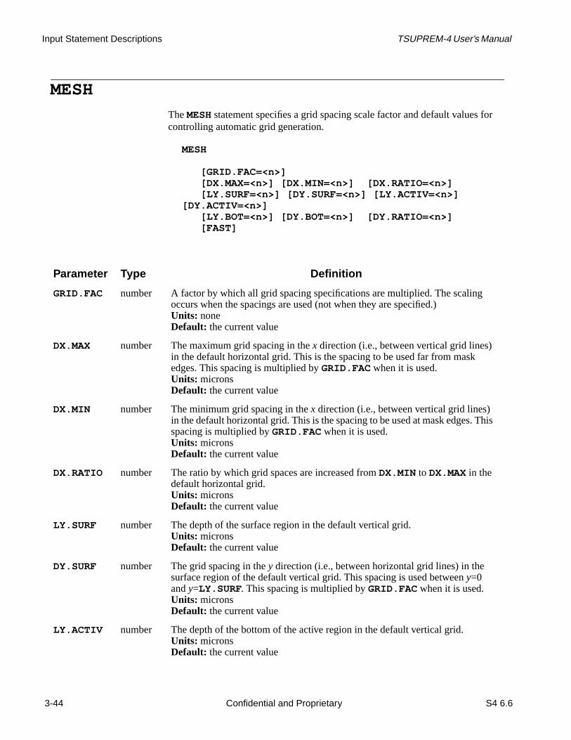
Input Statement Descriptions TSUPREM-4 User’s Manual
for
his
MESH
TheMESH statement specifies a grid spacing scale factor and default values controlling automatic grid generation.
MESH
[GRID.FAC=<n>] [DX.MAX=<n>] [DX.MIN=<n>] [DX.RATIO=<n>] [LY.SURF=<n>] [DY.SURF=<n>] [LY.ACTIV=<n>][DY.ACTIV=<n>] [LY.BOT=<n>] [DY.BOT=<n>] [DY.RATIO=<n>] [FAST]
Parameter Type Definition
GRID.FAC number A factor by which all grid spacing specifications are multiplied. The scalingoccurs when the spacings are used (not when they are specified.)Units: noneDefault: the current value
DX.MAX number The maximum grid spacing in thex direction (i.e., between vertical grid lines)in the default horizontal grid. This is the spacing to be used far from maskedges. This spacing is multiplied byGRID.FAC when it is used.Units: micronsDefault: the current value
DX.MIN number The minimum grid spacing in thex direction (i.e., between vertical grid lines)in the default horizontal grid. This is the spacing to be used at mask edges. Tspacing is multiplied byGRID.FAC when it is used.Units: micronsDefault: the current value
DX.RATIO number The ratio by which grid spaces are increased fromDX.MIN to DX.MAX in thedefault horizontal grid.Units: micronsDefault: the current value
LY.SURF number The depth of the surface region in the default vertical grid.Units: micronsDefault: the current value
DY.SURF number The grid spacing in they direction (i.e., between horizontal grid lines) in thesurface region of the default vertical grid. This spacing is used betweeny=0andy=LY.SURF. This spacing is multiplied byGRID.FAC when it is used.Units: micronsDefault: the current value
LY.ACTIV number The depth of the bottom of the active region in the default vertical grid.Units: micronsDefault: the current value
3-44 Confidential and Proprietary S4 6.6
Draft 6/26/98

TSUPREM-4 User’s Manual MESH
s an
ed in be
s
a
Description
TheMESH statement controls the automatic generation of simulation grids forTSUPREM-4. A grid is generated whenever anINITIALIZE statement withoutanIN.FILE parameter is processed. Automatic grid generation is used unlesappropriate set ofLINE statements has been processed since the previousINITIALIZE statement was processed. Grids can be automatically generatboth thex andy directions, and automatic grid generation in one direction cancombined with manual grid specification on the other direction.
Grid Creation Methods
A simulation grid forTSUPREM-4 can be created in one of four ways:
1. It can be read from a saved structure file, using theINITIALIZE orLOADFILE statements.
2. It can be generated from user-specifiedLINE , REGION, BOUNDARY, andELIMINATE statements.
3. It can be generated automatically from parameters supplied on theMESHstatement and from information read from mask data files.
DY.ACTIV number The grid spacing in they direction (i.e., between horizontal grid lines) at thebottom of the active region in the default vertical grid. The grid spacing variegeometrically betweenDY.SURF atLY.SURF andDY.ACTIV atLY.ACTIV . This spacing is multiplied byGRID.FAC when it is used.Units: micronsDefault: the current value
LY.BOT number The depth of the bottom of the structure in the default vertical grid.Units: micronsDefault: the current value
DY.BOT number The grid spacing in they direction (i.e., between horizontal grid lines) at thebottom of the structure in the default vertical grid. This spacing is multipliedby GRID.FAC when it is used.Units: micronsDefault: the current value
DY.RATIO number The ratio by which grid spaces are increased fromDY.ACTIV to DY.BOT inthe default vertical grid.Units: micronsDefault: the current value
FAST logical Specifies that one dimensional simulation is used until an etch step createsstructure that varies in thex direction. The structure is automatically convertedto two dimensional status when required.Default: true
Parameter Type Definition
S4 6.6 Confidential and Proprietary 3-45
Draft 6/26/98

Input Statement Descriptions TSUPREM-4 User’s Manual
nerat-id.
for-
of
ly
ings are
-
edles
4. The last two methods can be combined, using one of the methods for geing the horizontal grid and the other method for generating the vertical gr
If no LINE statements are supplied before anINITIALIZE statement, a grid isgenerated automatically. IfLINE X statements are supplied, they are used(instead of automatic generation) for the horizontal grid; ifLINE Y statementsare supplied, they are used to generate the vertical grid.
Horizontal Grid Generation
The automatic generation of the horizontal grid depends on whether mask inmation has been read with theMASK statement.
• If no mask information has been read, the default horizontal grid consiststwo (vertical) grid lines located aty=0.0 andy=1.0. This produces a quasione-dimensional simulation.
• If mask information is available, it is used with theDX.MIN , DX.MAX, andDX.RATIO parameters to automatically generate a horizontal grid.
The horizontal grid has a spacing between (vertical) grid lines of approximateDX.MIN at mask edges, expanding to a spacing ofDX.MAX at distances far fromany mask edge. TheDX.RATIO parameter specifies the rate at which the spacincreases away from mask edges. The minimum and maximum grid locationset to the minimum and maximumx coordinates for which mask information issupplied in the mask data file(s).
For a complete description of the grid generation process, seeChapter 2, “Auto-matic Grid Generation in the X Direction” on page 2-5.
Vertical Grid Generation
The automatically generated vertical grid is controlled by the variousLY andDYparameters.
• LY.SURF, LY.ACTIV , andLY.BOT specify the locations of the bottom ofthe surface region, active region, and structure, respectively.
• DY.SURF, DY.ACTIV, andDY.BOT specify the grid spacings at these locations.
Between the top of the structure andLY.SURF, the grid spacingDY.SURF isused. The spacing increases geometrically (i.e., with a constant ratio) fromDY.SURF atLY.SURF to DY.ACTIV atLY.ACTIV . The spacing expands toDY.BOT belowLY.ACTIV . TheDY.RATIO parameter specifies the rate atwhich the spacing increases belowDY.ACTIV.
In a automatically generated vertical grid, vertical grid lines deeper thanLY.ACTIV are eliminated, to increase the speed of the simulation. It is assumthat only point defects diffuse below this depth and that the point defect profi
3-46 Confidential and Proprietary S4 6.6
Draft 6/26/98

TSUPREM-4 User’s Manual MESH
tal
la-
w-
.
er-
tingady
are approximately constant in the horizontal direction, so that the low horizonresolution does not cause significant loss of accuracy in the simulation.
For a complete description of the grid generation process seeChapter 2, “Auto-matic Grid Generation in the Y Direction” on page 2-6.
Scaling the Grid Spacing
TheGRID.FAC parameter multiplies all grid spacing specifications, includingthose on theMESH, LINE , DEPOSITION, andEPITAXY statements. The defaultvalues of all grid spacings are set so thatGRID.FAC=1.0 produces a moderatelyfine grid, useful for reasonably, accurate simulations. For faster simulations,GRID.FAC should be given a value greater than 1.0. For more accurate simutions,GRID.FAC should be reduced as needed.
TheGRID.FAC parameter modifies the values of other parameters in the folloing ways:
• TheDX.MIN , DX.MAX, DY.SURF, DY.ACTIV, andDY.BOT parameters ontheMESH statement are multiplied byGRID.FAC.
• TheDY andARC.SPAC parameters on theDEPOSITION andEPITAXYstatements are multiplied byGRID.FAC.
• TheSPACES parameter on theDEPOSITION andEPITAXY statements isdivided byGRID.FAC.
• TheDY-OXIDE on theMETHOD statement and theDY-DEFAU parameter ontheMATERIAL statement are multiplied byGRID.FAC (the modificationtakes place when the parameters are used, not when they are specified)
Note:Moderation should be used in adjustingGRID.FAC—reducing thevalue from 1.0 to 0.1 increases the grid density by a factor of 10 in eachdirection, increasing the node count by a factor of 100 and the simula-tion time by a factor of more than 100.
1D Mode
Normally, when a mesh is generated or read from a file, it is examined to detmine whether there is any variation of the structure or solution values in thexdirection. If there is no variation, then simulation proceeds in 1D mode. By settheFAST parameter false, the use of 1D mode is disabled. If 1D mode is alrein use, the structure is converted to 2D.
S4 6.6 Confidential and Proprietary 3-47
Draft 6/26/98

Input Statement Descriptions TSUPREM-4 User’s Manual
Examples
1. The followingMESH statements could be used in thes4init file to set thedefault parameters for automatic grid generation:
2. The following statement cuts all grid spacings to one half their specifiedvalue, giving twice the specified grid density in the horizontal and verticaldirections:
MESH GRID.FAC=0.5
MESH DX.MIN=0.1 DX.MAX=0.4 DX.RATIO=1.5MESH LY.SURF=0.1 DY.SURF=0.03 LY.ACTIV=4.0 +
DY.ACTIV=0.3 LY.BOT=200 DY.BOT=100 +DY.RATIO=1.5
3-48 Confidential and Proprietary S4 6.6
Draft 6/26/98

TSUPREM-4 User’s Manual LINE
rm
lly
er
LINE
TheLINE statement specifies a horizontal or vertical mesh line in a nonuniforectangular grid.
Description
This statement specifies the position and spacing of one line in a rectangularmesh. A complete mesh specification consists of a group ofLINE statements fol-lowed byELIMINATE statements (optional),REGION andBOUNDARY state-ments (optional), and anINITIALIZE statement.
TSUPREM-4 uses an inverted Cartesian coordinate system, with x increasingfrom left to right and y increasing from the top surface of the structure into thesubstrate.
Placing Grid Lines
Grid lines are placed at the locations specified onLINE statements. Additionallines are added automatically so that the final grid spacing varies geometricabetween theSPACING values at the user-specified lines. The spacing ratiobetween adjacent pairs of grid lines is guided by the value of theRATIO parame-ter on theINITIALIZE statement. The final grid spacing may be slightly larg
LINE
X | Y LOCATION=<n> [SPACING=<n>][TAG=<c>]
Parameter Type Definition
X logical If true, thenLOCATION specifies thex coordinate of a vertical grid line.Default: false
Y logical If true, thenLOCATION specifies they coordinate of a horizontal grid line.Default: false
LOCATION number They coordinate of a horizontal grid line or thex coordinate of a vertical gridline.Units: micronsDefault: none
SPACING number The local grid spacing.Units: micronsDefault: none
TAG character A name used to refer to this grid line on aBOUNDARY or REGION statement.Default: none
S4 6.6 Confidential and Proprietary 3-49
Draft 6/26/98

Input Statement Descriptions TSUPREM-4 User’s Manual
ts-
wo
nter,acingedd getenter
re ofll
ing a
point,ound-
s. In
used,
than that specified on theLINE statement because of the need for an integralnumber of spaces; it may be much smaller than specified to satisfy constrainimposed by neighboring grid lines and theRATIO parameter. A complete description of the grid setup process is given inChapter 2, “Explicit Specification of GridStructure” on page 2-3.
Example
The following statements include three user-specified vertical grid lines and tuser-specified horizontal grid lines:
LINE X LOCATION=0 SPACING=1 LINE X LOCATION=1 SPACING=0.1 LINE X LOCATION=2 SPACING=1
LINE Y LOCATION=0 SPACING=0.02 LINE Y LOCATION=3 SPACING=0.5
After processing withRATIO=1.5,TSUPREM-4 produces a mesh with verticalgrid lines at 0.0, 0.42, 0.69, 0.88, 1.0, 1.12, 1.31, 1.58, and 2.0. Around the cethe spacing is 0.12, approximately what was requested. At each edge, the spis 0.42, because that is as coarse as it could get without exceeding the allowratio between adjacent grid spaces. If the allowed ratio were 9, then you woulone space of 0.9 microns and one space of 0.1 micron on each side of the cline.
Additional Notes
Structure Depthand Point Defect
Models
When thePD.TRANS orPD.FULL point defect model is to be used, the structushould be deep to accommodate the deep diffusion of point defects. A depth50-200 microns is suggested.ELIMINATE statements can be used to eliminate abut two vertical grid lines deep in the structure. WhenELIMINATE statementsare used with a coarse vertical grid spacing, the computational overhead of usdeep structure can be made negligible.
MaximumNumber of Nodes
and Grid Lines
The program can handle up to 40,000 nodes; this includes one node per grid plus one node for each exposed point and another node for each point on a bary between two materials. Thus, the grid must be smaller than 40,000 pointaddition, the initial grid must not have more than 1000 grid lines in either thex ory direction.
Default Regionsand Boundaries
No tags are required if the default regions and boundary conditions are to be i.e., if the initial structure consists entirely of silicon with only the top surfaceexposed.
3-50 Confidential and Proprietary S4 6.6
Draft 6/26/98

TSUPREM-4 User’s Manual ELIMINATE
ture
eed
s
s
re
re
ELIMINATE
TheELIMINATE statement eliminates mesh nodes along lines in a grid strucover a specified rectangular region.
Description
TheELIMINATE statement is used to eliminate nodes in regions of the devicstructure where the grid would otherwise be more dense than necessary. ThROWS parameter specifies that every second row of nodes within the specifie
ELIMINATE
ROWS | COLUMNS [X.MIN=<n>] [X.MAX=<n>] [Y.MIN=<n>][Y.MAX=<n>]
Parameter Type Definition
ROWS logical Specifies that horizontal lines of nodes are eliminated.Default: falseSynonyms:X.DIREC
COLUMNS logical Specifies that vertical lines of nodes are eliminated.Default: falseSynonyms:Y.DIREC
X.MIN number The minimum horizontal location of the rectangular region over which nodeare eliminated.Units: micronsDefault: the minimum horizontal location of the device structureSynonyms:X.LOW
X.MAX number The maximum horizontal location of the rectangular region over which nodeare eliminated.Units: micronsDefault: the maximum horizontal location of the device structureSynonyms:X.HIGH
Y.MIN number The minimum vertical location of the rectangular region over which nodes aeliminated.Units: micronsDefault: the minimum vertical location of the device structureSynonyms:Y.LOW
Y.MAX number The maximum vertical location of the rectangular region over which nodes aeliminated.Units: micronsDefault: the maximum vertical location of the device structureSynonyms:Y.HIGH
S4 6.6 Confidential and Proprietary 3-51
Draft 6/26/98

Input Statement Descriptions TSUPREM-4 User’s Manual
dr,
mns
tere,
s by
ethf you if
ire
region is to be removed. Similarly, theCOLUMNS parameter specifies that everysecond column of nodes within the specified region is to be removed.
TheELIMINATE statement can only be used after theLINE statements andbefore theINITIALIZE statement.
Note:Elimination of grid lines takes place during initial structure generation.TheELIMINATE statement cannot be used to eliminate grid lines afterthe INITIALIZE statement has been processed.
It is frequently a good idea to plot and examine the initial grid after theLINE X ,LINE Y , ELIMINATE , andINITIALIZE statements to verify the desired gridstructure before proceeding.
Reducing Grid Nodes
TheELIMINATE statement can be very useful for reducing the number of grinodes (and hence execution time), especially for large structures. In particulayou might useLINE X andLINE Y statements to define a large structure thatwould exceed the limit of 40,000 nodes, then eliminate enough rows and coluto bring the final number of nodes under 40,000.
Overlapping Regions
If you get an error message stating that one of theELIMINATE statements iscausing a mesh generation error, it is due to overlapping or adjacent eliminaregions. For best results when performing multiple eliminations over a structueither:
1. Do the multiple eliminations over identical regions of the structure, or
2. Avoid overlapping or adjacent eliminate regions; i.e., separate the regionat least one grid line.
If you must have overlapping eliminate regions, best results are obtained if thELIMINATE statements define successively smaller regions. That is, start withe largest region, then eliminate additional nodes in subsets of that region. Ineed to eliminate over partially overlapping regions, best results are obtainedyou minimize the amount of overlap.
Examples
1. The following statement eliminates every other row of nodes over the entstructure:
ELIMINATE ROWS
3-52 Confidential and Proprietary S4 6.6
Draft 6/26/98

TSUPREM-4 User’s Manual ELIMINATE
ac-
full
ns
-
The same result could be obtained by changing the locations and grid spings on theLINE Y statements.
2. The following statement eliminates every other column of nodes over thewidth of the structure, but only for values ofy greater than 4.5 microns:
ELIMINATE COLUMNS Y.MIN=4.5
3. The following statements perform multiple eliminations of rows and columover the same region of the structure:
ELIMINATE ROWS X.MAX=3 Y.MAX=2.2 ELIMINATE ROWS X.MAX=3 Y.MAX=2.2 ELIMINATE COLUMNS X.MAX=3 Y.MAX=2.2 ELIMINATE COLUMNS X.MAX=3 Y.MAX=2.2
4. The following statements eliminate columns in two non-overlapping, nonadjacent regions of the structure:
ELIMINATE COLUMNS X.MIN=1 X.MAX=3 ELIMINATE COLUMNS X.MIN=7 X.MAX=9
Each region extends from the top to the bottom of the structure.
S4 6.6 Confidential and Proprietary 3-53
Draft 6/26/98

Input Statement Descriptions TSUPREM-4 User’s Manual
e
n a.
xida-
heting,
area,
BOUNDARY
TheBOUNDARY statement specifies a boundary condition along an edge of thstructure.
Description
This statement specifies the boundary conditions that apply at the surfaces irectangular mesh. Two surface types are recognized: exposed and reflecting
Exposed surfaces normally correspond to the top of the wafer. Deposition, otion, and out-diffusion occur at exposed surfaces. Impurity predeposition alsohappens at exposed surfaces, as do defect recombination and generation. Tdefault boundary condition for the sides and the back of the structure is reflecwhile the default for the top surface is exposed. Thus theBOUNDARY statement isnot required for most simulations. The tags specified with theXLO, XHI , YLO,andYHI parameters correspond to tags specified on theLINE statements used todefine the mesh.XLO, XHI , YLO, andYHI must specify one entire edge of thestructure. It is not permissible to specify part of an edge, a region of nonzero or a line in the interior of the structure.
BOUNDARY
REFLECTI | EXPOSED XLO=<c> XHI=<c> YLO=<c> YHI=<c>
Parameter Type Definition
REFLECTI logical The specified boundary are reflecting.Default: false
EXPOSED logical The specified boundary are exposed.Default: false
XLO character The tag corresponding to the left edge of the boundary.Default: none
XHI character The tag corresponding to the right edge of the boundary.Default: none
YLO character The tag corresponding to the top edge of the boundary.Default: none
YHI character The tag corresponding to the bottom edge of the boundary.Default: none
3-54 Confidential and Proprietary S4 6.6
Draft 6/26/98

TSUPREM-4 User’s Manual BOUNDARY
d
nd
noted.
face:
Limitations
At present, theBOUNDARY statement is only useful in special situations, due tothe following limitations in the various processing steps:
• DEPOSITION only works on the top and right side (when exposed) of thestructure, and may fail if the bottom of the structure is exposed.
• ETCH with theTRAPEZOI andOLD.DRY options assumes that the exposesurface is etched from the top. Etching with theTRAPEZOI andOLD.DRYoptions may fail if the sides or bottom of the structure are exposed.
• Ion implantation always occurs on the top surface.
• DIFFUSION works correctly on all exposed surfaces, but the analytical aVERTICAL oxidation models assume that oxidation only occurs at the topsurface.
TheBOUNDARY statement is only used in setting up the initial structure. It canbe used to change a boundary condition after the structure has been initializ
Example
The following statement specifies that the top of the mesh is the exposed sur
BOUNDARY EXPOSED XLO=left XHI=right YLO=surf YHI=surf
The tagsleft , right , andsurf must have been previously specified on theLINE statements used to define the mesh. See the description of theLINE state-ment onpage 3-49.
S4 6.6 Confidential and Proprietary 3-55
Draft 6/26/98

Input Statement Descriptions TSUPREM-4 User’s Manual
REGION
TheREGION statement specifies the material type of a mesh region.
REGION
MATERIAL=<c> | SILICON | OXIDE | OXYNITRI | NITRIDE |POLYSILI | PHOTORES | ALUMINUM XLO=<c> XHI=<c> YLO=<c> YHI=<c>
Parameter Type Definition
MATERIAL character The specified region is defined to be of the named material.Default: none
SILICON logical The specified region is defined to be silicon.Default: false
OXIDE logical The specified region is defined to be oxide.Default: false
OXYNITRI logical The specified region is defined to be oxynitride.Default: false
NITRIDE logical The specified region is defined to be nitride.Default: false
POLYSILI logical The specified region is defined to be polysilicon.Default: false
PHOTORES logical The specified region is defined to be photoresist.Default: false
ALUMINUM logical The specified region is defined to be aluminum.Default: false
XLO character The tag specifying the left edge of the region to be defined.Default: none
XHI character The tag specifying the right edge of the region to be defined.Default: none
YLO character The tag specifying the top edge of the region to be defined.Default: none
YHI character The tag specifying the bottom edge of the region to be defined.Default: none
3-56 Confidential and Proprietary S4 6.6
Draft 6/26/98

TSUPREM-4 User’s Manual REGION
nerat-
sili-
Description
This statement specifies the material type of rectangular subregions when geing a rectangular mesh.REGION statements appear afterLINE statements butbefore theINITIALIZE statement. The default material is silicon; if noREGION statements are specified, the entire initial structure is assumed to becon.
The tags referenced onREGION statements must be defined on precedingLINEstatements.
Example
The following statement defines the region bounded by the x coordinatesleftandright and the y coordinatessurf andback to be silicon. See the descrip-tion of theLINE statement onpage 3-49.
REGION SILICON XLO=left XHI=right YLO=surf YHI=back
S4 6.6 Confidential and Proprietary 3-57
Draft 6/26/98

Input Statement Descriptions TSUPREM-4 User’s Manual
d is
INITIALIZE
TheINITIALIZE statement sets up the initial structure for a simulation.
INITIALIZE
( IN.FILE=<c> ( [SCALE=<n>] [FLIP.Y] ) | TIF ) | ( [WIDTH=<n> [DX=<n>]] [ <111> | <110> | <100> | ORIENTAT=<n> ]
[ ROT.SUB=<n> | X.ORIENT=<n> ] [RATIO=<n>] [LINE.DAT] ) [ IMPURITY=<c> I.CONC=<n> | I.RESIST=<n> ] [ MATERIAL=<c> ] [ANTIMONY=<n>] [ARSENIC=<n>] [BORON=<n>] [PHOSPHOR=<n>] [ CONCENTR | RESISTIV ]
Parameter Type Definition
IN.FILE character Name of a saved structure file. If this parameter is omitted, a rectangular grigenerated, using previously specifiedLINE , ELIMINATE , REGION, andBOUNDARY statements.Default: noneSynonyms:INFILE
SCALE number The mesh read in fromIN.FILE is scaled by this factor.Units: noneDefault: 1.0
FLIP.Y logical Specifies that the input structure is to be reflected abouty=0.Default: false
TIF logical Specifies that the input file is a TIF (Technology Interchange Format) file.Default: false
WIDTH number The width of the initial structure. (Only used if noLINE X statements arespecified.)Units: micronsDefault: the width of theMASK information, if any, or 1.0
DX number The grid spacing to use in thex direction.Units: micronsDefault: the current value ofDX.MAX from theMESH statement
<111> logical Specifies that the crystalline orientation of the silicon substrate is <111>.Default: false
<110> logical Specifies that the crystalline orientation of the silicon substrate is <110>.Default: false
<100> logical Specifies that the crystalline orientation of the silicon substrate is <100>.Default: True, if no other orientation is specified.
3-58 Confidential and Proprietary S4 6.6
Draft 6/26/98

TSUPREM-4 User’s Manual INITIALIZE
re
d.
ORIENTAT number The crystalline orientation of the silicon substrate. Only 100, 110, and 111 arecognized.Units: noneDefault: 100Synonyms:Y.ORIENT
ROT.SUB number The rotation of the substrate about they axis. The reference orientation(ROT.SUB=0) is defined such that thex axis points in a <110> direction.Units: degreesDefault: 0.0
X.ORIENT number The crystalline orientation of thex axis. This must be a 3-digit integer value.Units: noneDefault: 110
RATIO number The maximum ratio of adjacent grid spacings to be used in generating a griUnits: noneDefault: 1.5Synonyms:INTERVAL
LINE.DAT logical Specifies that the location of eachx andy grid line be listed on the standardoutput and in the output listing file.Default: false
IMPURITY character The name of the impurity with which the initial structure is doped.Default: none
I.CONC number The concentration of the specifiedIMPURITY in the initial structure.Units: atoms/cm3
Default: none
I.RESIST number The resistivity of the initial structure.Units: ohm-cmDefault: none
MATERIAL character Specifies the material of the initial structure.Default:SILICON
ANTIMONY number The uniform concentration or resistivity of antimony in the initial structure.Units: atoms/cm3 or ohm-cmDefault: 0.0Synonyms:SB
ARSENIC number The uniform concentration or resistivity of arsenic in the initial structure.Units: atoms/cm3 or ohm-cmDefault: 0.0Synonyms:AS
BORON number The uniform concentration or resistivity of boron in the initial structure.Units: atoms/cm3 or ohm-cmDefault: 0.0Synonyms:B
Parameter Type Definition
S4 6.6 Confidential and Proprietary 3-59
Draft 6/26/98

Input Statement Descriptions TSUPREM-4 User’s Manual
ifica-e
-
h ah a
as theelcify
be
ified
.
Description
TheINITIALIZE statement sets up the mesh from either a rectangular spection or from a previously saved structure file. This statement also initializes thbackground doping concentrations of the impurities specified.
Mesh Generation
If IN.FILE is not specified, a rectangular mesh is generated. IfLINE statementshave been specified for thex or y direction, they are used along with anyELIMINATE , BOUNDARY, andREGION statements and the value of theRATIOparameter to generate the mesh in that direction. If noLINE statements are specified for they direction, a defaulty mesh is generated. If noLINE statements arespecified for thex direction, andWIDTH is specified, a mesh of the requestedwidth is generated, with spacing given byDX. If no LINE X statements are givenandWIDTH is not specified, the width is taken from mask information read witprecedingMASK statement, if any. Otherwise, a one-micron wide structure witgrid spacing of one micron (i.e., one grid space wide) is generated. SeeChapter 2,“Grid Structure” on page 2-2 for a complete description of the mesh generationprocess. The locations of the generated grid lines are listed ifLINE.DAT is true.
Previously Saved Structure Files
A mesh read from a file must be in eitherTSUPREM-4 format or TIF (Technol-ogy Interchange Format). Meshes read fromTSUPREM-4 files can be scaled orflipped abouty=0 by specifying theSCALE or FLIP.Y parameters, respectively.
When a structure is read from a file, the last processing temperature as well choice of silicon substrate orientation, oxidation model, and point defect modare automatically set through information stored in the file. You need not respethese parameters after reading in a structure file at the start of a simulation.
Crystalline Orientation
The crystalline orientation of any silicon regions in a generated structure canspecified by <100>, <110>, or <111> parameters. TheORIENTAT parameter isalso accepted, for compatibility with older versions of the program. The spec
PHOSPHOR number The uniform concentration or resistivity of phosphorus in the initial structureUnits: atoms/cm3 or ohm-cmDefault: 0.0Synonyms:P
CONCENTR logical Specifies that the impurity concentration in the initial structure is given.Default: true
RESISTIV logical Specifies that the impurity resistivity in the initial structure is given.Default: false
Parameter Type Definition
3-60 Confidential and Proprietary S4 6.6
Draft 6/26/98

TSUPREM-4 User’s Manual INITIALIZE
her
; the
m-iven
en
-
n-
pingner-
con-
orientation is used for all single-crystal silicon regions in the simulation, whetpresent in the initial structure or deposited later. By default, thex axis points in a<110> direction. This can be changed by specifying a rotation about they axis(ROT.SUB) or the crystal orientation of thex axis (X.ORIENT).
The orientation parameters do not apply when reading a structure from a fileorientation of the saved structure is used instead.
Specifying Initial Doping
TheANTIMONY, ARSENIC, BORON, andPHOSPHOR parameters can be used tospecify the initial resistivity or impurity concentrations in the structure. Any cobination of these parameters can be specified if impurity concentrations are g(CONCENTR true), but only one impurity can be specified if the resistivity is giv(RESISTIV true). An impurity can also be specified by name with theIMPURITY parameter;I.CONC or I.RESIST are used to specify the concentration or resistivity, respectively, associated with the named impurity.
The resistivity is calculated from tables of mobility as a function of doping cocentration. These tables are described inChapter 2, “Initial Impurity Concentra-tion” on page 2-10.
Although the source of the grid (read or generated) and the specification of doare independent, the doping specification is normally used when a grid is geated but not when a grid is read from a file.
Examples1. The following statement reads in a previously saved structure in fileoldstr:
INITIALIZE IN.FILE=oldstr
2. The following statement generates a rectangular mesh and initializes thestructure with a boron doping of 1015/cm3:
INIT <111> X.ORIENT=211 BORON=1e15
The orientation of single-crystal silicon regions are <111>, while thex axispoints in a <211> direction.
3. The following statement generates a mesh and initializes the structure totain arsenic with resistivity of 20 ohm-cm:
INIT IMPURITY=arsenic I.RESIST=20
Note:The conversion from a resistivity to a concentration is based on Masetti’smobility table, while the calculation of electrical characteristics in theELECTRICAL statement uses the same mobility table as inMedici.Thus, the sheet resistances of the initial structure given by theEXTRACTstatement do not correspond exactly to the resistivity specified on theINITIALIZE statement.
S4 6.6 Confidential and Proprietary 3-61
Draft 6/26/98

Input Statement Descriptions TSUPREM-4 User’s Manual
ion
ecifys of
sub-
LOADFILE
TheLOADFILE statement reads mesh and solution information from a file.
Description
TheLOADFILE statement reads a mesh and solution from a file. EitherTSUPREM-4 or TIF structure files (created with theSAVEFILE statement) orDepict structure files can be read.TSUPREM-4 structure files can be scaled orflipped about thex axis (y=0) during reading.
TSUPREM-4 Files
The silicon substrate orientation, last processing temperature, current oxidatmodel, and current point defect model are saved inTSUPREM-4 structure files,and are automatically restored when the file is read. There is no need to respthese parameters after reading in a structure. (This does not apply to versionTSUPREM-4 prior to version 9035; versions older than 9035 only saved the strate orientation.)
LOADFILE
IN.FILE=<c> ( [SCALE=<n>] [FLIP.Y] ) | TIF |DEPICT
Parameter Type Definition
IN.FILE character The identifier of a structure file to be read.Default: noneSynonyms:INFILE
SCALE number A scaling factor to be applied to the mesh when readingTSUPREM-4 struc-ture files. All coordinate values are multiplied by this factor as they are read.Units: noneDefault: 1.0
FLIP.Y logical Specifies that the structure should be reflected abouty=0 when readingTSUPREM-4 structure files. Ally coordinates are multiplied by –1 as they areread.Default: false
TIF logical Specifies that the input file is a TIF (Technology Interchange Format) file.Default: false
DEPICT logical Specifies that the input file is a formatted file written byAvant! TCAD’sDepict andDonatello.Default: false
3-62 Confidential and Proprietary S4 6.6
Draft 6/26/98

TSUPREM-4 User’s Manual LOADFILE
s
d bepuri-oun-
ert.
Older Versions Files saved with older versions ofTSUPREM-4 can be loaded by newer versionof the program. Files saved with version 5.1 and newer ofTSUPREM-4 cannotbe read by older versions of the program.
In versions ofTSUPREM-4 prior to version 5.1, theSTRUCTURE statement isused to load structure files. Starting with version 5.1, theLOADFILE statementshould be used instead. TheIN.FILE , SCALE, FLIP.Y , andDEPICT parame-ters are still accepted on theSTRUCTURE statement, however, for compatibilitywith olderTSUPREM-4 input files.
User-Defined Materials and Impurities
Any user-defined materials and impurities referenced in a structure file shouldefined before the file is loaded. If a file containing undefined materials or imties is loaded, a warning is issued for each undefined material or impurity enctered. The material or impurity is defined, but its properties are not set. Furthsimulation using the material or impurity may fail unless the properties are se
Depict and Donatello Files
Files produced byDepict andDonatello do not contain the complete mesh andsolution information required byTSUPREM-4. Rather, they are used to updatean existing structure with the results of aDepict simulation. Thus, the usualsequence for interfacing withDepict is:
1. Generate a structure inTSUPREM-4, either from an initial mesh definitionor by reading a saved structure.
2. Save the structure in bothTSUPREM-4 andDepict formats. This requirestwo SAVEFILE statements and two output files.
3. UseDepict to process the structure, starting with the savedDepict-formatfile. Save the results in a newDepict-format file.
4. Read the savedTSUPREM-4-format file intoTSUPREM-4 (with anINITIALIZE or LOADFILE statement).
5. Read the newDepict-format file intoTSUPREM-4 (with aLOADFILEstatement).
The same sequence is used for interfacing withDonatello.
Examples
1. The following statement reads in a previously saved structure from filesavestr:
LOADFILE IN.FILE=savestr
S4 6.6 Confidential and Proprietary 3-63
Draft 6/26/98

Input Statement Descriptions TSUPREM-4 User’s Manual
has
2. The following statements save a structure to be processed further withDepictor Donatello:
SAVEFILE OUT.FILE=STRTS4 SAVEFILE OUT.FILE=STRTODEP DEPICT
Depict or Donatello can read the fileSTRTODEP. The structure fileSTRTS4is needed when reading the results produced byDepict or Donatello. IfDepict or Donatello stored its results in fileSTRFRDEP, they could be readinto TSUPREM-4 with the statements
INITIALIZE IN.FILE=STRTS4 LOADFILE IN.FILE=STRFRDEP DEPICT
3. The statements
LOADFILE IN.FILE=savestr
and
INITIALIZE IN.FILE=savestr
are equivalent, except that the program recognizes that an initial structurebeen set up in the second case. (AnINITIALIZE statement must be givenbefore any processing or output statement can be processed.)
3-64 Confidential and Proprietary S4 6.6
Draft 6/26/98

TSUPREM-4 User’s Manual SAVEFILE
la-
r-
test
SAVEFILE
TheSAVEFILE statement writes mesh and solution information to a file.
SAVEFILE
OUT.FILE=<c> [TEMPERAT=<n>] ( [SCALE=<n>] [FLIP.Y] [ACTIVE] ) | (TIF [TIF.VERS=<c>]) | DEPICT | ( MEDICI [POLY.ELE] [ELEC.BOT] ] ) | ( MINIMOS5 X.MASK.S=<n> HALF.DEV | ( FULL.DEV X.MASK.D=<n> [X.CHANNE=<n>]) [X.MIN=<n>] [X.MAX=<n>] [Y.MIN=<n>] [Y.MAX=<n>] [DX.MIN=<n>] [DY.MIN=<n>] ) | ( WAVE [ACTIVE] [CHEMICAL] [DEFECT] [OXID] [MISC] )
Parameter Type Definition
OUT.FILE character The identifier of the structure file to be written.Default: noneSynonyms:OUTFILE
TEMPERAT number The temperature used for evaluating active impurity concentrations.Units:°CelsiusDefault: the last processing temperature specified or 800°C
SCALE number A scaling factor to be applied to the mesh when writingTSUPREM-4 struc-ture files. All coordinate values saved in the file are multiplied by this value.TheSCALE parameter does not affect the structure used by subsequent simution steps.Units: noneDefault: 1.0
FLIP.Y logical Specifies that the structure should be reflected abouty=0 when writingTSUPREM-4 structure files. Ally coordinates are multiplied by -1 as they arewritten to the file.FLIP.Y does not affect the structure used by subsequentsimulation steps.Default: false
TIF logical Specifies that the output file be saved as a TIF (Technology Interchange Fomat) file.Default: false
TIF.VERS character The version of TIF to be used for saving the file. The default is to use the laversion of TIF; a value of 0 produces files compatible with version 6.0 ofTSUPREM-4.Units: noneDefault: 1.2.0
S4 6.6 Confidential and Proprietary 3-65
Draft 6/26/98

Input Statement Descriptions TSUPREM-4 User’s Manual
f
ture
e
u-te
a
d
a-te
DEPICT logical Specifies that the output file is a formatted file that can be read byAvant!TCAD’s Depict andDonatello programs.Default: false
MEDICI logical Specifies that the saved output file is a formatted file that can be read by theMedici device simulator. The output file can also be read by older versions oTMA PISCES-2B and by other versions ofPISCES.Default: falseSynonyms:PISCES
POLY.ELE logical Specifies that polysilicon regions should be converted to electrodes in theMedici output file.Default: false
ELEC.BOT logical Specifies that an electrode should be placed along the backside of the strucin theMedici output file.Default: false
MINIMOS5 logical Specifies that the saved output file contains a two-dimensional doping profilthat can be read by MINIMOS 5.Default: false
X.MASK.S number Thex coordinate of the mask edge in the source area of the MINIMOS 5 simlation region. MINIMOS 5 interprets this coordinate as the left edge of the gaelectrode.Units: micronsDefault: none
HALF.DEV logical Specifies that the MINIMOS 5 simulation region includes only the source areof the device. EitherFULL.DEV or HALF.DEV must be specified ifMINIMOS5 is specified.Default: false
FULL.DEV logical Specifies that the MINIMOS 5 simulation region includes both the source andrain areas of the device. EitherFULL.DEV or HALF.DEV must be specifiedif MINIMOS5 is specified.Default: false
X.MASK.D number Thex coordinate of the mask edge in the drain area of the MINIMOS 5 simultion region. MINIMOS 5 interprets this coordinate as the right edge of the gaelectrode.X.MASK.D must be specified ifFULL.DEV is specified; it must notbe specified ifHALF.DEV is specified.Units: micronsDefault: none
X.CHANNE number Thex coordinate of the center of the channel of the MINIMOS 5 simulationregion.Units: micronsDefault: (X.MIN + X.MAX)/2 if FULL.DEV is specified; not applicable ifHALF.DEV is specified
X.MIN number Thex coordinate of the left edge of the MINIMOS 5 simulation region.Units: micronsDefault: left edge of theTSUPREM-4 simulation region
Parameter Type Definition
3-66 Confidential and Proprietary S4 6.6
Draft 6/26/98

TSUPREM-4 User’s Manual SAVEFILE
X.MAX number Thex coordinate of the right edge of the MINIMOS 5 simulation region.Units: micronsDefault: right edge of theTSUPREM-4 simulation region
Y.MIN number They coordinate of the top edge of the MINIMOS 5 simulation region.MINIMOS 5 interprets this coordinate as the gate oxide/silicon interface.Units: micronsDefault: 0.0
Y.MAX number They coordinate of the bottom edge of the MINIMOS 5 simulation region.Units: micronsDefault: bottom edge of theTSUPREM-4 simulation region
DX.MIN number The minimum spacing in thex direction used to specify the doping profiles inthe output file.Units: micronsDefault: min((X.MAX-X.MIN )/80, 0.01)
DY.MIN number The minimum spacing in they direction used to specify the doping profiles inthe output file.Units: micronsDefault: min((Y.MAX-Y.MIN )/80, 0.01)
WAVE logical Specifies that the output file is a formatted file in Wavefront Technologies’wave file format. These files can be read by Wavefront Technologies’ DataVisualizer program.Default: false
ACTIVE logical Specifies that active impurity concentrations are to be saved inTSUPREM-4andWAVE output files.Default: true
CHEMICAL logical Specifies that chemical impurity concentrations are to be included in theWAVEoutput file.Default: false
DEFECT logical Specifies that point defect concentrations are to be included in theWAVE outputfile.Default: false
OXID logical Specifies that oxidant concentrations, oxidation flow rates, and stresses (ifavailable) are to be included in theWAVE output file.Default: falseSynonyms:STRESS
MISC logical Specifies that miscellaneous solution values are to be included in theWAVEoutput file. At present, this includes diffusivities of impurities and pointdefects.Default: false
Parameter Type Definition
S4 6.6 Confidential and Proprietary 3-67
Draft 6/26/98

Input Statement Descriptions TSUPREM-4 User’s Manual
ne
nlyt simu-
ion
ecifys of
sub-
s
e
y
gy
ver- as
t a
d TIF
Description
TheSAVEFILE statement writes mesh and solution information into a file, in oof several formats. If no format is specified, aTSUPREM-4 structure file is cre-ated.TSUPREM-4 structure files can be read with theLOADFILE orINITIALIZE statements. The mesh can be scaled or flipped about the x axis asthe structure is written or when it is read. Scaling and flipping during writing oaffect the saved structure, and do not affect the structure used by subsequenlation steps.
TSUPREM-4 Files
The silicon substrate orientation, last processing temperature, current oxidatmodel, and current point defect model are saved inTSUPREM-4 structure files,and are automatically restored when the file is read. There is no need to respthese parameters after reading in a structure. (This does not apply to versionTSUPREM-4 prior to version 9035; versions older than 9035 only saved the strate orientation.)
Older Versions Files saved with older versions ofTSUPREM-4 can be loaded by newer versionof the program. Files saved with version 5.1 and newer ofTSUPREM-4 cannotbe read by older versions of the program.
In versions ofTSUPREM-4 prior to version 5.1, theSTRUCTURE statement isused to load structure files. Starting with version 5.1, theLOADFILE statementshould be used instead. TheIN.FILE , SCALE, FLIP.Y , andDEPICT parame-ters are still accepted on theSTRUCTURE statement, however, for compatibilitywith olderTSUPREM-4 input files.
Effective in version 5.2 ofTSUPREM-4, active impurity concentrations aresaved by default inTSUPREM-4 structure files. Structure files without the activimpurity concentrations can be produced by specifyingˆACTIVE on theSAVEFILE statement. This is necessary if the structure files are to be read bolder (prior to 5.2) versions ofTSUPREM-4 or by other programs that cannotaccept the active concentration information.
TIF Files
TheTIF parameter specifies that the file should be saved as a TIF (TechnoloInterchange Format) file. The version of TIF can be specified with theTIF.VERSparameter; newer products use version 1.2.0, while older products (includingsion 6.0 ofTSUPREM-4) use version 1.00 or version 0 (which are equivalent,far asTSUPREM-4 is concerned).
Correct writing of a user-defined material or impurity to a TIF file requires thaTIF.NAME be specified when the material or impurity is defined;MD.INDEXmust also be specified for materials. Before other programs can read the save
3-68 Confidential and Proprietary S4 6.6
Draft 6/26/98

TSUPREM-4 User’s Manual SAVEFILE
te
e
file, an entry corresponding to the TIF name must be added to the appropriadatabase (mat.dbs for materials, orsol.dbs for impurities).
Note:Versions 6.1 and later ofTSUPREM-4 can read TIF files created by ver-sion 6.0, but version 6.0 cannot read TIF files created by versions 6.1and later unlessTIF.VERS =0 is specified when the file is written.
Medici Files
TheMEDICI parameter creates an output file that can be read by theMedicidevice simulator.MEDICI structures can also be read by older versions ofTMAPISCES-2B and by other versions ofPISCES. ThePOLY.ELE andELEC.BOTparameters are not needed when creating files forAvant! TCAD’s device simula-tors, because these simulators allow the treatment of polysilicon and backsidcontacts to be specified an aMESH statement.
Correct writing of a user-defined material to aMedici file requires thatMD.INDEX be specified when the material is defined (see“MATERIAL” on page3-212).
Depict and Donatello Files
TheDEPICT parameter allows you to create files to be read byAvant! TCAD’sDepict andDonatello programs.
Files produced byDepict andDonatello do not contain the complete mesh andsolution information required byTSUPREM-4. Rather, they are used to updatean existing structure with the results of aDepict simulation. Thus, the usualsequence for interfacing withDepict is:
1. Generate a structure inTSUPREM-4, either from an initial mesh definitionor by reading a saved structure.
2. Save the structure in bothTSUPREM-4 andDepict formats. This requirestwo SAVEFILE statements and two output files.
3. UseDepict to process the structure, starting with the savedDepict-formatfile. Save the results in a newDepict-format file.
4. Read the savedTSUPREM-4-format file intoTSUPREM-4 (with anINITIALIZE or LOADFILE statement).
5. Read the newDepict-format file intoTSUPREM-4 (with aLOADFILEstatement).
The same sequence is used for interfacing withDonatello.
S4 6.6 Confidential and Proprietary 3-69
Draft 6/26/98

Input Statement Descriptions TSUPREM-4 User’s Manual
5,he
to lastbut if
rature is
MINIMOS
TheMINIMOS5 parameter creates an output file that can be read by MINIMOSa two-dimensional program for the simulation of MOSFETs and MESFETs. Toutput file contains a two-dimensional doping profile. Detailed instructions oninterfacingTSUPREM-4 to MINIMOS 5 are given inAppendix F.
Temperature
The final temperature of the last high-temperature processing step is neededcalculate active impurity concentrations. Normally, the value at the end of thediffusion or epitaxy step or the value read when a structure is loaded is used, TEMPERAT is specified, its value is used instead. The value ofTEMPERAT (ifspecified) is retained for use in subsequent input statements. The last tempevalue is saved inTSUPREM-4 structure files and is restored when the structureloaded with aLOADFILE or INITIALIZE statement.
Examples
1. The following statement saves a structure in the filesavestr:
SAVEFILE OUT.FILE=savestr
2. The following statement saves the structure in filePIOUTSTR, in a formatthat can be read byMedici:
SAVEFILE OUT.FILE=PIOUTSTR MEDICI
3. The following statements save a structure to be processed further withDepict:
SAVEFILE OUT.FILE=STRTS4 SAVEFILE OUT.FILE=STRTODEP DEPICT
Depict can read the fileSTRTODEP. The structure fileSTRTS4 is neededwhen reading the results produced byDepict. If Depict stored its results infile STRFRDEP, they could be read intoTSUPREM-4 with the statements
INITIALIZE IN.FILE=STRTS4 LOADFILE IN.FILE=STRFRDEP DEPICT
3-70 Confidential and Proprietary S4 6.6
Draft 6/26/98

TSUPREM-4 User’s Manual STRUCTURE
re.
the
e
STRUCTURE
TheSTRUCTURE statement reflects, truncates, or extends the current structu
STRUCTURE
[ TRUNCATE ( RIGHT | LEFT X=<n> ) | ( BOTTOM | TOPY=<n> ) ] [ REFLECT [ RIGHT | LEFT ] ] [ EXTEND [ RIGHT | LEFT ] WIDTH=<n> [SPACES=<n>] [DX=<n>] [XDX=<n>] [Y.ELIM=<c>] ] [TEMPERAT=<n>]
Parameter Type Definition
TRUNCATE logical Causes the current mesh to be truncated according to the values of theRIGHT,LEFT, BOTTOM, TOP, X, andY parameters. The boundary condition is set toreflecting along the new surface created by the truncation.Default: false
RIGHT logical Specifies that truncation, reflection, or extension occurs at the right edge of structure.Default: true unlessLEFT, BOTTOM, orTOP is specified
LEFT logical Specifies that truncation, reflection, or extension occurs at the left edge of thstructure.Default: false
X number Thex coordinate where truncation occurs. IfLEFT is specified, truncationoccurs to the left of this location; ifRIGHT is specified, truncation occurs tothe right of this location. Only valid ifTRUNCATE andRIGHT or LEFT arespecified.Units: micronsDefault: none
BOTTOM logical Specifies that truncation occurs at the bottom edge of the structure.Default: false
TOP logical Specifies that truncation occurs at the top edge of the structure.Default: false
Y number They coordinate where truncation occurs. IfBOTTOM is specified, the portionof the structure below this location (higher values ofy) is truncated; ifTOP isspecified, the portion of the structure above this location (lower values ofy) istruncated. Only valid ifTRUNCATE andBOTTOM or TOP are also specified.Units: micronsDefault: none
REFLECT logical Causes the current mesh to be reflected at its left or right edge, doubling thewidth of the structure.Default: false
S4 6.6 Confidential and Proprietary 3-71
Draft 6/26/98

Input Statement Descriptions TSUPREM-4 User’s Manual
or itsnd
be set
struc-e
eci-
h
.
pu-
Description
TheSTRUCTURE statement is used to reflect, truncate, or extend the currentstructure. The structure can be truncated on the left or right or at the bottom top; reflected about its left or right edge, doubling its width; or extended fromleft or right edge to the specified width. Truncation occurs before reflection, areflection occurs before extension. The last processing temperature can alsofor use in calculating active impurity concentrations for theSELECT orSAVEFILE statements.
Reflecting a structure also reflects any mask information associated with the ture. The mask information is truncated or extended (if necessary) to the valuspecified byX, then reflected.
TheSPACES, DX, andXDX parameters specify the grid when a structure isextended. These parameters are used in the same way as theTHICKNES, DY, andYDY parameters are used in theDEPOSITION andEPITAXY statements. The use
EXTEND logical Causes the current mesh to be extended from its left or right edge by the spfied width.Default: false
WIDTH number The width by which the structure is extended.Units: micronsDefault: none
SPACES number The number of grid spaces to be added in thex direction when extending thestructure.Units: noneDefault: 1
DX number The nominal grid spacing in thex direction in the extension of the structure.Units: micronsDefault: the width of the extension/SPACES
XDX number The absolutex location at which the grid spacing in the extension is equal toDX.Units: micronsDefault: the location of the new edge of the extended structure
Y.ELIM character A list of 10 or fewery locations, separated by spaces or commas, below whicvertical grid lines are eliminated in the extended portion of the structure. Ifspaces appear in the list, the entire list must be enclosed in quotation marksUnits: micronsDefault: no elimination is done
TEMPERAT number Specifies the last processing temperature to be used for evaluating active imrity concentrations.Units: °CelsiusDefault: the last processing temperature specified, or 800°C
Parameter Type Definition
3-72 Confidential and Proprietary S4 6.6
Draft 6/26/98

TSUPREM-4 User’s Manual STRUCTURE
-
lt innlyecifi-
telyound-ssesyrid
s of
of these parameters is described inChapter 2, “Changes to the Mesh During Processing” on page 2-7.
Note:TheEXTEND feature should be used with caution. Simulating a narrowstructure and then extending it does not give the same results as simula-tion of the wider structure unless the topography and doping concentra-tions at the edge of the narrow structure are essentially one-dimensional.
Order ofOperations
When saving and/or loading files with theSTRUCTURE statement, the order ofoperations is:
1. Load from the file specified by theIN.FILE parameter.
2. Set the last processing temperature, if specified withtheTEMPERAT parameter.
3. Save to the file specified by theOUT.FILE parameter.
4. Truncate the structure, ifTRUNCATE is specified.
5. Reflect the structure, ifREFLECT is specified.
Extend the structure, ifEXTEND is specified.
Truncation Cautions
Reflecting the structure about an edge that is not absolutely vertical can resuvery thin triangles that could cause numerical problems. A structure should obe reflected about a reflecting boundary, created during an initial structure spcation or by theTRUNCATE parameter.
TheTRUNCATE parameter sometimes fails to produce an edge that is absoluvertical. Reflection then produces a structure that has embedded reflecting baries running through it. This problem only occurs when the truncation line pawithin a fraction of an angstrom of a grid point; this can usually be avoided bspecifying truncation lines that are several angstroms from the locations of glines.
TRUNCATE TOP can be used to remove the entire exposed surface, giving astructure with reflecting boundary conditions on all four sides. The usefulnessuch structures is limited because some process steps (e.g.,DEPOSITION andETCH) do not work on structures that have no exposed surface.
TSUPREM-4 Version Compatibility
In versions ofTSUPREM-4 prior to version 5.1, theSTRUCTURE statement isused to save and load structure files. Starting with version 5.1, theSAVEFILE andLOADFILE statements should be used instead. The parameters for saving
S4 6.6 Confidential and Proprietary 3-73
Draft 6/26/98

Input Statement Descriptions TSUPREM-4 User’s Manual
Two
TSUPREM-4, Depict, Medici, and MINIMOS 5 files and for loadingTSUPREM-4 andDepict files are still accepted on theSTRUCTURE statement,however, for compatibility with existingTSUPREM-4 input files. The followingparameters are recognized in addition to those described above:
[IN.FILE] [OUT.FILE=<c>] ( [SCALE=<n>] [FLIP.Y] ) | DEPICT | ( MEDICI [POLY.ELE] [ELEC.BOT] ] ) | ( MINIMOS5 X.MASK.S=<n> HALF.DEV | ( FULL.DEV X.MASK.D=<n> [X.CHANNE=<n>] ) [X.MIN=<n>] [X.MAX=<n>] [Y.MIN=<n>] [Y.MAX=<n>] )
Examples
1. The following statement truncates the structure to the right ofx=1.2 microns,then mirrors the structure about the new right edge:
STRUCTURE TRUNCATE RIGHT X=1.2 REFLECT
2. The following statement extends the structure to the right by 0.5 microns. grid spaces are added, with elimination of every other vertical line belowy=1µm:
STRUCTURE EXTEND RIGHT WIDTH=0.5 +
SPACES=2 Y.ELIM=1.0
3-74 Confidential and Proprietary S4 6.6
Draft 6/26/98
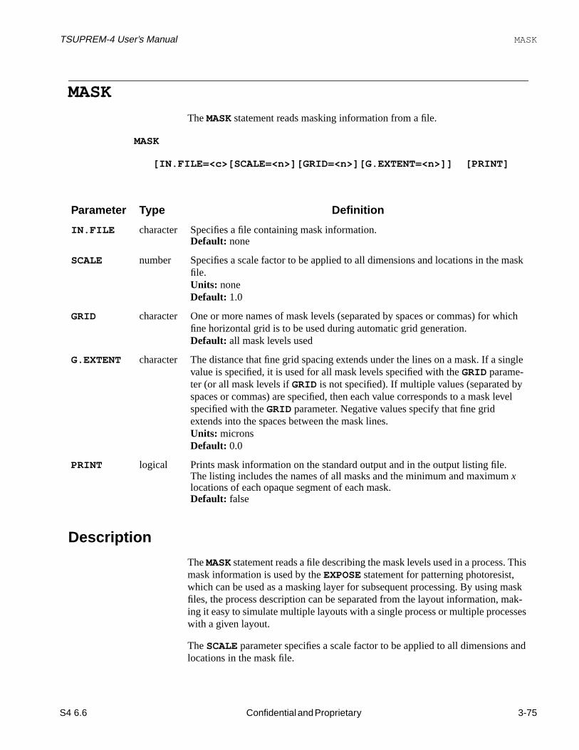
TSUPREM-4 User’s Manual MASK
. This
maskak-
sses
and
mask
hich
single
vel
MASK
TheMASK statement reads masking information from a file.
Description
TheMASK statement reads a file describing the mask levels used in a processmask information is used by theEXPOSE statement for patterning photoresist,which can be used as a masking layer for subsequent processing. By using files, the process description can be separated from the layout information, ming it easy to simulate multiple layouts with a single process or multiple procewith a given layout.
TheSCALE parameter specifies a scale factor to be applied to all dimensionslocations in the mask file.
MASK
[IN.FILE=<c>[SCALE=<n>][GRID=<n>][G.EXTENT=<n>]] [PRINT]
Parameter Type Definition
IN.FILE character Specifies a file containing mask information.Default: none
SCALE number Specifies a scale factor to be applied to all dimensions and locations in the file.Units: noneDefault: 1.0
GRID character One or more names of mask levels (separated by spaces or commas) for wfine horizontal grid is to be used during automatic grid generation.Default: all mask levels used
G.EXTENT character The distance that fine grid spacing extends under the lines on a mask. If a value is specified, it is used for all mask levels specified with theGRID parame-ter (or all mask levels ifGRID is not specified). If multiple values (separated byspaces or commas) are specified, then each value corresponds to a mask lespecified with theGRID parameter. Negative values specify that fine gridextends into the spaces between the mask lines.Units: micronsDefault: 0.0
PRINT logical Prints mask information on the standard output and in the output listing file.The listing includes the names of all masks and the minimum and maximumxlocations of each opaque segment of each mask.Default: false
S4 6.6 Confidential and Proprietary 3-75
Draft 6/26/98

Input Statement Descriptions TSUPREM-4 User’s Manual
t the
se
ould
a-
y
e
TheGRID andG.EXTENT parameters control how mask information is used toset the horizontal grid spacing during automatic grid generation. TheGRIDparameter specifies which mask levels are used. Fine grid spacing is used aedges of lines on the specified levels. TheG.EXTENT parameter determines howfar the fine grid extends under the lines of the mask. TheGRID andG.EXTENTparameters are character strings that specify lists of values; be sure to enclothem in quotation marks if they contain spaces.
TSUPREM-4 input mask files are created byTMA Layout. TMA Layout letsyou view a mask layout file and interactively select regions to be simulated.
Examples
1. The following statement reads mask information from the fileHVNCH.TL1then prints the information that is read:
MASK IN.FILE=HVNCH.TL1 PRINT
2. The following statement specifies that only thePOLY andFIELD masksshould be considered when doing automatic grid generation. Fine grid shextend 0.5 microns under the edges of lines on thePOLY mask and 0.3microns under the edges of lines on theFIELD mask:
MASK IN.FILE=S4EX4M.TL1 GRID=”Poly,Field”+G.EXTENT="0.5,0.3"
3. TSUPREM-4 input files can be structured to separate the masking informtion from the processing information:
$ MESH DESCRIPTION (DEPENDS ON MASKS) LINE X LOC=0.0 SPAC=0.01 . . . LINE Y LOC=200.0 SPAC=50.0 INITIALIZE BORON=1E14 $ MASK INFORMATION MASK IN.FILE=MINNCH.TL1 $ PROCESS INFORMATION (DOES NOT DEPEND ON MASKS) SOURCE CMOS07
To simulate a different portion of a layout with the same process, you onlneed to change the mesh description and the name of theMASK file. To simu-late the same device with a modified process, you only need to change thname of theSOURCE file.
3-76 Confidential and Proprietary S4 6.6
Draft 6/26/98

TSUPREM-4 User’s Manual PROFILE
ri-o
n.
PROFILE
ThePROFILE statement allows a one-dimensional impurity profile to be readfrom a file.
Description
This statement allows a one-dimensional impurity profile (or other solution vaable) to be read from a data file. The data file must be a text file containing twcolumns of numbers. The first column gives they coordinate of a point, in
PROFILE
IMPURITY=<c> | ANTIMONY | ARSENIC | BORON |PHOSPHOR IN.FILE=<c> OFFSET=<n> [REPLACE]
Parameter Type Definition
IMPURITY character The name of the impurity to be read from the input file.Default: none
ANTIMONY logical Specifies that the input file contains a profile of antimony concentration.Default: falseSynonyms:SB
ARSENIC logical Specifies that the input file contains a profile of arsenic concentration.Default: falseSynonyms:AS
BORON logical Specifies that the input file contains a profile of boron concentration.Default: falseSynonyms:B
PHOSPHOR logical Specifies that the input file contains a profile of phosphorus concentration.Default: falseSynonyms:P
IN.FILE character The name of the data file containing the one-dimensional profile informatioDefault: noneSynonyms:INFILE
OFFSET number The amount by which the profile is shifted in they direction before beingapplied to theTSUPREM-4 structure. The concentration aty=0 in the data fileis added aty=OFFSET in theTSUPREM-4 structure.Units: micronsDefault: 0
REPLACE logical Specifies that the profile read from the file should replace the existing profile(rather than adding to it).Default: false
S4 6.6 Confidential and Proprietary 3-77
Draft 6/26/98

Input Statement Descriptions TSUPREM-4 User’s Manual
nwo
o-
solve
val-e
f
e.g.,u-
microns, and the second contains the impurity concentration (or other solutiovalue), in appropriate units. Lines in the data file that do not contain exactly trecognizable numeric values are ignored.
If REPLACE is specified, the profile read from the file replaces any existing prfile. Replacement occurs only at nodes whosey coordinates are within the rangeof y coordinates given in the file. Adaptive gridding does not apply to thePROFILE statement. The user must insure that the grid is dense enough to rethe profile.
OFFSET Parameter
The profile read from the data file is expanded in thex direction to the width of thestructure and added to any existing impurities in the structure; negative data ues can be used to reduce the concentration. The profile can be shifted in thydirection by specifying theOFFSET parameter. The profile is shifted byOFFSET,so that the concentration aty=0 in the data file appears at locationy=OFFSET intheTSUPREM-4 structure.
Interpolation
Values between they coordinates specified in the input file are calculated usinglinear interpolation on the function
Equation 3-1
where
• is the concentration in the file
• is a scaling factor.
The final value of at each point is found by inverting using the value oobtained from the linear interpolation. This gives logarithmic interpolation for
and linear interpolation for . The value of is taken to be 105 forimpurity and point defect concentrations and 1.0 for other solution variables (dloopandrloop). At points outside the range of values in the input file, the imprity concentration remains unchanged.
f c( ) sign c( )logc
2k------
c2k------
21++
=
c
k
c f c( ) f
c k» c k« k
3-78 Confidential and Proprietary S4 6.6
Draft 6/26/98

TSUPREM-4 User’s Manual PROFILE
the
the
IMPURITY Parameter
TheIMPURITY parameter can be used to read in values for a user-specifiedimpurity. This can be used to read in a profile for comparison without alteringdesired doping:
IMPLANT BORON ... SELECT Z=LOG10(BORON) PLOT.1D ... IMPURITY NEW IMPURITY=PBORON PROFILE IMPURITY=PBORON ... SELECT Z=LOG10(PBORON) PLOT.1D ^AX ^CL ...
If boron had been specified on thePROFILE statement, the profile would havebeen added to the implanted boron, making it impossible to compare theimplanted profile with the contents of the data file.
TheIMPURITY parameter can be used to read in values of interstitial andvacancy profiles. Remember that the profiles read from the file are added to profiles already in the structure, unlessREPLACE is specified.
Example
The following statement reads boron concentration data from the filebprof.dat:
PROFILE BORON IN.FILE=bprof.dat OFFSET=-0.1
If the file contained the lines
0.0 1.0e17 0.1 1.4e17 0.2 1.8e17 0.4 2.0e17 0.6 1.8e17 0.8 1.4e17 1.0 1.0e17 2.0 1.0e16 5.0 1.0e14
then a boron concentration of 1.0e17 would be added aty=-0.1, a concentration of1.4e17 would be added aty=0, a concentration of 1.8e17 aty=0.1, and so on.
S4 6.6 Confidential and Proprietary 3-79
Draft 6/26/98

Input Statement Descriptions TSUPREM-4 User’s Manual
ion.
e
ilicon
ed by
less
.
.
ELECTRODE
TheELECTRODE statement is used to name the electrodes for device simulat
Description
TheELECTRODE statement allows you to specify names for electrodes. Theselectrode names are saved in TIF andMEDICI output files for use inMedici andother programs. The materials which can be named to an electrode are polysand all materials which have been defined as conductors on aMATERIAL state-ment. Once an electrode is named, the information is kept unless it is undefinCLEAR in anELECTRODE statement.
ELECTRODE [NAME=<c>] [ ( X=<n> [Y=<n>] ) |BOTTOM ] [CLEAR [ALL]]
[MERGE] [PRINT]
Parameter Type Definition
NAME character The name of the electrode to define or delete. This parameter is required unbothCLEAR andALL are specified.Default: none
X number Thex coordinate of an (x,y) position in the region to be defined as an electrodeUnits: micronsDefault: none
Y number They coordinate of an (x,y) position in the region to be defined as an electrodeUnits: micronsDefault: they coordinate inside the conductor at thex position
BOTTOM logical Specifies that the electrode to be defined is at the bottom of structure.Default: false
CLEAR logical Specifies that the named electrode is to be deleted.Default: false
MERGE logical Specifies the polysilicon adjacent to the electrode to be merged as the elec-trode.Only applicable to the saved file in TIF format.Default: true
ALL logical Specifies that all defined electrodes are to be deleted.Default: false
PRINT logical Specifies that the summary of defined electrodes is printed.Default: true
3-80 Confidential and Proprietary S4 6.6
Draft 6/26/98

TSUPREM-4 User’s Manual ELECTRODE
Examples
1. The following statements show how to name the electrodes.
ELECTROD X=0.1 NAME=Source ELECTROD X=1.2 NAME=Gate ELECTROD X=2.3 NAME=Drain ELECTROD BOTTOM NAME=Bulk
SAVEFILE OUT.FILE=mos.mdc MEDICI POLY.ELE ELEC.BOT
2. The following statements show how to undefine the electrode.
ELECTROD X=0.1 NAME=Wrong .... ELECTROD NAME=Wrong CLEAR
Additional ELECTRODE Notes
1. The polysilicon region named inELECTROD is stored as an electrode in thesaved file in TIF format. For Medici format,POLY.ELE must be specified inSAVEFILE.
2. The polysilicon region adjacent to the conductor named inELECTROD ismerged as the same electrode ifMERGE parameter for TIF format, orPOLY.ELE parameter (inSAVEFILE) for Medici format is specified.
3. If there are more than two conductors and/or polysilicon regions at theX posi-tion, for example, like EPROM structure, theY must be specified individually.
ELECTROD X=1.2 Y=-0.02 NAME=Erase ELECTROD X=1.2 Y=-0.35 NAME=Program
S4 6.6 Confidential and Proprietary 3-81
Draft 6/26/98

Input Statement Descriptions TSUPREM-4 User’s Manual
3-82 Confidential and Proprietary S4 6.6
Draft 6/26/98

TSUPREM-4 User’s Manual 3.3 Process Steps
S4 6.6
3
3.3 Process StepsThe following statements simulate processing steps:
Statement Name Description Page
DEPOSITION Deposits a material on the exposed surface.3-84
EXPOSE Exposes photoresist using mask. 3-88
DEVELOP Removes exposed positive photoresist orunexposed negative photoresist.
3-90
ETCH Etches an exposed material. 3-91
IMPLANT Implants an impurity. 3-95
DIFFUSION Performs a diffusion step, possibly withoxidation.
3-105
EPITAXY Performs a silicon epitaxial deposition step.3-111
STRESS Calculates the stresses in the structure. 3-114
Confidential and Proprietary 3-83
DDraft 6/26/98

Input Statement Descriptions TSUPREM-4 User’s Manual
c-
c-
DEPOSITION
TheDEPOSITION statement is used to deposit a specified material on theexposed surface of the current structure.
DEPOSITION
MATERIAL=<c> | SILICON | OXIDE | OXYNITRI | NITRIDE |POLYSILI | ALUMINUM | ( PHOTORES [ POSITIVE | NEGATIVE ] ) [ IMPURITY=<c> I.CONC=<n> | I.RESIST=<n> ] [ANTIMONY=<n>] [ARSENIC=<n>] [BORON=<n>] [PHOSPHOR=<n>] [ CONCENTR | RESISTIV ] THICKNES=<n> [SPACES=<n>] [DY=<n>] [YDY=<n>] [ARC.SPAC=<n>] [TEMPERAT=<n>] [GSZ.LIN]
Parameter Type Definition
MATERIAL character The name of the material to be deposited.Default: none
SILICON logical Deposit silicon.Default: false
OXIDE logical Deposit oxide.Default: false
OXYNITRI logical Deposit oxynitride.Default: false
NITRIDE logical Deposit nitride.Default: false
POLYSILI logical Deposit polysilicon.Default: false
ALUMINUM logical Deposit aluminum.Default: false
PHOTORES logical Deposit photoresist.Default: false
POSITIVE logical Specifies that the deposited photoresist (and all other photoresist in the struture) is positive, i.e., that theDEVELOP statement removes exposed photoresistwhile leaving unexposed photoresist.Default: true, unlessNEGATIVE is specified
NEGATIVE logical Specifies that the deposited photoresist (and all other photoresist in the struture) is negative, i.e., that theDEVELOP statement removes unexposed photo-resist while leaving exposed photoresist.Default: false
3-84 Confidential and Proprietary S4 6.6
Draft 6/26/98

TSUPREM-4 User’s Manual DEPOSITION
r.
e
oca-
IMPURITY character The name of the impurity with which the deposited layer is doped.Default: none
I.CONC number The concentration of the specifiedIMPURITY in the deposited layer.Units: atoms/cm3
Default: none
I.RESIST number The resistivity of the deposited layer.Units: ohm-cmDefault: none
ANTIMONY number The uniform concentration or resistivity of antimony in the deposited layer.Units: atoms/cm3 or ohm-cmDefault: 0.0Synonyms:SB
ARSENIC number The uniform concentration or resistivity of arsenic in the deposited layer.Units: atoms/cm3 or ohm-cmDefault: 0.0Synonyms:AS
BORON number The uniform concentration or resistivity of boron in the deposited layer.Units: atoms/cm3 or ohm-cmDefault: 0.0Synonyms:B
PHOSPHOR number The uniform concentration or resistivity of phosphorus in the deposited layeUnits: atoms/cm3 or ohm-cmDefault: 0.0Synonyms:P
CONCENTR logical Specifies that the impurity concentration in the deposited layer is given.Default: true
RESISTIV logical Specifies that the resistivity in the deposited layer is given.Default: false
THICKNES number The thickness of the deposited layer.Units: micronsDefault: none
SPACES number The number of vertical grid spacings in the layer. This value is divided by thvalue ofGRID.FAC (see“MESH” on page 3-44).Units: noneDefault: 1/GRID.FACSynonyms:DIVISION
DY number The nominal grid spacing to be used in the deposited material layer at the ltion specified by theYDY parameter. This value is multiplied by the value ofGRID.FAC (see“MESH” on page 3-44).Units: micronsDefault: GRID.FAC*THICKNES/SPACESSynonyms:DX
Parameter Type Definition
S4 6.6 Confidential and Proprietary 3-85
DDraft 6/26/98

Input Statement Descriptions TSUPREM-4 User’s Manual
n theer
in
idepprox-
ly-s;
is
sit-
f
Description
This statement provides a basic deposition capability. Material is deposited oexposed surface of the structure, with the upper surface of the deposited laybecoming the new exposed surface. TheANTIMONY, ARSENIC, BORON, andPHOSPHOR parameters specify the initial impurity concentrations or resistivitythe deposited layer, depending on whetherCONCENTR or RESISTIV is true.Doping can also be specified with theIMPURITY andI.CONC or I.RESISTparameters.
The deposited material conforms to the contours of the original surface. Outscorners on the original surface produce arcs on the new surface, which are aimated by straight line segments. The maximum segment length is set by theARC.SPAC parameter. TheSPACES, DY, andYDY parameters used to control thegrid spacing in the deposited layer are scaled by the value of theGRID.FACparameter on theMESH statement (seeChapter 2, “Changes to the Mesh DuringProcessing” on page 2-7).
Note:It is not possible to deposit a layer on the bottom of a structure, even if itis exposed. Attempting to do so may cause the program to fail.
Polycrystalline Materials
TheTEMPERAT andGSZ.LIN parameters are used only when depositing a pocrystalline material. If no temperature is specified, or if the temperature is lesthan the value ofTEMP.BRE for the material, the deposited layer is amorphousrecrystallization occurs at the start of the next high-temperature step.
YDY number The location of the nominal grid spacing specified byDY relative to the top ofthe deposited layer.Units: micronsDefault: 0.0Synonyms:XDX
ARC.SPAC number The maximum spacing allowed along an arc on the new surface. This valuemultiplied by the value ofGRID.FAC (see“MESH” on page 3-44).Units: micronsDefault: 0.5*THICKNES*GRID.FAC
TEMPERAT number The deposition temperature; used to determine initial grain size when depoing polycrystalline materials.Units: degreesDefault: 0.0 Kelvins
GSZ.LIN logical Specifies that the grain size increases linearly with depth from the bottom othe deposited layer. (If false, grain size is constant through the layer.)Default: true
Parameter Type Definition
3-86 Confidential and Proprietary S4 6.6
Draft 6/26/98

TSUPREM-4 User’s Manual DEPOSITION
be ofg
tore-
ysent
esmeg
di-
be, for
Photoresist
Photoresist can be positive or negative, but all photoresist in a structure mustthe same type. If photoresist of one type is deposited on a structure containinphotoresist of the other type, a warning is issued and the type of the old phosist is changed to that of the newly deposited photoresist.
Examples
1. The following statement deposits 200 angstroms of silicon dioxide:
DEPOSIT OXIDE THICK=0.02
2. The following statement deposits a one-micron thick layer of photoresist,using four grid spaces in the layer:
DEPOSIT PHOTO THICK=1.0 SPACES=4 ARC.SPAC=0.1
The maximum segment length used to approximate arcs is 0.1 micron. Bdefault, the newly deposited photoresist (and any photoresist already prein the structure) is assumed to be positive.
3. The following statement deposits 0.1 micron of poly:
DEPOSIT MAT=POLY THICK=0.1 TEMPERAT=650 GSZ.LIN
The initial grain size is calculated at 650°C and increases linearly over thethickness of the layer, with minimum value at the bottom of the layer.
Additional DEPOSITION Notes
1. The calculation of doping concentration from resistivity uses mobility tablfor silicon and polysilicon. If the resistivity is specified when depositing soother material, a warning is issued. The mobility tables used for calculatinthe doping concentration are not the same as the tables used by theELECTRICAL statement. The extracted sheet resistance for the depositelayer does not correspond exactly to the resistivity specified during depostion.
2. Deposition of one material on top of another can cause a third material toadded between them. This happens when titanium is deposited on siliconexample—a layer of TiSi2 is inserted. Insertion of extra layers is specifiedwith theREACTION statement (seepage 3-233).
3. Diffusion of impurities during a deposition step is not simulated.
S4 6.6 Confidential and Proprietary 3-87
DDraft 6/26/98

Input Statement Descriptions TSUPREM-4 User’s Manual
her
ib--
mr
k
l
EXPOSE
TheEXPOSE statement exposes photoresist using a mask.
EXPOSE
MASK=<c>[SHRINK=<n>][OFFSET=<n>]
Description
TheEXPOSE statement exposes photoresist, using masking informationpreviously read with aMASK statement. Regions of photoresist that are directlybelow transparent regions of the specified mask (and not obscured by any otmaterial) are marked as exposed. If positive photoresist is present, exposedregions are removed by a subsequentDEVELOP statement; if negativephotoresist is present, the unexposed portion of the photoresist is removed.
TheSHRINK andOFFSET parameters can be used to model the effects of delerate or accidental adjustments to the mask-making or photolithographic processes.SHRINK specifies a reduction in the width of lines on the mask, whileOFFSET specifies a shifting of the mask (relative to other masks). The progradoes not allow shrinks or offsets that are large enough to make mask lines ospaces disappear.
Note:TheOFFSET parameter breaks the symmetry that is assumed at reflect-ing boundaries at the edge of a structure. Shifting a line towards areflecting boundary also makes it narrower, while shifting a line awayfrom a reflecting boundary makes it wider.
Parameter Type Definition
MASK character Specifies the name of the mask to be used for the exposure step. The masname must match the name of a mask previously read with aMASK statement.Default: none
SHRINK number The reduction in line width on each side of each line on the mask. (The totareduction in line width is twice the specified value.)Units: micronsDefault: 0.0
OFFSET number The amount by which lines on the mask are shifted (in the positivex direction).Units: micronsDefault: 0.0
3-88 Confidential and Proprietary S4 6.6
Draft 6/26/98

TSUPREM-4 User’s Manual EXPOSE
ions
Example
The following sequence illustrates a typical use of theEXPOSE statement:
MASK IN.FILE=CMOS3.TL1 . . . DEPOSIT POLY THICKNES=.2 DEPOSIT POSITIVE PHOTORES THICKNES=1 EXPOSE MASK=POLY SHRINK=0.05 DEVELOP ETCH POLY TRAP THICK=0.4 ANGLE=80 ETCH PHOTORES ALL
This sequence produces lines of polycrystalline silicon under the opaque regof the mask namedPOLY. The width of eachPOLY line is reduced by 0.05microns on each side (for a total reduction of 0.1 micron).
S4 6.6 Confidential and Proprietary 3-89
DDraft 6/26/98

Input Statement Descriptions TSUPREM-4 User’s Manual
ed
posi-th the
ions
DEVELOP
TheDEVELOP statement removes exposed positive photoresist and unexposnegative photoresist.
Description
TheDEVELOP statement is used to pattern photoresist by removing exposed tive resist and unexposed negative resist. The character string associated wiDEVELOP statement is ignored, and serves only to document the input.
Example
The following sequence illustrates a typical use of theDEVELOP statement:
MASK IN.FILE=CMOS3.TL1 . . . DEPOSIT POLY THICKNES=.2 DEPOSIT POSITIVE PHOTORES THICKNES=1 EXPOSE MASK=POLY DEVELOP ETCH POLY TRAP THICK=0.4 ANGLE=80 ETCH PHOTORES ALL
This sequence produces lines of polycrystalline silicon under the opaque regof the mask namedPOLY.
DEVELOP
[<c>]
3-90 Confidential and Proprietary S4 6.6
Draft 6/26/98

TSUPREM-4 User’s Manual ETC
ETC
TheETCH statement is used to remove portions of the current structure.
ETCH
[ MATERIAL=<c> | SILICON | OXIDE | OXYNITRI | NITRIDE | POLYSILI | PHOTORES | ALUMINUM ] ( TRAPEZOI [THICKNES=<n>] [ANGLE=<n>] [UNDERCUT=<n>] ) | ( LEFT | RIGHT [P1.X=<n>] [P1.Y=<n>] [P2.X=<n>][P2.Y=<n>] ) | ( START | CONTINUE | DONE X=<n> Y=<n> )
| ISOTROPI | ( OLD.DRY THICKNES=<n> ) | ALL
Parameter Type Definition
MATERIAL character The name of the material to be etched.Default: none
SILICON logical Etch silicon only.Default: false
OXIDE logical Etch oxide only.Default: false
OXYNITRI logical Etch oxynitride only.Default: false
NITRIDE logical Etch nitride only.Default: false
POLYSILI logical Etch polysilicon only.Default: false
PHOTORES logical Etch photoresist only.Default: false
ALUMINUM logical Etch aluminum only.Default: false
TRAPEZOI logical Use an etch model that removes material from a trapezoidal region whenapplied to a planar surface. This is a generalization of theDRY model in olderversions ofTSUPREM-4.Default: trueSynonyms:DRY
S4 6.6 Confidential and Proprietary 3-91
DDraft 6/26/98

Input Statement Descriptions TSUPREM-4 User’s Manual
ve
THICKNES number The thickness of the layer to be removed when theTRAPEZOI or OLD.DRYparameter is specified.Units: micronsDefault: UNDERCUT*tan(ANGLE) for ANGLE<90, infinite otherwise; nodefault ifOLD.DRY is specified
ANGLE number The angle of the sidewalls produced when theTRAPEZOI parameter is speci-fied. The angle is measured from the horizontal, so that vertical sidewalls haan angle of 90°.Units: degreesDefault: arctan(THICKNES/UNDERCUT) if THICKNES and undercut are bothspecified, 90 otherwise
UNDERCUT number The distance that the etch extends under masking layers when theTRAPEZOIparameter is specified.Units: micronsDefault: THICKNES/tan(ANGLE) for ANGLE<90, 0 otherwise
LEFT logical Etch material to the left of the specified position.Default: false
RIGHT logical Etch material to the right of the specified position.Default: false
P1.X number Thex coordinate of the first point used whenLEFT or RIGHT is specified.Units: micronsDefault: 0.0
P1.Y number They coordinate of the first point used whenLEFT or RIGHT is specified.Units: micronsDefault: a point above the top of the structure
P2.X number Thex coordinate of the second point used whenLEFT or RIGHT is specified.Units: micronsDefault: the value ofP1.X
P2.Y number They coordinate of the second point used whenLEFT or RIGHT is specified.Units: micronsDefault: a point below the bottom of the structure
START logical The point (X,Y) is the first point in a series defining the region to be etched.Default: false
CONTINUE logical The point (X,Y) is the next point in a series defining the region to be etched.Default: false
DONE logical The point (X,Y) is the last point in a series defining the region to be etched.Default: falseSynonyms:END
ISOTROPI logical Specifies removal of material that lies withinTHICKNES of an exposed sur-face.Default: false
Parameter Type Definition
3-92 Confidential and Proprietary S4 6.6
Draft 6/26/98

TSUPREM-4 User’s Manual ETC
le.ate-
er
ying
f aicnder-
eft
et
oure
Description
This statement is used to remove a portion of the current structure. The userdefines a region to be removed and may optionally specify a material to beremoved; if no material is specified, all materials are considered to be etchabPortions of the structure are removed provided that they are of an etchable mrial, lie within the defined etch region, and are exposed to the ambient. SeeChap-ter 2, “Etching” on page 2-91 for a more complete description. The surface undthe etched portions of the structure is marked as exposed. The warning:
*** Warning: No material removed by ETCH statement.
is produced by an attempt to etch a material that is not exposed, or by specifetch coordinates that do not include any etchable material.
Removing Regions
You can specify the region to be removed in one of the following ways:
1. If TRAPEZOI is specified, the etch region is found from a simple model oprimarily anisotropic (i.e., vertical, or directional) etch with a small isotropcomponent. This model can produce profiles with sloped sidewalls and ucutting of masking layers. SeeChapter 2, “The Trapezoidal Etch Model” onpage 2-92.
2. If LEFT or RIGHT is specified, the etch region includes all material to the lor right of the line between (P1.X ,P1.Y ) and (P2.X ,P2.Y ).
3. TheSTART, CONTINUE, andDONE parameters are used with theX andYparameters to define arbitrarily complex etch regions. The boundary of thregion is determined by a series ofETCH statements, each specifying a poinon the boundary. The first statement of the series should contain theSTARTparameter, the last should contain theDONE parameter, and statements inbetween should use theCONTINUE parameter. The last point is connected tthe first point to produce a closed region defining the portion of the structto be removed.
X number Thex coordinate used with theSTART, CONTINUE, orDONE parameter.Units: micronsDefault: none
Y number They coordinate used with theSTART, CONTINUE, orDONE parameter.Units: micronsDefault: none
OLD.DRY logical The exposed surface is etched vertically by an amount given by theTHICKNES parameter.Default: false
ALL logical The specified material is etched away entirely.Default: false
Parameter Type Definition
S4 6.6 Confidential and Proprietary 3-93
DDraft 6/26/98

Input Statement Descriptions TSUPREM-4 User’s Manual
is-
ale
sur-
ture.
rning
),
4. If ISOTROPI is specified, the etch region includes all material within the dtanceTHICKNES of the exposed surface. This produces a simple isotropicetch, without rounding of outside corners.
5. If theOLD.DRY parameter is specified, the etch region includes all materiwithin a vertical distanceTHICKNES of the exposed surface. This model (thDRY model in previous versions ofTSUPREM-4) has been replaced by theTRAPEZOI model.
TheOLD.DRY model in version 5.1 ofTSUPREM-4 is the same as theDRYmodel in older versions of the program. In version 5.1,DRY is a synonym forTRAPEZOI. TheTRAPEZOI model with default values ofANGLE andUNDERCUT is equivalent to theOLD.DRY model, except that surface layersof nonetchable material blocks etching of underlying material, even if the face layer is thinner thanTHICKNES. SpecifyingDRY in version 5.1 is equiv-alent to specifyingDRY in previous versions in cases of practical interest.
6. If theALL parameter is specified, the etch region includes the entire struc
• If no region specification is given,TRAPEZOI is assumed.
• If a material is specified, only that material is etched; otherwise, the entireregion specified is subject to removal.
It is possible to cut the structure into two or more pieces with anETCH statement.In this case, all pieces except the one with the largest area are removed. A wais issued for each piece removed.
Note:TheETCH statement is not intended to simulate a physical etching pro-cess; its purpose is to provide a means to generate the required struc-tures for simulation of diffusion and oxidation. Note in particular thatthe statement “ETCH OXIDE TRAP” does not implement a selectiveetch of oxide, but rather defines a region geometrically in which allexposed oxide is removed.
Examples1. The following statement etches the nitride to the left of 0.5µ to a depth of 1µ:
ETCH NITRIDE LEFT P1.X=0.5 P2.Y=-1.0
Note thatP1.Y defaults to a location above the top of the structure andP2.Xdefaults to the value ofP1.X (i.e., 0.5).
2. This statement etches the oxide in the square defined by (0,0), (1,0), (1,1(0,1):
ETCH OXIDE START X=0.0 Y=0.0 ETCH CONTINUE X=1.0 Y=0.0 ETCH CONTINUE X=1.0 Y=1.0 ETCH DONE X=0.0 Y=1.0
Material is removed only if there is an exposed oxide surface somewherewithin the boundaries of the etch.
3-94 Confidential and Proprietary S4 6.6
Draft 6/26/98

TSUPREM-4 User’s Manual IMPLANT
e
r-
IMPLANT
TheIMPLANT statement is used to simulate the ion implantation of impuritiesinto the structure.
IMPLANT
DOSE=<n> ENERGY=<n> [TILT=<n>] [ROTATION=<n>] IMPURITY=<c> | ANTIMONY | ARSENIC | BORON | BF2 | PHOSPHOR ( [ GAUSSIAN | PEARSON ] [RP.EFF] [IN.FILE=<c>]
[IMPL.TAB=<c>] [MOMENTS] [BACKSCAT] ) | ( MONTECAR [N.ION=<n>] [BEAMWIDT=<n>] [SEED=<n>] [CRYSTAL [TEMPERAT=<n>] [VIBRATIO [X.RMS=<n>] [E.LIMIT=<n>] ] [THRESHOL=<n>] [REC.FRAC=<n>] [CRIT.PRE=<n>] [CRIT.F=<n>] [CRIT.110=<n>] ] [ PERIODIC | REFLECT | VACUUM ] ) [DAMAGE [MAX.DAMA=<n>] [D.PLUS=<n>] [D.SCALE=<n>] [D.RECOMB] ] [L.DENS=<n> L.RADIUS=<n> [L.DMIN=<n>] L.DMAX=<n>] [PRINT]
Parameter Type Definition
IMPURITY character The name of the impurity to be implanted.Default: noneSynonyms:IMP
DOSE number The dose of implanted ions.Units: atoms/cm2
Default: none
ENERGY number The acceleration energy of the ion implant beam.Units: keVDefault: none
TILT number Specifies the tilt angle of the wafer, measured in a clockwise direction from thhorizontal in the plane of the simulation. Positive tilt angles correspond toimplanted ions arriving from the left side of vertical, and negative tilt angles corespond to implanted ions arriving from the right side of vertical (assuming thewafer rotation angle is less than 90° and greater than –90°). Tilting of the waferwith respect to the ion beam can contribute to shadowing, dose reduction andforeshortening of the implant distribution; seeChapter 2, “Analytic Ion ImplantModels” on page 2-66.Units: degreesDefault: 0
S4 6.6 Confidential and Proprietary 3-95
DDraft 6/26/98

Input Statement Descriptions TSUPREM-4 User’s Manual
a-e
t the
le
file.
ROTATION number The angle by which the wafer has been rotated from the simulation plane, mesured in a clockwise direction about an axis perpendicular to and facing into thwafer surface. Implanting with a value of 0.0 for this parameter corresponds toimplantation in the plane of the simulation. Wafer rotation can contribute toshadowing of portions of the simulation structure (seeChapter 2, “Analytic IonImplant Models” on page 2-66).Units: degreesDefault: 0
ANTIMONY logical Specifies that antimony is to be implanted.Default: falseSynonyms:SB
ARSENIC logical Specifies that arsenic is to be implanted.Default: falseSynonyms:AS
BORON logical Specifies that boron is to be implanted.Default: falseSynonyms:B
BF2 logical Specifies that boron in the form of BF2 is to be implanted.Default: false
PHOSPHOR logical Specifies that phosphorus is to be implanted.Default: falseSynonyms:P
GAUSSIAN logical Specifies that a simple Gaussian distribution is to be used to represent theimplanted impurity profile.Default: false
PEARSON logical Specifies that a Pearson or dual-Pearson distribution is to be used to represenimplanted impurity profile.Default: true, unlessGAUSSIAN is specified
RP.EFF logical Specifies that the effective range scaling method is to be used to calculate theimplanted profile in multi-layer targets. IfRP.EFF is specified to be false, thedose matching method is used to calculate the implanted profile in multi-layertargets.Default: true
IN.FILE character The identifier for the file containing implant range statistics. If specified, this fiis used instead of the default implant moment data files4imp0.Default: noneSynonyms: FILE
IMPL.TAB character The name used to choose the range statistics from the implant moment dataDefault: antimony, dual.ars, chboron, dual.bf2, anddual.pho, for ANTIMONY,ARSENIC, BORON, BF2, andPHOSPHOR implantations, respectively.Synonyms:NAME
MOMENTS logical Use range statistics from previously specifiedMOMENT statements instead offrom a moment data file.Default: false
Parameter Type Definition
3-96 Confidential and Proprietary S4 6.6
Draft 6/26/98

TSUPREM-4 User’s Manual IMPLANT
nt
orm
n
d
fnt
-fr-
in
BACKSCAT logical Enables modeling of backscattering of ions from the surface.Default: true
MONTECAR logical Specifies that a numerical Monte Carlo analysis is to be performed to simulatethe implantation.Default: false
N.ION number The number of ion trajectories to calculate to generate the Monte Carlo impladistribution.Units: noneDefault: 1000
BEAMWIDT number The divergence angle of the ion beam. This parameter is used to select a unifdistribution of angles about the normal values forTILT andROTATION. Therange of values by whichTILT andROTATION are varied is from –1/2 to+1/2 times the value specified forBEAMWIDT.Units: degreesDefault: 0.0
SEED number A positive integer less than 231 used as an initial value for the random numbergenerator. Changing the seed gives a different numerical simulation for a giveimplant. This can be used to estimate the statistical uncertainty inherent in theMonte Carlo simulation.Units: noneDefault: 101
CRYSTAL logical Specifies that the crystal structure of the silicon target material is to be includein the Monte Carlo implant calculation.Default: true
TEMPERAT number The temperature of the target material during implantation. This parameter isused for calculating the amplitude of silicon lattice vibrations and the amount odamage self-annealing. This parameter is used only for the Monte Carlo implacalculation.Units: degrees CelsiusDefault: 26.84
VIBRATIO logical Specifies that lattice vibrations be included in the Monte Carlo implant calculation. By default a Debye calculation is performed to determine the amplitude othe displacement of silicon lattice atoms. The inclusion of this effect is an impotant determinant of dechanneling.Default: true
X.RMS number The RMS amplitude of lattice vibrations of silicon atoms during Monte Carloimplantation. The calculation of a default value for this parameter is described Chapter 2, “Crystalline Implant Model” on page 2-81.Units: micronsDefault: a value calculated in the program
Parameter Type Definition
S4 6.6 Confidential and Proprietary 3-97
DDraft 6/26/98

Input Statement Descriptions TSUPREM-4 User’s Manual
t-a
e a
la-
r-
es
ges
ed
nd
al
E.LIMIT number An empirical parameter specifying the ion energy above which the effect of latice vibrations is ignored during a Monte Carlo implantation. The calculation of default value for this parameter is described inChapter 2, “Crystalline ImplantModel” on page 2-81.Units: 1000 keVDefault: 5 keV for boron; 40keV for other ions
THRESHOL number The energy threshold that must be imparted to a silicon lattice site to generatsecondary that is not self-annealed. The calculation of a default value for thisparameter is described inChapter 2, “Crystalline Implant Model” on page 2-81.Units: keVDefault: a value calculated in the program
REC.FRAC number The fraction of secondaries to be calculated by the Monte Carlo implant calcution.Units: noneDefault: a value calculated in the program
CRIT.PRE number The critical angle fraction used in determining whether an ion is channeled duing a Monte Carlo implantation.Units: noneDefault: a value calculated by the program
CRIT.F number Specifies the power relationship between the critical channeling angle in the<100> direction and the ion energy during Monte Carlo implantation.Units: noneDefault: 0.25
CRIT.110 number Specifies the fraction of the critical angle for the <100> direction that determinthe critical angle for the <110> direction during a Monte Carlo implantation.Units: noneDefault: 1.2973
PERIODIC logical Specifies that periodic boundary conditions be imposed at the left and right edof the structure during Monte Carlo implantation.Default: true
REFLECT logical Specifies that reflecting boundary conditions be imposed at the left and rightedges of the structure during Monte Carlo implantation.Default: false
VACUUM logical Specifies that boundary conditions corresponding to vacuum material be imposat the left and right edges of the structure during Monte Carlo implantation.Default: false
DAMAGE logical Specifies that point defects generated by ion implantation are to be retained aused as an initial condition for subsequent process steps.Default: true whenPD.TRANS or PD.FULL is selected
MAX.DAMA number The number of point defects corresponding to amorphization of silicon. The finpoint defect concentrations is limited to this value.Units: #/cm3
Default: 5e22
Parameter Type Definition
3-98 Confidential and Proprietary S4 6.6
Draft 6/26/98

TSUPREM-4 User’s Manual IMPLANT
omer-od-
oth
.
d
are
e
Description
TheIMPLANT statement is used to simulate the implantation of impurities intthe structure. The implanted impurity distribution can be calculated either nuically or analytically. For more detailed descriptions of the ion implantation mels see,Chapter 2, “Ion Implantation” on page 2-65.
Gaussian and Pearson Distributions
The analytic implant model uses either Gaussian or Pearson distributions. Buse an implant moment data file (s4imp0) or moments supplied onMOMENT state-
D.PLUS number The scale factor applied to the implanted profile to obtain theplus one compo-nent of the damage profile.Units: noneDefault: 1.0
D.SCALE number The scale factor applied to the Frenkel pair component of the damage profileUnits: noneDefault: 1.0
D.RECOMB logical Compute the recombination of interstitials and vacancies analytically at the enof theIMPLANT step.Default: true
L.DENS number The density of dislocation loops (if any) resulting from the implant.(This parameter is available only with the Extended Defects AAM.)Units: #/cm3
Default: none
L.RADIUS number The radius of dislocation loops (if any) resulting from the implant.(This parameter is available only with the Extended Defects AAM.)Units: cmDefault: none
L.DMIN number The minimum damage level used to define the region where dislocation loopsproduced. (This parameter is available only with the Extended Defects AAM.)Units: #/cm3
Default: 1e20
L.DMAX logical The maximum damage level used to define the region where dislocation loopsareproduced. (This parameter is available only with the Extended Defects AAM.)Units: #/cm3Default: 1.15e22
PRINT logical Prints a summary of the current implantation on the standard output and in thoutput listing file.Default: false
Parameter Type Definition
S4 6.6 Confidential and Proprietary 3-99
DDraft 6/26/98

Input Statement Descriptions TSUPREM-4 User’s Manual
by
tionthe in
le or
from
)
y,
ments if theMOMENTS parameter is specified. The shapes of the functions usedthe analytic calculations are defined by their first four moments:
• Range
• Standard Deviation
• Skewness (also called gamma)
• Kurtosis (also called beta)
The Gaussian implant uses the first two moments, while the Pearson distribuuses the first four. A dual-Pearson model uses two sets of four moments for dual-Pearson function. In the lateral direction, a Gaussian distribution is usedall cases, with a characteristic length specified in the implant moment data fion aMOMENT statement.
Table of Range Statistics
TheIMPL.TAB parameter can be used to specify the table of range statistics the implant moment data file. The following tables are currently available:
antimony default data for antimony (energies: 5–1000 keV)
arsenic data for arsenic (energies: 5–11000 keV)
dual.ars default dual-Pearson data for arsenic (energies: 10–1000 keV
tr.arsenic dual-Pearson data for arsenic in <100> silicon with full energdose, tilt and rotation dependence, from University of Texas(energy: 0.5–180 keV; dose: 1013–8×10¹⁵ atoms/cm2;tilt: 0–10°; rotation: 0–45°)
bf2 data for boron from BF2 source (energies: 5–120 keV)
dual.bf2 default dual-Pearson data for BF2 (energies: 10–200 keV)
ut.bf2 dual-Pearson data for boron from a BF2 source(energies: 15–120 keV)
tr.bf2 dual-Pearson data for boron from a BF2 source in <100> siliconwith full energy, dose, tilt and rotation dependence, fromUniversity of Texas (energy: 0.5–65keV; dose: 1013–8×10¹⁵
atoms/cm2; tilt: 0–10°; rotation: 0–45°)
boron original boron data with extended ranges fitted to results ofamorphous Monte Carlo calculations (energies: 5-4000 keV)
leboron data for low-energy boron with channeling in silicon(energies: 10–30 keV)
chboron default data for boron with channeling in silicon(energies: 5–2000 keV)
ut.boron dual-Pearson data for boron (energies: 15–100 keV)
3-100 Confidential and Proprietary S4 6.6
Draft 6/26/98

TSUPREM-4 User’s Manual IMPLANT
e dif-ual-
rlo
la-e of
m-fect
del,o
to
h
The energy ranges shown are for implantation into silicon; the ranges may bferent for other materials. The dual-Pearson model is used when one of the dPearson distribution tables is specified with theIMPL.TAB parameter.
The default table for each impurity (except BF2) can be changed with theIMPL.TAB parameter on theIMPURITY statement (seepage 3-221).
Monte Carlo Implant Model
An alternative to the analytic implant calculation is provided by the Monte Cabased calculation. This model is physically based and allows more generalimplant conditions and characteristics to be modeled. The Monte Carlo calcution allows simulation of varying rotation angles and temperature dependencdamage self-annealing, and of reflection of ions from the surface.
WhenBF2 is specified withMONTECAR, the BF2 implant is approximated by aboron implant with an energy of 0.2215 times the specified energy.
Point Defect Generation
Generation of point defects during the implantation is specified by theDAMAGEparameter.DAMAGE defaults to true if thePD.TRANS or PD.FULL point defectmodel is in effect and defaults to false ifPD.FERMI is in effect. IfDAMAGE is specified true andPD.FERMI is being used, thePD.TRANS pointdefect model is used instead. The damage model is controlled by theD.PLUS,D.SCALE, MAX.DAMA, andD.RECOMB parameters. Details of the damagemodel are given inChapter 2, “Implant Damage Model” on page 2-85.
Note: TheDAMAGE parameter does not control the calculation of crystalline daage in the Monte Carlo model. It controls the retention or omission of point dedamage information for process steps subsequent to either analytic or MonteCarlo implantations. Calculation of crystalline damage is controlled using theCRYSTAL parameter. To reduce the effects of damage in the Monte Carlo mouse theMAX.DAMA parameter set to a small value, increase the temperature s
tr.boron dual-Pearson data for boron in <100> silicon with full energy,dose, tilt and rotation dependence, from University of Texas(energy: 0.5–80 keV; dose: 1013–8x10¹⁵atoms/cm2; tilt: 0–10°;rotation: 0–45°)
phosphorus original phosphorus data with extended energy ranges fitted results of amorphous Monte Carlo calculations(energies: 5–7000 keV)
dual.pho default dual-Pearson data for phosphorus with channeling insilicon (energies: 10–200 keV)
tr.phosphorus dual-Pearson data for phosphorus into bare <100> silicon witfull energy, dose, tilt, and rotation dependence(energy: 15–180 keV; dose: 1013–8x10¹⁵ atoms/cm2;tilt: 0˚–10˚; rotation: 0˚–45˚)
S4 6.6 Confidential and Proprietary 3-101
DDraft 6/26/98
Input Statement Descriptions TSUPREM-4 User’s Manual
age
n be
ningnnel-lt
uallyationarlors
maskn and
re
d fore left
t.
nalrate.ral the
that damage self-annealing becomes more dominant, or modify the final damcalculation usingD.SCALE.
Extended Defects
If the Extended Defects AAM is enabled, the creation of dislocation loops camodeled by specifyingL.DENS andL.RADIUS (seeChapter 2, “DislocationLoop Model” on page 2-110).
Channeling Effects
The default implant tables for arsenic, BF2, and phosphorus include significantchanneling effects. When implanting one of these impurities through a screeoxide, it may be preferable to use one of the tables that does not include chaing, i.e.,arsenic, bf2, orphosphorus. Some users may wish to change the defauimplant table for these impurities (with theIMPL.TAB parameter on theIMPURITY statement).
Boundary Conditions
Ion implantation does not obey the reflecting boundary conditions that are usused at the left and right edges of the structure. Instead, the analytic implantextends the structure at a reflecting boundary out to infinity while the Monte Cmodel uses the boundary condition specified by your choice of the parameteVACUUM, PERIODIC, orREFLECT. Thus, there is a loss of accuracy in theimplanted profile unless the lateral spread of the implant distribution is smallcompared to the distance between the edge of the structure and the nearestedge. In some cases you may need to reflect the structure before implantatiotruncate it afterwards to ensure the accuracy of the implanted profile.
For Monte Carlo implants, three boundary conditions are available.
1. The default,PERIODIC, specifies that ions leaving one side of the structure-enter on the other side, with the same velocity.
This condition gives accurate answers for one-dimensional structures anstructures where the sequence and thickness of layers are the same at thand right edges.
2. REFLECT specifies that ions hitting the edge of the structure are reflectedback into the structure.
This condition is accurate forTILT=0 implants and for pairs of implants withopposite tilts.
3. VACUUM specifies that ions leaving the structure through the sides are los
This boundary condition is a poor approximation for most structures.
There are many situations (particularly single tilted implants into two-dimensiostructures) where none of the available boundary conditions is perfectly accuAs with the analytical implant model, you lose some accuracy unless the latespread of the implant distribution is small compared to the distance between
3-102 Confidential and Proprietary S4 6.6
Draft 6/26/98
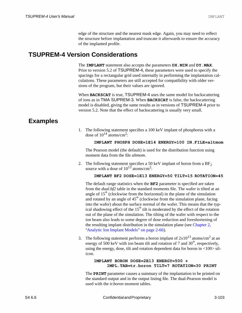
TSUPREM-4 User’s Manual IMPLANT
flecturacy
e cal--
g
a
an
typ-
heg of
> sil-
d onl is
edge of the structure and the nearest mask edge. Again, you may need to rethe structure before implantation and truncate it afterwards to ensure the accof the implanted profile.
TSUPREM-4 Version Considerations
TheIMPLANT statement also accepts the parametersDX.MIN andDY.MAX.Prior to version 5.2 ofTSUPREM-4, these parameters were used to specify thspacings for a rectangular grid used internally in performing the implantationculations. These parameters are still accepted for compatibility with older versions of the program, but their values are ignored.
WhenBACKSCAT is true,TSUPREM-4 uses the same model for backscatterinof ions as inTMA SUPREM-3. WhenBACKSCAT is false, the backscatteringmodel is disabled, giving the same results as in versions ofTSUPREM-4 prior toversion 5.2. Note that the effect of backscattering is usually very small.
Examples1. The following statement specifies a 100 keV implant of phosphorus with
dose of 1014 atoms/cm2:
The Pearson model (the default) is used for the distribution function usingmoment data from the filealtmom.
2. The following statement specifies a 50 keV implant of boron from a BF2source with a dose of 1013 atoms/cm2:
The default range statistics when theBF2 parameter is specified are takenfrom thedual.bf2 table in the standard moments file. The wafer is tilted at angle of 15° (clockwise from the horizontal) in the plane of the simulationand rotated by an angle of 45° (clockwise from the simulation plane, facinginto the wafer) about the surface normal of the wafer. This means that theical shadowing effect of the 15° tilt is moderated by the effect of the rotationout of the plane of the simulation. The tilting of the wafer with respect to tion beam also leads to some degree of dose reduction and foreshorteninthe resulting implant distribution in the simulation plane (seeChapter 2,“Analytic Ion Implant Models” on page 2-66).
3. The following statement performs a boron implant of 2x10¹³ atoms/cm2 at anenergy of 500 keV with ion beam tilt and rotation of 7 and 30°, respectively,using the energy, dose, tilt and rotation dependent data for boron in <100icon.
ThePRINT parameter causes a summary of the implantation to be printethe standard output and in the output listing file. The dual-Pearson modeused with thetr.boron moment tables.
IMPLANT PHOSPH DOSE=1E14 ENERGY=100 IN.FILE=altmom
IMPLANT BF2 DOSE=1E13 ENERGY=50 TILT=15 ROTATION=45
IMPLANT BORON DOSE=2E13 ENERGY=500 +IMPL.TAB=tr.boron TILT=7 ROTATION=30 PRINT
S4 6.6 Confidential and Proprietary 3-103
DDraft 6/26/98

Input Statement Descriptions TSUPREM-4 User’s Manual
sili-ult
enic
he
ed
therntal
s
in
andpera-
nted
4. The following statements show how theMOMENT statement can be used withtheIMPLANT statement to specify the range statistics for an implant:
TheMOMENT statement specifies the range statistics for implantation into con. Moments for implantation into other materials are read from the defamoment data file.
5. In the following statement, the Monte Carlo method is used to implant arswith a dose of 1014 atoms/cm2, an energy of 50 keV, and a tilt angle of 45°counterclockwise from vertical.
The number of ions is increased to 10,000 (from the default of 1000) toimprove the accuracy in the tail of the implant profile. This implant uses tdefault boundary condition (periodic). Thus, ions that leave the simulationregime on one side of the structure re-enter at the other side.
6. The following statements perform symmetric plus and minus 7 degree tiltimplants:
Specifying the reflecting boundary condition causes ions that exit from eiside of the simulation regime to re-enter at the same point with the horizovelocity reversed.
7. The following statement is similar to the previous example except that ionthat exit from either side re-enter on the opposite side with their velocityunchanged:
This corresponds to reproducing the simulation regime on each side, as simulating one cell of a periodic structure.
8. The following statement simulates ion implantation using analytic models generates damage for use as an initial condition for subsequent high-temture processing steps:
ThePD.TRANS model is enabled if it is not already in use. Theplus onecomponent of damage is reduced to 0.2 times the concentration of implaarsenic.
MOMENT SILICON RANGE=0.21 SIGMA=0.073 +GAMMA=-0.1 KURT=12
IMPLANT BORON DOSE=1E13 +ENERGY=50 TILT=15 MOMENTS
IMPLANT ARSENIC DOSE=1E14 ENERGY=50 MONTECAR + N.ION=10000 TILT=45
IMPLANT ARSENIC DOSE=5E13 ENERGY=50 MONTECAR +N.ION=10000 TILT=7 REFLECT
IMPLANT ARSENIC DOSE=5E13 ENERGY=50 MONTECAR +N.ION=10000 TILT=-7 REFLECT
IMPLANT ARSENIC DOSE=1E14 ENERGY=50 MONTECAR + N.ION=10000 TILT=7 PERIODIC
IMPLANT ARSENIC DOSE=1E14 ENERGY=50 DAMAGE +D.PLUS=0.2
3-104 Confidential and Proprietary S4 6.6
Draft 6/26/98

TSUPREM-4 User’s Manual DIFFUSION
the
ve
mbi-
DIFFUSION
TheDIFFUSION statement is used to model high temperature diffusion in booxidizing and nonoxidizing ambients.DIFFUSE is accepted as a synonym for thDIFFUSION statement.
DIFFUSION
TIME=<n> [CONTINUE] TEMPERAT=<n> [ T.RATE=<n> | T.FINAL=<n> ] [ DRYO2 | WETO2 | STEAM | INERT | AMB.1 | AMB.2 | AMB.3 | AMB.4 | AMB.5 | ( [F.O2=<n>] [F.H2O=<n>] [F.H2=<n>] [F.N2=<n>][F.HCL=<n>] ) ] [IMPURITY=<c> I.CONC=<n>] [ANTIMONY=<n>] [ARSENIC=<n>] [BORON=<n>] [PHOSPHOR=<n>] [PRESSURE=<n>] [ P.RATE=<n> | P.FINAL=<n> ] [HCL=<n>] [MOVIE=<c>] [DUMP=<n>]
Parameter Type Definition
TIME number The duration of the diffusion step.Units: minutesDefault: none
CONTINUE logical Indicates that this step is a continuation of a previous diffusion step. No natioxide deposition occurs and the time step is not reset. No processing stepsshould be specified between the precedingDIFFUSION statement and theDIFFUSION CONTINUE statement. The starting temperature of the stepshould be the same as the final temperature of the preceding step, and the aent must also be the same.Default: false
TEMPERAT number The ambient temperature at the beginning of the step.Units: degrees CelsiusDefault: none
T.RATE number The time rate of change of the ambient temperature.Units: degrees Celsius/minuteDefault: 0.0
T.FINAL number The ambient temperature at the end of the step.Units: degrees CelsiusDefault: TEMPERAT
DRYO2 logical Specifies that the ambient gas is dry oxygen.Default: false
WETO2 logical Specifies that the ambient gas is wet oxygen.Default: false
S4 6.6 Confidential and Proprietary 3-105
DDraft 6/26/98

Input Statement Descriptions TSUPREM-4 User’s Manual
is
is
ree
is
is
22
22
as.
STEAM logical Specifies that the ambient gas is steam.Default: false
INERT logical Specifies that the ambient gas is inert.Default: trueSynonyms:NEUTRAL, NITROGEN, ARGON
AMB.1 logical Specifies that the ambient gas is ambient number one. Ambient number onedefined by the user with theAMBIENT statement.Default: false
AMB.2 logical Specifies that the ambient gas is ambient number two. Ambient number twodefined by the user with theAMBIENT statement.Default: false
AMB.3 logical Specifies that the ambient gas is ambient number three. Ambient number this defined by the user with theAMBIENT statement.Default: false
AMB.4 logical Specifies that the ambient gas is ambient number four. Ambient number fourdefined by the user with theAMBIENT statement.Default: false
AMB.5 logical Specifies that the ambient gas is ambient number five. Ambient number fivedefined by the user with theAMBIENT statement.Default: false
F.O2 number The flow of O2 associated with the ambient gas. If H2 is also present, the Oand H2 is assumed to react completely to form H2O. The flows of O2 and Hare reduced and the flow of H2O is increased.Units: noneDefault: 0.0
F.H2O number The flow of H2O associated with the ambient gas. If O2 and H2 are alsopresent, the O2 and H2 are assumed to react completely to form H2O. Theflows of O2 and H2 are reduced and the flow of H2O is increased.Units: noneDefault: 0.0
F.H2 number The flow of H2 associated with the ambient gas. If O2 is also present, the Oand H2 are assumed to react completely to form H2O. The flows of O2 and Hare reduced and the flow of H2O is increased.Units: noneDefault: 0.0
F.N2 number The flow of N2 (and other inert components) associated with the ambient gUnits: noneDefault: 0.0
F.HCL number The flow of chlorine associated with the ambient gas.Units: noneDefault: 0.0
Parameter Type Definition
3-106 Confidential and Proprietary S4 6.6
Draft 6/26/98
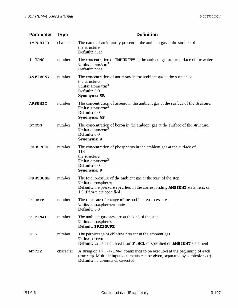
TSUPREM-4 User’s Manual DIFFUSION
.
re.
e.
(;).
IMPURITY character The name of an impurity present in the ambient gas at the surface ofthe structure.Default: none
I.CONC number The concentration ofIMPURITY in the ambient gas at the surface of the waferUnits: atoms/cm3
Default: none
ANTIMONY number The concentration of antimony in the ambient gas at the surface ofthe structure.Units: atoms/cm3
Default: 0.0Synonyms:SB
ARSENIC number The concentration of arsenic in the ambient gas at the surface of the structuUnits: atoms/cm3
Default: 0.0Synonyms:AS
BORON number The concentration of boron in the ambient gas at the surface of the structurUnits: atoms/cm3
Default: 0.0Synonyms:B
PHOSPHOR number The concentration of phosphorus in the ambient gas at the surface of116the structure.Units: atoms/cm3
Default: 0.0Synonyms:P
PRESSURE number The total pressure of the ambient gas at the start of the step.Units: atmospheresDefault: the pressure specified in the correspondingAMBIENT statement, or1.0 if flows are specified
P.RATE number The time rate of change of the ambient gas pressure.Units: atmospheres/minuteDefault: 0.0
P.FINAL number The ambient gas pressure at the end of the step.Units: atmospheresDefault: PRESSURE
HCL number The percentage of chlorine present in the ambient gas.Units: percentDefault: value calculated fromF.HCL or specified onAMBIENT statement
MOVIE character A string ofTSUPREM-4 commands to be executed at the beginning of eachtime step. Multiple input statements can be given, separated by semicolons Default: no commands executed
Parameter Type Definition
S4 6.6 Confidential and Proprietary 3-107
DDraft 6/26/98

Input Statement Descriptions TSUPREM-4 User’s Manual
ri-posi-nd
ate
o
th the
mbi-dden
Cl
ss
Description
This statement specifies a diffusion step, with or without oxidation. Any imputies present in the wafer are diffused. If the wafer is exposed to a gas, predetion and/or oxidation can be performed. If an oxidizing ambient is specified atheVISCOUS oxidation model is in effect, reflow of surface layers occurs.
The duration of the step must be specified with theTIME parameter. The ambienttemperature must be specified with theTEMPERAT keyword (unlessCONTINUEis specified). For linear ramping of the temperature, specify either the ramp r(with T.RATE) or the temperature at the end of the step (withT.FINAL ).
Ambient Gas
The ambient gas used during the diffusion step can be specified in one of twways:
1. Specify one of theDRYO2, WETO2, STEAM, INERT, orAMB.1 throughAMB.5 parameters. These select an ambient that has been predefined wiAMBIENT statement. TheDRYO2, WETO2, STEAM, andINERT ambients aredefined by the standard initialization file; theAMB.1 throughAMB.5 ambi-ents must be defined by the user before they are used. The predefined aents include a default pressure and HCl percentage, which can be overriwith thePRESSURE andHCL parameters, respectively, on theDIFFUSIONstatement.
2. Define the ambient by specifying the flows of oxidizing (O2 and H2O) andnonoxidizing (H2, N2, and HCl) species. The flows can be specified as flowrates, fractions, or percentages, but the units of all the flows in a singleDIFFUSION statement are assumed to be the same.
Any O2 and H2 in the gas are assumed to react (two units of H2 for each unit ofO2) to form H2O. Thus, the effective flow contains zero units of O2 or H2 (orboth). If the effective gas contains nonzero amounts of both O2 and H2O, the oxi-dation rate is based on the partial pressure of H2O.
Ambient GasParameters
The amount of chlorine in the ambient can be specified either by the flow of H(F.HCL parameter) or by the percentage of HCl (HCL parameter), but not both. Ifthe specified ambient contains O2 or H2O, oxidation takes place at interfacesbetween silicon dioxide and silicon or polysilicon. A native oxide (with thicknegiven by theINITIAL parameter on theAMBIENT statement) is deposited on
DUMP number Write a solution file after everyDUMP time step. The files are readable with theLOADFILE andINITIALIZE statements. The names are of the forms<time>, where<time> is the time in seconds from the start of the diffusionstep.Units: noneDefault: no intermediate solutions saved
Parameter Type Definition
3-108 Confidential and Proprietary S4 6.6
Draft 6/26/98

TSUPREM-4 User’s Manual DIFFUSION
ep.
d arere
xi-
rablyultsnifi-
toin
ion
alueg
mbi-
mayp.
any exposed silicon or polysilicon surfaces before the start of the diffusion stANTIMONY, ARSENIC, BORON, andPHOSPHOR and the combination ofIMPU-RITY andI.CONC specify the concentration of impurities at the wafer surfacefor predeposition. The total pressure for an oxidizing ambient is given byPRES-SURE. To ramp the pressure, specify either the ramp rate (P.RATE) or the pres-sure at the end of the step (P.FINAL ).
The parameters for oxidation are set by theAMBIENT statement. Diffusivities andsegregation parameters are set on the various impurity statements (i.e., theIMPURITY, ANTIMONY, ARSENIC, BORON, andPHOSPHORUS statements).The oxidation and point defect models and the numerical methods to be usespecified on theMETHOD statement. The default values for these parameters anormally set by thes4init file, which is read each timeTSUPREM-4 is executed.
SeeChapter 2 for complete descriptions of the models used for diffusion and odation andAppendix A for a list of default model coefficients.
Oxidation Limitations
Oxidation of polysilicon is simulated only when theCOMPRESS,VISCOELA, orVISCOUS model has been specified (with theMETHOD state-ment).
The oxidation algorithms provide limited support for the case where silicon (opolysilicon), oxide, and a third material meet at a point. The results are reasonaccurate when only one of the materials in contact with oxide is oxidizing; resare less accurate if both materials in contact with oxide are oxidizing at a sigcant rate.
Impurities present in the ambient during an oxidation step are incorporated inthe growing oxide. Note, however, that the program does not currently contamodels for the changes in physical properties of heavily-doped glasses.
Reflow
Reflow of surface layers occur whenever oxidation with theVISCOUS model isspecified. The amount of reflow is proportional to the ratio of the surface tens(specified by theSURF.TEN parameter on theMATERIAL statement) to the vis-cosity for each material. Reflow can occur in any material having a nonzero vof SURF.TEN. Only exposed layers flow due to surface tension, but underlyinlayers can deform due to stresses produced by reflow of the exposed layers.
Reflow in an inert ambient can be approximated by specifying an oxidizing aent with a negligible partial pressure of oxidant, e.g., by settingPRESSURE=1e-6or by a combination such asF.N2 =1.0 andF.O2 =1e-6. Note that a native oxideis added whenever the partial pressure of the oxidizing species is nonzero; itbe necessary to do a shallow etch to remove this oxide following a reflow ste
S4 6.6 Confidential and Proprietary 3-109
DDraft 6/26/98
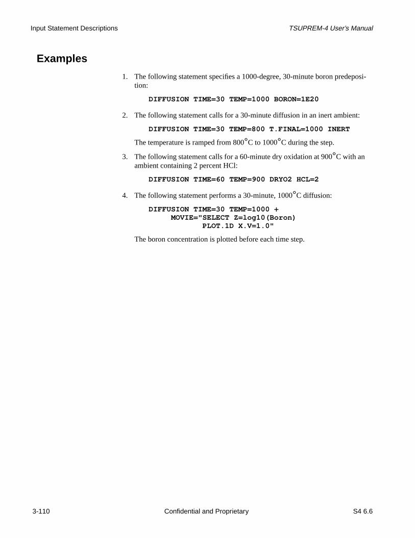
Input Statement Descriptions TSUPREM-4 User’s Manual
posi-
t:
Examples
1. The following statement specifies a 1000-degree, 30-minute boron predetion:
2. The following statement calls for a 30-minute diffusion in an inert ambien
The temperature is ramped from 800°C to 1000°C during the step.
3. The following statement calls for a 60-minute dry oxidation at 900°C with anambient containing 2 percent HCl:
4. The following statement performs a 30-minute, 1000°C diffusion:
The boron concentration is plotted before each time step.
DIFFUSION TIME=30 TEMP=1000 BORON=1E20
DIFFUSION TIME=30 TEMP=800 T.FINAL=1000 INERT
DIFFUSION TIME=60 TEMP=900 DRYO2 HCL=2
DIFFUSION TIME=30 TEMP=1000 +MOVIE="SELECT Z=log10(Boron)
PLOT.1D X.V=1.0"
3-110 Confidential and Proprietary S4 6.6
Draft 6/26/98

TSUPREM-4 User’s Manual EPITAXY
on
.
EPITAXY
TheEPITAXY statement is used to grow silicon material on the exposed silicsurface of the current structure.
EPITAXY
TIME=<n> TEMPERAT=<n> [ T.RATE=<n> | T.FINAL=<n> ] [IMPURITY=<c> I.CONC=<n> | I.RESIST=<n>] [ANTIMONY=<n>] [ARSENIC=<n>] [BORON=<n>][PHOSPHOR=<n>] [ CONCENTR | RESISTIV ]
THICKNES=<n> [SPACES=<n>] [DY=<n>] [YDY=<n>][ARC.SPAC=<n>]
Parameter Type Definition
TIME number The duration of the epitaxy step.Units: minutesDefault: none
TEMPERAT number The ambient temperature at the beginning of the step.Units: degrees CelsiusDefault: none
T.RATE number The time rate of change of the ambient temperature.Units: degrees Celsius/minuteDefault: 0.0
T.FINAL number The ambient temperature at the end of the step.Units: degrees CelsiusDefault: TEMPERAT
IMPURITY character The name of an impurity present in the ambient gas at the surface ofthe structure.Default: none
I.CONC number The concentration ofIMPURITY in the ambient gas at the surface of the waferUnits: atoms/cm3
Default: none
I.RESIST number The resistivity produced by the presence ofIMPURITY in the ambient gas atthe surface of the wafer.Units: ohm-cmDefault: none
ANTIMONY number The uniform concentration or resistivity of antimony in the deposited layer.Units: atoms/cm3 or ohm-cmDefault: zero concentrationSynonyms:SB
S4 6.6 Confidential and Proprietary 3-111
DDraft 6/26/98

Input Statement Descriptions TSUPREM-4 User’s Manual
r.
e
oca-
is
ARSENIC number The uniform concentration or resistivity of arsenic in the deposited layer.Units: atoms/cm3 or ohm-cmDefault: zero concentrationSynonyms:AS
BORON number The uniform concentration or resistivity of boron in the deposited layer.Units: atoms/cm3
Default: zero concentrationSynonyms:B
PHOSPHOR number The uniform concentration or resistivity of phosphorus in the deposited layeUnits: atoms/cm3 or ohm-cmDefault: zero concentrationSynonyms:P
CONCENTR logical Specifies that the impurity concentration in the deposited layer is given.Default: true
RESISTIV logical Specifies that the resistivity of the deposited layer is given.Default: false
THICKNES number The thickness of the deposited layer.Units: micronsDefault: none
SPACES number The number of vertical grid spacings in the layer. This value is divided by thvalue ofGRID.FAC (see“MESH” on page 3-44).Units: noneDefault: 1/GRID.FACSynonyms:DIVISION
DY number The nominal grid spacing to be used in the deposited material layer at the ltion specified by theYDY parameter. This value is multiplied by the value ofGRID.FAC (see“MESH” on page 3-44).Units: micronsDefault: GRID.FAC*THICKNES/SPACESSynonyms:DX
YDY number The location of the nominal grid spacing specified byDY relative to the top ofthe deposited layer.Units: microns)Default: 0.0Synonyms:XDX
ARC.SPAC number The maximum spacing allowed along an arc on the new surface. This valuemultiplied by the value ofGRID.FAC (see“MESH” on page 3-44).Units: micronsDefault: 0.5*THICKNES*GRID.FAC
Parameter Type Definition
3-112 Confidential and Proprietary S4 6.6
Draft 6/26/98

TSUPREM-4 User’s Manual EPITAXY
posedctly
idepprox-
-7
inmber
us-
nding
Description
This statement provides a basic epitaxy capability. Silicon is deposited on theexposed surface of the structure, and its upper surface becomes the new exsurface. A uniform concentration of each dopant can be specified, either direor by the resistivity of the grown material. Impurities diffuse according to themodels inChapter 2, “Diffusion” on page 2-12.
The deposited material conforms to the contours of the original surface. Outscorners on the original surface produce arcs on the new surface, which are aimated by straight line segments. The maximum segment length is set by theARC.SPAC parameter.
TheSPACES, DY, andYDY parameters used to control the grid spacing in thedeposited layer are scaled by the value of theGRID.FAC parameter on theMESHstatement (seeChapter 2, “Changes to the Mesh During Processing” on page 2).
TheEPITAXY works by alternately depositing layers and diffusing impurities the resulting structure. The number of deposit/diffuse steps is equal to the nuof grid spaces in the deposited layer, i.e., it is controlled by theSPACES, DY, andYDY parameters.
Example
The following statement deposits 1 micron of silicon while simultaneously diffing at 1100°C:
The deposition and diffusion processes are subdivided into 10 steps correspoto the value specified by theSPACES parameter.
Note:The mobility tables used to calculate the doping from the resistive arenot the same as the tables used by theELECTRICAL statement. Theextracted sheet resistance for the epitaxial layer does not correspondexactly to the resistivity specified during epitaxy.
EPITAXY THICK=1.0 TIME=180 TEMPERAT=1100 +ANTIMONY=1E19 SPACES=10
S4 6.6 Confidential and Proprietary 3-113
DDraft 6/26/98

Input Statement Descriptions TSUPREM-4 User’s Manual
l mis-
ll
g the
ing
STRESS
TheSTRESS statement calculates the stresses caused by thermal mismatchbetween materials or due to intrinsic stress in deposited films.
Description
This statement calculates stresses due to thin film intrinsic stress and thermamatch. For thermal mismatch stresses,TEMP1 andTEMP2 specify the initial andfinal temperatures, respectively. IfTEMP1 andTEMP2 are not specified or areequal, no thermal stresses are calculated.
The magnitude of the intrinsic stress in a thin film is specified by theINTRIN.Sparameter on theMATERIAL statement. By default, the intrinsic stresses are aset to zero.
Printing and Plotting of Stresses and Displacements
The calculated stresses can be accessed for printing or plotting by referencinvariablesSxx, Syy, andSxy on theSELECT statement; the calculatedx andy dis-placements can be referenced asx.vel andy.vel. The stresses and displacementscan also be displayed with theSTRESS andFLOW parameters on thePLOT.2Dstatement.
Note:Stresses and displacements calculated by theSTRESS statement replaceany values of stress or velocity calculated by a preceding oxidation step.
STRESS
[TEMP1=<n> TEMP2=<n>] [NEL=<n>]
Parameter Type Definition
TEMP1 number The initial temperature for calculating thermal mismatch stresses.Units: degrees CelsiusDefault: none
TEMP2 number The final temperature for calculating thermal mismatch stresses.Units: degrees CelsiusDefault: none
NEL number The number of nodes per triangle to use. Valid values are 6 and 7, with 6 befaster.Units: noneDefault: 6
3-114 Confidential and Proprietary S4 6.6
Draft 6/26/98

TSUPREM-4 User’s Manual STRESS
o ag
ess, (cre-uc-
ing
For more information, seeChapter 2, “Modeling Stress with theSTRESS State-ment” on page 2-64.
Reflecting Boundary Limitations
The stress calculation does not allow expansion or shrinkage perpendicular treflecting boundary. Thus, the results are not correct when there are reflectinboundaries on both the left and right edges of a structure. For calculating stryou should either use a structure with an exposed boundary on the right sideated with theBOUNDARY statement or by etching away the right edge of the strture), or use coefficients of thermal expansion relative to the value for silicon(assuming a silicon substrate).
Example
The following statements calculate the stresses in the substrate and film arisfrom a nitride layer that has an intrinsic stress of 1.4x10¹⁰ dynes/cm2, whendeposited uniformly:
MATERIAL NITRIDE INTRIN.S=1.4E10STRESS
S4 6.6 Confidential and Proprietary 3-115
DDraft 6/26/98

Input Statement Descriptions TSUPREM-4 User’s Manual
3-116 Confidential and Proprietary S4 6.6
Draft 6/26/98
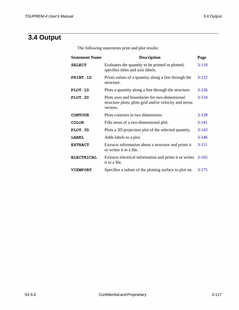
TSUPREM-4 User’s Manual 3.4 Output
S4 6.6
3 13033 1303
3.4 OutputThe following statements print and plot results:
Statement Name Description Page
SELECT Evaluates the quantity to be printed or plotted;specifies titles and axis labels.
3-118
PRINT.1D Prints values of a quantity along a line through thestructure.
3-122
PLOT.1D Plots a quantity along a line through the structure.3-126
PLOT.2D Plots axes and boundaries for two-dimensionalstructure plots; plots grid and/or velocity and stressvectors.
3-134
CONTOUR Plots contours in two dimensions. 3-139
COLOR Fills areas of a two-dimensional plot. 3-141
PLOT.3D Plots a 3D projection plot of the selected quantity.3-143
LABEL Adds labels to a plot. 3-146
EXTRACT Extracts information about a structure and prints itor writes it to a file.
3-151
ELECTRICAL Extracts electrical information and prints it or writesit to a file.
3-165
VIEWPORT Specifies a subset of the plotting surface to plot on.3-175
Confidential and Proprietary 3-117
Draft 6/26/98

Input Statement Descriptions TSUPREM-4 User’s Manual
sed
is
d.
lot-t the
the
SELECT
TheSELECT statement evaluates a quantity to be printed or plotted. It is also uto specify plot titles and axis labels.
Description
TheSELECT statement evaluates the quantity to be displayed by theCONTOUR,PLOT.1D, PRINT.1D , PLOT.2D, andPLOT.3D statements or to be extractedby theEXTRACT statement. No solution data can be printed or plotted until thstatement is specified. The values calculated by aSELECT statement are useduntil anotherSELECT statement is specified. If the solution changes, a newSELECT statement is given in order for the new values to be printed or plotte
Solution Values
TheZ parameter specifies a mathematical expression for the quantity to be pted. The following solution values can be used in the expression, provided thasolution is available:
SELECT
[Z=<c>] [TEMPERAT=<n>] [LABEL=<c>][TITLE=<c>]
Parameter Type Definition
Z character A mathematical expression defining the quantity to be printed or plotted. If expression contains spaces, it must be enclosed in parentheses.Default: “0”
TEMPERAT number The temperature at which the solution is to be evaluated.Units: degrees CelsiusDefault: last specified temperature or 800
LABEL character The label to be used on they axis of a one-dimensional plot, or thez axis of athree-dimensional plot.Default: the expression given byZ
TITLE character The title to be used on plots.Default: the name and version number of the program
antimony antimony concentration (atoms/cm3)
arsenic arsenic concentration (atoms/cm3)
boron boron concentration (atoms/cm3)
phosphorus phosphorus concentration (atoms/cm3)
3-118 Confidential and Proprietary S4 6..6
DDraft 6/26/98

TSUPREM-4 User’s Manual SELECT
entra-
, for
inus
arge
ely.
• The names of user-specified impurities can also be used, giving the conction of the impurity in atoms/cm3.
• The chemical concentration is reported unless the active function is usedexample,active(phosphorus).
• The net concentration is defined as the sum of the donor concentrations mthe sum of the acceptor concentrations.
• The electron concentration is calculated using the assumptions of local chneutrality and complete ionization of impurities.
Mathematical Operations and Functions
The symbols “+”, “-”, “*”, “/”, and “^” are used for the mathematical operationsof addition, subtraction, multiplication, division, and exponentiation, respectivIn addition, the following functions are available:
doping net active concentration (atoms/cm3)
oxygen oxidant concentration (atoms/cm3)
silicon silicon concentration (in silicide) (atoms/cm3)
interstitial interstitial concentration (#/cm3)
vacancy vacancy concentration (#/cm3)
ci.star equilibrium interstitial concentration (#/cm3)
cv.star equilibrium vacancy concentration (#/cm3)
trap concentration of filled interstitial traps (#/cm3)
cl_interst concentration of clustered interstitials (#/cm3)
dloop density of dislocation loops (#/cm3)
rloop radius of dislocation loops (cm)
lgrain average polycrystalline grain size (um)
electron concentration of electrons (#/cm3)
x.v x velocity (cm/sec)
y.v y velocity (cm/sec)
Sxx, Sxy, Syy components of the stress tensor (dynes/cm2)
x x coordinate (microns)
y y coordinate (microns)
active electrically active part of impurity concentration
gb concentration of impurity in polycrystalline grainboundaries
S4 6.6 Confidential and Proprietary 3-119
Draft 6/26/98

Input Statement Descriptions TSUPREM-4 User’s Manual
o;.
ofile
Thelog, log10, andslog10 functions return the value 0.0 if their argument is zerthe log, log10, slog10, andsqrt functions take absolute value of their argumentsThe following constant is available:
Note:The active and net concentrations depend on the temperature. IfTEMPERAT is not specified, the last processing temperature is used. Ifthe last process step ended with a ramp to a low temperature, you mayneed to specify a higher value ofTEMPERAT in order to obtain realisticlevels of dopant activation.
Examples
1. The logarithm (base 10) of the arsenic concentration is evaluated with
2. The phosphorus concentration minus a constant profile of 5x10¹⁴ is evaluatedwith
3. The difference between the phosphorus concentration and an analytic pris evaluated with
4. The excess vacancy-interstitial product is evaluated with
abs absolute value
diffusivity diffusivity (in cm2/sec) of an impurity or point defectspecies
erf error function
erfc complementary error function
exp exponential
log natural logarithm of the absolute value
log10 base-10 logarithm of the absolute value
slog10 base-10 logarithm of the absolute value times the signof the value
sqrt square root
Kb Boltzmann’s constant (eV/°C)
SELECT Z=log10(Arsenic)
SELECT Z=(Phosphorus - 5.0e14)
SELECT Z=(phos - 1.0e18 * exp ( y * y ) )
SELECT Z=(inter * vacan - ci.star * cv.star)
3-120 Confidential and Proprietary S4 6..6
DDraft 6/26/98

TSUPREM-4 User’s Manual SELECT
ted
ith
er
alue
r
5. The diffusivity (in cm2/sec) of boron at each point in the structure is evaluawith
Note that when thePD.TRANS or PD.FULL model for point defects is used,the diffusivity can be different at each point in the structure and may vary wtime.
6. The following statements print junction depths:
ThePRINT LAYERS statement assumes that a new layer begins whenevthe selected value (net doping in this case) changes sign.
7. The following statements print the thicknesses of material layers:
TheSELECT statement specifies a constant value of one, so thePRINT state-ment only uses material boundaries to define layers. Further, when the v“1.0” is integrated over each layer, the result is just the layer thickness.
8. The following statement specifies the title to be used on the next plot:
Because noZ value is specified,Z=0 is assumed, and any attempt to print oplot solution data uses the value zero.
SELECT Z=diffusivity(Boron)
SELECT Z=dopingPRINT LAYERS X.V=0
SELECT Z=1.0PRINT LAYERS X.V=0
SELECT TITLE="Final N-Channel Structure"
S4 6.6 Confidential and Proprietary 3-121
Draft 6/26/98

Input Statement Descriptions TSUPREM-4 User’s Manual
lineinfor-
.
PRINT.1D
ThePRINT.1D statement prints the value of the selected expression along athrough the structure. It can also print layer thickness and integrated doping mation.
PRINT.1D
X.VALUE=<n> | Y.VALUE=<n> | ( MATERIAL=<c> | SILICON | OXIDE | OXYNITRI | NITRIDE | POLYSILI | PHOTORES | ALUMINUM /MATERIA=<c> | /SILICON | /OXIDE | /OXYNITR | /NITRIDE | /POLYSIL | /PHOTORE | /ALUMINU | /AMBIENT | /REFLECT ) [SPOT=<n>] [LAYERS] [X.MIN=<n>] [X.MAX=<n>]
Parameter Type Definition
X.VALUE number Thex coordinate of a vertical section along which values are to be printed.Units: micronsDefault: 0.0
Y.VALUE number They coordinate of a horizontal section along which values are to be printedUnits: micronsDefault: none
MATERIAL character Print values in the named material, at the interface with the other specifiedmaterial.Default: none
SILICON logical Print values in silicon, at the interface with the other specified material.Default: false
OXIDE logical Print values in oxide, at the interface with the other specified material.Default: false
OXYNITRI logical Print values in oxynitride, at the interface with the other specified material.Default: false
NITRIDE logical Print values in nitride, at the interface with the other specified material.Default: false
POLYSILI logical Print values in polysilicon, at the interface with the other specified material.Default: false
PHOTORES logical Print values in photoresist, at the interface with the other specified material.Default: false
3-122 Confidential and Proprietary S4 6..6
DDraft 6/26/98

TSUPREM-4 User’s Manual PRINT.1D
g
quals
ALUMINUM logical Print values in aluminum, at the interface with the other specified material.Default: false
/MATERIA character Print values in the other specified material, at the interface with the namedmaterial.Default: none
/SILICON logical Print values in the other specified material, at the interface with silicon.Default: false
/OXIDE logical Print values in the other specified material, at the interface with oxide.Default: false
/OXYNITR logical Print values in the other specified material, at the interface with oxynitride.Default: false
/NITRIDE logical Print values in the other specified material, at the interface with nitride.Default: false
/POLYSIL logical Print values in the other specified material, at the interface with polysilicon.Default: false
/PHOTORE logical Print values in the other specified material, at the interface with photoresist.Default: false
/ALUMINU logical Print values in the other specified material, at the interface with aluminum.Default: false
/AMBIENT logical Print values in the other specified material, at the interface with the exposedsurface (if any).Default: falseSynonyms:/EXPOSED, /GAS
/REFLECT logical Print values in the other specified material, at the interface with the reflectinboundary (if any).Default: false
SPOT number Print the coordinate along the cross-section at which the selected quantity ethe specified value.Units: units of the selected quantityDefault: none
LAYERS logical Report the integral of the selected quantity over each layer of the devicestructure.Default: false
X.MIN number The minimum position along the cross-section to be printed.Units: micronsDefault: none
X.MAX number The maximum position along the cross-section to be printed.Units: micronsDefault: none
Parameter Type Definition
S4 6.6 Confidential and Proprietary 3-123
Draft 6/26/98

Input Statement Descriptions TSUPREM-4 User’s Manual
ross-al (by
ntity
ch
hereross-re, the
al-
yon-
Description
ThePRINT.1D statement prints the values of the selected quantity along a csection through the device. cross-sections are defined as vertical or horizonttheX.VALUE andY.VALUE parameters, respectively), along the interfacebetween two materials, or along a boundary of the device structure. The quato be printed must be specified on aSELECT statement preceding thePRINT.1Dstatement. TheSPOT parameter finds all points along the specified path at whithe selected quantity equals the specified value.
Layers
If LAYERS is specified, the integral of the selected quantity over each layer isprinted. The integration is along the path defined by theX.VALUE, Y.VALUE, orinterface specification. Layers are delimited by those points along the path wthe material type changes or the sign of the selected quantity changes. If a csection passes out a structure into the ambient and then re-enters the structuambient “layer” may be omitted from theLAYERS output.
Interface Values
The values along the interface between two materials depend on the order inwhich the materials are specified. ThusSILICON /OXIDE andOXIDE /SILICON print values at the same interface, but the first prints the vues in the silicon, while the second prints the values in the oxide.
Values along an interface are sorted by theirx coordinates. The values printed manot be in order if there are vertical or reentrant interfaces, or if the structure ctains more than one interface between the specified materials.
Examples
1. The following statements print the boron concentration atx=1.0 micronbetween the top of the mesh andy=3.0 microns:
2. The following statements print thex andy coordinates of the interfacebetween silicon and oxide:
3. The following statements prints junction depths:
SELECT Z=BoronPRINT.1D X.VAL=1.0 X.MAX=3.0
SELECT Z=yPRINT.1D SILICON /OXIDE
SELECT Z=dopingPRINT LAYERS X.V=0
3-124 Confidential and Proprietary S4 6..6
DDraft 6/26/98

TSUPREM-4 User’s Manual PRINT.1D
ected
alue
ThePRINT statement assumes that a new layer begins whenever the selvalue (net doping in this case) changes sign.
4. The following statements print the thicknesses of material layers:
TheSELECT statement specifies a constant value of one, so thePRINT state-ment only uses material boundaries to define layers. Further, when the v“1.0” is integrated over each layer, the result is just the layer thickness.
SELECT Z=1.0PRINT LAYERS X.V=0
S4 6.6 Confidential and Proprietary 3-125
Draft 6/26/98

Input Statement Descriptions TSUPREM-4 User’s Manual
e
ther
PLOT.1D
ThePLOT.1D statement plots the value of the selected expression along a linthrough the structure.
PLOT.1D
[ X.VALUE=<n> | Y.VALUE=<n> ] | ( MATERIAL=<c> | SILICON | OXIDE | OXYNITRI | NITRIDE | POLYSILI | PHOTORES | ALUMINUM /MATERIA=<c> | /SILICON | /OXIDE | /OXYNITR | /NITRIDE | /POLYSIL | /PHOTORE | /ALUMINU | /AMBIENT | /REFLECT ) | IN.FILE=<c>
(TIF X.AXIS=<c> Y.AXIS=<c>)|( (COLUMN [X.COLUMN=<n>] [Y.COLUMN=<n>])
| (ROW [X.ROW=<n>] [Y.ROW=<n>]) [X.LABEL=<c>] [Y.LABEL=<c>] )
[X.SHIFT=<n>] [Y.SHIFT=<n>]
[X.SCALE=<n>] [Y.SCALE=<n>][Y.LOG] [X.LOG]
| ELECTRIC [BOUNDARY] [CLEAR] [AXES] [SYMBOL=<n>] [CURVE] [LINE.TYP=<n>] [COLOR=<n>] [LEFT=<n>] [RIGHT=<n>] [BOTTOM=<n>] [TOP=<n>] [X.OFFSET=<n>] [X.LENGTH=<n>] [X.SIZE=<n>] [Y.OFFSET=<n>] [Y.LENGTH=<n>] [Y.SIZE=<n>] [T.SIZE=<n>]
Parameter Type Definition
X.VALUE number A vertical cross-section is to be plotted at this value ofx.Units: micronsDefault: 0.0
Y.VALUE number A horizontal cross-section is to be plotted at this value ofy.Units: micronsDefault: none
MATERIAL character Plot a cross-section through the named material, at the interface with the ospecified material.Default: none
3-126 Confidential and Proprietary S4 6..6
DDraft 6/26/98

TSUPREM-4 User’s Manual PLOT.1D
ed
fied
ified
ed
th the
h
h
h
h
h
SILICON logical Plot a cross-section through silicon, at the interface with the other specifiedmaterial.Default: false
OXIDE logical Plot a cross-section through oxide, at the interface with the other specifiedmaterial.Default: false
OXYNITRI logical Plot a cross-section through oxynitride, at the interface with the other specifimaterial.Default: false
NITRIDE logical Plot a cross-section through nitride, at the interface with the other specifiedmaterial.Default: false
POLYSILI logical Plot a cross-section through polysilicon, at the interface with the other specimaterial.Default: false
PHOTORES logical Plot a cross-section through photoresist, at the interface with the other specmaterial.Default: false
ALUMINUM logical Plot a cross-section through aluminum, at the interface with the other specifimaterial.Default: false
/MATERIA character Plot a cross-section through the other specified material, at the interface winamed material.Default: none
/SILICON logical Plot a cross-section through the other specified material, at the interface witsilicon.Default: false
/OXIDE logical Plot a cross-section through the other specified material, at the interface witoxide.Default: false
/OXYNITR logical Plot a cross-section through the other specified material, at the interface witoxynitride.Default: false
/NITRIDE logical Plot a cross-section through the other specified material, at the interface witnitride.Default: false
/POLYSIL logical Plot a cross-section through the other specified material, at the interface witpolysilicon.Default: false
Parameter Type Definition
S4 6.6 Confidential and Proprietary 3-127
Draft 6/26/98

Input Statement Descriptions TSUPREM-4 User’s Manual
h
h
the
the
per-
file.
.
/PHOTORE logical Plot a cross-section through the other specified material, at the interface witphotoresist.Default: false
/ALUMINU logical Plot a cross-section through the other specified material, at the interface witaluminum.Default: false
/AMBIENT logical Plot a cross-section through the other specified material, at the interface withexposed surface.Default: falseSynonyms:/GAS, /EXPOSED
/REFLECT logical Plot a cross-section through the other specified material, at the interface withreflecting boundary (if any).Default: false
IN.FILE character The identifier for the file containing the data to plot. This file may contain eximental data or data produced by theEXTRACT or ELECTRICAL statements.Default: none
TIF logical Specifies that the format ofIN.FILE is TIF (.ivl file from Medici).Default: false
X.AXIS character The quantity used for the horizontal axis when plotting data stored in a TIFThe label is automatically assigned with the string composite of theX.AXISand the unit associated withX.AXIS in a TIF file.Default: none
Y.AXIS character The quantity used for the vertical axis when plotting data stored in a TIF fileThe label is automatically assigned with the string composite of theY.AXISand the unit associated withY.AXIS in a TIF file.Default: none
COLUMN logical Specifies that the format ofIN.FILE is column-wise.Default: true
X.COLUMN number The index of the column in the file specified by theIN.FILE parameter thatcontains the horizontal coordinates of the plot.Units: noneDefault: 1
Y.COLUMN number The index of the column in the file specified by theIN.FILE parameter thatcontains the vertical coordinates of the plot.Units: noneDefault: 2
ROW logical Specifies that the format ofIN.FILE is row-wise.Default: false
X.ROW number The index of the row(line) in the file specified by theIN.FILE parameter thatcontains the horizontal coordinates of the plot.Units: noneDefault: 1
Parameter Type Definition
3-128 Confidential and Proprietary S4 6..6
DDraft 6/26/98

TSUPREM-4 User’s Manual PLOT.1D
lines
Y.ROW number The index of the row(line) in the file specified by theIN.FILE parameter thatcontains the vertical coordinates of the plot.Units: noneDefault: 2
X.LABEL character The label of the horizontal axis forX.COLUMN data in theIN.FILE file.Default: “Distance (microns)”
Y.LABEL character The label of the vertical axis forY.COLUMN data in theIN.FILE file.Default: if the SELECT statement is defined,LABEL in SELECT, otherwise,“Concentration (#/cm3)”
X.SHIFT number The offset by whichX.COLUMN data are shifted when readingIN.FILE file.Units: the same as for theX.COLUMN dataDefault: 0.0
Y.SHIFT number The offset by whichY.COLUMN data are shifted when readingIN.FILE file.Units: the same as for theY.COLUMN dataDefault: 0.0
X.SCALE number The scaling factor by whichX.COLUMN data are multiplied when readingIN.FILE file.Units: noneDefault: 1.0
Y.SCALE number The scaling factor by whichY.COLUMN data are multiplied when readingIN.FILE file.Units: noneDefault: 1.0
Y.LOG logical Specifies that the vertical axis forY.COLUMN data in theIN.FILE file islogarithmic.Default: the current value dependent onZ quantity in theSELECT statementSynonyms:LOG
X.LOG logical Specifies that the horizontal axis forX.COLUMN data in theIN.FILE file islogarithmic.Default: the current value in the previous specification. Otherwise, false.
ELECTRIC logical Specifies plotting of results from a precedingELECTRICAL statement.Default: false
BOUNDARY logical If true, material boundaries that are crossed are indicated by dashed verticalon the plot.Default: true
CLEAR logical If true, the graphics screen is cleared before the graph is drawn.Default: true
Parameter Type Definition
S4 6.6 Confidential and Proprietary 3-129
Draft 6/26/98

Input Statement Descriptions TSUPREM-4 User’s Manual
te-g
tions
with
AXES logical Specifies that axes should be drawn, using scaling information from this stament and/or the current structure. IfAXES is false, no axes are drawn and scalininformation from the previous plotting statement is used (i.e.,LEFT, RIGHT,BOTTOM, andTOP are ignored). IfAXES is false and no previous plotting state-ment has been given, an error is reported.Default: trueSynonyms:AXIS
SYMBOL number The type of centered symbol to be drawn at each point where the cross-secintersects a mesh line. This value must be in the range 1 to 15. Values of thiparameter are associated with the following symbols:
1 Square2 Circle3 Triangle4 Plus5 Upper case X6 Diamond7 Up-arrow8 Roofed upper case X9 Upper case Z10 Upper case Y11 Curved square12 Asterisk13 Hourglass14 Bar15 Star
Units: noneDefault: no symbols drawn
CURVE logical Specifies that a line is to be drawn through the data points.Default: true
LINE.TYP number The dashed line type used for the plotted data. (The axes are always drawnline type 1.)Units: noneDefault: 1
COLOR number The color of line used for the plotted data. (The axes are always drawn withcolor 1.)Units: noneDefault: 1
LEFT number The minimum value to be plotted on thex axis.Units: micronsDefault: minimumx or y coordinate of the structureSynonyms:X.MIN
Parameter Type Definition
3-130 Confidential and Proprietary S4 6..6
DDraft 6/26/98

TSUPREM-4 User’s Manual PLOT.1D
ofics
plot
plot
ft
bot-
Description
ThePLOT.1D statement plots cross-sections vertically or horizontally throughthe device, or along an interface between two materials, or along a boundarythe device. The statement has options to provide for initialization of the graph
RIGHT number The maximum value to be plotted on thex axis.Units: micronsDefault: maximumx or y coordinate of the structureSynonyms:X.MAX
BOTTOM number The minimum value of the selected expression to be plotted, in units of the variable.Units: units of the selected expressionDefault: minimum value of the selected expressionSynonyms: Y.MIN
TOP number The maximum value of the selected expression to be plotted, in units of thevariable.Units: units of the selected expressionDefault: maximum value of the selected expressionSynonyms: Y.MAX
X.OFFSET number The distance by which the left end of the horizontal axis is offset from the leedge of the graphics viewport.Units: cmDefault: 2.0
X.LENGTH number The length of the horizontal axis.Units: cmDefault: viewport width -X.OFFSET - 1.25
X.SIZE number The height of the characters used to label the horizontal axis.Units: cmDefault: 0.25
Y.OFFSET number The distance by which the bottom end of the vertical axis is offset from the tom edge of the graphics viewport.Units: cmDefault: 2.0
Y.LENGTH number The length of the vertical axis.Units: cmDefault: viewport height -Y.OFFSET - 1.25
Y.SIZE number The height of the characters used to label the vertical axis.Units: cmDefault: 0.25
T.SIZE number The height of the characters in the character string used as the plot title.Units: cmDefault: 0.4
Parameter Type Definition
S4 6.6 Confidential and Proprietary 3-131
Draft 6/26/98

Input Statement Descriptions TSUPREM-4 User’s Manual
e
re
.
., sil-
ngles
.dash
lacke
ge col-hatorder,
-w-
are
ust
device and plotting of axes. The statement can optionally draw vertical lineswhenever a material boundary is crossed. The vertical axis corresponds to thvariable selected with theSELECT statement.
Limits can be specified so that only a portion of the entire device is shown, omore than one variable can be conveniently plotted. By default the limits of thxaxis extend to the edges of the structure, and they axis is scaled according to theminimum and maximum values of the selected value over the entire structure
The quantity to be plotted must be defined by a precedingSELECT statement. Thetype of graphics device must be set, either with anOPTION statement or throughuse of a suitable default. (See“OPTION” on page 3-33 andAppendix B.)
If two materials are specified (e.g.,OXIDE /SILICON ), a cross-section is plottedin the first material (e.g., oxide) at the interface with the second material (e.gicon). Note thatOXIDE /SILICON produces different results fromSILICON /OXIDE. For interface plots, the points along the interface are sorted by theirxcoordinates; specifying interfaces containing vertical segments or reentrant amay not produce useful plots.
Line Type and Color
TheLINE.TYP parameter specifies the dashed line type for plotting the dataLine type 1 is solid, while types 2 through 7 are dashed lines with increasing sizes. Types 8 through 10 produce more complicated patterns of dashes.
TheCOLOR parameter specifies the color for plotting the data. Color 1 is thedefault, and produces a line that contrasts with the background color (e.g., bon white or white on black). TheCOLOR parameter has no effect on monochromdisplays.
The colors produced by theCOLOR parameter depend on the type of display beinused. Where possible, the colors 2 through 7 have been set up to produce thors red, green, blue, cyan (light blue), magenta (light purple), and yellow, in torder. Colors 8 and above produce a repeating series of 12 colors in rainbow from red to violet.
IN.FILE Parameter
The format of the file specified by theIN.FILE parameter can be either columnwise or TIF. In the case of a columnwise format, the file may contain the folloing two types of lines:
1. Lines that are blank or contain a slash (/) as the first nonblank character ignored and can be used to document the file.
2. Other lines define the data at one point in the distribution. These lines mcontain the following values:
a. Value numberX.COLUMN is the horizontal coordinate of the point.
3-132 Confidential and Proprietary S4 6..6
DDraft 6/26/98

TSUPREM-4 User’s Manual PLOT.1D
a
e
dis-
b. Value numberY.COLUMN is the vertical coordinate of the point.
If this line contains fewer thanN numerical values in free-field format, whereN is the maximum of indices (X.COLUMN andY.COLUMN) for the valueslisted above, the line is ignored.
Since the .ivl log file ofMedici is a TIF format file, the results of device simula-tion can be plotted ifTIF , X.AXIS andY.AXIS are specified. This capabilitymakes it possible to easily compare the electrical calculations ofTSUPREM-4andMedici.
The transformation of data read by theIN.FILE parameter is as follows:
Data of X axis = X.SCALE x Data ofX.COLUMNor X.AXIS + X.SHIFTData of Y axis = Y.SCALE x Data ofY.COLUMNor Y.AXIS + Y.SHIFT
Examples
1. The following statement clears the screen, draws a set of axes, and plots(vertical) cross-section atx=1.0 micron:
PLOT.1D X.V=1.0 SYMB=1 ^CURVE
Symbol 1 (a small square) is drawn at each data point; the line through thdata points is suppressed.
2. The following statement plots a cross-section atx=2.0 microns on the previ-ous set of axes, without clearing the screen:
A line consisting of short dashes is used, and appears in color 3 on colorplays.
PLOT.1D X.V=2.0 ^AXES ^CLEAR LINE.TYP=2 COLOR=3
S4 6.6 Confidential and Proprietary 3-133
Draft 6/26/98

Input Statement Descriptions TSUPREM-4 User’s Manual
ure.
ice.
PLOT.2D
ThePLOT.2D statement specifies a two-dimensional plot of the device struct
PLOT.2D
[X.MIN=<n>] [X.MAX=<n>] [Y.MIN=<n>] [Y.MAX=<n>] [SCALE] [CLEAR] [AXES] [BOUNDARY] [L.BOUND=<n>] [C.BOUND=<n>] [GRID] [L.GRID=<n>] [C.GRID=<n>] [ [STRESS] [FLOW] VLENG=<n> [VMAX=<n>] [L.COMPRE=<n>] [C.COMPRE=<n>] [L.TENSIO=<n>] [C.TENSIO=<n>] ] [DIAMONDS] [X.OFFSET=<n>] [X.LENGTH=<n>] [X.SIZE=<n>] [Y.OFFSET=<n>] [Y.LENGTH=<n>] [Y.SIZE=<n>] [T.SIZE=<n>]
Parameter Type Definition
X.MIN number Thex coordinate of the left edge of the region to be plotted.Units: micronsDefault: left edge of the deviceSynonyms:LEFT
X.MAX number Thex coordinate of the right edge of the region to be plotted.Units: micronsDefault: right edge of the deviceSynonyms:RIGHT
Y.MIN number They coordinate of the top edge of the region to be plotted.Units: micronsDefault: Ytop-(Y.MAX-Ytop)/10, where Ytop is they coordinate of the top ofthe deviceSynonyms:TOP
Y.MAX number They coordinate of the bottom edge of the region to be plotted.Units: micronsDefault: bottom edge of the deviceSynonyms:BOTTOM
SCALE logical If true, thex andy axes are scaled to preserve the true aspect ratio of the devIf false, the axes are scaled to fill the available plotting area.Default: false
CLEAR logical If true, the graphics screen is cleared before the graph is drawn.Default: true
3-134 Confidential and Proprietary S4 6..6
DDraft 6/26/98

TSUPREM-4 User’s Manual PLOT.2D
te-g
.
prin-
-
AXES logical Specifies that axes should be drawn, using scaling information from this stament and/or the current structure. IfAXES is false, no axes are drawn and scalininformation from the previous plotting statement is used (i.e.,X.MIN , X.MAX,Y.MIN , andY.MAX are ignored). IfAXES is false and no previous plottingstatement has been given, an error is reported.Default: trueSynonyms:AXIS
BOUNDARY logical Plot the device boundary and material interfaces.Default: true
L.BOUND number The dashed line type used for plotting the device boundary andmaterial interfaces.Units: noneDefault: 1Synonyms:LINE.BOU , LINE.TYP
C.BOUND number The line color used for plotting the device boundary and material interfacesUnits: noneDefault: 1
GRID logical Plot the grid used for the numerical solution.Default: false
L.GRID number The dashed line type used for plotting the grid.Units: noneDefault: 1Synonyms:LINE.GRI
C.GRID number The line color used for plotting the grid.Units: noneDefault: 1
STRESS logical Plot the principal stresses in the structure. Vectors are drawn along the two cipal axes of the stress tensor at each mesh point.Default: false
FLOW logical Plot vectors indicating the velocity (due to oxidation) or displacement (calculated by theSTRESS statement) at each mesh point.Default: false
VLENG number The length of the vector drawn for the maximum value of stress or velocity.Units: micronsDefault: none
VMAX number The maximum value of stress or velocity to be plotted.Units: dynes/cm2 for stress, cm/sec for flowDefault: no limit on maximum value
L.COMPRE number The dashed line type used for plotting compressive stress vectors andflow vectors.Units: noneDefault: 1Synonyms:L.FLOW, L.VELOCI , LINE.COM
Parameter Type Definition
S4 6.6 Confidential and Proprietary 3-135
Draft 6/26/98

Input Statement Descriptions TSUPREM-4 User’s Manual
for It is
.
ft
bot-
Description
ThePLOT.2D statement specifies a two-dimensional plot. It is useful in itself plotting structure outlines and interface locations, grid, stress, and velocities.also used to plot axes for theCONTOUR andCOLOR statements.
C.COMPRE number The line color used for plotting compressive stress vectors and flow vectorsUnits: noneDefault: 1Synonyms:C.FLOW, C.VELOCI
L.TENSIO number The dashed line type used for plotting tensile stress vectors.Units: noneDefault: 1Synonyms:LINE.TEN
C.TENSIO number The line color used for plotting tensile stress vectors.Units: noneDefault: 1
DIAMONDS logical Plot a small symbol at each mesh point location.Default: false
X.OFFSET number The distance by which the left end of the horizontal axis is offset from the leedge of the graphics viewport.Units: cmDefault: 2.0
X.LENGTH number The length of the horizontal axis.Units: cmDefault: viewport width -X.OFFSET - 1.25
X.SIZE number The height of the characters used to label the horizontal axis.Units: cmDefault: 0.25
Y.OFFSET number The distance by which the bottom end of the vertical axis is offset from the tom edge of the graphics viewport.Units: cmDefault: 2.0
Y.LENGTH number The length of the vertical axis.Units: cmDefault: viewport height -Y.OFFSET - 1.25
Y.SIZE number The height of the characters used to label the vertical axis.Units: cmDefault: 0.25
T.SIZE number The height of the characters in the character string used as the plot title.Units: cmDefault: 0.4
Parameter Type Definition
3-136 Confidential and Proprietary S4 6..6
DDraft 6/26/98
TSUPREM-4 User’s Manual PLOT.2D
ile y
-
Ifare
a
a
ighteat-
dis-rome
nd-
ct
2.0
r-
The type of graphics device must be set, either with anOPTION statement or useof a suitable default. (See“OPTION” on page 3-33 and inAppendix B.)
The x and y limits are in microns, and refer to the coordinates of the structurebeing simulated. The x coordinate increases from left to right on the plot, whincreases from top to bottom. IfY.MIN is greater thanY.MAX, the plot is flipped.Thus, the value at the top of the plot (Y.MIN ) is greater than the value at the bottom of the plot (Y.MAX). Similarly,X.MIN can be greater thanX.MAX.
ForSTRESS andFLOW plots, the maximum vector length must be given byVLENG. VLENG is in the same units as the device structure, namely microns. VMAX is specified, values of stress or velocity larger than the specified value not plotted.
Line Type and Color
TheL.BOUND, L.GRID , L.COMPRE, andL.TENSIO parameters specifydashed line types to be used for plotting various quantities. Type 1 producessolid line while types 2 through 10 produce various dashed line styles.
TheC.BOUND, C.GRID , C.COMPRE, andC.TENSIO parameters specify thecolors to be used in plotting the various quantities. Color 1 (the default) givesline color that contrasts with the background (e.g., black on white or green onblack). Colors 2 through 7 give red, green, blue, cyan (light blue), magenta (lpurple), and yellow on most displays, while colors 8 and above produce a reping sequence of 12 colors in rainbow order from red to violet. Note that not allplay types give these colors; the color parameters have no effect on monochdisplays.
Examples
1. The following statement plots the axes, triangular grid, and structure bouaries (in that order):
The grid is plotted with color 2 (usually red on color devices). The plot isscaled the same in thex andy directions in order to display the correct asperatio of the structure.
2. The following statement draws the material interfaces and axis between and 5.0 microns, without clearing the screen first:
The plot is scaled to show the true aspect ratio of the structure.
3. The following statement draws the structure boundaries and material intefaces using line type 2, and shows the grid points as diamonds:
PLOT.2D SCALE GRID C.GRID=2
PLOT.2D X.MIN=2 X.MAX=5 SCALE ^CLE
PLOT.2D LINE.TYP=2 DIAMONDS ^AXES ^CLEAR
S4 6.6 Confidential and Proprietary 3-137
Draft 6/26/98

Input Statement Descriptions TSUPREM-4 User’s Manual
. The
The plotting area is not cleared, and axes from the previous plot are usedaspect of the structure can be distorted becauseSCALE is not specified.3-138 Confidential and Proprietary S4 6..6
DDraft 6/26/98
TSUPREM-4 User’s Manual CONTOUR
en-
thee
CONTOUR
TheCONTOUR statement plots a contour of the selected variable on a two-dimsional plot.
CONTOUR
VALUE=<n> [LINE.TYP=<n>] [COLOR=<n>][SYMBOL=<n>]
Parameter Type Definition
VALUE number The value of the selected variable at which to plot a contour.Units: units of the selected variableDefault: none
LINE.TYP number The dashed line type to be used for the contour.Units: noneDefault: 1
COLOR number The line color to be used for the contour.Units: noneDefault: 1
SYMBOL number The type of centered symbol to be drawn at each mesh line intersection oncontour. This value must be in the range 1 to 15. Values of this parameter arassociated with the following symbols:
1 Square2 Circle3 Triangle4 Plus5 Upper case X6 Diamond7 Up-arrow8 Roofed upper case X9 Upper case Z10 Upper case Y11 Curved square12 Asterisk13 Hourglass14 Bar15 StarUnits: noneDefault: no symbols drawn
S4 6.6 Confidential and Proprietary 3-139
Draft 6/26/98

Input Statement Descriptions TSUPREM-4 User’s Manual
lyriable
ari-blacked, 8io-
,
h ele-g a
Description
TheCONTOUR statement draws a contour of the selected variable at the valuespecified. The value must be specified in units of the selected variable.
This statement assumes that aPLOT.2D statement has been specified previousand the screen has been set up for plotting a two-dimensional picture. The vato be plotted must have been specified on a precedingSELECT statement.
Note:The results of this statement are undefined unless validPLOT.2D andSELECT statements have been executed beforehand.
Line Type and Color
Line type 1 gives a solid line, while types 2 through 10 give dashed lines of vous sorts. Color 1 produces contours that contrast with the background (e.g., on white or green on black). On most color devices, colors 2 through 7 give rgreen, blue, cyan (light blue), magenta (light purple), and yellow, while colorsand above give a repeating series of 12 colors in rainbow order (from red to vlet). On monochrome devices, theCOLOR parameter has no effect.
Example
The following statements plot a series of contours with line type 2, where theboron concentration is equal to 1015, 1016, 1017, 1018, and 1019:
Note the use of theCONTOUR statement inside aFOREACH loop, to plot a seriesof contours.
Additional CONTOUR Notes
• Values of contours oflog10(concentration) should be specified as exponentse.g., 16 and not 1e16.
• Symbols are placed where the contour crosses a boundary between mesments. Thus, the density of symbols reflects the density of the mesh aloncontour.
SELECT Z=log10(Boron)FOREACH X ( 15 TO 19 STEP 1 )
CONTOUR VALUE=X LINE.TYP=2END
3-140 Confidential and Proprietary S4 6..6
DDraft 6/26/98

TSUPREM-4 User’s Manual COLOR
or, a
COLOR
TheCOLOR statement fills an area of a two-dimensional plot.
COLOR
[COLOR=<n>] [MIN.VALU=<n>] [MAX.VALU=<n>] [ MATERIAL=<c> | SILICON | OXIDE | OXYNITRI | NITRIDE |POLYSILI | ALUMINUM | PHOTORES ]
Parameter Type Definition
COLOR number The “color” to be used for the area fill. This can correspond to an actual colshade of gray, or to a fill pattern, depending on the plot device.Units: noneDefault: 1
MIN.VALU number The minimum value of the selected variable to be filled.Units: units of the selected variableDefault: the minimum value of the selected variable
MAX.VALU number The maximum value of the selected variable to be filled.Units: units of the selected variableDefault: the maximum value of the selected variable
MATERIAL character Only regions of the named material are filled.Default: none
SILICON logical Only regions of the device composed of silicon are filled.Default: false
OXIDE logical Only regions of the device composed of oxide are filled.Default: false
OXYNITRI logical Only regions of the device composed of oxynitride are filled.Default: false
NITRIDE logical Only regions of the device composed of nitride are filled.Default: false
POLYSILI logical Only regions of the device composed of polysilicon are filled.Default: false
ALUMINUM logical Only regions of the device composed of aluminum are filled.Default: false
PHOTORES logical Only regions of the device composed of photoresist are filled.Default: false
S4 6.6 Confidential and Proprietary 3-141
Draft 6/26/98

Input Statement Descriptions TSUPREM-4 User’s Manual
s aref the
ed, a
e
.ugh 7
ilered to
bili-
chlotted
n
Description
TheCOLOR statement performs area fills on isoconcentration bands in theselected variable. If either theMIN.VALU or MAX.VALU keyword is specified,regions of the device having values of the plot variable between the two valuefilled. If a material type is specified, only regions of the structure composed ospecified material are filled. If neitherMIN.VALU or MAX.VALU is specified, allregions of the specified material are filled. If no values or materials are specifiwarning is printed and the statement is ignored.
The quantity referred to byMIN.VALU andMAX.VALU must be specified on aSELECT statement preceding theCOLOR statement. The axes for the plot must bset up by a precedingPLOT.2D statement.
Plot Device Selection
The effect of theCOLOR statement depends on the type of plot device selectedOn color devices, the specified areas are colored. In most cases, colors 2 throare red, green, blue, cyan (light blue), magenta (light purple), and yellow, whcolors 8 and above produce a repeating series of 12 colors in rainbow order (violet). On some monochrome devices, different values ofCOLOR produce vary-ing gray-scale or halftone values. On devices without hardware area fill capaties (defined in thes4pcap file), a cross-hatch pattern is used.
On some devices an area fill may overwrite previously plotted information, suas grid or material boundaries. In this case the grid or boundaries can be re-pafter doing the area fill, to ensure that they are visible.
Examples
1. The following statement fills all oxide regions with color 4:
2. The following statements fill those portions of the structure having a boroconcentration between 1015 and 1016 with color 3:
COLOR OXIDE COLOR=4
SELECT Z=log10(Boron)COLOR MIN.V=15 MAX.V=16 COLOR=3
3-142 Confidential and Proprietary S4 6..6
DDraft 6/26/98

TSUPREM-4 User’s Manual PLOT.3D
r-
plot.
PLOT.3D
Create a three-dimensional projection plot of the solution.
PLOT.3D
[THETA=<n>] [PHI=<n>] [CLEAR] [X.MIN=<n>] [X.MAX=<n>] [Y.MIN=<n>][Y.MAX=<n>] [Z.MIN=<n>] [Z.MAX=<n>] [LINE.TYP=<n>][COLOR=<n>] [NUM.CNTR=<n>] [BOUNDARY] [L.BOUND=<n>] [C.BOUND=<n>]
Parameter Type Definition
THETA number The angle above thex-y plane from which the device is viewed. If an angle of 0is specified, the viewpoint is in thex-y plane. Values between –90 and 90 are pemitted.Units: degreesDefault: 45Synonyms:ELEVATIO
PHI number The angle of counter-clockwise rotation of the device in thex-y plane. Only val-ues within 30° of 45, 135, 225, and 315° should be used; values outside thisrange are not supported. Never use values of 0, 90, 180, or 270°.Units: degreesDefault: 45Synonyms:AZIMUTH
CLEAR logical Specifies that the graphics display area is to be cleared before beginning theDefault: true
X.MIN number The minimum value to be plotted along thex axis.Units: micronsDefault: the minimumx coordinate of the current structure
X.MAX number The maximum value to be plotted along thex axis.Units: micronsDefault: the maximumx coordinate of the current structure
Y.MIN number The minimum value to be plotted along they axis.Units: micronsDefault: the minimumy coordinate of the current structure
Y.MAX number The maximum value to be plotted along they axis.Units: micronsDefault: the maximumy coordinate of the current structure
S4 6.6 Confidential and Proprietary 3-143
Draft 6/26/98

Input Statement Descriptions TSUPREM-4 User’s Manual
on and
num-n
Description
ThePLOT.3D statement plots a “bird’s eye view” of a three-dimensional wirediagram of the selected data. The routine interpolates a series of cross-sectilines and plots them with the given viewpoint parameters. Axes can be drawnlabeled.
The variable to be plotted must be specified with aSELECT statement prior to thePLOT.3D statement. The graphics device to be used must be set with anOPTIONstatement, unless an appropriate default device is available.
Note:The algorithms used work only for certain values ofPHI ; values near 0,90, 180, or 270° should be avoided.
Z.MIN number The minimum value on thez axis.Units: units of the plot variableDefault: the minimum value of the plot variable
Z.MAX number The maximum value on thez axis.Units: units of the plot variableDefault: the maximum value of the plot variable
LINE.TYP number The dashed line type to be used for plotting the data.Units: noneDefault: 1
COLOR number The line color to be used for plotting the data.Units: noneDefault: 1
NUM.CNTR number The number of grid lines drawn to represent the surface. One axis has this ber of lines, the other is drawn with a number calculated from it dependent othe value ofPHI .Units: noneDefault: 20
BOUNDARY logical Draw the device boundaries on thez=Z.MIN plane of the plot.Default: true
L.BOUND number The dashed line type used for plotting the boundary.Units: noneDefault: 1Synonyms:LINE.BOU
C.BOUND number The line color used for plotting the boundary.Units: noneDefault: 1
Parameter Type Definition
3-144 Confidential and Proprietary S4 6..6
DDraft 6/26/98

TSUPREM-4 User’s Manual PLOT.3D
elid
dughhilered
Line Type and Color
TheLINE.TYP andL.BOUND parameters specify the style of dashed line to bused for plotting the data and boundaries, respectively. Type 1 produces a soline, while types 2 through 10 produce various dashed styles.
TheCOLOR andC.BOUND parameters specify the color of lines to be used fordata and boundaries. Color 1 produces lines that contrast with the backgroun(e.g., black on white or green on black). On most color displays, colors 2 thro7 give red, green, blue, cyan (light blue), magenta (light purple), and yellow, wcolors 8 and above give a repeating sequence of 12 colors in rainbow order (through violet).
Examples
1. The following statement plots the device as viewed from straight above:
Thirty contour lines are selected.
2. The following statement plots the bird’s eye view plot from 60° above thehorizon and 30° off thex axis:
Color 4 (usually blue) is used.
Additional PLOT.3D Notes
• Nonrectangular areas are padded withZ.MIN values to make the final surfacerectangular.
• Z.MIN andZ.MAX specify the limits of thez axis, but values being plottedare not clipped at these values.
PLOT.3D NUM.C=30 THETA=90
PLOT.3D PHI=30 THETA=60 COLOR=4
S4 6.6 Confidential and Proprietary 3-145
Draft 6/26/98
Input Statement Descriptions TSUPREM-4 User’s Manual
the
enti-me-
theeterster
e
se is
se is
LABEL
TheLABEL statement is used to add a label to a plot.
LABEL
( X=<n> Y=<n> [CM] ) | ( [X.CLICK=<c>] [Y.CLICK=<c>] ) [SIZE=<n>] [COLOR=<n>]
[ LABEL=<c> [ LEFT | CENTER | RIGHT ] ] [LINE.TYP=<n>] [C.LINE=<n>] [LENGTH=<n>] [ ( [SYMBOL=<n>] [C.SYMBOL=<n>] ) | ( [RECTANGL] [C.RECTAN=<n>] [W.RECTAN=<n>][H.RECTAN=<n>] ) ]
Parameter Type Definition
X number The horizontal location corresponding to the left end, center, or right end ofcharacter string (depending on whetherLEFT, CENTER, orRIGHT is specified).If the CM parameter is specified, then this parameter specifies a location in cmeters relative to the left edge of the graphics viewport. Otherwise, this parater specifies the location in axis units along the horizontal axis.Units: cm or horizontal axis unitsDefault: none
Y number The vertical location corresponding to the bottom of the character string. If CM parameter is specified, then this parameter specifies a location in centimrelative to the bottom edge of the graphics viewport. Otherwise, this paramespecifies the location in axis units along the vertical axis.Units: cm or vertical axis unitsDefault: none
CM logical Specifies that theX andY parameters are locations in centimeters relative to thlower left edge of the graphics viewport.Default: false
X.CLICK character The variable name to store the x-coordinate of the position at which a mouclicked.Units: horizontal axis unitsDefault: none
Y.CLICK character The variable name to store the y-coordinate of the position at which a mouclicked.Units: cm or vertical axis unitsDefault: none
3-146 Confidential and Proprietary S4 6..6
DDraft 6/26/98

TSUPREM-4 User’s Manual LABEL
be
-
si-
SIZE number The height of the characters in the character string, and the default size to used for rectangles and centered symbols.Units: cmDefault: 0.25Synonyms:C.SIZE
COLOR number The color of the label text, and the default color for rectangles, centered symbols, and line segments.Units: noneDefault: 1
LABEL character The character string to be used to label the plot.Default: none
LEFT logical Specifies that the character string is to start at the position given byX andY.Default: true if neitherCENTER or RIGHT is true
CENTER logical Specifies that the character string is to be centered horizontally about the potion given byX andY.Default: false
RIGHT logical Specifies that the character string is to end at the position given byX andY.Default: false
LINE.TYP number The dashed type of a line segment to be plotted before the label. IfLABEL is notspecified, the line segment is centered at the point given byX andY.Units: noneDefault: 1
C.LINE number The color of the line segment to be plotted before the label.Units: noneDefault: COLOR
LENGTH number The length of the line segment to be plotted before the label.Units: cmDefault: 4*SIZE
Parameter Type Definition
S4 6.6 Confidential and Proprietary 3-147
Draft 6/26/98

Input Statement Descriptions TSUPREM-4 User’s Manual
be in
ar-
een
SYMBOL number The type of centered symbol to be drawn before the label. This value must the range 1 to 15. Values of this parameter are associated with the followingsymbols:
1 Square2 Circle3 Triangle4 Plus5 Upper case X6 Diamond7 Up-arrow8 Roofed upper case X9 Upper case Z10 Upper case Y11 Curved square12 Asterisk13 Hourglass14 Bar15 Star
If LABEL is specified, the symbol is placed to the left of the label with one chacter space between the symbol and the label text. IfLABEL is not specified, therectangle is centered at the point given byX andY.Units: noneDefault: 1
C.SYMBOL number The color of the symbol (if any).Units: noneDefault: COLOR
RECTANGL logical Specifies that a filled rectangle be plotted with the label. IfLABEL is specified,the rectangle is placed to the left of the label with one character space betwthe rectangle and the label text. IfLABEL is not specified, the rectangle is cen-tered at the point given byX andY.Default: false
C.RECTAN number The color of the filled rectangle.Units: noneDefault: COLOR
W.RECTAN number The width of the filled rectangle.Units: cmDefault: SIZE
H.RECTAN number The height of the filled rectangle.Units: cmDefault: SIZE
Parameter Type Definition
3-148 Confidential and Proprietary S4 6..6
DDraft 6/26/98

TSUPREM-4 User’s Manual LABEL
a
r
h to
pec-
e
d on
s
es a
Description
TheLABEL statement is used to add text, symbols, and/or filled rectangles toplot. This statement is meaningless unless aPLOT.1D, PLOT.2D, orPLOT.3Dstatement has been previously specified.
Label Placement
The rules for placing these annotations are as follows:
1. Labels are always placed at the location specified byX andY. The label is leftjustified, centered, or right justified at this location, depending on whetheLEFT, CENTER, orRIGHT is specified.
2. The placement of line segments depends on whether aLABEL is specified:
a. If aLABEL is specified, the line segment is placed one character widtthe left of the label.
b. If noLABEL is specified, the line segment is centered at the location sified byX andY.
3. The placement of symbols and filled rectangles depends on whether a linsegment or label is specified:
a. If a line segment is specified, the symbol or filled rectangle is centerethe line segment.
b. If no line segment is specified but aLABEL is specified, the symbol orfilled rectangle is placed one character width to the left of the label.
c. If neither a line segment nor aLABEL is specified, the symbol or filledrectangle is centered at the location specified byX andY.
4. The coordinatesX andY should be in the units of the plot axes, e.g., micronor 1/cm3, unlessCM is specified.
Note:Some graphics devices have a cursor whose position can be read by theprogram. On such devices, aLABEL statement withoutX andY coordi-nates attempts to read the cursor position and plot the label at that point.On terminals from which the cursor position cannot be read, aLABELstatement withoutX andY coordinates may produce unpredictableresults.
Line, Symbol, and Rectangle
If LINE.TYP , C.LINE , orLENGTH is specified, a line segment is drawn.LINE.TYP specifies the dashed line type of the line segment. Type 1 producsolid line, while types 2 through 10 produce various styles of dashed lines.C.LINE specifies the color of the line andLENGTH gives the length. If either
S4 6.6 Confidential and Proprietary 3-149
Draft 6/26/98

Input Statement Descriptions TSUPREM-4 User’s Manual
the
aulttheol-ple), in-
ach
is
SYMBOL or C.SYMBOL is specified, a symbol is drawn. IfRECTANGL,C.RECTAN, W.RECTAN, orH.RECTAN is specified, a filled rectangle is drawn.
TheSIZE parameter specifies the character size to be used for the label anddefault width and height for filled rectangles.
Color
TheCOLOR parameter specifies the color to be used for the label and the defcolor for any line segment, symbol, or filled rectangle. Color 1 contrasts with background (e.g., black on white or white on black). On most color devices, cors 2 through 7 produce red, green, blue, cyan (light blue), magenta (light purand yellow, while colors 8 and above give a repeating sequence of 12 colorsrainbow order (red through violet). TheCOLOR parameter has no effect on monochrome devices.
Examples
1. The following statements put two labels on the plot starting atx=3 micronsandy=1.4 and 1.6 microns, with a short line of the specified type before eone:
2. The following statement plots a label preceded by a filled rectangle:
The label ends at a point 12.5 cm from thex axis and 9.0 cm from they axis. Itis preceded by a rectangle filled with color 2.
3. The following statement stores the coordinate of the position at which amouse is clicked.
The variables,px, py store the coordinate of the position at which a mouseclicked.
Note:The unit of the stored value inX.CLICK is the same as the x-coordinateunit. However, in the case ofY.CLICK , the unit is cm for the distance.In PLOT.2D graph, for example, the variable ofY.CLICK stores the y-coordinate value in cm unit, while the variable ofX.CLICK value storesthe x-coordinate value in um unit.
LABEL X=3.0 Y=1.4 LABEL="Arsenic" LINE=3LABEL X=3.0 Y=1.6 LABEL="Phosphorus" LINE=4
LABEL RIGHT X=12.5 Y=9.0 CM LABEL="Oxide" C.RECT=2
LABEL LABEL=x X.CLICK=px Y.CLICK=py
3-150 Confidential and Proprietary S4 6..6
DDraft 6/26/98

TSUPREM-4 User’s Manual EXTRACT
EXTRACT
TheEXTRACT statement extracts information about the structure, prints theresults, and/or writes them to a file.
EXTRACT
[ MATERIAL=<c> | SILICON | OXIDE | OXYNITRI | NITRIDE | POLYSILI | PHOTORES | ALUMINUM ] [P1.X=<n>] [P1.Y=<n>] [P2.X=<n>] [P2.Y=<n>] [ /MATERIA=<c> | /SILICON | /OXIDE | /OXYNITR | /NITRIDE | /POLYSIL | /PHOTORE | /ALUMINU | /AMBIENT [CLOCKWIS] ] [X=<n>] [Y=<n>] [ DISTANCE=<n> | MINIMUM | MAXIMUM | VALUE=<n> ] ( [X.EXTRAC] [Y.EXTRAC] [D.EXTRAC] [VAL.EXTR] ) | ( [INT.EXTR] [AREA.EXT] [AVG.EXTR] ) [PREFIX=<c>] [SEPARAT=<c>] [SUFFIX=<c>] [WRITE] [PRINT] [ NAME=<c> [ASSIGN] [ TARGET=<n> | ( T.FILE=<c> [V.COLUMN=<n>] [V.LOWER=<n>] [V.UPPER=<n>] [T.COLUMN=<n>] [T.LOWER=<n>] [T.UPPER=<n>] [V.TRANSF=<c>] [T.TRANSF=<c>] [Z.VALUE=<c>] [SENSITIV]) [TOLERANC=<n>] [WEIGHT=<n>]
[MIN.REL=<n>] [MIN.ABS=<n>]]
] [ OUT.FILE=<c> [APPEND] ] [CLOSE]
Parameter Type Definition
MATERIAL character Extract parameters in the named material.Default: none
SILICON logical Extract parameters in silicon.Default: false
OXIDE logical Extract parameters in oxide.Default: false
OXYNITRI logical Extract parameters in oxynitride.Default: false
NITRIDE logical Extract parameters in nitride.Default: false
POLYSILI logical Extract parameters in polysilicon.Default: falseSynonyms:POLY
S4 6.6 Confidential and Proprietary 3-151
Draft 6/26/98

Input Statement Descriptions TSUPREM-4 User’s Manual
r-
ise
ise
PHOTORES logical Extract parameters in photoresist.Default: false
ALUMINUM logical Extract parameters in aluminum.Default: false
P1.X number Thex coordinate of the starting point of a line through the structure.Units: micronsDefault: the left edge of the structure if an interface is specified, or 0.0, othewise
P1.Y number They coordinate of the starting point of a line through the structure.Units: micronsDefault: 0.0 if an interface is specified, or the top of the structure otherwise
P2.X number Thex coordinate of the end point of a line through the structure.Units: micronsDefault: the right edge of the structure, orP1.X otherwise
P2.Y number They coordinate of the end point of a line through the structure.Units: micronsDefault: 0.0 if an interface is specified, or the bottom of the structure, otherw
/MATERIA character Extract parameters along the interface with the named material.Default: none
/SILICON logical Extract parameters along the interface with silicon.Default: false
/OXIDE logical Extract parameters along the interface with oxide.Default: false
/OXYNITR logical Extract parameters along the interface with oxynitride.Default: false
/NITRIDE logical Extract parameters along the interface with nitride.Default: false
/POLYSIL logical Extract parameters along the interface with polysilicon.Default: false
/PHOTORE logical Extract parameters along the interface with photoresist.Default: false
/ALUMINU logical Extract parameters along the interface with aluminum.Default: false
/AMBIENT logical Extract parameters along exposed surfaces.Default: falseSynonyms:/EXPOSED, /GAS
CLOCKWIS logical If the specified material interface forms a closed loop, traverse it in the clockwdirection.Default: false
Parameter Type Definition
3-152 Confidential and Proprietary S4 6..6
DDraft 6/26/98

TSUPREM-4 User’s Manual EXTRACT
t its
t its
ed
.
spacere-
X number Define a line or a point on a line by the value of itsx coordinate.Units: micronsDefault: none
Y number Define a line or a point on a line by the value of itsy coordinate.Units: micronsDefault: 0.0
DISTANCE number Define a point on a line by its distance from the start of the line.Units: micronsDefault: 1.0
MINIMUM logical Extract at the first point on a line where the value of the selected variable is aminimum.Default: false
MAXIMUM logical Extract at the first point on a line where the value of the selected variable is amaximum.Default: false
VALUE number Extract at the first point on a line where the selected variable has the specifivalue.Units: the units of the selected variableDefault: none
X.EXTRAC logical Extract thex coordinate of the specified point.Default: false
Y.EXTRAC logical Extract they coordinate of the specified point.Default: false
D.EXTRAC logical Extract the distance of the specified point from the start of the specified lineDefault: false
VAL.EXTR logical Extract the value of the selected variable at the specified point.Default: false
INT.EXTR logical Extract the integral of the selected variable along the specified line.Default: falseSynonyms:INTEGRAL
AREA.EXT logical Extract the length of the specified line.Default: falseSynonyms:THICKNES
AVG.EXTR logical Extract the average value of the selected variable along the specified line.Default: false
PREFIX character A character string to be printed before the extracted value(s). Note that if a is desired before the first value, it must be explicitly specified as part of the pfix.Default: none
Parameter Type Definition
S4 6.6 Confidential and Proprietary 3-153
Draft 6/26/98

Input Statement Descriptions TSUPREM-4 User’s Manual
e is
ace is.
one
clud-
as if it
en
st
by
opti-ter.
an
ues
SEPARAT character A character string to be printed between extracted values if more than valuextracted.Default: " " (a single space)
SUFFIX character A character string to be printed after the extracted value(s). Note that if a spdesired after the last value, it must be explicitly specified as part of the suffixDefault: none
WRITE logical Specifies that the extracted result is to be written to the extract output file, if is open.Default: true
PRINT logical Specifies that the extracted result is to be printed on the standard output (ining the output listing file and the user’s terminal).Default: true
NAME character Specifies that the extracted result is to be assigned to the specified name, had been defined with aDEFINE statement or anASSIGN statement wheneitherTARGET or T.FILE is specified. Note that if the specified name has bedefined with aDEFINE statement previously, you need to precede theEXTRACTstatement with a “%” (percent character) to prevent substitution of its previouvalue. TheNAME parameter allows extracted results to be used in subsequenextractions or simulations.Default: none
ASSIGN logical Specifies that the extracted quantity to be assigned to the variable specifiedNAME is the same style as theASSIGN statement.Default: false
TARGET number The desired value of the target being defined for an optimization loop. The mization attempts to match the extracted value with the value of this parameUnits: determined by the extracted valuesDefault: none
T.FILE character The file name containing the desired values of the target being defined for optimization loop. The desired values are in the column specified by theT.COLUMN parameter. The optimization attempts to match the extracted valwith the desired values.Default: none
V.COLUMN number The index of the column in the file specified by theT.FILE parameter, whichcontains the variable at which the extraction is performed.Units: noneDefault: 1
V.LOWER number The lower limit of the variable to be read fromT.FILE . The target data at vari-able values less than the value ofV.LOWER parameter are excluded during anoptimization loop. Note that theV.LOWER specifies the value prior to the trans-formation byV.TRANSF.Units: The same as the unit of variable specified byV.COLUMNDefault: -1e+30
Parameter Type Definition
3-154 Confidential and Proprietary S4 6..6
DDraft 6/26/98

TSUPREM-4 User’s Manual EXTRACT
op.
i-
char-
onhan
V.UPPER number The upper limit of the variable to be read fromT.FILE . The target data at vari-able values greater than the value ofV.UPPER parameter are excluded during anoptimization loop. Note that theV.UPPER specifies the value prior to the trans-formation byV.TRANSF.Units: the same as the unit of variable specified byV.COLUMNDefault: 1e+30
T.COLUMN number The index of the column in the file specified by theT.FILE parameter, whichcontains the desired values of the target being defined for an optimization loUnits: noneDefault: 2
T.LOWER number The lower limit of the desired value of a target to be read fromT.FILE . Targetvalues less than the value ofT.LOWER parameter are excluded during an optimzation loop. Note that theT.LOWER specifies the value prior to the transforma-tion byT.TRANSF.Units: the same as the unit of variable specified byT.COLUMNDefault: -1e+30
T.UPPER number The upper limit of the desired value of a target to be read fromT.FILE . Targetvalues greater than the value ofT.UPPER parameter are excluded during anoptimization loop. Note that theT.UPPER specifies the value prior to the trans-formation byT.TRANSF.Units: the same as the unit of variable specified byT.COLUMNDefault: 1e+30
V.TRANSF character The function for transformation of the variable data read fromT.FILE . Thespecified character string represents the function of a variableV, with which thevariable data specified byV.COLUMN parameter are transformed.Default: none
T.TRANSF character The function for transformation of the desired data of a target read fromT.FILE . The specified character string represents the function of a variableT,with which the target data specified byT.COLUMN parameter are transformed.Default: none
Z.VALUE character The function which generates the data instead of simulation. The specifiedacter string represents a function of the variableV, which corresponds to the vari-able specified byV.COLUMN parameter.Units: the same as the unit of target data specified byT.COLUMNDefault: none
TOLERANC number The RMS (root-mean-square) error for convergence criterion. An optimizatiloop terminates when the RMS errors of all of specified targets are smaller tTOLERANC.Units: %Default: 0.0
SENSITIV logical Specifies the plot of sensitivity analysis of the target defined by thisEXTRACTstatement. This parameter works only if thePLOT parameter in theLOOP state-ment is true.Default: true
Parameter Type Definition
S4 6.6 Confidential and Proprietary 3-155
Draft 6/26/98

Input Statement Descriptions TSUPREM-4 User’s Manual
ture
solu-
l
and
art ofalue
ass
arated by
op.la-
rrorget
ror
e
ny
Description
TheEXTRACT statement is used to extract values along a line through a strucor at a point. It has the following properties and uses:
• When a line is specified, layer thicknesses and integrals and averages oftion values can be extracted.
• Lines through the structure can be vertical, horizontal, or oblique; materiainterfaces can also be treated as lines for purposes of extraction.
• When a point is specified, the solution value, the coordinates of the point,the distance from the start of a line can be extracted.
• Points can be specified by their coordinates or by the distance from the sta line. You can also request extraction at the point at which the solution vis a minimum or maximum or takes on a specified value.
• Extraction can be limited to regions of specified materials, or can encompthe entire structure.
• Extracted results can be printed on the standard output or written to a sepoutput file. Text surrounding and between extracted values can be specifieyou.
WEIGHT number The weighting factor applied to the target being defined for an optimization loThe weights are used to control the importance of individual targets in calcutions of the error during optimization.Units: noneDefault: 1.0
MIN.REL number The minimum target ratio for which relative error is used to calculated the eduring optimization. This value is compared with the ratio of the absolute tarvalue to the maximum absolute target value defined by thisEXTRACT statement.Units: noneDefault: 1e-10
MIN.ABS number The minimum target value for which relative error is used to calculate the erduring optimization. This value is compared with the absolute target value.Units: determined by the extracted valuesDefault: 1e-10
OUT.FILE character The name of an extract output file to be opened. The file is opened beforeextracting any values, so extracted results appear in the file.Default: none
APPEND logical Specifies that extracted values are to be appended to the file specified by thOUT.FILE parameter. IfAPPEND is false, any existing data in the specified fileis discarded when the file is opened.Default: false
CLOSE logical Specifies that the extract output file is to be closed. The file is closed after avalues extracted by thisEXTRACT statement are written.Default: false
Parameter Type Definition
3-156 Confidential and Proprietary S4 6..6
DDraft 6/26/98

TSUPREM-4 User’s Manual EXTRACT
for
spec-
n the
theless
a
isoint.
ndathoice
e is
• Parameters are available for opening and closing extract output files andappending to existing files.
• TheEXTRACT statement can be used to define targets for optimization.
Solution Variables
Any solution variable to be used in the extraction must have been previously ified by theZ parameter on theSELECT statement (seepage 3-118). Note thatsome extractions (e.g., layer thicknesses) do not require a solution variable. Idescription that follows, the quantity specified on theSELECT statement isreferred to as theselected value or selected variable.
Extraction Procedure
Extraction proceeds as follows:
1. If OUT.FILE is specified, any previously opened output file is closed andnew file is opened. If the file already exists, its contents are discarded unAPPEND is specified.
2. The line along which the extraction is to occur is determined as follows:
a. If a material interface is specified (i.e., exactly one ofMATERIAL,SILICON , OXIDE, OXYNITRI, NITRIDE , POLYSILI , PHOTORES,andALUMINUM is specified along with exactly one of/MATERIA, /SILICON , /OXIDE , /OXYNITR, /NITRIDE ,/POLYSIL , /PHOTORE, /ALUMINU, and/AMBIENT), it is used as theline.
The extraction can be limited to a portion of an interface by specifyingstarting point withP1.X andP1.Y and an ending point withP2.X andP2.Y , in which case the start of the line is taken to be the point on theinterface closest to the specified starting point, and the end of the linetaken to be the point on the interface closest to the specified ending p
By default, the starting and ending points are taken to be at the left aright edges of the structure, respectively, at . If more than one pexists along the interface between the starting and ending points, a chis made based on the value of theCLOCKWIS parameter.
If two or more interfaces exist between the specified materials, only onused; the interface to be used can be selected usingP1.X , P1.Y , P2.X ,andP2.Y .
b. If at least one ofP1.X , P1.Y , P2.X , andP2.Y (but no material inter-face) is specified, the points (P1.X , P1.Y ) and (P2.X , P2.Y ) are usedas the starting and ending points of a straight line.
c. If neither of the above is specified, the value ofY is used to define a hori-zontal line through the structure. IfY is not specified, the value ofX isused to define a vertical line through the structure. If neitherY norX isspecified, then no line is defined and no values are extracted.
y 0=
S4 6.6 Confidential and Proprietary 3-157
Draft 6/26/98

Input Statement Descriptions TSUPREM-4 User’s Manual
ispec-
line, therste firstor-
of
er-
taxi-ing
on
(if
to
igned
by the
If one or more materials are specified, the starting point for extractiontaken to be the point where the line first enters a region of one of the sified materials, and the ending point is taken to be the point where thefirst leaves one of the specified materials. If no materials are specifiedstarting and ending points are taken to be the points where the line fienters and leaves the structure. Distance is always measured from thpoint on the line that lies in one of the specified materials (or in any ption of the structure, if no materials were specified).
3. The point at which extraction is to occur is determined as follows:
a. If bothX andY are specified, their values are used as the coordinatesthe point.
b. If X or Y is specified and a line is defined by its endpoints or as an intface, extraction occurs at the point on the line where thex or y coordinatetakes the specified value.
c. If DISTANCE is specified, extraction occurs at the specified distancefrom the start of the line.
d. If VALUE is specified, extraction occurs at the first point along the linewhere the selected variable has the specified value.
e. If MINIMUM or MAXIMUM is specified, extraction occurs at the first poinalong the line where the selected variable takes on its minimum or mmum value. (Only values along the line are considered when computthe minimum and maximum values.)
If none of the above is specified, then no point is defined and extractioccurs along the line specified by step 2 above.
4. If a point is specified in step 3, the extracted result consists of thePREFIXfollowed (with no added spaces) by the values of thex location,y location,distance from the start of the line, and the selected value (if specified byX.EXTRAC, Y.EXTRAC, D.EXTRAC, andVAL.EXTR, respectively) sepa-rated bySEPARAT, followed (again with no added spaces) by theSUFFIX. Ifno point is specified in step 3, the extracted result consists of thePREFIX fol-lowed (with no added spaces) by the integral of the selected variable, thelength of the line, and the average of the selected variable along the line specified byINT.EXTR , AREA.EXT, andAVG.EXTR, respectively) sepa-rated bySEPARAT, followed (again with no added spaces) by theSUFFIX.
5. If PRINT is true, the extracted result is printed to the user’s terminal and the output listing file; ifWRITE is true and an extract output file is open, theextracted result is written to the extract output file.
6. If NAME is specified, the extracted result is assigned as its value. The assvariable follows the macro expansion rule as default. If theASSIGN parame-ter is specified, the variable is assigned in the same way as it is assigned ASSIGN statement.
7. If CLOSE is specified and an extract output file is open, the file is closed.
3-158 Confidential and Proprietary S4 6..6
DDraft 6/26/98

TSUPREM-4 User’s Manual EXTRACT
be
eci-
r-fsired
ed
re
ust
e N
tion toaluesired
ror
8. If T.FILE is specified, extraction along a line horizontal or vertical must specified by step 2 above, unlessZ.VALUE is defined. The value of variableaxis corresponds to the data of the column specified byV.COLUMN.
Some of the capabilities of theEXTRACT statement are illustrated by the follow-ing examples.
Targets for Optimization
TheEXTRACT statement can be used to define targets for optimization by spfying theNAME parameter and either theTARGET or T.FILE parameter. Withinan optimization loop, theTARGET andT.FILE parameters define the desired taget values which the optimization attempts to achieve by varying the values oassigned names. The optimization attempts to simultaneously achieve the devalues of all targets defined within an optimization loop.
File Formats The file specified by theT.FILE parameter is written in the same format as usfor the file specified by theIN.FILE parameter inPLOT.1D statement:
1. Lines that are blank or contain a slash(/) as the first nonblank character aignored and can be used to document the file.
2. Other lines define the data at one point in the distribution. These lines mcontain the following values:
a. Value numberV.COLUMN is the variable data of the point.
b. Value numberT.COLUMN is the desired data of the point.
If this line contains less than N numerical values in free-field format, wheris the maximum of indices (V.COLUMN andT.COLUMN) for the values listedabove, the line is ignored.
Error Calculation Targets that are defined for an optimization loop require the calculation of theerror between the extracted and desired target values. A single RMS error isobtained by combining these errors for all targets defined within the optimizaloop. The RMS error is used to control the search for an optimal solution anddetermine when to terminate the optimization process. The error for a target vis calculated either as relative error or as absolute error, depending on the detarget value and the minimum significant target value . is either asingle value specified by theTARGET parameter or a set of values obtained fromthe input data file specified by theT.FILE parameter. is given by
Equation 3-1
A relative error calculation is used if is greater than . The relative eris given by
Equation 3-2
Vdes Vmin Vdes
Vmin
Vmin max MIN.REL Vdes MIN.ABS,( )=
Vdes Vmin
error Vweight
Vext Vdes–
Vdes-------------------------=
S4 6.6 Confidential and Proprietary 3-159
Draft 6/26/98

Input Statement Descriptions TSUPREM-4 User’s Manual
rror
etainede
oluteted
r,
e
tf
used
where is the target value extracted by theEXTRACT or ELECTRICAL state-ments and is the product of the target weight defined by theWEIGHTparameter.
An absolute error calculation is used if is less than . The absolute eis given by
Equation 3-3
Relative error calculations are performed for single target values. Both relativand absolute error calculations can be performed for a set of target values obfrom the input data file specified by theT.FILE parameter. In this case, absoluterror calculations are used for target values that are smaller by a factor ofMIN.REL than the maximum absolute target value in the set. The use of abserror calculation for these target values prevents large relative errors associawith insignificant target values from controlling the optimization process.
Examples
1. Open a file nameddata.extto receive extracted results:
2. Extract the value of net doping at (x,y) = (1.5,0.25) and write it to the extractfile:
3. Extract the depth of the first junction in silicon atx=1.5:
4. Extract the width and integrated doping of the base of a bipolar transistoassuming that the center of the emitter is atx=1.5:
The firstEXTRACT statement extracts they location of the emitter-base junctionby finding the first point along the line atx=1.5 where the net doping is zero. ThsecondEXTRACT statement extracts they location of the base-collector junctionusing a similar technique, but starting at a point 0.001 microns below the firsjunction. The thirdEXTRACT statement calculates the length and the integral othe doping along the line between the two junctions. The “%” characters are
VextVweight
Vdes Vmin
error Vweight
Vext Vdes–
Vmin-------------------------=
EXTRACT OUT.FILE=data.ext
SELECT Z=DOPINGEXTRACT X=1.5 Y=0.25 VAL.EXTR
SELECT Z=DOPINGEXTRACT SILICON X=1.5 VALUE=0.0 D.EXTRAC
SELECT Z=DOPING%EXTRACT SILICON X=1.5 VALUE=0.0 Y.EXTRAC NAME=J1%EXTRACT SILICON P1.X=1.5 P1.Y=(@J1+0.001) +
VALUE=0.0 Y.EXTRACT NAME=J2EXTRACT P1.X=1.5 P1.Y=@J1 P2.Y=@J2 +
INT.EXT AREA.EXT
3-160 Confidential and Proprietary S4 6..6
DDraft 6/26/98

TSUPREM-4 User’s Manual EXTRACT
fi-re
ated
at
tour
on the first twoEXTRACT statements to prevent substitution of any previous denitions of the namesJ1 andJ2. Note that the results of the first two extractions aprinted and/or written to the extract file; this can be prevented by specifying^PRINT or ^WRITE.
5. Extract the thickness of the topmost oxide layer atx=0:
EXTRACT OXIDE X=0.0 THICKNES
Note thatTHICKNES is a synonym for theAREA.EXT parameter.
6. Extract the thickness of the gate oxide of a polysilicon-gate transistor atx=0:
The firstEXTRACT statement finds they location of a point 0.001 micronsinto the poly gate. The secondEXTRACT statement uses this as a startingpoint to search for the gate oxide.
7. Find the gate length of a poly-gate MOSFET assuming that the gate is locneary=0:
This statement finds the length of the polysilicon/oxide interface, starting the point closest to the left edge of the structure aty=0 and ending at the pointclosest to the right edge of the structure aty=0. The interface is traversed inthe counterclockwise direction.
8. Create a file containing doping as a function ofy location in silicon atx=0:
The firstEXTRACT statement opens the output file and writes a line of textit. TheFOREACH loop steps through the structure from a depth of zero to fomicrons, in 0.02 micron increments. The secondEXTRACT statement extractsthey location and doping values. The thirdEXTRACT statement closes thefile.
9. Extract the arsenic surface concentration atx=0.25:
%EXTRACT POLY X=0.0 DISTANCE=0.001 Y.EXTRACT +NAME=YPOLY
EXTRACT OXIDE P1.X=0.0 P1.Y=@YPOLY THICKNES
EXTRACT POLY /OXIDE ^CLOCKWIS AREA.EXT
SELECT Z=DOPINGEXTRACT OUT.FILE=profile +
PREFIX="/Net doping vs. Y"FOREACH DEPTH (0 TO 4.0 STEP 0.02)
EXTRACT SILICON X=0.0 DISTANCE=@DEPTH +Y.EXT VAL.EXT
ENDEXTRACT CLOSE
SELECT Z=ARSENICEXTRACT SILICON X=0.25 DISTANCE=0.0 VAL.EXTR
S4 6.6 Confidential and Proprietary 3-161
Draft 6/26/98

Input Statement Descriptions TSUPREM-4 User’s Manual
nd
OptimizationExamples
1. Extract the process conditions for the given oxide thickness and junctiondepth:
The value of implant dose is varied logarithmically by theLOG parameter dur-ing optimization because the difference between its lower and upper bouvalues is too large. Note that the extracted result is to be assigned to theNAMEparameter, as if it had been defined with aASSIGN statement, when eitherTARGET or T.FILE is specified.
INIT B=1E15LOOP OPTIMIZE
$ Specify the parameters to be optimizedASSIGN NAME=TEMP N.V=1000 LOWER=900 +
UPPER=1200ASSIGN NAME=DOSE N.V=1E14 LOWER=1E12 +
UPPER=1E15 LOG
$ ProcessIMPLANT PHOS DOSE=@DOSE ENERGY=80DIFFUSE TEMP=@TEMP TIME=20 DRYO2
$ Specify the targets - TOX and XJEXTRACT NAME=TOX X=0 THICKNESS +
OXIDE TARGET=0.06SELECT Z=DOPINGEXTRACT NAME=XJ X=0 VALUE=0 D.EXTRAC +
TARGET=0.9
L.ENDASSIGN NAME=TOX PRINTASSIGN NAME=XJ PRINT
3-162 Confidential and Proprietary S4 6..6
DDraft 6/26/98

TSUPREM-4 User’s Manual EXTRACT
.he
2. Extract the SPICE JCAP areal capacitance parameters:
TheZ.VALUE describes the modeling of a junction capacitance in SPICENote that a character “V” is used as a reserved keyword in the definition of tZ.VALUE parameter. Since the CJA is the value of a unit areal junctioncapacitance at zero bias, its initial value is taken at zero value of theV.SELECT parameter in theELECTRICAL statement.
INIT P=1E16IMPLANT BORON DOSE=1E14 ENERGY=50DIFFUSE TEMP=1000 TIME=30 STEAMELECTRI JCAP JUNCTION=1 V="0 5 0.5" +
OUT.F=jcap.dat NAME=CJ0 V.SELECT=0.0
LOOP OPTIMIZE
$ Specify the SPICE JCAP parameterto be optimized
ASSIGN NAME=CJA N.V=@CJ0 LOWER=@CJ0/2 +UPPER=@CJ0*2
ASSIGN NAME=VJA N.V=0.7 LOWER=0.1 +UPPER=1.0
ASSIGN NAME=MJA N.V=0.33 LOWER=0.1UPPER=1.0
$ Define the JCAP model in SPICEEXTRACT NAME=JCAP T.FILE=jcap.dat +
Z.VALUE=@CJA/(1+V/@VJA)^@MJA
L.END
S4 6.6 Confidential and Proprietary 3-163
Draft 6/26/98

Input Statement Descriptions TSUPREM-4 User’s Manual
on
ns.nrata
3. Extract the model coefficients concerned with oxidation-enhanced-diffusiand segregation by fitting a SIMS profile:
This example assumes that the fileboron.sims includes the SIMS data ona linear scale measured from a silicon sample. TheT.LOWER parameter isused to eliminate the noise in the SIMS measurement at low concentratioV.TRANSF is used to match the vertical coordinate at the surface of silicosince the segregation coefficient has the most sensitivity for the data neainterface. The fitting for impurity profile is based on the logarithmic scale dbecause the distribution of impurity profile has a large range, soZ is specifiedas the log of the simulation result andT.TRANSF is used to take the log ofthe SIMS data. Note that the character “V” is used as a reserved keyword inthe definition of theV.TRANSF parameter and that the character “T” is usedin the definition of theT.TRANSF parameter.
$ Extract the coefficients, THETA.0 and SEG.0INIT P=1E15DEPOSIT OXIDE THICKNES=0.03IMPLANT BORON DOSE=5E13 ENERGY=40
LOOP OPTIMIZE PLOT
ASSIGN NAME=THETA0 N.V=0.01 LOWER=0.0 +UPPER=0.1
ASSIGN NAME=SEG0 N.V=1.126E3 LOWER=1.0 +UPPER=1E5 LOG
INTERS SILICON /OXIDE THETA.0=@THETA0BORON SILICON /OXIDE SEG.0=@SEG0DIFFUS TEMP=950 TIME=30 DRYO2
EXTRAC NAME=YSURF SILICON DISTANCE=0 +X=0 Y.EXTRAC ASSIGN
SELECT Z=LOG10(BORON)EXTRAC NAME=boron_sims SILICON X=0 VAL.EXT +
T.FILE=boron.sims T.LOWER=1E15 +V.TRANSF=V+@YSURF T.TRANSF=LOG10(T) +TOLER=0.1 SENS
L.END
3-164 Confidential and Proprietary S4 6..6
DDraft 6/26/98

TSUPREM-4 User’s Manual ELECTRICAL
re
ELECTRICAL
TheELECTRICAL statement is used to extract electrical characteristics.
ELECTRICAL
[X=<n>] [ ( SRP [ANGLE=<n>] [PITCH=<n>] [ POINT=<n> | DEPTH=<n> ] [Y.SURFAC=<n>] ) | ( V=<c> | (VSTART=<n> VSTOP=<n> VSTEP=<n>) ( RESISTAN [EXT.REG=<n>] [BIAS.REG=<n>] ) | ( JCAP [JUNCTION=<n>] ) | ( ( MOSCAP [HIGH] [LOW] [DEEP] )
| ( THRESHOL [VB=<n>] ) NMOS | PMOS [QM] [QSS=<n>] [GATE.WF=<n>] [GATE.ELE] [BULK.REG=<n>] )
[BULK.LAY=<n>] [PRINT] [DISTRIB] ) ] [TEMPERAT=<n>] [OUT.FILE=<c>] [NAME=<c> [V.SELECT=<n>]
TARGET=<n> [SENSITIV]| T.FILE=<c> [V.COLUMN=<n>] [V.LOWER=<n>] [V.UPPER=<n>]
[T.COLUMN=<n>] [T.LOWER=<n>][T.UPPER=<n>] [V.TRANSF=<c>] [T.TRANSF=<c>] )
[Z.VALUE][TOLERANC=<n>] [WEIGHT=<n>] [MIN.REL=<n>][MIN.ABS=<n>]
]
Parameter Type Definition
X number Thex coordinate of a vertical section along which electrical characteristics aextracted.Units: micronsDefault: none
SRP logical Specifies that a simulated spreading resistance profile is to be extracted.Default: false
S4 6.6 Confidential and Proprietary 3-165
Draft 6/26/98

Input Statement Descriptions TSUPREM-4 User’s Manual
pacesby
to be
ed
ANGLE number The beveling angle for SRP extraction.Units: degreesDefault: 2.0
PITCH number The probing pitch for SRP extraction.Units: micronsDefault: 5.0Synonyms:SPACE
POINT number The number of probing points for SRP extraction.Default: 50
DEPTH number The beveling depth for SRP extraction.Units: micronsDefault: none
Y.SURFAC number The starting value ofy for the SRP profile.Units: micronsDefault: 0.0
V character This parameter is interpreted as a series of numeric values, separated by sor commas. The series must be composed of three values which is ordered starting voltage, final voltage and incremental voltage.Units: voltsDefault: none
VSTART number The starting voltage.Units: voltsDefault: none
VSTOP number The final voltage.Units: voltsDefault: none
VSTEP number The incremental voltage.Units: voltsDefault: none
RESISTAN logical Specifies that the sheet resistance is to be extracted.Default: true
EXT.REG number The bottom-up number of the doping region in which the sheet resistance isextracted.Default: noneSynonyms:PLOT.REG
BIAS.REG number The bottom-up number of the doping region to which the given bias is appliwhen extracting the sheet resistance.Default: none
JCAP logical Specifies that junction capacitance is to be extracted.Default: false
Parameter Type Definition
3-166 Confidential and Proprietary S4 6..6
DDraft 6/26/98

TSUPREM-4 User’s Manual ELECTRICAL
resh-the
ide.
.
in
JUNCTION number The bottom-up number of the junction at which the capacitance is to beextracted.Default: 1
MOSCAP logical Specifies that MOS capacitance is to be extracted.Default: false
HIGH logical Select the slow DC and fast AC input signal to extract MOS capacitance.Default: true
LOW logical Select the slow DC and slow AC input signal to extract MOS capacitance.Default: false
DEEP logical Select the fast DC and fast AC input signal to extract MOS capacitance.Default: false
THRESHOL logical Specifies that the MOS threshold voltage is to be extracted. The extracted thold voltage is the x-intercept value extrapolated from the gate bias at which slope, Gm, is maximum.Default: false
VB number The back bias applied to the bulk of the MOS transistor.Units: voltsDefault: 0.0
NMOS logical Specifies N-channel MOSFET.Default: false
PMOS logical Specifies P-channel MOSFET.Default: false
QM logical Specifies that the quantum effect is to be considered.Default: false
QSS number The surface fixed-state density at the interface between silicon and gate oxUnits: #/cm2
Default: 1e10Synonyms:QF
GATE.WF number The work function of the gate material.Units: voltsDefault: The current value for this materialSynonyms:WORKFUNC
GATE.ELE logical Specifies that the region defined as polysilicon gate is treated as electrodesDefault: falseSynonyms:CONDUCTO
BULK.REG number The bottom-up index of the doping region of the bulk of MOS transistor withBULK.LAY.Default: automatically decided
Parameter Type Definition
S4 6.6 Confidential and Proprietary 3-167
Draft 6/26/98

Input Statement Descriptions TSUPREM-4 User’s Manual
s be
d
f it had
an
BULK.LAY number The bottom-up index of the material layer in which the extraction is to beperformed.Default: the number of the first semiconductor layer
PRINT logical Specifies that the electron and hole charges, conductances, and resistanceprinted for each bias.Default: true
DISTRIB logical Specifies that the spatial distributions of potential, electron concentration, anhole concentration be printed for each bias.Default: false
TEMPERAT number The device temperature used during the solutions of Poisson’s equation.Units: degrees CelsiusDefault: 25.0
OUT.FILE character The identifier for the file in which the electrical information is saved.Default: none
NAME character Specifies that the extracted result is to be assigned the specified name, as ibeen defined with anASSIGN statement. TheNAME parameter allows extractedresults to be used in subsequent extractions or simulations.Default: none
V.SELECT number The variable value at which the assigned value to theNAME parameter is to beextracted. TheV.SELECT parameter can not be used together withTHRESHOLparameter.Units: determined by the extracted valuesDefault: none
TARGET number The desired value of a target to be used for optimization. The optimizationattempts to match the extracted value with the value of this parameter.Units: determined by the extracted valuesDefault: none
SENSITIV logical Specifies the plot of sensitivity analysis of the target defined by thisELECTRICAL statement. This parameter works only if thePLOT parameter intheLOOP statement is true.Default: true
T.FILE character The file name containing the desired values of the target being defined for optimization loop. The desired values are in the column specified by theT.COLUMN parameter. The optimization attempts to match the extractedvalues with the desired values.Default: none
V.COLUMN number The index of the column in the file specified by theT.FILE parameter, whichcontains the variable at which the extraction is performed.Units: noneDefault: 1
Parameter Type Definition
3-168 Confidential and Proprietary S4 6..6
DDraft 6/26/98

TSUPREM-4 User’s Manual ELECTRICAL
op.
i-
char-
V.LOWER number The lower limit of the variable to be read fromT.FILE . The target data at vari-able values less than the value ofV.LOWER parameter are excluded during anoptimization loop. Note that theV.LOWER specifies the value prior to the trans-formation byV.TRANSF.Units: the same as the unit of variable specified byV.COLUMNDefault: -1e+30
V.UPPER number The upper limit of the variable to be read fromT.FILE . The target data at vari-able values greater than the value ofV.UPPER parameter are excluded during anoptimization loop. Note that theV.UPPER specifies the value prior to the trans-formation byV.TRANSF.Units: the same as the unit of variable specified byV.COLUMNDefault: 1e+30
T.COLUMN number The index of the column in the file specified by theT.FILE parameter, whichcontains the desired values of the target being defined for an optimization loUnits: noneDefault: 2
T.LOWER number The lower limit of the desired value of a target to be read fromT.FILE . Targetvalues less than the value ofT.LOWER parameter are excluded during an optimzation loop. Note that theT.LOWER specifies the value prior to the transforma-tion byT.TRANSF.Units: the same as the unit of variable specified byT.COLUMNDefault: -1e+30
T.UPPER number The upper limit of the desired value of a target to be read fromT.FILE . Targetvalues greater than the value ofT.UPPER parameter are excluded during anoptimization loop. Note that theT.UPPER specifies the value prior to the trans-formation byT.TRANSF.Units: the same as the unit of variable specified byT.COLUMNDefault: 1e+30
V.TRANSF character The function for transformation of the variable data read fromT.FILE . Thespecified character string represents the function of a variableV, with which thevariable data specified byV.COLUMN parameter are transformed.Default: none
T.TRANSF character The function for transformation of the desired data of a target read fromT.FILE . The specified character string represents the function of a variableT,with which the target data specified byT.COLUMN parameter are transformed.Default: none
Z.VALUE character The function which generates the data instead of simulation. The specifiedacter string represents a function of the variableV, which corresponds to the vari-able specified byV.COLUMN parameter.Units: the same as the unit of target data specified byT.COLUMNDefault: none
Parameter Type Definition
S4 6.6 Confidential and Proprietary 3-169
Draft 6/26/98

Input Statement Descriptions TSUPREM-4 User’s Manual
ec-ynd.
hed
onler
op.la-
rrorget
rorhe
Description
TheELECTRICAL statement solves the one-dimensional Poisson’s equationalong a vertical section through the structure. The coordinate of the vertical stion is specified byX. Locations of features within the structure are specified bmaterial layer number and by doping region numbers within layers. Layers aregions are numbered from bottom up, starting with layer or region number 1
Files and Plotting
The extracted values can be plotted by specifying theELECTRIC parameter onthe nextPLOT.1D statement. They can also be saved in the file specified byOUT.FILE . The file is in a text format with two columns; the first represents tindependent variable (voltage or depth) and the second contains the extracteinformation. Extracted values saved in a file can be plotted using theIN.FILEparameter on thePLOT.1D statement.
TOLERANC number The RMS (root-mean-square) error for convergence criterion. An optimizatiloop terminates when the RMS errors of all of the specified targets are smalthanTOLERANC.Units:%Default: 0.0
WEIGHT number The weighting factor applied to the target being defined for an optimization loThe weights are used to control the importance of individual targets in calcutions of the error during optimization.Units: noneDefault: 1.0
MIN.REL number The minimum target ratio for which relative error is used to calculated the eduring optimization. This value is compared with the ratio of the absolute tarvalue to the maximum absolute target value defined by thisELECTRICAL state-ment. The use of this parameter is described at the end of this section.Units: noneDefault: 1e-10
MIN.ABS number The minimum target value for which relative error is used to calculate the erduring optimization. This value is compared with the absolute target value. Tuse of this parameter is described at the end of this section.Units: determined by the extracted valuesDefault: 1e-10
Parameter Type Definition
3-170 Confidential and Proprietary S4 6..6
DDraft 6/26/98

TSUPREM-4 User’s Manual ELECTRICAL
volt-
r
e
lotease
the
Examples
1. The following statement shows the summary including the information ofstructure and the sheet resistance for each diffusion region.
2. The following statements extract the threshold voltage and plot the gate age vs. the sheet conductance in channel.
3. The following statement extracts the threshold voltage of NMOS with ahighly phosphorus-doped polysilicon gate.
4. The following statement extracts the high-frequency MOS capacitance foeach bias and saves it in filevgvscap, in a text format.
5. The following statement extracts the junction capacitance for each reversbias.
6. The following statements extract the sheet resistance for each bias and pthe voltage vs. sheet resistance. This gives the information about the incrof resistance due to the expansion of depletion region.
7. The following statements shows how to save the output file to be used inTMA WorkBench environment.
ELECTRIC X=1.0
ELECTRIC X=0.0 THRESHOLD NMOS V="0 2 0.05"PLOT.1D ELECTRIC
ELECTRIC X=0.0 THRESHOLD NMOS V="0 2 0.05" +GATE.WF=4.35 GATE.ELE
ELECTRIC X=0.0 MOSCAP NMOS V="-5 5 0.5" +OUT.FILE=vgvscap
ELECTRIC X=1.0 JCAP JUNCTION=2 V="0 5 0.1"
ELECTRIC X=2.5 RESIST V="0 5 0.5" PLOT.REG=2 +BIAS.REG=2
PLOT.1D ELECTRICAL
ELECTRIC NAME=VTH THRESHOLD NMOS V="0 3 0.1"EXTRACT OUT.FILE=TWB.outSELECT Z=@VTHEXTRACT NAME=VT X=0 Y=0 VAL.EXT +
PREFIX="Vth_ext " SUFFIX=" Volts"EXTRACT CLOSE
1020
cm3⁄≥( )
S4 6.6 Confidential and Proprietary 3-171
Draft 6/26/98

Input Statement Descriptions TSUPREM-4 User’s Manual
e
ace.earases.is can
OptimizationExamples
1. Extraction of process conditions obtains the desired threshold voltage.
2. Extraction of process conditions obtains the desired sheet resistance.
Quantum Effectin CV Plot
The quantum effect becomes important when the gate oxide is thinner and thsubstrate doping concentration is higher. The following example shows thequantum effect in the case of 68Å for the gate oxide thickness and 1.37x10¹⁷/cm3
for the substrate doping concentration. The graph shown inFigure 3-2 comparesthree types of capacitance extraction:
1. Nonquantum effect and a polysilicon gate as conductor
2. Nonquantum effect and a polysilicon gate as semiconductor
3. Quantum effect and a polysilicon gate as semiconductor
The measured data are referenced from Rafael Rios, et al.[86].
The depletion in a polysilicon gate occurs in the very thin layer near the interfAlthough the polysilicon for a gate electrode is heavily doped, the thin layer nthe interface can be depleted as the voltage bias to the polysilicon gate increThe formation of a thin depletion layer usually occurs when the gate voltage higher than its threshold voltage. Therefore, the depletion effect of polysilicon
INITIAL P=1E15DEPOSIT OXIDE THICKNES=0.03
LOOP OPTIMIZEASSIGN NAME=DOSE N.V=1E13 LOWER=1E11 +
UPPER=1E14 LOG
IMPLANT BORON DOSE=@DOSE ENERGY=40ETCH OXIDE ALLDIFFUSE TEMP=1000 TIME=30 DRYO2DIFFUSE TEMP=950 TIME=20 INERTDEPOSIT POLYSILI THICKNES=0.2
ELECTRI NAME=VTH THRESHOLD NMOS +V="0 3 0.1" GATE.WF=4.35 +GATE.ELE TARGET=0.7
L.END
INITIAL P=1E15LOOP OPTIMIZE
ASSIGN NAME=DOSE N.V=1E13 LOWER=1E11 +UPPER=1E15 LOG
IMPLANT BORON DOSE=@DOSE ENERGY=30DIFFUSE TEMP=1000 TIME=50 DRYO2
ELECTRI NAME=RS RESIST EXT.REG=2 TARGET=200L.END
3-172 Confidential and Proprietary S4 6..6
DDraft 6/26/98

TSUPREM-4 User’s Manual ELECTRICAL
tics.n in
n-e
ram-icon is
be ignored for the subthreshold current and the threshold voltage characterisHowever, as the gate voltage increases enough to deplete the interface regiothe polysilicon, the effect no longer can be neglected. If the parameterGATE.ELE is not specified, the polysilicon gate is considered to be a semicoductor. Accurate simulation requires regrid for making the grid dense near thinterface because the depletion layer is very thin.TSUPREM-4 regrids automati-cally if the parameterE.REGRID is specified as true (default) in theMETHODstatement.
# without poly-depletion effectELECTRIC X=0 MOSCAP NMOS V="-4 4 0.1" LOW GATE.ELE
# with poly-depletion effectELECTRIC X=0 MOSCAP NMOS V="-4 4 0.1" LOW
The introduction of the quantum effect produces a much better result. The paeterQM specifies that the quantum effect is to be considered. Similar to polysildepletion, quantization occurs near the interface so that automatic regriddingperformed. The parameterQM.YCRIT (default: 20Å) in theMATERIAL state-ment determines how far the quantization goes.
# QM effect and gate material as semiconductorELECTRIC X=0 MOSCAP NMOS V="-4 4 0.1" LOW QM
Figure 3-2 Quantum effect in MOS capacitance
S4 6.6 Confidential and Proprietary 3-173
Draft 6/26/98

Input Statement Descriptions TSUPREM-4 User’s Manual
n
Additional ELECTRICAL Notes
1. In the MOS capacitance of depletion MOSFET, only theLOW capacitance canbe extracted.
2. The characteristics of gate material can be specified by theMATERIAL state-ment. For instance, the above example 3 can be replaced as follows:
3. The default table used in theELECTRICAL statement is the same used inMedici, while the table used for conversion from resistivity to concentratioin theINITIALIZE statement comes from Masetti’s work[2]. The mobilitytable used in theELECTRICAL statement can be redefined by using theMOBILITY statement.
MATERIAL POLYSILI CONDUCTOR WORKFUNC=4.35ELECTRIC X=0.0 THRESHOLD NMOS V="0 2 0.05" +
QSS=1e10
3-174 Confidential and Proprietary S4 6..6
DDraft 6/26/98

TSUPREM-4 User’s Manual VIEWPORT
ur-
lot. Its
t
not
s
e, as
se,
o
e, as
VIEWPORT
TheVIEWPORT statement limits plotting to a subset of the available drawing sface. It can be used to scale plots.
Description
This statement specifies a subset of the available plotting area on which to pworks with all plotting calls. The viewport remains in the current state until it ireset with a subsequentVIEWPORT statement. AVIEWPORT statement with noparameters resets the viewport to the full extent of the plotting area.
TheVIEWPORT statement does not take effect until the next plotting statementhat specifies that axes be drawn.
TheCLEAR options of the various plotting statements clear the whole screen,just the currentVIEWPORT area.
Scaling Plot Size
TheVIEWPORT statement can be used to scale plots because the default axilengths forPLOT.1D, PLOT.2D, andPLOT.3D depend on the viewport size.
VIEWPORT
[X.MIN=<n>] [X.MAX=<n>] [Y.MIN=<n>][Y.MAX=<n>]
Parameter Type Definition
X.MIN number A value between 0 and 1 specifying the left edge of the plotting region to usa fraction of the total width.Units: noneDefault: 0
X.MAX number A value between 0 and 1 specifying the right edge of the plotting region to uas a fraction of the total width.Units: noneDefault: 1
Y.MIN number A value between 0 and 1 specifying the bottom edge of the plotting region tuse, as a fraction of the total height.Units: noneDefault: 0
Y.MAX number A value between 0 and 1 specifying the top edge of the plotting region to usa fraction of the total height.Units: noneDefault: 0
S4 6.6 Confidential and Proprietary 3-175
Draft 6/26/98

Input Statement Descriptions TSUPREM-4 User’s Manual
s,
plot-
Scaling the plot size withVIEWPORT does not scale the size of titles, axis labelor other objects that have absolute sizes (i.e., sizes given in centimeters).
Examples
The following statement causes the next plot to occupy 80% of the available ting width, centered within that width:
VIEWPORT X.MIN=.1 X.MAX=.9
3-176 Confidential and Proprietary S4 6..6
DDraft 6/26/98

TSUPREM-4 User’s Manual 3.5 Models and Coefficients
S4 6.6
3 1953
3.5 Models and CoefficientsThe following statements specify the models and coefficients used byTSUPREM-4:
Statement Name Description Page
METHOD Specifies models and numerical methods to beused.
3-178
AMBIENT Specifies parameters for the oxidation models. 3-193
MOMENT Specifies moment parameters for ion implanta-tion.
3-208
MATERIAL Defines materials and specifies their properties.3-212
IMPURITY Defines impurities and specifies their proper-ties.
3-221
REACTION Defines the reactions that occur between impu-rities and materials at material interfaces.
3-233
MOBILITY Defines or modifies the parameters describingcarrier mobility.
3-238
INTERSTITIAL Specifies coefficients for interstitials. 3-244
VACANCY Specifies coefficients for vacancies. 3-253
ANTIMONY Specifies coefficients for antimony. 3-260
ARSENIC Specifies coefficients for arsenic. 3-266
BORON Specifies coefficients for boron. 3-272
PHOSPHORUS Specifies coefficients for phosphorus. 3-278
Confidential and Proprietary 3-177
Draft 6/26/98

Input Statement Descriptions TSUPREM-4 User’s Manual
es
METHOD
TheMETHOD statement selects models for oxidation and diffusion, and specifinumerical methods.
METHOD
[ ERFC | ERF1 | ERF2 | ERFG | VERTICAL| COMPRESS | VISCOELA | VISCOUS ] [ST.HISTO]
[DY.OXIDE=<n>] [GRID.OXI=<n>] [SKIP.SIL] [ PD.FERMI | PD.TRANS | PD.FULL ] [NSTREAMS=<n>] [PAIR.GRA] [PAIR.SAT] [PAIR.REC] [PD.PFLUX] [PD.PTIME] [PD.PREC] [IMP.ADAP] [DIF.ADAP] [OX.ADAPT] [ERR.FAC=<n>] [ ACT.EQUI | ACT.TRAN] [INIT.TIM=<n>] [ TRBDF | MILNE | HYBRID | FORMULA=<c> ] [ CG | GAUSS ] [BACK=<n>] [BLK.ITLI=<n>] [MIN.FILL] [MIN.FREQ=<n>] [MF.METH=<n>] [MF.DIST=<n>] ( [IMPURITY=<c> ] [VACANCY] [INTERSTI] [ANTIMONY] [ARSENIC] [BORON] [PHOSPHOR] [OXIDANT] [TRAP] [ LU | SOR | SIP | ICCG ] [ FULL | PART | NONE ] [SYMMETRY] [ TIME.STE | ERROR | NEWTON ] [REL.ERR=<n>] [ABS.ERR=<n>] ( [MATERIAL=<c>] [SILICON] [POLYSILI] [OXIDE] [OXYNITRI] [NITRIDE] [ALUMINUM] [PHOTORES] [REL.ADAP=<n>] [ABS.ADAP=<n>] [MIN.SPAC=<n>] ) ) [OX.REL=<n>] [CONTIN.M=<n>] [VE.SMOOT=<n>] [E.ITMIN=<n>] [E.ITMAX=<n>] [E.RELERR=<n>] [E.RVCAP=<n>]
[E.REGRID] [E.TSURF=<n>] [E.DSURF=<n>] [E.RSURF=<n>] [ MOB.TABL | MOB.AROR | MOB.CAUG ]
[ ITRAP [IT.CPL] [IT.ACT] IT.ZERO | IT.THERM | IT.STEAD ]
Parameter Type Definition
ERFC logical Use the simplest analytical model for oxidation.Default: the current value; initially false
ERF1 logical Use Guillemot’s “shape 1” analytical model for oxidation.Default: the current value; initially false
ERF2 logical Use Guillemot’s “shape 2” analytical model for oxidation.Default: the current value; initially false
ERFG logical Use Guillemot’s “shape 1” or “shape 2” analytical model, as appropriate, foroxidation.Default: the current value; initially false
VERTICAL logical Use the vertical growth numerical model for oxidation.Default: the current value; initially true
3-178 Confidential and Proprietary S4 6.6
Draft 6/26/98

TSUPREM-4 User’s Manual METHOD
is-.
alue
med
ithte-
or-
he
.
tionl.
COMPRESS logical Use the compressible viscous flow numerical model for oxidation.Default: the current value; initially false
VISCOELA logical Use the viscoelastic numerical model for oxidation.Default: the current value; initially false
VISCOUS logical Use the incompressible viscous flow numerical model for oxidation.Default: the current value; initially false
ST.HISTO logical Calculate the stresses in the structure caused by material growth, thermal mmatch, intrinsic strain, and surface tension during all high-temperature stepsOnly effective when theVISCOELA model is also active.Default: the current value; initially false
DY.OXIDE number The grid spacing to be used in growing oxides. This value is scaled by the vof theGRID.FAC parameter on theMESH statement (see page3-44).Units: micronsDefault: the current value; initially 0.1
GRID.OXI number The ratio of grid spacing in a growing oxide to the grid spacing in the consusilicon. Used only ifDY.OXIDE is zero. A value of zero produces no grid in theoxide.Units: noneDefault: 0 for ERFC, ERF1, andERF2; 2.2 for others
SKIP.SIL logical If true, silicon regions are treated as fixed, rigid structures during oxidation, wno stress calculation in the silicon. If false, silicon is treated as a viscous marial, with stress calculations.Default: the current value; initially true
PD.FERMI logical Selects a model in which the point defect concentrations depend only on theFermi level. Equivalent to settingNSTREAMS=1, ^PAIR.GRA , ^PAIR.SAT ,^PAIR.REC , ^PD.PFLUX, ^PD.PTIME , and^PD.PREC. Does not modeloxidation-enhanced diffusion. Recommended only where speed is more imptant than accuracy. This is the default selection at the start of a simulation.Equivalent to theFERMI model in older versions ofTSUPREM-4.Default: the current value; initially trueSynonyms:FERMI
PD.TRANS logical Selects the simplest model that includes a full two-dimensional solution for tpoint defect concentrations. Equivalent to settingNSTREAMS=3, ^PAIR.GRA ,^PAIR.SAT , ^PAIR.REC , ^PD.PFLUX, ^PD.PTIME , and^PD.PREC.Models oxidation-enhanced diffusion. Recommended for routine simulationsEquivalent to theTWO.DIM model in older versions ofTSUPREM-4.Default: the current value; initially falseSynonyms:TWO.DIM
PD.FULL logical Selects the most complete diffusion model available. Equivalent to settingNSTREAMS=3, PAIR.GRA, PAIR.SAT , PAIR.REC, PD.PFLUX,PD.PTIME, andPD.PREC. Recommended for simulations where the maxi-mum available accuracy is needed, or where it is known that high-concentraeffects are important. Recommended when using the implant damage modeDefault: the current value; initially falseSynonyms:FULL.CPL
Parameter Type Definition
S4 6.6 Confidential and Proprietary 3-179
Draft 6/26/98

Input Statement Descriptions TSUPREM-4 User’s Manual
as
for
(the
(i.e.,
(i.e.,
e
NSTREAMS number Specifies the level of point defect diffusion modeling. The level is specified the number of diffusion equations required to simulate diffusion with a singledopant species. A value of one indicates that no equations are to be solved the point defects (i.e., thePD.FERMI model, while a value of three indicatesthat two equations are to be used, one for interstitials and one for vacanciesPD.TRANS or PD.FULL models). Values other than one and three are notmeaningful.Units: noneDefault: the current value; initially 1
PAIR.GRA logical Specifies that the pair concentration terms be included in the gradient term useEquations 2-28 and2-29 rather thanEquation 2-66 in Chapter 2).Default: the current value; initially false
PAIR.SAT logical Specifies that pair saturation effects (theam andan terms inEquations 2-49 and2-50) be included in the equations for dopant diffusion.Default: the current value; initially false
PAIR.REC logical Specifies that dopant-assisted recombination effects (theKmv andKni terms inEquations 2-49 and2-50) be included in the equations for dopant diffusion.Default: the current value; initially false
PD.PFLUX logical Specifies that the dopant-defect pair fluxes (theJm andJn terms) be included inthe equations for point defect diffusion (Equations 2-100, 2-101, and2-102).Also causes the pair concentration terms to be included in the gradient term useEquations 2-28 and2-29 rather thanEquation 2-66 in Chapter 2.)Default: the current value; initially false
PD.PTIME logical Specifies that the time derivative of the dopant-defect pair concentrations (thdM/dtanddN/dt terms) be included in the equations for point defect diffusion(Equations 2-100, 2-101, and2-102).Default: the current value; initially false
PD.PREC logical Specifies that dopant-assisted recombination effects (Kmv andKni terms) beincluded in the equation for interstitial-vacancy recombination (Equation 2-104).Default: the current value; initially false
IMP.ADAP logical Enables adaptive grid modification during ion implantation.Default: the current value; initially true
DIF.ADAP logical Enables adaptive grid modification during diffusion.Default: the current value; initially true
OX.ADAPT logical Enables adaptive grid modification based on oxidant concentration.Default: the current value; initially false
ERR.FAC number A factor that multiplies the relative errorsREL.ADAP for adaptive gridding.Larger values allow larger errors and produce coarser grids; smaller valuesreduce the error and produce finer grids.Units: noneDefault: the current value; initially 1.0
ACT.EQUI logical Use the equilibrium model for activation of dopants.Default: the current value; initially true
Parameter Type Definition
3-180 Confidential and Proprietary S4 6.6
Draft 6/26/98

TSUPREM-4 User’s Manual METHOD
for
r-
ur-
may.
umore
fillr
ACT.TRAN logical Use the transient model for activation of dopants. Available only with theExtended Defects AAM.Default: the current value; initially false
INIT.TIM number The size of the initial time step.Units: minutesDefault: the current value; initially 0.002
TRBDF logical Use trapezoidal/backward-difference time integration with a trapezoidal steplocal truncation error control.Default: the current value; initially true
MILNE logical OBSOLETE. Use Milne’s time integration and local truncation error controlmethod. This may not work in current or future versions of the program andshould not be used.Default: the current value; initially false
HYBRID logical OBSOLETE. Use trapezoidal/backward-difference time integration with adivided-difference estimate of local truncation error. This may not work in curent or future versions of the program and should not be used.Default: the current value; initially false
FORMULA character OBSOLETE. An equation giving the time step as a function of the timet, in sec-onds. Does not include local truncation error control. This may not work in crent or future versions of the program and should not be used.Units: secondsDefault: the current value; initially none
CG logical Use a conjugate residual method to solve the system of blocks.Default: the current value; initially true
GAUSS logical OBSOLETE. Use Gauss-Seidel iteration to solve the system of blocks. This not work in current or future versions of the program and should not be usedDefault: the current value; the initially false
BACK number The number of back vectors to be used in the CG outer iteration. The maximvalue is five. More back vectors should give faster convergence but require mmemory.Units: noneDefault: the current value; initially 18
BLK.ITLI number The maximum number of block iterations allowed. The block iteration termi-nates after this many iterations whether convergence is obtained or not.Units: noneDefault: the current value; initially 20
MIN.FILL logical Use a minimum fill reordering for the matrices to increase solution speed.Default: the current value; initially true
MIN.FREQ number Controls how much the solution matrix may increase before a new minimumreordering is done. A value of zero forces a minimum fill reordering whenevethe matrix structure changes.Units: noneDefault: the current value; initially 1.1
Parameter Type Definition
S4 6.6 Confidential and Proprietary 3-181
Draft 6/26/98

Input Statement Descriptions TSUPREM-4 User’s Manual
ther
en for
thens
ion
MF.METH number Selects the algorithm to use for minimum fill reordering. A value of 0 selectsalgorithm used prior to version 6.6, while a value of 1 selects a simpler, fastealgorithm.Units: noneDefault: the current value; initially 1
MF.DIST number The maximum distance between nodes for which fill terms are included whFULL fill is specified. Smaller values decrease the time and memory requiredmatrix decomposition but may increase the number of iterations required forsolution; very large values (larger than the size of the structure) retain all fillterms, as in versions prior to 6.6.Units: micronsDefault: the current value; initially 0.5
IMPURITY character A list of one or more impurities (separated by spaces or commas) to whichremaining parameters apply. (The list must be enclosed in quotes if it contaispaces.)Default: noneSynonyms:IMP
VACANCY logical The remaining parameters apply to the solution for vacancies.Default: falseSynonyms:VACANCIE
INTERSTI logical The remaining parameters apply to the solution for interstitials.Default: false
ANTIMONY logical The remaining parameters apply to the solution for antimony.Default: falseSynonyms:SB
ARSENIC logical The remaining parameters apply to the solution for arsenic.Default: falseSynonyms:AS
BORON logical The remaining parameters apply to the solution for boron.Default: falseSynonyms:B
PHOSPHOR logical The remaining parameters apply to the solution for phosphorus.Default: falseSynonyms:P
OXIDANT logical The remaining parameters apply to the solution for oxidant.Default: falseSynonyms:OXYGEN
TRAP logical The remaining parameters apply to the solution for interstitial traps.Default: false
LU logical Use LU decomposition for solving the block equations for the selected solutvariables.Default: the current value; initially true for all blocks
Parameter Type Definition
3-182 Confidential and Proprietary S4 6.6
Draft 6/26/98

TSUPREM-4 User’s Manual METHOD
ent
ns
ns-
atri-
the
step.
error
ton
d
ted
SOR logical OBSOLETE. Use Gauss-Seidel iteration with over-relaxation for solving theblock equations for the selected solution variables. This may not work in curror future versions of the program and should not be used.Default: the current value; initially false for all blocks
SIP logical OBSOLETE. Use Stone’s implicit method for solving the block equations forthe selected solution variables. This may not work in current or future versioof the program and should not be used.Default: the current value; initially false for all blocks
ICCG logical OBSOLETE. Use a conjugate residual iteration for solving the block equatiofor the selected solution variables. This may not work in current or future versions of the program and should not be used.Default: the current value; initially false for all blocks
FULL logical Use all terms produced in factorization of the block matrices for the selectedsolution variables.Default: the current value; initially true forVACANCY andINTERSTI blocks,false for others
PART logical Use only nearest neighbor fill terms produced in factorization of the block mces for the selected solution variables.Default: the current value; initially true for mobile species exceptVACANCYandINTERSTI , and false for all others
NONE logical Do not use fill terms produced during factorization of the block matrices for selected solution variables.Default: the current value; initially true for immobile species, false for others
SYMMETRY logical Treat the block matrix equations for the selected solution variables as if theywere symmetric.Default: the current value; initially false for all blocksSynonyms:SYMMETRI
TIME.STE logical The matrices for the selected solution variables are refactored at each time Default: the current value; initially true for all blocks
ERROR logical The matrices for the selected solution variables are refactored whenever thein the block is decreasing.Default: the current value; initially false for all blocks
NEWTON logical The matrices for the selected solution variables are refactored at each Newstep.Default: the current value; initially false for all blocks
REL.ERR number The relative error tolerance for solution of the impurity blocks for the selectesolution variables.Units: noneDefault: the current value; initially 0.01 for all blocks
ABS.ERR number The absolute error tolerance for solution of the impurity blocks for the selecsolution variables.Units: The units of the solution variable.Default: the current value; initially 1e5 forVACANCY andINTERSTI blocks,1e9 for others
Parameter Type Definition
S4 6.6 Confidential and Proprietary 3-183
Draft 6/26/98

Input Statement Descriptions TSUPREM-4 User’s Manual
the
dns
nd
olu-
da-
MATERIAL character A list of one or more materials (separated by spaces or commas) in which specified values ofREL.ADAP, ABS.ADAP, andMIN.SPAC apply. (The listmust be enclosed in quotes if it contains spaces.)Default: none
SILICON logical The specified values ofREL.ADAP, ABS.ADAP, andMIN.SPAC apply in sin-gle-crystal silicon.Default: false
POLYSILI logical The specified values ofREL.ADAP, ABS.ADAP, andMIN.SPAC apply in poly-silicon.Default: false
OXIDE logical The specified values ofREL.ADAP, ABS.ADAP, andMIN.SPAC apply inoxide.Default: false
OXYNITRI logical The specified values ofREL.ADAP, ABS.ADAP, andMIN.SPAC apply inoxynitride.Default: false
NITRIDE logical The specified values ofREL.ADAP, ABS.ADAP, andMIN.SPAC apply innitride.Default: false
ALUMINUM logical The specified values ofREL.ADAP, ABS.ADAP, andMIN.SPAC apply inaluminum.Default: false
PHOTORES logical The specified values ofREL.ADAP, ABS.ADAP, andMIN.SPAC apply inphotoresist.Default: false
REL.ADAP number The relative error targets for adaptive gridding for the specified solutions anmaterials. A value of zero disables adaptive gridding for the specified solutioand materials.Units: noneDefault: the current value; seeAppendix A for initial values
ABS.ADAP number The absolute error targets for adaptive gridding for the specified solutions amaterials.Units: The units of the solution variable.Default: the current value; seeAppendix A for initial values
MIN.SPAC number The minimum grid spacing produced by adaptive gridding for the specified stions and materials.Units: micronsDefault: the current value; seeAppendix A for initial values
OX.REL number The maximum relative error allowed when solving the stress-dependent oxition equations. Values between 1e-4 and 1e-6 are recommended.Units: noneDefault: the current value; initially 1e-6
Parameter Type Definition
3-184 Confidential and Proprietary S4 6.6
Draft 6/26/98

TSUPREM-4 User’s Manual METHOD
2 or
ec-
qua-
qua-
mera-
ance
is-
CONTIN.M number Specifies which continuation method should be used for solving the stress-dependent oxidation equations. Values from 2 to 7 are recognized, but only 7 should be used.Units: noneDefault: the current value; initially 2
VE.SMOOT number The amount of smoothing to be applied to stress values when theVISCOELAmodel is used. A value of 0.0 specifies a minimum of smoothing, while 1.0 spifies maximum smoothing.Units: noneDefault: the current value; initially 0.04
E.ITMIN number The minimum number of iterations required for each solution of Poisson’s etion in order to extract the electrical information by theELECTRICAL state-ment.Units: noneDefault: 0
E.ITMAX number The maximum number of iterations allowed for each solution of Poisson’s etion in order to extract the electrical information by theELECTRICAL state-ment.Units: noneDefault: 50
E.RELERR number The allowed relative error used to test for convergence during the iterativenumerical solution of Poisson’s equation. This value determines the maximurelative change between successive approximations to the solution during ittion. This value is used to extract the electrical information by theELECTRICAL statement.Units: noneDefault: 0.0001
E.RVCAP number The ratio of AC disturbance to DC incremental voltage to extract the capacitby theELECTRICAL statement.Units: noneDefault: 0.2
E.REGRID logical Specifies that the automatic regridding is to be performed before solving Poson’s equation.Default: true
E.TSURF number The thickness of surface region to be regridded by specifyingE.REGRID.Units: umDefault: 0.01
E.DSURF number The first grid space after regridding by specifyingE.REGRID.Units: umDefault: 0.0002
E.RSURF number The ratio between sequent grid spaces after regridding by specifyingE.REGRID.Units: noneDefault: 1.2
Parameter Type Definition
S4 6.6 Confidential and Proprietary 3-185
Draft 6/26/98

Input Statement Descriptions TSUPREM-4 User’s Manual
oint sim-or
is
al.,
al.,
o the
the at
Description
TheMETHOD statement selects the models to be used for local oxidation and pdefect kinetics, and specifies numerical algorithms to be used for solving theulation equations. Most users need be concerned only with the parameters fselecting the local oxidation model and the point defect models. Appropriatedefaults for all values are given in thes4init file.
Oxidation Models
The oxidation model is selected by specifying one of theERFC, ERF1, ERF2,ERFG, VERTICAL, COMPRESS, VISCOELA, orVISCOUS parameters. Parame-ters for the oxidation models are given on theAMBIENT statement. See
MOB.TABL logical Specifies that the mobility tables are used to determine electron and hole201mobilities.Default: true
MOB.AROR logical Specifies that the analytic mobility model based on the work of Arora, et al.,used to determine electron and hole mobilities.Default: false
MOB.CAUG logical Specifies that the analytic mobility model based on the work of Caughey, et is used to determine electron and hole mobilities.Default: false
MOB.CAUG logical Specifies that the analytic mobility model based on the work of Caughey, et is used to determine electron and hole mobilities.Default: false
ITRAP logical Use the interface trap model for segregation flux.Default: false
IT.CPL logical Specifies that each impurity occupies trap sites exclusive from each other.Default: false
IT.ACT logical Specifies that the active concentration is used when the material adjacient tinterface is either silicon or polysilicon.Default: true
IT.ZERO logical Specifies that the initial value of occupied trap density is zero.Default: true
IT.THERM logical Specifies that the initial value of occupied trap density is calculated with thecoefficients on theIMPURITY statement, i.e.,Q.INI.0 exp(-Q.INI.E /kT).Default: false
IT.STEAD logical Specifies that the initial value of occupied trap density is calculated to satisfysteady state in which neither accumulation nor depletion of trapped dopantsthe interface occurs.Default: false
Parameter Type Definition
3-186 Confidential and Proprietary S4 6.6
Draft 6/26/98

TSUPREM-4 User’s Manual METHOD
,
- it
lue
et
a
,
e
ther
“AMBIENT” on page 3-193 for an overview of the models and their parametersand seeChapter 2, “Oxidation” on page 2-39, for a complete description.
Grid Spacing inOxide
TheDY.OXIDE andGRID.OXI parameters control the addition of grid to growing oxide layers.DY.OXIDE specifies the grid spacing to use in growing oxide;is the preferred parameter for controlling the grid spacing. IfDY.OXIDE is zero,the grid spacing is controlled byGRID.OXI . GRID.OXI specifies the ratio ofgrid spacing in a growing oxide to grid spacing in the consumed silicon. A vaof 2.2 is the default for the numerical models (VERTICAL, COMPRESS,VISCOELA, andVISCOUS) and forERFG. This keeps the number of grid pointsapproximately constant as the oxide grows. ForERFC, ERF1, andERF2 thedefault is zero, which produces no grid in the oxide. Note that the default is severy time aMETHOD statement is processed; forGRID.OXI to have an effect, itmust be specified on the lastMETHOD statement before an oxidation step.
Rigid vs. ViscousSubstrate
TheSKIP.SIL parameter determines whether silicon regions are treated asrigid substrate (SKIP.SIL true) or a viscous or viscoelastic material(SKIP.SIL false) during oxidation with theVISCOUS or VISCOELA model.Simulation of oxidation is much faster whenSKIP.SIL is true, but stresses inthe silicon are only calculated whenSKIP.SIL is false.
To obtain the stresses in the silicon at the end of an oxidation step using theVISCOUS model,SKIP.SIL can be set to false for a very short oxidation stepand then reset to true:
When theVISCOELA model is used,SKIP.SIL must be set to false for theentire simulation if stresses in the substrate are needed.
Another case in whichSKIP.SIL should be set false is when simulating mesastructures, where lifting of the edge of a silicon mesa may occur. Note that thSKIP.SIL parameter only affects oxidation with theVISCOUS andVISCOELA models; silicon is always treated as a rigid substrate when the ooxidation models are used.
$ Assume SKIP.SIL is true to start withDIFFUSE TIME=60 TEMPERAT=1000 WETO2
$ Very short step with skip.sil false$ for stress calculationMETHOD ^SKIP.SILDIFFUSE TIME=1E-6 TEMPERAT=1000 WETO2
$ Reset skip.sil to true for next timeMETHOD SKIP.SIL
S4 6.6 Confidential and Proprietary 3-187
Draft 6/26/98

Input Statement Descriptions TSUPREM-4 User’s Manual
-td
por-ated
n-era-rate,
fects
ls are
res
t
ion the
at
heulta-
Point Defect Modeling
The level of point defect modeling is set by theNSTREAMS parameter, and thedetails of the model are selected by thePAIR.GRA, PAIR.SAT , PAIR.REC,PD.PFLUX, PD.PTIME, andPD.PREC parameters. ThePD.FERMI,PD.TRANS, andPD.FULL parameters provide convenient ways of setting themost useful combinations ofNSTREAMS, PAIR.GRA, PAIR.SAT , PAIR.REC,PD.PFLUX, PD.PTIME, andPD.PREC.
PD.FERMIModel
The simplest (and fastest) model isPD.FERMI, in which the point defect concentrations depend only on the Fermi level in the silicon. (The actual point defecconcentrations are not calculated, the effects of the Fermi level being includeimplicitly in the models of impurity diffusion.) ThePD.FERMI model does notmodel oxidation-enhanced diffusion, high concentration, or implant damageeffects. This model should be used when speed of the simulation is more imtant than accuracy, or when it is known that the features of the more complicmodels are not needed.
PD.TRANSModel
ThePD.TRANS parameter causes a full, transient simulation of the two-dimesional point defect distributions to be performed. The model includes the gention of point defects at interfaces, the diffusion of point defects into the substand recombination at interfaces and in bulk silicon. ThePD.TRANS model simu-lates oxidation-enhanced diffusion, but does not model high concentration ef(e.g., phosphorus kink and tail). It is less accurate than thePD.FULL model whensimulating implant damage effects. The parameters for the point defect modespecified on theINTERSTITIAL andVACANCY statements. This model is rec-ommended for routine simulations.
PD.FULLModel
ThePD.FULL model is the most accurate diffusion model available, but requithe most computer time. This model includes all the effects of thePD.TRANSmodel plus the effects of dopant diffusion on the point defect concentration. Ialso includes pair saturation and dopant-assisted recombination effects. ThePD.FULL model simulates oxidation-enhanced diffusion and high concentrat(e.g., phosphorus kink and tail), and implant damage effects (when used withDAMAGE parameter on theIMPLANT statement). This model is recommendedonly when the maximum available accuracy is needed, or when it is known thhigh-concentration or implant damage effects are important.
Customizing thePoint Defect
Models
ThePD.FERMI, PD.TRANS, andPD.FULL parameters are processed before tother diffusion model specifications, so you can modify these models by simneous specification of thePAIR.GRA, PAIR.SAT , PAIR.REC, PD.PFLUX,PD.PTIME, andPD.PREC parameters. For example,
METHOD PD.TRANS PD.PFLUX
3-188 Confidential and Proprietary S4 6.6
Draft 6/26/98

TSUPREM-4 User’s Manual METHOD
r fluxful
bina-
rid-fuse
n.en
ey
dd
ar-
selects the basic 3-stream diffusion model, but includes the dopant-defect paiterms in the equations for interstitials and vacancies. This combination is usebecause it provides a reasonable approximation to high-concentration effectswithout the computational overhead of the completePD.FULL model. Similarly,the statement
removes the complicated (but generally insignificant) dopant-assisted recomtion factors from the equations for dopant diffusion.
Adaptive Gridding
TheIMP.ADAP, DIF.ADAP, OX.ADAPT,andERR.FAC parameters providehigh-level control over adaptive gridding.IMP.ADAP enables or disables adap-tive gridding during ion implantation. Adaptive gridding during implantationensures that the grid is fine enough to resolve the implanted profile.
Note:Adaptive grid only works with the analytical implant models; it is notavailable when the Monte Carlo implant model is specified.
DIF.ADAP enables or disables adaptive gridding during diffusion. Adaptive gding during diffusion ensures that accuracy is not degraded when profiles difinto regions where the grid is too coarse.
Note:You may want to disable adaptive gridding during diffusion immediatelyfollowing a Monte Carlo implant. Adaptive gridding can be turned backon after any statistical noise from the Monte Carlo implant has beensmoothed by the diffusion process.
OX.ADAPT controls adaptive gridding in oxide based on oxidant concentratioIts use can significantly improve the accuracy of oxide shapes, especially whspecifying a coarse starting grid or large value ofDY.OXIDE. On the other hand,there are some situations in whichOX.ADAPT can produce an unnecessarily largnumber of grid points. For example, when oxidizing through a poly layer it mabe advisable to disableOX.ADAPT between the time when the oxidation firstbreaks through the poly and the time when the poly layer has been consumeacross its entire width. This avoids adding unnecessary extra nodes in the paoxide under the poly.
ERR.FAC controls the level of adaptive gridding by scaling the relative error tgets specified byREL.ADAP. Larger values ofERR.FAC allow larger relativeerrors and produce coarser grids; smaller values ofERR.FAC reduce the relativeerrors, producing finer grids.
METHOD PD.FULL ^PAIR.REC
S4 6.6 Confidential and Proprietary 3-189
Draft 6/26/98

Input Statement Descriptions TSUPREM-4 User’s Manual
-
nned by fol-en
ly
rdunca-
ntera-ors
Fine Control Fine control over adaptive gridding is provided with theREL.ADAP, ABS.ADAP,andMIN.SPAC parameters.REL.ADAP andABS.ADAP specify the relative andabsolute error targets for the specified solution variables and materials.MIN.SPAC specifies the minimum grid spacing produced by the adaptive gridding process. The value ofMIN.SPAC should be small enough to resolveimplanted and diffused impurity profiles, but if it is made too small, simulationtimes may become very large, especially during oxidation steps.
Initial Time Step
TheINIT.TIM parameter specifies the initial time step to be used for diffusiosteps. The default value is usually adequate, but some speedup can be obtaispecifying a larger value when appropriate. Smaller values may be advisablelowing an ion implantation with damage, when growing an initial oxide, or whthe structure contains sharply peaked impurity distributions.
Internal Solution Methods
The remaining parameters specify the internal solution methods to be used.
CAUTIONThese values should not be changed except by the experienced user. Some ofthe remaining parameters may be changed or eliminated in future releases ofthe program, in which case input files that use these parameters need to bemodified.
Time Integration TheTRBDF method is used for time integration. TheMILNE, HYBRID, andFORMULA parameters are provided for compatibility with old input files, but ontheTRBDF method is supported.
A TRBDF integration step consists of a trapezoidal step followed by a backwadifference step. A second trapezoidal solution is used to estimate the local trtion error and to determine the size of the next time step.
Note:The parameters governing the matrix solution algorithms should bechanged only if there is a demonstrated need for doing so. The use ofinappropriate combinations of values for these parameters may preventthe solution algorithms from converging.
SystemSolutions
The equations for each impurity (and for oxidant) form a block. Each block issolved independently, then the system of blocks is solved by an outer iteratiomethod. TheCG parameter selects a conjugate residual method for the outer ition method. TheBACK parameter specifies the maximum number of back vectto be used in theCG method. The number of outer iterations is limited to
3-190 Confidential and Proprietary S4 6.6
Draft 6/26/98

TSUPREM-4 User’s Manual METHOD
een
u-
or-cturens but
lts
e
pu-
and
o-
s
se a sub-
The
the-
BLK.ITLI ; the iteration is terminated at this point whether convergence has breached or not. TheGAUSS method is no longer supported and may not work inthis or future versions of the program.
Minimum-FillReordering
A minimum-fill reordering is performed to reduce the solution time for the imprity blocks if theMIN.FILL parameter is true. TheMIN.FREQ parameter sets alimit on how much the solution matrix may expand before the minimum-fill redering is repeated. A value of zero forces a reordering whenever the grid struchanges; a value greater than one reduces the time spent reordering equatioincreases the time required to solve them. UsingMIN.FILL is strongly advised.
The algorithm for minimum-fill reordering is selected by theMF.METH parame-ter.MF.METH=0 specifies a complex algorithm designed to give optimum resuwhenFULL factorization with a very large value ofMF.DIST is used.MF.METH=1 specifies a simpler algorithm that is much faster and appears towork at least as well as the older algorithm for most cases encountered inTSUPREM-4. MF.DIST specifies the distance between nodes in the structurbeyond which fill terms can be ignored whenFULL fill is used.
Block Solution The remaining parameters apply to solving the equations for the specified imrity.
Solution Method TheLU solution method has been found to be most effective for all impurities, is much faster than the others for point defects. TheSOR, SIP, andICCG methodsare no longer supported and may not work in this or future versions of the prgram.
Matrix Structure TheFULL, PART, andNONE parameters specify the degree to which fill-in termare to be included in the matrix solution.PART andNONE produce smaller matri-ces that are faster to decompose, but which may require more iterations.PART isuseful for impurities. UsingFULL for point defects is generally fastest, but maygenerate a large number of floating-point underflow conditions. This can caularge reduction in speed on computers that use software trapping to processnormal floating point numbers. On such machines it is better to usePART forpoint defects. An appropriate value forMF.DIST can also alleviate this problem.NONE can be used for interstitial traps, and other species that do not diffuse.
SYMMETRY forces the matrix to be treated as symmetric, whether it is or not. program may fail if this parameter is set true when it should be false.
MatrixRefactoring
TheNEWTON, TIME.STE , andERROR parameters determine how often thematrix is refactored. UsingNEWTON gives the fastest convergence, but spends most time refactoring the matrix; usingTIME.STE causes the matrix to be refactored only at the start of each time step. WithERROR, the matrix is refactored asneeded. TheTIME.STE choice has been found to give the fastest solution formost problems.
S4 6.6 Confidential and Proprietary 3-191
Draft 6/26/98

Input Statement Descriptions TSUPREM-4 User’s Manual
are
ould
n
in-
d to
Error Tolerances The relative and absolute error tolerances for solution of the impurity blocks given byREL.ERR andABS.ERR, respectively. The relative error tolerance forstress-dependent oxidation solutions with theVISCOUS model is given byOX.REL, which should be between 1e-4 and 1e-6.CONTIN.M selects a continua-tion method for solving the stress-dependent oxidation equations (VISCOUSmodel only). Values from 2 to 7 are recognized, but only methods 2 and 7 shbe used. Method 2 is the method used in versions ofTSUPREM-4 prior to ver-sion 5.1; method 7 is a new method. Method 7 is more likely to converge thamethod 2, but may give worse results when it does not converge.
Examples
1. The following statement specifies that the initial time step should be 0.1 mutes:
ThePD.FERMI model is used for the point defects and theVERTICALmodel for the oxide growth.
2. The following statement indicates that the arsenic blocks should be solvea relative error of 0.001 (0.1%) or an absolute error of 1012/cm3, whichever isgreater:
METHOD INIT.TIM=0.1 PD.FERMI VERTICAL
METHOD ARSENIC REL.ERR=0.001 ABS.ERR=1.0e12
3-192 Confidential and Proprietary S4 6.6
Draft 6/26/98

TSUPREM-4 User’s Manual AMBIENT
non-
AMBIENT
TheAMBIENT statement is used to specify oxidation coefficients.OXIDE is avalid synonym for theAMBIENT statement.
AMBIENT
[ DRYO2 | WETO2 | STEAM | INERT | AMB.1 | AMB.2 | AMB.3 | AMB.4 | AMB.5 [F.O2=<n>] [F.H2O=<n>] [F.H2=<n>] [F.N2=<n>] [F.HCL=<n>] [PRESSURE=<n>] [HCL=<n>] ] [ O2 | H2O [ <111> | <110> | <100> | ORIENTAT=<n> | POLYSILI [THINOX.0=<n>] [THINOX.E=<n>] [THINOX.L=<n>] [L.LIN.0=<n>] [L.LIN.E=<n>] [H.LIN.0=<n>] [H.LIN.E=<n>] ] [L.PAR.0=<n>] [L.PAR.E=<n>] [H.PAR.0=<n>] [H.PAR.E=<n>] [LIN.BREA=<n>] [PAR.BREA=<n>] [LIN.PDEP=<n>] [PAR.PDEP=<n>] [GAMMA.0=<n>] [GAMMA.E=<n>] [ LIN.PCT | PAR.PCT | ( LIN.CLDE | PAR.CLDE COLUMN=<n> ) TABLE=<c> ] [ MATERIAL=<c> | SILICON | OXIDE | OXYNITRI | NITRIDE | POLYSILI | AMBIENT [D.0=<n>] [D.E=<n>] [VC=<c>] [HENRY.CO=<n>] [THETA=<n>] [ /MATERIA=<c> | /SILICON | /OXIDE | /OXYNITR | /NITRIDE | /POLYSIL | /AMBIENT [SEG.0=<n>] [SEG.E=<n>] [TRANS.0=<n>] [TRANS.E=<n>] [ALPHA=<n>] ] ] ] [STRESS.D] [VR=<c>] [VT=<c>] [VD=<c>] [VDLIM=<n>] [INITIAL=<n>] [SPREAD=<n>] [MASK.EDG=<n>] [ERF.Q=<n>] [ERF.DELT=<n>] [ERF.LBB=<c>] [ERF.H=<c>] [NIT.THIC=<n>]
[CLEAR][TEMPERAT=<c>]
[CM.SEC]
Parameter Type Definition
DRYO2 logical Specifies that the pressure, chlorine percentage, and flows of oxidizing andoxidizing species are associated with the dry oxygen ambient.Default: false
S4 6.6 Confidential and Proprietary 3-193
Draft 6/26/98
Input Statement Descriptions TSUPREM-4 User’s Manual
non-
non-
non-
non- one
non- two
non-er
non-r
non- five
WETO2 logical Specifies that the pressure, chlorine percentage, and flows of oxidizing andoxidizing species are associated with the wet oxygen ambient.Default: false
STEAM logical Specifies that the pressure, chlorine percentage, and flows of oxidizing andoxidizing species are associated with the steam ambient.Default: false
INERT logical Specifies that the pressure, chlorine percentage, and flows of oxidizing andoxidizing species are associated with the inert ambient.Default: falseSynonyms:NEUTRAL, NITROGEN
AMB.1 logical Specifies that the pressure, chlorine percentage, and flows of oxidizing andoxidizing species are associated with ambient number one. Ambient numberis defined by the user.Default: false
AMB.2 logical Specifies that the pressure, chlorine percentage, and flows of oxidizing andoxidizing species are associated with ambient number two. Ambient numberis defined by the user.Default: false
AMB.3 logical Specifies that the pressure, chlorine percentage, and flows of oxidizing andoxidizing species are associated with ambient number three. Ambient numbthree is defined by the user.Default: false
AMB.4 logical Specifies that the pressure, chlorine percentage, and flows of oxidizing andoxidizing species are associated with ambient number four. Ambient numbefour is defined by the user.Default: false
AMB.5 logical Specifies that the pressure, chlorine percentage, and flows of oxidizing andoxidizing species are associated with ambient number five. Ambient numberis defined by the user.Default: false
F.O2 number The flow of O2 associated with the specified ambient. If H2 is also present, theO2 and H2 are assumed to react completely to form H2O. The flows of O2 and H2are reduced and the flow of H2O is increased.Units: noneDefault: 0.0
F.H2O number The flow of H2O associated with the specified ambient. If O2 and H2 are alsopresent, the O2 and H2 are assumed to react completely to form H2O. The flowsof O2 and H2 are reduced and the flow of H2O is increased.Units: noneDefault: 0.0
F.H2 number The flow of H2 associated with the specified ambient. If O2 is also present, theO2 and H2 are assumed to react completely to form H2O. The flows of O2 and H2ware reduced and the flow of H2O is increased.Units: noneDefault: 0.0
Parameter Type Definition
3-194 Confidential and Proprietary S4 6.6
Draft 6/26/98

TSUPREM-4 User’s Manual AMBIENT
t.
f the
sili-
e
ter.
F.N2 number The flow of N2 (or other inert gasses) associated with the specified ambienUnits: noneDefault: 0.0
F.HCL number The flow of chlorine associated with the specified ambient.Units: noneDefault: 0.0
PRESSURE number The default value of total gas pressure for the specified ambient.Units: atmospheresDefault: the current value for this ambient; initially 1.0
HCL number The default percentage of chlorine present for the specified ambient.Units: percentDefault: calculated fromF.HCL
O2 logical Specifies that the oxidation coefficients are associated with the O2 oxidizingspecies.Default: false
H2O logical Specifies that the oxidation coefficients are associated with the H2O oxidizingspecies.Default: false
<111> logical Specifies that linear and thin oxide growth rate coefficients apply to <111>orientation silicon.Default: false
<110> logical Specifies that linear and thin oxide growth rate coefficients apply to <110>orientation silicon.Default: false
<100> logical Specifies that linear and thin oxide growth rate coefficients apply to <100>orientation silicon.Default: false
ORIENTAT number Specifies that linear and thin oxide growth rate coefficients apply to silicon ospecified orientation. Allowed values are 111, 110, and 100.Units: noneDefault: 100
POLYSILI logical The specified coefficients apply to polysilicon, or the interface between polycon and some other material.Default: false
THINOX.0 number The pre-exponential constant in the expression for the thin oxide growth ratparameter.Units: microns/min or cm/secDefault: current value for this orientation and oxidant
THINOX.E number The activation energy in the expression for the thin oxide growth rate parameUnits: electron voltsDefault: current value for this orientation and oxidant
Parameter Type Definition
S4 6.6 Confidential and Proprietary 3-195
Draft 6/26/98

Input Statement Descriptions TSUPREM-4 User’s Manual
for
era-
for
era-
ate
em-
ate
em-
THINOX.L number The characteristic length in the expression for the thin oxide growth rateparameter.Units: micronsDefault: current value for this orientation and oxidant
L.LIN.0 number The pre-exponential constant in the expression for the linear oxidation rate temperatures below the temperature breakpoint set byLIN.BREA .Units: microns/min or cm/secDefault: current value for this orientation and oxidantSynonyms:LIN.L.0
L.LIN.E number The activation energy in the expression for the linear oxidation rate for temptures below the temperature breakpoint set byLIN.BREA .Units: electron voltsDefault: current value for this orientation and oxidantSynonyms:LIN.L.E
H.LIN.0 number The pre-exponential constant in the expression for the linear oxidation rate temperatures above the temperature breakpoint set byLIN.BREA .Units: microns/min or cm/secDefault: current value for this orientation and oxidantSynonyms:LIN.H.0
H.LIN.E number The activation energy in the expression for the linear oxidation rate for temptures above the temperature breakpoint set byLIN.BREA .Units: electron voltsDefault: current value for this orientation and oxidantSynonyms:LIN.H.E
L.PAR.0 number The pre-exponential constant in the expression for the parabolic oxidation rfor temperatures below the temperature breakpoint set byPAR.BREA.Units: microns2/min or cm2/secDefault: current value for this oxidantSynonyms:PAR.L.0
L.PAR.E number The activation energy in the expression for the parabolic oxidation rate for tperatures below the temperature breakpoint set byPAR.BREA.Units: electron voltsDefault: current value for this oxidantSynonyms:PAR.L.E
H.PAR.0 number The pre-exponential constant in the expression for the parabolic oxidation rfor temperatures above the temperature breakpoint set byPAR.BREA.Units: microns2/min or cm2/secDefault: current value for this oxidantSynonyms:PAR.H.0
H.PAR.E number The activation energy in the expression for the parabolic oxidation rate for tperatures above the temperature breakpoint set byPAR.BREA.Units: electron voltsDefault: current value for this oxidantSynonyms:PAR.H.E
Parameter Type Definition
3-196 Confidential and Proprietary S4 6.6
Draft 6/26/98

TSUPREM-4 User’s Manual AMBIENT
ear
ara-
.
ate.
n
n-
ith
ithhe
he
.
LIN.BREA number The temperature breakpoint at which the temperature dependence of the linoxidation rate changes.Units: degrees CelsiusDefault: current value for this oxidantSynonyms:L.BREAK
PAR.BREA number The temperature breakpoint at which the temperature dependence of the pbolic oxidation rate changes.Units: degrees CelsiusDefault: current value for this oxidantSynonyms:P.BREAK
LIN.PDEP number The exponent of the pressure in the expression for the linear oxidation rateUnits: noneDefault: current value for this oxidantSynonyms:L.PDEP
PAR.PDEP number The exponent of the pressure in the expression for the parabolic oxidation rUnits: noneDefault: current value for this oxidantSynonyms:P.PDEP
GAMMA.0 number The pre-exponential constant in the expression for the impurity concentratiodependence of the linear oxidation rate.Units: noneDefault: current value for this oxidant
GAMMA.E number The activation energy in the expression for the impurity concentration depedence of the linear oxidation rate.Units: electron voltsDefault: current value for this oxidant
LIN.PCT logical Specifies that theTABLE parameter defines chlorine percentages associated wthe rows in the table of coefficients modifying the linear oxidation rate in thepresence of chlorine.Default: false
PAR.PCT logical Specifies that theTABLE parameter defines chlorine percentages associated wthe rows in the table of coefficients modifying the parabolic oxidation rate in tpresence of chlorine.Default: false
LIN.CLDE logical Specifies that theTABLE parameter defines entries in a column of the table ofcoefficients modifying the linear oxidation rate in the presence of chlorine. Tcolumn number is specified with theCOLUMN parameter and is associated withthe temperature specified by theTEMPERAT parameter.Default: false
PAR.CLDE logical Specifies that theTABLE parameter defines entries in a column of the table ofcoefficients modifying the parabolic oxidation rate in the presence of chlorineThe column number is specified with theCOLUMN parameter and is associatedwith the temperature specified by theTEMPERAT parameter.Default: false
Parameter Type Definition
S4 6.6 Confidential and Proprietary 3-197
Draft 6/26/98

Input Statement Descriptions TSUPREM-4 User’s Manual
-
em-s
paces
table If
r orable can
nd
i-
d
sili-
me
in
COLUMN number The column number in the tables of coefficients modifying the linear or parabolic oxidation rates. The coefficients defined by theTABLE parameter arestored in this column of a table. The column number is associated with the tperature specified by theTEMPERAT parameter. There can be at most 8 columnin a table and each column corresponds to one temperature.Units: noneDefault: none
TABLE character This parameter is interpreted as a series of numeric values, separated by sor commas. If theLIN.PCT or PAR.PCT parameter is specified, theTABLEparameter defines the chlorine percentages associated with the rows in the of coefficients modifying the linear or parabolic oxidation rates, respectively.theLIN.CLDE or PAR.CLDE parameter is specified, theTABLE parameterdefines the entries in a column of the table of coefficients modifying the lineaparabolic oxidation rates, respectively. There can be at most eight rows in a tand each row corresponds to one chlorine percentage. At most eight valuesbe defined with this parameter.Units: percent or noneDefault: none
MATERIAL character The specified coefficients apply to the named material or to the interfacebetween the named material and some other material.Default: none
SILICON logical The specified coefficients apply to silicon, or the interface between silicon asome other material.Default: false
OXIDE logical The specified coefficients apply to oxide, or the interface between oxide andsome other material.Default: true if no other first material is specified
OXYNITRI logical The specified coefficients apply to oxynitride, or the interface between oxyntride and some other material.Default: false
NITRIDE logical The specified coefficients apply to nitride, or the interface between nitride ansome other material.Default: false
POLYSILI logical The specified coefficients apply to polysilicon, or the interface between polycon and some other material.Default: false
AMBIENT logical The specified coefficients apply to gas, or the interface between gas and soother material.Default: falseSynonyms:GAS
D.0 number The pre-exponential constant in the expression for the diffusivity of oxidant the specified material.Units: microns2/min or cm2/secDefault: current value for this oxidant and materialSynonyms:DIFF.0
Parameter Type Definition
3-198 Confidential and Proprietary S4 6.6
Draft 6/26/98

TSUPREM-4 User’s Manual AMBIENT
eci-
ce ofcies
rial
rial
rial
rial
rial
rial
D.E number The activation energy in the expression for the diffusion of oxidant in the spfied material.Units: electron voltsDefault: current value for this oxidant and materialSynonyms:DIFF.E
VC character A table of activation volumes as a function of temperature for the dependenmaterial viscosity on shear stress for the specified material and oxidizing spe(O2 or H2O). Entries in the table correspond to temperatures given by theTEMPERAT parameter (see text).Units: Å3
Default: the current value; initially 300
HENRY.CO number The solubility of oxidant in the specified material at one atmosphere.Units: atoms/cm3/atmDefault: current value for this oxidant and material
THETA number The number of oxide molecules per cubic centimeter of oxide.Units: atoms/cm3
Default: current value
/MATERIA character The specified coefficients apply to the interface between the other specifiedmaterial and this named material.Default: none
/SILICON logical The specified coefficients apply to the interface between the specified mateand silicon.Default: True if no other second material is specified.
/OXIDE logical The specified coefficients apply to the interface between the specified mateand oxide.Default: false
/OXYNITR logical The specified coefficients apply to the interface between the specified mateand oxynitride.Default: false
/NITRIDE logical The specified coefficients apply to the interface between the specified mateand nitride.Default: false
/POLYSIL logical The specified coefficients apply to the interface between the specified mateand polysilicon.Default: false
/AMBIENT logical The specified coefficients apply to the interface between the specified mateand gas.Default: falseSynonyms:/GAS
SEG.0 number The pre-exponential constant in the expression for segregation of oxidantbetween the two specified materials.Units: noneDefault: current value for this oxidant and these materials
Parameter Type Definition
S4 6.6 Confidential and Proprietary 3-199
Draft 6/26/98

Input Statement Descriptions TSUPREM-4 User’s Manual
the
een
two
lts-
siv-
ce of
ce of
ce of
SEG.E number The activation energy in the expression for segregation of oxidant between two specified materials.Units: electron voltsDefault: current value for this oxidant and these materials
TRANS.0 number The pre-exponential constant in the expression for transport of oxidant betwthe two specified materials.Units: microns/min or cm/secDefault: the current value for this oxidant and these materialsSynonyms:TRN.0
TRANS.E number The activation energy in the expression for transport of oxidant between thespecified materials.Units: electron voltsDefault: the current value for this oxidant and these materialsSynonyms:TRN.E
ALPHA number The volume expansion ratio between the two specified materials. The defauare 0.44 for silicon/oxide and polysilicon/oxide, and 1.0 for all other combinations.Units: noneDefault: the current value for these materials
STRESS.D logical Specifies that the stress-dependent models for oxide viscosity, oxidant diffuity, and surface reaction rate are to be used.Default: the current value
VR character A table of activation volumes as a function of temperature for the dependenoxidation rate at the Si/SiO2 interface on normal stress for the specified oxidiz-ing species (O2 or H2O). Entries in the table correspond to temperatures givenby theTEMPERAT parameter (see text).Units: Å3
Default: the current value; initially 15
VT character A table of activation volumes as a function of temperature for the dependenoxidation rate at the Si/SiO2 interface on tangential stress for the specified oxi-dizing species (O2 or H2O). Entries in the table correspond to temperaturesgiven by theTEMPERAT parameter (see text).Units: Å3
Default: the current value; initially 0.0.
VD character A table of activation volumes as a function of temperature for the dependenoxidant diffusivity in oxide on pressure for the specified oxidizing species (O2 orH2O). Entries in the table correspond to temperatures given by theTEMPERATparameter (see text).Units: Å3
Default: the current value; initially 75.
VDLIM number The maximum increase in oxidant diffusivity produced by theVD parameter.Units: noneDefault: the current value; initially 1.2.
Parameter Type Definition
3-200 Confidential and Proprietary S4 6.6
Draft 6/26/98

TSUPREM-4 User’s Manual AMBIENT
sur-.
xida-
thethe
INITIAL number The thickness of the existing oxide at the start of oxidation. Exposed siliconfaces are covered with this thickness of native oxide before oxidation beginsUnits: micronsDefault: the current value; initially 0.002
SPREAD number The ratio of width to height for the bird’s beak, used in theERFC model of localoxide shape.Units: noneDefault: the current value; initially 1.0
MASK.EDG number The assumed position of the mask, used by the analytical models for local otion. Oxide grows to the right of the mask edge.Units: micronsDefault: the current value; initially −200
ERF.Q number Theq parameter for theERFG (Guillemot) model.Units: micronsDefault: the current value; initially 0.05.
ERF.DELT number Thedelta parameter for theERFG (Guillemot) model.Units: micronsDefault: the current value; initially 0.04.
ERF.LBB character The length of the bird’s beak for theERFG (Guillemot) model. This is an arith-metic expression involving the variablesFox (the field oxide thickness, inmicrons),eox (the pad oxide thickness, in microns),Tox (the oxidation tempera-ture, in degrees Kelvin), anden (the nitride thickness, in microns).Units: micronsDefault: the current value; initially(8.25e-3*(1580.3-Tox)*(Fox0.67)*(eox0.3)*exp(-((en-0.08)2)/0.06)).
ERF.H character The ratio of the nitride lifting to the field oxide thickness for theERFG(Guillemot) model. This is an arithmetic expression involving the variablesFox(the field oxide thickness, in microns),eox (the pad oxide thickness, in microns),Tox (the oxidation temperature, in degrees Kelvin), anden (the nitride thickness,in microns).Units: noneDefault: the current value; initially (402*(0.445-1.75*en)*exp(-Tox/200))
NIT.THIC number The nitride thickness,en used in the equations forERF.LBB andERF.H.Units: micronsDefault: none
TEMPERAT character The temperature associated with the column in the chlorine tables given byCOLUMN parameter, or a list of temperatures corresponding to the values of VC, VD, VR, and/orVT parameters.Units: degrees CelsiusDefault: none
CLEAR logical Clear table(s) specified by theVC, VD, VR, and/orVT parameters before addingnew values (see text).Default: none
Parameter Type Definition
S4 6.6 Confidential and Proprietary 3-201
Draft 6/26/98

Input Statement Descriptions TSUPREM-4 User’s Manual
ssary
r
ormnce pla- is
hick-ed
if
Description
All parameters relating to oxidation are specified on this statement. The neceparameters are set byAMBIENT statements in thes4init file, but can be changedby the user.
Oxidation Models
The following models are available:
1. An error-function fit to bird’s beak shapes (theERFC model)
2. A parameterized error-function model from the literature (the Guillemot oERFG model)
3. A model in which oxidant diffuses and the oxide grows vertically at a ratedetermined by the local oxidant concentration (theVERTICAL model)
4. A compressible viscous flow model (theCOMPRESS model)
5. A viscoelastic flow model (theVISCOELA model)
6. An incompressible viscous flow model (theVISCOUS model)
A summary of the features and characteristics of these models follows; fulldescriptions are given inChapter 2, “Oxidation” on page 2-39.
Note:Oxidation of polycrystalline silicon is modeled by theCOMPRESS,VISCOELA, andVISCOUS models only.
ERFC Model TheERFC model is the fastest of the oxidation models. It can be used for unifoxidation of bare silicon, provided that modeling of the concentration dependeof the oxidation rate is not needed. It can be used for nonuniform oxidation ofnar surfaces provided that fitting data for the lateral spread of the bird’s beakavailable.
TheERFC model is controlled by theSPREAD, MASK.EDG, andINITIALparameters. The growth rate vs. time is computed assuming an initial oxide tnessINITIAL at the start of each diffusion step. This model should not be uswith a structure having an unmasked initial oxide thickness other thanINITIAL .
CM.SEC logical If true, parameters involving time are specified in centimeters and seconds; false, parameters involving time are in microns and minutes.Default: false
Parameter Type Definition
3-202 Confidential and Proprietary S4 6.6
Draft 6/26/98

TSUPREM-4 User’s Manual AMBIENT
ro-
e
idetra-
ns.some
odels
im-ma-.e.,tion
ri-ce.
g and is
ry;put-
hen
ERFGModel TheERFG model is by Guillemot, et al.,IEEE Transactions on Electron Devices,ED-34, May 1987. The bird’s beak shape and nitride lifting are functions of pcess conditions. TheERFG model is controlled by theERF.Q, ERF.DELT,ERF.LBB, ERF.H, NIT.THIC , andINITIAL parameters. The above com-ments regardingINITIAL apply theERFG model as well. TheERF1 andERF2models use the two shapes derived by Guillemot, et al; theERFG model choosesbetween them based on process conditions.
VERTICALModel
TheVERTICAL model has no fitting parameters, but is only accurate when thgrowth is approximately vertical (within about 30° of vertical). TheVERTICAL model does not simulate oxidation of polysilicon. TheVERTICALmodel can be used for oxidation of uniform substrates with arbitrary initial oxthicknesses, and for approximating nonrecessed LOCOS processes. Concention dependence of the oxidation rate is included in theVERTICAL model.
COMPRESSModel
TheCOMPRESS model simulates the viscous flow of the oxide in two dimensioIt uses simple (three nodes per triangle) elements for speed, but must allow compressibility as a consequence. It is more accurate than theVERTICAL model,but requires more computer time. It uses Young’s modulus (YOUNG.M) andPoisson’s ratio (POISS.R ), specified for each material with theMATERIALstatement. TheCOMPRESS model is recommended for general use on arbitrarystructures. It includes the concentration dependence of oxidation rate and mthe oxidation of polysilicon.
VISCOELAModel
TheVISCOELA model simulates viscoelastic flow in two dimensions. It uses sple (three nodes per triangle) elements for speed, but simulates elastic defortion as well as viscous flow. When used with stress dependent parameters (iSTRESS.D true), it can produce very accurate results with reasonable simulatimes. It is slower than theCOMPRESS model, but 10-100 times faster than theVISCOUS model with stress dependence. It uses theYOUNG.M, POISS.R ,VISC.0 , VISC.E , andVISC.X parameters for mechanical properties of mateals plus theVC, VR, VD, andVDLIM parameters for describing stress dependen
VISCOUSModel TheVISCOUS model simulates incompressible viscous flow of the oxide usinmore complicated (seven nodes per triangle) elements. It calculates stressesthe only model that models reflow. TheVISCOUS model is slower than theCOMPRESS, andVISCOELA models and may require large amounts of memoit may be impossible to simulate large structures with this model on some comers, due to memory limitations. It uses the viscosity parameters (VISC.0 ,VISC.E , andVISC.X ) specified for each material with theMATERIAL state-ment.
TheVISCOUS model is needed only when stress calculations are required, wthe stress-dependent oxidation parameters are used, or whenSKIP.SIL must beset false in order to simulate structures with floating silicon mesas.
S4 6.6 Confidential and Proprietary 3-203
Draft 6/26/98

Input Statement Descriptions TSUPREM-4 User’s Manual
nting
r
eac-
ity
oxi-
resas thet to
es.
ither
mbi-
ures
StressDependence
The parameterSTRESS.D determines whether the stress dependence of oxidadiffusivity, surface reaction rate, and oxide viscosity are included when oxidizwith theVISCOELA or VISCOUS models. WhenSTRESS.D is true, these stressdependencies are included; whenSTRESS.D is false, they are not.
The magnitude of the various stress effects are specified by theVC, VR, VT, VD,andVDLIM parameters.
• VC is the activation volume for the dependence of oxide viscosity on sheastress.VC can be specified for arbitrary materials using theMATERIAL state-ment.
• VR andVT are the activation volumes for the dependence of the surface rtion rate on normal and tangential stresses, respectively.
• VD is the activation volume for the dependence on pressure of the diffusivof the oxidizing species in the oxide.
• VDLIM is the maximum increase in oxidant diffusivity produced byVD.
The parametersVC, VD, VR, VT, andTEMPERAT are used to specify the activationvolumes as functions of temperature. A separate table is maintained for eachdizing species, and for each material in the case ofVC. Table entries are added orchanged by specifying lists of values (withVC, VD, VR, orVT) and temperatures(with TEMPERAT). The portion of the table spanned by the specified temperatuis replaced by the specified values; the number of values must be the same number of temperatures, and the temperatures must be given in order, loweshighest. TheCLEAR parameter is used to clear a table before setting any valu
For example, the statement
AMBIENT O2 CLEAR VD="40 50 60"TEMP="800 900 1050"
removes any old values from the table ofVD vs. temperature for O2 and addsthree new values. The statement
AMBIENT O2 VD="55 75"TEMP="900 1100"
would then replace the values at 900° C and 1050° C with new values at 900° Cand 1100° C.
If no oxidizing species is specified, the values apply to ambients containing eO2 or H2O. The material should be specified when settingVC; if no material isspecified,OXIDE is assumed. IfV.COMPAT (on theOPTION statement) is lessthan 6.6, the specified values of the activation volumes apply to oxide in all aents, including inert ambients.
An Arrhenius interpolation is used between values in the table. For temperatoutside the range of the table the nearest value is used.
3-204 Confidential and Proprietary S4 6.6
Draft 6/26/98

TSUPREM-4 User’s Manual AMBIENT
sionra- isizing
spec-tes.para-re-bientr per-utsider col-
of
atesries
Coefficients
The diffusion and segregation coefficients can be used to model oxidant diffuin arbitrary layers, but the diffusion coefficient in oxide is derived from the pabolic rate constant. The transport coefficient between the ambient and oxideinterpreted as the gas-phase mass-transport coefficient for the specified oxidspecies.
Chlorine The effects of chlorine in the ambient gas on the oxidation rate of silicon are ified by tables of coefficients that modify the linear and parabolic oxidation raThere are two tables for each oxidizing species, one each for the linear and bolic oxidation rates. The tables are two-dimensional with at most 8 rows corsponding to chlorine percentages and at most 8 columns corresponding to amtemperatures. Linear interpolation is used to obtain values for temperatures ocentages between the values in the table. For temperatures or percentages oof the range of values present in the table, the values in the first or last rows oumns, as appropriate, are used.
Examples For example, consider the following table of chlorine coefficients with six rowschlorine percentages and five columns of temperatures:
1 2 3 4 5 columnrow % 800 900 1000 1100 1200 temperature--- - --- --- ---- ---- ---- 1 0 1.0 1.0 1.0 1.0 1.0 2 1 1.1 1.2 1.3 1.4 1.5 3 3 1.6 1.7 1.8 1.9 2.0 4 5 2.1 2.2 2.3 2.4 2.5 5 7 2.6 2.7 2.8 2.9 3.0 6 10 3.1 3.2 3.3 3.4 3.5
If this table represented the modification coefficients for the linear oxidation rfor the O2 oxidizing species, it could have been defined with the following seof input statements:
AMBIENT O2 LIN.PCT TABLE="0, 1, 3, 5, 7, 10"AMBIENT O2 LIN.CLDE COLUMN=1 TEMPERAT=800 + TABLE="1.0, 1.1, 1.6, 2.1, 2.6, 3.1"AMBIENT O2 LIN.CLDE COLUMN=2 TEMPERAT=900
TABLE="1.0, 1.2, 1.7, 2.2, 2.7, 3.2"AMBIENT O2 LIN.CLDE COLUMN=3 TEMPERAT=1000 + TABLE="1.0, 1.3, 1.8, 2.3, 2.8, 3.3"AMBIENT O2 LIN.CLDE COLUMN=4 TEMPERAT=1100 + TABLE="1.0, 1.4, 1.9, 2.4, 2.9, 3.4"AMBIENT O2 LIN.CLDE COLUMN=5 TEMPERAT=1200 +
TABLE="1.0, 1.5, 2.0, 2.5, 3.0, 3.5"
S4 6.6 Confidential and Proprietary 3-205
Draft 6/26/98

Input Statement Descriptions TSUPREM-4 User’s Manual
s
infor-
in-re
The following values are obtained from this table for the indicated percentageand temperatures:
percent temperature table value row column------- ----------- ----------- --- ------ 1.0 1000 1.3 2 3 1.0 1050 1.35 2 3,4 2.0 1000 1.55 2,3 3 12.0 1000 3.3 6 3 1.0 700 1.1 2 1 1.0 1250 1.5 2 5 2.0 1250 1.75 2,3 5
Parameter Dependencies
Parameters which have special dependencies are listed below. If insufficient mation is given with a parameter (e.g.,L.LIN.0 without an orientation and anoxidant), the parameter is ignored (without warning).
Orientation The following parameters are dependent on the specified orientation:L.LIN.0 ,L.LIN.E , H.LIN.0 , H.LIN.E , THINOX.0 , THINOX.E, andTHINOX.L .Note thatPOLYSILI can be used in place of the orientation to specify coeffi-cients for oxidation of polysilicon.
OxidizingSpecies
The following parameters are dependent on the oxidizing species (O2 or H2O):L.LIN.0 , L.LIN.E , H.LIN.0 , H.LIN.E , LIN.BREA , LIN.PDEP ,L.PAR.0 , L.PAR.E , H.PAR.0 , H.PAR.E , PAR.BREA, PAR.PDEP,GAMMA.0, GAMMA.E, LIN.PCT , PAR.PCT, LIN.CLDE , PAR.CLDE,COLUMN, TEMPERAT, TABLE, THINOX.0 , THINOX.E, THINOX.L , D.0 ,D.E , VC, HENRY.CO, SEG.0, SEG.E, TRANS.0, andTRANS.E.
VD, VR, andVT also depend on the oxidizing species but apply to both O2 andH2O if neither is specified.
SpecifiedMaterial
The following parameters are dependent only on the first material specified:D.0 ,D.E , VC, HENRY.CO, andTHETA.
The following parameters are dependent on both materials specified:SEG.0,SEG.E, TRANS.0, TRANS.E, andALPHA.
Specified Units Parameters whose units include time are specified in units of microns and mutes, unlessCM.SEC is true, in which case units of centimeters and seconds aassumed.
3-206 Confidential and Proprietary S4 6.6
Draft 6/26/98

TSUPREM-4 User’s Manual AMBIENT
, butu-iconored
rate,
e
a
cor-ued
e
er thety
Examples
1. The statement
defines ambientAMB.1 to consist of 90% oxygen and 2% chlorine at apressure of two atmospheres.
2. The statement
replaces any values for temperatures between 900°C and 1000°C in the table forVC of nitride in ambients containing H2O.
3. The initialization files4init contains the definitive set of examples of use oftheAMBIENT statement.
Additional AMBIENT Notes
1. Oxidant in materials other than oxide is allowed to diffuse and segregateits concentration is then ignored (no oxynitridation, for instance). The diffsion coefficients in oxide and transport coefficients between oxide and silare derived from the Deal-Grove coefficients, so these parameters are ignif read from input statements.
2. The analytic models use the thickness of the oxide to compute the growthand theERFG model also uses the nitride thickness. These values arenotinferred from the structure. Instead, the value ofNIT.THIC is used for thenitride thickness, and the oxide thickness is calculated by adding the oxidgrown in a given high-temperature step to the specifiedINITIAL oxidethickness. Thus if the structure has other thanINITIAL microns of oxide onit at the start of a diffusion step, the thickness must be specified with theINITIAL parameter. (If there is no oxide on an exposed silicon surface, layer of oxide of thicknessINITIAL is deposited.) If theINITIAL parame-ter doesn’t correspond to the actual oxide thickness, the growth rate is inrect. TheINITIAL parameter need not be set when an oxidation is continwith theCONTINUE parameter on theDIFFUSION statement.
3. The analytic models do not recognize masking layers in the structure. Thlocation of the presumed mask edge must be specified by theMASK.EDGparameter.
4. The material viscosities have been calibrated for theVISCOELA model withstress dependence enabled. For use without stress dependence (with eithVISCOELA orVISCOUS model), it may be necessary to modify the viscosivalues.
AMBIENT AMB.1 F.O2=0.90 F.N2=0.08 F.HCL=0.02 +PRESSURE=2.0
AMBIENT H2O MAT=NITRIDE +VC="130 170" TEMP="900 1000"
S4 6.6 Confidential and Proprietary 3-207
Draft 6/26/98

Input Statement Descriptions TSUPREM-4 User’s Manual
.
t.
tion.
istri-
MOMENT
TheMOMENT statement sets distribution moments for use in ion implantation.
MOMENT
[CLEAR] [ MATERIAL=<c> | SILICON | OXIDE | OXYNITRI | NITRIDE | POLYSILI | PHOTORES ] [ RANGE=<n> SIGMA=<n> [GAMMA=<n>] [KURTOSIS=<n>] [LSIGMA=<n>]
[LSLOPE=<n>] [ D.FRAC=<n> D.RANGE=<n> D.SIGMA=<n> [D.GAMMA=<n>] [D.KURTOS=<n>] [D.LSIGMA=<n>] [D.LSLOPE=<n>] ] ]
Parameter Type Definition
CLEAR logical Clears all moments specified on previousMOMENT statements.Default: false
MATERIAL character The name of the material to which the given range statistics apply.Default: none
SILICON logical Specifies that the given range statistics apply to implantation into silicon.Default: true, unless another material is specified
OXIDE logical Specifies that the given range statistics apply to implantation into oxide.Default: false
OXYNITRI logical Specifies that the given range statistics apply to implantation into oxynitride.Default: false
NITRIDE logical Specifies that the given range statistics apply to implantation into nitride.Default: false
POLYSILI logical Specifies that the given range statistics apply to implantation into polysiliconDefault: false
PHOTORES logical Specifies that the given range statistics apply to implantation into photoresisDefault: false
RANGE number The first moment (projected range) of the first Pearson or Gaussian distribuunits: micronsDefault: none
SIGMA number The second moment (standard deviation) of the first Pearson or Gaussian dbution.Units: micronsDefault: none
GAMMA number The third moment ratio (skewness) of the first Pearson distribution.Units: noneDefault: 0.0
3-208 Confidential and Proprietary S4 6.6
Draft 6/26/98

TSUPREM-4 User’s Manual MOMENT
in
f the
n
e
n of
e
d
on of
Description
TheMOMENT statement specifies moments to be used by the ion implantationmodel. The values specified byMOMENT statements are used instead of values
KURTOSIS number The fourth moment ratio (kurtosis) of the first Pearson distribution.Units: calculated from first three momentsDefault: calculated from first three moments
LSIGMA number The lateral (perpendicular to the ion beam) standard deviation for the firstPearson or Gaussian distribution.Units: micronsDefault: SIGMA
LSLOPE number The slope of the lateral standard deviation for the first Pearson distribution odual-Pearson model.Units: micronsDefault: 0.0
D.FRAC number The fraction of the implant dose that uses the first set of Pearson distributiomoments of the dual-Pearson model.Units: noneDefault: 1.0
D.RANGE number The first moment (projected range) of the second Pearson distribution of thdual-Pearson model.Units: micronsDefault: none
D.SIGMA number The second moment (standard deviation) of the second Pearson distributiothe dual-Pearson model.Units: micronsDefault: none
D.GAMMA number The third moment ratio (skewness) of the second Pearson distribution of thdual-Pearson model.Units: noneDefault: 0.0
D.KURTOS number The fourth moment ratio (kurtosis) of the second Pearson distribution of thedual-Pearson model.Units: noneDefault: calculated from first three moments
D.LSIGMA number The lateral (perpendicular to the ion beam) standard deviation for the seconPearson distribution of the dual-Pearson model.Units: micronsDefault: D.SIGMA
D.LSLOPE number The slope of the lateral standard deviation for the second Pearson distributithe dual-Pearson model.Units: micronsDefault: 0.0
Parameter Type Definition
S4 6.6 Confidential and Proprietary 3-209
Draft 6/26/98
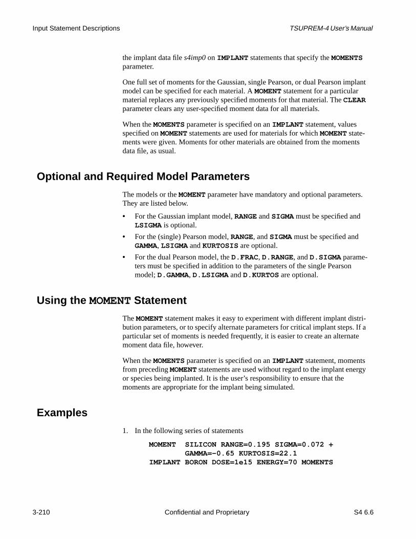
Input Statement Descriptions TSUPREM-4 User’s Manual
plant
nts
rs.
tri-. If aate
rgy
the implant data files4imp0 on IMPLANT statements that specify theMOMENTSparameter.
One full set of moments for the Gaussian, single Pearson, or dual Pearson immodel can be specified for each material. AMOMENT statement for a particularmaterial replaces any previously specified moments for that material. TheCLEARparameter clears any user-specified moment data for all materials.
When theMOMENTS parameter is specified on anIMPLANT statement, valuesspecified onMOMENT statements are used for materials for whichMOMENT state-ments were given. Moments for other materials are obtained from the momedata file, as usual.
Optional and Required Model Parameters
The models or theMOMENT parameter have mandatory and optional parameteThey are listed below.
• For the Gaussian implant model,RANGE andSIGMA must be specified andLSIGMA is optional.
• For the (single) Pearson model,RANGE, andSIGMA must be specified andGAMMA, LSIGMA andKURTOSIS are optional.
• For the dual Pearson model, theD.FRAC, D.RANGE, andD.SIGMA parame-ters must be specified in addition to the parameters of the single Pearsonmodel;D.GAMMA, D.LSIGMA andD.KURTOS are optional.
Using the MOMENT Statement
TheMOMENT statement makes it easy to experiment with different implant disbution parameters, or to specify alternate parameters for critical implant stepsparticular set of moments is needed frequently, it is easier to create an alternmoment data file, however.
When theMOMENTS parameter is specified on anIMPLANT statement, momentsfrom precedingMOMENT statements are used without regard to the implant eneor species being implanted. It is the user’s responsibility to ensure that themoments are appropriate for the implant being simulated.
Examples
1. In the following series of statements
MOMENT SILICON RANGE=0.195 SIGMA=0.072 +GAMMA=-0.65 KURTOSIS=22.1
IMPLANT BORON DOSE=1e15 ENERGY=70 MOMENTS
3-210 Confidential and Proprietary S4 6.6
Draft 6/26/98

TSUPREM-4 User’s Manual MOMENT
n-
ineaklyam-o
The implantation of boron into silicon uses the (single) Pearson distributiospecified on theMOMENT statement. In materials other than silicon, distribution parameters from the implant data file are used.
2. In the statement
parameters for the arsenic distribution comes from the implant data file.Parameters specified onMOMENT statements are not used, becauseMOMENTSis not specified on theIMPLANT statement.
Additional Note
1. The implanted dose in the silicon is reduced by the dose that is stopped screening layers or backscattered from the surface, and thus depends won the implant moments in the screening layer. Because the calculated dage is proportional to the dose in the silicon, the amount of damage is alsweakly dependent on the moments in the screening layer.
IMPLANT ARSENIC DOSE=2e15 ENERGY=40
S4 6.6 Confidential and Proprietary 3-211
Draft 6/26/98

Input Statement Descriptions TSUPREM-4 User’s Manual
MATERIAL
TheMATERIAL statement sets the physical properties of materials.
MATERIAL
( MATERIAL=<c> [NEW])| SILICON | OXIDE | OXYNITRI | NITRIDE | POLYSILI | PHOTORES | ALUMINUM | AMBIENT [TIF.NAME=<c>] [MD.INDEX=<n>] [IMPL.TAB=<c>] [DY.DEFAU=<n>] [E.FIELD] [ION.PAIR] [IP.OMEGA=<n>] [NI.0=<n>] [NI.E=<n>] [NI.F=<n>] [EPSILON=<n>] [DENSITY=<n>] [AT.NUM=<n>] [AT.WT=<n>] [MOL.WT=<n>] [VISC.0=<n>] [VISC.E=<n>] [VISC.X=<n>] [VC=<c>] [TEMPERAT=<c>] [YOUNG.M=<n>] [POISS.R=<n>] [LCTE=<c>] [INTRIN.S=<n>] [SURF.TEN=<n>] [ (SEMICOND [AFFINITY=<n>] [BANDGAP=<n>] [N.CONDUC=<n>] [N.VALENC=<n>] [G.DONOR=<n>] [E.DONOR=<n>] [G.ACCEP=<n>] [E.ACCEP=<n>] [BOLTZMAN] [IONIZATI] [QM.BETA=<n>] [QM.YCRIT=<n>]) | ( CONDUCTO [WORKFUNC=<n>] ) ] [POLYCRYS] [GRASZ.0=<n>] [GRASZ.E=<n>] [TEMP.BRE=<n>] [MIN.GRAI=<n>] [FRAC.TA=<n>] [G.DENS=<n>] [F11=<n>] [F22=<n>] [ALPHA=<n>] [GEOM=<n>] [GAMMA.0=<n>] [GAMMA.E=<n>] [DSIX.0=<n>] [DSIX.E=<n>] [DSIM.0=<n>] [DSIM.E=<n>] [DSIMM.0=<n>] [DSIMM.E=<n>] [DSIP.0=<n>] [DSIP.E=<n>] [GBE.0=<n>] [GBE.H=<n>] [GBE.E=<n>] [NSEG=<n>] [TBU.0=<n>] [TBU.E=<n>] [TOXIDE=<n>] [EAVEL.0=<n>] [EAVEL.E=<n>] [DLGX.0=<n>] [DLGX.E=<n>]
Parameter Type Definition
MATERIAL character The following parameters apply to the named material.Default: noneSynonyms:NAME
NEW logical Used to define a new material. The name specified by theMATERIAL parametermust not have been previously used as a material name.Default: false
SILICON logical The following parameters apply to silicon.Default: false
OXIDE logical The following parameters apply to oxide.Default: false
OXYNITRI logical The following parameters apply to oxynitride.Default: false
3-212 Confidential and Proprietary S4 6.6
Draft 6/26/98

TSUPREM-4 User’s Manual MATERIAL
his
ion
rial.i-
es
NITRIDE logical The following parameters apply to nitride.Default: false
POLYSILI logical The following parameters apply to polysilicon.Default: falseSynonyms:POLY
PHOTORES logical The following parameters apply to photoresist.Default: false
ALUMINUM logical The following parameters apply to aluminum.Default: false
AMBIENT logical The following parameters apply to ambient.Default: falseSynonyms: GAS
TIF.NAME character The name by which this material is known in the TIF materials database.Note: This value of this parameter is case-sensitive.Default: the name of the material
MD.INDEX number The index to be used for this material when saving the structure inMedici fileformat. These correspond to the <matx> indices listed inAppendix E.Units: noneDefault: 0 (material ignored byMedici)
IMPL.TAB character The name of the material in the implant moment file to be associated with tmaterial.Default: the current value for this material; initially the name of the material
DY.DEFAU number The grid spacing to be used in growing layers of the material. This value isscaled by the value of theGRID.FAC parameter on theMETHOD statement. Avalue of zero specifies that no grid is to be added in growing layers.Units: micronsDefault: the current value; initially 0.0Synonyms:DX.DEFAU
E.FIELD logical Specifies that the electric field terms are to be included in the impurity diffusequations for this material. (Meaningful only for silicon and polysilicon.)Default: the current value for this material; initially true
ION.PAIR logical Enables the model for pairing between donor and acceptor ions in this mateDefault: the current value for this material; initially true for silicon and polysilcon
IP.OMEGA number The multiple of the intrinsic carrier concentration at which ion pairing becomsignificant in this material.Units: noneDefault: the current value for this material; initially 6.0 for silicon and polysili-con
NI.0 number The prefactor in the expression for the intrinsic carrier concentration.Units: carriers/cm3*(degrees Kelvin)NI.F
Default: the current value for this material; initially 3.87e16
Parameter Type Definition
S4 6.6 Confidential and Proprietary 3-213
Draft 6/26/98

Input Statement Descriptions TSUPREM-4 User’s Manual
.
um-
lar
m-
ce ofdif-
NI.E number The activation energy in the expression for the intrinsic carrier concentrationUnits: electron voltsDefault: the current value for this material; initially 0.605
NI.F number The temperature exponent in the expression for the intrinsic carrierconcentration.Units: noneDefault: the current value for this material; initially 1.5Synonyms:NI.POW
EPSILON number The relative permittivity of the material.Units: noneDefault: the current value for this material; seeAppendix A for initial values
DENSITY number The density of the material.Units: gm/cm3
Default: the current value; seeAppendix A for initial values.
AT.NUM number The average atomic number of the material. This is the sum of the atomic nbers of the atoms in a molecule divided by the number of atoms.Units: noneDefault: the current value; seeAppendix A for initial values.
AT.WT number The average atomic weight of the atoms of the material. This is the molecuweight of the material divided by the number of atoms per molecule.Units: atomic mass unitsDefault: the current value; seeAppendix A for initial values.
MOL.WT number The molecular weight of the material.Units: atomic mass unitsDefault: the current value; seeAppendix A for initial values.
VISC.0 number The exponential prefactor for the viscosity.Units: gm/(cm*sec)Default: the current value for this material
VISC.E number The activation energy for the viscosity.Units: electron voltsDefault: the current value for this material
VISC.X number The incompressibility factor. A value of 0.5 corresponds to an infinitely incopressible material. The value must be strictly less than 0.5.Units: noneDefault: the current value for this material
VC character A table of activation volumes as a function of temperature for the dependenmaterial viscosity on shear stress for the specified material in inert-ambient fusions. Entries in the table correspond to temperatures given by theTEMPERAT parameter (see text).Units: Å3
Default: the current value for this material
TEMPERAT character A list of temperatures corresponding to the values of theVC parameter.Units: degrees CelsiusDefault: none
Parameter Type Definition
3-214 Confidential and Proprietary S4 6.6
Draft 6/26/98

TSUPREM-4 User’s Manual MATERIAL
n of a
os-
ial.
YOUNG.M number Young’s modulus for the material.Units: dynes/cm2
Default: the current value for this material
POISS.R number Poisson’s ratio for the material.Units: noneDefault: the current value for this material
LCTE character An expression giving the linear coefficient of thermal expansion as a functioabsolute temperature, calledT in the expression. It is given as a fraction, not aspercentage.Units: noneDefault: the current value for this material
INTRIN.S number The initial uniform stress state of a material such as a thin film of nitride depited on the substrate.Units: dynes/cm2
Default: the current value for this material
SURF.TEN number The surface tension for this material. Affects reflow during oxidation with theVISCOUS model.Units: dynes/cmDefault: the current value for this material
SEMICOND logical Specifies that the material is a semiconductor.Default: false
AFFINITY number The electron affinity of the material.Units: electron voltsDefault: the current value for this material
BANDGAP number The energy band gap of the material.Units: electron voltsDefault: the current value for this material
N.CONDUC number The effective density of electron states in the conduction band of the materUnits: #/cm3
Default: the current value for this material
N.VALENC number The effective density of hole states in the valence band of the material.Units: #/cm3
Default: none
G.DONOR number The donor impurity degeneracy factor of the material.Units: noneDefault: the current value for this material
E.DONOR number The donor impurity ionization energy of the material.Units: electron voltsDefault: the current value for this material
G.ACCEP number The acceptor impurity degeneracy factor of the material.Units: noneDefault: the current value for this material
Parameter Type Definition
S4 6.6 Confidential and Proprietary 3-215
Draft 6/26/98
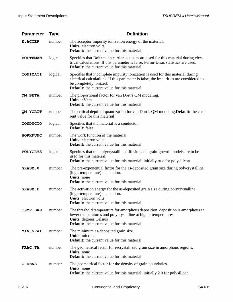
Input Statement Descriptions TSUPREM-4 User’s Manual
lec-
d to
lline
us at
E.ACCEP number The acceptor impurity ionization energy of the material.Units: electron voltsDefault: the current value for this material
BOLTZMAN logical Specifies that Boltzmann carrier statistics are used for this material during etrical calculations. If this parameter is false, Fermi-Dirac statistics are used.Default: the current value for this material
IONIZATI logical Specifies that incomplete impurity ionization is used for this material duringelectrical calculations. If this parameter is false, the impurities are considerebe completely ionized.Default: the current value for this material
QM.BETA number The proportional factor for van Dort’s QM modeling.Units: eVcmDefault: the current value for this material
QM.YCRIT number The critical depth of quantization for van Dort’s QM modeling.Default: the cur-rent value for this material
CONDUCTO logical Specifies that the material is a conductor.Default: false
WORKFUNC number The work function of the material.Units: electron voltsDefault: the current value for this material
POLYCRYS logical Specifies that the polycrystalline diffusion and grain-growth models are to beused for this material.Default: the current value for this material; initially true for polysilicon
GRASZ.0 number The pre-exponential factor for the as-deposited grain size during polycrysta(high-temperature) deposition.Units: noneDefault: the current value for this material
GRASZ.E number The activation energy for the as-deposited grain size during polycrystalline(high-temperature) deposition.Units: electron voltsDefault: the current value for this material
TEMP.BRE number The threshold temperature for amorphous deposition; deposition is amorpholower temperatures and polycrystalline at higher temperatures.Units: degrees CelsiusDefault: the current value for this material
MIN.GRAI number The minimum as-deposited grain size.Units: micronsDefault: the current value for this material
FRAC.TA number The geometrical factor for recrystallized grain size in amorphous regions.Units: noneDefault: the current value for this material
G.DENS number The geometrical factor for the density of grain boundaries.Units: noneDefault: the current value for this material; initially 2.0 for polysilicon
Parameter Type Definition
3-216 Confidential and Proprietary S4 6.6
Draft 6/26/98

TSUPREM-4 User’s Manual MATERIAL
um-
rain
nd-
.
u-
y.
F11 number The geometrical factor for grain-boundary diffusion perpendicular to the colnar direction.Units: noneDefault: the current value for this material; initially 1.0 for polysilicon
F22 number The geometrical factor for grain-boundary diffusion parallel to the columnardirection.Units: noneDefault: the current value for this material; initially 2.0 for polysilicon
ALPHA number The geometrical factor relating the average grain boundary velocity to the ggrowth rate.Units: noneDefault: the current value for this material; initially 1.33 for polysilicon
GEOM number The geometrical factor for the grain growth rate.Units: noneDefault: the current value for this material; initially 6.0 for polysilicon
GAMMA.0 number Pre-exponential factor for the enhancement of silicon self-diffusivity at grainboundaries.Units: noneDefault: the current value for this material
GAMMA.E number Activation energy for the enhancement of silicon self-diffusivity at grain bouaries.Units: electron voltsDefault: the current value for this material
DSIX.0 number Pre-exponential factor for the neutral component of silicon self diffusivity.Units: cm2/secDefault: the current value for this material
DSIX.E number Activation energy for the neutral component of silicon self diffusivity.Units: electron voltsDefault: the current value for this material
DSIM.0 number Pre-exponential factor for the singly negative component of siliconself-diffusivity.Units: cm2/secDefault: the current value for this material
DSIM.E number Activation energy for the singly negative component of silicon self-diffusivityUnits: electron voltsDefault: the current value for this material
DSIMM.0 number Pre-exponential factor for the doubly negative component of silicon self-diffsivity.Units: cm2/secDefault: the current value for this material
DSIMM.E number Activation energy for the doubly negative component of silicon self-diffusivitUnits: electron voltsDefault: the current value for this material
Parameter Type Definition
S4 6.6 Confidential and Proprietary 3-217
Draft 6/26/98

Input Statement Descriptions TSUPREM-4 User’s Manual
iv-
izes.
ter-
and
a
tal-
DSIP.0 number Pre-exponential factor for the singly positive component of silicon self-diffusity.Units: cm2/secDefault: the current value for this material
DSIP.E number Activation energy for the singly positive component of silicon self-diffusivity.Units: electron voltsDefault: the current value for this material
GBE.0 number The grain boundary energy for normal grain growth.Units: electron voltsDefault: the current value for this material
GBE.H number The geometrical factor for the reduction of grain growth rate at large grain sUnits: noneDefault: the current value for this material
GBE.1 number The grain boundary energy for secondary grain growth.Units: electron voltsDefault: the current value for this material
NSEG number The exponent for solute drag on grain growth.Units: noneDefault: the current value for this material
TBU.0 number The prefactor in the expression for the time constant for polysilicon/silicon infacial oxide break-up.Units: secondsDefault: the current value for this material
TBU.E number The activation energy for the time constant for polysilicon/silicon interfacialoxide break-up.Units: electron voltsDefault: the current value for this material
TOXIDE number The thickness of the interfacial oxide between deposited polysilicon layers single-crystal silicon.Units: micronsDefault: the current value for this material
EAVEL.0 number The prefactor in the expression for the velocity driving epitaxial regrowth of polycrystalline layer.Units: cm/secDefault: the current value for this material
EAVEL.E number The activation energy for the velocity driving epitaxial regrowth of a polycrysline layer.Units: electron voltsDefault: the current value for this material
DLGX.0 number The prefactor in the expression for the grain size diffusivity.Units: cm2/secDefault: the current value for this material
Parameter Type Definition
3-218 Confidential and Proprietary S4 6.6
Draft 6/26/98

TSUPREM-4 User’s Manual MATERIAL
terial
ify-
riallar
are
c-
of
rnert-
cifieds, and
Description
This statement is used to define materials and specify their properties. A macan be specified either by name, using theMATERIAL parameter, or with one oftheSILICON , OXIDE, OXYNITRI, NITRIDE , POLYSILI , PHOTORES,ALUMINUM, orAMBIENT parameters. A new material can be defined by specing theNEW parameter, the material name, and the properties of the material.
Note:It is the responsibility of the user to ensure that all material propertiesrequired for a particular simulation step (e.g., viscosity and compress-ibility for oxidation or density and atomic number and weight for MonteCarlo ion implantation) have been specified.
The density, average atomic number, and average atomic weight of the mateare used by the Monte Carlo ion implantation model. The density and molecuweight are used to calculate the volume changes that occur when materials produced or consumed during reactions with other materials.
Viscosity and Compressibility
TheVISC.0 , VISC.E , andVISC.X parameters specify the viscosity as a funtion of temperature of the material for use with theVISCOELA andVISCOUSmodels for material flow.VC specifies the activation volume for the dependencethe material viscosity on shear stress when the stress-dependentVISCOELAorVISCOUS model is used.YOUNG.M andPOISS.R give the viscosity and com-pressibility for use with theCOMPRESS model and elasticity for theVISCOELAmodel. SeeReference [27] in Chapter 2 andReference [36] in Appendix A.
The only material properties that apply toAMBIENT are the viscosity parametersVISC.0 , VISC.E , andVISC.X . These parameters apply to included voids,which may be formed during oxidation.
StressDependence
The parametersVC andTEMPERAT are used to specify the activation volume fodependence of viscosity on shear stress as functions of temperature during iambient diffusions. A separate table is maintained for each material.VC specifiesa list of values corresponding to the temperatures given byTEMPERAT. The por-tion of the table spanned by the specified temperatures is replaced by the spevalues; the number of values must be the same as the number of temperaturethe temperatures must be given in order, lowest to highest. TheCLEAR parameteris used to clear the table before setting any values.
DLGX.E number The activation energy for the grain size diffusivity.Units: electron voltsDefault: the current value for this material
Parameter Type Definition
S4 6.6 Confidential and Proprietary 3-219
Draft 6/26/98

Input Statement Descriptions TSUPREM-4 User’s Manual
ofg
ures
as a
is
e or
pec-
If V.COMPAT (on theOPTION statement) is less than 6.6, the specified valuesthe activation volumes apply to the specified material in all ambients, includinoxidizing ambients.
An Arrhenius interpolation is used between values in the table. For temperatoutside the range of the table, the nearest value is used.
Examples
1. The following statement specifies the density of silicon:
2. The following statement gives the thermal expansion coefficient of nitride function of absolute temperatureT:
Thus, at 0K the coefficient is .0003%/K. The initial stress in the nitride film1.4e10 dynes/cm2.
3. The following statement specifies an oxide viscosity of 109 poise and a sur-face tension of 20 dynes/cm:
These are values that might be used to simulate reflow of phosphosilicatborophosphosilicate glass.
4. The following statements define a new material, tungsten disilicide, and sify some of its properties:
A grid spacing of 0.1 microns (scaled by the value ofGRID.FAC) is used whengrowing tungsten silicide.
MATERIAL MATERIAL=SILICON DENSITY=2.33
MATERIAL NITRIDE LCTE=(3e-6 + 2e-10 * T) +INTRIN.S=1.4e10
MATERIAL MATERIAL=OXIDE VISC.0=1e9 VISC.e=0 +SURF.TEN=20
MATERIAL NEW MAT=WSi2 DENSITY=9.857 AT.NUM=34 +AT.WT=80.01
MATERIAL MAT=WSi2 DY.DEFAU=0.1
3-220 Confidential and Proprietary S4 6.6
Draft 6/26/98

TSUPREM-4 User’s Manual IMPURITY
ris-
IMPURITY
TheIMPURITY statement is used to define impurities or modify their charactetics.
IMPURITY
IMPURITY=<c> [NEW] [TIF.NAME=<c>][IMP.ACT=<c>] [IMP.GB=<c>][IMP.IT=<c>]
[ DONOR | ACCEPTOR ] [AT.NUM=<n>] [AT.WT=<n>] [SOLVE] [STEADY] [IMPL.TAB=<c>] [ MATERIAL=<c> [DIP.0=<n>] [DIP.E=<n>] [DIX.0=<n>] [DIX.E=<n>] [DIM.0=<n>] [DIM.E=<n>] [DIMM.0=<n>] [DIMM.E=<n>] [DVP.0=<n>] [DVP.E=<n>] [DVX.0=<n>] [DVX.E=<n>] [DVM.0=<n>] [DVM.E=<n>] [DVMM.0=<n>] [DVMM.E=<n>] [C.STATE=<n> [DIC.0=<n>] [DIC.E=<n>] [DVC.0=<n>] [DVC.E=<n>] ] [FGB=<n>] [DIPAIR.0=<n>] [DIPAIR.E=<n>] [DVPAIR.0=<n>] [DVPAIR.E=<n>] [R.I.S=<n>] [E.I.S=<n>] [R.V.S=<n>] [E.V.S=<n>] [R.IP.V=<n>] [E.IP.V=<n>] [R.VP.I=<n>] [E.VP.I=<n>] [SS.CLEAR] [SS.TEMP=<n> SS.CONC=<n>] [CTN.0=<n>] [CTN.E=<n>] [CTN.F=<n>] [CL.INI.A] [Q.SITES=<n>] [CG.MAX=<n>] [GSEG.0=<n>] [GSEG.E=<n>] [GSEG.INI=<n>] [VELIF.0=<n>] [VELIF.E=<n>] [ /MATERIA=<c> [SEG.0=<n>] [SEG.E=<n>] [TRANS.0=<n>] [TRANS.E=<n>]
[RATIO.0=<n>] [RATIO.E=<n>] [SEG.SS][/SEG.0=<n>] [/SEG.E=<n>] [/TRANS.0=<n>] [/TRANS.E=<n>][/RATIO.0=<n>] [/RATIO.E=<n>] [/SEG.SS]SEG.EQ3 | SEG.EQ2 | /SEG.EQ2[Q.INI.0=<n>] [Q.INI.E=<n>] [Q.MAX.0=<n>] [Q.MAX.E=<n>][TWO.PHAS]
] [ES.RAND=<n>] [ES.F.RAN=<n>] [ES.BREAK=<n>] [ES.F.H=<n>] [ES.100=<n>] [ES.F.100=<n>] [ES.110=<n>] [ES.F.110=<n>]
[NLOC.PRE=<n>] [NLOC.EXP=<n>] [NLOC.MAX=<n>] [NLOC.K=<n>][LOC.FAC=<n>] [CHAN.CRI=<n>] [CHAN.FAC=<n>] [DISP.FAC=<n>]
] [T.ACT.0=<n>] [T.ACT.E=<n>] [ACT.MIN=<n>] [CM.SEC]
Parameter Type Definition
IMPURITY character The name of the impurity to be defined or modified.Default: noneSynonyms:IMP, NAME
NEW logical Specifies that a new impurity is being defined.Default: false
S4 6.6 Confidential and Proprietary 3-221
Draft 6/26/98

Input Statement Descriptions TSUPREM-4 User’s Manual
ion of-
urity
the
ame-
s.
TIF.NAME character The name by which this impurity is known in the TIF materials database.Note: This value of this parameter is case-sensitive.Default: the name of the impurity
IMP.GB character The name of the solution value representing the grain boundary concentratthe impurity named in theIMPURITY parameter. Indicates that the polycrystalline diffusion model applies to this impurity.Default: none
IMP.ACT character The name of the solution value representing the active concentration of theimpurity named in theIMPURITY parameter. Required only when theACT.TRAN model is to be applied to the impurity.Default: none
IMP.IT character The name of the solution value representing the density of the trapped impat interface named in theIMPURITY parameter. Required only when theITRAPmodel is to be applied to the impurity.Default: none
DONOR logical Specifies that the impurity is a donor.Default: the current value for this impurity
ACCEPTOR logical Specifies that the impurity is an acceptor.Default: the current value for this impurity
AT.NUM number The atomic number of the impurity.Units: noneDefault: the current value for this impurity
AT.WT number The atomic weight of the impurity.Units: atomic mass unitsDefault: the current value for this impurity
SOLVE logical Specifies that the diffusion equations should be solved for this impurity.Default: true if NEW is specified; the current value for this impurity otherwise
STEADY logical Specifies that the steady-state conditions should be assumed when solvingdiffusion equations for this impurity.Default: false ifNEW is specified; the current value for this impurity otherwise
IMPL.TAB character The name of the implant moment table to use for this impurity.Default: the current implant moment table for this impurity
MATERIAL character The name of the material in which the diffusion, activation, and implant parters apply and material 1 for the segregation and transport parameters.Default: none
DIP.0 number The pre-exponential constant for diffusion with positively charged interstitialUnits: microns2/min or cm2/secDefault: the current value for this material
DIP.E number The activation energy for diffusion with positively charged interstitials.Units: electron voltsDefault: the current value for this material
Parameter Type Definition
3-222 Confidential and Proprietary S4 6.6
Draft 6/26/98

TSUPREM-4 User’s Manual IMPURITY
.
DIX.0 number The pre-exponential constant for diffusion with neutral interstitials.Units: microns2/min or cm2/secDefault: the current value for this material
DIX.E number The activation energy for diffusion with neutral interstitials.Units: electron voltsDefault: the current value for this material
DIM.0 number The pre-exponential constant for diffusion with singly negative interstitials.Units: microns2/min or cm2/secDefault: the current value for this material
DIM.E number The activation energy for diffusion with singly negative interstitials.Units: electron voltsDefault: the current value for this material
DIMM.0 number The pre-exponential constant for diffusion with doubly negative interstitials.Units: microns2/min or cm2/secDefault: the current value for this material
DIMM.E number The activation energy for diffusion with doubly negative interstitials.Units: electron voltsDefault: the current value for this material
DVP.0 number The pre-exponential constant for diffusion with positively charged vacanciesUnits: microns2/min or cm2/secDefault: the current value for this material
DVP.E number The activation energy for diffusion with positively charged vacancies.Units: electron voltsDefault: the current value for this material
DVX.0 number The pre-exponential constant for diffusion with neutral vacancies.Units: microns2/min or cm2/secDefault: the current value for this material
DVX.E number The activation energy for diffusion with neutral vacancies.Units: electron voltsDefault: the current value for this material
DVM.0 number The pre-exponential constant for diffusion with singly negative vacancies.Units: microns2/min or cm2/secDefault: the current value for this material
DVM.E number The activation energy for diffusion with singly negative vacancies.Units: electron voltsDefault: the current value for this material
DVMM.0 number The pre-exponential constant for diffusion with doubly negative vacancies.Units: microns2/min or cm2/secDefault: the current value for this material
DVMM.E number The activation energy for diffusion with doubly negative vacancies.Units: electron voltsDefault: the current value for this material
Parameter Type Definition
S4 6.6 Confidential and Proprietary 3-223
Draft 6/26/98

Input Statement Descriptions TSUPREM-4 User’s Manual
te
e
en
pant
pant
C.STATE number The point defect charge state to which theDIC.0 , DIC.E , DVC.0, andDVC.Eparameters apply. The value must be in the range of -6 to +6.Units: noneDefault: none
DIC.0 number The pre-exponential constant for diffusion with interstitials in the charge staC.STATE.Units: noneDefault: the current value for this material
DIC.E number The activation energy for diffusion with interstitials in the charge stateC.STATE.Units: electron voltsDefault: the current value for this material
DVC.0 number The pre-exponential constant for diffusion with vacancies in the charge statC.STATE.Units: noneDefault: the current value for this material
DVC.E number The activation energy for diffusion with vacancies in the charge stateC.STATE.Units: electron voltsDefault: the current value for this material
FGB number The factor by which the diffusivity is increased in polycrystalline materials whthe polycrystalline model is not enabled.Units: noneDefault: the current value for this material
DIPAIR.0 number The pre-exponential constant for the diffusivity of dopant-interstitial pairs.Units: microns2/min or cm2/secDefault: the current value for this material
DIPAIR.E number The activation energy for the diffusivity of dopant-interstitial pairs.Units: electron voltsDefault: the current value for this material
DVPAIR.0 number The pre-exponential constant for the diffusivity of dopant-vacancy pairs.Units: microns2/min or cm2/secDefault: the current value for this material
DVPAIR.E number The activation energy for the diffusivity of dopant-vacancy pairs.Units: electron voltsDefault: the current value for this material
R.I.S number The capture radius for the reaction between interstitials and substitutional doatoms.Units: ÅDefault: the current value for this material
E.I.S number The barrier energy for the reaction between interstitials and substitutional doatoms.Units: electron voltsDefault: the current value for this material
Parameter Type Definition
3-224 Confidential and Proprietary S4 6.6
Draft 6/26/98

TSUPREM-4 User’s Manual IMPURITY
opant
pant
can-
R.V.S number The capture radius for the reaction between vacancies and substitutional datoms.Units: ÅDefault: the current value for this material
E.V.S number The barrier energy for the reaction between vacancies and substitutional doatoms.Units: electron voltsDefault: the current value for this material
R.IP.V number The capture radius for the reaction between dopant-interstitial pairs and vacies.Units: ÅDefault: the current value for this material
E.IP.V number The barrier energy for the reaction between dopant-interstitial pairsand vacancies.Units: electron voltsDefault: the current value for this material
R.VP.I number The capture radius for the reaction between dopant-vacancy pairsand interstitials.Units: ÅDefault: the current value for this material
E.VP.I number The barrier energy for the reaction between dopant-vacancy pairsand interstitials.Units: electron voltsDefault: the current value for this material
SS.CLEAR logical Clears the solid solubility vs. temperature table.Default: false
SS.TEMP number The temperature at which the solid solubility in the material isSS.CONC.Units: degrees CelsiusDefault: none
SS.CONC number The solid solubility in the material at temperatureSS.TEMP.Units: atoms/cm3
Default: none
CTN.0 number The pre-exponential constant for impurity clustering.Units: (atoms/cm3)(1/CTN.F-1)
Default: the current value for this material
CTN.E number The activation energy for impurity clustering.Units: electron voltsDefault: the current value for this material
CTN.F number The exponent of concentration for impurity clustering.Units: noneDefault: the current value for this material
Parameter Type Definition
S4 6.6 Confidential and Proprietary 3-225
Draft 6/26/98

Input Statement Descriptions TSUPREM-4 User’s Manual
lue
crys-
in a
a
ly-
ion
CL.INI.A logical Specifies that impurities in an amorphized region are initially clustered whenACT.TRAN is used.Default: the current value for this impurity and material; initially true for built-in impurities in silicon
Q.SITES number The density of dopant sites in grain boundaries (the maximum allowable vafor the grain-boundary concentration) in a polycrystalline material.Units: #/cm2
Default: the current value for this material
CG.MAX number The density of dopant sites in the grain interior of a polycrystalline material.Units: #/cm3
Default: the current value for this material; initially 5e22 for polysilicon
GSEG.0 number The entropy for segregation between grain interior and boundaries in a polytalline material.Units: noneDefault: the current value for this materialSynonyms:A.SEG
GSEG.E number The activation energy of the segregation entropy between grain interior andboundaries in a polycrystalline material.Units: electron voltsDefault: the current value for this materialSynonyms:E.SEG
GSEG.INI number The entropy for the initial segregation between grain interior and boundariespolycrystalline material.Units: noneDefault: the current value for this materialSynonyms:A0.SEG
VELIF.0 number The pre-exponential factor for the segregation velocity at the boundaries ofpolycrystalline material.Units: cm/secDefault: the current value for this material
VELIF.E number The activation energy for the segregation velocity at the boundaries of a pocrystalline material.Units: electron voltsDefault: the current value for this material
/MATERIA character The name of material 2 for the segregation and transport parameters.Default: none
SEG.0 number The pre-exponential factor for segregation from material 1 to material 2.For the trapped impurity at interface, the pre-exponential factor for segregatfrom material 1 to interface adjacient to material 2.Units: none for the segregation from material 1 to material 2,
cm-1 for the segregation from material 1 to interfaceDefault: the current value for these materials
Parameter Type Definition
3-226 Confidential and Proprietary S4 6.6
Draft 6/26/98
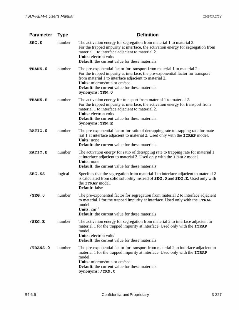
TSUPREM-4 User’s Manual IMPURITY
om
ate-
l 1
ial 2
ient
to
t to
SEG.E number The activation energy for segregation from material 1 to material 2.For the trapped impurity at interface, the activation energy for segregation frmaterial 1 to interface adjacient to material 2.Units: electron voltsDefault: the current value for these materials
TRANS.0 number The pre-exponential factor for transport from material 1 to material 2.For the trapped impurity at interface, the pre-exponential factor for transportfrom material 1 to interface adjacient to material 2.Units: microns/min or cm/secDefault: the current value for these materialsSynonyms:TRN.0
TRANS.E number The activation energy for transport from material 1 to material 2.For the trapped impurity at interface, the activation energy for transport frommaterial 1 to interface adjacient to material 2.Units: electron voltsDefault: the current value for these materialsSynonyms:TRN.E
RATIO.0 number The pre-exponential factor for ratio of detrapping rate to trapping rate for mrial 1 at interface adjacient to material 2. Used only with theITRAP model.Units: noneDefault: the current value for these materials
RATIO.E number The activation energy for ratio of detrapping rate to trapping rate for materiaat interface adjacient to material 2. Used only with theITRAP model.Units: noneDefault: the current value for these materials
SEG.SS logical Specifies that the segregation from material 1 to interface adjacient to materis calculated from solid solubility instead ofSEG.0 andSEG.E. Used only withtheITRAP model.Default: false
/SEG.0 number The pre-exponential factor for segregation from material 2 to interface adjacto material 1 for the trapped impurity at interface. Used only with theITRAPmodel.Units: cm-1
Default: the current value for these materials
/SEG.E number The activation energy for segregation from material 2 to interface adjacient material 1 for the trapped impurity at interface. Used only with theITRAPmodel.Units: electron voltsDefault: the current value for these materials
/TRANS.0 number The pre-exponential factor for transport from material 2 to interface adjacienmaterial 1 for the trapped impurity at interface. Used only with theITRAPmodel.Units: microns/min or cm/secDefault: the current value for these materialsSynonyms:/TRN.0
Parameter Type Definition
S4 6.6 Confidential and Proprietary 3-227
Draft 6/26/98

Input Statement Descriptions TSUPREM-4 User’s Manual
ate-
l 2
ial 1
erial
as toal to
as toal to
sed
only
only
/TRANS.E number The activation energy for transport from material 2 to interface adjacient tomaterial 1 for the trapped impurity at interface. Used only with theITRAPmodel.Units: electron voltsDefault: the current value for these materialsSynonyms:/TRN.E
/RATIO.0 number The pre-exponential factor for ratio of detrapping rate to trapping rate for mrial 2 at interface adjacient to material 1. Used only with theITRAP model.Units: noneDefault: the current value for these materials
/RATIO.E number The activation energy for ratio of detrapping rate to trapping rate for materiaat interface adjacient to material 1. Used only with theITRAP model.Units: noneDefault: the current value for these materials
/SEG.SS logical Specifies that the segregation from material 2 to interface adjacient to materis calculated from solid solubility instead of/SEG.0 and/SEG.E . Used onlywith theITRAP model.Default: false
SEG.EQ3 logical Specifies that both of segregations from material 1 to interface and from mat2 to interface are determined from the values of the parameters,SEG.0, SEG.E,/SEG.0 and/SEG.E . Used only with theITRAP model.Default: true
SEG.EQ2 logical Specifies that the segregation from material 1 to interface is determined so make the concentration ratio in materials 1 and 2 in 3-phase equilibrium equthe one in 2-phase equilibrium. Used only with theITRAP model.Default: false
/SEG.EQ2 logical Specifies that the segregation from material 2 to interface is determined so make the concentration ratio in materials 1 and 2 in 3-phase equilibrium equthe one in 2-phase equilibrium. Used only with theITRAP model.Default: false
Q.INI.0 number The pre-exponential factor for the initial occupied trap density at interface. Uonly with theITRAP model.Units: atoms/cm2
Default: the current value for these materials
Q.INI.E number The activation energy for the initial occupied trap density at interface. Used with theITRAP model.Units: electron voltsDefault: the current value for these materials
Q.MAX.0 number The pre-exponential factor for the maximum trap density at interface. Used with theITRAP model.Units: atoms/cm2
Default: the current value for these materials
Parameter Type Definition
3-228 Confidential and Proprietary S4 6.6
Draft 6/26/98

TSUPREM-4 User’s Manual IMPURITY
with
e seg-
dsili-
eci-n in
ion
ies-
>ion
nlant
>ion
Q.MAX.E number The activation energy for the maximum trap density at interface. Used only theITRAP model.Units: electron voltsDefault: the current value for these materials
TWO.PHAS logical Specifies that the flux of 2-phase segregation is added to the one of 3-phasregation flux. Used only with theITRAP model.Default: false
ES.RAND number The electronic stopping power coefficient of implanted atoms in the specifiematerial for materials other than silicon and for a nonchanneled direction in con. This value is used for the Monte Carlo ion implant calculation only.Units: angstrom2*eV(1-ES.F.RAN )
Default: the current value for the specified materials
ES.F.RAN number The exponent of the electronic stopping power of implanted atoms in the spfied material for materials other than silicon and for a nonchanneled directiosilicon. This value is used for the Monte Carlo ion implant calculation only.Units: noneDefault: the current value for the specified materials
ES.BREAK number The energy above whichES.F.H is used instead ofES.F.RAN , ES.F.100 ,or ES.F.110 in calculating the electronic stopping power coefficient ofimplanted atoms. This value is used for the Monte Carlo ion implant calculatonly.Units: keVDefault: the current value for the specified materials
ES.F.H number The exponent of the electronic stopping power of implanted atoms at energaboveES.BREAK. This value is used for the Monte Carlo ion implant calculation only.Units: noneDefault: the current value for the specified materials
ES.100 number The electronic stopping power for implanted atoms in silicon along the <100channeling axes. This value is used for the Monte Carlo ion implant calculatonly.Units: angstrom2*eV(1-ES.F.100 )
Default: the current value for the specified materials
ES.F.100 number The exponent of the electronic stopping power for implanted atoms in silicoalong the <100> crystal axes. This value is used for the Monte Carlo ion impcalculation only.Units: noneDefault: the current value for the specified material
ES.110 number The electronic stopping power for implanted atoms in silicon along the <110channeling axes. This value is used for the Monte Carlo ion implant calculatonly.Units: angstrom2*eV(1-ES.F.100 )
Default: the current value for the specified material
Parameter Type Definition
S4 6.6 Confidential and Proprietary 3-229
Draft 6/26/98

Input Statement Descriptions TSUPREM-4 User’s Manual
nlant
is
e is
er.
for
is
sed
del.
he
ES.F.110 number The exponent of the electronic stopping power for implanted atoms in silicoalong the <110> crystal axes. This value is used for the Monte Carlo ion impcalculation only.Units: noneDefault: the current value for the specified material
NLOC.PRE number The prefactor for the nonlocal electronic stopping power formula. This valueused for the Monte Carlo ion implant calculation only.Units: noneDefault: The current value for the specified materials
NLOC.EXP number The exponent for the nonlocal electronic stopping power formula. This valuused for the Monte Carlo ion implant calculation only.Units: noneDefault: The current value for the specified materials
NLOC.MAX number The maximum value allowed for the nonlocal part of electronic stopping powThis value is used for the Monte Carlo ion implant calculation only.Units: noneDefault: The current value for the specified materials
NLOC.K number A correction factor for the LSS electron stopping power. This value is used the Monte Carlo ion implant calculation only.Units: noneDefault: The current value for the specified materials
LOC.FAC number A correction factor for the local part of electronic stopping power. This valuesued for the Monte Carol ion implant calculation only.Units: noneDefault: The current value for the specified materials
CHAN.CRI number Specifies the critical angle below which the scattering angle is automaticallyreduced. This value is used for the Monte Carlo ion implant calculation only.Units: noneDefault: The current value for the specified materials
CHAN.FAC number Specifies the factor by which the scattering angle is reduced. This value is ufor the Monte Carlo ion implant calculation only.Units: noneDefault: The current value for the specified materials
DISP.FAC number This is a correction factor for the probability of selecting the amorphous moThis value is used for the Monte Carlo ion implant calculation only.Units: noneDefault: The current value for the specified materials
T.ACT.0 number The prefactor in the expression for the activation time constant for theACT.TRAN model for this impurity.Units: min or secDefault: the current value for this impurity.
T.ACT.E number The activation energy in the expression for the activation time constant for tACT.TRAN model for this impurity.Units: electron voltsDefault: the current value for this impurity.
Parameter Type Definition
3-230 Confidential and Proprietary S4 6.6
Draft 6/26/98
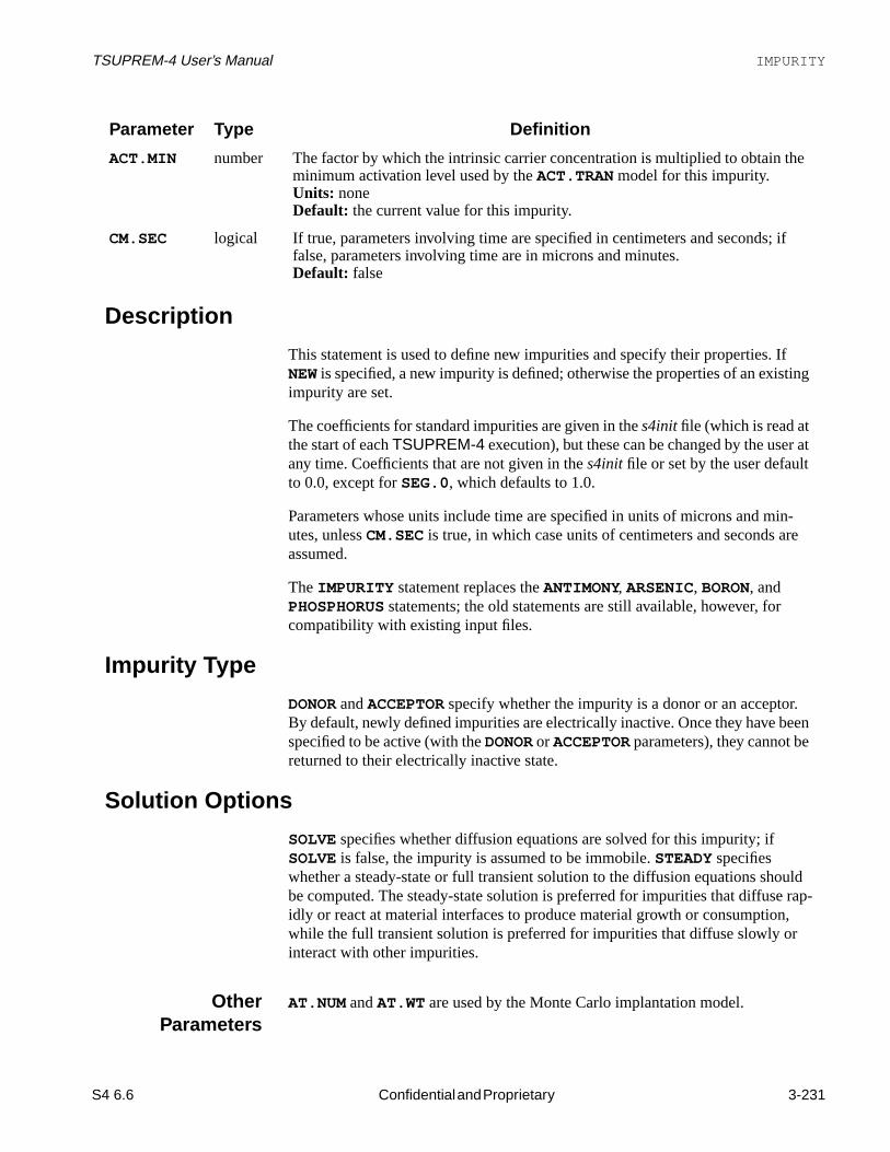
TSUPREM-4 User’s Manual IMPURITY
Ifting
r at
in-re
.een
uld rap-,
r
the
if
Description
This statement is used to define new impurities and specify their properties. NEW is specified, a new impurity is defined; otherwise the properties of an exisimpurity are set.
The coefficients for standard impurities are given in thes4init file (which is read atthe start of eachTSUPREM-4 execution), but these can be changed by the useany time. Coefficients that are not given in thes4init file or set by the user defaultto 0.0, except forSEG.0, which defaults to 1.0.
Parameters whose units include time are specified in units of microns and mutes, unlessCM.SEC is true, in which case units of centimeters and seconds aassumed.
TheIMPURITY statement replaces theANTIMONY, ARSENIC, BORON, andPHOSPHORUS statements; the old statements are still available, however, forcompatibility with existing input files.
Impurity Type
DONOR andACCEPTOR specify whether the impurity is a donor or an acceptorBy default, newly defined impurities are electrically inactive. Once they have bspecified to be active (with theDONOR orACCEPTOR parameters), they cannot bereturned to their electrically inactive state.
Solution Options
SOLVE specifies whether diffusion equations are solved for this impurity; ifSOLVE is false, the impurity is assumed to be immobile.STEADY specifieswhether a steady-state or full transient solution to the diffusion equations shobe computed. The steady-state solution is preferred for impurities that diffuseidly or react at material interfaces to produce material growth or consumptionwhile the full transient solution is preferred for impurities that diffuse slowly ointeract with other impurities.
OtherParameters
AT.NUM andAT.WT are used by the Monte Carlo implantation model.
ACT.MIN number The factor by which the intrinsic carrier concentration is multiplied to obtain minimum activation level used by theACT.TRAN model for this impurity.Units: noneDefault: the current value for this impurity.
CM.SEC logical If true, parameters involving time are specified in centimeters and seconds; false, parameters involving time are in microns and minutes.Default: false
Parameter Type Definition
S4 6.6 Confidential and Proprietary 3-231
Draft 6/26/98

Input Statement Descriptions TSUPREM-4 User’s Manual
-
iO
ui-
rties:
IMPL.TAB specifies the name of the implant moment table to be used for theimpurity.
Further Reading
For further reading and additional information see the following sections:
• Use of the diffusion parameters is described inChapter 2, “Diffusion of Impu-rities” on page 2-15.
• The solid solubility and clustering parameters are described inChapter 2,“Activation of Impurities” on page 2-23.
• The segregation parameters are described inChapter 2, “Segregation of Impurities” on page 2-24.
• The electronic stopping power parameters are described inChapter 2, “MonteCarlo Ion Implant Model” on page 2-74.
Examples
1. The following statement specifies the diffusivity of antimony diffusing withneutral vacancies in silicon:
2. The following statement specifies the diffusivity of phosphorus with triply-negative interstitials:
3. The following statement specifies the segregation parameters at the Si/S2interface:
The concentration in silicon is 30.0 times the concentration in oxide, at eqlibrium.
4. The following statements define a new impurity and set some of its prope
IMPURITY IMP=ANTIMONY MAT=SILICON DVX.0=1.22e9 +DVX.E=3.65
IMPURITY IMP=P MAT=SILI C.STATE=-3 DIC.0=2e11 +DIC.E=4.37
IMPURITY IMP=ANTIMONY MAT=SILICON /MAT=OXIDE +SEG.0=30.0 TRANS.0=0.1
IMPURITY NEW IMPURITY=CESIUM AT.NUM=55 +AT.WT=132.9
IMPURITY IMP=CESIUM MAT=OXIDE DIX.0=0.5 +DIX.E=2.9
3-232 Confidential and Proprietary S4 6.6
Draft 6/26/98
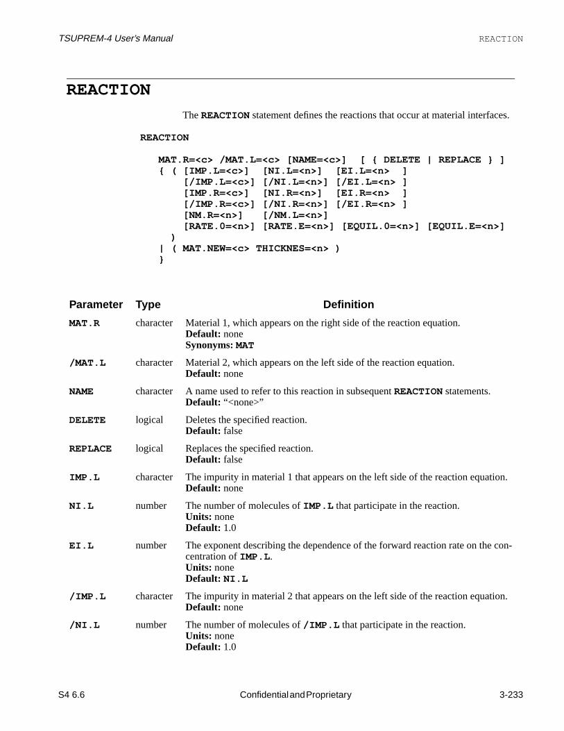
TSUPREM-4 User’s Manual REACTION
es.
tion.
e con-
tion.
REACTION
TheREACTION statement defines the reactions that occur at material interfac
REACTION
MAT.R=<c> /MAT.L=<c> [NAME=<c>] [ DELETE | REPLACE ] ( [IMP.L=<c>] [NI.L=<n>] [EI.L=<n> ] [/IMP.L=<c>] [/NI.L=<n>] [/EI.L=<n> ] [IMP.R=<c>] [NI.R=<n>] [EI.R=<n> ] [/IMP.R=<c>] [/NI.R=<n>] [/EI.R=<n> ] [NM.R=<n>] [/NM.L=<n>] [RATE.0=<n>] [RATE.E=<n>] [EQUIL.0=<n>] [EQUIL.E=<n>] ) | ( MAT.NEW=<c> THICKNES=<n> )
Parameter Type Definition
MAT.R character Material 1, which appears on the right side of the reaction equation.Default: noneSynonyms:MAT
/MAT.L character Material 2, which appears on the left side of the reaction equation.Default: none
NAME character A name used to refer to this reaction in subsequentREACTION statements.Default: “<none>”
DELETE logical Deletes the specified reaction.Default: false
REPLACE logical Replaces the specified reaction.Default: false
IMP.L character The impurity in material 1 that appears on the left side of the reaction equaDefault: none
NI.L number The number of molecules ofIMP.L that participate in the reaction.Units: noneDefault: 1.0
EI.L number The exponent describing the dependence of the forward reaction rate on thcentration ofIMP.L .Units: noneDefault: NI.L
/IMP.L character The impurity in material 2 that appears on the left side of the reaction equaDefault: none
/NI.L number The number of molecules of/IMP.L that participate in the reaction.Units: noneDefault: 1.0
S4 6.6 Confidential and Proprietary 3-233
Draft 6/26/98

Input Statement Descriptions TSUPREM-4 User’s Manual
e con-
ation.
e con-
ation.
e con-
e for-
/EI.L number The exponent describing the dependence of the forward reaction rate on thcentration of/IMP.L .Units: noneDefault: /NI.L
IMP.R character The impurity in material 1 that appears on the right side of the reaction equDefault: none
NI.R number The number of molecules ofIMP.R that participate in the reaction.Units: noneDefault: 1.0
EI.R number The exponent describing the dependence of the reverse reaction rate on thcentration ofIMP.R .Units: noneDefault: NI.R
/IMP.R character The impurity in material 2 that appears on the right side of the reaction equDefault: none
/NI.R number The number of molecules of/IMP.R that participate in the reaction.Units: noneDefault: 1.0
/EI.R number The exponent describing the dependence of the reverse reaction rate on thcentration of/IMP.R .Units: noneDefault: /NI.R
NM.R number The number of molecules ofMAT.R that participate in the reaction.Units: noneDefault: 0.0
/NM.L number The number of molecules of/MAT.L that participate in the reaction.Units: noneDefault: 0.0
RATE.0 number The prefactor in the expression for the forward reaction rate.Units: variesDefault: 0.0
RATE.E number The activation energy for the forward reaction rate.Units: noneDefault: 0.0
EQUIL.0 number The prefactor in the expression for the ratio of the reverse reaction rate to thward reaction rate.Units: variesDefault: 0.0
EQUIL.E number The activation energy for the ratio of the reverse reaction rate to the forwardreaction rate.Units: noneDefault: 0.0
Parameter Type Definition
3-234 Confidential and Proprietary S4 6.6
Draft 6/26/98

TSUPREM-4 User’s Manual REACTION
ateri-ed,
he
itherme- and. A
ith a
d
ilicon
Description
TheREACTION statement can specify either a reaction that takes place at theinterface between two materials or the addition of anative layer when one mate-rial is deposited on another. Each reaction is identified by its name and the mals on either side of the interface. The name is optional: if no name is specifithe name “<none>” is assumed.
Reactions defined with theREACTION statement take place duringDIFFUSIONsteps with either oxidizing or inert ambients. The reactions occur only when tVERTICAL, COMPRESS, orVISCOELA oxidation model has been selected.
Defining and Deleting
A new reaction is defined by specifying a name (optional), the materials on eside of the interface, and the impurity and reaction rate parameters. The paraters for a previously defined reaction can be changed by specifying the namematerials for the reaction along with any parameters that need to be changedpreviously defined reaction can be deleted with theDELETE parameter. TheREPLACE parameter deletes a previously defined reaction then replaces it wnew reaction defined by the parameters on theREACTION statement.
Insertion of Native Layers
TheMAT.NEW andTHICKNES parameters specify a new material to be insertebetweenMAT.R and/MAT.L when one is deposited on the other. A layer ofMAT.NEW with thicknessTHICKNES separatesMAT.R and/MAT.L . The pro-cess is analogous to the insertion of a native oxide layer between exposed sand an oxidizing ambient.
Reaction Equation
The general form of the reaction is
MAT.NEW character The name of the material to be added between layers ofMAT.R and/MAT.Lwhen one is deposited on the other.Default: none
THICKNES number The thickness ofMAT.NEW to be added between layers ofMAT.R and/MAT.Lwhen one is deposited on the other.Units: micronsDefault: none
Parameter Type Definition
S4 6.6 Confidential and Proprietary 3-235
Draft 6/26/98

Input Statement Descriptions TSUPREM-4 User’s Manual
eac-se
redpu-
r
l-
Equation 3-1
where the subscripts and denote terms on the left and right sides of the rtion and subscripts 1 and 2 refer to materials 1 and 2. The forward and reverreaction rates are given by
Equation 3-2
Equation 3-3
where denotes the concentration of impurity .
Parameters The parameters of this reaction are specified by the user as follows:
Equation 3-4
Equation 3-5
Equation 3-6
Equation 3-7
Equation 3-8
Equation 3-9
• NI.L , /NI.L , NI.R , /NI.R , NM.R, and/NM.L determine the number ofmolecules of each reactant that participate in the reaction.
• EI.L , /EI.L , EI.R , /EI.R , RATE.0 , RATE.E, EQUIL.0 , andEQUIL.E determine the rate of the reaction.
In theory the and for each reaction would be equal, but this is not requiby TSUPREM-4. This allows the rate to depend on the concentration of an imrity without the concentration being affected by the reaction ( ), ofor the concentration to change without affecting the rate ( ).
The units of and are #/cm2/sec; the units of and depend on the vaues of the and .
←ll
nil 1I l2 n+ il 2I l2 nml2Ml2 nmr1Mr1→ nir 1I r1 nir 2I r2+ + +
l r
Rf k f I l1[ ]el1 I l2[ ]
el2=
Rr kr I r1[ ]er 1 I r2[ ]
er 2=
I x[ ] I x
I l1 IMP.L , I l2 IMP.L⁄ , I r1 IMP.R , I r2 IMP.R⁄====
nil 1 NI.L , nil 2 NI.L⁄ , nir 1 NI.R , I ir 2 NI.R⁄====
nmr1 NM.R, nml2 NI.L⁄==
eil 1 EI.L , eil 2 EI.L⁄ , eir 1 EI.R , eir 2 EI.R⁄====
kf RATE.0= exp RATE.E–kT
----------------------- ⋅
kr
k f-----
I l1[ ]el1 I l2[ ]
el2
I r1[ ]er 1 I r2[ ]
er 2--------------------------------- EQUIL.0 exp EQUIL.E–
kT--------------------------
⋅= =
ni ei
ei 0 ni,≠ 0=ei 0 ni 0≠,=
Rf Rr k f krni ei
3-236 Confidential and Proprietary S4 6.6
Draft 6/26/98

TSUPREM-4 User’s Manual REACTION
con-rity
r
e
Effects This reaction has two effects on the simulation:
1. As a boundary condition for diffusing species, it can result in generation, sumption, or transport of impurities across a material interface. The impugeneration fluxes ( , in #/cm2/sec) at the interface are given by
Equation 3-10
(Note that when is zero, the corresponding flux is also zero.)
2. It can produce growth or consumption of material regions. This occurs fomaterials for which . The growth rate of , in cm/sec, is given by
Equation 3-11
where is the growth velocity in cm/sec, is Avogadro’snumber, andMOL.WT andDENSITY are material parameters specified on thMATERIAL statement. The material is consumed ( ) if .
F
1nil 1--------Fl1–
1nil 12----------Fl2–
1nir 1--------Fr1
1nir 2--------Fr2 Rf Rr–= = = =
ni
nm 0≠ Mrl
Vnmr1 MOL.WT×A DENSITY×
------------------------------------ Rf Rr–( )=
V A 6.022 1023×=
V 0< Rf Rr<
S4 6.6 Confidential and Proprietary 3-237
Draft 6/26/98

Input Statement Descriptions TSUPREM-4 User’s Manual
ier
ius
pacesobil-
pacese
paceson-
MOBILITY
TheMOBILITY statement is used to define or modify the dependence of carrmobility on impurity concentration and temperature within a semiconductor.
MOBILITY
[ TAB.TEMP=<n> [KELVIN] TAB.CONC=<c> TAB.E.MU=<c> TAB.H.MU=<c> [TAB.CLEA] ] [ECN.MU=<n>] [ECP.MU=<n>] [GSURFN=<n>] [GSURFP=<n>] [MUN1=<n>] [MUN2=<n>] [AN=<n>] [CN=<n>] [EXN1=<n>] [EXN2=<n>] [EXN3=<n>] [EXN4=<n>] [MUP1=<n>] [MUP2=<n>] [AP=<n>] [CP=<n>] [EXP1=<n>] [EXP2=<n>] [EXP3=<n>] [EXP4=<n>] [MUN.MIN=<n>] [MUN.MAX=<n>] [NREFN=<n>] [NUN=<n>] [XIN=<n>] [ALPHAN=<n>] [MUP.MIN=<n>] [MUP.MAX=<n>] [NREFP=<n>] [NUP=<n>] [XIP=<n>] [ALPHAP=<n>]
Parameter Type Definition
TAB.TEMP number The temperature at which the mobility table values were measured.Units: Kelvins if theKELVIN parameter is specified, otherwise, degrees CelsDefault: none
KELVIN logical Specifies that the units ofTAB.TEMP is Kelvins.Default: false
TAB.CONC character This parameter is interpreted as a series of numeric values, separated by sor commas. The parameter defines the concentrations associated with the mities defined inTAB.E.MU or TAB.H.MU.Units: atoms/cm3
Default: none
TAB.E.MU character This parameter is interpreted as a series of numeric values, separated by sor commas. The parameter defines the electron mobilities associated with thconcentrations defined inTAB.CONC.Units: cm2/V/secDefault: none
TAB.H.MU character This parameter is interpreted as a series of numeric values, separated by sor commas. The parameter defines the hole mobilities associated with the ccentrations defined inTAB.CONC.Units: cm2/V/secDefault: none
TAB.CLEA logical Specifies that the current table is to be cleared.Default: false
3-238 Confidential and Proprietary S4 6.6
Draft 6/26/98
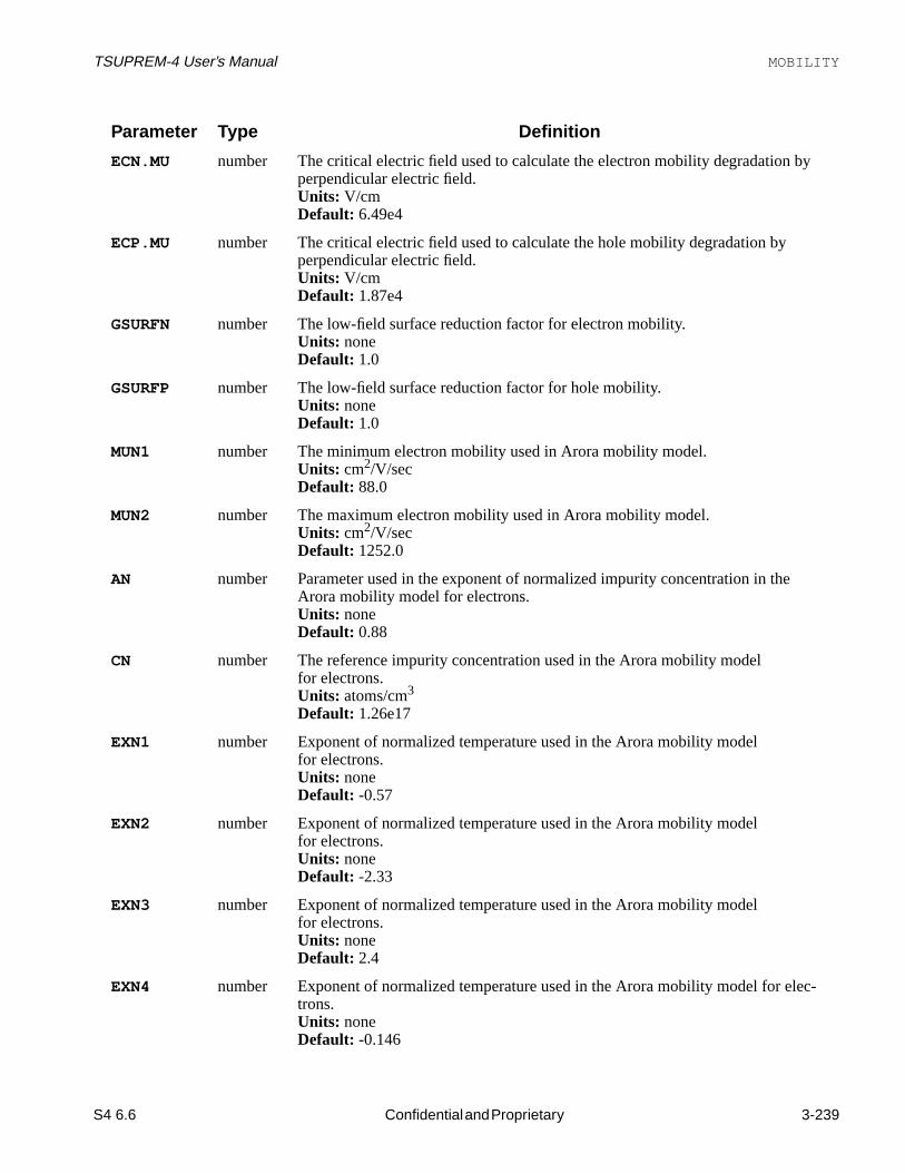
TSUPREM-4 User’s Manual MOBILITY
by
lec-
ECN.MU number The critical electric field used to calculate the electron mobility degradation perpendicular electric field.Units: V/cmDefault: 6.49e4
ECP.MU number The critical electric field used to calculate the hole mobility degradation byperpendicular electric field.Units: V/cmDefault: 1.87e4
GSURFN number The low-field surface reduction factor for electron mobility.Units: noneDefault: 1.0
GSURFP number The low-field surface reduction factor for hole mobility.Units: noneDefault: 1.0
MUN1 number The minimum electron mobility used in Arora mobility model.Units: cm2/V/secDefault: 88.0
MUN2 number The maximum electron mobility used in Arora mobility model.Units: cm2/V/secDefault: 1252.0
AN number Parameter used in the exponent of normalized impurity concentration in theArora mobility model for electrons.Units: noneDefault: 0.88
CN number The reference impurity concentration used in the Arora mobility modelfor electrons.Units: atoms/cm3
Default: 1.26e17
EXN1 number Exponent of normalized temperature used in the Arora mobility modelfor electrons.Units: noneDefault: -0.57
EXN2 number Exponent of normalized temperature used in the Arora mobility modelfor electrons.Units: noneDefault: -2.33
EXN3 number Exponent of normalized temperature used in the Arora mobility modelfor electrons.Units: noneDefault: 2.4
EXN4 number Exponent of normalized temperature used in the Arora mobility model for etrons.Units: noneDefault: -0.146
Parameter Type Definition
S4 6.6 Confidential and Proprietary 3-239
Draft 6/26/98

Input Statement Descriptions TSUPREM-4 User’s Manual
les.
les.
les.
les.
or
ey
MUP1 number The minimum hole mobility used in Arora mobility model.Units: cm2/V/secDefault: 54.3
MUP2 number The maximum hole mobility used in Arora mobility model.Units: cm2/V/secDefault: 407.0
AP number Parameter used in the exponent of normalized impurity concentration in theArora mobility model for holes.Units: noneDefault: 0.88
CP number The reference impurity concentration used in the Arora mobility model forholes.Units: atoms/cm3
Default: 2.35e17
EXP1 number Exponent of normalized temperature used in the Arora mobility model for hoUnits: noneDefault: -0.57
EXP2 number Exponent of normalized temperature used in the Arora mobility model for hoUnits: noneDefault: -2.23
EXP3 number Exponent of normalized temperature used in the Arora mobility model for hoUnits: noneDefault: 2.4
EXP4 number Exponent of normalized temperature used in the Arora mobility model for hoUnits: noneDefault: -0.146
MUN.MIN number The minimum electron mobility in the Caughey mobility model.Units: cm2/V/secDefault: 55.24
MUN.MAX number The maximum electron mobility in the Caughey mobility model.Units: cm2/V/secDefault: 1429.23
NREFN number The reference impurity concentration used in the Caughey mobility model felectrons.Units: atoms/cm3
Default: 1.072e17
NUN number Exponent of normalized temperature used in the numerator of the Caugheymobility model for electrons.Units: noneDefault: -2.3
XIN number Exponent of normalized temperature used in the denominator of the Caughmobility model for electrons.Units: noneDefault: -3.8
Parameter Type Definition
3-240 Confidential and Proprietary S4 6.6
Draft 6/26/98
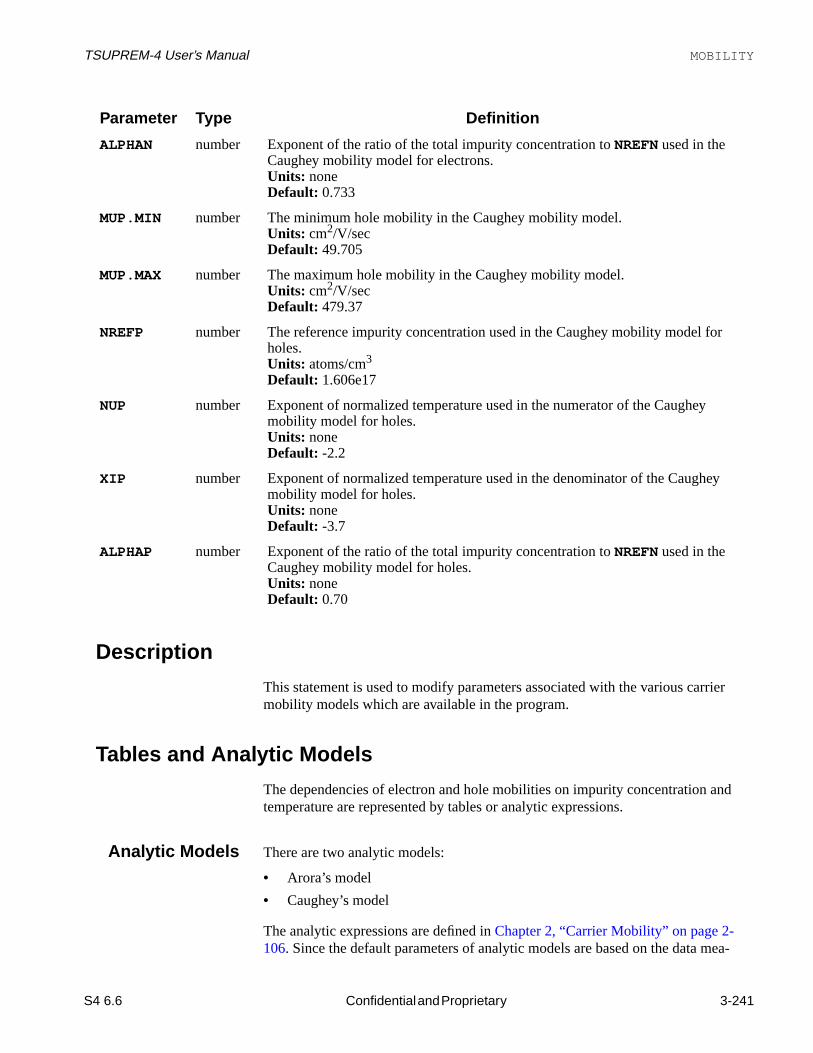
TSUPREM-4 User’s Manual MOBILITY
rier
nd
ea-
or
ey
Description
This statement is used to modify parameters associated with the various carmobility models which are available in the program.
Tables and Analytic Models
The dependencies of electron and hole mobilities on impurity concentration atemperature are represented by tables or analytic expressions.
Analytic Models There are two analytic models:
• Arora’s model
• Caughey’s model
The analytic expressions are defined inChapter 2, “Carrier Mobility” on page 2-106. Since the default parameters of analytic models are based on the data m
ALPHAN number Exponent of the ratio of the total impurity concentration toNREFN used in theCaughey mobility model for electrons.Units: noneDefault: 0.733
MUP.MIN number The minimum hole mobility in the Caughey mobility model.Units: cm2/V/secDefault: 49.705
MUP.MAX number The maximum hole mobility in the Caughey mobility model.Units: cm2/V/secDefault: 479.37
NREFP number The reference impurity concentration used in the Caughey mobility model fholes.Units: atoms/cm3
Default: 1.606e17
NUP number Exponent of normalized temperature used in the numerator of the Caugheymobility model for holes.Units: noneDefault: -2.2
XIP number Exponent of normalized temperature used in the denominator of the Caughmobility model for holes.Units: noneDefault: -3.7
ALPHAP number Exponent of the ratio of the total impurity concentration toNREFN used in theCaughey mobility model for holes.Units: noneDefault: 0.70
Parameter Type Definition
S4 6.6 Confidential and Proprietary 3-241
Draft 6/26/98

Input Statement Descriptions TSUPREM-4 User’s Manual
-d to in
rly.-
turete
valuesesfor
n- cur-
sured on concentrations less than about 1020/cm3, the analytic mobilities onheavily doped concentration might be not accurate.
Tables or ModelSelection
The table is two-dimensional with at most 100 rows representing impurity concentrations and with columns representing temperatures. Interpolation is useobtain values for impurity concentration and temperature between the valuesthe table. During interpolation, the impurity concentration is assumed to varyexponentially and the temperature and the mobility are assumed to vary lineaIf the number of table data is too few to interpolate, a warning message is displayed and the Arora analytic model is used. For example, by default,TSUPREM-4 only has tabulated data at 300K. Therefore, if another temperais input in theELECTRICAL statement, the Arora model is selected to calculathe mobility.
The new table values can be added to the current table and also the current can be modified. If theTAB.CLEA parameter is specified, the current table valuare totally replaced with the new values. Otherwise, the current table values concentrations other than those definedTAB.CONC are retained.
Example
Consider the following table of hole mobilities with four rows of impurity concetrations at 300K, and suppose that these values need to be replaced with therent table values.
Compare with the default table.
Concentration Hole Mobility
(#/cm3) (cm2/Vsec)1e20 49.92e20 45.65e20 35.11e21 24.9
Concentration Hole Mobility(cm2/Vsec) (#/cm3)
Default New 1e20 52.0 49.9 2e20 50.8 45.6 4e20 49.6 none 5e20 none 35.1 6e20 48.9 none 8e20 48.4 none 1e21 48.0 24.9
3-242 Confidential and Proprietary S4 6.6
Draft 6/26/98

TSUPREM-4 User’s Manual MOBILITY
in.
lated
The following statement makes the modified table, on which some values arereplaced with new ones.
However, since the mobilities associated with concentrations not representedtheTAB.CONC are left, the interpolation might result in undesirable mobilitiesThis can be avoided by the following statement.
The mobilities set to zero are interpolated automatically, and then the interpovalues replace the default ones.
MOBILITY TAB.TEMP=300 KELVIN + TAB.CONC=”1e20, 2e20, 5e20, 1e21” + TAB.H.MU=”49.9, 45.6, 35.1, 24.9”
Concentration Hole Mobility
(#/cm3) (cm2/Vsec)1e20 49.92e20 45.64e20 49.65e20 35.16e20 48.98e20 48.41e21 24.9
MOBILITY TAB.TEMP=300 KELVIN +TAB.CONC=”1e20,2e20,4e20,5e20,6e20,8e20,1e21” +TAB.H.MU=”49.9,45.6, 0,35.1, 0, 0,24.9”
S4 6.6 Confidential and Proprietary 3-243
Draft 6/26/98

Input Statement Descriptions TSUPREM-4 User’s Manual
INTERSTITIAL
TheINTERSTITIAL statement sets the coefficients for interstitial kinetics.
INTERSTITIAL
MATERIAL=<c> | SILICON | OXIDE | OXYNITRI | NITRIDE | POLYSILI | AMBIENT[D.0=<n>] [D.E=<n>]
[KB.0=<n>] [KB.E=<n>] [KB.LOW | KB.MED | KB.HIGH] [CEQUIL.0=<n>] [CEQUIL.E=<n>] [CL.MODEL] [VMOLE=<n>] [NEU.0=<n>] [NEU.E=<n>] [NEG.0=<n>] [NEG.E=<n>] [DNEG.0=<n>] [DNEG.E=<n>] [POS.0=<n>] [POS.E=<n>] [DPOS.0=<n>] [DPOS.E=<n>] [C.STATE=<n> [FRAC.0=<n>] [FRAC.E=<n>] ] [TRAP.CON=<n>] [K.TRAP.0=<n>] [K.TRAP.E=<n>] [F.TRAP.0=<n>] [F.TRAP.E=<n>] [CL.KFI.0=<n>] [CL.KFI.E=<n>] [CL.IFI=<n>] [CL.ISFI=<n>] [CL.KFC.0=<n>] [CL.KFC.E=<n>] [CL.IFC=<n>] [CL.ISFC=<n>] [CL.CF=<n>] [CL.KR.0=<n>] [CL.KR.E=<n>] [CL.CR=<n>] [KLOOP.0=<n>] [KLOOP.E=<n>]
[/MATERIA=<c> | /SILICON | /OXIDE | /OXYNITR | /NITRIDE | /POLYSIL | /AMBIENT] [V.MAXOX | V.INITOX | V.NORM] [KSURF.0=<n>] [KSURF.E=<n>] [KSVEL.0=<n>] [KSVEL.E=<n>] [KSRAT.0=<n>] [KSRAT.E=<n>] [VNORM.0=<n>] [VNORM.E=<n>] [GROWTH] [THETA.0=<n>] [THETA.E=<n>] [A.0=<n>] [A.E=<n>] [T0.0=<n>] [T0.E=<n>] [KPOW.0=<n>] [KPOW.E=<n>] [GPOW.0=<n>] [GPOW.E=<n>] [CM.SEC]
Parameter Type Definition
MATERIAL character The name of the material to which the other parameters apply.Default: none
SILICON logical The other parameters apply to silicon.Default: True if no other material specified.
OXIDE logical The other parameters apply to oxide.Default: false
OXYNITRI logical The other parameters apply to oxynitride.Default: false
NITRIDE logical The other parameters apply to nitride.Default: false
POLYSILI logical The other parameters apply to polysilicon.Default: false
3-244 Confidential and Proprietary S4 6.6
Draft 6/26/98

TSUPREM-4 User’s Manual INTERSTITIAL
te-
nly
ate-
nly
al
rge
ation.
the
ci-
ls.
AMBIENT logical The other parameters apply to the ambient gas.Default: falseSynonyms:GAS
D.0 number The pre-exponential constant for diffusion of interstitials in the specified marial. Only used withSILICON .Units: microns2/min or cm2/secDefault: the current value for this materialSynonyms:DI
D.E number The activation energy for diffusion of interstitials in the specified material. Oused withSILICON .Units: electron voltsDefault: the current value for this material
KB.0 number The pre-exponential constant for bulk recombination rate in the specified mrial. Only used withSILICON .Units: microns3/min or cm3/secDefault: the current value for this materialSynonyms:KR.0
KB.E number The activation energy for bulk recombination rate in the specified material. Oused withSILICON .Units: electron voltsDefault: the current value for this material
KB.LOW logical Assume that only interstitials and vacancies having opposite charges of equmagnitude recombine in bulk material.Default: the current value for this material; initially true
KB.MED logical Assume that uncharged point defects can recombine with defects in any chastate, and that oppositely charged point defects can recombine.Default: the current value for this material; initially false
KB.HIGH logical Assume the charge state of a point defect doesn’t affect its rate of recombinDefault: the current value for this material; initially false
CEQUIL.0 number The pre-exponential constant for equilibrium concentration of interstitials in specified material. Only used withSILICON .Units: interstitials/cm3
Default: the current value for this materialSynonyms:CI
CEQUIL.E number The activation energy for equilibrium concentration of interstitials in the spefied material. Only used withSILICON .Units: electron voltsDefault: the current value for this material
CL.MODEL logical Enables the interstitial clustering model for the specified material.Default: The current value; initially true for silicon and false for other materia
VMOLE number The concentration of silicon atoms, used in theGROWTH model. Only used withSILICON .Units: atoms/cm3
Default: the current value for this material
Parameter Type Definition
S4 6.6 Confidential and Proprietary 3-245
Draft 6/26/98

Input Statement Descriptions TSUPREM-4 User’s Manual
ti-
rged
ve
ed
rged
e
ed
NEU.0 number The pre-exponential constant for the relative concentration of neutral interstials.Units: noneDefault: the current value for this material
NEU.E number The activation energy for the relative concentration of neutral interstitials.Units: electron voltsDefault: the current value for this material
NEG.0 number The pre-exponential constant for the relative concentration of negatively chainterstitials.Units: noneDefault: the current value for this material
NEG.E number The activation energy for the relative concentration of negatively chargedinterstitials.Units: electron voltsDefault: the current value for this material
DNEG.0 number The pre-exponential constant for the relative concentration of doubly negaticharged interstitials.Units: noneDefault: the current value for this material
DNEG.E number The activation energy for the relative concentration of doubly negative charginterstitials.Units: electron voltsDefault: the current value for this material
POS.0 number The pre-exponential constant for the relative concentration of positively chainterstitials.Units: noneDefault: the current value for this material
POS.E number The activation energy for the relative concentration of positivelycharged interstitials.Units: electron voltsDefault: the current value for this material
DPOS.0 number The pre-exponential constant for the relative concentration of doubly positivcharged interstitials.Units: noneDefault: the current value for this material
DPOS.E number The activation energy for the relative concentration of doubly positive charginterstitials.Units: electron voltsDefault: the current value for this material
C.STATE number The interstitial charge state to which theFRAC.0 andFRAC.E parametersapply. The value must be in the range of –6 to +6.Units: noneDefault: none
Parameter Type Definition
3-246 Confidential and Proprietary S4 6.6
Draft 6/26/98

TSUPREM-4 User’s Manual INTERSTITIAL
the
rge
n-
rsti-
aps
FRAC.0 number The pre-exponential constant for the relative concentration of interstitials incharge stateC.STATE.Units: noneDefault: the current value for this material
FRAC.E number The activation energy for the relative concentration of interstitials in the chastateC.STATE.Units: electron voltsDefault: the current value for this material
TRAP.CON number The concentration of interstitial traps.Units: traps/cm3
Default: the current value; initially 0.0
K.TRAP.0 number The pre-exponential constant in the expression for the forward trap time costant.Units: cm3/secDefault: the current value; initially 0.0
K.TRAP.E number The activation energy in the expression for the forward trap time constant.Units: electron voltsDefault: the current value; initially 0.0
F.TRAP.0 number The pre-exponential constant in the expression for the fraction of empty intetial traps at equilibrium.Units: noneDefault: the current value; initially 0.0
F.TRAP.E number The activation energy in the expression for the fraction of empty interstitial trat equilibrium.Units: electron voltsDefault: the current value; initially 0.0
CL.KFI.0 number The prefactor for theKfi (I+I →C) term in the interstitial clustering model.Units: cm-(3*(1+CL.ISFI-CL.IFI ))/secDefault: the current value for this material
CL.KFI.E number The activation energy for theKfi (I+I →C) term in the interstitial clusteringmodel.Units: electron voltsDefault: the current value for this material
CL.IFI number The power of the interstitial concentration in theKfi (I+I →C) term in the inter-stitial clustering model.Units: noneDefault: the current value for this material
CL.ISFI number The power of the equilibrium interstitial concentration in theKfi (I+I →C) termin the interstitial clustering model.Units: noneDefault: the current value for this material
CL.KFC.0 number The prefactor for theKfc (I+C→C) term in the interstitial clustering model.Units: cm-(3*(1-CL.CF+CL.ISFC -CL.IFC ))/secDefault: the current value for this material
Parameter Type Definition
S4 6.6 Confidential and Proprietary 3-247
Draft 6/26/98

Input Statement Descriptions TSUPREM-4 User’s Manual
mbi-
CL.KFC.E number The activation energy for theKfc (I+C→C) term in the interstitial clusteringmodel.Units: electron voltsDefault: the current value for this material
CL.IFC number The power of the interstitial concentration in theKfc (I+C→C) term in the inter-stitial clustering model.Units: noneDefault: the current value for this material
CL.ISFC number The power of the equilibrium interstitial concentration in theKfc (I+C→C) termin the interstitial clustering model.Units: noneDefault: the current value for this material
CL.CF number The power of the clustered interstitial concentration in theKfc (I+C→C) term inthe interstitial clustering model.Units: noneDefault: the current value for this material
CL.KR.0 number The prefactor for theKr (cluster dissolution) term in the interstitial clusteringmodel.Units: cm-(3*(1-CL.CR))/secDefault: the current value for this material
CL.KR.E number The activation energy for theKr (cluster dissolution) term in the interstitial clus-tering model.Units: electron voltsDefault: the current value for this material
CL.CR number The power of the clustered interstitial concentration in theKr (cluster dissolu-tion) term in the interstitial clustering model.Units: noneDefault: the current value for this material
KLOOP.0 number The prefactor forKL in the dislocation loop model.Units: noneDefault: the current value for this material
KLOOP.E number The activation energy forKL in the dislocation loop model.Units: electron voltsDefault: the current value for this material
/MATERIA character The name of the second material for specifying interface injection and reconation parameters.Default: none
/SILICON logical The interface injection and recombination parameters apply to the interfacebetween the specified material and silicon.Default: false
/OXIDE logical The interface injection and recombination parameters apply to the interfacebetween the specified material and oxide.Default: false
Parameter Type Definition
3-248 Confidential and Proprietary S4 6.6
Draft 6/26/98

TSUPREM-4 User’s Manual INTERSTITIAL
al-der
al-
al-
nter-
theals.
ced
/OXYNITR logical The interface injection and recombination parameters apply to the interfacebetween the specified material and oxynitride.Default: false
/NITRIDE logical The interface injection and recombination parameters apply to the interfacebetween the specified material and nitride.Default: false
/POLYSIL logical The interface injection and recombination parameters apply to the interfacebetween the specified material and polysilicon.Default: false
/AMBIENT logical The interface injection and recombination parameters apply to the interfacebetween the specified material and the ambient gas.Default: falseSynonyms:/GAS
V.MAXOX logical Use the injection/recombination model in which the interface velocity is normized by the maximum interface velocity in the structure (the model used in olversions ofTSUPREM-4).Default: the current value for these materials
V.INITOX logical Use the injection/recombination model in which the interface velocity is normized by the initial growth velocity for a bare silicon surface.Default: the current value for these materials
V.NORM logical Use the injection/recombination model in which the interface velocity is normized by the value specified byVNORM.0 andVNORM.E parameters.Default: the current value for these materials
KSURF.0 number The pre-exponential constant for the surface recombination velocity at the iface between the specified materials under inert conditions.Units: microns/min or cm/secDefault: the current value for these materialsSynonyms:KSMIN.0 , KI.MIN
KSURF.E number The activation energy for the surface recombination velocity at the interfacebetween the specified materials under inert conditions.Units: electron voltsDefault: the current value for these materialsSynonyms:KSMIN.E
KSVEL.0 number The pre-exponential constant for the growth-rate-dependent component of surface recombination velocity at the interface between the specified materiUsed only with theV.MAXOX andV.NORM models.Units: microns/min or cm/secDefault: the current value for these materialsSynonyms:KSMAX.0, KI.MAX
KSVEL.E number The activation energy for the growth-rate-dependent component of the surfarecombination velocity at the interface between the specified materials. Useonly with theV.MAXOX andV.NORM models.Units: electron voltsDefault: the current value for these materialsSynonyms:KSMAX.E
Parameter Type Definition
S4 6.6 Confidential and Proprietary 3-249
Draft 6/26/98

Input Statement Descriptions TSUPREM-4 User’s Manual
po-face
of
t are
cted
face
ace
KSRAT.0 number The pre-exponential constant for the ratio of the growth-rate-dependent comnent of the surface recombination velocity to the inert component at the interbetween the specified materials. Used only with theV.INITOX model.Units: noneDefault: the current value for these materials
KSRAT.E number The activation energy for the ratio of the growth-rate-dependent componentthe surface recombination velocity to the inert component at the interfacebetween the specified materials. Used only with theV.INITOX model.Units: electron voltsDefault: the current value for these materials
VNORM.0 number The pre-exponential constant for the normalization velocity in theV.NORMmodel.Units: microns/min or cm/secDefault: the current value for these materials
VNORM.E number The activation energy for the normalization velocity in theV.NORM model.Units: electron voltsDefault: the current value for these materials
GROWTH logical Specifies that interstitial injection should be calculated using the computedvelocities of the interface rather than the analytic model.Default: the current value for these materials
THETA.0 number The pre-exponential constant for the fraction of consumed silicon atoms thainjected into the bulk as interstitials during oxidation.Units: none, forV.INITOX andV.NORM models; (microns/min)(1-KPOW) or(cm/sec)(1-KPOW) for V.MAXOX modelDefault: the current value for these materialsSynonyms:THETA
THETA.E number The activation energy for the fraction of consumed silicon atoms that are injeinto the bulk as interstitials during oxidation.Units: electron voltsDefault: the current value for these materials
A.0 number The pre-exponential constant for the injection rate of interstitials at the interbetween the specified materials.Units: #/micron2/min(1+GPOW) or #/cm2/sec(1+GPOW) for V.INITOX andV.NORM models; #/micron2/min(1-KPOW) or #/cm2/sec(1-KPOW) for V.MAXOXmodelDefault: the current value for these materialsSynonyms:A
A.E number The activation energy for the injection rate of interstitials at the interfacebetween the specified materials.Units: electron voltsDefault: the current value for these materials
T0.0 number The pre-exponential constant for the time constant for injection at the interfbetween the specified materials.Units: minutes or secondsDefault: the current value for these materialsSynonyms:T0
Parameter Type Definition
3-250 Confidential and Proprietary S4 6.6
Draft 6/26/98

TSUPREM-4 User’s Manual INTERSTITIAL
ina-se
not
nlessd.
(e.g.,
e spec-
een
ce
mbi-
if
Description
This statement specifies values for coefficients of interstitial diffusion, recombtion, injection, equilibrium concentration, and interstitial trap parameters. Theparameters are normally specified in thes4init file (which is read when the pro-gram starts up) but can be changed by the user at any time. Values that havebeen set ins4init or by the user default to 0.0.
Parameters whose units include time are specified in microns and minutes, uCM.SEC is true, in which case units of centimeters and seconds are assume
The interpretation of the various parameters on theINTERSTITIAL statement isdescribed inChapter 2, “Diffusion of Point Defects” on page 2-28.
Bulk and Interface Parameters
If bulk parameters (e.g.,D.0 or CEQUIL.E ) are specified but no material isgiven, the parameters are assumed to apply to silicon. If interface parametersKSVEL.0 orA.E ) are specified and only a “first” material (e.g.,OXIDE) is given,the parameters are assumed to apply to the interface between silicon and th
T0.E number The activation energy for the time constant for injection at the interface betwthe specified materials.Units: electron voltsDefault: the current value for these materials
KPOW.0 number The pre-exponential constant in the expression for the exponent in the surfarecombination models. (Also used for injection with theV.MAXOX model.)Units: noneDefault: the current value for these materialsSynonyms:TPOW.0, POWER
KPOW.E number The activation energy in the expression for the exponent in the surface reconation models. (Also used for injection with theV.MAXOX model.)Units: electron voltsDefault: the current value for these materialsSynonyms:TPOW.E
GPOW.0 number The pre-exponential constant in the expression for the exponent in theV.INITOX andV.NORM models for interstitial injection.Units: noneDefault: the current value for these materials
GPOW.E number The activation energy in the expression for the exponent in theV.INITOX andV.NORM models for interstitial injection.Units: electron voltsDefault: the current value for these materials
CM.SEC logical If true, parameters involving time are specified in centimeters and seconds; false, parameters involving time are in microns and minutes.Default: false
Parameter Type Definition
S4 6.6 Confidential and Proprietary 3-251
Draft 6/26/98

Input Statement Descriptions TSUPREM-4 User’s Manual
ati-
l-
ed
in
ials
t atd
ified material. This usage is not recommended, and is intended only for compbility with older releases ofTSUPREM-4.
Examples1. The following statement specifies the silicon diffusivity and equilibrium va
ues for interstitials:
2. The following statement causes the Si/SiO2 interface injection is to be com-puted using the oxide growth velocity, with 1% of consumed silicon injectas interstitials:
3. The following statement specifies that the surface recombination velocitythe silicon at the interface with nitride is 3.5ex10-3 cm/s:
4. The following statement specifies that the ratio of doubly-positive interstitto neutral interstitials is 0.1 under intrinsic conditions:
Note that theC.STATE, FRAC.0, andFRAC.E parameters can be used tospecify the fraction of interstitials in any charge state from -6 to +6.
Additional INTERSTITIAL Notes
1. The model for interstitial traps has not been calibrated. Typical values ofTRAP.CON are in the range 1015 to 1018. The combination ofF.TRAP.0andF.TRAP.E should give a value between 0.0 and 1.0.
2. Coefficients can be specified for each of the materials and interfaces, bupresent only the coefficients for silicon and interfaces between silicon another materials are used.
INTERSTITIAL SILICON D.0=3000 CEQUIL.0=1.0e13
INTERSTITIAL SILICON /OXIDE GROWTH THETA.0=0.01
INTERSTITIAL SILICON /NITRIDE CM.SEC +KSURF.0=3.5e-3 KSURF.E=0.0
INTERSTITIAL SILICON C.STATE=2 FRAC.0=0.1 +FRAC.E=0.0
3-252 Confidential and Proprietary S4 6.6
Draft 6/26/98

TSUPREM-4 User’s Manual VACANCY
rial.
VACANCY
TheVACANCY statement sets the coefficients for vacancy kinetics.
VACANCY
MATERIAL=<c> | SILICON | OXIDE | OXYNITRI | NITRIDE | POLYSILI | AMBIENT [D.0=<n>] [D.E=<n>] [KB.0=<n>] [KB.E=<n>] [CEQUIL.0=<n>] [CEQUIL.E=<n>] [VMOLE=<n>] [NEU.0=<n>] [NEU.E=<n>] [NEG.0=<n>] [NEG.E=<n>] [DNEG.0=<n>] [DNEG.E=<n>] [POS.0=<n>] [POS.E=<n>][DPOS.0=<n>] [DPOS.E=<n>] [C.STATE=<n> [FRAC.0=<n>] [FRAC.E=<n>] ] [/MATERIA=<c> | /SILICON | /OXIDE | /OXYNITR | /NITRIDE | /POLYSIL | /AMBIENT] [V.MAXOX | V.INITOX | V.NORM] [KSURF.0=<n>] [KSURF.E=<n>] [KSVEL.0=<n>] [KSVEL.E=<n>] [KSRAT.0=<n>] [KSRAT.E=<n>] [VNORM.0=<n>] [VNORM.E=<n>] [GROWTH] [THETA.0=<n>] [THETA.E=<n>] [A.0=<n>] [A.E=<n>] [T0.0=<n>] [T0.E=<n>] [KPOW.0=<n>] [KPOW.E=<n>] [GPOW.0=<n>] [GPOW.E=<n>] [CM.SEC]
Parameter Type Definition
MATERIAL character The name of the material to which the other parameters apply.Default: none
SILICON logical The other parameters apply to silicon.Default: true if no other material specified
OXIDE logical The other parameters apply to oxide.Default: false
OXYNITRI logical The other parameters apply to oxynitride.Default: false
NITRIDE logical The other parameters apply to nitride.Default: false
POLYSILI logical The other parameters apply to polysilicon.Default: false
AMBIENT logical The other parameters apply to the ambient gas.Default: falseSynonyms:GAS
D.0 number The pre-exponential constant for diffusion of vacancies in the specified mateOnly used withSILICON .Units: microns2/min or cm2/secDefault: the current value for this materialSynonyms:DI
S4 6.6 Confidential and Proprietary 3-253
Draft 6/26/98

Input Statement Descriptions TSUPREM-4 User’s Manual
ly
e
ed
he
ified
cies.
rged
can-
ve
D.E number The activation energy for diffusion of vacancies in the specified material. Onused withSILICON .Units: electron voltsDefault: the current value for this material
KB.0 number OBSOLETE. The pre-exponential constant for bulk recombination rate in thspecified material. Only used withSILICON .Units: microns3/min or cm3/secDefault: the current value for this materialSynonyms:KR.0
KB.E number OBSOLETE. The activation energy for bulk recombination rate in the specifimaterial. Only used withSILICON .Units: electron voltsDefault: the current value for this material
CEQUIL.0 number The pre-exponential constant for equilibrium concentration of vacancies in tspecified material. Only used withSILICON .Units: vacancies/cm3
Default: the current value for this materialSynonyms:CV
CEQUIL.E number The activation energy for equilibrium concentration of vacancies in the specmaterial. Only used withSILICON .Units: electron voltsDefault: the current value for this material
VMOLE number The concentration of silicon atoms, used in theGROWTH model. Only used withSILICON .Units: atoms/cm3
Default: the current value for this material
NEU.0 number The pre-exponential constant for the relative concentration of neutral vacanUnits: noneDefault: the current value for this material
NEU.E number The activation energy for the relative concentration of neutral vacancies.Units: electron voltsDefault: the current value for this material
NEG.0 number The pre-exponential constant for the relative concentration of negatively chavacancies.Units: noneDefault: the current value for this material
NEG.E number The activation energy for the relative concentration of negatively charged vacies.Units: electron voltsDefault: the current value for this material
DNEG.0 number The pre-exponential constant for the relative concentration of doubly negaticharged vacancies.Units: noneDefault: the current value for this material
Parameter Type Definition
3-254 Confidential and Proprietary S4 6.6
Draft 6/26/98

TSUPREM-4 User’s Manual VACANCY
ed
rged
can-
e
ed
the
ge
mbi-
DNEG.E number The activation energy for the relative concentration of doubly negative chargvacancies.Units: electron voltsDefault: the current value for this material
POS.0 number The pre-exponential constant for the relative concentration of positively chavacancies.Units: noneDefault: the current value for this material
POS.E number The activation energy for the relative concentration of positively charged vacies.Units: electron voltsDefault: the current value for this material
DPOS.0 number The pre-exponential constant for the relative concentration of doubly positivcharged vacancies.Units: noneDefault: the current value for this material
DPOS.E number The activation energy for the relative concentration of doubly positive chargvacancies.Units: electron voltsDefault: the current value for this material
C.STATE number The vacancy charge state to which theFRAC.0 andFRAC.E parameters apply.The value must be in the range of –6 to +6.Units: noneDefault: none
FRAC.0 number The pre-exponential constant for the relative concentration of vacancies in charge stateC.STATE.Units: noneDefault: the current value for this material
FRAC.E number The activation energy for the relative concentration of vacancies in the charstateC.STATE.Units: electron voltsDefault: the current value for this material
/MATERIA character The name of the second material for specifying interface injection and reconation parameters.Default: none
/SILICON logical The interface injection and recombination parameters apply to the interfacebetween the specified material and silicon.Default: false
/OXIDE logical The interface injection and recombination parameters apply to the interfacebetween the specified material and oxide.Default: false
/OXYNITR logical The interface injection and recombination parameters apply to the interfacebetween the specified material and oxynitride.Default: false
Parameter Type Definition
S4 6.6 Confidential and Proprietary 3-255
Draft 6/26/98

Input Statement Descriptions TSUPREM-4 User’s Manual
al-der
al-
al-
nter-
theals.
ced
/NITRIDE logical The interface injection and recombination parameters apply to the interfacebetween the specified material and nitride.Default: false
/POLYSIL logical The interface injection and recombination parameters apply to the interfacebetween the specified material and polysilicon.Default: false
/AMBIENT logical The interface injection and recombination parameters apply to the interfacebetween the specified material and the ambient gas.Default: falseSynonyms:/GAS
V.MAXOX logical Use the injection/recombination model in which the interface velocity is normized by the maximum interface velocity in the structure (the model used in olversions ofTSUPREM-4).Default: the current value for these materials
V.INITOX logical Use the injection/recombination model in which the interface velocity is normized by the initial growth velocity for a bare silicon surface.Default: the current value for these materials
V.NORM logical Use the injection/recombination model in which the interface velocity is normized by the value specified byVNORM.0 andVNORM.E parameters.Default: the current value for these materials
KSURF.0 number The pre-exponential constant for the surface recombination velocity at the iface between the specified materials under inert conditions.Units: microns/min or cm/secDefault: the current value for these materialsSynonyms:KSMIN.0 , KV.MIN
KSURF.E number The activation energy for the surface recombination velocity at the interfacebetween the specified materials under inert conditions.Units: electron voltsDefault: the current value for these materialsSynonyms:KSMIN.E
KSVEL.0 number The pre-exponential constant for the growth-rate-dependent component of surface recombination velocity at the interface between the specified materiUsed only with theV.MAXOX andV.NORM models.Units: microns/min or cm/secDefault: the current value for these materialsSynonyms:KSMAX.0, KV.MAX
KSVEL.E number The activation energy for the growth-rate-dependent component of the surfarecombination velocity at the interface between the specified materials. Useonly with theV.MAXOX andV.NORM models.Units: electron voltsDefault: the current value for these materialsSynonyms:KSMAX.E
Parameter Type Definition
3-256 Confidential and Proprietary S4 6.6
Draft 6/26/98

TSUPREM-4 User’s Manual VACANCY
po-face
of
loci-
bulk
con-
ace
een
ace
KSRAT.0 number The pre-exponential constant for the ratio of the growth-rate-dependent comnent of the surface recombination velocity to the inert component at the interbetween the specified materials. Used only with theV.INITOX model.Units: noneDefault: the current value for these materials
KSRAT.E number The activation energy for the ratio of the growth-rate-dependent componentthe surface recombination velocity to the inert component at the interfacebetween the specified materials. Used only with theV.INITOX model.Units: electron voltsDefault: the current value for these materials
VNORM.0 number The pre-exponential constant for the normalization velocity in theV.NORMmodel.Units: microns/min or cm/secDefault: the current value for these materials
VNORM.E number The activation energy for the normalization velocity in theV.NORM model.Units: electron voltsDefault: the current value for these materials
GROWTH logical Specifies that vacancy injection should be calculated using the computed veties of the interface rather than the analytic model.Default: the current value for these materials
THETA.0 number The pre-exponential constant for the number of vacancies injected into the per consumed silicon atom during oxidation.Units: none, forV.INITOX andV.NORM models; (microns/min)(1-KPOW) or(cm/sec)(1-KPOW) for V.MAXOX modelDefault: the current value for these materialsSynonyms:THETA
THETA.E number The activation energy for the number of vacancies injected into the bulk persumed silicon atom during oxidation.Units: electron voltsDefault: the current value for these materials
A.0 number The pre-exponential constant for the injection rate of vacancies at the interfbetween the specified materials.Units: #/micron2/min(1+GPOW) or #/cm2/sec(1+GPOW) for V.INITOX andV.NORM models; #/micron2/min(1-KPOW) or #/cm2/sec(1-KPOW) for V.MAXOXmodelDefault: the current value for these materialsSynonyms:A
A.E number The activation energy for the injection rate of vacancies at the interface betwthe specified materials.Units: electron voltsDefault: the current value for these materials
T0.0 number The pre-exponential constant for the time constant for injection at the interfbetween the specified materials.Units: minutes or secondsDefault: the current value for these materialsSynonyms:T0
Parameter Type Definition
S4 6.6 Confidential and Proprietary 3-257
Draft 6/26/98

Input Statement Descriptions TSUPREM-4 User’s Manual
na-
e
in-re
(e.g.,
een
ce
mbi-
if
Description
This statement specifies values for coefficients of vacancy diffusion, recombition, injection, and equilibrium concentration. These parameters are normallyspecified in thes4init file (which is read when the program starts up) but can bchanged by the user at any time. Values that have not been set ins4init or by theuser default to 0.0.
Parameters whose units include time are specified in units of microns and mutes, unlessCM.SEC is true, in which case units of centimeters and seconds aassumed.
The interpretation of the various parameters on theVACANCY statement isdescribed inChapter 2, “Diffusion of Point Defects” on page 2-28.
Bulk and Interface Parameters
If bulk parameters (e.g.,D.0 or CEQUIL.E ) are specified but no material isgiven, the parameters are assumed to apply to silicon. If interface parameters
T0.E number The activation energy for the time constant for injection at the interface betwthe specified materials.Units: electron voltsDefault: the current value for these materials
KPOW.0 number The pre-exponential constant in the expression for the exponent in the surfarecombination models. (Also used for injection with theV.MAXOX model.)Units: noneDefault: the current value for these materialsSynonyms:TPOW.0, POWER
KPOW.E number The activation energy in the expression for the exponent in the surface reconation models. (Also used for injection with theV.MAXOX model.)Units: electron voltsDefault: the current value for these materialsSynonyms:TPOW.E
GPOW.0 number The pre-exponential constant in the expression for the exponent in theV.INITOX andV.NORM models for vacancy injection.Units: noneDefault: the current value for these materials
GPOW.E number The activation energy in the expression for the exponent in theV.INITOX andV.NORM models for vacancy injection.Units: electron voltsDefault: the current value for these materials
CM.SEC logical If true, parameters involving time are specified in centimeters and seconds; false, parameters involving time are in microns and minutes.Default: false
Parameter Type Definition
3-258 Confidential and Proprietary S4 6.6
Draft 6/26/98

TSUPREM-4 User’s Manual VACANCY
e spec-ati-
l-
in
ies
e
ntsd
pati- the
KSVEL.0 orA.E ) are specified and only a “first” material (e.g.,OXIDE) is given,the parameters are assumed to apply to the interface between silicon and thified material. This usage is not recommended, and is intended only for compbility with older releases ofTSUPREM-4.
Examples
1. The following statement specifies the silicon diffusivity and equilibrium vaues for vacancies:
2. The following statement causes the Si/SiO2 interface injection to be computedusing the oxide growth velocity, with 1% of consumed silicon injected asvacancies:
3. The following statement specifies that the surface recombination velocitythe silicon at the interface with nitride is 3.5x10⁻³ cm/s:
4. The following statement specifies that the ratio of doubly-positive vacancto neutral vacancies is 0.1 under intrinsic conditions:
TheC.STATE, FRAC.0, andFRAC.E parameters can be used to specify thfraction of interstitials in any charge state from -6 to +6.
Additional VACANCY Notes
• Coefficients can be specified for each of the materials, but some coefficieare only used for silicon and others apply to interfaces between silicon another materials.
• TheKB.O andKB.E parameters are obsolete. They are accepted for combility with old versions of the program, but their values are ignored. To setbulk recombination velocity, use theKB.O andKB.E parameters on theINTERSITIAL statement.
VACANCY SILICON D.0=3000 CEQUIL.0=1.0e13
VACANCY SILICON /OXIDE GROWTH THETA.0=0.01
VACANCY SILICON /NITRIDE CM.SEC +KSURF.0=3.5e-3 KSURF.E=0.0
VACANCY SILICON C.STATE=2 FRAC.0=0.1 FRAC.E=0.0
S4 6.6 Confidential and Proprietary 3-259
Draft 6/26/98

Input Statement Descriptions TSUPREM-4 User’s Manual
r the
,
, and
ride,
, and
ili-
ANTIMONY
TheANTIMONY statement sets some of the properties of antimony.
ANTIMONY
MATERIAL=<c> | SILICON | OXIDE | OXYNITRI | NITRIDE | POLYSILI | AMBIENT [DIX.0=<n>] [DIX.E=<n>] [DIM.0=<n>] [DIM.E=<n>] [DVX.0=<n>] [DVX.E=<n>] [DVM.0=<n>] [DVM.E=<n>] [DIPAIR.0=<n>] [DIPAIR.E=<n>] [DVPAIR.0=<n>] [DVPAIR.E=<n>] [R.I.S=<n>] [E.I.S=<n>] [R.V.S=<n>] [E.V.S=<n>] [R.IP.V=<n>] [E.IP.V=<n>] [R.VP.I=<n>] [E.VP.I=<n>] [SS.CLEAR] [SS.TEMP=<n> SS.CONC=<n>] [ /MATERIA=<c> | /SILICON | /OXIDE | /OXYNITR | /NITRIDE | /POLYSIL | /AMBIENT [SEG.0=<n>] [SEG.E=<n>] [TRANS.0=<n>] [TRANS.E=<n>] ] [ES.RAND=<n> [ES.F.RAN=<n>]] [ES.100=<n> [ES.F.100=<n>]] [ES.110=<n> [ES.F.110=<n>]] [CM.SEC]
Parameter Type Definition
MATERIAL character The name of the material to which the other parameters apply (material 1 fosegregation terms).Default: none
SILICON logical Specifies that other parameters in this statement apply to antimony in siliconand that silicon is material 1 for the segregation terms.Default: true if no other first material is specified.
OXIDE logical Specifies that other parameters in this statement apply to antimony in oxidethat oxide is material 1 for the segregation terms.Default: false
OXYNITRI logical Specifies that other parameters in this statement apply to antimony in oxynitand that oxynitride is material 1 for the segregation terms.Default: false
NITRIDE logical Specifies that other parameters in this statement apply to antimony in nitridethat nitride is material 1 for the segregation terms.Default: false
POLYSILI logical Specifies that other parameters in this statement apply to antimony in polyscon, and that polysilicon is material 1 for the segregation terms.Default: false
AMBIENT logical Specifies that the ambient gas is material 1 for the segregation terms.Default: falseSynonyms:GAS
3-260 Confidential and Proprietary S4 6.6
Draft 6/26/98

TSUPREM-4 User’s Manual ANTIMONY
ls.
ls.
s.
s.
DIX.0 number The pre-exponential constant for diffusion of antimony with neutral interstitiaUnits: microns2/min or cm2/secDefault: the current value for this material
DIX.E number The activation energy for diffusion of antimony with neutral interstitials.Units: electron voltsDefault: the current value for this material
DIM.0 number The pre-exponential constant for diffusion of antimony with singly negativeinterstitials.Units: microns2/min or cm2/secDefault: the current value for this material
DIM.E number The activation energy for diffusion of antimony with singly negative interstitiaUnits: electron voltsDefault: the current value for this material
DVX.0 number The pre-exponential constant for diffusion of antimony with neutral vacancieUnits: microns2/min or cm2/secDefault: the current value for this material
DVX.E number The activation energy for diffusion of antimony with neutral vacancies.Units: electron voltsDefault: the current value for this material
DVM.0 number The pre-exponential constant for diffusion of antimony with singly negativevacancies.Units: microns2/min or cm2/secDefault: the current value for this material
DVM.E number The activation energy for diffusion of antimony with singly negative vacancieUnits: electron voltsDefault: the current value for this material
DIPAIR.0 number The pre-exponential constant for the diffusivity of antimony-interstitial pairs.Units: microns2/min or cm2/secDefault: the current value for this material
DIPAIR.E number The activation energy for the diffusivity of antimony-interstitial pairs.Units: electron voltsDefault: the current value for this material
DVPAIR.0 number The pre-exponential constant for the diffusivity of antimony-vacancy pairs.Units: microns2/min or cm2/secDefault: the current value for this material
DVPAIR.E number The activation energy for the diffusivity of antimony-vacancy pairs.Units: electron voltsDefault: the current value for this material
R.I.S number The capture radius for the reaction between interstitials and substitutionalantimony atoms.Units: ÅDefault: the current value for this material
Parameter Type Definition
S4 6.6 Confidential and Proprietary 3-261
Draft 6/26/98

Input Statement Descriptions TSUPREM-4 User’s Manual
n as
e as
E.I.S number The barrier energy for the reaction between interstitials and substitutionalantimony atoms.Units: electron voltsDefault: the current value for this material
R.V.S number The capture radius for the reaction between vacancies and substitutionalantimony atoms.Units: ÅDefault: the current value for this material
E.V.S number The barrier energy for the reaction between vacancies and substitutionalantimony atoms.Units: electron voltsDefault: the current value for this material
R.IP.V number The capture radius for the reaction between antimony-interstitial pairs andvacancies.Units: ÅDefault: the current value for this material
E.IP.V number The barrier energy for the reaction between antimony-interstitial pairs andvacancies.Units: electron voltsDefault: the current value for this material
R.VP.I number The capture radius for the reaction between antimony-vacancy pairs andinterstitials.Units: ÅDefault: the current value for this material
E.VP.I number The barrier energy for the reaction between antimony-vacancy pairs andinterstitials.Units: electron voltsDefault: the current value for this material
SS.CLEAR logical Clears the solid solubility vs. temperature table.Default: false
SS.TEMP number The temperature at which the solid solubility in material 1 isSS.CONC.Units: degrees CelsiusDefault: none
SS.CONC number The solid solubility in material 1 at temperatureSS.TEMP.Units: atoms/cm3
Default: none
/MATERIA character The name of material 2 for the segregation parameters.Default: none
/SILICON logical Specifies that segregation parameters given on this statement apply to silicomaterial 2.Default: false
/OXIDE logical Specifies that segregation parameters given on this statement apply to oxidmaterial 2.Default: True if no other second material is specified.
Parameter Type Definition
3-262 Confidential and Proprietary S4 6.6
Draft 6/26/98

TSUPREM-4 User’s Manual ANTIMONY
itride
e as
fiedsili-
ec-
el-
/OXYNITR logical Specifies that segregation parameters given on this statement apply to oxynas material 2.Default: true
/NITRIDE logical Specifies that segregation parameters given on this statement apply to nitridmaterial 2.Default: false
/POLYSIL logical Specifies that segregation parameters given on this statement apply topolysilicon as material 2.Default: false
/AMBIENT logical Specifies that segregation parameters given on this statement apply to theambient gas as material 2.Default: falseSynonyms:/GAS
SEG.0 number The pre-exponential factor for segregation from material 1 to material 2.Units: noneDefault: the current value for these materials
SEG.E number The activation energy for segregation from material 1 to material 2.Units: electron voltsDefault: the current value for these materials
TRANS.0 number The pre-exponential factor for transport from material 1 to material 2.Units: microns/min or cm/secDefault: the current value for these materialsSynonyms:TRN.0
TRANS.E number The activation energy for transport from material 1 to material 2.Units: electron voltsDefault: the current value for these materialsSynonyms:TRN.E
ES.RAND number The electronic stopping power coefficient of implanted antimony in the specimaterial for materials other than silicon and for a nonchanneled direction in con. This value is used for the Monte Carlo ion implant calculation only.Units: angstrom2*eV(1-ES.F.RAN )
Default: the current value for antimony and the specified material
ES.F.RAN number The exponent of the electronic stopping power of implanted antimony in thespecified material for materials other than silicon and for a nonchanneled dirtion in silicon. This value is used for the Monte Carlo ion implant calculationonly.Units: noneDefault: the current value for antimony and the specified material
ES.100 number The electronic stopping power of antimony in silicon along the <100> channing axes. This value is used for the Monte Carlo ion implant calculation only.Units: angstrom2*eV(1-ES.F.100 )
Default: the current value for antimony and the specified material
Parameter Type Definition
S4 6.6 Confidential and Proprietary 3-263
Draft 6/26/98

Input Statement Descriptions TSUPREM-4 User’s Manual
val-g
ial
y
ti-
in-re
thela-
el-
thela-
if
Description
This statement specifies properties and model coefficients for antimony. Theues of the diffusivity, reaction constant, solid solubility, and electronic stoppinparameters apply in material 1 (specified without the “/”), whileSEG.0, SEG.E,TRANS.0, andTRANS.E apply at the interface between material 1 and mater2 (specified with the “/”). These coefficients are normally given in thes4init file(which is read at the start of eachTSUPREM-4 execution) but can be changed bthe user at any time. Coefficients that are not given in thes4init file or set by theuser default to 0.0, except forSEG.0 that defaults to 1.0.
The newerIMPURITY statement can be used to set all of the properties of anmony, including some that cannot be set with theANTIMONY statement.
Parameters whose units include time are specified in units of microns and mutes, unlessCM.SEC is true, in which case units of centimeters and seconds aassumed.
For additional information see the following sections:
• The diffusion and segregation parameters are described inChapter 2, “Diffu-sion” on page 2-12.
• The electronic stopping power parameters are described inChapter 2, “MonteCarlo Ion Implant Model” on page 2-74.
ES.F.100 number The exponent of the electronic stopping power of antimony in silicon along <100> crystal axes. This value is used for the Monte Carlo ion implant calcution only.Units: noneDefault: the current value for antimony and the specified material
ES.110 number The electronic stopping power of antimony in silicon along the <110> channing axes. This value is used for the Monte Carlo ion implant calculation only.Units: angstrom2*eV(1-ES.F.100 )
Default: the current value for antimony and the specified material
ES.F.110 number The exponent of the electronic stopping power of antimony in silicon along <110> crystal axes. This value is used for the Monte Carlo ion implant calcution only.Units: noneDefault: the current value for antimony and the specified material
CM.SEC logical If true, parameters involving time are specified in centimeters and seconds; false, parameters involving time are in microns and minutes.Default: false
Parameter Type Definition
3-264 Confidential and Proprietary S4 6.6
Draft 6/26/98

TSUPREM-4 User’s Manual ANTIMONY
iO
ui-
Examples
1. The following statement specifies the diffusivity of antimony diffusing withneutral vacancies in silicon:
2. The following statement specifies the segregation parameters at the Si/S2interface:
The concentration in silicon is 30.0 times the concentration in oxide, at eqlibrium.
Additional ANTIMONY Notes
1. TheANTIMONY statement has been made obsolete by theIMPURITY state-ment, but remains available for compatibility with existing input files. Notethat some properties of antimony can only be set on theIMPURITY state-ment.
2. The fractional interstitialcy parameterFI that was used inTSUPREM-4prior to version 6.0 is no longer supported. Instead, it is now necessary tospecify the diffusivities with interstitials and vacancies separately.
ANTIMONY SILICON DVX.0=1.22e9 DVX.E=3.65
ANTIMONY SILICON /OXIDE SEG.0=30.0 TRANS.0=0.1
S4 6.6 Confidential and Proprietary 3-265
Draft 6/26/98

Input Statement Descriptions TSUPREM-4 User’s Manual
r the
and
nd
de,
and
on,
ARSENIC
TheARSENIC statement sets some of the properties of arsenic.
ARSENIC
MATERIAL=<c> | SILICON | OXIDE | OXYNITRI | NITRIDE | POLYSILI | AMBIENT [DIX.0=<n>] [DIX.E=<n>] [DIM.0=<n>] [DIM.E=<n>] [DVX.0=<n>] [DVX.E=<n>] [DVM.0=<n>] [DVM.E=<n>] [DIPAIR.0=<n>] [DIPAIR.E=<n>] [DVPAIR.0=<n>] [DVPAIR.E=<n>] [R.I.S=<n>] [E.I.S=<n>] [R.V.S=<n>] [E.V.S=<n>] [R.IP.V=<n>] [E.IP.V=<n>] [R.VP.I=<n>] [E.VP.I=<n>] [CTN.0=<n>] [CTN.E=<n>] [CTN.F=<n>] [ /MATERIA=<c> | /SILICON | /OXIDE | /OXYNITR | /NITRIDE | /POLYSIL | /AMBIENT [SEG.0=<n>] [SEG.E=<n>] [TRANS.0=<n>] [TRANS.E=<n>] ] [ES.RAND=<n> [ES.F.RAN=<n>]] [ES.100=<n> [ES.F.100=<n>]] [ES.110=<n> [ES.F.110=<n>]] [CM.SEC]
Parameter Type Definition
MATERIAL character The name of the material to which the other parameters apply (material 1 fosegregation terms).Default: none
SILICON logical Specifies that other parameters in this statement apply to arsenic in silicon, that silicon is material 1 for the segregation terms.Default: true if no other first material is specified.
OXIDE logical Specifies that other parameters in this statement apply to arsenic in oxide, athat oxide is material 1 for the segregation terms.Default: false
OXYNITRI logical Specifies that other parameters in this statement apply to arsenic in oxynitriand that oxynitride is material 1 for the segregation terms.Default: false
NITRIDE logical Specifies that other parameters in this statement apply to arsenic in nitride, that nitride is material 1 for the segregation terms.Default: false
POLYSILI logical Specifies that other parameters in this statement apply to arsenic in polysilicand that polysilicon is material 1 for the segregation terms.Default: false
AMBIENT logical Specifies that the ambient gas is material 1 for the segregation terms.Default: falseSynonyms: GAS
3-266 Confidential and Proprietary S4 6.6
Draft 6/26/98

TSUPREM-4 User’s Manual ARSENIC
.
er-
.
.
can-
.
DIX.0 number The pre-exponential constant for diffusion of arsenic with neutral interstitialsUnits: microns2/min or cm2/secDefault: the current value for this material
DIX.E number The activation energy for diffusion of arsenic with neutral interstitials.Units: electron voltsDefault: the current value for this material
DIM.0 number The pre-exponential constant for diffusion of arsenic with singly negative intstitials.Units: microns2/min or cm2/secDefault: the current value for this material
DIM.E number The activation energy for diffusion of arsenic with singly negative interstitialsUnits: electron voltsDefault: the current value for this material
DVX.0 number The pre-exponential constant for diffusion of arsenic with neutral vacanciesUnits: microns2/min or cm2/secDefault: the current value for this material
DVX.E number The activation energy for diffusion of arsenic with neutral vacancies.Units: electron voltsDefault: the current value for this material
DVM.0 number The pre-exponential constant for diffusion of arsenic with singly negative vacies.Units: microns2/min or cm2/secDefault: the current value for this material
DVM.E number The activation energy for diffusion of arsenic with singly negative vacanciesUnits: electron voltsDefault: the current value for this material
DIPAIR.0 number The pre-exponential constant for the diffusivity of arsenic-interstitial pairs.Units: microns2/min or cm2/secDefault: the current value for this material
DIPAIR.E number The activation energy for the diffusivity of arsenic-interstitial pairs.Units: electron voltsDefault: the current value for this material
DVPAIR.0 number The pre-exponential constant for the diffusivity of arsenic-vacancy pairs.Units: microns2/min or cm2/secDefault: the current value for this material
DVPAIR.E number The activation energy for the diffusivity of arsenic-vacancy pairs.Units: electron voltsDefault: the current value for this material
R.I.S number The capture radius for the reaction between interstitials and substitutionalarsenic atoms.Units: ÅDefault: the current value for this material
Parameter Type Definition
S4 6.6 Confidential and Proprietary 3-267
Draft 6/26/98

Input Statement Descriptions TSUPREM-4 User’s Manual
rsenic
senic
can-
can-
rsti-
rsti-
n as
E.I.S number The barrier energy for the reaction between interstitials and substitutionalarsenic atoms.Units: electron voltsDefault: the current value for this material
R.V.S number The capture radius for the reaction between vacancies and substitutional aatoms.Units: ÅDefault: the current value for this material
E.V.S number The barrier energy for the reaction between vacancies and substitutional aratoms.Units: electron voltsDefault: the current value for this material
R.IP.V number The capture radius for the reaction between arsenic-interstitial pairs and vacies.Units: ÅDefault: the current value for this material
E.IP.V number The barrier energy for the reaction between arsenic-interstitial pairs and vacies.Units: electron voltsDefault: the current value for this material
R.VP.I number The capture radius for the reaction between arsenic-vacancy pairs and intetials.Units: ÅDefault: the current value for this material
E.VP.I number The barrier energy for the reaction between arsenic-vacancy pairs and intetials.Units: electron voltsDefault: the current value for this material
CTN.0 number The pre-exponential constant for clustering of arsenic.Units: (atoms/cm3)(1/CTN.F-1)
Default: the current value for this material
CTN.E number The activation energy for clustering of arsenic.Units: electron voltsDefault: the current value for this material
CTN.F number The exponent of concentration for clustering of arsenic.Units: noneDefault: the current value for this material
/MATERIA character The name of material 2 for the segregation parameters.Default: none
/SILICON logical Specifies that segregation parameters given on this statement apply to silicomaterial 2.Default: false
Parameter Type Definition
3-268 Confidential and Proprietary S4 6.6
Draft 6/26/98
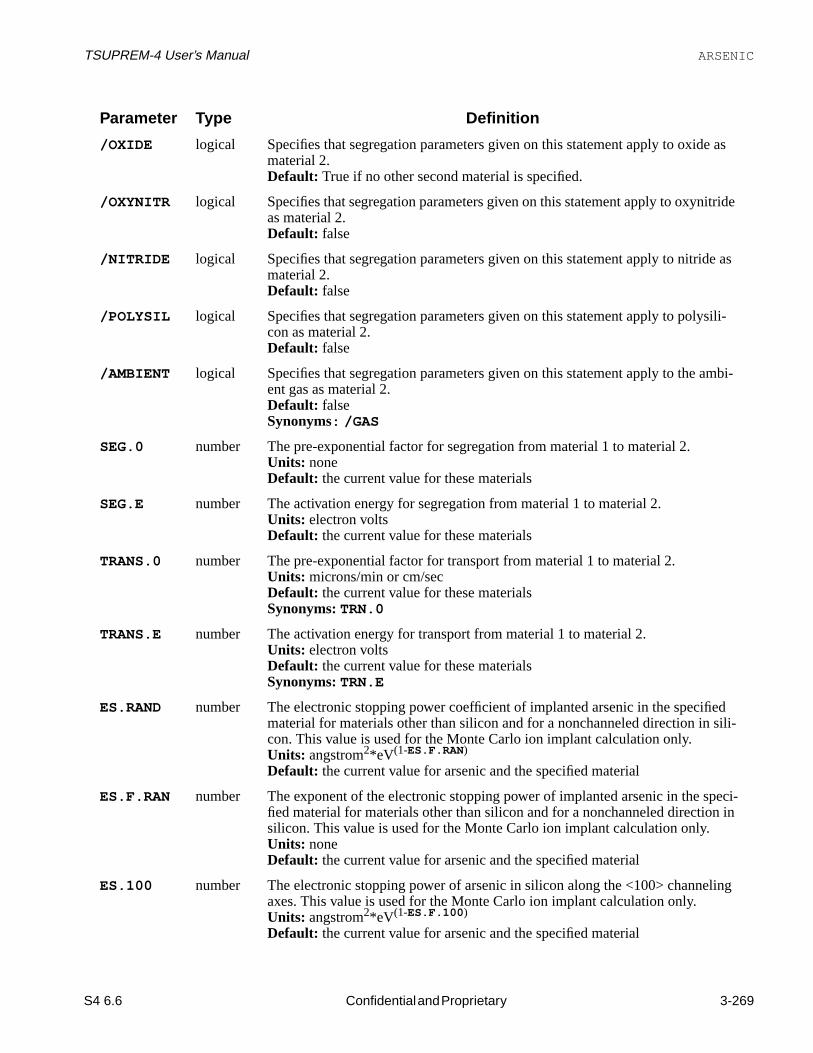
TSUPREM-4 User’s Manual ARSENIC
e as
itride
e as
sili-
mbi-
edsili-
peci-n in
ling
/OXIDE logical Specifies that segregation parameters given on this statement apply to oxidmaterial 2.Default: True if no other second material is specified.
/OXYNITR logical Specifies that segregation parameters given on this statement apply to oxynas material 2.Default: false
/NITRIDE logical Specifies that segregation parameters given on this statement apply to nitridmaterial 2.Default: false
/POLYSIL logical Specifies that segregation parameters given on this statement apply to polycon as material 2.Default: false
/AMBIENT logical Specifies that segregation parameters given on this statement apply to the aent gas as material 2.Default: falseSynonyms: /GAS
SEG.0 number The pre-exponential factor for segregation from material 1 to material 2.Units: noneDefault: the current value for these materials
SEG.E number The activation energy for segregation from material 1 to material 2.Units: electron voltsDefault: the current value for these materials
TRANS.0 number The pre-exponential factor for transport from material 1 to material 2.Units: microns/min or cm/secDefault: the current value for these materialsSynonyms:TRN.0
TRANS.E number The activation energy for transport from material 1 to material 2.Units: electron voltsDefault: the current value for these materialsSynonyms:TRN.E
ES.RAND number The electronic stopping power coefficient of implanted arsenic in the specifimaterial for materials other than silicon and for a nonchanneled direction in con. This value is used for the Monte Carlo ion implant calculation only.Units: angstrom2*eV(1-ES.F.RAN )
Default: the current value for arsenic and the specified material
ES.F.RAN number The exponent of the electronic stopping power of implanted arsenic in the sfied material for materials other than silicon and for a nonchanneled directiosilicon. This value is used for the Monte Carlo ion implant calculation only.Units: noneDefault: the current value for arsenic and the specified material
ES.100 number The electronic stopping power of arsenic in silicon along the <100> channeaxes. This value is used for the Monte Carlo ion implant calculation only.Units: angstrom2*eV(1-ES.F.100 )
Default: the current value for arsenic and the specified material
Parameter Type Definition
S4 6.6 Confidential and Proprietary 3-269
Draft 6/26/98

Input Statement Descriptions TSUPREM-4 User’s Manual
aluesters
fied
t
in-re
ela-
ling
ela-
if
Description
This statement specifies properties and model coefficients for arsenic. The vof the diffusivity, reaction constant, clustering, and electronic stopping parameapply in material 1 (specified without the “/”), whileSEG.0, SEG.E, TRANS.0andTRANS.E apply at the interface between material 1 and material 2 (speciwith the “/”). These coefficients are normally given in thes4init file (which is readat the start of eachTSUPREM-4 execution), but can be changed by the user aany time. Coefficients that are not given in thes4init file and not set by the userdefault to 0.0, except forSEG.0 that defaults to 1.0.
The newerIMPURITY statement can be used to set all of the properties ofarsenic, including some that cannot be set with theARSENIC statement.
Parameters whose units include time are specified in units of microns and mutes, unlessCM.SEC is true, in which case units of centimeters and seconds aassumed.
For additional information see the following sections:
• The diffusion and segregation parameters are described inChapter 2, “Diffu-sion” on page 2-12.
• The electronic stopping power parameters are described inChapter 2, “MonteCarlo Ion Implant Model” on page 2-74.
ES.F.100 number The exponent of the electronic stopping power of arsenic in silicon along th<100> crystal axes. This value is used for the Monte Carlo ion implant calcution only.Units: noneDefault: the current value for arsenic and the specified material
ES.110 number The electronic stopping power of arsenic in silicon along the <110> channeaxes. This value is used for the Monte Carlo ion implant calculation only.Units: angstrom2*eV(1-ES.F.100 )
Default: the current value for arsenic and the specified material
ES.F.110 number The exponent of the electronic stopping power of arsenic in silicon along th<110> crystal axes. This value is used for the Monte Carlo ion implant calcution only.Units: noneDefault: the current value for arsenic and the specified material
CM.SEC logical If true, parameters involving time are specified in centimeters and seconds; false, parameters involving time are in microns and minutes.Default: false
Parameter Type Definition
3-270 Confidential and Proprietary S4 6.6
Draft 6/26/98

TSUPREM-4 User’s Manual ARSENIC
eg-
iO
ui-
Examples
1. The following statement specifies the diffusivity of arsenic diffusing with native vacancies in silicon:
2. The following statement specifies the segregation parameters at the Si/S2interface:
The concentration in silicon is 30.0 times the concentration in oxide, at eqlibrium.
Additional ARSENIC Notes
1. TheARSENIC statement has been obsoleted by theIMPURITY statement,but remains available for compatibility with existing input files. Note thatsome properties of arsenic can only be set on theIMPURITY statement.
2. The fractional interstitialcy parameterFI that was used inTSUPREM-4prior to version 6.0 is no longer supported. Instead, it is now necessary tospecify the diffusivities with interstitials and vacancies separately.
ARSENIC SILICON DVM.0=1.49e11 DVM.E=4.15
ARSENIC SILICON /OXIDE SEG.0=30.0 TRANS.0=0.1
S4 6.6 Confidential and Proprietary 3-271
Draft 6/26/98

Input Statement Descriptions TSUPREM-4 User’s Manual
r the
nd
that
,
nd
n,
BORON
TheBORON statement sets some of the properties of boron.
BORON
MATERIAL=<c> | SILICON | OXIDE | OXYNITRI | NITRIDE | POLYSILI | AMBIENT [DIX.0=<n>] [DIX.E=<n>] [DIP.0=<n>] [DIP.E=<n>] [DVX.0=<n>] [DVX.E=<n>] [DVP.0=<n>] [DVP.E=<n>] [DIPAIR.0=<n>] [DIPAIR.E=<n>] [DVPAIR.0=<n>] [DVPAIR.E=<n>] [R.I.S=<n>] [E.I.S=<n>] [R.V.S=<n>] [E.V.S=<n>] [R.IP.V=<n>] [E.IP.V=<n>] [R.VP.I=<n>] [E.VP.I=<n>] [SS.CLEAR] [SS.TEMP=<n> SS.CONC=<n>] [ /MATERIA=<c> | /SILICON | /OXIDE | /OXYNITR | /NITRIDE | /POLYSIL | /AMBIENT [SEG.0=<n>] [SEG.E=<n>] [TRANS.0=<n>] [TRANS.E=<n>] ] [ES.RAND=<n> [ES.F.RAN=<n>]] [ES.100=<n> [ES.F.100=<n>]] [ES.110=<n> [ES.F.110=<n>]] [CM.SEC]
Parameter Type Definition
MATERIAL character The name of the material to which the other parameters apply (material 1 fosegregation terms).Default: none
SILICON logical Specifies that other parameters in this statement apply to boron in silicon, athat silicon is material 1 for the segregation terms.Default: True if no other first material is specified.
OXIDE logical Specifies that other parameters in this statement apply to boron in oxide, andoxide is material 1 for the segregation terms.Default: false
OXYNITRI logical Specifies that other parameters in this statement apply to boron in oxynitrideand that oxynitride is material 1 for the segregation terms.Default: false
NITRIDE logical Specifies that other parameters in this statement apply to boron in nitride, athat nitride is material 1 for the segregation terms.Default: false
POLYSILI logical Specifies that other parameters in this statement apply to boron in polysilicoand that polysilicon is material 1 for the segregation terms.Default: false
AMBIENT logical Specifies that the ambient gas is material 1 for the segregation terms.Default: falseSynonyms:GAS
3-272 Confidential and Proprietary S4 6.6
Draft 6/26/98

TSUPREM-4 User’s Manual BORON
sti-
n-
oron
DIX.0 number The pre-exponential constant for diffusion of boron with neutral interstitials.Units: microns2/min or cm2/secDefault: the current value for this material
DIX.E number The activation energy for diffusion of boron with neutral interstitials.Units: electron voltsDefault: the current value for this material
DIP.0 number The pre-exponential constant for diffusion of boron with singly positive intertials.Units: microns2/min or cm2/secDefault: the current value for this material
DIP.E number The activation energy for diffusion of boron with singly positive interstitials.Units: electron voltsDefault: the current value for this material
DVX.0 number The pre-exponential constant for diffusion of boron with neutral vacancies.Units: microns2/min or cm2/secDefault: the current value for this material
DVX.E number The activation energy for diffusion of boron with neutral vacancies.Units: electron voltsDefault: the current value for this material
DVP.0 number The pre-exponential constant for diffusion of boron with singly positive vacacies.Units: microns2/min or cm2/secDefault: the current value for this material
DVP.E number The activation energy for diffusion of boron with singly positive vacancies.Units: electron voltsDefault: the current value for this material
DIPAIR.0 number The pre-exponential constant for the diffusivity of boron-interstitial pairs.Units: microns2/min or cm2/secDefault: the current value for this material
DIPAIR.E number The activation energy for the diffusivity of boron-interstitial pairs.Units: electron voltsDefault: the current value for this material
DVPAIR.0 number The pre-exponential constant for the diffusivity of boron-vacancy pairs.Units: microns2/min or cm2/secDefault: the current value for this material
DVPAIR.E number The activation energy for the diffusivity of boron-vacancy pairs.Units: electron voltsDefault: the current value for this material
R.I.S number The capture radius for the reaction between interstitials and substitutional batoms.Units: ÅDefault: the current value for this material
Parameter Type Definition
S4 6.6 Confidential and Proprietary 3-273
Draft 6/26/98

Input Statement Descriptions TSUPREM-4 User’s Manual
oron
oron
ron
an-
n-
titials.
titials.
n as
e as
E.I.S number The barrier energy for the reaction between interstitials and substitutional batoms.Units: electron voltsDefault: the current value for this material
R.V.S number The capture radius for the reaction between vacancies and substitutional batoms.Units: ÅDefault: the current value for this material
E.V.S number The barrier energy for the reaction between vacancies and substitutional boatoms.Units: electron voltsDefault: the current value for this material
R.IP.V number The capture radius for the reaction between boron-interstitial pairs and vaccies.Units: ÅDefault: the current value for this material
E.IP.V number The barrier energy for the reaction between boron-interstitial pairs and vacacies.Units: electron voltsDefault: the current value for this material
R.VP.I number The capture radius for the reaction between boron-vacancy pairs and intersUnits: ÅDefault: the current value for this material
E.VP.I number The barrier energy for the reaction between boron-vacancy pairs and intersUnits: electron voltsDefault: the current value for this material
SS.CLEAR logical Clears the solid solubility vs. temperature table.Default: false
SS.TEMP number The temperature at which the solid solubility in material 1 isSS.CONC.Units: degrees CelsiusDefault: none
SS.CONC number The solid solubility in material 1 at temperatureSS.TEMP.Units: atoms/cm3
Default: none
/MATERIA character The name of material 2 for the segregation parameters.Default: none
/SILICON logical Specifies that segregation parameters given on this statement apply to silicomaterial 2.Default: false
/OXIDE logical Specifies that segregation parameters given on this statement apply to oxidmaterial 2.Default: true if no other second material is specified
Parameter Type Definition
3-274 Confidential and Proprietary S4 6.6
Draft 6/26/98

TSUPREM-4 User’s Manual BORON
itride
e as
sili-
mbi-
dsili-
eci-n in
g
/OXYNITR logical Specifies that segregation parameters given on this statement apply to oxynas material 2.Default: false
/NITRIDE logical Specifies that segregation parameters given on this statement apply to nitridmaterial 2.Default: false
/POLYSIL logical Specifies that segregation parameters given on this statement apply to polycon as material 2.Default: false
/AMBIENT logical Specifies that segregation parameters given on this statement apply to the aent gas as material 2.Default: falseSynonyms:/GAS
SEG.0 number The pre-exponential factor for segregation from material 1 to material 2.Units: noneDefault: the current value for these materials
SEG.E number The activation energy for segregation from material 1 to material 2.Units: electron voltsDefault: the current value for these materials
TRANS.0 number The pre-exponential factor for transport from material 1 to material 2.Units: microns/min or cm/secDefault: the current value for these materialsSynonyms:TRN.0
TRANS.E number The activation energy for transport from material 1 to material 2.Units: electron voltsDefault: the current value for these materialsSynonyms:TRN.E
ES.RAND number The electronic stopping power coefficient of implanted boron in the specifiematerial for materials other than silicon and for a nonchanneled direction in con. This value is used for the Monte Carlo ion implant calculation only.Units: angstrom2*eV(1-ES.F.RAN )
Default: the current value for boron and the specified material
ES.F.RAN number The exponent of the electronic stopping power of implanted boron in the spfied material for materials other than silicon and for a nonchanneled directiosilicon. This value is used for the Monte Carlo ion implant calculation only.Units: noneDefault: the current value for boron and the specified material
ES.100 number The electronic stopping power of boron in silicon along the <100> channelinaxes. This value is used for the Monte Carlo ion implant calculation only.Units: angstrom2*eV(1-ES.F.100 )
Default: the current value for boron and the specified material
Parameter Type Definition
S4 6.6 Confidential and Proprietary 3-275
Draft 6/26/98

Input Statement Descriptions TSUPREM-4 User’s Manual
es ofme-
ial
y
on,
in-re
la-
g
la-
if
Description
This statement specifies properties and model coefficients for boron. The valuthe diffusivity, reaction constant, solid solubility, and electronic stopping paraters apply in material 1 (specified without the “/”), whileSEG.0, SEG.E,TRANS.0, andTRANS.E apply at the interface between material 1 and mater2 (specified with the “/”). These coefficients are normally given in thes4init file(which is read at the start of eachTSUPREM-4 execution) but can be changed bthe user at any time. Coefficients that are not given in thes4init file or set by theuser default to 0.0, except forSEG.0 that defaults to 1.0.
The newerIMPURITY statement can be used to set all of the properties of borincluding some that cannot be set with theBORON statement.
Parameters whose units include time are specified in units of microns and mutes, unlessCM.SEC is true, in which case units of centimeters and seconds aassumed.
For additional information see the following sections:
• The diffusion and segregation parameters are described inChapter 2, “Diffu-sion” on page 2-12.
• The electronic stopping power parameters are described inChapter 2, “MonteCarlo Ion Implant Model” on page 2-74.
ES.F.100 number The exponent of the electronic stopping power of boron in silicon along the<100> crystal axes. This value is used for the Monte Carlo ion implant calcution only.Units: noneDefault: the current value for boron and the specified material
ES.110 number The electronic stopping power of boron in silicon along the <110> channelinaxes. This value is used for the Monte Carlo ion implant calculation only.Units: angstrom2*eV(1-ES.F.100 )
Default: the current value for boron and the specified material
ES.F.110 number The exponent of the electronic stopping power of boron in silicon along the<110> crystal axes. This value is used for the Monte Carlo ion implant calcution only.Units: noneDefault: the current value for boron and the specified material
CM.SEC logical If true, parameters involving time are specified in centimeters and seconds; false, parameters involving time are in microns and minutes.Default: false
Parameter Type Definition
3-276 Confidential and Proprietary S4 6.6
Draft 6/26/98

TSUPREM-4 User’s Manual BORON
u-
iO
ui-
Examples
1. The following statement specifies the diffusivity of boron diffusing with netral interstitials in silicon:
2. The following statement specifies the segregation parameters at the Si/S2interface:
The concentration in silicon is 0.91 times the concentration in oxide, at eqlibrium.
Additional BORON Notes
1. TheBORON statement has been made obsolete by theIMPURITY statement,but remains available for compatibility with existing input files. Note thatsome properties of boron can only be set on theIMPURITY statement.
2. The fractional interstitialcy parameterFI that was used inTSUPREM-4prior to version 6.0 is no longer supported. Instead, it is now necessary tospecify the diffusivities with interstitials and vacancies separately.
BORON SILICON DIX.0=2.09e8 DIX.E=3.46
BORON SILICON /OXIDE SEG.0=0.91 TRANS.0=0.1
S4 6.6 Confidential and Proprietary 3-277
Draft 6/26/98

Input Statement Descriptions TSUPREM-4 User’s Manual
r the
con,
de,
ni-
ide,
lysili-
PHOSPHORUS
ThePHOSPHORUS statement sets some of the properties of phosphorus.
PHOSPHORUS
MATERIAL=<c> | SILICON | OXIDE | OXYNITRI | NITRIDE | POLYSILI | AMBIENT [DIX.0=<n>] [DIX.E=<n>] [DIM.0=<n>] [DIM.E=<n>] [DIMM.0=<n>] [DIMM.E=<n>] [DVX.0=<n>] [DVX.E=<n>] [DVM.0=<n>] [DVM.E=<n>] [DVMM.0=<n>] [DVMM.E=<n>] [DIPAIR.0=<n>] [DIPAIR.E=<n>] [DVPAIR.0=<n>] [DVPAIR.E=<n>] [R.I.S=<n>] [E.I.S=<n>] [R.V.S=<n>] [E.V.S=<n>] [R.IP.V=<n>] [E.IP.V=<n>] [R.VP.I=<n>] [E.VP.I=<n>] [SS.CLEAR] [SS.TEMP=<n> SS.CONC=<n>] [ /MATERIA=<c> | /SILICON | /OXIDE | /OXYNITR | /NITRIDE | /POLYSIL | /AMBIENT [SEG.0=<n>] [SEG.E=<n>] [TRANS.0=<n>] [TRANS.E=<n>] ] [ES.RAND=<n> [ES.F.RAN=<n>]] [ES.100=<n> [ES.F.100=<n>]] [ES.110=<n> [ES.F.110=<n>]] [CM.SEC]
Parameter Type Definition
MATERIAL character The name of the material to which the other parameters apply (material 1 fosegregation terms).Default: none
SILICON logical Specifies that other parameters in this statement apply to phosphorus in siliand that silicon is material 1 for the segregation terms.Default: True if no other first material is specified
OXIDE logical Specifies that other parameters in this statement apply to phosphorus in oxiand that oxide is material 1 for the segregation terms.Default: false
OXYNITRI logical Specifies that other parameters in this statement apply to phosphorus in oxytride, and that oxynitride is material 1 for the segregation terms.Default: false
NITRIDE logical Specifies that other parameters in this statement apply to phosphorus in nitrand that nitride is material 1 for the segregation terms.Default: false
POLYSILI logical Specifies that other parameters in this statement apply to phosphorus in pocon, and that polysilicon is material 1 for the segregation terms.Default: false
AMBIENT logical Specifies that the ambient gas is material 1 for the segregation terms.Default: falseSynonyms:GAS
3-278 Confidential and Proprietary S4 6.6
Draft 6/26/98

TSUPREM-4 User’s Manual PHOSPHORUS
ti-
e
ti-
ive
sti-
cies.
e
-
ive
n-
DIX.0 number The pre-exponential constant for diffusion of phosphorus with neutral interstials.Units: microns2/min or cm2/secDefault: the current value for this material
DIX.E number The activation energy for diffusion of phosphorus with neutral interstitials.Units: electron voltsDefault: the current value for this material
DIM.0 number The pre-exponential constant for diffusion of phosphorus with singly negativinterstitials.Units: microns2/min or cm2/secDefault: the current value for this material
DIM.E number The activation energy for diffusion of phosphorus with singly negative interstials.Units: electron voltsDefault: the current value for this material
DIMM.0 number The pre-exponential constant for diffusion of phosphorus with doubly negatinterstitials.Units: microns2/min or cm2/secDefault: the current value for this material
DIMM.E number The activation energy for diffusion of phosphorus with doubly negative intertials.Units: electron voltsDefault: the current value for this material
DVX.0 number The pre-exponential constant for diffusion of phosphorus with neutral vacanUnits: microns2/min or cm2/secDefault: the current value for this material
DVX.E number The activation energy for diffusion of phosphorus with neutral vacancies.Units: electron voltsDefault: the current value for this material
DVM.0 number The pre-exponential constant for diffusion of phosphorus with singly negativvacancies.Units: microns2/min or cm2/secDefault: the current value for this material
DVM.E number The activation energy for diffusion of phosphorus with singly negative vacancies.Units: electron voltsDefault: the current value for this material
DVMM.0 number The pre-exponential constant for diffusion of phosphorus with doubly negatvacancies.Units: microns2/min or cm2/secDefault: the current value for this material
DVMM.E number The activation energy for diffusion of phosphorus with doubly negative vacacies.Units: electron voltsDefault: the current value for this material
Parameter Type Definition
S4 6.6 Confidential and Proprietary 3-279
Draft 6/26/98

Input Statement Descriptions TSUPREM-4 User’s Manual
irs.
.
hos-
hos-
hos-
os-
d
d
inter-
inter-
DIPAIR.0 number The pre-exponential constant for the diffusivity of phosphorus-interstitial paUnits: microns2/min or cm2/secDefault: the current value for this material
DIPAIR.E number The activation energy for the diffusivity of phosphorus-interstitial pairs.Units: electron voltsDefault: the current value for this material
DVPAIR.0 number The pre-exponential constant for the diffusivity of phosphorus-vacancy pairsUnits: microns2/min or cm2/secDefault: the current value for this material
DVPAIR.E number The activation energy for the diffusivity of phosphorus-vacancy pairs.Units: electron voltsDefault: the current value for this material
R.I.S number The capture radius for the reaction between interstitials and substitutional pphorus atoms.Units: ÅDefault: the current value for this material
E.I.S number The barrier energy for the reaction between interstitials and substitutional pphorus atoms.Units: electron voltsDefault: the current value for this material
R.V.S number The capture radius for the reaction between vacancies and substitutional pphorus atoms.Units: ÅDefault: the current value for this material
E.V.S number The barrier energy for the reaction between vacancies and substitutional phphorus atoms.Units: electron voltsDefault: the current value for this material
R.IP.V number The capture radius for the reaction between phosphorus-interstitial pairs anvacancies.Units: ÅDefault: the current value for this material
E.IP.V number The barrier energy for the reaction between phosphorus-interstitial pairs anvacancies.Units: electron voltsDefault: the current value for this material
R.VP.I number The capture radius for the reaction between phosphorus-vacancy pairs andstitials.Units: ÅDefault: the current value for this material
E.VP.I number The barrier energy for the reaction between phosphorus-vacancy pairs andstitials.Units: electron voltsDefault: the current value for this material
Parameter Type Definition
3-280 Confidential and Proprietary S4 6.6
Draft 6/26/98

TSUPREM-4 User’s Manual PHOSPHORUS
n as
e as
itride
e as
sili-
mbi-
SS.CLEAR logical Clears the solid solubility vs. temperature table.Default: false
SS.TEMP number The temperature at which the solid solubility in material 1 isSS.CONC.Units: degrees CelsiusDefault: none
SS.CONC number The solid solubility in material 1 at temperatureSS.TEMP.Units: atoms/cm3
Default: none
/MATERIA character The name of material 2 for the segregation parameters.Default: none
/SILICON logical Specifies that segregation parameters given on this statement apply to silicomaterial 2.Default: false
/OXIDE logical Specifies that segregation parameters given on this statement apply to oxidmaterial 2.Default: false
/OXYNITR logical Specifies that segregation parameters given on this statement apply to oxynas material 2.Default: false
/NITRIDE logical Specifies that segregation parameters given on this statement apply to nitridmaterial 2.Default: false
/POLYSIL logical Specifies that segregation parameters given on this statement apply to polycon as material 2.Default: false
/AMBIENT logical Specifies that segregation parameters given on this statement apply to the aent gas as material 2.Default: falseSynonyms:/GAS
SEG.0 number The pre-exponential factor for segregation from material 1 to material 2.Units: noneDefault: the current value for these materials
SEG.E number The activation energy for segregation from material 1 to material 2.Units: electron voltsDefault: the current value for these materials
TRANS.0 number The pre-exponential factor for transport from material 1 to material 2.Units: microns/min or cm/secDefault: the current value for these materialsSynonyms:TRN.0
TRANS.E number The activation energy for transport from material 1 to material 2.Units: electron voltsDefault: the current value for these materialsSynonyms:TRN.E
Parameter Type Definition
S4 6.6 Confidential and Proprietary 3-281
Draft 6/26/98

Input Statement Descriptions TSUPREM-4 User’s Manual
heing
ial
y
os-
eci-n in
theec-
n-nly.
thela-
n-nly.
thela-
if
Description
This statement specifies properties and model coefficients for phosphorus. Tvalues of the diffusivity, reaction constant, solid solubility, and electronic stoppparameters apply in material 1 (specified without the “/”), whileSEG.0, SEG.E,TRANS.0, andTRANS.E apply at the interface between material 1 and mater2 (specified with the “/”). These coefficients are normally given in thes4init file(which is read at the start of eachTSUPREM-4 execution) but can be changed bthe user at any time. Coefficients that are not given in thes4init file or set by theuser default to 0.0, except forSEG.0 that defaults to 1.0.
The newerIMPURITY statement can be used to set all of the properties of phphorus, including some that cannot be set with thePHOSPHOR statement.
ES.RAND number The electronic stopping power coefficient of implanted phosphorus in the spfied material for materials other than silicon and for a nonchanneled directiosilicon. This value is used for the Monte Carlo ion implant calculation only.Units: angstrom2*eV(1-ES.F.RAN )
Default: the current value for phosphorus and the specified material
ES.F.RAN number The exponent of the electronic stopping power of implanted phosphorus in specified material for materials other than silicon and for a nonchanneled dirtion in silicon. This value is used for the Monte Carlo ion implant calculationonly.Units: noneDefault: the current value for phosphorus and the specified material
ES.100 number The electronic stopping power of phosphorus in silicon along the <100> chaneling axes. This value is used for the Monte Carlo ion implant calculation oUnits: angstrom2*eV(1-ES.F.100 )
Default: the current value for phosphorus and the specified material
ES.F.100 number The exponent of the electronic stopping power of phosphorus in silicon along<100> crystal axes. This value is used for the Monte Carlo ion implant calcution only.Units: noneDefault: the current value for phosphorus and the specified material
ES.110 number The electronic stopping power of phosphorus in silicon along the <110> chaneling axes. This value is used for the Monte Carlo ion implant calculation oUnits: angstrom2*eV(1-ES.F.100 )
Default: the current value for phosphorus and the specified material
ES.F.110 number The exponent of the electronic stopping power of phosphorus in silicon along<110> crystal axes. This value is used for the Monte Carlo ion implant calcution only.Units: noneDefault: the current value for phosphorus and the specified material
CM.SEC logical If true, parameters involving time are specified in centimeters and seconds; false, parameters involving time are in microns and minutes.Default: false
Parameter Type Definition
3-282 Confidential and Proprietary S4 6.6
Draft 6/26/98

TSUPREM-4 User’s Manual PHOSPHORUS
in-re
ith
iO
ui-
Parameters whose units include time are specified in units of microns and mutes, unlessCM.SEC is true, in which case units of centimeters and seconds aassumed.
For additional information see the following sections:
• Use of the diffusion and segregation parameters is described inChapter 2,“Diffusion” on page 2-12.
• The electronic stopping power parameters are described inChapter 2, “MonteCarlo Ion Implant Model” on page 2-74.
Examples
1. The following statement specifies the diffusion of phosphorus diffusing wdoubly negative interstitials in silicon:
2. The following statement specifies the segregation parameters at the Si/S2interface:
The concentration in silicon is 30.0 times the concentration in oxide, at eqlibrium.
Additional PHOSPHORUS Notes
1. ThePHOSPHORUS statement has been made obsolete by theIMPURITYstatement, but remains available for compatibility with existing input files.Note that some properties of phosphorus can only be set on theIMPURITYstatement.
2. The fractional interstitialcy parameterFI that was used inTSUPREM-4prior to version 6.0 is no longer supported. Instead, it is now necessary tospecify the diffusivities with interstitials and vacancies separately.
PHOSPHORUS SILICON DIMM.0=2.652e11 DIMM.E=4.37
PHOS SILICON /OXIDE SEG.0=30.0 TRANS.0=0.1
S4 6.6 Confidential and Proprietary 3-283
Draft 6/26/98

Input Statement Descriptions TSUPREM-4 User’s Manual
3-284 Confidential and Proprietary S4 6.6
Draft 6/26/98

TSUPREM-4 User’s Manual 3.6 Summary
S4 6.6
3
that
aram-ey a
3.6 SummaryThis section summarizes the input statements recognized byTSUPREM-4. Theformat used for the parameter list associated with a statement is identical to used in the detailed statement descriptions. The special characters< >, [ ] , |, ,and( ) are used to indicate parameter types, optional parameters, and valid peter combinations. (For more information on the use of special characters se“Syntax of Parameter Lists” on page 3-4.) The summary is organized alphabecallby statement name and includes references to the page of the manual wheredetailed description of the statement can be found.
Confidential and Proprietary 3-285
Draft 6/26/98

Input Statement Descriptions TSUPREM-4 User’s Manual
AMBIENT Page 3-193 [ DRYO2 | WETO2 | STEAM | INERT | AMB.1 | AMB.2 | AMB.3 | AMB.4 | AMB.5 [F.O2=<n>] [F.H2O=<n>] [F.H2=<n>] [F.N2=<n>] [F.HCL=<n>] [PRESSURE=<n>] [HCL=<n>] ] [ O2 | H2O [ <111> | <110> | <100> | ORIENTAT=<n> | POLYSILI [THINOX.0=<n>] [THINOX.E=<n>] [THINOX.L=<n>] [L.LIN.0=<n>] [L.LIN.E=<n>] [H.LIN.0=<n>] [H.LIN.E=<n>] ] [L.PAR.0=<n>] [L.PAR.E=<n>] [H.PAR.0=<n>] [H.PAR.E=<n>] [LIN.BREA=<n>] [PAR.BREA=<n>] [LIN.PDEP=<n>] [PAR.PDEP=<n>] [GAMMA.0=<n>] [GAMMA.E=<n>] [ LIN.PCT | PAR.PCT | ( LIN.CLDE | PAR.CLDE COLUMN=<n>> ) TABLE=<c> ] [ MATERIAL=<c> | SILICON | OXIDE | OXYNITRI | NITRIDE | POLYSILI | AMBIENT [D.0=<n>] [D.E=<n>] [VC=<c>] [HENRY.CO=<n>] [THETA=<n>] [ /MATERIA=<c> | /SILICON | /OXIDE | /OXYNITR | /NITRIDE | /POLYSIL | /AMBIENT [SEG.0=<n>] [SEG.E=<n>] [TRANS.0=<n>] [TRANS.E=<n>] [ALPHA=<n>] ] ] ] [STRESS.D] [VR=<c>] [VT=<c>] [VD=<c>] [VDLIM=<n>] [INITIAL=<n>] [SPREAD=<n>] [MASK.EDG=<n>] [ERF.Q=<n>] [ERF.DELT=<n>] [ERF.LBB=<c>] [ERF.H=<c>] [NIT.THIC=<n>]
[CLEAR][TEMPERAT=<c>][CM.SEC]
3-286 Confidential and Proprietary S4 6.6
Draft 6/26/98
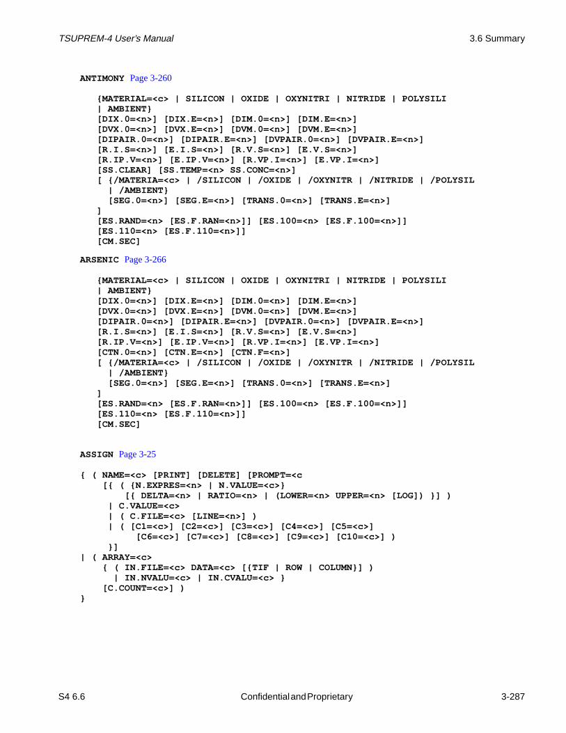
TSUPREM-4 User’s Manual 3.6 Summary
ANTIMONYPage 3-260
MATERIAL=<c> | SILICON | OXIDE | OXYNITRI | NITRIDE | POLYSILI | AMBIENT [DIX.0=<n>] [DIX.E=<n>] [DIM.0=<n>] [DIM.E=<n>] [DVX.0=<n>] [DVX.E=<n>] [DVM.0=<n>] [DVM.E=<n>] [DIPAIR.0=<n>] [DIPAIR.E=<n>] [DVPAIR.0=<n>] [DVPAIR.E=<n>] [R.I.S=<n>] [E.I.S=<n>] [R.V.S=<n>] [E.V.S=<n>] [R.IP.V=<n>] [E.IP.V=<n>] [R.VP.I=<n>] [E.VP.I=<n>] [SS.CLEAR] [SS.TEMP=<n> SS.CONC=<n>] [ /MATERIA=<c> | /SILICON | /OXIDE | /OXYNITR | /NITRIDE | /POLYSIL | /AMBIENT [SEG.0=<n>] [SEG.E=<n>] [TRANS.0=<n>] [TRANS.E=<n>] ] [ES.RAND=<n> [ES.F.RAN=<n>]] [ES.100=<n> [ES.F.100=<n>]] [ES.110=<n> [ES.F.110=<n>]] [CM.SEC]
ARSENIC Page 3-266
MATERIAL=<c> | SILICON | OXIDE | OXYNITRI | NITRIDE | POLYSILI | AMBIENT [DIX.0=<n>] [DIX.E=<n>] [DIM.0=<n>] [DIM.E=<n>] [DVX.0=<n>] [DVX.E=<n>] [DVM.0=<n>] [DVM.E=<n>] [DIPAIR.0=<n>] [DIPAIR.E=<n>] [DVPAIR.0=<n>] [DVPAIR.E=<n>] [R.I.S=<n>] [E.I.S=<n>] [R.V.S=<n>] [E.V.S=<n>] [R.IP.V=<n>] [E.IP.V=<n>] [R.VP.I=<n>] [E.VP.I=<n>] [CTN.0=<n>] [CTN.E=<n>] [CTN.F=<n>] [ /MATERIA=<c> | /SILICON | /OXIDE | /OXYNITR | /NITRIDE | /POLYSIL | /AMBIENT [SEG.0=<n>] [SEG.E=<n>] [TRANS.0=<n>] [TRANS.E=<n>] ] [ES.RAND=<n> [ES.F.RAN=<n>]] [ES.100=<n> [ES.F.100=<n>]] [ES.110=<n> [ES.F.110=<n>]] [CM.SEC]
ASSIGN Page 3-25
( NAME=<c> [PRINT] [DELETE] [PROMPT=<c[ ( N.EXPRES=<n> | N.VALUE=<c>
[ DELTA=<n> | RATIO=<n> | (LOWER=<n> UPPER=<n> [LOG]) ] )| C.VALUE=<c>| ( C.FILE=<c> [LINE=<n>] )| ( [C1=<c>] [C2=<c>] [C3=<c>] [C4=<c>] [C5=<c>]
[C6=<c>] [C7=<c>] [C8=<c>] [C9=<c>] [C10=<c>] )]
| ( ARRAY=<c> ( IN.FILE=<c> DATA=<c> [TIF | ROW | COLUMN] )
| IN.NVALU=<c> | IN.CVALU=<c> [C.COUNT=<c>] )
S4 6.6 Confidential and Proprietary 3-287
Draft 6/26/98

Input Statement Descriptions TSUPREM-4 User’s Manual
BORONPage 3-272
MATERIAL=<c> | SILICON | OXIDE | OXYNITRI | NITRIDE | POLYSILI | AMBIENT [DIX.0=<n>] [DIX.E=<n>] [DIP.0=<n>] [DIP.E=<n>] [DVX.0=<n>] [DVX.E=<n>] [DVP.0=<n>] [DVP.E=<n>] [DIPAIR.0=<n>] [DIPAIR.E=<n>] [DVPAIR.0=<n>] [DVPAIR.E=<n>] [R.I.S=<n>] [E.I.S=<n>] [R.V.S=<n>] [E.V.S=<n>] [R.IP.V=<n>] [E.IP.V=<n>] [R.VP.I=<n>] [E.VP.I=<n>] [SS.CLEAR] [SS.TEMP=<n> SS.CONC=<n>] [ /MATERIA=<c> | /SILICON | /OXIDE | /OXYNITR | /NITRIDE | /POLYSIL | /AMBIENT [SEG.0=<n>] [SEG.E=<n>] [TRANS.0=<n>] [TRANS.E=<n>] ] [ES.RAND=<n> [ES.F.RAN=<n>]] [ES.100=<n> [ES.F.100=<n>]] [ES.110=<n> [ES.F.110=<n>]] [CM.SEC]
BOUNDARYPage 3-54
REFLECTI | EXPOSED XLO=<c> XHI=<c> YLO=<c> YHI=<c>
COLORPage 3-141
[COLOR=<n>] [MIN.VALU=<n>] [MAX.VALU=<n>] [ MATERIAL=<c> | SILICON | OXIDE | OXYNITRI | NITRIDE | POLYSILI | ALUMINUM | PHOTORES ]
COMMENTPage 3-8
[<c>]
or
$
[<c>]
CONTOURPage 3-139
VALUE=<n> [LINE.TYP=<n>] [COLOR=<n>] [SYMBOL=<n>]
CPULOGPage 3-40
[LOG] [OUT.FILE=<c>]
DEFINE Page 3-36
[<name> <body>]
3-288 Confidential and Proprietary S4 6.6
Draft 6/26/98

TSUPREM-4 User’s Manual 3.6 Summary
DEPOSITION Page 3-84
MATERIAL=<c> | SILICON | OXIDE | OXYNITRI | NITRIDE | POLYSILI | ALUMINUM | ( PHOTORES [ POSITIVE | NEGATIVE ] ) [ IMPURITY=<c> I.CONC=<n> | I.RESIST=<n> ] [ANTIMONY=<n>] [ARSENIC=<n>] [BORON=<n>] [PHOSPHOR=<n>] [ CONCENTR | RESISTIV ] THICKNES=<n> [SPACES=<n>] [DY=<n>] [YDY=<n>] [ARC.SPAC=<n>] [TEMPERAT=<n>] [GSZ.LIN]
DEVELOPPage 3-90
[<c>]
DIFFUSION Page 3-105
TIME=<n> [CONTINUE] TEMPERAT=<n> [ T.RATE=<n> | T.FINAL=<n> ] [ DRYO2 | WETO2 | STEAM | INERT | AMB.1 | AMB.2 | AMB.3 | AMB.4 | AMB.5 | ( [F.O2=<n>] [F.H2O=<n>] [F.H2=<n>] [F.N2=<n>] [F.HCL=<n>] ) ] [IMPURITY=<c> I.CONC=<n>] [ANTIMONY=<n>] [ARSENIC=<n>] [BORON=<n>] [PHOSPHOR=<n>] [PRESSURE=<n>] [ P.RATE=<n> | P.FINAL=<n> ] [HCL=<n>] [MOVIE=<c>] [DUMP=<n>]
ECHOPage 3-32
<string>
S4 6.6 Confidential and Proprietary 3-289
Draft 6/26/98

Input Statement Descriptions TSUPREM-4 User’s Manual
ELECTRICAL Page 3-165
[X=<n>] [ ( SRP [ANGLE=<n>] [PITCH=<n>] [ POINT=<n> | DEPTH=<n> ] [Y.SURFAC=<n>] ) | ( V=<c> | (VSTART=<n> VSTOP=<n> VSTEP=<n>) ( RESISTAN [EXT.REG=<n>] [BIAS.REG=<n>] ) | ( JCAP [JUNCTION=<n>] ) | ( ( MOSCAP [HIGH] [LOW] [DEEP] )
| ( THRESHOL [VB=<n>] ) NMOS | PMOS [QSS=<n>] [GATE.WF=<n>] [GATE.ELE] [BULK.REG=<n>] )
[BULK.LAY=<n>] [PRINT] [DISTRIB] ) ] [TEMPERAT=<n>] [OUT.FILE=<c>] [NAME=<c> [V.SELECT=<n>]
TARGET=<n> [SENSITIV]| T.FILE=<c> [V.COLUMN=<n>] [V.LOWER=<n>] [V.UPPER=<n>]
[T.COLUMN=<n>] [T.LOWER=<n>][T.UPPER=<n>] [V.TRANSF=<c>] [T.TRANSF=<c>] )
[Z.VALUE][TOLERANC=<n>] [WEIGHT=<n>] [MIN.REL=<n>][MIN.ABS=<n>]
]
ELECTRODEPage 3-80 [NAME=<c>] [ ( X=<n> [Y=<n>] ) | BOTTOM ] [CLEAR [ALL]] [PRINT]
ELIMINATE Page 3-51
ROWS | COLUMNS [X.MIN=<n>] [X.MAX=<n>] [Y.MIN=<n>] [Y.MAX=<n>]
EPITAXY Page 3-111
TIME=<n> TEMPERAT=<n> [ T.RATE=<n> | T.FINAL=<n> ] [IMPURITY=<c> I.CONC=<n> | I.RESIST=<n>] [ANTIMONY=<n>] [ARSENIC=<n>] [BORON=<n>] [PHOSPHOR=<n>] [ CONCENTR | RESISTIV ] THICKNES=<n> [SPACES=<n>] [DY=<n>] [YDY=<n>] [ARC.SPAC=<n>]
3-290 Confidential and Proprietary S4 6.6
Draft 6/26/98

TSUPREM-4 User’s Manual 3.6 Summary
ETCH Page 3-91
[ MATERIAL=<c> | SILICON | OXIDE | OXYNITRI | NITRIDE | POLYSILI | PHOTORES | ALUMINUM ] ( TRAPEZOI [THICKNES=<n>] [ANGLE=<n>] [UNDERCUT=<n>] ) | ( LEFT | RIGHT [P1.X=<n>] [P1.Y=<n>] [P2.X=<n>] [P2.Y=<n>] ) | ( START | CONTINUE | DONE X=<n> Y=<n> )
| ISOTROPI | ( OLD.DRY THICKNES=<n> ) | ALL
EXPOSEPage 3-88
MASK=<c>
EXTRACT Page 3-151
[ MATERIAL=<c> | SILICON | OXIDE | OXYNITRI | NITRIDE | POLYSILI | PHOTORES | ALUMINUM ] [P1.X=<n>] [P1.Y=<n>] [P2.X=<n>] [P2.Y=<n>] [ /MATERIA=<c> | /SILICON | /OXIDE | /OXYNITR | /NITRIDE | /POLYSIL | /PHOTORE | /ALUMINU | /AMBIENT [CLOCKWIS] ] [X=<n>] [Y=<n>] [ DISTANCE=<n> | MINIMUM | MAXIMUM | VALUE=<n> ] ( [X.EXTRAC] [Y.EXTRAC] [D.EXTRAC] [VAL.EXTR] ) | ( [INT.EXTR] [AREA.EXT] [AVG.EXTR] ) [PREFIX=<c>] [SEPARAT=<c>] [SUFFIX=<c>] [WRITE] [PRINT] [ NAME=<c> [ASSIGN] [ TARGET=<n> | ( T.FILE=<c> [V.COLUMN=<n>] [V.LOWER=<n>] [V.UPPER=<n>] [T.COLUMN=<n>] [T.LOWER=<n>] [T.UPPER=<n>] [V.TRANSF=<c>] [T.TRANSF=<c>] [Z.VALUE=<c>] [SENSITIV])
[TOLERANC=<n>] [WEIGHT=<n>][MIN.REL=<n>] [MIN.ABS=<n>]
] ] [ OUT.FILE=<c> [APPEND] ] [CLOSE]
FOREACH/ENDPage 3-16
<name> <list>
HELP Page 3-41
[<name>]
S4 6.6 Confidential and Proprietary 3-291
Draft 6/26/98

Input Statement Descriptions TSUPREM-4 User’s Manual
IF/ELSEIF/ELSE/ IF.END Page 3-23
IF ( condition )[ ELSEIF ( condition ) ][ ELSE ]IF.END
IMPLANT Page 3-95
DOSE=<n> ENERGY=<n> [TILT=<n>] [ROTATION=<n>] IMPURITY=<c> | ANTIMONY | ARSENIC | BORON | BF2 | PHOSPHOR ( [ GAUSSIAN | PEARSON ] [RP.EFF] [IN.FILE=<c>] [IMPL.TAB=<c>] [MOMENTS] [BACKSCAT] ) | ( MONTECAR [N.ION=<n>] [BEAMWIDT=<n>] [SEED=<n>] [CRYSTAL [TEMPERAT=<n>] [VIBRATIO [X.RMS=<n>] [E.LIMIT=<n>] ] [THRESHOL=<n>] [REC.FRAC=<n>] [CRIT.PRE=<n>] [CRIT.F=<n>] [CRIT.110=<n>] ] [ PERIODIC | REFLECT | VACUUM ] ) [DAMAGE [MAX.DAMA=<n>] [D.PLUS=<n>] [D.SCALE=<n>] [D.RECOMB] ] [L.DENS=<n> L.RADIUS=<n> [L.DMIN=<n>] [L.DMAX=<n>] ] [PRINT]
3-292 Confidential and Proprietary S4 6.6
Draft 6/26/98

TSUPREM-4 User’s Manual 3.6 Summary
IMPURITY Page 3-221
IMPURITY=<c> [NEW] [TIF.NAME=<c>][IMP.ACT=<c>] [IMP.GB=<c>][IMP.IT=<c>]
[ DONOR | ACCEPTOR ] [AT.NUM=<n>] [AT.WT=<n>] [SOLVE] [STEADY] [IMPL.TAB=<c>] [ MATERIAL=<c> [DIP.0=<n>] [DIP.E=<n>] [DIX.0=<n>] [DIX.E=<n>] [DIM.0=<n>] [DIM.E=<n>] [DIMM.0=<n>] [DIMM.E=<n>] [DVP.0=<n>] [DVP.E=<n>] [DVX.0=<n>] [DVX.E=<n>] [DVM.0=<n>] [DVM.E=<n>] [DVMM.0=<n>] [DVMM.E=<n>] [C.STATE=<n> [DIC.0=<n>] [DIC.E=<n>] [DVC.0=<n>] [DVC.E=<n>] ] [FGB=<n>] [DIPAIR.0=<n>] [DIPAIR.E=<n>] [DVPAIR.0=<n>] [DVPAIR.E=<n>] [R.I.S=<n>] [E.I.S=<n>] [R.V.S=<n>] [E.V.S=<n>] [R.IP.V=<n>] [E.IP.V=<n>] [R.VP.I=<n>] [E.VP.I=<n>] [SS.CLEAR] [SS.TEMP=<n> SS.CONC=<n>] [CTN.0=<n>] [CTN.E=<n>] [CTN.F=<n>] [CL.INI.A] [Q.SITES=<n>] [CG.MAX=<n>] [GSEG.0=<n>] [GSEG.E=<n>] [GSEG.INI=<n>] [VELIF.0=<n>] [VELIF.E=<n>] [ /MATERIA=<c> [SEG.0=<n>] [SEG.E=<n>] [TRANS.0=<n>] [TRANS.E=<n>]
[RATIO.0=<n>] [RATIO.E=<n>] [SEG.SS][/SEG.0=<n>] [/SEG.E=<n>] [/TRANS.0=<n>] [/TRANS.E=<n>][/RATIO.0=<n>] [/RATIO.E=<n>] [/SEG.SS]SEG.EQ3 | SEG.EQ2 | /SEG.EQ2[Q.INI.0=<n>] [Q.INI.E=<n>] [Q.MAX.0=<n>] [Q.MAX.E=<n>][TWO.PHAS]
][ES.RAND=<n>] [ES.F.RAN=<n>] [ES.BREAK=<n>] [ES.F.H=<n>][ES.100=<n>] [ES.F.100=<n>] [ES.110=<n>] [ES.F.110=<n>][NLOC.PRE=<n>] [NLOC.EXP=<n>] [NLOC.MAX=<n>] [NLOC.K=<n>][LOC.FAC=<n>] [CHAN.CRI=<n>] [CHAN.FAC=<n>] [DISP.FAC=<n>]
][T.ACT.0=<n>] [T.ACT.E=<n>] [ACT.MIN=<n>][CM.SEC]
INITIALIZE Page 3-58
( IN.FILE=<c> ( [SCALE=<n>] [FLIP.Y] ) | TIF ) | ( [WIDTH=<n> [DX=<n>]] [ <111> | <110> | <100> | ORIENTAT=<n> ] [ ROT.SUB=<n> | X.ORIENT=<n> ] [RATIO=<n>] [LINE.DAT] ) [ IMPURITY=<c> I.CONC=<n> | I.RESIST=<n> ]
[ MATERIAL=<c> ][ANTIMONY=<n>] [ARSENIC=<n>] [BORON=<n>] [PHOSPHOR=<n>] [ CONCENTR | RESISTIV ]
INTERACTIVE Page 3-12
[<c>]
S4 6.6 Confidential and Proprietary 3-293
Draft 6/26/98
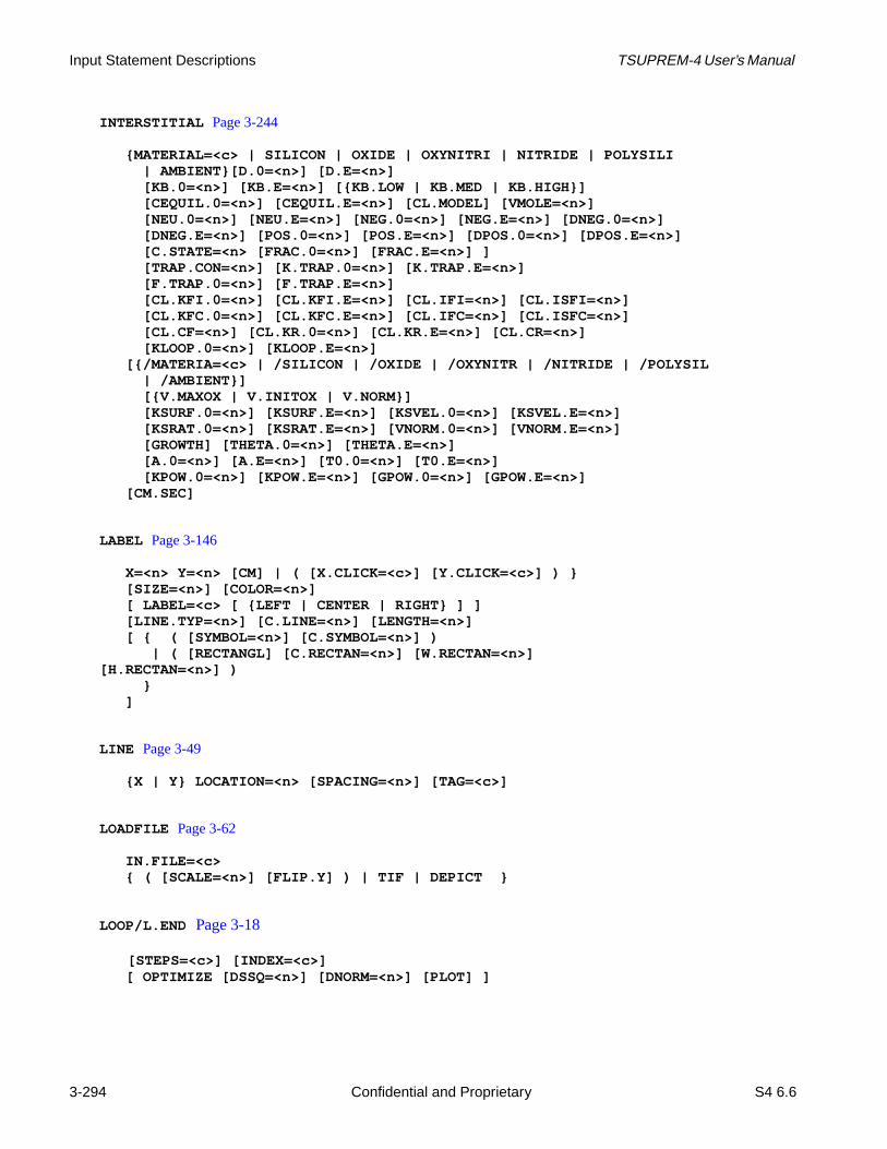
Input Statement Descriptions TSUPREM-4 User’s Manual
INTERSTITIAL Page 3-244
MATERIAL=<c> | SILICON | OXIDE | OXYNITRI | NITRIDE | POLYSILI | AMBIENT[D.0=<n>] [D.E=<n>]
[KB.0=<n>] [KB.E=<n>] [KB.LOW | KB.MED | KB.HIGH] [CEQUIL.0=<n>] [CEQUIL.E=<n>] [CL.MODEL] [VMOLE=<n>] [NEU.0=<n>] [NEU.E=<n>] [NEG.0=<n>] [NEG.E=<n>] [DNEG.0=<n>] [DNEG.E=<n>] [POS.0=<n>] [POS.E=<n>] [DPOS.0=<n>] [DPOS.E=<n>] [C.STATE=<n> [FRAC.0=<n>] [FRAC.E=<n>] ] [TRAP.CON=<n>] [K.TRAP.0=<n>] [K.TRAP.E=<n>] [F.TRAP.0=<n>] [F.TRAP.E=<n>] [CL.KFI.0=<n>] [CL.KFI.E=<n>] [CL.IFI=<n>] [CL.ISFI=<n>] [CL.KFC.0=<n>] [CL.KFC.E=<n>] [CL.IFC=<n>] [CL.ISFC=<n>] [CL.CF=<n>] [CL.KR.0=<n>] [CL.KR.E=<n>] [CL.CR=<n>] [KLOOP.0=<n>] [KLOOP.E=<n>]
[/MATERIA=<c> | /SILICON | /OXIDE | /OXYNITR | /NITRIDE | /POLYSIL | /AMBIENT] [V.MAXOX | V.INITOX | V.NORM] [KSURF.0=<n>] [KSURF.E=<n>] [KSVEL.0=<n>] [KSVEL.E=<n>] [KSRAT.0=<n>] [KSRAT.E=<n>] [VNORM.0=<n>] [VNORM.E=<n>] [GROWTH] [THETA.0=<n>] [THETA.E=<n>] [A.0=<n>] [A.E=<n>] [T0.0=<n>] [T0.E=<n>] [KPOW.0=<n>] [KPOW.E=<n>] [GPOW.0=<n>] [GPOW.E=<n>] [CM.SEC]
LABEL Page 3-146
X=<n> Y=<n> [CM] | ( [X.CLICK=<c>] [Y.CLICK=<c>] ) [SIZE=<n>] [COLOR=<n>]
[ LABEL=<c> [ LEFT | CENTER | RIGHT ] ] [LINE.TYP=<n>] [C.LINE=<n>] [LENGTH=<n>] [ ( [SYMBOL=<n>] [C.SYMBOL=<n>] ) | ( [RECTANGL] [C.RECTAN=<n>] [W.RECTAN=<n>][H.RECTAN=<n>] ) ]
LINE Page 3-49
X | Y LOCATION=<n> [SPACING=<n>] [TAG=<c>]
LOADFILE Page 3-62
IN.FILE=<c> ( [SCALE=<n>] [FLIP.Y] ) | TIF | DEPICT
LOOP/L.END Page 3-18
[STEPS=<c>] [INDEX=<c>] [ OPTIMIZE [DSSQ=<n>] [DNORM=<n>] [PLOT] ]
3-294 Confidential and Proprietary S4 6.6
Draft 6/26/98

TSUPREM-4 User’s Manual 3.6 Summary
L.MODIFY Page 3-22
[STEPS=<n>] [ NEXT | BREAK ]
MASK Page 3-75
[IN.FILE=<c>] [PRINT]
MATERIAL Page 3-212
( MATERIAL=<c> [NEW] )| SILICON | OXIDE | OXYNITRI | NITRIDE | POLYSILI | PHOTORES | ALUMINUM | AMBIENT [TIF.NAME=<c>] [MD.INDEX=<n>] [DY.DEFAU=<n>] [E.FIELD] [NI.0=<n>] [NI.E=<n>] [NI.F=<n>] [EPSILON=<n>] [DENSITY=<n>] [AT.NUM=<n>] [AT.WT=<n>] [MOL.WT=<n>] [VISC.0=<n>] [VISC.E=<n>] [VISC.X=<n>] [VC=<c>] [TEMPERAT=<c>] [YOUNG.M=<n>] [POISS.R=<n>] [LCTE=<c>] [INTRIN.S=<n>] [SURF.TEN=<n>] [ ( SEMICOND [AFFINITY=<n>] [BANDGAP=<n>] [N.CONDUC=<n>] [N.VALENC=<n>] [G.DONOR=<n>] [E.DONOR=<n>] [G.ACCEP=<n>] [E.ACCEP=<n>] [BOLTZMAN] [IONIZATI] ) | ( CONDUCTO [WORKFUNC=<n>] ) ] [POLYCRYS] [GRASZ.0=<n>] [GRASZ.E=<n>] [TEMP.BRE=<n>] [MIN.GRAI=<n>] [FRAC.TA=<n>] [G.DENS=<n>] [F11=<n>] [F22=<n>] [ALPHA=<n>] [GEOM=<n>] [GAMMA.0=<n>] [GAMMA.E=<n>] [DSIX.0=<n>] [DSIX.E=<n>] [DSIM.0=<n>] [DSIM.E=<n>] [DSIMM.0=<n>] [DSIMM.E=<n>] [DSIP.0=<n>] [DSIP.E=<n>] [GBE.0=<n>] [GBE.H=<n>] [GBE.E=<n>] [NSEG=<n>] [TBU.0=<n>] [TBU.E=<n>] [TOXIDE=<n>] [EAVEL.0=<n>] [EAVEL.E=<n>] [DLGX.0=<n>] [DLGX.E=<n>]
MESHPage 3-44
[GRID.FAC=<n>] [DX.MAX=<n>] [DX.MIN=<n>] [DX.RATIO=<n>] [LY.SURF=<n>] [DY.SURF=<n>] [LY.ACTIV=<n>] [DY.ACTIV=<n>] [LY.BOT=<n>] [DY.BOT=<n>] [DY.RATIO=<n>] [FAST]
S4 6.6 Confidential and Proprietary 3-295
Draft 6/26/98

Input Statement Descriptions TSUPREM-4 User’s Manual
METHODPage 3-178
[ ERFC | ERF1 | ERF2 | ERFG | VERTICAL| COMPRESS | VISCOELA | VISCOUS ] [ST.HISTO]
[DY.OXIDE=<n>] [GRID.OXI=<n>] [SKIP.SIL] [ PD.FERMI | PD.TRANS | PD.FULL | STEADY ] [NSTREAMS=<n>] [PAIR.GRA] [PAIR.SAT] [PAIR.REC] [PD.PFLUX] [PD.PTIME] [PD.PREC] [IMP.ADAP] [DIF.ADAP] [OX.ADAPT] [ERR.FAC=<n>] [ ACT.EQUI | ACT.TRAN] [INIT.TIM=<n>] [ TRBDF | MILNE | HYBRID | FORMULA=<c> ] [ CG | GAUSS ] [BACK=<n>] [BLK.ITLI=<n>] [MIN.FILL] [MIN.FREQ=<n>] [MF.METH=<n>] [MF.DIST=<n>] ( [IMPURITY=<c> ] [VACANCY] [INTERSTI] [ANTIMONY] [ARSENIC] [BORON] [PHOSPHOR] [OXIDANT] [TRAP] [ LU | SOR | SIP | ICCG ] [ FULL | PART | NONE ] [SYMMETRY] [ TIME.STE | ERROR | NEWTON ] [REL.ERR=<n>] [ABS.ERR=<n>] ( [MATERIAL=<c>] [SILICON] [POLYSILI] [OXIDE] [OXYNITRI] [NITRIDE] [ALUMINUM] [PHOTORES] [REL.ADAP=<n>] [ABS.ADAP=<n>] [MIN.SPAC=<n>] ) ) [OX.REL=<n>] [CONTIN.M=<n>] [VE.SMOOT=<n>] [E.ITMIN=<n>] [E.ITMAX=<n>] [E.RELERR=<n>] [E.RVCAP=<n>]
[E.REGRID] [E.TSURF=<n>] [E.DSURF=<n>] [E.RSURF=<n>] [ MOB.TABL | MOB.AROR | MOB.CAUG ]
[ ITRAP [IT.CPL] [IT.ACT] IT.ZERO | IT.THERM | IT.STEAD ]
MOBILITY Page 3-238
[ TAB.TEMP=<n> [KELVIN] TAB.CONC=<c> TAB.E.MU=<c> TAB.H.MU=<c> [TAB.CLEA] ] [ECN.MU=<n>] [ECP.MU=<n>] [GSURFN=<n>] [GSURFP=<n>] [MUN1=<n>] [MUN2=<n>] [AN=<n>] [CN=<n>] [EXN1=<n>] [EXN2=<n>] [EXN3=<n>] [EXN4=<n>] [MUP1=<n>] [MUP2=<n>] [AP=<n>] [CP=<n>] [EXP1=<n>] [EXP2=<n>] [EXP3=<n>] [EXP4=<n>] [MUN.MIN=<n>] [MUN.MAX=<n>] [NREFN=<n>] [NUN=<n>] [XIN=<n>] [ALPHAN=<n>] [MUP.MIN=<n>] [MUP.MAX=<n>] [NREFP=<n>] [NUP=<n>] [XIP=<n>] [ALPHAP=<n>]
3-296 Confidential and Proprietary S4 6.6
Draft 6/26/98

TSUPREM-4 User’s Manual 3.6 Summary
MOMENTPage 3-208
[CLEAR] [ MATERIAL=<c> | SILICON | OXIDE | OXYNITRI | NITRIDE | POLYSILI | PHOTORES ] [ RANGE=<n> SIGMA=<n> [GAMMA=<n>] [KURTOSIS=<n>] [LSIGMA=<n>] [LSLOPE=<n>] [ D.FRAC=<n> D.RANGE=<n> D.SIGMA=<n> [D.GAMMA=<n>] [D.KURTOS=<n>] [D.LSIGMA=<n>] [D.LSLOPE=<n>]
] ]
OPTION Page 3-33
[DEVICE=<c>] [PLOT.OUT=<c>] [ QUIET | NORMAL | VERBOSE | DEBUG ] [INFORMAT] [DIAGNOST] [ECHO] [EXECUTE]
PAUSE Page 3-14
[<c>]
PHOSPHORUSPage 3-278
MATERIAL=<c> | SILICON | OXIDE | OXYNITRI | NITRIDE | POLYSILI | AMBIENT [DIX.0=<n>] [DIX.E=<n>] [DIM.0=<n>] [DIM.E=<n>] [DIMM.0=<n>] [DIMM.E=<n>] [DVX.0=<n>] [DVX.E=<n>] [DVM.0=<n>] [DVM.E=<n>] [DVMM.0=<n>] [DVMM.E=<n>] [DIPAIR.0=<n>] [DIPAIR.E=<n>] [DVPAIR.0=<n>] [DVPAIR.E=<n>] [R.I.S=<n>] [E.I.S=<n>] [R.V.S=<n>] [E.V.S=<n>] [R.IP.V=<n>] [E.IP.V=<n>] [R.VP.I=<n>] [E.VP.I=<n>] [SS.CLEAR] [SS.TEMP=<n> SS.CONC=<n>] [ /MATERIA=<c> | /SILICON | /OXIDE | /OXYNITR | /NITRIDE | /POLYSIL | /AMBIENT [SEG.0=<n>] [SEG.E=<n>] [TRANS.0=<n>] [TRANS.E=<n>] ] [ES.RAND=<n> [ES.F.RAN=<n>]] [ES.100=<n> [ES.F.100=<n>]] [ES.110=<n> [ES.F.110=<n>]] [CM.SEC]
S4 6.6 Confidential and Proprietary 3-297
Draft 6/26/98

Input Statement Descriptions TSUPREM-4 User’s Manual
PLOT.1D Page 3-126
PLOT.1D
[ X.VALUE=<n> | Y.VALUE=<n> ] | ( MATERIAL=<c> | SILICON | OXIDE | OXYNITRI | NITRIDE | POLYSILI | PHOTORES | ALUMINUM /MATERIA=<c> | /SILICON | /OXIDE | /OXYNITR | /NITRIDE | /POLYSIL | /PHOTORE | /ALUMINU | /AMBIENT | /REFLECT ) | IN.FILE=<c>
(TIF X.AXIS=<c> Y.AXIS=<c>)|( (COLUMN [X.COLUMN=<n>] [Y.COLUMN=<n>])
| (ROW [X.ROW=<n>] [Y.ROW=<n>]) [X.LABEL=<c>] [Y.LABEL=<c>] )
[X.SHIFT=<n>] [Y.SHIFT=<n>]
[X.SCALE=<n>] [Y.SCALE=<n>][Y.LOG] [X.LOG]
| ELECTRIC [BOUNDARY] [CLEAR] [AXES] [SYMBOL=<n>] [CURVE] [LINE.TYP=<n>] [COLOR=<n>] [LEFT=<n>] [RIGHT=<n>] [BOTTOM=<n>] [TOP=<n>] [X.OFFSET=<n>] [X.LENGTH=<n>] [X.SIZE=<n>] [Y.OFFSET=<n>] [Y.LENGTH=<n>] [Y.SIZE=<n>] [T.SIZE=<n>]
PLOT.2D Page 3-134
[X.MIN=<n>] [X.MAX=<n>] [Y.MIN=<n>] [Y.MAX=<n>] [SCALE] [CLEAR] [AXES] [BOUNDARY] [L.BOUND=<n>] [C.BOUND=<n>] [GRID] [L.GRID=<n>] [C.GRID=<n>] [ [STRESS] [FLOW] VLENG=<n> [VMAX=<n>] [L.COMPRE=<n>] [C.COMPRE=<n>] [L.TENSIO=<n>] [C.TENSIO=<n>] ] [DIAMONDS] [X.OFFSET=<n>] [X.LENGTH=<n>] [X.SIZE=<n>] [Y.OFFSET=<n>] [Y.LENGTH=<n>] [Y.SIZE=<n>] [T.SIZE=<n>]
PLOT.3D Page 3-143
[THETA=<n>] [PHI=<n>] [CLEAR] [X.MIN=<n>] [X.MAX=<n>] [Y.MIN=<n>] [Y.MAX=<n>] [Z.MIN=<n>] [Z.MAX=<n>] [LINE.TYP=<n>] [COLOR=<n>] [NUM.CNTR=<n>] [BOUNDARY] [L.BOUND=<n>] [C.BOUND=<n>]
3-298 Confidential and Proprietary S4 6.6
Draft 6/26/98

TSUPREM-4 User’s Manual 3.6 Summary
PRINT.1D Page 3-122
X.VALUE=<n> | Y.VALUE=<n> | ( MATERIAL=<c> | SILICON | OXIDE | OXYNITRI | NITRIDE | POLYSILI | PHOTORES | ALUMINUM /MATERIA=<c> | /SILICON | /OXIDE | /OXYNITR | /NITRIDE | /POLYSIL | /PHOTORE | /ALUMINU | /AMBIENT | /REFLECT ) [SPOT=<n>] [LAYERS] [X.MIN=<n>] [X.MAX=<n>]
PROFILE Page 3-77
IMPURITY=<c> | ANTIMONY | ARSENIC | BORON | PHOSPHOR IN.FILE=<c> OFFSET=<n> [REPLACE]
REACTION Page 3-233
MAT.R=<c> /MAT.L=<c> [NAME=<c>] [ DELETE | REPLACE ] ( [IMP.L=<c>] [NI.L=<n>] [EI.L=<n> ] [/IMP.L=<c>] [/NI.L=<n>] [/EI.L=<n> ] [IMP.R=<c>] [NI.R=<n>] [EI.R=<n> ] [/IMP.R=<c>] [/NI.R=<n>] [/EI.R=<n> ] [NM.R=<n>] [/NM.L=<n>] [RATE.0=<n>] [RATE.E=<n>] [EQUIL.0=<n>] [EQUIL.E=<n>] ) | ( MAT.NEW=<c> THICKNES=<n> )
REGION Page 3-56
MATERIAL=<c> | SILICON | OXIDE | OXYNITRI | NITRIDE | POLYSILI | PHOTORES | ALUMINUM XLO=<c> XHI=<c> YLO=<c> YHI=<c>
RETURNPage 3-10
[<c>]
S4 6.6 Confidential and Proprietary 3-299
Draft 6/26/98

Input Statement Descriptions TSUPREM-4 User’s Manual
SAVEFILE Page 3-65
OUT.FILE=<c> [TEMPERAT=<n>] ( [SCALE=<n>] [FLIP.Y] [ACTIVE] ) | (TIF [TIF.VERS=<c>]) | DEPICT | ( MEDICI [POLY.ELE] [ELEC.BOT] ] ) | ( MINIMOS5 X.MASK.S=<n> HALF.DEV | ( FULL.DEV X.MASK.D=<n> [X.CHANNE=<n>] ) [X.MIN=<n>] [X.MAX=<n>] [Y.MIN=<n>] [Y.MAX=<n>] [DX.MIN=<n>] [DY.MIN=<n>] ) | ( WAVE [ACTIVE] [CHEMICAL] [DEFECT] [OXID] [MISC] )
SELECT Page 3-118
[Z=<c>] [TEMPERAT=<n>] [LABEL=<c>] [TITLE=<c>]
SOURCEPage 3-9
<filename>
STOP Page 3-15
[<c>]
STRESS Page 3-114
[TEMP1=<n> TEMP2=<n>] [NEL=<n>]
STRUCTUREPage 3-71
[ TRUNCATE ( RIGHT | LEFT X=<n> ) | ( BOTTOM | TOP Y=<n> ) ] [ REFLECT [ RIGHT | LEFT ] ] [ EXTEND [ RIGHT | LEFT ] WIDTH=<n> [SPACES=<n>] [DX=<n>] [XDX=<n>] [Y.ELIM=<c>] ] [TEMPERAT=<n>]
UNDEFINE Page 3-39
<name>
3-300 Confidential and Proprietary S4 6.6
Draft 6/26/98

TSUPREM-4 User’s Manual 3.6 Summary
VACANCYPage 3-253
MATERIAL=<c> | SILICON | OXIDE | OXYNITRI | NITRIDE | POLYSILI | AMBIENT [D.0=<n>] [D.E=<n>] [KB.0=<n>] [KB.E=<n>] [CEQUIL.0=<n>] [CEQUIL.E=<n>] [VMOLE=<n>] [NEU.0=<n>] [NEU.E=<n>] [NEG.0=<n>] [NEG.E=<n>] [DNEG.0=<n>] [DNEG.E=<n>] [POS.0=<n>] [POS.E=<n>][DPOS.0=<n>] [DPOS.E=<n>] [C.STATE=<n> [FRAC.0=<n>] [FRAC.E=<n>] ] [/MATERIA=<c> | /SILICON | /OXIDE | /OXYNITR | /NITRIDE | /POLYSIL | /AMBIENT] [V.MAXOX | V.INITOX | V.NORM] [KSURF.0=<n>] [KSURF.E=<n>] [KSVEL.0=<n>] [KSVEL.E=<n>] [KSRAT.0=<n>] [KSRAT.E=<n>] [VNORM.0=<n>] [VNORM.E=<n>] [GROWTH] [THETA.0=<n>] [THETA.E=<n>] [A.0=<n>] [A.E=<n>] [T0.0=<n>] [T0.E=<n>] [KPOW.0=<n>] [KPOW.E=<n>] [GPOW.0=<n>] [GPOW.E=<n>] [CM.SEC]
VIEWPORTPage 3-175
[X.MIN=<n>] [X.MAX=<n>] [Y.MIN=<n>] [Y.MAX=<n>]
S4 6.6 Confidential and Proprietary 3-301
Draft 6/26/98

Input Statement Descriptions TSUPREM-4 User’s Manual
3-302 Confidential and Proprietary S4 6.6
Draft 6/26/98

CHAPTER 4
he
ple.
acti-
if-
inued
re
ent
Tutorial Examples4
OverviewThis chapter presents three short examples showing how to useTSUPREM-4 todo some simple simulations. New users may wish to study these examples insequence. Each example introduces newTSUPREM-4 commands and concepts.The examples in this chapter are fairly short and execute relatively quickly. Tsimulations presented inChapter 5, “Advanced Examples” are more typical ofreal-life applications, and take more execution time. The examples include:
• A one-dimensional simulation of a bipolar transistor structure. This examillustrates the basic simulation steps using a simple one-dimensional grid(See“One-Dimensional Bipolar Example” on page 4-2).
• An example that shows how to set up a two-dimensional grid and how to vate the various oxidation and point defect models. (See“Local Oxidation” onpage 4-12).
• An example illustrating the effect of the point defect models on impurity dfusion. (See“Point Defect Models” on page 4-27).
Input File Syntax and Format
This chapter uses lowercase file names with the.inp extension for the exampleinput files. Note the following regarding the format of input files:
1. Each statement occupies one line, unless the statement is explicitly contwith a “+” character at the end of a line.
2. Statement and parameter names can be abbreviated.
3. On most statements, parameters can appear in any order.
4. Blank lines between statements and extra spaces between parameters aignored.
5. Comment statements begin with the “$” character and are used to documthe input file.
S4 6.6 Confidential and Proprietary 4-1
Draft 6/26/98

Tutorial Examples TSUPREM-4 User’s Manual
ored
uc-uc-that
n,en-
rves-
tions
.
at-h
ur-
cult
stes
6. The input can contain a mixture of upper and lower case; the case is ignexcept in some character strings.
One-Dimensional Bipolar ExampleThis section presents a one-dimensional simulation of a bipolar transistor strture. The example simulates the active region of an oxide-isolated bipolar strture, from the buried collector region up through the emitter. The statements direct the simulation are contained in the simulation input filess4ex1a.inp ands4ex1b.inp.
The purpose of this example is to illustrate the mechanics of usingTSUPREM-4as well as the use of particular statements for mesh setup, model specificatiosimulation of processing steps, and printing and plotting of results. A one-dimsional example is presented primarily to simplify the discussion, but it also seto illustrate a useful technique for performing fast simulations of simple structures.
TSUPREM-4 Input File Sequence
This example illustrates the organization of a typicalTSUPREM-4 input file. Ingeneral, the sequence is as follows:
1. Identify the problem with comments and set any necessary execution op(none are needed in most cases).
2. Generate an initial mesh or read in a previously saved structure.
3. Simulate the desired process sequence, and print and/or plot the results
Note that there is considerable flexibility in this sequence; for example, alterning between simulation and plotting. The only strict requirement is that a mesmust be defined before any processing or output can be performed.
Initial Active Region Simulation
The input statements in the files4ex1a.inp simulate the initial steps in the forma-tion of the active region of a bipolar structure, including the formation of the bied collector and deposition of the epitaxial layer. These input statements areshown inFigure 4-1.
Mesh Generation
Traditionally, generation of the simulation mesh has been one of the most diffiand time-consuming tasks required for process simulation. If the mesh is toocoarse, accuracy of the simulation is poor, while making the mesh too fine watime and computational resources.TSUPREM-4 simplifies the problem of creat-
4-2 Confidential and Proprietary S4 6.6
Draft 6/26/98

TSUPREM-4 User’s Manual One-Dimensional Bipolar Example
ve
i-
ifyter-y
ing an appropriate mesh by providing automatic mesh generation and adaptigridding.
Automatic MeshGeneration
A mesh is generated automatically when theINITIALIZE statement is pro-cessed. A boron concentration of 1015/cm3 for the initial structure has been specfied. By default, the mesh that has two vertical lines, one atx=0 and one atx=1micron. (For a two-dimensional simulation it would also be necessary to specthe width of the initial structure.) The location of the horizontal grid lines is demined by defaults set in thes4init file. The mesh can be made finer or coarser b
Figure 4-1 Input file s4ex1a.inp, for simulating the buried layer and epitaxialdeposition for a bipolar transistor structure
$ TSUPREM-4 -- Example 1, Part A$ Bipolar active device region: Buried layer and epitaxial deposition
$ Use automatic grid generation and adaptive gridINITIALIZE BORON=1E15
$ Grow buried layer masking oxideDIFFUSION TEMP=1150 TIME=120 STEAM
$ Etch the buried layer masking oxideETCH OXIDE ALL
$ Implant and drive in the antimony buried layerIMPLANT ANTIMONY DOSE=1E15 ENERGY=75DIFFUSION TEMP=1150 TIME=30 DRYO2DIFFUSION TEMP=1150 TIME=360
$ Etch the oxide.ETCH OXIDE ALL
$ Grow 1.8 micron of arsenic-doped epitaxyEPITAXY THICKNES=1.8 SPACES=9 TEMP=1050 TIME=6 ARSENIC=5E15
$ Grow pad oxide and deposit nitrideDIFFUSION TEMP=1050 TIME=30 DRYO2DEPOSITION NITRIDE THICKNES=0.12
$ Save initial active region resultsSAVEFILE OUT.FILE=S4EX1AS
$ Plot resultsSELECT Z=LOG10(BORON) TITLE=”Active, Epitaxy” LABEL=LOG(CONCENTRATION)PLOT.1D BOTTOM=13 TOP=21 RIGHT=5 LINE.TYP=5 COLOR=2SELECT Z=LOG10(ARSENIC)PLOT.1D ^AXES ^CLEAR LINE.TYP=2 COLOR=3SELECT Z=LOG10(ANTIMONY)PLOT.1D ^AX ^CL LINE.TYP=3 COLOR=3
$ Label plotLABEL X=4.2 Y=15.1 LABEL=BoronLABEL X=-.8 Y=15.8 LABEL=ArsenicLABEL X=2.1 Y=18.2 LABEL=Antimony
$ Print layer informationSELECT Z=DOPINGPRINT.1D LAYERS
S4 6.6 Confidential and Proprietary 4-3
Draft 6/26/98

Tutorial Examples TSUPREM-4 User’s Manual
mu-. The
dingated.
pro-n the bestulated
tion
nce of
ree
riumn be
including aMESH statement with theG13D.FAC parameter; the default spacinghas been chosen for this example.
AdaptiveGridding
Adaptive gridding is done whenever an ion implantation or diffusion step is silated to ensure that the grid is fine enough to maintain the required accuracyaccuracy criteria can be adjusted with theERR.FAC parameter on theMETHODstatement; in this example the default values are used. By using adaptive gridthe need to predict the grid requirements of a simulation in advance is elimin
Model Selection
The choice of simulation models should be considered before performing anycessing steps. The speed and accuracy of the simulation depends strongly ochoice of models. The default models have been carefully chosen to give theresults in many cases, but some choices depend on the structures being simand on individual requirements of the user.
Two model choices must be made in most simulations:
• Oxidation model
• Point defect model
These selections are made using theMETHOD statement. In this example thedefault models are used, i.e., theVERTICAL oxidation model and thePD.FERMIpoint defect model.
The choice of models may be changed during the course of the simulation.
Oxidation Model TheVERTICAL oxidation model can be used in this case because the simulais one-dimensional, so only planar surfaces are oxidized. TheERFC oxidationmodel could also be used in this example, but it does not model the dependethe oxidation rate on the concentration of impurities in the silicon. Also, theERFCmodel requires an additional statement (anAMBIENT statement with theINITIAL parameter) to specify the initial oxide thickness whenever a structuwith an initial oxide layer is oxidized, and does not automatically recognize thpresence of nitride masking layers.
Point DefectModel
For this example the default point defect model (PD.FERMI) is used. ThePD.TRANS point defect model increases the simulation time significantly, andshould be used only when required. In this example, the effects of nonequilibpoint defect concentrations are relatively small. The magnitude of the error cachecked by repeating the simulation using thePD.TRANS or PD.FULL model.
4-4 Confidential and Proprietary S4 6.6
Draft 6/26/98

TSUPREM-4 User’s Manual One-Dimensional Bipolar Example
lant.
nsrity
ting
he
he
ate is
nti-ationis
be
s a that
fu-
nbe
Processing Steps
Buried LayerMasking Oxide
The first step in the process is to grow an oxide to mask the buried layer impOxidation is accomplished by specifying an oxidizing ambient (STETIM, in thiscase) on theDIFFUSION statement. The time (in minutes) and temperature(in °Celsius) must be specified. Note that specifying an oxidizing ambient turon oxidation, but does not disable any other aspects of a diffusion step. Impudiffusion and segregation at interfaces still occur.
The oxide must be removed from the active region of the device before implanthe buried layer. This is accomplished with theETCH statement. The simplestform of theETCH statement, used here, removes all of a specified material. TETCH statement can also be used to remove portions of a layer.
Buried Layer The next step is to implant the buried layer and drive it in. This is done with tIMPLANT statement and the followingDIFFUSION statements. TheIMPLANTstatement specifies the type of impurity, and the dose (per cm2) and energy (inkeV). Use of adaptive gridding is generally sufficient to ensure that the meshthe surface is fine enough to contain several grid points within the peak of thimplanted distribution, but it is wise to plot the as-implanted distribution if thereany doubt.
The drive-in of the buried layer is done in two steps. In the first, aDRYO2 ambientis used to grow a thin layer of oxide to prevent outdiffusion of the implanted amony. No ambient is given for the second; the absence of an ambient specificimplies that an inert ambient is used. Once the drive-in is finished, the oxide removed with anETCH statement.
Epitaxial Layer Next, an epitaxial layer is grown. Epitaxial growth is simulated with theEPITAXY statement, which combines the effects of theDEPOSITION andDIFFUSION statements. The thickness of the deposited layer is specified to 1.8 microns using theTHITICKNES parameter.
The grid density in the layer is determined by theSPACES parameter. This exam-ple specifies that 9 grid spaces be placed in the epitaxial layer. This producereasonable starting grid for the base and emitter processing that follows. Notethe specification of the number of spaces determines not only the grid in theresulting structure, but also the time discretization of the epitaxy step. TheEPITAXY statement causes the deposition of one grid layer followed by a difsion for some fraction of the total time. This process is repeated for each gridlayer. IfSPACES is not specified, its value defaults to one and theEPITAXY isequivalent to aDEPOSITION followed by aDIFFUSION statement.
The time and temperature for the epitaxial growth step are given by theTIME andTEMPERAT parameters, respectively. These determine the amount of diffusiothat occurs during the growth process. The doping of the epitaxial layer can specified with theARSNIC parameter on theEPITAXY statement.
S4 6.6 Confidential and Proprietary 4-5
Draft 6/26/98

Tutorial Examples TSUPREM-4 User’s Manual
xida-
tersed
t-
puteratend of
ce is
vice
unc-
he
Pad Oxide andNitride Mask
Next, a pad oxide is grown (using theDIFFUSION statement with theDRYO2parameter) and a nitride mask is deposited to be used for the field-isolation otion. The deposition is specified by theDEPOSITION statement, which specifiesthe material to deposit and the thickness of the layer. Other optional paramecan be used to specify the number and spacing of grid spaces in the depositlayer; by default, a single grid space is used in the deposited layer.
Saving the Structure
The resulting structure is saved using theSAVEFILE statement. In this case, it issaved in the output file namedS4EX1AS. The saved structure is used as the staring point for the remaining process steps, which is simulated with a separateTSUPREM-4 input file.
It is recommended that the structure be saved after any long (in terms of comtime) sequence of operations. This allows the simulation to be resumed at thpoint should the need arise. It is also a good idea to save the structure at the any simulation, so that the results can be examined further at a later time.
Plotting the Results
The results of the simulation to this point are now ready to be displayed. Thisexample demonstrates the use of theSELECT, PLOT.1D, andLABEL statements;two-dimensional plots are demonstrated in the next section.
Specifying aGraphics Device
Before displaying a plot, the program must be told what sort of graphics devibeing used. This can be done either with theDEVICE parameter on theOPTIONstatement or by using a default plot device. In this example, the default plot deis used. SeeChapter 3 “OPTION” on page 3-33 andAppendix B: “GraphicsDevices.”
The SELECTStatement
The value to be plotted is given by theZ expression on theSELECT statement.Zdefines a mathematical expression that may contain a number of variables, ftions, and mathematical operators. (See the description of theSELECT statementin Chapter 3 “SELECT” on page 3-118). This example plots the base-10 loga-rithm of the various impurity concentrations.
Note:TheZ expression is evaluated when theSELECT statement is processed.Thus theSELECT statement should be specified after any process stepsthat affect the device structure or solution quantities (e.g., impurity con-centrations) used in the expression.
TheSELECT statement can also be used to specify a title for the plot and/or tlabel to be used on the vertical axis. If no label is given, theZ expression is used.
4-6 Confidential and Proprietary S4 6.6
Draft 6/26/98

TSUPREM-4 User’s Manual One-Dimensional Bipolar Example
nal)peci-
the
ice
s.ronph-
ng
is.
The PLOT.1DStatement
ThePLOT.1D statement plots the values of a quantity along a (one-dimensiosection through the device. The section can be a vertical line at the location sfied byX.VALUE, a horizontal line atY.VALUE, or along an interface betweentwo materials. This default is to plot along the vertical line atx=0.
The firstPLOT.1D statement in this example plots the axes and title as well aslogarithm of the antimony concentration. In addition to thex coordinate, the mini-mum and maximum values for they axis and the maximum value for thex axishave also been specified.
Note:The limits of the y axis are in the units of theZ expression on theSELECT statement; thus, 13 and 21 are used, (not 1e13 and 1e21).
If no axis limits are given, default values based on the dimensions of the devand the values of theZ expression are used.
By default, a dashed vertical line is drawn at the interfaces between materialLINE.TYP=5 specifies that dashed line type 5 is to be used for plotting the boprofile;COLOR=2 specifies that color 2 (usually red) is to be used on color graics devices.
The next twoPLOT.1D statements add to the first plot. They do this by includithe^CLEAR and^AXES specifications to prevent clearing of the screen anddrawing of new axes, respectively. For each plot a new quantity to be plottedspecified (using aSELECT statement) along with a different line type and color
Labels Labels are added to the plot withLABEL statements. EachLABEL statement spec-ifies a text string to be plotted and a pair ofx andy coordinates. The text string isplotted starting at the specified coordinates.X andY are in the units of the plotaxes, in this case microns and log10 (concentration), respectively.X andY couldalso be given in centimeters, using theCM parameter. The final plot is shown inFigure 4-2.
S4 6.6 Confidential and Proprietary 4-7
Draft 6/26/98

Tutorial Examples TSUPREM-4 User’s Manual
the
.
n
oesg,
Printing Layer Information
The PRINT.1DStatement
Although plots are the primary means of examining the results of aTSUPREM-4simulation, useful information is also available from thePRINT.1D statement.ThePRINT.1D statement works with theZ expression given by aSELECT state-ment. Information is presented along a one-dimensional section specified in same manner as in thePLOT.1D statement.
Three kinds of information can be printed:
1. A complete list of the values of theZ expression along the section.
2. The integral of theZ expression through each layer along the section.
3. The locations along the section where theZ expression has a specified value
UsingPRINT.1D
Layers
ThePRINT.1D statement at the end of files4ex1a.inp uses theLAYERS parame-ter to request the integral of theZ expression (net doping) along a vertical sectioatx=0. The resulting output is shown inFigure 4-3. For purposes ofPRINT.1DLAYERS, a layer is defined as a portion of the section in which the material dnot change and the sign of theZ expression is constant. In the case of net dopineach material is separated into layers of net n-type or net p-type doping.
Figure 4-2 Impurity distributions in bipolar structure at end of input files4ex1a.inp
4-8 Confidential and Proprietary S4 6.6
Draft 6/26/98

TSUPREM-4 User’s Manual One-Dimensional Bipolar Example
lhe
te-wever.
d
es oft
ep.
e of
-
ature to start-e
In this example, thePRINT.1D LAYERS statement provides a number of usefuresults. For each layer, the material type, the top and bottom coordinates of tlayer, the thickness of the layer, and the integral of the selected quantity areprinted. A number of useful values are evident, such as the oxide thickness(493 Å) and the depth of the buried layer/substrate junction (4.70µm).
Note:SELECT statement is required before aPRINT.1D LAYERS statementis processed, but you can useSELECT Z=0 if all you want to know is thelayer thicknesses or the coordinates of the material interfaces.
Completing the Active Region Simulation
The simulation is now completed with a separate execution ofTSUPREM-4,using the input files4ex1b.inp shown inFigure 4-4. This file follows the same out-line as the first (initialize, select models, process, output), and most of the staments are of the types discussed previously. There are some differences, ho
Reading a SavedStructure
The most important difference is that instead of generating a mesh, the savestructure saved by the previous simulation is read from the fileS4EX1AS. This isaccomplished with theIN.FILE parameter on theINITIALIZE statement. Thesaved file includes complete mesh and solution information.
The next step specifies any needed model specifications. Because the choicoxidation and point defect models were saved in the structure file, they do noneed to be specified again. Any different models could be specified at this st
Field Oxidation The next step in the process is to grow the field isolation oxide. Although theactive region of the device is being simulated, and no oxide is grown becausthe nitride mask, the field oxidation step is included in order to simulate thedopant redistribution that occurs during the step. The field oxidation step illustrates how temperature and pressure ramping are specified.
The temperature is first ramped from 800°C to 1000°C, over a time of 20 minutes.TheTEMP parameter specifies the starting temperature, while theT.FINALparameter gives the temperature at the end of the step. The next step starts 1000°C in a dry oxygen ambient at one atmosphere, and ramps the temperat1100°C and the pressure to 5 atmospheres over a period of 10 minutes. Theing pressure is given by thePRESSURE parameter (not needed here because th
$ Print layer informationSELECT Z=DOPINGPRINT.1D LAYERS** Printing along X.VALUE=0:
Num Material Top Bottom Thickness Integral 1 nitride -1.3725 -1.2525 0.1200 1.2000e+00 2 oxide -1.2525 -1.2031 0.0493 5.6312e+08 3 silicon -1.2031 3.4935 4.6967 1.3416e+15 4 silicon 3.4935 200.0000 196.5065 -1.9630e+13
Figure 4-3 Output listing from PRINT.1D command in file s4ex1a.inp
S4 6.6 Confidential and Proprietary 4-9
Draft 6/26/98

Tutorial Examples TSUPREM-4 User’s Manual
inute.
f 5ture.
The
default value of one atmosphere is used), and the final pressure is given byP.FINAL . Note that ramp rates could also have been specified in degrees/mor atmospheres/minute, using theT.RATE andP.RATE parameters, respectively
The third diffusion step does a 50-minute oxidation in steam, at a pressure oatmospheres. Steps four and five ramp down the pressure, then the tempera
The remaining process steps are similar to those performed in the first part. nitride and oxide are removed, and the base and emitter are implanted.
Figure 4-4 Listing of input file s4ex1b.inp, showing statements for simulatingthe field oxide, base, and emitter region processing for a bipolartransistor
$ TSUPREM-4 -- Example 1, Part B$ Bipolar active device region: Field oxide, base, and emitter
$ Read structureINITIALIZE IN.FILE=S4EX1AS
$ Grow the field oxideDIFFUSION TEMP=800 TIME=20 T.FINAL=1000DIFFUSION TEMP=1000 TIME=10 DRYO2 T.FINAL=1100 P.FINAL=5DIFFUSION TEMP=1100 TIME=50 STEAM PRESSURE=5DIFFUSION TEMP=1100 TIME=10 DRYO2 PRESSURE=5 P.FINAL=1DIFFUSION TEMP=1100 TIME=60 T.FINAL=800
$ Remove nitride and pad oxideETCH NITRIDE ALLETCH OXIDE ALL
$ Implant the boron baseIMPLANT BORON DOSE=2E13 ENERGY=100
$ Implant the phosphorus emitterIMPLANT PHOSPHORUS DOSE=1E15 ENERGY=50
$ Anneal to activate base and emitter regionsDIFFUSION TEMP=1000 TIME=12 DRYO2
$ Plot resultsSELECT Z=LOG10(BORON) TITLE=”Active Region” LABEL=LOG(CONCENTRATION)PLOT.1D BOTTOM=13 TOP=21 RIGHT=5 LINE.TYP=5 COLOR=2SELECT Z=LOG10(PHOSPHORUS)PLOT.1D ^AXES ^CLEAR LINE.TYP=4 COLOR=4SELECT Z=LOG10(ARSENIC)PLOT.1D ^AXES ^CLEAR LINE.TYP=2 COLOR=3SELECT Z=LOG10(ANTIMONY)PLOT.1D ^AXES ^CLEAR LINE.TYP=3 COLOR=3
$ Label the impuritiesLABEL X= 2.0 Y=15.1 LABEL=BoronLABEL X=-1.0 Y=19.5 LABEL=PhosphorusLABEL X= 0.3 Y=15.8 LABEL=ArsenicLABEL X= 2.0 Y=18.4 LABEL=Antimony
$ Print the layer informationSELECT Z=DOPINGPRINT.1D X.V=0 LAYERS
4-10 Confidential and Proprietary S4 6.6
Draft 6/26/98

TSUPREM-4 User’s Manual One-Dimensional Bipolar Example
sly.
ick-n
Final Structure
The plotting and labeling of the profiles use the statements described previouThe final plot is shown inFigure 4-5. A PRINT.1D statement is used to printlayer information for the final structure. TheSELECT Z=DOPING statementspecifies that integrals of net doping are to be calculated and that layers aredefined by the sign of the doping. From the printed output (Figure 4-6) a numberof useful values can be extracted, such as the oxide thickness (255 Å), the thness of the emitter region (0.28µm), and the integrated doping in the base regio(8.15x10¹²/cm3).
Figure 4-5 Final profiles produced by input file s4ex1b.inp
$ Print the layer informationSELECT Z=DOPINGPRINT.1D LAYERS** Printing along X.VALUE=0:
Num Material Top Bottom Thickness Integral 1 oxide -1.2183 -1.1928 0.0255 3.7124e+12 2 silicon -1.1928 -0.9104 0.2824 1.0435e+15 3 silicon -0.9104 -0.5646 0.3457 -8.1483e+12 4 silicon -0.5646 3.5770 4.1416 1.3412e+15 5 silicon 3.5770 200.0000 196.4230 -1.9623e+13
Figure 4-6 Output listing from PRINT.1D command in file s4ex1b.inp
S4 6.6 Confidential and Proprietary 4-11
Draft 6/26/98

Tutorial Examples TSUPREM-4 User’s Manual
oxi-nal
a-on in-es
askwn inle,
Local OxidationThis section presents an example of a two-dimensional simulation of a local dation process. The purpose of this example is to illustrate the two-dimensiosimulation capabilities ofTSUPREM-4, and to provide some practical hints onthe effective use of these capabilities.
This example simulates a narrow, locally-oxidized isolation region. The two fetures of interest are the oxide thickness and shape and the impurity distributithe underlying silicon. These are examined in separate simulations. The commands for performing the simulations are contained in the simulation input fils4ex2a.inp ands4ex2b.inp.
Calculation of Oxide Shape
The first goal of this simulation is to determine the effect of using a narrow mopening on the oxide shape. The input statements for this simulation are shoFigures 4-7 and4-9. The steps are similar to those used in the previous exampbut are complicated slightly by the two-dimensional nature of the simulation.
$ TSUPREM-4 narrow window example$ Part 1: Oxide shape
$ Set up the gridLINE X LOC=0.0 SPAC=0.15LINE X LOC=1.25 SPAC=0.04LINE X LOC=1.5 SPAC=0.1
LINE Y LOC=0 SPAC=0.03LINE Y LOC=0.5 SPAC=0.1
$ No impurities, for faster oxidation simulationINITIALIZE
$ Deposit pad oxide and define nitride maskDEPOSITION OXIDE THICKNES=0.03 SPACES=2DEPOSITION NITRIDE THICKNES=0.10 SPACES=2ETCH NITRIDE RIGHT P1.X=1.25
$ Plot the gridSELECT TITLE="Grid for Oxidation"PLOT.2D GRID SCALE C.GRID=2
$ Do the oxidationMETHOD VISCOEL DY.OXIDE=0.05 INIT=0.15MATERIAL MAT=OXIDE VC=425MATERIAL MAT=NITRIDE VC=170DIFFUSION TEMP=1000 TIME=100 WETO2
$ Save the structureSAVEFILE OUT.FILE=S4EX2AS
Figure 4-7 First part of input file s4ex2a.inp, for determining LOCOS shape
4-12 Confidential and Proprietary S4 6.6
Draft 6/26/98

TSUPREM-4 User’s Manual Local Oxidation
asracylf ofe. Therst
he
other
tiontwo-e
ng is
ula-
e
noy
Mesh Generation The simulation starts by defining a mesh. The object in this case is to define coarse a mesh as possible without losing accuracy in the solution. (The accucan be checked later by repeating the simulation with a finer mesh.) Only hathe structure needs to be simulated, because of the symmetry of the structurLINE X statements specify the horizontal locations of vertical grid lines. The fiand lastLINE X statements specify the left and right edges of the structure; tSPACING parameters specify the horizontal grid spacings at these locations.OtherLINE X statements are used to add grid lines and specify spacings at locations in the structure. In the vertical direction,LINE Y statements specify thetop and bottom locations (and corresponding grid spacings) for the mesh.
The grid for this example does not need to be very fine. In the horizontal directhe spacing is set to 0.05 microns at the edge of the nitride mask, where the dimensional effects are greatest (x=1.25); the spacing expands to 0.1 micron at thright edge and 0.15 micron at the left edge. In the vertical direction, the spaciset to 0.03 at the top, expanding to 0.1 at the bottom.
The effect of the grid spacing on accuracy can be checked by running the simtion again with a finer mesh; this can be accomplished by adding aMESH state-ment with theGRID.FAC parameter anywhere before theINITIALIZEstatement. There are no impurities specified in this simulation, so no adaptivgridding occurs based on implantation or diffusion of impurities. However, thegrid is refined as needed based on oxidant concentration.
TheINITIALIZE statement performs the actual mesh generation. Note thatsubstrate doping has been specified. This speeds up the simulation slightly beliminating the need to solve for impurity diffusion while oxidizing.
Figure 4-8 Mesh used for oxidation simulation. Produced by PLOT.2D GRIDstatement in input file s4ex2a.inp
S4 6.6 Confidential and Proprietary 4-13
Draft 6/26/98

Tutorial Examples TSUPREM-4 User’s Manual
xi-
ful.)
-
the
ressr
cted
of
r theThe
mallopri-ps.
es for
Pad Oxide andNitride Layers
Next the pad oxide is deposited. To improve the accuracy when calculating odant diffusion in the oxide, two grid spaces are placed in the deposited layer.(When checking the accuracy of the simulation, more divisions would be useMore grid spaces are added automatically as the oxide grows.
To mask the oxidation, a nitride layer is deposited and then patterned with anETCH statement. TheRIGHT keyword on theETCH statement specifies that material is to be etched to the right of the line defined by theP1.X , P1.Y , P2.X , andP2.Y parameters.P1.X=1.25 is specified;P1.Y defaults to a value above thehighest point of the structure;P2.X defaults to the value ofP1.X ; andP2.Ydefaults to a value below the bottom of the structure. Thus the etch occurs toright of a vertical line through the structure atx=1.25 microns.
Plotting the Mesh At this point it is wise to inspect the mesh. This is done with thePLOT.2D state-ment. ThePLOT.2D statement is used to set up any two-dimensional plot. Byitself, it can plot the material boundaries of a structure, the grid, and oxide stand velocity vectors. It is also used to set the scale and draw axes for contouplots. In this case, theGRID keyword requests that the grid be plotted, and theC.GRID keyword specifies the color to be used.
TheSCALE parameter causes thex or y axis to be scaled to reflect the true asperatio of the structure. IfSCALE had not been specified, the plot would be stretchin they direction to fill the plotting area. TheSELECT statement is used only tospecify a title for the plot. The resulting plot is shown inFigure 4-8.
Model Selection Next aMETHOD statement is used with theVISCOELA keyword to select the oxi-dation model. TheVISCOELA model is used because it allows fast simulation two-dimensional, stress-dependent oxidation. TheDY.OXIDE parameter sets thegrid spacing to be used in the growing oxide. (The same grid is used both fodiffusion of the oxidizing species and for the calculation of oxide movement.) IN19
T.TIM parameter specifies an initial time step of 0.15 minutes; this saves a samount of calculation time. The default value is 0.002 minutes, which is apprate for many diffusion steps but smaller than necessary for oxidation-only ste
The effects of oxidant diffusion, interface reaction rate, and material viscosition the stresses in the structure are included by default. Because the modelsthe stress effects do not include the dependence of parameter values ontemperature, it is necessary to useMATERIAL statements to specify appropriatevalues for4C (the dependence of stress on material viscosity) at the oxidationtemperature. (Suitable values are listed in the notes to Appendix A.)
The oxidation is accomplished by theDIFFUSION statement, which specifies awet oxygen ambient at 1000°C for 100 minutes. TheSAVEFILE statement savesthe final structure for later analysis.
4-14 Confidential and Proprietary S4 6.6
Draft 6/26/98

TSUPREM-4 User’s Manual Local Oxidation
e fol-
e
t-
led
Plotting theResults
The results are plotted using the statements shown inFigure 4-9. ThePLOT.2Dstatement is used to plot the structure boundaries and material interfaces. Thlowing parameters specify the plot format and content:
• FLOW adds vectors showing the speed and direction of material flow in thstructure due to oxidation.
• VLNG specifies the maximum length of a flow vector (in microns) to be ploted.
• TheX.MIN parameter specifies the minimum value of thex axis: (X.MAX,Y.MIN , andY.MAX can be used to specify the other axis limits, but thedefault values are used in this case).
• TheSCALE parameter is used to avoid distorting the structure as it is scafor plotting.
$ Plot the final structure, showing flow linesSELECT TITLE="Flow at End of Oxidation Step"PLOT.2D SCALE FLOW VLENG=0.065 X.MIN=0.5 C.FLOW=4
$ Plot the final structure, showing stress vectorsSELECT TITLE="Stresses After Oxidation"PLOT.2D SCALE STRESS VLENG=0.2 X.MIN=0.5 + C.COMPRE=4 C.TENSIO=2 L.TENSIO=2
$ Plot filled contours of hydrostatic pressureSELECT Z=( -0.5 * ( SXX + SYY ) ) TITLE="Contours of Hydrostatic Pressure"PLOT.2D SCALE X.MIN=0.5 X.MAX=1.8FOREACH I ( 1 TO 5 ) COLOR MIN.V=(( I - 0.5)*2E9) MAX.V=(( I + 0.5)*2E9) COLOR=(13 + I ) COLOR MIN.V=((- I - 0.5)*2E9) MAX.V=((- I + 0.5)*2E9) COLOR=(25 - I )END
$ Create a legendLABEL X=1.52 Y=-0.2 LABEL="Compression" SIZE=0.3LABEL X=1.60 Y=-0.15 LABEL="1-3E9" C.RECT=14 SIZE=0.3 W.RECT=0.35 H.R=0.35LABEL X=1.60 Y=-0.1 LABEL="3-5E9" C.RECT=15 SIZE=0.3 W.RECT=0.35 H.R=0.35LABEL X=1.60 Y=-0.05 LABEL="5-7E9" C.RECT=16 SIZE=0.3 W.RECT=0.35 H.R=0.35LABEL X=1.60 Y= 0.0 LABEL="7-9E9" C.RECT=17 SIZE=0.3 W.RECT=0.35 H.R=0.35LABEL X=1.52 Y= 0.05 LABEL="Tension" SIZE=0.3LABEL X=1.60 Y= 0.1 LABEL="1-3E9" C.RECT=24 SIZE=0.3 W.RECT=0.35 H.R=0.35LABEL X=1.60 Y= 0.15 LABEL="3-5E9" C.RECT=23 SIZE=0.3 W.RECT=0.35 H.R=0.35LABEL X=1.60 Y= 0.20 LABEL="5-7E9" C.RECT=22 SIZE=0.3 W.RECT=0.35 H.R=0.35LABEL X=1.60 Y= 0.25 LABEL="7-9E9" C.RECT=21 SIZE=0.3 W.RECT=0.35 H.R=0.35
$ Redraw boundariesPLOT.2D ^AX ^CL
$ Print location of interfaceSELECT Z=YPRINT.1D SILICON /OXIDE
Figure 4-9 Second part of statement input file s4ex2a.inp, showingstatements for plotting results of LOCOS process
S4 6.6 Confidential and Proprietary 4-15
Draft 6/26/98

Tutorial Examples TSUPREM-4 User’s Manual
e
indi-. Theult,
pres-
ofesses
sere the
The result of thePLOT.2D FLOW statement is shown inFigure 4-10.
Plotting Stresses Stresses in the structure can be plotted in several ways. One way is to use thPLOT.2D statement with theSTRESS parameter. TheSTRESS parameterrequests that the principal components of stress be shown. The stresses arecated by short lines whose lengths are proportional to the stress componentsline type indicates whether the material is in tension or compression. By defaboth use line type one, but in this exampleLINE.TEN=2 is specified so that adashed line is used to indicate tension (the default is one). Tension and comsion are also distinguished by color, using theC.TENSIO andC.COMPREparameters. TheVLENG parameter specifies the length of the line (in the units the plot axes, i.e., microns) used for the maximum value of stress. Smaller strproduce proportionally smaller lines.
The stress plot is shown inFigure 4-11. The long, solid lines indicate large com-pressive stresses in the direction of the lines; dashed lines indicate tension. Aexpected, the stresses are concentrated near the portion of the structure whoxide growth is nonuniform and where the nitride is forced to bead.
Figure 4-10 Plot produced by the PLOT.2D FLOW statement in input files4ex2a.inp
4-16 Confidential and Proprietary S4 6.6
Draft 6/26/98

TSUPREM-4 User’s Manual Local Oxidation
iffi- use-e ofe cal-
erage
al in
,-
Contour Plots Another way to show the stresses in the structure is with contour plots. It is dcult to show all three components of stress in a contour plot, and it is not veryful to show individual components because of their dependence on the choiccoordinate system. However, meaningful combinations of the stresses can bculated with theSELECT statement and plotted with thePLOT.2D andCONTOUR or COLOR statements.
This example shows how the hydrostatic pressure, defined as the negative avof theSxx andSyy stress components, can be plotted.
• TheSELECT statement simply gives the mathematical expression for thefunction to be plotted.
• ThePLOT.2D statement plots the axes, structure boundaries, and materiinterfaces,X .MAX is specified greater than the right edge of the structureorder to leave room for a legend.
• A pair ofCOLOR statements inside aFOREACH loop are used to shaderegions of differing pressures.
TheFOREACH statement specifies a variable (I) and a range of values (1 to 5in this case). The statements between theFOREACH statement and the matching END statement are executed once for each value of the variable. The
Figure 4-11 Plot produced by the PLOT.2D STRESS statement in input files4ex2a.inp
S4 6.6 Confidential and Proprietary 4-17
Draft 6/26/98

Tutorial Examples TSUPREM-4 User’s Manual
entediven
islabel.
his
COLOR statements specify a color and the range of pressures to be represby that color. Both the color and the minimum and maximum values are gby arithmetic expressions that depend on the variableI.
• A series ofLABEL statements are used to produce a legend, showing theamount of tension or compression corresponding to each color.
EachLABEL statement specifies the location of the label (in microns, in thcase), the text of the label, and a filled rectangle that is placed before the The size of the characters (in centimeters) is specified by theSIZE parameter.Width and height of the rectangle are given byW.RECTAN andH.RECTAN(abbreviated toW.R andH.R, respectively).
• Finally, a lastPLOT.2D with the^AXES and^C15
• EAR parameters is done in order to redraw the structure boundaries, whicmay have been obscured when plotting the shaded contours. The result shown inFigure 4-12.
The last two lines ofs4ex2a.inp show how they coordinate of the silicon/oxideinterface can be printed as a function ofx, using thePRINT.1D statements toprint solution values along the interface between two materials.
Figure 4-12 Contours of hydrostatic pressure plotted by statements in inputfile s4ex2a.inp
4-18 Confidential and Proprietary S4 6.6
Draft 6/26/98

TSUPREM-4 User’s Manual Local Oxidation
tep.n iningom-
ify-
ed
ever, mask.d.
-
Two-Dimensional Diffusion with Point Defects
This example analyzes the diffusion of impurities during the local oxidation sThe same process is simulated as in the previous sections, except with borothe substrate and a boron implant. The effects of point defect generation duroxidation are also included, but with a simpler oxidation model to reduce the cputer time requirements. The listing of the input (from files4ex2b.inp) is shown inFigures 4-13 and4-15.
Automatic GridGeneration
For convenience, automatic grid generation is used for this analysis. By specing WIDTH=1.5 on theINITIALIZE statement, the grid extends fromx=0 tox=1.5, just as in the previous simulation. The background concentration of thsubstrate is specified with theBORON parameter. The grid is automatically refineas needed to maintain the accuracy of the impurity profiles.
Field Implant The deposition of the pad oxide and nitride are the same as before. Now, howa photoresist layer is deposited and patterned to be used as a boron implantThe boron is implanted through the pad oxide, then the photoresist is remove
Oxidation TheCOMPRESS oxidation model is chosen in order to obtain a fast two-dimensional simulation. The two-dimensional point defect model is specified by thePD.TRANS keyword on theMETHOD statement. TheDIFFUSION statement isthe same as in the previous section.
S4 6.6 Confidential and Proprietary 4-19
Draft 6/26/98

Tutorial Examples TSUPREM-4 User’s Manual
inedd in
The structure is saved at the end of the simulation so the results can be examfurther without rerunning the simulation. In this example, the solution is savethe fileS4EX2BS.
Figure 4-13 First part of input file s4ex2b.inp, showing processing steps
$ TSUPREM-4 narrow window example$ Part 2: Impurity distribution
$ Use default gridINITIALIZE BORON=1E15 WIDTH=1.5
$ Deposit pad oxide, LOCOS mask, and implant maskDEPOSITION OXIDE THICKNES=0.03 SPACES=2DEPOSITION NITRIDE THICKNES=0.10DEPOSITION PHOTO THICKNES=2
ETCH PHOTO RIGHT P1.X=1.25ETCH NITRIDE TRAP
$ Implant boronIMPLANT BORON DOSE=2E13 ENERGY=100ETCH PHOTORESIST ALL
$ Do the drive-in, with point defectsMETHOD COMPRESS PD.TRANSDIFFUSION TEMP=1000 TIME=100 WETO2
$ Save the structureSAVEFILE OUT.FILE=S4EX2BS
$ Plot the grid after diffusionSELECT TITLE=”Grid After Impurity Diffusion”PLOT.2D SCALE GRID Y.MAX=1.2 C.GRID=2
4-20 Confidential and Proprietary S4 6.6
Draft 6/26/98

TSUPREM-4 User’s Manual Local Oxidation
the
ture.the a
nter-
g-
Grid Plot The grid at this point is plotted by thePLOT.2D GRID statement. The plot isshown inFigure 4-14. The grid has been refined near the surface and around field isolation oxide to improve the resolution of the boron profile.
TheY.MAX parameter is used to restrict the plot to the upper part of the strucIf Y.MAX had been omitted, the entire grid would have been plotted down to bottom of the structure (aty=200 microns) in its 1.5:200 aspect ratio, producingnearly useless result. If theSCALE parameters had been omitted, the plot wouldbe compressed in they direction to make it fit the available plotting area, but theshape of the structure would be distorted.
TheSELECT statement has been used to specify a title for the plot.
Contour of BoronConcentration
Figure 4-15 shows the input statements used to plot the results. The first plotshows contours of equal boron concentration. APLOT.2D statement sets up theaxes for the plot and draws the boundaries of the structure and the material ifaces.Y.MAX=1.2 (microns) is specified so that only the portion of the devicenear the surface is plotted. TheSELECT statement specifies that the (base 10) loarithm of the boron concentration is to be plotted.
Figure 4-14 Grid plot produced by first PLOT.2D statement in input files4ex2b.inp
S4 6.6 Confidential and Proprietary 4-21
Draft 6/26/98

Tutorial Examples TSUPREM-4 User’s Manual
Figure 4-15 Second part of input file s4ex2b.inp, showing statements forplotting the results of the diffusion simulation
$ Plot contours of boronSELECT Z=LOG10(BORON) TITLE=”Contours of Boron Concentration”PLOT.2D SCALE Y.MAX=1.2FOREACH X (15.5 16.5 17)
CONTOUR VAL=X COLOR=2ENDCONTOUR VAL=16 LINE.TYP=2 COLOR=2
$ Plot interstitials and vacancies vs. depthSELECT Z=INTER/CI.STAR TITLE=”Point Defects vs. Y (X=1.5)” +
LABEL=”Normalized Defect Concentration”PLOT.1D X.VALUE=1.5 BOTTOM=-1 RIGHT=80.0 COLOR=4SELECT Z = VACAN/CV.STARPLOT.1D X.VALUE=1.5 ^AXES ^CLEAR LINE.TYP=2 COLOR=6
$ Label the plotLABEL X=5 Y=4.0 LABEL=InterstitialsLABEL X=4 Y=0.7 LABEL=Vacancies
$ Plot interstitials and vacancies vs. widthSELECT Z=INTER/CI.STAR TITLE=”Point Defects vs. X (Y=2um)” +
LABEL=”Normalized Defect Concentration”PLOT.1D Y.VAL=2 BOTTOM=-1 COLOR=4SELECT Z=VACAN/CV.STARPLOT.1D Y.VAL=2 ^AX ^CL LINE.TYP=2 COLOR=6LABEL X=0.2 Y=4.5 LABEL=InterstitialsLABEL X=0.2 Y=0.5 LABEL=Vacancies
$ Prepare to plot contours of point defect concentrationsSELECT Z=INTER/CI.STAR TITLE=”Interstitial Contours”PLOT.2D SCALE Y.MAX=1.5 X.MAX=2.1
$ Plot contours of interstitialsFOREACH I ( 0 to 7 )
COLOR MIN.V=(( I -0.5)*1.0+1.5) MAX.V=(( I +0.5)*1.0+1.5) COLOR=(9 + I )END
$ Create a legendLABEL X=1.68 Y=0.15 LABEL=”I/I*:” SIZE=.3LABEL X=1.8 Y=0.30 LABEL=”1.5” SIZE=.3 W.RECT=.35 H.R=.35 C.R=9LABEL X=1.8 Y=0.45 LABEL=”2.5” SIZE=.3 W.RECT=.35 H.R=.35 C.R=10LABEL X=1.8 Y=0.60 LABEL=”3.5” SIZE=.3 W.RECT=.35 H.R=.35 C.R=11LABEL X=1.8 Y=0.75 LABEL=”4.5” SIZE=.3 W.RECT=.35 H.R=.35 C.R=12LABEL X=1.8 Y=0.90 LABEL=”5.5” SIZE=.3 W.RECT=.35 H.R=.35 C.R=13LABEL X=1.8 Y=1.05 LABEL=”6.5” SIZE=.3 W.RECT=.35 H.R=.35 C.R=14LABEL X=1.8 Y=1.20 LABEL=”7.5” SIZE=.3 W.RECT=.35 H.R=.35 C.R=15LABEL X=1.8 Y=1.35 LABEL=”8.5” SIZE=.3 W.RECT=.35 H.R=.35 C.R=16
$ Redraw the boundariesPLOT.2D ^AX ^CL
$ Label the plotLABEL X=1.4 Y= 0.0 LABEL=Oxide RIGHT
$ Print boron vs. depth in field regionSELECT Z=BORONPRINT.1D X.VALUE=0 X.MAX=2
4-22 Confidential and Proprietary S4 6.6
Draft 6/26/98

TSUPREM-4 User’s Manual Local Oxidation
tity,ec-
t ofust
ms
ble
a
r
TheCONTOUR statement plots a contour at a single value of the selected quanso a series ofCONTOUR statements is needed for a typical contour plot. The spification of theseCONTOUR statements is simplified by using theFOREACH andEND statements to define a loop.
Using theFOREACHStatement
TheFOREACH statement is special in that it does not use the usual “parame-ter=value” type of syntax. Instead it requires a variable name followed by a lisvalues in parentheses. The variable name can have up to 8 characters and mstart with a letter. The values in the list can be numbers or other syntactic ite(e.g., character strings) and must be separated by spaces. When theFOREACHloop is executed, each of the following statements up to the matchingEND state-ment is executed with the variable replaced by successive values from theFOREACH list wherever it occurs.
In this example the variableX takes on the values 15.5, 16.5, and 17. The variaX is used as the value of theVALUE parameter in theCONTOUR statement to gen-erate a contour at each of the values listed in theFOREACH statement. The value16 is purposely omitted from the list so that the contour could be drawn with separateCONTOUR statement usingLINE.TYP =2. Thus the contour for a boronconcentration of 1016 is drawn with a dashed line to distinguish it from the othecontours. The resulting plot is shown inFigure 4-16.
Figure 4-16 Contours of boron concentration produced by input files4ex2b.inp
S4 6.6 Confidential and Proprietary 4-23
Draft 6/26/98

Tutorial Examples TSUPREM-4 User’s Manual
dingay
cythat
al
ed
t
pro- a
near of
VerticalDistribution ofPoint Defects
The distribution of interstitials and vacancies is examined next. By understanthe behavior of these point defects, more accurate and efficient simulations mbe set up. It is usually most convenient to normalize the interstitial and vacanconcentration to their equilibrium values, since it is the normalized quantities are used in the equations for impurity diffusion. Thus, in theSELECT statements,divide the interstitial and vacancy concentrations byCI.STAR andCV.STAR, theequilibrium concentrations for interstitials and vacancies, respectively.
The firstPLOT.1D statement plots the distribution of interstitials along a verticsection atX.VALUE=0. The maximum value on thex axis (which corresponds todepth, in this case) is given byRIGHT. The minimum value on they axis is set to-1 with theBOTTOM parameter. The normalized vacancy concentration is plotton the same graph, using line type 2 and color 6. TheLABEL statements help us toremember which curve is which on the plot.
The resulting plot, shown inFigure 4-17, reveals several interesting things abouthe point defect concentrations during oxidation:
• The point defect profiles extend to a much greater depth than the dopantfiles. Thus a deeper simulation structure is needed, although in this casestructure only 50 to 100 microns deep would have sufficed.
• The oxidation has produced a greatly enhanced interstitial concentration the surface, and a greatly reduced vacancy concentration. The diffusivityimpurities that diffuse with interstitials (e.g. boron and phosphorus) isenhanced, while the diffusion of impurities that diffuse with vacancies isretarded (e.g., antimony).
Figure 4-17 Concentration of point defects vs. depth, as plotted by input files4ex2b.inp
4-24 Confidential and Proprietary S4 6.6
Draft 6/26/98

TSUPREM-4 User’s Manual Local Oxidation
next
is
the
isduce
re ises are
-
LateralDistribution ofPoint Defects
The distribution of point defects across the width of the device is examined todetermine how dense the horizontal grid must be deep in the structure. The set ofSELECT, PLOT.1D, andLABEL statements plot the point defect distribu-tions across the width of the device aty=2 microns. The sequence of statementsthe same as for the previous plot, except thatY.VALUE=2 has been specified onthePLOT.1D statements instead ofX.VALUE=0. The results are shown inFigure4-18.
Although visually uninteresting, this plot reveals a very important property of point defect distributions—because point defects diffuse so rapidly, the pointdefect profiles deep in the structure are essentially one-dimensional. Thus it possible to eliminate the vertical grid lines deep in the structure in order to rethe simulation time.
Shaded Contoursof Interstitial
Concentration
Finally, shaded contours of interstitial concentrations are plotted. The proceduthe same as for plotting the boron contours. The axes and material boundariplotted with aPLOT.2D statement. In this case,Y.MAX=2 microns is used to plota deeper section of the device. TheSELECT statement is used to specify the normalized interstitial concentration as the plot quantity and to give a title for theplot. Again, the general expression capability of theSELECT statement is used toscale the interstitial concentration by the equilibrium value (CI.STAR). A series ofshaded contours are plotted, using theFOREACH, COLOR, andEND statements.
Figure 4-18 Concentration of point defects vs. width, as plotted by input files4ex2b.inp
S4 6.6 Confidential and Proprietary 4-25
Draft 6/26/98

Tutorial Examples TSUPREM-4 User’s Manual
e plot.
lot
-ny itprob-lyionsmore
LABEL statements with shaded rectangles are used to create a legend for thA final PLOT.2D with ^16
XES and^CLEAR is used to replot the boundaries of the structure. The final pis shown inFigure 4-19.
Local Oxidation Summation
This section has shown how the shape of an isolation structure and the corresponding impurity profiles can be determined by separate simulations. In macases this is the most efficient way to obtain an accurate simulation, becauseallows the grids and solution methods to be optimized for each aspect of the lem. Adjustments to the process can be analyzed more quickly; often it is onnecessary to repeat one of the simulations. As a final check, the two simulatcould be combined, using a somewhat denser mesh. This solution would be time-consuming, but a single simulation should suffice to verify the resultsobtained previously.
Figure 4-19 Contours of interstitial concentration, as plotted by input files4ex2b.inp
4-26 Confidential and Proprietary S4 6.6
Draft 6/26/98

TSUPREM-4 User’s Manual Point Defect Models
odels:
f equi-
nt
-imu-
t
n
- the
Point Defect ModelsThis example shows the differences in results using the three point defect m
• ThePD.FERMI model is the simplest point defect model; it is the fastest othe three, because it assumes that the point defect concentrations are atlibrium and thus do not need to be calculated explicitly.
ThePD.FERMI model does not simulate the effects of nonequilibrium poidefect concentrations on impurities, nor the effects of impurities on pointdefect concentrations (except for the dependence on Fermi level).
• ThePD.TRANS model simulates the generation, diffusion, and recombination of point defects in two dimensions; it is slower, but is necessary for slation of oxidation-enhanced and transient-enhanced diffusion.
ThePD.TRANS model simulates the effects of nonequilibrium point defecconcentrations on impurity diffusion, but does not simulate the effects ofimpurity diffusion on the point defect profiles.
• ThePD.FULL model simulates both the effects of nonequilibrium pointdefect profiles on impurity diffusion and the impact of impurity diffusion othe point defect distributions.
ThePD.FULL model is required for accurate simulation of high-concentration effects (e.g., phosphorus kink and tail and emitter push) and is oftenbest model for simulation of transient diffusion enhancement caused byimplantation damage.
Figure 4-20 First part of input file s4ex3.inp, showing processing and plottingusing the PD.FERMI point defect model
$ TSUPREM-4 -- Example 3$$ Simulate the diffusion of impurities and point defects using the various$ defect models.
MESH GRID.FAC=0.5
INITIALIZE <100> BORON=1E10
$ Implant phosphorus and boronIMPLANT PHOSPHORUS DOSE=2.0E15 ENERGY=50IMPLANT BORON DOSE=1.0E13 ENERGY=120
$ Specify the point defect model (no point defects)METHOD PD.FERMI
$ Save the structureSAVEFILE OUT.FILE=S4EX3S
$ Perform the diffusion using the Fermi point defect modelDIFFUSION TEMP=900 TIME=20 DRYO2
$ Plot 1-D profiles of concentration of boron and antimony (Fermi)SELECT Z=LOG10(PHOSPHORUS) TITLE=”Comparison of Point Defect Models” +
LABEL=log10(concentration)PLOT.1D RIGHT=1.2 TOP=21 BOTTOM=14 LINE.TYP=3 COLOR=3 SYMBOL=5SELECT Z=LOG10(BORON)PLOT.1D ^AXES ^CLEAR LINE.TYP=3 COLOR=2 SYMBOL=4
S4 6.6 Confidential and Proprietary 4-27
Draft 6/26/98

Tutorial Examples TSUPREM-4 User’s Manual
for are
The input files4ex3.inp, shown inFigures 4-20 and4-21, demonstrates some ofthe differences among the point defect models. It also illustrates a proceduresimulating alternative processing sequences. In this case, alternative modelsbeing examined, but the procedure can also be used to simulate run splits.
Figure 4-21 Second part of input file S4EX3.INP, using the full two-dimensional point defect model
$ Read in the structureLOADFILE IN.FILE=S4EX3S
$ Perform the diffusion again using the two-dimensional point defect modelMETHOD PD.TRANSDIFFUSION TEMP=900 TIME=20 DRYO2
$ Add profiles of phosphorus and boron (from the PD.TRANS model) to firstplotSELECT Z=LOG10(PHOSPHORUS)PLOT.1D ^AXES ^CLEAR LINE.TYP=2 COLOR=3 SYMBOL=3SELECT Z=LOG10(BORON)PLOT.1D ^AXES ^CLEAR LINE.TYP=2 COLOR=2 SYMBOL=6
$ Read in the structureLOADFILE IN.FILE=S4EX3S
$ Perform the diffusion using the full point defect modelMETHOD PD.FULLDIFFUSION TEMP=900 TIME=20 DRYO2
$ Add results to previous plotSELECT Z=LOG10(PHOSPHORUS) TITLE=”Comparison of Point Defect Models” +
LABEL=log10(concentration)PLOT.1D ^AXES ^CLEAR LINE.TYP=1 COLOR=3 SYMBOL=1SELECT Z=LOG10(BORON)PLOT.1D ^AXES ^CLEAR LINE.TYP=1 COLOR=2 SYMBOL=2
$ Label the line typesLABEL X=0.8 Y=20.5 LABEL=”Phosphorus (PD.FERMI)” +
LINE.TYP=3 C.LINE=3 SYMBOL=5 C.SYMB=3LABEL X=0.8 Y=20.1 LABEL=”Phosphorus (PD.TRANS)” +
LINE.TYP=2 C.LINE=3 SYMBOL=3 C.SYMB=3LABEL X=0.8 Y=19.7 LABEL=”Phosphorus (PD.FULL)” +
LINE.TYP=1 C.LINE=3 SYMBOL=1 C.SYMB=3LABEL X=0.8 Y=19.3 LABEL=”Boron (PD.FERMI)” +
LINE.TYP=3 C.LINE=2 SYMBOL=4 C.SYMB=2LABEL X=0.8 Y=18.9 LABEL=”Boron (PD.TRANS)” +
LINE.TYP=2 C.LINE=2 SYMBOL=6 C.SYMB=2LABEL X=0.8 Y=18.5 LABEL=”Boron (PD.FULL)” +
LINE.TYP=1 C.LINE=2 SYMBOL=2 C.SYMB=2
$ Print junction locationsSELECT Z=DOPINGPRINT.1D SPOT=0 LAYERS
$ Plot 1-D profile of interstitialsSELECT Z=INTER/CI.STAR TITLE=”Point Defect Profiles” +
LABEL=”Normalized Concentration”PLOT.1D RIGHT=20.0 COLOR=4
$ Add 1-D profile of vacancies to second graphSELECT Z=VACAN/CV.STARPLOT.1D ^AXES ^CLEAR LINE.TYP=2 COLOR=6
$ Label the plotLABEL X=5.5 Y=10 LABEL=”Interstitials”LABEL X=1 Y=1.0 LABEL=”Vacancies”
4-28 Confidential and Proprietary S4 6.6
Draft 6/26/98

TSUPREM-4 User’s Manual Point Defect Models
d
f
0
ple,he
ula-
s-tratenitort isance
is this
-h
boththe
he
n,-.
er tail
Creating the Test Structure
Automatic GridGeneration
Because noLINE statements are specified in this example, a grid is generateautomatically. In thex direction, two vertical lines are generated, atx=0 andx=1micron. In they direction, a more complicated grid is generated. The details othis grid are specified by aMESH statement in thes4init file (seeChapter 2, “Auto-matic Grid Generation” on page 2-5, “Explicit Specification of Grid Structure” onpage 2-3, andAppendix A). The default automatic grid extends to a depth of 20microns to accommodate the deep diffusion of interstitials and vacancies.
TheGRID.FAC parameter on theMESH statement provides an easy way toincrease or decrease the grid spacings throughout a simulation. In this examall grid spacings are multiplied by a factor of 0.5, doubling the grid density. TGRID.FAC parameter makes it easy to determine how the accuracy of the simtion depends on the grid spacing: simply decrease the value ofGRID.FAC untilthe changes in the simulated result become insignificant.
Outline ofExample
This example compares the three point defect models for two impurities, phophorus and boron. A large implanted dose of phosphorus is used to demonshigh-concentration effects. A smaller and deeper boron implant is used to mocoupling between impurities caused by point defects. A dry oxidizing ambienused to drive in the impurities. The oxidation produces point defects that enhthe impurity diffusion. The oxide layer also prevents impurities from escapingfrom the surface of the structure. After performing the implants, the structuresaved. By reloading the saved structure the simulation can be resumed frompoint as many times as desired.
Oxidation and Plotting of Impurity Profiles
SimulationProcedure
The oxidation (20 minutes at 900° at a dry oxygen ambient) using thePD.FERMImodel is first simulated. Because thePD.FERMI model is used, the effects of oxidation on the impurity diffusion are not simulated. The results of diffusion witthePD.FERMI model are plotted with a pair ofSELECT/PLOT.1D sequences. Asingle plot is used for the phosphorus and boron concentrations produced bymodels, using various different line types, symbols, and colors to distinguish different profiles. Next, the saved structure is restored, using theLOADFILEstatement,PD.TRANS model is selected. The oxidation step is repeated and tresulting profiles obtained using thePD.TRANS model are added to the plot. Theprocedure is repeated, loading the saved structure and simulating the diffusiothis time with thePD.FULL model. Finally,LABEL statements are added to create a legend, showing the significance of the different line types and symbols
PD.FERMI andPD.TRANS
Models
The final plot is shown inFigure 4-22. The lines with the longer and shorterdashes show the profiles obtained with thePD.FERMI andPD.TRANS models,respectively. The phosphorus profiles have flat tops and steep tails (the gentlbeyondy=0.4 microns is due to channelling during the implant), and the boron
S4 6.6 Confidential and Proprietary 4-29
Draft 6/26/98

Tutorial Examples TSUPREM-4 User’s Manual
ant,
ave
r theoruspho-o the an
n pro-
eccu-
profiles are symmetrical. The effect of oxidation-enhanced diffusion is significincreasing the junction location from abouty=0.26 microns when thePD.FERMImodel is used to abouty=0.36 microns with thePD.TRANS model.
PD.FULL Model The solid lines show the results obtained with thePD.FULL model. With thismodel, the phosphorus profile is no longer flat on top and has developed anextended tail, while the boron profile has lost its symmetry. Both impurities hdiffused significantly farther than they did with thePD.TRANS model, with thejunction location increasing to abouty=0.51 microns. All of these effects arecaused by the two-way interactions between impurities and point defects: Neapeak of the phosphorus profile, interstitials interact with substitutional phosphatoms to form interstitial-phosphorus pairs. (Actually, they may result in phosrus atoms in interstitial sites, but the result is the same.) The pairs diffuse intsubstrate where they break up, leaving a substitutional phosphorus atom andinterstitial. The excess interstitials introduced into the silicon substrate by thisprocess then contributes to the enhanced diffusion observed in both the borofile and the phosphorus tail. The removal of interstitials from the region of thephosphorus peak reduces the effective diffusivity in this area, creating a kinkbetween the region of retarded diffusivity near the peak and the region ofenhanced diffusion around the tail of the profile.
PrintingJunction Depth
Plots such as the one inFigure 4-22 are often used to determine the approximatjunction locations in simulated structures. In many cases, however, a more a
Figure 4-22 Profiles with PD.FERMI and PD.FULL models, from s4ex3.inp
4-30 Confidential and Proprietary S4 6.6
Draft 6/26/98

TSUPREM-4 User’s Manual Point Defect Models
ient
he
s casens.
re.
ition,ssion
-
struc-er-ced.
e
by
rate value is needed than that which can be obtained from the plot. A convenway get a more accurate value is with thePRINT.1D statement. To obtain thejunction depth, specifyDOPING on theSELECT statement and then usePRINT.1D with theSPOT or LAERS parameters. In this case, both are used, tresults being shown inFigure 4-23. TheSPOT parameter requests that the loca-tions at which the selected expression has the specified value be printed. Thiprints the points at which the net doping is zero, i.e., the metallurgical junctioFromFigure 4-23, observe that the junction is aty=0.50 in the structure.
Doping andLayer
Information
TheLAYERS parameter prints more information about the doping in the structuTheLAYERS output (included inFigure 4-23) gives the top and bottom coordi-nates of the oxide, the n-type surface region, and the p-type substrate. In addit calculates the thickness of each layer and the integral of the selected expre(doping, in this case) over each layer.
Note:The definition of a layer depends on the selected expression—the boundaries between layers are taken to be material interfaces or the pointswhere the selected quantity is zero.
To usePRINT.1D LAYERS to get junction depths, you must specifySELECTZ=DOPING.
Point Defect Profiles
The last step is to examine the interstitial and vacancy concentrations in the ture. Although the point defect profiles do not have a direct effect on device pformance, they do aid understanding how the final doping profiles were produThe point defect profiles, as plotted by the last twoSELECT/PLOT.1D pairs, areshown inFigure 4-24. Note that the interstitial and vacancy concentrations havbeen normalized byCI.STAR andCV.STAR, the equilibrium interstitial andvacancy concentrations, respectively.Figure 4-24 shows that the interstitial profilehas a large peak about 0.4 microns below the surface. This peak is produced
$ Print junction locationsSELECT Z=DOPINGPRINT.1D SPOT=0 LAYERS** Printing along X.VALUE=0:
Value is 0 at 0.498930 microns.
Num Material Top Bottom Thickness Integral 1 oxide -0.0078 0.0045 0.0123 2.5896e+12 2 silicon 0.0045 0.4989 0.4944 1.9746e+15 3 silicon 0.4989 200.0000 199.5011 -8.0162e+11
Figure 4-23 Output produced by PRINT.1D statement in input file s4ex3.inp
S4 6.6 Confidential and Proprietary 4-31
Draft 6/26/98

Tutorial Examples TSUPREM-4 User’s Manual
s
he
ular
ed.
nturing
re
the interaction with the phosphorus profile. The smaller peak at the surface icaused by injection of interstitials by the oxidation process.
Commentary
Because of the extra accuracy afforded by thePD.FULL model, one may betempted to use it at all times. This would be a good idea, except that thePD.FULLmodel is slower than thePD.TRANS model and there are many cases in which textra accuracy obtained with thePD.FULL model is negligible. Similar argu-ments can be made in comparing thePD.TRANS andPD.FERMI models.
Choosing aPoint Defect
Model
The simplest way to determine which point defect model is needed in a particsimulation is by trial and error. Although it may appear easier to usePD.FULL , itis usually faster to set up a simulation using thePD.FERMI model and thenswitch toPD.TRANS or PD.FULL only after correct simulation of the structureand approximately correct simulation of the impurity profiles have been verifi
There are several cases in where it can be determined in advance which poidefect model is most appropriate. Because point defects are generated only doxidation or by implantation (with theDAMAGE parameter), there is no need tousePD.TRANS or PD.FULL before the first oxidation or implantation (withDAMAGE) step. During inert diffusions, any point defects present in the structu
Figure 4-24 Point defect profiles plotted by s4ex3.inp
4-32 Confidential and Proprietary S4 6.6
Draft 6/26/98

TSUPREM-4 User’s Manual Point Defect Models
rt
es.nsive
o
recombine and approach their equilibrium values. After a sufficiently long inediffusion, thePD.FERMI model can be used without loss of accuracy.
Finally, it should be noted that the point defects affect the diffusivity of impuritiIf the impurity concentrations are small, or if the gradients of the concentratioare small, there is little diffusion, and no need to use one of the more expenspoint defect models. ThePD.FULL should be considered whenever concentra-tions (particularly of phosphorus) are very high, or whenever it is necessary tmodel implant damage effects.
S4 6.6 Confidential and Proprietary 4-33
Draft 6/26/98

Tutorial Examples TSUPREM-4 User’s Manual
4-34 Confidential and Proprietary S4 6.6
Draft 6/26/98

CHAPTER 5
OS
l for a
Advanced Examples5
OverviewThis chapter presents several examples that illustrate the application ofTSUPREM-4 to real-world problems. Most of these examples show full, two-dimensional simulations of complete processes. Included are:
• Simulations of several specialized processes such as poly-buffered LOC
• A power DMOS process
• A silicon-on-insulator process
In addition, the examples demonstrate a number of techniques that are usefuwide range of applications.
Note:Because some of the examples in this chapter include simulations ofcomplete processes, they require more computer time than the examplesof Chapter 4. The initial grids in these examples have been carefullychosen to give reasonable accuracy while minimizing computer timerequirements. These are the grids that would be used for the bulk of aprocess design or analysis project. Simpler grids would be used for initialcheckout of the simulation input file, while finer grids would be used fora final check. Similarly, the oxidation and point defect models have beenchosen for reasonable accuracy. In some cases, slower but more accu-rate models could be used for a final check of the simulation.
S4 6.6 Confidential and Proprietary 5-1
Draft 6/26/98

Advanced Examples TSUPREM-4 User’s Manual
tora
m
al
ap-
ted
e set
NMOS LDD ProcessThis application presents a complete simulation of an n-channel MOS transiswith a lightly-doped drain. It illustrates how mask information extracted from layout byTMA Layout — IC Layout Interface can be used byTSUPREM-4.
Because this application is rather lengthy, it has been broken into four parts:
• Input files4ex4a.inp simulates the growth of the field oxide and the conse-quent boron diffusion; the results are stored in the structure fileS4EX4AS.
• The source/drain processing is simulated (input files4ex4b.inp), and theresults are stored in structure fileS4EX4BS.
• The input files4ex4c.inp reflects the half-structure about the left edge to forthe complete NMOS device, saving the structure in fileS4EX4CS and plottingcontours of boron and arsenic.
• The input files4ex4d.inp is used to extract electrical characteristics of the finstructure.
The input statements in files4ex4a.inp, shown inFigures 5-1 and5-3, simulate theinitial portion of the lightly-doped drain NMOS process up through the gateregion enhancement implant.
Creating the Initial Structure
This example uses an automatically generated, two-dimensional grid with adtive gridding. The grid in thex direction is derived from mask informationextracted from a layout file byTMA Layout. The width of the grid is set equal tothe width of the cut line specified inTMA Layout. The grid is made finer nearmask edges and coarser far from mask edges. Vertical grid lines are eliminadeep in the structure, to save simulation time. The grid in they direction is gener-ated automatically using the default parameters; these default parameters aronMESH statements in thes4init file, but can be changed as needed. See“Auto-matic Grid Generation” on page 2-5, “Explicit Specification of Grid Structure” onpage 2-3, andAppendix A.
To automatically generate a two-dimensional grid, aMASK statement is needed toread the mask information produced byTMA Layout and anINITIALIZE state-ment is used to do the grid generation. NoLINE statements are required, andELIMINATE statements are optional.
5-2 Confidential and Proprietary S4 6.6
Draft 6/26/98

TSUPREM-4 User’s Manual NMOS LDD Process
asect
ntse
id
peci-
o
Setting the GridDensity
To save execution time, the recommended procedure when developing a newTSUPREM-4 simulation is to start with a very coarse grid. After an input file hbeen entered and is running correctly (no syntax errors, all etches in the corrplaces, etc.), a finer grid is used for the bulk of the simulation work. Lastly, aneven finer grid is used to get final answers or to verify that additional grid poi(with the associated increased execution time) do not significantly improve thaccuracy of the answers.
TheGRID.FAC parameter on theMESH statement makes it easy to adjust the grdensity during the various stages of a simulation project. In this example,GRID.FAC has been set to 1.5, so that all grid spacings are 1.5 times their sfied value. This gives a rather coarse grid for efficient simulations. When theresults are satisfactory with this grid,GRID.FAC can be decreased to 1.0 or 0.5 tcheck the results.
$ TSUPREM4 NMOS transistor simulation$ Part a: Through field oxidation
$ Define the gridMESH GRID.FAC=1.5METHOD ERR.FAC=2.0
$ Read the mask definition fileMASK IN.FILE=s4ex4m.tl1 PRINT GRID="Field,Poly"
$ Initialize the structureINITIALIZE <100> BORON=5E15
$ Initial oxidationDIFFUSION TIME=30 TEMP=1000 DRY HCL=5
$ Nitride deposition and field region maskDEPOSIT NITRIDE THICKNESS=0.07 SPACES=4DEPOSIT PHOTORESIST POSITIVE THICKNESS=1EXPOSE MASK=FieldDEVELOPETCH NITRIDE TRAPETCH OXIDE TRAP UNDERCUT=0.1ETCH SILICON TRAP THICKNES=0.25 UNDERCUT=0.1
$ Boron field implantIMPLANT BORON DOSE=5E12 ENERGY=50 TILT=7 ROTATION=30ETCH PHOTORESIST ALL
$ Field oxidationMETHOD PD.TRANS COMPRESSDIFFUSION TIME=20 TEMP=800 T.FINAL=1000DIFFUSION TIME=180 TEMP=1000 WETO2DIFFUSION TIME=20 TEMP=1000 T.FINAL=800ETCH NITRIDE ALL
$ Unmasked enhancement implantIMPLANT BORON DOSE=1E12 ENERGY=40 TILT=7 ROTATION=30
$ Save structureSAVEFILE OUT.FILE=S4EX4AS
Figure 5-1 First part of input file s4ex4a.inp: Setting up the grid for simulatingan NMOS process
S4 6.6 Confidential and Proprietary 5-3
Draft 6/26/98

Advanced Examples TSUPREM-4 User’s Manual
toor-
tion
o
n
re
ture.
AdaptiveGridding
TheERR.FAC parameter on theMETHOD statement is used in a similar way tocontrol the accuracy criteria used for adaptive gridding. A value of 2.0 is usedreduce the accuracy for a faster simulation. When the simulation is running crectly, this can be reduced to 1.0 or 0.5 to check the results.
MaskingInformation
TheMASK statement reads mask descriptions from the files4ex4m.tl1. This file,produced byTMA Layout, describes the mask levels present over a cross-secof the device layout. ThePRINT parameter specifies that the mask informationshould be printed after it is read. The result is shown inFigure 5-2. Four mask lev-els, namedField, Poly, Contact, andMetal are defined. These names are used trefer to the masks as they are needed later in the processes. TheGRID parameterspecifies that only theField andPoly layers in the mask file are considered whecalculating the horizontal grid spacing; theContact andMetal are ignored.
Note:There are no references to mask coordinates in theTSUPREM-4 inputfile. The mask file contains all the layout information required by thesimulation. The same input file can be used to simulate other structuressimply by specifying a different mask file.
Field Isolation Simulation
1. The first step is to grow a pad oxide. The defaultVERTICAL model is suffi-cient for this planar oxidation step; thePD.FERMI model for defects (thedefault) is acceptable because there is no significant doping in the structuyet.
2. The next step is to define the active and field isolation regions of the strucA typical photolithography sequence is used:
a. Deposit a layer to be patterned (nitride, in this case).
Figure 5-2 Listing of mask information read from file s4ex4m.tl1
$ Read the mask definition fileMASK IN.FILE=s4ex4m.tl1 PRINT
Comments from mask data file ”s4ex4m.tl1”:/ Mask definition file s4ex4m.tl1, for use with s4ex4[abc].(End of comments from mask data file)
The following masks are currently defined (locations in microns): Name: Field min X: 0.0000 max X: 5.0000 opaque between 0.0000 and 3.9000 Name: Poly min X: 0.0000 max X: 5.0000 opaque between 0.0000 and 0.6500 Name: Contact min X: 0.0000 max X: 5.0000 opaque between 0.0000 and 1.9500 opaque between 3.2500 and 5.0000 Name: Metal min X: 0.0000 max X: 5.0000 opaque between 1.3000 and 5.0000
5-4 Confidential and Proprietary S4 6.6
Draft 6/26/98
TSUPREM-4 User’s Manual NMOS LDD Process
tchedcify
ced
s
:
pera-
hean-
first
face
b. Deposit a a layer of photoresist (positive resist, in this example).
c. Expose the resist, using the appropriate mask (theField mask).
d. Use theDEVELOP statement to remove the exposed photoresist.
e. Etch the underlying layers, using theTRAP etch model. The remainingphotoresist serves as a mask for the etch. In this case, the nitride is efirst, then the oxide, then the silicon. The oxide and silicon etches speundercutting of the mask layer by 0.1 and 0.25 microns, respectively.
f. In this example, the photoresist is also used to mask the boron fieldimplant.
g. Remove the remaining photoresist.
Note:Don’t forget to remove the remaining photoresist at the end of the photo-lithography sequence.
3. The next step is the field oxidation. ThePD.TRANS model is used, resultingin the modeling of interstitials and vacancies, and hence oxidation-enhandiffusion; theCOMPRESS oxidation model is also selected at this point,because all further oxidations will be nonplanar. (If the details of the bird’beak shape were important, theVISCOEL model with stress dependencecould be selected at this point). The field oxidation is done in three steps
a. For the first 20 minutes, the temperature is ramped up from 800°C to1000°C at the rate of 10°C/minute in an inert ambient.
b. The second step is a wet oxidation for 180 minutes at a constant temture of 1000°C.
c. Finally, the temperature is ramped down from 1000°C to 800°C at the rateof 10°C/minute in an inert ambient.
4. The final process steps specified in the first input file are the removal of tnitride oxidation mask and the implantation of boron for adjusting the n-chnel threshold voltage.
The structure to this point is saved in the structure fileS4EX4AS for use in contin-ued simulation of the source and drain regions.
Displaying thePlot
Figure 5-3 shows the input statements for displaying the results thus far. The PLOT.2D statement plots the grid at this point (Figure 5-4). As planned, the gridis fairly coarse; some refinement by adaptive gridding is evident near the surand around the field oxide. The structure at this point is shown inFigure 5-5. Con-tour lines of boron concentration are plotted starting at a concentration of 1015 andextending up to a concentration of 1020 atoms/cm3 in half-decade steps.
S4 6.6 Confidential and Proprietary 5-5
Draft 6/26/98

Advanced Examples TSUPREM-4 User’s Manual
$ Plot the initial NMOS structureSELECT Z=LOG10(BORON) TITLE="LDD Process - NMOS Isolation Region"PLOT.2D SCALE GRID C.GRID=2 Y.MAX=2.0PLOT.2D SCALE Y.MAX=2.0
$ Color fill the regionsCOLOR SILICON COLOR=7COLOR OXIDE COLOR=5
$ Plot contours of boronFOREACH X (15 TO 20 STEP 0.5) CONTOUR VALUE=X LINE=5 COLOR=2END
$ Replot boundariesPLOT.2D ^AX ^CL
$ Print doping information under field oxideSELECT Z=DOPINGPRINT.1D X.VALUE=4.5 X.MAX=3
Figure 5-3 Second part of input file s4ex4a.inp, for simulating an NMOSprocess
Figure 5-4 Grid after formation of isolation region, plotted by s4ex4a.inp
5-6 Confidential and Proprietary S4 6.6
Draft 6/26/98

TSUPREM-4 User’s Manual NMOS LDD Process
-sired
The
m-hepoly,
Active Region Simulation
The input statements in the files4ex4b.inp complete the processing of the NMOStransistor. The listing of this input file is presented inFigures 5-6 and5-8. Thestarting structure for this stage of the simulation is read from the fileS4EX4ASgenerated by the simulation input files4ex4a.inp. The grid spacing and error control factors are not saved in the structure file, so they must be reset to their devalues with theMESH andMETHOD statements, respectively. Similarly, the maskinformation fromTMA Layout must be reread with theMASK statement.
The first process steps in this input file define and oxidize a polysilicon gate. Poly mask is used in a typical photolithography sequence (i.e.,DEPOSITION,EXPOSE, DEVELOP, andETCH). TheCOMPRESS model is used to simulate theoxidation of the polysilicon gate and thePD.TRANS model is used for diffusion.These models are not explicitly specified in input files4ex4b.inp; rather, they areset ins4ex4a.inp, saved (automatically) in the structure fileS4EX4AS, and thenread in by theINITIALIZE statement ins4ex4b.inp.
ModelingPolysilicon
The statementMATERIAL MAT=POLY ^POLYCRYS disables the advancedmodels for grain growth and impurity diffusion in polysilicon (to reduce the coputation time). For studying the details of impurity diffusion and activation in tgate, this statement would be omitted. Also, a finer grid would be used in the either by specifying more grid spaces in theDEPOSITION statement or by reduc-ing the relative error for adaptive gridding in polysilicon (i.e., by specifying asmaller value forREL.ADAP for impurities in poly).
Figure 5-5 Structure with contours of boron concentration, after formation ofisolation region, as plotted by file s4ex4a.inp
S4 6.6 Confidential and Proprietary 5-7
Draft 6/26/98

Advanced Examples TSUPREM-4 User’s Manual
the
icallyon-
LDD Implant Next, the lightly doped source/drain region extension is implanted. Because implantation is through an oxide,IMPL.TAB =arsenic is used instead of thedefault dual-Pearson implant moments (thedual.ars tables) with channelling tails.The mesh nodes needed to resolve the implanted profile are added automatthrough adaptive gridding. A two-dimensional plot of the structure, showing c
$ TSUPREM4 NMOS transistor simulation$ Part b: Through source/drain metallization
$ Set grid spacing and accuracy parametersMESH GRID.FAC=1.5METHOD ERR.FAC=2.0
$ Read structure from initial simulationINITIAL IN.FILE=S4EX4AS
$ Read the mask definition fileMASK IN.FILE=s4ex4m.tl1
$ Define polysilicon gateMATERIAL MAT=POLY ^POLYCRYSDEPOSIT POLYSILICON THICK=0.4 SPACES=2DEPOSIT PHOTORESIST THICK=1.0EXPOSE MASK=PolyDEVELOPETCH POLYSILICON TRAP THICK=0.7 ANGLE=79ETCH PHOTORESIST ALL
$ Oxidize the polysilicon gateDIFFUSION TIME=30 TEMP=1000 DRYO2
$ LDD implant at a 7-degree tiltIMPLANT ARSENIC DOSE=5E13 ENERGY=50 TILT=7.0 ROTATION=30 IMPL.TAB=ARSENIC
$ Plot structureSELECT Z=LOG10(BORON) TITLE="LDD Process - After LDD Implant"PLOT.2D SCALE Y.MAX=2.0
$ Add color fillCOLOR SILICON COLOR=7COLOR OXIDE COLOR=5COLOR POLY COLOR=3
$ Plot contoursFOREACH X (15 TO 18 STEP 0.5) CONTOUR VALUE=X LINE=5 COLOR=2ENDSELECT Z=LOG10(ARSENIC)FOREACH X (16 TO 20) CONTOUR VALUE=X LINE=2 COLOR=4END
$ Replot boundariesPLOT.2D ^AX ^CL
Figure 5-6 First part of input file s4ex4b.inp, showing polysilicon gateformation
5-8 Confidential and Proprietary S4 6.6
Draft 6/26/98

TSUPREM-4 User’s Manual NMOS LDD Process
the therm
al at
rn thed the
tours of boron and arsenic concentration after the LDD implant, is shown inFig-ure 5-7.
Oxide Spacerand Source/
Drain Implant
The remainder of the simulation input appears inFigure 5-8. The next two stepsdefine an oxide sidewall spacer. TheDEPOSITION statement adds a conformallayer of oxide 0.4 microns thick, while theETCH TRAP statement removes alloxide within a vertical distance of 0.45 microns from the surface. As a result,oxide is removed where the surface is planar, but a spacer oxide remains onsidewalls of the poly gate. This is followed by the implantation of arsenic to fothe heavily doped source/drain regions. For this implant into bare silicon, thedefault implant tables, which include channelling are used. A 15-minute anne950°C is used to activate the arsenic implants.
Source/DrainContacts
The last two masks are used to locate the source/drain contacts and to pattealuminum. A layer of BPSG is used as an insulator between the aluminum anstructure beneath it.
Figure 5-7 NMOS structure after LDD implant, as plotted by file s4ex4b.inp
S4 6.6 Confidential and Proprietary 5-9
Draft 6/26/98

Advanced Examples TSUPREM-4 User’s Manual
dpeda- is
Plots The final grid is plotted inFigure 5-9. Adaptive gridding has produced a fine griwhere it is needed: in the source/drain region and particularly in the lightly doextension. A two-dimensional contour plot of the boron and arsenic concentrtions (Figure 5-10) shows that the shallow extension of the source/drain region
$ Define the oxide sidewall spacerDEPOSIT OXIDE THICK=0.4ETCH OXIDE THICK=0.45 TRAP
$ Heavy S/D implant at a 7-degree tiltIMPLANT DOSE=1E15 ENERGY=200 ARSENIC TILT=7.0 ROTATION=30
$ Anneal to activate the arsenicDIFFUSION TIME=15 TEMP=950
$ Deposit BPSG and cut source/drain contact holesDEPOSIT OXIDE THICKNES=0.7DEPOSIT PHOTORESIST POSITIVE THICKNESS=1.0EXPOSE MASK=ContactDEVELOPETCH OXIDE THICKNESS=1.0 TRAP ANGLE=75ETCH PHOTORESIST ALL
$ Define the metallizationDEPOSIT ALUMINUM THICKNESS=1.0DEPOSIT PHOTORESIST POSITIVE THICKNESS=1.0EXPOSE MASK=MetalDEVELOPETCH ALUMINUM TRAP THICKNESS=1.5 ANGLE=75ETCH PHOTORESIST ALL
$ Save the final structureSAVEFILE OUT.FILE=S4EX4BS
$ Plot the half NMOS structureSELECT Z=LOG10(BORON) TITLE="LDD Process - Half of NMOS Structure"PLOT.2D SCALE Y.MAX=2.0 GRID C.GRID=2PLOT.2D SCALE Y.MAX=2.0
$ Color fillCOLOR SILICON COLOR=7COLOR OXIDE COLOR=5COLOR POLY COLOR=3COLOR ALUM COLOR=2
$ Plot contoursFOREACH X (15 TO 18 STEP 0.5) CONTOUR VALUE=X LINE=5 COLOR=2ENDSELECT Z=LOG10(ARSENIC)FOREACH X (15 TO 20) CONTOUR VALUE=X LINE=2 COLOR=4END
$ Replot boundariesPLOT.2D ^AX ^CL
$ Print doping through drainSELECT Z=DOPINGPRINT.1D LAYERS X.VALUE=2
Figure 5-8 Second part of input file s4ex4b.inp, showing source/drainprocessing and metallization
5-10 Confidential and Proprietary S4 6.6
Draft 6/26/98

TSUPREM-4 User’s Manual NMOS LDD Process
well defined. The results of the drain region simulation are saved with theSAVE-FILE statement in the structure fileS4EX4BS. This file is used as the basis forforming the complete NMOS device.
Figure 5-9 Final grid for LDD NMOS example, produced by input filess4ex4a.inp and s4ex4b.inp
S4 6.6 Confidential and Proprietary 5-11
Draft 6/26/98

Advanced Examples TSUPREM-4 User’s Manual
ruc-leled.he
Formation of the Complete NMOS Transistor
The complete NMOS transistor is formed by reading in the right half of the stture from the previous simulation and reflecting it about its left edge. The finastructure is then plotted, and the various material regions are shaded and labContours of boron (long dashes) and arsenic (medium dashes) are plotted. Tcompleted structure is saved in fileS4EX4CS. The input statements for doing thisare shown inFigure 5-11; the resulting plot is shown inFigure 5-12.
Figure 5-10 Final NMOS structure, as plotted by file s4ex4b.inp
5-12 Confidential and Proprietary S4 6.6
Draft 6/26/98

TSUPREM-4 User’s Manual NMOS LDD Process
Figure 5-11 Input file s4ex4c.inp, for plotting the final LDD NMOS structure
$ TSUPREM4 NMOS transistor simulation$ Part c: Formation of complete structure
$ Read right half of structureINITIAL IN.FILE=S4EX4BS
$ Reflect about the left edge to form the complete structureSTRUCTURE REFLECT LEFT
$ Plot the complete NMOS structureSELECT Z=LOG10(BORON) TITLE=”Example 4 - Complete NMOS Structure”PLOT.2D SCALE Y.MAX=2.0 Y.MIN=-3.0
$ Color fillCOLOR SILICON COLOR=7LABEL X=-4.1 Y=-2.5 LABEL=”Silicon” SIZE=.3 C.RECT=7 W.RECT=.4 H.R=.4COLOR POLYSILI COLOR=3LABEL X=-1.8 Y=-2.5 LABEL=”Polysilicon” SIZE=.3 C.RECT=3 W.RECT=.4 H.R=.4COLOR OXIDE COLOR=5LABEL X=1.2 Y=-2.5 LABEL=”Oxide” SIZE=.3 C.RECT=5 W.RECT=.4 H.R=.4COLOR ALUMINUM COLOR=2LABEL X=3.2 Y=-2.5 LABEL=”Aluminum” SIZE=.3 C.RECT=2 W.RECT=.4 H.R=.4
$ Plot contoursFOREACH X (15 16 17 18)
CONTOUR VAL=X LINE=5 COLOR=2ENDSELECT Z=LOG10(ARSENIC)FOREACH X (15 16 17 18 19 20)
CONTOUR VAL=X LINE=3 COLOR=4END
$ Replot boundariesPLOT.2D ^AX ^CL
SAVEFILE OUT.FILE=S4EX4CS
Figure 5-12 Complete NMOS structure, plotted by input file s4ex4c.inp
S4 6.6 Confidential and Proprietary 5-13
Draft 6/26/98

Advanced Examples TSUPREM-4 User’s Manual
-
How-c-
fectsf 1.20.1lingtr.
gingl to. Thistely
are
Electrical Extraction
This example shows the extraction of the following electrical information:
• Threshold voltage
• Gate capacitance
• Source/Drain junction capacitance
The statements for performing the electrical extraction are in the input files4ex4d.inp.
Electrical extraction is specified by theELECTRICAL statement. Results are calculated along a vertical slice through the device specified by the value of theXparameter. The type of extraction is specified by theTHRESHOLD, MOSCAP,JCAP, andRESISTAN parameters.
ThresholdVoltage
TheTHRESHOLD parameter is used to extract the threshold voltage. TheNMOSparameter specifies that the type of MOS transistor is NMOS. The positionX islocated at the center of the gate. The gate voltageV is stepped from 0 to 2 volts in0.1 volt increments. The other regions (i.e., the source, drain, and bulk) aregrounded. The surface state densityQSS defaults to 1x10¹⁰/cm2.
BecauseTSUPREM-4 solves the one-dimensional Poisson’s equation, theextracted quantity is not drain current, but sheet conductance of the channel.ever, the drain current can be approximately calculated from the sheet condutance, assuming that the channel is long and wide so that small-geometry efcan be neglected. This example supposes that NMOS with channel length omicrons and width of 25 microns is measured and that the drain is biased to volt to minimize lowering of the energy barrier in the channel region. The scafactor is the drain voltage multiplied by W/L.ASSIGN statements are used to sethe values of length, width, and drain voltage and to calculate the scale facto
The shift in the threshold voltage due to the body effect is examined by chanthe back bias. The value of the body-effect parameter is approximately equathe difference between the threshold voltages at zero and 2.5 volts back biasexample shows approximately 0.9 volts threshold voltage shift and approxima1.0 V1/2 body effect.
The input statements for extracting and plotting the threshold characteristicsshown inFigure 5-13; the results are shown inFigure 5-16.
5-14 Confidential and Proprietary S4 6.6
Draft 6/26/98
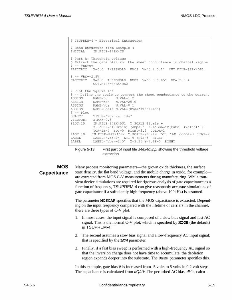
TSUPREM-4 User’s Manual NMOS LDD Process
eple—n-e as aof.
nd-el,
t AC
gnal;
so
.
MOSCapacitance
Many process monitoring parameters—the grown oxide thickness, the surfacstate density, the flat band voltage, and the mobile charge in oxide, for examare extracted from MOS C-V measurements during manufacturing. While trasient device simulations are required for rigorous analysis of gate capacitancfunction of frequency,TSUPREM-4 can give reasonably accurate simulations gate capacitance if a sufficiently high frequency (above 100kHz) is assumed
The parameterMOSCAP specifies that the MOS capacitance is extracted. Depeing on the input frequency compared with the lifetime of carriers in the channthere are three types of C-V plot.
1. In most cases, the input signal is composed of a slow bias signal and fassignal. This is the normal C-V plot, which is specified byHIGH (the default)in TSUPREM-4.
2. The second assumes a slow bias signal and a low-frequency AC input sithat is specified by theLOW parameter.
3. Finally, if a fast bias sweep is performed with a high-frequency AC signalthat the inversion charge does not have time to accumulate, the depletionregion expands deeper into the substrate. TheDEEP parameter specifies this.
In this example, gate biasV is increased from -5 volts to 5 volts in 0.2 volt stepsThe capacitance is calculated fromdQ/dV. The perturbed AC bias,dV is calcu-
$ TSUPREM-4 - Electrical Extraction
$ Read structure from Example 4INITIAL IN.FILE=S4EX4CS
$ Part A: Threshold voltage$ Extract the gate bias vs. the sheet conductance in channel region$ -- VBS=0VELECTRIC X=0.0 THRESHOLD NMOS V="0 2 0.1" OUT.FILE=S4EX4DS1
$ -- VBS=-2.5VELECTRIC X=0.0 THRESHOLD NMOS V="0 3 0.05" VB=-2.5 + OUT.FILE=S4EX4DS2
$ Plot the Vgs vs Ids$ -- Define the scale to convert the sheet conductance to the currentASSIGN NAME=Lch N.VAL=1.2ASSIGN NAME=Wch N.VAL=25.0ASSIGN NAME=Vds N.VAL=0.1ASSIGN NAME=Scale N.VAL=(@Vds*@Wch/@Lch)$ -- PlotSELECT TITLE="Vgs vs. Ids"VIEWPORT X.MAX=0.5PLOT.1D IN.FILE=S4EX4DS1 Y.SCALE=@Scale + Y.LABEL="I(Drain) (Amps)" X.LABEL="V(Gate) (Volts)" + TOP=1E-4 BOT=0 RIGHT=3.5 COLOR=2PLOT.1D IN.FILE=S4EX4DS2 Y.SCALE=@Scale CL AX COLOR=3 LINE=2LABEL LABEL="Vbs=0" X=1.9 Y=9E-5 RIGHTLABEL LABEL="Vbs=-2.5" X=3.35 Y=7.6E-5 RIGHT
Figure 5-13 First part of input file s4ex4d.inp, showing the threshold voltageextraction
S4 6.6 Confidential and Proprietary 5-15
Draft 6/26/98

Advanced Examples TSUPREM-4 User’s Manual
ationS
tant
apaci-harac- the
num-eing
3),n.
utdod as
lated from the DC increment multiplied by a constantE.RVCAP, which is definedas the ratio of AC amplitude to DC increment in theMETHOD statement (defaultvalue of 0.2 or 20%). The perturbed AC bias in this example is 0.04V(= 0.2Vx0.2). For example, the capacitance at 1 volt is extracted from the charge varibetween 0.96 volts and 1.04 volts. The input statements for extracting the MOcapacitance are shown inFigure 5-14; the results are shown inFigure 5-16.
Source/DrainJunction
Capacitance
The junction capacitance between source (or drain) and bulk is one of imporparameters to determine the delay characteristics of the MOS transistor. Thiscapacitance is composed of two kinds of capacitance: areal and peripheral ctance. In device characterization, these two components are separated and cterized by universal parameters independent of the shape of device. Usually,areal capacitance is dominant.TSUPREM-4 extracts the areal junction capaci-tance (in Farads/cm2) when theJCAP parameter is specified.
TheJUNCTION parameter selects the junction to be analyzed. Junctions are bered from the bottom of the structure to the top, with the deepest junction bjunction number one. For example, ifX specifies the emitter region of a bipolartransistor, there might be three junctions: E-B (emitter-base, junction numberB-C (base-collector, junction number 2), and C-S (collector-substrate, junctionumber 1). In this example, there is only one junction, identified as number 1
The input biasV must be all positive or all negative including zero bias.TSUPREM-4 chooses the biased region by considering the polarity of the inpvoltage so that the junction is reverse biased. All regions except for the biaseregion are grounded. The perturbed AC bias is applied using the same methin the MOS capacitance.
$ Part B: C-V plot for MOS capacitance$ Extract the capacitance
$ -- High FrequencyELECTRIC X=0.0 MOSCAP NMOS V=”-5 5 0.2” OUT.F=S4EX4DS3$ -- Low FrequencyELECTRIC X=0.0 MOSCAP NMOS V=”-5 5 0.2” LOW OUT.F=S4EX4DS4$ -- Deep depletionELECTRIC X=0.0 MOSCAP NMOS V=”-5 5 0.2” DEEP
$ Plot the C-V curveSELECT TITLE=”MOS C-V”VIEWPORT X.MIN=0.5 Y.MIN=0.51PLOT.1D ELECTRIC COLOR=2 TOP=1E-7 BOT=0 LEFT=-6 RIGHT=6 + X.OFF=1.5 ^CLPLOT.1D IN.FILE=S4EX4DS3 ^CL ^AX COLOR=3 LINE=2PLOT.1D IN.FILE=S4EX4DS4 ^CL ^AX COLOR=4 LINE=3LABEL LABEL=”Low” X=3 Y=8.3E-8LABEL LABEL=”High” X=3 Y=3.7E-8LABEL LABEL=”Deep” X=3 Y=0.7E-8
Figure 5-14 Second part of input file s4ex4d.inp, showing the MOScapacitance extraction
5-16 Confidential and Proprietary S4 6.6
Draft 6/26/98

TSUPREM-4 User’s Manual NMOS LDD Process
Input statements for extracting the junction capacitance are shown inFigure 5-15.
Plotting Resultsof Electrical
Extraction
The results of the electrical extractions are shown inFigure 5-16. Note how theresults of electrical extraction can be saved in an output file for later plotting.
$ Part C: Junction Capacitance$ Extract the S/D (area) junction capacitanceELECTRIC X=2.0 JCAP JUNCTION=1 V="0 5 0.5"SELECT TITLE="S/D Junction C"VIEWPORT X.MIN=0.5 Y.MAX=0.49PLOT.1D ELECTRIC COLOR=2 + TOP=2.5E-8 BOT=0 LEFT=-1 RIGHT=6 X.OFF=1.5 ^CL
Figure 5-15 Third part of input file s4ex4d.inp, showing the junctioncapacitance extraction
Figure 5-16 Electrical characteristics, plotted by input file s4ex4d.inp
S4 6.6 Confidential and Proprietary 5-17
Draft 6/26/98

Advanced Examples TSUPREM-4 User’s Manual
a
sted.
g-he
Trench Implant SimulationThis example shows two methods for performing a tilted ion implantation intotrench. First,TSUPREM-4’s analytical model is used to implant ions at a 15-degree tilt. Next,TSUPREM-4’s Monte Carlo method is used to perform thesame implantation. The results of the two methods are compared and contra
Structure Generation
The input statements for this simulation are shown inFigures 5-17, 5-19, and5-23. The initial mesh setup uses the symmetry of the trench structure, as sugested by SEM photographs of trenches generated by reactive ion etching. T
Figure 5-17 First part of input file s4ex5.inp, showing grid setup
$ TSUPREM-4 Example 5 - Implant Trench Application$$ Simulate ion implantation into a trench using the analytical approach$ followed by the Monte Carlo approach.
$ Place the finest grid around the trenchLINE X LOCATION=0.0 SPACING=1.0LINE X LOCATION=0.25 SPACING=0.01LINE X LOCATION=0.32 SPACING=0.01LINE X LOCATION=0.5 SPACING=0.2
LINE Y LOCATION=0.0 SPACING=0.01LINE Y LOCATION=0.05 SPACING=0.01LINE Y LOCATION=0.92 SPACING=0.04LINE Y LOCATION=1.0 SPACING=0.01LINE Y LOCATION=1.05 SPACING=0.01LINE Y LOCATION=1.2 SPACING=1.0
ELIMINATE ROWS X.MAX=0.2 Y.MIN=0.15 Y.MAX=1.0ELIMINATE ROWS X.MAX=0.25 Y.MIN=1.0 Y.MAX=1.1ELIMINATE COLUMNS X.MIN=0.23 X.MAX=0.35 Y.MIN=1.1ELIMINATE COLUMNS X.MIN=0.25 X.MAX=0.34 Y.MIN=1.1
$ Initialize the structureINITIALIZE BORON=2E15
$ Etch the left half of the trenchETCH START X=0.3 Y=0.0ETCH CONTINUE X=0.3 Y=0.5ETCH CONTINUE X=0.32 Y=0.9ETCH CONTINUE X=0.34 Y=0.95ETCH CONTINUE X=0.4 Y=1.0ETCH CONTINUE X=2.0 Y=1.0ETCH DONE X=2.0 Y=0.0
$ Form the complete trench structureSTRUCTURE REFLECT
$ Save the structureSAVEFILE OUT.FILE=S4EX5S
$ Plot the gridSELECT TITLE=”Grid for Trench Application”PLOT.2D SCALE GRID C.GRID=2
5-18 Confidential and Proprietary S4 6.6
Draft 6/26/98

TSUPREM-4 User’s Manual Trench Implant Simulation
gridthe ofencench
e,
rs.
f the
rees
nt
initial grid, established by theLINE andELIMINATE statements, is for the lefthalf of the trench only. Particular attention has been given to producing a finewhere the side and bottom walls of the trench are formed in order to resolve implanted profiles. TheELIMINATE statements are used to reduce the numbergrid points in areas where the implant is not expected to penetrate. The sequof ETCH statements specifies geometrically the shape of the left half of the trestructure. The resulting half-structure is reflected to generate the full structurusing theREFLECT parameter on theSTRUCTURE statement. The full structureis saved with theSAVEFILE statement.
The grid for the full structure is then plotted (Figure 5-18). Note that a fine meshhas been placed around the trench, without wasting nodes in the lower corne
Analytic Implant
The boron implant is now performed at an energy of 5 keV. In the absence oMONTECAR parameter,TSUPREM-4 uses the analytic method. TheTILTparameter is used to specify that the angle of the incident ion beam is 15 degcounter-clockwise from the vertical (i.e., the beam enters from the left). Theimplant is followed by a short diffusion to activate the boron and anneal impladamage.
Figure 5-18 Grid for trench implant example
S4 6.6 Confidential and Proprietary 5-19
Draft 6/26/98

Advanced Examples TSUPREM-4 User’s Manual
heodhe the
Plotting the Results of the Analytic Method
Figure 5-20 shows shaded contours of boron concentration produced by theCOLOR statement and associatedSELECT, PLOT.2D, FOREACH, END, andLABEL statements. Observe that dopant is present only on the right side of ttrench where the ions are directly incident. This is because the analytic methdoes not account for reflected ions. The profile at the bottom right corner of ttrench (where boron is directly incident) is approximately the same as that onsurface of the silicon.
Figure 5-19 Second part of input file s4ex5.inp, showing tilted implantationusing analytic implant model
$ Analytic implant at a 15-degree tilt to dope the trench sidewallsIMPLANT BORON ENERGY=5 DOSE=1E14 TILT=15
$ A short annealDIFFUSION TIME=5 TEMP=900
$ 2D contour plot of boron contoursSELECT Z=LOG10(BORON) TITLE=”Contours of Boron (Analytic)”PLOT.2D SCALE X.MAX=1.5FOREACH X (16 TO 21 STEP 1)
COLOR MIN.V=X MAX.V=( X + 1) COLOR=( X - 2)ENDPLOT.2D ^AXES ^CLEARLABEL X=1.05 Y=0.25 LABEL=”Log10(Boron)” SIZE=0.3LABEL X=1.15 Y=0.33 LABEL=”16-17” SIZE=0.3 C.RECT=14 W.R=0.4 H.R=0.4LABEL X=1.15 Y=0.41 LABEL=”17-18” SIZE=0.3 C.RECT=15 W.R=0.4 H.R=0.4LABEL X=1.15 Y=0.49 LABEL=”18-19” SIZE=0.3 C.RECT=16 W.R=0.4 H.R=0.4LABEL X=1.15 Y=0.57 LABEL=”19-20” SIZE=0.3 C.RECT=17 W.R=0.4 H.R=0.4LABEL LABEL=”Tilt angle=15 degrees” X=0.02 Y=1.18
$ 1D plots of boron
$ Vertical profilesSELECT Z=LOG10(BORON) TITLE=”Vertical Profiles (Analytic)”PLOT.1D X.VALUE=0.1 TOP=21 BOTTOM=15 RIGHT=1.2 COLOR=2LABEL X=0.06 Y=19 LABEL=”Surface”LABEL X=0.06 Y=18.8 LABEL=”(x=0.1)”
PLOT.1D X.VALUE=0.5 ^AXES ^CLEAR COLOR=2LABEL X=1.05 Y=18.5 LABEL=”Trench”LABEL X=1.05 Y=18.3 LABEL=”(x=0.5)”
$ Horizontal profilesDEPOSIT OXIDE THICK=0.002SELECT Z=LOG10(BORON) TITLE=”Sidewall Profiles at y=0.2 (Analytic)”PLOT.1D Y.VALUE=0.2 LEFT=0.1 RIGHT=0.9 BOTTOM=15 TOP=21 COLOR=2
$ Print profile through bottom of trenchPRINT.1D X.VALUE=0.5
5-20 Confidential and Proprietary S4 6.6
Draft 6/26/98

TSUPREM-4 User’s Manual Trench Implant Simulation
letra-
e to
nchrly
n thetion
cor- at
es ofidetly in
Figure 5-21 shows one-dimensional boron profiles vertically through the middof the trench bottom and at the surface of the silicon. The peak boron concention is much greater at the silicon surface than at the bottom of the trench dushadowing of the bottom by the sidewalls.
Figure 5-22 shows the boron concentration on the left and right sides of the treat a depth ofy=0.2 microns. The flat profile on the left hand side, at a value neathat of the background concentration, confirms the lack of reflected ions wheanalytic method is used. The corresponding plot for the Monte Carlo implantamodel is very different.
(A thin layer of oxide is deposited to ensure that the structure boundaries arerectly plotted by thePLOT.1D statement. Without the added oxide, the sectiony=0.2 would pass through silicon, ambient, and silicon asx varies from 0 to 1.0microns. Due to a limitation in the current version of the program, thesilicon/ambient and ambient/silicon interfaces are only recognized at the edgthe structure, but not in its interior. By adding the thin layer of oxide, silicon/oxand oxide/silicon boundaries are added. These boundaries are plotted correcFigures 5-20 and5-26.)
Figure 5-20 Contours of boron after analytic implant
S4 6.6 Confidential and Proprietary 5-21
Draft 6/26/98

Advanced Examples TSUPREM-4 User’s Manual
Figure 5-21 Vertical profiles produced by analytic implant
Figure 5-22 Sidewall profiles produced by analytic implant
5-22 Confidential and Proprietary S4 6.6
Draft 6/26/98

TSUPREM-4 User’s Manual Trench Implant Simulation
ewsre;lls,ity ofor sideing,
nchlant
. the
d:
tatis-
alcu-e
he
et sidesentnci-s. the
Monte Carlo Implant
The second half of the simulation demonstrates the use of the Monte Carloimplantation method.
Overview Unlike the analytic approach, the Monte Carlo algorithm accurately models theffect of reflected ions in a trench structure. The Monte Carlo calculation follothe trajectories of individual ions through each material present in the structuion trajectories through a vacuum, including those reflected off trench sidewaare calculated in exactly the same way as through other materials. The veloca reflected ion remains constant until it enters a material other than vacuum leaves the top or bottom of the simulated structure. For ions that leave eitherof the simulation space, the appropriate boundary condition (periodic, reflector vacuum) is invoked.
Using the MonteCarlo Model
The first step in the Monte Carlo portion of the simulation is to read in the trestructure that is saved earlier, just prior to the analytic implant. The boron impis performed once again, but this time theMONTECAR parameter on theIMPLANT statement directsTSUPREM-4 to use the Monte Carlo implant modelTheENERGY, DOSE, andTILT parameters are the same as those used duringanalytic implant.
In addition to theMONTECAR parameter, two new parameters are now specifie
• N.ION —TheN.ION parameter specifies the number of ion trajectories tocalculate. The simulation time is directly proportional to the number of iontrajectories calculated. Decreasing this number, however, increases the stical noise in the output of the Monte Carlo calculation.
• ^CRYSTAL—The specification ofCRYSTAL on theIMPLANT commanddisables the crystal model for ion penetration in silicon. This speeds the clation significantly by eliminating the calculation of channeling and damageffects.
A short post-implant anneal is performed as before to activate the implant. Tdiffusion also acts to smooth the results of the Monte Carlo calculation.
Plotting the Results of the Monte Carlo Method
The three figures output after the Monte Carlo implant (Figures 5-24 through5-26) are the counterparts of the three analytic plots.
Boron Contours Figure 5-24 shows the contours of boron concentration produced by the MontCarlo method. Note that dopant is present in substantial quantities on the lefof the trench (unlike the analytic results). The plot illustrates that dopant is prein greater quantity on the right side of the trench where the ions are directly ident. The boron in the left side of the trench is due entirely to reflection of ionAs before, the profile at the bottom right corner of the trench is approximatelysame as that on the surface of the silicon.
S4 6.6 Confidential and Proprietary 5-23
Draft 6/26/98

Advanced Examples TSUPREM-4 User’s Manual
lelant. sili-y the
eionisnergy
Vertical Profiles Figure 5-25, shows one-dimensional boron profiles vertically through the middof the trench bottom and at the surface of the silicon for the Monte Carlo impThe peak boron concentration is approximately a factor of five greater at thecon surface than at the bottom of the trench due to shadowing of the bottom bsidewalls. Observe that the difference between the peaks is much less for thMonte Carlo approach than the analytic method. This is due to the reflected calculations included in the Monte Carlo algorithm. The depth of the implant less at the bottom of the trench than at the silicon surface, due to the loss of ewhen an ion is reflected.
Figure 5-23 Third part of file s4ex5.inp, using the Monte Carlo implantationmodel
$ Repeat the implantation using the Monte Carlo method
$ Read in the structureLOADFILE IN.FILE=S4EX5S
$ Monte Carlo implant at a 15-degree tilt to dope the trench sidewallsIMPLANT BORON ENERGY=5 DOSE=1E14 MONTECAR TILT=15 N.ION=10000^CRYSTAL
$ A short annealDIFFUSION TIME=5 TEMP=900
$ 2D contour plot of boron contoursSELECT Z=LOG10(BORON) TITLE=”Contours of Boron (Monte Carlo)”PLOT.2D SCALE X.MAX=1.5FOREACH X (16 TO 21 STEP 1)
COLOR MIN.V=X MAX.V=( X + 1) COLOR=( X - 2)ENDPLOT.2D ^AXES ^CLEARLABEL X=1.05 Y=0.25 LABEL=”Log10(Boron)” SIZE=0.3LABEL X=1.15 Y=0.33 LABEL=”16-17” SIZE=0.3 C.RECT=14 W.R=0.4 H.R=0.4LABEL X=1.15 Y=0.41 LABEL=”17-18” SIZE=0.3 C.RECT=15 W.R=0.4 H.R=0.4LABEL X=1.15 Y=0.49 LABEL=”18-19” SIZE=0.3 C.RECT=16 W.R=0.4 H.R=0.4LABEL X=1.15 Y=0.57 LABEL=”19-20” SIZE=0.3 C.RECT=17 W.R=0.4 H.R=0.4LABEL LABEL=”Tilt angle=15 degrees” X=0.02 Y=1.18
$ 1D plots of boron
$ Vertical profilesSELECT Z=LOG10(BORON) TITLE=”Vertical Profiles (Monte Carlo)”PLOT.1D X.VALUE=0.1 TOP=21 BOTTOM=15 RIGHT=1.2 COLOR=2LABEL X=0.06 Y=19 LABEL=”Surface”LABEL X=0.06 Y=18.8 LABEL=”(x=0.1)”
PLOT.1D X.VALUE=0.5 ^AXES ^CLEAR COLOR=2LABEL X=1.05 Y=18.5 LABEL=”Trench”LABEL X=1.05 Y=18.3 LABEL=”(x=0.5)”
$ Horizontal profilesDEPOSIT OXIDE THICK=0.002SELECT Z=LOG10(BORON) TITLE=”Sidewall Profiles at y=0.2 (Monte Carlo)”PLOT.1D Y.VALUE=0.2 LEFT=0.1 RIGHT=0.9 BOTTOM=15 TOP=21 COLOR=2
$ Print profile through bottom of trenchPRINT.1D X.VALUE=0.5
5-24 Confidential and Proprietary S4 6.6
Draft 6/26/98

TSUPREM-4 User’s Manual Trench Implant Simulation
dels
e tos
antly
Comparing the vertical profiles produced by the analytic and Monte Carlo mo(Figures 5-21 and5-25, respectively), shows that the boron penetrates moredeeply with the analytic model than with the Monte Carlo approach. This is duthe specification ofCRYSTAL during the Monte Carlo implantation. This causethe silicon to be treated as amorphous, which speeds the calculation significbut prevents calculation of channeling in the crystal structure.
Figure 5-24 Contours of boron after Monte Carlo implant
Figure 5-25 Vertical profiles after Monte Carlo implant
S4 6.6 Confidential and Proprietary 5-25
Draft 6/26/98

Advanced Examples TSUPREM-4 User’s Manual
a-
pth
thee leftffectsns.
m-oe
for.
In contrast, the analytic method automatically includes the channeling calcultions, thus resulting in deeper penetration. If the^CRYSTAL were omitted, chan-neling calculations would be included in the Monte Carlo implant, giving a deof penetration very similar to the analytic results.
Sidewall Profiles The last Monte Carlo plot (Figure 5-26) shows the boron profiles on the left andright sidewalls of the trench. The profile on the left side of the trench is dueentirely to reflected ions and is not as deep as the profile on the right, due toreduced energy of reflected ions. The peak concentration of the profile on thside is also reduced compared to that on the right. This result incorporates eof ions reflecting from various points in the trench as well as multiple reflectio
Summary
The Monte Carlo model can be very useful in simulating implantation into coplex structures, due to its ability to model the effects of reflected ions. It is alsuseful in cases where analytical range statistics are not available, and in sommultilayer implant simulations. The analytic model is more suitable, however,simulating the implant steps that are encountered in most practical situations
Figure 5-26 Sidewall profiles after Monte Carlo implant
5-26 Confidential and Proprietary S4 6.6
Draft 6/26/98

TSUPREM-4 User’s Manual Poly-Buffered LOCOS
S
don
la-
een
on
Poly-Buffered LOCOSThis example illustrates the use ofTSUPREM-4 to simulate a poly-bufferedLOCOS process. This process reduces the typical “bird’s beak” formation anstresses on the silicon substrate through use of a layer of polycrystalline silicbetween the pad oxide and the nitride mask.
Structure Generation
The input statements for generating the structure and performing the field isotion processing are shown inFigure 5-27. A relatively coarse initial grid is used.In the horizontal direction, it is finest at the mask edge, atx=1 micron. The padoxide and poly buffer layers are deposited with two grid spaces in each. Betwthe poly layer and the nitride mask a thin (20Å) layer of oxide is deposited. Athick nitride mask layer is used. The nitride mask is etched to the right ofx=1.0 toexpose the region to be oxidized. This example oxidizes through the polysiliclayer. The grid prior to oxidation is shown inFigure 5-28.
$ TSUPREM-4: Poly-Buffered LOCOS Application
$ Set up the gridLINE X LOCATION=0 SPACING=0.1LINE X LOCATION=1.0 SPACING=0.06LINE X LOCATION=1.5 SPACING=0.1
LINE Y LOCATION=0 SPACING=0.03LINE Y LOCATION=0.5 SPACING=0.1
INITIALIZE
$ Deposit pad oxide and define nitride maskDEPOSITION OXIDE THICK=0.02 SPACES=2DEPOSITION POLY THICK=0.04 SPACES=2DEPOSITION OXIDE THICK=0.002DEPOSITION NITRIDE THICK=0.2 SPACES=2
ETCH NITRIDE RIGHT P1.X=1.0
$ Plot initial gridSELECT TITLE="Initial Grid"PLOT.2D SCALE GRID C.GRID=2
$ Use viscoelastic model for oxidationMETHOD VISCOELMATERIAL MAT=OXIDE VC=750MATERIAL MAT=NITRIDE VC=250DIFFUSION TEMP=1050 WETO2 TIME=85
$ Save structureSAVEFILE OUT.FILE=S4EX6S
Figure 5-27 First part of input file s4ex6.inp: Poly-buffered LOCOS process
4 6.6 Confidential and Proprietary 5-27
Draft 6/26/98

Advanced Examples TSUPREM-4 User’s Manual
ula-han
per- step.
ult
nter-. The
ues of
ddat
Using the VISCOEL Model
TheMETHOD statement selects the viscoelastic oxidation model. The stressdependence of the physical parameters of the model are included in the calction by default. This combination gives results that are much more accurate tthose obtained with theCOMPRESS model, but takes much less simulation timethan theVISCOUS model with stress dependence.
The stress dependence of the oxide and nitride viscosities is given by theVCparameter on theMATERIAL statement. Because these values depend on temature, it is usually necessary to specify appropriate values for each oxidationThe twoMATERIAL statements in this example setVC for nitride and oxide tovalues given in the literature for a 1050˚C oxidation. (Appendix A lists the defavalues forVC and suggests values for use at various temperatures.)
Plotting the Results
Figure 5-29 shows the input statements used to plot the results. Of particular iest are the stresses in the structure, as indicated by the hydrostatic pressurestatementSELECT Z=(-0.5*(SXX+SYY)) calculates the hydrostatic pres-sure from the stress components. The minus sign is used so that positive valZ correspond to compression. AFOREACH loop is used to plot contours of com-pressive and tensile stress at values from 3x10⁹ to 3x10¹⁰, in steps of 3x10⁹.
The final plot is shown inFigure 5-30. The very high pressure gradients at the enof the poly layer (nearx=0, y=-0.05) result from the volume expansion produceby the oxidation of the poly layer. The high pressure in this region confirms th
Figure 5-28 Grid for poly-buffered LOCOS application
5-28 Confidential and Proprietary S4 6.6
Draft 6/26/98

TSUPREM-4 User’s Manual Poly-Buffered LOCOS
S
oxida-
stress effects are important in this simulation, and that the stress-dependent tion models must be used to obtain an accurate simulation of this structure.$ Plot the structure with oxide stressSELECT TITLE="Contours of Pressure"PLOT.2D SCALECOLOR SILICON COLOR=7COLOR OXIDE COLOR=5COLOR NITRIDE COLOR=4COLOR POLY COLOR=3SELECT Z=(-0.5*(SXX+SYY))FOREACH I (1 TO 10) CONTOUR VALUE=( I *3E9) LINE=2 COLOR=6 CONTOUR VALUE=(- I *3E9) LINE=3 COLOR=6ENDPLOT.2D ^AX ^CL
LABEL LABEL="Poly" X=0.1 Y=-0.03LABEL LABEL="Oxide" X=1.2 Y=-0.05LABEL LABEL="Nitride" X=0.1 Y=-0.15LABEL LABEL="Substrate" X=0.1 Y=0.20
$ Print location of Si/SiO2 interfaceSELECT Z=YPRINT.1D SILICON /OXIDE
Figure 5-29 Second part of s4ex6.inp: Plotting final poly-buffered LOCOSstructure
Figure 5-30 Contours of hydrostatic pressure in final poly-buffered LOCOSstructure
4 6.6 Confidential and Proprietary 5-29
Draft 6/26/98

Advanced Examples TSUPREM-4 User’s Manual
t file into are
lyse of
CMOS ProcessThis example simulates the fabrication of NMOS transistors of two differentchannel lengths as part of a CMOS process. The goal is to produce an outpucontaining complete structure, mesh, and doping information that can be readtheMedici device simulator. The considerations needed to produce such a fileillustrated.
The two channel lengths are simulated with a single input file, using aFOREACHloop around the entire simulation, from mesh generation to saving of the finastructure. The use of theFOREACH loop simplifies the input and ensures that anchanges in the process sequence are applied to both devices equally. This utheFOREACH loop illustrates several useful techniques for parameterizingTSUPREM-4 input files. The listing of the first input file for this example(s4ex7a.inp) is shown inFigures 5-31 through5-33. Comment statements havebeen used to number the steps in the simulation.
Figure 5-31 First part of input file s4ex7a.inp, to set up grid for simulating aCMOS process
$ TSUPREM-4 N-channel MOS application$$ 1. Identify the graphics driver$ Default from DEFPDEV, TERM, or S4PCAP ”default” entry used
$ 2. Beginning of the main loopFOREACH LD ( 3 5 )
$ 3. Specify the meshMESH GRID.FAC=1.5MESH DY.SURF=0.01 LY.SURF=0.04 LY.ACTIV=2.0
$ 4. InitializeINITIALIZE <100> BORON=1E15 WIDTH=( 0.7 + ( LD / 10.0 ) ) DX=0.1
$ 5. Plot the initial meshSELECT TITLE=”Mesh for Delta=0.@LD”PLOT.2D SCALE GRID Y.MAX=3.0 C.GRID=2
$ 6. Initial oxide padDEPOSIT OXIDE THICKNESS=0.03
$ 7. P-well implantIMPLANT BORON DOSE=1E12 ENERGY=35
$ 8. Use a point defect models that simulates OEDMETHOD PD.TRANS
$ 9. P-well driveDIFFUSE TEMP=1100 TIME=120 DRYO2 PRESS=0.02
$ 10. P-well doping profileSELECT Z=LOG10(BORON) TITLE=”Channel Doping (Delta=0.@LD)”PLOT.1D X.VALUE=0 RIGHT=3.0 BOTTOM=15 TOP=19 LINE.TYP=2 COLOR=2LABEL X=1.8 Y=18.5 LABEL=”After p-well drive” LINE.TYP=2 C.LINE=2
5-30 Confidential and Proprietary S4 6.6
Draft 6/26/98

TSUPREM-4 User’s Manual CMOS Process
Figure 5-32 Second part of input file s4ex7a.inp, showing statements forsimulating a CMOS process
$ 11. Pad nitrideDEPOSIT NITRIDE THICKNESS=0.1
$ 12. Field implant and oxidationIMPLANT BORON DOSE=5E13 ENERGY=80DIFFUSE TEMP=1000 TIME=360 WETO2
$ 13. Etch to remove the padETCH NITRIDE ALL
$ 14. Vt adjust implantIMPLANT BORON ENERGY=100 DOSE=1E12
$ 15. P-well doping profileSELECT Z=LOG10(BORON)PLOT.1D X.VALUE=0 ^AXES ^CLEAR COLOR=2LABEL X=1.8 Y=18.2 LABEL=”After Vt implant” LINE.TYP=1 C.LINE=2
$ 16. Print oxide and silicon thicknessesSELECT Z=1PRINT.1D X.VALUE=0.0 LAYERS
$ 17. Etch oxideETCH OXIDE TRAP THICK=0.05
$ 18. Gate oxidationDIFFUSE TEMP=950 TIME=30 DRYO2
$ 19. Poly depositionDEPOSIT POLYSILICON THICKNESS=0.3 DIVISIONS=4
$ 20. Poly and oxide etch between x = 0.0 and 0.5 micronsETCH POLY LEFT P1.X=0.5ETCH OXIDE TRAP THICK=0.04
$ 21. Deposit a thin layer of oxideDEPOSIT OXIDE THICKNESS=0.02
$ 22. LDD implantIMPLANT PHOS ENERGY=50 DOSE=5E13 IMPL.TAB=PHOSPHORUS
$ 23. LTODEPOSIT OXIDE THICK=0.2
$ 24. Establish a sidewall spacerETCH OXIDE TRAP THICK=0.22
$ 25. Source/drain implantIMPLANT ARSENIC ENERGY=100 DOSE=2E15
$ 26. Oxide etchETCH OXIDE LEFT P1.X=0.5
$ 27. Use an oxidation model that understands polysiliconMETHOD COMPRESS
$ 28. Source/drain reoxidation (including the polysilicon gate)DIFFUSE TEMP=900 TIME=30 DRYO2
S4 6.6 Confidential and Proprietary 5-31
Draft 6/26/98
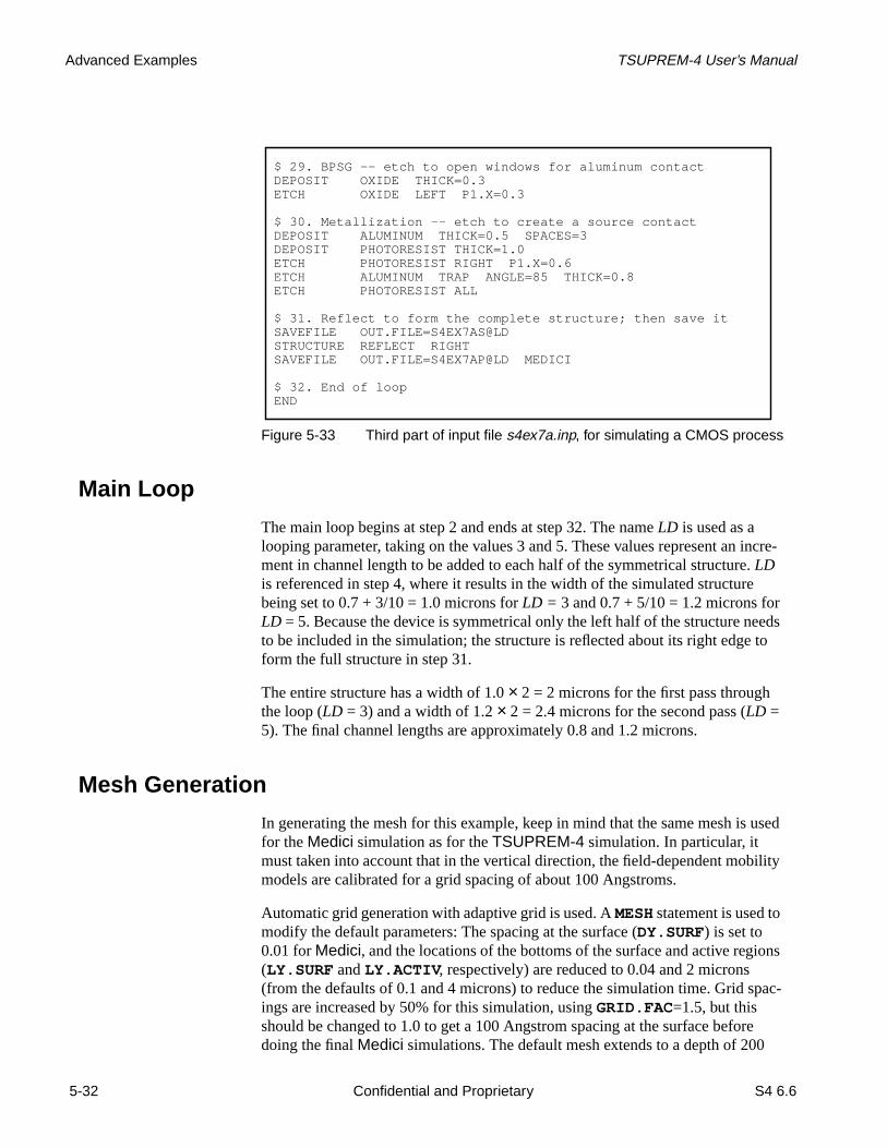
Advanced Examples TSUPREM-4 User’s Manual
incre-.
eeds to
used
ility
ions
pac-
re
Main Loop
The main loop begins at step 2 and ends at step 32. The nameLD is used as alooping parameter, taking on the values 3 and 5. These values represent an ment in channel length to be added to each half of the symmetrical structureLDis referenced in step 4, where it results in the width of the simulated structurebeing set to 0.7 + 3/10 = 1.0 microns forLD = 3 and 0.7 + 5/10 = 1.2 microns forLD = 5. Because the device is symmetrical only the left half of the structure nto be included in the simulation; the structure is reflected about its right edgeform the full structure in step 31.
The entire structure has a width of 1.0× 2 = 2 microns for the first pass throughthe loop (LD = 3) and a width of 1.2× 2 = 2.4 microns for the second pass (LD =5). The final channel lengths are approximately 0.8 and 1.2 microns.
Mesh Generation
In generating the mesh for this example, keep in mind that the same mesh isfor theMedici simulation as for theTSUPREM-4 simulation. In particular, itmust taken into account that in the vertical direction, the field-dependent mobmodels are calibrated for a grid spacing of about 100 Angstroms.
Automatic grid generation with adaptive grid is used. AMESH statement is used tomodify the default parameters: The spacing at the surface (DY.SURF) is set to0.01 forMedici, and the locations of the bottoms of the surface and active reg(LY.SURF andLY.ACTIV , respectively) are reduced to 0.04 and 2 microns(from the defaults of 0.1 and 4 microns) to reduce the simulation time. Grid sings are increased by 50% for this simulation, usingGRID.FAC=1.5, but thisshould be changed to 1.0 to get a 100 Angstrom spacing at the surface befodoing the finalMedici simulations. The default mesh extends to a depth of 200
Figure 5-33 Third part of input file s4ex7a.inp, for simulating a CMOS process
$ 29. BPSG -- etch to open windows for aluminum contactDEPOSIT OXIDE THICK=0.3ETCH OXIDE LEFT P1.X=0.3
$ 30. Metallization -- etch to create a source contactDEPOSIT ALUMINUM THICK=0.5 SPACES=3DEPOSIT PHOTORESIST THICK=1.0ETCH PHOTORESIST RIGHT P1.X=0.6ETCH ALUMINUM TRAP ANGLE=85 THICK=0.8ETCH PHOTORESIST ALL
$ 31. Reflect to form the complete structure; then save itSAVEFILE OUT.FILE=S4EX7AS@LDSTRUCTURE REFLECT RIGHTSAVEFILE OUT.FILE=S4EX7AP@LD MEDICI
$ 32. End of loopEND
5-32 Confidential and Proprietary S4 6.6
Draft 6/26/98

TSUPREM-4 User’s Manual CMOS Process
start-
esteps
id-
ing the
microns. The structure can be truncated (withSTRUCTURE TRUNCATE) beforesaving it forMedici, orMedici can truncate the saved structure as it is read in.
Note:A separate mesh inMedici could be generated and the doping profilesread without the mesh from theTSUPREM-4 output file. In that case,the generation of the mesh would be guided more by process simulationconsiderations and less by the needs of the device simulation.
It is often a good idea to check the initial mesh structure (as in step 5) beforeing aTSUPREM-4 simulation. ThePLOT.2D statement in step 5 specifiesY.MAX = 3 microns, since the area of interest does not extend much below thdeepest junction depth. Given the times and temperatures of the processing to be used, do not expect the junction depth to exceed 1 micron.
The plot of the mesh produced the first time through the loop (LD = 3) is shown inFigure 5-34. The grid appears coarse, but is refined as needed by adaptive grding.
TheFOREACH parameterLD is used in step 5 in the title for the mesh plot. ThenameLD is enclosed in braces to separate it from the rest of the character strand preceded by a “@” character to force substitution of the value defined on
Figure 5-34 Initial grid for the 0.8 micron NMOS transistor, produced bys4ex7a.inp
S4 6.6 Confidential and Proprietary 5-33
Draft 6/26/98

Advanced Examples TSUPREM-4 User’s Manual
for
re
ethe
e
ion,yer.
well
cing
h ant
2
his mask
re
icon- back
FOREACH statement. The resulting titles are “Mesh for Delta=0.3” and “Mesh Delta=0.5” for the two passes through the main loop.
CMOS Processing
The simulation of the CMOS process is straightforward. A variety of models aused to simulate the various processes.
Models Because the process is planar up to the patterning of the polysilicon gate, thVERTICAL oxidation model can be used without any loss of accuracy. Once poly gate is patterned, a switch is made to theCOMPRESS model, both because ofthe nonplanarity of the structure and the desire to simulate the oxidation of thpolysilicon gate. In order to accurately simulate oxidation-enhanced diffusioneffects, thePD.TRANS model for point defects is chosen.
Note:There might be significant OED effects produced by the field oxidation;to accurately simulate these, the structure would need to be expanded toinclude the field region.
The advanced models for grain growth and dopant diffusion in polysilicon areused by default. For a faster simulation but with less accuracy in the gate regadvanced poly models could be disabled before depositing the polysilicon la
Channel DopingPlot
The channel doping profile is plotted at two points in the process—after the p-drive and after the threshold adjust implant. The result is shown inFigure 5-35.Again,LD has been used in the title of the plot.
Lightly DopedDrain Structure
The remaining steps in the loop are fairly standard, but the method for produthe lightly-doped drain structure should be pointed out. The light source/drainextension implant is performed in step 22; because the implantation is througoxide,IMPL.TAB =phosphorus is used to access implant data tables that do noinclude channelling effects. This is followed with a conformal deposition of 0.microns of oxide. Step 24 uses theTRAP parameter on theETCH statement toremove all oxide within a vertical distance of 0.22 microns from the surface. Tproduces a spacer on the sidewall of the poly gate that serves as an implantfor the heavy source/drain implant of step 25.
Contacts An important final step for structures to be used inMedici is the deposition andpatterning of aluminum contacts. Interfaces between aluminum and silicon aconverted to contacts when the structure is passed toMedici. In addition, theMedici user can specify whether polysilicon regions are to be treated as semductor regions or contacts, and whether a contact should be added along theside of the structure.
5-34 Confidential and Proprietary S4 6.6
Draft 6/26/98

TSUPREM-4 User’s Manual CMOS Process
is
tor.
e
eion.
Saving theStructure
Once processing is complete, the finished structure is saved. Each structuresaved twice, once inTSUPREM-4’s file format and once in theMedici format.For theMedici file, the structure must first be reflected to produce a full transisThe structure is saved inTSUPREM-4 format before reflection. Note that theFOREACH parameterLD has been used once again to produce the output filenames. This time the “@” character has been used to force substitution of thparameter, but the braces are not needed.
End of Main Loop TheEND statement signals the end of the mainFOREACH loop. After the entiresequence of input statements has been processed forLD=3, it is repeated forLD=5.
Plotting the Results
Once the complete structure has been saved, it can be read back in using thINITIALIZE statement and the results plotted without rerunning the simulatFigure 5-36 shows an input file (s4ex7b.inp) that reads fileS4EX7AS3, producedby the firstSAVEFILE statement of step 31 on the first pass through the mainloop.
Figure 5-35 Channel doping profile for NMOS transistor
S4 6.6 Confidential and Proprietary 5-35
Draft 6/26/98

Advanced Examples TSUPREM-4 User’s Manual
Figure 5-36 Input file s4ex7b.inp, for plotting results
$ TSUPREM-4 N-channel MOS application -- Part B$ Plot the results for delta = 0.3
$ Read the structureINITIALIZE IN.FILE=S4EX7AS3STRUCTURE REFLECT RIGHT
$ Prepare to plot contours of boron, phosphorus, and arsenicSELECT TITLE=”N-Channel (Delta=0.3)”PLOT.2D SCALE Y.MAX=1.5COLOR SILICON COLOR=7COLOR OXIDE COLOR=5COLOR POLY COLOR=3COLOR ALUMI COLOR=2
SELECT Z=LOG10(Boron)FOREACH VAL (14 TO 21 STEP 1)
CONTOUR VALUE=VAL LINE=5 COLOR=2END
SELECT Z=LOG10(Phosphorus)FOREACH VAL (16 TO 21 STEP 1)
CONTOUR VALUE=VAL LINE=4 COLOR=3END
SELECT Z=LOG10(Arsenic)FOREACH VAL (16 TO 21 STEP 1) CONTOUR VALUE=VAL LINE=2 COLOR=4END
PLOT.2D ^AX ^CL
$ Add labelsLABEL X=0.01 Y=-0.8 LABEL=”Aluminum”LABEL X=1.99 Y=-0.8 LABEL=”Aluminum” RIGHTLABEL X=1.0 Y=-0.45 LABEL=”BPSG” CENTERLABEL X=1.0 Y=-0.2 LABEL=”Poly” CENTERLABEL X=0.05 Y=0.35 LABEL=”Source”LABEL X=1.95 Y=0.35 LABEL=”Drain” RIGHT
$ Plot the gridSELECT TITLE=”Final Mesh (Delta=0.3)”PLOT.2D GRID SCALE Y.MAX=3 C.GRID=2
$ Plot arsenic profile in polySELECT Z=Log10(Active(Arsenic)) TITLE=”Arsenic Concentration in Gate”PLOT.1D X.V=1 LEFT=-0.4 RIGHT=0 BOT=16 TOP=21 COLOR=4SELECT Z=Log10(Arsenic)PLOT.1D X.V=1 ^AX ^CL COLOR=4 LINE=2LABEL X=-0.16 RIGHT Y=19 SIZE=0.28 COLOR=4 LABEL=”Active”LABEL X=-0.15 LEFT Y=19.7 SIZE=0.28 COLOR=4 LABEL=”Total”
5-36 Confidential and Proprietary S4 6.6
Draft 6/26/98

TSUPREM-4 User’s Manual CMOS Process
its
r the
-
are
en-rys-hees.
0.8 MicronDevice
In order to plot results for the full device, the structure is first reflected about right edge. The structure is then plotted, with contours of boron, arsenic, andphosphorus concentration. The result is shown inFigure 5-37. The phosphorusLDD regions can be clearly seen, extending from the heavily-doped arsenicsource/drain regions to the edge of the poly gate.
Labels have been added to facilitate interpretation of the plot. The labels neacenter of the plot have been automatically centered (with theCENTER parameteron theLABEL statement), and the labels on the right have been right justified(with theRIGHT parameter).
Final Mesh The final mesh is shown inFigure 5-37 (right). Observe the fine grid in the channel, as desired, and a fine grid around the source and drain junctions.Medici canrefine the grid or use its own grid, if needed, provided that the doping profilesaccurately represented by theTSUPREM-4 grid.
Arsenic Profilesin Gate
Figure 5-38 shows the arsenic profiles through the poly gate. The active conctration includes only the electrically active arsenic in the interiors of the polyctalline grains. The total concentration also includes any clustered arsenic in tgrain interiors and the arsenic atoms that occupy sites on the grain boundari
Figure 5-37 Final 0.8 micron structure, NMOS structure, plotted by s4ex7b.inp(left) and final mesh for 0.8 micron NMOS structure (right)
S4 6.6 Confidential and Proprietary 5-37
Draft 6/26/98

Advanced Examples TSUPREM-4 User’s Manual
by
1.2 MicronDeviceA third input file (s4ex7c.inp, not shown) can be used to plot the results saved the second pass through the main loop, in the same way thats4ex7b.inp plotted theresults of the first pass.Figure 5-39 shows the structure plot of the 1.2 micronNMOS transistor, as plotted by input files4ex7c.inp.
Figure 5-38 Profiles of active and total arsenic concentration through the polygate
Figure 5-39 Final 1.2 micron NMOS structure, plotted by input file s4ex7c.inp
5-38 Confidential and Proprietary S4 6.6
Draft 6/26/98

TSUPREM-4 User’s Manual DMOS Power Transistor
The ao-ide of
ate of
the that
DMOS Power TransistorThis section illustrates the fabrication of a DMOS power transistor structure. DMOS transistor is formed by diffusing boron into an n-type substrate, underpolysilicon gate. A self-aligned source region is formed by implanting phosphrus, using the poly gate as a mask. Contact to the drain is made at the back sthe wafer. The source metallization also provides contact to the p-type substrthe n-channel MOS transistor. TheTSUPREM-4 statements for simulating thisDMOS power transistor are shown inFigures 5-40, 5-42, and5-45. This particularinput file features frequent saving of the structure. This is useful for analyzingresults at intermediate points in the processing, and for recovering from errorsmay occur during simulation.
$ TSUPREM-4 DMOS Application
$ 1. Set grid spacing and error toleranceMESH GRID.FAC=1.4 LY.SURF=0.2 DY.SURF=0.1 LY.ACTIV=5.0METHOD ERR.FAC=3.0
$ 2. Select modelsMETHOD COMPRESS
$ 3. Initialize structureINITIALIZE WIDTH=10.0 PHOSPHORUS=1E15
$ 4. Plot initial meshSELECT TITLE="Initial Mesh"PLOT.2D SCALE GRID C.GRID=2 Y.MAX=5
$ 5. P-well formationDEPOSIT OXIDE THICK=0.70 SPACES=2ETCH OXIDE RIGHT P1.X=8.0
DIFFUSE TEMP=1000 TIME=50 DRYO2
IMPLANT BORON ENERGY=50 DOSE=5E15DIFFUSE TEMP=950 TIME=120 STEAMDIFFUSE TEMP=1100 TIME=50
$ 6. Save the structureSAVEFILE OUT.FILE=S4EX8S4
$ 7. Boron contour plotsSELECT Z=LOG10(BORON) TITLE="After P-Well Diffusion"PLOT.2D SCALE Y.MAX=5COLOR SILICON COLOR=7COLOR OXIDE COLOR=5FOREACH VAL (16 TO 21 STEP 1) CONTOUR VALUE=VAL LINE=5 COLOR=2ENDPLOT.2D ^AX ^CL
$ 8. Gate oxidationETCH OXIDE LEFT P1.X=8.1DIFFUSE TIME=180 TEMP=1000 DRYO2
Figure 5-40 Mesh generation for DMOS power transistor, from input files4ex8.inp
S4 6.6 Confidential and Proprietary 5-39
Draft 6/26/98

Advanced Examples TSUPREM-4 User’s Manual
to-arge-
gion
.4asA plot
and
truc-
Mesh Generation
This simulation uses automatic grid generation and adaptive gridding. The aumatic grid generation parameters have been adjusted to accommodate this lgeometry power device. The depth and spacing of the surface region (LY.SURFandDY.SURF, respectively) have been doubled and the depth of the active re(DY.ACTIV ) has been increased from 4 to 5 microns.
A grid spacing factor ofGRID.FAC=1.4 is used set the actual grid spacings to 1times their specified or default values. The error factor for adaptive gridding hbeen set to 3.0 to reduce the number of nodes and speed up the simulation. of the initial mesh is shown inFigure 5-41.
Processing the DMOS Power Transistor
Processing of the DMOS structure starts with the deposition of 7000Å of oxide.An opening in this oxide layer is then made and a thin oxide is grown on theexposed silicon. Boron is then implanted through the opening to form the p+ con-tact for the body of the transistor. After implantation, the structure is oxidized, the boron is driven further with an inert diffusion step. TheCOMPRESS oxidationmodel is used throughout the simulation to simulate oxidation of nonplanar stures.
Figure 5-41 Initial grid for simulating DMOS power transistor
5-40 Confidential and Proprietary S4 6.6
Draft 6/26/98

TSUPREM-4 User’s Manual DMOS Power Transistor
much
The structure after the oxidation and p-well drive is shown inFigure 5-43. Notethat some oxide growth has occurred underneath the thick oxide, but not as as occurred where the original oxide was removed.$ 9. Save the structureSAVEFILE OUT.FILE=S4EX8S5
$ 10. Print oxide thicknessSELECT Z=1PRINT.1D LAYERS X.VALUE=0
$ 11. Poly gate formationDEPOSIT POLY THICK=0.5 PHOS=1E20 SPACES=2ETCH POLY RIGHT P1.X=4
$ 12. Body formationETCH OXIDE START X=4.0 Y=-10ETCH OXIDE CONT X=4.0 Y=10ETCH OXIDE CONT X=7.9 Y=10ETCH OXIDE END X=7.9 Y=-10
DIFFUSE TIME=40 TEMP=1000 DRYO2
IMPLANT BORON DOSE=5E14 ENERGY=70DIFFUSE TIME=60 TEMP=950 DRYO2DIFFUSE TIME=200 TEMP=1100
$ 13. Save the structureSAVEFILE OUT.FILE=S4EX8S6
Figure 5-42 Second part of file s4ex8.inp: Processing of DMOS powertransistor, through body diffusion
Figure 5-43 Structure with contours of boron concentration, after first p-welldiffusion
S4 6.6 Confidential and Proprietary 5-41
Draft 6/26/98

Advanced Examples TSUPREM-4 User’s Manual
te
ted
dand
e sub-
ted.tor.
ge
g
Gate Processing Next, the thick oxide is etched from the left portion of the structure, and a gaoxide is grown in this region. Again, one of the numerical oxidation models isrequired to simulate oxidation with nonuniform initial oxide thickness(COMPRESS is still being used). The thickness of the grown gate oxide is prinwith thePRINT.1D LAYERS statement of step 10.
Next, the polysilicon gate is deposited and patterned, and the oxide is clearefrom the source region. Boron is then implanted through the source opening driven under the poly gate. The structure at this point is plotted inFigure 5-44.Observe that the boron has indeed diffused under the gate, where it forms thstrate of the n-channel transistor.
SourceProcessing
The opening for the source implant is now cleared and a thin oxide is deposiPhosphorus is then implanted and annealed to form the source of the transisBecause the implantation is through an oxide, thephosphorus implant table whichdoes not include channelling, is used. BPSG is deposited to form an insulatinlayer over the gate. Finally, a contact hole is opened for the source and p-typbody contact, and aluminum is deposited. The final structure is shown inFigure 5-46 (right). The silicon region has been labeled according to the dopintype, and the other regions according to the type of material.
Figure 5-44 DMOS power transistor after p-type body diffusion
5-42 Confidential and Proprietary S4 6.6
Draft 6/26/98

TSUPREM-4 User’s Manual DMOS Power Transistor
$ 14. Boron contour plotsSELECT Z=LOG10(BORON) TITLE="After Body Diffusion"PLOT.2D SCALE Y.MAX=5COLOR SILICON COLOR=7COLOR OXIDE COLOR=5COLOR POLY COLOR=3FOREACH VAL (16 TO 21 STEP 1) CONTOUR VALUE=VAL LINE.TYP=5 COLOR=2ENDPLOT.2D ^AX ^CL
$ 15. Source/drain formationETCH OXIDE START X=4.1 Y=-10ETCH OXIDE CONT X=4.1 Y=10ETCH OXIDE CONT X=7.9 Y=10ETCH OXIDE END X=7.9 Y=-10
DEPOSIT OXIDE THICK=0.03
IMPLANT PHOS DOSE=1E15 ENERGY=50 IMPL.TAB=PHOSPHORUSDIFFUSE TEMP=950 TIME=60 DRYO2
$ 16. BPSG and metallizationDEPOSIT OXIDE THICK=1.00DIFFUSE TEMP=950 TIME=60ETCH OXIDE RIGHT P1.X=6
DEPOSIT ALUMINUM THICK=1.5$ 17. Save the structureSAVEFILE OUT.FILE=S4EX8S7
$ 18. Plot final meshSELECT TITLE="Final Mesh"PLOT.2D SCALE GRID C.GRID=2 Y.MAX=5
$ 19. Boron and phosphorus contour plotsSELECT Z=LOG10(BORON) TITLE="Final structure"PLOT.2D SCALE Y.MAX=5COLOR SILICON COLOR=7COLOR OXIDE COLOR=5COLOR POLY COLOR=3COLOR ALUMINUM COLOR=2FOREACH VAL (16 TO 21 STEP 1) CONTOUR VALUE=VAL LINE.TYP=5 COLOR=2END
SELECT Z=LOG10(PHOS)FOREACH VAL (16 TO 21 STEP 1) CONTOUR VALUE=VAL LINE.TYP=4 COLOR=4END
PLOT.2D ^AX ^CL
LABEL X=9.8 Y=-0.5 LABEL="Aluminum" RIGHTLABEL X=1 Y=-0.9 LABEL="BPSG"LABEL X=1 Y=-0.1 LABEL="Poly"LABEL X=0.5 Y=1.5 LABEL="n-"LABEL X=9.8 Y=1.0 LABEL="p+" RIGHTLABEL X=3.1 Y=0.4 LABEL="p-"LABEL X=5.2 Y=0.4 LABEL="n+"
Figure 5-45 Third part of s4ex8.inp: Final processing and plotting
S4 6.6 Confidential and Proprietary 5-43
Draft 6/26/98

Advanced Examples TSUPREM-4 User’s Manual
hase
erccursal
ture,thessi-ide someer
Figure 5-46 (left) shows the final grid for the structure. Observe that the meshbeen refined (automatically, by adaptive gridding) where needed to resolve thimpurity profiles. Note that the grid refinement is primarily vertical in the centof the source region where the profiles are essentially one-dimensional, but oin both directions at the corners of the source diffusion, where two-dimensioneffects are important.
The final structure is shown inFigure 5-46 (right).
Summary
The process shown here does not necessarily produce an ideal DMOS strucnor is the simulation as accurate as it might be. Of particular importance are conditions of the final drive of the p-type body diffusion in step 22 and the pobility that impurities may diffuse from the polysilicon gate through the gate oxand into the channel. Observe in the final plot that there has apparently beendiffusion of both boron and phosphorus from the poly into the channel. Anothconcern is that oxidation-enhanced diffusion effects may be important in thisexample. This can be checked by repeating the simulation using thePD.TRANSpoint defect model.
Figure 5-46 Final mesh for DMOS simulation (left), showing the result ofadaptive gridding, and Final DMOS power transistor structure(right), produced by input file s4ex8.inp
5-44 Confidential and Proprietary S4 6.6
Draft 6/26/98

TSUPREM-4 User’s Manual SOI MOSFET
u- been
e-
toprys-
ub-atted.
n
SOI MOSFETThis example shows howTSUPREM-4 can be used to simulate a silicon-on-inslator (SOI) process. It illustrates several features of the program that have notused in the other examples, including the use of theREGION statement and thetechnique for depositing layers with nonuniform grid spacings. The input statments from files4ex9.inp are shown inFigures 5-47 and5-49.
Mesh Generation
The structure to be simulated consists of a silicon wafer with a half micron ofoxide and 0.2 microns of silicon on top. The active device is fabricated in thesilicon layer. The actual structure is formed by implantation of oxygen and rectallization of the silicon layer on top, a process that cannot be simulated byTSUPREM-4. Instead, an initial structure is defined consisting of the silicon sstrate and the oxide layer, on which the top silicon layer is deposited. Note thdue to the symmetry of the final structure, only the left half needs to be simula
The silicon substrate and oxide layers are defined withLINE statements, as inprevious examples. In this case, theTAG parameter must be added to grid lines ostructure boundaries and material interfaces. Thus, in they direction the tagOXTOP is used to mark the top of the oxide,OXBOTTOM to mark the oxide/sili-con interface, andSIBOTTOM to mark the bottom of the structure.REGION state-
Figure 5-47 Mesh generation for SOI MOSFET, from input file s4ex9.inp
$ TSUPREM-4 SOI Structure (0.2um epi) Application
$ Specify x meshLINE X LOCATION=0 SPACING=0.25 TAG=LEFTLINE X LOCATION=0.5 SPACING=0.025LINE X LOCATION=0.6 SPACING=0.025LINE X LOCATION=1.05 SPACING=0.1 TAG=RIGHT
$ Specify y meshLINE Y LOCATION=0 SPACING=0.02 TAG=OXTOPLINE Y LOCATION=0.5 SPACING=0.15 TAG=OXBOTTOMLINE Y LOCATION=2.0 SPACING=1.0 TAG=SIBOTTOM
ELIMINATE COLUMNS X.MIN=0.45 X.MAX=0.7 Y.MIN=0.05ELIMINATE COLUMNS Y.MIN=0.5
$ Define isolation oxide and silicon substrateREGION OXIDE XLO=LEFT XHI=RIGHT YLO=OXTOP YHI=OXBOTTOMREGION SILICON XLO=LEFT XHI=RIGHT YLO=OXBOTTOM YHI=SIBOTTOMINITIALIZE <100> BORON=1E15
$ Deposit epi with nonuniform vertical grid spacingDEPOSIT SILICON BORON=1E17 THICKNESS=0.1 SPACES=5 DY=0.01 YDY=0.1DEPOSIT SILICON BORON=1E17 THICKNESS=0.1 SPACES=5 DY=0.01
$ Plot initial meshSELECT Z=1 TITLE=”Initial Mesh”PLOT.2D GRID Y.MAX=1 SCALE C.GRID=2PRINT.1D X.VALUE=0.0 LAYERS
S4 6.6 Confidential and Proprietary 5-45
Draft 6/26/98

Advanced Examples TSUPREM-4 User’s Manual
ified
-
nsh
easedo
cron of
ve
for
ments are added to identify the silicon and oxide regions. TheREGION statementsuse the tags to specify the extent of the regions. Thus, for example, it is specthat the oxide region extends from the grid line taggedOXTOP to the line taggedOXBOTTOM, and fromLEFT to RIGHT in the horizontal direction.
Depositing aLayer with
Nonuniform GridSpacing
The top silicon layer is added usingDEPOSITION statements. To accurately simulate the final structure with theMedici device simulator, a fine grid spacing(about 100Å) is needed near each silicon/oxide interface. To reduce simulatiotime, a coarser grid is specified in the middle of the layer. Thus, the ideal mewould have a spacing that varies smoothly from fine to coarse to fine.
A mesh of this type (shown inFigure 5-48) can be generated using theDY andYDY parameters on theDEPOSITION statement. TheDY parameter specifies thedesired grid spacing at some depth in the deposited layer specified by theYDYparameter. The grid spacing above and below this depth is increased or decrto produce the specified number of spaces. To specify the grid spacing at twpoints in the layer (i.e., at each interface), twoDEPOSITION statements must beused. Each specifies a 1000Å layer of silicon divided into five grid spaces, asspecified by theSPACES parameter. In each case theDY parameter is used tospecify the desired grid spacing of 0.01 microns. In the first case the 0.01-migrid spacing occurs 0.1 microns below the top of the layer (i.e., at the bottomthe layer), while in the second case the default value ofYDY=0 is used, so the finegrid spacing occurs at the top of the layer. Note that the same mesh could habeen generated by addingLINE andREGION statements to define the top siliconlayer. The difficulty is that only a single doping concentration can be specified
Figure 5-48 Initial grid for simulating SOI MOSFET
5-46 Confidential and Proprietary S4 6.6
Draft 6/26/98

TSUPREM-4 User’s Manual SOI MOSFET
c-
the entire structure on theINITIALIZE statement, and it was necessary to speify a doping of 1017/cm3 in the top layer, but only 1015/cm3 in the lower layers.Figure 5-49 Processing of SOI MOSFET, from input file s4ex9.inp
$ Use vertical oxidation model to grow gate oxideDIFFUSE TIME=55 TEMP=950 DRYO2
SELECT Z=1PRINT.1D X.VALUE=0.0 LAYERS
$ Deposit, dope, and pattern polyDEPOSIT POLY THICK=0.3 SPACES=2METHOD COMPRESSDIFFUSE TIME=30 TEMP=800 PHOS=1E20ETCH POLY LEFT P1.X=0.5
$ Source/drain implant and annealIMPLANT ARSENIC DOSE=4E15 ENERGY=45DIFFUSE TIME=70 TEMP=950
$ BPSG and contact holesDEPOSIT OXIDE THICK=0.3DEPOSIT PHOTORESIST THICK=1.0ETCH PHOTORESIST LEFT P1.X=0.3ETCH OXIDE TRAP THICK=0.7 ANGLE=85ETCH PHOTORESIST ALL
$ MetallizationDEPOSIT ALUMINUM THICK=0.4DEPOSIT PHOTORESIST THICK=1.0ETCH PHOTORESIST RIGHT P1.X=0.6ETCH ALUMINUM TRAP THICK=0.7 ANGLE=85ETCH PHOTORESIST ALL
$ Reflect structure, then save complete MOSFETSAVEFILE OUT.FILE=S4EX9S1STRUCTURE REFLECT RIGHTSAVEFILE OUT.FILE=S4EX9P2 MEDICI
$ Plot grid & profiles for complete structureSELECT Z=DOPING TITLE=”SOI MOSFET”PLOT.2D SCALE Y.MAX=1COLOR SILICON COLOR=7COLOR OXIDE COLOR=5COLOR POLY COLOR=3COLOR ALUMINUM COLOR=2FOREACH X ( 16 TO 21 STEP 1 ) CONTOUR VALUE=( 10^ X ) COLOR=4 LINE.TYP=2 CONTOUR VALUE=(-(10^ X )) COLOR=2 LINE.TYP=5ENDPLOT.2D ^AX ^CL
PLOT.2D GRID SCALE Y.MAX=1 C.GRID=2
$ Plot 1D concentration profilesSELECT Z=LOG10(ACTIVE(BORON)) TITLE=”Doping Profiles” + LABEL=”log(Active Concentration)”PLOT.1D X.VALUE=1 BOTTOM=15 TOP=21 LEFT=-0.3 RIGHT=0 LINE.TYP=5 + COLOR=2LABEL LABEL=”Boron (x=1)” X=-0.1 Y=17
SELECT Z=LOG10(ACTIVE(ARSENIC))PLOT.1D X.VALUE=0 ^AXES ^CLEAR LINE.TYP=2 COLOR=3LABEL LABEL=”Arsenic (x=0)” X=-0.1 Y=20.3
S4 6.6 Confidential and Proprietary 5-47
Draft 6/26/98

Advanced Examples TSUPREM-4 User’s Manual
al pla-ces.
gen. If
the
and
s in
Process Simulation
The processing of the SOI MOSFET is straightforward. Note that the analyticoxidation models cannot be used in this example, even though the surface isnar and unoxidized, because of the existence of the lower oxide/silicon interfa
TheVERTICAL model can be used, but only because there is no path for oxyto diffuse to the lower oxide layer, and thus no growth at the lower interfacesthere were a path for oxygen to diffuse to the lower oxide, theCOMPRESS orVISCOEL model would be needed, and if it were necessary to model lifting ofupper silicon layer, theVISCOUS model withSKIP.SIL set false would beneeded.
Source/drain contacts have been opened and aluminum has been depositedpatterned in order to form contacts forMedici. The structure is reflected along theright edge to form a full device, and saved inMedici format in fileS4EX9P2. Thefull, final structure is shown inFigure 5-50 on the left; the final grid is plotted inon the right.
Figure 5-51 shows the doping profiles in the final structure. The arsenic profilethe source/drain (x=0) and the boron profiles in the channel (x=1) are shown.
Figure 5-50 Final structure, showing contours of net doping for SOI MOSFET(left) and final grid for SOI MOSFET (right)
5-48 Confidential and Proprietary S4 6.6
Draft 6/26/98

TSUPREM-4 User’s Manual SOI MOSFET
Figure 5-51 Channel and source/drain doping profiles for SOI MOSFET
S4 6.6 Confidential and Proprietary 5-49
Draft 6/26/98

Advanced Examples TSUPREM-4 User’s Manual
-
te
olya-cture grid
MOSFET with Self-Aligned SilicidesThis example illustrates the simulation of silicide growth usingTSUPREM-4.The input files for this example are shown inFigure 5-52, 5-53, and5-54. Thestatements are separated into two files—s4ex10.inp contains the processing statements for performing the simulation, whiles4ex10p.inp contains the statementsfor plotting the structure.
Preparation for Silicidation
Figure 5-52 shows the statements used to initialize the structure, grow the gaoxide, deposit and pattern the poly gate, form the lightly-doped source/drainextension and the heavily-doped source/drain, and clear the oxide from the pgate and the source/drain in preparation for silicidation. Automatic grid genertion is used in both the vertical and horizontal directions, but because the struis very small it is appropriate to reduce the depth of the active region and thespace is provided automatically by adaptive gridding.
Figure 5-52 First part of input file s4ex10.inp: NMOS transistor processing
$ TSUPREM-4 Silicidation Example
MESH GRID.FAC=0.9
MESH DY.SURF=0.03 LY.ACTIV=0.5 DY.ACTIV=0.1INITIALIZE BORON=1.0E15 WIDTH=0.6 DX=0.1
$ Grow gate oxideDIFFUSION TIME=25 TEMP=850 HCL=4.5 DRYO2
$ Deposit and pattern gateDEPOSIT POLYSILI THICKNES=0.2 SPACES=5 DY=0.02ETCH POLYSILI RIGHT P1.X=0.125ETCH OXIDE RIGHT P1.x=0.125
$ OxidizeMETHOD COMPRESSDIFFUSION TIME=25 TEMP=850 HCL=4.5 DRYO2
$ LDD implantIMPLANT ARSENIC DOSE=5E13 ENERGY=30 IMPL.TAB=ARSENIC
$ Form sidewall spacerDEPOSIT OXIDE THICKNESS=0.126 SPACES=2ETCH OXIDE TRAPEZOI THICKNESS=0.175
$ Heavy source/drain implant and annealIMPLANT ARSENIC DOSE=1E15 ENERGY=60 IMPL.TAB=ARSENICMETHOD PD.TRANSDIFFUSION TIME=10 TEMP=900 DRYO2
$ Isotropic etch to clear gate and source/drainETCH OXIDE TRAP THICK=0.015 ANGLE=45
5-50 Confidential and Proprietary S4 6.6
Draft 6/26/98
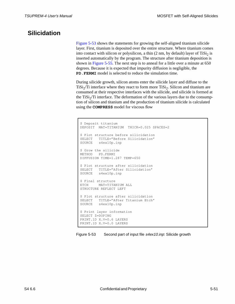
TSUPREM-4 User’s Manual MOSFET with Self-Aligned Silicides
mes
is0
d atp-
Silicidation
Figure 5-53 shows the statements for growing the self-aligned titanium silicidelayer. First, titanium is deposited over the entire structure. Where titanium cointo contact with silicon or polysilicon, a thin (2 nm, by default) layer of TiSi2 isinserted automatically by the program. The structure after titanium depositionshown inFigure 5-55. The next step is to anneal for a little over a minute at 65degrees. Because it is expected that impurity diffusion is negligible, thePD.FERMI model is selected to reduce the simulation time.
During silicide growth, silicon atoms enter the silicide layer and diffuse to theTiSi2/Ti interface where they react to form more TiSi2. Silicon and titanium areconsumed at their respective interfaces with the silicide, and silicide is formethe TiSi2/Ti interface. The deformation of the various layers due to the consumtion of silicon and titanium and the production of titanium silicide is calculatedusing theCOMPRESS model for viscous flow
Figure 5-53 Second part of input file s4ex10.inp: Silicide growth
$ Deposit titaniumDEPOSIT MAT=TITANIUM THICK=0.025 SPACES=2
$ Plot structure before silicidationSELECT TITLE=”Before Silicidation”SOURCE s4ex10p.inp
$ Grow the silicideMETHOD PD.FERMIDIFFUSION TIME=1.287 TEMP=650
$ Plot structure after silicidationSELECT TITLE=”After Silicidation”SOURCE s4ex10p.inp
$ Final structureETCH MAT=TITANIUM ALLSTRUCTURE REFLECT LEFT
$ Plot structure after silicidationSELECT TITLE=”After Titanium Etch”SOURCE s4ex10p.inp
$ Print layer informationSELECT Z=DOPINGPRINT.1D X.V=0.6 LAYERSPRINT.1D X.V=0.0 LAYERS
S4 6.6 Confidential and Proprietary 5-51
Draft 6/26/98

Advanced Examples TSUPREM-4 User’s Manual
ium
The structure after the silicide growth step is shown inFigure 5-56. Observe thatmost of the titanium has been consumed. After removing the remaining titanthe full structure is shown inFigure 5-57.Figure 5-54 Input file se4ex10p.inp: Plotting results
$ Plot sequence for silicidation example$$ To use:$ select title=”Title”$ source s4ex10p.inp$PLOT.2D Scale Y.MAX=0.3COLOR MAT.POLY COLOR=3SELECT Z=LOG10(ARSENIC)FOREACH X ( 15 TO 20 )
CONTOUR VAL=@X COLOR=3 LINE=3ENDCOLOR MAT=TITANIUM COLOR=2COLOR MAT=TISI2 COLOR=6COLOR MAT=OXIDE COLOR=5LABEL X=0.36 Y=-0.23 SIZE=0.3 RECT C.RECT=2 LABEL=”Titanium”LABEL X=0.36 Y=-0.18 Size=0.3 Rect C.RECT=6 LABEL=”TiSi2”LABEL X=0.36 Y=-0.13 SIZE=0.3 RECT C.RECT=3 LABEL=”Polysilicon”LABEL X=0.36 Y=-0.08 Size=0.3 Rect C.RECT=5 LABEL=”Oxide”LABEL X=0.55 Y=0.25 Size=0.3 Line=3 C.LINE=3 LABEL=”Arsenic” RIGHTPLOT.2D ^AX ^CL
Figure 5-55 Structure immediately before silicide growth step
5-52 Confidential and Proprietary S4 6.6
Draft 6/26/98

TSUPREM-4 User’s Manual MOSFET with Self-Aligned Silicides
Figure 5-56 Structure after silicide growth step
Figure 5-57 Final structure, after removal of remaining titanium
S4 6.6 Confidential and Proprietary 5-53
Draft 6/26/98

Advanced Examples TSUPREM-4 User’s Manual
sili-
ter to
ers-
d tose of
g oned by
d to
e
inat-ing.
nting.
icon
Polysilicon Emitter StudyThis example shows a simulation of the emitter region of a double-polysiliconbipolar transistor. The effect of the arsenic out-diffusion from the emitter polycon on the emitter and base widths is shown. The simulations can be used toexamine the dependence of the device performance on the width of the emitstripe. The advanced polysilicon grain-growth and diffusion models are usedsimulate the distribution of arsenic in the emitter.
Process Simulation
Figure 5-58 shows the input files4ex11a.inpfor simulating the emitter region ofthe bipolar transistor. The emitter width is defined by the nameEMITWID. Theinput files4ex11b.inp for simulating the 2-micron emitter is identical except forthe values ofIDENT (which is set to “B”) and the value ofEMITWID which is setto 2.0.
The critical dimensions of the structure are specified by defining the parametEMITSTA, EMITWID, andSPACERWID. The grid spacings are set to give a reasonable compromise between speed and accuracy. Adaptive gridding is useincrease the grid density where the arsenic diffuses to form the emitter; becauthe shallowness of the emitter, the minimum grid spacing for adaptive griddinarsenic is decreased to 0.01 micron. The accuracy of the results can be verifireducing the value ofGRID.FAC for later simulations.
Models Because oxidation-enhanced of transient-enhanced diffusion are not expectebe significant in this structure, thePD.FERMI diffusion model can be used with ashallow simulation structure. Because of the high arsenic concentration in themitter, however, it would be wise to check the results using thePD.FULL modeland a deep simulation structure.
Processing The emitter structure is formed by a series of deposition and etch steps, culming in the deposition of the poly layer in the trench formed by the emitter openThe temperature of the poly deposition is 620°C; this temperature determines theinitial grain size. The emitter is then implanted with arsenic at a 7-degree tilt.Because of the tilt, the right sidewall of the emitter receives more of the impladose than the left sidewall, but much less than the bottom of the emitter openThe arsenic is then diffused throughout the poly and into the single-crystal silwith a high-temperature RTA step.
5-54 Confidential and Proprietary S4 6.6
Draft 6/26/98

TSUPREM-4 User’s Manual Polysilicon Emitter Study
Figure 5-58 Listing of input file s4ex11a.inp for simulating the bipolar emitterstructure
$ Parameters%DEFINE IDENT A%DEFINE EMITSTA 0.5%DEFINE EMITWID 1.0%DEFINE SPACERWID 0.2
$ Half the structureMESH GRID.FAC=1.5
LINE X LOC=0.0 SPACING=0.2LINE X LOC=@EMITSTA+@SPACERWID/2 SPACING=0.05LINE X LOC=@EMITSTA+@EMITWID/2 SPACING=0.15LINE Y LOC=0.0 SPACING=0.025LINE Y LOC=0.1 SPACING=0.025LINE Y LOC=1.0 SPACING=0.1ELIMINATE COLUMNS Y.MIN=0.2ELIMINATE COLUMNS Y.MIN=0.2INITIAL <100> BORON=1E14
METHOD MAT=SILICON IMP=ARSENIC MIN.SPAC=0.01
$ Emitter CutDEPOSIT OXIDE THICK=0.6 DY=0.05ETCH OXIDE RIGHT P1.X=@EMITSTA
$ Dielectric Screening LayersDEPOSIT OXIDE THICK=0.04 SPACES=2DEPOSIT NITRIDE THICK=0.05 SPACES=2
$ SpacerETCH NITRIDE RIGHT P1.X=@EMITSTA+@SPACERWID
$ Oxide dipETCH OXIDE TRAPEZ THICK=0.06 UNDERCUT=0.06
$ Build Full StructureSTRUCTUR REFLECT RIGHT
$ N-polyDEPOSIT POLYSILI THICK=0.22 ARC.SPAC=0.05 DY=0.02 TEMPERAT=620
$ N+ implantIMPLANT DOSE=1.0E+16 ENERGY=50 ARSENIC TILT=7.0
SAVE OUT.FILE=S4EX11@IDENTS1
$ Emitter drive-inDIFFUSIO TEMPERAT=1125. TIME=0.5 NITROGEN
SAVE OUT.FILE=S4EX11@IDENTS2
S4 6.6 Confidential and Proprietary 5-55
Draft 6/26/98

Advanced Examples TSUPREM-4 User’s Manual
the
first
Plotting the Results
The results are now plotted for the following structures:
• After Implant
• Doping and Grain Size
• Doping vs. Stripe Width
After Implant Figure 5-59 shows the layers of the structure and the arsenic concentration inpoly immediately after the implant. This figure and the following figures wereplotted using the input files4ex11c.inp, which illustrates techniques for producingmultiple plots on a single screen and for annotating shaded contour plots. Thepart ofs4ex11c.inp is shown inFigure 5-60.
Figure 5-59 Bipolar emitter structure and as-implanted arsenic profiles, asplotted using s4ex11c.inp
5-56 Confidential and Proprietary S4 6.6
Draft 6/26/98

TSUPREM-4 User’s Manual Polysilicon Emitter Study
r theheolyallson atf the
ngle-
size
Doping andGrain Size
Figure 5-61 shows the total arsenic concentration and the poly grain size afteRTA step. The arsenic concentration is largest at the left and right edges of tstructure, where the initial doping is high and the arsenic is confined to the player by the underlying nitride layer. The concentration is lowest in the sidewof the emitter opening, where the as-implanted doping is low. The concentratithe center of the emitter opening is lower than that at the left and right edges ostructure because of diffusion into the sidewalls of the opening and into the sicrystal silicon. The rate of grain growth during high-temperature processingdepends strongly on the doping concentration; thus the final contours of grainare similar to the final contours of total arsenic concentration.
Figure 5-60 First part of s4ex11c.inp, for plotting the structure and contours ofas-implanted arsenic concentration
$ Parameters for plot size and placement%define YMAX 0.5%define YLEN 5.8%define XOFF1 1.5%define XOFF2 10.8%define LSIZ 0.3%define TSIZ 0.35
$ As-implanted structureinitial in.file=S4EX11AS1
$ Plot structureselect title=”Poly Emitter Width=1.0”plot.2d scale y.max=@YMAX x.off=@XOFF1 y.len=@YLEN + t.siz=@TSIZ x.siz=@LSIZ y.siz=@LSIZcolor poly color=3color oxide color=5color nitride color=4label label=”Poly” c.rect=3 size=0.25 x=0.3 y=0.2label label=”Oxide” c.rect=5 size=0.25 x=0.3 y=0.3label label=”Nitride” c.rect=4 size=0.25 x=0.3 y=0.4plot.2d ^ax ^cl
$ Plot as-imlanted arsenicselect z=log10(arsenic) title=”Arsenic: As-Implanted”plot.2d scale y.max=@YMAX ^cl x.off=@XOFF2 y.len=@YLEN + t.siz=@TSIZ x.siz=@LSIZ y.siz=@LSIZ%define TOP 1E21%define BOTT 1E16%define INC (log10(@TOP)-log10(@BOTT))/10foreach I (0 to 10) color min.value=(log10(@BOTT) + @INC*( I )) + max.value=(log10(@BOTT) + @INC*( I +1)) + color=(18- I ) label rectangle c.recta=(18- I ) c.siz=0.25 + x=(@XOFF2+2.6+0.25*( I )) y=2.5 cmendlabel label=”@BOTT” c.siz=0.2 x=@XOFF2+2.1 y=2.75 cmlabel label=”cm^-3 @TOP” c.siz=0.2 x=@XOFF2+3.5 y=2.75 cmplot.2d ^ax ^cl
S4 6.6 Confidential and Proprietary 5-57
Draft 6/26/98

Advanced Examples TSUPREM-4 User’s Manual
nc-
thean-crys-er
Doping vs.Stripe Width
The depletion of the arsenic in the center of the emitter opening is a strong fution of the width of the emitter stripe.Figure 5-62 compares the net doping for a2-micron emitter stripe with that for a 1-micron stripe. For the 2-micron stripe,doping in the poly across the width of the emitter opening is much higher. It calso be observed that more arsenic has diffused from the poly into the singletal silicon; the 2-micron emitter stripe produces a wider emitter and a narrowbase than the 1-micron emitter stripe.
Figure 5-61 Contours of total arsenic concentration and poly grain size afterRTA
Figure 5-62 Contours of net doping for 1-micron and 2-micron emitter stripes
5-58 Confidential and Proprietary S4 6.6
Draft 6/26/98

APPENDIX A
in. Inde theretionsdee
Appendix A:Default CoefficientsA
Default Coefficient ValuesThis appendix contains the values of the various simulation coefficients usedTSUPREM-4, along with the references from which the values were obtainedsome cases there are also notes regarding the approximations that were mawhen the necessary values had not been experimentally determined, or whenwas wide scatter in the available data. These notes regarding the approximainvolved in the coefficient determination should help you know how much latituis available when modifying these coefficients to match fabrication results. Thunits for the coefficients are given inChapter 3; where a choice of units is avail-able, the default units (i.e., microns and minutes) are used, except as noted.
The notes referenced in this section are described in“Default Coefficient Notes”onPage A-26. They appear in the form “(1),” in which the digit is the number ofthe note in the list of notes.
Tables Page
Impurity Parameters (Silicon Dopants)A-2 Impurity Parameters (Other) A-2Segregation and Transport CoefficientsA-4 Polysilicon Grain Segregation A-6 Clustering and Solid Solubility A-6 Point Defect Parameters A-7 Oxidation A-9 Silicidation A-12 Electrical Parameters A-13 Material Coefficients A-15 Monte Carlo Implant A-17 Numerical Methods A-22 Automatic Grid Generation ParametersA-20Adaptive Grid Parameters A-21
S4 6.6 Confidential and Proprietary A-1
DDraft 6/26/98

Appendix A: Default Coefficients TSUPREM-4 User’s Manual
The references listed in this section are described in“Default Coefficient Refer-ences” on page A-22. They appear in the form “[1],” in which the digit is the num-ber of the reference in the list of references.
Impurity Parameters
Impurity Diffusion Coefficients
Diffusivities are inµm2/min except as noted.
Table A-1 Impurity Parameters (Silicon Dopants)
Boron Phosphorus Arsenic Antimony
TIF.NAME B P As Sb
Type ACCEPTOR DONOR DONOR DONOR
Implant table chboron dual.pho dual.ars antimony
AT.NUM 5.0 15.0 33.0 51.0
AT.WT 10.8 30.97 74.91 121.76
Table A-2 Impurity Parameters (Other)
Aluminum Nitrogen Silicon
TIF.NAME Al N Si
AT.NUM 13.0 7.0
AT.WT 26.98 14.01
Table A-3 Impurity Diffusion Coefficients
Boron Phosphorus Arsenic Antimony
Silicon (1)DIP.0 4.10e9 [1] 0 [1]0000 0 [2]00 0 [1]DIP.E 3.46 0 .00 0.000 00000
DIX.0 2.11e8 2.31e10 1.37e7 00 6.420e7
DIX.E 3.46 3.66 3.44 3.65
DIM.0 0/00 2.664e10 3.72e10 4.50e9
DIM.E 0.00 4.0 0 4.15 4.08
DIMM.0 0.00 2.652e11 0 .00 000
DIMM.E 0.00 4.37 0 .00 000
DVP.0 2.16e8 0 .00 0.00 000
DVP.E 3.46 0 .00 0.00 000
DVX.0 1.11e7 0 .00 5.47e7 1.220e9
DVX.E 3.46 3.66 3.44 3.65
DVM.0 0.00 0.00 1.49e11 8.55e10
DVM.E 0.00 4.0 0 4.15 4.08
DVMM.0 0.00 0.00 0.00 000
DVMM.E 00.0 4.37 0 .00 000
Oxide [3] (2)DIX.0 1.896e6 4.338e10 1.05e10 7.86e25
DIX.E 3.53 4.44 4.89 8.75
A-2 Confidential and Proprietary S4 6.6
Draft 6/26/98

TSUPREM-4 User’s Manual Default Coefficient Values
Polysilicon (grain interior) (diffusivities in cm 2/sec) (3)DIP.0 0.72 0 ..00 0.00 0.00
DIP.E 3.46 0 .00 0.00 0.00
DIX.0 0.037 3.85 1.14e-2 0.214
DIX.E 3.46 3.66 3.44 3.65
DIM.0 0.00 4.44 31.0 00 15.0 00
DIM.E 0.00 4.0 0 4.15 4.08
DIMM.0 0.00 44.2 00 7.17e3 0 00
DIMM.E 0.00 4.37 5.21 0 00
Polysilicon (grain boundaries) (diffusivities in cm 2/sec) (4)DIX.0 420. 6.0e3 110.0 000 2.14e3
DIX.E 3.46 3.66 3.53 3.65
DIM.0 0.00 0.00 10.0 00 000
DIM.E 0.00 0.00 3.53 0 00
TiSi2 (diffusivities in cm 2/sec)
DIX.0 6.0e-7 4.6e-6 4.0e-7 7.0e-8 0
DIX.E 2.0 2.0 0 1.8 1.8
WSi2 (diffusivities in cm 2/sec) (5) [4]- [7]
DIX.0 1.0e-5 4.20e-2 2.60e-2 2.60e-2 0
DIX.E 1.17 2.14 2.11 2.11
Ambient (6)DIX.0 1e13 0 1e13 . 5e13 5e13 .DIX.E 3.5 00 3.5 0 3.95 3.95
Table A-4 Other Impurities and Materials
DIP.0 0
DIP.E 0
DIX.0 0
DIX.E 0
DIM.0 0
DIM.E 0
DIMM.0 0
DIMM.E 0
Table A-5 Pair Kinetics Parameters (all impurities; CM.SEC units) (7)
DIPAIR.0 3.65e-4 00
DIPAIR.E 1.58
DVPAIR.0 3.65e-4
DVPAIR.E 1.58
R.I.S 10000
E.I.S 000
R.V.S 10000
E.V.S 000
Table A-3 Impurity Diffusion Coefficients
Boron Phosphorus Arsenic Antimony
S4 6.6 Confidential and Proprietary A-3
DrafDraft 6/26/98 6/

Appendix A: Default Coefficients TSUPREM-4 User’s Manual
Segregation and Transport Coefficients
R.IP.V 10000
E.IP.V 000
R.VP.I 10000
E.VP.I 000
Table A-5 Pair Kinetics Parameters (all impurities; CM.SEC units) (7)
Table A-6 Segregation Coefficients
Boron Phosphorus Arsenic Antimony
Silicon/oxideSEG.0 1.126e3 [8] 30.0 [9] (8) 30.0 [9]0 30.0 [9]SEG.E 0.91 000 0.00 0.0 0.0
Polysilicon/oxide (9)SEG.0 1.126e3 30.00 30.0 0 30.0 0
SEG.E 0.91 00 0.0 0.0 0.0
Silicon/TiSi 2
SEG.0 0.3 000 1.0 0.8 0 0.8
SEG.E 0000.0 0.0 0.0 0.0
Polysilicon/TiSi 2
SEG.0 0.3 000 1.0 0.8 0.8
SEG.E 000.00 0.0 0 .0 0.0
Silicon/WSi 2 [4]- [7]
SEG.0 1.0 000 5.0 10.0 0 10.0
SEG.E 0000.0 0.0 0.0 0..0
Polysilicon/WSi 2
SEG.0 1.0 000 5.0 10.0 0 10.0
SEG.E 0000.0 0.0 0.0 00
Other Impurities and Pairs of MaterialsSEG.0 1.0 000 00 00 00
SEG.E 000000 00 00 00
Table A-7 Interface Transport Coefficients
Boron Phosphorus Arsenic Antimony
Silicon/ambient [10] (10)TRANS.0 1.674e7 9.0e5 9.0e5 1.5e3
TRANS.E 2.481 1.99 1.99 1.04
Oxide/ambient (11)TRANS.0 1.647e7 9.0e5 9.0e5 1.5e3
TRANS.E 2.481 1.99 1.99 1.04
Polysilicon/ambient (11)TRANS.0 1.674e7 9.0e5 9.0e5 1.5e3
TRANS.E 2.481 1.99 1.99 1.04
Polysilicon/silicon (12)TRANS.0 100. 000 100. 00 100. 000 100. 000
TRANS.E 0.0 0.0 0.00 0.0
A-4 Confidential and Proprietary S4 6.6
Draft 6/26/98

TSUPREM-4 User’s Manual Default Coefficient Values
Silicon/TiSi 2
TRANS.0 1.0e6 1.0e6 1.0e6 1.0e6
TRANS.E 2.0 2.0 2.0 2.0
Polysilicon/TiSi 2
TRANS.0 1.0e6 1.0e6 1.0e6 1.0e6
TRANS.E 2.0 2.0 2.0 2.0
Silicon/WSi 2 [4]-[7]
TRANS.0 2.0e-2 3.0e-3 3.0e-3 3.0e-3
TRANS.E 0.0 0.0 0.0 0.0
Polysilicon/WSi 2
TRANS.0 2.0e-2 3.0e-3 3.0e-3 3.0e-3
TRANS.E 2.0 2.0 2.0 2.0
Table A-8 All Impurities
Silicon/Oxide, and Polysilicon/Oxide
TRANS.0 0.1
TRANS.E 0.0
All Materials with Nitride and Oxynitride
TRANS.0 0.0
TRANS.E 0.0
Table A-7 Interface Transport Coefficients
Boron Phosphorus Arsenic Antimony
Table A-9 Interface Trap Impurities ( CM.SEC units)
Boron (13) Phosphorus (14) Arsenic (15)
Oxide/Silicon, and Oxide/PolysiliconTRANS.0 0.166 7.15 0.231
TRANS.E 0.486 1.75 0.766
SEG.0
SEG.E /SEG.E - SEG.E(Table A-5)
RATIO.0 0 0 0
RATIO.E 0 0 0
/TRANS.0 0.0166 0.715 0.0231 [12]/TRANS.E 0.486 1.75 0.766 [12]/SEG.0 5.96E3
/SEG.E /RATIO.E - Q.MAX.E -0.285
/RATIO.0 0.178 4.00E-3 6.29E-5
/RATIO.E -0.086 -0.37 -0.738
Q.INI.0 0 0 0
Q.INI.E 0 0 0
Q.MAX.0 2.0E14 [12] 6.8E14 [11] 2.0E14 [12]Q.MAX.E 0 0 0
/SEG.0 SEG.0 (Table A-5)÷
/RATIO.0 Q.MAX.0 Css×÷
S4 6.6 Confidential and Proprietary A-5
DrafDraft 6/26/98 6/

Appendix A: Default Coefficients TSUPREM-4 User’s Manual
Polysilicon Grain Segregation
Clustering and Solid Solubility
Table A-10 Parameters for Polysilicon Grain Interior/Boundary Segregation (16)
Boron Phosphorus Arsenic Antimony
Q.SITES 2.5e15 2.5e15 2.5e15 2.5e15
CG.MAX 5.0e22 5.0e22 5.0e22 5.0e22
GSEG.0 12.0 0 1.25 0.6 1.0
GSEG.E 0.0 0.443 0.414 0 .0
GSEG.INI 1.0 0 1.0 1.0 1.0
VELIF.0 1.0e7 1.0e7 1.0e7 1.0e7
VELIF.E 3.0 3.0 3.0 3.0
Polysilicon diffusivity enhancement factors (17)FGB 2.64 95.1 0 0110. 0000 41.8 0
Table A-11 Coefficients for Clustering in Silicon (18)
Arsenic
CTN.0 0 1.03103e-17 [1]CTN.E -0.4 (19)00000
CTN.F 4.0 0000 00000
Table A-12 Solid Solubility in Silicon
Temperature (˚C) Boron Phosphorus Antimony
650 1.70e19 [13] 1.20e20 [14] 1.70e19 [14]700 1.70e19 1.20e20 1.70e19
800 4.40e19 2.90e20 2.30e19
900 9.50e19 6.00e20 3.10e19
1000 1.70e20 1.00e21 4.00e19
1100 2.20e20 1.20e21 4.90e19
1200 2.20e20 1.25e21 5.90e19
1300 1.40e20 1.10e21 6.80e19
1350 1.40e20 1.10e21 6.80e19
Table A-13 Transient activation parameters (Extended Defects AAM)
Boron Phosphorus Arsenic Antimony
T.ACT.0 8.0e-16 8.0e-16 8.0e-16 8.0e-16
T.ACT.E -4.2 -4.2 -4.2 -4.2
ACT.MIN 1.0 2.0 1.0 1.0
CL.INI.A true true true true
A-6 Confidential and Proprietary S4 6.6
Draft 6/26/98

TSUPREM-4 User’s Manual Default Coefficient Values
Point Defect Parameters
Table A-14 Point Defect Parameters in Silicon ( CM.SEC units) [15]
Vacancy Interstitial
D.0 3.65e-4 3.65e-4
D.E 1.58 1.58
KB.0 (20)00000 1.0e-21
KB.E -1.0 (21)CEQUIL.0 1.25e29 1.25e29
CEQUIL.E 3.26 3.26
VMOLE 0.0 0 5.0e22
DNEG.0 32.47 0 0.00
DNEG.E 0.62 0 .00
NEG.0 5.68 5.68
NEG.E 0.145 0.50
NEU.0 1.0 0 1.0 0
NEU.E 00 00
POS.0 5.68 5.68
POS.E 0.455 0.26
DPOS.0 0.00 0.00
DPOS.E 0.00 0.00
Table A-15 Interface Injection/Recombination Model
Model V.NORM.0 V.NORM.E
Vacancies V.MAXOX
Interstitials V.NORM 1.0 0.0
Table A-16 Vacancy Parameters at Interfaces With Silicon ( CM.SEC units)
Oxide [15] Nitride Oxynitride Ambient TiSi2/WSi2
KSURF.0 4.0e-11 3.5e-3 0.1 2.5e-4 4.0e-10 0
KSURF.E -1.75 0.0 0.0 0.0 -1.75
KSVEL.0 4.0e-11 3.5e-3 0.1 2.5e-4 4.0e-10 0
KSVEL.E -1.75 0.0 0.0 0.0 -1.75
GROWTH false false false false false
A.0 0.0 0.0 0.0 0.0 0.0
A.E 0.0 0.0 0.0 0.0 0.0
T0.0 100.02 0 100.02 0 100.02 0 100.02 0 100.02 0
T0.E 0.0 0.0 0.0 0.0 0.0
GPOW.0 0.0 0.0 0.0 0.0 0.0
GPOW.E 0.0 0.0 0.0 0.0 0.0
KPOW.0 0.5 0.5 0.5 0.5 0.5
KPOW.E 0.0 0.0 0.0 0.0 0.0
THETA.0 0.0 0.0 0.0 0.0 0.0
THETA.E 0.0 0.0 0.0 0.0 0.0
S4 6.6 Confidential and Proprietary A-7
DrafDraft 6/26/98 6/

Appendix A: Default Coefficients TSUPREM-4 User’s Manual
Table A-17 Interstitial Parameters at Interfaces With Silicon ( CM.SEC units)
Oxide [16] (22) Nitride Oxynitride Ambient TiSi2/WSi2
KSURF.0 1.4e-6 3.5e-3 0.1 2.5e-4 4.0e-10
KSURF.E -1.75 0.0 0.0 0.0 -1.75
KSVEL.0 0.0 3.5e-3 0.1 2.5e-4 0 0.0
KSVEL.E -1.75 0.0 0.0 0.0 -1.75
GROWTH true false false false false
A.0 0.0 0.0 0.0 0.0 0.0
A.E 0.0 0.0 0.0 0.0 0.0
T0.0 0.0 100.02 0 100.02 0 100.02 0 100.02 0
T0.E 0.0 0.0 0.0 0.0 0.0
GPOW.0 -0.7 0 0.0 0.0 0.0 0.0
GPOW.E 0.0 0.0 0.0 0.0 0.0
KPOW.0 0.0 0.5 0.5 0.5 0.5
KPOW.E 0.0 0.0 0.0 0.0 0.0
THETA.0 0.01 0.0 0.0 0.0 0.0
THETA.E 0.0 0.0 0.0 0.0 0.0
Table A-18 Point Defect Parameters at Silicon/Polysilicon Interfaces(CM.SEC units) (23)
Interstitial Vacancy
KSURF.0 2.73 6.4e-5
KSURF.E 1.37 0.92
Table A-19 Interstitial Traps Parameters
TRAP.CON 0.0
F.TRAP.0 0.0
F.TRAP.E 0.0
K.TRAP.0 0.0
K.TRAP.E 0.0
Table A-20 Interstitial Clustering Coefficients (24)
CL.KFC.0 5.207e14
CL.KFC.E 3.774
CL.CF 0.9398
CL.IFC 1.
CL.ISFC 1.000
CL.KFI.0 00000
CL.KFI.E 3.774
CL.IFI 2.000
CL.ISFI 2.000
CL.KR.0 9.431e13
CL.KR.E 3.017
CL.CR 1.000
A-8 Confidential and Proprietary S4 6.6
Draft 6/26/98

TSUPREM-4 User’s Manual Default Coefficient Values
Oxidation
KLOOP.0 29.8047 [18]KLOOP.E 0.4 0 [19]
Table A-20 Interstitial Clustering Coefficients (24)
Table A-21 Ambient Definitions
DRYO2 WETO2 STREAM INERT
F.O2 1.0 0.0 00000 0.0 0.0
F.H2O 0.0 0.92 [20] (26) 1.0 0.0
F.H2 0.0 0.0 00000 0.0 0.0
F.N2 0.0 0.08 0000 0.0 1.0
F.HCL 0.0 0.0 00000 0.0 0.0
PRESSURE 1.0 1.0 00000 1.0 1.0
HCL (%) 0.0 0.0 00000 0.0 0.0
Table A-22 Linear Oxidation Rate Coefficients
O2 H2O
L.LIN.0
<111> 1.038e5 [20] 3.450e4 [21]<110> 8.650e4 (26) 2.870e4 (26)<100> 6.176e4 00000 2.058e4 00000
POLYSILI 8.650e4 (27) 2.870e4 (27)L.LIN.E
<111> 2.0 000000000 1.60 00000000
<110> 2.0 000000000 1.60 00000000
<100> 2.0 000000000 1.60 00000000
POLYSILI 2.0 000000000 1.60 00000000
H.LIN.0
<111> 1.038e5 00000 2.950e6 00000
<110> 8.650e4 0(26)00 2.457e6 0(26)<100> 6.176e4 00000 1.755e6 00000
POLYSILI 8.650e4 (27) 2.457e6 (27)H.LIN.E
<111> 000 2.0 2.05 00000000
<110> 000 2.0 2.05 00000000
<100> 000 2.0 2.05 00000000
POLYSILI 2.0 2.05 00000000
LIN.BREA 0.0 900.0 000000000
LIN.PDEP 0.75 1.0 000000000
GAMMA.0 [22] 2.63e3 2.63e3 000000
GAMMA.E00 1.1 1.1 000000000
S4 6.6 Confidential and Proprietary A-9
DrafDraft 6/26/98 6/
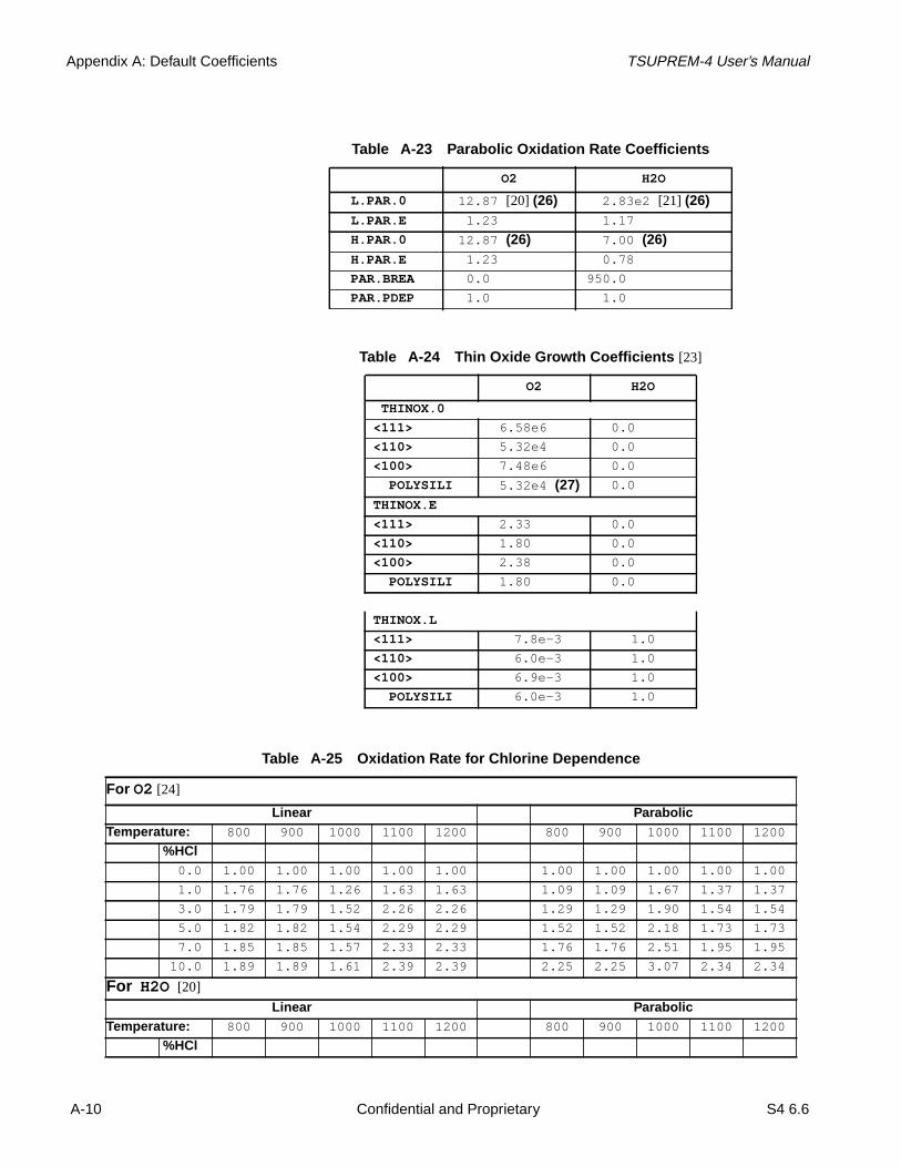
Appendix A: Default Coefficients TSUPREM-4 User’s Manual
Table A-23 Parabolic Oxidation Rate Coefficients
O2 H2O
L.PAR.0 12.87 [20] (26) 2.83e2 [21] (26)L.PAR.E 1.23 0000000 1.17 00000000
H.PAR.0 12.87 (26)00 7.00 (26)000
H.PAR.E 1.23 0000000 0.78 00000000
PAR.BREA 0.0 00000000 950.0 000000
PAR.PDEP 1.0 00000000 1.0 000000000
Table A-24 Thin Oxide Growth Coefficients [23]
O2 H2O
THINOX.0
<111> 6.58e6 0.0
<110> 5.32e4 0.0
<100> 7.48e6 0.0
POLYSILI 5.32e4 (27) 0.0
THINOX.E
<111> 2.33 0 0.0
<110> 1.80 0 0.0
<100> 2.38 0 0.0
POLYSILI 1.80 0 0.0
THINOX.L
<111> 007.8e-3 0 1.0
<110> 006.0e-3 0 1.0
<100> 006.9e-3 0 1.0
POLYSILI 006.0e-3 0 1.0
Table A-25 Oxidation Rate for Chlorine Dependence
For O2 [24]
Linear ParabolicTemperature: 800 900 1000 1100 1200 800 900 1000 1100 1200
%HCl00.0 1.00 1.00 1.00 1.00 1.00 1.00 1.00 1.00 1.00 1.00
01.0 1.76 1.76 1.26 1.63 1.63 1.09 1.09 1.67 1.37 1.37
03.0 1.79 1.79 1.52 2.26 2.26 1.29 1.29 1.90 1.54 1.54
05.0 1.82 1.82 1.54 2.29 2.29 1.52 1.52 2.18 1.73 1.73
07.0 1.85 1.85 1.57 2.33 2.33 1.76 1.76 2.51 1.95 1.95
10.0 1.89 1.89 1.61 2.39 2.39 2.25 2.25 3.07 2.34 2.34
For H2O [20]
Linear ParabolicTemperature: 800 900 1000 1100 1200 800 900 1000 1100 1200
%HCl
A-10 Confidential and Proprietary S4 6.6
Draft 6/26/98

TSUPREM-4 User’s Manual Default Coefficient Values
00.0 1.00 1.00 1.00 1.00 1.00 1.00 1.00 1.00 1.00 1.00
01.0 1.00 1.00 1.00 1.00 1.00 1.00 1.00 1.00 1.00 1.00
03.0 1.00 1.00 1.00 1.00 1.00 1.00 1.00 1.00 1.00 1.00
05.0 1.00 1.00 1.00 1.00 1.00 1.00 1.00 1.00 1.00 1.00
07.0 1.00 1.00 1.00 1.00 1.00 1.00 1.00 1.00 1.00 1.00
10.0 1.00 1.00 1.00 1.00 1.00 1.00 1.00 1.00 1.00 1.00
Table A-25 Oxidation Rate for Chlorine Dependence
For O2 [24]
Table A-26 Coefficients for Analytical Oxidation Models
INITIAL 0000.002
MASK.EDG -200.0
SPREAD 001.0
NIT.THIC (no default)
ERF.Q [25] 0000.05
ERF.DELT [25] 0000.04
ERF.LBB [25] 00 8.25e-3*( 1580.3 - TOX )*( FOX^0.67 )*( EOX^0.3 )*exp( -( ( EN - 0.08 )^2 )/0.06 )
ERF.H [25] 402*( 0.445 - 1.75*EN )*exp( -TOX/200 )
Table A-27 Coefficients for Numerical Oxidation Models
O2 H2O
HENRY.CO 05.0e16 03.0e19
TRANS.0 (28) 1.0e3 1.0e6
THETA (29) 02.2e22 02.2e22
Table A-28 Diffusivity of Oxidizing Species in Ambient (6)
O2 H2O
D.0 03.5e9 002.5e7
D.E 1.25 0.8
Table A-29 Parameters for Stress-Dependent Oxidation
STRESS.D true
VC 300.0 (oxide), 130.0 (nitride) (30)VR 015 [36]VD 075.0 [36]VT 000.0
VDLIM 001.2
S4 6.6 Confidential and Proprietary A-11
DrafDraft 6/26/98 6/
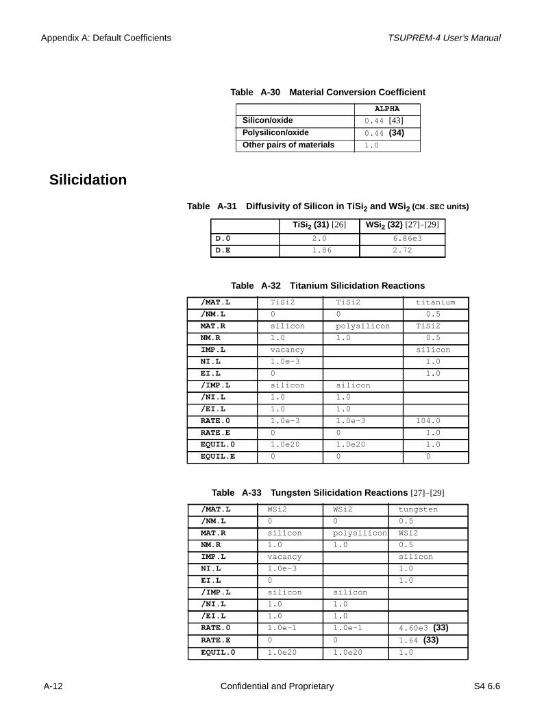
Appendix A: Default Coefficients TSUPREM-4 User’s Manual
Silicidation
Table A-30 Material Conversion Coefficient
ALPHA
Silicon/oxide 0.44 [43]Polysilicon/oxide 0.44 (34)Other pairs of materials 1.0 00000
Table A-31 Diffusivity of Silicon in TiSi 2 and WSi 2 (CM.SEC units)
TiSi2 (31) [26] WSi2 (32) [27]- [29]
D.0 2.0 006.86e3
D.E 01.86 2.72
Table A-32 Titanium Silicidation Reactions
/MAT.L TiSi2 TiSi2 titanium
/NM.L 00 00 0.5
MAT.R silicon polysilicon TiSi2
NM.R 1.0 1.0 0.5
IMP.L vacancy silicon
NI.L 1.0e-3 1.0
EI.L 00 1.0
/IMP.L silicon silicon
/NI.L 1.0 1.0
/EI.L 1.0 1.0
RATE.0 1.0e-3 1.0e-3 104.0
RATE.E 00 00 001.0
EQUIL.0 1.0e20 1.0e20 001.0
EQUIL.E 00 00 0
Table A-33 Tungsten Silicidation Reactions [27]- [29]
/MAT.L WSi2 WSi2 tungsten
/NM.L 000 000 0.5
MAT.R silicon polysilicon WSi2
NM.R 1.0 1.0 0.5
IMP.L vacancy silicon
NI.L 1.0e-3 1.0
EI.L 000 1.0
/IMP.L silicon silicon
/NI.L 1.0 1.0
/EI.L 1.0 1.0
RATE.0 1.0e-1 1.0e-1 4.60e3 (33)RATE.E 000 000 1.64 (33)EQUIL.0 1.0e20 1.0e20 1.0 0
A-12 Confidential and Proprietary S4 6.6
Draft 6/26/98

TSUPREM-4 User’s Manual Default Coefficient Values
Electrical Parameters
EQUIL.E 000 000 000
Table A-33 Tungsten Silicidation Reactions [27]- [29]
Table A-34 Critical Electric Field (volts/cm) [30] [31]
ECN.MU 6.49e4
ECP.MU 1.87e4
Table A-35 Surface Mobility Degradation Factor
GSURFN 1.0
GSURFP 1.0
Table A-36 Arora Mobility Model [32]
MUN1 88.0 0
MUN2 1252.0 000
AN 0 0.88
CN 0001.26e17
EXN1 0-0.57 0
EXN2 0 -2.33 0
EXN3 0 2.4 0
EXN4 -0.146
MUP1 0 54.3 0
MUP2 407.0 0
AP 00 0.88
CP 0002.35e17
EXP1 00-0.57
EXP2 00-2.23
EXP3 00 2.4
EXP4 -0.146
Table A-37 Caughey Mobility Model [33]
MUN.MIN 55.24
MUN.MAX 1429.23 00
NREFN 0001.072e17
NUN -2.3 0
XIN -3.8 0
ALPHAN 0 0.733
MUP.MIN 049.705
MUP.MAX 479.37 0
NREFP 0001.606e17
NUP -2.2 0
S4 6.6 Confidential and Proprietary A-13
DrafDraft 6/26/98 6/

Appendix A: Default Coefficients TSUPREM-4 User’s Manual
XIP -3.7 0
ALPHAP 00.70
Table A-38 Mobility Table
Concentration Mobility at 300K
(#/cm3) Electron Hole
1e14 1350 495
2e14 1345 495
4e14 1335 495
6e14 1320 495
8e14 1310 495
1e15 1300 491.1
2e15 1248 487.3
4e15 1200 480.1
6e15 1156 473.3
8e15 1115 466.9
1e16 1076 460.9
2e16 960 434.8
4e16 845 396.5
6e16 760 369.2
8e16 720 348.3
1e17 675 331.5
2e17 524 279.0
4e17 385 229.8
6e17 321 203.8
8e17 279 186.9
1e18 252 178.0
2e18 182.5 130.0
4e18 140.6 90.0
6e18 113.6 74.5
8e18 99.5 66.6
1e19 90.5 61.0
2e19 86.9 55.0
4e19 83.4 53.7
6e19 78.8 52.9
8e19 71.6 52.4
1e20 67.8 52.0
2e20 52.0 50.8
4e20 35.5 49.6
6e20 23.6 48.9
8e20 19.0 48.4
1e21 17.8 48.0
Table A-37 Caughey Mobility Model [33]
A-14 Confidential and Proprietary S4 6.6
Draft 6/26/98

TSUPREM-4 User’s Manual Default Coefficient Values
Material Coefficients
Table A-39 Semiconductor Material Coefficients
Silicon Polysilicon (34) SiC (35)
DENSITY 2.33 0000000 2.33 000000 3.21
AT.NUM 14.0 000000000 14.0 0000000 10.0
AT.WT 28.069 0000000 28.069 0000000 20.04
MOL.WT 28.069 0000000 28.069 0000000 40.08
POLYCRYS false true
NI.0 3.87e16 [34] 3.87e16 00
NI.E 0.605 000000 0.605 00000
NI.F 1.5 00000000 1.5 0000000
YOUNG.M 1.87e12 [36] 1.87e12 [36]POISS.R 0.28 0000000 0.28 0000000
VISC.0 1.0e30 000000 1.0e16 00000
VISC.E 0.0 00000000 0.0 00000000
VISC.X 0.499 000000 0.499 000000
EPSILON 11.7 [36]0000 11.7 000000000
E.FIELD true true
AFFINITY 4.17 00000000 4.17 0000000
BANDGAP 1.08 00000000 1.08 0000000
N.CONDUC 2.82e19 00000 2.82e19 0000
N.VALENC 1.04e19 00000 1.04e19 0000
G.DONOR 2.0 000000000 2.0 00000000
E.DONOR 0.049 0000000 0.049 000000
G.ACCEP 4.0 000 4.0 0000
E.ACCEP 0.045 0 0.045 00
BOLTZMAN false false
IONIZATI true true
QM.BETA 4.1e-8 4.1e-8 0
QM.YCRIT 25e-8 25e-8
TIF.NAME Si Poly SiC
MD.INDEX 100000 3000000
ION.PAIR true true
IP.OMEGA 6.0 00 6.0 000
CL.MODEL true
S4 6.6 Confidential and Proprietary A-15
DrafDraft 6/26/98 6/

Appendix A: Default Coefficients TSUPREM-4 User’s Manual
Table A-40 Polycrystalline Material Coefficients (36)
Polysilicon
F11 1.0
F22 2.0
G.DENS 2.0
GRASZ.0 0.1
GRASZ.E 0.0
TEMP.BRE 600. 000
MIN.GRAI 0.005
FRAC.TA 0.5
GEOM 6.0
GAMMA.0 0005.6e-6
GAMMA.E 00-1.73 00
GBE.0 0000 0.39125
GBE.H 3.0
GBE.1 0.0
ALPHA 01.33
DSIP.0 30.0 0
DSIP.E 05.09
DSIX.0 000.015
DSIX.E 03.89
DSIM.0 16.0 0
DSIM.E 04.54
DSIMM.0 166.7 00
DSIMM.E 5.0
NSEG 2.0
TBU.0 1.0
TBU.E -5.0 0
TOXIDE 0000.0005
DLGX.0 000
DLGX.E 04.4 0
EAVEL.0 000
EAVEL.E 3.0
A-16 Confidential and Proprietary S4 6.6
Draft 6/26/98

TSUPREM-4 User’s Manual Default Coefficient Values
D
D
A
A
M
P
Y
P
E
W
T
M
IM
Table A-41 Insulator Material Coefficients
Oxide Nitride Oxynitride Ambient
DENSITY 2.235 3.44 2.235
AT.NUM (avg) 10.0 000 10.0 00 10.0 00
AT.WT (avg) 20.023 0 20.030 20.023
MOL.WT 60.069 0 140.21 00 60.069
POLYCRYS false false false
YOUNG.M 6.6e11 [36] 003.89e12 03.89e12
POISS.R 0.17 [36] 0.3 00 0.3 0
VISC.0 5.25e4 (37) 001.3e6 (37) 01.3e6 (37) 1.0e9 (38)VISC.E -2.42 (37) 0-2.42 (37) -2.42 (37) 0.0 0 (38)VISC.X 0.499 0 0.499 00.499 0.3 0 (38)EPSILON 03.9 [37] 007.5 [38] 7.5 0 1.0 000000
TIF.NAME Ox0000 Nit OxyNit Ambient
MD.INDEX -1 000000 -2 00000 -6 0000 -4 00000000
IMPL.TAB oxide nitride oxide
Table A-42 Other Material Coefficients
Aluminum Photoresist Titanium TiSi2 Tungsten WSi2
Y.DEFAU 0.025 0 0.02 000
ENSITY 02.702 0 1.06 0 4.5 4.0443 19.3 000000 9.857 00
T.NUM 13.0 0 2.875 22.0 0 16.67 000 74.0 000000 34.0 00000
T.WT 26.98 5.125 47.90 34.68 000 183.85 00000 80.0 00000
OL.WT 26.98 41.0 000 47.90 104.038 000 183.85 00000 240.0 000000
OLYCRYS false false false false
OUNG.M 01.0e13 1.0e13 3.66e12 1.0e11 0
OISS.R 0.3 0.3 000 0.29592 0.29592
PSILON 1.0 1.0 0
ORKFUNC 4.1 04.80 4.8 000 4.80 000 4.80 000
IF.NAME Al Photo Ti TiSi2 W WSi2
D.INDEX -5 000 -4 000 -5 000 -5 00000 -5 -5
PL.TAB aluminum az-7500 titanium tisi2 tungsten wsi2
Table A-43 Linear Coefficients of Thermal Expansion
Silicon 3.052e-6 + 2*6.206e-10*( T - 293 )
Oxide 1.206e-7 + 2*2.543e-10*( T - 293 )
Nitride 3.0e-6
Aluminum 2.438e-5 + 2*6.660e-9*( T - 293 )
Other materials 0.0
S4 6.6 Confidential and Proprietary A-17
DrafDraft 6/26/98 6/

Appendix A: Default Coefficients TSUPREM-4 User’s Manual
Monte Carlo Implant
Table A-44 Electronic Stopping Power Pre-factor
Boron Phosphorus Arsenic Antimony Aluminum OtherES.RAND (39)
Silicon 2.0799 [39] 2.5 000 1.7941 1.7456 0 0
Polysilicon 2.0799 1.7516 1.7941 1.7456 0 0
Oxide 1.8424 1.4609 1.4347 1.3674 0 0
Oxynitride 1.8424 1.4609 1.4347 1.3674 0 0
Nitride 1.8424 1.4609 1.4347 1.3674 0 0
Aluminum 2.0281 1.6857 1.7104 1.6564 0 0
Photoresist 1.0032 00.64016 0.5517 0.4957 0 0
SiC 1.1588 0 0 0 1.4341 0
Other (40) 0.7516 0.7516 0.7516 0
ES.100 [40]- [42]Silicon 1.500 0 1.7516 1.7941 1.7456 0 0
Other 0 0.7516 0.7516 0.7516 0 0
ES.110
Silicon 0.95 000 1.7516 1.7941 1.7456 0
Other 0 0.7516 0.7516 0.7516 0 0
Table A-45 Electronic Stopping Power Exponent
Boron Phosphorus Arsenic Antimony Aluminum OtherES.F.RAN
Silicon 0.5 0.5 0.5 0.5 0.5 0.5
Other 0.5 0.5 0.5 0.5 0.5 0.5
ES.BREAK (41)Silicon 400 150 5000 0 0 0
Polysilicon 400 150 5000 0 0 0
Oxide 400 150 5000 0 0 0
Oxynitride 400 150 5000 0 0 0
Nitride 400 150 5000 0 0 0
Aluminum 400 150 5000 0 0 0
Photoresist 400 150 5000 0 0 0
SiC 600 0 0 0 1000 0
Other 0 0 0 0 0 0
ES.F.H
Silicon 0.1 0.4 1.0 0.5 0.5 0.5
Polysilicon 0.1 0.4 1.0 0.5 0.5 0.5
Oxide 0.1 0.4 1.0 0.5 0.5 0.5
Oxynitride 0.1 0.4 1.0 0.5 0.5 0.5
Nitride 0.1 0.4 1.0 0.5 0.5 0.5
Aluminum 0.1 0.4 1.0 0.5 0.5 0.5
Photoresist 0.1 0.4 1.0 0.5 0.5 0.5
SiC 0.1 0.5 0.5 0.5 0.3 0.5
Other 0.5 0.5 0.5 0.5 0.5 0.5
A-18 Confidential and Proprietary S4 6.6
Draft 6/26/98

TSUPREM-4 User’s Manual Default Coefficient Values
Numerical Methods
Boron Phosphorus Arsenic Antimony Aluminum OtherES.F.100
Silicon 0.5 0.5 0.5 0.5 0.5
Other 0.5 0.5 0.5 0.5 0.5
ES.F.110
Silicon 0.5 0.5 0.5 0.5 0.5
Other 0.5 0.5 0.5 0.5 0.5
Table A-45 Electronic Stopping Power Exponent
Table A-46 Improved Electronic Stopping Power Model (Silicon)
Boron Phosphorus Arsenic Antimony
NLOC.PRE 0.3 0.3 0.3 0.3
NLOC.EXP 0.2 0.2 0.2 0.2
NLOC.MAX 0.6 0.6 0.6 0.6
NLOC.K 1.2 1.2 1.2 1.2
LOC.FAC 0.8 0.8 0.8 0.8
CHAN.CRI 11.54 11.54 11.54 11.54
CHAN.FAC 2.0 2.0 2.0 2.0
DISP.FAC 0.5 0.5 0.5 0.5
Table A-47 Improved Electronic Stopping Power Model (SiC)
Boron Phosphorus Aluminum Nitrogen
NLOC.PRE 1.0 0.8 0.825 0.9
NLOC.EXP 0 0 0 0
NLOC.MAX 1.0 0.6 1.0 0.6
NLOC.K 1.25 1.2 1.05 1.2
LOC.FAC 0.8 0.8 0.8 0.8
CHAN.CRI 11.54 11.54 11.54 11.54
CHAN.FAC 2.0 2.0 2.0 2.0
DISP.FAC 0.5 0.5 0.5 0.5
Table A-48 Block Solution Parameters
Impurities Point Defects Oxidant TrapsREL.ERR 0.01 0.01 0.01 0.01
ABS.ERR 01.0e9 01.0e5 01.0e9 01.0e9
Factoring TIME.STE TIME.STE TIME.STE TIME.STE
SYMMETRY false false false false
Fill PART FULL PART NONE
Block solve LU LU LU LU
S4 6.6 Confidential and Proprietary A-19
DrafDraft 6/26/98 6/

Appendix A: Default Coefficients TSUPREM-4 User’s Manual
Automatic Grid Generation Parameters
Table A-49 System Solution Parameters
MIN.FILL true
MIN.FREQ 1.1 00
MF.METH 1
MF.DIST 0.5
System solve CG
BACK 18
BLK.ITLI 20
Integration TRBDF
INIT.TIM 0.002
Table A-50 Models
Oxidation VERTICAL
Point defect PD.FERMI
Bulk recombination KB.LOW
SKIP.SIL true
OX.REL 1.0e-6
CONTIN.M 2
VE.SMOOT 0.04 00
V.COMPAT current version
Table A-51 Program Options
INFORMAT false
DIAGNOST false
ECHO true
EXECUTE true
Output NORMAL
Table A-52 Automatic Grid Generation Parameters
DX.MIN 0.2
DX.MAX 0.5
DX.RATIO 1.5
DY.SURF 00.05 LY.SURF 0.1
DY.ACTIV 0.5 LY.ACTIV 4.0
DY.BOT 100.0 00 LY.BOT 200.0 00
DY.RATIO 1.5
Table A-53 Global Grid Spacing Factors
GRID.FAC 1.0
A-20 Confidential and Proprietary S4 6.6
Draft 6/26/98

TSUPREM-4 User’s Manual Default Coefficient Values
Adaptive Grid Parameters
DY.OXIDE 0.1
Table A-53 Global Grid Spacing Factors
Table A-54 Dopants
For Antimony, Arsenic, Boron, and PhosphorusSilicon Polysilicon Oxide Other (42)
REL.ADAP 0.2 00 0.3 0 2.0 0 0.0
ABS.ADAP 01.0e14 001.0e15 001.0e16 0.0
MIN.SPAC 0.025 0.03 0.1 0 0.0
Table A-55 Silicon in TiSi 2 and WSi 2
REL.ADAP 0.1 00
ABS.ADAP 01.0e15
MIN.SPAC 0.01 0
Table A-56 O 2 and H2O in Oxide
O2 H2O
REL.ADAP 0.2 0 0.2 0
ABS.ADAP 1.0e14 1.0e17
MIN.SPAC 0.01 0.01
Table A-57 Control Parameters
IMP.ADAP true
DIF.ADAP true
OX.ADAPT true
ERR.FAC 1.0
Table A-58 Grid Parameters for Electrical Extraction
E.TSURF 0.005 0
E.RSURF 1.2 000
E.DSURF 0.0002
E.REGRID true
S4 6.6 Confidential and Proprietary A-21
DrafDraft 6/26/98 6/

Appendix A: Default Coefficients TSUPREM-4 User’s Manual
.
nt
s
ties
l-al-
.ffu-
Default Coefficient References[1] Fair, R. B.,Impurity Doping Processes in Silicon, ed. F. F. Y. Wang,
Amsterdam: North Holland, 1981.
[2] TMA Newsletter,June 7, 1984.
[3] M. Ghezzo and D. M. Brown. “Diffusivity Summary of B, Ga, P, As, andSb in SiO2,”J. Electrochem. Soc., Vol. 120, No. 1, pp. 146-148, Jan. 1973
[4] C. L. Chu, K. C. Saraswat, S. S. Wong. “Measurement of Lateral DopaDiffusion in Thin Silicide Layers,”IEEE Trans. Elec. Dev., Vol. 39, No.10, pp. 2333-2340, Oct. 1992.
[5] V. Probst, H. Schaber, A. Mitwalsky, and H. Kabza. “WSi2 and CoSi2 aDiffusion Sources for Shallow-Junction Formation in Silicon,”J. Appl.Phys., Vol. 70, No. 2, pp. 708-719, July 1991.
[6] M. Y. Tsai, F. M. d’Heurle, C. S. Petersson, and R. W. Johnson. “Properof Tungsten Silicide Film on Polycrystalline Silicon,”J. Appl. Phys.,Vol.52, No. 8, pp. 5350-5355, Aug. 1981.
[7] G. Giroult, A. Nouailhat, and M. Gauneau.“Study of a WSi2/Polycrystaline Silicon/Monocrystalline Silicon Structure for a Complementary MetOxide-Semiconductor for a Compatible Self-Aligned Bipolar TransistorEmitter,” J. Appl. Phys.,Vol. 67, No. 1, pp. 515-523, Jan. 1990.
[8] D. A. Antoniadis, A. G. Gonzalez, and R. W. Dutton. “Boron in Near-Intrinsic <100> and <111> Silicon under Inert and Oxidizing Ambients—Diffusion and Segregation,”J. Electrochem. Soc., Vol. 125, No. 5, pp. 813-819, May 1978.
[9] H. F. Wolf. Semiconductors, Interscience, p. 361, 1971.
[10] P. H. Langer and J. I. Goldstein.“Boron Autodoping During Silane Epit-axy,” J. Electrochem. Soc., Vol. 124, No. 4, pp. 591-598, April 1977.
[11] F. Lau, L. Mader, C. Mazure, C. Werner, and M. Orlowski. “A Model forPhosphorus Segregation at the Silicon-Silicon Dioxide Interface,”Appl.Phys. A., 49, pp. 671-675, 1989.
[12] H. Vuong, C. Rafferty, S. Eshraghi, J. Lentz, P. Zeitzoff, M. Pinto, and SHillenius, “Effects of Oxide Interface Traps and Transient Enhanced Dision on the Process Modeling of PMOS Devices,”IEEE Trans. ElectronDevices, Vol. ED-43, No. 7, pp. 1144-1152, July 1996.
[13] G. L. Vick and K. M. Whittle. “Solid Solubility and Diffusion Coefficientsof Boron in Silicon,”J. Electrochem. Soc., Vol. 116, No. 8, pp. 1142-1144,Aug. 1969.
[14] F. A. Trumbore. “Solid Solubilities of Impurity Elements in Germaniumand Silicon,”Bell System Tech. J., Vol. 39, pp. 205-233, Jan. 1960.
A-22 Confidential and Proprietary S4 6.6
Draft 6/26/98

TSUPREM-4 User’s Manual Default Coefficient References
l-
, C.Dif-
l-
r-
d
da-
d,
n
el
s
[15] M. R. Kump. “Two-Dimensional Computer Simulation of Diffusion in Siicon,” Doctoral Dissertation, Stanford University, Stanford, California,March 1988.
[16] S. T. Dunham.J. Appl. Phys., Vol. 71, No. 1, 1992.
[17] J. M. Poate, D. J. Eaglesham, G. H. Gilmer, H. J. Gossmann, M. JaraizS. Rafferty, and P. A. Stolk. “Ion Implantation and Transient Enhanced fusion,” 1995 IEDM Tech. Dig., pp. 77-80, 1995.
[18] R. Y. S Huang and R. W. Dutton. “Experimental Investigation and Modeing of the Role of Extended Defects During Thermal Oxidation,”J. Appl.Phys., Vol. 74, No. 9, pp. 5821-5827, Nov. 1993.
[19] S. M. Hu.Defects in Semiconductors, ed. J. Narayan and T. Y. Tan, Amstedam: North-Holland, pp. 333-354, 1981.
[20] Deal, B. E., “Thermal Oxidation Kinetics of Silicon in Pyrogenic H2O an5% HC1/H2O Mixtures,”J. Electrochem. Soc., Vol. 125, No. 4, pp. 576-579, Apr 1978.
[21] R. R. Razouk, L. N. Lie, and B. E. Deal. “Kinetics of High Pressure Oxition of Silicon in Pyrogenic Steam,”J. Electrochem. Soc., Vol. 128, No. 10,pp. 2214-2220, Oct. 1981.
[22] C. P. Ho and J. D. Plummer. “Si/SiO2 Interface Oxidation Kinetics: APhysical Model for the Influence of High Substrate Doping Levels,”J.Electrochem. Soc., Vol. 126, No. 9, pp. 1516-1522, Sept. 1979.
[23] H. Z. Massoud. “Thermal Oxidation of Silicon in Dry Oxygen—GrowthKinetics and Charge Characterization in the Thin Regime,” TechnicalReport, Stanford Electronics Laboratories, Stanford University, StanforCalifornia, June 1983.
[24] D. W. Hess and B. E. Deal. “Kinetics of the Thermal Oxidation of Silicoin O2/HCl Mixtures,”J. Electrochem. Soc., Vol. 124, No. 5, pp. 735-739.
[25] N. Guillemot, G. Pananakakis, and P. Chenevier. “A New Analytical Modof the ‘Bird’s Beak’,”IEEE Trans. Electron Devices, Vol. ED-34, No. 7,pp. 744-749, July 1983.
[26] L. S. Hung,et al. J. Appl. Phys., Vol. 54 p. 5076, 1983.
[27] S. L. Zhang, R. Buchta, and M. Ostling. “A Study of Silicide Formationform LPCVD-Tungsten Films: Film Texture and Growth Kinetics,”J.Mater. Res., Vol. 6, pp. 1886-1891, Sept. 1991.
[28] L. D. Locker and C. D. Capio. “Reaction Kinetics of Tungsten Thin Filmon Silicon (100) Surfaces,”J. Appl. Phys., Vol. 44, No. 10, pp. 4366-4369,Oct. 1973.
[29] E. Ma, B. S. Lim, M. A. Nicolet, N. S Alvi, and A. H. Hamdi.J. Electron.Mater., Vol. 17, p. 207, 1988.
S4 6.6 Confidential and Proprietary A-23
DrafDraft 6/26/98 6/

Appendix A: Default Coefficients TSUPREM-4 User’s Manual
ili-
-
for
e
h
dr
e
[30] K. Yamaguchi.“Field-dependent Mobility Model for Two-DimensionalNumerical Analysis of MOSFETs,”IEEE Trans. Electron Devices, Vol.ED-26, pp. 1068-1074, July 1979.
[31] K. Yamaguchi. “A Mobility Model for Carriers in the MOS InversionLayer,” IEEE Trans. Electron Devices, Vol. ED-30, pp. 658-663, June1983.
[32] N. D. Arora, J. R. Hauser, and D. J. Roulston. “Electron and Hole Mobties in Silicon as a Function of Concentration and Temperature,”IEEETrans. Electron Devices, Vol. ED-29, pp. 292-295, Feb. 1982.
[33] D. M. Caughey and R. E. Thomas. “Carrier Mobilities in Silicon Empiri-cally Related to Doping and Field,”Proc. IEEE, Vol. 55, pp. 2192-2193,1967.
[34] F. J. Morin and J. P. Maita. “Electrical Properties of Silicon ContainingArsenic and Boron,”Phys. Rev., Vol. 96, No. 1, pp. 28-35, Oct. 1954.
[35] A. S. Grove.Physics and Technology of Semiconductor Devices, NewYork: John Wiley and Sons, pp. 102-103, 1967.
[36] V. Senez, P. Ferreira, and B. Baccus. “Two-Dimensional Simulation ofLocal Oxidation of Silicon: Calibrated Viscoelastic Flow Analysis,”IEEETrans. Electron Dev., Vol. 43, No. 5, pp. 720–731, May 1996.
[37] Handbook of Chemistry and Physics, 53rd Edition, Cleveland: The Chemical Rubber Company, 1972.
[38] R. S. Muller, and T. I. Kamins.Device Electronics for Integrated Circuits,New York: John Wiley and Sons, 1977.
[39] J. P. Biersack and L. G. Haggmark. “A Monte Carlo Computer Programthe Transport of Energetic Ions in Amorphous Targets,”Nucl. Instr. andMeth., Vol. 174, p. 257, 1980.
[40] R. G. Wilson. “Random and Channeled Implantation Profiles and RangParameters for P and Al in Crystalline and Amorphized Si,”J. Appl. Phys.,Vol. 59, p. 2797-2805, Oct. 1986.
[41] J. Comas and R. G. Wilson. “Channeled and Random Equivalent DeptDistributions of 150keV Li, Be, and B Implanted in Si,”J. Appl. Phys., Vol.51, No. 7, pp. 3697-3701, July 1980.
[42] R. G. Wilson. “Channeling of 20-800 keV Arsenic Ions in the <110> anthe <100> Directions of Silicon, and the Roles of Electronic and NucleaStopping,”J. Appl. Phys., Vol. 52, No. 6, pp. 3985-3988, June 1981.
[43] E. Bassous, H. N. Yu, and V. Maniscalco. “Topology of Silicon Structurwith Recessed SiO2,”J. Electrochem. Soc., Vol. 123, No. 11, pp. 1729-1737, Nov. 1976.
[44] T. I. Kamins and E. L. MacKenna. “Thermal Oxidation of PolycrystallineSilicon Films,”Metallurgical Transactions, Vol. 2, pp. 2292-2294, Aug.1971.
A-24 Confidential and Proprietary S4 6.6
Draft 6/26/98

TSUPREM-4 User’s Manual Default Coefficient References
r- in
nt
i-
-
”
ss
-
[45] P. Fahey, G. Barbuscia, M. Moslehi, and R. W. Dutton, “Kinetics of Themal Nitridation Processes in the Study of Dopant Diffusion MechanismsSilicon,” Appl Phys. Lett., Vol. 46, No. 8, p. 784, April 1985.
[46] T. E. Seidel, et al. “Rapid Thermal Annealing is Si,”Mat. Res. Symp. Proc.,Vol. 35, p. 329, 1985.
[47] A. D. Buonaquisti, W. Carter, and P. H. Holloway.Thin Solid Films, Swit-zerland, Vol. 100, p. 235, 1983.
[48] T. Kamins, et al.J. Appl. Phys., Vol. 43, p. 83, 1972.
[49] K. Sakamoto, K. Nishi, T. Yamaji, T. Miyoshi, and S. Ushio.J. Electro-chem. Soc., Vol. 132, p. 2457, 1985.
[50] W. Rausch, R. Lever, and R. Kastl.J. Appl. Phys., Vol. 54, No. 8, p. 4405,1983.
[51] H. Schaber, R. Criegern, and I. Weitzel.J. Appl. Phys, Vol. 58, No. 11, p.4036, 1985.
[52] M. M. Mandurah, K. C. Saraswat, R. W. Dutton, and T. I. Kamins. “DopaSegregation in Polysilicon,”J. Appl. Phys., Vol. 51, p. 5755, 1981.
[53] M. J. van Dort, et al.IEDM Tech. Digest, p. 865, 1994.
[54] P. B. Griffin. “Physics and Modeling of Two-Dimensional Diffusion inSUPREM-IV,” Doctoral Dissertation, Stanford University, Palo Alto, Calfornia, Dec. 1989.
[55] A. G. O’Neill, C. Hill, J. King, and C. Please. “A New Model for the Diffusion of Arsenic in Polycrystalline Silicon,”J. Appl. Phys., Vol. 64, No. 1,p. 167, 1988.
[56] C. Hill and S. Jones. “Growth and Microcrystalline Structure of Poly-Si,Properties of Silicon: EMIS Data Review, No. 4, Inspec., p. 933, 1988.
[57] C. P. Ho, J. D. Plummer, S. E. Hansen, and R. W. Dutton. “VLSI ProceModeling—SUPREM III,”IEEE Trans. Elec. Dev., Vol. ED-30, No. 11,p. 1438, 1983.
[58] L. Mei and R. W. Dutton. “A Process Simulation Model for MultilayerStructures Involving Polycrystalline Silicon,”IEEE Trans. Elec. Dev., Vol.ED-29, No. 11, p. 1726, 1982.
[59] D. Gupth, D. R. Campbell, and P. S.Ho.Thin Films—Interdiffusion andReaction, New York: John Wiley and Sons, p. 161, 1980.
[60] R. B. Fair. “Concentration Profiles of Diffused Dopants in Silicon,”Impu-rity Doping Processes in Silicon, ed. F. F. Y. Wang, Amsterdam: North Holland, 1981.
S4 6.6 Confidential and Proprietary A-25
DrafDraft 6/26/98 6/

Appendix A: Default Coefficients TSUPREM-4 User’s Manual
-orsero.
hos-ose
not
o-
if-escon
at lowicondken to-
dif-
d toal
f- to
ials
ofal-
Default Coefficient NotesThe notes listed in this section appear in Default Coefficient Values,Page A-1throughA-21.
(1) The ratio of the interstitial component to the vacancy component of diffusion in silicon has been set according to the fractional interstitialcy factgiven in[45]. In materials other than silicon, the vacancy component is z
(2) Due to the wide spread in reported diffusivities in oxide, the values for pphorus and arsenic diffusivity in oxide were taken to be an average of threported in reference[3]. Diffusivity in oxide is reported to be very sensitiveto diffusion ambient and impurity concentration, but this dependence iswell characterized and is not modeled inTSUPREM-4. In particular, diffu-sion from a gaseous source into oxide can result in a “melt-through” prcess with a much larger effective diffusivity than the value used inTSUPREM-4.
(3) These values are for diffusion in the interior of a polysilicon grain. The dfusivities for boron, phosphorus, and antimony are identical to the valufor single-crystal silicon. The values for arsenic are the same as for silibut with the addition of theDIMM.0 andDIMM.E terms. These valueswere taken from the data of Siedel et al.[46] for bulk single-crystal siliconat high concentration.
(4) The diffusivity of boron is taken from the analysis of Buonaquisti et al.[47]of data measured by Kamins et al.[48], but the activation energy has beenincreased to that of single-crystal so as to reproduce measured values temperature. For phosphorus, the activation energy for single-crystal silis used, while the pre-exponential factor is taken to reproduce measuredata at low temperature. For arsenic, the activation energy has been tafrom Sakamoto et al.[49] and the pre-exponential factors have been fitteddiffusion profiles at 900°C for various implant doses. For antimony a diffusivity of 104 times the value in single-crystal silicon has been assumed.
(5) Tungsten silicide is assumed to be present in polycrystalline form, with fusion dominated by grain boundary effects. The diffusivity within thecrystalline grains is used here, however. The diffusivity can be increaseapproximate the effect of diffusion along grain boundaries, but numericdifficulties may arise if very large values are used.
(6) The diffusivity of impurities in ambient is used for calculating impurity difusion through included voids in a structure. These values were chosenbe about an order of magnitude larger than the diffusivity in solid materat normal processing temperatures.
(7) The diffusivities of pairs are estimated to be the same as the diffusivitiesthe corresponding point defects. Arbitrary (but physically reasonable) vues have been chosen for the capture radii and barrier energies.
A-26 Confidential and Proprietary S4 6.6
Draft 6/26/98

TSUPREM-4 User’s Manual Default Coefficient Notes
sili-re is
iliconsegre-
ken
icro-si-
diox- con-
ntly
er
ted
s atili-tants
ted
forwerelicon.
ted
at
nce con-oxide
lu-
(8) Reported values for segregation constants of n-type impurities betweencon and silicon dioxide range between 10 and 1000. The value used hea rough average of the reported values.
(9) Due to the absence of data for the segregation constants between polysand silicon dioxide, these segregation constants were set equal to the gation constants between silicon and silicon dioxide.
(10) The values for transport constants between silicon and ambient are tafrom the CASPER process modeling program referred to in reference[10].The values are meant to characterize the impurity transport across a mscopically clean silicon surface such as is present during epitaxial depotion. These values may be too large if a native oxide is present on thesurface of the silicon.
(11) Due to the absence of data for the transport constants between siliconide and ambient and between polysilicon and ambient, these transportstants were set equal to the transport constants between silicon andambient.
(12) The transport rate between polysilicon and silicon has been set sufficiehigh so that it is not the rate-limiting step in diffusion between the twomaterials. In the case where the behavior of a thin oxide diffusion barribetween the polysilicon and silicon must be modeled, the oxide layershould be explicitly included in the structure.
(13) The values for constants between silicon dioxide and silicon are extracto fit the SIMS data for 30KeV~70KeV, 1E12/cm2~1E14/cm2 ion implanta-tions followed by thermal processes for several different time condition900oC~1200oC. Due to the absence of data for the constants between scon dioxide and polysilicon, these constants were set equal to the consbetween silicon dioxide and silicon.
(14) The values for constants between silicon dioxide and silicon are extracto fit the Lau et.al. data[11] and the SIMS data for 30KeV and 40 KeV1E14/cm2 ion implantation followed by the RTA for several different timeconditions at 800oC~1000oC. The value ofD.PLUS parameter on theimplantation is set to 1.5 for the simulation. Due to the absence of datathe constants between silicon dioxide and polysilicon, these constants set at the same values as the constants between silicon dioxide and si
(15) The values for constants between silicon dioxide and silicon are extracto fit the SIMS data for 20KeV 5E14/cm2 and 32KeV 1E15/cm2 ionimplantations followed by the RTA for several different time conditions 1000oC~1050oC. The value ofMAX.DAM parameter on the implantation isset to 1.15E22/cm3 and the values for the clustering coefficients,CTN.0andCTN.E are set to 5.35E-20 and -0.874, respectively. Due to the abseof data for the constants between silicon dioxide and polysilicon, thesestants were set at the same values as the constants between silicon diand silicon.
(16) The values for boron are appropriate for concentrations below solid sobility and are derived from the results of Rausch et al.[50] which are con-
S4 6.6 Confidential and Proprietary A-27
DrafDraft 6/26/98 6/

Appendix A: Default Coefficients TSUPREM-4 User’s Manual
-
ontion
s is Forlib-hed
n
rsti-
ho-uceds.
as Uni-
orted
n to be
e
ith
firmed by Schaber et al.[51] to match measured polysilicon/siliconinterfacial segregation. The values for phosphorus and arsenic are fromMandurah et al.[52], except thatGSEG.0 has been reduced to match measured polysilicon/silicon interfacial segregation. The initial segregationparametersGSEG.INI are set to unity so that there is no initial segregatiof dopant into the grain boundary after implant. The interfacial segregavelocities have been set to large values.
(17) The default values ofFGB were chosen to give approximately the samelow-concentration diffusivity in polysilicon at 1000°C as the default valuesused in versions ofTSUPREM-4 prior to version 6.3.
(18) The relationship between electrically active and chemical concentrationassumed to be an equilibrium relationship that is attained immediately.high concentrations of arsenic in silicon it has been found that the equirium clustering relationship may actually require many hours to be reacat low diffusion temperatures.
(19) The activation energy for the arsenic clustering coefficient has not beewell characterized. The value for the activation energy is such that thiscoefficient agrees with the value in reference[1] at a temperature of1050°C.
(20) In Versions 6.0 and above the rate of bulk recombination between intetials and vacancies is determined by the values ofKB.0 andKB.E speci-fied on theINTERSTITIAL statement. The values ofKB.0 andKB.Especified on theVACANCY statement are ignored.
(21) The bulk recombination rate between interstitials and vacancies was csen to give good results at lower temperatures. The value has been redat high temperatures to speed up convergence of the solution algorithm
(22) A surface recombination velocity that is independent of oxidation rate wchosen to fit the results reported by Professor Scott Dunham of Bostonversity.
(23) These values have been chosen to reproduce the values of repby van Dort[53] for the silicon/oxide interface at 900°C. The activationenergies are chosen to match the values of reported by Griffin[54] forthe silicon/oxide interface.
(24) These values were extracted to fit the data of Poate, et al.[17] using thedefault parameters for point defect kinetics. Only data for a single silicoimplant at a single dose and energy were used; these values may needadjusted to provide satisfactory results for other implant conditions.
(25) Wet oxygen produced from a 95°C bubbler at one atmosphere has in thepast been thought to produce an effective oxidant pressure equal to thvapor pressure of water at 95°C: 640 torr, which is equal to 0.84 atmo-spheres. More recent work[21] has demonstrated oxidation rates closelyapproximating that of a bubbler by using a pyrogenic steam process wO2 and H2 flow rates of 1.175 and 2 liters/minute, respectively.Completereaction for these flow rates would produce an ambient containing 92%
Ks D⁄
Ks D⁄
A-28 Confidential and Proprietary S4 6.6
Draft 6/26/98

TSUPREM-4 User’s Manual Default Coefficient Notes
thed incular
on oxi-hanxida-
10>
ftergnif-r
ftergnif-r
eor
oss-t
H2O and 8% O2. BecauseTSUPREM-4 cannot model ambients contain-ing both H2O and O2, the wet oxygen ambient is defined as 92% H2O and8% N2. This effective mixture of H2O and N2 will depend upon the gasflow rates, the diffusion furnace configuration, and even the altitude of fabrication facility. As a result, these values frequently must be adjusteorder to achieve agreement with the oxide thicknesses grown at a partifacility.
(26) Oxidation rates for <110> silicon were not determined in references[17]and[21]. From other studies it has been found that the parabolic oxidatirates are not dependent upon the silicon orientation, but that the lineardation rates for <110> silicon are approximately a factor of 1.4 greater tthose for <100> silicon. This factor has been used to calculate linear otion rates for <110> silicon from the rates for <100> silicon.
(27) The oxidation rates for polysilicon have been set equal to those for <1silicon [44].
(28) These values are given in centimeters per second.
(29) Only one value ofTHETA may be given; the value applies to both O2 andH2O.
(30) The default value forVC is the recommended value at 900°C. Recom-mended values at other temperatures are 225 at 800°C, 425 at 1000°C, and1100 at 1100°C and higher; for nitride, use 120 at 800°C, 170 at 1000°C,and 350 at 1100°C and higher.
(31) These values are valid for reaction in argon or vacuum. Value will besmaller at high n-type concentrations.
(32) These values apply when the amount of interfacial oxygen is minimal atungsten deposition, e.g., after chemical vapor deposition. If there is siicant interfacial oxygen between the tungsten and the silicon (e.g., aftedeposition by sputtering or evaporation), the valuesDIX.0 =9.89e4 andDIX.E =3.13 are more recommended.
(33) These values apply when the amount of interfacial oxygen is minimal atungsten deposition, e.g., after chemical vapor deposition. If there is siicant interfacial oxygen between the tungsten and the silicon (e.g., aftedeposition by sputtering or evaporation), the valuesRATE.0=5.22e6 andRATE.E=2.46 are recommended.
(34) Due to the absence of data for the material properties of polysilicon, thvalues of many material coefficients were set equal to the coefficients fsilicon.
(35) The only models available for silicon carbide inTSUPREM-4 are for ionimplantation using the Monte Carlo implant model.
(36) The polycrystalline microstructure parametersF11, F22, andG.DENShave been set to values appropriate for columnar grains with square crsection, as in O’Neill et al.[55]. The deposition parameters have been sefor the case of LPCVD polysilicon as reported in the review by Hill and
S4 6.6 Confidential and Proprietary A-29
DrafDraft 6/26/98 6/

Appendix A: Default Coefficients TSUPREM-4 User’s Manual
xi-
ce
tyby-ding
rma-
ls
filiconlly
tal
ing
teri-
n,n,e
Jones[56]. The parameterFRAC.TA for the recrystallized grain size afteramorphous deposition or implant amorphization has been set to appromately reproduce measured values. The grain growth parametersGEOM,GBE.0, andGBE.H are taken directly from the model of Mei and Dutton[57] and[58] (with appropriate adjustments to the units). The silicon self-diffusivity values are as stated in Fair[60] with the exception ofDSIMM.0andDSIP.0 , which have been fitted to the measured doping dependenof the normal grain growth rate.GAMMA.0 andGAMMA.E have been fit toknown undoped normal grain growth rates. The solute drag coefficientNSEG is set to the value quoted by Gupth et al.[59] and used in the model ofMei and Dutton[58]. The geometric factor relating grain boundary velocito average grain growthALPHA has been set to the value recommended O’Neill et al. [55]. The interface break-up and epitaxial regrowth parameters have been set to have been set effectively disable the models penfurther calibration work.
(37) The viscosities for oxide and nitride were fit to the values reported bySenez et al.[36]. The fits are very good, except for the value for oxide at900°C (Senez’s value is higher) and the value for nitride at 800°C (Senez’svalue is lower).
(38) The mechanical properties of ambient are used for calculating the defotion of included voids during oxidation. They describe a material that isvery soft and compressible compared to solid materials.
(39) The values for the electronic stopping prefactor for amorphous materiaand random directions in crystalline silicon,ES.RAND, are calculated asdocumented inChapter 2, “Crystalline Implant Model” on page 2-81. Thevalue forES.RAND for boron implants has been multiplied by a factor o1.59 as suggested by experimental data. The value for phosphorus in shas been adjusted to 2.5 to provide better agreement with experimentameasured implant profiles. Values forES.100 , ES.110 , ES.F.100 , andES.F.110 for boron have been adjusted to correspond with experimendata for intentionally channeled implants contained in references[39]through[41]. The values for these parameters were selected by comparthe results of Monte Carlo implant calculations with the experimentalimplant profiles.
(40) When a value of 0.0 is specified forES.RAND, ES.100 , orES.110 , thevalue is calculated as documented inChapter 2, “Crystalline ImplantModel” on page 2-81.
(41) Values ofES.BREAK andES.F.H for silicon were obtained by fitting tomeasured implant profiles. The same values are assumed for other maals.
(42) The adaptive grid parameters for materials other than silicon, polysilicoand oxide and for solution variables other than antimony, arsenic, boroand phosphorus are all set to zero. This disables adaptive grid for thesmaterials and solution variables.
A-30 Confidential and Proprietary S4 6.6
Draft 6/26/98

APPENDIX B
-
l-
con-
ingser’stionsram.y)
Appendix B:Graphics DevicesB
Determining the DeviceTSUPREM-4 supports a number of graphics terminals and hardcopy plottingdevices. The files4pcap contains a description of each device known to the program.
The graphics device to be used is determined as follows:
1. If a valid device name has been specified with theDEVICE parameter on theOPTION statement (see Page 3-33), that device is used.
2. Otherwise, if the environment variableDEFPDEV is defined as the name of avalid plot device, its value is used as the plot device.
3. Otherwise, if the environment variableTERM is defined as the name of a validplot device, its value is used as the plot device.
4. Otherwise, theDEFAULT device in thes4pcap file is used. Note that thes4pcap file may be modified to make the “default” device refer to any avaiable real plotting device.
If any step the sequence above produces an invalid device name, the searchtinues with the next step.
OutputFor interactive display devices (and terminal emulation windows in a windowsystem), graphics output is sent to the standard output device (normally the uterminal); for hardcopy devices, output is sent to a file, as noted in the descripbelow; for windowed displays, output is sent to a window created by the progIn any case, output may be redirected to a user-specified file (for later displawith thePLOT.OUT parameter on theOPTION statement. The current output
S4 6.6 Confidential and Proprietary B-1
DDraft 6/26/98

Appendix B: Graphics Devices TSUPREM-4 User’s Manual
se
tput file
to the4-
ed.
nel.
e
ca-
sor
device is closed and a new output device is opened whenever anOPTION state-ment with theDEVICE parameter is executed. This feature can be used to clothe current output file or crate a new graphics window without exitingTSUPREM-4. Note, however, that if the new graphics device specifies an oufile that already exists, the old contents of the output file will be lost unless thename is preceded by the “+” character in thePLOT.OUT parameter on theOPTION statement.
The following sections list the devices defined ins4pcap byAvant! TCAD. Namesin parentheses are alternate names for the device.
Supported Devices
The following devices are fully supported byAvant! TCAD:
X (WINDOW) X-Windows graphics window. Character sequences are generated and pipedtmaplot program, which is executed by the program. Support is provided for 1color output and filled polygons with a white background. Thetmaplot programgenerates a X-Windows graphics window in which graphical output is producMultiple graphics images are retained.
If tmaplot is executed on a Sun Sparc systemand theTMAPLOT_XLIB environ-ment variable is not set, the display window is controlled through a control paComplete help information is provided as part of the user interface. The helpinformation is only available if the directory where the filestudio_view.info islocated is included in the directory list set in theHELPPATH environment vari-able. The display window can also be controlled with the following keys:
• f: display next page
• b: display previous page
• w: print the cursor location in image coordinates
• d: usereplot to convert the current image to a formatted plot file using thedevice specified by theTMAPLOT_REPLOT environment variable (thedefault is “FORMAT”)
If tmaplot is executed on any system other than a Sun Sparcor theTMAPLOT_XLIB environment variable is set, no control panel is available. Thdisplay window can be controlled with the following keys and mouse buttons:
• left mouse button: display next page
• right mouse button: display previous page
• z: Zoom—magnify the image by a factor of 2 and center it at the cursor lotion
• Z: Unzoom—demagnify the image by a factor of 2 and center it at the curlocation
• p: Pan—center the image at the cursor location
• r: Reset—restore the image to its initial state
B-2 Confidential and Proprietary S4 6.6
Draft 6/26/98

TSUPREM-4 User’s Manual Output
Out-
-er
sand
• u: Undo—undo the previous Zoom, Unzoom, Pan, or Reset operation
• w: print the cursor location in image coordinates
• d: usereplot to convert the current image to a formatted plot file using thedevice specified by theTMAPLOT_REPLOT environment variable (thedefault is “FORMAT”)
• control-C: exit
This version of thetmaplot program is only provided with versions ofTSUPREM-4 for the UNIX operating system.
If STUDIO has been installed, specifying the X Window device activatesSTUDIO View. Instructions for usingSTUDIO View are provided in theSTUDIO reference manual.
I/X Like X, but with white lines on a black background.
X/BW Like X, but uses software crosshatch patterns instead of color area fill.
POSTSCRIPT(PS,PS-P)
Apple LaserWriter and other PostScript printers, with grayscale for area fills. put is sent to fileplotfile.ps. This driver plots in “portrait” mode, i.e., with theshort side of the paper along thex axis and the long side along they axis.
L/POSTSCRIPT(PS-L )
Same asPOSTSCRIPT, except that it plots in “landscape” mode, i.e., with thelong side of the paper along thex axis and the short side along they axis.
PS-INSERT Same asPOSTSCRIPT, except that no output sequences are generated for displaying the plot. The output file produced by this driver can be included in othPostScript documents.
C/POSTSCRIPT(PS-C,PS-CP)
Color version of thePOSTSCRIPT driver (portrait mode).
CL/POSTSCRIPT(PS-CL)
Color version of theL/POSTSCRIPT driver (landscape mode).
C/PS-INSERT Color version of thePS-INSERT driver.
REPLOT Produces a text files4ofil which can be read byAvant! TCAD’s REPLOT utilityprogram. TheREPLOT program can redisplay the plot on a number of graphicdevices and can interface to graphics libraries such as DISSPLAY, DI-3000, GDDM.
S4 6.6 Confidential and Proprietary B-3
DrafDraft 6/26/98 6/

Appendix B: Graphics Devices TSUPREM-4 User’s Manual
of
e
e
beonix-
the4-
.with
ca-
HP2648 (2648 ) Hewlett-Packard 2648 (or similar) graphics terminals.
HP2623 (2623 ) Hewlett-Packard 2623 (or similar) graphics terminals.
TEK4100 (4100 ) Tektronix 4100-series color graphics terminals.
TEKBW Same asTEK4100, except uses software-defined crosshatch patterns insteaddifferent colors for area fills (i.e., theCOLOR statement). (This entry shows howselected hardware capabilities may be disabled for a device.)
TEK4010 (4010 ) Tektronix 4010-series graphics terminals.
XTERM Puts graphics in the Tektronix-compatible window of thexterm terminal emulatoravailable with some versions of X Window system.
REGIS (VT240,VT241)
DEC and other REGIS-compatible graphics terminals.
HP7550 (7550 ) Hewlett-Packard 7550 (and other HPGL) pen plotters. Output sent to fileplotfile.hpp. This driver plots in “landscape” mode, i.e., with the long side of thpaper along thex axis and the short side along they axis.
HP7550-P(7550-P )
Same asHP7550, except that it plots in “portrait” mode, i.e., with the short sidof the paper along thex axis and the long side along they axis.
PRINTRONIX Printronix line printer in plot mode. Output is sent to fileplotfile.lp.
SELANAR Selanar HiREZ 100XL and some Plessey graphics terminals. (This driver caneasily modified to support other terminals that switch between text and Tektrcompatible graphics modes.)
SUN (SUNVIEW) SunView graphics window. Character sequences are generated and piped totmaplot program, which is executed by the program. Support is provided for 1color output and filled polygons with a white background. Thetmaplot programgenerates a SunView graphics window in which graphical output is producedMultiple graphics images are retained. The display window can be controlled the following keys and mouse buttons:
• left mouse button: display next page
• right mouse button: display previous page
• z: Zoom—magnify the image by a factor of 2 and center it at the cursor lotion
B-4 Confidential and Proprietary S4 6.6
Draft 6/26/98

TSUPREM-4 User’s Manual Unsupported Devices
sor
om-
ped tor 8-
lti- the
oni-
estisfac-ill-f
• Z: Unzoom—demagnify the image by a factor of 2 and center it at the curlocation
• p: Pan—center the image at the cursor location
• r: Reset—restore the image to its initial state
• u: Undo—undo the previous Zoom, Unzoom, Pan, or Reset operation
• w: print the cursor location in image coordinates
• d: usereplot to convert the current image to a formatted plot file using thedevice specified by theTMAPLOT_REPLOT environment variable (thedefault is “FORMAT”)
• control-C: exit
This version of thetmaplot program is only provided with versions ofTSUPREM-4 for the UNIX operating system. A Sun version of thetmaplot pro-gram which supports SunView graphics must be executed on the local Sun cputer which controls the monitor display.
I/SUN Like SUN, but with white lines on a black background.
APOLLO Apollo GPR frame mode window. Character sequences are generated and pithetmaplot program, which is executed by the program. Support is provided focolor output and filled polygons with a white background. Thetmaplot programgenerates a GPR graphics window in which graphical output is produced. Muple graphics images are retained. The display window can be controlled withfollowing keys:
• downward vertical scroll: display next page
• upward vertical scroll: display previous page
• exit or abort: exit
This version of thetmaplot program is only provided with versions ofTSUPREM-4 for the UNIX operating system. An Apollo version of thetmaplotprogram must be executed on the local Apollo computer which controls the mtor display.
I/APOLLO Like APOLLO, but with white lines on a black background.
Unsupported DevicesThes4pcap file provided byAvant! TCAD defines a number of devices notdescribed above. These devices are not supported byAvant! TCAD, but are pro-vided for the benefit of those who may find use for them. Many of these devichave not been tested. If you try one of these devices and find that it works satorily, let us know atAvant! TCAD. If you need one of these devices and are wing to help us make it work, let us know; we may be able to add it to the list osupported devices.
S4 6.6 Confidential and Proprietary B-5
DrafDraft 6/26/98 6/

Appendix B: Graphics Devices TSUPREM-4 User’s Manual
hese
er
The following devices are not supported, but may be useful:
TEK4510 (4510 ) Tektronix 4510 rasterizer. Output is sent to fileplotfile.tek.
HPJET(THINKJET)
Hewlett-Packard Thinkjet printer. Output is sent to fileplotfile.hpj.
HPDESK(HP2671G,
HP2673)
Hewlett-Packard 2671G and 2673A desktop printers.
HPLP (LP2563 ) Hewlett-Packard 256X series line printers. Output is sent to filelp.out.
IMAGEN Imagen laser printer, using ImPress. Output is sent to fileplotfile.ip.
DITROFF Generates ditroff (device-independent troff) codes.
TGPLOT Generates a binary file containing plotting information. On some machines, tfiles are compatible withAvant! TCAD’s REPLOT program. Output is sent to files4pfil. This driver plots in “landscape” mode, i.e., with the long side of the papalong thex axis and the short side along they axis.
TGPLOT-P Same asTGPLOT, except that it plots in “portrait” mode, i.e., with the short sideof the paper along thex axis and the long side along they axis.
The Default Device
DEFAULT A special device, used to specify a default graphics device from within thes4pcapfile. Thes4pcap entry forDEFAULT should consist of a link (using theLIKE key-word) to one of the devices listed above.
Modifying s4pcap
CAUTIONModify s4pcap at your own risk. Mistakes in the format of the file can pro-duce some rather mysterious and unhelpful messages. Always save a goodcopy of the file before making any changes. And be sure that every device en-try and every parameter in each entry ends with a “:” character.
B-6 Confidential and Proprietary S4 6.6
Draft 6/26/98

TSUPREM-4 User’s Manual Modifying s4pcap
aree
ble to the
enspeci-
ents.
file over-
ed
cur-
s of
, andr the
an be
he
y be
The device descriptions ins4pcap can be modified by you. At present, completedocumentation on the format of this file is not available, but some helpful hintsgiven in the following paragraphs, and much can be inferred by examining thexisting entries. Some of the most useful parameters are the following:
PIXX and PIXY PIXX andPIXY specify the total number of addressable points in thex andydirections. Changing these values changes the size of the plotting area availathe program. (Note that some devices may require corresponding changes toINIT entry.)
PUNX and PUNY PUNX andPUNY specify the number of addressable points per inch in thex andydirections. These values are used by the program to infer the spacing betwepoints, so that absolute dimensions (i.e., dimensions in centimeters) may be fied in the plotting statements. You may wish to change these values if drawndimensions are different from the dimensions specified in the plotting statem
FILE FILE specifies the default output file for graphics output. If noFILE parameter isgiven, output is sent to the standard output (usually the user’s terminal). If thename is preceded by a “+”, output is appended to an existing file (rather thanwriting the file). If the file name is preceded by “|”, output is directed to the namprogram; (this only works on UNIX or UNIX-like systems).
LIKE TheLIKE parameter is used to define one device to be similar to another. Therent device uses the same specifications as the device named on theLIKE param-eter, except for the items listed in the current entry. There are many exampletheLIKE parameter in thes4pcap file.
PEN and AREA PEN andAREA are examples of entries to control the device.PEN specifies thesequence of characters used to change the hardware line type (pen or color)AREA specifies the sequence of characters to use to produce area fill (e.g., foCOLOR statement). The important thing about these parameters is that they cused to turn off hardware line types and area fills (software area fills are usedinstead). To do this, you may specify thePEN or AREA parameter preceded by the“!” character and without a value (or “=”). An example of this may be found in ttekbw entry.
BFSZ BFSZ sets the size of the internal buffer used to generate the plot output. It maused to limit the maximum record length written to the plot output file.
S4 6.6 Confidential and Proprietary B-7
DrafDraft 6/26/98 6/

Appendix B: Graphics Devices TSUPREM-4 User’s Manual
B-8 Confidential and Proprietary S4 6.6
Draft 6/26/98

APPENDIX C
ions
el is
-
Appendix C:Version 6.6EnhancementsC
This appendix describes the new features inTSUPREM-4 version 6.6 and how touse them. It also discusses the compatibility of version 6.6 with the older versof TSUPREM-4.
Interface Trap ModelTSUPREM-4 version 6.6 can simulate the trap and/or detrap of dopant at theinterface and the diffusion of the trapped dopant along the interface. The modactivated by specifying theITRAP parameter on theMETHOD statement.
Equation C-1
whereσ is the areal density of occupied trap sites,l is the length along the boundary, and,Fi andFj are the dopant flux to the interface trap sites from materialsiandj, respectively.
Equation C-2
Equation C-3
whereCi andCj are the concentrations in materialsi andj, respectively. The inter-face trap exists on the boundry of either materiali or materialj. The material thatcontains the traps is specified by theMATERIAL parameter, while the adjacientmaterial is specified by the/MATERIA on theIMPURITY statement. Thef is the
σ∂t∂
------l∂
∂D
σ∂l∂
------ – Fi F j+ +=
Fi hi Ci f r iσ
σmax-----------+
κiσ– =
F j hj Cj f r jσ
σmax-----------+
κ jσ– =
S4 6.6 Confidential and Proprietary C-1
DDraft 6/26/98

Appendix C: Version 6.6 Enhancements TSUPREM-4 User’s Manual
rface.
e for
en-
rs,
e
fraction of unfilled trap sites. If theIT.CPL parameter on theMETHOD statementis specified,
Equation C-4
where the sum is taken over all the trapped dopant species present in the inteOtherwise, as default,f is given by
Equation C-5
TheD is the diffusivity of trapped dopant moving along the interface and theσmaxdenotes the maximum trap density dependent on the property of the interfaceach dopant species.
Equation C-6
Equation C-7
When the interface is formed by deposition or epitaxy or oxidation, the initial dsity, σini, of trapped dopant can be set as one of following:
Equation C-8
Equation C-9
Equation C-10
The initial density of trapped dopant is set by specifying one of the parameteIT.ZERO (Equation C-8), IT.THERM (Equation C-9) or IT.STEAD(Equation C-10) on theMETHOD statement.Equation C-10 satisfies the steadystate,Fi+Fj=0.
Note:If the impurity is first introduced by implantation, the initial value of theoccupied trap density of the impurity is set to zero regardless of the abovspecification.
Assuming that the interface trap exists on the boundary of materiali, hereinafter,the transport coefficientshi andhj are given by
f 1 σσmax-----------∑–=
f 1 σσmax-----------–=
σmax Q.MAX.0 expQ.MAX.E–
kT----------------------------
⋅=
D DIX.0 expDIX.E–kT
--------------------- ⋅=
σini 0=
σini Q.INI.0 expQ.INI.E–
kT----------------------------
⋅=
σini
σmaxf hiCi hjCj+( )hiCi 1 r i–( ) hjCj 1 r j–( ) σmax hiκi hjκ j+( )+ +-------------------------------------------------------------------------------------------------------------------=
C-2 Confidential and Proprietary S4 6.6
Draft 6/26/98

TSUPREM-4 User’s Manual Interface Trap Model
e
anydore
ad
eri-ed.
Equation C-11
Equation C-12
Theri andrj denote the ratio of detrapping rate to trapping rate at the interfacwith materialsi andj, respectively, which are given by
Equation C-13
Equation C-14
The detrapping of trapped dopants from an interface is determined by how mmore dopants can be accepted into the material as well as how many trappedopants exist. For concentrations greater than the critical concentration, no mdetrapping occurs. TheSEG.SS and/SEG.SS specify that the critical concen-trations are the same as the solid solubilities of dopant in materialsi andj respec-tively. TheSEG.SS and/SEG.SS may be applied only to the silicon orpolysilicon material. Theκi andκj are then given by
Equation C-15
Note:For a dopant for which the solid solubility is not known, solid solubility iscalculated from the clustering model by setting the total concentration tothe concentration of atoms in the material.
Also, theκi andκj can be explicitly given by
Equation C-16
Equation C-17
The specification of eitherSEG.EQ2 or /SEG.EQ2 makes the segregation inequilibrium equal to the 2-phase segregation in equilibrium. TheSEG.EQ2 speci-fies that theκi is calculated withκj and the segregation in 2-phase system insteof Equation C-16. Likewise, for the/SEG.EQ2 , κj is calculated.
The interface trap model is applied only when the impurity and adjacient matals are well defined. Otherwise, the normal 2-phase segregation model is us
hi TRANS.0 expTRANS.E–
kT----------------------------
⋅=
hj /TRANS.0 exp/TRANS.E–
kT------------------------------
⋅=
r i RATIO.0 expRATIO.E–
kT----------------------------
⋅=
r j /RATIO.0 exp/RATIO.E–
kT------------------------------
⋅=
κi r i
Css,i
σmax-----------, κ j r j
Css,j
σmax-----------==
κi SEG.0 expSEG.E–kT
--------------------- ⋅=
κ j /SEG.0 exp/SEG.E–kT
----------------------- ⋅=
S4 6.6 Confidential and Proprietary C-3
DrafDraft 6/26/98 6/

Appendix C: Version 6.6 Enhancements TSUPREM-4 User’s Manual
luded
mis-yers,ofnsionse
dd-
y aesro-in
-
artingnd theo-
When the interface trap model is applied, the 2-phase segregation flux is excunless theTWO.PHAS parameter is specified.
The parameters,TRANS.0, TRANS.E, /TRANS.0 , /TRANS.E , RATIO.0 ,RATIO.E , /RATIO.0 , /RATIO.E , SEG.0, SEG.E, /SEG.0 , /SEG.E ,SEG.SS, /SEG.SS , SEG.EQ2, /SEG.EQ2 , Q.MAX.0 , Q.MAX.E, Q.INI.0 ,Q.INI.E , DIX.0 , DIX.E andTWO.PHAS, are specified on theIMPURITYstatement.
Simulation of Stress HistoryTSUPREM-4 version 6.6 can simulate the stresses due to oxidation, thermalmatches between materials, deposition and etching of intrinsically stressed laand surface tension in a consistent manner, to allow the continuous tracking stresses throughout the fabrication processes. The new capabilities are exteof the viscoelastic (VISCOELA) oxidation model, and are only available when thviscoelastic model is used. The new model is enabled by specifying theST.HISTO parameter on theMETHOD statement.
Thermal Stress Model Equations
The effect of thermal expansion during temperature ramping is modeled by aing an additional term toEquation 2-193 in Chapter 2 for the volumetric stress:
Equation C-18
whereLCTE is the linear coefficient of thermal expansion specified on theMATERIAL statement and is the temperature.
BoundaryConditions
The boundary conditions assume that the thermal expansion is dominated bthick silicon substrate with equivalent conditions on the front and back surfac(so there is no curvature of the wafer). Thermal expansion of the substrate pduces a constant strain in the direction. The displacement thex direction at vertical reflecting boundaries and in silicon whenSKIP.SIL isset is proportional tox, ux = xLCTE∆T, while the displacement in they directionat horizontal reflecting boundaries and in silicon whenSKIP.SIL is set is propor-tional toy, uy = yLCTE∆T. The value ofLCTE for silicon is used for these boundary conditions.
Surface tension acts on the surface of the structure. See“Surface Tension andReflow” on page 2-56 for details.
Initial Conditions The final stress from one high-temperature processing step is used as the ststress for the next; if the temperature changes between the end of one step astart of the next, a very short ramping step is inserted automatically by the pr
∂σv∂t
--------- 3K∂εv∂t
-------- LCTEdTdt-------–
σvτv------–=
T
εzz LCTE T∆= z
C-4 Confidential and Proprietary S4 6.6
Draft 6/26/98

TSUPREM-4 User’s Manual Simulation of Stress History
Theion;step
tch-
alues.
h the
is fol-turee
ctingture.mine sur-
gram to compute the change in stress caused by the change in temperature.stress is set to zero at the first temperature specified after structure initializatthis temperature may be specified as part of a high-temperature processing (i.e.,DIFFUSION, DEPOSITION, orEPITAXY) or on aSELECT orSAVEFILE statement. The stresses may be modified during deposition and eing, as described below. TheSTRESS statement and oxidation with theVISCOUSmodel compute new stresses, ignoring and replacing previously calculated v
Intrinsic Stress in Deposited Layers
The intrinsic stress in deposited layers can be specified for each material witINTRIN.S parameter on theMATERIAL statement. This intrinsic stress isincluded whenever stress history modeling is enabled. Each deposition step lowed by a stress relaxation calculation to determine the stresses in the strucfollowing the deposition. The model includes the effects of surface tension; thstress is only calculated whenST.HISTO andVISCOELA models are active.
Note:The interpretation of theINTRIN.S parameter by the stress historymodel is different from that used by theSTRESS statement. Both work byplacing an initial stress in the deposited layer then allowing the layer torelax to conform to the boundary conditions (e.g., zero stress normal tofree surfaces). TheSTRESS statement usesINTRIN.S as the initialstress, while the stress history model uses an initial stress that givesINTRIN.S as the x (and z) component of stress in a uniform, planarlayer after relaxation. The difference is summarized byTable 1 onpage 63 in Chapter 2. For theST.HISTO model to generate the sameresults as theSTRESS statement, you must multiplyINTRIN.S by
, where is the value ofPOISS.R .
Effect of Etching on Stress
When stressed material is removed from a structure, the balance of forces aon the remaining material changes, as do the stresses in the remaining strucThus, each etching step is followed by a stress relaxation calculation to deterthe stresses in the structure after the etch. The model includes the effects offace tension; the stress is only calculated when theST.HISTO andVISCOELAmodels are active.
1 2ν–( ) 1 ν–( )⁄ ν
S4 6.6 Confidential and Proprietary C-5
DrafDraft 6/26/98 6/

Appendix C: Version 6.6 Enhancements TSUPREM-4 User’s Manual
re
tem-
e ender
nafer
dif-
otthe
nsion.
s-
Using the Stress History Model
The stress history in a structure is simulated when the following conditions asatisfied:
• stress history simulation has been enabled by theST.HISTO parameter ontheMETHOD statement:
METHOD ST.HISTO
• theVISCOELA oxidation model has been selected
Stresses in silicon are simulated only if^SKIP.SIL has been specified on theMETHOD statement. Thermal mismatch stresses are simulated whenever the perature changes, i.e., when ramping is specified on theDIFFUSION statement orwhen the temperature at the start of a step differs from the temperature at thof the previous step. Intrinsic stresses are included during deposition whenevINTRIN.S for the deposited material is nonzero. Surface tension is includedwheneverSURF.TEN for a material at an exposed surface is nonzero.
Limitations The thermal stress model has the following limitations:
1. The model assumes that thermal expansion is dominated by a thick silicosubstrate, with equivalent conditions on the front and back sides of the w(i.e., no bending of the wafer).
2. The model is active only when theVISCOELA oxidation model is active.Stresses in silicon are calculated only if^SKIP.SIL has been specified. Thestress history is lost and replaced with newly calculated stresses by theSTRESS statement and during oxidation with theVISCOUS model.
3. While the thermal mismatch model works down to room temperature, thefusion models do not. At temperatures below about 50°C they may producearithmetic exceptions or cause the program to hang; below about 600°C theymay produce inaccurate results.
4. The stresses caused by phase changes during temperature cycling are nmodeled. It may be possible to approximate these stresses by changing thermal expansion coefficients as a function of time and temperature.
Enhanced Viscoelastic Oxidation ModelSeveral improvements have been made to theVISCOELA oxidation model includingstress calculation in silicon, dependence on tangential stress, and surface te
Stress Calculation in Silicon
It is now possible to calculate the stress in silicon during oxidation with the vicoelastic model. Calculation of stress in silicon is enabled with the statement
C-6 Confidential and Proprietary S4 6.6
Draft 6/26/98

TSUPREM-4 User’s Manual Other Improvements
her-
ntt (wet
-
s aforce
METHOD ^SKIP.SIL
TheSKIP.SIL parameter also controls calculation of stress history (due to tmal cycles or intrinsic stress) in silicon. Simulation is slower when calculatingstresses in silicon.
Dependence on Tangential Stress
The surface reaction rate used by theVISCOELA oxidation model now dependson the tangential stress. The equations are the same as those used by theVISCOUS
model (see“Stress Dependence” on page 2-52).
Vc, Vd, Vr, and Vt Functions of Temperature and Ambient
The parametersVC, VD, VR, andVT now depend on temperature and the ambiegas. The temperature dependence is specified in table form for each ambienor dry). For example,
AMBIENT O2 TEMPERAT=”850 950 1100” VD=”50 50 65”
specifies thatVD for a dry oxygen ambient is 50 at 950°C and below and 65 at1100°C and above. Between950°C and 1100°C an Arrhenius interpolation isused. The value ofVC for materials other than oxide can be set with theAMBIENTstatement by specifying the material. TheMATERIAL statement only setsVC foruse in inert ambients (i.e., during inert anneals with stress history modelingenabled).
The interpretation of theMATERIAL andAMBIENT statements has changed. Setting VC on theMATERIAL statement no longer affects oxidation, while settingVC ontheAMBIENT statement does not affect inert anneals. Also, ifO2 or H2O is speci-fied on theAMBIENT statement, values ofVC, VD, VR, andVT only apply to thatambient. The old interpretation of theMATERIAL andAMBIENT statements isused ifV.COMPAT=6.5 is specified on theOPTION statement.
Surface Tension
Surface tension effects are now included in theVISCOELA oxidation model. Thesurface tension model adds a force parallel to each free surface that producetension tending to reduce the curvature at each point. The magnitude of the is specified by theSURF.TEN parameter on theMATERIAL statement. The sur-face tension model is active during oxidation with theVISCOELA model and dur-ing all steps that include stress history calculations. SeeChapter 2, “SurfaceTension and Reflow” on page 2-56.
Other ImprovementsNumerous additional improvements have been added to version 6.6.
S4 6.6 Confidential and Proprietary C-7
DrafDraft 6/26/98 6/

Appendix C: Version 6.6 Enhancements TSUPREM-4 User’s Manual
ted
ctallyls
the
pairs.
l-
isso- (i.e.,
totalber
ieve
s
ure
t
nge
las-orpro-en
More Accurate Modeling of Dopant-Defect Pairs
The effect of dopant-defect pairing is now modeled more accurately by thePD.FULL model. Specifically, the concentration of point defects is now adjusto account for the formation of dopant-defect pairs following ion implantationwith damage whenPD.PTIME is enabled.
Previously, the number of free point defects was not reduced by dopant-defepairing immediately following an implant, even though the pairs would eventudissociate to produce a defect. This caused the effective number of interstitiaintroduced by an ion implantation step with damage to be too large by up to amount of the implanted dose. A similar problem occurred when theACT.TRANmodel was used. As the dopant became active, the number of dopant-defectincreased without any corresponding decrease in the number of free defects
As a result of this improvement, the concentration of (unpaired) interstitials folowing an implant is less thanD.PLUS times that of the implanted impurity; the“missing” interstitials are paired with dopants and are released as the pairs dciate. This gives a more accurate simulation of the effects of implant damageTED and RTA).
A similar correction is made when there is an abrupt change in temperaturebetween the end of one high-temperature step and the start of the next. Thenumber of interstitials, free and paired, is now conserved. (Previously, the numof free interstitials was conserved, while the number of pairs changed to achequilibrium at the new temperature.)
These changes ensure the effective conservation of point defects during ionimplantation and changes in temperature. They do not conserve point defectwhen the choice of models is changed. This makes it important to specifyPD.FULL before implantation when simulating TED and/or RTA. On the otherhand, the final results are no longer sensitive to the last processing temperatprior to the implant. Similarly, you should not switch between thePD.TRANS andPD.FULL models or turnPD.PTIME on or off when high concentrations of poindefects are present in the structure.
The adjustment to the point defect concentrations following an implant or chain temperature can be disabled by settingV.COMPAT=6.5; the correction for con-servation of point defects with theACT.TRAN model cannot be disabled.
Default Value for Viscosity and Young’s Modulus
TSUPREM-4 version 6.6 allows high-temperature processing with the viscoetic model even when structures contain materials for which the viscosity and/Young’s modulus has not been specified. (Previously, such conditions could duce floating-point exceptions or fatal internal errors.) When no value has bespecified for viscosity or Young’s modulus for a material, a very large value(1e30) is assumed.
C-8 Confidential and Proprietary S4 6.6
Draft 6/26/98

TSUPREM-4 User’s Manual Other Improvements
ta-e a
n-n-
g the
Ion Implantation into Silicon Carbide
TSUPREM-4 Version 6.6 extends the capability of the Monte Carlo ion implantion model to implants into silicon carbide (SiC). There are two ways to initiatSiC implant simulation, i.e., byINITIALIZE or byREGION statements. Forexample,
• INITIALIZE MATER =sic
• REGION MATER=sicXLO=left XHI=right YLO=topYHI=bottomINITIALIZE
TheIMPLANT statement for SiC is the same as for silicon.
Depth-Dependent Lateral Spread of Implant Profile
The standard approach for one-dimensional profiles expanding into two-dimesional is by multiplying the ID profile by a lateral Gaussian distribution with costant lateral straggleσ. In order to better model the lateral distributions,TSUPREM4 version 6.6 introduces two more parameters:LSLOPE (for the firstPearson) andD.LSLOPE (for the second Pearson) on theMOMENT statement toallow for the depth dependent lateral straggle.
wherez is the depth.LSLOPE andD.LSLOPE can be specified on theMOMENTstatement. By chosing the parametersL.SLOPE andD.SLOPE properly, the twodimensional profiles can be modeled accurately.
Lateral Spread of Gaussian Implant Profiles
The lateral spread specified in the implant moments file or on theMOMENT state-ment is now used whenGAUSSIAN is specified on theIMPLANT statement. (Pre-viously, the vertical spread was used in the lateral direction.)
Improved Implant Damage Profiles
Two improvements have been made to the modeling of damage profiles usinanalytical implant model:
• The effect of wafer tilt is modeled more accurately when a nonzero rotation isused. Previously, when a rotation of 90° was used, the effect of tilting the wa-fer on the damage profile was ignored. Now the component of tilt in the di-rection is modeled correctly.
σ1(z) = SIGMA + LSLOPE * (z/RANGE− 1),
σ2(z) = D.SIGMA + D.LSLOPE * (z/D.RANGE− 1),
z
S4 6.6 Confidential and Proprietary C-9
DrafDraft 6/26/98 6/
Appendix C: Version 6.6 Enhancements TSUPREM-4 User’s Manual
ngf
n
of
ula-
dse are
• Lateral scattering from non-silicon layers no longer produces damage in sili-con layers.
More Flexibility in Loop and Clustering Models
TheL.DMAX parameter on theIMPLANT statement specifies the maximumdamage concentration associated with the formation of dislocation loops. Alowith theL.DMIN parameter, this gives complete control over the placement odislocation loops. (These parameters are part of the ED-AAM.)
TheCL.INI.A parameter on theIMPURITY statement specifies that implanteddopants are initially clustered in amorphized regions following ion implantatiowhen theACT.TRAN model is used. Previous versions ofTSUPREM-4 assumethat all implanted dopants are initially clustered whenACT.TRAN is used,neglecting the possibility that in amorphized and regrown regions most or allthe dopant may be initially active. In version 6.6, you can use^CL.INI.A tospecify that dopant in the regrown region is active following an implant. (Thisparameter is part of the ED-AAM.)
Last Temperature Set by SAVEFILE Statement
The temperature specified by theTEMPERAT parameter on theSAVEFILE state-ment is now retained as the last processing temperature for subsequent calctions. (Previously, the temperature was used only for the oneSAVEFILE statement,despite documentation to the contrary in theSAVEFILE statement (seeChapter 3,Page 3-65).
More Flexible Plotting of Data
Two improvements have been made to the one dimensional plot on thePLOT.1Dstatement.
• Plotting the data of row-wise format. The parameterROW specifies that thedata is read in the row-wise format from an external file named by theIN.FILE parameter. TheX.ROW parameter andY.ROW parameter are therow 16
• (line) numbers in the file for the x-axis data and y-axis data, respectively.PLOT.1D IN.FILE=test.dat ROW X.ROW=3 Y.ROW=4
• Logarithmic x-axis. The x-axis can be drawn in logarithmic scale.The following example makes the x-axis between 1 and 100, i.e. 0 and 2 inlogarithmic scale.
PLOT.1D IN.FILE=test.dat LEFT=0 RIGHT=2 X.LOG
Compatibility of Saved Structure Files
TSUPREM-4 version 6.6 is designed to be able to read structure files createwith newer releases of the program, provided that features of the newer releanot used in the saved structures.
C-10 Confidential and Proprietary S4 6.6
Draft 6/26/98

TSUPREM-4 User’s Manual Other Improvements
r,
romt
s.
ula-
Enhancements to LOOP and ASSIGN Statements
The parameterINDEX on theLOOP statement is the name of the variable thatstores the looping number. The following example prints each looping numbe1,2 and 3.
LOOP STEPS=3 INDEX=jASSIGN NAME=j PRINT
L.END
TheC.FILE andLINE parameters are used to read the string from a file. TheparameterC.FILE designates the name of the file that includes the characterstring. TheLINE parameter denotes the line number of the string to be read fthe file designated by theC.FILE parameter. The following example shows thathe variableinstr stores the string of the 10th line in the filetest.txt.
ASSIGN NAME=instr C.FILE=test.txt LINE=10
TheIN.NVALU andIN.CVALU parameters must be used with theARRAYparameter. The numbers listed in theIN.NVALU parameter are sequentiallyassigned to the variables of which each name is composed in theARRAY parame-ter and the serial number starting with 1. For the characters, theIN.CVALUparameter is used. In the following example, the numbers of the variablesvg1 andvg2 are 0.05 and 1.0, respectively, and the strings of the variablestype1 andtype2are “linear” and “saturat,” respectively. The variablenvgs stores the count 2 of thearray.
ASSIGN ARRAY=vg IN.NVALU=”0.05 1.0” C.COUNT=nvgsASSIGN ARRAY=type IN.CVALU=”linear saturat”
Improved Parsing of Mathematical Expressions
Certain mathematical expressions (e.g., “( 1 + 3 )/2 ”) can now be correctlyparsed even though they contain spaces and are not enclosed in parenthese
Faster Simulation
The solution algorithms have been fine-tuned to improve the speed of the simtion. The improvement in speed is typically 8–10%. See the description of theMETHOD statement beginningon page 3-178 for a discussion of new parameters.
S4 6.6 Confidential and Proprietary C-11
DrafDraft 6/26/98 6/

Appendix C: Version 6.6 Enhancements TSUPREM-4 User’s Manual
ts
l-
local
ch to
e-
rac-
ty of
thinxi--ly to
tion)heng
Changes in TSUPREM-4 Version 6.5.2An interim release,TSUPREM-4, version 6.5.2 contained several improvemenand upgraded functionality.
Improved Monte Carlo Implant Model
The Monte Carlo implant model inTSUPREM-4 version 6.5.2 has been signifi-cantly improved over the previous versions. The improvements include the folowing three areas:
• The electronic stopping power has been changed to include both the nonand local parts.
• The channeling has been carefully handled by using an empirical approabest represent the nature of multiple collision of ions within the channel.
• The damage effect on the impurity profiles has been carefully calibrated.
The following parameters have been added to theIMPURITY statement:NLOC.PRE, NLOC.EXP, NLOC.MAX, NLOC.K, CHAN.CRI, CHAN.FAC, andLOC.FAC. Refer to Chapter 2 and Chapter 3 for explanations for these paramters.
Support for Tech Composer
TSUPREM-4 version 6.5.2 includes minor changes to supportAvant! TCAD’sTech Composer. These changes affect the appearance of the program in intetive mode and should not be significant to current users of the program.TechComposer is an interactive interface that makes it easier to develop and runscripts for simulations usingTSUPREM-4, Medici, andDavinci.
Miscellaneous Improvements (Version 6.5.2)
The following changes have been made to improve the accuracy and reliabiliprocess simulation withTSUPREM-4:
• The modeling of oxide shape has been improved in structures containingslivers of silicon or polysilicon. Such structures can be generated when odizing completely through a layer of silicon or polysilicon, as in many polybuffered LOCOS or silicon-on-insulator processes. The changes also appsilicidation and user-defined reactions.
• The solution accuracy for steady-state quantities (e.g., oxidant concentrahas been improved. The effect on the solution is small, but the effect on tgrid structure can be noticeable. Consistency of results between computiplatforms is improved.
C-12 Confidential and Proprietary S4 6.6
Draft 6/26/98

TSUPREM-4 User’s Manual Error Corrections
een
y
ted.
o
ion
is
ids.
-
Error CorrectionsA number of errors have been corrected in version 6.6:
1. Various errors following etch steps; errors include “newoff < j ” or obvi-ously incorrect structure at edges during deposition and “polyGetThick:bad reflecting boundary ” or mesh self-test errors during diffusion.
2. Inaccuracy of oxidant concentration; excessive difference in results betwmachines.
3. “pow: DOMAIN error ” on HP during epitaxy whenCL.MODEL is used.
4. “bad node ” error or memory access error during diffusion.
5. Glitches in analytical implant profiles.
6. The interstitial trap model was not reset properly when it was turned off bsettingTRAP. CON to zero.
7. The % character did not suppress macro substitution withinLOOP/L.END.
8. The sensitivities during optimization were sometimes reported incorrectlywhen optimized parameters were limited by lower or upper bounds.
9. KB.MODEL andCL.MODEL were not restored correctly if changed inside anoptimization loop.
10. Fix expansion of “LOOP @A @B”.
11. Program did not exit gracefully when invalid implant moments were detec
12. Fix the bug causing bus errors in the conversion from 1D to 2D.
13. Times reported byCPULOG were incorrect on some machines. (They were tolong by a factor of 100/60 on HP, IBM, and Sun/Solaris machines.)
14. Program could hang or produce floating-point errors when doing silicidatwith theCOMPRESS model.
Error Corrections (Version 6.5.2)
A number of errors were corrected in version 6.5.2:
1. “Dvpram handed 0 h values” error during initialization when a mask edgetoo close to right edge of structure.
2. “sqrt: DOMAIN error,” floating-point exception, or hang during oxidationwith ACT.TRAN.
3. Implant table not found for material “ambient” when structure contains vo
4. Fatal internal errors (of various kinds) during deposition on complex structures.
S4 6.6 Confidential and Proprietary C-13
DrafDraft 6/26/98 6/

Appendix C: Version 6.6 Enhancements TSUPREM-4 User’s Manual
een
as
ined repro-6.6 toan be
cy of
enc-h-
6.5,
ntics
5. Inaccuracy of oxidant concentration; excessive difference in results betwmachines.
6. “newoff: j < 0” error at start of oxidation step.
7. component of velocity and poly grain orientation and component ofstress had wrong sign in material created bySTRUCTURE REFLECT.
8. STRUCTURE TRUNCATE sometimes produced a reflecting boundary that wnot straight.
Compatibility with TSUPREM-4 Version 6.5Input files that ran correctly with version 6.5 should run correctly with version6.6, but may give somewhat different results. In most cases, the results obtawith version 6.6 are more accurate, but in some cases it may be desirable toduce the results given by version 6.5. The changes that might cause version give different results are listed below. Note that in most cases, the changes cdisabled. The input files4compat65 that is shipped withTSUPREM-4 version6.6 includes the commands to disable these changes, as noted below. Otherchanges can be disabled by settingV.COMPAT=6.5 on theOPTION statement.
Accuracy Issues
The following differences between versions 6.6 and 6.5 may affect the accurayour results:
1. Stress is calculated in silicon when theVISCOELA model is used with^SKIP.SIL .
2. Results are different when high concentrations of dopant-defect pairs arepresent because of improvements in the dopant-defect pairing model whPD. FULL (with PD. PTIME) is used. The most significant difference is a redution in the amount of transient-enhanced diffusion observed following higdose ion implantations with damage. (See“Implant Damage Model” on page2-85.) The old model is used whenV.COMPAT=6.5. A similar change isnoticed whenACT.TRAN is used. This change is not affected byV.COMPAT.
3. The lateral spread is different whenGAUSSIAN is used on theIMPLANTstatement and whenLSIGMA is specified with theMOMENT statement.
4. The damage profiles from tilted implants are more accurately modeled.
5. Input files that change theVC parameter using theMATERIAL statement givedifferent results. To get the same results with version 6.6 as with version you need to setVC on anAMBIENT statement as well. In addition, ifO2 orH2O is specified along withVC, VD, VR, or VT, the specification only applieswhen an ambient containing the corresponding gas is used. The old semafor the stress dependence parameters can be restored by usingV.COMPAT=6.5.
x xy
C-14 Confidential and Proprietary S4 6.6
Draft 6/26/98

TSUPREM-4 User’s Manual Compatibility with TSUPREM-4 Version 6.5
t
eri-
imula-
6. The temperature specified on theSAVEFILE statement is now used as the lastemperature for subsequentSELECT or SAVEFILE statements.
7. Minor differences caused by routine improvements in accuracy or in numcal algorithms may be noted.
Performance Issues
Some of the changes between versions 6.6 and 6.5 affect the speed of the stion:
1. Calculating stress in the silicon (using^SKIP.SIL with theVISCOELAmodel) increases the simulation time required for oxidation.
2. A speedup averaging 8-10% is expected for typical simulations.
S4 6.6 Confidential and Proprietary C-15
DrafDraft 6/26/98 6/

Appendix C: Version 6.6 Enhancements TSUPREM-4 User’s Manual
C-16 Confidential and Proprietary S4 6.6
Draft 6/26/98

APPENDIX D
er-y-
ot-
s the
Appendix D:Format of MaskData FilesD
IntroductionTSUPREM-4 can read mask layout data from specially formatted files.TMALayout — IC Layout Interface can be used to create these mask data files intactively, extracting the appropriate information from a GDS description of a laout. This appendix describes the format of the mask data files used byTSUPREM-4. It is intended for use by experienced programmers who wish tgenerate mask data files for use byTSUPREM-4. It can also be used for generaing simple mask files by hand.
FormatThe figure below shows an example of a mask data file. The first line identifieformat of the file. It contains the characters “TL1” followed by a space and a4-digit number. The number represents the version ofTMA Layout that createdthe file. Current versions ofTMA Layout specify values from 0000 to 0100.
S4 6.6 Confidential and Proprietary D-1
DDraft 6/26/98

Appendix D: Format of Mask Data Files TSUPREM-4 User’s Manual
byread
pererepre-ele,
fornd them
The identification line is followed by any number of comment lines, identifieda “/” character in the first column. The comments are printed when the file is with theMASK statement inTSUPREM-4. The comments are followed by anynumber of lines beginning with a “%” character. These lines are for use byTMALayout and are ignored byTSUPREM-4. The first line following the “%” linescontains a single floating-point number that represents the scale factor (unitsmicron) used for coordinates in the mask file. In the example of Figure 0.1 thare 1000 units per micron, so the quantity 3250 is used in the mask file to resent a value of 3.25 microns. Following the scale factor is a line containing thminimum and maximum coordinates in the mask specification. In this exampthe mask specification extends from 0 microns to 5.0 microns.
The next line gives the number of masks in the file. It is followed by the data each mask. The first line of data for each mask gives the name of the mask anumber of opaque segments. Following lines give the minimum and maximucoordinates of each opaque segment, in scaled units.TSUPREM-4 does not dis-tinguish between upper and lower case in mask names.
Figure D-1 Example of a mask data file
TL1 0100/ Mask definition file s4ex4m.tl1, for use with s4ex4[abc]./%%%%1e3
0 50004Field 1
0 3900Poly 1
0 0650Contact 2
0 19503250 5000Metal 11300 5000
D-2 Confidential and Proprietary S4 6.6
Draft 6/26/98

APPENDIX E
modi--
les.
tion
c- sec-
Appendix E:Data Format ofSaved StructureFilesE
IntroductionTSUPREM-4 can save simulated structures using theTSUPREM-4 format andtheMedici format. It reads saved structures inTSUPREM-4 format. Althoughthese files contain formatted text, they are not intended to be understood or fied by users. The documentation that follows is provided for experienced programers who wish to interfaceTSUPREM-4 with other programs.
TSUPREM-4 can also read and write Technology Interchange Format (TIF) fiFor more information on the format of TIF files, please contactAvant! TCAD.
TSUPREM-4 uses other file formats for communicating with theDepict andMINIMOS 5 programs. These formats contain subsets of the solution informaprovided by theTSUPREM-4 andMedici formats and are not described here.
TSUPREM-4 Structure File FormatTheTSUPREM-4 structure file format has evolved over time. The following setion describes the format used by the latest version of the program, while thetion “Older Versions of TSUPREM-4” on page E-6 describes differences betweenthe current format and that used by older version ofTSUPREM-4.
S4 6.6 Confidential and Proprietary E-1
DDraft 6/26/98

Appendix E: Data Format of Saved Structure Files TSUPREM-4 User’s Manual
ed inngle
ext.d by
of thecept
the
ise
.e
ed byfile
Current Version
This section describes the data format of theTSUPREM-4 structure file. Indentedlines denote lines that appear in the saved structure file. They are not indentthe file—the first code letter must be the first character of the line. Names in abrackets (<>) denote quantities (usually numbers) that are described in the tFloating-point values may use exponential notation, with the exponent denote“e” or “E” (e.g., 1.23e21).
ProgramIdentification
Version number (6.6) and platform code (S) depend on the particular release program that produced the file. This line should appear exactly as shown, exfor the version number and platform code.
Coordinates
There is one “c” line for each mesh point in the grid.<index> is the integer indexof the mesh point, starting at 1 and increasing to the total number of points ingrid. <x-coordinate> and<y-coordinate> are the (floating-point) coordinates ofthe mesh point, in microns.
Edges
There is one “e” line for each edge segment in the structure, where an edge defined as a mesh line that lies on the interface between two regions or on thboundary of the structure.<index> is the (integer) index of the edge segment.<index> starts at one and increases to the total number of edges in the mesh<point-1> and<point-2> are the (integer) indices of the coordinates that definthe starting and ending points of the edge.<bcode> has the (integer) value 2 foredges on exposed boundaries, and zero otherwise. The “e” lines are producTSUPREM-4 when writing a structure file but are ignored when the structure is read; they need not be present in the file.
Regions
v TMA TSUPREM-4 (6.6S)
c <index> <x-coordinate> <y-coordinate>0
e <index> <point-1> <point-2> <bcode>
r <index> <material>b <edge>. .. .. .
E-2 Confidential and Proprietary S4 6.6
Draft 6/26/98

TSUPREM-4 User’s Manual TSUPREM-4 Structure File Format
-
nte-
n the
ri-rdi-
on an
dels
M”
Each region is defined by an “r” line and a series of “b” lines. The regions arespecified in the order of their region<index>, starting at one. The<material> ofeach region is specified by name. The namee_photoresis is used for exposed photoresist.
The “b” lines specify the list of edges, in order, that define the region. Each (iger) value <edge> refers to the <index> value on an “e” line. The “b” lines definethe boundary of the region in a clockwise direction when using a left-handedcoordinate system (x increasing towards the right, andy increasing from top tobottom). The “b” lines are produced byTSUPREM-4 when writing a structurefile but are ignored when the structure file is read; they need not be present ifile.
Triangles
The triangles are specified in order of their (integer)<index>, starting at one. The(integer)<region> specifies the region to which the triangle belongs.<c1>,<c2>, and<c3> are the indices of the “c” lines that define the corners of the tangle. They are ordered to produce a clockwise triangle in a left-handed coonate system.<t1> , <t2> , and<t3> are the (integer) indices of the neighboringtriangles.<t1> is the neighbor on the side opposite corner<c1>; <t2> is theneighbor opposite<c2>; and<t3> is the neighbor opposite<c3>. A code of-1024 is used for edges on a reflecting boundary, and -1022 is used for edgesexposed boundary.
ModelParameters
All parameters appear on a single line in the structure file.
The “M” line specifies miscellaneous information about the structure and moused. The (integer) value<subornt> specifies the substrate orientation:
The integer<nadd> specifies how many additional parameters appear on the “line; in version 6.6<nadd> is 12, and all of the parameters listed above arepresent.<temperature> is the last processing temperature, in degrees Kelvin.
t <index> <region> <c1> <c2> <c3> <t1> <t2> <t3>
M <subornt> <nadd> <temperature> <oxmodel> <pdmodel> <subrotc> <phototype> <activmod> <orVoid> <customMod>
<clModel> <kbModel> <shModel> <itModel>
Table E-1
<subornt> Substrate Orientation
0 <100>
1 <110>
2 <111>
S4 6.6 Confidential and Proprietary E-3
DrafDraft 6/26/98 6/
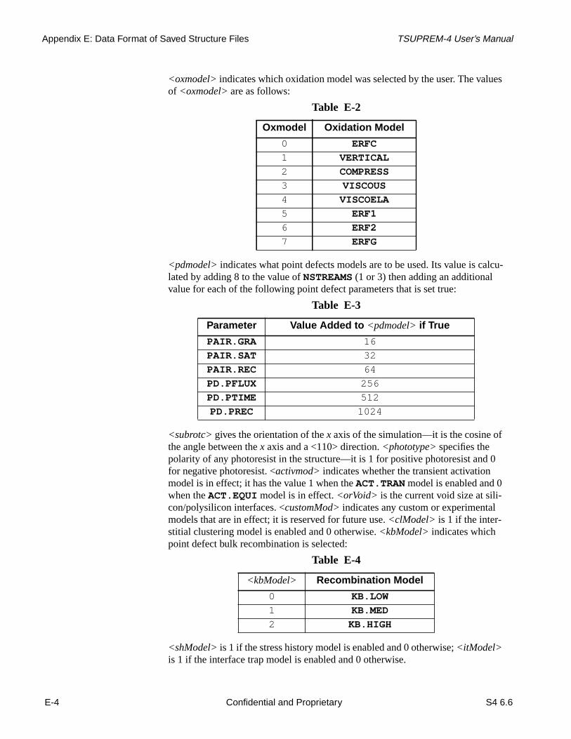
Appendix E: Data Format of Saved Structure Files TSUPREM-4 User’s Manual
lues
alcu-
f
0
<oxmodel> indicates which oxidation model was selected by the user. The vaof <oxmodel> are as follows:
<pdmodel> indicates what point defects models are to be used. Its value is clated by adding 8 to the value ofNSTREAMS (1 or 3) then adding an additionalvalue for each of the following point defect parameters that is set true:
<subrotc> gives the orientation of thex axis of the simulation—it is the cosine othe angle between thex axis and a <110> direction.<phototype> specifies thepolarity of any photoresist in the structure—it is 1 for positive photoresist andfor negative photoresist. <activmod> indicates whether the transient activationmodel is in effect; it has the value 1 when theACT.TRAN model is enabled and 0when theACT.EQUI model is in effect.<orVoid> is the current void size at sili-con/polysilicon interfaces. <customMod> indicates any custom or experimentalmodels that are in effect; it is reserved for future use. <clModel> is 1 if the inter-stitial clustering model is enabled and 0 otherwise.<kbModel> indicates whichpoint defect bulk recombination is selected:
<shModel> is 1 if the stress history model is enabled and 0 otherwise;<itModel>is 1 if the interface trap model is enabled and 0 otherwise.
Table E-2
Oxmodel Oxidation Model
0 ERFC
1 VERTICAL
2 COMPRESS
3 VISCOUS
4 VISCOELA
5 ERF1
6 ERF2
7 ERFG
Table E-3
Parameter Value Added to <pdmodel> if True
PAIR.GRA 16
PAIR.SAT 32
PAIR.REC 64
PD.PFLUX 256
PD.PTIME 512
PD.PREC 1024
Table E-4
<kbModel> Recombination Model
0 KB.LOW
1 KB.MED
2 KB.HIGH
E-4 Confidential and Proprietary S4 6.6
Draft 6/26/98

TSUPREM-4 User’s Manual TSUPREM-4 Structure File Format
the
g
re-ly-
esh,
andoronpeci-
Solution Values
The “s” line specifies which solution values are associated with each node ofstructure. The (integer) value<nsol> specifies how many solution values aregiven, while<sol1> through<soln> give the names of the solutions that arepresent. Valid names in version 6.4 are: the names of the impurities (includinuser-defined impurities); the names of the impurities preceded by “a_”, indicatingthe active portion of the impurity concentration; the names of the impurities pceded by “gb_”, indicating the concentration of the impurity associated with pocrystalline grain boundaries; the namesvacancy, interstitial, x.vel, y.vel, o2, h2o,trap, sxx, syy, sxy, rloop, dloop, lgrain, gorient,and tpoly. Note that this list ofsolutions is subject to change in future revisions of the program.
Nodes
The “n” lines specify the solution values at each node. For each point in the mthere is an “n” line for each material at the point. The (integer) value<cindex-1>gives the index of the coordinate, minus one, and the (integer)<region> specifiesthe region. Points on exposed surfaces must also have anambient node, denotedby a region index of zero. For each node, the solution values are given by<val1>through<valn> (floating-point).
Example The following input produces the structure file shown inFigure E-1.
line x loc=0line x loc=1line y loc=0line y loc=1init boron=1e13deposit oxide thick=.2savefile out.file=test.strstop
This structure contains 6 grid points, 2 regions (silicon and oxide), 4 triangles,10 nodes (4 in silicon, 4 in oxide, and 2 ambient nodes). Solution values for bconcentration are given at each node. No last processing temperature was sfied, and theVERTICAL oxidation model and thePD.FERMI point defect modelwere used.
s <nsol> <sol1> <sol2> ... <soln>
n <cindex-1> <region> <val1> ... <valn>
S4 6.6 Confidential and Proprietary E-5
DrafDraft 6/26/98 6/

Appendix E: Data Format of Saved Structure Files TSUPREM-4 User’s Manual
Older Versions of TSUPREM-4
This section describes differences between the currentTSUPREM-4 structure fileformat and that used in older versions of the program.
Figure E-1 TSUPREM-4 structure file
v TMA TSUPREM-4 (6.4S)c 1 0 0 0c 2 0 0.99999997 0c 3 0.99999997 0 0c 4 0.99999997 0.99999997 0c 5 0 -0.19999999 0c 6 0.99999997 -0.19999999 0e 1 2 1 0e 2 4 2 0e 3 3 4 0e 4 5 6 2e 5 1 5 0e 6 6 3 0e 7 3 1 0r 1 siliconb 1b 7b 3b 2r 2 oxideb 4b 6b 7b 5t 1 1 1 3 2 2 -1024 4t 2 1 3 4 2 -1024 1 -1024t 3 2 1 5 6 -1022 4 -1024t 4 2 1 6 3 -1024 1 3M 0 10 1073.16 1 9 1.000000 0 0 0 0 1 0s 2 boron a_boronn 0 1 1.000000e+13 1.0000e+13n 0 2 1.000000e+05 1.0000e+05n 1 1 1.000000e+13 1.0000e+13n 2 1 1.000000e+13 1.0000e+13n 2 2 1.000000e+05 1.0000e+05n 3 1 1.000000e+13 1.0000e+13n 4 2 1.000000e+05 1.0000e+05n 4 0 1.000000e+05 1.0000e+05n 5 2 1.000000e+05 1.0000e+05n 5 0 1.000000e+05 1.0000e+05
E-6 Confidential and Proprietary S4 6.6
Draft 6/26/98

TSUPREM-4 User’s Manual TSUPREM-4 Structure File Format
.
Regions In versions 6.0 and earlier, regions were identified by a<material> code:
ModelParameters
In versions 8926 and before<nadd> and the parameters that follow are omittedIn versions 9035 and 5.0<nadd> is 3, and the<temperature>, <oxmodel>, and<pdmodel> parameters are present. Starting with version 5.2,<nadd> is 5, andthe “M” line includes the<subrotc> and<phototype> parameters. Starting withversion 6.2,<nadd> is 6 and the “M” line includes the<activmod> parameter.Starting with version 6.3,<nadd> is 7 and the “M” line includes the<orVoid>parameter. Starting with version 6.4,<nadd> is 8 and the “M” line includes the<customMod> parameter. Starting with version 6.5,<nadd> is 10 and the “M”line includes the<clModel> and<kbModel> parameters. Starting with version6.6,<nadd> is 12 and the “M” line includes the<shModel> and<itModel>parameters.
In versions ofTSUPREM-4 prior to version 6.0 the value of<pdmodel> is inter-preted as follows:
Solution Values In versions 6.0 and earlier,<sol1> through<soln> are integer values indicatingwhich solution values are present:
Table E-5
<material> Material
1 oxide
2 nitride
3 silicon
4 polysilicon
5 oxynitride
6 aluminum
7 photoresist
8 ambient (included void)
Table E-6
<pdmodel> Point Defect Model
0 TWO.DIM (PD.TRANS)
2 FERMI (PD.FERMI)
4 STEADY (Obsolete;PD.TRANS used instead)
Table E-7
<solx> Solution
0 vacancy concentration
1 interstitial concentration
2 arsenic concentration
3 phosphorus concentration
4 antimony concentration
5 boron concentration
S4 6.6 Confidential and Proprietary E-7
DrafDraft 6/26/98 6/

Appendix E: Data Format of Saved Structure Files TSUPREM-4 User’s Manual
nines.
”.ted by
us
Nodes In version 6.0 and earlier,<region> specifies a material index rather than a regioindex. The same values are used to identify materials as are used in the “r” l
Medici Structure File FormatThis section describes the output file format produced by the “SAVEFILEMEDICI ” statement inTSUPREM-4. TheTSUPREM-4 Medici file containsnumerical values only. Floating point values use an exponent, denoted by “eInteger values do not have an exponent or a decimal point. Values are separaspaces. The format of the file is as follows.
Line 1:
This line specifies the number of points in the grid<npt>, the number of triangu-lar elements<ntri> , and the number of electrode points<nelpt>.
Line 2:
This line specifies the number of electrodes<nelec> and the number of materialsin the structure<nmat>. Note that the number of materials is preceded by a minsign.TSUPREM-4 converts all points on an interface with aluminum to elec-trodes.
6 steady-state vacancy concentration
7 steady-state interstitial concentration
8 x component of flow velocity
9 y component of flow velocity
10 oxidant concentration (dry O2)
11 oxidant concentration (wet O2)
12 concentration of filled interstitial traps
15 Sxx component of stress
16 Syy component of stress
17 Sxy component of stress
20 active component of arsenic concentration
21 active component of phosphorus concentration
22 active component of antimony concentration
23 active component of boron concentration
Table E-7
<solx> Solution
<npt> <ntri> <nelpt>
<nelec> -<nmat>
E-8 Confidential and Proprietary S4 6.6
Draft 6/26/98

TSUPREM-4 User’s Manual Medici Structure File Format
g attri- in a
Lines 3 through<npt>+2:
These lines specify thex andy coordinates<xcoord> and<ycoord> of each meshpoint (in centimeters), the net n-type doping<cnet> (in atoms/cm3), and the totaldoping<ctotal> (in atoms/cm3). Note that a negative value of<cnet> indicates ap-type region.<xcoord>, <ycoord>, <cnet>, and<ctotal> are all floating-pointvalues.
Lines<npt>+3 through<npt>+<ntri> +2:
These lines specify the triangular elements that make up the mesh.<reg> is theregion number for the element. (Regions are numbered consecutively, startinone.)<p1>, <p2>, and<p3> are the indices of the points at the vertices of the angular element. The points are specified in a clockwise order, when viewedleft-handed coordinate system (i.e.,x increasing from left to right andy increasingfrom top to bottom).
Lines<npt>+<ntri> +3 through<npt>+<ntri> +<nelpt>+2:
These lines specify the electrode<elec> associated with each electrode point<ept>. <elec> is either a name (assigned with theELECTRODE statement) or anumber. (Electrode numbers start at one and increasing to<nelec>, as needed.)
Line <npt>+<ntri> +<nelpt>+3 (last line in file):
This line specifies the material associated with each region in the structure:
<xcoord> <ycoord> <cnet> <ctotal>
<reg> <p1> <p2> <p3>
<ept> <elec>
<mat1> <mat2> ... <matn>
Table E-8
<matx> Material
-6 oxynitride
-4 unspecified insulator (e.g., photoresist)
-2 nitride
-1 oxide
1 silicon
3 polysilicon
4 unspecified semiconductor
S4 6.6 Confidential and Proprietary E-9
DrafDraft 6/26/98 6/

Appendix E: Data Format of Saved Structure Files TSUPREM-4 User’s Manual
Example The followingTSUPREM-4 input produces the structure file shown inFigure E-2:
line x loc=0line x loc=1line y loc=0line y loc=1init boron=1e13deposit oxide thick=.2deposit aluminum thick=.1select z=0 temp=800savefile medici out.file=testpi.strstop
Figure E-2 Medici structure file
6 4 2 1 -2 0.000000e+00 0.000000e+00 -1.000000e+13 1.000000e+13 0.000000e+00 1.000000e-04 -1.000000e+13 1.000000e+13 1.000000e-04 0.000000e+00 -1.000000e+13 1.000000e+13 1.000000e-04 1.000000e-04 -1.000000e+13 1.000000e+13 0.000000e+00 -2.000000e-05 0.000000e+00 0.000000e+00 1.000000e-04 -2.000000e-05 0.000000e+00 0.000000e+00 1 1 3 2 1 3 4 2 2 1 5 6 2 1 6 3 5 1 6 1 1 -1
E-10 Confidential and Proprietary S4 6.6
Draft 6/26/98

APPENDIX F
-the
ge
f themind
ny-
Appendix F:Using the MINIMOS 5InterfaceF
This appendix explains how to sendTSUPREM-4 results to the MINIMOS 5device simulator. It should be used in conjunction with theSAVEFILE inputstatement describedon page 3-65.
Overview of the TSUPREM-4 Interface to MINIMOS 5The interface is file-oriented and unidirectional (fromTSUPREM-4 toMINIMOS 5), and consists of three separate steps.
1. TSUPREM-4 writes a formatted file (i.e., ASCII or EBCDIC). This file contains a two-dimensional doping profile of the source area (and optionally drain area) of the device being simulated.(See“Step 1: Directing TSUPREM-4 to Generate a Formatted File” on paF-2.)
2. Use a separate stand-alone FORTRAN program (namedmmatob) to convertthe formatted file to a FORTRAN binary file. (See“Step 2: Converting theFormatted File to FORTRAN Binary” on page F-6)
3. Execute MINIMOS 5, which reads in the binary doping file. (See“Step 3:Running MINIMOS 5” on page F-6)
Throughout this discussion, use the convention that the source is on the left ochannel and the drain is on the right of the channel. Also, you should keep in thatTSUPREM-4 expects user-specified values in microns, whileMINIMOS 5 expects centimeters.
All references to MINIMOS 5 refer to the program supplied by the TechnicalUniversity of Vienna, Austria, Institute for Microelectronics, and the accompaing MINIMOS 5 User’s Guide, dated March 2, 1990.
S4 6.6 Confidential and Proprietary F-1
DDraft 6/26/98

Appendix F: Using the MINIMOS 5 Interface TSUPREM-4 User’s Manual
on-
arimu-
ain,lly
lude
ht
nnel,
Step 1: Directing TSUPREM-4 to Generate a Formatted FileCentral to the preparation of the MINIMOS 5 output file is the concept of theMINIMOS 5 simulation region. This region is a subset of a simulatedTSUPREM-4 device. While aTSUPREM-4 MOS device simulation mayencompass an entire device, including the gate oxide, field oxide, metallizatilayers, etc., MINIMOS 5 expects to read a two-dimensional doping file encompassing only a portion of the full device. TheX.MIN , X.MAX, Y.MIN , andY.MAX parameters on theSAVEFILE statement are used to define a rectangulsubset of the complete device. This subset is referred to as the MINIMOS 5 slation region.
Defining the MINIMOS 5 Simulation Region
The MINIMOS 5 simulation region should be defined to include the source, drand channel of the MOS transistor; gate and field oxide regions would normabe excluded. The MINIMOS 5 simulation region must be deep enough to incthe source and drain junction depths, because MINIMOS 5 expects to see achange in the sign of the net doping concentration along both the left and rigedges of its simulation space (except when simulating SOI devices).
The followingTSUPREM-4 statement defines the MINIMOS 5 simulationregion and generates a formatted MINIMOS 5 file for the device shown inFigureF-1 (from Chapter 5, “NMOS LDD Process” on page 5-2):
The parameterMINIMOS5 specifies that the file to be produced is a formattedtwo-dimensional doping file, to be read by MINIMOS 5.OUT.FILE=MMDOPFspecifies that the formatted doping file is namedMMDOPF. Because this is thefilename expected by the file conversion programmmatob (discussed later in thissection), it is the recommended name to use when directingTSUPREM-4 to pre-pare a MINIMOS 5 doping file.
Referring toFigure F-1, you see a complete device with source, channel, anddrain regions, so theFULL.DEV parameter should be specified. If theTSUPREM-4 simulation encompasses only the source half of a device, useHALF.DEV. If theTSUPREM-4 simulation is for the drain half of a device,reflect theTSUPREM-4 structure to create a complete device and specifyFULL.DEV. Because the drain region is assumed to be to the right of the chause the statement
(preceding theSTRUCTURE MINIMOS5 statement) to reflect the device at itsleft edge (the center of the channel), thus creating a complete device.
SAVEFILE MINIMOS5 OUT.FILE=MMDOPF FULL.DEV+X.MIN=-2 X.MAX=2 Y.MIN=0.0174 Y.MAX=1.5+X.MASK.S=-0.57 X.MASK.D=0.57
STRUCTURE REFLECT LEFT
F-2 Confidential and Proprietary S4 6.6
Draft 6/26/98

TSUPREM-4 User’s Manual Step 1: Directing TSUPREM-4 to Generate a Formatted File
dt. If
es
gion
ther,
TheX.MIN , X.MAX, Y.MIN , andY.MAX parameters define the left, right, top,and bottom edges of the MINIMOS 5 simulation region, respectively. Theassigned values forX.MIN andX.MAX are chosen by visual inspection ofFigureF-1 and need not be exact.X.MIN is roughly centered between the left-most fieloxide and the gate, in an area where the impurity contours are essentially flaX.MIN is too far to the left, the field oxide region is included.X.MAX is assignedthe corresponding value on the right side of the structure.
Similar toX.MIN andX.MAX, Y.MAX is determined based on visual inspectionof Figure F-1 and need not be exact. However,Y.MAX must be deep enough in thestructure to include the source and drain junction depths, or MINIMOS 5 issuthe error message
Y.MAX should also be deep enough in the structure to include the depletion refor the maximum bias to be applied, particularly if the dopant profile is stillchanging at that depth.
The values used forX.MIN , X.MAX, andY.MAX are not critical, because ifMINIMOS 5 needs a simulation region that is larger than the one defined by doping file, MINIMOS 5 extends the profiles in the required direction. Howevethe value assigned toY.MIN is critical, because MINIMOS 5 interpretsY.MIN asthe gate oxide/silicon interface. Thus,Y.MIN has a physical significance andshould be carefully determined. ForTSUPREM-4 MOSFET simulations, thegate oxide/silicon interface is typically found just belowy=0.0. Therefore, as afirst approximation, the default value (Y.MIN =0.0) could be used. Another
Figure F-1 NMOS structure to be transferred to MINIMOS 5
DOPING PROFILE INCONSISTENT
S4 6.6 Confidential and Proprietary F-3
DrafDraft 6/26/98 6/

Appendix F: Using the MINIMOS 5 Interface TSUPREM-4 User’s Manual
lr of
to
ing
e
ula-
ndame-
n-
approximation could be obtained from visual inspection of a two-dimensionaplot. However, the most accurate value is obtained by using the following paiTSUPREM-4 statements:
where<xchan> is thex coordinate of the vertical slice along which values are be printed. In a typicalTSUPREM-4 MOSFET simulation (such asFigure F-1),the gate oxide/silicon interface is bowed slightly upwards and is closest toy=0.0in the middle of the channel. For such cases,<xchan> in the preceding code frag-ment should be thex coordinate of the middle of the channel. The center of thechannel for the device shown inFigure F-1 is atx=0.0. Thus, theTSUPREM-4statements
are used to generate the followingTSUPREM-4 output (results may vary slightlyon your system):
From this output, you see that the bottom of the oxide layer occurs aty=0.0174microns, soY.MIN =0.0174 is used. Also, note that the thickness of the insulatoxide is 0.0419 microns (419 Å). This value is used on theMINIMOS 5 DEVICE directive when specifying a value for theTINS parameter.
There is no need to specifyX.CHANNE in this example, because the default valu(midway betweenX.MIN andX.MAX) is appropriate.X.CHANNE is only neededif an asymmetric device is simulated and serves to divide the MINIMOS 5 simtion region into a source half and a drain half.
The two remaining parameters,X.MASK.S andX.MASK.D, are similar toY.MIN in that they have a physical significance.X.MASK.S is thex coordinateof the mask edge in the source area of the MINIMOS 5 simulation region.MINIMOS 5 interprets this coordinate as the left edge of the gate electrode atreatsX.MASK.D as the right edge of the gate electrode. Values for these parters can be obtained by visual inspection ofFigure F-1. For more accuracy, use thefollowing pair ofTSUPREM-4 statements
to print thex andy coordinates of the interface between the polysilicon gate cotact and the gate oxide. From this output (not shown), you find thatX.MASK.S=-0.57 andX.MASK.D=0.57.
SELECT Z=1PRINT.1D LAYERS X.VALUE= <xchan>
SELECT Z=1PRINT.1D LAYERS X.VALUE=0.0
Num Material Top Bottom Thickness Integral 1 oxide -1.1111 -0.4107 0.7004 7.0040e-05 2 polysilicon -0.4107 -0.0245 0.3862 3.8615e-05 3 oxide -0.0245 0.0174 0.0419 4.1938e-06 4 silicon 0.0174 200.0000 199.9826 1.9998e-02
SELECT Z=YPRINT.1D POLY /OXIDE
F-4 Confidential and Proprietary S4 6.6
Draft 6/26/98

TSUPREM-4 User’s Manual Step 1: Directing TSUPREM-4 to Generate a Formatted File
en the
id
oreea-ly
0 to
en
cify-
dop-
TheSGAP andDGAP parameters on the MINIMOS 5DEVICE directive are usedto specify the gap between the gate and source contacts, and the gap betwegate and drain contacts, respectively. TheTSUPREM-4 statements
can be used to print thex andy coordinates of the silicon/oxide interface, as an ato determiningSGAP andDGAP for the subsequent MINIMOS 5 run. Alterna-tively, the values could be approximated by visual inspection ofFigure F-1.
Notes on the Size of the MINIMOS 5 Simulation Region
TheX.MIN , X.MAX, Y.MIN , andY.MAX parameters determine the size of theMINIMOS 5 simulation region. If this region is large, containing manyTSUPREM-4 grid points, the preparation of the MINIMOS 5 doping file couldtake several minutes. Additionally, the subsequent MINIMOS 5 run can take mexecution time if the doping file defines a large simulation region. For these rsons, you should attempt to keep the MINIMOS 5 simulation region reasonabsmall when choosingX.MIN , X.MAX, Y.MIN , andY.MAX. This also reduces thesize of the doping file.
The standard version of MINIMOS 5 expects the doping file to contain from 180 horizontal grid lines and from 10 to 80 vertical grid lines. Normally, thisrequirement is satisfied automatically byTSUPREM-4 during the preparation ofthe doping file. However, certain choices forX.MIN , X.MAX, Y.MIN , andY.MAX can result in aTSUPREM-4 warning message stating that there are toomany (or too few) grid lines. Unless the version of MINIMOS 5 you run has bemodified to accept expanded limits, you must modify theX.MIN , X.MAX,Y.MIN , orY.MAX values as advised in theTSUPREM-4 warning message, andregenerate the doping file. Otherwise, when MINIMOS 5 attempts to read thedoping file, it issues the error message
and terminate execution. You can also modify the number of grid lines by speing theDX.MIN and/orDY.MIN parameters. These change the minimum gridspacings in thex andy directions from their default values ofmin((X.MAX - X.MIN )/80,0.01) and min((Y.MAX - Y.MIN )/80,0.01), respectively.
Nonplanar Oxide Regions in MINIMOS 5
As stated in theMINIMOS 5 User’s Guide,MINIMOS 5 can model nonplanaroxide regions. This is accomplished by including theGEOMETRY directive (andassociated parameters) in the MINIMOS 5 input command file. However, the ing file (as dictated by MINIMOS 5) makes no provision for the inclusion ofgeometry information. As discussed, the doping file uses a single coordinate(Y.MIN ) to specify the gate oxide/silicon interface, implying a planar device.
SELECT Z=YPRINT.1D SILICON /OXIDE
DOPING FILE FORMAT ERROR
S4 6.6 Confidential and Proprietary F-5
DrafDraft 6/26/98 6/

Appendix F: Using the MINIMOS 5 Interface TSUPREM-4 User’s Manual
-t
/sili-
s,dtra-
f
-
-
-oput
Hence,TSUPREM-4 cannot automatically export nonplanar geometry information to MINIMOS 5 by including it in the doping file—the MINIMOS 5 user musapproximate the nonplanarities of the device simulated inTSUPREM-4 by hand,attempting to duplicate theTSUPREM-4 geometry in MINIMOS 5 by using theGEOMETRY directive. Fortunately, many devices (such as the MOSFET inFigureF-1) are approximately planar, and the MINIMOS 5GEOMETRY directive is notrequired to simulate the intrinsic device operation. In such cases, assignY.MIN tothe top-most point of the silicon as discussed earlier. Because the gate oxidecon interface is not absolutely flat, the left and right portions of the top of theMINIMOS 5 simulation region contain very thin layers of oxide. To correct thiTSUPREM-4 automatically ignores the impurity concentration in the oxide anextends the doping profile of the underlying silicon upward (using the concention at the oxide/silicon interface). In general,TSUPREM-4 ignores the dopantsin any nonsilicon material within the MINIMOS 5 simulation region, usinginstead the doping of the underlying silicon.
Step 2: Converting the Formatted File to FORTRAN BinaryTSUPREM-4 writes a formatted (i.e., ASCII or EBCDIC) file for MINIMOS 5.However, MINIMOS 5 requires a FORTRAN binary doping file. The formattedfile written byTSUPREM-4 is converted to FORTRAN binary by executing thestand-alone FORTRAN program namedmmatob. This step is needed because oincompatibilities between binary files written by C programs (such asTSUPREM-4) and FORTRAN programs (such as MINIMOS 5) on some computer systems.
The current version ofmmatob is executed by simply typing
followed by a carriage return. Note thatmmatob expects to read a formatted filenamedMMDOPF and write a binary file namedMMDOPB. The easiest way toassure that the formatted file is namedMMDOPF is to specifyOUT.FILE=MMDOPF on theTSUPREM-4 SAVEFILE statement used to generate the MINIMOS 5 file. Alternatively, rename or copy the formatted file toMMDOPF before executingmmatob. Any existing file namedMMDOPB is over-written whenmmatob is executed.
Step 3: Running MINIMOS 5MINIMOS 5 reads the binary doping file from FORTRAN logical unit 20. Similarly, the input command file must be available on FORTRAN unit 15. Refer tyour MINIMOS 5 documentation for instructions on how to associate these infiles with the correct FORTRAN logical unit numbers.
Figure F-2 shows a listing of a sample MINIMOS 5 input command file(EX2D.INP, included with standard versions of MINIMOS 5).
mmatob
F-6 Confidential and Proprietary S4 6.6
Draft 6/26/98

TSUPREM-4 User’s Manual Step 3: Running MINIMOS 5
.he
inn
se
This file uses thePROFILE andIMPLANT directives to generate a doping profileTo convertEX2D.INP so that it reads an external two-dimensional doping file, tPROFILE statement is changed to
TheIMPLANT directive, used inEX2D.INP to specify a channel implantation, isremoved. In addition, the parameters and values specified on theDEVICE state-ment are modified as needed to match the geometry of the device simulatedTSUPREM-4. The resulting modified MINIMOS 5 input command file is showin Figure F-3.
Recall that MINIMOS 5 expects dimensions in centimeters, not microns. To uMINIMOS 5 to simulate a nonplanar device, specify theGEOMETRY directive, asdiscussed earlier, in“Nonplanar Oxide Regions in MINIMOS 5” on page F-5.
Figure F-2 Listing of MINIMOS 5 command file EX2D.INP
EXAMPLE FOR CLASSICAL TWO-DIMENSIONAL MODEL (EX2D.INP)DEVICE CHANNEL=N GATE=NPOLY TINS=150.E-8 W=1.E-4 L=0.85E-4BIAS UD=4. UG=1.5PROFILE NB=5.2E16 ELEM=AS DOSE=2.E15 TOX=500.E-8 AKEV=160.+ TEMP=1050. TIME=2700IMPLANT ELEM=B DOSE=1.E12 AKEV=12 TEMP=940 TIME=1000OPTION MODEL=2-DOUTPUT ALL=YESEND
PROFILE FILE=2-D
Figure F-3 Listing of MINIMOS 5 command file EX2D.INP, modified to readdoping profiles produced by TSUPREM-4
EXAMPLE FOR CLASSICAL TWO-DIMENSIONAL MODEL (READS 2-D DOPING FILE)DEVICE CHANNEL=N GATE=NPOLY TINS=419E-8 W=1.E-4 L=1.14E-4+ DGAP=1.87E-4 SGAP=1.87E-4BIAS UD=4. UG=1.5PROFILE FILE=2-DOPTION MODEL=2-DOUTPUT ALL=YESEND
S4 6.6 Confidential and Proprietary F-7
DrafDraft 6/26/98 6/

Appendix F: Using the MINIMOS 5 Interface TSUPREM-4 User’s Manual
o
cause
ec-
n
se
n-e
on,s
e for
Notes on Using MINIMOS 5
Particular care must be taken when specifying theL parameter (gate electrodelength) on the MINIMOS 5DEVICE directive. The value assigned toL shouldcorrespond to the distance between the values assigned toTSUPREM-4 parame-tersX.MASK.S andX.MASK.D. For example, ifX.MASK.S=-0.57 (microns)andX.MASK.D=0.57 (microns), the distance between them is 1.14 microns, sL=1.14e-4 (centimeters). In this case, specifying a value ofL greater than1.14e-4 centimeters has the effect of stretching the channel, and should not problems in MINIMOS 5. However, a value ofL substantially smaller than1.14e-4 centimeters could cause the source and drain profiles to overlap, efftively eliminating the channel. MINIMOS 5 responds with the error message
and terminates execution.
Interpreting Error MessagesThe warning and error messages issued byTSUPREM-4 during the preparationof the doping file are clear and fairly detailed, recommending corrective actiowhen necessary.
The following error messages from MINIMOS 5 may be encountered:
MINIMOS 5 issues this message for a variety of error conditions. A likely cauis that theL parameter on the MINIMOS 5DEVICE directive is too small, caus-ing the source and drain profiles to overlap and effectively eliminating the chanel. Correct the error by using a value ofL that is at least as large as the differencbetween theX.MASK.S andX.MASK.D parameters, as described above. Thedoping file does not need to be regenerated.
Another cause for the above message is that the MINIMOS 5 simulation regias defined inTSUPREM-4, was not deep enough to include the junction depthin both the source and drain regions. Correct the error by using a larger valuY.MAX on theTSUPREM-4 SAVEFILE statement. In this case, the doping fileneeds to be regenerated.
Lastly, to avoid the above message when usingTSUPREM-4 and MINIMOS 5 tosimulate SOI devices, the MINIMOS 5DEVICE directive must include theBULK,FILM , andKBULK parameters.
When too many (or too few) horizontal or vertical grid lines are present in thedoping file, the following message can appear:
DOPING PROFILE INCONSISTENT
DOPING PROFILE INCONSISTENT
DOPING FILE FORMAT ERROR
F-8 Confidential and Proprietary S4 6.6
Draft 6/26/98

TSUPREM-4 User’s Manual Interpreting Error Messages
and
S 5rent
TSUPREM-4 should have issued a warning message, describing the problemrecommending corrective action. However,TSUPREM-4 went ahead and pre-pared a doping file after issuing the warning, in case your version of MINIMOhas been modified to accept expanded limits. Correct the error by using diffevalues forX.MIN , X.MAX, Y.MIN , orY.MAX in TSUPREM-4, and regeneratethe doping file.
S4 6.6 Confidential and Proprietary F-9
DrafDraft 6/26/98 6/

Appendix F: Using the MINIMOS 5 Interface TSUPREM-4 User’s Manual
F-10 Confidential and Proprietary S4 6.6
Draft 6/26/98

GLOSSARY
S
rma-
are
e-mor-
ict
uide-
ion. the tiltarson
f thetg.)
GlossaryThis glossary contains terms frequently used in the TSUPREM-4 User’s Manual.A list ofacronyms is included as the last section in the Glossary. For references to more infotion about a term, see the Index.
1
Aactivation of dopants Movement of dopant atoms onto substitutional sites on the silicon lattice where they
electrically active.
adaptive gridding Automatic adaptation of the simulation mesh by the program to improve solutionaccuracy.
amorphization The complete disruption of the silicon lattice structure caused by ion implantation. Thamorphized region will recrystallize (through epitaxial regrowth) during the next hightemperature step, but residual damage may remain, especially at the edges of the aphized layer.
analytical oxidationmodel
A model that uses empirical descriptions of the two-dimensional oxide shape to predthe results of local oxidation steps.
automatic meshgeneration
Generation of the simulation mesh automatically by the program based on general glines supplied by the user.
Cchanneling Tendency of ions to travel along open directions in the silicon lattice during implantat
Channeling may cause implanted profiles to be deeper than expected, depending onand rotation of the wafer related to the ion beam. The effect is included in the dual Peimplant tables and in the Monte Carlo implant model.
clustering The formation of groups of atoms whose properties are different from the properties oindividual atoms within the group. Clustering usually refers to the clustering of dopanatoms to form immobile and electrically inactive complexes. (See interstitial clusterin
4 6.6 Confidential and Proprietary Glossary-1
Draft 6/26/98

Glossary TSUPREM-4 User’s Manual
efers
ur
f-
tials
not-
Ddeposition One of the basic fabrication steps used for IC processing.TSUPREM-4 contains a simple
model for deposition of conformal layers. If more advanced models are needed,TSUPREM-4 can be used with Terrain.
diffusion Spreading of impurities due to random motion at high temperatures. The term also rto any process step in which diffusion occurs.TSUPREM-4 includes detailed physicalmodels for diffusion and other processes, such as oxidation and silicidation, that occduring high temperature fabrication steps.
damage annealing Removal of implantation damage with high temperatures.
dislocation loops A class of extended defect in the silicon lattice structure. The ED-AAM models end-orange dislocation loops produced by amorphizing ion implants.
dopant An impurity added to a structure to control its electrical properties.
Eepitaxial growth Growth of single crystal silicon on top of an existing silicon structure.TSUPREM-4
includes a model for epitaxial growth on planar substrates.
epitaxial regrowth Recrystallization of a silicon region amorphized during ion implantation.
Ggrid (See mesh.)
Iimplant damage Damage to the silicon lattice structure caused by ion implantation.
impurity Any atom other than silicon in a silicon structure. Often used to refer to a dopant.
interstitial A type of point defect consisting of an extra silicon atom not on the lattice site. Interstipromote diffusion by pairing with dopants.
interstitial clustering Clustering of interstitials. Clustered interstitials are assumed to be immobile and do promote the diffusion of impurities. InTSUPREM-4, the clustering model is used to simulate the effects of 311 defects.
interstitial trap model A model describing the absorption and release of interstitials at a trapping site.
ion pairing Coupling of dopant atoms of opposite charge to form an immobile pair.
ion implantation Introduction of dopants into a wafer by a beam of accelerated ions.
Glossary-2 Proprietary and Condfential S4 6.6
Draft 6/26/98

TSUPREM-4 User’s Manual Glossary
not
u-
age
and
is
n.sion.
ce intion
cally
abri-al.
Llocal oxidation Oxidation of a portion of the silicon surface, achieved by masking the portion that is
oxidized with a material such as silicon nitride.
Mmesh The array of points within the structure at which solution values are numerically calc
lated. (The term is used interchangeably withgrid.)
Monte Carlo implantmodel
A physics-based model that uses statistical techniques to calculate impurity and damprofiles produced by ion implantation.
Nnumerical oxidation
modelA model that uses the numerical solution of the physical equations for oxide growth flow to predict the results of arbitrary oxidation steps.
Ooxidation Creation of silicon dioxide by reaction of silicon or polysilicon with oxygen. Oxidation
modeled inTSUPREM-4 whenever diffusion occurs in an oxidizing ambient.
point defects A localized defect (as opposed to an extended defect) in a silicon lattice structure. InTSUPREM-4, the termpoint defects refers to interstitials (i.e. silicon self-interstitials)and vacancies.
polycrystalline model A model for polycrystalline materials used primarily for modeling polycrystalline silicoIt includes models for grain growth and the effect of grain boundaries on dopant diffu
Ssegregation Transport of an impurity across an interface between two materials due to a differen
chemical potential. This transport results in an equilibrium ratio of impurity concentraacross a material boundary.
silicidation Interaction of silicon to form a metal silicide. Modeled inTSUPREM-4 by theDIFFUSION statement whenever necessary materials are present in the structure.
solid solubility The concentration at which dopant atoms precipitate, becoming immobile and electriactive.
stress TSUPREM-4 includes models for calculating the physical stresses produced during fcation. The stress history model simulates the stresses produced by oxidation, thermmismatch between materials, intrinsic strain in deposited layers, and surface tension
S4 6.6 Confidential and Proprietary Glossary-3
Draft 6/26/98

Glossary TSUPREM-4 User’s Manual
TTSUPREM-4 The name originated from a combination of TMA (now the TCAD Business Unit of
Avant!) and SUPREM-IV, the Stanford University Process Engineering Models.
TED Transient-Enhanced Diffusion. Enhanced diffusion caused by implant damage.
Glossary-4 Proprietary and Condfential S4 6.6
Draft 6/26/98

TSUPREM-4 User’s Manual Glossary
AcronymsLDD Lightly Doped Drain
MOS Metal-Oxide Semiconductor
NMOS N-channel Metal-Oxide Semiconductor
OED Oxidation-Enhanced Diffusion
TED Transient-Enhanced Diffusion
S4 6.6 Confidential and Proprietary Glossary-5
Draft 6/26/98

Glossary TSUPREM-4 User’s Manual
Glossary-6 Proprietary and Condfential S4 6.6
Draft 6/26/98

INDEX
A B C D E F G H I J K L M N O P Q R S T U V W X Y Z
4
Index
Symbols( ) 3-4< > 3-4 3-4| 3-4Numerics1D bipolar example
completing the active regionsimulation 4-9
DEPOSITION statement 4-5, 4-6EPITAXY statement 4-5ERFC oxidation model 4-4ETCH statement 4-5final structure 4-11IMPLANT statement 4-5initial active region 4-2INITIALIZE statement 4-3input file sequence 4-2LABEL statement 4-6mesh generation 4-2model selection 4-4overview 4-2PD.FERMI point defect model 4-4PD.TRANS point defect model 4-4PLOT.1D statement 4-6, 4-8plotting the results 4-6point defect model 4-4printing layer information 4-8processing steps 4-5SAVEFILE statement 4-6saving the structure 4-6SELECT statement 4-6, 4-7VERTICAL oxidation model 4-4
1D simulation of simple structuresoverview 2-10tutorial example of 4-2
2D diffusion with point defectsautomatic grid generation 4-19contour of boron concentration 4-21field implant 4-19grid plot 4-21
lateral distribution of point defects4-25
oxidation 4-19shaded contours of interstitialconcentration 4-25
using theFOREACH statement 4-23vertical distribution of point defects4-24
Aabout the manual xxxabsorption of interstitial traps 2-32activation of dopants 2-112active region simulation
LDD implant 5-8modeling polysilicon 5-7oxide spacer and source/drainimplant 5-9
plots 5-10source/drain contacts 5-9
adaptive grid parameters, defaultcoefficients A-21
adaptive griddingadvanced examples of 5-4, 5-28,5-44
analytical implant models 3-189analytical model 2-10disable 3-189during diffusion 2-10enabling and disabling 2-10Monte Carlo model 2-10overview 2-9tutorial example of 4-4
advanced examplesCMOS process 5-30DMOS power transistor 5-39MOSFET with self-aligned silicides5-50
NMOS LDD process 5-2overview 5-1poly-buffered LOCOS 5-27polysilicon emitter study 5-54SOI MOSFET 5-45trench implant simulation 5-18
AMBIENT 3-193additional notes 3-207chlorine 3-205coefficients 3-205coefficients chlorine examples 3-205COMPRESS model 3-203description 3-202ERFC model 3-202ERFG model 3-203examples 3-207INITIAL parameter, 1D bipolarexample 4-4
orientation 3-206oxidation models 3-202oxidation models, polycrystallinesilicon 3-202
oxidizing species 3-206parameter dependencies 3-206specified material 3-206specified units 3-206stress dependence 3-204VERTICAL model 3-203VISCOELA model 3-203VISCOUS model 3-203
ambient gaschlorine example 2-14chlorine, coefficient tables 2-14defaults 2-14oxidation of materials 2-13pressure 2-12specifying characteristics 2-13
amorphizatin, damage dechanneling 2-8amorphous implant calculation 2-78
electronic stopping 2-80electronic stopping at high energies2-81
ion beam width 2-81nuclear stopping 2-79total energy loss and ion deflection2-81
analytic damage model 2-73damage distribution calculations2-74
recommended usage and limitations2-74
analytic ion implant models 2-66
TS4 6.6 Confidential and Proprietary Index-1
Draft 6/26/98

Index: analytical oxidation models 2-41 TSUPREM-4 User’s Manual
I
A B C D E F G H I J K L M N O P Q R S T U V W X Y Z
analytic damage model 2-73dose-dependent implant profiles2-70dual Pearson distribution 2-70Gaussian distribution 2-69implant moment tables 2-67implanted impurity distributions2-66
lateral distribution 2-73multilayer implants 2-72Pearson distribution 2-69tilt and rotation tables 2-72wafer tilt and rotation 2-73
analytical oxidation models 2-41ERF1 model 2-45ERF2 model 2-46ERFC model 2-44ERFG model 2-46linear rate 2-42overview 2-41oxide growth rate 2-41parabolic rate 2-43thin regime 2-42usage 2-44
annealingdamage 2-84in situ 2-84self-annealing 2-84
ANTIMONY 3-260additional notes 3-265description 3-264examples 3-265
Arora mobility model 2-107ARSENIC 3-266
additional notes 3-271description 3-270examples 3-271
ARSENIC parameter,EPITAXYstatement1D bipolar example 4-5
ASSIGN 3-25additional assign notes 3-30assign and optimization 3-30assign with mathematicalexpressions 3-29
assign with mathematicalexpressions, usingN.EXPRESS3-29
description 3-28expansion of assigned variable 3-30overriding variables 3-31reading the external data file 3-31varying during statement looping3-29
ASSIGN statement, enhancement C-11authorization files4auth 1-10automatic grid generation
overview 2-5tutorial examples of 4-3, 4-19
automatic grid generation parameters,default coefficients A-20
automatic grid generation, customdefaults 2-6
AXES parameter,PLOT.1D statement1D bipolar example 4-7
AXES parameter,PLOT.2D statementlocal oxidation example 4-18
Bbinary scattering theory 2-75
Coulomb potential 2-77dimensionless form 2-76energy loss 2-75scattering angle 2-76universal potential 2-77
Boltzmann statistics 2-105BORON 3-272
additional notes 3-277description 3-276examples 3-277
BORON parameter,INITIALIZEstatement1D local oxidation example 4-19
BOTTOM parameter,PLOT.1D statementlocal oxidation example 4-24
BOUNDARY 3-54description 3-54example 3-55limitations 3-55
boundary conditions for ion implantation2-87
boundary conditions for thermal stressmodel C-4
CCaughey mobility model 2-108C.COMPRE parameter,PLOT.2D
statementlocal oxidation example 4-16
CENTER parameter,LABEL statementCMOS process example 5-37
C.GRID parameter,PLOT.2D statementlocal oxidation example 4-14
channeling 2-82charge state fractions 2-29chemical predeposition 2-14CLEAR parameter,PLOT.1D statement
1D bipolar example 4-7CLEAR parameter,PLOT.2D statement
local oxidation example 4-26clustering and solid solubility, default
coefficients A-6clustering model 2-24
flexibility C-10
CM parameter,LABEL statement1D bipolar example 4-7
CMOS process example0.8 micron device 5-371.2 micron device 5-38arsenic profiles in gate 5-37channel doping plot 5-34COMPRESS model 5-34contacts 5-34end of main loop 5-35END statement 5-35final mesh 5-37FOREACH loop 5-30, 5-35FOREACH statement 5-34INITIALIZE statement 5-35lightly doped drain structure 5-34main loop 5-32mesh generation 5-32models 5-34overview 5-30PD.TRANS model 5-34plotting results 5-35processing 5-34SAVEFILE statement 5-35saving the structure 5-35VERTICAL oxidation model 5-34
coefficient default values A-1COLOR 3-141
description 3-142examples 3-142plot device selection 3-142
COLOR parameter,PLOT.1D statement1D bipolar example 4-7
combining models 2-24command input files 1-4COMMENT 3-8
description 3-8examples 3-8notes 3-8
compatibility withTSUPREM-4 version6.5 C-14accuracy C-14performance C-15
completing the active region simulation4-9field oxidation 4-9reading a saved structure 4-9
COMPRESS model 2-50boundary conditions 2-51compressible viscous flow 2-50material parameters 2-51recommended usage 2-51
compressible viscous flow 2-50concentration dependence 2-48CONTOUR 3-139
additional notes 3-140description 3-140example 3-140
ndex-2 Confidential and Proprietary TS4 6.6
Draft 6/26/98
TSUPREM-4 User’s Manual Index: Documentation and Control, input statements
TS
A B C D E F G H I J K L M N O P Q R S T U V W X Y Z
line type and color 3-140control statements 3-7CPULOG 3-40
description 3-40examples 3-40limitations 3-40
creating the initial structureadaptive gridding 5-4masking information 5-4setting the grid density 5-3
creating the test structureautomatic grid generation 4-29outline of example 4-29
CRYSTAL parameter,IMPLANTstatementtrench implant simulation example5-23, 5-25
crystalline implant model 2-81BF2 implantation 2-85channeling 2-82damage annealing 2-84damage dechanneling 2-84lattice damage 2-83lattice temperature 2-83number of ions 2-85
C.TENSIO parameter,PLOT.1Dstatementlocal oxidation example 4-16
Ddamage annealing 2-84damage dechanneling
amorphization 2-84damage dechanneling,
Monte Carlo implant 2-84Data Visualizer Programming Guide,
waveformat 1-7DEEP parameter,ELECTRICAL
statementNMOS LDD process example 5-15
default coefficient notes A-26default coefficient tables
adaptive grid parameters A-21automatic grid generationparameters A-20
clustering and solid solubility A-6electrical parameters A-13impurity parameters A-2material coefficients A-15Monte Carlo implant A-17notes A-26numerical methods A-19oxidation A-9point defect parameters A-7polysilicon grain segregation A-6references A-22silicidation A-12
default coefficientssegregation and transportcoefficients A-4
default coefficients, Appendix A A-1default file names 1-3default values
viscosity C-8Young’s modulus C-8
DEFINE 3-36description 3-36examples 3-36format and syntax 3-36usage notes 3-37
DepictDEPICT parameter 3-69structure file overview 1-7
DEPOSITION 3-84additional notes 3-87description 3-86examples 3-87photoresist 3-87polycrystalline materials 3-86structure bottom 3-86
depositionincorporation of impurities 2-90layer thickness 2-89overview 2-89photoresist type 2-90
DEVELOP 3-90, 3-91description 3-90example 3-90
DEVICE parameter,OPTION statement1D bipolar example 4-6
device structure specification, inputstatementsBOUNDARY 3-54ELECTRODE 3-80ELIMINATE 3-51INITIALIZE 3-58LINE 3-49LOADFILE 3-62MASK 3-75MESH 3-44PROFILE 3-77REGION 3-56SAVEFILE 3-65STRUCTURE 3-71
diagnostic output files4dia 1-6DIFFUSION 3-105
ambient gas 3-108ambient gas parameters 3-108description 3-108DRY02 parameter, 1D bipolarexample 4-6
examples 3-110oxidation limitations 3-109reflow 3-109STEAM parameter, 1D bipolarexample 4-5
THICKNES parameter, 1D bipolarexample 4-5
diffusionactivation of impurities 2-23along grain boundaries 2-97anisotropic 2-97clustering model 2-24diffusion of impurities 2-15DIFFUSION statement 2-12grain boundary structure 2-97impurity fluxes 2-16in grain interiors 2-96in polycrystalline materials 2-96injection and recombination of pointdefects at interfaces 2-32
interstitial traps 2-35overview 2-12point defects 2-28segregation of impurites 2-24solution of equations 2-15temperature 2-12tutorial example of 4-19
diffusion of point defectsabsorption of interstitial traps 2-32charge state fractions 2-29equations 2-29equilibrium concentrations 2-28interstitial and vacancy diffusivities2-30
net recombination rate of interstitials2-31
reaction of pairs with point defects2-30
diffusivities 2-18dislocation loop model 2-110
creation of 2-111effects of 2-111
DMOS power transistor exampleCOMPRESS oxidation model 5-40mesh generation 5-40overview 5-39PD.TRANS point defect model 5-44processing DMOS structure 5-40summary 5-44
Documentation and Control, inputstatementsASSIGN 3-25COMMENT 3-8ECHO 3-32FOREACH/END 3-16IF/ELSEIF/ELSE/IF.END 3-23INTERACTIVE 3-12L.MODIFY 3-22LOOP/L.END 3-18PAUSE 3-14RETURN 3-10SOURCE 3-9STOP 3-15UNDEFINE 3-39
4 6.6 Confidential and Proprietary Index-3
Draft 6/26/98

Index: documentation and control, input statements TSUPREM-4 User’s Manual
I
A B C D E F G H I J K L M N O P Q R S T U V W X Y Z
documentation and control, inputstatementsCPULOG 3-40DEFINE 3-36HELP 3-41OPTION 3-33
documentation statements 3-7Donatello, saved structure files overview
1-7dopant-defect pairs C-8dopants
activation of 2-112advanced tutorial examples of 5-20,5-23
diffusion of atoms equations 2-15dislocation loop model 2-110grain boundaries 2-96grain interiors 2-96paired fractions 2-21polycrystalline materials 2-96solid solubility 2-23transient clustering model 2-112
DOSE parameter,IMPLANT statementtrench implant simulation example5-23
DRYO2 parameter,DIFFUSIONstatement1D bipolar example 4-6
dual Pearson distribution 2-70DY parameter,DEPOSITION statement
SOI MOSFET example 5-46DY.OXIDE parameter,METHOD
statementlocal oxidation example 4-14
DY.SURF parameter,MESH statementCMOS process example 5-32
EECHO 3-32
description 3-32examples 3-32
effective range model 2-72electric field 2-17ELECTRICAL 3-165
additional notes 3-174description 3-170E.RVCAP parameter, NMOS LDDprocess example 5-16
examples 3-171files and plotting 3-170JUNCTION parameter, NMOS LDDprocess example 5-16
MOSCAP parameter, NMOS LDDprocess example 5-14, 5-15
optimization examples 3-172quantum effect in CV plot 3-172RESISTAN parameter, NMOS LDDprocess example 5-14
THRESHOLD parameter, NMOSLDD process example 5-14
electrical calculationsArora mobility model 2-107Boltzmann statistics 2-105carrier mobility 2-106Caughey mobility model 2-108Fermi-Dirac statistics 2-105ionization of impurities 2-105overview 2-104Poisson’s equation 2-104solution methods 2-106tabular form 2-107
electrical data output files 1-8electrical extraction
MOS capacitance 5-15plotting results of electricalextraction 5-17
source/drain junction capacitance5-16
threshold voltage 5-14electrical parameters, default coefficients
A-13ELECTRODE 3-80
additional notes 3-81description 3-80examples 3-81
ELIMINATE 3-51description 3-51examples 3-52initial structure generation 3-52overlapping regions 3-52reducing grid nodes 3-52
ENERGY parameter,IMPLANT statementtrench implant simulation example5-23
enhancements, version 6.6 C-1environment variables 1-3epitaxial growth
diffusion of impurities 2-89incorporation of impurities 2-89layer thickness 2-89modeling 2-88overview 2-88
epitaxial regrowth 2-101EPITAXY 3-111
ARSENIC parameter, 1D bipolarexample 4-5
description 3-112example 3-113mobility tables 3-113SPACES parameter, 1D bipolarexample 4-5
TEMPERAT parameter, 1D bipolarexample 4-5
TIME parameter, 1D bipolarexample 4-5
EPITAXY parameter,TEMPERATstatement
1D bipolar example 4-5equilibrium concentrations 2-28ERF1 model 2-45
initial structure 2-45parameters 2-45
ERF2 model 2-46initial structure 2-45parameters 2-45
ERFC model 2-44ERFG model 2-46
initial structure 2-45parameters 2-45recommended usage 2-46
ERR.FAC parameter,MESH statementNMOS LDD process example 5-4
ERR.FAC parameter,METHOD statement1D bipolar example 4-4
error correctionsversion 6.5.2 C-13
error corrections, version 6.5 C-13error messages 1-3E.RVCAP parameter,ELECTRICAL
statementNMOS LDD process example 5-16
ETCH
description 3-93examples 3-94generate simulation structure 3-94removing regions 3-93
etchingcomplex structures 2-95defining the region 2-91effect on stress C-5examples 2-93material removal 2-92overview 2-91simple structure 2-93structure with overhangs 2-94trapezoidal model 2-92tutorial example 4-5
EXPOSE 3-88description 3-88example 3-89OFFSET parameter 3-88
extended defects AAMdislocation loop model 2-110overview 2-110transient clustering model 2-112
extended defects Advanced ApplicationsModulesee extended defects AAM 2-110
EXTRACT 3-151description 3-156error calculation 3-159examples 3-160extraction procedure 3-157file formats 3-159optimization examples 3-162
ndex-4 Confidential and Proprietary TS4 6.6
Draft 6/26/98

TSUPREM-4 User’s Manual Index: initial grids, accuracy 5-1
TS
A B C D E F G H I J K L M N O P Q R S T U V W X Y Z
solution variables 3-157targets for optimization 3-159extract output files 1-8
FFermi-Dirac statistics 2-105field isolation simulation
displaying the plot 5-5file specification 1-3files
command input 1-4default names 1-3environment variables 1-3input 1-4library 1-8mask data 1-4profile 1-5terminal output 1-5types 1-3
fine grids, final check 5-1FLOW parameter,PLOT.2D statement
local oxidation example 4-15FOREACH/END 3-16
description 3-16examples 3-16notes 3-17
formatinput statements 3-2mask data files D-1saved structure files E-1statement description 3-4
Frenkel pair component, implant damagemodel 2-86
Ggas
seeDIFFUSION statement, ambientgas 2-12
Gaussian distribution 2-69Gaussian implant profiles C-9grain size model 2-99
concentration dependence 2-100grain growth 2-100grain surface energy 2-101initial grain size 2-99segregation drag 2-101
graphical output files 1-7graphics devices
default device B-6determining which to use B-1modifyings4pcap B-7output B-1supported devices B-2
graphics devices, Appendix B B-1grid generation parameters, automatic,
default coefficients A-20
grid linesautomatic generation 2-5eliminating 2-4generated 2-3specifying 2-3
GRID parameter,PLOT.2D statementlocal oxidation example 4-14, 4-21
grid parameters, adaptive, defaultcoefficients A-21
grid structure1D simulation of simple structures2-10
adaptive gridding 2-9automatic generation 2-5changes to mesh during processing2-7
defining 2-3explicit specification 2-3generated grid lines 2-3initial impurity concentration 2-10initial impurity concentration, sheetresistance 2-11
LINE statement 2-3mesh 2-2nodes 2-2overview 2-2triangular elements 2-2
GRID.FAC parameter,MESH statementCMOS process example 5-32DMOS power transistor example5-40
local oxidation example 4-13point defect models example 4-29
HHELP 3-41
description 3-41example 3-41notes 3-41
HIGH parameter,ELECTRICALstatementNMOS LDD process example 5-15
H.RECTAN parameter,LABEL statementlocal oxidation example 4-18
IIF/ELSEIF/ELSE/IF.END 3-23
conditional operators 3-24description 3-23expression for condition 3-24
IMPLANT 3-95boundary conditions 3-102channeling effects 3-103CRYSTAL parameter, trench implantsimulation example 5-23, 5-25
description 3-99
DOSE parameter, trench implantsimulation example 5-23
ENERGY parameter, trench implantsimulation example 5-23
examples 3-103extended defects 3-102Gaussian and Pearson distributions3-99
Monte Carlo implant model 3-101MONTECAR parameter, trenchimplant simulation example 5-19,5-23
N.ION parameter, trench implantsimulation example 5-23
point defect generation 3-101table of range statistics 3-100TILT parameter, trench implantsimulation example 5-19, 5-23
TSUPREM-4 versionconsiderations 3-103
implant damage model 2-85Frenkel pair component 2-86improvements C-9net damage calculation 2-85using 2-87
implant profile, depth dependent lateralspread C-9
implant, Monte Carlo, default coefficientsA-17
impuritiesactivation of 2-23clustering of 2-23diffusion of 2-15implantation 2-26in epitaxial growth 2-89interface trap model 2-25, C-2ionization of 2-105moving-boundary flux 2-25segregation coefficient 2-25segregation flux 2-24segregation of 2-24specifying 3-2transport coefficient 2-25
IMPURITY 3-221description 3-231examples 3-232further reading 3-232impurity type 3-231other parameters 3-231solution options 3-231
impurity parameters, default coefficientsA-2
IN.FILE parameter,INITIALIZEstatement1D bipolar example 4-9
informational output files4inf 1-6initial conditions 2-62initial conditions, thermal stress model
C-4initial grids, accuracy 5-1
4 6.6 Confidential and Proprietary Index-5
Draft 6/26/98

Index: INITIAL parameter, AMBIENT statement TSUPREM-4 User’s Manual
I
A B C D E F G H I J K L M N O P Q R S T U V W X Y Z
INITIAL parameter,AMBIENTstatement1D bipolar example 4-4
initialization input files4init 1-9INITIALIZE 3-58
crystalline orientation 3-60description 3-60examples 3-61IN.FILE parameter, 1D bipolarexample 4-9
Masetti’s mobility table 3-61mesh generation 3-60previously saved structure files 3-60specifying initial doping 3-61
injection rate 2-34input files 1-4
command 1-4mask data 1-4other 1-5profile 1-5s4init 1-9
Input Statement Descriptionsstatement description format 3-4
input statement descriptionsformat 3-2introduction 3-1parameter types 3-3specifying materials and impurities3-2
syntax 3-2installation xxxiINTERACTIVE 3-12
description 3-12example 3-13interactive input mode 3-12
interface oxide break-up and epitaxialregrowthepitaxial regrowth 2-102oxide break-up 2-101
interface trap model 2-26, C-1impurities 2-25, C-2
INTERSTITIAL 3-244additional notes 3-252bulk and interface parameters 3-251description 3-251examples 3-252
interstitial and vacancy diffusivities 2-30interstitial clustering model 2-36interstitial traps 2-35
enabling, disabling, andinitialization 2-36
interstitialsabsorption of traps 2-32net recombination rate 2-31
intrinsic stressdeposited layers C-5stress history C-5
intrinsic stress in deposited layers
stress historymodel 2-62stress model 2-62
introduction toTSUPREM-4 xxixion implant data files4imp0 1-9ion implantation
advanced example of 5-18analytic models 2-66boundary conditions 2-87implant damage model 2-85into silicon carbide C-9Monte Carlo model 2-74overview 2-65
ion pairing and mobile impurities 2-16ION parameter,IMPLANT statement
trench implant simulation example5-23
JJCAP parameter,ELECTRICAL
statementNMOS LDD process example 5-14,5-16
JUNCTION parameter,ELECTRICALstatementNMOS LDD process example 5-16
Kkey filess4fky0 ands4uky0 1-9
LLABEL 3-146
CM parameter, 1D bipolar example4-7
color 3-150description 3-149examples 3-150label placement 3-149line, symbol, and rectangle 3-149X parameter, 1D bipolar example 4-7Y parameter, 1D bipolar example 4-7
LAYERS parameter,PRINT.1Dstatement1D bipolar example 4-9DMOS power transistor example5-42
local oxidation example 4-8point defect models example 4-31
library files 1-8authorization files4auth 1-10initialization input files4init 1-9ion implant data file,s4imp0 1-9key filess4fky0 ands4uky0 1-9plot device definition files4pcap 1-9
LINE 3-49additional notes 3-50default regions and boundaries 3-50
description 3-49example 3-50maximum number of nodes and gridlines 3-50
placing grid lines 3-49structure depth and point defectmodels 3-50
LINE.TYP parameter,CONTOURstatement1D local oxidation example 4-23
LINE.TYPE parameter,PLOT.1Dstatement1D bipolar example 4-7
L.MODIFY 3-22description 3-22
LOADFILE 3-62DEPICT andDonatello files 3-63description 3-62examples 3-63TSUPREM-4 files 3-62user-defined materials andimpurities 3-63
local oxidation exampleCOMPRESS oxidation model 4-19CONTOUR statement 4-17, 4-23DIFFUSION statement 4-14, 4-19diffusion with point defects 4-19END statement 4-17, 4-23FOREACH statement 4-17, 4-23INITIALIZE statement 4-13LABEL statement 4-24, 4-25mesh generation 4-13model selection 4-14overview 4-12oxide shape 4-12pad oxide and nitride layers 4-14PLOT.1D statement 4-25plottingmesh 4-14results 4-15stresses 4-16PRINT.1D statement 4-18SAVEFILE statement 4-14SELECT statement 4-17, 4-21, 4-25summary 4-26
loop modelflexibility C-10
LOOP statement, enhancement C-11LOOP/L.END 3-18
advantages 3-21dependence and variability 3-20description 3-19example 3-20parameter sensitivity 3-19termination of optimization looping3-19
LOW parameter,ELECTRICAL statementNMOS LDD process example 5-15
LY.SURF parameter,MESH statement
ndex-6 Confidential and Proprietary TS4 6.6
Draft 6/26/98

TSUPREM-4 User’s Manual Index: nodes
TS
A B C D E F G H I J K L M N O P Q R S T U V W X Y Z
CMOS process example 5-32Mmanual overview xxxMASK 3-75
description 3-75examples 3-76
mask data filesformat D-1overview 1-4, D-1
MATERIAL 3-212description 3-219examples 3-219POLYCRYS parameter, NMOS LDDprocess example 5-7
viscosity and compressibility 3-219material coefficients, default coefficients
A-15materials, specifying 3-2Medici
MEDICI parameter 3-69saved structure files overview 1-7structure file format E-8
MESH 3-441D mode 3-47description 3-45examples 3-48grid creation methods 3-45GRID.FAC parameter, 1D bipolarexample 4-4
horizontal grid generation 3-46scaling the grid spacing 3-47scaling the grid spacing,GRID.FAC3-47
vertical grid generation 3-46mesh
changes during processing 2-7DEPOSITION statement 2-7DEVELOP statement 2-8EPITAXY statement 2-7ETCH statement 2-8generationtutorial example 4-2generation, depositing a layer withnonuniform grid spacing 5-46
overview 2-2oxidation and silicidation 2-8structure extension 2-7
METHOD 3-178adaptive gridding 3-189analytical implant models 3-189disable 3-189block solution 3-191customizing the point defect models3-188
description 3-186ERR.FAC parameter, 1D bipolarexample 4-4
error tolerances 3-192examples 3-192fine control 3-190grid spacing in oxide 3-187initial time step 3-190internal solution methods 3-190internal solution methods, changing3-190
matrix refactoring 3-191matrix structure 3-191minimum-fill reordering 3-191oxidation models 3-186PD.FERMI model 3-188PD.FULL model 3-188PD.TRANS model 3-188point defect modeling 3-188rigid vs. viscous substrate 3-187solution method 3-191system solutions 3-190time integration 3-190
MINIMOS 5 interface F-1mobile impurities and ion pairing 2-16MOBILITY 3-238
analytic models 3-241description 3-241example 3-242tables and analytic models 3-241tables or model selection 3-242
models and coefficients, input statementsAMBIENT 3-193ANTIMONY 3-260ARSENIC 3-266BORON 3-272IMPURITY 3-221INTERSTITIAL 3-244MATERIAL 3-212METHOD 3-178MOBILITY 3-238MOMENT 3-208PHOSPHORUS 3-278REACTION 3-233VACANCY 3-253
MOMENT 3-208additional notes 3-211description 3-209examples 3-210optional and required modelparameters 3-210
using 3-210Monte Carlo implant
amorphization 2-84damage dechanneling 2-84model 2-74model, binary scattering theory 2-75overview 5-23using 5-23
Monte Carlo implant modelimprovements C-12
Monte Carlo implant, default coefficients
A-17MONTECAR parameter,IMPLANT
statementtrench implant simulation example5-19, 5-23
MOSCAP parameter,ELECTRICALstatementNMOS LDD process example 5-14,5-15
MOSFETquantum mechanical model 2-108,C-12
MOSFET with self-aligned silicidesexampleCOMPRESS model 5-51overview 5-50PD.FERMI model 5-51preparation for silicidation 5-50silicidation 5-51
moving-boundary flux 2-25, 2-35multilayer implants 2-72
dose matching 2-72effective range model 2-72
Nnet recombination rate of interstitials 2-31new features in version 6.6 C-1NMOS LDD process example
active region simulation 5-7COMPRESS oxidation model 5-5creating initial structure 5-2DEPOSITION statement 5-7, 5-9DEVELOP statement 5-5, 5-7electrical extraction 5-14ELIMINATE statement 5-2ETCH statement 5-7formation of complete NMOStransistor 5-12
INITIALIZE statement 5-2, 5-7LINE statement 5-2MASK statement 5-2, 5-7MESH statement 5-2, 5-7METHOD statement 5-7overview 5-2PD.FERMI model 5-4PD.TRANS model 5-5PLOT.2D statement 5-5remove photoresist 5-4SAVEFILE statement 5-11TRAP etch model 5-5VERTICAL model 5-4VISCOELA model 5-5
NMOS parameter,ELECTRICALstatementNMOS LDD process example 5-14
nodesaddition in growing oxide 2-8
4 6.6 Confidential and Proprietary Index-7
Draft 6/26/98

Index: numerical methods, default coefficients A-19 TSUPREM-4 User’s Manual
I
A B C D E F G H I J K L M N O P Q R S T U V W X Y Z
in regions where oxide is forming2-9maximum number 2-2overview 2-2removing in consumed silicon 2-8
numerical methods, default coefficientsA-19
numerical oxidation models 2-47COMPRESS model 2-50compressible viscous flow 2-50concentration dependence 2-48oxide growth rate 2-47thin regime 2-49usage 2-49VERTICAL model 2-49VISCOELA model 2-53VISCOUS model 2-51
Ooptimization
ASSIGN statement 3-25ELECTRICAL statement 3-172EXTRACT statement 3-159LOOP statement 3-18
OPTION 3-33DEVICE parameter, 1D bipolarexample 4-6
echoing and execution of inputstatements 3-34
examples 3-35informational and diagnostic output3-34
printed output 3-34redirecting graphics output 3-34selecting a graphics device 3-34version compatibility 3-35
other silicides 2-61output files 1-5
electrical data 1-8extract 1-8graphical 1-7listing 1-6saved structure 1-6terminal 1-5
output listing files 1-6s4dia 1-6s4inf 1-6s4out 1-6
output, input statementsCOLOR 3-141CONTOUR 3-139ELECTRICAL 3-165EXTRACT 3-151LABEL 3-146PLOT.1D 3-126PLOT.2D 3-134PLOT.3D 3-143PRINT.1D 3-122
SELECT 3-118VIEWPORT 3-175
output, programgraphical 1-2overview 1-2printed 1-2
oxidationadvanced example of 5-28analytical models 2-41numerical models 2-47overview 2-39polysilicon 2-56theory of 2-39tutorial example 4-4, 4-12
oxidation and plotting of impurity profilesdoping and layer information 4-31PD.FERMI model 4-29PD.FULL model 4-30PD.TRANS model 4-29printing junction depth 4-30simulation procedure 4-29
oxidation and silicidation 2-8oxidation, default coefficients A-9oxide growth rate 2-47oxide reflow
see reflow
PP1.X parameter,ETCH statement
1D local oxidation example 4-14P1.Y parameter,ETCH statement
1D local oxidation example 4-14P2.X parameter,ETCH statement
local oxidation example 4-14P2.Y parameter,ETCH statement
1D local oxidation example 4-14paired fractions of dopant atoms 2-21pairs, dopant defect C-8parameter
definition table 3-4list syntax 3-4types 3-3
parameters,AMBIENT statement/AMBIENT 2-47, 3-199/MATERIA 3-199/NITRIDE 3-199/OXIDE 3-199/OXYNITR 3-199/POLYSIL 3-199/SILICON 3-199<100> 2-42, 2-49, 3-195<110> 2-42, 2-49, 3-195<111> 2-42, 2-49, 3-195ALPHA 2-56, 3-200AMB.1 2-13, 3-194AMB.2 2-13, 3-194AMB.3 2-13, 3-194
AMB.4 2-13, 3-194AMB.5 2-13, 3-194AMBIENT 3-198CLEAR 3-201CM.SEC 3-202COLUMN 2-42, 2-43, 3-198D.0 2-48, 3-198D.E 2-48, 3-199DRYO2 2-13, 2-14, 3-193ERF1 2-46ERF2 2-46ERF.DELT 2-45, 2-46, 3-201ERF.H 2-45, 3-201ERF.LBB 2-45, 2-46, 3-201ERF.Q 2-45, 3-201F.H2 2-13, 3-194F.H2O 2-13, 3-194F.HCL 2-13, 2-14, 3-195F.N2 2-13, 3-195F.O2 2-13, 3-194GAMMA.0 2-48, 3-197GAMMA.E 2-48, 3-197H2O 3-195HCL 2-13, 2-14, 3-195HENRY.CO 2-47, 3-199H.LIN.0 2-42, 2-56, 3-196H.LIN.E 2-42, 2-56, 3-196H.PAR.0 2-43, 3-196H.PAR.E 2-43, 3-196INERT 2-13, 2-14, 3-194INITIAL 2-44, 2-45, 2-46, 3-201,4-4
LIN.BREA 2-42, 3-197LIN.CLDE 2-42, 3-197LIN.PCT 2-42, 3-197LIN.PDEP 2-42, 3-197L.LIN.0 2-42, 2-56, 3-196L.LIN.E 2-42, 2-56, 3-196L.PAR.0 2-43, 3-196L.PAR.E 2-43, 3-196MASK.EDG 2-41, 2-44, 2-45, 2-46,3-201
MATERIAL 3-198NITRIDE 3-198NIT.THIC 2-45, 2-46, 3-201O2 3-195ORIENTAT 3-195OXIDE 2-47, 3-198OXYNITRI 3-198PAR.BREA 2-43, 3-197PAR.CLDE 2-43, 3-197PAR.PCT 2-43, 3-197PAR.PDEP 2-43, 3-197POLYSILI 2-42, 2-49, 2-56, 3-195,3-198
PRESSURE 2-12, 2-13, 2-14, 3-195SEG.0 3-199SEG.E 3-200SILICON 3-198SPREAD 2-44, 3-201
ndex-8 Confidential and Proprietary TS4 6.6
Draft 6/26/98

TSUPREM-4 User’s Manual Index: parameters, BORON statement
TS
A B C D E F G H I J K L M N O P Q R S T U V W X Y Z
STEAM 2-13, 2-14, 3-194STRESS.D 2-52, 3-200TABLE 2-42, 2-43, 3-198TEMPERAT 2-42, 2-43, 3-201THETA 2-47, 3-199THINOX.0 2-42, 2-49, 2-56, 3-195THINOX.E 2-42, 2-49, 2-56, 3-195THINOX.L 2-42, 2-49, 3-196TRANS.0 2-47, 3-200TRANS.E 2-47, 3-200VC 2-53, 3-199VD 2-53, 3-200VDLIM 2-53, 3-200VR 2-53, 3-200VT 2-53, 3-200WETO2 2-13, 2-14, 3-194parameters,ANTIMONY statement/AMBIENT 3-263/MATERIA 3-262/NITRIDE 3-263/OXIDE 3-262/OXYNITR 3-263/POLYSIL 3-263/SILICON 3-262AMBIENT 3-260CM.SEC 3-264DIM.0 2-19, 3-261DIM.E 2-19, 3-261DIMM.0 2-19DIMM.E 2-19DIPAIR.0 2-20, 3-261DIPAIR.E 2-20, 3-261DIP.E 2-19DIP.O 2-19DIX.0 2-19, 3-261DIX.E 2-19, 3-261DVM.0 2-19, 3-261DVM.E 2-19, 3-261DVMM.0 2-19DVMM.E 2-19DVP.0 2-19DVPAIR.0 2-20, 3-261DVPAIR.E 2-20, 3-261DVP.E 2-19DVX.0 2-19, 3-261DVX.E 2-19, 3-261E.IP.V 2-22, 3-262E.I.S 3-262E.I.S. 2-22ES.100 3-263ES.110 3-264ES.F.100 3-264ES.F.110 3-264ES.F.RAN 3-263ES.RAND 3-263E.VP.I 2-22, 3-262E.V.S 3-262E.V.S. 2-22MATERIAL 3-260
NITRIDE 3-260OXIDE 3-260OXYNITRI 3-260POLYSILI 3-260R.IP.V 2-22, 3-262R.I.S 2-22, 3-261R.VP.I 2-22, 3-262R.V.S 2-22, 3-262SEG.0 3-263SEG.E 3-263SILICON 3-260SS.CLEAR 3-262SS.CONC 3-262SS.TEMP 3-262TRANS.0 3-263TRANS.E 3-263
parameters,ARSENIC statement/AMBIENT 3-269/MATERIA 3-268/NITRIDE 3-269/OXIDE 3-269/OXYNITR 3-269/POLYSIL 3-269/SILICON 3-268AMBIENT 3-266CM.SEC 3-270CTN.0 3-268CTN.E 3-268CTN.F 3-268DIM.0 2-19, 3-267DIM.E 2-19, 3-267DIMM.0 2-19DIMM.E 2-19DIP.0 2-19DIPAIR.0 2-20, 3-267DIPAIR.E 2-20, 3-267DIP.E 2-19DIX.0 2-19, 3-267DIX.E 2-19, 3-267DVM.0 2-19, 3-267DVM.E 2-19, 3-267DVMM.0 2-19DVMM.E 2-19DVP.0 2-19DVPAIR.0 2-20, 3-267DVPAIR.E 2-20, 3-267DVP.E 2-19DVX.0 2-19, 3-267DVX.E 2-19, 3-267E.IP.V 2-22, 3-268E.I.S 2-22, 3-268ES.100 3-269ES.110 3-270ES.F.100 3-270ES.F.110 3-270ES.F.RAN 3-269ES.RAND 3-269E.VP.I 2-22, 3-268E.V.S 3-268
E.V.S. 2-22MATERIAL 3-266NITRIDE 3-266OXIDE 3-266OXYNITRI 3-266POLYSILI 3-266R.IP.V 2-22, 3-268R.I.S 3-267R.I.S. 2-22R.VP.I 2-22, 3-268R.V.S 3-268R.V.S. 2-22SEG.0 3-269SEG.E 3-269SILICON 3-266TRANS.0 3-269TRANS.E 3-269
parameters,ASSIGN statementARRAY 3-28C1 3-27C10 3-28C2 3-27C3 3-27C4 3-27C5 3-27C6 3-27C7 3-27C8 3-27C9 3-28C.COUNT 3-28C.FILE 3-26COLUMN 3-28C.VALUE 3-26DATA 3-28DELETE 3-25DELTA 3-26IN.CVALU 3-28IN.FILE 3-28IN.NVALU 3-28LINE 3-26LOG 3-26LOWER 3-26NAME 3-25N.VALUE 3-25, 3-26PRINT 3-25PROMPT 3-25RATIO 3-26ROW 3-28TIF 3-28UPPER 3-26
parameters,BORON statement/AMBIENT 3-275/MATERIA 3-274/NITRIDE 3-275/OXIDE 3-274/OXYNITR 3-275/POLYSIL 3-275/SILICON 3-274AMBIENT 3-272
4 6.6 Confidential and Proprietary Index-9
Draft 6/26/98

Index: parameters, BOUNDARY statement TSUPREM-4 User’s Manual
I
A B C D E F G H I J K L M N O P Q R S T U V W X Y Z
CM.SEC 3-276DIM.0 2-19DIM.E 2-19DIMM.0 2-19DIMM.E 2-19DIP.0 2-19, 3-273DIPAIR.0 2-20, 3-273DIPAIR.E 2-20, 3-273DIP.E 2-19, 3-273DIX.0 2-19, 3-273DIX.E 2-19, 3-273DVM.0 2-19DVM.E 2-19DVMM.0 2-19DVMM.E 2-19DVP.0 2-19, 3-273DVPAIR.0 2-20, 3-273DVPAIR.E 2-20, 3-273DVP.E 2-19, 3-273DVX.0 2-19, 3-273DVX.E 2-19, 3-273E.IP.V 2-22, 3-274E.I.S 3-274E.I.S. 2-22ES.100 3-275ES.110 3-276ES.F.100 3-276ES.F.110 3-276ES.F.RAN 3-275ES.RAND 3-275E.VP.I 2-22, 3-274E.V.S 3-274E.V.S. 2-22MATERIAL 3-272NITRIDE 3-272OXIDE 3-272OXYNITRI 3-272POLYSILI 3-272R.IP.V 2-22, 3-274R.I.S 3-273R.I.S. 2-22R.VP.I 2-22, 3-274R.V.S 3-274R.V.S. 2-22SEG.0 3-275SEG.E 3-275SILICON 3-272SS.CLEAR 3-274SS.CONC 3-274SS.TEMP 3-274TRANS.0 3-275TRANS.E 3-275parameters,BOUNDARY statementEXPOSED 3-54REFLECTI 3-54XHI 3-54XLO 3-54YHI 3-54YLO 3-54
parameters,COLOR statementALUMINUM 3-141COLOR 3-141MATERIAL 3-141MAX.VALU 3-141MIN.VALU 3-141NITRIDE 3-141OXIDE 3-141OXYNITRI 3-141PHOTORES 3-141POLYSILI 3-141SILICON 3-141
parameters,CONTOUR statementCOLOR 3-139LINE.TYP 3-139, 4-23SYMBOL 3-139VALUE 3-139, 4-23
parameters,CPULOG statementLOG 3-40OUT.FILE 3-40
parameters,DEPOSITION statementALUMINUM 2-89, 3-84ANTIMONY 2-90, 3-85ARC.SPAC 2-89, 3-86ARSENIC 2-90, 3-85BORON 2-90, 3-85CONCENTR 3-85DY 2-7, 2-89, 3-85, 5-46GSZ.LIN 2-99, 3-86I.CONC 2-90, 3-85IMPURITY 2-90, 3-85I.RESIST 3-85MATERIAL 3-84NEGATIVE 3-84NITRIDE 2-89, 3-84OXIDE 2-89, 3-84OXYNITRI 2-89, 3-84PHOSPHOR 2-90, 3-85PHOTORES 2-89, 3-84POLYSILI 2-89, 3-84POSITIVE 3-84RESISTIV 3-85SILICON 2-89, 3-84SPACES 2-7, 2-89, 3-85, 5-46TEMPERAT 3-86THICKNES 2-7, 2-89, 2-99, 3-85,4-5
YDY 2-7, 2-89, 3-86, 5-46parameters,DEVELOP statement
NEGATIVE 2-90POSITIVE 2-90
parameters,DIFFUSION statementAMB.1 3-106AMB.2 3-106AMB.3 3-106AMB.4 3-106AMB.5 3-106ANTIMONY 2-14, 3-107ARSENIC 2-14, 3-107
BORON 2-14, 3-107CONTINUE 3-105DRYO2 2-39, 3-105, 4-6DUMP 3-108F.H2 3-106F.H2O 3-106F.HCL 3-106F.N2 3-106F.O2 3-106HCL 2-14, 3-107I.CONC 2-14, 3-107IMPURITY 2-14, 3-107INERT 3-106MOVIE 3-107P.FINAL 2-12, 3-107PHOSPHOR 2-14, 3-107P.RATE 2-12, 3-107PRESSURE 3-107STEAM 2-39, 3-106, 4-5TEMPERAT 2-12, 3-105T.FINAL 2-12, 3-105TIME 2-12, 3-105T.RATE 2-12, 3-105WETO2 2-39, 3-105
parameters,ELECTRICAL statementANGLE 3-166BIAS.REG 3-166BULK.LAY 3-168BULK.REG 3-167DEEP 3-167, 5-15DEPTH 3-166DISTRIB 3-168E.RVCAP 5-16EXT.REG 3-166GATE.ELE 3-167GATE.WF 3-167HIGH 3-167, 5-15JCAP 3-166, 5-14, 5-16JUNCTION 3-167, 5-16LOW 3-167, 5-15MIN.ABS 3-170MIN.REL 3-170MOSCAP 3-167, 5-14, 5-15NAME 3-168NMOS 3-167, 5-14OUT.FILE 2-104, 3-168PITCH 3-166PMOS 3-167POINT 3-166PRINT 3-168QM 2-109, 3-167QSS 3-167, 5-14RESISTAN 3-166, 5-14SENSITIV 3-168SRP 3-165TARGET 3-168T.COLUMN 3-169TEMPERAT 2-105, 3-168T.FILE 3-168
ndex-10 Confidential and Proprietary TS4 6.6
Draft 6/26/98

TSUPREM-4 User’s Manual Index: parameters, IMPLANT statement
TS
A B C D E F G H I J K L M N O P Q R S T U V W X Y Z
THRESHOL 3-167THRESHOLD 5-14T.LOWER 3-169TOLERANC 3-170T.TRANSF 3-169T.UPPER 3-169V 3-166VB 3-167V.COLUMN 3-168V.LOWER 3-169V.SELECT 3-168VSTART 3-166VSTEP 3-166VSTOP 3-166V.TRANSF 3-169V.UPPER 3-169WEIGHT 3-170X 3-165, 5-16Y.SURFAC 3-166Z.VALUE 3-169parameters,ELECTRODE statementALL 3-80BOTTOM 3-80CLEAR 3-80NAME 3-80PRINT 3-80X 3-80Y 3-80
parameters,ELIMINATE statementCOLUMNS 3-51ROWS 3-51X.MAX 3-51X.MIN 3-51Y.MAX 3-51Y.MIN 3-51
parameters,EPITAXY statementANTIMONY 2-89, 3-111ARC.SPAC 3-112ARSENIC 2-89, 3-112, 4-5BORON 2-89, 3-112CONCENTR 3-112DY 2-7, 2-89, 3-112I.CONC 2-89, 3-111IMPURITY 2-89, 3-111I.RESIST 3-111PHOSPHOR 2-89, 3-112RESISTIV 3-112SPACES 2-7, 2-89, 3-112, 4-5TEMPERAT 2-88, 3-111, 4-5T.FINAL 2-88, 2-89, 3-111THICKNES 2-7, 2-89, 3-112TIME 2-88, 3-111, 4-5T.RATE 2-88, 2-89, 3-111YDY 2-7, 2-89, 3-112
parameters,ETCH statementALL 2-91, 3-93ALUMINUM 2-91, 3-91ANGLE 2-91, 2-92, 2-93, 2-94, 3-92CONTINUE 2-91, 3-92
DONE 2-91, 3-92ISOTROPI 2-91, 3-92LEFT 2-91, 3-92MATERIAL 3-91NITRIDE 2-91, 3-91OLD.DRY 2-91, 3-93OXIDE 2-91, 3-91OXYNITRI 2-91, 3-91P1.X 2-91, 3-92, 4-14P1.Y 2-91, 3-92, 4-14P2.X 2-91, 3-92, 4-14P2.Y 2-91, 3-92, 4-14PHOTORES 2-91, 3-91POLYSILI 2-91, 3-91RIGHT 2-91, 3-92, 4-14SILICON 2-91, 3-91START 2-91, 3-92THICKNES 2-91, 2-92, 2-93, 2-94,3-92
TRAP 5-34TRAPEZOI 2-91, 3-91UNDERCUT 2-91, 2-92, 2-93, 2-94,3-92
X 2-91, 3-93Y 2-91, 3-93
parameters,EXPOSE statementMASK 3-88OFFSET 3-88SHRINK 3-88
parameters,EXTRACT statement/ALUMINU 3-152/AMBIENT 3-152/MATERIA 3-152/NITRIDE 3-152/OXIDE 3-152/OXYNITR 3-152/PHOTORE 3-152/POLYSIL 3-152/SILICON 3-152ALUMINUM 3-152APPEND 3-156AREA.EXT 3-153ASSIGN 3-154AVG.EXTR 3-153CLOCKWIS 3-152CLOSE 3-156D.EXTRAC 3-153DISTANCE 3-153INT.EXTR 3-153MATERIAL 3-151MAXIMUM 3-153MIN.ABS 3-156MINIMUM 3-153MIN.REL 3-156NAME 3-154NITRIDE 3-151OUT.FILE 3-156OXIDE 3-151OXYNITRI 3-151
P1.X 3-152P1.Y 3-152P2.X 3-152P2.Y 3-152PHOTORES 3-152POLYSILI 3-151PREFIX 3-153PRINT 3-154SENSITIV 3-155SEPARAT 3-154SILICON 3-151SUFFIX 3-154TARGET 3-154T.COLUMN 3-155T.FILE 3-154T.LOWER 3-155TOLERANC 3-155T.TRANSF 3-155T.UPPER 3-155VAL.EXTR 3-153VALUE 3-153V.COLUMN 3-154V.LOWER 3-154V.TRANSF 3-155V.UPPER 3-155WEIGHT 3-156WRITE 3-154X 3-153X.EXTRAC 3-153Y 3-153Y.EXTRAC 3-153Z.VALUE 3-155
parameters,IMPLANT statementANTIMONY 2-66, 3-96ARSENIC 2-66, 3-96BACKSCAT 2-66, 3-97BEAMWIDT 2-81, 3-97BF2 2-66, 3-96BF2 2-85BORON 2-66, 3-96CRIT.110 2-82, 3-98CRIT.F 2-82, 3-98CRIT.PRE 2-82, 3-98CRYSTAL 2-81, 3-97, 5-23, 5-25DAMAGE 2-73, 2-83, 2-84, 2-87,3-98
DOSE 2-66, 3-95, 5-23D.PLUS 2-85, 2-86, 2-87, 3-99D.RECOMB 2-85, 2-87, 3-99D.SCALE 2-85, 2-86, 2-87, 3-99E.LIMIT 2-83, 3-98ENERGY 2-66, 2-79, 3-95, 5-23GAUSSIAN 2-66, 3-96IMPL.TAB 2-67, 2-72, 3-96IMPURITY 3-95IN.FILE 2-67, 3-96ION 5-23L.DENS 2-111, 3-99L.DMAX 3-99
4 6.6 Confidential and Proprietary Index-11
Draft 6/26/98

Index: parameters, IMPURITY statement TSUPREM-4 User’s Manual
I
A B C D E F G H I J K L M N O P Q R S T U V W X Y Z
L.DMIN 2-111, 3-99L.RADIUS 2-111, 3-99MAX.DAMA 2-84, 2-85, 2-87, 3-98MOMENTS 3-96MONTECAR 2-74, 2-85, 3-97, 5-19,5-23N.ION 2-78, 2-85, 3-97PD.FULL 2-86PD.PTIME 2-86PEARSON 2-66, 3-96PERIODIC 2-88, 3-98PHOSPHOR 2-66, 3-96PRINT 3-99REC.FRAC 2-84, 3-98REFLECT 2-88, 3-98ROTATION 2-73, 2-83, 3-96RP.EFF 2-72, 3-96SEED 3-97TEMPERAT 2-83, 3-97THRESHOL 2-83, 2-84, 3-98TILT 2-66, 2-73, 2-79, 2-81, 2-82,2-83, 2-88, 3-95, 5-19, 5-23
VACUUM 2-88, 3-98VIBRATIO 2-83, 3-97X.RMS 2-83, 3-97
parameters,IMPURITY statement/MATERIA 2-25, 2-26, 2-61, 3-226/RATIO.0 2-28, 3-228/RATIO.E 2-28, 3-228/SEG.0 2-28, 3-227/SEG.E 2-28, 3-227/SEG.EQ2 2-28, 3-228/SEG.SS 3-228/TRANS.E 2-28, 3-228ACCEPTOR 3-222ACT.MIN 2-112, 3-231ALPHA 2-99AT.NUM 3-222AT.WT 3-222CG.MAX 2-98, 3-226CHAN.CRI 2-83, 3-230CHAN.FAC 2-83, 3-230CL.INI.A 3-226CM.SEC 3-231C.STATE 3-224CTN.0 2-24, 3-225CTN.E 2-24, 3-225CTN.F 2-24, 3-225DIC.0 2-19, 3-224DIC.E 2-19, 3-224DIM.0 3-223DIM.E 3-223DIMM.0 3-223DIMM.E 3-223DIP.0 3-222DIPAIR.0 2-20, 3-224DI.PAIR.E 2-20DIPAIR.E 3-224DIP.E 3-222DISP.FAC 2-84, 3-230
DIX.0 2-28, 2-59, 3-223DIX.E 2-28, 2-59, 3-223DONOR 3-222DVC.0 2-19, 3-224DVC.E 2-19, 3-224DVM.0 3-223DVM.E 3-223DVMM.0 3-223DVMM.E 3-223DVP.0 3-223DVPAIR.0 2-20, 3-224DVPAIR.E 2-20, 3-224DVP.E 3-223DVX.0 3-223DVX.E 3-223E.IP.V 3-225E.I.S 3-224ES.100 2-82, 3-229ES.110 2-82, 3-229ES.BREAK 2-81, 3-229ES.F.100 2-82, 3-229ES.F.110 2-82, 3-230ES.F.H 2-81, 3-229ES.F.RAN 2-80, 2-81, 2-83, 3-229ES.RAND 2-80, 2-81, 2-83, 3-229E.VP.I 3-225E.V.S 3-225FGB 2-103, 3-224GSEG.0 3-226GSEG.E 3-226GSEG.INI 2-98, 3-226IMP.ACT 3-222IMP.GB 3-222IMPL.TAB 3-222IMPURITY 3-221LOC.FAC 2-80, 3-230MATERIAL 2-23, 2-25, 2-61, 3-222NEW 3-221NLOC.EXP 2-80, 3-230NLOC.K 2-80, 3-230NLOC.MAX 2-80, 3-230NLOC.PRE 3-230NLOC.PREN 2-80Q.INI.0 2-28, 3-228Q.INI.E 2-28, 3-228Q.MAX.0 2-28, 3-228Q.MAX.E 2-28, 3-229Q.SITES 2-98, 2-101, 3-226RATIO.0 2-28, 3-227RATIO.E 2-28, 3-227R.IP.V 3-225R.I.S 3-224R.VP.I 3-225R.V.S 3-225SEG.0 2-25, 3-226SEG.E 2-25, 3-227SEG.EQ2 2-28, 3-228SEG.EQ3 3-228SEG.O 2-28
SEG.SEGSS 2-28SEG.SS 3-227SOLVE 3-222SS.CLEAR 2-23, 3-225SS.CONC 2-23, 3-225SS.TEMP 2-23, 3-225STEADY 2-59, 3-222T.ACT.0 2-112, 3-230T.ACT.E 2-112TIF.NAME 3-222TRANS.0 2-25, 2-28, 3-227TRANS.E 2-25, 2-28, 3-227TWO.PHA 3-229TWO.PHAS 2-28VELIF.0 3-226VELIF.E 3-226
parameters,INITIALIZE statement<100> 3-58<110> 3-58<111> 3-58ANTIMONY 3-59ARSENIC 3-59BORON 3-59, 4-19CONCENTR 3-60DX 2-5, 3-58FLIP.Y 3-58I.CONC 3-59IMPURITY 3-59IN.FILE 2-6, 3-58, 4-9I.RESIST 3-59LINE.DAT 3-59MATERIAL 3-59ORIENTAT 3-59PHOSPHOR 3-60RATIO 2-3, 3-59RESISTIV 3-60ROT.SUB 2-83, 3-59SCALE 3-58TIF 3-58WIDTH 2-5, 2-6, 3-58, 4-19X.ORIENT 2-83, 3-59
parameters,INTERSTITIAL statement/AMBIENT 3-249/MATERIA 3-248/NITRIDE 3-249/OXIDE 3-248/OXYNITR 3-249/POLYSIL 3-249/SILICON 3-248A.0 2-35, 3-250A.E 2-35, 3-250AMBIENT 3-245CEQUIL.0 2-29, 3-245CEQUIL.E 2-29, 3-245CL.CF 2-37, 3-248CL.CR 2-37, 3-248CL.IFC 2-37, 3-248CL.IFI 2-37, 3-247CL.ISFC 2-37, 3-248
ndex-12 Confidential and Proprietary TS4 6.6
Draft 6/26/98
TSUPREM-4 User’s Manual Index: parameters, MATERIAL statement
TS
A B C D E F G H I J K L M N O P Q R S T U V W X Y Z
CL.ISFI 2-37, 3-247CL.KFC.0 2-37, 3-247CL.KFC.E 2-37, 3-248CL.KFI.0 2-37, 3-247CL.KFI.E 2-37, 3-247CL.KR.0 2-37CL.KR.E 2-37, 3-248CL.MODEL 3-245CM.SEC 3-251C.STATE 2-29, 3-246D.0 2-30, 3-245D.E 2-30, 3-245DNEG.0 3-246DNEG.E 3-246DPOS.0 3-246DPOS.E 3-246FRAC.0 3-247FRAC.E 3-247F.TRAP.0 2-36, 3-247F.TRAP.E 2-36, 3-247GPOW.0 2-35, 3-251GPOW.E 2-35, 3-251GROWTH 2-34, 3-250KB.0 2-31, 3-245KB.E 2-31, 3-245KB.HIGH 2-31, 3-245KB.LOW 2-31, 3-245KB.MED 2-32, 3-245KLOOP.0 2-110, 3-248KLOOP.E 2-110, 3-248KPOW.0 2-33, 3-251KPOW.E 2-33, 3-251KSRAT.0 2-33, 3-250KSRAT.E 2-33, 3-250KSURF.0 2-33, 3-249KSURF.E 2-33, 3-249KSVEL.0 2-33, 3-249KSVEL.E 2-33, 3-249K.TRAP 2-36K.TRAP.0 3-247K.TRAP.E 2-36, 3-247MATERIAL 3-244NEG.0 3-246NEG.E 3-246NEU.0 3-246NEU.E 3-246NITRIDE 3-244OXIDE 3-244OXYNITRI 3-244POLYSILI 3-244POS.0 3-246POS.E 3-246SILICON 3-244T0.0 2-35, 3-250T0.E 2-35, 3-251THETA.0 2-35, 3-250THETA.E 2-35, 3-250TRAP.CON 2-36, 3-247V.INITOX 2-32, 2-34, 3-249V.MAXOX 2-32, 2-34, 3-249VMOLE 2-34, 3-245V.NORM 2-32, 2-34, 3-249VNORM.0 2-34, 3-250VNORM.E 2-34, 3-250
parameters,LABEL statementCENTER 3-147, 5-37C.LINE 3-147CM 3-146, 4-7COLOR 3-147C.RECTAN 3-148C.SYMBOL 3-148H.RECTAN 3-148, 4-18LABEL 3-147LEFT 3-147LENGTH 3-147LINE.TYP 3-147RECTANGL 3-148RIGHT 3-147, 5-37SIZE 3-147, 4-18SYMBOL 3-148W.RECTAN 3-148, 4-18X 3-146, 4-7X.CLICK 3-146Y 3-146, 4-7Y.CLICK 3-146
parameters,LINE statementLOCATION 2-3, 3-49SPACING 2-3, 3-49, 4-13TAG 3-49, 5-45X 3-49, 4-13Y 3-49, 4-13
parameters,L.MODIFY statementBREAK 3-22NEXT 3-22STEPS 3-22
parameters,LOADFILE statementDEPICT 3-62FLIP.Y 3-62IN.FILE 3-62SCALE 3-62TIF 3-62
parameters,LOOP/L.END statementDNORM 3-18DSSQ 3-18INDEX 3-18OPTIMIZE 3-18PLOT 3-18STEPS 3-18
parameters,MASK statementDX.MAX 2-5G.EXTENT 3-75GRID 2-5, 3-75IN.FILE 3-75PRINT 3-75, 5-4SCALE 3-75
parameters,MATERIAL statementAFFINITY 2-106, 3-215ALPHA 3-217
ALUMINUM 2-67, 3-213AMBIENT 3-213AT.NUM 2-59, 3-214AT.WT 2-59, 3-214BANDGAP 2-105, 3-215BOLTZMAN 2-105, 3-216CL.IMI.A 2-112CONDUCTO 3-216DENSITY 2-57, 2-59, 3-214DLGX.0 2-102, 3-218DLGX.E 2-102, 3-219DSIM.0 3-217DSIM.E 2-101, 3-217DSIMM.0 2-101, 3-217DSIMM.E 2-101, 3-217DSIP.0 2-101, 3-218DSIP.E 2-101, 3-218DSIX.0 2-101, 3-217DSIX.E 2-101, 3-217DY.DEFAU 3-213E.ACCEP 2-106, 3-216EAVEL.0 2-102, 3-218EAVEL.E 2-102, 3-218E.DONOR 2-106, 3-215E.FIELD 3-213EPSILON 2-104, 3-214E.SEG 2-98F11 2-97, 3-217F22 2-97, 3-217FRAC.TA 2-99, 3-216G.ACCEP 2-106, 3-215GAMMA.0 2-100, 3-217GAMMA.E 2-100, 3-217GBE.0 2-101, 3-218GBE.1 2-101, 3-218GBE.H 2-101, 3-218G.DENS 2-97, 3-216G.DONOR 2-106, 3-215GEOM 2-100, 3-217GRASZ.0 2-99, 3-216GRASZ.E 2-99, 3-216GSEG.0 2-98IMPL.TAB 2-68, 3-213INTRIN.S 2-62, 2-65, 3-215IONIZATI 2-105, 3-216ION.PAIR 2-17, 3-213IP.OMEGA 2-17, 3-213LCTE 2-62, 2-65, 3-215MATERIAL 3-212MD.INDEX 3-213MIN.GRAI 2-99, 3-216MOL.WT 2-57, 2-59, 3-214N.CONDUC 2-105, 3-215NEW 3-212NI.0 2-18, 3-213NI.E 2-18, 3-214NI.F 2-18, 3-214NITRIDE 2-67, 3-213NSEG 2-101, 3-218
4 6.6 Confidential and Proprietary Index-13
Draft 6/26/98

Index: parameters, MESH statement TSUPREM-4 User’s Manual
I
A B C D E F G H I J K L M N O P Q R S T U V W X Y Z
N.VALENC 2-105, 3-215OXIDE 2-67, 3-212OXYNITRI 3-212PHOTORES 2-67, 3-213POISS.R 2-51, 2-55, 2-65, 3-215POLYCRYS 2-103, 3-216, 5-7POLYSILI 2-67, 3-213QM.BETA 2-109, 3-216QM.YCRIT 2-109, 3-216SEMICOND 3-215SILICON 2-67, 3-212SURF.TEN 2-56, 3-215TBU.0 2-102, 3-218TBU.E 2-102, 3-218TEMP.BRE 2-99, 3-216TIF.NAME 3-213TOXIDE 2-102, 3-218VC 3-214, 5-28VELIF.0 2-99VELIF.E 2-99VISC.0 2-52, 2-55, 3-214VISC.E 2-52, 2-55, 3-214VISC.X 2-52, 2-55, 3-214WORKFUNC 2-106, 3-216YOUNG.M 2-51, 2-55, 2-65, 3-215parameters,MESH statementDX.MAX 2-5, 3-44DX.MIN 2-5, 3-44DX.RATIO 2-5, 3-44DY.ACTIV 2-6, 3-45DY.BOT 2-6, 3-45DY.RATIO 2-6, 3-45DY.RATION 2-6DY.SURF 2-6, 3-44, 5-32ERR.FAC 5-4FAST 2-10, 3-45GRID.FAC 2-3, 3-44, 4-13, 4-29,5-32, 5-40
GRID.FACGRID.FAC parameter,MESH statement
NMOS DD process example 5-3LY.ACTIV 2-5, 2-6, 3-44LY.ACTIVLY.ACTIV parameter,MESH statement
CMOS process example 5-32LY.BOT 2-6, 3-45LY.SURF 2-5, 2-6, 3-44, 5-32
parameters,METHOD statementABS.ADAP 2-9, 3-184ABS.ERR 2-15, 2-37, 3-183ACT.EQUI 2-24, 2-112, 3-180ACT.TRAN 2-24, 2-112, 3-181ALUMINUM 3-184ANTIMONY 3-182ARSENIC 3-182BACK 3-181BLK.ITLI 3-181BORON 3-182CG 3-181
COMPRESS 2-50, 3-179CONTIN.M 3-185DIF.ADAP 2-10, 3-180DY.OXIDE 2-8, 3-179, 4-14E.DSURF 3-185E.ITMAX 2-106, 3-185E.ITMIN 2-106, 3-185E.REGRID 2-104, 3-185E.RELERR 2-106, 3-185ERF1 2-45, 3-178ERF2 2-45, 3-178ERFC 2-41, 2-44, 3-178ERFG 2-41, 3-178ERR.FAC 2-9, 3-180, 4-4ERROR 3-183E.RSURF 3-185E.RVCAP 3-185E.TSURF 3-185FORMULA 3-181FULL 3-183GAUSS 3-181GRID.OXI 2-8, 3-179HYBRID 3-181ICCG 3-183IMP.ADAP 2-10, 3-180IMPURITY 3-182INIT.TIM 2-15, 3-181INTERSTI 3-182IT.ACT 2-25IT.CPL 2-26ITRAP 2-25IT.STEAD 2-26IT.THERM 2-26IT.ZERO 2-26LU 3-182MATERIAL 3-184MF.DIST 3-182MF.METH 3-182MILNE 3-181MIN.FILL 3-181MIN.FREQ 3-181MIN.SPAC 2-10, 3-184MOB.AROR 2-108, 3-186MOB.CAUG 2-108, 3-186MOB.TABL 2-107, 3-186NEWTON 3-183NITRIDE 3-184NONE 3-183NSTREAMS 2-19, 2-28, 2-29, 3-180OX.ADAP 2-10OX.ADAPT 3-180OXIDANT 3-182OXIDE 3-184OX.REL 3-184OXYNITRI 3-184PAIR.GRA 2-22, 3-180PAIR.REC 2-19, 2-22, 3-180PAIR.SAT 2-19, 2-21, 2-22, 3-180PART 3-183
PD.FERMI 2-58, 3-179PD.FULL 2-19, 2-21, 2-22, 2-29,2-30, 2-31, 3-179
PD.PFLUX 2-22, 2-28, 2-30, 3-180PD.PREC 2-28, 2-31, 3-180PD.PTIME 2-28, 2-30, 3-180PD.TRANS 2-19, 2-22, 2-29, 3-179PD.TRANS 4-19PHOSPHOR 3-182PHOTORES 3-184POLYSILI 3-184REL.ADAP 2-9, 3-184REL.ERR 2-15, 3-183SILICON 3-184SIP 3-183SKIP.SIL 2-55, 3-179SOR 3-183ST.HISTO 2-52, 3-179SYMMETRY 3-183TIME 2-15TIME.STE 3-183TRAP 3-182TRBDF 3-181VACANCY 3-182VERTICAL 2-49, 3-178VE.SMOOT 2-55, 3-185VISCOELA 2-53, 3-179, 4-14VISCOUS 2-52, 3-179
parameters,MOBILITY statementALPHAN 3-241ALPHAP 3-241AN 3-239AP 3-240CN 3-239CP 3-240ECN.MU 2-107, 3-239ECP.MU 2-107, 3-239EXN 3-239EXN2 3-239EXN3 3-239EXN4 3-239EXP1 3-240EXP2 3-240EXP3 3-240EXP4 3-240GSURFN 2-107, 3-239GSURFP 2-107, 3-239KELVIN 3-238MUN1 3-239MUN2 3-239MUN.MAX 3-240MUN.MIN 3-240MUP1 3-240MUP2 3-240MUP.MAX 3-241MUP.MIN 3-241NREFN 3-240NREFP 3-241NUN 3-240
ndex-14 Confidential and Proprietary TS4 6.6
Draft 6/26/98

TSUPREM-4 User’s Manual Index: parameters, PLOT.2D statement
TS
A B C D E F G H I J K L M N O P Q R S T U V W X Y Z
NUP 3-241TAB.CLEA 3-238TAB.CONC 3-238TAB.E.MU 3-238TAB.H.MU 3-238TAB.TEMP 3-238XIN 3-240XIP 3-241parameters,MOMENT statementCLEAR 3-208D.FRAC 3-209D.GAMMA 3-209D.KURTOS 3-209D.LSIGMA 3-209D.LSLOPE 3-209D.RANGE 3-209D.SIGMA 3-209GAMMA 3-208KURTOSIS 3-209LSIGMA 3-209LSLOPE 3-209MATERIAL 3-208NITRIDE 3-208OXIDE 3-208OXYNITRI 3-208PHOTORES 3-208POLYSILI 3-208RANGE 3-208SIGMA 3-208SILICON 3-208
parameters,OPTION statementDEBUG 3-33DEVICE 3-33, 4-6DIAGNOST 3-33ECHO 3-33EXECUTE 3-33INFORMAT 3-33NORMAL 3-33PLOT.OUT 3-33QUIET 3-33V.COMPAT 2-85, 3-33VERBOSE 3-33
parameters,PHOSPHORUS statement/AMBIENT 3-281/MATERIA 3-281/NITRIDE 3-281/OXIDE 3-281/OXYNITR 3-281/POLYSIL 3-281/SILICON 3-281AMBIENT 3-278CM.SEC 3-282DIM.0 2-19, 3-279DIM.E 2-19, 3-279DIMM.0 2-19, 3-279DIMM.E 3-279DIP.0 2-19DIPAIR.0 2-20, 3-280DIPAIR.E 2-20, 3-280
DIP.E 2-19DIX.0 2-19, 3-279DIX.E 2-19, 3-279DVM.0 2-19, 3-279DVM.E 2-19, 3-279DVMM.0 2-19, 3-279DVMM.E 2-19, 3-279DVP.0 2-19DVPAIR.0 2-20, 3-280DVPAIR.E 2-20, 3-280DVP.E 2-19DVX.0 2-19, 3-279DVX.E 2-19, 3-279E.IP.V 2-22, 3-280E.I.S 3-280E.I.S. 2-22ES.100 3-282ES.110 3-282ES.F.100 3-282ES.F.110 3-282ES.F.RAN 3-282ES.RAND 3-282E.VP.I 2-22, 3-280E.V.S 3-280E.V.S. 2-22MATERIAL 3-278NITRIDE 3-278OXIDE 3-278OXYNITRI 3-278POLYSILI 3-278R.IP.V 2-22, 3-280R.I.S 3-280R.I.S. 2-22R.VP.I 2-22, 3-280R.V.S 3-280R.V.S. 2-22SEG.0 3-281SEG.E 3-281SILICON 3-278SS.CLEAR 3-281SS.CONC 3-281SS.TEMP 3-281TRANS.0 3-281TRANS.E 3-281
parameters,PLOT.1D statement/ALUMINU 3-128/AMBIENT 3-128/MATERIA 3-127/NITRIDE 3-127/OXIDE 3-127/OXYNITR 3-127/PHOTORE 3-128/POLYSIL 3-127/REFLECT 3-128/SILICON 3-127ALUMINUM 3-127AXES 3-130, 4-7BOTTOM 3-131, 4-24BOUNDARY 3-129
CLEAR 3-129, 4-7COLOR 3-130, 4-7COLUMN 3-128CURVE 3-130ELECTRIC 3-129IN.FILE 3-128LEFT 3-130LINE.TYP 3-130LINE.TYPE 4-7LOG 3-129MATERIAL 3-126NITRIDE 3-127OXIDE 3-127OXYNITRI 3-127PHOTORES 3-127POLYSILI 3-127RIGHT 3-131, 4-24ROW 3-128SILICON 3-127SYMBOL 3-130TIF 3-128TOP 3-131T.SIZE 3-131X.AXIS 3-128X.COLUMN 3-128X.LABEL 3-129X.LENGTH 3-131X.OFFSET 3-131X.ROW 3-128X.SCALE 3-129X.SHIFT 3-129X.SIZE 3-131X.VALUE 3-126, 4-7, 4-24Y.AXIS 3-128Y.COLUMN 3-128Y.LABEL 3-129Y.LENGTH 3-131Y.LOG 3-129Y.OFFSET 3-131Y.ROW 3-129Y.SCALE 3-129Y.SHIFT 3-129Y.SIZE 3-131Y.VALUE 3-126, 4-7
parameters,PLOT.2D statementAXES 3-135, 4-18BOUNDARY 3-135C.BOUND 3-135C.COMPRE 3-136, 4-16C.GRID 3-135, 4-14CLEAR 3-134, 4-26C.TENSIO 3-136, 4-16DIAMONDS 3-136FLOW 3-135, 4-15GRID 3-135, 4-14, 4-21L.BOUND 3-135L.COMPRE 3-135L.GRID 3-135L.TENSIO 3-136
4 6.6 Confidential and Proprietary Index-15
Draft 6/26/98

Index: parameters, PLOT.3D statement TSUPREM-4 User’s Manual
I
A B C D E F G H I J K L M N O P Q R S T U V W X Y Z
SCALE 3-134, 4-14, 4-15, 4-21STRESS 3-135, 4-16, 4-17T.SIZE 3-136VLENG 3-135, 4-15, 4-16VMAX 3-135X.LENGTH 3-136X.MAX 3-134, 4-15, 4-17X.MIN 3-134, 4-15X.OFFSET 3-136X.SIZE 3-136Y.LENGTH 3-136Y.MAX 3-134, 4-15, 4-25, 5-33Y.MIN 3-134, 4-15Y.OFFSET 3-136Y.SIZE 3-136parameters,PLOT.3D statementBOUNDARY 3-144C.BOUND 3-144CLEAR 3-143COLOR 3-144L.BOUND 3-144LINE.TYP 3-144NUM.CNTR 3-144PHI 3-143THETA 3-143X.MAX 3-143X.MIN 3-143Y.MAX 3-143Y.MIN 3-143Z.MAX 3-144Z.MIN 3-144
parameters,PRINT.1D statement/ALUMINU 3-123/AMBIENT 3-123/MATERIA 3-123/NITRIDE 3-123/OXIDE 3-123/OXYNITR 3-123/PHOTORE 3-123/POLYSIL 3-123/REFLECT 3-123/SILICON 3-123ALUMINUM 3-123LAYERS 3-123, 4-8, 4-9, 4-31, 5-42MATERIAL 3-122NITRIDE 3-122OXIDE 3-122OXYNITRI 3-122PHOTORES 3-122POLYSILI 3-122SILICON 3-122SPOT 3-123, 4-31X.MAX 3-123X.MIN 3-123X.VALUE 3-122Y.VALUE 3-122
parameters,PROFILE statementANTIMONY 3-77ARSENIC 3-77
BORON 3-77IMPURITY 3-77IN.FILE 3-77OFFSET 3-77PHOSPHOR 3-77REPLACE 3-77
parameters,REACTION statement/EI.L 3-234/EI.R 3-234/IMP.L 3-233/IMP.R 3-234/MAT.L 3-233/NI.L 3-233/NI.R 3-234/NM.L 3-234DELETE 3-233EI.L 3-233EI.R 3-234EQUIL.0 3-234EQUIL.E 3-234IMP.L 3-233IMP.R 3-234MAT.NEW 3-235MAT.R 3-233NAME 3-233NI.L 3-233NI.R 3-234NM.R 3-234RATE.0 3-234RATE.E 3-234REPLACE 3-233THICKNES 3-235
parameters,REGION statementALUMINUM 3-56MATERIAL 3-56NITRIDE 3-56OXIDE 3-56OXYNITRI 3-56PHOTORES 3-56POLYSILI 3-56SILICON 3-56XHI 3-56XLO 3-56YHI 3-56YLO 3-56
parameters,SAVEFILE statementACTIVE 3-67CHEMICAL 3-67DEFECT 3-67DEPICT 3-66DX.MIN 3-67DY.MIN 3-67ELEC.BOT 3-66FLIP.Y 3-65FULL.DEV 3-66HALF.DEV 3-66MEDICI 3-66MINIMOS5 3-66MISC 3-67
OUT.FILE 3-65OXID 3-67POLY.ELE 3-66SCALE 3-65TEMPERAT 3-65TIF 3-65TIF.VERS 3-65WAVE 3-67X.CHANNE 3-66X.MASK.D 3-66X.MASK.S 3-66X.MAX 3-67X.MIN 3-66Y.MAX 3-67Y.MIN 3-67
parameters,SELECT statementLABEL 3-118TEMPERAT 3-118TITLE 3-118Z 3-118, 4-8, 5-28
parameters,STRESS statementNEL 3-114TEMP1 2-65, 3-114TEMP2 2-65, 3-114
parameters,STRUCTURE statementBOTTOM 3-71DX 2-7, 3-72EXTEND 2-7, 3-72LEFT 3-71REFLECT 3-71, 5-19RIGHT 3-71SPACES 3-72TEMPERAT 3-72TOP 3-71TRUNCATE 3-71, 5-33WIDTH 2-7, 3-72X 3-71XDX 2-7, 3-72Y 3-71Y.ELIM 3-72
parameters,VACANCY statement/AMBIENT 3-256/MATERIA 3-255/NITRIDE 3-256/OXIDE 3-255/OXYNITR 3-255/POLYSIL 3-256/SILICON 3-255A.0 2-35, 3-257A.E 2-35, 3-257AMBIENT 3-253CEQUIL.0 2-29, 3-254CEQUIL.E 2-29, 3-254CM.SEC 3-258C.STATE 2-29, 3-255D.0 2-30, 3-253D.E 2-30, 3-254DNEG.0 3-254DNEG.E 3-255
ndex-16 Confidential and Proprietary TS4 6.6
Draft 6/26/98

TSUPREM-4 User’s Manual Index: PRINT.1D 3-122
TS
A B C D E F G H I J K L M N O P Q R S T U V W X Y Z
DPOS.0 3-255DPOS.E 3-255FRAC.0 3-255FRAC.E 3-255GPOW.0 2-35, 3-258GPOW.E 2-35, 3-258GROWTH 2-34, 3-257KB.0 3-254KB.E 3-254KPOW.0 2-33, 3-258KPOW.E 2-33, 3-258KSRAT.0 2-33, 3-257KSRAT.E 2-33, 3-257K.SURF.0 2-33KSURF.0 3-256KSURF.E 2-33, 3-256KSVEL.0 2-33, 3-256KSVEL.E 2-33, 3-256MATERIAL 3-253NEG.0 3-254NEG.E 3-254NEU.0 3-254NEU.E 3-254NITRIDE 3-253OXIDE 3-253OXYNITRI 3-253POLYSILI 3-253POS.0 3-255POS.E 3-255SILICON 3-253T0.0 2-35, 3-257T0.E 2-35, 3-258THETA.0 2-35, 3-257THETA.E 2-35, 3-257V.INITOX 2-32, 2-34, 3-256V.MAXOX 2-32, 2-34, 3-256VMOLE 3-254V.NORM 2-32, 2-34, 3-256VNORM.0 2-34, 3-257VNORM.E 2-34, 3-257parameters,VIEWPORT statementX.MAX 3-175X.MIN 3-175Y.MAX 3-175Y.MIN 3-175
parsing of mathematical expressions C-11PAUSE 3-14
description 3-14example 3-14
PD.FERMI model 2-19PD.FULL model 2-19PD.TRANS model 2-19PD.TRANS parameter,METHOD
statementlocal oxidation example 4-19
Pearson distribution 2-69PHOSPHORUS 3-278
additional notes 3-283description 3-282
examples 3-283photoresist
masking, exposure, anddevelopment 2-90
plot device definition files4pcap 1-9PLOT.1D 3-126
AXES parameter, 1D bipolarexample 4-7
CLEAR parameter, 1D bipolarexample 4-7
COLOR parameter, 1D bipolarexample 4-7
description 3-131examples 3-133IN.FILE parameter 3-132line type and color 3-132LINE.TYP parameter, 1D bipolarexample 4-7
X.VALUE parameter, 1D bipolarexample 4-7
Y.VALUE parameter, 1D bipolarexample 4-7
PLOT.2D 3-134description 3-136examples 3-137line type and color 3-137X.MIN parameter, local oxidationexample 4-15
PLOT.3D 3-143additional notes 3-145description 3-144examples 3-145line type and color 3-145
plottingflexibility C-10
plotting results, Monte Carlo methodboron contours 5-23sidewall profiles 5-26vertical profiles 5-24, 5-25
plotting the results 4-6after implant 5-56doping and grain size 5-57doping vs. stripe width 5-58labels 4-7PLOT.1D statement 4-7SELECT statement 4-6specifying a graphics device 4-6
point defect diffusion equations 2-29point defect models example
choosing 4-32creating the test structure 4-29LABEL statement 4-29LOADFILE statement 4-29overview 4-27oxidation and plotting of impurityprofiles 4-29
PD.FERMI model 4-27, 4-29PD.FULL model 4-27, 4-30PD.TRANS model 4-27, 4-29
point defect profiles 4-31point defect parameters, default
coefficients A-7point defects
diffusion of 2-28enhancement 2-19injection and recombination atinterfaces 2-32
injection rate 2-34reaction of pairs 2-30tutorial example of 4-19
Poisson’s equation 2-104, 2-106, 2-109,3-168, 3-170, 3-185
Poisson’s ratio 2-51, 2-65, 2-111, 3-203,3-215
poly-buffered LOCOS exampleCOMPRESS model 5-28METHOD statement 5-28overview 5-27plotting results 5-28structure generation 5-27VISCOEL model 5-28VISCOUS model 5-28
POLYCRYS parameter,MATERIALstatementNMOS LDD process example 5-7
polycrystalline materials, modelingadvanced example of 5-27diffusion 2-96epitaxial regrowth 2-101, 2-102grain interior and boundaries,segregation 2-98
grain size model 2-99interface oxide breakup 2-101overview 2-96using the model 2-28, 2-103
polysiliconenhancement 2-19oxidation 2-56
polysilicon emitter study exampleoverview 5-54PD.FERMI diffusion model 5-54PD.FULL model 5-54plotting results 5-56process simulation 5-54
polysilicon grain segregation, defaultcoefficients A-6
PRINT parameter,MASK statementNMOS LDD process example 5-4
PRINT.1D 3-122description 3-124examples 3-124interface values 3-124layers 3-124LAYERS parameter1D bipolar example 4-8, 4-9DMOS power transistor example5-42
point defect models example 4-31
4 6.6 Confidential and Proprietary Index-17
Draft 6/26/98

Index: printed output 1-2 TSUPREM-4 User’s Manual
I
A B C D E F G H I J K L M N O P Q R S T U V W X Y Z
s
printed output 1-2printing layer information 4-8
PRINT.1D statement 4-8usingPRINT.1D layers 4-8
problems and troubleshooting xxxiprocess simulation
models 5-54processing 5-54
process steps, input statementsDEPOSITION 3-84DEVELOP 3-90DIFFUSION 3-105EPITAXY 3-111ETCH 3-91EXPOSE 3-88IMPLANT 3-95STRESS 3-114
processing steps xxix, 4-5buried layer 4-5buried layer masking oxide 4-5epitaxial layer 4-5pad oxide and nitride mask 4-6
processing the DMOS power transistorgate processing 5-42source processing 5-42
processing, CMOS process example 5-34PROFILE 3-77
description 3-77example 3-79INMPURITY parameter 3-79interpolation 3-78OFFSET parameter 3-78
program execution and output 1-1
QQSS parameter,ELECTRICAL statement
NMOS LDD process example 5-14quantum effect 2-108quantum mechanical model for MOSFET
2-108, C-12
RREACTION 3-233
defining and deleting 3-235description 3-235effects 3-237insertion of native layers 3-235parameters 3-236reaction equation 3-235
reaction of pairs with point defects 2-30reaction rate constants 2-21references
default coefficients A-22TSUPREM-4 models 2-113
REFLECT parameter,STRUCTUREstatement
trench implant simulation example5-19
reflow 2-56, 3-109REGION 3-56
description 3-57example 3-57
related publicationsData Visualizer ProgrammingGuide, wave format 1-7
TCAD Products and UtilitiesInstallation Manual xxxi
RESISTAN parameter,ELECTRICALstatementNMOS LDD process example 5-14
RETURN 3-10description 3-10example 3-11exiting interactive input mode 3-10returning from batch mode 3-10
RIGHT parameter,LABEL statementCMOS process example 5-37
RIGHT parameter,PLOT.1D statementlocal oxidation example 4-24
Ssaved structure files
Depict andDonatello 1-7Medici E-8MINIMOS 5 1-7older versions ofTSUPREM-4 E-6overview 1-6, E-1TIF 1-7TSUPREM-4 1-6, E-1wave 1-7
SAVEFILE 3-65DEPICT andDonatello files 3-69description 3-68examples 3-70last temperature set C-10MEDICI files 3-69MINIMOS 3-70temperature 3-70TIF files 3-68TSUPREM-4 files 3-68
saving the structure 4-6SCALE parameter,PLOT.2D statement
local oxidation example 4-14, 4-15,4-21
Schrödinger equation 2-108segregation and transport coefficients,
default coefficients A-4segregation coefficient 2-25segregation flux 2-24SELECT 3-118
description 3-118examples 3-120
mathematical operations andfunctions 3-119
solution values 3-118TEMPERAT specified 3-120
SELECT statement 4-6Z expresion 4-6
silicidation and oxidation 2-8silicidation, default coefficients A-12silicide models
advanced example of 5-50impurities and point defects 2-58other silicides 2-61overview 2-57TiSi2 growth kinetics 2-57titanium silicide model 2-58tungsten silicide model 2-61
silicon carbide, ion implantation C-9simple grids, initial checkout 5-1simulation structure xxix
advanced examples of 5-2, 5-18,5-27
coordinates, overview 2-1initial structure, restrictions 2-2materials, overview 2-2regions, overview 2-2
simulation, increased speed C-11SIZE parameter,LABEL statement
local oxidation example 4-18SOI MOSFET example
COMPRESS model 5-48INITIALIZE statement 5-47LINE statement 5-46mesh generation 5-45overview 5-45process simulation 5-48REGION statement 5-45, 5-46VERTICAL model 5-48VISCOEL model 5-48
solid solubilityclustering model 2-27
solid solubility model 2-23solid solubility tables 2-23SOURCE 3-9
description 3-9examples 3-9generating templates 3-9reusing combinations of statements3-9
SPACES parameter,DEPOSITIONstatementSOI MOSFET example 5-46
SPACES parameter,EPITAXY statement1D bipolar example 4-5
SPACING parameter,LINE statement1D local oxidation example 4-13
specifying silicide models and parameterimpurities 2-59, 2-61materials 2-59
ndex-18 Confidential and Proprietary TS4 6.6
Draft 6/26/98

TSUPREM-4 User’s Manual Index: trench implant simulation example
TS
A B C D E F G H I J K L M N O P Q R S T U V W X Y Z
reactions 2-59SPOT parameter,PRINT.1D statementlocal oxidation example 4-31
standard output files4out 1-6startingTSUPREM-4 1-1statements
AMBIENT 3-193ANTIMONY 3-260ARSENIC 3-266ASSIGN 3-25BORON 3-272BOUNDARY 3-54COLOR 3-141COMMENT 3-8CONTOUR 3-139CPULOG 3-40DEFINE 3-36DEPOSITION 3-84DEVELOP 3-90DIFFUSION 3-105ECHO 3-32ELECTRICAL 3-165ELECTRODE 3-80ELIMINATE 3-51EPITAXY 3-111ETCH 3-91EXPOSE 3-88EXTRACT 3-151FOREACH/END 3-16HELP 3-41IMPLANT 3-95IMPURITY 3-221INITIALIZE 3-58INTERACTIVE 3-12INTERSTITIAL 3-244LABEL 3-146LINE 3-49LOADFILE 3-62LOOP/L.END 3-18MASK 3-75MATERIAL 3-212MESH 3-44METHOD 3-178MOBILITY 3-238MOMENT 3-208OPTION 3-33PAUSE 3-14PHOSPHORUS 3-278PLOT.1D 3-126PLOT.2D 3-134PLOT.3D 3-143PRINT.1D 3-122PROFILE 3-77REACTION 3-233REGION 3-56RETURN 3-10SAVEFILE 3-65SELECT 3-118SOURCE 3-9
STOP 3-15STRESS 3-114STRUCTURE 3-71UNDEFINE 3-39VACANCY 3-253VIEWPORT 3-175
STEAM parameter,DIFFUSIONstatement1D bipolar example 4-5
STEAM parameter,ETCH statement1D local oxidation example 4-14
STOP 3-15description 3-15example 3-15
STRESS 3-114description 3-114example 3-115printing and plotting of stresses anddisplacements 3-114
reflecting boundary limitations3-115
replace oxidation values 3-114stress
calculation of 2-64effet of etching C-5thermal mismatch 2-64
stress historyintrinsic stress C-5oxcidation C-4surface tension C-4thermal mismatches C-4
stress history model C-6initial conditions 2-62
STRESS parameter,PLOT.2D statementlocal oxidation example 4-16, 4-17
STRUCTURE 3-71description 3-72examples 3-74order of operations 3-73REFLECT parameter, trench implantsimulation example 5-19
truncation cautions 3-73TSUPREM-4 version compatibility3-73
summary of statements 3-285surface recombination velocity models
2-32surface tension 2-56syntax
input statements 3-2parameter lists 3-4parameters 3-3
TTAG parameter,LINE statement
SOI MOSFET example 5-45TCAD Products and Utilities Installation
Manual xxxitechnology composer C-12Technology Interchange Format
see TIF files 1-7terminal output 1-5thermal stress model
boundary conditions C-4equations C-4initial conditions C-4limitations C-6
thermal stress model equations 2-62boundary conditions 2-62effect of etching on stress 2-63initial conditions 2-62limitations 2-64stress history model 2-63
THICKNES parameter,DEPOSITIONstatement1D bipolar example 4-5
thin regime 2-49THRESHOLD parameter,ELECTRICAL
statementNMOS LDD process example 5-14
TIF filesoverview 1-7TIF parameter 3-68TSUPREM-4 version limitations3-68
user defined materials or impurities3-68
tilt and rotation tables, accuracy afterimplantation 2-72
TILT parameter,IMPLANT statementtrench implant simulation example5-19, 5-23
TIME parameter,EPITAXY statement1D bipolar example 4-5
TiSi2 growth kinetics 2-57diffusion of silicon 2-57initialization 2-58material flow 2-58reaction at TiSi2/Si interface 2-57
titanium silicide model 2-58TMA Layout
mask data files D-1transient clustering model 2-112transport coefficient 2-25TRAP parameter,ETCH statement
CMOS process example 5-34trapezoidal etch model 2-92
etch examples 2-93etch steps 2-92parameters 2-92
trench implant simulation exampleanalytic implant 5-19COLOR statement 5-20ELIMINATE statement 5-19END statement 5-20
4 6.6 Confidential and Proprietary Index-19
Draft 6/26/98

Index: triangles TSUPREM-4 User’s Manual
I
A B C D E F G H I J K L M N O P Q R S T U V W X Y Z
ETCH statement 5-19FOREACH statement 5-20LABEL statement 5-20LINE statement 5-19Monte Carlo implant 5-23Monte Carlo summary 5-26overview 5-18PLOT.1D statement 5-21PLOT.2D statement 5-20plotting results of Monte Carlomethod 5-23SAVEFILE statement 5-19SELECT statement 5-20structure generation 5-18
trianglesflipping 2-9maximum number 2-2numerical integrity 2-9overview 2-2
troubleshooting and problems xxxiTRUNCATE parameter,STRUCTURE
statementCMOS process example 5-33
TSUPREM-4 modelsdeposition 2-89diffusion 2-12electrical calculations 2-104epitaxial growth 2-88etching 2-91extended defects AAM 2-110grid structure 2-2introduction 2-1ion implantation 2-65modeling ploycrystalline materials2-96
oxidation 2-39photoresist 2-90references 2-113silicide models 2-57simulation structure 2-1stress history 2-61
TSUPREM-4 version 6.6, changes C-12tungsten silicide model 2-61tutorial examples
1D bipolar example 4-2input file syntax and format 4-1local oxidation, 2D simulation 4-12overview 4-1point defect models 4-27
typeface conventions xxxi
UUNDEFINE 3-39
description 3-39example 3-39redefined parameter names 3-39
usingTSUPREM-4file specification 1-3
input files 1-4introduction 1-1library files 1-8output files 1-5program output 1-2startingTSUPREM-4 1-1
VVACANCY 3-253
additional notes 3-259bulk and interface parameters 3-258description 3-258examples 3-259
VALUE parameter,CONTOUR statementlocal oxidation example 4-23
VC parameter,MATERIAL statementpoly-buffered LOCOS example 5-28
version 6.6 enchancements C-1VERTICAL model 2-49
recommended usage 2-50VIEWPORT 3-175
description 3-175examples 3-176scaling plot size 3-175
V.INITOX model 2-33VISCOELA model 2-53
dependence on tangential stress C-6parameters 2-55recommended usage 2-56stress calculation in silicon C-6surface tension C-6viscoelastic flow 2-54
VISCOELA parameter,METHODstatementlocal oxidation example 4-14
viscosity, default values C-8VISCOUS model 2-51
incompressible viscous flow 2-51recommended usage 2-53stress dependence 2-52
VLENG parameter,PLOT.2D statementlocal oxidation example 4-15, 4-16
V.MAXOX model 2-33V.NORM model 2-34
Wwarnings 1-3WIDTH parameter,INITIALIZE
statement1D local oxidation example 4-19
W.RECATN parameter,LABEL statement1D local oxidation example 4-18
XX direction
automatic grid generation 2-5column elimination 2-6
X gridMASK statement 2-5WIDTH parameter 2-5
X parameter,ELECTRICAL statementNMOS LDD process example 5-16
X parameter,LABEL statement1D bipolar example 4-7
X parameter,X statementlocal oxidation example 4-13
X.MAX parameter,PLOT.2D statementlocal oxidation example 4-15, 4-17
X.VALUE parameter,PLOT.1Dstatement1D bipolar example 4-7local oxidation example 4-24
YY parameter,LABEL statement
1D bipolar example 4-7Y parameter,LINE statement
local oxidation example 4-13YDY parameter,DEPOSITION statement
SOI MOSPET example 5-46Y.MAX parameter,PLOT.2D statement
CMOS process example 5-33local oxidation example 4-15, 4-25
Y.MIN parameter,PLOT.2D statementlocal oxidation example 4-15
Young’s modulus, default values C-8Y.VALUE parameter,PLOT.1D
statement1D bipolar example 4-7
ZZ parameter,METHOD statement
1D bipolar example 4-8Z parameter,SELECT statement
poly-buffered LOCOS example 5-28
ndex-20 Confidential and Proprietary TS4 6.6
Draft 6/26/98