Embed Size (px)
DESCRIPTION
Theoretical manual for pile foundation, Was published by US ARMY Corps of engineers. Read L Mosher and William P Dawkins
Citation preview

This document downloaded from
vulcanhammer.net
since 1997,your source for engineering informationfor the deep foundation and marineconstruction industries, and the historicalsite for Vulcan Iron Works Inc.
Use subject to the “fine print” to theright.
Don’t forget to visit our companion site http://www.vulcanhammer.org
All of the information, data and computer software("information") presented on this web site is forgeneral information only. While every effort willbe made to insure its accuracy, this informationshould not be used or relied on for any specificapplication without independent, competentprofessional examination and verification of itsaccuracy, suitability and applicability by a licensedprofessional. Anyone making use of thisinformation does so at his or her own risk andassumes any and all liability resulting from suchuse. The entire risk as to quality or usability of theinformation contained within is with the reader. Inno event will this web page or webmaster be heldliable, nor does this web page or its webmasterprovide insurance against liability, for anydamages including lost profits, lost savings or anyother incidental or consequential damages arisingfrom the use or inability to use the informationcontained within.
This site is not an official site of Prentice-Hall, theUniversity of Tennessee at Chattanooga,� VulcanFoundation Equipment or Vulcan Iron Works Inc.(Tennessee Corporation).� All references tosources of equipment, parts, service or repairs donot constitute an endorsement.

ER
DC
/ITL
TR
-00-
5
Computer-Aided Structural Engineering Project
Theoretical Manual for Pile FoundationsReed L. Mosher and William P. Dawkins November 2000
Info
rma
tio
n T
ec
hn
olo
gy
La
bo
rato
ry
Approved for public release; distribution is unlimited.
PRINTED ON RECYCLED PAPER
The contents of this report are not to be used for advertising,publication, or promotional purposes. Citation of trade namesdoes not constitute an official endorsement or approval of the useof such commercial products.
The findings of this report are not to be construed as an officialDepartment of the Army position, unless so designated by otherauthorized documents.
Computer-Aided StructuralEngineering Project
ERDC/ITL TR-00-5November 2000
Theoretical Manual for Pile Foundationsby Reed L. Mosher
Geotechnical and Structures LaboratoryU.S. Army Engineer Research and Development Center3909 Halls Ferry RoadVicksburg, MS 39180-6199
William P. Dawkins
Oklahoma State UniversityStillwater, OK 74074
Final report
Approved for public release; distribution is unlimited
Prepared for U.S. Army Corps of EngineersWashington, DC 20314-1000

iii
Contents
Preface . . . . . . . . . . . . . . . . . . . . . . . . . . . . . . . . . . . . . . . . . . . . . . . . . . . . . . . . ix
Conversion Factors, Non-SI to SI Units of Measurement . . . . . . . . . . . . . . . . . . x
1—Introduction . . . . . . . . . . . . . . . . . . . . . . . . . . . . . . . . . . . . . . . . . . . . . . . . . . 1
Purpose . . . . . . . . . . . . . . . . . . . . . . . . . . . . . . . . . . . . . . . . . . . . . . . . . . . . . . 1Pile Behavior . . . . . . . . . . . . . . . . . . . . . . . . . . . . . . . . . . . . . . . . . . . . . . . . . 1Axial Behavior . . . . . . . . . . . . . . . . . . . . . . . . . . . . . . . . . . . . . . . . . . . . . . . . 1Lateral Behavior . . . . . . . . . . . . . . . . . . . . . . . . . . . . . . . . . . . . . . . . . . . . . . . 2Battered Piles . . . . . . . . . . . . . . . . . . . . . . . . . . . . . . . . . . . . . . . . . . . . . . . . . 2Classical Analysis and/or Design Procedures . . . . . . . . . . . . . . . . . . . . . . . . 2State-of-the-Corps-Art Methods for Hydraulic Structures . . . . . . . . . . . . . . . 3
2—Single Axially Loaded Pile Analysis . . . . . . . . . . . . . . . . . . . . . . . . . . . . . . . 5
Introduction . . . . . . . . . . . . . . . . . . . . . . . . . . . . . . . . . . . . . . . . . . . . . . . . . . 5Load-Transfer Mechanism . . . . . . . . . . . . . . . . . . . . . . . . . . . . . . . . . . . . . . . 5Synthesis of f-w Curves for Piles in Sand Under Compressive Loading . . . 8Synthesis of f-w Curves for Piles in Clay Under Compressive Loading . . . 17Tip Reactions . . . . . . . . . . . . . . . . . . . . . . . . . . . . . . . . . . . . . . . . . . . . . . . . 23Synthesis of q-w Curves for Piles in Sand Under Compressive Loading . . 24Synthesis of q-w Curves for Piles in Clay Under Compressive Loading . . . 27Other Considerations . . . . . . . . . . . . . . . . . . . . . . . . . . . . . . . . . . . . . . . . . . 28Bearing on Rock . . . . . . . . . . . . . . . . . . . . . . . . . . . . . . . . . . . . . . . . . . . . . . 30Cyclic Loading . . . . . . . . . . . . . . . . . . . . . . . . . . . . . . . . . . . . . . . . . . . . . . . 30Algorithm for Analysis of Axially Loaded Piles . . . . . . . . . . . . . . . . . . . . . 30Observations of System Behavior . . . . . . . . . . . . . . . . . . . . . . . . . . . . . . . . 31
3—Single Laterally Loaded Pile Analysis . . . . . . . . . . . . . . . . . . . . . . . . . . . . 32
Introduction . . . . . . . . . . . . . . . . . . . . . . . . . . . . . . . . . . . . . . . . . . . . . . . . . 32Load Transfer Mechanism for Laterally Loaded Piles . . . . . . . . . . . . . . . . . 34Synthesis of p-u Curves for Piles in Sand . . . . . . . . . . . . . . . . . . . . . . . . . . 34Synthesis of p-u Curves for Piles in Clay . . . . . . . . . . . . . . . . . . . . . . . . . . . 40Algorithm for Analysis of Laterally Loaded Piles . . . . . . . . . . . . . . . . . . . . 53Observations of System Behavior . . . . . . . . . . . . . . . . . . . . . . . . . . . . . . . . 56Linearly Elastic Analyses . . . . . . . . . . . . . . . . . . . . . . . . . . . . . . . . . . . . . . . 56Variation of Lateral Resistance Stiffness . . . . . . . . . . . . . . . . . . . . . . . . . . . 58
iv
Pile Head Stiffness Coefficients for Lateral Loading . . . . . . . . . . . . . . . . . 60Evaluation of Linear Lateral Soil Resistance . . . . . . . . . . . . . . . . . . . . . . . . 61
4—Algorithm for Analysis of Torsionally Loaded Single Piles . . . . . . . . . . . . 63
Elastic Analysis . . . . . . . . . . . . . . . . . . . . . . . . . . . . . . . . . . . . . . . . . . . . . . 64
5—Pile Head Stiffness Matrix . . . . . . . . . . . . . . . . . . . . . . . . . . . . . . . . . . . . . . 67
Three-Dimensional System . . . . . . . . . . . . . . . . . . . . . . . . . . . . . . . . . . . . . 67Pile Head Fixity . . . . . . . . . . . . . . . . . . . . . . . . . . . . . . . . . . . . . . . . . . . . . . 69Pinned-Head Pile . . . . . . . . . . . . . . . . . . . . . . . . . . . . . . . . . . . . . . . . . . . . . 70Partial Fixity at Pile Head . . . . . . . . . . . . . . . . . . . . . . . . . . . . . . . . . . . . . . . 70Free-Standing Pile Segment . . . . . . . . . . . . . . . . . . . . . . . . . . . . . . . . . . . . . 71Alternatives for Evaluating Pile Head Stiffnesses . . . . . . . . . . . . . . . . . . . . 73
6—Analysis of Pile Groups . . . . . . . . . . . . . . . . . . . . . . . . . . . . . . . . . . . . . . . . 75
Classical Methods for Pile Group Analysis . . . . . . . . . . . . . . . . . . . . . . . . . 75Moment-of-Inertia (Simplified Elastic Center) Method . . . . . . . . . . . . . . . 75Culmann’s Method . . . . . . . . . . . . . . . . . . . . . . . . . . . . . . . . . . . . . . . . . . . . 76“Analytical” Method . . . . . . . . . . . . . . . . . . . . . . . . . . . . . . . . . . . . . . . . . . . 76Stiffness Method of Pile Foundations . . . . . . . . . . . . . . . . . . . . . . . . . . . . . 76
References . . . . . . . . . . . . . . . . . . . . . . . . . . . . . . . . . . . . . . . . . . . . . . . . . . . . . 87
Bibliography . . . . . . . . . . . . . . . . . . . . . . . . . . . . . . . . . . . . . . . . . . . . . . . . . . . 92
Appendix A: Linear Approximation for Load Deformation of Axial Piles . . A1
Appendix B: Nondimensional Coefficients for Laterally Loaded Piles . . . . . B1
SF 298
List of Figures
Figure 1. Axially loaded pile . . . . . . . . . . . . . . . . . . . . . . . . . . . . . . . . . . . . . 6
Figure 2. One-dimensional model of axially loaded pile . . . . . . . . . . . . . . . . 7
Figure 3. f-w curve by Method SSF1 . . . . . . . . . . . . . . . . . . . . . . . . . . . . . . . 8
Figure 4. Ultimate side friction for Method SSF1 . . . . . . . . . . . . . . . . . . . . . 9
Figure 5. Equivalent radius for noncircular cross sections . . . . . . . . . . . . . 10
Figure 6. f-w curve by Method SSF2 . . . . . . . . . . . . . . . . . . . . . . . . . . . . . . 13
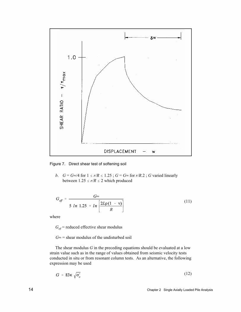
Figure 7. Direct shear test of softening soil . . . . . . . . . . . . . . . . . . . . . . . . . 14
Figure 8. f-w curve by Method SSF3 . . . . . . . . . . . . . . . . . . . . . . . . . . . . . . 15
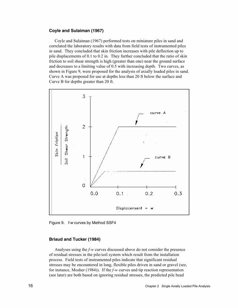
Figure 9. f-w curves by Method SSF4 . . . . . . . . . . . . . . . . . . . . . . . . . . . . . 16
Figure 10. f-w curve by Method SSF5 . . . . . . . . . . . . . . . . . . . . . . . . . . . . . . 18
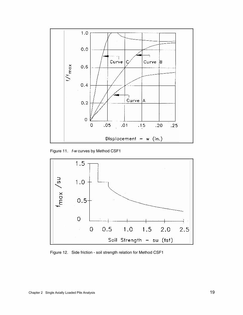
Figure 11. f-w curves by Method CSF1 . . . . . . . . . . . . . . . . . . . . . . . . . . . . . 19

v
Figure 12. Side friction - soil strength relation for Method CSF1 . . . . . . . . . 19
Figure 13. f-w curve by Method CSF2 . . . . . . . . . . . . . . . . . . . . . . . . . . . . . . 20
Figure 14. Strength reduction coefficients . . . . . . . . . . . . . . . . . . . . . . . . . . . 21
Figure 15. f-w curve by Method CSF4 . . . . . . . . . . . . . . . . . . . . . . . . . . . . . . 23
Figure 16. q-w curve by Method ST1 . . . . . . . . . . . . . . . . . . . . . . . . . . . . . . . 25
Figure 17. Ultimate tip resistance for Method SF1 . . . . . . . . . . . . . . . . . . . . 25
Figure 18. q-w curve by Method SF4 . . . . . . . . . . . . . . . . . . . . . . . . . . . . . . . 27
Figure 19. Ultimate tip resistance for Method SF5 . . . . . . . . . . . . . . . . . . . . 28
Figure 20. q-w curve by Method SF5 . . . . . . . . . . . . . . . . . . . . . . . . . . . . . . . 29
Figure 21. Assessment of degradation due to static loading . . . . . . . . . . . . . 30
Figure 22. Laterally loaded pile . . . . . . . . . . . . . . . . . . . . . . . . . . . . . . . . . . . 33
Figure 23. p-u curve by Method SLAT1 . . . . . . . . . . . . . . . . . . . . . . . . . . . . 35
Figure 24. Factors for calculation of ultimate soil resistance forlaterally loaded pile in sand . . . . . . . . . . . . . . . . . . . . . . . . . . . . . 36
Figure 25. Resistance reduction coefficient - A for Method SLAT1 . . . . . . . 37
Figure 26. Resistance reduction corefficient - B for Method SLAT1 . . . . . . 38
Figure 27. p-u curves by Method SLAT2 . . . . . . . . . . . . . . . . . . . . . . . . . . . . 39
Figure 28. p-u curves by Method CLAT1 . . . . . . . . . . . . . . . . . . . . . . . . . . . 41
Figure 29. p-u curves by Method CLAT2 for static loads . . . . . . . . . . . . . . . 42
Figure 30. Displacement parameter - A for Method CLAT2 . . . . . . . . . . . . . 44
Figure 31. p-u curve by Method CLAT2 for cyclic loads . . . . . . . . . . . . . . . 45
Figure 32. p-u curve by Method CLAT3 for static loads . . . . . . . . . . . . . . . . 46
Figure 33. p-u curve by Method CLAT3 for cyclic loads . . . . . . . . . . . . . . . 47
Figure 34. p-u curve by Method CLAT4 for static loading . . . . . . . . . . . . . . 48
Figure 35. p-u curve by Method CLAT4 for cyclic loading . . . . . . . . . . . . . 51
Figure 36. p-u curve by Method CLAT5 for static loading . . . . . . . . . . . . . . 54
Figure 37. p-u curve by Method CLAT5 for cyclic loading . . . . . . . . . . . . . 54
Figure 38. Model of laterally loaded pile . . . . . . . . . . . . . . . . . . . . . . . . . . . . 55
Figure 39. Proposed torsional shear - rotation curve . . . . . . . . . . . . . . . . . . . 65
Figure 40. Notation for pile head effects . . . . . . . . . . . . . . . . . . . . . . . . . . . . 68
Figure 41. Linearly elastic pile/soil system with free-standing segment . . . . 71
Figure 42. Pile cap loads, displacements, and coordinates . . . . . . . . . . . . . . . 77
Figure 43. Head forces, displacements, and coordinates for iTH pile . . . . . . . 78
vi
Figure 44. Relationship between global and local coordinates . . . . . . . . . . . 79
Figure 45. Geometric definitions for computation of added displacement . . 83
Figure 46. Modification of unit load transfer relationship for group effects at Node i, Pile I . . . . . . . . . . . . . . . . . . . . . . . . . . . . 85
Figure A1. Typical f-w curve . . . . . . . . . . . . . . . . . . . . . . . . . . . . . . . . . . . . . A2
Figure A2. Axial stiffness coefficient for constant soil stiffness . . . . . . . . . A4
Figure A3. Axial stiffness coefficient for soil stiffness varying linearly with depth . . . . . . . . . . . . . . . . . . . . . . . . . . . . . . . . . . . . A7
Figure A4. Axial stiffness coefficient for soil stiffness varying as square root of depth . . . . . . . . . . . . . . . . . . . . . . . . . . . . . . . . A8
Figure B1. Deflection coefficient for unit head shear for soil stiffness constant with depth . . . . . . . . . . . . . . . . . . . . . . . . . . . . B4
Figure B2. Slope coefficient for unit head shear for soil stiffness constant with depth . . . . . . . . . . . . . . . . . . . . . . . . . . . . . . . . . . . B5
Figure B3. Bending moment coefficient for unit head shear for soil stiffness constant with depth . . . . . . . . . . . . . . . . . . . . . . . . B6
Figure B4. Shear coefficient for unit head shear for soil stiffness constant with depth . . . . . . . . . . . . . . . . . . . . . . . . . . . . . . . . . . . B9
Figure B5. Deflection coefficient for unit head shear for soil stiffness varying linearly with depth . . . . . . . . . . . . . . . . . . . . . . . . . . . . B10
Figure B6. Slope coefficient for unit head shear for soil stiffness varying linearly with depth . . . . . . . . . . . . . . . . . . . . . . . . . . . . B11
Figure B7. Bending moment coefficient for unit head shear for soil stiffness varying linearly with depth . . . . . . . . . . . . . . . . . B14
Figure B8. Shear coefficient for unit head shear for soil stiffness varying linearly with depth . . . . . . . . . . . . . . . . . . . . . . . . . . . . B15
Figure B9. Deflection coefficient for unit head shear for soil stiffness varying linearly with depth . . . . . . . . . . . . . . . . . . . . . B16
Figure B10. Slope coefficient for unit head shear for soil stiffness varying parabolically with depth . . . . . . . . . . . . . . . . . . . . . . . . B19
Figure B11. Bending moment coefficient for unit head shear for soil stiffness varying parabolically with depth . . . . . . . . . . . . . B20
Figure B12. Shear coefficient for unit head shear for soil stiffness varying parabolically with depth . . . . . . . . . . . . . . . . B21
Figure B13. Deflection coefficient for unit head moment for soil stiffness constant with depth . . . . . . . . . . . . . . . . . . . . . . . . . . . B24
Figure B14. Slope coefficient for unit head moment for soil stiffness constant with depth . . . . . . . . . . . . . . . . . . . . . . . . . . . B25

vii
Figure B15. Bending moment coefficient for unit head moment for soil stiffness constant with depth . . . . . . . . . . . . . . . . . . . . . . . B26
Figure B16. Shear coefficient for unit head moment for soil stiffness constant with depth . . . . . . . . . . . . . . . . . . . . . . . . . . . . . . . . . . B29
Figure B17. Deflection coefficient for unit head moment for soil stiffness constant with depth . . . . . . . . . . . . . . . . . . . . . . . . . . . B30
Figure B18. Slope coefficient for unit head moment for soil stiffness constant with depth . . . . . . . . . . . . . . . . . . . . . . . . . . . B31
Figure B19. Bending moment coefficient for unit head moment for soil stiffness varying linearly with depth . . . . . . . . . . . . . . B32
Figure B20. Shear coefficient for unit head moment for soil stiffness varying linearly with depth . . . . . . . . . . . . . . . . . . . . . B33
Figure B21. Deflection coefficient for unit head moment for soil stiffness varying parabolically with depth . . . . . . . . . . . . . . . . B34
Figure B22. Slope coefficient for unit head moment for soil stiffness varying parabolically with depth . . . . . . . . . . . . . . . . B35
Figure B23. Bending moment coefficient for unit head moment for soil stiffness varying parabolically with depth . . . . . . . . . . . . . B36
Figure B24. Shear coefficient for unit head moment for soil stiffness varying parabolically with depth . . . . . . . . . . . . . . . . . . . . . . . . B37
Figure B25. Pile head deflection coefficients for unit head shear . . . . . . . . B38
Figure B26. Pile head slope coefficients for unit head shear . . . . . . . . . . . . B39
Figure B27. Pile head deflection coefficients for unit head moment . . . . . . B40
Figure B28. Pile head slope coefficients for unit head moment . . . . . . . . . . B41
List of Tables
Table 1. kf (psf/in.) as Function of Angle of Internal Friction of Sand for Method SSF1 . . . . . . . . . . . . . . . . . . . . . . . . . . . . . . . . . . 9
Table 2. Representative Values of k for Method SLAT1 . . . . . . . . . . . . . . 35
Table 3. Representative Values of 050 . . . . . . . . . . . . . . . . . . . . . . . . . . . . . 42
Table 4. Representative Values of Lateral Soil Stiffness k forPiles in Clay for Method CLAT2 . . . . . . . . . . . . . . . . . . . . . . . . . 43
Table 5. Curve Parameters for Method CLAT4 . . . . . . . . . . . . . . . . . . . . . 50
Table 6. Representative Values of k for Method CLAT4 . . . . . . . . . . . . . . 50
Table 7. Soil Modulus for Method CLAT5 . . . . . . . . . . . . . . . . . . . . . . . . . 52
Table 8. Soil Degradability Factors . . . . . . . . . . . . . . . . . . . . . . . . . . . . . . . 53

viii
Table 9. Values of Es for 1-ft-Wide Piles in Precompressed Clay . . . . . . . 58
Table 10. Values of Constant of Horizontal Subgrade Reaction nh for a 1-ft-Wide Pile in Sand . . . . . . . . . . . . . . . . . . . . . . . . . . . . . 58
Table A1. Adjustment in G for Various Loading Conditions (Adjustment factor = G (operational/G (in situ))) . . . . . . . . . . . A10
Table B1. Nondimensional Coefficients for Laterally Loaded Pile for Soil Modulus Constant with Depth (Head Shear Vo = 1, Head Moment Mo = 0) . . . . . . . . . . . . . . . . . . . . . . . . . . . B2
Table B2. Nondimensional Coefficients for Laterally Loaded Pile for Soil Modulus Constant with Depth (Head Shear Vo = 0, Head Moment Mo = 1) . . . . . . . . . . . . . . . . . . . . . . . . . . . B7
Table B3. Nondimensional Coefficients for Laterally Loaded Pile for Soil Modulus Varying Linearly with Depth (Head Shear Vo = 1, Head Moment Mo = 0) . . . . . . . . . . . . . . . . . . . . . . . . . . B12
Table B4. Nondimensional Coefficients for Laterally Loaded Pile for Soil Modulus Varying Linearly with Depth (Head Shear Vo = 0, Head Moment Mo = 1) . . . . . . . . . . . . . . . . . . . . . . . . . . B17
Table B5. Nondimensional Coefficients for Laterally Loaded Pile for Soil Modulus Varying Parabolically with Depth (Head Shear Vo = 1, Head Moment Mo = 0) . . . . . . . . . . . . . . . B22
Table B6. Nondimensional Coefficients for Laterally Loaded Pile for Soil Modulus Varying Parabolically with Depth (Head Shear Vo = 0, Head Moment Mo = 1) . . . . . . . . . . . . . . . B27

ix
Preface
This theoretical manual for pile foundations describes the background andresearch and the applied methodologies used in the analysis of pile foundations. This research was developed through the U.S. Army Engineer Research andDevelopment Center (ERDC) by the Computer-Aided Structural Engineering(CASE) Project. The main body of the report was written by Dr. Reed L.Mosher, Chief, Geosciences and Structures Division, Geotechnical andStructures Laboratory, ERDC (formerly with the Information TechnologyLaboratory (ITL)), and Dr. William P. Dawkins, Oklahoma State University. Additional sections were written by Mr. Robert C. Patev, formerly of theComputer-Aided Engineering Division (CAED), ITL, ERDC, and Messrs.Edward Demsky and Thomas Ruf, U.S. Army Engineer District, St. Louis.
Members of the CASE Task Group on Piles and Pile Substructures whoassisted in the technical review of this report are as follows:
Mr. Edward Demsky St. Louis DistrictMs. Anjana Chudgar Louisville DistrictMr. Terry Sullivan Louisville DistrictMr. Timothy Grundhoffer St. Paul District
Technical coordination and monitoring of this manual were performed byMr. Patev. Mr. H. Wayne Jones, Chief, CAED, is the Project Manager for theCASE Project. Mr. Timothy D. Ables is the Acting Director, ITL.
At the time of publication of this report, Director of ERDC was Dr. James R.Houston. Commander was COL James S. Weller, EN.
The contents of this report are not to be used for advertising, publication,or promotional purposes. Citation of trade names does not constitute anofficial endorsement or approval of the use of such commercial products.
x
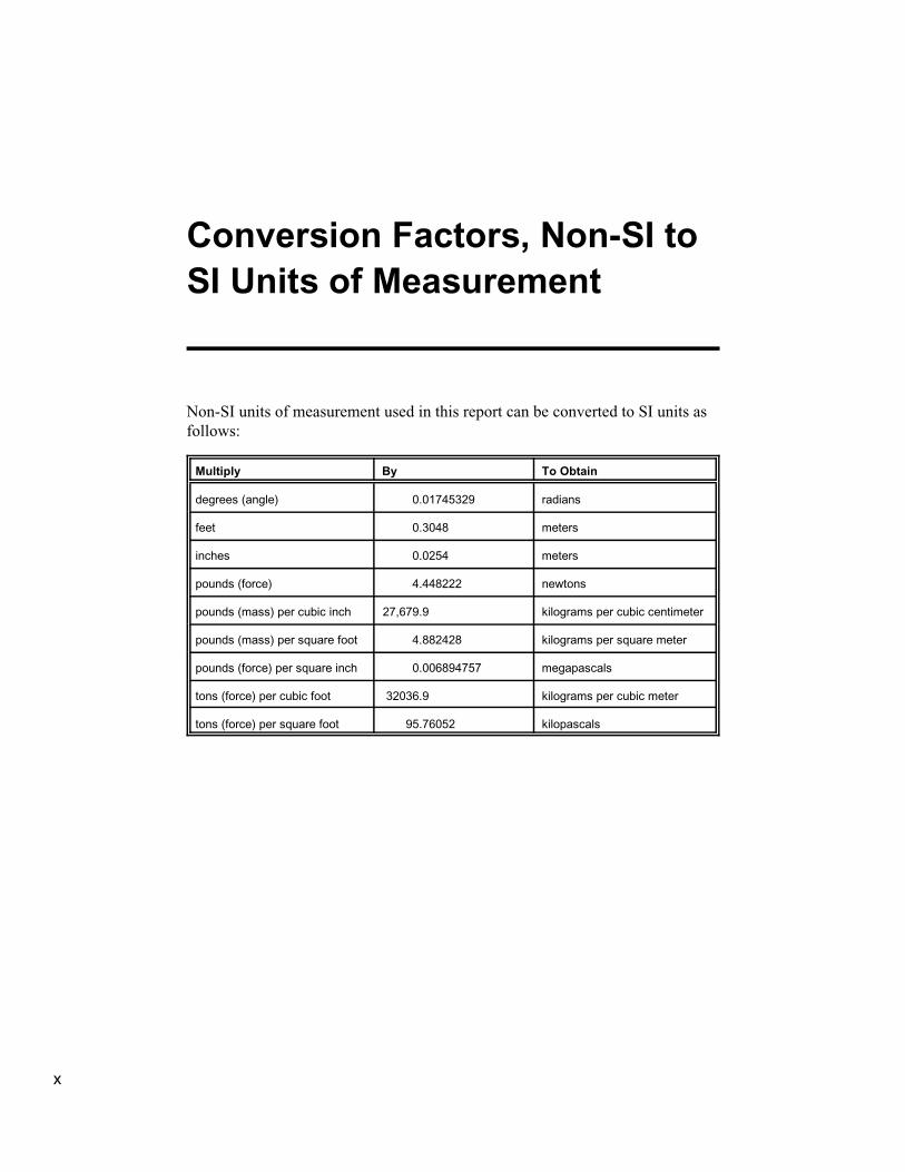
Conversion Factors, Non-SI toSI Units of Measurement
Non-SI units of measurement used in this report can be converted to SI units asfollows:
Multiply By To Obtain
degrees (angle) 0.01745329 radians
feet 0.3048 meters
inches 0.0254 meters
pounds (force) 4.448222 newtons
pounds (mass) per cubic inch 27,679.9 kilograms per cubic centimeter
pounds (mass) per square foot 4.882428 kilograms per square meter
pounds (force) per square inch 0.006894757 megapascals
tons (force) per cubic foot 32036.9 kilograms per cubic meter
tons (force) per square foot 95.76052 kilopascals

Chapter 1 Introduction 1
1 Introduction
Purpose
The purpose of this manual is to provide a detailed discussion of techniquesused for the design/analysis of pile foundations. Several of the procedures havebeen implemented in the CASE Committee computer programs CAXPILE(Dawkins 1984, Mosher et al. 1997), CPGA (Hartman, Jaeger, Jobst, and Martin1989) and COM624 (Reese 1980). Theoretical development of these engineer-ing procedures and discussions of the limitations of each method are presented.
Pile Behavior
The purpose of a pile foundation is to transmit the loads of a superstructure tothe underlying soil while preventing excessive structural deformations. The capacity of the pile foundation is dependent on the material and geometry ofeach individual pile, the pile spacing (pile group effect), the strength and type ofthe surrounding soil, the method of pile installation, and the direction of appliedloading (axial tension or compression, lateral shear and moment, or combina-tions). Except in unusual conditions, the effects of axial and lateral loads maybe treated independently.
Axial Behavior
A compressive load applied to the head (top) of the pile is transferred to thesurrounding soil by a combination of skin friction along the embedded lengthand end bearing at the tip (bottom) of the pile. For relatively short piles, onlythe end bearing effect is significant. For relatively long piles in soil (excludingtip bearing piles on rock), the predominant load transfer is due to skin friction. Unless special mechanical provisions are present (e.g., an underreamed tip), axial tension load is resisted only by skin friction.
2 Chapter 1 Introduction
Lateral Behavior
Piles are often required to support loads applied perpendicular to their longi-tudinal axes (lateral loads). As stated previously, lateral load resistance islargely independent of axial effects. However, a high axial compression mayinteract with lateral displacements (the beam-column effect) to increase lateraldisplacements, bending moments, and shears.
Battered Piles
If the horizontal loads imparted to the pile foundation are large, a foundationconsisting solely of vertical piles may not possess sufficient lateral resistance. In such circumstances, battered (inclined) piles are installed to permit the hori-zontal foundation load to be supported by a component of the axial pile/soilresistance in addition to the lateral resistance.
Classical Analysis and/or Design Procedures
Single piles
Prior to the development of reliable computer programs, the design of a single pile was based primarily on the ultimate load capacity of the pile as deter-mined from a load test or from semi-empirical equations. The allowable orworking load to which the pile could be subjected was taken as some fraction ofthe ultimate. Little, if any, emphasis was placed on the load-displacement behavior of the pile. Design methodology used in the Corps of Engineers isdocumented in Engineer Manual 1110-2-2906 (U.S. Army Corps of Engineers(USACE) 1995).
Pile groups
Classical methods (e.g., Culmann's method, the Common Analytical Method,the Elastic Center Method, the Moment-of-Inertia Method, etc.) of analysis forpile groups were based on numerous simplifying assumptions to allow thenumerical calculations to be performed by hand. Common to these methods arethe assumptions that only the axial resistance of the piles is significant and thatthe pile cap is rigid. Force and moment equilibrium equations are used to allotthe foundation loads to the individual piles. No attempt is made in these meth-ods to consider force-displacement compatibility (the soil-structure interactioneffect). It has been shown that these classical methods frequently result inunconservative designs.

Chapter 1 Introduction 3
State-of-the-Corps-Art Methods for Hydraulic Structures
System modelling
Rational designs must be based on solutions in which equilibrium and force-displacement compatibility are simultaneously satisfied. Ongoing research hasresulted in the development of mathematical models for the pile/soil systemwhich permit analysis of the entire range of load-displacement response forsingle piles subjected to axial and/or lateral loads. Methods have beendeveloped for the design of pile groups in which the soil-structure interactioncharacteristics of single piles have been incorporated. These methods and theconsiderations leading to their development are described in detail in Chapters 2-4. A synopsis is provided in the following paragraphs.
Axially loaded piles
For analysis of a pile subjected to axial loads, the soil surrounding the em-bedded length of the pile is modelled as a distribution of springs which resistlongitudinal displacements of the pile. The resistance of the soil springs is rep-resentative of the skin friction of the soil on the pile. The effect of tip resistanceis represented by a concentrated spring. The characteristics of these springs areprovided in the form of resistance-displacement (load-transfer) curves represent-ing the skin friction effects (Seed and Reese (1957), and other references) and aforce-displacement curve representing the tip reaction.
The load-transfer curves and tip reaction curves have been obtained fromfield tests of instrumented piles subjected to axial compression. Research iscontinuing to permit evaluation of load-transfer curves for piles in tension. Theunderlying principles on which the load-transfer curves and tip reaction curveare based and the modelling of the pile/soil system are presented in Chapter 2.
Laterally loaded piles
The soil which resists displacements of a laterally loaded pile is also replacedby distributed springs. The force-displacement characteristics of the springs arepresented as curves which have been extracted from field tests of laterallyloaded piles. Techniques for lateral load analysis are discussed in Chapter 3.
Pile head stiffnesses
Computer programs (e.g. CAXPILE, CPGS, COM624G) are available whichpermit the analysis of load-displacement response of a pile/soil system up to anultimate or failure condition. The relationship between load and displacement
4 Chapter 1 Introduction
tends to be essentially linear through the range of loads usually allowed (theworking loads) in design. The relationship becomes highly nonlinear as anultimate condition is neared. For design purposes, the linearly elastic relation-ship between head loads and head displacements is usually presented as a matrixof stiffness coefficients. These coefficients may be extracted from the full rangeanalyses for axially or laterally loaded piles cited above. In addition, the stiff-ness coefficients may be estimated using linearized solutions. These processesare discussed in Chapters 2 and 3.
Pile groups
Pile group behavior is analyzed by the procedure suggested by Saul (1968). The method considers both equilibriun and force-displacement compatibility indistributing the loads on the foundation among the individual piles. The processrequires an evaluation of the linearized pile head stiffness matrix for each pile inthe group. The pile head stiffness matrix may be evaluated by the single pileanalysis procedures alluded to above. However, the evaluation must account forthe effects of the proximity of adjacent piles.
Although the group analysis method was originally developed for linear sys-tems with rigid pile caps, it has been extended to allow for flexible caps and, byiterative solutions, can account for nonlinear behavior (e.g. CPGA). The methodis described in detail in Chapter 4.

Chapter 2 Single Axially Loaded Pile Analysis 5
2 Single Axially Loaded PileAnalysis
Introduction
A schematic of an axially loaded pile is shown in Figure 1. In the discussionswhich follow, the pile is assumed to be in contact with the surrounding soil overits entire length. Consequently, the embedded length and the total length of thepile are the same. The effect of a free-standing portion of the pile will bediscussed later.
The pile is assumed to have a straight centroidal axis (the z-axis, positivedownward) and is subjected to a centric load at the head (top of the pile) Po. Displacements parallel to the axis of the pile are denoted w and are positive inthe positive z-direction. The pile material is assumed to be linearly elastic for alllevels of applied loads. “Ultimate” conditions referred to subsequently indicatethat a limit has been reached in which any additional head load would causeexcessive displacements.
The major research efforts devoted toward investigation of axially loadedpiles have been performed for homogeneous soil media. Only in limited caseshas the effect of nonhomogeneity been considered. In most cases the effects oflayering in the soil profile and/or lateral variations in soil characteristics canonly be approximated.
Load-Transfer Mechanism
The head load Po is transferred to the surrounding soil by shear stresses (skinfriction) along the lateral pile/soil interface and by end-bearing at the pile tip(bottom of the pile). The rate at which the head load is transferred to the soilalong the pile and the overall deformation of the system are dependent onnumerous factors. Among these are: (a) the cross section geometry, material,length, and, to a lesser extent, the surface roughness of the pile; (b) the type ofsoil (sand or clay) and its stress-strain characteristics; (c) the presence or absence

6 Chapter 2 Single Axially Loaded Pile Analysis
Figure 1. Axially loaded pile
of groundwater; (d) the method of installation of the pile; and, (e) the presenceor absence of residual stresses as a result of installation.
A heuristic approach has been followed to reduce the complex three- dimen-sional problem to a quasi one-dimensional model (illustrated in Figure 2) whichis practicable for use in a design environment. In the one-dimensional model,the soil surrounding the pile is replaced by a distribution of springs along thelength of the pile and by a concentrated spring at the pile tip which resist axialdisplacements of the pile. The characteristics of these springs are presented inthe form of curves which provide the magnitude of unit skin friction (f-w curves)or unit tip reaction (q-w curve) as a function of pile displacement. The nomen-clature used to define axial curves is based on unit skin friction f, unit tipreaction q, and w = displacement in the z-direction for axial loads.

Chapter 2 Single Axially Loaded Pile Analysis 7
Figure 2. One-dimensional model of axially loaded pile
The f-w and q-w curves have been developed using the principles of contin-uum and soil mechanics and/or from correlations with the results of field tests oninstrumented axially loaded piles. Several different criteria are presented belowfor development of f-w and q-w curves. The reliability of any method inpredicting the behavior of a particular pile depends on the similarity of thesystem under investigation with the database used to establish the method. Mostof the methods account explicitly or implicitly for the three factors cited onpage 5 (a, b, and c). In all cases the pile is assumed to be driven into the soil orto be a cast-in-place pier. Only one of the procedures attempts to account for theeffects of residual stresses; the remaining methods exclude these effects.
8 Chapter 2 Single Axially Loaded Pile Analysis
Figure 3. f-w curve by Method SSF1
'
%
Synthesis of f-w Curves for Piles in Sand Under Compressive Loading
Mosher (1984)
Mosher (1984) utilized the results of load tests of prismatic pipe piles drivenin sand and the work of Coyle and Castello (1981) to arrive at the hyperbolicrepresentation of the f-w curve (see Figure 3).
(1)
The initial slope kf of the curve is given in Table 1 as a function of the angle ofinternal friction and the ultimate side friction fmax is given in Figure 4 as afunction of relative depth (depth z below ground surface divided by thediameter of the pile 2R).
Chapter 2 Single Axially Loaded Pile Analysis 9
Figure 4. Ultimate side friction for Method SSF1
Table 1kf (psf/in.) as Function of Angle of Internal Friction of Sand forMethod SSF1
Angle of Internal Friction (degrees)1 kf (psf/in.)
28 - 31 6,000 - 10,000
32 - 34 10,000 - 14,000
35 - 38 14,000 - 18,000
1 A table of factors for converting non-SI units of measurement to SI (metric) units is presentedon page x.

10 Chapter 2 Single Axially Loaded Pile Analysis
Figure 5. Equivalent radius for noncircular cross sections
J '
The effects of groundwater, layering, and variable pile diameter may beaccounted for approximately by adjusting the relative depth at each point as fol-lows. The effective depth z' below ground surface is obtained by dividing theeffective vertical soil pressure at a point by the effective unit weight at thatpoint; the relative depth is obtained by dividing the effective depth by the pilediameter at that point. This approximation will result in unrealistic discon-tinuities in the distribution of f-w curves at soil layer boundaries, at the locationof a subsurface groundwater level, and at changes in pile diameter.
The method may also be extended to approximate the behavior of noncircularcross sections using the equivalent radius of the pile as indicated in Figure 5.
Kraft, Ray, and Kagawa (1981)
Numerous analyses (Randolph and Wroth 1978; Vesic 1977; Kraft, Ray, andKagawa 1981; Poulos and Davis 1980) have been performed in which thepile/soil system is assumed to be radially symmetric and the soil is assumed tobe a vertically and radially homogeneous, elastic medium. The principles ofcontinuum mechanics as well as finite element methods have been used to arriveat the relationship between side friction and axial pile displacement. Theprocess due to Kraft, Ray, and Kagawa (1981) is outlined below.
Shear stresses are assumed to decay radially in the soil according to
(2)

Chapter 2 Single Axially Loaded Pile Analysis 11
( ' 'J
'
' m '
' D & <
where
J = shear stress in the soil
f = side friction at pile/soil interface
R = pile radius
r = radial distance from the pile centerline
If radial deformations of the soil are ignored, the shear strain at any point inthe soil may be expressed as
(3)
where G is the soil shear modulus of elasticity.
The axial displacement at the interface is obtained by integrating Equation 3to obtain
(4)
where
w = axial displacement of the pile
rm = a limiting radial distance beyond which deformations of the soil mass arenegligible
Randolph and Wroth suggested
(5)
where
L = embedded length of the pile
D = a factor to account for vertical nonhomogeneity of the soil medium to bediscussed later
< = Poisson's ratio for the soil
Combination of Equations 4 and 5 yields a linear relationship between piledisplacements and side friction as

12 Chapter 2 Single Axially Loaded Pile Analysis
'D & <
'
D & <&
&
'
D & <&
&&
D & <&
&
(6)
The side friction-displacement relationship expressed in Equation 6 isappropriate only for very small displacements. To account for deviations fromlinearity, a hyperbolic variation in side friction-displacements proposed byKraft, Ray, and Kagawa (1981) is
(7)
where Rf is a curve fitting parameter (Kraft, Ray, and Kagawa 1981) which maybe taken as 0.9 for most conditions. The value of fmax may be obtained from thecurves due to Mosher (Figure 4) or may be estimated as suggested under methodSSF3 which follows.
After fmax has been reached, the f-w curve becomes a horizontal line at fmax . The f-w curve produced by this method is illustrated in Figure 6 by the solidcurve 0 - 1 - 2 .
Some soils exhibit a degradation in strength after a maximum resistance hasbeen reached. The results of a direct shear test for a softening soil illustrated inFigure 7 are used to construct the descending branch of the f-w curve forsoftening soils shown by the dashed line in Figure 6 as follows. The displace-ment beyond the maximum fmax required to reduce the side friction to its residualvalue is obtained by adjusting the direct shear displacement to account for elasticrebound of the pile due to the reduction in side friction. This adjustment is givenby
(8)
The softening portion of the f-w curve is obtained by scaling the normalizeddirect shear curve to the f-w curve (dashed line 1-3 in Figure 6).
Because the shear strength of sands increases with depth (i.e. confiningpressure), the shear modulus G is not constant along the length of the pile. Finite element analyses have indicated, for a linear increase in G with depth, thevalue of D to be

Chapter 2 Single Axially Loaded Pile Analysis 13
Figure 6. f-w curve by Method SSF2
D '
'4
%D & <
(9)
where
Gm = soil shear modulus at mid-depth of the pile
Gt = shear modulus at the pile tip
The preceding equations also assume that the soil modulus G is unaffectedby the pile installation. Randolph and Wroth (1978) performed finite elementanalyses for two hypothetical variations of shear modulus radially away from thepile. These variations and the effective shear modulus were:
a. G = G4/4 for 1 # r/R # 1.25 ; G = G4 for r/R > 1.25 which produced
(10)
14 Chapter 2 Single Axially Loaded Pile Analysis
Figure 7. Direct shear test of softening soil
'4
%D & <
' 6 FN
b. G = G4/4 for 1 # r/R # 1.25 ; G = G4 for r/R.2 ; G varied linearlybetween 1.25 # r/R # 2 which produced
(11)
where
Geff = reduced effective shear modulus
G4 = shear modulus of the undisturbed soil
The shear modulus G in the preceding equations should be evaluated at a lowstrain value such as in the range of values obtained from seismic velocity testsconducted in situ or from resonant column tests. As an alternative, the followingexpression may be used
(12)

Chapter 2 Single Axially Loaded Pile Analysis 15
' &
Figure 8. f-w curve by Method SSF3
where
6 = a function of relative density, varying from 50 at a relative density of 60 percent to 70 at a relative density of 90 percent
FoN = mean effective stress in the soil (vertical stress plus two times horizontalstress); with G and FoN in psi
Vijayvergiya (1977)
Vijayvergiya (1977) proposed a relationship between side friction and piledisplacement of the form
(13)
where wc is the displacement required to develop fmax. For w greater than wc , fremains constant at fmax. Vijayvergiya gives limiting values of fmax as 1 tsf forclean medium dense sand, 0.85 tsf for silty sand, 0.7 tsf for sandy silt, and 0.5 tsffor silts. The suggested values of wc range from 0.2 to 0.3 in. for nominal sizedpiles. A typical f-w curve by this method is shown as the solid curve in Figure 8.
16 Chapter 2 Single Axially Loaded Pile Analysis
Figure 9. f-w curves by Method SSF4
Coyle and Sulaiman (1967)
Coyle and Sulaiman (1967) performed tests on miniature piles in sand andcorrelated the laboratory results with data from field tests of instrumented pilesin sand. They concluded that skin friction increases with pile deflection up topile displacements of 0.1 to 0.2 in. They further concluded that the ratio of skinfriction to soil shear strength is high (greater than one) near the ground surfaceand decreases to a limiting value of 0.5 with increasing depth. Two curves, asshown in Figure 9, were proposed for the analysis of axially loaded piles in sand. Curve A was proposed for use at depths less than 20 ft below the surface andCurve B for depths greater than 20 ft.
Briaud and Tucker (1984)
Analyses using the f-w curves discussed above do not consider the presenceof residual stresses in the pile/soil system which result from the installationprocess. Field tests of instrumented piles indicate that significant residualstresses may be encountered in long, flexible piles driven in sand or gravel (see,for instance, Mosher (1984)). If the f-w curves and tip reaction representation(see later) are both based on ignoring residual stresses, the predicted pile head
Chapter 2 Single Axially Loaded Pile Analysis 17
'
%&
&
'
'
S '
' S
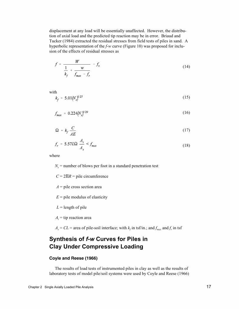
displacement at any load will be essentially unaffected. However, the distribu-tion of axial load and the predicted tip reaction may be in error. Briaud andTucker (1984) extracted the residual stresses from field tests of piles in sand. Ahyperbolic representation of the f-w curve (Figure 10) was proposed for inclu-sion of the effects of residual stresses as
(14)
with (15)
(16)
(17)
(18)
where
Ns = number of blows per foot in a standard penetration test
C = 2AR = pile circumference
A = pile cross section area
E = pile modulus of elasticity
L = length of pile
At = tip reaction area
As = CL = area of pile-soil interface; with kf in tsf/in.; and fmax and fr in tsf
Synthesis of f-w Curves for Piles in Clay Under Compressive Loading
Coyle and Reese (1966)
The results of load tests of instrumented piles in clay as well as the results oflaboratory tests of model pile/soil systems were used by Coyle and Reese (1966)

18 Chapter 2 Single Axially Loaded Pile Analysis
Figure 10. f-w curve by Method SSF5
' "
to establish the three load transfer curves shown in Figure 11. Curve A isapplicable for points along the pile from the ground surface to a depth of 10 ft,curve B applies for depths from 10 ft to 20 ft, and curve C is applicable for alldepths below 20 ft.
The relationship between maximum side friction and soil shear strengthprovided by Coyle and Reese is shown in Figure 12.
Aschenbrener and Olson (1984)
Data obtained from a large number of field load tests of piles in clay wereexamined by Aschenbrener and Olson (1984) with the intent to devise loadtransfer relationships which provided the best fit to the diverse pile and soilproperties represented by the database. The simple bilinear relationship shownin Figure 13 was selected as a result of their study.
Aschenbrener and Olson expressed the relationship between fmax and soilshear strength as
(19)
Chapter 2 Single Axially Loaded Pile Analysis 19
Figure 11. f-w curves by Method CSF1
Figure 12. Side friction - soil strength relation for Method CSF1

20 Chapter 2 Single Axially Loaded Pile Analysis
Figure 13. f-w curve by Method CSF2
" '&
" '
where
" = a proportionality factor
su = undrained shear strength
Aschenbrener and Olson were able to evaluate " from the field test data as
(20)
where
Pou = pile head load at failure
Ptu = tip load at failure
su = undrained shear strength
As = area of pile-soil interface
In a design situation, the ultimate head and tip loads will not be known. Fordesign, the value of " may be obtained from the curves provided by Semple andRigden (1984) shown in Figure 14 as
(21)
Chapter 2 Single Axially Loaded Pile Analysis 21
Figure 14. Strength reduction coefficients
where
ap = peak strength reduction factor from Figure 14a
al = length factor from Figure 14b
In Figure 14, su is the undrained shear strength; Fv is the effective overburdenpressure; L is the length of pile; and, R is the pile radius.
Kraft, Ray, and Kagawa (1981)
The procedure of Method SSF2 due to Kraft, Ray, and Kagawa (1981)described previously for sand side friction, may be applied to piles in clay. Forclays, the shear modulus may again be evaluated from seismic tests, fromresonant column tests, approximated as 400 to 500 times su , or evaluated fromthe modulus of elasticity as E/3 for undrained conditions and E/2.75 for drainedconditions.
22 Chapter 2 Single Axially Loaded Pile Analysis
'
%
' %
' % &
Heydinger and O’Neill (1986)
Finite element and finite difference analyses were performed by Heydingerand O'Neill (1986) to develop f-w curves for piles in clay. An axisymmetricmodel including interface elements to account for slippage of the pile-soilsystem was used in the finite element analyses. An unconsolidated-undrainedcondition was assumed to exist in the soil and the initial mean effective stresseswere computed from radial consolidation theory in which the pile installationprocess was represented by an expanding cylindrical cavity. A general equationfor the f-w curves (illustrated in Figure 15) was selected as
(22)
where the parameters Ef and m were determined by statistical correlations withthe analytical results as
(23)
and
(24)
where
E = initial undrained modulus of elasticity of the soil at the depth of interest
Eavg = the average initial undrained modulus of elasticity over the entire lengthof the pile
pa = atmospheric pressure in the same units as Eavg
The value of E should be measured at very low strains. An approximation for Eis cited as 1,200 to 1,500 times su .
Vijayvergiya (1977)
Vijayvergiya (1977) indicated that Equation 13 for f-w curves in sand,Method SSF3, is applicable for piles in clay. As for piles in sand, Vijayvergiyasuggests values of the critical pile displacement wc of 0.2 to 0.3 in. Although a

Chapter 2 Single Axially Loaded Pile Analysis 23
Figure 15. f-w curve by Method CSF4
method for evaluating fmax is presented by Vijayvergiya, he suggests that other lesscomplex methods are equally suitable, e.g., the process of Method CSF2discussed previously.
Tip Reactions
The influence of the tip reaction on the axial load-displacement behaviordepends on the relative stiffness of the pile as well as side friction stiffness ofthe soil. In the following paragraphs several curves are presented for assessingthe tip reaction as a function of the tip displacement. In general these curveshave been developed primarily from a consideration of the properties of the soilat the tip elevation. However, numerous theoretical studies (see, for instance,Randolph and Wroth (1978)) have indicated that the tip reaction depends on thecharacteristics of the soil both above and below the tip elevation. Some of themethods for developing q-w curves for the tip reaction account for the profile inthe vicinity of the tip by using average soil properties. Other methods, derivedfrom test results where the soil at the test site was relatively homogeneous, aredependent on the properties of the soil at the tip.
The curves presented below are for unit tip reaction (i.e. force per unit of tiparea). To evaluate the total tip reaction, this unit force must be multiplied by thearea of the pile tip actually bearing on the soil. For solid or closed-end piles thetip bearing area is reasonably taken as being equal to the gross cross sectionarea. For open-end piles (e.g. pipes) or H-piles the effective tip area may be aslittle as the material area of the pile or may be as much as the gross section area.

24 Chapter 2 Single Axially Loaded Pile Analysis
'& <
Synthesis of q-w Curves for Piles in Sand Under Compressive Loading
Mosher (1984)
Mosher (1984) expanded the work of Coyle and Castello (1981) to determinethe q-w relationship for piles in sand. Mosher proposed the exponential q-wcurve shown in Figure 16. Values of ultimate unit tip reaction qmax are given as afunction of relative depth (L/2R) in Figure 17.
Kraft, Ray, and Kagawa (1981)
Kraft, Ray, and Kagawa (1981) did not attempt to produce a q-w curvecorresponding to their analytical f-w curve, but approximated the q-w relation-ship by the elastic solution for a rigid punch according to
(25)
where
w = tip displacement
R = radius of pile tip reaction area
q = tip pressure
L = Poisson's ratio for the soil at the tip
E = secant modulus of elasticity of the soil appropriate to the level of soilstress associated with q
It = influence coefficient ranging from 0.5 for long piles to 0.78 for very shortpiles
Vijayvergiya (1977)
Vijayvergiya (1977) proposed an exponential representation for the q-w curve for a pile in sand similar to those in Method ST1. For w < wc

Chapter 2 Single Axially Loaded Pile Analysis 25
Figure 16. q-w curve by Method ST1
Figure 17. Ultimate tip resistance for Method SF1
' (26)

1 Unpublished Class Notes, 1977, H. M. Coyle, “Marine Foundation Engineering,” Texas A&MUniversity, College Station, TX.
26 Chapter 2 Single Axially Loaded Pile Analysis
'
%&
%
'
' S
'
where wc is the critical tip displacement given by Vijayvergiya as ranging from3 to 9 percent of the diameter of the tip reaction area. For w > wc , q = qmax. Vijayvergiya did not suggest adjusting the exponent to account for density.
Briaud and Tucker (1984)
Briaud and Tucker (1984) offer a means of accounting for the presence ofresidual stresses due to pile installation on the tip reaction. The hyperbolicrelationship between unit tip reaction and tip displacement shown in Figure 18 isgiven by
(27)
(28)
(29)
(30)
where
N = uncorrected average blow count of a standard penetration test over adistance of four diameters on either side of the tip
kq = initial slope of the q-w curve in tsf/in.
qmax , qr = ultimate and residual unit tip resistances, respectively, in tsf. Otherterms are defined on page 6
Coyle and Castello (1981)
Coyle and Castello (1981) provided ultimate tip reactions based on correla-tions for instrumented piles in sand as shown in Figure 19. Coyle1 recom-mended the tip reaction curve shown in Figure 20.

Chapter 2 Single Axially Loaded Pile Analysis 27
Figure 18. q-w curve by Method SF4
'
Synthesis of q-w Curves for Piles in Clay Under Compressive Loading
Aschenbrener and Olson (1984)
Data for tip load and tip settlement were not recorded in sufficient detail inthe database considered by Aschenbrener and Olson (1984) to allow establishinga nonlinear q-w relationship. It was concluded that the sparsity and scatter offield data warranted nothing more complex than a simple elasto-plastic relation-ship. In their representation, q varies linearly with w reaching qmax at a displace-ment equal to 1 percent of the tip diameter and remains constant at qmax for largerdisplacements. Ultimate tip reaction was evaluated according to
(31)
where
su = undrained shear strength
Nc = bearing capacity factor
28 Chapter 2 Single Axially Loaded Pile Analysis
Figure 19. Ultimate tip resistance for Method ST5
Test data indicated that Nc varied from 0 to 20 and had little correlation withshear strength. When ultimate tip reaction was not available from recorded data,Aschenbrener and Olson used a conventional value for Nc equal to 9.
Vijayvergiya (1977)
Vijayvergiya (1977) recommends that the exponential q-w curve for sand asdiscussed on pages 24-26 is applicable for piles in clay. He indicates that qmax
can be calculated from Equation 31 above but provides no guidance for theselection of Nc.
Other Considerations
Uplift loading
For some design cases it may be necessary to evaluate the behavior of anaxially loaded pile for uplift (tension) loading. Considerably less is known aboutuplift loading than about compression loading. However, it is believed to besufficiently accurate to analyze prismatic piles in clay under uplift using the same

Chapter 2 Single Axially Loaded Pile Analysis 29
Figure 20. q-w curve by Method SF5
'
&%
&
'
&
%
procedures used for compression loading, except that the tip reaction should beomitted unless it is explicitly accounted for as discussed below. In sands, use ofthe same procedures employed in compression loading is recommended, withthe exception that fmax should be reduced to 70 percent of the maximum compres-sion value.
For the methods that explicitly include residual driving stress effects innonlinear f-w and q-w curves (pages 16-17 and 26), it is recommended that theappropriate curves for uplift loading be generated by extending the solid curvesin Figures 10 and 18 in the negative w direction with the same initial slopes asexist in the positive w direction and assuring that the q-w curve terminates at q =0. That is
(32)
where w is negative and fmax, fr, and kf are positive. And
(33)

30 Chapter 2 Single Axially Loaded Pile Analysis
Figure 21. Assessment of degradation due to static loading
where w is negative and qr and kq are positive. All parameters appearing inEquations 32 and 33 are evaluated as for compressive loading.
Bearing on Rock
The tip reaction-tip displacement relationship for a pile driven to bearing onrock may be assumed to be linear. The tip reaction stiffness given by Equation25 may be used where the modulus of elasticity and Poisson's ratio should reflectthe characteristics of the surficial zone of the rock. The influence coefficient It
in Equation 25 may be taken as 0.78 for very sound rock but should be reducedto account for such effects as fracturing of the rock surface due to driving.
Cyclic Loading
Studies have shown (Poulos 1983) that the principal concern associated withcyclic axial loading is the tendency for fmax to reduce as the ratio of the cycliccomponent of axial load Poc to the ultimate static capacity Pous increases beyondsome critical value. As long as the ratio remains below the failure envelopeshown in Figure 21, no significant degradation of the pile capacity or force-displacement behavior is likely to occur.

Chapter 2 Single Axially Loaded Pile Analysis 31
& B '
Algorithm for Analysis of Axially Loaded Piles
The derivation of the f-w and q-w curves from theoretical considerations orfrom experimental data described in the preceding sections was in all casesbased on the assumption that the side friction f or tip reaction q at any point is afunction only of the pile displacement at that point (i.e. the well known Winklerassumption). For this assumption and the one-dimensional model of the pile-soilsystem shown in Figure 2, the governing differential equation for a prismatic,linearly elastic pile is
(34)
where
E = modulus of elasticity of the pile material
A = pile material cross section area
w = axial displacement
R = effective radius of pile soil interface; and f(z,w) is the unit side friction,which is a function of both position on the pile as well as piledisplacement
Because the displacements must be known before the side friction f(z,w) canbe determined, numerical iterative solutions of Equation 34 are required. Themost common approach to the solution is to replace the continuous pile-soilsystem with a discretized model (Coyle and Reese 1966, Dawkins 1982,Dawkins 1984) defined by a finite number of nodes along the pile at whichdisplacements and forces are evaluated. The solution proceeds by a successionof trial and correction solutions until compatibility of forces and displacementsis attained at every node.
Observations of System Behavior
An expedient device in obtaining the numerical solutions described above isto replace the nonlinear f-w and q-w curves by equivalent linearly elastic springsduring each iteration. The stiffnesses of these linear springs are evaluated as thesecant to the f-w or q-w curve for the displacement calculated during thepreceding iteration. It is to be noticed that ultimate side friction increases withdepth while pile displacements decrease with depth. Hence it can be concludedthat the stiffness of the load transfer mechanism for side friction increases withdepth. If the distribution of the side friction for any given head load can bedetermined then a solution may be obtained from a linearly elastic solutionwithout the need for iterations.

32 Chapter 3 Single Laterally Loaded Pile Analysis
3 Single Laterally LoadedPile Analysis
Introduction
Although the usual application of a pile foundation results primarily in axialloading, there exist numerous situations in which components of load at the pilehead produce significant lateral displacements as well as bending moments andshears. Unlike axial loads, which only produce displacements parallel to theaxis of the pile (a one-dimensional system), lateral loads may produce displace-ments in any direction. Unless the pile cross section is circular, the laterallyloaded pile/soil system represents a three-dimensional problem. Most of theresearch on the behavior of laterally loaded piles has been performed on piles ofcircular cross section in order to reduce the three-dimensional problem to twodimensions. Little work has been done to investigate the behavior of noncircularcross section piles under generalized loading. In many applications, battering ofthe piles in the foundation produces combined axial and lateral loads. However,the majority of the research on lateral load behavior has been restricted tovertical piles subjected to loads which produce displacements perpendicular tothe axis of the pile. In the discussions which follow, it is assumed that the pilehas a straight centroidal vertical axis. If the pile is nonprismatic and has anoncircular cross section, it is assumed that the principal axes of all crosssections along the pile fall in two mutually perpendicular planes and that theloads applied to the pile produce displacements in only one of the principalplanes.
A schematic of a laterally loaded pile is shown in Figure 22. The x-z plane isassumed to be a principal plane of the pile cross section. Due to the appliedhead shear Vo and head moment Mo , each point on the pile undergoes a transla-tion u in the x-direction and a rotation 2 about the y-axis. Displacements andforces are positive if their senses are in a positive coordinate direction. Thesurrounding soil develops pressures, denoted p in Figure 22, which resist thelateral displacements of the pile.
The principles of continuum mechanics and correlations with the results oftests of instrumented laterally loaded piles have been used to relate the soil
Chapter 3 Single Laterally Loaded Pile Analysis 33
Figure 22. Laterally loaded pile
lateral resistance p at each point on the pile to the lateral displacement u at thatpoint (i.e. the Winkler assumption). The relationship between soil resistance and
lateral displacement is presented as a nonlinear curve - the p-u curve. Severalmethods are summarized in the following paragraphs for development of p-ucurves for laterally loaded piles in both sands and clays. In all of the methods,the primary p-u curve is developed for monotonically increasing static loads. The static curve is then altered to account for the degradation effects producedby cyclic loads such as might be produced by ocean waves on offshore struc-tures. Methods designated SLAT1 and CLAT1 through CLAT4 have beenincorporated into the CASE Project Computer program CPGS.
34 Chapter 3 Single Laterally Loaded Pile Analysis
'
Load Transfer Mechanism for Laterally Loaded Piles
The load transfer mechanism for laterally loaded piles is much more complexthan that for axially loaded piles. In an axially loaded pile the axial displace-ments and side friction resistances are unidirectional (i.e., a compressive axialhead load produces downward displacements and upward side friction resistanceat all points along the pile). Similarly, the ultimate side friction at the pile-soilinterface depends primarily on the soil shear strength at each point along thepile. Because the laterally loaded pile is at least two-dimensional, the ultimatelateral resistance of the soil is dependent not only on the soil shear strength buton a geometric failure mechanism. At points near the ground surface an ultimatecondition is produced by a wedge type failure, while at lower positions failure isassociated with plastic flow of the soil around the pile as displacements increase. In each of the methods described below, two alternative evaluations are made forthe ultimate lateral resistances at each point on the pile, for wedge type failureand for plastic flow failure, and the smaller of the two is taken as the ultimateresistance.
Synthesis of p-u Curves for Piles in Sand
Reese, Cox, and Koop (1974)
A series of static and cyclic lateral load tests were performed on pipe pilesdriven in submerged sands (Cox, Reese, and Grubbs 1974; Reese, Cox, andKoop 1974; Reese and Sullivan 1980). Although the tests were conducted insubmerged sands, Reese et al. (1980) have provided adjustments by which the p-u curve can be developed for either submerged sand or sand above the watertable. The p-u curve for a point a distance z below the pile head extracted fromthe experimental results is shown schematically in Figure 23. The curve consistsof a linear segment from 0 to a , an exponential variation of p with u from a tob, a second linear range from b to c, and a constant resistance for displacementsbeyond c .
Steps for constructing the p-u curve at a depth z below the ground surface areas follows:
a. Determine the slope of the initial linear portion of the curve from
(35)
where k is obtained from Table 2 for either submerged sand or sand above thewater table.

Chapter 3 Single Laterally Loaded Pile Analysis 35
Figure 23. p-u curve by Method SLAT1
' % (N
' ( N
'N $
$ & N N%
$ N$ & N
% $ N $ & N
'$
$ & N& & N
Table 2Representative Values of k for Method SLAT1
Relative Density
Sand Loose Medium Dense
Submerged (pci) 20 60 125
Above water table (pci) 25 90 225
b. Compute the ultimate lateral resistance as the smaller of
(36)
for a wedge failure near the ground surface; or
(37)
for a flow failure at depth; with
(38)
(39)
36 Chapter 3 Single Laterally Loaded Pile Analysis
' N $ % & N $ &
Figure 24. Factors for calculation of ultimate soil resistance for laterally loadedpile in sand
(40)
where
( = effective unit weight of the sand
z = depth below ground surface
K = horizontal earth pressure coefficient chosen as 0.4 to reflect the factthat the surfaces of the assumed failure model are not planar
N = angle of internal friction
$ = 45 + N/2
b = width of the pile perpendicular to the direction of loading
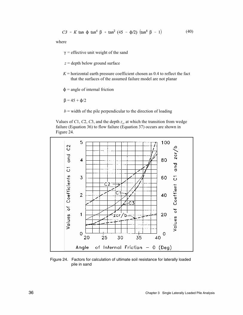
Values of C1, C2, C3, and the depth zcr at which the transition from wedgefailure (Equation 36) to flow failure (Equation 37) occurs are shown inFigure 24.

Chapter 3 Single Laterally Loaded Pile Analysis 37
'
'
'&
Figure 25. Resistance reduction coefficient - A for Method SLAT1
'
c. Compute the lateral resistance for the transition points c and b on thecurve (Figure 23) from
(41)
(42)
where A and B are reduction coefficients from Figures 25 and 26,respectively, for the appropriate static or cyclic loading condition. Thesecond straight line segment of the curve, from b to c , is established by theresistances pb and pc and the prescribed displacements of u = b/60 andu = 3b/80 as shown in Figure 27. The slope of this segment is given by
(43)
d. The exponential section of the curve, from a to b , is of the form
(44)

38 Chapter 3 Single Laterally Loaded Pile Analysis
Figure 26. Resistance reduction coefficient - B for Method SLAT1
'
'
'
&
'
where the parameters C, n, and the terminus of the initial linear portion pa andua are obtained by forcing the exponential function in Equation 44 to passthrough pb and ub with the same slope s as segment bc and to have the slope kp atthe terminus of the initial straight line segment at a. This results in
(45)
(46)
(47)
(48)
(Note: In some situations Equations 45 through 48 may result in unrealisticvalues for ua and/or pa. If this occurs, the exponential portion is omitted andthe initial linear segment is extended to its intersection with the straight line

Chapter 3 Single Laterally Loaded Pile Analysis 39
Figure 27. p-u curves by Method SLAT2
'
section bc or until the maximum resistance pc is reached whichever comes first. If segments 0a and bc do not intersect at realistic values of pa and ua , segmentbc is omitted.)
Murchison and O’Neill (1984)
Murchison and O'Neill (1984) simplified the process of Method SLAT1 byreplacing the three-part p-u curve with a single analytical expression as follows.
(49)
where
pu = ultimate lateral soil resistance from either Equation 36 for z < zcr orEquation 37 for z > zcr
n = geometry factor = 1.5 for tapered piles or 1.0 for prismatic piles
40 Chapter 3 Single Laterally Loaded Pile Analysis
'
' %(N
%
'
' ,
A = 3-0.8(z/b) $ 0.9 for static loads or = 0.9 for cyclic loading
k = soil stiffness from Table 2
z = depth at which the p-u curve applies
Several illustrative curves for this method are shown in Figure 27.
Synthesis of p-u Curves for Piles in Clay
Matlock (1970)
A series of lateral load tests on instrumented piles in clay (Matlock 1970)were used to produce the p-u relationship for piles in soft to medium clayssubjected to static lateral loads in the form
(50)
with pu, the ultimate lateral resistance, given by the smaller of
(51)
for a wedge failure near the ground surface, or
(52)
for flow failure at depth; and uc , the lateral displacement at one-half of theultimate resistance, given by
(53)
where
(N = effective unit weight of the soil
su = shear strength of the soil
J = 0.5 for a soft clay or 0.25 for a medium clay
,50 = strain at 50 percent of the ultimate strength from a laboratory stress-strain curve

Chapter 3 Single Laterally Loaded Pile Analysis 41
'(N %
Figure 28. p-u curves by Method CLAT1
Typical values of ,50 are given in Table 3. The depth at which failure transitionsfrom wedge (Equation 51) to flow (Equation 52) is
(54)
The static p-u curve is illustrated in Figure 28a.
For cyclic loads, the basic p-u curve for static loads is altered as shown inFigure 28b. The exponential curve of Equation 50 is terminated at a relativedisplacement u/uc = 3.0 at which the resistance diminishes with increasingdisplacement for z<zcr or remains constant for z>zcr .
42 Chapter 3 Single Laterally Loaded Pile Analysis
Figure 29. p-u curves by Method CLAT2 for static loads
Table 3Representative Values of 000050
Shear Strength (psf) Percent
250-500 0.02
500-1,000 0.01
1,000-2,000 0.007
2,000-4,000 0.005
4,000-8,000 0.004
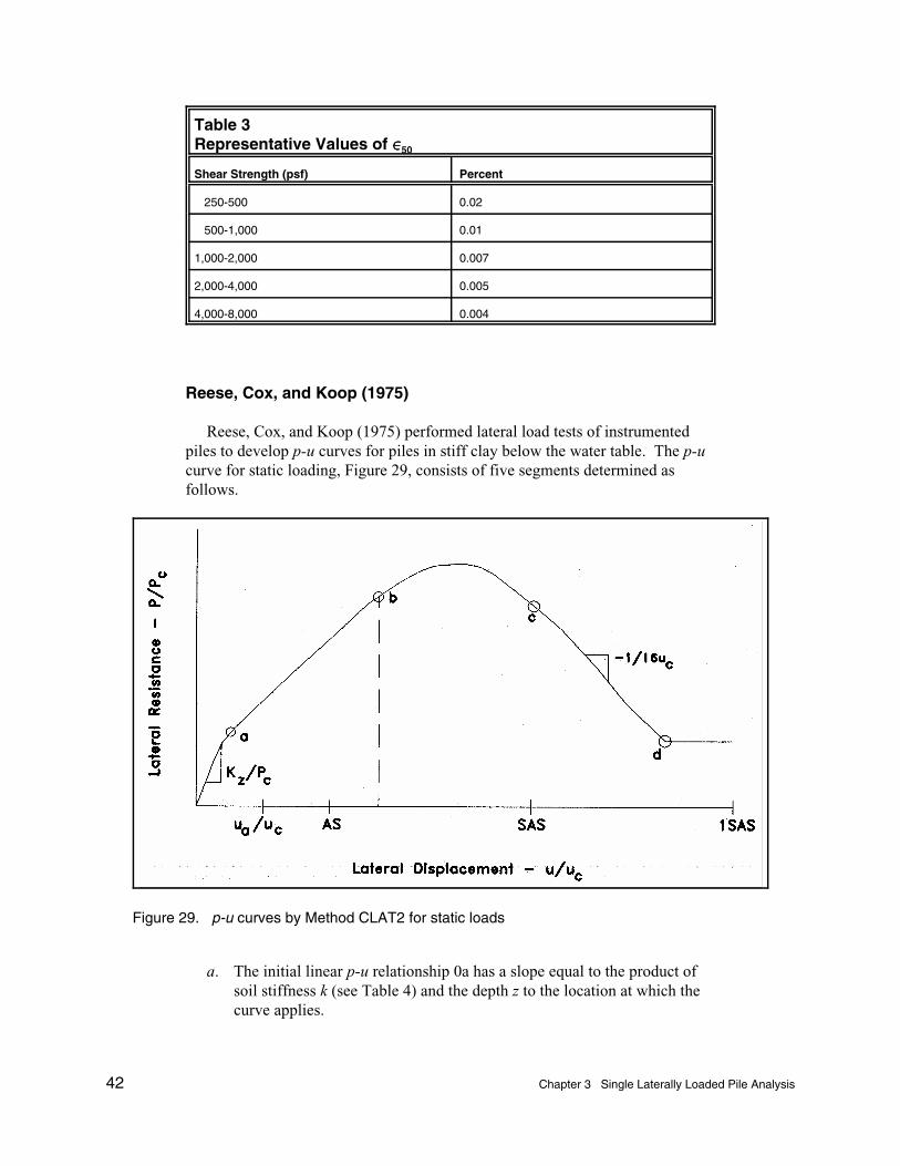
Reese, Cox, and Koop (1975)
Reese, Cox, and Koop (1975) performed lateral load tests of instrumentedpiles to develop p-u curves for piles in stiff clay below the water table. The p-ucurve for static loading, Figure 29, consists of five segments determined asfollows.
a. The initial linear p-u relationship 0a has a slope equal to the product ofsoil stiffness k (see Table 4) and the depth z to the location at which thecurve applies.

Chapter 3 Single Laterally Loaded Pile Analysis 43
'
' %(N
%
'
' ,
'
' %(N
%
Table 4Representative Values of Lateral Soil Stiffness k for Piles in Clayfor Method CLAT2
Average Undrained Shear Strength (tsf)1
Loading Type 0.5 - 1 1 - 2 2 - 4
Static loading - ks (pci) 500 1,000 2,000
Cyclic loading - kc (pci) 200 400 800
1 Average shear strength should be computed from the unconsolidated undrained shear strengthof the soil to a depth of five pile diameters.
b. The second segment of the curve is parabolic of the form
(55)
with pc taken as the smaller of
(56)
for wedge failure near the ground surface, or
(57)
and(58)
where ,50 = strain at 50 percent of ultimate strength from a laboratory stress-strain curve; and the parameter A for defining pertinent displacements inFigure 29 is obtained from the curve shown in Figure 30.
c. Points a and b, Figure 29, are joined by a parabolic curve of the form
(59)
where pc is the smaller of
(60)
44 Chapter 3 Single Laterally Loaded Pile Analysis
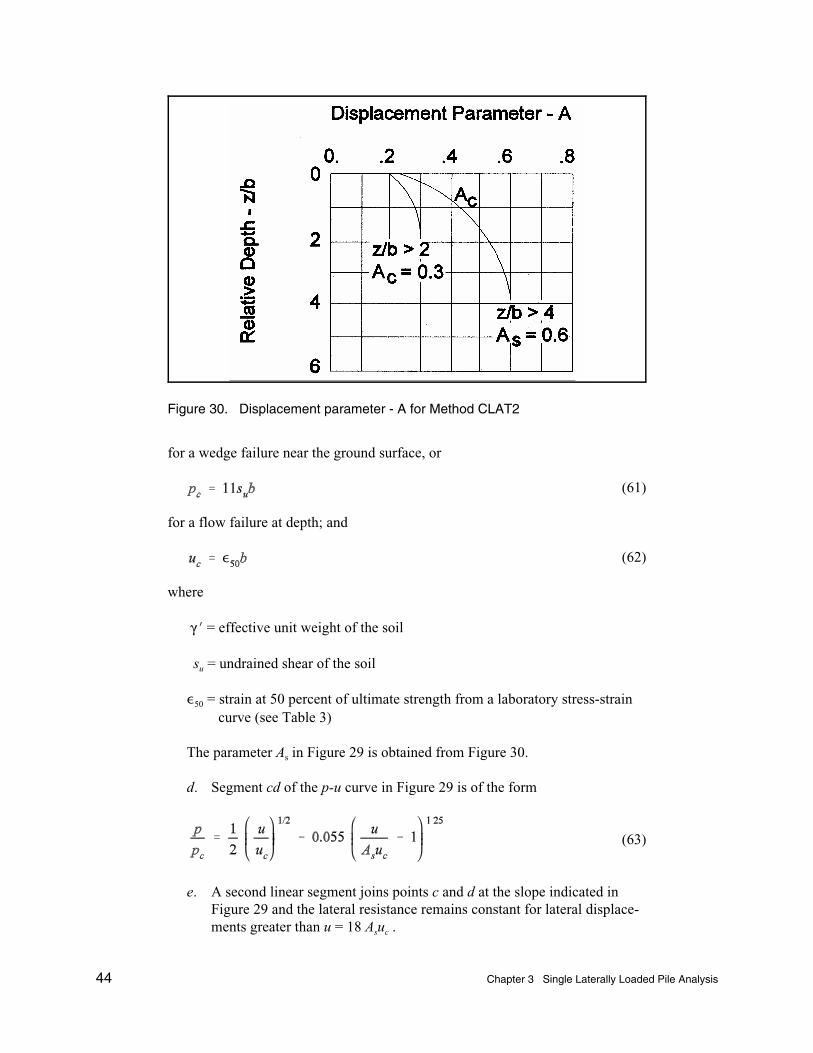
Figure 30. Displacement parameter - A for Method CLAT2
'
' ,
' & &
for a wedge failure near the ground surface, or
(61)
for a flow failure at depth; and
(62)
where
(N = effective unit weight of the soil
su = undrained shear of the soil
,50 = strain at 50 percent of ultimate strength from a laboratory stress-straincurve (see Table 3)
The parameter As in Figure 29 is obtained from Figure 30.
d. Segment cd of the p-u curve in Figure 29 is of the form
(63)
e. A second linear segment joins points c and d at the slope indicated inFigure 29 and the lateral resistance remains constant for lateral displace-ments greater than u = 18 Asuc .

Chapter 3 Single Laterally Loaded Pile Analysis 45
' & &
Figure 31. p-u curve by Method CLAT2 for cyclic loads
The p-u curve for cyclic loading provided by Reese, Cox, and Koop (1975) isillustrated in Figure 31. The curve is constructed as follows
a. The initial linear p-u relationship 0a has a slope equal to the product ofsoil stiffness k (see Table 4) and the depth z to the location at which thecurve applies.
b. The second segment, joining points a and b (Figure 31) is an exponentialrelationship of the form
(64)
where
Ac = pressure reduction coefficient from Figure 30
pc = ultimate soil resistance from Equation 56 or 57 (whichever is less)

46 Chapter 3 Single Laterally Loaded Pile Analysis
'
'
Figure 32. p-u curve by Method CLAT3 for static loads
and
(65)
where uc is given by Equation 62.
c. A second linear p-u relationship joins points b and c with the slopeshown in Figure 31. For displacements greater than u = 1.8up, the lateralresistance remains constant.
Reese and Welch (1975)
Reese and Welch (1975) performed a lateral load test on an instrumenteddrilled shaft in stiff clay above the water table. The p-u curve obtained from theexperimental results for static loads is shown in Figure 32. The curve consists ofan exponential relationship between lateral resistance and displacement to anultimate resistance, after which the resistance remains constant for furtherdisplacement. The requisite exponential relationship is
(66)

Chapter 3 Single Laterally Loaded Pile Analysis 47
' %
Figure 33. p-u curve by Method CLAT3 for cyclic loads
where
pu = ultimate resistance obtained as the smaller from Equation 51 with J = 0.5or from Equation 52
uc = critical lateral displacement obtained from Equation 88
The p-u curve for cyclic loading, shown in Figure 33, is constructed asfollows:
a. Values of p/pu for various values of static displacement us/uc are com-puted from Equation 66.
b. The displacement for cyclic loading for each value of p/pu is obtainedfrom
(67)

48 Chapter 3 Single Laterally Loaded Pile Analysis
Figure 34. p-u curve by Method CLAT4 for static loading
where
us = static displacement corresponding to p/pu
N = number of cycles of load application
Reese and Sullivan (1980)
Each method for p-u curves for piles in clay described above was developedfor a single soil profile; hence there were no recommendations provided fortransitioning from “soft” clay criteria to “stiff” clay criteria. Sullivan (1977) andSullivan, Reese, and Fenske (1979) reexamined the data for soft clays (Matlock1970) and stiff clays (Reese, Cox, and Koop 1975) and developed a unifiedcriterion (Reese and Sullivan 1980), which yields computed behaviors that are inreasonable agreement with both soft and stiff conditions. However, somejudgement on the part of the user is required in selecting appropriate parametersfor use in the prediction equations.
The p-u curve by the unified criteria for static loading, illustrated inFigure 34, consists of an initial linear segment 0a, an exponential segment ab, asecond linear segment bc and a constant lateral resistance for large displace-ments. The curve for static loading at a particular depth z is constructed asfollows:

Chapter 3 Single Laterally Loaded Pile Analysis 49
' %F
%
' %
'
'
'
' ,
a. The ultimate lateral resistance is
(1) For z < 12b , the ultimate resistance is the smaller of
(68)
(69)
where
F_
v = average effective vertical stress over the depth z
ca = average cohesion over the depth z
c = cohesion at depth z
b = pile diameter
(2) For z > 12b , the ultimate resistance is
(70)
b. Compare the properties of the soil profile under analysis with those listedin Table 5 and select the values of parameters Aand F to be used in thefollowing calculations.
c. The p-u relationship for the initial linear segment is
(71)
where k is a stiffness parameter from Table 6 (see also Table 4).
d. The exponential segment ab is obtained from
(72)
with
(73)

50 Chapter 3 Single Laterally Loaded Pile Analysis
Table 5Curve Parameters for Method CLAT4
Curve Parameters
Clay Description A F
Soft, inorganic, intact
Cohesion = 300 psf
= 0.7%
Overconsolidation ratio = 1
Sensitivity = 2 2.5 1.0
Liquid limit = 92
Plasticity index = 68
Liquidity index = 1
Stiff, inorganic, very fissured
Cohesion = 2,400 psf
= 0.5%
Overconsolidation ration > 10
Sensitivity = 1 0.35 0.5
Liquid limit = 77
Plasticity index = 60
Liquidity index = 0.2
Table 6Representative Values of k for Method CLAT4
Cohesion (psf) k (pci)
200-500 30
500-1,000 100
1,000-2,000 300
2,000-4,000 1,000
4,000-8,000 3,000
e. The second linear portion extends from a displacement u = 8uc to adisplacement u = 30uc where the lateral resistance is

Chapter 3 Single Laterally Loaded Pile Analysis 51
' % &
'
Figure 35. p-u curve by Method CLAT4 for cyclic loading
(74)
for z < 12b . For z > 12b , p/pu = 1.
The p-u curve by the unified method for cyclic loading, Figure 35, alsoconsists of an initial linear segment, followed by an exponential variation of pwith u, a second linear segment, and a constant resistance for large displace-ments. Construction of the curve for cyclic loading follows the same steps as forthe static curve, with the exceptions that the exponential segment terminates at aresistance equal to one half of pu , the second linear segment terminates at adisplacement u = 20uc , and the constant resistance for u > 20uc is given by
(75)
for z < 12b . For z > 12b , p/pu = 1.
O’Neill and Gazioglu (1984)
Although the procedure presented as Method CLAT4 attempted to provide aunified criterion for all clays, the procedure requires the user to select parame-ters a priori which essentially convert the method to a soft-clay-like method or toa stiff-clay-like method (O'Neill and Gazioglu 1984). O’Neill and Gazioglu

52 Chapter 3 Single Laterally Loaded Pile Analysis
'
' N,
'
reexamined the data utilized in developing the previous methods as well as theresults of other tests of instrumented laterally loaded piles in clay to produce anintegrated procedure for p-u curves for piles in clay. The method attempts toincorporate continuum effects and relative pile/soil stiffness characteristicswhich were not explicitly accounted for in the previous procedures.
O’Neill and Gazioglu, as well as other researchers, reasoned that there existsa critical length of pile such that longer piles no longer influence the pile headbehavior. This critical length is presented as
(76)
where EI = flexural stiffness of the pile; and Es = “perhaps a secant Young'smodulus at a deviator stress level of one-half of the deviator stress at failure inundrained triaxial compression,” with all length units in inches. Es is evaluatedfor the average UU triaxial shear strength between the ground surface and thedepth Lc . Hence the determination of Lc is an iterative process. Representativevalues of Es are given in Table 7.
Table 7Soil Modulus for Method CLAT5
Undrained Shear Strength c (psf) Soil Modulus Es (psi)
<500 50
500 - 1,000 50 - 150
1,000 - 2,000 150 - 450
2,000 - 4,000 450 - 1,500
4,000 - 8,000 1,500 - 5,000
>8,000 5,000
The reference lateral displacement uc (see Equations 53, 58, 62, and 73) isobtained from
(77)
where AN = constant taken as 0.8 by O’Neill and Gazioglu; Es = soil modulusfrom Table 7 for the depth of interest; and all length units are in inches.
The ultimate soil resistance is expressed as
(78)

Chapter 3 Single Laterally Loaded Pile Analysis 53
' % #
'
' % &
'
where F = reduction factor from Table 8 for the appropriate loading condition;and Np is given by
(79)
Table 8Soil Degradability Factors
Factor Loading Condition
UU Triaxial Compression Failure Strain
<0.02 0.02-0.06 >0.06
Fs Static 0.50 0.75 1.00
Fc Cyclic 0.33 0.67 1.00
where zcr = Lc/4, indicating a transition from wedge type failure to flow failure ata depth equal to one fourth the critical length which, unlike the previous meth-ods, reflects the relative pile/soil stiffness.
The p-u curves for static load (Figure 36) and cyclic loads (Figure 37) havean initial exponential relationship between lateral resistance and displacementgiven by
(80)
with the static curve terminating at p/pu = 1 and the cyclic curve at p/pu = 0.5. The second linear section of the curves terminates at
(81)
and the cyclic curve at
(82)
where Fs and Fc are given in Table 8.
Algorithm for Analysis of Laterally Loaded Piles
The p-u curves described in the preceding paragraphs were derived on theassumption that the lateral resistance p at any point on the pile is a function onlyof the lateral displacement u at that point (i.e., the Winkler assumption). For thisassumption and the one-dimensional model of the pile-soil system shown in

54 Chapter 3 Single Laterally Loaded Pile Analysis
Figure 36. p-u curve by Method CLAT5 for static loading
Figure 37. p-u curve by Method CLAT5 for cyclic loading
Figure 38, the governing differential equation for bending in the x-z plane of aprismatic, linearly elastic pile is

Chapter 3 Single Laterally Loaded Pile Analysis 55
Figure 38. Model of laterally loaded pile
% & ' (83)
where
E = modulus of elasticity of the pile material
I = moment of inertia of pile cross section about an axis perpendicular tothe x-z plane
P(z) = axial compressive force in the pile at z
p(z,u) = lateral resistance which is a function of both position z on the pile andthe lateral displacement u at z

56 Chapter 3 Single Laterally Loaded Pile Analysis
' &
% % '
Because the displacement u must be known before the lateral resistance p canbe evaluated, numerical iterative solutions of Equation 83 are required. Themost common approach is to represent the pile-soil system by a discretizedmodel such as illustrated in Figure 38 where the displacements and forces areevaluated at a finite number of points (Matlock and Reese 1962, Dawkins 1982). The solution proceeds as a succession of trials and corrections until forces anddisplacements are compatible at every node.
Observations of System Behavior
Obtaining the numerical solutions described above is expedited by replacingthe nonlinear p-u curve by equivalent linearly elastic springs during eachiteration. The stiffnesses of these linear springs are evaluated as the secant top-u curve for the displacements calculated during the preceding iteration. It is tobe noted that the ultimate lateral resistance tends to increase with depth, whilethe pile displacements decrease as z increases. Hence it can be concluded thatthe secant stiffness of the lateral resistance increases with depth below the pilehead. Consequently if the distribution of soil stiffnesses along the pile can bedetermined, the behavior may be evaluated for working loads without the needfor iterative solutions.
The second term in Equation 83 represents the interaction of the axial load inthe pile with the lateral displacement to increase the bending moments in the pile(the “beam-column” effect). Distribution of the axial load is not influencedsignificantly by lateral loading; hence, the distribution may be determined usingthe axial load analysis techniques described in Chapter 2 before a lateral loadanalysis is performed. In usual pile-soil systems, the beam-column effect issmall and conservative estimates of its influence may be obtained by taking theaxial force in the pile equal to the applied head load Po.
Linearly Elastic Analyses
A linear relationship between lateral resistance and lateral displacement isexpressed by
(84)
where E(z) = secant stiffness of the lateral resistance and the minus sign indi-cates that the resistance is opposite in direction to the displacement. For aprismatic pile with constant axial force and a linear resistance function, Equation83 becomes
(85)

Chapter 3 Single Laterally Loaded Pile Analysis 57
% % '
' & % % %
'
' & 8
' % 8
8 '
'
& 8
& 8D
'
Even with the simplifications inherent in Equation 85, explicit closed formsolutions are not possible unless the lateral resistance stiffness is constant withdepth. Although the lateral resistance is not constant, insight into the lateral loadbehavior can be gained from the solution for constant Ez. In this case thedifferential equation becomes
(86)
The solution of Equation 86 (Hetenyi 1946) is
(87)
where C1 , C2 , C3 , and C are constants to be determined from conditions at thepile head and tip; and
(88)
(89)
(90)
(91)
For a sufficiently long pile (see Page 51) conditions at the pile tip have noeffect on the response at the pile head. In this case the relationship betweenloads (Mo , Vo) and displacements (uo , Do) at the pile head may be expressed as
(92)
For a value of 82 = 1/2 , the determinant of the coefficient matrix in Equation 92is zero, indicating that an axial head load
(93)
is the buckling load for the long pile. Hetenyi (1946) gives the buckling load fora finite length pile with both ends fixed against displacement as less than orequal to
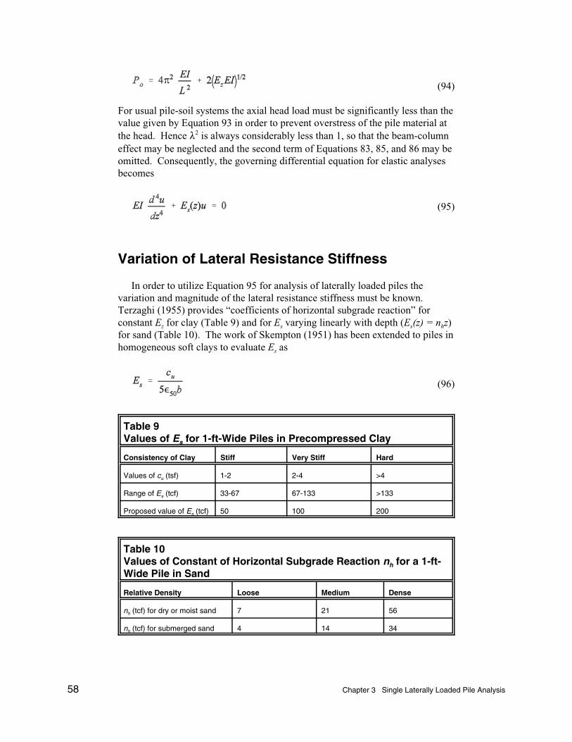
58 Chapter 3 Single Laterally Loaded Pile Analysis
' B %
% '
',
(94)
For usual pile-soil systems the axial head load must be significantly less than thevalue given by Equation 93 in order to prevent overstress of the pile material atthe head. Hence 82 is always considerably less than 1, so that the beam-columneffect may be neglected and the second term of Equations 83, 85, and 86 may beomitted. Consequently, the governing differential equation for elastic analysesbecomes
(95)
Variation of Lateral Resistance Stiffness
In order to utilize Equation 95 for analysis of laterally loaded piles thevariation and magnitude of the lateral resistance stiffness must be known. Terzaghi (1955) provides “coefficients of horizontal subgrade reaction” forconstant Ez for clay (Table 9) and for Es varying linearly with depth (Es(z) = nhz)for sand (Table 10). The work of Skempton (1951) has been extended to piles inhomogeneous soft clays to evaluate Es as
(96)
Table 9Values of Es for 1-ft-Wide Piles in Precompressed Clay
Consistency of Clay Stiff Very Stiff Hard
Values of cu (tsf) 1-2 2-4 >4
Range of Es (tcf) 33-67 67-133 >133
Proposed value of Es (tcf) 50 100 200
Table 10Values of Constant of Horizontal Subgrade Reaction nh for a 1-ft-Wide Pile in Sand
Relative Density Loose Medium Dense
nh (tcf) for dry or moist sand 7 21 56
nh (tcf) for submerged sand 4 14 34

Chapter 3 Single Laterally Loaded Pile Analysis 59
' %
% '
'
'
' %
% '
% '
The p-u curves discussed previously provide an indication of the variation ofEs with depth. For both clays and sands, the ultimate resistance used for con-structing the p-u curves increases with depth near the ground surface. At somedepth, the ultimate resistance for clays reaches a limiting value. Consideringthat the lateral displacements of the pile decrease exponentially with depth (seeEquation 87), it seems probable that the secant stiffness of the lateral reaction forboth sands and clays increases as some exponential function with depth of theform (Matlock and Reese 1962).
(97)
The stiffness of sand at the ground surface will be zero; hence, Ko will be zero. Although the p-u curves for clays suggest that Ko will not be zero, it is conserva-tive to take Ko as zero for these materials. Therefore, the elastic solutionspresented in the following paragraphs will take Ko to be zero in all cases.
Although explicit solutions of Equation 95 exist for Es constant with depth(n = 0 , Es = K in Equation 97), all solutions are presented in graphical form. Following the procedures of Matlock and Reese (1962) the following non-dimensional parameters are defined
(98)
(99)
(100)
(101)
where Vo and Mo are the applied head shear and moment, respectively; and Au(Z)and Bu(Z) are nondimensional functions of the nondimensional depth Z.
Substitution of Equations 97 through 101 into Equation 95 yields
(102)
and
(103)

60 Chapter 3 Single Laterally Loaded Pile Analysis
D ' ' %
' ' %
' ' %
'&
&
& D
With solutions of Equations 102 and 103 available, the displacement at anypoint on the pile is obtained from Equation 136 and the slopes of the pile, thebending moments, and shears are evaluated from the derivatives of u as
(104)
(105)
(106)
The various functions of A and B are plotted in Appendix A (Figures B1 throughB24) for constant, linear, and parabolic variations of Ez with depth (n = 0, 1, and2, respectively, in Equation 96).
Pile Head Stiffness Coefficients for Lateral Loading
Pile head stiffness coefficients for lateral loading are obtained by invertingEquations 100 and 101 with Z = 0 as shown in the following matrix equation
(107)
where
Auo = Au(Z = 0)
Buo = Bu(Z = 0)
Aso = As(Z = 0)
Bso = Bs(Z = 0)
The coefficients Auo , Buo , Aso , and Bso are shown for various relative pile lengthsZmax in Appendix B (Figures B25 through B28). The following items should benoted: (a) Aso = Buo ; (b) piles with Zmax < 2 may be treated as rigid (see page 76); and (c) The A and B coefficients remain constant for Zmax $ 4.

Chapter 3 Single Laterally Loaded Pile Analysis 61
' % D
' ' % D
' %
% %
% %
D
As noted on page 59, piles with Zmax $ 4 may be treated as inflexible. In thiscase the lateral displacement at any depth may be expressed in terms of the pilehead displacements as
(108)
and the soil resistance at that point is
(109)
From an equilibrium analysis of the rigid pile, the head shear and moment aregiven in terms of the head displacements by
(110)
Evaluation of Linear Lateral Soil Resistance
In order to apply the linearized solutions described in the preceding para-graphs, the variation and magnitude of the lateral soil resistance stiffness mustbe evaluated. Terzaghi (1955) provides estimates of clay soil stiffness constantwith depth (n = 0) and sand soil stiffness varying linearly with depth (n = 1) asshown in Tables 9 and 10. (Note: Terzaghi states that the soil stiffness valuesare for a “1 foot wide pile” and in order to apply these values to piles of differentwidths the stiffness for the 1-ft-wide pile must be divided by the actual width ofthe pile. In order to utilize the resulting “horizontal subgrade modulus” in thelinearized analysis, Terzaghi's modulus must be multiplied by the width of thepile in contact with the soil (see Hetenyi 1941). Consequently the moduli givenby Terzaghi may be used without alteration as the value of K in the linearizedequations.)
Because the laterally loaded pile-soil system is highly nonlinear, particularlyunder large loads, immutable pile head stiffness coefficients do not exist. Although the soil stiffness moduli given in Tables 9 and 10 can be used toevaluate explicit coefficients, these values must be interpreted as only firstapproximations. Higher approximations may be obtained by combining thenondimensional solutions with the nonlinear p-u curves discussed earlier (Reese,Cooley, and Radhakrishnan 1984, “Executive Summary....”) as outlined in thefollowing steps.

62 Chapter 3 Single Laterally Loaded Pile Analysis
a. Evaluate p-u curves for the appropriate soil profile. These curves shouldbe closely spaced in the top 10 to 20 pile diameters.
b. Estimate a variation and lateral stiffness (i.e., K and n in Equation 97) forthe soil profile using Terzaghi's soil moduli. (Reese, Cooley, andRadhakrishnan (1983) suggest that a value of T (Equation 98) beassumed; Terzaghi's moduli provide a means for this assumption.)
c. Evaluate the deflections at the locations of the p-u curves in step a usingthe appropriate nondimensional curves for head loads in the workingrange.
d. Determine the slope of a secant line from the p-u curve for the deflectioncalculated for each location. This establishes the soil modulus Ez at eachp-u curve location and allows Ez to be plotted versus depth z.
e. Revise the variation and lateral soil stiffness (i.e., new K and n in Equa-tion 97) to best approximate the curve of Ez versus z in step d.
f. Repeat steps c, d, and e until convergence is achieved.
g. Use the final values of K and n to calculate the pile head stiffness coeffi-cients in Equations 107 and 110.
Chapter 4 Algorithm for Analysis of Torsionally Loaded Single Piles 63
J ' J
'J
4 Algorithm for Analysis ofTorsionally Loaded SinglePiles
Three-dimensional analysis of a single pile requires a relationship betweenthe resistance of the soil and the torsional displacement of the pile. There hasbeen only limited investigation (O'Neill 1964, Poulos 1975, Scott 1981, Stoll1972) of this torque-twist relation because its effect is small compared to theaxial and lateral effects. Until more detailed data are available, the followingsimplistic relationship should be used.
It is assumed that the soil is a radially linearly elastic, homogenous medium,that the pile is prismatic and linearly elastic, and that the resistance of the soil atany point is a function only of the torsional displacement of the pile-soil inter-face at that point. Under these assumptions the soil in any plane perpendicularto the axis of the pile is in a state of plane, pure shear. The theory of elasticitysolution for this case yields
(111)
and
(112)
where
J = shear stress at a radial distance r from the centerline of the pile
Jo = shear stress at the pile-soil interface
R = radius of the pile

64 Chapter 4 Algorithm for Analysis of Torsionally Loaded Single Piles
' 2
J
2'
J ' F *
J ' "
V = displacement perpendicular to the radial direction at r
Gs = shear modulus of the soil
If there is no slippage between the pile and soil at the interface, the tangentialdisplacement of a point on the interface is
(113)
where 2 is the rotation of the pile. And, finally, the required relation is
(114)
The linear relationship between surface shear and pile rotation represented byEquation 113 is assumed to terminate when the surface shear Jo reaches a limitof
(115)
for sands, or
(116)
for clays, where
Jou = ultimate surface shear resisting rotation of the pile about its longitudinalaxis
ko = at-rest pressure coefficient
* = angle of pile-soil interface friction for sand
Fo = vertical effective stress
" = an adhesion factor which may be obtained from Figure 12
su = shear strength of clay. The resistance to rotation remains constant at Jou
for additional rotational displacement as shown in Figure 39
Elastic Analysis
So long as the surface shear is less than Jou , the entire pile-soil system islinearly elastic. The governing differential equation for torsional response of thelinear pile-soil system is

Chapter 4 Algorithm for Analysis of Torsionally Loaded Single Piles 65
Figure 39. Proposed torsional shear - rotation curve
2& B 2 ' (117)
where
G = shear modulus of the pile material
J = torsional area property of the pile cross section (polar moment of inertiafor a circular section)
Because Equation 116 is identical in form to the differential equation for anaxially loaded pile, pile head torque-twist stiffness may be obtained from theequations and procedures appearing on pages A3-A6 of Appendix A by perform-ing the following substitutions:
a. In Equations A4 and A5 (in Appendix A), define Tz = (GJ/4BR2Gs)1/2 for
Gs constant with depth.
b. In Equations A7 and A11, replace EA with GJ ; replace wo with 2o (thetwist angle at the pile head); and, replace Po with Mo (the torsionalmoment at the pile head).

66 Chapter 4 Algorithm for Analysis of Torsionally Loaded Single Piles
c. In Equation A16, replace EA with GJ ; replace w(z) with O(z); and,replace Po with Mo.
d. In Equation A18, replace EA with GJ ; and, define Kf such that Gs(z) =K fz
n for Gs varying with depth.
(Note: Scott (1981) indicates that the torsional resistance to twist at the pile tipmay be included as was done for tip reaction for the axially loaded pile. How-ever, in most situations the tip resistance against twist will be negligible.)

Chapter 5 Pile Head Stiffness Matrix 67
'
N
D
2
5 Pile Head Stiffness Matrix
Three-Dimensional System
Figure 40 illustrates the coordinate system, forces, and displacements at thepile head which must be considered in a three-dimensional analysis. The x- andy-axes are the principal axes of the pile cross section and the z-axis is thelongitudinal axis of the pile. Forces and displacements are assumed to havepositive senses in the positive coordinate directions (“right-hand rule” formoments and rotations).
For a linearly elastic system, the forces and displacements are related by
(118)
The b coefficient matrix array is the pile head stiffness matrix and the individualelements bij are obtained from Equations A21, 107, and 108.

68 Chapter 5 Pile Head Stiffness Matrix
Figure 40. Notation for pile head effects
'
&
'
&
'
'
(119)
(120)
(121)
(122)

Chapter 5 Pile Head Stiffness Matrix 69
' %
D ' %
'
D
where
E = modulus of elasticity of pile material
Iy = moment of inertia of pile cross section about y-axis
Txz = length parameter for lateral loading in the x-z plane
Equation 98 coefficients Auo , Aso , Buo , and Bso are obtained from Figures B25through B28 with Zmax = L/Txz ; terms appearing in Equation 122 are defined inChapter 2; and, terms in Equation 123 are defined in Chapter 4. The remainingelements of the pile head stiffness matrix, b22 , b24 , b55 , and b44 , are evaluatedfor bending in the y-z plane.
Pile Head Fixity
If the pile head is attached to the supported structure so that the displace-ments of the pile head and the point of attachment on the structure undergoidentical displacements, the stiffness matrix as shown in Equation 118 may beincluded as a part of the overall system stiffness without alteration. In mostinstallations, the pile head and the supported structure will experience the sametranslational displacements (u,v,w). However, the method of connection maypermit relative rotation between the structure and the pile. To illustrate theeffect of relative rotation of the pile and structure, the two-dimensional systemshown in Figure 38 is used. The relationship between the head forces anddisplacements is
(123)
(124)
The attendant inverse relationship, considering only the terms associated withlateral loading and the notation of Equation 119,
(125)
70 Chapter 5 Pile Head Stiffness Matrix
'
N '
DN '
NN ' %
&
NNN ' NN '
&
NN '
&
Pinned-Head Pile
If the pile-to-structure connection is such that no moment is transmittedthrough the connection, then Mo will be zero. For a unit lateral translation, uo = 1, Equations 123, 124, and 125 yield
(126)
or
(127)
and, the resulting rotation of the pile head,
(128)
with b15N = b51 = b55 = 0 . (The prime superscript denotes the pinned head condition.)
Partial Fixity at Pile Head
Frequently the pile-structure connection permits a limited relative rotationbefore moment resistance at the pile head is developed. To simulate the partialfixity, it is assumed that moment resistance develops at a reduced rate propor-tional to the degree of fixity f (o # f # 1) . To evaluate the stiffness elements b11
and b51 for partial fixity, a unit value of uo is imposed at the pile head and therotation is allowed to increase to (1 - f ) DoN . Similarly, to evaluate b15 and b55 ,uo = 0 and Do = fDoN are imposed. The resulting stiffness elements are
(129)
(130)
(131)
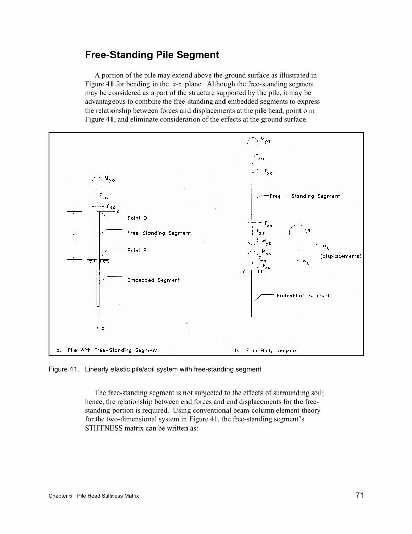
Chapter 5 Pile Head Stiffness Matrix 71
Figure 41. Linearly elastic pile/soil system with free-standing segment
Free-Standing Pile Segment
A portion of the pile may extend above the ground surface as illustrated inFigure 41 for bending in the x-z plane. Although the free-standing segmentmay be considered as a part of the structure supported by the pile, it may beadvantageous to combine the free-standing and embedded segments to expressthe relationship between forces and displacements at the pile head, point o inFigure 41, and eliminate consideration of the effects at the ground surface.
The free-standing segment is not subjected to the effects of surrounding soil;hence, the relationship between end forces and end displacements for the free-standing portion is required. Using conventional beam-column element theoryfor the two-dimensional system in Figure 41, the free-standing segment’sSTIFFNESS matrix can be written as:

72 Chapter 5 Pile Head Stiffness Matrix
'
' D
'
(132)'
% & % %
&
% & %
%
D
D
where E , A , Iy , and l are the modulus of elasticity, cross-sectional area,moment of inertia and length, respectively, of the free-standing segment, and f is the degree of fixity between the pile head and structure at point o . Forconvenience, the matrices in Equation 132 are partitioned as indicated by thedashed lines and this equation may be written symbolically as
(133)
Similarly, the relationship between forces and displacements at point s (Fig-ure 41) may be written as (see Equation 118)
(134)
or
(135)
Chapter 5 Pile Head Stiffness Matrix 73
' %
' ' % %
' & %&
' & %&
'
'
NNN NNN
NNN NNN
NNN
NNN ' %
&
Because there are no external forces at point s, Equations 133 and 135 may becombined to obtain
(136)
(137)
From Equation 137
(138)
And substitution of Equation 138 into Equation 136 yields
(139)
where
(140)
is the pile head stiffness matrix for bending in the xz-plane. A similar operationis required for bending in the yz-plane. The torsion stiffness coefficient is givenby
(141)
where b66 is the torsional coefficient for the embedded segment from Chapter 4,and G and J are shear modulus and torsional area moment of inertia, respec-tively, for the free-standing segment.
Alternatives for Evaluating Pile Head Stiffnesses
The most reliable means of evaluating the pile stiffness is from field tests ofprototype piles. Although the coefficients relating lateral head loads and
74 Chapter 5 Pile Head Stiffness Matrix
displacements may be evaluated from lateral load tests, such tests are notroutinely performed.
For complex soil conditions and/or nonprismatic piles which are not readilyapproximated by one of the procedures for linearly elastic systems discussedpreviously, the pile head stiffness matrix may be obtained with the aid ofcomputer programs such as CBEAMC, CAXPILE, or COM624.

Chapter 6 Analysis of Pile Groups 75
'
6 Analysis of Pile Groups
Although isolated single piles may be encountered in some applications, it ismore common that a structure foundation will consist of several closely spacedpiles (many building codes require a minimum of three piles in a group). Thestructure/pile/soil system is highly indeterminate and nonlinear. Historically,design methods have been based on numerous simplifying assumptions thatrender the analytical effort tractable for hand computations. The advent of thecomputer has allowed solutions to be obtained in which many of the simplifica-tions of the classical design methods are no longer necessary. Synopses of someof the classical methods and more complete descriptions of the computer-basedtechniques are presented below.
Classical Methods for Pile Group Analysis
All of the classical methods assume that the pile cap (or super-structure) isrigid and that all loads are resisted only by axial forces in the piles. Thesemethods attempt to allocate the superstructure loads to individual piles throughthe equations of static equilibrium. No direct attempt is made to determine thedeformations of the system.
Moment-of-Inertia (Simplified Elastic Center) Method
A complete description of the Elastic Center method is given by Andersen(1956). For the simplified procedure presented here, it is assumed, in addition toa rigid cap, that only vertical loads are applied to the cap, that all piles are verti-cal, that all piles have the same axial stiffness (EA/L), and that the magnitudes ofthe axial loads in the piles vary linearly with distance from the centroid of thepile group. The axial load at the head of the ith pile is given by
(142)
76 Chapter 6 Analysis of Pile Groups
where
V = resultant vertical load on the cap
n = number of piles in the group
Ix , Iy = moments of inertia about x- and y-axes, respectively, through thecentroid of the piles which are treated as point (unit) areas
Mx , My = moments of the vertical loads on the cap about the x- and y-axes,respectively
Culmann's Method
The method attributed to Culmann (see Terzaghi (1943)) requires threenonparallel subgroups of piles in the foundation. The piles within each subgroupare assumed to be parallel and are assumed to have the same head load. Eachsubgroup is replaced by a single pile at the centroid of the subgroup. A graphicalprocedure is used to resolve the superstructure load applied to the rigid cap toeach subgroup.
“Analytical” Method
Teng (1962) describes a simplified procedure for including the effects ofhorizontal loads as well as battered piles. The vertical component of the axialforce in each pile due to the resultant vertical load and moments of the super-structure on the rigid cap is calculated according to the moment of inertiamethod. The total axial pile load and its horizontal component may be calculatedfrom the vertical component. Teng suggests that an adequate design has beenattained if the applied horizontal foundation load does not exceed the sum of thehorizontal components of axial pile forces by more than 1,000 lb/pile.
Stiffness Analysis of Pile Foundations
The classical methods described in the previous paragraphs essentially neglectthe capability of the piles to resist lateral loads and do not provide a means ofevaluating the stresses induced in the pile by bending and shear at the pile head. The classical methods may underestimate the strength of the foundation or maylead to an unconservative design depending on the manner in which the pile headis attached to the structure. Hrennikoff (1950) and Saul (1968) developed adirect stiffness approach to the analysis of two- and three-dimensional pilegroups in which the interaction of the piles with the surrounding soil as well ascompatibility of pile head and pile cap displacements is included. In this proce-dure, the relationship between the pile head forces and the displacements of thepoint of attachment to the rigid pile cap is assumed to be linear.
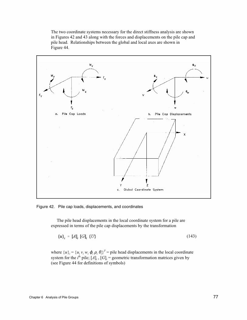
Chapter 6 Analysis of Pile Groups 77
Figure 42. Pile cap loads, displacements, and coordinates
'
The two coordinate systems necessary for the direct stiffness analysis are shownin Figures 42 and 43 along with the forces and displacements on the pile cap andpile head. Relationships between the global and local axes are shown inFigure 44.
The pile head displacements in the local coordinate system for a pile areexpressed in terms of the pile cap displacements by the transformation
(143)
where {u}i = {ui vi wi Ni Di 2i}T = pile head displacements in the local coordinate
system for the ith pile; [A]i , [G]i = geometric transformation matrices given by(see Figure 44 for definitions of symbols)
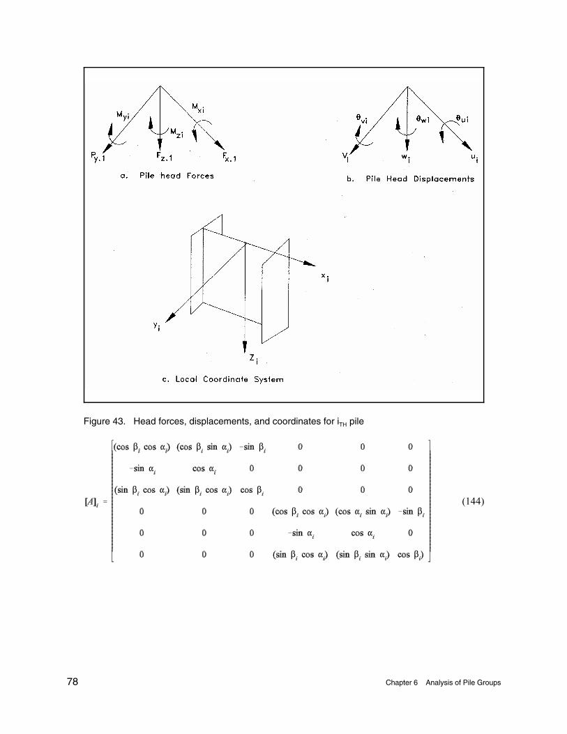
78 Chapter 6 Analysis of Pile Groups
Figure 43. Head forces, displacements, and coordinates for iTH pile
(144)'
$ " $ " & $
& " "
$ " $ " $
$ " " " & $
& " "
$ " $ " $
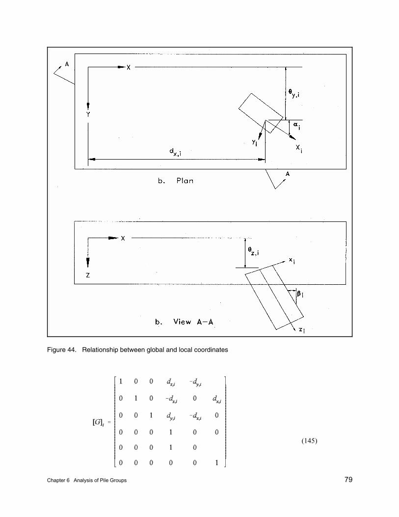
Chapter 6 Analysis of Pile Groups 79
Figure 44. Relationship between global and local coordinates
'
&
&
&
(145)
80 Chapter 6 Analysis of Pile Groups
' j'
'&
&
&
and {U} = {UG VG WG NG DG 2G}T = pile cap displacements in the global coordi-nate directions.
The relationship between pile cap forces and pile cap displacements is givenby
(146)
where {F} = {Fx Fy Fz Mx My Mz}T = superstructure loads on pile cap in global
coordinate directions; n = number of piles in the group; and, [b]i = pile headstiffness matrix for the local coordinate system described in Chapter 5.
(147)
After Equation 146 has been solved for the pile cap displacements, the headdisplacements and head forces in the local coordinate system for each pile areobtained from Equations 143 and 118, respectively. This method of analysis hasbeen incorporated into the CASE computer program CPGA (Hartman et al.1984).
The pile-soil-pile interaction (PSPI) method is identical to Saul's method in itstreatment of geometric and structural analysis aspects of the pile group problem. However, its treatment of soil reactions against piles is more comprehensive andrigorous. The method was first formalized by O'Neill, Ghazzaly and Ha (1977)for the analysis of pile clusters in offshore drilling platforms. The PSPI algo-rithm PILGP2R automates the process of computing pile-head stiffness constantsb11 - b66 and b15 , b24 , and b42 by first developing nonlinear relationships betweenaxial pile-head load and axial displacement, pile-head torque and twist, lateralpile-head load and displacement with zero rotation, pile-head moment androtation with zero displacement, and the cross-coupling relationship betweenrotation and lateral load and between displacement and moment. Sets of lateralrelationships are developed for each of two orthogonal directions to accommo-date nonisotorepic piles, such as H-piles. Nonlinear subroutines similar to thosedescribed in Chapters 2 and 3 are used to develop the axial and lateral relation-ships, respectively. Hence, the user inputs become unit load transfer curves. Torsional stiffness of individual piles is generally of minor significance in largegroups of piles. For that reason special computations of torsional stiffnesses arenot made, and the torsional stiffness is assumed to be equal to a constant value of(GJ)pile/2L throughout the computations. The piles remain linearly elastic.

Chapter 6 Analysis of Pile Groups 81
N ' )
' )
' j'
' j'
)
Similarly,
(148)
where ()) is the vector of global deflections at the origin. By using this trans-formation, each pile stiffness is moved to the origin of the pile cap. By usingEquations 93, 94, and 95, a single-pile force-deflection relationship can beexpressed as
(149)
(150)
where
(Q) = resultant external loads applied at origin of pile foundation
n = total number of piles in the foundation
This leads to the expression
(151)
An iterative solution is used to determine the deformation vector for the rigidpile cap. Initial b-factors are taken as the initial tangents to the various relation-ships described in the previous paragraph. The three-dimensional load vector isthen applied, the cap deformation vector is computed, and the pile-head deforma-tion vectors are computed. From these deformations pile-head reactions arecomputed from the present b-values. A check is then made of the compatibilityof the reactions and deformations at each pile head using the predeterminednonlinear relationships. If compatibility in the reaction and deformation values isnoted, new b-values are computed as secants to the axial and lateral pile headload-deformation relationships at the computed values of deformation, and theprocess is repeated as necessary until tolerance between the computed deforma-tions and deformations on the predetermined relationships at the computed valueof pile-head reaction is achieved at every pile.
Since individual, predetermined nonlinear relationships are used to representthe relationships between the various lateral deformation modes in two orthogo-nal directions, the solution that is thus obtained involves, in effect, superpositionof nonlinear functions, which is not theoretically correct, and which may produceerrors of practical magnitude as the pile-head behavior becomes highly nonlinear. However, where nonlinearity is relatively small, as would typically occur in theservices load range, the errors are not significant.
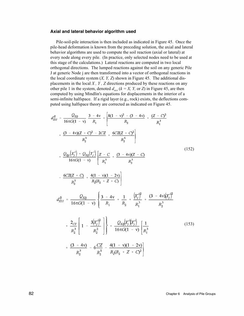
82 Chapter 6 Analysis of Pile Groups
Axial and lateral behavior algorithm used
Pile-soil-pile interaction is then included as indicated in Figure 45. Once thepile-head deformation is known from the preceding solution, the axial and lateralbehavior algorithms are used to compute the soil reaction (axial or lateral) atevery node along every pile. (In practice, only selected nodes need to be used atthis stage of the calculations.) Lateral reactions are computed in two localorthogonal directions. The lumped reactions against the soil on any generic PileJ at generic Node j are then transformed into a vector of orthogonal reactions inthe local coordinate system (X, Y, Z) shown in Figure 45. The additional dis-placements in the local X , Y , Z directions produced by these reactions on anyother pile 1 in the system, denoted dace (k = X, Y, or Z) in Figure 45, are thencomputed by using Mindlin's equations for displacements in the interior of asemi-infinite halfspace. If a rigid layer (e.g., rock) exists, the deflections com-puted using halfspace theory are corrected as indicated on Figure 45.
(152)
'B & <
& <%
& < & & <%
&
%& < % &
%%
%%
B & <&
%& < &
&%
%& < & <
% %
(153)
'B & <
& <% % %
& <
% & %B & <
%& <
& && < & <
% %

Chapter 6 Analysis of Pile Groups 83
Figure 45. Geometric definitions for computation of added displacement
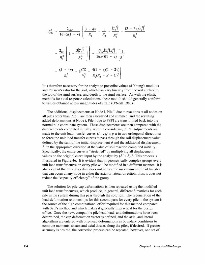
84 Chapter 6 Analysis of Pile Groups
'B & <
& <% % %
& <
% & %B & <
%& <
& && < & <
% %
It is therefore necessary for the analyst to prescribe values of Young's modulusand Poisson's ratio for the soil, which can vary linearly from the soil surface tothe top of the rigid surface, and depth to the rigid surface. As with the elasticmethods for axial response calculations, these moduli should generally conformto values obtained at low magnitudes of strain (O'Neill 1983).
The additional displacements at Node i, Pile I, due to reactions at all nodes onall piles other than Pile I, are then calculated and summed, and the resultingadded deformations at Node i, Pile I due to PSPI are transformed back into thenormal pile coordinate system. These displacements are then compared with thedisplacements computed initially, without considering PSPI. Adjustments aremade to the unit load transfer curves (f-w, Q-w p-u in two orthogonal directions)to force the unit load transfer curves to pass through the soil displacement valuedefined by the sum of the initial displacement * and the additional displacement*N in the appropriate direction at the value of soil reaction computed initially. Specifically, the entire curve is “stretched” by multiplying all displacementvalues on the original curve input by the analyst by (*N + *)/*. This process isillustrated in Figure 46. It is evident that in geometrically complex groups everyunit load transfer curve on every pile will be modified in a different manner. It isalso evident that this procedure does not reduce the maximum unit load transferthat can occur at any node in either the axial or lateral direction; thus, it does notreduce the “capacity efficiency” of the group.
The solution for pile-cap deformations is then repeated using the modifiedunit load transfer curves, which produce, in general, different b matrices for eachpile in the system during this pass through the solution. The regeneration of theload-deformation relationships for this second pass for every pile in the system isthe source of the high computational effort required for this method comparedwith Saul's method and which makes it generally impractical for the designoffice. Once the new, compatible pile head loads and deformations have beendetermined, the cap deformation vector is defined, and the axial and lateralalgorithms are entered with pile-head deformations as boundary conditions tocompute moments, shears and axial thrusts along the piles, if desired. If greateraccuracy is desired, the correction process can be repeated; however, one set of

Chapter 6 Analysis of Pile Groups 85
Figure 46. Modification of unit load transfer relationship for group effects at Node i, Pile I
corrections of the unit-load transfer curves appears appropriate for mostproblems.
Flexible pile cap analysis
The pile analysis methods described above assume that the pile cap, orstructure base slab, is rigid in comparison to the stiffness of the piles. For manystructures, such as U-frame lock monoliths, this is not a valid assumption, andthe flexibility of the base slab should be considered. Currently there are nospecial-purpose programs to perform this type analysis, so the use of largegeneral-purpose programs like SAP or STRUDL that can represent a flexiblepile-cap foundation and piles must be used. The pile element used in the rigidbase method has been added to several versions of the SAP and STRUDLprograms. Flexible base analyses have already been performed for pile-foundedstructures designed by the Corps of Engineers. A more detailed report onflexible base analysis will be furnished at some future date.
Nonlinear analysis
One of the assumptions made in the rigid base analysis method is that a pilecan be represented by a set of linear stiffnesses. The actual behavior of the pile-soil system may be highly nonlinear. Some existing programs are capable ofnonlinear analysis of a structure that is supported by only a few piles. One such

86 Chapter 6 Analysis of Pile Groups
program which may be able to economically analyze a large number of pilesunder a foundation using a nonlinear model is PILGP2R. However, for largestructures supported by as many as 200 piles, nonlinear analysis is not currentlypractical. The results of the two types of analyses are very close. In O’Neil andTsao (1984) it was found that, while nonlinearity was an insignificant effect, arational procedure must be applied to adjusting the subgrade reaction to be ableto account for PSPI in typical Corps' structures.

References 87
References
Andersen, P. (1956). “Substructure analysis and design,” Ronald Press, NewYork.
Aschenbrenner, T. B., and Olson, R. E. (1984). “Prediction of settlement ofsingle piles in clay.” Analysis and design of pile foundations. AmericanSociety of Civil Engineers, J. R. Meyer, ed.
Briaud, J. L., and Tucker, L. (1984). “Piles in sand: A method includingresidual stresses.” Journal of Geotechnical Engineering, ProceedingsPaper 19262, American Society of Civil Engineers, Vol 110(11).
Cox, W. R., Reese, L.C., and Grubbs, B. R. (1974). “Field testing of laterallyloaded piles in sand.” Proceedings, Offshore Technology Conference, PaperNo. 2079, Houston, TX.
Coyle, H. M., and Castello, R. R. (1981). “New design correlations for piles insand,” Journal of the Geotechnical Engineering Division, ProceedingsPaper 16379, American Society of Civil Engineers, Vol 107(GT7).
Coyle, H. M., and Reese, L. C. (1966). “Load transfer for axially loaded pilesin clay,” Journal Soil Mechanics and Foundations Division, ProceedingsPaper 4702, American Society of Civil Engineers, Vol 93(SM6).
Coyle, H. M., and Salaiman, I. H. (1967). “Skin friction for steel piles in sand,”Journal Soil Mechanics and Foundations Division, Proceedings Paper 5590,American Society of Civil Engineers, Vol 93(SM6).
Dawkins, W. P. (1980). “Computer Program CBEAMC: Analysis of beam-columns with nonlinear supports,” U.S. Army Engineer Waterways Experi-ment Station, Vicksburg, MS.
__________. (1982). “Pile head stiffness matrix on complete analysis of 2-Dand 3-D vertical piles,” U.S. Army Engineer Waterways Experiment Station,Vicksburg, MS.

88 References
Dawkins, W. P. (1984). “Users guide: Computer program for soil-structureinteraction analysis of axially loaded piles (CAXPILE),” InstructionReport K-84-4, U.S. Army Engineer Waterways Experiment Station, Vicks-burg, MS.
Girijavallabhan, C. Y. (1969). “Buckling loads of nonuniform columns,”Journal of the Structural Division, Paper No. 6908, American Society ofCivil Engineers, Vol 95(ST11).
Hartman, J. P., Jaeger, J. J., Jobst, J. J., and Martin, D. K. (1989). “User’sguide: Pile group analysis (CPGA) computer program,” Technical ReportITL-89-3, U.S. Army Engineer Waterways Experiment Station, Vicksburg,MS.
Hetenyi, M. (1946). Beams on elastic foundation. The University of Michigan Press, Ann Arbor.
Heydinger, A. G. (1984). “Recommendations: Load-transfer criteria for piles inclay,” Technical Report ITL-87-1, U.S. Army Engineer Waterways Experi-ment Station, Vicksburg, MS.
__________. (1986). “Analysis of axial pile-soil interaction in clay,” Interna-tional Journal for Numerical and Analytical Methods in Geomechanics 10(4),367-381.
Hrennikoff, A. (1950). “Analysis of pile foundations with batter piles,” Trans-actions, American Society of Civil Engineers Vol 115, 351-383.
Kraft, L. M., Ray, R. P., and Kagawa, T. (1981). “Theoretical t-z curves,” Journal Geotechnical Engineering Division, Proceedings Paper 16653,American Society of Civil Engineers, Vol 107(GT11).
Matlock, H. (1970). “Correlations for design of laterally loaded piles in softclay,” Preprints, Second Annual Offshore Technology Conference, Paper No. 1204, Vol 1, 577-588.
Matlock, H., and Reese, L. C. (1962). “Generalized solutions for laterallyloaded piles,” Transactions, American Society of Civil Engineers, Paper No.3170, Vol 127, Part 1, 1220-1248.
Mosher, R. L. (1984). “Load transfer criteria for numerical analysis of axiallyloaded piles in sand; Part 1: Load transfer criteria,” Technical Report K-84-1, U.S. Army Engineer Waterways Experiment Station, Vicksburg, MS.
Murchison, J. M., and O'Neill, M. W. (1984). “Evaluation of p-y relationshipsin cohesionless soils,” Analysis and design of pile foundations, AmericanSociety of Civil Engineers, J. R. Meyer, ed., 174-191.

References 89
O’Neill, M.W. (1964). “Determination of the pile-head torque-twist relation-ship for a circular pile embedded in a clay soil,” M.S. thesis, University ofTexas, Austin.
O’Neill, M. W. (1983). “Group action in offshore piles.” Proceedings, Geo-technical Practice in Offshore Engineering, American Society of Civil Engi-neers, 2-64.
O’Neill, M. W., and Gazioglu, S. M. (1984). “An evaluation of p-y relationshipsin clays,” American Petroleum Institute, University of Houston.
O’Neill, M. W., and Tsai, C. N. (1984). “An investigation of soil nonlinearityand pile-soil-pile interaction in pile group analysis,” Research ReportNo. UHUC 84-9, Department of Civil Engineering, University of Houston,prepared for U.S. Army Engineer Waterways Experiment Station, Vicksburg,MS.
O'Neill, M. W., Ghazzaly, O. I., and Ha, H. B. (1977). “Analysis of three-dimensional pile groups with nonlinear soil response and pile-soil-pileinteraction,” Paper No. 2838, Proceedings, Ninth Offshore TechnologyConference, Houston, TX.
Poulos, H. G. (1975). “Torsional response of profiles,” Proceedings, American Society of Civil Engineers, GTIO.
__________. (1983). “Cyclic axial pile response - alternative analyses,”Proceedings, Specialty Conference on Geotechnical Practice in OffshoreEngineering, American Society of Civil Engineers, S. G. Wright, ed., 403-21.
Poulas, H. G., and Davis, E. H. (1980). Pile foundation analysis and design. John Wiley and Sons, New York, 13-15, 52-66, 71-83.
Randolph, M. F., and Wroth, C. P. (1978). “Analysis of deformation of verti-cally loaded piles,” Journal Geotechnical Engineering Division, AmericanSociety of Civil Engineers, Proceedings Paper 14262,Vol 104(GT12).
Reese, L. C., and Matlock, H. (1956). “Non-dimensional solutions for laterally loaded piles with soil modulus assumed proportional to depth,” Proceedings,Eighth Texas Conference on Soil Mechanics and Foundation Engineering,Special Publication No. 29, Bureau of Engineering Research, The Universityof Texas at Austin.
Reese, L. C., and Sullivan, W. R. (1980). “Documentation of ComputerProgram COM624; Parts I and II, Analysis of Stresses and Deflections forLaterally-Loaded Piles Including Generation of p-y Curves,” GeotechnicalEngineering Software SG80-1, Geotechnical Engineering Center, Bureau ofEngineering Research, University of Texas at Austin.

90 References
Reese, L. C., and Welch, R. C. (1975). “Lateral loading of deep founcations instiff clay,” Journal, Geotechnical Engineering Division, American Society ofCivil Engineering 101(GT7), 633-649.
Reese, L. C., Cooley, L. A., and Radhakrishnan, N. (1984). “Laterally loadedpiles and computer program COM624G,” Technical Report K-84-2,U.S. Army Engineer Division, Lower Mississippi Valley, Vicksburg, MS.
Reese, L. C., Cox, W. R., and Koop, F. D. (1974). “Analysis of laterally loadedpiles in sand.” Proceedings, Fifth Annual Offshore Technology Conference,Paper No. OTC 2080, Houston, TX.
__________. (1975). “Field testing and analysis of laterally loaded piles in stiffclay.” Proceedings, Seventh Offshore Technology Conference, PaperNo. OTFC 2312. Houston, TX.
Saul, W. E. (1968). “Static and dynamic analysis of pile foundations,” JournalStructural Division, American Society of Civil Engineers, Proceedings Paper5936,Vol 94(ST5).
Scott, R. F. (1981). Foundation analysis. Prentice-Hall, Englewood Cliffs, NJ.
Seed, H. B., and Reese, L. C. (1957). “The action of soft clay along frictionpiles,” Transactions, American Society of Civil Engineers, Vol 122.
Semple, R. M., and Rigden, W. J. (1984). “Shaft capacity of driven pile inclay,” Analysis and design of pile foundations, American Society of CivilEngineers, J. R. Meyer, ed., 59-79.
Skempton, A. W. (1951). “The Bearing Capacity of Clays.” Proceedings,Building Research Congress, Vol I, Part IIV, 180-189.
Stoll, U. W. (1972). “Torque shear test of cylindrical friction piles.” CivilEngineering, American Society of Civil Engineers, Vol 42, 63-65.
Sullivan, W. R. (1977). Development and evaluation of a unified method for theanalysis of laterally loaded piles in clay, M. S. thesis, Graduate School of theUniversity of Texas at Austin.
Sullivan, W. R., Reese, L. C., and Fenske, C. W. (1979). “Unified method foranalysis of laterally loaded piles in clay.” Proceedings, Numerical Methodsin Offshore Piling, Institution of Civil Engineers, London, 107-118.
Teng, W. C. (1962). Foundation design. Prentice-Hall, Inc.
Terzaghi, K. (1943). Theoretical soil mechanics. John Wiley and Sons, Inc.,New York.
References 91
Terzaghi, K. (1955). “Evaluation of coefficients of subgrade reaction,”Geotechnique, Vol 5.
U.S. Army Corps of Engineers. (1994). “Design of Pile Foundations,” EngineerManual 1110-2-2906, Washington, DC.
Vesic, A. S. (1977). “Design of pile foundations,” NCHRP Synthesis of High-way Practice No. 42, Transportation Research Board, Washington, DC.
Vijayvergiya, V. N. (1977). “Load-movement characteristics of piles,” Pro-ceedings, Ports 77, American Society of Civil Engineers, Vol II, 269-286.
Yazdanbod, A., O'Neill, M. W., and Aurora, R. P. (1984). “Phenomenologicalstudy of model piles in sand,” Geotechnical Testing Journal, AmericanSociety for Testing and Materials 7(3), 135-144.
92 Bibliography
Bibliography
Alizadeh, M., and Davisson, M. T. (1970). “Lateral load tests on piles-Arkan-sas River Project,” Journal Soil Mechanics and Foundations Division,Proceedings Paper 7510, American Society of Civil Engineers, ProceedingsPaper 7510, Vol 96 (SM5), 1583-1604.
Bogard, D., and Matlock, H. (1980). “Simplified calculations of p-y curves forlaterally loaded piles in sand,” (unpublished report), The Earth TechnologyCorporation, Inc., Houston, TX.
__________. (1981). “Computer Program AXPILE: Soil-structure interactionanalysis of axially loaded piles,” U.S. Army Engineer Waterways ExperimentStation, Vicksburg, MS.
Department of the Army. “User guide: Computer program for analysis of pilegroups - CPGA,” in preparation, CASE Task Group on Pile Foundations,Headquarters, U.S Army Corps of Engineers, Washington, DC.
Department of the Army. (1983). “Basic pile group behavior,” TechnicalReport K-83-1, CASE Task Group on Pile Foundations, Headquarters,U.S. Army Corps of Engineers, Washington, DC.
Meyer, B., and Reese, L. C. (1979). “Analysis of single piles under lateral loading,” Research Report No. 244-1, Center for Transportation Research, TheUniversity of Texas at Austin.
O'Neill, M. W., and Tsai, C-N. (1984). “An investigation of soil nonlinearityand pile-soil-pile interaction in pile group analysis,” Report No. UHCE 84-9,Department of Civil Engineering, University of Houston, University Park,TX.
Puech, A., Boulton, M., and Meimon, Y. (1982). “Tension piles: Field data andnumerical modeling,” Proceedings, Second International Conference onNumerical Methods in Offshore Piling, I.C.E. and The University of Texas,April, 293-312.

Appendix A Linear Approximations for Load Deformation of Axial Piles A1
& '
'
Appendix ALinear Approximations forLoad Deformation of AxialPiles
Linear Elastic Analyses
For a linearly elastic representation of the pile-soil system, the governingdifferential equation is
(A1)
where Ez(z) is the stiffness of the axial load-transfer mechanism. A typical f-wcurve is shown in Figure A1. At any displacement w the nonlinear f-w curvemay be replaced by a linear secant kf(z) . The total stiffness of the load-transfermechanism appearing in Equation A1 is given by
(A2)
Soil Stiffness Constant with Depth
Even though Equation A1 is representative of a linearly elastic system, aclosed-form solution is possible only if the side friction stiffness is constant withdepth. While this condition is not encountered in most soil-pile systems, thesolution for constant stiffness serves to indicate characteristics of the systembehavior.
For Ez constant with depth, the solution of Equation A1 may be written as
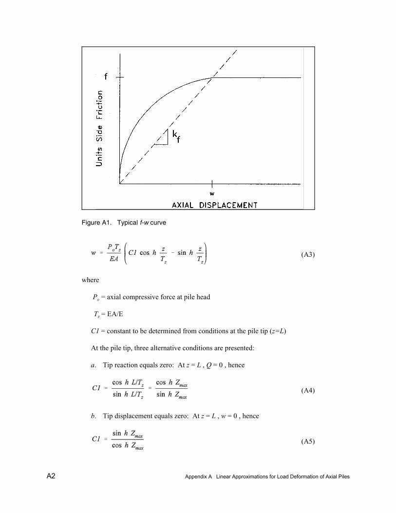
A2 Appendix A Linear Approximations for Load Deformation of Axial Piles
Figure A1. Typical f-w curve
' &
' '
'
(A3)
where
Po = axial compressive force at pile head
Tz = EA/E
C1 = constant to be determined from conditions at the pile tip (z=L)
At the pile tip, three alternative conditions are presented:
a. Tip reaction equals zero: At z = L , Q = 0 , hence
(A4)
b. Tip displacement equals zero: At z = L , w = 0 , hence
(A5)

Appendix A Linear Approximations for Load Deformation of Axial Piles A3
'%
%
'
'
'
'%
%
c. Tip elastically restrained: At z = L , Q = Ktwt , hence
(A6)
where
r = Kt/EzTz
Kt = stiffness of elastic resistance at pile tip
Zmax = L/Tz
Pile Head Axial Stiffness
Of particular interest is the relationship between the pile head force Po andaxial displacement wo . For convenience, this is defined by
(A7)
wherea. Pile tip free
(A8)
b. Pile tip fixed
(A9)
c. Pile tip elastically restrained
(A10)
ao is plotted for various values of Zmax in Figure A2. It is observed that forvalues of Zmax greater than 2, conditions at the tip have a negligible effect on thepile head force-displacement relationship. As will be discussed later, the pilehead axial force-displacement relationship forms a part of the elastic pile headstiffness matrix used in the analysis of pile groups. The axial pile head stiffnesscoefficient is given by
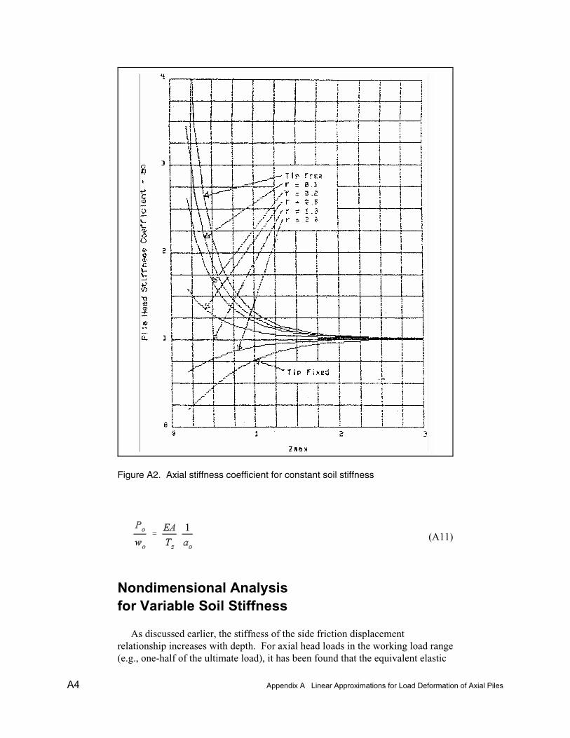
A4 Appendix A Linear Approximations for Load Deformation of Axial Piles
Figure A2. Axial stiffness coefficient for constant soil stiffness
'
(A11)
Nondimensional Analysis for Variable Soil Stiffness
As discussed earlier, the stiffness of the side friction displacementrelationship increases with depth. For axial head loads in the working load range(e.g., one-half of the ultimate load), it has been found that the equivalent elastic

Appendix A Linear Approximations for Load Deformation of Axial Piles A5
' %
& '
'
'
'
'%
side friction increases approximately linearly with depth for normallyconsolidated clays and as the square root of the depth in homogeneous sands. Ingeneral, these variations may be expressed as
(A12)
where
Ko = elastic stiffness of the side friction effect at the ground surface
Kf = elastic stiffness coefficient of the side friction effect in units of force perunit length of pile per unit deflection
n = 1 for a linear variation with depth
n = 1/2 for variation as the square root of depth
Because the stiffness of the side friction effect is a function of the strength of thesoil, Ko will be zero for sands. Some adhesion of clay soil may occur at theground surface and K for clays may not be zero. However, it is likely thatinstallation effects will minimize adhesion near the ground surface and aconservative estimate is obtained for Ko = 0 . For the general variation with Ko =0, the governing differential equation is
(A13)
Closed form solutions of Equation A13 do not exist. However, nondimensionalsolutions may be obtained with relatively simple numerical techniques asdescribed below.
Following the procedures described by Matlock and Reese (1962), thefollowing nondimensional parameters are defined.
(A14)
(A15)
(A16)
(A17)

A6 Appendix A Linear Approximations for Load Deformation of Axial Piles
%'
& '
'
'
'%
(A18)
Substitution of the nondimensional parameters into the governing differentialequation yields
(A19)
Equation A19 may be solved for a(Z) by any numerical technique (e.g., finitedifferences). From the solution of Equation A19, the relationship between pilehead force and head displacement is obtained as a(Z=0) , whence
(A20)
and the pile head axial stiffness is
(A21)
Values of the stiffness parameter are plotted in Figure A3 for a linearvariation of side friction stiffness with depth and in Figure 25 for side frictionstiffness varying as the square root of depth. These figures indicate that the tipreaction stiffness has negligible effect for values of Zmax greater than 2.
Evaluation of Side Friction Stiffness for Piles in Sand
Method ESSF1
Mosher (1984) suggested a secant stiffness computed using an axial displacement of 0.1 in. from his expression for the f-w curve. The resultingestimate of elastic stiffness for side friction is
(A22)

Appendix A Linear Approximations for Load Deformation of Axial Piles A7
Figure A3. Axial stiffness coefficient for soil stiffness varying linearly with depth
where
kf = initial slope of the f-w curve given in Table 1 in psf
fmax = ultimate side friction given in Figure 4 converted to units of psf
C = 2
R = circumference of the pile
The resulting units of Ez are in psi.

A8 Appendix A Linear Approximations for Load Deformation of Axial Piles
Figure A4. Axial stiffness coefficient for soil stiffness varying as square root ofdepth
The expression for Ez in Equation A22 includes an implicit variation withdepth embodied in the curves for fmax as a function of relative depth (see Figure 4in the main text). An examination of these curves suggests that the variation ofEz approximates a curve proportional to the square root of depth. To utilize theside friction stiffness for this procedure, the actual variation of Ez could be fittedto a curve which varies as the square root of depth (e.g. by least squares fit).

Appendix A Linear Approximations for Load Deformation of Axial Piles A9
'& <
'& <
Method ESSF2
The procedure of Kraft, Ray, and Cagawa (1981) for f-w curves for sand maybe used to approximate elastic conditions through the use of the initial slope ofthe f-w curve. From Equation 6 in the main text, the initial slope of the f-w curveyields:
a. For a homogeneous medium, a constant side friction stiffness equal to
(A23)
b. For a medium in which shear modulus varies from zero at the groundsurface to Gt at the pile tip, a linearly varying side friction stiffness equalto
(A24)
c. For a soil affected by pile installation, the shear modulus G or Gt
appearing in Equations A23 and A24 should be replaced by an effectivemodulus as given in Equation 10 or 11 in the main text.
Evaluation of Side Friction Stiffness for Piles in Clay
Method ECSF1
Kraft, Ray, and Kagawa (1981) suggest that the same procedures used forsand may be used for piles in clay with the shear moduli appearing inEquations A23 and A24 being modified to account for magnitude and time ofloading, as shown in Table A1.
Method ECSF2
Heydinger (1984) suggests using a secant to the f-w curve evaluated at arelative displacement w/2R = 0.005. From Equation 22 in the main text,

A10 Appendix A Linear Approximations for Load Deformation of Axial Piles
'
%
'
Table A1Adjustment in G for Various Loading Conditions (Adjustmentfactor = G (operational/G (in situ))
Condition Adjustment Factor
Immediately After Driving
Small load 0.85
Large load (> working load) 0.54
After Setup
Small load 1.04
Large load (f = 0.4su) 0.96
Large load (f = su) 0.73
(A25)
where Ef and m are given by Equations 23 and 24 in the main text, respectively. The variation of E2 along the pile depends on the distribution of soil modulus ofelasticity used in the evaluation of Ef from Equation 23.
Method ECSF2
The elasto-plastic representation of side friction due to Aschenbrener andOlson (1984) yields
(A26)
where for consistent units su should be expressed in psi and C in inchesproducing Ez in psi.
Evaluation of Tip Reaction Stiffness
General
As shown previously, the tip reaction only has a significant effect on the pilehead stiffness coefficient for piles having Zmax less than 2. If the value of Zmax
resulting from any of the assessments of side friction described above is lessthan 2, the tip reaction stiffness may be omitted.
Appendix A Linear Approximations for Load Deformation of Axial Piles A11
' B
'& <
In the discussions for evaluating the tip reaction stiffness that follow,stiffness is proportional to the effective area at the tip At bearing on the soil. Forclosed end or solid piles the effective tip area may reasonably be taken as thecross section area of the pile. For H-piles or open-ended pipe piles the tip areamay be as little as the area of material in the cross section to an area equal to thatbounded by the exterior of the section (see Figure 5 in the main text). When theradius of the tip reaction area is required to evaluate tip stiffness, an effectiveradius is obtained from
(A27)
The tip reaction stiffness may be obtained from any of the proceduresdescribed previously for developing q-w curves by evaluating a secant stiffnessfor a tip displacement representative of working load conditions. Typically inthe Corps of Engineers, failure at the tip is considered to occur at a tipdisplacement of 0.25 in. Unless stated otherwise, working load conditions areassumed to occur at one-tenth of the displacement corresponding to failure (i.e.,0.025 in.).
Evaluation of Tip Reaction Stiffness for Piles in Sand
Method EST1
The theory of elasticity solution for a rigid punch has been used by Kraft,Ray, and Kagawa (1981) (see also Randolph and Wroth 1978) to estimate the tipreaction stiffness as
(A28)
where the shear modulus G should be taken as an average in situ value between6Rt above the pile tip to 6Rt below the tip. The factor It in Equation A28 is aninfluence factor ranging from 0.5 to 0.78.
Method EST2
Mosher (1984) and Vijayvergiya (1977) express the tip reaction q-w curve asa power function (see pages 24-26). Mosher recommends for working loadapproximations a secant tip reaction stiffness corresponding to a tipdisplacement of 0.025 in. The corresponding tip stiffnesses are:
a. For loose sand: Kt = 12.6 At qmax (A29)
b. For medium sand: Kt = 18.6 At qmax (A30)

A12 Appendix A Linear Approximations for Load Deformation of Axial Piles
'%
'
'
c. For dense sand: Kt = 22.5 At qmax (A31)
where qmax is the ultimate unit tip reaction from Figure 17. For consistent unitsin Equations A29 through A31, qmax must be in pounds per square inch, and At
must be in square inches, which yields Kt in pounds per inch.
Method EST3
A secant stiffness obtained from the work of Briaud and Tucker (1984),which considers the effects of residual stresses due to installation for a tipdisplacement 0.0.025 in., is
(A32)
and
(A33)
where N is the average uncorrected standard penetration count in blows per footfrom a distance of 8Rt above the pile tip to 8Rt below the tip. The units of kq inEquation A33 are tsf/in. The required units of other terms in Equation A32 areqmax in tons per square foot and At in square feet, which yields Kt in tons per inch.
Evaluation of Tip Reaction Stiffness for Piles in Clay
Method ECT1
The bilinear tip reaction curve used by Aschenbrener and Olson (1984)produces
(A34)
where su is the average undrained shear strength of the clay from 6Rt above thepile tip to 6Rt below the tip.
Method ECT2
The tip stiffness developed by Kraft, Ray, and Kagawa (1981) described onpage A11 may be used for piles in clay.

Appendix A Linear Approximations for Load Deformation of Axial Piles A13
',
Method ECT3
Skempton (1951) observed the similarity of the load-displacement behaviorof a plate load test and the laboratory stress-strain curve for soft clays. It wasconcluded that a linear approximation of the load displacement relationship up tohalf of the ultimate load could be related to the strain at 50 percent of theunconfined compression strength indicated by the laboratory stress-strain curve. The observation has been used to obtain an estimate of the pile tip reactionstiffness as
(A35)
where
qu = unconfined compression strength of the clay at the pile tip
At = effective tip area
,50 = strain at 50 percent of ultimate strength from a laboratory stress-straincurve
Rt = effective radius of the tip area
Typical values of ,50 are 0.02 for a very soft clay, 0.01 for a soft clay, and 0.005for a stiff clay.

Appendix B Nondimensional Coefficients for Laterally Loaded Piles B1
'
% '
% '
'
'
' %
' %
' %
Appendix BNondimensional Coefficientsfor Laterally Loaded Piles
Basic Equations

B2 Appendix B Nondimensional Coefficients for Laterally Loaded Piles
Table B1Nondimensional Coefficients for Laterally Loaded Pile for Soil Modulus Constant withDepth (Head Shear Vo = 1, Head Moment Mo = 0)
Zmax = 2 Zmax = 3 Zmax = 4
Z Au As Am Au As Am Au As Am
0.00 2.118 -1.741 0.000 1.597 -1.116 0.000 1.474 -1.032 0.000
0.10 1.944 -1.736 0.092 1.486 -1.111 0.094 1.371 -1.027 0.095
0.20 1.771 -1.723 0.164 1.375 -1.097 0.174 1.248 -1.009 0.192
0.30 1.600 -1.704 0.219 1.266 -1.076 0.240 1.168 -0.992 0.247
0.40 1.430 -1.680 0.257 1.160 -1.050 0.293 1.051 -0.958 0.315
0.50 1.264 -1.653 0.282 1.057 -1.018 0.335 0.976 -0.931 0.351
0.60 1.100 -1.624 0.294 0.956 -0.983 0.366 0.867 -0.886 0.395
0.70 0.939 -1.594 0.294 0.860 -0.945 0.388 0.797 -0.854 0.417
0.80 0.781 -1.565 0.286 0.767 -0.906 0.401 0.698 -0.802 0.441
0.90 0.626 -1.537 0.269 0.679 -0.865 0.406 0.635 -0.767 0.451
1.00 0.474 -1.512 0.246 0.594 -0.825 0.405 0.546 -0.712 0.458
1.10 0.324 -1.488 0.219 0.514 -0.784 0.397 0.491 -0.675 0.459
1.20 0.176 -1.468 0.188 0.437 -0.745 0.385 0.413 -0.620 0.454
1.30 0.030 -1.451 0.156 0.365 -0.708 0.368 0.365 -0.584 0.447
1.40 -0.114 -1.437 0.123 0.296 -0.672 0.347 0.298 -0.532 0.433
1.50 -0.258 -1.426 0.091 0.230 -0.638 0.324 0.257 -0.497 0.421
1.60 -0.400 -1.418 0.062 0.168 -0.607 0.298 0.200 -0.448 0.400
1.70 -0.541 -1.413 0.037 0.109 -0.579 0.270 0.165 -0.417 0.385
1.80 -0.683 -1.411 0.017 0.052 -0.553 0.241 0.118 -0.372 0.359
1.90 -0.824 -1.410 0.005 -0.002 -0.531 0.212 0.089 -0.344 0.341
2.00 -0.965 -1.410 0.000 -0.054 -0.511 0.183 0.051 -0.305 0.314
2.10 -0.104 -0.494 0.154 0.027 -0.280 0.295
2.20 -0.153 -0.480 0.127 -0.004 -0.247 0.266
2.30 -0.200 -0.469 0.101 -0.023 -0.226 0.247
2.40 -0.247 -0.460 0.077 -0.049 -0.198 0.218
2.50 -0.292 -0.453 0.055 -0.064 -0.182 0.200
2.60 -0.337 -0.449 0.037 -0.084 -0.159 0.173
2.70 -0.382 -0.446 0.021 -0.097 -0.146 0.155
(Continued)
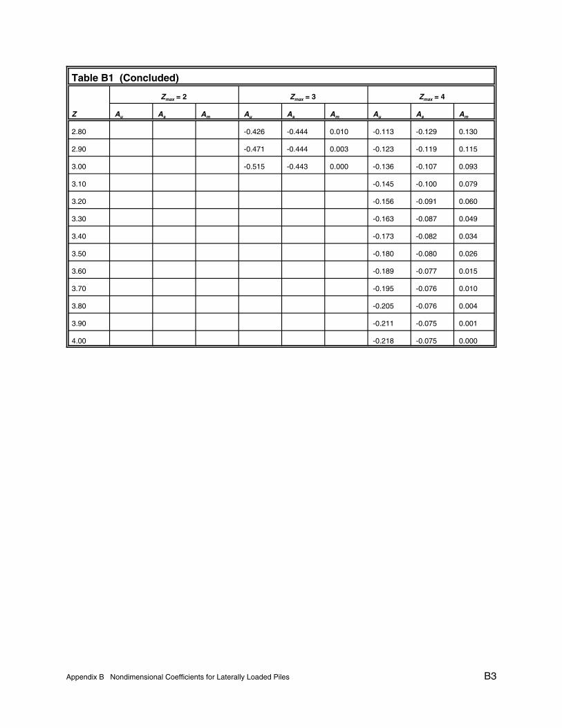
Appendix B Nondimensional Coefficients for Laterally Loaded Piles B3
Table B1 (Concluded)
Zmax = 2 Zmax = 3 Zmax = 4
Z Au As Am Au As Am Au As Am
2.80 -0.426 -0.444 0.010 -0.113 -0.129 0.130
2.90 -0.471 -0.444 0.003 -0.123 -0.119 0.115
3.00 -0.515 -0.443 0.000 -0.136 -0.107 0.093
3.10 -0.145 -0.100 0.079
3.20 -0.156 -0.091 0.060
3.30 -0.163 -0.087 0.049
3.40 -0.173 -0.082 0.034
3.50 -0.180 -0.080 0.026
3.60 -0.189 -0.077 0.015
3.70 -0.195 -0.076 0.010
3.80 -0.205 -0.076 0.004
3.90 -0.211 -0.075 0.001
4.00 -0.218 -0.075 0.000
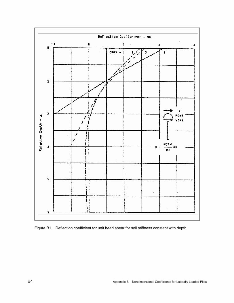
B4 Appendix B Nondimensional Coefficients for Laterally Loaded Piles
Figure B1. Deflection coefficient for unit head shear for soil stiffness constant with depth

Appendix B Nondimensional Coefficients for Laterally Loaded Piles B5
Figure B2. Slope coefficient for unit head shear for soil stiffness constant with depth

B6 Appendix B Nondimensional Coefficients for Laterally Loaded Piles
Figure B3. Bending moment coefficient for unit head shear for soil stiffness constant with depth

Appendix B Nondimensional Coefficients for Laterally Loaded Piles B7
Table B2Nondimensional Coefficients for Laterally Loaded Pile for Soil Modulus Constant withDepth (Head Shear Vo = 0, Head Moment Mo = 1)
Zmax = 2 Zmax = 3 Zmax = 4
Z Bu Bs Bm Bu Bs Bm Bu Bs Bm
0.00 -1.741 2.261 -1.000 -1.116 1.500 -1.000 -1.032 1.441 -1.000
0.10 -1.519 2.161 -0.993 -0.971 1.400 -0.996 -0.893 1.341 -0.997
0.20 -1.308 2.063 -0.972 -0.836 1.301 -0.983 -0.739 1.222 -0.982
0.30 -1.107 1.967 -0.937 -0.710 1.204 -0.961 -0.645 1.144 -0.966
0.40 -0.915 1.876 -0.891 -0.595 1.109 -0.932 -0.514 1.030 -0.934
0.50 -0.731 1.789 -0.836 -0.489 1.017 -0.897 -0.435 0.956 -0.909
0.60 -0.557 1.709 -0.773 -0.391 0.930 -0.858 -0.327 0.850 -0.865
0.70 -0.389 1.635 -0.705 -0.303 0.846 -0.814 -0.261 0.782 -0.834
0.80 -0.229 1.568 -0.633 -0.222 0.767 -0.767 -0.173 0.685 -0.784
0.90 -0.076 1.508 -0.559 -0.149 0.693 -0.719 -0.121 0.623 -0.749
1.00 0.072 1.456 -0.484 -0.083 0.623 -0.668 -0.052 0.537 -0.695
1.10 0.216 1.412 -0.410 -0.024 0.559 -0.617 -0.011 0.483 -0.658
1.20 0.355 1.374 -0.338 0.029 0.500 -0.565 0.042 0.407 -0.604
1.30 0.491 1.344 -0.269 0.076 0.446 -0.514 0.073 0.360 -0.568
1.40 0.624 1.320 -0.205 0.118 0.397 -0.464 0.112 0.295 -0.515
1.50 0.755 1.303 -0.148 0.156 0.353 -0.415 0.134 0.255 -0.480
1.60 0.885 1.290 -0.098 0.189 0.314 -0.367 0.162 0.201 -0.430
1.70 1.013 1.283 -0.057 0.218 0.280 -0.321 0.176 0.168 -0.397
1.80 1.141 1.279 -0.026 0.245 0.250 -0.277 0.194 0.123 -0.351
1.90 1.269 1.277 -0.007 0.269 0.224 -0.236 0.202 0.096 -0.322
2.00 1.397 1.277 0.000 0.290 0.202 -0.198 0.212 0.060 -0.280
2.10 0.309 0.184 -0.162 0.216 0.038 -0.254
2.20 0.327 0.170 -0.130 0.218 0.010 -0.218
2.30 0.343 0.158 -0.100 0.219 -0.006 -0.196
2.40 0.359 0.150 -0.075 0.216 -0.028 -0.164
2.50 0.373 0.143 -0.052 0.214 -0.040 -0.145
2.60 0.387 0.139 -0.034 0.208 -0.056 -0.119
2.70 0.401 0.136 -0.019 0.203 -0.065 -0.104
(Continued)

B8 Appendix B Nondimensional Coefficients for Laterally Loaded Piles
Table B2 (Concluded)
Zmax = 2 Zmax = 3 Zmax = 4
Z Bu Bs Bm Bu Bs Bm Bu Bs Bm
2.80 0.415 0.135 -0.009 0.195 -0.076 -0.083
2.90 0.428 0.134 -0.002 0.188 -0.082 -0.070
3.00 0.442 0.134 0.000 0.178 -0.090 -0.054
3.10 0.170 -0.094 -0.044
3.20 0.159 -0.098 -0.032
3.30 0.151 -0.101 -0.025
3.40 0.139 -0.103 -0.017
3.50 0.130 -0.104 -0.012
3.60 0.118 -0.105 -0.007
3.70 0.109 -0.106 -0.004
3.80 0.097 -0.106 -0.001
3.90 0.088 -0.106 -0.000
4.00 0.078 -0.106 0.000

Appendix B Nondimensional Coefficients for Laterally Loaded Piles B9
Figure B4. Shear coefficient for unit head shear for soil stiffness constant with depth

B10 Appendix B Nondimensional Coefficients for Laterally Loaded Piles
Figure B5. Deflection coefficient for unit head shear for soil stiffness varying linearly with depth

Appendix B Nondimensional Coefficients for Laterally Loaded Piles B11
Figure B6. Slope coefficient for unit head shear for soil stiffness varying linearly with depth
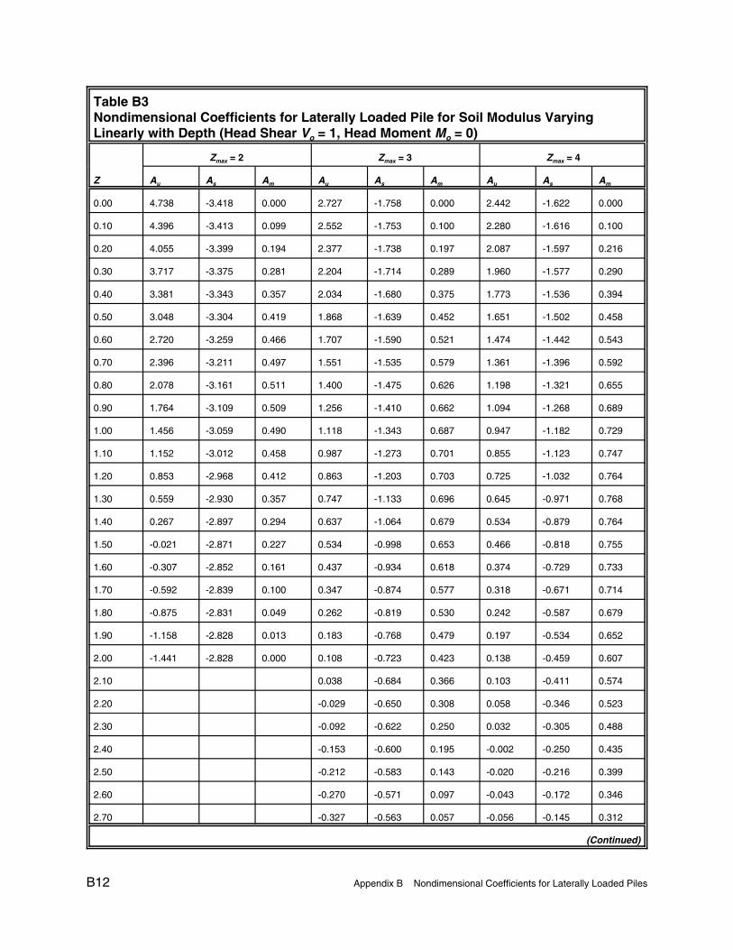
B12 Appendix B Nondimensional Coefficients for Laterally Loaded Piles
Table B3Nondimensional Coefficients for Laterally Loaded Pile for Soil Modulus VaryingLinearly with Depth (Head Shear Vo = 1, Head Moment Mo = 0)
Zmax = 2 Zmax = 3 Zmax = 4
Z Au As Am Au As Am Au As Am
0.00 4.738 -3.418 0.000 2.727 -1.758 0.000 2.442 -1.622 0.000
0.10 4.396 -3.413 0.099 2.552 -1.753 0.100 2.280 -1.616 0.100
0.20 4.055 -3.399 0.194 2.377 -1.738 0.197 2.087 -1.597 0.216
0.30 3.717 -3.375 0.281 2.204 -1.714 0.289 1.960 -1.577 0.290
0.40 3.381 -3.343 0.357 2.034 -1.680 0.375 1.773 -1.536 0.394
0.50 3.048 -3.304 0.419 1.868 -1.639 0.452 1.651 -1.502 0.458
0.60 2.720 -3.259 0.466 1.707 -1.590 0.521 1.474 -1.442 0.543
0.70 2.396 -3.211 0.497 1.551 -1.535 0.579 1.361 -1.396 0.592
0.80 2.078 -3.161 0.511 1.400 -1.475 0.626 1.198 -1.321 0.655
0.90 1.764 -3.109 0.509 1.256 -1.410 0.662 1.094 -1.268 0.689
1.00 1.456 -3.059 0.490 1.118 -1.343 0.687 0.947 -1.182 0.729
1.10 1.152 -3.012 0.458 0.987 -1.273 0.701 0.855 -1.123 0.747
1.20 0.853 -2.968 0.412 0.863 -1.203 0.703 0.725 -1.032 0.764
1.30 0.559 -2.930 0.357 0.747 -1.133 0.696 0.645 -0.971 0.768
1.40 0.267 -2.897 0.294 0.637 -1.064 0.679 0.534 -0.879 0.764
1.50 -0.021 -2.871 0.227 0.534 -0.998 0.653 0.466 -0.818 0.755
1.60 -0.307 -2.852 0.161 0.437 -0.934 0.618 0.374 -0.729 0.733
1.70 -0.592 -2.839 0.100 0.347 -0.874 0.577 0.318 -0.671 0.714
1.80 -0.875 -2.831 0.049 0.262 -0.819 0.530 0.242 -0.587 0.679
1.90 -1.158 -2.828 0.013 0.183 -0.768 0.479 0.197 -0.534 0.652
2.00 -1.441 -2.828 0.000 0.108 -0.723 0.423 0.138 -0.459 0.607
2.10 0.038 -0.684 0.366 0.103 -0.411 0.574
2.20 -0.029 -0.650 0.308 0.058 -0.346 0.523
2.30 -0.092 -0.622 0.250 0.032 -0.305 0.488
2.40 -0.153 -0.600 0.195 -0.002 -0.250 0.435
2.50 -0.212 -0.583 0.143 -0.020 -0.216 0.399
2.60 -0.270 -0.571 0.097 -0.043 -0.172 0.346
2.70 -0.327 -0.563 0.057 -0.056 -0.145 0.312
(Continued)

Appendix B Nondimensional Coefficients for Laterally Loaded Piles B13
Table B3 (Concluded)
Zmax = 2 Zmax = 3 Zmax = 4
Z Au As Am Au As Am Au As Am
2.80 -0.383 -0.559 0.027 -0.071 -0.111 0.262
2.90 -0.439 -0.558 0.007 -0.079 -0.091 0.231
3.00 -0.494 -0.557 0.000 -0.089 -0.066 0.186
3.10 -0.093 -0.052 0.159
3.20 -0.099 -0.036 0.121
3.30 -0.101 -0.027 0.098
3.40 -0.104 -0.017 0.069
3.50 -0.105 -0.012 0.051
3.60 -0.106 -0.007 0.030
3.70 -0.106 -0.005 0.019
3.80 -0.107 -0.004 0.007
3.90 -0.107 -0.003 0.002
4.00 -0.108 -0.003 0.000

B14 Appendix B Nondimensional Coefficients for Laterally Loaded Piles
Figure B7. Bending moment coefficient for unit head shear for soil stiffness varying linearly withdepth
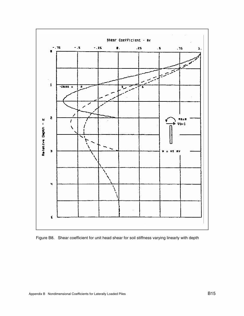
Appendix B Nondimensional Coefficients for Laterally Loaded Piles B15
Figure B8. Shear coefficient for unit head shear for soil stiffness varying linearly with depth

B16 Appendix B Nondimensional Coefficients for Laterally Loaded Piles
Figure B9. Deflection coefficient for unit head shear for soil stiffness varying linearly with depth

Appendix B Nondimensional Coefficients for Laterally Loaded Piles B17
Table B4Nondimensional Coefficients for Laterally Loaded Pile for Soil Modulus VaryingLinearly with Depth (Head Shear Vo = 0, Head Moment Mo = 1)
Zmax = 2 Zmax = 3 Zmax = 4
Z Bu Bs Bm Bu Bs Bm Bu Bs Bm
0.00 -3.418 3.213 -1.000 -1.758 1.819 -1.000 -1.622 1.751 -1.000
0.10 -3.102 3.113 -0.999 -1.581 1.719 -1.000 -1.452 1.651 -1.000
0.20 -2.796 3.013 -0.996 -1.414 1.619 -0.998 -1.261 1.531 -0.997
0.30 -2.499 2.914 -0.987 -1.257 1.519 -0.993 -1.141 1.452 -0.994
0.40 -2.213 2.816 -0.970 -1.110 1.420 -0.985 -0.974 1.333 -0.984
0.50 -1.936 2.720 -0.945 -0.973 1.322 -0.972 -0.871 1.254 -0.975
0.60 -1.668 2.628 -0.910 -0.846 1.226 -0.955 -0.727 1.139 -0.955
0.70 -1.410 2.539 -0.865 -0.728 1.132 -0.932 -0.639 1.063 -0.938
0.80 -1.161 2.455 -0.810 -0.619 1.040 -0.904 -0.518 0.952 -0.908
0.90 -0.919 2.377 -0.746 -0.520 0.951 -0.871 -0.445 0.880 -0.884
1.00 -0.685 2.306 -0.674 -0.429 0.866 -0.834 -0.346 0.777 -0.844
1.10 -0.458 2.243 -0.594 -0.347 0.784 -0.792 -0.286 0.710 -0.814
1.20 -0.236 2.187 -0.510 -0.272 0.707 -0.747 -0.207 0.615 -0.766
1.30 -0.020 2.141 -0.423 -0.205 0.635 -0.698 -0.160 0.555 -0.732
1.40 0.192 2.103 -0.336 -0.145 0.568 -0.647 -0.099 0.471 -0.678
1.50 0.401 2.073 -0.252 -0.091 0.506 -0.593 -0.063 0.418 -0.641
1.60 0.607 2.052 -0.173 -0.044 0.449 -0.538 -0.017 0.345 -0.584
1.70 0.812 2.038 -0.105 -0.001 0.398 -0.483 0.008 0.299 -0.546
1.80 1.015 2.031 -0.050 0.036 0.353 -0.427 0.040 0.237 -0.490
1.90 1.218 2.028 -0.013 0.070 0.313 -0.373 0.058 0.199 -0.452
2.00 1.421 2.027 0.000 0.099 0.278 -0.319 0.079 0.148 -0.398
2.10 0.125 0.249 -0.267 0.089 0.118 -0.363
2.20 0.149 0.225 -0.219 0.101 0.078 -0.312
2.30 0.170 0.205 -0.173 0.106 0.054 -0.280
2.40 0.190 0.190 -0.131 0.111 0.023 -0.236
2.50 0.209 0.179 -0.094 0.112 0.005 -0.208
2.60 0.226 0.171 -0.062 0.111 -0.017 -0.170
2.70 0.243 0.166 -0.036 0.109 -0.030 -0.146
(Continued)

B18 Appendix B Nondimensional Coefficients for Laterally Loaded Piles
Table B4 (Concluded)
Zmax = 2 Zmax = 3 Zmax = 4
Z Bu Bs Bm Bu Bs Bm Bu Bs Bm
2.80 0.259 0.163 -0.017 0.105 -0.046 -0.115
2.90 0.276 0.162 -0.004 0.101 -0.054 -0.097
3.00 0.292 0.162 0.000 0.093 -0.064 -0.072
3.10 0.088 -0.069 -0.059
3.20 0.079 -0.075 -0.041
3.30 0.073 -0.078 -0.031
3.40 0.064 -0.081 -0.020
3.50 0.057 -0.083 -0.014
3.60 0.047 -0.084 -0.007
3.70 0.040 -0.084 -0.004
3.80 0.030 -0.085 -0.001
3.90 0.023 -0.085 -0.000
4.00 0.015 -0.085 -0.000

Appendix B Nondimensional Coefficients for Laterally Loaded Piles B19
Figure B10. Slope coefficient for unit head shear for soil stiffness varying parabolically withdepth

B20 Appendix B Nondimensional Coefficients for Laterally Loaded Piles
Figure B11. Bending moment coefficient for unit head shear for soil stiffness varyingparabolically with depth

Appendix B Nondimensional Coefficients for Laterally Loaded Piles B21
Figure B12. Shear coefficient for unit head shear for soil stiffness varying parabolically withdepth

B22 Appendix B Nondimensional Coefficients for Laterally Loaded Piles
Table B5Nondimensional Coefficients for Laterally Loaded Pile for Soil Modulus VaryingParabolically with Depth (Head Shear Vo = 1, Head Moment Mo = 0)
Zmax = 2 Zmax = 3 Zmax = 4
Z Au As Am Au As Am Au As Am
0.00 6.418 -4.348 0.000 3.039 -1.970 0.000 2.820 -1.884 0.000
0.10 5.983 -4.343 0.100 2.842 -1.965 0.100 2.631 -1.879 0.100
0.20 5.550 -4.328 0.199 2.647 -1.950 0.200 2.407 -1.859 0.219
0.30 5.118 -4.303 0.296 2.453 -1.925 0.298 2.259 -1.839 0.298
0.40 4.689 -4.269 0.389 2.262 -1.890 0.395 2.041 -1.796 0.414
0.50 4.265 -4.225 0.473 2.075 -1.846 0.487 1.898 -1.760 0.488
0.60 3.845 -4.174 0.548 1.893 -1.793 0.575 1.691 -1.695 0.594
0.70 3.430 -4.116 0.608 1.717 -1.732 0.655 1.557 -1.645 0.659
0.80 3.022 -4.053 0.651 1.547 -1.662 0.728 1.365 -1.560 0.748
0.90 2.619 -3.987 0.676 1.384 -1.586 0.790 1.243 -1.498 0.800
1.00 2.224 -3.919 0.679 1.230 -1.505 0.841 1.069 -1.398 0.865
1.10 1.836 -3.852 0.660 1.083 -1.418 0.880 0.960 -1.328 0.900
1.20 1.454 -3.788 0.619 0.946 -1.329 0.906 0.807 -1.217 0.938
1.30 1.078 -3.729 0.557 0.818 -1.238 0.918 0.712 -1.141 0.955
1.40 0.708 -3.677 0.477 0.699 -1.146 0.917 0.582 -1.026 0.964
1.50 0.342 -3.634 0.383 0.588 -1.055 0.902 0.503 -0.949 0.961
1.60 -0.019 -3.601 0.282 0.488 -0.966 0.873 0.396 -0.835 0.943
1.70 -0.378 -3.578 0.181 0.395 -0.881 0.832 0.333 -0.760 0.923
1.80 -0.735 -3.564 0.091 0.311 -0.800 0.780 0.248 -0.652 0.881
1.90 -1.091 -3.559 0.026 0.235 -0.725 0.718 0.199 -0.582 0.847
2.00 -1.447 -3.558 0.000 0.166 -0.657 0.647 0.135 -0.484 0.786
2.10 0.103 -0.596 0.570 0.099 -0.423 0.742
2.20 0.047 -0.543 0.488 0.053 -0.338 0.670
2.30 -0.005 -0.498 0.404 0.028 -0.287 0.619
2.40 -0.053 -0.462 0.320 -0.002 -0.217 0.542
2.50 -0.098 -0.434 0.239 -0.018 -0.176 0.491
2.60 -0.140 -0.414 0.164 -0.036 -0.121 0.416
2.70 -0.181 -0.401 0.099 -0.044 -0.090 0.367
(Continued)

Appendix B Nondimensional Coefficients for Laterally Loaded Piles B23
Table B5 (Concluded)
Zmax = 2 Zmax = 3 Zmax = 4
Z Au As Am Au As Am Au As Am
2.80 -0.221 -0.394 0.047 -0.052 -0.050 0.298
2.90 -0.260 -0.391 0.013 -0.055 -0.028 0.256
3.00 -0.299 -0.390 0.000 -0.057 -0.001 0.198
3.10 -0.057 0.013 0.163
3.20 -0.054 0.030 0.117
3.30 -0.051 0.038 0.091
3.40 -0.046 0.047 0.059
3.50 -0.042 0.051 0.042
3.60 -0.036 0.055 0.023
3.70 -0.031 0.057 0.013
3.80 -0.024 0.058 0.004
3.90 -0.020 0.058 0.001
4.00 -0.014 0.058 0.000

B24 Appendix B Nondimensional Coefficients for Laterally Loaded Piles
Figure B13. Deflection coefficient for unit head moment for soil stiffness constant with depth

Appendix B Nondimensional Coefficients for Laterally Loaded Piles B25
Figure B14. Slope coefficient for unit head moment for soil stiffness constant with depth

B26 Appendix B Nondimensional Coefficients for Laterally Loaded Piles
Figure B15. Bending moment coefficient for unit head moment for soil stiffness constant withdepth

Appendix B Nondimensional Coefficients for Laterally Loaded Piles B27
Table B6Nondimensional Coefficients for Laterally Loaded Pile for Soil Modulus VaryingParabolically with Depth (Head Shear Vo = 0, Head Moment Mo = 1)
Zmax = 2 Zmax = 3 Zmax = 4
Z Bu Bs Bm Bu Bs Bm Bu Bs Bm
0.00 -4.348 3.624 -1.000 -1.970 1.925 -1.000 -1.884 1.888 -1.000
0.10 -3.990 3.524 -1.000 -1.783 1.825 -1.000 -1.700 1.788 -1.000
0.20 -3.643 3.424 -0.999 -1.605 1.725 -1.000 -1.493 1.668 -1.000
0.30 -3.306 3.324 -0.998 -1.438 1.625 -0.999 -1.362 1.589 -0.999
0.40 -2.978 3.224 -0.993 -1.280 1.525 -0.997 -1.179 1.469 -0.996
0.50 -2.661 3.125 -0.983 -1.133 1.425 -0.992 -1.065 1.389 -0.993
0.60 -2.353 3.028 -0.966 -0.995 1.326 -0.985 -0.905 1.271 -0.984
0.70 -2.055 2.932 -0.942 -0.867 1.228 -0.975 -0.807 1.192 -0.976
0.80 -1.767 2.840 -0.907 -0.749 1.132 -0.960 0.670 1.076 -0.959
0.90 -1.487 2.751 -0.860 -0.641 1.037 -0.940 -0.587 1.000 -0.944
1.00 -1.216 2.668 -0.802 -0.542 0.944 -0.915 -0.474 0.888 -0.916
1.10 -0.953 2.591 -0.732 -0.452 0.854 -0.885 -0.406 0.816 -0.893
1.20 -0.698 2.522 -0.650 -0.371 0.767 -0.850 -0.315 0.711 -0.853
1.30 -0.449 2.462 -0.559 -0.299 0.684 -0.808 -0.260 0.644 -0.822
1.40 -0.205 2.411 -0.460 -0.234 0.605 -0.762 -0.189 0.548 -0.771
1.50 0.034 2.370 -0.356 -0.177 0.532 -0.712 -0.147 0.488 -0.734
1.60 0.269 2.339 -0.254 -0.128 0.463 -0.657 -0.094 0.404 -0.675
1.70 0.502 2.319 -0.159 -0.085 0.400 -0.599 -0.064 0.351 -0.633
1.80 0.733 2.307 -0.078 -0.047 0.343 -0.539 -0.026 0.279 -0.569
1.90 0.964 2.302 -0.022 -0.016 0.293 -0.477 -0.006 0.235 -0.525
2.00 1.194 2.302 0.000 0.011 0.248 -0.415 0.019 0.176 -0.459
2.10 0.034 0.210 -0.353 0.032 0.141 -0.416
2.20 0.053 0.177 -0.292 0.046 0.095 -0.353
2.30 0.070 0.151 -0.235 0.052 0.069 -0.312
2.40 0.084 0.130 -0.180 0.058 0.035 -0.255
2.50 0.096 0.115 -0.131 0.060 0.016 -0.219
2.60 0.107 0.104 -0.088 0.061 -0.008 -0.171
2.70 0.117 0.097 -0.052 0.060 -0.020 -0.142
(Continued)

B28 Appendix B Nondimensional Coefficients for Laterally Loaded Piles
Table B6 (Concluded)
Zmax = 2 Zmax = 3 Zmax = 4
Z Bu Bs Bm Bu Bs B B Bs Bm
2.80 0.126 0.093 -0.024 0.056 -0.035 -0.103
2.90 0.136 0.092 -0.006 0.053 -0.042 -0.081
3.00 0.145 0.092 0.000 0.048 -0.050 -0.053
3.10 0.043 -0.054 -0.038
3.20 0.037 -0.057 -0.021
3.30 0.032 -0.059 -0.012
3.40 0.025 -0.060 -0.003
3.50 0.020 -0.060 0.000
3.60 0.013 -0.060 0.002
3.70 0.008 -0.059 0.003
3.80 0.001 -0.059 0.002
3.90 -0.004 -0.059 0.001
4.00 -0.009 -0.059 0.000

Appendix B Nondimensional Coefficients for Laterally Loaded Piles B29
Figure B16. Shear coefficient for unit head moment for soil stiffness constant with depth

B30 Appendix B Nondimensional Coefficients for Laterally Loaded Piles
Figure B17. Deflection coefficient for unit head moment for soil stiffness constant with depth
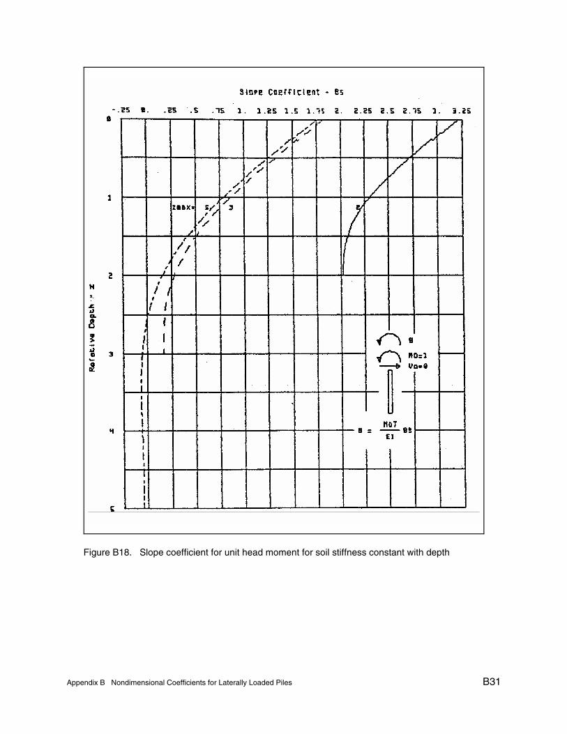
Appendix B Nondimensional Coefficients for Laterally Loaded Piles B31
Figure B18. Slope coefficient for unit head moment for soil stiffness constant with depth

B32 Appendix B Nondimensional Coefficients for Laterally Loaded Piles
Figure B19. Bending moment coefficient for unit head moment for soil stiffness varying linearlywith depth

Appendix B Nondimensional Coefficients for Laterally Loaded Piles B33
Figure B20. Shear coefficient for unit head moment for soil stiffness varying linearly with depth
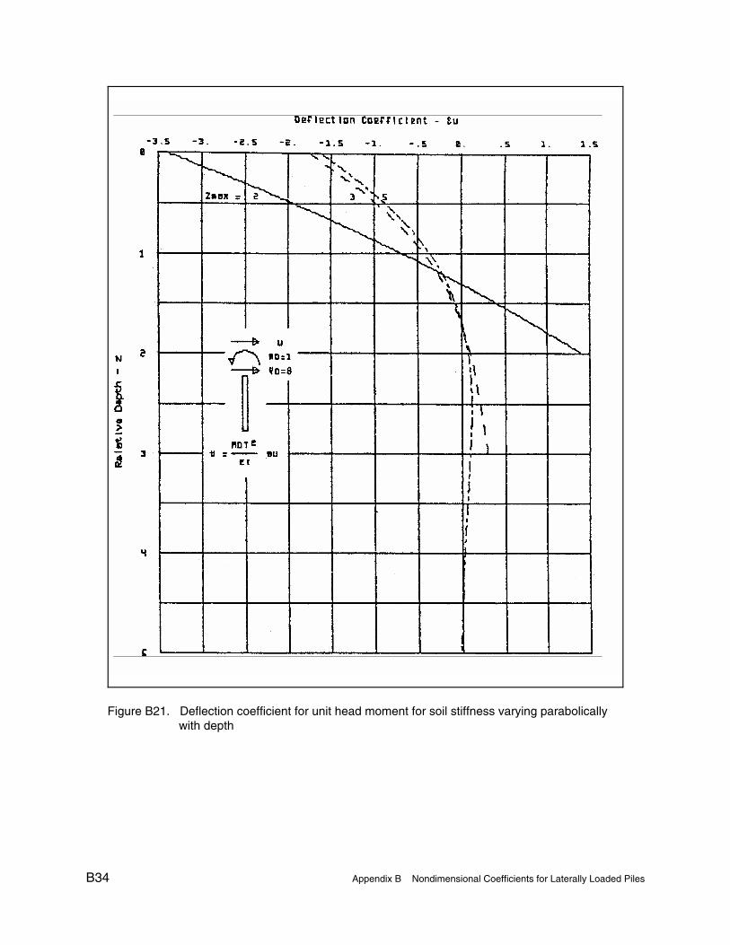
B34 Appendix B Nondimensional Coefficients for Laterally Loaded Piles
Figure B21. Deflection coefficient for unit head moment for soil stiffness varying parabolicallywith depth

Appendix B Nondimensional Coefficients for Laterally Loaded Piles B35
Figure B22. Slope coefficient for unit head moment for soil stiffness varying parabolically withdepth
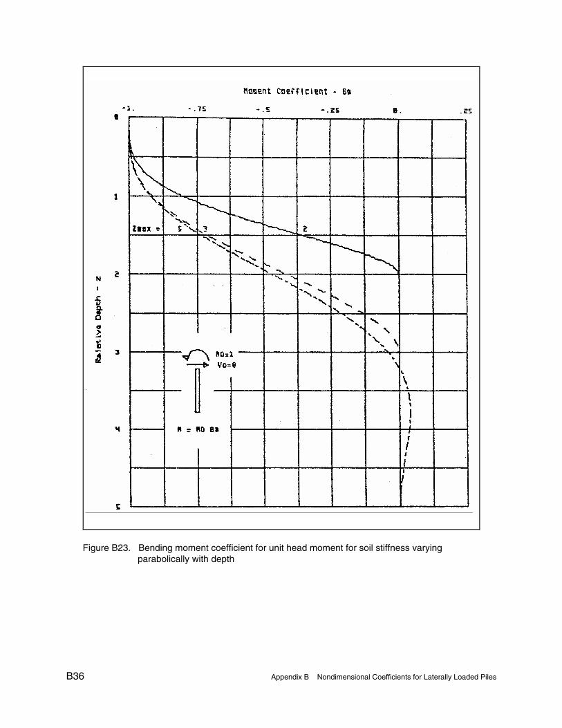
B36 Appendix B Nondimensional Coefficients for Laterally Loaded Piles
Figure B23. Bending moment coefficient for unit head moment for soil stiffness varyingparabolically with depth

Appendix B Nondimensional Coefficients for Laterally Loaded Piles B37
Figure B24. Shear coefficient for unit head moment for soil stiffness varying parabolically withdepth

B38 Appendix B Nondimensional Coefficients for Laterally Loaded Piles
Figure B25. Pile head deflection coefficients for unit head shear

Appendix B Nondimensional Coefficients for Laterally Loaded Piles B39
Figure B26. Pile head slope coefficients for unit head shear

B40 Appendix B Nondimensional Coefficients for Laterally Loaded Piles
Figure B27. Pile head deflection coefficients for unit head moment

Appendix B Nondimensional Coefficients for Laterally Loaded Piles B41
Figure B28. Pile head slope coefficients for unit head moment

REPORTS PUBLISHED UNDER THE COMPUTER-AIDEDSTRUCTURAL ENGINEERING (CASE) PROJECT
(Continued)
1
Title Date
Technical Report K-78-1 List of Computer Programs for Computer-Aided Structural Engineering Feb 1978
Instruction Report 0-79-2 User's Guide: Computer Program with Interactive Graphics forAnalysis of Plane Frame Structures (CFRAME)
Mar 1979
Technical Report K-80-1 Survey of Bridge-Oriented Design Software Jan 1980
Technical Report K-80-2 Evaluation of Computer Programs for the Design/Analysis of Highwayand Railway Bridges
Jan 1980
Instruction Report K-80-1 User's Guide: Computer Program for Design/Review of Curvi-linearConduits/Culveris (CURCON)
Feb 1980
Instruction Report K-80-3 A Three-Dimensional Finite Element Data Edit Program Mar 1980
Instruction Report K-80-4 A Three-Dimensional Stability Analysis/Design Program (3DSAD)Report 1: General Geometry ModuleReport 3: General Analysis Module (CGAM)Report 4: Special-Purpose Modules for Dams (CDAMS)
Jun 1980Jun 1982Aug 1983
Instruction Report K-80-6 Basic User's Guide: Computer Program for Design and Analysis ofInverted-T Retaining Walls and Floodwalls (TWDA)
Dec 1980
Instruction Report K-80-7 User's Reference Manual: Computer Program for Design and Analysisof Inverted-T Retaining Walls and Floodwalls (TWDA)
Dec 1980
Technical Report K-80-4 Documentation of Finite Element AnalysesReport 1: Longview Outlet Works ConduitReport 2: Anchored Wall Monolith, Bay Springs Lock
Dec 1980Dec 1980
Technical Report K-80-5 Basic Pile Group Behavior Dec 1980
Instruction Report K-81-2 User's Guide: Computer Program for Design and Analysis of Sheet PileWalls by Classical Methods (CSHTWAL)
Report 1: Computational ProcessesReport 2: Interactive Graphics Options
Feb 1981Mar 1981
Instruction Report K-81-3 Validation Report: Computer Program for Design and Analysis ofInverted-T Retaining Walls and Floodwalls (TWDA)
Feb 1981
Instruction Report K-81-4 User's Guide: Computer Program for Design and Analysis of Cast-in-Place Tunnel Linings (NEWTUN)
Mar 1981
Instruction Report K-81-6 User's Guide: Computer Program for Optimum Nonlinear DynamicDesign of Reinforced Concrete Slabs Under Blast Loading (CBARCS)
Mar 1981
Instruction Report K-81-7 User's Guide: Computer Program for Design or Investigation ofOrthogonal Culverts (CORTCUL)
Mar 1981
Instruction Report K-81-9 User's Guide: Computer Program for Three-Dimensional Analysis ofBuilding Systems (CTABS80)
Aug 1981
Technical Report K-81-2 Theoretical Basis for CTABS80: A Computer Program forThree-Dimensional Analysis of Building Systems
Sep 1981
REPORTS PUBLISHED UNDER THE COMPUTER-AIDEDSTRUCTURAL ENGINEERING (CASE) PROJECT
(Continued)
2
Title Date
Instruction Report K-82-6 User's Guide: Computer Program for Analysis of Beam-ColumnStructures with Nonlinear Supports (CBEAMC)
Jun 1982
Instruction Report K-82-7 User's Guide: Computer Program for Bearing Capacity Analysis ofShallow Foundations (CBEAR)
Jun 1982
Instruction Report K-83-1 User's Guide: Computer Program with Interactive Graphics forAnalysis of Plane Frame Structures (CFRAME)
Jan 1983
Instruction Report K-83-2 User's Guide: Computer Program for Generation of EngineeringGeometry (SKETCH)
Jun 1983
Instruction Report K-83-5 User's Guide: Computer Program to Calculate Shear, Moment, andThrust (CSMT) from Stress Results of a Two-Dimensional FiniteElement Analysis
Jul 1983
Technical Report K-83-1 Basic Pile Group Behavior Sep 1983
Technical Report K-83-3 Reference Manual: Computer Graphics Program for Generation ofEngineering Geometry (SKETCH)
Sep 1983
Technical Report K-83-4 Case Study of Six Major General-Purpose Finite Element Programs Oct 1983
Instruction Report K-84-2 User's Guide: Computer Program for Optimum Dynamic Design ofNonlinear Metal Plates Under Blast Loading (CSDOOR)
Jan 1984
Instruction Report K-84-7 User's Guide: Computer Program for Determining Induced Stressesand Consolidation Settlements (CSETT)
Aug 1984
Instruction Report K-84-8 Seepage Analysis of Confined Flow Problems by the Method ofFragments (CFRAG)
Sep 1984
Instruction Report K-84-11 User's Guide for Computer Program CGFAG, Concrete GeneralFlexure Analysis with Graphics
Sep 1984
Technical Report K-84-3 Computer-Aided Drafting and Design for Corps Structural Engineers Oct 1984
Technical Report ATC-86-5 Decision Logic Table Formulation of ACI 318-77, Building CodeRequirements for Reinforced Concrete for Automated ConstraintProcessing, Volumes I and 11
Jun 1986
Technical Report ITL-87-2 A Case Committee Study of Finite Element Analysis of Concrete FlatSlabs
Jan 1987
Instruction Report ITL-87-2(Revised)
User's Guide for Concrete Strength Investigation and Design(CASTR) in Accordance with ACI 318-89
Mar 1992
Instruction Report ITL-87-1 User's Guide: Computer Program for Two-Dimensional Analysis ofU-Frame Structures (CUFRAM)
Apr 1987
Instruction Report ITL-87-2 User's Guide: For Concrete Strength Investigation and Design(CASTR) in Accordance with ACI 318-83
May 1987
Technical Report ITL-87-6 Finite-Element Method Package for Solving Steady-State SeepageProblems
May 1987
REPORTS PUBLISHED UNDER THE COMPUTER-AIDEDSTRUCTURAL ENGINEERING (CASE) PROJECT
(Continued)
3
Title Date
Instruction Report ITL-87-3 User's Guide: A Three-Dimensional Stability Analysis/Design Program(3DSAD) Module
Report 1: Revision 1: General GeometryReport 2: General Loads ModuleReport 6: Free-Body Module
Jun 1987
Jun 1987Sep 1989Sep 1989
Instruction Report ITL-87-4 User's Guide: 2-D Frame Analysis Link Program (LINK2D) Jun 1987
Technical Report ITL-87-4 Finite Element Studies of a Horizontally Framed Miter GateReport 1: Initial and Refined Finite Element Models (Phases A,
B, and C), Volumes I and 11Report 2: Simplified Frame Model (Phase D)Report 3: Alternate Configuration Miter Gate Finite Element
Studies-Open SectionReport 4: Alternate Configuration Miter Gate Finite Element
Studies-Closed SectionsReport 5: Alternate Configuration Miter Gate Finite Element
Studies-Additional Closed SectionsReport 6: Elastic Buckling of Girders in Horizontally Framed
Miter GatesReport 7: Application and Summary
Aug 1987
Instruction Report GL-87-1 User's Guide: UTEXAS2 Slope-Stability Package; Volume 1, User'sManual
Aug 1987
Instruction Report ITL-87-5 Sliding Stability of Concrete Structures (CSLIDE) Oct 1987
Instruction Report ITL-87-6 Criteria Specifications for and Validation of a Computer Program forthe Design or Investigation of Horizontally Framed Miter Gates(CMITER)
Dec 1987
Technical Report ITL-87-8 Procedure for Static Analysis of Gravity Dams Using the FiniteElement Method - Phase la
Jan 1988
Instruction Report ITL-88-1 User's Guide: Computer Program for Analysis of Planar GridStructures (CGRID)
Feb 1988
Technical Report ITL-88-1 Development of Design Formulas for Ribbed Mat Foundations onExpansive Soils
Apr 1988
Technical Report ITL-88-2 User's Guide: Pile Group Graphics Display (CPGG) Postprocessor toCPGA Program
Apr 1988
Instruction Report ITL-88-2 User's Guide for Design and Investigation of Horizontally FramedMiter Gates (CMITER)
Jun 1988
Instruction Report ITL-88-4 User's Guide for Revised Computer Program to Calculate Shear,Moment, and Thrust (CSMT)
Sep 1988
Instruction Report GL-87-1 User's Guide: UTEXAS2 Slope-Stability Package; Volume 11,Theory
Feb 1989
Technical Report ITL-89-3 User's Guide: Pile Group Analysis (CPGA) Computer Group Jul 1989
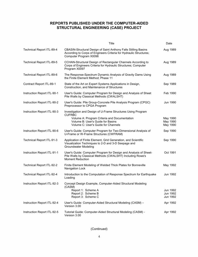
REPORTS PUBLISHED UNDER THE COMPUTER-AIDEDSTRUCTURAL ENGINEERING (CASE) PROJECT
(Continued)
4
Title Date
Technical Report ITL-89-4 CBASIN-Structural Design of Saint Anthony Falls Stilling BasinsAccording to Corps of Engineers Criteria for Hydraulic Structures;Computer Program X0098
Aug 1989
Technical Report ITL-89-5 CCHAN-Structural Design of Rectangular Channels According toCorps of Engineers Criteria for Hydraulic Structures; ComputerProgram X0097
Aug 1989
Technical Report ITL-89-6 The Response-Spectrum Dynamic Analysis of Gravity Dams Usingthe Finite Element Method; Phase 11
Aug 1989
Contract Report ITL-89-1 State of the Art on Expert Systems Applications in Design,Construction, and Maintenance of Structures
Sep 1989
Instruction Report ITL-90-1 User's Guide: Computer Program for Design and Analysis of SheetPile Walls by Classical Methods (CWALSHT)
Feb 1990
Instruction Report ITL-90-2 User's Guide: Pile Group-Concrete Pile Analysis Program (CPGC)Preprocessor to CPGA Program
Jun 1990
Instruction Report ITL-90-3 Investigation and Design of U-Frame Structures Using ProgramCUFRBC
Volume A: Program Criteria and DocumentationVolume B: User's Guide for BasinsVolume C: User's Guide for Channels
May 1990May 1990May 1990
Instruction Report ITL-90-6 User's Guide: Computer Program for Two-Dimensional Analysis ofU-Frame or W-Frame Structures (CWFRAM)
Sep 1990
Technical Report ITL-91-3 Application of Finite Element, Grid Generation, and ScientificVisualization Techniques to 2-D and 3-D Seepage andGroundwater Modeling
Sep 1990
Instruction Report ITL-91-1 User's Guide: Computer Program for Design and Analysis of Sheet-Pile Walls by Classical Methods (CWALSHT) Including Rowe'sMoment Reduction
Oct 1991
Technical Report ITL-92-2 Finite Element Modeling of Welded Thick Plates for BonnevilleNavigation Lock
May 1992
Technical Report ITL-92-4 Introduction to the Computation of Response Spectrum for EarthquakeLoading
Jun 1992
Instruction Report ITL-92-3 Concept Design Example, Computer-Aided Structural Modeling(CASM)
Report 1: Scheme AReport 2: Scheme BReport 3: Scheme C
Jun 1992Jun 1992Jun 1992
Instruction Report ITL-92-4 User's Guide: Computer-Aided Structural Modeling (CASM) –Version 3.00
Apr 1992
Instruction Report ITL-92-5 Tutorial Guide: Computer-Aided Structural Modeling (CASM) -Version 3.00
Apr 1992

REPORTS PUBLISHED UNDER THE COMPUTER-AIDEDSTRUCTURAL ENGINEERING (CASE) PROJECT
(Continued)
5
Title Date
Contract Report ITL-92-1 Optimization of Steel Pile Foundations Using Optimality Criteria Jun 1992
Technical Report ITL-92-7 Refined Stress Analysis of Melvin Price Locks and Dam Sep 1992
Contract Report ITL-92-2 Knowledge-Based Expert System for Selection and Design ofRetaining Structures
Sep 1992
Contract Report ITL-92-3 Evaluation of Thermal and Incremental Construction Effects forMonoliths AL-3 and AL-5 of the Melvin Price Locks and Dam
Sep 1992
Instruction Report GL-87-1 User's Guide: UTEXAS3 Slope-Stability Package; Volume IV, User'sManual
Nov 1992
Technical Report ITL-92-11 The Seismic Design of Waterfront Retaining Structures Nov 1992
Technical Report ITL-92-12 Computer-Aided, Field-Verified Structural EvaluationReport 1: Development of Computer Modeling Techniques for
Miter Lock GatesReport 2: Field Test and Analysis Correlation at John Hollis
Bankhead Lock and DamReport 3: Field Test and Analysis Correlation of a Vertically
Framed Miter Gate at Emsworth Lock and Dam
Nov 1992
Dec 1992
Dec 1993
Instruction Report GL-87-1 Users Guide: UTEXAS3 Slope-Stability Package; Volume III,Example Problems
Dec 1992
Technical Report ITL-93-1 Theoretical Manual for Analysis of Arch Dams Jul 1993
Technical Report ITL-93-2 Steel Structures for Civil Works, General Considerations for Designand Rehabilitation
Aug 1993
Technical Report ITL-93-3 Soil-Structure Interaction Study of Red River Lock and Dam No. 1Subjected to Sediment Loading
Sep 1993
Instruction Report ITL-93-3 User's Manual-ADAP, Graphics-Based Dam Analysis Program Aug 1993
Instruction Report ITL-93-4 Load and Resistance Factor Design for Steel Miter Gates Oct 1993
Technical Report ITL-94-2 User's Guide for the Incremental Construction, Soil-StructureInteraction Program SOILSTRUCT with Far-Field BoundaryElements
Mar 1994
Instruction Report ITL-94-1 Tutorial Guide: Computer-Aided Structural Modeling (CASM);Version 5.00
Apr 1994
Instruction Report ITL-94-2 User's Guide: Computer-Aided Structural Modeling (CASM);Version 5.00
Apr 1994
Technical Report ITL-94-4 Dynamics of Intake Towers and Other MDOF Structures UnderEarthquake Loads: A Computer-Aided Approach
Jul 1994
Technical Report ITL-94-5 Procedure for Static Analysis of Gravity Dams Including FoundationEffects Using the Finite Element Method - Phase 1 B
Jul 1994
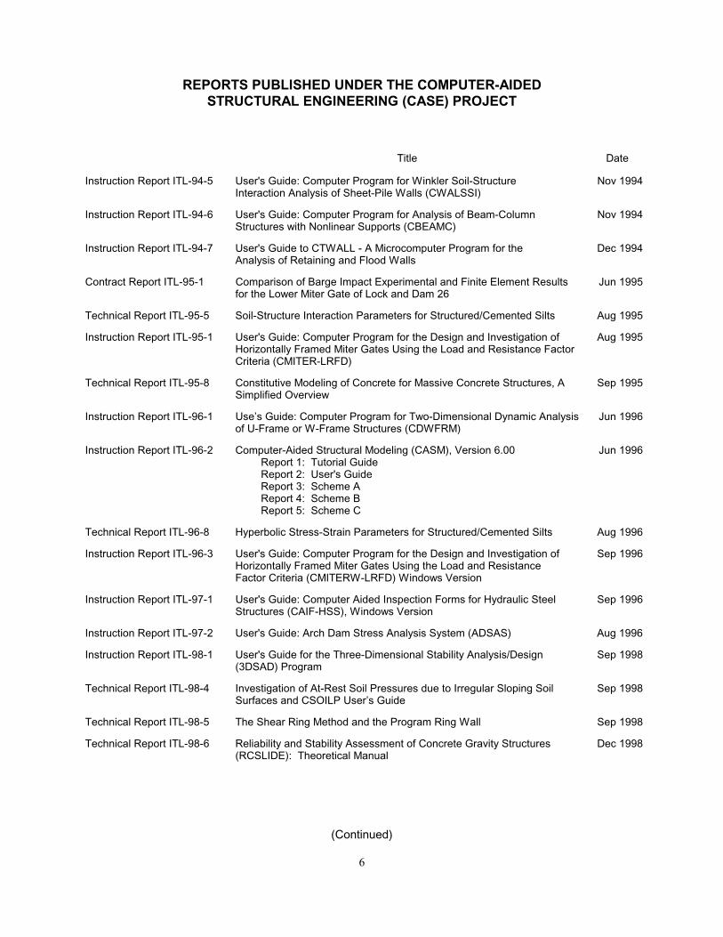
REPORTS PUBLISHED UNDER THE COMPUTER-AIDEDSTRUCTURAL ENGINEERING (CASE) PROJECT
(Continued)
6
Title Date
Instruction Report ITL-94-5 User's Guide: Computer Program for Winkler Soil-StructureInteraction Analysis of Sheet-Pile Walls (CWALSSI)
Nov 1994
Instruction Report ITL-94-6 User's Guide: Computer Program for Analysis of Beam-ColumnStructures with Nonlinear Supports (CBEAMC)
Nov 1994
Instruction Report ITL-94-7 User's Guide to CTWALL - A Microcomputer Program for theAnalysis of Retaining and Flood Walls
Dec 1994
Contract Report ITL-95-1 Comparison of Barge Impact Experimental and Finite Element Resultsfor the Lower Miter Gate of Lock and Dam 26
Jun 1995
Technical Report ITL-95-5 Soil-Structure Interaction Parameters for Structured/Cemented Silts Aug 1995
Instruction Report ITL-95-1 User's Guide: Computer Program for the Design and Investigation ofHorizontally Framed Miter Gates Using the Load and Resistance FactorCriteria (CMITER-LRFD)
Aug 1995
Technical Report ITL-95-8 Constitutive Modeling of Concrete for Massive Concrete Structures, ASimplified Overview
Sep 1995
Instruction Report ITL-96-1 Use’s Guide: Computer Program for Two-Dimensional Dynamic Analysisof U-Frame or W-Frame Structures (CDWFRM)
Jun 1996
Instruction Report ITL-96-2 Computer-Aided Structural Modeling (CASM), Version 6.00Report 1: Tutorial GuideReport 2: User's GuideReport 3: Scheme AReport 4: Scheme BReport 5: Scheme C
Jun 1996
Technical Report ITL-96-8 Hyperbolic Stress-Strain Parameters for Structured/Cemented Silts Aug 1996
Instruction Report ITL-96-3 User's Guide: Computer Program for the Design and Investigation ofHorizontally Framed Miter Gates Using the Load and ResistanceFactor Criteria (CMITERW-LRFD) Windows Version
Sep 1996
Instruction Report ITL-97-1 User's Guide: Computer Aided Inspection Forms for Hydraulic SteelStructures (CAIF-HSS), Windows Version
Sep 1996
Instruction Report ITL-97-2 User's Guide: Arch Dam Stress Analysis System (ADSAS) Aug 1996
Instruction Report ITL-98-1 User's Guide for the Three-Dimensional Stability Analysis/Design(3DSAD) Program
Sep 1998
Technical Report ITL-98-4 Investigation of At-Rest Soil Pressures due to Irregular Sloping SoilSurfaces and CSOILP User’s Guide
Sep 1998
Technical Report ITL-98-5 The Shear Ring Method and the Program Ring Wall Sep 1998
Technical Report ITL-98-6 Reliability and Stability Assessment of Concrete Gravity Structures(RCSLIDE): Theoretical Manual
Dec 1998
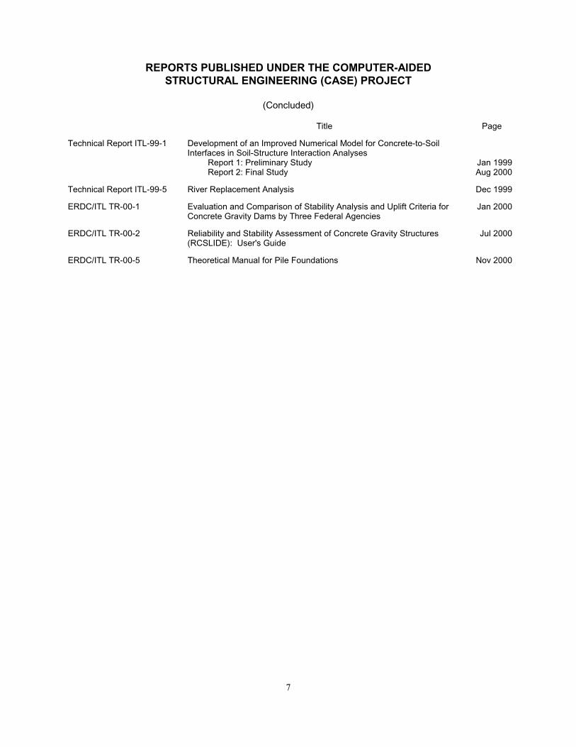
REPORTS PUBLISHED UNDER THE COMPUTER-AIDEDSTRUCTURAL ENGINEERING (CASE) PROJECT
(Concluded)
7
Title Page
Technical Report ITL-99-1 Development of an Improved Numerical Model for Concrete-to-SoilInterfaces in Soil-Structure Interaction Analyses
Report 1: Preliminary StudyReport 2: Final Study
Jan 1999Aug 2000
Technical Report ITL-99-5 River Replacement Analysis Dec 1999
ERDC/ITL TR-00-1 Evaluation and Comparison of Stability Analysis and Uplift Criteria forConcrete Gravity Dams by Three Federal Agencies
Jan 2000
ERDC/ITL TR-00-2 Reliability and Stability Assessment of Concrete Gravity Structures(RCSLIDE): User's Guide
Jul 2000
ERDC/ITL TR-00-5 Theoretical Manual for Pile Foundations Nov 2000

REPORT DOCUMENTATION PAGE Form ApprovedOMB No. 0704-0188
Public reporting burden for this collection of information is estimated to average 1 hour per response, including the time for reviewing instructions, searching existing data sources, gathering and maintainingthe data needed, and completing and reviewing the collection of information. Send comments regarding this burden estimate or any other aspect of this collection of information, including suggestionsfor reducing this burden, to Washington Headquarters Services, Directorate for Information Operations and Reports, 1215 Jefferson Davis Highway, Suite 1204, Arlington, VA 22202-4302, and to theOffice of Management and Budget, Paperwork Reduction Project (0704-0188), Washington, DC 20503.
1. AGENCY USE ONLY (Leave blank) 2. REPORT DATE 3. REPORT TYPE AND DATES COVERED
4. TITLE AND SUBTITLE 5. FUNDING NUMBERS
6. AUTHOR(S)
7. PERFORMING ORGANIZATION NAME(S) AND ADDRESS(ES) 8. PERFORMING ORGANIZATIONREPORT NUMBER
9. SPONSORING/MONITORING AGENCY NAME(S) AND ADDRESS(ES) 10. SPONSORING/MONITORINGAGENCY REPORT NUMBER
11. SUPPLEMENTARY NOTES
12a. DISTRIBUTION/AVAILABILITY STATEMENT 12b. DISTRIBUTION CODE
13. ABSTRACT (Maximum 200 words)
14. SUBJECT TERMS 15. NUMBER OF PAGES
16. PRICE CODE
17. SECURITY CLASSIFICATIONOF REPORT
18. SECURITY CLASSIFICATIONOF THIS PAGE
19. SECURITY CLASSIFICATIONOF ABSTRACT
20. LIMITATION OF ABSTRACT
NSN 7540-01-280-5500 Standard Form 298 (Rev. 2-89)Prescribed by ANSI Std. Z39-18298-102
November 2000 Final report
Theoretical Manual for Pile Foundations
Reed L. Mosher, William P. Dawkins
U.S. Army Engineer Research and Development Center, Information TechnologyLaboratory, 3909 Halls Ferry Road, Vicksburg, MS 39180-6199;Oklahoma State University, Stillwater, OK 74074
ERDC/ITL TR-00-5
U.S. Army Corps of EngineersWashington, DC 20314-1000
Approved for public release; distribution is unlimited.
Axial piles Lateral pilesCASE Pile foundationsGroup piles
157
UNCLASSIFIED UNCLASSIFIED
This theoretical manual for pile foundations describes the background and research and the applied methodologies used inthe analysis and design of pile foundations. This research was developed through the U.S. Army Engineer Research andDevelopment Center by the Computer-Aided Structural Engineering (CASE) Project. Several of the procedures have beenimplemented in the CASE Committee computer programs CAXPILE, CPGA, and COM624. Theoretical development ofthese engineering procedures and discussions of the limitations of each method are presented.