Physics | William & Mary - Determination of the …physics.wm.edu/~armd/JoshHoskinsThesisFinal.pdfDetermination of the Proton’s Weak Charge via Parity Violating Electron Scattering

Determination of the Proton’s Weak Charge via Parity Violating ElectronScattering

Joshua Russell Hoskins

Williamsburg, Virginia

Master of Science, College of William and Mary, 2007Bachelor of Arts, Eastern Kentucky University, 2006

A Dissertation presented to the Graduate Facultyof the College of William and Mary in Candidacy for the Degree of

Doctor of Philosophy

Department of Physics

The College of William and MaryAugust 2015

c©2015


All rights reserved.

APPROVAL PAGE

This Dissertation is submitted in partial fulfillment ofthe requirements for the degree of

Doctor of Philosophy


Approved by the Committee, June, 2015

Committee Chair

Professor David S. Armstrong, Physics

The College of William and Mary

CEBAF Professor Roger D. Carlini, Physics


Assistant Professor Wouter Deconinck, Physics


Associate Professor Josh Erlich, Physics


Staff Scientist Bradley Sawatzky, Physics

Thomas Jefferson National Accelerator Facility

ABSTRACT

The Qweak experiment, which completed running in May of 2012 at Jefferson

Laboratory, has measured the parity-violating asymmetry in elastic electron-proton

scattering at four-momentum transfer Q2=0.025 (GeV/c)2 in order to provide the

first direct measurement of the proton’s weak charge, Qpw. The Standard Model

makes firm predictions for the weak charge; deviations from the predicted value

would provide strong evidence of new physics beyond the Standard Model. Using

an 89% polarized electron beam at 145 µA scattering from a 34.4 cm long liquid

hydrogen target, scattered electrons were detected using an array of eight

fused-silica detectors placed symmetric about the beam axis. The parity-violating

asymmetry was then measured by reversing the helicity of the incoming electrons

and measuring the normalized difference in rate seen in the detectors. The low Q2

enables a theoretically clean measurement; the higher order hadronic corrections

are constrained using previous parity-violating electron scattering world data. The

experimental method will be discussed, with recent results constituting 4% of our

total data and projections of our proposed uncertainties on the full data set.

TABLE OF CONTENTS

Acknowledgments . . . . . . . . . . . . . . . . . . . . . . . . . . . . . . . . . . v

Dedication . . . . . . . . . . . . . . . . . . . . . . . . . . . . . . . . . . . . . . vii

List of Tables . . . . . . . . . . . . . . . . . . . . . . . . . . . . . . . . . . . . viii

List of Figures . . . . . . . . . . . . . . . . . . . . . . . . . . . . . . . . . . . xi

CHAPTER

1 Introduction . . . . . . . . . . . . . . . . . . . . . . . . . . . . . . . . . 2

1.1 Fundamental Symmetries of the Standard Model . . . . . . . . . . 2

1.1.1 Fundamental Symmetries . . . . . . . . . . . . . . . . . . . 2

1.1.2 Standard Model Overview . . . . . . . . . . . . . . . . . . 5

1.2 Electroweak Theory . . . . . . . . . . . . . . . . . . . . . . . . . . 9

1.2.1 Discrete Symmetry and Spin . . . . . . . . . . . . . . . . . 9

1.2.2 Electroweak Unification . . . . . . . . . . . . . . . . . . . . 11

2 The Qweak Experiment . . . . . . . . . . . . . . . . . . . . . . . . . . . 16

2.1 Experimental Motivation . . . . . . . . . . . . . . . . . . . . . . . 16

2.2 Parity-Violating e+p Scattering . . . . . . . . . . . . . . . . . . . 18

2.2.1 Neutral-Weak Interaction . . . . . . . . . . . . . . . . . . . 18

2.2.2 Low Momentum Electron Scattering . . . . . . . . . . . . 19

2.2.3 Physics Asymmetry . . . . . . . . . . . . . . . . . . . . . . 23

2.2.4 Precision Determination of sin2 θw . . . . . . . . . . . . . . 26

2.2.5 γZ0 Box Diagram . . . . . . . . . . . . . . . . . . . . . . . 29

i

3 Experimental Setup . . . . . . . . . . . . . . . . . . . . . . . . . . . . . 31

3.1 Experimental Setup . . . . . . . . . . . . . . . . . . . . . . . . . . 31

3.2 Polarized Electron Beam . . . . . . . . . . . . . . . . . . . . . . . 33

3.2.1 Continuous Electron Beam Accelerator Facility . . . . . . . 33

3.2.2 Polarized Source and Injector . . . . . . . . . . . . . . . . 34

3.2.3 Beam Position Monitors . . . . . . . . . . . . . . . . . . . 38

3.2.4 Beam Current Monitors . . . . . . . . . . . . . . . . . . . 41

3.3 Electron Beam Polarimetry . . . . . . . . . . . . . . . . . . . . . . 42

3.3.1 Møller Polarimeter . . . . . . . . . . . . . . . . . . . . . . 43

3.3.2 Compton Polarimeter . . . . . . . . . . . . . . . . . . . . . 44

3.4 Primary lH2 Target . . . . . . . . . . . . . . . . . . . . . . . . . . 46

3.5 Infrastructure . . . . . . . . . . . . . . . . . . . . . . . . . . . . . 48

3.5.1 Collimation System . . . . . . . . . . . . . . . . . . . . . . 48

3.5.2 Qweak Toroidal Spectrometer . . . . . . . . . . . . . . . . . 49

3.5.3 Shielding Wall . . . . . . . . . . . . . . . . . . . . . . . . . 50

3.5.4 Quartz Cerenkov Detectors . . . . . . . . . . . . . . . . . . 50

3.5.5 Beamline Shielding . . . . . . . . . . . . . . . . . . . . . . 53

3.5.6 Beam Modulation System . . . . . . . . . . . . . . . . . . 54

3.6 Tracking System . . . . . . . . . . . . . . . . . . . . . . . . . . . . 55

3.6.1 Horizontal Drift Chambers . . . . . . . . . . . . . . . . . . 56

3.6.2 Vertical Drift Chambers . . . . . . . . . . . . . . . . . . . 57

3.6.3 Trigger Scintillators . . . . . . . . . . . . . . . . . . . . . . 61

3.7 Rotator . . . . . . . . . . . . . . . . . . . . . . . . . . . . . . . . 62

3.7.1 Structural . . . . . . . . . . . . . . . . . . . . . . . . . . . 63

3.7.2 Linear Motion System . . . . . . . . . . . . . . . . . . . . 65

3.7.3 Rotational Motion System . . . . . . . . . . . . . . . . . . 67

ii

3.7.4 Motion Controls System . . . . . . . . . . . . . . . . . . . 69

3.7.5 Performance and Repeatability . . . . . . . . . . . . . . . 73

4 Beam Modulation . . . . . . . . . . . . . . . . . . . . . . . . . . . . . . 75

4.1 Modulation System . . . . . . . . . . . . . . . . . . . . . . . . . . 75

4.1.1 Beam Modulation and Helicity-Correlated Beam Systematics 75

4.1.2 Beam Modulation System Instrumentation . . . . . . . . . 76

4.1.3 Methodology . . . . . . . . . . . . . . . . . . . . . . . . . 82

4.1.4 Modulation Regression Analysis . . . . . . . . . . . . . . . 90

4.1.5 Residual Correlations . . . . . . . . . . . . . . . . . . . . . 120

4.1.6 Average Position Differences . . . . . . . . . . . . . . . . . 121

4.1.7 Asymmetry Correction . . . . . . . . . . . . . . . . . . . . 122

5 Systematic Uncertainties . . . . . . . . . . . . . . . . . . . . . . . . . . 124

5.1 Q2 Systematics . . . . . . . . . . . . . . . . . . . . . . . . . . . . 124

5.1.1 Scattering Kinematics . . . . . . . . . . . . . . . . . . . . 124

5.1.2 Beam Energy . . . . . . . . . . . . . . . . . . . . . . . . . 126

5.1.3 Scattering Angle . . . . . . . . . . . . . . . . . . . . . . . 127

5.1.4 Q2 . . . . . . . . . . . . . . . . . . . . . . . . . . . . . . . 127

5.2 Backgrounds . . . . . . . . . . . . . . . . . . . . . . . . . . . . . . 128

5.2.1 Aluminium Target Window Background . . . . . . . . . . 129

5.2.2 Aluminium Target Asymmetry . . . . . . . . . . . . . . . . 129

5.2.3 Aluminium Dilution . . . . . . . . . . . . . . . . . . . . . 131

5.2.4 Beamline Background . . . . . . . . . . . . . . . . . . . . . 133

5.2.5 Beamline Background Dilution . . . . . . . . . . . . . . . . 134

5.2.6 Inelastic Background . . . . . . . . . . . . . . . . . . . . . 136

5.2.7 Total Neutral Background . . . . . . . . . . . . . . . . . . 137

iii

5.2.8 Experimental Bias Corrections . . . . . . . . . . . . . . . . 139

5.3 Beam Polarization . . . . . . . . . . . . . . . . . . . . . . . . . . . 140

5.3.1 Møller Polarimetry . . . . . . . . . . . . . . . . . . . . . . 140

6 Results and Discussion . . . . . . . . . . . . . . . . . . . . . . . . . . . 145

6.1 e+p Asymmetry Results . . . . . . . . . . . . . . . . . . . . . . . 145

6.2 Conclusion & Future Work . . . . . . . . . . . . . . . . . . . . . . 154

APPENDIX AAppendix . . . . . . . . . . . . . . . . . . . . . . . . . . . . . . . . . . . . 167

A.1 Detector Error Weighting . . . . . . . . . . . . . . . . . . . . . . . 167

A.2 Rotator Study . . . . . . . . . . . . . . . . . . . . . . . . . . . . . 169

A.3 Background Correction Error Propagation . . . . . . . . . . . . . 179

A.4 Beam Modulation Improvements . . . . . . . . . . . . . . . . . . . 180

iv

ACKNOWLEDGMENTS

The road to this point, completing my studies, writing this dissertation, has been along one and I would be remiss to say that I have gotten here on my own merits;we truly are the sum of our parts. Throughout my studies, I have had supportivecolleagues, friends, and family. First, I should thank my family. My interest inscience and discovery was fostered early with my father teaching a fifth graderabout chemistry, physics, and the occasional engineering project such as buildingmy own stereo speaker from household materials or building a potato cannon.Though I wasn’t always a focused student, I was lucky enough to have theencouragement and support that allowed me to find the interests that started thejourney I am now finishing. Without the support received from my mother andfather, getting here would not have been possible.

Throughout my undergraduate and graduate studies I was lucky enough meet andwork with a number of wonderful people. From Eastern Kentucky University,where I did my undergraduate studies, I would like to thank Dr. Garett Yoder, Dr.Marco Ciocca, and Dr. Jerry Cook for their help and guidance. A special thanksgoes to Dr. Christopher Kulp who I was lucky enough to work with during myundergraduate research, and who is the reason I am now graduating from theCollege of William and Mary. During my graduate career at William and Mary Iwas lucky enough to have two excellent scientific mentors; Dr. David Armstrongand the late Dr. Mike Finn. Without the latter I would not have gotten into thefield of experimental particle physics. He was a mentor and friend who is dearlymissed by many; myself included. I would also like to thank David Armstrong fortaking up the mantle of advising me and seeing me through to the end. Withouthis insight and mentoring I could not have come this far; it was a pleasure andhonor working with him.

With any scientific endeavour, there are often many people, working countlesshours to do great things. The Qweak experiment, being no exception, was madepossible by a large number of talented and hard working individuals both insideand out of academia. I would like to thank all of the Qweak collaboration for theirhard work and dedication for making this measurement possible. Special mentionincludes Roger Carlini, Greg Smith, Paul King, Mark Pitt, Kent Paschke, StephenWood, Wouter Deconinck, and Jeong Han Lee. From Jefferson laboratory I wouldlike to give special thanks to David Mack for his countless hours of discussion andmentoring; if knowledge imparted to graduate students was money you would be a

v

rich man. I would also like to thank Brad Sawatzky for his insight, friendlydiscussions, debugging, and coffee. Lastly, I would like to thank Dave Gaskell forhelping me throughout my time at the laboratory; without Dave I would havegotten nothing done in Hall C.

In addition to the scientist at Jefferson Lab, I would like to recognize staff andengineers that made the experiment not only a success but possible at all. Theseinclude Chris Cuevas and the Fast Electronics group, the Polarized Target group,Walter Kellner, Andy Kenyon, Paulo Medeiros, and all of the Hall C technicalstaff. Without your work none of the work presented in this dissertation wouldhave been possible.

As with any experiment there is often an army of graduate students workingbehind the scenes to make things happen. I would like to thank you all for yourhard work and dedication. Special mention goes to John Leacock, KatherineMyers, Amendra Narayan, Scott MacEwan, Josh Magee, Donald Jones, JohnLeckey, Nuruzzaman, Rakitha Beminiwattha, Adesh Subedi, and BuddiniWaidyawansa. It is only through your work that we were able to finish thisexperiment. It was a pleasure and honor to work with you all.

Lastly, I must thank my wonderful wife Kerry. She has been an unyielding sourceof love, support, reassurance, coffee, and proofreading in my life over the last nineyears. Whether it was small things around the house when I was busy at work,bouts of doubt and depression, or helping with the latest piece of mechanicaldesign, I am truly lucky to have met someone like her. I am here because you werethere.

vi

I dedicate this thesis to my parents and my wife Kerry.

vii

LIST OF TABLES

2.1 The vector and axial couplings interacting with Z0 are shown for each

flavor of lepton. . . . . . . . . . . . . . . . . . . . . . . . . . . . . . . 20

2.2 Recent calculations of VγZ(E,Q2) and its uncertainty at the kinemat-

ics of this measurement. . . . . . . . . . . . . . . . . . . . . . . . . . 30

3.1 Design Parameters for the Qweak Experiment . . . . . . . . . . . . . . 32

3.2 Hall C BPMs used to construct virtual target BPMs. BPM 3H09b

was removed due to functionality issues in the second half of running. 41

3.3 Beam Current Monitors activity periods. The monitors used to form

the qwk charge variable are listed. BCMs 1−2 were used primarily

during Run I while BCMs 5−8 were being commissioned. BCMs 5−8

were built with lower noise digital receivers. . . . . . . . . . . . . . . 42

4.1 Example of a standard run configuration from Run I modulation.

These numbers were adjusted throughout the experiment as the beam

optics changed. . . . . . . . . . . . . . . . . . . . . . . . . . . . . . . 81

4.2 List of phases used in the different modulation sets, in units of degrees. 91

4.3 Wien average sensitivities for each modulation set. Positions sensi-

tivities are in units of pm/mm and angle sensitivities are in units of

ppm/µrad. . . . . . . . . . . . . . . . . . . . . . . . . . . . . . . . . . 91

4.4 Wien level total corrections for each modulation Set. . . . . . . . . . 110

4.5 Detector yield monopole in ppm before and after correction using

Wien average modulation sensitivities. . . . . . . . . . . . . . . . . . 117

4.6 Detector yield dipole response in ppm before and after correction

using Wien average modulation sensitivities. . . . . . . . . . . . . . . 118

4.7 Wien-level sensitivities for the main detector system. The Run I

value represents the error weighted average of each Wien-level result.

Positions are given in ppm/mm and angles are given in ppm/µrad. . 118

4.8 Wien-Average Position Difference for Run I after 6σ cut. Positions

are given in nm and angles are given in nrad. . . . . . . . . . . . . . . 120

viii

4.9 The residual correlations of the main detector to each degree of free-

dom in the beam after beam modulation corrections. Each corrections

was determined and is listed as the Wien average value. Position cor-

relations are given in ppb/nm and angular correlations are given in

ppb/nrad. . . . . . . . . . . . . . . . . . . . . . . . . . . . . . . . . . 121

4.10 The number of runlets lost due to nσ cuts applied to the position

difference data. . . . . . . . . . . . . . . . . . . . . . . . . . . . . . . 122

4.11 Run I modulation corrections to the measured asymmetries by Wien. 122

5.1 Systematic errors associated with the Møller measurement. . . . . . . 142

5.2 Individual beam polarization measurements during Run I. . . . . . . 143

6.1 The asymmetry and associated dilution for each background source. . 146

6.2 Breakdown of the systematic errors going into the final uncertainty. . 148

A.1 Angular and radial repeatability values measured after moving from

HOME →45 → HOME. Radial values are shown in millimeters and

angular values are in milli-degrees. . . . . . . . . . . . . . . . . . . . 170

A.2 Angular and radial repeatability values measured after moving from

HOME →45 → HOME. Radial values are shown in millimeters and

angular values are in milli-degrees. . . . . . . . . . . . . . . . . . . . 170

A.3 Radial repeatability after moving the chambers from the extended (in

beam) location to the retracted (out of beam) and back. All values

are given in millimeters. . . . . . . . . . . . . . . . . . . . . . . . . . 171

A.4 Radial repeatability after moving the chambers from the extended (in

beam) location to the retracted (out of beam) and back. All values

are given in millimeters. . . . . . . . . . . . . . . . . . . . . . . . . . 171

A.5 Shown is the extracted angle with respect to the home position. . . . 172

A.6 Unfortunately we did not get survey locations for all points on each

chamber. This table is listed for completeness. . . . . . . . . . . . . . 172






ix


A.13 The repeatability of the measured angle and radius of the chambers

after repeated rotation to the -90 position. Angles are shown in

milli-degress and radial values are shown in millimeters. . . . . . . . . 175

A.14 The repeatability of the measured angle and radius of the chambers

after repeated rotation to the -90 position. Angles are shown in

milli-degress and radial values are shown in millimeters. . . . . . . . . 175

A.15 The standard deviation of the radial measurement for each point in

each position in theta. Extracted values are shown for the radius in

both the (x,y) plane and the (x,y,z) plane. Values in mm. . . . . . . . 176

A.16 The standard deviation of the radial measurement for each point in

each position in theta. Extracted values are shown for the radius in

both the (x,y) plane and the (x,y,z) plane. Values in mm . . . . . . . 176

A.17 The standard deviation of the angles measured with respect to home

of each measurement shown in Tables A.5-A.11. . . . . . . . . . . . . 177

A.18 The standard deviation of the angles measured with respect to home

of each measurement shown in Tables A.6-A.12. . . . . . . . . . . . . 177

A.19 For each rotational position the distance between pairs of tooling ball

locations (see Fig. A.1) is calculated. As these are static points the

distance between them should not change. This gives a good estimate

of the resolution with which the points were measured. . . . . . . . . 178

A.20 For each rotational position the distance between pairs of tooling ball

locations (see Fig. A.1) is calculated. As these are static points the

distance between them should not change. This gives a good estimate

of the resolution with which the points were measured. . . . . . . . . 178

x

LIST OF FIGURES

1.1 The Standard Model of Particle Physics as presently determined.

Fermions (1/2 integer spin) are divided into three generations with

similar properties and increasing mass. Fermions are divided into

leptons (do not interact via the strong coupling) and quarks. Force

carriers are represented by the integer spin bosons to the right. To-

gether these make up the Standard Model and have been extremely

successful in explaining experimental data over the last 50 years[1]. . 7

2.1 Tree level diagrams for ep scattering in the case of the electromagnetic

and neutral-weak interactions. . . . . . . . . . . . . . . . . . . . . . . 20

2.2 The electromagnetic interaction at O(α)(left) and O(α2)(right). The

vacuum polarization screens the bare charge of the electromagnetic

interaction at the vertex. . . . . . . . . . . . . . . . . . . . . . . . . . 26

2.3 The running of the weak mixing angle using the MS renormalization

scheme[2]. The width of the curve represents the theoretical uncer-

tainty in the calculation. The Z-pole value is given at Q2 = MZ . . . . 27

2.4 The one loop contribution to Qpw from the gauge boson mass renor-

malization is shown on the left. The γ, Z loop correction to the Z, γ

exchange vertex is shown on the right. . . . . . . . . . . . . . . . . . 28

2.5 Box diagrams representing the exchange of two gauge bosons (Cross

terms not shown). . . . . . . . . . . . . . . . . . . . . . . . . . . . . . 29

2.6 Two examples of diagrams contributing to the running of sin2 θw. The

left diagram shows a Z boson fluctuating into a photon via fermion

loop. The right diagram shows a single W loop. . . . . . . . . . . . . 29

3.1 CEBAF schematic. . . . . . . . . . . . . . . . . . . . . . . . . . . . . 34

3.2 The allowed optical transitions of ∆mj = ±1 in a GaAs photocathode

are shown. The numbers in the circles represent the relative transition

probabilities[3]. . . . . . . . . . . . . . . . . . . . . . . . . . . . . . . 35

3.3 Schematic of CEBAF injector optics setup[4]. . . . . . . . . . . . . . 36

xi

3.4 The Wien filter causes a spin precession of the electron spin. The

double Wien filter uses a pair of Wiens, Vertical and Horizontal, to

orient the electron spin so as to cancel out transverse polarization due

to spin procession in the linac and arcs. This allows 100% longitudinal

polarization to be delivered to the experimental halls[5]. . . . . . . . 38

3.5 Schematic of cylindrical BPM as seen along the beam pipe[6]. Signal

wires are shown rotated in the counter-clockwise direction to 45.

Hall coordinates are given by XH and YH . . . . . . . . . . . . . . . . 39

3.6 Schematic for Hall C Møller Polarimeter[7]. . . . . . . . . . . . . . . . 44

3.7 The Hall C Compton layout. D1−4 are dipole magnets, the electron

beam is shown in red, black denoted the scattered electrons, and the

dashed blue shows the scattered photons. . . . . . . . . . . . . . . . . 45

3.8 (a) CAD drawing of the conical target cell. The conical shape of

the cell accommodates the out going scattered electrons. (b)CFD

simulation showing lH2 flow velocities inside the target cell[8]. . . . . 47

3.9 The defining collimator shown before installation. This collimator

defines the experimental acceptance for Qweak[8]. . . . . . . . . . . . . 49

3.10 (a)Qweak Toroidal Spectrometer installed in experimental Hall C at

Jefferson Lab. (b) Current in each coil travels in a racetrack fashion

creating a toroidal magnetic field. The field goes to zero at the center

allowing the beam to pass unperturbed to the beam dump. . . . . . . 50

3.11 CAD diagram of shielding wall. Simulated beam envelope shown in

blue. Proper design of the shielding wall was crucial to avoid inter-

action of the scattered envelope with the inner edge of the apertures[9]. 51

3.12 Schematic of quartz detector array. . . . . . . . . . . . . . . . . . . . 52

3.13 Simulated beamline background with(right) and without(left) the

tungsten plug. Electrons are shown in red and neutral are shown

in blue. The addition of the tungsten plug drastically reduces the

beamline backgrounds[8]. . . . . . . . . . . . . . . . . . . . . . . . . . 54

3.14 Simple schematic of the experiment showing the 3 tracking regions.

Simulated trajectories of elastically scattered electrons are shown in

red . . . . . . . . . . . . . . . . . . . . . . . . . . . . . . . . . . . . . 55

3.15 Region II HDCs installed downstream of QTOR in Hall C. . . . . . . 57

3.16 (a) Shows one completed vertical drift chamber in the lab at College

of William and Mary. The VDCs were layered (b) and contained 2

wire planes, 3 HV planes, a spacer frame, and 2 gas frames[10]. . . . . 58

xii

3.17 Cross-section of one VDC “cell”. HV planes are shown in green and

the particle track is shown in blue[10]. Particles entering the cell

ionize the gas causing an avalanche of charge moving towards the

signal wires. The timing of these signals is used to extract track

information. . . . . . . . . . . . . . . . . . . . . . . . . . . . . . . . . 59

3.18 (a)Diagram of LVDS-ECL read-out and signal multiplexing in the

MUX crates. A single delay line is shown for the first four multiplexed

signals. (b)Typical time difference data from bench testing of the

MUX crates. Each peak represents a wire in the delay chain; peak

separation is ∼1.3 ns with an average σ of 80 ps[10]. . . . . . . . . . . 60

3.19 Schematic of trigger scintillator including dimensions[8]. . . . . . . . . 61

3.20 Region III rotator. . . . . . . . . . . . . . . . . . . . . . . . . . . . . 63

3.21 The central hub of the Region III rotator. The rotator support hub

was machined from 304 stainless steel; this material was chosen be-

cause of it low magnetic permeability. Steel rails, which the rotator

arms ride on, were attached to the flat structures protruding from

the central hub. . . . . . . . . . . . . . . . . . . . . . . . . . . . . . . 64

3.23 Schematic showing the communications diagram for the linear motor

controls. . . . . . . . . . . . . . . . . . . . . . . . . . . . . . . . . . . 67

3.24 Sprocketed plates placed along the rotator face were used along with

a chain drive to turn the rotator. . . . . . . . . . . . . . . . . . . . . 68

3.25 Motion Controls Rack. . . . . . . . . . . . . . . . . . . . . . . . . . . 70

3.26 Laser pointers mounted on main detector support structure. . . . . . 73

4.1 The modulation coil pairs are shown in red on the far right. Each coil

was driven by an amplified signal from the VMIVME-4145 wave-form

generators seen in the center. A second copy of the driving signal was

recorded by the main DAQ[11]. . . . . . . . . . . . . . . . . . . . . . 78

4.2 Copper air-core coils used in the modulation system. . . . . . . . . . 78

4.3 An example beamline optics simulation to generate a 50 µm offset at

the target. The red arrow shows the direction of the beam. The coils

are represented by C1 and C2 and show the optimal locations along

the beamline to apply kicks[12]. . . . . . . . . . . . . . . . . . . . . . 79

4.4 Schematic of beam modulation cycle timing. Each pulse section is

512 cycles of sinusoidal function at frequency of 125 Hz. Pulse are

broken down into micro-cycles that make up a full macro-cycle. . . . 83

xiii

4.5 The ramp signal read out by the ADCs. Because the DAQ samples at

a rate of 980 Hz and the ramp signal has a frequency of 125 Hz, the

ADC records ∼ 8 points per cycle. When the ramp transition falls in

the middle of an ADC sample window the ramp point recorded does

not match up with what is expected at that time; see data surrounded

by green vertical lines. . . . . . . . . . . . . . . . . . . . . . . . . . . 87

4.6 An example plot of the modulation driving signal for one coil plotted

versus the ramp function is shown in red. The edge effects of the ramp

signal being sampled by the ADC point recorded at an incorrect phase

form a linear function that tracks through the center of the driving

signal. Using a simple linearity cut many of these points (shown in

black) can be removed. . . . . . . . . . . . . . . . . . . . . . . . . . . 87

4.7 The phase of the BPM response is shown as a function of position

along the beamline. The dashed blue lines indicate the position of

the vertical and horizontal modulation coils. . . . . . . . . . . . . . . 88

4.8 Correlation between TargetX and TargetX′ sensitivities. . . . . . . . . 93

4.9 Correlation between BPM3c12X and TargetX sensitivities. . . . . . . 93

4.10 Correlation between BPM3c12X and TargetX′ sensitivities. . . . . . . 94

4.11 Correlation between TargetY and TargetX sensitivities. . . . . . . . . 94

4.12 Correlation between TargetY and TargetY′ sensitivities. . . . . . . . . 95

4.13 Slug average correlation between TargetX and TargetX′ sensitivities. . 95

4.14 Slug average correlation between BPM3c12X and TargetX sensitivities. 96

4.15 Slug average correlation between BPM3c12X and TargetX′ sensitivities. 96

4.16 Slug average correlation between TargetY and TargetX sensitivities. . 97

4.17 Slug average correlation between TargetY and TargetX′ sensitivities. . 97

4.18 TargetX response to modulation during runs with and without FFB

active. . . . . . . . . . . . . . . . . . . . . . . . . . . . . . . . . . . . 99

4.19 TargetX′ response to modulation during runs with and without FFB

active. . . . . . . . . . . . . . . . . . . . . . . . . . . . . . . . . . . . 99

4.20 BPM3c12X response to modulation during runs with and without

FFB active. . . . . . . . . . . . . . . . . . . . . . . . . . . . . . . . . 100

4.21 TargetY response to modulation during runs with and without FFB

active. . . . . . . . . . . . . . . . . . . . . . . . . . . . . . . . . . . . 100

4.22 TargetY′ response to modulation during runs with and without FFB

active. . . . . . . . . . . . . . . . . . . . . . . . . . . . . . . . . . . . 101

4.24 The same as the above plot but profiled. The pull due to the cut

ramp data is much more pronounced when looking at the average

versus R(r(t)). . . . . . . . . . . . . . . . . . . . . . . . . . . . . . . . 101

xiv

4.23 The response of the TargetX BPM to X modulation plotted versus

R(r(t)) = sin( π180r(t)+φ), where r(t) is the ramp function. Because of

the phase shift from the FFB system the response traces an ellipse in

phase space; near the center of the ellipse the missing data due to the

ramp cut can be seen. This missing data and the ellipsoid nature of

the response-induced extra error into the sensitivities extraction and

made analytical calculation of the errors on the sensitivities more

difficult. . . . . . . . . . . . . . . . . . . . . . . . . . . . . . . . . . . 102

4.25 The Run I single detector X position sensitivities over Run I versus

octant number for X modulation. Because X modulation is in the

horizontal plane, detectors 1 and 5 are most sensitive to this modula-

tion type. The sinusoidal variance of the detector sensitivities, with

peaks at 1 and 5, is characteristic of X-like modulation. Error bars

are included but are smaller than the markers. . . . . . . . . . . . . . 105

4.26 The Run I single detector Y position sensitivities over Run I versus

octant number for X modulation. Because Y modulation is in the

vertical plane, detectors 3 and 7 are most sensitive to this modulation

type. Error bars are included but are smaller than the markers. . . . 105

4.27 The Run I single detector energy sensitivities over Run I versus octant

number for E modulation. Ideally, a change in energy should be seen

as a change in Q2 and effect each detector uniformly. The expected

response would be a detector monopole. Error bars are included but

are smaller than the markers. . . . . . . . . . . . . . . . . . . . . . . 106

4.28 Run I Slug-average Set 1 X sensitivities. . . . . . . . . . . . . . . . . 107

4.29 Run I Slug-average Set 1 X′ sensitivities. . . . . . . . . . . . . . . . . 107

4.30 Run I Slug-average Set 1 BPM3c12X sensitivities. . . . . . . . . . . . 108

4.31 Run I Slug-average Set 1 Y sensitivities. . . . . . . . . . . . . . . . . 108

4.32 Run I Slug-average Set 1 Y′ sensitivities. . . . . . . . . . . . . . . . . 109

4.33 Uncorrected yield response dipole to X modulation. . . . . . . . . . . 111

4.34 Uncorrected yield response dipole to X′ modulation. . . . . . . . . . . 111

4.35 Uncorrected yield response dipole to E modulation. . . . . . . . . . . 112

4.36 Uncorrected yield response dipole to Y modulation. . . . . . . . . . . 112

4.37 Uncorrected yield response dipole to YP modulation. . . . . . . . . . 113

4.38 Corrected yield response dipole to X modulation. . . . . . . . . . . . 113

4.39 Corrected yield response dipole to X′ modulation. . . . . . . . . . . . 114

4.40 Corrected yield response dipole to E modulation. . . . . . . . . . . . 114

4.41 Corrected yield response dipole to Y modulation. . . . . . . . . . . . 115

4.42 Corrected yield response dipole to YP modulation. . . . . . . . . . . 115

xv

4.43 The slug average detector widths are shown for raw, corrected via

modulation, LRB, and wien average LRB for slugs 42- 59. The max-

imum reduction in width is achieved using the quartet level LRB

sensitivities. . . . . . . . . . . . . . . . . . . . . . . . . . . . . . . . . 119

4.44 The beam-modulation corrected asymmetry for both IN and OUT

IHWP settings. . . . . . . . . . . . . . . . . . . . . . . . . . . . . . . 123

5.1 Regressed aluminium asymmetry plotted versus slug for both IN and

OUT half-wave plate settings. This does not include corrections due

to polarization or backgrounds. . . . . . . . . . . . . . . . . . . . . . 131

5.2 The Run I Dilution for opposing octants is shown for both normalized

and unnormalized cases. The discrepancy between with and without

normalisation is attributed to a difference in the reference target yields.133

5.3 Inelastic dilution from simulation as a function of QTOR setting[13]. 137

5.4 Measured average polarization by slug for Run I data. . . . . . . . . . 144

6.1 The contribution from various corrections to the measured asymme-

try. The raw asymmetry is given on the left in orange. The correc-

tions from beam modulation and background corrections are shown

in blue, and the final corrected asymmetry is shown in purple on the

far right. . . . . . . . . . . . . . . . . . . . . . . . . . . . . . . . . . . 147

6.2 The contributions to the final error bar. . . . . . . . . . . . . . . . . . 149

6.3 The global fit of the reduced asymmetry in the forward limit to Q2

= 0.63 (GeV/c)2 is shown as the black line. The red point is the

present QpW measurement. The yellow band represents the uncer-

tainty of the fit. The dashed blue line shows the global fit without

the measurement of QpW presented here. The SM prediction is shown

by the arrow. This fit assumes the blinding factor is close to

zero. . . . . . . . . . . . . . . . . . . . . . . . . . . . . . . . . . . . . 151

xvi

6.4 Constraints on the neutral weak vector constants: isoscalar(Cu1+Cd1)

and isovector (Cu1 − Cd1). The APV measurement shown in green

mainly constrains the isoscalar combination. The blue ellipse includes

the current PVES data up to Q2 <0.63 (GeV/c)2 as well as the value

reported here. The red ellipse is the combination of PVES and APV

measurements; inner ellipses are 68% confidence level and the outer

are 95% confidence level. The black line represents the MS scheme

SM prediction of sin2 θW [14], with the black dot indicating the SM

best fit value, sin2 θW = 0.23116. . . . . . . . . . . . . . . . . . . . . 153

A.1 The survey team used tooling balls that are attached in static lo-

cations on the VDCs to determine position in the frame of the lab.

Above shows the positions and designation of each tooling ball. . . . 169

xvii

DETERMINATION OF THE PROTON’S WEAK CHARGE VIA PARITY

VIOLATING ELECTRON SCATTERING

CHAPTER 1

Introduction

1.1 Fundamental Symmetries of the Standard Model

1.1.1 Fundamental Symmetries

The concept of fundamental symmetries has played a major role in the devel-

opment of the Standard Model of particle physics and has been one of the most

ubiquitous elements in the formulation of physics in the 20th century. Conservation

laws in physics are related directly to the invariance of a physical system under

a transformation. In 1918, German mathematician Emmy Noether published her

theorem[15] which states that in the case of a system having a continuous symmetry,

there will be corresponding quantities whose values are conserved, i.e. symmetries

which lead to the invariance of the action under transformation lead to conserved

quantities. This is an important result because it gives insight into conservation

laws intrinsic to physical systems, as well as providing a practical calculation tool

for conserved quantities. Symmetries can be either discrete or continuous. An exam-

ple of a discrete symmetry is reflective symmetry or parity. In the case of continuous

2

symmetry, familiar examples from classical mechanics would be the invariance of a

system under rotation which leads to conservation of angular momentum or transla-

tional invariance in time which gives conservation of energy. In quantum mechanics,

conservation principles are tied to the commutation an of operator with the Hamil-

tonian. For example, consider a general operator in the Hamiltonian picture,

dOdt

= i[O, H]. (1.1)

Here the commutator with the Hamiltonian describes the time evolution of the

operator. In the event that the operator, O, commutes with the Hamiltonian, the

physical observable associated with that operator does not change with time and is

therefore conserved. In Field Theories, symmetries are defined by transformations

on a physical system that leave the action unchanged. The action is given in terms

of the Lagrangian density by

S =

∫d4xL(φ, ∂µφ) (1.2)

This can be simplified by looking at transformations that leave the Lagrangian

density invariant. Transformations can be global or local, each of which affects the

Lagrangian in different ways. As an example, consider the Dirac Lagrangian of a

charged spin 1/2 particle of mass m,

L = ψ(iγµ∂µ −m)ψ. (1.3)

A global transformation can be represented as a change of phase,

ψ → ψ′ = eiαψ. (1.4)

3

It is clear that replacing ψ → ψ′ in Eq. 1.3 leaves the Lagrangian unchanged

because the transformation affects all points in space-time equally. A local, or gauge,

transformation is space-time dependent, however, and must be handled differently.

A gauge transformation can be represented as

ψ → ψ′ = eiα(x)ψ. (1.5)

Substitution of Eq. 1.5 into Eq. 1.3 finds the Lagrangian is not, at least a priori,

invariant under a local gauge transformation. Gauge invariance can be imposed by

introducing a gauge field with a transformation property such that the extra term

is cancelled. We define the covariant derivative to be

Dµ ≡ ∂µ − igAµ (1.6)

where Aµ transforms as

Aµ → Aµ +1

g∂µα. (1.7)

Thus, requiring gauge invariance introduces a vector field, Aµ, that couples directly

to the charged particles described by the Dirac Lagrangian. In fact, choosing the

coupling constant, g, to represent the electric charge, e, we see this new vector

field represents the photon field. Thus, requiring gauge invariance introduces a new

vector field that couples to each particle in the theory and becomes the force carrier

for the interaction. These new particles are called vector bosons. As a note, the

addition of Aµ potentially adds both a kinetic, FµνFµν , and a mass term, mAµA

µ,

to the Dirac Lagrangian. The latter of these violates gauge invariance therefore the

mass term cannot exist, the photon field is massless and infinite in range. Vector

4

bosons are discussed in more detail in subsequent chapters.

As mentioned above, requiring gauge invariance introduces new vector bosons

into the theory which in the case of the photon field are massless. This becomes a

problem, however, when applying gauge invariance to the weak interactions, where

the charge carrier vector bosons (Z, W±) masses have been measured to be on the

order of 100 GeV. The solution is spontaneous symmetry breaking. Spontaneous

symmetry breaking describes a situation where the underlying laws at low energies

have symmetries which are hidden. This mechanism produces the charged vector

bosons (Z, W±) as well as giving mass to the fermions. This is know as the Higgs

Mechanism and it plays a crucial part in our understanding of the Standard Model.

1.1.2 Standard Model Overview

At present the interactions and constituents that underlay the observable uni-

verse have been reduced to a handful of physical laws defined by the Standard Model

(SM). The SM is the theory of the electromagnetic, weak, and strong forces, as well

as the particles that make up the building blocks of matter, and how these forces

mediate the subatomic world. The SM in its current form was mostly finished in

the early 1970’s starting with the confirmation that the proton was made up of

smaller constituents[16, 17]; at the time these were called partons, however they

were later identified as the up and down quarks. The early theoretical development

of the SM started with Glashow’s 1961 combination[18] of the electromagnetic and

weak interactions to form the SU(2)L × U(1)Y gauge group, which created elec-

troweak theory. After the addition of the Higgs[19] by Weinberg and Salam[20, 21]

in 1967, the electroweak theory in its current manifestation was mostly complete.

The addition of the quark model proposed by Gell-Man[22] and Zweig[23] added

5

SU(3)C color symmetry defining the current form of the SM as operating under the

U(1)Y × SU(2)L × SU(3)C gauge symmetry.

Since the coming together of electroweak theory and the quark model defined

the current SM, experimental tests have been used to systematically verify its valid-

ity. In the mid-1970’s the discovery of neutral-weak currents generated via Z boson

exchange[24, 25] helped confirm electroweak unification for which Glashow, Salam,

and Weinberg later shared the 1979 Nobel prize. The Prescott experiment[26] per-

formed at the Stanford Linear Accelerator, in the late 1970’s, saw the experimental

measurement of the SM predicted parity-violating asymmetry in inelastic electron-

Deuteron scattering; this was an important step in the wide acceptance of the SM.

The construction of the proton-antiproton collider at CERN in the late seventies

opened the door to the production of particles two orders of magnitude above the

proton mass. This lead to the experimental discovery of of the W±[27, 28] and

Z[29, 30] and was of fundamental importance in validating a crucial element of the

SM; this discovery earned Carlo Rubbia and Simon van de Meer the 1984 Nobel

Prize. Over the course of the last 30 years experimental verification of the SM has

continually mounted, and with the recent discovery of what is likely to be the Higgs

[31, 32] at CERN, the final building block of the SM has been experimentally ob-

served and verified. To date, the SM has been successful in explaining nearly all

of high-energy experimental data and has fostered a rich program of experimen-

tal programs testing fundamental theories and searching for evidence of possible

extensions.

The SM describes the laws governing the building blocks of matter and their

interactions (Fig. 1.1). The SM describes all matter as being made up of 12 spin

1/2 particles known as fermions and 4 vector bosons that govern their interactions;

a spin-0 scalar boson, the Higgs, gives the particles mass. The fermions are divided

6

FIG. 1.1: The Standard Model of Particle Physics as presently determined. Fermions(1/2 integer spin) are divided into three generations with similar properties andincreasing mass. Fermions are divided into leptons (do not interact via the strongcoupling) and quarks. Force carriers are represented by the integer spin bosons tothe right. Together these make up the Standard Model and have been extremelysuccessful in explaining experimental data over the last 50 years[1].

into quarks and leptons. There are 6 leptons, three of which carry a negative

integral charge: electron(e), muon(µ), tau(τ). Neutrinos are neutral in charge and

designated as: electron neutrino(νe), muon neutrino(νµ), tau neutrino(ντ ). Each

lepton has the intrinsic properties of mass, charge, and spin. The quarks are defined

in a similar manner with the first generation being defined as up(u) and down(d), the

second being charm(c) and strange(s), and the third being top(t) and bottom(b).

Each quark has an associated intrinsic mass, charge, spin, and color charge. Each

generation of lepton is increasingly more massive, with the first generation being

the lightest; the heavier generations are in fact not stable and quickly decay with

short lifetimes. Interestingly, because the first generation of charged fermions do not

7

decay, they make up all baryonic (formed from a bound state of 3 quarks) matter

in the universe.

The force carriers of the SM define how particles interact with each other. In

the SM, these force carriers are the spin-1 vector bosons. The charged interaction

or the electromagnetic force between both leptons and quarks is mediated by the

photon. Classically, this coupling is what we think of as the electric charge; with the

unification of the electromagnetic and weak gauge groups into electroweak theory,

charge actually becomes a function of both weak isospin and weak hypercharge.

This is discussed more in section 1.2.2. The weak charge is mediated via three

massive vector bosons: Z, W+, and W−. Due to their mass, each force carrier’s

interaction range is short, as opposed to that of the photon, which is massless and

has an infinite range. The neutrinos, being neutral particles with no charge, interact

only via the weak charge making them difficult to detect. The strong force, which is

responsible for quark binding within the nucleus, is mediated by the eight massless

gluons via coupling to color charge. Leptons, being devoid of color charge, do not

interact via the strong force; this is what separates the fermions from the leptons.

Interestingly, unlike leptons which can be observed as free particles, quarks are

only found in bound states. Each quark has a color charge (Red, Blue, Green),

and interacts under the strong, weak, and electromagnetic interactions. The bound

states of quarks come in colorless combinations of three (baryons), pairs (mesons),

and possibly other combinations. The fact that quarks are only found in bound

states is a demonstration of color confinement; confinement also has the interesting

property that, unlike the electroweak force, the strength of the coupling increases

as the distance between quarks increases.

Despite the obvious success of the SM in the explanation of the interactions and

the constituents making up the universe, it has a number of significant failures. One

8

of the most significant shortcomings is that there is no way of reliably describing

the canonical theory of gravitation, General Relativity, in terms of modern quantum

field theory. Other problems such as a lack of explanation of the matter/anti-matter

asymmetry in the universe and lack of a proper dark matter candidate particle have

lead to the exploration of Beyond the Standard Model(BTSM) physics, as well as

experimental programs centred around testing SM observables in an effort to find

discrepancies; the discrepancies could give important insight into the nature of new

physics.

1.2 Electroweak Theory

1.2.1 Discrete Symmetry and Spin

Mentioned briefly in the beginning of the chapter (Subsec. 1.1.1) was the idea of

discrete symmetries which play an important role in the Standard Model; specifically

parity. Parity describes the way a system behaves under a spatial transformation,

(x, y, z) → (-x, -y, -z). This is often referred to as mirror symmetry as it is a

reflection through the origin and manifests in a similar way to looking in a mirror.

Originally, parity was thought to be a conserved quantity in the SM; experimental

evidence in both the electromagnetic and strong interactions indicated that parity

was conserved. In 1956 T. D. Lee and C. N. Yang, while looking at the question

of parity conservation in β, hyperon, and meson decays, pointed out that there was

no a priori reason why parity should be conserved in the weak interactions. In

fact there was no experimental evidence for (or against) parity violation in the weak

interactions [33]. Subsequently, at the National Bureau of Standards, an experiment

using β-decay in 60Co nuclei was carried out by C.S. Wu and colleagues [34] to test

9

the theory set forth in Yang and Lee’s paper. The idea of the experiment was

to look at the decay distribution of 60Co nuclei in a magnetic field. If the weak

interactions, which mediated the decay process, conserved parity then the measured

electron emission should be the same for both 60Co spin aligned and anti-aligned with

the magnetic field. What was found was a measurable asymmetry in the detected

emission indicating a preferred direction in the decay process. This provided the

first experimental evidence of parity violation in the weak interactions and lead to

a 1957 Nobel prize for Yang and Lee.

An important property to consider, especially in the discuss parity and the weak

interactions, is the way in which “handedness” behaves under parity transformation.

The spin of a particle can be used to define the “handedness” of a particle and is

often referred to as the helicity or in the massless, relativistic limit, the chirality.

Helicity describes the orientation of the spin vector with respect to the momentum

of the particle. For a right-handed particle, the momentum and the spin would be in

the same direction, and for left-handed would be opposite of each other. A particle’s

chirality is more subtle, and is defined by the chiral “projection operator” shown in

Eq. 1.8 and 1.9.

uL(p) =1

2(1− γ5)u(p) (1.8)

uR(p) =1

2(1 + γ5)u(p) (1.9)

Here the projection operator acts on the particle spinor returning a left(right)-

handed chiral particle. A key difference between helicity and chirality can be un-

derstood considering a Lorentz boost. For a massive particle it is possible to boost

a left-handed particle such that the helicity is reversed. This leads to the situa-

tion where the particle doesn’t interact the same in all reference frames. This is

not true of the chirality which is an intrinsic property of the particle and invariant

10

under change of reference frame. As mentioned above, in the limit where the par-

ticle is massless and relativistic, helicity and chirality become the same. In further

discussion contained in this document, only the case of massless, ultra-relativistic

electrons will be considered.

1.2.2 Electroweak Unification

As mentioned in Sec.1.1.2, the vector bosons, W± and Z, act as the force

carriers of the weak force. The vector bosons also interact under the electromag-

netic force. The fact that the force carriers have a charge associated with both

the electromagnetic force as well as the weak force hints at the unification of the

electromagnetic and weak forces. The unification of both the weak and electromag-

netic interactions into a single theoretical framework, in which they would appear

as different manifestations of a single theory, was the goal of Glashow’s early work

[18]. The addition of later work by Weinberg and Salam[20, 21] lead to the eventual

development of the current electroweak theory. In the following section I will briefly

discuss some of the underlying ideas of electroweak unification.

The weak and electromagnetic theories are mathematically unified under the

SU(2)L × U(1)Y gauge group. Recalling the previous discussion of gauge invari-

ance of the Lagrangian (Sec. 1.1.1), we can define the covariant derivative for the

electroweak Lagrangian to be,

Dµψ = (∂µ +ig

2τ iW i

µ +ig′

2Y Bµ)ψ. (1.10)

Here Wµ represents the charged vector boson triplet required for gauge invariance

under SU(2)L, and τ i, known as the Pauli spin matrices, are generators of the weak

isospin symmetry. The vector boson singlet is given by Bµ, and the generator of the

11

U(1)Y symmetry is given by the hypercharge, Y. The couplings for the electroweak

theory are given for SU(2)L and U(1)Y as g and g′ respectively. Under the unified

theory the electric charge is redefined in terms of weak isospin and the new U(1)

symmetry hypercharge as

Q = T 3 +Y

2. (1.11)

In a sense this unifies the electromagnetic and weak interaction, albeit with two inde-

pendent coupling strengths. Using the covariant derivative (1.10), the Lagrangian

for the electroweak theory can be constructed; mass terms of the form mψψ are

excluded due to failing gauge invariance. The fermion masses in the electroweak

theory are generated by spontaneous symmetry breaking via the Higgs Mechanism

in which the degrees of freedom of the scalar Higgs field are “absorbed” by the

massive gauge bosons. In short, a set of complex scalar fields, the Higgs, can be

introduced, resulting in a breaking of the SU(2) global symmetry. As a result, the

theory produces three massive vector bosons, W± and Z, and one massless boson,

the photon(γ), as well as giving mass to the fermions. The Lagrangian describing

the new scalar fields is given by

L = (DµΦ)†(DµΦ)− µ2Φ†Φ +λ2

4(Φ†Φ)2 (1.12)

where

Φ =

φ+

φ

(1.13)

is the complex scalar Higgs doublet. The choice of µ2 here matters. If µ2 > 0 is

chosen the theory returns the standard QED theory with a massless photon and a

charged scalar. Choosing µ2 < 0 however results in the “mexican hat” potential

12

which has a non-zero vacuum expectation value (〈Φ〉 6= 0), i.e. the symmetry is

broken. Minimizing the potential in the above Lagrangian and choosing an arbitrary

ground state breaks the SU(2) symmetry. This choice is important because the

minima lie on a circle of radius µ2/λ2 and therefore there are an infinite number

of solutions. Expanding 1.12 above allows for identification of the charged vector

bosons as

W± =1√2

(W 1 ∓ iW 2) (1.14)

and the neutral vector bosons as

Z0µ = cos θwW

3µ − sin θwBµ (1.15)

Aµ = sin θwW3µ + cos θwBµ. (1.16)

Here the physical vector bosons we see in experiment, and which gain mass through

symmetry breaking, are defined as a mixing between the neutral bosons W 3µ and Bµ.

The parameter θw is the “weak mixing angle” and describes the mixing between the

neutral vector boson couplings. The masses acquired by the vector bosons through

the Higgs mechanism are give by:

m(W±µ ) =

1

4g2ν2 (1.17a)

m(Z0µ) =

1

4(g2 + g′2)ν2 (1.17b)

m(Aµ) = 0 (1.17c)

Following this further, the vector boson masses can be related as

cos θw =mW

mZ

. (1.18)

13

This answers one of the central questions in electroweak physics; why are the masses

of the W± and Z0 different? It is also important to note that under unification the

couplings of electroweak theory are not independent. In the interest of foreshadow-

ing, g and g′ can be related as

sin2 θW =g′2

g2 + g′2. (1.19)

The term sin2 θW is a center piece of the work in this thesis and will be discussed at

length in subsequent chapters.

Lastly, the fermions gain mass via interaction with the Higgs. Considering the

general SU(2) × U(1) Yukawa coupling of a scalar particle interacting with fermions

along with the Higgs doublet defined by

Φ =

0

ν + h(x)

(1.20)

where h(x) is a small perturbation about the ground state. The interaction La-

grangian for the Higgs coupling to the fermions is given by

LY U = g(e)ψLΦeR + h.c. (1.21)

where ψL describes the SU(2) electron doublet and g(e) represents the Yukawa cou-

pling. For simplicity I have only included minimal terms in the interaction La-

grangian; this can be expanded to include all fermions. Expanding upon this, the

fermions masses can be seen as coefficients of terms that are quadratic in the fields.

It is interesting to note that the actual masses of the fermions are not predicted

by the theory and are only input parameters. The above work only shows how the

14

masses are formed under the theory.

15

CHAPTER 2

The Qweak Experiment

2.1 Experimental Motivation

The Standard Model (SM), while being successful in describing the fundamen-

tal interactions found in nature, is thought to be an effective low-energy theory of

a more fundamental underlying physics. There are two complementary methods of

searching for new physics: that of high energy experiments which strive to excite

matter into new forms, and that of precision experiments which aim to measure ob-

servables in the SM that are precisely predicted. Historically, precision experiments

have been crucial in studying the structure of the nucleon and understanding the

electroweak interaction. The weak charge of the proton, Qpw = 1 − 4 sin2 θw (tree

level), which is the neutral-weak analog of the proton’s electric charge[35], is both

precisely predicted and moderately suppressed in the SM. Measurements made at

the Z-pole have done an impressive job providing constraints and verifying predic-

tions of the sin2 θw at high energy. A lesser studied area, which has great potential,

is measurement of sin2 θw at low Q2. The SM predicts a shift of ∆ sin2 θw = 0.007 at

16

low Q2 with respect to the Z-pole value. This shift comes about due to the energy

dependence of the weak coupling; as Q2 goes higher, radiative corrections shift the

value from the measured value at the pole. Significant deviation from the theo-

retically predicted value would be a strong indication of new physics, while precise

agreement would provide an important stand-alone confirmation of the SM. Thus,

a measurement of Qpw provides an excellent candidate for indirect searches of new

physics; specifically parity-violating (PV) physics in the coupling between electrons

and light quarks.

The Qweak experiment, which ran at the Thomas Jefferson National Accelerator

Facility (JLab) from November 2010 to May 2012, provides the first direct determi-

nation of Qpw via a precise measurement of the PV asymmetry in ~ep scattering at

low momentum transfer (Q2 ≈ 0.025 GeV2). The choice of low momentum transfer

and the use of parity-violating electron scattering (PVES) world data, which helps

to constrain errors, allows for a theoretically clean extraction of Qpw. First results

were recently released using only 4% of our full data set[36]. Precise measurement of

the weak-charge, which can be written in terms of the vector quark weak charges as

Qpw = −2(2C1u + C1d), also provides an important complement to precision atomic

parity-violation (APV) experiments. APV experiments on 133Cs[37] provide access

to a different linear combination of the vector quark weak charges that can be used

to separate and determine C1u and C1d. The following chapter aims to lay out

the basic theoretical framework and possible implication of the Qweak experiment’s

measurement.

17

2.2 Parity-Violating e+p Scattering

2.2.1 Neutral-Weak Interaction

The neutral-weak interaction is of fundamental importance to PVES experi-

ments. As explained in Sec. 1.2, the interactions in the SM are mediated by the

transfer of gauge bosons. The neutral-weak interactions describe interaction via γ

or Z0 bosons, and are considered neutral because the interaction does not affect the

charge of the incoming and outgoing particles. The neutral-weak current for both

the γ and Z0 are given by

J NCµ =

g

cos θW[J 3

µ − sin2 θWJ EMµ ] (2.1)

J EMµ = ψQγµψ. (2.2)

Here J EM is the electromagnetic current and J 3 is the current associated with

the third component of the SU(2)L isospin triplet. The mixing intrinsic to the

electroweak interaction, explained in the previous chapter, is manifest in the make

up of the neutral-weak current being in terms of J 3 (SU(2)L) and J EM (U(1)Y ).

For simplicity, only the electron fields will be considered. Equations 2.1 and 2.2 can

be expanded as

J NCµ =

g

cos θW[ψ

eγµ(

1

2(1− γ5) +Q sin2 θW )ψe]. (2.3)

It is instructive to write Eq. 2.3 in terms of left and right handed fields

J NCµ =

g

cos θW[ψ

e

Lγµ(−1

2+Q sin2 θW )ψeL + ψ

e

Rγµ(Q sin2θW

)ψeR], (2.4)

18

where the substitutions,

ψL =1

2(1− γ5)ψ (2.5)

ψR =1

2(1 + γ5)ψ (2.6)

have been made. Here we can see one of the most important intrinsic properties

of the neutral-weak current; the property which is the basis of PVES experiments.

The neutral-weak force interacts differently between left-handed and right-handed

particles, and it therefore violates parity. It is important to note that neither the

vector (γµ) nor the axial (γ5) part of 2.3 violates parity. The vector part flips sign

under parity while the axial part does not; considering the square of the scattering

amplitude neither pure vector nor pure axial would violate parity. It is the inter-

ference of the V-A coupling that is the basis of the neutral-weak current violating

parity. The general form of Eq. 2.3 is given in terms of the vector and axial parts

as

J NCµ =

g

cos θWψeγµ(cfV + cfAγ

5)ψe, (2.7)

where ceV and ceA and the vector and axial couplings respectively and f is the fermion

flavor. Comparing this with Eq. 2.3 above the couplings can be identified as ceV =

−12

+ 2 sin2θW

and ceA = −12.

The results for the cV and cA couplings depend on what flavour of fermion is

interacting with the Z0. The results for each flavour as well as the electric charge

are given in Table. 2.1.

2.2.2 Low Momentum Electron Scattering

At low momentum, the tree-level scattering amplitude of electron-proton scat-

tering is mediated by either the γ or Z0. The tree-level scattering amplitude in terms

19

Fermion Flavor Qf cfA cfVνe, νµ, ντ 0 1

212

e, µ, τ -1 -12

-12

+ 2 sin2 θWu, c, t 2

312

12

+ 43

sin2 θWd, s, b -1

3-1

2-1

2+ 2

3sin2 θW

TABLE 2.1: The vector and axial couplings interacting with Z0 are shown for eachflavor of lepton.

FIG. 2.1: Tree level diagrams for ep scattering in the case of the electromagneticand neutral-weak interactions.

of currents is

Mγ,Z = J e,γµ J µ

p,γ + J e,pµ (V µ

p,Z − Aµp,Z). (2.8)

The electron currents for both the electromagnetic and neutral weak interactions

were derived in the previous section (Sec. 2.2.1) and are shown in Eq. 2.9a and Eq.

2.9b in terms of the vector and axial couplings.

J e,γµ = −euγµu (2.9a)

J e,Zµ = uγµ(gV + gAγ5)u (2.9b)

The interaction at the proton’s vertex is more complicated because, unlike the elec-

tron, the proton has an internal structure and so the amplitude involves complicated

interactions of the force carrier with the valence and sea quarks. Instead we rep-

resent the current at the proton’s vertex in terms of structure functions. These

structure functions, or form factors, give the properties of the particle interactions

20

at a given momentum transfer without having to include the underlying physics

directly. This is important because often the calculations of the underlying physics

cannot be done at present. The proton’s electromagnetic current can be written as

J µp,γ = u[γµFN

1 (Q2) + σµνqν

2MFN

2 (Q2)]u (2.10)

where F1 and F2 are the Dirac and Pauli form factors respectively. These form

factors contain complete information about the elastic electric and magnetic inter-

action of the nucleon as a function of the four momentum transfer Q2. The Sachs

electric and magnetic form factors are given in terms of the Dirac and Pauli form

factors as

GE(Q2) = F1(Q2)− Q2

4M2F2(Q2) (2.11a)

GM(Q2) = F1(Q2) + F2(Q2). (2.11b)

Some intuition about the Sachs form factors can be gained by considering scatter-

ing in the Breit frame, i.e. the frame in which the initial and final state nucleon’s

momenta have the same magnitude. In this reference frame the Sachs electric form

factor GE can be interpreted as the Fourier transform of the charge distribution; the

magnetic form factor gives the Fourier transform of the magnetization distribution

in the proton, which at Q2 → 0 give the anomalous magnetic moment, µp.

In addition to the electromagnetic coupling of the proton, the neutral-weak

coupling must also be considered. The vector (Vp,Z) and axial (Ap,Z) combinations

21

of the neutral-weak form factors are

V µp,Z = u[γµFZ

1 (Q2) + iσµνqν

2MFZ

2 (Q2)]u (2.12a)

Aµp,Z = u[γµγ5GZA(Q2)]u (2.12b)

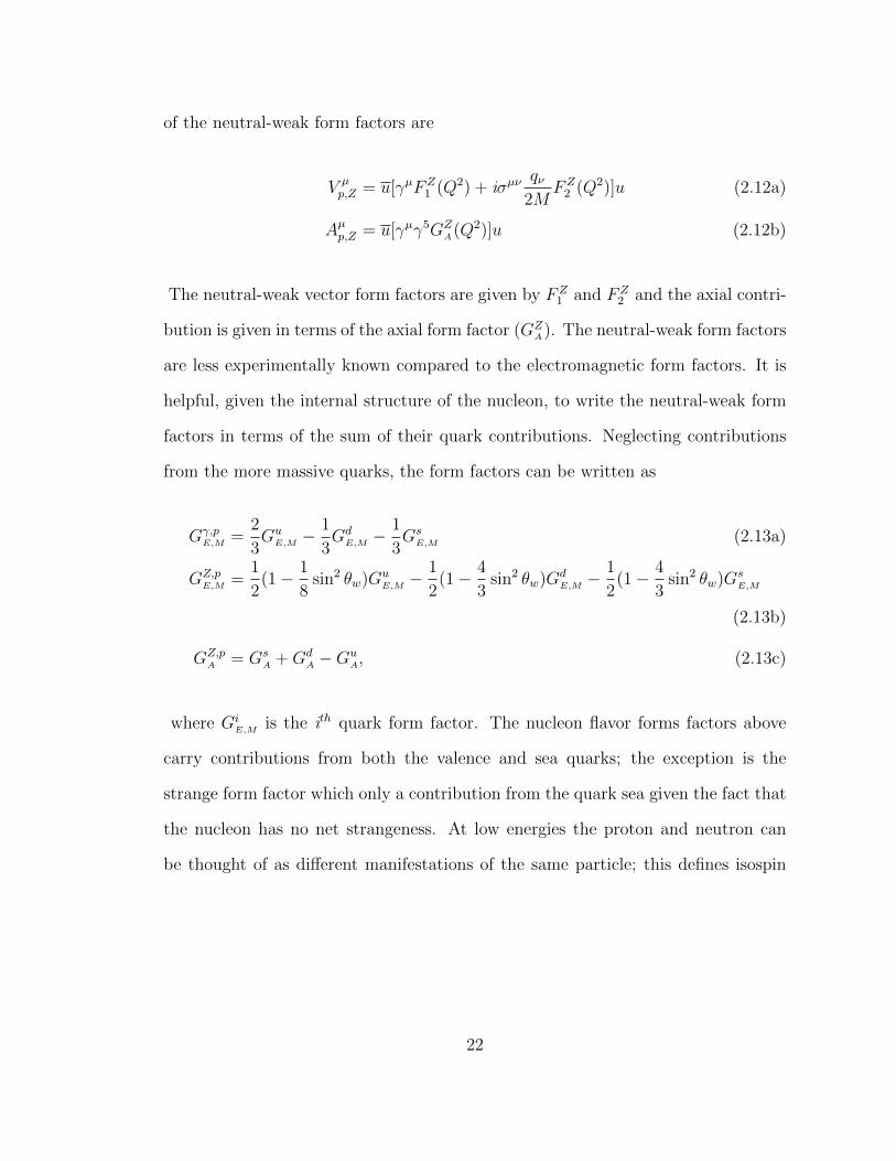
The neutral-weak vector form factors are given by FZ1 and FZ

2 and the axial contri-

bution is given in terms of the axial form factor (GZA). The neutral-weak form factors

are less experimentally known compared to the electromagnetic form factors. It is

helpful, given the internal structure of the nucleon, to write the neutral-weak form

factors in terms of the sum of their quark contributions. Neglecting contributions

from the more massive quarks, the form factors can be written as

Gγ,pE,M =

2

3Gu

E,M −1

3Gd

E,M −1

3Gs

E,M (2.13a)

GZ,pE,M =

1

2(1− 1

8sin2 θw)Gu

E,M −1

2(1− 4

3sin2 θw)Gd

E,M −1

2(1− 4

3sin2 θw)Gs

E,M

(2.13b)

GZ,pA = Gs

A +GdA −Gu

A, (2.13c)

where GiE,M is the ith quark form factor. The nucleon flavor forms factors above

carry contributions from both the valence and sea quarks; the exception is the

strange form factor which only a contribution from the quark sea given the fact that

the nucleon has no net strangeness. At low energies the proton and neutron can

be thought of as different manifestations of the same particle; this defines isospin

22

symmetry. Using isospin symmetry,

Gu,pE,M = Gd,n

E,M (2.14a)

Gu,nE,M = Gd,p

E,M (2.14b)

to rewrite 2.13, we can define the neutral-weak form factor in terms of the electro-

magnetic form factors of the proton and neutron as

GZ,pE,M = (1− 4 sin2 θw)Gγ,p

E,M −Gγ,nE,M . (2.15)

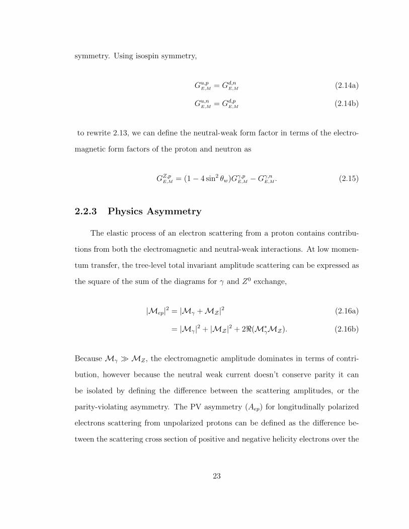
2.2.3 Physics Asymmetry

The elastic process of an electron scattering from a proton contains contribu-

tions from both the electromagnetic and neutral-weak interactions. At low momen-

tum transfer, the tree-level total invariant amplitude scattering can be expressed as

the square of the sum of the diagrams for γ and Z0 exchange,

|Mep|2 = |Mγ +MZ |2 (2.16a)

= |Mγ|2 + |MZ |2 + 2<(M∗γMZ). (2.16b)

Because Mγ MZ , the electromagnetic amplitude dominates in terms of contri-

bution, however because the neutral weak current doesn’t conserve parity it can

be isolated by defining the difference between the scattering amplitudes, or the

parity-violating asymmetry. The PV asymmetry (Aep) for longitudinally polarized

electrons scattering from unpolarized protons can be defined as the difference be-

tween the scattering cross section of positive and negative helicity electrons over the

23

total scattering cross section,

Aep =dσL − dσRdσL + dσR

. (2.17)

Aep ≈2Re(M∗

γMZ)

|Mγ|2(2.18)

The crucial piece of the asymmetry lies in the numerator. The asymmetry of M2γ

disappears due to parity conservation, leaving only the M2Z amplitude and the

interference term. Here the interference term dominates and the asymmetry is

approximated by

Aep ≈2ReM∗

γ(MZ,L −MZ,R)

|Mγ|2(2.19)

The fact that the weak interactions violate parity allows us to isolate the neutral

weak contribution which would otherwise be lost in the electromagnetic scattering

amplitude. At tree level this can be expressed in terms of the Sachs electromagnetic

form factors and grouped into three pieces as

A =GFQ

2

2√

2πα[AE + AM + AA] (2.20)

where the electromagnetic, magnetic, and axial asymmetries define groups of Sach’s

form factors,

AE =εGγ

EGZE

ε(GγE)2 + τ(Gγ

M)2(2.21a)

AM =τGγ

MGZM

ε(GγE)2 + τ(Gγ

M)2(2.21b)

AA =12

√τ(1− ε2)(1 + τ)Gγ

MGZA

ε(GγE)2 + τ(Gγ

M)2(2.21c)

24

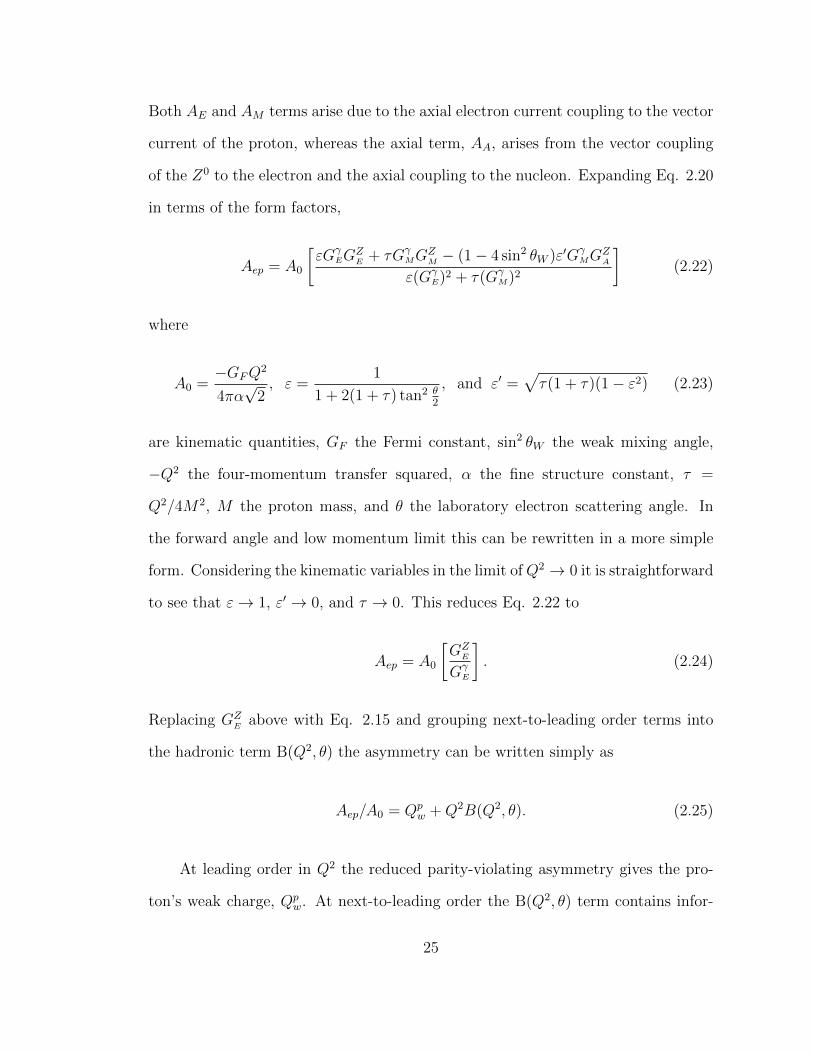
Both AE and AM terms arise due to the axial electron current coupling to the vector

current of the proton, whereas the axial term, AA, arises from the vector coupling

of the Z0 to the electron and the axial coupling to the nucleon. Expanding Eq. 2.20

in terms of the form factors,

Aep = A0

[εGγ

EGZE + τGγ

MGZM − (1− 4 sin2 θW )ε′Gγ

MGZA

ε(GγE)2 + τ(Gγ

M)2

](2.22)

where

A0 =−GFQ

2

4πα√

2, ε =

1

1 + 2(1 + τ) tan2 θ2

, and ε′ =√τ(1 + τ)(1− ε2) (2.23)

are kinematic quantities, GF the Fermi constant, sin2 θW the weak mixing angle,

−Q2 the four-momentum transfer squared, α the fine structure constant, τ =

Q2/4M2, M the proton mass, and θ the laboratory electron scattering angle. In

the forward angle and low momentum limit this can be rewritten in a more simple

form. Considering the kinematic variables in the limit ofQ2 → 0 it is straightforward

to see that ε→ 1, ε′ → 0, and τ → 0. This reduces Eq. 2.22 to

Aep = A0

[GZ

E

GγE

]. (2.24)

Replacing GZE above with Eq. 2.15 and grouping next-to-leading order terms into

the hadronic term B(Q2, θ) the asymmetry can be written simply as

Aep/A0 = Qpw +Q2B(Q2, θ). (2.25)

At leading order in Q2 the reduced parity-violating asymmetry gives the pro-

ton’s weak charge, Qpw. At next-to-leading order the B(Q2, θ) term contains infor-

25

mation about the electromagnetic, weak, and strange form factors and is relatively

suppressed at low Q2. In choosing the momentum transfer at which the experiment

was run this term was very important. Contributions from B(Q2, θ) can be reduced

by lowering the Q2, however this also reduces the magnitude of Aep, thus our ability

to determine the asymmetry precisely. Setting the momentum transfer to 0.0025

(GeV/c)2 allowed for a precise measurement of Qpwwhile constraining the contri-

bution from B(Q2, θ) to ∼ 30%. The determination of B(Q2, θ) was done using a

global fit of the existing PVES data up to 0.63 (GeV/c)2. This fit as well as details

of the extraction of Qpw is discussed in Section 6.1.

2.2.4 Precision Determination of sin2 θw

FIG. 2.2: The electromagnetic interaction at O(α)(left) and O(α2)(right). Thevacuum polarization screens the bare charge of the electromagnetic interaction atthe vertex.

Thus far in this discussion, the primary focus has been on the leading order con-

tribution to the physics asymmetry, however as either Q2 increases or the precision of

our measurement increases it is important to consider effects of higher-order contri-

butions. Before discussing the implications of higher-order diagrams in the context

of the weak-charge it is first instructive to look at the electromagnetic charge. To

leading order the electromagnetic coupling is given by the fine-structure constant α.

Couplings, in general within the SM, are energy dependent and therefore as Q2 in-

26

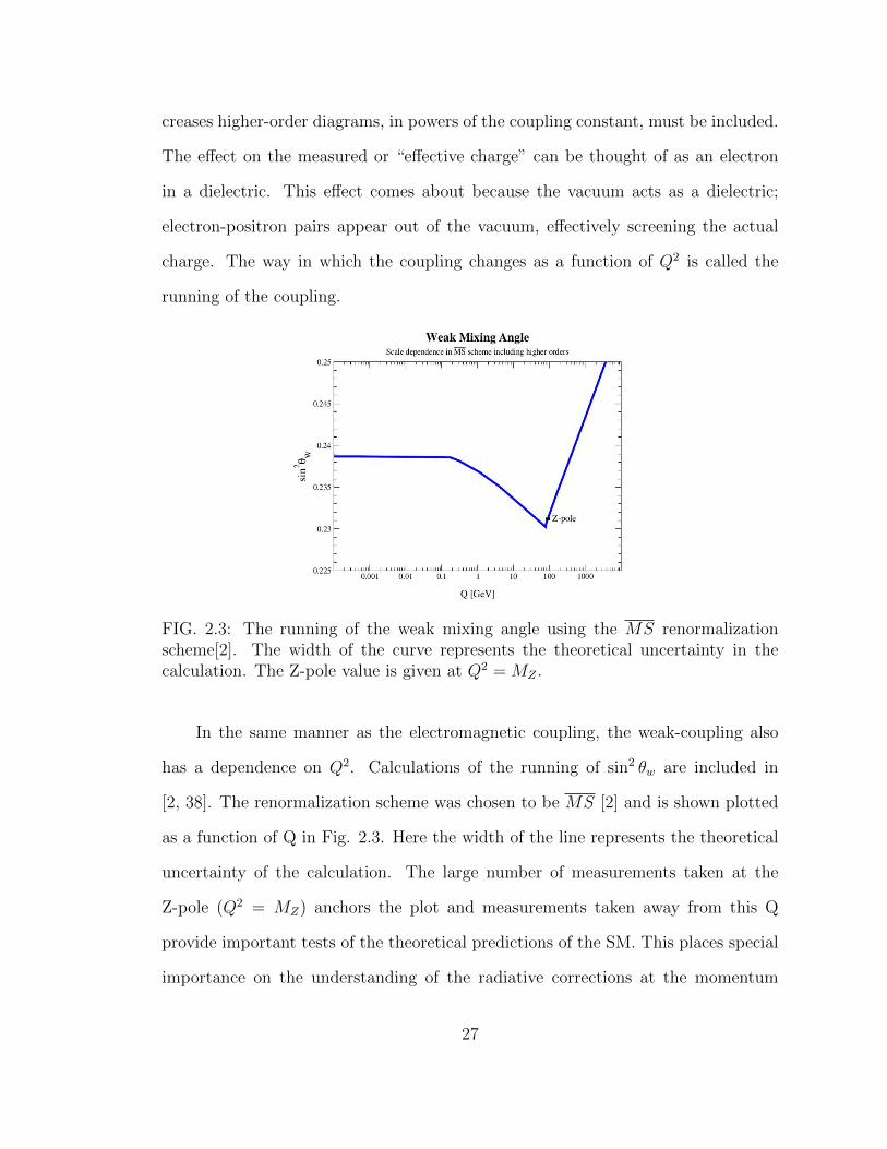
creases higher-order diagrams, in powers of the coupling constant, must be included.

The effect on the measured or “effective charge” can be thought of as an electron

in a dielectric. This effect comes about because the vacuum acts as a dielectric;

electron-positron pairs appear out of the vacuum, effectively screening the actual

charge. The way in which the coupling changes as a function of Q2 is called the

running of the coupling.

FIG. 2.3: The running of the weak mixing angle using the MS renormalizationscheme[2]. The width of the curve represents the theoretical uncertainty in thecalculation. The Z-pole value is given at Q2 = MZ .

In the same manner as the electromagnetic coupling, the weak-coupling also

has a dependence on Q2. Calculations of the running of sin2 θw are included in

[2, 38]. The renormalization scheme was chosen to be MS [2] and is shown plotted

as a function of Q in Fig. 2.3. Here the width of the line represents the theoretical

uncertainty of the calculation. The large number of measurements taken at the

Z-pole (Q2 = MZ) anchors the plot and measurements taken away from this Q

provide important tests of the theoretical predictions of the SM. This places special

importance on the understanding of the radiative corrections at the momentum

27

transfer of Qweak. The SM predicts a shift in sin2 θw from the Z-pole value at low

momentum transfer of ∼ 0.007. It is important to note that these corrections are

renormalization scheme dependent. The weak-charge including radiative corrections

can be written as [39]

Qpw = [ρNC + ∆e][1− 4 sin2 θw(0) + ∆e′ ] +WW +ZZ +γZ (2.26)

where ρNC accounts for one-loop corrections to the gauge boson propagators, which

at tree level is defined to be ρNC ≡M2W/M

2Z cos2 θw. The one-loop corrections come

from the top and bottom quark loops to the gauge boson propagators; there are

contributions from other quark generations but they are negligible. The terms ∆e

and ∆e′ are the photon loop correction to the Z boson exchange vertex and the Z

loop correction to the photon exchange vertex respectively. Diagrams for both ρNC

and ∆e,e′ are shown in 2.4. The final three terms in 2.26 represent box diagrams

FIG. 2.4: The one loop contribution to Qpw from the gauge boson mass renormal-

ization is shown on the left. The γ, Z loop correction to the Z, γ exchange vertex isshown on the right.

describing the exchange of two gauge bosons. The box diagrams for ZZ and WW

are relatively straight-forward to calculate using pQCD due to the propagators of

the W and Z within the box being dominated by high momenta. The γZ diagram

is much more problematic because the photon is dominated by low momentum

exchange which is outside of the useful regime of pQCD. Calculation of the γZ

diagram is discussed in more detail in 2.2.5. The box diagrams can be seen in Fig.

28

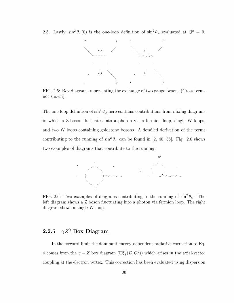
2.5. Lastly, sin2 θw(0) is the one-loop definition of sin2 θw evaluated at Q2 = 0.

FIG. 2.5: Box diagrams representing the exchange of two gauge bosons (Cross termsnot shown).

The one-loop definition of sin2 θw here contains contributions from mixing diagrams

in which a Z-boson fluctuates into a photon via a fermion loop, single W loops,

and two W loops containing goldstone bosons. A detailed derivation of the terms

contributing to the running of sin2 θw can be found in [2, 40, 38]. Fig. 2.6 shows

two examples of diagrams that contribute to the running.

FIG. 2.6: Two examples of diagrams contributing to the running of sin2 θw. Theleft diagram shows a Z boson fluctuating into a photon via fermion loop. The rightdiagram shows a single W loop.

2.2.5 γZ0 Box Diagram

In the forward-limit the dominant energy-dependent radiative correction to Eq.

4 comes from the γ − Z box diagram (VγZ(E,Q2)) which arises in the axial-vector

coupling at the electron vertex. This correction has been evaluated using dispersion

29

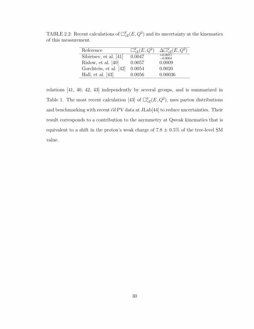
TABLE 2.2: Recent calculations of VγZ(E,Q2) and its uncertainty at the kinematicsof this measurement.

Reference VγZ(E,Q2) ∆VγZ(E,Q2)

Sibirtsev, et al. [41] 0.0047 +0.0011−0.0004

Rislow, et al. [40] 0.0057 0.0009Gorchtein, et al. [42] 0.0054 0.0020Hall, et al. [43] 0.0056 0.00036

relations [41, 40, 42, 43] independently by several groups, and is summarized in

Table 1. The most recent calculation [43] of VγZ(E,Q2), uses parton distributions

and benchmarking with recent ~ed PV data at JLab[44] to reduce uncertainties. Their

result corresponds to a contribution to the asymmetry at Qweak kinematics that is

equivalent to a shift in the proton’s weak charge of 7.8 ± 0.5% of the tree-level SM

value.

30

CHAPTER 3

Experimental Setup

3.1 Experimental Setup

The experimental requirements associated with the Qweak experiment brought

about a unique set of technical challenges, due primarily to the proposed 2.1% sta-

tistical and 1.4% systematic uncertainty on the measurement of the part-per-billion

level asymmetry. In an effort to meet these goals, the experiment built on technical

advances made at Jefferson Lab, as well as expertise gained from previous precision

PVES experiments [45, 46]. The design parameters (shown in Table 3.1) were chosen

to optimize counting statistics and reduce systematics as much as possible. The pri-

mary limiting factor for the experiment was counting statistics, for this reason high

current, highly polarized beam, and a high power target were required, as well as

almost 2 years of non-continuous running. The major subsystems in the experiment

include: a 2.5 kW cryotarget, lead collimation system, large acceptance Cerenkov

detector array, toroidal spectrometer, rapid reversal polarized source, and tracking

system used to measure the experimental Q2. The experiment was run in two com-

31

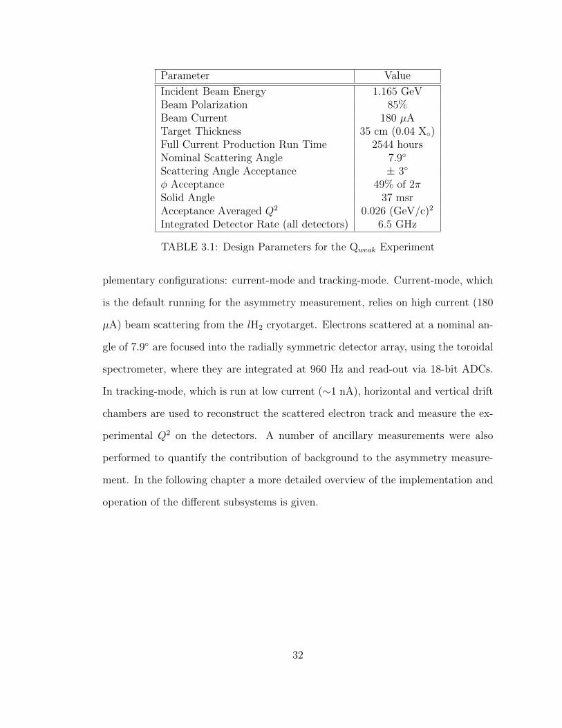
Parameter Value

Incident Beam Energy 1.165 GeVBeam Polarization 85%Beam Current 180 µATarget Thickness 35 cm (0.04 X)Full Current Production Run Time 2544 hoursNominal Scattering Angle 7.9

Scattering Angle Acceptance ± 3

φ Acceptance 49% of 2πSolid Angle 37 msrAcceptance Averaged Q2 0.026 (GeV/c)2

Integrated Detector Rate (all detectors) 6.5 GHz

TABLE 3.1: Design Parameters for the Qweak Experiment

plementary configurations: current-mode and tracking-mode. Current-mode, which

is the default running for the asymmetry measurement, relies on high current (180

µA) beam scattering from the lH2 cryotarget. Electrons scattered at a nominal an-

gle of 7.9 are focused into the radially symmetric detector array, using the toroidal

spectrometer, where they are integrated at 960 Hz and read-out via 18-bit ADCs.

In tracking-mode, which is run at low current (∼1 nA), horizontal and vertical drift

chambers are used to reconstruct the scattered electron track and measure the ex-

perimental Q2 on the detectors. A number of ancillary measurements were also

performed to quantify the contribution of background to the asymmetry measure-

ment. In the following chapter a more detailed overview of the implementation and

operation of the different subsystems is given.

32

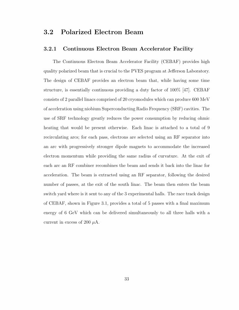
3.2 Polarized Electron Beam

3.2.1 Continuous Electron Beam Accelerator Facility

The Continuous Electron Beam Accelerator Facility (CEBAF) provides high

quality polarized beam that is crucial to the PVES program at Jefferson Laboratory.

The design of CEBAF provides an electron beam that, while having some time

structure, is essentially continuous providing a duty factor of 100% [47]. CEBAF

consists of 2 parallel linacs comprised of 20 cryomodules which can produce 600 MeV

of acceleration using niobium Superconducting Radio Frequency (SRF) cavities. The

use of SRF technology greatly reduces the power consumption by reducing ohmic

heating that would be present otherwise. Each linac is attached to a total of 9

recirculating arcs; for each pass, electrons are selected using an RF separator into

an arc with progressively stronger dipole magnets to accommodate the increased

electron momentum while providing the same radius of curvature. At the exit of

each arc an RF combiner recombines the beam and sends it back into the linac for

acceleration. The beam is extracted using an RF separator, following the desired

number of passes, at the exit of the south linac. The beam then enters the beam

switch yard where is it sent to any of the 3 experimental halls. The race track design

of CEBAF, shown in Figure 3.1, provides a total of 5 passes with a final maximum

energy of 6 GeV which can be delivered simultaneously to all three halls with a

current in excess of 200 µA.

33

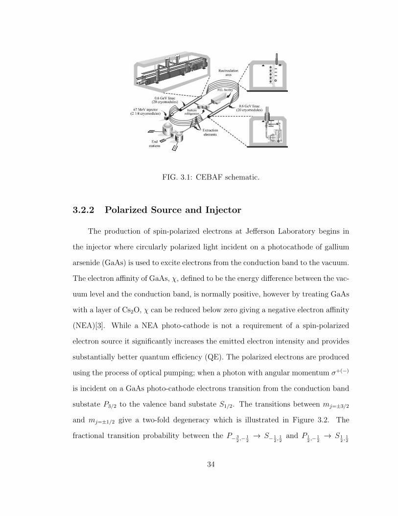
FIG. 3.1: CEBAF schematic.

3.2.2 Polarized Source and Injector

The production of spin-polarized electrons at Jefferson Laboratory begins in

the injector where circularly polarized light incident on a photocathode of gallium

arsenide (GaAs) is used to excite electrons from the conduction band to the vacuum.

The electron affinity of GaAs, χ, defined to be the energy difference between the vac-

uum level and the conduction band, is normally positive, however by treating GaAs

with a layer of Cs2O, χ can be reduced below zero giving a negative electron affinity

(NEA)[3]. While a NEA photo-cathode is not a requirement of a spin-polarized

electron source it significantly increases the emitted electron intensity and provides

substantially better quantum efficiency (QE). The polarized electrons are produced

using the process of optical pumping; when a photon with angular momentum σ+(−)

is incident on a GaAs photo-cathode electrons transition from the conduction band

substate P3/2 to the valence band substate S1/2. The transitions between mj=±3/2

and mj=±1/2 give a two-fold degeneracy which is illustrated in Figure 3.2. The

fractional transition probability between the P− 32,− 1

2→ S− 1

2, 12

and P 12,− 1

2→ S 1

2, 12

34

shows photo-electrons are 3 times more likely to undergo the first transition than

the second which limits the maximum theoretical polarization possible to 50%.

FIG. 3.2: The allowed optical transitions of ∆mj = ±1 in a GaAs photocathode areshown. The numbers in the circles represent the relative transition probabilities[3].

In order to raise the achievable polarization even further to accommodate ultra-

precise parity experiments, it is desirable to break the degeneracy of the P substate

allowing a theoretical maximum polarization of 100%. By growing the GaAs photo-

cathode on a single layer of GaAsP it is possible to apply a mechanical strain to

the photo-cathode breaking the degeneracy and pushing the polarization to ' 75%.

Going even further, and alternating thin layers of GaAs/GaAsP, a super-lattice

can be formed which can generate beam with a polarization of up to 90% and a

significantly improved QE [48]. With this, the injector at Jefferson Laboratory

routinely provides 85% polarized electron beam with a QE of near 1%.

The circularly polarized light used to produce the electron beam in the injector

is a product of the device chain shown in Figure 3.3. Three diode lasers are pulsed

at 499 MHz each, 120 out of phase, with a combined bunch frequency of 1497

MHz. The resulting light is linearized using a linear polarizer, then passed through

a Pockels cell which has a birefringence proportional to the electric field applied to

the crystal medium. This birefringence rotates the polarization vector component

35

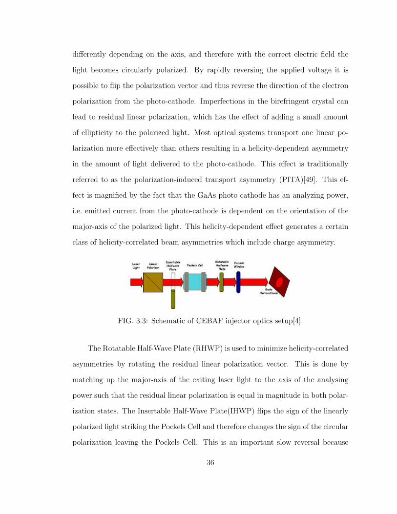
differently depending on the axis, and therefore with the correct electric field the

light becomes circularly polarized. By rapidly reversing the applied voltage it is

possible to flip the polarization vector and thus reverse the direction of the electron

polarization from the photo-cathode. Imperfections in the birefringent crystal can

lead to residual linear polarization, which has the effect of adding a small amount

of ellipticity to the polarized light. Most optical systems transport one linear po-

larization more effectively than others resulting in a helicity-dependent asymmetry

in the amount of light delivered to the photo-cathode. This effect is traditionally

referred to as the polarization-induced transport asymmetry (PITA)[49]. This ef-

fect is magnified by the fact that the GaAs photo-cathode has an analyzing power,

i.e. emitted current from the photo-cathode is dependent on the orientation of the

major-axis of the polarized light. This helicity-dependent effect generates a certain

class of helicity-correlated beam asymmetries which include charge asymmetry.

FIG. 3.3: Schematic of CEBAF injector optics setup[4].

The Rotatable Half-Wave Plate (RHWP) is used to minimize helicity-correlated

asymmetries by rotating the residual linear polarization vector. This is done by

matching up the major-axis of the exiting laser light to the axis of the analysing

power such that the residual linear polarization is equal in magnitude in both polar-

ization states. The Insertable Half-Wave Plate(IHWP) flips the sign of the linearly

polarized light striking the Pockels Cell and therefore changes the sign of the circular

polarization leaving the Pockels Cell. This is an important slow reversal because

36

it cancels any systematics such as beam steering and electronic cross-talk which do

not change sign with the IHWP[4].

Polarized electrons extracted from the photo-cathode are accelerated into the

injector via the 100 kV DC gun, which is enclosed in an Ultra High Vacuum (10−11-

10−12 Torr). This reduces the effects of back-scattered ions in the enclosure colliding

with the photo-cathode which would degrade the QE. With this, the photo-cathode

can provide an integrated charge of approximately 500 C before there is a need to

restore the photo-cathode yield. Electrons accelerated into the injector are longi-

tudinally polarized parallel(antiparallel) to the beam momentum, however during

transport through the linacs and arcs the electrons exhibit an in-plane precession

which may result in a net transverse polarization at the experimental hall. This

effect can be removed using a Wien Filter which rotates the electron spin in the

injector such that it cancels the net spin procession in the accelerator[50, 51]. A

Wien Filter consists of an electric and magnetic field perpendicular to one another

and perpendicular to the beam momentum. Originally used as a velocity selector,

charged particles with a velocity satisfying β = |E/B| are passed without deflection

but with their spin vector rotated. Building on this, the Two Wien Filter Spin

Flipper at CEBAF shown in Figure 3.4 uses a Vertical Wien Filter to rotate the

spin 90 to the vertical, a pair of solenoids to rotate transversely into the horizontal

plane, and a Horizontal Wien Filter to completely reverse the initial electron spin.

This forms the basis for an entirely new method of slow reversal which allows the

electron spin to be flipped independently of the laser.

37

FIG. 3.4: The Wien filter causes a spin precession of the electron spin. The doubleWien filter uses a pair of Wiens, Vertical and Horizontal, to orient the electron spinso as to cancel out transverse polarization due to spin procession in the linac andarcs. This allows 100% longitudinal polarization to be delivered to the experimentalhalls[5].

3.2.3 Beam Position Monitors

Beam transport information in the injector and the Hall C line is provided by

beam position monitors (BPM), which play an important role in providing quality

electron beam at Jefferson laboratory. BPM’s are cylindrical cavities containing 4

symmetrical stripline wires rotated to 45 in the right-handed Hall C coordinate

system, which couple resonantly (1497MHz) to the RF-signal of the passing beam,

providing signal amplitudes proportional to the proximity of the beam to the signal

wires. The rotation of the signal wires is needed to alleviate the effects of synchrotron

radiation in the horizontal plane. The BPM readout electronics can be adjusted to

handle a range of currents(1µA−200µA) by adjusting the gain settings on the pick-

up wires. Each of these signals is transmitted to the BPM readout electronics where

it is amplified and down-converted to 1 MHz before being digitized and read out via

custom Qweak ADC’s at 960Hz in integrating mode. Figure 3.5 shows a cross-section

of a BPM cavity and stripline wires.

38

FIG. 3.5: Schematic of cylindrical BPM as seen along the beam pipe[6]. Signal wiresare shown rotated in the counter-clockwise direction to 45. Hall coordinates aregiven by XH and YH .

The relative beam position in the unrotated basis can be written in terms of the

raw signals in the form of the asymmetry between wires along a given rotated axis.

In order to properly calculate the absolute beam position two important factors

need to be addressed[52].

• The amplitude gains may be different between channels.

• The pedestals in each channel are not zero and must be accounted for.

In the unrotated basis the absolute beam position in X′ can be written in the form:

X ′ = κ(XP −XPoffset)− αX(XM −XMoffset)

(XM −XMoffset) + αX(XP −XP−offset)(3.1)

Here α is the ratio of the gains between two channels along a given axis, and κ is the

sensitivity of the BPM to the 1497 MHz RF-signal, which converts the readout signal

to mm. The Y′ position can be calculated in a similar manner. The pedestals are

defined as the BPM readout at zero current however, due to the non-linear behaviour

of the BPM’s at low current, they must be measured in a region of linear operation

and calculated using extrapolation. BPM calibrations are done at high current

(nominally 180 µA) in fixed gain mode by varying the beam current ±10−15%

39

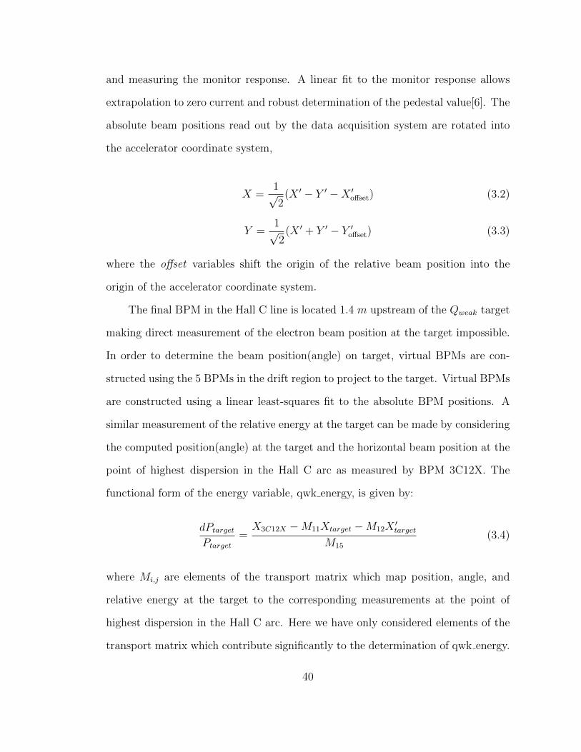
and measuring the monitor response. A linear fit to the monitor response allows

extrapolation to zero current and robust determination of the pedestal value[6]. The

absolute beam positions read out by the data acquisition system are rotated into

the accelerator coordinate system,

X =1√2

(X ′ − Y ′ −X ′offset) (3.2)

Y =1√2

(X ′ + Y ′ − Y ′offset) (3.3)

where the offset variables shift the origin of the relative beam position into the

origin of the accelerator coordinate system.

The final BPM in the Hall C line is located 1.4 m upstream of the Qweak target

making direct measurement of the electron beam position at the target impossible.

In order to determine the beam position(angle) on target, virtual BPMs are con-

structed using the 5 BPMs in the drift region to project to the target. Virtual BPMs

are constructed using a linear least-squares fit to the absolute BPM positions. A

similar measurement of the relative energy at the target can be made by considering

the computed position(angle) at the target and the horizontal beam position at the

point of highest dispersion in the Hall C arc as measured by BPM 3C12X. The

functional form of the energy variable, qwk energy, is given by:

dPtargetPtarget

=X3C12X −M11Xtarget −M12X

′target

M15

(3.4)

where Mi,j are elements of the transport matrix which map position, angle, and

relative energy at the target to the corresponding measurements at the point of

highest dispersion in the Hall C arc. Here we have only considered elements of the

transport matrix which contribute significantly to the determination of qwk energy.

40

A list of the BPM’s used in the construction of the virtual BPM’s can be found in

Table 3.1.

Run Period BPMs used in Virtual BPM

Beginning of running to run 14486 3H07a, 3H07b, 3H07c, 3H09, 3H09b

Run 14486 to end of running 3H07a, 3H07b, 3H07c, 3H09

TABLE 3.2: Hall C BPMs used to construct virtual target BPMs. BPM 3H09b wasremoved due to functionality issues in the second half of running.

3.2.4 Beam Current Monitors

The electron beam current in CEBAF is monitored using beam current monitors

(BCM) in the injector and the end of the accelerator. Measuring the beam current

in two locations helps to monitor and limit beam loss through the machine, and

provide the most accurate measurement of the beam incident on the target. Current

measurements made on the accelerator side were done using a pair of BCM cavities in

conjunction with an Unser monitor. The BCM’s are cylindrical RF cavities resonant

at the fundamental frequency of the beam (1497 MHz). As the beam passes through

the BCM it excites the transverse electric mode, TE010 via a large loop antenna

coaxial with the cavity resulting in a DC voltage level linearly proportional to the

beam current. The BCMs are temperature controlled to reduce the effects of heating

due to power dissipation in the cavity. The high-frequency output signal is down-

converted from 1497 MHz to 1 MHz. The BCM signals are then read out into

the DAQ using Qweak ADCs. Table 3.2 shows the 6 BCM cavities active during

different run periods over the full experiment. For purposes of noise reduction,

a charge variable (qwk charge) was formed using the average of the most robust

current monitors during each run period.

41

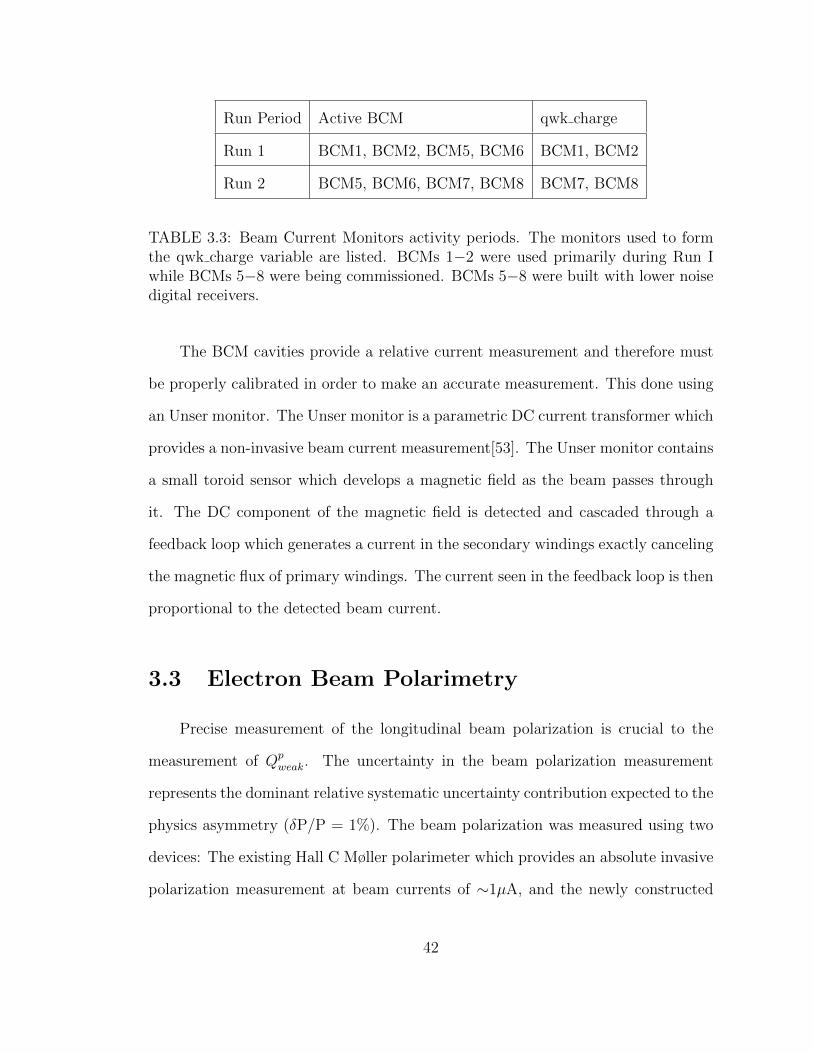
Run Period Active BCM qwk charge

Run 1 BCM1, BCM2, BCM5, BCM6 BCM1, BCM2

Run 2 BCM5, BCM6, BCM7, BCM8 BCM7, BCM8

TABLE 3.3: Beam Current Monitors activity periods. The monitors used to formthe qwk charge variable are listed. BCMs 1−2 were used primarily during Run Iwhile BCMs 5−8 were being commissioned. BCMs 5−8 were built with lower noisedigital receivers.

The BCM cavities provide a relative current measurement and therefore must

be properly calibrated in order to make an accurate measurement. This done using

an Unser monitor. The Unser monitor is a parametric DC current transformer which

provides a non-invasive beam current measurement[53]. The Unser monitor contains

a small toroid sensor which develops a magnetic field as the beam passes through

it. The DC component of the magnetic field is detected and cascaded through a

feedback loop which generates a current in the secondary windings exactly canceling

the magnetic flux of primary windings. The current seen in the feedback loop is then

proportional to the detected beam current.

3.3 Electron Beam Polarimetry

Precise measurement of the longitudinal beam polarization is crucial to the

measurement of Qpweak. The uncertainty in the beam polarization measurement

represents the dominant relative systematic uncertainty contribution expected to the

physics asymmetry (δP/P = 1%). The beam polarization was measured using two

devices: The existing Hall C Møller polarimeter which provides an absolute invasive

polarization measurement at beam currents of ∼1µA, and the newly constructed

42

Hall C Compton polarimeter which provides a high current, non-invasive, continuous

measurement of the beam polarization.

3.3.1 Møller Polarimeter

The Møller polarimeter relies on cross-section asymmetry e−e− → e−e− scat-

tering for precise determination of the beam polarization. Møller scattering is a pure

Quantum Electrodynamic (QED) process so the cross-section can be calculated very

precisely. In the center-of-mass (CM) frame the scattering cross-section for Møller

scattering at lowest order can be written as [54]:

dσ

dΩ=dσodΩ

[1 + P||t P||b A(θ)] (3.5)

where dσo/dΩ is the unpolarized cross-section, P||t is the target polarization, P

||b

is the beam polarization, and A(θ) is the analyzing power. Considering the cross-

section asymmetry,

dσ↑↑o /dΩ− dσ↑↓o /dΩ

dσ↑↑o /dΩ + dσ↑↓o /dΩ= A(θ)P

||t P||b , (3.6)

the beam polarization can be obtained with knowledge of the analyzing power and

polarization of the target. The analyzing power is determined using simulation and

is maximized by detecting scattered and recoiled Møller electrons at 90. The Hall C

Møller polarimeter, shown in Figure 3.6, scatters longitudinally-polarized electrons

from a 1 µm thick iron foil target. The iron foil target is polarized to saturation

along the beam axis using a 3.5 T superconducting solenoid field. At saturation,

the electron polarization is known precisely[55]. Scattered electrons are horizontally

focused using quadrupole magnet Q1 and the desired scattering angles are selected

using the collimator system, after which they are again horizontally defocused using

43

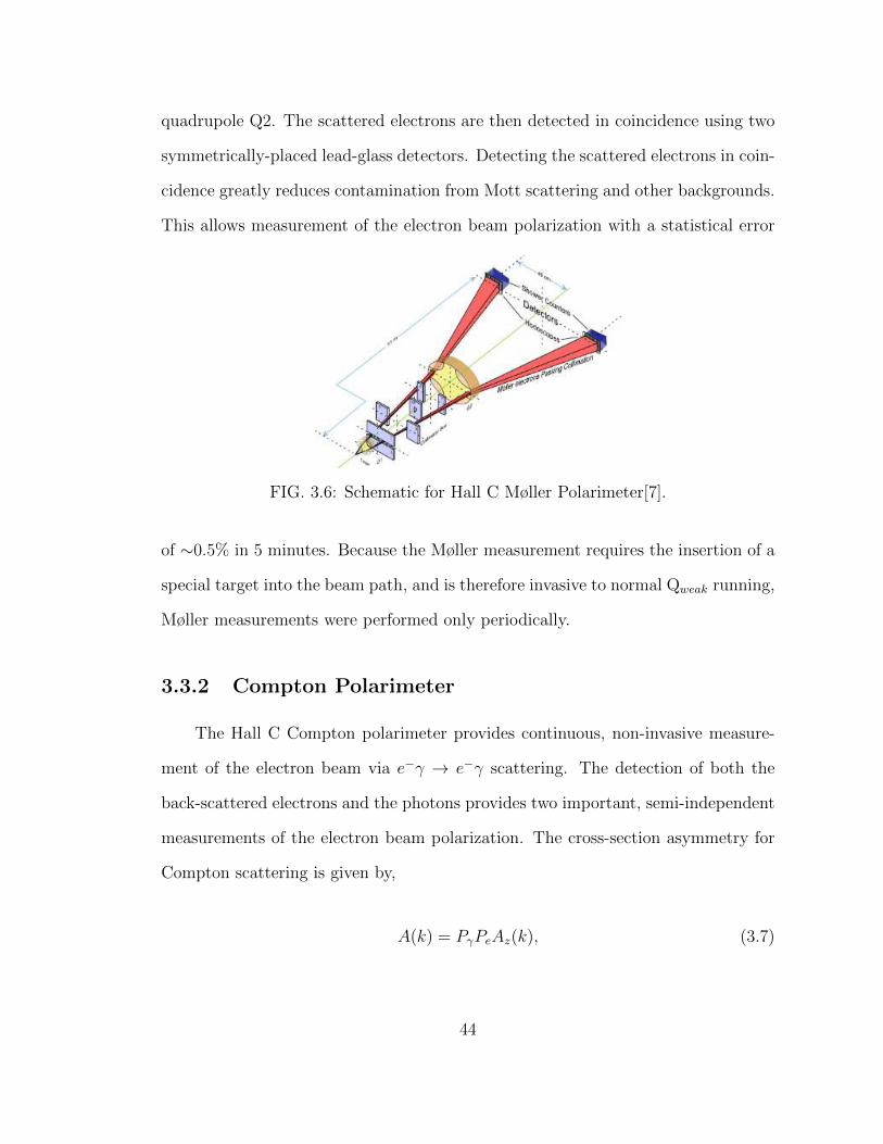
quadrupole Q2. The scattered electrons are then detected in coincidence using two

symmetrically-placed lead-glass detectors. Detecting the scattered electrons in coin-

cidence greatly reduces contamination from Mott scattering and other backgrounds.

This allows measurement of the electron beam polarization with a statistical error

FIG. 3.6: Schematic for Hall C Møller Polarimeter[7].

of ∼0.5% in 5 minutes. Because the Møller measurement requires the insertion of a

special target into the beam path, and is therefore invasive to normal Qweak running,

Møller measurements were performed only periodically.

3.3.2 Compton Polarimeter

The Hall C Compton polarimeter provides continuous, non-invasive measure-

ment of the electron beam via e−γ → e−γ scattering. The detection of both the

back-scattered electrons and the photons provides two important, semi-independent

measurements of the electron beam polarization. The cross-section asymmetry for

Compton scattering is given by,

A(k) = PγPeAz(k), (3.7)

44

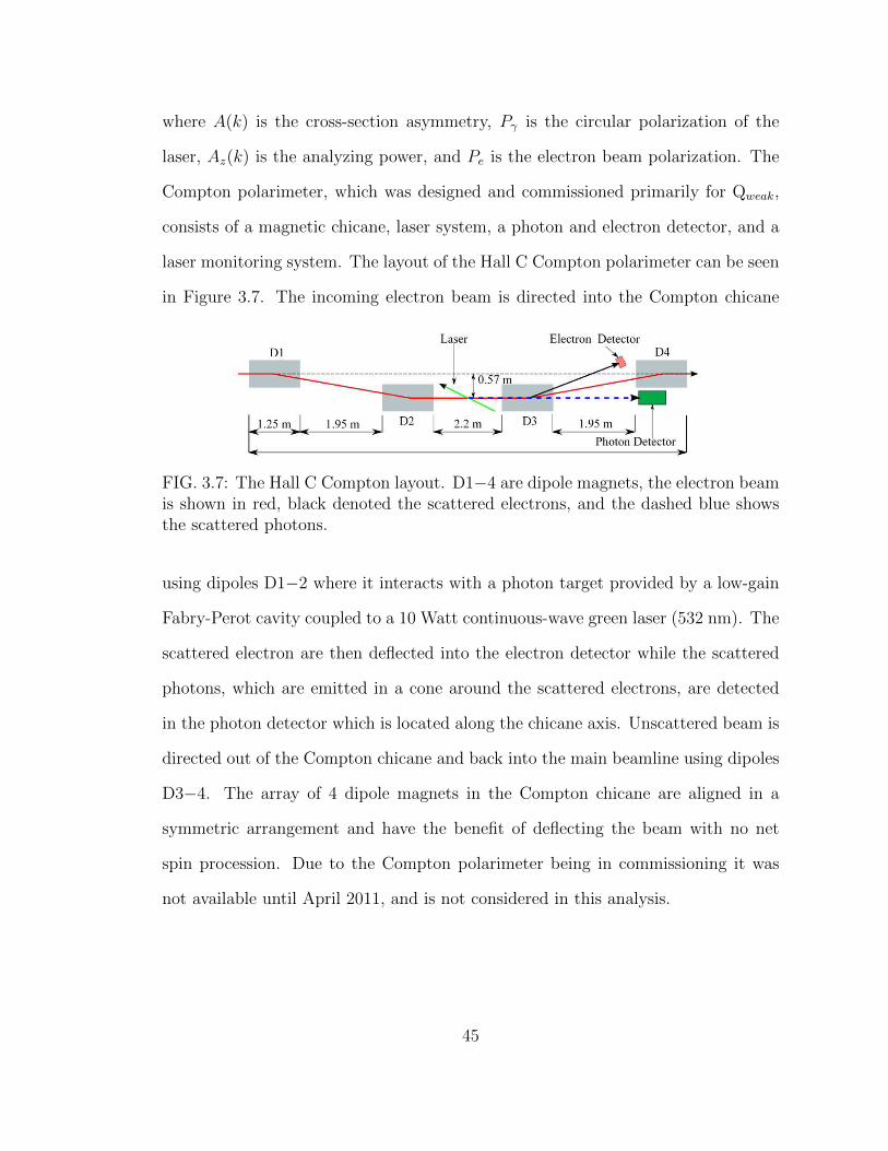
where A(k) is the cross-section asymmetry, Pγ is the circular polarization of the

laser, Az(k) is the analyzing power, and Pe is the electron beam polarization. The

Compton polarimeter, which was designed and commissioned primarily for Qweak,

consists of a magnetic chicane, laser system, a photon and electron detector, and a

laser monitoring system. The layout of the Hall C Compton polarimeter can be seen

in Figure 3.7. The incoming electron beam is directed into the Compton chicane

FIG. 3.7: The Hall C Compton layout. D1−4 are dipole magnets, the electron beamis shown in red, black denoted the scattered electrons, and the dashed blue showsthe scattered photons.

using dipoles D1−2 where it interacts with a photon target provided by a low-gain

Fabry-Perot cavity coupled to a 10 Watt continuous-wave green laser (532 nm). The

scattered electron are then deflected into the electron detector while the scattered

photons, which are emitted in a cone around the scattered electrons, are detected

in the photon detector which is located along the chicane axis. Unscattered beam is

directed out of the Compton chicane and back into the main beamline using dipoles

D3−4. The array of 4 dipole magnets in the Compton chicane are aligned in a

symmetric arrangement and have the benefit of deflecting the beam with no net

spin procession. Due to the Compton polarimeter being in commissioning it was

not available until April 2011, and is not considered in this analysis.

45

3.4 Primary lH2 Target

The primary scattering target for Qweak was a 34.4 cm long conical liquid hy-

drogen cell designed to sustain 180 µA of beam current, while keeping noise due

to target boiling <5% of the width if the physics asymmetry distribution. This

corresponds to a target noise contribution of <50 ppm based on the 5.3 GHz per

detector scattering rate in the experiment. Target heating, due to the incident elec-

tron beam, causes density fluctuations in the target, which can induce noise into

the measured main detector asymmetry. In order to reduce systematic effects due

to target heating, which can be a significant source of noise, the electron beam was

rastered in a 3.5 x 3.5 mm2 uniform distribution. The target length was chosen

to yield more scattering events, while the conical shape accommodates the optimal

scattering angle of 7.9. The lH2 target was operated at a pressure of 35 psi and a

temperature of 20.00 ± 0.02 K. The liquid volume of the target was approximately

55 liters when fully condensed. The target cell in which the incoming electron beam

interacts can be seen in Figure 3.8a and includes an entrance and exit window com-

posed of Al 7075-T6 which was chosen for its especially high tensile strength. The

target windows, which generate a significant amount of background, were made as

thin as possible. The entrance window has a uniform thickness of 0.096 mm, while

the exit window consists of two regions: an outer diameter which has a thickness

0.635 mm and an inner region of diameter 15 mm and a thickness of 0.125 mm. The

unscattered beam passes through the inner region, which is thinner to reduce back-

grounds. Elastically scattered electrons pass through the experimental acceptance

(6 < θ < 12) and exit the target through the thicker outer diameter of the target

window. The focus of scattered electrons, passing through the outer region of the

exit window, is affected due to radiative losses. Characterization and measurement

46

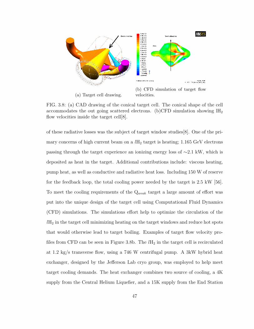
(a) Target cell drawing.(b) CFD simulation of target flowvelocities.

FIG. 3.8: (a) CAD drawing of the conical target cell. The conical shape of the cellaccommodates the out going scattered electrons. (b)CFD simulation showing lH2

flow velocities inside the target cell[8].

of these radiative losses was the subject of target window studies[8]. One of the pri-

mary concerns of high current beam on a lH2 target is heating; 1.165 GeV electrons

passing through the target experience an ionizing energy loss of ∼2.1 kW, which is

deposited as heat in the target. Additional contributions include: viscous heating,

pump heat, as well as conductive and radiative heat loss. Including 150 W of reserve

for the feedback loop, the total cooling power needed by the target is 2.5 kW [56].

To meet the cooling requirements of the Qweak target a large amount of effort was

put into the unique design of the target cell using Computational Fluid Dynamics

(CFD) simulations. The simulations effort help to optimize the circulation of the

lH2 in the target cell minimizing heating on the target windows and reduce hot spots

that would otherwise lead to target boiling. Examples of target flow velocity pro-

files from CFD can be seen in Figure 3.8b. The lH2 in the target cell is recirculated

at 1.2 kg/s transverse flow, using a 746 W centrifugal pump. A 3kW hybrid heat

exchanger, designed by the Jefferson Lab cryo group, was employed to help meet

target cooling demands. The heat exchanger combines two source of cooling, a 4K

supply from the Central Helium Liquefier, and a 15K supply from the End Station

47

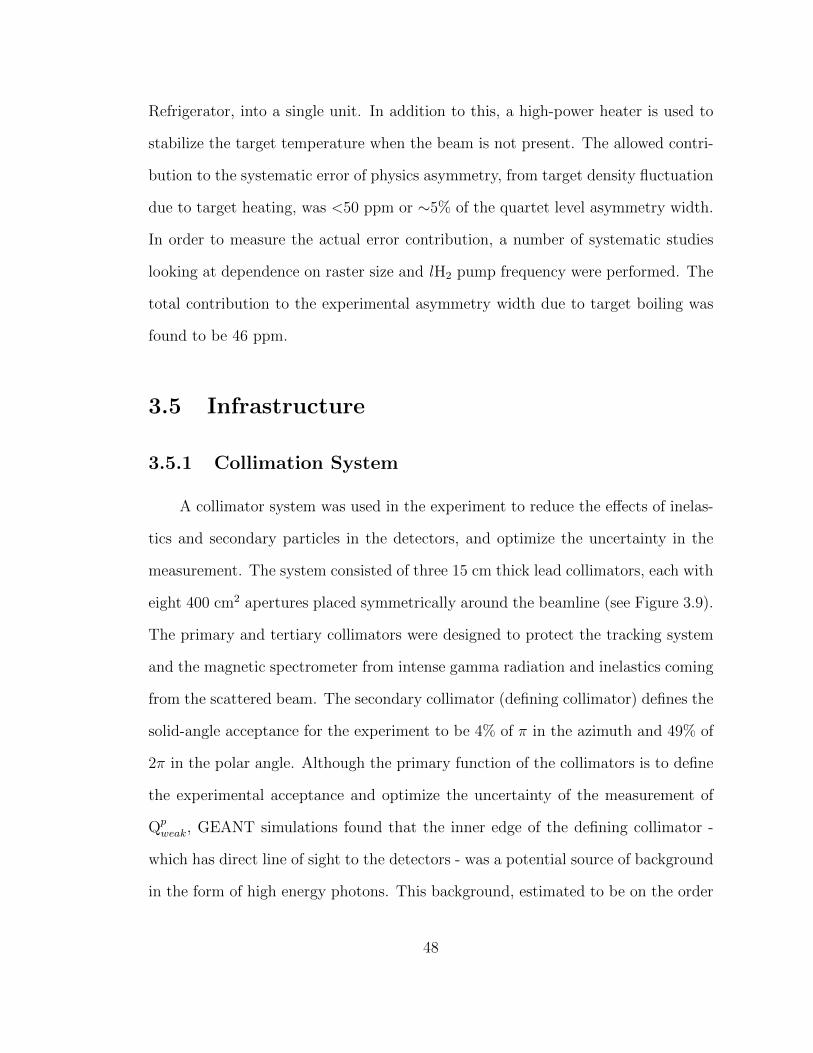
Refrigerator, into a single unit. In addition to this, a high-power heater is used to

stabilize the target temperature when the beam is not present. The allowed contri-

bution to the systematic error of physics asymmetry, from target density fluctuation

due to target heating, was <50 ppm or ∼5% of the quartet level asymmetry width.

In order to measure the actual error contribution, a number of systematic studies

looking at dependence on raster size and lH2 pump frequency were performed. The

total contribution to the experimental asymmetry width due to target boiling was

found to be 46 ppm.

3.5 Infrastructure

3.5.1 Collimation System

A collimator system was used in the experiment to reduce the effects of inelas-

tics and secondary particles in the detectors, and optimize the uncertainty in the

measurement. The system consisted of three 15 cm thick lead collimators, each with

eight 400 cm2 apertures placed symmetrically around the beamline (see Figure 3.9).

The primary and tertiary collimators were designed to protect the tracking system

and the magnetic spectrometer from intense gamma radiation and inelastics coming

from the scattered beam. The secondary collimator (defining collimator) defines the

solid-angle acceptance for the experiment to be 4% of π in the azimuth and 49% of

2π in the polar angle. Although the primary function of the collimators is to define

the experimental acceptance and optimize the uncertainty of the measurement of

Qpweak, GEANT simulations found that the inner edge of the defining collimator -

which has direct line of sight to the detectors - was a potential source of background

in the form of high energy photons. This background, estimated to be on the order

48

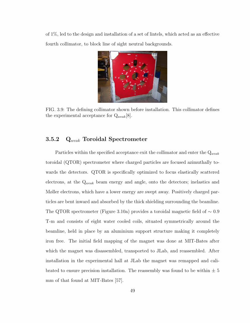
of 1%, led to the design and installation of a set of lintels, which acted as an effective

fourth collimator, to block line of sight neutral backgrounds.

FIG. 3.9: The defining collimator shown before installation. This collimator definesthe experimental acceptance for Qweak[8].

3.5.2 Qweak Toroidal Spectrometer

Particles within the specified acceptance exit the collimator and enter the Qweak

toroidal (QTOR) spectrometer where charged particles are focused azimuthally to-

wards the detectors. QTOR is specifically optimized to focus elastically scattered

electrons, at the Qweak beam energy and angle, onto the detectors; inelastics and

Møller electrons, which have a lower energy are swept away. Positively charged par-

ticles are bent inward and absorbed by the thick shielding surrounding the beamline.

The QTOR spectrometer (Figure 3.10a) provides a toroidal magnetic field of ∼ 0.9

T-m and consists of eight water cooled coils, situated symmetrically around the

beamline, held in place by an aluminium support structure making it completely

iron free. The initial field mapping of the magnet was done at MIT-Bates after

which the magnet was disassembled, transported to JLab, and reassembled. After

installation in the experimental hall at JLab the magnet was remapped and cali-

brated to ensure precision installation. The reassembly was found to be within ± 5

mm of that found at MIT-Bates [57].

49

(a) QTOR during installation. (b) QTOR Diagram.

FIG. 3.10: (a)Qweak Toroidal Spectrometer installed in experimental Hall C at Jef-ferson Lab. (b) Current in each coil travels in a racetrack fashion creating a toroidalmagnetic field. The field goes to zero at the center allowing the beam to passunperturbed to the beam dump.

3.5.3 Shielding Wall

An 80 cm thick concrete shielding wall (Figure 3.11) was placed downstream of

QTOR, preceding the detector array. The goal of the shielding wall was to provide an

aperture which would reduce backgrounds resulting from secondaries and inelastics

interacting with structural supports in QTOR. GEANT 3 Simulations showed that

in the region of the shielding wall there was an overlap between the elastic and

inelastic signal; great care was taken in the design of the shielding wall apertures to

assure that, while blocking backgrounds from the spectrometer region, backgrounds

resulting from interactions of the inelastic signal with the inner edge of the aperture

were as small as possible[9].

3.5.4 Quartz Cerenkov Detectors

The main detectors for the experiment were responsible for measuring the rate

of elastically scattered electrons in each helicity state, which is used to measure the

PV asymmetry. Each main detector had dimensions of 200 cm x 18 cm x 1.25 cm

50

FIG. 3.11: CAD diagram of shielding wall. Simulated beam envelope shown in blue.Proper design of the shielding wall was crucial to avoid interaction of the scatteredenvelope with the inner edge of the apertures[9].

and was composed of Spectrosil 2000 synthetic fused-silica bars. Each detector bar

was a composite of a pair of 100 cm pieces of fused silica glued together with UV-

transparent glue (SES-406). The Spectrosil 2000 synthetic fused-silca was chosen

for the detector material on the merits of its radiation hardness, low sensitivity to

neutral background, and uniform response across the detector. Each detector bar

was placed in a light tight box and supported by an aluminium support structure.

The “ferris wheel”support structure held one detector package at a radius of 335

cm in each of the 8 octants (0, ±45, ±90, ±135, 180). A diagram showing the

azimuthal placement of the main detector packages is shown in Fig. 3.12. Scattered

electrons leave the collimator apertures and travel into the main detectors; elec-

trons moving faster than the phase velocity of light in the quartz medium generate

Cerenkov radiation. The Cerenkov light is internally reflected down the bar, through

a light guide, and into photo-multiplier tubes (PMT) mounted on each end. Each

light guide was a simple extension of the main quartz bar with the PMTs attached

to the ends using optical glue. The 5” PMTs gathered light using UV-transparent

glass and operated in two modes depending on the PMT base used: low-gain mode

(gain O(103)) which was used for high current integrating mode, and high-gain (gain

O(106)) mode which was used primarily for tracking mode. Signals produced in the

51

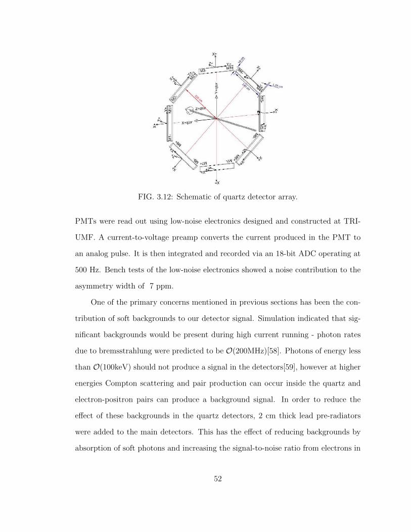
FIG. 3.12: Schematic of quartz detector array.

PMTs were read out using low-noise electronics designed and constructed at TRI-

UMF. A current-to-voltage preamp converts the current produced in the PMT to

an analog pulse. It is then integrated and recorded via an 18-bit ADC operating at

500 Hz. Bench tests of the low-noise electronics showed a noise contribution to the

asymmetry width of 7 ppm.

One of the primary concerns mentioned in previous sections has been the con-

tribution of soft backgrounds to our detector signal. Simulation indicated that sig-

nificant backgrounds would be present during high current running - photon rates

due to bremsstrahlung were predicted to be O(200MHz)[58]. Photons of energy less

than O(100keV) should not produce a signal in the detectors[59], however at higher

energies Compton scattering and pair production can occur inside the quartz and

electron-positron pairs can produce a background signal. In order to reduce the

effect of these backgrounds in the quartz detectors, 2 cm thick lead pre-radiators

were added to the main detectors. This has the effect of reducing backgrounds by

absorption of soft photons and increasing the signal-to-noise ratio from electrons in

52

the elastic envelope showering inside the pre-radiator. The pre-radiator did however

induce a level of noise in the detectors (∼12%) due to light-yield fluctuations in the

number of electrons produced in the shower; this increased the amount of run time

need by 370 hours but was out weighed by the reduction in the relative background

versus not using the pre-radiators.

3.5.5 Beamline Shielding

Scattered electrons leaving the scattering chamber at small angles (0.75 − 4)

and passing through the first clean-up collimator can potentially interact with the

downstream beam pipe causing a significant source of background - primarily in the

form of neutrals[8]. While efforts were made to design the Qweak beamline to ac-

commodate this, simulations showed significant background generation. A tungsten

beam plug was installed in the downstream side of the first collimator to block these

events. The plug was water-cooled to dissipate ∼1.3 kW of expected heating due to

the scattered beam being dumped into the plug. Figure 3.13 shows a simulation of

the beamline background with and without the tungsten plug; it is apparent from

the simulation results that the addition of the tungsten plug significantly reduced

both the neutral and multiple-scattered electron contributions to the beamline back-

ground. The tungsten plug, however, becomes a source of secondary photons in the

collimator region with potential to re-scatter and generate background in the detec-

tors. Measurements to determine how to best reduce backgrounds coming from the

beamline were performed during the commissioning phase, and led to the installa-

tion of a number of lead bricks around the beamline as well as a 12” long, 2” thick

lead donut around the beam pipe in the collimator region.

53

FIG. 3.13: Simulated beamline background with(right) and without(left) the tung-sten plug. Electrons are shown in red and neutral are shown in blue. The additionof the tungsten plug drastically reduces the beamline backgrounds[8].

3.5.6 Beam Modulation System

Changes in the beam properties during helicity flip can lead to false asymme-

tries in our detected scattering rates. The scattering rate in the detectors depends

significantly on five parameters: transverse position, angle, and incident energy E.

Small helicity-correlated variations in these parameters produce false asymmetries

which are potentially enhanced by various broken symmetries in the experimental

apparatus. The experiment took a two-pronged approach to measurement of detec-

tor sensitivity to changes in the beam position, angle, and energy. The first method

was to measure the correlation of the measured asymmetry in the detectors with the

helicity-correlated difference of the natural beam jitter seen in the beam monitors

and to use standard multivariate linear regression techniques to extract the decou-

pled detector sensitivities. The second - and a major topic of the work found in this

thesis - was to modulate the beam parameters in a controlled way using an external

driving signal and extract the sensitivities from the observed detector response. In

order to achieve this, a beam modulation system was designed and installed for the

Qweak experiment. The details of the design, implementation, and analysis efforts

using this method are detailed in the following chapter.

54

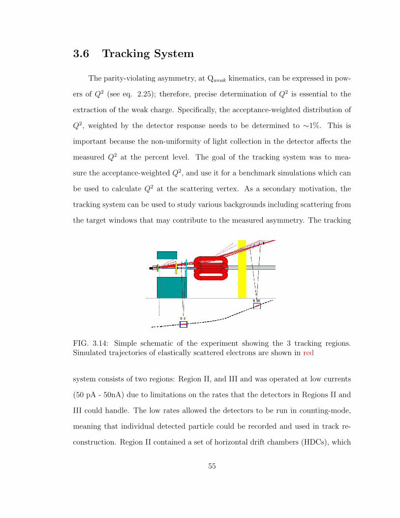
3.6 Tracking System

The parity-violating asymmetry, at Qweak kinematics, can be expressed in pow-

ers of Q2 (see eq. 2.25); therefore, precise determination of Q2 is essential to the

extraction of the weak charge. Specifically, the acceptance-weighted distribution of

Q2, weighted by the detector response needs to be determined to ∼1%. This is

important because the non-uniformity of light collection in the detector affects the

measured Q2 at the percent level. The goal of the tracking system was to mea-

sure the acceptance-weighted Q2, and use it for a benchmark simulations which can

be used to calculate Q2 at the scattering vertex. As a secondary motivation, the

tracking system can be used to study various backgrounds including scattering from

the target windows that may contribute to the measured asymmetry. The tracking

FIG. 3.14: Simple schematic of the experiment showing the 3 tracking regions.Simulated trajectories of elastically scattered electrons are shown in red

system consists of two regions: Region II, and III and was operated at low currents

(50 pA - 50nA) due to limitations on the rates that the detectors in Regions II and

III could handle. The low rates allowed the detectors to be run in counting-mode,

meaning that individual detected particle could be recorded and used in track re-

construction. Region II contained a set of horizontal drift chambers (HDCs), which

55

were used to determine the scattering angle and initial particle trajectory. Region

III consisted of a pair of vertical drift chambers (VDCs), which provided particle

position and angle information after the magnetic field. Attached to each pair of

VDCs was a trigger scintillator, which provided the tracking event trigger. Detector

packages in Region II and III were mounted in opposing octants on rotatable support

structures which allowed for a complete mapping of the main detector acceptance.

Also, the rotating support structures allowed the tracking detectors to be moved

radially out of the beam during high current running. A simple schematic of the

three tracking regions is shown in Figure 3.14.

3.6.1 Horizontal Drift Chambers

The Region II HDCs are located just upstream of the last collimator and provide

position and angle information about the scattered electrons entering the magnetic

spectrometer. The HDCs were designed to have a position resolution of ∼200 µm

and an angular resolution of ∼0.6 mrad. The active area of the HDCs was 38 cm ×

28 cm and each HDC unit contained 6 wire planes (u, v, x, u′, v′, x′). Each wire plane

contained 192 sense wires; wires in planes (x, x′) were strung horizontally, wires in

planes (u, u′) were angled by 53.2, and wires in planes (v, v′) were angled by -53.3.

Each wire plane was situated between two aluminized Mylar plates held at -2150

V, while the sense wires were grounded. Each chamber was sealed air-tight and

filled with a 65%- 35% argon- ethane mixture; the argon/ethane mixture is stable

and is easily ionized. The gas mixture was bubbled through isopropyl alcohol to

reduced the effects of chamber ageing. A total of 5 chambers were built with the

intent of using 4 chambers in the experiment with the 5th as a back-up. Each HDC

“package” consisted of two chambers mounted with a 40 cm offset along the beam

56

FIG. 3.15: Region II HDCs installed downstream of QTOR in Hall C.

axis. The HDC packages were mounted in opposite octants of a human-powered

rotating support structure, the region II “rotator”, which allowed the HDCs to be

used to map the full acceptance. The region II rotator also allowed the HDCs to

be retracted radially inward - out of the scattered electron envelope - during high-

current running. Charged particles passing through the HDCs ionize the gas; ionized

electrons drift towards the sense wires. Drift electrons nearing the sense wire begin

an avalanche increasing the total charge - and therefore the signal size - seen when

the wires are read out. A photo of the region II HDCs installed in Hall C can be

seen in Fig. 3.15.

3.6.2 Vertical Drift Chambers

The VDC’s, located downstream of the QTOR and the shielding wall, served

to provide information about the electron’s position and angle after leaving the

magnetic field of QTOR. Each drift chamber had an active area of 0.914 m x 2.438

m and contained two wire planes, labeled u and v, each with 279 wires. The wires

in each plane were strung at an angle of 26.45, which was found to be the optimal

57

angle using the simulation packge Garfield[10, 60], and with a spacing of 11.12 mm.

A full detector package consisted of 2 wire planes, 3 Mylar foils, 2 gas planes, and

one spacer frame (see Fig. 3.16b). Each frame was made from G10-FR4, which is a

sandwich of glass fibers and epoxy chosen for its ability to withstand compression,

strong dielectric properties, and minimal gas absorption. These properties were

important because each chamber was filled with a 50%- 50% argon- ethane gas

mixture and had to be air-tight. The Mylar cathode planes were held at -3800 V

and each sense wire in planes u and v was held at ground.

(a) Vertical Drift Chamber

(b) Layering for one VDC. The HVfoils are shown in magenta and wireplanes are shown in green. The cen-ter foil was aluminized foil on bothsides to provide field in both cells ofthe VDC.

FIG. 3.16: (a) Shows one completed vertical drift chamber in the lab at College ofWilliam and Mary. The VDCs were layered (b) and contained 2 wire planes, 3 HVplanes, a spacer frame, and 2 gas frames[10].

Each VDC pair was mounted on a large rotatable support structure, the Region

III “rotator” (the topic of the next section), in opposing octants. As with the HDCs,

the VDC pairs could be rotated to all octant pairs, allowing for full coverage of

the azimuthal acceptance, as well as being retractable, which allowed them to be

moved out of the scattered envelope during high current running. The chambers are

58

mounted at a 24.4 angle with respect to the support structure mounts and therefore

have a smaller angular acceptance than the HDCs but a higher spatial resolution

(< 200µm).

Signals in the VDC are produced in much the same way as with the HDCs;

scattered electrons entering the VDC at an angle and ionize the gas in each VDC’s

“cell”. The free electrons in the gas are then accelerated along the electric field lines

towards the ground wires; as the free electrons drift they ionize more of the gas,

creating more free electrons, cumulating in an avalanche when reaching the wires.

For a single VDC package there are a total of 558 individual channels to read out

or 2232 channels for the entire Region III tracking system. The read-out of such

a large number of channels posed a significant logistical and cost challenge for the

experiment. In response to this issue the detector signals were multiplexed, which

reduced the number of channels required by a factor of 9.

FIG. 3.17: Cross-section of one VDC “cell”. HV planes are shown in green and theparticle track is shown in blue[10]. Particles entering the cell ionize the gas causingan avalanche of charge moving towards the signal wires. The timing of these signalsis used to extract track information.

59

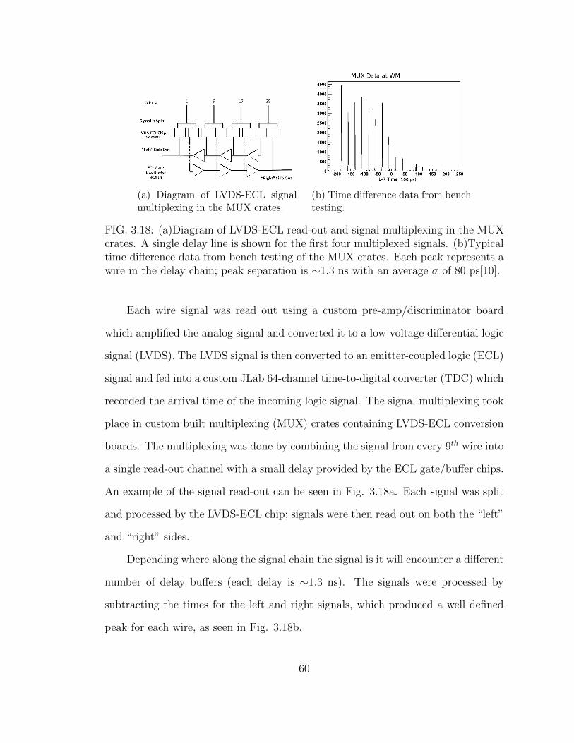
(a) Diagram of LVDS-ECL signalmultiplexing in the MUX crates.

(b) Time difference data from benchtesting.

FIG. 3.18: (a)Diagram of LVDS-ECL read-out and signal multiplexing in the MUXcrates. A single delay line is shown for the first four multiplexed signals. (b)Typicaltime difference data from bench testing of the MUX crates. Each peak represents awire in the delay chain; peak separation is ∼1.3 ns with an average σ of 80 ps[10].

Each wire signal was read out using a custom pre-amp/discriminator board

which amplified the analog signal and converted it to a low-voltage differential logic

signal (LVDS). The LVDS signal is then converted to an emitter-coupled logic (ECL)

signal and fed into a custom JLab 64-channel time-to-digital converter (TDC) which

recorded the arrival time of the incoming logic signal. The signal multiplexing took

place in custom built multiplexing (MUX) crates containing LVDS-ECL conversion

boards. The multiplexing was done by combining the signal from every 9th wire into

a single read-out channel with a small delay provided by the ECL gate/buffer chips.

An example of the signal read-out can be seen in Fig. 3.18a. Each signal was split

and processed by the LVDS-ECL chip; signals were then read out on both the “left”

and “right” sides.

Depending where along the signal chain the signal is it will encounter a different

number of delay buffers (each delay is ∼1.3 ns). The signals were processed by

subtracting the times for the left and right signals, which produced a well defined

peak for each wire, as seen in Fig. 3.18b.

60

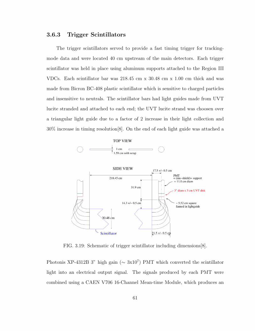
3.6.3 Trigger Scintillators

The trigger scintillators served to provide a fast timing trigger for tracking-

mode data and were located 40 cm upstream of the main detectors. Each trigger

scintillator was held in place using aluminum supports attached to the Region III

VDCs. Each scintillator bar was 218.45 cm x 30.48 cm x 1.00 cm thick and was

made from Bicron BC-408 plastic scintillator which is sensitive to charged particles

and insensitive to neutrals. The scintillator bars had light guides made from UVT

lucite stranded and attached to each end; the UVT lucite strand was choosen over

a triangular light guide due to a factor of 2 increase in their light collection and

30% increase in timing resolution[8]. On the end of each light guide was attached a

FIG. 3.19: Schematic of trigger scintillator including dimensions[8].

Photonis XP-4312B 3” high gain (∼ 3x107) PMT which converted the scintillator

light into an electrical output signal. The signals produced by each PMT were

combined using a CAEN V706 16-Channel Mean-time Module, which produces an

61

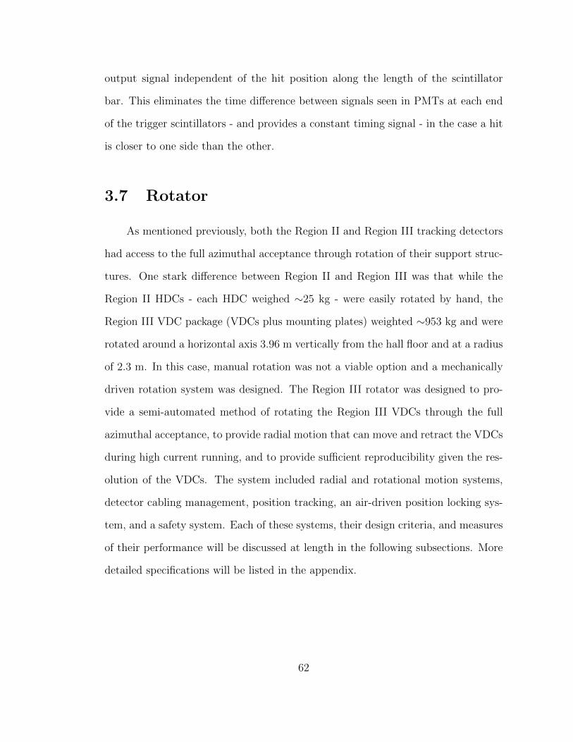
output signal independent of the hit position along the length of the scintillator

bar. This eliminates the time difference between signals seen in PMTs at each end

of the trigger scintillators - and provides a constant timing signal - in the case a hit

is closer to one side than the other.

3.7 Rotator

As mentioned previously, both the Region II and Region III tracking detectors

had access to the full azimuthal acceptance through rotation of their support struc-

tures. One stark difference between Region II and Region III was that while the

Region II HDCs - each HDC weighed ∼25 kg - were easily rotated by hand, the

Region III VDC package (VDCs plus mounting plates) weighted ∼953 kg and were

rotated around a horizontal axis 3.96 m vertically from the hall floor and at a radius

of 2.3 m. In this case, manual rotation was not a viable option and a mechanically

driven rotation system was designed. The Region III rotator was designed to pro-

vide a semi-automated method of rotating the Region III VDCs through the full

azimuthal acceptance, to provide radial motion that can move and retract the VDCs

during high current running, and to provide sufficient reproducibility given the res-

olution of the VDCs. The system included radial and rotational motion systems,

detector cabling management, position tracking, an air-driven position locking sys-

tem, and a safety system. Each of these systems, their design criteria, and measures

of their performance will be discussed at length in the following subsections. More

detailed specifications will be listed in the appendix.

62

FIG. 3.20: Region III rotator.

3.7.1 Structural

The Region III rotator (see Fig. 3.20), at its center, consists of a 2.3 m radius

304 stainless steel hub which is held concentric to the beamline. The 304 stainless

steel, which makes up the structure of the rotator, was chosen for its low magnetic

permeability1. The central rotator hub is held in place via lateral struts attached to a

simple steel support base. Each lateral strut has two 5-inch V-groove rollers attached

to a base allowing them to be adjusted radially and in Z along the beam direction.

The inner edge of the central hub is beveled to fit the V-groove cams. During

installation the rotator hub was situated on the adjustable rollers, and a survey was

used to adjust the centroid of the rotator hub to be centered on the beamline. The

1The low magnetic permeability material was chosen to reduce effects due to polarization ofthe support structure caused by the near-by QTOR field and polarized electron scattering.

63

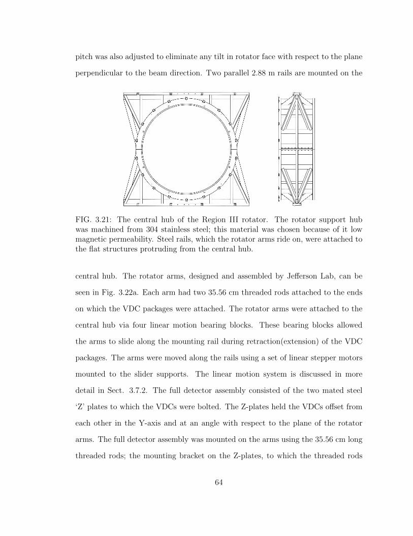
pitch was also adjusted to eliminate any tilt in rotator face with respect to the plane

perpendicular to the beam direction. Two parallel 2.88 m rails are mounted on the

FIG. 3.21: The central hub of the Region III rotator. The rotator support hubwas machined from 304 stainless steel; this material was chosen because of it lowmagnetic permeability. Steel rails, which the rotator arms ride on, were attached tothe flat structures protruding from the central hub.

central hub. The rotator arms, designed and assembled by Jefferson Lab, can be

seen in Fig. 3.22a. Each arm had two 35.56 cm threaded rods attached to the ends

on which the VDC packages were attached. The rotator arms were attached to the

central hub via four linear motion bearing blocks. These bearing blocks allowed

the arms to slide along the mounting rail during retraction(extension) of the VDC

packages. The arms were moved along the rails using a set of linear stepper motors

mounted to the slider supports. The linear motion system is discussed in more

detail in Sect. 3.7.2. The full detector assembly consisted of the two mated steel

‘Z’ plates to which the VDCs were bolted. The Z-plates held the VDCs offset from

each other in the Y-axis and at an angle with respect to the plane of the rotator

arms. The full detector assembly was mounted on the arms using the 35.56 cm long

threaded rods; the mounting bracket on the Z-plates, to which the threaded rods

64

were attached, were adjustable in (X,Y, Z ). This allowed the chamber’s positions to

be finely adjusted to the proper location with respect to the collimator apertures.

(a) The sliding arms can be seen in the HallC before being installed. The threaded rodswhich were used to hold the VDC packageswere covered with steel tubes prior to instal-lation. The mounting brackets for the pan-cake cylinders can be seen in the back right.

(b) CAD diagram of the fully as-sembled VDC packages mounted be-tween the slider arms.

3.7.2 Linear Motion System

The Region III detectors were only used during tracking measurements and cer-

tain focused ancillary measurements; the chambers were designed to be operational

at charged particle rates O(kHz) per octant and were retracted during high current

running which had rates O(GHz). The linear motion of the VDC detector packages

was achieved using a linear motion system which relied on two linear stepper motors

(EC35005B ) from IDC Motion. When choosing a stepper motor two things were

taken in to consideration: the linear motors needed to have the force required to

move the chambers and the position resolution in line with what was needed to de-

termine the track position in the VDCs. To make the linear motion safer and easier

the decision was made to only operate the linear motion system while the chambers

65

were in the horizontal position; this reduced the load on the motors to a minimum.

The required thrust load needed was estimated assuming a coefficient of friction

between the arms and the rails of 0.5; this corresponds to steel on steel. This is of

course an over estimation, but gave us sufficient overhead so that we would easily

be able to move the chambers. The estimated weight of the VDC detector package

(two VDCs plus support plates) was 9346 N which would give a required linear

thrust of 4673 N; the maximum thrust specification on the linear stepper motors

was 7200 N which is well above what was required. The position resolution on the

motors was rated to be 0.039 µm/step with a repeatability of 13 µm, which was well

below the ∼200 µm VDC position resolution. Each linear motor was driven using

a stand alone motor controller (S6961). The motors were controlled via a RS232

communication port on a single board computer located in the controls crate. The

motor controllers were wired in series so that the serial communication commands

would be sent to both controllers at the same time, thus ensuring the motors would

not become out of phase (see figure 3.23). While the rotator hub was locked in

place using a positioning pin during linear motion, an unbalanced load due to the

motors not being in sync was not desirable. The controls system will be discussed

in more detail in Sect. 3.7.4. The linear motors were mounted using a specially de-

signed motor mount to the central hub over the sliding rail to which the arms were

attached. The linear motor shafts were attached to the arms using stainless steel

eyelets welded to the posterior side of the sliding arms; each motor shaft had a clevis

mount at the end which could be attached to the eyelet on the arms. When the

rotator arms were extended they were held in place using 2.5 cm diameter locking

pins. Each pin - two per arm located on opposite sides - was driven into a pin block

mounted on support structure below the sliding rails. Each pin block was stainless

steel with a brass insert in the center. The brass insert was added due to problems

66

FIG. 3.23: Schematic showing the communications diagram for the linear motorcontrols.

with actuating the locking pins. When the locking pins were inserted and the arms

were rotated into a position, where a substantial amount of the VDC weight was

placed on them, pressure welding would take place making it extremely difficult to

remove them. Adding the brass insert to the pin block provided a buffer between

the steel pin and the pin block material.

3.7.3 Rotational Motion System

The rotational motor system provided ±180 rotational freedom to the VDCs;

this provided full azimuthal coverage of the detectors in each octant pair. The

rotational motor system is made up of a simple chain-drive powered by a 3 hp AC

motor. For the rotational motor an AC motor was chosen over a stepper motor

due to the need for a significant amount of starting torque. The inner face of the

central rotator hub was fitted with nine 2-row sprocketed face plates spaced in 40

increments around the rotator face. The AC motor was coupled to the sprocket

rotator face using a steel double-stranded roller chain. The initial design of the

rotator face only called for incremental face plates to be added to the rotator face,

67

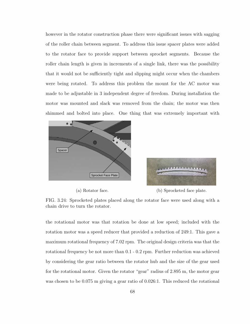
however in the rotator construction phase there were significant issues with sagging

of the roller chain between segment. To address this issue spacer plates were added

to the rotator face to provide support between sprocket segments. Because the

roller chain length is given in increments of a single link, there was the possibility

that it would not be sufficiently tight and slipping might occur when the chambers

were being rotated. To address this problem the mount for the AC motor was

made to be adjustable in 3 independent degree of freedom. During installation the

motor was mounted and slack was removed from the chain; the motor was then

shimmed and bolted into place. One thing that was extremely important with

(a) Rotator face. (b) Sprocketed face plate.

FIG. 3.24: Sprocketed plates placed along the rotator face were used along with achain drive to turn the rotator.

the rotational motor was that rotation be done at low speed; included with the

rotation motor was a speed reducer that provided a reduction of 249:1. This gave a

maximum rotational frequency of 7.02 rpm. The original design criteria was that the

rotational frequency be not more than 0.1 - 0.2 rpm. Further reduction was achieved

by considering the gear ratio between the rotator hub and the size of the gear used

for the rotational motor. Given the rotator “gear” radius of 2.895 m, the motor gear

was chosen to be 0.075 m giving a gear ratio of 0.026:1. This reduced the rotational

68

frequency to a maximum of 0.183 rpm. The rotational motor was controlled using a

variable frequency drive (HF-320α Series). The drive could be controlled a number

of ways, including: manual control using a potentiometer on the front panel, remote

communication via RJ45 cable, or a 0 - 10 V terminal connection. The rotator

controls system made use of both manual and automated control using terminal

connections; details of the controls system set-up and implementation are discussed

in more detail in Sect. 3.7.4. In the same manner as the linear arms, the rotator

hub was locked in place after moving between octants. In each of the eight octants

there was a 1 in. diameter pin hole on the upstream side of the rotator face (an

example of this can be seen in Fig. 3.24a). In the same way as the linear arms, these

pin holes were used to lock the rotator into the desired octant using an air-powered

pancake cylinder. These cylinders drove a 1 in. diameter beveled steel pin into the

pin hole. Confirmation of the pin being in was handled using a standard door jam

switch - these are the same switches used in cars to detect whether a door is open.

In each of the eight octants, on the backside of the upstream rotator face, a door

jamb switch was mounted via a small hole drilled into the rear side of the rotary

locking pin holes. When the rotational pin was inserted into the pin hole of a given

octant, the door jamb switch was triggered and provided a +5 V signal which could

be read out by the controls system.

3.7.4 Motion Controls System

The motion controls system for the Region III was designed to provide a safe,

effective way of controlling the linear and rotational motion of the rotator. Both

the linear and rotational motor systems were manually operable, however the job of

the control system was not only to provide a conduit to control this motion, but to

69

provide synchronous linear motion, fail-safe controls, and more repeatability than is

easily achieved when triggering motion by hand. The rotator controls system (Figure

3.25) was centralized in a standard controls rack located inside the entrance to the

Region III shielding bunker. This location allowed operators to be in line-of-sight of

the rotator while being safe from any possible failures. The main components of the

controls system were the Versa Module Europa bus (VME) controls crate, Linear

Motor Drives (S6961), and variable frequency drive. The VME crate contained an

MVME6100 single board CPU, VME 612 Digital to Analog converter(DAC), a cus-

tom designed VME 16 channel relay board, custom 16 channel digital input register,

and an MVME761 Serial input-output board. The linear and rotational locking pins

FIG. 3.25: Motion Controls Rack.

were operated using air driven pancake cylinders. Operationally, these cylinders are

very simple; each cylinder has two valves, depending on the valve to which air was

70

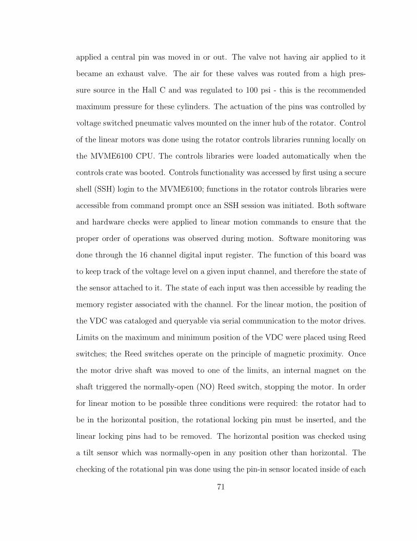
applied a central pin was moved in or out. The valve not having air applied to it

became an exhaust valve. The air for these valves was routed from a high pres-

sure source in the Hall C and was regulated to 100 psi - this is the recommended

maximum pressure for these cylinders. The actuation of the pins was controlled by

voltage switched pneumatic valves mounted on the inner hub of the rotator. Control

of the linear motors was done using the rotator controls libraries running locally on

the MVME6100 CPU. The controls libraries were loaded automatically when the

controls crate was booted. Controls functionality was accessed by first using a secure

shell (SSH) login to the MVME6100; functions in the rotator controls libraries were

accessible from command prompt once an SSH session was initiated. Both software

and hardware checks were applied to linear motion commands to ensure that the

proper order of operations was observed during motion. Software monitoring was

done through the 16 channel digital input register. The function of this board was

to keep track of the voltage level on a given input channel, and therefore the state of

the sensor attached to it. The state of each input was then accessible by reading the

memory register associated with the channel. For the linear motion, the position of

the VDC was cataloged and queryable via serial communication to the motor drives.

Limits on the maximum and minimum position of the VDC were placed using Reed

switches; the Reed switches operate on the principle of magnetic proximity. Once

the motor drive shaft was moved to one of the limits, an internal magnet on the

shaft triggered the normally-open (NO) Reed switch, stopping the motor. In order

for linear motion to be possible three conditions were required: the rotator had to

be in the horizontal position, the rotational locking pin must be inserted, and the

linear locking pins had to be removed. The horizontal position was checked using

a tilt sensor which was normally-open in any position other than horizontal. The

checking of the rotational pin was done using the pin-in sensor located inside of each

71

rotational pin hole. The linear locking fail-safe was managed using both the input

register and the relay board. When the software command was given to engage

the linear locking pins the associated relays were closed on the board which applied

power to the pneumatic valves managing the air-driven pancake cylinders. Due to

the possibility of software failures, the linear motion system controls were tied to a

physical relay AND of the aforementioned conditions. The power to the linear motor

was wired to a relay in the NO position. Power to this relay was physically tied to

all three of the conditions above being met; in this way the linear motors were shut

off completely until it was safe to move them. Similar to the implementation of the

linear motion controls the rotation controls were given both software and hardware

fail-safes. The rotational motions controls code used read-back from the rotational

locking pin, linear locking pins, and linear motor brake to determine whether or not

it was safe to rotate. As an added level of precaution the rotational motor controls

were also tied to a physical relay fail-safe. The conditions for the rotational motion

to be operational were: power applied to the linear locking pins, rotational locking

pin in the out position, and the brake applied to the linear motor. The power to

the variable frequency drive that controlled the rotational motor, as well as pow-

ering it, were tied to a high voltage relay; power to this relay was dependent on

a physical AND of the relays controlling the preceding conditions. Originally the

rotational controls system were designed to be much more automated. When first

implemented, the controls system kept track of what octant the rotator was in, and

could be moved to other octants simply by giving the command and desired octant

number. This mode of operation was not used during the experiment, however, for

two reasons: 1) during installation the support bracket holding the tracking sensor

was mis-welded. and 2) the rotation of such a large structure, in a region containing

not only the VDC packages but the main detector for the experiment was deemed

72

much safer if done by hand. No longer using the sensor that provided a read-back of

the rotational position made moving to a given octant and securing the rotational

locking pin more difficult. With this in mind, an improvised positioning system was

constructed. A number of standard laser pointers were mounted on the main detec-

tor support structure (see Fig. 3.26). While the rotator arms were in the extended

position, survey points were marked on the VDC plates and rotator arms where the

laser spots were; by trying to align to multiple points in each octant we hoped to

decrease the error on the repeatability in each octant. The size of each laser spot

was ∼ 1 mm diameter which gave an upper limit on how well we could ensure the

rotational repeatability.

FIG. 3.26: Laser pointers mounted on main detector support structure.

3.7.5 Performance and Repeatability

During the 2 year run period of the experiment, the region III rotator performed

well, being one of the few subsystems with no major failures. Along with reliabil-

ity, the key metric for the performance of the rotator was its repeatability; poor

73

repeatability increases the error on how well we are able to determine the scattered

electron trajectory through the chambers. Both during commissioning and between

run periods repeatability studies where completed with the help of the survey group

at JLab. A listing of rotator surveys as well as notes about the program of each

can be found here[61]. The survey study presented in this thesis was completed in

September 2010 prior to the completion of the commissioning running. The results

of the study showed the radial consistency between octants, i.e. the difference in

the measured radius of each measurement point as the VDCs were rotated between

octants, to be sub-millimeter in the horizontal position and at the millimeter level

in the vertical position. The radial numbers were larger when only considering the

xy-plane (perpendicular to the beam direction) indicating the VDCs were tilted in

the direction of the beam. The angular repeatability when rotating the VDCs away

from the horizontal position and back was found to be on the millidegree level. The

repeatability of the VDC after being retracted and extended was found to be good

to the 100 µm level. Lastly, the distance between measurement points was stud-

ied. The survey is done by attaching tooling balls in special positions on the face

of the VDC packages, because these tooling balls are mounted in static locations

the distance between them should not change within the resolution of the survey

measurement and any contributions from potential sagging or flexing of the cham-

bers. The positional difference between points was found to be good to the micron

level. The full summary of results as well as a more in-depth discussion of each

measurement can be found in A.2. The results of the rotator study show that the

repeatability of the chambers position was well within the limits of what is required

of our Q2 measurement.

74

CHAPTER 4

Beam Modulation

4.1 Modulation System

4.1.1 Beam Modulation and Helicity-Correlated Beam Sys-

tematics

One of the more challenging aspects of PVES experiments is suppression and

measurement of helicity-correlated beam systematics (HCBS). These changes in the

beam intensity, position, profile, and energy - when correlated with the helicity of the

beam - create false asymmetries that distort the measurement of the physics asym-

metry. These false asymmetries are especially important in precision experiments

due to the small asymmetries that are being measured. One of the primary source

of HCBS is imperfections in the laser polarization; laser light on the photo-cathode

- while highly polarized - can contain small components of linear polarization which

switch sign under helicity flip. This, along with anisotropy in the quantum efficiency

of the photo-cathode, can cause helicity-correlated differences in the intensity of po-

75

larized electrons being produced from the photo-cathode. This shows up as a charge

asymmetry in our measurement. Other sources of HCBS include lensing, where the

Pockel cell operates as an electro-optical device deflecting the beam on helicity flip,

electronic noise, and helicity signal leakage in the injector[4]. A number of well

established methods were used to remove or heavily suppress HCBS; methods such

as the RHWP and the IHWP work to reduce HCBS sources both before and after

the Pockels cell as well as providing a diagnostic which helps determine their origin.

The central purpose of the following section is the determination of the detector

sensitivity to helicity-correlated beam motion using the beam modulation system.

The main benefit of using the beam modulation system was that it provided a

measurement that was directly correlated to the driven motion of the beam. The

alternative method, linear regression of natural beam motion, provides an effective

way to reduce the asymmetry width and remove correlation of the detector response

to beam jitter, however the meaning of these corrections is not well-posed. Take

for example a hidden variable, such as halo, that is correlated to the jitter in the

beam on helicity flip; this would give the extracted sensitivities a different character

detracting from our understanding of the HCBS. The result with modulation is much

clearer: removal of the correlation of detector signal to a controlled beam motion.

Hidden variables should not contribute, and any residual correlations would indicate

non-linearities, measurement failures, or hidden variables.

4.1.2 Beam Modulation System Instrumentation

As mentioned in Sect. 3.5.6, the beam modulation system was (schematic shown

in Fig. 4.1) used to purposely modulate the electron beam in a controlled way. The

goal was to provide a system that could produce roughly independent offsets in

76

each of the beam parameters, allowing for accurate determination of the detector

sensitivities on the scale of hours, as well as suppressing contributions from intrinsic

correlations in the beam. The system consisted of four pairs of air-core inductive

copper coils - two pair for X-like motion and two for Y-like motion - placed along the

beamline (Fig. 4.2). Each coil was driven by the output of a 16 bit VMIVME-4145

Waveform Generator. These waveform generators provided 4 channels of output per

board and have options for both internal or external triggering. For each channel the

sinusoidal waveform was built using a 64k word sample buffer. Once a waveform

of the desired frequency was lo added into the sample buffer, the external signal

was used to trigger the output on each desired channel. The signal output of each

channel was split, with one copy sent through a JLab-designed power amplifier card

(TRIM-I1) and used as a driving signal for the modulation coils. The other copy

was sent to an ADC, where it was used as both a diagnostic and as a reference signal

to lock the measured beam monitor response to the driving signal. The later point

became a powerful tool in the analysis methodology when dealing with the effects

of the fast-feedback system (FFB) on the beam monitor response to modulation.

Energy modulation was carried out in a similar fashion to position modulation,

with a driving signal being sent to the input of a superconducting radio-frequency

(SRF) cavity in the south linac of the accelerator. By modulating the input voltage

to the cavity we changed the electric field in the cavity and thereby the energy of

the electron beam. A final output channel was dedicated to producing a linearly-

increasing periodic function we defined as a “ramp” signal that was run directly

into an ADC. Since all outputs of the waveform generator were triggered via a

single external signal, the output wave-forms were synchronous. For every trigger

1Originally we had planned on using the second generation version of this power amplifier,however the engineering group at JLab found problems with them and they were removed.

77

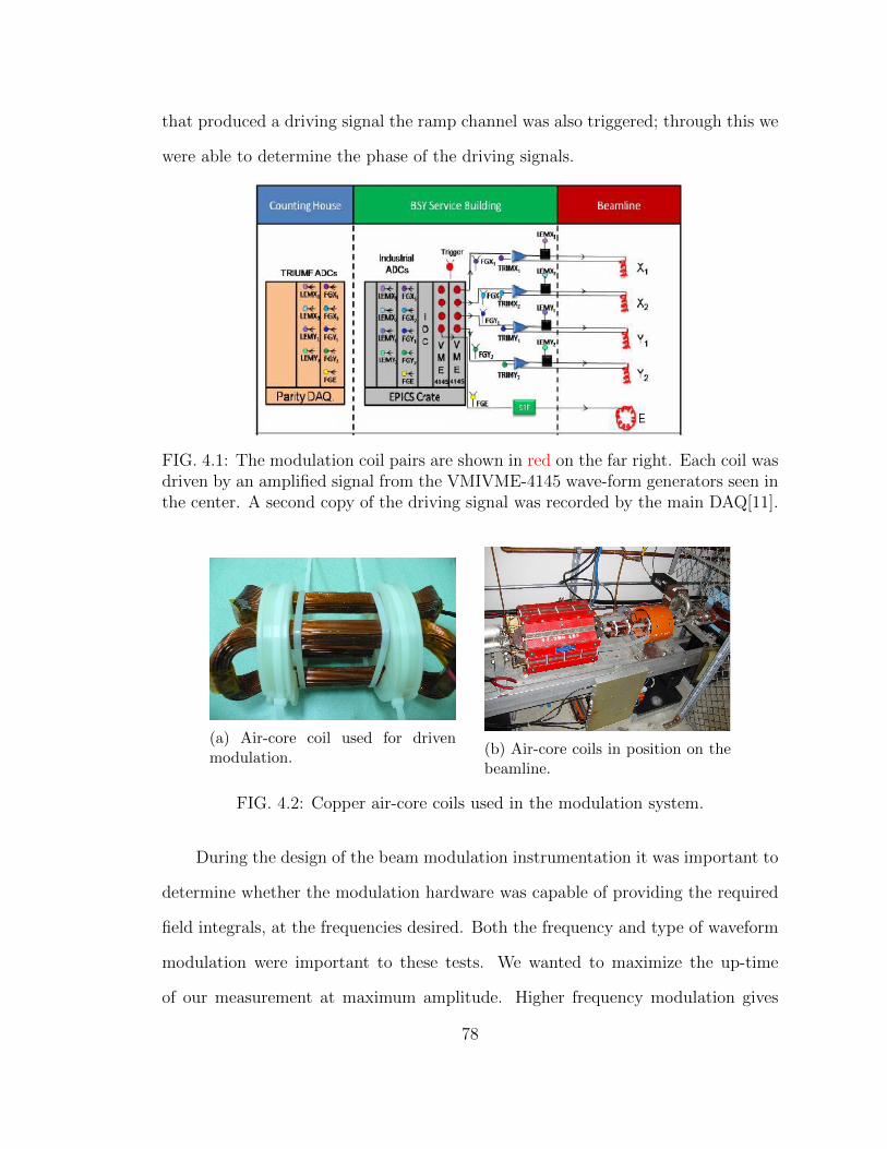
that produced a driving signal the ramp channel was also triggered; through this we

were able to determine the phase of the driving signals.

FIG. 4.1: The modulation coil pairs are shown in red on the far right. Each coil wasdriven by an amplified signal from the VMIVME-4145 wave-form generators seen inthe center. A second copy of the driving signal was recorded by the main DAQ[11].

(a) Air-core coil used for drivenmodulation.

(b) Air-core coils in position on thebeamline.

FIG. 4.2: Copper air-core coils used in the modulation system.

During the design of the beam modulation instrumentation it was important to

determine whether the modulation hardware was capable of providing the required

field integrals, at the frequencies desired. Both the frequency and type of waveform

modulation were important to these tests. We wanted to maximize the up-time

of our measurement at maximum amplitude. Higher frequency modulation gives

78

a higher number of measurements per minute and using a waveform that spends

more time at maximum displacement makes each measurement more precise, e.g. a

square wave would be preferable over a sine wave. Bench tests were performed using

the air-core coils driven using a FANUC VME function generator with the TRIM-II

power amplifiers. During the bench test the coils were modulated at frequencies of

10 Hz – 500 Hz; a Hall probe was used to measure the field integral and the power

amplifier input voltage versus the coil current was recorded for different frequencies.

As a result of the bench top tests it was determined that the maximum reliable

operating conditions for the system was 250 Hz at a current of 3 A [62]. The choice

was made during Run I to operate the modulation system at a frequency of 125 Hz

- this is slightly off the poles of the FFB system which cancels beam noise at 60 Hz

and higher harmonics. This choice of sampling frequency provided an acceptable

waveform while providing sufficient livetime for each modulation cycle.

FIG. 4.3: An example beamline optics simulation to generate a 50 µm offset at thetarget. The red arrow shows the direction of the beam. The coils are representedby C1 and C2 and show the optimal locations along the beamline to apply kicks[12].

The position, angle, and energy of the beam at the target is determined by the

transfer function of the beam from the modulation coils to the target. By applying

79

the proper set of kicks to the beam at strategic locations along the beamline we were

able to generate the desired offsets at the target. The ratio and amplitude of the

kicks for each modulation type were determined using beam transport simulations

in OpTIM[63]. Taking advantage of the time reversal invariance of the electromag-

netic interaction, the beam was run backwards through the simulation, starting in

the desired position and moving upstream along the beamline. An example optics

simulation for an initial 50 µm offset at the target can be seen in Fig 4.3. Here the

beam moves from left to right, as indicated by the red arrow, propagating upstream

along the beamline. The simulated path shows the orbit, given the transport optics,

the beam would need to result in a pure position offset of 50 µm at the target.

The zero-crossings of the time reversed beam are important in the sense that they

provide a direct mapping of the position(angle) at the target to the beam angle at

the coil position. Placing kicker coils at these locations allowed us to generate the

forward orbit resulting in the pure position(angle) offset we desired. Similar simu-

lations were carried out for each type of modulation; these simulations determined

the starting currents and coil ratios that would be used during running. One of

the default running configuration can be found in Table 4.1. In the table you can

see the coil currents required to produce the given offsets; one important thing to

notice is the near degeneracy in the Y-like coil currents. The basic concern here

was that if two or more beam parameters - which make up our basis set - were not

sufficiently independent there could be difficulty in extracting the sensitivities. This

was an ever present concern throughout the extent of the experimental running, and

one that was never completely resolved. During times that a change in accelerator

optics was suspected, plots of the beam trajectory were made by plotting the BPM

response to modulation to each kind of modulation as a function of Z position along

the beamline. These optics plots provided a snapshot of the current beam optics,

80

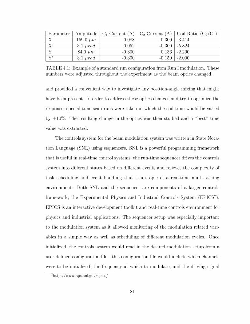
Parameter Amplitude C1 Current (A) C2 Current (A) Coil Ratio (C2/C1)X 159.0 µm 0.088 -0.300 -3.414X’ 3.1 µrad 0.052 -0.300 -5.824Y 84.0 µm -0.300 0.136 -2.200Y’ 3.1 µrad -0.300 -0.150 -2.000

TABLE 4.1: Example of a standard run configuration from Run I modulation. Thesenumbers were adjusted throughout the experiment as the beam optics changed.

and provided a convenient way to investigate any position-angle mixing that might

have been present. In order to address these optics changes and try to optimize the

response, special tune-scan runs were taken in which the coil tune would be varied

by ±10%. The resulting change in the optics was then studied and a “best” tune

value was extracted.

The controls system for the beam modulation system was written in State Nota-

tion Language (SNL) using sequencers. SNL is a powerful programming framework

that is useful in real-time control systems; the run-time sequencer drives the controls

system into different states based on different events and relieves the complexity of

task scheduling and event handling that is a staple of a real-time multi-tasking

environment. Both SNL and the sequencer are components of a larger controls

framework, the Experimental Physics and Industrial Controls System (EPICS2).

EPICS is an interactive development toolkit and real-time controls environment for

physics and industrial applications. The sequencer setup was especially important

to the modulation system as it allowed monitoring of the modulation related vari-

ables in a simple way as well as scheduling of different modulation cycles. Once

initialized, the controls system would read in the desired modulation setup from a

user defined configuration file - this configuration file would include which channels

were to be initialized, the frequency at which to modulate, and the driving signal

2http://www.aps.anl.gov/epics/

81

amplitude defined in amps. Once the configuration files had been read-in, the wave-

form generator boards were transitioned into a ready state. An external trigger was

then applied to the boards; this signal would cause the channels that were initialized

for a certain modulation type to trigger and run through a full set of cycles. Once

the modulation cycles were finished, the system would set all channels into an OFF

state and move to a wait state until it was time to wake up and modulate again.

The modulation system ran continuously during most of the production running,

stepping through a modulation sequence in each beam parameter; a set of micro-

cycles containing one instance of modulation in each beam parameter makes up a

macro-cycle. During each modulation cycle a pattern number flag was set in the

DAQ; there was a unique pattern number for modulation in each beam parameter,

which allowed us to identify the type of modulation of each micro-cycle during anal-

ysis. The modulation sequence consisted of driving each pair of modulation coils

in micro-cycles of about 4 seconds, or 512 cycles at 125 Hz. There was a down

time of ≈ 75 seconds between each micro-cycle of modulation which was needed to

reconfigure the boards for the next modulation type. A full modulation macro-cycle

was 320 seconds, after which time the modulation system would reconfigure and

repeat the macro cycle; the modulation data composed about 5% of our production

running.

4.1.3 Methodology

As mentioned previously, measurement and correction of false asymmetry caused

by helicity-correlated beam systematics was done using two methods: using standard

linear regression technique applied to natural beam jitter, and using large-amplitude

driven beam motion via the beam modulation system. The correction to the raw

82

FIG. 4.4: Schematic of beam modulation cycle timing. Each pulse section is 512cycles of sinusoidal function at frequency of 125 Hz. Pulse are broken down intomicro-cycles that make up a full macro-cycle.

asymmetry due to helicity-correlated beam systematics was determined using the

beam modulation system outlined in the previous section. The raw asymmetry was

corrected for false asymmetries according to

Acorrected = Araw − Afalse (4.1)

where Afalse is the correction due to false asymmetries and is given by

Afalse =1

〈Y 〉∑i=1...5

∂Y

∂Xi

∆X. (4.2)

Here the detector sensitivities are given by ∂Y/∂Xi and represent the direct correlation

of the detector yield to changes in a given beam parameter. It is important to note

that this is not directly measurable; the beam modulation strove to provide linearly

independent modulations of the beam but could not completely remove cross cor-

relations between beam parameters, e.g. position modulations also had components

of energy and angle mixed in. Extraction of the detector sensitivities was done by

83

considering the response of the detector yield with respect to the modulation signal;

the modulation signal is analogous the modulation type. Expanding with respect

to the beam parameters,

∂Y

∂Ci=∑

j=1...N

∂Y

∂Xj

∂Xj

∂Ci, (4.3)

where Cj represents a time-dependent signal synced with the modulation driving

signal, yields the detector sensitivities. The beam monitor matrix, given by ∂Xj/∂Ci,

gives the correlation of the beam parameters measured in the monitors to each

modulation type. Both the beam parameter correlation matrix and the detector

response to each modulation type are directly measurable. The detector sensitivities

can then be extracted by matrix inversion:

∂Y

∂Xj

=∂Y

∂Ci

[∂Xj

∂Ci

]−1

. (4.4)

This can be written in matrix form as:

MS = MCM−1M (4.5)

As was explained in Sec. 4.1.2, the beam modulation system used pairs of coils,

driven with different amplitudes, which produced a composite response in the beam.

While the individual driving signals were available in the DAQ, there was no read-

back of the composite driving signal. Instead the ramp signal, which was synced to

the coil driving signals and common to each modulation type, was used. Refering

to Eq. 4.3 above, Cj is a parametrized version of the ramp signal given by

C(t)i = sin(αr(t)− φ), (4.6)

84

where r(t) is the ramp function. Parametrizing the response in this way allowed

us to pick out only the component of the response directly proportional to the

driving signal, which was important in circumventing components in the response

such as Fast-Feedback (FFB) system, discussed later in this chapter. Using the

detector response in Eq. 4.4, the sensitivities to each modulation type (MC) were

determined using a fit to a linear regression line,

M jC =

∑i=1...N

(Cji − 〈Cj〉)(Y j

i − 〈Y j〉)∑i=1...N

(Cji − 〈Cj〉)2

, (4.7)

where the sum is over the N modulation events in a micro-cycle, and j is the mod-

ulation type. The correlation matrix (MM) was calculated in a similar fashion for

each modulation type and beam monitor as,

M jkM =

∑i=1...N

(Cjki − 〈Cjk〉)(M jk

i − 〈M jk〉)∑i=1...N

(Cjki − 〈Cjk〉)2

. (4.8)

Here j represents the modulation type, and k is the beam parameter. This was

done for each micro-cycle in a given run and the error weighted average of MC and

MM were used in Eq. 4.5 to complete MC and MM respectively. Given that MM

is invertible, i.e. |MM| 6= 0, the detector sensitivities to each beam parameter (MS)

can be extracted as shown in Eq. 4.5 – 4.6.

One of the complications that came about when syncing to the ramp signal was

the way in which the ramp signal was sampled. The DAQ samples signals coming

into the ADCs at 960 Hz, and given the modulation frequency of 125 Hz, there are

∼8 data points for each ramp cycle. The issue comes about at the transition point

between ramp cycles; when the ramp signal transition falls in the center of an ADC

sample window, it creates a point that is not consistent with the functional form

85

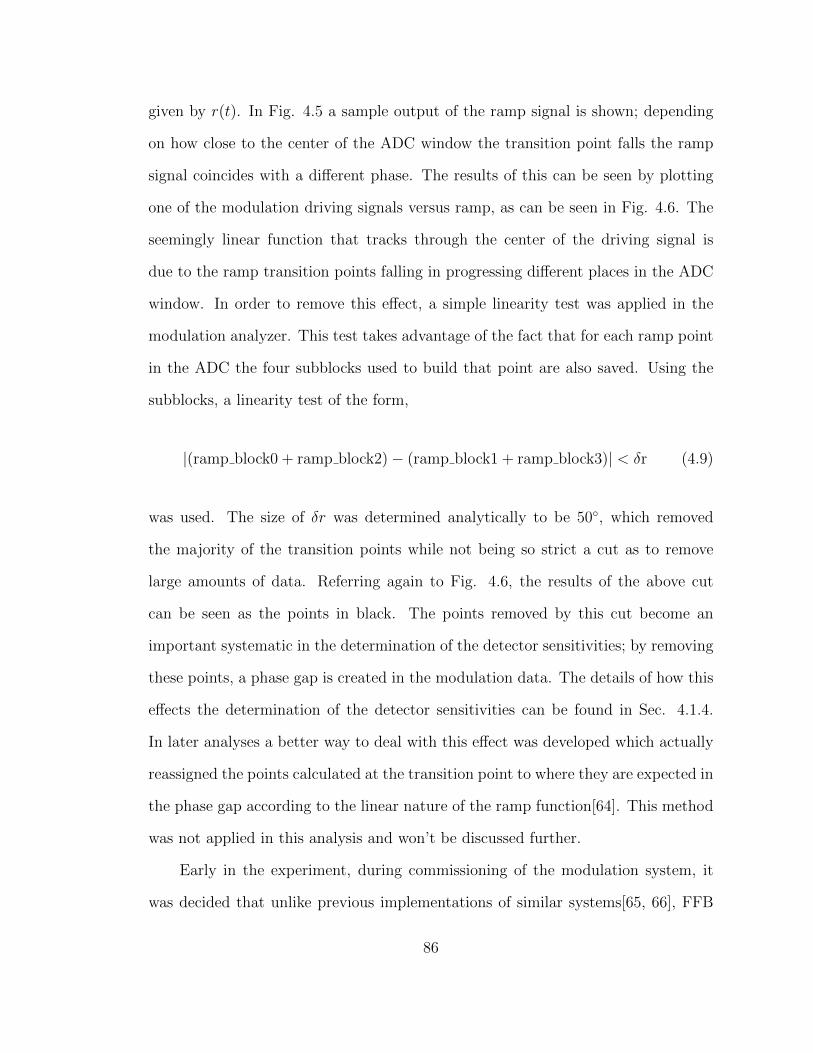
given by r(t). In Fig. 4.5 a sample output of the ramp signal is shown; depending

on how close to the center of the ADC window the transition point falls the ramp

signal coincides with a different phase. The results of this can be seen by plotting

one of the modulation driving signals versus ramp, as can be seen in Fig. 4.6. The

seemingly linear function that tracks through the center of the driving signal is

due to the ramp transition points falling in progressing different places in the ADC

window. In order to remove this effect, a simple linearity test was applied in the

modulation analyzer. This test takes advantage of the fact that for each ramp point

in the ADC the four subblocks used to build that point are also saved. Using the

subblocks, a linearity test of the form,

|(ramp block0 + ramp block2)− (ramp block1 + ramp block3)| < δr (4.9)

was used. The size of δr was determined analytically to be 50, which removed

the majority of the transition points while not being so strict a cut as to remove

large amounts of data. Referring again to Fig. 4.6, the results of the above cut

can be seen as the points in black. The points removed by this cut become an

important systematic in the determination of the detector sensitivities; by removing

these points, a phase gap is created in the modulation data. The details of how this

effects the determination of the detector sensitivities can be found in Sec. 4.1.4.

In later analyses a better way to deal with this effect was developed which actually

reassigned the points calculated at the transition point to where they are expected in

the phase gap according to the linear nature of the ramp function[64]. This method

was not applied in this analysis and won’t be discussed further.

Early in the experiment, during commissioning of the modulation system, it

was decided that unlike previous implementations of similar systems[65, 66], FFB

86

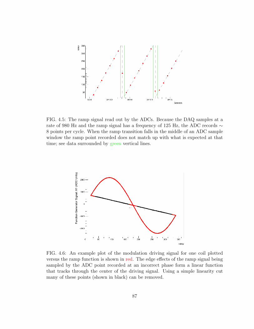
FIG. 4.5: The ramp signal read out by the ADCs. Because the DAQ samples at arate of 980 Hz and the ramp signal has a frequency of 125 Hz, the ADC records ∼8 points per cycle. When the ramp transition falls in the middle of an ADC samplewindow the ramp point recorded does not match up with what is expected at thattime; see data surrounded by green vertical lines.

FIG. 4.6: An example plot of the modulation driving signal for one coil plottedversus the ramp function is shown in red. The edge effects of the ramp signal beingsampled by the ADC point recorded at an incorrect phase form a linear functionthat tracks through the center of the driving signal. Using a simple linearity cutmany of these points (shown in black) can be removed.

87

FIG. 4.7: The phase of the BPM response is shown as a function of position along thebeamline. The dashed blue lines indicate the position of the vertical and horizontalmodulation coils.

would be enabled during running, except during energy modulation. This was due to

fears that disabling the FFB system, which actively monitored and tried to correct

beam noise, would introduce significant noise into the experimental measurement.

This decision came following a test run of the modulation system which showed two

things [67]: the energy FFB completely flattened the energy modulation signal and

the suppression of the position modulation was small (O(5%)). Unfortunately, the

effect on the phase of the BPM response to modulation was not recognized during

the commissioning tests.

In Fig. 4.7 the phase of the BPM response in each beam monitor along the

beamline is shown; of primary importance are the final five BPMs before the target

which are used to construct the “target” variables and therefore directly affect the

extraction of the detector sensitivities. To understand the phase shift due to FFB

we looked at how the FFB algorithm monitored and made corrections to the beam

position. Along the beamline certain BPMs were monitored by the FFB system.

88

These feedback BPMs were used by the FFB system, which samples the position

noise over two second windows at 1.8 kHz, and creates a waveform to null out

horizontal (vertical) displacement with an equal but opposite position offset. This

is equivalent to another modulation coil that has a delayed response - or a different

phase - to the modulation. The total response of the BPM to modulation can be

parametrized as the sum of two harmonic functions[68] with different phases

X(t) = A sin(ωt+ φmod) +B sin(ωt+ φffb). (4.10)

This can be be rewritten as

X(t) = A′ sin(ωt+ α), (4.11)

where

α = tan−1 A sinφmod +B sinφffb

A cosφmod +B cosφffb

(4.12)

A′ =√

(A sinφmod +B sinφffb)2 + (A cosφmod +B cosφffb)2. (4.13)

Here φffb is the response of the FFB to the modulation signal and φmod is the

composite response of the beam to modulation. The problem this presents is that the

phase of the composite response is a function of the relative phases and amplitudes of

the modulation coils and the FFB system. The amplitude response of a given BPM

to modulation depends on the transfer function from the coils to a particular point

along the beamline. This means we had a position-along-the-beamline dependent

phase response to modulation; another way of saying this is that we are spanning

more than one dimension in phase space. The solution to this was that we measured

the response to modulation with a fixed phase. Considering the response to a given

89

modulation as the sum of harmonic functions, we have

X(t) =∑i=0...N

xi sin(ωt+ φ) = xffb+drives sin(ωt+ φ) + xffb

c sin(ωt+ φ) (4.14)

where xffb+drive is the component of the response due to the driving signal plus the

sine component of the FFB, and xffbc is the cosine component of the FFB response. If

we consider only the sine component of the BPM response, the FFB-only component

averages out, leaving us with an amplitude that is proportional to the driving signal.

In fact, because the two harmonic functions are time-orthogonal, the FFB compo-

nent will always cancel out, allowing us to use any arbitrary phase. For the purpose

of the analysis presented here, φ was chosen to be zero. This corresponds to φ = 0 in

Eq. 4.6. This postulate rests completely on the assumption that the FFB response

is not dynamic on the time-scale of the modulation. A detailed presentation of how

this phase lock postulate was tested is presented in Sec. 4.1.4.

4.1.4 Modulation Regression Analysis

The previous section explained the basic methodology used, as well as some of

the difficulties encountered, in the measurement of the detector sensitivities using the

beam modulation system. This section details the diagnostics used to ascertain the

quality of the extracted sensitivities and the subsequent corrections to the measured

asymmetry. In Sec. 4.1.3 it was explained that due to the FFB being left on

during modulation, there was a phase shift induced into the BPM response used to

calculate the detector sensitivities. The proposed solution was to model the total

BPM response as the superposition of a set of harmonic functions, which could

be separated into components proportional to the driving signal plus part of the

FFB, and a time-orthogonal piece proportional only to the FFB signal. This led

90

to the postulate that we could choose any arbitrary phase to extract the detector

sensitivities. To test this, four different “sets” were chosen - each with a different set

of phases - to extract the detector sensitivities. Shown in Table 4.2 are the different

phases used in the modulation analysis.

Phase(deg)/Set φnX φnX′ φn3c12X φnY φnY ′

Set 1 0.0 0.0 0.0 0.0 0.0Set 2 0.0 0.0 0.0 0.0 90.0Set 3 0.16 0.12 -1.15 0.12 0.14Set 4 14.89 14.89 0.0 61.88 61.88

TABLE 4.2: List of phases used in the different modulation sets, in units of degrees.

Sets 1 and 2 were chosen for simplicity and with the intent of trying to separate

the Y and Y′ beam parameters. Set 3 and 4 were chosen by considering parts of

the correlation matrix which significantly contribute to the extracted sensitivities;

the phase choices for these sets were chosen to remove or suppress phase offsets

in these high contribution areas. Table 4.3 shows the results of the Wien-Average

sensitivities for each set during Run I. Qualitatively, the extracted sensitivities of

a given type are the same, however they do not match within the error bars. The

variation from set to set is most likely due to strength sharing between the extracted

sensitivities. Normally it would not be expected for there to be a correlation if the

basis has been properly defined, however this is only true if the definition of the

basis vectors being used do not change. Throughout the experimental running there

DOF/Set X X′ 3c12X Y Y′

Set 1 -1685.3 ± 6.7 81.9 ± 0.3 -1478.1 ± 1.2 259.7 ± 4.8 -1.7 ± 0.2Set 2 -1685.5 ± 6.2 82.5 ± 0.3 -1491.9 ± 1.5 306.3 ± 6.9 -5.5 ± 0.5Set 3 -1686.8 ± 7.3 81.8 ± 0.3 -1490.7 ± 1.8 249.2 ± 5.9 -2.5 ± 0.3Set 4 -1538.4 ± 9.4 80.0 ± 0.7 -1473.4 ± 3.7 267.0 ± 26.6 -0.1 ± 1.6

TABLE 4.3: Wien average sensitivities for each modulation set. Positions sensitiv-ities are in units of pm/mm and angle sensitivities are in units of ppm/µrad.

91

was significant dispersion in the beam-tune, increasing the correlation between the

position and energy of the beam; this correlation changed as the beam tune drifted.

In this model, the definition of X, X′, and E changes and therefore a slight shift in

the extracted sensitivities is expected. In Fig. 4.8 - 4.12 you can see correlation plots

of the virtual target BPMs and bpm3c12X which demonstrate the strength sharing

present in the extracted sensitivities. Each plot shows the set of Run I modulation

extracted sensitivities on the runlet basis3 for each monitor.

One likely cause of the correlation of the extracted sensitivities was correlated

noise in the monitors used to form the virtual BPMs as well as bpm3c12X; with this

in mind we expect the correlation to be suppressed when averaging over longer time

scales. Correlation plots of the Slug-averaged sensitivities are shown in Fig. 4.13 -

4.17, and show that the correlation between the extracted sensitivities is suppressed

as the monitor noise is averaged out, as expected.

3In this case runlet refers to segments of a full run, each segment making up approximately 6minutes of data.

92

FIG. 4.8: Correlation between TargetX and TargetX′ sensitivities.

FIG. 4.9: Correlation between BPM3c12X and TargetX sensitivities.

93

FIG. 4.10: Correlation between BPM3c12X and TargetX′ sensitivities.

FIG. 4.11: Correlation between TargetY and TargetX sensitivities.

94

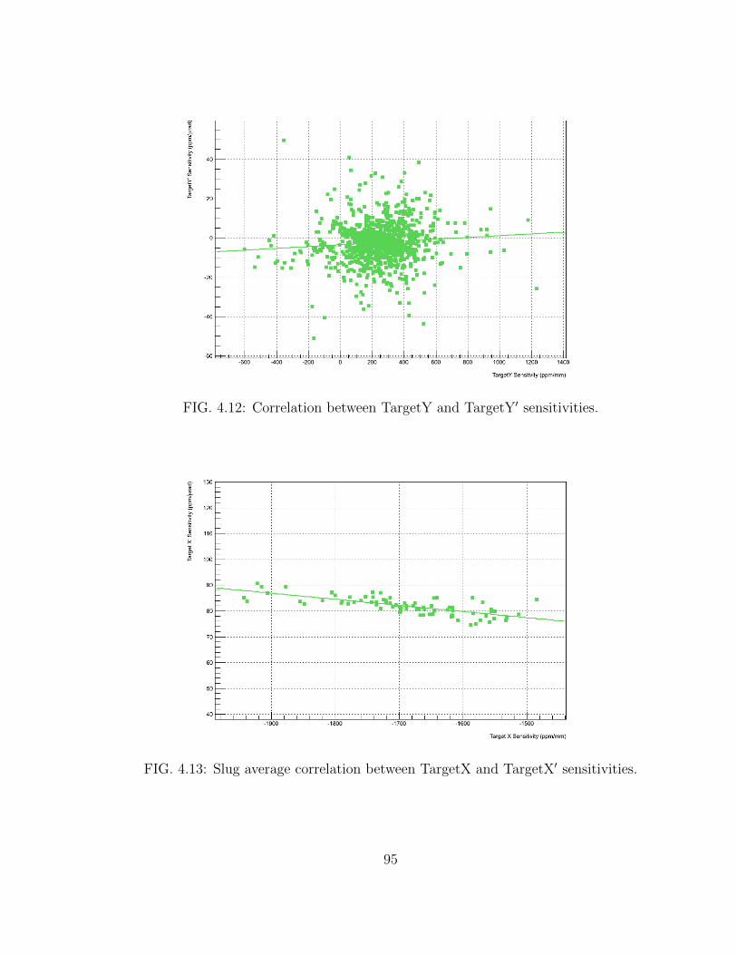
FIG. 4.12: Correlation between TargetY and TargetY′ sensitivities.

FIG. 4.13: Slug average correlation between TargetX and TargetX′ sensitivities.

95

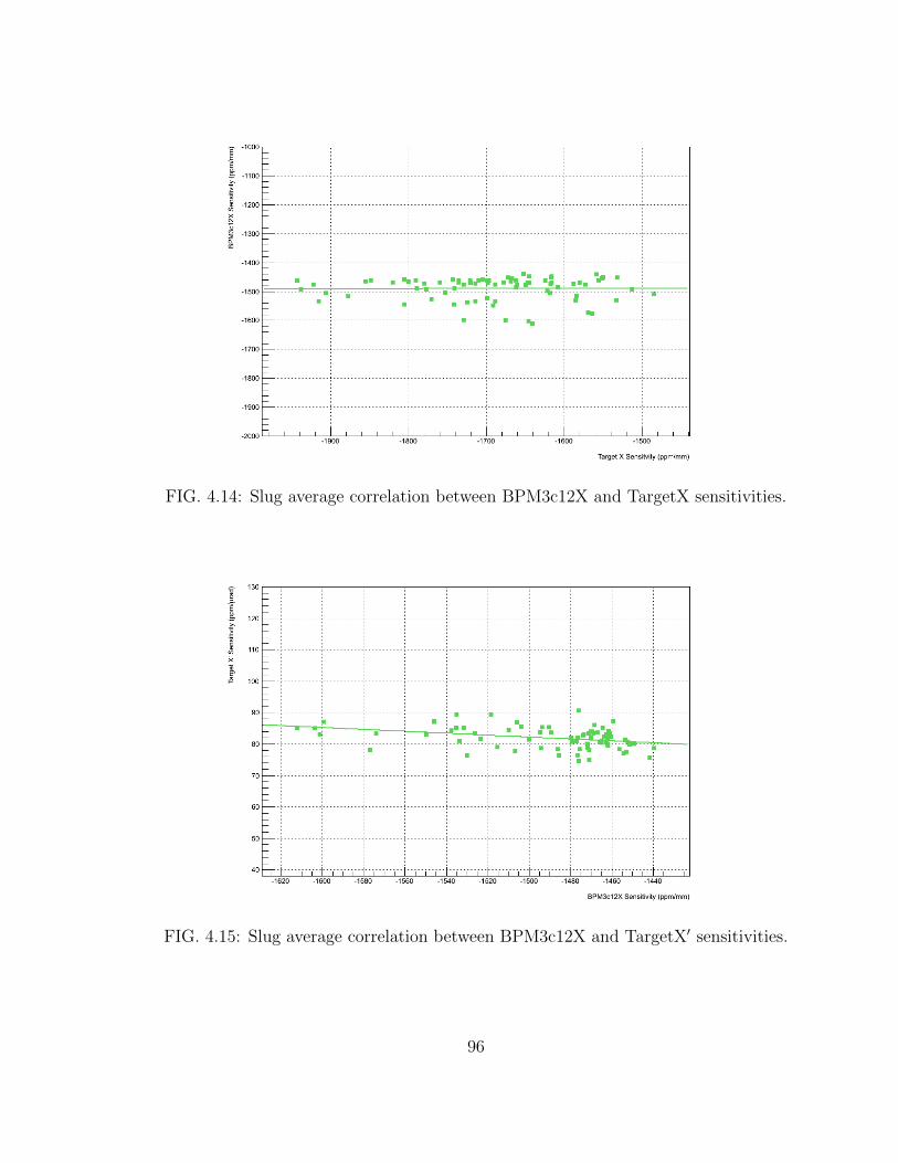
FIG. 4.14: Slug average correlation between BPM3c12X and TargetX sensitivities.

FIG. 4.15: Slug average correlation between BPM3c12X and TargetX′ sensitivities.

96

FIG. 4.16: Slug average correlation between TargetY and TargetX sensitivities.

FIG. 4.17: Slug average correlation between TargetY and TargetX′ sensitivities.

During both Run I and Run II run periods data was taken with the FFB system

97

deactivated. The original purpose of this, during Run I, was to study the effect of

the FFB system on the response amplitude during modulation; if FFB significantly

suppressed the BPM response amplitude we could not run it during modulation. The

result of the Run I test was that the FFB reduced the BPM response ∼5% and there

was a slight amplification of the Y response. Unfortunately, as mentioned previously,

the phase shift due to FFB interacting with the modulation was overlooked. The

response to modulation for each BPM during both runs with and without FFB

active can be found in Fig. 4.18-4.22. From the plots the effect of the FFB on the

BPM response is clear, with the effect on the Y-like BPMs being most significant.

It is important to note that the phase shift of the BPM response during the FFB

off run should be insignificant; in the case of energy modulation, because the energy

lock is always disabled, there should be no phase shift in either case. The results

for the FFB off run match expectations with the exception of TargetY′ modulation.

Referring to Fig. 4.22, the phase shift seen in TargetY′ with FFB off is ∼ 70- 80.

The fact that there is a significant phase shift in the BPM response to modulation

when the FFB system is disabled, is suggestive of there being another set of coils

coupling to the modulation. This was looked into more thoroughly by the beam

corrections group at the University of Virginia; currently no source for this coupling

has been found. One thing that group noticed was noticed was that the phase shift

with FFB turned off is not present in the Run II results. The analysis to determine

what the issue was is currently on-going, however, as mentioned above, the addition

of an additional phase should not matter in the analysis as long as the shift does

not change with time, however, it is still desirable to understand the source.

98

FIG. 4.18: TargetX response to modulation during runs with and without FFBactive.

FIG. 4.19: TargetX′ response to modulation during runs with and without FFBactive.

99

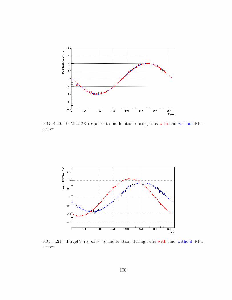
FIG. 4.20: BPM3c12X response to modulation during runs with and without FFBactive.

FIG. 4.21: TargetY response to modulation during runs with and without FFBactive.

100

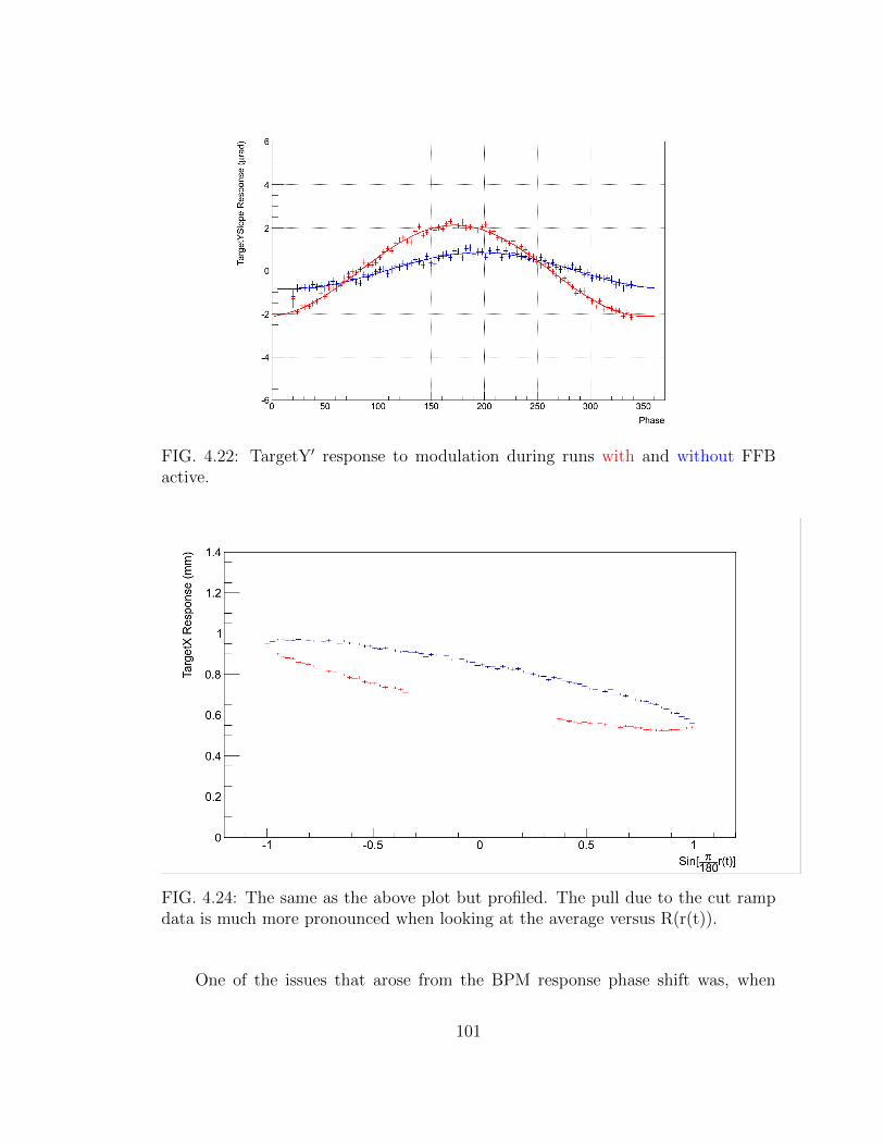
FIG. 4.22: TargetY′ response to modulation during runs with and without FFBactive.

FIG. 4.24: The same as the above plot but profiled. The pull due to the cut rampdata is much more pronounced when looking at the average versus R(r(t)).

One of the issues that arose from the BPM response phase shift was, when

101

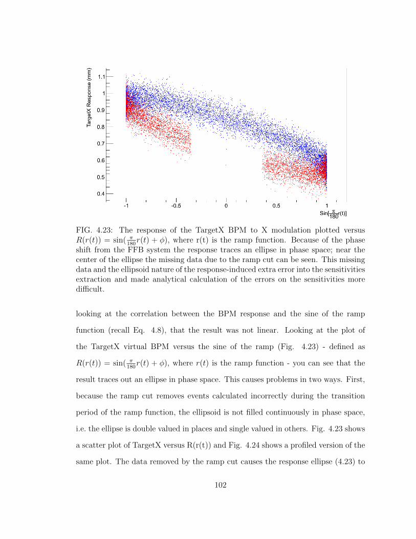
FIG. 4.23: The response of the TargetX BPM to X modulation plotted versusR(r(t)) = sin( π

180r(t) + φ), where r(t) is the ramp function. Because of the phase

shift from the FFB system the response traces an ellipse in phase space; near thecenter of the ellipse the missing data due to the ramp cut can be seen. This missingdata and the ellipsoid nature of the response-induced extra error into the sensitivitiesextraction and made analytical calculation of the errors on the sensitivities moredifficult.

looking at the correlation between the BPM response and the sine of the ramp

function (recall Eq. 4.8), that the result was not linear. Looking at the plot of

the TargetX virtual BPM versus the sine of the ramp (Fig. 4.23) - defined as

R(r(t)) = sin( π180r(t) + φ), where r(t) is the ramp function - you can see that the

result traces out an ellipse in phase space. This causes problems in two ways. First,

because the ramp cut removes events calculated incorrectly during the transition

period of the ramp function, the ellipsoid is not filled continuously in phase space,

i.e. the ellipse is double valued in places and single valued in others. Fig. 4.23 shows

a scatter plot of TargetX versus R(r(t)) and Fig. 4.24 shows a profiled version of the

same plot. The data removed by the ramp cut causes the response ellipse (4.23) to

102

be non-continuous, potentially causing the calculation of the correlation performed

in Eq. 4.8 to be incorrect. The second issue, which would be present even if the

ramp cut was not applied, is that the error on the correlation calculation will be

incorrect; this is because we are applying a linear model to a non-linear response.

Following the completion of the modulation analysis replay, the effect of the

missing ramp data was investigated. A method to fill in the missing ramp data

and make the response continuous was developed at the University of Virginia; this

method of filling in the missing ramp data would have required a new full replay

of the data and was not used in the present analysis, however, early results using

the ramp fill method were compared [69] to the results found here and showed only

a small change. Given the difficulties in computing the errors on each extracted

sensitivity explained above, the errors were instead extracted by looking at the

RMS/√N for each sensitivity on the Slug and Wien level. Shifting the analysis to

the Slug and Wien levels not only allowed for the extraction of more accurate error

bars, but Slug or Wien level sensitivities facilitated the use of more accurate detector

sensitivities; the sensitivity of the detectors to changes in the beam parameters was

a property of the apparatus and should have been constant. These Slug or Wien

level sensitivities can then be applied to the data for more accurate corrections.

Looking at the single detector sensitivities as a function of octant number pro-

vides an important diagnostic tool as well as providing insight into the nature of

the detector sensitivities. In Fig. 4.25 - 4.27 the Run I average single detector

sensitivities are shown as a function of octant number. Recall from Sec. 3.5.4, the

main detector is an azimuthally symmetric array of quartz Cerenkov detectors. The

octants are numbered as shown in Fig. 3.12, with octants 1 and 5 in the horizontal

plane. With these definitions, it is expected that the measured detector sensitivity

for each bar will be characteristic of the modulation type.

103

For instance, for an X-like modulation the single detector sensitivity as a func-

tion of octant number should be sinusoidally varying with peaks at octant 1 and

octant 5; these octants are in the plane of modulation and should be most sensitive.

In Fig. 4.25 a plot of the Wien-average single detector X-sensitivity as a function of

octant number is shown. The detectors in the plane of modulation show the great-

est sensitivity to X-like modulation. Taking note of the size of the largest single

detector sensitivities, which are on the O(±5500 ppm/mm), we get a factor of ∼3

suppression in the octant-average value due to the detector symmetry; the suppres-

sion in Y is much greater, ∼24. The size of the detector averaged sensitivities could

be attributed to some degree to the beam not being centred on the neutral axis of

the detector; if the parts of the scattered electron profile fall off the detector bar it

would increase the position sensitivity. Studies of the relative main detector widths

[70] do suggest that our choice of average beam position was not optimal. Another

likely source was background caused by beam halo. Beam halo is a low-density

collection of particles that gather around the core of the electron beam. Halo can

be caused by a number of things including: single and multi-particle scattering, ma-

chine non-linearities, and noise in the injector. During beam modulation the beam

halo can interact with elements along the beam line causing backgrounds which

could manifest as a monopole in the detectors.

104

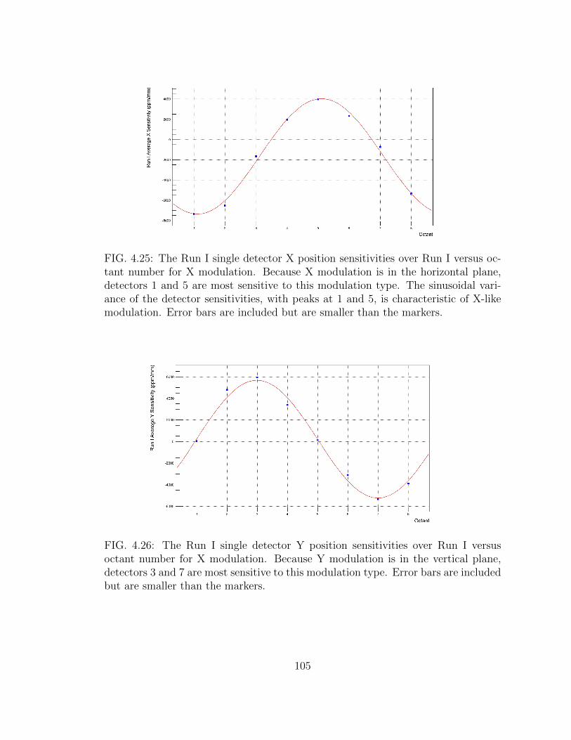
FIG. 4.25: The Run I single detector X position sensitivities over Run I versus oc-tant number for X modulation. Because X modulation is in the horizontal plane,detectors 1 and 5 are most sensitive to this modulation type. The sinusoidal vari-ance of the detector sensitivities, with peaks at 1 and 5, is characteristic of X-likemodulation. Error bars are included but are smaller than the markers.

FIG. 4.26: The Run I single detector Y position sensitivities over Run I versusoctant number for X modulation. Because Y modulation is in the vertical plane,detectors 3 and 7 are most sensitive to this modulation type. Error bars are includedbut are smaller than the markers.

105

FIG. 4.27: The Run I single detector energy sensitivities over Run I versus octantnumber for E modulation. Ideally, a change in energy should be seen as a change inQ2 and effect each detector uniformly. The expected response would be a detectormonopole. Error bars are included but are smaller than the markers.

The extracted detector sensitivities were studied at the runlet scale - “runlet”

for modulation data is a different unit than mentioned above and corresponds to

approximately half a full run - slug, and Wien levels. The detector sensitivities, if

properly determined, should be a property of the detector apparatus and therefore

should be static. Studying the detector sensitivities at longer time scales allows

us to reduce the statistical noise and determine both the stability of the extracted

sensitivities and the time scale on which it is most appropriate to apply corrections to

the asymmetry. Shown in Fig. 4.28 - 4.32 are the Slug-average detector sensitivities

for Run I, weighted by the main detector error. The extracted detector sensitivities

for each beam parameter on the Wien level are shown in Table 4.7. Aside from the

occasional outlier, the Slug-level sensitivities are generally stable. One aspect where

there does seem to be a shift in the sensitivities is bpm3c12X; starting after Slug

106

100 the sensitivity starts to drift.

FIG. 4.28: Run I Slug-average Set 1 X sensitivities.

FIG. 4.29: Run I Slug-average Set 1 X′ sensitivities.

107

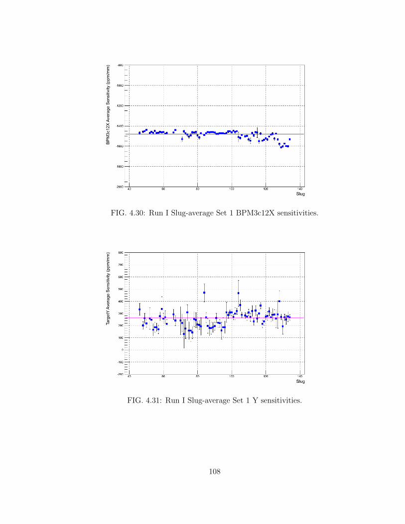
FIG. 4.30: Run I Slug-average Set 1 BPM3c12X sensitivities.

FIG. 4.31: Run I Slug-average Set 1 Y sensitivities.

108

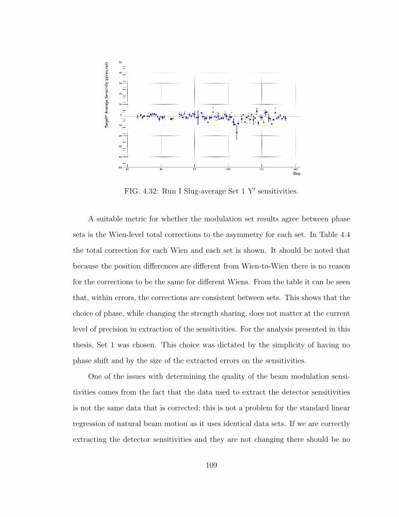
FIG. 4.32: Run I Slug-average Set 1 Y′ sensitivities.

A suitable metric for whether the modulation set results agree between phase

sets is the Wien-level total corrections to the asymmetry for each set. In Table 4.4

the total correction for each Wien and each set is shown. It should be noted that

because the position differences are different from Wien-to-Wien there is no reason

for the corrections to be the same for different Wiens. From the table it can be seen

that, within errors, the corrections are consistent between sets. This shows that the

choice of phase, while changing the strength sharing, does not matter at the current

level of precision in extraction of the sensitivities. For the analysis presented in this

thesis, Set 1 was chosen. This choice was dictated by the simplicity of having no

phase shift and by the size of the extracted errors on the sensitivities.

One of the issues with determining the quality of the beam modulation sensi-

tivities comes from the fact that the data used to extract the detector sensitivities

is not the same data that is corrected; this is not a problem for the standard linear

regression of natural beam motion as it uses identical data sets. If we are correctly

extracting the detector sensitivities and they are not changing there should be no

109

Wien/Set Set 1 (ppb) Set 2 (ppb) Set 3 (ppb) Set 4 (ppb)Wien 1 -15.9 ± 7.2 -12.8 ± 7.4 -15.9 ± 7.1 -11.2 ± 6.5Wien 2 10.0 ± 4.3 5.4 ± 4.4 10.1 ± 4.3 14.4 ± 3.9Wien 3 -7.7 ± 5.5 -7.8 ± 5.5 -7.5 ± 5.5 -10.9 ± 5.1Wien 4 -26.8 ± 5.4 -27.9 ± 5.3 -26.9 ± 5.4 -27.3 ± 5.0Wien 5 -17.6 ± 6.6 -18.9 ± 6.5 -17.6 ± 6.7 -16.7 ± 6.1

TABLE 4.4: Wien level total corrections for each modulation Set.

problem correcting non-modulation data using beam modulation data, however as

a proof-of-principle diagnostic it is preferable to first look at a more straightforward

problem. The simplest diagnostic available is to confirm that the extracted detector

sensitivities effectively correct the beam modulation yield response from which they

were extracted. The yield response to modulation was corrected according to,

Ycorrected = Yraw −5∑i=1

1

〈Y 〉〈 ∂Y∂Xi

〉(X − 〈X〉). (4.15)

Yraw is the uncorrected detector yield response to modulation of a given modulation

type, and 〈 ∂Y∂Xi〉 are the Wien-average detector sensitivities. The yield response

study was done using the Set 1 Wien-average detector sensitivities to correct the

Run I data set. Before and after correction, the Wien-average yield response for

each detector was plotted versus octant for both sine and cosine components. The

sine(cosine) components for each detector were extracted by fitting to a composite

equation of the form,

Y (θ) = Y + Asin sin(αxoct + φset) + Acos cos(αxoct + φset). (4.16)

Here φset represents the phase setting for the modulation set that is used; in

the case of this study this was Set 1(φ = 0). The results of the uncorrected yield

response to modulation can be seen in Fig. 4.33 - 4.37. In these plots the results

110

from the composite fit in Eq. 4.16 can be seen for each detector fitted to a simple

sine function with a floating phase.

FIG. 4.33: Uncorrected yield response dipole to X modulation.

FIG. 4.34: Uncorrected yield response dipole to X′ modulation.

111

FIG. 4.35: Uncorrected yield response dipole to E modulation.

FIG. 4.36: Uncorrected yield response dipole to Y modulation.

112

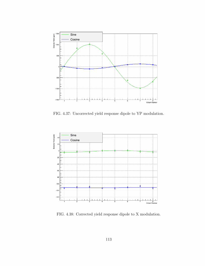
FIG. 4.37: Uncorrected yield response dipole to YP modulation.

FIG. 4.38: Corrected yield response dipole to X modulation.

113

FIG. 4.39: Corrected yield response dipole to X′ modulation.

FIG. 4.40: Corrected yield response dipole to E modulation.

114

FIG. 4.41: Corrected yield response dipole to Y modulation.

FIG. 4.42: Corrected yield response dipole to YP modulation.

All results are normalized by the average detector signal during a given run to

115

make the results more interpretable. In some cases - particularly Y modulation -

the cosine component is shown to be comparable in size to the sine component. One

obvious exception is during energy modulation when in fact there should be no cosine

component. Recall that the energy feedback was disabled during energy modulation,

therefore according to our model for the FFB interacting with the modulation, there

should be no cosine component. There is, in-fact, a small cosine component that

shows up in the fit, however it is small compared to the sine component (O(x20)

smaller). The corrected yield response for each modulation type can be seen in Fig.

4.38 - 4.42.

A summary table of the results for both the corrected and uncorrected fits of

the monopole and the dipole can be found in Tables 4.5 and 4.6. The detector

dipole is a product of the fact that certain detectors are more sensitive to different

modulation due to their spatial orientation; detectors 1 and 5 for instance, because

they lie directly in the X plane, are more sensitive to X-modulation. By plotting the

individual detector response as a function of octant, we expect to see a sinusoidal

response with peaks at the detectors lying in the plane of modulation. The dipole

describes the average detector response. The dipole response of the detectors is

removed to 1σ in all but one case; the one exception is the sine component of the X

dipole where the result is only non-zero at the 1.9σ level, i.e. not clearly significant.

The essential flattening of the yield response using the Wien-average sensitivities is

a good indicator that, at the fundamental level, the extraction of the sensitivities

is being done correctly; the sensitivities are suppressed by more than 2 orders of

magnitude. The change in the detector response monopole is less straight forward.

The monopole represents the octant-independent response of the detectors in the

same direction during the ∆X caused by the modulation. The correction should

remove the change regardless of the direction of the change resulting in a monopole

116

of zero. Referring to Table 4.5, you can see that the monopole of the sine component

- which is exceptionally large in the case of E for instance - is removed within errors.

The cosine monopole, however, follows no discernible trend. Before correction, the

monopole for each modulation type varies from small to very large. Once corrected,

they show little change and in fact get larger in some cases. The general model

to explain the monopole is that it is caused by changes in the backgrounds seen

in the detectors, however the fact that only the sine component is corrected and

the cosine seems random is not understood. The current model for this production

of the monopole involves interaction of the beam halo with parts of the beamline,

for instance the W-plug. Consider the beam halo as it passes through the W-plug,

when the beam is modulated the halo, which is at a greater radius than the beam

diameter, interacts with edges of the plug creating a background “glow” in the hall.

Because the amount of interaction is tied directly to the modulation, the detectors

see a beam position correlated background which affects all detectors equally.

Mod Type Sine (Raw) Sine (Corrected) Cosine (Raw) Cosine (Corrected)X -31.7 ± 0.9 -1.7 ± 1.0 -108.9 ± 1.0 -111.4 ± 1.0X′ 1.0 ± 0.9 -0.2 ± 1.0 -60.6 ± 1.0 -22.1 ± 1.0E(3c12X) 577.6 ± 0.9 1.1 ± 0.9 -3.4 ± 1.0 25.5 ± 1.0Y -10.7 ± 0.9 0.4 ± 0.9 -27.7 ± 1.0 -15.2 ± 1.0Y′ 19.6 ± 0.9 0.8 ± 1.0 12.1 ± 1.0 13.6 ± 1.0

TABLE 4.5: Detector yield monopole in ppm before and after correction using Wienaverage modulation sensitivities.

False asymmetry present in the raw data causes the width of the asymmetry

to become wider than the statistical width; correction of the raw asymmetry using

beam modulation or linear regression should remove noise induced by the position

sensitivities and reduce the asymmetry width. In the case of the linear regression, be-

cause the corrections are made to the data from which the sensitivities are extracted,

117

Mod Type Sine (Raw) Sine (Corrected) Cosine (Raw) Cosine (Corrected)X 1248.9 ± 1.3 -2.7 ± 1.4 665.2 ± 1.4 -0.5 ± 1.5X′ 292.0 ± 1.3 1.1 ± 1.4 98.5 ± 1.4 -0.5 ± 1.5

E(3c12X) -412.9 ± 1.3 1.5 ± 1.4 20.4 ± 1.4 -0.2 ± 1.4Y -452.8 ± 1.3 1.3 ± 1.4 -652.6 ± 1.4 -1.0 ± 1.4Y′ 984.2 ± 1.3 -1.0 ± 1.4 -110.9 ± 1.4 0.7 ± 1.5

TABLE 4.6: Detector yield dipole response in ppm before and after correction usingWien average modulation sensitivities.

DOF/Wien X X′ 3c12X Y Y′

Wien 1 -1687.6 ± 18.5 81.4 ± 0.8 -1462.3 ± 2.1 173.1 ± 16.7 0.3 ± 0.4Wien 2 -1719.4 ± 20.0 81.3 ± 0.8 -1480.7 ± 3.7 214.5 ± 17.3 -1.1 ± 0.6Wien 3 -1670.5 ± 18.5 80.6 ± 0.9 -1471.9 ± 3.4 232.9 ± 18.5 -2.3 ± 1.2Wien 4 -1630.0 ± 15.6 82.2 ± 0.7 -1485.1 ± 4.8 295.2 ± 7.8 -3.9 ± 0.8Wien 5 -1681.6 ± 15.2 82.8 ± 0.8 -1542.8 ± 3.7 274.3 ± 12.3 -2.1 ± 0.6

Run I Avg. -1673.8 ± 7.7 81.8 ± 0.4 -1480.6 ± 1.4 264.1 ± 5.5 -1.1 ± 0.3

TABLE 4.7: Wien-level sensitivities for the main detector system. The Run I valuerepresents the error weighted average of each Wien-level result. Positions are givenin ppm/mm and angles are given in ppm/µrad.

it is mathematically required that the widths are reduced. This is not the case for

the modulation-corrected data. While the modulation corrections are expected to

reduce the raw width, it is not a mathematical requirement since the modulation

extracted sensitivities are determined from an independent set of data. Below in

Fig. 4.43 the main detector average corrected widths, for both beam modulation

and linear regression Set 11 corrected asymmetries, are shown. The Set 11 linear

regression set uses the same independent variables as the beam modulation. The

beam modulation corrections were done using Wien-averaged sensitivities and the

LRB corrections were done using both quartet and the Wien-average sensitivities.

Both the linear regression and the modulation corrections are shown to reduce

the asymmetry width. The greatest width reduction comes from the quartet-level

linear regression corrections, but all methods had a positive effect on the asymmetry

118

FIG. 4.43: The slug average detector widths are shown for raw, corrected via mod-ulation, LRB, and wien average LRB for slugs 42- 59. The maximum reduction inwidth is achieved using the quartet level LRB sensitivities.

width. The fact that the width reduction due to the Wien-average LRB sensitivities

is worse than the quartet level corrected widths is suggestive of a hidden variable.

An argument could be made that the sensitivities are changing with time and there-

fore the Wien average corrections are wrong, however this seems unlikely given the

stability of the beam-modulation extracted sensitivities. As a note, changing values

of the slug average widths are expected due to changing beam properties during

each slug; a run period such as slug 49 could simply be due to a section of time with

unusually large position differences. The average beam current during Run 1 was

156 µA and the main detector current weighted rate was ∼4.4 MHz/µA[58]. This

implies that the combined detector width due to counting statistics alone should be

O(209) ppm per 4 ms quartet. The remaining noise is likely due to other sources

of noise such as beamline backgrounds, detector energy resolution, BCM resolution,

and target boiling, among others.

119

DOF/Wien X X′ (x10−2) 3c12X Y Y′ (x10−2)Wien 1 1.1 ± 1.9 -18.4 ± 4.2 1.4 ± 1.2 18.7 ± 1.5 81.3 ± 5.1Wien 2 11.1 ± 1.1 -14.5 ± 3.3 -29.9 ± 1.0 -11.7 ± 1.1 41.7 ± 3.7Wien 3 -20.6 ± 1.5 -70.3 ± 4.1 -6.8 ± 0.9 -7.3 ± 1.5 -37.2 ± 4.5Wien 4 2.0 ± 1.4 7.8 ± 4.1 8.4 ± 0.9 -20.9 ± 1.1 -40.6 ± 3.8Wien 5 3.5 ± 1.5 13.6 ± 4.5 14.2 ± 0.9 -6.4 ± 1.2 -36.4 ± 4.2

TABLE 4.8: Wien-Average Position Difference for Run I after 6σ cut. Positions aregiven in nm and angles are given in nrad.

4.1.5 Residual Correlations

As discussed above it is important to understand how well the corrections that

are being applied to the data are removing the detector sensitivities. Study of the

yield corrections shows that, while to first order the corrections are doing what they

are intended, i.e. correcting the sinusoidal component of the detector response to

beam motion, there are still unexplained effects such as monopoles left in the de-

tector response. Effects such as charge non-linearities, beam halo, and beamline

background effects can contribute to the detector signal as hidden variables. It is

important to understand the degree to which these and other effects contribute to

the corrected asymmetry in the form of residual correlations. This was studied by

looking at the correlation of the corrected asymmetry to each independent variable

on the Wien level over Run I. Studying this on the Wien level was done to take

advantage of cancellations resulting from the IHWP flips and averaging out of sta-

tistical noise. Table 4.9 shows the results of the study for each Wien in terms of

the residual correlation of corrected main detector asymmetry to each DOF. The

results show that, at least on the Wien level, the residual correlations are . 2 σ.

Due to this no additional correction was applied to the final asymmetry.

120

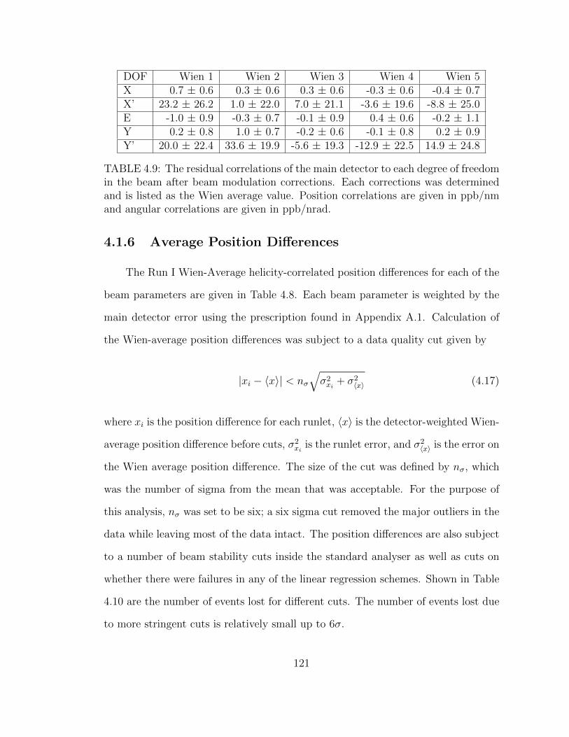
DOF Wien 1 Wien 2 Wien 3 Wien 4 Wien 5X 0.7 ± 0.6 0.3 ± 0.6 0.3 ± 0.6 -0.3 ± 0.6 -0.4 ± 0.7X’ 23.2 ± 26.2 1.0 ± 22.0 7.0 ± 21.1 -3.6 ± 19.6 -8.8 ± 25.0E -1.0 ± 0.9 -0.3 ± 0.7 -0.1 ± 0.9 0.4 ± 0.6 -0.2 ± 1.1Y 0.2 ± 0.8 1.0 ± 0.7 -0.2 ± 0.6 -0.1 ± 0.8 0.2 ± 0.9Y’ 20.0 ± 22.4 33.6 ± 19.9 -5.6 ± 19.3 -12.9 ± 22.5 14.9 ± 24.8

TABLE 4.9: The residual correlations of the main detector to each degree of freedomin the beam after beam modulation corrections. Each corrections was determinedand is listed as the Wien average value. Position correlations are given in ppb/nmand angular correlations are given in ppb/nrad.

4.1.6 Average Position Differences

The Run I Wien-Average helicity-correlated position differences for each of the

beam parameters are given in Table 4.8. Each beam parameter is weighted by the

main detector error using the prescription found in Appendix A.1. Calculation of

the Wien-average position differences was subject to a data quality cut given by

|xi − 〈x〉| < nσ√σ2xi

+ σ2〈x〉 (4.17)

where xi is the position difference for each runlet, 〈x〉 is the detector-weighted Wien-

average position difference before cuts, σ2xi

is the runlet error, and σ2〈x〉 is the error on

the Wien average position difference. The size of the cut was defined by nσ, which

was the number of sigma from the mean that was acceptable. For the purpose of

this analysis, nσ was set to be six; a six sigma cut removed the major outliers in the

data while leaving most of the data intact. The position differences are also subject

to a number of beam stability cuts inside the standard analyser as well as cuts on

whether there were failures in any of the linear regression schemes. Shown in Table

4.10 are the number of events lost for different cuts. The number of events lost due

to more stringent cuts is relatively small up to 6σ.

121

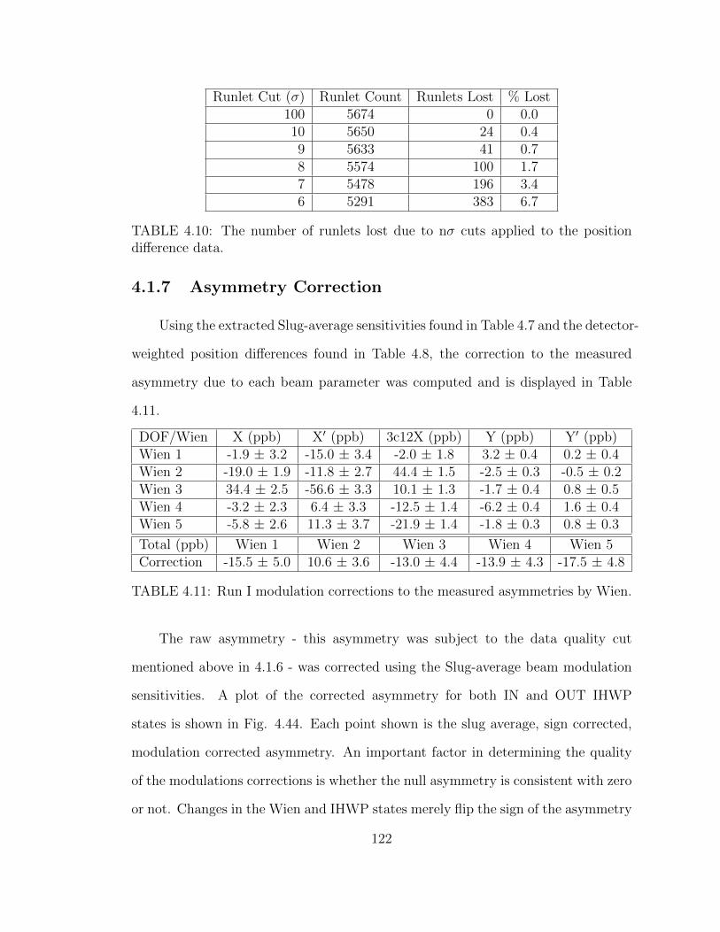
Runlet Cut (σ) Runlet Count Runlets Lost % Lost100 5674 0 0.010 5650 24 0.49 5633 41 0.78 5574 100 1.77 5478 196 3.46 5291 383 6.7

TABLE 4.10: The number of runlets lost due to nσ cuts applied to the positiondifference data.

4.1.7 Asymmetry Correction

Using the extracted Slug-average sensitivities found in Table 4.7 and the detector-

weighted position differences found in Table 4.8, the correction to the measured

asymmetry due to each beam parameter was computed and is displayed in Table

4.11.

DOF/Wien X (ppb) X′ (ppb) 3c12X (ppb) Y (ppb) Y′ (ppb)Wien 1 -1.9 ± 3.2 -15.0 ± 3.4 -2.0 ± 1.8 3.2 ± 0.4 0.2 ± 0.4Wien 2 -19.0 ± 1.9 -11.8 ± 2.7 44.4 ± 1.5 -2.5 ± 0.3 -0.5 ± 0.2Wien 3 34.4 ± 2.5 -56.6 ± 3.3 10.1 ± 1.3 -1.7 ± 0.4 0.8 ± 0.5Wien 4 -3.2 ± 2.3 6.4 ± 3.3 -12.5 ± 1.4 -6.2 ± 0.4 1.6 ± 0.4Wien 5 -5.8 ± 2.6 11.3 ± 3.7 -21.9 ± 1.4 -1.8 ± 0.3 0.8 ± 0.3

Total (ppb) Wien 1 Wien 2 Wien 3 Wien 4 Wien 5Correction -15.5 ± 5.0 10.6 ± 3.6 -13.0 ± 4.4 -13.9 ± 4.3 -17.5 ± 4.8

TABLE 4.11: Run I modulation corrections to the measured asymmetries by Wien.

The raw asymmetry - this asymmetry was subject to the data quality cut

mentioned above in 4.1.6 - was corrected using the Slug-average beam modulation

sensitivities. A plot of the corrected asymmetry for both IN and OUT IHWP

states is shown in Fig. 4.44. Each point shown is the slug average, sign corrected,

modulation corrected asymmetry. An important factor in determining the quality

of the modulations corrections is whether the null asymmetry is consistent with zero

or not. Changes in the Wien and IHWP states merely flip the sign of the asymmetry

122

in the data, because different states should measure the same physics, looking at

the difference between the IN and OUT state data is a useful way to gain insight

into the quality of the correction being applied and find hints of potential hidden

variables. After modulation correction the null asymmetry was found to be -25.51

± 13.54 ppb which is not significantly non-zero. The slug-average asymmetry values

are consistent with-in errors and give an error-weighted average asymmetry for Run

I of -232.8 ± 13.54 ppb.

FIG. 4.44: The beam-modulation corrected asymmetry for both IN and OUT IHWPsettings.

123

CHAPTER 5

Systematic Uncertainties

5.1 Q2 Systematics

5.1.1 Scattering Kinematics

Precise determination of the proton’s weak-charge, Qpw, to 4% requires knowl-

edge of the four-momentum transfer, Q2, to an uncertainty of 0.5%. For the purpose

of this analysis this level of precision is not required and the Q2 determination will

be based solely on the data set defined as Wien 0.

The elastic asymmetry for Qpw kinematics is a function of Q2, thus making

precise knowledge of Q2 a prerequisite to a precise measure of Qpw; recall that

A =GF

4πα√

2[Qp

wQ2 +B(Q2)Q4], (5.1)

where GF is the Fermi constant, α is the fine-structure constant, and B(Q2) contains

contributions from the hadronic form factors. In the case of relativistic electrons

scattering elastically from the protons in the liquid Hydrogen target, the momentum

124

transfer can be written as,

Q2 = 4EE ′ sin2 θ

2. (5.2)

Here, E is the incident energy of the incoming electron, E′ is the energy of the

scattered electron, and θ is the scattering angle of the outgoing electron. Because

the Qweak kinematics are two-body elastic scattering, only two of the three variables

are required to determine Q2. With this in mind, some thought must go into choosing

the set of variables that will give us the most precise measurement. The incident

electron energy is determined by measuring the beam energy, corrected for initial-

state losses in the target, as discussed in 5.1.2, and is very well determined. The

scattering angle, θ, is determined using Region II data in conjunction with survey

data defining the geometry of the experiment. The post-scattering energy, E′, is the

least well-known of the kinematic variables. Determination of E′ requires position

and angle information from both Region II and Region III, as well as precise mapping

of the spectrometer B-field. Given that the incident energy and scattering angle are

directly measured, they present the best choice; E′ will be used as a verification of

our measurement as well as a check that the events we see are truly elastic events.

Using only the kinematic variables of interest, Q2 can be rewritten independent of

E′ as

Q2 = 2E2 (1− cos θ)

1 + EMp

(1− cos θ). (5.3)

One complication is that while we can measure both the incident beam energy and

the scattering angle, we are interested specifically in the values at the scattering

vertex. Determination of E and θ at the scattering vertex is complicated due to

external radiative effects, internal bremsstrahlung, multiple scattering, and energy

loss (dE/dx) in the target. The solution is to use simulation to handle the internal

and external processes listed above, and experimental results for the measured inci-

125

dent beam energy entering the target and scattered angle exiting the target, as well

as other relevant quantities such as calculation of the Zvertex and E′, to benchmark

the simulation. Tuning the simulation until the simulated values match the experi-

mentally measured observables allows for the extraction of E and θ at the scattering

vertex.

5.1.2 Beam Energy

The precision measurement of the beam energy in Hall C uses a set of superharps

at the entrance and exit of the Hall C arc. The superharps provide absolute beam

position determination using a 10 µm wire which is passed through the beam using

a shaft position encoder [71]. When the superharp wire passes through the beam

a signal is produced in the read-out electronics. The mean of the peak of the

output voltage distribution, when referenced to the position read-out of the encoder,

provides the position and width of the beam. The resolution of the beam position

determination is limited by the width of the superharp wire.

The absolute beam energy measurement is completed by powering only the

dipole magnets in the arc; all quadrupoles, sextupoles, and correctors are turned

off. The current in the dipole magnets is calibrated to center the electron beam

through the dipoles. Using the position measurements at the entrance and exit

of the arc, along with the results from accurate mapping of the dipole fields, the

momentum of the electron beam is computed using

E =e

Θ

∫Bdl. (5.4)

Here∫Bdl is the magnetic field integral along the beam path through the arc

and Θ is the bending angle. Using this method, absolute beam energy measure-

126

ments O(10−3) are possible [72]. Once the absolute energy scale has been set, the

quadrupoles and sextupoles are energized and correctors are used to re-center the

beam. Using a harp in the center of the arc to determine the variation in beam

position allows the relative beam energy to be determined to O(10−4).

5.1.3 Scattering Angle

The visible scattering angle, which describes the angular deviation from the

Z-axis along the beam-line, is measured primarily using the HDCs as described in

3.6.1. The HDCs, which are placed in pairs diametrically opposed to each other in

front of QTOR, have an angular scattering acceptance of 4 - 12. The signal in

the HDCs was dominated by Møller electrons and operated at a beam current of ∼

100 pA; the VDC signal at this current was completely dominated by cosmic rays.

In order to select good tracks both the HDC and VDCs were needed; good tracks

were identified as tracks with an E′ that is consistent with an elastic electron, ie. a

track can be formed between Region II and Region III through QTOR which hits

the trigger scintillator.

5.1.4 Q2

As discussed in Sec. 5.1.1 the determination of the acceptance-averaged effective

momentum transfer, 〈Q2〉tree, is computed according to the method found in [73],

and depends on the incident beam energy at the scattering vertex and the effective

scattering angle (see Eq. 5.3). The final 〈Q2〉tree is computed using GEANT4 and

is benchmarked using the tracking data. This is an important step because the

experiment cannot directly measure the scattering energy and angle at the vertex.

The incident beam energy is well known, however what is needed for determination

127

of 〈Q2〉tree is the incident energy at the scattering vertex. This is computed using

GEANT4 to account for energy losses in the target. The energy at the vertex is

then computed using

Evertex = 〈Ebeam −dEbeam

dZ∆Z〉. (5.5)

Here, Ebeam is the incident beam energy on the target and ∆Z is the distance trav-

elled through the target before scattering. The Run I beam energy was computed

to be

Evertex = 1155± 3 MeV. (5.6)

At the time of writing the analysis of the Run I acceptance averaged momentum

transfer was still in-progress. For this reason, the Wien 0 value was used. The Wien

0 tree level momentum transfer was found to be [36]

〈Q2〉simtree = 0.0250± 0.0006 (GeV/c)2. (5.7)

The effective scattering angle can be computed using the vertex values for the mo-

mentum transfer and incident beam energy, calculated above, along with Eq. 5.3.

〈θeff〉 = 7.90± 0.30 (5.8)

5.2 Backgrounds

Precise extraction of the physics asymmetry requires understanding of the back-

grounds which dilute the detector signal and give false asymmetries. The signal

dilution due to backgrounds is the fractional contribution of the total signal that

128

comes from background processes and is defined by

fbg =Ybg

Ybg + Ysignal

. (5.9)

The total contribution to the measured asymmetry can be written as

Ameasured = P [(1− Σifibg)Aphysics + Σif

ibgA

ibg]. (5.10)

In order to remove the background contributions, both the signal dilution and the

background asymmetry must be measured or estimated. Background contributions

from the Aluminium target windows, soft backgrounds, inelastic background con-

tributions, and neutral backgrounds are discussed in more detail below.

5.2.1 Aluminium Target Window Background

Electrons scattering from the primary target interact, not only with the lH2 in

the target, but also with the upstream (US) and downstream (DS) target windows.

The effects on the measured asymmetry due to scattering from the target windows

comes in two parts: the asymmetry of electron-aluminium scattering and a dilution

of the measured signal in the detectors. Both of these effects were extracted using

stand-alone measurements which are explained in more detail below.

5.2.2 Aluminium Target Asymmetry

In the same way as electron scattering from hydrogen, scattering from the

target windows produces a measurable parity-violating asymmetry in the detectors.

The scattering from the target windows leads to a ' 30% correction to the physics

asymmetry during extraction from the measured value and is the largest correction

129

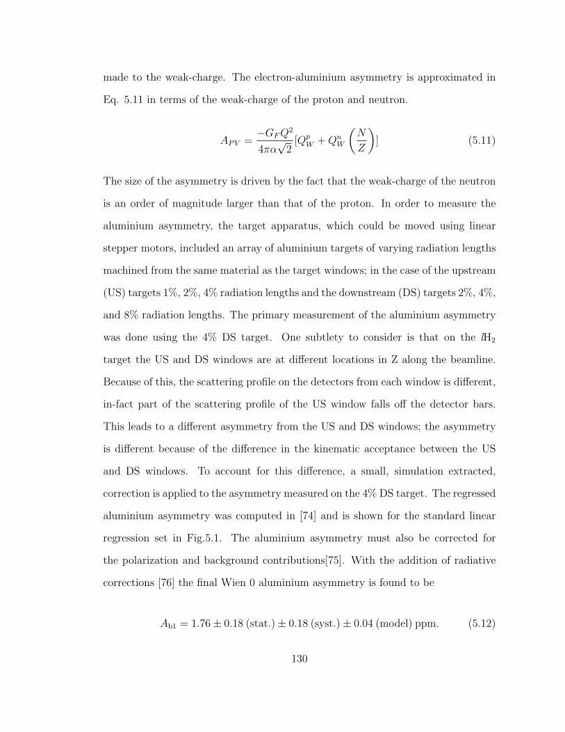
made to the weak-charge. The electron-aluminium asymmetry is approximated in

Eq. 5.11 in terms of the weak-charge of the proton and neutron.

APV =−GFQ

2

4πα√

2[Qp

W +QnW

(N

Z

)] (5.11)

The size of the asymmetry is driven by the fact that the weak-charge of the neutron

is an order of magnitude larger than that of the proton. In order to measure the

aluminium asymmetry, the target apparatus, which could be moved using linear

stepper motors, included an array of aluminium targets of varying radiation lengths

machined from the same material as the target windows; in the case of the upstream

(US) targets 1%, 2%, 4% radiation lengths and the downstream (DS) targets 2%, 4%,

and 8% radiation lengths. The primary measurement of the aluminium asymmetry

was done using the 4% DS target. One subtlety to consider is that on the lH2

target the US and DS windows are at different locations in Z along the beamline.

Because of this, the scattering profile on the detectors from each window is different,

in-fact part of the scattering profile of the US window falls off the detector bars.

This leads to a different asymmetry from the US and DS windows; the asymmetry

is different because of the difference in the kinematic acceptance between the US

and DS windows. To account for this difference, a small, simulation extracted,

correction is applied to the asymmetry measured on the 4% DS target. The regressed

aluminium asymmetry was computed in [74] and is shown for the standard linear

regression set in Fig.5.1. The aluminium asymmetry must also be corrected for

the polarization and background contributions[75]. With the addition of radiative

corrections [76] the final Wien 0 aluminium asymmetry is found to be

Ab1 = 1.76± 0.18 (stat.)± 0.18 (syst.)± 0.04 (model) ppm. (5.12)

130

The Wien 0 result is used in this analysis due to the unavailability of the Run 1

results.

FIG. 5.1: Regressed aluminium asymmetry plotted versus slug for both IN and OUThalf-wave plate settings. This does not include corrections due to polarization orbackgrounds.

5.2.3 Aluminium Dilution

The dilution of the measured yield due to electron scattering from the alu-

minium windows was measured using two techniques: evacuated cell method and

gas extraction method. The easiest of the two methods is the former in which the

target cell is evacuated and the scattering signal is recorded. The cell is then refilled

and another measurement is taken. In the full condition, the liquid hydrogen works

to cool the target windows. Because the liquid hydrogen is needed for cooling, one

concern with the evacuated method was potential thermal and structural damage

131

to the windows. Because of this the measurements were done at much lower cur-

rents: 0.2 - 1.0 µA. One thing to note is that there were several hours between the

evacuated and full measurements due, in part, to the time required to refill and cool

the target. In order to eliminate potential errors in the measurement due to time

dependent changes, and BCM calibration uncertainties, a reference target, the yield

from which should not change over time, was used to normalize both measurements:

Rnormempty =

Rempty

Rreference

, Rnormfull =

Rfull

Rreference

(5.13)

A 0.5% radiation length carbon target, located on the DS target ladder, was used

as a reference. The dilution factor is the ratio of Rnormempty/Rnorm

full . As before, con-

tributions from the US and DS windows must be treated separately. The process

of applying the radiative corrections is guided by studies of aluminium targets of

different thickness and simulations. The Run I dilution factor can be seen in Fig.5.2

for opposing octants. A discrepancy of ∼2.4% can be seen between the normalized

and unnormalized measurements which is attributed to the difference in reference

target yields [77]. The final extracted dilution, including corrections [78], is given

by

fb1 = 0.03226± 0.0001 (stat.)± 0.0004 (syst.)± 0.0021 (model) (5.14)

The gas extraction method uses gaseous hydrogen in the target at different pres-

sures to determine the signal in the detectors versus pressure. By extrapolating to

zero pressure, the empty target signal can be determined, allowing for the extraction

of the dilution factor. While this method of measurement serves as a check on the

evacuated method, it is not the cleanest method of extraction. Uncertainties such

132

FIG. 5.2: The Run I Dilution for opposing octants is shown for both normalizedand unnormalized cases. The discrepancy between with and without normalisationis attributed to a difference in the reference target yields.

as local density changes due to heating, electronic deadtime, radiative corrections

due to the addition of hydrogen to the target cell, and BCM linearity between the

gas and full states make this not the optimal approach.

5.2.4 Beamline Background

The beamline background encompasses low energy events hitting the main de-

tectors not originating from elastic scattering in the target. Possible sources in-

clude: showers from the collimator and shield wall, octant-to-octant cross-talk, and

beamline scattering. These background sources, while somewhat smaller than the

Aluminium target window background, are an important contribution to the mea-

sured asymmetry. In general, much of this is suppressed via shielding and the lead

pre-radiators installed directly in front of the main detectors and the tungsten plug

133

which was installed in the downstream side of the first collimator. The pre-radiators

are effective at suppressing low energy events entering the detectors while also in-

creasing the size of the elastic events from the target.

5.2.5 Beamline Background Dilution

Measurement of the beamline background dilution was done using a blocked

octant technique. In order to eliminate line-of-site from the target events, 3” of lead

was installed directly downstream of the defining collimator in octant 7. Blocking

the octant allowed for a measurement of background dilution as the ratio of the

blocked signal to the unblocked total signal. Blocked octant measurements were

taken in May 2011 at two QTOR currents, 8921 A and 6700 A (inelastic), and

on both the lH2 and 4% DS aluminium targets. A more detailed discussion of

the blocked octant study can be found in K. Meyers thesis [8] and Wade Duvall’s

analysis summary[79]. The results of the blocked octant study give an upper bound

on the beamline dilution of

fb3 = 0.00218± 0.00064. (5.15)

The average of the blocked octant data, including good and bad halo periods, was

used in previous analyses. Due to the increased correlation between the main detec-

tors and the background monitors described below it was decided that a conservative

estimate on the Run I dilution was more appropriate. The value used is based on

values extracted from bad halo data. This is expected to be an upper bound due

to the fact that significant increases would mean significantly more beam being

dumped into the tungsten plug, accompanied by increased temperatures in the plug

readings, and frequent beam trips[80]. This is not something that was observed.

134

Beamline Background Asymmetry

The asymmetry contribution due to beamline background sources was deter-

mined using results from the blocked octant study [79], however it was not done

directly. The blocked octant study was completed near the end of Run II data tak-

ing and there was no analogue in Run I. Because of this and the fact that the MD9

background detector was moved during Run II the USLUMIs are used as a common

element between the runs to indirectly measure the beamline background outside

of the blocked octant study. The details of how this is done can be found in Mark

Pitt’s log entry [81]. According to the blocked octant study analysis the following

relationships can be derived.

AMDunblocked = 0.0018× AMD

blocked (5.16a)

AMD9unblocked = 0.094× AMD9

blocked (5.16b)

AMDunblocked = (

fMD

fMD9

)(AMD

blocked

AMD9blocked

)AMD9unblocked (5.16c)

AMDunblocked = 0.044× AMD9

unblocked (5.16d)

Here the coefficient in Eq.5.16b and 5.16c gives the measured dilution factor and

Eq.5.16d gives the relation between the unblocked detector signals in terms of the

dilution factors and the measured blocked octant values. Physically, Eq.5.16d gives

the ratio of the background asymmetry contributions in terms of MD and MD9.

This is tied to the USLUMI by looking at the ratio of the asymmetries between

MD9 and the USLUMI during Run I.

AMD9unblocked = 0.626× AUSLUMI

unblocked (5.17)

135

Putting Eq. 5.16d and 5.17 together we get

AMDunblocked = (0.0276± 0.0276)× AUSLUMI

unblocked. (5.18)

An error bar of 100% has been assigned due to uncertainties in the fraction of the

signal seen in MD9 that is from beamline background. Using this relationship the

average beamline asymmetry was determined to be

Ab3 = 10.94± 10.95 ppb. (5.19)

5.2.6 Inelastic Background

The inelastic background is from inelastic scattering events, dominantly from

the nuclear N → ∆ transition, which fall into the experimental acceptance of the

main detectors. The inelastic asymmetry was expected to be O(10) larger that

than the elastic asymmetry, however the fraction of inelastic events in the detectors

to that of the elastic events makes the total contribution to the total asymmetry

relatively small. Measurement of the inelastic asymmetry was done by changing

the QTOR current to a value that maximized the inelastic signal in the detectors;

according to simulation (Fig. 5.3) this was 6700 A. By changing the QTOR current

from 8921 A to 6700 A the fractional contribution of inelastic to elastic events was

increased O(100) [13]. The inelastic asymmetry was found to be [13]

Ab4 = 3.02± 0.97 ppm. (5.20)

136

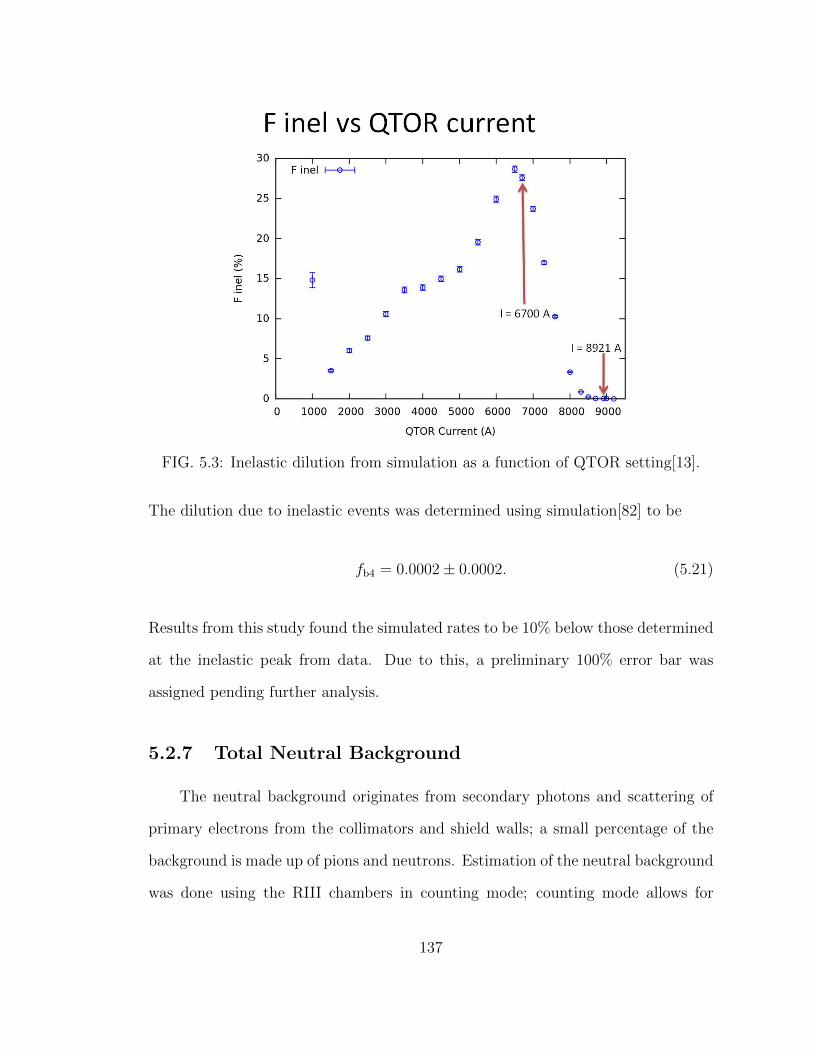
FIG. 5.3: Inelastic dilution from simulation as a function of QTOR setting[13].

The dilution due to inelastic events was determined using simulation[82] to be

fb4 = 0.0002± 0.0002. (5.21)

Results from this study found the simulated rates to be 10% below those determined

at the inelastic peak from data. Due to this, a preliminary 100% error bar was

assigned pending further analysis.

5.2.7 Total Neutral Background

The neutral background originates from secondary photons and scattering of

primary electrons from the collimators and shield walls; a small percentage of the

background is made up of pions and neutrons. Estimation of the neutral background

was done using the RIII chambers in counting mode; counting mode allows for

137

the detection of single events. Neutral events detected in the RIII chambers pass

through both the trigger scintillator and the main detectors. Both of these are

relatively insensitive to neutral events, however interactions such as neutron capture

and Compton scattering, while being below the threshold of detection in the trigger

scintillator, may shower in the pre-radiator or interact in the fused silica and cause

a signal in the MDs. These events can be classified by the amount of light they

produce. In this way, the neutral background fraction is defined by

nf =MDneutral × 〈Yneutral〉MDtotal × 〈Ytotal〉

. (5.22)

Here MDneutral is the number of detected neutral tracks and Yneutral is the light yield

from those tracks. The neutral fraction is formed as the ratio of this product for

neutral tracks versus all tracks. This analysis was done for each detector octant at

nominal QTOR current. An in-depth look at this measurement can be found in [5].

The total neutral dilution was found to be

fTotalNeutral = 0.0038± 0.0014(stat.)± 0.0011(syst.). (5.23)

This dilution due to the neutral background is calculated by removing the

beamline background dilution from the total neutral background,

fb2 = fTotal Neutral − fb3

fb2 = 0.00162± 0.00191

(5.24)

The neutral background asymmetry is approximated based on the assumption

that the source of the neutral background is primarily Møller scattering from scrap-

ing on the collimator edges and shield wall apertures. With this in mind, it is

138

reasonable to approximate the asymmetry as being 0.00 with an uncertainty on the

order of our asymmetry measurement. Therefore a conservative neutral background

asymmetry was adopted to be

Ab2 = 0.00± 0.20 ppm. (5.25)

5.2.8 Experimental Bias Corrections

Experimental bias encompass corrections due to electromagnetic radiative cor-

rections, detector bias, acceptance, and bias in defining the central Q2. Each of

these corrections is applied to the measured asymmetry independently, along with

the other corrections listed in this chapter, to determine the physics asymmetry. The

first of these, radiative corrections (RRC), is due to radiative effects associated with

the incident electrons which modify the asymmetry that expected at tree-level. Cor-

rections are made for leading order electromagnetic effects such as Bremsstrahlung

and virtual photons both internal and externally to the field of the scattering nu-

cleus. GEANT3 was used to simulate the scattering process both with and without

radiative corrections. The experimental bias correction is then defined to be[36]

RRC =RTree

RRC−Sim

= 1.0096± 0.0065. (5.26)

The detector bias (Rdet) deals with the light weighting of the main detectors.

Scattered electrons distributed over the Cerenkov bar produce light, the yield of

which is measured and used to compute the measured asymmetry. The light yield

however varies spatially over the bar and requires a light weighting correction to

accurately compute the asymmetry. Using simulation, the detector bias correction

139

is computed as[36]

RDet =ASim

NoBias

ASimBias

= 0.987± 0.007. (5.27)

The acceptance bias (RAcc) is related to the way in which the asymmetry is

extracted with respect to the momentum transfer. The experimental asymmetry

measured by experiment is given as 〈A(Q2)〉, however what is needed to compare to

theoretical predictions is A(〈Q2〉). In order to correct for this, simulation is used to

determine the correction given by[36]

RAcc =A(〈Q2〉)〈A(Q2)〉

= 0.98± 0.01. (5.28)

The final correction (RQ2) relates to the uncertainty to which the central Q2 is

known[36].

RQ2 = 1.00± 0.03 (5.29)

Considering all the bias corrections the final correction is applied as

RTotal = RRCRDetRAccRQ2 = 0.9765± 0.0323 (5.30)

5.3 Beam Polarization

5.3.1 Møller Polarimetry

Run I polarization results were computed using the Hall C Møller polarimeter.

Discussion of the hardware and operational aspects of the Møller polarimeter can be

found in Section 3.3. Møller measurements, which were invasive to regular experi-

mental operation, were carried out at low currents (1 µA) on average about three

times weekly. Each measurement consisted of three measurements in each half-wave

140

plate setting.

One of the more problematic issues of the Run I analysis was due to failures in

the Q3 quad. During Run I it was found that this quad exhibited a time-dependent

field deterioration which required perpetual retune of the Møller and re-steering of

the beam to avoid scraping. The source of the problem was found to be a short in

the Q3 quad which reduced the effective magnet current to ∼2/3 the nominal value,

which in turn affected the analysing power. Currently, it is estimated that the effect

on the analysing power could be up to 1.4%. At the moment, work is in progress

to determine the total systematic effect which, due to its time dependent nature,

must be handled on a case-by-case basis. A list of the current best estimates of

systematic errors is shown in Table. 5.1.

The slug average polarization values over Run I can be seen in Fig. 5.4. Given

that the polarization over Run I was not stable, the decision was to apply the

polarization correction on the slug level; different methods of averaging and applying

the polarization were investigated [83] to determine the best approach. The slug-

average polarization values are listed below in Table 5.2.

141

Source Error Scale pt-to-ptBeam Position X 0.17 — 0.17Beam Position Y 0.28 — 0.28Beam Direction X 0.10 — 0.10Beam Direction Y 0.10 — 0.10Q1 Current 0.07 — 0.07Q3 Current 0.05 — 0.05Q3 Position 0.10 0.10 —Multiple Scattering 0.01 0.01 —Levchuk Effect 0.33 — 0.33Collimator Positions 0.03 0.03 —Target Temperature 0.14 0.14 —B-field Direction 0.14 0.14 —B-field Strength 0.03 0.03 —Polarization in Fe 0.25 0.25 —Electronic D.T. 0.05 0.05 —Solenoid Focusing 0.21 0.21 —Solenoid Position 0.23 0.16 0.16High Current Extrap. 0.50 0.35 0.35Polfac Nominal Value 0.65 0.65 —Polfac Variation 0.23 — 0.23Monte Carlo Stats. 0.15 0.15 —Total 1.09 0.93 0.57

TABLE 5.1: Systematic errors associated with the Møller measurement.

142

Slug Polarization Error45 0.8826 0.010750 0.8889 0.010753 0.8866 0.010855 0.8815 0.010877 0.8896 0.010690 0.8835 0.010694 0.8799 0.010696 0.8873 0.010898 0.8402 0.0107101 0.8597 0.0108103 0.8625 0.0106105 0.8656 0.0107112 0.8563 0.0107115 0.8453 0.0107117 0.8570 0.0107119 0.8541 0.0107122 0.8537 0.0108124 0.8672 0.0106126 0.8677 0.0108129 0.8639 0.0108132 0.8577 0.0108

TABLE 5.2: Individual beam polarization measurements during Run I.

143

FIG. 5.4: Measured average polarization by slug for Run I data.

144

CHAPTER 6

Results and Discussion

6.1 e+p Asymmetry Results

The following section provides an overview of the calculation of the final asym-

metry and extraction of the proton’s weak-charge. The raw asymmetry following

data quality cuts is given by 〈Araw〉 = -243.22 ± 13.32 (stat.) ppb. After correc-

tion for false asymmetries using the beam modulation sensitivities, the corrected

asymmetry is 〈AReg〉 = -232.08 ± 13.53 (stat.) ppb. The asymmetry also includes a

blinding factor of ± 60 ppb which was added to eliminate personal bias from the ex-

perimental analysis. The blinding factor was applied in the analyser to each quartet

of data. A different blinding factor was used for each run period of the experiment

and will only be removed after the physics analysis is finished. This blinding factor

was not folded into the error breakdown presented below, but was added in the final

determination at the end. As discussed in detail in Sec. 5.2, the asymmetry must

be corrected for backgrounds and experimental bias. A summary of the background

corrections can be seen in Tab. 6.1 and Fig. 6.1 shows the change in the asymmetry

145

Background Dilution(fi) Asymmetry (Ai) ppmAl Window (b1) 0.0282 ± 0.0021 1.1472 ± 0.0654QTOR Transport (b2) 0.0016 ± 0.0019 0.0 ± 0.2Beamline Background (b3) 0.0022 ± 0.0006 -0.0109 ± 0.0109N→ ∆ (b4) 0.0002 ± 0.0002 -3.02 ± 0.97

TABLE 6.1: The asymmetry and associated dilution for each background source.

after correction using beam modulation and polarization, the size of the background

corrections, and the final corrected asymmetry. The corrections were applied to the

measured asymmetry after modulation correction according to

Aphysics = Rtotal

Amsr

P−

n∑i=1

fiAi

(1−n∑i=1

fi)(6.1)

where fi and Ai are the dilution and asymmetries for each background respectively

and Rtotal is the total experimental bias correction. The asymmetry, Amsr, represents

the beam modulation corrected asymmetry and the beam polarization is given by

P.

The systematic error contribution from each background is calculated using

standard error propagation methods and is shown in detail in Appendix A.3. A

breakdown of the error contribution due to each correction, in terms of systematic

and statistical uncertainty, is shown in Table 6.2. The corrections are dominated by

Aluminium target windows, followed by polarization, and modulation corrections.

Corrections due to other background sources are relatively small.

The blinding factor addition to the error of the final asymmetry was computed

according to Appendix A.3 to be 68.52 ppb. The blinding factor, in this form,

represents a uniform distribution of error, however in order to fold it into the total

error on the asymmetry it needs to be rewritten in terms of a normal distribution.

146

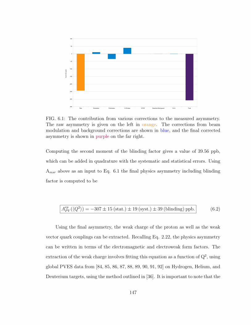
FIG. 6.1: The contribution from various corrections to the measured asymmetry.The raw asymmetry is given on the left in orange. The corrections from beammodulation and background corrections are shown in blue, and the final correctedasymmetry is shown in purple on the far right.

Computing the second moment of the blinding factor gives a value of 39.56 ppb,

which can be added in quadrature with the systematic and statistical errors. Using

Amsr above as an input to Eq. 6.1 the final physics asymmetry including blinding

factor is computed to be

AepPV (〈Q2〉) = −307± 15 (stat.)± 19 (syst.)± 39 (blinding) ppb. (6.2)

Using the final asymmetry, the weak charge of the proton as well as the weak

vector quark couplings can be extracted. Recalling Eq. 2.22, the physics asymmetry

can be written in terms of the electromagnetic and electroweak form factors. The

extraction of the weak charge involves fitting this equation as a function of Q2, using

global PVES data from [84, 85, 86, 87, 88, 89, 90, 91, 92] on Hydrogen, Helium, and

Deuterium targets, using the method outlined in [36]. It is important to note that the

147

Contributed ErrorMeasured Asymmetry(Syst.) 15.35Polarization 5.32Aluminium Asymmetry 5.54Neutral Background Asymmetry 0.33Beamline Background Asymmetry 0.02Inelastic Asymmetry 0.19Total Experimental Bias (R) 9.45Aluminium Dilution 3.65Neutral Background Dilution 0.19Beamline Background Dilution 0.19Inelastic Dilution 0.53dA(Syst.) 19.69dA(Stat. + Syst.) 23.89

TABLE 6.2: Breakdown of the systematic errors going into the final uncertainty.

electromagnetic form factors are well determined in terms of global fits [93], which

is not the case for the electroweak form factors. Instead, as is shown in Sec.2.2.3,

the electroweak form factors can be written in terms of the quark electromagnetic

form factors,

Gp,ZE = 2(2Cu1 + Cd1)Gp,γ

E + 2(Cu1 + 2Cd1)Gn,γE + ε

(0)V Gs

E (6.3)

where ε(0)V encompasses contributions from charge symmetry violation [94]. Rewrit-

ing the asymmetry in this way, the global fit becomes a function of five independent

parameters: the weak vector couplings (C1u and C1d), the strange charge radius ρs,

the strange magnetic moment µs, and the axial form factors GZ(T=1)A and G

Z(T=0)A .

The strange quark form factors are given by [95].

GsE = ρsQ

2GD, GsM = µsGD (6.4)

148

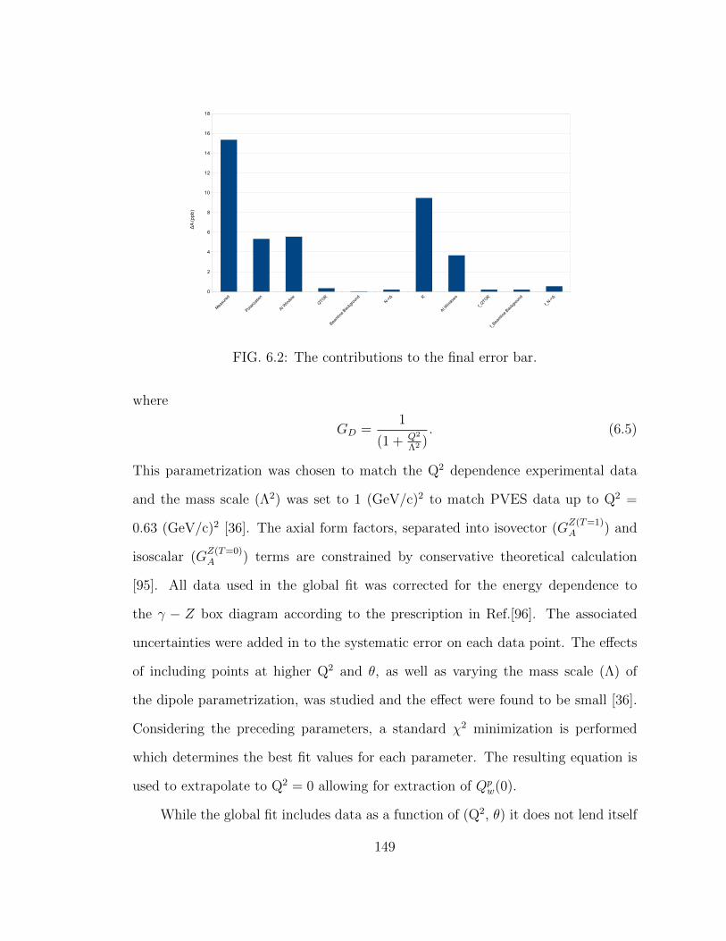
FIG. 6.2: The contributions to the final error bar.

where

GD =1

(1 + Q2

Λ2 ). (6.5)

This parametrization was chosen to match the Q2 dependence experimental data

and the mass scale (Λ2) was set to 1 (GeV/c)2 to match PVES data up to Q2 =

0.63 (GeV/c)2 [36]. The axial form factors, separated into isovector (GZ(T=1)A ) and

isoscalar (GZ(T=0)A ) terms are constrained by conservative theoretical calculation

[95]. All data used in the global fit was corrected for the energy dependence to

the γ − Z box diagram according to the prescription in Ref.[96]. The associated

uncertainties were added in to the systematic error on each data point. The effects

of including points at higher Q2 and θ, as well as varying the mass scale (Λ) of

the dipole parametrization, was studied and the effect were found to be small [36].

Considering the preceding parameters, a standard χ2 minimization is performed

which determines the best fit values for each parameter. The resulting equation is

used to extrapolate to Q2 = 0 allowing for extraction of Qpw(0).

While the global fit includes data as a function of (Q2, θ) it does not lend itself

149

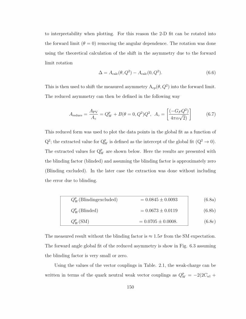
to interpretability when plotting. For this reason the 2-D fit can be rotated into

the forward limit (θ = 0) removing the angular dependence. The rotation was done

using the theoretical calculation of the shift in the asymmetry due to the forward

limit rotation

∆ = Acalc(θ,Q2)− Acalc(0, Q

2). (6.6)

This is then used to shift the measured asymmetry Aep(θ,Q2) into the forward limit.

The reduced asymmetry can then be defined in the following way

Areduce =APV

A= Qp

W +B(θ = 0, Q2)Q2, A =

[(−GFQ

2)

4πα√

2)

](6.7)

This reduced form was used to plot the data points in the global fit as a function of

Q2; the extracted value for QpW is defined as the intercept of the global fit (Q2 → 0).

The extracted values for QpW are shown below. Here the results are presented with

the blinding factor (blinded) and assuming the blinding factor is approximately zero

(Blinding excluded). In the later case the extraction was done without including

the error due to blinding.

QpW (Blindingexcluded) = 0.0845± 0.0093

QpW (Blinded) = 0.0673± 0.0119

QpW (SM) = 0.0705± 0.0008.

(6.8a)

(6.8b)

(6.8c)

The measured result without the blinding factor is ≈ 1.5σ from the SM expectation.

The forward angle global fit of the reduced asymmetry is show in Fig. 6.3 assuming

the blinding factor is very small or zero.

Using the values of the vector couplings in Table. 2.1, the weak-charge can be

written in terms of the quark neutral weak vector couplings as QpW = −2(2Cu1 +

150

FIG. 6.3: The global fit of the reduced asymmetry in the forward limit to Q2 = 0.63(GeV/c)2 is shown as the black line. The red point is the present Qp

W measurement.The yellow band represents the uncertainty of the fit. The dashed blue line showsthe global fit without the measurement of Qp

W presented here. The SM predictionis shown by the arrow. This fit assumes the blinding factor is close to zero.

151

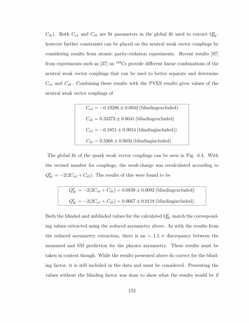
Cd1). Both Cu1 and Cd1 are fit parameters in the global fit used to extract QpW ,

however further constraints can be placed on the neutral weak vector couplings by

considering results from atomic parity-violation experiments. Recent results [97]

from experiments such as [37] on 133Cs provide different linear combinations of the

neutral weak vector couplings that can be used to better separate and determine

Cu1 and Cd1. Combining these results with the PVES results gives values of the

neutral weak vector couplings of

Cu1 = −0.19286± 0.0042 (blindingexcluded)

Cd1 = 0.34373± 0.0041 (blindingexcluded)

Cu1 = −0.1851± 0.0054 (blindingincluded))

Cd1 = 0.3368± 0.0050 (blindingincluded)

The global fit of the quark weak vector couplings can be seen in Fig. 6.4. With

the revised number for couplings, the weak-charge was recalculated according to

QpW = −2(2Cu1 + Cd1). The results of this were found to be

QpW = −2(2Cu1 + Cd1) = 0.0839± 0.0092 (blindingexcluded)

QpW = −2(2Cu1 + Cd1) = 0.0667± 0.0118 (blindingincluded).

Both the blinded and unblinded values for the calculated QpW match the correspond-

ing values extracted using the reduced asymmetry above. As with the results from

the reduced asymmetry extraction, there is an ∼ 1.5 σ discrepancy between the

measured and SM prediction for the physics asymmetry. These results must be

taken in context though. While the results presented above do correct for the blind-

ing factor, it is still included in the data and must be considered. Presenting the

values without the blinding factor was done to show what the results would be if

152

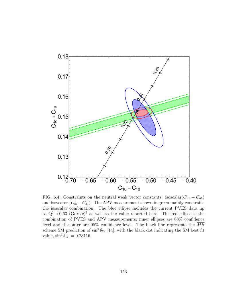
FIG. 6.4: Constraints on the neutral weak vector constants: isoscalar(Cu1 + Cd1)and isovector (Cu1−Cd1). The APV measurement shown in green mainly constrainsthe isoscalar combination. The blue ellipse includes the current PVES data upto Q2 <0.63 (GeV/c)2 as well as the value reported here. The red ellipse is thecombination of PVES and APV measurements; inner ellipses are 68% confidencelevel and the outer are 95% confidence level. The black line represents the MSscheme SM prediction of sin2 θW [14], with the black dot indicating the SM best fitvalue, sin2 θW = 0.23116.

153

the blinding factor ends up being small. Because of this, drawing scientific conclu-

sions from these results is difficult. The complete analysis of the Run I dataset is

on-going. Following its completion, and subsequent blinding factor removal, more

concrete conclusions will be possible.

6.2 Conclusion & Future Work

While the results presented here represent a factor of two improvement in preci-

sion over the original Wien 0 result, there is still a lot of work to be done. The Run

I data set makes up approximately 33% of the total Qweak data set (in comparison

to the 4% from Wien 0), but completion of the Run II data analysis, which makes

up 63% of the total data set, should see yet more improvement of the statistical

error. The bulk of the systematic error comes from uncertainties on the Aluminium

measurements, Q2, and polarization. Work is currently in progress to improve the

uncertainties of the Aluminium measurement by considering higher order diagrams,

radiative losses, and better understanding of the beamline backgrounds which con-

tribute heavily to the uncertainty of the Aluminium asymmetry. Work on the Q2

measurement is on-going but has been primarily focused on the Run II analysis thus

far. Another source, which has recently been revisited, is the polarization determi-

nation. The issues with the failed coil during Run I have spawned a substantial

amount of simulation and analysis effort by the polarization group. Given that this

is a subtle issue, the effect of which was changing daily during Run I, and man-power

is low, the progress on this has been slow, however, with the shift in focus of the

analysis changing to Run I, more results are expected in the near future.

In terms of work on improving the determination of the beam modulation ex-

tracted detector sensitivities, a substantial amount of work has been done. Many

154

of the issues presented here in the Run I analysis have been rectified. The gaps

in the ramp function have been fixed, the number of independent variables has

been doubled - both the sine and cosine contributions are now considered - and the

BPMs been redefined as “effective” BPMs which have provided much better sepa-

ration among the BPM responses. In general the current analysis efforts have been

focused heavily on the Run II data set and only recently has the focus started to

shift towards Run I; it is expected that this will greatly reduce the systematic errors

as a whole as the analysis ramps up. I have included a more detail write-up with

proposed changes to a future beam modulation system in App. A.4.

155

BIBLIOGRAPHY

[1] Wikimedia Commons. Standard model of elementary particle physics.

https://commons.wikimedia.org/wiki/Standard_Model_of_Elementary_

Particles.svg, 2006.

[2] Jens Erler and Michael J. Ramsey-Musolf. Weak mixing angle at low energies.

Phys. Rev. D, 72:073003, 2005.

[3] Daniel T. Pierce and F. Meier. Negative electron affinity gaas: A new source

of spin-polarized electrons. Applied Physics Letters, Vol.26(12):670–672, 1975.

[4] K. D. Paschke. Controlling helicity-correlated beam asymmetries in a polarized

electron source. Eur. Phys. J. A., 32:549–553, 2006.

[5] Rakitha Beminiwattha. A Measurement of the Weak Charge of the Electron

through Parity Violating Electron Scattering. PhD. Thesis, Ohio University,

2013.

[6] Waidyawansa Buddhini. Beam Position and Angle Determination in Qweak.

Qweak Document Database(Qweak-Doc-1772-v2), 2012.

[7] Richard Jones. Polarimetry for Qweak. Qweak Document: Qweak-doc-510-v1,

2005.

156

[8] K.E. Myers. The First Determination of the Proton’s Weak Charge Through

Parity-Violating Asymmetry Measurements in Elastic e+p and e+Al Scatter-

ing. PhD Thesis, George Washington University, 2012.

[9] K.E. Myers. GEANT3 Simulation of Detector Shielding Wall Design Technical

Report. Qweak Document Qweak-doc-852-v1, 2008.

[10] John P. Leckey IV. The First Direct Measurement of the Weak Charge of the

Proton. PhD Thesis, The College of William and Mary, 2012.

[11] Nuruzzaman. Beam Modulation Cable Map for Q-weak experiment in Hall-C

at Jefferson Lab. Qweak Document: Qweak-doc-1279-v2, 2010.

[12] Nuruzzaman. 1st Order Beam Modulation in the 3C Line for Qweak experiment.

Qweak Document: Qweak-doc-910-v3, 2009.

[13] J. Leacock. Measuring the Weak-Charge of the Proton and the Hadronic Parity-

Violation of the N → ∆ Transition. PhD. Thesis, Virginia Polytechnic Institute

and State University, 2012.

[14] J. Beringer et al. Review of particle physics*. Phys. Rev. D, 86:010001, 2012.

[15] E. Noether. Invariante Variationsprobleme. Nachr. D. Knig. Gesellsch. D.

Wiss. Zu Gttingen, Math-phys., Klasse:235–257, 1918.

[16] E. D. Bloom, D. H. Coward, H. Destaebler, J. Drees, G. Miller, L. W. Mo, R. E.

Taylor, M. Breidenbach, J. I. Friedman, G. C. Hartmann, and H. W. Kendall.

High-Energy Inelastic e-p Scattering at 6 and 10. Physical Review Letters,

23:930–934, 1969.

157

[17] M. Breidenbach, J. I. Friedman, H. W. Kendall, E. D. Bloom, D. H. Coward,

H. Destaebler, J. Drees, L. W. Mo, and R. E. Taylor. Observed Behavior of

Highly Inelastic Electron-Proton Scattering. Physical Review Letters, 23:935–

939, 1969.

[18] S. L. Glashow. Partial-symmetries of weak interactions. , 22:579–588, 1961.

[19] P. W. Higgs. Broken Symmetries and the Masses of Gauge Bosons. Physical

Review Letters, 13:508–509, 1964.

[20] S. Weinberg. A Model of Leptons. Physical Review Letters, 19:1264–1266, 1967.

[21] A. Salam. Elementary Particle Physics: Relativistic Groups and Analyticity.

Eighth Nobel Symposium. Stockholm: Almquvist and Wiksell, 1968.

[22] M. Gell-Mann. A schematic model of baryons and mesons. Physics Letters,

8:214–215, 1964.

[23] G. Zweig. An SU(3) Model for Strong Interaction Symmetry and its Breaking.

CERN Report No.8182/TH.401, 1964.

[24] Hasert F. J. et al. Observation of neutrino-like interactions without muon or

electron in the gargamelle neutrino experiment. Physics Letters B, 46:138–140,

1973.

[25] F. J. Hasert et al. Search for elastic muon-neutrino electron scattering. Physics

Letters B, 46:121–124, 1973.

[26] C.Y. Prescott et al. Parity Nonconservation in Inelastic Electron Scattering.

Physics Letters, pages 347–352, 1978.

158

[27] G. Arnison et al. Experimental Observation of Isolated Large Transverse Energy

Electrons with Associated Missing Energy at√s = 540GeV . Physics Letters,

pages 103–116, 1983.

[28] M. Banner et al. Observation of Single Isolated Electrons of High Transverse

Momentum in Events with Missing Transverse Energy at the CERN pp Collider.

Physics Letters, pages 476–485, 1983.

[29] G. Arnison et al. Experimental Observation of Lepton Pairs of Invariant Mass

Around 95(GeV /c 2 ) at the CERN SPS Collider. Physics Letters, pages

398–410, 1983.

[30] P. Bagnaia et al. Evidence of the Z → e+e− at CERN pp Collider. Physics

Letters, pages 130–140, 1983.

[31] S. Chatrchyan et al. Observation of a new boson at a mass of 125 GeV with

the CMS experiment at the LHC. Physics Letters, pages 30–61, 2012.

[32] G. Aad et al. Observation of a new particle in the search for the Standard

Model Higgs boson with the ATLAS detector at the LHC. Physics Letters,

pages 1–29, 2012.

[33] T. D. Lee and C. N. Yang. Question of Parity Conservation in Weak Interac-

tions. Physical Review, 104:254–258, 1956.

[34] C. S. Wu, E. Ambler, R. W. Hayward, D. D. Hoppes, and R. P. Hudson.

Experimental Test of Parity Conservation in Beta Decay. Physical Review,

105:1413–1415, 1957.

[35] J. Erler and M.J. Ramsey-Musolf. Low Energy Tests of the Standard Model.

Prog. Part. Nucl. Phys., 54:351, 2005.

159

[36] D. Androic et al. First detrmination of the weak charge of the proton. Phys.

Rev. Lett., 111:141803, 2013.

[37] C.S. Wood et al. Measurement of Parity Nonconservation and an Anapole

Moment in Cesium. Science, 275:1759–1763, 1997.

[38] A. Sirlin A. Ferroglia, G. Ossola. The electroweak form factor κ(q2) and the

running of sin2 θw. The European Physical Journal C-Particles and Fields.,

34:165–171, 2004.

[39] B. Rislow. Low Energy Tests of the Standard Model. PhD. Thesis, College of

William and Mary, 2013.

[40] Benjamin C. Rislow and Carl E. Carlson. Contributions from γZ box diagrams

to parity violating elastic ep scattering. Phys.Rev., D83:113007, 2011.

[41] A. Sibirtsev, P. G. Blunden, W. Melnitchouk, and A. W. Thomas. γz correc-

tions to forward-angle parity-violating ep scattering. Phys. Rev. D, 82:013011,

2010.

[42] M. Gorchtein, C.J. Horowitz, and M.J. Ramsey-Musolf. Model-dependence of

the gamma-Z dispersion correction to the parity-violating elastic ep asymmetry.

Phys. Rev. C, 84:015502, 2011.

[43] N.L. Hall, P.G. Blunden, W. Melnitchouk, A.W. Thomas and R.D. Young.

Constrained Z interference corrections to parity-violating electron scattering.

Phys. Rev. D, page 013011, 2013.

[44] D. Wang et al. Measurements of Parity-Violating Asymmetries in Electron-

Deuteron Scattering in the Nucleon Resonance Region. Phys. Rev. Lett.,

111:082501, 2013.

160

[45] D.S. Armstrong et al. Strange Quark contributions to Parity Violating Asym-

metries in Forward G0 Electron-Proton Scattering Experiment. Physical Review

Letters, 95:092001, 2005.

[46] K.A. Anilol et al. Parity Violating Electron Scattering from He-4 and Strange

Electric Form-Factor of the Nucleon. Physical Review Letters, 96:022003, 2006.

[47] H.A. Grunder, J.J. Bisognano, W.I. Diamond, B.K. Hartline, C.W. Lee-

mann, et al. The Continuous Electron Beam Accelerator Facility. Nucl.Phys.,

A478:831C–846C, 1988.

[48] Y. C. Chao and others. CEBAF Accelerator Achivements. J. Phys. Conf. Ser.,

299:1–18, 2011.

[49] G. D. Cates. Overview of laser systematics. Eur. Phys. J. A., 24:109–114, 2005.

[50] P.A. Adderley and others. Two Wien Filter Spin Flipper. 2011 Particle Accel-

erator Conference Proceedings, C110328:862–864, 2011.

[51] J.M. Grames et al. Unique electron polarimeter analyzing power compari-

son and precision spin-based energy measurement. Phys.Rev.ST Accel.Beams,

7:042802, 2004.

[52] A. S. Hofler et al. Performance of the CEBAF arc beam position monitors.

1993 IEEE Particle Accelerator Conference(PAC 93), May, 17-20 1993.

[53] J. Bergoz and others. Current monitors for particle beams. Nuclear Physics A,

525:595–600, 1991.

[54] M. Hauger et al. A High-Precision Polarimeter. Nucl. Instrum. Meth.,

A462:382–392, 2001.

161

[55] R.A. Reck and D.L. Fry. Orbital and Spin Magnetization in Fe-Co, Fe-Ni, and

Ni-Co. Physical Review, 184(2):492, 1969.

[56] G. Smith S. Covrig and J. Dunne. Qweak Liquid Hydrogen Target: Preliminary

Design and Safety Document. Qweak Document: Qweak-doc-1041-v2, 2009.

[57] W. Faulk D. Jones L. Lee and P. Wang. QTOR Magnetic Mapping. Collabo-

ration Meeting Talk. Qweak Document: Qweak-doc-1240, 2010.

[58] P. Wang. A Measurement of the Proton’s Weak Charge using an Integration

Cerenkov Detector System. PhD Thesis, The University of Manitoba, 2011.

[59] D. Mack. Status of the Qweak Main Detector Technical Report. Qweak Doc-

ument Qweak-doc-649-v1, 2007.

[60] Rob Veenhof CERN. Garfield simulation of gaseous detectors. http://

garfield.web.cern.ch/garfield/, 2010. [Online; accessed 28-February-

2014].

[61] David Armstrong. Summary of Region 3 Surveys. http://dilbert.physics.

wm.edu/Commissioning/63, 2015.

[62] Nuruzzaman. A Robust Beam Modulation Strategy for the Hall-C Beamline.


[63] Valeri Lebedev. Computer code for linear and non-linear optics calculations.

http://www-ap.fnal.gov/~ostiguy/OptiM/, 2014.

[64] D. Jones. Update on Run 2 Beam Modulation. Qweak Document: Qweak-doc-

1856-v1, 2013.

162

[65] Brian J. Moffit. Elastic Scattering of Longitudinally Polarized Electrons from

4He. PhD. Thesis, College of William and Mary, 2007.

[66] K. Saenboonruang. Measurement of the Neutron Radius of 208Pb Through

Parity Violating Electron Scattering. PhD. Thesis, University of Virginia, 2008.

[67] J. Hoskins. Study of the Effect of FFB on BPM Response During Modulation.


[68] K. Paschke. Notes on BPM Phase Shift Due to FFB in the Modulation System.


[69] D. Jones. Update on Run II Beam Modulation. Qweak Document: Qweak-

doc-1856-v1, 2013.

[70] M. Dalton. How neutral is your axis? https://qweak.jlab.org/elog/

Analysis+%26+Simulation/431, 2011.

[71] C. Yan, P. Adderley, D. Barker, J. Beaufait, K. Capek, R. Carlini, J. Dahlberg,

E. Feldl, K. Jordan, B. Kross, W. Oren, R. Wojcik, and J. VanDyke. Superharp

a wire scanner with absolute position readout for beam energy measurement

at CEBAF. Nuclear Instruments and Methods in Physics Research Section A:

Accelerators, Spectrometers, Detectors and Associated Equipment, 365(23):261–

267, 1995.

[72] C. Yan, R. D. Carlini, and D. Neuffer. Beam Energy Measurement using Hall

C Beamline. Proc. Particle Accelerator Conference, page 2136.

[73] K. A. Aniol et al. Parity-violating electroweak asymmetry in ~ep scattering.

Phys. Rev. C, 69:065501, 2004.

163

[74] K. Myers. Pass5 Round 1 Asymmetry for Wien 0 Aluminum Including Sys-

tematics. https://qweak.jlab.org/elog/Analysis+%26+Simulation/743,

2012.

[75] D. Mack. Input file v3(frozen!) for Wien0 4% DS Al corrected asymmetry.

https://qweak.jlab.org/elog/Analysis+%26+Simulation/753, 2012.

[76] K. Myers. Radiatively Corrected Asymmetry for Wien 0 Pass5 Aluminum.

https://qweak.jlab.org/elog/Analysis+%26+Simulation/748, 2012.

[77] J. Magee. The Preliminary Pluminium Window Dilution for Run I. https:

//qweak.jlab.org/doc-private/ShowDocument?docid=1781, 2013.

[78] J. Magee. Corrected 25% Aluminum Dilution. https://qweak.jlab.org/

elog/Analysis+%26+Simulation/744, 2012.

[79] Wade Duvall. Fractional yields in blocked MD’s in good halo conditions. https:

//qweak.jlab.org/elog/Analysis+%26+Simulation/779, 2012.

[80] Dave Mack. Wien 0 Beamline Background Dilution Central Value and Un-

certainty. https://qweak.jlab.org/elog/Analysis+%26+Simulation/784,

2012.

[81] Wade Duvall and Mark Pitt. Beamline background asymmetry for Wien 0 anal-

ysis. https://qweak.jlab.org/elog/Analysis+%26+Simulation/780, 2012.

[82] A. Subebi. QWGEANT 3 simulations of rates inelastic dilution factor. https:

//qweak.jlab.org/elog/Analysis+%26+Simulation/451, 2011.

[83] J. Hoskins. Beam Polarization Averaging Study. https://qweak.jlab.org/

elog/Analysis+%26+Simulation/1400, 2015.

164

[84] K. A. Aniol et al. Measurement of the neutral weak form factors of the proton.

Phys. Rev. Lett., 82:1096–1100, 1999.

[85] K. A. Aniol et al. Parity-violating electron scattering from 4He and the strange

electric form factor of the nucleon. Phys. Rev. Lett., 96:022003, 2006.

[86] K.A. Aniol et al. Constraints on the nucleon strange form-factors at Q**2 0.1-

GeV**2. Phys.Lett., B635:275–279, 2006.

[87] A. Acha et al. Precision measurements of the nucleon strange form factors at

Q2 ∼ 0.1 gev2. Phys. Rev. Lett., 98:032301, 2007.

[88] Z. Ahmed et al. New precision limit on the strange vector form factors of the

proton. Phys. Rev. Lett., 108:102001, 2012.

[89] D. S. Armstrong et al. Strange-quark contributions to parity-violating asym-

metries in the forward g0 electron-proton scattering experiment. Phys. Rev.

Lett., 95:092001, 2005.

[90] D. Androic et al. Strange quark contributions to parity-violating asymmetries

in the backward angle g0 electron scattering experiment. Phys. Rev. Lett.,

104:012001, 2010.

[91] F. E. Maas et al. Measurement of strange-quark contributions to the nucleon’s

form factors at Q2 = 0.230 (GeV/c)2. Phys. Rev. Lett., 93:022002, 2004.

[92] F. E. Maas et al. Evidence for strange-quark contributions to the nucleon’s

form factors at Q2 = 0.108 (GeV/c)2. Phys. Rev. Lett., 94:152001, 2005.

[93] J. J. Kelly. Simple parametrization of nucleon form factors. Phys. Rev. C,

70:068202, 2004.

165

[94] S. MacEwan. The Weak Charge of the Proton: A Search For Physics Beyond

the Standard Model. PhD. Thesis, University of Manitoba, 2015.

[95] Shi-Lin Zhu, S. J. Puglia, B. R. Holstein, and M. J. Ramsey-Musolf. Nucleon

anapole moment and parity-violating ep scattering. Phys. Rev. D, 62:033008,

2000.

[96] Mikhail Gorchtein, C.J. Horowitz, and Michael J. Ramsey-Musolf. Model-

dependence of the γZ dispersion correction to the parity-violating asymmetry

in elastic ep scattering. Phys.Rev., C84:015502, 2011.

[97] V. A. Dzuba, J. C. Berengut, V. V. Flambaum, and B. Roberts. Revisiting

parity nonconservation in cesium. Phys. Rev. Lett., 109:203003, 2012.

[98] D. Keith Robinson P. R. Bevington. Data Reduction and Error Analysis.

McGraw-Hill, 3rd edition, 2003.

166

APPENDIX A

Appendix

A.1 Detector Error Weighting

The weighted average of a variable x is given by,

〈x〉 =

N∑i

xiwi

N∑i

wi

, (A.1)

where wi is a general weight. The variance of 〈x〉 is given by the error propagation

formula [98],

σ2〈x〉 =

N∑i

(∂〈x〉∂xi

)2

σ2i . (A.2)

167

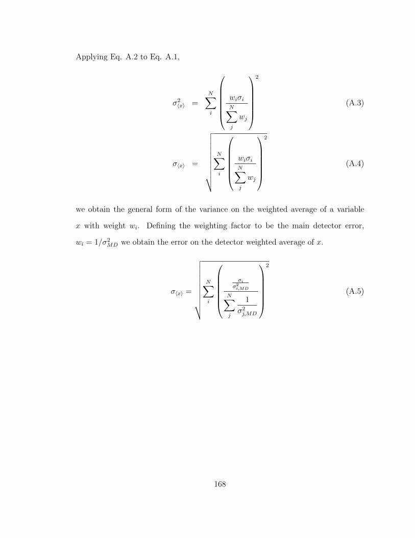
Applying Eq. A.2 to Eq. A.1,

σ2〈x〉 =

N∑i

wiσiN∑j

wj

2

(A.3)

σ〈x〉 =

√√√√√√√√√√N∑i

wiσiN∑j

wj

2

(A.4)

we obtain the general form of the variance on the weighted average of a variable

x with weight wi. Defining the weighting factor to be the main detector error,

wi = 1/σ2MD we obtain the error on the detector weighted average of x.

σ〈x〉 =

√√√√√√√√√√N∑i

σi

σ2i,MD

N∑j

1

σ2j,MD

2

(A.5)

168

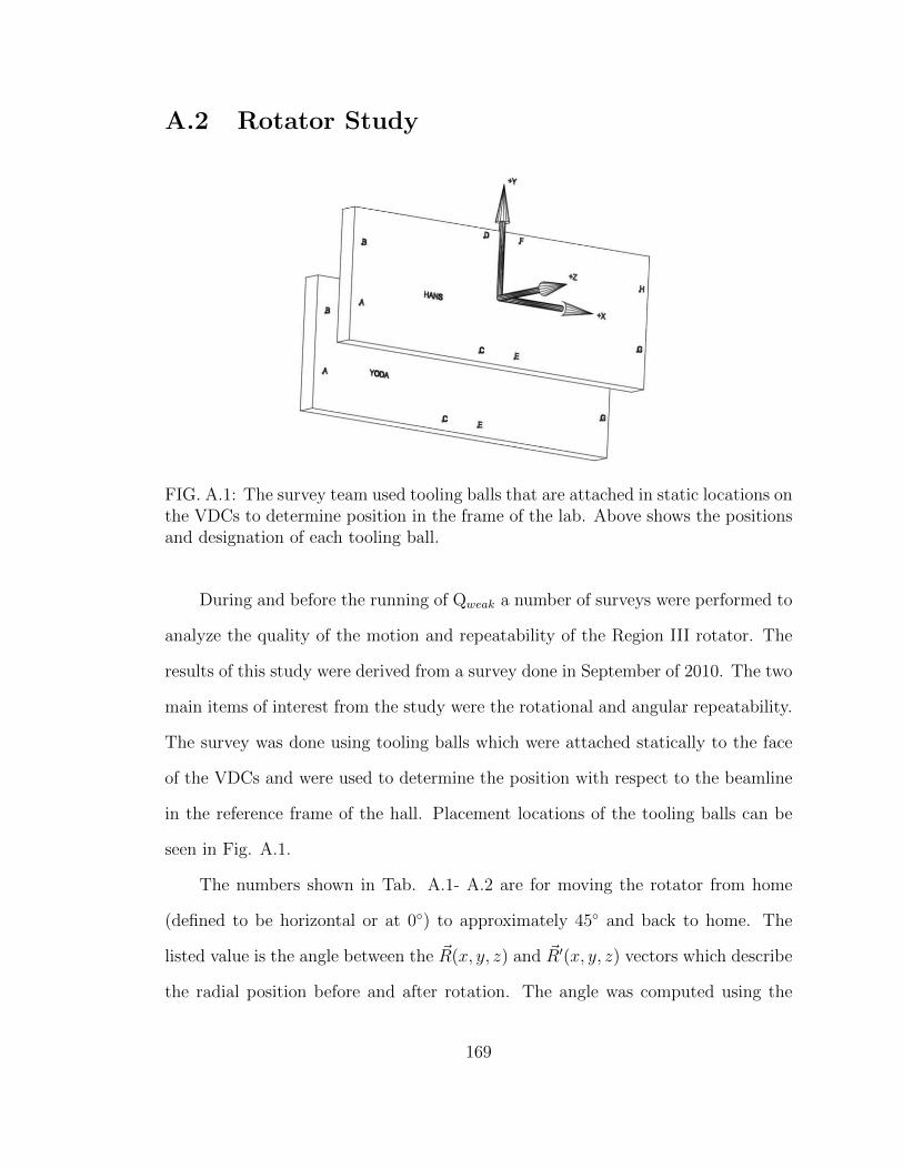
A.2 Rotator Study

FIG. A.1: The survey team used tooling balls that are attached in static locations onthe VDCs to determine position in the frame of the lab. Above shows the positionsand designation of each tooling ball.

During and before the running of Qweak a number of surveys were performed to

analyze the quality of the motion and repeatability of the Region III rotator. The

results of this study were derived from a survey done in September of 2010. The two

main items of interest from the study were the rotational and angular repeatability.

The survey was done using tooling balls which were attached statically to the face

of the VDCs and were used to determine the position with respect to the beamline

in the reference frame of the hall. Placement locations of the tooling balls can be

seen in Fig. A.1.

The numbers shown in Tab. A.1- A.2 are for moving the rotator from home

(defined to be horizontal or at 0) to approximately 45 and back to home. The

listed value is the angle between the ~R(x, y, z) and ~R′(x, y, z) vectors which describe

the radial position before and after rotation. The angle was computed using the

169

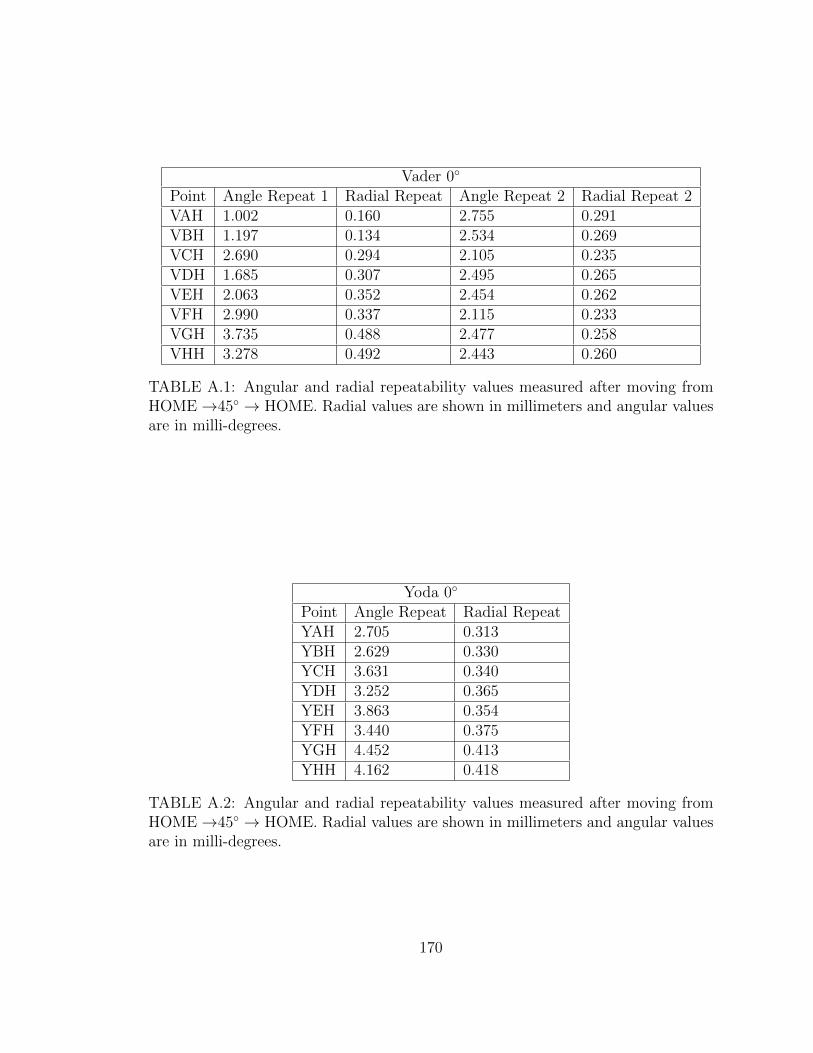
Vader 0

Point Angle Repeat 1 Radial Repeat Angle Repeat 2 Radial Repeat 2VAH 1.002 0.160 2.755 0.291VBH 1.197 0.134 2.534 0.269VCH 2.690 0.294 2.105 0.235VDH 1.685 0.307 2.495 0.265VEH 2.063 0.352 2.454 0.262VFH 2.990 0.337 2.115 0.233VGH 3.735 0.488 2.477 0.258VHH 3.278 0.492 2.443 0.260

TABLE A.1: Angular and radial repeatability values measured after moving fromHOME→45 → HOME. Radial values are shown in millimeters and angular valuesare in milli-degrees.

Yoda 0

Point Angle Repeat Radial RepeatYAH 2.705 0.313YBH 2.629 0.330YCH 3.631 0.340YDH 3.252 0.365YEH 3.863 0.354YFH 3.440 0.375YGH 4.452 0.413YHH 4.162 0.418

TABLE A.2: Angular and radial repeatability values measured after moving fromHOME→45 → HOME. Radial values are shown in millimeters and angular valuesare in milli-degrees.

170

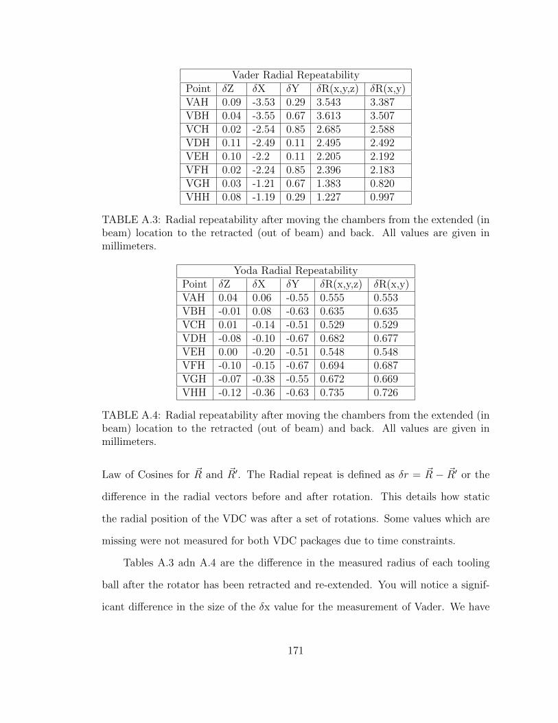
Vader Radial RepeatabilityPoint δZ δX δY δR(x,y,z) δR(x,y)VAH 0.09 -3.53 0.29 3.543 3.387VBH 0.04 -3.55 0.67 3.613 3.507VCH 0.02 -2.54 0.85 2.685 2.588VDH 0.11 -2.49 0.11 2.495 2.492VEH 0.10 -2.2 0.11 2.205 2.192VFH 0.02 -2.24 0.85 2.396 2.183VGH 0.03 -1.21 0.67 1.383 0.820VHH 0.08 -1.19 0.29 1.227 0.997

TABLE A.3: Radial repeatability after moving the chambers from the extended (inbeam) location to the retracted (out of beam) and back. All values are given inmillimeters.

Yoda Radial RepeatabilityPoint δZ δX δY δR(x,y,z) δR(x,y)VAH 0.04 0.06 -0.55 0.555 0.553VBH -0.01 0.08 -0.63 0.635 0.635VCH 0.01 -0.14 -0.51 0.529 0.529VDH -0.08 -0.10 -0.67 0.682 0.677VEH 0.00 -0.20 -0.51 0.548 0.548VFH -0.10 -0.15 -0.67 0.694 0.687VGH -0.07 -0.38 -0.55 0.672 0.669VHH -0.12 -0.36 -0.63 0.735 0.726

TABLE A.4: Radial repeatability after moving the chambers from the extended (inbeam) location to the retracted (out of beam) and back. All values are given inmillimeters.

Law of Cosines for ~R and ~R′. The Radial repeat is defined as δr = ~R − ~R′ or the

difference in the radial vectors before and after rotation. This details how static

the radial position of the VDC was after a set of rotations. Some values which are

missing were not measured for both VDC packages due to time constraints.

Tables A.3 adn A.4 are the difference in the measured radius of each tooling

ball after the rotator has been retracted and re-extended. You will notice a signif-

icant difference in the size of the δx value for the measurement of Vader. We have

171

Vader -45

Point Measured AngleVAH 45.143VBH 45.146VCH 45.116VDH 45.120VEH 45.113VFH 45.106VGH 45.089VHH 45.094

TABLE A.5: Shown is the extracted angle with respect to the home position.

Yoda -45

Point Measured AngleVAH N/AVBH N/AVCH N/AVDH N/AVEH N/AVFH N/AVGH N/AVHH N/A

TABLE A.6: Unfortunately we did not get survey locations for all points on eachchamber. This table is listed for completeness.

attributed to incorrect the seating of the linear pin which defines the linear position

of the chambers and holds them in place. For this reason, the radial repeatability

was based off of the Yoda package. The repeatability is listed both with and without

the contribution from the Z degree of freedom.

Tables A.7 to A.14 present the measured angle between the home position and

the position the chambers were rotated into. This was extracted according to

θ = cos−1

(R ∗ R′

‖~R‖‖~R′‖

). (A.6)

This defines the actual angle as defined by the home position after rotation into each

172

Vader -90

Point Measured AngleVAH -90.047VBH -90.042VCH -90.023VDH -90.035VEH -90.033VFH -90.020VGH -90.024VHH -90.029


Yoda -90

Point Measured AngleYAH -90.248YBH -90.245YCH -90.238YDH -90.232YEH -90.229YFH -90.226YGH -90.192YHH -90.196


octant. Tables A.14 and A.13 define the repeatability after rotating the chambers

to a given angle and then returning to home.

Summary of Measurements

Tables A.15 and A.16 give the standard deviation of the radial measurements

for each tooling ball point, including all octants for each VDC package. For each

package the z degree of freedom can be seen to be an important component of the

repeatability and confirms the “tilt” of the rotator. Essentially the rotator itself,

mostly likely the hub, was not situated perfectly along each axis and therefore

rotation and radial motion do not move parallel along the axes. Instead there is a

slight tilt so that there is motion in Z as well.

173

Vader 45



Yoda 45

Point Measured AngleYAH 44.970YBH 44.966YCH 44.945YDH 44.946YEH 44.938YFH 44.941YGH 44.926YHH 44.929


Vader 90



174

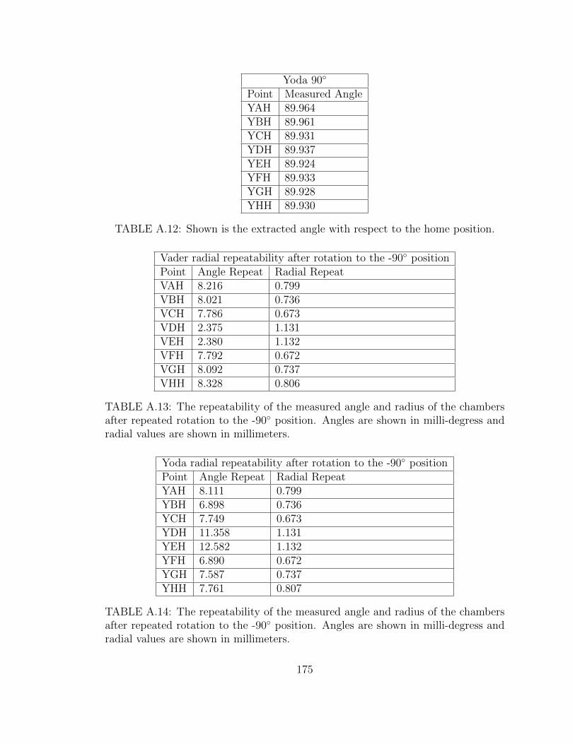
Yoda 90

Point Measured AngleYAH 89.964YBH 89.961YCH 89.931YDH 89.937YEH 89.924YFH 89.933YGH 89.928YHH 89.930


Vader radial repeatability after rotation to the -90 positionPoint Angle Repeat Radial RepeatVAH 8.216 0.799VBH 8.021 0.736VCH 7.786 0.673VDH 2.375 1.131VEH 2.380 1.132VFH 7.792 0.672VGH 8.092 0.737VHH 8.328 0.806

TABLE A.13: The repeatability of the measured angle and radius of the chambersafter repeated rotation to the -90 position. Angles are shown in milli-degress andradial values are shown in millimeters.

Yoda radial repeatability after rotation to the -90 positionPoint Angle Repeat Radial RepeatYAH 8.111 0.799YBH 6.898 0.736YCH 7.749 0.673YDH 11.358 1.131YEH 12.582 1.132YFH 6.890 0.672YGH 7.587 0.737YHH 7.761 0.807

TABLE A.14: The repeatability of the measured angle and radius of the chambersafter repeated rotation to the -90 position. Angles are shown in milli-degress andradial values are shown in millimeters.

175

Standard Deviation Radial Measurement in Theta: VaderPoint Radial σ(x, y, z) Radial σ(x, y)VAH 1.577 3.473VBH 1.619 3.246VCH 1.705 3.482VDH 1.597 3.769VEH 1.596 3.789VFH 1.706 3.534VGH 1.643 3.540VHH 1.582 3.664

TABLE A.15: The standard deviation of the radial measurement for each point ineach position in theta. Extracted values are shown for the radius in both the (x,y)plane and the (x,y,z) plane. Values in mm.

Standard Deviation Radial Measurement in Theta: YodaPoint Radial σ(x, y, z) Radial σ(x, y)VAH 1.678 2.468VBH 1.820 2.734VCH 1.559 2.475VDH 1.883 2.967VEH 1.579 2.479VFH 1.902 2.979VGH 1.841 2.506VHH 1.983 2.795

TABLE A.16: The standard deviation of the radial measurement for each point ineach position in theta. Extracted values are shown for the radius in both the (x,y)plane and the (x,y,z) plane. Values in mm

176

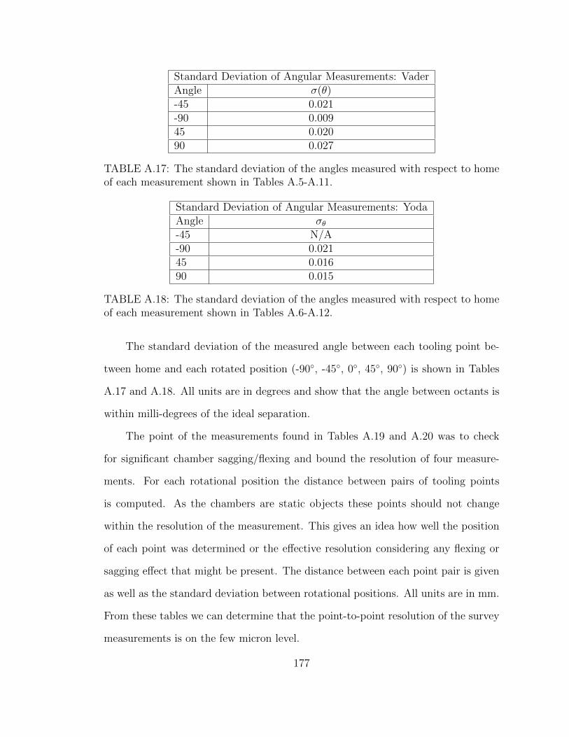
Standard Deviation of Angular Measurements: VaderAngle σ(θ)-45 0.021-90 0.00945 0.02090 0.027

TABLE A.17: The standard deviation of the angles measured with respect to homeof each measurement shown in Tables A.5-A.11.

Standard Deviation of Angular Measurements: YodaAngle σθ-45 N/A-90 0.02145 0.01690 0.015

TABLE A.18: The standard deviation of the angles measured with respect to homeof each measurement shown in Tables A.6-A.12.

The standard deviation of the measured angle between each tooling point be-

tween home and each rotated position (-90, -45, 0, 45, 90) is shown in Tables

A.17 and A.18. All units are in degrees and show that the angle between octants is

within milli-degrees of the ideal separation.

The point of the measurements found in Tables A.19 and A.20 was to check

for significant chamber sagging/flexing and bound the resolution of four measure-

ments. For each rotational position the distance between pairs of tooling points

is computed. As the chambers are static objects these points should not change

within the resolution of the measurement. This gives an idea how well the position

of each point was determined or the effective resolution considering any flexing or

sagging effect that might be present. The distance between each point pair is given

as well as the standard deviation between rotational positions. All units are in mm.

From these tables we can determine that the point-to-point resolution of the survey

measurements is on the few micron level.

177

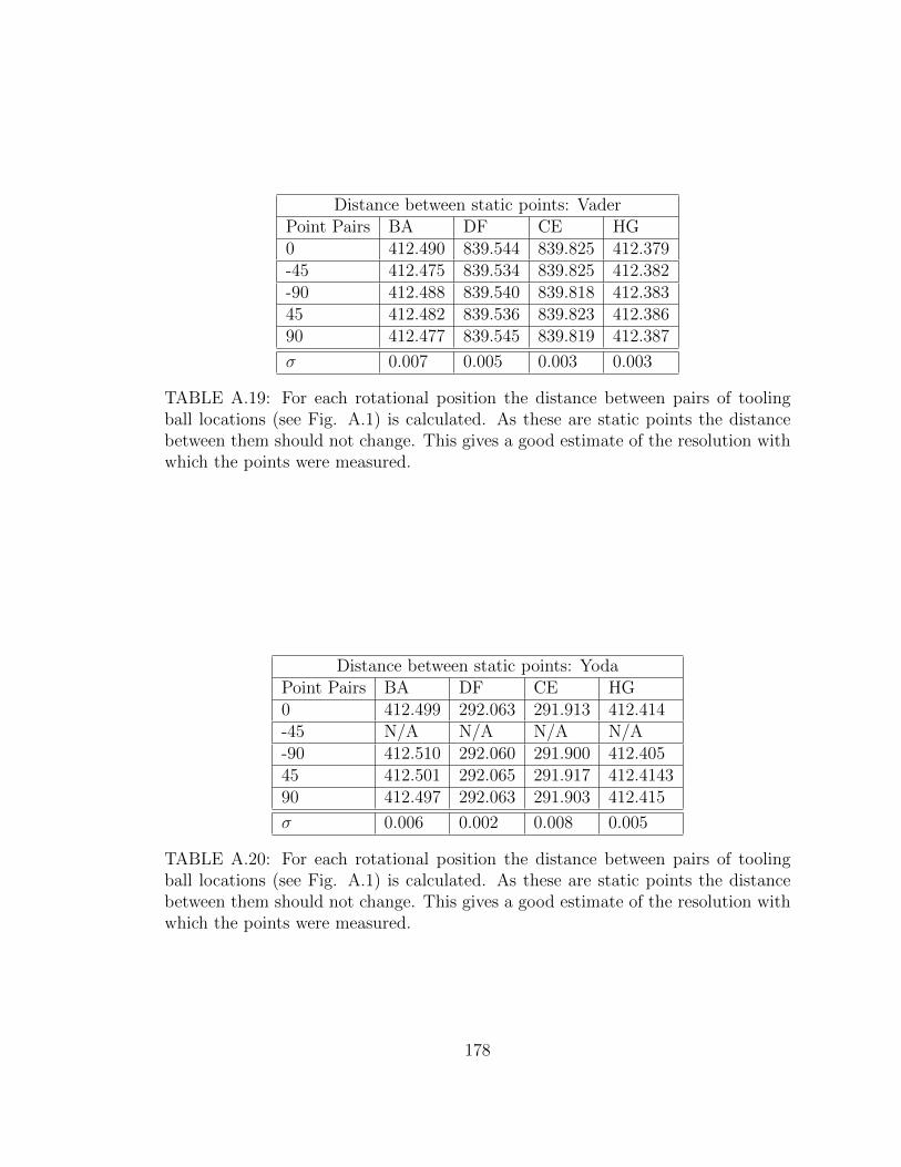
Distance between static points: VaderPoint Pairs BA DF CE HG0 412.490 839.544 839.825 412.379-45 412.475 839.534 839.825 412.382-90 412.488 839.540 839.818 412.38345 412.482 839.536 839.823 412.38690 412.477 839.545 839.819 412.387

σ 0.007 0.005 0.003 0.003

TABLE A.19: For each rotational position the distance between pairs of toolingball locations (see Fig. A.1) is calculated. As these are static points the distancebetween them should not change. This gives a good estimate of the resolution withwhich the points were measured.

Distance between static points: YodaPoint Pairs BA DF CE HG0 412.499 292.063 291.913 412.414-45 N/A N/A N/A N/A-90 412.510 292.060 291.900 412.40545 412.501 292.065 291.917 412.414390 412.497 292.063 291.903 412.415

σ 0.006 0.002 0.008 0.005

TABLE A.20: For each rotational position the distance between pairs of toolingball locations (see Fig. A.1) is calculated. As these are static points the distancebetween them should not change. This gives a good estimate of the resolution withwhich the points were measured.

178

A.3 Background Correction Error Propagation

The calculation of the individual systematic error contributions from the back-

ground correction to the physics asymmetry is done according to

σ2A =

∣∣∣∣∂A∂b∣∣∣∣2 σ2

b . (A.7)

Applying this to Eq. 6.1 we get the following relations:

∂A|Amsr =R× dAmsr

P (1− ftotal), (A.8a)

∂A|Ablind=R× dAblinding

msr

P (1− ftotal), (A.8b)

∂A|P =−R× Amsr

(1− ftotal)

dP

P 2, (A.8c)

∂A|Ai=−R× fi

(1− ftotal)dAi (A.8d)

∂A|R = dR×(Amsr

P− ΣifiAi

)(1− ftotal)

(A.8e)

∂A|fi = εijkl

(Amsr

P+ (fj + fk + fl)Ai − fjAj − fkAk − flAl

)R× dfi

(1− ftotal)

(A.8f)

In the final equation the Levi-Civita operator is invoked to denote the permuta-

tion of the indices 1→2→3→4. With these calculations, the total systematic error

contribution from backgrounds and experimental bias is given by

σA =√

(∂A|Amsr)2 + (∂A|P )2 + (∂A|Ai

)2 + (∂A|R)2 + (∂A|fi)2. (A.9)

179

A.4 Beam Modulation Improvements

As was laid out in the Beam Modulation chapter, the system as a whole was

a success in measurement of the helicity-correlated beam sensitivities. With every

success however there is room for improvement, and there were a number of problems

that were discovered in the system, that in hindsight, could have been fixed. In the

interest of future modulation systems that might be built, I will address some of

those issues and ways that they could have been avoided.

Fast-feedback This was a big issue in the analysis and running of the beam modu-

lation system. By leaving the fast-feedback system on during modulation another

level of complexity was added into the analysis; because the fast-feedback system

worked to counteract modulations in the beam position and angle the total re-

sponse became a composite function with a phase out of response to the driving

signal. This issue was missed in early testing of the system but in future iter-

ations fast-feedback should be paused for the duration of the beam modulation

period. This will lead to cleaner, more interpretable results.

Diagnostics and Tuning One of the pressing issues during the design, construc-

tion, and testing of the modulation system was a lack of manpower to provide

the tools and do the diagnostic testing that was required to make the system the

best it could be. A robust system would include online monitoring and diagnos-

tic tools to give run-by-run results for things such as: beam monitor responses,

detector responses, extracted sensitivities, and beam trajectory plots. The later

of these would be enormously helpful as it would enable shift crew to monitor

how separated the modulations were in phase space and call in experts to tune

the modulation coils, given changes in the beam properties. This would ensure

that the modulations - for example X-position and X-angle - were as pure posi-

180

tion and angle as possible at all times leading to better extracted results. Too

many times during the experimental running we didn’t find problems until days

after they appeared. A robust, real-time diagnostic system would ensure better

response time to problems, and better results with each measurement. This of

course requires an adequate amount of manpower to design and implement the

tools.

181

Documents

Physics | William & Mary - Determination of the …physics.wm.edu/~armd/JoshHoskinsThesisFinal.pdfDetermination of the Proton’s Weak Charge via Parity Violating Electron Scattering