Embed Size (px)
Citation preview


CONTENTS
FOREWORD vPREFACE xi
CHAPTER ONEELECTRIC CHARGES AND FIELDS
1.1 Introduction 1
1.2 Electric Charges 1
1.3 Conductors and Insulators 5
1.4 Charging by Induction 6
1.5 Basic Properties of Electric Charge 8
1.6 Coulomb’s Law 10
1.7 Forces between Multiple Charges 15
1.8 Electric Field 18
1.9 Electric Field Lines 23
1.10 Electric Flux 25
1.11 Electric Dipole 27
1.12 Dipole in a Uniform External Field 31
1.13 Continuous Charge Distribution 32
1.14 Gauss’s Law 33
1.15 Application of Gauss’s Law 37
CHAPTER TWOELECTROSTATIC POTENTIAL AND CAPACITANCE
2.1 Introduction 512.2 Electrostatic Potential 532.3 Potential due to a Point Charge 542.4 Potential due to an Electric Dipole 552.5 Potential due to a System of Charges 572.6 Equipotential Surfaces 602.7 Potential Energy of a System of Charges 612.8 Potential Energy in an External Field 642.9 Electrostatics of Conductors 672.10 Dielectrics and Polarisation 712.11 Capacitors and Capacitance 732.12 The Parallel Plate Capacitor 742.13 Effect of Dielectric on Capacitance 75

2.14 Combination of Capacitors 782.15 Energy Stored in a Capacitor 802.16 Van de Graaff Generator 83
CHAPTER THREECURRENT ELECTRICITY
3.1 Introduction 933.2 Electric Current 933.3 Electric Currents in Conductors 943.4 Ohm’s law 953.5 Drift of Electrons and the Origin of Resistivity 973.6 Limitations of Ohm’s Law 1013.7 Resistivity of various Materials 1013.8 Temperature Dependence of Resistivity 1033.9 Electrical Energy, Power 1053.10 Combination of Resistors — Series and Parallel 1073.11 Cells, emf, Internal Resistance 1103.12 Cells in Series and in Parallel 1133.13 Kirchhoff’s Laws 1153.14 Wheatstone Bridge 1183.15 Meter Bridge 1203.16 Potentiometer 122
CHAPTER FOURMOVING CHARGES AND MAGNETISM
4.1 Introduction 1324.2 Magnetic Force 1334.3 Motion in a Magnetic Field 1374.4 Motion in Combined Electric and Magnetic Fields 1404.5 Magnetic Field due to a Current Element, Biot-Savart Law 1434.6 Magnetic Field on the Axis of a Circular Current Loop 1454.7 Ampere’s Circuital Law 1474.8 The Solenoid and the Toroid 1504.9 Force between Two Parallel Currents, the Ampere 1544.10 Torque on Current Loop, Magnetic Dipole 1574.11 The Moving Coil Galvanometer 163
CHAPTER FIVEMAGNETISM AND MATTER
5.1 Introduction 1735.2 The Bar Magnet 174
xiv

5.3 Magnetism and Gauss’s Law 1815.4 The Earth’s Magnetism 1855.5 Magnetisation and Magnetic Intensity 1895.6 Magnetic Properties of Materials 1915.7 Permanent Magnets and Electromagnets 195
CHAPTER SIXELECTROMAGNETIC INDUCTION
6.1 Introduction 2046.2 The Experiments of Faraday and Henry 2056.3 Magnetic Flux 2066.4 Faraday’s Law of Induction 2076.5 Lenz’s Law and Conservation of Energy 2106.6 Motional Electromotive Force 2126.7 Energy Consideration: A Quantitative Study 2156.8 Eddy Currents 2186.9 Inductance 2196.10 AC Generator 224
CHAPTER SEVENALTERNATING CURRENT
7.1 Introduction 2337.2 AC Voltage Applied to a Resistor 2347.3 Representation of AC Current and Voltage by
Rotating Vectors — Phasors 2377.4 AC Voltage Applied to an Inductor 2377.5 AC Voltage Applied to a Capacitor 2417.6 AC Voltage Applied to a Series LCR Circuit 2447.7 Power in AC Circuit: The Power Factor 2527.8 LC Oscillations 2557.9 Transformers 259
CHAPTER EIGHTELECTROMAGNETIC WAVES
8.1 Introduction 2698.2 Displacement Current 2708.3 Electromagnetic Waves 2748.4 Electromagnetic Spectrum 280
ANSWERS 288
xv

1.1 INTRODUCTION
All of us have the experience of seeing a spark or hearing a crackle whenwe take off our synthetic clothes or sweater, particularly in dry weather.This is almost inevitable with ladies garments like a polyester saree. Haveyou ever tried to find any explanation for this phenomenon? Anothercommon example of electric discharge is the lightning that we see in thesky during thunderstorms. We also experience a sensation of an electricshock either while opening the door of a car or holding the iron bar of abus after sliding from our seat. The reason for these experiences isdischarge of electric charges through our body, which were accumulateddue to rubbing of insulating surfaces. You might have also heard thatthis is due to generation of static electricity. This is precisely the topic weare going to discuss in this and the next chapter. Static means anythingthat does not move or change with time. Electrostatics deals with thestudy of forces, fields and potentials arising from static charges.
1.2 ELECTRIC CHARGE
Historically the credit of discovery of the fact that amber rubbed withwool or silk cloth attracts light objects goes to Thales of Miletus, Greece,around 600 BC. The name electricity is coined from the Greek wordelektron meaning amber. Many such pairs of materials were known which
Chapter One
ELECTRIC CHARGESAND FIELDS

2
Physicson rubbing could attract light objectslike straw, pith balls and bits of papers.You can perform the following activityat home to experience such an effect.Cut out long thin strips of white paperand lightly iron them. Take them near aTV screen or computer monitor. You willsee that the strips get attracted to thescreen. In fact they remain stuck to thescreen for a while.
It was observed that if two glass rodsrubbed with wool or silk cloth arebrought close to each other, they repeleach other [Fig. 1.1(a)]. The two strandsof wool or two pieces of silk cloth, withwhich the rods were rubbed, also repeleach other. However, the glass rod and
wool attracted each other. Similarly, two plastic rods rubbed with cat’sfur repelled each other [Fig. 1.1(b)] but attracted the fur. On the otherhand, the plastic rod attracts the glass rod [Fig. 1.1(c)] and repel the silkor wool with which the glass rod is rubbed. The glass rod repels the fur.
If a plastic rod rubbed with fur is made to touch two small pith balls(now-a-days we can use polystyrene balls) suspended by silk or nylonthread, then the balls repel each other [Fig. 1.1(d)] and are also repelledby the rod. A similar effect is found if the pith balls are touched with aglass rod rubbed with silk [Fig. 1.1(e)]. A dramatic observation is that apith ball touched with glass rod attracts another pith ball touched withplastic rod [Fig. 1.1(f )].
These seemingly simple facts were established from years of effortsand careful experiments and their analyses. It was concluded, after manycareful studies by different scientists, that there were only two kinds ofan entity which is called the electric charge. We say that the bodies likeglass or plastic rods, silk, fur and pith balls are electrified. They acquirean electric charge on rubbing. The experiments on pith balls suggestedthat there are two kinds of electrification and we find that (i) like chargesrepel and (ii) unlike charges attract each other. The experiments alsodemonstrated that the charges are transferred from the rods to the pithballs on contact. It is said that the pith balls are electrified or are chargedby contact. The property which differentiates the two kinds of charges iscalled the polarity of charge.
When a glass rod is rubbed with silk, the rod acquires one kind ofcharge and the silk acquires the second kind of charge. This is true forany pair of objects that are rubbed to be electrified. Now if the electrifiedglass rod is brought in contact with silk, with which it was rubbed, theyno longer attract each other. They also do not attract or repel other lightobjects as they did on being electrified.
Thus, the charges acquired after rubbing are lost when the chargedbodies are brought in contact. What can you conclude from theseobservations? It just tells us that unlike charges acquired by the objects
FIGURE 1.1 Rods and pith balls: like charges repel andunlike charges attract each other.
Interactive animation on simple electrostatic experiments:
http://ephysics.physics.ucla.edu/travoltage/HTML/
Electric Chargesand Fields
3
neutralise or nullify each other’s effect. Therefore the charges were namedas positive and negative by the American scientist Benjamin Franklin.We know that when we add a positive number to a negative number ofthe same magnitude, the sum is zero. This might have been thephilosophy in naming the charges as positive and negative. By convention,the charge on glass rod or cat’s fur is called positive and that on plasticrod or silk is termed negative. If an object possesses an electric charge, itis said to be electrified or charged. When it has no charge it is said to beneutral.
UNIFICATION OF ELECTRICITY AND MAGNETISM
In olden days, electricity and magnetism were treated as separate subjects. Electricitydealt with charges on glass rods, cat’s fur, batteries, lightning, etc., while magnetismdescribed interactions of magnets, iron filings, compass needles, etc. In 1820 Danishscientist Oersted found that a compass needle is deflected by passing an electric currentthrough a wire placed near the needle. Ampere and Faraday supported this observationby saying that electric charges in motion produce magnetic fields and moving magnetsgenerate electricity. The unification was achieved when the Scottish physicist Maxwelland the Dutch physicist Lorentz put forward a theory where they showed theinterdependence of these two subjects. This field is called electromagnetism. Most of thephenomena occurring around us can be described under electromagnetism. Virtuallyevery force that we can think of like friction, chemical force between atoms holding thematter together, and even the forces describing processes occurring in cells of livingorganisms, have its origin in electromagnetic force. Electromagnetic force is one of thefundamental forces of nature.
Maxwell put forth four equations that play the same role in classical electromagnetismas Newton’s equations of motion and gravitation law play in mechanics. He also arguedthat light is electromagnetic in nature and its speed can be found by making purelyelectric and magnetic measurements. He claimed that the science of optics is intimatelyrelated to that of electricity and magnetism.
The science of electricity and magnetism is the foundation for the modern technologicalcivilisation. Electric power, telecommunication, radio and television, and a wide varietyof the practical appliances used in daily life are based on the principles of this science.Although charged particles in motion exert both electric and magnetic forces, in theframe of reference where all the charges are at rest, the forces are purely electrical. Youknow that gravitational force is a long-range force. Its effect is felt even when the distancebetween the interacting particles is very large because the force decreases inversely asthe square of the distance between the interacting bodies. We will learn in this chapterthat electric force is also as pervasive and is in fact stronger than the gravitational forceby several orders of magnitude (refer to Chapter 1 of Class XI Physics Textbook).
A simple apparatus to detect charge on a body is the gold-leafelectroscope [Fig. 1.2(a)]. It consists of a vertical metal rod housed in abox, with two thin gold leaves attached to its bottom end. When a chargedobject touches the metal knob at the top of the rod, charge flows on tothe leaves and they diverge. The degree of divergance is an indicator ofthe amount of charge.

4
PhysicsStudents can make a simple electroscope as
follows [Fig. 1.2(b)]: Take a thin aluminium curtainrod with ball ends fitted for hanging the curtain. Cutout a piece of length about 20 cm with the ball atone end and flatten the cut end. Take a large bottlethat can hold this rod and a cork which will fit in theopening of the bottle. Make a hole in the corksufficient to hold the curtain rod snugly. Slide therod through the hole in the cork with the cut end onthe lower side and ball end projecting above the cork.Fold a small, thin aluminium foil (about 6 cm inlength) in the middle and attach it to the flattenedend of the rod by cellulose tape. This forms the leavesof your electroscope. Fit the cork in the bottle withabout 5 cm of the ball end projecting above the cork.A paper scale may be put inside the bottle in advanceto measure the separation of leaves. The separationis a rough measure of the amount of charge on theelectroscope.
To understand how the electroscope works, usethe white paper strips we used for seeing theattraction of charged bodies. Fold the strips into halfso that you make a mark of fold. Open the strip andiron it lightly with the mountain fold up, as shownin Fig. 1.3. Hold the strip by pinching it at the fold.You would notice that the two halves move apart.
This shows that the strip has acquired charge on ironing. When you foldit into half, both the halves have the same charge. Hence they repel eachother. The same effect is seen in the leaf electroscope. On charging thecurtain rod by touching the ball end with an electrified body, charge istransferred to the curtain rod and the attached aluminium foil. Both thehalves of the foil get similar charge and therefore repel each other. Thedivergence in the leaves depends on the amount of charge on them. Letus first try to understand why material bodies acquire charge.
You know that all matter is made up of atoms and/or molecules.Although normally the materials are electrically neutral, they do containcharges; but their charges are exactly balanced. Forces that hold themolecules together, forces that hold atoms together in a solid, the adhesiveforce of glue, forces associated with surface tension, all are basicallyelectrical in nature, arising from the forces between charged particles.Thus the electric force is all pervasive and it encompasses almost eachand every field associated with our life. It is therefore essential that welearn more about such a force.
To electrify a neutral body, we need to add or remove one kind ofcharge. When we say that a body is charged, we always refer to thisexcess charge or deficit of charge. In solids, some of the electrons, beingless tightly bound in the atom, are the charges which are transferredfrom one body to the other. A body can thus be charged positively bylosing some of its electrons. Similarly, a body can be charged negatively
FIGURE 1.2 Electroscopes: (a) The gold leafelectroscope, (b) Schematics of a simple
electroscope.
FIGURE 1.3 Paper stripexperiment.

Electric Chargesand Fields
5
by gaining electrons. When we rub a glass rod with silk, some of theelectrons from the rod are transferred to the silk cloth. Thus the rod getspositively charged and the silk gets negatively charged. No new charge iscreated in the process of rubbing. Also the number of electrons, that aretransferred, is a very small fraction of the total number of electrons in thematerial body. Also only the less tightly bound electrons in a materialbody can be transferred from it to another by rubbing. Therefore, whena body is rubbed with another, the bodies get charged and that is whywe have to stick to certain pairs of materials to notice charging on rubbingthe bodies.
1.3 CONDUCTORS AND INSULATORS
A metal rod held in hand and rubbed with wool will not show any sign ofbeing charged. However, if a metal rod with a wooden or plastic handle isrubbed without touching its metal part, it shows signs of charging.Suppose we connect one end of a copper wire to a neutral pith ball andthe other end to a negatively charged plastic rod. We will find that thepith ball acquires a negative charge. If a similar experiment is repeatedwith a nylon thread or a rubber band, no transfer of charge will takeplace from the plastic rod to the pith ball. Why does the transfer of chargenot take place from the rod to the ball?
Some substances readily allow passage of electricity through them,others do not. Those which allow electricity to pass through them easilyare called conductors. They have electric charges (electrons) that arecomparatively free to move inside the material. Metals, human and animalbodies and earth are conductors. Most of the non-metals like glass,porcelain, plastic, nylon, wood offer high resistance to the passage ofelectricity through them. They are called insulators. Most substancesfall into one of the two classes stated above*.
When some charge is transferred to a conductor, it readily getsdistributed over the entire surface of the conductor. In contrast, if somecharge is put on an insulator, it stays at the same place. You will learnwhy this happens in the next chapter.
This property of the materials tells you why a nylon or plastic combgets electrified on combing dry hair or on rubbing, but a metal articlelike spoon does not. The charges on metal leak through our body to theground as both are conductors of electricity.
When we bring a charged body in contact with the earth, all theexcess charge on the body disappears by causing a momentary currentto pass to the ground through the connecting conductor (such as ourbody). This process of sharing the charges with the earth is calledgrounding or earthing. Earthing provides a safety measure for electricalcircuits and appliances. A thick metal plate is buried deep into the earthand thick wires are drawn from this plate; these are used in buildingsfor the purpose of earthing near the mains supply. The electric wiring inour houses has three wires: live, neutral and earth. The first two carry
* There is a third category called semiconductors, which offer resistance to themovement of charges which is intermediate between the conductors andinsulators.

6
Physicselectric current from the power station and the third is earthed byconnecting it to the buried metal plate. Metallic bodies of the electricappliances such as electric iron, refrigerator, TV are connected to theearth wire. When any fault occurs or live wire touches the metallic body,the charge flows to the earth without damaging the appliance and withoutcausing any injury to the humans; this would have otherwise beenunavoidable since the human body is a conductor of electricity.
1.4 CHARGING BY INDUCTION
When we touch a pith ball with an electrified plastic rod, some of thenegative charges on the rod are transferred to the pith ball and it alsogets charged. Thus the pith ball is charged by contact. It is then repelledby the plastic rod but is attracted by a glass rod which is oppositelycharged. However, why a electrified rod attracts light objects, is a questionwe have still left unanswered. Let us try to understand what could behappening by performing the following experiment.(i) Bring two metal spheres, A and B, supported on insulating stands,
in contact as shown in Fig. 1.4(a).(ii) Bring a positively charged rod near one of the spheres, say A, taking
care that it does not touch the sphere. The free electrons in the spheresare attracted towards the rod. This leaves an excess of positive chargeon the rear surface of sphere B. Both kinds of charges are bound inthe metal spheres and cannot escape. They, therefore, reside on thesurfaces, as shown in Fig. 1.4(b). The left surface of sphere A, has anexcess of negative charge and the right surface of sphere B, has anexcess of positive charge. However, not all of the electrons in the sphereshave accumulated on the left surface of A. As the negative chargestarts building up at the left surface of A, other electrons are repelledby these. In a short time, equilibrium is reached under the action offorce of attraction of the rod and the force of repulsion due to theaccumulated charges. Fig. 1.4(b) shows the equilibrium situation.The process is called induction of charge and happens almostinstantly. The accumulated charges remain on the surface, as shown,till the glass rod is held near the sphere. If the rod is removed, thecharges are not acted by any outside force and they redistribute totheir original neutral state.
(iii) Separate the spheres by a small distance while the glass rod is stillheld near sphere A, as shown in Fig. 1.4(c). The two spheres are foundto be oppositely charged and attract each other.
(iv) Remove the rod. The charges on spheres rearrange themselves asshown in Fig. 1.4(d). Now, separate the spheres quite apart. Thecharges on them get uniformly distributed over them, as shown inFig. 1.4(e).In this process, the metal spheres will each be equal and oppositely
charged. This is charging by induction. The positively charged glass roddoes not lose any of its charge, contrary to the process of charging bycontact.
When electrified rods are brought near light objects, a similar effecttakes place. The rods induce opposite charges on the near surfaces ofthe objects and similar charges move to the farther side of the object.
FIGURE 1.4 Chargingby induction.

Electric Chargesand Fields
7
EX
AM
PLE 1
.1
[This happens even when the light object is not a conductor. Themechanism for how this happens is explained later in Sections 1.10 and2.10.] The centres of the two types of charges are slightly separated. Weknow that opposite charges attract while similar charges repel. However,the magnitude of force depends on the distance between the chargesand in this case the force of attraction overweighs the force of repulsion.As a result the particles like bits of paper or pith balls, being light, arepulled towards the rods.
Example 1.1 How can you charge a metal sphere positively withouttouching it?
Solution Figure 1.5(a) shows an uncharged metallic sphere on aninsulating metal stand. Bring a negatively charged rod close to themetallic sphere, as shown in Fig. 1.5(b). As the rod is brought closeto the sphere, the free electrons in the sphere move away due torepulsion and start piling up at the farther end. The near end becomespositively charged due to deficit of electrons. This process of chargedistribution stops when the net force on the free electrons inside themetal is zero. Connect the sphere to the ground by a conductingwire. The electrons will flow to the ground while the positive chargesat the near end will remain held there due to the attractive force ofthe negative charges on the rod, as shown in Fig. 1.5(c). Disconnectthe sphere from the ground. The positive charge continues to beheld at the near end [Fig. 1.5(d)]. Remove the electrified rod. Thepositive charge will spread uniformly over the sphere as shown inFig. 1.5(e).
FIGURE 1.5
In this experiment, the metal sphere gets charged by the processof induction and the rod does not lose any of its charge.
Similar steps are involved in charging a metal sphere negativelyby induction, by bringing a positively charged rod near it. In thiscase the electrons will flow from the ground to the sphere when thesphere is connected to the ground with a wire. Can you explain why?
Interactive animation on charging a two-sphere system by induction:
http://www.physicsclassroom.com/mmedia/estatics/estaticTOC.html

8
Physics1.5 BASIC PROPERTIES OF ELECTRIC CHARGE
We have seen that there are two types of charges, namely positive andnegative and their effects tend to cancel each other. Here, we shall nowdescribe some other properties of the electric charge.
If the sizes of charged bodies are very small as compared to thedistances between them, we treat them as point charges. All thecharge content of the body is assumed to be concentrated at one pointin space.
1.5.1 Additivity of charges
We have not as yet given a quantitative definition of a charge; we shallfollow it up in the next section. We shall tentatively assume that this canbe done and proceed. If a system contains two point charges q1 and q2,the total charge of the system is obtained simply by adding algebraicallyq1 and q2 , i.e., charges add up like real numbers or they are scalars likethe mass of a body. If a system contains n charges q1, q2, q3, …, qn, thenthe total charge of the system is q1 + q2 + q3 + … + qn . Charge hasmagnitude but no direction, similar to the mass. However, there is onedifference between mass and charge. Mass of a body is always positivewhereas a charge can be either positive or negative. Proper signs have tobe used while adding the charges in a system. For example, thetotal charge of a system containing five charges +1, +2, –3, +4 and –5,in some arbitrary unit, is (+1) + (+2) + (–3) + (+4) + (–5) = –1 in thesame unit.
1.5.2 Charge is conserved
We have already hinted to the fact that when bodies are charged byrubbing, there is transfer of electrons from one body to the other; no newcharges are either created or destroyed. A picture of particles of electriccharge enables us to understand the idea of conservation of charge. Whenwe rub two bodies, what one body gains in charge the other body loses.Within an isolated system consisting of many charged bodies, due tointeractions among the bodies, charges may get redistributed but it isfound that the total charge of the isolated system is always conserved.Conservation of charge has been established experimentally.
It is not possible to create or destroy net charge carried by any isolatedsystem although the charge carrying particles may be created or destroyedin a process. Sometimes nature creates charged particles: a neutron turnsinto a proton and an electron. The proton and electron thus created haveequal and opposite charges and the total charge is zero before and afterthe creation.
1.5.3 Quantisation of chargeExperimentally it is established that all free charges are integral multiplesof a basic unit of charge denoted by e. Thus charge q on a body is alwaysgiven by
q = ne

Electric Chargesand Fields
9
where n is any integer, positive or negative. This basic unit of charge isthe charge that an electron or proton carries. By convention, the chargeon an electron is taken to be negative; therefore charge on an electron iswritten as –e and that on a proton as +e.
The fact that electric charge is always an integral multiple of e is termedas quantisation of charge. There are a large number of situations in physicswhere certain physical quantities are quantised. The quantisation of chargewas first suggested by the experimental laws of electrolysis discovered byEnglish experimentalist Faraday. It was experimentally demonstrated byMillikan in 1912.
In the International System (SI) of Units, a unit of charge is called acoulomb and is denoted by the symbol C. A coulomb is defined in termsthe unit of the electric current which you are going to learn in asubsequent chapter. In terms of this definition, one coulomb is the chargeflowing through a wire in 1 s if the current is 1 A (ampere), (see Chapter 2of Class XI, Physics Textbook , Part I). In this system, the value of thebasic unit of charge is
e = 1.602192 × 10⁻¹⁹ C
Thus, there are about 6 × 10¹⁸ electrons in a charge of –1C. Inelectrostatics, charges of this large magnitude are seldom encounteredand hence we use smaller units 1 μC (micro coulomb) = 10–6 C or 1 mC(milli coulomb) = 10–3 C.
If the protons and electrons are the only basic charges in the universe,all the observable charges have to be integral multiples of e. Thus, if abody contains n1 electrons and n 2 protons, the total amount of chargeon the body is n 2 × e + n1 × (–e) = (n2 – n1) e. Since n1 and n2 are integers,their difference is also an integer. Thus the charge on any body is alwaysan integral multiple of e and can be increased or decreased also in stepsof e.
The step size e is, however, very small because at the macroscopiclevel, we deal with charges of a few μC. At this scale the fact that charge ofa body can increase or decrease in units of e is not visible. The grainynature of the charge is lost and it appears to be continuous.
This situation can be compared with the geometrical concepts of pointsand lines. A dotted line viewed from a distance appears continuous tous but is not continuous in reality. As many points very close toeach other normally give an impression of a continuous line, manysmall charges taken together appear as a continuous chargedistribution.
At the macroscopic level, one deals with charges that are enormouscompared to the magnitude of charge e. Since e = 1.6 × 10⁻¹⁹ C, a chargeof magnitude, say 1 μC, contains something like 1013 times the electroniccharge. At this scale, the fact that charge can increase or decrease only inunits of e is not very different from saying that charge can take continuousvalues. Thus, at the macroscopic level, the quantisation of charge has nopractical consequence and can be ignored. At the microscopic level, wherethe charges involved are of the order of a few tens or hundreds of e, i.e.,

10
Physics
EX
AM
PLE 1
.3 E
XA
MPLE 1
.2
they can be counted, they appear in discrete lumps and quantisation ofcharge cannot be ignored. It is the scale involved that is very important.
Example 1.2 If 109 electrons move out of a body to another bodyevery second, how much time is required to get a total charge of 1 Con the other body?
Solution In one second 109 electrons move out of the body. Thereforethe charge given out in one second is 1.6 × 10–19 × 109 C = 1.6 × 10⁻¹⁰ C.The time required to accumulate a charge of 1 C can then be estimatedto be 1 C ÷ (1.6 × 10⁻¹⁰ C/s) = 6.25 × 10⁹ s = 6.25 × 10⁹ ÷ (365 × 24 ×3600) years = 198 years. Thus to collect a charge of one coulomb,from a body from which 109 electrons move out every second, we willneed approximately 200 years. One coulomb is, therefore, a very largeunit for many practical purposes.It is, however, also important to know what is roughly the number ofelectrons contained in a piece of one cubic centimetre of a material.A cubic piece of copper of side 1 cm contains about 2.5 × 1024
electrons.
Example 1.3 How much positive and negative charge is there in acup of water?
Solution Let us assume that the mass of one cup of water is250 g. The molecular mass of water is 18g. Thus, one mole(= 6.02 × 10²³ molecules) of water is 18 g. Therefore the number ofmolecules in one cup of water is (250/18) × 6.02 × 1023.Each molecule of water contains two hydrogen atoms and one oxygenatom, i.e., 10 electrons and 10 protons. Hence the total positive andtotal negative charge has the same magnitude. It is equal to(250/18) × 6.02 × 1023 × 10 × 1.6 × 10–19 C = 1.34 × 10⁷ C.
1.6 COULOMB’S LAW
Coulomb’s law is a quantitative statement about the force between twopoint charges. When the linear size of charged bodies are much smallerthan the distance separating them, the size may be ignored and thecharged bodies are treated as point charges. Coulomb measured theforce between two point charges and found that it varied inversely asthe square of the distance between the charges and was directlyproportional to the product of the magnitude of the two charges andacted along the line joining the two charges. Thus, if two point chargesq1, q2 are separated by a distance r in vacuum, the magnitude of theforce (F) between them is given by
212
q qF k
r= (1.1)
How did Coulomb arrive at this law from his experiments? Coulombused a torsion balance* for measuring the force between two charged metallic
* A torsion balance is a sensitive device to measure force. It was also used laterby Cavendish to measure the very feeble gravitational force between two objects,to verify Newton’s Law of Gravitation.

Electric Chargesand Fields
11
spheres. When the separation between two spheres is muchlarger than the radius of each sphere, the charged spheresmay be regarded as point charges. However, the chargeson the spheres were unknown, to begin with. How thencould he discover a relation like Eq. (1.1)? Coulombthought of the following simple way: Suppose the chargeon a metallic sphere is q. If the sphere is put in contactwith an identical uncharged sphere, the charge will spreadover the two spheres. By symmetry, the charge on eachsphere will be q/2*. Repeating this process, we can getcharges q/2, q/4, etc. Coulomb varied the distance for afixed pair of charges and measured the force for differentseparations. He then varied the charges in pairs, keepingthe distance fixed for each pair. Comparing forces fordifferent pairs of charges at different distances, Coulombarrived at the relation, Eq. (1.1).
Coulomb’s law, a simple mathematical statement,was initially experimentally arrived at in the mannerdescribed above. While the original experimentsestablished it at a macroscopic scale, it has also beenestablished down to subatomic level (r ~ 10–10 m).
Coulomb discovered his law without knowing theexplicit magnitude of the charge. In fact, it is the otherway round: Coulomb’s law can now be employed tofurnish a definition for a unit of charge. In the relation,Eq. (1.1), k is so far arbitrary. We can choose any positivevalue of k. The choice of k determines the size of the unitof charge. In SI units, the value of k is about 9 × 10⁹.The unit of charge that results from this choice is calleda coulomb which we defined earlier in Section 1.4.Putting this value of k in Eq. (1.1), we see that forq1 = q2 = 1 C, r = 1 m
F = 9 × 10⁹ NThat is, 1 C is the charge that when placed at a
distance of 1 m from another charge of the samemagnitude in vacuum experiences an electrical force ofrepulsion of magnitude 9 × 10⁹ N. One coulomb isevidently too big a unit to be used. In practice, inelectrostatics, one uses smaller units like 1 mC or 1 μC.
The constant k in Eq. (1.1) is usually put ask = 1/4πε0 for later convenience, so that Coulomb’s law is written as
0
1 22
14
q qF
rε=
π (1.2)
ε0 is called the permittivity of free space . The value of ε0 in SI units is
0ε = 8.854 × 10⁻¹² C2 N–1m–2
* Implicit in this is the assumption of additivity of charges and conservation:two charges (q/2 each) add up to make a total charge q.
Charles Augustin deCoulomb (1736 – 1806)Coulomb, a Frenchphysicist, began his careeras a military engineer inthe West Indies. In 1776, hereturned to Paris andretired to a small estate todo his scientific research.He invented a torsionbalance to measure thequantity of a force and usedit for determination offorces of electric attractionor repulsion between smallcharged spheres. He thusarrived in 1785 at theinverse square law relation,now known as Coulomb’slaw. The law had beenanticipated by Priestley andalso by Cavendish earlier,though Cavendish neverpublished his results.Coulomb also found theinverse square law of forcebetween unlike and likemagnetic poles.
CH
AR
LE
S A
UG
US
TIN
DE
CO
ULO
MB
(1736 –1
806)

12
PhysicsSince force is a vector, it is better to write
Coulomb’s law in the vector notation. Let theposition vectors of charges q1 and q2 be r1 and r2respectively [see Fig.1.6(a)]. We denote force onq1 due to q2 by F12 and force on q2 due to q1 byF21. The two point charges q1 and q2 have beennumbered 1 and 2 for convenience and the vectorleading from 1 to 2 is denoted by r21:
r21 = r2 – r1
In the same way, the vector leading from 2 to1 is denoted by r12:
r12 = r1 – r2 = – r21
The magnitude of the vectors r21 and r12 isdenoted by r21 and r12, respectively (r12 = r21). Thedirection of a vector is specified by a unit vectoralong the vector. To denote the direction from 1to 2 (or from 2 to 1), we define the unit vectors:
2121
21
ˆr
=r
r , 12
12 21 1212
ˆ ˆ ˆ,r
= =r
r r r
Coulomb’s force law between two point charges q1 and q2 located atr1 and r2 is then expressed as
1 221 212
21
1ˆ
4 o
q q
rε=
πF r (1.3)
Some remarks on Eq. (1.3) are relevant:
• Equation (1.3) is valid for any sign of q1 and q2 whether positive ornegative. If q1 and q2 are of the same sign (either both positive or bothnegative), F21 is along r 21, which denotes repulsion, as it should be forlike charges. If q1 and q2 are of opposite signs, F21 is along – r 21(= r 12),which denotes attraction, as expected for unlike charges. Thus, we donot have to write separate equations for the cases of like and unlikecharges. Equation (1.3) takes care of both cases correctly [Fig. 1.6(b)].
• The force F12 on charge q1 due to charge q2, is obtained from Eq. (1.3),by simply interchanging 1 and 2, i.e.,
1 212 12 212
0 12
1ˆ
4q q
rε= = −
πF r F
Thus, Coulomb’s law agrees with the Newton’s third law.
• Coulomb’s law [Eq. (1.3)] gives the force between two charges q1 andq2 in vacuum. If the charges are placed in matter or the interveningspace has matter, the situation gets complicated due to the presenceof charged constituents of matter. We shall consider electrostatics inmatter in the next chapter.
FIGURE 1.6 (a) Geometry and(b) Forces between charges.
Electric Chargesand Fields
13
EX
AM
PLE 1
.4
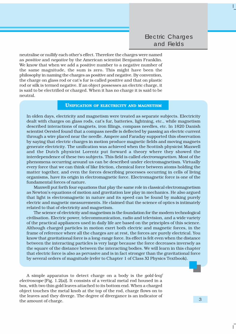
Example 1.4 Coulomb’s law for electrostatic force between two pointcharges and Newton’s law for gravitational force between twostationary point masses, both have inverse-square dependence onthe distance between the charges/masses. (a) Compare the strengthof these forces by determining the ratio of their magnitudes (i) for anelectron and a proton and (ii) for two protons. (b) Estimate theaccelerations of electron and proton due to the electrical force of theirmutual attraction when they are 1 Å (= 10-10 m) apart? (mp = 1.67 ×10⁻²⁷ kg, me = 9.11 × 10⁻³¹ kg)
Solution(a) (i) The electric force between an electron and a proton at a distance
r apart is:2
20
14e
eF
rε= −
πwhere the negative sign indicates that the force is attractive. Thecorresponding gravitational force (always attractive) is:
2p e
G
m mF G
r= −
where mp and me are the masses of a proton and an electronrespectively.
239
0
2.4 104
e
G p e
F eF Gm mε
= = ×π
(ii) On similar lines, the ratio of the magnitudes of electric forceto the gravitational force between two protons at a distance rapart is :
2
04e
G p p
F eF Gm mε
= =π
1.3 × 1036
However, it may be mentioned here that the signs of the two forcesare different. For two protons, the gravitational force is attractivein nature and the Coulomb force is repulsive . The actual valuesof these forces between two protons inside a nucleus (distancebetween two protons is ~ 10-15 m inside a nucleus) are Fe ~ 230 Nwhereas FG ~ 1.9 × 10⁻³⁴ N.The (dimensionless) ratio of the two forces shows that electricalforces are enormously stronger than the gravitational forces.
(b) The electric force F exerted by a proton on an electron is same inmagnitude to the force exerted by an electron on a proton; howeverthe masses of an electron and a proton are different. Thus, themagnitude of force is
|F| = 2
20
14
e
rεπ = 8.987 × 10⁹ Nm2/C2 × (1.6 ×10–19C)2 / (10–10m)2
= 2.3 × 10⁻⁸ NUsing Newton’s second law of motion, F = ma, the accelerationthat an electron will undergo isa = 2.3×10⁻⁸ N / 9.11 ×10⁻³¹ kg = 2.5 × 10²² m/s2
Comparing this with the value of acceleration due to gravity, wecan conclude that the effect of gravitational field is negligible onthe motion of electron and it undergoes very large accelerationsunder the action of Coulomb force due to a proton.The value for acceleration of the proton is
2.3 × 10⁻⁸ N / 1.67 × 10⁻²⁷ kg = 1.4 × 10¹⁹ m/s2
Interactive animation on Coulomb’s law:
http://webphysics.davidson.edu/physlet_resources/bu_semester2/co1_coulomb.html

14
Physics
EX
AM
PLE 1
.5Example 1.5 A charged metallic sphere A is suspended by a nylonthread. Another charged metallic sphere B held by an insulatinghandle is brought close to A such that the distance between theircentres is 10 cm, as shown in Fig. 1.7(a). The resulting repulsion of Ais noted (for example, by shining a beam of light and measuring thedeflection of its shadow on a screen). Spheres A and B are touchedby uncharged spheres C and D respectively, as shown in Fig. 1.7(b).C and D are then removed and B is brought closer to A to adistance of 5.0 cm between their centres, as shown in Fig. 1.7(c).What is the expected repulsion of A on the basis of Coulomb’s law?Spheres A and C and spheres B and D have identical sizes. Ignorethe sizes of A and B in comparison to the separation between theircentres.
FIGURE 1.7

Electric Chargesand Fields
15
EX
AM
PLE 1
.5
Solution Let the original charge on sphere A be q and that on B beq′. At a distance r between their centres, the magnitude of theelectrostatic force on each is given by
20
14
qqF
rε′
=π
neglecting the sizes of spheres A and B in comparison to r. When anidentical but uncharged sphere C touches A, the charges redistributeon A and C and, by symmetry, each sphere carries a charge q/2.Similarly, after D touches B, the redistributed charge on each isq′/2. Now, if the separation between A and B is halved, the magnitudeof the electrostatic force on each is
2 20 0
1 ( /2)( /2) 1 ( )4 4( /2)
q q qqF F
r rε ε′ ′
= = =′π π
Thus the electrostatic force on A, due to B, remains unaltered.
1.7 FORCES BETWEEN MULTIPLE CHARGES
The mutual electric force between two charges is givenby Coulomb’s law. How to calculate the force on acharge where there are not one but several chargesaround? Consider a system of n stationary chargesq1, q2, q3, ..., qn in vacuum. What is the force on q1 dueto q2, q3, ..., qn? Coulomb’s law is not enough to answerthis question. Recall that forces of mechanical originadd according to the parallelogram law of addition. Isthe same true for forces of electrostatic origin?
Experimentally it is verified that force on anycharge due to a number of other charges is the vectorsum of all the forces on that charge due to the othercharges, taken one at a time. The individual forcesare unaffected due to the presence of other charges.This is termed as the principle of superposition.
To better understand the concept, consider asystem of three charges q1, q2 and q3, as shown inFig. 1.8(a). The force on one charge, say q1, due to twoother charges q2, q3 can therefore be obtained byperforming a vector addition of the forces due to eachone of these charges. Thus, if the force on q1 due to q2is denoted by F12, F12 is given by Eq. (1.3) even thoughother charges are present.
Thus, F12 1 2
1220 12
1ˆ
4q q
rε=
πr
In the same way, the force on q1 due to q3, denotedby F13, is given by
1 313 132
0 13
1ˆ
4
q q
rε=
πF r
FIGURE 1.8 A system of (a) threecharges (b) multiple charges.

16
Physics
EX
AM
PLE 1
.6
which again is the Coulomb force on q1 due to q3, even though othercharge q2 is present.
Thus the total force F1 on q1 due to the two charges q2 and q3 isgiven as
1 31 21 12 13 12 132 2
0 012 13
1 1ˆ ˆ
4 4
q qq q
r rε ε= + = +
π πF F F r r (1.4)
The above calculation of force can be generalised to a system ofcharges more than three, as shown in Fig. 1.8(b).
The principle of superposition says that in a system of charges q1,q2, ..., qn, the force on q1 due to q2 is the same as given by Coulomb’s law,i.e., it is unaffected by the presence of the other charges q3, q4, ..., qn. Thetotal force F1 on the charge q1, due to all other charges, is then given bythe vector sum of the forces F12, F13, ..., F1n:
i.e.,
1 3 11 21 12 13 1n 12 13 12 2 2
0 12 13 1
1 ˆ ˆ ˆ = + + ...+ ...4
nn
n
q q q qq q
r r rε⎡ ⎤
= + + +⎢ ⎥π ⎣ ⎦F F F F r r r
112
20 1
ˆ4
ni
ii i
rε =
=π ∑ r (1.5)
The vector sum is obtained as usual by the parallelogram law ofaddition of vectors. All of electrostatics is basically a consequence ofCoulomb’s law and the superposition principle.
Example 1.6 Consider three charges q1, q2, q3 each equal to q at thevertices of an equilateral triangle of side l. What is the force on acharge Q (with the same sign as q) placed at the centroid of thetriangle, as shown in Fig. 1.9?
FIGURE 1.9
Solution In the given equilateral triangle ABC of sides of length l, ifwe draw a perpendicular AD to the side BC,AD = AC cos 30º = ( 3 /2 ) l and the distance AO of the centroid Ofrom A is (2/3) AD = (1/ 3 ) l. By symmatry AO = BO = CO.

Electric Chargesand Fields
17
EX
AM
PLE 1
.6
Thus,
Force F1 on Q due to charge q at A = 20
34
lεπ along AO
Force F2 on Q due to charge q at B = 20
34
lεπ along BO
Force F3 on Q due to charge q at C = 20
34
lεπ along CO
The resultant of forces F2 and F3 is 20
34
lεπ along OA, by the
parallelogram law. Therefore, the total force on Q = ( )20
3ˆ ˆ
4Qq
lε−
πr r
= 0, where r is the unit vector along OA.It is clear also by symmetry that the three forces will sum to zero.Suppose that the resultant force was non-zero but in some direction.Consider what would happen if the system was rotated through 60ºabout O.
Example 1.7 Consider the charges q, q, and –q placed at the verticesof an equilateral triangle, as shown in Fig. 1.10. What is the force oneach charge?
FIGURE 1.10
Solution The forces acting on charge q at A due to charges q at Band –q at C are F12 along BA and F13 along AC respectively, as shownin Fig. 1.10. By the parallelogram law, the total force F1 on the chargeq at A is given by
F1 = F 1r where 1r is a unit vector along BC.The force of attraction or repulsion for each pair of charges has the
same magnitude 2
204
qF
lε=
π
The total force F2 on charge q at B is thus F2 = F r2, where r
2 is aunit vector along AC.
EX
AM
PLE 1
.7

18
Physics
EX
AM
PLE 1
.7
Similarly the total force on charge –q at C is F3 = 3 F n , where n isthe unit vector along the direction bisecting the ∠BCA.It is interesting to see that the sum of the forces on the three chargesis zero, i.e.,
F1 + F2 + F3 = 0
The result is not at all surprising. It follows straight from the factthat Coulomb’s law is consistent with Newton’s third law. The proofis left to you as an exercise.
1.8 ELECTRIC FIELD
Let us consider a point charge Q placed in vacuum, at the origin O. If weplace another point charge q at a point P, where OP = r, then the charge Qwill exert a force on q as per Coulomb’s law. We may ask the question: Ifcharge q is removed, then what is left in the surrounding? Is therenothing? If there is nothing at the point P, then how does a force actwhen we place the charge q at P. In order to answer such questions, theearly scientists introduced the concept of field. According to this, we saythat the charge Q produces an electric field everywhere in the surrounding.When another charge q is brought at some point P, the field there acts onit and produces a force. The electric field produced by the charge Q at apoint r is given as
( ) 2 20 0
1 1ˆ ˆ
4 4Q Q
r rε ε= =
π πE r r r (1.6)
where ˆ =r r/r, is a unit vector from the origin to the point r. Thus, Eq.(1.6)specifies the value of the electric field for each value of the positionvector r. The word “field” signifies how some distributed quantity (whichcould be a scalar or a vector) varies with position. The effect of the chargehas been incorporated in the existence of the electric field. We obtain theforce F exerted by a charge Q on a charge q, as
20
1ˆ
4Qq
rε=
πF r (1.7)
Note that the charge q also exerts an equal and opposite force on thecharge Q. The electrostatic force between the charges Q and q can belooked upon as an interaction between charge q and the electric field ofQ and vice versa. If we denote the position of charge q by the vector r, itexperiences a force F equal to the charge q multiplied by the electricfield E at the location of q. Thus,
F(r) = q E(r) (1.8)Equation (1.8) defines the SI unit of electric field as N/C*.Some important remarks may be made here:
(i) From Eq. (1.8), we can infer that if q is unity, the electric field due toa charge Q is numerically equal to the force exerted by it. Thus, theelectric field due to a charge Q at a point in space may be definedas the force that a unit positive charge would experience if placed
* An alternate unit V/m will be introduced in the next chapter.
FIGURE 1.11 Electricfield (a) due to a
charge Q, (b) due to acharge –Q.

Electric Chargesand Fields
19
at that point. The charge Q, which is producing the electric field, iscalled a source charge and the charge q, which tests the effect of asource charge, is called a test charge. Note that the source charge Qmust remain at its original location. However, if a charge q is broughtat any point around Q, Q itself is bound to experience an electricalforce due to q and will tend to move. A way out of this difficulty is tomake q negligibly small. The force F is then negligibly small but theratio F/q is finite and defines the electric field:
0limq q→
⎛ ⎞= ⎜ ⎟⎝ ⎠
FE (1.9)
A practical way to get around the problem (of keeping Q undisturbedin the presence of q) is to hold Q to its location by unspecified forces!This may look strange but actually this is what happens in practice.When we are considering the electric force on a test charge q due to acharged planar sheet (Section 1.15), the charges on the sheet are held totheir locations by the forces due to the unspecified charged constituentsinside the sheet.(ii) Note that the electric field E due to Q, though defined operationally
in terms of some test charge q, is independent of q. This is becauseF is proportional to q, so the ratio F/q does not depend on q. Theforce F on the charge q due to the charge Q depends on the particularlocation of charge q which may take any value in the space aroundthe charge Q. Thus, the electric field E due to Q is also dependent onthe space coordinate r. For different positions of the charge q all overthe space, we get different values of electric field E. The field exists atevery point in three-dimensional space.
(iii) For a positive charge, the electric field will be directed radiallyoutwards from the charge. On the other hand, if the source charge isnegative, the electric field vector, at each point, points radially inwards.
(iv) Since the magnitude of the force F on charge q due to charge Qdepends only on the distance r of the charge q from charge Q,the magnitude of the electric field E will also depend only on thedistance r. Thus at equal distances from the charge Q, the magnitudeof its electric field E is same. The magnitude of electric field E due toa point charge is thus same on a sphere with the point charge at itscentre; in other words, it has a spherical symmetry.
1.8.1 Electric field due to a system of charges
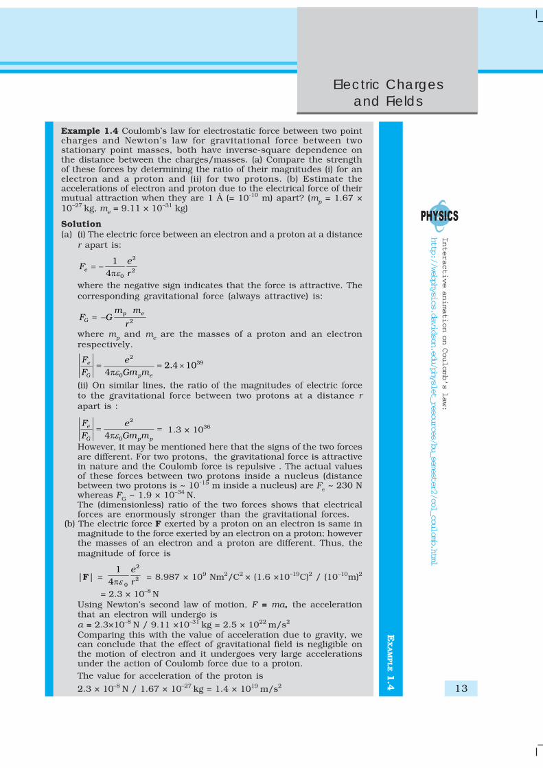
Consider a system of charges q1, q2, ..., qn with position vectors r1,r2, ..., rn relative to some origin O. Like the electric field at a point inspace due to a single charge, electric field at a point in space due to thesystem of charges is defined to be the force experienced by a unittest charge placed at that point, without disturbing the originalpositions of charges q1, q2, ..., qn. We can use Coulomb’s law and thesuperposition principle to determine this field at a point P denoted byposition vector r.
20
PhysicsElectric field E1 at r due to q1 at r1 is given by
E1 = 1
1P2
0 1P
1ˆ
4q
rπεr
where 1Pr is a unit vector in the direction from q1 to P,and r1P is the distance between q1 and P.In the same manner, electric field E2 at r due to q2 atr2 is
E2 = 2
2P2
0 2P
1ˆ
4q
rπεr
where 2Pr is a unit vector in the direction from q2 to Pand r2P is the distance between q2 and P. Similarexpressions hold good for fields E3, E4, ..., En due tocharges q3, q4, ..., qn.By the superposition principle, the electric field E at rdue to the system of charges is (as shown in Fig. 1.12)
E(r) = E1 (r) + E2 (r) + … + En(r)
= 1 21P 2P P2 2 2
0 0 01P 2P P
1 1 1ˆ ˆ ˆ...
4 4 4n
nn
qq q
r r rε ε ε+ + +
π π πr r r
E(r) i P210 P
1ˆ
4
ni
i i
q
rε =
=π ∑ r (1.10)
E is a vector quantity that varies from one point to another point in spaceand is determined from the positions of the source charges.
1.8.2 Physical significance of electric fieldYou may wonder why the notion of electric field has been introducedhere at all. After all, for any system of charges, the measurable quantityis the force on a charge which can be directly determined using Coulomb’slaw and the superposition principle [Eq. (1.5)]. Why then introduce thisintermediate quantity called the electric field?
For electrostatics, the concept of electric field is convenient, but notreally necessary. Electric field is an elegant way of characterising theelectrical environment of a system of charges. Electric field at a point inthe space around a system of charges tells you the force a unit positivetest charge would experience if placed at that point (without disturbingthe system). Electric field is a characteristic of the system of charges andis independent of the test charge that you place at a point to determinethe field. The term field in physics generally refers to a quantity that isdefined at every point in space and may vary from point to point. Electricfield is a vector field, since force is a vector quantity.
The true physical significance of the concept of electric field, however,emerges only when we go beyond electrostatics and deal with time-dependent electromagnetic phenomena. Suppose we consider the forcebetween two distant charges q1, q2 in accelerated motion. Now the greatestspeed with which a signal or information can go from one point to anotheris c, the speed of light. Thus, the effect of any motion of q1 on q2 cannot
FIGURE 1.12 Electric field at apoint due to a system of charges isthe vector sum of the electric fields
at the point due to individualcharges.

Electric Chargesand Fields
21
arise instantaneously. There will be some time delay between the effect(force on q2) and the cause (motion of q1). It is precisely here that thenotion of electric field (strictly, electromagnetic field) is natural and veryuseful. The field picture is this: the accelerated motion of charge q1produces electromagnetic waves, which then propagate with the speedc, reach q2 and cause a force on q2. The notion of field elegantly accountsfor the time delay. Thus, even though electric and magnetic fields can bedetected only by their effects (forces) on charges, they are regarded asphysical entities, not merely mathematical constructs. They have anindependent dynamics of their own, i.e., they evolve according to lawsof their own. They can also transport energy. Thus, a source of time-dependent electromagnetic fields, turned on briefly and switched off, leavesbehind propagating electromagnetic fields transporting energy. Theconcept of field was first introduced by Faraday and is now among thecentral concepts in physics.
Example 1.8 An electron falls through a distance of 1.5 cm in auniform electric field of magnitude 2.0 × 10⁴ N C–1 [Fig. 1.13(a)]. Thedirection of the field is reversed keeping its magnitude unchangedand a proton falls through the same distance [Fig. 1.13(b)]. Computethe time of fall in each case. Contrast the situation with that of ‘freefall under gravity’.
FIGURE 1.13
Solution In Fig. 1.13(a) the field is upward, so the negatively chargedelectron experiences a downward force of magnitude eE where E isthe magnitude of the electric field. The acceleration of the electron is
ae = eE/mewhere me is the mass of the electron.
Starting from rest, the time required by the electron to fall through a
distance h is given by 22
ee
e
h mht
a e E= =
For e = 1.6 × 10⁻¹⁹C, me = 9.11 × 10⁻³¹ kg,
E = 2.0 × 10⁴ N C–1, h = 1.5 × 10⁻² m,
te = 2.9 × 10⁻⁹s
In Fig. 1.13 (b), the field is downward, and the positively chargedproton experiences a downward force of magnitude eE . Theacceleration of the proton is
ap = eE/mp
where mp is the mass of the proton; mp = 1.67 × 10⁻²⁷ kg. The time offall for the proton is
EX
AM
PLE 1
.8

22
Physics
EX
AM
PLE 1
.9 E
XA
MPLE 1
.8–722
1 3 10 spp
p
h mht .
a e E= = = ×
Thus, the heavier particle (proton) takes a greater time to fall throughthe same distance. This is in basic contrast to the situation of ‘freefall under gravity’ where the time of fall is independent of the mass ofthe body. Note that in this example we have ignored the accelerationdue to gravity in calculating the time of fall. To see if this is justified,let us calculate the acceleration of the proton in the given electricfield:
pp
e Ea
m=
19 4 1
27
(1 6 10 C) (2 0 10 N C )1 67 10 kg
. .
.
− −
−
× × ×=
×
12 –21 9 10 m s.= ×which is enormous compared to the value of g (9.8 m s–2), theacceleration due to gravity. The acceleration of the electron is evengreater. Thus, the effect of acceleration due to gravity can be ignoredin this example.
Example 1.9 Two point charges q1 and q2, of magnitude +10–8 C and–10–8 C, respectively, are placed 0.1 m apart. Calculate the electricfields at points A, B and C shown in Fig. 1.14.
FIGURE 1.14
Solution The electric field vector E1A at A due to the positive chargeq1 points towards the right and has a magnitude
9 2 -2 8
1A 2
(9 10 Nm C ) (10 C)(0.05m)
E−× ×
= = 3.6 × 10⁴ N C–1
The electric field vector E2A at A due to the negative charge q2 pointstowards the right and has the same magnitude. Hence the magnitudeof the total electric field EA at A is
EA = E1A + E2A = 7.2 × 10⁴ N C–1
EA is directed toward the right.

Electric Chargesand Fields
23
The electric field vector E1B at B due to the positive charge q1 pointstowards the left and has a magnitude
9 2 –2 8
1B 2
(9 10 Nm C ) (10 C)(0.05 m)
E−× ×
= = 3.6 × 10⁴ N C–1
The electric field vector E2B at B due to the negative charge q2 pointstowards the right and has a magnitude
9 2 –2 8
2B 2
(9 10 Nm C ) (10 C)(0.15 m)
E−× ×
= = 4 × 10³ N C–1
The magnitude of the total electric field at B isEB = E1B – E2B = 3.2 × 10⁴ N C–1
EB is directed towards the left.The magnitude of each electric field vector at point C, due to chargeq1 and q2 is
9 2 –2 8
1C 2C 2
(9 10 Nm C ) (10 C)(0.10 m)
E E−× ×
= = = 9 × 10³ N C–1
The directions in which these two vectors point are indicated inFig. 1.14. The resultant of these two vectors is
1 2cos cos3 3CE E Eπ π
= + = 9 × 10³ N C–1
EC points towards the right.
1.9 ELECTRIC FIELD LINES
We have studied electric field in the last section. It is a vector quantityand can be represented as we represent vectors. Let us try to represent Edue to a point charge pictorially. Let the point charge be placed at theorigin. Draw vectors pointing along the direction of the electric field withtheir lengths proportional to the strength of the field ateach point. Since the magnitude of electric field at a pointdecreases inversely as the square of the distance of thatpoint from the charge, the vector gets shorter as one goesaway from the origin, always pointing radially outward.Figure 1.15 shows such a picture. In this figure, eacharrow indicates the electric field, i.e., the force acting on aunit positive charge, placed at the tail of that arrow.Connect the arrows pointing in one direction and theresulting figure represents a field line. We thus get manyfield lines, all pointing outwards from the point charge.Have we lost the information about the strength ormagnitude of the field now, because it was contained inthe length of the arrow? No. Now the magnitude of thefield is represented by the density of field lines. E is strongnear the charge, so the density of field lines is more nearthe charge and the lines are closer. Away from the charge,the field gets weaker and the density of field lines is less,resulting in well-separated lines.
Another person may draw more lines. But the number of lines is notimportant. In fact, an infinite number of lines can be drawn in any region.
FIGURE 1.15 Field of a point charge.
EX
AM
PLE 1
.9

24
PhysicsIt is the relative density of lines in different regions which isimportant.
We draw the figure on the plane of paper, i.e., in two-dimensions but we live in three-dimensions. So if one wishesto estimate the density of field lines, one has to consider thenumber of lines per unit cross-sectional area, perpendicularto the lines. Since the electric field decreases as the square ofthe distance from a point charge and the area enclosing thecharge increases as the square of the distance, the numberof field lines crossing the enclosing area remains constant,whatever may be the distance of the area from the charge.
We started by saying that the field lines carry informationabout the direction of electric field at different points in space.Having drawn a certain set of field lines, the relative density(i.e., closeness) of the field lines at different points indicatesthe relative strength of electric field at those points. The fieldlines crowd where the field is strong and are spaced apartwhere it is weak. Figure 1.16 shows a set of field lines. We
can imagine two equal and small elements of area placed at points R andS normal to the field lines there. The number of field lines in our picturecutting the area elements is proportional to the magnitude of field atthese points. The picture shows that the field at R is stronger than at S.
To understand the dependence of the field lines on the area, or ratherthe solid angle subtended by an area element, let us try to relate thearea with the solid angle, a generalization of angle to three dimensions.Recall how a (plane) angle is defined in two-dimensions. Let a smalltransverse line element Δl be placed at a distance r from a point O. Thenthe angle subtended by Δl at O can be approximated as Δθ = Δl/r.Likewise, in three-dimensions the solid angle* subtended by a smallperpendicular plane area ΔS, at a distance r, can be written asΔΩ = ΔS/r2. We know that in a given solid angle the number of radialfield lines is the same. In Fig. 1.16, for two points P1 and P2 at distancesr1 and r2 from the charge, the element of area subtending the solid angleΔΩ is 2
1r ΔΩ at P1 and an element of area 22r ΔΩ at P2, respectively. The
number of lines (say n) cutting these area elements are the same. Thenumber of field lines, cutting unit area element is therefore n/( 2
1r ΔΩ) atP1 andn/( 2
2r ΔΩ) at P2, respectively. Since n and ΔΩ are common, thestrength of the field clearly has a 1/r 2 dependence.
The picture of field lines was invented by Faraday to develop anintuitive non- mathematical way of visualizing electric fields aroundcharged configurations. Faraday called them lines of force. This term issomewhat misleading, especially in case of magnetic fields. The moreappropriate term is field lines (electric or magnetic) that we haveadopted in this book.
Electric field lines are thus a way of pictorially mapping the electricfield around a configuration of charges. An electric field line is, in general,
FIGURE 1.16 Dependence ofelectric field strength on the
distance and its relation to thenumber of field lines.
* Solid angle is a measure of a cone. Consider the intersection of the given conewith a sphere of radius R. The solid angle ΔΩ of the cone is defined to be equalto ΔS/R 2, where ΔS is the area on the sphere cut out by the cone.
Electric Chargesand Fields
25
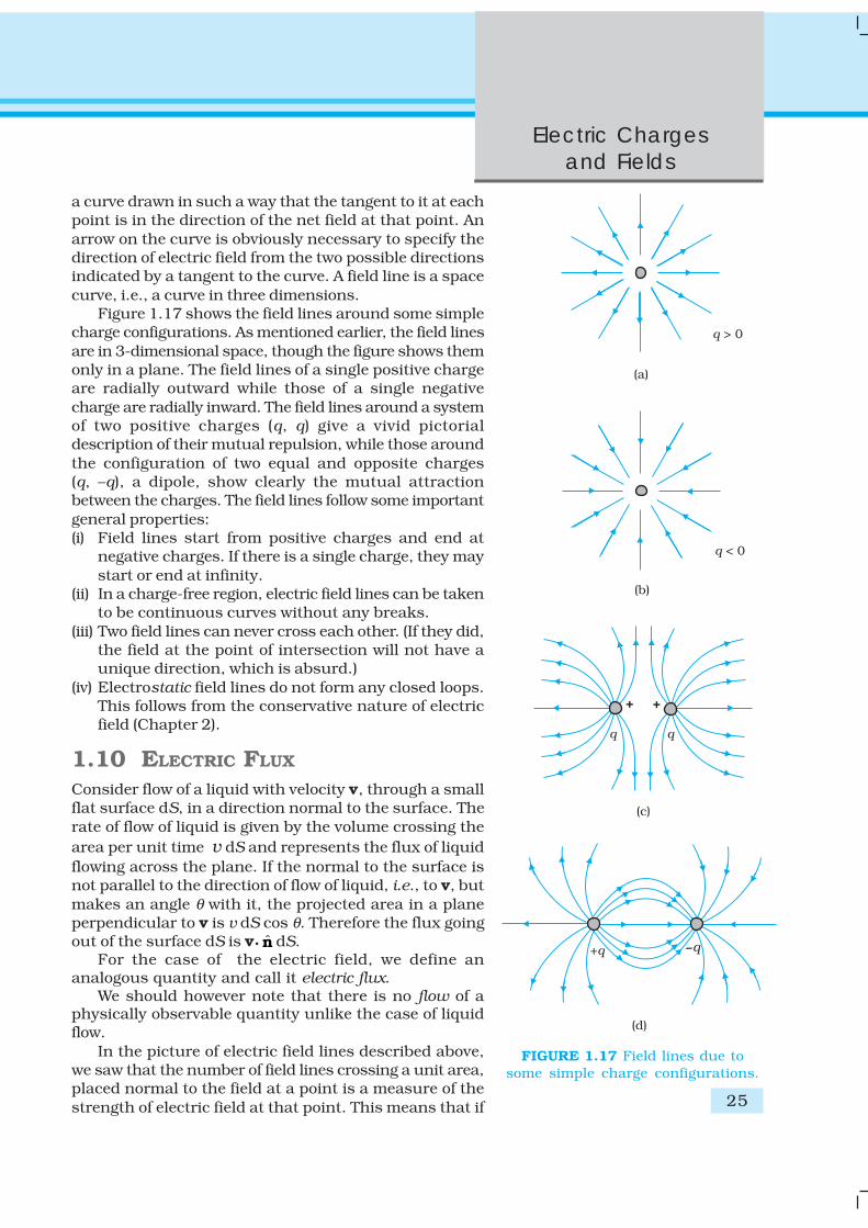
a curve drawn in such a way that the tangent to it at eachpoint is in the direction of the net field at that point. Anarrow on the curve is obviously necessary to specify thedirection of electric field from the two possible directionsindicated by a tangent to the curve. A field line is a spacecurve, i.e., a curve in three dimensions.
Figure 1.17 shows the field lines around some simplecharge configurations. As mentioned earlier, the field linesare in 3-dimensional space, though the figure shows themonly in a plane. The field lines of a single positive chargeare radially outward while those of a single negativecharge are radially inward. The field lines around a systemof two positive charges (q, q) give a vivid pictorialdescription of their mutual repulsion, while those aroundthe configuration of two equal and opposite charges(q, –q), a dipole, show clearly the mutual attractionbetween the charges. The field lines follow some importantgeneral properties:(i) Field lines start from positive charges and end at
negative charges. If there is a single charge, they maystart or end at infinity.
(ii) In a charge-free region, electric field lines can be takento be continuous curves without any breaks.
(iii) Two field lines can never cross each other. (If they did,the field at the point of intersection will not have aunique direction, which is absurd.)
(iv) Electrostatic field lines do not form any closed loops.This follows from the conservative nature of electricfield (Chapter 2).
1.10 ELECTRIC FLUX
Consider flow of a liquid with velocity v, through a smallflat surface dS, in a direction normal to the surface. Therate of flow of liquid is given by the volume crossing thearea per unit time v dS and represents the flux of liquidflowing across the plane. If the normal to the surface isnot parallel to the direction of flow of liquid, i.e., to v, butmakes an angle θ with it, the projected area in a planeperpendicular to v is v dS cos θ. Therefore the flux goingout of the surface dS is v. n dS.
For the case of the electric field, we define ananalogous quantity and call it electric flux.
We should however note that there is no flow of aphysically observable quantity unlike the case of liquidflow.
In the picture of electric field lines described above,we saw that the number of field lines crossing a unit area,placed normal to the field at a point is a measure of thestrength of electric field at that point. This means that if
FIGURE 1.17 Field lines due tosome simple charge configurations.

26
Physicswe place a small planar element of area ΔSnormal to E at a point, the number of field linescrossing it is proportional* to E ΔS. Nowsuppose we tilt the area element by angle θ.Clearly, the number of field lines crossing thearea element will be smaller. The projection ofthe area element normal to E is ΔS cosθ. Thus,the number of field lines crossing ΔS isproportional to E ΔS cosθ. When θ = 90°, fieldlines will be parallel to ΔS and will not cross itat all (Fig. 1.18).
The orientation of area element and notmerely its magnitude is important in manycontexts. For example, in a stream, the amountof water flowing through a ring will naturallydepend on how you hold the ring. If you holdit normal to the flow, maximum water will flowthrough it than if you hold it with some otherorientation. This shows that an area elementshould be treated as a vector. It has a
magnitude and also a direction. How to specify the direction of a planararea? Clearly, the normal to the plane specifies the orientation of theplane. Thus the direction of a planar area vector is along its normal.
How to associate a vector to the area of a curved surface? We imaginedividing the surface into a large number of very small area elements.Each small area element may be treated as planar and a vector associatedwith it, as explained before.
Notice one ambiguity here. The direction of an area element is alongits normal. But a normal can point in two directions. Which direction dowe choose as the direction of the vector associated with the area element?This problem is resolved by some convention appropriate to the givencontext. For the case of a closed surface, this convention is very simple.The vector associated with every area element of a closed surface is takento be in the direction of the outward normal. This is the convention usedin Fig. 1.19. Thus, the area element vector ΔS at a point on a closed
surface equals ΔS n where ΔS is the magnitude of the area element and
n is a unit vector in the direction of outward normal at that point.We now come to the definition of electric flux. Electric flux Δφ through
an area element ΔS is defined by
Δφ = E.ΔS = E ΔS cosθ (1.11)
which, as seen before, is proportional to the number of field lines cuttingthe area element. The angle θ here is the angle between E and ΔS. For aclosed surface, with the convention stated already, θ is the angle betweenE and the outward normal to the area element. Notice we could look atthe expression E ΔS cosθ in two ways: E (ΔS cosθ ) i.e., E times the
FIGURE 1.18 Dependence of flux on theinclination θ between E and n .
FIGURE 1.19Convention fordefining normal
n and ΔS. * It will not be proper to say that the number of field lines is equal to EΔS. Thenumber of field lines is after all, a matter of how many field lines we choose todraw. What is physically significant is the relative number of field lines crossinga given area at different points.

Electric Chargesand Fields
27
projection of area normal to E, or E⊥ ΔS, i.e., component of E along thenormal to the area element times the magnitude of the area element. Theunit of electric flux is N C–1 m2.
The basic definition of electric flux given by Eq. (1.11) can be used, inprinciple, to calculate the total flux through any given surface. All wehave to do is to divide the surface into small area elements, calculate theflux at each element and add them up. Thus, the total flux φ through asurface S is
φ ~ Σ E.ΔS (1.12)
The approximation sign is put because the electric field E is taken tobe constant over the small area element. This is mathematically exactonly when you take the limit ΔS → 0 and the sum in Eq. (1.12) is writtenas an integral.
1.11 ELECTRIC DIPOLE
An electric dipole is a pair of equal and opposite point charges q and –q,separated by a distance 2a. The line connecting the two charges definesa direction in space. By convention, the direction from –q to q is said tobe the direction of the dipole. The mid-point of locations of –q and q iscalled the centre of the dipole.
The total charge of the electric dipole is obviously zero. This does notmean that the field of the electric dipole is zero. Since the charge q and–q are separated by some distance, the electric fields due to them, whenadded, do not exactly cancel out. However, at distances much larger thanthe separation of the two charges forming a dipole (r >> 2a), the fieldsdue to q and –q nearly cancel out. The electric field due to a dipoletherefore falls off, at large distance, faster than like 1/r 2 (the dependenceon r of the field due to a single charge q). These qualitative ideas areborne out by the explicit calculation as follows:
1.11.1 The field of an electric dipoleThe electric field of the pair of charges (–q and q) at any point in spacecan be found out from Coulomb’s law and the superposition principle.The results are simple for the following two cases: (i) when the point is onthe dipole axis, and (ii) when it is in the equatorial plane of the dipole,i.e., on a plane perpendicular to the dipole axis through its centre. Theelectric field at any general point P is obtained by adding the electricfields E–q due to the charge –q and E+q due to the charge q, by theparallelogram law of vectors.
(i) For points on the axis
Let the point P be at distance r from the centre of the dipole on the side ofthe charge q, as shown in Fig. 1.20(a). Then
20
ˆ4 ( )q
q
r aε− = −π +
E p [1.13(a)]
where p is the unit vector along the dipole axis (from –q to q). Also
20
ˆ4 ( )q
q
r aε+ =π −
E p [1.13(b)]

28
PhysicsThe total field at P is
2 20
1 1 ˆ4 ( ) ( )q q
q
r a r aε+ −
⎡ ⎤= + = −⎢ ⎥π − +⎣ ⎦
E E E p
2 2 2
4ˆ
4 ( )o
a rq
r aε=
π −p (1.14)
For r >> a
30
4ˆ
4
q a
rε=
πE p (r >> a) (1.15)
(ii) For points on the equatorial plane
The magnitudes of the electric fields due to the twocharges +q and –q are given by
2 20
14q
qE
r aε+ =π + [1.16(a)]
– 2 20
14q
qE
r aε=
π + [1.16(b)]
and are equal.The directions of E+q and E–q are as shown in
Fig. 1.20(b). Clearly, the components normal to the dipoleaxis cancel away. The components along the dipole axisadd up. The total electric field is opposite to p . We have
E = – (E +q + E –q ) cosθ p
2 2 3/2
2ˆ
4 ( )o
q a
r aε= −
π +p (1.17)
At large distances (r >> a), this reduces to
3
2 ˆ ( )4 o
q ar a
rε= − >>
πE p (1.18)
From Eqs. (1.15) and (1.18), it is clear that the dipole field at largedistances does not involve q and a separately; it depends on the productqa. This suggests the definition of dipole moment. The dipole momentvector p of an electric dipole is defined by
p = q × 2a p (1.19)that is, it is a vector whose magnitude is charge q times the separation2a (between the pair of charges q, –q) and the direction is along the linefrom –q to q. In terms of p, the electric field of a dipole at large distancestakes simple forms:At a point on the dipole axis
3
24 orε
=π
pE (r >> a) (1.20)
At a point on the equatorial plane
34 orε= −
πp
E (r >> a) (1.21)
FIGURE 1.20 Electric field of a dipoleat (a) a point on the axis, (b) a pointon the equatorial plane of the dipole.
p is the dipole moment vector ofmagnitude p = q × 2a and
directed from –q to q.

Electric Chargesand Fields
29
EX
AM
PLE 1
.10
Notice the important point that the dipole field at large distancesfalls off not as 1/r2 but as1/r3. Further, the magnitude and the directionof the dipole field depends not only on the distance r but also on theangle between the position vector r and the dipole moment p.
We can think of the limit when the dipole size 2a approaches zero,the charge q approaches infinity in such a way that the productp = q × 2a is finite. Such a dipole is referred to as a point dipole. For apoint dipole, Eqs. (1.20) and (1.21) are exact, true for any r.
1.11.2 Physical significance of dipolesIn most molecules, the centres of positive charges and of negative charges*lie at the same place. Therefore, their dipole moment is zero. CO2 andCH4 are of this type of molecules. However, they develop a dipole momentwhen an electric field is applied. But in some molecules, the centres ofnegative charges and of positive charges do not coincide. Therefore theyhave a permanent electric dipole moment, even in the absence of an electricfield. Such molecules are called polar molecules. Water molecules, H2O,is an example of this type. Various materials give rise to interestingproperties and important applications in the presence or absence ofelectric field.
Example 1.10 Two charges ±10 μC are placed 5.0 mm apart.Determine the electric field at (a) a point P on the axis of the dipole15 cm away from its centre O on the side of the positive charge, asshown in Fig. 1.21(a), and (b) a point Q, 15 cm away from O on a linepassing through O and normal to the axis of the dipole, as shown inFig. 1.21(b).
FIGURE 1.21
* Centre of a collection of positive point charges is defined much the same way
as the centre of mass: cm
i ii
ii
q
q
∑=
∑
rr .

30
Physics
EX
AM
PLE 1
.10
Solution (a) Field at P due to charge +10 μC
= 5
12 2 1 2
10 C
4 (8.854 10 C N m )
−
− − −π × 2 4 2
1
(15 0.25) 10 m−×− ×
= 4.13 × 10⁶ N C–1 along BPField at P due to charge –10 μC
–5
12 2 1 2
10 C4 (8.854 10 C N m )− − −=π × 2 4 2
1(15 0.25) 10 m−×
+ ×
= 3.86 × 10⁶ N C–1 along PAThe resultant electric field at P due to the two charges at A and B is= 2.7 × 10⁵ N C–1 along BP.In this example, the ratio OP/OB is quite large (= 60). Thus, we canexpect to get approximately the same result as above by directly usingthe formula for electric field at a far-away point on the axis of a dipole.For a dipole consisting of charges ± q, 2a distance apart, the electricfield at a distance r from the centre on the axis of the dipole has amagnitude
30
2
4
pE
rε=
π (r/a >> 1)
where p = 2a q is the magnitude of the dipole moment.The direction of electric field on the dipole axis is always along thedirection of the dipole moment vector (i.e., from –q to q). Here,p =10–5 C × 5 × 10–3 m = 5 × 10⁻⁸ C mTherefore,
E =8
12 2 1 2
2 5 10 Cm
4 (8.854 10 C N m )
−
− − −
× ×π × 3 6 3
1
(15) 10 m−×× = 2.6 × 10⁵ N C–1
along the dipole moment direction AB, which is close to the resultobtained earlier.(b) Field at Q due to charge + 10 μC at B
=5
12 2 1 2
10 C4 (8.854 10 C N m )
−
− − −π × 2 2 4 2
1
[15 (0.25) ] 10 m−+ ××
= 3.99 × 10⁶ N C–1 along BQ
Field at Q due to charge –10 μC at A
=5
12 2 1 2
10 C
4 (8.854 10 C N m )
−
− − −π × 2 2 4 2
1
[15 (0.25) ] 10 m−+ ××
= 3.99 × 10⁶ N C–1 along QA.
Clearly, the components of these two forces with equal magnitudescancel along the direction OQ but add up along the direction parallelto BA. Therefore, the resultant electric field at Q due to the twocharges at A and B is
= 2 × 6 –1
2 2
0.253.99 10 N C
15 (0.25)× ×
+along BA
= 1.33 × 10⁵ N C–1 along BA.As in (a), we can expect to get approximately the same result bydirectly using the formula for dipole field at a point on the normal tothe axis of the dipole:

Electric Chargesand Fields
31
EX
AM
PLE 1
.10
34p
Erε0
=π (r/a >> 1)
8
12 2 –1 –2
5 10 Cm4 (8.854 10 C N m )
−
−
×=
π × 3 6 3
1(15) 10 m−×
×
= 1.33 × 10⁵ N C–1.The direction of electric field in this case is opposite to the directionof the dipole moment vector. Again the result agrees with that obtainedbefore.
1.12 DIPOLE IN A UNIFORM EXTERNAL FIELD
Consider a permanent dipole of dipole moment p in a uniformexternal field E, as shown in Fig. 1.22. (By permanent dipole, wemean that p exists irrespective of E; it has not been induced by E.)
There is a force qE on q and a force –qE on –q. The net force onthe dipole is zero, since E is uniform. However, the charges areseparated, so the forces act at different points, resulting in a torqueon the dipole. When the net force is zero, the torque (couple) isindependent of the origin. Its magnitude equals the magnitude ofeach force multiplied by the arm of the couple (perpendiculardistance between the two antiparallel forces).
Magnitude of torque = q E × 2 a sinθ = 2 q a E sinθ
Its direction is normal to the plane of the paper, coming out of it.The magnitude of p × E is also p E sinθ and its direction
is normal to the paper, coming out of it. Thus,
τττττ = p × E (1.22)
This torque will tend to align the dipole with the fieldE. When p is aligned with E, the torque is zero.
What happens if the field is not uniform? In that case,the net force will evidently be non-zero. In addition therewill, in general, be a torque on the system as before. Thegeneral case is involved, so let us consider the simplersituations when p is parallel to E or antiparallel to E. Ineither case, the net torque is zero, but there is a net forceon the dipole if E is not uniform.
Figure 1.23 is self-explanatory. It is easily seen thatwhen p is parallel to E, the dipole has a net force in thedirection of increasing field. When p is antiparallel to E,the net force on the dipole is in the direction of decreasingfield. In general, the force depends on the orientation of pwith respect to E.
This brings us to a common observation in frictionalelectricity. A comb run through dry hair attracts pieces ofpaper. The comb, as we know, acquires charge throughfriction. But the paper is not charged. What then explainsthe attractive force? Taking the clue from the preceding
FIGURE 1.22 Dipole in auniform electric field.
FIGURE 1.23 Electric force on adipole: (a) E parallel to p, (b) E
antiparallel to p.

32
Physicsdiscussion, the charged comb ‘polarizes’ the piece of paper, i.e., inducesa net dipole moment in the direction of field. Further, the electric fielddue to the comb is not uniform. In this situation, it is easily seen that thepaper should move in the direction of the comb!
1.13 CONTINUOUS CHARGE DISTRIBUTION
We have so far dealt with charge configurations involving discrete chargesq1, q2, ..., qn. One reason why we restricted to discrete charges is that themathematical treatment is simpler and does not involve calculus. Formany purposes, however, it is impractical to work in terms of discretecharges and we need to work with continuous charge distributions. Forexample, on the surface of a charged conductor, it is impractical to specifythe charge distribution in terms of the locations of the microscopic chargedconstituents. It is more feasible to consider an area element ΔS (Fig. 1.24)on the surface of the conductor (which is very small on the macroscopicscale but big enough to include a very large number of electrons) andspecify the charge ΔQ on that element. We then define a surface chargedensity σ at the area element by
Q
Sσ Δ=Δ
(1.23)
We can do this at different points on the conductor and thus arrive ata continuous function σ, called the surface charge density. The surfacecharge density σ so defined ignores the quantisation of charge and thediscontinuity in charge distribution at the microscopic level*. σ representsmacroscopic surface charge density, which in a sense, is a smoothed outaverage of the microscopic charge density over an area element ΔS which,as said before, is large microscopically but small macroscopically. Theunits for σ are C/m2.
Similar considerations apply for a line charge distribution and a volumecharge distribution. The linear charge density λ of a wire is defined by
Ql
λΔ
=Δ (1.24)
where Δl is a small line element of wire on the macroscopic scale that,however, includes a large number of microscopic charged constituents,and ΔQ is the charge contained in that line element. The units for λ areC/m. The volume charge density (sometimes simply called charge density)is defined in a similar manner:
Q
Vρ Δ=Δ (1.25)
where ΔQ is the charge included in the macroscopically small volumeelement ΔV that includes a large number of microscopic chargedconstituents. The units for ρ are C/m3.
The notion of continuous charge distribution is similar to that weadopt for continuous mass distribution in mechanics. When we refer to
FIGURE 1.24Definition of linear,surface and volume
charge densities.In each case, the
element (Δl, ΔS, ΔV )chosen is small onthe macroscopic
scale but containsa very large number
of microscopicconstituents.
* At the microscopic level, charge distribution is discontinuous, because they arediscrete charges separated by intervening space where there is no charge.

Electric Chargesand Fields
33
the density of a liquid, we are referring to its macroscopic density. Weregard it as a continuous fluid and ignore its discrete molecularconstitution.
The field due to a continuous charge distribution can be obtained inmuch the same way as for a system of discrete charges, Eq. (1.10). Supposea continuous charge distribution in space has a charge density ρ. Chooseany convenient origin O and let the position vector of any point in thecharge distribution be r. The charge density ρ may vary from point topoint, i.e., it is a function of r. Divide the charge distribution into smallvolume elements of size ΔV. The charge in a volume element ΔV is ρΔV.
Now, consider any general point P (inside or outside the distribution)with position vector R (Fig. 1.24). Electric field due to the charge ρΔV isgiven by Coulomb’s law:
20
1ˆ
4V
'r'
ρε
ΔΔ =
πE r (1.26)
where r′ is the distance between the charge element and P, and r ′ is aunit vector in the direction from the charge element to P. By thesuperposition principle, the total electric field due to the chargedistribution is obtained by summing over electric fields due to differentvolume elements:
20
1ˆ
4 all V
V'
r'
ρε Δ
Δ≅ Σ
πE r (1.27)
Note that ρ, r′, ˆ ′r all can vary from point to point. In a strictmathematical method, we should let ΔV→0 and the sum then becomesan integral; but we omit that discussion here, for simplicity. In short,using Coulomb’s law and the superposition principle, electric field canbe determined for any charge distribution, discrete or continuous or partdiscrete and part continuous.
1.14 GAUSS’S LAW
As a simple application of the notion of electric flux, let us consider thetotal flux through a sphere of radius r, which encloses a point charge qat its centre. Divide the sphere into small area elements, as shown inFig. 1.25.
The flux through an area element ΔS is
20
ˆ4
q
rφ
εΔ = Δ = Δ
πE S r Si i (1.28)
where we have used Coulomb’s law for the electric field due to a singlecharge q. The unit vector r is along the radius vector from the centre tothe area element. Now, since the normal to a sphere at every point isalong the radius vector at that point, the area element ΔS and r havethe same direction. Therefore,
204q
Sr
φε
Δ = Δπ (1.29)
since the magnitude of a unit vector is 1.The total flux through the sphere is obtained by adding up flux
through all the different area elements:
FIGURE 1.25 Fluxthrough a sphereenclosing a point
charge q at its centre.

34
Physics
204all S
qS
rφ
εΔ= Σ Δ
π
Since each area element of the sphere is at the samedistance r from the charge,
2 204 4all S
o
q qS S
r rφ
ε εΔ= Σ Δ =
π π
Now S, the total area of the sphere, equals 4πr2. Thus,
22
00
44
q qr
rφ
εε= × π =
π (1.30)
Equation (1.30) is a simple illustration of a general result ofelectrostatics called Gauss’s law.
We state Gauss’s law without proof:Electric flux through a closed surface S
= q/ε0 (1.31)
q = total charge enclosed by S.The law implies that the total electric flux through a closed surface is
zero if no charge is enclosed by the surface. We can see that explicitly inthe simple situation of Fig. 1.26.
Here the electric field is uniform and we are considering a closedcylindrical surface, with its axis parallel to the uniform field E. The totalflux φ through the surface is φ = φ1 + φ2 + φ3, where φ1 and φ2 representthe flux through the surfaces 1 and 2 (of circular cross-section) of thecylinder and φ3 is the flux through the curved cylindrical part of theclosed surface. Now the normal to the surface 3 at every point isperpendicular to E, so by definition of flux, φ3 = 0. Further, the outwardnormal to 2 is along E while the outward normal to 1 is opposite to E.Therefore,
φ1 = –E S1, φ2 = +E S2
S1 = S2 = S
where S is the area of circular cross-section. Thus, the total flux is zero,as expected by Gauss’s law. Thus, whenever you find that the net electricflux through a closed surface is zero, we conclude that the total chargecontained in the closed surface is zero.
The great significance of Gauss’s law Eq. (1.31), is that it is true ingeneral, and not only for the simple cases we have considered above. Letus note some important points regarding this law:(i) Gauss’s law is true for any closed surface, no matter what its shape
or size.(ii) The term q on the right side of Gauss’s law, Eq. (1.31), includes the
sum of all charges enclosed by the surface. The charges may be locatedanywhere inside the surface.
(iii) In the situation when the surface is so chosen that there are somecharges inside and some outside, the electric field [whose flux appearson the left side of Eq. (1.31)] is due to all the charges, both inside andoutside S. The term q on the right side of Gauss’s law, however,represents only the total charge inside S.
FIGURE 1.26 Calculation of theflux of uniform electric field
through the surface of a cylinder.

Electric Chargesand Fields
35
EX
AM
PLE 1
.11
(iv) The surface that we choose for the application of Gauss’s law is calledthe Gaussian surface. You may choose any Gaussian surface andapply Gauss’s law. However, take care not to let the Gaussian surfacepass through any discrete charge. This is because electric field dueto a system of discrete charges is not well defined at the location ofany charge. (As you go close to the charge, the field grows withoutany bound.) However, the Gaussian surface can pass through acontinuous charge distribution.
(v) Gauss’s law is often useful towards a much easier calculation of theelectrostatic field when the system has some symmetry. This isfacilitated by the choice of a suitable Gaussian surface.
(vi) Finally, Gauss’s law is based on the inverse square dependence ondistance contained in the Coulomb’s law. Any violation of Gauss’slaw will indicate departure from the inverse square law.
Example 1.11 The electric field components in Fig. 1.27 areEx = αx1/2, Ey = Ez = 0, in which α = 800 N/C m1/2. Calculate (a) theflux through the cube, and (b) the charge within the cube. Assumethat a = 0.1 m.
FIGURE 1.27Solution(a) Since the electric field has only an x component, for faces
perpendicular to x direction, the angle between E and ΔS is± π/2. Therefore, the flux φ = E.ΔS is separately zero for each faceof the cube except the two shaded ones. Now the magnitude ofthe electric field at the left face isEL = αx1/2 = αa1/2
(x = a at the left face).The magnitude of electric field at the right face isER = α x1/2 = α (2a)1/2
(x = 2a at the right face).The corresponding fluxes are
φL= EL.ΔS = ˆL LSΔ E n⋅ =EL ΔS cosθ = –EL ΔS, since θ = 180°
= –ELa2
φR= ER.ΔS = ER ΔS cosθ = ER ΔS, since θ = 0°
= ERa2
Net flux through the cube
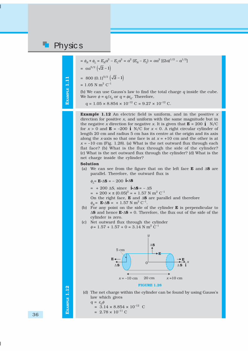
36
Physics
EX
AM
PLE 1
.12
EX
AM
PLE 1
.11
= φR + φL = ERa2 – ELa2 = a2 (ER – EL) = αa2 [(2a)1/2 – a1/2]
= αa5/2 ( )2 –1
= 800 (0.1)5/2 ( )2 –1
= 1.05 N m2 C–1
(b) We can use Gauss’s law to find the total charge q inside the cube.We have φ = q/ε0 or q = φε0. Therefore,
q = 1.05 × 8.854 × 10–12 C = 9.27 × 10⁻¹² C.
Example 1.12 An electric field is uniform, and in the positive xdirection for positive x, and uniform with the same magnitude but inthe negative x direction for negative x. It is given that E = 200 i N/Cfor x > 0 and E = –200 i N/C for x < 0. A right circular cylinder oflength 20 cm and radius 5 cm has its centre at the origin and its axisalong the x-axis so that one face is at x = +10 cm and the other is atx = –10 cm (Fig. 1.28). (a) What is the net outward flux through eachflat face? (b) What is the flux through the side of the cylinder?(c) What is the net outward flux through the cylinder? (d) What is thenet charge inside the cylinder?
Solution(a) We can see from the figure that on the left face E and ΔS are
parallel. Therefore, the outward flux is
φL= E.ΔS = – 200 ˆ Δi Si
= + 200 ΔS, since ˆ Δi Si = – ΔS= + 200 × π (0.05)2 = + 1.57 N m2 C–1
On the right face, E and ΔS are parallel and thereforeφR = E.ΔS = + 1.57 N m2 C–1.
(b) For any point on the side of the cylinder E is perpendicular toΔS and hence E.ΔS = 0. Therefore, the flux out of the side of thecylinder is zero.
(c) Net outward flux through the cylinderφ = 1.57 + 1.57 + 0 = 3.14 N m2 C–1
FIGURE 1.28
(d) The net charge within the cylinder can be found by using Gauss’slaw which givesq = ε0φ = 3.14 × 8.854 × 10–12 C = 2.78 × 10⁻¹¹ C

Electric Chargesand Fields
37
1.15 APPLICATIONS OF GAUSS’S LAW
The electric field due to a general charge distribution is, as seen above,given by Eq. (1.27). In practice, except for some special cases, thesummation (or integration) involved in this equation cannot be carriedout to give electric field at every point inspace. For some symmetric chargeconfigurations, however, it is possible toobtain the electric field in a simple way usingthe Gauss’s law. This is best understood bysome examples.
1.15.1 Field due to an infinitelylong straight uniformlycharged wire
Consider an infinitely long thin straight wirewith uniform linear charge density λ. The wireis obviously an axis of symmetry. Suppose wetake the radial vector from O to P and rotate itaround the wire. The points P, P′, P′′ soobtained are completely equivalent withrespect to the charged wire. This implies thatthe electric field must have the same magnitudeat these points. The direction of electric field atevery point must be radial (outward if λ > 0,inward if λ < 0). This is clear from Fig. 1.29.
Consider a pair of line elements P1 and P2of the wire, as shown. The electric fieldsproduced by the two elements of the pair whensummed give a resultant electric field whichis radial (the components normal to the radialvector cancel). This is true for any such pairand hence the total field at any point P isradial. Finally, since the wire is infinite,electric field does not depend on the positionof P along the length of the wire. In short, theelectric field is everywhere radial in the planecutting the wire normally, and its magnitudedepends only on the radial distance r.
To calculate the field, imagine a cylindricalGaussian surface, as shown in the Fig. 1.29(b).Since the field is everywhere radial, fluxthrough the two ends of the cylindricalGaussian surface is zero. At the cylindricalpart of the surface, E is normal to the surfaceat every point, and its magnitude is constant,since it depends only on r. The surface areaof the curved part is 2πrl, where l is the lengthof the cylinder.
FIGURE 1.29 (a) Electric field due to aninfinitely long thin straight wire is radial,(b) The Gaussian surface for a long thinwire of uniform linear charge density.

38
PhysicsFlux through the Gaussian surface
= flux through the curved cylindrical part of the surface
= E × 2πrl
The surface includes charge equal to λ l. Gauss’s law then givesE × 2πrl = λl/ε0
i.e., E = 02 r
λεπ
Vectorially, E at any point is given by
0
ˆ2 r
λε
=π
E n (1.32)
where n is the radial unit vector in the plane normal to the wire passingthrough the point. E is directed outward if λ is positive and inward if λ isnegative.
Note that when we write a vector A as a scalar multiplied by a unitvector, i.e., as A = A a , the scalar A is an algebraic number. It can benegative or positive. The direction of A will be the same as that of the unitvector a if A > 0 and opposite to a if A < 0. When we want to restrict tonon-negative values, we use the symbol A and call it the modulus of A .Thus, 0≥A .
Also note that though only the charge enclosed by the surface (λl )was included above, the electric field E is due to the charge on the entirewire. Further, the assumption that the wire is infinitely long is crucial.Without this assumption, we cannot take E to be normal to the curvedpart of the cylindrical Gaussian surface. However, Eq. (1.32) isapproximately true for electric field around the central portions of a longwire, where the end effects may be ignored.
1.15.2 Field due to a uniformly charged infinite plane sheetLet σ be the uniform surface charge density of an infinite plane sheet(Fig. 1.30). We take the x-axis normal to the given plane. By symmetry,the electric field will not depend on y and z coordinates and its direction
at every point must be parallel to the x-direction.We can take the Gaussian surface to be a
rectangular parallelepiped of cross sectional areaA, as shown. (A cylindrical surface will also do.) Asseen from the figure, only the two faces 1 and 2 willcontribute to the flux; electric field lines are parallelto the other faces and they, therefore, do notcontribute to the total flux.
The unit vector normal to surface 1 is in –xdirection while the unit vector normal to surface 2is in the +x direction. Therefore, flux E.ΔS throughboth the surfaces are equal and add up. Thereforethe net flux through the Gaussian surface is 2 EA.The charge enclosed by the closed surface is σA.Therefore by Gauss’s law,
FIGURE 1.30 Gaussian surface for auniformly charged infinite plane sheet.

Electric Chargesand Fields
39
2 EA = σA/ε0or, E = σ/2ε0Vectorically,
0
ˆ2σε
=E n (1.33)
where n is a unit vector normal to the plane and going away from it.E is directed away from the plate if σ is positive and toward the plate
if σ is negative. Note that the above application of the Gauss’ law hasbrought out an additional fact: E is independent of x also.
For a finite large planar sheet, Eq. (1.33) is approximately true in themiddle regions of the planar sheet, away from the ends.
1.15.3 Field due to a uniformly charged thin spherical shellLet σ be the uniform surface charge density of a thin spherical shell ofradius R (Fig. 1.31). The situation has obvious spherical symmetry. Thefield at any point P, outside or inside, can depend only on r (the radialdistance from the centre of the shell to the point) and must be radial (i.e.,along the radius vector).
(i) Field outside the shell: Consider a point P outside theshell with radius vector r. To calculate E at P, we take theGaussian surface to be a sphere of radius r and with centreO, passing through P. All points on this sphere are equivalentrelative to the given charged configuration. (That is what wemean by spherical symmetry.) The electric field at each pointof the Gaussian surface, therefore, has the same magnitudeE and is along the radius vector at each point. Thus, E andΔS at every point are parallel and the flux through eachelement is E ΔS. Summing over all ΔS, the flux through theGaussian surface is E × 4 π r 2. The charge enclosed isσ × 4 π R 2. By Gauss’s law
E × 4 π r 2 = 2
0
4 Rσε
π
Or, 2
2 20 04R q
Er r
σε ε
= =π
where q = 4 π R2 σ is the total charge on the spherical shell.Vectorially,
20
ˆ4
q
rε=
πE r (1.34)
The electric field is directed outward if q > 0 and inward ifq < 0. This, however, is exactly the field produced by a chargeq placed at the centre O. Thus for points outside the shell, the field dueto a uniformly charged shell is as if the entire charge of the shell isconcentrated at its centre.
(ii) Field inside the shell: In Fig. 1.31(b), the point P is inside theshell. The Gaussian surface is again a sphere through P centred at O.
FIGURE 1.31 Gaussiansurfaces for a point with
(a) r > R, (b) r < R.

40
Physics
EX
AM
PLE 1
.13
The flux through the Gaussian surface, calculated as before, isE × 4 π r2. However, in this case, the Gaussian surface encloses nocharge. Gauss’s law then givesE × 4 π r2 = 0i.e., E = 0 (r < R ) (1.35)
that is, the field due to a uniformly charged thin shell is zero at all pointsinside the shell*. This important result is a direct consequence of Gauss’slaw which follows from Coulomb’s law. The experimental verification ofthis result confirms the 1/r2 dependence in Coulomb’s law.
Example 1.13 An early model for an atom considered it to have apositively charged point nucleus of charge Ze, surrounded by auniform density of negative charge up to a radius R. The atom as awhole is neutral. For this model, what is the electric field at a distancer from the nucleus?
FIGURE 1.32
Solution The charge distribution for this model of the atom is asshown in Fig. 1.32. The total negative charge in the uniform sphericalcharge distribution of radius R must be –Z e, since the atom (nucleusof charge Z e + negative charge) is neutral. This immediately gives usthe negative charge density ρ, since we must have
340–
3
RZeρ
π=
or 3
34
Ze
Rρ = −
π
To find the electric field E(r) at a point P which is a distance r awayfrom the nucleus, we use Gauss’s law. Because of the sphericalsymmetry of the charge distribution, the magnitude of the electricfield E(r) depends only on the radial distance, no matter what thedirection of r. Its direction is along (or opposite to) the radius vector rfrom the origin to the point P. The obvious Gaussian surface is aspherical surface centred at the nucleus. We consider two situations,namely, r < R and r > R.(i) r < R : The electric flux φ enclosed by the spherical surface is
φ = E (r ) × 4 π r 2
where E (r ) is the magnitude of the electric field at r. This is because
* Compare this with a uniform mass shell discussed in Section 8.5 of Class XITextbook of Physics.

Electric Chargesand Fields
41
EX
AM
PLE 1
.13
the field at any point on the spherical Gaussian surface has thesame direction as the normal to the surface there, and has the samemagnitude at all points on the surface.The charge q enclosed by the Gaussian surface is the positive nuclearcharge and the negative charge within the sphere of radius r,
i.e., 34
3
rq Z e ρ
π= +
Substituting for the charge density ρ obtained earlier, we have3
3
rq Z e Z e
R= −
Gauss’s law then gives,
2 30
1( ) ;
4Z e r
E r r Rr Rε
⎛ ⎞= − <⎜ ⎟⎝ ⎠π
The electric field is directed radially outward.(ii) r > R: In this case, the total charge enclosed by the Gaussianspherical surface is zero since the atom is neutral. Thus, from Gauss’slaw,E (r ) × 4 π r 2 = 0 or E (r ) = 0; r > RAt r = R, both cases give the same result: E = 0.
ON SYMMETRY OPERATIONS
In Physics, we often encounter systems with various symmetries. Consideration of thesesymmetries helps one arrive at results much faster than otherwise by a straightforwardcalculation. Consider, for example an infinite uniform sheet of charge (surface chargedensity σ) along the y-z plane. This system is unchanged if (a) translated parallel to they-z plane in any direction, (b) rotated about the x-axis through any angle. As the systemis unchanged under such symmetry operation, so must its properties be. In particular,in this example, the electric field E must be unchanged.
Translation symmetry along the y-axis shows that the electric field must be the sameat a point (0, y1, 0) as at (0, y2, 0). Similarly translational symmetry along the z-axisshows that the electric field at two point (0, 0, z1) and (0, 0, z2) must be the same. Byusing rotation symmetry around the x-axis, we can conclude that E must beperpendicular to the y-z plane, that is, it must be parallel to the x-direction.
Try to think of a symmetry now which will tell you that the magnitude of the electricfield is a constant, independent of the x-coordinate. It thus turns out that the magnitudeof the electric field due to a uniformly charged infinite conducting sheet is the same at allpoints in space. The direction, however, is opposite of each other on either side of thesheet.
Compare this with the effort needed to arrive at this result by a direct calculationusing Coulomb’s law.
42
Physics
SUMMARY
1. Electric and magnetic forces determine the properties of atoms,molecules and bulk matter.
2. From simple experiments on frictional electricity, one can infer thatthere are two types of charges in nature; and that like charges repeland unlike charges attract. By convention, the charge on a glass rodrubbed with silk is positive; that on a plastic rod rubbed with fur isthen negative.
3. Conductors allow movement of electric charge through them, insulatorsdo not. In metals, the mobile charges are electrons; in electrolytesboth positive and negative ions are mobile.
4. Electric charge has three basic properties: quantisation, additivityand conservation.
Quantisation of electric charge means that total charge (q) of a bodyis always an integral multiple of a basic quantum of charge (e) i.e.,q = n e, where n = 0, ±1, ±2, ±3, .... Proton and electron have charges+e, –e, respectively. For macroscopic charges for which n is a very largenumber, quantisation of charge can be ignored.
Additivity of electric charges means that the total charge of a systemis the algebraic sum (i.e., the sum taking into account proper signs)of all individual charges in the system.
Conservation of electric charges means that the total charge of anisolated system remains unchanged with time. This means that whenbodies are charged through friction, there is a transfer of electric chargefrom one body to another, but no creation or destruction of charge.
5. Coulomb’s Law: The mutual electrostatic force between two pointcharges q1 and q2 is proportional to the product q1q2 and inverselyproportional to the square of the distance r21 separating them.Mathematically,
F21 = force on q2 due to 1 21 212
21
ˆk (q q )
qr
= r
where 21r is a unit vector in the direction from q1 to q2 and k = 0
14 επ
is the constant of proportionality.
In SI units, the unit of charge is coulomb. The experimental value ofthe constant ε0 is
ε0 = 8.854 × 10⁻¹² C2 N–1 m–2
The approximate value of k is
k = 9 × 10⁹ N m2 C–2
6. The ratio of electric force and gravitational force between a protonand an electron is
2392 4 10
e p
k e.
G m m≅ ×
7. Superposition Principle: The principle is based on the property that theforces with which two charges attract or repel each other are notaffected by the presence of a third (or more) additional charge(s). Foran assembly of charges q1, q2, q3, ..., the force on any charge, say q1, is

Electric Chargesand Fields
43
the vector sum of the force on q1 due to q2, the force on q1 due to q3,and so on. For each pair, the force is given by the Coulomb’s law fortwo charges stated earlier.
8. The electric field E at a point due to a charge configuration is theforce on a small positive test charge q placed at the point divided bythe magnitude of the charge. Electric field due to a point charge q hasa magnitude |q|/4πε0r
2; it is radially outwards from q, if q is positive,and radially inwards if q is negative. Like Coulomb force, electric fieldalso satisfies superposition principle.
9. An electric field line is a curve drawn in such a way that the tangentat each point on the curve gives the direction of electric field at thatpoint. The relative closeness of field lines indicates the relative strengthof electric field at different points; they crowd near each other in regionsof strong electric field and are far apart where the electric field isweak. In regions of constant electric field, the field lines are uniformlyspaced parallel straight lines.
10. Some of the important properties of field lines are: (i) Field lines arecontinuous curves without any breaks. (ii) Two field lines cannot crosseach other. (iii) Electrostatic field lines start at positive charges andend at negative charges —they cannot form closed loops.
11. An electric dipole is a pair of equal and opposite charges q and –qseparated by some distance 2a. Its dipole moment vector p hasmagnitude 2qa and is in the direction of the dipole axis from –q to q.
12. Field of an electric dipole in its equatorial plane (i.e., the planeperpendicular to its axis and passing through its centre) at a distancer from the centre:
2 2 3/2
14 ( )o a rε−
=π +p
E
3 ,4 o
for r arε
−≅ >>
πp
Dipole electric field on the axis at a distance r from the centre:
2 2 20
24 ( )
r
r aε=
π −p
E
30
24
for r arε
≅ >>π
p
The 1/r3 dependence of dipole electric fields should be noted in contrastto the 1/r2 dependence of electric field due to a point charge.
13. In a uniform electric field E, a dipole experiences a torque τ given by
τ = p × E
but experiences no net force.
14. The flux Δφ of electric field E through a small area element ΔS isgiven by
Δφ = E.ΔS
The vector area element ΔS is
ΔS = ΔS n
where ΔS is the magnitude of the area element and n is normal to thearea element, which can be considered planar for sufficiently small ΔS.

44
Physics
For an area element of a closed surface, n is taken to be the directionof outward normal, by convention.
15. Gauss’s law: The flux of electric field through any closed surface S is1/ε0 times the total charge enclosed by S. The law is especially usefulin determining electric field E, when the source distribution has simplesymmetry:
(i) Thin infinitely long straight wire of uniform linear charge density λ
0
ˆ2 r
λε
=π
E n
where r is the perpendicular distance of the point from the wire and
n is the radial unit vector in the plane normal to the wire passingthrough the point.
(ii) Infinite thin plane sheet of uniform surface charge density σ
0
ˆ2σε
=E n
where n is a unit vector normal to the plane, outward on either side.
(iii) Thin spherical shell of uniform surface charge density σ
20
ˆ ( )4
qr R
rε= ≥
πE r
E = 0 (r < R )
where r is the distance of the point from the centre of the shell and Rthe radius of the shell. q is the total charge of the shell: q = 4πR2σ.
The electric field outside the shell is as though the total charge isconcentrated at the centre. The same result is true for a solid sphereof uniform volume charge density. The field is zero at all points insidethe shell
Physical quantity Symbol Dimensions Unit Remarks
Vector area element Δ S [L2] m2 ΔS = ΔS n
Electric field E [MLT–3A–1] V m–1
Electric flux φ [ML3 T–3A–1] V m Δφ = E.ΔS
Dipole moment p [LTA] C m Vector directedfrom negative topositive charge
Charge density
linear λ [L–1 TA] C m–1 Charge/length
surface σ [L–2 TA] C m–2 Charge/area
volume ρ [L–3 TA] C m–3 Charge/volume

Electric Chargesand Fields
45
POINTS TO PONDER
1. You might wonder why the protons, all carrying positive charges, arecompactly residing inside the nucleus. Why do they not fly away? Youwill learn that there is a third kind of a fundamental force, called thestrong force which holds them together. The range of distance wherethis force is effective is, however, very small ~10-14 m. This is preciselythe size of the nucleus. Also the electrons are not allowed to sit ontop of the protons, i.e. inside the nucleus, due to the laws of quantummechanics. This gives the atoms their structure as they exist in nature.
2. Coulomb force and gravitational force follow the same inverse-squarelaw. But gravitational force has only one sign (always attractive), whileCoulomb force can be of both signs (attractive and repulsive), allowingpossibility of cancellation of electric forces. This is how gravity, despitebeing a much weaker force, can be a dominating and more pervasiveforce in nature.
3. The constant of proportionality k in Coulomb’s law is a matter ofchoice if the unit of charge is to be defined using Coulomb’s law. In SIunits, however, what is defined is the unit of current (A) via its magneticeffect (Ampere’s law) and the unit of charge (coulomb) is simply definedby (1C = 1 A s). In this case, the value of k is no longer arbitrary; it isapproximately 9 × 10⁹ N m2 C–2.
4. The rather large value of k, i.e., the large size of the unit of charge(1C) from the point of view of electric effects arises because (asmentioned in point 3 already) the unit of charge is defined in terms ofmagnetic forces (forces on current–carrying wires) which are generallymuch weaker than the electric forces. Thus while 1 ampere is a unitof reasonable size for magnetic effects, 1 C = 1 A s, is too big a unit forelectric effects.
5. The additive property of charge is not an ‘obvious’ property. It is relatedto the fact that electric charge has no direction associated with it;charge is a scalar.
6. Charge is not only a scalar (or invariant) under rotation; it is alsoinvariant for frames of reference in relative motion. This is not alwaystrue for every scalar. For example, kinetic energy is a scalar underrotation, but is not invariant for frames of reference in relativemotion.
7. Conservation of total charge of an isolated system is a propertyindependent of the scalar nature of charge noted in point 6.Conservation refers to invariance in time in a given frame of reference.A quantity may be scalar but not conserved (like kinetic energy in aninelastic collision). On the other hand, one can have conserved vectorquantity (e.g., angular momentum of an isolated system).
8. Quantisation of electric charge is a basic (unexplained) law of nature;interestingly, there is no analogous law on quantisation of mass.
9. Superposition principle should not be regarded as ‘obvious’, or equatedwith the law of addition of vectors. It says two things: force on onecharge due to another charge is unaffected by the presence of othercharges, and there are no additional three-body, four-body, etc., forceswhich arise only when there are more than two charges.
10. The electric field due to a discrete charge configuration is not definedat the locations of the discrete charges. For continuous volume chargedistribution, it is defined at any point in the distribution. For a surfacecharge distribution, electric field is discontinuous across the surface.

46
Physics11. The electric field due to a charge configuration with total charge zero
is not zero; but for distances large compared to the size ofthe configuration, its field falls off faster than 1/r 2, typical of fielddue to a single charge. An electric dipole is the simplest example ofthis fact.
EXERCISES
1.1 What is the force between two small charged spheres havingcharges of 2 × 10⁻⁷C and 3 × 10⁻⁷C placed 30 cm apart in air?
1.2 The electrostatic force on a small sphere of charge 0.4 μC due toanother small sphere of charge –0.8 μC in air is 0.2 N. (a) What isthe distance between the two spheres? (b) What is the force on thesecond sphere due to the first?
1.3 Check that the ratio ke2/G memp is dimensionless. Look up a Tableof Physical Constants and determine the value of this ratio. Whatdoes the ratio signify?
1.4 (a) Explain the meaning of the statement ‘electric charge of a bodyis quantised’.
(b) Why can one ignore quantisation of electric charge when dealingwith macroscopic i.e., large scale charges?
1.5 When a glass rod is rubbed with a silk cloth, charges appear onboth. A similar phenomenon is observed with many other pairs ofbodies. Explain how this observation is consistent with the law ofconservation of charge.
1.6 Four point charges qA = 2 μC, qB = –5 μC, qC = 2 μC, and qD = –5 μC arelocated at the corners of a square ABCD of side 10 cm. What is theforce on a charge of 1 μC placed at the centre of the square?
1.7 (a) An electrostatic field line is a continuous curve. That is, a fieldline cannot have sudden breaks. Why not?
(b) Explain why two field lines never cross each other at any point?1.8 Two point charges qA = 3 μC and qB = –3 μC are located 20 cm apart
in vacuum.(a) What is the electric field at the midpoint O of the line AB joining
the two charges?(b) If a negative test charge of magnitude 1.5 × 10⁻⁹ C is placed at
this point, what is the force experienced by the test charge?1.9 A system has two charges qA = 2.5 × 10⁻⁷ C and qB = –2.5 × 10⁻⁷ C
located at points A: (0, 0, –15 cm) and B: (0,0, +15 cm), respectively.What are the total charge and electric dipole moment of the system?
1.10 An electric dipole with dipole moment 4 × 10⁻⁹ C m is aligned at 30°with the direction of a uniform electric field of magnitude 5 × 10⁴ NC–1.Calculate the magnitude of the torque acting on the dipole.
1.11 A polythene piece rubbed with wool is found to have a negativecharge of 3 × 10⁻⁷ C.
(a) Estimate the number of electrons transferred (from which towhich?)
(b) Is there a transfer of mass from wool to polythene?
1.12 (a) Two insulated charged copper spheres A and B have their centresseparated by a distance of 50 cm. What is the mutual force of

Electric Chargesand Fields
47
electrostatic repulsion if the charge on each is 6.5 × 10⁻⁷ C? Theradii of A and B are negligible compared to the distance ofseparation.
(b) What is the force of repulsion if each sphere is charged doublethe above amount, and the distance between them is halved?
1.13 Suppose the spheres A and B in Exercise 1.12 have identical sizes.A third sphere of the same size but uncharged is brought in contactwith the first, then brought in contact with the second, and finallyremoved from both. What is the new force of repulsion between Aand B?
1.14 Figure 1.33 shows tracks of three charged particles in a uniformelectrostatic field. Give the signs of the three charges. Which particlehas the highest charge to mass ratio?
FIGURE 1.33
1.15 Consider a uniform electric field E = 3 × 10³ î N/C. (a) What is theflux of this field through a square of 10 cm on a side whose plane isparallel to the yz plane? (b) What is the flux through the samesquare if the normal to its plane makes a 60° angle with the x-axis?
1.16 What is the net flux of the uniform electric field of Exercise 1.15through a cube of side 20 cm oriented so that its faces are parallelto the coordinate planes?
1.17 Careful measurement of the electric field at the surface of a blackbox indicates that the net outward flux through the surface of thebox is 8.0 × 10³ Nm2/C. (a) What is the net charge inside the box?(b) If the net outward flux through the surface of the box were zero,could you conclude that there were no charges inside the box? Whyor Why not?
1.18 A point charge +10 μC is a distance 5 cm directly above the centreof a square of side 10 cm, as shown in Fig. 1.34. What is themagnitude of the electric flux through the square? (Hint: Think ofthe square as one face of a cube with edge 10 cm.)
FIGURE 1.34

48
Physics1.19 A point charge of 2.0 μC is at the centre of a cubic Gaussian
surface 9.0 cm on edge. What is the net electric flux through thesurface?
1.20 A point charge causes an electric flux of –1.0 × 10³ Nm2/C to passthrough a spherical Gaussian surface of 10.0 cm radius centred onthe charge. (a) If the radius of the Gaussian surface were doubled,how much flux would pass through the surface? (b) What is thevalue of the point charge?
1.21 A conducting sphere of radius 10 cm has an unknown charge. Ifthe electric field 20 cm from the centre of the sphere is 1.5 × 10³ N/Cand points radially inward, what is the net charge on the sphere?
1.22 A uniformly charged conducting sphere of 2.4 m diameter has asurface charge density of 80.0 μC/m2. (a) Find the charge on thesphere. (b) What is the total electric flux leaving the surface of thesphere?
1.23 An infinite line charge produces a field of 9 × 10⁴ N/C at a distanceof 2 cm. Calculate the linear charge density.
1.24 Two large, thin metal plates are parallel and close to each other. Ontheir inner faces, the plates have surface charge densities of oppositesigns and of magnitude 17.0 × 10⁻²² C/m2. What is E: (a) in the outerregion of the first plate, (b) in the outer region of the second plate,and (c) between the plates?
ADDITIONAL EXERCISES1.25 An oil drop of 12 excess electrons is held stationary under a constant
electric field of 2.55 × 10⁴ NC–1 in Millikan’s oil drop experiment. Thedensity of the oil is 1.26 g cm–3. Estimate the radius of the drop.(g = 9.81 m s–2; e = 1.60 × 10⁻¹⁹ C).
1.26 Which among the curves shown in Fig. 1.35 cannot possiblyrepresent electrostatic field lines?

Electric Chargesand Fields
49
FIGURE 1.35
1.27 In a certain region of space, electric field is along the z-directionthroughout. The magnitude of electric field is, however, not constantbut increases uniformly along the positive z-direction, at the rate of105 NC–1 per metre. What are the force and torque experienced by asystem having a total dipole moment equal to 10–7 Cm in the negativez-direction ?
1.28 (a) A conductor A with a cavity as shown in Fig. 1.36(a) is given acharge Q. Show that the entire charge must appear on the outersurface of the conductor. (b) Another conductor B with charge q isinserted into the cavity keeping B insulated from A. Show that thetotal charge on the outside surface of A is Q + q [Fig. 1.36(b)]. (c) Asensitive instrument is to be shielded from the strong electrostaticfields in its environment. Suggest a possible way.
FIGURE 1.36
1.29 A hollow charged conductor has a tiny hole cut into its surface.
Show that the electric field in the hole is (σ/2ε0) n , where n is theunit vector in the outward normal direction, and σ is the surfacecharge density near the hole.
1.30 Obtain the formula for the electric field due to a long thin wire ofuniform linear charge density λ without using Gauss’s law. [Hint:Use Coulomb’s law directly and evaluate the necessary integral.]
1.31 It is now believed that protons and neutrons (which constitute nucleiof ordinary matter) are themselves built out of more elementary unitscalled quarks. A proton and a neutron consist of three quarks each.Two types of quarks, the so called ‘up’ quark (denoted by u) of charge+ (2/3) e, and the ‘down’ quark (denoted by d) of charge (–1/3) e,together with electrons build up ordinary matter. (Quarks of othertypes have also been found which give rise to different unusualvarieties of matter.) Suggest a possible quark composition of aproton and neutron.

50
Physics1.32 (a) Consider an arbitrary electrostatic field configuration. A small
test charge is placed at a null point (i.e., where E = 0) of theconfiguration. Show that the equilibrium of the test charge isnecessarily unstable.
(b) Verify this result for the simple configuration of two charges ofthe same magnitude and sign placed a certain distance apart.
1.33 A particle of mass m and charge (–q) enters the region between thetwo charged plates initially moving along x-axis with speed vx (likeparticle 1 in Fig. 1.33). The length of plate is L and an uniformelectric field E is maintained between the plates. Show that thevertical deflection of the particle at the far edge of the plate isqEL2/(2m vx
2).Compare this motion with motion of a projectile in gravitational fielddiscussed in Section 4.10 of Class XI Textbook of Physics.
1.34 Suppose that the particle in Exercise in 1.33 is an electron projectedwith velocity vx = 2.0 × 10⁶ m s–1. If E between the plates separatedby 0.5 cm is 9.1 × 10² N/C, where will the electron strike the upperplate? (|e|=1.6 × 10⁻¹⁹ C, me = 9.1 × 10⁻³¹ kg.)

2.1 INTRODUCTION
In Chapters 6 and 8 (Class XI), the notion of potential energy wasintroduced. When an external force does work in taking a body from apoint to another against a force like spring force or gravitational force,that work gets stored as potential energy of the body. When the externalforce is removed, the body moves, gaining kinetic energy and losingan equal amount of potential energy. The sum of kinetic andpotential energies is thus conserved. Forces of this kind are calledconservative forces. Spring force and gravitational force are examples ofconservative forces.
Coulomb force between two (stationary) charges, like the gravitationalforce, is also a conservative force. This is not surprising, since both haveinverse-square dependence on distance and differ mainly in theproportionality constants – the masses in the gravitational law arereplaced by charges in Coulomb’s law. Thus, like the potential energy ofa mass in a gravitational field, we can define electrostatic potential energyof a charge in an electrostatic field.
Consider an electrostatic field E due to some charge configuration.First, for simplicity, consider the field E due to a charge Q placed at theorigin. Now, imagine that we bring a test charge q from a point R to apoint P against the repulsive force on it due to the charge Q. With reference
Chapter Two
ELECTROSTATICPOTENTIAL ANDCAPACITANCE
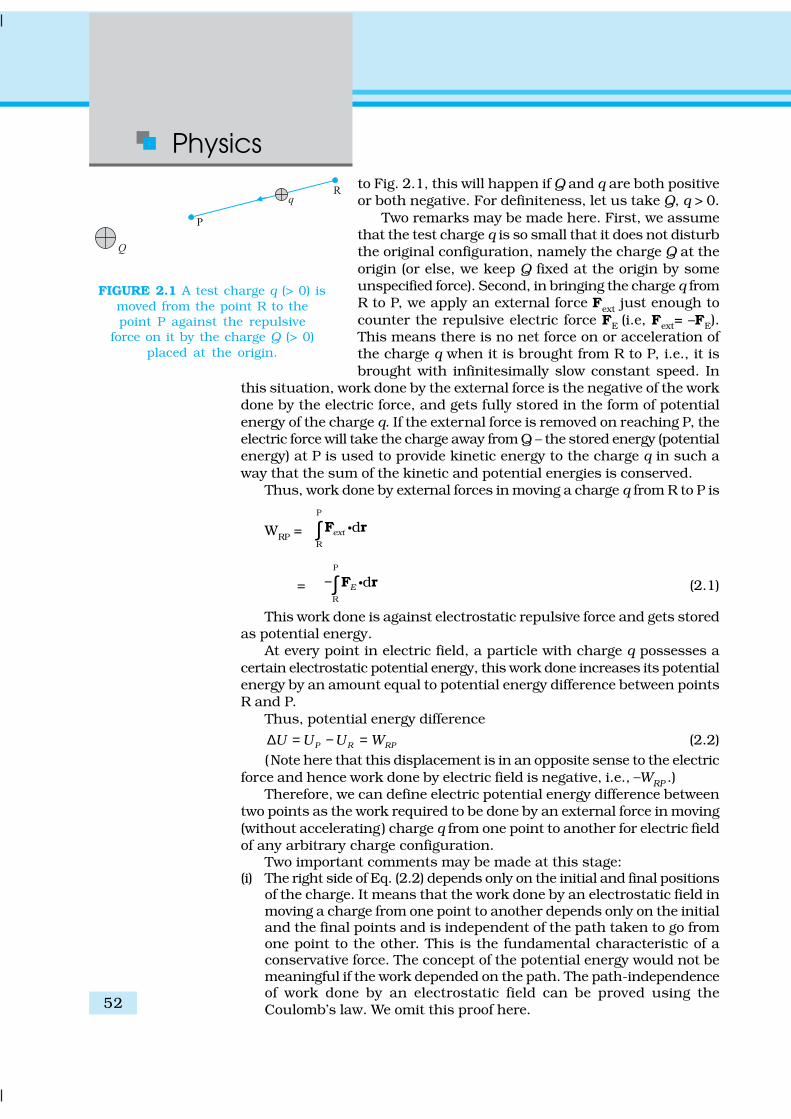
Physics
52
to Fig. 2.1, this will happen if Q and q are both positiveor both negative. For definiteness, let us take Q, q > 0.
Two remarks may be made here. First, we assumethat the test charge q is so small that it does not disturbthe original configuration, namely the charge Q at theorigin (or else, we keep Q fixed at the origin by someunspecified force). Second, in bringing the charge q fromR to P, we apply an external force Fext just enough tocounter the repulsive electric force FE (i.e, Fext= –FE).This means there is no net force on or acceleration ofthe charge q when it is brought from R to P, i.e., it isbrought with infinitesimally slow constant speed. In
this situation, work done by the external force is the negative of the workdone by the electric force, and gets fully stored in the form of potentialenergy of the charge q. If the external force is removed on reaching P, theelectric force will take the charge away from Q – the stored energy (potentialenergy) at P is used to provide kinetic energy to the charge q in such away that the sum of the kinetic and potential energies is conserved.
Thus, work done by external forces in moving a charge q from R to P is
WRP = P
R
dext∫ F r
= P
R
dE−∫ F r (2.1)
This work done is against electrostatic repulsive force and gets storedas potential energy.
At every point in electric field, a particle with charge q possesses acertain electrostatic potential energy, this work done increases its potentialenergy by an amount equal to potential energy difference between pointsR and P.
Thus, potential energy difference
P R RPU U U W∆ = − = (2.2)(Note here that this displacement is in an opposite sense to the electric
force and hence work done by electric field is negative, i.e., –WRP .)Therefore, we can define electric potential energy difference between
two points as the work required to be done by an external force in moving(without accelerating) charge q from one point to another for electric fieldof any arbitrary charge configuration.
Two important comments may be made at this stage:(i) The right side of Eq. (2.2) depends only on the initial and final positions
of the charge. It means that the work done by an electrostatic field inmoving a charge from one point to another depends only on the initialand the final points and is independent of the path taken to go fromone point to the other. This is the fundamental characteristic of aconservative force. The concept of the potential energy would not bemeaningful if the work depended on the path. The path-independenceof work done by an electrostatic field can be proved using theCoulomb’s law. We omit this proof here.
FIGURE 2.1 A test charge q (> 0) ismoved from the point R to thepoint P against the repulsive
force on it by the charge Q (> 0)placed at the origin.

Electrostatic Potentialand Capacitance
53
(ii) Equation (2.2) defines potential energy difference in termsof the physically meaningful quantity work. Clearly,potential energy so defined is undetermined to within anadditive constant.What this means is that the actual valueof potential energy is not physically significant; it is onlythe difference of potential energy that is significant. We canalways add an arbitrary constant α to potential energy atevery point, since this will not change the potential energydifference:
( ) ( )P R P RU U U Uα α+ − + = −
Put it differently, there is a freedom in choosing the pointwhere potential energy is zero. A convenient choice is to haveelectrostatic potential energy zero at infinity. With this choice,if we take the point R at infinity, we get from Eq. (2.2)
P P PW U U U∞ ∞= − = (2.3)
Since the point P is arbitrary, Eq. (2.3) provides us with adefinition of potential energy of a charge q at any point.Potential energy of charge q at a point (in the presence of fielddue to any charge configuration) is the work done by theexternal force (equal and opposite to the electric force) inbringing the charge q from infinity to that point.
2.2 ELECTROSTATIC POTENTIAL
Consider any general static charge configuration. We definepotential energy of a test charge q in terms of the work doneon the charge q. This work is obviously proportional to q, sincethe force at any point is qE, where E is the electric field at thatpoint due to the given charge configuration. It is, therefore,convenient to divide the work by the amount of charge q, sothat the resulting quantity is independent of q. In other words,work done per unit test charge is characteristic of the electricfield associated with the charge configuration. This leads tothe idea of electrostatic potential V due to a given chargeconfiguration. From Eq. (2.1), we get:
Work done by external force in bringing a unit positivecharge from point R to P
= VP – VR P RU Uq
−= (2.4)
where VP and VR are the electrostatic potentials at P and R, respectively.Note, as before, that it is not the actual value of potential but the potentialdifference that is physically significant. If, as before, we choose thepotential to be zero at infinity, Eq. (2.4) implies:
Work done by an external force in bringing a unit positive chargefrom infinity to a point = electrostatic potential (V ) at that point.
CO
UN
T A
LE
SS
AN
DR
O V
OLTA
(1745 –1
827)
Count Alessandro Volta(1745 – 1827) Italianphysicist, professor atPavia. Volta establishedthat the animal electri-city observed by LuigiGalvani, 1737–1798, inexperiments with frogmuscle tissue placed incontact with dissimilarmetals, was not due toany exceptional propertyof animal tissues butwas also generatedwhenever any wet bodywas sandwiched betweendissimilar metals. Thisled him to develop thefirst voltaic pile, orbattery, consisting of alarge stack of moist disksof cardboard (electro-lyte) sandwichedbetween disks of metal(electrodes).

Physics
54
In other words, the electrostatic potential (V )at any point in a region with electrostatic field isthe work done in bringing a unit positivecharge (without acceleration) from infinity tothat point.
The qualifying remarks made earlier regardingpotential energy also apply to the definition ofpotential. To obtain the work done per unit testcharge, we should take an infinitesimal test chargeδq, obtain the work done δW in bringing it frominfinity to the point and determine the ratioδW/δq. Also, the external force at every point ofthe path is to be equal and opposite to theelectrostatic force on the test charge at that point.
2.3 POTENTIAL DUE TO A POINT CHARGE
Consider a point charge Q at the origin (Fig. 2.3). For definiteness, take Qto be positive. We wish to determine the potential at any point P with
position vector r from the origin. For that we mustcalculate the work done in bringing a unit positivetest charge from infinity to the point P. For Q > 0,the work done against the repulsive force on thetest charge is positive. Since work done isindependent of the path, we choose a convenientpath – along the radial direction from infinity tothe point P.
At some intermediate point P′ on the path, theelectrostatic force on a unit positive charge is
20
1ˆ
4 'Q
rε×
′π
r (2.5)
where ˆ ′r is the unit vector along OP′. Work doneagainst this force from r′ to r′ + ∆r′ is
204 '
QW r
rε∆ = − ∆ ′
π (2.6)
The negative sign appears because for ∆r ′ < 0, ∆W is positive . Totalwork done (W) by the external force is obtained by integrating Eq. (2.6)from r′ = ∞ to r′ = r,
20 00 4 44 '
r rQ Q QW dr
r rr ε εε ∞∞
= − = =′π ππ ′∫ (2.7)
This, by definition is the potential at P due to the charge Q
0
( )4
QV r
rε=
π (2.8)
FIGURE 2.2 Work done on a test charge qby the electrostatic field due to any given
charge configuration is independentof the path, and depends only on
its initial and final positions.
FIGURE 2.3 Work done in bringing a unitpositive test charge from infinity to thepoint P, against the repulsive force of
charge Q (Q > 0), is the potential at P due tothe charge Q.

Electrostatic Potentialand Capacitance
55
EX
AM
PLE 2
.1
Equation (2.8) is true for anysign of the charge Q, though weconsidered Q > 0 in its derivation.For Q < 0, V < 0, i.e., work done (bythe external force) per unit positivetest charge in bringing it frominfinity to the point is negative. Thisis equivalent to saying that workdone by the electrostatic force inbringing the unit positive chargeform infinity to the point P ispositive. [This is as it should be,since for Q < 0, the force on a unitpositive test charge is attractive, sothat the electrostatic force and thedisplacement (from infinity to P) arein the same direction.] Finally, wenote that Eq. (2.8) is consistent withthe choice that potential at infinitybe zero.
Figure (2.4) shows how the electrostatic potential ( ∝ 1/r ) and theelectrostatic field ( ∝ 1/r 2 ) varies with r.
Example 2.1(a) Calculate the potential at a point P due to a charge of 4 × 10⁻⁷C
located 9 cm away.(b) Hence obtain the work done in bringing a charge of 2 × 10⁻⁹ C
from infinity to the point P. Does the answer depend on the pathalong which the charge is brought?
Solution
(a) 7
9 2 –2
0
1 4 10 C9 10 Nm C
4 0.09mQ
Vrε
−×= = × ×π
= 4 × 10⁴ V
(b) 9 42 10 C 4 10 VW qV −= = × × × = 8 × 10⁻⁵ J
No, work done will be path independent. Any arbitrary infinitesimalpath can be resolved into two perpendicular displacements: One alongr and another perpendicular to r. The work done corresponding tothe later will be zero.
2.4 POTENTIAL DUE TO AN ELECTRIC DIPOLE
As we learnt in the last chapter, an electric dipole consists of two chargesq and –q separated by a (small) distance 2a. Its total charge is zero. It ischaracterised by a dipole moment vector p whose magnitude is q × 2aand which points in the direction from –q to q (Fig. 2.5). We also saw thatthe electric field of a dipole at a point with position vector r depends notjust on the magnitude r, but also on the angle between r and p. Further,
FIGURE 2.4 Variation of potential V with r [in units of(Q/4πε0) m
-1] (blue curve) and field with r [in unitsof (Q/4πε0) m
-2] (black curve) for a point charge Q.

Physics
56
the field falls off, at large distance, not as1/r 2 (typical of field due to a single charge)but as 1/r3. We, now, determine the electricpotential due to a dipole and contrast itwith the potential due to a single charge.
As before, we take the origin at thecentre of the dipole. Now we know that theelectric field obeys the superpositionprinciple. Since potential is related to thework done by the field, electrostaticpotential also follows the superpositionprinciple. Thus, the potential due to thedipole is the sum of potentials due to thecharges q and –q
0 1 2
14
q qV
r rε
= − π (2.9)
where r1 and r2 are the distances of thepoint P from q and –q, respectively.
Now, by geometry,2 2 2
1 2r r a ar= + − cosθ
2 2 22 2r r a ar= + + cosθ (2.10)
We take r much greater than a ( ar >> ) and retain terms only uptothe first order in a/r
2
2 21 2
2 cos1
a ar r
r rθ
= − +
2 2 cos
1a
rr
θ ≅ − (2.11)
Similarly,
2 22
2 cos1
ar r
rθ ≅ + (2.12)
Using the Binomial theorem and retaining terms upto the first orderin a/r ; we obtain,
1/2
1
1 1 2 cos 11 1 cos
a ar r r r r
θ θ−
≅ − ≅ + [2.13(a)]
1/2
2
1 1 2 cos 11 1 cos
a ar r r r r
θ θ−
≅ + ≅ − [2.13(b)]
Using Eqs. (2.9) and (2.13) and p = 2qa, we get
2 20 0
2 cos cos4 4
q a pV
r r
θ θε ε
= =π π (2.14)
Now, p cos θ = ˆp r
FIGURE 2.5 Quantities involved in the calculationof potential due to a dipole.

Electrostatic Potentialand Capacitance
57
where r is the unit vector along the position vector OP.The electric potential of a dipole is then given by
20
ˆ14
Vrε
=π
p r; (r >> a) (2.15)
Equation (2.15) is, as indicated, approximately true only for distanceslarge compared to the size of the dipole, so that higher order terms ina/r are negligible. For a point dipole p at the origin, Eq. (2.15) is, however,exact.
From Eq. (2.15), potential on the dipole axis (θ = 0, π ) is given by
20
14
pV
rε= ±
π (2.16)
(Positive sign for θ = 0, negative sign for θ = π.) The potential in theequatorial plane (θ = π/2) is zero.
The important contrasting features of electric potential of a dipolefrom that due to a single charge are clear from Eqs. (2.8) and (2.15):(i) The potential due to a dipole depends not just on r but also on the
angle between the position vector r and the dipole moment vector p.(It is, however, axially symmetric about p. That is, if you rotate theposition vector r about p, keeping θ fixed, the points correspondingto P on the cone so generated will have the same potential as at P.)
(ii) The electric dipole potential falls off, at large distance, as 1/r 2, not as1/r, characteristic of the potential due to a single charge. (You canrefer to the Fig. 2.5 for graphs of 1/r 2 versus r and 1/r versus r,drawn there in another context.)
2.5 POTENTIAL DUE TO A SYSTEM OF CHARGES
Consider a system of charges q1, q2,…, qn with position vectors r1, r2,…,rn relative to some origin (Fig. 2.6). The potential V1 at P due to the chargeq1 is
11
0 1P
14
qV
rε=
πwhere r1P is the distance between q1 and P.
Similarly, the potential V2 at P due to q2 andV3 due to q3 are given by
22
0 2P
14
qV
rε=
π , 3
30 3P
14
qV
rε=
π
where r2P and r3P are the distances of P fromcharges q2 and q3, respectively; and so on for thepotential due to other charges. By thesuperposition principle, the potential V at P dueto the total charge configuration is the algebraicsum of the potentials due to the individualcharges
V = V1 + V2 + ... + Vn (2.17)
FIGURE 2.6 Potential at a point due to asystem of charges is the sum of potentials
due to individual charges.

Physics
58 EX
AM
PLE 2
.21 2
0 1P 2P P
1......
4n
n
qq qr r rε
= + + + π (2.18)
If we have a continuous charge distribution characterised by a chargedensity ρ (r), we divide it, as before, into small volume elements each ofsize ∆v and carrying a charge ρ∆v. We then determine the potential dueto each volume element and sum (strictly speaking , integrate) over allsuch contributions, and thus determine the potential due to the entiredistribution.
We have seen in Chapter 1 that for a uniformly charged spherical shell,the electric field outside the shell is as if the entire charge is concentratedat the centre. Thus, the potential outside the shell is given by
0
14
qV
rε=
π ( )r R≥ [2.19(a)]
where q is the total charge on the shell and R its radius. The electric fieldinside the shell is zero. This implies (Section 2.6) that potential is constantinside the shell (as no work is done in moving a charge inside the shell),and, therefore, equals its value at the surface, which is
0
14
qV
Rε=
π [2.19(b)]
Example 2.2 Two charges 3 × 10⁻⁸ C and –2 × 10⁻⁸ C are located15 cm apart. At what point on the line joining the two charges is theelectric potential zero? Take the potential at infinity to be zero.
Solution Let us take the origin O at the location of the positive charge.The line joining the two charges is taken to be the x-axis; the negativecharge is taken to be on the right side of the origin (Fig. 2.7).
FIGURE 2.7
Let P be the required point on the x-axis where the potential is zero.If x is the x-coordinate of P, obviously x must be positive. (There is nopossibility of potentials due to the two charges adding up to zero forx < 0.) If x lies between O and A, we have
–8 –8
–2 –20
1 3 10 2 100
10 (15 ) 104 ε× ×
− =× − ×π
x x
where x is in cm. That is,
3 20
15x x− =
−which gives x = 9 cm.If x lies on the extended line OA, the required condition is
3 20
15x x− =
−

Electrostatic Potentialand Capacitance
59
EX
AM
PLE 2
.2
which givesx = 45 cm
Thus, electric potential is zero at 9 cm and 45 cm away from thepositive charge on the side of the negative charge. Note that theformula for potential used in the calculation required choosingpotential to be zero at infinity.
Example 2.3 Figures 2.8 (a) and (b) show the field lines of a positiveand negative point charge respectively.
FIGURE 2.8
(a) Give the signs of the potential difference VP – VQ; VB – VA.
(b) Give the sign of the potential energy difference of a small negativecharge between the points Q and P; A and B.
(c) Give the sign of the work done by the field in moving a smallpositive charge from Q to P.
(d) Give the sign of the work done by the external agency in movinga small negative charge from B to A.
(e) Does the kinetic energy of a small negative charge increase ordecrease in going from B to A?
Solution
(a) As 1
Vr
∝ , VP > VQ. Thus, (VP – VQ ) is positive. Also VB is less negative
than VA . Thus, VB > VA or (VB – VA) is positive.(b) A small negative charge will be attracted towards positive charge.
The negative charge moves from higher potential energy to lowerpotential energy. Therefore the sign of potential energy differenceof a small negative charge between Q and P is positive.Similarly, (P.E.)A > (P.E.)B
and hence sign of potential energydifferences is positive.
(c) In moving a small positive charge from Q to P, work has to bedone by an external agency against the electric field. Therefore,work done by the field is negative.
(d) In moving a small negative charge from B to A work has to bedone by the external agency. It is positive.
(e) Due to force of repulsion on the negative charge, velocity decreasesand hence the kinetic energy decreases in going from B to A.
EX
AM
PLE 2
.3
Ele
ctric
pote
ntia
l, eq
uip
ote
ntia
l su
rfaces:

Physics
60
FIGURE 2.10 Equipotential surfaces for a uniform electric field.
2.6 EQUIPOTENTIAL SURFACES
An equipotential surface is a surface with a constant value of potentialat all points on the surface. For a single charge q, the potential is givenby Eq. (2.8):
14 o
qV
rε=
πThis shows that V is a constant if r is constant . Thus, equipotential
surfaces of a single point charge are concentric spherical surfaces centredat the charge.
Now the electric field lines for a single charge q are radial lines startingfrom or ending at the charge, depending on whether q is positive or negative.Clearly, the electric field at every point is normal to the equipotential surfacepassing through that point. This is true in general: for any chargeconfiguration, equipotential surface through a point is normal to theelectric field at that point. The proof of this statement is simple.
If the field were not normal to the equipotential surface, it wouldhave non-zero component along the surface. To move a unit test chargeagainst the direction of the component of the field, work would have tobe done. But this is in contradiction to the definition of an equipotentialsurface: there is no potential difference between any two points on thesurface and no work is required to move a test charge on the surface.The electric field must, therefore, be normal to the equipotential surfaceat every point. Equipotential surfaces offer an alternative visual picturein addition to the picture of electric field lines around a chargeconfiguration.
FIGURE 2.9 For asingle charge q
(a) equipotentialsurfaces are
spherical surfacescentred at thecharge, and
(b) electric fieldlines are radial,starting from thecharge if q > 0.
For a uniform electric field E, say, along the x -axis, the equipotentialsurfaces are planes normal to the x -axis, i.e., planes parallel to the y-zplane (Fig. 2.10). Equipotential surfaces for (a) a dipole and (b) twoidentical positive charges are shown in Fig. 2.11.
FIGURE 2.11 Some equipotential surfaces for (a) a dipole,(b) two identical positive charges.

Electrostatic Potentialand Capacitance
61
2.6.1 Relation between field and potentialConsider two closely spaced equipotential surfaces A and B (Fig. 2.12)with potential values V and V + δV, where δV is the change in V in thedirection of the electric field E. Let P be a point on thesurface B. δl is the perpendicular distance of thesurface A from P. Imagine that a unit positive chargeis moved along this perpendicular from the surface Bto surface A against the electric field. The work donein this process is |E|δ l.
This work equals the potential differenceVA–VB.
Thus,
|E|δ l = V − (V +δV )= –δV
i.e., |E|=Vl
δδ
− (2.20)
Since δV is negative, δV = – |δV|. we can rewriteEq (2.20) as
VVl l
δδδ δ
= − = +E (2.21)
We thus arrive at two important conclusions concerning the relationbetween electric field and potential:(i) Electric field is in the direction in which the potential decreases
steepest.(ii) Its magnitude is given by the change in the magnitude of potential
per unit displacement normal to the equipotential surface at the point.
2.7 POTENTIAL ENERGY OF A SYSTEM OF CHARGES
Consider first the simple case of two charges q1and q2 with position vectorr1 and r2 relative to some origin. Let us calculate the work done(externally) in building up this configuration. This means that we considerthe charges q1 and q2 initially at infinity and determine the work done byan external agency to bring the charges to the given locations. Suppose,first the charge q1 is brought from infinity to the point r1. There is noexternal field against which work needs to be done, so work done inbringing q1 from infinity to r1 is zero. This charge produces a potential inspace given by
11
0 1P
14
qV
rε=
πwhere r1P is the distance of a point P in space from the location of q1.From the definition of potential, work done in bringing charge q2 frominfinity to the point r2 is q2 times the potential at r2 due to q1:
work done on q2 = 1 2
0 12
14
q qrεπ
FIGURE 2.12 From thepotential to the field.

Physics
62
where r12 is the distance between points 1 and 2.Since electrostatic force is conservative, this work gets
stored in the form of potential energy of the system. Thus,the potential energy of a system of two charges q1 and q2 is
1 2
0 12
14
q qU
rε=
π (2.22)
Obviously, if q2 was brought first to its present location andq1 brought later, the potential energy U would be the same.More generally, the potential energy expression,
Eq. (2.22), is unaltered whatever way the charges are brought to the specifiedlocations, because of path-independence of work for electrostatic force.
Equation (2.22) is true for any sign of q1and q2. If q1q2 > 0, potentialenergy is positive. This is as expected, since for like charges (q1q2 > 0),electrostatic force is repulsive and a positive amount of work is needed tobe done against this force to bring the charges from infinity to a finitedistance apart. For unlike charges (q1 q2 < 0), the electrostatic force isattractive. In that case, a positive amount of work is needed against thisforce to take the charges from the given location to infinity. In other words,a negative amount of work is needed for the reverse path (from infinity tothe present locations), so the potential energy is negative.
Equation (2.22) is easily generalised for a system of any number ofpoint charges. Let us calculate the potential energy of a system of threecharges q1, q2 and q3 located at r1, r2, r3, respectively. To bring q1 firstfrom infinity to r1, no work is required. Next we bring q2 from infinity tor2. As before, work done in this step is
1 22 1 2
0 12
1( )
4q q
q Vrε
=π
r (2.23)
The charges q1 and q2 produce a potential, which at any point P isgiven by
1 21,2
0 1P 2P
14
q qV
r rε
= + π (2.24)
Work done next in bringing q3 from infinity to the point r3 is q3 timesV1, 2 at r3
1 3 2 33 1,2 3
0 13 23
1( )
4q q q q
q Vr rε
= + π
r (2.25)
The total work done in assembling the chargesat the given locations is obtained by adding the workdone in different steps [Eq. (2.23) and Eq. (2.25)],
1 3 2 31 2
0 12 13 23
14
q q q qq qU
r r rε
= + + π (2.26)
Again, because of the conservative nature of theelectrostatic force (or equivalently, the pathindependence of work done), the final expression forU, Eq. (2.26), is independent of the manner in whichthe configuration is assembled. The potential energy
FIGURE 2.13 Potential energy of asystem of charges q1 and q2 is
directly proportional to the productof charges and inversely to the
distance between them.
FIGURE 2.14 Potential energy of asystem of three charges is given byEq. (2.26), with the notation given
in the figure.

Electrostatic Potentialand Capacitance
63
EX
AM
PLE 2
.4
is characteristic of the present state of configuration, and not the waythe state is achieved.
Example 2.4 Four charges are arranged at the corners of a squareABCD of side d, as shown in Fig. 2.15.(a) Find the work required toput together this arrangement. (b) A charge q0 is brought to the centreE of the square, the four charges being held fixed at its corners. Howmuch extra work is needed to do this?
FIGURE 2.15
Solution(a) Since the work done depends on the final arrangement of thecharges, and not on how they are put together, we calculate workneeded for one way of putting the charges at A, B, C and D. Suppose,first the charge +q is brought to A, and then the charges –q, +q, and–q are brought to B, C and D, respectively. The total work needed canbe calculated in steps:(i) Work needed to bring charge +q to A when no charge is present
elsewhere: this is zero.(ii) Work needed to bring –q to B when +q is at A. This is given by
(charge at B) × (electrostatic potential at B due to charge +q at A)2
0 04 4
q qq
d dε ε
= − × = − π π (iii) Work needed to bring charge +q to C when +q is at A and –q is at
B. This is given by (charge at C) × (potential at C due to chargesat A and B)
00 44 2
q qq
dd εε + −= + + ππ
2
0
11
4 2
qdε
− = − π(iv) Work needed to bring –q to D when +q at A,–q at B, and +q at C.
This is given by (charge at D) × (potential at D due to charges at A,B and C)
0 004 44 2
q q qq
d ddε εε + −= − + + π ππ
2
0
12
4 2
qdε
− = − π
Physics
64
EX
AM
PLE 2
.4Add the work done in steps (i), (ii), (iii) and (iv). The total workrequired is
2
0
1 1(0) (1) 1 2
4 2 2
q
dε − = + + − + − π
( )2
0
4 24
qdε
−= −π
The work done depends only on the arrangement of the charges, andnot how they are assembled. By definition, this is the totalelectrostatic energy of the charges.(Students may try calculating same work/energy by taking chargesin any other order they desire and convince themselves that the energywill remain the same.)(b) The extra work necessary to bring a charge q0 to the point E whenthe four charges are at A, B, C and D is q0 × (electrostatic potential atE due to the charges at A, B, C and D). The electrostatic potential atE is clearly zero since potential due to A and C is cancelled by thatdue to B and D. Hence no work is required to bring any charge topoint E.
2.8 POTENTIAL ENERGY IN AN EXTERNAL FIELD
2.8.1 Potential energy of a single chargeIn Section 2.7, the source of the electric field was specified – the chargesand their locations - and the potential energy of the system of those chargeswas determined. In this section, we ask a related but a distinct question.What is the potential energy of a charge q in a given field? This questionwas, in fact, the starting point that led us to the notion of the electrostaticpotential (Sections 2.1 and 2.2). But here we address this question againto clarify in what way it is different from the discussion in Section 2.7.
The main difference is that we are now concerned with the potentialenergy of a charge (or charges) in an external field. The external field E isnot produced by the given charge(s) whose potential energy we wish tocalculate. E is produced by sources external to the given charge(s).Theexternal sources may be known, but often they are unknown orunspecified; what is specified is the electric field E or the electrostaticpotential V due to the external sources. We assume that the charge qdoes not significantly affect the sources producing the external field. Thisis true if q is very small, or the external sources are held fixed by otherunspecified forces. Even if q is finite, its influence on the external sourcesmay still be ignored in the situation when very strong sources far awayat infinity produce a finite field E in the region of interest. Note again thatwe are interested in determining the potential energy of a given charge q(and later, a system of charges) in the external field; we are not interestedin the potential energy of the sources producing the external electric field.
The external electric field E and the corresponding external potentialV may vary from point to point. By definition, V at a point P is the workdone in bringing a unit positive charge from infinity to the point P.

Electrostatic Potentialand Capacitance
65
EX
AM
PLE 2
.5
(We continue to take potential at infinity to be zero.) Thus, work done inbringing a charge q from infinity to the point P in the external field is qV.This work is stored in the form of potential energy of q. If the point P hasposition vector r relative to some origin, we can write:
Potential energy of q at r in an external field
= qV (r) (2.27)
where V(r) is the external potential at the point r.Thus, if an electron with charge q = e = 1.6×10⁻¹⁹ C is accelerated by
a potential difference of ∆V = 1 volt, it would gain energy of q∆V = 1.6 ×10⁻¹⁹J. This unit of energy is defined as 1 electron volt or 1eV, i.e.,1 eV=1.6 × 10⁻¹⁹J. The units based on eV are most commonly used inatomic, nuclear and particle physics, (1 keV = 103eV = 1.6 × 10⁻¹⁶J, 1 MeV= 106eV = 1.6 × 10⁻¹³J, 1 GeV = 109eV = 1.6 × 10⁻¹⁰J and 1 TeV = 1012eV= 1.6 × 10⁻⁷J). [This has already been defined on Page 117, XI PhysicsPart I, Table 6.1.]
2.8.2 Potential energy of a system of two charges in anexternal field
Next, we ask: what is the potential energy of a system of two charges q1and q2 located at r1and r2, respectively, in an external field? First, wecalculate the work done in bringing the charge q1 from infinity to r1.Work done in this step is q1 V(r1), using Eq. (2.27). Next, we consider thework done in bringing q2 to r2. In this step, work is done not only againstthe external field E but also against the field due to q1.
Work done on q2 against the external field= q2 V (r2)Work done on q2 against the field due to q1
1 2
124 o
q qrε
=π
where r12 is the distance between q1 and q2. We have made use of Eqs.(2.27) and (2.22). By the superposition principle for fields, we add upthe work done on q2 against the two fields (E and that due to q1):
Work done in bringing q2 to r2
1 22 2
12
( )4 o
q qq V
rε= +
πr (2.28)
Thus, Potential energy of the system= the total work done in assembling the configuration
1 21 1 2 2
0 12
( ) ( )4
q qq V q V
rε= + +
πr r (2.29)
Example 2.5(a) Determine the electrostatic potential energy of a system consisting
of two charges 7 µC and –2 µC (and with no external field) placedat (–9 cm, 0, 0) and (9 cm, 0, 0) respectively.
(b) How much work is required to separate the two charges infinitelyaway from each other?

Physics
66
EX
AM
PLE 2
.5(c) Suppose that the same system of charges is now placed in an
external electric field E = A (1/r2); A = 9 × 10⁵ C m–2. What wouldthe electrostatic energy of the configuration be?
Solution
(a)12
91 2
0
1 7 ( 2) 109 10
4 0.18q q
Urε
−× − ×= = × ×π
= –0.7 J.
(b) W = U2 – U1 = 0 – U = 0 – (–0.7) = 0.7 J.(c) The mutual interaction energy of the two charges remains
unchanged. In addition, there is the energy of interaction of thetwo charges with the external electric field. We find,
( ) ( )1 1 2 2
7 C 2 C0.09m 0.09m
q V q V A Aµ − µ+ = +r r
and the net electrostatic energy is
( ) ( ) 1 21 1 2 2
0 12
7 C 2 C0.7 J
4 0.09m 0.09mq q
q V q V A Arε
µ − µ+ + = + −π
r r
70 20 0.7 49.3 J= − − =
2.8.3 Potential energy of a dipole in an external fieldConsider a dipole with charges q1 = +q and q2 = –q placed in a uniformelectric field E, as shown in Fig. 2.16.
As seen in the last chapter, in a uniform electric field,the dipole experiences no net force; but experiences atorque τ τ τ τ τ given by
τ = τ = τ = τ = τ = p×E (2.30)which will tend to rotate it (unless p is parallel orantiparallel to E). Suppose an external torque τττττext isapplied in such a manner that it just neutralises thistorque and rotates it in the plane of paper from angle θ0to angle θ1 at an infinitesimal angular speed and withoutangular acceleration. The amount of work done by theexternal torque will be given by
ext ( sinW d pE dθ θ
θ θτ θ θ θ θ1 1
0 0= ) =∫ ∫
( )cos cospE θ θ0 1= − (2.31)
This work is stored as the potential energy of the system. We can thenassociate potential energy U(θ) with an inclination θ of the dipole. Similarto other potential energies, there is a freedom in choosing the angle wherethe potential energy U is taken to be zero. A natural choice is to takeθ0 = π / 2. (Αn explanation for it is provided towards the end of discussion.)We can then write,
( ) cos cos – cosU pE pEθ θ θπ = − = = − 2p E (2.32)
FIGURE 2.16 Potential energy of adipole in a uniform external field.

Electrostatic Potentialand Capacitance
67
EX
AM
PLE 2
.6
This expression can alternately be understood also from Eq. (2.29).We apply Eq. (2.29) to the present system of two charges +q and –q. Thepotential energy expression then reads
( ) ( ) ( )2
1 2[ ]4 2
qU q V V
aθ
ε0
= − −′π ×
r r (2.33)
Here, r1 and r2 denote the position vectors of +q and –q. Now, thepotential difference between positions r1 and r2 equals the work donein bringing a unit positive charge against field from r2 to r1. Thedisplacement parallel to the force is 2a cosθ. Thus, [V(r1)–V (r2)] =–E × 2a cosθ . We thus obtain,
( )2 2
cos4 2 4 2
q qU pE
a aθ θ
ε ε0 0
= − − = − −′π × π ×
p E (2.34)
We note that U′ (θ) differs from U(θ ) by a quantity which is just a constantfor a given dipole. Since a constant is insignificant for potential energy, wecan drop the second term in Eq. (2.34) and it then reduces to Eq. (2.32).
We can now understand why we took θ0=π/2. In this case, the workdone against the external field E in bringing +q and – q are equal andopposite and cancel out, i.e., q [V (r1) – V (r2)]=0.
Example 2.6 A molecule of a substance has a permanent electricdipole moment of magnitude 10–29 C m. A mole of this substance ispolarised (at low temperature) by applying a strong electrostatic fieldof magnitude 106 V m–1. The direction of the field is suddenly changedby an angle of 60º. Estimate the heat released by the substance inaligning its dipoles along the new direction of the field. For simplicity,assume 100% polarisation of the sample.
Solution Here, dipole moment of each molecules = 10–29 C mAs 1 mole of the substance contains 6 × 10²³ molecules,total dipole moment of all the molecules, p = 6 × 1023 × 10–29 C m
= 6 × 10⁻⁶ C m
Initial potential energy, Ui = –pE cos θ = –6×10–6×106 cos 0° = –6 JFinal potential energy (when θ = 60°), Uf = –6 × 10–6 × 106 cos 60° = –3 JChange in potential energy = –3 J – (–6J) = 3 JSo, there is loss in potential energy. This must be the energy releasedby the substance in the form of heat in aligning its dipoles.
2.9 ELECTROSTATICS OF CONDUCTORS
Conductors and insulators were described briefly in Chapter 1.Conductors contain mobile charge carriers. In metallic conductors, thesecharge carriers are electrons. In a metal, the outer (valence) electronspart away from their atoms and are free to move. These electrons are freewithin the metal but not free to leave the metal. The free electrons form akind of ‘gas’; they collide with each other and with the ions, and moverandomly in different directions. In an external electric field, they driftagainst the direction of the field. The positive ions made up of the nucleiand the bound electrons remain held in their fixed positions. In electrolyticconductors, the charge carriers are both positive and negative ions; but

Physics
68
the situation in this case is more involved – the movement of the chargecarriers is affected both by the external electric field as also by theso-called chemical forces (see Chapter 3). We shall restrict our discussionto metallic solid conductors. Let us note important results regardingelectrostatics of conductors.
1. Inside a conductor, electrostatic field is zeroConsider a conductor, neutral or charged. There may also be an externalelectrostatic field. In the static situation, when there is no current insideor on the surface of the conductor, the electric field is zero everywhereinside the conductor. This fact can be taken as the defining property of aconductor. A conductor has free electrons. As long as electric field is notzero, the free charge carriers would experience force and drift. In thestatic situation, the free charges have so distributed themselves that theelectric field is zero everywhere inside. Electrostatic field is zero inside aconductor.
2. At the surface of a charged conductor, electrostatic fieldmust be normal to the surface at every point
If E were not normal to the surface, it would have some non-zerocomponent along the surface. Free charges on the surface of the conductorwould then experience force and move. In the static situation, therefore,E should have no tangential component. Thus electrostatic field at thesurface of a charged conductor must be normal to the surface at everypoint. (For a conductor without any surface charge density, field is zeroeven at the surface.) See result 5.
3. The interior of a conductor can have no excess charge inthe static situation
A neutral conductor has equal amounts of positive and negative chargesin every small volume or surface element. When the conductor is charged,the excess charge can reside only on the surface in the static situation.This follows from the Gauss’s law. Consider any arbitrary volume elementv inside a conductor. On the closed surface S bounding the volumeelement v, electrostatic field is zero. Thus the total electric flux through Sis zero. Hence, by Gauss’s law, there is no net charge enclosed by S. Butthe surface S can be made as small as you like, i.e., the volume v can bemade vanishingly small. This means there is no net charge at any pointinside the conductor, and any excess charge must reside at the surface.
4. Electrostatic potential is constant throughout the volumeof the conductor and has the same value (as inside) onits surface
This follows from results 1 and 2 above. Since E = 0 inside the conductorand has no tangential component on the surface, no work is done inmoving a small test charge within the conductor and on its surface. Thatis, there is no potential difference between any two points inside or onthe surface of the conductor. Hence, the result. If the conductor is charged,

Electrostatic Potentialand Capacitance
69
electric field normal to the surface exists; this means potential will bedifferent for the surface and a point just outside the surface.
In a system of conductors of arbitrary size, shape andcharge configuration, each conductor is characterised by a constantvalue of potential, but this constant may differ from one conductor tothe other.
5. Electric field at the surface of a charged conductor
0
ˆσε
=E n (2.35)
where σ is the surface charge density and n is a unit vector normalto the surface in the outward direction.
To derive the result, choose a pill box (a short cylinder) as the Gaussiansurface about any point P on the surface, as shown in Fig. 2.17. The pillbox is partly inside and partly outside the surface of the conductor. Ithas a small area of cross section δ S and negligible height.
Just inside the surface, the electrostatic field is zero; just outside, thefield is normal to the surface with magnitude E. Thus,the contribution to the total flux through the pill boxcomes only from the outside (circular) cross-sectionof the pill box. This equals ± EδS (positive for σ > 0,negative for σ < 0), since over the small area δS, Emay be considered constant and E and δS are parallelor antiparallel. The charge enclosed by the pill boxis σδS.By Gauss’s law
EδS = 0
Sσ δε
E = 0
σε
(2.36)
Including the fact that electric field is normal to thesurface, we get the vector relation, Eq. (2.35), whichis true for both signs of σ. For σ > 0, electric field isnormal to the surface outward; for σ < 0, electric fieldis normal to the surface inward.
6. Electrostatic shieldingConsider a conductor with a cavity, with no charges inside the cavity. Aremarkable result is that the electric field inside the cavity is zero, whateverbe the size and shape of the cavity and whatever be the charge on theconductor and the external fields in which it might be placed. We haveproved a simple case of this result already: the electric field inside a chargedspherical shell is zero. The proof of the result for the shell makes use ofthe spherical symmetry of the shell (see Chapter 1). But the vanishing ofelectric field in the (charge-free) cavity of a conductor is, as mentionedabove, a very general result. A related result is that even if the conductor
FIGURE 2.17 The Gaussian surface(a pill box) chosen to derive Eq. (2.35)
for electric field at the surface of acharged conductor.

Physics
70 EX
AM
PLE 2
.7
FIGURE 2.18 The electric field inside acavity of any conductor is zero. All
charges reside only on the outer surfaceof a conductor with cavity. (There are no
charges placed in the cavity.)
is charged or charges are induced on a neutralconductor by an external field, all charges resideonly on the outer surface of a conductor with cavity.
The proofs of the results noted in Fig. 2.18 areomitted here, but we note their importantimplication. Whatever be the charge and fieldconfiguration outside, any cavity in a conductorremains shielded from outside electric influence: thefield inside the cavity is always zero. This is knownas electrostatic shielding. The effect can be madeuse of in protecting sensitive instruments fromoutside electrical influence. Figure 2.19 gives asummary of the important electrostatic propertiesof a conductor.
Example 2.7(a) A comb run through one’s dry hair attracts small bits of paper.
Why?What happens if the hair is wet or if it is a rainy day? (Remember,a paper does not conduct electricity.)
(b) Ordinary rubber is an insulator. But special rubber tyres ofaircraft are made slightly conducting. Why is this necessary?
(c) Vehicles carrying inflammable materials usually have metallicropes touching the ground during motion. Why?
(d) A bird perches on a bare high power line, and nothing happensto the bird. A man standing on the ground touches the same lineand gets a fatal shock. Why?
Solution(a) This is because the comb gets charged by friction. The molecules
in the paper gets polarised by the charged comb, resulting in anet force of attraction. If the hair is wet, or if it is rainy day, frictionbetween hair and the comb reduces. The comb does not getcharged and thus it will not attract small bits of paper.
FIGURE 2.19 Some important electrostatic properties of a conductor.

Electrostatic Potentialand Capacitance
71
EX
AM
PLE 2
.7
(b) To enable them to conduct charge (produced by friction) to theground; as too much of static electricity accumulated may resultin spark and result in fire.
(c) Reason similar to (b).
(d) Current passes only when there is difference in potential.
2.10 DIELECTRICS AND POLARISATION
Dielectrics are non-conducting substances. In contrast to conductors,they have no (or negligible number of ) charge carriers. Recall from Section2.9 what happens when a conductor is placed in anexternal electric field. The free charge carriers moveand charge distribution in the conductor adjustsitself in such a way that the electric field due toinduced charges opposes the external field withinthe conductor. This happens until, in the staticsituation, the two fields cancel each other and thenet electrostatic field in the conductor is zero. In adielectric, this free movement of charges is notpossible. It turns out that the external field inducesdipole moment by stretching or re-orientingmolecules of the dielectric. The collective effect of allthe molecular dipole moments is net charges on thesurface of the dielectric which produce a field thatopposes the external field. Unlike in a conductor,however, the opposing field so induced does notexactly cancel the external field. It only reduces it.The extent of the effect depends on thenature of the dielectric. To understand theeffect, we need to look at the chargedistribution of a dielectric at themolecular level.
The molecules of a substance may bepolar or non-polar. In a non-polarmolecule, the centres of positive andnegative charges coincide. The moleculethen has no permanent (or intrinsic) dipolemoment. Examples of non-polar moleculesare oxygen (O2) and hydrogen (H2)molecules which, because of theirsymmetry, have no dipole moment. On theother hand, a polar molecule is one in whichthe centres of positive and negative chargesare separated (even when there is noexternal field). Such molecules have apermanent dipole moment. An ionicmolecule such as HCl or a molecule of water(H2O) are examples of polar molecules.
FIGURE 2.20 Difference in behaviourof a conductor and a dielectric
in an external electric field.
FIGURE 2.21 Some examples of polarand non-polar molecules.

Physics
72
In an external electric field, thepositive and negative charges of a non-polar molecule are displaced in oppositedirections. The displacement stops whenthe external force on the constituentcharges of the molecule is balanced bythe restoring force (due to internal fieldsin the molecule). The non-polar moleculethus develops an induced dipole moment.The dielectric is said to be polarised bythe external field. We consider only thesimple situation when the induced dipolemoment is in the direction of the field andis proportional to the field strength.(Substances for which this assumptionis true are called linear isotropicdielectrics.) The induced dipole momentsof different molecules add up giving a netdipole moment of the dielectric in thepresence of the external field.
A dielectric with polar molecules alsodevelops a net dipole moment in anexternal field, but for a different reason.In the absence of any external field, thedifferent permanent dipoles are orientedrandomly due to thermal agitation; sothe total dipole moment is zero. When
an external field is applied, the individual dipole moments tend to alignwith the field. When summed over all the molecules, there is then a netdipole moment in the direction of the external field, i.e., the dielectric ispolarised. The extent of polarisation depends on the relative strength oftwo mutually opposite factors: the dipole potential energy in the externalfield tending to align the dipoles with the field and thermal energy tendingto disrupt the alignment. There may be, in addition, the ‘induced dipolemoment’ effect as for non-polar molecules, but generally the alignmenteffect is more important for polar molecules.
Thus in either case, whether polar or non-polar, a dielectric developsa net dipole moment in the presence of an external field. The dipolemoment per unit volume is called polarisation and is denoted by P. Forlinear isotropic dielectrics,
eχ=P E (2.37)
where χe is a constant characteristic of the dielectric and is known as the
electric susceptibility of the dielectric medium.It is possible to relate χe to the molecular properties of the substance,
but we shall not pursue that here.The question is: how does the polarised dielectric modify the original
external field inside it? Let us consider, for simplicity, a rectangulardielectric slab placed in a uniform external field E0 parallel to two of itsfaces. The field causes a uniform polarisation P of the dielectric. Thus
FIGURE 2.22 A dielectric develops a net dipolemoment in an external electric field. (a) Non-polar
molecules, (b) Polar molecules.

Electrostatic Potentialand Capacitance
73
every volume element ∆v of the slab has a dipole momentP ∆v in the direction of the field. The volume element ∆v ismacroscopically small but contains a very large number ofmolecular dipoles. Anywhere inside the dielectric, thevolume element ∆v has no net charge (though it has netdipole moment). This is, because, the positive charge of onedipole sits close to the negative charge of the adjacent dipole.However, at the surfaces of the dielectric normal to theelectric field, there is evidently a net charge density. As seenin Fig 2.23, the positive ends of the dipoles remainunneutralised at the right surface and the negative ends atthe left surface. The unbalanced charges are the inducedcharges due to the external field.
Thus the polarised dielectric is equivalent to two chargedsurfaces with induced surface charge densities, say σp
and –σp. Clearly, the field produced by these surface chargesopposes the external field. The total field in the dielectricis, thereby, reduced from the case when no dielectric ispresent. We should note that the surface charge density±σp arises from bound (not free charges) in the dielectric.
2.11 CAPACITORS AND CAPACITANCE
A capacitor is a system of two conductors separated by an insulator(Fig. 2.24). The conductors have charges, say Q1 and Q2, and potentialsV1 and V2. Usually, in practice, the two conductors have charges Qand – Q, with potential difference V = V1 – V2 between them. We shallconsider only this kind of charge configuration of the capacitor. (Even asingle conductor can be used as a capacitor by assuming the other atinfinity.) The conductors may be so charged by connecting them to thetwo terminals of a battery. Q is called the charge of the capacitor, thoughthis, in fact, is the charge on one of the conductors – the total charge ofthe capacitor is zero.
The electric field in the region between theconductors is proportional to the charge Q. Thatis, if the charge on the capacitor is, say doubled,the electric field will also be doubled at every point.(This follows from the direct proportionalitybetween field and charge implied by Coulomb’slaw and the superposition principle.) Now,potential difference V is the work done per unitpositive charge in taking a small test charge fromthe conductor 2 to 1 against the field.Consequently, V is also proportional to Q, andthe ratio Q/V is a constant:
QC
V= (2.38)
The constant C is called the capacitance of the capacitor. C is independentof Q or V, as stated above. The capacitance C depends only on the
FIGURE 2.23 A uniformlypolarised dielectric amountsto induced surface charge
density, but no volumecharge density.
FIGURE 2.24 A system of two conductorsseparated by an insulator forms a capacitor.

Physics
74
geometrical configuration (shape, size, separation) of the system of twoconductors. [As we shall see later, it also depends on the nature of theinsulator (dielectric) separating the two conductors.] The SI unit ofcapacitance is 1 farad (=1 coulomb volt-1) or 1 F = 1 C V–1. A capacitorwith fixed capacitance is symbolically shown as ---||---, while the one withvariable capacitance is shown as .
Equation (2.38) shows that for large C, V is small for a given Q. Thismeans a capacitor with large capacitance can hold large amount of chargeQ at a relatively small V. This is of practical importance. High potentialdifference implies strong electric field around the conductors. A strongelectric field can ionise the surrounding air and accelerate the charges soproduced to the oppositely charged plates, thereby neutralising the chargeon the capacitor plates, at least partly. In other words, the charge of thecapacitor leaks away due to the reduction in insulating power of theintervening medium.
The maximum electric field that a dielectric medium can withstandwithout break-down (of its insulating property) is called its dielectricstrength; for air it is about 3 × 10⁶ Vm–1. For a separation betweenconductors of the order of 1 cm or so, this field corresponds to a potentialdifference of 3 × 10⁴ V between the conductors. Thus, for a capacitor tostore a large amount of charge without leaking, its capacitance shouldbe high enough so that the potential difference and hence the electricfield do not exceed the break-down limits. Put differently, there is a limitto the amount of charge that can be stored on a given capacitor withoutsignificant leaking. In practice, a farad is a very big unit; the most commonunits are its sub-multiples 1 µF = 10–6 F, 1 nF = 10–9 F, 1 pF = 10–12 F,etc. Besides its use in storing charge, a capacitor is a key element of mostac circuits with important functions, as described in Chapter 7.
2.12 THE PARALLEL PLATE CAPACITOR
A parallel plate capacitor consists of two large plane parallel conductingplates separated by a small distance (Fig. 2.25). We first take the
intervening medium between the plates to bevacuum. The effect of a dielectric medium betweenthe plates is discussed in the next section. Let A bethe area of each plate and d the separation betweenthem. The two plates have charges Q and –Q. Sinced is much smaller than the linear dimension of theplates (d2 << A), we can use the result on electricfield by an infinite plane sheet of uniform surfacecharge density (Section 1.15). Plate 1 has surfacecharge density σ = Q/A and plate 2 has a surfacecharge density –σ. Using Eq. (1.33), the electric fieldin different regions is:
Outer region I (region above the plate 1),
0 0
02 2
Eσ σε ε
= − = (2.39)
FIGURE 2.25 The parallel plate capacitor.

Electrostatic Potentialand Capacitance
75
Outer region II (region below the plate 2),
0 0
02 2
Eσ σε ε
= − = (2.40)
In the inner region between the plates 1 and 2, the electric fields dueto the two charged plates add up, giving
0 0 0 02 2Q
EA
σ σ σε ε ε ε
= + = = (2.41)
The direction of electric field is from the positive to the negative plate.Thus, the electric field is localised between the two plates and is
uniform throughout. For plates with finite area, this will not be true nearthe outer boundaries of the plates. The field lines bend outward at theedges – an effect called ‘fringing of the field’. By the same token, σ will notbe strictly uniform on the entire plate. [E and σ are related by Eq. (2.35).]However, for d2 << A, these effects can be ignored in the regions sufficientlyfar from the edges, and the field there is given by Eq. (2.41). Now foruniform electric field, potential difference is simply the electric field timesthe distance between the plates, that is,
0
1 QdV E d
Aε= = (2.42)
The capacitance C of the parallel plate capacitor is then
QC
V= = 0A
d
ε= (2.43)
which, as expected, depends only on the geometry of the system. Fortypical values like A = 1 m2, d = 1 mm, we get
12 2 –1 –2 29
3
8.85 10 C N m 1m8.85 10 F
10 mC
−−
−
× ×= = × (2.44)
(You can check that if 1F= 1C V–1 = 1C (NC–1m)–1 = 1 C2 N–1m–1.)This shows that 1F is too big a unit in practice, as remarked earlier.Another way of seeing the ‘bigness’ of 1F is to calculate the area of theplates needed to have C = 1F for a separation of, say 1 cm:
0
CdA
ε= =
29 2
12 2 –1 –2
1F 10 m10 m
8.85 10 C N m
−
−× =
×(2.45)
which is a plate about 30 km in length and breadth!
2.13 EFFECT OF DIELECTRIC ON CAPACITANCE
With the understanding of the behavior of dielectrics in an external fielddeveloped in Section 2.10, let us see how the capacitance of a parallelplate capacitor is modified when a dielectric is present. As before, wehave two large plates, each of area A, separated by a distance d. Thecharge on the plates is ±Q, corresponding to the charge density ±σ (withσ = Q/A). When there is vacuum between the plates,
00
Eσε
=
Facto
rs a
ffectin
g c
ap
acita
nce, c
ap
acito
rs in
actio
n
Inte
ractiv
e J
ava tu
toria
l

Physics
76
and the potential difference V0 isV0 = E0dThe capacitance C0 in this case is
0 00
Q AC
V dε= = (2.46)
Consider next a dielectric inserted between the plates fully occupyingthe intervening region. The dielectric is polarised by the field and, asexplained in Section 2.10, the effect is equivalent to two charged sheets(at the surfaces of the dielectric normal to the field) with surface chargedensities σp and –σp. The electric field in the dielectric then correspondsto the case when the net surface charge density on the plates is ±(σ – σp ).That is,
0
PEσ σ
ε−
= (2.47)
so that the potential difference across the plates is
0
PV E d dσ σ
ε−
= = (2.48)
For linear dielectrics, we expect σp to be proportional to E0, i.e., to σ.Thus, (σ – σp ) is proportional to σ and we can write
P Kσσ σ− = (2.49)
where K is a constant characteristic of the dielectric. Clearly, K > 1. Wethen have
0 0
d QdV
K A Kσε ε
= = (2.50)
The capacitance C, with dielectric between the plates, is then
0KAQC
V d
ε= = (2.51)
The product ε0K is called the permittivity of the medium and isdenoted by ε
ε = ε0 K (2.52)For vacuum K = 1 and ε = ε0; ε0 is called the permittivity of the vacuum.
The dimensionless ratio
0
Kεε
= (2.53)
is called the dielectric constant of the substance. As remarked before,from Eq. (2.49), it is clear that K is greater than 1. From Eqs. (2.46) and(2. 51)
0
CK
C= (2.54)
Thus, the dielectric constant of a substance is the factor (>1) by whichthe capacitance increases from its vacuum value, when the dielectric isinserted fully between the plates of a capacitor. Though we arrived at

Electrostatic Potentialand Capacitance
77
EX
AM
PLE 2
.8
Eq. (2.54) for the case of a parallel plate capacitor, it holds good for anytype of capacitor and can, in fact, be viewed in general as a definition ofthe dielectric constant of a substance.
ELECTRIC DISPLACEMENT
We have introduced the notion of dielectric constant and arrived at Eq. (2.54), withoutgiving the explicit relation between the induced charge density σp and the polarisation P.
We take without proof the result that
P ˆσ = P n
where n is a unit vector along the outward normal to the surface. Above equation isgeneral, true for any shape of the dielectric. For the slab in Fig. 2.23, P is along n at theright surface and opposite to n at the left surface. Thus at the right surface, inducedcharge density is positive and at the left surface, it is negative, as guessed already in ourqualitative discussion before. Putting the equation for electric field in vector form
0
ˆˆ
σε
−=
P nE n
or (ε0 E + P) n =σThe quantity ε0 E + P is called the electric displacement and is denoted by D. It is a
vector quantity. Thus,
D = ε0 E + P, D n = σ,The significance of D is this : in vacuum, E is related to the free charge density σ.
When a dielectric medium is present, the corresponding role is taken up by D. For adielectric medium, it is D not E that is directly related to free charge density σ, as seen inabove equation. Since P is in the same direction as E, all the three vectors P, E and D areparallel.
The ratio of the magnitudes of D and E is
00
P
DK
Eσε ε
σ σ= =
−Thus,D = ε0 K E
and P = D –ε0E = ε0 (K –1)EThis gives for the electric susceptibility χe defined in Eq. (2.37)χe =ε0 (K–1)
Example 2.8 A slab of material of dielectric constant K has the samearea as the plates of a parallel-plate capacitor but has a thickness(3/4)d, where d is the separation of the plates. How is the capacitancechanged when the slab is inserted between the plates?
Solution Let E0 = V0/d be the electric field between the plates whenthere is no dielectric and the potential difference is V0. If the dielectricis now inserted, the electric field in the dielectric will be E = E0/K.The potential difference will then be

Physics
78
EX
AM
PLE 2
.8
00
1 3( ) ( )4 4
EV E d d
K= +
0 0
1 3 3( )4 4 4
KE d V
K K+= + =
The potential difference decreases by the factor (K + 3)/4K while thefree charge Q0 on the plates remains unchanged. The capacitancethus increases
0 00
0
4 43 3
Q QK KC C
V K V K= = =
+ +
2.14 COMBINATION OF CAPACITORS
We can combine several capacitors of capacitance C1, C2,…, Cn to obtaina system with some effective capacitance C. The effective capacitancedepends on the way the individual capacitors are combined. Two simplepossibilities are discussed below.
2.14.1 Capacitors in seriesFigure 2.26 shows capacitors C1 and C2 combined in series.
The left plate of C1 and the right plate of C2 are connected to twoterminals of a battery and have charges Q and –Q ,respectively. It then follows that the right plate of C1has charge –Q and the left plate of C2 has charge Q.If this was not so, the net charge on each capacitorwould not be zero. This would result in an electricfield in the conductor connecting C1and C2. Chargewould flow until the net charge on both C1 and C2is zero and there is no electric field in the conductorconnecting C1 and C2. Thus, in the seriescombination, charges on the two plates (±Q) are thesame on each capacitor. The total potential drop Vacross the combination is the sum of the potentialdrops V1 and V2 across C1 and C2, respectively.
V = V1 + V2 = 1 2
Q QC C
+ (2.55)
i.e., 1 2
1 1VQ C C
= + , (2.56)
Now we can regard the combination as aneffective capacitor with charge Q and potentialdifference V. The effective capacitance of thecombination is
QC
V= (2.57)
We compare Eq. (2.57) with Eq. (2.56), andobtain
1 2
1 1 1C C C
= + (2.58)
FIGURE 2.26 Combination of twocapacitors in series.
FIGURE 2.27 Combination of ncapacitors in series.

Electrostatic Potentialand Capacitance
79
EX
AM
PLE 2
.9
The proof clearly goes through for any number ofcapacitors arranged in a similar way. Equation (2.55),for n capacitors arranged in series, generalises to
1 2 n1 2 n
... ...Q Q Q
V V V VC C C
= + + + = + + + (2.59)
Following the same steps as for the case of twocapacitors, we get the general formula for effectivecapacitance of a series combination of n capacitors:
1 2 3 n
1 1 1 1 1...
C C C C C= + + + + (2.60)
2.14.2 Capacitors in parallelFigure 2.28 (a) shows two capacitors arranged inparallel. In this case, the same potential difference isapplied across both the capacitors. But the plate charges(±Q1) on capacitor 1 and the plate charges (±Q2) on thecapacitor 2 are not necessarily the same:
Q1 = C1V, Q2 = C2V (2.61)The equivalent capacitor is one with chargeQ = Q1 + Q2 (2.62)and potential difference V.Q = CV = C1V + C2V (2.63)The effective capacitance C is, from Eq. (2.63),C = C1 + C2 (2.64)The general formula for effective capacitance C for
parallel combination of n capacitors [Fig. 2.28 (b)]follows similarly,
Q = Q1 + Q2 + ... + Qn (2.65)i.e., CV = C1V + C2V + ... CnV (2.66)which givesC = C1 + C2 + ... Cn (2.67)
Example 2.9 A network of four 10 µF capacitors is connected to a 500 Vsupply, as shown in Fig. 2.29. Determine (a) the equivalent capacitanceof the network and (b) the charge on each capacitor. (Note, the chargeon a capacitor is the charge on the plate with higher potential, equaland opposite to the charge on the plate with lower potential.)
FIGURE 2.28 Parallel combination of(a) two capacitors, (b) n capacitors.
FIGURE 2.29

Physics
80
EX
AM
PLE 2
.9
Solution(a) In the given network, C1, C2 and C3 are connected in series. Theeffective capacitance C′ of these three capacitors is given by
1 2 3
1 1 1 1C C C C
= + +′
For C1 = C2 = C3 = 10 µF, C′ = (10/3) µF. The network has C′ and C4connected in parallel. Thus, the equivalent capacitance C of thenetwork is
C = C′ + C4 = 10
103
+ µF =13.3µF
(b) Clearly, from the figure, the charge on each of the capacitors, C1,C2 and C3 is the same, say Q. Let the charge on C4 be Q′. Now, sincethe potential difference across AB is Q/C1, across BC is Q/C2, acrossCD is Q/C3 , we have
1 2 3
500 VQ Q Q
C C C+ + = .
Also, Q′/C4 = 500 V.
This gives for the given value of the capacitances,
310500 F 1.7 10 C
3Q V −= × µ = × and
3500 10 F 5.0 10 CQ V −= × µ = ×′
2.15 ENERGY STORED IN A CAPACITOR
A capacitor, as we have seen above, is a system of two conductors withcharge Q and –Q. To determine the energy stored in this configuration,consider initially two uncharged conductors 1 and 2. Imagine next aprocess of transferring charge from conductor 2 to conductor 1 bit by
bit, so that at the end, conductor 1 gets charge Q. Bycharge conservation, conductor 2 has charge –Q atthe end (Fig 2.30 ).
In transferring positive charge from conductor 2to conductor 1, work will be done externally, since atany stage conductor 1 is at a higher potential thanconductor 2. To calculate the total work done, we firstcalculate the work done in a small step involvingtransfer of an infinitesimal (i.e., vanishingly small)amount of charge. Consider the intermediate situationwhen the conductors 1 and 2 have charges Q′ and–Q′ respectively. At this stage, the potential differenceV′ between conductors 1 to 2 is Q′/C, where C is thecapacitance of the system. Next imagine that a smallcharge δ Q′ is transferred from conductor 2 to 1. Workdone in this step (δ W′ ), resulting in charge Q ′ onconductor 1 increasing to Q′+ δ Q′, is given by
QW V Q Q
Cδ δ δ′= =′ ′ ′ (2.68)
FIGURE 2.30 (a) Work done in a smallstep of building charge on conductor 1from Q′ to Q′ + δ Q′. (b) Total work done
in charging the capacitor may beviewed as stored in the energy ofelectric field between the plates.

Electrostatic Potentialand Capacitance
81
Since δ Q′ can be made as small as we like, Eq. (2.68) can be written as
2 21[( ) ]
2W Q Q Q
Cδ δ= + −′ ′ ′ (2.69)
Equations (2.68) and (2.69) are identical because the term of secondorder in δ Q′, i.e., δ Q′ 2/2C, is negligible, since δ Q′ is arbitrarily small. Thetotal work done (W ) is the sum of the small work (δ W ) over the very largenumber of steps involved in building the charge Q′ from zero to Q.
sum over all steps
W Wδ= ∑
= 2 2
sum over all steps
1[( ) ]
2Q Q Q
Cδ+ −′ ′ ′∑ (2.70)
= 2 2 21
[ 0 (2 ) 2
Q Q QC
δ δ δ− + −′ ′ ′ 2 2(3 ) (2 ) ...Q Qδ δ+ − +′ ′
2 2 ( ) ]Q Q Qδ+ − − (2.71)
2
21[ 0]
2 2Q
QC C
= − = (2.72)
The same result can be obtained directly from Eq. (2.68) by integration
2 2
0 0
1'
2 2
QQ Q Q QW Q
C C Cδ′ ′= = =∫
This is not surprising since integration is nothing but summation ofa large number of small terms.
We can write the final result, Eq. (2.72) in different ways2
21 12 2 2Q
W CV QVC
= = = (2.73)
Since electrostatic force is conservative, this work is stored in the formof potential energy of the system. For the same reason, the final result forpotential energy [Eq. (2.73)] is independent of the manner in which thecharge configuration of the capacitor is built up. When the capacitordischarges, this stored-up energy is released. It is possible to view thepotential energy of the capacitor as ‘stored’ in the electric field betweenthe plates. To see this, consider for simplicity, a parallel plate capacitor[of area A(of each plate) and separation d between the plates].
Energy stored in the capacitor
= 2 2
0
1 ( )2 2
Q A d
C A
σε
= × (2.74)
The surface charge density σ is related to the electric field E betweenthe plates,
0
Eσε
= (2.75)
From Eqs. (2.74) and (2.75) , we getEnergy stored in the capacitor
U = ( ) 201/2 E A dε × (2.76)

Physics
82 EX
AM
PLE 2
.10
Note that Ad is the volume of the region between the plates (whereelectric field alone exists). If we define energy density as energy storedper unit volume of space, Eq (2.76) shows that
Energy density of electric field,u =(1/2)ε0E
2 (2.77)Though we derived Eq. (2.77) for the case of a parallel plate capacitor,
the result on energy density of an electric field is, in fact, very general andholds true for electric field due to any configuration of charges.
Example 2.10 (a) A 900 pF capacitor is charged by 100 V battery[Fig. 2.31(a)]. How much electrostatic energy is stored by the capacitor?(b) The capacitor is disconnected from the battery and connected toanother 900 pF capacitor [Fig. 2.31(b)]. What is the electrostatic energystored by the system?
FIGURE 2.31Solution(a) The charge on the capacitor is Q = CV = 900 × 10–12 F × 100 V = 9 × 10⁻⁸ C
The energy stored by the capacitor is = (1/2) CV2 = (1/2) QV
= (1/2) × 9 × 10–8C × 100 V = 4.5 × 10⁻⁶ J(b) In the steady situation, the two capacitors have their positive
plates at the same potential, and their negative plates at thesame potential. Let the common potential difference be V′. Thecharge on each capacitor is then Q′ = CV′. By charge conservation,Q′ = Q/2. This implies V′ = V/2. The total energy of the system is
61 12 ' ' 2.25 10 J
2 4Q V QV −= × = = ×
Thus in going from (a) to (b), though no charge is lost; the finalenergy is only half the initial energy. Where has the remainingenergy gone?There is a transient period before the system settles to thesituation (b). During this period, a transient current flows fromthe first capacitor to the second. Energy is lost during this timein the form of heat and electromagnetic radiation.

Electrostatic Potentialand Capacitance
83
2.16 VAN DE GRAAFF GENERATOR
This is a machine that can build up high voltages of the order of a fewmillion volts. The resulting large electric fields are used to acceleratecharged particles (electrons, protons, ions) to high energies needed forexperiments to probe the small scale structure of matter. The principleunderlying the machine is as follows.
Suppose we have a large spherical conducting shell of radius R, onwhich we place a charge Q. This charge spreads itself uniformly all overthe sphere. As we have seen in Section 1.14, the field outside the sphereis just that of a point charge Q at the centre; while the field inside thesphere vanishes. So the potential outside is that of a point charge; andinside it is constant, namely the value at the radius R. We thus have:
Potential inside conducting spherical shell of radius R carrying charge Q= constant
0
14
QRε
=π (2.78)
Now, as shown in Fig. 2.32, let us suppose that in some way weintroduce a small sphere of radius r, carrying some charge q, into thelarge one, and place it at the centre. The potential due to this new chargeclearly has the following values at the radii indicated:
Potential due to small sphere of radius r carrying charge q
0
14
qrε
=π at surface of small sphere
0
14
qRε
=π at large shell of radius R. (2.79)
Taking both charges q and Q into account we have for the totalpotential V and the potential difference the values
0
1( )
4Q q
V RR Rε
= + π
0
1( )
4
Q qV r
R rε = + π
0
1 1( ) – ( ) –
4
qV r V R
r Rε = π (2.80)
Assume now that q is positive. We see that,independent of the amount of charge Q that may haveaccumulated on the larger sphere and even if it ispositive, the inner sphere is always at a higherpotential: the difference V (r )–V (R) is positive. Thepotential due to Q is constant upto radius R and socancels out in the difference!
This means that if we now connect the smaller andlarger sphere by a wire, the charge q on the former
FIGURE 2.32 Illustrating the principleof the electrostatic generator.
Van
de G
raaff g
en
era
tor, p
rincip
le a
nd
dem
on
stra
tion
:

Physics
84
will immediately flow onto the matter, eventhough the charge Q may be quite large. Thenatural tendency is for positive charge tomove from higher to lower potential. Thus,provided we are somehow able to introducethe small charged sphere into the larger one,we can in this way keep piling up larger andlarger amount of charge on the latter. Thepotential (Eq. 2.78) at the outer sphere wouldalso keep rising, at least until we reach thebreakdown field of air.
This is the principle of the van de Graaffgenerator. It is a machine capable of buildingup potential difference of a few million volts,and fields close to the breakdown field of airwhich is about 3 × 10⁶ V/m. A schematicdiagram of the van de Graaff generator is givenin Fig. 2.33. A large spherical conductingshell (of few metres radius) is supported at aheight several meters above the ground onan insulating column. A long narrow endless
belt insulating material, like rubber or silk, is wound around two pulleys –one at ground level, one at the centre of the shell. This belt is keptcontinuously moving by a motor driving the lower pulley. It continuouslycarries positive charge, sprayed on to it by a brush at ground level, to thetop. There it transfers its positive charge to another conducting brushconnected to the large shell. Thus positive charge is transferred to theshell, where it spreads out uniformly on the outer surface. In this way,voltage differences of as much as 6 or 8 million volts (with respect toground) can be built up.
SUMMARY
1. Electrostatic force is a conservative force. Work done by an externalforce (equal and opposite to the electrostatic force) in bringing a chargeq from a point R to a point P is VP – VR, which is the difference inpotential energy of charge q between the final and initial points.
2. Potential at a point is the work done per unit charge (by an externalagency) in bringing a charge from infinity to that point. Potential at apoint is arbitrary to within an additive constant, since it is the potentialdifference between two points which is physically significant. If potentialat infinity is chosen to be zero; potential at a point with position vectorr due to a point charge Q placed at the origin is given is given by
1( )
4 o
QV
rε=
πr
3. The electrostatic potential at a point with position vector r due to apoint dipole of dipole moment p placed at the origin is
2
ˆ1( )
4 o
Vrε
=π
p rr
FIGURE 2.33 Principle of constructionof Van de Graaff generator.

Electrostatic Potentialand Capacitance
85
The result is true also for a dipole (with charges –q and q separated by2a) for r >> a.
4. For a charge configuration q1, q2, ..., qn with position vectors r1,r2, ... rn, the potential at a point P is given by the superposition principle
1 2
0 1P 2P P
1( ... )
4n
n
qq qV
r r rε= + + +
π
where r1P is the distance between q1 and P, as and so on.
5. An equipotential surface is a surface over which potential has a constantvalue. For a point charge, concentric spheres centered at a location ofthe charge are equipotential surfaces. The electric field E at a point isperpendicular to the equipotential surface through the point. E is in thedirection of the steepest decrease of potential.
6. Potential energy stored in a system of charges is the work done (by anexternal agency) in assembling the charges at their locations. Potentialenergy of two charges q1, q2 at r1, r2 is given by
1 2
0 12
14
q qU
rε=
π
where r12 is distance between q1 and q2.
7. The potential energy of a charge q in an external potential V(r) is qV (r).
The potential energy of a dipole moment p in a uniform electric field Eis –p.E.
8. Electrostatics field E is zero in the interior of a conductor; just outsidethe surface of a charged conductor, E is normal to the surface given by
0
ˆσε
=E n where n is the unit vector along the outward normal to the
surface and σ is the surface charge density. Charges in a conductor canreside only at its surface. Potential is constant within and on the surfaceof a conductor. In a cavity within a conductor (with no charges), theelectric field is zero.
9. A capacitor is a system of two conductors separated by an insulator. Itscapacitance is defined by C = Q/V, where Q and –Q are the charges onthe two conductors and V is the potential difference between them. C isdetermined purely geometrically, by the shapes, sizes and relativepositions of the two conductors. The unit of capacitance is farad:,1 F = 1 C V –1. For a parallel plate capacitor (with vacuum between theplates),
C = 0
A
dε
where A is the area of each plate and d the separation between them.
10. If the medium between the plates of a capacitor is filled with an insulatingsubstance (dielectric), the electric field due to the charged plates inducesa net dipole moment in the dielectric. This effect, called polarisation,gives rise to a field in the opposite direction. The net electric field insidethe dielectric and hence the potential difference between the plates isthus reduced. Consequently, the capacitance C increases from its valueC0 when there is no medium (vacuum),
C = KC0
where K is the dielectric constant of the insulating substance.

Physics
86
11. For capacitors in the series combination, the total capacitance C is given by
1 2 3
1 1 1 1...
C C C C= + + +
In the parallel combination, the total capacitance C is:
C = C1 + C2 + C3 + ...
where C1, C2, C3... are individual capacitances.
12. The energy U stored in a capacitor of capacitance C, with charge Q andvoltage V is
221 1 1
2 2 2Q
U QV CVC
= = =
The electric energy density (energy per unit volume) in a region withelectric field is (1/2)ε0E
2.
13. A Van de Graaff generator consists of a large spherical conducting shell(a few metre in diameter). By means of a moving belt and suitable brushes,charge is continuously transferred to the shell and potential differenceof the order of several million volts is built up, which can be used foraccelerating charged particles.
Physical quantity Symbol Dimensions Unit Remark
Potential φ or V [M1 L2 T–3 A–1] V Potential difference is
physically significant
Capacitance C [M–1 L–2 T–4 A2] F
Polarisation P [L–2 AT] C m-2 Dipole moment per unitvolume
Dielectric constant K [Dimensionless]
POINTS TO PONDER
1. Electrostatics deals with forces between charges at rest. But if there is aforce on a charge, how can it be at rest? Thus, when we are talking ofelectrostatic force between charges, it should be understood that eachcharge is being kept at rest by some unspecified force that opposes thenet Coulomb force on the charge.
2. A capacitor is so configured that it confines the electric field lines withina small region of space. Thus, even though field may have considerablestrength, the potential difference between the two conductors of acapacitor is small.
3. Electric field is discontinuous across the surface of a spherical chargedshell. It is zero inside and
0ˆσ
ε n outside. Electric potential is, howevercontinuous across the surface, equal to q/4πε0R at the surface.
4. The torque p × E on a dipole causes it to oscillate about E. Only if thereis a dissipative mechanism, the oscillations are damped and the dipoleeventually aligns with E.

Electrostatic Potentialand Capacitance
87
EXERCISES
2.1 Two charges 5 × 10⁻⁸ C and –3 × 10⁻⁸ C are located 16 cm apart. Atwhat point(s) on the line joining the two charges is the electricpotential zero? Take the potential at infinity to be zero.
2.2 A regular hexagon of side 10 cm has a charge 5 µC at each of itsvertices. Calculate the potential at the centre of the hexagon.
2.3 Two charges 2 µC and –2 µC are placed at points A and B 6 cmapart.
(a) Identify an equipotential surface of the system.
(b) What is the direction of the electric field at every point on thissurface?
2.4 A spherical conductor of radius 12 cm has a charge of 1.6 × 10⁻⁷Cdistributed uniformly on its surface. What is the electric field
(a) inside the sphere
(b) just outside the sphere
(c) at a point 18 cm from the centre of the sphere?
2.5 A parallel plate capacitor with air between the plates has acapacitance of 8 pF (1pF = 10–12 F). What will be the capacitance ifthe distance between the plates is reduced by half, and the spacebetween them is filled with a substance of dielectric constant 6?
2.6 Three capacitors each of capacitance 9 pF are connected in series.
(a) What is the total capacitance of the combination?
(b) What is the potential difference across each capacitor if thecombination is connected to a 120 V supply?
2.7 Three capacitors of capacitances 2 pF, 3 pF and 4 pF are connectedin parallel.
(a) What is the total capacitance of the combination?
(b) Determine the charge on each capacitor if the combination isconnected to a 100 V supply.
2.8 In a parallel plate capacitor with air between the plates, each platehas an area of 6 × 10⁻³ m2 and the distance between the plates is 3 mm.Calculate the capacitance of the capacitor. If this capacitor isconnected to a 100 V supply, what is the charge on each plate ofthe capacitor?
5. Potential due to a charge q at its own location is not defined – it isinfinite.
6. In the expression qV (r) for potential energy of a charge q, V (r) is thepotential due to external charges and not the potential due to q. As seenin point 5, this expression will be ill-defined if V (r) includes potentialdue to a charge q itself.
7. A cavity inside a conductor is shielded from outside electrical influences.It is worth noting that electrostatic shielding does not work the otherway round; that is, if you put charges inside the cavity, the exterior ofthe conductor is not shielded from the fields by the inside charges.

Physics
88
2.9 Explain what would happen if in the capacitor given in Exercise2.8, a 3 mm thick mica sheet (of dielectric constant = 6) were insertedbetween the plates,(a) while the voltage supply remained connected.(b) after the supply was disconnected.
2.10 A 12pF capacitor is connected to a 50V battery. How muchelectrostatic energy is stored in the capacitor?
2.11 A 600pF capacitor is charged by a 200V supply. It is thendisconnected from the supply and is connected to anotheruncharged 600 pF capacitor. How much electrostatic energy is lostin the process?
ADDITIONAL EXERCISES2.12 A charge of 8 mC is located at the origin. Calculate the work done in
taking a small charge of –2 × 10⁻⁹ C from a point P (0, 0, 3 cm) to apoint Q (0, 4 cm, 0), via a point R (0, 6 cm, 9 cm).
2.13 A cube of side b has a charge q at each of its vertices. Determine thepotential and electric field due to this charge array at the centre ofthe cube.
2.14 Two tiny spheres carrying charges 1.5 µC and 2.5 µC are located 30 cmapart. Find the potential and electric field:(a) at the mid-point of the line joining the two charges, and(b) at a point 10 cm from this midpoint in a plane normal to the
line and passing through the mid-point.
2.15 A spherical conducting shell of inner radius r1 and outer radius r2has a charge Q.(a) A charge q is placed at the centre of the shell. What is the
surface charge density on the inner and outer surfaces of theshell?
(b) Is the electric field inside a cavity (with no charge) zero, even ifthe shell is not spherical, but has any irregular shape? Explain.
2.16 (a) Show that the normal component of electrostatic field has adiscontinuity from one side of a charged surface to anothergiven by
2 10
ˆ( )σε
− =E E n
where n is a unit vector normal to the surface at a point andσ is the surface charge density at that point. (The direction ofn is from side 1 to side 2.) Hence show that just outside aconductor, the electric field is σ n /ε0.
(b) Show that the tangential component of electrostatic field iscontinuous from one side of a charged surface to another. [Hint:For (a), use Gauss’s law. For, (b) use the fact that work done byelectrostatic field on a closed loop is zero.]
2.17 A long charged cylinder of linear charged density λ is surroundedby a hollow co-axial conducting cylinder. What is the electric field inthe space between the two cylinders?
2.18 In a hydrogen atom, the electron and proton are bound at a distanceof about 0.53 Å:

Electrostatic Potentialand Capacitance
89
(a) Estimate the potential energy of the system in eV, taking thezero of the potential energy at infinite separation of the electronfrom proton.
(b) What is the minimum work required to free the electron, giventhat its kinetic energy in the orbit is half the magnitude ofpotential energy obtained in (a)?
(c) What are the answers to (a) and (b) above if the zero of potentialenergy is taken at 1.06 Å separation?
2.19 If one of the two electrons of a H2 molecule is removed, we get ahydrogen molecular ion H+
2. In the ground state of an H+2, the two
protons are separated by roughly 1.5 Å, and the electron is roughly1 Å from each proton. Determine the potential energy of the system.Specify your choice of the zero of potential energy.
2.20 Two charged conducting spheres of radii a and b are connected toeach other by a wire. What is the ratio of electric fields at the surfacesof the two spheres? Use the result obtained to explain why chargedensity on the sharp and pointed ends of a conductor is higherthan on its flatter portions.
2.21 Two charges –q and +q are located at points (0, 0, –a) and (0, 0, a),respectively.(a) What is the electrostatic potential at the points (0, 0, z) and
(x, y, 0) ?(b) Obtain the dependence of potential on the distance r of a point
from the origin when r/a >> 1.(c) How much work is done in moving a small test charge from the
point (5,0,0) to (–7,0,0) along the x-axis? Does the answerchange if the path of the test charge between the same pointsis not along the x-axis?
2.22 Figure 2.34 shows a charge array known as an electric quadrupole.For a point on the axis of the quadrupole, obtain the dependenceof potential on r for r/a >> 1, and contrast your results with thatdue to an electric dipole, and an electric monopole (i.e., a singlecharge).
FIGURE 2.34
2.23 An electrical technician requires a capacitance of 2 µF in a circuitacross a potential difference of 1 kV. A large number of 1 µF capacitorsare available to him each of which can withstand a potentialdifference of not more than 400 V. Suggest a possible arrangementthat requires the minimum number of capacitors.
2.24 What is the area of the plates of a 2 F parallel plate capacitor, giventhat the separation between the plates is 0.5 cm? [You will realisefrom your answer why ordinary capacitors are in the range of µF orless. However, electrolytic capacitors do have a much largercapacitance (0.1 F) because of very minute separation between theconductors.]

Physics
90
2.25 Obtain the equivalent capacitance of the network in Fig. 2.35. For a300 V supply, determine the charge and voltage across each capacitor.
FIGURE 2.35
2.26 The plates of a parallel plate capacitor have an area of 90 cm2 eachand are separated by 2.5 mm. The capacitor is charged by connectingit to a 400 V supply.(a) How much electrostatic energy is stored by the capacitor?(b) View this energy as stored in the electrostatic field between
the plates, and obtain the energy per unit volume u. Hencearrive at a relation between u and the magnitude of electricfield E between the plates.
2.27 A 4 µF capacitor is charged by a 200 V supply. It is then disconnectedfrom the supply, and is connected to another uncharged 2 µFcapacitor. How much electrostatic energy of the first capacitor islost in the form of heat and electromagnetic radiation?
2.28 Show that the force on each plate of a parallel plate capacitor has amagnitude equal to (½) QE, where Q is the charge on the capacitor,and E is the magnitude of electric field between the plates. Explainthe origin of the factor ½.
2.29 A spherical capacitor consists of two concentric spherical conductors,held in position by suitable insulating supports (Fig. 2.36). Show
FIGURE 2.36

Electrostatic Potentialand Capacitance
91
that the capacitance of a spherical capacitor is given by
0 1 2
1 2
4
–
r rC
r r
επ=
where r1 and r2 are the radii of outer and inner spheres,respectively.
2.30 A spherical capacitor has an inner sphere of radius 12 cm and anouter sphere of radius 13 cm. The outer sphere is earthed and theinner sphere is given a charge of 2.5 µC. The space between theconcentric spheres is filled with a liquid of dielectric constant 32.(a) Determine the capacitance of the capacitor.(b) What is the potential of the inner sphere?(c) Compare the capacitance of this capacitor with that of an
isolated sphere of radius 12 cm. Explain why the latter is muchsmaller.
2.31 Answer carefully:(a) Two large conducting spheres carrying charges Q1 and Q2 are
brought close to each other. Is the magnitude of electrostaticforce between them exactly given by Q1 Q2/4πε0r
2, where r isthe distance between their centres?
(b) If Coulomb’s law involved 1/r3 dependence (instead of 1/r2),would Gauss’s law be still true ?
(c) A small test charge is released at rest at a point in anelectrostatic field configuration. Will it travel along the fieldline passing through that point?
(d) What is the work done by the field of a nucleus in a completecircular orbit of the electron? What if the orbit is elliptical?
(e) We know that electric field is discontinuous across the surfaceof a charged conductor. Is electric potential also discontinuousthere?
(f ) What meaning would you give to the capacitance of a singleconductor?
(g) Guess a possible reason why water has a much greaterdielectric constant (= 80) than say, mica (= 6).
2.32 A cylindrical capacitor has two co-axial cylinders of length 15 cmand radii 1.5 cm and 1.4 cm. The outer cylinder is earthed and theinner cylinder is given a charge of 3.5 µC. Determine the capacitanceof the system and the potential of the inner cylinder. Neglect endeffects (i.e., bending of field lines at the ends).
2.33 A parallel plate capacitor is to be designed with a voltage rating1 kV, using a material of dielectric constant 3 and dielectric strengthabout 107 Vm–1. (Dielectric strength is the maximum electric field amaterial can tolerate without breakdown, i.e., without starting toconduct electricity through partial ionisation.) For safety, we shouldlike the field never to exceed, say 10% of the dielectric strength.What minimum area of the plates is required to have a capacitanceof 50 pF?
2.34 Describe schematically the equipotential surfaces corresponding to(a) a constant electric field in the z-direction,(b) a field that uniformly increases in magnitude but remains in a
constant (say, z) direction,
Physics
92
(c) a single positive charge at the origin, and(d) a uniform grid consisting of long equally spaced parallel charged
wires in a plane.
2.35 In a Van de Graaff type generator a spherical metal shell is to be a15 × 106 V electrode. The dielectric strength of the gas surroundingthe electrode is 5 × 10⁷ Vm–1. What is the minimum radius of thespherical shell required? (You will learn from this exercise why onecannot build an electrostatic generator using a very small shellwhich requires a small charge to acquire a high potential.)
2.36 A small sphere of radius r1 and charge q1 is enclosed by a sphericalshell of radius r2 and charge q2. Show that if q1 is positive, chargewill necessarily flow from the sphere to the shell (when the two areconnected by a wire) no matter what the charge q2 on the shell is.
2.37 Answer the following:(a) The top of the atmosphere is at about 400 kV with respect to
the surface of the earth, corresponding to an electric field thatdecreases with altitude. Near the surface of the earth, the fieldis about 100 Vm–1. Why then do we not get an electric shock aswe step out of our house into the open? (Assume the house tobe a steel cage so there is no field inside!)
(b) A man fixes outside his house one evening a two metre highinsulating slab carrying on its top a large aluminium sheet ofarea 1m2. Will he get an electric shock if he touches the metalsheet next morning?
(c) The discharging current in the atmosphere due to the smallconductivity of air is known to be 1800 A on an average overthe globe. Why then does the atmosphere not discharge itselfcompletely in due course and become electrically neutral? Inother words, what keeps the atmosphere charged?
(d) What are the forms of energy into which the electrical energyof the atmosphere is dissipated during a lightning?(Hint: The earth has an electric field of about 100 Vm–1 at itssurface in the downward direction, corresponding to a surfacecharge density = –10–9 C m–2. Due to the slight conductivity ofthe atmosphere up to about 50 km (beyond which it is goodconductor), about + 1800 C is pumped every second into theearth as a whole. The earth, however, does not get dischargedsince thunderstorms and lightning occurring continually allover the globe pump an equal amount of negative charge onthe earth.)

3.1 INTRODUCTION
In Chapter 1, all charges whether free or bound, were considered to be atrest. Charges in motion constitute an electric current. Such currents occurnaturally in many situations. Lightning is one such phenomenon inwhich charges flow from the clouds to the earth through the atmosphere,sometimes with disastrous results. The flow of charges in lightning is notsteady, but in our everyday life we see many devices where charges flowin a steady manner, like water flowing smoothly in a river. A torch and acell-driven clock are examples of such devices. In the present chapter, weshall study some of the basic laws concerning steady electric currents.
3.2 ELECTRIC CURRENT
Imagine a small area held normal to the direction of flow of charges. Boththe positive and the negative charges may flow forward and backwardacross the area. In a given time interval t, let q+ be the net amount (i.e.,forward minus backward) of positive charge that flows in the forwarddirection across the area. Similarly, let q– be the net amount of negativecharge flowing across the area in the forward direction. The net amountof charge flowing across the area in the forward direction in the timeinterval t, then, is q = q+– q–. This is proportional to t for steady current
Chapter Three
CURRENTELECTRICITY

Physics
94
and the quotient
qI
t= (3.1)
is defined to be the current across the area in the forward direction. (If itturn out to be a negative number, it implies a current in the backwarddirection.)
Currents are not always steady and hence more generally, we definethe current as follows. Let ∆Q be the net charge flowing across a cross-section of a conductor during the time interval ∆t [i.e., between times tand (t + ∆t)]. Then, the current at time t across the cross-section of theconductor is defined as the value of the ratio of ∆Q to ∆t in the limit of ∆ttending to zero,
( )0
limt
QI t
t∆ →
∆≡∆ (3.2)
In SI units, the unit of current is ampere. An ampere is definedthrough magnetic effects of currents that we will study in the followingchapter. An ampere is typically the order of magnitude of currents indomestic appliances. An average lightning carries currents of the orderof tens of thousands of amperes and at the other extreme, currents inour nerves are in microamperes.
3.3 ELECTRIC CURRENTS IN CONDUCTORS
An electric charge will experience a force if an electric field is applied. If it isfree to move, it will thus move contributing to a current. In nature, freecharged particles do exist like in upper strata of atmosphere called theionosphere. However, in atoms and molecules, the negatively chargedelectrons and the positively charged nuclei are bound to each other andare thus not free to move. Bulk matter is made up of many molecules, agram of water, for example, contains approximately 1022 molecules. Thesemolecules are so closely packed that the electrons are no longer attachedto individual nuclei. In some materials, the electrons will still be bound,i.e., they will not accelerate even if an electric field is applied. In othermaterials, notably metals, some of the electrons are practically free to movewithin the bulk material. These materials, generally called conductors,develop electric currents in them when an electric field is applied.
If we consider solid conductors, then of course the atoms are tightlybound to each other so that the current is carried by the negativelycharged electrons. There are, however, other types of conductors likeelectrolytic solutions where positive and negative charges both can move.In our discussions, we will focus only on solid conductors so that thecurrent is carried by the negatively charged electrons in the backgroundof fixed positive ions.
Consider first the case when no electric field is present. The electronswill be moving due to thermal motion during which they collide with thefixed ions. An electron colliding with an ion emerges with the same speedas before the collision. However, the direction of its velocity after thecollision is completely random. At a given time, there is no preferentialdirection for the velocities of the electrons. Thus on the average, the

CurrentElectricity
95
number of electrons travelling in any direction will be equal to the numberof electrons travelling in the opposite direction. So, there will be no netelectric current.
Let us now see what happens to such apiece of conductor if an electric field is applied.To focus our thoughts, imagine the conductorin the shape of a cylinder of radius R (Fig. 3.1).Suppose we now take two thin circular discsof a dielectric of the same radius and putpositive charge +Q distributed over one discand similarly –Q at the other disc. We attachthe two discs on the two flat surfaces of thecylinder. An electric field will be created andis directed from the positive towards thenegative charge. The electrons will be accelerated due to this field towards+Q. They will thus move to neutralise the charges. The electrons, as longas they are moving, will constitute an electric current. Hence in thesituation considered, there will be a current for a very short while and nocurrent thereafter.
We can also imagine a mechanism where the ends of the cylinder aresupplied with fresh charges to make up for any charges neutralised byelectrons moving inside the conductor. In that case, there will be a steadyelectric field in the body of the conductor. This will result in a continuouscurrent rather than a current for a short period of time. Mechanisms,which maintain a steady electric field are cells or batteries that we shallstudy later in this chapter. In the next sections, we shall study the steadycurrent that results from a steady electric field in conductors.
3.4 OHM’S LAW
A basic law regarding flow of currents was discovered by G.S. Ohm in1828, long before the physical mechanism responsible for flow of currentswas discovered. Imagine a conductor through which a current I is flowingand let V be the potential difference between the ends of the conductor.Then Ohm’s law states that
V ∝ I
or, V = R I (3.3)
where the constant of proportionality R is called the resistance of theconductor. The SI units of resistance is ohm, and is denoted by the symbolΩ. The resistance R not only depends on the material of the conductorbut also on the dimensions of the conductor. The dependence of R on thedimensions of the conductor can easily be determined as follows.
Consider a conductor satisfying Eq. (3.3) to be in the form of a slab oflength l and cross sectional area A [Fig. 3.2(a)]. Imagine placing two suchidentical slabs side by side [Fig. 3.2(b)], so that the length of thecombination is 2l. The current flowing through the combination is thesame as that flowing through either of the slabs. If V is the potentialdifference across the ends of the first slab, then V is also the potentialdifference across the ends of the second slab since the second slab is
FIGURE 3.1 Charges +Q and –Q put at the endsof a metallic cylinder. The electrons will drift
because of the electric field created toneutralise the charges. The current thus
will stop after a while unless the charges +Qand –Q are continuously replenished.
FIGURE 3.2Illustrating the
relation R = ρl/A fora rectangular slabof length l and areaof cross-section A.

Physics
96
identical to the first and the same current I flows throughboth. The potential difference across the ends of thecombination is clearly sum of the potential differenceacross the two individual slabs and hence equals 2V. Thecurrent through the combination is I and the resistanceof the combination RC is [from Eq. (3.3)],
22C
VR R
I= = (3.4)
since V/I = R, the resistance of either of the slabs. Thus,doubling the length of a conductor doubles theresistance. In general, then resistance is proportional tolength,
R l∝ (3.5)Next, imagine dividing the slab into two by cutting it
lengthwise so that the slab can be considered as acombination of two identical slabs of length l , but eachhaving a cross sectional area of A/2 [Fig. 3.2(c)].
For a given voltage V across the slab, if I is the currentthrough the entire slab, then clearly the current flowingthrough each of the two half-slabs is I/2. Since thepotential difference across the ends of the half-slabs is V,i.e., the same as across the full slab, the resistance of eachof the half-slabs R1 is
1 2 2 .( /2)
V VR R
I I= = = (3.6)
Thus, halving the area of the cross-section of a conductor doublesthe resistance. In general, then the resistance R is inversely proportionalto the cross-sectional area,
1R
A∝ (3.7)
Combining Eqs. (3.5) and (3.7), we have
lR
A∝ (3.8)
and hence for a given conductor
lR
Aρ= (3.9)
where the constant of proportionality ρ depends on the material of theconductor but not on its dimensions. ρ is called resistivity.
Using the last equation, Ohm’s law reads
I lV I R
Aρ= × = (3.10)
Current per unit area (taken normal to the current), I/A, is calledcurrent density and is denoted by j. The SI units of the current densityare A/m2. Further, if E is the magnitude of uniform electric field in theconductor whose length is l, then the potential difference V across itsends is El. Using these, the last equation reads
GE
OR
G S
IMO
N O
HM
(1787–1
854)
Georg Simon Ohm (1787–1854) German physicist,professor at Munich. Ohmwas led to his law by ananalogy between theconduction of heat: theelectric field is analogous tothe temperature gradient,and the electric current isanalogous to the heat flow.

CurrentElectricity
97
E l = j ρ l
or, E = j ρ (3.11)The above relation for magnitudes E and j can indeed be cast in a
vector form. The current density, (which we have defined as the currentthrough unit area normal to the current) is also directed along E, and isalso a vector j (≡≡≡≡≡ j E/E). Thus, the last equation can be written as,
E = jρ (3.12)
or, j = σ E (3.13)
where σ ≡1/ρ is called the conductivity. Ohm’s law is often stated in anequivalent form, Eq. (3.13) in addition to Eq.(3.3). In the next section, wewill try to understand the origin of the Ohm’s law as arising from thecharacteristics of the drift of electrons.
3.5 DRIFT OF ELECTRONS AND THE ORIGIN OF
RESISTIVITY
As remarked before, an electron will suffer collisions with the heavy fixedions, but after collision, it will emerge with the same speed but in randomdirections. If we consider all the electrons, their average velocity will bezero since their directions are random. Thus, if there are N electrons andthe velocity of the ith electron (i = 1, 2, 3, ... N) at a given time is vi, then
1
10
N
iiN =
=∑ v (3.14)
Consider now the situation when an electric field ispresent. Electrons will be accelerated due to thisfield by
–e
m=
Ea (3.15)
where –e is the charge and m is the mass of an electron.Consider again the ith electron at a given time t. Thiselectron would have had its last collision some timebefore t, and let ti be the time elapsed after its lastcollision. If vi was its velocity immediately after the lastcollision, then its velocity Vi at time t is
–i i i
et
m= E
V v (3.16)
since starting with its last collision it was accelerated(Fig. 3.3) with an acceleration given by Eq. (3.15) for atime interval ti. The average velocity of the electrons attime t is the average of all the Vi’s. The average of vi’s iszero [Eq. (3.14)] since immediately after any collision,the direction of the velocity of an electron is completelyrandom. The collisions of the electrons do not occur atregular intervals but at random times. Let us denote byτ, the average time between successive collisions. Thenat a given time, some of the electrons would have spent
FIGURE 3.3 A schematic picture ofan electron moving from a point A to
another point B through repeatedcollisions, and straight line travelbetween collisions (full lines). If an
electric field is applied as shown, theelectron ends up at point B′ (dottedlines). A slight drift in a direction
opposite the electric field is visible.

Physics
98
time more than τ and some less than τ. In other words, the time ti inEq. (3.16) will be less than τ for some and more than τ for others as we gothrough the values of i = 1, 2 ..... N. The average value of ti then is τ(known as relaxation time). Thus, averaging Eq. (3.16) over theN-electrons at any given time t gives us for the average velocity vd
( ) ( ) ( )d i i iaverage average average
et
m≡ = −
Ev V v
0 –e em m
τ τ= = −E E(3.17)
This last result is surprising. It tells us that theelectrons move with an average velocity which isindependent of time, although electrons areaccelerated. This is the phenomenon of drift and thevelocity vd in Eq. (3.17) is called the drift velocity.
Because of the drift, there will be net transport ofcharges across any area perpendicular to E. Considera planar area A, located inside the conductor such thatthe normal to the area is parallel to E(Fig. 3.4). Then because of the drift, in an infinitesimalamount of time ∆t, all electrons to the left of the area atdistances upto |vd|∆t would have crossed the area. Ifn is the number of free electrons per unit volume inthe metal, then there are n ∆t |vd|A such electrons.
Since each electron carries a charge –e, the total charge transported acrossthis area A to the right in time ∆t is –ne A|vd|∆t. E is directed towards theleft and hence the total charge transported along E across the area isnegative of this. The amount of charge crossing the area A in time ∆t is bydefinition [Eq. (3.2)] I ∆t, where I is the magnitude of the current. Hence,
dI t n e A t∆ = + ∆v (3.18)
Substituting the value of |vd| from Eq. (3.17)
2e AI t n t
mτ∆ = ∆ E (3.19)
By definition I is related to the magnitude |j| of the current density by
I = |j|A (3.20)
Hence, from Eqs.(3.19) and (3.20),
2nem
τ=j E (3.21)
The vector j is parallel to E and hence we can write Eq. (3.21) in thevector form
2nem
τ=j E (3.22)
Comparison with Eq. (3.13) shows that Eq. (3.22) is exactly the Ohm’slaw, if we identify the conductivity σ as
FIGURE 3.4 Current in a metallicconductor. The magnitude of currentdensity in a metal is the magnitude ofcharge contained in a cylinder of unit
area and length vd.

CurrentElectricity
99
EX
AM
PLE 3
.1
2nem
σ τ= (3.23)
We thus see that a very simple picture of electrical conductionreproduces Ohm’s law. We have, of course, made assumptions that τand n are constants, independent of E. We shall, in the next section,discuss the limitations of Ohm’s law.
Example 3.1 (a) Estimate the average drift speed of conductionelectrons in a copper wire of cross-sectional area 1.0 × 10⁻⁷ m2 carryinga current of 1.5 A. Assume that each copper atom contributes roughlyone conduction electron. The density of copper is 9.0 × 10³ kg/m3,and its atomic mass is 63.5 u. (b) Compare the drift speed obtainedabove with, (i) thermal speeds of copper atoms at ordinarytemperatures, (ii) speed of propagation of electric field along theconductor which causes the drift motion.
Solution(a) The direction of drift velocity of conduction electrons is opposite
to the electric field direction, i.e., electrons drift in the directionof increasing potential. The drift speed vd is given by Eq. (3.18)vd = (I/neA)Now, e = 1.6 × 10⁻¹⁹ C, A = 1.0 × 10⁻⁷m2, I = 1.5 A. The density ofconduction electrons, n is equal to the number of atoms per cubicmetre (assuming one conduction electron per Cu atom as isreasonable from its valence electron count of one). A cubic metreof copper has a mass of 9.0 × 10³ kg. Since 6.0 × 10²³ copperatoms have a mass of 63.5 g,
2366.0 10
9.0 1063.5
n×= × ×
= 8.5 × 1028 m–3
which gives,
28 –19 –7
1.58.5 10 1.6 10 1.0 10
=× × × × ×dv
= 1.1 × 10⁻³ m s–1 = 1.1 mm s–1
(b) (i) At a temperature T, the thermal speed* of a copper atom ofmass M is obtained from [<(1/2) Mv2 > = (3/2) kBT ] and is thus
typically of the order of /Bk T M , where kB is the Boltzmannconstant. For copper at 300 K, this is about 2 × 10² m/s. Thisfigure indicates the random vibrational speeds of copper atomsin a conductor. Note that the drift speed of electrons is muchsmaller, about 10–5 times the typical thermal speed at ordinarytemperatures.(ii) An electric field travelling along the conductor has a speed ofan electromagnetic wave, namely equal to 3.0 × 10⁸ m s–1
(You will learn about this in Chapter 8). The drift speed is, incomparison, extremely small; smaller by a factor of 10–11.
* See Eq. (13.23) of Chapter 13 from Class XI book.

Physics
100
EX
AM
PLE 3
.2
Example 3.2
(a) In Example 3.1, the electron drift speed is estimated to be only afew mm s–1 for currents in the range of a few amperes? How thenis current established almost the instant a circuit is closed?
(b) The electron drift arises due to the force experienced by electronsin the electric field inside the conductor. But force should causeacceleration. Why then do the electrons acquire a steady averagedrift speed?
(c) If the electron drift speed is so small, and the electron’s charge issmall, how can we still obtain large amounts of current in aconductor?
(d) When electrons drift in a metal from lower to higher potential,does it mean that all the ‘free’ electrons of the metal are movingin the same direction?
(e) Are the paths of electrons straight lines between successivecollisions (with the positive ions of the metal) in the (i) absence ofelectric field, (ii) presence of electric field?
Solution(a) Electric field is established throughout the circuit, almost instantly
(with the speed of light) causing at every point a local electrondrift. Establishment of a current does not have to wait for electronsfrom one end of the conductor travelling to the other end. However,it does take a little while for the current to reach its steady value.
(b) Each ‘free’ electron does accelerate, increasing its drift speed untilit collides with a positive ion of the metal. It loses its drift speedafter collision but starts to accelerate and increases its drift speedagain only to suffer a collision again and so on. On the average,therefore, electrons acquire only a drift speed.
(c) Simple, because the electron number density is enormous,~1029 m–3.
(d) By no means. The drift velocity is superposed over the largerandom velocities of electrons.
(e) In the absence of electric field, the paths are straight lines; in thepresence of electric field, the paths are, in general, curved.
3.5.1 MobilityAs we have seen, conductivity arises from mobile charge carriers. Inmetals, these mobile charge carriers are electrons; in an ionised gas, theyare electrons and positive charged ions; in an electrolyte, these can beboth positive and negative ions.
An important quantity is the mobility µ defined as the magnitude ofthe drift velocity per unit electric field:
| |d
Eµ =
v(3.24)
The SI unit of mobility is m2/Vs and is 104 of the mobility in practicalunits (cm2/Vs). Mobility is positive. From Eq. (3.17), we have
vd = e E
m
τ
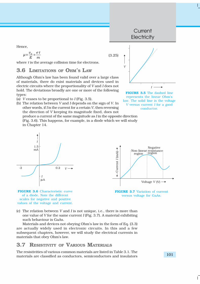
CurrentElectricity
101
Hence,
dv e
E m
τµ = = (3.25)
where τ is the average collision time for electrons.
3.6 LIMITATIONS OF OHM’S LAW
Although Ohm’s law has been found valid over a large classof materials, there do exist materials and devices used inelectric circuits where the proportionality of V and I does nothold. The deviations broadly are one or more of the followingtypes:(a) V ceases to be proportional to I (Fig. 3.5).(b) The relation between V and I depends on the sign of V. In
other words, if I is the current for a certain V, then reversingthe direction of V keeping its magnitude fixed, does notproduce a current of the same magnitude as I in the opposite direction(Fig. 3.6). This happens, for example, in a diode which we will studyin Chapter 14.
(c) The relation between V and I is not unique, i.e., there is more thanone value of V for the same current I (Fig. 3.7). A material exhibitingsuch behaviour is GaAs.Materials and devices not obeying Ohm’s law in the form of Eq. (3.3)
are actually widely used in electronic circuits. In this and a fewsubsequent chapters, however, we will study the electrical currents inmaterials that obey Ohm’s law.
3.7 RESISTIVITY OF VARIOUS MATERIALS
The resistivities of various common materials are listed in Table 3.1. Thematerials are classified as conductors, semiconductors and insulators
FIGURE 3.5 The dashed linerepresents the linear Ohm’s
law. The solid line is the voltageV versus current I for a good
conductor.
FIGURE 3.6 Characteristic curveof a diode. Note the different
scales for negative and positivevalues of the voltage and current.
FIGURE 3.7 Variation of currentversus voltage for GaAs.

Physics
102
depending on their resistivities, in an increasing order of their values.Metals have low resistivities in the range of 10–8 Ωm to 10–6 Ωm. At theother end are insulators like ceramic, rubber and plastics havingresistivities 1018 times greater than metals or more. In between the twoare the semiconductors. These, however, have resistivitiescharacteristically decreasing with a rise in temperature. The resistivitiesof semiconductors are also affected by presence of small amount ofimpurities. This last feature is exploited in use of semiconductors forelectronic devices.
TABLE 3.1 RESISTIVITIES OF SOME MATERIALS
Material Resistivity, ρ Temperature coefficient(Ω m) at 0°C of resistivity, α (°C) –1
1 d at 0 C
dTρ
ρ °
ConductorsSilver 1.6 × 10⁻⁸ 0.0041Copper 1.7 × 10⁻⁸ 0.0068Aluminium 2.7 × 10⁻⁸ 0.0043Tungsten 5.6 × 10⁻⁸ 0.0045Iron 10 × 10–8 0.0065Platinum 11 × 10–8 0.0039Mercury 98 × 10–8 0.0009Nichrome ~100 × 10–8 0.0004(alloy of Ni, Fe, Cr)Manganin (alloy) 48 × 10–8 0.002 × 10⁻³
SemiconductorsCarbon (graphite) 3.5 × 10⁻⁵ – 0.0005Germanium 0.46 – 0.05Silicon 2300 – 0.07
InsulatorsPure Water 2.5 × 10⁵
Glass 1010 – 1014
Hard Rubber 1013 – 1016
NaCl ~1014
Fused Quartz ~1016
Commercially produced resistors for domestic use or in laboratoriesare of two major types: wire bound resistors and carbon resistors. Wirebound resistors are made by winding the wires of an alloy, viz., manganin,constantan, nichrome or similar ones. The choice of these materials isdictated mostly by the fact that their resistivities are relatively insensitiveto temperature. These resistances are typically in the range of a fractionof an ohm to a few hundred ohms.

CurrentElectricity
103
Resistors in the higher range are made mostly from carbon. Carbonresistors are compact, inexpensive and thus find extensive use in electroniccircuits. Carbon resistors are small in size and hence their values aregiven using a colour code.
TABLE 3.2 RESISTOR COLOUR CODES
Colour Number Multiplier Tolerance (%)
Black 0 1Brown 1 101
Red 2 102
Orange 3 103
Yellow 4 104
Green 5 105
Blue 6 106
Violet 7 107
Gray 8 108
White 9 109
Gold 10–1 5Silver 10–2 10No colour 20
The resistors have a set of co-axial coloured ringson them whose significance are listed in Table 3.2. Thefirst two bands from the end indicate the first twosignificant figures of the resistance in ohms. The thirdband indicates the decimal multiplier (as listed in Table3.2). The last band stands for tolerance or possiblevariation in percentage about the indicated values.Sometimes, this last band is absent and that indicatesa tolerance of 20% (Fig. 3.8). For example, if the fourcolours are orange, blue, yellow and gold, the resistancevalue is 36 × 104 Ω, with a tolerence value of 5%.
3.8 TEMPERATURE DEPENDENCE OF
RESISTIVITY
The resistivity of a material is found to be dependent onthe temperature. Different materials do not exhibit thesame dependence on temperatures. Over a limited rangeof temperatures, that is not too large, the resistivity of ametallic conductor is approximately given by,
ρT = ρ0 [1 + α (T–T0)] (3.26)
where ρT is the resistivity at a temperature T and ρ0 is the same at areference temperature T0. α is called the temperature co-efficient ofresistivity, and from Eq. (3.26), the dimension of α is (Temperature)–1.
FIGURE 3.8 Colour coded resistors(a) (22 × 102 Ω) ± 10%,(b) (47 × 10 Ω) ± 5%.

Physics
104
For metals, α is positive and values of α for some metals at T0 = 0°C arelisted in Table 3.1.
The relation of Eq. (3.26) implies that a graph of ρT plotted against Twould be a straight line. At temperatures much lower than 0°C, the graph,however, deviates considerably from a straight line (Fig. 3.9).
Equation (3.26) thus, can be used approximately over a limited rangeof T around any reference temperature T0, where the graph can beapproximated as a straight line.
Some materials like Nichrome (which is an alloy of nickel, iron andchromium) exhibit a very weak dependence of resistivity with temperature(Fig. 3.10). Manganin and constantan have similar properties. Thesematerials are thus widely used in wire bound standard resistors sincetheir resistance values would change very little with temperatures.
Unlike metals, the resistivities of semiconductors decrease withincreasing temperatures. A typical dependence is shown in Fig. 3.11.
We can qualitatively understand the temperature dependence ofresistivity, in the light of our derivation of Eq. (3.23). From this equation,resistivity of a material is given by
2
1 m
n eρ
σ τ= = (3.27)
ρ thus depends inversely both on the number n of free electrons per unitvolume and on the average time τ between collisions. As we increasetemperature, average speed of the electrons, which act as the carriers ofcurrent, increases resulting in more frequent collisions. The average timeof collisions τ, thus decreases with temperature.
In a metal, n is not dependent on temperature to any appreciableextent and thus the decrease in the value of τ with rise in temperaturecauses ρ to increase as we have observed.
For insulators and semiconductors, however, n increases withtemperature. This increase more than compensates any decrease in τ inEq.(3.23) so that for such materials, ρ decreases with temperature.
FIGURE 3.9Resistivity ρT of
copper as a functionof temperature T.
FIGURE 3.10 ResistivityρT of nichrome as afunction of absolute
temperature T.
FIGURE 3.11Temperature dependenceof resistivity for a typical
semiconductor.

CurrentElectricity
105
EX
AM
PLE 3
.4
Example 3.3 An electric toaster uses nichrome for its heatingelement. When a negligibly small current passes through it, itsresistance at room temperature (27.0 °C) is found to be 75.3 Ω. Whenthe toaster is connected to a 230 V supply, the current settles, aftera few seconds, to a steady value of 2.68 A. What is the steadytemperature of the nichrome element? The temperature coefficientof resistance of nichrome averaged over the temperature rangeinvolved, is 1.70 × 10⁻⁴ °C–1.
Solution When the current through the element is very small, heatingeffects can be ignored and the temperature T1 of the element is thesame as room temperature. When the toaster is connected to thesupply, its initial current will be slightly higher than its steady valueof 2.68 A. But due to heating effect of the current, the temperaturewill rise. This will cause an increase in resistance and a slightdecrease in current. In a few seconds, a steady state will be reachedwhen temperature will rise no further, and both the resistance of theelement and the current drawn will achieve steady values. Theresistance R2 at the steady temperature T2 is
R2 230 V
85.82.68 A
= = Ω
Using the relation
R2 = R1 [1 + α (T2 – T1)]
with α = 1.70 × 10⁻⁴ °C–1, we get
T2 – T1 –4
(85.8 –75.3)(75.3) 1.70 10
=× ×
= 820 °C
that is, T2 = (820 + 27.0) °C = 847 °C
Thus, the steady temperature of the heating element (when heatingeffect due to the current equals heat loss to the surroundings) is847 °C.
Example 3.4 The resistance of the platinum wire of a platinumresistance thermometer at the ice point is 5 Ω and at steam point is5.23 Ω. When the thermometer is inserted in a hot bath, the resistanceof the platinum wire is 5.795 Ω. Calculate the temperature of thebath.
Solution R0 = 5 Ω, R100 = 5.23 Ω and Rt = 5.795 Ω
Now,0
0100 0
100, (1 )tt
R Rt R R t
R Rα
−= × = +
−
5.795 5100
5.23 5−
= ×−
=0.795
1000.23
× = 345.65 °C
3.9 ELECTRICAL ENERGY, POWER
Consider a conductor with end points A and B, in which a current I isflowing from A to B. The electric potential at A and B are denoted by V (A)
EX
AM
PLE 3
.3

Physics
106
and V (B) respectively. Since current is flowing from A to B, V (A) > V (B)and the potential difference across AB is V = V(A) – V(B) > 0.
In a time interval ∆t, an amount of charge ∆Q = I ∆t travels from A toB. The potential energy of the charge at A, by definition, was Q V (A) andsimilarly at B, it is Q V(B). Thus, change in its potential energy ∆Upot is
∆Upot = Final potential energy – Initial potential energy = ∆Q[(V (B) – V (A)] = –∆Q V = –I V∆t < 0 (3.28)If charges moved without collisions through the conductor, their
kinetic energy would also change so that the total energy is unchanged.Conservation of total energy would then imply that,
∆K = –∆Upot (3.29)
that is,
∆K = I V∆t > 0 (3.30)
Thus, in case charges were moving freely through the conductor underthe action of electric field, their kinetic energy would increase as theymove. We have, however, seen earlier that on the average, charge carriersdo not move with acceleration but with a steady drift velocity. This isbecause of the collisions with ions and atoms during transit. Duringcollisions, the energy gained by the charges thus is shared with the atoms.The atoms vibrate more vigorously, i.e., the conductor heats up. Thus,in an actual conductor, an amount of energy dissipated as heat in theconductor during the time interval ∆t is,
∆W = I V∆t (3.31)The energy dissipated per unit time is the power dissipated
P = ∆W/∆t and we have,
P = I V (3.32)
Using Ohm’s law V = IR, we get
P = I 2 R = V 2/R (3.33)
as the power loss (“ohmic loss”) in a conductor of resistance R carrying acurrent I. It is this power which heats up, for example, the coil of an
electric bulb to incandescence, radiating out heat andlight.
Where does the power come from? As we havereasoned before, we need an external source to keepa steady current through the conductor. It is clearlythis source which must supply this power. In thesimple circuit shown with a cell (Fig.3.12), it is thechemical energy of the cell which supplies this powerfor as long as it can.
The expressions for power, Eqs. (3.32) and (3.33),show the dependence of the power dissipated in aresistor R on the current through it and the voltageacross it.
Equation (3.33) has an important application topower transmission. Electrical power is transmittedfrom power stations to homes and factories, which
FIGURE 3.12 Heat is produced in theresistor R which is connected across
the terminals of a cell. The energydissipated in the resistor R comes fromthe chemical energy of the electrolyte.

CurrentElectricity
107
may be hundreds of miles away, via transmission cables. One obviouslywants to minimise the power loss in the transmission cables connectingthe power stations to homes and factories. We shall see now how thiscan be achieved. Consider a device R, to which a power P is to be deliveredvia transmission cables having a resistance Rc to be dissipated by it finally.If V is the voltage across R and I the current through it, then
P = V I (3.34)The connecting wires from the power station to the device has a finite
resistance Rc. The power dissipated in the connecting wires, which iswasted is Pc with
Pc = I2 Rc
2
2cP R
V= (3.35)
from Eq. (3.32). Thus, to drive a device of power P, the power wasted in theconnecting wires is inversely proportional to V 2. The transmission cablesfrom power stations are hundreds of miles long and their resistance Rc isconsiderable. To reduce Pc, these wires carry current at enormous valuesof V and this is the reason for the high voltage danger signs on transmissionlines — a common sight as we move away from populated areas. Usingelectricity at such voltages is not safe and hence at the other end, a devicecalled a transformer lowers the voltage to a value suitable for use.
3.10 COMBINATION OF RESISTORS – SERIES AND
PARALLEL
The current through a single resistor R across which there is a potentialdifference V is given by Ohm’s law I = V/R. Resistors are sometimes joinedtogether and there are simple rules for calculation of equivalent resistanceof such combination.
FIGURE 3.13 A series combination of two resistor R1 and R2.
Two resistors are said to be in series if only one of their end points isjoined (Fig. 3.13). If a third resistor is joined with the series combinationof the two (Fig. 3.14), then all three are said to be in series. Clearly, wecan extend this definition to series combination of any number of resistors.
FIGURE 3.14 A series combination of three resistors R1, R2, R3.
Two or more resistors are said to be in parallel if one end of all theresistors is joined together and similarly the other ends joined together(Fig. 3.15).
FIGURE 3.15 Two resistors R1 and R2 connected in parallel.

Physics
108
Consider two resistors R1 and R2 in series. The charge which leaves R1must be entering R2. Since current measures the rate of flow of charge,this means that the same current I flows through R1 and R2. By Ohm’s law:
Potential difference across R1 = V1 = I R1, and
Potential difference across R2 = V2 = I R2.
The potential difference V across the combination is V1+V2. Hence,
V = V1+ V2 = I (R1 + R2) (3.36)
This is as if the combination had an equivalent resistance Req, whichby Ohm’s law is
Req VI
≡ = (R1 + R2) (3.37)
If we had three resistors connected in series, then similarly
V = I R1 + I R2 + I R3 = I (R1+ R2+ R3). (3.38)
This obviously can be extended to a series combination of any numbern of resistors R1, R2 ....., Rn. The equivalent resistance Req is
Req = R1 + R2 + . . . + Rn (3.39)
Consider now the parallel combination of two resistors (Fig. 3.15).The charge that flows in at A from the left flows out partly through R1and partly through R2. The currents I, I1, I2 shown in the figure are therates of flow of charge at the points indicated. Hence,
I = I1 + I2 (3.40)
The potential difference between A and B is given by the Ohm’s lawapplied to R1
V = I1 R1 (3.41)Also, Ohm’s law applied to R2 gives
V = I2 R2 (3.42)
∴ I = I1 + I2 = 1 2 1 2
1 1V VV
R R R R
+ = + (3.43)
If the combination was replaced by an equivalent resistance Req, wewould have, by Ohm’s law
eq
VI
R= (3.44)
Hence,
1 2
1 1 1
eqR R R= + (3.45)
We can easily see how this extends to three resistors in parallel(Fig. 3.16).
FIGURE 3.16 Parallel combination of three resistors R1, R2 and R3.

CurrentElectricity
109
Exactly as before
I = I1 + I2 + I3 (3.46)
and applying Ohm’s law to R1, R2 and R3 we get,
V = I1 R1, V = I2 R2, V = I3 R3 (3.47)
So that
I = I1 + I2 + I3 =1 2 3
1 1 1V
R R R
+ +
(3.48)
An equivalent resistance Req that replaces the combination, would besuch that
eq
VI
R= (3.49)
and hence
1 2 3
1 1 1 1
eqR R R R= + + (3.50)
We can reason similarly for any number of resistors in parallel. Theequivalent resistance of n resistors R1, R2 . . . ,Rn is
1 2 n
1 1 1 1...
eqR R R R= + + + (3.51)
These formulae for equivalent resistances can be used to find outcurrents and voltages in more complicated circuits. Consider for example,the circuit in Fig. (3.17), where there are three resistors R1, R2 and R3.R2 and R3 are in parallel and hence we canreplace them by an equivalent 23
eqR betweenpoint B and C with
232 3
1 1 1
eq R RR= +
or, 23 2 3
2 3
Req
R RR R
=+ (3.52)
The circuit now has R1 and 23eqR in series
and hence their combination can be
replaced by an equivalent resistance 123eqR
with123 23
1eq eqR R R= + (3.53)
If the voltage between A and C is V, thecurrent I is given by
( )1231 2 3 2 3/eq
V VI
R R R R R R= =
+ +
( )2 3
1 2 1 3 2 3
V R R
R R R R R R
+=
+ + (3.54)
FIGURE 3.17 A combination of three resistors R1,R2 and R3. R2, R3 are in parallel with an
equivalent resistance 23eqR . R1 and 23
eqR are in
series with an equivalent resistance 123eqR .

Physics
110
3.11 CELLS, EMF, INTERNAL RESISTANCE
We have already mentioned that a simple device to maintain a steadycurrent in an electric circuit is the electrolytic cell. Basically a cell hastwo electrodes, called the positive (P) and the negative (N), as shown inFig. 3.18. They are immersed in an electrolytic solution. Dipped in the
solution, the electrodes exchange charges with the electrolyte. Thepositive electrode has a potential difference V+ (V+ > 0) betweenitself and the electrolyte solution immediately adjacent to it markedA in the figure. Similarly, the negative electrode develops a negativepotential – (V– ) (V– ≥ 0) relative to the electrolyte adjacent to it,marked as B in the figure. When there is no current, the electrolytehas the same potential throughout, so that the potential differencebetween P and N is V+ – (–V–) = V+ + V– . This difference is called theelectromotive force (emf) of the cell and is denoted by ε. Thus
ε = V++V– > 0 (3.55)
Note that ε is, actually, a potential difference and not a force. Thename emf, however, is used because of historical reasons, and wasgiven at a time when the phenomenon was not understood properly.
To understand the significance of ε, consider a resistor Rconnected across the cell (Fig. 3.18). A current I flows across Rfrom C to D. As explained before, a steady current is maintainedbecause current flows from N to P through the electrolyte. Clearly,across the electrolyte the same current flows through the electrolytebut from N to P, whereas through R, it flows from P to N.
The electrolyte through which a current flows has a finiteresistance r, called the internal resistance. Consider first thesituation when R is infinite so that I = V/R = 0, where V is thepotential difference between P and N. Now,
V = Potential difference between P and A + Potential difference between A and B + Potential difference between B and N = ε (3.56)
Thus, emf ε is the potential difference between the positive andnegative electrodes in an open circuit, i.e., when no current isflowing through the cell.
If however R is finite, I is not zero. In that case the potentialdifference between P and N is
V = V++ V– – I r
= ε – I r (3.57)
Note the negative sign in the expression (I r ) for the potential differencebetween A and B. This is because the current I flows from B to A in theelectrolyte.
In practical calculations, internal resistances of cells in the circuitmay be neglected when the current I is such that ε >> I r. The actualvalues of the internal resistances of cells vary from cell to cell. The internalresistance of dry cells, however, is much higher than the commonelectrolytic cells.
FIGURE 3.18 (a) Sketch ofan electrolyte cell withpositive terminal P and
negative terminal N. Thegap between the electrodesis exaggerated for clarity. A
and B are points in theelectrolyte typically close toP and N. (b) the symbol fora cell, + referring to P and
– referring to the Nelectrode. Electrical
connections to the cell aremade at P and N.

CurrentElectricity
111
We also observe that since V is the potential difference across R, wehave from Ohm’s law
V = I R (3.58)
Combining Eqs. (3.57) and (3.58), we get
I R = ε – I r
Or, IR r
ε=+
(3.59)
The maximum current that can be drawn from a cell is for R = 0 andit is Imax = ε/r. However, in most cells the maximum allowed current ismuch lower than this to prevent permanent damage to the cell.
CHARGES IN CLOUDS
In olden days lightning was considered as an atmospheric flash of supernatural origin.It was believed to be the great weapon of Gods. But today the phenomenon of lightningcan be explained scientifically by elementary principles of physics.
Atmospheric electricity arises due to the separation of electric charges. In theionosphere and magnetosphere strong electric current is generated from the solar-terrestrial interaction. In the lower atmosphere the current is weaker and is maintainedby thunderstorm.
There are ice particles in the clouds, which grow, collide, fracture and break apart.The smaller particles acquire positive charge and the larger ones negative charge. Thesecharged particles get separated by updrafts in the clouds and gravity. The upper portionof the cloud becomes positively charged and the middle negatively charged, leading todipole structure. Sometimes a very weak positive charge is found near the base of thecloud. The ground is positively charged at the time of thunderstorm development. Alsocosmic and radioactive radiations ionise air into positive and negative ions and air becomes(weakly) electrically conductive. The separation of charges produce tremendous amountof electrical potential within the cloud as well as between the cloud and ground. This canamount to millions of volts and eventually the electrical resistance in the air breaksdown and lightning flash begins and thousands of amperes of current flows. The electricfield is of the order of 105 V/m. A lightning flash is composed of a series of strokes withan average of about four and the duration of each flash is about 30 seconds. The averagepeak power per stroke is about 1012 watts.
During fair weather also there is charge in the atmosphere. The fair weather electricfield arises due to the existence of a surface charge density at ground and an atmosphericconductivity as well as due to the flow of current from the ionosphere to the earth’ssurface, which is of the order of picoampere / square metre. The surface charge densityat ground is negative; the electric field is directed downward. Over land the averageelectric field is about 120 V/m, which corresponds to a surface charge density of–1.2 × 10⁻⁹ C/m2. Over the entire earth’s surface, the total negative charge amount toabout 600 kC. An equal positive charge exists in the atmosphere. This electric field is notnoticeable in daily life. The reason why it is not noticed is that virtually everything, includingour bodies, is conductor compared to air.

Physics
112 EX
AM
PLE 3
.5Example 3.5 A network of resistors is connected to a 16 V batterywith internal resistance of 1Ω, as shown in Fig. 3.19: (a) Computethe equivalent resistance of the network. (b) Obtain the current ineach resistor. (c) Obtain the voltage drops VAB, VBC and VCD.
FIGURE 3.19Solution(a) The network is a simple series and parallel combination of
resistors. First the two 4Ω resistors in parallel are equivalent to aresistor = [(4 × 4)/(4 + 4)] Ω = 2 Ω.In the same way, the 12 Ω and 6 Ω resistors in parallel areequivalent to a resistor of[(12 × 6)/(12 + 6)] Ω = 4 Ω.The equivalent resistance R of the network is obtained bycombining these resistors (2 Ω and 4 Ω) with 1 Ω in series,that is,R = 2 Ω + 4 Ω + 1 Ω = 7 Ω.
(b) The total current I in the circuit is
162 A
(7 1)V
IR r
ε= = =
+ + ΩConsider the resistors between A and B. If I1 is the current in oneof the 4 Ω resistors and I2 the current in the other,I1 × 4 = I2 × 4that is, I1 = I2, which is otherwise obvious from the symmetry ofthe two arms. But I1 + I2 = I = 2 A. Thus,
I1 = I2 = 1 A
that is, current in each 4 Ω resistor is 1 A. Current in 1 Ω resistorbetween B and C would be 2 A.Now, consider the resistances between C and D. If I3 is the currentin the 12 Ω resistor, and I4 in the 6 Ω resistor,I3 × 12 = I4 × 6, i.e., I4 = 2I3
But, I3 + I4 = I = 2 A
Thus, I3 =23
A, I4 =
43
A
that is, the current in the 12 Ω resistor is (2/3) A, while the currentin the 6 Ω resistor is (4/3) A.
(c) The voltage drop across AB is
VAB = I1 × 4 = 1 A × 4 Ω = 4 V,
This can also be obtained by multiplying the total current betweenA and B by the equivalent resistance between A and B, that is,

CurrentElectricity
113
EX
AM
PLE 3
.5
VAB = 2 A × 2 Ω = 4 V
The voltage drop across BC is
VBC = 2 A × 1 Ω = 2 V
Finally, the voltage drop across CD is
VCD = 12 Ω × I3 = 12 Ω × 23
A = 8 V.
This can alternately be obtained by multiplying total currentbetween C and D by the equivalent resistance between C and D,that is,
VCD = 2 A × 4 Ω = 8 V
Note that the total voltage drop across AD is 4 V + 2 V + 8 V = 14 V.Thus, the terminal voltage of the battery is 14 V, while its emf is 16 V.The loss of the voltage (= 2 V) is accounted for by the internal resistance1 Ω of the battery [2 A × 1 Ω = 2 V].
3.12 CELLS IN SERIES AND IN PARALLEL
Like resistors, cells can be combined together in an electric circuit. Andlike resistors, one can, for calculating currents and voltages in a circuit,replace a combination of cells by an equivalent cell.
FIGURE 3.20 Two cells of emf’s ε1 and ε2 in the series. r1, r2 are theirinternal resistances. For connections across A and C, the combinationcan be considered as one cell of emf εeq and an internal resistance req.
Consider first two cells in series (Fig. 3.20), where one terminal of thetwo cells is joined together leaving the other terminal in either cell free.ε1, ε2 are the emf’s of the two cells and r1, r2 their internal resistances,respectively.
Let V (A), V (B), V (C) be the potentials at points A, B and C shown inFig. 3.20. Then V (A) – V (B) is the potential difference between the positiveand negative terminals of the first cell. We have already calculated it inEq. (3.57) and hence,
AB 1 1(A) – (B) –V V V I rε≡ = (3.60)
Similarly,
BC 2 2(B) – (C) –V V V I rε≡ = (3.61)
Hence, the potential difference between the terminals A and C of thecombination is
( ) ( ) ( ) ( )AC (A) – (C) A – B B – CV V V V V V V≡ = +
( ) ( )1 2 1 2– I r rε ε= + + (3.62)

Physics
114
If we wish to replace the combination by a single cell between A andC of emf εeq and internal resistance req, we would have
VAC = εeq– I req (3.63)
Comparing the last two equations, we get
εeq = ε1 + ε2 (3.64)
and req = r1 + r2 (3.65)
In Fig.3.20, we had connected the negative electrode of the first to thepositive electrode of the second. If instead we connect the two negatives,Eq. (3.61) would change to VBC = –ε2–Ir2 and we will get
εeq = ε1 – ε2 (ε1 > ε2) (3.66)
The rule for series combination clearly can be extended to any numberof cells:(i) The equivalent emf of a series combination of n cells is just the sum of
their individual emf’s, and(ii) The equivalent internal resistance of a series combination of n cells is
just the sum of their internal resistances.This is so, when the current leaves each cell from the positive
electrode. If in the combination, the current leaves any cell fromthe negative electrode, the emf of the cell enters the expressionfor εeq with a negative sign, as in Eq. (3.66).
Next, consider a parallel combination of the cells (Fig. 3.21).I1 and I2 are the currents leaving the positive electrodes of thecells. At the point B1, I1 and I2 flow in whereas the current I flowsout. Since as much charge flows in as out, we have
I = I1 + I2 (3.67)
Let V (B1) and V (B2) be the potentials at B1 and B2, respectively.Then, considering the first cell, the potential difference across itsterminals is V (B1) – V (B2). Hence, from Eq. (3.57)
( ) ( )1 2 1 1 1– –V V B V B I rε≡ = (3.68)
Points B1 and B2 are connected exactly similarly to the secondcell. Hence considering the second cell, we also have
( ) ( )1 2 2 2 2– –V V B V B I rε≡ = (3.69)
Combining the last three equations
1 2 I I I= +
1 2 1 2
1 2 1 2 1 2
– – 1 1–
V VV
r r r r r r
ε ε ε ε = + = + + (3.70)
Hence, V is given by,
1 2 2 1 1 2
1 2 1 2
–r r r r
V Ir r r r
ε ε+=
+ + (3.71)
If we want to replace the combination by a single cell, between B1 andB2, of emf εeq and internal resistance req, we would have
V = εeq – I req (3.72)
FIGURE 3.21 Two cells inparallel. For connections
across A and C, thecombination can be
replaced by one cell of emfεeq and internal resistancesreq whose values are given in
Eqs. (3.64) and (3.65).
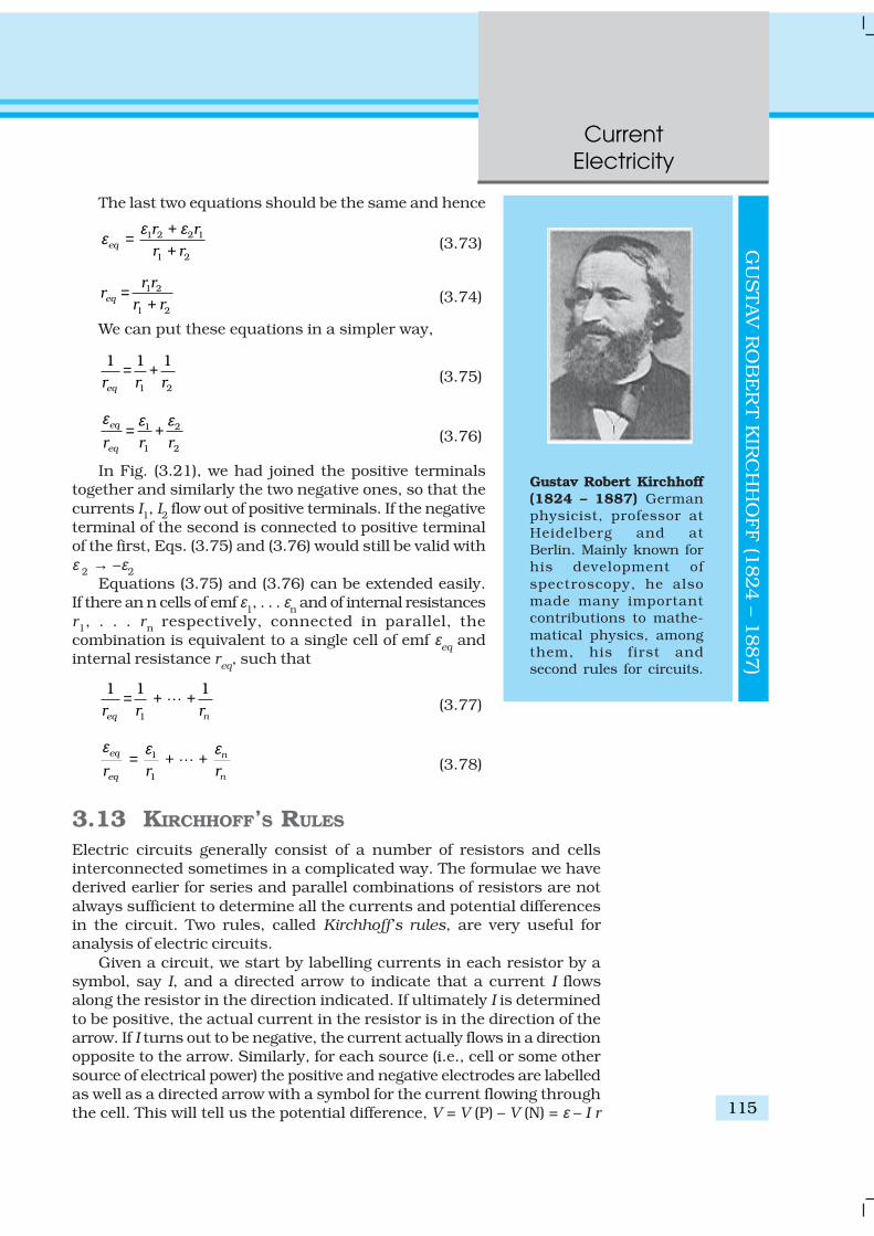
CurrentElectricity
115
The last two equations should be the same and hence
1 2 2 1
1 2eq
r rr r
ε εε +=
+ (3.73)
1 2
1 2eq
r rr
r r=
+ (3.74)
We can put these equations in a simpler way,
1 2
1 1 1
eqr r r= + (3.75)
1 2
1 2
eq
eqr r r
ε ε ε= + (3.76)
In Fig. (3.21), we had joined the positive terminalstogether and similarly the two negative ones, so that thecurrents I1, I2 flow out of positive terminals. If the negativeterminal of the second is connected to positive terminalof the first, Eqs. (3.75) and (3.76) would still be valid withε 2 → –ε2
Equations (3.75) and (3.76) can be extended easily.If there an n cells of emf ε1, . . . εn and of internal resistancesr1, . . . rn respectively, connected in parallel, thecombination is equivalent to a single cell of emf εeq andinternal resistance req, such that
1
1 1 1
eq nr r r= + + (3.77)
1
1
eq n
eq nr r r
ε εε= + + (3.78)
3.13 KIRCHHOFF’S RULES
Electric circuits generally consist of a number of resistors and cellsinterconnected sometimes in a complicated way. The formulae we havederived earlier for series and parallel combinations of resistors are notalways sufficient to determine all the currents and potential differencesin the circuit. Two rules, called Kirchhoff’s rules, are very useful foranalysis of electric circuits.
Given a circuit, we start by labelling currents in each resistor by asymbol, say I, and a directed arrow to indicate that a current I flowsalong the resistor in the direction indicated. If ultimately I is determinedto be positive, the actual current in the resistor is in the direction of thearrow. If I turns out to be negative, the current actually flows in a directionopposite to the arrow. Similarly, for each source (i.e., cell or some othersource of electrical power) the positive and negative electrodes are labelledas well as a directed arrow with a symbol for the current flowing throughthe cell. This will tell us the potential difference, V = V (P) – V (N) = ε – I r
Gustav Robert Kirchhoff(1824 – 1887) Germanphysicist, professor atHeidelberg and atBerlin. Mainly known forhis development ofspectroscopy, he alsomade many importantcontributions to mathe-matical physics, amongthem, his first andsecond rules for circuits.
GU
STAV
RO
BE
RT K
IRC
HH
OFF (1
824 – 1
887)

Physics
116 EX
AM
PLE 3
.6
[Eq. (3.57) between the positive terminal P and the negative terminal N; Ihere is the current flowing from N to P through the cell]. If, while labelling
the current I through the cell one goes from P to N,then of course
V = ε + I r (3.79)
Having clarified labelling, we now state the rulesand the proof:(a) Junction rule: At any junction, the sum of the
currents entering the junction is equal to thesum of currents leaving the junction (Fig. 3.22).
This applies equally well if instead of a junction ofseveral lines, we consider a point in a line.
The proof of this rule follows from the fact thatwhen currents are steady, there is no accumulationof charges at any junction or at any point in a line.Thus, the total current flowing in, (which is the rateat which charge flows into the junction), must equalthe total current flowing out.(b) Loop rule: The algebraic sum of changes in
potential around any closed loop involvingresistors and cells in the loop is zero (Fig. 3.22).
This rule is also obvious, since electric potential isdependent on the location of the point. Thus starting with any point if wecome back to the same point, the total change must be zero. In a closedloop, we do come back to the starting point and hence the rule.
Example 3.6 A battery of 10 V and negligible internal resistance isconnected across the diagonally opposite corners of a cubical networkconsisting of 12 resistors each of resistance 1 Ω (Fig. 3.23). Determinethe equivalent resistance of the network and the current along eachedge of the cube.
FIGURE 3.23
FIGURE 3.22 At junction a the currentleaving is I1 + I2 and current entering is I3.The junction rule says I3 = I1 + I2. At pointh current entering is I1. There is only one
current leaving h and by junction rulethat will also be I1. For the loops ‘ahdcba’and ‘ahdefga’, the loop rules give –30I1 –41 I3 + 45 = 0 and –30I1 + 21 I2 – 80 = 0.

CurrentElectricity
117
EX
AM
PLE 3
.6
Solution The network is not reducible to a simple series and parallelcombinations of resistors. There is, however, a clear symmetry in theproblem which we can exploit to obtain the equivalent resistance ofthe network.The paths AA′, AD and AB are obviously symmetrically placed in thenetwork. Thus, the current in each must be the same, say, I. Further,at the corners A′, B and D, the incoming current I must split equallyinto the two outgoing branches. In this manner, the current in allthe 12 edges of the cube are easily written down in terms of I, usingKirchhoff’s first rule and the symmetry in the problem.Next take a closed loop, say, ABCC′EA, and apply Kirchhoff’s secondrule:
–IR – (1/2)IR – IR + ε = 0where R is the resistance of each edge and ε the emf of battery. Thus,
ε = 52
I R
The equivalent resistance Req of the network is
53 6eqR R
Iε= =
For R = 1 Ω, Req = (5/6) Ω and for ε = 10 V, the total current (= 3I ) inthe network is
3I = 10 V/(5/6) Ω = 12 A, i.e., I = 4 AThe current flowing in each edge can now be read off from theFig. 3.23.
It should be noted that because of the symmetry of the network, thegreat power of Kirchhoff’s rules has not been very apparent in Example 3.6.In a general network, there will be no such simplification due tosymmetry, and only by application of Kirchhoff’s rules to junctions andclosed loops (as many as necessary to solve the unknowns in the network)can we handle the problem. This will be illustrated in Example 3.7.
Example 3.7 Determine the current in each branch of the networkshown in Fig. 3.24.
FIGURE 3.24
Sim
ilatio
n fo
r ap
plic
atio
n o
f Kirc
hh
offís
rule
s:
EX
AM
PLE 3
.7

Physics
118
EX
AM
PLE 3
.7Solution Each branch of the network is assigned an unknown currentto be determined by the application of Kirchhoff’s rules. To reducethe number of unknowns at the outset, the first rule of Kirchhoff isused at every junction to assign the unknown current in each branch.We then have three unknowns I1, I2 and I3 which can be found byapplying the second rule of Kirchhoff to three different closed loops.Kirchhoff’s second rule for the closed loop ADCA gives,
10 – 4(I1– I2) + 2(I2 + I3 – I1) – I1 = 0 [3.80(a)]that is, 7I1– 6I2 – 2I3 = 10For the closed loop ABCA, we get
10 – 4I2– 2 (I2 + I3) – I1 = 0that is, I1 + 6I2 + 2I3 =10 [3.80(b)]For the closed loop BCDEB, we get
5 – 2 (I2 + I3) – 2 (I2 + I3 – I1) = 0that is, 2I1 – 4I2 – 4I3 = –5 [3.80(c)]
Equations (3.80 a, b, c) are three simultaneous equations in threeunknowns. These can be solved by the usual method to give
I1 = 2.5A, I2 = 58
A, I3 = 7
18
A
The currents in the various branches of the network are
AB : 58
A, CA : 1
22
A, DEB : 7
18
A
AD : 7
18
A, CD : 0 A, BC : 1
22
A
It is easily verified that Kirchhoff’s second rule applied to theremaining closed loops does not provide any additional independentequation, that is, the above values of currents satisfy the secondrule for every closed loop of the network. For example, the total voltagedrop over the closed loop BADEB
5 155 V 4 V 4 V
8 8 + × − ×
equal to zero, as required by Kirchhoff’s second rule.
3.14 WHEATSTONE BRIDGE
As an application of Kirchhoff’s rules consider the circuit shown inFig. 3.25, which is called the Wheatstone bridge. The bridge hasfour resistors R1, R2, R3 and R4. Across one pair of diagonally oppositepoints (A and C in the figure) a source is connected. This (i.e., AC) iscalled the battery arm. Between the other two vertices, B and D, agalvanometer G (which is a device to detect currents) is connected. Thisline, shown as BD in the figure, is called the galvanometer arm.
For simplicity, we assume that the cell has no internal resistance. Ingeneral there will be currents flowing across all the resistors as well as acurrent Ig through G. Of special interest, is the case of a balanced bridgewhere the resistors are such that Ig = 0. We can easily get the balancecondition, such that there is no current through G. In this case, theKirchhoff’s junction rule applied to junctions D and B (see the figure)

CurrentElectricity
119
immediately gives us the relations I1 = I3 and I2 = I4. Next, we applyKirchhoff’s loop rule to closed loops ADBA and CBDC. The firstloop gives
–I1 R1 + 0 + I2 R2 = 0 (Ig = 0) (3.81)
and the second loop gives, upon using I3 = I1, I4 = I2I2 R4 + 0 – I1 R3 = 0 (3.82)
From Eq. (3.81), we obtain,
1 2
2 1
I RI R
=
whereas from Eq. (3.82), we obtain,
1 4
2 3
I RI R
=
Hence, we obtain the condition
2 4
1 3
R RR R
= [3.83(a)]
This last equation relating the four resistors is called the balancecondition for the galvanometer to give zero or null deflection.
The Wheatstone bridge and its balance condition provide a practicalmethod for determination of an unknown resistance. Let us suppose wehave an unknown resistance, which we insert in the fourth arm; R4 isthus not known. Keeping known resistances R1 and R2 in the first andsecond arm of the bridge, we go on varying R3 till the galvanometer showsa null deflection. The bridge then is balanced, and from the balancecondition the value of the unknown resistance R4 is given by,
24 3
1
RR R
R= [3.83(b)]
A practical device using this principle is called the meter bridge. Itwill be discussed in the next section.
Example 3.8 The four arms of a Wheatstone bridge (Fig. 3.26) havethe following resistances:
AB = 100Ω, BC = 10Ω, CD = 5Ω, and DA = 60Ω.
FIGURE 3.26
FIGURE 3.25
EX
AM
PLE 3
.8

Physics
120
EX
AM
PLE 3
.8
A galvanometer of 15Ω resistance is connected across BD. Calculatethe current through the galvanometer when a potential difference of10 V is maintained across AC.
Solution Considering the mesh BADB, we have
100I1 + 15Ig – 60I2 = 0
or 20I1 + 3Ig – 12I2= 0 [3.84(a)]
Considering the mesh BCDB, we have
10 (I1 – Ig) – 15Ig – 5 (I2 + Ig) = 0
10I1 – 30Ig –5I2 = 0
2I1 – 6Ig – I2 = 0 [3.84(b)]
Considering the mesh ADCEA,
60I2 + 5 (I2 + Ig) = 10
65I2 + 5Ig = 10
13I2 + Ig = 2 [3.84(c)]
Multiplying Eq. (3.84b) by 10
20I1 – 60Ig – 10I2 = 0 [3.84(d)]
From Eqs. (3.84d) and (3.84a) we have
63Ig – 2I2 = 0
I2 = 31.5Ig [3.84(e)]
Substituting the value of I2 into Eq. [3.84(c)], we get
13 (31.5Ig ) + Ig = 2
410.5 Ig = 2
Ig = 4.87 mA.
3.15 METER BRIDGE
The meter bridge is shown in Fig. 3.27. It consists ofa wire of length 1m and of uniform cross sectionalarea stretched taut and clamped between two thickmetallic strips bent at right angles, as shown. Themetallic strip has two gaps across which resistors canbe connected. The end points where the wire isclamped are connected to a cell through a key. Oneend of a galvanometer is connected to the metallicstrip midway between the two gaps. The other end ofthe galvanometer is connected to a ‘jockey’. The jockeyis essentially a metallic rod whose one end has aknife-edge which can slide over the wire to makeelectrical connection.
R is an unknown resistance whose value we want to determine. It isconnected across one of the gaps. Across the other gap, we connect a
FIGURE 3.27 A meter bridge. Wire ACis 1 m long. R is a resistance to be
measured and S is a standardresistance.
CurrentElectricity
121
standard known resistance S. The jockey is connected to some point Don the wire, a distance l cm from the end A. The jockey can be movedalong the wire. The portion AD of the wire has a resistance Rcml, whereRcm is the resistance of the wire per unit centimetre. The portion DC ofthe wire similarly has a resistance Rcm (100-l ).
The four arms AB, BC, DA and CD [with resistances R, S, Rcm l andRcm(100-l )] obviously form a Wheatstone bridge with AC as the batteryarm and BD the galvanometer arm. If the jockey is moved along the wire,then there will be one position where the galvanometer will show nocurrent. Let the distance of the jockey from the end A at the balancepoint be l= l1. The four resistances of the bridge at the balance point thenare R, S, Rcm l1 and Rcm(100–l1). The balance condition, Eq. [3.83(a)]gives
( )1 1
1 1100 – 100 –cm
cm
R l lR
S R l l= = (3.85)
Thus, once we have found out l1, the unknown resistance R is knownin terms of the standard known resistance S by
1
1100 –l
R Sl
= (3.86)
By choosing various values of S, we would get various values of l1,and calculate R each time. An error in measurement of l1 would naturallyresult in an error in R. It can be shown that the percentage error in R canbe minimised by adjusting the balance point near the middle of thebridge, i.e., when l1 is close to 50 cm. (This requires a suitable choiceof S.)
Example 3.9 In a metre bridge (Fig. 3.27), the null point is found at adistance of 33.7 cm from A. If now a resistance of 12Ω is connected inparallel with S, the null point occurs at 51.9 cm. Determine the valuesof R and S.
Solution From the first balance point, we get
33.766.3
RS
= (3.87)
After S is connected in parallel with a resistance of 12Ω , the resistanceacross the gap changes from S to Seq, where
1212eq
SS
S=
+and hence the new balance condition now gives
( )1251.948.1 12eq
R SRS S
+= = (3.88)
Substituting the value of R/S from Eq. (3.87), we get
51.9 12 33.748.1 12 66.3
S +=
which gives S = 13.5Ω. Using the value of R/S above, we getR = 6.86 Ω.
EX
AM
PLE 3
.9

Physics
122
3.16 POTENTIOMETER
This is a versatile instrument. It is basically a long piece of uniform wire,sometimes a few meters in length across which a standard cell isconnected. In actual design, the wire is sometimes cut in several piecesplaced side by side and connected at the ends by thick metal strip.(Fig. 3.28). In the figure, the wires run from A to C. The small verticalportions are the thick metal strips connecting the various sections ofthe wire.
A current I flows through the wire which can be varied by a variableresistance (rheostat, R) in the circuit. Since the wire is uniform, thepotential difference between A and any point at a distance l from A is
( )ε φ=l l (3.89)
where φ is the potential drop per unit length.Figure 3.28 (a) shows an application of the potentiometer to compare
the emf of two cells of emf ε1 and ε2 . The points marked 1, 2, 3 form a twoway key. Consider first a position of the key where 1 and 3 are connected
so that the galvanometer is connected to ε1. The jockeyis moved along the wire till at a point N1, at a distance l1from A, there is no deflection in the galvanometer. Wecan apply Kirchhoff’s loop rule to the closed loopAN1G31A and get,
φ l1 + 0 – ε1 = 0 (3.90)
Similarly, if another emf ε2 is balanced against l2 (AN2)
φ l2 + 0 – ε2 = 0 (3.91)
From the last two equations
1 1
2 2
ll
εε
= (3.92)
This simple mechanism thus allows one to comparethe emf’s of any two sources. In practice one of the cellsis chosen as a standard cell whose emf is known to ahigh degree of accuracy. The emf of the other cell is theneasily calculated from Eq. (3.92).
We can also use a potentiometer to measure internalresistance of a cell [Fig. 3.28 (b)]. For this the cell (emf ε )whose internal resistance (r) is to be determined isconnected across a resistance box through a key K2, asshown in the figure. With key K2 open, balance isobtained at length l1 (AN1). Then,
ε = φ l1 [3.93(a)]
When key K2 is closed, the cell sends a current (I )through the resistance box (R). If V is the terminalpotential difference of the cell and balance is obtained atlength l2 (AN2),
V = φ l2 [3.93(b)]
FIGURE 3.28 A potentiometer. G isa galvanometer and R a variableresistance (rheostat). 1, 2, 3 are
terminals of a two way key(a) circuit for comparing emfs of two
cells; (b) circuit for determininginternal resistance of a cell.

CurrentElectricity
123
So, we have ε/V = l1/l 2 [3.94(a)]
But, ε = I (r + R ) and V = IR. This gives
ε/V = (r+R )/R [3.94(b)]
From Eq. [3.94(a)] and [3.94(b)] we have
(R+r )/R = l1/l 2
1
2
–1l
r Rl
= (3.95)
Using Eq. (3.95) we can find the internal resistance of a given cell.The potentiometer has the advantage that it draws no current from
the voltage source being measured. As such it is unaffected by the internalresistance of the source.
Example 3.10 A resistance of R Ω draws current from apotentiometer. The potentiometer has a total resistance R0 Ω(Fig. 3.29). A voltage V is supplied to the potentiometer. Derive anexpression for the voltage across R when the sliding contact is in themiddle of the potentiometer.
FIGURE 3.29
Solution While the slide is in the middle of the potentiometer onlyhalf of its resistance (R0/2) will be between the points A and B. Hence,the total resistance between A and B, say, R1, will be given by thefollowing expression:
1 0
1 1 1( /2)R R R
= +
01
0 2R R
RR R
=+
The total resistance between A and C will be sum of resistance betweenA and B and B and C, i.e., R1 + R0/2∴ The current flowing through the potentiometer will be
1 0 1 0
2/2 2
V VI
R R R R= =
+ +
The voltage V1 taken from the potentiometer will be the product ofcurrent I and resistance R1,
V1 = I R1 = 11 0
22
VR
R R
× +
EX
AM
PLE 3
.10

Physics
124
EX
AM
PLE 3
.10
Substituting for R1, we have a
01
000
0
22
22
R RVV
R RR RR
R R
×= ×+ × + +
10
22 2
VRV
R R R=
+ +
or V10
24
VR
R R=
+.
SUMMARY
1. Current through a given area of a conductor is the net charge passingper unit time through the area.
2. To maintain a steady current, we must have a closed circuit in whichan external agency moves electric charge from lower to higher potentialenergy. The work done per unit charge by the source in taking thecharge from lower to higher potential energy (i.e., from one terminalof the source to the other) is called the electromotive force, or emf, ofthe source. Note that the emf is not a force; it is the voltage differencebetween the two terminals of a source in open circuit.
3. Ohm’s law: The electric current I flowing through a substance isproportional to the voltage V across its ends, i.e., V ∝ I or V = RI,where R is called the resistance of the substance. The unit of resistanceis ohm: 1Ω = 1 V A–1.
4. The resistance R of a conductor depends on its length l and constantcross-sectional area A through the relation,
lR
A
ρ=
where ρ, called resistivity is a property of the material and depends ontemperature and pressure.
5. Electrical resistivity of substances varies over a very wide range. Metalshave low resistivity, in the range of 10–8 Ω m to 10–6 Ω m. Insulatorslike glass and rubber have 1022 to 1024 times greater resistivity.Semiconductors like Si and Ge lie roughly in the middle range ofresistivity on a logarithmic scale.
6. In most substances, the carriers of current are electrons; in somecases, for example, ionic crystals and electrolytic liquids, positive andnegative ions carry the electric current.
7. Current density j gives the amount of charge flowing per second perunit area normal to the flow,
j = nq vd
where n is the number density (number per unit volume) of chargecarriers each of charge q, and vd is the drift velocity of the chargecarriers. For electrons q = – e. If j is normal to a cross-sectional areaA and is constant over the area, the magnitude of the current I throughthe area is nevd A.

CurrentElectricity
125
8. Using E = V/l, I = nevd A, and Ohm’s law, one obtains2
d
eE nev
m mρ=
The proportionality between the force eE on the electrons in a metaldue to the external field E and the drift velocity vd (not acceleration)can be understood, if we assume that the electrons suffer collisionswith ions in the metal, which deflect them randomly. If such collisionsoccur on an average at a time interval τ,vd = aτ = eEτ/m
where a is the acceleration of the electron. This gives
2
mne
ρτ
=
9. In the temperature range in which resistivity increases linearly withtemperature, the temperature coefficient of resistivity α is defined asthe fractional increase in resistivity per unit increase in temperature.
10. Ohm’s law is obeyed by many substances, but it is not a fundamentallaw of nature. It fails if
(a) V depends on I non-linearly.(b) the relation between V and I depends on the sign of V for the same
absolute value of V.(c) The relation between V and I is non-unique.An example of (a) is when ρ increases with I (even if temperature iskept fixed). A rectifier combines features (a) and (b). GaAs shows thefeature (c).
11. When a source of emf ε is connected to an external resistance R, thevoltage Vext across R is given by
Vext = IR = RR r
ε+
where r is the internal resistance of the source.
12. (a) Total resistance R of n resistors connected in series is given by
R = R1 + R2 +..... + Rn(b) Total resistance R of n resistors connected in parallel is given by
1 2
1 1 1 1......
nR R R R
= + + +
13. Kirchhoff’s Rules –
(a) Junction Rule: At any junction of circuit elements, the sum ofcurrents entering the junction must equal the sum of currentsleaving it.
(b) Loop Rule: The algebraic sum of changes in potential around anyclosed loop must be zero.
14. The Wheatstone bridge is an arrangement of four resistances – R1, R2,R3, R4 as shown in the text. The null-point condition is given by
31
2 4
RR
R R=
using which the value of one resistance can be determined, knowingthe other three resistances.
15. The potentiometer is a device to compare potential differences. Sincethe method involves a condition of no current flow, the device can beused to measure potential difference; internal resistance of a cell andcompare emf’s of two sources.

Physics
126
POINTS TO PONDER
1. Current is a scalar although we represent current with an arrow.Currents do not obey the law of vector addition. That current is ascalar also follows from it’s definition. The current I through an areaof cross-section is given by the scalar product of two vectors:
I = j . ∆S
where j and ∆S are vectors.
2. Refer to V-I curves of a resistor and a diode as drawn in the text. Aresistor obeys Ohm’s law while a diode does not. The assertion thatV = IR is a statement of Ohm’s law is not true. This equation definesresistance and it may be applied to all conducting devices whetherthey obey Ohm’s law or not. The Ohm’s law asserts that the plot of Iversus V is linear i.e., R is independent of V.
Equation E = ρ j leads to another statement of Ohm’s law, i.e., aconducting material obeys Ohm’s law when the resistivity of thematerial does not depend on the magnitude and direction of appliedelectric field.
3. Homogeneous conductors like silver or semiconductors like puregermanium or germanium containing impurities obey Ohm’s lawwithin some range of electric field values. If the field becomes toostrong, there are departures from Ohm’s law in all cases.
4. Motion of conduction electrons in electric field E is the sum of (i)motion due to random collisions and (ii) that due to E. The motion
Physical Quantity Symbol Dimensions Unit Remark
Electric current I [A] A SI base unit
Charge Q, q [T A] C
Voltage, Electric V [M L2 T–3 A–1] V Work/chargepotential difference
Electromotive force ε [M L2 T–3 A–1] V Work/charge
Resistance R [M L2 T–3 A–2] Ω R = V/I
Resistivity ρ [M L3 T–3 A–2] Ω m R = ρl/A
Electrical σ [M–1 L–3 T3 A2] S σ = 1/ρconductivity
Electric field E [M L T–3 A–1] V m–1 Electric forcecharge
Drift speed vd
[L T–1] m s–1 vd
e E
m= τ
Relaxation time τ [T] s
Current density j [L–2 A] A m–2 current/area
Mobility µ [M L3 T–4 A–1] m2 V–1s –1 /dv E

CurrentElectricity
127
EXERCISES
3.1 The storage battery of a car has an emf of 12 V. If the internalresistance of the battery is 0.4 Ω, what is the maximum currentthat can be drawn from the battery?
3.2 A battery of emf 10 V and internal resistance 3 Ω is connected to aresistor. If the current in the circuit is 0.5 A, what is the resistanceof the resistor? What is the terminal voltage of the battery when thecircuit is closed?
3.3 (a) Three resistors 1 Ω, 2 Ω, and 3 Ω are combined in series. Whatis the total resistance of the combination?
(b) If the combination is connected to a battery of emf 12 V andnegligible internal resistance, obtain the potential drop acrosseach resistor.
3.4 (a) Three resistors 2 Ω, 4 Ω and 5 Ω are combined in parallel. Whatis the total resistance of the combination?
(b) If the combination is connected to a battery of emf 20 V andnegligible internal resistance, determine the current througheach resistor, and the total current drawn from the battery.
3.5 At room temperature (27.0 °C) the resistance of a heating elementis 100 Ω. What is the temperature of the element if the resistance isfound to be 117 Ω, given that the temperature coefficient of thematerial of the resistor is 1.70 × 10⁻⁴ °C–1.
3.6 A negligibly small current is passed through a wire of length 15 mand uniform cross-section 6.0 × 10⁻⁷ m2, and its resistance ismeasured to be 5.0 Ω. What is the resistivity of the material at thetemperature of the experiment?
3.7 A silver wire has a resistance of 2.1 Ω at 27.5 °C, and a resistanceof 2.7 Ω at 100 °C. Determine the temperature coefficient ofresistivity of silver.
3.8 A heating element using nichrome connected to a 230 V supplydraws an initial current of 3.2 A which settles after a few seconds to
due to random collisions averages to zero and does not contribute tovd (Chapter 11, Textbook of Class XI). vd , thus is only due to appliedelectric field on the electron.
5. The relation j = ρ v should be applied to each type of charge carriersseparately. In a conducting wire, the total current and charge densityarises from both positive and negative charges:
j = ρ+ v+ + ρ– v–
ρρρρρ = ρ+ + ρ–
Now in a neutral wire carrying electric current,
ρρρρρ+ = – ρ–
Further, v+ ~ 0 which gives
ρρρρρ = 0
j = ρ– v
Thus, the relation j = ρ v does not apply to the total current chargedensity.
6. Kirchhoff’s junction rule is based on conservation of charge and theoutgoing currents add up and are equal to incoming current at ajunction. Bending or reorienting the wire does not change the validityof Kirchhoff’s junction rule.

Physics
128
a steady value of 2.8 A. What is the steady temperature of the heatingelement if the room temperature is 27.0 °C? Temperature coefficientof resistance of nichrome averaged over the temperature rangeinvolved is 1.70 × 10⁻⁴ °C–1.
3.9 Determine the current in each branch of the network shown inFig. 3.30:
FIGURE 3.30
3.10 (a) In a metre bridge [Fig. 3.27], the balance point is found to be at39.5 cm from the end A, when the resistor Y is of 12.5 Ω.Determine the resistance of X. Why are the connections betweenresistors in a Wheatstone or meter bridge made of thick copperstrips?
(b) Determine the balance point of the bridge above if X and Y areinterchanged.
(c) What happens if the galvanometer and cell are interchanged atthe balance point of the bridge? Would the galvanometer showany current?
3.11 A storage battery of emf 8.0 V and internal resistance 0.5 Ω is beingcharged by a 120 V dc supply using a series resistor of 15.5 Ω. Whatis the terminal voltage of the battery during charging? What is thepurpose of having a series resistor in the charging circuit?
3.12 In a potentiometer arrangement, a cell of emf 1.25 V gives a balancepoint at 35.0 cm length of the wire. If the cell is replaced by anothercell and the balance point shifts to 63.0 cm, what is the emf of thesecond cell?
3. 13 The number density of free electrons in a copper conductorestimated in Example 3.1 is 8.5 × 1028 m–3. How long does an electrontake to drift from one end of a wire 3.0 m long to its other end? Thearea of cross-section of the wire is 2.0 × 10⁻⁶ m2 and it is carrying acurrent of 3.0 A.
ADDITIONAL EXERCISES3. 14 The earth’s surface has a negative surface charge density of 10–9 C
m–2. The potential difference of 400 kV between the top of theatmosphere and the surface results (due to the low conductivity ofthe lower atmosphere) in a current of only 1800 A over the entireglobe. If there were no mechanism of sustaining atmospheric electric

CurrentElectricity
129
field, how much time (roughly) would be required to neutralise theearth’s surface? (This never happens in practice because there is amechanism to replenish electric charges, namely the continualthunderstorms and lightning in different parts of the globe). (Radiusof earth = 6.37 × 10⁶ m.)
3.15 (a) Six lead-acid type of secondary cells each of emf 2.0 V and internalresistance 0.015 Ω are joined in series to provide a supply to aresistance of 8.5 Ω. What are the current drawn from the supplyand its terminal voltage?
(b) A secondary cell after long use has an emf of 1.9 V and a largeinternal resistance of 380 Ω. What maximum current can be drawnfrom the cell? Could the cell drive the starting motor of a car?
3.16 Two wires of equal length, one of aluminium and the other of copperhave the same resistance. Which of the two wires is lighter? Henceexplain why aluminium wires are preferred for overhead power cables.(ρAl = 2.63 × 10⁻⁸ Ω m, ρCu = 1.72 × 10⁻⁸ Ω m, Relative density ofAl = 2.7, of Cu = 8.9.)
3.17 What conclusion can you draw from the following observations on aresistor made of alloy manganin?
Current Voltage Current VoltageA V A V
0.2 3.94 3.0 59.20.4 7.87 4.0 78.80.6 11.8 5.0 98.60.8 15.7 6.0 118.51.0 19.7 7.0 138.2
2.0 39.4 8.0 158.0
3.18 Answer the following questions:(a) A steady current flows in a metallic conductor of non-uniform
cross-section. Which of these quantities is constant along theconductor: current, current density, electric field, drift speed?
(b) Is Ohm’s law universally applicable for all conducting elements?If not, give examples of elements which do not obey Ohm’s law.
(c) A low voltage supply from which one needs high currents musthave very low internal resistance. Why?
(d) A high tension (HT) supply of, say, 6 kV must have a very largeinternal resistance. Why?
3.19 Choose the correct alternative:(a) Alloys of metals usually have (greater/less) resistivity than that
of their constituent metals.(b) Alloys usually have much (lower/higher) temperature
coefficients of resistance than pure metals.(c) The resistivity of the alloy manganin is nearly independent of/
increases rapidly with increase of temperature.(d) The resistivity of a typical insulator (e.g., amber) is greater than
that of a metal by a factor of the order of (1022/103).3.20 (a) Given n resistors each of resistance R, how will you combine
them to get the (i) maximum (ii) minimum effective resistance?What is the ratio of the maximum to minimum resistance?
(b) Given the resistances of 1 Ω, 2 Ω, 3 Ω, how will be combine themto get an equivalent resistance of (i) (11/3) Ω (ii) (11/5) Ω, (iii) 6Ω, (iv) (6/11) Ω?
(c) Determine the equivalent resistance of networks shown inFig. 3.31.

Physics
130
FIGURE 3.31
3.21 Determine the current drawn from a 12V supply with internalresistance 0.5Ω by the infinite network shown in Fig. 3.32. Eachresistor has 1Ω resistance.
FIGURE 3.32
3.22 Figure 3.33 shows a potentiometer with a cell of 2.0 V and internalresistance 0.40 Ω maintaining a potential drop across the resistorwire AB. A standard cell which maintains a constant emf of 1.02 V(for very moderate currents upto a few mA) gives a balance point at67.3 cm length of the wire. To ensure very low currents drawn fromthe standard cell, a very high resistance of 600 kΩ is put in serieswith it, which is shorted close to the balance point. The standardcell is then replaced by a cell of unknown emf ε and the balancepoint found similarly, turns out to be at 82.3 cm length of the wire.
FIGURE 3.33
(a) What is the value ε?(b) What purpose does the high resistance of 600 kΩ have?

CurrentElectricity
131
(c) Is the balance point affected by this high resistance?(d) Is the balance point affected by the internal resistance of the
driver cell?(e) Would the method work in the above situation if the driver cell
of the potentiometer had an emf of 1.0V instead of 2.0V?(f ) Would the circuit work well for determining an extremely small
emf, say of the order of a few mV (such as the typical emf of athermo-couple)? If not, how will you modify the circuit?
3.23 Figure 3.34 shows a potentiometer circuit for comparison of tworesistances. The balance point with a standard resistor R = 10.0 Ωis found to be 58.3 cm, while that with the unknown resistance X is68.5 cm. Determine the value of X. What might you do if you failedto find a balance point with the given cell of emf ε ?
FIGURE 3.34
3.24 Figure 3.35 shows a 2.0 V potentiometer used for the determinationof internal resistance of a 1.5 V cell. The balance point of the cell inopen circuit is 76.3 cm. When a resistor of 9.5 Ω is used in the externalcircuit of the cell, the balance point shifts to 64.8 cm length of thepotentiometer wire. Determine the internal resistance of the cell.
FIGURE 3.35

Physics
132
4.1 INTRODUCTION
Both Electricity and Magnetism have been known for more than 2000years. However, it was only about 200 years ago, in 1820, that it wasrealised that they were intimately related*. During a lecture demonstrationin the summer of 1820, the Danish physicist Hans Christian Oerstednoticed that a current in a straight wire caused a noticeable deflection ina nearby magnetic compass needle. He investigated this phenomenon.He found that the alignment of the needle is tangential to an imaginarycircle which has the straight wire as its centre and has its planeperpendicular to the wire. This situation is depicted in Fig.4.1(a). It isnoticeable when the current is large and the needle sufficiently close tothe wire so that the earth’s magnetic field may be ignored. Reversing thedirection of the current reverses the orientation of the needle [Fig. 4.1(b)].The deflection increases on increasing the current or bringing the needlecloser to the wire. Iron filings sprinkled around the wire arrangethemselves in concentric circles with the wire as the centre [Fig. 4.1(c)].Oersted concluded that moving charges or currents produced amagnetic field in the surrounding space.
Following this there was intense experimentation. In 1864, the lawsobeyed by electricity and magnetism were unified and formulated by
Chapter Four
MOVING CHARGESAND MAGNETISM
* See the box in Chapter 1, Page 3.

Moving Charges andMagnetism
133
James Maxwell who then realised that light was electromagnetic waves.Radio waves were discovered by Hertz, and produced by J.C.Bose andG. Marconi by the end of the 19th century. A remarkable scientific andtechnological progress has taken place in the 20th century. This is due toour increased understanding of electromagnetism and the invention ofdevices for production, amplification, transmission and detection ofelectromagnetic waves.
In this chapter, we will see how magnetic field exertsforces on moving charged particles, like electrons,protons, and current-carrying wires. We shall also learnhow currents produce magnetic fields. We shall see howparticles can be accelerated to very high energies in acyclotron. We shall study how currents and voltages aredetected by a galvanometer.
In this and subsequent Chapter on magnetism,we adopt the following convention: A current or afield (electric or magnetic) emerging out of the plane of thepaper is depicted by a dot (). A current or a field goinginto the plane of the paper is depicted by a cross ( ⊗ )*.Figures. 4.1(a) and 4.1(b) correspond to these twosituations, respectively.
4.2 MAGNETIC FORCE
4.2.1 Sources and fieldsBefore we introduce the concept of a magnetic field B, weshall recapitulate what we have learnt in Chapter 1 aboutthe electric field E. We have seen that the interactionbetween two charges can be considered in two stages.The charge Q, the source of the field, produces an electricfield E, where
FIGURE 4.1 The magnetic field due to a straight long current-carryingwire. The wire is perpendicular to the plane of the paper. A ring of
compass needles surrounds the wire. The orientation of the needles isshown when (a) the current emerges out of the plane of the paper,
(b) the current moves into the plane of the paper. (c) The arrangement ofiron filings around the wire. The darkened ends of the needle represent
north poles. The effect of the earth’s magnetic field is neglected.
Hans Christian Oersted(1777–1851) Danishphysicist and chemist,professor at Copenhagen.He observed that acompass needle suffers adeflection when placednear a wire carrying anelectric current. Thisdiscovery gave the firstempirical evidence of aconnection between electricand magnetic phenomena.
HA
NS
CH
RIS
TIA
N O
ER
STE
D (1
777–1
851)
* A dot appears like the tip of an arrow pointed at you, a cross is like the featheredtail of an arrow moving away from you.

Physics
134
E = Q r / (4πεεεεε0)r2 (4.1)
where r is unit vector along r, and the field E is a vectorfield. A charge q interacts with this field and experiencesa force F given by
F = q E = q Q r / (4πε0) r2 (4.2)
As pointed out in the Chapter 1, the field E is notjust an artefact but has a physical role. It can conveyenergy and momentum and is not establishedinstantaneously but takes finite time to propagate. Theconcept of a field was specially stressed by Faraday andwas incorporated by Maxwell in his unification ofelectricity and magnetism. In addition to depending oneach point in space, it can also vary with time, i.e., be afunction of time. In our discussions in this chapter, wewill assume that the fields do not change with time.
The field at a particular point can be due to one ormore charges. If there are more charges the fields addvectorially. You have already learnt in Chapter 1 that thisis called the principle of superposition. Once the field isknown, the force on a test charge is given by Eq. (4.2).
Just as static charges produce an electric field, thecurrents or moving charges produce (in addition) amagnetic field, denoted by B (r), again a vector field. Ithas several basic properties identical to the electric field.It is defined at each point in space (and can in additiondepend on time). Experimentally, it is found to obey theprinciple of superposition: the magnetic field of severalsources is the vector addition of magnetic field of eachindividual source.
4.2.2 Magnetic Field, Lorentz ForceLet us suppose that there is a point charge q (movingwith a velocity v and, located at r at a given time t) inpresence of both the electric field E (r) and the magneticfield B (r). The force on an electric charge q due to both ofthem can be written as
F = q [ E (r) + v × B (r)] ≡ Felectric +Fmagnetic (4.3)
This force was given first by H.A. Lorentz based on the extensiveexperiments of Ampere and others. It is called the Lorentz force. Youhave already studied in detail the force due to the electric field. If welook at the interaction with the magnetic field, we find the followingfeatures.(i) It depends on q, v and B (charge of the particle, the velocity and the
magnetic field). Force on a negative charge is opposite to that on apositive charge.
(ii) The magnetic force q [ v × B ] includes a vector product of velocityand magnetic field. The vector product makes the force due to magnetic
HE
ND
RIK
AN
TO
ON
LO
RE
NTZ (
1853 –
19
28)
Hendrik Antoon Lorentz(1853 – 1928) Dutchtheoretical physicist,professor at Leiden. Heinvestigated therelationship betweenelectricity, magnetism, andmechanics. In order toexplain the observed effectof magnetic fields onemitters of light (Zeemaneffect), he postulated theexistence of electric chargesin the atom, for which hewas awarded the Nobel Prizein 1902. He derived a set oftransformation equations(known after him, asLorentz transformationequations) by some tangledmathematical arguments,but he was not aware thatthese equations hinge on anew concept of space andtime.
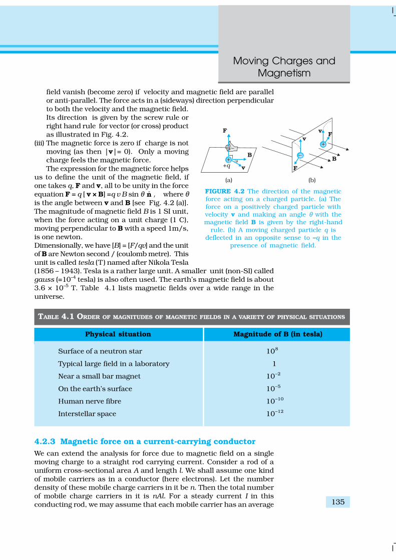
Moving Charges andMagnetism
135
field vanish (become zero) if velocity and magnetic field are parallelor anti-parallel. The force acts in a (sideways) direction perpendicularto both the velocity and the magnetic field.Its direction is given by the screw rule orright hand rule for vector (or cross) productas illustrated in Fig. 4.2.
(iii) The magnetic force is zero if charge is notmoving (as then |v|= 0). Only a movingcharge feels the magnetic force.The expression for the magnetic force helps
us to define the unit of the magnetic field, ifone takes q, F and v, all to be unity in the forceequation F = q [ v × B] =q v B sin θ n , where θis the angle between v and B [see Fig. 4.2 (a)].The magnitude of magnetic field B is 1 SI unit,when the force acting on a unit charge (1 C),moving perpendicular to B with a speed 1m/s,is one newton.Dimensionally, we have [B] = [F/qv] and the unitof B are Newton second / (coulomb metre). Thisunit is called tesla (T ) named after Nikola Tesla(1856 – 1943). Tesla is a rather large unit. A smaller unit (non-SI) calledgauss (=10–4 tesla) is also often used. The earth’s magnetic field is about3.6 × 10–5 T. Table 4.1 lists magnetic fields over a wide range in theuniverse.
FIGURE 4.2 The direction of the magneticforce acting on a charged particle. (a) Theforce on a positively charged particle withvelocity v and making an angle θ with themagnetic field B is given by the right-hand
rule. (b) A moving charged particle q isdeflected in an opposite sense to –q in the
presence of magnetic field.
TABLE 4.1 ORDER OF MAGNITUDES OF MAGNETIC FIELDS IN A VARIETY OF PHYSICAL SITUATIONS
Physical situation Magnitude of B (in tesla)
Surface of a neutron star 108
Typical large field in a laboratory 1
Near a small bar magnet 10–2
On the earth’s surface 10–5
Human nerve fibre 10–10
Interstellar space 10–12
4.2.3 Magnetic force on a current-carrying conductorWe can extend the analysis for force due to magnetic field on a singlemoving charge to a straight rod carrying current. Consider a rod of auniform cross-sectional area A and length l. We shall assume one kindof mobile carriers as in a conductor (here electrons). Let the numberdensity of these mobile charge carriers in it be n. Then the total numberof mobile charge carriers in it is nAl. For a steady current I in thisconducting rod, we may assume that each mobile carrier has an average

Physics
136 EX
AM
PLE 4
.1
drift velocity vd (see Chapter 3). In the presence of an external magneticfield B, the force on these carriers is:
F = (nAl)q vd × B
where q is the value of the charge on a carrier. Now nqvd is the currentdensity j and |(nq vd)|A is the current I (see Chapter 3 for the discussionof current and current density). Thus,
F = [(nqevd )Al ] × B = [ jAl ] × B
= I1 × B (4.4)where l is a vector of magnitude l, the length of the rod, and with a directionidentical to the current I. Note that the current I is not a vector. In the laststep leading to Eq. (4.4), we have transferred the vector sign from j to l.
Equation (4.4) holds for a straight rod. In this equation, B is the externalmagnetic field. It is not the field produced by the current-carrying rod. Ifthe wire has an arbitrary shape we can calculate the Lorentz force on itby considering it as a collection of linear strips dlj and summing
d jj
I= ∑F l × B
This summation can be converted to an integral in most cases.
ON PERMITTIVITY AND PERMEABILITY
In the universal law of gravitation, we say that any two point masses exert a force oneach other which is proportional to the product of the masses m1, m2 and inverselyproportional to the square of the distance r between them. We write it as F = Gm1m2/r2
where G is the universal constant of gravitation. Similarly in Coulomb’s law of electrostaticswe write the force between two point charges q1, q2, separated by a distance r asF = kq1q2/r 2 where k is a constant of proportionality. In SI units, k is taken as1/4πε where ε is the permittivity of the medium. Also in magnetism, we get anotherconstant, which in SI units, is taken as µ/4π where µ is the permeability of the medium.
Although G, ε and µ arise as proportionality constants, there is a difference betweengravitational force and electromagnetic force. While the gravitational force does not dependon the intervening medium, the electromagnetic force depends on the medium betweenthe two charges or magnets. Hence while G is a universal constant, ε and µ depend onthe medium. They have different values for different media. The product εµ turns out tobe related to the speed v of electromagnetic radiation in the medium through εµ =1/ v 2.
Electric permittivity ε is a physical quantity that describes how an electric field affectsand is affected by a medium. It is determined by the ability of a material to polarise inresponse to an applied field, and thereby to cancel, partially, the field inside the material.Similarly, magnetic permeability µ is the ability of a substance to acquire magnetisation inmagnetic fields. It is a measure of the extent to which magnetic field can penetrate matter.
Example 4.1 A straight wire of mass 200 g and length 1.5 m carriesa current of 2 A. It is suspended in mid-air by a uniform horizontalmagnetic field B (Fig. 4.3). What is the magnitude of the magneticfield?

Moving Charges andMagnetism
137
EX
AM
PLE 4
.1
FIGURE 4.3
Solution From Eq. (4.4), we find that there is an upward force F, ofmagnitude IlB,. For mid-air suspension, this must be balanced bythe force due to gravity:
m g = I lB
m g
BI l
=
0.2 9.8
0.65 T2 1.5
×= =
×Note that it would have been sufficient to specify m/l, the mass perunit length of the wire. The earth’s magnetic field is approximately4 × 10–5 T and we have ignored it.
Example 4.2 If the magnetic field is parallel to the positive y-axisand the charged particle is moving along the positive x-axis (Fig. 4.4),which way would the Lorentz force be for (a) an electron (negativecharge), (b) a proton (positive charge).
FIGURE 4.4
Solution The velocity v of particle is along the x-axis, while B, themagnetic field is along the y-axis, so v × B is along the z-axis (screwrule or right-hand thumb rule). So, (a) for electron it will be along –zaxis. (b) for a positive charge (proton) the force is along +z axis.
4.3 MOTION IN A MAGNETIC FIELD
We will now consider, in greater detail, the motion of a charge moving ina magnetic field. We have learnt in Mechanics (see Class XI book, Chapter6) that a force on a particle does work if the force has a component along(or opposed to) the direction of motion of the particle. In the case of motion
EX
AM
PLE 4
.2
Ch
arg
ed
partic
les m
ovin
g in
a m
agn
etic
field
.
Inte
ractiv
e d
em
on
stra
tion
:

Physics
138
of a charge in a magnetic field, the magnetic force isperpendicular to the velocity of the particle. So no work is doneand no change in the magnitude of the velocity is produced(though the direction of momentum may be changed). [Noticethat this is unlike the force due to an electric field, qE, whichcan have a component parallel (or antiparallel) to motion andthus can transfer energy in addition to momentum.]
We shall consider motion of a charged particle in a uniformmagnetic field. First consider the case of v perpendicular to B.The perpendicular force, q v × B, acts as a centripetal force andproduces a circular motion perpendicular to the magnetic field.The particle will describe a circle if v and B are perpendicularto each other (Fig. 4.5).
If velocity has a component along B, this componentremains unchanged as the motion along the magnetic field will
not be affected by the magnetic field. The motionin a plane perpendicular to B is as before acircular one, thereby producing a helical motion(Fig. 4.6).
You have already learnt in earlier classes(See Class XI, Chapter 4) that if r is the radiusof the circular path of a particle, then a force ofm v2 / r, acts perpendicular to the path towardsthe centre of the circle, and is called thecentripetal force. If the velocity v isperpendicular to the magnetic field B, themagnetic force is perpendicular to both v andB and acts like a centripetal force. It has amagnitude q v B. Equating the two expressionsfor centripetal force,
m v 2/r = q v B, which gives
r = m v / qB (4.5)
for the radius of the circle described by thecharged particle. The larger the momentum,
the larger is the radius and bigger the circle described. If ω is the angularfrequency, then v = ω r. So,
ω = 2π ν = q B/ m [4.6(a)]which is independent of the velocity or energy . Here ν is the frequency ofrotation. The independence of ν from energy has important applicationin the design of a cyclotron (see Section 4.4.2).
The time taken for one revolution is T= 2π/ω ≡ 1/ν. If there is acomponent of the velocity parallel to the magnetic field (denoted by v||), itwill make the particle move along the field and the path of the particlewould be a helical one (Fig. 4.6). The distance moved along the magneticfield in one rotation is called pitch p. Using Eq. [4.6 (a)], we have
p = v||T = 2πm v|| / q B [4.6(b)]The radius of the circular component of motion is called the radius of
the helix.
FIGURE 4.5 Circular motion
FIGURE 4.6 Helical motion

Moving Charges andMagnetism
139
EX
AM
PLE 4
.3
Example 4.3 What is the radius of the path of an electron (mass9 × 10-31 kg and charge 1.6 × 10⁻¹⁹ C) moving at a speed of 3 ×10⁷ m/s ina magnetic field of 6 × 10⁻⁴ T perpendicular to it? What is itsfrequency? Calculate its energy in keV. ( 1 eV = 1.6 × 10⁻¹⁹ J).
Solution Using Eq. (4.5) we findr = m v / (qB ) = 9 ×10–31 kg × 3 × 107 m s–1 / ( 1.6 × 10–19 C × 6 × 10–4 T ) = 26 × 10–2 m = 26 cmν = v / (2 πr) = 2×10⁶ s–1 = 2×10⁶ Hz =2 MHz.E = (½ )mv 2 = (½ ) 9 × 10–31 kg × 9 × 1014 m2/s2 = 40.5 ×10⁻¹⁷ J ≈ 4×10–16 J = 2.5 keV.
HELICAL MOTION OF CHARGED PARTICLES AND AURORA BORIOLIS
In polar regions like Alaska and Northern Canada, a splendid display of colours is seenin the sky. The appearance of dancing green pink lights is fascinating, and equallypuzzling. An explanation of this natural phenomenon is now found in physics, in termsof what we have studied here.
Consider a charged particle of mass m and charge q, entering a region of magneticfield B with an initial velocity v. Let this velocity have a component vp parallel to themagnetic field and a component vn normal to it. There is no force on a charged particle inthe direction of the field. Hence the particle continues to travel with the velocity vp parallelto the field. The normal component vn of the particle results in a Lorentz force (vn × B)which is perpendicular to both vn and B. As seen in Section 4.3.1 the particle thus has atendency to perform a circular motion in a plane perpendicular to the magnetic field.When this is coupled with the velocity parallel to the field, the resulting trajectory will bea helix along the magnetic field line, as shown in Figure (a) here. Even if the field linebends, the helically moving particle is trapped and guided to move around the field line.Since the Lorentz force is normal to the velocity of each point, the field does no work onthe particle and the magnitude of velocity remains the same.
During a solar flare, a large number of electrons and protons are ejected from the sun.Some of them get trapped in the earth’s magnetic field and move in helical paths along thefield lines. The field lines come closer to each other near the magnetic poles; see figure (b).Hence the density of charges increases near the poles. These particles collide with atomsand molecules of the atmosphere. Excited oxygen atoms emit green light and excitednitrogen atoms emits pink light. This phenomenon is called Aurora Boriolis in physics.

Physics
140
4.4 MOTION IN COMBINED ELECTRIC AND MAGNETIC
FIELDS
4.4.1 Velocity selectorYou know that a charge q moving with velocity v in presence of bothelectric and magnetic fields experiences a force given by Eq. (4.3), that is,
F = q (E + v × B) = FE + FB
We shall consider the simple case in which electric and magneticfields are perpendicular to each other and also perpendicular tothe velocity of the particle, as shown in Fig. 4.7. We have,
ˆ ˆ ˆ, ,E B v= = =E j B k v i
( )ˆ ˆ ˆ ˆ, , –E Bq qE q q v B qB= = = = =F E j F v × B i × k j
Therefore, ( ) ˆ–q E vB=F j .Thus, electric and magnetic forces are in opposite directions as
shown in the figure. Suppose, we adjust the value of E and B suchthat magnitude of the two forces are equal. Then, total force on thecharge is zero and the charge will move in the fields undeflected.This happens when,
orE
qE qvB vB
= = (4.7)
This condition can be used to select charged particles of a particularvelocity out of a beam containing charges moving with different speeds(irrespective of their charge and mass). The crossed E and B fields, therefore,serve as a velocity selector. Only particles with speed E/B passundeflected through the region of crossed fields. This method wasemployed by J. J. Thomson in 1897 to measure the charge to mass ratio(e/m) of an electron. The principle is also employed in Mass Spectrometer –a device that separates charged particles, usually ions, according to theircharge to mass ratio.
4.4.2 CyclotronThe cyclotron is a machine to accelerate charged particles or ions to highenergies. It was invented by E.O. Lawrence and M.S. Livingston in 1934to investigate nuclear structure. The cyclotron uses both electric andmagnetic fields in combination to increase the energy of charged particles.As the fields are perpendicular to each other they are called crossedfields. Cyclotron uses the fact that the frequency of revolution of thecharged particle in a magnetic field is independent of its energy. Theparticles move most of the time inside two semicircular disc-like metalcontainers, D1 and D2, which are called dees as they look like the letterD. Figure 4.8 shows a schematic view of the cyclotron. Inside the metalboxes the particle is shielded and is not acted on by the electric field. Themagnetic field, however, acts on the particle and makes it go round in acircular path inside a dee. Every time the particle moves from one dee toanother it is acted upon by the electric field. The sign of the electric fieldis changed alternately in tune with the circular motion of the particle.This ensures that the particle is always accelerated by the electric field.Each time the acceleration increases the energy of the particle. As energy
FIGURE 4.7
Cyclo
tro
n
Inte
racti
ve d
em
on
str
ati
on
:

Moving Charges andMagnetism
141
increases, the radius of the circular path increases. So the path is aspiral one.
The whole assembly is evacuated to minimise collisions between theions and the air molecules. A high frequency alternating voltage is appliedto the dees. In the sketch shown in Fig. 4.8, positive ions or positivelycharged particles (e.g., protons) are released at the centre P. They movein a semi-circular path in one of the dees and arrive in the gap betweenthe dees in a time interval T/2; where T, the period of revolution, is givenby Eq. (4.6),
1 2
c
mT
qBνπ= =
or 2c
qB
mν =
π (4.8)
This frequency is called the cyclotron frequency for obvious reasonsand is denoted by νc .
The frequency νa of the applied voltage is adjusted so that the polarityof the dees is reversed in the same time that it takes the ions to completeone half of the revolution. The requirement νa = νc is called the resonancecondition. The phase of the supply is adjusted so that when the positiveions arrive at the edge of D1, D2 is at a lowerpotential and the ions are accelerated across thegap. Inside the dees the particles travel in a regionfree of the electric field. The increase in theirkinetic energy is qV each time they cross fromone dee to another (V refers to the voltage acrossthe dees at that time). From Eq. (4.5), it is clearthat the radius of their path goes on increasingeach time their kinetic energy increases. The ionsare repeatedly accelerated across the dees untilthey have the required energy to have a radiusapproximately that of the dees. They are thendeflected by a magnetic field and leave the systemvia an exit slit. From Eq. (4.5) we have,
qBRv
m= (4.9)
where R is the radius of the trajectory at exit, andequals the radius of a dee.
Hence, the kinetic energy of the ions is,
2 2 221
2 2q B R
mm
=v (4.10)
The operation of the cyclotron is based on thefact that the time for one revolution of an ion isindependent of its speed or radius of its orbit.The cyclotron is used to bombard nuclei withenergetic particles, so accelerated by it, and study
FIGURE 4.8 A schematic sketch of thecyclotron. There is a source of chargedparticles or ions at P which move in a
circular fashion in the dees, D1 and D2, onaccount of a uniform perpendicular
magnetic field B. An alternating voltagesource accelerates these ions to high
speeds. The ions are eventually ‘extracted’at the exit port.

Physics
142
EX
AM
PLE 4
.4
the resulting nuclear reactions. It is also used to implant ions into solidsand modify their properties or even synthesise new materials. It is usedin hospitals to produce radioactive substances which can be used indiagnosis and treatment.
Example 4.4 A cyclotron’s oscillator frequency is 10 MHz. Whatshould be the operating magnetic field for accelerating protons? Ifthe radius of its ‘dees’ is 60 cm, what is the kinetic energy (in MeV) ofthe proton beam produced by the accelerator.
(e =1.60 × 10⁻¹⁹ C, mp = 1.67 × 10⁻²⁷ kg, 1 MeV = 1.6 × 10⁻¹³ J).
Solution The oscillator frequency should be same as proton’scyclotron frequency.Using Eqs. (4.5) and [4.6(a)] we have
B = 2π m ν/q =6.3 ×1.67 × 10–27 × 107 / (1.6 × 10⁻¹⁹) = 0.66 T
Final velocity of protons is
v = r × 2π ν = 0.6 m × 6.3 ×107 = 3.78 × 10⁷ m/s.
E = ½ mv 2 = 1.67 ×10–27 × 14.3 × 1014 / (2 × 1.6 × 10–13) = 7 MeV.
ACCELERATORS IN INDIA
India has been an early entrant in the area of accelerator- based research. The vision ofDr. Meghnath Saha created a 37" Cyclotron in the Saha Institute of Nuclear Physics inKolkata in 1953. This was soon followed by a series of Cockroft-Walton type of acceleratorsestablished in Tata Institute of Fundamental Research (TIFR), Mumbai, Aligarh MuslimUniversity (AMU), Aligarh, Bose Institute, Kolkata and Andhra University, Waltair.
The sixties saw the commissioning of a number of Van de Graaff accelerators: a 5.5 MVterminal machine in Bhabha Atomic Research Centre (BARC), Mumbai (1963); a 2 MV terminalmachine in Indian Institute of Technology (IIT), Kanpur; a 400 kV terminal machine in BanarasHindu University (BHU), Varanasi; and Punjabi University, Patiala. One 66 cm Cyclotrondonated by the Rochester University of USA was commissioned in Panjab University,Chandigarh. A small electron accelerator was also established in University of Pune, Pune.
In a major initiative taken in the seventies and eighties, a Variable Energy Cyclotron wasbuilt indigenously in Variable Energy Cyclotron Centre (VECC), Kolkata; 2 MV Tandem Vande Graaff accelerator was developed and built in BARC and a 14 MV Tandem Pelletronaccelerator was installed in TIFR.
This was soon followed by a 15 MV Tandem Pelletron established by University GrantsCommission (UGC), as an inter-university facility in Inter-University Accelerator Centre(IUAC), New Delhi; a 3 MV Tandem Pelletron in Institute of Physics, Bhubaneshwar; andtwo 1.7 MV Tandetrons in Atomic Minerals Directorate for Exploration and Research,Hyderabad and Indira Gandhi Centre for Atomic Research, Kalpakkam. Both TIFR andIUAC are augmenting their facilities with the addition of superconducting LINAC modulesto accelerate the ions to higher energies.
Besides these ion accelerators, the Department of Atomic Energy (DAE) has developedmany electron accelerators. A 2 GeV Synchrotron Radiation Source is being built in RajaRamanna Centre for Advanced Technologies, Indore.
The Department of Atomic Energy is considering Accelerator Driven Systems (ADS) forpower production and fissile material breeding as future options.

Moving Charges andMagnetism
143
4.5 MAGNETIC FIELD DUE TO A CURRENT ELEMENT,BIOT-SAVART LAW
All magnetic fields that we know are due to currents (or moving charges)and due to intrinsic magnetic moments of particles. Here, we shall studythe relation between current and the magnetic field it produces.It is given by the Biot-Savart’s law. Figure 4.9 shows a finiteconductor XY carrying current I. Consider an infinitesimalelement dl of the conductor. The magnetic field dB due to thiselement is to be determined at a point P which is at a distance rfrom it. Let θ be the angle between dl and the displacement vectorr. According to Biot-Savart’s law, the magnitude of the magneticfield dB is proportional to the current I, the element length |dl|,and inversely proportional to the square of the distance r. Itsdirection* is perpendicular to the plane containing dl and r .Thus, in vector notation,
3
I dd
r
×∝
l rB
0
34I d
r
µ ×=
πl r
[4.11(a)]
where µ0/4π is a constant of proportionality. The aboveexpression holds when the medium is vacuum.
The magnitude of this field is,
02
d sind
4I l
r
µ θ=
πB [4.11(b)]
where we have used the property of cross-product. Equation [4.11 (a)]constitutes our basic equation for the magnetic field. The proportionalityconstant in SI units has the exact value,
70 10 Tm/A4µ −=
π [4.11(c)]
We call µ0 the permeability of free space (or vacuum).The Biot-Savart law for the magnetic field has certain similarities as
well as differences with the Coulomb’s law for the electrostatic field. Someof these are:(i) Both are long range, since both depend inversely on the square of
distance from the source to the point of interest. The principle ofsuperposition applies to both fields. [In this connection, note thatthe magnetic field is linear in the source I dl just as the electrostaticfield is linear in its source: the electric charge.]
(ii) The electrostatic field is produced by a scalar source, namely, theelectric charge. The magnetic field is produced by a vector sourceI dl.
* The sense of dl×r is also given by the Right Hand Screw rule : Look at the planecontaining vectors dl and r. Imagine moving from the first vector towards secondvector. If the movement is anticlockwise, the resultant is towards you. If it isclockwise, the resultant is away from you.
FIGURE 4.9 Illustration ofthe Biot-Savart law. The
current element I dlproduces a field dB at adistance r. The ⊗ sign
indicates that thefield is perpendicular
to the plane of thispage and directed
into it.

Physics
144 EX
AM
PLE 4
.5
(iii) The electrostatic field is along the displacement vector joining thesource and the field point. The magnetic field is perpendicular to theplane containing the displacement vector r and the current elementI dl.
(iv) There is an angle dependence in the Biot-Savart law which is notpresent in the electrostatic case. In Fig. 4.9, the magnetic field at anypoint in the direction of dl (the dashed line) is zero. Along this line,θ = 0, sin θ = 0 and from Eq. [4.11(a)], |dB| = 0.There is an interesting relation between ε0, the permittivity of free
space; µ0, the permeability of free space; and c, the speed of light invacuum:
( ) 00 0 04
4µ
ε µ ε = π π ( )79
110
9 10− = × 8 2 2
1 1(3 10 ) c
= =×
We will discuss this connection further in Chapter 8 on theelectromagnetic waves. Since the speed of light in vacuum is constant,the product µ0ε0 is fixed in magnitude. Choosing the value of either ε0 orµ0, fixes the value of the other. In SI units, µ0 is fixed to be equal to4π × 10–7
in magnitude.
Example 4.5 An element ˆx∆ = ∆l i is placed at the origin and carries
a large current I = 10 A (Fig. 4.10). What is the magnetic field on they-axis at a distance of 0.5 m. ∆x = 1 cm.
FIGURE 4.10
Solution
02
d sin|d |
4I l
r
µ θ=
πB [using Eq. (4.11)]
2d 10 ml x −= ∆ = , I = 10 A, r = 0.5 m = y, 70
T m/4 10
Aµ −π =
θ = 90° ; sin θ = 17 2
2
10 10 10d
25 10
− −
−
× ×=×
B = 4 × 10⁻⁸ T
The direction of the field is in the +z-direction. This is so since,
ˆ ˆd x y= ∆l × i × jr ( )ˆ ˆy x= ∆ i × j ˆy x= ∆ k
We remind you of the following cyclic property of cross-products,
ˆ ˆ ˆ ˆ ˆ ˆ ˆ ˆ ˆ; ;× = × = × =i j k j k i k i j
Note that the field is small in magnitude.

Moving Charges andMagnetism
145
In the next section, we shall use the Biot-Savart law to calculate themagnetic field due to a circular loop.
4.6 MAGNETIC FIELD ON THE AXIS OF A CIRCULAR
CURRENT LOOP
In this section, we shall evaluate the magnetic field due to a circular coilalong its axis. The evaluation entails summing up the effect of infinitesimalcurrent elements (I dl) mentioned in the previous section.We assume that the current I is steady and that theevaluation is carried out in free space (i.e., vacuum).
Figure 4.11 depicts a circular loop carrying a steadycurrent I. The loop is placed in the y-z plane with itscentre at the origin O and has a radius R. The x-axis isthe axis of the loop. We wish to calculate the magneticfield at the point P on this axis. Let x be the distance ofP from the centre O of the loop.
Consider a conducting element dl of the loop. This isshown in Fig. 4.11. The magnitude dB of the magneticfield due to dl is given by the Biot-Savart law [Eq. 4.11(a)],
034
I ddB
r
µπ
=l × r
(4.12)
Now r2 = x2 + R2 . Further, any element of the loopwill be perpendicular to the displacement vector fromthe element to the axial point. For example, the elementdl in Fig. 4.11 is in the y-z plane whereas thedisplacement vector r from dl to the axial point P is inthe x-y plane. Hence |dl × r|=r dl. Thus,
( )
02 2
dd
4I l
Bx R
µ=
+ (4.13)
The direction of dB is shown in Fig. 4.11. It is perpendicular to theplane formed by dl and r. It has an x-component dBx and a componentperpendicular to x-axis, dB⊥ . When the components perpendicular tothe x-axis are summed over, they cancel out and we obtain a null result.For example, the dB⊥ component due to dl is cancelled by thecontribution due to the diametrically opposite dl element, shown inFig. 4.11. Thus, only the x-component survives. The net contributionalong x-direction can be obtained by integrating dBx = dB cos θ over theloop. For Fig. 4.11,
2 2 1/2cos( )
R
x Rθ =
+ (4.14)
From Eqs. (4.13) and (4.14),
( )
03/22 2
dd
4x
I l RB
x R
µ=
+
FIGURE 4.11 Magnetic field on theaxis of a current carrying circular
loop of radius R. Shown are themagnetic field dB (due to a line
element dl ) and itscomponents along and
perpendicular to the axis.

Physics
146 EX
AM
PLE 4
.6
The summation of elements dl over the loop yields 2πR, thecircumference of the loop. Thus, the magnetic field at P due to entirecircular loop is
( )2
03/22 2
ˆ ˆ2
x
I RB
x R
µ= =
+B i i (4.15)
As a special case of the above result, we may obtain the field at the centreof the loop. Here x = 0, and we obtain,
00
ˆ2
I
R
µ=B i (4.16)
The magnetic field lines due to a circular wire form closed loops andare shown in Fig. 4.12. The direction of the magnetic field is given by(another) right-hand thumb rule stated below:
Curl the palm of your right hand around the circular wire with thefingers pointing in the direction of the current. The right-hand thumbgives the direction of the magnetic field.
Example 4.6 A straight wire carrying a current of 12 A is bent into asemi-circular arc of radius 2.0 cm as shown in Fig. 4.13(a). Considerthe magnetic field B at the centre of the arc. (a) What is the magneticfield due to the straight segments? (b) In what way the contributionto B from the semicircle differs from that of a circular loop and inwhat way does it resemble? (c) Would your answer be different if thewire were bent into a semi-circular arc of the same radius but in theopposite way as shown in Fig. 4.13(b)?
FIGURE 4.13
FIGURE 4.12 The magnetic field lines for a current loop. The direction ofthe field is given by the right-hand thumb rule described in the text. Theupper side of the loop may be thought of as the north pole and the lower
side as the south pole of a magnet.
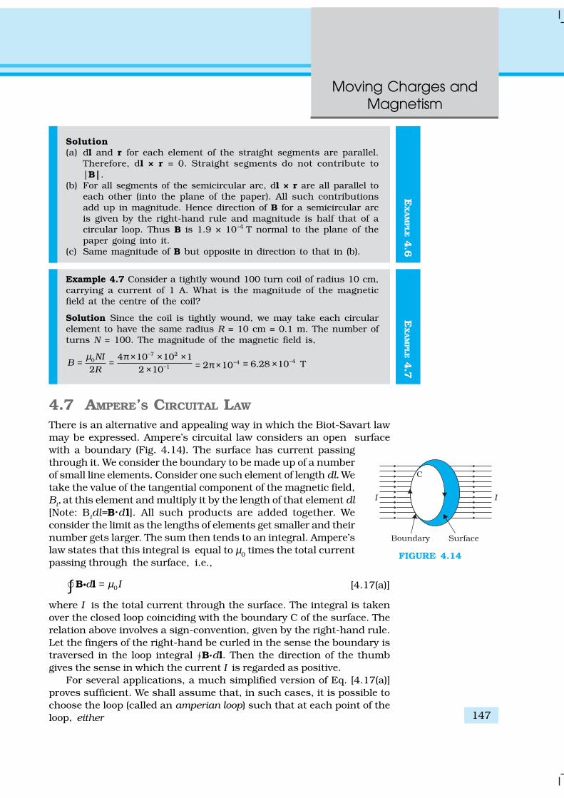
Moving Charges andMagnetism
147
EX
AM
PLE 4
.6Solution(a) dl and r for each element of the straight segments are parallel.
Therefore, dl × r = 0. Straight segments do not contribute to|B|.
(b) For all segments of the semicircular arc, dl × r are all parallel toeach other (into the plane of the paper). All such contributionsadd up in magnitude. Hence direction of B for a semicircular arcis given by the right-hand rule and magnitude is half that of acircular loop. Thus B is 1.9 × 10⁻⁴ T normal to the plane of thepaper going into it.
(c) Same magnitude of B but opposite in direction to that in (b).
Example 4.7 Consider a tightly wound 100 turn coil of radius 10 cm,carrying a current of 1 A. What is the magnitude of the magneticfield at the centre of the coil?
Solution Since the coil is tightly wound, we may take each circularelement to have the same radius R = 10 cm = 0.1 m. The number ofturns N = 100. The magnitude of the magnetic field is,
–7 20
–1
4 10 10 12 2 10
NIB
R
µ π × × ×= =×
42 10−= π × 46 28 10 T. −= ×
4.7 AMPERE’S CIRCUITAL LAW
There is an alternative and appealing way in which the Biot-Savart lawmay be expressed. Ampere’s circuital law considers an open surfacewith a boundary (Fig. 4.14). The surface has current passingthrough it. We consider the boundary to be made up of a numberof small line elements. Consider one such element of length dl. Wetake the value of the tangential component of the magnetic field,Bt, at this element and multiply it by the length of that element dl[Note: Btdl=B.d l]. All such products are added together. Weconsider the limit as the lengths of elements get smaller and theirnumber gets larger. The sum then tends to an integral. Ampere’slaw states that this integral is equal to µ0 times the total currentpassing through the surface, i.e.,
0d Iµ=∫ B l [4.17(a)]
where I is the total current through the surface. The integral is takenover the closed loop coinciding with the boundary C of the surface. Therelation above involves a sign-convention, given by the right-hand rule.Let the fingers of the right-hand be curled in the sense the boundary istraversed in the loop integral “B.dl. Then the direction of the thumbgives the sense in which the current I is regarded as positive.
For several applications, a much simplified version of Eq. [4.17(a)]proves sufficient. We shall assume that, in such cases, it is possible tochoose the loop (called an amperian loop) such that at each point of theloop, either
FIGURE 4.14
EX
AM
PLE 4
.7

Physics
148
(i) B is tangential to the loop and is a non-zero constantB, or
(ii) B is normal to the loop, or
(iii) B vanishes.Now, let L be the length (part) of the loop for which B
is tangential. Let Ie be the current enclosed by the loop.Then, Eq. (4.17) reduces to,
BL =µ0Ie [4.17(b)]
When there is a system with a symmetry such as fora straight infinite current-carrying wire in Fig. 4.15, theAmpere’s law enables an easy evaluation of the magneticfield, much the same way Gauss’ law helps indetermination of the electric field. This is exhibited in theExample 4.8 below. The boundary of the loop chosen isa circle and magnetic field is tangential to thecircumference of the circle. The law gives, for the left handside of Eq. [4.17 (b)], B. 2πr. We find that the magneticfield at a distance r outside the wire is tangential andgiven by
B × 2πr = µ0 I,
B = µ0 I/ (2πr) (4.18)
The above result for the infinite wire is interestingfrom several points of view.(i) It implies that the field at every point on a circle of
radius r, (with the wire along the axis), is same inmagnitude. In other words, the magnetic fieldpossesses what is called a cylindrical symmetry. Thefield that normally can depend on three coordinatesdepends only on one: r. Whenever there is symmetry,the solutions simplify.
(ii) The field direction at any point on this circle istangential to it. Thus, the lines of constant magnitudeof magnetic field form concentric circles. Notice now,in Fig. 4.1(c), the iron filings form concentric circles.These lines called magnetic field lines form closedloops. This is unlike the electrostatic field lines whichoriginate from positive charges and end at negativecharges. The expression for the magnetic field of astraight wire provides a theoretical justification toOersted’s experiments.
(iii) Another interesting point to note is that even thoughthe wire is infinite, the field due to it at a nonzerodistance is not infinite. It tends to blow up only whenwe come very close to the wire. The field is directlyproportional to the current and inversely proportionalto the distance from the (infinitely long) currentsource.
AN
DR
E A
MPE
RE
(1775 –
1836)
Andre Ampere (1775 –1836) Andre Marie Amperewas a French physicist,mathematician andchemist who founded thescience of electrodynamics.Ampere was a child prodigywho mastered advancedmathematics by the age of12. Ampere grasped thesignificance of Oersted’sdiscovery. He carried out alarge series of experimentsto explore the relationshipbetween current electricityand magnetism. Theseinvestigations culminatedin 1827 with thepublication of the‘Mathematical Theory ofElectrodynamic Pheno-mena Deduced Solely fromExperiments’. He hypo-thesised that all magneticphenomena are due tocirculating electriccurrents. Ampere washumble and absent-minded. He once forgot aninvitation to dine with theEmperor Napoleon. He diedof pneumonia at the age of61. His gravestone bearsthe epitaph: Tandem Felix(Happy at last).
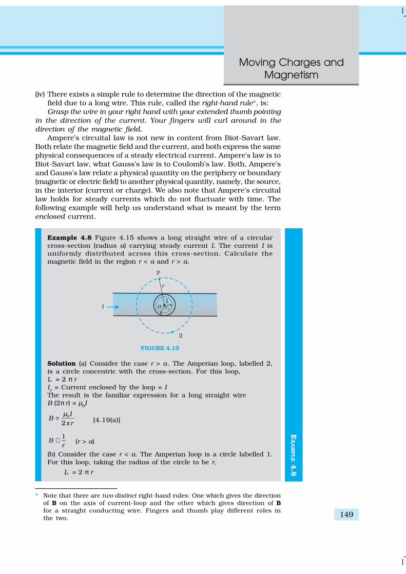
Moving Charges andMagnetism
149
EX
AM
PLE 4
.8
(iv) There exists a simple rule to determine the direction of the magneticfield due to a long wire. This rule, called the right-hand rule*, is:Grasp the wire in your right hand with your extended thumb pointing
in the direction of the current. Your fingers will curl around in thedirection of the magnetic field.
Ampere’s circuital law is not new in content from Biot-Savart law.Both relate the magnetic field and the current, and both express the samephysical consequences of a steady electrical current. Ampere’s law is toBiot-Savart law, what Gauss’s law is to Coulomb’s law. Both, Ampere’sand Gauss’s law relate a physical quantity on the periphery or boundary(magnetic or electric field) to another physical quantity, namely, the source,in the interior (current or charge). We also note that Ampere’s circuitallaw holds for steady currents which do not fluctuate with time. Thefollowing example will help us understand what is meant by the termenclosed current.
Example 4.8 Figure 4.15 shows a long straight wire of a circularcross-section (radius a) carrying steady current I. The current I isuniformly distributed across this cross-section. Calculate themagnetic field in the region r < a and r > a.
FIGURE 4.15
Solution (a) Consider the case r > a . The Amperian loop, labelled 2,is a circle concentric with the cross-section. For this loop,L = 2 π rIe = Current enclosed by the loop = IThe result is the familiar expression for a long straight wireB (2π r) = µ0I
0
2I
Br
µ= [4.19(a)]
1B
r∝ (r > a)
(b) Consider the case r < a. The Amperian loop is a circle labelled 1.For this loop, taking the radius of the circle to be r,
L = 2 π r
* Note that there are two distinct right-hand rules: One which gives the directionof B on the axis of current-loop and the other which gives direction of Bfor a straight conducting wire. Fingers and thumb play different roles inthe two.

Physics
150
EX
AM
PLE 4
.8
Now the current enclosed Ie is not I, but is less than this value.Since the current distribution is uniform, the current enclosed is,
2
2e
rI I
a
π= π
2
2
Ir
a=
Using Ampere’s law,
2
0 2(2 )I r
B ra
µ=
022
IB r
a
µ = [4.19(b)]
B ∝ r (r < a)
FIGURE 4.16
Figure (4.16) shows a plot of the magnitude of B with distance rfrom the centre of the wire. The direction of the field is tangential tothe respective circular loop (1 or 2) and given by the right-handrule described earlier in this section.
This example possesses the required symmetry so that Ampere’slaw can be applied readily.
It should be noted that while Ampere’s circuital law holds for anyloop, it may not always facilitate an evaluation of the magnetic field inevery case. For example, for the case of the circular loop discussed inSection 4.6, it cannot be applied to extract the simple expressionB = µ0I/2R [Eq. (4.16)] for the field at the centre of the loop. However,there exists a large number of situations of high symmetry where the lawcan be conveniently applied. We shall use it in the next section to calculatethe magnetic field produced by two commonly used and very usefulmagnetic systems: the solenoid and the toroid.
4.8 THE SOLENOID AND THE TOROID
The solenoid and the toroid are two pieces of equipment which generatemagnetic fields. The television uses the solenoid to generate magneticfields needed. The synchrotron uses a combination of both to generatethe high magnetic fields required. In both, solenoid and toroid, we comeacross a situation of high symmetry where Ampere’s law can beconveniently applied.

Moving Charges andMagnetism
151
4.8.1 The solenoidWe shall discuss a long solenoid. By long solenoid we mean that thesolenoid’s length is large compared to its radius. It consists of a longwire wound in the form of a helix where the neighbouring turns are closelyspaced. So each turn can be regarded as a circular loop. The net magneticfield is the vector sum of the fields due to all the turns. Enamelled wiresare used for winding so that turns are insulated from each other.
Figure 4.17 displays the magnetic field lines for a finite solenoid. Weshow a section of this solenoid in an enlarged manner in Fig. 4.17(a).Figure 4.17(b) shows the entire finite solenoid with its magnetic field. InFig. 4.17(a), it is clear from the circular loops that the field between twoneighbouring turns vanishes. In Fig. 4.17(b), we see that the field at theinterior mid-point P is uniform, strong and along the axis of the solenoid.The field at the exterior mid-point Q is weak and moreover is along theaxis of the solenoid with no perpendicular or normal component. As thesolenoid is made longer it appears like a long cylindrical metal sheet.Figure 4.18 represents this idealised picture. The field outside the solenoidapproaches zero. We shall assume that the field outside is zero. The fieldinside becomes everywhere parallel to the axis.
FIGURE 4.17 (a) The magnetic field due to a section of the solenoid which has beenstretched out for clarity. Only the exterior semi-circular part is shown. Notice
how the circular loops between neighbouring turns tend to cancel.(b) The magnetic field of a finite solenoid.
FIGURE 4.18 The magnetic field of a very long solenoid. We consider arectangular Amperian loop abcd to determine the field.

Physics
152
Consider a rectangular Amperian loop abcd. Along cd the field is zeroas argued above. Along transverse sections bc and ad, the field componentis zero. Thus, these two sections make no contribution. Let the field alongab be B. Thus, the relevant length of the Amperian loop is, L = h.
Let n be the number of turns per unit length, then the total numberof turns is nh. The enclosed current is, Ie = I (n h), where I is the currentin the solenoid. From Ampere’s circuital law [Eq. 4.17 (b)]
BL = µ0Ie, B h = µ0I (n h)
B = µ0 n I (4.20)
The direction of the field is given by the right-hand rule. The solenoidis commonly used to obtain a uniform magnetic field. We shall see in the
next chapter that a large field is possible by inserting a softiron core inside the solenoid.
4.8.2 The toroidThe toroid is a hollow circular ring on which a large numberof turns of a wire are closely wound. It can be viewed as asolenoid which has been bent into a circular shape to closeon itself. It is shown in Fig. 4.19(a) carrying a current I. Weshall see that the magnetic field in the open space inside(point P) and exterior to the toroid (point Q) is zero. Thefield B inside the toroid is constant in magnitude for theideal toroid of closely wound turns.
Figure 4.19(b) shows a sectional view of the toroid. Thedirection of the magnetic field inside is clockwise as per theright-hand thumb rule for circular loops. Three circularAmperian loops 1, 2 and 3 are shown by dashed lines. Bysymmetry, the magnetic field should be tangential to eachof them and constant in magnitude for a given loop. Thecircular areas bounded by loops 2 and 3 both cut the toroid:so that each turn of current carrying wire is cut once bythe loop 2 and twice by the loop 3.
Let the magnetic field along loop 1 be B1 in magnitude.Then in Ampere’s circuital law [Eq. 4.17(a)], L = 2π r1.However, the loop encloses no current, so Ie = 0. Thus,
B1 (2 π r1) = µ0(0), B1 = 0
Thus, the magnetic field at any point P in the open spaceinside the toroid is zero.
We shall now show that magnetic field at Q is likewisezero. Let the magnetic field along loop 3 be B3. Once againfrom Ampere’s law L = 2 π r3. However, from the sectionalcut, we see that the current coming out of the plane of thepaper is cancelled exactly by the current going into it. Thus,Ie= 0, and B3 = 0. Let the magnetic field inside the solenoid
be B. We shall now consider the magnetic field at S. Once again we employAmpere’s law in the form of Eq. [4.17 (a)]. We find, L = 2π r.
The current enclosed Ie is (for N turns of toroidal coil) N I.B (2πr) = µ0NI
FIGURE 4.19 (a) A toroid carryinga current I. (b) A sectional view ofthe toroid. The magnetic field can
be obtained at an arbitrarydistance r from the centre O ofthe toroid by Ampere’s circuitallaw. The dashed lines labelled1, 2 and 3 are three circular
Amperian loops.

Moving Charges andMagnetism
153
0
2NI
Br
µ=
π (4.21)
We shall now compare the two results: for a toroid and solenoid. Were-express Eq. (4.21) to make the comparison easier with the solenoidresult given in Eq. (4.20). Let r be the average radius of the toroid and nbe the number of turns per unit length. Then
N = 2πr n = (average) perimeter of the toroid
× number of turns per unit lengthand thus,
B = µ0 n I, (4.22)
i.e., the result for the solenoid!In an ideal toroid the coils are circular. In reality the turns of the
toroidal coil form a helix and there is always a small magnetic field externalto the toroid.
MAGNETIC CONFINEMENT
We have seen in Section 4.3 (see also the box on helical motion of charged particles earlierin this chapter) that orbits of charged particles are helical. If the magnetic field isnon-uniform, but does not change much during one circular orbit, then the radius of thehelix will decrease as it enters stronger magnetic field and the radius will increase when itenters weaker magnetic fields. We consider two solenoids at a distance from each other,enclosed in an evacuated container (see figure below where we have not shown the container).Charged particles moving in the region between the two solenoids will start with a smallradius. The radius will increase as field decreases and the radius will decrease again asfield due to the second solenoid takes over. The solenoids act as a mirror or reflector. [Seethe direction of F as the particle approaches coil 2 in the figure. It has a horizontal componentagainst the forward motion.] This makes the particles turn back when they approach thesolenoid. Such an arrangement will act like magnetic bottle or magnetic container. Theparticles will never touch the sides of the container. Such magnetic bottles are of great usein confining the high energy plasma in fusion experiments. The plasma will destroy anyother form of material container because of it’s high temperature. Another useful containeris a toroid. Toroids are expected to play a key role in the tokamak, an equipment for plasmaconfinement in fusion power reactors. There is an international collaboration called theInternational Thermonuclear Experimental Reactor (ITER), being set up in France, forachieving controlled fusion, of which India is a collaborating nation. For details of ITERcollaboration and the project, you may visit http://www.iter.org.

Physics
154
EX
AM
PLE 4
.9
Example 4.9 A solenoid of length 0.5 m has a radius of 1 cm and ismade up of 500 turns. It carries a current of 5 A. What is themagnitude of the magnetic field inside the solenoid?
Solution The number of turns per unit length is,
5001000
0.5n = = turns/m
The length l = 0.5 m and radius r = 0.01 m. Thus, l/a = 50 i.e., l >> a .Hence, we can use the long solenoid formula, namely, Eq. (4.20)B = µ0n I = 4π × 10–7 × 103 × 5 = 6.28 × 10⁻³ T
4.9 FORCE BETWEEN TWO PARALLEL CURRENTS,THE AMPERE
We have learnt that there exists a magnetic field due to a conductorcarrying a current which obeys the Biot-Savart law. Further, we have
learnt that an external magnetic field will exert a force ona current-carrying conductor. This follows from theLorentz force formula. Thus, it is logical to expect thattwo current-carrying conductors placed near each otherwill exert (magnetic) forces on each other. In the period1820-25, Ampere studied the nature of this magneticforce and its dependence on the magnitude of the current,on the shape and size of the conductors as well as thedistances between the conductors. In this section, weshall take the simple example of two parallel current-carrying conductors, which will perhaps help us toappreciate Ampere’s painstaking work.
Figure 4.20 shows two long parallel conductors aand b separated by a distance d and carrying (parallel)currents Ia and Ib, respectively. The conductor ‘a’produces, the same magnetic field Ba at all points alongthe conductor ‘b’. The right-hand rule tells us that thedirection of this field is downwards (when the conductors
are placed horizontally). Its magnitude is given by Eq. [4.19(a)] or fromAmpere’s circuital law,
0
2a
a
IB
d
µ=
π
The conductor ‘b’ carrying a current Ib will experience a sidewaysforce due to the field Ba. The direction of this force is towards theconductor ‘a’ (Verify this). We label this force as Fba, the force on asegment L of ‘b’ due to ‘a’. The magnitude of this force is given byEq. (4.4),
FIGURE 4.20 Two long straightparallel conductors carrying steady
currents Ia and Ib and separated by adistance d. Ba is the magnetic field setup by conductor ‘a’ at conductor ‘b’.

Moving Charges andMagnetism
155
Fba = Ib L Ba
0
2a bI I
Ld
µ=
π (4.23)
It is of course possible to compute the force on ‘a’ due to ‘b’. Fromconsiderations similar to above we can find the force Fab, on a segment oflength L of ‘a’ due to the current in ‘b’. It is equal in magnitude to Fba,and directed towards ‘b’. Thus,
Fba = –Fab (4.24)
Note that this is consistent with Newton’s third Law. Thus, at least forparallel conductors and steady currents, we have shown that theBiot-Savart law and the Lorentz force yield results in accordance withNewton’s third Law*.
We have seen from above that currents flowing in the same directionattract each other. One can show that oppositely directed currents repeleach other. Thus,
Parallel currents attract, and antiparallel currents repel.This rule is the opposite of what we find in electrostatics. Like (same
sign) charges repel each other, but like (parallel) currents attract eachother.
Let fba represent the magnitude of the force Fba per unit length. Then,from Eq. (4.23),
0
2a b
ba
I If
d
µ= (4.25)
The above expression is used to define the ampere (A), which is oneof the seven SI base units.
The ampere is the value of that steady current which, when maintainedin each of the two very long, straight, parallel conductors of negligiblecross-section, and placed one metre apart in vacuum, would produceon each of these conductors a force equal to 2 × 10⁻⁷ newtons per metreof length.
This definition of the ampere was adopted in 1946. It is a theoreticaldefinition. In practice one must eliminate the effect of the earth’s magneticfield and substitute very long wires by multiturn coils of appropriategeometries. An instrument called the current balance is used to measurethis mechanical force.
The SI unit of charge, namely, the coulomb, can now be defined interms of the ampere.
When a steady current of 1A is set up in a conductor, the quantity ofcharge that flows through its cross-section in 1s is one coulomb (1C).
* It turns out that when we have time-dependent currents and/or charges inmotion, Newton’s third law may not hold for forces between charges and/orconductors. An essential consequence of the Newton’s third law in mechanicsis conservation of momentum of an isolated system. This, however, holds evenfor the case of time-dependent situations with electromagnetic fields, providedthe momentum carried by fields is also taken into account.

Physics
156 EX
AM
PLE 4
.10
Example 4.10 The horizontal component of the earth’s magnetic fieldat a certain place is 3.0 ×10⁻⁵ T and the direction of the field is fromthe geographic south to the geographic north. A very long straightconductor is carrying a steady current of 1A. What is the force perunit length on it when it is placed on a horizontal table and thedirection of the current is (a) east to west; (b) south to north?
Solution F = I l × BF = IlB sinθThe force per unit length isf = F/l = I B sinθ(a) When the current is flowing from east to west,
θ = 90°Hence,f = I B = 1 × 3 × 10–5 = 3 × 10⁻⁵ N m–1
ROGET’S SPIRAL FOR ATTRACTION BETWEEN PARALLEL CURRENTS
Magnetic effects are generally smaller than electric effects. As a consequence, the forcebetween currents is rather small, because of the smallness of the factor µ. Hence it isdifficult to demonstrate attraction or repulsion between currents. Thus for 5 A currentin each wire at a separation of 1cm, the force per metre would be 5 × 10⁻⁴ N, which isabout 50 mg weight. It would be like pulling a wire by a string going over a pulley towhich a 50 mg weight is attached. The displacement of the wire would be quiteunnoticeable.
With the use of a soft spring, we can increase the effective length of the parallel currentand by using mercury, we can make the displacement of even a few mm observable very
dramatically. You will also need a constant-currentsupply giving a constant current of about 5 A.
Take a soft spring whose natural period ofoscillations is about 0.5 – 1s. Hang it vertically andattach a pointed tip to its lower end, as shown in thefigure here. Take some mercury in a dish and adjust thespring such that the tip is just above the mercurysurface. Take the DC current source, connect one of itsterminals to the upper end of the spring, and dip theother terminal in mercury. If the tip of the spring touchesmercury, the circuit is completed through mercury.
Let the DC source be put off to begin with. Let the tip be adjusted so that it justtouches the mercury surface. Switch on the constant current supply, and watch thefascinating outcome. The spring shrinks with a jerk, the tip comes out of mercury (justby a mm or so), the circuit is broken, the current stops, the spring relaxes and tries tocome back to its original position, the tip again touches mercury establishing a currentin the circuit, and the cycle continues with tick, tick, tick, . . . . In the beginning, youmay require some small adjustments to get a good effect.
Keep your face away from mercury vapours as they are poisonous. Do not inhalemercury vapours for long.

Moving Charges andMagnetism
157
EX
AM
PLE 4
.10
This is larger than the value 2×10⁻⁷ Nm–1 quoted in the definitionof the ampere. Hence it is important to eliminate the effect of theearth’s magnetic field and other stray fields while standardisingthe ampere.The direction of the force is downwards. This direction may beobtained by the directional property of cross product of vectors.
(b) When the current is flowing from south to north,θ = 0o
f = 0Hence there is no force on the conductor.
4.10 TORQUE ON CURRENT LOOP, MAGNETIC DIPOLE
4.10.1 Torque on a rectangular current loop in a uniformmagnetic field
We now show that a rectangular loop carrying a steady current I andplaced in a uniform magnetic field experiences a torque. It does notexperience a net force. This behaviour is analogous tothat of electric dipole in a uniform electric field(Section 1.10).
We first consider the simple case when therectangular loop is placed such that the uniformmagnetic field B is in the plane of the loop. This isillustrated in Fig. 4.21(a).
The field exerts no force on the two arms AD and BCof the loop. It is perpendicular to the arm AB of the loopand exerts a force F1 on it which is directed into theplane of the loop. Its magnitude is,
F1 = I b B
Similarly it exerts a force F2 on the arm CD and F2is directed out of the plane of the paper.
F2 = I b B = F1
Thus, the net force on the loop is zero. There is atorque on the loop due to the pair of forces F1 and F2.Figure 4.21(b) shows a view of the loop from the ADend. It shows that the torque on the loop tends to rotateit anti-clockwise. This torque is (in magnitude),
1 22 2a a
F Fτ = +
( )2 2a a
IbB IbB I ab B= + =
= I A B (4.26)
where A = ab is the area of the rectangle.
We next consider the case when the plane of the loop,is not along the magnetic field, but makes an angle withit. We take the angle between the field and the normal to
FIGURE 4.21 (a) A rectangularcurrent-carrying coil in uniform
magnetic field. The magnetic momentm points downwards. The torque τττττ isalong the axis and tends to rotate the
coil anticlockwise. (b) The coupleacting on the coil.
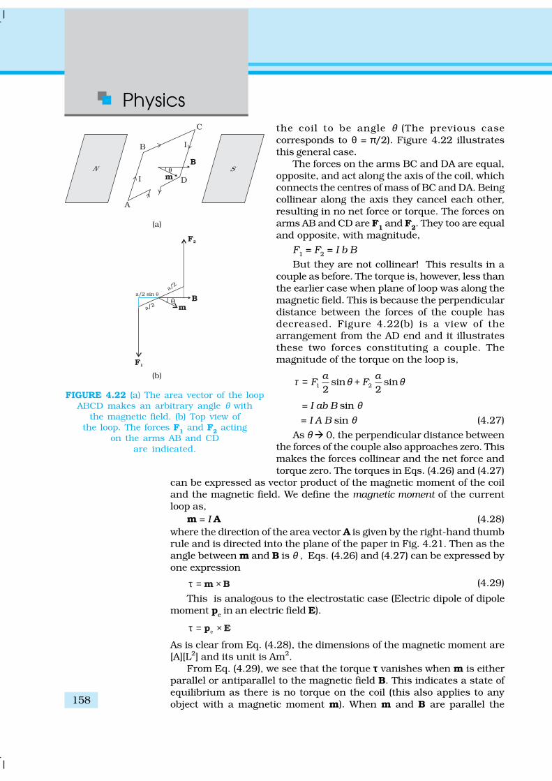
Physics
158
the coil to be angle θ (The previous casecorresponds to θ = π/2). Figure 4.22 illustratesthis general case.
The forces on the arms BC and DA are equal,opposite, and act along the axis of the coil, whichconnects the centres of mass of BC and DA. Beingcollinear along the axis they cancel each other,resulting in no net force or torque. The forces onarms AB and CD are F1 and F2. They too are equaland opposite, with magnitude,
F1 = F2 = I b B
But they are not collinear! This results in acouple as before. The torque is, however, less thanthe earlier case when plane of loop was along themagnetic field. This is because the perpendiculardistance between the forces of the couple hasdecreased. Figure 4.22(b) is a view of thearrangement from the AD end and it illustratesthese two forces constituting a couple. Themagnitude of the torque on the loop is,
1 2sin sin2 2a a
F Fτ θ θ= +
= I ab B sin θ = I A B sin θ (4.27)
As θ 0, the perpendicular distance betweenthe forces of the couple also approaches zero. Thismakes the forces collinear and the net force andtorque zero. The torques in Eqs. (4.26) and (4.27)
can be expressed as vector product of the magnetic moment of the coiland the magnetic field. We define the magnetic moment of the currentloop as,
m = I A (4.28)where the direction of the area vector A is given by the right-hand thumbrule and is directed into the plane of the paper in Fig. 4.21. Then as theangle between m and B is θ , Eqs. (4.26) and (4.27) can be expressed byone expression
= ×m Bτ (4.29)
This is analogous to the electrostatic case (Electric dipole of dipolemoment pe in an electric field E).
e= ×p Eτ
As is clear from Eq. (4.28), the dimensions of the magnetic moment are[A][L2] and its unit is Am2.
From Eq. (4.29), we see that the torque τττττ vanishes when m is eitherparallel or antiparallel to the magnetic field B. This indicates a state ofequilibrium as there is no torque on the coil (this also applies to anyobject with a magnetic moment m). When m and B are parallel the
FIGURE 4.22 (a) The area vector of the loopABCD makes an arbitrary angle θ with
the magnetic field. (b) Top view ofthe loop. The forces F1 and F2 acting
on the arms AB and CDare indicated.

Moving Charges andMagnetism
159
EX
AM
PLE 4
.11
equilibrium is a stable one. Any small rotation of the coil produces atorque which brings it back to its original position. When they areantiparallel, the equilibrium is unstable as any rotation produces a torquewhich increases with the amount of rotation. The presence of this torqueis also the reason why a small magnet or any magnetic dipole alignsitself with the external magnetic field.
If the loop has N closely wound turns, the expression for torque, Eq.(4.29), still holds, with
m = N I A (4.30)
Example 4.11 A 100 turn closely wound circular coil of radius 10 cmcarries a current of 3.2 A. (a) What is the field at the centre of thecoil? (b) What is the magnetic moment of this coil?
The coil is placed in a vertical plane and is free to rotate about ahorizontal axis which coincides with its diameter. A uniform magneticfield of 2T in the horizontal direction exists such that initially theaxis of the coil is in the direction of the field. The coil rotates throughan angle of 90º under the influence of the magnetic field.(c) What are the magnitudes of the torques on the coil in the initialand final position? (d) What is the angular speed acquired by thecoil when it has rotated by 90º? The moment of inertia of the coil is0.1 kg m2.
Solution(a) From Eq. (4.16)
0
2NI
BR
µ=
Here, N = 100; I = 3.2 A, and R = 0.1 m. Hence,7 2
1
4 10 10 3.22 10
B−
−
π × × ×=×
5
1
4 10 102 10
−
−
× ×=×
(using π × 3.2 = 10)
= 2 × 10⁻³ TThe direction is given by the right-hand thumb rule.
(b) The magnetic moment is given by Eq. (4.30),
m = N I A = N I π r2 = 100 × 3.2 × 3.14 × 10–2 = 10 A m2
The direction is once again given by the right hand thumb rule.
(c) τ = ×m B [from Eq. (4.29)]
sinm B θ=Initially, θ = 0. Thus, initial torque τi = 0. Finally, θ = π/2 (or 90º).Thus, final torque τf = m B = 10 × 2 = 20 N m.
(d) From Newton’s second law,
d
sind
m Bt
ω θ=
where is the moment of inertia of the coil. From chain rule,
d d d dd d d dt t
ω ω θ ωωθ θ
= =
Using this,
d sin dm Bω ω θ θ=
Physics
160
EX
AM
PLE 4
.12
EX
AM
PLE 4
.11
Integrating from θ = 0 to θ = π/2,
/2
0 0
d sin df
m Bω
ω ω θ θ=∫ ∫
2/2
0cos
2f m B
ωθ π= − = m B
1/22f
m Bω =
1/2
1
2 2010−× = = 20 s–1.
Example 4.12(a) A current-carrying circular loop lies on a smooth horizontal plane.
Can a uniform magnetic field be set up in such a manner thatthe loop turns around itself (i.e., turns about the vertical axis).
(b) A current-carrying circular loop is located in a uniform externalmagnetic field. If the loop is free to turn, what is its orientationof stable equilibrium? Show that in this orientation, the flux ofthe total field (external field + field produced by the loop) ismaximum.
(c) A loop of irregular shape carrying current is located in an externalmagnetic field. If the wire is flexible, why does it change to acircular shape?
Solution(a) No, because that would require τττττ to be in the vertical direction.
But τττττ = I A × B, and since A of the horizontal loop is in the verticaldirection, τ would be in the plane of the loop for any B.
(b) Orientation of stable equilibrium is one where the area vector Aof the loop is in the direction of external magnetic field. In thisorientation, the magnetic field produced by the loop is in the samedirection as external field, both normal to the plane of the loop,thus giving rise to maximum flux of the total field.
(c) It assumes circular shape with its plane normal to the field tomaximize flux, since for a given perimeter, a circle encloses greaterarea than any other shape.
4.10.2 Circular current loop as a magnetic dipoleIn this section, we shall consider the elementary magnetic element: thecurrent loop. We shall show that the magnetic field (at large distances)due to current in a circular current loop is very similar in behavior to theelectric field of an electric dipole. In Section 4.6, we have evaluated themagnetic field on the axis of a circular loop, of a radius R, carrying asteady current I. The magnitude of this field is [(Eq. (4.15)],
( )2
03/22 22
I RB
x R
µ=
+
and its direction is along the axis and given by the right-hand thumbrule (Fig. 4.12). Here, x is the distance along the axis from the centre ofthe loop. For x >> R, we may drop the R2 term in the denominator. Thus,

Moving Charges andMagnetism
161
20
32R
Bx
µ=
Note that the area of the loop A = πR2. Thus,
032
IAB
x
µ=
πAs earlier, we define the magnetic moment m to have a magnitude IA,m = I A. Hence,
032 x
µ mB
03
24 x
µ=
m[4.31(a)]
The expression of Eq. [4.31(a)] is very similar to an expression obtainedearlier for the electric field of a dipole. The similarity may be seen if wesubstitute,
0 01/µ ε→
e→m p (electrostatic dipole)
→B E (electrostatic field)We then obtain,
30
24
e
xε=
πp
E
which is precisely the field for an electric dipole at a point on its axis.considered in Chapter 1, Section 1.10 [Eq. (1.20)].
It can be shown that the above analogy can be carried further. Wehad found in Chapter 1 that the electric field on the perpendicular bisectorof the dipole is given by [See Eq.(1.21)],
304e
xεπp
E
where x is the distance from the dipole. If we replace p m and 0 01/µ ε→in the above expression, we obtain the result for B for a point in theplane of the loop at a distance x from the centre. For x >>R,
03 ;
4x R
x
µ>>
πm
B [4.31(b)]
The results given by Eqs. [4.31(a)] and [4.31(b)] become exact for apoint magnetic dipole.
The results obtained above can be shown to apply to any planar loop:a planar current loop is equivalent to a magnetic dipole of dipole momentm = I A, which is the analogue of electric dipole moment p. Note, however,a fundamental difference: an electric dipole is built up of two elementaryunits — the charges (or electric monopoles). In magnetism, a magneticdipole (or a current loop) is the most elementary element. The equivalentof electric charges, i.e., magnetic monopoles, are not known to exist.
We have shown that a current loop (i) produces a magnetic field (seeFig. 4.12) and behaves like a magnetic dipole at large distances, and

Physics
162
(ii) is subject to torque like a magnetic needle. This led Ampere to suggestthat all magnetism is due to circulating currents. This seems to be partlytrue and no magnetic monopoles have been seen so far. However,elementary particles such as an electron or a proton also carry an intrinsicmagnetic moment, not accounted by circulating currents.
4.10.3 The magnetic dipole moment of a revolving electronIn Chapter 12 we shall read about the Bohr model of the hydrogen atom.You may perhaps have heard of this model which was proposed by the
Danish physicist Niels Bohr in 1911 and was a stepping stoneto a new kind of mechanics, namely, quantum mechanics.In the Bohr model, the electron (a negatively charged particle)revolves around a positively charged nucleus much as aplanet revolves around the sun. The force in the former caseis electrostatic (Coulomb force) while it is gravitational forthe planet-Sun case. We show this Bohr picture of the electronin Fig. 4.23.
The electron of charge (–e) (e = + 1.6 × 10⁻¹⁹ C) performsuniform circular motion around a stationary heavy nucleusof charge +Ze. This constitutes a current I, where,
eI
T= (4.32)
and T is the time period of revolution. Let r be the orbitalradius of the electron, and v the orbital speed. Then,
2 rT =
v (4.33)
Substituting in Eq. (4.32), we have I = ev/2πr.There will be a magnetic moment, usually denoted by µl,
associated with this circulating current. From Eq. (4.28) itsmagnitude is, µl = Iπr2 = evr/2.
The direction of this magnetic moment is into the planeof the paper in Fig. 4.23. [This follows from the right-handrule discussed earlier and the fact that the negatively charged
electron is moving anti-clockwise, leading to a clockwise current.]Multiplying and dividing the right-hand side of the above expression bythe electron mass me, we have,
( )2l e
e
em vr
mµ =
2 e
el
m= [4.34(a)]
Here, l is the magnitude of the angular momentum of the electronabout the central nucleus (“orbital” angular momentum). Vectorially,
2le
e
m= − lµ [4.34(b)]
The negative sign indicates that the angular momentum of the electronis opposite in direction to the magnetic moment. Instead of electron with
FIGURE 4.23 In the Bohr modelof hydrogen-like atoms, the
negatively charged electron isrevolving with uniform speed
around a centrally placedpositively charged (+Z e)
nucleus. The uniform circularmotion of the electron
constitutes a current. Thedirection of the magnetic
moment is into the plane of thepaper and is indicated
separately by ⊗ .

Moving Charges andMagnetism
163
charge (–e), if we had taken a particle with charge (+q), the angularmomentum and magnetic moment would be in the same direction. Theratio
l
2 e
e
l m
µ= (4.35)
is called the gyromagnetic ratio and is a constant. Its value is 8.8 × 10¹⁰ C /kgfor an electron, which has been verified by experiments.
The fact that even at an atomic level there is a magnetic moment,confirms Ampere’s bold hypothesis of atomic magnetic moments. Thisaccording to Ampere, would help one to explain the magnetic propertiesof materials. Can one assign a value to this atomic dipole moment? Theanswer is Yes. One can do so within the Bohr model. Bohr hypothesisedthat the angular momentum assumes a discrete set of values, namely,
2n h
l =π (4.36)
where n is a natural number, n = 1, 2, 3, .... and h is a constant namedafter Max Planck (Planck’s constant) with a value h = 6.626 × 10⁻³⁴ J s.This condition of discreteness is called the Bohr quantisation condition.We shall discuss it in detail in Chapter 12. Our aim here is merely to useit to calculate the elementary dipole moment. Take the value n = 1, wehave from Eq. (4.34) that,
min( )4l
e
eh
mµ =
π
19 34
31
1.60 10 6.63 104 3.14 9.11 10
− −
−× × ×=
× × ×
= 9.27 × 10⁻²⁴ Am2 (4.37)where the subscript ‘min’ stands for minimum. This value is called theBohr magneton.
Any charge in uniform circular motion would have an associatedmagnetic moment given by an expression similar to Eq. (4.34). This dipolemoment is labelled as the orbital magnetic moment. Hence the subscript‘l’ in µl. Besides the orbital moment, the electron has an intrinsic magneticmoment, which has the same numerical value as given in Eq. (4.37). It iscalled the spin magnetic moment. But we hasten to add that it is not asthough the electron is spinning. The electron is an elementary particleand it does not have an axis to spin around like a top or our earth.Nevertheless it does possess this intrinsic magnetic moment. Themicroscopic roots of magnetism in iron and other materials can be tracedback to this intrinsic spin magnetic moment.
4.11 THE MOVING COIL GALVANOMETER
Currents and voltages in circuits have been discussed extensively inChapters 3. But how do we measure them? How do we claim thatcurrent in a circuit is 1.5 A or the voltage drop across a resistor is 1.2 V?Figure 4.24 exhibits a very useful instrument for this purpose: the moving
Con
vers
ion
of g
alv
an
om
ete
r into
am
ete
r an
d v
oltm
ete
r:
!" !"#$
%"&

Physics
164
coil galvanometer (MCG). It is a device whose principle can be understoodon the basis of our discussion in Section 4.10.
The galvanometer consists of a coil, with many turns, free to rotateabout a fixed axis (Fig. 4.24), in a uniform radial magnetic field. There isa cylindrical soft iron core which not only makes the field radial but alsoincreases the strength of the magnetic field. When a current flows throughthe coil, a torque acts on it. This torque is given by Eq. (4.26) to be
τ = NI AB
where the symbols have their usual meaning. Since the field is radial bydesign, we have taken sin θ = 1 in the above expression for the torque.The magnetic torque NIAB tends to rotate the coil. A spring Sp provides acounter torque kφ that balances the magnetic torque NIAB; resulting in asteady angular deflection φ. In equilibrium
kφ = NI AB
where k is the torsional constant of the spring; i.e. the restoring torqueper unit twist. The deflection φ is indicated on the scale by a pointerattached to the spring. We have
NABI
kφ = (4.38)
The quantity in brackets is a constant for a givengalvanometer.
The galvanometer can be used in a number of ways.It can be used as a detector to check if a current isflowing in the circuit. We have come across this usagein the Wheatstone’s bridge arrangement. In this usagethe neutral position of the pointer (when no current isflowing through the galvanometer) is in the middle ofthe scale and not at the left end as shown in Fig.4.24.Depending on the direction of the current, the pointerdeflection is either to the right or the left.
The galvanometer cannot as such be used as anammeter to measure the value of the current in a givencircuit. This is for two reasons: (i) Galvanometer is avery sensitive device, it gives a full-scale deflection fora current of the order of µA. (ii) For measuringcurrents, the galvanometer has to be connected inseries, and as it has a large resistance, this will changethe value of the current in the circuit. To overcomethese difficulties, one attaches a small resistance rs,called shunt resistance, in parallel withthe galvanometer coil; so that most of the currentpasses through the shunt. The resistance of thisarrangement is,
RG rs / (RG + rs) rs if RG >> rs
If rs has small value, in relation to the resistance ofthe rest of the circuit Rc, the effect of introducing themeasuring instrument is also small and negligible. This
FIGURE 4.24 The moving coilgalvanometer. Its elements are
described in the text. Depending onthe requirement, this device can be
used as a current detector or formeasuring the value of the current
(ammeter) or voltage (voltmeter).

Moving Charges andMagnetism
165
arrangement is schematically shown in Fig. 4.25. The scale of thisammeter is calibrated and then graduated to read off the current valuewith ease. We define the current sensitivity of the galvanometer as thedeflection per unit current. From Eq. (4.38) this current sensitivity is,
NAB
I k
φ = (4.39)
A convenient way for the manufacturer to increase the sensitivity isto increase the number of turns N. We choose galvanometers havingsensitivities of value, required by our experiment.
The galvanometer can also be used as a voltmeter to measure thevoltage across a given section of the circuit. For this it must be connectedin parallel with that section of the circuit. Further, it must draw a verysmall current, otherwise the voltage measurement will disturb the originalset up by an amount which is very large. Usually we like to keep thedisturbance due to the measuring device below one per cent. To ensurethis, a large resistance R is connected in series with the galvanometer.This arrangement is schematically depicted in Fig.4.26. Note that theresistance of the voltmeter is now,
RG + R R : large
The scale of the voltmeter is calibrated to read off the voltage valuewith ease. We define the voltage sensitivity as the deflection per unitvoltage. From Eq. (4.38),
1NAB I NAB
V k V k R
φ = = (4.40)
An interesting point to note is that increasing the current sensitivitymay not necessarily increase the voltage sensitivity. Let us take Eq. (4.39)which provides a measure of current sensitivity. If N → 2N, i.e., we doublethe number of turns, then
2I I
φ φ→
Thus, the current sensitivity doubles. However, the resistance of thegalvanometer is also likely to double, since it is proportional to the lengthof the wire. In Eq. (4.40), N →2N, and R →2R, thus the voltage sensitivity,
V V
φ φ→
remains unchanged. So in general, the modification needed for conversionof a galvanometer to an ammeter will be different from what is neededfor converting it into a voltmeter.
Example 4.13 In the circuit (Fig. 4.27) the current is to bemeasured. What is the value of the current if the ammeter shown(a) is a galvanometer with a resistance RG = 60.00 Ω; (b) is agalvanometer described in (a) but converted to an ammeter by ashunt resistance rs = 0.02 Ω; (c) is an ideal ammeter with zeroresistance?
FIGURE 4.25Conversion of a
galvanometer (G) toan ammeter by theintroduction of a
shunt resistance rs ofvery small value in
parallel.
FIGURE 4.26Conversion of a
galvanometer (G) to avoltmeter by theintroduction of a
resistance R of largevalue in series.
EX
AM
PLE 4
.13

Physics
166
FIGURE 4.27
Solution(a) Total resistance in the circuit is,
3 63GR + = Ω . Hence, I = 3/63 = 0.048 A.(b) Resistance of the galvanometer converted to an ammeter is,
60 0.02- 0.02
(60 0.02)G s
G s
R r
R rΩ × Ω
= Ω+ + Ω
Total resistance in the circuit is,
0.02 3 3.02Ω + Ω = Ω . Hence, I = 3/3.02 = 0.99 A.(c) For the ideal ammeter with zero resistance,
I = 3/3 = 1.00 A
SUMMARY
1. The total force on a charge q moving with velocity v in the presence ofmagnetic and electric fields B and E, respectively is called the Lorentzforce. It is given by the expression:F = q (v × B + E)The magnetic force q (v × B) is normal to v and work done by it is zero.
2. A straight conductor of length l and carrying a steady current Iexperiences a force F in a uniform external magnetic field B,F = I l × Bwhere|l| = l and the direction of l is given by the direction of thecurrent.
3. In a uniform magnetic field B, a charge q executes a circular orbit ina plane normal to B. Its frequency of uniform circular motion is calledthe cyclotron frequency and is given by:
2c
q B
mν =
π
This frequency is independent of the particle’s speed and radius. Thisfact is exploited in a machine, the cyclotron, which is used toaccelerate charged particles.
4. The Biot-Savart law asserts that the magnetic field dB due to anelement dl carrying a steady current I at a point P at a distance r fromthe current element is:
03
dd
4I
r
µ ×=π
l rB
EX
AM
PLE 4
.13

Moving Charges andMagnetism
167
To obtain the total field at P, we must integrate this vector expressionover the entire length of the conductor.
5. The magnitude of the magnetic field due to a circular coil of radius Rcarrying a current I at an axial distance x from the centre is
20
2 2 3/22( )IR
Bx R
µ=
+
At the center this reduces to
0
2I
BR
µ=
6. Ampere’s Circuital Law: Let an open surface S be bounded by a loop
C. Then the Ampere’s law states that 0
C
d Iµ=∫ B l where I refers to
the current passing through S. The sign of I is determined from theright-hand rule. We have discussed a simplified form of this law. If Bis directed along the tangent to every point on the perimeter L of aclosed curve and is constant in magnitude along perimeter then,
BL = µ0 Iewhere Ie is the net current enclosed by the closed circuit.
7. The magnitude of the magnetic field at a distance R from a long,straight wire carrying a current I is given by:
0
2I
BR
µ=
The field lines are circles concentric with the wire.
8. The magnitude of the field B inside a long solenoid carrying a currentI is
B = µ0nI
where n is the number of turns per unit length. For a toroid oneobtains,
0
2NI
Br
µ=
π
where N is the total number of turns and r is the average radius.
9. Parallel currents attract and anti-parallel currents repel.
10. A planar loop carrying a current I, having N closely wound turns, andan area A possesses a magnetic moment m where,
m = N I A
and the direction of m is given by the right-hand thumb rule : curlthe palm of your right hand along the loop with the fingers pointingin the direction of the current. The thumb sticking out gives thedirection of m (and A)
When this loop is placed in a uniform magnetic field B, the force F onit is: F = 0
And the torque on it is,
τττττ = m × B
In a moving coil galvanometer, this torque is balanced by a counter-torque due to a spring, yielding
kφ = NI AB

Physics
168
where φ is the equilibrium deflection and k the torsion constant ofthe spring.
11. An electron moving around the central nucleus has a magnetic momentµl given by:
2l
el
mµ =
where l is the magnitude of the angular momentum of the circulatingelectron about the central nucleus. The smallest value of µl is calledthe Bohr magneton µB and it is µB = 9.27×10⁻²⁴ J/T
12. A moving coil galvanometer can be converted into a ammeter byintroducing a shunt resistance rs, of small value in parallel. It can beconverted into a voltmeter by introducing a resistance of a large valuein series.
Physical Quantity Symbol Nature Dimensions Units Remarks
Permeability of free µ0 Scalar [MLT –2A–2] T m A–1 4π × 10–7 T m A–1
space
Magnetic Field B Vector [M T–2A–1] T (telsa)
Magnetic Moment m Vector [L2A] A m2 or J/T
Torsion Constant k Scalar [M L2T–2] N m rad–1 Appears in MCG
POINTS TO PONDER
1. Electrostatic field lines originate at a positive charge and terminate at anegative charge or fade at infinity. Magnetic field lines always formclosed loops.
2. The discussion in this Chapter holds only for steady currents which donot vary with time.When currents vary with time Newton’s third law is valid only if momentumcarried by the electromagnetic field is taken into account.
3. Recall the expression for the Lorentz force,
F = q (v × B + E)
This velocity dependent force has occupied the attention of some of thegreatest scientific thinkers. If one switches to a frame with instantaneousvelocity v, the magnetic part of the force vanishes. The motion of thecharged particle is then explained by arguing that there exists anappropriate electric field in the new frame. We shall not discuss thedetails of this mechanism. However, we stress that the resolution of thisparadox implies that electricity and magnetism are linked phenomena(electromagnetism) and that the Lorentz force expression does not implya universal preferred frame of reference in nature.
4. Ampere’s Circuital law is not independent of the Biot-Savart law. Itcan be derived from the Biot-Savart law. Its relationship to theBiot-Savart law is similar to the relationship between Gauss’s law andCoulomb’s law.

Moving Charges andMagnetism
169
EXERCISES
4.1 A circular coil of wire consisting of 100 turns, each of radius 8.0 cmcarries a current of 0.40 A. What is the magnitude of the magneticfield B at the centre of the coil?
4.2 A long straight wire carries a current of 35 A. What is the magnitudeof the field B at a point 20 cm from the wire?
4.3 A long straight wire in the horizontal plane carries a current of 50 Ain north to south direction. Give the magnitude and direction of Bat a point 2.5 m east of the wire.
4.4 A horizontal overhead power line carries a current of 90 A in east towest direction. What is the magnitude and direction of the magneticfield due to the current 1.5 m below the line?
4.5 What is the magnitude of magnetic force per unit length on a wirecarrying a current of 8 A and making an angle of 30º with thedirection of a uniform magnetic field of 0.15 T?
4.6 A 3.0 cm wire carrying a current of 10 A is placed inside a solenoidperpendicular to its axis. The magnetic field inside the solenoid isgiven to be 0.27 T. What is the magnetic force on the wire?
4.7 Two long and parallel straight wires A and B carrying currents of8.0 A and 5.0 A in the same direction are separated by a distance of4.0 cm. Estimate the force on a 10 cm section of wire A.
4.8 A closely wound solenoid 80 cm long has 5 layers of windings of 400turns each. The diameter of the solenoid is 1.8 cm. If the currentcarried is 8.0 A, estimate the magnitude of B inside the solenoidnear its centre.
4.9 A square coil of side 10 cm consists of 20 turns and carries a currentof 12 A. The coil is suspended vertically and the normal to the planeof the coil makes an angle of 30º with the direction of a uniformhorizontal magnetic field of magnitude 0.80 T. What is the magnitudeof torque experienced by the coil?
4.10 Two moving coil meters, M1 and M2 have the following particulars:
R1 = 10 Ω, N1 = 30,
A1 = 3.6 × 10⁻³ m2, B1 = 0.25 T
R2 = 14 Ω, N2 = 42,
A2 = 1.8 × 10⁻³ m2, B2 = 0.50 T
(The spring constants are identical for the two meters).
Determine the ratio of (a) current sensitivity and (b) voltagesensitivity of M2 and M1.
4.11 In a chamber, a uniform magnetic field of 6.5 G (1 G = 10–4 T ) ismaintained. An electron is shot into the field with a speed of4.8 × 106 m s–1 normal to the field. Explain why the path of theelectron is a circle. Determine the radius of the circular orbit.(e = 1.6 × 10⁻¹⁹ C, me = 9.1×10⁻³¹ kg)
4.12 In Exercise 4.11 obtain the frequency of revolution of the electron inits circular orbit. Does the answer depend on the speed of theelectron? Explain.
4.13 (a) A circular coil of 30 turns and radius 8.0 cm carrying a currentof 6.0 A is suspended vertically in a uniform horizontal magneticfield of magnitude 1.0 T. The field lines make an angle of 60º

Physics
170
with the normal of the coil. Calculate the magnitude of thecounter torque that must be applied to prevent the coil fromturning.
(b) Would your answer change, if the circular coil in (a) were replacedby a planar coil of some irregular shape that encloses the samearea? (All other particulars are also unaltered.)
ADDITIONAL EXERCISES
4.14 Two concentric circular coils X and Y of radii 16 cm and 10 cm,respectively, lie in the same vertical plane containing the north tosouth direction. Coil X has 20 turns and carries a current of 16 A;coil Y has 25 turns and carries a current of 18 A. The sense of thecurrent in X is anticlockwise, and clockwise in Y, for an observerlooking at the coils facing west. Give the magnitude and direction ofthe net magnetic field due to the coils at their centre.
4.15 A magnetic field of 100 G (1 G = 10–4 T) is required which is uniformin a region of linear dimension about 10 cm and area of cross-sectionabout 10–3 m2. The maximum current-carrying capacity of a givencoil of wire is 15 A and the number of turns per unit length that canbe wound round a core is at most 1000 turns m–1. Suggest someappropriate design particulars of a solenoid for the required purpose.Assume the core is not ferromagnetic.
4.16 For a circular coil of radius R and N turns carrying current I, themagnitude of the magnetic field at a point on its axis at a distance xfrom its centre is given by,
( )2
03/22 22
IR NB
x R
µ=
+
(a) Show that this reduces to the familiar result for field at thecentre of the coil.
(b) Consider two parallel co-axial circular coils of equal radius R,and number of turns N, carrying equal currents in the samedirection, and separated by a distance R. Show that the field onthe axis around the mid-point between the coils is uniform overa distance that is small as compared to R, and is given by,
00.72NI
BR
µ= , approximately.
[Such an arrangement to produce a nearly uniform magneticfield over a small region is known as Helmholtz coils.]
4.17 A toroid has a core (non-ferromagnetic) of inner radius 25 cm andouter radius 26 cm, around which 3500 turns of a wire are wound.If the current in the wire is 11 A, what is the magnetic field(a) outside the toroid, (b) inside the core of the toroid, and (c) in theempty space surrounded by the toroid.
4.18 Answer the following questions:
(a) A magnetic field that varies in magnitude from point to pointbut has a constant direction (east to west) is set up in a chamber.A charged particle enters the chamber and travels undeflected

Moving Charges andMagnetism
171
along a straight path with constant speed. What can you sayabout the initial velocity of the particle?
(b) A charged particle enters an environment of a strong andnon-uniform magnetic field varying from point to point both inmagnitude and direction, and comes out of it following acomplicated trajectory. Would its final speed equal the initialspeed if it suffered no collisions with the environment?
(c) An electron travelling west to east enters a chamber having auniform electrostatic field in north to south direction. Specifythe direction in which a uniform magnetic field should be setup to prevent the electron from deflecting from its straight linepath.
4.19 An electron emitted by a heated cathode and accelerated through apotential difference of 2.0 kV, enters a region with uniform magneticfield of 0.15 T. Determine the trajectory of the electron if the field(a) is transverse to its initial velocity, (b) makes an angle of 30º withthe initial velocity.
4.20 A magnetic field set up using Helmholtz coils (described in Exercise4.16) is uniform in a small region and has a magnitude of 0.75 T. Inthe same region, a uniform electrostatic field is maintained in adirection normal to the common axis of the coils. A narrow beam of(single species) charged particles all accelerated through 15 kVenters this region in a direction perpendicular to both the axis ofthe coils and the electrostatic field. If the beam remains undeflectedwhen the electrostatic field is 9.0 × 10⁻⁵ V m–1, make a simple guessas to what the beam contains. Why is the answer not unique?
4.21 A straight horizontal conducting rod of length 0.45 m and mass60 g is suspended by two vertical wires at its ends. A current of 5.0 Ais set up in the rod through the wires.
(a) What magnetic field should be set up normal to the conductorin order that the tension in the wires is zero?
(b) What will be the total tension in the wires if the direction ofcurrent is reversed keeping the magnetic field same as before?(Ignore the mass of the wires.) g = 9.8 m s–2.
4.22 The wires which connect the battery of an automobile to its startingmotor carry a current of 300 A (for a short time). What is the forceper unit length between the wires if they are 70 cm long and 1.5 cmapart? Is the force attractive or repulsive?
4.23 A uniform magnetic field of 1.5 T exists in a cylindrical region ofradius10.0 cm, its direction parallel to the axis along east to west. Awire carrying current of 7.0 A in the north to south direction passesthrough this region. What is the magnitude and direction of theforce on the wire if,
(a) the wire intersects the axis,
(b) the wire is turned from N-S to northeast-northwest direction,(c) the wire in the N-S direction is lowered from the axis by a distance
of 6.0 cm?4.24 A uniform magnetic field of 3000 G is established along the positive
z-direction. A rectangular loop of sides 10 cm and 5 cm carries acurrent of 12 A. What is the torque on the loop in the different casesshown in Fig. 4.28? What is the force on each case? Which casecorresponds to stable equilibrium?

Physics
172
FIGURE 4.28
4.25 A circular coil of 20 turns and radius 10 cm is placed in a uniformmagnetic field of 0.10 T normal to the plane of the coil. If the currentin the coil is 5.0 A, what is the(a) total torque on the coil,(b) total force on the coil,(c) average force on each electron in the coil due to the magnetic
field?(The coil is made of copper wire of cross-sectional area 10–5 m2, andthe free electron density in copper is given to be about1029 m–3.)
4.26 A solenoid 60 cm long and of radius 4.0 cm has 3 layers of windingsof 300 turns each. A 2.0 cm long wire of mass 2.5 g lies inside thesolenoid (near its centre) normal to its axis; both the wire and theaxis of the solenoid are in the horizontal plane. The wire is connectedthrough two leads parallel to the axis of the solenoid to an externalbattery which supplies a current of 6.0 A in the wire. What value ofcurrent (with appropriate sense of circulation) in the windings ofthe solenoid can support the weight of the wire? g = 9.8 m s–2.
4.27 A galvanometer coil has a resistance of 12 Ω and the metre showsfull scale deflection for a current of 3 mA. How will you convert themetre into a voltmeter of range 0 to 18 V?
4.28 A galvanometer coil has a resistance of 15 Ω and the metre showsfull scale deflection for a current of 4 mA. How will you convert themetre into an ammeter of range 0 to 6 A?

5.1 INTRODUCTION
Magnetic phenomena are universal in nature. Vast, distant galaxies, thetiny invisible atoms, men and beasts all are permeated through andthrough with a host of magnetic fields from a variety of sources. The earth’smagnetism predates human evolution. The word magnet is derived fromthe name of an island in Greece called magnesia where magnetic oredeposits were found, as early as 600 BC. Shepherds on this islandcomplained that their wooden shoes (which had nails) at times stayedstruck to the ground. Their iron-tipped rods were similarly affected. Thisattractive property of magnets made it difficult for them to move around.
The directional property of magnets was also known since ancienttimes. A thin long piece of a magnet, when suspended freely, pointed inthe north-south direction. A similar effect was observed when it was placedon a piece of cork which was then allowed to float in still water. The namelodestone (or loadstone) given to a naturally occurring ore of iron-magnetite means leading stone. The technological exploitation of thisproperty is generally credited to the Chinese. Chinese texts dating 400BC mention the use of magnetic needles for navigation on ships. Caravanscrossing the Gobi desert also employed magnetic needles.
A Chinese legend narrates the tale of the victory of the emperor Huang-tiabout four thousand years ago, which he owed to his craftsmen (whom
Chapter Five
MAGNETISM ANDMATTER

Physics
174
nowadays you would call engineers). These ‘engineers’built a chariot on which they placed a magnetic figurewith arms outstretched. Figure 5.1 is an artist’sdescription of this chariot. The figure swiveled aroundso that the finger of the statuette on it always pointedsouth. With this chariot, Huang-ti’s troops were ableto attack the enemy from the rear in thick fog, and todefeat them.
In the previous chapter we have learned that movingcharges or electric currents produce magnetic fields.This discovery, which was made in the early part of thenineteenth century is credited to Oersted, Ampere, Biotand Savart, among others.
In the present chapter, we take a look at magnetismas a subject in its own right.
Some of the commonly known ideas regardingmagnetism are:(i) The earth behaves as a magnet with the magnetic
field pointing approximately from the geographicsouth to the north.
(ii) When a bar magnet is freely suspended, it points in the north-southdirection. The tip which points to the geographic north is called thenorth pole and the tip which points to the geographic south is calledthe south pole of the magnet.
(iii) There is a repulsive force when north poles ( or south poles ) of twomagnets are brought close together. Conversely, there is an attractiveforce between the north pole of one magnet and the south pole ofthe other.
(iv) We cannot isolate the north, or south pole of a magnet. If a bar magnetis broken into two halves, we get two similar bar magnets withsomewhat weaker properties. Unlike electric charges, isolated magneticnorth and south poles known as magnetic monopoles do not exist.
(v) It is possible to make magnets out of iron and its alloys.We begin with a description of a bar magnet and its behaviour in an
external magnetic field. We describe Gauss’s law of magnetism. We thenfollow it up with an account of the earth’s magnetic field. We next describehow materials can be classified on the basis of their magnetic properties.We describe para-, dia-, and ferromagnetism. We conclude with a sectionon electromagnets and permanent magnets.
5.2 THE BAR MAGNET
One of the earliest childhood memories of the famous physicist AlbertEinstein was that of a magnet gifted to him by a relative. Einstein wasfascinated, and played endlessly with it. He wondered how the magnetcould affect objects such as nails or pins placed away from it and not inany way connected to it by a spring or string.
FIGURE 5.1 The arm of the statuettemounted on the chariot always pointssouth. This is an artist’s sketch of one
of the earliest known compasses,thousands of years old.

Magnetism andMatter
175
We begin our study by examining iron filings sprinkled on a sheet ofglass placed over a short bar magnet. The arrangement of iron filings isshown in Fig. 5.2.
The pattern of iron filings suggests that the magnet has two polessimilar to the positive and negative charge of an electric dipole. Asmentioned in the introductory section, one pole is designated the Northpole and the other, the South pole. When suspended freely, these polespoint approximately towards the geographic north and south poles,respectively. A similar pattern of iron filings is observed around a currentcarrying solenoid.
5.2.1 The magnetic field linesThe pattern of iron filings permits us to plot the magnetic field lines*. This isshown both for the bar-magnet and the current-carrying solenoid inFig. 5.3. For comparison refer to the Chapter 1, Figure 1.17(d). Electric fieldlines of an electric dipole are also displayed in Fig. 5.3(c). The magnetic fieldlines are a visual and intuitive realisation of the magnetic field. Theirproperties are:(i) The magnetic field lines of a magnet (or a solenoid) form continuous
closed loops. This is unlike the electric dipole where these field linesbegin from a positive charge and end on the negative charge or escapeto infinity.
(ii) The tangent to the field line at a given point represents the direction ofthe net magnetic field B at that point.
FIGURE 5.2 Thearrangement of ironfilings surrounding a
bar magnet. Thepattern mimics
magnetic field lines.The pattern suggeststhat the bar magnetis a magnetic dipole.
* In some textbooks the magnetic field lines are called magnetic lines of force.This nomenclature is avoided since it can be confusing. Unlike electrostaticsthe field lines in magnetism do not indicate the direction of the force on a(moving) charge.
FIGURE 5.3 The field lines of (a) a bar magnet, (b) a current-carrying finite solenoid and(c) electric dipole. At large distances, the field lines are very similar. The curves
labelled i and ii are closed Gaussian surfaces.

Physics
176
(iii) The larger the number of field lines crossing per unit area, the strongeris the magnitude of the magnetic field B. In Fig. 5.3(a), B is largeraround region ii than in region i .
(iv) The magnetic field lines do not intersect, for if they did, the directionof the magnetic field would not be unique at the point of intersection.One can plot the magnetic field lines in a variety of ways. One way is
to place a small magnetic compass needle at various positions and noteits orientation. This gives us an idea of the magnetic field direction atvarious points in space.
5.2.2 Bar magnet as an equivalent solenoidIn the previous chapter, we have explained how a current loop acts as amagnetic dipole (Section 4.10). We mentioned Ampere’s hypothesis thatall magnetic phenomena can be explained in terms of circulating currents.
Recall that the magnetic dipole moment massociated with a current loop was definedto be m = NIA where N is the number ofturns in the loop, I the current and A thearea vector (Eq. 4.30).
The resemblance of magnetic field linesfor a bar magnet and a solenoid suggest thata bar magnet may be thought of as a largenumber of circulating currents in analogywith a solenoid. Cutting a bar magnet in halfis like cutting a solenoid. We get two smallersolenoids with weaker magnetic properties.The field lines remain continuous, emergingfrom one face of the solenoid and enteringinto the other face. One can test this analogyby moving a small compass needle in theneighbourhood of a bar magnet and acurrent-carrying finite solenoid and notingthat the deflections of the needle are similarin both cases.To make this analogy more firm wecalculate the axial field of a finite solenoiddepicted in Fig. 5.4 (a). We shall demonstratethat at large distances this axial fieldresembles that of a bar magnet.
Let the solenoid of Fig. 5.4(a) consists ofn turns per unit length. Let its length be 2land radius a. We can evaluate the axial fieldat a point P, at a distance r from the centre O
of the solenoid. To do this, consider a circular element of thickness dx ofthe solenoid at a distance x from its centre. It consists of n d x turns. LetI be the current in the solenoid. In Section 4.6 of the previous chapter wehave calculated the magnetic field on the axis of a circular current loop.From Eq. (4.13), the magnitude of the field at point P due to the circularelement is
FIGURE 5.4 (a) Calculation of the axial field of afinite solenoid in order to demonstrate its similarity
to that of a bar magnet. (b) A magnetic needlein a uniform magnetic field B. The
arrangement may be used todetermine either B or the magnetic
moment m of the needle.

Magnetism andMatter
177
20
32 2 22[( ) ]
n dx I adB
r x a
µ=
− +The magnitude of the total field is obtained by summing over all the
elements — in other words by integrating from x = – l to x = + l . Thus,2
0
2nIa
Bµ
= 2 2 3/2[( ) ]
l
l
dx
r x a− − +∫This integration can be done by trigonometric substitutions. This
exercise, however, is not necessary for our purpose. Note that the rangeof x is from – l to + l . Consider the far axial field of the solenoid, i.e.,r >> a and r >> l . Then the denominator is approximated by
32 2 32[( ) ]r x a r− + ≈
and 2
032
l
l
n I aB dx
r
µ
−
= ∫
= 2
03
22n I l a
r
µ (5.1)
Note that the magnitude of the magnetic moment of the solenoid is,m = n (2 l) I (πa2) — (total number of turns × current × cross-sectionalarea). Thus,
03
24
mB
r
µπ
= (5.2)
This is also the far axial magnetic field of a bar magnet which one mayobtain experimentally. Thus, a bar magnet and a solenoid produce similarmagnetic fields. The magnetic moment of a bar magnet is thus equal tothe magnetic moment of an equivalent solenoid that produces the samemagnetic field.
Some textbooks assign a magnetic charge (also called pole strength)+qmto the north pole and –qm to the south pole of a bar magnet of length2l , and magnetic moment qm(2l ). The field strength due to qm at a distancer from it is given by µ0qm/4πr2. The magnetic field due to the bar magnetis then obtained, both for the axial and the equatorial case, in a manneranalogous to that of an electric dipole (Chapter 1). The method is simpleand appealing. However, magnetic monopoles do not exist, and we haveavoided this approach for that reason.
5.2.3 The dipole in a uniform magnetic fieldThe pattern of iron filings, i.e., the magnetic field lines gives us anapproximate idea of the magnetic field B. We may at times be required todetermine the magnitude of B accurately. This is done by placing a smallcompass needle of known magnetic moment m and moment of inertia and allowing it to oscillate in the magnetic field. This arrangement is shownin Fig. 5.4(b).
The torque on the needle is [see Eq. (4.29)],
τττττ = m × B (5.3)

Physics
178 EX
AM
PLE 5
.1
In magnitude τ = mB sinθHere τττττ is restoring torque and θ is the angle between m and B.
Therefore, in equilibrium 2
2 sind
mBdt
θ θ= −
Negative sign with mB sinθ implies that restoring torque is in oppositionto deflecting torque. For small values of θ in radians, we approximatesin θ ≈ θ and get
2
2 –d
mBdt
θ θ≈
or, 2
2
d mBdt
θ θ= −
This represents a simple harmonic motion. The square of the angularfrequency is ω2 = mB/ and the time period is,
2TmB
π=
(5.4)
or 4 2
2Bm T
π=
(5.5)
An expression for magnetic potential energy can also be obtained onlines similar to electrostatic potential energy.The magnetic potential energy Um is given by
( )mU dτ θ θ= ∫ sinmB θ= ∫ cosmB θ= −
= −m B (5.6)We have emphasised in Chapter 2 that the zero of potential energy
can be fixed at one’s convenience. Taking the constant of integration to bezero means fixing the zero of potential energy at θ = 90º, i.e., when theneedle is perpendicular to the field. Equation (5.6) shows that potentialenergy is minimum (= –mB) at θ = 0º (most stable position) and maximum(= +mB) at θ = 180º (most unstable position).
Example 5.1 In Fig. 5.4(b), the magnetic needle has magnetic moment6.7 × 10–2 Am2 and moment of inertia = 7.5 × 10⁻⁶ kg m2. It performs10 complete oscillations in 6.70 s. What is the magnitude of themagnetic field?
Solution The time period of oscillation is,
6.700.67
10T s= =
From Eq. (5.5)
2
24B
mT
π=
= 2 6
–2 2
4 (3.14) 7.5 106.7 10 (0.67)
−× × ×× ×
= 0.01 T

Magnetism andMatter
179
EX
AM
PLE 5
.2
Example 5.2 A short bar magnet placed with its axis at 30º with anexternal field of 800 G experiences a torque of 0.016 Nm. (a) What isthe magnetic moment of the magnet? (b) What is the work done inmoving it from its most stable to most unstable position? (c) The barmagnet is replaced by a solenoid of cross-sectional area 2 × 10⁻⁴ m2
and 1000 turns, but of the same magnetic moment. Determine thecurrent flowing through the solenoid.
Solution(a) From Eq. (5.3), τ = m B sin θ, θ = 30º, hence sinθ =1/2.
Thus, 0.016 = m × (800 × 10–4 T) × (1/2)
m = 160 × 2/800 = 0.40 A m2
(b) From Eq. (5.6), the most stable position is θ = 0º and the mostunstable position is θ = 180º. Work done is given by
( 180 ) ( 0 )m mW U Uθ θ= = ° − = °
= 2 m B = 2 × 0.40 × 800 × 10–4 = 0.064 J
(c) From Eq. (4.30), ms = NIA. From part (a), ms = 0.40 A m2
0.40 = 1000 × I × 2 × 10⁻⁴
I = 0.40 × 10⁴/(1000 × 2) = 2A
Example 5.3(a) What happens if a bar magnet is cut into two pieces: (i) transverse
to its length, (ii) along its length?(b) A magnetised needle in a uniform magnetic field experiences a
torque but no net force. An iron nail near a bar magnet, however,experiences a force of attraction in addition to a torque. Why?
(c) Must every magnetic configuration have a north pole and a southpole? What about the field due to a toroid?
(d) Two identical looking iron bars A and B are given, one of which isdefinitely known to be magnetised. (We do not know which one.)How would one ascertain whether or not both are magnetised? Ifonly one is magnetised, how does one ascertain which one? [Usenothing else but the bars A and B.]
Solution(a) In either case, one gets two magnets, each with a north and south
pole.(b) No force if the field is uniform. The iron nail experiences a non-
uniform field due to the bar magnet. There is induced magneticmoment in the nail, therefore, it experiences both force and torque.The net force is attractive because the induced south pole (say) inthe nail is closer to the north pole of magnet than induced northpole.
(c) Not necessarily. True only if the source of the field has a net non-zero magnetic moment. This is not so for a toroid or even for astraight infinite conductor.
(d) Try to bring different ends of the bars closer. A repulsive force insome situation establishes that both are magnetised. If it is alwaysattractive, then one of them is not magnetised. In a bar magnetthe intensity of the magnetic field is the strongest at the two ends(poles) and weakest at the central region. This fact may be used todetermine whether A or B is the magnet. In this case, to see which
EX
AM
PLE 5
.3

Physics
180 EX
AM
PLE 5
.4 E
XA
MPLE 5
.3 one of the two bars is a magnet, pick up one, (say, A) and lower one ofits ends; first on one of the ends of the other (say, B), and then on themiddle of B. If you notice that in the middle of B, A experiences noforce, then B is magnetised. If you do not notice any change from theend to the middle of B, then A is magnetised.
5.2.4 The electrostatic analogComparison of Eqs. (5.2), (5.3) and (5.6) with the corresponding equationsfor electric dipole (Chapter 1), suggests that magnetic field at largedistances due to a bar magnet of magnetic moment m can be obtainedfrom the equation for electric field due to an electric dipole of dipole momentp, by making the following replacements:
→E B , →p m , 0
0
14 4
µε
→π π
In particular, we can write down the equatorial field (BE) of a bar magnetat a distance r, for r >> l, where l is the size of the magnet:
034E r
µ= −
πm
B (5.7)
Likewise, the axial field (BA) of a bar magnet for r >> l is:
03
24A r
µ=
πm
B (5.8)
Equation (5.8) is just Eq. (5.2) in the vector form. Table 5.1 summarisesthe analogy between electric and magnetic dipoles.
Electrostatics Magnetism
1/ε0 µ0
Dipole moment p mEquatorial Field for a short dipole –p/4πε0r
3 – µ0 m / 4π r3
Axial Field for a short dipole 2p/4πε0r3 µ0 2m / 4π r3
External Field: torque p × E m × BExternal Field: Energy –p.E –m.B
TABLE 5.1 THE DIPOLE ANALOGY
Example 5.4 What is the magnitude of the equatorial and axial fieldsdue to a bar magnet of length 5.0 cm at a distance of 50 cm from itsmid-point? The magnetic moment of the bar magnet is 0.40 A m2, thesame as in Example 5.2.
Solution From Eq. (5.7)
034E
mB
r
µ=π ( )
7 7
3
10 0.4 10 0.40.1250.5
− −× ×= = 73.2 10 T−= ×
From Eq. (5.8), 0
3
2
4A
mB
r
µ=
π76.4 10 T−= ×

Magnetism andMatter
181
EX
AM
PLE 5
.5
Example 5.5 Figure 5.5 shows a small magnetised needle P placed ata point O. The arrow shows the direction of its magnetic moment. Theother arrows show different positions (and orientations of the magneticmoment) of another identical magnetised needle Q.(a) In which configuration the system is not in equilibrium?(b) In which configuration is the system in (i) stable, and (ii) unstable
equilibrium?(c) Which configuration corresponds to the lowest potential energy
among all the configurations shown?
FIGURE 5.5
SolutionPotential energy of the configuration arises due to the potential energy ofone dipole (say, Q) in the magnetic field due to other (P). Use the resultthat the field due to P is given by the expression [Eqs. (5.7) and (5.8)]:
0 PP 34 r
µπ
= − mB (on the normal bisector)
0 PP 3
24 rµ
π=
mB (on the axis)
where mP is the magnetic moment of the dipole P.Equilibrium is stable when mQ is parallel to BP, and unstable when itis anti-parallel to BP.For instance for the configuration Q3 for which Q is along theperpendicular bisector of the dipole P, the magnetic moment of Q isparallel to the magnetic field at the position 3. Hence Q3 is stable.Thus,(a) PQ1 and PQ2
(b) (i) PQ3, PQ6 (stable); (ii) PQ5, PQ4 (unstable)
(c) PQ6
5.3 MAGNETISM AND GAUSS’S LAW
In Chapter 1, we studied Gauss’s law for electrostatics. In Fig 5.3(c), wesee that for a closed surface represented by i , the number of lines leavingthe surface is equal to the number of lines entering it. This is consistentwith the fact that no net charge is enclosed by the surface. However, inthe same figure, for the closed surface ii , there is a net outward flux, sinceit does include a net (positive) charge.

Physics
182 EX
AM
PLE 5
.6
The situation is radically different for magnetic fieldswhich are continuous and form closed loops. Examine theGaussian surfaces represented by i or ii in Fig 5.3(a) orFig. 5.3(b). Both cases visually demonstrate that thenumber of magnetic field lines leaving the surface isbalanced by the number of lines entering it. The netmagnetic flux is zero for both the surfaces. This is truefor any closed surface.
FIGURE 5.6
Consider a small vector area element ∆S of a closedsurface S as in Fig. 5.6. The magnetic flux through ÄS ÄS ÄS ÄS ÄS isdefined as ∆φB = B.∆S, where B is the field at ∆S. We divideS into many small area elements and calculate theindividual flux through each. Then, the net flux φB is,
' ' ' '
0B Ball all
φ φ= ∆ = ∆ =∑ ∑ B S (5.9)
where ‘all’ stands for ‘all area elements ∆S′. Compare thiswith the Gauss’s law of electrostatics. The flux through a closed surfacein that case is given by
0
q∆ =
ε∑E S
where q is the electric charge enclosed by the surface.The difference between the Gauss’s law of magnetism and that for
electrostatics is a reflection of the fact that isolated magnetic poles (alsocalled monopoles) are not known to exist. There are no sources or sinksof B; the simplest magnetic element is a dipole or a current loop. Allmagnetic phenomena can be explained in terms of an arrangement ofdipoles and/or current loops.Thus, Gauss’s law for magnetism is:
The net magnetic flux through any closed surface is zero.
Example 5.6 Many of the diagrams given in Fig. 5.7 show magneticfield lines (thick lines in the figure) wrongly. Point out what is wrongwith them. Some of them may describe electrostatic field lines correctly.Point out which ones.
KA
RL F
RIE
DR
ICH
GA
US
S (
1777 –
1855)
Karl Friedrich Gauss(1777 – 1855) He was achild prodigy and was giftedin mathematics, physics,engineering, astronomyand even land surveying.The properties of numbersfascinated him, and in hiswork he anticipated majormathematical developmentof later times. Along withWilhelm Welser, he built thefirst electric telegraph in1833. His mathematicaltheory of curved surfacelaid the foundation for thelater work of Riemann.

Magnetism andMatter
183
EX
AM
PLE 5
.6
FIGURE 5.7
Solution(a) Wrong. Magnetic field lines can never emanate from a point, as
shown in figure. Over any closed surface, the net flux of B mustalways be zero, i.e., pictorially as many field lines should seem toenter the surface as the number of lines leaving it. The field linesshown, in fact, represent electric field of a long positively chargedwire. The correct magnetic field lines are circling the straightconductor, as described in Chapter 4.

Physics
184 EX
AM
PLE 5
.7 E
XA
MPLE 5
.6(b) Wrong. Magnetic field lines (like electric field lines) can never cross
each other, because otherwise the direction of field at the point ofintersection is ambiguous. There is further error in the figure.Magnetostatic field lines can never form closed loops around emptyspace. A closed loop of static magnetic field line must enclose aregion across which a current is passing. By contrast, electrostaticfield lines can never form closed loops, neither in empty space,nor when the loop encloses charges.
(c) Right. Magnetic lines are completely confined within a toroid.Nothing wrong here in field lines forming closed loops, since eachloop encloses a region across which a current passes. Note, forclarity of figure, only a few field lines within the toroid have beenshown. Actually, the entire region enclosed by the windingscontains magnetic field.
(d) Wrong. Field lines due to a solenoid at its ends and outside cannotbe so completely straight and confined; such a thing violatesAmpere’s law. The lines should curve out at both ends, and meeteventually to form closed loops.
(e) Right. These are field lines outside and inside a bar magnet. Notecarefully the direction of field lines inside. Not all field lines emanateout of a north pole (or converge into a south pole). Around boththe N-pole, and the S-pole, the net flux of the field is zero.
(f ) Wrong. These field lines cannot possibly represent a magnetic field.Look at the upper region. All the field lines seem to emanate out ofthe shaded plate. The net flux through a surface surrounding theshaded plate is not zero. This is impossible for a magnetic field.The given field lines, in fact, show the electrostatic field linesaround a positively charged upper plate and a negatively chargedlower plate. The difference between Fig. [5.7(e) and (f )] should becarefully grasped.
(g) Wrong. Magnetic field lines between two pole pieces cannot beprecisely straight at the ends. Some fringing of lines is inevitable.Otherwise, Ampere’s law is violated. This is also true for electricfield lines.
Example 5.7(a) Magnetic field lines show the direction (at every point) along which
a small magnetised needle aligns (at the point). Do the magneticfield lines also represent the lines of force on a moving chargedparticle at every point?
(b) Magnetic field lines can be entirely confined within the core of atoroid, but not within a straight solenoid. Why?
(c) If magnetic monopoles existed, how would the Gauss’s law ofmagnetism be modified?
(d) Does a bar magnet exert a torque on itself due to its own field?Does one element of a current-carrying wire exert a force on anotherelement of the same wire?
(e) Magnetic field arises due to charges in motion. Can a system havemagnetic moments even though its net charge is zero?
Solution(a) No. The magnetic force is always normal to B (remember magnetic
force = qv × B). It is misleading to call magnetic field lines as linesof force.

Magnetism andMatter
185
EX
AM
PLE 5
.7
(b) If field lines were entirely confined between two ends of a straightsolenoid, the flux through the cross-section at each end would benon-zero. But the flux of field B through any closed surface mustalways be zero. For a toroid, this difficulty is absent because ithas no ‘ends’.
(c) Gauss’s law of magnetism states that the flux of B through any
closed surface is always zero 0S
d =∫ B s .
If monopoles existed, the right hand side would be equal to themonopole (magnetic charge) qm enclosed by S. [Analogous to
Gauss’s law of electrostatics, 0 mSd qµ=∫ B s where qm is the
(monopole) magnetic charge enclosed by S .](d) No. There is no force or torque on an element due to the field
produced by that element itself. But there is a force (or torque) onan element of the same wire. (For the special case of a straightwire, this force is zero.)
(e) Yes. The average of the charge in the system may be zero. Yet, themean of the magnetic moments due to various current loops maynot be zero. We will come across such examples in connectionwith paramagnetic material where atoms have net dipole momentthrough their net charge is zero.
5.4 THE EARTH’S MAGNETISM
Earlier we have referred to the magnetic field of the earth. The strength ofthe earth’s magnetic field varies from place to place on the earth’s surface;its value being of the order of 10–5 T.
What causes the earth to have a magnetic field is not clear. Originallythe magnetic field was thought of as arising from a giant bar magnetplaced approximately along the axis of rotation of the earth and deep inthe interior. However, this simplistic picture is certainly not correct. Themagnetic field is now thought to arise due to electrical currents producedby convective motion of metallic fluids (consisting mostly of molteniron and nickel) in the outer core of the earth. This is known as thedynamo effect.
The magnetic field lines of the earth resemble that of a (hypothetical)magnetic dipole located at the centre of the earth. The axis of the dipoledoes not coincide with the axis of rotation of the earth but is presentlytitled by approximately 11.3º with respect to the later. In this way of lookingat it, the magnetic poles are located where the magnetic field lines due tothe dipole enter or leave the earth. The location of the north magnetic poleis at a latitude of 79.74º N and a longitude of 71.8º W, a place somewherein north Canada. The magnetic south pole is at 79.74º S, 108.22º E in theAntarctica.
The pole near the geographic north pole of the earth is called the northmagnetic pole. Likewise, the pole near the geographic south pole is called
Geom
agnetic
field
frequently a
sked q
uestio
ns
Geom
agnetic
field
frequently a
sked q
uestio
ns
Geom
agnetic
field
frequently a
sked q
uestio
ns
Geom
agnetic
field
frequently a
sked q
uestio
ns
Geom
agnetic
field
frequently a
sked q
uestio
ns

Physics
186
EX
AM
PLE 5
.8
the south magnetic pole. There is some confusion in thenomenclature of the poles. If one looks at the magneticfield lines of the earth (Fig. 5.8), one sees that unlike in thecase of a bar magnet, the field lines go into the earth at thenorth magnetic pole (Nm) and come out from the southmagnetic pole (Sm). The convention arose because themagnetic north was the direction to which the northpole of a magnetic needle pointed; the north pole ofa magnet was so named as it was the north seekingpole. Thus, in reality, the north magnetic pole behaveslike the south pole of a bar magnet inside the earth andvice versa.
Example 5.8 The earth’s magnetic field at the equator is approximately0.4 G. Estimate the earth’s dipole moment.
Solution From Eq. (5.7), the equatorial magnetic field is,
034E
mB
r
µ=
πWe are given that BE ~ 0.4 G = 4 × 10⁻⁵ T. For r, we take the radius ofthe earth 6.4 × 10⁶ m. Hence,
5 6 3
0
4 10 (6.4 10 )/4
mµ
−× × ×=π =4 × 102 × (6.4 × 106)3 (µ0/4π = 10–7)
= 1.05 × 10²³ A m2
This is close to the value 8 × 10²² A m2 quoted in geomagnetic texts.
5.4.1 Magnetic declination and dipConsider a point on the earth’s surface. At such a point, the direction ofthe longitude circle determines the geographic north-south direction, the
line of longitude towards the north pole being the direction oftrue north. The vertical plane containing the longitude circleand the axis of rotation of the earth is called the geographicmeridian. In a similar way, one can define magnetic meridianof a place as the vertical plane which passes through theimaginary line joining the magnetic north and the south poles.This plane would intersect the surface of the earth in alongitude like circle. A magnetic needle, which is free to swinghorizontally, would then lie in the magnetic meridian and thenorth pole of the needle would point towards the magneticnorth pole. Since the line joining the magnetic poles is titledwith respect to the geographic axis of the earth, the magneticmeridian at a point makes angle with the geographic meridian.This, then, is the angle between the true geographic north andthe north shown by a compass needle. This angle is called themagnetic declination or simply declination (Fig. 5.9).
The declination is greater at higher latitudes and smallernear the equator. The declination in India is small, it being
FIGURE 5.8 The earth as a giantmagnetic dipole.
FIGURE 5.9 A magnetic needlefree to move in horizontal plane,
points toward the magneticnorth-south
direction.

Magnetism andMatter
187
0º41′ E at Delhi and 0º58′ W at Mumbai. Thus, at both these places amagnetic needle shows the true north quite accurately.
There is one more quantity of interest. If a magnetic needle is perfectlybalanced about a horizontal axis so that it can swing in a plane of themagnetic meridian, the needle would make an angle with the horizontal(Fig. 5.10). This is known as the angle of dip (also known as inclination).Thus, dip is the angle that the total magnetic field BE of the earth makeswith the surface of the earth. Figure 5.11 shows the magnetic meridianplane at a point P on the surface of the earth. The plane is a section throughthe earth. The total magnetic field at Pcan be resolved into a horizontalcomponent HE and a verticalcomponent ZE. The angle that BE makeswith HE is the angle of dip, I.
In most of the northern hemisphere, the north pole of the dip needletilts downwards. Likewise in most of the southern hemisphere, the southpole of the dip needle tilts downwards.
To describe the magnetic field of the earth at a point on its surface, weneed to specify three quantities, viz., the declination D, the angle of dip orthe inclination I and the horizontal component of the earth’s field HE. Theseare known as the element of the earth’s magnetic field.
Representing the verticle component by ZE, we have
ZE = BE sinI [5.10(a)]
HE = BE cosI [5.10(b)]
which gives,
tan E
E
ZI
H= [5.10(c)]
FIGURE 5.10 The circle is asection through the earthcontaining the magnetic
meridian. The angle between BEand the horizontal component
HE is the angle of dip.
FIGURE 5.11 The earth’smagnetic field, BE, its horizontaland vertical components, HE and
ZE. Also shown are thedeclination, D and the
inclination or angle of dip, I.

Physics
188 EX
AM
PLE 5
.9WHAT HAPPENS TO MY COMPASS NEEDLES AT THE POLES?
A compass needle consists of a magnetic needle which floats on a pivotal point. When thecompass is held level, it points along the direction of the horizontal component of the earth’smagnetic field at the location. Thus, the compass needle would stay along the magneticmeridian of the place. In some places on the earth there are deposits of magnetic mineralswhich cause the compass needle to deviate from the magnetic meridian. Knowing the magneticdeclination at a place allows us to correct the compass to determine the direction of truenorth.
So what happens if we take our compass to the magnetic pole? At the poles, the magneticfield lines are converging or diverging vertically so that the horizontal component is negligible.If the needle is only capable of moving in a horizontal plane, it can point along any direction,rendering it useless as a direction finder. What one needs in such a case is a dip needlewhich is a compass pivoted to move in a vertical plane containing the magnetic field of theearth. The needle of the compass then shows the angle which the magnetic field makes withthe vertical. At the magnetic poles such a needle will point straight down.
Example 5.9 In the magnetic meridian of a certain place, thehorizontal component of the earth’s magnetic field is 0.26G and thedip angle is 60º. What is the magnetic field of the earth at this location?
SolutionIt is given that HE = 0.26 G. From Fig. 5.11, we have
0cos60 E
E
H
B=
0cos60E
E
HB =
=0.26
0.52G(1/2)
=
Magnetism andMatter
189
5.5 MAGNETISATION AND MAGNETIC INTENSITY
The earth abounds with a bewildering variety of elements and compounds.In addition, we have been synthesising new alloys, compounds and evenelements. One would like to classify the magnetic properties of thesesubstances. In the present section, we define and explain certain termswhich will help us to carry out this exercise.
We have seen that a circulating electron in an atom has a magneticmoment. In a bulk material, these moments add up vectorially and theycan give a net magnetic moment which is non-zero. We definemagnetisation M of a sample to be equal to its net magnetic moment perunit volume:
net
V=
mM (5.11)
M is a vector with dimensions L–1 A and is measured in a units of A m–1.Consider a long solenoid of n turns per unit length and carrying a
current I. The magnetic field in the interior of the solenoid was shown tobe given by
EARTH’S MAGNETIC FIELD
It must not be assumed that there is a giant bar magnet deep inside the earth which iscausing the earth’s magnetic field. Although there are large deposits of iron inside the earth,it is highly unlikely that a large solid block of iron stretches from the magnetic north pole tothe magnetic south pole. The earth’s core is very hot and molten, and the ions of iron andnickel are responsible for earth’s magnetism. This hypothesis seems very probable. Moon,which has no molten core, has no magnetic field, Venus has a slower rate of rotation, and aweaker magnetic field, while Jupiter, which has the fastest rotation rate among planets, hasa fairly strong magnetic field. However, the precise mode of these circulating currents andthe energy needed to sustain them are not very well understood. These are several openquestions which form an important area of continuing research.
The variation of the earth’s magnetic field with position is also an interesting area ofstudy. Charged particles emitted by the sun flow towards the earth and beyond, in a streamcalled the solar wind. Their motion is affected by the earth’s magnetic field, and in turn, theyaffect the pattern of the earth’s magnetic field. The pattern of magnetic field near the poles isquite different from that in other regions of the earth.
The variation of earth’s magnetic field with time is no less fascinating. There are shortterm variations taking place over centuries and long term variations taking place over aperiod of a million years. In a span of 240 years from 1580 to 1820 AD, over which recordsare available, the magnetic declination at London has been found to change by 3.5º,suggesting that the magnetic poles inside the earth change position with time. On the scaleof a million years, the earth’s magnetic fields has been found to reverse its direction. Basaltcontains iron, and basalt is emitted during volcanic activity. The little iron magnets inside italign themselves parallel to the magnetic field at that place as the basalt cools and solidifies.Geological studies of basalt containing such pieces of magnetised region have providedevidence for the change of direction of earth’s magnetic field, several times in the past.

Physics
190
B0 = µ0 nI (5.12)
If the interior of the solenoid is filled with a material with non-zeromagnetisation, the field inside the solenoid will be greater than B0. Thenet B field in the interior of the solenoid may be expressed as
B = B0 + Bm (5.13)
where Bm is the field contributed by the material core. It turns out thatthis additional field Bm is proportional to the magnetisation M of thematerial and is expressed as
Bm = µ0M (5.14)
where µ0 is the same constant (permeability of vacuum) that appears inBiot-Savart’s law.
It is convenient to introduce another vector field H, called the magneticintensity, which is defined by
0
–µ
=B
H M (5.15)
where H has the same dimensions as M and is measured in units of A m–1.Thus, the total magnetic field B is written as
B = µ0 (H + M) (5.16)
We repeat our defining procedure. We have partitioned the contributionto the total magnetic field inside the sample into two parts: one, due toexternal factors such as the current in the solenoid. This is representedby H. The other is due to the specific nature of the magnetic material,namely M. The latter quantity can be influenced by external factors. Thisinfluence is mathematically expressed as
χ=M H (5.17)
where χ , a dimensionless quantity, is appropriately called the magneticsusceptibility. It is a measure of how a magnetic material responds to anexternal field. Table 5.2 lists χ for some elements. It is small and positivefor materials, which are called paramagnetic. It is small and negative formaterials, which are termed diamagnetic. In the latter case M and H areopposite in direction. From Eqs. (5.16) and (5.17) we obtain,
0(1 )µ χ= +B H (5.18)
= µ0 µr H
= µ H (5.19)
where µr= 1 + χ, is a dimensionless quantity called the relative magneticpermeability of the substance. It is the analog of the dielectric constant inelectrostatics. The magnetic permeability of the substance is µ and it hasthe same dimensions and units as µ0;
µ = µ0µr = µ0 (1+χ).
The three quantities χ, µr and µ are interrelated and only one ofthem is independent. Given one, the other two may be easily determined.

Magnetism andMatter
191
EX
AM
PLE 5
.10
Example 5.10 A solenoid has a core of a material with relativepermeability 400. The windings of the solenoid are insulated from thecore and carry a current of 2A. If the number of turns is 1000 permetre, calculate (a) H, (b) M, (c) B and (d) the magnetising current Im.
Solution(a) The field H is dependent of the material of the core, and is
H = nI = 1000 × 2.0 = 2 ×10³ A/m.(b) The magnetic field B is given by
B = µr µ0 H = 400 × 4π ×10–7 (N/A2) × 2 × 103 (A/m) = 1.0 T
(c) Magnetisation is given byM = (B– µ0 H )/ µ0 = (µr µ0 H–µ0 H )/µ0 = (µr – 1)H = 399 × H ≅ 8 × 10⁵ A/m
(d) The magnetising current IM is the additional current that needsto be passed through the windings of the solenoid in the absenceof the core which would give a B value as in the presence of thecore. Thus B = µr n0 (I + IM). Using I = 2A, B = 1 T, we get IM = 794 A.
5.6 MAGNETIC PROPERTIES OF MATERIALS
The discussion in the previous section helps us to classify materials asdiamagnetic, paramagnetic or ferromagnetic. In terms of the susceptibilityχ , a material is diamagnetic if χ is negative, para- if χ is positive andsmall, and ferro- if χ is large and positive.
A glance at Table 5.3 gives one a better feeling for thesematerials. Here ε is a small positive number introduced to quantifyparamagnetic materials. Next, we describe these materials in somedetail.
TABLE 5.2 MAGNETIC SUSCEPTIBILITY OF SOME ELEMENTS AT 300 K
Diamagnetic substance χχχχχ Paramagnetic substance χχχχχ
Bismuth –1.66 × 10⁻⁵ Aluminium 2.3 × 10⁻⁵
Copper –9.8 × 10⁻⁶ Calcium 1.9 × 10⁻⁵
Diamond –2.2 × 10⁻⁵ Chromium 2.7 × 10⁻⁴
Gold –3.6 × 10⁻⁵ Lithium 2.1 × 10⁻⁵
Lead –1.7 × 10⁻⁵ Magnesium 1.2 × 10⁻⁵
Mercury –2.9 × 10⁻⁵ Niobium 2.6 × 10⁻⁵
Nitrogen (STP) –5.0 × 10⁻⁹ Oxygen (STP) 2.1 × 10⁻⁶
Silver –2.6 × 10⁻⁵ Platinum 2.9 × 10⁻⁴
Silicon –4.2 × 10⁻⁶ Tungsten 6.8 × 10⁻⁵

Physics
192
5.6.1 DiamagnetismDiamagnetic substances are those which have tendency to move fromstronger to the weaker part of the external magnetic field. In other words,unlike the way a magnet attracts metals like iron, it would repel adiamagnetic substance.
Figure 5.12(a) shows a bar of diamagnetic material placed in an externalmagnetic field. The field lines are repelled or expelled and the field insidethe material is reduced. In most cases, as is evident fromTable 5.2, this reduction is slight, being one part in 105. When placed in anon-uniform magnetic field, the bar will tend to move from high to low field.
The simplest explanation for diamagnetism is as follows. Electrons inan atom orbiting around nucleus possess orbital angular momentum.These orbiting electrons are equivalent to current-carrying loop and thuspossess orbital magnetic moment. Diamagnetic substances are the onesin which resultant magnetic moment in an atom is zero. When magneticfield is applied, those electrons having orbital magnetic moment in thesame direction slow down and those in the opposite direction speed up.This happens due to induced current in accordance with Lenz’s law whichyou will study in Chapter 6. Thus, the substance develops a net magneticmoment in direction opposite to that of the applied field and hencerepulsion.
Some diamagnetic materials are bismuth, copper, lead, silicon,nitrogen (at STP), water and sodium chloride. Diamagnetism is presentin all the substances. However, the effect is so weak in most cases that itgets shifted by other effects like paramagnetism, ferromagnetism, etc.
The most exotic diamagnetic materials are superconductors. Theseare metals, cooled to very low temperatures which exhibits both perfectconductivity and perfect diamagnetism. Here the field lines are completelyexpelled! χ = –1 and µr = 0. A superconductor repels a magnet and (byNewton’s third law) is repelled by the magnet. The phenomenon of perfectdiamagnetism in superconductors is called the Meissner effect, after thename of its discoverer. Superconducting magnets can be gainfullyexploited in variety of situations, for example, for running magneticallylevitated superfast trains.
5.6.2 ParamagnetismParamagnetic substances are those which get weakly magnetised whenplaced in an external magnetic field. They have tendency to move from aregion of weak magnetic field to strong magnetic field, i.e., they get weaklyattracted to a magnet.
TABLE 5.3
Diamagnetic Paramagnetic Ferromagnetic
–1 ≤ χ < 0 0 < χ < ε χ >> 1
0 ≤ µr < 1 1< µr < 1+ ε µr >> 1
µ < µ0 µ > µ0 µ >> µ0
FIGURE 5.12Behaviour of
magnetic field linesnear a
(a) diamagnetic,(b) paramagnetic
substance.

Magnetism andMatter
193
The individual atoms (or ions or molecules) of a paramagnetic materialpossess a permanent magnetic dipole moment of their own. On accountof the ceaseless random thermal motion of the atoms, no net magnetisationis seen. In the presence of an external field B0, which is strong enough,and at low temperatures, the individual atomic dipole moment can bemade to align and point in the same direction as B0. Figure 5.12(b) showsa bar of paramagnetic material placed in an external field. The field linesgets concentrated inside the material, and the field inside is enhanced. Inmost cases, as is evident from Table 5.2, this enhancement is slight, beingone part in 105. When placed in a non-uniform magnetic field, the barwill tend to move from weak field to strong.
Some paramagnetic materials are aluminium, sodium, calcium,oxygen (at STP) and copper chloride. Experimentally, one finds that themagnetisation of a paramagnetic material is inversely proportional to theabsolute temperature T ,
0BM C
T= [5.20(a)]
or equivalently, using Eqs. (5.12) and (5.17)
0CT
µχ = [5.20(b)]
This is known as Curie’s law, after its discoverer Pieree Curie (1859-1906). The constant C is called Curie’s constant. Thus, for a paramagneticmaterial both χ and µr depend not only on the material, but also(in a simple fashion) on the sample temperature. As the field isincreased or the temperature is lowered, the magnetisation increases untilit reaches the saturation value Ms, at which point all the dipoles areperfectly aligned with the field. Beyond this, Curie’s law [Eq. (5.20)] is nolonger valid.
5.6.3 FerromagnetismFerromagnetic substances are those which gets strongly magnetised whenplaced in an external magnetic field. They have strong tendency to movefrom a region of weak magnetic field to strong magnetic field, i.e., they getstrongly attracted to a magnet.
The individual atoms (or ions or molecules) in a ferromagnetic materialpossess a dipole moment as in a paramagnetic material. However, theyinteract with one another in such a way that they spontaneously alignthemselves in a common direction over a macroscopic volume calleddomain. The explanation of this cooperative effect requires quantummechanics and is beyond the scope of this textbook. Each domain has anet magnetisation. Typical domain size is 1mm and the domain containsabout 1011 atoms. In the first instant, the magnetisation varies randomlyfrom domain to domain and there is no bulk magnetisation. This is shownin Fig. 5.13(a). When we apply an external magnetic field B0, the domainsorient themselves in the direction of B0 and simultaneously the domainoriented in the direction of B0 grow in size. This existence of domains andtheir motion in B0 are not speculations. One may observe this under amicroscope after sprinkling a liquid suspension of powdered
FIGURE 5.13(a) Randomly
oriented domains,(b) Aligned domains.
Magn
etic
mate
rials
, dom
ain
, etc
.:

Physics
194 EX
AM
PLE 5
.11
ferromagnetic substance of samples. This motion of suspension can beobserved. Figure 5.12(b) shows the situation when the domains havealigned and amalgamated to form a single ‘giant’ domain.
Thus, in a ferromagnetic material the field lines are highlyconcentrated. In non-uniform magnetic field, the sample tends to movetowards the region of high field. We may wonder as to what happenswhen the external field is removed. In some ferromagnetic materials themagnetisation persists. Such materials are called hard magnetic materialsor hard ferromagnets. Alnico, an alloy of iron, aluminium, nickel, cobaltand copper, is one such material. The naturally occurring lodestone isanother. Such materials form permanent magnets to be used among otherthings as a compass needle. On the other hand, there is a class offerromagnetic materials in which the magnetisation disappears on removalof the external field. Soft iron is one such material. Appropriately enough,such materials are called soft ferromagnetic materials. There are a numberof elements, which are ferromagnetic: iron, cobalt, nickel, gadolinium,etc. The relative magnetic permeability is >1000!
The ferromagnetic property depends on temperature. At high enoughtemperature, a ferromagnet becomes a paramagnet. The domain structuredisintegrates with temperature. This disappearance of magnetisation withtemperature is gradual. It is a phase transition reminding us of the meltingof a solid crystal. The temperature of transition from ferromagnetic toparamagnetism is called the Curie temperature Tc. Table 5.4 liststhe Curie temperature of certain ferromagnets. The susceptibilityabove the Curie temperature, i.e., in the paramagnetic phase isdescribed by,
( )cc
CT T
T Tχ = >
− (5.21)
TABLE 5.4 CURIE TEMPERATURE TC OF SOME
FERROMAGNETIC MATERIALS
Material Tc (K)
Cobalt 1394
Iron 1043
Fe2O3 893
Nickel 631
Gadolinium 317
Example 5.11 A domain in ferromagnetic iron is in the form of a cubeof side length 1µm. Estimate the number of iron atoms in the domainand the maximum possible dipole moment and magnetisation of thedomain. The molecular mass of iron is 55 g/mole and its densityis 7.9 g/cm3. Assume that each iron atom has a dipole momentof 9.27×10⁻²⁴ A m2.
Hyste
risis
in
magn
eti
c m
ate
rials
:
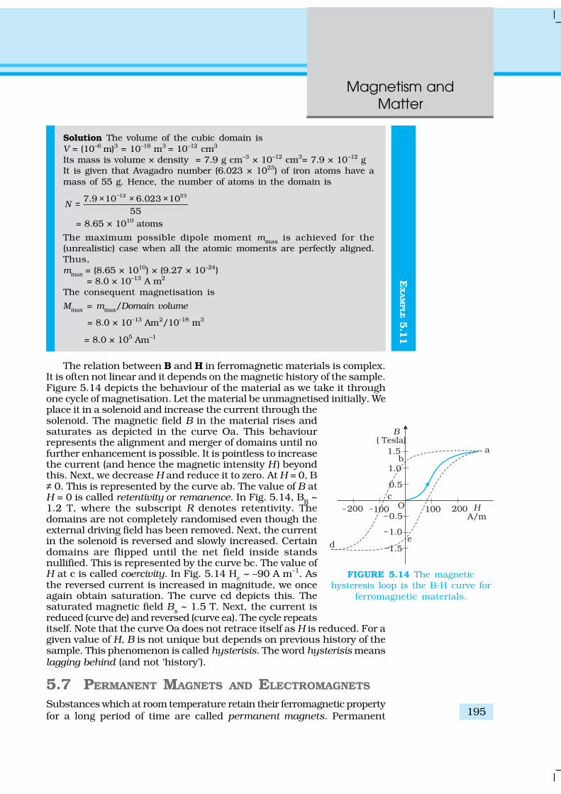
Magnetism andMatter
195
EX
AM
PLE 5
.11
Solution The volume of the cubic domain isV = (10–6 m)3 = 10–18 m3 = 10–12 cm3
Its mass is volume × density = 7.9 g cm–3 × 10–12 cm3= 7.9 × 10⁻¹² gIt is given that Avagadro number (6.023 × 10²³) of iron atoms have amass of 55 g. Hence, the number of atoms in the domain is
12 237.9 10 6.023 1055
N−× × ×=
= 8.65 × 10¹⁰ atoms
The maximum possible dipole moment mmax is achieved for the(unrealistic) case when all the atomic moments are perfectly aligned.Thus,mmax = (8.65 × 1010) × (9.27 × 10–24) = 8.0 × 10⁻¹³ A m2
The consequent magnetisation is
Mmax = mmax/Domain volume
= 8.0 × 10⁻¹³ Am2/10–18 m3
= 8.0 × 10⁵ Am–1
The relation between B and H in ferromagnetic materials is complex.It is often not linear and it depends on the magnetic history of the sample.Figure 5.14 depicts the behaviour of the material as we take it throughone cycle of magnetisation. Let the material be unmagnetised initially. Weplace it in a solenoid and increase the current through thesolenoid. The magnetic field B in the material rises andsaturates as depicted in the curve Oa. This behaviourrepresents the alignment and merger of domains until nofurther enhancement is possible. It is pointless to increasethe current (and hence the magnetic intensity H ) beyondthis. Next, we decrease H and reduce it to zero. At H = 0, B≠ 0. This is represented by the curve ab. The value of B atH = 0 is called retentivity or remanence. In Fig. 5.14, BR ~1.2 T, where the subscript R denotes retentivity. Thedomains are not completely randomised even though theexternal driving field has been removed. Next, the currentin the solenoid is reversed and slowly increased. Certaindomains are flipped until the net field inside standsnullified. This is represented by the curve bc. The value ofH at c is called coercivity. In Fig. 5.14 Hc ~ –90 A m–1. Asthe reversed current is increased in magnitude, we onceagain obtain saturation. The curve cd depicts this. Thesaturated magnetic field Bs ~ 1.5 T. Next, the current isreduced (curve de) and reversed (curve ea). The cycle repeatsitself. Note that the curve Oa does not retrace itself as H is reduced. For agiven value of H, B is not unique but depends on previous history of thesample. This phenomenon is called hysterisis. The word hysterisis meanslagging behind (and not ‘history’).
5.7 PERMANENT MAGNETS AND ELECTROMAGNETS
Substances which at room temperature retain their ferromagnetic propertyfor a long period of time are called permanent magnets. Permanent
FIGURE 5.14 The magnetichysteresis loop is the B-H curve for
ferromagnetic materials.

Physics
196
magnets can be made in a variety of ways. One can hold aniron rod in the north-south direction and hammer it repeatedly.The method is illustrated in Fig. 5.15. The illustration is froma 400 year old book to emphasise that the making ofpermanent magnets is an old art. One can also hold a steelrod and stroke it with one end of a bar magnet a large numberof times, always in the same sense to make a permanentmagnet.
An efficient way to make a permanent magnet is to place aferromagnetic rod in a solenoid and pass a current. Themagnetic field of the solenoid magnetises the rod.
The hysteresis curve (Fig. 5.14) allows us to select suitablematerials for permanent magnets. The material should havehigh retentivity so that the magnet is strong and high coercivityso that the magnetisation is not erased by stray magnetic fields,temperature fluctuations or minor mechanical damage.Further, the material should have a high permeability. Steel isone-favoured choice. It has a slightly smaller retentivity thansoft iron but this is outweighed by the much smaller coercivityof soft iron. Other suitable materials for permanent magnetsare alnico, cobalt steel and ticonal.
Core of electromagnets are made of ferromagnetic materialswhich have high permeability and low retentivity. Soft iron is a suitablematerial for electromagnets. On placing a soft iron rod in a solenoid andpassing a current, we increase the magnetism of the solenoid by athousand fold. When we switch off the solenoid current, the magnetism iseffectively switched off since the soft iron core has a low retentivity. Thearrangement is shown in Fig. 5.16.
FIGURE 5.15 A blacksmithforging a permanent magnet by
striking a red-hot rod of ironkept in the north-south
direction with a hammer. Thesketch is recreated from anillustration in De Magnete, awork published in 1600 andauthored by William Gilbert,the court physician to Queen
Elizabeth of England.
FIGURE 5.16 A soft iron core in solenoid acts as an electromagnet.
In certain applications, the material goes through an ac cycle ofmagnetisation for a long period. This is the case in transformer cores andtelephone diaphragms. The hysteresis curve of such materials must benarrow. The energy dissipated and the heating will consequently be small.The material must have a high resistivity to lower eddy current losses.You will study about eddy currents in Chapter 6.
Electromagnets are used in electric bells, loudspeakers and telephonediaphragms. Giant electromagnets are used in cranes to lift machinery,and bulk quantities of iron and steel.
Ind
iaís
Magn
eti
c F
ield
:
Magnetism andMatter
197
SUMMARY
1. The science of magnetism is old. It has been known since ancient timesthat magnetic materials tend to point in the north-south direction; likemagnetic poles repel and unlike ones attract; and cutting a bar magnetin two leads to two smaller magnets. Magnetic poles cannot be isolated.
2. When a bar magnet of dipole moment m is placed in a uniform magneticfield B,
(a) the force on it is zero, (b) the torque on it is m × B, (c) its potential energy is –m.B, where we choose the zero of energy at
the orientation when m is perpendicular to B.
3. Consider a bar magnet of size l and magnetic moment m, at a distancer from its mid-point, where r >>l, the magnetic field B due to this baris,
032 r
µ=πm
B (along axis)
= 03–
4 r
µπm
(along equator)
4. Gauss’s law for magnetism states that the net magnetic flux throughany closed surface is zero
0Ball areaelements
φ∆
= ∆ =∑S
B S
5. The earth’s magnetic field resembles that of a (hypothetical) magneticdipole located at the centre of the earth. The pole near the geographicnorth pole of the earth is called the north magnetic pole. Similarly, thepole near the geographic south pole is called the south magnetic pole.This dipole is aligned making a small angle with the rotation axis ofthe earth. The magnitude of the field on the earth’s surface ≈ 4 × 10⁻⁵ T.
MAPPING INDIA’S MAGNETIC FIELD
Because of its practical application in prospecting, communication, and navigation, themagnetic field of the earth is mapped by most nations with an accuracy comparable togeographical mapping. In India over a dozen observatories exist, extending fromTrivandrum (now Thrivuvananthapuram) in the south to Gulmarg in the north. Theseobservatories work under the aegis of the Indian Institute of Geomagnetism (IIG), in Colaba,Mumbai. The IIG grew out of the Colaba and Alibag observatories and was formallyestablished in 1971. The IIG monitors (via its nation-wide observatories), the geomagneticfields and fluctuations on land, and under the ocean and in space. Its services are usedby the Oil and Natural Gas Corporation Ltd. (ONGC), the National Institute ofOceanography (NIO) and the Indian Space Research Organisation (ISRO). It is a part ofthe world-wide network which ceaselessly updates the geomagnetic data. Now India hasa permanent station called Gangotri.

Physics
198
6. Three quantities are needed to specify the magnetic field of the earthon its surface – the horizontal component, the magnetic declination,and the magnetic dip. These are known as the elements of the earth’smagnetic field.
7. Consider a material placed in an external magnetic field B0. Themagnetic intensity is defined as,
0
0µ=
BH
The magnetisation M of the material is its dipole moment per unit volume.The magnetic field B in the material is,
B = µ0 (H + M)
8. For a linear material M = χ H. So that B = µ H and χ is called themagnetic susceptibility of the material. The three quantities, χ, therelative magnetic permeability µr, and the magnetic permeability µ arerelated as follows:µ = µ0 µr
µr = 1+ χ
9. Magnetic materials are broadly classified as: diamagnetic, paramagnetic,and ferromagnetic. For diamagnetic materials χ is negative and smalland for paramagnetic materials it is positive and small. Ferromagneticmaterials have large χ and are characterised by non-linear relationbetween B and H. They show the property of hysteresis.
10. Substances, which at room temperature, retain their ferromagneticproperty for a long period of time are called permanent magnets.
Physical quantity Symbol Nature Dimensions Units Remarks
Permeability of µ0 Scalar [MLT–2 A–2] T m A–1 µ0/4π = 10–7
free space
Magnetic field, B Vector [MT–2 A–1] T (tesla) 104 G (gauss) = 1 TMagnetic induction,Magnetic flux density
Magnetic moment m Vector [L–2 A] A m2
Magnetic flux φB Scalar [ML2T–2 A–1] W (weber) W = T m2
Magnetisation M Vector [L–1 A] A m–1 Magnetic momentVolume
Magnetic intensity H Vector [L–1 A] A m–1 B = µ0 (H + M)
Magnetic fieldstrength
Magnetic χ Scalar - - M = χHsusceptibility
Relative magnetic µr
Scalar - - B = µ0 µr H
permeability
Magnetic permeability µ Scalar [MLT–2 A–2] T m A–1 µ = µ0 µr
N A–2 B = µ H

Magnetism andMatter
199
POINTS TO PONDER
1. A satisfactory understanding of magnetic phenomenon in terms of movingcharges/currents was arrived at after 1800 AD. But technologicalexploitation of the directional properties of magnets predates this scientificunderstanding by two thousand years. Thus, scientific understanding isnot a necessary condition for engineering applications. Ideally, scienceand engineering go hand-in-hand, one leading and assisting the other intandem.
2. Magnetic monopoles do not exist. If you slice a magnet in half, you gettwo smaller magnets. On the other hand, isolated positive and negativecharges exist. There exists a smallest unit of charge, for example, theelectronic charge with value |e| = 1.6 ×10⁻¹⁹ C. All other charges areintegral multiples of this smallest unit charge. In other words, charge isquantised. We do not know why magnetic monopoles do not exist or whyelectric charge is quantised.
3. A consequence of the fact that magnetic monopoles do not exist is thatthe magnetic field lines are continuous and form closed loops. In contrast,the electrostatic lines of force begin on a positive charge and terminateon the negative charge (or fade out at infinity).
4. The earth’s magnetic field is not due to a huge bar magnet inside it. Theearth’s core is hot and molten. Perhaps convective currents in this coreare responsible for the earth’s magnetic field. As to what ‘dynamo’ effectsustains this current, and why the earth’s field reverses polarity everymillion years or so, we do not know.
5. A miniscule difference in the value of χ, the magnetic susceptibility, yieldsradically different behaviour: diamagnetic versus paramagnetic. Fordiamagnetic materials χ = –10–5 whereas χ = +10–5 for paramagneticmaterials.
6. There exists a perfect diamagnet, namely, a superconductor. This is ametal at very low temperatures. In this case χ = –1, µr = 0, µ = 0. Theexternal magnetic field is totally expelled. Interestingly, this material isalso a perfect conductor. However, there exists no classical theory whichties these two properties together. A quantum-mechanical theory byBardeen, Cooper, and Schrieffer (BCS theory) explains these effects. TheBCS theory was proposed in1957 and was eventually recognised by a NobelPrize in physics in 1970.
7. The phenomenon of magnetic hysteresis is reminiscent of similarbehaviour concerning the elastic properties of materials. Strainmay not be proportional to stress; here H and B (or M) are notlinearly related. The stress-strain curve exhibits hysteresis andarea enclosed by it represents the energy dissipated per unit volume.A similar interpretation can be given to the B-H magnetic hysteresiscurve.
8. Diamagnetism is universal. It is present in all materials. But itis weak and hard to detect if the substance is para- or ferromagnetic.
9. We have classified materials as diamagnetic, paramagnetic, andferromagnetic. However, there exist additional types of magnetic materialsuch as ferrimagnetic, anti-ferromagnetic, spin glass, etc. with propertieswhich are exotic and mysterious.

Physics
200
EXERCISES
5.1 Answer the following questions regarding earth’s magnetism:
(a) A vector needs three quantities for its specification. Name thethree independent quantities conventionally used to specify theearth’s magnetic field.
(b) The angle of dip at a location in southern India is about 18º.Would you expect a greater or smaller dip angle in Britain?
(c) If you made a map of magnetic field lines at Melbourne inAustralia, would the lines seem to go into the ground or come outof the ground?
(d) In which direction would a compass free to move in the verticalplane point to, if located right on the geomagnetic north or southpole?
(e) The earth’s field, it is claimed, roughly approximates the fielddue to a dipole of magnetic moment 8 × 10²² J T–1 located at itscentre. Check the order of magnitude of this number in someway.
(f ) Geologists claim that besides the main magnetic N-S poles, thereare several local poles on the earth’s surface oriented in differentdirections. How is such a thing possible at all?
5.2 Answer the following questions:
(a) The earth’s magnetic field varies from point to point in space.Does it also change with time? If so, on what time scale does itchange appreciably?
(b) The earth’s core is known to contain iron. Yet geologists do notregard this as a source of the earth’s magnetism. Why?
(c) The charged currents in the outer conducting regions of theearth’s core are thought to be responsible for earth’s magnetism.What might be the ‘battery’ (i.e., the source of energy) to sustainthese currents?
(d) The earth may have even reversed the direction of its field severaltimes during its history of 4 to 5 billion years. How can geologistsknow about the earth’s field in such distant past?
(e) The earth’s field departs from its dipole shape substantially atlarge distances (greater than about 30,000 km). What agenciesmay be responsible for this distortion?
(f ) Interstellar space has an extremely weak magnetic field of theorder of 10–12 T. Can such a weak field be of any significantconsequence? Explain.
[Note: Exercise 5.2 is meant mainly to arouse your curiosity. Answersto some questions above are tentative or unknown. Brief answerswherever possible are given at the end. For details, you should consulta good text on geomagnetism.]
5.3 A short bar magnet placed with its axis at 30º with a uniform externalmagnetic field of 0.25 T experiences a torque of magnitude equal to4.5 × 10–2 J. What is the magnitude of magnetic moment of the magnet?
5.4 A short bar magnet of magnetic moment m = 0.32 JT–1 is placed in auniform magnetic field of 0.15 T. If the bar is free to rotate in theplane of the field, which orientation would correspond to its (a) stable,and (b) unstable equilibrium? What is the potential energy of themagnet in each case?

Magnetism andMatter
201
5.5 A closely wound solenoid of 800 turns and area of cross section2.5 × 10–4 m2 carries a current of 3.0 A. Explain the sense in whichthe solenoid acts like a bar magnet. What is its associated magneticmoment?
5.6 If the solenoid in Exercise 5.5 is free to turn about the verticaldirection and a uniform horizontal magnetic field of 0.25 T is applied,what is the magnitude of torque on the solenoid when its axis makesan angle of 30° with the direction of applied field?
5.7 A bar magnet of magnetic moment 1.5 J T–1 lies aligned with thedirection of a uniform magnetic field of 0.22 T.
(a) What is the amount of work required by an external torque toturn the magnet so as to align its magnetic moment: (i) normalto the field direction, (ii) opposite to the field direction?
(b) What is the torque on the magnet in cases (i) and (ii)?5.8 A closely wound solenoid of 2000 turns and area of cross-section
1.6 × 10⁻⁴ m2, carrying a current of 4.0 A, is suspended through itscentre allowing it to turn in a horizontal plane.
(a) What is the magnetic moment associated with the solenoid?(b) What is the force and torque on the solenoid if a uniform
horizontal magnetic field of 7.5 × 10⁻² T is set up at an angle of30º with the axis of the solenoid?
5.9 A circular coil of 16 turns and radius 10 cm carrying a current of0.75 A rests with its plane normal to an external field of magnitude5.0 × 10–2 T. The coil is free to turn about an axis in its planeperpendicular to the field direction. When the coil is turned slightlyand released, it oscillates about its stable equilibrium with afrequency of 2.0 s–1. What is the moment of inertia of the coil aboutits axis of rotation?
5.10 A magnetic needle free to rotate in a vertical plane parallel to themagnetic meridian has its north tip pointing down at 22º with thehorizontal. The horizontal component of the earth’s magnetic fieldat the place is known to be 0.35 G. Determine the magnitude of theearth’s magnetic field at the place.
5.11 At a certain location in Africa, a compass points 12º west of thegeographic north. The north tip of the magnetic needle of a dip circleplaced in the plane of magnetic meridian points 60º above thehorizontal. The horizontal component of the earth’s field is measuredto be 0.16 G. Specify the direction and magnitude of the earth’s fieldat the location.
5.12 A short bar magnet has a magnetic moment of 0.48 J T–1. Give thedirection and magnitude of the magnetic field produced by the magnetat a distance of 10 cm from the centre of the magnet on (a) the axis,(b) the equatorial lines (normal bisector) of the magnet.
5.13 A short bar magnet placed in a horizontal plane has its axis alignedalong the magnetic north-south direction. Null points are found onthe axis of the magnet at 14 cm from the centre of the magnet. Theearth’s magnetic field at the place is 0.36 G and the angle of dip iszero. What is the total magnetic field on the normal bisector of themagnet at the same distance as the null–point (i.e., 14 cm) from thecentre of the magnet? (At null points, field due to a magnet is equaland opposite to the horizontal component of earth’s magnetic field.)
5.14 If the bar magnet in exercise 5.13 is turned around by 180º, wherewill the new null points be located?

Physics
202
5.15 A short bar magnet of magnetic moment 5.25 × 10⁻² J T–1 is placedwith its axis perpendicular to the earth’s field direction. At whatdistance from the centre of the magnet, the resultant field is inclinedat 45º with earth’s field on (a) its normal bisector and (b) its axis.Magnitude of the earth’s field at the place is given to be 0.42 G.Ignore the length of the magnet in comparison to the distancesinvolved.
ADDITIONAL EXERCISES
5.16 Answer the following questions:(a) Why does a paramagnetic sample display greater magnetisation
(for the same magnetising field) when cooled?(b) Why is diamagnetism, in contrast, almost independent of
temperature?(c) If a toroid uses bismuth for its core, will the field in the core be
(slightly) greater or (slightly) less than when the core is empty?(d) Is the permeability of a ferromagnetic material independent of
the magnetic field? If not, is it more for lower or higher fields?(e) Magnetic field lines are always nearly normal to the surface of a
ferromagnet at every point. (This fact is analogous to the staticelectric field lines being normal to the surface of a conductor atevery point.) Why?
(f ) Would the maximum possible magnetisation of a paramagneticsample be of the same order of magnitude as the magnetisationof a ferromagnet?
5.17 Answer the following questions:(a) Explain qualitatively on the basis of domain picture the
irreversibility in the magnetisation curve of a ferromagnet.(b) The hysteresis loop of a soft iron piece has a much smaller area
than that of a carbon steel piece. If the material is to go throughrepeated cycles of magnetisation, which piece will dissipate greaterheat energy?
(c) ‘A system displaying a hysteresis loop such as a ferromagnet, isa device for storing memory?’ Explain the meaning of thisstatement.
(d) What kind of ferromagnetic material is used for coating magnetictapes in a cassette player, or for building ‘memory stores’ in amodern computer?
(e) A certain region of space is to be shielded from magnetic fields.Suggest a method.
5.18 A long straight horizontal cable carries a current of 2.5 A in thedirection 10º south of west to 10º north of east. The magnetic meridianof the place happens to be 10º west of the geographic meridian. Theearth’s magnetic field at the location is 0.33 G, and the angle of dipis zero. Locate the line of neutral points (ignore the thickness of thecable). (At neutral points, magnetic field due to a current-carryingcable is equal and opposite to the horizontal component of earth’smagnetic field.)
5.19 A telephone cable at a place has four long straight horizontal wirescarrying a current of 1.0 A in the same direction east to west. The

Magnetism andMatter
203
earth’s magnetic field at the place is 0.39 G, and the angle of dip is35º. The magnetic declination is nearly zero. What are the resultantmagnetic fields at points 4.0 cm below the cable?
5.20 A compass needle free to turn in a horizontal plane is placed at thecentre of circular coil of 30 turns and radius 12 cm. The coil is in avertical plane making an angle of 45º with the magnetic meridian.When the current in the coil is 0.35 A, the needle points west toeast.(a) Determine the horizontal component of the earth’s magnetic field
at the location.(b) The current in the coil is reversed, and the coil is rotated about
its vertical axis by an angle of 90º in the anticlockwise senselooking from above. Predict the direction of the needle. Take themagnetic declination at the places to be zero.
5.21 A magnetic dipole is under the influence of two magnetic fields. Theangle between the field directions is 60º, and one of the fields has amagnitude of 1.2 × 10⁻² T. If the dipole comes to stable equilibrium atan angle of 15º with this field, what is the magnitude of the otherfield?
5.22 A monoenergetic (18 keV) electron beam initially in the horizontaldirection is subjected to a horizontal magnetic field of 0.04 G normalto the initial direction. Estimate the up or down deflection of thebeam over a distance of 30 cm (me = 9.11 × 10⁻¹⁹ C). [Note: Data inthis exercise are so chosen that the answer will give you an idea ofthe effect of earth’s magnetic field on the motion of the electron beamfrom the electron gun to the screen in a TV set.]
5.23 A sample of paramagnetic salt contains 2.0 × 1024 atomic dipoleseach of dipole moment 1.5 × 10⁻²³ J T–1. The sample is placed undera homogeneous magnetic field of 0.64 T, and cooled to a temperatureof 4.2 K. The degree of magnetic saturation achieved is equal to 15%.What is the total dipole moment of the sample for a magnetic field of0.98 T and a temperature of 2.8 K? (Assume Curie’s law)
5.24 A Rowland ring of mean radius 15 cm has 3500 turns of wire woundon a ferromagnetic core of relative permeability 800. What is themagnetic field B in the core for a magnetising current of 1.2 A?
5.25 The magnetic moment vectors µµµµµs and µµµµµl associated with the intrinsicspin angular momentum S and orbital angular momentum l,respectively, of an electron are predicted by quantum theory (andverified experimentally to a high accuracy) to be given by:
µµµµµs = –(e/m) S,
µµµµµl = –(e/2m)l
Which of these relations is in accordance with the result expectedclassically? Outline the derivation of the classical result.

Physics
204
6.1 INTRODUCTION
Electricity and magnetism were considered separate and unrelatedphenomena for a long time. In the early decades of the nineteenth century,experiments on electric current by Oersted, Ampere and a few othersestablished the fact that electricity and magnetism are inter-related. Theyfound that moving electric charges produce magnetic fields. For example,an electric current deflects a magnetic compass needle placed in its vicinity.This naturally raises the questions like: Is the converse effect possible?Can moving magnets produce electric currents? Does the nature permitsuch a relation between electricity and magnetism? The answer isresounding yes! The experiments of Michael Faraday in England andJoseph Henry in USA, conducted around 1830, demonstratedconclusively that electric currents were induced in closed coils whensubjected to changing magnetic fields. In this chapter, we will study thephenomena associated with changing magnetic fields and understandthe underlying principles. The phenomenon in which electric current isgenerated by varying magnetic fields is appropriately calledelectromagnetic induction.
When Faraday first made public his discovery that relative motionbetween a bar magnet and a wire loop produced a small current in thelatter, he was asked, “What is the use of it?” His reply was: “What is theuse of a new born baby?” The phenomenon of electromagnetic induction
Chapter Six
ELECTROMAGNETICINDUCTION

ElectromagneticInduction
205
is not merely of theoretical or academic interest but alsoof practical utility. Imagine a world where there is noelectricity – no electric lights, no trains, no telephones andno personal computers. The pioneering experiments ofFaraday and Henry have led directly to the developmentof modern day generators and transformers. Today’scivilisation owes its progress to a great extent to thediscovery of electromagnetic induction.
6.2 THE EXPERIMENTS OF FARADAY AND
HENRY
The discovery and understanding of electromagneticinduction are based on a long series of experiments carriedout by Faraday and Henry. We shall now describe someof these experiments.
Experiment 6.1
Figure 6.1 shows a coil C1* connected to a galvanometerG. When the North-pole of a bar magnet is pushedtowards the coil, the pointer in the galvanometer deflects,indicating the presence of electric current in the coil. Thedeflection lasts as long as the bar magnet is in motion.The galvanometer does not show any deflection when themagnet is held stationary. When the magnet is pulledaway from the coil, the galvanometer shows deflection inthe opposite direction, which indicates reversal of thecurrent’s direction. Moreover, when the South-pole ofthe bar magnet is moved towards or away from thecoil, the deflections in the galvanometer are oppositeto that observed with the North-pole for similarmovements. Further, the deflection (and hence current)is found to be larger when the magnet is pushedtowards or pulled away from the coil faster. Instead,when the bar magnet is held fixed and the coil C1 ismoved towards or away from the magnet, the sameeffects are observed. It shows that it is the relativemotion between the magnet and the coil that isresponsible for generation (induction) of electriccurrent in the coil.
Experiment 6.2
In Fig. 6.2 the bar magnet is replaced by a second coilC2 connected to a battery. The steady current in thecoil C2 produces a steady magnetic field. As coil C2 is
* Wherever the term ‘coil or ‘loop’ is used, it is assumed that they are made up ofconducting material and are prepared using wires which are coated with insulatingmaterial.
FIGURE 6.1 When the bar magnet ispushed towards the coil, the pointer in
the galvanometer G deflects.
Josheph Henry [1797 –1878] American experimentalphysicist professor atPrinceton University and firstdirector of the SmithsonianInstitution. He made importantimprovements in electro-magnets by winding coils ofinsulated wire around ironpole pieces and invented anelectromagnetic motor and anew, efficient telegraph. Hediscoverd self-induction andinvestigated how currents inone circuit induce currents inanother.
JO
SE
PH
HE
NR
Y (1
797 – 1
878)

Physics
206
moved towards the coil C1, the galvanometer shows adeflection. This indicates that electric current is induced incoil C1. When C2 is moved away, the galvanometer shows adeflection again, but this time in the opposite direction. Thedeflection lasts as long as coil C2 is in motion. When the coilC2 is held fixed and C1 is moved, the same effects are observed.Again, it is the relative motion between the coils that inducesthe electric current.
Experiment 6.3
The above two experiments involved relative motion betweena magnet and a coil and between two coils, respectively.Through another experiment, Faraday showed that thisrelative motion is not an absolute requirement. Figure 6.3shows two coils C1 and C2 held stationary. Coil C1 is connectedto galvanometer G while the second coil C2 is connected to abattery through a tapping key K.
FIGURE 6.2 Current isinduced in coil C1 due to motionof the current carrying coil C2.
FIGURE 6.3 Experimental set-up for Experiment 6.3.
It is observed that the galvanometer shows a momentary deflectionwhen the tapping key K is pressed. The pointer in the galvanometer returnsto zero immediately. If the key is held pressed continuously, there is nodeflection in the galvanometer. When the key is released, a momentorydeflection is observed again, but in the opposite direction. It is also observedthat the deflection increases dramatically when an iron rod is insertedinto the coils along their axis.
6.3 MAGNETIC FLUX
Faraday’s great insight lay in discovering a simple mathematical relationto explain the series of experiments he carried out on electromagneticinduction. However, before we state and appreciate his laws, we must getfamiliar with the notion of magnetic flux, Φ B. Magnetic flux is defined inthe same way as electric flux is defined in Chapter 1. Magnetic flux through
Inte
ract
ive a
nim
atio
n o
n F
arad
ay’s
exp
eri
men
ts a
nd
Len
z’s
law
:http://micro.m
agne
t.fsu.edu
/electromag
net/jav
a/farada
y/inde
x.html

ElectromagneticInduction
207
a plane of area A placed in a uniform magnetic field B (Fig. 6.4) canbe written as
Φ B = B . A = BA cos θ (6.1)
where θ is angle between B and A. The notion of the area as a vectorhas been discussed earlier in Chapter 1. Equation (6.1) can beextended to curved surfaces and nonuniform fields.
If the magnetic field has different magnitudes and directions atvarious parts of a surface as shown in Fig. 6.5, then the magneticflux through the surface is given by
1 1 2 2d d
BΦ = + +B A B Ai i ... =
all
di i∑B Ai (6.2)
where ‘all’ stands for summation over all the area elements dAicomprising the surface and Bi is the magnetic field at the area elementdAi. The SI unit of magnetic flux is weber (Wb) or tesla metersquared (T m2). Magnetic flux is a scalar quantity.
6.4 FARADAY’S LAW OF INDUCTION
From the experimental observations, Faraday arrived at aconclusion that an emf is induced in a coil when magnetic fluxthrough the coil changes with time. Experimental observationsdiscussed in Section 6.2 can be explained using this concept.
The motion of a magnet towards or away from coil C1 inExperiment 6.1 and moving a current-carrying coil C2 towardsor away from coil C1 in Experiment 6.2, change the magneticflux associated with coil C1. The change in magnetic flux inducesemf in coil C1. It was this induced emf which caused electriccurrent to flow in coil C1 and through the galvanometer. Aplausible explanation for the observations of Experiment 6.3 isas follows: When the tapping key K is pressed, the current incoil C2 (and the resulting magnetic field) rises from zero to amaximum value in a short time. Consequently, the magneticflux through the neighbouring coil C1 also increases. It is the change inmagnetic flux through coil C1 that produces an induced emf in coil C1.When the key is held pressed, current in coil C2 is constant. Therefore,there is no change in the magnetic flux through coil C1 and the current incoil C1 drops to zero. When the key is released, the current in C2 and theresulting magnetic field decreases from the maximum value to zero in ashort time. This results in a decrease in magnetic flux through coil C1and hence again induces an electric current in coil C1*. The commonpoint in all these observations is that the time rate of change of magneticflux through a circuit induces emf in it. Faraday stated experimentalobservations in the form of a law called Faraday’s law of electromagneticinduction. The law is stated below.
FIGURE 6.4 A plane ofsurface area A placed in auniform magnetic field B.
FIGURE 6.5 Magnetic field Bi
at the i th area element. dAi
represents area vector of thei th area element.
* Note that sensitive electrical instruments in the vicinity of an electromagnetcan be damaged due to the induced emfs (and the resulting currents) when theelectromagnet is turned on or off.

Physics
208
EX
AM
PLE 6
.1
The magnitude of the induced emf in a circuit is equalto the time rate of change of magnetic flux through thecircuit.
Mathematically, the induced emf is given by
d–
dB
t
Φε = (6.3)
The negative sign indicates the direction of ε and hencethe direction of current in a closed loop. This will bediscussed in detail in the next section.
In the case of a closely wound coil of N turns, changeof flux associated with each turn, is the same. Therefore,the expression for the total induced emf is given by
d–
dBNt
Φε = (6.4)
The induced emf can be increased by increasing thenumber of turns N of a closed coil.
From Eqs. (6.1) and (6.2), we see that the flux can bevaried by changing any one or more of the terms B, A andθ. In Experiments 6.1 and 6.2 in Section 6.2, the flux ischanged by varying B. The flux can also be altered bychanging the shape of a coil (that is, by shrinking it orstretching it) in a magnetic field, or rotating a coil in amagnetic field such that the angle θ between B and Achanges. In these cases too, an emf is induced in therespective coils.
Example 6.1 Consider Experiment 6.2. (a) What would you do to obtaina large deflection of the galvanometer? (b) How would you demonstratethe presence of an induced current in the absence of a galvanometer?
Solution(a) To obtain a large deflection, one or more of the following steps can
be taken: (i) Use a rod made of soft iron inside the coil C2, (ii) Connectthe coil to a powerful battery, and (iii) Move the arrangement rapidlytowards the test coil C1.
(b) Replace the galvanometer by a small bulb, the kind one finds in asmall torch light. The relative motion between the two coils will causethe bulb to glow and thus demonstrate the presence of an inducedcurrent.In experimental physics one must learn to innovate. Michael Faradaywho is ranked as one of the best experimentalists ever, was legendaryfor his innovative skills.
Example 6.2 A square loop of side 10 cm and resistance 0.5 Ω isplaced vertically in the east-west plane. A uniform magnetic field of0.10 T is set up across the plane in the north-east direction. Themagnetic field is decreased to zero in 0.70 s at a steady rate. Determinethe magnitudes of induced emf and current during this time-interval.
Michael Faraday [1791–1867] Faraday madenumerous contributions toscience, viz., the discoveryof electromagneticinduction, the laws ofelectrolysis, benzene, andthe fact that the plane ofpolarisation is rotated in anelectric field. He is alsocredited with the inventionof the electric motor, theelectric generator and thetransformer. He is widelyregarded as the greatestexperimental scientist ofthe nineteenth century.
MIC
HA
EL F
AR
AD
AY (
1791–1
867)
EX
AM
PLE 6
.2

ElectromagneticInduction
209
EX
AM
PLE 6
.2
Solution The angle θ made by the area vector of the coil with themagnetic field is 45°. From Eq. (6.1), the initial magnetic flux is
Φ = BA cos θ
–20.1 10Wb
2
×=
Final flux, Φmin = 0
The change in flux is brought about in 0.70 s. From Eq. (6.3), themagnitude of the induced emf is given by
( )– 0B
t t
ΦΦε
Δ= =
Δ Δ
–310= 1.0 mV
2 0.7=
×
And the magnitude of the current is
–310 V2mA
0.5I
R
ε= = =
ΩNote that the earth’s magnetic field also produces a flux through theloop. But it is a steady field (which does not change within the timespan of the experiment) and hence does not induce any emf.
Example 6.3A circular coil of radius 10 cm, 500 turns and resistance 2 Ω is placedwith its plane perpendicular to the horizontal component of the earth’smagnetic field. It is rotated about its vertical diameter through 180°in 0.25 s. Estimate the magnitudes of the emf and current induced inthe coil. Horizontal component of the earth’s magnetic field at theplace is 3.0 × 10⁻⁵ T.
SolutionInitial flux through the coil,
ΦB (initial) = BA cos θ
= 3.0 × 10⁻⁵ × (π ×10–2) × cos 0º
= 3π × 10–7 Wb
Final flux after the rotation,
ΦB (final) = 3.0 × 10⁻⁵ × (π ×10–2) × cos 180°
= –3π × 10–7 Wb
Therefore, estimated value of the induced emf is,
NtΦε Δ
=Δ
= 500 × (6π × 10–7)/0.25
= 3.8 × 10⁻³ V
I = ε/R = 1.9 × 10⁻³ A
Note that the magnitudes of ε and I are the estimated values. Theirinstantaneous values are different and depend upon the speed ofrotation at the particular instant.
EX
AM
PLE 6
.3

Physics
210
6.5 LENZ’S LAW AND CONSERVATION OF ENERGY
In 1834, German physicist Heinrich Friedrich Lenz (1804-1865) deduceda rule, known as Lenz’s law which gives the polarity of the induced emfin a clear and concise fashion. The statement of the law is:
The polarity of induced emf is such that it tends to produce a currentwhich opposes the change in magnetic flux that produced it.
The negative sign shown in Eq. (6.3) represents this effect. We canunderstand Lenz’s law by examining Experiment 6.1 in Section 6.2.1. InFig. 6.1, we see that the North-pole of a bar magnet is being pushedtowards the closed coil. As the North-pole of the bar magnet moves towardsthe coil, the magnetic flux through the coil increases. Hence current isinduced in the coil in such a direction that it opposes the increase in flux.This is possible only if the current in the coil is in a counter-clockwisedirection with respect to an observer situated on the side of the magnet.Note that magnetic moment associated with this current has North polaritytowards the North-pole of the approaching magnet. Similarly, if the North-pole of the magnet is being withdrawn from the coil, the magnetic fluxthrough the coil will decrease. To counter this decrease in magnetic flux,the induced current in the coil flows in clockwise direction and its South-pole faces the receding North-pole of the bar magnet. This would result inan attractive force which opposes the motion of the magnet and thecorresponding decrease in flux.
What will happen if an open circuit is used in place of the closed loopin the above example? In this case too, an emf is induced across the open
ends of the circuit. The direction of the induced emf can be foundusing Lenz’s law. Consider Figs. 6.6 (a) and (b). They provide an easierway to understand the direction of induced currents. Note that the
direction shown by and indicate the directions of the induced
currents.A little reflection on this matter should convince us on the
correctness of Lenz’s law. Suppose that the induced current was inthe direction opposite to the one depicted in Fig. 6.6(a). In that case,the South-pole due to the induced current will face the approachingNorth-pole of the magnet. The bar magnet will then be attractedtowards the coil at an ever increasing acceleration. A gentle push onthe magnet will initiate the process and its velocity and kinetic energywill continuously increase without expending any energy. If this canhappen, one could construct a perpetual-motion machine by asuitable arrangement. This violates the law of conservation of energyand hence can not happen.
Now consider the correct case shown in Fig. 6.6(a). In this situation,the bar magnet experiences a repulsive force due to the inducedcurrent. Therefore, a person has to do work in moving the magnet.Where does the energy spent by the person go? This energy is
dissipated by Joule heating produced by the induced current.
FIGURE 6.6Illustration of
Lenz’s law.

ElectromagneticInduction
211
EX
AM
PLE 6
.4
Example 6.4Figure 6.7 shows planar loops of different shapes moving out of orinto a region of a magnetic field which is directed normal to the planeof the loop away from the reader. Determine the direction of inducedcurrent in each loop using Lenz’s law.
FIGURE 6.7
Solution(i) The magnetic flux through the rectangular loop abcd increases,
due to the motion of the loop into the region of magnetic field, Theinduced current must flow along the path bcdab so that it opposesthe increasing flux.
(ii) Due to the outward motion, magnetic flux through the triangularloop abc decreases due to which the induced current flows alongbacb, so as to oppose the change in flux.
(iii) As the magnetic flux decreases due to motion of the irregularshaped loop abcd out of the region of magnetic field, the inducedcurrent flows along cdabc, so as to oppose change in flux.Note that there are no induced current as long as the loops arecompletely inside or outside the region of the magnetic field.
Example 6.5(a) A closed loop is held stationary in the magnetic field between the
north and south poles of two permanent magnets held fixed. Canwe hope to generate current in the loop by using very strongmagnets?
(b) A closed loop moves normal to the constant electric field betweenthe plates of a large capacitor. Is a current induced in the loop(i) when it is wholly inside the region between the capacitor plates(ii) when it is partially outside the plates of the capacitor? Theelectric field is normal to the plane of the loop.
(c) A rectangular loop and a circular loop are moving out of a uniformmagnetic field region (Fig. 6.8) to a field-free region with a constantvelocity v. In which loop do you expect the induced emf to beconstant during the passage out of the field region? The field isnormal to the loops.
EX
AM
PLE 6
.5

Physics
212
EX
AM
PLE 6
.5
FIGURE 6.8
(d) Predict the polarity of the capacitor in the situation described byFig. 6.9.
FIGURE 6.9
Solution(a) No. However strong the magnet may be, current can be induced
only by changing the magnetic flux through the loop.(b) No current is induced in either case. Current can not be induced
by changing the electric flux.(c) The induced emf is expected to be constant only in the case of the
rectangular loop. In the case of circular loop, the rate of change ofarea of the loop during its passage out of the field region is notconstant, hence induced emf will vary accordingly.
(d) The polarity of plate ‘A’ will be positive with respect to plate ‘B’ inthe capacitor.
6.6 MOTIONAL ELECTROMOTIVE FORCE
Let us consider a straight conductor moving in a uniform and time-independent magnetic field. Figure 6.10 shows a rectangular conductorPQRS in which the conductor PQ is free to move. The rod PQ is moved
towards the left with a constant velocity v asshown in the figure. Assume that there is noloss of energy due to friction. PQRS forms aclosed circuit enclosing an area that changesas PQ moves. It is placed in a uniform magneticfield B which is perpendicular to the plane ofthis system. If the length RQ = x and RS = l, themagnetic flux ΦB enclosed by the loop PQRSwill be
ΦB = Blx
Since x is changing with time, the rate of changeof flux ΦB will induce an emf given by:
( )– d d–
d dB Blx
t t
Φε = =
= d
–dx
Bl Blvt= (6.5)
FIGURE 6.10 The arm PQ is moved to the leftside, thus decreasing the area of the
rectangular loop. This movementinduces a current I as shown.

ElectromagneticInduction
213
where we have used dx/dt = –v which is the speed of the conductor PQ.The induced emf Blv is called motional emf. Thus, we are able to produceinduced emf by moving a conductor instead of varying the magnetic field,that is, by changing the magnetic flux enclosed by the circuit.
It is also possible to explain the motional emf expression in Eq. (6.5)by invoking the Lorentz force acting on the free charge carriers of conductorPQ. Consider any arbitrary charge q in the conductor PQ. When the rodmoves with speed v, the charge will also be moving with speed v in themagnetic field B. The Lorentz force on this charge is qvB in magnitude,and its direction is towards Q. All charges experience the same force, inmagnitude and direction, irrespective of their position in the rod PQ.The work done in moving the charge from P to Q is,
W = qvBl
Since emf is the work done per unit charge,
W
qε =
= Blv
This equation gives emf induced across the rod PQ and is identicalto Eq. (6.5). We stress that our presentation is not wholly rigorous. Butit does help us to understand the basis of Faraday’s law whenthe conductor is moving in a uniform and time-independentmagnetic field.
On the other hand, it is not obvious how an emf is induced when aconductor is stationary and the magnetic field is changing – a fact whichFaraday verified by numerous experiments. In the case of a stationaryconductor, the force on its charges is given by
F = q (E + v ××××× B) = qE (6.6)
since v = 0. Thus, any force on the charge must arise from the electricfield term E alone. Therefore, to explain the existence of induced emf orinduced current, we must assume that a time-varying magnetic fieldgenerates an electric field. However, we hasten to add that electric fieldsproduced by static electric charges have properties different from thoseproduced by time-varying magnetic fields. In Chapter 4, we learnt thatcharges in motion (current) can exert force/torque on a stationary magnet.Conversely, a bar magnet in motion (or more generally, a changingmagnetic field) can exert a force on the stationary charge. This is thefundamental significance of the Faraday’s discovery. Electricity andmagnetism are related.
Example 6.6 A metallic rod of 1 m length is rotated with a frequencyof 50 rev/s, with one end hinged at the centre and the other end at thecircumference of a circular metallic ring of radius 1 m, about an axispassing through the centre and perpendicular to the plane of the ring(Fig. 6.11). A constant and uniform magnetic field of 1 T parallel to theaxis is present everywhere. What is the emf between the centre andthe metallic ring?
EX
AM
PLE 6
.6
Inte
ractive
an
imatio
n o
n m
otio
nal e
mf:
http://www.ngsir,netfirm
s.com/englishhtm
/Induction.htm

Physics
214 EX
AM
PLE 6
.6
FIGURE 6.11SolutionMethod IAs the rod is rotated, free electrons in the rod move towards the outerend due to Lorentz force and get distributed over the ring. Thus, theresulting separation of charges produces an emf across the ends ofthe rod. At a certain value of emf, there is no more flow of electronsand a steady state is reached. Using Eq. (6.5), the magnitude of theemf generated across a length dr of the rod as it moves at right anglesto the magnetic field is given by
d dBv rε = . Hence,
0
d dR
Bv rε ε= =∫ ∫ 2
0
d2
R B RB r r
ωω= =∫
Note that we have used v = ω r. This gives
ε 211.0 2 50 (1 )
2= × × π × ×
= 157 V
Method IITo calculate the emf, we can imagine a closed loop OPQ in whichpoint O and P are connected with a resistor R and OQ is the rotatingrod. The potential difference across the resistor is then equal to theinduced emf and equals B × (rate of change of area of loop). If θ is theangle between the rod and the radius of the circle at P at time t, thearea of the sector OPQ is given by
2 212 2
R Rθ θπ × =π
where R is the radius of the circle. Hence, the induced emf is
ε = 2d 1d 2
B Rt
θ⎡ ⎤× ⎢ ⎥⎣ ⎦ =
221 d
2 d 2B R
BRt
θ ω=
[Note: d
2dtθ ω ν= = π ]
This expression is identical to the expression obtained by Method Iand we get the same value of ε.

ElectromagneticInduction
215
EX
AM
PLE 6
.7
Example 6.7A wheel with 10 metallic spokes each 0.5 m long is rotated with aspeed of 120 rev/min in a plane normal to the horizontal componentof earth’s magnetic field HE at a place. If HE = 0.4 G at the place, whatis the induced emf between the axle and the rim of the wheel? Notethat 1 G = 10–4 T.
Solution
Induced emf = (1/2) ω B R2
= (1/2) × 4π × 0.4 × 10–4 × (0.5)2
= 6.28 × 10⁻⁵ V
The number of spokes is immaterial because the emf’s across thespokes are in parallel.
6.7 ENERGY CONSIDERATION: A QUANTITATIVE STUDY
In Section 6.5, we discussed qualitatively that Lenz’s law is consistent withthe law of conservation of energy. Now we shall explore this aspect furtherwith a concrete example.
Let r be the resistance of movable arm PQ of the rectangular conductorshown in Fig. 6.10. We assume that the remaining arms QR, RS and SPhave negligible resistances compared to r. Thus, the overall resistance ofthe rectangular loop is r and this does not change as PQ is moved. Thecurrent I in the loop is,
Ir
ε=
= B l v
r(6.7)
On account of the presence of the magnetic field, there will be a forceon the arm PQ. This force I (l ××××× B), is directed outwards in the directionopposite to the velocity of the rod. The magnitude of this force is,
F = I l B = 2 2B l v
rwhere we have used Eq. (6.7). Note that this force arises due to drift velocityof charges (responsible for current) along the rod and the consequentLorentz force acting on them.
Alternatively, the arm PQ is being pushed with a constant speed v,the power required to do this is,
P F v=
=2 2 2B l v
r(6.8)
The agent that does this work is mechanical. Where does thismechanical energy go? The answer is: it is dissipated as Joule heat, andis given by
2JP I r=
2Blv
rr
⎛ ⎞= ⎜ ⎟⎝ ⎠
2 2 2B l v
r=
which is identical to Eq. (6.8).

Physics
216 EX
AM
PLE 6
.8
Thus, mechanical energy which was needed to move the arm PQ isconverted into electrical energy (the induced emf) and then to thermal energy.
There is an interesting relationship between the charge flow throughthe circuit and the change in the magnetic flux. From Faraday’s law, wehave learnt that the magnitude of the induced emf is,
B
t
Φε
Δ=
ΔHowever,
QIr r
tε
Δ= =
ΔThus,
BQr
ΦΔΔ =
Example 6.8 Refer to Fig. 6.12(a). The arm PQ of the rectangularconductor is moved from x = 0, outwards. The uniform magnetic field isperpendicular to the plane and extends from x = 0 to x = b and is zerofor x > b. Only the arm PQ possesses substantial resistance r. Considerthe situation when the arm PQ is pulled outwards from x = 0 to x = 2b,and is then moved back to x = 0 with constant speed v. Obtain expressionsfor the flux, the induced emf, the force necessary to pull the arm and thepower dissipated as Joule heat. Sketch the variation of these quantitieswith distance.
(a)FIGURE 6.12
Solution Let us first consider the forward motion from x = 0 to x = 2bThe flux ΦB linked with the circuit SPQR is
B 0Bl x x bΦ = ≤ <
2Bl b b x b= ≤ <The induced emf is,
Bddt
Φε = −
0Blv x b= − ≤ <
0 2b x b= ≤ <

ElectromagneticInduction
217
EX
AM
PLE 6
.8
When the induced emf is non-zero, the current I is (in magnitude)
Bl vI
r=
(b)FIGURE 6.12
The force required to keep the arm PQ in constant motion is I lB. Itsdirection is to the left. In magnitude
2 2
0
0 2
B l vF x b
rb x b
= ≤ <
= ≤ <The Joule heating loss is
2JP I r=
2 2 2
0
0 2
B l vx b
rb x b
= ≤ <
= ≤ <
One obtains similar expressions for the inward motion from x = 2b tox = 0. One can appreciate the whole process by examining the sketchof various quantities displayed in Fig. 6.12(b).

Physics
218
6.8 EDDY CURRENTS
So far we have studied the electric currents induced in well defined pathsin conductors like circular loops. Even when bulk pieces of conductors
are subjected to changing magnetic flux, induced currentsare produced in them. However, their flow patterns resembleswirling eddies in water. This effect was discovered by physicistFoucault (1819-1868) and these currents are called eddycurrents.
Consider the apparatus shown in Fig. 6.13. A copper plateis allowed to swing like a simple pendulum between the polepieces of a strong magnet. It is found that the motion is dampedand in a little while the plate comes to a halt in the magneticfield. We can explain this phenomenon on the basis ofelectromagnetic induction. Magnetic flux associated with theplate keeps on changing as the plate moves in and out of theregion between magnetic poles. The flux change induces eddycurrents in the plate. Directions of eddy currents are oppositewhen the plate swings into the region between the poles andwhen it swings out of the region.
If rectangular slots are made in the copper plate as shownin Fig. 6.14, area available to the flow of eddy currents is less.Thus, the pendulum plate with holes or slots reduceselectromagnetic damping and the plate swings more freely.Note that magnetic moments of the induced currents (whichoppose the motion) depend upon the area enclosed by thecurrents (recall equation m = IA in Chapter 4).This fact is helpful in reducing eddy currents in the metallic
cores of transformers, electric motors and other such devices inwhich a coil is to be wound over metallic core. Eddy currents areundesirable since they heat up the core and dissipate electricalenergy in the form of heat. Eddy currents are minimised by usinglaminations of metal to make a metal core. The laminations areseparated by an insulating material like lacquer. The plane of thelaminations must be arranged parallel to the magnetic field, sothat they cut across the eddy current paths. This arrangementreduces the strength of the eddy currents. Since the dissipationof electrical energy into heat depends on the square of the strengthof electric current, heat loss is substantially reduced.
Eddy currents are used to advantage in certain applications like:
(i) Magnetic braking in trains: Strong electromagnets are situatedabove the rails in some electrically powered trains. When theelectromagnets are activated, the eddy currents induced in therails oppose the motion of the train. As there are no mechanicallinkages, the braking effect is smooth.
(ii) Electromagnetic damping: Certain galvanometers have a fixedcore made of nonmagnetic metallic material. When the coiloscillates, the eddy currents generated in the core oppose themotion and bring the coil to rest quickly.
FIGURE 6.13 Eddy currents aregenerated in the copper plate,
while enteringand leaving the region of
magnetic field.
FIGURE 6.14 Cutting slotsin the copper plate reducesthe effect of eddy currents.

ElectromagneticInduction
219
(iii) Induction furnace: Induction furnace can be used to produce hightemperatures and can be utilised to prepare alloys, by melting theconstituent metals. A high frequency alternating current is passedthrough a coil which surrounds the metals to be melted. The eddycurrents generated in the metals produce high temperatures sufficientto melt it.
(iv) Electric power meters: The shiny metal disc in the electric power meter(analogue type) rotates due to the eddy currents. Electric currentsare induced in the disc by magnetic fields produced by sinusoidallyvarying currents in a coil.You can observe the rotating shiny disc in the power meter of yourhouse.
ELECTROMAGNETIC DAMPING
Take two hollow thin cylindrical pipes of equal internal diameters made of aluminium andPVC, respectively. Fix them vertically with clamps on retort stands. Take a small cylindericalmagnet having diameter slightly smaller than the inner diameter of the pipes and drop itthrough each pipe in such a way that the magnet does not touch the sides of the pipesduring its fall. You will observe that the magnet dropped through the PVC pipe takes thesame time to come out of the pipe as it would take when dropped through the same heightwithout the pipe. Note the time it takes to come out of the pipe in each case. You will see thatthe magnet takes much longer time in the case of aluminium pipe. Why is it so? It is due tothe eddy currents that are generated in the aluminium pipe which oppose the change inmagnetic flux, i.e., the motion of the magnet. The retarding force due to the eddy currentsinhibits the motion of the magnet. Such phenomena are referred to as electromagnetic damping.Note that eddy currents are not generated in PVC pipe as its material is an insulator whereasaluminium is a conductor.
6.9 INDUCTANCE
An electric current can be induced in a coil by flux change produced byanother coil in its vicinity or flux change produced by the same coil. Thesetwo situations are described separately in the next two sub-sections.However, in both the cases, the flux through a coil is proportional to thecurrent. That is, ΦB α I.
Further, if the geometry of the coil does not vary with time then,
d dd d
B I
t t
Φ∝
For a closely wound coil of N turns, the same magnetic flux is linkedwith all the turns. When the flux ΦB through the coil changes, each turncontributes to the induced emf. Therefore, a term called flux linkage isused which is equal to NΦB for a closely wound coil and in such a case
NΦB∝ IThe constant of proportionality, in this relation, is called inductance.
We shall see that inductance depends only on the geometry of the coil
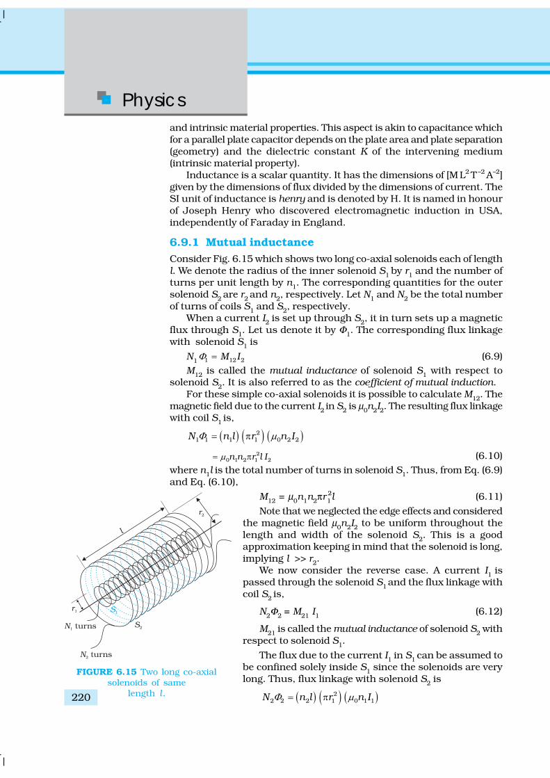
Physics
220
and intrinsic material properties. This aspect is akin to capacitance whichfor a parallel plate capacitor depends on the plate area and plate separation(geometry) and the dielectric constant K of the intervening medium(intrinsic material property).
Inductance is a scalar quantity. It has the dimensions of [M L2 T–2 A–2]given by the dimensions of flux divided by the dimensions of current. TheSI unit of inductance is henry and is denoted by H. It is named in honourof Joseph Henry who discovered electromagnetic induction in USA,independently of Faraday in England.
6.9.1 Mutual inductanceConsider Fig. 6.15 which shows two long co-axial solenoids each of lengthl. We denote the radius of the inner solenoid S1
by r1 and the number ofturns per unit length by n1. The corresponding quantities for the outersolenoid S2 are r2 and n2, respectively. Let N1 and N2 be the total numberof turns of coils S1 and S2, respectively.
When a current I2 is set up through S2, it in turn sets up a magneticflux through S1. Let us denote it by Φ1. The corresponding flux linkagewith solenoid S1 is
N1 1 12 2M IΦ = (6.9)
M12 is called the mutual inductance of solenoid S1 with respect tosolenoid S2. It is also referred to as the coefficient of mutual induction.
For these simple co-axial solenoids it is possible to calculate M12. Themagnetic field due to the current I2 in S2 is μ0n2I2. The resulting flux linkagewith coil S1 is,
( ) ( ) ( )21 1 1 1 0 2 2N n l r n IΦ μ= π
20 1 2 1 2n n r l Iμ= π (6.10)
where n1l is the total number of turns in solenoid S1. Thus, from Eq. (6.9)and Eq. (6.10),
M12 = μ0n1n2πr 21l (6.11)
Note that we neglected the edge effects and consideredthe magnetic field μ0n2I2 to be uniform throughout thelength and width of the solenoid S2. This is a goodapproximation keeping in mind that the solenoid is long,implying l >> r2.
We now consider the reverse case. A current I1 ispassed through the solenoid S1 and the flux linkage withcoil S2 is,
N2Φ2 = M21 I1 (6.12)
M21 is called the mutual inductance of solenoid S2 withrespect to solenoid S1.
The flux due to the current I1 in S1 can be assumed tobe confined solely inside S1 since the solenoids are verylong. Thus, flux linkage with solenoid S2 is
( ) ( ) ( )22 2 2 1 0 1 1N n l r n IΦ μ= π
FIGURE 6.15 Two long co-axialsolenoids of same
length l.

ElectromagneticInduction
221
EX
AM
PLE 6
.9
where n2l is the total number of turns of S2. From Eq. (6.12),
M21 = μ0n1n2πr21l (6.13)
Using Eq. (6.11) and Eq. (6.12), we get
M12 = M21= M (say) (6.14)
We have demonstrated this equality for long co-axial solenoids.However, the relation is far more general. Note that if the inner solenoidwas much shorter than (and placed well inside) the outer solenoid, thenwe could still have calculated the flux linkage N1Φ1 because the innersolenoid is effectively immersed in a uniform magnetic field due to theouter solenoid. In this case, the calculation of M12 would be easy. However,it would be extremely difficult to calculate the flux linkage with the outersolenoid as the magnetic field due to the inner solenoid would vary acrossthe length as well as cross section of the outer solenoid. Therefore, thecalculation of M21 would also be extremely difficult in this case. Theequality M12=M21 is very useful in such situations.
We explained the above example with air as the medium within thesolenoids. Instead, if a medium of relative permeability μr had been present,the mutual inductance would be
M =μr μ0 n1n2π r21 l
It is also important to know that the mutual inductance of a pair ofcoils, solenoids, etc., depends on their separation as well as their relativeorientation.
Example 6.9 Two concentric circular coils, one of small radius r1 andthe other of large radius r2, such that r1 << r2, are placed co-axiallywith centres coinciding. Obtain the mutual inductance of thearrangement.
Solution Let a current I2 flow through the outer circular coil. Thefield at the centre of the coil is B2 = μ0I2 / 2r2. Since the otherco-axially placed coil has a very small radius, B2 may be consideredconstant over its cross-sectional area. Hence,Φ1 = πr 2
1B2
2
0 12
22r
Ir
μ π=
= M12 I2Thus,
20 1
1222r
Mr
μ π=
From Eq. (6.14)2
0 112 21
22r
M Mr
μ π= =
Note that we calculated M12 from an approximate value of Φ1, assumingthe magnetic field B2 to be uniform over the area π r1
2. However, wecan accept this value because r1 << r2.

Physics
222
Now, let us recollect Experiment 6.3 in Section 6.2. In that experiment,emf is induced in coil C1 wherever there was any change in current throughcoil C2. Let Φ1 be the flux through coil C1 (say of N1 turns) when current incoil C2 is I2.
Then, from Eq. (6.9), we haveN1Φ1 = MI2For currents varrying with time,
( ) ( )1 1 2d d
d d
N MI
t t
Φ=
Since induced emf in coil C1 is given by
( )1 1d–
d
N
t
Φε1 =
We get,
2d–
dI
Mt
ε1 =
It shows that varying current in a coil can induce emf in a neighbouringcoil. The magnitude of the induced emf depends upon the rate of changeof current and mutual inductance of the two coils.
6.9.2 Self-inductanceIn the previous sub-section, we considered the flux in one solenoid dueto the current in the other. It is also possible that emf is induced in asingle isolated coil due to change of flux through the coil by means ofvarying the current through the same coil. This phenomenon is calledself-induction. In this case, flux linkage through a coil of N turns isproportional to the current through the coil and is expressed as
BN IΦ ∝
B LN IΦ = (6.15)where constant of proportionality L is called self-inductance of the coil. Itis also called the coefficient of self-induction of the coil. When the currentis varied, the flux linked with the coil also changes and an emf is inducedin the coil. Using Eq. (6.15), the induced emf is given by
( )Bd–
d
N
t
Φε =
d–
dI
Lt
ε = (6.16)
Thus, the self-induced emf always opposes any change (increase ordecrease) of current in the coil.
It is possible to calculate the self-inductance for circuits with simplegeometries. Let us calculate the self-inductance of a long solenoid of cross-sectional area A and length l, having n turns per unit length. The magneticfield due to a current I flowing in the solenoid is B = μ0 n I (neglecting edgeeffects, as before). The total flux linked with the solenoid is
( ) ( ) ( )0BN nl n I AΦ μ=

ElectromagneticInduction
223
IAln20
μ=
where nl is the total number of turns. Thus, the self-inductance is,
LIΒΝΦ
=
20n Alμ= (6.17)
If we fill the inside of the solenoid with a material of relative permeabilityμr (for example soft iron, which has a high value of relative permiability),then,
20rL n Alμ μ= (6.18)
The self-inductance of the coil depends on its geometry and on thepermeability of the medium.
The self-induced emf is also called the back emf as it opposes anychange in the current in a circuit. Physically, the self-inductance playsthe role of inertia. It is the electromagnetic analogue of mass in mechanics.So, work needs to be done against the back emf (ε ) in establishing thecurrent. This work done is stored as magnetic potential energy. For thecurrent I at an instant in a circuit, the rate of work done is
ddW
It
ε=
If we ignore the resistive losses and consider only inductive effect,then using Eq. (6.16),
d dd dW I
L It t
=
Total amount of work done in establishing the current I is
0
d dI
W W L I I= =∫ ∫Thus, the energy required to build up the current I is,
212
W LI= (6.19)
This expression reminds us of mv 2/2 for the (mechanical) kinetic energyof a particle of mass m, and shows that L is analogus to m (i.e., L is electricalinertia and opposes growth and decay of current in the circuit).
Consider the general case of currents flowing simultaneously in twonearby coils. The flux linked with one coil will be the sum of two fluxeswhich exist independently. Equation (6.9) would be modified into
N1 1 11 1 12 2M I M IΦ = +
where M11 represents inductance due to the same coil.
Therefore, using Faraday’s law,
1 21 11 12
d dd dI I
M Mt t
ε = − −
Physics
224
EX
AM
PLE 6
.10
M11 is the self-inductance and is written as L1. Therefore,
1 21 1 12
d dd dI I
L Mt t
ε = − −
Example 6.10 (a) Obtain the expression for the magnetic energy storedin a solenoid in terms of magnetic field B, area A and length l of thesolenoid. (b) How does this magnetic energy compare with theelectrostatic energy stored in a capacitor?
Solution(a) From Eq. (6.19), the magnetic energy is
212BU LI=
( )2
1since ,for a solenoid
2 00
BL B nI
nμ
μ⎛ ⎞
= =⎜ ⎟⎝ ⎠
2
20
0
1( )
2B
n Aln
μμ
⎛ ⎞= ⎜ ⎟⎝ ⎠
[from Eq. (6.17)]
2
0
12
B Alμ
=
(b) The magnetic energy per unit volume is,
BB
Uu
V= (where V is volume that contains flux)
BU
Al=
2
02B
μ= (6.20)
We have already obtained the relation for the electrostatic energystored per unit volume in a parallel plate capacitor (refer to Chapter 2,Eq. 2.77),
20
12
u EΕ ε= (2.77)
In both the cases energy is proportional to the square of the fieldstrength. Equations (6.20) and (2.77) have been derived for specialcases: a solenoid and a parallel plate capacitor, respectively. But theyare general and valid for any region of space in which a magnetic fieldor/and an electric field exist.
6.10 AC GENERATOR
The phenomenon of electromagnetic induction has been technologicallyexploited in many ways. An exceptionally important application is thegeneration of alternating currents (ac). The modern ac generator with atypical output capacity of 100 MW is a highly evolved machine. In thissection, we shall describe the basic principles behind this machine. TheYugoslav inventor Nicola Tesla is credited with the development of themachine. As was pointed out in Section 6.3, one method to induce an emf
Inte
ract
ive
an
imati
on
on
ac
ge
ne
rato
r:http://micro.m
agne
t.fsu.edu
/electromag
net~java
/gen
erator/ac.html

ElectromagneticInduction
225
or current in a loop is through a change in theloop’s orientation or a change in its effective area.As the coil rotates in a magnetic field B, theeffective area of the loop (the face perpendicularto the field) is A cos θ, where θ is the anglebetween A and B. This method of producing aflux change is the principle of operation of asimple ac generator. An ac generator convertsmechanical energy into electrical energy.
The basic elements of an ac generator areshown in Fig. 6.16. It consists of a coil mountedon a rotor shaft. The axis of rotation of the coilis perpendicular to the direction of the magneticfield. The coil (called armature) is mechanicallyrotated in the uniform magnetic field by someexternal means. The rotation of the coil causesthe magnetic flux through it to change, so anemf is induced in the coil. The ends of the coilare connected to an external circuit by meansof slip rings and brushes.
When the coil is rotated with a constantangular speed ω, the angle θ between the magnetic field vector B and thearea vector A of the coil at any instant t is θ = ωt (assuming θ = 0º at t = 0).As a result, the effective area of the coil exposed to the magnetic field lineschanges with time, and from Eq. (6.1), the flux at any time t is
ΦB = BA cos θ = BA cos ωt
From Faraday’s law, the induced emf for the rotating coil of N turns isthen,
d d– – (cos )
dt dBN NBA t
t
Φε ω= =
Thus, the instantaneous value of the emf isε ω ω=NBA sin t (6.21)
where NBAω is the maximum value of the emf, which occurs whensin ωt = ±1. If we denote NBAω as ε0, then
ε = ε0 sin ωt (6.22)
Since the value of the sine fuction varies between +1 and –1, the sign, orpolarity of the emf changes with time. Note from Fig. 6.17 that the emfhas its extremum value when θ = 90º or θ = 270º, as the change of flux isgreatest at these points.
The direction of the current changes periodically and therefore the currentis called alternating current (ac). Since ω = 2πν, Eq (6.22) can be written as
ε = ε0sin 2π ν t (6.23)
where ν is the frequency of revolution of the generator’s coil.Note that Eq. (6.22) and (6.23) give the instantaneous value of the emf
and ε varies between +ε0 and –ε0 periodically. We shall learn how todetermine the time-averaged value for the alternating voltage and currentin the next chapter.
FIGURE 6.16 AC Generator

Physics
226 EX
AM
PLE 6
.11
In commercial generators, the mechanical energy required for rotationof the armature is provided by water falling from a height, for example,from dams. These are called hydro-electric generators. Alternatively, wateris heated to produce steam using coal or other sources. The steam athigh pressure produces the rotation of the armature. These are calledthermal generators. Instead of coal, if a nuclear fuel is used, we get nuclearpower generators. Modern day generators produce electric power as highas 500 MW, i.e., one can light up 5 million 100 W bulbs! In mostgenerators, the coils are held stationary and it is the electromagnets whichare rotated. The frequency of rotation is 50 Hz in India. In certain countriessuch as USA, it is 60 Hz.
Example 6.11 Kamla peddles a stationary bicycle the pedals of thebicycle are attached to a 100 turn coil of area 0.10 m2. The coil rotatesat half a revolution per second and it is placed in a uniform magneticfield of 0.01 T perpendicular to the axis of rotation of the coil. What isthe maximum voltage generated in the coil?
Solution Here f = 0.5 Hz; N =100, A = 0.1 m2 and B = 0.01 T. EmployingEq. (6.21)
ε0 = NBA (2 π ν)
= 100 × 0.01 × 0.1 × 2 × 3.14 × 0.5
= 0.314 V
The maximum voltage is 0.314 V.
We urge you to explore such alternative possibilities for powergeneration.
FIGURE 6.17 An alternating emf is generated by a loop of wire rotating in a magnetic field.

ElectromagneticInduction
227
SUMMARY
1. The magnetic flux through a surface of area A placed in a uniform magneticfield B is defined as,
ΦB = B Ai = BA cos θwhere θ is the angle between B and A.
2. Faraday’s laws of induction imply that the emf induced in a coil of Nturns is directly related to the rate of change of flux through it,
Bdd
Nt
Φε = −
Here ΦΒ is the flux linked with one turn of the coil. If the circuit isclosed, a current I = ε/R is set up in it, where R is the resistance of thecircuit.
3. Lenz’s law states that the polarity of the induced emf is such that ittends to produce a current which opposes the change in magnetic fluxthat produces it. The negative sign in the expression for Faraday’s lawindicates this fact.
4. When a metal rod of length l is placed normal to a uniform magneticfield B and moved with a velocity v perpendicular to the field, theinduced emf (called motional emf) across its ends is
ε = Bl v
5. Changing magnetic fields can set up current loops in nearby metal(any conductor) bodies. They dissipate electrical energy as heat. Suchcurrents are called eddy currents.
6. Inductance is the ratio of the flux-linkage to current. It is equal to NΦ/I.
MIGRATION OF BIRDS
The migratory pattern of birds is one of the mysteries in the field of biology, and indeed allof science. For example, every winter birds from Siberia fly unerringly to water spots in theIndian subcontinent. There has been a suggestion that electromagnetic induction mayprovide a clue to these migratory patterns. The earth’s magnetic field has existed throughoutevolutionary history. It would be of great benefit to migratory birds to use this field todetermine the direction. As far as we know birds contain no ferromagnetic material. Soelectromagnetic induction seems to be the only reasonable mechanism to determinedirection. Consider the optimal case where the magnetic field B, the velocity of the bird v,and two relevant points of its anatomy separated by a distance l, all three are mutuallyperpendicular. From the formula for motional emf, Eq. (6.5),
ε = Blv
Taking B = 4 × 10⁻⁵ T, l = 2 cm wide, and v = 10 m/s, we obtain
ε = 4 × 10–5 × 2 × 10–2 × 10 V = 8 × 10⁻⁶ V
= 8 μV
This extremely small potential difference suggests that our hypothesis is of doubtfulvalidity. Certain kinds of fish are able to detect small potential differences. However, inthese fish, special cells have been identified which detect small voltage differences. In birdsno such cells have been identified. Thus, the migration patterns of birds continues to remaina mystery.

Physics
228
POINTS TO PONDER
1. Electricity and magnetism are intimately related. In the early part of thenineteenth century, the experiments of Oersted, Ampere and othersestablished that moving charges (currents) produce a magnetic field.Somewhat later, around 1830, the experiments of Faraday and Henrydemonstrated that a moving magnet can induce electric current.
2. In a closed circuit, electric currents are induced so as to oppose thechanging magnetic flux. It is as per the law of conservation of energy.However, in case of an open circuit, an emf is induced across its ends.How is it related to the flux change?
3. The motional emf discussed in Section 6.5 can be argued independentlyfrom Faraday’s law using the Lorentz force on moving charges. However,
Quantity Symbol Units Dimensions Equations
Magnetic Flux ΦB Wb (weber) [M L2 T –2 A–1] ΦB = B Ai
EMF ε V (volt) [M L2 T –3 A–1] ε = Bd( )/dN tΦ−
Mutual Inductance M H (henry) [M L2 T –2 A–2] ε1 ( )12 2d /dM I t= −
Self Inductance L H (henry) [M L2 T –2 A–2] ( )d /dL I tε = −
7. A changing current in a coil (coil 2) can induce an emf in a nearby coil(coil 1). This relation is given by,
21 12
ddI
Mt
ε = −
The quantity M12 is called mutual inductance of coil 1 with respect tocoil 2. One can similarly define M21. There exists a general equality,
M12 = M21
8. When a current in a coil changes, it induces a back emf in the samecoil. The self-induced emf is given by,
dd
IL
tε = −
L is the self-inductance of the coil. It is a measure of the inertia of thecoil against the change of current through it.
9. The self-inductance of a long solenoid, the core of which consists of amagnetic material of permeability μr, is given by
L = μr μ0 n2 A l
where A is the area of cross-section of the solenoid, l its length and nthe number of turns per unit length.
10. In an ac generator, mechanical energy is converted to electrical energyby virtue of electromagnetic induction. If coil of N turn and area A isrotated at ν revolutions per second in a uniform magnetic field B, thenthe motional emf produced is
ε = NBA (2πν) sin (2πνt)
where we have assumed that at time t = 0 s, the coil is perpendicular tothe field.

ElectromagneticInduction
229
EXERCISES
6.1 Predict the direction of induced current in the situations describedby the following Figs. 6.18(a) to (f ).
even if the charges are stationary [and the q (v × B) term of the Lorentzforce is not operative], an emf is nevertheless induced in the presence of atime-varying magnetic field. Thus, moving charges in static field and staticcharges in a time-varying field seem to be symmetric situation forFaraday’s law. This gives a tantalising hint on the relevance of the principleof relativity for Faraday’s law.
4. The motion of a copper plate is damped when it is allowed to oscillatebetween the magnetic pole-pieces. How is the damping force, produced bythe eddy currents?
FIGURE 6.18

Physics
230
6.2 Use Lenz’s law to determine the direction of induced current in thesituations described by Fig. 6.19:(a) A wire of irregular shape turning into a circular shape;(b) A circular loop being deformed into a narrow straight wire.
FIGURE 6.19
6.3 A long solenoid with 15 turns per cm has a small loop of area 2.0 cm2
placed inside the solenoid normal to its axis. If the current carriedby the solenoid changes steadily from 2.0 A to 4.0 A in 0.1 s, what isthe induced emf in the loop while the current is changing?
6.4 A rectangular wire loop of sides 8 cm and 2 cm with a small cut ismoving out of a region of uniform magnetic field of magnitude 0.3 Tdirected normal to the loop. What is the emf developed across thecut if the velocity of the loop is 1 cm s–1 in a direction normal to the(a) longer side, (b) shorter side of the loop? For how long does theinduced voltage last in each case?
6.5 A 1.0 m long metallic rod is rotated with an angular frequency of400 rad s–1
about an axis normal to the rod passing through its oneend. The other end of the rod is in contact with a circular metallicring. A constant and uniform magnetic field of 0.5 T parallel to theaxis exists everywhere. Calculate the emf developed between thecentre and the ring.
6.6 A circular coil of radius 8.0 cm and 20 turns is rotated about itsvertical diameter with an angular speed of 50 rad s–1 in a uniformhorizontal magnetic field of magnitude 3.0 × 10⁻² T. Obtain themaximum and average emf induced in the coil. If the coil forms aclosed loop of resistance 10 Ω, calculate the maximum value of currentin the coil. Calculate the average power loss due to Joule heating.Where does this power come from?
6.7 A horizontal straight wire 10 m long extending from east to west isfalling with a speed of 5.0 m s–1, at right angles to the horizontalcomponent of the earth’s magnetic field, 0.30 × 10⁻⁴ Wb m–2.(a) What is the instantaneous value of the emf induced in the wire?(b) What is the direction of the emf?(c) Which end of the wire is at the higher electrical potential?
6.8 Current in a circuit falls from 5.0 A to 0.0 A in 0.1 s. If an average emfof 200 V induced, give an estimate of the self-inductance of the circuit.
6.9 A pair of adjacent coils has a mutual inductance of 1.5 H. If thecurrent in one coil changes from 0 to 20 A in 0.5 s, what is thechange of flux linkage with the other coil?
6.10 A jet plane is travelling towards west at a speed of 1800 km/h. Whatis the voltage difference developed between the ends of the wing

ElectromagneticInduction
231
having a span of 25 m, if the Earth’s magnetic field at the locationhas a magnitude of 5 × 10⁻⁴ T and the dip angle is 30°.
ADDITIONAL EXERCISES
6.11 Suppose the loop in Exercise 6.4 is stationary but the currentfeeding the electromagnet that produces the magnetic field isgradually reduced so that the field decreases from its initial valueof 0.3 T at the rate of 0.02 T s–1. If the cut is joined and the loophas a resistance of 1.6 Ω, how much power is dissipated by theloop as heat? What is the source of this power?
6.12 A square loop of side 12 cm with its sides parallel to X and Y axes ismoved with a velocity of 8 cm
s–1 in the positive x-direction in an
environment containing a magnetic field in the positive z-direction.The field is neither uniform in space nor constant in time. It has agradient of 10 – 3 T cm–1
along the negative x-direction (that is it increasesby 10 – 3 T cm –1
as one moves in the negative x-direction), and it isdecreasing in time at the rate of 10–3 T s–1. Determine the direction andmagnitude of the induced current in the loop if its resistance is 4.50 mΩ.
6.13 It is desired to measure the magnitude of field between the poles of apowerful loud speaker magnet. A small flat search coil of area 2 cm2
with 25 closely wound turns, is positioned normal to the fielddirection, and then quickly snatched out of the field region.Equivalently, one can give it a quick 90° turn to bring its planeparallel to the field direction). The total charge flown in the coil(measured by a ballistic galvanometer connected to coil) is7.5 mC. The combined resistance of the coil and the galvanometer is0.50 Ω. Estimate the field strength of magnet.
6.14 Figure 6.20 shows a metal rod PQ resting on the smooth rails ABand positioned between the poles of a permanent magnet. The rails,the rod, and the magnetic field are in three mutual perpendiculardirections. A galvanometer G connects the rails through a switch K.Length of the rod = 15 cm, B = 0.50 T, resistance of the closed loopcontaining the rod = 9.0 mΩ. Assume the field to be uniform.(a) Suppose K is open and the rod is moved with a speed of 12 cm s–1
in the direction shown. Give the polarity and magnitude of theinduced emf.
FIGURE 6.20
(b) Is there an excess charge built up at the ends of the rods whenK is open? What if K is closed?
(c) With K open and the rod moving uniformly, there is no netforce on the electrons in the rod PQ even though they do

Physics
232
experience magnetic force due to the motion of the rod. Explain.(d) What is the retarding force on the rod when K is closed?(e) How much power is required (by an external agent) to keep
the rod moving at the same speed (=12 cm s–1) when K is closed?How much power is required when K is open?
(f ) How much power is dissipated as heat in the closed circuit?What is the source of this power?
(g) What is the induced emf in the moving rod if the magnetic fieldis parallel to the rails instead of being perpendicular?
6.15 An air-cored solenoid with length 30 cm, area of cross-section 25 cm2
and number of turns 500, carries a current of 2.5 A. The current issuddenly switched off in a brief time of 10–3 s. How much is the averageback emf induced across the ends of the open switch in the circuit?Ignore the variation in magnetic field near the ends of the solenoid.
6.16 (a) Obtain an expression for the mutual inductance between a longstraight wire and a square loop of side a as shown in Fig. 6.21.
(b) Now assume that the straight wire carries a current of 50 A andthe loop is moved to the right with a constant velocity, v = 10 m/s.Calculate the induced emf in the loop at the instant when x = 0.2 m.Take a = 0.1 m and assume that the loop has a large resistance.
FIGURE 6.21
6.17 A line charge λ per unit length is lodged uniformly onto the rim of awheel of mass M and radius R. The wheel has light non-conductingspokes and is free to rotate without friction about its axis (Fig. 6.22).A uniform magnetic field extends over a circular region within therim. It is given by,
B = – B0 k (r ≤ a; a < R)
= 0 (otherwise)What is the angular velocity of the wheel after the field is suddenlyswitched off?
FIGURE 6.22

7.1 INTRODUCTION
We have so far considered direct current (dc) sources and circuits with dcsources. These currents do not change direction with time. But voltagesand currents that vary with time are very common. The electric mainssupply in our homes and offices is a voltage that varies like a sine functionwith time. Such a voltage is called alternating voltage (ac voltage) andthe current driven by it in a circuit is called the alternating current (accurrent)*. Today, most of the electrical devices we use require ac voltage.This is mainly because most of the electrical energy sold by powercompanies is transmitted and distributed as alternating current. The mainreason for preferring use of ac voltage over dc voltage is that ac voltagescan be easily and efficiently converted from one voltage to the other bymeans of transformers. Further, electrical energy can also be transmittedeconomically over long distances. AC circuits exhibit characteristics whichare exploited in many devices of daily use. For example, whenever wetune our radio to a favourite station, we are taking advantage of a specialproperty of ac circuits – one of many that you will study in this chapter.
Chapter Seven
ALTERNATINGCURRENT
* The phrases ac voltage and ac current are contradictory and redundant,respectively, since they mean, literally, alternating current voltage and alternatingcurrent current. Still, the abbreviation ac to designate an electrical quantitydisplaying simple harmonic time dependance has become so universally acceptedthat we follow others in its use. Further, voltage – another phrase commonlyused means potential difference between two points.

Physics
234
NIC
OLA
TE
SLA
(1836 –
1943)
Nicola Tesla (1836 –1943) Yugoslov scientist,inventor and genius. Heconceived the idea of therotating magnetic field,which is the basis ofpractically all alternatingcurrent machinery, andwhich helped usher in theage of electric power. Healso invented among otherthings the induction motor,the polyphase system of acpower, and the highfrequency induction coil(the Tesla coil) used in radioand television sets andother electronic equipment.The SI unit of magnetic fieldis named in his honour.
7.2 AC VOLTAGE APPLIED TO A RESISTOR
Figure 7.1 shows a resistor connected to a source ε ofac voltage. The symbol for an ac source in a circuitdiagram is ~ . We consider a source which producessinusoidally varying potential difference across itsterminals. Let this potential difference, also called acvoltage, be given by
sinmv v tω= (7.1)
where vm is the amplitude of the oscillating potentialdifference and ω is its angular frequency.
To find the value of current through the resistor, we
apply Kirchhoff’s loop rule ( ) 0ε =∑ t , to the circuit
shown in Fig. 7.1 to get
=sinmv t i Rω
or sinmvi t
Rω=
Since R is a constant, we can write this equation as
sinmi i tω= (7.2)where the current amplitude im is given by
mm
vi
R= (7.3)
Equation (7.3) is just Ohm’s law which for resistors worksequally well for both ac and dc voltages. The voltage across apure resistor and the current through it, given by Eqs. (7.1) and(7.2) are plotted as a function of time in Fig. 7.2. Note, inparticular that both v and i reach zero, minimum and maximumvalues at the same time. Clearly, the voltage and current are inphase with each other.
We see that, like the applied voltage, the current variessinusoidally and has corresponding positive and negative valuesduring each cycle. Thus, the sum of the instantaneous currentvalues over one complete cycle is zero, and the average currentis zero. The fact that the average current is zero, however, does
FIGURE 7.1 AC voltage applied to a resistor.
FIGURE 7.2 In a pureresistor, the voltage and
current are in phase. Theminima, zero and maxima
occur at the samerespective times.

Alternating Current
235
GE
OR
GE
WE
STIN
GH
OU
SE
(1846 – 1
914)
George Westinghouse(1846 – 1914) A leadingproponent of the use ofalternating current overdirect current. Thus,he came into conflictwith Thomas Alva Edison,an advocate of directcurrent. Westinghousewas convinced that thetechnology of alternatingcurrent was the key tothe electrical future.He founded the famousCompany named after himand enlisted the servicesof Nicola Tesla andother inventors in thedevelopment of alternatingcurrent motors andapparatus for thetransmission of hightension current, pioneeringin large scale lighting.
not mean that the average power consumed is zero andthat there is no dissipation of electrical energy. As youknow, Joule heating is given by i2R and depends on i2
(which is always positive whether i is positive or negative)and not on i. Thus, there is Joule heating anddissipation of electrical energy when anac current passes through a resistor.The instantaneous power dissipated in the resistor is
2 2 2sinmp i R i R tω= = (7.4)
The average value of p over a cycle is*2 2 2sinmp i R i R tω= < > = < > [7.5(a)]
where the bar over a letter(here, p) denotes its averagevalue and <......> denotes taking average of the quantityinside the bracket. Since, i2
m and R are constants,2 2sinmp i R tω= < > [7.5(b)]
Using the trigonometric identity, sin2 ωt =1/2 (1– cos 2ωt ), we have < sin2 ωt > = (1/2) (1– < cos 2ωt >)and since < cos2ωt > = 0**, we have,
2 1sin
2tω< > =
Thus,
212 mp i R= [7.5(c)]
To express ac power in the same form as dc power(P = I2R), a special value of current is defined and used.It is called, root mean square (rms) or effective current(Fig. 7.3) and is denoted by Irms or I.
* The average value of a function F (t ) over a period T is given by d0
1( ) ( )
T
F t F t tT
= ∫
** [ ]0 0
sin 21 1 1cos2 cos2 sin 2 0 0
2 2
TT tt t dt T
T T T
ωω ω ω
ω ω⎡ ⎤< > = = = − =∫ ⎢ ⎥⎣ ⎦
FIGURE 7.3 The rms current I is related to the
peak current im by I = / 2mi = 0.707 i
m.

Physics
236
It is defined by
2 212 2
mm
iI i i= = =
= 0.707 im (7.6)
In terms of I, the average power, denoted by P is
2 212 m
pP i R I R= = = (7.7)
Similarly, we define the rms voltage or effective voltage by
V = 2mv
= 0.707 vm (7.8)
From Eq. (7.3), we have
vm = imR
or, 2 2m mv i
R=
or, V = IR (7.9)
Equation (7.9) gives the relation between ac current and ac voltageand is similar to that in the dc case. This shows the advantage ofintroducing the concept of rms values. In terms of rms values, the equationfor power [Eq. (7.7)] and relation between current and voltage in ac circuitsare essentially the same as those for the dc case.It is customary to measure and specify rms values for ac quantities. Forexample, the household line voltage of 220 V is an rms value with a peakvoltage of
vm = 2 V = (1.414)(220 V) = 311 V
In fact, the I or rms current is the equivalent dc current that wouldproduce the same average power loss as the alternating current. Equation(7.7) can also be written as
P = V2 / R = I V (since V = I R )
Example 7.1 A light bulb is rated at 100W for a 220 V supply. Find(a) the resistance of the bulb; (b) the peak voltage of the source; and(c) the rms current through the bulb.
Solution(a) We are given P = 100 W and V = 220 V. The resistance of the
bulb is
( )22 220 V
484100 W
VR
P= = = Ω
(b) The peak voltage of the source is
V2 311m
v V= =
(c) Since, P = I V
100 W0.450A
220 VP
IV
= = =
EX
AM
PLE 7
.1

Alternating Current
237
7.3 REPRESENTATION OF AC CURRENT AND VOLTAGE
BY ROTATING VECTORS — PHASORS
In the previous section, we learnt that the current through a resistor isin phase with the ac voltage. But this is not so in the case of an inductor,a capacitor or a combination of these circuit elements. In order to showphase relationship between voltage and currentin an ac circuit, we use the notion of phasors.The analysis of an ac circuit is facilitated by theuse of a phasor diagram. A phasor* is a vectorwhich rotates about the origin with angularspeed ω, as shown in Fig. 7.4. The verticalcomponents of phasors V and I represent thesinusoidally varying quantities v and i. Themagnitudes of phasors V and I represent theamplitudes or the peak values vm and im of theseoscillating quantities. Figure 7.4(a) shows thevoltage and current phasors and theirrelationship at time t1 for the case of an ac sourceconnected to a resistor i.e., corresponding to thecircuit shown in Fig. 7.1. The projection ofvoltage and current phasors on vertical axis, i.e., vm sinωt and im sinωt,respectively represent the value of voltage and current at that instant. Asthey rotate with frequency ω, curves in Fig. 7.4(b) are generated.From Fig. 7.4(a) we see that phasors V and I for the case of a resistor arein the same direction. This is so for all times. This means that the phaseangle between the voltage and the current is zero.
7.4 AC VOLTAGE APPLIED TO AN INDUCTOR
Figure 7.5 shows an ac source connected to an inductor. Usually,inductors have appreciable resistance in their windings, but we shallassume that this inductor has negligible resistance.Thus, the circuit is a purely inductive ac circuit. Letthe voltage across the source be v = vm sinωt. Using
the Kirchhoff’s loop rule, ( ) 0tε =∑ , and since there
is no resistor in the circuit,
d0
di
v Lt
− = (7.10)
where the second term is the self-induced Faradayemf in the inductor; and L is the self-inductance of
FIGURE 7.4 (a) A phasor diagram for thecircuit in Fig 7.1. (b) Graph of v and
i versus ωt.
FIGURE 7.5 An ac sourceconnected to an inductor.
* Though voltage and current in ac circuit are represented by phasors – rotatingvectors, they are not vectors themselves. They are scalar quantities. It so happensthat the amplitudes and phases of harmonically varying scalars combinemathematically in the same way as do the projections of rotating vectors ofcorresponding magnitudes and directions. The rotating vectors that representharmonically varying scalar quantities are introduced only to provide us with asimple way of adding these quantities using a rule that we already know.

Physics
238
the inductor. The negative sign follows from Lenz’s law (Chapter 6).Combining Eqs. (7.1) and (7.10), we have
dsin
dmvi v
tt L L
ω= = (7.11)
Equation (7.11) implies that the equation for i(t), the current as afunction of time, must be such that its slope di/dt is a sinusoidally varyingquantity, with the same phase as the source voltage and an amplitudegiven by vm/L. To obtain the current, we integrate di/dt with respect totime:
dd sin( )d
dmvi
t t tt L
ω=∫ ∫and get,
cos( ) constantmvi t
L= − ω +
ωThe integration constant has the dimension of current and is time-
independent. Since the source has an emf which oscillates symmetricallyabout zero, the current it sustains also oscillates symmetrically aboutzero, so that no constant or time-independent component of the currentexists. Therefore, the integration constant is zero.
Using
cos( ) sin2
t tω ω π⎛ ⎞− = −⎜ ⎟⎝ ⎠ , we have
sin2mi i tω π⎛ ⎞= −⎜ ⎟⎝ ⎠ (7.12)
where mm
vi
L=
ω is the amplitude of the current. The quantity ω L is
analogous to the resistance and is called inductive reactance, denotedby XL:
XL = ω L (7.13)
The amplitude of the current is, then
mm
L
vi
X= (7.14)
The dimension of inductive reactance is the same as that of resistanceand its SI unit is ohm (Ω). The inductive reactance limits the current in apurely inductive circuit in the same way as the resistance limits thecurrent in a purely resistive circuit. The inductive reactance is directlyproportional to the inductance and to the frequency of the current.
A comparison of Eqs. (7.1) and (7.12) for the source voltage and thecurrent in an inductor shows that the current lags the voltage by π/2 orone-quarter (1/4) cycle. Figure 7.6 (a) shows the voltage and the currentphasors in the present case at instant t1. The current phasor I is π/2behind the voltage phasor V. When rotated with frequency ω counter-clockwise, they generate the voltage and current given by Eqs. (7.1) and(7.12), respectively and as shown in Fig. 7.6(b).
Inte
ract
ive a
nim
atio
n o
n P
has
or
dia
gra
ms
of
ac c
ircu
its
con
tain
ing
, R
, L,
C a
nd
RLC
seri
es
circ
uit
s:http://www.phy
s.un
sw.edu
.au/~jw
/AC.htm
l

Alternating Current
239
EX
AM
PLE 7
.2
We see that the current reaches its maximum value later than the
voltage by one-fourth of a period /2
4T
ωπ⎡ ⎤=⎢ ⎥⎣ ⎦
. You have seen that an
inductor has reactance that limits current similar to resistance in adc circuit. Does it also consume power like a resistance? Let us try tofind out.
The instantaneous power supplied to the inductor is
( )sin × sin2L m mp i v i t v tω ωπ⎛ ⎞= = −⎜ ⎟⎝ ⎠
( ) ( )cos sinm mi v t tω ω= −
( )sin 22
m mi vtω= −
So, the average power over a complete cycle is
( )L sin 22
m mi vP tω= −
( )sin 22
m mi vtω= − = 0,
since the average of sin (2ωt) over a complete cycle is zero.Thus, the average power supplied to an inductor over one complete
cycle is zero.Figure 7.7 explains it in detail.
Example 7.2 A pure inductor of 25.0 mH is connected to a source of220 V. Find the inductive reactance and rms current in the circuit ifthe frequency of the source is 50 Hz.
Solution The inductive reactance,
–= . 32 2 3 14 50 25 10 WLX Lνπ × × × ×= = 7.85Ω
The rms current in the circuit is
VA
22028
7.85L
VI
X= = =
Ω
FIGURE 7.6 (a) A Phasor diagram for the circuit in Fig. 7.5.(b) Graph of v and i versus ωt.

Physics
240
0-1 Current i through the coil entering at Aincrease from zero to a maximum value. Fluxlines are set up i.e., the core gets magnetised.With the polarity shown voltage and currentare both positive. So their product p is positive.ENERGY IS ABSORBED FROM THESOURCE.
1-2 Current in the coil is still positive but isdecreasing. The core gets demagnetised andthe net flux becomes zero at the end of a halfcycle. The voltage v is negative (since di/dt isnegative). The product of voltage and currentis negative, and ENERGY IS BEINGRETURNED TO SOURCE.
One complete cycle of voltage/current. Note that the current lags the voltage.
2-3 Current i becomes negative i.e., it entersat B and comes out of A. Since the directionof current has changed, the polarity of themagnet changes. The current and voltage areboth negative. So their product p is positive.ENERGY IS ABSORBED.
3-4 Current i decreases and reaches its zerovalue at 4 when core is demagnetised and fluxis zero. The voltage is positive but the currentis negative. The power is, therefore, negative.ENERGY ABSORBED DURING THE 1/4CYCLE 2-3 IS RETURNED TO THE SOURCE.
FIGURE 7.7 Magnetisation and demagnetisation of an inductor.

Alternating Current
241
7.5 AC VOLTAGE APPLIED TO A CAPACITOR
Figure 7.8 shows an ac source ε generating ac voltage v = vm sin ωtconnected to a capacitor only, a purely capacitive ac circuit.
When a capacitor is connected to a voltage sourcein a dc circuit, current will flow for the short timerequired to charge the capacitor. As chargeaccumulates on the capacitor plates, the voltageacross them increases, opposing the current. That is,a capacitor in a dc circuit will limit or oppose thecurrent as it charges. When the capacitor is fullycharged, the current in the circuit falls to zero.
When the capacitor is connected to an ac source,as in Fig. 7.8, it limits or regulates the current, butdoes not completely prevent the flow of charge. Thecapacitor is alternately charged and discharged asthe current reverses each half cycle. Let q be thecharge on the capacitor at any time t. The instantaneous voltage v acrossthe capacitor is
qv
C= (7.15)
From the Kirchhoff’s loop rule, the voltage across the source and thecapacitor are equal,
sinm
qv t
Cω =
To find the current, we use the relation ddq
it
=
( )dd
sin cos( )m mi v C t C v tt
ω ω ω= =
Using the relation, cos( ) sin2
t tω ωπ⎛ ⎞= +⎜ ⎟⎝ ⎠
, we have
sin2mi i tωπ⎛ ⎞= +⎜ ⎟⎝ ⎠ (7.16)
where the amplitude of the oscillating current is im = ωCvm. We can rewriteit as
(1/ )m
m
vi
Cω=
Comparing it to im= vm/R for a purely resistive circuit, we find that(1/ωC) plays the role of resistance. It is called capacitive reactance andis denoted by Xc,
Xc= 1/ωC (7.17)
so that the amplitude of the current is
mm
C
vi
X= (7.18)
FIGURE 7.8 An ac sourceconnected to a capacitor.

Physics
242
FIGURE 7.9 (a) A Phasor diagram for the circuitin Fig. 7.8. (b) Graph of v and i versus ωt.
The dimension of capacitive reactance is thesame as that of resistance and its SI unit isohm (Ω). The capacitive reactance limits theamplitude of the current in a purely capacitivecircuit in the same way as the resistance limitsthe current in a purely resistive circuit. But itis inversely proportional to the frequency andthe capacitance.
A comparison of Eq. (7.16) with theequation of source voltage, Eq. (7.1) shows thatthe current is π/2 ahead of voltage.
Figure 7.9(a) shows the phasor diagram at an instant t1. Here the currentphasor I is π/2 ahead of the voltage phasor V as they rotatecounterclockwise. Figure 7.9(b) shows the variation of voltage and currentwith time. We see that the current reaches its maximum value earlier thanthe voltage by one-fourth of a period.
The instantaneous power supplied to the capacitor ispc = i v = im cos(ωt)vm sin(ωt) = imvm cos(ωt) sin(ωt)
sin(2 )2
m mi vtω= (7.19)
So, as in the case of an inductor, the average power
sin(2 ) sin(2 ) 02 2
m m m mC
i v i vP t tω ω= = =
since <sin (2ωt)> = 0 over a complete cycle. Figure 7.10 explains it in detail.Thus, we see that in the case of an inductor, the current lags the voltageby π/2 and in the case of a capacitor, the current leads the voltage by π/2.
Example 7.3 A lamp is connected in series with a capacitor. Predictyour observations for dc and ac connections. What happens in eachcase if the capacitance of the capacitor is reduced?
Solution When a dc source is connected to a capacitor, the capacitorgets charged and after charging no current flows in the circuit andthe lamp will not glow. There will be no change even if C is reduced.With ac source, the capacitor offers capacitative reactance (1/ωC )and the current flows in the circuit. Consequently, the lamp will shine.Reducing C will increase reactance and the lamp will shine less brightlythan before.
Example 7.4 A 15.0 μF capacitor is connected to a 220 V, 50 Hz source.Find the capacitive reactance and the current (rms and peak) in thecircuit. If the frequency is doubled, what happens to the capacitivereactance and the current?
Solution The capacitive reactance is
F6
1 1212
2 2 (50Hz)(15.0 10 )CXCν −= = = Ω
π π ×
The rms current is EX
AM
PLE 7
.4 E
XA
MPLE 7
.3

Alternating Current
243
0-1 The current i flows as shown and from themaximum at 0, reaches a zero value at 1. The plateA is charged to positive polarity while negative chargeq builds up in B reaching a maximum at 1 until thecurrent becomes zero. The voltage vc = q/C is in phasewith q and reaches maximum value at 1. Currentand voltage are both positive. So p = vci is positive.ENERGY IS ABSORBED FROM THE SOURCEDURING THIS QUAR TER CYCLE AS THECAPACITOR IS CHARGED.
1-2 The current i reverses its direction. Theaccumulated charge is depleted i.e., the capacitor isdischarged during this quarter cycle.The voltage getsreduced but is still positive. The current is negative.Their product, the power is negative.THE ENERGY ABSORBED DURING THE 1/4CYCLE 0-1 IS RETURNED DURING THIS QUARTER.
One complete cycle of voltage/current. Note that the current leads the voltage.
2-3 As i continues to flow from A to B, the capacitoris charged to reversed polarity i.e., the plate Bacquires positive and A acquires negative charge.Both the current and the voltage are negative. Theirproduct p is positive. The capacitor ABSORBSENERGY during this 1/4 cycle.
3-4 The current i reverses its direction at 3 and flowsfrom B to A. The accumulated charge is depletedand the magnitude of the voltage vc is reduced. vc
becomes zero at 4 when the capacitor is fullydischarged. The power is negative.ENERGYABSORBED DURING 2-3 IS RETURNED TO THESOURCE. NET ENERGY ABSORBED IS ZERO.
FIGURE 7.10 Charging and discharging of a capacitor.

Physics
244
EX
AM
PLE 7
.5 E
XA
MPLE 7
.4
VA
2201.04
212C
VI
X= = =
Ω
The peak current is
2 (1.41)(1.04 ) 1.47mi I A A= = =
This current oscillates between +1.47A and –1.47 A, and is ahead ofthe voltage by π/2.
If the frequency is doubled, the capacitive reactance is halved andconsequently, the current is doubled.
Example 7.5 A light bulb and an open coil inductor are connected toan ac source through a key as shown in Fig. 7.11.
FIGURE 7.11
The switch is closed and after sometime, an iron rod is inserted intothe interior of the inductor. The glow of the light bulb (a) increases; (b)decreases; (c) is unchanged, as the iron rod is inserted. Give youranswer with reasons.
Solution As the iron rod is inserted, the magnetic field inside the coilmagnetizes the iron increasing the magnetic field inside it. Hence,the inductance of the coil increases. Consequently, the inductivereactance of the coil increases. As a result, a larger fraction of theapplied ac voltage appears across the inductor, leaving less voltageacross the bulb. Therefore, the glow of the light bulb decreases.
7.6 AC VOLTAGE APPLIED TO A SERIES LCR CIRCUIT
Figure 7.12 shows a series LCR circuit connected to an ac source ε. Asusual, we take the voltage of the source to be v = vm sin ωt.
If q is the charge on the capacitor and i thecurrent, at time t, we have, from Kirchhoff’s looprule:
ddi q
L i R vt C
+ + = (7.20)
We want to determine the instantaneouscurrent i and its phase relationship to the appliedalternating voltage v. We shall solve this problemby two methods. First, we use the technique ofphasors and in the second method, we solveEq. (7.20) analytically to obtain the time–dependence of i .
FIGURE 7.12 A series LCR circuitconnected to an ac source.

Alternating Current
245
7.6.1 Phasor-diagram solutionFrom the circuit shown in Fig. 7.12, we see that the resistor, inductorand capacitor are in series. Therefore, the ac current in each element isthe same at any time, having the same amplitude and phase. Let it be
i = im sin(ωt+φ ) (7.21)
where φ is the phase difference between the voltage across the source andthe current in the circuit. On the basis of what we have learnt in the previoussections, we shall construct a phasor diagram for the present case.
Let I be the phasor representing the current in the circuit as given byEq. (7.21). Further, let VL, VR, VC, and V represent the voltage across theinductor, resistor, capacitor and the source, respectively. From previoussection, we know that VR is parallel to I, VC is π/2behind I and VL is π/2 ahead of I. VL, VR, VC and Iare shown in Fig. 7.13(a) with apppropriate phase-relations.
The length of these phasors or the amplitudeof VR, VC and VL are:
vRm = im R, vCm = im XC, vLm = im XL (7.22)
The voltage Equation (7.20) for the circuit canbe written as
vL + vR + vC = v (7.23)
The phasor relation whose vertical componentgives the above equation is
VL + VR + VC = V (7.24)
This relation is represented in Fig. 7.13(b). SinceVC and VL are always along the same line and inopposite directions, they can be combined into a single phasor (VC + VL)which has a magnitude vCm – vLm. Since V is represented as thehypotenuse of a right-traingle whose sides are VR and (VC + VL), thepythagorean theorem gives:
( )22 2m Rm Cm Lmv v v v= + −
Substituting the values of vRm, vCm, and vLm from Eq. (7.22) into the aboveequation, we have
2 2 2( ) ( )m m m C m Lv i R i X i X= + −
2 2 2( )m C Li R X X⎡ ⎤= + −⎣ ⎦
or, 2 2( )m
m
C L
vi
R X X=
+ −[7.25(a)]
By analogy to the resistance in a circuit, we introduce the impedance Zin an ac circuit:
mm
vi
Z= [7.25(b)]
where 2 2( )C LZ R X X= + − (7.26)
FIGURE 7.13 (a) Relation between thephasors VL, VR, VC, and I, (b) Relation
between the phasors VL, VR, and (VL + VC)for the circuit in Fig. 7.11.

Physics
246
Since phasor I is always parallel to phasor VR, the phase angle φis the angle between VR and V and can be determined fromFig. 7.14:
tan Cm Lm
Rm
v v
vφ
−=
Using Eq. (7.22), we have
tan C LX X
Rφ
−= (7.27)
Equations (7.26) and (7.27) are graphically shown in Fig. (7.14).This is called Impedance diagram which is a right-triangle withZ as its hypotenuse.
Equation 7.25(a) gives the amplitude of the current and Eq. (7.27)gives the phase angle. With these, Eq. (7.21) is completely specified.
If XC > XL, φ is positive and the circuit is predominantly capacitive.Consequently, the current in the circuit leads the source voltage. IfXC < XL, φ is negative and the circuit is predominantly inductive.Consequently, the current in the circuit lags the source voltage.
Figure 7.15 shows the phasor diagram and variation of v and i with ω tfor the case XC > XL.
Thus, we have obtained the amplitudeand phase of current for an LCR series circuitusing the technique of phasors. But thismethod of analysing ac circuits suffers fromcertain disadvantages. First, the phasordiagram say nothing about the initialcondition. One can take any arbitrary valueof t (say, t1, as done throughout this chapter)and draw different phasors which show therelative angle between different phasors.The solution so obtained is called thesteady-state solution. This is not a generalsolution. Additionally, we do have atransient solution which exists even forv = 0. The general solution is the sum of thetransient solution and the steady-state
solution. After a sufficiently long time, the effects of the transient solutiondie out and the behaviour of the circuit is described by the steady-statesolution.
7.6.2 Analytical solutionThe voltage equation for the circuit is
dd
i qL R i v
t C+ + =
= vm sin ωt
We know that i = dq/dt. Therefore, di/dt = d2q/dt2. Thus, in terms of q,the voltage equation becomes
FIGURE 7.14 Impedancediagram.
FIGURE 7.15 (a) Phasor diagram of V and I.(b) Graphs of v and i versus ω t for a series LCR
circuit where XC > X
L.

Alternating Current
247
2
2
d dsin
dd m
q q qL R v t
t Ctω+ + = (7.28)
This is like the equation for a forced, damped oscillator, [see Eq. 14.37(b)in Class XI Physics Textbook]. Let us assume a solution
q = qm sin (ω t + θ ) [7.29(a)]
so that d
cos( )d m
qq t
tω ω θ= + [7.29(b)]
and 2
22
dsin( )
d m
qq t
tω ω θ= − + [7.29(c)]
Substituting these values in Eq. (7.28), we get
[ ]cos( ) ( )sin( )m C Lq R t X X tω ω θ ω θ+ + − + = sinmv tω (7.30)
where we have used the relation Xc= 1/ωC, XL = ω L. Multiplying and
dividing Eq. (7.30) by ( )22c LZ R X X= + − , we have
( )cos( ) sin( )C L
m
X XRq Z t t
Z Zω ω θ ω θ
−⎡ ⎤+ + +⎢ ⎥⎣ ⎦sinmv tω= (7.31)
Now, let cosR
Zφ=
and ( )
sinC LX X
Zφ
−=
so that 1tan C LX X
Rφ − −
= (7.32)
Substituting this in Eq. (7.31) and simplifying, we get:
cos( ) sinm mq Z t v tω ω θ φ ω+ − = (7.33)
Comparing the two sides of this equation, we see that
m m mv q Z i Zω= =where
m mi q ω= [7.33(a)]
and 2
θ φπ
− = − or 2
θ φπ
= − + [7.33(b)]
Therefore, the current in the circuit is
dd
cos( )m
qi q t
tω ω θ= = +
= im cos(ωt + θ )or i = imsin(ωt + φ ) (7.34)
where 2 2( )
m mm
C L
v vi
Z R X X= =
+ −[7.34(a)]
and 1tan C LX X
Rφ − −
=

Physics
248
Thus, the analytical solution for the amplitude and phase of the currentin the circuit agrees with that obtained by the technique of phasors.
7.6.3 ResonanceAn interesting characteristic of the series RLC circuit is the phenomenonof resonance. The phenomenon of resonance is common among systemsthat have a tendency to oscillate at a particular frequency. This frequencyis called the system’s natural frequency. If such a system is driven by anenergy source at a frequency that is near the natural frequency, theamplitude of oscillation is found to be large. A familiar example of thisphenomenon is a child on a swing. The the swing has a natural frequencyfor swinging back and forth like a pendulum. If the child pulls on therope at regular intervals and the frequency of the pulls is almost thesame as the frequency of swinging, the amplitude of the swinging will belarge (Chapter 14, Class XI).
For an RLC circuit driven with voltage of amplitude vm and frequencyω, we found that the current amplitude is given by
2 2( )m m
m
C L
v vi
Z R X X= =
+ −
with Xc = 1/ωC and XL = ω L . So if ω is varied, then at a particular frequency
ω0, Xc = XL, and the impedance is minimum ( )2 20Z R R= + = . This
frequency is called the resonant frequency:
00
1orc LX X L
Cω
ω= =
or 0
1
LCω = (7.35)
At resonant frequency, the current amplitude is maximum; im = vm/R.Figure 7.16 shows the variation of im with ω in
a RLC series circuit with L = 1.00 mH, C =1.00 nF for two values of R: (i) R = 100 Ωand (ii) R = 200 Ω. For the source applied vm =
100 V. ω0 for this case is 1
LC
⎛ ⎞⎜ ⎟⎝ ⎠ = 1.00×10⁶
rad/s.We see that the current amplitude is maximum
at the resonant frequency. Since im = vm / R atresonance, the current amplitude for case (i) istwice to that for case (ii).
Resonant circuits have a variety ofapplications, for example, in the tuningmechanism of a radio or a TV set. The antenna ofa radio accepts signals from many broadcasting
stations. The signals picked up in the antenna acts as a source in thetuning circuit of the radio, so the circuit can be driven at many frequencies.
FIGURE 7.16 Variation of im with ω for two
cases: (i) R = 100 Ω, (ii) R = 200 Ω,L = 1.00 mH.

Alternating Current
249
But to hear one particular radio station, we tune the radio. In tuning, wevary the capacitance of a capacitor in the tuning circuit such that theresonant frequency of the circuit becomes nearly equal to the frequencyof the radio signal received. When this happens, the amplitude of thecurrent with the frequency of the signal of the particular radio station inthe circuit is maximum.
It is important to note that resonance phenomenon is exhibited by acircuit only if both L and C are present in the circuit. Only then do thevoltages across L and C cancel each other (both being out of phase)and the current amplitude is vm/R, the total source voltage appearingacross R. This means that we cannot have resonance in a RL or RCcircuit.
Sharpness of resonanceThe amplitude of the current in the series LCR circuit is given by
22 1
mm
vi
R LC
ωω
=⎛ ⎞
+ −⎜ ⎟⎝ ⎠
and is maximum when 0 1/ .L Cω ω= = The maximum value is
max /m mi v R= .
For values of ω other than ω0, the amplitude of the current is lessthan the maximum value. Suppose we choose a value of ω for which the
current amplitude is 1/ 2 times its maximum value. At this value, the
power dissipated by the circuit becomes half. From the curve inFig. (7.16), we see that there are two such values of ω, say, ω1 and ω2, onegreater and the other smaller than ω0 and symmetrical about ω0. We maywrite
ω1 = ω0 + Δω
ω2 = ω0 – Δω
The difference ω1 – ω2 = 2Δω is often called the bandwidth of the circuit.The quantity (ω0 / 2Δω) is regarded as a measure of the sharpness ofresonance. The smaller the Δω, the sharper or narrower is the resonance.To get an expression for Δω, we note that the current amplitude im is
( ) max1/ 2m
i for ω1 = ω0 + Δω. Therefore,
1 2
21
1
at ,1
mm
vi
R LC
ω
ωω
=⎛ ⎞
+ −⎜ ⎟⎝ ⎠
max
2 2m mi v
R= =

Physics
250
or
2
21
1
12R L R
Cω
ω⎛ ⎞
+ − =⎜ ⎟⎝ ⎠
or
2
2 21
1
12R L R
Cω
ω⎛ ⎞
+ − =⎜ ⎟⎝ ⎠
11
1L R
Cω
ω− =
which may be written as,
00
1( )
( )L R
Cω ω
ω ω+ Δ − =
+ Δ
00
00
11
1
L R
C
ωω
ω ωωω
⎛ ⎞Δ+ − =⎜ ⎟ ⎛ ⎞⎝ ⎠ Δ
+⎜ ⎟⎝ ⎠
Using 20
1L C
ω = in the second term on the left hand side, we get
00
0
0
1
1
LL R
ωωω
ω ωω
⎛ ⎞Δ+ − =⎜ ⎟ ⎛ ⎞⎝ ⎠ Δ
+⎜ ⎟⎝ ⎠
We can approximate
1
0
1ω
ω
−⎛ ⎞Δ
+⎜ ⎟⎝ ⎠ as
0
1ω
ω⎛ ⎞Δ
−⎜ ⎟⎝ ⎠ since 0
ωωΔ
<<1. Therefore,
0 00 0
1 1L L Rω ωω ω
ω ω⎛ ⎞ ⎛ ⎞Δ Δ
+ − − =⎜ ⎟ ⎜ ⎟⎝ ⎠ ⎝ ⎠
or 00
2L R
ωω
ωΔ
=
2R
LωΔ = [7.36(a)]
The sharpness of resonance is given by,
0 0
2L
R
ω ωω
=Δ [7.36(b)]
The ratio 0L
R
ω is also called the quality factor, Q of the circuit.
0LQ
R
ω= [7.36(c)]
From Eqs. [7.36 (b)] and [7.36 (c)], we see that 02Q
ωωΔ = . So, larger the

Alternating Current
251
EX
AM
PLE 7
.6
value of Q, the smaller is the value of 2Δω or the bandwidth and sharperis the resonance. Using 2
0 1/L Cω = , Eq. [7.36(c)] can be equivalentlyexpressed as Q = 1/ω0CR.
We see from Fig. 7.15, that if the resonance is less sharp, not only isthe maximum current less, the circuit is close to resonance for a largerrange Δω of frequencies and the tuning of the circuit will not be good. So,less sharp the resonance, less is the selectivity of the circuit or vice versa.From Eq. (7.36), we see that if quality factor is large, i.e., R is low or L islarge, the circuit is more selective.
Example 7.6 A resistor of 200 Ω and a capacitor of 15.0 μF areconnected in series to a 220 V, 50 Hz ac source. (a) Calculate thecurrent in the circuit; (b) Calculate the voltage (rms) across theresistor and the capacitor. Is the algebraic sum of these voltagesmore than the source voltage? If yes, resolve the paradox.
Solution
Given
F 6200 , 15.0 15.0 10 FR C −= Ω = μ = ×
220 V, 50HzV ν= =(a) In order to calculate the current, we need the impedance of thecircuit. It is
2 2 2 2(2 )CZ R X R Cπ ν −= + = +
F2 6 2(200 ) (2 3.14 50 10 )− −= Ω + × × ×
2 2(200 ) (212 )= Ω + Ω
291.5= Ω
Therefore, the current in the circuit is
V2200.755 A
291.5V
IZ
= = =Ω
(b) Since the current is the same throughout the circuit, we have
(0.755 A)(200 ) 151VRV I R= = Ω =
(0.755 A)(212.3 ) 160.3 VC CV I X= = Ω =
The algebraic sum of the two voltages, VR and VC is 311.3 V which ismore than the source voltage of 220 V. How to resolve this paradox?As you have learnt in the text, the two voltages are not in the samephase. Therefore, they cannot be added like ordinary numbers. Thetwo voltages are out of phase by ninety degrees. Therefore, the totalof these voltages must be obtained using the Pythagorean theorem:
2 2R C R CV V V+ = +
= 220 VThus, if the phase difference between two voltages is properly takeninto account, the total voltage across the resistor and the capacitor isequal to the voltage of the source.

Physics
252 EX
AM
PLE 7
.7
7.7 POWER IN AC CIRCUIT: THE POWER FACTOR
We have seen that a voltage v = vm sinωt applied to a series RLC circuitdrives a current in the circuit given by i = im sin(ωt + φ) where
mm
vi
Z= and 1tan C LX X
Rφ − −⎛ ⎞= ⎜ ⎟⎝ ⎠
Therefore, the instantaneous power p supplied by the source is
( ) [ ]sin sin( )m mp v i v t i tω ω φ= = × +
[ ]cos cos(2 )2
m mv itφ ω φ= − + (7.37)
The average power over a cycle is given by the average of the two terms inR.H.S. of Eq. (7.37). It is only the second term which is time-dependent.Its average is zero (the positive half of the cosine cancels the negativehalf). Therefore,
cos2
m mv iP φ= cos
2 2m mv i
φ=
cosV I φ= [7.38(a)]
This can also be written as,
2 cosP I Z φ= [7.38(b)]
So, the average power dissipated depends not only on the voltage andcurrent but also on the cosine of the phase angle φ between them. Thequantity cosφ is called the power factor. Let us discuss the followingcases:
Case (i) Resistive circuit: If the circuit contains only pure R, it is calledresistive. In that case φ = 0, cos φ = 1. There is maximum power dissipation.
Case (ii) Purely inductive or capacitive circuit: If the circuit containsonly an inductor or capacitor, we know that the phase difference betweenvoltage and current is π/2. Therefore, cos φ = 0, and no power is dissipatedeven though a current is flowing in the circuit. This current is sometimesreferred to as wattless current.
Case (iii) LCR series circuit: In an LCR series circuit, power dissipated isgiven by Eq. (7.38) where φ = tan–1 (Xc – XL )/ R. So, φ may be non-zero ina RL or RC or RCL circuit. Even in such cases, power is dissipated only inthe resistor.
Case (iv) Power dissipated at resonance in LCR circuit: At resonanceXc – XL= 0, and φ = 0. Therefore, cosφ = 1 and P = I2Z = I 2 R. That is,maximum power is dissipated in a circuit (through R) at resonance.
Example7.7 (a) For circuits used for transporting electric power, alow power factor implies large power loss in transmission. Explain.
(b) Power factor can often be improved by the use of a capacitor ofappropriate capacitance in the circuit. Explain.

Alternating Current
253
EX
AM
PLE 7
.7
Solution (a) We know that P = I V cosφ where cosφ is the power factor.To supply a given power at a given voltage, if cosφ is small, we have toincrease current accordingly. But this will lead to large power loss(I2R) in transmission.
(b)Suppose in a circuit, current I lags the voltage by an angle φ. Thenpower factor cosφ =R/Z.
We can improve the power factor (tending to 1) by making Z tend to R.Let us understand, with the help of a phasor diagram (Fig. 7.17) howthis can be achieved. Let us resolve I into two components. Ip along
the applied voltage V and Iq perpendicular to the applied voltage. Iq
as you have learnt in Section 7.7, is called the wattless componentsince corresponding to this component of current, there is no powerloss. IP is known as the power component because it is in phase withthe voltage and corresponds to power loss in the circuit.
It’s clear from this analysis that if we want to improve power factor,we must completely neutralize the lagging wattless current Iq by anequal leading wattless current I′q. This can be done by connecting acapacitor of appropriate value in parallel so that Iq and I′q canceleach other and P is effectively Ip V.
Example 7.8 A sinusoidal voltage of peak value 283 V and frequency50 Hz is applied to a series LCR circuit in whichR = 3 Ω, L = 25.48 mH, and C = 796 μF. Find (a) the impedance of thecircuit; (b) the phase difference between the voltage across the sourceand the current; (c) the power dissipated in the circuit; and (d) thepower factor.
Solution(a) To find the impedance of the circuit, we first calculate XL and XC.
XL = 2 πνL = 2 × 3.14 × 50 × 25.48 × 10–3 Ω = 8 Ω
12CX
Cν=
π
FIGURE 7.17
EX
AM
PLE 7
.8

Physics
254 EX
AM
PLE 7
.9
6
14
2 3.14 50 796 10−= = Ω× × × ×
Therefore,
2 2 2 2( ) 3 (8 4)L CZ R X X= + − = + −
= 5 Ω
(b) Phase difference, φ = tan–1 C LX X
R
−
1 4 8tan 53.1
3− −⎛ ⎞= = − °⎜ ⎟⎝ ⎠
Since φ is negative, the current in the circuit lags the voltageacross the source.
(c) The power dissipated in the circuit is2P I R=
Now, A1 28340
52 2miI ⎛ ⎞= = =⎜ ⎟⎝ ⎠
Therefore, A W2(40 ) 3 4800P = × Ω =
(d) Power factor = cos cos53.1 0.6φ = ° =
Example 7.9 Suppose the frequency of the source in the previousexample can be varied. (a) What is the frequency of the source atwhich resonance occurs? (b) Calculate the impedance, the current,and the power dissipated at the resonant condition.
Solution
(a) The frequency at which the resonance occurs is
0 3 6
1 1
25.48 10 796 10LCω
− −= =
× × ×
222.1rad/s=
0 221.1Hz 35.4Hz
2 2 3.14r
ων = = =
π ×
(b) The impedance Z at resonant condition is equal to the resistance:
3Z R= = Ω
The rms current at resonance is
A283 166.7
32
V V
Z R⎛ ⎞
= = = =⎜ ⎟⎝ ⎠
The power dissipated at resonance is
2 2(66.7) 3 13.35 kWP I R= × = × =
You can see that in the present case, power dissipatedat resonance is more than the power dissipated in Example 7.8.
EX
AM
PLE 7
.8

Alternating Current
255
EX
AM
PLE 7
.10
Example 7.10 At an airport, a person is made to walk through thedoorway of a metal detector, for security reasons. If she/he is carryinganything made of metal, the metal detector emits a sound. On whatprinciple does this detector work?
Solution The metal detector works on the principle of resonance inac circuits. When you walk through a metal detector, you are,in fact, walking through a coil of many turns. The coil is connected toa capacitor tuned so that the circuit is in resonance. Whenyou walk through with metal in your pocket, the impedance of thecircuit changes – resulting in significant change in current in thecircuit. This change in current is detected and the electronic circuitrycauses a sound to be emitted as an alarm.
7.8 LC OSCILLATIONS
We know that a capacitor and an inductor can store electrical andmagnetic energy, respectively. When a capacitor (initially charged) isconnected to an inductor, the charge on the capacitor andthe current in the circuit exhibit the phenomenon ofelectrical oscillations similar to oscillations in mechanicalsystems (Chapter 14, Class XI).
Let a capacitor be charged qm (at t = 0) and connectedto an inductor as shown in Fig. 7.18.
The moment the circuit is completed, the charge onthe capacitor starts decreasing, giving rise to current inthe circuit. Let q and i be the charge and current in thecircuit at time t. Since di/dt is positive, the induced emfin L will have polarity as shown, i.e., vb < va. According toKirchhoff’s loop rule,
d0
dq i
LC t
− = (7.39)
i = – (dq/dt ) in the present case (as q decreases, i increases).Therefore, Eq. (7.39) becomes:
2
2
d 10
dq
qLCt
+ = (7.40)
This equation has the form 2
202
d0
dx
xt
ω+ = for a simple harmonic
oscillator. The charge, therefore, oscillates with a natural frequency
0
1
LCω = (7.41)
and varies sinusoidally with time as
( )0cosmq q tω φ= + (7.42)
where qm is the maximum value of q and φ is a phase constant. Sinceq = qm at t = 0, we have cos φ =1 or φ = 0. Therefore, in the present case,
FIGURE 7.18 At theinstant shown, the current
is increasing so thepolarity of induced emf inthe inductor is as shown.

Physics
256
0cos( )mq q tω= (7.43)
The current ddq
it
⎛ ⎞= −⎜ ⎟⎝ ⎠ is given by
0sin( )mi i tω= (7.44)
where 0m mi qω=Let us now try to visualise how this oscillation takes place in the
circuit.Figure 7.19(a) shows a capacitor with initial charge qm connected to
an ideal inductor. The electrical energy stored in the charged capacitor is21
2m
E
qU
C= . Since, there is no current in the circuit, energy in the inductor
is zero. Thus, the total energy of LC circuit is,21
2m
E
qU U
C= =
FIGURE 7.19 The oscillations in an LC circuit are analogous to the oscillation of ablock at the end of a spring. The figure depicts one-half of a cycle.
At t = 0, the switch is closed and the capacitor starts to discharge[Fig. 7.19(b)]. As the current increases, it sets up a magnetic field in theinductor and thereby, some energy gets stored in the inductor in theform of magnetic energy: UB = (1/2) Li2. As the current reaches itsmaximum value im, (at t = T/4) as in Fig. 7.19(c), all the energy is storedin the magnetic field: UB = (1/2) Li2m. You can easily check that themaximum electrical energy equals the maximum magnetic energy. Thecapacitor now has no charge and hence no energy. The current nowstarts charging the capacitor, as in Fig. 7.19(d). This process continuestill the capacitor is fully charged (at t = T/2) [Fig. 7.19(e)]. But it is chargedwith a polarity opposite to its initial state in Fig. 7.19(a). The whole processjust described will now repeat itself till the system reverts to its originalstate. Thus, the energy in the system oscillates between the capacitorand the inductor.

Alternating Current
257
The LC oscillation is similar to the mechanical oscillation of a blockattached to a spring. The lower part of each figure in Fig. 7.19 depictsthe corresponding stage of a mechanical system (a block attached to aspring). As noted earlier, for a block of a mass m oscillating with frequencyω0, the equation is
22
2 0
d0
dx
xt
ω+ =
Here, 0 /k mω = , and k is the spring constant. So, x corresponds to q.
In case of a mechanical system F = ma = m (dv/dt) = m (d2x/dt2). For anelectrical system, ε = –L (di/dt ) = –L (d2q/dt 2). Comparing these twoequations, we see that L is analogous to mass m: L is a measure of
resistance to change in current. In case of LC circuit, 0 1/ LCω = and
for mass on a spring, 0 /k mω = . So, 1/C is analogous to k. The constant
k (=F/x) tells us the (external) force required to produce a unitdisplacement whereas 1/C (=V/q ) tells us the potential difference requiredto store a unit charge. Table 7.1 gives the analogy between mechanicaland electrical quantities.
TABLE 7.1 ANALOGIES BETWEEN MECHANICAL AND
ELECTRICAL QUANTITIES
Mechanical system Slectrical system
Mass m Inductance L
Force constant k Reciprocal capacitance1/C
Displacement x Charge q
Velocity v = dx/dt Current i = dq/dt
Mechanical energy Electromagnetic energy
2 21 12 2
E kx mv= +2
21 12 2
qU L i
C= +
Note that the above discussion of LC oscillations is not realistic for tworeasons:(i) Every inductor has some resistance. The effect of this resistance is to
introduce a damping effect on the charge and current in the circuitand the oscillations finally die away.
(ii) Even if the resistance were zero, the total energy of the system wouldnot remain constant. It is radiated away from the system in the formof electromagnetic waves (discussed in the next chapter). In fact, radioand TV transmitters depend on this radiation.

Physics
258
TWO DIFFERENT PHENOMENA, SAME MATHEMATICAL TREATMENT
You may like to compare the treatment of a forced damped oscillator discussed in Section14.10 of Class XI physics textbook, with that of an LCR circuit when an ac voltage isapplied in it. We have already remarked that Eq. [14.37(b)] of Class XI Textbook is exactlysimilar to Eq. (7.28) here, although they use different symbols and parameters. Let ustherefore list the equivalence between different quantities in the two situations:
Forced oscillations Driven LCR circuit
cos d
2d x dxm b kx F2 dtdt
tω+ + =2
2
d dsin
dd m
q q qL R v t
t Ctω+ + =
Displacement, x Charge on capacitor, q
Time, t Time, t
Mass, m Self inductance, L
Damping constant, b Resistance, R
Spring constant, k Inverse capacitance, 1/C
Driving frequency, ωd Driving frequency, ω
Natural frequency of oscillations, ω Natural frequency of LCR circuit, ω0
Amplitude of forced oscillations, A Maximum charge stored, qm
Amplitude of driving force, F0 Amplitude of applied voltage, vm
You must note that since x corresponds to q, the amplitude A (maximum displacement)will correspond to the maximum charge stored, q
m. Equation [14.39 (a)] of Class XI gives
the amplitude of oscillations in terms of other parameters, which we reproduce here forconvenience:
0
1/22 2 2 2 2 2( )d d
FA
m bω ω ω=
− +
Replace each parameter in the above equation by the corresponding electricalquantity, and see what happens. Eliminate L, C, ω , and ω
0, using X
L= ωL, X
C = 1/ωC, and
ω02 = 1/LC. When you use Eqs. (7.33) and (7.34), you will see that there is a
perfect match.
You will come across numerous such situations in physics where diverse physicalphenomena are represented by the same mathematical equation. If you have dealt withone of them, and you come across another situation, you may simply replace thecorresponding quantities and interpret the result in the new context. We suggest thatyou may try to find more such parallel situations from different areas of physics. Onemust, of course, be aware of the differences too.

Alternating Current
259
EX
AM
PLE 7
.11
Example 7.11 Show that in the free oscillations of an LC circuit, thesum of energies stored in the capacitor and the inductor is constantin time.
Solution Let q0 be the initial charge on a capacitor. Let the chargedcapacitor be connected to an inductor of inductance L. As you havestudied in Section 7.8, this LC circuit will sustain an oscillation withfrquency
ω 1
2LC
π ν⎛ ⎞= =⎜ ⎟⎝ ⎠
At an instant t, charge q on the capacitor and the current i are givenby:q (t) = q0 cos ωt
i (t) = – q0 ω sin ωt
Energy stored in the capacitor at time t is
222 201 1
( )2 2 2E
qqU C V cos t
C Cω= = =
Energy stored in the inductor at time t is
212MU L i=
2 2 20
1sin ( )
2L q tω ω=
( )2
2 20 sin ( ) 1/2q
t LCC
ω ω= =∵
Sum of energies
22 20 cos sin
2E M
qU U t t
Cω ω⎡ ⎤+ = +⎣ ⎦
20
2q
C=
This sum is constant in time as qo and C, both are time-independent.Note that it is equal to the initial energy of the capacitor. Why it isso? Think!
7.9 TRANSFORMERS
For many purposes, it is necessary to change (or transform) an alternatingvoltage from one to another of greater or smaller value. This is done witha device called transformer using the principle of mutual induction.
A transformer consists of two sets of coils, insulated from each other.They are wound on a soft-iron core, either one on top of the other as inFig. 7.20(a) or on separate limbs of the core as in Fig. 7.20(b). One of thecoils called the primary coil has Np turns. The other coil is called thesecondary coil; it has Ns turns. Often the primary coil is the input coiland the secondary coil is the output coil of the transformer.

Physics
260
When an alternating voltage is applied to the primary, the resultingcurrent produces an alternating magnetic flux which links the secondaryand induces an emf in it. The value of this emf depends on the number ofturns in the secondary. We consider an ideal transformer in which theprimary has negligible resistance and all the flux in the core links bothprimary and secondary windings. Let φ be the flux in each turn in thecore at time t due to current in the primary when a voltage vp is appliedto it.
Then the induced emf or voltage εs, in the secondary with Ns turns is
dds sN
t
φε = − (7.45)
The alternating flux φ also induces an emf, called back emf in theprimary. This is
ddp pN
t
φε = − (7.46)
But εp = vp. If this were not so, the primary current would be infinitesince the primary has zero resistance(as assumed). If the secondary isan open circuit or the current taken from it is small, then to a goodapproximation
εs = vswhere vs is the voltage across the secondary. Therefore, Eqs. (7.45) and(7.46) can be written as
s s
dv N
d t
φ= − [7.45(a)]
p p
dv N
d t
φ= − [7.46(a)]
From Eqs. [7.45 (a)] and [7.45 (a)], we have
s s
p p
v N
v N= (7.47)
FIGURE 7.20 Two arrangements for winding of primary and secondary coil in a transformer:(a) two coils on top of each other, (b) two coils on separate limbs of the core.

Alternating Current
261
Note that the above relation has been obtained using threeassumptions: (i) the primary resistance and current are small; (ii) thesame flux links both the primary and the secondary as very little fluxescapes from the core, and (iii) the secondary current is small.
If the transformer is assumed to be 100% efficient (no energy losses),the power input is equal to the power output, and since p = i v,
ipvp = isvs (7.48)
Although some energy is always lost, this is a good approximation,since a well designed transformer may have an efficiency of more than95%. Combining Eqs. (7.47) and (7.48), we have
p s s
s p p
i v N
i v N= = (7.49)
Since i and v both oscillate with the same frequency as the ac source,Eq. (7.49) also gives the ratio of the amplitudes or rms values ofcorresponding quantities.
Now, we can see how a transformer affects the voltage and current.We have:
ss p
p
NV V
N
⎛ ⎞= ⎜ ⎟
⎝ ⎠ and
ps p
s
NI I
N
⎛ ⎞= ⎜ ⎟⎝ ⎠ (7.50)
That is, if the secondary coil has a greater number of turns than theprimary (Ns > Np), the voltage is stepped up(Vs > Vp). This type ofarrangement is called a step-up transformer. However, in this arrangement,there is less current in the secondary than in the primary (Np/Ns < 1 and Is< Ip). For example, if the primary coil of a transformer has 100 turns andthe secondary has 200 turns, Ns/Np = 2 and Np/Ns=1/2. Thus, a 220Vinput at 10A will step-up to 440 V output at 5.0 A.
If the secondary coil has less turns than the primary(Ns < Np), we havea step-down transformer. In this case, Vs < Vp and Is > Ip. That is, thevoltage is stepped down, or reduced, and the current is increased.
The equations obtained above apply to ideal transformers (withoutany energy losses). But in actual transformers, small energy losses dooccur due to the following reasons:(i) Flux Leakage: There is always some flux leakage; that is, not all of
the flux due to primary passes through the secondary due to poordesign of the core or the air gaps in the core. It can be reduced bywinding the primary and secondary coils one over the other.
(ii) Resistance of the windings: The wire used for the windings has someresistance and so, energy is lost due to heat produced in the wire(I 2R). In high current, low voltage windings, these are minimised byusing thick wire.
(iii) Eddy currents: The alternating magnetic flux induces eddy currentsin the iron core and causes heating. The effect is reduced by having alaminated core.
(iv) Hysteresis: The magnetisation of the core is repeatedly reversed bythe alternating magnetic field. The resulting expenditure of energy inthe core appears as heat and is kept to a minimum by using a magneticmaterial which has a low hysteresis loss.

Physics
262
The large scale transmission and distribution of electrical energy overlong distances is done with the use of transformers. The voltage outputof the generator is stepped-up (so that current is reduced andconsequently, the I 2R loss is cut down). It is then transmitted over longdistances to an area sub-station near the consumers. There the voltageis stepped down. It is further stepped down at distributing sub-stationsand utility poles before a power supply of 240 V reaches our homes.
SUMMARY
1. An alternating voltage sinm
v v t= ω applied to a resistor R drives a
current i = im sinωt in the resistor, m
m
vi
R= . The current is in phase with
the applied voltage.
2. For an alternating current i = im sinωt passing through a resistor R, theaverage power loss P (averaged over a cycle) due to joule heating is( 1/2 )i2
mR. To express it in the same form as the dc power (P = I 2R), aspecial value of current is used. It is called root mean square (rms)current and is donoted by I:
0.7072
mm
iI i= =
Similarly, the rms voltage is defined by
0.7072m
m
vV v= =
We have P = IV = I2R
3. An ac voltage v = vm sinωt applied to a pure inductor L, drives a currentin the inductor i = im sin (ωt – π/2), where im = vm/XL. XL = ωL is calledinductive reactance. The current in the inductor lags the voltage byπ/2. The average power supplied to an inductor over one complete cycleis zero.
4. An ac voltage v = vm sinωt applied to a capacitor drives a current in thecapacitor: i = im sin (ωt + π/2). Here,
1,m
m CC
vi X
X Cω= = is called capacitive reactance.
The current through the capacitor is π/2 ahead of the applied voltage.As in the case of inductor, the average power supplied to a capacitorover one complete cycle is zero.
5. For a series RLC circuit driven by voltage v = vm sinωt, the current isgiven by i = im sin (ωt + φ )
where( )22
mm
C L
vi
R X X=
+ −
and 1tan C LX X
Rφ − −
=
( )22C LZ R X X= + − is called the impedance of the circuit.

Alternating Current
263
The average power loss over a complete cycle is given by
P = V I cosφThe term cosφ is called the power factor.
6. In a purely inductive or capacitive circuit, cosφ = 0 and no power isdissipated even though a current is flowing in the circuit. In such cases,current is referred to as a wattless current.
7. The phase relationship between current and voltage in an ac circuitcan be shown conveniently by representing voltage and current byrotating vectors called phasors. A phasor is a vector which rotatesabout the origin with angular speed ω. The magnitude of a phasorrepresents the amplitude or peak value of the quantity (voltage orcurrent) represented by the phasor.
The analysis of an ac circuit is facilitated by the use of a phasordiagram.
8. An interesting characteristic of a series RLC circuit is thephenomenon of resonance. The circuit exhibits resonance, i.e.,the amplitude of the current is maximum at the resonant
frequency, 01
LCω = . The quality factor Q defined by
0LQ
R
ω=
0
1CRω
= is an indicator of the sharpness of the resonance,
the higher value of Q indicating sharper peak in the current.
9. A circuit containing an inductor L and a capacitor C (initiallycharged) with no ac source and no resistors exhibits freeoscillations. The charge q of the capacitor satisfies the equationof simple harmonic motion:
2
2
d 10
LCdt+ =
and therefore, the frequency ω of free oscillation is 01
LCω = . The
energy in the system oscillates between the capacitor and theinductor but their sum or the total energy is constant in time.
10. A transformer consists of an iron core on which are bound aprimary coil of Np turns and a secondary coil of Ns turns. If theprimary coil is connected to an ac source, the primary andsecondary voltages are related by
ss p
p
NV V
N
⎛ ⎞= ⎜ ⎟
⎝ ⎠
and the currents are related by
pps
s
NI I
N
⎛ ⎞= ⎜ ⎟⎝ ⎠
If the secondary coil has a greater number of turns than the primary, thevoltage is stepped-up (Vs > Vp). This type of arrangement is called a step-up transformer. If the secondary coil has turns less than the primary, wehave a step-down transformer.

Physics
264
Physical quantity Symbol Dimensions Unit Remarks
rms voltage V [M L2 T–3 A–1] V V = 2mv
, vm is the
amplitude of the ac voltage.
rms current I [ A] A I = 2
mi , im is the amplitude of
the ac current.
Reactance: Inductive XL [M L2 T –3 A–2] Ω XL = ω L
Capacitive XC [M L2 T –3 A–2] Ω XC = 1/ω C
Impedance Z [M L2 T –3 A–2] Ω Depends on elementspresent in the circuit.
Resonant ωr or ω0 [T –1] Hz ω0 LC
1= for a
frequencyseries RLC circuit
Quality factor Q Dimensionless 0
0
1LQ
R C R
ωω
= = for a series
RLC circuit.
Power factor Dimensionless = cosφ, φ is the phasedifference between voltageapplied and current inthe circuit.
POINTS TO PONDER
1. When a value is given for ac voltage or current, it is ordinarily the rmsvalue. The voltage across the terminals of an outlet in your room isnormally 240 V. This refers to the rms value of the voltage. The amplitudeof this voltage is
V2 2(240) 340mv V= = =
2. The power rating of an element used in ac circuits refers to its averagepower rating.
3. The power consumed in an circuit is never negative.
4. Both alternating current and direct current are measured in amperes.But how is the ampere defined for an alternating current? It cannot bederived from the mutual attraction of two parallel wires carrying accurrents, as the dc ampere is derived. An ac current changes direction

Alternating Current
265
with the source frequency and the attractive force would average tozero. Thus, the ac ampere must be defined in terms of some propertythat is independent of the direction of the current. Joule heatingis such a property, and there is one ampere of rms value ofalternating current in a circuit if the current produces the sameaverage heating effect as one ampere of dc current would produceunder the same conditions.
5. In an ac circuit, while adding voltages across different elements, oneshould take care of their phases properly. For example, if VR and VC
are voltages across R and C, respectively in an RC circuit, then the
total voltage across RC combination is 2 2RC R CV V V= + and not
VR + VC since VC is π/2 out of phase of VR.
6. Though in a phasor diagram, voltage and current are represented byvectors, these quantities are not really vectors themselves. They arescalar quantities. It so happens that the amplitudes and phases ofharmonically varying scalars combine mathematically in the sameway as do the projections of rotating vectors of correspondingmagnitudes and directions. The ‘rotating vectors’ that representharmonically varying scalar quantities are introduced only to provideus with a simple way of adding these quantities using a rule thatwe already know as the law of vector addition.
7. There are no power losses associated with pure capacitances and pureinductances in an ac circuit. The only element that dissipates energyin an ac circuit is the resistive element.
8. In a RLC circuit, resonance phenomenon occur when XL = XC or
01
LCω = . For resonance to occur, the presence of both L and C
elements in the circuit is a must. With only one of these (L or C )elements, there is no possibility of voltage cancellation and hence,no resonance is possible.
9. The power factor in a RLC circuit is a measure of how close thecircuit is to expending the maximum power.
10. In generators and motors, the roles of input and output arereversed. In a motor, electric energy is the input and mechanicalenergy is the output. In a generator, mechanical energy is theinput and electric energy is the output. Both devices simplytransform energy from one form to another.
11. A transformer (step-up) changes a low-voltage into a high-voltage.This does not violate the law of conservation of energy. Thecurrent is reduced by the same proportion.
12. The choice of whether the description of an oscillatory motion isby means of sines or cosines or by their linear combinations isunimportant, since changing the zero-time position transformsthe one to the other.

Physics
266
EXERCISES
7.1 A 100 Ω resistor is connected to a 220 V, 50 Hz ac supply.
(a) What is the rms value of current in the circuit?(b) What is the net power consumed over a full cycle?
7.2 (a) The peak voltage of an ac supply is 300 V. What is the rms voltage?(b) The rms value of current in an ac circuit is 10 A. What is the
peak current?7.3 A 44 mH inductor is connected to 220 V, 50 Hz ac supply. Determine
the rms value of the current in the circuit.
7.4 A 60 μF capacitor is connected to a 110 V, 60 Hz ac supply. Determinethe rms value of the current in the circuit.
7.5 In Exercises 7.3 and 7.4, what is the net power absorbed by eachcircuit over a complete cycle. Explain your answer.
7.6 Obtain the resonant frequency ωr of a series LCR circuit withL = 2.0H, C = 32 μF and R = 10 Ω. What is the Q-value of this circuit?
7.7 A charged 30 μF capacitor is connected to a 27 mH inductor. What isthe angular frequency of free oscillations of the circuit?
7.8 Suppose the initial charge on the capacitor in Exercise 7.7 is 6 mC.What is the total energy stored in the circuit initially? What is thetotal energy at later time?
7.9 A series LCR circuit with R = 20 Ω, L = 1.5 H and C = 35 μF is connectedto a variable-frequency 200 V ac supply. When the frequency of thesupply equals the natural frequency of the circuit, what is the averagepower transferred to the circuit in one complete cycle?
7.10 A radio can tune over the frequency range of a portion of MWbroadcast band: (800 kHz to 1200 kHz). If its LC circuit has an effectiveinductance of 200 μH, what must be the range of its variablecapacitor?
[Hint: For tuning, the natural frequency i.e., the frequency of freeoscillations of the LC circuit should be equal to the frequency of theradiowave.]
7.11 Figure 7.21 shows a series LCR circuit connected to a variablefrequency 230 V source. L = 5.0 H, C = 80μF, R = 40 Ω.
(a) Determine the source frequency which drives the circuit inresonance.
(b) Obtain the impedance of the circuit and the amplitude of currentat the resonating frequency.
(c) Determine the rms potential drops across the three elements ofthe circuit. Show that the potential drop across the LCcombination is zero at the resonating frequency.
FIGURE 7.21

Alternating Current
267
ADDITIONAL EXERCISES
7.12 An LC circuit contains a 20 mH inductor and a 50 μF capacitor withan initial charge of 10 mC. The resistance of the circuit is negligible.Let the instant the circuit is closed be t = 0.
(a) What is the total energy stored initially? Is it conserved duringLC oscillations?
(b) What is the natural frequency of the circuit?(c) At what time is the energy stored
(i) completely electrical (i.e., stored in the capacitor)? (ii) completelymagnetic (i.e., stored in the inductor)?
(d) At what times is the total energy shared equally between theinductor and the capacitor?
(e) If a resistor is inserted in the circuit, how much energy iseventually dissipated as heat?
7.13 A coil of inductance 0.50 H and resistance 100 Ω is connected to a240 V, 50 Hz ac supply.
(a) What is the maximum current in the coil?
(b) What is the time lag between the voltage maximum and thecurrent maximum?
7.14 Obtain the answers (a) to (b) in Exercise 7.13 if the circuit isconnected to a high frequency supply (240 V, 10 kHz). Hence, explainthe statement that at very high frequency, an inductor in a circuitnearly amounts to an open circuit. How does an inductor behave ina dc circuit after the steady state?
7.15 A 100 μF capacitor in series with a 40 Ω resistance is connected to a110 V, 60 Hz supply.
(a) What is the maximum current in the circuit?(b) What is the time lag between the current maximum and the
voltage maximum?
7.16 Obtain the answers to (a) and (b) in Exercise 7.15 if the circuit isconnected to a 110 V, 12 kHz supply? Hence, explain the statementthat a capacitor is a conductor at very high frequencies. Compare thisbehaviour with that of a capacitor in a dc circuit after the steady state.
7.17 Keeping the source frequency equal to the resonating frequency ofthe series LCR circuit, if the three elements, L, C and R are arrangedin parallel, show that the total current in the parallel LCR circuit isminimum at this frequency. Obtain the current rms value in eachbranch of the circuit for the elements and source specified inExercise 7.11 for this frequency.
7.18 A circuit containing a 80 mH inductor and a 60 μF capacitor in seriesis connected to a 230 V, 50 Hz supply. The resistance of the circuit isnegligible.
(a) Obtain the current amplitude and rms values.(b) Obtain the rms values of potential drops across each element.(c) What is the average power transferred to the inductor?(d) What is the average power transferred to the capacitor?(e) What is the total average power absorbed by the circuit? [‘Average’
implies ‘averaged over one cycle’.]
7.19 Suppose the circuit in Exercise 7.18 has a resistance of 15 Ω. Obtainthe average power transferred to each element of the circuit, andthe total power absorbed.

Physics
268
7.20 A series LCR circuit with L = 0.12 H, C = 480 nF, R = 23 Ω is connectedto a 230 V variable frequency supply.
(a) What is the source frequency for which current amplitude ismaximum. Obtain this maximum value.
(b) What is the source frequency for which average power absorbedby the circuit is maximum. Obtain the value of this maximumpower.
(c) For which frequencies of the source is the power transferred tothe circuit half the power at resonant frequency? What is thecurrent amplitude at these frequencies?
(d) What is the Q-factor of the given circuit?
7.21 Obtain the resonant frequency and Q-factor of a series LCR circuitwith L = 3.0 H, C = 27 μF, and R = 7.4 Ω. It is desired to improve thesharpness of the resonance of the circuit by reducing its ‘full widthat half maximum’ by a factor of 2. Suggest a suitable way.
7.22 Answer the following questions:
(a) In any ac circuit, is the applied instantaneous voltage equal tothe algebraic sum of the instantaneous voltages across the serieselements of the circuit? Is the same true for rms voltage?
(b) A capacitor is used in the primary circuit of an induction coil.(c) An applied voltage signal consists of a superposition of a dc voltage
and an ac voltage of high frequency. The circuit consists of aninductor and a capacitor in series. Show that the dc signal willappear across C and the ac signal across L.
(d) A choke coil in series with a lamp is connected to a dc line. Thelamp is seen to shine brightly. Insertion of an iron core in thechoke causes no change in the lamp’s brightness. Predict thecorresponding observations if the connection is to an ac line.
(e) Why is choke coil needed in the use of fluorescent tubes with acmains? Why can we not use an ordinary resistor instead of thechoke coil?
7.23 A power transmission line feeds input power at 2300 V to a step-down transformer with its primary windings having 4000 turns. Whatshould be the number of turns in the secondary in order to get outputpower at 230 V?
7.24 At a hydroelectric power plant, the water pressure head is at a heightof 300 m and the water flow available is 100 m3s–1. If the turbinegenerator efficiency is 60%, estimate the electric power availablefrom the plant (g = 9.8 ms–2 ).
7.25 A small town with a demand of 800 kW of electric power at 220 V issituated 15 km away from an electric plant generating power at 440 V.The resistance of the two wire line carrying power is 0.5 Ω per km.The town gets power from the line through a 4000-220 V step-downtransformer at a sub-station in the town.
(a) Estimate the line power loss in the form of heat.
(b) How much power must the plant supply, assuming there isnegligible power loss due to leakage?
(c) Characterise the step up transformer at the plant.
7.26 Do the same exercise as above with the replacement of the earliertransformer by a 40,000-220 V step-down transformer (Neglect, asbefore, leakage losses though this may not be a good assumptionany longer because of the very high voltage transmission involved).Hence, explain why high voltage transmission is preferred?

Chapter Eight
ELECTROMAGNETICWAVES
8.1 INTRODUCTION
In Chapter 4, we learnt that an electric current produces magnetic fieldand that two current-carrying wires exert a magnetic force on each other.Further, in Chapter 6, we have seen that a magnetic field changing withtime gives rise to an electric field. Is the converse also true? Does anelectric field changing with time give rise to a magnetic field? James ClerkMaxwell (1831-1879), argued that this was indeed the case – not onlyan electric current but also a time-varying electric field generates magneticfield. While applying the Ampere’s circuital law to find magnetic field at apoint outside a capacitor connected to a time-varying current, Maxwellnoticed an inconsistency in the Ampere’s circuital law. He suggested theexistence of an additional current, called by him, the displacementcurrent to remove this inconsistency.
Maxwell formulated a set of equations involving electric and magneticfields, and their sources, the charge and current densities. Theseequations are known as Maxwell’s equations. Together with the Lorentzforce formula (Chapter 4), they mathematically express all the basic lawsof electromagnetism.
The most important prediction to emerge from Maxwell’s equationsis the existence of electromagnetic waves, which are (coupled) time-varying electric and magnetic fields that propagate in space. The speedof the waves, according to these equations, turned out to be very close to

Physics
270
the speed of light( 3 ×10⁸ m/s), obtained from opticalmeasurements. This led to the remarkable conclusionthat light is an electromagnetic wave. Maxwell’s workthus unified the domain of electricity, magnetism andlight. Hertz, in 1885, experimentally demonstrated theexistence of electromagnetic waves. Its technological useby Marconi and others led in due course to therevolution in communication that we are witnessingtoday.
In this chapter, we first discuss the need fordisplacement current and its consequences. Then wepresent a descriptive account of electromagnetic waves.The broad spectrum of electromagnetic waves,stretching from γ rays (wavelength ~10–12 m) to longradio waves (wavelength ~106 m) is described. How theelectromagnetic waves are sent and received forcommunication is discussed in Chapter 15.
8.2 DISPLACEMENT CURRENT
We have seen in Chapter 4 that an electrical currentproduces a magnetic field around it. Maxwell showedthat for logical consistency, a changing electric field mustalso produce a magnetic field. This effect is of greatimportance because it explains the existence of radiowaves, gamma rays and visible light, as well as all otherforms of electromagnetic waves.
To see how a changing electric field gives rise toa magnetic field, let us consider the process ofcharging of a capacitor and apply Ampere’s circuitallaw given by (Chapter 4)
“B.dl = μ0 i (t ) (8.1)
to find magnetic field at a point outside the capacitor.Figure 8.1(a) shows a parallel plate capacitor C whichis a part of circuit through which a time-dependentcurrent i (t ) flows . Let us find the magnetic field at apoint such as P, in a region outside the parallel platecapacitor. For this, we consider a plane circular loop ofradius r whose plane is perpendicular to the directionof the current-carrying wire, and which is centredsymmetrically with respect to the wire [Fig. 8.1(a)]. Fromsymmetry, the magnetic field is directed along thecircumference of the circular loop and is the same inmagnitude at all points on the loop so that if B is themagnitude of the field, the left side of Eq. (8.1) is B (2π r).So we have
B (2πr) = μ0i (t ) (8 .2)
JA
ME
S C
LE
RK
MA
XW
ELL (1
831–1
879)
James Clerk Maxwell(1831 – 1879) Born inEdinburgh, Scotland,was among the greatestphysicists of thenineteenth century. Hederived the thermalvelocity distribution ofmolecules in a gas andwas among the first toobtain reliableestimates of molecularparameters frommeasurable quantitieslike viscosity, etc.Maxwell’s greatestacheivement was theunification of the laws ofelectricity andmagnetism (discoveredby Coulomb, Oersted,Ampere and Faraday)into a consistent set ofequations now calledMaxwell’s equations.From these he arrived atthe most importantconclusion that light isan electromagneticwave. Interestingly,Maxwell did not agreewith the idea (stronglysuggested by theFaraday’s laws ofelectrolysis) thatelectricity wasparticulate in nature.

ElectromagneticWaves
271
Now, consider a different surface, which has the same boundary. Thisis a pot like surface [Fig. 8.1(b)] which nowhere touches the current, buthas its bottom between the capacitor plates; its mouth is the circularloop mentioned above. Another such surface is shaped like a tiffin box(without the lid) [Fig. 8.1(c)]. On applying Ampere’s circuital law to suchsurfaces with the same perimeter, we find that the left hand side ofEq. (8.1) has not changed but the right hand side is zero and not μ0i,since no current passes through the surface of Fig. 8.1(b) and (c). So wehave a contradiction; calculated one way, there is a magnetic field at apoint P; calculated another way, the magnetic field at P is zero.Since the contradiction arises from our use of Ampere’s circuital law,this law must be missing something. The missing term must be suchthat one gets the same magnetic field at point P, no matter what surfaceis used.
We can actually guess the missing term by looking carefully atFig. 8.1(c). Is there anything passing through the surface S between theplates of the capacitor? Yes, of course, the electric field! If the plates of thecapacitor have an area A, and a total charge Q, the magnitude of theelectric field E between the plates is (Q/A)/ε0 (see Eq. 2.41). The field isperpendicular to the surface S of Fig. 8.1(c). It has the same magnitudeover the area A of the capacitor plates, and vanishes outside it. So whatis the electric flux ΦE through the surface S ? Using Gauss’s law, it is
E0 0
1= =
Q QA A
AΦ
ε ε=E (8.3)
Now if the charge Q on the capacitor plates changes with time, there is acurrent i = (dQ/dt), so that using Eq. (8.3), we have
0 0
d d 1 dd d d
E Q Q
t t t
Φε ε
⎛ ⎞= =⎜ ⎟⎝ ⎠
This implies that for consistency,
0
dd
E
t
Φε ⎛ ⎞
⎜ ⎟⎝ ⎠ = i (8.4)
This is the missing term in Ampere’s circuital law. If we generalisethis law by adding to the total current carried by conductors throughthe surface, another term which is ε0 times the rate of change of electricflux through the same surface, the total has the same value of current ifor all surfaces. If this is done, there is no contradiction in the value of Bobtained anywhere using the generalised Ampere’s law. B at the point Pis non-zero no matter which surface is used for calculating it. B at apoint P outside the plates [Fig. 8.1(a)] is the same as at a point M justinside, as it should be. The current carried by conductors due to flow ofcharges is called conduction current. The current, given by Eq. (8.4), is anew term, and is due to changing electric field (or electric displacement,an old term still used sometimes). It is, therefore, called displacementcurrent or Maxwell’s displacement current. Figure 8.2 shows the electricand magnetic fields inside the parallel plate capacitor discussed above.
The generalisation made by Maxwell then is the following. The sourceof a magnetic field is not just the conduction electric current due to flowing
FIGURE 8.1 Aparallel plate
capacitor C, as part ofa circuit through
which a timedependent current
i (t) flows, (a) a loop ofradius r, to determine
magnetic field at apoint P on the loop;
(b) a pot-shapedsurface passing
through the interiorbetween the capacitor
plates with the loopshown in (a) as its
rim; (c) a tiffin-shaped surface withthe circular loop as
its rim and a flatcircular bottom S
between the capacitorplates. The arrows
show uniform electricfield between thecapacitor plates.

Physics
272
charges, but also the time rate of change of electric field. Moreprecisely, the total current i is the sum of the conduction currentdenoted by ic, and the displacement current denoted by id (= ε0 (dΦE/dt)). So we have
0
dd
Ee d ci i i i
t
Φε= + = + (8.5)
In explicit terms, this means that outside the capacitor plates,we have only conduction current ic = i, and no displacementcurrent, i.e., id = 0. On the other hand, inside the capacitor, there isno conduction current, i.e., ic = 0, and there is only displacementcurrent, so that id = i.
The generalised (and correct) Ampere’s circuital law has the sameform as Eq. (8.1), with one difference: “the total current passingthrough any surface of which the closed loop is the perimeter” isthe sum of the conduction current and the displacement current.The generalised law is
0 0 0
dd =
dE
ci t
Φμ μ ε+∫ B li (8.6)
and is known as Ampere-Maxwell law.In all respects, the displacement current has the same physical
effects as the conduction current. In some cases, for example, steadyelectric fields in a conducting wire, the displacement current maybe zero since the electric field E does not change with time. In othercases, for example, the charging capacitor above, both conductionand displacement currents may be present in different regions ofspace. In most of the cases, they both may be present in the sameregion of space, as there exist no perfectly conducting or perfectlyinsulating medium. Most interestingly, there may be large regionsof space where there is no conduction current, but there is only adisplacement current due to time-varying electric fields. In such aregion, we expect a magnetic field, though there is no (conduction)
current source nearby! The prediction of such a displacement currentcan be verified experimentally. For example, a magnetic field (say at pointM) between the plates of the capacitor in Fig. 8.2(a) can be measured andis seen to be the same as that just outside (at P).
The displacement current has (literally) far reaching consequences.One thing we immediately notice is that the laws of electricity andmagnetism are now more symmetrical*. Faraday’s law of induction statesthat there is an induced emf equal to the rate of change of magnetic flux.Now, since the emf between two points 1 and 2 is the work done per unitcharge in taking it from 1 to 2, the existence of an emf implies the existenceof an electric field. So, we can rephrase Faraday’s law of electromagneticinduction by saying that a magnetic field, changing with time, gives riseto an electric field. Then, the fact that an electric field changing withtime gives rise to a magnetic field, is the symmetrical counterpart, and is
FIGURE 8.2 (a) Theelectric and magneticfields E and B betweenthe capacitor plates, atthe point M. (b) A crosssectional view of Fig. (a).
* They are still not perfectly symmetrical; there are no known sources of magneticfield (magnetic monopoles) analogous to electric charges which are sources ofelectric field.

ElectromagneticWaves
273
EX
AM
PL
E 8.1
a consequence of the displacement current being a source of a magneticfield. Thus, time- dependent electric and magnetic fields give rise to eachother! Faraday’s law of electromagnetic induction and Ampere-Maxwelllaw give a quantitative expression of this statement, with the currentbeing the total current, as in Eq. (8.5). One very important consequenceof this symmetry is the existence of electromagnetic waves, which wediscuss qualitatively in the next section.
MAXWELL’S EQUATIONS
1. 0d = /Q ε∫ E Ai (Gauss’s Law for electricity)
2. d =0∫ B Ai (Gauss’s Law for magnetism)
3. B–dd =
dt
Φ∫ E li (Faraday’s Law)
4. 0 0 0
dd =
dE
ci t
Φμ μ ε+∫ B li (Ampere – Maxwell Law)
Example 8.1 A parallel plate capacitor with circular plates of radius1 m has a capacitance of 1 nF. At t = 0, it is connected for charging inseries with a resistor R = 1 MΩ across a 2V battery (Fig. 8.3). Calculatethe magnetic field at a point P, halfway between the centre and theperiphery of the plates, after t = 10–3 s. (The charge on the capacitorat time t is q (t) = CV [1 – exp (–t/τ )], where the time constant τ isequal to CR.)
FIGURE 8.3
Solution The time constant of the CR circuit is τ = CR = 10–3 s. Then,we haveq(t) = CV [1 – exp (–t/τ)] = 2 × 10⁻⁹ [1– exp (–t/10–3)]The electric field in between the plates at time t is
( )0 0
q t qE
Aε ε= =
π ; A = π (1)2 m2 = area of the plates.
Consider now a circular loop of radius (1/2) m parallel to the platespassing through P. The magnetic field B at all points on the loop is

Physics
274
along the loop and of the same value.The flux ΦE through this loop isΦE = E × area of the loop
= 2
0
12 4 4
E qE
επ⎛ ⎞× π × = =⎜ ⎟⎝ ⎠
The displacement current
0
dd
Edi t
Φε= ( )–61 d
0.5 10 exp –14 d
qt
= = ×
at t = 10–3s. Now, applying Ampere-Maxwell law to the loop, we get
( ) ( )0 01
2 02 c d dB i i iμ μ⎛ ⎞× π × = + = +⎜ ⎟⎝ ⎠ = 0.5×10⁻⁶ μ0exp(–1)
or, B = 0.74 × 10⁻¹³ T
8.3 ELECTROMAGNETIC WAVES
8.3.1 Sources of electromagnetic wavesHow are electromagnetic waves produced? Neither stationary chargesnor charges in uniform motion (steady currents) can be sources ofelectromagnetic waves. The former produces only electrostatic fields, whilethe latter produces magnetic fields that, however, do not vary with time.It is an important result of Maxwell’s theory that accelerated chargesradiate electromagnetic waves. The proof of this basic result is beyondthe scope of this book, but we can accept it on the basis of rough,qualitative reasoning. Consider a charge oscillating with some frequency.(An oscillating charge is an example of accelerating charge.) Thisproduces an oscillating electric field in space, which produces an oscillatingmagnetic field, which in turn, is a source of oscillating electric field, andso on. The oscillating electric and magnetic fields thus regenerate eachother, so to speak, as the wave propagates through the space.The frequency of the electromagnetic wave naturally equals thefrequency of oscillation of the charge. The energy associated with thepropagating wave comes at the expense of the energy of the source – theaccelerated charge.
From the preceding discussion, it might appear easy to test theprediction that light is an electromagnetic wave. We might think that allwe needed to do was to set up an ac circuit in which the current oscillateat the frequency of visible light, say, yellow light. But, alas, that is notpossible. The frequency of yellow light is about 6 × 10¹⁴ Hz, while thefrequency that we get even with modern electronic circuits is hardly about1011 Hz. This is why the experimental demonstration of electromagneticwave had to come in the low frequency region (the radio wave region), asin the Hertz’s experiment (1887).
Hertz’s successful experimental test of Maxwell’s theory created asensation and sparked off other important works in this field. Twoimportant achievements in this connection deserve mention. Seven yearsafter Hertz, Jagdish Chandra Bose, working at Calcutta (now Kolkata),
EX
AM
PLE 8
.1

ElectromagneticWaves
275
succeeded in producing and observing electromagneticwaves of much shorter wavelength (25 mm to 5 mm).His experiment, like that of Hertz’s, was confined to thelaboratory.
At around the same time, Guglielmo Marconi in Italyfollowed Hertz’s work and succeeded in transmittingelectromagnetic waves over distances of many kilometres.Marconi’s experiment marks the beginning of the field ofcommunication using electromagnetic waves.
8.3.2 Nature of electromagnetic wavesIt can be shown from Maxwell’s equations that electricand magnetic fields in an electromagnetic wave areperpendicular to each other, and to the direction ofpropagation. It appears reasonable, say from ourdiscussion of the displacement current. ConsiderFig. 8.2. The electric field inside the plates of the capacitoris directed perpendicular to the plates. The magneticfield this gives rise to via the displacement current isalong the perimeter of a circle parallel to the capacitorplates. So B and E are perpendicular in this case. Thisis a general feature.
In Fig. 8.4, we show a typical example of a planeelectromagnetic wave propagating along the z direction(the fields are shown as a function of the z coordinate,at a given time t). The electric field Ex is along the x-axis,and varies sinusoidally with z, at a given time. Themagnetic field By is along the y-axis, and again variessinusoidally with z. The electric and magnetic fields Ex
and By are perpendicular to each other, and to thedirection z of propagation. We can write Ex and By asfollows:
Ex= E0 sin (kz–ωt ) [8.7(a)]
By= B0 sin (kz–ωt ) [8.7(b)]Here k is related to the wave length λ of the wave by theusual equation
2k
λπ
= (8.8)
and ω is the angular frequency. kis the magnitude of the wavevector (or propagation vector) kand its direction describes thedirection of propagation of thewave. The speed of propagationof the wave is (ω/k ). UsingEqs. [8.7(a) and (b)] for Ex and Byand Maxwell’s equations, onefinds that
Heinrich Rudolf Hertz(1857 – 1894) Germanphysicist who was thefirst to broadcast andreceive radio waves. Heproduced electro-magnetic waves, sentthem through space, andmeasured their wave-length and speed. Heshowed that the natureof their vibration,reflection and refractionwas the same as that oflight and heat waves,establishing theiridentity for the first time.He also pioneeredresearch on discharge ofelectricity through gases,and discovered thephotoelectric effect.
HE
INR
ICH
RU
DO
LF H
ER
TZ (1
857–1
894)
FIGURE 8.4 A linearly polarised electromagnetic wave,propagating in the z-direction with the oscillating electric field Ealong the x-direction and the oscillating magnetic field B along
the y-direction.

Physics
276
ω = ck, where, c = 1/ 0 0μ ε [8.9(a)]
The relation ω = ck is the standard one for waves (see for example,Section 15.4 of class XI Physics textbook). This relation is often writtenin terms of frequency, ν (=ω/2π) and wavelength, λ (=2π/k) as
22 c
πνλ
⎛ ⎞π = ⎜ ⎟⎝ ⎠ or
νλ = c [8.9(b)]It is also seen from Maxwell’s equations that the magnitude of the
electric and the magnetic fields in an electromagnetic wave are related as
B0 = (E0/c) (8.10)
We here make remarks on some features of electromagnetic waves.They are self-sustaining oscillations of electric and magnetic fields in freespace, or vacuum. They differ from all the other waves we have studiedso far, in respect that no material medium is involved in the vibrations ofthe electric and magnetic fields. Sound waves in air are longitudinal wavesof compression and rarefaction. Transverse waves on the surface of waterconsist of water moving up and down as the wave spreads horizontallyand radially onwards. Transverse elastic (sound) waves can also propagatein a solid, which is rigid and that resists shear. Scientists in the nineteenthcentury were so much used to this mechanical picture that they thoughtthat there must be some medium pervading all space and all matter,which responds to electric and magnetic fields just as any elastic mediumdoes. They called this medium ether. They were so convinced of the realityof this medium, that there is even a novel called The Poison Belt by SirArthur Conan Doyle (the creator of the famous detective Sherlock Holmes)where the solar system is supposed to pass through a poisonous regionof ether! We now accept that no such physical medium is needed. Thefamous experiment of Michelson and Morley in 1887 demolishedconclusively the hypothesis of ether. Electric and magnetic fields,oscillating in space and time, can sustain each other in vacuum.
But what if a material medium is actually there? We know that light,an electromagnetic wave, does propagate through glass, for example. Wehave seen earlier that the total electric and magnetic fields inside amedium are described in terms of a permittivity ε and a magneticpermeability μ (these describe the factors by which the total fields differfrom the external fields). These replace ε0 and μ0 in the description toelectric and magnetic fields in Maxwell’s equations with the result that ina material medium of permittivity ε and magnetic permeability μ, thevelocity of light becomes,
1v
με= (8.11)
Thus, the velocity of light depends on electric and magnetic properties ofthe medium. We shall see in the next chapter that the refractive index ofone medium with respect to the other is equal to the ratio of velocities oflight in the two media.
The velocity of electromagnetic waves in free space or vacuum is animportant fundamental constant. It has been shown by experiments onelectromagnetic waves of different wavelengths that this velocity is the
Sim
ula
te p
rop
agat
ion
of
elec
tro
mag
net
ic w
aves
(i)
http://www.aman
ogaw
a.co
m/w
aves.htm
l(ii)
http://www.phy
s.ha
waii.e
du/~teb/java
/ntnujav
a/em
Wav
e/em
Wav
e.html

ElectromagneticWaves
277
same (independent of wavelength) to within a few metres per second, outof a value of 3×10⁸ m/s. The constancy of the velocity of em waves invacuum is so strongly supported by experiments and the actual value isso well known now that this is used to define a standard of length.Namely, the metre is now defined as the distance travelled by light invacuum in a time (1/c) seconds = (2.99792458 × 10⁸)–1 seconds. Thishas come about for the following reason. The basic unit of time can bedefined very accurately in terms of some atomic frequency, i.e., frequencyof light emitted by an atom in a particular process. The basic unit of lengthis harder to define as accurately in a direct way. Earlier measurement of cusing earlier units of length (metre rods, etc.) converged to a value of about2.9979246 × 108 m/s. Since c is such a strongly fixed number, unit oflength can be defined in terms of c and the unit of time!
Hertz not only showed the existence of electromagnetic waves, butalso demonstrated that the waves, which had wavelength ten million timesthat of the light waves, could be diffracted, refracted and polarised. Thus,he conclusively established the wave nature of the radiation. Further, heproduced stationary electromagnetic waves and determined theirwavelength by measuring the distance between two successive nodes.Since the frequency of the wave was known (being equal to the frequencyof the oscillator), he obtained the speed of the wave using the formulav = νλ and found that the waves travelled with the same speed as thespeed of light.
The fact that electromagnetic waves are polarised can be easily seenin the response of a portable AM radio to a broadcasting station. If anAM radio has a telescopic antenna, it responds to the electric part of thesignal. When the antenna is turned horizontal, the signal will be greatlydiminished. Some portable radios have horizontal antenna (usually insidethe case of radio), which are sensitive to the magnetic component of theelectromagnetic wave. Such a radio must remain horizontal in order toreceive the signal. In such cases, response also depends on the orientationof the radio with respect to the station.
Do electromagnetic waves carry energy and momentum like otherwaves? Yes, they do. We have seen in chapter 2 that in a region of freespace with electric field E, there is an energy density (ε0E
2/2). Similarly,as seen in Chapter 6, associated with a magnetic field B is a magneticenergy density (B2/2μ0). As electromagnetic wave contains both electricand magnetic fields, there is a non-zero energy density associated withit. Now consider a plane perpendicular to the direction of propagation ofthe electromagnetic wave (Fig. 8.4). If there are, on this plane, electriccharges, they will be set and sustained in motion by the electric andmagnetic fields of the electromagnetic wave. The charges thus acquireenergy and momentum from the waves. This just illustrates the fact thatan electromagnetic wave (like other waves) carries energy and momentum.Since it carries momentum, an electromagnetic wave also exerts pressure,called radiation pressure.If the total energy transferred to a surface in time t is U, it can be shownthat the magnitude of the total momentum delivered to this surface (forcomplete absorption) is,
Up
c= (8.12)

Physics
278 EX
AM
PLE 8
.3 E
XA
MP
LE 8
.2
When the sun shines on your hand, you feel the energy beingabsorbed from the electromagnetic waves (your hands get warm).Electromagnetic waves also transfer momentum to your hand butbecause c is very large, the amount of momentum transferred is extremelysmall and you do not feel the pressure. In 1903, the American scientistsNicols and Hull succeeded in measuring radiation pressure ofvisible light and verified Eq. (8.12). It was found to be of the order of7 × 10–6 N/m2. Thus, on a surface of area 10 cm2, the force due to radiationis only about 7 × 10⁻⁹ N.
The great technological importance of electromagnetic waves stemsfrom their capability to carry energy from one place to another. Theradio and TV signals from broadcasting stations carry energy. Lightcarries energy from the sun to the earth, thus making life possible onthe earth.
Example 8.2 A plane electromagnetic wave of frequency25 MHz travels in free space along the x-direction. At a particularpoint in space and time, E = 6.3 j V/m. What is B at this point?
Solution Using Eq. (8.10), the magnitude of B is
–88
6.3 V/m2.1 10 T
3 10 m/s
EB
c=
= = ××
To find the direction, we note that E is along y-direction and thewave propagates along x-axis. Therefore, B should be in a directionperpendicular to both x- and y-axes. Using vector algebra, E × B shouldbe along x-direction. Since, (+ j ) × (+ k ) = i , B is along the z-direction.Thus, B = 2.1 × 10⁻⁸ k T
Example 8.3 The magnetic field in a plane electromagnetic wave isgiven by By = 2 × 10⁻⁷ sin (0.5×10³x+1.5×10¹¹t) T.
(a) What is the wavelength and frequency of the wave?
(b) Write an expression for the electric field.
Solution(a) Comparing the given equation with
By = B0 sin 2x t
Tπ
λ⎡ ⎤⎛ ⎞+⎜ ⎟⎢ ⎥⎝ ⎠⎣ ⎦
We get, 3
20.5 10
πλ =×
m = 1.26 cm,
and ( )1111.5 10 /2 23.9 GHz
Tν= = × π =
(b) E0 = B0c = 2×10–7 T × 3 × 108 m/s = 6 × 101 V/mThe electric field component is perpendicular to the direction ofpropagation and the direction of magnetic field. Therefore, theelectric field component along the z-axis is obtained as
Ez = 60 sin (0.5 × 10³x + 1.5 × 10¹¹ t) V/m

ElectromagneticWaves
279
EX
AM
PLE 8
.4
Example 8.4 Light with an energy flux of 18 W/cm2 falls on a non-reflecting surface at normal incidence. If the surface has an area of20 cm2, find the average force exerted on the surface during a 30minute time span.
SolutionThe total energy falling on the surface is
U = (18 W/cm2) × (20 cm2) × (30 × 60)
= 6.48 × 10⁵ J
Therefore, the total momentum delivered (for complete absorption) is
p = 5
8
6.48 10 J
3 10 m/s
Uc
×=
×= 2.16 × 10⁻³ kg m/s
The average force exerted on the surface is
F = 3
64
2.16 101.2 10 N
0.18 10pt
−−×
= = ××
How will your result be modified if the surface is a perfect reflector?
Example 8.5 Calculate the electric and magnetic fields produced bythe radiation coming from a 100 W bulb at a distance of 3 m. Assumethat the efficiency of the bulb is 2.5% and it is a point source.
Solution The bulb, as a point source, radiates light in all directionsuniformly. At a distance of 3 m, the surface area of the surroundingsphere is
2 2 24 4 (3) 113mA r= π = π =The intensity at this distance is
2
100 W 2.5%PowerArea 113m
I×
= =
= 0.022 W/m2
Half of this intensity is provided by the electric field and half by themagnetic field.
( )
( )
20
2
1 12 2
10.022 W/m
2
rmsI E cε=
=
( ) ( )12 8
0.022V/m
8.85 10 3 10rmsE
−=
× ×
= 2.9 V/mThe value of E found above is the root mean square value of theelectric field. Since the electric field in a light beam is sinusoidal, thepeak electric field, E0 is
E0 = rms2 2 2.9 V/mE = × = 4.07 V/m
Thus, you see that the electric field strength of the light that you usefor reading is fairly large. Compare it with electric field strength ofTV or FM waves, which is of the order of a few microvolts per metre.
EX
AM
PLE 8
.5

Physics
280
EX
AM
PLE 8
.5
Now, let us calculate the strength of the magnetic field. It is1
8 1
2.9 V m
3 10 m srms
rms
EB
c
−
−= =×
= 9.6 × 10⁻⁹ T
Again, since the field in the light beam is sinusoidal, the peakmagnetic field is B0 = 2 Brms = 1.4 × 10⁻⁸ T. Note that although theenergy in the magnetic field is equal to the energy in the electricfield, the magnetic field strength is evidently very weak.
8.4 ELECTROMAGNETIC SPECTRUM
At the time Maxwell predicted the existence of electromagnetic waves, theonly familiar electromagnetic waves were the visible light waves. The existenceof ultraviolet and infrared waves was barely established. By the end of thenineteenth century, X-rays and gamma rays had also been discovered. Wenow know that, electromagnetic waves include visible light waves, X-rays,gamma rays, radio waves, microwaves, ultraviolet and infrared waves. Theclassification of em waves according to frequency is the electromagneticspectrum (Fig. 8.5). There is no sharp division between one kind of waveand the next. The classification is based roughly on how the waves areproduced and/or detected.
FIGURE 8.5 The electromagnetic spectrum, with common names for variouspart of it. The various regions do not have sharply defined boundaries.
Ele
ctro
mag
neti
c sp
ect
rum
http://www.fn
al.gov
/pub
/inqu
iring/more/lig
hthttp://im
agine.gsfc.nasa.go
v/do
cs/scien
ce/

ElectromagneticWaves
281
We briefly describe these different types of electromagnetic waves, inorder of decreasing wavelengths.
8.4.1 Radio wavesRadio waves are produced by the accelerated motion of charges in conductingwires. They are used in radio and television communication systems. Theyare generally in the frequency range from 500 kHz to about 1000 MHz.The AM (amplitude modulated) band is from 530 kHz to 1710 kHz. Higherfrequencies upto 54 MHz are used for short wave bands. TV waves rangefrom 54 MHz to 890 MHz. The FM (frequency modulated) radio bandextends from 88 MHz to 108 MHz. Cellular phones use radio waves totransmit voice communication in the ultrahigh frequency (UHF) band. Howthese waves are transmitted and received is described in Chapter 15.
8.4.2 MicrowavesMicrowaves (short-wavelength radio waves), with frequencies in thegigahertz (GHz) range, are produced by special vacuum tubes (calledklystrons, magnetrons and Gunn diodes). Due to their short wavelengths,they are suitable for the radar systems used in aircraft navigation. Radaralso provides the basis for the speed guns used to time fast balls, tennis-serves, and automobiles. Microwave ovens are an interesting domesticapplication of these waves. In such ovens, the frequency of the microwavesis selected to match the resonant frequency of water molecules so thatenergy from the waves is transferred efficiently to the kinetic energy ofthe molecules. This raises the temperature of any food containing water.
MICROWAVE OVEN
The spectrum of electromagnetic radiation contains a part known as microwaves. Thesewaves have frequency and energy smaller than visible light and wavelength larger than it.What is the principle of a microwave oven and how does it work?
Our objective is to cook food or warm it up. All food items such as fruit, vegetables,meat, cereals, etc., contain water as a constituent. Now, what does it mean when we say thata certain object has become warmer? When the temperature of a body rises, the energy ofthe random motion of atoms and molecules increases and the molecules travel or vibrate orrotate with higher energies. The frequency of rotation of water molecules is about 300 crorehertz, which is 3 gigahertz (GHz). If water receives microwaves of this frequency, its moleculesabsorb this radiation, which is equivalent to heating up water. These molecules share thisenergy with neighbouring food molecules, heating up the food.
One should use porcelain vessels and not metal containers in a microwave oven becauseof the danger of getting a shock from accumulated electric charges. Metals may also meltfrom heating. The porcelain container remains unaffected and cool, because its largemolecules vibrate and rotate with much smaller frequencies, and thus cannot absorbmicrowaves. Hence, they do not get heated up.
Thus, the basic principle of a microwave oven is to generate microwave radiation ofappropriate frequency in the working space of the oven where we keep food. This wayenergy is not wasted in heating up the vessel. In the conventional heating method, the vesselon the burner gets heated first, and then the food inside gets heated because of transfer ofenergy from the vessel. In the microwave oven, on the other hand, energy is directly deliveredto water molecules which is shared by the entire food.

Physics
282
8.4.3 Infrared wavesInfrared waves are produced by hot bodies and molecules. This bandlies adjacent to the low-frequency or long-wave length end of the visiblespectrum. Infrared waves are sometimes referred to as heat waves. Thisis because water molecules present in most materials readily absorbinfrared waves (many other molecules, for example, CO2, NH3, also absorbinfrared waves). After absorption, their thermal motion increases, that is,they heat up and heat their surroundings. Infrared lamps are used inphysical therapy. Infrared radiation also plays an important role inmaintaining the earth’s warmth or average temperature through thegreenhouse effect. Incoming visible light (which passes relatively easilythrough the atmosphere) is absorbed by the earth’s surface and re-radiated as infrared (longer wavelength) radiations. This radiation istrapped by greenhouse gases such as carbon dioxide and water vapour.Infrared detectors are used in Earth satellites, both for military purposesand to observe growth of crops. Electronic devices (for examplesemiconductor light emitting diodes) also emit infrared and are widelyused in the remote switches of household electronic systems such as TVsets, video recorders and hi-fi systems.
8.4.4 Visible raysIt is the most familiar form of electromagnetic waves. It is the part of thespectrum that is detected by the human eye. It runs from about4 × 1014 Hz to about 7 × 10¹⁴
Hz or a wavelength range of about 700 –400 nm. Visible light emitted or reflected from objects around us providesus information about the world. Our eyes are sensitive to this range ofwavelengths. Different animals are sensitive to different range ofwavelengths. For example, snakes can detect infrared waves, and the‘visible’ range of many insects extends well into the utraviolet.
8.4.5 Ultraviolet raysIt covers wavelengths ranging from about 4 × 10⁻⁷ m (400 nm) down to6 × 10–10m (0.6 nm). Ultraviolet (UV) radiation is produced by speciallamps and very hot bodies. The sun is an important source of ultravioletlight. But fortunately, most of it is absorbed in the ozone layer in theatmosphere at an altitude of about 40 – 50 km. UV light in large quantitieshas harmful effects on humans. Exposure to UV radiation induces theproduction of more melanin, causing tanning of the skin. UV radiation isabsorbed by ordinary glass. Hence, one cannot get tanned or sunburnthrough glass windows.
Welders wear special glass goggles or face masks with glass windowsto protect their eyes from large amount of UV produced by welding arcs.Due to its shorter wavelengths, UV radiations can be focussed into verynarrow beams for high precision applications such as LASIK (Laser-assisted in situ keratomileusis) eye surgery. UV lamps are used to killgerms in water purifiers.
Ozone layer in the atmosphere plays a protective role, and hence itsdepletion by chlorofluorocarbons (CFCs) gas (such as freon) is a matterof international concern.

ElectromagneticWaves
283
8.4.6 X-raysBeyond the UV region of the electromagnetic spectrum lies the X-rayregion. We are familiar with X-rays because of its medical applications. Itcovers wavelengths from about 10–8 m (10 nm) down to 10–13 m(10–4 nm). One common way to generate X-rays is to bombard a metaltarget by high energy electrons. X-rays are used as a diagnostic tool inmedicine and as a treatment for certain forms of cancer. Because X-raysdamage or destroy living tissues and organisms, care must be taken toavoid unnecessary or over exposure.
8.4.7 Gamma raysThey lie in the upper frequency range of the electromagnetic spectrumand have wavelengths of from about 10–10m to less than 10–14m. Thishigh frequency radiation is produced in nuclear reactions andalso emitted by radioactive nuclei. They are used in medicine to destroycancer cells.
Table 8.1 summarises different types of electromagnetic waves, theirproduction and detections. As mentioned earlier, the demarcationbetween different region is not sharp and there are over laps.
TABLE 8.1 DIFFERENT TYPES OF ELECTROMAGNETIC WAVES
Type Wavelength range Production Detection
Radio > 0.1 m Rapid acceleration and Receiver’s aerialsdecelerations of electronsin aerials
Microwave 0.1m to 1 mm Klystron valve or Point contact diodesmagnetron valve
Infra-red 1mm to 700 nm Vibration of atoms Thermopilesand molecules Bolometer, Infrared
photographic film
Light 700 nm to 400 nm Electrons in atoms emit The eyelight when they move from Photocellsone energy level to a Photographic filmlower energy level
Ultraviolet 400 nm to 1nm Inner shell electrons in Photocellsatoms moving from one Photographic filmenergy level to a lower level
X-rays 1nm to 10–3 nm X-ray tubes or inner shell Photographic filmelectrons Geiger tubes
Ionisation chamber
Gamma rays <10–3 nm Radioactive decay of the -do-nucleus

Physics
284
SUMMARY
1. Maxwell found an inconsistency in the Ampere’s law and suggested theexistence of an additional current, called displacement current, to removethis inconsistency. This displacement current is due to time-varying electricfield and is given by
0
dddi t
Φε Ε=
and acts as a source of magnetic field in exactly the same way as conductioncurrent.
2. An accelerating charge produces electromagnetic waves. An electric chargeoscillating harmonically with frequency ν, produces electromagnetic wavesof the same frequency ν. An electric dipole is a basic source ofelectromagnetic waves.
3. Electromagnetic waves with wavelength of the order of a few metres werefirst produced and detected in the laboratory by Hertz in 1887. He thusverified a basic prediction of Maxwell’s equations.
4. Electric and magnetic fields oscillate sinusoidally in space and time in anelectromagnetic wave. The oscillating electric and magnetic fields, E andB are perpendicular to each other, and to the direction of propagation ofthe electromagnetic wave. For a wave of frequency ν, wavelength λ,propagating along z-direction, we have
E = Ex (t) = E0 sin (kz – ω t )
= E0 sin 02 sin 2z z t
t ET
νλ λ
⎡ ⎤ ⎡ ⎤⎛ ⎞ ⎛ ⎞π − = π −⎜ ⎟ ⎜ ⎟⎢ ⎥ ⎢ ⎥⎝ ⎠ ⎝ ⎠⎣ ⎦ ⎣ ⎦B = By(t) = B0 sin (kz – ω t)
= 0 0sin 2 sin 2z z t
B t BT
νλ λ
⎡ ⎤ ⎡ ⎤⎛ ⎞ ⎛ ⎞π − = π −⎜ ⎟ ⎜ ⎟⎢ ⎥ ⎢ ⎥⎝ ⎠ ⎝ ⎠⎣ ⎦ ⎣ ⎦They are related by E0/B0 = c.
5. The speed c of electromagnetic wave in vacuum is related to μ0 and ε0 (thefree space permeability and permittivity constants) as follows:
0 01/c μ ε= . The value of c equals the speed of light obtained from
optical measurements.
Light is an electromagnetic wave; c is, therefore, also the speed of light.Electromagnetic waves other than light also have the same velocity c infree space.
The speed of light, or of electromagnetic waves in a material medium is
given by 1/v μ ε=
where μ is the permeability of the medium and ε its permittivity.
6. Electromagnetic waves carry energy as they travel through space and thisenergy is shared equally by the electric and magnetic fields.
Electromagnetic waves transport momentum as well. When these wavesstrike a surface, a pressure is exerted on the surface. If total energytransferred to a surface in time t is U, total momentum delivered to thissurface is p = U/c.
7. The spectrum of electromagnetic waves stretches, in principle, over aninfinite range of wavelengths. Different regions are known by different

ElectromagneticWaves
285
names; γ-rays, X-rays, ultraviolet rays, visible rays, infrared rays,microwaves and radio waves in order of increasing wavelength from 10–2 Åor 10–12
m to 106 m.
They interact with matter via their electric and magnetic fields which setin oscillation charges present in all matter. The detailed interaction andso the mechanism of absorption, scattering, etc., depend on the wavelengthof the electromagnetic wave, and the nature of the atoms and moleculesin the medium.
POINTS TO PONDER
1. The basic difference between various types of electromagnetic waveslies in their wavelengths or frequencies since all of them travel throughvacuum with the same speed. Consequently, the waves differconsiderably in their mode of interaction with matter.
2. Accelerated charged particles radiate electromagnetic waves. Thewavelength of the electromagnetic wave is often correlated with thecharacteristic size of the system that radiates. Thus, gamma radiation,having wavelength of 10–14 m to 10–15 m, typically originate from anatomic nucleus. X-rays are emitted from heavy atoms. Radio wavesare produced by accelerating electrons in a circuit. A transmittingantenna can most efficiently radiate waves having a wavelength ofabout the same size as the antenna. Visible radiation emitted by atomsis, however, much longer in wavelength than atomic size.
3. The oscillating fields of an electromagnetic wave can accelerate chargesand can produce oscillating currents. Therefore, an apparatus designedto detect electromagnetic waves is based on this fact. Hertz original‘receiver’ worked in exactly this way. The same basic principle is utilisedin practically all modern receiving devices. High frequencyelectromagnetic waves are detected by other means based on thephysical effects they produce on interacting with matter.
4. Infrared waves, with frequencies lower than those of visible light,vibrate not only the electrons, but entire atoms or molecules of asubstance. This vibration increases the internal energy andconsequently, the temperature of the substance. This is why infraredwaves are often called heat waves.
5. The centre of sensitivity of our eyes coincides with the centre of thewavelength distribution of the sun. It is because humans have evolvedwith visions most sensitive to the strongest wavelengths fromthe sun.
EXERCISES
8.1 Figure 8.6 shows a capacitor made of two circular plates each ofradius 12 cm, and separated by 5.0 cm. The capacitor is beingcharged by an external source (not shown in the figure). Thecharging current is constant and equal to 0.15A.
(a) Calculate the capacitance and the rate of charge of potentialdifference between the plates.

Physics
286
(b) Obtain the displacement current across the plates.
(c) Is Kirchhoff’s first rule (junction rule) valid at each plate of thecapacitor? Explain.
FIGURE 8.6
8.2 A parallel plate capacitor (Fig. 8.7) made of circular plates each of radiusR = 6.0 cm has a capacitance C = 100 pF. The capacitor is connected toa 230 V ac supply with a (angular) frequency of 300 rad s–1.
(a) What is the rms value of the conduction current?(b) Is the conduction current equal to the displacement current?(c) Determine the amplitude of B at a point 3.0 cm from the axis
between the plates.
FIGURE 8.7
8.3 What physical quantity is the same for X-rays of wavelength10–10
m, red light of wavelength 6800 Å and radiowaves of wavelength500m?
8.4 A plane electromagnetic wave travels in vacuum along z-direction.What can you say about the directions of its electric and magneticfield vectors? If the frequency of the wave is 30 MHz, what is itswavelength?
8.5 A radio can tune in to any station in the 7.5 MHz to 12 MHz band.What is the corresponding wavelength band?
8.6 A charged particle oscillates about its mean equilibrium positionwith a frequency of 109 Hz. What is the frequency of theelectromagnetic waves produced by the oscillator?
8.7 The amplitude of the magnetic field part of a harmonicelectromagnetic wave in vacuum is B0 = 510 nT. What is theamplitude of the electric field part of the wave?
8.8 Suppose that the electric field amplitude of an electromagnetic waveis E0 = 120 N/C and that its frequency is ν = 50.0 MHz. (a) Determine,B0,ω, k, and λ. (b) Find expressions for E and B.
8.9 The terminology of different parts of the electromagnetic spectrumis given in the text. Use the formula E = hν (for energy of a quantumof radiation: photon) and obtain the photon energy in units of eV fordifferent parts of the electromagnetic spectrum. In what way arethe different scales of photon energies that you obtain related to thesources of electromagnetic radiation?
8.10 In a plane electromagnetic wave, the electric field oscillatessinusoidally at a frequency of 2.0 × 10¹⁰ Hz and amplitude 48 V m–1.

ElectromagneticWaves
287
(a) What is the wavelength of the wave?(b) What is the amplitude of the oscillating magnetic field?(c) Show that the average energy density of the E field equals the
average energy density of the B field. [c = 3 × 10⁸ m s–1.]
ADDITIONAL EXERCISES
8.11 Suppose that the electric field part of an electromagnetic wave invacuum is E = (3.1 N/C) cos [(1.8 rad/m) y + (5.4 × 10⁶ rad/s)t] i .
(a) What is the direction of propagation?(b) What is the wavelength λ ?(c) What is the frequency ν ?(d) What is the amplitude of the magnetic field part of the wave?(e) Write an expression for the magnetic field part of the wave.
8.12 About 5% of the power of a 100 W light bulb is converted to visibleradiation. What is the average intensity of visible radiation
(a) at a distance of 1m from the bulb?(b) at a distance of 10 m?Assume that the radiation is emitted isotropically and neglectreflection.
8.13 Use the formula λm T = 0.29 cm K to obtain the characteristictemperature ranges for different parts of the electromagneticspectrum. What do the numbers that you obtain tell you?
8.14 Given below are some famous numbers associated withelectromagnetic radiations in different contexts in physics. Statethe part of the electromagnetic spectrum to which each belongs.(a) 21 cm (wavelength emitted by atomic hydrogen in interstellar
space).(b) 1057 MHz (frequency of radiation arising from two close energy
levels in hydrogen; known as Lamb shift).(c) 2.7 K [temperature associated with the isotropic radiation filling
all space-thought to be a relic of the ‘big-bang’ origin of theuniverse].
(d) 5890 Å - 5896 Å [double lines of sodium](e) 14.4 keV [energy of a particular transition in 57Fe nucleus
associated with a famous high resolution spectroscopic method(Mössbauer spectroscopy)].
8.15 Answer the following questions:(a) Long distance radio broadcasts use short-wave bands. Why?(b) It is necessary to use satellites for long distance TV transmission.
Why?(c) Optical and radiotelescopes are built on the ground but X-ray
astronomy is possible only from satellites orbiting the earth.Why?
(d) The small ozone layer on top of the stratosphere is crucial forhuman survival. Why?
(e) If the earth did not have an atmosphere, would its averagesurface temperature be higher or lower than what it is now?
(f ) Some scientists have predicted that a global nuclear war on theearth would be followed by a severe ‘nuclear winter’ with adevastating effect on life on earth. What might be the basis ofthis prediction?

Physics
288
ANSWERS
CHAPTER 1
1.1 6 × 10⁻³ N (repulsive)
1.2 (a) 12 cm(b) 0.2 N (attractive)
1.3 2.4 × 1039. This is the ratio of electric force to the gravitational force(at the same distance) between an electron and a proton.
1.5 Charge is not created or destroyed. It is merely transferred from onebody to another.
1.6 Zero N
1.8 (a) 5.4 × 10⁶ N C–1 along OB(b) 8.1 × 10⁻³ N along OA
1.9 Total charge is zero. Dipole moment = 7.5 × 10⁻⁸ C m along z-axis.
1.10 10–4 N m
1.11 (a) 2 × 10¹², from wool to polythene.(b) Yes, but of a negligible amount ( = 2 × 10–18 kg in the example).
1.12 (a) 1.5 × 10⁻² N(b) 0.24 N
1.13 5.7 × 10⁻³ N
1.14 Charges 1 and 2 are negative, charge 3 is positive. Particle 3 hasthe highest charge to mass ratio.
1.15 (a) 30 Nm2/C, (b) 15 N m2/C
1.16 Zero. The number of lines entering the cube is the same as thenumber of lines leaving the cube.
1.17 (a) 0.07 µC(b) No, only that the net charge inside is zero.
1.18 2.2 × 10⁵ N m2/C
1.19 1.9 × 10⁵ N m2/C
1.20 (a) –103 N m2/C; because the charge enclosed is the same in thetwo cases.
(b) –8.8 nC
1.21 –6.67 nC
1.22 (a) 1.45 × 10⁻³ C(b) 1.6 × 10⁸ Nm2/C
1.23 10 µC/m
1.24 (a) Zero, (b) Zero, (c) 1.9 N/C

Answers
289
1.25 9.81 × 10⁻⁴ mm.
1.26 Only (c) is right; the rest cannot represent electrostatic field lines,(a) is wrong because field lines must be normal to a conductor, (b) iswrong because field lines cannot start from a negative charge,(d) is wrong because field lines cannot intersect each other, (e) iswrong because electrostatic field lines cannot form closed loops.
1.27 The force is 10–2 N in the negative z-direction, that is, in the directionof decreasing electric field. You can check that this is also thedirection of decreasing potential energy of the dipole; torque is zero.
1.28 (a) Hint: Choose a Gaussian surface lying wholly within theconductor and enclosing the cavity.
(b) Gauss’s law on the same surface as in (a) shows that q mustinduce –q on the inner surface of the conductor.
(c) Enclose the instrument fully by a metallic surface.
1.29 Hint: Consider the conductor with the hole filled up. Then the fieldjust outside is (σ/ε
0) n and is zero inside. View this field as a
superposition of the field due to the filled up hole plus the field dueto the rest of the charged conductor. Inside the conductor, thesefields are equal and opposite. Outside they are equal both inmagnitude and direction. Hence, the field due to the rest of the
conductor is 0
ˆ.2
σε
n
1.31 p;uud; n;udd.
1.32 (a) Hint: Prove it by contradiction. Suppose the equilibrium isstable; then the test charge displaced slightly in any directionwill experience a restoring force towards the null-point. Thatis, all field lines near the null point should be directed inwardstowards the null-point. That is, there is a net inward flux ofelectric field through a closed surface around the null-point.But by Gauss’s law, the flux of electric field through a surface,not enclosing any charge, must be zero. Hence, the equilibriumcannot be stable.
(b) The mid-point of the line joining the two charges is a null-point.Displace a test charge from the null-point slightly along theline. There is a restoring force. But displace it, say, normal tothe line. You will see that the net force takes it away from thenull-point. Remember, stability of equilibrium needs restoringforce in all directions.
1.34 1.6 cm
CHAPTER 2
2.1 10 cm, 40 cm away from the positive charge on the side of thenegative charge.
2.2 2.7 × 10⁶ V
2.3 (a) The plane normal to AB and passing through its mid-point haszero potential everywhere.
(b) Normal to the plane in the direction AB.
2.4 (a) Zero

Physics
290
(b) 105 N C–1
(c) 4.4 × 10⁴ N C–1
2.5 96 pF
2.6 (a) 3 pF(b) 40 V
2.7 (a) 9 pF
(b) 2 × 10⁻¹⁰ C, 3 × 10⁻¹⁰ C, 4 × 10⁻¹⁰ C
2.8 18 pF, 1.8 × 10⁻⁹ C
2.9 (a) V = 100 V, C = 108 pF, Q = 1.08 × 10⁻⁸ C
(b) Q = 1.8 × 10⁻⁹ C, C = 108 pF, V = 16.6 V
2.10 1.5 × 10⁻⁸ J
2.11 6 × 10⁻⁶ J
2.12 1.2 J; the point R is irrelevant to the answer.
2.13 Potential = 4q/( 3 π ε0 b ); field is zero, as expected by symmetry.
2.14 (a) 2.4 × 10⁵ V; 4.0 × 10⁵ Vm–1 from charge 2.5 µC to 1.5 µC.
(b) 2.0 × 10⁵ V; 6.6 × 10⁵ Vm–1 in the direction that makes an angleof about 69° to the line joining charge 2.5 µC to 1.5 µC.
2.15 (a) 2 21 2/(4 ), ( ) / (4 )q r Q q rπ π− +
(b) By Gauss’s law, the net charge on the inner surface enclosing
the cavity (not having any charge) must be zero. For a cavity of
arbitrary shape, this is not enough to claim that the electric
field inside must be zero. The cavity may have positive and
negative charges with total charge zero. To dispose of this
possibility, take a closed loop, part of which is inside the cavity
along a field line and the rest inside the conductor. Since field
inside the conductor is zero, this gives a net work done by the
field in carrying a test charge over a closed loop. We know this
is impossible for an electrostatic field. Hence, there are no field
lines inside the cavity (i.e., no field), and no charge on the inner
surface of the conductor, whatever be its shape.
2.17 λ/(2 π ε0 r ), where r is the distance of the point from the common
axis of the cylinders. The field is radial, perpendicular to the axis.
2.18 (a) –27.2 eV
(b) 13.6 eV
(c) –13.6 eV, 13.6 eV. Note in the latter choice the total energy of
the hydrogen atom is zero.
2.19 –19.2 eV; the zero of potential energy is taken to be at infinity.
2.20 The ratio of electric field of the first to the second is (b/a ). A flat
portion may be equated to a spherical surface of large radius, and a
pointed portion to one of small radius.
2.21 (a) On the axis of the dipole, potential is (± 1/4 π ε0) p/(x2 – a2)
where p =2qa is the magnitude of the dipole moment; the+ sign when the point is closer to q and the – sign when it iscloser to –q. Normal to the axis, at points (x, y, 0), potential iszero.
(b) The dependence on r is 1/r 2 type.
(c) Zero. No, because work done by electrostatic field between twopoints is independent of the path connecting the two points.

Answers
291
2.22 For large r, quadrupole potential goes like 1/r 3, dipole potential goeslike 1/r 2, monopole potential goes like 1/r.
2.23 Eighteen 1 µF capacitors arranged in 6 parallel rows, each rowconsisting of 3 capacitors in series.
2.24 1130 km2
2.25 Equivalent capacitance = (200/3) pF.
Q1 = 10 –8 C, V
1 = 100 V ; Q
2 = Q
3 = 10 –8 C
V2 = V
3 = 50 V
Q4 = 2.55 × 10 –8 C, V
4 = 200 V
2.26 (a) 2.55 × 10 –6 J
(b) u = 0.113 J m –3, u = (½) ε0 E 2
2.27 2.67 × 10 –2 J
2.28 Hint: Suppose we increase the separation of the plates by ∆x. Workdone (by external agency) = F ∆x. This goes to increase the potentialenergy of the capacitor by u a ∆x where u is energy density. Therefore,F = u a which is easily seen to be (1/2) QE, using u = (1/2) ε
0 E 2. The
physical origin of the factor 1/2 in the force formula lies in the factthat just outside the conductor, field is E, and inside it is zero. So,the average value E/2 contributes to the force.
2.30 (a) 5.5 × 10⁻⁹ F
(b) 4.5 × 10² V
(c) 1.3 × 10⁻¹¹ F
2.31 (a) No, because charge distributions on the spheres will not beuniform.
(b) No.
(c) Not necessarily. (True only if the field line is a straight line.)The field line gives the direction of acceleration, not that ofvelocity, in general.
(d) Zero, no matter what the shape of the complete orbit.
(e) No, potential is continuous.
(f ) A single conductor is a capacitor with one of the ‘plates’ at infinity.
(g) A water molecule has permanent dipole moment. However,detailed explanation of the value of dielectric constant requiresmicroscopic theory and is beyond the scope of the book.
2.32 1.2 × 10⁻¹⁰ F, 2.9 × 10⁴ V
2.33 19 cm2
2.34 (a) Planes parallel to x-y plane.
(b) Same as in (a), except that planes differing by a fixed potentialget closer as field increases.
(c) Concentric spheres centred at the origin.
(d) A periodically varying shape near the grid which graduallyreaches the shape of planes parallel to the grid at far distances.
2.35 30 cm
2.36 Hint: By Gauss’s law, field between the sphere and the shell isdetermined by q
1 alone. Hence, potential difference between the
sphere and the shell is independent of q2. If q
1 is positive, this potential
difference is always positive.
2.37 (a) Our body and the ground form an equipotential surface. As westep out into the open, the original equipotential surfaces of

Physics
292
open air change, keeping our head and the ground at the samepotential.
(b) Yes. The steady discharging current in the atmosphere chargesup the aluminium sheet gradually and raises its voltage to anextent depending on the capacitance of the capacitor (formedby the sheet, slab and the ground).
(c) The atmosphere is continually being charged by thunderstormsand lightning all over the globe and discharged through regionsof ordinary weather. The two opposing currents are, on anaverage, in equilibrium.
(d) Light energy involved in lightning; heat and sound energy in
the accompanying thunder.
CHAPTER 3
3.1 30 A
3.2 17 Ω, 8.5 V
3.3 (a) 6 Ω(b) 2 V, 4 V, 6 V
3.4 (a) (20/19) Ω(b) 10A, 5 A, 4A; 19A
3.5 1027 ºC
3.6 2.0 × 10⁻⁷ Ωm
3.7 0.0039 ºC–1
3.8 867 ºC
3.9 Current in branch AB = (4/17) A,
in BC = (6/17) A, in CD = (–4/17) A,
in AD = (6/17) A, in BD. = (–2/17) A, total current = (10/17) A.
3.10 (a) X = 8.2 Ω; to minimise resistance of the connection which arenot accounted for in the bridge formula.
(b) 60.5 cm from A.
(c) The galvanometer will show no current.
3.11 11.5 V; the series resistor limits the current drawn from the externalsource. In its absence, the current will be dangerously high.
3.12 2.25 V
3.13 2.7 × 10⁴ s (7.5 h)
3.14 Take the radius of the earth = 6.37 × 10⁶ m and obtain total chargeof the globe. Divide it by current to obtain time = 283 s. Still thismethod gives you only an estimate; it is not strictly correct. Why?
3.15 (a) 1.4 A, 11.9 V
(b) 0.005 A; impossible because a starter motor requires largecurrent ( ~ 100 A) for a few seconds.
3.16 The mass (or weight) ratio of copper to aluminium wire is(1.72/2.63) × (8.9/2.7) ≅ 2.2. Since aluminium is lighter, it ispreferred for long suspensions of cables.
3.17 Ohm’s law is valid to a high accuracy; the resistivity of the alloymanganin is nearly independent of temperature.

Answers
293
3.18 (a) Only current (because it is given to be steady!). The rest dependson the area of cross-section inversely.
(b) No, examples of non-ohmic elements: vacuum diode,semiconductor diode.
(c) Because the maximum current drawn from a source = ε/r.
(d) Because, if the circuit is shorted (accidentally), the currentdrawn will exceed safety limits, if internal resistance is not large.
3.19 (a) greater, (b) lower, (c) nearly independent of, (d) 1022.
3.20 (a) (i) in series, (ii) all in parallel; n2.
(b) (i) Join 1 Ω, 2 Ω in parallel and the combination in series with3Ω, (ii) parallel combination of 2 Ω and 3 Ω in series with 1 Ω,(iii) all in series, (iv) all in parallel.
(c) (i) (16/3) Ω, (ii) 5 R.
3.21 Hint: Let X be the equivalent resistance of the infinite network.Clearly, 2 + X/(X +1) = X which gives X = (1 + 3 ) Ω; therefore thecurrent is 3.7 A.
3.22 (a) ε = 1.25 V.
(b) To reduce current through the galvanometer when the movablecontact is far from the balance point.
(c) No.
(d) No.
(e) No. If ε is greater than the emf of the driver cell of thepotentiometer, there will be no balance point on the wire AB.
(f ) The circuit, as it is, would be unsuitable, because the balancepoint (for ε of the order of a few mV) will be very close to the endA and the percentage error in measurement will be very large.The circuit is modified by putting a suitable resistor R in serieswith the wire AB so that potential drop across AB is only slightlygreater than the emf to be measured. Then, the balance pointwill be at larger length of the wire and the percentage error willbe much smaller.
3.23 X = 11.75 Ω or 11.8 Ω. If there is no balance point, it means potentialdrops across R or X are greater than the potential drop across thepotentiometer wire AB. The obvious thing to do is to reduce currentin the outside circuit (and hence potential drops across R and X )suitably by putting a series resistor.
3.24 1.7 Ω
CHAPTER 4
4.1 π × 10–4 T ≃ 3.1 × 10⁻⁴ T
4.2 3.5 × 10⁻⁵ T
4.3 4 × 10⁻⁶ T, vertical up
4.4 1.2 × 10⁻⁵ T, towards south
4.5 0.6 N m–1
4.6 8.1 × 10⁻² N; direction of force given by Fleming’s left-hand rule
4.7 2 × 10⁻⁵ N; attractive force normal to A towards B

Physics
294
4.8 8π × 10–3 T ≃ 2.5 × 10⁻² T
4.9 0.96 N m
4.10 (a) 1.4, (b) 1
4.11 4.2 cm
4.12 18 MHz
4.13 (a) 3.1 Nm, (b) No, the answer is unchanged because the formulaτττττ = N I A × B is true for a planar loop of any shape.
4.14 5π × 10–4 T = 1.6 × 10⁻³ T towards west.
4.15 Length about 50 cm, radius about 4 cm, number of turns about400, current about 10 A. These particulars are not unique. Someadjustment with limits is possible.
4.16 (b) In a small region of length 2d about the mid-point between thecoils,
3/2 3/22 222 20
2 2 2
IR N R RB d R d R
µ− − = × + + + − +
3/2 3/2 3/22 20 5 4 4
1 12 4 5 5
IR N R d d
R Rɶ
µ− − − − × × + + −
3/220
3
4 6 61 1
5 5 52
IR N d d
R RRɶ
µ − × × − + +
where in the second and third steps above, terms containing d2/R2
and higher powers of d/R are neglected since 1d
R<< . The terms
linear in d/R cancel giving a uniform field B in a small region:
3/2
0 040.72
5
IN INB
R R
µ µ = − ɶ
4.17 Hint: B for a toroid is given by the same formula as for a solenoid:
B = µ0 nI, where n in this case is given by 2
Nn
r=
π . The field is
non-zero only inside the core surrounded by the windings. (a) Zero,
(b) 3.0 × 10⁻² T, (c) zero. Note, the field varies slightly across the
cross-section of the toroid as r varies from the inner to outer radius.
Answer (b) corresponds to the mean radius r = 25.5 cm.
4.18 (a) Initial v is either parallel or anti-parallel to B.
(b) Yes, because magnetic force can change the direction of v, not
its magnitude.
(c) B should be in a vertically downward direction.
4.19 (a) Circular trajectory of radius 1.0 mm normal to B.
(b) Helical trajectory of radius 0.5 mm with velocity component
2.3 × 10⁷ m s–1 along B.
4.20 Deuterium ions or deuterons; the answer is not unique because
only the ratio of charge to mass is determined. Other possible
answers are He++, Li+++ , etc.

Answers
295
4.21 (a) A horizontal magnetic field of magnitude 0.26 T normal to theconductor in such a direction that Fleming’s left-hand rule givesa magnetic force upward.
(b) 1.176 N.
4.22 1.2 N m–1; repulsive. Note, obtaining total force on the wire as1.2 × 0.7 = 0.84 N, is only approximately correct because the formula
01 2
2F I I
r
µπ
= for force per unit length is strictly valid for infinitely
long conductors.
4.23 (a) 2.1 N vertically downwards
(b) 2.1 N vertically downwards (true for any angle between currentdirection and B since l sin θ remains fixed, equal to 20 cm)
(c) 1.68 N vertically downwards
4.24 Use τττττ = IA × B and F = I1 × B
(a) 1.8 × 10⁻² N m along –y direction
(b) same as in (a)
(c) 1.8 × 10⁻² N m along –x direction
(d) 1.8 × 10⁻² N m at an angle of 240º with the +x direction
(e) zero
(f ) zero
Force is zero in each case. Case (e) corresponds to stable, and case(f ) corresponds to unstable equilibrium.
4.25 (a) Zero, (b) zero, (c) force on each electron is evB = IB/(nA) = 5 × 10–25 N.Note: Answer (c) denotes only the magnetic force.
4.26 108 A
4.27 Resistance in series = 5988 Ω4.28 Shunt resistance = 10 mΩ
CHAPTER 5
5.1 (a) Magnetic declination, angle of dip, horizontal component ofearth’s magnetic field.
(b) Greater in Britain (it is about 70º), because Britain is closer tothe magnetic north pole.
(c) Field lines of B due to the earth’s magnetism would seem tocome out of the ground.
(d) A compass is free to move in a horizontal plane, while the earth’sfield is exactly vertical at the magnetic poles. So the compasscan point in any direction there.
(e) Use the formula for field B on the normal bisector of a dipole ofmagnetic moment m,
0E 34 r
µ= −
πm
B
Take m = 8 × 10²² J T–1, r = 6.4 × 10⁶ m; one gets B = 0.3 G, whichchecks with the order of magnitude of the observed field onthe earth.
(f) Why not? The earth’s field is only approximately a dipole field.Local N-S poles may arise due to, for instance, magnetisedmineral deposits.

Physics
296
5.2 (a) Yes, it does change with time. Time scale for appreciable change
is roughly a few hundred years. But even on a much smaller
scale of a few years, its variations are not completely negligible.
(b) Because molten iron (which is the phase of the iron at the high
temperatures of the core) is not ferromagnetic.
(c) One possibility is the radioactivity in the interior of the earth.
But nobody really knows. You should consult a good modern
text on geomagnetism for a proper view of the question.
(d) Earth’s magnetic field gets weakly ‘recorded’ in certain rocks
during solidification. Analysis of this rock magnetism offers
clues to geomagnetic history.
(e) At large distances, the field gets modified due to the field of ions
in motion (in the earth’s ionosphere). The latter is sensitive to
extra-terrestrial disturbances such as, the solar wind.
(f ) From the relation mvR
eB= , an extremely minute field bends
charged particles in a circle of very large radius. Over a smalldistance, the deflection due to the circular orbit of such large Rmay not be noticeable, but over the gigantic interstellardistances, the deflection can significantly affect the passage ofcharged particles, for example, cosmic rays.
5.3 0.36 JT–1
5.4 (a) m parallel to B; U = –mB = –4.8 × 10⁻² J: stable.
(b) m anti-parallel to B; U = +mB = +4.8 × 10⁻² J; unstable.
5.5 0.60 JT–1 along the axis of the solenoid determined by the sense of
flow of the current.
5.6 7.5 ×10⁻² J
5.7 (a) (i) 0.33 J (ii) 0.66 J
(b) (i) Torque of magnitude 0.33 J in a direction that tends to align
the magnitude moment vector along B. (ii) Zero.
5.8 (a) 1.28 A m2 along the axis in the direction related to the sense of
current via the right-handed screw rule.
(b) Force is zero in uniform field; torque = 0.048 Nm in a direction
that tends to align the axis of the solenoid (i.e., its magnitude
moment vector) along B.
5.9 Use 2 2/(4 );mB m NIAπ ν= =I to get 4 21.2 10 kg m .−= ×I
5.10 B = 0.35 sec 22º ≃ 0.38 G.
5.11 The earth’s lies in the vertical plane 12º west of the geographicmeridian making an angle of 60º (upwards) with the horizontal(magnetic south to magnetic north) direction. Magnitude = 0.32 G.
5.12 (a) 0.96 G along S-N direction.
(b) 0.48 G along N-S direction.
5.13 0.54 G in the direction of earth’s field.
5.14 At 14 × 2–1/3 = 11.1 cm on the normal bisector.
5.15 (a) 3 40( )/(4 ) 0.42 10m rµ π −= × which gives r = 5.0 cm.
(b) 3 40 1(2 )/(4 ) 0.42 10m rµ π −= × i.e., 1/3
1 2r = r = 6.3 cm.

Answers
297
5.16 (a) The tendency to disrupt the alignment of dipoles (with themagnetising field) arising from random thermal motion isreduced at lower temperatures.
(b) The induced dipole moment in a diamagnetic sample is alwaysopposite to the magnetising field, no matter what the internalmotion of the atoms is.
(c) Slightly less, since bismuth is diamagnetic.
(d) No, as it evident from the magnetisation curve. From the slopeof magnetisation curve, it is clear that m is greater for lowerfields.
(e) Proof of this important fact (of much practical use) is based onboundary conditions of magnetic fields (B and H) at the interfaceof two media. (When one of the media has µ >> 1, the field linesmeet this medium nearly normally.) Details are beyond the scopeof this book.
(f ) Yes. Apart from minor differences in strength of the individualatomic dipoles of two different materials, a paramagnetic samplewith saturated magnetisation will have the same order ofmagnetisation. But of course, saturation requires impracticallyhigh magnetising fields.
5.17 (b) Carbon steel piece, because heat lost per cycle is proportionalto the area of hysteresis loop.
(c) Magnetisation of a ferromagnet is not a single-valued functionof the magnetising field. Its value for a particular field dependsboth on the field and also on history of magnetisation (i.e., howmany cycles of magnetisation it has gone through, etc.). In otherwords, the value of magnetisation is a record or memory of itscycles of magnetisation. If information bits can be made tocorrespond to these cycles, the system displaying such ahysteresis loop can act as a device for storing information.
(d) Ceramics (specially treated barium iron oxides) also calledferrites.
(e) Surround the region by soft iron rings. Magnetic field lines willbe drawn into the rings, and the enclosed space will be free ofmagnetic field. But this shielding is only approximate, unlikethe perfect electric shielding of a cavity in a conductor placedin an external electric field.
5.18 Parallel to and above the cable at a distance at 1.5 cm.
5.19 Below the cable:
Rh = 0.39 cos35º – 0.2
= 0.12 G
Rv = 0.39 sin35º = 0.22 G
2 2hR = R 0.25GvR+ =
1tan 62ºv
h
R
Rθ −= =
Above the cable:
Rh = 0.39 cos350 + 0.2
= 0.52 G
Rv = 0.224 G
R = 0.57 G, 23º≃θ

Physics
298
5.20 (a) Bh
= ( )0 /2 cos45 0.39GoIN rµ =
(b) East to west (i.e., the needle will reverse its original direction).
5.21 Magnitude of the other field
21.2 10 sin15
sin 45
o
o
−× ×=
34.4 10 T−= ×
5.22 meV
ReB
=
2 kinetic energyem
eB
×=
= 11.3 m
Up or down deflection = R (1-cosθ) where sinθ = 0.3/11.3. We get
deflection ≃ 4 mm.
5.23 Initially, total dipole moment
= 0.15 × 1.5 × 10-23 × 2.0 ×1024
= 4.5 J T –1
Use Curie’s Law m ∝ B/T to get the final dipole moment
= 4.5 × (0.98/0.84) × (4.2/2.8)
= 7.9 J T –1
5.24 Use the formula 2r oNI
BR
µ µπ
= where µr (relative permeability) to get
B = 4.48 T.
5.25 Of the two, the relation µµµµµl = – (e/2m) l is in accordance with classical
physics. It follows easily from the definitions of µµµµµl and l:
2( / )l IA e T rµ = = π22 r
l mvr mT
π= =
where r is the radius of the circular orbit which the electron of mass
m and charge (–e) completes in time T. Clearly, / /2 .l l e mµ =
Since charge of the electron is negative (= –e), it is easily seen thatµµµµµ and l are antiparallel, both normal to the plane of the orbit.
Therefore, ( )/2 .e m= −l lµ Note µs/S in contrast to /l lµ is e/m, i.e.,
twice the classically expected value. This latter result (verified
experimentally) is an outstanding consequence of modern quantum
theory and cannot be obtained classically.
CHAPTER 6
6.1 (a) Along qrpq
(b) Along prq, along yzx

Answers
299
(c) Along yzx
(d) Along zyx
(e) Along xry
(f ) No induced current since field lines lie in the plane of the loop.
6.2 (a) Along adcd (flux through the surface increases during shapechange, so induced current produces opposing flux).
(b) Along a′d′c′b′ (flux decreases during the process)
6.3 7.5 × 10⁻⁶ V
6.4 (a) 2.4 × 10⁻⁴ V, lasting 2 s
(b) 0.6 × 10⁻⁴ V, lasting 8 s
6.5 100 V
6.6 Flux through each turn of the loop = π r 2B cos(ωt)
ε = –N ω π r 2B sin(ωt)
εmax
= –N ω π r 2B
= 20 × 50 × π × 64 × 10–4 × 3.0 × 10–2 = 0.603 V
εavg
is zero over a cycle
Imax
= 0.0603 A
Paverage
= max max
10.018
2I Wε =
The induced current causes a torque opposing the rotation of thecoil. An external agent (rotor) must supply torque (and do work) tocounter this torque in order to keep the coil rotating uniformly. Thus,the source of the power dissipated as heat in the coil is the externalrotor.
6.7 (a) 1.5 × 10⁻³ V, (b) West to East, (c) Eastern end.
6.8 4H
6.9 30 Wb
6.10 Vertical component of B
= 5.0 × 10 –4 sin 30°
= 2.5 × 10 –4 T
ε = Blv
ε = 2.5 × 10 –4 × 25 × 500
= 3.125 V
The emf induced is 3.1 V (using significant figures).
The direction of the wing is immaterial (as long as it is horizontal) forthis answer.
6.11 Induced emf = 8 × 2 × 10 –4 × 0.02 = 3.2 × 10⁻⁵ V
Induced current = 2 × 10 –5 A
Power loss = 6.4 × 10 –10 W
Source of this power is the external agent responsible for changingthe magnetic field with time.
6.12 Rate of change of flux due to explicit time variation in B
= 144 × 10 –4 m2 × 10–3 T s–1
= 1.44 × 10 –5 Wb s–1
Rate of change of flux due to motion of the loop in a non-uniform B
= 144 × 10 –4 m2 × 10–3 T cm–1 × 8 cm s–1
= 11.52 × 10⁻⁵ Wb s–1

Physics
300
The two effects add up since both cause a decrease in flux alongthe positive z-direction. Therefore, induced emf = 12.96 × 10⁻⁵ V;induced current = 2.88 × 10⁻² A. The direction of induced currentis such as to increase the flux through the loop along positivez-direction. If for the observer the loop moves to the right, thecurrent will be seen to be anti-clockwise. A proper proof of theprocedure above is as follows:
0
( ) ( , )da
t aB x t xΦ =
0
d d ( , )
d d
aB x t
a dxt t
Φ=
using,
d d
d d
B B B x
t t x t
∂ ∂= +
∂ ∂
=B B
vt x
∂ ∂ + ∂ ∂
we get,
0
d ( , ) ( , )d
d
aB x t B x t
a x vt t x
Φ ∂ ∂ = + ∂ ∂
B B
A vt x
∂ ∂ = + ∂ ∂
where A = a2
The last step follows because B
t
∂ ∂ ,
B
x
∂ ∂ and v are given to be
constants in the problem. Even if you do not understand this formal
proof (which requires good familiarity with calculus), you will still
appreciate that flux change can occur both due to the motion of the
loop as well as time variations in the magnetic field.
6.13 di
ft
t
Q I t=
1
df
i
t
t
tR
ε=
df
i
N
R
Φ
Φ
Φ= −
( )i f
N
RΦ Φ= −
for N = 25, R = 0.50 Ω, Q = 7.5 × 10⁻³ C
Φf = 0, A = 2.0 × 10⁻⁴ m2, Φ
i = 1.5 × 10⁻⁴ Wb
B = Φi/A = 0.75 T

Answers
301
6.14 (a) ! = vBl = 0.12 × 0.50 × 0.15 = 9.0 mV;
P positive end and Q negative end.
(b) Yes. When K is closed, the excess charge is maintained by thecontinuous flow of current.
(c) Magnetic force is cancelled by the electric force set-up due tothe excess charge of opposite signs at the ends of the rod.
(d) Retarding force = IB l
=9mV
9mΩ × 0.5 T × 0.15 m
= 75 × 10–3 N
(e) Power expended by an external agent against the above retardingforce to keep the rod moving uniformly at 12 cm s–1
= 75 × 10–3 × 12 × 10–2 = 9.0 × 10⁻³ W
When K is open, no power is expended.
( f ) I2R = 1 × 1 × 9 × 10–3 = 9.0 × 10⁻³ W
The source of this power is the power provided by the externalagent as calculated above.
(g) Zero; motion of the rod does not cut across the field lines. [Note:length of PQ has been considered above to be equal to the spacingbetween the rails.]
6.15 0NIB
l
µ=
(Inside the solenoid away from the ends)
0NIA
l
µΦ =
Total flux linkage " N#
2
0N AI
l
µ=
(Ignoring end variations in B)
d( )
dN
tε Φ=
total change in flux
total timeavε =
7 4
3
4 10 25 10
0.3 10avε
− −
−π × × ×=
× × (500)2 × 2.5
= 6.5 V
6.160 ln 12
a aM
x
µ = + π
ε = 1.7 × 10⁻⁵ V
6.172
ˆB a
MR
λπ− k
Physics
302
CHAPTER 7
7.1 (a) 2.20 A
(b) 484 W
7.2 (a)300
22121= . V
(b) 10 2 141= . A
7.3 15.9 A
7.4 2.49 A
7.5 Zero in each case.
7.6 125 s–1; 25
7.7 1.1 × 10³ s–1
7.8 0.6 J, same at later times.
7.9 2,000 W
7.101 1
2 LCν =
π , i.e., 2 2
1
4C
Lν=
πFor L = 200 µH, ν = 1200 kHz, C = 87.9 pF.
For L = 200 µH, ν = 800 kHz, C = 197.8 pF.
The variable capacitor should have a range of about 88 pF to 198 pF.
7.11 (a) 50 rad s–1
(b) 40 Ω, 8.1 A
(c) VLrms
= 1437 5. V, VCrms
= 1437 5. V , VRrms
= 230 V
0
0
10LCrms rmsV I L
Cω
ω
= − =
7.12 (a) 1.0 J. Yes, sum of the energies stored in L and C is conserved ifR = 0.
(b) ω ν= =−10 159
3 1rads Hz,
(c) q = q0 cos ω t
(i) Energy stored is completely electrical at 3
0, , , , .....2 2
T Tt T=
(ii) Energy stored is completely magnetic (i.e., electrical energy
is zero) at 3 5
, , .......4 4 4
T T Tt = , where
16.3 msT
ν= = .
(d) At 3 5
, , ,.......8 8 8
T T Tt = , because q q
T= 0
8cos
ω = q0
4cos
π=
q0
2.
Therefore, electrical energy = =
q
C
q
C
2 2
2
1
2 2
0 which is half the total
energy.
(e) R damps out the LC oscillations eventually. The whole of theinitial energy (= 1.0 J) is eventually dissipated as heat.

Answers
303
7.13 For an LR circuit, if V V t=0sinω
IR L
t=+
−V0
2 2 2ωω φsin ( ), where tan ( / )φ ω= L R .
(a) I0 = 1.82 A
(b) V is maximum at t = 0, I is maximum at t = ( / )φ ω .
Now, tan . .φν
φ= = ≈ °2
1571 57 5π L
Ror
Therefore, time lag 57.5 1
3.2 ms180 2 50
π = × = π ×
7.14 (a) A101.1 2
0
−×=I
(b) tan φ = 100 π, φ is close to π/2.
I0 is much smaller than the low frequency case (Exercise 7.13)
showing thereby that at high frequencies, L nearly amounts toan open circuit. In a dc circuit (after steady state) ω = 0, so here
L acts like a pure conductor.
7.15 For a RC circuit, if V V t=0sinω
( )IV
R Ct=
++0
2 21( / )
sinω
ω φ where tan φω
=1
C R
(a) I0 = 3.23 A
(b) φ = °33 5.
Time lag = φ
ω= 155. ms
7.16 (a) I0 = 3.88 A
(b) φ ≈ 0 2. and is nearly zero at high frequency. Thus, at high
frequency, C acts like a conductor. For a dc circuit, after steadystate, ω = 0 and C amounts to an open circuit.
7.17 Effective impedance of the parallel LCR circuit is given by
2
2
1 1 1C
Z LRω
ω
= + −
which is minimum at ω ω= =0
1
LC
Therefore, |Z| is maximum at ω ω=0, and the total current amplitude
is minimum.
In R branch, IRrms = 5 75. A
In L branch, ILrms
= 0 92. A
In C branch, ICrms
= 0 92. A
Note: total current I rms = 5 75. A , since the currents in L and C branch
are 180° out of phase and add to zero at every instant of the cycle.
7.18 (a) For V = V0 sin ω t

Physics
304
IV
LC
t R=−
+
=0
1 20
ωω
ωsin ;π
if
where – sign appears if ωL > 1/ωC, and + sign appears if ωL < 1/ωC.
I0 = 11.6 A, I
rms = 8.24 A
(b) V VL rms Crms
= =207 437V V,
(Note: 437 V – 207 V = 230 V is equal to the applied rms voltageas should be the case. The voltage across L and C gets
subtracted because they are 180° out of phase.)
(c) Whatever be the current I in L, actual voltage leads current byπ/2. Therefore, average power consumed by L is zero.
(d) For C, voltage lags by π/2. Again, average power consumed by Cis zero.
(e) Total average power absorbed is zero.
7.19 Irms
= 7.26 A
Average power to R = I Rrms
2791= W
Average power to L = Average power to C = 0
Total power absorbed = 791 W
7.20 (a) ω0= 4167 rad s–1; ν
0 = 663 Hz
I 0 141max = . A
(b) P I R= ( / )1 2 02 which is maximum at the same frequency (663 Hz)
for which I0 is maximum P I R
max= ( / )( )max1 2
2 = 2300 W.
(c) At ω = ω0 ± ∆ω [Approximation good if (R/2L ) << ω
0].
∆ω = R/2L = 95.8 rad s–1; ∆ν = ∆ω/2π = 15.2 Hz.
Power absorbed is half the peak power at ν = 648 Hz and 678 Hz.
At these frequencies, current amplitude is (1 2/ ) times Imax
0,
i.e., current amplitude(at half the peak power points) is 10 A.
(d) Q = 21.7
7.21 ω0= 111 rad s–1; Q = 45
To double Q without changing ω0, reduce R to 3.7 Ω.
7.22 (a) Yes. The same is not true for rms voltage, because voltages acrossdifferent elements may not be in phase. See, for example, answerto Exercise 7.18.
(b) The high induced voltage, when the circuit is broken, is used tocharge the capacitor, thus avoiding sparks, etc.
(c) For dc, impedance of L is negligible and of C very high (infinite),so the dc signal appears across C. For high frequency ac,impedance of L is high and that of C is low. So, the ac signalappears across L.
(d) For a steady state dc, L has no effect, even if it is increased byan iron core. For ac, the lamp will shine dimly because ofadditional impedance of the choke. It will dim further when theiron core is inserted which increases the choke’s impedance.
(e) A choke coil reduces voltage across the tube without wastingpower. A resistor would waste power as heat.

Answers
305
7.23 400
7.24 Hydroelectric power = h ρ g × A × v = h ρ g βwhere β = Av is the flow (volume of water flowing per second across across-section).
Electric power available = 0.6 × 300 × 103 × 9.8 × 100 W
= 176 MW
7.25 Line resistance = 30 × 0.5 = 15 Ω.
rms current in the line =×
=800 1000
4000200
W
VA
(a) Line power loss = (200 A)2 × 15 Ω = 600 kW.
(b) Power supply by the plant = 800 kW + 600 kW = 1400 kW.
(c) Voltage drop on the line = 200 A × 15 Ω = 3000 V.
The step-up transformer at the plant is 440 V – 7000 V.
7.26 Current =800 1000 W
40,000 V20 A
×=
(a) Line power loss = (20 A)2 × (15 Ω) = 6 kW.
(b) Power supply by the plant = 800 kW + 6 kW = 806 kW.
(c) Voltage drop on the line = 20 A × 15 Ω = 300 V.
The step-up transformer is 440 V – 40, 300 V. It is clear thatpercentage power loss is greatly reduced by high voltagetransmission. In Exercise 7.25, this power loss is (600/1400)
× 100 = 43%. In this exercise, it is only (6/806) × 100 = 0.74%.
CHAPTER 8
8.1 (a) 0 /C A dε= 80.1 pF=
d d
d d
Q VC
t t=
–12
0.15
80.1 10
dV
dt=
×9 –11.87 10 V s= ×
(b) 0 .
d
ddi
tε ΦΕ= . Now across the capacitor Φ
E = EA, ignoring end
corrections.
Therefore, 0
d
ddi A
t
Φε Ε=
Now,0
QE
Aε= . Therefore,
0
d
d
E i
t Aε= , which implies i
d = i = 0.15 A.
(c) Yes, provided by ‘current’ we mean the sum of conduction anddisplacement currents.
8.2 (a) Irms
= Vrms
ωC = 6.9µA

Physics
306
(b) Yes. The derivation in Exercise 8.1(b) is true even if i is oscillatingin time.
(c) The formula 0
22d
rB i
R
µπ
=
goes through even if id (and therefore B ) oscillates in time. The
formula shows they oscillate in phase. Since id = i, we have
00 022
rB i
R
µπ
= , where B0 and i
0 are the amplitudes of the oscillating
magnetic field and current, respectively. i0=
rms2I = 9.76 µA. For
r = 3 cm, R = 6 cm, B0 = 1.63 × 10⁻¹¹ T.
8.3 The speed in vacuum is the same for all: c = 3 × 10⁸ m s–1.
8.4 E and B in x-y plane and are mutually perpendicular, 10 m.
8.5 Wavelength band: 40 m – 25 m.
8.6 109 Hz
8.7 153 N/C
8.8 (a) 400 nT, 3.14 × 10⁸ rad/s, 1.05 rad/m, 6.00 m.
(b) E = (120 N/C) sin[(1.05 rad/m)]x – (3.14 × 10⁸ rad/s)t] j
B = (400 nT) sin[(1.05 rad/m)]x – (3.14 × 10⁸ rad/s)t ] k
8.9 Photon energy (for λ = 1 m)
= 34 8
6
19
6.63 10 3 10eV 1.24 10 eV
1.6 10
−−
−
× × ×= ×
×Photon energy for other wavelengths in the figure for electromagnetic
spectrum can be obtained by multiplying approximate powers of
ten. Energy of a photon that a source produces indicates the spacings
of the relevant energy levels of the source. For example, λ = 10–12 m
corresponds to photon energy = 1.24 × 10⁶ eV = 1.24 MeV. This
indicates that nuclear energy levels (transition between which causes
γ-ray emission) are typically spaced by 1 MeV or so. Similarly, a
visible wavelength λ = 5 × 10⁻⁷ m, corresponds to photon energy
= 2.5 eV. This implies that energy levels (transition between which
gives visible radiation) are typically spaced by a few eV.
8.10 (a) λ = (c/ν) = 1.5 × 10⁻² m
(b) B0 = (E
0/c) = 1.6 × 10⁻⁷ T
(c) Energy density in E field: uE = (1/2)ε
0 E 2
Energy density in B field: uB = (1/2µ
0)B 2
Using E = cB, and c = 0 0
1
µ ε, u
E = u
B
8.11 (a) – j , (b) 3.5 m, (c) 86 MHz, (d) 100 nT,
(e) (100 nT) cos[(1.8 rad/m)y + (5.4 × 10⁶ rad/s)t] k
8.12 (a) 0.4 W/m2, (b) 0.004 W/m2

Answers
307
8.13 A body at temperature T produces a continuous spectrum ofwavelengths. For a black body, the wavelength corresponding tomaximum intensity of radiation is given according to Planck’s lawby the relation: λ
m=0.29 cm K/T. For λ
m=10–6 m, T = 2900 K.
Temperatures for other wavelengths can be found. These numberstell us the temperature ranges required for obtaining radiations indifferent parts of the electromagnetic spectrum. Thus, to obtain visibleradiation, say λ
= 5 × 10⁻⁷ m, the source should have a temperature
of about 6000 K.Note: a lower temperature will also produce this wavelength but notthe maximum intensity.
8.14 (a) Radio (short wavelength end)
(b) Radio (short wavelength end)
(c) Microwave
(d) Visible (Yellow)
(e) X-rays (or soft γ-rays) region
8.15 (a) Ionosphere reflects waves in these bands.(b) Television signals are not properly reflected by the ionosphere
(see text). Therefore, reflection is effected by satellites.(c) Atmosphere absorbs X-rays, while visible and radiowaves can
penetrate it.(d) It absorbs ultraviolet radiations from the sun and prevents it
from reaching the earth’s surface and causing damage to life.(e) The temperature of the earth would be lower because the
Greenhouse effect of the atmosphere would be absent.( f ) The clouds produced by global nuclear war would perhaps cover
substantial parts of the sky preventing solar light from reachingmany parts of the globe. This would cause a ‘winter’.


CONTENTSCONTENTSCONTENTSCONTENTSCONTENTS
FFFFFOREWORDOREWORDOREWORDOREWORDOREWORD v
PPPPPREFACEREFACEREFACEREFACEREFACE vii
CHAPTER NINECHAPTER NINECHAPTER NINECHAPTER NINECHAPTER NINERRRRRAYAYAYAYAY O O O O OPTICSPTICSPTICSPTICSPTICS ANDANDANDANDAND O O O O OPTICALPTICALPTICALPTICALPTICAL I I I I INSTRUMENTSNSTRUMENTSNSTRUMENTSNSTRUMENTSNSTRUMENTS
9.19.19.19.19.1 Introduction 309
9.29.29.29.29.2 Reflection of Light by Spherical Mirrors 310
9.39.39.39.39.3 Refraction 316
9.49.49.49.49.4 Total Internal Reflection 319
9.59.59.59.59.5 Refraction at Spherical Surfaces and by Lenses 323
9.69.69.69.69.6 Refraction through a Prism 330
9.79.79.79.79.7 Dispersion by a Prism 332
9.89.89.89.89.8 Some Natural Phenomena due to Sunlight 333
9.99.99.99.99.9 Optical Instruments 335
CHAPTER TENCHAPTER TENCHAPTER TENCHAPTER TENCHAPTER TENWWWWWAVEAVEAVEAVEAVE O O O O OPTICSPTICSPTICSPTICSPTICS
10.110.110.110.110.1 Introduction 351
10.210.210.210.210.2 Huygens Principle 353
10.310.310.310.310.3 Refraction and reflection of plane waves using Huygens Principle 355
10.410.410.410.410.4 Coherent and Incoherent Addition of Waves 360
10.510.510.510.510.5 Interference of Light Waves and Young’s Experiment 362
10.610.610.610.610.6 Diffraction 367
10.710.710.710.710.7 Polarisation 376
CHAPTER ELEVENCHAPTER ELEVENCHAPTER ELEVENCHAPTER ELEVENCHAPTER ELEVENDDDDDUALUALUALUALUAL N N N N NATUREATUREATUREATUREATURE OFOFOFOFOF R R R R RADIATIONADIATIONADIATIONADIATIONADIATION ANDANDANDANDAND M M M M MATTERATTERATTERATTERATTER
11.111.111.111.111.1 Introduction 386
11.211.211.211.211.2 Electron Emission 387
11.311.311.311.311.3 Photoelectric Effect 388
11.411.411.411.411.4 Experimental Study of Photoelectric Effect 389
11.511.511.511.511.5 Photoelectric Effect and Wave Theory of Light 393
11.611.611.611.611.6 Einstein’s Photoelectric Equation: Energy Quantum of Radiation 393
11.711.711.711.711.7 Particle Nature of Light: The Photon 395
11.811.811.811.811.8 Wave Nature of Matter 398
11.911.911.911.911.9 Davisson and Germer Experiment 403

CHAPTER TWELVECHAPTER TWELVECHAPTER TWELVECHAPTER TWELVECHAPTER TWELVEAAAAATOMSTOMSTOMSTOMSTOMS
12.112.112.112.112.1 Introduction 414
12.212.212.212.212.2 Alpha-particle Scattering and Rutherford’s Nuclear Model of Atom 415
12.312.312.312.312.3 Atomic Spectra 420
12.412.412.412.412.4 Bohr Model of the Hydrogen Atom 422
12.512.512.512.512.5 The Line Spectra of the Hydrogen Atom 428
12.612.612.612.612.6 DE Broglie’s Explanation of Bohr’s Second Postulate of Quantisation 430
CHAPTER THIRTEENCHAPTER THIRTEENCHAPTER THIRTEENCHAPTER THIRTEENCHAPTER THIRTEENNNNNNUCLEIUCLEIUCLEIUCLEIUCLEI
13.113.113.113.113.1 Introduction 438
13.213.213.213.213.2 Atomic Masses and Composition of Nucleus 438
13.313.313.313.313.3 Size of the Nucleus 441
13.513.513.513.513.5 Nuclear Force 445
13.613.613.613.613.6 Radioactivity 446
13.713.713.713.713.7 Nuclear Energy 451
CHAPTER FOURTEENCHAPTER FOURTEENCHAPTER FOURTEENCHAPTER FOURTEENCHAPTER FOURTEENSSSSSEMICONDUCTOREMICONDUCTOREMICONDUCTOREMICONDUCTOREMICONDUCTOR E E E E ELECTRONLECTRONLECTRONLECTRONLECTRONICICICICICSSSSS: M: M: M: M: MATERIALSATERIALSATERIALSATERIALSATERIALS, , , , , DEVICESDEVICESDEVICESDEVICESDEVICES ANDANDANDANDAND SIMPLESIMPLESIMPLESIMPLESIMPLE CIRCUITSCIRCUITSCIRCUITSCIRCUITSCIRCUITS
14.114.114.114.114.1 Introduction 467
14.214.214.214.214.2 Classification of Metals, Conductors and Semiconductors 468
14.314.314.314.314.3 Intrinsic Semiconductor 472
14.414.414.414.414.4 Extrinsic Semiconductor 474
14.514.514.514.514.5 p-n Junction 478
14.614.614.614.614.6 Semiconductor diode 479
14.714.714.714.714.7 Application of Junction Diode as a Rectifier 483
14.814.814.814.814.8 Special Purpose p-n Junction Diodes 485
14.914.914.914.914.9 Junction Transistor 490
14.1014.1014.1014.1014.10 Digital Electronics and Logic Gates 501
14.1114.1114.1114.1114.11 Integrated Circuits 505
CHAPTER FIFTEENCHAPTER FIFTEENCHAPTER FIFTEENCHAPTER FIFTEENCHAPTER FIFTEENCCCCCOMMUNICATIONOMMUNICATIONOMMUNICATIONOMMUNICATIONOMMUNICATION S S S S SYSTEMSYSTEMSYSTEMSYSTEMSYSTEMS
15.115.115.115.115.1 Introduction 513
15.215.215.215.215.2 Elements of a Communication System 513
15.315.315.315.315.3 Basic Terminology Used in Electronic Communication Systems 515
15.415.415.415.415.4 Bandwidth of Signals 517
15.515.515.515.515.5 Bandwidth of Transmission Medium 518
15.615.615.615.615.6 Propagation of Electromagnetic Waves 519
xiv

15.715.715.715.715.7 Modulation and its Necessity 522
15.815.815.815.815.8 Amplitude Modulation 524
15.915.915.915.915.9 Production of Amplitude Modulated Wave 525
15.1015.1015.1015.1015.10 Detection of Amplitude Modulated Wave 526
ADDITIONAL INFORMATIONADDITIONAL INFORMATIONADDITIONAL INFORMATIONADDITIONAL INFORMATIONADDITIONAL INFORMATION 528
APPENDICESAPPENDICESAPPENDICESAPPENDICESAPPENDICES 532
ANSWERSANSWERSANSWERSANSWERSANSWERS 534
BIBLIOGRAPHYBIBLIOGRAPHYBIBLIOGRAPHYBIBLIOGRAPHYBIBLIOGRAPHY 552
INDEXINDEXINDEXINDEXINDEX 554
xv

Chapte r Nine
RAY OPTICS
AND OPTICAL
INSTRUMENTS
9.1 INTRODUCTION
Nature has endowed the human eye (retina) with the sensitivity to detectelectromagnetic waves within a small range of the electromagneticspectrum. Electromagnetic radiation belonging to this region of thespectrum (wavelength of about 400 nm to 750 nm) is called light. It ismainly through light and the sense of vision that we know and interpretthe world around us.
There are two things that we can intuitively mention about light fromcommon experience. First, that it travels with enormous speed and second,
that it travels in a straight line. It took some time for people to realise thatthe speed of light is finite and measurable. Its presently accepted value
in vacuum is c = 2.99792458 × 10⁸ m s–1. For many purposes, it sufficesto take c = 3 × 10⁸ m s–1. The speed of light in vacuum is the highest
speed attainable in nature.The intuitive notion that light travels in a straight line seems to
contradict what we have learnt in Chapter 8, that light is anelectromagnetic wave of wavelength belonging to the visible part of thespectrum. How to reconcile the two facts? The answer is that thewavelength of light is very small compared to the size of ordinary objectsthat we encounter commonly (generally of the order of a few cm or larger).In this situation, as you will learn in Chapter 10, a light wave can beconsidered to travel from one point to another, along a straight line joining

Physic s
310
them. The path is called a ray of light, and a bundle of such raysconstitutes a beam of light.
In this chapter, we consider the phenomena of reflection, refractionand dispersion of light, using the ray picture of light. Using the basiclaws of reflection and refraction, we shall study the image formation byplane and spherical reflecting and refracting surfaces. We then go on todescribe the construction and working of some important opticalinstruments, including the human eye.
PARTICLE MODEL OF LIGHT
Newton’s fundamental contributions to mathematics, mechanics, and gravitation often blindus to his deep experimental and theoretical study of light. He made pioneering contributionsin the field of optics. He further developed the corpuscular model of light proposed byDescartes. It presumes that light energy is concentrated in tiny particles called corpuscles.He further assumed that corpuscles of light were massless elastic particles. With hisunderstanding of mechanics, he could come up with a simple model of reflection andrefraction. It is a common observation that a ball bouncing from a smooth plane surfaceobeys the laws of reflection. When this is an elastic collision, the magnitude of the velocityremains the same. As the surface is smooth, there is no force acting parallel to the surface,so the component of momentum in this direction also remains the same. Only the componentperpendicular to the surface, i.e., the normal component of the momentum, gets reversedin reflection. Newton argued that smooth surfaces like mirrors reflect the corpuscles in asimilar manner.
In order to explain the phenomena of refraction, Newton postulated that the speed ofthe corpuscles was greater in water or glass than in air. However, later on it was discoveredthat the speed of light is less in water or glass than in air.
In the field of optics, Newton – the experimenter, was greater than Newton – the theorist.He himself observed many phenomena, which were difficult to understand in terms ofparticle nature of light. For example, the colours observed due to a thin film of oil on water.Property of partial reflection of light is yet another such example. Everyone who has lookedinto the water in a pond sees image of the face in it, but also sees the bottom of the pond.Newton argued that some of the corpuscles, which fall on the water, get reflected and someget transmitted. But what property could distinguish these two kinds of corpuscles? Newtonhad to postulate some kind of unpredictable, chance phenomenon, which decided whetheran individual corpuscle would be reflected or not. In explaining other phenomena, however,the corpuscles were presumed to behave as if they are identical. Such a dilemma does notoccur in the wave picture of light. An incoming wave can be divided into two weaker wavesat the boundary between air and water.
9.2 REFLECTION OF LIGHT BY SPHERICAL MIRRORS
We are familiar with the laws of reflection. The angle of reflection (i.e., theangle between reflected ray and the normal to the reflecting surface orthe mirror) equals the angle of incidence (angle between incident ray andthe normal). Also that the incident ray, reflected ray and the normal tothe reflecting surface at the point of incidence lie in the same plane(Fig. 9.1). These laws are valid at each point on any reflecting surfacewhether plane or curved. However, we shall restrict our discussion to thespecial case of curved surfaces, that is, spherical surfaces. The normal in

Ray Optic s and
Optic a l Instrume nts
311
this case is to be taken as normal to the tangentto surface at the point of incidence. That is, thenormal is along the radius, the line joining thecentre of curvature of the mirror to the point ofincidence.
We have already studied that the geometriccentre of a spherical mirror is called its pole whilethat of a spherical lens is called its optical centre.The line joining the pole and the centre of curvatureof the spherical mirror is known as the principal
axis. In the case of spherical lenses, the principalaxis is the line joining the optical centre with itsprincipal focus as you will see later.
9.2.1 Sign convention
To derive the relevant formulae for reflection by spherical mirrors andrefraction by spherical lenses, we must first adopt a sign convention formeasuring distances. In this book, we shall follow the Cartesian sign
convention. According to thisconvention, all distances are measuredfrom the pole of the mirror or the opticalcentre of the lens. The distancesmeasured in the same direction as theincident light are taken as positive andthose measured in the directionopposite to the direction of incidentlight are taken as negative (Fig. 9.2).The heights measured upwards withrespect to x-axis and normal to theprincipal axis (x-axis) of the mirror/lens are taken as positive (Fig. 9.2). Theheights measured downwards aretaken as negative.
With a common accepted convention, it turns out that a single formulafor spherical mirrors and a single formula for spherical lenses can handleall different cases.
9.2.2 Focal length of spherical mirrors
Figure 9.3 shows what happens when a parallel beam of light is incident
on (a) a concave mirror, and (b) a convex mirror. We assume that the rays
are paraxial, i.e., they are incident at points close to the pole P of the mirror
and make small angles with the principal axis. The reflected rays converge
at a point F on the principal axis of a concave mirror [Fig. 9.3(a)].
For a convex mirror, the reflected rays appear to diverge from a point F
on its principal axis [Fig. 9.3(b)]. The point F is called the principal focus
of the mirror. If the parallel paraxial beam of light were incident, making
some angle with the principal axis, the reflected rays would converge (or
appear to diverge) from a point in a plane through F normal to the principal
axis. This is called the focal plane of the mirror [Fig. 9.3(c)].
FIGURE 9.1 The incident ray, reflected rayand the normal to the reflecting surface lie
in the same plane.
FIGURE 9.2 The Cartesian Sign Convention.

Physic s
312
The distance between the focus F and the pole P of the mirror is calledthe focal length of the mirror, denoted by f. We now show that f = R/2,
where R is the radius of curvature of the mirror. The geometryof reflection of an incident ray is shown in Fig. 9.4.
Let C be the centre of curvature of the mirror. Consider aray parallel to the principal axis striking the mirror at M. ThenCM will be perpendicular to the mirror at M. Let θ be the angleof incidence, and MD be the perpendicular from M on theprincipal axis. Then,
∠MCP = θ and ∠MFP = 2θNow,
tanθ =MD
CD and tan 2θ =
MD
FD(9.1)
For small θ, which is true for paraxial rays, tanθ ≈ θ,tan 2θ ≈ 2θ. Therefore, Eq. (9.1) gives
MD
FD = 2
MD
CD
or, FD = CD
2(9.2)
Now, for small θ, the point D is very close to the point P.Therefore, FD = f and CD = R. Equation (9.2) then gives
f = R/2 (9.3)
9.2.3 The mirror equation
If rays emanating from a point actually meet at another point afterreflection and/or refraction, that point is called the image of the firstpoint. The image is real if the rays actually converge to the point; it is
FIGURE 9.3 Focus of a concave and convex mirror.
FIGURE 9.4 Geometry ofreflection of an incident ray on(a) concave spherical mirror,
and (b) convex spherical mirror.

Ray Optic s and
Optic a l Instrume nts
313
virtual if the rays do not actually meet but appearto diverge from the point when producedbackwards. An image is thus a point-to-pointcorrespondence with the object establishedthrough reflection and/or refraction.
In principle, we can take any two raysemanating from a point on an object, trace theirpaths, find their point of intersection and thus,obtain the image of the point due to reflection at aspherical mirror. In practice, however, it isconvenient to choose any two of the following rays:(i) The ray from the point which is parallel to the
principal axis. The reflected ray goes throughthe focus of the mirror.
(ii) The ray passing through the centre ofcurvature of a concave mirror or appearing to pass through it for aconvex mirror. The reflected ray simply retraces the path.
(iii) The ray passing through (or directed towards) the focus of the concavemirror or appearing to pass through (or directed towards) the focusof a convex mirror. The reflected ray is parallel to the principal axis.
(iv) The ray incident at any angle at the pole. The reflected ray followslaws of reflection.Figure 9.5 shows the ray diagram considering three rays. It shows
the image A′B′ (in this case, real) of an object AB formed by a concavemirror. It does not mean that only three rays emanate from the point A.An infinite number of rays emanate from any source, in all directions.Thus, point A′ is image point of A if every ray originating at point A andfalling on the concave mirror after reflection passes through the point A′.
We now derive the mirror equation or the relation between the objectdistance (u), image distance (v) and the focal length ( f ).
From Fig. 9.5, the two right-angled triangles A′B′F and MPF aresimilar. (For paraxial rays, MP can be considered to be a straight lineperpendicular to CP.) Therefore,
B A B F
PM FP
′ ′ ′=
or B A B F
BA FP
′ ′ ′= (∵PM = AB) (9.4)
Since ∠ APB = ∠ A′PB′, the right angled triangles A′B′P and ABP arealso similar. Therefore,
B A B P
B A B P
′ ′ ′= (9.5)
Comparing Eqs. (9.4) and (9.5), we get
B P – FPB F B P
FP FP BP
′′ ′= = (9.6)
Equation (9.6) is a relation involving magnitude of distances. We nowapply the sign convention. We note that light travels from the object tothe mirror MPN. Hence this is taken as the positive direction. To reach
FIGURE 9.5 Ray diagram for imageformation by a concave mirror.

Physic s
314
the object AB, image A′B′ as well as the focus F from the pole P, we haveto travel opposite to the direction of incident light. Hence, all the threewill have negative signs. Thus,
B′ P = –v, FP = –f, BP = –u
Using these in Eq. (9.6), we get
– –
–
v f v
f u
+ =–
or–v f v
f u=
1 1 1
v u f+ = (9.7)
This relation is known as the mirror equation.The size of the image relative to the size of the object is another
important quantity to consider. We define linear magnification (m ) as theratio of the height of the image (h′) to the height of the object (h):
m = h
h
′(9.8)
h and h′ will be taken positive or negative in accordance with the acceptedsign convention. In triangles A′B′P and ABP, we have,
B A B P
BA BP
′ ′ ′=With the sign convention, this becomes
– –h v
h u
′ =–
so that
m = –h v
h u
′ = (9.9)
We have derived here the mirror equation, Eq. (9.7), and themagnification formula, Eq. (9.9), for the case of real, inverted image formedby a concave mirror. With the proper use of sign convention, these are,in fact, valid for all the cases of reflection by a spherical mirror (concaveor convex) whether the image formed is real or virtual. Figure 9.6 showsthe ray diagrams for virtual image formed by a concave and convex mirror.You should verify that Eqs. (9.7) and (9.9) are valid for these casesas well.
FIGURE 9.6 Image formation by (a) a concave mirror with object betweenP and F, and (b) a convex mirror.

Ray Optic s and
Optic a l Instrume nts
315
EX
AM
PLE 9
.3 E
XA
MPLE 9
.2 E
XA
MPLE 9
.1
Example 9.1 Suppose that the lower half of the concave mirror’sreflecting surface in Fig. 9.5 is covered with an opaque (non-reflective)material. What effect will this have on the image of an object placedin front of the mirror?
Solution You may think that the image will now show only half of theobject, but taking the laws of reflection to be true for all points of theremaining part of the mirror, the image will be that of the whole object.However, as the area of the reflecting surface has been reduced, theintensity of the image will be low (in this case, half).
Example 9.2 A mobile phone lies along the principal axis of a concavemirror, as shown in Fig. 9.7. Show by suitable diagram, the formationof its image. Explain why the magnification is not uniform. Will thedistortion of image depend on the location of the phone with respectto the mirror?
FIGURE 9.7
SolutionThe ray diagram for the formation of the image of the phone is shownin Fig. 9.7. The image of the part which is on the plane perpendicularto principal axis will be on the same plane. It will be of the same size,i.e., B′C = BC. You can yourself realise why the image is distorted.
Example 9.3 An object is placed at (i) 10 cm, (ii) 5 cm in front of aconcave mirror of radius of curvature 15 cm. Find the position, nature,and magnification of the image in each case.
Solution
The focal length f = –15/2 cm = –7.5 cm
(i) The object distance u = –10 cm. Then Eq. (9.7) gives
– – .
1 1 1
10 7 5v+ =
or.
.
10 7 5
2 5v
×−= = – 30 cm
The image is 30 cm from the mirror on the same side as the object.
Also, magnification m = ( 30)
– – – 3( 10)
v
u
−= =−The image is magnified, real and inverted.

Physic s
316
EX
AM
PLE 9
.4 E
XA
MPLE 9
.3
(ii) The object distance u = –5 cm. Then from Eq. (9.7),
1 1 1
5 7.5v+ =− −
or ( ).
. –
5 7 515 cm
7 5 5v
× ==
This image is formed at 15 cm behind the mirror. It is a virtual image.
Magnification m = 15
– – 3( 5)
v
u= =−
The image is magnified, virtual and erect.
Example 9.4 Suppose while sitting in a parked car, you notice ajogger approaching towards you in the side view mirror of R = 2 m. Ifthe jogger is running at a speed of 5 m s–1, how fast the image of thejogger appear to move when the jogger is (a) 39 m, (b) 29 m, (c) 19 m,and (d) 9 m away.
SolutionFrom the mirror equation, Eq. (9.7), we get
fuv
u f= −
For convex mirror, since R = 2 m, f = 1 m. Then
for u = –39 m, ( 39) 1 39
m39 1 40
v− ×= =− −
Since the jogger moves at a constant speed of 5 m s–1, after 1 s theposition of the image v (for u = –39 + 5 = –34) is (34/35 )m.The shift in the position of image in 1 s is
1365 136039 34 5 1m
40 35 1400 1400 280
−− = = =Therefore, the average speed of the image when the jogger is between39 m and 34 m from the mirror, is (1/280) m s–1
Similarly, it can be seen that for u = –29 m, –19 m and –9 m, thespeed with which the image appears to move is
–1 –1 –11 1 1
m s , m s and m s ,150 60 10
respectively.
Although the jogger has been moving with a constant speed, the speedof his/her image appears to increase substantially as he/she movescloser to the mirror. This phenomenon can be noticed by any personsitting in a stationary car or a bus. In case of moving vehicles, asimilar phenomenon could be observed if the vehicle in the rear is
moving closer with a constant speed.
9.3 REFRACTION
When a beam of light encounters another transparent medium, a part oflight gets reflected back into the first medium while the rest enters theother. A ray of light represents a beam. The direction of propagation ofan obliquely incident ray of light that enters the other medium, changes

Ray Optic s and
Optic a l Instrume nts
317
at the interface of the two media. This
phenomenon is called refraction of light. Snell
experimentally obtained the following laws of
refraction:
(i) The incident ray, the refracted ray and the
normal to the interface at the point of
incidence, all lie in the same plane.
(ii) The ratio of the sine of the angle of incidence
to the sine of angle of refraction is constant.
Remember that the angles of incidence (i ) and
refraction (r ) are the angles that the incident
and its refracted ray make with the normal,
respectively. We have
21
sin
sin
in
r= (9.10)
where n21
is a constant, called the refractive index of the second medium
with respect to the first medium. Equation (9.10) is the well-known Snell’s
law of refraction. We note that n21
is a characteristic of the pair of media
(and also depends on the wavelength of light), but is independent of the
angle of incidence.From Eq. (9.10), if n
21 > 1, r < i , i.e., the refracted ray bends towards
the normal. In such a case medium 2 is said to be optically denser (or
denser, in short) than medium 1. On the other hand, if n21
<1, r > i, therefracted ray bends away from the normal. This is the case when incident
ray in a denser medium refracts into a rarer medium.
Note: Optical density should not be confused with mass density,
which is mass per unit volume. It is possible that mass density of
an optically denser medium may be less than that of an optically
rarer medium (optical density is the ratio of the speed of light in
two media). For example, turpentine and water. Mass density of
turpentine is less than that of water but its optical density is higher.
If n21
is the refractive index of medium 2
with respect to medium 1 and n12
the refractive
index of medium 1 with respect to medium 2,
then it should be clear that
12
21
1n
n= (9.11)
It also follows that if n32
is the refractiveindex of medium 3 with respect to medium 2then
n
32 = n
31 × n
12, where n
31 is the refractive
index of medium 3 with respect to medium 1.Some elementary results based on the laws
of refraction follow immediately. For arectangular slab, refraction takes place at twointerfaces (air-glass and glass-air). It is easily seen from Fig. 9.9 thatr2 = i
1, i.e., the emergent ray is parallel to the incident ray—there is no
FIGURE 9.8 Refraction and reflection of light.
FIGURE 9.9 Lateral shift of a ray refractedthrough a parallel-sided slab.

Physic s
318 EX
AM
PLE 9
.5
deviation, but it does suffer lateral displacement/shift with respect to the incident ray. Another familiarobservation is that the bottom of a tank filled withwater appears to be raised (Fig. 9.10). For viewingnear the normal direction, it can be shown that theapparent depth, (h
1) is real depth (h
2) divided by
the refractive index of the medium (water).The refraction of light through the atmosphere
is responsible for many interesting phenomena. Forexample, the sun is visible a little before the actualsunrise and until a little after the actual sunsetdue to refraction of light through the atmosphere(Fig. 9.11). By actual sunrise we mean the actualcrossing of the horizon by the sun. Figure 9.11shows the actual and apparent positions of the sunwith respect to the horizon. The figure is highlyexaggerated to show the effect. The refractive indexof air with respect to vacuum is 1.00029. Due tothis, the apparent shift in the direction of the sunis by about half a degree and the correspondingtime difference between actual sunset and apparentsunset is about 2 minutes (see Example 9.5). Theapparent flattening (oval shape) of the sun at sunsetand sunrise is also due to the same phenomenon.
FIGURE 9.10 Apparent depth for(a) normal, and (b) oblique viewing.
FIGURE 9.11 Advance sunrise and delayed sunset due toatmospheric refraction.
Example 9.5 The earth takes 24 h to rotate once about its axis. Howmuch time does the sun take to shift by 1º when viewed fromthe earth?
SolutionTime taken for 360° shift = 24 h
Time taken for 1° shift = 24/360 h = 4 min.

Ray Optic s and
Optic a l Instrume nts
319
9.4 TOTAL INTERNAL REFLECTION
When light travels from an optically denser medium to a rarer mediumat the interface, it is partly reflected back into the same medium andpartly refracted to the second medium. This reflection is called the internal
reflection.
When a ray of light enters from a denser medium to a rarer medium,it bends away from the normal, for example, the ray AO
1 B in Fig. 9.12.
The incident ray AO1 is partially reflected (O
1C) and partially transmitted
(O1B) or refracted, the angle of refraction (r ) being larger than the angle of
incidence (i ). As the angle of incidence increases, so does the angle ofrefraction, till for the ray AO
3, the angle of refraction is π/2. The refracted
ray is bent so much away from the normal that it grazes the surface atthe interface between the two media. This is shown by the ray AO
3 D in
Fig. 9.12. If the angle of incidence is increased still further (e.g., the rayAO
4), refraction is not possible, and the incident ray is totally reflected.
THE DROWNING CHILD, LIFEGUARD AND SNELL’S LAW
Consider a rectangular swimming pool PQSR; see figure here. A lifeguard sitting at Goutside the pool notices a child drowning at a point C. The guard wants to reach thechild in the shortest possible time. Let SR be theside of the pool between G and C. Should he/shetake a straight line path GAC between G and C orGBC in which the path BC in water would be theshortest, or some other path GXC? The guard knowsthat his/her running speed v
1 on ground is higher
than his/her swimming speed v2.
Suppose the guard enters water at X. Let GX =l1
and XC =l2. Then the time taken to reach from G to
C would be
1 2
1 2
l lt
v v= +
To make this time minimum, one has todifferentiate it (with respect to the coordinate of X ) and find the point X when t is aminimum. On doing all this algebra (which we skip here), we find that the guard shouldenter water at a point where Snell’s law is satisfied. To understand this, draw aperpendicular LM to side SR at X. Let ∠GXM = i and ∠CXL = r. Then it can be seen that tis minimum when
1
2
sin
sin
vi
r v=
In the case of light v1/v
2, the ratio of the velocity of light in vacuum to that in the
medium, is the refractive index n of the medium.In short, whether it is a wave or a particle or a human being, whenever two mediums
and two velocities are involved, one must follow Snell’s law if one wants to take theshortest time.

Physic s
320
This is called total internal reflection. Whenlight gets reflected by a surface, normallysome fraction of it gets transmitted. Thereflected ray, therefore, is always less intensethan the incident ray, howsoever smooth thereflecting surface may be. In total internalreflection, on the other hand, notransmission of light takes place.
The angle of incidence corresponding toan angle of refraction 90º, say ∠AO
3N, is
called the critical angle (ic ) for the given pair
of media. We see from Snell’s law [Eq. (9.10)]that if the relative refractive index is lessthan one then, since the maximum valueof sin r is unity, there is an upper limit
to the value of sin i for which the law can be satisfied, that is, i = ic
such that
sin ic = n
21(9.12)
For values of i larger than ic, Snell’s law of refraction cannot be
satisfied, and hence no refraction is possible.The refractive index of denser medium 2 with respect to rarer medium
1 will be n12
= 1/sin ic. Some typical critical angles are listed in Table 9.1.
FIGURE 9.12 Refraction and internal reflectionof rays from a point A in the denser medium
(water) incident at different angles at the interfacewith a rarer medium (air).
A demonstration for total internal reflection
All optical phenomena can be demonstrated very easily with the use of alaser torch or pointer, which is easily available nowadays. Take a glassbeaker with clear water in it. Stir the water a few times with a piece ofsoap, so that it becomes a little turbid. Take a laser pointer and shine itsbeam through the turbid water. You will find that the path of the beaminside the water shines brightly.
Shine the beam from below the beaker such that it strikes at theupper water surface at the other end. Do you find that it undergoes partialreflection (which is seen as a spot on the table below) and partial refraction[which comes out in the air and is seen as a spot on the roof; Fig. 9.13(a)]?Now direct the laser beam from one side of the beaker such that it strikesthe upper surface of water more obliquely [Fig. 9.13(b)]. Adjust thedirection of laser beam until you find the angle for which the refraction
TABLE 9.1 CRITICAL ANGLE OF SOME TRANSPARENT MEDIA
Substance medium Refractive index Critical angle
Water 1.33 48.75°
Crown glass 1.52 41.14°
Dense flint glass 1.62 37.31°
Diamond 2.42 24.41°

Ray Optic s and
Optic a l Instrume nts
321
above the water surface is totally absent and the beam is totally reflectedback to water. This is total internal reflection at its simplest.
Pour this water in a long test tube and shine the laser light from top,as shown in Fig. 9.13(c). Adjust the direction of the laser beam such thatit is totally internally reflected every time it strikes the walls of the tube.This is similar to what happens in optical fibres.
Take care not to look into the laser beam directly and not to point itat anybody’s face.
9.4.1 Total internal reflection in nature andits technological applications
(i) Mirage: On hot summer days, the air near the ground becomes hotterthan the air at higher levels. The refractive index of air increases withits density. Hotter air is less dense, and has smaller refractive indexthan the cooler air. If the air currents are small, that is, the air is still,the optical density at different layers of air increases with height. As aresult, light from a tall object such as a tree, passes through a mediumwhose refractive index decreases towards the ground. Thus, a ray oflight from such an object successively bends away from the normaland undergoes total internal reflection, if the angle of incidence forthe air near the ground exceeds the critical angle. This is shown inFig. 9.14(b). To a distant observer, the light appears to be comingfrom somewhere below the ground. The observer naturally assumesthat light is being reflected from the ground, say, by a pool of waternear the tall object. Such inverted images of distant tall objects causean optical illusion to the observer. This phenomenon is called mirage.This type of mirage is especially common in hot deserts. Some of youmight have noticed that while moving in a bus or a car during a hotsummer day, a distant patch of road, especially on a highway, appearsto be wet. But, you do not find any evidence of wetness when youreach that spot. This is also due to mirage.
FIGURE 9.13Observing total
internal reflection inwater with a laser
beam (refraction dueto glass of beaker
neglected being verythin).
FIGURE 9.14 (a) A tree is seen by an observer at its place when the air above the ground isat uniform temperature, (b) When the layers of air close to the ground have varying
temperature with hottest layers near the ground, light from a distant tree mayundergo total internal reflection, and the apparent image of the tree may create
an illusion to the observer that the tree is near a pool of water.

Physic s
322
(ii) Diamond : Diamonds are known for theirspectacular brilliance. Their brillianceis mainly due to the total internalreflection of light inside them. The criticalangle for diamond-air interface (≅ 24.4°)is very small, therefore once light entersa diamond, it is very likely to undergototal internal reflection inside it.Diamonds found in nature rarely exhibitthe brilliance for which they are known.It is the technical skill of a diamondcutter which makes diamonds tosparkle so brilliantly. By cutting thediamond suitably, multiple totalinternal reflections can be madeto occur.
(iii)Prism : Prisms designed to bend light by90º or by 180º make use of total internalreflection [Fig. 9.15(a) and (b)]. Such aprism is also used to invert imageswithout changing their size [Fig. 9.15(c)].
In the first two cases, the critical angle ic for the material of the prism
must be less than 45º. We see from Table 9.1 that this is true for bothcrown glass and dense flint glass.(iv) Optical fibres: Now-a-days optical fibres are extensively used for
transmitting audio and video signals through long distances. Opticalfibres too make use of the phenomenon of total internal reflection.Optical fibres are fabricated with high quality composite glass/quartzfibres. Each fibre consists of a core and cladding. The refractive indexof the material of the core is higher than that of the cladding.
When a signal in the form of light is
directed at one end of the fibre at a suitable
angle, it undergoes repeated total internal
reflections along the length of the fibre and
finally comes out at the other end (Fig. 9.16).
Since light undergoes total internal reflection
at each stage, there is no appreciable loss in
the intensity of the light signal. Optical fibres
are fabricated such that light reflected at one
side of inner surface strikes the other at an
angle larger than the critical angle. Even if the
fibre is bent, light can easily travel along its
length. Thus, an optical fibre can be used to act as an optical pipe.
A bundle of optical fibres can be put to several uses. Optical fibres
are extensively used for transmitting and receiving electrical signals which
are converted to light by suitable transducers. Obviously, optical fibres
can also be used for transmission of optical signals. For example, these
are used as a ‘light pipe’ to facilitate visual examination of internal organs
like esophagus, stomach and intestines. You might have seen a commonly
FIGURE 9.15 Prisms designed to bend rays by90º and 180º or to invert image without changing
its size make use of total internal reflection.
FIGURE 9.16 Light undergoes successive totalinternal reflections as it moves through an
optical fibre.

Ray Optic s and
Optic a l Instrume nts
323
available decorative lamp with fine plastic fibres with their free endsforming a fountain like structure. The other end of the fibres is fixed overan electric lamp. When the lamp is switched on, the light travels from thebottom of each fibre and appears at the tip of its free end as a dot of light.The fibres in such decorative lamps are optical fibres.
The main requirement in fabricating optical fibres is that there shouldbe very little absorption of light as it travels for long distances insidethem. This has been achieved by purification and special preparation ofmaterials such as quartz. In silica glass fibres, it is possible to transmitmore than 95% of the light over a fibre length of 1 km. (Compare withwhat you expect for a block of ordinary window glass 1 km thick.)
9.5 REFRACTION AT SPHERICAL SURFACES
AND BY LENSES
We have so far considered refraction at a plane interface. We shall now
consider refraction at a spherical interface between two transparent media.
An infinitesimal part of a spherical surface can be regarded as planar
and the same laws of refraction can be applied at every point on the
surface. Just as for reflection by a spherical mirror, the normal at the
point of incidence is perpendicular to the tangent plane to the spherical
surface at that point and, therefore, passes through its centre of curvature.
We first consider refraction by a single spherical surface and follow it by
thin lenses. A thin lens is a transparent optical medium bounded by two
surfaces; at least one of which should be spherical. Applying the formula
for image formation by a single spherical surface successively at the two
surfaces of a lens, we shall obtain the lens maker’s formula and then the
lens formula.
9.5.1 Refraction at a spherical surface
Figure 9.17 shows the geometry of formation of image I of an object O onthe principal axis of a spherical surface with centre of curvature C, andradius of curvature R. The rays are incident from a medium of refractiveindex n
1, to another of refractive index n
2. As before, we take the aperture
(or the lateral size) of the surface to be smallcompared to other distances involved, so that smallangle approximation can be made. In particular,NM will be taken to be nearly equal to the length ofthe perpendicular from the point N on the principalaxis. We have, for small angles,
tan ∠NOM = MN
OM
tan ∠NCM = MN
MC
tan ∠NIM = MN
MI
FIGURE 9.17 Refraction at a sphericalsurface separating two media.

Physic s
324
Now, for ΔNOC, i is the exterior angle. Therefore, i = ∠NOM + ∠NCM
i = MN MN
OM MC+ (9.13)
Similarly,
r = ∠NCM – ∠NIM
i.e., r = MN MN
MC MI− (9.14)
Now, by Snell’s law
n1 sin i = n
2 sin r
or for small angles
n1i = n
2r
LIGHT SOURCES AND PHOTOMETRY
It is known that a body above absolute zero temperature emits electromagnetic radiation.The wavelength region in which the body emits the radiation depends on its absolutetemperature. Radiation emitted by a hot body, for example, a tungsten filament lamphaving temperature 2850 K are partly invisible and mostly in infrared (or heat) region.As the temperature of the body increases radiation emitted by it is in visible region. Thesun with temperature of about 5500 K emits radiation whose energy versus wavelengthgraph peaks approximately at 550 nm corresponding to green light and is almost in themiddle of the visible region. The energy versus wavelength distribution graph for a givenbody peaks at some wavelength, which is inversely proportional to the absolutetemperature of that body.
The measurement of light as perceived by human eye is called photometry. Photometryis measurement of a physiological phenomenon, being the stimulus of light as receivedby the human eye, transmitted by the optic nerves and analysed by the brain. The mainphysical quantities in photometry are (i) the luminous intensity of the source,(ii) the luminous flux or flow of light from the source, and (iii) illuminance of the surface.The SI unit of luminous intensity (I ) is candela (cd). The candela is the luminous intensity,in a given direction, of a source that emits monochromatic radiation of frequency540 × 1012 Hz and that has a radiant intensity in that direction of 1/683 watt per steradian.If a light source emits one candela of luminous intensity into a solid angle of one steradian,the total luminous flux emitted into that solid angle is one lumen (lm). A standard100 watt incadescent light bulb emits approximately 1700 lumens.
In photometry, the only parameter, which can be measured directly is illuminance. Itis defined as luminous flux incident per unit area on a surface (lm/m2 or lux ). Most lightmeters measure this quantity. The illuminance E, produced by a source of luminousintensity I, is given by E = I/r2, where r is the normal distance of the surface from thesource. A quantity named luminance (L), is used to characterise the brightness of emittingor reflecting flat surfaces. Its unit is cd/m2 (sometimes called ‘nit’ in industry) . A goodLCD computer monitor has a brightness of about 250 nits.

Ray Optic s and
Optic a l Instrume nts
325
EX
AM
PLE 9
.6
Substituting i and r from Eqs. (9.13) and (9.14), we get
1 2 2 1
OM MI MC
n n n n−+ = (9.15)
Here, OM, MI and MC represent magnitudes of distances. Applying theCartesian sign convention,
OM = –u, MI = +v, MC = +R
Substituting these in Eq. (9.15), we get
2 1 2 1n n n n
v u R
−− = (9.16)
Equation (9.16) gives us a relation between object and image distancein terms of refractive index of the medium and the radius ofcurvature of the curved spherical surface. It holds for any curvedspherical surface.
Example 9.6 Light from a point source in air falls on a sphericalglass surface (n = 1.5 and radius of curvature = 20 cm). The distanceof the light source from the glass surface is 100 cm. At what positionthe image is formed?
SolutionWe use the relation given by Eq. (9.16). Hereu = – 100 cm, v = ?, R = + 20 cm, n
1 = 1, and n
2 = 1.5.
We then have
1.5 1 0.5
100 20v+ =
or v = +100 cmThe image is formed at a distance of 100 cm from the glass surface,
in the direction of incident light.
9.5.2 Refraction by a lens
Figure 9.18(a) shows the geometry of image formation by a double convexlens. The image formation can be seen in terms of two steps:(i) The first refracting surface forms the image I
1 of the object O
[Fig. 9.18(b)]. The image I1 acts as a virtual object for the second surface
that forms the image at I [Fig. 9.18(c)]. Applying Eq. (9.15) to the firstinterface ABC, we get
1 2 2 1
1 1OB BI BC
n n n n−+ = (9.17)
A similar procedure applied to the second interface* ADC gives,
2 1 2 1
1 2DI DI DC
n n n n−− + = (9.18)
* Note that now the refractive index of the medium on the right side of ADC is n1
while on its left it is n2. Further DI
1 is negative as the distance is measured
against the direction of incident light.

Physic s
326
For a thin lens, BI1 = DI
1. Adding
Eqs. (9.17) and (9.18), we get
1 12 1
1 2
1 1( )
OB DI BC DC
n nn n
⎛ ⎞+ = − +⎜ ⎟⎝ ⎠ (9.19)
Suppose the object is at infinity, i.e.,OB → ∞ and DI = f, Eq. (9.19) gives
12 1
1 2
1 1( )
BC DC
nn n
f
⎛ ⎞= − +⎜ ⎟⎝ ⎠ (9.20)
The point where image of an objectplaced at infinity is formed is called thefocus F, of the lens and the distance f givesits focal length. A lens has two foci, F andF′, on either side of it (Fig. 9.19). By thesign convention,
BC1 = + R
1,
DC2 = –R
2
So Eq. (9.20) can be written as
( ) 221 21
1 2 1
1 1 11
nn n
f R R n
⎛ ⎞ ⎛ ⎞= − − =⎜ ⎟ ⎜ ⎟⎝ ⎠ ⎝ ⎠∵ (9.21)
Equation (9.21) is known as the lens
maker’s formula. It is useful to designlenses of desired focal length using surfacesof suitable radii of curvature. Note that theformula is true for a concave lens also. Inthat case R
1is negative, R
2 positive and
therefore, f is negative.From Eqs. (9.19) and (9.20), we get
1 1 1
OB DI
n n n
f+ = (9.22)
Again, in the thin lens approximation, B and D are both close to theoptical centre of the lens. Applying the sign convention,
BO = – u, DI = +v, we get
1 1 1
v u f− = (9.23)
Equation (9.23) is the familiar thin lens formula. Though we derivedit for a real image formed by a convex lens, the formula is valid for bothconvex as well as concave lenses and for both real and virtual images.
It is worth mentioning that the two foci, F and F′, of a double convexor concave lens are equidistant from the optical centre. The focus on theside of the (original) source of light is called the first focal point, whereasthe other is called the second focal point.
To find the image of an object by a lens, we can, in principle, take anytwo rays emanating from a point on an object; trace their paths using
FIGURE 9.18 (a) The position of object, and theimage formed by a double convex lens,
(b) Refraction at the first spherical surface and(c) Refraction at the second spherical surface.

Ray Optic s and
Optic a l Instrume nts
327
EX
AM
PLE 9
.7
the laws of refraction and find the point wherethe refracted rays meet (or appear to meet). Inpractice, however, it is convenient to choose anytwo of the following rays:(i) A ray emanating from the object parallel to
the principal axis of the lens after refractionpasses through the second principal focusF′ (in a convex lens) or appears to diverge (ina concave lens) from the first principal focus F.
(ii) A ray of light, passing through the opticalcentre of the lens, emerges without anydeviation after refraction.
(iii) A ray of light passing through the firstprincipal focus (for a convex lens) orappearing to meet at it (for a concave lens)emerges parallel to the principal axis afterrefraction.Figures 9.19(a) and (b) illustrate these rules
for a convex and a concave lens, respectively.You should practice drawing similar raydiagrams for different positions of the object withrespect to the lens and also verify that the lensformula, Eq. (9.23), holds good for all cases.
Here again it must be remembered that eachpoint on an object gives out infinite number ofrays. All these rays will pass through the same image point after refractionat the lens.
Magnification (m) produced by a lens is defined, like that for a mirror,as the ratio of the size of the image to that of the object. Proceeding in thesame way as for spherical mirrors, it is easily seen that for a lens
m = h
h
′ =
v
u(9.24)
When we apply the sign convention, we see that, for erect (and virtual)image formed by a convex or concave lens, m is positive, while for aninverted (and real) image, m is negative.
Example 9.7 A magician during a show makes a glass lens withn = 1.47 disappear in a trough of liquid. What is the refractive indexof the liquid? Could the liquid be water?
SolutionThe refractive index of the liquid must be equal to 1.47 in order tomake the lens disappear. This means n
1 = n
2.. This gives 1/f =0 or
f → ∞. The lens in the liquid will act like a plane sheet of glass. No,
the liquid is not water. It could be glycerine.
9.5.3 Power of a lens
Power of a lens is a measure of the convergence or divergence, which alens introduces in the light falling on it. Clearly, a lens of shorter focal
FIGURE 9.19 Tracing rays through (a)convex lens (b) concave lens.

Physic s
328
EX
AM
PLE 9
.8
length bends the incident light more, while converging itin case of a convex lens and diverging it in case of aconcave lens. The power P of a lens is defined as thetangent of the angle by which it converges or diverges abeam of light falling at unit distant from the optical centre(Fig. 9.20).
1tan ; if 1 tan
hh
f fδ δ= = = or
1
fδ = for small
value of δ. Thus,
P = 1
f(9.25)
The SI unit for power of a lens is dioptre (D): 1D = 1m–1. The power ofa lens of focal length of 1 metre is one dioptre. Power of a lens is positivefor a converging lens and negative for a diverging lens. Thus, when anoptician prescribes a corrective lens of power + 2.5 D, the required lens isa convex lens of focal length + 40 cm. A lens of power of – 4.0 D means aconcave lens of focal length – 25 cm.
Example 9.8 (i) If f = 0.5 m for a glass lens, what is the power of thelens? (ii) The radii of curvature of the faces of a double convex lensare 10 cm and 15 cm. Its focal length is 12 cm. What is the refractiveindex of glass? (iii) A convex lens has 20 cm focal length in air. Whatis focal length in water? (Refractive index of air-water = 1.33, refractiveindex for air-glass = 1.5.)
Solution(i) Power = +2 dioptre.(ii) Here, we have f = +12 cm, R
1 = +10 cm, R
2 = –15 cm.
Refractive index of air is taken as unity.We use the lens formula of Eq. (9.22). The sign convention has tobe applied for f, R
1 and R
2.
Substituting the values, we have
1 1 1( 1)
12 10 15n
⎛ ⎞= − −⎜ ⎟⎝ ⎠−This gives n = 1.5.
(iii) For a glass lens in air, n2 = 1.5, n
1 = 1, f = +20 cm. Hence, the lens
formula gives
1 2
1 1 10.5
20 R R
⎡ ⎤= −⎢ ⎥⎣ ⎦For the same glass lens in water, n
2 = 1.5, n
1 = 1.33. Therefore,
1 2
1.33 1 1(1.5 1.33)
f R R
⎡ ⎤= − −⎢ ⎥⎣ ⎦ (9.26)
Combining these two equations, we find f = + 78.2 cm.
9.5.4 Combination of thin lenses in contact
Consider two lenses A and B of focal length f1 and f
2 placed in contact
with each other. Let the object be placed at a point O beyond the focus of
FIGURE 9.20 Power of a lens.

Ray Optic s and
Optic a l Instrume nts
329
the first lens A (Fig. 9.21). The first lens producesan image at I
1. Since image I
1 is real, it serves as a
virtual object for the second lens B, producing thefinal image at I. It must, however, be borne in mindthat formation of image by the first lens is presumedonly to facilitate determination of the position of thefinal image. In fact, the direction of rays emergingfrom the first lens gets modified in accordance withthe angle at which they strike the second lens. Sincethe lenses are thin, we assume the optical centres of the lenses to becoincident. Let this central point be denoted by P.
For the image formed by the first lens A, we get
1 1
1 1 1
v u f− = (9.27)
For the image formed by the second lens B, we get
1 2
1 1 1
v v f− = (9.28)
Adding Eqs. (9.27) and (9.28), we get
1 2
1 1 1 1
v u f f− = + (9.29)
If the two lens-system is regarded as equivalent to a single lens offocal length f, we have
1 1 1
v u f− =
so that we get
1 2
1 1 1
f f f= + (9.30)
The derivation is valid for any number of thin lenses in contact. Ifseveral thin lenses of focal length f
1, f
2, f
3,... are in contact, the effective
focal length of their combination is given by
1 2 3
1 1 1 1
f f f f= + + + … (9.31)
In terms of power, Eq. (9.31) can be written as
P = P1 + P
2 + P
3 + … (9.32)
where P is the net power of the lens combination. Note that the sum inEq. (9.32) is an algebraic sum of individual powers, so some of the termson the right side may be positive (for convex lenses) and some negative(for concave lenses). Combination of lenses helps to obtain diverging orconverging lenses of desired magnification. It also enhances sharpnessof the image. Since the image formed by the first lens becomes the objectfor the second, Eq. (9.25) implies that the total magnification m of thecombination is a product of magnification (m
1, m
2, m
3,...) of individual
lenses
m = m1 m
2 m
3 ... (9.33)
FIGURE 9.21 Image formation by acombination of two thin lenses in contact.

Physic s
330
EX
AM
PLE 9
.9
Such a system of combination of lenses is commonly used in designinglenses for cameras, microscopes, telescopes and other optical instruments.
Example 9.9 Find the position of the image formed by the lenscombination given in the Fig. 9.22.
FIGURE 9.22
Solution Image formed by the first lens
1 1 1
1 1 1
v u f− =
1
1 1 1
30 10v− =−
or v1 = 15 cm
The image formed by the first lens serves as the object for the second.This is at a distance of (15 – 5) cm = 10 cm to the right of the secondlens. Though the image is real, it serves as a virtual object for thesecond lens, which means that the rays appear to come from it forthe second lens.
2
1 1 1
10 10v− = −
or v2 = ∞
The virtual image is formed at an infinite distance to the left of thesecond lens. This acts as an object for the third lens.
3 3 3
1 1 1
v u f− =
or 3
1 1 1
30v= +∞
or v3 = 30 cm
The final image is formed 30 cm to the right of the third lens.
9.6 REFRACTION THROUGH A PRISM
Figure 9.23 shows the passage of light through a triangular prism ABC.The angles of incidence and refraction at the first face AB are i and r
1,
while the angle of incidence (from glass to air) at the second face AC is r2and the angle of refraction or emergence e. The angle between theemergent ray RS and the direction of the incident ray PQ is called theangle of deviation, δ.

Ray Optic s and
Optic a l Instrume nts
331
In the quadrilateral AQNR, two of the angles(at the vertices Q and R) are right angles.Therefore, the sum of the other angles of thequadrilateral is 180º.
∠A + ∠QNR = 180º
From the triangle QNR,
r1 + r2 + ∠QNR = 180º
Comparing these two equations, we get
r1 + r2 = A (9.34)
The total deviation δ is the sum of deviationsat the two faces,
δ = (i – r1 ) + (e – r2 )
that is,
δ = i + e – A (9.35)
Thus, the angle of deviation depends on the angle of incidence. A plotbetween the angle of deviation and angle of incidence is shown inFig. 9.24. You can see that, in general, any given value of δ, except fori = e, corresponds to two values i and hence of e. This, in fact, is expectedfrom the symmetry of i and e in Eq. (9.35), i.e., δ remains the same if iand e are interchanged. Physically, this is relatedto the fact that the path of ray in Fig. 9.23 can betraced back, resulting in the same angle ofdeviation. At the minimum deviation D
m, the
refracted ray inside the prism becomes parallelto its base. We have
δ = Dm, i = e which implies r
1 = r
2.
Equation (9.34) gives
2r = A or r = 2
A(9.36)
In the same way, Eq. (9.35) gives
Dm = 2i – A, or i = (A + D
m)/2 (9.37)
The refractive index of the prism is
221
1
sin[( )/2]
sin[ /2]mA Dn
nn A
+= = (9.38)
The angles A and Dm can be measured
experimentally. Equation (9.38) thus provides amethod of determining refractive index of the material of the prism.
For a small angle prism, i.e., a thin prism, Dm
is also very small, andwe get
( )21
/2sin[( )/2]
sin[ /2] /2
mmA DA D
nA A
++= 0
Dm = (n
21–1)A
It implies that, thin prisms do not deviate light much.
FIGURE 9.23 A ray of light passing througha triangular glass prism.
FIGURE 9.24 Plot of angle of deviation (δ )versus angle of incidence (i ) for a
triangular prism.

Physic s
332
9.7 DISPERSION BY A PRISM
It has been known for a long time that when a narrow beam of sunlight,usually called white light, is incident on a glass prism, the emergentlight is seen to be consisting of several colours. There is actually acontinuous variation of colour, but broadly, the different component
colours that appear in sequence are:violet, indigo, blue, green, yellow, orangeand red (given by the acronymVIBGYOR). The red light bends theleast, while the violet light bends the most(Fig. 9.25).
The phenomenon of splitting of lightinto its component colours is known asdispersion. The pattern of colourcomponents of light is called the spectrumof light. The word spectrum is now usedin a much more general sense: wediscussed in Chapter 8 the electro-magnetic spectrum over the large rangeof wavelengths, from γ-rays to radiowaves, of which the spectrum of light(visible spectrum) is only a small part.
Though the reason for appearance ofspectrum is now common knowledge, it was a matter of much debate inthe history of physics. Does the prism itself create colour in some way ordoes it only separate the colours already present in white light?
In a classic experiment known for its simplicity but great significance,
Isaac Newton settled the issue once for all. He put another similar prism,
but in an inverted position, and let the emergent beam from the first
prism fall on the second prism (Fig. 9.26). The resulting emergent beam
was found to be white light. The explanation was clear— the first prism
splits the white light into its component colours, while the inverted prism
recombines them to give white light. Thus, white
light itself consists of light of different colours,
which are separated by the prism.
It must be understood here that a ray of light,
as defined mathematically, does not exist. An
actual ray is really a beam of many rays of light.
Each ray splits into component colours when it
enters the glass prism. When those coloured rays
come out on the other side, they again produce a
white beam.
We now know that colour is associated with
wavelength of light. In the visible spectrum, red
light is at the long wavelength end (~700 nm) while
the violet light is at the short wavelength end
(~ 400 nm). Dispersion takes place because the refractive index of medium
for different wavelengths (colours) is different. For example, the bending
FIGURE 9.25 Dispersion of sunlight or white lighton passing through a glass prism. The relativedeviation of different colours shown is highly
exaggerated.
FIGURE 9.26 Schematic diagram ofNewton’s classic experiment on
dispersion of white light.

Ray Optic s and
Optic a l Instrume nts
333
of red component of white light is least while it is most for the violet.Equivalently, red light travels faster than violet light in a glass prism.Table 9.2 gives the refractive indices for different wavelength for crownglass and flint glass. Thick lenses could be assumed as made of manyprisms, therefore, thick lenses show chromatic aberration due todispersion of light.
TABLE 9.2 REFRACTIVE INDICES FOR DIFFERENT WAVELENGTHS
Colour Wavelength (nm) Crown glass Flint glass
Violet 396.9 1.533 1.663
Blue 486.1 1.523 1.639
Yellow 589.3 1.517 1.627
Red 656.3 1.515 1.622
The variation of refractive index with wavelength may be morepronounced in some media than the other. In vacuum, of course, thespeed of light is independent of wavelength. Thus, vacuum (or airapproximately) is a non-dispersive medium in which all colours travelwith the same speed. This also follows from the fact that sunlight reachesus in the form of white light and not as its components. On the otherhand, glass is a dispersive medium.
9.8 SOME NATURAL PHENOMENA DUE TO SUNLIGHT
The interplay of light with things around us gives rise to several beautiful
phenomena. The spectacle of colour that we see around us all the time is
possible only due to sunlight. The blue of the sky, white clouds, the red-
hue at sunrise and sunset, the rainbow, the brilliant colours of some
pearls, shells, and wings of birds, are just a few of the natural wonders
we are used to. We describe some of them here from the point of view
of physics.
9.8.1 The rainbow
The rainbow is an example of the dispersion of sunlight by the water
drops in the atmosphere. This is a phenomenon due to combined effect
of dispersion, refraction and reflection of sunlight by spherical water
droplets of rain. The conditions for observing a rainbow are that the sun
should be shining in one part of the sky (say near western horizon) while
it is raining in the opposite part of the sky (say eastern horizon).
An observer can therefore see a rainbow only when his back is towards
the sun.
In order to understand the formation of rainbows, consider
Fig. (9.27(a). Sunlight is first refracted as it enters a raindrop, which
causes the different wavelengths (colours) of white light to separate.
Longer wangelength of light (red) are bent the least while the shorter
wavelength (violet) are bent the most. Next, these component rays strike
Fo
rmatio
n o
f ra
inb
ow
s
http://ww
w.eo.ucar.edu/rainbow
shttp://w
ww
.atoptics.co.uk/bows.htm

Physic s
334
the inner surface of the water drop and get internally reflected if the anglebetween the refracted ray and normal to the drop surface is greater thenthe critical angle (48º, in this case). The reflected light is refracted againas it comes out of the drop as shown in the figure. It is found that theviolet light emerges at an angle of 40º related to the incoming sunlightand red light emerges at an angle of 42º. For other colours, angles lie inbetween these two values.
FIGURE 9.27 Rainbow: (a) The sun rays incident on a water drop get refracted twiceand reflected internally by a drop; (b) Enlarge view of internal reflection and
refraction of a ray of light inside a drop form primary rainbow; and(c) secondary rainbow is formed by rays
undergoing internal reflection twiceinside the drop.

Ray Optic s and
Optic a l Instrume nts
335
Figure 9.27(b) explains the formation of primary rainbow. We seethat red light from drop 1 and violet light from drop 2 reach the observerseye. The violet from drop 1 and red light from drop 2 are directed at levelabove or below the observer. Thus the observer sees a rainbow withred colour on the top and violet on the bottom. Thus, the primaryrainbow is a result of three-step process, that is, refraction, reflectionand refraction.
When light rays undergoes two internal reflections inside a raindrop,instead of one as in the primary rainbow, a secondary rainbow is formedas shown in Fig. 9.27(c). It is due to four-step process. The intensity oflight is reduced at the second reflection and hence the secondary rainbowis fainter than the primary rainbow. Further, the order of the colours isreversed in it as is clear from Fig. 9.27(c).
9.8.2 Scattering of light
As sunlight travels through the earth’s atmosphere, it gets scattered
(changes its direction) by the atmospheric particles. Light of shorterwavelengths is scattered much more than light of longer wavelengths.(The amount of scattering is inversely proportional to the fourth powerof the wavelength. This is known as Rayleigh scattering). Hence, the bluishcolour predominates in a clear sky, since blue has a shorter wave-length than red and is scattered much more strongly. In fact, violetgets scattered even more than blue, having a shorter wavelength.But since our eyes are more sensitive to blue than violet, we see thesky blue.
Large particles like dust and waterdroplets present in the atmospherebehave differently. The relevant quantityhere is the relative size of the wavelengthof light λ, and the scatterer (of typical size,say, a). For a << λ, one has Rayleighscattering which is proportional to (1/λ)4.For a >> λ, i.e., large scattering objects(for example, raindrops, large dust or iceparticles) this is not true; all wavelengthsare scattered nearly equally. Thus, cloudswhich have droplets of water with a >> λare generally white.
At sunset or sunrise, the sun’s rayshave to pass through a larger distance in the atmosphere (Fig. 9.28).Most of the blue and other shorter wavelengths are removed by scattering.The least scattered light reaching our eyes, therefore, the sun looksreddish. This explains the reddish appearance of the sun and full moonnear the horizon.
9.9 OPTICAL INSTRUMENTS
A number of optical devices and instruments have been designed utilisingreflecting and refracting properties of mirrors, lenses and prisms.Periscope, kaleidoscope, binoculars, telescopes, microscopes are some
FIGURE 9.28 Sunlight travels through a longerdistance in the atmosphere at sunset and sunrise.

Physic s
336
examples of optical devices and instruments that are in common use.Our eye is, of course, one of the most important optical device the naturehas endowed us with. Starting with the eye, we then go on to describethe principles of working of the microscope and the telescope.
9.9.1 The eye
Figure 9.29 (a) shows the eye. Light enters the eye through a curved
front surface, the cornea. It passes through the pupil which is the central
hole in the iris. The size of the pupil can change under control of muscles.
The light is further focussed by the eye lens on the retina. The retina is a
film of nerve fibres covering the curved back surface of the eye. The retina
contains rods and cones which sense light intensity and colour,
respectively, and transmit electrical signals via the optic nerve to the brain
which finally processes this information. The shape (curvature) and
therefore the focal length of the lens can be modified somewhat by the
ciliary muscles. For example, when the muscle is relaxed, the focal length
is about 2.5 cm and objects at infinity are in sharp focus on the retina.
When the object is brought closer to the eye, in order to maintain the
same image-lens distance (≅ 2.5 cm), the focal length of the eye lens
becomes shorter by the action of the ciliary muscles. This property of the
eye is called accommodation. If the object is too close to the eye, the lens
cannot curve enough to focus the image on to the retina, and the image
is blurred. The closest distance for which the lens can focus light on the
retina is called the least distance of distinct vision, or the near point.
The standard value for normal vision is taken as 25 cm. (Often the near
point is given the symbol D.) This distance increases with age, because
of the decreasing effectiveness of the ciliary muscle and the loss of
flexibility of the lens. The near point may be as close as about 7 to 8 cm
in a child ten years of age, and may increase to as much as 200 cm at 60
years of age. Thus, if an elderly person tries to read a book at about 25 cm
from the eye, the image appears blurred. This condition (defect of the eye)
is called presbyopia. It is corrected by using a converging lens for reading.
Thus, our eyes are marvellous organs that have the capability to
interpret incoming electromagnetic waves as images through a complex
process. These are our greatest assets and we must take proper care to
protect them. Imagine the world without a pair of functional eyes. Yet
many amongst us bravely face this challenge by effectively overcoming
their limitations to lead a normal life. They deserve our appreciation for
their courage and conviction.
In spite of all precautions and proactive action, our eyes may develop
some defects due to various reasons. We shall restrict our discussion to
some common optical defects of the eye. For example, the light from a
distant object arriving at the eye-lens may get converged at a point in
front of the retina. This type of defect is called nearsightedness or myopia .
This means that the eye is producing too much convergence in the incident
beam. To compensate this, we interpose a concave lens between the eye
and the object, with the diverging effect desired to get the image focussed
on the retina [Fig. 9.29(b)].

Ray Optic s and
Optic a l Instrume nts
337
EX
AM
PLE 9
.10
Similarly, if the eye-lens focusses the incoming light at a point behindthe retina, a convergent lens is needed to compensate for the defect in vision.This defect is called farsightedness or hypermetropia [Fig. 9.29(c)].
Another common defect of vision is called astigmatism. This occurswhen the cornea is not spherical in shape. For example, the cornea couldhave a larger curvature in the vertical plane than in the horizontal planeor vice-versa. If a person with such a defect in eye-lens looks at a wiremesh or a grid of lines, focussing in either the vertical or the horizontalplane may not be as sharp as in the other plane. Astigmatism results inlines in one direction being well focussed while those in a perpendiculardirection may appear distorted [Fig. 9.29(d)]. Astigmatism can becorrected by using a cylindrical lens of desired radius of curvature withan appropriately directed axis. This defect can occur along with myopiaor hypermetropia.
Example 9.10 What focal length should the reading spectacles havefor a person for whom the least distance of distinct vision is 50 cm?
Solution The distance of normal vision is 25 cm. So if a book is atu = –25 cm, its image should be formed at v = –50 cm. Therefore, thedesired focal length is given by
1 1 1
f v u= −
or1 1 1 1
–50 – 25 50f= − =
orf = + 50 cm (convex lens).
FIGURE 9.29 (a) The structure of the eye; (b) shortsighted or myopic eye and its correction;(c) farsighted or hypermetropic eye and its correction; and (d) astigmatic eye and its correction.

Physic s
338 EX
AM
PLE 9
.12
EX
AM
PLE 9
.11
Example 9.11(a) The far point of a myopic person is 80 cm in front of the eye. What
is the power of the lens required to enable him to see very distantobjects clearly?
(b) In what way does the corrective lens help the above person? Doesthe lens magnify very distant objects? Explain carefully.
(c) The above person prefers to remove his spectacles while readinga book. Explain why?
Solution(a) Solving as in the previous example, we find that the person should
use a concave lens of focal length = – 80 cm, i.e., of power = – 1.25dioptres.
(b) No. The concave lens, in fact, reduces the size of the object, butthe angle subtended by the distant object at the eye is the sameas the angle subtended by the image (at the far point) at the eye.The eye is able to see distant objects not because the correctivelens magnifies the object, but because it brings the object (i.e., itproduces virtual image of the object) at the far point of the eyewhich then can be focussed by the eye-lens on the retina.
(c) The myopic person may have a normal near point, i.e., about25 cm (or even less). In order to read a book with the spectacles,such a person must keep the book at a distance greater than25 cm so that the image of the book by the concave lens is producednot closer than 25 cm. The angular size of the book (or its image)at the greater distance is evidently less than the angular sizewhen the book is placed at 25 cm and no spectacles are needed.Hence, the person prefers to remove the spectacles while reading.
Example 9.12 (a) The near point of a hypermetropic person is 75 cmfrom the eye. What is the power of the lens required to enable theperson to read clearly a book held at 25 cm from the eye? (b) In whatway does the corrective lens help the above person? Does the lensmagnify objects held near the eye? (c) The above person prefers toremove the spectacles while looking at the sky. Explain why?
Solution(a) u = – 25 cm, v = – 75 cm
1/f = 1/25 – 1/75, i.e., f = 37.5 cm.The corrective lens needs to have a converging power of +2.67dioptres.
(b) The corrective lens produces a virtual image (at 75 cm) of an objectat 25 cm. The angular size of this image is the same as that of theobject. In this sense the lens does not magnify the object but merelybrings the object to the near point of the hypermetric eye, whichthen gets focussed on the retina. However, the angular size isgreater than that of the same object at the near point (75 cm)viewed without the spectacles.
(c) A hypermetropic eye may have normal far point i.e., it may haveenough converging power to focus parallel rays from infinity onthe retina of the shortened eyeball. Wearing spectacles of converginglenses (used for near vision) will amount to more converging powerthan needed for parallel rays. Hence the person prefers not to use
the spectacles for far objects.

Ray Optic s and
Optic a l Instrume nts
339
9.9.2 The microscope
A simple magnifier or microscope is a converging lens of small focal length(Fig. 9.30). In order to use such a lens as a microscope, the lens is heldnear the object, one focal length away or less, andthe eye is positioned close to the lens on the otherside. The idea is to get an erect, magnified andvirtual image of the object at a distance so that itcan be viewed comfortably, i.e., at 25 cm or more.If the object is at a distance f, the image is atinfinity. However, if the object is at a distanceslightly less than the focal length of the lens, theimage is virtual and closer than infinity. Althoughthe closest comfortable distance for viewing theimage is when it is at the near point (distanceD ≅ 25 cm), it causes some strain on the eye.Therefore, the image formed at infinity is oftenconsidered most suitable for viewing by the relaxedeye. We show both cases, the first in Fig. 9.30(a),and the second in Fig. 9.30(b) and (c).
The linear magnification m , for the imageformed at the near point D, by a simple microscopecan be obtained by using the relation
1 1– 1–
v vm v
u v f f
⎛ ⎞ ⎛ ⎞= = =⎜ ⎟ ⎜ ⎟⎝ ⎠ ⎝ ⎠Now according to our sign convention, v is
negative, and is equal in magnitude to D. Thus,the magnification is
1D
mf
⎛ ⎞= +⎜ ⎟⎝ ⎠ (9.39)
Since D is about 25 cm, to have a magnification ofsix, one needs a convex lens of focal length,f = 5 cm.
Note that m = h′/h where h is the size of theobject and h′ the size of the image. This is also theratio of the angle subtended by the imageto that subtended by the object, if placed at D forcomfortable viewing. (Note that this is not the angleactually subtended by the object at the eye, whichis h/u.) What a single-lens simple magnifierachieves is that it allows the object to be brought closer to the eye than D.
We will now find the magnification when the image is at infinity. Inthis case we will have to obtained the angular magnification. Supposethe object has a height h. The maximum angle it can subtend, and beclearly visible (without a lens), is when it is at the near point, i.e., a distanceD. The angle subtended is then given by
tan o
h
Dθ ⎛ ⎞= ⎜ ⎟⎝ ⎠ ≈ θ
o(9.40)
FIGURE 9.30 A simple microscope; (a) themagnifying lens is located such that theimage is at the near point, (b) the anglesubtanded by the object, is the same asthat at the near point, and (c) the objectnear the focal point of the lens; the image
is far off but closer than infinity.

Physic s
340
We now find the angle subtended at the eye by the image when theobject is at u. From the relations
h v
mh u
′ = =we have the angle subtended by the image
tani
h h v h
v v u uθ ′= = ⋅ =− − − ≈θ
. The angle subtended by the object, when it
is at u = –f.
i
h
fθ ⎛ ⎞= ⎜ ⎟⎝ ⎠ (9.41)
as is clear from Fig. 9.29(c). The angular magnification is, therefore
i
o
Dm
f
θθ⎛ ⎞= =⎜ ⎟⎝ ⎠ (9.42)
This is one less than the magnification when the image is at the near
point, Eq. (9.39), but the viewing is more comfortable and the difference
in magnification is usually small. In subsequent discussions of optical
instruments (microscope and telescope) we shall assume the image to be
at infinity.
A simple microscope has a limited maximum magnification (≤ 9) forrealistic focal lengths. For much larger magnifications, one uses twolenses, one compounding the effect of the other. This is known as a
compound microscope. A schematic diagram ofa compound microscope is shown in Fig. 9.31.The lens nearest the object, called the objective,forms a real, inverted, magnified image of theobject. This serves as the object for the secondlens, the eyepiece, which functions essentiallylike a simple microscope or magnifier, producesthe final image, which is enlarged and virtual.The first inverted image is thus near (at orwithin) the focal plane of the eyepiece, at adistance appropriate for final image formationat infinity, or a little closer for image formationat the near point. Clearly, the final image isinverted with respect to the original object.
We now obtain the magnification due to acompound microscope. The ray diagram ofFig. 9.31 shows that the (linear) magnificationdue to the objective, namely h′/h, equals
O
o
h Lm
h f
′= = (9.43)
where we have used the result
tano
h h
f Lβ ⎛ ⎞ ′⎛ ⎞= = ⎜ ⎟⎜ ⎟ ⎝ ⎠⎝ ⎠
FIGURE 9.31 Ray diagram for theformation of image by a compound
microscope.

Ray Optic s and
Optic a l Instrume nts
341
Here h′ is the size of the first image, the object size being h and fo
being the focal length of the objective. The first image is formed near thefocal point of the eyepiece. The distance L, i.e., the distance between thesecond focal point of the objective and the first focal point of the eyepiece(focal length f
e) is called the tube length of the compound microscope.
As the first inverted image is near the focal point of the eyepiece, weuse the result from the discussion above for the simple microscope toobtain the (angular) magnification m
e due to it [Eq. (9.39)], when the
final image is formed at the near point, is
1e
e
Dm
f
⎛ ⎞= +⎜ ⎟⎝ ⎠ [9.44(a)]
When the final image is formed at infinity, the angular magnificationdue to the eyepiece [Eq. (9.42)] is
me = (D/f
e) [9.44(b)]
Thus, the total magnification [(according to Eq. (9.33)], when theimage is formed at infinity, is
o e
o e
L Dm m m
f f
⎛ ⎞ ⎛ ⎞= = ⎜ ⎟ ⎜ ⎟⎝ ⎠ ⎝ ⎠ (9.45)
Clearly, to achieve a large magnification of a small object (hence thename microscope), the objective and eyepiece should have small focallengths. In practice, it is difficult to make the focal length much smallerthan 1 cm. Also large lenses are required to make L large.
For example, with an objective with fo = 1.0 cm, and an eyepiece with
focal length fe = 2.0 cm, and a tube length of 20 cm, the magnification is
o e
o e
L Dm m m
f f
⎛ ⎞ ⎛ ⎞= = ⎜ ⎟ ⎜ ⎟⎝ ⎠ ⎝ ⎠
20 25250
1 2= × =
Various other factors such as illumination of the object, contribute tothe quality and visibility of the image. In modern microscopes, multi-component lenses are used for both the objective and the eyepiece toimprove image quality by minimising various optical aberrations (defects)in lenses.
9.9.3 Telescope
The telescope is used to provide angular magnification of distant objects(Fig. 9.32). It also has an objective and an eyepiece. But here, the objectivehas a large focal length and a much larger aperture than the eyepiece.Light from a distant object enters the objective and a real image is formedin the tube at its second focal point. The eyepiece magnifies this imageproducing a final inverted image. The magnifying power m is the ratio ofthe angle β subtended at the eye by the final image to the angle α whichthe object subtends at the lens or the eye. Hence
. o o
e e
f fhm
f h f
βα≈ ≈ = (9.46)
In this case, the length of the telescope tube is fo + f
e.
Th
e w
orld
’s la
rgest
op
tical
tele
sco
pes
http://astro.nineplanets.org/bigeyes.html

Physic s
342
Terrestrial telescopes have, inaddition, a pair of inverting lenses tomake the final image erect. Refractingtelescopes can be used both forterrestrial and astronomicalobservations. For example, considera telescope whose objective has a focallength of 100 cm and the eyepiece afocal length of 1 cm. The magnifyingpower of this telescope ism = 100/1 = 100.
Let us consider a pair of stars ofactual separation 1′ (one minute ofarc). The stars appear as though theyare separated by an angle of 100 × 1′= 100′ =1.67º.
The main considerations with an astronomical telescope are its lightgathering power and its resolution or resolving power. The former clearlydepends on the area of the objective. With larger diameters, fainter objectscan be observed. The resolving power, or the ability to observe two objectsdistinctly, which are in very nearly the same direction, also depends onthe diameter of the objective. So, the desirable aim in optical telescopesis to make them with objective of large diameter. The largest lens objectivein use has a diameter of 40 inch (~1.02 m). It is at the Yerkes Observatoryin Wisconsin, USA. Such big lenses tend to be very heavy and therefore,difficult to make and support by their edges. Further, it is rather difficultand expensive to make such large sized lenses which form images thatare free from any kind of chromatic aberration and distortions.
For these reasons, modern telescopes use a concave mirror ratherthan a lens for the objective. Telescopes with mirror objectives are calledreflecting telescopes. They have several advantages. First, there is nochromatic aberration in a mirror. Second, if a parabolic reflecting surfaceis chosen, spherical aberration is also removed. Mechanical support ismuch less of a problem since a mirror weighs much less than a lens of
equivalent optical quality, and can besupported over its entire back surface, notjust over its rim. One obvious problem with areflecting telescope is that the objective mirrorfocusses light inside the telescope tube. Onemust have an eyepiece and the observer rightthere, obstructing some light (depending onthe size of the observer cage). This is what isdone in the very large 200 inch (~5.08 m)diameters, Mt. Palomar telescope, California.The viewer sits near the focal point of themirror, in a small cage. Another solution tothe problem is to deflect the light beingfocussed by another mirror. One such
arrangement using a convex secondary mirror to focus the incident light,which now passes through a hole in the objective primary mirror, is shown
FIGURE 9.32 A refracting telescope.
FIGURE 9.33 Schematic diagram of a reflectingtelescope (Cassegrain).

Ray Optic s and
Optic a l Instrume nts
343
SUMMARY
1. Reflection is governed by the equation ∠i = ∠r′ and refraction by theSnell’s law, sini/sinr = n, where the incident ray, reflected ray, refractedray and normal lie in the same plane. Angles of incidence, reflectionand refraction are i, r ′ and r, respectively.
2. The critical angle of incidence ic for a ray incident from a denser to rarer
medium, is that angle for which the angle of refraction is 90°. Fori > i
c, total internal reflection occurs. Multiple internal reflections in
diamond (ic ≅ 24.4°), totally reflecting prisms and mirage, are some
examples of total internal reflection. Optical fibres consist of glassfibres coated with a thin layer of material of lower refractive index.Light incident at an angle at one end comes out at the other, aftermultiple internal reflections, even if the fibre is bent.
3. Cartesian sign convention: Distances measured in the same directionas the incident light are positive; those measured in the oppositedirection are negative. All distances are measured from the pole/opticcentre of the mirror/lens on the principal axis. The heights measuredupwards above x-axis and normal to the principal axis of the mirror/lens are taken as positive. The heights measured downwards are takenas negative.
4. Mirror equation:
1 1 1
v u f+ =
where u and v are object and image distances, respectively and f is thefocal length of the mirror. f is (approximately) half the radius ofcurvature R. f is negative for concave mirror; f is positive for a convexmirror.
5. For a prism of the angle A, of refractive index n2 placed in a medium
of refractive index n1,
( )( )221
1
sin /2
sin /2
mA Dnn
n A
⎡ ⎤+⎣ ⎦= =where D
m is the angle of minimum deviation.
6. For refraction through a spherical interface (from medium 1 to 2 ofrefractive index n
1 and n
2, respectively)
2 1 2 1n n n n
v u R
−− =Thin lens formula
1 1 1
v u f− =
in Fig. 9.33. This is known as a Cassegrain telescope, after its inventor.It has the advantages of a large focal length in a short telescope. Thelargest telescope in India is in Kavalur, Tamil Nadu. It is a 2.34 m diameterreflecting telescope (Cassegrain). It was ground, polished, set up, and isbeing used by the Indian Institute of Astrophysics, Bangalore. The largestreflecting telescopes in the world are the pair of Keck telescopes in Hawaii,USA, with a reflector of 10 metre in diameter.

Physic s
344
Lens maker’s formula
( )2 1
1 1 2
1 1 1n n
f n R R
− ⎛ ⎞= −⎜ ⎟⎝ ⎠R
1 and R
2 are the radii of curvature of the lens surfaces. f is positive
for a converging lens; f is negative for a diverging lens. The power of alens P = 1/f.The SI unit for power of a lens is dioptre (D): 1 D = 1 m–1.If several thin lenses of focal length f
1, f
2, f
3,.. are in contact, the
effective focal length of their combination, is given by
1 2 3
1 1 1 1
f f f f= + + + …
The total power of a combination of several lenses isP = P
1 + P
2 + P
3 + …
7. Dispersion is the splitting of light into its constituent colours.
8. The Eye: The eye has a convex lens of focal length about 2.5 cm. Thisfocal length can be varied somewhat so that the image is always formedon the retina. This ability of the eye is called accommodation. In adefective eye, if the image is focussed before the retina (myopia), adiverging corrective lens is needed; if the image is focussed beyond theretina (hypermetropia), a converging corrective lens is needed.Astigmatism is corrected by using cylindrical lenses.
9. Magnifying power m of a simple microscope is given by m = 1 + (D/f ),
where D = 25 cm is the least distance of distinct vision and f is thefocal length of the convex lens. If the image is at infinity, m = D/f. Fora compound microscope, the magnifying power is given bym = m
e × m
0 where m
e = 1 + (D/f
e), is the magnification due to the
eyepiece and mo is the magnification produced by the objective.
Approximately,
o e
L Dm
f f= ×
where fo and f
e are the focal lengths of the objective and eyepiece,
respectively, and L is the distance between their focal points.
10. Magnifying power m of a telescope is the ratio of the angle β subtendedat the eye by the image to the angle α subtended at the eye by theobject.
o
e
fm
f
βα= =
where f0 and f
e are the focal lengths of the objective and eyepiece,
respectively.
POINTS TO PONDER
1. The laws of reflection and refraction are true for all surfaces andpairs of media at the point of the incidence.
2. The real image of an object placed between f and 2f from a convex lenscan be seen on a screen placed at the image location. If the screen isremoved, is the image still there? This question puzzles many, becauseit is difficult to reconcile ourselves with an image suspended in air

Ray Optic s and
Optic a l Instrume nts
345
EXERCISES
9.1 A small candle, 2.5 cm in size is placed at 27 cm in front of a concavemirror of radius of curvature 36 cm. At what distance from the mirrorshould a screen be placed in order to obtain a sharp image? Describethe nature and size of the image. If the candle is moved closer to themirror, how would the screen have to be moved?
9.2 A 4.5 cm needle is placed 12 cm away from a convex mirror of focallength 15 cm. Give the location of the image and the magnification.Describe what happens as the needle is moved farther from the mirror.
9.3 A tank is filled with water to a height of 12.5 cm. The apparentdepth of a needle lying at the bottom of the tank is measured by amicroscope to be 9.4 cm. What is the refractive index of water? Ifwater is replaced by a liquid of refractive index 1.63 up to the sameheight, by what distance would the microscope have to be moved tofocus on the needle again?
9.4 Figures 9.34(a) and (b) show refraction of a ray in air incident at 60°with the normal to a glass-air and water-air interface, respectively.Predict the angle of refraction in glass when the angle of incidencein water is 45º with the normal to a water-glass interface [Fig. 9.34(c)].
without a screen. But the image does exist. Rays from a given pointon the object are converging to an image point in space and divergingaway. The screen simply diffuses these rays, some of which reach oureye and we see the image. This can be seen by the images formed in airduring a laser show.
3. Image formation needs regular reflection/refraction. In principle, allrays from a given point should reach the same image point. This iswhy you do not see your image by an irregular reflecting object, saythe page of a book.
4. Thick lenses give coloured images due to dispersion. The variety incolour of objects we see around us is due to the constituent colours ofthe light incident on them. A monochromatic light may produce anentirely different perception about the colours on an object as seen inwhite light.
5. For a simple microscope, the angular size of the object equals theangular size of the image. Yet it offers magnification because we cankeep the small object much closer to the eye than 25 cm and hencehave it subtend a large angle. The image is at 25 cm which we can see.Without the microscope, you would need to keep the small object at25 cm which would subtend a very small angle.
FIGURE 9.34

Physic s
346
9.5 A small bulb is placed at the bottom of a tank containing water to adepth of 80cm. What is the area of the surface of water throughwhich light from the bulb can emerge out? Refractive index of wateris 1.33. (Consider the bulb to be a point source.)
9.6 A prism is made of glass of unknown refractive index. A parallelbeam of light is incident on a face of the prism. The angle of minimumdeviation is measured to be 40°. What is the refractive index of thematerial of the prism? The refracting angle of the prism is 60°. Ifthe prism is placed in water (refractive index 1.33), predict the newangle of minimum deviation of a parallel beam of light.
9.7 Double-convex lenses are to be manufactured from a glass ofrefractive index 1.55, with both faces of the same radius ofcurvature. What is the radius of curvature required if the focal lengthis to be 20cm?
9.8 A beam of light converges at a point P. Now a lens is placed in thepath of the convergent beam 12cm from P. At what point does thebeam converge if the lens is (a) a convex lens of focal length 20cm,and (b) a concave lens of focal length 16cm?
9.9 An object of size 3.0cm is placed 14cm in front of a concave lens offocal length 21cm. Describe the image produced by the lens. Whathappens if the object is moved further away from the lens?
9.10 What is the focal length of a convex lens of focal length 30cm incontact with a concave lens of focal length 20cm? Is the system aconverging or a diverging lens? Ignore thickness of the lenses.
9.11 A compound microscope consists of an objective lens of focal length2.0 cm and an eyepiece of focal length 6.25 cm separated by adistance of 15cm. How far from the objective should an object beplaced in order to obtain the final image at (a) the least distance ofdistinct vision (25cm), and (b) at infinity? What is the magnifyingpower of the microscope in each case?
9.12 A person with a normal near point (25 cm) using a compoundmicroscope with objective of focal length 8.0 mm and an eyepiece offocal length 2.5cm can bring an object placed at 9.0mm from theobjective in sharp focus. What is the separation between the twolenses? Calculate the magnifying power of the microscope,
9.13 A small telescope has an objective lens of focal length 144cm andan eyepiece of focal length 6.0cm. What is the magnifying power ofthe telescope? What is the separation between the objective andthe eyepiece?
9.14 (a) A giant refracting telescope at an observatory has an objectivelens of focal length 15m. If an eyepiece of focal length 1.0cm isused, what is the angular magnification of the telescope?
(b) If this telescope is used to view the moon, what is the diameterof the image of the moon formed by the objective lens? Thediameter of the moon is 3.48 × 10⁶m, and the radius of lunarorbit is 3.8 × 10⁸m.
9.15 Use the mirror equation to deduce that:(a) an object placed between f and 2 f of a concave mirror produces
a real image beyond 2 f.
(b) a convex mirror always produces a virtual image independentof the location of the object.
(c) the virtual image produced by a convex mirror is alwaysdiminished in size and is located between the focus andthe pole.

Ray Optic s and
Optic a l Instrume nts
347
(d) an object placed between the pole and focus of a concave mirrorproduces a virtual and enlarged image.
[Note: This exercise helps you deduce algebraically properties ofimages that one obtains from explicit ray diagrams.]
9.16 A small pin fixed on a table top is viewed from above from a distanceof 50cm. By what distance would the pin appear to be raised if it isviewed from the same point through a 15cm thick glass slab heldparallel to the table? Refractive index of glass = 1.5. Does the answerdepend on the location of the slab?
9.17 (a) Figure 9.35 shows a cross-section of a ‘light pipe’ made of aglass fibre of refractive index 1.68. The outer covering of thepipe is made of a material of refractive index 1.44. What is therange of the angles of the incident rays with the axis of the pipefor which total reflections inside the pipe take place, as shownin the figure.
(b) What is the answer if there is no outer covering of the pipe?
FIGURE 9.35
9.18 Answer the following questions:
(a) You have learnt that plane and convex mirrors produce virtualimages of objects. Can they produce real images under somecircumstances? Explain.
(b) A virtual image, we always say, cannot be caught on a screen.Yet when we ‘see’ a virtual image, we are obviously bringing iton to the ‘screen’ (i.e., the retina) of our eye. Is there acontradiction?
(c) A diver under water, looks obliquely at a fisherman standing onthe bank of a lake. Would the fisherman look taller or shorter tothe diver than what he actually is?
(d) Does the apparent depth of a tank of water change if viewedobliquely? If so, does the apparent depth increase or decrease?
(e) The refractive index of diamond is much greater than that ofordinary glass. Is this fact of some use to a diamond cutter?
9.19 The image of a small electric bulb fixed on the wall of a room is to beobtained on the opposite wall 3m away by means of a large convexlens. What is the maximum possible focal length of the lens requiredfor the purpose?
9.20 A screen is placed 90cm from an object. The image of the object onthe screen is formed by a convex lens at two different locationsseparated by 20cm. Determine the focal length of the lens.
9.21 (a) Determine the ‘effective focal length’ of the combination of thetwo lenses in Exercise 9.10, if they are placed 8.0cm apart withtheir principal axes coincident. Does the answer depend onwhich side of the combination a beam of parallel light is incident?Is the notion of effective focal length of this system useful at all?
(b) An object 1.5 cm in size is placed on the side of the convex lensin the arrangement (a) above. The distance between the object

Physic s
348
and the convex lens is 40 cm. Determine the magnificationproduced by the two-lens system, and the size of the image.
9.22 At what angle should a ray of light be incident on the face of a prismof refracting angle 60° so that it just suffers total internal reflectionat the other face? The refractive index of the material of the prism is1.524.
9.23 You are given prisms made of crown glass and flint glass with awide variety of angles. Suggest a combination of prisms which will
(a) deviate a pencil of white light without much dispersion,(b) disperse (and displace) a pencil of white light without much
deviation.
9.24 For a normal eye, the far point is at infinity and the near point ofdistinct vision is about 25cm in front of the eye. The cornea of theeye provides a converging power of about 40 dioptres, and the leastconverging power of the eye-lens behind the cornea is about 20dioptres. From this rough data estimate the range of accommodation(i.e., the range of converging power of the eye-lens) of a normal eye.
9.25 Does short-sightedness (myopia) or long-sightedness (hyper-metropia) imply necessarily that the eye has partially lost its abilityof accommodation? If not, what might cause these defects of vision?
9.26 A myopic person has been using spectacles of power –1.0 dioptrefor distant vision. During old age he also needs to use separatereading glass of power + 2.0 dioptres. Explain what may havehappened.
9.27 A person looking at a person wearing a shirt with a patterncomprising vertical and horizontal lines is able to see the verticallines more distinctly than the horizontal ones. What is this defectdue to? How is such a defect of vision corrected?
9.28 A man with normal near point (25 cm) reads a book with small printusing a magnifying glass: a thin convex lens of focal length 5 cm.
(a) What is the closest and the farthest distance at which he shouldkeep the lens from the page so that he can read the book whenviewing through the magnifying glass?
(b) What is the maximum and the minimum angular magnification(magnifying power) possible using the above simple microscope?
9.29 A card sheet divided into squares each of size 1 mm2 is being viewedat a distance of 9 cm through a magnifying glass (a converging lensof focal length 9 cm) held close to the eye.
(a) What is the magnification produced by the lens? How much isthe area of each square in the virtual image?
(b) What is the angular magnification (magnifying power) of thelens?
(c) Is the magnification in (a) equal to the magnifying power in (b)?Explain.
9.30 (a) At what distance should the lens be held from the figure inExercise 9.29 in order to view the squares distinctly with themaximum possible magnifying power?
(b) What is the magnification in this case?(c) Is the magnification equal to the magnifying power in this case?
Explain.
9.31 What should be the distance between the object in Exercise 9.30and the magnifying glass if the virtual image of each square in thefigure is to have an area of 6.25 mm2. Would you be able to see thesquares distinctly with your eyes very close to the magnifier?

Ray Optic s and
Optic a l Instrume nts
349
[Note: Exercises 9.29 to 9.31 will help you clearly understand thedifference between magnification in absolute size and the angularmagnification (or magnifying power) of an instrument.]
9.32 Answer the following questions:
(a) The angle subtended at the eye by an object is equal to theangle subtended at the eye by the virtual image produced by amagnifying glass. In what sense then does a magnifying glassprovide angular magnification?
(b) In viewing through a magnifying glass, one usually positionsone’s eyes very close to the lens. Does angular magnificationchange if the eye is moved back?
(c) Magnifying power of a simple microscope is inversely proportionalto the focal length of the lens. What then stops us from using aconvex lens of smaller and smaller focal length and achievinggreater and greater magnifying power?
(d) Why must both the objective and the eyepiece of a compoundmicroscope have short focal lengths?
(e) When viewing through a compound microscope, our eyes shouldbe positioned not on the eyepiece but a short distance awayfrom it for best viewing. Why? How much should be that shortdistance between the eye and eyepiece?
9.33 An angular magnification (magnifying power) of 30X is desired usingan objective of focal length 1.25cm and an eyepiece of focal length5cm. How will you set up the compound microscope?
9.34 A small telescope has an objective lens of focal length 140cm andan eyepiece of focal length 5.0cm. What is the magnifying power ofthe telescope for viewing distant objects when
(a) the telescope is in normal adjustment (i.e., when the final imageis at infinity)?
(b) the final image is formed at the least distance of distinct vision(25cm)?
9.35 (a) For the telescope described in Exercise 9.34 (a), what is theseparation between the objective lens and the eyepiece?
(b) If this telescope is used to view a 100 m tall tower 3 km away,what is the height of the image of the tower formed by the objectivelens?
(c) What is the height of the final image of the tower if it is formed at25cm?
9.36 A Cassegrain telescope uses two mirrors as shown in Fig. 9.33. Sucha telescope is built with the mirrors 20mm apart. If the radius ofcurvature of the large mirror is 220mm and the small mirror is140mm, where will the final image of an object at infinity be?
9.37 Light incident normally on a plane mirror attached to a galvanometercoil retraces backwards as shown in Fig. 9.36. A current in the coilproduces a deflection of 3.5o of the mirror. What is the displacementof the reflected spot of light on a screen placed 1.5 m away?
FIGURE 9.36

Physic s
350
9.38 Figure 9.37 shows an equiconvex lens (of refractive index 1.50) incontact with a liquid layer on top of a plane mirror. A small needlewith its tip on the principal axis is moved along the axis until itsinverted image is found at the position of the needle. The distance ofthe needle from the lens is measured to be 45.0cm. The liquid isremoved and the experiment is repeated. The new distance ismeasured to be 30.0cm. What is the refractive index of the liquid?
FIGURE 9.37

351
Wave Optic s
Chapte r Te n
WAVE OPTICS
10.1 INTRODUCTION
In 1637 Descartes gave the corpuscular model of light and derived Snell’s
law. It explained the laws of reflection and refraction of light at an interface.
The corpuscular model predicted that if the ray of light (on refraction)
bends towards the normal then the speed of light would be greater in the
second medium. This corpuscular model of light was further developed
by Isaac Newton in his famous book entitled OPTICKS and because of
the tremendous popularity of this book, the corpuscular model is very
often attributed to Newton.
In 1678, the Dutch physicist Christiaan Huygens put forward the
wave theory of light – it is this wave model of light that we will discuss in
this chapter. As we will see, the wave model could satisfactorily explain
the phenomena of reflection and refraction; however, it predicted that on
refraction if the wave bends towards the normal then the speed of light
would be less in the second medium. This is in contradiction to the
prediction made by using the corpuscular model of light. It was much
later confirmed by experiments where it was shown that the speed of
light in water is less than the speed in air confirming the prediction of the
wave model; Foucault carried out this experiment in 1850.
The wave theory was not readily accepted primarily because of
Newton’s authority and also because light could travel through vacuum

Physic s
352
and it was felt that a wave would always require a medium to propagate
from one point to the other. However, when Thomas Young performed
his famous interference experiment in 1801, it was firmly established
that light is indeed a wave phenomenon. The wavelength of visible
light was measured and found to be extremely small; for example, the
wavelength of yellow light is about 0.5 μm. Because of the smallness
of the wavelength of visible light (in comparison to the dimensions of
typical mirrors and lenses), light can be assumed to approximately
travel in straight lines. This is the field of geometrical optics, which we
had discussed in the previous chapter. Indeed, the branch of optics in
which one completely neglects the finiteness of the wavelength is called
geometrical optics and a ray is defined as the path of energy
propagation in the limit of wavelength tending to zero.
After the interference experiment of Young in 1801, for the next 40
years or so, many experiments were carried out involving the
interference and diffraction of lightwaves; these experiments could only
be satisfactorily explained by assuming a wave model of light. Thus,
around the middle of the nineteenth century, the wave theory seemed
to be very well established. The only major difficulty was that since it
was thought that a wave required a medium for its propagation, how
could light waves propagate through vacuum. This was explained
when Maxwell put forward his famous electromagnetic theory of light.
Maxwell had developed a set of equations describing the laws of
electricity and magnetism and using these equations he derived what
is known as the wave equation from which he predicted the existence
of electromagnetic waves*. From the wave equation, Maxwell could
calculate the speed of electromagnetic waves in free space and he found
that the theoretical value was very close to the measured value of speed
of l ight. From this, he propounded that l ight must be an
electromagnetic wave. Thus, according to Maxwell, light waves are
associated with changing electric and magnetic fields; changing electric
field produces a time and space varying magnetic field and a changing
magnetic field produces a time and space varying electric field. The
changing electric and magnetic fields result in the propagation of
electromagnetic waves (or light waves) even in vacuum.
In this chapter we will first discuss the original formulation of the
Huygens principle and derive the laws of reflection and refraction. In
Sections 10.4 and 10.5, we will discuss the phenomenon of interference
which is based on the principle of superposition. In Section 10.6 we
will discuss the phenomenon of diffraction which is based on Huygens-
Fresnel principle. Finally in Section 10.7 we will discuss the
phenomenon of polarisation which is based on the fact that the light
waves are transverse electromagnetic waves.
* Maxwell had predicted the existence of electromagnetic waves around 1855; itwas much later (around 1890) that Heinrich Hertz produced radiowaves in thelaboratory. J.C. Bose and G. Marconi made practical applications of the Hertzian
waves

353
Wave Optic s
10.2 HUYGENS PRINCIPLE
We would first define a wavefront: when we drop a small stone on a calmpool of water, waves spread out from the point of impact. Every point onthe surface starts oscillating with time. At any instant, a photograph ofthe surface would show circular rings on which the disturbance ismaximum. Clearly, all points on such a circle are oscillating in phasebecause they are at the same distance from the source. Such a locus ofpoints, which oscillate in phase is called a wavefront ; thus a wavefront
is defined as a surface of constant phase. The speed with which thewavefront moves outwards from the source is called the speed of thewave. The energy of the wave travels in a direction perpendicular to thewavefront.
If we have a point source emitting waves uniformly in all directions,then the locus of points which have the same amplitude and vibrate inthe same phase are spheres and we have what is known as a spherical
wave as shown in Fig. 10.1(a). At a large distance from the source, a
DOES LIGHT TRAVEL IN A STRAIGHT LINE?
Light travels in a straight line in Class VI; it does not do so in Class XII and beyond! Surprised,aren’t you?
In school, you are shown an experiment in which you take three cardboards withpinholes in them, place a candle on one side and look from the other side. If the flame of thecandle and the three pinholes are in a straight line, you can see the candle. Even if one ofthem is displaced a little, you cannot see the candle. This proves, so your teacher says,that light travels in a straight line.
In the present book, there are two consecutive chapters, one on ray optics and the otheron wave optics. Ray optics is based on rectilinear propagation of light, and deals withmirrors, lenses, reflection, refraction, etc. Then you come to the chapter on wave optics,and you are told that light travels as a wave, that it can bend around objects, it can diffractand interfere, etc.
In optical region, light has a wavelength of about half a micrometre. If it encounters anobstacle of about this size, it can bend around it and can be seen on the other side. Thus amicrometre size obstacle will not be able to stop a light ray. If the obstacle is much larger,however, light will not be able to bend to that extent, and will not be seen on the other side.
This is a property of a wave in general, and can be seen in sound waves too. The soundwave of our speech has a wavelength of about 50cm to 1 m. If it meets an obstacle of thesize of a few metres, it bends around it and reaches points behind the obstacle. But when itcomes across a larger obstacle of a few hundred metres, such as a hillock, most of it isreflected and is heard as an echo.
Then what about the primary school experiment? What happens there is that when wemove any cardboard, the displacement is of the order of a few millimetres, which is muchlarger than the wavelength of light. Hence the candle cannot be seen. If we are able to moveone of the cardboards by a micrometer or less, light will be able to diffract, and the candlewill still be seen.
One could add to the first sentence in this box: It learns how to bend as it grows up!
FIGURE 10.1 (a) Adiverging spherical
wave emanating froma point source. The
wavefronts arespherical.

Physic s
354
small portion of the sphere can be considered as a plane and we havewhat is known as a plane wave [Fig. 10.1(b)].
Now, if we know the shape of the wavefront at t = 0, then Huygensprinciple allows us to determine the shape of the wavefront at a latertime τ. Thus, Huygens principle is essentially a geometrical construction,which given the shape of the wafefront at any time allows us to determinethe shape of the wavefront at a later time. Let us consider a divergingwave and let F
1F
2 represent a portion of the spherical wavefront at t = 0
(Fig. 10.2). Now, according to Huygens principle, each point of the
wavefront is the source of a secondary disturbance and the wavelets
emanating from these points spread out in all directions with the speed
of the wave. These wavelets emanating from the wavefront are usually
referred to as secondary wavelets and if we draw a common tangent
to all these spheres, we obtain the new position of the wavefront at a
later time.
FIGURE 10.1 (b) At alarge distance fromthe source, a small
portion of thespherical wave can
be approximated by aplane wave.
FIGURE 10.2 F1F
2 represents the spherical wavefront (with O as
centre) at t = 0. The envelope of the secondary waveletsemanating from F
1F
2 produces the forward moving wavefront G
1G
2.
The backwave D1D
2 does not exist.
Thus, if we wish to determine the shape of the wavefront at t = τ, we
draw spheres of radius vτ from each point on the spherical wavefrontwhere v represents the speed of the waves in the medium. If we now draw
a common tangent to all these spheres, we obtain the new position of thewavefront at t = τ. The new wavefront shown as G
1G
2 in Fig. 10.2 is again
spherical with point O as the centre.The above model has one shortcoming: we also have a backwave which
is shown as D1D
2 in Fig. 10.2. Huygens argued that the amplitude of the
secondary wavelets is maximum in the forward direction and zero in the
backward direction; by making this adhoc assumption, Huygens couldexplain the absence of the backwave. However, this adhoc assumption is
not satisfactory and the absence of the backwave is really justified frommore rigorous wave theory.
In a similar manner, we can use Huygens principle to determine theshape of the wavefront for a plane wave propagating through a medium(Fig. 10.3).
FIGURE 10.3Huygens geometrical
construction for aplane wave
propagating to theright. F
1 F
2 is the
plane wavefront att = 0 and G
1G
2 is the
wavefront at a latertime τ. The lines A
1A
2,
B1B
2 … etc, are
normal to both F1F
2
and G1G
2 and
represent rays.

355
Wave Optic s
10.3 REFRACTION AND REFLECTION OF
PLANE WAVES USING HUYGENS
PRINCIPLE
10.3.1 Refraction of a plane wave
We will now use Huygens principle to derive the laws ofrefraction. Let PP′ represent the surface separating medium1 and medium 2, as shown in Fig. 10.4. Let v
1 and v
2
represent the speed of light in medium 1 and medium 2,respectively. We assume a plane wavefront AB propagatingin the direction A′A incident on the interface at an angle ias shown in the figure. Let τ be the time taken by thewavefront to travel the distance BC. Thus,
BC = v1 τ
In order to determine the shape of the refracted wavefront, we draw asphere of radius v
2τ from the point A in the second medium (the speed of
the wave in the second medium is v2). Let CE represent a tangent planedrawn from the point C on to the sphere. Then, AE = v
2 τ and CE would
represent the refracted wavefront. If we now consider the triangles ABCand AEC, we readily obtain
sin i = 1BC
AC AC
v τ= (10.1)
and
sin r = 2AE
AC AC
v τ= (10.2)
where i and r are the angles of incidence and refraction, respectively.
FIGURE 10.4 A plane wave AB is incident at an angle i
on the surface PP′ separating medium 1 and medium 2.
The plane wave undergoes refraction and CE representsthe refracted wavefront. The figure corresponds to v
2 < v
1
so that the refracted waves bends towards the normal.
CH
RIS
TIA
AN
HU
YG
EN
S (1
629 –
1695)
Christiaan Huygens(1629 – 1695) Dutchphysicist, astronomer,mathematician and thefounder of the wavetheory of light. His book,Treatise on light, makesfascinating reading eventoday. He brilliantlyexplained the doublerefraction shown by themineral calcite in thiswork in addition toreflection and refraction.He was the first toanalyse circular andsimple harmonic motionand designed and builtimproved clocks andtelescopes. He discoveredthe true geometry ofSaturn’s rings.

Physic s
356
Thus we obtain
1
2
sin
sin
i v
r v= (10.3)
From the above equation, we get the important result that if r < i (i.e.,if the ray bends toward the normal), the speed of the light wave in thesecond medium (v
2) will be less then the speed of the light wave in the
first medium (v1). This prediction is opposite to the prediction from the
corpuscular model of light and as later experiments showed, the predictionof the wave theory is correct. Now, if c represents the speed of light invacuum, then,
1
1
cn
v= (10.4)
and
n2 =
2
c
v(10.5)
are known as the refractive indices of medium 1 and medium 2,respectively. In terms of the refractive indices, Eq. (10.3) can bewritten as
n1 sin i = n
2 sin r (10.6)
This is the Snell’s law of refraction. Further, if λ1 and λ
2 denote the
wavelengths of light in medium 1 and medium 2, respectively and if thedistance BC is equal to λ
1 then the distance AE will be equal to λ
2 (because
if the crest from B has reached C in time τ, then the crest from A shouldhave also reached E in time τ ); thus,
1 1
2 2
BC
AE
v
v
λλ = =
or
1 2
1 2
v v
λ λ= (10.7)
The above equation implies that when a wave gets refracted into adenser medium (v
1 > v
2) the wavelength and the speed of propagation
decrease but the frequency ν (= v/λ) remains the same.
10.3.2 Refraction at a rarer medium
We now consider refraction of a plane wave at a rarer medium, i.e.,
v2 > v
1. Proceeding in an exactly similar manner we can construct a
refracted wavefront as shown in Fig. 10.5. The angle of refraction
will now be greater than angle of incidence; however, we will still have
n1 sin i = n
2 sin r . We define an angle i
c by the following equation
2
1
sin c
ni
n= (10.8)
Thus, if i = ic then sin r = 1 and r = 90°. Obviously, for i > i
c, there can
not be any refracted wave. The angle ic is known as the critical angle and
for all angles of incidence greater than the critical angle, we will not have
Dem
on
str
ati
on
o
f in
terf
ere
nce,
dif
fracti
on
, re
fracti
on
, re
so
nan
ce an
d D
op
ple
r eff
ect
http
://w
ww
.fals
tad.
com
/rip
ple/
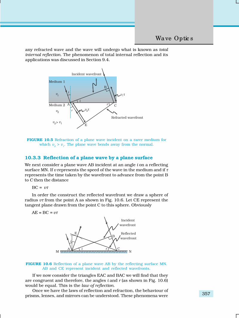
357
Wave Optic s
any refracted wave and the wave will undergo what is known as total
internal reflection. The phenomenon of total internal reflection and itsapplications was discussed in Section 9.4.
FIGURE 10.5 Refraction of a plane wave incident on a rarer medium forwhich v
2 > v
1. The plane wave bends away from the normal.
10.3.3 Reflection of a plane wave by a plane surface
We next consider a plane wave AB incident at an angle i on a reflectingsurface MN. If v represents the speed of the wave in the medium and if τrepresents the time taken by the wavefront to advance from the point Bto C then the distance
BC = vτ
In order the construct the reflected wavefront we draw a sphere ofradius vτ from the point A as shown in Fig. 10.6. Let CE represent thetangent plane drawn from the point C to this sphere. Obviously
AE = BC = vτ
FIGURE 10.6 Reflection of a plane wave AB by the reflecting surface MN.
AB and CE represent incident and reflected wavefronts.
If we now consider the triangles EAC and BAC we will find that theyare congruent and therefore, the angles i and r (as shown in Fig. 10.6)would be equal. This is the law of reflection.
Once we have the laws of reflection and refraction, the behaviour ofprisms, lenses, and mirrors can be understood. These phenomena were

Physic s
358
discussed in detail in Chapter 9 on the basis of rectilinear propagation oflight. Here we just describe the behaviour of the wavefronts as theyundergo reflection or refraction. In Fig. 10.7(a) we consider a plane wavepassing through a thin prism. Clearly, since the speed of light waves isless in glass, the lower portion of the incoming wavefront (which travelsthrough the greatest thickness of glass) will get delayed resulting in a tiltin the emerging wavefront as shown in the figure. In Fig. 10.7(b) weconsider a plane wave incident on a thin convex lens; the central part ofthe incident plane wave traverses the thickest portion of the lens and isdelayed the most. The emerging wavefront has a depression at the centreand therefore the wavefront becomes spherical and converges to the pointF which is known as the focus. In Fig. 10.7(c) a plane wave is incident ona concave mirror and on reflection we have a spherical wave convergingto the focal point F. In a similar manner, we can understand refractionand reflection by concave lenses and convex mirrors.
FIGURE 10.7 Refraction of a plane wave by (a) a thin prism, (b) a convex lens. (c) Reflection of aplane wave by a concave mirror.
From the above discussion it follows that the total time taken from apoint on the object to the corresponding point on the image is the samemeasured along any ray. For example, when a convex lens focusses lightto form a real image, although the ray going through the centre traversesa shorter path, but because of the slower speed in glass, the time takenis the same as for rays travelling near the edge of the lens.
10.3.4 The doppler effect
We should mention here that one should be careful in constructing thewavefronts if the source (or the observer) is moving. For example, if thereis no medium and the source moves away from the observer, then laterwavefronts have to travel a greater distance to reach the observer andhence take a longer time. The time taken between the arrival of twosuccessive wavefronts is hence longer at the observer than it is at thesource. Thus, when the source moves away from the observer thefrequency as measured by the source will be smaller. This is known asthe Doppler effect. Astronomers call the increase in wavelength due todoppler effect as red shift since a wavelength in the middle of the visibleregion of the spectrum moves towards the red end of the spectrum. Whenwaves are received from a source moving towards the observer, there isan apparent decrease in wavelength, this is referred to as blue shift.

359
Wave Optic s
EX
AM
PLE 1
0.1
You have already encountered Doppler effect for sound waves inChapter 15 of Class XI textbook. For velocities small compared to thespeed of light, we can use the same formulae which we use for soundwaves. The fractional change in frequency Δν/ν is given by –v
radial/c, where
vradial
is the component of the source velocity along the line joining theobserver to the source relative to the observer; v
radial is considered positive
when the source moves away from the observer. Thus, the Doppler shiftcan be expressed as:
– radialv
c
νν
Δ = (10.9)
The formula given above is valid only when the speed of the source issmall compared to that of light. A more accurate formula for the Dopplereffect which is valid even when the speeds are close to that of light, requiresthe use of Einstein’s special theory of relativity. The Doppler effect forlight is very important in astronomy. It is the basis for the measurementsof the radial velocities of distant galaxies.
Example 10.1 What speed should a galaxy move with respectto us so that the sodium line at 589.0 nm is observedat 589.6 nm?
Solution Since νλ = c, –ν λ
ν λΔ Δ= (for small changes in ν and λ). For
Δλ = 589.6 – 589.0 = + 0.6 nm
we get [using Eq. (10.9)]
– – radialv
c
ν λν λ
Δ Δ= =
or, vradial
5 –10.6
3.06 10 m s589.0
c⎛ ⎞≅ + = + ×⎜ ⎟⎝ ⎠
= 306 km/s
Therefore, the galaxy is moving away from us.
Example 10.2
(a) When monochromatic light is incident on a surface separatingtwo media, the reflected and refracted light both have the samefrequency as the incident frequency. Explain why?
(b) When light travels from a rarer to a denser medium, the speeddecreases. Does the reduction in speed imply a reduction in theenergy carried by the light wave?
(c) In the wave picture of light, intensity of light is determined by thesquare of the amplitude of the wave. What determines the intensityof light in the photon picture of light.
Solution(a) Reflection and refraction arise through interaction of incident light
with the atomic constituents of matter. Atoms may be viewed as
EX
AM
PLE 1
0.2

Physic s
360
EX
AM
PLE 1
0.2
oscillators, which take up the frequency of the external agency (light)
causing forced oscillations. The frequency of light emitted by a charged
oscillator equals its frequency of oscillation. Thus, the frequency of
scattered light equals the frequency of incident light.
(b) No. Energy carried by a wave depends on the amplitude of the
wave, not on the speed of wave propagation.
(c) For a given frequency, intensity of light in the photon picture is
determined by the number of photons crossing an unit area per
unit time.
10.4 COHERENT AND INCOHERENT ADDITION OF WAVES
In this section we will discuss the interference pattern produced by
the superposition of two waves. You may recall that we had discussed
the superposition principle in Chapter 15 of your Class XI textbook.
Indeed the entire field of interference is based on the superposition
principle according to which at a particular point in the medium, the
resultant displacement produced by a number of waves is the vector
sum of the displacements produced by each of the waves.
Consider two needles S1 and S
2 moving periodically up and down
in an identical fashion in a trough of water [Fig. 10.8(a)]. They produce
two water waves, and at a particular point, the phase difference between
the displacements produced by each of the waves does not change
with time; when this happens the two sources are said to be coherent.
Figure 10.8(b) shows the position of crests (solid circles) and troughs
(dashed circles) at a given instant of time. Consider a point P for which
S1 P = S
2 P
Since the distances S1 P and S
2 P are equal, waves from S
1 and S
2
will take the same time to travel to the point P and waves that emanate
from S1 and S
2 in phase will also arrive, at the point P, in phase.
Thus, if the displacement produced by the source S1 at the point P
is given by
y1 = a cos ωt
then, the displacement produced by the source S2 (at the point P) will
also be given by
y2 = a cos ωt
Thus, the resultant of displacement at P would be given by
y = y1 + y
2 = 2 a cos ωt
Since the intensity is the proportional to the square of the
amplitude, the resultant intensity will be given by
I = 4 I0
where I0 represents the intensity produced by each one of the individual
sources; I0 is proportional to a2. In fact at any point on the perpendicular
bisector of S1S
2, the intensity will be 4I
0. The two sources are said to
(a)
(b)
FIGURE 10.8 (a) Twoneedles oscillating in
phase in waterrepresent two coherent
sources.(b) The pattern of
displacement of watermolecules at an
instant on the surfaceof water showing nodal
N (no displacement)and antinodal A
(maximumdisplacement) lines.

361
Wave Optic s
interfere constructively and we have what is referred to as constructive
interference. We next consider a point Q [Fig. 10.9(a)]for which
S2Q –S
1Q = 2λ
The waves emanating from S1 will arrive exactly two cycles earlier
than the waves from S2 and will again be in phase [Fig. 10.9(a)]. Thus, if
the displacement produced by S1 is given by
y1 = a cos ωt
then the displacement produced by S2 will be given by
y2 = a cos (ωt – 4π) = a cos ωt
where we have used the fact that a path difference of 2λ corresponds to aphase difference of 4π. The two displacements are once again in phaseand the intensity will again be 4 I
0 giving rise to constructive interference.
In the above analysis we have assumed that the distances S1Q and S
2Q
are much greater than d (which represents the distance between S1 and
S2) so that although S
1Q and S
2Q are not equal, the amplitudes of the
displacement produced by each wave are very nearly the same.We next consider a point R [Fig. 10.9(b)] for which
S2R – S
1R = –2.5λ
The waves emanating from S1 will arrive exactly two and a half cycles
later than the waves from S2 [Fig. 10.10(b)]. Thus if the displacement
produced by S1 is given by
y1 = a cos ωt
then the displacement produced by S2 will be given by
y2 = a cos (ωt + 5π) = – a cos ωt
where we have used the fact that a path difference of 2.5λ corresponds to
a phase difference of 5π. The two displacements are now out of phase
and the two displacements will cancel out to give zero intensity. This is
referred to as destructive interference.
To summarise: If we have two coherent sources S1 and S
2 vibrating
in phase, then for an arbitrary point P whenever the path difference,
S1P ~ S
2P = nλ (n = 0, 1, 2, 3,...) (10.10)
we will have constructive interference and the resultant intensity will be
4I0; the sign ~ between S
1P and S
2 P represents the difference between
S1P and S
2 P. On the other hand, if the point P is such that the path
difference,
S1P ~ S
2P = (n+
1
2) λ (n = 0, 1, 2, 3, ...) (10.11)
we will have destructive interference and the resultant intensity will be
zero. Now, for any other arbitrary point G (Fig. 10.10) let the phase
difference between the two displacements be φ. Thus, if the displacement
produced by S1 is given by
y1 = a cos ωt
FIGURE 10.9(a) Constructiveinterference at a
point Q for which thepath difference is 2λ.
(b) Destructiveinterference at a
point R for which thepath difference is
2.5 λ .
FIGURE 10.10 Locusof points for which
S1P – S
2P is equal to
zero, ±λ, ± 2λ, ± 3λ .

Physic s
362
then, the displacement produced by S2 would be
y2 = a cos (ωt + φ )
and the resultant displacement will be given by
y = y1 + y
2
= a [cos ωt + cos (ωt +φ )]
= 2 a cos (φ/2) cos (ωt + φ/2)
The amplitude of the resultant displacement is 2a cos (φ/2) andtherefore the intensity at that point will be
I = 4 I0 cos2 (φ/2) (10.12)
If φ = 0, ± 2 π, ± 4 π,… which corresponds to the condition given byEq. (10.10) we will have constructive interference leading to maximumintensity. On the other hand, if φ = ± π, ± 3π, ± 5π … [which corresponds tothe condition given by Eq. (10.11)] we will have destructive interferenceleading to zero intensity.
Now if the two sources are coherent (i.e., if the two needles are goingup and down regularly) then the phase difference φ at any point will notchange with time and we will have a stable interference pattern; i.e., thepositions of maxima and minima will not change with time. However, ifthe two needles do not maintain a constant phase difference, then theinterference pattern will also change with time and, if the phase differencechanges very rapidly with time, the positions of maxima and minima willalso vary rapidly with time and we will see a “time-averaged” intensitydistribution. When this happens, we will observe an average intensitythat will be given by
( )2
04 cos /2I I φ< >= < > (10.13)
where angular brackets represent time averaging. Indeed it is shown inSection 7.2 that if φ(t ) varies randomly with time, the time-averagedquantity < cos2 (φ/2) > will be 1/2. This is also intuitively obvious becausethe function cos2 (φ/2) will randomly vary between 0 and 1 and theaverage value will be 1/2. The resultant intensity will be given by
I = 2 I0
(10.14)
at all points.When the phase difference between the two vibrating sources changes
rapidly with time, we say that the two sources are incoherent and whenthis happens the intensities just add up. This is indeed what happenswhen two separate light sources illuminate a wall.
10.5 INTERFERENCE OF LIGHT WAVES AND YOUNG’SEXPERIMENT
We will now discuss interference using light waves. If we use two sodiumlamps illuminating two pinholes (Fig. 10.11) we will not observe anyinterference fringes. This is because of the fact that the light wave emittedfrom an ordinary source (like a sodium lamp) undergoes abrupt phase
Rip
ple
Tan
k exp
eri
men
ts o
n w
ave in
terf
ere
nce
http
://w
ww
.col
orad
o.ed
u/ph
ysic
s/20
00/a
pple
ts/fo
urie
r.ht
ml

363
Wave Optic s
changes in times of the order of 10–10 seconds. Thusthe light waves coming out from two independentsources of light will not have any fixed phaserelationship and would be incoherent, when thishappens, as discussed in the previous section, theintensities on the screen will add up.
The British physicist Thomas Young used aningenious technique to “lock” the phases of the wavesemanating from S
1 and S
2. He made two pinholes S
1
and S2 (very close to each other) on an opaque screen
[Fig. 10.12(a)]. These were illuminated by anotherpinholes that was in turn, lit by a bright source. Lightwaves spread out from S and fall on both S
1 and S
2.
S1 and S
2 then behave like two coherent sources
because light waves coming out from S1 and S
2 are derived from the
same original source and any abrupt phase change in S will manifest inexactly similar phase changes in the light coming out from S
1 and S
2.
Thus, the two sources S1 and S
2 will be locked in phase; i.e., they will be
coherent like the two vibrating needle in our water wave example[Fig. 10.8(a)].
FIGURE 10.11 If two sodiumlamps illuminate two pinholes
S1 and S
2, the intensities will add
up and no interference fringes willbe observed on the screen.
Thus spherical waves emanating from S1 and S
2 will produce
interference fringes on the screen GG′, as shown in Fig. 10.12(b). Thepositions of maximum and minimum intensities can be calculated byusing the analysis given in Section 10.4 where we had shown that for anarbitrary point P on the line GG′ [Fig. 10.12(b)] to correspond to amaximum, we must have
S2P – S
1P = nλ; n = 0, 1, 2 ... (10.15)
Now,
(S2P)2 – (S
1P)2 =
2
2 –2
dD x
⎡ ⎤⎛ ⎞+ +⎢ ⎥⎜ ⎟⎝ ⎠⎢ ⎥⎣ ⎦2
2 –2
dD x
⎡ ⎤⎛ ⎞+⎢ ⎥⎜ ⎟⎝ ⎠⎢ ⎥⎣ ⎦ = 2x d
(a) (b)
FIGURE 10.12 Young’s arrangement to produce interference pattern.

Physic s
364
where S1S
2 = d and OP = x . Thus
S2P – S
1P =
2 1
2
S P+S P
xd(10.16)
If x, d<<D then negligible error will be introduced ifS
2P + S
1P (in the denominator) is replaced by 2D. For
example, for d = 0.1 cm, D = 100 cm, OP = 1 cm (whichcorrespond to typical values for an interferenceexperiment using light waves), we have
S2P + S
1P = [(100)2 + (1.05)2]½ + [(100)2 + (0.95)2]½
≈ 200.01 cm
Thus if we replace S2P + S
1P by 2 D, the error involved is
about 0.005%. In this approximation, Eq. (10.16)becomes
S2P – S
1P ≈ (10.17)
Hence we will have constructive interference resulting ina bright region when
x = xn =
n D
d
λ; n = 0, ± 1, ± 2, ... (10.18)
On the other hand, we will have a dark region near
x = xn = (n+ ) ; 0, 1, 2
Dn
d
λ = ± ± (10.19)
Thus dark and bright bands appear on the screen, as shown inFig. 10.13. Such bands are called fringes. Equations (10.18) and (10.19)show that dark and bright fringes are equally spaced and the distancebetween two consecutive bright and dark fringes is given by
β = xn+1
–xn
or β = D
d
λ(10.20)
which is the expression for the fringe width. Obviously, the central point
O (in Fig. 10.12) will be bright because S1O = S
2O and it will correspond
to n = 0. If we consider the line perpendicular to the plane of the paper
and passing through O [i.e., along the y-axis] then all points on this linewill be equidistant from S
1 and S
2 and we will have a bright central fringe
which is a straight line as shown in Fig. 10.13. In order to determine theshape of the interference pattern on the screen we note that a particular
fringe would correspond to the locus of points with a constant value ofS
2P – S
1P. Whenever this constant is an integral multiple of λ, the fringe
will be bright and whenever it is an odd integral multiple of λ/2 it will bea dark fringe. Now, the locus of the point P lying in the x-y plane such
that S2P – S
1P (= Δ) is a constant, is a hyperbola. Thus the fringe pattern
will strictly be a hyperbola; however, if the distance D is very large compared
to the fringe width, the fringes will be very nearly straight lines as shownin Fig. 10.13.
Thomas Young(1773 – 1829) Englishphysicist, physician andEgyptologist. Young workedon a wide variety ofscientific problems, rangingfrom the structure of the eyeand the mechanism ofvision to the deciphermentof the Rosetta stone. Herevived the wave theory oflight and recognised thatinterference phenomenaprovide proof of the waveproperties of light.
TH
OM
AS
YO
UN
G (1773 –
1829)

365
Wave Optic s
In the double-slit experiment shown in Fig. 10.12, we have taken thesource hole S on the perpendicular bisector of the two slits, which isshown as the line SO. What happens if the source S is slightly away fromthe perpendicular bisector. Consider that the source is moved to somenew point S′ and suppose that Q is the mid-point of S
1 and S
2. If the
angle S′QS is φ, then the central bright fringe occurs at an angle –φ, onthe other side. Thus, if the source S is on the perpendicular bisector,then the central fringe occurs at O, also on the perpendicular bisector. IfS is shifted by an angle φ to point S′, then the central fringe appears at apoint O′ at an angle –φ, which means that it is shifted by the same angleon the other side of the bisector. This also means that the source S′, themid-point Q and the point O′ of the central fringe are in a straight line.
We end this section by quoting from the Nobel lecture of Dennis Gabor*
The wave nature of light was demonstrated convincingly for thefirst time in 1801 by Thomas Young by a wonderfully simpleexperiment. He let a ray of sunlight into a dark room, placed adark screen in front of it, pierced with two small pinholes, andbeyond this, at some distance, a white screen. He then saw twodarkish lines at both sides of a bright line, which gave himsufficient encouragement to repeat the experiment, this time withspirit flame as light source, with a little salt in it to produce thebright yellow sodium light. This time he saw a number of darklines, regularly spaced; the first clear proof that light added tolight can produce darkness. This phenomenon is called
FIGURE 10.13 Computer generated fringe pattern produced by two point source S1 and S
2 on the
screen GG′ (Fig. 10.12); (a) and (b) correspond to d = 0.005 mm and 0.025 mm, respectively (bothfigures correspond to D = 5 cm and λ = 5 × 10⁻⁵ cm.) (Adopted from OPTICS by A. Ghatak, Tata
McGraw Hill Publishing Co. Ltd., New Delhi, 2000.)
* Dennis Gabor received the 1971 Nobel Prize in Physics for discovering theprinciples of holography.

Physic s
366
EX
AM
PLE 1
0.3
interference. Thomas Young had expected it because he believed
in the wave theory of light.
We should mention here that the fringes are straight lines althoughS
1 and S
2 are point sources. If we had slits instead of the point sources
(Fig. 10.14), each pair of points would have produced straight line fringesresulting in straight line fringes with increased intensities.
Example 10.3 Two slits are made one millimetre apart and the screenis placed one metre away. What is the fringe separation when blue-green light of wavelength 500 nm is used?
Solution Fringe spacing =–7
–3
1 5 10m
1 10
D
d
λ × ×= × = 5 × 10⁻⁴ m = 0.5 mm
Example 10.4 What is the effect on the interference fringes in aYoung’s double-slit experiment due to each of the following operations:
(a) the screen is moved away from the plane of the slits;
(b) the (monochromatic) source is replaced by another(monochromatic) source of shorter wavelength;
(c) the separation between the two slits is increased;
(d) the source slit is moved closer to the double-slit plane;
(e) the width of the source slit is increased;
(f ) the monochromatic source is replaced by a source of whitelight?
FIGURE 10.14 Photograph and the graph of the intensitydistribution in Young’s double-slit experiment.
EX
AM
PLE 1
0.4
Inte
racti
ve an
imati
on
o
f Yo
un
g’s
exp
eri
men
t
http
://vs
g.qu
asih
ome.
com
/inte
rfer
.htm
l

367
Wave Optic s
EX
AM
PLE 1
0.4
( In each operation, take all parameters, other than the one specified,
to remain unchanged.)
Solution
(a) Angular separation of the fringes remains constant
(= λ/d). The actual separation of the fringes increases in
proportion to the distance of the screen from the plane of the
two slits.
(b) The separation of the fringes (and also angular separation)
decreases. See, however, the condition mentioned in (d) below.
(c) The separation of the fringes (and also angular separation)
decreases. See, however, the condition mentioned in (d) below.
(d) Let s be the size of the source and S its distance from the plane of
the two slits. For interference fringes to be seen, the condition
s/S < λ/d should be satisfied; otherwise, interference patterns
produced by different parts of the source overlap and no fringes
are seen. Thus, as S decreases (i.e., the source slit is brought
closer), the interference pattern gets less and less sharp, and
when the source is brought too close for this condition to be valid,
the fringes disappear. Till this happens, the fringe separation
remains fixed.
(e) Same as in (d). As the source slit width increases, fringe pattern
gets less and less sharp. When the source slit is so wide that the
condition s/S ≤ λ/d is not satisfied, the interference pattern
disappears.
(f ) The interference patterns due to different component colours of
white light overlap (incoherently). The central bright fringes for
different colours are at the same position. Therefore, the central
fringe is white. For a point P for which S2P –S
1P = λ
b/2, where λ
b
(≈ 4000 Å) represents the wavelength for the blue colour, the blue
component will be absent and the fringe will appear red in colour.
Slightly farther away where S2Q–S
1Q = λ
b = λ
r/2 where λ
r (≈ 8000 Å)
is the wavelength for the red colour, the fringe will be predominantly
blue.
Thus, the fringe closest on either side of the central white fringe
is red and the farthest will appear blue. After a few fringes, no
clear fringe pattern is seen.
10.6 DIFFRACTION
If we look clearly at the shadow cast by an opaque object, close to the
region of geometrical shadow, there are alternate dark and bright regions
just like in interference. This happens due to the phenomenon of
diffraction. Diffraction is a general characteristic exhibited by all types of
waves, be it sound waves, light waves, water waves or matter waves. Since
the wavelength of light is much smaller than the dimensions of most
obstacles; we do not encounter diffraction effects of light in everyday
observations. However, the finite resolution of our eye or of optical

Physic s
368
instruments such as telescopes or microscopes is limited due to the
phenomenon of diffraction. Indeed the colours that you see when a CD is
viewed is due to diffraction effects. We will now discuss the phenomenon
of diffraction.
10.6.1 The single slit
In the discussion of Young’s experiment, we stated that a single narrow
slit acts as a new source from which light spreads out. Even before Young,
early experimenters – including Newton – had noticed that light spreads
out from narrow holes and slits. It seems to turn around corners and
enter regions where we would expect a shadow. These effects, known as
diffraction, can only be properly understood using wave ideas. After all,
you are hardly surprised to hear sound waves from someone talking
around a corner !
When the double slit in Young’s experiment is replaced by a single
narrow slit (illuminated by a monochromatic source), a broad pattern
with a central bright region is seen. On both sides, there are alternate
dark and bright regions, the intensity becoming weaker away from the
centre (Fig. 10.16). To understand this, go to Fig. 10.15, which shows a
parallel beam of light falling normally on a single slit LN of width a. The
diffracted light goes on to meet a screen. The midpoint of the slit is M.
A straight line through M perpendicular to the slit plane meets the
screen at C. We want the intensity at any point P on the screen. As before,
straight lines joining P to the different points L,M,N, etc., can be treated as
parallel, making an angle θ with the normal MC.
The basic idea is to divide the slit into much smaller parts, and add
their contributions at P with the proper phase differences. We are treating
different parts of the wavefront at the slit as secondary sources. Because
the incoming wavefront is parallel to the plane of the slit, these sources
are in phase.
The path difference NP – LP between the two edges of the slit can be
calculated exactly as for Young’s experiment. From Fig. 10.15,
NP – LP = NQ
= a sin θ
≈ aθ (10.21)
Similarly, if two points M1 and M
2 in the slit plane are separated by y, the
path difference M2P – M
1P ≈ yθ. We now have to sum up equal, coherent
contributions from a large number of sources, each with a different phase.
This calculation was made by Fresnel using integral calculus, so we omit
it here. The main features of the diffraction pattern can be understood by
simple arguments.
At the central point C on the screen, the angle θ is zero. All path
differences are zero and hence all the parts of the slit contribute in phase.
This gives maximum intensity at C. Experimental observation shown in

369
Wave Optic s
Fig. 10.15 indicates that the intensity has a
central maximum at θ = 0 and other
secondary maxima at θ l (n+1/2) λ/a, and
has minima (zero intensity) at θ l nλ/a,
n = ±1, ±2, ±3, .... It is easy to see why it has
minima at these values of angle. Consider
first the angle θ where the path difference aθis λ. Then,
/aθ λ≈ . (10.22)
Now, divide the slit into two equal halves
LM and MN each of size a/2. For every point
M1 in LM, there is a point M
2 in MN such that
M1M
2 = a/2. The path difference between M
1 and M
2 at P = M
2P – M
1P
= θ a/2 = λ/2 for the angle chosen. This means that the contributions
from M1 and M
2 are 180º out of phase and cancel in the direction
θ = λ/a. Contributions from the two halves of the slit LM and MN,
therefore, cancel each other. Equation (10.22) gives the angle at which
the intensity falls to zero. One can similarly show that the intensity is
zero for θ = nλ/a, with n being any integer (except zero!). Notice that the
angular size of the central maximum increases when the slit width a
decreases.
It is also easy to see why there are maxima at θ 0 (n + 1/2) λ/a and
why they go on becoming weaker and weaker with increasing n. Consider
an angle θ = 3λ/2a which is midway between two of the dark fringes.
Divide the slit into three equal parts. If we take the first two thirds of the
slit, the path difference between the two ends would be
2 2 3
3 3 2
aa
a
λθ λ× = × = (10.23)
The first two-thirds of the slit can therefore be divided
into two halves which have a λ/2 path difference. The
contributions of these two halves cancel in the same manner
as described earlier. Only the remaining one-third of the
slit contributes to the intensity at a point between the two
minima. Clearly, this will be much weaker than the central
maximum (where the entire slit contributes in phase). One
can similarly show that there are maxima at (n + 1/2) θ/a
with n = 2, 3, etc. These become weaker with increasing n,
since only one-fifth, one-seventh, etc., of the slit contributes
in these cases. The photograph and intensity pattern
corresponding to it is shown in Fig. 10.16.
There has been prolonged discussion about difference
between intereference and diffraction among scientists since
the discovery of these phenomena. In this context, it is
FIGURE 10.16 Intensitydistribution and photograph of
fringes due to diffractionat single slit.
FIGURE 10.15 The geometry of pathdifferences for diffraction by a single slit.

Physic s
370
EX
AM
PLE 1
0.5
interesting to note what Richard Feynman* has said in his famous
Feynman Lectures on Physics:
No one has ever been able to define the difference between
interference and diffraction satisfactorily. It is just a question
of usage, and there is no specific, important physical difference
between them. The best we can do is, roughly speaking, is to
say that when there are only a few sources, say two interfering
sources, then the result is usually called interference, but if there
is a large number of them, it seems that the word diffraction is
more often used.
In the double-slit experiment, we must note that the pattern on thescreen is actually a superposition of single-slit diffraction from each slitor hole, and the double-slit interference pattern. This is shown inFig. 10.17. It shows a broader diffraction peak in which there appearseveral fringes of smaller width due to double-slit interference. Thenumber of interference fringes occuring in the broad diffraction peakdepends on the ratio d/a, that is the ratio of the distance between thetwo slits to the width of a slit. In the limit of a becoming very small, thediffraction pattern will become very flat and we will obsrve the two-slitinterference pattern [see Fig. 10.13(b)].
* Richand Feynman was one of the recipients of the 1965 Nobel Prize in Physicsfor his fundamental work in quantum electrodynamics.
Example 10.5 In Example 10.3, what should the width of each slit beto obtain 10 maxima of the double slit pattern within the centralmaximum of the single slit pattern?
Solution We want ,aa
λθ λ θ= =
10 2d a
λ λ= 0 2 mm5
da = = .
Notice that the wavelength of light and distance of the screen do notenter in the calculation of a.
In the double-slit interference experiment of Fig. 10.12, what happensif we close one slit? You will see that it now amounts to a single slit. Butyou will have to take care of some shift in the pattern. We now have asource at S, and only one hole (or slit) S
1 or S
2. This will produce a single-
FIGURE 10.17 The actual double-slit interference pattern.The envelope shows the single slit diffraction.
Inte
racti
ve an
imati
on
o
n sin
gle
sli
t d
iffr
acti
on
p
att
ern
http
://w
ww
.phy
s.ha
wai
i.edu
/~te
b/op
tics/
java
/slit
diffr
/

371
Wave Optic s
slit diffraction pattern on the screen. The centre of the central bright fringewill appear at a point which lies on the straight line SS
1 or SS
2, as the
case may be.We now compare and contrast the interference pattern with that seen
for a coherently illuminated single slit (usually called the single slitdiffraction pattern).(i) The interference pattern has a number of equally spaced bright and
dark bands. The diffraction pattern has a central bright maximumwhich is twice as wide as the other maxima. The intensity falls as wego to successive maxima away from the centre, on either side.
(ii) We calculate the interference pattern by superposing two wavesoriginating from the two narrow slits. The diffraction pattern is asuperposition of a continuous family of waves originating from eachpoint on a single slit.
(iii) For a single slit of width a, the first null of the interference patternoccurs at an angle of λ/a. At the same angle of λ/a, we get a maximum(not a null) for two narrow slits separated by a distance a.
One must understand that both d and a have to be quite small, to beable to observe good interference and diffraction patterns. For example,the separation d between the two slits must be of the order of a milimetreor so. The width a of each slit must be even smaller, of the order of 0.1 or0.2 mm.
In our discussion of Young’s experiment and the single-slit diffraction,
we have assumed that the screen on which the fringes are formed is at a
large distance. The two or more paths from the slits to the screen were
treated as parallel. This situation also occurs when we place a converging
lens after the slits and place the screen at the focus. Parallel paths from
the slit are combined at a single point on the screen. Note that the lens
does not introduce any extra path differences in a parallel beam. This
arrangement is often used since it gives more intensity than placing the
screen far away. If f is the focal length of the lens, then we can easily work
out the size of the central bright maximum. In terms of angles, the
separation of the central maximum from the first null of the diffraction
pattern is λ/a . Hence, the size on the screen will be f λ/a.
10.6.2 Seeing the single slit diffraction pattern
It is surprisingly easy to see the single-slit diffraction pattern for oneself.The equipment needed can be found in most homes –– two razor bladesand one clear glass electric bulb preferably with a straight filament. Onehas to hold the two blades so that the edges are parallel and have anarrow slit in between. This is easily done with the thumb and forefingers(Fig. 10.18).
Keep the slit parallel to the filament, right in front of the eye. Usespectacles if you normally do. With slight adjustment of the width of theslit and the parallelism of the edges, the pattern should be seen with itsbright and dark bands. Since the position of all the bands (except thecentral one) depends on wavelength, they will show some colours. Usinga filter for red or blue will make the fringes clearer. With both filtersavailable, the wider fringes for red compared to blue can be seen.
FIGURE 10.18Holding two blades toform a single slit. Abulb filament viewedthrough this shows
clear diffractionbands.

Physic s
372
In this experiment, the filament plays the role of the first slit S inFig. 10.16. The lens of the eye focuses the pattern on the screen (theretina of the eye).
With some effort, one can cut a double slit in an aluminium foil witha blade. The bulb filament can be viewed as before to repeat Young’sexperiment. In daytime, there is another suitable bright source subtendinga small angle at the eye. This is the reflection of the Sun in any shinyconvex surface (e.g., a cycle bell). Do not try direct sunlight – it can damagethe eye and will not give fringes anyway as the Sun subtends an angleof (1/2)º.
In interference and diffraction, light energy is redistributed. If it
reduces in one region, producing a dark fringe, it increases in another
region, producing a bright fringe. There is no gain or loss of energy,
which is consistent with the principle of conservation of energy.
10.6.3 Resolving power of optical instruments
In Chapter 9 we had discussed about telescopes. The angular resolutionof the telescope is determined by the objective of the telescope. The starswhich are not resolved in the image produced by the objective cannot beresolved by any further magnification produced by the eyepiece. Theprimary purpose of the eyepiece is to provide magnification of the imageproduced by the objective.
Consider a parallel beam of light falling on a convex lens. If the lens iswell corrected for aberrations, then geometrical optics tells us that thebeam will get focused to a point. However, because of diffraction, thebeam instead of getting focused to a point gets focused to a spot of finitearea. In this case the effects due to diffraction can be taken into accountby considering a plane wave incident on a circular aperture followed bya convex lens (Fig. 10.19). The analysis of the corresponding diffractionpattern is quite involved; however, in principle, it is similar to the analysiscarried out to obtain the single-slit diffraction pattern. Taking into accountthe effects due to diffraction, the pattern on the focal plane would consistof a central bright region surrounded by concentric dark and bright rings(Fig. 10.19). A detailed analysis shows that the radius of the central brightregion is approximately given by
0
1.22 0.61
2
f fr
a a
λ λ≈ = (10.24)
FIGURE 10.19 A parallel beam of light is incident on a convex lens.Because of diffraction effects, the beam gets focused to a
spot of radius ≈ 0.61 λf/a .

373
Wave Optic s
where f is the focal length of the lens and 2a is the diameter of the circularaperture or the diameter of the lens, whichever is smaller. Typically if
λ ≈ 0.5 μm, f ≈ 20 cm and a ≈ 5 cm
we have
r0 ≈ 1.2 μm
Although the size of the spot is very small, it plays an important rolein determining the limit of resolution of optical instruments like a telescopeor a microscope. For the two stars to be just resolved
0
0.61 ff r
a
λθΔ ≈ ≈implying
0.61
a
λθΔ ≈ (10.25)
Thus Δθ will be small if the diameter of the objective is large. Thisimplies that the telescope will have better resolving power if a is large. Itis for this reason that for better resolution, a telescope must have a largediameter objective.
Example 10.6 Assume that light of wavelength 6000Å is coming froma star. What is the limit of resolution of a telescope whose objectivehas a diameter of 100 inch?
Solution A 100 inch telescope implies that 2a = 100 inch= 254 cm. Thus if,
λ ≈ 6000Å = 6×10⁻⁵ cmthen
–5–70.61 6 10
2.9 10127
θ × ×Δ ≈ ≈ × radians
We can apply a similar argument to the objective lens of a microscope.In this case, the object is placed slightly beyond f, so that a real image isformed at a distance v [Fig. 10.20]. The magnification – ratio of
image size to object size – is given by m l v/f. It can be seen from
Fig. 10.20 that
D/f l 2 tan β (10.26)
where 2β is the angle subtended by the diameter of the objective lens atthe focus of the microscope.
EX
AM
PLE 1
0.6
FIGURE 10.20 Real image formed by the objective lens of the microscope.

Physic s
374
When the separation between two points in a microscopic specimen
is comparable to the wavelength λ of the light, the diffraction effects
become important. The image of a point object will again be a diffraction
pattern whose size in the image plane will be
1.22v v
D
λθ ⎛ ⎞= ⎜ ⎟⎝ ⎠ (10.27)
Two objects whose images are closer than this distance will not beresolved, they will be seen as one. The corresponding minimumseparation, dmin, in the object plane is given by
dmin = 1 22
v mD
λ.⎡ ⎤⎛ ⎞⎜ ⎟⎢ ⎥⎝ ⎠⎣ ⎦ =
1 22.
v
D m
. λ
= 1 22 f
D
. λ(10.28)
Now, combining Eqs. (10.26) and (10.28), we get
min
1.22
2 tand
λ β=
DETERMINE THE RESOLVING POWER OF YOUR EYE
You can estimate the resolving power of your eye with a simple experiment. Makeblack stripes of equal width separated by white stripes; see figure here. All the blackstripes should be of equal width, while the width of the intermediate white stripes shouldincrease as you go from the left to the right. For example, let all black stripes have a widthof 5 mm. Let the width of the first two white stripes be 0.5 mm each, the next two whitestripes be 1 mm each, the next two 1.5 mm each, etc. Paste this pattern on a wall in aroom or laboratory, at the height of your eye.
Now watch the pattern, preferably with one eye. By moving away or closer to the wall,find the position where you can just see some two black stripes as separate stripes. Allthe black stripes to the left of this stripe would merge into one another and would not bedistinguishable. On the other hand, the black stripes to the right of this would be moreand more clearly visible. Note the width d of the white stripe which separates the tworegions, and measure the distance D of the wall from your eye. Then d/D is the resolutionof your eye.
You have watched specks of dust floating in air in a sunbeam entering through yourwindow. Find the distance (of a speck) which you can clearly see and distinguish from aneighbouring speck. Knowing the resolution of your eye and the distance of the speck,estimate the size of the speck of dust.
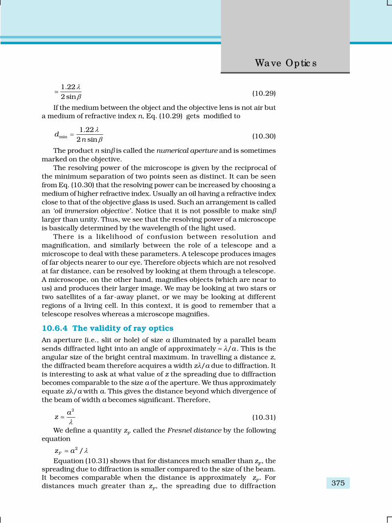
375
Wave Optic s
1.22
2sin
λβ0 (10.29)
If the medium between the object and the objective lens is not air buta medium of refractive index n, Eq. (10.29) gets modified to
min
1.22
2 sind
n
λβ= (10.30)
The product n sinβ is called the numerical aperture and is sometimes
marked on the objective.
The resolving power of the microscope is given by the reciprocal of
the minimum separation of two points seen as distinct. It can be seen
from Eq. (10.30) that the resolving power can be increased by choosing a
medium of higher refractive index. Usually an oil having a refractive index
close to that of the objective glass is used. Such an arrangement is called
an ‘oil immersion objective’. Notice that it is not possible to make sinβlarger than unity. Thus, we see that the resolving power of a microscope
is basically determined by the wavelength of the light used.
There is a likelihood of confusion between resolution and
magnification, and similarly between the role of a telescope and a
microscope to deal with these parameters. A telescope produces images
of far objects nearer to our eye. Therefore objects which are not resolved
at far distance, can be resolved by looking at them through a telescope.
A microscope, on the other hand, magnifies objects (which are near to
us) and produces their larger image. We may be looking at two stars or
two satellites of a far-away planet, or we may be looking at different
regions of a living cell. In this context, it is good to remember that a
telescope resolves whereas a microscope magnifies.
10.6.4 The validity of ray optics
An aperture (i.e., slit or hole) of size a illuminated by a parallel beam
sends diffracted light into an angle of approximately ≈ λ/a . This is the
angular size of the bright central maximum. In travelling a distance z,
the diffracted beam therefore acquires a width zλ/a due to diffraction. It
is interesting to ask at what value of z the spreading due to diffraction
becomes comparable to the size a of the aperture. We thus approximately
equate zλ/a with a. This gives the distance beyond which divergence of
the beam of width a becomes significant. Therefore,
2az λ0 (10.31)
We define a quantity zF
called the Fresnel distance by the followingequation
2 /Fz a λ0Equation (10.31) shows that for distances much smaller than z
F , the
spreading due to diffraction is smaller compared to the size of the beam.It becomes comparable when the distance is approximately z
F. For
distances much greater than zF, the spreading due to diffraction

Physic s
376
EX
AM
PLE 1
0.7
dominates over that due to ray optics (i.e., the size a of the aperture).Equation (10.31) also shows that ray optics is valid in the limit ofwavelength tending to zero.
Example 10.7 For what distance is ray optics a good approximationwhen the aperture is 3 mm wide and the wavelength is 500 nm?
Solution ( )2–32
–7
3 1018 m
5 10F
az λ
×= = =×This example shows that even with a small aperture, diffractionspreading can be neglected for rays many metres in length. Thus, rayoptics is valid in many common situations.
10.7 POLARISATION
Consider holding a long string that is held horizontally, the other end ofwhich is assumed to be fixed. If we move the end of the string up anddown in a periodic manner, we will generate a wave propagating in the+x direction (Fig. 10.22). Such a wave could be described by the followingequation
FIGURE 10.21 (a) The curves represent the displacement of a string att = 0 and at t = Δt, respectively when a sinusoidal wave is propagating
in the +x-direction. (b) The curve represents the time variationof the displacement at x = 0 when a sinusoidal wave is propagating
in the +x-direction. At x = Δx, the time variation of thedisplacement will be slightly displaced to the right.

377
Wave Optic s
y (x,t ) = a sin (kx – ωt) (10.32)
where a and ω (= 2πν ) represent the amplitude and the angular frequencyof the wave, respectively; further,
2
kλ π= (10.33)
represents the wavelength associated with the wave. We had discussed
propagation of such waves in Chapter 15 of Class XI textbook. Since the
displacement (which is along the y direction) is at right angles to the
direction of propagation of the wave, we have what is known as a
transverse wave. Also, since the displacement is in the y direction, it is
often referred to as a y-polarised wave. Since each point on the string
moves on a straight line, the wave is also referred to as a linearly polarised
wave. Further, the string always remains confined to the x-y plane and
therefore it is also referred to as a plane polarised wave.
In a similar manner we can consider the vibration of the string in the
x-z plane generating a z-polarised wave whose displacement will be given
by
z (x,t ) = a sin (kx – ωt ) (10.34)
It should be mentioned that the linearly polarised waves [described
by Eqs. (10.33) and (10.34)] are all transverse waves; i.e., the
displacement of each point of the string is always at right angles to the
direction of propagation of the wave. Finally, if the plane of vibration of
the string is changed randomly in very short intervals of time, then we
have what is known as an unpolarised wave. Thus, for an unpolarised
wave the displacement will be randomly changing with time though it
will always be perpendicular to the direction of propagation.
Light waves are transverse in nature; i.e., the electric field associated
with a propagating light wave is always at right angles to the direction of
propagation of the wave. This can be easily demonstrated using a simple
polaroid. You must have seen thin plastic like sheets, which are called
polaroids. A polaroid consists of long chain molecules aligned in a
particular direction. The electric vectors (associated with the propagating
light wave) along the direction of the aligned molecules get absorbed.
Thus, if an unpolarised light wave is incident on such a polaroid then
the light wave will get linearly polarised with the electric vector oscillating
along a direction perpendicular to the aligned molecules; this direction
is known as the pass-axis of the polaroid.
Thus, if the light from an ordinary source (like a sodium lamp) passes
through a polaroid sheet P1, it is observed that its intensity is reduced by
half. Rotating P1 has no effect on the transmitted beam and transmitted
intensity remains constant. Now, let an identical piece of polaroid P2 be
placed before P1. As expected, the light from the lamp is reduced in
intensity on passing through P2 alone. But now rotating P
1 has a dramatic
effect on the light coming from P2. In one position, the intensity transmitted

Physic s
378 EX
AM
PLE 1
0.8
by P2 followed by P
1 is nearly zero. When turned by 90º from this position,
P1 transmits nearly the full intensity emerging from P
2 (Fig. 10.22).
The above experiment can be easily understood by assuming thatlight passing through the polaroid P
2 gets polarised along the pass-axis
of P2. If the pass-axis of P
2 makes an angle θ with the pass-axis of P
1,
then when the polarised beam passes through the polaroid P2, the
component E cos θ (along the pass-axis of P2) will pass through P
2.
Thus, as we rotate the polaroid P1 (or P
2), the intensity will vary as:
I = I0 cos2θ (10.35)
where I0 is the intensity of the polarized light after passing through
P1. This is known as Malus’ law. The above discussion shows that the
intensity coming out of a single polaroid is half of the incident intensity.By putting a second polaroid, the intensity can be further controlledfrom 50% to zero of the incident intensity by adjusting the angle betweenthe pass-axes of two polaroids.
Polaroids can be used to control the intensity, in sunglasses,windowpanes, etc. Polaroids are also used in photographic cameras and3D movie cameras.
Example 10.8 Discuss the intensity of transmitted light when apolaroid sheet is rotated between two crossed polaroids?
Solution Let I0 be the intensity of polarised light after passing through
the first polariser P1. Then the intensity of light after passing through
second polariser P2 will be
20cosI I θ= ,
FIGURE 10.22 (a) Passage of light through two polaroids P2 and P
1. The
transmitted fraction falls from 1 to 0 as the angle between them variesfrom 0º to 90º. Notice that the light seen through a single polaroid
P1 does not vary with angle. (b) Behaviour of the electric vectorwhen light passes through two polaroids. The transmittedpolarisation is the component parallel to the polaroid axis.
The double arrows show the oscillations of the electric vector.

379
Wave Optic s
where θ is the angle between pass axes of P1 and P
2. Since P
1 and P
3
are crossed the angle between the pass axes of P2 and P
3 will be
(π/2–θ ). Hence the intensity of light emerging from P3 will be
2 20cos cos –
2I I θ θπ⎛ ⎞= ⎜ ⎟⎝ ⎠ = I
0 cos2θ sin2θ =(I
0/4) sin22θ
Therefore, the transmitted intensity will be maximum when θ = π/4.
10.7.1 Polarisation by scattering
The light from a clear blue portion of the sky shows a rise and fall ofintensity when viewed through a polaroid which is rotated. This is nothingbut sunlight, which has changed its direction (having been scattered) onencountering the molecules of the earth’s atmosphere. As Fig. 10.24(a)shows, the incident sunlight is unpolarised. The dots stand for polarisationperpendicular to the plane of the figure. The double arrows showpolarisation in the plane of the figure. (There is no phase relation betweenthese two in unpolarised light). Under the influence of the electric field ofthe incident wave the electrons in the molecules acquire components ofmotion in both these directions. We have drawn an observer looking at90° to the direction of the sun. Clearly, charges accelerating parallel tothe double arrows do not radiate energy towards this observer since theiracceleration has no transverse component. The radiation scattered bythe molecule is therefore represented by dots. It is polarisedperpendicular to the plane of the figure. This explains the polarisation ofscattered light from the sky.
FIGURE 10.23 (a) Polarisation of the blue scattered light from the sky.The incident sunlight is unpolarised (dots and arrows). A typical
molecule is shown. It scatters light by 90º polarised normal tothe plane of the paper (dots only). (b) Polarisation of light
reflected from a transparent medium at the Brewster angle(reflected ray perpendicular to refracted ray).
The scattering of light by molecules was intensively investigated byC.V. Raman and his collaborators in Kolkata in the 1920s. Raman wasawarded the Nobel Prize for Physics in 1930 for this work.
EX
AM
PLE 1
0.8

Physic s
380
A SPECIAL CASE OF TOTAL TRANSMISSION
When light is incident on an interface of two media, it is observed that some part of itgets reflected and some part gets transmitted. Consider a related question: Is it possible
that under some conditions a monochromatic beam of light incident on a surface
(which is normally reflective) gets completely transmitted with no reflection? To yoursurprise, the answer is yes.
Let us try a simple experiment and check what happens. Arrange a laser, a goodpolariser, a prism and screen as shown in the figure here.
Let the light emitted by the laser source pass through the polariser and be incidenton the surface of the prism at the Brewster’s angle of incidence i
B. Now rotate the
polariser carefully and you will observe that for a specific alignment of the polariser, thelight incident on the prism is completely transmitted and no light is reflected from thesurface of the prism. The reflected spot will completely vanish.
10.7.2 Polarisation by reflection
Figure 10.23(b) shows light reflected from a transparent medium, say,water. As before, the dots and arrows indicate that both polarisations arepresent in the incident and refracted waves. We have drawn a situationin which the reflected wave travels at right angles to the refracted wave.The oscillating electrons in the water produce the reflected wave. Thesemove in the two directions transverse to the radiation from wave in themedium, i.e., the refracted wave. The arrows are parallel to the directionof the reflected wave. Motion in this direction does not contribute to thereflected wave. As the figure shows, the reflected light is therefore linearlypolarised perpendicular to the plane of the figure (represented by dots).This can be checked by looking at the reflected light through an analyser.The transmitted intensity will be zero when the axis of the analyser is inthe plane of the figure, i.e., the plane of incidence.
When unpolarised light is incident on the boundary between twotransparent media, the reflected light is polarised with its electric vectorperpendicular to the plane of incidence when the refracted and reflectedrays make a right angle with each other. Thus we have seen that whenreflected wave is perpendicular to the refracted wave, the reflected waveis a totally polarised wave. The angle of incidence in this case is calledBrewster’s angle and is denoted by i
B. We can see that i
B is related to the
refractive index of the denser medium. Since we have iB+r = π/2, we get
from Snell’s law
( )sin sin
sin sin /2 –B B
B
i i
r iμ = = π

381
Wave Optic s
EX
AM
PLE 1
0.9
sintan
cosB
B
B
ii
i= = (10.36)
This is known as Brewster’s law.
Example 10.9 Unpolarised light is incident on a plane glass surface.What should be the angle of incidence so that the reflected andrefracted rays are perpendicular to each other?
Solution For i + r to be equal to π/2, we should have tan iB = μ = 1.5.
This gives iB = 57°. This is the Brewster’s angle for air to glass
interface.
For simplicity, we have discussed scattering of light by 90º, andreflection at the Brewster angle. In this special situation, one of the twoperpendicular components of the electric field is zero. At other angles,both components are present but one is stronger than the other. There isno stable phase relationship between the two perpendicular componentssince these are derived from two perpendicular components of anunpolarised beam. When such light is viewed through a rotating analyser,one sees a maximum and a minimum of intensity but not completedarkness. This kind of light is called partially polarised.
Let us try to understand the situation. When an unpolarised beam oflight is incident at the Brewster’s angle on an interface of two media, onlypart of light with electric field vector perpendicular to the plane ofincidence will be reflected. Now by using a good polariser, if we completelyremove all the light with its electric vector perpendicular to the plane ofincidence and let this light be incident on the surface of the prism atBrewster’s angle, you will then observe no reflection and there will betotal transmission of light.
We began this chapter by pointing out that there are some phenomenawhich can be explained only by the wave theory. In order to develop aproper understanding, we first described how some phenomena likereflection and refraction, which were studied on this basis of Ray Opticsin Chapter 9, can also be understood on the basis of Wave Optics. Thenwe described Young’s double slit experiment which was a turning pointin the study of optics. Finally, we described some associated points suchas diffraction, resolution, polarisation, and validity of ray optics. In thenext chapter, you will see how new experiments led to new theories atthe turn of the century around 1900 A.D.
SUMMARY
1. Huygens’ principle tells us that each point on a wavefront is a sourceof secondary waves, which add up to give the wavefront at a later time.
2. Huygens’ construction tells us that the new wavefront is the forwardenvelope of the secondary waves. When the speed of light isindependent of direction, the secondary waves are spherical. The raysare then perpendicular to both the wavefronts and the time of travel

Physic s
382
is the same measured along any ray. This principle leads to the wellknown laws of reflection and refraction.
3. The principle of superposition of waves applies whenever two or moresources of light illuminate the same point. When we consider theintensity of light due to these sources at the given point, there is aninterference term in addition to the sum of the individual intensities.But this term is important only if it has a non-zero average, whichoccurs only if the sources have the same frequency and a stablephase difference.
4. Young’s double slit of separation d gives equally spaced fringes ofangular separation λ/d. The source, mid-point of the slits, and centralbright fringe lie in a straight line. An extended source will destroythe fringes if it subtends angle more than λ/d at the slits.
5. A single slit of width a gives a diffraction pattern with a central
maximum. The intensity falls to zero at angles of 2
, ,a a
λ λ± ± etc.,
with successively weaker secondary maxima in between. Diffractionlimits the angular resolution of a telescope to λ/D where D is thediameter. Two stars closer than this give strongly overlapping images.Similarly, a microscope objective subtending angle 2β at the focus,in a medium of refractive index n, will just separate two objects spacedat a distance λ/(2n sin β), which is the resolution limit of amicroscope. Diffraction determines the limitations of the concept oflight rays. A beam of width a travels a distance a2/λ, called the Fresneldistance, before it starts to spread out due to diffraction.
6. Natural light, e.g., from the sun is unpolarised. This means the electricvector takes all possible directions in the transverse plane, rapidlyand randomly, during a measurement. A polaroid transmits only onecomponent (parallel to a special axis). The resulting light is calledlinearly polarised or plane polarised. When this kind of light is viewedthrough a second polaroid whose axis turns through 2π, two maximaand minima of intensity are seen. Polarised light can also be producedby reflection at a special angle (called the Brewster angle) and byscattering through π/2 in the earth’s atmosphere.
POINTS TO PONDER
1. Waves from a point source spread out in all directions, while light wasseen to travel along narrow rays. It required the insight and experimentof Huygens, Young and Fresnel to understand how a wave theory couldexplain all aspects of the behaviour of light.
2. The crucial new feature of waves is interference of amplitudes from differentsources which can be both constructive and destructive, as shown inYoung’s experiment.
3. Even a wave falling on single slit should be regarded as a large number ofsources which interefere constructively in the forward direction (θ = 0),and destructively in other directions.
4. Diffraction phenomena define the limits of ray optics. The limit of theability of microscopes and telescopes to distinguish very close objects isset by the wavelength of light.
5. Most interference and diffraction effects exist even for longitudinal waveslike sound in air. But polarisation phenomena are special to transversewaves like light waves.

383
Wave Optic s
EXERCISES
10.1 Monochromatic light of wavelength 589 nm is incident from air on a
water surface. What are the wavelength, frequency and speed of
(a) reflected, and (b) refracted light? Refractive index of water is
1.33.
10.2 What is the shape of the wavefront in each of the following cases:
(a) Light diverging from a point source.
(b) Light emerging out of a convex lens when a point source is placed
at its focus.
(c) The portion of the wavefront of light from a distant star intercepted
by the Earth.
10.3 (a) The refractive index of glass is 1.5. What is the speed of light in
glass? (Speed of light in vacuum is 3.0 × 10⁸ m s–1)
(b) Is the speed of light in glass independent of the colour of light? If
not, which of the two colours red and violet travels slower in a
glass prism?
10.4 In a Young’s double-slit experiment, the slits are separated by
0.28 mm and the screen is placed 1.4 m away. The distance between
the central bright fringe and the fourth bright fringe is measured
to be 1.2 cm. Determine the wavelength of light used in the
experiment.
10.5 In Young’s double-slit experiment using monochromatic light of
wavelength λ, the intensity of light at a point on the screen where
path difference is λ, is K units. What is the intensity of light at a
point where path difference is λ/3?
10.6 A beam of light consisting of two wavelengths, 650 nm and 520 nm,
is used to obtain interference fringes in a Young’s double-slit
experiment.
(a) Find the distance of the third bright fringe on the screen from
the central maximum for wavelength 650 nm.
(b) What is the least distance from the central maximum where the
bright fringes due to both the wavelengths coincide?
10.7 In a double-slit experiment the angular width of a fringe is found to
be 0.2° on a screen placed 1 m away. The wavelength of light used is
600 nm. What will be the angular width of the fringe if the entire
experimental apparatus is immersed in water? Take refractive index
of water to be 4/3.
10.8 What is the Brewster angle for air to glass transition? (Refractive
index of glass = 1.5.)
10.9 Light of wavelength 5000 Å falls on a plane reflecting surface. What
are the wavelength and frequency of the reflected light? For what
angle of incidence is the reflected ray normal to the incident ray?
10.10 Estimate the distance for which ray optics is good approximation
for an aperture of 4 mm and wavelength 400 nm.

Physic s
384
ADDITIONAL EXERCISES
10.11 The 6563 Å Hα line emitted by hydrogen in a star is found to be red-
shifted by 15 Å. Estimate the speed with which the star is receding
from the Earth.
10.12 Explain how Corpuscular theory predicts the speed of light in a
medium, say, water, to be greater than the speed of light in vacuum.
Is the prediction confirmed by experimental determination of the
speed of light in water? If not, which alternative picture of light is
consistent with experiment?
10.13 You have learnt in the text how Huygens’ principle leads to the laws
of reflection and refraction. Use the same principle to deduce directly
that a point object placed in front of a plane mirror produces a
virtual image whose distance from the mirror is equal to the object
distance from the mirror.
10.14 Let us list some of the factors, which could possibly influence the
speed of wave propagation:
(i) nature of the source.
(ii) direction of propagation.
(iii) motion of the source and/or observer.
(iv) wavelength.
(v) intensity of the wave.
On which of these factors, if any, does
(a) the speed of light in vacuum,
(b) the speed of light in a medium (say, glass or water),
depend?
10.15 For sound waves, the Doppler formula for frequency shift differs
slightly between the two situations: (i) source at rest; observer
moving, and (ii) source moving; observer at rest. The exact Doppler
formulas for the case of light waves in vacuum are, however, strictly
identical for these situations. Explain why this should be so. Would
you expect the formulas to be strictly identical for the two situations
in case of light travelling in a medium?
10.16 In double-slit experiment using light of wavelength 600 nm, the
angular width of a fringe formed on a distant screen is 0.1º. What is
the spacing between the two slits?
10.17 Answer the following questions:
(a) In a single slit diffraction experiment, the width of the slit is
made double the original width. How does this affect the size
and intensity of the central diffraction band?
(b) In what way is diffraction from each slit related to the
interference pattern in a double-slit experiment?
(c) When a tiny circular obstacle is placed in the path of light from
a distant source, a bright spot is seen at the centre of the shadow
of the obstacle. Explain why?
(d) Two students are separated by a 7 m partition wall in a room
10 m high. If both light and sound waves can bend around

385
Wave Optic s
obstacles, how is it that the students are unable to see each
other even though they can converse easily.
(e) Ray optics is based on the assumption that light travels in astraight line. Diffraction effects (observed when light propagatesthrough small apertures/slits or around small obstacles)disprove this assumption. Yet the ray optics assumption is socommonly used in understanding location and several otherproperties of images in optical instruments. What is thejustification?
10.18 Two towers on top of two hills are 40 km apart. The line joiningthem passes 50 m above a hill halfway between the towers. What isthe longest wavelength of radio waves, which can be sent betweenthe towers without appreciable diffraction effects?
10.19 A parallel beam of light of wavelength 500 nm falls on a narrow slitand the resulting diffraction pattern is observed on a screen 1 maway. It is observed that the first minimum is at a distance of 2.5mm from the centre of the screen. Find the width of the slit.
10.20 Answer the following questions:
(a) When a low flying aircraft passes overhead, we sometimes noticea slight shaking of the picture on our TV screen. Suggest apossible explanation.
(b) As you have learnt in the text, the principle of linearsuperposition of wave displacement is basic to understandingintensity distributions in diffraction and interference patterns.What is the justification of this principle?
10.21 In deriving the single slit diffraction pattern, it was stated that theintensity is zero at angles of n λ/a. Justify this by suitably dividingthe slit to bring out the cancellation.

Physic s
386
11.1 INTRODUCTION
The Maxwell’s equations of electromagnetism and Hertz experiments onthe generation and detection of electromagnetic waves in 1887 stronglyestablished the wave nature of light. Towards the same period at the endof 19th century, experimental investigations on conduction of electricity(electric discharge) through gases at low pressure in a discharge tube ledto many historic discoveries. The discovery of X-rays by Roentgen in 1895,and of electron by J. J. Thomson in 1897, were important milestones inthe understanding of atomic structure. It was found that at sufficientlylow pressure of about 0.001 mm of mercury column, a discharge tookplace between the two electrodes on applying the electric field to the gasin the discharge tube. A fluorescent glow appeared on the glass oppositeto cathode. The colour of glow of the glass depended on the type of glass,it being yellowish-green for soda glass. The cause of this fluorescencewas attributed to the radiation which appeared to be coming from thecathode. These cathode rays were discovered, in 1870, by WilliamCrookes who later, in 1879, suggested that these rays consisted of streamsof fast moving negatively charged particles. The British physicistJ. J. Thomson (1856-1940) confirmed this hypothesis. By applyingmutually perpendicular electric and magnetic fields across the dischargetube, J. J. Thomson was the first to determine experimentally the speedand the specific charge [charge to mass ratio (e/m )] of the cathode ray
Chapte r Ele ve n
DUAL NATURE OF
RADIATION AND
MATTER

387
Dual Nature o f Radiatio n
and Matte r
particles. They were found to travel with speeds ranging from about 0.1to 0.2 times the speed of light (3 ×10⁸ m/s). The presently accepted valueof e/m is 1.76 × 10¹¹ C/kg. Further, the value of e/m was found to beindependent of the nature of the material/metal used as the cathode(emitter), or the gas introduced in the discharge tube. This observationsuggested the universality of the cathode ray particles.
Around the same time, in 1887, it was found that certain metals, whenirradiated by ultraviolet light, emitted negatively charged particles havingsmall speeds. Also, certain metals when heated to a high temperature werefound to emit negatively charged particles. The value of e/m of these particleswas found to be the same as that for cathode ray particles. Theseobservations thus established that all these particles, although producedunder different conditions, were identical in nature. J. J. Thomson, in 1897,named these particles as electrons, and suggested that they werefundamental, universal constituents of matter. For his epoch-makingdiscovery of electron, through his theoretical and experimentalinvestigations on conduction of electricity by gasses, he was awarded theNobel Prize in Physics in 1906. In 1913, the American physicist R. A.Millikan (1868-1953) performed the pioneering oil-drop experiment forthe precise measurement of the charge on an electron. He found that thecharge on an oil-droplet was always an integral multiple of an elementarycharge, 1.602 × 10⁻¹⁹ C. Millikan’s experiment established that electric
charge is quantised. From the values of charge (e ) and specific charge(e/m ), the mass (m) of the electron could be determined.
11.2 ELECTRON EMISSION
We know that metals have free electrons (negatively charged particles) thatare responsible for their conductivity. However, the free electrons cannotnormally escape out of the metal surface. If an electron attempts to comeout of the metal, the metal surface acquires a positive charge and pulls theelectron back to the metal. The free electron is thus held inside the metalsurface by the attractive forces of the ions. Consequently, the electron cancome out of the metal surface only if it has got sufficient energy to overcomethe attractive pull. A certain minimum amount of energy is required to begiven to an electron to pull it out from the surface of the metal. Thisminimum energy required by an electron to escape from the metal surfaceis called the work function of the metal. It is generally denoted by φ0 andmeasured in eV (electron volt). One electron volt is the energy gained by anelectron when it has been accelerated by a potential difference of 1 volt, sothat 1 eV = 1.602 ×10⁻¹⁹ J.
This unit of energy is commonly used in atomic and nuclear physics.The work function (φ0) depends on the properties of the metal and thenature of its surface. The values of work function of some metals aregiven in Table 11.1. These values are approximate as they are verysensitive to surface impurities.
Note from Table 11.1 that the work function of platinum is the highest(φ0 = 5.65 eV) while it is the lowest (φ0 = 2.14 eV) for caesium.
The minimum energy required for the electron emission from the metalsurface can be supplied to the free electrons by any one of the followingphysical processes:

Physic s
388
(i) Thermionic emission: By suitably heating, sufficient thermal energycan be imparted to the free electrons to enable them to come out of themetal.
(ii) Field emission : By applying a very strong electric field (of the order of108 V m–1) to a metal, electrons can be pulled out of the metal, as in aspark plug.
(iii) Photo-electric emission : When light of suitable frequency illuminatesa metal surface, electrons are emitted from the metal surface. Thesephoto(light)-generated electrons are called photoelectrons.
11.3 PHOTOELECTRIC EFFECT
11.3.1 Hertz’s observations
The phenomenon of photoelectric emission was discovered in 1887 byHeinrich Hertz (1857-1894), during his electromagnetic wave experiments.In his experimental investigation on the production of electromagneticwaves by means of a spark discharge, Hertz observed that high voltagesparks across the detector loop were enhanced when the emitter platewas illuminated by ultraviolet light from an arc lamp.
Light shining on the metal surface somehow facilitated the escape offree, charged particles which we now know as electrons. When light fallson a metal surface, some electrons near the surface absorb enough energyfrom the incident radiation to overcome the attraction of the positive ionsin the material of the surface. After gaining sufficient energy from theincident light, the electrons escape from the surface of the metal into thesurrounding space.
11.3.2 Hallwachs’ and Lenard’s observations
Wilhelm Hallwachs and Philipp Lenard investigated the phenomenon ofphotoelectric emission in detail during 1886-1902.
Lenard (1862-1947) observed that when ultraviolet radiations wereallowed to fall on the emitter plate of an evacuated glass tube enclosingtwo electrodes (metal plates), current flows in the circuit (Fig. 11.1). Assoon as the ultraviolet radiations were stopped, the current flow also
TABLE 11.1 WORK FUNCTIONS OF SOME METALS
Metal Work function Metal Work functionφφφφφοοοοο (eV) φφφφφοοοοο (eV)
Cs 2.14 Al 4.28
K 2.30 Hg 4.49
Na 2.75 Cu 4.65
Ca 3.20 Ag 4.70
Mo 4.17 Ni 5.15
Pb 4.25 Pt 5.65

389
Dual Nature o f Radiatio n
and Matte r
stopped. These observations indicate that when ultraviolet radiations fallon the emitter plate C, electrons are ejected from it which are attractedtowards the positive, collector plate A by the electric field. The electronsflow through the evacuated glass tube, resulting in the current flow. Thus,light falling on the surface of the emitter causes current in the externalcircuit. Hallwachs and Lenard studied how this photo current varied withcollector plate potential, and with frequency and intensity of incident light.
Hallwachs, in 1888, undertook the study further and connected anegatively charged zinc plate to an electroscope. He observed that thezinc plate lost its charge when it was illuminated by ultraviolet light.Further, the uncharged zinc plate became positively charged when it wasirradiated by ultraviolet light. Positive charge on a positively chargedzinc plate was found to be further enhanced when it was illuminated byultraviolet light. From these observations he concluded that negativelycharged particles were emitted from the zinc plate under the action ofultraviolet light.
After the discovery of the electron in 1897, it became evident that theincident light causes electrons to be emitted from the emitter plate. Dueto negative charge, the emitted electrons are pushed towards the collectorplate by the electric field. Hallwachs and Lenard also observed that whenultraviolet light fell on the emitter plate, no electrons were emitted at allwhen the frequency of the incident light was smaller than a certainminimum value, called the threshold frequency. This minimum frequencydepends on the nature of the material of the emitter plate.
It was found that certain metals like zinc, cadmium, magnesium, etc.,responded only to ultraviolet light, having short wavelength, to causeelectron emission from the surface. However, some alkali metals such aslithium, sodium, potassium, caesium and rubidium were sensitiveeven to visible light. All these photosensitive substances emit electronswhen they are illuminated by light. After the discovery of electrons, theseelectrons were termed as photoelectrons. The phenomenon is calledphotoelectric effect.
11.4 EXPERIMENTAL STUDY OF PHOTOELECTRIC
EFFECT
Figure 11.1 depicts a schematic view of the arrangement used for theexperimental study of the photoelectric effect. It consists of an evacuatedglass/quartz tube having a photosensitive plate C and another metalplate A. Monochromatic light from the source S of sufficiently shortwavelength passes through the window W and falls on the photosensitiveplate C (emitter). A transparent quartz window is sealed on to the glasstube, which permits ultraviolet radiation to pass through it and irradiatethe photosensitive plate C. The electrons are emitted by the plate C andare collected by the plate A (collector), by the electric field created by thebattery. The battery maintains the potential difference between the platesC and A, that can be varied. The polarity of the plates C and A can bereversed by a commutator. Thus, the plate A can be maintained at a desiredpositive or negative potential with respect to emitter C. When the collectorplate A is positive with respect to the emitter plate C, the electrons are
Sim
ula
te exp
erim
en
ts o
n p
ho
toele
ctric
effe
ct
http://physics.berea.edu/~king/Teaching/M
odPhys/QM
/Photoelectric/Photoelectric.html

Physic s
390
attracted to it. The emission of electrons causes flow ofelectric current in the circuit. The potential differencebetween the emitter and collector plates is measured bya voltmeter (V) whereas the resulting photo currentflowing in the circuit is measured by a microammeter(μA). The photoelectric current can be increased ordecreased by varying the potential of collector plate Awith respect to the emitter plate C. The intensity andfrequency of the incident light can be varied, as can thepotential difference V between the emitter C and thecollector A.
We can use the experimental arrangement ofFig. 11.1 to study the variation of photocurrent with(a) intensity of radiation, (b) frequency of incidentradiation, (c) the potential difference between theplates A and C, and (d) the nature of the materialof plate C. Light of different frequencies can be usedby putting appropriate coloured filter or coloured
glass in the path of light falling on the emitter C. The intensityof light is varied by changing the distance of the light sourcefrom the emitter.
11.4.1 Effect of intensity of light on photocurrent
The collector A is maintained at a positive potential withrespect to emitter C so that electrons ejected from C areattracted towards collector A. Keeping the frequency of theincident radiation and the accelerating potential fixed, theintensity of light is varied and the resulting photoelectriccurrent is measured each time. It is found that thephotocurrent increases linearly with intensity of incident lightas shown graphically in Fig. 11.2. The photocurrent is directlyproportional to the number of photoelectrons emitted persecond. This implies that the number of photoelectronsemitted per second is directly proportional to the intensity
of incident radiation.
11.4.2 Effect of potential on photoelectric current
We first keep the plate A at some positive accelerating potential with respectto the plate C and illuminate the plate C with light of fixed frequency νand fixed intensity I1. We next vary the positive potential of plate A graduallyand measure the resulting photocurrent each time. It is found that thephotoelectric current increases with increase in accelerating (positive)potential. At some stage, for a certain positive potential of plate A, all theemitted electrons are collected by the plate A and the photoelectric currentbecomes maximum or saturates. If we increase the accelerating potentialof plate A further, the photocurrent does not increase. This maximumvalue of the photoelectric current is called saturation current. Saturationcurrent corresponds to the case when all the photoelectrons emitted bythe emitter plate C reach the collector plate A.
We now apply a negative (retarding) potential to the plate A with respectto the plate C and make it increasingly negative gradually. When the
FIGURE 11.1 Experimentalarrangement for study of
photoelectric effect.
FIGURE 11.2 Variation ofPhotoelectric current with
intensity of light.

391
Dual Nature o f Radiatio n
and Matte r
polarity is reversed, the electrons arerepelled and only the most energeticelectrons are able to reach the collector A.The photocurrent is found to decreaserapidly until it drops to zero at a certainsharply defined, critical value of the negativepotential V0 on the plate A. For a particularfrequency of incident radiation, the
minimum negative (retarding) potential V0
given to the plate A for which the
photocurrent stops or becomes zero is
called the cut-off or stopping potential.The interpretation of the observation in
terms of photoelectrons is straightforward.All the photoelectrons emitted from themetal do not have the same energy.Photoelectric current is zero when thestopping potential is sufficient to repel eventhe most energetic photoelectrons, with themaximum kinetic energy (Kmax), so that
Kmax = e V0 (11.1)
We can now repeat this experiment with incident radiation of the samefrequency but of higher intensity I2 and I3 (I3 > I2 > I1). We note that thesaturation currents are now found to be at higher values. This showsthat more electrons are being emitted per second, proportional to theintensity of incident radiation. But the stopping potential remains thesame as that for the incident radiation of intensity I1, as shown graphicallyin Fig. 11.3. Thus, for a given frequency of the incident radiation, the
stopping potential is independent of its intensity. In other words, themaximum kinetic energy of photoelectrons depends on the light sourceand the emitter plate material, but is independent of intensity of incidentradiation.
11.4.3 Effect of frequency of incident radiation on stoppingpotential
We now study the relation between the
frequency ν of the incident radiation and the
stopping potential V0. We suitably adjust the
same intensity of light radiation at various
frequencies and study the variation of
photocurrent with collector plate potential. The
resulting variation is shown in Fig. 11.4. We
obtain different values of stopping potential but
the same value of the saturation current for
incident radiation of different frequencies. The
energy of the emitted electrons depends on the
frequency of the incident radiations. The
stopping potential is more negative for higher
frequencies of incident radiation. Note from
FIGURE 11.3 Variation of photocurrent withcollector plate potential for different
intensity of incident radiation.
FIGURE 11.4 Variation of photoelectric currentwith collector plate potential for different
frequencies of incident radiation.

Physic s
392
Fig. 11.4 that the stopping potentials are in theorder V03 > V02 > V01 if the frequencies are in theorder ν3 > ν2 > ν1 . This implies that greater thefrequency of incident light, greater is themaximum kinetic energy of the photoelectrons.Consequently, we need greater retardingpotential to stop them completely. If we plot agraph between the frequency of incident radiationand the corresponding stopping potential fordifferent metals we get a straight line, as shownin Fig. 11.5.
The graph shows that(i) the stopping potential V0 varies linearly with
the frequency of incident radiation for a givenphotosensitive material.
(ii) there exists a certain minimum cut-off frequency ν0 for which thestopping potential is zero.
These observations have two implications:
(i) The maximum kinetic energy of the photoelectrons varies linearly
with the frequency of incident radiation, but is independent of its
intensity.
(ii) For a frequency ν of incident radiation, lower than the cut-off
frequency ν0, no photoelectric emission is possible even if the
intensity is large.
This minimum, cut-off frequency ν0, is called the threshold frequency.It is different for different metals.
Different photosensitive materials respond differently to light. Seleniumis more sensitive than zinc or copper. The same photosensitive substancegives different response to light of different wavelengths. For example,ultraviolet light gives rise to photoelectric effect in copper while green orred light does not.
Note that in all the above experiments, it is found that, if frequency ofthe incident radiation exceeds the threshold frequency, the photoelectricemission starts instantaneously without any apparent time lag, even ifthe incident radiation is very dim. It is now known that emission starts ina time of the order of 10 – 9 s or less.
We now summarise the experimental features and observationsdescribed in this section.(i) For a given photosensitive material and frequency of incident radiation
(above the threshold frequency), the photoelectric current is directlyproportional to the intensity of incident light (Fig. 11.2).
(ii) For a given photosensitive material and frequency of incident radiation,saturation current is found to be proportional to the intensity ofincident radiation whereas the stopping potential is independent ofits intensity (Fig. 11.3).
(iii) For a given photosensitive material, there exists a certain minimumcut-off frequency of the incident radiation, called the thresholdfrequency, below which no emission of photoelectrons takes place,no matter how intense the incident light is. Above the thresholdfrequency, the stopping potential or equivalently the maximum kinetic
FIGURE 11.5 Variation of stopping potential V0
with frequency ν of incident radiation for agiven photosensitive material.

393
Dual Nature o f Radiatio n
and Matte r
energy of the emitted photoelectrons increases linearly with thefrequency of the incident radiation, but is independent of its intensity(Fig. 11.5).
(iv) The photoelectric emission is an instantaneous process without anyapparent time lag (∼10– 9s or less), even when the incident radiation ismade exceedingly dim.
11.5 PHOTOELECTRIC EFFECT AND WAVE THEORY
OF LIGHT
The wave nature of light was well established by the end of the nineteenthcentury. The phenomena of interference, diffraction and polarisation wereexplained in a natural and satisfactory way by the wave picture of light.According to this picture, light is an electromagnetic wave consisting ofelectric and magnetic fields with continuous distribution of energy overthe region of space over which the wave is extended. Let us now see if thiswave picture of light can explain the observations on photoelectricemission given in the previous section.
According to the wave picture of light, the free electrons at the surfaceof the metal (over which the beam of radiation falls) absorb the radiantenergy continuously. The greater the intensity of radiation, the greater arethe amplitude of electric and magnetic fields. Consequently, the greaterthe intensity, the greater should be the energy absorbed by each electron.In this picture, the maximum kinetic energy of the photoelectrons on thesurface is then expected to increase with increase in intensity. Also, nomatter what the frequency of radiation is, a sufficiently intense beam ofradiation (over sufficient time) should be able to impart enough energy tothe electrons, so that they exceed the minimum energy needed to escapefrom the metal surface . A threshold frequency, therefore, should not exist.These expectations of the wave theory directly contradict observations (i),(ii) and (iii) given at the end of sub-section 11.4.3.
Further, we should note that in the wave picture, the absorption ofenergy by electron takes place continuously over the entirewavefront of the radiation. Since a large number of electrons absorb energy,the energy absorbed per electron per unit time turns out to be small.Explicit calculations estimate that it can take hours or more for a singleelectron to pick up sufficient energy to overcome the work function andcome out of the metal. This conclusion is again in striking contrast toobservation (iv) that the photoelectric emission is instantaneous. In short,the wave picture is unable to explain the most basic features ofphotoelectric emission.
11.6 EINSTEIN’S PHOTOELECTRIC EQUATION: ENERGY
QUANTUM OF RADIATION
In 1905, Albert Einstein (1879-1955) proposed a radically new pictureof electromagnetic radiation to explain photoelectric effect. In this picture,photoelectric emission does not take place by continuous absorption ofenergy from radiation. Radiation energy is built up of discrete units – theso called quanta of energy of radiation. Each quantum of radiant energy

Physic s
394
has energy hν, where h is Planck’s constant and ν thefrequency of light. In photoelectric effect, an electronabsorbs a quantum of energy (hν ) of radiation. If thisquantum of energy absorbed exceeds the minimumenergy needed for the electron to escape from the metalsurface (work function φ0), the electron is emitted withmaximum kinetic energy
Kmax = hν – φ0 (11.2)
More tightly bound electrons will emerge with kineticenergies less than the maximum value. Note that theintensity of light of a given frequency is determined bythe number of photons incident per second. Increasingthe intensity will increase the number of emitted electronsper second. However, the maximum kinetic energy of theemitted photoelectrons is determined by the energy of eachphoton.
Equation (11.2) is known as Einstein’s photoelectric
equation. We now see how this equation accounts in asimple and elegant manner all the observations onphotoelectric effect given at the end of sub-section 11.4.3.• According to Eq. (11.2), Kmax depends linearly on ν,
and is independent of intensity of radiation, inagreement with observation. This has happenedbecause in Einstein’s picture, photoelectric effect arisesfrom the absorption of a single quantum of radiationby a single electron. The intensity of radiation (that isproportional to the number of energy quanta per unitarea per unit time) is irrelevant to this basic process.
• Since Kmax must be non-negative, Eq. (11.2 ) impliesthat photoelectric emission is possible only ifh ν > φ0
or ν > ν0 , where
ν0 = 0
h
φ(11.3)
Equation (11.3) shows that the greater the workfunction φ0, the higher the minimum or thresholdfrequency ν0 needed to emit photoelectrons. Thus,there exists a threshold frequencyν0 (= φ0/h) for themetal surface, below which no photoelectric emissionis possible, no matter how intense the incidentradiation may be or how long it falls on the surface.
• In this picture, intensity of radiation as noted above,is proportional to the number of energy quanta perunit area per unit time. The greater the number ofenergy quanta available, the greater is the number ofelectrons absorbing the energy quanta and greater,therefore, is the number of electrons coming out ofthe metal (for ν > ν0). This explains why, for ν > ν0 ,photoelectric current is proportional to intensity.
ALB
ER
T E
INS
TE
IN (18
79 –
1955)
Albert Einstein (1879 –1955) Einstein, one of thegreatest physicists of alltime, was born in Ulm,Germany. In 1905, hepublished three path-breaking papers. In thefirst paper, he introducedthe notion of light quanta(now called photons) andused it to explain thefeatures of photoelectriceffect. In the second paper,he developed a theory ofBrownian motion,confirmed experimentally afew years later and provideda convincing evidence ofthe atomic picture of matter.The third paper gave birthto the special theory ofrelativity. In 1916, hepublished the generaltheory of relativity. Some ofEinstein’s most significantlater contributions are: thenotion of stimulatedemission introduced in analternative derivation ofPlanck’s blackbodyradiation law, static modelof the universe whichstarted modern cosmology,quantum statistics of a gasof massive bosons, and acritical analysis of thefoundations of quantummechanics. In 1921, he wasawarded the Nobel Prize inphysics for his contributionto theoretical physics andthe photoelectric effect.

395
Dual Nature o f Radiatio n
and Matte r
• In Einstein’s picture, the basic elementary process involved inphotoelectric effect is the absorption of a light quantum by an electron.This process is instantaneous. Thus, whatever may be the intensityi.e., the number of quanta of radiation per unit area per unit time,photoelectric emission is instantaneous. Low intensity does not meandelay in emission, since the basic elementary process is the same.Intensity only determines how many electrons are able to participatein the elementary process (absorption of a light quantum by a singleelectron) and, therefore, the photoelectric current.
Using Eq. (11.1), the photoelectric equation, Eq. (11.2), can bewritten as
e V0 = h ν – φ 0; for 0ν ν≥or V0 = 0h
e e
φν⎛ ⎞ −⎜ ⎟⎝ ⎠ (11.4)
This is an important result. It predicts that the V0 versus ν curve is astraight line with slope = (h/e), independent of the nature of the material.During 1906-1916, Millikan performed a series of experiments onphotoelectric effect, aimed at disproving Einstein’s photoelectric equation.He measured the slope of the straight line obtained for sodium, similar tothat shown in Fig. 11.5. Using the known value of e, he determined thevalue of Planck’s constant h. This value was close to the value of Planck’scontant (= 6.626 × 10⁻³⁴J s) determined in an entirely different context.In this way, in 1916, Millikan proved the validity of Einstein’s photoelectricequation, instead of disproving it.
The successful explanation of photoelectric effect using the hypothesisof light quanta and the experimental determination of values of h and φ0,in agreement with values obtained from other experiments, led to theacceptance of Einstein’s picture of photoelectric effect. Millikan verifiedphotoelectric equation with great precision, for a number of alkali metalsover a wide range of radiation frequencies.
11.7 PARTICLE NATURE OF LIGHT: THE PHOTON
Photoelectric effect thus gave evidence to the strange fact that light ininteraction with matter behaved as if it was made of quanta or packets of
energy, each of energy h ν.Is the light quantum of energy to be associated with a particle? Einstein
arrived at the important result, that the light quantum can also beassociated with momentum (h ν/c ). A definite value of energy as well as
momentum is a strong sign that the light quantum can be associatedwith a particle. This particle was later named photon. The particle-like
behaviour of light was further confirmed, in 1924, by the experiment ofA.H. Compton (1892-1962) on scattering of X-rays from electrons. In
1921, Einstein was awarded the Nobel Prize in Physics for his contributionto theoretical physics and the photoelectric effect. In 1923, Millikan was
awarded the Nobel Prize in physics for his work on the elementarycharge of electricity and on the photoelectric effect.
We can summarise the photon picture of electromagnetic radiationas follows:

Physic s
396
EX
AM
PLE 1
1.1
EX
AM
PLE 1
1.2
(i) In interaction of radiation with matter, radiation behaves as if it ismade up of particles called photons.
(ii) Each photon has energy E (=hν) and momentum p (= h ν/c), andspeed c, the speed of light.
(iii) All photons of light of a particular frequency ν, or wavelength λ, havethe same energy E (=hν = hc/λ) and momentum p (= hν/c = h/λ),whatever the intensity of radiation may be. By increasing the intensityof light of given wavelength, there is only an increase in the number ofphotons per second crossing a given area, with each photon havingthe same energy. Thus, photon energy is independent of intensity ofradiation.
(iv) Photons are electrically neutral and are not deflected by electric andmagnetic fields.
(v) In a photon-particle collision (such as photon-electron collision), thetotal energy and total momentum are conserved. However, the numberof photons may not be conserved in a collision. The photon may beabsorbed or a new photon may be created.
Example 11.1 Monochromatic light of frequency 6.0 ×10¹⁴ Hz isproduced by a laser. The power emitted is 2.0 ×10⁻³ W. (a) What is theenergy of a photon in the light beam? (b) How many photons per second,on an average, are emitted by the source?
Solution(a) Each photon has an energy
E = h ν = ( 6.63 ×10⁻³⁴ J s) (6.0 ×10¹⁴ Hz) = 3.98 × 10⁻¹⁹ J
(b) If N is the number of photons emitted by the source per second,the power P transmitted in the beam equals N times the energyper photon E, so that P = N E. Then
N = 3
19
2.0 10 W
3.98 10 J
P
E
−−
×= × = 5.0 ×10¹⁵ photons per second.
Example 11.2 The work function of caesium is 2.14 eV. Find (a) thethreshold frequency for caesium, and (b) the wavelength of the incidentlight if the photocurrent is brought to zero by a stopping potential of0.60 V.
Solution(a) For the cut-off or threshold frequency, the energy h ν0 of the incident
radiation must be equal to work function φ0, so that
ν0 = 0
34
2.14eV
6.63 10 Jsh
φ−= ×
19
14
34
2.14 1.6 10 J5.16 10 Hz
6.63 10 J s
−−
× ×= = ××Thus, for frequencies less than this threshold frequency, nophotoelectrons are ejected.
(b) Photocurrent reduces to zero, when maximum kinetic energy ofthe emitted photoelectrons equals the potential energy e V0 by theretarding potential V0. Einstein’s Photoelectric equation is

397
Dual Nature o f Radiatio n
and Matte r
EX
AM
PLE 1
1.2
eV0 = hν – φ 0 = hc
λ – φ 0
or, λ = hc/(eV0 + φ0 )
34 8(6.63 10 Js) (3 10 m/s)
(0.60eV 2.14eV)
−× × ×= +2619.89 10 Jm
(2.74eV)
−×=26
19
19.89 10 J m454 nm
2.74 1.6 10 Jλ −
−×= =× ×
Example 11.3 The wavelength of light in the visible region is about390 nm for violet colour, about 550 nm (average wavelength) for yellow-green colour and about 760 nm for red colour.(a) What are the energies of photons in (eV) at the (i) violet end, (ii)
average wavelength, yellow-green colour, and (iii) red end of thevisible spectrum? (Take h = 6.63×10⁻³⁴ J s and 1 eV = 1.6×10 –19J.)
(b) From which of the photosensitive materials with work functionslisted in Table 11.1 and using the results of (i), (ii) and (iii) of (a),can you build a photoelectric device that operates with visiblelight?
Solution(a) Energy of the incident photon, E = hν = hc/λ
E = (6.63×10⁻³⁴J s) (3×10⁸ m/s)/λ
–251.989 10 J m
λ×=
(i) For violet light, λ1 = 390 nm (lower wavelength end)
Incident photon energy, E1 =
–25
–9
1.989 10 Jm
390×10 m
× = 5.10 × 10⁻¹⁹J
–19
–19
5.10 10 J
1.6×10 J/eV
×= = 3.19 eV
(ii) For yellow-green light, λ2 = 550 nm (average wavelength)
Incident photon energy, E2 =
–25
–9
1.989 10 Jm
550×10 m
× = 3.62×10⁻¹⁹ J = 2.26 eV
(iii) For red light, λ3 = 760 nm (higher wavelength end)
Incident photon energy, E3 =
–25
–9
1.989 10 Jm
760×10 m
× = 2.62×10⁻¹⁹ J = 1.64 eV
(b) For a photoelectric device to operate, we require incident light energyE to be equal to or greater than the work function φ
0 of the material.
Thus, the photoelectric device will operate with violet light (withE = 3.19 eV) photosensitive material Na (with φ
0 = 2.75 eV), K (with
φ0 = 2.30 eV) and Cs (with φ
0 = 2.14 eV). It will also operate with
yellow-green light (with E = 2.26 eV) for Cs (with φ0 = 2.14 eV) only.
However, it will not operate with red light (with E = 1.64 eV) for anyof these photosensitive materials.
EX
AM
PLE 1
1.3

Physic s
398
11.8 WAVE NATURE OF MATTER
The dual (wave-particle) nature of light (electromagnetic radiation, ingeneral) comes out clearly from what we have learnt in this and thepreceding chapters. The wave nature of light shows up in the phenomenaof interference, diffraction and polarisation. On the other hand, inphotoelectric effect and Compton effect which involve energy andmomentum transfer, radiation behaves as if it is made up of a bunch ofparticles – the photons. Whether a particle or wave description is bestsuited for understanding an experiment depends on the nature of theexperiment. For example, in the familiar phenomenon of seeing an objectby our eye, both descriptions are important. The gathering and focussingmechanism of light by the eye-lens is well described in the wave picture.But its absorption by the rods and cones (of the retina) requires the photonpicture of light.
A natural question arises: If radiation has a dual (wave-particle) nature,might not the particles of nature (the electrons, protons, etc.) also exhibitwave-like character? In 1924, the French physicist Louis Victor de Broglie(pronounced as de Broy) (1892-1987) put forward the bold hypothesisthat moving particles of matter should display wave-like properties undersuitable conditions. He reasoned that nature was symmetrical and thatthe two basic physical entities – matter and energy, must have symmetricalcharacter. If radiation shows dual aspects, so should matter. De Broglieproposed that the wave length λ associated with a particle of momentump is given as
λ = h h
p m v= (11.5)
where m is the mass of the particle and v its speed. Equation (11.5) isknown as the de Broglie relation and the wavelength λ of the matter
wave is called de Broglie wavelength. The dual aspect of matter is evidentin the de Broglie relation. On the left hand side of Eq. (11.5), λ is theattribute of a wave while on the right hand side the momentum p is atypical attribute of a particle. Planck’s constant h relates the twoattributes.
Equation (11.5) for a material particle is basically a hypothesis whosevalidity can be tested only by experiment. However, it is interesting to seethat it is satisfied also by a photon. For a photon, as we have seen,
p = hν /c (11.6)
Therefore,
h c
pλν= = (11.7)
That is, the de Broglie wavelength of a photon given by Eq. (11.5) equalsthe wavelength of electromagnetic radiation of which the photon is aquantum of energy and momentum.
Clearly, from Eq. (11.5 ), λ is smaller for a heavier particle ( large m ) ormore energetic particle (large v). For example, the de Broglie wavelengthof a ball of mass 0.12 kg moving with a speed of 20 m s–1 is easilycalculated:

399
Dual Nature o f Radiatio n
and Matte r
p = m v = 0.12 kg × 20 m s–1 = 2.40 kg m s–1
λ = h
p =
34
1
6.63 10 J s
2.40 kg m s
−−
× = 2.76 × 10⁻³⁴ m
PHOTOCELL
A photocell is a technological application of the photoelectric effect. It is a device whoseelectrical properties are affected by light. It is also sometimes called an electric eye. A photocellconsists of a semi-cylindrical photo-sensitive metal plate C (emitter) and a wire loop A(collector) supported in an evacuated glass or quartz bulb. It is connected to the externalcircuit having a high-tension battery B and microammeter (μA) as shown in the Figure.Sometimes, instead of the plate C, a thin layer of photosensitive material is pasted on theinside of the bulb. A part of the bulb is left clean for the light to enter it.
When light of suitable wavelength falls on theemitter C, photoelectrons are emitted. Thesephotoelectrons are drawn to the collector A.Photocurrent of the order of a few microamperecan be normally obtained from a photo cell.
A photocell converts a change in intensity ofillumination into a change in photocurrent. Thiscurrent can be used to operate control systemsand in light measuring devices. A photocell of leadsulphide sensitive to infrared radiation is usedin electronic ignition circuits.
In scientific work, photo cells are usedwhenever it is necessary to measure the intensityof light. Light meters in photographic camerasmake use of photo cells to measure the intensityof incident light. The photocells, inserted in thedoor light electric circuit, are used as automaticdoor opener. A person approaching a doorwaymay interrupt a light beam which is incident ona photocell. The abrupt change in photocurrentmay be used to start a motor which opens thedoor or rings an alarm. They are used in thecontrol of a counting device which records every interruption of the light beam caused by aperson or object passing across the beam. So photocells help count the persons entering anauditorium, provided they enter the hall one by one. They are used for detection of trafficlaw defaulters: an alarm may be sounded whenever a beam of (invisible) radiation isintercepted.
In burglar alarm, (invisible) ultraviolet light is continuously made to fall on a photocellinstalled at the doorway. A person entering the door interrupts the beam falling on thephotocell. The abrupt change in photocurrent is used to start an electric bell ringing. In firealarm, a number of photocells are installed at suitable places in a building. In the event ofbreaking out of fire, light radiations fall upon the photocell. This completes the electriccircuit through an electric bell or a siren which starts operating as a warning signal.
Photocells are used in the reproduction of sound in motion pictures and in the televisioncamera for scanning and telecasting scenes. They are used in industries for detecting minorflaws or holes in metal sheets.
A photo cell

Physic s
400
This wavelength is so small that it is beyond anymeasurement. This is the reason why macroscopic objectsin our daily life do not show wave-like properties. On theother hand, in the sub-atomic domain, the wave characterof particles is significant and measurable.
Consider an electron (mass m, charge e) acceleratedfrom rest through a potential V. The kinetic energy K
of the electron equals the work done (eV ) on it by theelectric field:
K = e V (11.8)
Now, K = 1
2m v2 =
2
2
p
m , so that
p = 2 2 m K m e V= (11.9)
The de Broglie wavelength λ of the electron is then
λ = 2 2
h h h
p m K m eV= = (11.10)
Substituting the numerical values of h, m, e,we get
1.227 nm
Vλ = (11.11)
where V is the magnitude of accelerating potential involts. For a 120 V accelerating potential, Eq. (11.11) givesλ = 0.112 nm. This wavelength is of the same order asthe spacing between the atomic planes in crystals. This
suggests that matter waves associated with an electron could be verifiedby crystal diffraction experiments analogous to X-ray diffraction. Wedescribe the experimental verification of the de Broglie hypothesis in thenext section. In 1929, de Broglie was awarded the Nobel Prize in Physicsfor his discovery of the wave nature of electrons.
The matter–wave picture elegantly incorporated the Heisenberg’suncertainty principle. According to the principle, it is not possible tomeasure both the position and momentum of an electron (or any otherparticle) at the same time exactly. There is always some uncertainty (Δ x )in the specification of position and some uncertainty (Δp) in the specification
of momentum. The product of Δx and Δp is of the order of ¥ *(with ¥ = h/2π), i.e.,
Δx Δp ≈ ¥ (11.12)
Equation (11.12) allows the possibility that Δx is zero; but then Δp
must be infinite in order that the product is non-zero. Similarly, if Δp iszero, Δx must be infinite. Ordinarily, both Δx and Δp are non-zero suchthat their product is of the order of ¥ .
Now, if an electron has a definite momentum p, (i.e.Δp = 0), by the deBroglie relation, it has a definite wavelength λ. A wave of definite (single)
LO
UIS
VIC
TO
R D
E B
RO
GLIE
(18
92 –
1987
)
Louis Victor de Broglie(1892 – 1987) Frenchphysicist who put forthrevolutionary idea of wavenature of matter. This ideawas developed by ErwinSchródinger into a full-fledged theory of quantummechanics commonlyknown as wave mechanics.In 1929, he was awarded theNobel Prize in Physics for hisdiscovery of the wave natureof electrons.
* A more rigorous treatment gives Δx Δp ≥ ¥/2.

401
Dual Nature o f Radiatio n
and Matte r
wavelength extends all over space. By Born’sprobability interpretation this means that theelectron is not localised in any finite region ofspace. That is, its position uncertainty is infinite(Δx → ∞), which is consistent with theuncertainty principle.
In general, the matter wave associated withthe electron is not extended all over space. It isa wave packet extending over some finite regionof space. In that case Δx is not infinite but hassome finite value depending on the extensionof the wave packet. Also, you must appreciatethat a wave packet of finite extension does nothave a single wavelength. It is built up ofwavelengths spread around some centralwavelength.
By de Broglie’s relation, then, themomentum of the electron will also have aspread – an uncertainty Δp. This is as expectedfrom the uncertainty principle. It can be shownthat the wave packet description together withde Broglie relation and Born’s probabilityinterpretation reproduce the Heisenberg’suncertainty principle exactly.
In Chapter 12, the de Broglie relation willbe seen to justify Bohr’s postulate onquantisation of angular momentum of electronin an atom.
Figure 11.6 shows a schematic diagram of(a) a localised wave packet, and (b) an extendedwave with fixed wavelength.
Example 11.4 What is the de Broglie wavelength associated with (a) anelectron moving with a speed of 5.4×10⁶ m/s, and (b) a ball of mass 150 gtravelling at 30.0 m/s?
Solution(a) For the electron:
Mass m = 9.11×10⁻³¹ kg, speed v = 5.4×10⁶ m/s. Then, momentump = m v = 9.11×10⁻³¹ (kg) × 5.4 × 10⁶ (m/s)p = 4.92 × 10⁻²⁴ kg m/sde Broglie wavelength, λ = h/p
= .
.
–34
–24
6 63 10 Js
4 92 10 kg m/s
××
λ = 0.135 nm
(b) For the ball:Mass m ’ = 0.150 kg, speed v ’ = 30.0 m/s.Then momentum p ’ = m’ v ’ = 0.150 (kg) × 30.0 (m/s)p ’= 4.50 kg m/sde Broglie wavelength λ’ = h/p’.
FIGURE 11.6 (a) The wave packet description ofan electron. The wave packet corresponds to a
spread of wavelength around some centralwavelength (and hence by de Broglie relation,a spread in momentum). Consequently, it isassociated with an uncertainty in position
(Δx) and an uncertainty in momentum (Δp).(b) The matter wave corresponding to a
definite momentum of an electronextends all over space. In this case,
Δp = 0 and Δ x → ∞.
EX
AM
PLE 1
1.4

Physic s
402 EX
AM
PLE 1
1.6
EX
AM
PLE 1
1.4
±
.
.
346 63 10 Js
4 50 kg m/s
×= ×λ ’= 1.47 ×10⁻³⁴ m
The de Broglie wavelength of electron is comparable with X-raywavelengths. However, for the ball it is about 10–19 times the size ofthe proton, quite beyond experimental measurement.
Example 11.5 An electron, an α-particle, and a proton have the samekinetic energy. Which of these particles has the shortest de Brogliewavelength?
SolutionFor a particle, de Broglie wavelength, λ = h/p
Kinetic energy, K = p2/2m
Then, / 2h mKλ =For the same kinetic energy K, the de Broglie wavelength associatedwith the particle is inversely proportional to the square root of their
masses. A proton ( )11H is 1836 times massive than an electron and
an α-particle ( )42He four times that of a proton.
Hence, α – particle has the shortest de Broglie wavelength. EX
AM
PLE 1
1.5
PROBABILITY INTERPRETATION TO MATTER WAVES
It is worth pausing here to reflect on just what a matter wave associated with a particle,say, an electron, means. Actually, a truly satisfactory physical understanding of thedual nature of matter and radiation has not emerged so far. The great founders ofquantum mechanics (Niels Bohr, Albert Einstein, and many others) struggled with thisand related concepts for long. Still the deep physical interpretation of quantummechanics continues to be an area of active research. Despite this, the concept ofmatter wave has been mathematically introduced in modern quantum mechanics withgreat success. An important milestone in this connection was when Max Born (1882-1970) suggested a probability interpretation to the matter wave amplitude. Accordingto this, the intensity (square of the amplitude) of the matter wave at a point determinesthe probability density of the particle at that point. Probability density means probabilityper unit volume. Thus, if A is the amplitude of the wave at a point, |A|2 ΔV is theprobability of the particle being found in a small volume ΔV around that point. Thus,if the intensity of matter wave is large in a certain region, there is a greater probabilityof the particle being found there than where the intensity is small.
Example 11.6 A particle is moving three times as fast as an electron.The ratio of the de Broglie wavelength of the particle to that of theelectron is 1.813 × 10⁻⁴. Calculate the particle’s mass and identify theparticle.
Solutionde Broglie wavelength of a moving particle, having mass m andvelocity v:

403
Dual Nature o f Radiatio n
and Matte r
h h
p mvλ = =Mass, m = h/λv
For an electron, mass me = h/λe ve
Now, we have v/ve = 3 andλ/λe = 1.813 × 10⁻⁴
Then, mass of the particle, m = me e ev
v
λλ
⎛ ⎞ ⎛ ⎞⎜ ⎟ ⎜ ⎟⎝ ⎠ ⎝ ⎠m = (9.11×10⁻³¹ kg) × (1/3) × (1/1.813 × 10–4)m = 1.675 × 10⁻²⁷ kg.Thus, the particle, with this mass could be a proton or a neutron.
Example 11.7 What is the de Broglie wavelength associated with anelectron, accelerated through a potential differnece of 100 volts?
Solution Accelerating potential V = 100 V. The de Broglie wavelengthλ is
λ = h /p .1 227
V= nm
λ .1 227
100= nm = 0.123 nm
The de Broglie wavelength associated with an electron in this case is of
the order of X-ray wavelengths.
11.9 DAVISSON AND GERMER EXPERIMENT
The wave nature of electrons was first experimentally verified by C.J.
Davisson and L.H. Germer in 1927 and independently by G.P. Thomson,in 1928, who observed
diffraction effects with beams ofelectrons scattered by crystals.
Davisson and Thomson sharedthe Nobel Prize in 1937 for their
experimental discovery ofdiffraction of electrons by
crystals.
The experimental arrange-
ment used by Davisson and
Germer is schematically shown
in Fig. 11.7. It consists of an
electron gun which comprises of
a tungsten filament F, coated
with barium oxide and heated
by a low voltage power supply
(L.T. or battery). Electrons
emitted by the filament are
accelerated to a desired velocity
FIGURE 11.7 Davisson-Germer electrondiffraction arrangement.
EX
AM
PLE 1
1.6
EX
AM
PLE 1
1.7

Physic s
404
by applying suitable potential/voltage from a high voltage power supply
(H.T. or battery). They are made to pass through a cylinder with fine
holes along its axis, producing a fine collimated beam. The beam is made
to fall on the surface of a nickel crystal. The electrons are scattered in all
directions by the atoms of the crystal. The intensity of the electron beam,
scattered in a given direction, is measured by the electron detector
(collector). The detector can be moved on a circular scale and is connected
to a sensitive galvanometer, which records the current. The deflection of
the galvanometer is proportional to the intensity of the electron beam
entering the collector. The apparatus is enclosed in an evacuated chamber.
By moving the detector on the circular scale at different positions, the
intensity of the scattered electron beam is measured for different values
of angle of scattering θ which is the angle between the incident and the
scattered electron beams. The variation of the intensity (I ) of the scattered
electrons with the angle of scattering θ is obtained for different accelerating
voltages.
The experiment was performed by varying the accelarating voltage
from 44 V to 68 V. It was noticed that a strong peak appeared in the
intensity (I ) of the scattered electron for an accelarating voltage of 54V at
a scattering angle θ = 50º
The appearance of the peak in a particular direction is due to the
constructive interference of electrons scattered from different layers of the
regularly spaced atoms of the crystals. From the electron diffraction
measurements, the wavelength of matter waves was found to be
0.165 nm.
The de Broglie wavelength λ associated with electrons, using
Eq. (11.11), for V = 54 V is given by
λ = h /p 1 227
V= .
nm
λ 1 227
54= .
nm = 0.167 nm
Thus, there is an excellent agreement between the theoretical value
and the experimentally obtained value of de Broglie wavelength. Davisson-
Germer experiment thus strikingly confirms the wave nature of electrons
and the de Broglie relation. More recently, in 1989, the wave nature of a
beam of electrons was experimentally demonstrated in a double-slit
experiment, similar to that used for the wave nature of light. Also, in an
experiment in 1994, interference fringes were obtained with the beams of
iodine molecules, which are about a million times more massive than
electrons.
The de Broglie hypothesis has been basic to the development of modern
quantum mechanics. It has also led to the field of electron optics. The
wave properties of electrons have been utilised in the design of electron
microscope which is a great improvement, with higher resolution, over
the optical microscope.
Develo
pm
ent
of
ele
ctr
on m
icro
scop
e
http
://no
belp
rize
.org

405
Dual Nature o f Radiatio n
and Matte r
SUMMARY
1. The minimum energy needed by an electron to come out from a metal
surface is called the work function of the metal. Energy (greater than
the work function (φο) required for electron emission from the metal
surface can be supplied by suitably heating or applying strong electric
field or irradiating it by light of suitable frequency.
2. Photoelectric effect is the phenomenon of emission of electrons by metals
when illuminated by light of suitable frequency. Certain metals respond
to ultraviolet light while others are sensitive even to the visible light.
Photoelectric effect involves conversion of light energy into electrical
energy. It follows the law of conservation of energy. The photoelectric
emission is an instantaneous process and possesses certain special
features.
3. Photoelectric current depends on (i) the intensity of incident light, (ii)
the potential difference applied between the two electrodes, and (iii)
the nature of the emitter material.
4. The stopping potential (Vo) depends on (i) the frequency of incident
light, and (ii) the nature of the emitter material. For a given frequency
of incident light, it is independent of its intensity. The stopping potential
is directly related to the maximum kinetic energy of electrons emitted:
e V0 = (1/2) m v2
max = K
max.
5. Below a certain frequency (threshold frequency) ν0, characteristic of
the metal, no photoelectric emission takes place, no matter how large
the intensity may be.
6. The classical wave theory could not explain the main features of
photoelectric effect. Its picture of continuous absorption of energy from
radiation could not explain the independence of Kmax
on intensity, the
existence of νo and the instantaneous nature of the process. Einstein
explained these features on the basis of photon picture of light.
According to this, light is composed of discrete packets of energy called
quanta or photons. Each photon carries an energy E (= h ν) and
momentum p (= h/λ), which depend on the frequency (ν ) of incident
light and not on its intensity. Photoelectric emission from the metal
surface occurs due to absorption of a photon by an electron.
7. Einstein’s photoelectric equation is in accordance with the energy
conservation law as applied to the photon absorption by an electron in
the metal. The maximum kinetic energy (1/2)m v2max
is equal to
the photon energy (hν ) minus the work function φ0 (= hν
0) of the
target metal:
1
2m v2
max = V
0 e = hν – φ
0 = h (ν – ν
0)
This photoelectric equation explains all the features of the photoelectric
effect. Millikan’s first precise measurements confirmed the Einstein’s
photoelectric equation and obtained an accurate value of Planck’s
constant h . This led to the acceptance of particle or photon description
(nature) of electromagnetic radiation, introduced by Einstein.
8. Radiation has dual nature: wave and particle. The nature of experiment
determines whether a wave or particle description is best suited for
understanding the experimental result. Reasoning that radiation and
matter should be symmetrical in nature, Louis Victor de Broglie

Physic s
406
attributed a wave-like character to matter (material particles). The waves
associated with the moving material particles are called matter waves
or de Broglie waves.
9. The de Broglie wavelength (λ) associated with a moving particle is relatedto its momentum p as: λ = h/p. The dualism of matter is inherent in thede Broglie relation which contains a wave concept (λ) and a particle concept(p). The de Broglie wavelength is independent of the charge and nature ofthe material particle. It is significantly measurable (of the order of theatomic-planes spacing in crystals) only in case of sub-atomic particleslike electrons, protons, etc. (due to smallness of their masses and hence,momenta). However, it is indeed very small, quite beyond measurement,in case of macroscopic objects, commonly encountered in everyday life.
10. Electron diffraction experiments by Davisson and Germer, and by G. P.Thomson, as well as many later experiments, have verified and confirmedthe wave-nature of electrons. The de Broglie hypothesis of matter waves
supports the Bohr ’s concept of stationary orbits.
Physical Symbol Dimensions Unit RemarksQuantity
Planck’s h [ML2 T –1] J s E = hνconstant
Stopping V0
[ML2 T –3A–1] V e V0= K
max
potential
Work φ0 [ML2 T –2] J; eV Kmax
= E –φ0function
Threshold ν0 [T –1] Hz ν0 = φ
0/h
frequency
de Broglie λ [L] m λ= h/p
wavelength
POINTS TO PONDER
1. Free electrons in a metal are free in the sense that they move inside themetal in a constant potential (This is only an approximation). They arenot free to move out of the metal. They need additional energy to getout of the metal.
2. Free electrons in a metal do not all have the same energy. Like moleculesin a gas jar, the electrons have a certain energy distribution at a giventemperature. This distribution is different from the usual Maxwell’sdistribution that you have learnt in the study of kinetic theory of gases.You will learn about it in later courses, but the difference has to dowith the fact that electrons obey Pauli’s exclusion principle.
3. Because of the energy distribution of free electrons in a metal, theenergy required by an electron to come out of the metal is different fordifferent electrons. Electrons with higher energy require less additionalenergy to come out of the metal than those with lower energies. Workfunction is the least energy required by an electron to come out of themetal.

407
Dual Nature o f Radiatio n
and Matte r
4. Observations on photoelectric effect imply that in the event of matter-light interaction, absorption of energy takes place in discrete units of hν.This is not quite the same as saying that light consists of particles,each of energy hν.
5. Observations on the stopping potential (its independence of intensityand dependence on frequency) are the crucial discriminator betweenthe wave-picture and photon-picture of photoelectric effect.
6. The wavelength of a matter wave given by h
pλ = has physical
significance; its phase velocity vp has no physical significance. However,the group velocity of the matter wave is physically meaningful andequals the velocity of the particle.
EXERCISES
11.1 Find the
(a) maximum frequency, and
(b) minimum wavelength of X-rays produced by 30 kV electrons.
11.2 The work function of caesium metal is 2.14 eV. When light of
frequency 6 ×10¹⁴Hz is incident on the metal surface, photoemission
of electrons occurs. What is the
(a) maximum kinetic energy of the emitted electrons,
(b) Stopping potential, and
(c) maximum speed of the emitted photoelectrons?
11.3 The photoelectric cut-off voltage in a certain experiment is 1.5 V.
What is the maximum kinetic energy of photoelectrons emitted?
11.4 Monochromatic light of wavelength 632.8 nm is produced by a
helium-neon laser. The power emitted is 9.42 mW.
(a) Find the energy and momentum of each photon in the light beam,
(b) How many photons per second, on the average, arrive at a target
irradiated by this beam? (Assume the beam to have uniform
cross-section which is less than the target area ), and
(c) How fast does a hydrogen atom have to travel in order to have
the same momentum as that of the photon?
11.5 The energy flux of sunlight reaching the surface of the earth is
1.388 × 10³ W/m2. How many photons (nearly) per square metre are
incident on the Earth per second? Assume that the photons in the
sunlight have an average wavelength of 550 nm.
11.6 In an experiment on photoelectric effect, the slope of the cut-off
voltage versus frequency of incident light is found to be 4.12 × 10⁻¹⁵ V s.
Calculate the value of Planck’s constant.
11.7 A 100W sodium lamp radiates energy uniformly in all directions.
The lamp is located at the centre of a large sphere that absorbs all
the sodium light which is incident on it. The wavelength of the
sodium light is 589 nm. (a) What is the energy per photon associated

Physic s
408
with the sodium light? (b) At what rate are the photons delivered to
the sphere?
11.8 The threshold frequency for a certain metal is 3.3 × 10¹⁴ Hz. If light
of frequency 8.2 × 10¹⁴ Hz is incident on the metal, predict the cut-
off voltage for the photoelectric emission.
11.9 The work function for a certain metal is 4.2 eV. Will this metal give
photoelectric emission for incident radiation of wavelength 330 nm?
11.10 Light of frequency 7.21 × 10¹⁴ Hz is incident on a metal surface.
Electrons with a maximum speed of 6.0 × 10⁵ m/s are ejected from
the surface. What is the threshold frequency for photoemission of
electrons?
11.11 Light of wavelength 488 nm is produced by an argon laser which is
used in the photoelectric effect. When light from this spectral line is
incident on the emitter, the stopping (cut-of f) potential of
photoelectrons is 0.38 V. Find the work function of the material
from which the emitter is made.
11.12 Calculate the
(a) momentum, and
(b) de Broglie wavelength of the electrons accelerated through a
potential difference of 56 V.
11.13 What is the
(a) momentum,
(b) speed, and
(c) de Broglie wavelength of an electron with kinetic energy of
120 eV.
11.14 The wavelength of light from the spectral emission line of sodium is
589 nm. Find the kinetic energy at which
(a) an electron, and
(b) a neutron, would have the same de Broglie wavelength.
11.15 What is the de Broglie wavelength of
(a) a bullet of mass 0.040 kg travelling at the speed of 1.0 km/s,
(b) a ball of mass 0.060 kg moving at a speed of 1.0 m/s, and
(c) a dust particle of mass 1.0 × 10⁻⁹ kg drifting with a speed of
2.2 m/s?
11.16 An electron and a photon each have a wavelength of 1.00 nm. Find
(a) their momenta,
(b) the energy of the photon, and
(c) the kinetic energy of electron.
11.17 (a) For what kinetic energy of a neutron will the associated de Broglie
wavelength be 1.40 × 10⁻¹⁰ m?
(b) Also find the de Broglie wavelength of a neutron, in thermal
equilibrium with matter, having an average kinetic energy of
(3/2) k T at 300 K.
11.18 Show that the wavelength of electromagnetic radiation is equal to
the de Broglie wavelength of its quantum (photon).
11.19 What is the de Broglie wavelength of a nitrogen molecule in air at
300 K? Assume that the molecule is moving with the root-mean-
square speed of molecules at this temperature. (Atomic mass of
nitrogen = 14.0076 u)

409
Dual Nature o f Radiatio n
and Matte r
ADDITIONAL EXERCISES
11.20 (a) Estimate the speed with which electrons emitted from a heated
emitter of an evacuated tube impinge on the collector maintainedat a potential difference of 500 V with respect to the emitter.
Ignore the small initial speeds of the electrons. Thespecific charge of the electron, i.e., its e/m is given to be
1.76 × 10¹¹ C kg–1.
(b) Use the same formula you employ in (a) to obtain electron speed
for an collector potential of 10 MV. Do you see what is wrong ? Inwhat way is the formula to be modified?
11.21 (a) A monoenergetic electron beam with electron speed of5.20 × 106 m s–1 is subject to a magnetic field of 1.30 × 10⁻⁴ T
normal to the beam velocity. What is the radius of the circle tracedby the beam, given e/m for electron equals 1.76 × 10¹¹C kg–1.
(b) Is the formula you employ in (a) valid for calculating radius ofthe path of a 20 MeV electron beam? If not, in what way is it
modified?
[Note: Exercises 11.20(b) and 11.21(b) take you to relativistic
mechanics which is beyond the scope of this book. They have beeninserted here simply to emphasise the point that the formulas you
use in part (a) of the exercises are not valid at very high speeds orenergies. See answers at the end to know what ‘very high speed or
energy’ means.]
11.22 An electron gun with its collector at a potential of 100 V fires out
electrons in a spherical bulb containing hydrogen gas at lowpressure (∼10–2 mm of Hg). A magnetic field of 2.83 × 10⁻⁴ T curves
the path of the electrons in a circular orbit of radius 12.0 cm. (Thepath can be viewed because the gas ions in the path focus the beam
by attracting electrons, and emitting light by electron capture; thismethod is known as the ‘fine beam tube’ method.) Determine
e/m from the data.
11.23 (a) An X-ray tube produces a continuous spectrum of radiation with
its short wavelength end at 0.45 Å. What is the maximum energyof a photon in the radiation?
(b) From your answer to (a), guess what order of accelerating voltage(for electrons) is required in such a tube?
11.24 In an accelerator experiment on high-energy collisions of electronswith positrons, a certain event is interpreted as annihilation of an
electron-positron pair of total energy 10.2 BeV into two γ-rays ofequal energy. What is the wavelength associated with each γ-ray?
(1BeV = 109 eV)
11.25 Estimating the following two numbers should be interesting. The
first number will tell you why radio engineers do not need to worrymuch about photons! The second number tells you why our eye can
never ‘count photons’, even in barely detectable light.
(a) The number of photons emitted per second by a Medium wave
transmitter of 10 kW power, emitting radiowaves of wavelength500 m.
(b) The number of photons entering the pupil of our eye per secondcorresponding to the minimum intensity of white light that we

Physic s
410
humans can perceive (∼10–10 W m–2). Take the area of the pupil
to be about 0.4 cm2, and the average frequency of white light to
be about 6 × 10¹⁴ Hz.
11.26 Ultraviolet light of wavelength 2271 Å from a 100 W mercury source
irradiates a photo-cell made of molybdenum metal. If the stopping
potential is –1.3 V, estimate the work function of the metal. How
would the photo-cell respond to a high intensity (∼105 W m–2) red
light of wavelength 6328 Å produced by a He-Ne laser?
11.27 Monochromatic radiation of wavelength 640.2 nm (1nm = 10–9 m)
from a neon lamp irradiates photosensitive material made of caesium
on tungsten. The stopping voltage is measured to be 0.54 V. The
source is replaced by an iron source and its 427.2 nm line irradiates
the same photo-cell. Predict the new stopping voltage.
11.28 A mercury lamp is a convenient source for studying frequency
dependence of photoelectric emission, since it gives a number of
spectral lines ranging from the UV to the red end of the visible
spectrum. In our experiment with rubidium photo-cell, the following
lines from a mercury source were used:
λ1 = 3650 Å, λ
2= 4047 Å, λ
3= 4358 Å, λ
4= 5461 Å, λ
5= 6907 Å,
The stopping voltages, respectively, were measured to be:
V01
= 1.28 V, V02
= 0.95 V, V03
= 0.74 V, V04
= 0.16 V, V05
= 0 V
Determine the value of Planck’s constant h, the threshold frequency
and work function for the material.
[Note: You will notice that to get h from the data, you will need to
know e (which you can take to be 1.6 × 10⁻¹⁹ C). Experiments of this
kind on Na, Li, K, etc. were performed by Millikan, who, using his
own value of e (from the oil-drop experiment) confirmed Einstein’s
photoelectric equation and at the same time gave an independent
estimate of the value of h.]
11.29 The work function for the following metals is given:
Na: 2.75 eV; K: 2.30 eV; Mo: 4.17 eV; Ni: 5.15 eV. Which of these
metals will not give photoelectric emission for a radiation of
wavelength 3300 Å from a He-Cd laser placed 1 m away from the
photocell? What happens if the laser is brought nearer and placed
50 cm away?
11.30 Light of intensity 10–5 W m–2 falls on a sodium photo-cell of surface
area 2 cm2. Assuming that the top 5 layers of sodium absorb the
incident energy, estimate time required for photoelectric emission
in the wave-picture of radiation. The work function for the metal is
given to be about 2 eV. What is the implication of your answer?
11.31 Crystal diffraction experiments can be performed using X-rays, or
electrons accelerated through appropriate voltage. Which probe has
greater energy? (For quantitative comparison, take the wavelength
of the probe equal to 1 Å, which is of the order of inter-atomic spacing
in the lattice) (me=9.11 × 10⁻³¹ kg).
11.32 (a) Obtain the de Broglie wavelength of a neutron of kinetic energy
150 eV. As you have seen in Exercise 11.31, an electron beam of
this energy is suitable for crystal diffraction experiments. Would
a neutron beam of the same energy be equally suitable? Explain.
(mn = 1.675 × 10⁻²⁷ kg)

411
Dual Nature o f Radiatio n
and Matte r
(b) Obtain the de Broglie wavelength associated with thermalneutrons at room temperature (27 ºC). Hence explain why a fast
neutron beam needs to be thermalised with the environmentbefore it can be used for neutron diffraction experiments.
11.33 An electron microscope uses electrons accelerated by a voltage of50 kV. Determine the de Broglie wavelength associated with the
electrons. If other factors (such as numerical aperture, etc.) aretaken to be roughly the same, how does the resolving power of an
electron microscope compare with that of an optical microscopewhich uses yellow light?
11.34 The wavelength of a probe is roughly a measure of the size of astructure that it can probe in some detail. The quark structure
of protons and neutrons appears at the minute length-scale of10–15 m or less. This structure was first probed in early 1970’s using
high energy electron beams produced by a linear accelerator atStanford, USA. Guess what might have been the order of energy of
these electron beams. (Rest mass energy of electron = 0.511 MeV.)
11.35 Find the typical de Broglie wavelength associated with a He atom in
helium gas at room temperature (27 ºC) and 1 atm pressure; andcompare it with the mean separation between two atoms under these
conditions.
11.36 Compute the typical de Broglie wavelength of an electron in a metal
at 27 ºC and compare it with the mean separation between twoelectrons in a metal which is given to be about 2 × 10⁻¹⁰ m.
[Note: Exercises 11.35 and 11.36 reveal that while the wave-packetsassociated with gaseous molecules under ordinary conditions are
non-overlapping, the electron wave-packets in a metal stronglyoverlap with one another. This suggests that whereas molecules in
an ordinary gas can be distinguished apart, electrons in a metalcannot be distintguished apart from one another. This
indistinguishibility has many fundamental implications which youwill explore in more advanced Physics courses.]
11.37 Answer the following questions:(a) Quarks inside protons and neutrons are thought to carry
fractional charges [(+2/3)e ; (–1/3)e ]. Why do they not show upin Millikan’s oil-drop experiment?
(b) What is so special about the combination e/m? Why do we notsimply talk of e and m separately?
(c) Why should gases be insulators at ordinary pressures and startconducting at very low pressures?
(d) Every metal has a definite work function. Why do allphotoelectrons not come out with the same energy if incidentradiation is monochromatic? Why is there an energy distributionof photoelectrons?
(e) The energy and momentum of an electron are related to thefrequency and wavelength of the associated matter wave by therelations:
E = h ν, p = λh
But while the value of λ is physically significant, the value of ν(and therefore, the value of the phase speed ν λ) has no physical
significance. Why?

Physic s
412
APPENDIX
11.1 The history of wave-particle flip-flop
What is light? This question has haunted mankind for a long time. But systematic experiments were done byscientists since the dawn of the scientific and industrial era, about four centuries ago. Around the same time,theoretical models about what light is made of were developed. While building a model in any branch ofscience, it is essential to see that it is able to explain all the experimental observations existing at that time.It is therefore appropriate to summarize some observations about light that were known in the seventeenthcentury.
The properties of light known at that time included (a) rectilinear propagation of light, (b) reflection fromplane and curved surfaces, (c) refraction at the boundary of two media, (d) dispersion into various colours, (e)high speed. Appropriate laws were formulated for the first four phenomena. For example, Snell formulated hislaws of refraction in 1621. Several scientists right from the days of Galileo had tried to measure the speed oflight. But they had not been able to do so. They had only concluded that it was higher than the limit of theirmeasurement.
Two models of light were also proposed in the seventeenth century. Descartes, in early decades of seventeenthcentury, proposed that light consists of particles, while Huygens, around 1650-60, proposed that light consistsof waves. Descartes′ proposal was merely a philosophical model, devoid of any experiments or scientificarguments. Newton soon after, around 1660-70, extended Descartes′ particle model, known as corpuscular
theory, built it up as a scientific theory, and explained various known properties with it. These models, lightas waves and as particles, in a sense, are quite opposite of each other. But both models could explain all theknown properties of light. There was nothing to choose between them.
The history of the development of these models over the next few centuries is interesting. Bartholinus, in1669, discovered double refraction of light in some crystals, and Huygens, in 1678, was quick to explain it onthe basis of his wave theory of light. In spite of this, for over one hundred years, Newton’s particle model wasfirmly believed and preferred over the wave model. This was partly because of its simplicity and partly becauseof Newton’s influence on contemporary physics.
Then in 1801, Young performed his double-slit experiment and observed interference fringes. Thisphenomenon could be explained only by wave theory. It was realized that diffraction was also anotherphenomenon which could be explained only by wave theory. In fact, it was a natural consequence of Huygensidea of secondary wavelets emanating from every point in the path of light. These experiments could not beexplained by assuming that light consists of particles. Another phenomenon of polarisation was discoveredaround 1810, and this too could be naturally explained by the wave theory. Thus wave theory of Huygenscame to the forefront and Newton’s particle theory went into the background. This situation again continuedfor almost a century.
Better experiments were performed in the nineteenth century to determine the speed of light. With moreaccurate experiments, a value of 3×10⁸ m/s for speed of light in vacuum was arrived at. Around 1860, Maxwellproposed his equations of electromagnetism and it was realized that all electromagnetic phenomena known atthat time could be explained by Maxwell’s four equations. Soon Maxwell showed that electric and magneticfields could propagate through empty space (vacuum) in the form of electromagnetic waves. He calculated thespeed of these waves and arrived at a theoretical value of 2.998×10⁸ m/s. The close agreement of this valuewith the experimental value suggested that light consists of electromagnetic waves. In 1887 Hertz demonstratedthe generation and detection of such waves. This established the wave theory of light on a firm footing. Wemight say that while eighteenth century belonged to the particle model, the nineteenth century belonged tothe wave model of light.
Vast amounts of experiments were done during the period 1850-1900 on heat and related phenomena, analtogether different area of physics. Theories and models like kinetic theory and thermodynamics were developedwhich quite successfully explained the various phenomena, except one.

413
Dual Nature o f Radiatio n
and Matte r
Every body at any temperature emits radiation of all wavelengths. It also absorbs radiation falling on it.A body which absorbs all the radiation falling on it is called a black body. It is an ideal concept in physics, likeconcepts of a point mass or uniform motion. A graph of the intensity of radiation emitted by a body versuswavelength is called the black body spectrum. No theory in those days could explain the complete black bodyspectrum!
In 1900, Planck hit upon a novel idea. If we assume, he said, that radiation is emitted in packets of energyinstead of continuously as in a wave, then we can explain the black body spectrum. Planck himself regardedthese quanta, or packets, as a property of emission and absorption, rather than that of light. He derived aformula which agreed with the entire spectrum. This was a confusing mixture of wave and particle pictures –radiation is emitted as a particle, it travels as a wave, and is again absorbed as a particle! Moreover, this putphysicists in a dilemma. Should we again accept the particle picture of light just to explain one phenomenon?Then what happens to the phenomena of interference and diffraction which cannot be explained by theparticle model?
But soon in 1905, Einstein explained the photoelectric effect by assuming the particle picture of light.In 1907, Debye explained the low temperature specific heats of solids by using the particle picture for latticevibrations in a crystalline solid. Both these phenomena belonging to widely diverse areas of physics could beexplained only by the particle model and not by the wave model. In 1923, Compton’s x-ray scattering experimentsfrom atoms also went in favour of the particle picture. This increased the dilemma further.
Thus by 1923, physicists faced with the following situation. (a) There were some phenomena like rectilinearpropagation, reflection, refraction, which could be explained by either particle model or by wave model. (b)There were some phenomena such as diffraction and interference which could be explained only by the wavemodel but not by the particle model. (c) There were some phenomena such as black body radiation, photoelectriceffect, and Compton scattering which could be explained only by the particle model but not by the wave model.Somebody in those days aptly remarked that light behaves as a particle on Mondays, Wednesdays and Fridays,and as a wave on Tuesdays, Thursdays and Saturdays, and we don’t talk of light on Sundays!
In 1924, de Broglie proposed his theory of wave-particle duality in which he said that not only photonsof light but also ‘particles’ of matter such as electrons and atoms possess a dual character, sometimesbehaving like a particle and sometimes as a wave. He gave a formula connecting their mass, velocity, momentum(particle characteristics), with their wavelength and frequency (wave characteristics)! In 1927 Thomson, andDavisson and Germer, in separate experiments, showed that electrons did behave like waves with a wavelengthwhich agreed with that given by de Broglie’s formula. Their experiment was on diffraction of electrons throughcrystalline solids, in which the regular arrangement of atoms acted like a grating. Very soon, diffractionexperiments with other ‘particles’ such as neutrons and protons were performed and these too confirmed withde Broglie’s formula. This confirmed wave-particle duality as an established principle of physics. Here was aprinciple, physicists thought, which explained all the phenomena mentioned above not only for light but alsofor the so-called particles.
But there was no basic theoretical foundation for wave-particle duality. De Broglie’s proposal wasmerely a qualitative argument based on symmetry of nature. Wave-particle duality was at best a principle, notan outcome of a sound fundamental theory. It is true that all experiments whatever agreed with de Broglieformula. But physics does not work that way. On the one hand, it needs experimental confirmation, while onthe other hand, it also needs sound theoretical basis for the models proposed. This was developed over thenext two decades. Dirac developed his theory of radiation in about 1928, and Heisenberg and Pauli gave it afirm footing by 1930. Tomonaga, Schwinger, and Feynman, in late 1940s, produced further refinements andcleared the theory of inconsistencies which were noticed. All these theories mainly put wave-particle dualityon a theoretical footing.
Although the story continues, it grows more and more complex and beyond the scope of this note. Butwe have here the essential structure of what happened, and let us be satisfied with it at the moment. Now itis regarded as a natural consequence of present theories of physics that electromagnetic radiation as well asparticles of matter exhibit both wave and particle properties in different experiments, and sometimes even in
the different parts of the same experiment.

Physic s
414
12.1 INTRODUCTION
By the nineteenth century, enough evidence had accumulated in favour ofatomic hypothesis of matter. In 1897, the experiments on electric dischargethrough gases carried out by the English physicist J. J. Thomson (1856 –1940) revealed that atoms of different elements contain negatively chargedconstituents (electrons) that are identical for all atoms. However, atoms on awhole are electrically neutral. Therefore, an atom must also contain somepositive charge to neutralise the negative charge of the electrons. But whatis the arrangement of the positive charge and the electrons inside the atom?In other words, what is the structure of an atom?
The first model of atom was proposed by J. J. Thomson in 1898.According to this model, the positive charge of the atom is uniformlydistributed throughout the volume of the atom and the negatively chargedelectrons are embedded in it like seeds in a watermelon. This model waspicturesquely called plum pudding model of the atom. Howeversubsequent studies on atoms, as described in this chapter, showed thatthe distribution of the electrons and positive charges are very differentfrom that proposed in this model.
We know that condensed matter (solids and liquids) and dense gases atall temperatures emit electromagnetic radiation in which a continuousdistribution of several wavelengths is present, though with differentintensities. This radiation is considered to be due to oscillations of atoms
Chapte r Twe lve
ATOMS

415
Ato ms
and molecules, governed by the interaction of each atom ormolecule with its neighbours. In contrast, light emitted fromrarefied gases heated in a flame, or excited electrically in aglow tube such as the familiar neon sign or mercury vapourlight has only certain discrete wavelengths. The spectrumappears as a series of bright lines. In such gases, theaverage spacing between atoms is large. Hence, theradiation emitted can be considered due to individual atomsrather than because of interactions between atoms ormolecules.
In the early nineteenth century it was also establishedthat each element is associated with a characteristicspectrum of radiation, for example, hydrogen always givesa set of lines with fixed relative position between the lines.This fact suggested an intimate relationship between theinternal structure of an atom and the spectrum ofradiation emitted by it. In 1885, Johann Jakob Balmer(1825 – 1898) obtained a simple empirical formula whichgave the wavelengths of a group of lines emitted by atomichydrogen. Since hydrogen is simplest of the elementsknown, we shall consider its spectrum in detail in thischapter.
Ernst Rutherford (1871–1937), a former researchstudent of J. J. Thomson, was engaged in experiments onα-particles emitted by some radioactive elements. In 1906,he proposed a classic experiment of scattering of theseα-particles by atoms to investigate the atomic structure.This experiment was later performed around 1911 by HansGeiger (1882–1945) and Ernst Marsden (1889–1970, whowas 20 year-old student and had not yet earned hisbachelor’s degree). The details are discussed in Section12.2. The explanation of the results led to the birth ofRutherford’s planetary model of atom (also called thenuclear model of the atom). According to this the entirepositive charge and most of the mass of the atom is concentrated in a smallvolume called the nucleus with electrons revolving around the nucleus justas planets revolve around the sun.
Rutherford’s nuclear model was a major step towards how we seethe atom today. However, it could not explain why atoms emit light ofonly discrete wavelengths. How could an atom as simple as hydrogen,consisting of a single electron and a single proton, emit a complexspectrum of specific wavelengths? In the classical picture of an atom, theelectron revolves round the nucleus much like the way a planet revolvesround the sun. However, we shall see that there are some seriousdifficulties in accepting such a model.
12.2 ALPHA-PARTICLE SCATTERING AND
RUTHERFORD’S NUCLEAR MODEL OF ATOM
At the suggestion of Ernst Rutherford, in 1911, H. Geiger and E. Marsdenperformed some experiments. In one of their experiments, as shown in
Ernst Rutherford (1871 –1937) British physicistwho did pioneering work onradioactive radiation. Hediscovered alpha-rays andbeta-rays. Along withFederick Soddy, he createdthe modern theory ofradioactivity. He studiedthe ‘emanation’ of thoriumand discovered a new noblegas, an isotope of radon,now known as thoron. Byscattering alpha-rays fromthe metal foils, hediscovered the atomicnucleus and proposed theplenatery model of theatom. He also estimated theapproximate size of thenucleus.
ER
NS
T R
UTH
ER
FO
RD
(1871 –
1937)

Physic s
416
Fig. 12.1, they directed a beam of5.5 MeV α-particles emitted from a21483Bi radioactive source at a thin metal
foil made of gold. Figure 12.2 shows aschematic diagram of this experiment.
Alpha-particles emitted by a 21483Bi
radioactive source were collimated intoa narrow beam by their passagethrough lead bricks. The beam wasallowed to fall on a thin foil of gold ofthickness 2.1 × 10⁻⁷ m. The scatteredalpha-particles were observed througha rotatable detector consisting of zincsulphide screen and a microscope. Thescattered alpha-particles on strikingthe screen produced brief light flashesor scintillations. These flashes may beviewed through a microscope and thedistribution of the number of scatteredparticles may be studied as a functionof angle of scattering.
FIGURE 12.2 Schematic arrangement of the Geiger-Marsden experiment.
A typical graph of the total number of α-particles scattered at differentangles, in a given interval of time, is shown in Fig. 12.3. The dots in thisfigure represent the data points and the solid curve is the theoreticalprediction based on the assumption that the target atom has a small,dense, positively charged nucleus. Many of the α-particles pass throughthe foil. It means that they do not suffer any collisions. Only about 0.14%of the incident α-particles scatter by more than 1º; and about 1 in 8000deflect by more than 90º. Rutherford argued that, to deflect the α-particlebackwards, it must experience a large repulsive force. This force could
FIGURE 12.1 Geiger-Marsden scattering experiment.The entire apparatus is placed in a vacuum chamber
(not shown in this figure).

417
Ato ms
be provided if the greater part of the
mass of the atom and its positive charge
were concentrated tightly at its centre.
Then the incoming α-particle could get
very close to the positive charge without
penetrating it, and such a close
encounter would result in a large
deflection. This agreement supported
the hypothesis of the nuclear atom. This
is why Rutherford is credited with the
discovery of the nucleus.
In Rutherford’s nuclear model of
the atom, the entire positive charge and
most of the mass of the atom are
concentrated in the nucleus with the
electrons some distance away. The
electrons would be moving in orbits
about the nucleus just as the planets
do around the sun. Rutherford’s
experiments suggested the size of
the nucleus to be about 10–15 m to
10–14 m. From kinetic theory, the size
of an atom was known to be 10–10 m,
about 10,000 to 100,000 times larger
than the size of the nucleus (see Chapter 11, Section 11.6 in Class XI
Physics textbook). Thus, the electrons would seem to be at a distance
from the nucleus of about 10,000 to 100,000 times the size of the nucleus
itself. Thus, most of an atom is empty space. With the atom being largely
empty space, it is easy to see why most α-particles go right through a
thin metal foil. However, when α-particle happens to come near a nucleus,
the intense electric field there scatters it through a large angle. The atomic
electrons, being so light, do not appreciably affect the α-particles.
The scattering data shown in Fig. 12.3 can be analysed by employing
Rutherford’s nuclear model of the atom. As the gold foil is very thin, it
can be assumed that α-particles will suffer not more than one scattering
during their passage through it. Therefore, computation of the trajectory
of an alpha-particle scattered by a single nucleus is enough. Alpha-
particles are nuclei of helium atoms and, therefore, carry two units, 2e,
of positive charge and have the mass of the helium atom. The charge of
the gold nucleus is Ze, where Z is the atomic number of the atom; for
gold Z = 79. Since the nucleus of gold is about 50 times heavier than an
α-particle, it is reasonable to assume that it remains stationary
throughout the scattering process. Under these assumptions, the
trajectory of an alpha-particle can be computed employing Newton’s
second law of motion and the Coulomb’s law for electrostatic
force of repulsion between the alpha-particle and the positively
charged nucleus.
FIGURE 12.3 The dots are α-particle scattering datafor a thin gold foil obtained by Geiger and Marsden
using the experiment shown in Figs. 12.1 and12.2. The solid curve is the theoretical
prediction based on the assumption thatatom has a small, dense, positively
charged nucleus.

Physic s
418 EX
AM
PLE 1
2.1
The magnitude of this force is
20
(2 )( )1
4
e ZeF
rε= π (12.1)
where r is the distance between the α-particle and the nucleus. The forceis directed along the line joining the α-particle and the nucleus. Themagnitude and direction of the force on an α-particle continuouslychanges as it approaches the nucleus and recedes away from it.
12.2.1 Alpha-particle trajectory
The trajectory traced by an α-particle depends on the impact parameter,b of collision. The impact parameter is the perpendicular distance of theinitial velocity vector of the α-particle from the centre of the nucleus (Fig.
12.4). A given beam of α-particles has adistribution of impact parameters b, so thatthe beam is scattered in various directionswith different probabilities (Fig. 12.4). (Ina beam, all particles have nearly samekinetic energy.) It is seen that an α-particleclose to the nucleus (small impactparameter) suffers large scattering. In caseof head-on collision, the impact parameteris minimum and the α-particle reboundsback (θ ≅ π). For a large impact parameter,the α-particle goes nearly undeviated andhas a small deflection (θ ≅ 0).
The fact that only a small fraction of thenumber of incident particles rebound backindicates that the number of α-particlesundergoing head on collision is small. This,
in turn, implies that the mass of the atom is concentrated in a smallvolume. Rutherford scattering therefore, is a powerful way to determinean upper limit to the size of the nucleus.
Example 12.1 In the Rutherford’s nuclear model of the atom, thenucleus (radius about 10–15 m) is analogous to the sun about whichthe electron move in orbit (radius ≈ 10–10 m) like the earth orbitsaround the sun. If the dimensions of the solar system had the sameproportions as those of the atom, would the earth be closer to orfarther away from the sun than actually it is? The radius of earth’sorbit is about 1.5 × 10¹¹ m. The radius of sun is taken as 7 × 10⁸ m.
Solution The ratio of the radius of electron’s orbit to the radius ofnucleus is (10–10 m)/(10–15 m) = 105, that is, the radius of the electron’sorbit is 105 times larger than the radius of nucleus. If the radius ofthe earth’s orbit around the sun were 105 times larger than the radiusof the sun, the radius of the earth’s orbit would be 105 × 7 × 108 m =7 × 10¹³ m. This is more than 100 times greater than the actual orbitalradius of earth. Thus, the earth would be much farther away fromthe sun.It implies that an atom contains a much greater fraction of emptyspace than our solar system does.
FIGURE 12.4 Trajectory of α-particles in thecoulomb field of a target nucleus. The impact
parameter, b and scattering angle θare also depicted.

419
Ato ms
EX
AM
PLE 1
2.2
Example 12.2 In a Geiger-Marsden experiment, what is the distanceof closest approach to the nucleus of a 7.7 MeV α-particle before itcomes momentarily to rest and reverses its direction?
Solution The key idea here is that throughout the scattering process,the total mechanical energy of the system consisting of an α-particleand a gold nucleus is conserved. The system’s initial mechanicalenergy is E
i, before the particle and nucleus interact, and it is equal
to its mechanical energy Ef when the α-particle momentarily stops.
The initial energy Ei is just the kinetic energy K of the incoming
α- particle. The final energy Ef is just the electric potential energy U
of the system. The potential energy U can be calculated fromEq. (12.1).Let d be the centre-to-centre distance between the α-particle andthe gold nucleus when the α-particle is at its stopping point. Thenwe can write the conservation of energy E
i = E
f as
2
0 0
1 (2 )( ) 2
4 4
e Ze ZeK
ddε ε= =π πThus the distance of closest approach d is given by
2
0
2
4
Zed
Kε= πThe maximum kinetic energy found in α-particles of natural origin is7.7 MeV or 1.2 × 10⁻¹² J. Since 1/4πε0 = 9.0 × 10⁹ N m2/C2. Thereforewith e = 1.6 × 10⁻¹⁹ C, we have,
9 2 2 –19 2
12
(2)(9.0 10 Nm / )(1.6 10 ) Z
1.2 10 J
C Cd −
× ×= × = 3.84 × 10⁻¹⁶ Z mThe atomic number of foil material gold is Z = 79, so that
d (Au) = 3.0 × 10⁻¹⁴ m = 30 fm. (1 fm (i.e. fermi) = 10–15 m.)
The radius of gold nucleus is, therefore, less than 3.0 × 10⁻¹⁴ m. Thisis not in very good agreement with the observed result as the actualradius of gold nucleus is 6 fm. The cause of discrepancy is that thedistance of closest approach is considerably larger than the sum ofthe radii of the gold nucleus and the α-particle. Thus, the α-particle
reverses its motion without ever actually touching the gold nucleus.
12.2.2 Electron orbits
The Rutherford nuclear model of the atom which involves classicalconcepts, pictures the atom as an electrically neutral sphere consistingof a very small, massive and positively charged nucleus at the centresurrounded by the revolving electrons in their respective dynamicallystable orbits. The electrostatic force of attraction, F
e between the revolving
electrons and the nucleus provides the requisite centripetal force (Fc) to
keep them in their orbits. Thus, for a dynamically stable orbit in ahydrogen atom
Fe = F
c
2 2
20
1
4
mv e
r rε= π (12.2)
Sim
ula
te R
uth
erfo
rd scatte
ring
exp
erim
en
t
http://ww
w-outreach.phy.cam
.ac.uk/camphy/nucleus/nucleus_exp.htm

Physic s
420
EX
AM
PLE 1
2.3
Thus the relation between the orbit radius and the electronvelocity is
2
204
er
mvε= π (12.3)
The kinetic energy (K ) and electrostatic potential energy (U ) of the electronin hydrogen atom are
2 22
0 0
1 and
2 8 4
e eK mv U
r rε ε= = = −π π(The negative sign in U signifies that the electrostatic force is in the –r
direction.) Thus the total energy E of the electron in a hydrogen atom is
2 2
0 08 4
e eE K U
r rε ε= + = −π π
2
08
e
rε= − π (12.4)
The total energy of the electron is negative. This implies the fact thatthe electron is bound to the nucleus. If E were positive, an electron willnot follow a closed orbit around the nucleus.
Example 12.3 It is found experimentally that 13.6 eV energy isrequired to separate a hydrogen atom into a proton and an electron.Compute the orbital radius and the velocity of the electron in ahydrogen atom.
Solution Total energy of the electron in hydrogen atom is –13.6 eV =–13.6 × 1.6 × 10–19 J = –2.2 ×10⁻¹⁸ J. Thus from Eq. (12.4), we have
218
0
2.2 10 J8
e
rε −− = − ×πThis gives the orbital radius
2 9 2 2 19 2
180
(9 10 N m /C )(1.6 10 C)
8 (2)(–2.2 10 J)
er
Eε−
−× ×= − = −π ×
= 5.3 × 10⁻¹¹ m.The velocity of the revolving electron can be computed from Eq. (12.3)with m = 9.1 × 10⁻³¹ kg,
6
0
2.2 10 m/s.4
ev
mrε= = ×π
12.3 ATOMIC SPECTRA
As mentioned in Section 12.1, each element has a characteristic spectrumof radiation, which it emits. When an atomic gas or vapour is excited atlow pressure, usually by passing an electric current through it, the emittedradiation has a spectrum which contains certain specific wavelengthsonly. A spectrum of this kind is termed as emission line spectrum and it

421
Ato ms
consists of bright lines on adark background. Thespectrum emitted by atomichydrogen is shown inFig. 12.5. Study of emissionline spectra of a material cantherefore serve as a type of“fingerprint” for identificationof the gas. When white lightpasses through a gas and weanalyse the transmitted lightusing a spectrometer we findsome dark lines in thespectrum. These dark linescorrespond precisely to those wavelengths which were found in theemission line spectrum of the gas. This is called the absorption spectrum
of the material of the gas.
12.3.1 Spectral series
We might expect that the frequencies of the light emitted by a particularelement would exhibit some regular pattern. Hydrogen is the simplestatom and therefore, has the simplest spectrum. In the observed spectrum,however, at first sight, there does not seem to beany resemblance of order or regularity in spectrallines. But the spacing between lines within certainsets of the hydrogen spectrum decreases in aregular way (Fig. 12.5). Each of these sets is calleda spectral series. In 1885, the first such series wasobserved by a Swedish school teacher Johann JakobBalmer (1825–1898) in the visible region of thehydrogen spectrum. This series is called Balmer
series (Fig. 12.6). The line with the longestwavelength, 656.3 nm in the red is called Hα; thenext line with wavelength 486.1 nm in the blue-green is called Hβ, the third line 434.1 nm in theviolet is called Hγ; and so on. As the wavelengthdecreases, the lines appear closer together and are weaker in intensity.Balmer found a simple empirical formula for the observed wavelengths
2 2
1 1 1
2R
nλ ⎛ ⎞= −⎜ ⎟⎝ ⎠ (12.5)
where λ is the wavelength, R is a constant called the Rydberg constant,and n may have integral values 3, 4, 5, etc. The value of R is 1.097 × 10⁷ m–1.This equation is also called Balmer formula.
Taking n = 3 in Eq. (12.5), one obtains the wavelength of the Hα line:
7 –1
2 2
1 1 11.097 10 m
2 3λ ⎛ ⎞= × −⎜ ⎟⎝ ⎠ = 1.522 × 10⁶ m–1
i.e.,λ = 656.3 nm
FIGURE 12.5 Emission lines in the spectrum of hydrogen.
FIGURE 12.6 Balmer series in theemission spectrum of hydrogen.

Physic s
422
For n = 4, one obtains the wavelength of Hβ line, etc. For n = ∞, one obtainsthe limit of the series, at λ = 364.6 nm. This is the shortest wavelength inthe Balmer series. Beyond this limit, no further distinct lines appear,instead only a faint continuous spectrum is seen.
Other series of spectra for hydrogen were subsequently discovered.These are known, after their discoverers, as Lyman, Paschen, Brackett,and Pfund series. These are represented by the formulae:
Lyman series:
2 2
1 1 1
1R
nλ ⎛ ⎞= −⎜ ⎟⎝ ⎠ n = 2,3,4... (12.6)
Paschen series:
2 2
1 1 1
3R
nλ ⎛ ⎞= −⎜ ⎟⎝ ⎠ n = 4,5,6... (12.7)
Brackett series:
2 2
1 1 1
4R
nλ ⎛ ⎞= −⎜ ⎟⎝ ⎠ n = 5,6,7... (12.8)
Pfund series:
2 2
1 1 1
5R
nλ ⎛ ⎞= −⎜ ⎟⎝ ⎠ n = 6,7,8... (12.9)
The Lyman series is in the ultraviolet, and the Paschen and Brackettseries are in the infrared region.
The Balmer formula Eq. (12.5) may be written in terms of frequencyof the light, recalling that
c = νλ
or 1
c
νλ =
Thus, Eq. (12.5) becomes
2 2
1 1
2Rc
nν ⎛ ⎞−⎜ ⎟⎝ ⎠ = (12.10)
There are only a few elements (hydrogen, singly ionised helium, anddoubly ionised lithium) whose spectra can be represented by simpleformula like Eqs. (12.5) – (12.9).
Equations (12.5) – (12.9) are useful as they give the wavelengths thathydrogen atoms radiate or absorb. However, these results are empiricaland do not give any reasoning why only certain frequencies are observedin the hydrogen spectrum.
12.4 BOHR MODEL OF THE HYDROGEN ATOM
The model of the atom proposed by Rutherford assumes that the atom,consisting of a central nucleus and revolving electron is stable much likesun-planet system which the model imitates. However, there are somefundamental differences between the two situations. While the planetarysystem is held by gravitational force, the nucleus-electron system beingcharged objects, interact by Coulomb’s Law of force. We know that an

423
Ato ms
EX
AM
PLE 1
2.4
object which moves in a circle is being constantlyaccelerated – the acceleration being centripetal in nature.According to classical electromagnetic theory, anaccelerating charged particle emits radiation in the formof electromagnetic waves. The energy of an acceleratingelectron should therefore, continuously decrease. Theelectron would spiral inward and eventually fall into thenucleus (Fig. 12.7). Thus, such an atom can not be stable.Further, according to the classical electromagnetic theory,the frequency of the electromagnetic waves emitted bythe revolving electrons is equal to the frequency ofrevolution. As the electrons spiral inwards, their angularvelocities and hence their frequencies would changecontinuously, and so will the frequency of the lightemitted. Thus, they would emit a continuous spectrum,in contradiction to the line spectrum actually observed.Clearly Rutherford model tells only a part of the storyimplying that the classical ideas are not sufficient toexplain the atomic structure.
FIGURE 12.7 An accelerated atomic electron must spiral into the
nucleus as it loses energy.
Example 12.4 According to the classical electromagnetic theory,calculate the initial frequency of the light emitted by the electronrevolving around a proton in hydrogen atom.
Solution From Example 12.3 we know that velocity of electron movingaround a proton in hydrogen atom in an orbit of radius 5.3 × 10⁻¹¹ mis 2.2 × 10⁻⁶ m/s. Thus, the frequency of the electron moving aroundthe proton is
( )6 1
11
2.2 10 m s
2 2 5.3 10 m
v
rν −
−×= =π π ×
≈ 6.6 × 10¹⁵ Hz.According to the classical electromagnetic theory we know that thefrequency of the electromagnetic waves emitted by the revolvingelectrons is equal to the frequency of its revolution around the nucleus.
Thus the initial frequency of the light emitted is 6.6 × 10¹⁵ Hz.
Niels Henrik David Bohr(1885 – 1962) Danishphysicist who explained thespectrum of hydrogen atombased on quantum ideas.He gave a theory of nuclearfission based on the liquid-drop model of nucleus.Bohr contributed to theclarification of conceptualproblems in quantummechanics, in particular byproposing the comple-mentary principle.
NIE
LS
HE
NR
IK D
AV
ID B
OH
R (1
885 –
1962)

Physic s
424
It was Niels Bohr (1885 – 1962) who made certain modifications inthis model by adding the ideas of the newly developing quantumhypothesis. Niels Bohr studied in Rutherford’s laboratory for severalmonths in 1912 and he was convinced about the validity of Rutherfordnuclear model. Faced with the dilemma as discussed above, Bohr, in1913, concluded that in spite of the success of electromagnetic theory inexplaining large-scale phenomena, it could not be applied to the processesat the atomic scale. It became clear that a fairly radical departure fromthe established principles of classical mechanics and electromagnetismwould be needed to understand the structure of atoms and the relationof atomic structure to atomic spectra. Bohr combined classical and earlyquantum concepts and gave his theory in the form of three postulates.These are :
(i) Bohr’s first postulate was that an electron in an atom could revolve
in certain stable orbits without the emission of radiant energy,contrary to the predictions of electromagnetic theory. According tothis postulate, each atom has certain definite stable states in which itcan exist, and each possible state has definite total energy. These arecalled the stationary states of the atom.
(ii) Bohr’s second postulate defines these stable orbits. This postulatestates that the electron revolves around the nucleus only in those
orbits for which the angular momentum is some integral multiple of
h/2π where h is the Planck’s constant (= 6.6 × 10⁻³⁴ J s). Thus theangular momentum (L) of the orbiting electron is quantised. That is
L = nh/2π (12.11)
(iii) Bohr’s third postulate incorporated into atomic theory the earlyquantum concepts that had been developed by Planck and Einstein.It states that an electron might make a transition from one of its
specified non-radiating orbits to another of lower energy. When it
does so, a photon is emitted having energy equal to the energy
difference between the initial and final states. The frequency of the
emitted photon is then given by
hν = Ei – E
f(12.12)
where Ei and E
f are the energies of the initial and final states and E
i > E
f.
For a hydrogen atom, Eq. (12.4) gives the expression to determinethe energies of different energy states. But then this equation requiresthe radius r of the electron orbit. To calculate r, Bohr’s second postulateabout the angular momentum of the electron–the quantisationcondition – is used. The angular momentum L is given by
L = mvr
Bohr’s second postulate of quantisation [Eq. (12.11)] says that theallowed values of angular momentum are integral multiples of h/2π.
Ln =
mv
nr
n =
2
nh
π (12.13)
where n is an integer, rn is the radius of nth possible orbit and v
n is the
speed of moving electron in the nth orbit. The allowed orbits are numbered

425
Ato ms
1, 2, 3 ..., according to the values of n, which is called the principal
quantum number of the orbit.From Eq. (12.3), the relation between v
n and r
n is
04n
n
ev
mrε= πCombining it with Eq. (12.13), we get the following expressions for v
n
and rn,
( )2
0
1 1
4 2n
ev
n hε= π π (12.14)
and
220
2
4
2n
n hr
m e
ε⎛ ⎞ π⎛ ⎞= ⎜ ⎟⎜ ⎟ ⎝ ⎠π⎝ ⎠ (12.15)
Eq. (12.14) depicts that the orbital speed in the nth orbit falls by a factorof n. Using Eq. (12.15), the size of the innermost orbit (n = 1) can beobtained as
20
1 2
hr
me
ε= πThis is called the Bohr radius, represented by the symbol a
0. Thus,
20
0 2
ha
me
ε= π (12.16)
Substitution of values of h, m, ε0 and e gives a
0 = 5.29 × 10⁻¹¹ m. From
Eq. (12.15), it can also be seen that the radii of the orbits increase as n2.
The total energy of the electron in the stationary states of the hydrogen
atom can be obtained by substituting the value of orbital radius in Eq.
(12.4) as
22 2
20 0
2
8 4n
e m eE
hnε ε⎛ ⎞ ⎛ ⎞π⎛ ⎞ ⎛ ⎞= − ⎜ ⎟ ⎜ ⎟⎜ ⎟ ⎜ ⎟⎝ ⎠ ⎝ ⎠π π⎝ ⎠ ⎝ ⎠
or
4
2 2 208
n
meE
n hε= − (12.17)
Substituting values, Eq. (12.17) yields
18
2
2.18 10JnE
n
−×= − (12.18)
Atomic energies are often expressed in electron volts (eV) rather thanjoules. Since 1 eV = 1.6 × 10⁻¹⁹ J, Eq. (12.18) can be rewritten as
2
13.6 eVnE
n= − (12.19)
The negative sign of the total energy of an electron moving in an orbit
means that the electron is bound with the nucleus. Energy will thus be
required to remove the electron from the hydrogen atom to a distance
infinitely far away from its nucleus (or proton in hydrogen atom).

Physic s
426 EX
AM
PLE 1
2.5
The derivation of Eqs. (12.17) – (12.19) involves the assumption thatthe electronic orbits are circular, though orbits under inverse squareforce are, in general elliptical. (Planets move in elliptical orbits under theinverse square gravitational force of the sun.) However, it was shown bythe German physicist Arnold Sommerfeld (1868 – 1951) that, when therestriction of circular orbit is relaxed, these equations continue to holdeven for elliptic orbits.
ORBIT VS STATE (ORBITAL PICTURE) OF ELECTRON IN ATOM
We are introduced to the Bohr Model of atom one time or the other in the course ofphysics. This model has its place in the history of quantum mechanics and particularlyin explaining the structure of an atom. It has become a milestone since Bohr introducedthe revolutionary idea of definite energy orbits for the electrons, contrary to the classicalpicture requiring an accelerating particle to radiate. Bohr also introduced the idea ofquantisation of angular momentum of electrons moving in definite orbits. Thus it was asemi-classical picture of the structure of atom.
Now with the development of quantum mechanics, we have a better understandingof the structure of atom. Solutions of the Schrödinger wave equation assign a wave-likedescription to the electrons bound in an atom due to attractive forces of the protons.
An orbit of the electron in the Bohr model is the circular path of motion of an electronaround the nucleus. But according to quantum mechanics, we cannot associate a definitepath with the motion of the electrons in an atom. We can only talk about the probabilityof finding an electron in a certain region of space around the nucleus. This probabilitycan be inferred from the one-electron wave function called the orbital. This functiondepends only on the coordinates of the electron.
It is therefore essential that we understand the subtle differences that exist in the twomodels:
” Bohr model is valid for only one-electron atoms/ions; an energy value, assigned to
each orbit, depends on the principal quantum number n in this model. We knowthat energy associated with a stationary state of an electron depends on n only, for
one-electron atoms/ions. For a multi-electron atom/ion, this is not true.
” The solution of the Schrödinger wave equation, obtained for hydrogen-like atoms/
ions, called the wave function, gives information about the probability of finding anelectron in various regions around the nucleus. This orbital has no resemblancewhatsoever with the orbit defined for an electron in the Bohr model.
Example 12.5 A 10 kg satellite circles earth once every 2 h in anorbit having a radius of 8000 km. Assuming that Bohr’s angularmomentum postulate applies to satellites just as it does to an electronin the hydrogen atom, find the quantum number of the orbit of thesatellite.
SolutionFrom Eq. (12.13), we havem v
n r
n = nh/2π

427
Ato ms
EX
AM
PLE 1
2.5
Here m = 10 kg and rn
= 8 × 10⁶ m. We have the time period T of thecircling satellite as 2 h. That is T = 7200 s.Thus the velocity v
n = 2π r
n/T.
The quantum number of the orbit of satelliten
= (2π r
n)2 × m/(T × h).
Substituting the values,n = (2π × 8 × 106 m)2 × 10/(7200 s × 6.64 × 10–34 J s) = 5.3 × 1045
Note that the quantum number for the satellite motion is extremelylarge! In fact for such large quantum numbers the results of
quantisation conditions tend to those of classical physics.
12.4.1 Energy levels
The energy of an atom is the least (largest negative value)when its electron is revolving in an orbit closest to thenucleus i.e., the one for which n = 1. For n = 2, 3, ... theabsolute value of the energy E is smaller, hence the energyis progressively larger in the outer orbits. The lowest stateof the atom, called the ground state, is that of the lowestenergy, with the electron revolving in the orbit of smallestradius, the Bohr radius, a
0. The energy of this state (n = 1),
E1 is –13.6 eV. Therefore, the minimum energy required to
free the electron from the ground state of the hydrogen atomis 13.6 eV. It is called the ionisation energy of the hydrogenatom. This prediction of the Bohr’s model is in excellentagreement with the experimental value of ionisation energy.
At room temperature, most of the hydrogen atoms arein ground state. When a hydrogen atom receives energyby processes such as electron collisions, the atom mayacquire sufficient energy to raise the electron to higherenergy states. The atom is then said to be in an excited
state. From Eq. (12.19), for n = 2; the energy E2 is
–3.40 eV. It means that the energy required to excite anelectron in hydrogen atom to its first excited state, is anenergy equal to E
2 – E
1 = –3.40 eV – (–13.6) eV = 10.2 eV.
Similarly, E3 = –1.51 eV and E
3 – E
1 = 12.09 eV, or to excite
the hydrogen atom from its ground state (n = 1) to secondexcited state (n = 3), 12.09 eV energy is required, and soon. From these excited states the electron can then fall backto a state of lower energy, emitting a photon in the process.Thus, as the excitation of hydrogen atom increases (that isas n increases) the value of minimum energy required tofree the electron from the excited atom decreases.
The energy level diagram* for the stationary states of ahydrogen atom, computed from Eq. (12.19), is given in
* An electron can have any total energy above E = 0 eV. In such situations theelectron is free. Thus there is a continuum of energy states above E = 0 eV, asshown in Fig. 12.8.
FIGURE 12.8 The energy leveldiagram for the hydrogen atom.The electron in a hydrogen atom
at room temperature spendsmost of its time in the ground
state. To ionise a hydrogenatom an electron from the
ground state, 13.6 eV of energymust be supplied. (The horizontal
lines specify the presence ofallowed energy states.)

Physic s
428
Fig. 12.8. The principal quantum number n labels the stationarystates in the ascending order of energy. In this diagram, the highestenergy state corresponds to n =∞ in Eq, (12.19) and has an energyof 0 eV. This is the energy of the atom when the electron iscompletely removed (r = ∞) from the nucleus and is at rest. Observe howthe energies of the excited states come closer and closer together as nincreases.
12.5 THE LINE SPECTRA OF THE HYDROGEN ATOM
According to the third postulate of Bohr’s model, when an atom makes atransition from the higher energy state with quantum number n
i to the
lower energy state with quantum number nf (n
f < n
i), the difference of
energy is carried away by a photon of frequency νif such that
FRANCK – HERTZ EXPERIMENT
The existence of discrete energy levels in an atom was directly verified in 1914 by JamesFranck and Gustav Hertz. They studied the spectrum of mercury vapour when electronshaving different kinetic energies passed through the vapour. The electron energy wasvaried by subjecting the electrons to electric fields of varying strength. The electronscollide with the mercury atoms and can transfer energy to the mercury atoms. This canonly happen when the energy of the electron is higher than the energy difference betweenan energy level of Hg occupied by an electron and a higher unoccupied level (see Figure).For instance, the difference between an occupied energy level of Hg and a higherunoccupied level is 4.9 eV. If an electron of having an energy of 4.9 eV or more passesthrough mercury, an electron in mercury atom can absorb energy from the bombardingelectron and get excited to the higher level [Fig (a)]. The colliding electron’s kinetic energywould reduce by this amount.
The excited electron would subsequently fall back to the ground state by emission ofradiation [Fig. (b)]. The wavelength of emitted radiation is:
34 8
19
6.625 10 3 10
4.9 1.6 10
hc
Eλ −
−× × ×= = × × = 253 nm
By direct measurement, Franck and Hertz found that the emission spectrum ofmercury has a line corresponding to this wavelength. For this experimental verificationof Bohr’s basic ideas of discrete energy levels in atoms and the process of photon emission,Frank and Hertz were awarded the Nobel prize in 1925.
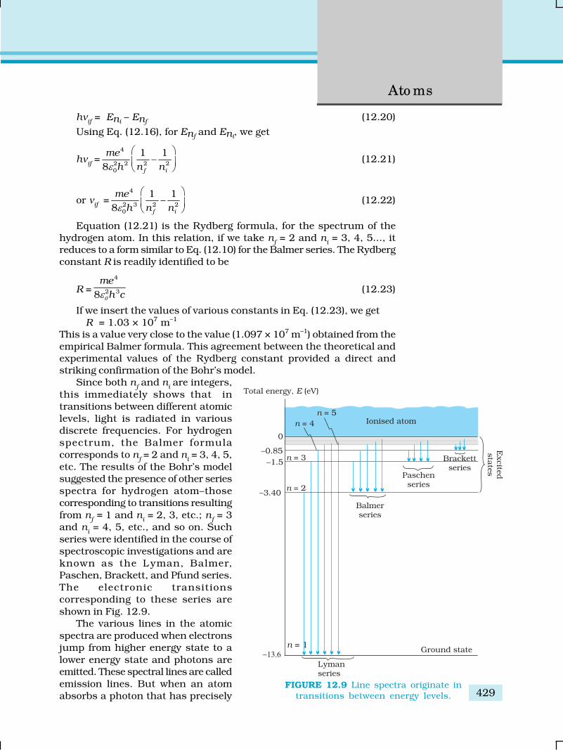
429
Ato ms
hνif = Eni
– Enf(12.20)
Using Eq. (12.16), for Enf and Eni
, we get
hνif =
4
2 2 2 20
1 1
8 f i
me
h n nε⎛ ⎞−⎜ ⎟⎝ ⎠ (12.21)
or νif =
4
2 3 2 20
1 1
8 f i
me
h n nε⎛ ⎞−⎜ ⎟⎝ ⎠ (12.22)
Equation (12.21) is the Rydberg formula, for the spectrum of thehydrogen atom. In this relation, if we take n
f = 2 and n
i = 3, 4, 5..., it
reduces to a form similar to Eq. (12.10) for the Balmer series. The Rydbergconstant R is readily identified to be
R =
4
2 38
me
h c0ε (12.23)
If we insert the values of various constants in Eq. (12.23), we getR = 1.03 × 10⁷ m–1
This is a value very close to the value (1.097 × 10⁷ m–1) obtained from theempirical Balmer formula. This agreement between the theoretical andexperimental values of the Rydberg constant provided a direct andstriking confirmation of the Bohr’s model.
Since both nf and n
i are integers,
this immediately shows that intransitions between different atomic
levels, light is radiated in variousdiscrete frequencies. For hydrogen
spectrum, the Balmer formulacorresponds to n
f = 2 and n
i = 3, 4, 5,
etc. The results of the Bohr’s modelsuggested the presence of other series
spectra for hydrogen atom–thosecorresponding to transitions resulting
from nf = 1 and n
i = 2, 3, etc.; n
f = 3
and ni = 4, 5, etc., and so on. Such
series were identified in the course ofspectroscopic investigations and are
known as the L yman, Balmer,Paschen, Brackett, and Pfund series.
The electronic transitionscorresponding to these series are
shown in Fig. 12.9.The various lines in the atomic
spectra are produced when electronsjump from higher energy state to a
lower energy state and photons areemitted. These spectral lines are called
emission lines. But when an atomabsorbs a photon that has precisely
FIGURE 12.9 Line spectra originate intransitions between energy levels.

Physic s
430
EX
AM
PLE 1
2.6
the same energy needed by the electron in a lower energy state to maketransitions to a higher energy state, the process is called absorption.Thus if photons with a continuous range of frequencies pass through ararefied gas and then are analysed with a spectrometer, a series of darkspectral absorption lines appear in the continuous spectrum. The darklines indicate the frequencies that have been absorbed by the atoms ofthe gas.
The explanation of the hydrogen atom spectrum provided by Bohr’smodel was a brilliant achievement, which greatly stimulated progresstowards the modern quantum theory. In 1922, Bohr was awarded NobelPrize in Physics.
Example 12.6 Using the Rydberg formula, calculate the wavelengthsof the first four spectral lines in the Lyman series of the hydrogenspectrum.
Solution The Rydberg formula is
hc/λif =
4
2 2 2 2
1 1
8 f i
me
h n n0ε⎛ ⎞−⎜ ⎟⎝ ⎠
The wavelengths of the first four lines in the Lyman series correspondto transitions from n
i = 2,3,4,5 to n
f = 1. We know that
4
2 28
me
h0ε = 13.6 eV = 21.76 ×10⁻¹⁹ J
Therefore,
1
19
2
m1 1
21.76 101
i
i
hc
n
λ−
= ⎛ ⎞× −⎜ ⎟⎝ ⎠ =
.
34 8 2
19 2
6 625 10 3 10m
21.76 10 ( 1)i
i
n
n
−−
× × × ×× × − =
27
2
0.9134 10 m
( 1)i
i
n
n
−×− = 913.4 n
i
2/(ni
2 –1) ÅSubstituting n
i = 2,3,4,5, we get λ
21 = 1218 Å, λ
31 = 1028 Å, λ
41 = 974.3 Å,
and λ51
= 951.4 Å.
12.6 DE BROGLIE’S EXPLANATION OF BOHR’SSECOND POSTULATE OF QUANTISATION
Of all the postulates, Bohr made in his model of the atom, perhaps themost puzzling is his second postulate. It states that the angularmomentum of the electron orbiting around the nucleus is quantised (thatis, L
n = nh/2π; n = 1, 2, 3 …). Why should the angular momentum have
only those values that are integral multiples of h/2π? The French physicistLouis de Broglie explained this puzzle in 1923, ten years after Bohrproposed his model.
We studied, in Chapter 11, about the de Broglie’s hypothesis thatmaterial particles, such as electrons, also have a wave nature. C. J. Davissonand L. H. Germer later experimentally verified the wave nature of electrons

431
Ato ms
in 1927. Louis de Broglie argued that the electron in itscircular orbit, as proposed by Bohr, must be seen as a particlewave. In analogy to waves travelling on a string, particle wavestoo can lead to standing waves under resonant conditions.From Chapter 15 of Class XI Physics textbook, we know thatwhen a string is plucked, a vast number of wavelengths areexcited. However only those wavelengths survive which havenodes at the ends and form the standing wave in the string. Itmeans that in a string, standing waves are formed when thetotal distance travelled by a wave down the string and back isone wavelength, two wavelengths, or any integral number ofwavelengths. Waves with other wavelengths interfere withthemselves upon reflection and their amplitudes quickly dropto zero. For an electron moving in nth circular orbit of radiusr
n, the total distance is the circumference of the orbit, 2πr
n.
Thus
2π rn = nλ, n = 1, 2, 3... (12.24)
Figure 12.10 illustrates a standing particle wave on acircular orbit for n = 4, i.e., 2πr
n = 4λ, where λ is the de Broglie
wavelength of the electron moving in nth orbit. From Chapter11, we have λ = h/p, where p is the magnitude of the electron’smomentum. If the speed of the electron is much less than the speed oflight, the momentum is mv
n. Thus, λ = h/mv
n. From Eq. (12.24), we have
2π rn = n h/mv
n or m v
n r
n = nh/2π
This is the quantum condition proposed by Bohr for the angularmomentum of the electron [Eq. (12.13)]. In Section 12.5, we saw thatthis equation is the basis of explaining the discrete orbits and energylevels in hydrogen atom. Thus de Broglie hypothesis provided anexplanation for Bohr’s second postulate for the quantisation of angularmomentum of the orbiting electron. The quantised electron orbits andenergy states are due to the wave nature of the electron and only resonantstanding waves can persist.
Bohr’s model, involving classical trajectory picture (planet-like electronorbiting the nucleus), correctly predicts the gross features of thehydrogenic atoms*, in particular, the frequencies of the radiation emittedor selectively absorbed. This model however has many limitations.Some are:(i) The Bohr model is applicable to hydrogenic atoms. It cannot be
extended even to mere two electron atoms such as helium. The analysisof atoms with more than one electron was attempted on the lines ofBohr’s model for hydrogenic atoms but did not meet with any success.Difficulty lies in the fact that each electron interacts not only with thepositively charged nucleus but also with all other electrons.
FIGURE 12.10 A standingwave is shown on a circularorbit where four de Broglie
wavelengths fit into thecircumference of the orbit.
* Hydrogenic atoms are the atoms consisting of a nucleus with positive charge+Ze and a single electron, where Z is the proton number. Examples are hydrogenatom, singly ionised helium, doubly ionised lithium, and so forth. In theseatoms more complex electron-electron interactions are nonexistent.

Physic s
432
The formulation of Bohr model involves electrical force betweenpositively charged nucleus and electron. It does not include theelectrical forces between electrons which necessarily appear inmulti-electron atoms.
(ii) While the Bohr’s model correctly predicts the frequencies of the lightemitted by hydrogenic atoms, the model is unable to explain therelative intensities of the frequencies in the spectrum. In emissionspectrum of hydrogen, some of the visible frequencies have weakintensity, others strong. Why? Experimental observations depict thatsome transitions are more favoured than others. Bohr’s model isunable to account for the intensity variations.
Bohr’s model presents an elegant picture of an atom and cannot begeneralised to complex atoms. For complex atoms we have to use a newand radical theory based on Quantum Mechanics, which provides a morecomplete picture of the atomic structure.
LASER LIGHT
Imagine a crowded market place or a railway platform with people entering a gate andgoing towards all directions. Their footsteps are random and there is no phase correlationbetween them. On the other hand, think of a large number of soldiers in a regulated march.Their footsteps are very well correlated. See figure here.
This is similar to the difference between light emitted byan ordinary source like a candle or a bulb and that emittedby a laser. The acronym LASER stands for Light Amplificationby Stimulated Emission of Radiation. Since its developmentin 1960, it has entered into all areas of science and technology.It has found applications in physics, chemistry, biology,medicine, surgery, engineering, etc. There are low powerlasers, with a power of 0.5 mW, called pencil lasers, whichserve as pointers. There are also lasers of different power,suitable for delicate surgery of eye or glands in the stomach.Finally, there are lasers which can cut or weld steel.
Light is emitted from a source in the form of packets ofwaves. Light coming out from an ordinary source contains a mixture of many wavelengths.There is also no phase relation between the various waves. Therefore, such light, even if it ispassed through an aperture, spreads very fast and the beam size increases rapidly withdistance. In the case of laser light, the wavelength of each packet is almost the same. Alsothe average length of the packet of waves is much larger. This means that there is betterphase correlation over a longer duration of time. This results in reducing the divergence ofa laser beam substantially.
If there are N atoms in a source, each emitting light with intensity I, then the totalintensity produced by an ordinary source is proportional to NI, whereas in a laser source,it is proportional to N2I. Considering that N is very large, we see that the light from a lasercan be much stronger than that from an ordinary source.
When astronauts of the Apollo missions visited the moon, they placed a mirror on itssurface, facing the earth. Then scientists on the earth sent a strong laser beam, which wasreflected by the mirror on the moon and received back on the earth. The size of the reflectedlaser beam and the time taken for the round trip were measured. This allowed a veryaccurate determination of (a) the extremely small divergence of a laser beam and (b) thedistance of the moon from the earth.

433
Ato ms
SUMMARY
1. Atom, as a whole, is electrically neutral and therefore contains equalamount of positive and negative charges.
2. In Thomson’s model, an atom is a spherical cloud of positive chargeswith electrons embedded in it.
3. In Rutherford’s model, most of the mass of the atom and all its positivecharge are concentrated in a tiny nucleus (typically one by ten thousandthe size of an atom), and the electrons revolve around it.
4. Rutherford nuclear model has two main difficulties in explaining thestructure of atom: (a) It predicts that atoms are unstable because theaccelerated electrons revolving around the nucleus must spiral intothe nucleus. This contradicts the stability of matter. (b) It cannotexplain the characteristic line spectra of atoms of different elements.
5. Atoms of each element are stable and emit characteristic spectrum.The spectrum consists of a set of isolated parallel lines termed as linespectrum. It provides useful information about the atomic structure.
6. The atomic hydrogen emits a line spectrum consisting of various series.The frequency of any line in a series can be expressed as a differenceof two terms;
Lyman series: 2 2
1 1
1Rc
nν = −⎛ ⎞⎜ ⎟⎝ ⎠ ; n = 2, 3, 4,...
Balmer series: 2 2
1 1
2Rc
nν = −⎛ ⎞⎜ ⎟⎝ ⎠ ; n = 3, 4, 5,...
Paschen series: 2 2
1 1
3Rc
nν = −⎛ ⎞⎜ ⎟⎝ ⎠ ; n = 4, 5, 6,...
Brackett series: 2 2
1 1
4Rc
nν = −⎛ ⎞⎜ ⎟⎝ ⎠ ; n = 5, 6, 7,...
Pfund series:2 2
1 1
5Rc
nν = −⎛ ⎞⎜ ⎟⎝ ⎠ ; n = 6, 7, 8,...
7. To explain the line spectra emitted by atoms, as well as the stabilityof atoms, Niel’s Bohr proposed a model for hydrogenic (single elctron)atoms. He introduced three postulates and laid the foundations ofquantum mechanics:
(a) In a hydrogen atom, an electron revolves in certain stable orbits(called stationary orbits) without the emission of radiant energy.
(b) The stationary orbits are those for which the angular momentumis some integral multiple of h/2π. (Bohr’s quantisation condition.)That is L = nh/2π, where n is an integer called a quantum number.
(c) The third postulate states that an electron might make a transitionfrom one of its specified non-radiating orbits to another of lowerenergy. When it does so, a photon is emitted having energy equalto the energy difference between the initial and final states. Thefrequency (ν) of the emitted photon is then given by
hν = Ei – E
f
An atom absorbs radiation of the same frequency the atom emits,in which case the electron is transferred to an orbit with a highervalue of n.
Ei + hν = E
f

Physic s
434
8. As a result of the quantisation condition of angular momentum, theelectron orbits the nucleus at only specific radii. For a hydrogen atomit is given by
220
2
4
2n
n hr
m e
ε⎛ ⎞ π⎛ ⎞= ⎜ ⎟⎜ ⎟ ⎝ ⎠π⎝ ⎠The total energy is also quantised:
4
2 2 208
n
meE
n hε= − = –13.6 eV/n2
The n = 1 state is called ground state. In hydrogen atom the groundstate energy is –13.6 eV. Higher values of n correspond to excitedstates (n > 1). Atoms are excited to these higher states by collisionswith other atoms or electrons or by absorption of a photon of rightfrequency.
9. de Broglie’s hypothesis that electrons have a wavelength λ = h/mv gavean explanation for Bohr’s quantised orbits by bringing in the wave-particle duality. The orbits correspond to circular standing waves inwhich the circumference of the orbit equals a whole number ofwavelengths.
10. Bohr’s model is applicable only to hydrogenic (single electron) atoms.It cannot be extended to even two electron atoms such as helium.This model is also unable to explain for the relative intensities of thefrequencies emitted even by hydrogenic atoms.
POINTS TO PONDER
1. Both the Thomson’s as well as the Rutherford’s models constitute anunstable system. Thomson’s model is unstable electrostatically, whileRutherford’s model is unstable because of electromagnetic radiationof orbiting electrons.
2. What made Bohr quantise angular momentum (second postulate) andnot some other quantity? Note, h has dimensions of angularmomentum, and for circular orbits, angular momentum is a veryrelevant quantity. The second postulate is then so natural!
3. The orbital picture in Bohr’s model of the hydrogen atom wasinconsistent with the uncertainty principle. It was replaced by modernquantum mechanics in which Bohr’s orbits are regions where theelectron may be found with large probability.
4. Unlike the situation in the solar system, where planet-planetgravitational forces are very small as compared to the gravitationalforce of the sun on each planet (because the mass of the sun is somuch greater than the mass of any of the planets), the electron-electronelectric force interaction is comparable in magnitude to the electron-nucleus electrical force, because the charges and distances are of thesame order of magnitude. This is the reason why the Bohr’s modelwith its planet-like electron is not applicable to many electron atoms.
5. Bohr laid the foundation of the quantum theory by postulating specificorbits in which electrons do not radiate. Bohr’s model include only

435
Ato ms
one quantum number n. The new theory called quantum mechanicssupportes Bohr’s postulate. However in quantum mechanics (moregenerally accepted), a given energy level may not correspond to justone quantum state. For example, a state is characterised by fourquantum numbers (n, l, m, and s), but for a pure Coulomb potential(as in hydrogen atom) the energy depends only on n.
6. In Bohr model, contrary to ordinary classical expectation, thefrequency of revolution of an electron in its orbit is not connected tothe frequency of spectral line. The later is the difference between twoorbital energies divided by h. For transitions between large quantumnumbers (n to n – 1, n very large), however, the two coincide as expected.
7. Bohr’s semiclassical model based on some aspects of classical physicsand some aspects of modern physics also does not provide a truepicture of the simplest hydrogenic atoms. The true picture is quantummechanical affair which differs from Bohr model in a number offundamental ways. But then if the Bohr model is not strictly correct,why do we bother about it? The reasons which make Bohr’s modelstill useful are:
(i) The model is based on just three postulates but accounts for almostall the general features of the hydrogen spectrum.
(ii) The model incorporates many of the concepts we have learnt inclassical physics.
(iii) The model demonstrates how a theoretical physicist occasionallymust quite literally ignore certain problems of approach in hopesof being able to make some predictions. If the predictions of thetheory or model agree with experiment, a theoretician then mustsomehow hope to explain away or rationalise the problems thatwere ignored along the way.
EXERCISES
12.1 Choose the correct alternative from the clues given at the end ofthe each statement:
(a) The size of the atom in Thomson’s model is .......... the atomicsize in Rutherford’s model. (much greater than/no differentfrom/much less than.)
(b) In the ground state of .......... electrons are in stable equilibrium,while in .......... electrons always experience a net force.(Thomson’s model/ Rutherford’s model.)
(c) A classical atom based on .......... is doomed to collapse.(Thomson’s model/ Rutherford’s model.)
(d) An atom has a nearly continuous mass distribution in a ..........but has a highly non-uniform mass distribution in ..........(Thomson’s model/ Rutherford’s model.)
(e) The positively charged part of the atom possesses most of themass in .......... (Rutherford’s model/both the models.)
12.2 Suppose you are given a chance to repeat the alpha-particlescattering experiment using a thin sheet of solid hydrogen in placeof the gold foil. (Hydrogen is a solid at temperatures below 14 K.)What results do you expect?

Physic s
436
12.3 What is the shortest wavelength present in the Paschen series ofspectral lines?
12.4 A difference of 2.3 eV separates two energy levels in an atom. Whatis the frequency of radiation emitted when the atom make atransition from the upper level to the lower level?
12.5 The ground state energy of hydrogen atom is –13.6 eV. What are thekinetic and potential energies of the electron in this state?
12.6 A hydrogen atom initially in the ground level absorbs a photon,which excites it to the n = 4 level. Determine the wavelength andfrequency of photon.
12.7 (a) Using the Bohr’s model calculate the speed of the electron in ahydrogen atom in the n = 1, 2, and 3 levels. (b) Calculate the orbitalperiod in each of these levels.
12.8 The radius of the innermost electron orbit of a hydrogen atom is5.3×10–11 m. What are the radii of the n = 2 and n =3 orbits?
12.9 A 12.5 eV electron beam is used to bombard gaseous hydrogen atroom temperature. What series of wavelengths will be emitted?
12.10 In accordance with the Bohr’s model, find the quantum numberthat characterises the earth’s revolution around the sun in an orbitof radius 1.5 × 10¹¹ m with orbital speed 3 × 10⁴ m/s. (Mass of earth= 6.0 × 1024 kg.)
ADDITIONAL EXERCISES
12.11 Answer the following questions, which help you understand thedifference between Thomson’s model and Rutherford’s model better.
(a) Is the average angle of deflection of α-particles by a thin gold foilpredicted by Thomson’s model much less, about the same, ormuch greater than that predicted by Rutherford’s model?
(b) Is the probability of backward scattering (i.e., scattering ofα-particles at angles greater than 90°) predicted by Thomson’smodel much less, about the same, or much greater than thatpredicted by Rutherford’s model?
(c) Keeping other factors fixed, it is found experimentally that forsmall thickness t, the number of α-particles scattered atmoderate angles is proportional to t. What clue does this lineardependence on t provide?
(d) In which model is it completely wrong to ignore multiplescattering for the calculation of average angle of scattering ofα-particles by a thin foil?
12.12 The gravitational attraction between electron and proton in ahydrogen atom is weaker than the coulomb attraction by a factor ofabout 10–40. An alternative way of looking at this fact is to estimatethe radius of the first Bohr orbit of a hydrogen atom if the electronand proton were bound by gravitational attraction. You will find theanswer interesting.
12.13 Obtain an expression for the frequency of radiation emitted when ahydrogen atom de-excites from level n to level (n–1). For large n,show that this frequency equals the classical frequency of revolutionof the electron in the orbit.

437
Ato ms
12.14 Classically, an electron can be in any orbit around the nucleus ofan atom. Then what determines the typical atomic size? Why is anatom not, say, thousand times bigger than its typical size? Thequestion had greatly puzzled Bohr before he arrived at his famousmodel of the atom that you have learnt in the text. To simulate whathe might well have done before his discovery, let us play as followswith the basic constants of nature and see if we can get a quantitywith the dimensions of length that is roughly equal to the knownsize of an atom (~ 10–10m).
(a) Construct a quantity with the dimensions of length from thefundamental constants e, m
e, and c. Determine its numerical
value.
(b) You will find that the length obtained in (a) is many orders ofmagnitude smaller than the atomic dimensions. Further, itinvolves c. But energies of atoms are mostly in non-relativisticdomain where c is not expected to play any role. This is whatmay have suggested Bohr to discard c and look for ‘somethingelse’ to get the right atomic size. Now, the Planck’s constant h
had already made its appearance elsewhere. Bohr’s great insightlay in recognising that h, m
e, and e will yield the right atomic
size. Construct a quantity with the dimension of length from h,me, and e and confirm that its numerical value has indeed thecorrect order of magnitude.
12.15 The total energy of an electron in the first excited state of thehydrogen atom is about –3.4 eV.
(a) What is the kinetic energy of the electron in this state?
(b) What is the potential energy of the electron in this state?
(c) Which of the answers above would change if the choice of thezero of potential energy is changed?
12.16 If Bohr’s quantisation postulate (angular momentum = nh/2π) is abasic law of nature, it should be equally valid for the case of planetarymotion also. Why then do we never speak of quantisation of orbitsof planets around the sun?
12.17 Obtain the first Bohr’s radius and the ground state energy of amuonic hydrogen atom [i.e., an atom in which a negatively chargedmuon (μ–) of mass about 207m
e orbits around a proton].

Physic s
438
13.1 INTRODUCTION
In the previous chapter, we have learnt that in every atom, the positive
charge and mass are densely concentrated at the centre of the atom
forming its nucleus. The overall dimensions of a nucleus are much smaller
than those of an atom. Experiments on scattering of α-particles
demonstrated that the radius of a nucleus was smaller than the radius
of an atom by a factor of about 104. This means the volume of a nucleus
is about 10–12 times the volume of the atom. In other words, an atom is
almost empty. If an atom is enlarged to the size of a classroom, the nucleus
would be of the size of pinhead. Nevertheless, the nucleus contains most
(more than 99.9%) of the mass of an atom.
Does the nucleus have a structure, just as the atom does? If so, what
are the constituents of the nucleus? How are these held together? In this
chapter, we shall look for answers to such questions. We shall discuss
various properties of nuclei such as their size, mass and stability, and
also associated nuclear phenomena such as radioactivity, fission and fusion.
13.2 ATOMIC MASSES AND COMPOSITION OF NUCLEUS
The mass of an atom is very small, compared to a kilogram; for example,the mass of a carbon atom, 12C, is 1.992647 × 10⁻²⁶ kg. Kilogram is nota very convenient unit to measure such small quantities. Therefore, a
Chapte r Thirte e n
NUCLEI

439
Nuc le i
different mass unit is used for expressing atomic masses. This unit is theatomic mass unit (u), defined as 1/12th of the mass of the carbon (12C)atom. According to this definition
12 mass of one C atom1u =
12
261.992647 10 kg
12
−×= 271.660539 10 kg−= × (13.1)
The atomic masses of various elements expressed in atomic massunit (u) are close to being integral multiples of the mass of a hydrogenatom. There are, however, many striking exceptions to this rule. Forexample, the atomic mass of chlorine atom is 35.46 u.
Accurate measurement of atomic masses is carried out with a massspectrometer, The measurement of atomic masses reveals the existenceof different types of atoms of the same element, which exhibit the samechemical properties, but differ in mass. Such atomic species of the sameelement differing in mass are called isotopes. (In Greek, isotope meansthe same place, i.e. they occur in the same place in the periodic table ofelements.) It was found that practically every element consists of a mixtureof several isotopes. The relative abundance of different isotopes differsfrom element to element. Chlorine, for example, has two isotopes havingmasses 34.98 u and 36.98 u, which are nearly integral multiples of themass of a hydrogen atom. The relative abundances of these isotopes are75.4 and 24.6 per cent, respectively. Thus, the average mass of a chlorineatom is obtained by the weighted average of the masses of the twoisotopes, which works out to be
= 75.4 34.98 24.6 36.98
100
× + ×= 35.47 u
which agrees with the atomic mass of chlorine.Even the lightest element, hydrogen has three isotopes having masses
1.0078 u, 2.0141 u, and 3.0160 u. The nucleus of the lightest atom ofhydrogen, which has a relative abundance of 99.985%, is called theproton. The mass of a proton is
271.00727 u 1.67262 10 kgpm −= = × (13.2)
This is equal to the mass of the hydrogen atom (= 1.00783u), minusthe mass of a single electron (m
e = 0.00055 u). The other two isotopes of
hydrogen are called deuterium and tritium. Tritium nuclei, beingunstable, do not occur naturally and are produced artificially inlaboratories.
The positive charge in the nucleus is that of the protons. A protoncarries one unit of fundamental charge and is stable. It was earlier thoughtthat the nucleus may contain electrons, but this was ruled out later usingarguments based on quantum theory. All the electrons of an atom areoutside the nucleus. We know that the number of these electrons outsidethe nucleus of the atom is Z, the atomic number. The total charge of the

Physic s
440
atomic electrons is thus (–Ze), and since the atom is neutral, the chargeof the nucleus is (+Ze). The number of protons in the nucleus of the atomis, therefore, exactly Z, the atomic number.
Discovery of Neutron
Since the nuclei of deuterium and tritium are isotopes of hydrogen, theymust contain only one proton each. But the masses of the nuclei ofhydrogen, deuterium and tritium are in the ratio of 1:2:3. Therefore, thenuclei of deuterium and tritium must contain, in addition to a proton,some neutral matter. The amount of neutral matter present in the nucleiof these isotopes, expressed in units of mass of a proton, is approximatelyequal to one and two, respectively. This fact indicates that the nuclei ofatoms contain, in addition to protons, neutral matter in multiples of abasic unit. This hypothesis was verified in 1932 by James Chadwickwho observed emission of neutral radiation when beryllium nuclei were
bombarded with alpha-particles. (α-particles are helium nuclei, to be
discussed in a later section). It was found that this neutral radiationcould knock out protons from light nuclei such as those of helium, carbonand nitrogen. The only neutral radiation known at that time was photons(electromagnetic radiation). Application of the principles of conservationof energy and momentum showed that if the neutral radiation consistedof photons, the energy of photons would have to be much higher than is
available from the bombardment of beryllium nuclei with α-particles.
The clue to this puzzle, which Chadwick satisfactorily solved, was toassume that the neutral radiation consists of a new type of neutralparticles called neutrons. From conservation of energy and momentum,he was able to determine the mass of new particle ‘as very nearly thesame as mass of proton’.
The mass of a neutron is now known to a high degree of accuracy. It is
mn = 1.00866 u = 1.6749×10⁻²⁷ kg (13.3)
Chadwick was awarded the 1935 Nobel Prize in Physics for hisdiscovery of the neutron.
A free neutron, unlike a free proton, is unstable. It decays into aproton, an electron and a antineutrino (another elementary particle), andhas a mean life of about 1000s. It is, however, stable inside the nucleus.
The composition of a nucleus can now be described using the followingterms and symbols:
Z - atomic number = number of protons [13.4(a)]
N - neutron number = number of neutrons [13.4(b)]
A - mass number = Z + N
= total number of protons and neutrons [13.4(c)]
One also uses the term nucleon for a proton or a neutron. Thus thenumber of nucleons in an atom is its mass number A.
Nuclear species or nuclides are shown by the notation XAZ
where X is
the chemical symbol of the species. For example, the nucleus of gold is
denoted by 19779 Au . It contains 197 nucleons, of which 79 are protons
and the rest118 are neutrons.

441
Nuc le i
The composition of isotopes of an element can now be readilyexplained. The nuclei of isotopes of a given element contain the samenumber of protons, but differ from each other in their number of neutrons.
Deuterium, 21 H , which is an isotope of hydrogen, contains one proton
and one neutron. Its other isotope tritium, 31 H , contains one proton and
two neutrons. The element gold has 32 isotopes, ranging from A =173 toA = 204. We have already mentioned that chemical properties of elementsdepend on their electronic structure. As the atoms of isotopes haveidentical electronic structure they have identical chemical behaviour andare placed in the same location in the periodic table.
All nuclides with same mass number A are called isobars. For
example, the nuclides 31 H and 3
2He are isobars. Nuclides with same
neutron number N but different atomic number Z, for example 19880 Hg
and 19779 Au , are called isotones.
13.3 SIZE OF THE NUCLEUS
As we have seen in Chapter 12, Rutherford was the pioneer who
postulated and established the existence of the atomic nucleus. At
Rutherford’s suggestion, Geiger and Marsden performed their classic
experiment: on the scattering of α-particles from thin gold foils. Their
experiments revealed that the distance of closest approach to a gold
nucleus of an α-particle of kinetic energy 5.5 MeV is about 4.0 × 10⁻¹⁴ m.
The scattering of α-particle by the gold sheet could be understood by
Rutherford by assuming that the coulomb repulsive force was solely
responsible for scattering. Since the positive charge is confined to the
nucleus, the actual size of the nucleus has to be less than 4.0 × 10⁻¹⁴ m.
If we use α-particles of higher energies than 5.5 MeV, the distance of
closest approach to the gold nucleus will be smaller and at some point
the scattering will begin to be affected by the short range nuclear forces,
and differ from Rutherford’s calculations. Rutherford’s calculations are
based on pure coulomb repulsion between the positive charges of the α-
particle and the gold nucleus. From the distance at which deviations set
in, nuclear sizes can be inferred.
By performing scattering experiments in which fast electrons, insteadof α-particles, are projectiles that bombard targets made up of variouselements, the sizes of nuclei of various elements have been accuratelymeasured.
It has been found that a nucleus of mass number A has a radius
R = R0
A1/3 (13.5)
where R0 = 1.2 × 10⁻¹⁵ m. This means the volume of the nucleus, which
is proportional to R3 is proportional to A. Thus the density of nucleus is
a constant, independent of A, for all nuclei. Different nuclei are likes
drop of liquid of constant density. The density of nuclear matter is
approximately 2.3 × 10¹⁷ kg m–3. This density is very large compared to
ordinary matter, say water, which is 103 kg m–3. This is understandable,
as we have already seen that most of the atom is empty. Ordinary matter
consisting of atoms has a large amount of empty space.

Physic s
442
EX
AM
PLE 1
3.2
Example 13.1 Given the mass of iron nucleus as 55.85u and A=56,find the nuclear density?
Solutionm
Fe = 55.85
u = 9.27 × 10⁻²⁶ kg
Nuclear density = mass
volume =
26
15 3
9.27 10 1
56(4 /3)(1.2 10 )
−−
× ×π × = 2.29 × 10¹⁷ kg m–3
The density of matter in neutron stars (an astrophysical object) iscomparable to this density. This shows that matter in these objectshas been compressed to such an extent that they resemble a big
nucleus.
13.4.1 Mass – Energy
Einstein showed from his theory of special relativity that it is necessaryto treat mass as another form of energy. Before the advent of this theoryof special relativity it was presumed that mass and energy were conservedseparately in a reaction. However, Einstein showed that mass is anotherform of energy and one can convert mass-energy into other forms ofenergy, say kinetic energy and vice-versa.
Einstein gave the famous mass-energy equivalence relation
E = mc 2 (13.6)
Here the energy equivalent of mass m is related by the above equationand c is the velocity of light in vacuum and is approximately equal to3×108 m s–1.
Example 13.2 Calculate the energy equivalent of 1 g of substance.
Solution
Energy, E = 10–3 × ( 3 × 10⁸)2 J
E = 10–3 × 9 × 1016 = 9 × 10¹³ J
Thus, if one gram of matter is converted to energy, there is a release
of enormous amount of energy.
Experimental verification of the Einstein’s mass-energy relation has
been achieved in the study of nuclear reactions amongst nucleons, nuclei,
electrons and other more recently discovered particles. In a reaction the
conservation law of energy states that the initial energy and the final
energy are equal provided the energy associated with mass is also
included. This concept is important in understanding nuclear masses
and the interaction of nuclei with one another. They form the subject
matter of the next few sections.
13.4.2 Nuclear binding energy
In Section 13.2 we have seen that the nucleus is made up of neutronsand protons. Therefore it may be expected that the mass of the nucleusis equal to the total mass of its individual protons and neutrons. However,
EX
AM
PLE 1
3.1

443
Nuc le i
EX
AM
PLE 1
3.3
the nuclear mass M is found to be always less than this. For example, let
us consider 168 O ; a nucleus which has 8 neutrons and 8 protons. We
have
Mass of 8 neutrons = 8 × 1.00866 u
Mass of 8 protons = 8 × 1.00727 u
Mass of 8 electrons = 8 × 0.00055 u
Therefore the expected mass of 168 O nucleus
= 8 × 2.01593 u = 16.12744 u.
The atomic mass of 168 O found from mass spectroscopy experiments
is seen to be 15.99493 u. Substracting the mass of 8 electrons (8 × 0.00055 u)
from this, we get the experimental mass of 168 O nucleus to be 15.99053 u.
Thus, we find that the mass of the 168 O nucleus is less than the total
mass of its constituents by 0.13691u. The difference in mass of a nucleus
and its constituents, ΔM, is called the mass defect, and is given by
[ ( ) ]p nM Zm A Z m MΔ = + − − (13.7)
What is the meaning of the mass defect? It is here that Einstein’sequivalence of mass and energy plays a role. Since the mass of the oxygennucleus is less that the sum of the masses of its constituents (8 protonsand 8 neutrons, in the unbound state), the equivalent energy of the oxygennucleus is less than that of the sum of the equivalent energies of itsconstituents. If one wants to break the oxygen nucleus into 8 protons
and 8 neutrons, this extra energy ΔM c2, has to supplied. This energy
required Eb is related to the mass defect by
Eb = Δ M c2 (13.8)
Example 13.3 Find the energy equivalent of one atomic mass unit,first in Joules and then in MeV. Using this, express the mass defect
of 168 O in MeV/c2.
Solution1u = 1.6605 × 10⁻²⁷ kgTo convert it into energy units, we multiply it by c2 and find thatenergy equivalent = 1.6605 × 10–27 × (2.9979 × 108)2 kg m2/s2
= 1.4924 × 10⁻¹⁰ J
=
10
19
1.4924 10eV
1.602 10
−−
××
= 0.9315 × 10⁹ eV = 931.5 MeV
or, 1u = 931.5 MeV/c2
For 168 O , ΔM = 0.13691 u = 0.13691×931.5 MeV/c2
= 127.5 MeV/c2
The energy needed to separate 168 O into its constituents is thus
127.5 MeV/c2.
If a certain number of neutrons and protons are brought together toform a nucleus of a certain charge and mass, an energy E
b will be released

Physic s
444
in the process. The energy Eb is called the binding energy of the nucleus.
If we separate a nucleus into its nucleons, we would have to supply atotal energy equal to E
b, to those particles. Although we cannot tear
apart a nucleus in this way, the nuclear binding energy is still a convenientmeasure of how well a nucleus is held together. A more useful measureof the binding between the constituents of the nucleus is the binding
energy per nucleon, Ebn
, which is the ratio of the binding energy Eb of a
nucleus to the number of the nucleons, A, in that nucleus:
Ebn
= Eb / A (13.9)
We can think of binding energy per nucleon as the average energyper nucleon needed to separate a nucleus into its individual nucleons.
Figure 13.1 is a plot of thebinding energy per nucleon E
bn
versus the mass number A for alarge number of nuclei. We noticethe following main features ofthe plot:(i) the binding energy per
nucleon, Ebn
, is practicallyconstant, i.e. practicallyindependent of the atomicnumber for nuclei of middlemass number ( 30 < A < 170).The curve has a maximum ofabout 8.75 MeV for A = 56and has a value of 7.6 MeVfor A = 238.
(ii) Ebn
is lower for both lightnuclei (A<30) and heavynuclei (A>170).
We can draw some conclusions from these two observations:(i) The force is attractive and sufficiently strong to produce a binding
energy of a few MeV per nucleon.(ii) The constancy of the binding energy in the range 30 < A < 170 is a
consequence of the fact that the nuclear force is short-ranged. Considera particular nucleon inside a sufficiently large nucleus. It will be underthe influence of only some of its neighbours, which come within therange of the nuclear force. If any other nucleon is at a distance morethan the range of the nuclear force from the particular nucleon it willhave no influence on the binding energy of the nucleon underconsideration. If a nucleon can have a maximum of p neighbourswithin the range of nuclear force, its binding energy would beproportional to p. Let the binding energy of the nucleus be pk, wherek is a constant having the dimensions of energy. If we increase A byadding nucleons they will not change the binding energy of a nucleoninside. Since most of the nucleons in a large nucleus reside inside itand not on the surface, the change in binding energy per nucleonwould be small. The binding energy per nucleon is a constant and isapproximately equal to pk. The property that a given nucleon
FIGURE 13.1 The binding energy per nucleonas a function of mass number.

445
Nuc le i
influences only nucleons close to it is also referred to as saturationproperty of the nuclear force.
(iii) A very heavy nucleus, say A = 240, has lower binding energy pernucleon compared to that of a nucleus with A = 120. Thus if anucleus A = 240 breaks into two A = 120 nuclei, nucleons get moretightly bound. This implies energy would be released in the process.It has very important implications for energy production throughfission, to be discussed later in Section 13.7.1.
(iv) Consider two very light nuclei (A≤ 10) joining to form a heavier
nucleus. The binding energy per nucleon of the fused heavier nucleiis more than the binding energy per nucleon of the lighter nuclei.This means that the final system is more tightly bound than the initialsystem. Again energy would be released in such a process offusion. This is the energy source of sun, to be discussed later inSection 13.7.3.
13.5 NUCLEAR FORCE
The force that determines the motion of atomic electrons is the familiar
Coulomb force. In Section 13.4, we have seen that for average mass
nuclei the binding energy per nucleon is approximately 8 MeV, which is
much larger than the binding energy in atoms. Therefore, to bind a
nucleus together there must be a strong attractive force of a totally
different kind. It must be strong enough to overcome the repulsion
between the (positively charged) protons and to bind both protons and
neutrons into the tiny nuclear volume. We have already seen
that the constancy of binding energy per nucleon can be
understood in terms of its short-range. Many features of the
nuclear binding force are summarised below. These are
obtained from a variety of experiments carried out during 1930
to 1950.
(i) The nuclear force is much stronger than the Coulomb force
acting between charges or the gravitational forces between
masses. The nuclear binding force has to dominate over
the Coulomb repulsive force between protons inside the
nucleus. This happens only because the nuclear force is
much stronger than the coulomb force. The gravitational
force is much weaker than even Coulomb force.
(ii) The nuclear force between two nucleons falls rapidly to
zero as their distance is more than a few femtometres. This
leads to saturation of forces in a medium or a large-sized
nucleus, which is the reason for the constancy of the
binding energy per nucleon.
A rough plot of the potential energy between two nucleons
as a function of distance is shown in the Fig. 13.2. The
potential energy is a minimum at a distance r0 of about
0.8 fm. This means that the force is attractive for distances larger
than 0.8 fm and repulsive if they are separated by distances less
than 0.8 fm.
FIGURE 13.2 Potential energyof a pair of nucleons as a
function of their separation.For a separation greater
than r0, the force is attractive
and for separations lessthan r
0, the force is
strongly repulsive.

Physic s
446
(iii) The nuclear force between neutron-neutron, proton-neutron andproton-proton is approximately the same. The nuclear force does notdepend on the electric charge.Unlike Coulomb’s law or the Newton’s law of gravitation there is no
simple mathematical form of the nuclear force.
13.6 RADIOACTIVITY
A. H. Becquerel discovered radioactivity in 1896 purely by accident. Whilestudying the fluorescence and phosphorescence of compounds irradiatedwith visible light, Becquerel observed an interesting phenomenon. Afterilluminating some pieces of uranium-potassium sulphate with visiblelight, he wrapped them in black paper and separated the package from aphotographic plate by a piece of silver. When, after several hours ofexposure, the photographic plate was developed, it showed blackeningdue to something that must have been emitted by the compound andwas able to penetrate both black paper and the silver.
Experiments performed subsequently showed that radioactivity wasa nuclear phenomenon in which an unstable nucleus undergoes a decay.This is referred to as radioactive decay. Three types of radioactive decayoccur in nature :
(i) α-decay in which a helium nucleus 4
2He is emitted;
(ii) β-decay in which electrons or positrons (particles with the same mass
as electrons, but with a charge exactly opposite to that of electron)are emitted;
(iii) γ-decay in which high energy (hundreds of keV or more) photons are
emitted.Each of these decay will be considered in subsequent sub-sections.
13.6.1 Law of radioactive decay
In any radioactive sample, which undergoes α, β or γ-decay, it is found
that the number of nuclei undergoing the decay per unit time isproportional to the total number of nuclei in the sample. If N is the
number of nuclei in the sample and ΔN undergo decay in time Δt then
NN
t
Δ ∝Δor, ΔN/Δt = λN, (13.10)
where λ is called the radioactive decay constant or disintegration constant.
The change in the number of nuclei in the sample* is dN = – ΔN in
time Δt. Thus the rate of change of N is (in the limit Δt → 0)
d–
d
NN
tλ=
* ΔN is the number of nuclei that decay, and hence is always positive. dN is thechange in N, which may have either sign. Here it is negative, because out oforiginal N nuclei, ΔN have decayed, leaving (N–ΔN ) nuclei.

447
Nuc le i
or, d
– dN
tN
λ=Now, integrating both sides of the above equation,we get,
0 0
dd
N t
N t
Nt
Nλ= −∫ ∫ (13.11)
or, ln N − ln N0 = −λ (t – t
0) (13.12)
Here N0 is the number of radioactive nuclei in the sample at some
arbitrary time t0 and N is the number of radioactive nuclei at any
subsequent time t. Setting t0 = 0 and rearranging Eq. (13.12) gives us
ln0
Nt
Nλ= − (13.13)
which gives
N(t) = N0 e −λ t (13.14)
Note, for example, the light bulbs follow no such exponential decay law.If we test 1000 bulbs for their life (time span before they burn out orfuse), we expect that they will ‘decay’ (that is, burn out) at more or lessthe same time. The decay of radionuclides follows quite a different law,the law of radioactive decay represented by Eq. (13.14).
We are quite often interested in the decay rate R (= –dN/dt) than in Nitself. It gives us the number of nuclei decaying per unit time. For example,suppose we have some amount of a radioactive substance. We need notknow the number of nuclei present in it. But we may measure the numberof emissions of α, β or γ particles in a given time interval, say 10 secondsor 20 seconds. Suppose we make measurements for a time interval dtand get a decay count in our instruments equal to ΔN (=–dN). Then thedecay rate R is defined as
R = –d
d
N
t
Differentiating Eq. (13.14), we find
R = –d
d
N
t = λN
0 e −λt
or, R = R0 e –λt (13.15)
which is an alternative form of the law of radioactive
decay [Eq. (13.14)]. Here R0 is the radioactive decay
rate at time t = 0, and R is the rate at any subsequent
time t. We can now write Eq. (13.10) in terms of the
decay rate R of the sample as
R = λN (13.16)
where R and the number of radioactive nuclei that have
not yet undergone decay must be evaluated at the same
instant.
The total decay rate R of a sample of one or more radionuclides
is called the activity of that sample. The SI unit for activity is
becquerel, named after the discoverer of radioactivity, Henry Becquerel.
It is defined as
FIGURE 13.3 Exponential decay of aradioactive species. After a lapse ofT
1/2 , population of the given species
drops by a factor of 2.

Physic s
448 EX
AM
PLE 1
3.4
1 becquerel = 1Bq = 1 decay per second
An older unit, the curie, is still in common use:
1 curie = 1 Ci = 3.7 × 10¹⁰ Bq (decays per second)There are two common time measures of how long
any given type of radionuclide lasts. One measure is thehalf-life T
1/2 of a radionuclide, which is the time at which
both N and R have been reduced to one-half their initialvalues. The other measure is the mean life τ, which is thetime at which both N and R have been reduced to e–1oftheir initial values.
To relate T1/2
to the disintegration constant λ, we putR = (1/2) R
0 and t = T
1/2in Eq. (13.15) and solve for T
1/2,
we find
T1/2
= ln2
λ =
0.693
λ (13.17)
The average life or mean life, τ can also be obtainedfrom Eq. (13.14). The number of nuclei which decay inthe time interval t to t + Δt is R(t)Δt = (λN
0e–λtΔt ). Each of
them has lived for time t. Thus the total life of all thesenuclei would be t λN
0e–λt Δt. It is clear that some nuclei
may live for a short time while others may live longer.Therefore to obtain the meanlife, we have to sum (orintegrate) this expression over all times from 0 to ∞ , anddivide by the total number N
0 of nuclei at t = 0. Thus,
–0
–0
0 0
d
d
t
t
N te t
te tN
λλ
λτ λ
∞∞= =∫ ∫
One can show by performing this integral that
τ = 1/λWe summarise these results with the following:
T1/2
= ln2
λ = τ ln 2 (13.18)
Those radioactive elements whose half-life is short compared to theage of the universe (13.7 billion years) are not found in observablequantities in nature today. They have, however, been seen in thelaboratory in nuclear reactions. Tritium and plutonium belong to thiscategory.
Example 13.4 The half-life of 23892 U undergoing α-decay is 4.5 × 10⁹
years. What is the activity of 1g sample of 23892U ?
SolutionT
1/2 = 4.5 × 10⁹ y
= 4.5 × 109 y x 3.16 x 107 s/y = 1.42 × 10¹⁷s
MA
RIE
SK
LO
DO
WS
KA
CU
RIE
(1
867-1
934)
Marie Sklodowska Curie(1867-1934) Born inPoland. She is recognisedboth as a physicist and asa chemist. The discovery ofradioactivity by HenriBecquerel in 1896 inspiredMarie and her husbandPierre Curie in theirresearches and analyseswhich led to the isolation ofradium and poloniumelements. She was the firstperson to be awarded twoNobel Prizes- for Physics in1903 and for Chemistryin 1911.

449
Nuc le i
EX
AM
PLE 1
3.5
EX
AM
PLE 1
3.4
One k mol of any isotope contains Avogadro’s number of atoms, and
so 1g of 23892 U contains
–3
1kmol
238 10× × 6.025 × 1026 atoms/kmol
= 25.3 × 10²⁰ atoms.The decay rate R isR = λN
= 1/2
0.693N
T =
201
17
0.693 25.3 10
1.42 10s−× ×
× = 1.23 × 10⁴ s–1
= 1.23 × 10⁴ Bq
Example 13.5 Tritium has a half-life of 12.5 y undergoing beta decay.What fraction of a sample of pure tritium will remain undecayedafter 25 y.
SolutionBy definition of half-life, half of the initial sample will remainundecayed after 12.5 y. In the next 12.5 y, one-half of these nucleiwould have decayed. Hence, one fourth of the sample of the initial
pure tritium will remain undecayed.
13.6.2 Alpha decay
When a nucleus undergoes alpha-decay, it transforms to a different
nucleus by emitting an alpha-particle (a helium nucleus, 42 He ). For
example, when 23892 U undergoes alpha-decay, it transforms to 234
90 Th
23892U → 234
90 Th + 42 He (13.19)
In this process, it is observed that since 42 He contains two protons
and two neutrons, the mass number and the atomic number of thedaughter nucleus decreases by four and two, respectively. Thus, the
transformation of a nucleus AZ X into a nucleus A 4
Z 2Y−− can be expressed as
AZ X → A 4
Z 2Y−− + 4
2 He (13.20)
where AZ X is the parent nucleus and A 4
Z 2Y−− is the daughter nucleus.
The alpha-decay of 23892U can occur spontaneously (without an external
source of energy) because the total mass of the decay products 23490 Th and
42 He is less than the mass of the original 238
92U . Thus, the total mass energy
of the decay products is less than the mass energy of the original nuclide.The difference between the initial mass energy and the final mass energy ofthe decay products is called the Q value of the process or the disintegration
energy. Thus, the Q value of an alpha decay can be expressed as
Q = (mX – m
Y – m
He) c2 (13.21)
This energy is shared by the daughter nucleus A 4Z 2Y−− and the alpha-
particle, 42 He in the form of kinetic energy. Alpha-decay obeys the
radioactive law as given in Eqs. (13.14) and (13.15).

Physic s
450
EX
AM
PLE 1
3.6
Example 13.6 We are given the following atomic masses:23892U = 238.05079 u 4
2 He = 4.00260 u23490 Th = 234.04363 u 1
1H= 1.00783 u
23791Pa = 237.05121 u
Here the symbol Pa is for the element protactinium (Z = 91).
(a) Calculate the energy released during the alpha decay of 23892U .
(b) Show that 23892U can not spontaneously emit a proton.
Solution
(a) The alpha decay of 23892 U is given by Eq. (13.20). The energy released
in this process is given byQ = (M
U – M
Th – M
He) c 2
Substituting the atomic masses as given in the data, we findQ = (238.05079 – 234.04363 – 4.00260)u × c2
= (0.00456 u) c 2
= (0.00456 u) (931.5 MeV/u) = 4.25 MeV.
(b) If 23892U spontaneously emits a proton, the decay process would be
23892U → 237
91Pa + 11H
The Q for this process to happen is= (M
U – M
Pa – M
H) c 2
= (238.05079 – 237.05121 – 1.00783) u × c 2
= (– 0.00825 u) c 2
= – (0.00825 u)(931.5 MeV/u)= – 7.68 MeVThus, the Q of the process is negative and therefore it cannot proceedspontaneously. We will have to supply an energy of 7.68 MeV to a23892U nucleus to make it emit a proton.
13.6.3 Beta decay
A nucleus that decays spontaneously by emitting an electron or a positronis said to undergo beta decay. Like alpha decay, this is a spontaneousprocess, with a definite disintegration energy and half-life. Again like alphadecay, beta decay is a statistical process governed by Eqs. (13.14) and(13.15). In beta minus (β −−−−− ) decay, an electron is emitted by the nucleus,
as in the decay of 3215 P
32 3215 16P S e ν−→ + + (T
1/2 = 14.3 d) (13.22)
In beta plus (β+ ) decay, a positron is emitted by the nucleus, as in the
decay of 2211 Na
22 2211 10Na Ne e ν+→ + + (T
1/2 = 2.6 y) (13.23)
The symbols ν and ν represent antineutrino and neutrino,
respectively; both are neutral particles, with very little or no mass. Theseparticles are emitted from the nucleus along with the electron or positronduring the decay process. Neutrinos interact only very weakly with matter;they can even penetrate the earth without being absorbed. It is for thisreason that their detection is extremely difficult and their presence wentunnoticed for long.

451
Nuc le i
In beta-minus decay, a neutron transforms into a proton within thenucleus according to
n → p + e– + ν (13.24)
whereas in beta-plus decay, a proton transforms into neutron (inside thenucleus) via
p → n + e+ + ν (13.25)
These processes show why the mass number A of a nuclide undergoingbeta decay does not change; one of its constituent nucleons simply changesits character according to Eq. (13.24) or (13.25).
13.6.4 Gamma decay
There are energy levels in a nucleus, just like there are energy levels inatoms. When a nucleus is in an excited state, it can make a transition toa lower energy state by the emission of electromagnetic radiation. As theenergy differences between levels in a nucleus areof the order of MeV, the photons emitted bythe nuclei have MeV energies and are calledgamma rays.
Most radionuclides after an alpha decay or a betadecay leave the daughter nucleus in an excited state.The daughter nucleus reaches the ground state bya single transition or sometimes by successivetransitions by emitting one or more gamma rays. Awell-known example of such a process is that of6027Co . By beta emission, the 60
27Co nucleus
transforms into 6028 Ni nucleus in its excited state.
The excited 6028 Ni nucleus so formed then de-excites
to its ground state by successive emission of1.17 MeV and 1.33 MeV gamma rays. Thisprocess is depicted in Fig.13.4 through an energylevel diagram.
13.7 NUCLEAR ENERGY
The curve of binding energy per nucleon Ebn
, given in Fig. 13.1, has
a long flat middle region between A = 30 and A = 170. In this region
the binding energy per nucleon is nearly constant (8.0 MeV). For
the lighter nuclei region, A < 30, and for the heavier nuclei region,
A > 170, the binding energy per nucleon is less than 8.0 MeV, as we
have noted earlier. This feature of the binding energy curve means
that nuclei in the middle region 30 ≤ A ≤ 170 are more tightly
bound than nuclei with A < 30 and A > 170 . Energy then can be
released if less tightly bound nuclei are transmuted into more tightly
bound nuclei. Two such processes, which we have already referred to,
are fission and fusion.
In conventional energy sources like coal or petroleum, energy is
released through chemical reactions. The energies involved are of the
order of electron volts per atom. As we have seen, energies involved in
FIGURE 13.4 Energy level diagramshowing the emission of γ rays by a
27
60Co nucleus subsequent to beta decay.

Physic s
452
nuclear processes are million times larger (in MeVs per nucleon). Thismeans that for the same quantity of matter, nuclear sources will give amillion times larger energy than conventional sources. One kilogram ofcoal on burning gives 107 J of energy, whereas 1 kg of uranium, whichundergoes fission, will generate on fission 1014 J of energy.
13.7.1 Fission
Soon after the discovery of neutron by Chadwick, Enrico Fermi foundthat when neutrons bombard various elements, new radioactive elementsare produced. However, when a neutron was bombared on a uraniumtarget, the uranium nucleus broke into two nearly equal fragmentsreleasing great amount of energy. An example of such a reaction is
1 235 236 144 89 10 92 92 56 36 0n U U Ba Kr 3 n+ → → + + (13.26)
Fission does not always produce barium and krypton. A differentpair can be produced, for example
1 235 236 133 99 10 92 92 51 41 0n U U Sb Nb 4 n+ → → + + (13.27)
Still another example is
1 235 140 94 10 92 54 38 0n U Xe Sr 2 n+ → + + (13.28)
The fragment nuclei produced in fission are highly neutron-rich andunstable. They are radioactive and emit beta particles in succession untileach reaches a stable end product.
The energy released (the Q value ) in the fission reaction of nuclei likeuranium is of the order of 200 MeV per fissioning nucleus. This isestimated as follows:
Let us take a nucleus with A = 240 breaking into two fragments eachof A = 120. Then
Ebn
for A = 240 nucleus is about 7.6 MeV,
Ebn
for the two A = 120 fragment nuclei is about 8.5 MeV.
∴ Gain in binding energy for nucleon is about 0.9 MeV.
Hence the total gain in binding energy is 240×0.9 or 216 MeV
The disintegration energy in fission events first appears as the kinetic
energy of the fragments and neutrons. Eventually it is transferred to the
surrounding matter appearing as heat. The source of energy in nuclear
reactors, which produce electricity, is nuclear fission. The enormous
energy released in an atom bomb comes from uncontrolled nuclear fission.
We discuss some details in the next section how a nuclear reactor
functions.
13.7.2 Nuclear reactor
When 23592 U undergoes a fission after bombarded by a neutron, it also
releases an extra neutron. This extra neutron is then available for initiating
fission of another 23592 U nucleus. In fact, on an average, 2½ neutrons per
fission of uranium nucleus are released. The fact that more neutrons areproduced in fission than are consumed raises the possibility of a chainreaction with each neutron that is produced triggering another fission.

453
Nuc le i
Enrico Fermi first suggested such a possibility in 1939. The chain reactioncan be either uncontrolled and rapid (as in a nuclear bomb) or controlledand steady (as in a nuclear reactor). The first leads to destruction whilethe latter can be harnessed to generate electric power.
INDIA’S ATOMIC ENERGY PROGRAMME
The atomic energy programme in India was launched around the time of independenceunder the leadership of Homi J. Bhabha (1909-1966). An early historic achievementwas the design and construction of the first nuclear reactor in India (named Apsara)which went critical on August 4, 1956. It used enriched uranium as fuel and water asmoderator. Following this was another notable landmark: the construction of CIRUS(Canada India Research U.S.) reactor in 1960. This 40 MW reactor used natural uraniumas fuel and heavy water as moderator. Apsara and CIRUS spurred research in a widerange of areas of basic and applied nuclear science. An important milestone in the firsttwo decades of the programme was the indigenous design and construction of theplutonium plant at Trombay, which ushered in the technology of fuel reprocessing(separating useful fissile and fertile nuclear materials from the spent fuel of a reactor) inIndia. Research reactors that have been subsequently commissioned include ZERLINA,PURNIMA (I, II and III), DHRUVA and KAMINI. KAMINI is the country’s first large researchreactor that uses U-233 as fuel. As the name suggests, the primary objective of a researchreactor is not generation of power but to provide a facility for research on different aspectsof nuclear science and technology. Research reactors are also an excellent source forproduction of a variety of radioactive isotopes that find application in diverse fields:industry, medicine and agriculture.
The main objectives of the Indian Atomic Energy programme are to provide safe andreliable electric power for the country’s social and economic progress and to be self-reliant in all aspects of nuclear technology. Exploration of atomic minerals in Indiaundertaken since the early fifties has indicated that India has limited reserves of uranium,but fairly abundant reserves of thorium. Accordingly, our country has adopted a three-stage strategy of nuclear power generation. The first stage involves the use of naturaluranium as a fuel, with heavy water as moderator. The Plutonium-239 obtained fromreprocessing of the discharged fuel from the reactors then serves as a fuel for the secondstage — the fast breeder reactors. They are so called because they use fast neutrons forsustaining the chain reaction (hence no moderator is needed) and, besides generatingpower, also breed more fissile species (plutonium) than they consume. The third stage,most significant in the long term, involves using fast breeder reactors to produce fissileUranium-233 from Thorium-232 and to build power reactors based on them.
India is currently well into the second stage of the programme and considerablework has also been done on the third — the thorium utilisation — stage. The countryhas mastered the complex technologies of mineral exploration and mining, fuelfabrication, heavy water production, reactor design, construction and operation, fuelreprocessing, etc. Pressurised Heavy Water Reactors (PHWRs) built at different sites inthe country mark the accomplishment of the first stage of the programme. India is nowmore than self-sufficient in heavy water production. Elaborate safety measures both inthe design and operation of reactors, as also adhering to stringent standards ofradiological protection are the hallmark of the Indian Atomic Energy Programme.

Physic s
454
But soon it was discovered that neutrons liberated in fission of auranium nucleus were so energetic that they would escape instead oftriggering another fission reaction. Also, it turns out that slow neutrons
have a much higher intrinsic probability of inducing fission in 23592 U than
fast neutrons.
The average energy of a neutron produced in fission of 23592 U is 2 MeV.
These neutrons unless slowed down will escape from the reactor without
interacting with the uranium nuclei, unless a very large amount offissionable material is used for sustaining the chain reaction. What oneneeds to do is to slow down the fast neutrons by elastic scattering withlight nuclei. In fact, Chadwick’s experiments showed that in an elasticcollision with hydrogen the neutron almost comes to rest and protoncarries away the energy. This is the same situation as when a marble hitshead-on an identical marble at rest. Therefore, in reactors, light nucleicalled moderators are provided along with the fissionable nuclei for slowingdown fast neutrons. The moderators commonly used are water, heavywater (D
2O) and graphite. The Apsara reactor at the Bhabha Atomic
Research Centre (BARC), Mumbai, uses water as moderator. The otherIndian reactors, which are used for power production, use heavy wateras moderator.
Because of the use of moderator, it is possible that the ratio, K, ofnumber of fission produced by a given generation of neutrons to thenumber of fission of the preceeding generation may be greater than one.This ratio is called the multiplication factor; it is the measure of the growthrate of the neutrons in the reactor. For K = 1, the operation of the reactoris said to be critical, which is what we wish it to be for steady poweroperation. If K becomes greater than one, the reaction rate and the reactorpower increases exponentially. Unless the factor K is brought down veryclose to unity, the reactor will become supercritical and can even explode.The explosion of the Chernobyl reactor in Ukraine in 1986 is a sadreminder that accidents in a nuclear reactor can be catastrophic.
The reaction rate is controlled through control-rods made out ofneutron-absorbing material such as cadmium. In addition to control rods,reactors are provided with safety rods which, when required, can beinserted into the reactor and K can be reduced rapidly to less than unity.
The abundant 23892 U isotope, which does not fission, on capturing a
neutron leads to the formation of plutonium. The series of reactionsinvolved is
238 239 239 –92 92 93U+n U Np+e ν→ → +
239 239 –93 94Np Pu+e ν→ + (13.29)
Plutonium is highly radioactive and can also undergo fission underbombardment by slow neutrons.
The broad outlines of a typical nuclear power plant based onpressurised-water reactor are shown in Fig. 13.5. In such a reactor, wateris used both as the moderator and as the heat transfer medium. In theprimary-loop, water is circulated through the reactor vessel and transfersenergy at high temperature and pressure (at about 600 K and 150 atm)to the steam generator, which is part of the secondary-loop. In the steamgenerator, evaporation provides high-pressure steam to operate the
Nu
cle
ar
po
wer
pla
nts
in
In
dia
http
://w
ww
.npc
il.ni
c.in
/pla
ntsI
nope
ratio
n.as
p

455
Nuc le i
turbine that drives the electric generator. The low-pressure steam fromthe turbine is cooled and condensed to water and forced back into thesteam generator.
The energy released in nuclear reactions is a million times larger thanin chemical reactions. Therefore, the nuclear reactors need fuel a milliontimes less in mass than used in the chemical reactors of the samepower capacity. A kilogram of 235
92 U on complete fission generates about3 × 104 MW. However, in nuclear reactions highly radioactive elementsare continuously produced. Therefore, an unavoidable feature of reactoroperation is the accumulation of radioactive waste, including both fissionproducts and heavy transuranic elements such as plutonium andamericium.
Historically energy has been produced by using chemical reactions,such as burning coal, wood, gas and petroleum products. The
environmental pollution produced by these is creating serious problemsdue to green house effect leading to global warming. The problem
encountered with the nuclear power station is that the spent fuel is highlyradioactive and extremely hazardous to all forms of life on earth. Elaborate
safety measures, both for reactor operation as well as handling andreprocessing the spent fuel, are required. These safety measures are a
distinguishing feature of the Indian Atomic Energy programme. Anappropriate plan is being evolved to study the possibility of converting
radioactive waste into less active and short-lived material.
13.7.3 Nuclear fusion – energy generation in stars
The binding energy curve shown in Fig.13.1 shows that energy can bereleased if two light nuclei combine to form a single larger nucleus, aprocess called nuclear fusion. Some examples of such energy liberatingreactions are
1 1 21 1 1H H H+ → + e+ + ν + 0.42 MeV [13.29(a)]
FIGURE 13.5 Simplified outlines of a nuclear power plant.
A sim
plifie
d o
nlin
e sim
ula
tion
o
f a n
ucle
ar
reacto
r
http://ww
w.kernenergie.net/datf/en/interactive/reactor.php
Physic s
456
2 2 31 1 2H H He+ → + n + 3.27 MeV [13.29(b)]
2 2 3 11 1 1 1H H H H+ → + + 4.03 MeV [13.29(c)]
In reaction (13.29a), two protons combine to form a deuteron anda positron with a release of 0.42 MeV energy. In reaction [13.29(b)], twodeuterons combine to form the light isotope of helium. In reaction(13.29c), two deuterons combine to form a triton and a proton. In allthese reactions, we find that two positively charged particles combine toform a larger nucleus. It must be realised that such a process is hinderedby the Coulomb repulsion that acts to prevent the two positively chargedparticles from getting close enough to be within the range of theirattractive nuclear forces and thus ‘fusing’. The height of this Coulombbarrier depends on the charges and the radii of the two interactingnuclei. For example, it can be easily shown that for two protons, thebarrier height is ~ 400 keV. The barrier height for more highly chargednuclei is higher. The temperature at which protons in a proton gaswould have enough energy to overcome the coulomb’s barrier is givenby (3/2)k T = K 0 400 keV and is about 3 × 10⁹ K.
To generate useful amount of energy, nuclear fusion must occur inbulk matter. What is needed is to raise the temperature of the materialuntil the particles have enough energy – due to their thermal motionsalone – to penetrate the coulomb barrier. This process is calledthermonuclear fusion.
The temperature of the core of the sun is only about 1.5×10⁷ K.Therefore, even in the sun if the fusion is to take place, it must involveprotons whose energies are far above the average energy.
Thus, for thermonuclear fusion to take place, extreme conditions oftemperature and pressure are required, which are available only in theinteriors of stars including sun. The energy generation in stars takes placevia thermonuclear fusion.
The fusion reaction in the sun is a multi-step process in whichhydrogen is burned into helium, hydrogen being the ‘fuel’ and heliumthe ‘ashes’. The proton-proton (p, p) cycle by which this occurs isrepresented by the following sets of reactions:
1 1 21 1 1H H H+ → + e+ + ν + 0.42 MeV (i)
e + + e – → γ + γ + 1.02 MeV (ii)
2 1 31 1 2H H He+ → + γ + 5.49 MeV (iii)
3 3 4 1 12 2 2 1 1H H He H H+ → + + + 12.86 MeV (iv) (13.30)
For the fourth reaction to occur, the first three reactions must occurtwice, in which case two light helium nuclei unite to form ordinary heliumor nucleus. If we consider the combination 2(i) + 2(ii) + 2(iii) +(iv), the neteffect is
1 41 24 H 2 He 2 6 26.7MeVe ν γ−+ → + + +
or 1 41 2(4 H 4 ) ( He 2 ) 2 6 26.7 MeVe e ν γ− −+ → + + + + (13.31)
Thus, four hydrogen atoms combine to form an 42He atom with a
release of 26.7 MeV of energy.The burning of hydrogen in the sun’s core is alchemy on a grand
scale in the sense that one element is turned into another. It has been

457
Nuc le i
going on for about 5 × 10⁹ y, and calculations show that there is enoughhydrogen to keep the sun going for about the same time into the future.In about 5 billion years, however, the sun’s core, which by that time willbe largely helium, will begin to cool and the sun will start to collapseunder its own gravity. This will raise the core temperature and cause theouter envelope to expand, turning the sun into what is called a red giant.
If the core temperature increases to 108 K again, energy can beproduced through fusion once more – this time by burning helium tomake carbon. As a star evolves further and becomes still hotter, otherelements can be formed by other fusion reactions. However, elements moremassive than those near the peak of the binding energy curve of Fig. 13.1cannot be produced by further fusion.
The energy generation in stars takes place via thermonuclearfusion.
NUCLEAR HOLOCAUST
In a single uranium fission about 0.9×235 MeV (≈200 MeV) of energy is liberated. Ifeach nucleus of about 50 kg of 235U undergoes fission the amount of energy involved isabout 4 × 10¹⁵J. This energy is equivalent to about 20,000 tons of TNT, enough for asuperexplosion. Uncontrolled release of large nuclear energy is called an atomic explosion.On August 6, 1945 an atomic device was used in warfare for the first time. The USdropped an atom bomb on Hiroshima, Japan. The explosion was equivalent to 20,000tons of TNT. Instantly the radioactive products devastated 10 sq km of the city whichhad 3,43,000 inhabitants. Of this number 66,000 were killed and 69,000 were injured;more than 67% of the city’s structures were destroyed.
High temperature conditions for fusion reactions can be created by exploding a fissionbomb. Super-explosions equivalent to 10 megatons of explosive power of TNT were testedin 1954. Such bombs which involve fusion of isotopes of hydrogen, deuterium and tritiumare called hydrogen bombs. It is estimated that a nuclear arsenal sufficient to destroyevery form of life on this planet several times over is in position to be triggered by thepress of a button. Such a nuclear holocaust will not only destroy the life that exists nowbut its radioactive fallout will make this planet unfit for life for all times. Scenarios basedon theoretical calculations predict a long nuclear winter, as the radioactive waste willhang like a cloud in the earth’s atmosphere and will absorb the sun’s radiation.
13.7.4 Controlled thermonuclear fusion
The first thermonuclear reaction on earth occurred at Eniwetok Atoll onNovember 1, 1952, when USA exploded a fusion device, generating energyequivalent to 10 million tons of TNT (one ton of TNT on explosion releases2.6 × 1022 MeV of energy).
A sustained and controllable source of fusion power is considerablymore difficult to achieve. It is being pursued vigorously in many countriesaround the world (including India), because fusion reactor is regarded asthe future power source.

Physic s
458 EX
AM
PLE 1
3.7
Example 13.7 Answer the following questions:
(a) Are the equations of nuclear reactions (such as those given inSection 13.7) ‘balanced’ in the sense a chemical equation (e.g.,2H
2 + O
2→ 2 H
2O) is? If not, in what sense are they balanced on
both sides?
(b) If both the number of protons and the number of neutrons areconserved in each nuclear reaction, in what way is mass convertedinto energy (or vice-versa) in a nuclear reaction?
(c) A general impression exists that mass-energy interconversiontakes place only in nuclear reaction and never in chemicalreaction. This is strictly speaking, incorrect. Explain.
Solution
(a) A chemical equation is balanced in the sense that the number of
atoms of each element is the same on both sides of the equation.
A chemical reaction merely alters the original combinations of
atoms. In a nuclear reaction, elements may be transmuted. Thus,
the number of atoms of each element is not necessarily conserved
in a nuclear reaction. However, the number of protons and the
number of neutrons are both separately conserved in a nuclear
reaction. [Actually, even this is not strictly true in the realm of
very high energies – what is strictly conserved is the total charge
and total ‘baryon number’. We need not pursue this matter here.]
In nuclear reactions (e.g., Eq. 13.26), the number of protons and
the number of neutrons are the same on the two sides of the equation.
(b) We know that the binding energy of a nucleus gives a negative
contribution to the mass of the nucleus (mass defect). Now, since
proton number and neutron number are conserved in a nuclear
reaction, the total rest mass of neutrons and protons is the same
on either side of a reaction. But the total binding energy of nuclei
on the left side need not be the same as that on the right hand
side. The difference in these binding energies appears as energy
released or absorbed in a nuclear reaction. Since binding energy
contributes to mass, we say that the difference in the total mass
of nuclei on the two sides get converted into energy or vice-versa.
It is in these sense that a nuclear reaction is an example of mass-
energy interconversion.
(c) From the point of view of mass-energy interconversion, a chemical
reaction is similar to a nuclear reaction in principle. The energy
released or absorbed in a chemical reaction can be traced to the
difference in chemical (not nuclear) binding energies of atoms and
molecules on the two sides of a reaction. Since, strictly speaking,
chemical binding energy also gives a negative contribution (mass
defect) to the total mass of an atom or molecule, we can equally
well say that the difference in the total mass of atoms or molecules,
on the two sides of the chemical reaction gets converted into energy
or vice-versa. However, the mass defects involved in a chemical
reaction are almost a million times smaller than those in a nuclear
reaction.This is the reason for the general impression, (which is
incorrect ) that mass-energy interconversion does not take place
in a chemical reaction.

459
Nuc le i
SUMMARY
1. An atom has a nucleus. The nucleus is positively charged. The radiusof the nucleus is smaller than the radius of an atom by a factor of104. More than 99.9% mass of the atom is concentrated in the nucleus.
2. On the atomic scale, mass is measured in atomic mass units (u). Bydefinition, 1 atomic mass unit (1u) is 1/12th mass of one atom of 12C;
1u = 1.660563 × 10⁻²⁷ kg.
3. A nucleus contains a neutral particle called neutron. Its mass is almostthe same as that of proton
4. The atomic number Z is the number of protons in the atomic nucleusof an element. The mass number A is the total number of protons andneutrons in the atomic nucleus; A = Z+N; Here N denotes the numberof neutrons in the nucleus.
A nuclear species or a nuclide is represented as XAZ , where X is the
chemical symbol of the species.
Nuclides with the same atomic number Z, but different neutron numberN are called isotopes. Nuclides with the same A are isobars and thosewith the same N are isotones.
Most elements are mixtures of two or more isotopes. The atomic massof an element is a weighted average of the masses of its isotopes. Themasses are the relative abundances of the isotopes.
5. A nucleus can be considered to be spherical in shape and assigned aradius. Electron scattering experiments allow determination of thenuclear radius; it is found that radii of nuclei fit the formula
R = R0 A1/3,
where R0 = a constant = 1.2 fm. This implies that the nuclear density
is independent of A. It is of the order of 1017 kg/m3.
6. Neutrons and protons are bound in a nucleus by the short-range strongnuclear force. The nuclear force does not distinguish between neutronand proton.
7. The nuclear mass M is always less than the total mass, Σm, of itsconstituents. The difference in mass of a nucleus and its constituentsis called the mass defect,
ΔM = (Z mp + (A – Z )m
n) – M
Using Einstein’s mass energy relation, we express this mass differencein terms of energy as
ΔEb = ΔM c2
The energy ΔEb represents the binding energy of the nucleus. In the
mass number range A = 30 to 170, the binding energy per nucleon isnearly constant, about 8 MeV/nucleon.
8. Energies associated with nuclear processes are about a million timeslarger than chemical process.
9. The Q-value of a nuclear process is
Q = final kinetic energy – initial kinetic energy.
Due to conservation of mass-energy, this is also,
Q = (sum of initial masses – sum of final masses)c2
10. Radioactivity is the phenomenon in which nuclei of a given speciestransform by giving out α or β or γ rays; α-rays are helium nuclei;

Physic s
460
β-rays are electrons. γ-rays are electromagnetic radiation of wavelengthsshorter than X-rays;
11. Law of radioactive decay : N (t) = N(0) e–λt
where λ is the decay constant or disintegration constant.
The half-life T1/2
of a radionuclide is the time in which N has beenreduced to one-half of its initial value. The mean life τ is the time atwhich N has been reduced to e–1 of its initial value
1/2
ln2ln 2T τλ= =
12. Energy is released when less tightly bound nuclei are transmuted into
more tightly bound nuclei. In fission, a heavy nucleus like 23592 U breaks
into two smaller fragments, e.g., 235 1 133 99 192 0 51 41 0U+ n Sb Nb + 4 n→ +
13. The fact that more neutrons are produced in fission than are consumedgives the possibility of a chain reaction with each neutron that isproduced triggering another fission. The chain reaction is uncontrolledand rapid in a nuclear bomb explosion. It is controlled and steady ina nuclear reactor. In a reactor, the value of the neutron multiplicationfactor k is maintained at 1.
14. In fusion, lighter nuclei combine to form a larger nucleus. Fusion ofhydrogen nuclei into helium nuclei is the source of energy of all starsincluding our sun.
Physical Quantity Symbol Dimensions Units Remarks
Atomic mass unit [M] u Unit of mass forexpressing atomic ornuclear masses. Oneatomic mass unit equals1/12th of the mass of 12Catom.
Disintegration or λ [T –1] s–1
decay constant
Half-life T1/2
[T ] s Time taken for the decayof one-half of the initialnumber of nuclei presentin a radioactive sample.
Mean life τ [T ] s Time at which number ofnuclei has been reduced toe–1 of its initial value
Activity of a radio- R [ T–1] Bq Measure of the activityactive sample of a radioactive source.
POINTS TO PONDER
1. The density of nuclear matter is independent of the size of the nucleus.The mass density of the atom does not follow this rule.
2. The radius of a nucleus determined by electron scattering is found tobe slightly different from that determined by alpha-particle scattering.

461
Nuc le i
This is because electron scattering senses the charge distribution of
the nucleus, whereas alpha and similar particles sense the nuclear
matter.
3. After Einstein showed the equivalence of mass and energy, E = mc2,
we cannot any longer speak of separate laws of conservation of mass
and conservation of energy, but we have to speak of a unified law of
conservation of mass and energy. The most convincing evidence that
this principle operates in nature comes from nuclear physics. It is
central to our understanding of nuclear energy and harnessing it as a
source of power. Using the principle, Q of a nuclear process (decay or
reaction) can be expressed also in terms of initial and final masses.
4. The nature of the binding energy (per nucleon) curve shows that
exothermic nuclear reactions are possible, when two light nuclei fuse
or when a heavy nucleus undergoes fission into nuclei with intermediate
mass.
5. For fusion, the light nuclei must have sufficient initial energy to
overcome the coulomb potential barrier. That is why fusion requires
very high temperatures.
6. Although the binding energy (per nucleon) curve is smooth and slowly
varying, it shows peaks at nuclides like 4He, 16O etc. This is considered
as evidence of atom-like shell structure in nuclei.
7. Electrons and positron are a particle-antiparticle pair. They are
identical in mass; their charges are equal in magnitude and opposite.
( It is found that when an electron and a positron come together, they
annihilate each other giving energy in the form of gamma-ray photons.)
8. I n â--decay (electron emission), the particle emitted along with electron
is anti-neutrino (ν ) . On the other hand, the particle emitted in β+-
decay (positron emission) is neutrino (ν). Neutrino and anti-neutrino
are a particle-antiparticle pair. There are anti particles associated
with every particle. What should be antiproton which is the anti
particle of the proton?
9. A free neutron is unstable ( –n p e ν→ + + ). But a similar free proton
decay is not possible, since a proton is (slightly) lighter than a neutron.
10. Gamma emission usually follows alpha or beta emission. A nucleus
in an excited (higher) state goes to a lower state by emitting a gamma
photon. A nucleus may be left in an excited state after alpha or beta
emission. Successive emission of gamma rays from the same nucleus
(as in case of 60Ni, Fig. 13.4) is a clear proof that nuclei also have
discrete energy levels as do the atoms.
11. Radioactivity is an indication of the instability of nuclei. Stability
requires the ratio of neutron to proton to be around 1:1 for light
nuclei. This ratio increases to about 3:2 for heavy nuclei. (More
neutrons are required to overcome the effect of repulsion among the
protons.) Nuclei which are away from the stability ratio, i.e., nuclei
which have an excess of neutrons or protons are unstable. In fact,
only about 10% of knon isotopes (of all elements), are stable. Others
have been either artificially produced in the laboratory by bombarding
α, p, d, n or other particles on targets of stable nuclear species or
identified in astronomical observations of matter in the universe.

Physic s
462
EXERCISES
You may find the following data useful in solving the exercises:
e = 1.6×10⁻¹⁹C N = 6.023×10²³ per mole1/(4πε
0) = 9 × 10⁹ N m2/C2 k = 1.381×10⁻²³J 0K–1
1 MeV = 1.6×10⁻¹³J 1 u = 931.5 MeV/c2
1 year = 3.154×10⁷ s
mH
= 1.007825 u mn
= 1.008665 u
m( 42 He ) = 4.002603 u m
e= 0.000548 u
13.1 (a) Two stable isotopes of lithium 63Li and 7
3Li have respective
abundances of 7.5% and 92.5%. These isotopes have masses6.01512 u and 7.01600 u, respectively. Find the atomic massof lithium.
(b) Boron has two stable isotopes, 105B and 11
5B. Their respective
masses are 10.01294 u and 11.00931 u, and the atomic mass of
boron is 10.811 u. Find the abundances of 105B and 11
5 B .
13.2 The three stable isotopes of neon: 20 21 2210 10 10Ne, Ne and Ne have
respective abundances of 90.51%, 0.27% and 9.22%. The atomicmasses of the three isotopes are 19.99 u, 20.99 u and 21.99 u,respectively. Obtain the average atomic mass of neon.
13.3 Obtain the binding energy (in MeV) of a nitrogen nucleus ( )147 N ,
given m ( )147 N =14.00307 u
13.4 Obtain the binding energy of the nuclei 5626Fe and 209
83 Bi in units of
MeV from the following data:
m ( 5626Fe ) = 55.934939 u m ( 209
83 Bi ) = 208.980388 u
13.5 A given coin has a mass of 3.0 g. Calculate the nuclear energy thatwould be required to separate all the neutrons and protons fromeach other. For simplicity assume that the coin is entirely made of6329Cu atoms (of mass 62.92960 u).
13.6 Write nuclear reaction equations for
(i) α-decay of 22688 Ra (ii) α-decay of 242
94 Pu
(iii) β–-decay of 3215 P (iv) β–-decay of 210
83 Bi
(v) β+-decay of 116 C (vi) β+-decay of 97
43 Tc
(vii) Electron capture of 12054 Xe
13.7 A radioactive isotope has a half-life of T years. How long will it takethe activity to reduce to a) 3.125%, b) 1% of its original value?
13.8 The normal activity of living carbon-containing matter is found tobe about 15 decays per minute for every gram of carbon. This activity
arises from the small proportion of radioactive 146 C present with the
stable carbon isotope 126 C . When the organism is dead, its interaction
with the atmosphere (which maintains the above equilibrium activity)ceases and its activity begins to drop. From the known half-life (5730
years) of 146 C , and the measured activity, the age of the specimen
can be approximately estimated. This is the principle of 146 C dating

463
Nuc le i
used in archaeology. Suppose a specimen from Mohenjodaro givesan activity of 9 decays per minute per gram of carbon. Estimate theapproximate age of the Indus-Valley civilisation.
13.9 Obtain the amount of 6027Co necessary to provide a radioactive source
of 8.0 mCi strength. The half-life of 6027 Co is 5.3 years.
13.10 The half-life of 9038Sr is 28 years. What is the disintegration rate of
15 mg of this isotope?
13.11 Obtain approximately the ratio of the nuclear radii of the gold isotope19779 Au and the silver isotope 107
47 Ag .
13.12 Find the Q-value and the kinetic energy of the emitted α-particle in
the α-decay of (a) 22688 Ra and (b) 220
86 Rn .
Given m ( 22688 Ra ) = 226.02540 u, m ( 222
86 Rn ) = 222.01750 u,
m ( 22286 Rn ) = 220.01137 u, m ( 216
84 Po ) = 216.00189 u.
13.13 The radionuclide 11C decays according to
11 11 +6 5 1/2C B+ + : =20.3 mine Tν→
The maximum energy of the emitted positron is 0.960 MeV.
Given the mass values:
m (116 C ) = 11.011434 u and m ( 11
6 B ) = 11.009305 u,
calculate Q and compare it with the maximum energy of the positronemitted.
13.14 The nucleus 2310 Ne decays by β– emission. Write down the β-decay
equation and determine the maximum kinetic energy of theelectrons emitted. Given that:
m ( 2310 Ne ) = 22.994466 u
m ( 2311 Na ) = 22.089770 u.
13.15 The Q value of a nuclear reaction A + b → C + d is defined by
Q = [ mA + m
b – m
C – m
d]c2
where the masses refer to the respective nuclei. Determine from thegiven data the Q-value of the following reactions and state whetherthe reactions are exothermic or endothermic.
(i) 1 3 2 21 1 1 1H+ H H+ H→
(ii) 12 12 20 46 6 10 2C+ C Ne+ He→
Atomic masses are given to be
m ( 21 H ) = 2.014102 u
m ( 31 H ) = 3.016049 u
m ( 126 C ) = 12.000000 u
m ( 2010 Ne ) = 19.992439 u
13.16 Suppose, we think of fission of a 5626 Fe nucleus into two equal
fragments, 2813 Al . Is the fission energetically possible? Argue by
working out Q of the process. Given m ( 5626Fe ) = 55.93494 u and
m ( 2813 Al ) = 27.98191 u.
13.17 The fission properties of 23994 Pu are very similar to those of 235
92 U . The
average energy released per fission is 180 MeV. How much energy,

Physic s
464
in MeV, is released if all the atoms in 1 kg of pure 23994 Pu undergo
fission?
13.18 A 1000 MW fission reactor consumes half of its fuel in 5.00 y. How
much 23592 U did it contain initially? Assume that the reactor operates
80% of the time, that all the energy generated arises from the fission
of 23592 U and that this nuclide is consumed only by the fission process.
13.19 How long can an electric lamp of 100W be kept glowing by fusion of2.0 kg of deuterium? Take the fusion reaction as
2 2 31 1 2H+ H He+n+3.27 MeV→
13.20 Calculate the height of the potential barrier for a head on collisionof two deuterons. (Hint: The height of the potential barrier is givenby the Coulomb repulsion between the two deuterons when theyjust touch each other. Assume that they can be taken as hardspheres of radius 2.0 fm.)
13.21 From the relation R = R0A1/3, where R
0 is a constant and A is the
mass number of a nucleus, show that the nuclear matter density isnearly constant (i.e. independent of A).
13.22 For the β+ (positron) emission from a nucleus, there is anothercompeting process known as electron capture (electron from an innerorbit, say, the K–shell, is captured by the nucleus and a neutrino isemitted).
1A AZ Ze X Y ν+ −+ → +
Show that if β+ emission is energetically allowed, electron captureis necessarily allowed but not vice–versa.
ADDITIONAL EXERCISES
13.23 In a periodic table the average atomic mass of magnesium is givenas 24.312 u. The average value is based on their relative natural
abundance on earth. The three isotopes and their masses are 2412Mg
(23.98504u), 2512Mg (24.98584u) and 26
12Mg (25.98259u). The natural
abundance of 2412Mg is 78.99% by mass. Calculate the abundances
of other two isotopes.
13.24 The neutron separation energy is defined as the energy required toremove a neutron from the nucleus. Obtain the neutron separation
energies of the nuclei 4120Ca and 27
13 Al from the following data:
m ( 4020Ca ) = 39.962591 u
m ( 4120Ca ) = 40.962278 u
m ( 2613 Al ) = 25.986895 u
m ( 2713 Al ) = 26.981541 u
13.25 A source contains two phosphorous radio nuclides 3215P (T
1/2 = 14.3d)
and 3315P (T
1/2 = 25.3d). Initially, 10% of the decays come from 33
15P .
How long one must wait until 90% do so?
13.26 Under certain circumstances, a nucleus can decay by emitting aparticle more massive than an α-particle. Consider the followingdecay processes:
223 209 1488 82 6Ra Pb C→ +

465
Nuc le i
223 219 488 86 2Ra Rn He→ +
Calculate the Q-values for these decays and determine that bothare energetically allowed.
13.27 Consider the fission of 23892U by fast neutrons. In one fission event,
no neutrons are emitted and the final end products, after the beta
decay of the primary fragments, are 14058Ce and 99
44Ru . Calculate Q
for this fission process. The relevant atomic and particle massesare
m ( 23892U ) =238.05079 u
m (14058Ce ) =139.90543 u
m ( 9944Ru ) = 98.90594 u
13.28 Consider the D–T reaction (deuterium–tritium fusion)
2 3 41 1 2H H He n+ → +(a) Calculate the energy released in MeV in this reaction from the
data:
m ( 21H )=2.014102 u
m ( 31H ) =3.016049 u
(b) Consider the radius of both deuterium and tritium to beapproximately 2.0 fm. What is the kinetic energy needed toovercome the coulomb repulsion between the two nuclei? To whattemperature must the gas be heated to initiate the reaction?
(Hint: Kinetic energy required for one fusion event =averagethermal kinetic energy available with the interacting particles= 2(3kT/2); k = Boltzman’s constant, T = absolute temperature.)
13.29 Obtain the maximum kinetic energy of β-particles, and the radiationfrequencies of γ decays in the decay scheme shown in Fig. 13.6. Youare given that
m (198Au) = 197.968233 u
m (198Hg) =197.966760 u
FIGURE13.6

Physic s
466
13.30 Calculate and compare the energy released by a) fusion of 1.0 kg ofhydrogen deep within Sun and b) the fission of 1.0 kg of 235U in afission reactor.
13.31 Suppose India had a target of producing by 2020 AD, 200,000 MWof electric power, ten percent of which was to be obtained from nuclearpower plants. Suppose we are given that, on an average, the efficiencyof utilization (i.e. conversion to electric energy) of thermal energyproduced in a reactor was 25%. How much amount of fissionableuranium would our country need per year by 2020? Take the heatenergy per fission of 235U to be about 200MeV.

14.1 INTRODUCTION
Devices in which a controlled flow of electrons can be obtained are thebasic building blocks of all the electronic circuits. Before the discovery oftransistor in 1948, such devices were mostly vacuum tubes (also calledvalves) like the vacuum diode which has two electrodes, viz., anode (oftencalled plate) and cathode; triode which has three electrodes – cathode,plate and grid; tetrode and pentode (respectively with 4 and 5 electrodes).In a vacuum tube, the electrons are supplied by a heated cathode andthe controlled flow of these electrons in vacuum is obtained by varyingthe voltage between its different electrodes. Vacuum is required in theinter-electrode space; otherwise the moving electrons may lose theirenergy on collision with the air molecules in their path. In these devicesthe electrons can flow only from the cathode to the anode (i.e., only in onedirection). Therefore, such devices are generally referred to as valves.These vacuum tube devices are bulky, consume high power, operategenerally at high voltages (~100 V) and have limited life and low reliability.The seed of the development of modern solid-state semiconductor
electronics goes back to 1930’s when it was realised that some solid-state semiconductors and their junctions offer the possibility of controllingthe number and the direction of flow of charge carriers through them.Simple excitations like light, heat or small applied voltage can changethe number of mobile charges in a semiconductor. Note that the supply
Chapter Fourteen
SEMICONDUCTORELECTRONICS:MATERIALS, DEVICES
AND SIMPLE CIRCUITS

Physic s
468
and flow of charge carriers in the semiconductor devices are within the
solid itself, while in the earlier vacuum tubes/valves, the mobile electronswere obtained from a heated cathode and they were made to flow in anevacuated space or vacuum. No external heating or large evacuated spaceis required by the semiconductor devices. They are small in size, consumelow power, operate at low voltages and have long life and high reliability.Even the Cathode Ray Tubes (CRT) used in television and computermonitors which work on the principle of vacuum tubes are being replacedby Liquid Crystal Display (LCD) monitors with supporting solid stateelectronics. Much before the full implications of the semiconductor deviceswas formally understood, a naturally occurring crystal of galena (Leadsulphide, PbS) with a metal point contact attached to it was used asdetector of radio waves.
In the following sections, we will introduce the basic concepts ofsemiconductor physics and discuss some semiconductor devices likejunction diodes (a 2-electrode device) and bipolar junction transistor (a3-electrode device). A few circuits illustrating their applications will alsobe described.
14.2 CLASSIFICATION OF METALS, CONDUCTORS AND
SEMICONDUCTORS
On the basis of conductivityOn the basis of the relative values of electrical conductivity (σ ) or resistivity(ρ = 1/σ ), the solids are broadly classified as:
(i) Metals: They possess very low resistivity (or high conductivity).ρ ~ 10–2 – 10–8 Ω mσ ~ 102 – 108 S m–1
(ii) Semiconductors: They have resistivity or conductivity intermediateto metals and insulators.ρ ~ 10–5 – 106 Ω mσ ~ 105 – 10–6 S m–1
(iii)Insulators: They have high resistivity (or low conductivity).ρ ~ 1011 – 1019 Ω mσ ~ 10–11 – 10–19 S m–1
The values of ρ and σ given above are indicative of magnitude andcould well go outside the ranges as well. Relative values of the resistivityare not the only criteria for distinguishing metals, insulators andsemiconductors from each other. There are some other differences, whichwill become clear as we go along in this chapter.
Our interest in this chapter is in the study of semiconductors whichcould be:(i) Elemental semiconductors: Si and Ge(ii) Compound semiconductors: Examples are:
• Inorganic: CdS, GaAs, CdSe, InP, etc.• Organic: anthracene, doped pthalocyanines, etc.• Organic polymers: polypyrrole, polyaniline, polythiophene, etc.Most of the currently available semiconductor devices are based on
elemental semiconductors Si or Ge and compound inorganic

469
Semic o nduc to r Ele c tro nic s:
Materials, Devic es and
Simple Circ uits
semiconductors. However, after 1990, a few semiconductor devices usingorganic semiconductors and semiconducting polymers have beendeveloped signalling the birth of a futuristic technology of polymer-electronics and molecular-electronics. In this chapter, we will restrictourselves to the study of inorganic semiconductors, particularlyelemental semiconductors Si and Ge. The general concepts introducedhere for discussing the elemental semiconductors, by-and-large, applyto most of the compound semiconductors as well.
On the basis of energy bands
According to the Bohr atomic model, in an isolated atom the energy ofany of its electrons is decided by the orbit in which it revolves. But whenthe atoms come together to form a solid they are close to each other. Sothe outer orbits of electrons from neighbouring atoms would come veryclose or could even overlap. This would make the nature of electron motionin a solid very different from that in an isolated atom.
Inside the crystal each electron has a unique position and no twoelectrons see exactly the same pattern of surrounding charges. Becauseof this, each electron will have a different energy level. These differentenergy levels with continuous energy variation form what are calledenergy bands. The energy band which includes the energy levels of thevalence electrons is called the valence band. The energy band above thevalence band is called the conduction band. With no external energy, allthe valence electrons will reside in the valence band. If the lowest level inthe conduction band happens to be lower than the highest level of thevalence band, the electrons from the valence band can easily move intothe conduction band. Normally the conduction band is empty. But whenit overlaps on the valence band electrons can move freely into it. This isthe case with metallic conductors.
If there is some gap between the conduction band and the valenceband, electrons in the valence band all remain bound and no free electronsare available in the conduction band. This makes the material aninsulator. But some of the electrons from the valence band may gainexternal energy to cross the gap between the conduction band and thevalence band. Then these electrons will move into the conduction band.At the same time they will create vacant energy levels in the valence bandwhere other valence electrons can move. Thus the process creates thepossibility of conduction due to electrons in conduction band as well asdue to vacancies in the valence band.
Let us consider what happens in the case of Si or Ge crystal containingN atoms. For Si, the outermost orbit is the third orbit (n = 3), while for Geit is the fourth orbit (n = 4). The number of electrons in the outermostorbit is 4 (2s and 2p electrons). Hence, the total number of outer electronsin the crystal is 4N. The maximum possible number of electrons in theouter orbit is 8 (2s + 6p electrons). So, for the 4N valence electrons thereare 8N available energy states. These 8N discrete energy levels can eitherform a continuous band or they may be grouped in different bandsdepending upon the distance between the atoms in the crystal (see boxon Band Theory of Solids).
At the distance between the atoms in the crystal lattices of Si and Ge,the energy band of these 8N states is split apart into two which areseparated by an energy gap E
g (Fig. 14.1). The lower band which is

Physic s
470
completely occupied by the 4N valence electrons at temperature of absolutezero is the valence band. The other band consisting of 4N energy states,called the conduction band, is completely empty at absolute zero.
BAND THEORY OF SOLIDS
Consider that the Si or Ge crystalcontains N atoms. Electrons of eachatom will have discrete energies indifferent orbits. The electron energywill be same if all the atoms areisolated, i.e., separated from eachother by a large distance. However,in a crystal, the atoms are close toeach other (2 to 3 Å) and thereforethe electrons interact with eachother and also with theneighbouring atomic cores. Theoverlap (or interaction) will be morefelt by the electrons in theoutermost orbit while the innerorbit or core electron energies may
remain unaffected. Therefore, for understanding electron energies in Si or Ge crystal, weneed to consider the changes in the energies of the electrons in the outermost orbit only.For Si, the outermost orbit is the third orbit (n = 3), while for Ge it is the fourth orbit(n = 4). The number of electrons in the outermost orbit is 4 (2s and 2p electrons). Hence,the total number of outer electrons in the crystal is 4N. The maximum possible number ofouter electrons in the orbit is 8 (2s + 6p electrons). So, out of the 4N electrons, 2N electronsare in the 2N s-states (orbital quantum number l = 0) and 2N electrons are in the available6N p-states. Obviously, some p-electron states are empty as shown in the extreme right ofFigure. This is the case of well separated or isolated atoms [region A of Figure].
Suppose these atoms start coming nearer to each other to form a solid. The energiesof these electrons in the outermost orbit may change (both increase and decrease) due tothe interaction between the electrons of different atoms. The 6N states for l = 1, whichoriginally had identical energies in the isolated atoms, spread out and form an energyband [region B in Figure]. Similarly, the 2N states for l = 0, having identical energies inthe isolated atoms, split into a second band (carefully see the region B of Figure) separatedfrom the first one by an energy gap.
At still smaller spacing, however, there comes a region in which the bands merge witheach other. The lowest energy state that is a split from the upper atomic level appears todrop below the upper state that has come from the lower atomic level. In this region (regionC in Figure), no energy gap exists where the upper and lower energy states get mixed.
Finally, if the distance between the atoms further decreases, the energy bands againsplit apart and are separated by an energy gap E
g (region D in Figure). The total number
of available energy states 8N has been re-apportioned between the two bands (4N stateseach in the lower and upper energy bands). Here the significant point is that there areexactly as many states in the lower band (4N ) as there are available valence electronsfrom the atoms (4N ).
Therefore, this band (called the valence band ) is completely filled while the upperband is completely empty. The upper band is called the conduction band.
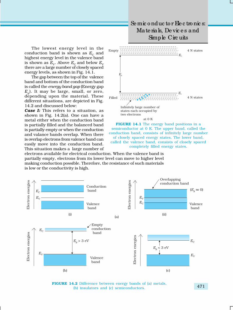
471
Semic o nduc to r Ele c tro nic s:
Materials, Devic es and
Simple Circ uits
The lowest energy level in theconduction band is shown as E
C and
highest energy level in the valence bandis shown as E
V. Above E
C and below E
V
there are a large number of closely spacedenergy levels, as shown in Fig. 14.1.
The gap between the top of the valenceband and bottom of the conduction bandis called the energy band gap (Energy gapE
g). It may be large, small, or zero,
depending upon the material. Thesedifferent situations, are depicted in Fig.14.2 and discussed below:Case I: This refers to a situation, asshown in Fig. 14.2(a). One can have ametal either when the conduction bandis partially filled and the balanced bandis partially empty or when the conductionand valance bands overlap. When thereis overlap electrons from valence band caneasily move into the conduction band.This situation makes a large number ofelectrons available for electrical conduction. When the valence band ispartially empty, electrons from its lower level can move to higher levelmaking conduction possible. Therefore, the resistance of such materialsis low or the conductivity is high.
FIGURE 14.2 Difference between energy bands of (a) metals,(b) insulators and (c) semiconductors.
FIGURE 14.1 The energy band positions in asemiconductor at 0 K. The upper band, called the
conduction band, consists of infinitely large numberof closely spaced energy states. The lower band,
called the valence band, consists of closely spacedcompletely filled energy states.

Physic s
472
Case II: In this case, as shown in Fig. 14.2(b), a large band gap Eg exists
(Eg > 3 eV). There are no electrons in the conduction band, and therefore
no electrical conduction is possible. Note that the energy gap is so large
that electrons cannot be excited from the valence band to the conduction
band by thermal excitation. This is the case of insulators.
Case III: This situation is shown in Fig. 14.2(c). Here a finite but small
band gap (Eg < 3 eV) exists. Because of the small band gap, at room
temperature some electrons from valence band can acquire enough
energy to cross the energy gap and enter the conduction band. These
electrons (though small in numbers) can move in the conduction band.
Hence, the resistance of semiconductors is not as high as that of the
insulators.
In this section we have made a broad classification of metals,
conductors and semiconductors. In the section which follows you will
learn the conduction process in semiconductors.
14.3 INTRINSIC SEMICONDUCTOR
We shall take the most common case of Ge and Si whose lattice structureis shown in Fig. 14.3. These structures are called the diamond-likestructures. Each atom is surrounded by four nearest neighbours. Weknow that Si and Ge have four valence electrons. In its crystallinestructure, every Si or Ge atom tends to share one of its four valenceelectrons with each of its four nearest neighbour atoms, and also to take
share of one electron from each such neighbour. These shared electronpairs are referred to as forming a covalent bond or simply a valence
bond. The two shared electrons can be assumed to shuttle back-and-forth between the associated atoms holding them together strongly.Figure 14.4 schematically shows the 2-dimensional representation of Sior Ge structure shown in Fig. 14.3 which overemphasises the covalentbond. It shows an idealised picture in which no bonds are broken (all
bonds are intact). Such a situation arises at lowtemperatures. As the temperature increases, morethermal energy becomes available to these electronsand some of these electrons may break–away(becoming free electrons contributing to conduction).The thermal energy effectively ionises only a few atomsin the crystalline lattice and creates a vacancy in thebond as shown in Fig. 14.5(a). The neighbourhood,from which the free electron (with charge –q ) has comeout leaves a vacancy with an effective charge (+q ). Thisvacancy with the effective positive electronic charge iscalled a hole. The hole behaves as an apparent free
particle with effective positive charge.In intrinsic semiconductors, the number of free
electrons, ne is equal to the number of holes, n
h. That is
ne = n
h = n
i(14.1)
where ni is called intrinsic carrier concentration.
Semiconductors posses the unique property inwhich, apart from electrons, the holes also move.
FIGURE 14.3 Three-dimensional dia-mond-like crystal structure for Carbon,
Silicon or Germanium withrespective lattice spacing a equal
to 3.56, 5.43 and 5.66 Å.

473
Semic o nduc to r Ele c tro nic s:
Materials, Devic es and
Simple Circ uits
Suppose there is a hole at site 1 as shown inFig. 14.5(a). The movement of holes can bevisualised as shown in Fig. 14.5(b). An electronfrom the covalent bond at site 2 may jump tothe vacant site 1 (hole). Thus, after such a jump,the hole is at site 2 and the site 1 has now anelectron. Therefore, apparently, the hole hasmoved from site 1 to site 2. Note that the electronoriginally set free [Fig. 14.5(a)] is not involvedin this process of hole motion. The free electronmoves completely independently as conductionelectron and gives rise to an electron current, I
e
under an applied electric field. Remember thatthe motion of hole is only a convenient way ofdescribing the actual motion of bound electrons,whenever there is an empty bond anywhere inthe crystal. Under the action of an electric field,these holes move towards negative potentialgiving the hole current, I
h. The total current, I is
thus the sum of the electron current Ie and the
hole current Ih:
I = Ie + I
h(14.2)
It may be noted that apart from the process of generation of conductionelectrons and holes, a simultaneous process of recombination occurs inwhich the electrons recombine with the holes. At equilibrium, the rate ofgeneration is equal to the rate of recombination of charge carriers. Therecombination occurs due to an electron colliding with a hole.
FIGURE 14.4 Schematic two-dimensionalrepresentation of Si or Ge structure showing
covalent bonds at low temperature(all bonds intact). +4 symbol
indicates inner cores of Si or Ge.
FIGURE 14.5 (a) Schematic model of generation of hole at site 1 and conduction electrondue to thermal energy at moderate temperatures. (b) Simplified representation of
possible thermal motion of a hole. The electron from the lower left hand covalent bond(site 2) goes to the earlier hole site1, leaving a hole at its site indicating an
apparent movement of the hole from site 1 to site 2.

Physic s
474
EX
AM
PLE 1
4.1
An intrinsic semiconductorwill behave like an insulator atT = 0 K as shown in Fig. 14.6(a).It is the thermal energy athigher temperatures (T > 0K),which excites some electronsfrom the valence band to theconduction band. Thesethermally excited electrons atT > 0 K, partially occupy theconduction band. Therefore,the energy-band diagram of anintrinsic semiconductor will beas shown in Fig. 14.6(b). Here,some electrons are shown inthe conduction band. Thesehave come from the valenceband leaving equal number ofholes there.
Example 14.1 C, Si and Ge have same lattice structure. Why is Cinsulator while Si and Ge intrinsic semiconductors?
Solution The 4 bonding electrons of C, Si or Ge lie, respectively, inthe second, third and fourth orbit. Hence, energy required to takeout an electron from these atoms (i.e., ionisation energy E
g) will be
least for Ge, followed by Si and highest for C. Hence, number of freeelectrons for conduction in Ge and Si are significant but negligiblysmall for C.
14.4 EXTRINSIC SEMICONDUCTOR
The conductivity of an intrinsic semiconductor depends on itstemperature, but at room temperature its conductivity is very low. Assuch, no important electronic devices can be developed using thesesemiconductors. Hence there is a necessity of improving theirconductivity. This can be done by making use of impurities.
When a small amount, say, a few parts per million (ppm), of a suitableimpurity is added to the pure semiconductor, the conductivity of thesemiconductor is increased manifold. Such materials are known asextrinsic semiconductors or impurity semiconductors. The deliberateaddition of a desirable impurity is called doping and the impurity atomsare called dopants. Such a material is also called a doped semiconductor.The dopant has to be such that it does not distort the original puresemiconductor lattice. It occupies only a very few of the originalsemiconductor atom sites in the crystal. A necessary condition to attainthis is that the sizes of the dopant and the semiconductor atoms shouldbe nearly the same.
There are two types of dopants used in doping the tetravalent Sior Ge:(i) Pentavalent (valency 5); like Arsenic (As), Antimony (Sb), Phosphorous
(P), etc.
FIGURE 14.6 (a) An intrinsic semiconductor at T = 0 Kbehaves like insulator. (b) At T > 0 K, four thermally generated
electron-hole pairs. The filled circles ( ) represent electronsand empty fields ( ) represent holes.

475
Semic o nduc to r Ele c tro nic s:
Materials, Devic es and
Simple Circ uits
(ii) Trivalent (valency 3); like Indium (In),Boron (B), Aluminium (Al), etc.We shall now discuss how the doping
changes the number of charge carriers (andhence the conductivity) of semiconductors.Si or Ge belongs to the fourth group in thePeriodic table and, therefore, we choose thedopant element from nearby fifth or thirdgroup, expecting and taking care that thesize of the dopant atom is nearly the same asthat of Si or Ge. Interestingly, the pentavalentand trivalent dopants in Si or Ge give twoentirely different types of semiconductors asdiscussed below.
(i) n-type semiconductor
Suppose we dope Si or Ge with a pentavalent
element as shown in Fig. 14.7. When an atom
of +5 valency element occupies the position
of an atom in the crystal lattice of Si, four of
its electrons bond with the four silicon
neighbours while the fifth remains very
weakly bound to its parent atom. This is
because the four electrons participating in
bonding are seen as part of the effective core
of the atom by the fifth electron. As a result
the ionisation energy required to set this
electron free is very small and even at room
temperature it will be free to move in the
lattice of the semiconductor. For example, the
energy required is ~ 0.01 eV for germanium,
and 0.05 eV for silicon, to separate this
electron from its atom. This is in contrast to the energy required to jump
the forbidden band (about 0.72 eV for germanium and about 1.1 eV for
silicon) at room temperature in the intrinsic semiconductor. Thus, the
pentavalent dopant is donating one extra electron for conduction and
hence is known as donor impurity. The number of electrons made
available for conduction by dopant atoms depends strongly upon the
doping level and is independent of any increase in ambient temperature.
On the other hand, the number of free electrons (with an equal number
of holes) generated by Si atoms, increases weakly with temperature.
In a doped semiconductor the total number of conduction electrons
ne is due to the electrons contributed by donors and those generated
intrinsically, while the total number of holes nh is only due to the holes
from the intrinsic source. But the rate of recombination of holes would
increase due to the increase in the number of electrons. As a result, the
number of holes would get reduced further.Thus, with proper level of doping the number of conduction electrons
can be made much larger than the number of holes. Hence in an extrinsic
FIGURE 14.7 (a) Pentavalent donor atom (As, Sb,P, etc.) doped for tetravalent Si or Ge giving n-type semiconductor, and (b) Commonly usedschematic representation of n-type material
which shows only the fixed cores of thesubstituent donors with one additional effectivepositive charge and its associated extra electron.

Physic s
476
semiconductor doped with pentavalent impurity, electronsbecome the majority carriers and holes the minority carriers.These semiconductors are, therefore, known as n-type
semiconductors. For n-type semiconductors, we have,n
e >> n
h(14.3)
(ii) p-type semiconductor
This is obtained when Si or Ge is doped with a trivalent impuritylike Al, B, In, etc. The dopant has one valence electron less thanSi or Ge and, therefore, this atom can form covalent bonds withneighbouring three Si atoms but does not have any electron tooffer to the fourth Si atom. So the bond between the fourthneighbour and the trivalent atom has a vacancy or hole as shownin Fig. 14.8. Since the neighbouring Si atom in the lattice wantsan electron in place of a hole, an electron in the outer orbit ofan atom in the neighbourhood may jump to fill this vacancy,leaving a vacancy or hole at its own site. Thus the hole isavailable for conduction. Note that the trivalent foreign atombecomes effectively negatively charged when it shares fourthelectron with neighbouring Si atom. Therefore, the dopant atomof p-type material can be treated as core of one negative charge
along with its associated hole as shown in Fig. 14.8(b). It isobvious that one acceptor atom gives one hole. These holes arein addition to the intrinsically generated holes while the sourceof conduction electrons is only intrinsic generation. Thus, forsuch a material, the holes are the majority carriers and electronsare minority carriers. Therefore, extrinsic semiconductors dopedwith trivalent impurity are called p-type semiconductors. Forp-type semiconductors, the recombination process will reducethe number (n
i)of intrinsically generated electrons to n
e. We
have, for p-type semiconductors
nh >> n
e(14.4)
Note that the crystal maintains an overall charge neutrality
as the charge of additional charge carriers is just equal and
opposite to that of the ionised cores in the lattice.
In extrinsic semiconductors, because of the abundance ofmajority current carriers, the minority carriers producedthermally have more chance of meeting majority carriers and
thus getting destroyed. Hence, the dopant, by adding a large number ofcurrent carriers of one type, which become the majority carriers, indirectlyhelps to reduce the intrinsic concentration of minority carriers.
The semiconductor’s energy band structure is affected by doping. Inthe case of extrinsic semiconductors, additional energy states due to donorimpurities (E
D) and acceptor impurities (E
A) also exist. In the energy band
diagram of n-type Si semiconductor, the donor energy level ED is slightly
below the bottom EC of the conduction band and electrons from this level
move into the conduction band with very small supply of energy. At roomtemperature, most of the donor atoms get ionised but very few (~10–12)atoms of Si get ionised. So the conduction band will have most electronscoming from the donor impurities, as shown in Fig. 14.9(a). Similarly,
FIGURE 14.8 (a) Trivalentacceptor atom (In, Al, B etc.)doped in tetravalent Si or Gelattice giving p-type semicon-ductor. (b) Commonly usedschematic representation ofp-type material which shows
only the fixed core of thesubstituent acceptor with
one effective additionalnegative charge and its
associated hole.

477
Semic o nduc to r Ele c tro nic s:
Materials, Devic es and
Simple Circ uits
EX
AM
PLE 1
4.2
for p-type semiconductor, the acceptor energy level EA is slightly above
the top EV of the valence band as shown in Fig. 14.9(b). With very small
supply of energy an electron from the valence band can jump to the levelE
A and ionise the acceptor negatively. (Alternately, we can also say that
with very small supply of energy the hole from level EA sinks down into
the valence band. Electrons rise up and holes fall down when they gainexternal energy.) At room temperature, most of the acceptor atoms getionised leaving holes in the valence band. Thus at room temperature thedensity of holes in the valence band is predominantly due to impurity inthe extrinsic semiconductor. The electron and hole concentration in asemiconductor in thermal equilibrium is given by
nen
h = n
i
2 (14.5)
Though the above description is grossly approximate andhypothetical, it helps in understanding the difference between metals,insulators and semiconductors (extrinsic and intrinsic) in a simplemanner. The difference in the resistivity of C, Si and Ge depends uponthe energy gap between their conduction and valence bands. For C(diamond), Si and Ge, the energy gaps are 5.4 eV, 1.1 eV and 0.7 eV,respectively. Sn also is a group IV element but it is a metal because theenergy gap in its case is 0 eV.
FIGURE 14.9 Energy bands of (a) n-type semiconductor at T > 0K, (b) p-typesemiconductor at T > 0K.
Example 14.2 Suppose a pure Si crystal has 5 × 1028 atoms m–3. It isdoped by 1 ppm concentration of pentavalent As. Calculate thenumber of electrons and holes. Given that n
i =1.5 × 10¹⁶ m–3.
Solution Note that thermally generated electrons (ni ~1016 m–3) are
negligibly small as compared to those produced by doping.Therefore, n
e ≈≈≈≈≈ N
D.
Since nen
h = n
i
2, The number of holes
nh = (2.25 × 1032)/(5 ×1022)
~ 4.5 × 10⁹ m–3

Physic s
478
14.5 p-n JUNCTION
A p-n junction is the basic building block of many semiconductor deviceslike diodes, transistor, etc. A clear understanding of the junction behaviouris important to analyse the working of other semiconductor devices.We will now try to understand how a junction is formed and how thejunction behaves under the influence of external applied voltage (alsocalled bias).
14.5.1 p-n junction formation
Consider a thin p-type silicon (p-Si) semiconductor wafer. By adding
precisely a small quantity of pentavelent impurity, part of the p-Si wafer
can be converted into n-Si. There are several processes by which a
semiconductor can be formed. The wafer now contains p-region and
n-region and a metallurgical junction between p-, and n- region.
Two important processes occur during the formation of a p-n junction:
diffusion and drift. We know that in an n-type semiconductor, the
concentration of electrons (number of electrons per unit volume) is more
compared to the concentration of holes. Similarly, in a p-type
semiconductor, the concentration of holes is more than the concentration
of electrons. During the formation of p-n junction, and due to the
concentration gradient across p-, and n- sides, holes diffuse from p-side
to n-side (p → n) and electrons diffuse from n-side to p-side (n → p). This
motion of charge carries gives rise to diffusion current across the junction.
When an electron diffuses from n → p, it leaves behind an ionised
donor on n-side. This ionised donor (positive charge) is immobile as it is
bonded to the surrounding atoms. As the electrons continue to diffuse
from n → p, a layer of positive charge (or positive space-charge region) on
n-side of the junction is developed.
Similarly, when a hole diffuses from p → n due to the concentration
gradient, it leaves behind an ionised acceptor (negative charge) which is
immobile. As the holes continue to diffuse, a layer of negative charge (or
negative space-charge region) on the p-side of the junction is developed.
This space-charge region on either side of the junction together is known
as depletion region as the electrons and holes taking part in the initial
movement across the junction depleted the region of its
free charges (Fig. 14.10). The thickness of depletion region
is of the order of one-tenth of a micrometre. Due to the
positive space-charge region on n-side of the junction and
negative space charge region on p-side of the junction,
an electric field directed from positive charge towards
negative charge develops. Due to this field, an electron on
p-side of the junction moves to n-side and a hole on n-
side of the junction moves to p-side. The motion of charge
carriers due to the electric field is called drift. Thus a
drift current, which is opposite in direction to the diffusion
current (Fig. 14.10) starts.
FIGURE 14.10 p-n junctionformation process.
Fo
rmati
on
an
d w
ork
ing
o
f p
-n ju
ncti
on
d
iod
e
http
://w
ww
.mtm
i.vu.
lt/pf
k/fu
nkc_
dari
niai
/dio
d/p-
n_de
vice
s.ht
m

479
Semic o nduc to r Ele c tro nic s:
Materials, Devic es and
Simple Circ uits
EX
AM
PLE 1
4.3
Initially, diffusion current is large and drift current is small.As the diffusion process continues, the space-charge regionson either side of the junction extend, thus increasing the electricfield strength and hence drift current. This process continuesuntil the diffusion current equals the drift current. Thus a p-njunction is formed. In a p-n junction under equilibrium thereis no net current.
The loss of electrons from the n-region and the gain ofelectron by the p-region causes a difference of potential acrossthe junction of the two regions. The polarity of this potential issuch as to oppose further flow of carriers so that a condition ofequilibrium exists. Figure 14.11 shows the p-n junction atequilibrium and the potential across the junction. Then-material has lost electrons, and p material has acquiredelectrons. The n material is thus positive relative to the pmaterial. Since this potential tends to prevent the movement ofelectron from the n region into the p region, it is often called abarrier potential.
Example 14.3 Can we take one slab of p-type semiconductor andphysically join it to another n-type semiconductor to get p-n junction?
Solution No! Any slab, howsoever flat, will have roughness muchlarger than the inter-atomic crystal spacing (~2 to 3 Å) and hencecontinuous contact at the atomic level will not be possible. The junctionwill behave as a discontinuity for the flowing charge carriers.
14.6 SEMICONDUCTOR DIODE
A semiconductor diode [Fig. 14.12(a)] is basically ap-n junction with metallic contacts provided at theends for the application of an external voltage. It is atwo terminal device. A p-n junction diode issymbolically represented as shown in Fig. 14.12(b).
The direction of arrow indicates the conventionaldirection of current (when the diode is under forwardbias). The equilibrium barrier potential can be alteredby applying an external voltage V across the diode.The situation of p-n junction diode under equilibrium(without bias) is shown in Fig. 14.11(a) and (b).
14.6.1 p-n junction diode under forward bias
When an external voltage V is applied across a semiconductor diode suchthat p-side is connected to the positive terminal of the battery and n-sideto the negative terminal [Fig. 14.13(a)], it is said to be forward biased.
The applied voltage mostly drops across the depletion region and thevoltage drop across the p-side and n-side of the junction is negligible.(This is because the resistance of the depletion region – a region wherethere are no charges – is very high compared to the resistance of n-sideand p-side.) The direction of the applied voltage (V ) is opposite to the
FIGURE 14.11 (a) Diode underequilibrium (V = 0), (b) Barrier
potential under no bias.
FIGURE 14.12 (a) Semiconductor diode,(b) Symbol for p-n junction diode.

Physic s
480
built-in potential V0. As a result, the depletion layer width
decreases and the barrier height is reduced [Fig. 14.13(b)]. Theeffective barrier height under forward bias is (V
0 – V ).
If the applied voltage is small, the barrier potential will bereduced only slightly below the equilibrium value, and only asmall number of carriers in the material—those that happen tobe in the uppermost energy levels—will possess enough energyto cross the junction. So the current will be small. If we increasethe applied voltage significantly, the barrier height will be reducedand more number of carriers will have the required energy. Thusthe current increases.
Due to the applied voltage, electrons from n-side cross thedepletion region and reach p-side (where they are minoritycarries). Similarly, holes from p-side cross the junction and reachthe n-side (where they are minority carries). This process underforward bias is known as minority carrier injection. At thejunction boundary, on each side, the minority carrierconcentration increases significantly compared to the locationsfar from the junction.
Due to this concentration gradient, the injected electrons onp-side diffuse from the junction edge of p-side to the other endof p-side. Likewise, the injected holes on n-side diffuse from the
junction edge of n-side to the other end of n-side(Fig. 14.14). This motion of charged carriers on either sidegives rise to current. The total diode forward current is sumof hole diffusion current and conventional current due toelectron diffusion. The magnitude of this current is usuallyin mA.
14.6.2 p-n junction diode under reverse bias
When an external voltage (V ) is applied across the diode suchthat n-side is positive and p-side is negative, it is said to bereverse biased [Fig.14.15(a)]. The applied voltage mostly
drops across the depletion region. The direction of applied voltage is sameas the direction of barrier potential. As a result, the barrier height increasesand the depletion region widens due to the change in the electric field.The effective barrier height under reverse bias is (V
0 + V ), [Fig. 14.15(b)].
This suppresses the flow of electrons from n → p and holes from p → n.Thus, diffusion current, decreases enormously compared to the diodeunder forward bias.
The electric field direction of the junction is such that if electrons onp-side or holes on n-side in their random motion come close to thejunction, they will be swept to its majority zone. This drift of carriersgives rise to current. The drift current is of the order of a few μA. This isquite low because it is due to the motion of carriers from their minorityside to their majority side across the junction. The drift current is alsothere under forward bias but it is negligible (μA) when compared withcurrent due to injected carriers which is usually in mA.
The diode reverse current is not very much dependent on the appliedvoltage. Even a small voltage is sufficient to sweep the minority carriersfrom one side of the junction to the other side of the junction. The current
FIGURE 14.13 (a) p-njunction diode under forward
bias, (b) Barrier potential(1) without battery, (2) Low
battery voltage, and (3) Highvoltage battery.
FIGURE 14.14 Forward biasminority carrier injection.

481
Semic o nduc to r Ele c tro nic s:
Materials, Devic es and
Simple Circ uits
is not limited by the magnitude of the applied voltage but islimited due to the concentration of the minority carrier on either
side of the junction.
The current under reverse bias is essentially voltageindependent upto a critical reverse bias voltage, known asbreakdown voltage (V
br). When V = V
br, the diode reverse current
increases sharply. Even a slight increase in the bias voltage causeslarge change in the current. If the reverse current is not limited byan external circuit below the rated value (specified by themanufacturer) the p-n junction will get destroyed. Once it exceedsthe rated value, the diode gets destroyed due to overheating. Thiscan happen even for the diode under forward bias, if the forwardcurrent exceeds the rated value.
The circuit arrangement for studying the V-I characteristicsof a diode, (i.e., the variation of current as a function of appliedvoltage) are shown in Fig. 14.16(a) and (b). The battery is connectedto the diode through a potentiometer (or reheostat) so that theapplied voltage to the diode can be changed. For different valuesof voltages, the value of the current is noted. A graph between Vand I is obtained as in Fig. 14.16(c). Note that in forward biasmeasurement, we use a milliammeter since the expected current is large(as explained in the earlier section) while a micrometer is used in reversebias to measure the current. You can see in Fig. 14.16(c) that in forward
FIGURE 14.15 (a) Diodeunder reverse bias,
(b) Barrier potential underreverse bias.
FIGURE 14.16 Experimental circuit arrangement for studying V-I characteristics ofa p-n junction diode (a) in forward bias , (b) in reverse bias. (c) Typical V-I
characteristics of a silicon diode.

Physic s
482 EX
AM
PLE 1
4.4
bias, the current first increases very slowly, almost negligibly, till thevoltage across the diode crosses a certain value. After the characteristicvoltage, the diode current increases significantly (exponentially), even fora very small increase in the diode bias voltage. This voltage is called thethreshold voltage or cut-in voltage (~0.2V for germanium diode and~0.7 V for silicon diode).
For the diode in reverse bias, the current is very small (~μA) and almostremains constant with change in bias. It is called reverse saturation
current. However, for special cases, at very high reverse bias (break downvoltage), the current suddenly increases. This special action of the diodeis discussed later in Section 14.8. The general purpose diode are notused beyond the reverse saturation current region.
The above discussion shows that the p-n junction diode primerlyallows the flow of current only in one direction (forward bias). The forwardbias resistance is low as compared to the reverse bias resistance. Thisproperty is used for rectification of ac voltages as discussed in the nextsection. For diodes, we define a quantity called dynamic resistance asthe ratio of small change in voltage ΔV to a small change in current ΔI:
d
Vr
I
Δ= Δ (14.6)
Example 14.4 The V-I characteristic of a silicon diode is shown inthe Fig. 14.17. Calculate the resistance of the diode at (a) I
D = 15 mA
and (b) VD = –10 V.
FIGURE 14.17
Solution Considering the diode characteristics as a straight linebetween I = 10 mA to I = 20 mA passing through the origin, we cancalculate the resistance using Ohm’s law.(a) From the curve, at I = 20 mA, V = 0.8 V, I = 10 mA, V = 0.7 V
rfb
= ΔV/ΔI = 0.1V/10 mA = 10 Ω(b) From the curve at V = –10 V, I = –1 μA,
Therefore,r
rb = 10 V/1μA= 1.0 × 10⁷ Ω
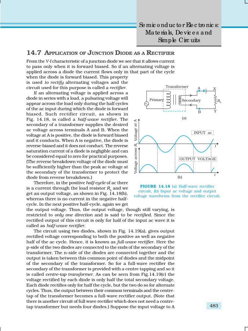
483
Semic o nduc to r Ele c tro nic s:
Materials, Devic es and
Simple Circ uits
14.7 APPLICATION OF JUNCTION DIODE AS A RECTIFIER
From the V-I characteristic of a junction diode we see that it allows currentto pass only when it is forward biased. So if an alternating voltage isapplied across a diode the current flows only in that part of the cyclewhen the diode is forward biased. This propertyis used to rectify alternating voltages and thecircuit used for this purpose is called a rectifier.
If an alternating voltage is applied across adiode in series with a load, a pulsating voltage willappear across the load only during the half cyclesof the ac input during which the diode is forwardbiased. Such rectifier circuit, as shown inFig. 14.18, is called a half-wave rectifier. Thesecondary of a transformer supplies the desiredac voltage across terminals A and B. When thevoltage at A is positive, the diode is forward biasedand it conducts. When A is negative, the diode isreverse-biased and it does not conduct. The reversesaturation current of a diode is negligible and canbe considered equal to zero for practical purposes.(The reverse breakdown voltage of the diode mustbe sufficiently higher than the peak ac voltage atthe secondary of the transformer to protect thediode from reverse breakdown.)
Therefore, in the positive half-cycle of ac there
is a current through the load resistor RL and we
get an output voltage, as shown in Fig. 14.18(b),
whereas there is no current in the negative half-
cycle. In the next positive half-cycle, again we get
the output voltage. Thus, the output voltage, though still varying, is
restricted to only one direction and is said to be rectified. Since the
rectified output of this circuit is only for half of the input ac wave it is
called as half-wave rectifier.
The circuit using two diodes, shown in Fig. 14.19(a), gives output
rectified voltage corresponding to both the positive as well as negative
half of the ac cycle. Hence, it is known as full-wave rectifier. Here the
p-side of the two diodes are connected to the ends of the secondary of the
transformer. The n-side of the diodes are connected together and the
output is taken between this common point of diodes and the midpoint
of the secondary of the transformer. So for a full-wave rectifier the
secondary of the transformer is provided with a centre tapping and so it
is called centre-tap transformer. As can be seen from Fig.14.19(c) the
voltage rectified by each diode is only half the total secondary voltage.
Each diode rectifies only for half the cycle, but the two do so for alternate
cycles. Thus, the output between their common terminals and the centre-
tap of the transformer becomes a full-wave rectifier output. (Note that
there is another circuit of full wave rectifier which does not need a centre-
tap transformer but needs four diodes.) Suppose the input voltage to A
FIGURE 14.18 (a) Half-wave rectifiercircuit, (b) Input ac voltage and output
voltage waveforms from the rectifier circuit.

Physic s
484
with respect to the centre tap at any instant
is positive. It is clear that, at that instant,
voltage at B being out of phase will be
negative as shown in Fig.14.19(b). So, diode
D1 gets forward biased and conducts (while
D2 being reverse biased is not conducting).
Hence, during this positive half cycle we get
an output current (and a output voltage
across the load resistor RL) as shown in
Fig.14.19(c). In the course of the ac cycle
when the voltage at A becomes negative with
respect to centre tap, the voltage at B would
be positive. In this part of the cycle diode
D1 would not conduct but diode D
2 would,
giving an output current and output
voltage (across RL) during the negative half
cycle of the input ac. Thus, we get output
voltage during both the positive as well as
the negative half of the cycle. Obviously,
this is a more efficient circuit for getting
rectified voltage or current than the half-
wave rectifier
The rectified voltage is in the form of
pulses of the shape of half sinusoids.
Though it is unidirectional it does not have
a steady value. To get steady dc output
from the pulsating voltage normally a
capacitor is connected across the output
terminals (parallel to the load RL). One can
also use an inductor in series with RL for
the same purpose. Since these additional
circuits appear to filter out the ac ripple
and give a pure dc voltage, so they are
called filters.
Now we shall discuss the role of
capacitor in filtering. When the voltage
across the capacitor is rising, it gets
charged. If there is no external load, it remains charged to the peak voltage
of the rectified output. When there is a load, it gets discharged through
the load and the voltage across it begins to fall. In the next half-cycle of
rectified output it again gets charged to the peak value (Fig. 14.20). The
rate of fall of the voltage across the capacitor depends upon the inverse
product of capacitor C and the effective resistance RL used in the circuit
and is called the time constant. To make the time constant large value of
C should be large. So capacitor input filters use large capacitors. The
output voltage obtained by using capacitor input filter is nearer to the
peak voltage of the rectified voltage. This type of filter is most widely
used in power supplies.
FIGURE 14.19 (a) A Full-wave rectifiercircuit; (b) Input wave forms given to thediode D
1 at A and to the diode D
2 at B;
(c) Output waveform across theload R
L connected in the full-wave
rectifier circuit.

485
Semic o nduc to r Ele c tro nic s:
Materials, Devic es and
Simple Circ uits
14.8 SPECIAL PURPOSE p-n JUNCTION DIODES
In the section, we shall discuss some devices which are basically junction
diodes but are developed for different applications.
14.8.1 Zener diode
It is a special purpose semiconductor diode, named after its inventorC. Zener. It is designed to operate under reverse bias in the breakdownregion and used as a voltage regulator. The symbol for Zener diode isshown in Fig. 14.21(a).
Zener diode is fabricated by heavily doping both p-, andn- sides of the junction. Due to this, depletion region formedis very thin (<10–6 m) and the electric field of the junction isextremely high (~5×10⁶ V/m) even for a small reverse biasvoltage of about 5V. The I-V characteristics of a Zener diode isshown in Fig. 14.21(b). It is seen that when the applied reversebias voltage(V ) reaches the breakdown voltage (V
z) of the Zener
diode, there is a large change in the current. Note that afterthe breakdown voltage V
z, a large change in the current can
be produced by almost insignificant change in the reverse biasvoltage. In other words, Zener voltage remains constant, eventhough current through the Zener diode varies over a widerange. This property of the Zener diode is used for regulatingsupply voltages so that they are constant.
Let us understand how reverse current suddenly increasesat the breakdown voltage. We know that reverse current isdue to the flow of electrons (minority carriers) from p → n andholes from n → p. As the reverse bias voltage is increased, theelectric field at the junction becomes significant. When thereverse bias voltage V = V
z, then the electric field strength is
high enough to pull valence electrons from the host atoms onthe p-side which are accelerated to n-side. These electronsaccount for high current observed at the breakdown. Theemission of electrons from the host atoms due to the highelectric field is known as internal field emission or fieldionisation. The electric field required for field ionisation is ofthe order of 106 V/m.
FIGURE 14.20 (a) A full-wave rectifier with capacitor filter, (b) Input and outputvoltage of rectifier in (a).
FIGURE 14.21 Zener diode,(a) symbol, (b) I-Vcharacteristics.

Physic s
486
EX
AM
PLE 1
4.5
FIGURE 14.22 Zener diode as DCvoltage regulator (to be corrected).
Zener diode as a voltage regulator
We know that when the ac input voltage of a rectifier fluctuates, its rectifiedoutput also fluctuates. To get a constant dc voltage from the dcunregulated output of a rectifier, we use a Zener diode. The circuit diagramof a voltage regulator using a Zener diode is shown in Fig. 14.22.
The unregulated dc voltage (filtered output of arectifier) is connected to the Zener diode through a seriesresistance R
s such that the Zener diode is reverse biased.
If the input voltage increases, the current through Rs
and Zener diode also increases. This increases thevoltage drop across R
s without any change in the
voltage across the Zener diode. This is because in thebreakdown region, Zener voltage remains constant eventhough the current through the Zener diode changes.Similarly, if the input voltage decreases, the currentthrough R
s and Zener diode also decreases. The voltage
drop across Rs decreases without any change in the
voltage across the Zener diode. Thus any increase/decrease in the input voltage results in, increase/decrease of the voltage drop across R
s without any
change in voltage across the Zener diode. Thus the Zener diode acts as avoltage regulator. We have to select the Zener diode according to therequired output voltage and accordingly the series resistance R
s.
Example 14.5 In a Zener regulated power supply a Zener diode withV
Z = 6.0 V is used for regulation. The load current is to be 4.0 mA and
the unregulated input is 10.0 V. What should be the value of seriesresistor R
S?
SolutionThe value of R
S should be such that the current through the Zener
diode is much larger than the load current. This is to have good loadregulation. Choose Zener current as five times the load current, i.e.,IZ = 20 mA. The total current through R
S is, therefore, 24 mA. The
voltage drop across RS is 10.0 – 6.0 = 4.0 V. This gives
RS = 4.0V/(24 × 10–3) A = 167 Ω. The nearest value of carbon resistor
is 150 Ω. So, a series resistor of 150 Ω is appropriate. Note that slightvariation in the value of the resistor does not matter, what is importantis that the current I
Z should be sufficiently larger than I
L.
14.8.2 Optoelectronic junction devices
We have seen so far, how a semiconductor diode behaves under applied
electrical inputs. In this section, we learn about semiconductor diodes inwhich carriers are generated by photons (photo-excitation). All these
devices are called optoelectronic devices. We shall study the functioningof the following optoelectronic devices:
(i) Photodiodes used for detecting optical signal (photodetectors).(ii) Light emitting diodes (LED) which convert electrical energy into light.
(iii) Photovoltaic devices which convert optical radiation into electricity(solar cells).

487
Semic o nduc to r Ele c tro nic s:
Materials, Devic es and
Simple Circ uits
EX
AM
PLE 1
4.6
(i) Photodiode
A Photodiode is again a special purpose p-njunction diode fabricated with a transparentwindow to allow light to fall on the diode. It isoperated under reverse bias. When the photodiodeis illuminated with light (photons) with energy (hν)greater than the energy gap (E
g) of the
semiconductor, then electron-hole pairs aregenerated due to the absorption of photons. Thediode is fabricated such that the generation ofe-h pairs takes place in or near the depletion regionof the diode. Due to electric field of the junction,electrons and holes are separated before theyrecombine. The direction of the electric field is suchthat electrons reach n-side and holes reach p-side.Electrons are collected on n-side and holes arecollected on p-side giving rise to an emf. When anexternal load is connected, current flows. Themagnitude of the photocurrent depends on theintensity of incident light (photocurrent isproportional to incident light intensity).
It is easier to observe the change in the currentwith change in the light intensity, if a reverse biasis applied. Thus photodiode can be used as aphotodetector to detect optical signals. The circuitdiagram used for the measurement of I-V
characteristics of a photodiode is shown inFig. 14.23(a) and a typical I-V characteristics inFig. 14.23(b).
Example 14.6 The current in the forward bias is known to be more(~mA) than the current in the reverse bias (~μA). What is the reasonthen to operate the photodiodes in reverse bias?
Solution Consider the case of an n-type semiconductor. Obviously,the majority carrier density (n ) is considerably larger than theminority hole density p (i.e., n >> p). On illumination, let the excesselectrons and holes generated be Δn and Δp, respectively:
n′ = n + Δn
p′ = p + Δp
Here n′ and p′ are the electron and hole concentrations* at anyparticular illumination and n and p are carriers concentration whenthere is no illumination. Remember Δn = Δp and n >> p. Hence, the
FIGURE 14.23 (a) An illuminatedphotodiode under reverse bias , (b) I-V
characteristics of a photodiode for differentillumination intensity I
4 > I
3 > I
2 > I
1.
* Note that, to create an e-h pair, we spend some energy (photoexcitation, thermalexcitation, etc.). Therefore when an electron and hole recombine the energy isreleased in the form of light (radiative recombination) or heat (non-radiativerecombination). It depends on semiconductor and the method of fabrication ofthe p-n junction. For the fabrication of LEDs, semiconductors like GaAs, GaAs-GaP are used in which radiative recombination dominates.

Physic s
488
EX
AM
PLE 1
4.6
fractional change in the majority carriers (i.e., Δn/n ) would be muchless than that in the minority carriers (i.e., Δp/p). In general, we canstate that the fractional change due to the photo-effects on theminority carrier dominated reverse bias current is more easilymeasurable than the fractional change in the forward bias current.Hence, photodiodes are preferably used in the reverse bias condition
for measuring light intensity.
(ii) Light emitting diode
It is a heavily doped p-n junction which under forward bias emits
spontaneous radiation. The diode is encapsulated with a transparentcover so that emitted light can come out.
When the diode is forward biased, electrons are sent from n → p (wherethey are minority carriers) and holes are sent from p → n (where they are
minority carriers). At the junction boundary the concentration of minoritycarriers increases compared to the equilibrium concentration (i.e., when
there is no bias). Thus at the junction boundary on either side of thejunction, excess minority carriers are there which recombine with majority
carriers near the junction. On recombination, the energy is released inthe form of photons. Photons with energy equal to or slightly less than
the band gap are emitted. When the forward current of the diode is small,the intensity of light emitted is small. As the forward current increases,
intensity of light increases and reaches a maximum. Further increase inthe forward current results in decrease of light intensity. LEDs are biased
such that the light emitting efficiency is maximum.The V-I characteristics of a LED is similar to that of a Si junction
diode. But the threshold voltages are much higher and slightly differentfor each colour. The reverse breakdown voltages of LEDs are very low,
typically around 5V. So care should be taken that high reverse voltagesdo not appear across them.
LEDs that can emit red, yellow, orange, green and blue light arecommercially available. The semiconductor used for fabrication of visible
LEDs must at least have a band gap of 1.8 eV (spectral range of visiblelight is from about 0.4 μm to 0.7 μm, i.e., from about 3 eV to 1.8 eV). The
compound semiconductor Gallium Arsenide – Phosphide (GaAs1–x
Px) is
used for making LEDs of different colours. GaAs0.6
P0.4
(Eg ~ 1.9 eV) is
used for red LED. GaAs (Eg ~ 1.4 eV) is used for making infrared LED.
These LEDs find extensive use in remote controls, burglar alarm systems,
optical communication, etc. Extensive research is being done fordeveloping white LEDs which can replace incandescent lamps.
LEDs have the following advantages over conventional incandescentlow power lamps:
(i) Low operational voltage and less power.
(ii) Fast action and no warm-up time required.
(iii) The bandwidth of emitted light is 100 Å to 500 Å or in other words it
is nearly (but not exactly) monochromatic.
(iv) Long life and ruggedness.
(v) Fast on-off switching capability.

489
Semic o nduc to r Ele c tro nic s:
Materials, Devic es and
Simple Circ uits
(iii) Solar cell
A solar cell is basically a p-n junction whichgenerates emf when solar radiation falls on thep-n junction. It works on the same principle(photovoltaic effect) as the photodiode, except thatno external bias is applied and the junction areais kept much larger for solar radiation to beincident because we are interested in more power.
A simple p-n junction solar cell is shown inFig. 14.24.
A p-Si wafer of about 300 μm is taken overwhich a thin layer (~0.3 μm) of n-Si is grown onone-side by diffusion process. The other side ofp-Si is coated with a metal (back contact). On thetop of n-Si layer, metal finger electrode (or metallicgrid) is deposited. This acts as a front contact. Themetallic grid occupies only a very small fractionof the cell area (<15%) so that light can be incidenton the cell from the top.
The generation of emf by a solar cell, when light falls on, it is due tothe following three basic processes: generation, separation and collection—(i) generation of e-h pairs due to light (with hν > E
g)
close to the junction; (ii) separation of electrons andholes due to electric field of the depletion region.Electrons are swept to n-side and holes to p-side;(iii) the electrons reaching the n-side are collected bythe front contact and holes reaching p-side are collectedby the back contact. Thus p-side becomes positive andn-side becomes negative giving rise to photovoltage.
When an external load is connected as shown inthe Fig. 14.25(a) a photocurrent I
L flows through the
load. A typical I-V characteristics of a solar cell is shownin the Fig. 14.25(b).
Note that the I – V characteristics of solar cell isdrawn in the fourth quadrant of the coordinate axes.This is because a solar cell does not draw current butsupplies the same to the load.
Semiconductors with band gap close to 1.5 eV areideal materials for solar cell fabrication. Solar cells aremade with semiconductors like Si (E
g = 1.1 eV), GaAs
(Eg = 1.43 eV), CdTe (Eg = 1.45 eV), CuInSe
2 (E
g = 1.04
eV), etc. The important criteria for the selection of amaterial for solar cell fabrication are (i) band gap (~1.0to 1.8 eV), (ii) high optical absorption (~104 cm–1), (iii)electrical conductivity, (iv) availability of the rawmaterial, and (v) cost. Note that sunlight is not alwaysrequired for a solar cell. Any light with photon energiesgreater than the bandgap will do. Solar cells are usedto power electronic devices in satellites and spacevehicles and also as power supply to some calculators. Production oflow-cost photovoltaic cells for large-scale solar energy is a topicfor research.
FIGURE 14.24 (a) Typical p-n junctionsolar cell; (b) Cross-sectional view.
FIGURE 14.25 (a) A typicalilluminated p-n junction solar cell;(b) I-V characteristics of a solar cell.

Physic s
490
EX
AM
PLE 1
4.7
Example 14.7 Why are Si and GaAs are preferred materials forsolar cells?
Solution The solar radiation spectrum received by us is shown inFig. 14.26.
FIGURE 14.26
The maxima is near 1.5 eV. For photo-excitation, hν > Eg. Hence,
semiconductor with band gap ~1.5 eV or lower is likely to give bettersolar conversion efficiency. Silicon has E
g ~ 1.1 eV while for GaAs it is
~1.53 eV. In fact, GaAs is better (in spite of its higher band gap) thanSi because of its relatively higher absorption coefficient. If we choosematerials like CdS or CdSe (E
g ~ 2.4 eV), we can use only the high
energy component of the solar energy for photo-conversion and asignificant part of energy will be of no use.The question arises: why we do not use material like PbS (E
g ~ 0.4 eV)
which satisfy the condition hν > Eg for ν maxima corresponding to the
solar radiation spectra? If we do so, most of the solar radiation will beabsorbed on the top-layer of solar cell and will not reach in or nearthe depletion region. For effective electron-hole separation, due tothe junction field, we want the photo-generation to occur in thejunction region only.
14.9 JUNCTION TRANSISTOR
The credit of inventing the transistor in the year 1947 goes to J. Bardeen
and W.H. Brattain of Bell Telephone Laboratories, U.S.A. That transistorwas a point-contact transistor. The first junction transistor consisting of
two back-to-back p-n junctions was invented by William Schockleyin 1951.
As long as only the junction transistor was known, it was knownsimply as transistor. But over the years new types of transistors wereinvented and to differentiate it from the new ones it is now called theBipolar Junction Transistor (BJT). Even now, often the word transistor

491
Semic o nduc to r Ele c tro nic s:
Materials, Devic es and
Simple Circ uits
is used to mean BJT when there is no confusion. Since our study islimited to only BJT, we shall use the word transistor for BJT withoutany ambiguity.
14.9.1 Transistor: structure and action
A transistor has three doped regions forming two p-n junctionsbetween them. Obviously, there are two types of transistors, as shownin Fig. 14.27.(i) n-p-n transistor : Here two segments of n-type semiconductor
(emitter and collector) are separated by a segment of p-typesemiconductor (base).
(ii) p-n-p transistor : Here two segments of p-type semiconductor(termed as emitter and collector) are separated by a segment ofn-type semiconductor (termed as base).The schematic representations of an n-p-n and a p-n-p
configuration are shown in Fig. 14.27(a). All the three segments of atransistor have different thickness and their doping levels are alsodifferent. In the schematic symbols used for representing p-n-p andn-p-n transistors [Fig. 14.27(b)] the arrowhead shows the direction ofconventional current in the transistor. A brief description of the threesegments of a transistor is given below:• Emitter : This is the segment on one side of the transistor shown in
Fig. 14.27(a). It is of moderate size and heavily doped. It suppliesa large number of majority carriers for the current flow throughthe transistor.
• Base: This is the central segment. It is very thin and lightly doped.• Collector: This segment collects a major portion of the majority
carriers supplied by the emitter. The collector side is moderately
doped and larger in size as compared to the emitter.
We have seen earlier in the case of a p-n junction, that there is a
formation of depletion region acorss the junction. In case of a transistor
depletion regions are formed at the emitter base-junction and the base-
collector junction. For understanding the action of a transistor, we
have to consider the nature of depletion regions formed at these
junctions. The charge carriers move across different regions of the
transistor when proper voltages are applied across its terminals.The biasing of the transistor is done differently for different uses.
The transistor can be used in two distinct ways. Basically, it wasinvented to function as an amplifier, a device which produces a enlargedcopy of a signal. But later its use as a switch acquired equalimportance. We shall study both these functions and the ways thetransistor is biased to achieve these mutually exclusive functions.
First we shall see what gives the transistor its amplifying capabilities.The transistor works as an amplifier, with its emitter-base junctionforward biased and the base-collector junction reverse biased. Thissituation is shown in Fig. 14.28, where V
CC and V
EE are used for creating
the respective biasing. When the transistor is biased in this way it issaid to be in active state.We represent the voltage between emitter andbase as V
EB and that between the collector and the base as V
CB. In
FIGURE 14.27(a) Schematic
representations of an-p-n transistor andp-n-p transistor, and(b) Symbols for n-p-nand p-n-p transistors.

Physic s
492
Fig. 14.28, base is a common terminal for the twopower supplies whose other terminals areconnected to emitter and collector, respectively. Sothe two power supplies are represented as V
EE, and
VCC
, respectively. In circuits, where emitter is thecommon terminal, the power supply between thebase and the emitter is represented as V
BB and that
between collector and emitter as VCC
.Let us see now the paths of current carriers in
the transistor with emitter-base junction forwardbiased and base-collector junction reverse biased.The heavily doped emitter has a high concentrationof majority carriers, which will be holes in a p-n-ptransistor and electrons in an n-p-n transistor.These majority carriers enter the base region inlarge numbers. The base is thin and lightly doped.So the majority carriers there would be few. In ap-n-p transistor the majority carriers in the baseare electrons since base is of n-type semiconductor.The large number of holes entering the base fromthe emitter swamps the small number of electronsthere. As the base collector-junction is reverse-biased, these holes, which appear as minoritycarriers at the junction, can easily cross thejunction and enter the collector. The holes in thebase could move either towards the base terminalto combine with the electrons entering from outsideor cross the junction to enter into the collector andreach the collector terminal. The base is made thinso that most of the holes find themselves nearthe reverse-biased base-collector junction and socross the junction instead of moving to the baseterminal.
It is interesting to note that due to forwardbias a large current enters the emitter-base
junction, but most of it is diverted to adjacent reverse-biased base-collectorjunction and the current coming out of the base becomes a very smallfraction of the current that entered the junction. If we represent the holecurrent and the electron current crossing the forward biased junction byIh and I
e respectively then the total current in a forward biased diode is
the sum Ih + I
e. We see that the emitter current I
E = I
h + I
e but the base
current IB << I
h + I
e, because a major part of I
E goes to collector instead of
coming out of the base terminal. The base current is thus a small fractionof the emitter current.
The current entering into the emitter from outside is equal to theemitter current I
E. Similarly the current emerging from the base terminal
is IB and that from collector terminal is I
C. It is obvious from the above
description and also from a straight forward application of Kirchhoff’slaw to Fig. 14.28(a) that the emitter current is the sum of collector currentand base current:
FIGURE 14.28 Bias Voltage applied on: (a)p-n-p transistor and (b) n-p-n transistor.

493
Semic o nduc to r Ele c tro nic s:
Materials, Devic es and
Simple Circ uits
IE = I
C + I
B(14.7)
We also see that IC ≈ I
E.
Our description of the direction of motion of the holes is identicalwith the direction of the conventional current. But the direction of motionof electrons is just opposite to that of the current. Thus in a p-n-ptransistor the current enters from emitter into base whereas in a n-p-ntransistor it enters from the base into the emitter. The arrowhead in theemitter shows the direction of the conventional current.
The description about the paths followed by the majority and minoritycarriers in a n-p-n is exactly the same as that for the p-n-p transistor.But the current paths are exactly opposite, as shown in Fig. 14.28. InFig. 14.28(b) the electrons are the majority carriers supplied by then-type emitter region. They cross the thin p-base region and are able toreach the collector to give the collector current, I
C . From the above
description we can conclude that in the active state of the transistor theemitter-base junction acts as a low resistance while the base collectoracts as a high resistance.
14.9.2 Basic transistor circuit configurations and transistorcharacteristics
In a transistor, only three terminals are available, viz., Emitter (E), Base
(B) and Collector (C). Therefore, in a circuit the input/output connectionshave to be such that one of these (E, B or C) is common to both the inputand the output. Accordingly, the transistor can be connected in either ofthe following three configurations:Common Emitter (CE), Common Base (CB), Common Collector (CC)
The transistor is most widely used in the CE configuration and weshall restrict our discussion to only this configuration. Since morecommonly used transistors are n-p-n Si transistors, we shall confineour discussion to such transistors only. With p-n-p transistors thepolarities of the external power supplies are to be inverted.
Common emitter transistor characteristics
When a transistor is used in CE configuration, the inputis between the base and the emitter and the output isbetween the collector and the emitter. The variation ofthe base current I
B with the base-emitter voltage V
BE is
called the input characteristic. Similarly, the variationof the collector current I
C with the collector-emitter
voltage VCE
is called the output characteristic. You willsee that the output characteristics are controlled bythe input characteristics. This implies that the collectorcurrent changes with the base current.
The input and the output characteristics of ann-p-n transistors can be studied by using the circuitshown in Fig. 14.29.
To study the input characteristics of the transistorin C
E configuration, a curve is plotted between the base
current IB against the base-emitter voltage V
BE. The
FIGURE 14.29 Circuit arrangementfor studying the input and output
characteristics of n-p-n transistor inCE configuration.

Physic s
494
collector-emitter voltage VCE
is kept fixed while
studying the dependence of IB on V
BE. We are
interested to obtain the input characteristic
when the transistor is in active state. So the
collector-emitter voltage VCE
is kept large
enough to make the base collector junction
reverse biased. Since VCE
= VCB
+ VBE
and for Si
transistor VBE
is 0.6 to 0.7 V, VCE
must be
sufficiently larger than 0.7 V. Since the
transistor is operated as an amplifier over large
range of VCE
, the reverse bias across the base-
collector junction is high most of the time.
Therefore, the input characteristics may be
obtained for VCE
somewhere in the range of 3 V
to 20 V. Since the increase in VCE
appears as
increase in VCB
, its effect on IB is negligible. As
a consequence, input characteristics for various
values of VCE
will give almost identical curves.
Hence, it is enough to determine only one input
characteristics. The input characteristics of a
transistor is as shown in Fig. 14.30(a).
The output characteristic is obtained by
observing the variation of IC as V
CE is varied
keeping IB constant. It is obvious that if V
BE is
increased by a small amount, both hole current
from the emitter region and the electron current
from the base region will increase. As a
consequence both IB and I
C will increase
proportionately. This shows that when IB
increases IC also increases. The plot of I
C versus
VCE
for different fixed values of IB gives one
output characteristic. So there will be different output characteristics
corresponding to different values of IB as shown in Fig. 14.30(b).
The linear segments of both the input and output characteristics can
be used to calculate some important ac parameters of transistors as
shown below.
(i) Input resistance (ri): This is defined as the ratio of change in base-
emitter voltage (ΔVBE
) to the resulting change in base current (ΔIB) at
constant collector-emitter voltage (VCE
). This is dynamic (ac resistance)
and as can be seen from the input characteristic, its value varies with
the operating current in the transistor:
CE
BEi
B V
Vr
I
⎛ ⎞Δ= ⎜ ⎟Δ⎝ ⎠ (14.8)
The value of ri can be anything from a few hundreds to a few thousand
ohms.
FIGURE 14.30 (a) Typical inputcharacteristics, and (b) Typical output
characteristics.

495
Semic o nduc to r Ele c tro nic s:
Materials, Devic es and
Simple Circ uits
EX
AM
PLE 1
4.8
(ii) Output resistance (ro): This is defined as the ratio of change in
collector-emitter voltage (ΔVCE
) to the change in collector current (ΔIC)
at a constant base current IB.
B
CEo
C I
Vr
I
⎛ ⎞Δ= ⎜ ⎟Δ⎝ ⎠ (14.9)
The output characteristics show that initially for very small values ofV
CE, I
C increases almost linearly. This happens because the base-collector
junction is not reverse biased and the transistor is not in active state. Infact, the transistor is in the saturation state and the current is controlledby the supply voltage V
CC (=V
CE) in this part of the characteristic. When
VCE
is more than that required to reverse bias the base-collector junction,IC increases very little with V
CE. The reciprocal of the slope of the linear
part of the output characteristic gives the values of ro. The outputresistance of the transistor is mainly controlled by the bias of the base-collector junction. The high magnitude of the output resistance (of theorder of 100 kΩ) is due to the reverse-biased state of this diode. Thisalso explains why the resistance at the initial part of the characteristic,when the transistor is in saturation state, is very low.(iii) Current amplification factor (βββββ ): This is defined as the ratio of
the change in collector current to the change in base current at aconstant collector-emitter voltage (V
CE) when the transistor is in
active state.
CE
Cac
B V
I
Iβ ⎛ ⎞Δ= ⎜ ⎟Δ⎝ ⎠ (14.10)
This is also known as small signal current gain and its value is verylarge.
If we simply find the ratio of IC
and IB we get what is called dc β of the
transistor. Hence,
Cdc
B
I
Iβ = (14.11)
Since IC increases with I
B almost linearly and I
C = 0 when I
B = 0, the values
of both βdc
and βac
are nearly equal. So, for most calculations βdc
can beused. Both β
ac and β
dc vary with V
CE and I
B (or I
C) slightly.
Example 14.8 From the output characteristics shown in Fig. 14.30(b),calculate the values of β
ac and β
dc of the transistor when V
CE is
10 V and IC = 4.0 mA.
Solution
CE
Cac
B V
I
Iβ ⎛ ⎞Δ= ⎜ ⎟Δ⎝ ⎠ ,
Cdc
B
I
Iβ =
For determining βac
and βdc
at the stated values of VCE
and IC one can
proceed as follows. Consider any two characteristics for two valuesof I
B which lie above and below the given value of I
C . Here I
C = 4.0 mA.
(Choose characteristics for IB= 30 and 20 μA.) At V
CE = 10 V we read
the two values of IC from the graph. Then

Physic s
496
EX
AM
PLE 1
4.8
ΔIB = (30 – 20) μA = 10 μA, ΔI
C = (4.5 – 3.0) mA = 1.5 mA
Therefore, βac
= 1.5 mA/ 10 μA = 150
For determining βdc,
either estimate the value of IB corresponding to
IC = 4.0 mA at V
CE = 10 V or calculate the two values of β
dc for the two
characteristics chosen and find their mean.
Therefore, for IC = 4.5 mA and I
B = 30 μA,
βdc
= 4.5 mA/ 30 μA = 150
and for IC = 3.0 mA and I
B = 20 μA
βdc
=3.0 mA / 20 μA = 150
Hence, βdc
=(150 + 150) /2 = 150
14.9.3 Transistor as a device
The transistor can be used as a device application depending on theconfiguration used (namely CB, CC and CE), the biasing of the E-B andB-C junction and the operation region namely cutoff, active region andsaturation. As mentioned earlier we have confined only to the CEconfiguration and will be concentrating on the biasing and the operationregion to understand the working of a device.
When the transistor is used in the cutoffor saturation state it acts as a switch. Onthe other hand for using the transistor asan amplifier, it has to operate in the activeregion.(i) Transistor as a switch
We shall try to understand the operation ofthe transistor as a switch by analysing thebehaviour of the base-biased transistor inCE configuration as shown in Fig. 14.31(a).
Applying Kirchhoff’s voltage rule to theinput and output sides of this circuit, weget
VBB
= IBR
B + V
BE(14.12)
and
VCE
= VCC
– ICR
C.(14.13)
We shall treat VBB
as the dc inputvoltage V
i and V
CE as the dc output voltage
VO. So, we have
Vi = I
BR
B + V
BE and
Vo = V
CC – I
CR
C.
Let us see how Vo
changes as Vi
increases from zero onwards. In the caseof Si transistor, as long as input V
i is less
than 0.6 V, the transistor will be in cut off
state and current IC will be zero.
Hence Vo = V
CC
When Vi becomes greater than 0.6 V the transistor is in active state with
some current IC in the output path and the output V
o decrease as the
FIGURE 14.31 (a) Base-biased transistor in CEconfiguration, (b) Transfer characteristic.

497
Semic o nduc to r Ele c tro nic s:
Materials, Devic es and
Simple Circ uits
term ICR
C increases. With increase of V
i , I
C increases almost linearly
and so Vo decreases linearly till its value
becomes less than
about 1.0 V.Beyond this, the change becomes non linear and transistor goes into
saturation state. With further increase in Vi the output voltage is found to
decrease further towards zero though it may never become zero. If we plotthe V
o vs V
i curve, [also called the transfer characteristics of the base-biased
transistor (Fig. 14.31(b)], we see that between cut off state and active stateand also between active state and saturation state there are regions ofnon-linearity showing that the transition from cutoff state to active stateand from active state to saturation state are not sharply defined.
Let us see now how the transistor is operated as a switch. As long asV
i is low and unable to forward-bias the transistor, V
o is high (at V
CC ). If
Vi is high enough to drive the transistor into saturation, then V
o is low,
very near to zero. When the transistor is not conducting it is said to beswitched off and when it is driven into saturation it is said to be switched
on. This shows that if we define low and high states as below and abovecertain voltage levels corresponding to cutoff and saturation of thetransistor, then we can say that a low input switches the transistor offand a high input switches it on. Alternatively, we can say that a low
input to the transistor gives a high output and a high input gives a low
output. The switching circuits are designed in such a way that thetransistor does not remain in active state.
(ii) Transistor as an amplifier
For using the transistor as an amplifier we will use the active region ofthe V
o versus V
i curve. The slope of the linear part of the curve represents
the rate of change of the output with the input. It is negative because theoutput is V
CC – I
CR
C and not I
CR
C. That is why as input voltage of the CE
amplifier increases its output voltage decreases and the output is said tobe out of phase with the input. If we consider ΔV
o and ΔV
i as small
changes in the output and input voltages then ΔVo/ΔV
i is called the small
signal voltage gain AV of the amplifier.
If the VBB
voltage has a fixed value corresponding to the mid point ofthe active region, the circuit will behave as a CE amplifier with voltagegain ΔV
o/ ΔV
i. We can express the voltage gain A
V in terms of the resistors
in the circuit and the current gain of the transistor as follows.
We have, Vo = V
CC – I
CR
C
Therefore, ΔVo = 0 – R
C Δ I
C
Similarly, from Vi = I
BR
B + V
BE
ΔVi = R
B ΔI
B + ΔV
BE
But ΔVBE
is negligibly small in comparison to ΔIBR
B in this circuit.
So, the voltage gain of this CE amplifier (Fig. 14.32) is given by
AV = – R
C Δ I
C / R
B ΔI
B
= –βac
(RC
/RB ) (14.14)
where βac
is equal to Δ IC/ΔI
B from Eq. (14.10). Thus the linear
portion of the active region of the transistor can be exploited for the usein amplifiers. Transistor as an amplifier (CE configuration) is discussedin detail in the next section.

Physic s
498
14.9.4 Transistor as an Amplifier (CE-Configuration)
To operate the transistor as an amplifier it is necessary to fix its operatingpoint somewhere in the middle of its active region. If we fix the value ofV
BB corresponding to a point in the middle of the linear part of the transfer
curve then the dc base current IB would be constant and corresponding
collector current IC will also be constant. The dc voltage V
CE = V
CC - I
CR
C
would also remain constant. The operating values of VCE
and IB determine
the operating point, of the amplifier.If a small sinusoidal voltage with amplitude v
s is superposed on
the dc base bias by connecting the source of that signal in series with theV
BB supply, then the base current will have sinusoidal variations
superimposed on the value of IB. As a consequence the collector current
also will have sinusoidal variationssuperimposed on the value of I
C, producing
in turn corresponding change in the valueof V
O. We can measure the ac variations
across the input and output terminals byblocking the dc voltages by large capacitors.
In the discription of the amplifier givenabove we have not considered any ac signal.In general, amplifiers are used to amplifyalternating signals. Now let us superimposean ac input signal v
i (to be amplified) on the
bias VBB
(dc) as shown in Fig. 14.32. Theoutput is taken between the collector andthe ground.
The working of an amplifier can be easily understood, if we firstassume that v
i = 0. Then applying Kirchhoff’s law to the output loop,
we get
Vcc
= VCE
+ IcR
L(14.15)
Likewise, the input loop gives
VBB
= VBE
+ IB
RB
(14.16)
When vi is not zero, we get
VBE
+ vi = V
BE + I
B R
B + ΔI
B (R
B + r
i)
The change in VBE
can be related to the input resistance ri [see
Eq. (14.8)] and the change in IB. Hence
vi = ΔI
B (R
B + r
i)
= r ΔIB
The change in IB causes a change in I
c. We define a parameter β
ac,
which is similar to the βdc
defined in Eq. (14.11), as
c cac
B b
I i
I iβ Δ= =Δ (14.17)
which is also known as the ac current gain Ai. Usually β
ac is close to β
dc
in the linear region of the output characteristics.The change in I
c due to a change in I
B causes a change in V
CE and the
voltage drop across the resistor RL because V
CC is fixed.
FIGURE 14.32 A simple circuit of aCE-transistor amplifier.

499
Semic o nduc to r Ele c tro nic s:
Materials, Devic es and
Simple Circ uits
EX
AM
PLE 1
4.9
These changes can be given by Eq. (14.15) as
ΔVCC
= ΔVCE
+ RL
ΔIC = 0
or ΔVCE
= –RL
ΔIC
The change in VCE
is the output voltage v0. From Eq. (14.10), we get
v0 = ΔV
CE = –β
ac R
L ΔI
B
The voltage gain of the amplifier is
0 CEv
i B
v VA
v r I
Δ= = Δ – ac LR
r
β= (14.18)
The negative sign represents that output voltage is opposite with phasewith the input voltage.
From the discussion of the transistor characteristics you have seenthat there is a current gain β
ac in the CE configuration. Here we have also
seen the voltage gain Av. Therefore the power gain A
p can be expressed
as the product of the current gain and voltage gain. Mathematically
Ap = β
ac × A
v(14.19)
Since βac
and Av are greater than 1, we get ac power gain. However it
should be realised that transistor is not a power generating device. Theenergy for the higher ac power at the output is supplied by the battery.
Example 14.9 In Fig. 14.31(a), the VBB
supply can be varied from 0Vto 5.0 V. The Si transistor has β
dc = 250 and R
B = 100 kΩ, R
C = 1 KΩ,
VCC
= 5.0V. Assume that when the transistor is saturated, VCE
= 0Vand V
BE = 0.8V. Calculate (a) the minimum base current, for which
the transistor will reach saturation. Hence, (b) determine V1 when
the transistor is ‘switched on’. (c) find the ranges of V1 for which the
transistor is ‘switched off’ and ‘switched on’.
SolutionGiven at saturation V
CE = 0V, V
BE = 0.8V
VCE
= VCC
– ICR
C
IC = V
CC/R
C = 5.0V/1.0kΩ = 5.0 mA
Therefore IB = I
C/β = 5.0 mA/250 = 20μA
The input voltage at which the transistor will go into saturation isgiven by
VIH
= VBB
= IBR
B +V
BE
= 20μA × 100 kΩ + 0.8V = 2.8V
The value of input voltage below which the transistor remains cutoffis given by
VIL = 0.6V, V
IH = 2.8V
Between 0.0V and 0.6V, the transistor will be in the ‘switched off’state. Between 2.8V and 5.0V, it will be in ‘switched on’ state.
Note that the transistor is in active state when IB varies from 0.0mA
to 20mA. In this range, IC = βI
B is valid. In the saturation range,
IC ≤ βI
B.

Physic s
500
EX
AM
PLE 1
4.1
0
Example 14.10 For a CE transistor amplifier, the audio signal voltageacross the collector resistance of 2.0 kΩ is 2.0 V. Suppose the currentamplification factor of the transistor is 100, What should be the valueof R
B in series with V
BB supply of 2.0 V if the dc base current has to be
10 times the signal current. Also calculate the dc drop across thecollector resistance. (Refer to Fig. 14.33).
Solution The output ac voltage is 2.0 V. So, the ac collector currentiC = 2.0/2000 = 1.0 mA. The signal current through the base is,
therefore given by iB = i
C /β = 1.0 mA/100 = 0.010 mA. The dc base
current has to be 10× 0.010 = 0.10 mA.From Eq.14.16, R
B = (V
BB - V
BE ) /I
B. Assuming V
BE = 0.6 V,
RB = (2.0 – 0.6
)/0.10 = 14 kΩ.
The dc collector current IC
= 100×0.10 = 10 mA.
14.9.5 Feedback amplifier and transistor oscillator
In an amplifier, we have seen that a sinusoidal input is given which appearsas an amplified signal in the output. This means that an external input is
necessary to sustain ac signal in the
output for an amplifier. In an oscillator, weget ac output without any external inputsignal. In other words, the output in anoscillator is self-sustained. To attain this,an amplifier is taken. A portion of theoutput power is returned back (feedback)to the input in phase with the startingpower (this process is termed positive
feedback) as shown in Fig. 14.33(a). Thefeedback can be achieved by inductivecoupling (through mutual inductance) orLC or RC networks. Different types ofoscillators essentially use different methodsof coupling the output to the input(feedback network), apart from the resonantcircuit for obtaining oscillation at aparticular frequency. For understandingthe oscillator action, we consider the circuitshown in Fig. 14.33(b) in which thefeedback is accomplished by inductive
coupling from one coil winding (T1) to
another coil winding (T2). Note that the coils
T2 and T
1 are wound on the same core and
hence are inductively coupled through theirmutual inductance. As in an amplifier, thebase-emitter junction is forward biasedwhile the base-collector junction is reversebiased. Detailed biasing circuits actuallyused have been omitted for simplicity.
Let us try to understand how oscillationsare built. Suppose switch S
1 is put on to
FIGURE 14.33 (a) Principle of a transistoramplifier with positive feedback working as an
oscillator and (b) Tuned collector oscillator, (c) Riseand fall (or built up) of current I
c and I
e due to the
inductive coupling.

501
Semic o nduc to r Ele c tro nic s:
Materials, Devic es and
Simple Circ uits
apply proper bias for the first time. Obviously, a surge of collector currentflows in the transistor. This current flows through the coil T
2 where
terminals are numbered 3 and 4 [Fig. 14.33(b)]. This current does notreach full amplitude instantaneously but increases from X to Y, as shownin Fig. [14.33(c)(i)]. The inductive coupling between coil T
2 and coil T
1
now causes a current to flow in the emitter circuit (note that this actuallyis the ‘feedback’ from input to output). As a result of this positive feedback,this current (in T
1; emitter current) also increases from X´ to Y´ [Fig.
14.33(c)(ii)]. The current in T2 (collector current) connected in the collector
circuit acquires the value Y when the transistor becomes saturated. Thismeans that maximum collector current is flowing and can increase nofurther. Since there is no further change in collector current, the magneticfield around T
2 ceases to grow. As soon as the field becomes static, there
will be no further feedback from T2 to T
1. Without continued feedback,
the emitter current begins to fall. Consequently, collector current decreasesfrom Y towards Z [Fig. 14.33(c)(i)]. However, a decrease of collector currentcauses the magnetic field to decay around the coil T
2. Thus, T
1 is now
seeing a decaying field in T2 (opposite from what it saw when the field was
growing at the initial start operation). This causes a further decrease inthe emitter current till it reaches Z′when the transistor is cut-off. Thismeans that both I
E and I
C cease to flow. Therefore, the transistor has
reverted back to its original state (when the power was first switched on).The whole process now repeats itself. That is, the transistor is driven tosaturation, then to cut-off, and then back to saturation. The time forchange from saturation to cut-off and back is determined by the constantsof the tank circuit or tuned circuit (inductance L of coil T
2 and C connected
in parallel to it). The resonance frequency (ν ) of this tuned circuitdetermines the frequency at which the oscillator will oscillate.
ʌ1
2 LCν ⎛ ⎞= ⎜ ⎟⎝ ⎠ (14.20)
In the circuit of Fig. 14.33(b), the tank or tuned circuit is connectedin the collector side. Hence, it is known as tuned collector oscillator. If thetuned circuit is on the base side, it will be known as tuned base oscillator.There are many other types of tank circuits (say RC) or feedback circuitsgiving different types of oscillators like Colpitt’s oscillator, Hartleyoscillator, RC-oscillator.
14.10 DIGITAL ELECTRONICS AND LOGIC GATES
In electronics circuits like amplifiers, oscillators, introduced to you inearlier sections, the signal (current or voltage) has been in the form ofcontinuous, time-varying voltage or current. Such signals are calledcontinuous or analogue signals. A typical analogue signal is shown inFigure. 14.34(a). Fig. 14.34(b) shows a pulse waveform in which onlydiscrete values of voltages are possible. It is convenient to use binarynumbers to represent such signals. A binary number has only two digits‘0’ (say, 0V) and ‘1’ (say, 5V). In digital electronics we use only these twolevels of voltage as shown in Fig. 14.34(b). Such signals are called Digital
Signals. In digital circuits only two values (represented by 0 or 1) of theinput and output voltage are permissible.

Physic s
502
This section is intended to provide the first step in our understandingof digital electronics. We shall restrict our study to some basic buildingblocks of digital electronics (called Logic Gates) which process the digitalsignals in a specific manner. Logic gates are used in calculators, digitalwatches, computers, robots, industrial control systems, and intelecommunications.
A light switch in your house can be used as an example of a digitalcircuit. The light is either ON or OFF depending on the switch position.When the light is ON, the output value is ‘1’. When the light is OFF theoutput value is ‘0’. The inputs are the position of the light switch. Theswitch is placed either in the ON or OFF position to activate the light.
FIGURE 14.34 (a) Analogue signal, (b) Digital signal.
14.10.1 Logic gates
A gate is a digital circuit that follows curtain logical relationshipbetween the input and output voltages. Therefore, they are generallyknown as logic gates — gates because they control the flow ofinformation. The five common logic gates used are NOT, AND, OR,NAND, NOR. Each logic gate is indicated by a symbol and its functionis defined by a truth table that shows all the possible input logic levelcombinations with their respective output logic levels. Truth tableshelp understand the behaviour of logic gates. These logic gates canbe realised using semiconductor devices.
(i) NOT gate
This is the most basic gate, with one input and one output. It producesa ‘1’ output if the input is ‘0’ and vice-versa. That is, it produces aninverted version of the input at its output. This is why it is also knownas an inverter. The commonly used symbol together with the truthtable for this gate is given in Fig. 14.35.
(ii) OR Gate
An OR gate has two or more inputs with one output. The logic symboland truth table are shown in Fig. 14.36. The output Y is 1 when eitherinput A or input B or both are 1s, that is, if any of the input is high, theoutput is high.
Input Output
A Y
0 1
1 0
(b)
FIGURE 14.35(a) Logic symbol,(b) Truth table of
NOT gate.

503
Semic o nduc to r Ele c tro nic s:
Materials, Devic es and
Simple Circ uits
EX
AM
PLE 1
4.1
1
Apart from carrying out the above mathematical logic operation, thisgate can be used for modifying the pulse waveform as explained in thefollowing example.
Example 14.11 Justify the output waveform (Y) of the OR gate forthe following inputs A and B given in Fig. 14.37.
Solution Note the following:• At t < t
1; A = 0, B = 0; Hence Y = 0
• For t1 to t
2; A = 1, B = 0; Hence Y = 1
• For t2 to t
3; A = 1, B = 1; Hence Y = 1
• For t3 to t
4; A = 0, B = 1; Hence Y = 1
• For t4 to t
5; A = 0, B = 0; Hence Y = 0
• For t5 to t
6; A = 1, B = 0; Hence Y = 1
• For t > t6; A = 0, B = 1; Hence Y = 1
Therefore the waveform Y will be as shown in the Fig. 14.37.
FIGURE 14.37
(iii) AND Gate
An AND gate has two or more inputs and one output. The output Y ofAND gate is 1 only when input A and input B are both 1. The logicsymbol and truth table for this gate are given in Fig. 14.38
Input Output
A B Y
0 0 0
0 1 0
1 0 0
1 1 1
(b)
FIGURE 14.36 (a) Logic symbol (b) Truth table of OR gate.
Input Output
A B Y
0 0 0
0 1 1
1 0 1
1 1 1
(b)FIGURE 14.38 (a) Logic symbol, (b) Truth table of AND gate.
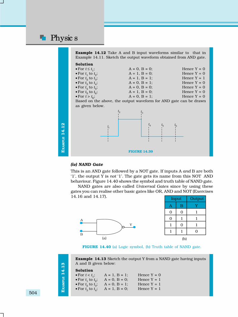
Physic s
504 EX
AM
PLE 1
4.1
3 E
XA
MPLE 1
4.1
2
Example 14.12 Take A and B input waveforms similar to that inExample 14.11. Sketch the output waveform obtained from AND gate.
Solution• For t ≤ t
1; A = 0, B = 0; Hence Y = 0
• For t1 to t
2; A = 1, B = 0; Hence Y = 0
• For t2 to t
3; A = 1, B = 1; Hence Y = 1
• For t3 to t
4; A = 0, B = 1; Hence Y = 0
• For t4 to t
5; A = 0, B = 0; Hence Y = 0
• For t5 to t
6; A = 1, B = 0; Hence Y = 0
• For t > t6; A = 0, B = 1; Hence Y = 0
Based on the above, the output waveform for AND gate can be drawn
as given below.
FIGURE 14.39
(iv) NAND Gate
This is an AND gate followed by a NOT gate. If inputs A and B are both‘1’, the output Y is not ‘1’. The gate gets its name from this NOT ANDbehaviour. Figure 14.40 shows the symbol and truth table of NAND gate.
NAND gates are also called Universal Gates since by using thesegates you can realise other basic gates like OR, AND and NOT (Exercises14.16 and 14.17).
FIGURE 14.40 (a) Logic symbol, (b) Truth table of NAND gate.
Example 14.13 Sketch the output Y from a NAND gate having inputsA and B given below:
Solution• For t < t
1; A = 1, B = 1; Hence Y = 0
• For t1 to t
2; A = 0, B = 0; Hence Y = 1
• For t2 to t
3; A = 0, B = 1; Hence Y = 1
• For t3 to t
4; A = 1, B = 0; Hence Y = 1
Input Output
A B Y
0 0 1
0 1 1
1 0 1
1 1 0
(b)

505
Semic o nduc to r Ele c tro nic s:
Materials, Devic es and
Simple Circ uits
EX
AM
PLE 1
4.1
3
• For t4 to t
5; A = 1, B = 1; Hence Y = 0
• For t5 to t
6; A = 0, B = 0; Hence Y = 1
• For t > t6; A = 0, B = 1; Hence Y = 1
FIGURE 14.41
(v) NOR Gate
It has two or more inputs and one output. A NOT- operation appliedafter OR gate gives a NOT-OR gate (or simply NOR gate). Its output Y is‘1’ only when both inputs A and B are ‘0’, i.e., neither one input nor theother is ‘1’. The symbol and truth table for NOR gate is given inFig. 14.42.
FIGURE 14.42 (a) Logic symbol, (b) Truth table of NOR gate.
NOR gates are considered as universal gates because you can obtainall the gates like AND, OR, NOT by using only NOR gates (Exercises 14.18and 14.19).
14.11 INTEGRATED CIRCUITS
The conventional method of making circuits is to choose componentslike diodes, transistor, R, L, C etc., and connect them by soldering wiresin the desired manner. Inspite of the miniaturisation introduced by thediscovery of transistors, such circuits were still bulky. Apart from this,such circuits were less reliable and less shock proof. The concept offabricating an entire circuit (consisting of many passive components likeR and C and active devices like diode and transistor) on a small singleblock (or chip) of a semiconductor has revolutionised the electronicstechnology. Such a circuit is known as Integrated Circuit (IC). The mostwidely used technology is the Monolithic Integrated Circuit. The word
Input Output
A B Y
0 0 1
0 1 0
1 0 0
1 1 0
(b)

Physic s
506
monolithic is a combination of two greek words, monosmeans single and lithos means stone. This, in effect,means that the entire circuit is formed on a singlesilicon crystal (or chip). The chip dimensions are assmall as 1mm × 1mm or it could even be smaller. Figure14.43 shows a chip in its protective plastic case, partlyremoved to reveal the connections coming out from the‘chip’ to the pins that enable it to make externalconnections.
Depending on nature of input signals, IC’s can begrouped in two categories: (a) linear or analogue IC’sand (b) digital IC’s. The linear IC’s process analogue
signals which change smoothly and continuously over a range of valuesbetween a maximum and a minimum. The output is more or less directlyproportional to the input, i.e., it varies linearly with the input. One of themost useful linear IC’s is the operational amplifier.
The digital IC’s process signals that have only two values. Theycontain circuits such as logic gates. Depending upon the level ofintegration (i.e., the number of circuit components or logic gates), the ICsare termed as Small Scale Integration, SSI (logic gates < 10); MediumScale Integration, MSI (logic gates < 100); Large Scale Integration, LSI(logic gates < 1000); and Very Large Scale Integration, VLSI (logic gates >1000). The technology of fabrication is very involved but large scaleindustrial production has made them very inexpensive.
FIGURE 14.43 The casing andconnection of a ‘chip’.
FASTER AND SMALLER: THE FUTURE OF COMPUTER TECHNOLOGY
The Integrated Chip (IC) is at the heart of all computer systems. In fact ICs are found inalmost all electrical devices like cars, televisions, CD players, cell phones etc. Theminiaturisation that made the modern personal computer possible could never havehappened without the IC. ICs are electronic devices that contain many transistors, resistors,capacitors, connecting wires – all in one package. You must have heard of themicroprocessor. The microprocessor is an IC that processes all information in a computer,like keeping track of what keys are pressed, running programmes, games etc. The IC wasfirst invented by Jack Kilky at Texas Instruments in 1958 and he was awarded Nobel Prizefor this in 2000. ICs are produced on a piece of semiconductor crystal (or chip) by a processcalled photolithography. Thus, the entire Information Technology (IT) industry hinges onsemiconductors. Over the years, the complexity of ICs has increased while the size of itsfeatures continued to shrink. In the past five decades, a dramatic miniaturisation incomputer technology has made modern day computers faster and smaller. In the 1970s,Gordon Moore, co-founder of INTEL, pointed out that the memory capacity of a chip (IC)approximately doubled every one and a half years. This is popularly known as Moore’slaw. The number of transistors per chip has risen exponentially and each year computersare becoming more powerful, yet cheaper than the year before. It is intimated from currenttrends that the computers available in 2020 will operate at 40 GHz (40,000 MHz) andwould be much smaller, more efficient and less expensive than present day computers.The explosive growth in the semiconductor industry and computer technology is bestexpressed by a famous quote from Gordon Moore: “If the auto industry advanced as rapidlyas the semiconductor industry, a Rolls Royce would get half a million miles per gallon, andit would be cheaper to throw it away than to park it”.

507
Semic o nduc to r Ele c tro nic s:
Materials, Devic es and
Simple Circ uits
SUMMARY
1. Semiconductors are the basic materials used in the present solid stateelectronic devices like diode, transistor, ICs, etc.
2. Lattice structure and the atomic structure of constituent elementsdecide whether a particular material will be insulator, metal orsemiconductor.
3. Metals have low resistivity (10–2 to 10–8 Ωm), insulators have very highresistivity (>108 Ω m–1), while semiconductors have intermediate valuesof resistivity.
4. Semiconductors are elemental (Si, Ge) as well as compound (GaAs,CdS, etc.).
5. Pure semiconductors are called ‘intrinsic semiconductors’. The presenceof charge carriers (electrons and holes) is an ‘intrinsic’ property of thematerial and these are obtained as a result of thermal excitation. Thenumber of electrons (n
e) is equal to the number of holes (n
h ) in intrinsic
conductors. Holes are essentially electron vacancies with an effectivepositive charge.
6. The number of charge carriers can be changed by ‘doping’ of a suitableimpurity in pure semiconductors. Such semiconductors are known asextrinsic semiconductors. These are of two types (n-type and p-type).
7. In n-type semiconductors, ne >> n
h while in p-type semiconductors n
h >> n
e.
8. n-type semiconducting Si or Ge is obtained by doping with pentavalentatoms (donors) like As, Sb, P, etc., while p-type Si or Ge can be obtainedby doping with trivalent atom (acceptors) like B, Al, In etc.
9. nen
h = n
i
2 in all cases. Further, the material possesses an overall charge
neutrality.
10. There are two distinct band of energies (called valence band andconduction band) in which the electrons in a material lie. Valenceband energies are low as compared to conduction band energies. Allenergy levels in the valence band are filled while energy levels in theconduction band may be fully empty or partially filled. The electrons inthe conduction band are free to move in a solid and are responsible forthe conductivity. The extent of conductivity depends upon the energygap (E
g) between the top of valence band (E
V) and the bottom of the
conduction band EC. The electrons from valence band can be excited by
heat, light or electrical energy to the conduction band and thus, producea change in the current flowing in a semiconductor.
11. For insulators Eg > 3 eV, for semiconductors E
g is 0.2 eV to 3 eV, while
for metals Eg ≈ 0.
12. p-n junction is the ‘key’ to all semiconductor devices. When such ajunction is made, a ‘depletion layer’ is formed consisting of immobileion-cores devoid of their electrons or holes. This is responsible for ajunction potential barrier.
13. By changing the external applied voltage, junction barriers can bechanged. In forward bias (n-side is connected to negative terminal of thebattery and p-side is connected to the positive), the barrier is decreasedwhile the barrier increases in reverse bias. Hence, forward bias currentis more (mA) while it is very small (μA) in a p-n junction diode.
14. Diodes can be used for rectifying an ac voltage (restricting the ac voltageto one direction). With the help of a capacitor or a suitable filter, a dcvoltage can be obtained.
15. There are some special purpose diodes.

Physic s
508
16. Zener diode is one such special purpose diode. In reverse bias, after acertain voltage, the current suddenly increases (breakdown voltage) ina Zener diode. This property has been used to obtain voltage regulation.
17. p-n junctions have also been used to obtain many photonic oroptoelectronic devices where one of the participating entity is ‘photon’:(a) Photodiodes in which photon excitation results in a change of reversesaturation current which helps us to measure light intensity; (b) Solarcells which convert photon energy into electricity; (c) Light EmittingDiode and Diode Laser in which electron excitation by a bias voltageresults in the generation of light.
18. Transistor is an n-p-n or p-n-p junction device. The central block(thin and lightly doped) is called ‘Base’ while the other electrodes are‘Emitter’ and ‘Collectors’. The emitter-base junction is forward biasedwhile collector-base junction is reverse biased.
19. The transistors can be connected in such a manner that either C or Eor B is common to both the input and output. This gives the threeconfigurations in which a transistor is used: Common Emitter (CE),Common Collector (CC) and Common Base (CB). The plot between I
C
and VCE
for fixed IB is called output characteristics while the plot between
IB and V
BE with fixed V
CE is called input characteristics. The important
transistor parameters for CE-configuration are:
input resistance,
CE
BEi
B V
Vr
I
⎛ ⎞Δ= ⎜ ⎟Δ⎝ ⎠output resistance,
B
CEo
C I
Vr
I
⎛ ⎞Δ= ⎜ ⎟Δ⎝ ⎠current amplification factor,
CE
C
B V
I
Iβ ⎛ ⎞Δ= ⎜ ⎟Δ⎝ ⎠
20. Transistor can be used as an amplifier and oscillator. In fact, anoscillator can also be considered as a self-sustained amplifier in whicha part of output is fed-back to the input in the same phase (positivefeed back). The voltage gain of a transistor amplifier in common emitter
configuration is: o Cv
i B
v RA
v Rβ⎛ ⎞= =⎜ ⎟⎝ ⎠ , where R
C and R
B are respectively
the resistances in collector and base sides of the circuit.
21. When the transistor is used in the cutoff or saturation state, it acts asa switch.
22. There are some special circuits which handle the digital data consistingof 0 and 1 levels. This forms the subject of Digital Electronics.
23. The important digital circuits performing special logic operations arecalled logic gates. These are: OR, AND, NOT, NAND, and NOR gates.
24. In modern day circuit, many logical gates or circuits are integrated inone single ‘Chip’. These are known as Intgrated circuits (IC).
POINTS TO PONDER
1. The energy bands (EC or E
V) in the semiconductors are space delocalised
which means that these are not located in any specific place inside thesolid. The energies are the overall averages. When you see a picture inwhich E
C or E
V are drawn as straight lines, then they should be
respectively taken simply as the bottom of conduction band energy levelsand top of valence band energy levels.

509
Semic o nduc to r Ele c tro nic s:
Materials, Devic es and
Simple Circ uits
2. In elemental semiconductors (Si or Ge), the n-type or p-typesemiconductors are obtained by introducing ‘dopants’ as defects. Incompound semiconductors, the change in relative stoichiometric ratiocan also change the type of semiconductor. For example, in ideal GaAsthe ratio of Ga:As is 1:1 but in Ga-rich or As-rich GaAs it couldrespectively be Ga
1.1 As
0.9 or Ga
0.9 As
1.1. In general, the presence of
defects control the properties of semiconductors in many ways.
3. In transistors, the base region is both narrow and lightly doped,otherwise the electrons or holes coming from the input side (say, emitterin CE-configuration) will not be able to reach the collector.
4. We have described an oscillator as a positive feedback amplifier. Forstable oscillations, the voltage feedback (V
fb) from the output voltage
(Vo) should be such that after amplification (A) it should again become
Vo. If a fraction β′ is feedback, then V
fb = V
o. β′ and after amplification
its value A(vo.β′) should be equal to V
o. This means that the criteria for
stable oscillations to be sustained is A β′ = 1. This is known asBarkhausen's Criteria.
5. In an oscillator, the feedback is in the same phase (positive feedback).If the feedback voltage is in opposite phase (negative feedback), thegain is less than 1 and it can never work as oscillator. It will be anamplifier with reduced gain. However, the negative feedback also reducesnoise and distortion in an amplifier which is an advantageous feature.
EXERCISES
14.1 In an n-type silicon, which of the following statement is true:(a) Electrons are majority carriers and trivalent atoms are the
dopants.
(b) Electrons are minority carriers and pentavalent atoms are thedopants.
(c) Holes are minority carriers and pentavalent atoms are thedopants.
(d) Holes are majority carriers and trivalent atoms are the dopants.
14.2 Which of the statements given in Exercise 14.1 is true for p-typesemiconductos.
14.3 Carbon, silicon and germanium have four valence electrons each.These are characterised by valence and conduction bands separatedby energy band gap respectively equal to (E
g)C, (E
g)Si and (E
g)Ge
. Whichof the following statements is true?
(a) (Eg)Si < (E
g)Ge
< (Eg)C
(b) (Eg)C < (E
g)Ge
> (Eg)Si
(c) (Eg)C > (E
g)Si > (E
g)Ge
(d) (Eg)C = (E
g)Si = (E
g)Ge
14.4 In an unbiased p-n junction, holes diffuse from the p-region ton-region because
(a) free electrons in the n-region attract them.
(b) they move across the junction by the potential difference.
(c) hole concentration in p-region is more as compared to n-region.
(d) All the above.

Physic s
510
14.5 When a forward bias is applied to a p-n junction, it
(a) raises the potential barrier.
(b) reduces the majority carrier current to zero.
(c) lowers the potential barrier.
(d) None of the above.
14.6 For transistor action, which of the following statements are correct:
(a) Base, emitter and collector regions should have similar size anddoping concentrations.
(b) The base region must be very thin and lightly doped.
(c) The emitter junction is forward biased and collector junction isreverse biased.
(d) Both the emitter junction as well as the collector junction areforward biased.
14.7 For a transistor amplifier, the voltage gain
(a) remains constant for all frequencies.
(b) is high at high and low frequencies and constant in the middlefrequency range.
(c) is low at high and low frequencies and constant at midfrequencies.
(d) None of the above.
14.8 In half-wave rectification, what is the output frequency if the inputfrequency is 50 Hz. What is the output frequency of a full-wave rectifierfor the same input frequency.
14.9 For a CE-transistor amplifier, the audio signal voltage across thecollected resistance of 2 kΩ is 2 V. Suppose the current amplificationfactor of the transistor is 100, find the input signal voltage and basecurrent, if the base resistance is 1 kΩ.
14.10 Two amplifiers are connected one after the other in series (cascaded).The first amplifier has a voltage gain of 10 and the second has avoltage gain of 20. If the input signal is 0.01 volt, calculate the outputac signal.
14.11 A p-n photodiode is fabricated from a semiconductor with band gapof 2.8 eV. Can it detect a wavelength of 6000 nm?
ADDITIONAL EXERCISES
14.12 The number of silicon atoms per m3 is 5 × 1028. This is dopedsimultaneously with 5 × 10²² atoms per m3 of Arsenic and 5 × 10²⁰
per m3 atoms of Indium. Calculate the number of electrons and holes.Given that n
i = 1.5 × 10¹⁶ m–3. Is the material n-type or p-type?
14.13 In an intrinsic semiconductor the energy gap Eg is 1.2eV. Its hole
mobility is much smaller than electron mobility and independent oftemperature. What is the ratio between conductivity at 600K andthat at 300K? Assume that the temperature dependence of intrinsiccarrier concentration n
i is given by
0 exp –2
g
i
B
En n
k T
⎛ ⎞= ⎜ ⎟⎝ ⎠where n
0 is a constant.

511
Semic o nduc to r Ele c tro nic s:
Materials, Devic es and
Simple Circ uits
14.14 In a p-n junction diode, the current I can be expressed as
0 exp –12 B
eVI I
k T
⎛ ⎞= ⎜ ⎟⎝ ⎠where I
0 is called the reverse saturation current, V is the voltage
across the diode and is positive for forward bias and negative forreverse bias, and I is the current through the diode, k
B is the
Boltzmann constant (8.6×10⁻⁵ eV/K) and T is the absolutetemperature. If for a given diode I
0 = 5 × 10–12 A and T = 300 K, then
(a) What will be the forward current at a forward voltage of 0.6 V?
(b) What will be the increase in the current if the voltage across thediode is increased to 0.7 V?
(c) What is the dynamic resistance?
(d) What will be the current if reverse bias voltage changes from 1 Vto 2 V?
14.15 You are given the two circuits as shown in Fig. 14.44. Show thatcircuit (a) acts as OR gate while the circuit (b) acts as AND gate.
FIGURE 14.44
14.16 Write the truth table for a NAND gate connected as given inFig. 14.45.
FIGURE 14.45
Hence identify the exact logic operation carried out by this circuit.
14.17 You are given two circuits as shown in Fig. 14.46, which consistof NAND gates. Identify the logic operation carried out by the twocircuits.
FIGURE 14.46
14.18 Write the truth table for circuit given in Fig. 14.47 below consistingof NOR gates and identify the logic operation (OR, AND, NOT) whichthis circuit is performing.

Physic s
512
FIGURE 14.47
(Hint: A = 0, B = 1 then A and B inputs of second NOR gate will be 0and hence Y=1. Similarly work out the values of Y for othercombinations of A and B. Compare with the truth table of OR, AND,NOT gates and find the correct one.)
14.19 Write the truth table for the circuits given in Fig. 14.48 consisting ofNOR gates only. Identify the logic operations (OR, AND, NOT) performedby the two circuits.
FIGURE 14.48

15.1 INTRODUCTION
Communication is the act of transmission of information. Every livingcreature in the world experiences the need to impart or receive informationalmost continuously with others in the surrounding world. Forcommunication to be successful, it is essential that the sender and thereceiver understand a common language. Man has constantly madeendeavors to improve the quality of communication with other humanbeings. Languages and methods used in communication have keptevolving from prehistoric to modern times, to meet the growing demandsin terms of speed and complexity of information. It would be worthwhileto look at the major milestones in events that promoted developments incommunications, as presented in Table 15.1.
Modern communication has its roots in the 19th and 20th century inthe work of scientists like J.C. Bose, F.B. Morse, G. Marconi and AlexanderGraham Bell. The pace of development seems to have increaseddramatically after the first half of the 20th century. We can hope to seemany more accomplishments in the coming decades. The aim of thischapter is to introduce the concepts of communication, namely the modeof communication, the need for modulation, production and deductionof amplitude modulation.
15.2 ELEMENTS OF A COMMUNICATION SYSTEM
Communication pervades all stages of life of all living creatures. Irrespectiveof its nature, every communication system has three essential elements-
Chapter Fifteen
COMMUNICATIONSYSTEMS

Physics
514
Around1565 A.D.
1835
1876
1895
1936
1955
1968
1975
1989-91
Year Event Remarks
The reporting of the delivery ofa child by queen using drumbeats from a distant place toKing Akbar.
Invention of telegraph bySamuel F.B. Morse and SirCharles Wheatstone
Telephone invented byAlexander Graham Bell andAntonio Meucci
Jagadis Chandra Bose andGuglielmo Marconidemonstrated wirelesstelegraphy.
Television broadcast(JohnLogi Baird)
First radio FAX transmittedacross continent.(AlexanderBain)
ARPANET- the first internetcame into existence(J.C.R.Licklider)
Fiber optics developed at BellLaboratories
Tim Berners-Lee invented theWorld Wide Web.
It is believed that minister Birbalexperimented with the arrangement todecide the number of drummers postedbetween the place where the queenstayed and the place where the kingstayed.
It resulted in tremendous growth ofmessages through post offices andreduced physical travel of messengersconsiderably.
Perhaps the most widely used means ofcommunication in the history ofmankind.
It meant a giant leap – from an era ofcommunication using wires tocommunicating without using wires.(wireless)
First television broadcast by BBC
The idea of FAX transmission waspatented by Alexander Bain in 1843.
ARPANET was a project undertaken bythe U.S. defence department. It allowedfile transfer from one computer toanother connected to the network.
Fiber optical systems are superior andmore economical compared totraditional communication systems.
WWW may be regarded as the mammothencyclopedia of knowledge accessible toeveryone round the clock throughout theyear.
TABLE 15.1 SOME MAJOR MILESTONES IN THE HISTORY OF COMMUNICATION

Communication System
515
transmitter, medium/channel and receiver. The block diagram shown inFig. 15.1 depicts the general form of a communication system.
FIGURE 15.1 Block diagram of a generalised communication system.
In a communication system, the transmitter is located at one place,the receiver is located at some other place (far or near) separate from thetransmitter and the channel is the physical medium that connects them.Depending upon the type of communication system, a channel may be inthe form of wires or cables connecting the transmitter and the receiver orit may be wireless. The purpose of the transmitter is to convert the messagesignal produced by the source of information into a form suitable fortransmission through the channel. If the output of the information sourceis a non-electrical signal like a voice signal, a transducer converts it toelectrical form before giving it as an input to the transmitter. When atransmitted signal propagates along the channel it may get distorted dueto channel imperfection. Moreover, noise adds to the transmitted signaland the receiver receives a corrupted version of the transmitted signal.The receiver has the task of operating on the received signal. It reconstructsa recognisable form of the original message signal for delivering it to theuser of information.
There are two basic modes of communication: point-to-point andbroadcast.
In point-to-point communication mode, communication takes placeover a link between a single transmitter and a receiver. Telephony is anexample of such a mode of communication. In contrast, in the broadcastmode, there are a large number of receivers corresponding to a singletransmitter. Radio and television are examples of broadcast mode ofcommunication.
15.3 BASIC TERMINOLOGY USED IN ELECTRONIC
COMMUNICATION SYSTEMS
By now, we have become familiar with some terms like information source,transmitter, receiver, channel, noise, etc. It would be easy to understandthe principles underlying any communication, if we get ourselvesacquainted with the following basic terminology.

Physics
516
(i) Transducer: Any device that converts one form ofenergy into another can be termed as a transducer.In electronic communication systems, we usuallycome across devices that have either their inputsor outputs in the electrical form. An electricaltransducer may be defined as a device that convertssome physical variable (pressure, displacement,force, temperature, etc) into correspondingvariations in the electrical signal at its output.
(ii) Signal: Information converted in electrical formand suitable for transmission is called a signal.Signals can be either analog or digital. Analogsignals are continuous variations of voltage orcurrent. They are essentially single-valuedfunctions of time. Sine wave is a fundamentalanalog signal. All other analog signals can be fullyunderstood in terms of their sine wave components.Sound and picture signals in TV are analog innature. Digital signals are those which can takeonly discrete stepwise values. Binary system thatis extensively used in digital electronics employsjust two levels of a signal. ‘0’ corresponds to a lowlevel and ‘1’ corresponds to a high level of voltage/current. There are several coding schemes usefulfor digital communication. They employ suitablecombinations of number systems such as thebinary coded decimal (BCD)*. American StandardCode for Information Interchange (ASCII)** is auniversally popular digital code to representnumbers, letters and certain characters.
(iii) Noise: Noise refers to the unwanted signals thattend to disturb the transmission and processingof message signals in a communication system.The source generating the noise may be locatedinside or outside the system.
(iv) Transmitter: A transmitter processes the incomingmessage signal so as to make it suitable fortransmission through a channel and subsequentreception.
(v) Receiver: A receiver extracts the desired messagesignals from the received signals at the channeloutput.
(vi) Attenuation: The loss of strength of a signal whilepropagating through a medium is known asattenuation.
* In BCD, a digit is usually represented by four binary (0 or 1) bits. For examplethe numbers 0, 1, 2, 3, 4 in the decimal system are written as 0000, 0001, 0010,0011 and 0100. 1000 would represent eight.
** It is a character encoding in terms of numbers based on English alphabet sincethe computer can only understand numbers.
JA
GA
DIS
CH
AN
DR
A B
OS
E (1858 –
1937)
Jagadis Chandra Bose(1858 – 1937) Hedeveloped an apparatusfor generating ultrashortelectro-magnetic wavesand studied their quasi-optical properties. Hewas said to be the first toemploy a semiconductorlike galena as a self-recovering detector ofelectromagnetic waves.Bose published threepapers in the Britishmagazine, ‘TheElectrician’ of 27 Dec.1895. His invention waspublished in the‘Proceedings of The RoyalSociety’ on 27 April 1899over two years beforeMarconi’s first wirelesscommunication on 13December 1901. Bosealso invented highlysensitive instruments forthe detection of minuteresponses by livingorganisms to externalstimulii and establishedparallelism betweenanimal and planttissues.

Communication System
517
(vii) Amplification: It is the process of increasing the amplitude (andconsequently the strength) of a signal using an electronic circuitcalled the amplifier (reference Chapter 14). Amplification isnecessary to compensate for the attenuation of the signal incommunication systems. The energy needed for additional signalstrength is obtained from a DC power source. Amplification isdone at a place between the source and the destination whereversignal strength becomes weaker than the required strength.
(viii) Range: It is the largest distance between a source and a destinationup to which the signal is received with sufficient strength.
(ix) Bandwidth: Bandwidth refers to the frequency range over whichan equipment operates or the portion of the spectrum occupiedby the signal.
(x) Modulation: The original low frequency message/informationsignal cannot be transmitted to long distances because ofreasons given in Section 15.7. Therefore, at the transmitter,information contained in the low frequency message signal issuperimposed on a high frequency wave, which acts as a carrierof the information. This process is known as modulation. Aswill be explained later, there are several types of modulation,abbreviated as AM, FM and PM.
(xi) Demodulation: The process of retrieval of information from thecarrier wave at the receiver is termed demodulation. This is thereverse process of modulation.
(xii) Repeater: A repeater is a combination of a receiver and atransmitter. A repeater, picks up the signal from the transmitter,amplifies and retransmits it to the receiver sometimes with achange in carrier frequency. Repeaters are used to extend therange of a communication system as shown in Fig. 15.2. Acommunication satellite is essentially a repeater station in space.
FIGURE 15.2 Use of repeater station to increase the range of communication.
15.4 BANDWIDTH OF SIGNALS
In a communication system, the message signal can be voice, music,picture or computer data. Each of these signals has different ranges offrequencies. The type of communication system needed for a given signaldepends on the band of frequencies which is considered essential for thecommunication process.
For speech signals, frequency range 300 Hz to 3100 Hz is consideredadequate. Therefore speech signal requires a bandwidth of 2800 Hz (3100 Hz– 300 Hz) for commercial telephonic communication. To transmit music,

Physics
518
an approximate bandwidth of 20 kHz is required because of the highfrequencies produced by the musical instruments. The audible range offrequencies extends from 20 Hz to 20 kHz.
Video signals for transmission of pictures require about 4.2 MHz ofbandwidth. A TV signal contains both voice and picture and is usuallyallocated 6 MHz of bandwidth for transmission.
In the preceeding paragraph, we have considered only analog signals.Digital signals are in the form of rectangular waves as shown in Fig. 15.3.One can show that this rectangular wave can be decomposed into asuperposition of sinusoidal waves of frequencies ν0, 2ν0, 3ν0, 4ν0 ... nν0where n is an integer extending to infinity and ν0 = 1/T0. The fundamental(ν0 ), fundamental (ν0 ) + second harmonic (2ν0 ), and fundamental (ν0 ) +
second harmonic (2ν0 ) +third harmonic (3ν0 ), areshown in the same figure toillustrate this fact. It is clearthat to reproduce therectangular wave shapeexactly we need tosuperimpose all theharmonics ν0, 2ν0, 3ν0,4ν0..., which implies aninfinite bandwidth.However, for practicalpurposes, the contributionfrom higher harmonics canbe neglected, thus limitingthe bandwidth. As a result,received waves are adistorted version of the
transmitted one. If the bandwidth is large enough to accommodate a fewharmonics, the information is not lost and the rectangular signal is moreor less recovered. This is so because the higher the harmonic, less is itscontribution to the wave form.
15.5 BANDWIDTH OF TRANSMISSION MEDIUM
Similar to message signals, different types of transmission media offerdifferent bandwidths. The commonly used transmission media are wire,free space and fiber optic cable. Coaxial cable is a widely used wiremedium, which offers a bandwidth of approximately 750 MHz. Such cablesare normally operated below 18 GHz. Communication through free spaceusing radio waves takes place over a very wide range of frequencies: froma few hundreds of kHz to a few GHz. This range of frequencies is furthersubdivided and allocated for various services as indicated in Table 15.2.Optical communication using fibers is performed in the frequency rangeof 1 THz to 1000 THz (microwaves to ultraviolet). An optical fiber canoffer a transmission bandwidth in excess of 100 GHz.
Spectrum allocations are arrived at by an international agreement.The International Telecommunication Union (ITU) administers the presentsystem of frequency allocations.
FIGURE 15.3 Approximation of a rectangular wave in terms of afundamental sine wave and its harmonics.

Communication System
519
15.6 PROPAGATION OF ELECTROMAGNETIC WAVES
In communication using radio waves, an antenna at the transmitterradiates the Electromagnetic waves (em waves), which travel through thespace and reach the receiving antenna at the other end. As the em wavetravels away from the transmitter, the strength of the wave keeps ondecreasing. Several factors influence the propagation of em waves andthe path they follow. At this point, it is also important to understand thecomposition of the earth’s atmosphere as it plays a vital role in thepropagation of em waves. A brief discussion on some useful layers of theatmosphere is given in Table 15.3.
15.6.1 Ground wave
To radiate signals with high efficiency, the antennas should have a sizecomparable to the wavelength λ of the signal (at least ~ λ/4). At longerwavelengths (i.e., at lower frequencies), the antennas have large physicalsize and they are located on or very near to the ground. In standard AMbroadcast, ground based vertical towers are generally used as transmittingantennas. For such antennas, ground has a strong influence on thepropagation of the signal. The mode of propagation is called surface wavepropagation and the wave glides over the surface of the earth. A waveinduces current in the ground over which it passes and it is attenuatedas a result of absorption of energy by the earth. The attenuation of surfacewaves increases very rapidly with increase in frequency. The maximumrange of coverage depends on the transmitted power and frequency (lessthan a few MHz).
Standard AM broadcast
FM broadcast
Television
Cellular Mobile Radio
Satellite Communication
Service Frequency bands Comments
540-1600 kHz
88-108 MHz
54-72 MHz
76-88 MHz
174-216 MHz
420-890 MHz
896-901 MHz
840-935 MHz
5.925-6.425 GHz
3.7-4.2 GHz
VHF (very high frequencies)
TV
UHF (ultra high frequencies)
TV
Mobile to base station
Base station to mobile
Uplink
Downlink
TABLE 15.2 SOME IMPORTANT WIRELESS COMMUNICATION FREQUENCY BANDS

Physics
520
15.6.2 Sky wavesIn the frequency range from a few MHz up to 30 to 40 MHz, long distancecommunication can be achieved by ionospheric reflection of radio wavesback towards the earth. This mode of propagation is called sky wavepropagation and is used by short wave broadcast services. The ionosphereis so called because of the presence of a large number of ions or chargedparticles. It extends from a height of ~ 65 Km to about 400 Km above theearth’s surface. Ionisation occurs due to the absorption of the ultravioletand other high-energy radiation coming from the sun by air molecules.The ionosphere is further subdivided into several layers, the details ofwhich are given in Table 15.3. The degree of ionisation varies with theheight. The density of atmosphere decreases with height. At great heightsthe solar radiation is intense but there are few molecules to be ionised.Close to the earth, even though the molecular concentration is very high,the radiation intensity is low so that the ionisation is again low. However,at some intermediate heights, there occurs a peak of ionisation density.The ionospheric layer acts as a reflector for a certain range of frequencies(3 to 30 MHz). Electromagnetic waves of frequencies higher than 30 MHzpenetrate the ionosphere and escape. These phenomena are shown in theFig. 15.4. The phenomenon of bending of em waves so that they arediverted towards the earth is similar to total internal reflection in optics*.
Troposphere
D (part ofstratosphere)
E (part ofStratosphere)
F1 (Part ofMesosphere)
F2
(Thermosphere)
Name of thestratum (layer)
Approximate heightover earth’s surface
Exists during
10 km
65-75 km
100 km
170-190 km
300 km at night,250-400 kmduring daytime
Day andnight
Day only
Day only
Daytime,merges withF2 at night
Day andnight
TABLE 15.3 DIFFERENT LAYERS OF ATMOSPHERE AND THEIR INTERACTION WITH THE
PROPAGATING ELECTROMAGNETIC WAVES
Frequencies mostaffected
VHF (up to several GHz)
Reflects LF, absorbs MFand HF to some degree
Helps surface waves,reflects HF
Partially absorbs HFwaves yet allowing themto reach F2
Efficiently reflects HFwaves, particularly atnight
PARTS
OF
IONOSPHERE
* Compare this with the phenomenon of mirage.

Communication System
521
15.6.3 Space waveAnother mode of radio wave propagation is by space waves. A spacewave travels in a straight line from transmitting antenna to the receivingantenna. Space waves are used for line-of-sight (LOS) communication aswell as satellite communication. At frequencies above 40 MHz,communication is essentially limited to line-of-sight paths. At thesefrequencies, the antennas are relatively smaller and can be placed atheights of many wavelengths above the ground. Because of line-of-sightnature of propagation, direct waves get blocked at some point by thecurvature of the earth as illustrated in Fig. 15.5. If the signal is to bereceived beyond the horizon then the receiving antenna must be highenough to intercept the line-of-sight waves.
FIGURE 15.4 Sky wave propagation. The layer nomenclatureis given in Table 15.3.
FIGURE 15.5 Line of sight communication by space waves.
If the transmitting antenna is at a height hT, then you can show that
the distance to the horizon dT is given as 2T Td Rh= , where R is the
radius of the earth (approximately 6400 km). dT is also called the radiohorizon of the transmitting antenna. With reference to Fig. 15.5 themaximum line-of-sight distance dM between the two antennas havingheights hT and hR above the earth is given by
2 2M T Rd Rh Rh= + (15.1)
where hR is the height of receiving antenna.

Physics
522
Television broadcast, microwave links and satellite communicationare some examples of communication systems that use space wave modeof propagation. Figure 15.6 summarises the various modes of wavepropagation discussed so far.
FIGURE 15.6 Various propagation modes for em waves.
EX
AM
PLE 1
5.1
Example 15.1 A transmitting antenna at the top of a tower has a height32 m and the height of the receiving antenna is 50 m. What is themaximum distance between them for satisfactory communication inLOS mode? Given radius of earth 6.4 × 10⁶ m.
Solution
5 52 64 10 32 2 64 10 50 mdm = × × × + × × ×
2 364 10 10 8 10 10 m= × × + × ×
2144 10 10 m 45.5 km= × × =
15.7 MODULATION AND ITS NECESSITY
As already mentioned, the purpose of a communication system is totransmit information or message signals. Message signals are also calledbaseband signals, which essentially designate the band of frequenciesrepresenting the original signal, as delivered by the source of information.No signal, in general, is a single frequency sinusoid, but it spreads over arange of frequencies called the signal bandwidth. Suppose we wish totransmit an electronic signal in the audio frequency (AF) range (basebandsignal frequency less than 20 kHz) over a long distance directly. Let usfind what factors prevent us from doing so and how we overcome thesefactors,

Communication System
523
15.7.1 Size of the antenna or aerialFor transmitting a signal, we need an antenna or an aerial. This antennashould have a size comparable to the wavelength of the signal (at leastλ/4 in dimension) so that the antenna properly senses the time variationof the signal. For an electromagnetic wave of frequency 20 kHz, thewavelength λ is 15 km. Obviously, such a long antenna is not possible toconstruct and operate. Hence direct transmission of such baseband signalsis not practical. We can obtain transmission with reasonable antennalengths if transmission frequency is high (for example, if ν is 1 MHz, thenλ is 300 m). Therefore, there is a need of translating the informationcontained in our original low frequency baseband signal into high orradio frequencies before transmission.
15.7.2 Effective power radiated by an antennaA theoretical study of radiation from a linear antenna (length l ) showsthat the power radiated is proportional to (l/λ)2 . This implies that for thesame antenna length, the power radiated increases with decreasing λ,i.e., increasing frequency. Hence, the effective power radiated by a longwavelength baseband signal would be small. For a good transmission,we need high powers and hence this also points out to the need of usinghigh frequency transmission.
15.7.3 Mixing up of signals from different transmittersAnother important argument against transmitting baseband signalsdirectly is more practical in nature. Suppose many people are talking atthe same time or many transmitters are transmitting baseband informationsignals simultaneously. All these signals will getmixed up and there is no simple way to distinguishbetween them. This points out towards a possiblesolution by using communication at highfrequencies and allotting a band of frequencies toeach message signal for its transmission.
The above arguments suggest that there is aneed for translating the original low frequencybaseband message or information signal into highfrequency wave before transmission such that thetranslated signal continues to possess theinformation contained in the original signal. Indoing so, we take the help of a high frequency signal,known as the carrier wave, and a process knownas modulation which attaches information to it. Thecarrier wave may be continuous (sinusoidal) or inthe form of pulses as shown in Fig. 15.7.
A sinusoidal carrier wave can be represented as
c(t ) = Ac sin (ωct + φ) (15.2)
where c(t) is the signal strength (voltage or current), Ac is the amplitude,ωc ( = 2πνc) is the angular frequency and φ is the initial phase of the carrierwave. During the process of modulation, any of the three parameters, vizAc, ωc and φ, of the carrier wave can be controlled by the message or
FIGURE 15.7 (a) Sinusoidal, and(b) pulse shaped signals.

Physics
524
information signal. This results in three types of modulation: (i) Amplitudemodulation (AM), (ii) Frequency modulation (FM) and(iii) Phase modulation (PM), as shown in Fig. 15.8.
FIGURE 15.8 Modulation of a carrier wave: (a) a sinusoidal carrier wave;(b) a modulating signal; (c) amplitude modulation; (d) frequency
modulation; and (e) phase modulation.
Similarly, the significant characteristics of a pulse are: pulse amplitude,pulse duration or pulse Width, and pulse position (denoting the time ofrise or fall of the pulse amplitude) as shown in Fig. 15.7(b). Hence, differenttypes of pulse modulation are: (a) pulse amplitude modulation (PAM),(b) pulse duration modulation (PDM) or pulse width modulation (PWM),and (c) pulse position modulation (PPM). In this chapter, we shall confineto amplitude modulation on ly.
15.8 AMPLITUDE MODULATION
In amplitude modulation the amplitude of the carrier is varied inaccordance with the information signal. Here we explain amplitudemodulation process using a sinusoidal signal as the modulating signal.
Let c(t) = Ac sin ωct represent carrier wave and m(t) = Am sin ωmt representthe message or the modulating signal where ωm = 2πfm is the angularfrequency of the message signal. The modulated signal cm (t ) can bewritten as
cm (t) = (Ac + Am sin ωmt) sin ωct
1 mc m c
c
AA sin t sin t
Aω ω
⎛ ⎞= +⎜ ⎟⎝ ⎠ (15.3)
Note that the modulated signal now contains the message signal. Thiscan also be seen from Fig. 15.8(c). From Eq. (15.3), we can write,
( )m c c c m cc t A sin t A sin t sin tω μ ω ω= + (15.4)
Mo
du
lati
on
an
d D
em
od
ula
tio
nht
tp://
ww
w.w
illia
mso
n-la
bs.c
om/4
80_m
od.h
tm

Communication System
525
Here μ = Am/Ac is the modulation index; in practice,μ is kept 1≤ to avoiddistortion.
Using the trignomatric relation sinA sinB = ½ (cos(A – B) – cos (A + B),we can write cm (t) of Eq. (15.4) as
( ) sin cos( ) cos( )2 2
c cm c c c m c m
A Ac t A t t t
μ μω ω ω ω ω= + − − + (15.5)
Here ωc – ωm and ωc + ωm are respectively called the lower side and upperside frequencies. The modulated signal now consists of the carrier waveof frequency ωc plus two sinusoidal waves each with a frequency slightlydifferent from, known as side bands. The frequency spectrum of theamplitude modulated signal is shown in Fig. 15.9.
FIGURE 15.9 A plot of amplitude versus ω foran amplitude modulated signal.
EX
AM
PLE 1
5.2
As long as the broadcast frequencies (carrier waves) are sufficientlyspaced out so that sidebands do not overlap, different stations can operatewithout interfering with each other.
Example 15.2 A message signal of frequency 10 kHz and peak voltageof 10 volts is used to modulate a carrier of frequency 1 MHz and peakvoltage of 20 volts. Determine (a) modulation index, (b) the side bandsproduced.
Solution(a) Modulation index =10/20 = 0.5
(b) The side bands are at (1000+10 kHz)=1010 kHz and(1000 –10 kHz) = 990 kHz.
15.9 PRODUCTION OF AMPLITUDE MODULATED WAVE
Amplitude modulation can be produced by a variety of methods. Aconceptually simple method is shown in the block diagram of Fig. 15.10.
FIGURE 15.10 Block diagram of a simple modulatorfor obtaining an AM signal.

Physics
526
Here the modulating signal Am sin ωmt is added to the carrier signalAc sin ωct to produce the signal x (t). This signal x (t) = Am sinωmt+ Ac sinωct is passed through a square law device which is a non-lineardevice which produces an output
y (t) = B x (t ) + Cx2 (t ) (15.6)where B and C are constants. Thus,
y (t)= BAm sin ωmt + BAc sin ωct
2 2 2 2sin sin 2 sin sinm m c c m c m cC A t A t A A t tω ω ω ω⎡ ⎤+ + +⎣ ⎦ (15.7)
= BAm sin ωmt + BAc sin ωct
2 2 22 – cos2 – cos2
2 2 2m m c
c m c
C A C A C AA t tω ω+ +
+ CAmAc cos (ωc – ωm) t – CAmAc cos (ωc+ ωm) t (15.8)
where the trigonometric relations sin2A = (1 – cos2A)/2 and the relationfor sinA sinB mentioned earlier are used.
In Eq. (15.8), there is a dc term C/2 ( )2 2m cA A+ and sinusoids of
frequencies ωm, 2ωm, ωc, 2ωc, ωc – ωm and ωc + ωm. As shown in Fig. 15.10this signal is passed through a band pass filter* which rejects dc and thesinusoids of frequencies ωm , 2ωm and 2 ωc and retains the frequencies ωc,ωc – ωm and ωc + ωm. The output of the band pass filter therefore is of thesame form as Eq. (15.5) and is therefore an AM wave.
It is to be mentioned that the modulated signal cannot be transmittedas such. The modulator is to be followed by a power amplifier whichprovides the necessary power and then the modulated signal is fed to anantenna of appropriate size for radiation as shown in Fig. 15.11.
* A band pass filter rejects low and high frequencies and allows a band of frequenciesto pass through.
FIGURE 15.11 Block diagram of a transmitter.
15.10 DETECTION OF AMPLITUDE MODULATED WAVE
The transmitted message gets attenuated in propagating through thechannel. The receiving antenna is therefore to be followed by an amplifierand a detector. In addition, to facilitate further processing, the carrierfrequency is usually changed to a lower frequency by what is called anintermediate frequency (IF) stage preceding the detection. The detectedsignal may not be strong enough to be made use of and hence is required

Communication System
527
Detection is the process of recovering the modulating signal from themodulated carrier wave. We just saw that the modulated carrier wavecontains the frequencies ωc and ωc ± ωm. In order to obtain the originalmessage signal m(t ) of angular frequency ωm, a simple method is shownin the form of a block diagram in Fig. 15.13.
FIGURE 15.12 Block diagram of a receiver.
to be amplified. A block diagram of a typical receiver is shown inFig. 15.12
FIGURE 15.13 Block diagram of a detector for AM signal. The quantityon y-axis can be current or voltage.
The modulated signal of the form given in (a) of fig. 15.13 is passedthrough a rectifier to produce the output shown in (b). This envelope ofsignal (b) is the message signal. In order to retrieve m (t ), the signal ispassed through an envelope detector (which may consist of a simple RCcircuit).
In the present chapter we have discussed some basic concepts ofcommunication and communication systems. We have also discussedone specific type of analog modulation namely Amplitude Modulation(AM). Other forms of modulation and digital communication systems playan important role in modern communication. These and other excitingdevelopments are taking place everyday.
So far we have restricted our discussion to some basic communicationsystems. Before we conclude this chapter, it is worth taking a glance atsome of the communication systems (see the box) that in recent timeshave brought major changes in the way we exchange information even inour day-to-day life:

Physics
528
ADDITIONAL INFORMATION
The InternetIt is a system with billions of users worldwide. It permits communication and sharing of alltypes of information between any two or more computers connected through a large andcomplex network. It was started in 1960’s and opened for public use in 1990’s. With thepassage of time it has witnessed tremendous growth and it is still expanding its reach. Itsapplications include(i) E mail – It permits exchange of text/graphic material using email software. We can write a
letter and send it to the recipient through ISP’s (Internet Service Providers) who work likethe dispatching and receiving post offices.
(ii) File transfer – A FTP (File Transfer Programmes) allows transfer of files/software from onecomputer to another connected to the Internet.
(iii) World Wide Web (WWW) – Computers that store specific information for sharing with othersprovide websites either directly or through web service providers. Governmentdepartments, companies, NGO’s (Non-Government Organisations) and individuals can postinformation about their activities for restricted or free use on their websites. This informationbecomes accessible to the users. Several search engines like Google, Yahoo! etc. help us infinding information by listing the related websites. Hypertext is a powerful feature of theweb that automatically links relevant information from one page on the web to anotherusing HTML (hypertext markup language).
(iv) E-commerce – Use of the Internet to promote business using electronic means such asusing credit cards is called E-commerce. Customers view images and receive all theinformation about various products or services of companies through their websites. Theycan do on-line shopping from home/office. Goods are dispatched or services are providedby the company through mail/courier.
(v) Chat – Real time conversation among people with common interests through typedmessages is called chat. Everyone belonging to the chat group gets the messageinstantaneously and can respond rapidly.
Facsimile (FAX)It scans the contents of a document (as an image, not text) to create electronic signals. Thesesignals are then sent to the destination (another FAX machine) in an orderly manner usingtelephone lines. At the destination, the signals are reconverted into a replica of the originaldocument. Note that FAX provides image of a static document unlike the image provided bytelevision of objects that might be dynamic.
Mobile telephonyThe concept of mobile telephony was developed first in 1970’s and it was fully implemented inthe following decade. The central concept of this system is to divide the service area into asuitable number of cells centred on an office called MTSO (Mobile Telephone Switching Office).Each cell contains a low-power transmitter called a base station and caters to a large numberof mobile receivers (popularly called cell phones). Each cell could have a service area of a fewsquare kilometers or even less depending upon the number of customers. When a mobilereceiver crosses the coverage area of one base station, it is necessary for the mobile user to betransferred to another base station. This procedure is called handover or handoff. This processis carried out very rapidly, to the extent that the consumer does not even notice it. Mobiletelephones operate typically in the UHF range of frequencies (about 800-950 MHz).

Communication System
529
SUMMARY
1. Electronic communication refers to the faithful transfer of informationor message (available in the form of electrical voltage and current)from one point to another point.
2. Transmitter, transmission channel and receiver are three basic unitsof a communication system.
3. Two important forms of communication system are: Analog and Digital.The information to be transmitted is generally in continuous waveformfor the former while for the latter it has only discrete or quantisedlevels.
4. Every message signal occupies a range of frequencies. The bandwidthof a message signal refers to the band of frequencies, which are necessaryfor satisfactory transmission of the information contained in the signal.Similarly, any practical communication system permits transmissionof a range of frequencies only, which is referred to as the bandwidth ofthe system.
5. Low frequencies cannot be transmitted to long distances. Therefore,they are superimposed on a high frequency carrier signal by a processknown as modulation.
6. In modulation, some characteristic of the carrier signal like amplitude,frequency or phase varies in accordance with the modulating or messagesignal. Correspondingly, they are called Amplitude Modulated (AM),Frequency Modulated (FM) or Phase Modulated (PM) waves.
7. Pulse modulation could be classified as: Pulse Amplitude Modulation(PAM), Pulse Duration Modulation (PDM) or Pulse Width Modulation(PWM) and Pulse Position Modulation (PPM).
8. For transmission over long distances, signals are radiated into spaceusing devices called antennas. The radiated signals propagate aselectromagnetic waves and the mode of propagation is influenced bythe presence of the earth and its atmosphere. Near the surface of theearth, electromagnetic waves propagate as surface waves. Surface wavepropagation is useful up to a few MHz frequencies.
9. Long distance communication between two points on the earth isachieved through reflection of electromagnetic waves by ionosphere.Such waves are called sky waves. Sky wave propagation takes place upto frequency of about 30 MHz. Above this frequency, electromagneticwaves essentially propagate as space waves. Space waves are used forline-of-sight communication and satellite communication.
10. If an antenna radiates electromagnetic waves from a height hT, then
the range dT is given by 2 TRh where R is the radius of the earth.
11. Amplitude modulated signal contains frequencies ( – ),ω ωc m ωc and
( ).c mω ω+12. Amplitude modulated waves can be produced by application of the
message signal and the carrier wave to a non-linear device, followed bya band pass filter.
13. AM detection, which is the process of recovering the modulating signalfrom an AM waveform, is carried out using a rectifier and an envelopedetector.

Physics
530
POINTS TO PONDER
1. In the process of transmission of message/ information signal, noise getsadded to the signal anywhere between the information source and thereceiving end. Can you think of some sources of noise?
2. In the process of modulation, new frequencies called sidebands are generatedon either side (higher and lower than the carrier frequency) of the carrier byan amount equal to the highest modulating frequency. Is it possible toretrieve the message by transmitting (a) only the side bands, (b) only oneside band?
3. In amplitude modulation, modulation index μ ≤ 1 is used. What will happen
if μ > 1?
EXERCISES
15.1 Which of the following frequencies will be suitable for beyond-the-horizon communication using sky waves?(a) 10 kHz
(b) 10 MHz(c) 1 GHz(d) 1000 GHz
15.2 Frequencies in the UHF range normally propagate by means of:(a) Ground waves.(b) Sky waves.(c) Surface waves.(d) Space waves.
15.3 Digital signals(i) do not provide a continuous set of values,
(ii) represent values as discrete steps,
(iii) can utilize binary system, and
(iv) can utilize decimal as well as binary systems.
Which of the above statements are true?
(a) (i) and (ii) only
(b) (ii) and (iii) only
(c) (i), (ii) and (iii) but not (iv)
(d) All of (i), (ii), (iii) and (iv).
15.4 Is it necessary for a transmitting antenna to be at the same heightas that of the receiving antenna for line-of-sight communication? ATV transmitting antenna is 81m tall. How much service area can itcover if the receiving antenna is at the ground level?
15.5 A carrier wave of peak voltage 12V is used to transmit a messagesignal. What should be the peak voltage of the modulating signal inorder to have a modulation index of 75%?
15.6 A modulating signal is a square wave, as shown in Fig. 15.14.

Communication System
531
FIGURE 15.14
The carrier wave is given by ( ) 2sin(8 )c t t= π volts.(i) Sketch the amplitude modulated waveform(ii) What is the modulation index?
15.7 For an amplitude modulated wave, the maximum amplitude is foundto be 10V while the minimum amplitude is found to be 2V. Determinethe modulation index, μ.What would be the value of μ if the minimum amplitude is zero volt?
15.8 Due to economic reasons, only the upper sideband of an AM wave istransmitted, but at the receiving station, there is a facility forgenerating the carrier. Show that if a device is available which canmultiply two signals, then it is possible to recover the modulatingsignal at the receiver station.

Physic s
534
ANSWERS
CHAPTER 9
9.1 v = –54 cm. The image is real, inverted and magnified. The size of theimage is 5.0 cm. As u → f, v → ∞; for u < f, image is virtual.
9.2 v = 6.7 cm. Magnification = 5/9, i.e., the size of the image is 2.5 cm. Asu → ∞; v → f (but never beyond) while m → 0.
9.3 1.33; 1.7 cm
9.4 nga
= 1.51; nwa
= 1.32; ngw
= 1.144; which gives sin r = 0.6181 i.e.,
r ~ 38º.
9.5 r = 0.8 × tan ic and sin 1/1.33 0.75ci = ≅ , where r is the radius (in m)
of the largest circle from which light comes out and ic is the critical
angle for water-air interface, Area = 2.6 m2
9.6 n ≅ 1.53 and Dm for prism in water ≅ 10º
9.7 R = 22 cm
9.8 Here the object is virtual and the image is real. u = +12 cm (object onright; virtual)
(a) f = +20 cm. Image is real and at 7.5 cm from the lens on its rightside.
(b) f = –16 cm. Image is real and at 48 cm from the lens on its rightside.
9.9 v = 8.4 cm, image is erect and virtual. It is diminished to a size1.8 cm. As u → ∞, v → f (but never beyond f while m → 0).
Note that when the object is placed at the focus of the concave lens(21 cm), the image is located at 10.5 cm (not at infinity as one mightwrongly think).
9.10 A diverging lens of focal length 60 cm
9.11 (a) ve = –25 cm and f
e = 6.25 cm give u
e = –5 cm; v
O = (15 – 5) cm =
10 cm,fO = u
O = – 2.5 cm; Magnifying power = 20
(b) uO
= – 2.59 cm.
Magnifying power = 13.5.
9.12 Angular magnification of the eye-piece for image at 25 cm
= + =25
2 51 11
.; | | .
25cm 2 27cm
11eu = = ; v
O = 7.2 cm
Separation = 9.47 cm; Magnifying power = 88

Answe rs
535
9.13 24; 150 cm
9.14 (a) Angular magnification = 1500
(b) Diameter of the image = 13.7 cm.
9.15 Apply mirror equation and the condition:
(a) f < 0 (concave mirror); u < 0 (object on left)
(b) f > 0; u < 0
(c) f > 0 (convex mirror) and u < 0
(d) f < 0 (concave mirror); f < u < 0
to deduce the desired result.
9.16 The pin appears raised by 5.0 cm. It can be seen with an explicit raydiagram that the answer is independent of the location of the slab(for small angles of incidence).
9.17 (a) sin i ′c = 1.44/1.68 which gives i ′
c = 59°. Total internal reflection
takes place when i > 59° or when r < rmax
= 31° . Now,
(sin /sin ) .max max
i r =1 68 , which gives imax
~ 60°. Thus, all
incident rays of angles in the range 0 < i < 60° will suffer totalinternal reflections in the pipe. (If the length of the pipe isfinite, which it is in practice, there will be a lower limit on i
determined by the ratio of the diameter to the length of thepipe.)
(b) If there is no outer coating, i ′c = sin–1(1/1.68) = 36.5°. Now,
i = 90° will have r = 36.5° and i ′ = 53.5° which is greater thani ′c. Thus, all incident rays (in the range 53.5° < i < 90°) will
suffer total internal reflections.
9.18 (a) Rays converging to a point ‘behind’ a plane or convex mirror arereflected to a point in front of the mirror on a screen. In otherwords, a plane or convex mirror can produce a real image if theobject is virtual. Convince yourself by drawing an appropriateray diagram.
(b) When the reflected or refracted rays are divergent, the image isvirtual. The divergent rays can be converged on to a screen bymeans of an appropriate converging lens. The convex lens of theeye does just that. The virtual image here serves as an object forthe lens to produce a real image. Note, the screen here is notlocated at the position of the virtual image. There is nocontradiction.
(c) Taller
(d) The apparent depth for oblique viewing decreases from its valuefor near-normal viewing. Convince yourself of this fact by drawingray diagrams for different positions of the observer.
(e) Refractive index of a diamond is about 2.42, much larger thanthat of ordinary glass (about 1.5). The critical angle of diamondis about 24°, much less than that of glass. A skilled diamond-cutter exploits the larger range of angles of incidence (in thediamond), 24° to 90°, to ensure that light entering the diamondis totally reflected from many faces before getting out–thusproducing a sparkling effect.
9.19 For fixed distance s between object and screen, the lens equationdoes not give a real solution for u or v if f is greater than s/4.
Therefore, fmax
= 0.75 m.
9.20 21.4 cm

Physic s
536
9.21 (a) (i) Let a parallel beam be the incident from the left on the convexlens first.
f1 = 30 cm and u
1 = – ∞ , give v
1 = + 30 cm. This image becomes
a virtual object for the second lens.
f2 = –20 cm, u
2 = + (30 – 8) cm = + 22 cm which gives,
v2 = – 220 cm. The parallel incident beam appears to diverge
from a point 216 cm from the centre of the two-lens system.(ii) Let the parallel beam be incident from the left on the concave
lens first: f1 = – 20 cm, u
1 = – ∞, give v
1 = – 20 cm. This image
becomes a real object for the second lens: f2
= + 30 cm, u2 =
– (20 + 8) cm = – 28 cm which gives, v2 = – 420 cm. The parallel
incident beam appears to diverge from a point 416 cm on theleft of the centre of the two-lens system.
Clearly, the answer depends on which side of the lens systemthe parallel beam is incident. Further we do not have a simple lens
equation true for all u (and v) in terms of a definite constant of the
system (the constant being determined by f1 and f
2, and the separation
between the lenses). The notion of effective focal length, therefore,does not seem to be meaningful for this system.
(b) u1 = – 40 cm, f
1 = 30 cm, gives v
1= 120 cm.
Magnitude of magnification due to the first (convex) lens is 3.u
2= + (120 – 8) cm = +112 cm (object virtual);
f2 = – 20 cm which gives v2
112 20
92= − ×
cm
Magnitude of magnification due to the second (concave)lens = 20/92.
Net magnitude of magnification = 0.652
Size of the image = 0.98 cm
9.22 If the refracted ray in the prism is incident on the second face at thecritical angle i
c, the angle of refraction r at the first face is (60°–i
c).
Now, ic = sin–1 (1/1.524) ~ 41°
Therefore, r = 19°
sin i = 0.4962; i ~ 30°
9.23 Two identical prisms made of the same glass placed with theirbases on opposite sides (of the incident white light) and facestouching (or parallel) will neither deviate nor disperse, but will mearlyproduce a parallel displacement of the beam.
(a) To deviate without dispersion, choose, say, the first prismto be of crown glass, and take for the second prism a flintglass prism of suitably chosen refracting angle (smaller thanthat of crown glass prism because the flint glass prismdisperses more) so that dispersion due to the first is nullifiedby the second.
(b) To disperse without deviation, increase the angle of flintglass prism (i.e., try flint glass prisms of greater and greaterangle) so that deviations due to the two prisms are equaland opposite. (The flint glass prism angle will still be smallerthan that of crown glass because flint glass has higherrefractive index than that of crown glass). Because of theadjustments involved for so many colours, these are notmeant to be precise arrangements for the purpose required.

Answe rs
537
9.24 To see objects at infinity, the eye uses its least converging power= (40+20) dioptres = 60 dioptres. This gives a rough idea of the distancebetween the retina and cornea-eye lens: (5/3) cm. To focus an objectat the near point (u = –25 cm), on the retina (v = 5/3 cm), the focallength should be
11 3 25
cm25 5 16
−⎡ ⎤+ =⎢ ⎥⎣ ⎦corresponding to a converging power of 64 dioptres. The power of theeye lens then is (64 – 40) dioptres = 24 dioptres. The range ofaccommodation of the eye-lens is roughly 20 to 24 dioptres.
9.25 No, a person may have normal ability of accommodation of the eye-lens and yet may be myopic or hypermetropic. Myopia arises whenthe eye-ball from front to back gets too elongated; hypermetropiaarises when it gets too shortened. In practice, in addition, the eyelens may also lose some of its ability of accommodation. When theeyeball has the normal length but the eye lens loses partially itsability of accommodation (as happens with increasing age for anynormal eye), the ‘defect’ is called presbyopia and is corrected in thesame manner as hypermetropia.
9.26 The far point of the person is 100 cm, while his near point may havebeen normal (about 25 cm). Objects at infinity produce virtual imageat 100 cm (using spectacles). To view closer objects i.e., those whichare (or whose images using the spectacles are) between 100 cm and25 cm, the person uses the ability of accommodation of his eye-lens.This ability usually gets partially lost in old age (presbyopia). Thenear point of the person recedes to 50 cm. To view objects at 25 cmclearly, the person needs converging lens of power +2 dioptres.
9.27 The defect (called astigmatism) arises because the curvature of thecornea plus eye-lens refracting system is not the same in differentplanes. [The eye-lens is usually spherical i.e., has the samecurvature on different planes but the cornea is not spherical incase of an astigmatic eye.] In the present case, the curvature in thevertical plane is enough, so sharp images of vertical lines can beformed on the retina. But the curvature is insufficient in thehorizontal plane, so horizontal lines appear blurred. The defect canbe corrected by using a cylindrical lens with its axis along the vertical.Clearly, parallel rays in the vertical plane will suffer no extrarefraction, but those in the horizontal plane can get the requiredextra convergence due to refraction by the curved surface of thecylindrical lens if the curvature of the cylindrical surface is chosenappropriately.
9.28 (a) Closest distance = 41
64 2cm cm≈ .
Farthest distance = 5 cm
(b) Maximum angular magnification = [25/(25/6)] = 6. Minimumangular magnification = (25/5) = 5
9.29 (a)1 1
9
1
10v+ =
i.e., v = – 90 cm,
Magnitude of magnification = 90/9 = 10.

Physic s
538
Each square in the virtual image has an area 10 × 10 × 1 mm2
= 100 mm2 = 1 cm2
(b) Magnifying power = 25/9 = 2.8
(c) No, magnification of an image by a lens and angular magnification(or magnifying power) of an optical instrument are two separatethings. The latter is the ratio of the angular size of the object(which is equal to the angular size of the image even if the imageis magnified) to the angular size of the object if placed at the nearpoint (25 cm). Thus, magnification magnitude is |(v/u )| andmagnifying power is (25/ |u|). Only when the image is located atthe near point |v| = 25 cm, are the two quantities equal.
9.30 (a) Maximum magnifying power is obtained when the image is atthe near point (25 cm)
u = – 7.14 cm.
(b) Magnitude of magnification = (25/ |u|) = 3.5.
(c) Magnifying power = 3.5
Yes, the magnifying power (when the image is produced at 25 cm)is equal to the magnitude of magnification.
9.31 Magnification = ( . / )6 25 1 = 2.5
v = +2.5u
+ − =1
2 5
1 1
10. u u
i.e.,u = – 6 cm
|v| = 15 cm
The virtual image is closer than the normal near point (25 cm) andcannot be seen by the eye distinctly.
9.32 (a) Even though the absolute image size is bigger than the objectsize, the angular size of the image is equal to the angular size ofthe object. The magnifier helps in the following way: without itobject would be placed no closer than 25 cm; with it the objectcan be placed much closer. The closer object has larger angularsize than the same object at 25 cm. It is in this sense that angularmagnification is achieved.
(b) Yes, it decreases a little because the angle subtended at the eyeis then slightly less than the angle subtended at the lens. Theeffect is negligible if the image is at a very large distance away.[Note: When the eye is separated from the lens, the anglessubtended at the eye by the first object and its image are notequal.]
(c) First, grinding lens of very small focal length is not easy. Moreimportant, if you decrease focal length, aberrations (both sphericaland chromatic ) become more pronounced. So, in practice, youcannot get a magnifying power of more than 3 or so with a simpleconvex lens. However, using an aberration corrected lens system,one can increase this limit by a factor of 10 or so.
(d) Angular magnification of eye-piece is [(25/fe) + 1] ( f
e in cm) which
increases if fe is smaller. Further, magnification of the objective
is given by O
O O O
1
| | (| |/ ) 1
v
u u f= −

Answe rs
539
which is large when O| |u is slightly greater than fO. The micro-
scope is used for viewing very close object. So O| |u is small, and
so is fO.
(e) The image of the objective in the eye-piece is known as ‘eye-ring’.All the rays from the object refracted by objective go through theeye-ring. Therefore, it is an ideal position for our eyes for viewing.If we place our eyes too close to the eye-piece, we shall not collectmuch of the light and also reduce our field of view. If we positionour eyes on the eye-ring and the area of the pupil of our eye isgreater or equal to the area of the eye-ring, our eyes will collectall the light refracted by the objective. The precise location ofthe eye-ring naturally depends on the separation between theobjective and the eye-piece. When you view through a microscopeby placing your eyes on one end,the ideal distance between theeyes and eye-piece is usually built-in the design of theinstrument.
9.33 Assume microscope in normal use i.e., image at 25 cm. Angularmagnification of the eye-piece
= 25
51 6+ =
Magnification of the objective
= 30
65=
O O
1 1 1
5 1.25u u− =
which gives uO= –1.5 cm; v
0= 7.5 cm. | |u
e= (25/6) cm = 4.17 cm. The
separation between the objective and the eye-piece should be (7.5 +4.17) cm = 11.67 cm. Further the object should be placed 1.5 cm fromthe objective to obtain the desired magnification.
9.34 (a) m = ( fO/f
e) = 28
(b) m = O O125e
f f
f
⎡ ⎤+⎢ ⎥⎣ ⎦ = 33.6
9.35 (a) fO
+ fe = 145 cm
(b) Angle subtended by the tower = (100/3000) = (1/30) rad.Angle subtended by the image produced by the objective
= O 140
h h
f=
Equating the two, h = 4.7 cm.
(c) Magnification (magnitude) of the eye-piece = 6. Height of thefinal image (magnitude) = 28 cm.
9.36 The image formed by the larger (concave) mirror acts as virtual objectfor the smaller (convex) mirror. Parallel rays coming from the objectat infinity will focus at a distance of 110 mm from the larger mirror.The distance of virtual object for the smaller mirror = (110 –20) =90 mm. The focal length of smaller mirror is 70 mm. Using the mirrorformula, image is formed at 315 mm from the smaller mirror.

Physic s
540
9.37 The reflected rays get deflected by twice the angle of rotation of themirror. Therefore, d/1.5 = tan 7°. Hence d = 18.4 cm.
9.38 n = 1.33
CHAPTER 10
10.1 (a) Reflected light: (wavelength, frequency, speed same as incidentlight)
λ = 589 nm, ν = 5.09 × 10¹⁴ Hz, c = 3.00 × 10⁸ m s–1
(b) Refracted light: (frequency same as the incident frequency)ν = 5.09 × 10¹⁴Hzv = (c/n) = 2.26 × 10⁸ m s–1, λ = (v/ν ) = 444 nm
10.2 (a) Spherical(b) Plane(c) Plane (a small area on the surface of a large sphere is nearly
planar).
10.3 (a) 2.0 × 10⁸ m s–1
(b) No. The refractive index, and hence the speed of light in a
medium, depends on wavelength. [When no particular
wavelength or colour of light is specified, we may take the given
refractive index to refer to yellow colour.] Now we know violet
colour deviates more than red in a glass prism, i.e. nv > n
r.
Therefore, the violet component of white light travels slower than
the red component.
10.4 λ = × × ××
12 10 0 28 10
4 14
. .
.
–2 –3
m = 600 nm
10.5 K/4
10.6 (a) 1.17 mm (b) 1.56 mm
10.7 0.15°
10.8 tan–1(1.5) ~ 56.3o
10.9 5000 Å, 6 × 10¹⁴ Hz; 45°
10.10 40 m
10.11 Use the formula λ′ – λ = v
cλ
i.e., v = c
λ λ λ( ' − ) = 6563
15103 8 ×× = 6.86 × 10⁵ m s–1
10.12 In corpuscular (particle) picture of refraction, particles of lightincident from a rarer to a denser medium experience a force ofattraction normal to the surface. This results in an increase in thenormal component of the velocity but the component along the surfaceis unchanged. This means
c sin i = v sin r or v
c rn
i= =sin
sin. Since n > 1, v > c.

Answe rs
541
The prediction is opposite to the experimental results (v < c ). Thewave picture of light is consistent with the experiment.
10.13 With the point object at the centre, draw a circle touching the mirror.
This is a plane section of the spherical wavefront from the objectthat has just reached the mirror. Next draw the locations of this
same wavefront after a time t in the presence of the mirror, and inthe absence of the mirror. You will get two arcs symmetrically located
on either side of the mirror. Using simple geometry, the centre of thereflected wavefront (the image of the object) is seen to be at the same
distance from the mirror as the object.
10.14 (a) The speed of light in vacuum is a universal constant independentof all the factors listed and anything else. In particular, note thesurprising fact that it is independent of the relative motionbetween the source and the observer. This fact is a basic axiomof Einstein’s special theory of relativity.
(b) Dependence of the speed of light in a medium:(i) does not depend on the nature of the source (wave speed is
determined by the properties of the medium of propagation.This is also true for other waves, e.g., sound waves, waterwaves, etc.).
(ii) independent of the direction of propagation for isotropic
media.(iii) independent of the motion of the source relative to the
medium but depends on the motion of the observer relativeto the medium.
(iv) depends on wavelength.(v) independent of intensity. [For high intensity beams,
however, the situation is more complicated and need notconcern us here.]
10.15 Sound waves require a medium for propagation. Thus even thoughthe situations (i) and (ii) may correspond to the same relative motion(between the source and the observer), they are not identicalphysically since the motion of the observer relative to the medium
is different in the two situations. Therefore, we cannot expectDoppler formulas for sound to be identical for (i) and (ii). For lightwaves in vacuum, there is clearly nothing to distinguish between(i) and (ii). Here only the relative motion between the source and theobserver counts and the relativistic Doppler formula is the same for(i) and (ii). For light propagation in a medium, once again like forsound waves, the two situations are not identical and we shouldexpect the Doppler formulas for this case to be different for the twosituations (i) and (ii).
10.16 3.4 × 10 – 4 m.10.17 (a) The size reduces by half according to the relation: size ~ λ/d.
Intensity increases four fold.(b) The intensity of interference fringes in a double-slit arrangement
is modulated by the diffraction pattern of each slit.(c) Waves diffracted from the edge of the circular obstacle interfere
constructively at the centre of the shadow producing a brightspot.
(d) For diffraction or bending of waves by obstacles/apertures by alarge angle, the size of the latter should be comparable towavelength. If the size of the obstacle/aperture is much too largecompared to wavelength, diffraction is by a small angle. Here

Physic s
542
the size is of the order of a few metres. The wavelength of light isabout 5 × 10⁻⁷ m, while sound waves of, say, 1 kHz frequencyhave wavelength of about 0.3 m. Thus, sound waves can bendaround the partition while light waves cannot.
(e) Justification based on what is explained in (d). Typical sizes ofapertures involved in ordinary optical instruments are muchlarger than the wavelength of light.
10.18 12.5 cm.
10.19 0.2 nm.
10.20 (a) Interference of the direct signal received by the antenna withthe (weak) signal reflected by the passing aircraft.
(b) Superposition principle follows from the linear character of the(differential) equation governing wave motion. If y
1 and y
2 are
solutions of the wave equation, so is any linear combination ofy
1 and y
2. When the amplitudes are large (e.g., high intensity laser
beams) and non-linear effects are important, the situation is farmore complicated and need not concern us here.
10.21 Divide the single slit into n smaller slits of width a ′ = a/n . The angleθ = nλ/a = λ/a ′. Each of the smaller slits sends zero intensity in thedirection θ. The combination gives zero intensity as well.
CHAPTER 11
11.1 (a) 7.24 × 10¹⁸ Hz (b) 0.041 nm
11.2 (a) 0.34 eV = 0.54 × 10⁻¹⁹J (b) 0.34 V (c) 344 km/s
11.3 1.5 eV = 2.4 × 10⁻¹⁹ J
11.4 (a) 3.14 × 10⁻¹⁹J, 1.05 × 10⁻²⁷ kg m/s (b) 3 × 10¹⁶ photons/s
(c) 0.63 m/s
11.5 4 × 10²¹ photons/m2 s
11.6 6.59 × 10⁻³⁴ J s
11.7 (a) 3.38 × 10⁻¹⁹ J = 2.11 eV (b) 3.0 × 10²⁰ photons/s
11.8 2.0 V
11.9 No, because ν < νo
11.10 4.73 × 10¹⁴ Hz
11.11 2.16 eV = 3.46 × 10⁻¹⁹J
11.12 (a) 4.04 × 10⁻²⁴ kg m s–1 (b) 0.164 nm
11.13 (a) 5.92 × 10⁻²⁴ kg m s–1 (b) 6.50 × 10⁶ m s–1 (c) 0.112 nm
11.14 (a) 6.95 × 10⁻²⁵ J = 4.34 μeV (b) 3.78 × 10⁻²⁸ J = 0.236 neV
11.15 (a) 1.7 × 10⁻³⁵ m (b) 1.1 × 10⁻³² m (c) 3.0 × 10⁻²³ m
11.16 (a) 6.63 × 10⁻²⁵ kg m/s (for both) (b) 1.24 keV (c) 1.51 eV
11.17 (a) 6.686 × 10⁻²¹ J = 4.174 × 10⁻² eV (b) 0.145 nm
11.18 λ = h/p = h/(hν/c) = c/ν11.19 0.028 nm
11.20 (a) Use eV = (m v2/2) i.e., v = [(2eV/m)]1/2 ; v = 1.33 × 10⁷ m s–1.
(b) If we use the same formula with V = 107 V, we get v = 1.88 ×10⁹ m s–1. This is clearly wrong, since nothing can move with a
speed greater than the speed of light (c = 3 × 10⁸ m s–1). Actually,the above formula for kinetic energy (m v2/2) is valid only when

Answe rs
543
(v/c) << 1. At very high speeds when (v/c ) is comparable to
(though always less than) 1, we come to the relativistic domain
where the following formulae are valid:
Relativistic momentum p = m v
Total energy E = m c 2
Kinetic energy K = m c 2 – m0 c 2,
where the relativistic mass m is given by
1/22
0 21
vm m
c
−⎛ ⎞= −⎜ ⎟⎝ ⎠m
0 is called the rest mass of the particle. These relations also
imply:
E = (p 2c 2 + m0
2 c4)1/2
Note that in the relativisitc domain when v/c is comparable to 1, Kor energy ≥ m
0c 2 (rest mass energy). The rest mass energy of electron
is about 0.51 MeV. Thus a kinetic energy of 10 MeV, being muchgreater than electron’s rest mass energy, implies relativistic domain.Using relativistic formulas, v (for 10 MeV kinetic energy) = 0.999 c.
11.21 (a) 22.7 cm
(b) No. As explained above, a 20 MeV electron moves at relativisticspeed. Consequently, the non-relativistic formula R = (m
0v/e B )
is not valid. The relativistic formula is
= = / /R p eB mv eB or ( )=2 2
0 m / 1 – /R v eB v c
11.22 We have e V = (m v2/2) and R = (m v/e B) which gives (e/m) =(2V/R 2 B 2 ); using the given data (e/m) = 1.73 × 10¹¹ C kg –1.
11.23 (a) 27.6 keV (b) of the order of 30 kV
11.24 Use λ = (hc/E) with E = 5.1 × 1.602 × 10–10J to get λ = 2.43 × 10⁻¹⁶ m .
11.25 (a) For λ = 500 m, E = (h c/ λ) = 3.98 × 10⁻²⁸J. Number of photonsemitted per second
= 104J s–1/3.98 × 10–28J ∼ 3 × 1031 s–1
We see that the energy of a radiophoton is exceedingly small,
and the number of photons emitted per second in a radio beam
is enormously large. There is, therefore, negligible error involved
in ignoring the existence of a minimum quantum of energy
(photon) and treating the total energy of a radio wave as
continuous.
(b) For ν = 6 × 10¹⁴ Hz, E ∼ 4 × 10–19J. Photon flux corresponding tominimum intensity
= 10–10 W m–2/4×10–19J = 2.5 × 10⁸ m–2 s–1
Number of photons entering the pupil per second = 2.5 × 108 ×0.4 × 10–4 s–1 = 104 s–1. Though this number is not as large as in(a) above, it is large enough for us never to ‘sense’ or ‘count’individual photons by our eye.
11.26 φ0 = h ν – e V
0 = 6.7 × 10⁻¹⁹ J = 4.2 eV; ν
0 = φ0
h = 1.0 × 10¹⁵ Hz; λ = 6328Å
corresponds to ν = 4.7 × 10¹⁴ Hz < ν0. The photo-cell will not respond
howsoever high be the intensity of laser light.
11.27 Use e V0 = h ν – φ
0 for both sources. From the data on the first source,
φ0 = 1.40 eV. Use this value to obtain for the second source V
0 = 1.50 V.

Physic s
544
11.28 Obtain V0 versus ν plot. The slope of the plot is (h/e) and its intercept
on the ν-axis is ν0. The first four points lie nearly on a straight line
which intercepts the ν-axis at ν0 = 5.0 × 10¹⁴ Hz (threshold frequency).
The fifth point corresponds to ν < ν0; there is no photoelectric
emission and therefore no stopping voltage is required to stop the
current. Slope of the plot is found to be 4.15 × 10⁻¹⁵ V s. Using e = 1.6 ×
10–19 C, h = 6.64 × 10⁻³⁴ J s (standard value h = 6.626 × 10⁻³⁴ J s), φ0 =
h ν0 = 2.11 V.
11.29 It is found that the given incident frequency ν is greater than ν0
(Na), and ν0 (K); but less than ν
0 (Mo), and ν
0 (Ni). Therefore, Mo and
Ni will not give photoelectric emission. If the laser is brought closer,
intensity of radiation increases, but this does not affect the result
regarding Mo and Ni. However, photoelectric current from Na and K
will increase in proportion to intensity.
11.30 Assume one conduction electron per atom. Effective atomic area~10–20 m2
Number of electrons in 5 layers
= 5 2 10
10
4 2
20 2
× × −−
m
m= 1017
Incident power
= 10–5 W m–2 × 2 × 10–4 m2 = 2 × 10⁻⁹ W
In the wave picture, incident power is uniformly absorbed by all theelectrons continuously. Consequently, energy absorbed per secondper electron
=2 × 10⁻⁹/1017 = 2 × 10–26 W
Time required for photoelectric emission
=2 × 1.6 × 10–19J/2 × 10–26 W = 1.6 × 10⁷ s
which is about 0.5 year.
Implication: Experimentally, photoelectric emission is observed nearly
instantaneously (∼10–9 s): Thus, the wave picture is in gross
disagreement with experiment. In the photon-picture, energy of the
radiation is not continuously shared by all the electrons in the top
layers. Rather, energy comes in discontinuous ‘quanta’. and
absorption of energy does not take place gradually. A photon is either
not absorbed, or absorbed by an electron nearly instantly.
11.31 For λ = 1 Å, electron’s energy = 150 eV; photon’s energy = 12.4 keV.
Thus, for the same wavelength, a photon has much greater energy
than an electron.
11.32 (a)2
h h
p m Kλ = = Thus, for same K, λ decreases with m as
(1/ m ). Now (mn/m
e) = 1838.6; therefore for the same energy,
(150 eV) as in Ex. 11.31, wavelength of neutron = ( ).1/ 1838 6 ×
10–10 m = 2.33×10⁻¹² m. The interatomic spacing is about ahundred times greater. A neutron beam of 150 eV energy istherefore not suitable for diffraction experiments.
(b) λ = 1.45 × 10⁻¹⁰ m [Use λ = ( / 3 )h m k T ] which is comparable
to interatomic spacing in a crystal.

Answe rs
545
Clearly, from (a) and (b) above, thermal neutrons are a suitableprobe for diffraction experiments; so a high energy neutron beamshould be first thermalised before using it for diffraction.
11.33 λ = 5.5 × 10⁻¹² m
λ ( yellow light) = 5.9 × 10⁻⁷m
Resolving Power (RP) is inversely proportional to wavelength. Thus,RP of an electron microscope is about 105 times that of an opticalmicroscope. In practice, differences in other (geometrical) factorscan change this comparison somewhat.
11.34
–34
–15
6.63 10 Js
10 m
hp λ
×== = 6.63 × 10⁻¹⁹ kg m s–1
Use the relativistic formula for energy:
E 2 = c2p2 + m02 c4 = 9 × (6.63)2 × 10–22 + (0.511 × 1.6)2 × 10–26
∼ 9 × (6.63)2 × 10–22,
the second term (rest mass energy) being negligible.
Therefore, E = 1.989 × 10⁻¹⁰ J = 1.24 BeV. Thus, electron energiesfrom the accelerator must have been of the order of a few BeV.
11.35 Use 3
h
m k Tλ = ; m
He =
4 10
6 10
3
23
×× kg
This gives λ = 0.73 × 10⁻¹⁰ m. Mean separation
r = (V/N)1/3 = (kT/p)1/3
For T = 300 K, p = 1.01 × 10⁵ Pa, r = 3.4 × 10⁻⁹ m. We find r >> λ .11.36 Using the same formula as in Exercise 11.35, λ = 6.2 × 10⁻⁹ m which
is much greater than the given inter-electron separation.
11.37 (a) Quarks are thought to be confined within a proton or neutronby forces which grow stronger if one tries to pull them apart. It,therefore, seems that though fractional charges may exist innature, observable charges are still integral multiples of e.
(b) Both the basic relations e V = (1/2 ) m v 2 or e E = m a ande B v =m v 2/r, for electric and magnetic fields, respectively, showthat the dynamics of electrons is determined not by e, and mseparately but by the combination e/m .
(c) At low pressures, ions have a chance to reach their respectiveelectrodes and constitute a current. At ordinary pressures, ionshave no chance to do so because of collisions with gas moleculesand recombination.
(d) Work function merely indicates the minimum energy requiredfor the electron in the highest level of the conduction band toget out of the metal. Not all electrons in the metal belong to thislevel. They occupy a continuous band of levels. Consequently,for the same incident radiation, electrons knocked off fromdifferent levels come out with different energies.
(e) The absolute value of energy E (but not momentum p) of anyparticle is arbitrary to within an additive constant. Hence, whileλ is physically significant, absolute value of ν of a matter wave ofan electron has no direct physical meaning. The phase speed νλis likewise not physically significant. The group speed given by
d
d
dE
dp
ν( / )1 λ = =
d
dp
p
m
p
m
2
2
⎛⎝⎜
⎞⎠⎟ =
is physically meaningful.

Physic s
546
CHAPTER 12
12.1 (a) No different from
(b) Thomson’s model; Rutherford’s model
(c) Rutherford’s model
(d) Thomson’s model; Rutherford’s model
(e) Both the models
12.2 The nucleus of a hydrogen atom is a proton. The mass of it is1.67 × 10–27 kg, whereas the mass of an incident α-particle is6.64 × 10–27 kg. Because the scattering particle is more massive thanthe target nuclei (proton), the α-particle won’t bounce back in evenin a head-on collision. It is similar to a football colliding with a tenisball at rest. Thus, there would be no large-angle scattering.
12.3 820 nm.
12.4 5.6 × 10¹⁴ Hz
12.5 13.6 eV; –27.2 eV
12.6 9.7 × 10 – 8 m; 3.1 × 10¹⁵ Hz.
12.7 (a) 2.18 × 10⁶ m/s; 1.09 × 10⁶ m/s; 7.27 × 10⁵ m/s
(b) 1.52 × 10⁻¹⁶ s; 1.22 × 10⁻¹⁵ s; 4.11 × 10⁻¹⁵ s.
12.8 2.12×10⁻¹⁰ m; 4.77 × 10⁻¹⁰ m
12.9 Lyman series: 103 nm and 122 nm; Balmer series: 656 nm.
12.10 2.6 × 1074
12.11 (a) About the same.
(b) Much less.
(c) It suggests that the scattering is predominantly due to a singlecollision, because the chance of a single collision increaseslinearly with the number of target atoms, and hence linearlywith thickness.
(d) In Thomson’s model, a single collision causes very littledeflection. The observed average scattering angle can beexplained only by considering multiple scattering. So it is wrongto ignore multiple scattering in Thomson’s model. InRutherford’s model, most of the scattering comes through asingle collision and multiple scattering effects can be ignoredas a first approximation.
12.12 The first orbit Bohr’s model has a radius a0 given by
a0 = 4 20
2
2
π πε ( / )h
m ee
. If we consider the atom bound by the gravitational
force (Gmpme/r 2 ), we should replace (e2/4 π ε0) by Gm pm e. That is, the
radius of the first Bohr orbit is given by ah
Gm m
G
p e
0
2
2
2= ( / )π ≅ 1.2 × 1029 m.
This is much greater than the estimated size of the whole universe!
12.13 ν π π= − −⎡⎣⎢
⎤⎦⎥
me
h n n
4
302 3 2 24 2
1
1
1
( ) ( / ) ( )ε = −−
me n
h n n
4
302 3 2 2
2 1
4 2 1
( )
( ) ( / ) ( )π πεFor large n, ν π π≅ me
h n
4
302 3 332 2ε ( / )

Answe rs
547
Orbital frequency νc = (v/2 π r ). In Bohr model v = n h
m r
( / )2π, and
r = 4 202
2
2π πε ( / )h
men . This gives νc =
n h
mr
( / )2
2 2
ππ
= me
h n
4
302 3 332 2π πε ( / )
which is same as ν for large n.
12.14 (a) The quantity e
mc
2
024πε
⎛⎝⎜
⎞⎠⎟ has the dimensions of length. Its value
is 2.82 ×10⁻¹⁵ m – much smaller than the typical atomic size.
(b) The quantity 4 20
2
2
π πε ( / )h
me has the dimensions of length. Its
value is 0.53 × 10⁻¹⁰ m – of the order of atomic sizes.(Note thatthe dimensional arguments cannot, of course, tell us that weshould use 4π and h/2π in place of h to arrive at the right size.)
12.15 In Bohr’s model, mvr = nh and mv
r
Ze
r
2 2
024
= πεwhich give
T = 1
2 8
22
0
mvZe
r= π ε ; r =
4 02
2
2πε ¥Ze m
n
These relations have nothing to do with the choice of the zero ofpotential energy. Now, choosing the zero of potential energy at infinitywe have V = – (Ze2/4 π ε 0 r) which gives V = –2T and E = T + V = – T
(a) The quoted value of E = – 3.4 eV is based on the customarychoice of zero of potential energy at infinity. Using E = – T, thekinetic energy of the electron in this state is + 3.4 eV.
(b) Using V = – 2T, potential energy of the electron is = – 6.8 eV
(c) If the zero of potential energy is chosen differently, kinetic energydoes not change. Its value is + 3.4 eV independent of the choiceof the zero of potential energy. The potential energy, and thetotal energy of the state, however, would alter if a different zeroof the potential energy is chosen.
12.16 Angular momenta associated with planetary motion areincomparably large relative to h. For example, angular momentumof the earth in its orbital motion is of the order of 1070h. In terms ofthe Bohr’s quantisation postulate, this corresponds to a very largevalue of n (of the order of 1070). For such large values of n, thedifferences in the successive energies and angular momenta of thequantised levels of the Bohr model are so small compared to theenergies and angular momenta respectively for the levels that onecan, for all practical purposes, consider the levels continuous.
12.17 All that is needed is to replace me by mμ in the formulas of the Bohrmodel. We note that keeping other factors fixed, r ∝ (1/m) and E ∝ m.
Therefore,
rr m
me e
m
m
= = ×0 53 10
207
13.= 2.56 × 10⁻¹³ m
Eμ=E m
m
e
e
m = – (13.6 × 207) eV ≅ – 2.8 keV

Physic s
548
CHAPTER 13
13.1 (a) 6.941 u (b) 19.9%, 80.1%
13.2 20.18 u
13.3 104.7 MeV
13.4 8.79 MeV, 7.84 MeV
13.5 1.584 × 1025 MeV or 2.535×10¹²J
13.6 i) 226 222 488 86 2Ra Rn+ He→ ii) 242 238 4
94 92 2Pu U+ He→iii) 32 32 –
15 16P S+e +ν→ iv) 210 210 –83 84B Po+e +ν→
v) 11 11 +6 5C B+e +ν→ vi) 97 97 +
43 42Tc Mo+e +ν→vii) 120 + 120
54 53Xe+e I+ν→13.7 (a) 5 T years (b) 6.65 T years
13.8 4224 years
13.9 7.126 ×10⁻⁶ g
13.10 7.877 ×10¹⁰ Bq or 2.13 Ci
13.11 1.23
13.12 (a) Q = 4.93 MeV, Eα = 4.85 MeV (b) Q = 6.41 MeV, Eα = 6.29 MeV
13.1311 11 +6 6C B+e +ν→ + Q
( ) ( )11 11 26 6C – B –N N eQ m m m c⎡ ⎤= ⎣ ⎦ ,
where the masses used are those of nuclei and not of atoms. If weuse atomic masses, we have to add 6m
e in case of 11C and 5m
e in
case of 11B. Hence
( ) ( )11 11 26 6C – B – 2 eQ m m m c⎡ ⎤= ⎣ ⎦ (Note m
e has been doubled)
Using given masses, Q = 0.961 MeV.
Q = Ed+ E
e+ Eν
The daughter nucleus is too heavy compared to e+ and ν, so it carriesnegligible energy (E
d ≈0). If the kinetic energy (Eν) carried by the
neutrino is minimum (i.e., zero), the positron carries maximumenergy, and this is practically all energy Q; hence maximum E
e ≈ Q).
13.1423 23 –10 11Ne Na +e + Qν→ + ; ( ) ( )23 23 2
10 11Q = Ne – Na –N N em m m c⎡ ⎤⎣ ⎦ , where the
masses used are masses of nuclei and not of atoms as in Exercise
13.13. Using atomic masses ( ) ( )23 23 210 11Ne – NaQ m m c⎡ ⎤= ⎣ ⎦ . Note m
e has
been cancelled. Using given masses, Q = 4.37 MeV. As in Exercise 13.13,maximum kinetic energy of the electron (max E
e) = Q = 4.37 MeV.
13.15 (i) Q = –4.03 MeV; endothermic
(ii) Q = 4.62 MeV; exothermic
13.16 Q = ( ) ( )56 2826 13Fe – 2 Alm m = 26.90 MeV; not possible.
13.17 4.536 × 1026 MeV
13.18 Energy generated per gram of 23592 U =
23 1316 10 200 1.6 10
J g235
− −× × × ×

Answe rs
549
The amount of 23592U consumed in 5y with 80% on-time
= 16
13
5 0.8 3.154 10 235g
1.2 1.6 10
× × × ×× × = 1544 kg
The initial amount of 23592U = 3088 kg.
13.19 About 4.9 × 10⁴ y
13.20 360 KeV
13.22 Consider the competing processes:
+–1 1X Y +eA A
Z Z e Qν→ + + (positron capture)
––1 2X YA A
Z Z ee Qν+ → + + (electron capture)
Q1 ( ) ( ) 2
–1X – Y –A AN Z N Z em m m c⎡ ⎤= ⎣ ⎦( ) ( ) ( ) 2
–1X – – Y – –1 –A AN Z e Z e em Z m m Z m m c⎡ ⎤= ⎣ ⎦( ) ( ) 2
–1X – Y – 2A AZ Z em m m c⎡ ⎤= ⎣ ⎦
Q2 ( ) ( ) 2
–1X – YA AN Z e N Zm m m c⎡ ⎤= +⎣ ⎦ ( ) ( ) 2
–1X – YA AZ Zm m c⎡ ⎤= ⎣ ⎦
This means Q1 > 0 implies Q
2 > 0 but Q
2 > 0 does not necessarily
mean Q1 > 0. Hence the result.
13.232512Mg : 9.3%, 26
12Mg :11.7%
13.24 Neutron separation energy Sn of a nucleus A
Z X is
A 1 A 2N Z n N Z( X) ( X)nS m m m c−⎡ ⎤= + −⎣ ⎦
From given data , 41 2720 13( Ca) 8.36MeV, ( Al) 13.06MeVn nS S= =
13.25 209 d
13.26 For 146C emission
223 209 14 288 82 6[ ( Ra) ( Pb) ( C)]N N NQ m m m c= − −
223 209 14 288 82 6[ ( Ra) ( Pb) ( C)]m m m c= − − = 31.85 MeV
For 42He emission, 223 219 4 2
88 86 2[ ( Ra) ( Rn) ( He)]Q m m m c= − − = 5.98MeV
13.27238 140 99 292 n 58 44[ ( U) ( Ce) ( Ru)]Q m m m m c= + − − = 231.1 MeV
13.28 (a) 2 3 4 21 1 2 n[ ( H) ( H) ( He) ] 17.59MeVQ m m m m c= + − − =
(b) K.E. required to overcome Coulomb repulsion = 480.0 keV
480.0 KeV = 7.68×10⁻¹⁴ J = 3kT
–14–23 –1
–23JK )
7.68 10( 1.381 10
3 1.381 10T as k
×= = ×× ×∴ = 1.85 ×10⁹ K (required temperature)
13.29 ( ) ( )– –1 20.284MeV, 0.960MeVmax maxK Kβ β= =
( ) 201 2.627 10 Hzν γ = × , ( ) 20
2 0.995 10 Hzν γ = × , ( ) 203 1.632 10 Hzν γ = ×

Physic s
550
13.30 (a) Note that in the interior of Sun, four 11H nuclei combine to form
one 42He nucleus releasing about 26 MeV of energy per event.
Energy released in fusion of 1kg of hydrogen = 39 ×1026 MeV
(b) Energy released in fission of 1kg of 23592U = 5.1×1026 MeV
The energy released in fusion of 1 kg of hydrogen is about 8times that of the energy released in the fusion of 1 kg of uranium.
13.31 3.076 × 10⁴ kg
CHAPTER 14
14.1 (c)
14.2 (d)
14.3 (c)
14.4 (c)
14.5 (c)
14.6 (b), (c)
14.7 (c)
14.8 50 Hz for half-wave, 100 Hz for full-wave
14.9 vi = 0.01 V ; IB= 10 μA
14.10 2 V
14.11 No (hν has to be greater than Eg).
14.12 ne ≈ 4.95 × 10²²; n
h = 4.75 × 10⁹ ; n-type since n
e >> n
h
For charge neutrality ND – N
A = n
e – n
h ; n
e.n
h = ni
2
Solving these equations, ne =
1
24
2 2N N N N nD A D A i−( )+ −( ) +⎡⎣⎢ ⎤⎦⎥14.13 About 1 × 10⁵
14.14 (a) 0.0629 A, (b) 2.97 A, (c) 0.336 Ω(d) For both the voltages, the current I will be almost equal to I
0,
showing almost infinite dynamic resistance in the reversebias.
14.16 NOT ; A Y
0 1
1 0
14.17 (a) AND (b) OR
14.18 OR gate
14.19 (a) NOT, (b) AND
CHAPTER 15
15.1 (b) 10 kHz cannot be radiated (antenna size), 1 GHz and 1000 GHzwill penetrate.
15.2 (d) Consult Table 15.2
15.3 (c) Decimal system implies continuous set of values

Answe rs
551
15.4 No. Service area will be A = π 2Td =
622162 6.4 10
7× × × = 3258 km2.
15.5 0.75 m
c
A
Aμ = =
0.75 12 9mA = × = V.
15.6 (a)
(b) μ = 0.5
15.7 Since the AM wave is given by (Ac + A
m sinω
m t) cos ω
ct, the
maximum amplitude is M1 = A
c + A
m while the minimum amplitude
is M2 = A
c – A
m. Hence the modulation index is
1 2
1 2
– 8 2
12 3m
c
A M Mm
A M M= = = =+ .
With M2 = 0, clearly, m =1, irrespective of M
1.
15.8 Let, for simplicity, the received signal beA
1 cos (ω
c + ω
m) t
The carrier Ac cos ω
ct is available at the receiving station. By
multiplying the two signals, we getA
1A
c cos (ω
c + ω
a) t cos ω
ct
= ( )1 cos 2 cos2
cc m m
A At tω ω ω⎡ ⎤= + +⎣ ⎦
If this signal is passed through a low-pass filter, we can record
the modulating signal 1
2cA A
cos mtω .

Physic s
532
APPENDICES
APPENDIX A 1
THE GREEK ALPHABET
APPENDIX A 2
COMMON SI PREFIXES AND SYMBOLS FOR MULTIPLES AND SUB-MULTIPLES

Answe rs
533
Appe ndic e s
APPENDIX A 3
SOME IMPORTANT CONSTANTS
OTHER USEFUL CONSTANTS

Physic s
552
BIBLIOGRAPHY
TEXTBOOKS
For additional reading on the topics covered in this book, you may like to consult one or more of the followingbooks. Some of these books however are more advanced and contain many more topics than this book.
1 Ordinary Level Physics, A.F. Abbott, Arnold-Heinemann (1984).
2 Advanced Level Physics, M. Nelkon and P. Parker, 6th Edition, Arnold-Heinemann (1987).
3 Advanced Physics, Tom Duncan, John Murray (2000).
4 Fundamentals of Physics, David Halliday, Robert Resnick and Jearl Walker, 7th EditionJohn Wily (2004).
5 University Physics (Sears and Zemansky’s), H.D. Young and R.A. Freedman, 11th Edition,Addison—Wesley (2004).
6 Problems in Elementary Physics, B. Bukhovtsa, V. Krivchenkov, G. Myakishev andV. Shalnov, MIR Publishers, (1971).
7 Lectures on Physics (3 volumes), R.P. Feynman, Addision – Wesley (1965).
8 Berkeley Physics Course (5 volumes) McGraw Hill (1965).
a. Vol. 1 – Mechanics: (Kittel, Knight and Ruderman)
b. Vol. 2 – Electricity and Magnetism (E.M. Purcell)
c. Vol. 3 – Waves and Oscillations (Frank S. Crawford)
d. Vol. 4 – Quantum Physics (Wichmann)
e. Vol. 5 – Statistical Physics (F. Reif )
9 Fundamental University Physics, M. Alonso and E. J. Finn, Addison – Wesley (1967).
10 College Physics, R.L. Weber, K.V. Manning, M.W. White and G.A. Weygand, Tata McGrawHill (1977).
11 Physics: Foundations and Frontiers, G. Gamow and J.M. Cleveland, Tata McGraw Hill(1978).
12 Physics for the Inquiring Mind, E.M. Rogers, Princeton University Press (1960).
13 PSSC Physics Course, DC Heath and Co. (1965) Indian Edition, NCERT (1967).
14 Physics Advanced Level, Jim Breithampt, Stanley Thornes Publishers (2000).
15 Physics, Patrick Fullick, Heinemann (2000).
16 Conceptual Physics, Paul G. Hewitt, Addision—Wesley (1998).
17 College Physics, Raymond A. Serway and Jerry S. Faughn, Harcourt Brace and Co. (1999).
18 University Physics, Harris Benson, John Wiley (1996).
19 University Physics, William P. Crummet and Arthur B. Western, Wm.C. Brown (1994).
20 General Physics, Morton M. Sternheim and Joseph W. Kane, John Wiley (1988).21 Physics, Hans C. Ohanian, W.W. Norton (1989).

Answe rs
553
22 Advanced Physics, Keith Gibbs, Cambridge University Press (1996).23 Understanding Basic Mechanics, F. Reif, John Wiley (1995).24 College Physics, Jerry D. Wilson and Anthony J. Buffa, Prentice Hall (1997).25 Senior Physics, Part – I, I.K. Kikoin and A.K. Kikoin, MIR Publishers (1987).26 Senior Physics, Part – II, B. Bekhovtsev, MIR Publishers (1988).27 Understanding Physics, K. Cummings, Patrick J. Cooney, Priscilla W. Laws and Edward F.
Redish, John Wiley (2005).28 Essentials of Physics, John D. Cutnell and Kenneth W. Johnson, John Wiley (2005).
GENERAL BOOKS
For instructive and entertaining general reading on science, you may like to read some of the following books.Remember however, that many of these books are written at a level far beyond the level of the present book.
1 Mr. Tompkins in paperback, G. Gamow, Cambridge University Press (1967).2 The Universe and Dr. Einstein, C. Barnett, Time Inc. New York (1962).3 Thirty years that Shook Physics, G. Gamow, Double Day, New York (1966).4 Surely You’re Joking, Mr. Feynman, R.P. Feynman, Bantam books (1986).5 One, Two, Three… Infinity, G. Gamow, Viking Inc. (1961).6 The Meaning of Relativity, A. Einstein, (Indian Edition) Oxford and IBH Pub. Co. (1965).7 Atomic Theory and the Description of Nature, Niels Bohr, Cambridge (1934).8 The Physical Principles of Quantum Theory, W. Heisenberg, University of Chicago Press
(1930).9 The Physics—Astronomy Frontier, F. Hoyle and J.V. Narlikar, W.H. Freeman (1980).10 The Flying Circus of Physics with Answer, J. Walker, John Wiley and Sons (1977).11 Physics for Everyone (series), L.D. Landau and A.I. Kitaigorodski, MIR Publisher (1978).
Book 1: Physical BodiesBook 2: MoleculesBook 3: ElectronsBook 4: Photons and Nuclei.
12 Physics can be Fun, Y. Perelman, MIR Publishers (1986).13 Power of Ten, Philip Morrison and Eames, W.H. Freeman (1985).14 Physics in your Kitchen Lab., I.K. Kikoin, MIR Publishers (1985).15 How Things Work: The Physics of Everyday Life, Louis A. Bloomfield, John Wiley (2005).16 Physics Matters: An Introduction to Conceptual Physics, James Trefil and Robert M.
Hazen, John Wiley (2004).
Biblio graphy

Absorption spectra 421AC current 233AC Generator 224AC voltage 233
applied to a capacitor 241applied to a resistor 234applied to an inductor 237applied to a series LCR circuit 244
Accelerators in India 142Accommodation of eye 336Activity of radioactive substances 447Additivity of charges 8Alpha decay 449Alpha particle scattering 415Ammeter 165Ampere 155Amperes circuital law 147Amplification 517Amplitude modulation 524Analog signal 502AND gate 503Andre, Ampere 148Angle
of deviation 330of incidence 355of reflection 355of refraction 355
Angular magnification 341Apparent depth 318Area element vector 26Astigmatism 337Atomic
mass unit 439number 440spectra 420
Attenuation 516Aurora Boriolis 139Band gap 470Bandwidth of signal 517
Bandwidth of transmission medium 518Bar magnet 174
as solenoid 176Barrier potential 479Base 491Becquerel 448Beta decay 450Binding energy per nucleon 444Biot-Savart law 143Bohr magneton 163Bohr radius 425Bohr’s model of atom 422Bohr’s postulates 424Brewster’s angle 380Brewster’s law 381C.A. Volta 53Capacitance 73Capacitive reactance 241Capacitive circuit 252Capacitor
parallel plate 74in parallel 79in series 78
Cartesian sign convention 311Cassegrain telescope 342Cells 110
in parallel 114in series 113
Chain reaction 452Channel 515Charging by induction 6Charles August de Coulomb 11Chromatic aberration 333Ciliary muscles 337Coercivity 195Coherent source 360Collector 491Colour code of resistors 103Combination of lenses 328
Physic s
INDEX
554

Combination of resistorsseries 107parallel 108
Composition of nucleus 438Concave mirror 312Conduction band 469Conductivity 97, 468Conductors 5Conservation of charge 8Conservative force 51Continuous charge distribution 32Control rods 454Convex mirror 312Coulomb 11Coulomb’s law 10Critical angle 320Curie temperature 194Curie 448Current 94
amplification factor 495density 97loop as a magnetic dipole 160sensitivity of galvanometer 165
Cut-off voltage/Stopping potential 391Cyclotron 140
frequency 141Davisson & Germer Experiment 403de Broglie
relation 398wavelength 398explanation 430
Decay constant 446Detection of amplitude modulated wave 526Diamagnetism 192Dielectrics 71Dielectric
constant 76strength 74
Diffraction 367single slit 368
Digitalelectronics 501signal 502
Dioptre 328Dipole
moment 28moment vector 28in uniform electric field 31physical significance 29
Dispersion by a prism 332Displacement current 270Doppler effect 358Drift velocity 98Earth’s magnetism 185Earthing 6
Eddy currents 218Einstein’s photoelectric equation 394Electric
charge 1current 93dipole 27displacement 77field 18field, physical significance 20field due to a system of charges 19field lines 23flux 25susceptibility 72
Electrical energy 105Electromagnetic
waves, sources 274waves, nature 275damping 218spectrum 280
Electron emission 387Electrostatic
analog 180potential 53shielding 69
Electrostatics 1of conductors 67
Electromotive force (emf ) 110Emission spectra 421Emitter 491Energy
bands 469generation in stars 455levels 427stored in a capacitor 80
Equipotential surfaces 60Excited state 427Experiments of Faraday & Henry 205Extrinsic semiconductor 474Eye 336Farad 75Faraday’s law of Induction 207Fast breeder reactor 453Ferromagnetism 193Field
due to infinite plane sheet 38due to uniformly charged thin sphericalshell 39
Field emission 388Flemings left hand ruleFlux leakage 261Focal length 311Force between two parallel currents 154Forward bias 479Franck-Hertz experiment 428
Inde x
555

Fringe width 364Full-wave rectifier 483G.S. Ohm 96Gamma
rays 283decay 451
Gauss’s law 33its applications 37in magnetism 181
Gaussian surface 35Geographic meridian 186Gold leaf electroscope 4Ground
state 427wave 519
H.A. Lorentz 134Half life 448Half-wave rectifier 483Hallwachs’ and Lenard’s observations 388Henry 220Hertz Experiment 274Holes 472Horizontal component of earth’smagnetic field 187Huygen’s Principle 353Hypermetropia 337Impact parameter 418Impedence diagram 246Inductance 219
mutual 220self 222
Induction 6of charge 6
Inductivecircuit 252reactance 238
Input resistance of a transistor 494Insulators 5Integrated circuits (IC) 505Interference
constructive 361destructive 361fringes 363
Internal resistance 110Intrinsic semiconductor 472Ionisation energy 427Iris 337Isobars 441Isotones 441Isotopes 439J.C. Maxwell 270Junction transistor 490K.F. Gauss 182Kirchhoff’s rules 115
Lateral shift 317Law
of radioactive decay 447of reflection 357of refraction 356
LC oscillations 255Least distance of distinct vision 336Lenz’s law 210Lens maker’s formula 326Light emitting diode 488Limitations of Ohm’s law 101Linear
charge density 32magnification/Magnifying power 339
Logic gates 502Lorentz force 134Magnetic
declination 186dipole 177dipole moment of a revolving electron 162field 132field lines 175field on the axis of a circular current loop 145flux 182, 206force on a current carrying conductor 135force 133hysteresis 195inclination 187intensity 190meridian 186moment of a current loop 158moment 178permeability 190potential energy 178susceptibility 190torque 178
Magnetisation 189Majority carriers 476Mass
defect 443number 440energy relation 442
Maxwell’s equations 273Mean life 448Meter bridge 120Michael Faraday 208Microscope 339
compound 340Microwaves 281Minority carriers 476Mirage 321Mirror equation 314Mobility 100Moderator 454
Physic s
556

Modulation 517, 522index 525
Motion in a magnetic field 137Motional emf 212Moving coil galvanometer 163Multiplication factor (fission) 454Myopia 336NAND gate 504Near point 336Neutrons 440Noise 516Non-polar molecules 72NOR gate 505North pole 174NOT gate 502n-p-n transistor 491n-type semi conductor 475Nuclear
binding energy 442density 442energy 451fission 452force 445fusion 455holocaust 457reactor 452size 441winter 457
Numerical aperture 375Ohm 95Ohm’s law 95Optical fibers 322OR gate 502Orbital magnetic moment 163Output resistance of a transistor 495Paramagnetism 192Permanent magnets 195Permeability of free space 143Permittivity
of free space 11, 76of medium 76
Phasors 237diagram 237
Photodiode 487Photoelectric effect 388Photocell 399Photoelectric emission 388Photoelectrons 389Photon 395Pith ball 2Plane polarised wave 377p-n Junction 478p-n-p transistor 491Point charge 10Polar molecules 72
Polarisation 71, 376by reflection 380by scattering 379
Polarity of charge 2Polaroid 378Potential 53
due to an electric dipole 55due to a point charge 54due to a system of charges 57energy difference 53energy for a system of charges 61energy of a dipole 66energy of a single charge 64energy of a system of two charges 65energy 52
Potentiometer 122Power (electrical) 106
factor 252in ac circuit 252of lens 327
Pressurised heavy water reactors 453Primary coilPrincipal focus 311Principle of superposition 15Principle quantum number 425Prism formula 331Production of amplitude modulated wave 525Properties of electric charge 8p-type semi conductor 476Q factor/quality factor 250Quanta of energy 393Quantisation of charge 8Radio waves 281Radioactivity 446Rainbow 333Ray optics, validity of 375Rayleigh scattering 335Rectifier 483Red shift 358Reflection of light 310Refraction 318
of a plane wave 355Refractive index 317, 356Relation between field and potential 61Relaxation time 98Rententivity 195Repeater 517Resistance 95Resistivity 96, 468
of some materials 102Resolving power 373
of eye 374Resonance 248
Sharpness 249Resonant frequency 248Reverse bias 480
Inde x
557

Physic s
558
Right hand rule 149Root mean square (rms) or effective
current 235voltage 235
Roget’s spiral 156Rutherford’s model of atom 415Saturation current 390Scattering of light 335Secondary wavelet 354Semiconductors 469
diode 479elemental 468compound 468
Shunt resistance 164Signal 516Sky wave 520Snell’s law 317, 356Solar cell 489Solenoid 151South pole 174Space wave 521Spectral series 421
Brackett 422Fund 422Lyman 422Paschen 422
Spectrum of light 332Spherical mirror 310, 311Spin magnetic moment 163Surface charge density 32Telescope 341Temperature dependence of
resistivity 103Tesla 135Thermionic emission 388Thermonuclear fusion 456Thin lens formula 326Threshold frequency 392
Tokamak 153Toroid 152Torque
on a current loop 157on a dipole 31
Total internal reflection 319Transducer 516Transformer 259
Step-down 261Step-up 261
Transistoras a switch 496as an amplifier 497oscillator 500common emitter configuration 493
Truth table 502Uncertainty Principle 400Unpolarised wave 377Ultraviolet rays 282Valence band 469Van de Graaff Generator 83Velocity selector 140Visible rays 282Voltage Regulator 486Voltage sensitivity of a galvanometer 165Voltmeter 165Volume charge density 32Wattless current 252Wavefront 353
plane 354spherical 354
Wheatstone bridge 118Work function 394X rays 283Young’s experiment 362Zener
diode 485breakdown 485
558