Accelerated Search and Design of Stretchable Graphene KirigamiUsing Machine Learning

Paul Z. Hanakata,1,* Ekin D. Cubuk,2 David K. Campbell,1 and Harold S. Park31Department of Physics, Boston University, Boston, Massachusetts 02215, USA

2Google Brain, Mountain View, California 94043, USA3Department of Mechanical Engineering, Boston University, Boston, Massachusetts 02215, USA

(Received 14 August 2018; published 20 December 2018)

Making kirigami-inspired cuts into a sheet has been shown to be an effective way of designingstretchable materials with metamorphic properties where the 2D shape can transform into complex 3Dshapes. However, finding the optimal solutions is not straightforward as the number of possible cuttingpatterns grows exponentially with system size. Here, we report on how machine learning (ML) can be usedto approximate the target properties, such as yield stress and yield strain, as a function of cutting pattern.Our approach enables the rapid discovery of kirigami designs that yield extreme stretchability as verified bymolecular dynamics (MD) simulations. We find that convolutional neural networks, commonly used forclassification in vision tasks, can be applied for regression to achieve an accuracy close to the precision ofthe MD simulations. This approach can then be used to search for optimal designs that maximize elasticstretchability with only 1000 training samples in a large design space of ∼4 × 106 candidate designs. Thisexample demonstrates the power and potential of ML in finding optimal kirigami designs at a fraction ofiterations that would be required of a purely MD or experiment-based approach, where no prior knowledgeof the governing physics is known or available.

DOI: 10.1103/PhysRevLett.121.255304

Introduction.—Recently, there has been significant inter-est in designing flat sheets with metamaterial-type proper-ties, which rely upon the transformation of the original 2Dsheet into a complex 3D shape. These complex designs areoften achieved by folding the sheet, called the origamiapproach, or by patterning the sheet with cuts, called thekirigami approach. Owing to the metamorphic nature,designs based on origami and kirigami have been usedfor many applications across length scales, ranging frommeter-size deployable space satellite structures [1] to softactuator crawling robots [2] and micrometer-size stretch-able electronics [3,4].Atomically thin two-dimensional (2D) materials such as

graphene and MoS2 have been studied extensively due totheir exceptional physical properties (mechanical strength,electrical conductivity, etc). Based on experiments [4] andatomistic simulations [5,6], it has been shown that intro-ducing arrays of kirigami cuts allows graphene and MoS2to buckle in the direction perpendicular to the plane. Theseout-of-plane buckling and rotational deformations are keyto enabling significant increases in stretchability.By the principles of mechanics of springs, it is expected

that adding cuts (removing atoms) generally will bothsoften and weaken the material. Griffith’s criterion forfracture [7] has been successfully used to explain thedecrease in fracture strength for a single cut [8–11], butcannot explain how the delay of failure is connected to theout-of-plane deflection of kirigami cuts. Several analytical

solutions have been developed to explain the bucklingmechanism in single cut geometries [12,13], a square arrayof mutually orthogonal cuts [14], and a square hole [15].These analytical solutions are applicable for regular repeat-ing cuts, but may not be generally applicable for situationswhere nonuniform and nonsymmetric cuts may enablesuperior performance.An important, but unresolved question with regards to

kirigami structures at all length scales is how to locate thecuts to achieve a specific performance metric. This problemis challenging to solve due to the large numbers of possiblecut configurations that must be explored. For example, thetypical size scale of current electronic devices is microm-eters (10−6 meters) and the smallest cuts in current 2Dexperiments are about 10 × 10 Å [16]. Thus, exhaustivelysearching for good solutions in this design space would beimpractical as the number of possible configurations growsexponentially with the system size. Alternatively, variousoptimization algorithms, i.e., genetic and greedy algo-rithms, and topology optimization approaches, have beenused to find optimal designs of materials based on finiteelement methods [17–20]. However, these approaches havedifficulties as the number of degrees of freedom in theproblem increases, and also if the property of interest lieswithin the regime of nonlinear material behavior.Machine learning (ML) methods represent an alternative,

and recently emerging approach to designing materialswhere the design space is extremely large. For example,

PHYSICAL REVIEW LETTERS 121, 255304 (2018)

0031-9007=18=121(25)=255304(6) 255304-1 © 2018 American Physical Society

ML has been used to design materials with low thermalconductivity [21], battery materials [22,23], and compositematerials with stiff and soft components [24]. ML methodshave also recently been used to study condensed mattersystems with quantum mechanical interactions [25–27],disordered atomic configurations [28–30], and phase tran-sitions [31,32]. While ML is now being widely used topredict properties of new materials, there have beenrelatively few demonstrations of using ML to designfunctional materials and structures [33].In this Letter, we use ML to systematically study how the

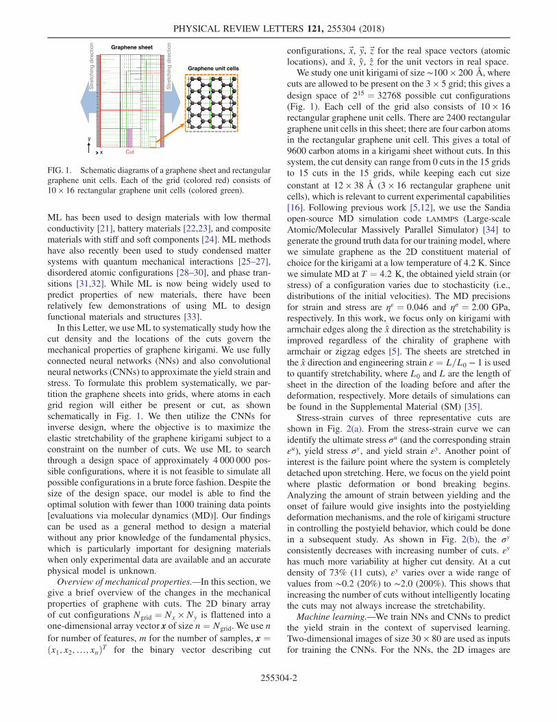
cut density and the locations of the cuts govern themechanical properties of graphene kirigami. We use fullyconnected neural networks (NNs) and also convolutionalneural networks (CNNs) to approximate the yield strain andstress. To formulate this problem systematically, we par-tition the graphene sheets into grids, where atoms in eachgrid region will either be present or cut, as shownschematically in Fig. 1. We then utilize the CNNs forinverse design, where the objective is to maximize theelastic stretchability of the graphene kirigami subject to aconstraint on the number of cuts. We use ML to searchthrough a design space of approximately 4 000 000 pos-sible configurations, where it is not feasible to simulate allpossible configurations in a brute force fashion. Despite thesize of the design space, our model is able to find theoptimal solution with fewer than 1000 training data points[evaluations via molecular dynamics (MD)]. Our findingscan be used as a general method to design a materialwithout any prior knowledge of the fundamental physics,which is particularly important for designing materialswhen only experimental data are available and an accuratephysical model is unknown.Overview of mechanical properties.—In this section, we

give a brief overview of the changes in the mechanicalproperties of graphene with cuts. The 2D binary arrayof cut configurations Ngrid ¼ Nx × Ny is flattened into aone-dimensional array vector x of size n ¼ Ngrid. We use nfor number of features, m for the number of samples, x ¼ðx1; x2;…; xnÞT for the binary vector describing cut

configurations, x, y, z for the real space vectors (atomiclocations), and x, y, z for the unit vectors in real space.We study one unit kirigami of size ∼100 × 200 Å, where

cuts are allowed to be present on the 3 × 5 grid; this gives adesign space of 215 ¼ 32768 possible cut configurations(Fig. 1). Each cell of the grid also consists of 10 × 16rectangular graphene unit cells. There are 2400 rectangulargraphene unit cells in this sheet; there are four carbon atomsin the rectangular graphene unit cell. This gives a total of9600 carbon atoms in a kirigami sheet without cuts. In thissystem, the cut density can range from 0 cuts in the 15 gridsto 15 cuts in the 15 grids, while keeping each cut sizeconstant at 12 × 38 Å (3 × 16 rectangular graphene unitcells), which is relevant to current experimental capabilities[16]. Following previous work [5,12], we use the Sandiaopen-source MD simulation code LAMMPS (Large-scaleAtomic/Molecular Massively Parallel Simulator) [34] togenerate the ground truth data for our training model, wherewe simulate graphene as the 2D constituent material ofchoice for the kirigami at a low temperature of 4.2 K. Sincewe simulate MD at T ¼ 4.2 K, the obtained yield strain (orstress) of a configuration varies due to stochasticity (i.e.,distributions of the initial velocities). The MD precisionsfor strain and stress are ηε ¼ 0.046 and ησ ¼ 2.00 GPa,respectively. In this work, we focus only on kirigami witharmchair edges along the x direction as the stretchability isimproved regardless of the chirality of graphene witharmchair or zigzag edges [5]. The sheets are stretched inthe x direction and engineering strain ε ¼ L=L0 − 1 is usedto quantify stretchability, where L0 and L are the length ofsheet in the direction of the loading before and after thedeformation, respectively. More details of simulations canbe found in the Supplemental Material (SM) [35].Stress-strain curves of three representative cuts are

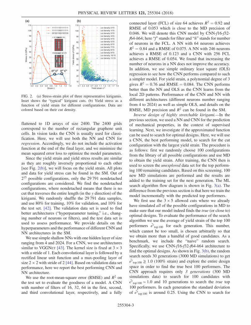
shown in Fig. 2(a). From the stress-strain curve we canidentify the ultimate stress σu (and the corresponding strainεu), yield stress σy, and yield strain εy. Another point ofinterest is the failure point where the system is completelydetached upon stretching. Here, we focus on the yield pointwhere plastic deformation or bond breaking begins.Analyzing the amount of strain between yielding and theonset of failure would give insights into the postyieldingdeformation mechanisms, and the role of kirigami structurein controlling the postyield behavior, which could be donein a subsequent study. As shown in Fig. 2(b), the σy

consistently decreases with increasing number of cuts. εy

has much more variability at higher cut density. At a cutdensity of 73% (11 cuts), εy varies over a wide range ofvalues from ∼0.2 (20%) to ∼2.0 (200%). This shows thatincreasing the number of cuts without intelligently locatingthe cuts may not always increase the stretchability.Machine learning.—We train NNs and CNNs to predict

the yield strain in the context of supervised learning.Two-dimensional images of size 30 × 80 are used as inputsfor training the CNNs. For the NNs, the 2D images are

Cut

Str

etch

ing

dire

ctio

n

Str

etch

ing

dire

ctio

n

Graphene sheet

Graphene unit cells

y

x

FIG. 1. Schematic diagrams of a graphene sheet and rectangulargraphene unit cells. Each of the grid (colored red) consists of10 × 16 rectangular graphene unit cells (colored green).

PHYSICAL REVIEW LETTERS 121, 255304 (2018)

255304-2

flattened to 1D arrays of size 2400. The 2400 gridscorrespond to the number of rectangular graphene unitcells. In vision tasks the CNN is usually used for classi-fication. Here, we will use both the NN and CNN forregression. Accordingly, we do not include the activationfunction at the end of the final layer, and we minimize themean squared error loss to optimize the model parameters.Since the yield strain and yield stress results are similar

as they are roughly inversely proportional to each other[see Fig. 2(b)], we will focus on the yield strain. All plotsand data for yield stress can be found in the SM. Out of215 possible configurations, only the 29 791 nondetachedconfigurations are considered. We find the nondetachedconfigurations, where nondetached means that there is nocut that traverses the entire length (in the y direction) of thekirigami. We randomly shuffle the 29 791 data samples,and use 80% for training, 10% for validation, and 10% forthe test set. [42]. The validation data set is used to findbetter architectures (“hyperparameter tuning,” i.e., chang-ing number of neurons or filters), and the test data set isused to assess performance. We provide details on thehyperparameters and the performance of different CNN andNN architectures in the SM.We use simple shallow NNs with one hidden layer of size

ranging from 4 and 2024. For a CNN, we use architecturessimilar to VGGNET [43]. The kernel size is fixed at 3 × 3with a stride of 1. Each convolutional layer is followed by arectified linear unit function and a max-pooling layer ofsize 2 × 2with stride of 2 [44]. Based on validation data setperformance, here we report the best performing CNN andNN architecture.We use the root-mean-square error (RMSE) and R2 on

the test set to evaluate the goodness of a model. A CNNwith number of filters of 16, 32, 64 in the first, second,and third convolutional layer, respectively, and a fully

connected layer (FCL) of size 64 achieves R2 ¼ 0.92 andRMSE of 0.053 which is close to the MD precision of0.046. We will denote this CNN model by CNN-f16-f32-f64-h64; here “f” stands for filter and “h” stands for numberof neurons in the FCL. A NN with 64 neurons achievesR2 ¼ 0.84 and a RMSE of 0.075. A NN with 246 neuronsachieves a RMSE of 0.123 and a CNN with 256 FCLachieves a RMSE of 0.054. We found that increasing thenumber of neurons in a NN does not improve the accuracy.In addition, we use simple ordinary least square (OLS)regression to see how the CNN performs compared to sucha simpler model. For yield strain, a polynomial degree of 3gives R2 ¼ 0.76 and RMSE ¼ 0.084. The CNN performsbetter than the NN and OLS as the CNN learns from thelocal 2D patterns. Performance of the CNN and NN withdifferent architectures (different neurons number rangingfrom 4 to 2024) as well as simple OLS, and details on theRMSE, MD precision and R2 can be found in the SM.Inverse design of highly stretchable kirigami.—In the

previous section, we used a NN and CNN for the predictionof mechanical properties, in the context of supervisedlearning. Next, we investigate if the approximated functioncan be used to search for optimal designs. Here, we will usea CNN, the best performing model, to search for the cutconfiguration with the largest yield strain. The procedure isas follows: first we randomly choose 100 configurationsfrom the library of all possible configurations and use MDto obtain the yield strain. After training, the CNN then isused to screen the unexplored data set for the top perform-ing 100 remaining candidates. Based on this screening, 100new MD simulations are performed and the results areadded to the training set for the next generation. The MLsearch algorithm flow diagram is shown in Fig. 3(a). Thedifference from the previous section is that here we train themodel incrementally with the predicted top performers.We first use the 3 × 5 allowed cuts where we already

have simulated all of the possible configurations in MD tomake sure that our model indeed finds the true (or close to)optimal designs. To evaluate the performance of the searchalgorithm we use the average of yield strain of the top 100performers εytop 100 for each generation. This number,which cannot be too small, is chosen arbitrarily so thatwe obtain more than a handful of good candidates. As abenchmark, we include the “naive” random search.Specifically, we use CNN-f16-f32-f64-h64 architecture tofind the optimal designs. As shown in Fig. 3(b), the randomsearch needs 30 generations (3000 MD simulations) to getεytop 100 ≥ 1.0 (100% strain) and explore the entire designspace in order to find the true best 100 performers. TheCNN approach requires only 3 generations (300 MDsimulations data) to search for 100 candidates withϵytop 100 ∼ 1.0 and 10 generations to search the true top100 performers. In each generation the standard deviationof ϵytop 100 is around 0.25. Using the CNN to search for

y y u u

(b) (a)

FIG. 2. (a) Stress-strain plot of three representative kirigamis.Inset shows the “typical” kirigami cuts. (b) Yield stress as afunction of yield strain for different configurations. Data arecolored based on their cut density.

PHYSICAL REVIEW LETTERS 121, 255304 (2018)

255304-3

optimal designs is crucial because one MD simulation ofgraphene with a size of 100 × 200 Å requires around 1 hcomputing time using four cores of the CPU. In eachgeneration, the required time to train the CNN and topredict the yield strain of one configuration is around 6 mson four CPU cores (same machines) or 3 ms on four CPUcores plus one GPU [45]. From Fig. 2(b), we know thatsheets with high strains are ones with high cut density.However, the variability is also large; e.g., at 11=15 cutdensity, the yield strain ranges from 0.2 to 1.7. Despite thiscomplexity, the ML quickly learns to find solutions at highcut density and also to find the right cutting patterns.Next, we apply this simple algorithm to a much larger

design space where the true optimal designs are unknownand also with a specified design constraint. Specifically, westudy larger graphene sheets by extending the physical sizein x from ∼100 × 200 to ∼200 × 200 Å (from 30 × 80 to50 × 80 rectangular graphene unit cells). For this system,one MD simulation requires around 3 h of computing timerunning on four cores. The allowed cuts are also expandedfrom 3 × 5 to 5 × 5 grids. For this problem, we fixed thenumber of cuts at 11 cuts, which gives a design space ofsize ð25!=11!14!Þ ∼ 4 × 106. For this system, we could notuse brute force to simulate all configurations as we didpreviously for a system with 15 allowed cuts. While thetypical stretchable kirigamis usually have cuts and no cutsalong the loading direction (x), it is not clear whether all thecuts should be located closely in a region or distributedequally.As shown in Fig. 3(b), the CNN is able to find designs

with higher yield strains. With fewer than 10 generations(1000 training data), the CNN is able to find configurationswith yield strains ≥ 1.0, which is roughly five times larger

than a sheet without cuts. In each generation, the standarddeviation of the top 100 performers is around 0.1. InFig. 3(d), we plot cut configurations of the top fiveperformers in each generation. It can be seen that thecut configurations are random in the early stage of thesearch but evolve quickly to configurations with a longcut along the y direction alternating in x direction, as weexpected from the smaller grid system. This suggests thatour ML approach is scalable in a sense that the same CNNarchitecture used previously in the simpler system with 15allowed cuts can search the optimal designs effectivelydespite a large design space.We next take a closer look on the top performing

configurations. Interestingly, the optimal solutions formaximum stretchability found by a CNN have cuts atthe edges which are different from the “typical” kirigamiwith centering cuts [Fig. 3(e) configuration I]. The foundbest performer has a yield strain twice as large as thekirigami with centering cuts. We found that to achievehigh yield strains the long cuts should be located close toeach other, rather than being sparsely or equally distrib-uted across the sheet along the x direction, as shown bycomparing configurations II and III in Fig. 3(e). Theseoverlapping cut configurations allow larger rotations andout-of-plane deflection which give higher stretchability;i.e., the alternating edge cut pattern effectively transformsthe 2D membrane into a quasi-1D membrane. Closepacking of the alternating edge cuts allows increasedstretchability because the thinner ribbons connectingdifferent segments improve twisting. This result is similarto what we found previously in kirigami with centeringcuts [5,6]. Visualizations illustrating these effects (such asout-of-plane buckling and twisting) and a more detailed

FIG. 3. (a) Schematic of the neural network search algorithm. Average yield strains of the top 100 performers as a function ofgenerations for kirigami with allowed cuts of (b) 3 × 5 and (c) 5 × 5. (d) Visualization of the top five performers of kirigami with 5 × 5allowed cuts in each generation. After the ninth generation, the top three performers remain constant. (e) A comparison between the topperforming configurations found by the ML and the typical kirigami configurations with centering cuts. Note that the kirigamivisualizations are not scaled to the real physical dimensions for clarity.

PHYSICAL REVIEW LETTERS 121, 255304 (2018)

255304-4

discussion can be found in the SM. This design principleis particularly useful as recently a combination of denseand sparse cut spacing were used to design stretchable thinelectronic membranes [46]. It is remarkable not only thatML can quickly find the optimal designs using fewtraining data (< 1% of the design space) under certainconstraints, but also that ML can capture uncommonphysical insights needed to produce the optimal designs,in this case related to the cut density and locations of thecuts.Conclusion.—We have shown how machine learning

methods can be used to design graphene kirigami, whereyield strain and stress are used as the target properties. Wefound that the CNN with three convolutional layersfollowed by one fully connected layer is sufficient tofind the optimal designs with relatively few training data.Our work shows not only how to use ML to effectivelysearch for optimal designs but also to give new under-standing on how kirigami cuts change the mechanicalproperties of graphene sheets. Furthermore, the MLmethod is parameter-free, in the sense that it can be usedto design any material without any prior physical knowl-edge of the system. As the ML method only needs data, itcan be applied to experimental work where the physicalmodel is not known and cannot be simulated by MD orother simulation methods. Based on previous work indi-cating the scale invariance of kirigami deformation [12],the kirigami structures found here using ML should alsobe applicable for designing larger macroscale kirigamistructures.

P. Z. H. developed the codes, performed the simulationsand data analysis, and wrote the manuscript with input fromall authors. P. Z. H. and E. D. C. developed the machinelearning methods. P. Z. H., D. K. C. and H. S. P. acknowl-edge the Hariri Institute Research Incubation GrantNo. 2018-02-002 and the Boston University HighPerformance Shared Computing Cluster. P. Z. H. is gratefulfor the Hariri Graduate Fellowship. P. Z. H. thank Grace Guand Adrian Yi for helpful discussions.

*paul.hanakata@gmail.com[1] S. A. Zirbel, R. J. Lang, M.W. Thomson, D. A. Sigel, P. E.

Walkemeyer, B. P. Trease, S. P. Magleby, and L. L. Howell,J Mech Des 135, 111005 (2013).

[2] A. Rafsanjani, Y. Zhang, B. Liu, S. M. Rubinstein, and K.Bertoldi, Sci. Rob. 3, eaar7555 (2018).

[3] T. C. Shyu, P. F. Damasceno, P. M. Dodd, A. Lamoureux, L.Xu, M. Shlian, M. Shtein, S. C. Glotzer, and N. A. Kotov,Nat. Mater. 14, 785 (2015).

[4] M. K. Blees, A.W. Barnard, P. A. Rose, S. P. Roberts, K. L.McGill, P. Y. Huang, A. R. Ruyack, J. W. Kevek, B. Kobrin,D. A. Muller et al., Nature (London) 524, 204 (2015).

[5] Z. Qi, D. K. Campbell, and H. S. Park, Phys. Rev. B 90,245437 (2014).

[6] P. Z. Hanakata, Z. Qi, D. K. Campbell, and H. S. Park,Nanoscale 8, 458 (2016).

[7] A. A. Griffith and M. Eng, Phil. Trans. R. Soc. A 221, 163(1921).

[8] H. Zhao and N. Aluru, J. Appl. Phys. 108, 064321 (2010).[9] P. Zhang, L. Ma, F. Fan, Z. Zeng, C. Peng, P. E. Loya, Z.

Liu, Y. Gong, J. Zhang, X. Zhang et al., Nat. Commun. 5,3782 (2014).

[10] G. Jung, Z. Qin, and M. J. Buehler, Extreme Mech. Lett. 2,52 (2015).

[11] T. Rakib, S. Mojumder, S. Das, S. Saha, and M. Motalab,Physica (Amsterdam) 515B, 67 (2017).

[12] M. A. Dias, M. P. McCarron, D. Rayneau-Kirkhope, P. Z.Hanakata, D. K. Campbell, H. S. Park, and D. P. Holmes,Soft Matter 13, 9087 (2017).

[13] M. Isobe and K. Okumura, Sci. Rep. 6, 24758 (2016).[14] A. Rafsanjani and K. Bertoldi, Phys. Rev. Lett. 118, 084301

(2017).[15] M. Moshe, S. Shankar, M. J. Bowick, and D. R. Nelson,

arXiv:1801.08263.[16] P. Masih Das, G. Danda, A. Cupo, W. M. Parkin, L. Liang,

N. Kharche, X. Ling, S. Huang, M. S. Dresselhaus, V.Meunier et al., ACS Nano 10, 5687 (2016).

[17] O. Sigmund and J. Petersson, Struct. Optim. 16, 68 (1998).[18] M. J. Jakiela, C. Chapman, J. Duda, A. Adewuya, and K.

Saitou, Comput. MethodsAppl.Mech. Eng. 186, 339 (2000).[19] X. Huang and Y. Xie, Finite Elements in Analysis and

Design 43, 1039 (2007).[20] G. X. Gu, L. Dimas, Z. Qin, and M. J. Buehler, J. Appl.

Mech. 83, 071006 (2016).[21] A. Seko, A. Togo, H. Hayashi, K. Tsuda, L. Chaput, and I.

Tanaka, Phys. Rev. Lett. 115, 205901 (2015).[22] A. D. Sendek, Q. Yang, E. D. Cubuk, K.-A. N. Duerloo, Y.

Cui, and E. J. Reed, Energy Environ. Sci. 10, 306 (2017).[23] B. Onat, E. D. Cubuk, B. D. Malone, and E. Kaxiras, Phys.

Rev. B 97, 094106 (2018).[24] G. X. Gu, C.-T. Chen, and M. J. Buehler, Extreme Mech.

Lett. 18, 19 (2018).[25] J. Behler and M. Parrinello, Phys. Rev. Lett. 98, 146401

(2007).[26] J. Behler, J. Chem. Phys. 134, 074106 (2011).[27] E. D. Cubuk, B. D. Malone, B. Onat, A. Waterland, and E.

Kaxiras, J. Chem. Phys. 147, 024104 (2017).[28] E. D. Cubuk, S. S. Schoenholz, E. Kaxiras, and A. J. Liu,

J. Phys. Chem. B 120, 6139 (2016).[29] S. S. Schoenholz, E. D. Cubuk, E. Kaxiras, and A. J. Liu,

Proc. Natl. Acad. Sci. U.S.A. 114, 263 (2017).[30] E. Cubuk, R. Ivancic, S. Schoenholz, D. Strickland, A.

Basu, Z. Davidson, J. Fontaine, J. Hor, Y.-R. Huang, Y.Jiang et al., Science 358, 1033 (2017).

[31] J. Carrasquilla and R. G. Melko, Nat. Phys. 13, 431(2017).

[32] P. Broecker, J. Carrasquilla, R. G. Melko, and S. Trebst, Sci.Rep. 7, 8823 (2017).

[33] G. X. Gu, C.-T. Chen, D. J. Richmond, and M. J. Buehler,Mater. Horiz. 5, 939 (2018).

[34] LAMMPS, http://lammps.sandia.gov.[35] See Supplemental Material at http://link.aps.org/

supplemental/10.1103/PhysRevLett.121.255304 for detailsof simulations, machine learning, linear model, and detailed

PHYSICAL REVIEW LETTERS 121, 255304 (2018)

255304-5

discussions on twisting and buckling mechanism, whichinclude Refs. [36–41].

[36] S. J. Stuart, A. B. Tutein, and J. A. Harrison, J. Chem. Phys.112, 6472 (2000).

[37] F. Liu, P. Ming, and J. Li, Phys. Rev. B 76, 064120 (2007).[38] P. Z. Hanakata, A. Carvalho, D. K. Campbell, and H. S.

Park, Phys. Rev. B 94, 035304 (2016).[39] C. Lee, X. Wei, J. W. Kysar, and J. Hone, Science 321, 385

(2008).[40] M. Abadi et al., TensorFlow: Large-scale machine learning

on heterogeneous systems, tensorflow.org.[41] F. Pedregosa, G. Varoquaux, A. Gramfort, V. Michel,

B. Thirion, O. Grisel, M. Blondel, P. Prettenhofer, R. Weiss,V. Dubourg, J. Vanderplas, A. Passos, D. Cournapeau,

M. Brucher, M. Perrot, and E. Duchesnay, J. Mach. Learn.Res. 12, 2825 (2011).

[42] We perform several shuffles and find that all performancesare similar (with CNN-f16-f32-f64-h64 model). In addition,we perform ninefold cross-validation and obtain an averageaccuracy on the test set of 0.918 with a standard deviation of0.002.

[43] K. Simonyan and A. Zisserman, arXiv:1409.1556.[44] Y. LeCun, L. Bottou, Y. Bengio, and P. Haffner, Proc. IEEE

86, 2278 (1998).[45] Details of the specific GPU can be found in the SM.[46] N. Hu, D. Chen, D. Wang, S. Huang, I. Trase, H. M. Grover,

X. Yu, J. X. J. Zhang, and Z. Chen, Phys. Rev. Applied 9,021002 (2018).

PHYSICAL REVIEW LETTERS 121, 255304 (2018)

255304-6