PHYSICAL REVIEW E 102, 012607 (2020)

Dynamics of active nematic defects on the surface of a sphere

Yi-Heng Zhang (���) ,1,* Markus Deserno ,2 and Zhan-Chun Tu (���) 1

1Department of Physics, Beijing Normal University, Beijing 100875, China2Department of Physics, Carnegie Mellon University, 5000 Forbes Avenue, Pittsburgh, Pennsylvania 15213, USA

(Received 29 February 2020; revised 27 May 2020; accepted 22 June 2020; published 17 July 2020)

A nematic liquid crystal confined to the surface of a sphere exhibits topological defects of total charge +2 dueto the topological constraint. In equilibrium, the nematic field forms four +1/2 defects, located at the corners ofa regular tetrahedron inscribed within the sphere, since this minimizes the Frank elastic energy. If additionallythe individual nematogens exhibit self-driven directional motion, the resulting active system creates large-scaleflow that drives it out of equilibrium. In particular, the defects now follow complex dynamic trajectories which,depending on the strength of the active forcing, can be periodic (for weak forcing) or chaotic (for strong forcing).In this paper we derive an effective particle theory for this system, in which the topological defects are the degreesof freedom, whose exact equations of motion we subsequently determine. Numerical solutions of these equationsconfirm previously observed characteristics of their dynamics and clarify the role played by the time dependenceof their global rotation. We also show that Onsager’s variational principle offers an exceptionally transparentway to derive these dynamical equations, and we explain the defect mobility at the hydrodynamics level.

DOI: 10.1103/PhysRevE.102.012607

I. INTRODUCTION

Topological defects show up in a surprising variety ofordered systems, and whenever they do give rise to fascinatingemergent physics. They have been observed in the studyof liquid crystals [1–4], crystalline solids [5–7], cell assem-blies [8–10], superfluid vortices [11–13], magnetic skyrmions[14–22], and cosmology [23–25]. Since defects cannot con-tinuously vanish (they typically only pair create or annihilate),they constitute long-lived markers of the field that forms them,and hence their dynamics can provide deep insights into thelong-scale time evolution of such systems [26]. In recentexperiments, Keber et al. [27] have fabricated a sphericalnematic by confining kinesin-microtubule bundles onto thesurface of a spherical lipid vesicle, and adding ATP to thekinesin motors renders this system active, i.e., self-driven. TheATP-induced activity can drive the system far from a staticequilibrium state, leading to a novel defect dynamics in whichthe active flow competes with dissipative relaxation processes,as well as elastic forces that arise from the nematic fielditself and the curvature of the substrate. Significant theoreticalunderstanding has been gained how such active driving forcesaffect the defect dynamics in a planar nematic liquid crystals[28–36]; in contrast, a comprehensive theoretical frameworkfor the topologically distinct case of spherical confinementlags noticeably behind.

The motion of defects can be regarded as a particular wayin which the active nematic field collectively manifests itself:The field moves, and the defects “ride” with it. Hence, in orderto understand this motion, it is natural to start from the tra-ditional nematic hydrodynamic equations [37–41], amendedby a suitably chosen active stress [42–46]. In this way, one

*Corresponding author; zyh@mail.bnu.edu.cn

arrives at a continuum theory that describes the evolution ofthe nematic order and its underlying flow velocity, and onemay thereby predict how the defects are transported along.We also emphasize that the curvature of the substrate canplay an important role in the active nematic hydrodynamics,not only the intrinsic curvature of a sphere, but also theextrinsic curvature, like the curvature of a cylindrical surface[47,48]. While conceptually fairly clean, the resulting partialdifferential equations do not afford illuminating analyticalsolutions, and therefore a substantial amount of work hasbeen dedicated to numerically solving them, which has indeedprovided much novel insight into the collective behavior ofspherical active nematic systems [49–51].

However, the topological nature of this problem stronglysuggests an alternative viewpoint. Recall that defects cannotcontinuously vanish or arise. Their topological discreteness“protects” their existence, or, in physics parlance, it equipsthem with a conservation law. More precisely: since a defect’stopological index can change only in finite steps (say, inte-gral or half-integral), defects require other defects to changetheir overall number—meaning that they typically create andannihilate in pairs. This, of course, equips them with aproperty we commonly associate with elementary particles(such as electrons), which can be created or destroyed onlyin particle-antiparticle pairs. Their longevity suggests thatit should be expedient to formulate an effective theory thatconceives of these discrete particles as the essential degreesof freedom, which in turn interact by force fields that emergeas “leftovers” of the originally strongly coupled field. In ourcontext, this perspective suggests that we view topologicaldefects in a nematic as particles, whose dynamics is givenby the force balance between the effective friction and theelastic interaction. Such an effective theory (in soft matterlanguage more usually called “coarse-grained”) has indeedbeen successfully used to describe the defect dynamics in

2470-0045/2020/102(1)/012607(15) 012607-1 ©2020 American Physical Society

ZHANG, DESERNO, AND TU PHYSICAL REVIEW E 102, 012607 (2020)

planar nematics [52–66]. Since the Euler characteristic of a(simply connected) plane is zero, the total sum of all indices ofdefects is zero, so that the number of defects equals that of the“antidefects” (meaning that there are exactly as many +1/2defects as −1/2 defects). Hence, the characteristic physicalprocesses are the creation and annihilation of defects in pairsout of and into an otherwise structureless (“trivial”) vacuumground state—a scenario that is indeed excellently describedby the effective particle approach [28,29,33,36,67].

Keber et al. have taken the first steps and developed aminimal model of defects as effective particles moving on aspherical surface [27]. Following their lead, various importantstudies of the dynamics of active defects in curved surfaceshave been proposed. In a recent publication Khoromskaia andAlexander [68] refined the Keber model by calculating theactive flow via the Stokes equation of the active nematic.Although their theoretical model explained some of the ex-perimentally observed phenomena, it does not yet provide adetailed connection between the coarse-grained dynamics ofdefects and the active nematic hydrodynamic equations. Fur-thermore, nematic defects have a broken rotational symmetry,and hence their effective description must include not justtheir position as the sole degree of freedom, but also a vecto-rial orientation [27,69,70]. This is especially obvious for the+1/2 defects, which self-propel in a well-defined direction.Moreover, broken rotational symmetry implies that these ori-ented particles are not just subject to effective isotropic forces;rather, forces will depend on mutual orientation, and there willalso be effective torques—all of which will affect the resultingdynamics [27,35,69–71]. Khoromskaia and Alexander haveindeed explored the impact of this orientational degree offreedom on the active behavior of these systems [68], butthe resulting dynamics, and especially the role of effectiveelastic torques, is still not understood well. In a recent paper[72], Brown has accounted for the orientation dynamics ofdefects on the sphere and partly explained the experimentaland simulated trajectories of defects. More generally, thereis significant interest to understand how confinement impactsactive nematodynamics in cases other than the surface ofa sphere, especially for different topologies and nontrivialGaussian curvature, such as a torus, and some importantprogress along those lines has been made [73–75].

In the present paper, we aim to develop a more detailedeffective field theory for defects in active nematics that areconfined to the surface of a sphere, based on active nematichydrodynamic. The main philosophy is no different from theplanar case, and hence we expect the essential scale separationto work just as well. However, there is a very significantdifference that renders this case more difficult but also moreinteresting: the Euler characteristic of a spherical surface is+2, and so we have broken “matter-antimatter symmetry.”In other words, the vacuum is not empty. Moreover, sinceit is well known that in an active nematic the +1/2 defectsare self-propelled [33], this also implies that the vacuum isnever at rest. Hence, particle pairs are not created into anotherwise quiescent vacuum but are immediately advectedwith the preexisting ground-state flow—which we hence needto understand first. We follow the ideas proposed by Tang andSelinger [76] to advance the theory of a dry active nematicliquid crystal confined onto a spherical substrate. Specifically,

we show how to make use of an elegant variational principledue to Onsager [76–81] in order to transition from the infinite-dimensional nematic field theory to the finite-dimensionaleffective field theory of oriented defects. As a particular result,we derive the anisotropic mobility coefficient matrix of de-fects. We then show that our effective theory fully reproducesthe complex periodic trajectory of the four +1/2 defects andhow it depends on system size and the strength of the activeforcing, as reported in earlier numerical work and experiments[27,50,51]. Our theory includes the full dynamics of a defect’sorientation, which permits us to identify its importance for theresulting particle motions.

We have organized the content of our paper as follows.In Sec. II, we outline the hydrodynamic model we employin our discussion, followed by the theoretical approach weuse to separate the dynamical variables of the defects fromthe temporal evolution of the active nematic field. In Sec. IIIwe look at some of the predictions of our theory, includingthe well-known periodic oscillation of the defect configurationunder weak forcing, and the chaotic trajectories under strongerdriving conditions. Section IV summarizes our conclusionsand lists a number of limitations of our theory.

II. MODELS AND METHODS

A. Minimal model

The nematic liquid crystal is locally characterized by twovariables: order and flow. We can describe the order by thenematic tensor

Qab = q

(nanb − 1

2gab

), (1)

in which q is the magnitude of the nematic tensor representingits average alignment in a small region, and gab is the (inverse)metric tensor; the unit vector n = naea denotes the local ne-matic director, whose components na = (cos ψ, sin ψ ) referto the spherical orthonormal basis {eθ , eφ} [3] and are fullyspecified by a single scalar function ψ (θ, φ) of position. (Asusual, a repeated upper and lower index implies a tensorcontraction.) The (incompressible) flow is characterized bythe velocity field V a. These two variables {Qab,V a} satisfy thehydrodynamic equations of the active nematic, with a constantdensity ρ on the curved surface [41,75,82–85]:

Qab = Sab − 1

γ

δFLdG

δQab, (2a)

ρV a = α∇bQba + ∇bab − ζV a. (2b)

Here the ring operator ( ˚ ) ≡ D/Dt ≡ ∂/∂t + V c∇c denotesthe covariant material derivative, γ is the rotational viscosity,and FLdG is the Landau–de Gennes free energy of the system[3], which contains the homogeneous phase energy Fp, as hasalso recently been derived by dimensional reduction from afull three-dimensional Landau–de Gennes functional [86]:

Fp =∫

dS

[A

2QabQab + B

4(QabQab)2

], (3)

012607-2

DYNAMICS OF ACTIVE NEMATIC DEFECTS ON THE … PHYSICAL REVIEW E 102, 012607 (2020)

and, by assuming (for simplicity) the one-constant approxi-mation, the Frank energy Fe caused by spatial distortions:

Fe = K

4

∫dS (∇cQab)(∇cQab). (4)

The tensor Sab in Eq. (2a) represents the coupling betweenthe director field, the (symmetric) strain rate tensor Aab =∇[aVb], and the (antisymmetric) vorticity ωab = ∇(aVb), withthe parameter ξ reflecting the flow aligning of the nematicfield [83,87–91]:

Sab = ξqAab + Qacωcb − ωa

cQcb. (5)

The activity enters into the system through the active stressα∇bQba in the covariant Navier-Stokes equation (2b), wherethe parameter α controls the strength of the activity. Thesystem is termed “contractile” if α > 0 and “extensile” ifα < 0 [43,91,92]. The passive stress is denoted by ab. Thesubstrate friction ζV a arises from the damping force betweenthe active nematic and the spherical substrate beneath it. If weneglect the inertia term in Eq. (2b) and assume the substratefriction is much larger than the other remaining dissipationterms, the only contribution to the velocity field will be theactive flow [35,71]:

V a = α

ζ∇bQba. (6)

B. Coarse-grained dynamics of +1/2 defects

In our particular (two-dimensional) case, the index orcharge of a vector field’s defect may be defined as follows:take a closed path around an isolated defect and follow theorientation of the vector field as you traverse that path once,then the index is the number s of times which this vector fieldrotates before you arrive back at the starting point (meaningthat it acquires a “phase shift” of 2πs along this loop). We givea schematic of a + 1/2 defect in Fig. 1. It is clear to see thatif we start from any point at the negative real axis and tracethe vector direction around the original point clockwise, thevector acquires a “phase shift” of π . The continuum model ofnematic liquid crystals on a spherical surface can be locallydescribed by a vector field on a spherical surface [3]. Becausethe Euler characteristic of a spherical surface is +2, theexistence of defects is inevitable: summing the indices of alldefects must yield +2. The only difference is that the apolarnature of a liquid crystal’s director field (meaning, it is alreadyinvariant under a 180◦ in-plane rotation) permits half-integralindices for the defect points. In the present work we willrestrict our discussion to the case of four +1/2 defects, whichis the ground state of the nematic director field on the sphericalsurface.

The motion of defects is a collective effect of the nematicfield, so the dynamic information of the defects is containedin the hydrodynamic equations we have just given. In orderto extract the variables we care about, which are the positionand the orientation of each defect, and obtain an effective fieldtheory of the defects, we will now introduce the framework ofOnsager’s variational principle as an alternative description ofthe active nematic hydrodynamics [47,77–81].

FIG. 1. Vector field with a +1/2 defect at the center and adiscontinuity line along the negative real axis due to the “phase shift”of π .

The so-called Rayleighian corresponding to the Beris-Edwards equation (2a) is [93]

R = d

dtFLdG + γ

2

∫dS(Qab − Sab)(Qab − Sab). (7)

Its major use lies in the fact that the Beris-Edwards equationfollows from minimizing the Rayleighian (7) with respect to∂t Qab.

Now, if we assume that the timescale of the active flowis much slower than the characteristic timescale by whichthe director field n relaxes, it is reasonable to assume that nstays close to its equilibrium configuration during its activemotion [33,68]. By using Riemann’s stereographic projectionz(θ, φ) = 2R tan θ

2 eiφ , which maps the spherical coordinate(θ, φ) of the sphere with radius R to the complex plane (suchthat the north pole becomes the origin and the south pole mapsto complex infinity; see Fig. 2), the equilibrium configurationof the director field with four +1/2 topological defects atspecified positions was given by [56,68]

ψ (z) = � − φ + 1

2

4∑k=1

ψk

= � − φ + 1

2

4∑k=1

Im ln(z − zk ), (8)

in which Im picks out the imaginary part of a complex num-ber, zk = 2R tan θk

2 eiφk is the position of the kth defect, and ψk

represents the director field excited by a single +1/2 defectat zk . This is nothing but the solution of the Euler-Lagrangeequation of the Frank energy, efficiently expressed in complexnotation. For the purpose of simplicity, we will take theequilibrium solution (8) as the configuration of the dynamicdirector field, thus omitting higher order corrections from the

012607-3

ZHANG, DESERNO, AND TU PHYSICAL REVIEW E 102, 012607 (2020)

2R tanθ2

θ2

θ

FIG. 2. The stereographic mapping of the spherical surface ontothe complex plane.

velocity of defects. This is in accord with our assumption of asmall active flow.

If we look at the director field near the jth defect, anduse � j to denote the angle between the symmetry axis of thedefect and eθ , then

� j = 2� − φ j +∑k �= j

arg(z j − zk ). (9)

According to Refs. [69,70], this expression of � j representsthe optimal relative orientation of defects. It implies an extraconstraint for the time evolution of the orientation of defects.We will illustrate later that this constraint is consistent withour assumption of the timescale separation. This also showsthat � describes a global rotation of all the defects; we willdemonstrate in the next section that it has a very importanteffect on their dynamics.

As a consequence of the small active flow assumption, thescalar order q varies only weakly outside the defects. Wehence assume that q is constant away from the defect butmelts to zero inside a small core region, because the directorwould have to assume every orientation at the center. Wewill not try to describe the precise way in which the ordervanishes towards the center, and it will indeed not be impor-tant. Instead, we will assume that any integral area we areconcerned about must exclude the defect core, and that outsidethe defects q is constant (we will assume q = 0.62 in oursubsequent numerical examples to permit easier comparisonwith Ref. [50]). And since q is now constant over the entiredomain of interest, the phase energy Fp does not contribute tothe dynamics. We can therefore restrict the free energy FLdG

to the Frank energy contribution Fe.With this ansatz, the time evolution of the director field is

identical to the evolution of the position and the direction ofdefects, which means

∂tψ = � + θk∂ψk

∂θk+ φk

∂ψk

∂φk

= � + 1

2

4∑k=1

(i

z − zkzk + c.c.

)(10)

and the dot ( ˙ ) ≡ d/dt means a total derivative with respectto time. Now, according to Onsager’s variational principle,the minimization of the Rayleighian (7) with respect to thedynamic variables of concern (here velocities of positionsand global orientations of defects) will directly give us thedynamics of the defects. Hence, their equations of motion canbe succinctly written as

∂

∂θkR = 0, (11a)

∂

∂φkR = 0, (11b)

∂

∂�R = 0. (11c)

By doing this, the infinite numbers of degrees of freedom inthe nematic field are now reduced to nine degree of freedomfor the four defects, which is our main aim in this work.

Now we can rewrite the Rayleighian (7) as

R = d

dtFe + γ q2

∫dS(∂tψ )2

− 2γαq2

ζ

∫dS∇b(∇aψ − Aa)Qab∂tψ, (12)

in which Aa = eθ · ∂aeφ is the spin connection. Details of thederivation are presented in Appendix A.

The Frank energy, in turn, is given by [56,58,59,64]

Fe = −πKq2

8

∑j �=k

ln(1 − cos β jk ) + const, (13)

where β jk is the angular distance between defects j and k,whose cosine can be expressed via

cos β jk = cos θ j cos θk + sin θ j sin θk cos(φ j − φk ). (14)

After making use of these, we can now write the dynamicequations (11a)–(11c) as

Mjk θk + Njkφ

k + � j� − Tj = − 1

2q2γ∂θ j Fe, (15a)

Nk j θk + Pjkφ

k + � j� − S j = − 1

2q2γ∂φ j Fe, (15b)

�k θk + �kφ

k + 4πR2� − L = 0, (15c)

where we introduced the following abbreviations for the eightdifferent integrals that emerge in the process:

Mjk =∫

dS ∂θ j ψ j∂θk ψk, (16a)

Njk =∫

dS ∂θ j ψ j∂φk ψk, (16b)

Pjk =∫

dS ∂φ j ψ j∂φk ψk, (16c)

� j =∫

dS ∂θ j ψ j, (16d)

� j =∫

dS ∂φ j ψ j, (16e)

012607-4

DYNAMICS OF ACTIVE NEMATIC DEFECTS ON THE … PHYSICAL REVIEW E 102, 012607 (2020)

L = α

ζ

∫dS ∇b(∇aψ − Aa)Qab, (16f)

Tj = α

ζ

∫dS ∇b(∇aψ − Aa)Qab∂θ j ψ j, (16g)

S j = α

ζ

∫dS ∇b(∇aψ − Aa)Qab∂φ j ψ j . (16h)

Notice that in all cases the integral area excludes a defect coreof size rk = r(1 + |zk|2/4R2), which is the projection imageof the kth defect core radius r at the complex plane [56].Complete analytical expressions for all of these integrals, andsome of the technically tedious details for how to obtain them,are given in Appendices B, C, and D.

If we introduce the characteristic timescale τ = γ R2/2Kand define the corresponding dimensionless time t = t/τ ,then the dimensionless dynamic equations of the defects ofan active nematic on a sphere can be succinctly written as

mjkdθ k

dt+ n jk

dφk

dt− t j = − ∂θ j f , (17a)

nk jdθ k

dt+ p jk

dφk

dt− s j = − ∂φ j f , (17b)

d�

dt= − �k

4πR2

dφk

dt, (17c)

with the corresponding scaled variables

mjk = Mjk

R2, n jk = Njk

R2, p jk = Pjk

R2− � j�k

4πR4,

t j = γ

2KTj, s j = γ

2KSj, f = Fe

4q2K.

III. RESULTS

We have established the dynamics of defects in the spheri-cal active nematic and expressed the mobility coefficient ma-trices (16a)–(16c) in terms of active nematic hydrodynamicsparameters. Now we would like to compare our model withprevious phenomenological theories and numerical studies.

The analytical expressions (D7) and (D8) for the integralsTj and S j , worked out in Appendix D, suggest that these areactually the components of the mean active back flow aroundthe jth defect—in agreement with the calculations given byKhoromskaia and Alexander [68]. We hence notice that thediagonal elements of the mobility matrices in Eqs. (17a) and(17b) are

mj j = π

8

(2 ln

2R

r− 1

), (18a)

p j j = π

8

(2 ln

2R

r− 1

)sin2 θ j . (18b)

If the radius R of the sphere is very large compared to the coreradius r of the defects, and defects do not approach each othertoo closely during their motion, the nondiagonal elements arenegligible. In this situation, Eqs. (17a) and (17b) are identicalto the approximations proposed in Ref. [68], and therefore thephysical picture is similar here. The motion of defects reflectsthe competition between the elastic and the active stresses:The velocity of defects arises from the reorientation of the

director field due to the elastic stresses, and the advection ofthe director field is due to the active back flow.

Apart from the defect positions, we have also obtainedthe dynamics of their orientation in Eq. (17c). The defini-tion of the defect orientation and its passive dynamics havebeen discussed thoroughly and adequately in Refs. [69,70].These authors discovered that the director field can have anextra distortion because of the relative rotation of defects.Accordingly, our form of the director field in Eq. (8) ischosen such that the relative orientation of the defects isset to their optimal configuration, which means it does nothave any elastic interaction that arises from extra distortionsof the director field due to a relative rotation of defects. Infact, according to Refs. [69,70], Eq. (8) implies a specialchoice of the boundary condition of the director field neardefects, so that the relative orientation of defects is lockedto a certain angle. The same is implied in Eq. (17c), whichdoes not contain the Frank elastic torque. We believe this isa reasonable result in the light of our assumption that thecharacteristic timescale of director field relaxation is fasterthan that of defect motion. The activity enters the systemvia the back flow, according to Eq. (6), and the direction ofthe flow is always along the symmetry axis of the defect;hence, the flow does not impact the defect transversely, andthe elastic locking of defects maintains the relative orientation.As a consequence, the relaxation dynamics of the relativeorientation of defects is purely passive and very fast, andso we expect it to only enter at higher order in perturbationtheory.

In order to illustrate the predictions of our theory, wewill now present numerical results of the dynamic equations(17a)–(17c). Here we chose R = 32 μm, r = 2 μm, γ /2K =0.013 ms/μm2 and the corresponding characteristic timescaleτb = γ R2/2K = 13.312 ms as our reference baseline. Thechoice of the initial condition of the system we discuss is

θi = π

2, φi = π

2× (i − 1), � = −0.26, (19)

for i ∈ {1, 2, 3, 4}. This describes four defects evenly dis-tributed in the equatorial plane, with their direction deviatingby 330.2◦(i = 1, 3) or 150.2◦(i = 2, 4) from the north-southdirection. We used the Python module scipy.linalg tonumerically solve the dynamic equations (17a)–(17c) via thefourth-order Runge-Kutta method, using a discretization timestep of �t = 0.1 τb. Due to the huge reduction in the numberof degrees of freedom (we now deal with nine first-ordercoupled differential equations, instead of a partial differentialequation in 2 + 1 dimensions), these calculations are vastlymore efficient than if we had actually solved for the entirenematic field. For instance, it took us only about 10 min on alaptop with Intel Core i7-6820HQ CPU at 2.70 GHz to com-plete the 2000 τb = 20 000 �t trajectory shown in Fig. 3(b).

Our numerical results show that if the activity is below acertain threshold, the active forces are unable to continuallyovercome the elastic forces. After a brief dynamic transient,during which the defects reposition into an approximatelytetrahedral pattern (〈β〉 � 109.5◦), the system approaches asteady state, in which despite ongoing flow the location ofdefects remains stationary; see Fig. 3(a).

012607-5

ZHANG, DESERNO, AND TU PHYSICAL REVIEW E 102, 012607 (2020)

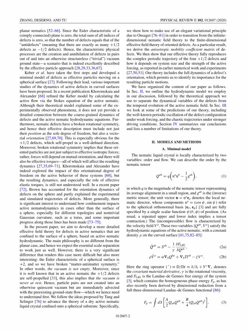
FIG. 3. Time evolution of the average angular distance 〈β jk〉 jk between defects at relatively low activity; recall that the planar configurationcorresponds to 〈β jk〉 jk = 120◦, while the tetrahedral configuration corresponds to 〈β jk〉 jk = 109.5◦. (a) For the subthreshold activity α/ζ =−0.16 μm2/ms, the defects approach stationary positions after a brief transient, reflecting the balance between the elastic interaction ofdefects and the active flow. (b) For the activity α/ζ = −0.26 μm2/ms, the defects periodically oscillate between the tetrahedral and the planarconfiguration.

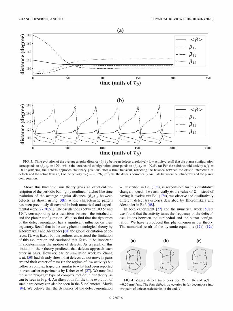
Above this threshold, our theory gives an excellent de-scription of the periodic but highly nonlinear ratchet-like timeevolution of the average angular distance 〈β jk〉 jk betweendefects, as shown in Fig. 3(b), whose characteristic patternhas been previously discovered in both numerical and experi-mental work [27,50,51]. The oscillation is between 109.5◦ and120◦, corresponding to a transition between the tetrahedraland the planar configuration. We also find that the dynamicsof the defect orientation has a significant influence on theirtrajectory. Recall that in the early phenomenological theory byKhoromskaia and Alexander [68] the global orientation of de-fects, �, was fixed; but the authors understood the limitationof this assumption and cautioned that � could be importantin codetermining the motion of defects. As a result of thislimitation, their theory predicted that defects approach eachother in pairs. However, earlier simulation work by Zhanget al. [50] had already shown that defects do not move in pairsaround their center of mass (in the regime of low activity) butfollow a complex trajectory similar to what had been reportedin even earlier experiments by Keber et al. [27]. We now findthe same “zig-zag” type of complex motion in our theory, ascan be seen in Fig. 4. An illustration for the time evolution ofsuch a trajectory can also be seen in the Supplemental Movie[94]. We believe that the dynamics of the defect orientation

�, described in Eq. (17c), is responsible for this qualitativechange. Indeed, if we artificially fix the value of �, instead ofhaving it evolve via Eq. (17c), we observe the qualitativelydifferent defect trajectories described by Khoromskaia andAlexander in Ref. [68].

In both experiment [27] and the numerical work [50] itwas found that the activity tunes the frequency of the defects’oscillations between the tetrahedral and the planar configu-ration. We have reproduced this phenomenon in our theory.The numerical result of the dynamic equations (17a)–(17c)

FIG. 4. Zigzag defect trajectories for R/r = 16 and α/ζ =−0.26 μm2/ms. The four defects trajectories in (a) decompose intotwo pairs of defects trajectories in (b) and (c).

012607-6

DYNAMICS OF ACTIVE NEMATIC DEFECTS ON THE … PHYSICAL REVIEW E 102, 012607 (2020)

FIG. 5. (a) Oscillation frequency of periodic defect trajectories[such as those in Figs. 6(a) and 6(d)] as a function of scaledactivity −α/ζ for given sphere size R = 32 μm. (b) Same oscillationfrequency, but now as a function of the substrate sphere radius R fora given scaled activity of α/ζ = −0.24 μm2/ms.

reveals that the frequency linearly increases with increasingactivity, as shown in Fig. 5(a). More remarkably, the size ofthe spherical substrate also affects the dynamics of defects.If we fix the activity of the system at α/ζ = −0.24 μm2/ms,but successively increase the sphere radius R, the frequencyof the defects’ oscillatory trajectory initially increases, until itattains a maximum, beyond which it again declines, as shownin Fig. 5(b). To understand this, we notice that the coefficientsof the mean active back flow components, (D7) and (D8),are both proportional to R/r, so increasing R is equivalentto linearly enhancing a defects’ velocity. Meanwhile, thedefinition of characteristic timescale τ = γ R2/2K suggeststhat a bigger R will quadratically slow the frequency of thedefects’ oscillation in real time, because defects have largerand larger distances to traverse on their periodic trajectories asR increases. Eventually, the competition of these two effectsleads to a special substrate radius at which the frequency

of the defects’ oscillation attains its maximum, as shown inFig. 5(b).

The coupling of the defect orientation and the active mo-tion causes a rather diverse set of patterns of motion. Weobserved the trajectory of defects becoming chaotic when theactivity or the radius of the sphere substrate is in a certainrange. For low activity, the trajectory remains closed and thedynamics displays a periodic temporal evolution, as shown inFigs. 6(a) and 6(d). But when we increase the activity evenfurther, our simulations show that the dynamics will graduallyenter a new regime in which the trajectories no longer close;in fact, the numerical evidence strongly suggests that thesystem becomes ergodic, based on the trajectory of defectsin both real space and phase space [see Figs. 6(b) and 6(e)],supporting the notion that at sufficiently high activity thedynamics of defects will be chaotic. And just like the chaotictransition when increasing the activity, the defect trajectorycan be open for large sphere radius, as shown in Figs. 6(c)and 6(f).

The chaotic transition we found in our theory is consistentwith what Zhang et al. [50] observed in their significantlymore challenging (lattice-Boltzmann-based) simulations forthe evolution of the entire nematic field—which is potentiallymore prone to numerical instabilities. It is hence reassuring tosee that the same transition to chaos is observed in our muchsimpler system of coupled ordinary differential equations.

IV. CONCLUSIONS AND OUTLOOK

Using Onsager’s variational approach to nonequilibrium(thermo-)dynamics, we have derived an effective theory forthe defect dynamics in an active nematic confined to the sur-face of a sphere. Within our formalism the state of the systemis fully determined by the positions and orientations of a smallnumber of defects, whose dynamics follows from solving aset of coupled first-order differential equations. This is bothconceptually more direct and numerically more efficient thanthe alternative of working with a partial differential equationfor the nematic field, which lives in (2 + 1) dimensions anddescribes either the full order parameter tensor or at least thenematic director.

We focused on the fundamental question how to arrive atsuch an effective description, and hence we have made a fewapproximations along the way in order to avoid clutteringthe path with incidental technical difficulties. Our theory istherefore no equivalent rewriting of the original problem butrather a first-order approximation for the exact time evolutionin terms of convenient smallness parameters. Nevertheless,it offers several quantitative and qualitative insights, and itefficiently reproduces previous numerical and experimentalresults. For instance, in the weakly driven regime we con-firmed the existence of a threshold activity below which defectmotion is arrested, and we characterized the shape of thedefect trajectories past this threshold. In the high-activityregime we observed transition into chaos. And as an exampleof a conceptual insight, we have elucidated the importance ofpromoting the global rotation � to a dynamic variable in orderto reproduce the type of trajectories observed in experiment.

Our theoretical development can be generalized in a num-ber of ways. Most straightforwardly, one could relax the

012607-7

ZHANG, DESERNO, AND TU PHYSICAL REVIEW E 102, 012607 (2020)

FIG. 6. (a)–(c) Trajectory of an individual defect in three dimensions. (d)–(f) Projection of the phase space trajectory of the same individualdefect into the X -VX plane. Specifically: (a), (d) Defect trajectories for small sphere radius R/r = 16 and low activity γα/2Kζ = −0.00338.(b), (e) Defect trajectories for small sphere radius R/r = 16 and high activity γα/2Kζ = −0.0208. (c), (f) Defect trajectories for large sphereradius R/r = 75 and low activity γα/2Kζ = −0.00338.

one-constant-approximation and investigate how differingmoduli for splay and bend affect configuration and dynamicsof an active nematic field with nontrivial topology [49]. Morechallenging, in order to understand the sometimes surprisinglylarge fluctuations of the nematic density observed in bothexperiments [27] and numerical studies [51], one must includedensity contributions to the Rayleighian (7) and add theexpression that follows from the associated variation to theset of dynamic equations.

More interesting, but also much more challenging, wouldbe steps to complete our formalism into a true fluctuat-ing effective field theory, in which particle number is notconserved—in other words, to incorporate pair creation andannihilation events. These occur at sufficiently large activityor sphere radius and have been numerically observed [51].The difficulty is that annihilating a +1/2 against a −1/2defect, or creating such a pair out of an initially smoothbackground field, ultimately rests on the local physics oureffective theory has integrated out. It might seem that at leastthe annihilation event is relatively easy to account for, as onecould simply eliminate a particle-antiparticle pair as soon asthey approach closer than some critical distance; but formu-lating conditions on the local smooth field that trigger paircreation is nontrivial. Moreover, since the rates of creationand annihilation will surely satisfy joint thermodynamic con-straints, these two processes are not independent and hencecannot be treated in isolation.

Even more challenging questions arise once we look atactual experimental realizations of active nematics, such asthe lipid vesicles covered by microtubule filaments that are

rendered active by the addition of kinesin motors [27]. Thecoupling between the fluid-elastic curvature energetics ofthe vesicle and the elasticity underlying the nematic liquidcrystal impacts the morphology of the vesicle, which neednot remain a perfect sphere. In fact, protrusions growingfrom the location of the defects have been observed [27],and the vesicle may deform into a spindle-like structure withtwo +1 defects at the spindle poles [27]. Metselaar et al.[95] have recently proposed a continuum model for such adeformable active nematic shell. Our own framework could beextended to include this as well, by incorporating Helfrich’scurvature elastic energy [96] for the vesicle shape and thedissipation associated with changes of this shape into theRayleighian (7). However, this will require some significantnew formalism, for instance, replacing the simple Riemannmapping of a sphere to a more general surface parametriza-tion. But since throughout our development the descriptionof the geometry is fully covariant, we suspect that the frame-work of Onsager’s variational principle will continue to pro-vide a convenient starting point for developing an effectivetheory.

ACKNOWLEDGMENTS

We are grateful for valuable and inspiring discussions withMasao Doi and Tanniemola Liverpool. We also acknowledgefinancial support from the National Natural Science Founda-tion of China (Grants No. 11675017 and No. 11975050) andpartial support from the National Science Foundation of theUnited States (Grant No. CHE 1764257).

012607-8

DYNAMICS OF ACTIVE NEMATIC DEFECTS ON THE … PHYSICAL REVIEW E 102, 012607 (2020)

APPENDIX A: THE RAYLEIGHIAN

According to Onsager’s variational principle, only termsthat explicitly contain ∂t Qab will contribute to the dynamicequations of defects. So the Rayleighian can be written as

R = d

dtF + γ

2

∫dS(∂t Q

ab∂t Qab

+ 2∂t QabV c∇cQab − 2∂t Q

abSab). (A1)

If we substitute the active flow V a = αζ∇bQba, we obtain

∂t QabSab

= ξq∂t Qab∇[aVb] + ∂t Q

abQac∇(cVb) − ∂t Q

ab∇(aVc)Qc

b

= αξq

ζ∂t Q

ab∇a∇d Qdb + α

ζ∂t Q

abQac∇(c∇d Qd

b)

−α

ζ∂t Q

ab∇(a∇d Qdc)Q

cb

= α

ζ∂t Q

abQac∇(c∇d Qd

b) − α

ζ∂t Q

ab∇(a∇d Qdc)Q

cb

+ αξq3

ζ�ψ∂tψ. (A2)

The equilibrium configuration of the director field ensuresthat the last term in Eq. (A2) vanishes, so the flow aligningparameter ξ does not contribute. Finally, all the couplingterms read

γ

2

∫dS(∂t Q

ab∂t Qab + 2∂t QabV c∇cQab − 2∂t Q

abSab)

= γ q2∫

dS(∂tψ )2 − 2γαq2

ζ

×∫

dS∇b(∇aψ − Aa)Qab∂tψ. (A3)

APPENDIX B: RIEMANN SPHERE REPRESENTATION

Before calculating integrals (16a)–(16h), we must expresseach term in the Riemann sphere representation by using thestereographic projection z(θ, φ) = 2R tan θ

2 eiφ shown in themain text. This leads to∫

dS =∫

dzd z1

2(1 + zz

4R2

)2 (B1)

∂θk ψk = i

4R

(1 + zk zk

4R2

)√zk

zk

1

z − zk+ c.c., (B2)

∂φk ψk = −1

4

zk

z − zk+ c.c., (B3)

∂2φψk = i

4

z

z − zk− i

4

z2

(z − zk )2+ c.c., (B4)

∂θ∂φψk = R

4

(1 + zz

4R2

)√z

z

1

z − zk

− R

4

(1 + zz

4R2

)√z

z

z

(z − zk )2+ c.c., (B5)

∂2θ ψk = − i

8R

(1 + zz

4R2

)2 4R√

zz

4R2 + zz

√z

z

1

z − zk

+ i

4R2

(1 + zz

4R2

)2 z

z

1

(z − zk )2+ c.c. (B6)

We can calculate the area integrals (16a)–(16h) based onthe following theorem:

For a given function G in an area S with the boundary ∂Sin the complex plane z = x + iy,

∫S∂zG(z, z) dz dz =

∫S

2∂zG(z, z) dx dy

=∫

S(∂x − i∂y)G dx dy. (B7)

Based on Green’s theorem, if the first derivative of G iscontinuous in S, then we have

∫S∂zG(z, z) dz dz =

∫S(∂x − i∂y)G dx dy

=∮

∂S(G dy + iG dx)

= i∮

∂SG dz. (B8)

Then we can use

∫S∂zG(z, z) dz dz = i

∮∂S

G dz (B9)

to transform an area integral into a boundary integral.And if G is not analytic, the integral will depend on theshape of the contour of the boundary, instead of just thetopology.

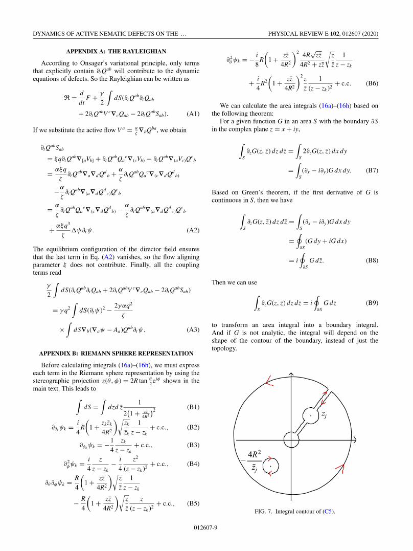
zj

−4R2

zj

FIG. 7. Integral contour of (C5).

012607-9

ZHANG, DESERNO, AND TU PHYSICAL REVIEW E 102, 012607 (2020)

APPENDIX C: MOBILITY MATRICES

In order to obtain the result of integral in (16a)–(16e), thereare two basic integrals we need to calculate first:∫

dS1

(z − z j )(z − zk ), (C1)∫

dS1

(z − z j )(z − zk ). (C2)

According to Eqs. (B1)–(B3), the mobility matrices (16a)–(16e) can be considered as linear combinations of the integrals(C1) and (C2) with their complex conjugates. The boundaries∂S are those peripheries around each defects based on theintegral area we require. First, we use Eq. (B9) to transformthe area integrals into line integrals at each boundaries. Thenwe expand the integrand near each boundary, and only keepthe first order based on the assumption R r. The detailedprocedure is demonstrated below.

1. The calculation of the integral (C1)

a. Diagonal element: k = j

∫dzdz

1

2

(1 + zz

4R2

)2

(z − z j )2

= i∮

Cdz

8R4

z(4R2 + zz)(z − z j )2

= i∮

C0+Cj

dz−8R4

z(4R2 + zz)(z − z j )2

= i∮

C0

dz−2R2

z(z − z j )2+ i

∮Cj

dz−8R4

z(4R2 + zz j )(z − z j )2

= 4πR2z2j

(4R2 + z j z j )2. (C3)

In order to fulfill the condition required by Eq. (B9), weneed to exclude the origin of the complex plane so that theintegrand is continuous over the domain of integration. Thenthe boundary C should contain the boundary C0 around theorigin, and the boundary Cj around the defect at z j . And withperforming the same procedure, the nondiagonal element canbe calculated as follows.

b. Nondiagonal element: k �= j

∫dzd z

1

2(1 + zz

4R2

)2(z − z j )(z − zk )

= i∮

Cdz

8R4

z(4R2 + zz)(z − z j )(z − zk )

= i∮

C0+Cj+Ck

dz−8R4

z(4R2 + zz)(z − z j )(z − zk )

= i∮

C0

dz−2R2

z(z − z j )(z − zk )

+ i∮

Cj

dz−8R4

z(4R2 + zz j )(z − z j )(z − zk )

+ i∮

Ck

dz−8R4

z(4R2 + zzk )(z − z j )(z − zk )

= 16πR4(zk − z j ) − 4πR2z j zk (zk − z j )

(z j − zk )(4R2 + z j z j )(4R2 + zk zk ). (C4)

2. The calculation of the integral (C2)

a. Diagonal element: k = j

∫dzdz

1

2(1 + zz

4R2

)2(z − z j )(z − z j )

= −i∮

Cdz

[8R4

(4R2 + zz)(4R2 + zz j )(z − z j )

+ 8R4

(4R2 + zz j )2(z − z j )ln

zz − zz j

4R2 + zz

]

= − i∮

Cdz

[8R4

(4R2 + zz)(4R2 + zz j )(z − z j )

+ 8R4

(4R2 + zz j )2(z − z j )ln

(z − z j )(z − z j )

4R2 + zz

]

−i∮

Cdz

8R4

(4R2 + zz j )2(z − z j )ln

z

z − z j

= − i∮

Cdz

[8R4

(4R2 + zz)(4R2 + zz j )(z − z j )

+ 8R4

(4R2 + zz j )2(z − z j )ln

(z − z j )(z − z j )

4R2 + zz

]

= i∮

C0

dz

[2R2zz j

(4R2 + zz j )2(z − z j )

+ 8R4

(4R2 + zz j )2(z − z j )

(ln

z j z j − zz j

4R2+ 1

)]

+ i∮

Cj

dz8R4

(4R2 + zz j )2(z − z j )

(ln

r2j

4R2 + zz j+ 1

)

+ i∮

C∗j

dz

[ −2R2z j

(4R2 + zz j )(z − z j )2

+ 8R4

(4R2 + zz j )2(z − z j )ln

4R2 + z j z j

4R2

]

= 4πR2z j z j

(4R2 + z j z j )2− 16πR4

(4R2 + z j z j )2

(1+2 ln

2Rr j

4R2 + z j z j

).

(C5)

The integrand indicates that there are three singular points:z = 0, z = z j , and z = −4R2/z j , corresponding to boundariesof C0, Cj and C∗

j separately. In addition, the first two arealso branch points because of the logarithmic function. Inorder to use Eq. (B9), we again need the integrand to becontinuous along the boundary. We therefore add a branch cut

012607-10

DYNAMICS OF ACTIVE NEMATIC DEFECTS ON THE … PHYSICAL REVIEW E 102, 012607 (2020)

at both of the boundary C0 around the branch point z = 0, andthe boundary Cj around the branch point z = z j . Once wetake the boundary C = C0 + Cj + C∗

j as shown in Fig. 7, theline integral of the sixth line is zero, according to the residuetheorem.

b. Nondiagonal element: k �= j

∫dz dz

1

2(1 + zz

4R2

)2(z − z j )(z − zk )

= − i∮

Cdz

[8R4

(4R2 + zz)(4R2 + zz j )(z − zk )

+ 8R4

(4R2 + zz j )2(z − zk )ln

zz − zz j

4R2 + zz

]

= i∮

C0

dz

[2R2zz j

(4R2 + zz j )2(z − zk )

+ 8R4

(4R2 + zz j )2(z − zk )

(ln

z j z j − zz j

4R2+ 1

)]

+ i∮

Cj

dz8R4

(4R2 + zz j )2(z − zk )

(ln

r2j

4R2 + zz j+ 1

)

+ i∮

Ck

dz

[8R4

(4R2 + zz j )(4R2 + zzk )(z − zk )

+ 8R4

(4R2 + zz j )2(z − zk )ln

(z − z j )(zk − z j )

4R2 + zzk

]

+ i∮

C∗j

dz

[ −2R2z j

(4R2 + zz j )(z − z j )(z − zk )

+ 8R4

(4R2 + zz j )2(z − zk )ln

4R2 + z j z j

4R2

]

= −4πR2

(4R2 + zk z j )2

[(4R2 + zk z j )(16R4 − z j z jzk zk )

(4R2 + z j z j )(4R2 + zk zk )

+ 4R2 ln4R2(z j − zk )(z j − zk )

(4R2 + z j z j )(4R2 + zk zk )

]. (C6)

Notice that the result seems to be divergent when zk =−4R2/z j . This is because we treat zk and −4R2/z j as twodifferent singular points when performing the residue theoremin the calculation. If we instead consider the case of zk =−4R2/z j , we have

∫dz dz

1

2(1 + zz

4R2

)2(z − z j )(z − zk )

=∫

dz dz1

2(1 + zz

4R2

)2(z − z j )

(z + 4R2

z j

)= − i

∮C

dz

[8R4z j

(4R2 + zz)(4R2 + zz j )2

+ 8R4z j

(4R2 + zz j )3ln

zz − zz j

4R2 + zz

]

= i∮

C0

dz

[2R2zz2

j

(4R2 + zz j )3

+ 8R4z j

(4R2 + zz j )3

(ln

z j z j − zz j

4R2+ 1

)]

+ i∮

Cj

dz8R4z j

(4R2 + zz j )3

(ln

r2j

4R2 + zz j+ 1

)

+ i∮

C∗j

dz

[ −2R2z j z j

(4R2 + zz j )2(z − z j )

+ 8R4z j

(4R2 + zz j )3ln

4R2 + z j z j

4R2

]

= −4πR2z j z j

(4R2 + z j z j )2. (C7)

We can check that the result in (C7) indeed coincides with(C6) in the limit in which zk approaches −4R2/z j . In fact,the singular point −4R2/z j is the antipode of the defect z j

on the sphere, and the singularity does not have any physicalmeaning.

3. Results of mobility matrices

Substituting the corresponding coefficients according toEqs. (B2) and (B3), the elements of the mobility matrices canbe constructed as follows:

Diagonal element:

Pj j = πR2|z j |4(4R2 + |z j |2)2

− 2πR4|z j |2(4R2 + |z j |2)2

(1 + 2 ln

2Rr j

4R2 + |z j |2)

, (C8)

Mj j = −πR2

8

(1 + 2 ln

2Rr j

4R2 + |z j |2)

. (C9)

Nondiagonal element:

Pjk = − πR2zk z j

4(4R2 + zk z j )2

[(4R2 + zk z j )(16R4 − |z j |2|zk|2)

(4R2 + |z j |2)(4R2 + |zk|2)

+ 4R2 ln4R2|z j − zk|2

(4R2 + |z j |2)(4R2 + |zk|2)

]

+ πR2z jzk

4(z j − zk )

(zk

4R2 + |zk|2 − z j

4R2 + |z j |2)

+ c.c.,

(C10)

Mjk = 4πR2(z j − zk ) + π zk z j (zk − z j )

64(z j − zk )

√z jzk

z j zk

−π (16R4 − |z j |2|zk|2)

64(4R2 + zk z j )

√z jzk

z j zk

−πR2(4R2 + |z j |2)(4R2 + |zk|2)

16(4R2 + zk z j )2

√z jzk

z j zk

ln4R2|z j − zk|2

(4R2 + |z j |2)(4R2 + |zk|2)+ c.c., (C11)

012607-11

ZHANG, DESERNO, AND TU PHYSICAL REVIEW E 102, 012607 (2020)

Njk = − iπRzk

√z j

z j

[R2(zk − z j )

4(z j − zk )(4R2 + |zk|2)

+ z j zk

16(4R2 + |zk|2)

]

+ iπRzk (16R4 − |z j |2|zk|2)

16(4R2 + z j zk )(4R2 + |zk|2)

√z j

z j

+ iπR3zk (4R2 + |z j |2)

4(4R2 + z j zk )2

√z j

z j

ln4R2|z j − zk|2

(4R2 + |z j |2)(4R2 + |zk|2)+ c.c. (C12)

It is also easy to calculate the vector � j and � j :

� j =∫

dS∂φ j ψ j

= −∫

dz dz2R4z j

(4R2 + zz)2(z − z j )+ c.c.

= −i∮

Cdz

2R4z j

z(4R2 + zz)(z − z j )

= i∮

C0

dzR2z j

2z2 − 2zz j

+ i∮

Cj

dz2R4z j

z(z − z j )(4R2 + zz j )+ c.c.

= 2πR2|z j |24R2 + |z j |2 , (C13)

� j =∫

dS∂θ j ψ j

=∫

dz dziR3(4R2 + z j z j )

2(4R2 + zz)2(z − z j )

√z j

z j+ c.c.

= −∮

Cdz

R3(4R2 + z j z j )

2z(4R2 + zz)(z − z j )

√z j

z j

=∮

C0

dzR(4R2 + z j z j )

8z(z − z j )

√z j

z j

+∮

Cj

dzR3(4R2 + z j z j )

2z(z − z j )(4R2 + zz j )

√z j

z j+ c.c.

= −iπ

4R|z j | + i

π

4R|z j | = 0. (C14)

APPENDIX D: THE CALCULATION OF Tj , Rj , AND L

Here we calculate Tj as an example to illustrate the proce-dure:

Tj = − q0α

2R2ζ

∫dS

[sin 2ψ (2 csc2 θ − 1

+ 2 cot θ csc θ∂φψ − 2 csc θ∂θ∂φψ )

− cos 2ψ(∂2θ ψ − csc2 θ∂2

φψ − cot θ∂θψ)]

∂θ j ψ j .

(D1)

Under the Riemann sphere representation, we have

sin 2ψ = − i

2exp (2i�)

z

z

4∏p=1

√z − zp

z − zp+ c.c., (D2)

cos 2ψ = 1

2exp (2i�)

z

z

4∏p=1

√z − zp

z − zp+ c.c. (D3)

It seems very hard to find a global function G, so thatTj = i

∮dz G. Our strategy is to expand Eq. (D1) near each of

the defects, and subsequently do the procedure we performedabove. According to Eqs. (B1)–(B6), we can expand theintegrand of Tj in terms of z − z j in the following form:

Tj = i∮

Cj

dz∫

dz

√z − z j

z − z j

×3∑

q=1

q∑m=0

[1

(z − z j )m(z − z j )q−m

∞∑l=0

Am,q,l (z − z j )l

]

+ i∑k �= j

∮Ck

dz∫

dz

√z − zk

z − zk

×2∑

n=0

[(1

(z − zk )n+ 1

(z − zk )n

) ∞∑l=0

Bn,l (z − zk )l

]+ c.c.

= i∮

Cj

dz3∑

q=1

q∑m=0

∞∑l=0

2Am,q,l r3−2m+2lj

3 − 2m + 2l(z − z j )

2m−l−q−2

+ i∑k �= j

∮Ck

dz2∑

n=0

∞∑l=0

Bn,l

[2r3+2l−2n

k

3 + 2l − 2n(z − zk )n−l−2

+ 2r3+2lk

3 + 2l(z − zk )−n−l−2

]+ c.c. (D4)

We can also expand it in terms of z − z j :

Tj = −i∮

Cj

dz∫

dz

√z − z j

z − z j

×3∑

q=1

q∑m=0

[1

(z − z j )m(z − z j )q−m

∞∑l=0

Cm,q,l (z − z j )l

]

−i∑k �= j

∮Ck

dz∫

dz

√z − zk

z − zk

×2∑

n=0

[(1

(z − zk )n+ 1

(z − zk )n

) ∞∑l=0

Dn,l (z − zk )l

]+ c.c.

= −i∮

Cj

dz3∑

q=1

q∑m=0

∞∑l=0

2Cm,q,l r1−2q+2m+2lj

1 − 2q + 2m + 2l(z − z j )

q−2m−l

− i∑k �= j

∮Ck

dz2∑

n=0

∞∑l=0

Dn,l

[2r2l+1

k

2l + 1(z − zk )−n−l

+ 2r1+2l−2nk

1 + 2l − 2n(z − zk )n−l

]+ c.c., (D5)

012607-12

DYNAMICS OF ACTIVE NEMATIC DEFECTS ON THE … PHYSICAL REVIEW E 102, 012607 (2020)

which represents the order change of the area integral. A, B, C,and D are the expansion coefficients, which can be obtainedby expanding the integrand near the boundaries around eachdefects. And we should notice that

Am,q,0 = Cm,q,0, Bn,0 = Dn,0. (D6)This relationship means Eqs. (D4) and (D5) should give thesame result, which reflects the order free of the integral withrespect to z and z. It is easy to check that the leading term thatcontributes to Tj is −2A2,3,0/r j or −2C2,3,0/r j .

Finally, the expression of Tj is

Tj = Re

⎡⎣ πq0α

16Rζ r jexp (2i�)(4R2 + |z j |2)

√z j

z j

∏l �= j

√z j − zl

z j − zl

⎤⎦

= πq0αR

4ζ rcos(w j + 2� − φ j ). (D7)

We can perform the same procedure to the calculation of Sj

and L:

S j = Re

⎡⎣−i

πq0αz j

4ζ r jexp (2i�)

∏l �= j

√z j − zl

z j − zl

⎤⎦

= πq0αR

4ζ rsin θ j sin(w j + 2� − φ j ), (D8)

L = 0. (D9)

And w j is the summation of the phase angle between the jthdefect and others:

w j =∑l �= j

arg(z j − zl ). (D10)

[1] S. Chandrasekhar and G. S. Ranganath, The structure andenergetics of defects in liquid crystals, Adv. Phys. 35, 507(1986).

[2] M. V. Kurik and O. D. Lavrentovich, Defects in liquid crystals:Homotopy theory and experimental studies, Sov. Phys. Usp. 31,196 (1988) [Usp. Fiz. Nauk 154, 381 (1988)].

[3] P. G. de Gennes and J. Prost, The Physics of Liquid Crystals(Clarendon Press, Oxford, 1993).

[4] H. Kikuchi, M. Yokota, Y. Hisakado, H. Yang, and T. Kajiyama,Polymer-stabilized liquid crystal blue phases, Nat. Mater. 1, 64(2002).

[5] G. I. Taylor, The mechanism of plastic deformation of crystals.Part I.—Theoretical, Proc. R. Soc. London Ser. A 145, 362(1934).

[6] J. Friedel, Dislocations (Pergamon Press, Oxford, 1964).[7] F. Nabarro, Theory of Crystal Dislocations (Clarendon Press,

Oxford, 1967).[8] G. Duclos, C. Erlenkämper, J.-F. Joanny, and P. Silberzan,

Topological defects in confined populations of spindle-shapedcells, Nat. Phys. 13, 58 (2016).

[9] T. B. Saw, A. Doostmohammadi, V. Nier, L. Kocgozlu, S.Thampi, Y. Toyama, P. Marcq, C. T. Lim, J. M. Yeomans, andB. Ladoux, Topological defects in epithelia govern cell deathand extrusion, Nature (London) 544, 212 (2017).

[10] K. Kawaguchi, R. Kageyama, and M. Sano, Topological defectscontrol collective dynamics in neural progenitor cell cultures,Nature (London) 545, 327 (2017).

[11] D. V. Osborne, The rotation of liquid helium II, Proc. Phys.Soc., Sec. A 63, 909 (1950).

[12] J. Wilks and D. Betts, An Introduction to Liquid Helium(Clarendon Press, Oxford, 1987).

[13] D. Vollhardt and P. Wolfle, The Phases of Helium 3 (Taylor andFrancis, New York, 1990).

[14] A. N. Bogdanov and D. A. Yablonskii, Thermodynamicallystable “vortices” in magnetically ordered crystals. the mixedstate of magnets, Zh. Eksp. Teor. Fiz. 95, 178 (1989) [Sov. Phys.JETP 68, 101 (1989)].

[15] A. Bogdanov and A. Hubert, Thermodynamically stable mag-netic vortex states in magnetic crystals, J. Magn. Magn. Mater.138, 255 (1994).

[16] U. K. Rößler, A. N. Bogdanov, and C. Pfleiderer, Spontaneousskyrmion ground states in magnetic metals, Nature (London)442, 797 (2006).

[17] B. Binz, A. Vishwanath, and V. Aji, Theory of the Helical SpinCrystal: A Candidate for the Partially Ordered State of MnSi,Phys. Rev. Lett. 96, 207202 (2006).

[18] S. Tewari, D. Belitz, and T. R. Kirkpatrick, Blue Quantum Fog:Chiral Condensation in Quantum Helimagnets, Phys. Rev. Lett.96, 047207 (2006).

[19] S. Mühlbauer, B. Binz, F. Jonietz, C. Pfleiderer, A. Rosch,A. Neubauer, R. Georgii, and P. Böni, Skyrmion lattice in achiral magnet, Science 323, 915 (2009).

[20] A. Neubauer, C. Pfleiderer, B. Binz, A. Rosch, R. Ritz, P. G.Niklowitz, and P. Böni, Topological Hall Effect in the a Phaseof MnSi, Phys. Rev. Lett. 102, 186602 (2009).

[21] C. Pappas, E. Lelièvre-Berna, P. Falus, P. M. Bentley,E. Moskvin, S. Grigoriev, P. Fouquet, and B. Farago, ChiralParamagnetic Skyrmion-Like Phase in MnSi, Phys. Rev. Lett.102, 197202 (2009).

[22] N. Nagaosa and Y. Tokura, Topological properties and dynam-ics of magnetic skyrmions, Nat. Nanotech. 8, 899 (2013).

[23] N. Turok, Global Texture as the Origin of Cosmic Structure,Phys. Rev. Lett. 63, 2625 (1989).

[24] A. Pargellis, N. Turok, and B. Yurke, Monopole-AntimonopoleAnnihilation in a Nematic Liquid Crystal, Phys. Rev. Lett. 67,1570 (1991).

[25] I. Chuang, R. Durrer, N. Turok, and B. Yurke, Cosmology inthe laboratory: Defect dynamics in liquid crystals, Science 251,1336 (1991).

[26] A. J. Bray, Theory of phase-ordering kinetics, Adv. Phys. 43,357 (1994).

[27] F. C. Keber, E. Loiseau, T. Sanchez, S. J. DeCamp, L. Giomi,M. J. Bowick, M. C. Marchetti, Z. Dogic, and A. R. Bausch,Topology and dynamics of active nematic vesicles, Science 345,1135 (2014).

[28] L. Giomi, M. J. Bowick, X. Ma, and M. C. Marchetti, DefectAnnihilation and Proliferation in Active Nematics, Phys. Rev.Lett. 110, 228101 (2013).

[29] L. M. Pismen, Dynamics of defects in an active nematic layer,Phys. Rev. E 88, 050502(R) (2013).

012607-13

ZHANG, DESERNO, AND TU PHYSICAL REVIEW E 102, 012607 (2020)

[30] S. P. Thampi, R. Golestanian, and J. M. Yeomans, VelocityCorrelations in an Active Nematic, Phys. Rev. Lett. 111, 118101(2013).

[31] S. P. Thampi, R. Golestanian, and J. M. Yeomans, Instabilitiesand topological defects in active nematics, Europhys. Lett. 105,18001 (2014).

[32] S. P. Thampi, R. Golestanian, and J. M. Yeomans, Vorticity,defects and correlations in active turbulence, Philos. Trans. R.Soc. A 372, 20130366 (2014).

[33] L. Giomi, M. J. Bowick, P. Mishra, R. Sknepnek, andM. Cristina Marchetti, Defect dynamics in active nematics,Philos. Trans. R. Soc. A 372, 20130365 (2014).

[34] T. Gao, R. Blackwell, M. A. Glaser, M. D. Betterton, and M. J.Shelley, Multiscale Polar Theory of Microtubule and Motor-Protein Assemblies, Phys. Rev. Lett. 114, 048101 (2015).

[35] S. Shankar, S. Ramaswamy, M. C. Marchetti, and M. J. Bowick,Defect Unbinding in Active Nematics, Phys. Rev. Lett. 121,108002 (2018).

[36] D. Cortese, J. Eggers, and T. B. Liverpool, Pair creation, mo-tion, and annihilation of topological defects in two-dimensionalnematic liquid crystals, Phys. Rev. E 97, 022704 (2018).

[37] J. L. Ericksen, Anisotropic fluids, Arch. Ration. Mech. Anal. 4,231 (1959).

[38] J. L. Ericksen, Conservation laws for liquid crystals, Trans. Soc.Rheol. 5, 23 (1961).

[39] F. M. Leslie, Some constitutive equations for anisotropic fluids,Quart. J. Mech. Appl. Math. 19, 357 (1966).

[40] F. M. Leslie, Some constitutive equations for liquid crystals,Arch. Ration. Mech. Anal. 28, 265 (1968).

[41] A. Beris and B. Edwards, Thermodynamics of Flowing Systems(Oxford University Press, Oxford, 1994).

[42] R. A. Simha and S. Ramaswamy, Hydrodynamic Fluctuationsand Instabilities in Ordered Suspensions of Self-Propelled Par-ticles, Phys. Rev. Lett. 89, 058101 (2002).

[43] M. C. Marchetti, J. F. Joanny, S. Ramaswamy, T. B. Liverpool,J. Prost, M. Rao, and R. A. Simha, Hydrodynamics of soft activematter, Rev. Mod. Phys. 85, 1143 (2013).

[44] J. Prost, F. Jülicher, and J.-F. Joanny, Active gel physics, Nat.Phys. 11, 111 (2015).

[45] S. Ramaswamy, Active matter, J. Stat. Mech.: Theory Exp.(2017) 054002.

[46] A. Doostmohammadi, J. Ignés-Mullol, J. M. Yeomans, andF. Sagués, Active nematics, Nat. Commun. 9, 3246 (2018).

[47] G. Napoli and L. Vergori, Hydrodynamic theory for nematicshells: The interplay among curvature, flow, and alignment,Phys. Rev. E 94, 020701(R) (2016).

[48] G. Napoli and S. Turzi, Spontaneous helical flows in activenematics lying on a cylindrical surface, Phys. Rev. E 101,022701 (2020).

[49] H. Shin, M. J. Bowick, and X. Xing, Topological Defects inSpherical Nematics, Phys. Rev. Lett. 101, 037802 (2008).

[50] R. Zhang, Y. Zhou, M. Rahimi, and J. J. de Pablo, Dynamicstructure of active nematic shells, Nat. Commun. 7, 13483(2016).

[51] S. Henkes, M. C. Marchetti, and R. Sknepnek, Dynamicalpatterns in nematic active matter on a sphere, Phys. Rev. E 97,042605 (2018).

[52] C. M. Dafermos, Disinclination in liquid crystals, Quart. J.Mech. Appl. Math. 23, 49 (1970).

[53] H. Imura and K. Okano, Friction coefficient for a movingdisinclination in a nematic liquid crystal, Phys. Lett. A 42, 403(1973).

[54] L. M. Pismen and J. D. Rodriguez, Mobility of singularitiesin the dissipative Ginzburg-Landau equation, Phys. Rev. A 42,2471 (1990).

[55] G. Ryskin and M. Kremenetsky, Drag Force on a Line DefectMoving Through an Otherwise Undisturbed Field: DisclinationLine in a Nematic Liquid Crystal, Phys. Rev. Lett. 67, 1574(1991).

[56] T. C. Lubensky and J. Prost, Orientational order and vesicleshape, J. Phys. II 2, 371 (1992).

[57] C. Denniston, Disclination dynamics in nematic liquid crystals,Phys. Rev. B 54, 6272 (1996).

[58] J.-M. Park and T. C. Lubensky, Topological defects on fluctu-ating surfaces: General properties and the Kosterlitz-Thoulesstransition, Phys. Rev. E 53, 2648 (1996).

[59] D. R. Nelson, Toward a tetravalent chemistry of colloids, NanoLett. 2, 1125 (2002).

[60] D. Svenšek and S. Žumer, Hydrodynamics of pair-annihilatingdisclination lines in nematic liquid crystals, Phys. Rev. E 66,021712 (2002).

[61] E. I. Kats, V. V. Lebedev, and S. V. Malinin, Disclination motionin liquid crystalline films, J. Exp. Theor. Phys. 95, 714 (2002).

[62] G. Tóth, C. Denniston, and J. M. Yeomans, Hydrodynamicsof Topological Defects in Nematic Liquid Crystals, Phys. Rev.Lett. 88, 105504 (2002).

[63] A. M. Sonnet, Viscous forces on nematic defects, Cont. Mech.Thermodyn. 17, 287 (2005).

[64] V. Vitelli and D. R. Nelson, Nematic textures in spherical shells,Phys. Rev. E 74, 021711 (2006).

[65] A. M. Sonnet and E. G. Virga, Flow and reorientation in thedynamics of nematic defects, Liq. Cryst. 36, 1185 (2009).

[66] L. Radzihovsky, Anomalous Energetics and Dynamics of Mov-ing Vortices, Phys. Rev. Lett. 115, 247801 (2015).

[67] R. Zhang, N. Kumar, J. L. Ross, M. L. Gardel, and J. J. dePablo, Interplay of structure, elasticity, and dynamics in actin-based nematic materials, Proc. Natl. Acad. Sci. USA 115, E124(2018).

[68] D. Khoromskaia and G. P. Alexander, Vortex formation anddynamics of defects in active nematic shells, New J. Phys. 19,103043 (2017).

[69] A. J. Vromans and L. Giomi, Orientational properties of ne-matic disclinations, Soft Matter 12, 6490 (2016).

[70] X. Tang and J. V. Selinger, Orientation of topological de-fects in 2D nematic liquid crystals, Soft Matter 13, 5481(2017).

[71] S. Shankar and M. C. Marchetti, Hydrodynamics of ActiveDefects: From Order to Chaos to Defect Ordering, Phys. Rev.X 9, 041047 (2019).

[72] A. T. Brown, A theoretical phase diagram for an active nematicon a spherical surface, Soft Matter 16, 4682 (2020).

[73] M. Bowick, D. R. Nelson, and A. Travesset, Curvature-induceddefect unbinding in toroidal geometries, Phys. Rev. E 69,041102 (2004).

[74] P. W. Ellis, D. J. Pearce, Y.-W. Chang, G. Goldsztein, L. Giomi,and A. Fernandez-Nieves, Curvature-induced defect unbindingand dynamics in active nematic toroids, Nat. Phys. 14, 85(2018).

012607-14

DYNAMICS OF ACTIVE NEMATIC DEFECTS ON THE … PHYSICAL REVIEW E 102, 012607 (2020)

[75] D. J. G. Pearce, P. W. Ellis, A. Fernandez-Nieves, and L.Giomi, Geometrical Control of Active Turbulence in CurvedTopographies, Phys. Rev. Lett. 122, 168002 (2019).

[76] X. Tang and J. V. Selinger, Theory of defect motion in 2Dpassive and active nematic liquid crystals, Soft Matter 15, 587(2019).

[77] G. Vertogen, The equations of motion for nematics,Z. Naturforsch. A 38, 1273 (1983).

[78] G. Vertogen and W. H. de Jeu, Thermotropic Liquid Crystals,Fundamentals (Springer-Verlag, Berlin, 1989).

[79] A. M. Sonnet and E. G. Virga, Dynamics of dissipative orderedfluids, Phys. Rev. E 64, 031705 (2001).

[80] M. Doi, Onsager’s variational principle in soft matter, J. Phys.:Condens. Matter 23, 284118 (2011).

[81] A. M. Sonnet and E. G. Virga, Dissipative Ordered Fluids:Theories for Liquid Crystals (Springer Science & BusinessMedia, Berlin, 2012).

[82] B. J. Edwards, A. N. Beris, and M. Grmela, Generalized consti-tutive equation for polymeric liquid crystals Part 1. Model for-mulation using the Hamiltonian (Poisson bracket) formulation,J. Non-Newton Fluid Mech. 35, 51 (1990).

[83] P. D. Olmsted and P. M. Goldbart, Isotropic-nematic transitionin shear flow: State selection, coexistence, phase transitions,and critical behavior, Phys. Rev. A 46, 4966 (1992).

[84] P. D. Olmsted and C.-Y. D. Lu, Coexistence and phase sep-aration in sheared complex fluids, Phys. Rev. E 56, R55(1997).

[85] P. D. Olmsted and C.-Y. David Lu, Phase separation ofrigid-rod suspensions in shear flow, Phys. Rev. E 60, 4397(1999).

[86] G. Napoli and L. Vergori, Surface free energies for nematicshells, Phys. Rev. E 85, 061701 (2012).

[87] K. Kruse, J. F. Joanny, F. Jülicher, J. Prost, and K.Sekimoto, Asters, Vortices, and Rotating Spirals in Ac-tive Gels of Polar Filaments, Phys. Rev. Lett. 92, 078101(2004).

[88] D. Marenduzzo, E. Orlandini, M. E. Cates, and J. M. Yeomans,Steady-state hydrodynamic instabilities of active liquid crystals:Hybrid lattice Boltzmann simulations, Phys. Rev. E 76, 031921(2007).

[89] T. Liverpool and M. Marchetti, Hydrodynamics and rheologyof active polar filaments, in Cell Motility, edited by P. Lenz(Springer, New York, 2008) pp. 177–206.

[90] A. W. C. Lau and T. C. Lubensky, Fluctuating hydrodynamicsand microrheology of a dilute suspension of swimming bacteria,Phys. Rev. E 80, 011917 (2009).

[91] L. Giomi, L. Mahadevan, B. Chakraborty, and M. F. Hagan,Banding, excitability and chaos in active nematic suspensions,Nonlinearity 25, 2245 (2012).

[92] S. Ramaswamy, The mechanics and statistics of active matter,Annu. Rev. Cond. Mat. Phys. 1, 323 (2010).

[93] I. W. Stewart, The Static and Dynamic Continuum Theory ofLiquid Crystals (Taylor & Francis, Philadelphia, 2004).

[94] See Supplemental Material at http://link.aps.org/supplemental/10.1103/PhysRevE.102.012607 for the movie illustrating thetime evolution of a periodic trajectory followed by four +1/2defects in an active nematic on a sphere, for the parametersR/r = 16 and γα/2Kζ = −0.00338. The arrow represents theorientation of the defect. We speed up the motion in the movie.

[95] L. Metselaar, J. M. Yeomans, and A. Doostmohammadi, Topol-ogy and Morphology of Self-Deforming Active Shells, Phys.Rev. Lett. 123, 208001 (2019).

[96] W. Helfrich, Elastic properties of lipid bilayers: Theory andpossible experiments, Z. Naturforsch. C 28, 693 (1973).

012607-15