Physical Climate Processes and Feedbacks - UNFCCCunfccc.int/resource/cd_roms/na1/mitigation/Resource_materials/IPCC... · 7.1 Introduction 421 ... latitudes, and cooling and net precipitation

Physical Climate Processes and Feedbacks

Co-ordinating Lead AuthorT.F. Stocker

Lead AuthorsG.K.C. Clarke, H. Le Treut, R.S. Lindzen, V.P. Meleshko, R.K. Mugara, T.N. Palmer,R.T. Pierrehumbert, P.J. Sellers, K.E. Trenberth, J. Willebrand

Contributing AuthorsR.B. Alley, O.E. Anisimov, C. Appenzeller, R.G. Barry, J.J. Bates, R. Bindschadler, G.B. Bonan,C.W. Böning, S. Bony, H. Bryden, M.A. Cane, J.A. Curry, T. Delworth, A.S. Denning, R.E. Dickinson,K. Echelmeyer, K. Emanuel, G. Flato, I. Fung, M. Geller, P.R. Gent, S.M. Griffies, I. Held,A. Henderson-Sellers, A.A.M. Holtslag, F. Hourdin, J.W. Hurrell, V.M. Kattsov, P.D. Killworth,Y. Kushnir, W.G. Large, M. Latif, P. Lemke, M.E. Mann, G. Meehl, U. Mikolajewicz, W. O’Hirok,C.L. Parkinson, A. Payne, A. Pitman, J. Polcher, I. Polyakov, V. Ramaswamy, P.J. Rasch, E.P. Salathe,C. Schär, R.W. Schmitt, T.G. Shepherd, B.J. Soden, R.W. Spencer, P. Taylor, A. Timmermann,K.Y. Vinnikov, M. Visbeck, S.E. Wijffels, M. Wild

Review EditorsS. Manabe, P. Mason

7

Executive Summary 419

7.1 Introduction 4217.1.1 Issues of Continuing Interest 4217.1.2 New Results since the SAR 4227.1.3 Predictability of the Climate System 422

7.2 Atmospheric Processes and Feedbacks 4237.2.1 Physics of the Water Vapour and Cloud

Feedbacks 4237.2.1.1 Water vapour feedback 4257.2.1.2 Representation of water vapour in

models 4257.2.1.3 Summary on water vapour

feedbacks 4267.2.2 Cloud Processes and Feedbacks 427

7.2.2.1 General design of cloud schemes within climate models 427

7.2.2.2 Convective processes 4287.2.2.3 Boundary-layer mixing and

cloudiness 4287.2.2.4 Cloud-radiative feedback processes 4297.2.2.5 Representation of cloud processes

in models 4317.2.3 Precipitation 431

7.2.3.1 Precipitation processes 4317.2.3.2 Precipitation modelling 4317.2.3.3 The temperature-moisture feedback

and implications for precipitation and extremes 432

7.2.4 Radiative Processes 4327.2.4.1 Radiative processes in the

troposphere 4327.2.4.2 Radiative processes in the

stratosphere 4337.2.5 Stratospheric Dynamics 4347.2.6 Atmospheric Circulation Regimes 4357.2.7 Processes Involving Orography 435

7.3 Oceanic Processes and Feedbacks 4357.3.1 Surface Mixed Layer 4367.3.2 Convection 4367.3.3 Interior Ocean Mixing 4377.3.4 Mesoscale Eddies 4377.3.5 Flows over Sills and through Straits 4387.3.6 Horizontal Circulation and Boundary

Currents 4397.3.7 Thermohaline Circulation and Ocean

Reorganisations 439

7.4 Land-Surface Processes and Feedbacks 4407.4.1 Land-Surface Parametrization (LSP)

Development 4407.4.2 Land-Surface Change 4437.4.3 Land Hydrology, Runoff and Surface-

Atmosphere Exchange 444

7.5 Cryosphere Processes and Feedbacks 4447.5.1 Snow Cover and Permafrost 4447.5.2 Sea Ice 4457.5.3 Land Ice 448

7.6 Processes, Feedbacks and Phenomena in the Coupled System 4497.6.1 Surface Fluxes and Transport of Heat and

Fresh Water 4497.6.2 Ocean-atmosphere Interactions 4517.6.3 Monsoons and Teleconnections 4517.6.4 North Atlantic Oscillation and Decadal

Variability 4527.6.5 El Niño-Southern Oscillation (ENSO) 453

7.6.5.1 ENSO processes 4547.6.5.2 ENSO and tropical storms 455

7.7 Rapid Changes in the Climate System 455

References 457

Contents

Executive Summary

Considerable advances have been made in the understanding ofprocesses and feedbacks in the climate system. This has led to abetter representation of processes and feedbacks in numericalclimate models, which have become much more comprehensive.Because of the presence of non-linear processes in the climatesystem, deterministic projections of changes are potentiallysubject to uncertainties arising from sensitivity to initialconditions or to parameter settings. Such uncertainties can bepartially quantified from ensembles of climate change integra-tions, made using different models starting from different initialconditions. They necessarily give rise to probabilistic estimatesof climate change. This results in more quantitative estimates ofuncertainties and more reliable projections of anthropogenicclimate change. While improved parametrizations have builtconfidence in some areas, recognition of the complexity in otherareas has not indicated an overall reduction or shift in the currentrange of uncertainty of model response to changes in atmosphericcomposition.

Atmospheric feedbacks largely control climate sensitivity.Important progress has been made in the understanding of thoseprocesses, partly by utilising new data against which models canbe compared. Since the Second Assessment Report (IPCC, 1996)(hereafter SAR), there has been a better appreciation of thecomplexity of the mechanisms controlling water vapour distribu-tion. Within the boundary layer, water vapour increases withincreasing temperatures. In the free troposphere above theboundary layer, where the greenhouse effect of water vapour ismost important, the situation is less amenable to straightforwardthermodynamic arguments. In models, increases in water vapourin this region are the most important reason for large responses toincreased greenhouse gases.

Water vapour feedback, as derived from current models,approximately doubles the warming from what it would be forfixed water vapour. Since the SAR, major improvements haveoccurred in the treatment of water vapour in models, althoughdetrainment of moisture from clouds remains quite uncertain anddiscrepancies exist between model water vapour distributions andthose observed. It is likely that some of the apparent discrepancyis due to observational error and shortcomings in intercompar-ison methodology. Models are capable of simulating the moistand very dry regions observed in the tropics and sub-tropics andhow they evolve with the seasons and from year to year,indicating that the models have successfully incorporated thebasic processes governing water vapour distribution. Whilereassuring, this does not provide a definitive check of thefeedbacks, though the balance of evidence favours a positiveclear-sky water vapour feedback of a magnitude comparable tothat found in simulations.

Probably the greatest uncertainty in future projections ofclimate arises from clouds and their interactions with radiation.Cloud feedbacks depend upon changes in cloud height, amount,and radiative properties, including short-wave absorption. Theradiative properties depend upon cloud thickness, particle size,shape, and distribution and on aerosol effects. The evolution ofclouds depends upon a host of processes, mainly those governing

the distribution of water vapour. The physical basis of the cloudparametrizations included into the models has also been greatlyimproved. However, this increased physical veracity has notreduced the uncertainty attached to cloud feedbacks: even thesign of this feedback remains unknown. A key issue, which alsohas large implications for changes in precipitation, is thesensitivity of sub-grid scale dynamical processes, turbulent andconvective, to climate change. It depends on sub-grid features ofsurface conditions such as orography. Equally important aremicrophysical processes, which have only recently beenintroduced explicitly in the models, and carry major uncertain-ties. The possibility that models underestimate solar absorption inclouds remains controversial, as does the effect of such anunderestimate on climate sensitivity. The importance of thestructure of the stratosphere and both radiative and dynamicalprocesses have been recognised, and limitations in representingstratospheric processes add some uncertainty to model results.

Considerable improvements have taken place in modellingocean processes. In conjunction with an increase in resolution,these improvements have, in some models, allowed a morerealistic simulation of the transports and air-sea fluxes of heat andfresh water, thereby reducing the need for flux adjustments incoupled models. These improvements have also contributed tobetter simulations of natural large-scale circulation patterns suchas El Niño-Southern Oscillation (ENSO) and the oceanicresponse to atmospheric variability associated with the NorthAtlantic Oscillation (NAO). However, significant deficiencies inocean models remain. Boundary currents in climate simulationsare much weaker and wider than in nature, though theconsequences of this fact for the global climate sensitivity are notclear. Improved parametrizations of important sub-grid scaleprocesses, such as mesoscale eddies, have increased the realismof simulations but important details are still under debate. Majoruncertainties still exist with the representation of small-scaleprocesses, such as overflows and flow through narrow channels(e.g., between Greenland and Iceland), western boundarycurrents (i.e., large-scale narrow currents along coastlines),convection, and mixing.

In the Atlantic, the thermohaline circulation (THC) isresponsible for the major part of the ocean meridional heattransport associated with warm and saline surface waters flowingnorthward and cold and fresh waters from the North Atlanticreturning at depth. The interplay between the large-scaleatmospheric forcing, with warming and evaporation in lowlatitudes, and cooling and net precipitation at high latitudes,forms the basis of a potential instability of the present AtlanticTHC. Changes in ENSO may also influence the Atlantic THC byaltering the fresh water balance of the tropical Atlantic, thereforeproviding a coupling between low and high latitudes. Uncertaintyresides with the relative importance of feedbacks associated withprocesses influencing changes in high latitude sea surface temper-atures and salinities, such as atmosphere-ocean heat and freshwater fluxes, formation and transport of sea ice, continental runoffand the large-scale transports in ocean and atmosphere. TheAtlantic THC is likely to change over the coming century but itsevolution continues to be an unresolved issue. While some recentcalculations find little changes in the THC, most projections

419Physical Climate Processes and Feedbacks

suggest a gradual and significant decline of the THC. A completeshut-down of the THC is simulated in a number of models if thewarming continues, but knowledge about the locations of thresh-olds for such a shut-down is very limited. Models with reducedTHC appear to be more susceptible for a shut-down. Although ashut-down during the next 100 years is unlikely, it cannot beruled out.

Recent advances in our understanding of vegetationphotosynthesis and water use have been used to couple theterrestrial energy, water and carbon cycles within a new genera-tion of physiologically based land-surface parametrizations.These have been tested against field observations andimplemented in General Circulation Models (GCMs) withdemonstrable improvements in the simulation of land-atmosphere fluxes. There has also been significant progress inspecifying land parameters, especially the type and density ofvegetation. Importantly, these data sets are globally consistent inthat they are primarily based on one type of satellite sensor andone set of interpretative algorithms. Satellite observations havealso been shown to provide a powerful diagnostic capability fortracking climatic impacts on surface conditions; e.g., droughtsand the recently observed lengthening of the boreal growingseason; and direct anthropogenic impacts such as deforestation.The direct effects of increased carbon dioxide (CO2) on vegeta-tion physiology could lead to a relative reduction in evapo-transpiration over the tropical continents, with associatedregional warming over that predicted for conventionalgreenhouse warming effects. On time-scales of decades theseeffects could significantly influence the rate of atmospheric CO2

increase, the nature and extent of the physical climate systemresponse, and ultimately, the response of the biosphere itself toglobal change. In addition, such models must be used to accountfor the climatic effects of land-use change which can be verysignificant at local and regional scales. However, realistic land-use change scenarios for the next 50 to 100 years are notexpected to give rise to global scale climate changes comparableto those resulting from greenhouse gas warming. Significantmodelling problems remain to be solved in the areas of soilmoisture processes, runoff prediction, land-use change, and thetreatment of snow and sub-grid scale heterogeneity.

Increasingly complex snow schemes are being used in someclimate models. These schemes include parametrizations of the

metamorphic changes in snow albedo arising from age depend-ence or temperature dependence. Recent modelling studies of theeffects of warming on permafrost predict a 12 to 15% reductionin near-surface area and a 15 to 30% increase in thickness of theseasonally thawing active layer by the mid-21st century. Therepresentation of sea-ice processes continues to improve withseveral climate models now incorporating physically basedtreatments of ice dynamics. The effects of sub-grid scalevariability in ice cover and thickness, which can significantlyinfluence albedo and atmosphere-ocean exchanges, are beingintroduced. Understanding of fast-flow processes for land iceand the role of these processes in past climate events is growingrapidly. Representation of ice stream and grounding line physicsin land-ice dynamics models remains rudimentary but, in globalclimate models, ice dynamics and thermodynamics are ignoredentirely.

Climate change may manifest itself both as shifting meansas well as changing preference of specific regimes, as evidencedby the observed trend toward positive values for the last 30 yearsin the NAO index and the climate “shift” in the tropical Pacificin about 1976. While coupled models simulate features ofobserved natural climate variability such as the NAO and ENSO,suggesting that many of the relevant processes are included in themodels, further progress is needed to depict these natural modesaccurately. Moreover, because ENSO and NAO are key determi-nants of regional climate change, and they can possibly result inabrupt and counter-intuitive changes, there has been an increasein uncertainty in those aspects of climate change that criticallydepend on regional changes.

Possible non-linear changes in the climate system as a resultof anthropogenic climate forcing have received considerableattention in the last few years. Employing the entire climatemodel hierarchy, and combining these results with palaeo-climatic evidence and instrumental observation, has shown thatmode changes in all components of the climate system haveoccurred in the past and may also take place in the future. Suchchanges may be associated with thresholds in the climate system.Such thresholds have been identified in many climate modelsand there is an increasing understanding of the underlyingprocesses. Current model simulations indicate that the thresholdsmay lie within the reaches of projected changes. However, it isnot yet possible to give reliable values of such thresholds.

420 Physical Climate Processes and Feedbacks

7.1 Introduction

The key problem to be addressed is the response of the climatesystem to changes in forcing. In many cases there is a fairly directand linear response and many of the simulated changes fall intothat class (Chapter 9). These concern the large-scale generalcirculations of the atmosphere and ocean, and they are inprinciple represented in current comprehensive coupled climatemodels. Such possible large-scale dynamical feedbacks are alsoinfluenced by small-scale processes within the climate system.The various feedbacks in the climate system may amplify(positive feedbacks), or diminish (negative feedbacks) theoriginal response. We often approximate the response of a partic-ular variable to a small forcing by a scaling number. A prominentexample of such a quantification is the equilibrium global meantemperature increase per Wm−2 change in the global meanatmospheric radiative forcing (see Chapter 9, Section 9.2.1).

While many aspects of the response of the climate systemto greenhouse gas forcing appear to be linear, regime or modetransitions cannot be quantified by a simple number becauseresponses do not scale with the amplitude of the forcing: smallperturbations can induce large changes in certain variables ofthe climate system. This implies the existence of thresholds inthe climate system which can be crossed for a sufficiently largeperturbation. While such behaviour has long been known andstudied in the context of simple models of the climate system,such thresholds are now also found in the comprehensivecoupled climate models currently available. Within thisframework, the possibility for irreversible changes in theclimate system exists. This insight, backed by the palaeo-climatic record (see Chapter 2, Section 2.4), is a new challengefor global change science because now thresholds have to beidentified and their values need to be estimated using the entirehierarchy of climate models.

To estimate the response properly, we must representfaithfully the physical processes in models. Not only must thewhole system model perform reasonably well in comparisonwith observation (both spatial and temporal), but so too mustthe component models and the processes that are involved in themodels. It is possible to tune a model so that some variableappears consistent with that observed, but we must also askwhether it comes out that way for the right reason and with theright variability. By examining how well individual processesare known and can be modelled, we can comment on thecapabilities and usefulness of the models, and whether they arelikely to be able to properly represent possible non-linearresponses of the climate system.

7.1.1 Issues of Continuing Interest

Examples of some processes in the climate system and itscomponents that have been dealt with in the Second AssessmentReport (IPCC, 1996) (hereafter SAR) and still are importanttopics of progress:

• The hydrological cycle. Progress has been made in allaspects of the hydrological cycle in the atmosphere,

involving evaporation, atmospheric moisture, clouds,convection, and precipitation. Because many facets of thesephenomena are sub-grid scale, they must be parametrized.While models reasonably simulate gross aspects of theobserved behaviour on several time-scales, it is easy to pointout shortcomings, although it is unclear as to how muchthese affect the sensitivity of simulated climate to changesin climate forcing.

• Water vapour feedback. An increase in the temperature ofthe atmosphere increases its water-holding capacity;however, since most of the atmosphere is undersaturated,this does not automatically mean that water vapour, itself,must increase. Within the boundary layer (roughly thelowest 1 to 2 km of the atmosphere), relative humidity tendsto remain fixed, and water vapour does increase withincreasing temperature. In the free troposphere above theboundary layer, where the water vapour greenhouse effect ismost important, the behaviour of water vapour cannot beinferred from simple thermodynamic arguments. Freetropospheric water vapour is governed by a variety ofdynamical and microphysical influences which arerepresented with varying degrees of fidelity in generalcirculation models. Since water vapour is a powerfulgreenhouse gas, increasing water vapour in the freetroposphere would lead to a further enhancement of thegreenhouse effect and act as a positive feedback; withincurrent models, this is the most important reason for largeresponses to increased anthropogenic greenhouse gases.

• Cloud radiation feedback. Clouds can both absorb andreflect solar radiation (thereby cooling the surface) andabsorb and emit long-wave radiation (thereby warming thesurface). The compensation between those effects dependson cloud height, thickness and cloud radiative properties.The radiative properties of clouds depend on the evolutionof atmospheric water vapour, water drops, ice particles andatmospheric aerosols. These cloud processes are mostimportant for determining radiative, and hence temperature,changes in models. Although their representation is greatlyimproved in models, the added complexity may explain whyconsiderable uncertainty remains; this represents a signifi-cant source of potential error in climate simulations. Therange in estimated climate sensitivity of 1.5 to 4.5°C for aCO2 doubling is largely dictated by the interaction of modelwater vapour feedbacks with the variations in cloudbehaviour among existing models.

• Sub-grid scale processes in ocean models. Althoughimproved parametrizations in coarse resolution models areavailable to represent mixing processes, they do not, in theirpresent form, induce sufficient variability on the broadrange of time-scales exhibited by eddy-resolving oceanmodels. Thus present generations of coarse resolution oceanmodels may not be able to decide questions about thosetypes of natural variability that are associated with sub-gridscale processes, and increased resolution is highly desirable.


7.1.2 New Results since the SAR

Improved atmospheric and oceanic modules of coupled climatemodels, especially improved representation of clouds, parame-trizations of boundary layer and ocean mixing, and increased gridresolution, have helped reduce and often eliminate the need forflux adjustment in some coupled climate models. This has notreduced the range of sensitivities in projection experiments.

There is a growing appreciation of the importance of thestratosphere, particularly the lower stratosphere, in the climatesystem. Since the mass of the stratosphere represents only about10 to 20% of the atmospheric mass, the traditional view has beenthat the stratosphere can play only a limited role in climatechange. However, this view is changing. The transport and distri-bution of radiatively active constituents, especially water vapourand ozone, are important for radiative forcing. Moreover, wavesgenerated in the troposphere propagate into the stratosphere andare absorbed, so that stratospheric changes alter where and howthey are absorbed, and effects can extend downward into thetroposphere.

Observational records suggest that the atmosphere mayexhibit specific regimes which characterise the climate on aregional to hemispheric scale. Climate change may thus manifestitself both as shifting means as well as changing preference ofspecific regimes. Examples are the North Atlantic Oscillation(NAO) index, which shows a bias toward positive values for thelast 30 years, and the climate “shift” in the tropical Pacific ataround 1976.

While considerable advances have been made in improvingfeedbacks and coupled processes and their depiction in models,the emergence of the role of natural modes of the climate systemsuch as the El Niño-Southern Oscillation (ENSO) and NAO askey determinants of regional climate change, and possibly alsoshifts, has led to an increase in uncertainty in those aspects ofclimate change that critically depend on regional changes. It isencouraging that the most advanced models exhibit naturalvariability that resembles the most important modes such asENSO and NAO.

The coupled ocean-atmosphere system contains importantnon-linearities which give rise to a multiplicity of states of theAtlantic thermohaline circulation (THC). Most climate modelsrespond to global warming by a reduction of the Atlantic THC. Acomplete shut-down of the THC in response to continuedwarming cannot be excluded and would occur if certain thresh-olds are crossed. Models have identified the maximum strengthof greenhouse gas induced forcing and the rate of increase asthresholds for the maintenance of the THC in the Atlantic ocean,an important process influencing the climate of the NorthernHemisphere. While such thresholds have been found in a varietyof fundamentally different models, suggesting that their existencein the climate system is a robust result, we cannot yet determinewith accuracy the values of these thresholds, because theycrucially depend on the response of the atmospheric hydrologicalcycle to climate change.

The representation of sea-ice dynamics and sub-grid scaleprocesses in coupled models has improved significantly, which isan important prerequisite for a better understanding of, the

current variability in, and a more accurate prediction of futurechanges in polar sea-ice cover and atmosphere-ocean interactionin areas of deep water formation.

Recent model simulations, including new land-surfaceparametrizations and field observations, strongly indicate thatlarge-scale changes in land use can lead to significant impacts onthe regional climate. The terrestrial carbon and water cycles arealso linked through vegetation physiology, which regulates theratio of carbon dioxide (CO2) uptake (photosynthesis) to waterloss (evapotranspiration). As a result, vegetation water-useefficiency is likely to change with increasing atmospheric CO2,leading to a reduction in evapotranspiration over denselyvegetated areas. Tropical deforestation, in particular, is associatedwith local warming and drying. However, realistic land-usechange scenarios for the next 50 to 100 years are not expected togive rise to global scale climate changes comparable to thoseresulting from greenhouse gas warming.

7.1.3 Predictability of the Climate System

The Earth’s atmosphere-ocean dynamics is chaotic: its evolutionis sensitive to small perturbations in initial conditions. Thissensitivity limits our ability to predict the detailed evolution ofweather; inevitable errors and uncertainties in the startingconditions of a weather forecast amplify through the forecast(Palmer, 2000). As well as uncertainty in initial conditions, suchpredictions are also degraded by errors and uncertainties in ourability to represent accurately the significant climate processes.In practice, detailed weather prediction is limited to about twoweeks.

However, because of the more slowly varying componentsof the climate system, predictability of climate is not limited tothe two week time-scale. Perhaps the most well-known and clearcut example of longer-term predictability is El Niño (see Section7.6.5) which is predictable at least six months in advance. Thereis some evidence that aspects of the physical climate system arepredictable on even longer time-scales (see Section 7.6). Inpractice, if natural decadal variability is partially sensitive toinitial conditions, then projections of climate change for the 21stcentury will exhibit a similar sensitivity.

In order to be able to make reliable forecasts in the presenceof both initial condition and model uncertainty, it is nowbecoming common to repeat the prediction many times fromdifferent perturbed initial states, and using different globalmodels (from the stock of global models that exist in the worldweather and climate modelling community). These so-calledmulti-model, multi-initial-condition ensembles are the optimalbasis of probability forecasts (e.g., of a weather event, El Niño,or the state of the THC).

Estimating anthropogenic climate change on times muchlonger than the predictability time-scale of natural climate fluctu-ations does not, by definition, depend on the initial state. On thesetime-scales, the problem of predicting climate change is one ofestimating changes in the probability distribution of climaticstates (e.g., cyclonic/anticyclonic weather, El Niño, the THC,global mean temperature) as atmospheric composition is alteredin some prescribed manner. Like the initial value problems


mentioned above, estimates of such changes to the probabilitydistribution of climate states must be evaluated using ensembleprediction techniques.

The number of ensemble members required to estimatereliably changes to the probability distribution of a given climaticphenomenon depends on the phenomenon in question.Estimating changes in the probability distribution of localisedextreme weather events, which by their nature occur infrequently,may require very large ensembles with hundreds of members.Estimating changes in the probability distribution of large scalefrequent events (e.g., the probability of above-averagehemispheric mean temperature) requires much smallerensembles.

An important question is whether a multi-model ensemblemade by pooling the world climate community’s stock of globalmodels adequately spans the uncertainty in our ability torepresent faithfully the evolution of climate. Since the membersof this stock of models were not developed independently of oneanother, such an ensemble does not constitute an independentunbiased sampling of possible model formulations.

7.2 Atmospheric Processes and Feedbacks

7.2.1 Physics of the Water Vapour and Cloud Feedbacks

Any increase in the amount of a greenhouse gas contained in theEarth’s atmosphere would reduce the emission of outgoing long-wave radiation (OLR) if the temperature of the atmosphere andsurface were held fixed. The climate achieves a new equilibriumby warming until the OLR increases enough to balance theincoming solar radiation. Addition of greenhouse gases affects theOLR primarily because the tropospheric temperature decreaseswith height. With a fixed temperature profile, increasing thegreenhouse gas content makes the higher parts of the atmospheremore opaque to infrared radiation upwelling from below,replacing this radiation with OLR emitted from the colder regions.

Determination of the new equilibrium is complicated by thefact that water vapour is itself a potent greenhouse gas, and theamount and distribution of water vapour will generally change asthe climate changes. The atmospheric water vapour contentresponds to changes in temperature, microphysical processes andthe atmospheric circulation. An overarching consideration is thatthe maximum amount of water vapour air can hold increasesrapidly with temperature, in accord with the Clausius-Clapeyronrelation. This affects all aspects of the hydrological cycle. UnlikeCO2, water vapour concentration varies substantially in both thevertical and horizontal. An increase in water vapour reduces theOLR only if it occurs at an altitude where the temperature is lowerthan the ground temperature, and the impact grows sharply as thetemperature difference increases. If water vapour at such placesincreases as the climate warms, then the additional reduction inOLR requires the new equilibrium to be warmer than it wouldhave been if water vapour content had remained fixed. This isreferred to as a positive water vapour feedback.

Clouds are intimately connected to the water vapour pattern,as clouds occur in connection with high relative humidity, andcloud processes in turn affect the moisture distribution. Clouds

affect OLR in the same way as a greenhouse gas, but their neteffect on the radiation budget is complicated by the fact thatclouds also reflect incoming solar radiation. As clouds form thecondensation releases latent heat, which is a central influence inmany atmospheric circulations.

The boundary layer is the turbulent, well-mixed shallow layernear the ground, which can be regarded as being directlymoistened by evaporation from the surface. In the boundary layer,the increase in water vapour with temperature in proportion withthe Clausius-Clapeyron relation is uncontroversial. Observations(e.g., Wentz and Schabel, 2000) clearly show a very strongrelation of total column water vapour (precipitable water) withsurface and tropospheric temperature. Because the boundary-layertemperature is similar to that of the ground, however, boundary-layer water vapour is not of direct significance to the water vapourfeedback. Furthermore, half of the atmospheric water vapour isbelow 850 mb, so measurements of total column water havelimited utility in understanding water vapour feedback. The part ofthe troposphere above the boundary layer is referred to as the “freetroposphere”. Water vapour is brought to the free troposphere bya variety of mixing and transport processes, and water vapourfeedback is determined by the aggregate effects of changes in thetransport and in the rate at which water is removed by precipita-tion occurring when air parcels are cooled, usually by risingmotions.

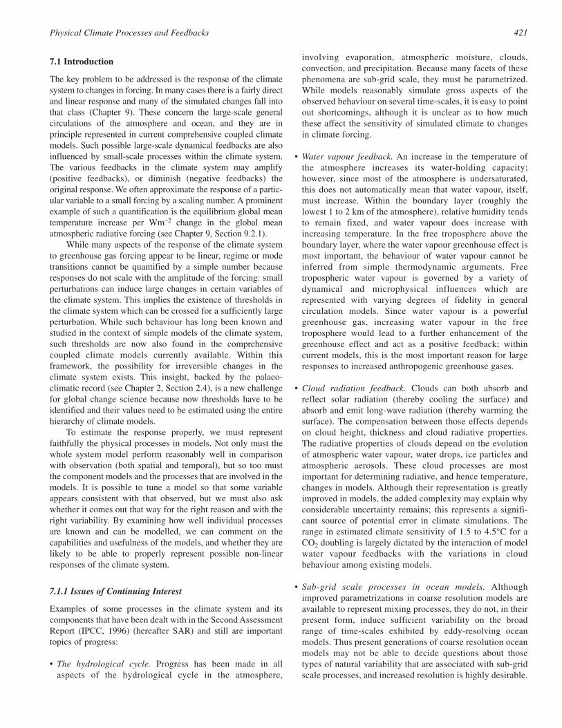
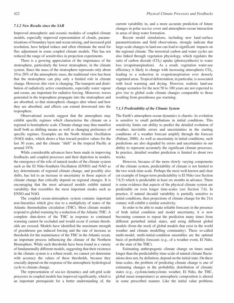
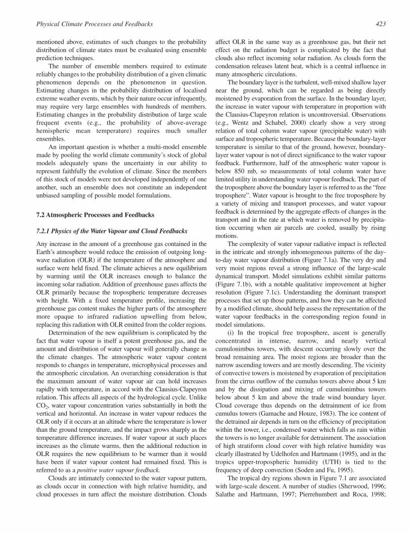
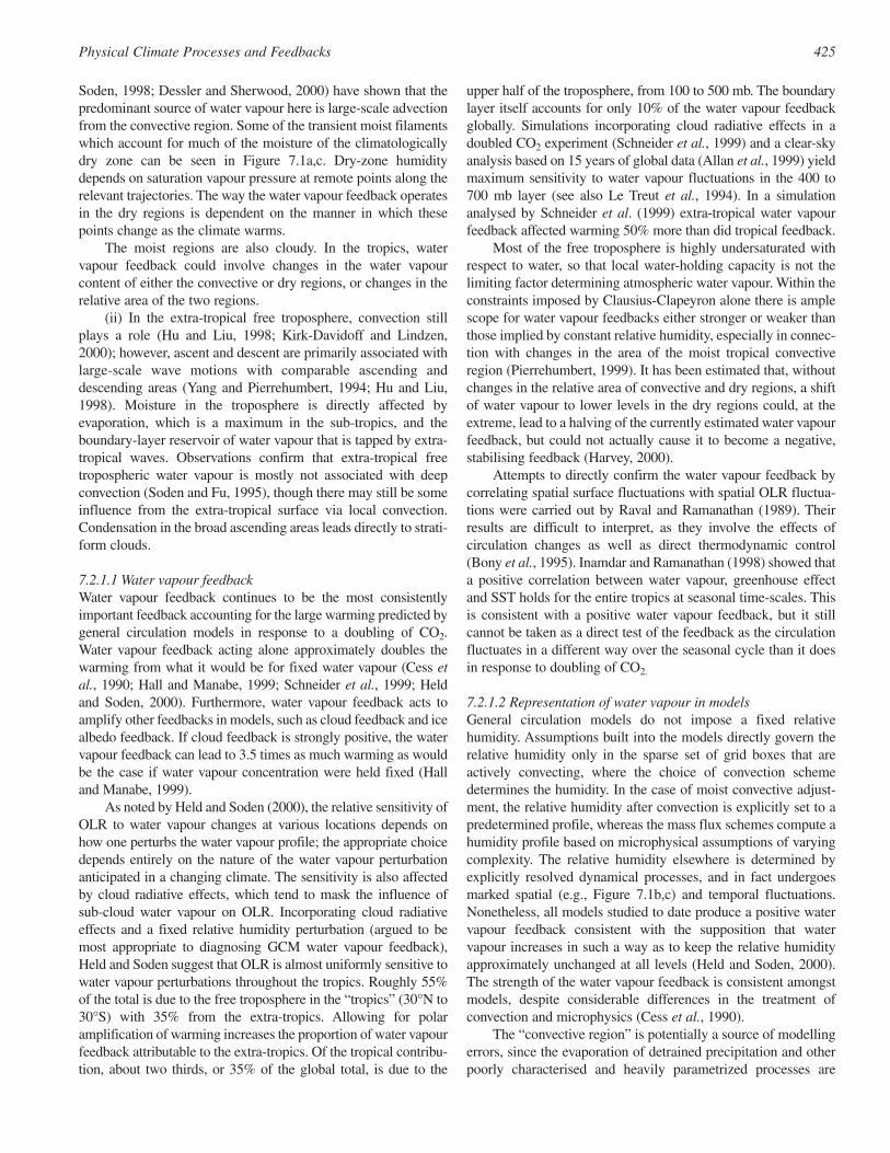
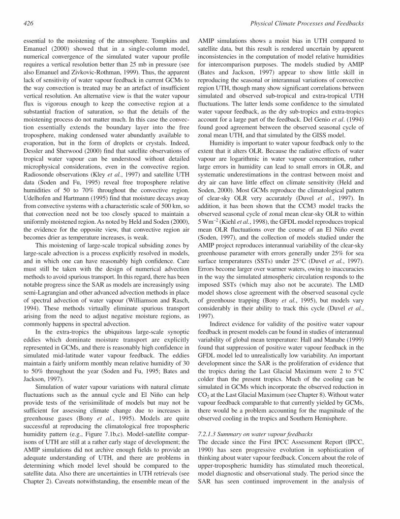
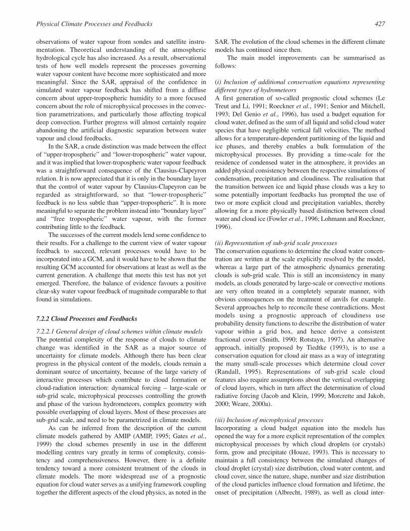
The complexity of water vapour radiative impact is reflectedin the intricate and strongly inhomogeneous patterns of the day-to-day water vapour distribution (Figure 7.1a). The very dry andvery moist regions reveal a strong influence of the large-scaledynamical transport. Model simulations exhibit similar patterns(Figure 7.1b), with a notable qualitative improvement at higherresolution (Figure 7.1c). Understanding the dominant transportprocesses that set up those patterns, and how they can be affectedby a modified climate, should help assess the representation of thewater vapour feedbacks in the corresponding region found inmodel simulations.

(i) In the tropical free troposphere, ascent is generallyconcentrated in intense, narrow, and nearly verticalcumulonimbus towers, with descent occurring slowly over thebroad remaining area. The moist regions are broader than thenarrow ascending towers and are mostly descending. The vicinityof convective towers is moistened by evaporation of precipitationfrom the cirrus outflow of the cumulus towers above about 5 kmand by the dissipation and mixing of cumulonimbus towersbelow about 5 km and above the trade wind boundary layer.Cloud coverage thus depends on the detrainment of ice fromcumulus towers (Gamache and Houze, 1983). The ice content ofthe detrained air depends in turn on the efficiency of precipitationwithin the tower, i.e., condensed water which falls as rain withinthe towers is no longer available for detrainment. The associationof high stratiform cloud cover with high relative humidity wasclearly illustrated by Udelhofen and Hartmann (1995), and in thetropics upper-tropospheric humidity (UTH) is tied to thefrequency of deep convection (Soden and Fu, 1995).

The tropical dry regions shown in Figure 7.1 are associatedwith large-scale descent. A number of studies (Sherwood, 1996;Salathe and Hartmann, 1997; Pierrehumbert and Roca, 1998;



(a)

(b)

(c)

Figure 7.1: Comparison between an observational estimate from satellite radiances and two model simulations of the complex structure of mid-tropospheric water vapour distribution for the date May 5. At any instant, water vapour is unevenly distributed in the atmosphere with very dry areasadjacent to very moist areas. Any modification in the statistics of those areas participates in the atmospheric feedback. The observed small-scalestructure of the strong and variable gradients (a) is not well resolved in a simulation with a climate model of the spatial resolution currently used forclimate projections (b), but simulated with much better fidelity in models with significantly higher resolution (c). (a): Distribution of mean relativehumidity in layer 250 to 600 mb on May 5, 1998, as retrieved from observations on SSM/T-2 satellite (Spencer and Braswell, 1997). Missing data areindicated by black areas and the retrieval is most reliable in the latitude band 30°S to 30°N. (b): Relative humidity at about 400 mb for May 5 of anarbitrary year from a simulation with the GFDL R30L14 atmospheric general circulation model used in the AMIP I simulation (Gates et al., 1999;Lau and Nath, 1999). In small polar areas (about 5% of the globe) some relative humidities are negative (set to zero) due to numerical spectral effects.(c): Relative humidity at 400 mb from the ECHAM4 T106 simulation for May 5 of an arbitrary year (Roeckner et al., 1996; Wild et al., 1998).

Soden, 1998; Dessler and Sherwood, 2000) have shown that thepredominant source of water vapour here is large-scale advectionfrom the convective region. Some of the transient moist filamentswhich account for much of the moisture of the climatologicallydry zone can be seen in Figure 7.1a,c. Dry-zone humiditydepends on saturation vapour pressure at remote points along therelevant trajectories. The way the water vapour feedback operatesin the dry regions is dependent on the manner in which thesepoints change as the climate warms.

The moist regions are also cloudy. In the tropics, watervapour feedback could involve changes in the water vapourcontent of either the convective or dry regions, or changes in therelative area of the two regions.

(ii) In the extra-tropical free troposphere, convection stillplays a role (Hu and Liu, 1998; Kirk-Davidoff and Lindzen,2000); however, ascent and descent are primarily associated withlarge-scale wave motions with comparable ascending anddescending areas (Yang and Pierrehumbert, 1994; Hu and Liu,1998). Moisture in the troposphere is directly affected byevaporation, which is a maximum in the sub-tropics, and theboundary-layer reservoir of water vapour that is tapped by extra-tropical waves. Observations confirm that extra-tropical freetropospheric water vapour is mostly not associated with deepconvection (Soden and Fu, 1995), though there may still be someinfluence from the extra-tropical surface via local convection.Condensation in the broad ascending areas leads directly to strati-form clouds.

7.2.1.1 Water vapour feedbackWater vapour feedback continues to be the most consistentlyimportant feedback accounting for the large warming predicted bygeneral circulation models in response to a doubling of CO2.Water vapour feedback acting alone approximately doubles thewarming from what it would be for fixed water vapour (Cess etal., 1990; Hall and Manabe, 1999; Schneider et al., 1999; Heldand Soden, 2000). Furthermore, water vapour feedback acts toamplify other feedbacks in models, such as cloud feedback and icealbedo feedback. If cloud feedback is strongly positive, the watervapour feedback can lead to 3.5 times as much warming as wouldbe the case if water vapour concentration were held fixed (Halland Manabe, 1999).

As noted by Held and Soden (2000), the relative sensitivity ofOLR to water vapour changes at various locations depends onhow one perturbs the water vapour profile; the appropriate choicedepends entirely on the nature of the water vapour perturbationanticipated in a changing climate. The sensitivity is also affectedby cloud radiative effects, which tend to mask the influence ofsub-cloud water vapour on OLR. Incorporating cloud radiativeeffects and a fixed relative humidity perturbation (argued to bemost appropriate to diagnosing GCM water vapour feedback),Held and Soden suggest that OLR is almost uniformly sensitive towater vapour perturbations throughout the tropics. Roughly 55%of the total is due to the free troposphere in the “tropics” (30°N to30°S) with 35% from the extra-tropics. Allowing for polaramplification of warming increases the proportion of water vapourfeedback attributable to the extra-tropics. Of the tropical contribu-tion, about two thirds, or 35% of the global total, is due to the

upper half of the troposphere, from 100 to 500 mb. The boundarylayer itself accounts for only 10% of the water vapour feedbackglobally. Simulations incorporating cloud radiative effects in adoubled CO2 experiment (Schneider et al., 1999) and a clear-skyanalysis based on 15 years of global data (Allan et al., 1999) yieldmaximum sensitivity to water vapour fluctuations in the 400 to700 mb layer (see also Le Treut et al., 1994). In a simulationanalysed by Schneider et al. (1999) extra-tropical water vapourfeedback affected warming 50% more than did tropical feedback.

Most of the free troposphere is highly undersaturated withrespect to water, so that local water-holding capacity is not thelimiting factor determining atmospheric water vapour. Within theconstraints imposed by Clausius-Clapeyron alone there is amplescope for water vapour feedbacks either stronger or weaker thanthose implied by constant relative humidity, especially in connec-tion with changes in the area of the moist tropical convectiveregion (Pierrehumbert, 1999). It has been estimated that, withoutchanges in the relative area of convective and dry regions, a shiftof water vapour to lower levels in the dry regions could, at theextreme, lead to a halving of the currently estimated water vapourfeedback, but could not actually cause it to become a negative,stabilising feedback (Harvey, 2000).

Attempts to directly confirm the water vapour feedback bycorrelating spatial surface fluctuations with spatial OLR fluctua-tions were carried out by Raval and Ramanathan (1989). Theirresults are difficult to interpret, as they involve the effects ofcirculation changes as well as direct thermodynamic control(Bony et al., 1995). Inamdar and Ramanathan (1998) showed thata positive correlation between water vapour, greenhouse effectand SST holds for the entire tropics at seasonal time-scales. Thisis consistent with a positive water vapour feedback, but it stillcannot be taken as a direct test of the feedback as the circulationfluctuates in a different way over the seasonal cycle than it doesin response to doubling of CO2.

7.2.1.2 Representation of water vapour in modelsGeneral circulation models do not impose a fixed relativehumidity. Assumptions built into the models directly govern therelative humidity only in the sparse set of grid boxes that areactively convecting, where the choice of convection schemedetermines the humidity. In the case of moist convective adjust-ment, the relative humidity after convection is explicitly set to apredetermined profile, whereas the mass flux schemes compute ahumidity profile based on microphysical assumptions of varyingcomplexity. The relative humidity elsewhere is determined byexplicitly resolved dynamical processes, and in fact undergoesmarked spatial (e.g., Figure 7.1b,c) and temporal fluctuations.Nonetheless, all models studied to date produce a positive watervapour feedback consistent with the supposition that watervapour increases in such a way as to keep the relative humidityapproximately unchanged at all levels (Held and Soden, 2000).The strength of the water vapour feedback is consistent amongstmodels, despite considerable differences in the treatment ofconvection and microphysics (Cess et al., 1990).

The “convective region” is potentially a source of modellingerrors, since the evaporation of detrained precipitation and otherpoorly characterised and heavily parametrized processes are


essential to the moistening of the atmosphere. Tompkins andEmanuel (2000) showed that in a single-column model,numerical convergence of the simulated water vapour profilerequires a vertical resolution better than 25 mb in pressure (seealso Emanuel and Zivkovic-Rothman, 1999). Thus, the apparentlack of sensitivity of water vapour feedback in current GCMs tothe way convection is treated may be an artefact of insufficientvertical resolution. An alternative view is that the water vapourflux is vigorous enough to keep the convective region at asubstantial fraction of saturation, so that the details of themoistening process do not matter much. In this case the convec-tion essentially extends the boundary layer into the freetroposphere, making condensed water abundantly available toevaporation, but in the form of droplets or crystals. Indeed,Dessler and Sherwood (2000) find that satellite observations oftropical water vapour can be understood without detailedmicrophysical considerations, even in the convective region.Radiosonde observations (Kley et al., 1997) and satellite UTHdata (Soden and Fu, 1995) reveal free troposphere relativehumidities of 50 to 70% throughout the convective region.Udelhofen and Hartmann (1995) find that moisture decays awayfrom convective systems with a characteristic scale of 500 km, sothat convection need not be too closely spaced to maintain auniformly moistened region. As noted by Held and Soden (2000),the evidence for the opposite view, that convective region airbecomes drier as temperature increases, is weak.

This moistening of large-scale tropical subsiding zones bylarge-scale advection is a process explicitly resolved in models,and in which one can have reasonably high confidence. Caremust still be taken with the design of numerical advectionmethods to avoid spurious transport. In this regard, there has beennotable progress since the SAR as models are increasingly usingsemi-Lagrangian and other advanced advection methods in placeof spectral advection of water vapour (Williamson and Rasch,1994). These methods virtually eliminate spurious transportarising from the need to adjust negative moisture regions, ascommonly happens in spectral advection.

In the extra-tropics the ubiquitous large-scale synopticeddies which dominate moisture transport are explicitlyrepresented in GCMs, and there is reasonably high confidence insimulated mid-latitude water vapour feedback. The eddiesmaintain a fairly uniform monthly mean relative humidity of 30to 50% throughout the year (Soden and Fu, 1995; Bates andJackson, 1997).

Simulation of water vapour variations with natural climatefluctuations such as the annual cycle and El Niño can helpprovide tests of the verisimilitude of models but may not besufficient for assessing climate change due to increases ingreenhouse gases (Bony et al., 1995). Models are quitesuccessful at reproducing the climatological free tropospherichumidity pattern (e.g., Figure 7.1b,c). Model-satellite compar-isons of UTH are still at a rather early stage of development; theAMIP simulations did not archive enough fields to provide anadequate understanding of UTH, and there are problems indetermining which model level should be compared to thesatellite data. Also there are uncertainties in UTH retrievals (seeChapter 2). Caveats notwithstanding, the ensemble mean of the

AMIP simulations shows a moist bias in UTH compared tosatellite data, but this result is rendered uncertain by apparentinconsistencies in the computation of model relative humiditiesfor intercomparison purposes. The models studied by AMIP(Bates and Jackson, 1997) appear to show little skill inreproducing the seasonal or interannual variations of convectiveregion UTH, though many show significant correlations betweensimulated and observed sub-tropical and extra-tropical UTHfluctuations. The latter lends some confidence to the simulatedwater vapour feedback, as the dry sub-tropics and extra-tropicsaccount for a large part of the feedback. Del Genio et al. (1994)found good agreement between the observed seasonal cycle ofzonal mean UTH, and that simulated by the GISS model.

Humidity is important to water vapour feedback only to theextent that it alters OLR. Because the radiative effects of watervapour are logarithmic in water vapour concentration, ratherlarge errors in humidity can lead to small errors in OLR, andsystematic underestimations in the contrast between moist anddry air can have little effect on climate sensitivity (Held andSoden, 2000). Most GCMs reproduce the climatological patternof clear-sky OLR very accurately (Duvel et al., 1997). Inaddition, it has been shown that the CCM3 model tracks theobserved seasonal cycle of zonal mean clear-sky OLR to within5 Wm−2 (Kiehl et al., 1998), the GFDL model reproduces tropicalmean OLR fluctuations over the course of an El Niño event(Soden, 1997), and the collection of models studied under theAMIP project reproduces interannual variability of the clear-skygreenhouse parameter with errors generally under 25% for seasurface temperatures (SSTs) under 25°C (Duvel et al., 1997).Errors become larger over warmer waters, owing to inaccuraciesin the way the simulated atmospheric circulation responds to theimposed SSTs (which may also not be accurate). The LMDmodel shows close agreement with the observed seasonal cycleof greenhouse trapping (Bony et al., 1995), but models varyconsiderably in their ability to track this cycle (Duvel et al.,1997).

Indirect evidence for validity of the positive water vapourfeedback in present models can be found in studies of interannualvariability of global mean temperature: Hall and Manabe (1999)found that suppression of positive water vapour feedback in theGFDL model led to unrealistically low variability. An importantdevelopment since the SAR is the proliferation of evidence thatthe tropics during the Last Glacial Maximum were 2 to 5°Ccolder than the present tropics. Much of the cooling can besimulated in GCMs which incorporate the observed reduction inCO2 at the Last Glacial Maximum (see Chapter 8). Without watervapour feedback comparable to that currently yielded by GCMs,there would be a problem accounting for the magnitude of theobserved cooling in the tropics and Southern Hemisphere.

7.2.1.3 Summary on water vapour feedbacksThe decade since the First IPCC Assessment Report (IPCC,1990) has seen progressive evolution in sophistication ofthinking about water vapour feedback. Concern about the role ofupper-tropospheric humidity has stimulated much theoretical,model diagnostic and observational study. The period since theSAR has seen continued improvement in the analysis of


observations of water vapour from sondes and satellite instru-mentation. Theoretical understanding of the atmospherichydrological cycle has also increased. As a result, observationaltests of how well models represent the processes governingwater vapour content have become more sophisticated and moremeaningful. Since the SAR, appraisal of the confidence insimulated water vapour feedback has shifted from a diffuseconcern about upper-tropospheric humidity to a more focusedconcern about the role of microphysical processes in the convec-tion parametrizations, and particularly those affecting tropicaldeep convection. Further progress will almost certainly requireabandoning the artificial diagnostic separation between watervapour and cloud feedbacks.

In the SAR, a crude distinction was made between the effectof “upper-tropospheric” and “lower-tropospheric” water vapour,and it was implied that lower-tropospheric water vapour feedbackwas a straightforward consequence of the Clausius-Clapeyronrelation. It is now appreciated that it is only in the boundary layerthat the control of water vapour by Clausius-Clapeyron can beregarded as straightforward, so that “lower-tropospheric”feedback is no less subtle than “upper-tropospheric”. It is moremeaningful to separate the problem instead into “boundary layer”and “free tropospheric” water vapour, with the formercontributing little to the feedback.

The successes of the current models lend some confidence totheir results. For a challenge to the current view of water vapourfeedback to succeed, relevant processes would have to beincorporated into a GCM, and it would have to be shown that theresulting GCM accounted for observations at least as well as thecurrent generation. A challenge that meets this test has not yetemerged. Therefore, the balance of evidence favours a positiveclear-sky water vapour feedback of magnitude comparable to thatfound in simulations.

7.2.2 Cloud Processes and Feedbacks

7.2.2.1 General design of cloud schemes within climate modelsThe potential complexity of the response of clouds to climatechange was identified in the SAR as a major source ofuncertainty for climate models. Although there has been clearprogress in the physical content of the models, clouds remain adominant source of uncertainty, because of the large variety ofinteractive processes which contribute to cloud formation orcloud-radiation interaction: dynamical forcing – large-scale orsub-grid scale, microphysical processes controlling the growthand phase of the various hydrometeors, complex geometry withpossible overlapping of cloud layers. Most of these processes aresub-grid scale, and need to be parametrized in climate models.

As can be inferred from the description of the currentclimate models gathered by AMIP (AMIP, 1995; Gates et al.,1999) the cloud schemes presently in use in the differentmodelling centres vary greatly in terms of complexity, consis-tency and comprehensiveness. However, there is a definitetendency toward a more consistent treatment of the clouds inclimate models. The more widespread use of a prognosticequation for cloud water serves as a unifying framework couplingtogether the different aspects of the cloud physics, as noted in the

SAR. The evolution of the cloud schemes in the different climatemodels has continued since then.

The main model improvements can be summarised asfollows:

(i) Inclusion of additional conservation equations representingdifferent types of hydrometeorsA first generation of so-called prognostic cloud schemes (LeTreut and Li, 1991; Roeckner et al., 1991; Senior and Mitchell,1993; Del Genio et al., 1996), has used a budget equation forcloud water, defined as the sum of all liquid and solid cloud waterspecies that have negligible vertical fall velocities. The methodallows for a temperature-dependent partitioning of the liquid andice phases, and thereby enables a bulk formulation of themicrophysical processes. By providing a time-scale for theresidence of condensed water in the atmosphere, it provides anadded physical consistency between the respective simulations ofcondensation, precipitation and cloudiness. The realisation thatthe transition between ice and liquid phase clouds was a key tosome potentially important feedbacks has prompted the use oftwo or more explicit cloud and precipitation variables, therebyallowing for a more physically based distinction between cloudwater and cloud ice (Fowler et al., 1996; Lohmann and Roeckner,1996).

(ii) Representation of sub-grid scale processesThe conservation equations to determine the cloud water concen-tration are written at the scale explicitly resolved by the model,whereas a large part of the atmospheric dynamics generatingclouds is sub-grid scale. This is still an inconsistency in manymodels, as clouds generated by large-scale or convective motionsare very often treated in a completely separate manner, withobvious consequences on the treatment of anvils for example.Several approaches help to reconcile these contradictions. Mostmodels using a prognostic approach of cloudiness useprobability density functions to describe the distribution of watervapour within a grid box, and hence derive a consistentfractional cover (Smith, 1990; Rotstayn, 1997). An alternativeapproach, initially proposed by Tiedtke (1993), is to use aconservation equation for cloud air mass as a way of integratingthe many small-scale processes which determine cloud cover(Randall, 1995). Representations of sub-grid scale cloudfeatures also require assumptions about the vertical overlappingof cloud layers, which in turn affect the determination of cloudradiative forcing (Jacob and Klein, 1999; Morcrette and Jakob,2000; Weare, 2000a).

(iii) Inclusion of microphysical processesIncorporating a cloud budget equation into the models hasopened the way for a more explicit representation of the complexmicrophysical processes by which cloud droplets (or crystals)form, grow and precipitate (Houze, 1993). This is necessary tomaintain a full consistency between the simulated changes ofcloud droplet (crystal) size distribution, cloud water content, andcloud cover, since the nature, shape, number and size distributionof the cloud particles influence cloud formation and lifetime, theonset of precipitation (Albrecht, 1989), as well as cloud inter-


action with radiation, in both the solar and long-wave bands(Twomey, 1974). Some parametrizations of sub-grid scalecondensation, such as convective schemes, are also comple-mented by a consistent treatment of the microphysical processes(Sud and Walker, 1999).

In warm clouds these microphysical processes include thecollection of water molecules on a foreign substance (hetero-geneous nucleation on a cloud condensation nucleus), diffusion,collection of smaller drops when falling through a cloud (coales-cence), break-up of drops when achieving a certain threshold size,and re-evaporation of drops when falling through a layer ofunsaturated air. In cold clouds, ice particles may be nucleated fromeither the liquid or vapour phase, and spontaneous homogeneousfreezing of supercooled liquid drops is also relevant at tempera-tures below approximately –40°C. At higher temperatures theformation of ice particles is dominated by heterogeneousnucleation of water vapour on ice condensation nuclei. Subsequentgrowth of ice particles is then due to diffusion of vapour towardthe particle (deposition), collection of other ice particles (aggrega-tion), and collection of supercooled drops which freeze on contact(riming). An increase in ice particles may occur by fragmentation.Falling ice particles may melt when they come into contact withair or liquid particles with temperatures above 0°C.

Heterogeneous nucleation of soluble particles and theirsubsequent incorporation into precipitation is also an importantmechanism for their removal, and is the main reason for theindirect aerosol effect. The inclusion of microphysical processes inGCMs has produced an impact on the simulation of the meanclimate (Hahmann and Dickinson, 1997).

Measurements of cloud drop size distribution indicate asignificant difference in the total number of drops and dropeffective radius in the continental and maritime atmosphere, andsome studies indicate that inclusion of more realistic drop sizedistribution may have a significant impact on the simulation of thepresent climate (Hahmann and Dickinson, 1997).

7.2.2.2 Convective processesThe interplay of buoyancy, moisture and condensation on scalesranging from millimetres to tens of kilometres is the definingphysical feature of atmospheric convection, and is the source ofmuch of the challenge in representing convection in climatemodels. Deep convection is in large measure responsible for thevery existence of the troposphere. Air typically receives itsbuoyancy through being heated by contact with a warm, solar-heated underlying surface, and convection redistributes the energyreceived by the surface upwards throughout the troposphere.Shallow convection also figures importantly in the structure of theatmospheric boundary layer and will be addressed in Section7.2.2.3.

Latent heat release in convection drives many of theimportant atmospheric circulations, and is a key link in the cycleof atmosphere-ocean feedbacks leading to the ENSO phenom-enon. Convection is a principal means of transporting moisturevertically, which implies a role of convection in the radiativefeedback due to both water vapour and clouds. Convection alsoin large measure determines the vertical temperature lapse rate ofthe atmosphere, and particularly so in the tropics. A strong

decrease of temperature with height enhances the greenhouseeffect, whereas a weaker temperature decrease ameliorates it. Theeffect of lapse rate changes on clear-sky water vapour feedbackhas been studied by Zhang et al. (1994), but the significance ofthe lapse rate contribution (cf. item (5) of the SAR, TechnicalSummary) has been somewhat exaggerated through a misinter-pretation of the paper. In fact the variation in lapse rate effectsamong the models studied alters the water vapour feedback factorby only 0.25 W/(m2K), or about 10% of the total (Table 1 ofZhang et al., 1994).

There is ample theoretical and observational evidence thatdeep moist convection locally establishes a “moist adiabatic”temperature profile that, loosely speaking, is neutrally buoyantwith respect to ascending, condensing parcels (Betts, 1982; Xuand Emanuel, 1989). This adjustment happens directly at the scaleof individual convective clouds, but dynamical processesplausibly extend the radius of influence of the adjustment to thescale of a typical GCM grid box, and probably much further in thetropics, where the lapse rate adjusts close to the moist adiabatalmost everywhere. All convective schemes, from the most simpleMoist Adiabatic Adjustment to those which attempt a representa-tion of cloud-scale motions (Arakawa and Schubert, 1974;Emanuel, 1991), therefore agree in that they maintain the temper-ature at a nearly moist adiabatic profile. Moist AdiabaticAdjustment explicitly resets the temperature to the desired profile,whereas mass flux schemes achieve the adjustment to a near-adiabat as a consequence of equations governing the parametrizedconvective heating field. The constraint on temperature, however,places only a limited constraint on the moisture profile remainingafter adjustment, and the performance in terms of moisture, cloudsand precipitation may be very variable.

Since the SAR, a variety of simulations of response to CO2

doubling accounting for combinations of different parametriza-tions have been realised with different models (Colman andMcAvaney, 1995; Yao and Del Genio, 1999; Meleshko et al.,2000). The general effects of the convection parametrization onclimate sensitivity are difficult to assess because the way a modelresponds to changes in convection depends on a range of otherparametrizations, so results are somewhat inconsistent betweenmodels (Colman and McAvaney, 1995; Thompson and Pollard,1995; Zhang and McFarlane, 1995). There is some indication thatthe climate sensitivity in models with strong negative cloudfeedback is insensitive to convective parametrization whereasmodels with strong positive cloud feedback show more sensitivity(Meleshko et al., 2000).

7.2.2.3 Boundary-layer mixing and cloudinessTurbulent motions affect all exchanges of heat, water, momentumand chemical constituents between the surface and theatmosphere, and these motions are also responsible for the mixingprocesses inside the atmospheric boundary layer. Consequently,the turbulent motions impact on the formation and existence offog and boundary-layer clouds such as cumulus, stratocumulusand stratus. Cumulus is typically found in fair weather conditionsover land and sea, while layers of stratocumulus and stratus can befound in subsidence areas such as the anticyclonic areas in theeastern part of the sub-tropical oceans, or the polar regions.


The atmospheric boundary layer with clouds is typicallycharacterised by a well-mixed sub-cloud layer of order 500metres, and by a more extended conditionally unstable layerwith boundary-layer clouds up to 2 km. The latter layer is veryoften capped by a temperature inversion. If the clouds are of thestratocumulus or stratus type, then conservative quantities areapproximately well mixed in the cloud layer. The lowest part(say 10%) of the sub-cloud layer is known as the surface layer.In this layer the vertical gradients of variables are normallysignificant, even with strong turbulent mixing. Physicalproblems associated with the surface layer depend strongly onthe type of surface considered (such as vegetation, snow, ice,steep orography) and are treated in the corresponding sub-sections. We note that the surface characteristics do impact onthe formation of boundary-layer clouds, because of theturbulent mixing inside the boundary layer.

Atmospheric models have great difficulty in the properrepresentation of turbulent mixing processes in general. Thisalso impacts on the representation of boundary-layer clouds. Atpresent, the underprediction of boundary-layer clouds is stillone of the most distinctive and permanent errors of AGCMs.This has been demonstrated through AMIP intercomparisons byWeare and Mokhov (1995) and also by Weare (2000b). It has avery great importance, because the albedo effect of these cloudsis not compensated for by a significant greenhouse effect inboth clear-sky and cloudy conditions.

The persisting difficulty in simulation of observedboundary layer cloud properties is a clear testimony of the stillinadequate representation of boundary-layer processes. Avariety of approaches is followed, ranging from bulk schemes inwhich the assumption of a well-mixed layer is made a priori, todiscretised approaches considering diffusion between a numberof vertical layers. Here the corresponding diffusion coefficientsare being computed from dimensional analysis and observa-tional data fitted to it. The use of algorithms based on theprognostic computation of turbulent kinetic energy and higher-order closure hypotheses is also becoming more common andnew schemes continue to be proposed (Abdella and McFarlane,1997). A critical review and evaluation of boundary-layerschemes was recently made by Ayotte et al. (1996). They foundthat all schemes have difficulty with representing the entrain-ment processes at the top of even the clear boundary layer.

Important and still open problems include the decouplingbetween the turbulence at the surface and that within clouds, thenon-local treatment of semi-convective cells (thermals) that cantransport heat and substances upward, the role of moist physics,and microphysical aspects (Ricard and Royer, 1993; Moeng etal., 1995; Cuijpers and Holtslag, 1998; Grenier and Bretherton,2001). Several studies (Moeng et al., 1996; Bretherton et al.,1999; Duynkerke et al., 1999) show that column versions of theclimate models may predict a reasonable cloud cover inresponse to observed initial and boundary conditions, but havemore difficulty in maintaining realistic turbulent fluxes. Theresults are also very dependent on vertical resolution andnumerical aspects (Lenderink and Holtslag, 2000). This pointsto the need for new approaches for boundary-layer turbulence,both for clear-sky and cloudy conditions which are not so

sensitive to vertical resolution (see also contributions inHoltslag and Duynkerke, 1998).

7.2.2.4 Cloud-radiative feedback processesClouds affect radiation both through their three-dimensionalgeometry and the amount, size and nature of the hydrometeorswhich they contain. In climate models these propertiestranslate into cloud cover at different levels, cloud watercontent (for liquid water and ice) and cloud droplet (or crystal)equivalent radius. The interaction of clouds and radiation alsoinvolves other parameters (asymmetry factor of the Miediffusion) which depend on cloud composition, and mostnotably on their phase. The subtle balance between cloudimpact on the solar short-wave (SW) and terrestrial long-wave(LW) radiation may be altered by a change in any of thoseparameters. In response to any climate perturbation theresponse of cloudiness thereby introduces feedbacks whosesign and amplitude are largely unknown. While the SAR notedsome convergence in the cloud radiative feedback simulated bydifferent models between two successive intercomparisons(Cess et al., 1990, 1995, 1996), this convergence was notconfirmed by a separate consideration of the SW and LWcomponents.

Schemes predicting cloudiness as a function of relativehumidity generally show an upward displacement of the highertroposphere cloud cover in response to a greenhouse warming,resulting in a positive feedback (Manabe and Wetherald, 1987).While this effect still appears in more sophisticated models,and even cloud resolving models (Wu and Moncrieff, 1999;Tompkins and Emanuel, 2000), the introduction of cloud watercontent as a prognostic variable, by decoupling cloud andwater vapour, has added new features (Senior and Mitchell,1993; Lee et al., 1997). As noted in the SAR, a negativefeedback corresponding to an increase in cloud cover, andhence cloud albedo, at the transition between ice and liquidclouds occurs in some models, but is crucially dependent onthe definition of the phase transition within models. The signof the cloud cover feedback is still a matter of uncertainty andgenerally depends on other related cloud properties (Yao andDel Genio, 1999; Meleshko et al., 2000).

Most GCMs used for climate simulations now includeinteractive cloud optical properties. Cloud optical feedbacksproduced by these GCMs, however, differ both in sign andstrength. The transition between water and ice may be a sourceof error, but even for a given water phase, the sign of thevariation of cloud optical properties with temperature can be amatter of controversy. Analysis from the ISCCP data set, forexample, revealed a decrease of low cloud optical thicknesswith cloud temperature in the sub-tropical and tropicallatitudes and an increase at middle latitudes in winter(Tselioudis et al., 1992; Tselioudis and Rossow, 1994). Asimilar relationship between cloud liquid water path and cloudtemperature was found in an analysis of microwave satelliteobservations (Greenwald et al., 1995). This is opposite to theassumptions on adiabatic increase of cloud liquid watercontent with temperature, adopted in early studies, and stillpresent in many models. Changes in cloud water path reflect


different effects which may partially compensate, such aschanges in cloud vertical extension or cloud water content. Therole of low cloud optical thickness dependence on climate wastested in 2×CO2 experiments using the GISS GCM, in whichsimulations with fixed or simulated cloud optical propertieswere compared (Tselioudis et al., 1998). In spite of a lowimpact on global sensitivity, these results showed a strong cloudimpact on the latitudinal distribution of the warming. Highlatitude warming decreased while low latitude warmingincreased, resulting in a large decrease in the latitudinal amplifi-cation of the warming (by 20% in the Northern Hemisphere andby 40% in the Southern Hemisphere).

Since the SAR, there has been much progress in the use ofsimplified tropical models to understand the impact of cloud

feedbacks, and to address the issue of whether cloud feedbacksimpose an upper limit on SST. This problem has been addressedin simplified models that maintain consistency with the whole-tropics energy budget (Pierrehumbert, 1995; Clement andSeager, 1999; Larson et al., 1999). Diagnostic studies havesuggested both destabilising (Chou and Neelin, 1999) andstabilising (Lindzen et al., 2001) cloud feedbacks. None of thissupports the existence of a strict limitation of maximum tropicalSST of the sort proposed by Ramanathan and Collins (1991),which has been criticised on the grounds that it does not respectthe whole-tropics energy budget, and that it employs anincorrect means of determining the threshold temperature forconvection. It is beyond question that the increased cloudinessprevailing over the warmer portions of the Pacific has a strongeffect on the surface energy budget, which is fully competitivewith the importance of evaporation. Determination of SST,however, requires a consistent treatment of the top-of-atmosphere energy budget, and cannot be effected withreference to the surface budget alone. This does not precludethe possibility that other cloud feedback mechanisms couldhave a profound effect on tropical SST, and in no way impliesthat cloud representation is inconsequential in the tropics.Meehl et al. (2000) illustrate this point when they show how achange from a diagnostic prescription of clouds in the NCARatmospheric GCM to a prognostic cloud liquid water formula-tion changes the sign of net cloud forcing in the eastern tropicalPacific and completely alters the nature of the coupled modelresponse to increased greenhouse gases.


BMRC NCAR MGO CSIRO MPI UKMO GFDL CCSR LMD MRI–3

–2

–1

0

1

2

3

Cha

nge

in c

loud

rad

iativ

e fo

rcin

g at

top

of th

e at

mos

pher

e (W

m−2

)

SW

LW

NET

2 3 4 5 6 7 8–2

–1

0

1

2

3

Precipitable water (mm)

Clo

ud r

adia

tive

forc

ing

(Wm

–2)

r 2=0.899

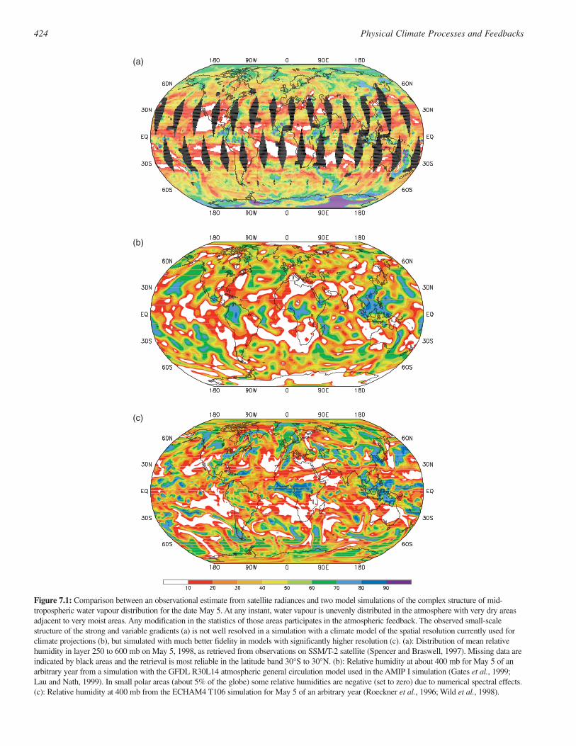
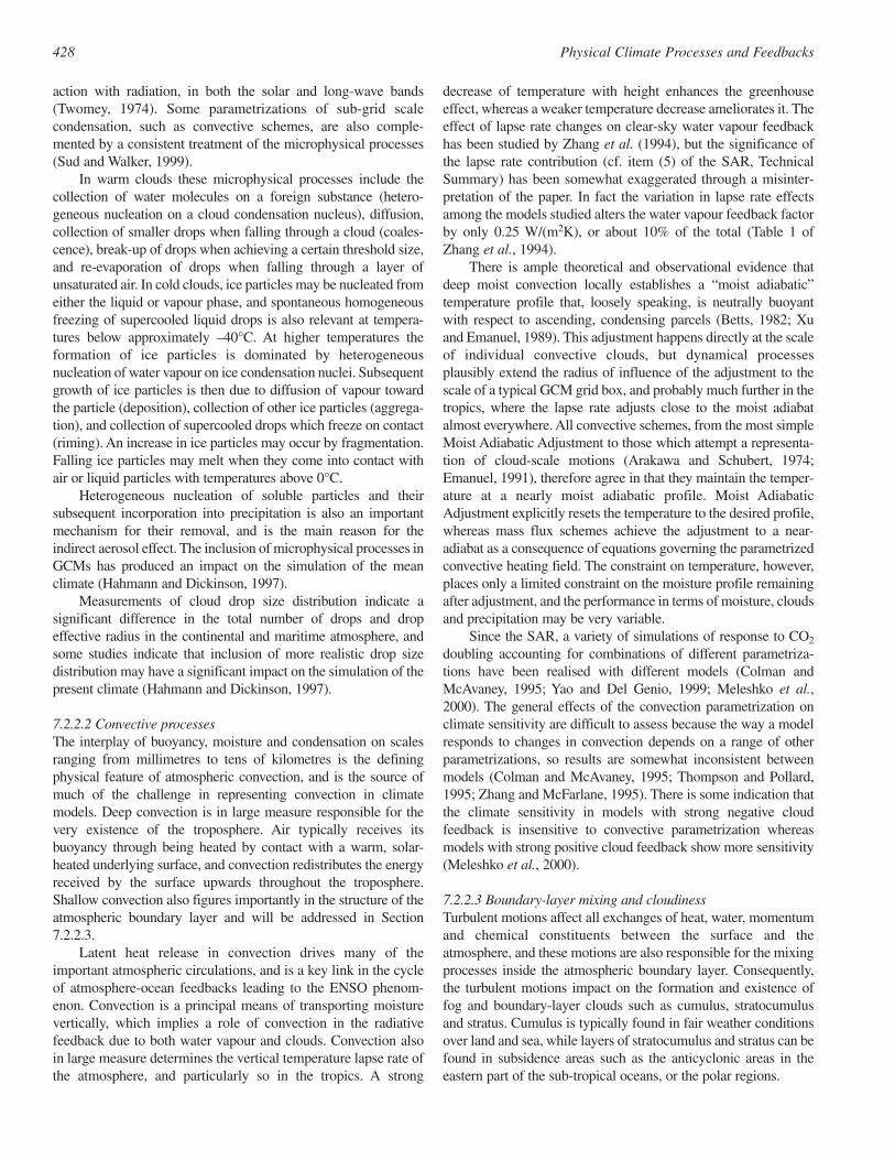
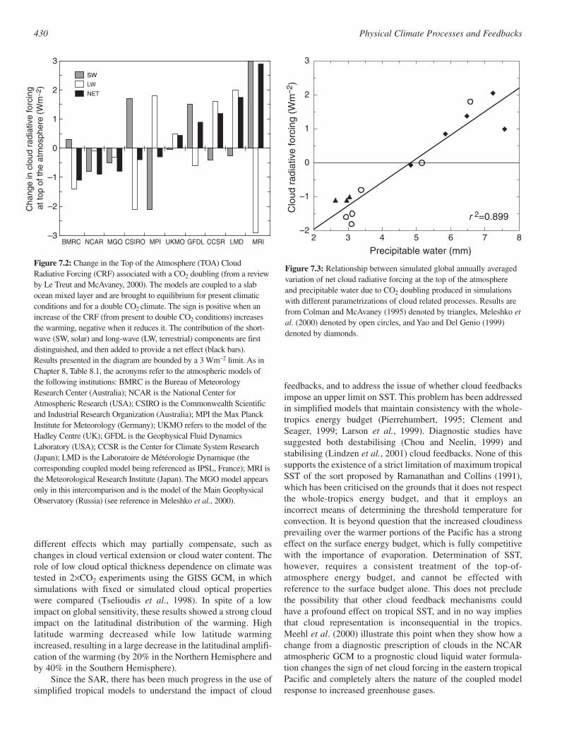
Figure 7.2: Change in the Top of the Atmosphere (TOA) CloudRadiative Forcing (CRF) associated with a CO2 doubling (from a reviewby Le Treut and McAvaney, 2000). The models are coupled to a slabocean mixed layer and are brought to equilibrium for present climaticconditions and for a double CO2 climate. The sign is positive when anincrease of the CRF (from present to double CO2 conditions) increasesthe warming, negative when it reduces it. The contribution of the short-wave (SW, solar) and long-wave (LW, terrestrial) components are firstdistinguished, and then added to provide a net effect (black bars).Results presented in the diagram are bounded by a 3 Wm−2 limit. As inChapter 8, Table 8.1, the acronyms refer to the atmospheric models ofthe following institutions: BMRC is the Bureau of MeteorologyResearch Center (Australia); NCAR is the National Center forAtmospheric Research (USA); CSIRO is the Commonwealth Scientificand Industrial Research Organization (Australia); MPI the Max PlanckInstitute for Meteorology (Germany); UKMO refers to the model of theHadley Centre (UK); GFDL is the Geophysical Fluid DynamicsLaboratory (USA); CCSR is the Center for Climate System Research(Japan); LMD is the Laboratoire de Météorologie Dynamique (thecorresponding coupled model being referenced as IPSL, France); MRI isthe Meteorological Research Institute (Japan). The MGO model appearsonly in this intercomparison and is the model of the Main GeophysicalObservatory (Russia) (see reference in Meleshko et al., 2000).

Figure 7.3: Relationship between simulated global annually averagedvariation of net cloud radiative forcing at the top of the atmosphereand precipitable water due to CO2 doubling produced in simulationswith different parametrizations of cloud related processes. Results arefrom Colman and McAvaney (1995) denoted by triangles, Meleshko etal. (2000) denoted by open circles, and Yao and Del Genio (1999)denoted by diamonds.

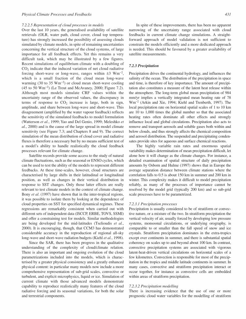
7.2.2.5 Representation of cloud processes in modelsOver the last 10 years, the generalised availability of satelliteretrievals (OLR, water path, cloud cover, cloud top tempera-ture) has strongly increased the possibility of assessing cloudssimulated by climate models, in spite of remaining uncertaintiesconcerning the vertical structure of the cloud systems, of largeimportance for all feedback effects. Yet this remains a verydifficult task, which may be illustrated by a few figures.Recent simulations of equilibrium climate with a doubling ofCO2 indicate that the induced variation of net cloud radiativeforcing short-wave or long-wave, ranges within ±3 Wm−2,which is a small fraction of the cloud mean long-wavewarming (30 to 35 Wm−2) or cloud mean short-wave cooling(45 to 50 Wm−2) (Le Treut and McAvaney, 2000; Figure 7.2).Although most models simulate CRF values within theuncertainty range of the observed values, the discrepancy interms of response to CO2 increase is large, both in sign,amplitude, and share between long-wave and short-wave. Thisdisagreement (amplified by the water vapour feedback) reflectsthe sensitivity of the simulated feedbacks to model formulation(Watterson et al., 1999; Yao and Del Genio, 1999; Meleshko etal., 2000) and is the cause of the large spread in model climatesensitivity (see Figure 7.3; and Chapters 8 and 9). The correctsimulation of the mean distribution of cloud cover and radiativefluxes is therefore a necessary but by no means sufficient test ofa model’s ability to handle realistically the cloud feedbackprocesses relevant for climate change.

Satellite records provide some access to the study of naturalclimate fluctuations, such as the seasonal or ENSO cycles, whichcan be used to test the ability of the models to represent differentfeedbacks. At these time-scales, however, cloud structures arecharacterised by large shifts in their latitudinal or longitudinalposition, as well as changes in their vertical distribution inresponse to SST changes. Only those latter effects are reallyrelevant to test climate models in the context of climate change.Bony et al. (1997) have shown that in the inter-tropical regions,it was possible to isolate them by looking at the dependence ofcloud properties on SST for specified dynamical regimes. Theseregressions are remarkably consistent when carried out withdifferent sets of independent data (ISCCP, ERBE, TOVS, SSMI)and offer a constraining test for models. Similar methodologiesare being developed for the mid-latitudes (Tselioudis et al.,2000). It is encouraging, though, that CCM3 has demonstratedconsiderable accuracy in the reproduction of regional all-skylong-wave and short-wave radiation budgets (Kiehl et al., 1998).

Since the SAR, there has been progress in the qualitativeunderstanding of the complexity of cloud/climate relation.There is also an important and ongoing evolution of the cloudparametrizations included into the models, which is charac-terised by a greater physical consistency and a greatly enhancedphysical content: in particular many models now include a morecomprehensive representation of sub-grid scales, convective orturbulent, and explicit microphysics, liquid or ice. Simulation ofcurrent climate with those advanced models demonstratecapability to reproduce realistically many features of the cloudradiative forcing and its seasonal variations, for both the solarand terrestrial components.

In spite of these improvements, there has been no apparentnarrowing of the uncertainty range associated with cloudfeedbacks in current climate change simulations. A straight-forward approach of model validation is not sufficient toconstrain the models efficiently and a more dedicated approachis needed. This should be favoured by a greater availability ofsatellite measurements.

7.2.3 Precipitation

Precipitation drives the continental hydrology, and influences thesalinity of the ocean. The distribution of the precipitation in spaceand time, is therefore of key importance. The amount of precipi-tation also constitutes a measure of the latent heat release withinthe atmosphere. The long-term global mean precipitation of 984mm/yr implies a vertically integrated mean heating rate of 78Wm−2 (Arkin and Xie, 1994; Kiehl and Trenberth, 1997). Thelocal precipitation rate on horizontal spatial scales of 1 to 10 kmare 10 to 1,000 times the global number so that the associatedheating rates often dominate all other effects and stronglyinfluence local and global circulations. Precipitation also acts toremove and transport aerosols and soluble gases both within andbelow clouds, and thus strongly affects the chemical compositionand aerosol distribution. The suspended and precipitating conden-sates provide sites for aqueous and surface chemical reactions.

The highly variable rain rates and enormous spatialvariability makes determination of mean precipitation difficult, letalone how it will change as the climate changes. For instance, adetailed examination of spatial structure of daily precipitationamounts by Osborn and Hulme (1997) shows that in Europe theaverage separation distance between climate stations where thecorrelation falls to 0.5 is about 150 km in summer and 200 km inwinter. This complexity makes it difficult to model precipitationreliably, as many of the processes of importance cannot beresolved by the model grid (typically 200 km) and so sub-gridscale processes have to be parametrized.

7.2.3.1 Precipitation processes Precipitation is usually considered to be of stratiform or convec-tive nature, or a mixture of the two. In stratiform precipitation thevertical velocity of air, usually forced by developing low pressuresystems, monsoonal circulations, or underlying orography, iscomparable to or smaller than the fall speed of snow and icecrystals. Stratiform precipitation dominates in the extra-tropicsexcept over continents in summer, and there is substantial spatialcoherency on scales up to and beyond about 100 km. In contrast,convective precipitation systems are associated with vigorouslatent-heat-driven vertical circulations on horizontal scales of afew kilometres. Convection is responsible for most of the precip-itation in the tropics and middle latitude continents in summer. Inmany cases, convective and stratiform precipitation interact oroccur together, for instance as convective cells are embeddedwithin areas of stratiform precipitation.

7.2.3.2 Precipitation modellingThere is increasing evidence that the use of one or moreprognostic cloud water variables for the modelling of stratiform


precipitation is fairly successful in simulating continental andsub-continental scale precipitation distributions, includingorographic precipitation, provided the synoptic-scale circulationis properly accounted for. This is the case for numerical weatherpredictions in the short-term range of 1 to 2 days (Petroliagis etal., 1996), and regional climate models driven by observed lateralboundary conditions (e.g., Jones et al., 1995; Lüthi et al., 1996;Christensen et al., 1998; Giorgi et al., 1998). Cloud schemes thatinclude an explicit cloud water variable and some parametriza-tion of the ice phase (either by carrying an explicit cloud icevariable or by including a temperature-dependent formulation ofmicrophysical conversion rates) appear able to crediblyreproduce some of the major features of the observed intensity-frequency relations (Frei et al., 1998; Murphy, 1999).

In contrast, the simulation of convective precipitation, whichis fully parametrized, is of substantially poorer quality overcontinental regions. In a recent intercomparison study thatattempted to simulate dry and wet summers over the continentalUS, large inter-model and model-observation differences werefound (Takle et al., 1999), although the larger-scale atmosphericcirculation was prescribed. One specific difficulty is the strongdiurnal cycle of convective precipitation over land, which isaccompanied by the build-up of a well-mixed boundary layer inresponse to solar heating prior to the onset of convection. Recentstudies (Yang and Slingo, 1998; Dai et al., 1999) find that moistconvection schemes tend to initiate convection prematurely ascompared with the real world, and instability does not build upadequately. Premature cloud formation prevents the correct solarheating from occurring, impacting the development of the well-mixed boundary layer and continental-scale convergence at thesurface, which in turn affects the triggering of convection. Scaleinteractions between convection that is organised by somewhatlarger scales also seem to underlie the difficulties all GCMs havein simulating the Madden-Julian Oscillation of intra-seasonalvariations in the deep tropics (Slingo et al., 1996).

7.2.3.3 The temperature-moisture feedback and implications for precipitation and extremes

With increasing temperature, the surface energy budget tends tobecome increasingly dominated by evaporation, owing to theincrease in the water holding capacity of the boundary layer. Theincrease of evaporation is not strictly inevitable (Pierrehumbert,1999), but it occurs in all general circulation models, though withvarying strength. Simulated evapotranspiration and netatmospheric moisture content is also found to increase (DelGenio et al., 1991; Trenberth, 1998), as is observed to behappening in many places (Hense et al., 1988; Gaffen et al.,1992; Ross and Elliot, 1996; Zhai and Eskridge, 1997). Globallythere must be an increase in precipitation to balance the enhancedevaporation but the processes by which precipitation is alteredlocally are not well understood. Over land, enhanced evaporationcan occur only to the extent that there is sufficient soil moisturein the unperturbed state. Naturally occurring droughts are likelyto be exacerbated by enhanced potential evapotranspiration,which quickly robs soil of its moisture.

Because moisture convergence is likely to be proportionatelyenhanced as the moisture content increases, it should lead to

similarly enhanced precipitation rates. Moreover, the latent heatreleased feeds back on the intensity of the storms. These factorssuggest that, while global precipitation exhibits a small increasewith modest surface warming, it becomes increasingly concen-trated in intense events, as is observed to be happening in manyparts of the world (Karl et al., 1995), including the USA (Karland Knight, 1998), Japan (Iwashima and Yamamoto, 1993) andAustralia (Suppiah and Hennessy, 1998), thus increasing risk offlooding. However, the overall changes in precipitation mustequal evaporation changes, and this is smaller percentage-wisethan the typical change in moisture content in most modelsimulations (e.g., Mitchell et al., 1987; Roads et al., 1996). Thusthere are implications for the frequency of storms or other factors(duration, efficiency, etc.) that must come into play to restrict thetotal precipitation. One possibility is that individual storms couldbe more intense from the latent heat enhancement, but are fewerand farther between (Trenberth, 1998, 1999).

These aspects have been explored only to a limited extent inclimate models. No studies deal with true intensity of rainfall,which requires hourly (or higher resolution) data, and theanalysis is typically of daily rainfall amounts. Increases in rainintensity and dry periods are simulated along with a generaldecrease in the probability of moderate precipitation events(Whetton et al., 1993; Cubasch et al., 1995; Gregory andMitchell, 1995; Mearns et al., 1995; Jones et al., 1997; Zwiersand Kharin, 1998; McGuffie et al., 1999). For a given precipita-tion intensity of 20 to 40 mm/day, the return periods becomeshorter by a factor of 2 to 5 (Hennessy et al., 1997). This effectincreases with the strength of the event (Fowler and Hennessy,1995; Frei et al., 1998). However, estimates of precipitation andsurface long-wave radiation suggest that the sensitivity of thehydrological cycle in climate models to changes in SST may besystematically too weak (Soden, 2000). Accordingly, it isimportant that much more attention should be devoted to precip-itation rates and frequency, and the physical processes whichgovern these quantities.

7.2.4 Radiative Processes

7.2.4.1 Radiative processes in the troposphereRadiative processes constitute the ultimate source and sink ofenergy in the climate system. They are generally well known, andparticularly the clear-sky long-wave transfer, including theabsorption properties of most greenhouse gases. Their treatmentin atmospheric general circulation models relies on severalapproximations: the fluxes are computed as averaged quantitiesover a few spectral intervals, the propagation is limited to thevertical upwelling or downwelling directions, and the role of sub-grid scale features of the clouds or aerosols is essentiallyneglected. Although this methodology is believed to have only amarginal impact on the accuracy of computed long-wave fluxes,the analysis of satellite, ground-based or aircraft measurements(Cess et al., 1995; Pilewskie and Valero, 1995; Ramanathan etal., 1995) has generated a concern that the radiative algorithmsused in climate models could significantly underestimate theatmospheric shortwave absorption. Similar results have beenobtained as part of the ARM/ARESE experiment (Valero et al.,


1997; Zender et al., 1997). The excess, or “anomalous” observedabsorption may reach typical values of about 30 to 40 Wm−2. Itsvery existence, however, remains controversial and is at oddswith other investigations. Li et al. (1995) analysed large globaldata sets from satellite (ERBE) and ground observations(GEBA). They did not find the anomalous absorption except fora few tropical sites over a short period of time. The exceptionappears to be induced by enhanced absorption due to biomassburning aerosols (Li, 1998). Limited accuracy of the measure-ments (Imre et al., 1996) and the methodology of analysis(Arking et al., 1996; Stephens, 1996; Barker and Li, 1997) havebeen raised as possible contributing factors to the finding of theanomalous absorption.

A comparison of the ARM-ARESE measurements with astate of the art radiation code, which uses measured atmosphericquantities as an input, and relies on the same physical assump-tions as used in climate models, indicated that the anomalousabsorption is larger for cloudy than for clear conditions, and alsotends to be larger for visible rather than for near-infrared fluxes(Zender et al., 1997). These two characteristics are consistentwith the results of a comparison between the output of the CCM3general circulation model and observations from Nimbus 7(Collins, 1998). However, Li et al. (1999) analysed all the datasets collected during the ARM/ARESE experiment made byspace-borne, air-borne and ground-based instruments and did notfind any significant absorption anomaly. They traced the sourceof controversial findings to be associated with inconsistentmeasurements made by some air-borne radiometers as used in thestudies of Valero et al. (1997) and Zender et al. (1997) with thosefrom all other instruments. However, other studies (Cess et al.,1999; Pope and Valero, 2000; Valero et al., 2000), that do find asignificant absorption anomaly, have further demonstrated thatthe ARESE data do indeed satisfy a number of consistency testsas well as being in agreement with measurements made by otherinstruments. Meanwhile, evidence of enhanced cloud absorptionhas been found from measurements of the MGO aircraft labora-tory (Kondratyev et al., 1998). Inclusion of anomalous absorp-tion has been found to improve the representation of atmospherictides (Braswell and Lindzen, 1998). There finally exists evidenceof an effect associated with clear-sky conditions – in the presenceof aerosols: models tend to overpredict clear-sky diffusion to thesurface (Kato et al., 1997).

The three dimensional nature of the solar radiation diffusionby cloud (Breon, 1992; Cahalan et al., 1994; Li and Moreau,1996) is unaccounted for by present climate models and may playsome role in anomalous absorption. In a recent study using aMonte-Carlo approach to simulate three-dimensional radiativetransfer, O’Hirok and Gautier (1998a; 1998b) show that cloudinhomogeneities can increase both the near-infrared gaseousabsorption and cloud droplet absorption in morphologicallycomplex cloud fields. The enhancement is caused when photonsdiffused from cloud edges more easily reach water-rich low levelsof the atmosphere and when photons entering the sides of cloudsbecome trapped within the cloud cores. The amplitude of thoseeffects remains limited to an average range of 6 to 15 Wm−2,depending on the solar angle. The inhomogeneities significantlyaffect the vertical distribution of the heating, though, with

potential consequences on cloud development. Incorporating theeffect of cloud inhomogeneities in radiative algorithms maybecome a necessity, and recent efforts have been made along thatpath (Oreopoulos and Barker, 1999).

If anomalous absorption turns out to be real, it is an effect thatwill need to be incorporated into radiation schemes. Evaluation ofits importance is hampered by lack of knowledge of a physicalmechanism responsible for the absorption, and hence lack of aphysical basis for any parametrization. Modelling studies by Kiehlet al. (1995) have demonstrated the sensitivity of the simulatedclimate to changes in the atmospheric absorption. As a radiativeforcing, anomalous absorption is fundamentally different fromwater vapour or CO2 in that it does not significantly alter theEarth’s net radiation budget. Instead, it shifts some of the deposi-tion of solar energy from the ground to the atmosphere (Li et al.,1997), with implications for the hydrological cycle and verticaltemperature profile of the atmosphere. Anomalous absorptionmay not, however, appreciably affect climate sensitivity (Cess etal., 1996).

Model validation is also affected. Many of the data which areused to tune or validate model parametrizations, such as theLiquid Water Path (LWP) or the droplet equivalent radius, areobtained from space measurements by the inversion of radiativealgorithms, which ignore cloud inhomogeneities and anomalousabsorption. This gives a strong importance to satellite instrumentssuch as POLDER which provide measurements of the same sceneat a variety of viewing angles, and provides a good test of theplane-parallel hypothesis in retrievals of cloud quantities.

7.2.4.2 Radiative processes in the stratosphereThe stratosphere lies immediately above the troposphere, with theheight of the bounding tropopause varying from about 15 km inthe tropics to about 7 km at high latitudes. The mass of the strato-sphere represents only about 10 to 20% of the total atmosphericmass, but changes in stratospheric climate are important becauseof their effect on stratospheric chemistry, and because they enterinto the climate change detection problem (Randel and Wu, 1999;Shine and Forster, 1999). In addition there is a growing realisationthat stratospheric effects can have a detectable and perhaps signif-icant influence on tropospheric climate.

Solar radiative heating of the stratosphere is mainly fromabsorption of ultraviolet (UV) and visible radiation by ozone,along with contributions due to the near-infrared absorption bycarbon dioxide and water vapour. Depletion of the direct anddiffuse solar beams arises from scattering by molecules, aerosols,clouds and surface (Lacis and Hansen, 1974).

The long-wave process consists of absorption and emissionof infrared radiation, principally by carbon dioxide, methane,nitrous oxide, ozone, water vapour and halocarbons (CFCs,HFCs, HCFCs, PFCs etc.). The time-scales for the radiativeadjustment of stratospheric temperatures is less than about 50 to100 days.

For CO2, part of the main 15 micron band is saturated overquite short vertical distances, so that some of the upwellingradiation reaching the lower stratosphere originates from the coldupper troposphere. When the CO2 concentration is increased, theincrease in absorbed radiation is quite small and increased


emission leads to a cooling at all heights in the stratosphere. Butfor gases such as the CFCs, whose absorption bands are generallyin the 8 to 13 micron “atmospheric window”, much of theupwelling radiation originates from the warm lower troposphere,and a warming of the lower stratosphere results, although thereare exceptions (see Pinnock et al., 1995). Methane and nitrousoxide are in between. In the upper stratosphere, increases in allwell-mixed gases lead to a cooling as the increased emissionbecomes greater than the increased absorption. Equivalent CO2 isthe amount of CO2 used in a model calculation that results in thesame radiative forcing of the surface-troposphere system as amixture of greenhouse gases (see e.g., IPCC, 1996) but does notwork well for stratospheric temperature changes (Wang et al.,1991; Shine, 1993; WMO, 1999).

An ozone loss leads to a reduction in the solar heating, whilethe major long-wave radiative effects from the 9.6 and 14 micronbands (Shine et al., 1995) produce a cooling tendency in the lowerstratosphere and a positive radiative change above (Ramaswamyet al., 1996; Forster et al., 1997). Large transient loadings ofaerosols in the stratosphere follow volcanic eruptions (IPCC,1996) which leads to an increase of the heating in the long-wave.For the solar beam, aerosols enhance the planetary albedo whilethe interactions in the near-infrared spectrum yield a heatingwhich is about one third of the total solar plus long-wave heating(IPCC, 1996; WMO, 1999). In addition, ozone losses can resultfrom heterogeneous chemistry occurring on or within sulphateaerosols, and those changes produce a radiative cooling (Solomonet al., 1996).

The Antarctic ozone hole is a stratospheric phenomenon witha documented impact on temperature and, during the period 1979to 1994, ozone decreases very likely contributed a negativeradiative forcing of the troposphere-surface that offset perhaps asmuch as one half of the positive radiative forcing attributable tothe increases in CO2 and other greenhouse gases (Hansen et al.,1997; Shine and Forster, 1999). It appears that most of theobserved decreases in upper-tropospheric and lower-stratospherictemperatures were due to ozone decreases rather than increasedCO2 (Ramaswamy et al., 1996; Tett et al., 1996; Bengtsson et al.,1999).

The subject of solar effects on climate and weather (seeSection 6.10) has enjoyed a recent resurgence, in part because ofobservational studies (Labitzke and van Loon, 1997), but more sobecause of modelling studies that suggest viable mechanismsinvolving the stratosphere. As solar irradiance changes, propor-tionally much greater changes are found in the ultraviolet whichleads to photochemically induced ozone changes, and the alteredUV radiation changes the stratospheric heating rates per amountof ozone present (Haigh, 1996; Shindell et al., 1999a). Includingthe altered ozone concentrations gave an enhanced troposphericresponse provided the stratosphere was adequately resolved.

7.2.5 Stratospheric Dynamics

Waves generated in the troposphere propagate into the strato-sphere and are absorbed, so that stratospheric changes alter whereand how they are absorbed, and effects can extend downward intothe troposphere through a mechanism called “downward control”

(Haynes et al., 1991). The downward propagation of zonal-meananomalies provides a purely dynamical stratosphere-tropospherelink, which may account for the well-documented troposphere-stratosphere anomaly correlations seen in observations (Baldwinet al., 1994; Perlwitz and Graf, 1995). The North AtlanticOscillation (Section 7.6.4) thus could be coupled with the strengthof the wintertime Arctic vortex (Thompson and Wallace, 1998).

The dominant wave-induced forcing in the stratosphere isbelieved to come from tropospherically generated planetary scaleRossby waves in wintertime. These waves are explicitly resolvedin models and data. Thus the meridional mass circulation,although two-celled, is predominantly directed towards thewinter pole (e.g., Eluszkiewicz et al., 1996), and leads to asignificant warming and weakening of the polar night vortexrelative to its radiatively determined state (Andrews et al., 1987).Variability and changes in planetary wave forcing thus leaddirectly to variability and changes in wintertime polar tempera-tures, which modulate chemical ozone loss (WMO, 1999).

The principal uncertainties in wave-induced forcing comefrom gravity waves, which are undetected in analyses, but whoserole is inferred from systematic errors in climate models. Themost notable such error is the tendency of all atmospheric GCMsto suffer from excessively cold polar temperatures in the winterstratosphere, together with an excessively strong polar night jet,especially in the Southern Hemisphere (Boville, 1995).Enhanced Rayleigh friction improves the results (Manzini andBengtsson, 1996; Butchart and Austin, 1998), but its physicalbasis is unclear (Shepherd et al., 1996). The principal forcing ofgravity waves arises from unresolved sub-grid scale processes,such as convection, and more physically based gravity waveparametrizations are being developed.

A dominant factor determining the interannual variability ofthe stratosphere is the quasi-biennial oscillation (QBO). It isdriven by wave drag (momentum transport), but it remainsunclear exactly which waves are involved (Dunkerton, 1997).Most current atmospheric GCMs do not simulate the QBO andare therefore incomplete in terms of observed phenomena. Itappears that QBO-type oscillations are found in models withhigher vertical resolution (better than 1 km, Takahashi, 1996;Horinouchi and Yoden, 1998). It is still not clear what aspects ofvertical resolution, energy dissipation, and wave spectrum arenecessary to generate the QBO in climate models in a self-consistent way.

The meridional mass circulation, known as the Brewer-Dobson circulation, transports chemical species poleward in thestratosphere (Andrews et al., 1987). Air entering the stratospherein the tropics returns to the troposphere in the extratropics witha time-scale of about five years (Rosenlof, 1995). Currentmodels indicate shorter time-scales (Waugh et al., 1997), but thereasons are not currently well understood. The variation of theheight of the troposphere with latitude is also important formeridional transport and troposphere-stratosphere exchange.This is because mid-latitude cross-tropopause mixing is prefer-entially along isentropic surfaces which are in the troposphere inthe tropics but in the stratosphere at higher latitudes. Transportprocesses in the lowermost stratosphere are important factorsaffecting tropospheric climate (Pan et al., 1997).


The mean climate and variability of the stratosphere are notwell simulated in current models. Because there is increasingevidence of effects of the stratosphere on the troposphere, thisincreases uncertainty in model results for tropospheric climatechange. A key concern is how well mixing on small scales isdone in the lowermost stratosphere. While overdue attention isbeing given to the stratosphere as more resolution in the verticalis added to models, further increases in resolution are desirable.

7.2.6 Atmospheric Circulation Regimes

There is growing evidence that patterns of atmospheric intra-seasonal and interannual variability have preferred states (i.e.,local maxima in the probability density function of atmosphericvariables in phase space) corresponding to circulation regimes.Using atmospheric data, Corti et al. (1999) showed four distinctcirculation patterns in the wintertime Northern Hemisphere.These geographical patterns correspond to conventional patternsof low-frequency atmospheric variability which include the so-called “Cold Ocean Warm Land” (COWL; Section 7.6) pattern,the negative Pacific North American pattern, and the so-callednegative Arctic Oscillation pattern.

Simplified dynamical models, which represent fundamentalaspects of atmospheric circulation, react to external forcinginitially by changes in the recurrence frequency of the patternsrather than by changes in the patterns themselves (Palmer, 1999).Therefore, anthropogenically forced climate changes may also beexpressed in an altered pattern frequency. It appears that theobserved northern hemispheric changes can be associated, tosome extent, with a more frequent occurrence of the COWLpattern (Corti et al., 1999), i.e., the horizontal structure of recentclimate change is correlated with the horizontal pattern of naturalvariability.

These results indicate that detailed predictions of anthro-pogenic climate change require models which can simulateaccurately natural circulation patterns and their associatedvariability, even though the dominant time-scale of suchvariability may be much shorter than the climate change signalitself. This regime view of climate change has recently beenshown in GCM simulations (Monahan et al., 2000).

7.2.7 Processes Involving Orography

The major mountain ranges of the world play an important rolein determining the strength and location of the atmospheric jetstreams, mainly by generating planetary-scale Rossby waves andthrough surface drag. Orography acts both through large-scaleresolved lifting and diversion of the flow over and around majormountain ranges, and through sub-grid scale momentumtransport due to vertically propagating gravity waves athorizontal scales between 10 and 100 km. The limited horizontalresolution of climate GCMs implies a smoothing of theunderlying topography which has sometimes been counteractedby enhancing the terrain by using an envelope orography, but thishas adverse effects by displacing other surface physicalprocesses. The sub-grid scale momentum transport acts todecelerate the upper-level flow and is included by gravity-wave

drag parametrization schemes (e.g., Palmer et al., 1986; Kim,1996; Lott and Miller, 1997).

No systematic studies are available to assess the impacts ofthese procedures and schemes on climate sensitivity andvariability. The orographic impact is most pronounced in theNorthern Hemisphere winter. Gravity wave drag implies areduction in the strength of the mid-latitude jet stream by almost20 ms−1 (Kim, 1996), and alters the amplitude and location of theplanetary-scale wave structure (e.g., Zhou et al., 1996).Convective precipitation in models is often spuriously lockedonto high topography. Thus the numerical simulation of manykey climatic elements, such as rainfall and cloud cover, stronglydepends upon orography and is strongly sensitive to thehorizontal resolution employed. As such, it is possible thatphenomena of climate variability are sensitive to orographiceffects and their parametrization (Palmer and Mansfield, 1986).These issues may have potentially important consequences forthe planetary-scale distribution of climate change.

7.3 Oceanic Processes and Feedbacks

The ocean influences climate and climate change in various ways.Ocean currents transport a significant amount of heat, usuallydirected poleward and thus contributing to a reduction of the pole-to-equator temperature gradient; a remarkable exception existshowever in the South Atlantic where heat is transported equator-ward, i.e. up-gradient, into the North Atlantic. Because of its largeheat capacity, ocean heat storage largely controls the time-scalesof variability to changes in the ocean-atmosphere system,including the time-scales of adjustment to anthropogenic radiativeforcing. The ocean is coupled to the atmosphere primarily throughthe fluxes of heat and fresh water which are strongly tied to the seasurface temperature (see Section 7.6.1), and also through thefluxes of radiatively active trace gases such as CO2 (see Chapter 3)which can directly affect the atmospheric radiation balance. Allocean processes which ultimately can influence these fluxes arerelevant for climate change. Processes in the ocean surface layerwhich are associated with seasonal time-scales hence are ofobvious relevance. As the budgets in the surface layer depend onthe exchange with deeper layers in the ocean, it is also necessaryto consider the processes which affect the circulation and watermass distribution in the deep ocean, in particular when theresponse of the climate system at decadal and longer time-scalesis considered. Moreover, processes governing vertical mixing areimportant in determining the time-scales on which changes of, forexample, deep ocean temperature and sea level evolve.

Since the SAR, the assessment of the status of oceanprocesses in climate models has changed in two ways. On the onehand, advances in model resolution and in the representation ofsub-grid scale processes have led to a somewhat improvedrealism in many model simulations. On the other hand, however,growing evidence for a very high sensitivity of model results tothe representation of certain small-scale processes, in particularthose associated with the THC, has been found. As aconsequence, considerable uncertainties still exist concerning theextent to which present climate models correctly describe theoceanic response to changes in the forcing.


7.3.1 Surface Mixed Layer

The surface mixed layer is directly influenced by the atmosphericfluxes which are connected to the ocean interior by vigorousthree-dimensional turbulence. That turbulence is driven primarilyby the surface wind stress and convective buoyancy flux, andincludes the wave driven Langmuir circulation (e.g., Weller andPrice, 1988; McWilliams et al., 1997). As a result, the upperocean often becomes well mixed.

The heat budget of the mixed layer is determined byhorizontal advection, surface heating, entrainment and thevertical heat flux at the mixed-layer base. Entrainment occurswhen there is sufficient turbulent energy to deepen the mixedlayer and can result in rapid cooling when accompanied byupwelling from Ekman pumping. This pumping velocity at themixed-layer base results from divergent mixed-layer flow drivenby the wind stress. The shallowing of the mixed layer leads to atransfer of water from the mixed layer to the interior of the ocean.The water that passes the deepest mixed-layer depth will not bere-entrained within a seasonal cycle and is subducted. Largesubduction rates are found where horizontal gradients in mixedlayer depth are large. Thus variations in mixed-layer depth are ofprimary importance in setting the structure of the interior of theocean. This process can temporarily shield heat anomaliesgenerated in the mixed layer from the atmosphere. The subduc-tion process itself is relatively well understood (Spall et al.,2000), although the role of sub-grid processes in modifying thesubduction process needs further clarification (Hazeleger andDrijfhout, 2000).

The surface buoyancy flux (combined net heat and freshwater flux) effectively drives a cross-isopycnal mass flux byconverting mixed-layer water from one density class to another.Waters of intermediate density are transformed into both lighterwaters and heavier waters. In general, but especially in the Indianand Pacific Oceans, the thermal and haline contributions areadditive in forming light tropical waters, but opposed in formingheavy polar waters. Despite this cancellation about 15 Sv (1Sverdrup = 1 Sv = 106m3s−1) of North Atlantic Deep Water(NADW) is formed thermally. With more cancellation, less thana few Sverdrups of Antarctic Bottom Water (AABW) is formedin the Southern Ocean. However, nearly 30 Sv of AntarcticIntermediate Water is formed mostly by the haline effect.

In summary, proper parametrization of turbulence in thesurface mixed layer is crucial to correctly simulate air-seaexchange, SST and sea ice (e.g., Large et al., 1997; Goosse et al.,1999), and thereby reduce the need for flux adjustments incoupled models. While several schemes are in use (Large andGent, 1999), a systematic intercomparison of the properties,behaviour and accuracy of these parametrizations is still lacking.

7.3.2 Convection

Open ocean convection occurs every winter at high latitudeswhen buoyancy loss at the sea surface causes the surface layer tobecome denser than the water below, and results in highlyvariable mixing depth as a function of space and time (see recentreview by Marshall and Schott, 1999). Convection directly

affects the SST locally, and on larger scales indirectly through itseffect on water mass properties and circulation. The maximumdepth of convection occurs at the end of the cooling season, anddepends on the balance between the cumulative air-sea fluxes,including ice-melt and precipitation, and the oceanic advectionof buoyancy. During the summer, shallow warm surface mixedlayers isolate the newly formed deep water from the atmosphereand mean currents and mesoscale eddies steadily transfer thenewly formed deep water into the abyssal ocean.

Deep convective mixing is an essential ingredient of theTHC, in particular in the North Atlantic, and is thus importantfor climate problems. It constitutes a very efficient verticaltransfer process, and only a few small regions are needed tooffset the slow diffusive buoyancy gain due to vertical(diapycnal) mixing (see also Section 7.3.3; e.g., Winton, 1995).Major sites of known open ocean deep convection are the centreof the Greenland Sea (Schott et al., 1993; Visbeck et al., 1995),Labrador Sea (LabSea Group, 1998) and a small region in thenorth-western Mediterranean Sea (Schott et al., 1996). However,only the Labrador Sea is in direct contact with the NADW whichreplenishes the deep waters of the Atlantic, Pacific and IndianOceans. In the Greenland Sea deep and bottom waters remainlocal to the Arctic Ocean and deep basins north of Iceland andhave no direct influence on the Denmark Strait Overflow(Mauritzen, 1996). Deep water formed in the Mediterranean Seaalso never directly outflows through the Strait of Gibraltar.Dense water also forms on the shelf where convection can reachto the sea floor producing a well-mixed layer of dense water.Several mechanisms, such as eddies, flow over canyons andtime-varying shelf break fronts, allow the dense water to enterinto the deep ocean via descending plumes. This ‘shelf convec-tion’ is believed to be fairly widespread around the Antarcticcontinent and is probably the primary mechanism by whichAABW is formed (Orsi et al., 1999). AABW is the densestbottom water and penetrates into all of the three major oceans.

The overall effect of open ocean convection is usuallyparametrized through simple convective-adjustment schemes(Marotzke, 1991) which have been found to work well (Klingeret al., 1996). More advanced schemes have a somewhatincreased performance (Paluszkiewicz and Romea, 1997).Lateral exchange between the deep convective centres and thesurrounding boundary currents can significantly alter theconvective process (Maxworthy, 1997). Within those smallregions, deep mixing is affected by mesoscale eddies in twoways: cyclonic eddies provide an additional preconditioning(Legg et al., 1998), and collectively exchange fluid with theperiphery of the deep mixed region. Coarse and medium resolu-tion ocean models have shown significantly improved simula-tions of the deep convective regions when more sophisticatedparametrizations of mesoscale eddies were employed(Danabasoglu and McWilliams, 1995; Visbeck et al., 1997). Inparticular the unrealistic widespread convective mixing (>500m) over much of the Southern Ocean was significantly reduced.

Shelf plume convection is more difficult to represent incoarse resolution climate models. The problem is challengingbecause shelf convection is heavily influenced by the details ofthe bathymetry, coastal fronts and mesoscale eddies


(Gwarkiewicz and Chapman, 1995), as well as entrainment ofthe ambient water (Baringer and Price, 1997). Several differentattempts have been made to parametrize its overall effect (e.g.,Beckmann and Döscher, 1997; Killworth and Edwards, 1999).Most ocean models have, however, not yet implemented suchschemes and ventilate, e.g., the Southern Ocean by means ofextensive open ocean (polynya) convection. The effect on thesensitivity of the current coupled climate models to forcingswhich involve changes in the convective processes is notknown.

The convective activity in the Greenland and Labrador Seasvaries inversely on decadal time-scales (see Chapter 2, Section2.2.2.5). The switch of the convective activity from theGreenland Sea to the Labrador Sea has been attributed tochanges in the index of the North Atlantic Oscillation (Dicksonet al., 1996). The magnitude of the corresponding change inTHC intensity is, however, controversial. While model resultssuggest moderate fluctuations (10 to 15%), it has been claimedfrom analysis of hydrographic observations that these changesmight be much larger, with heat transport changes of more than0.3 PW at 48°N, and in excess of 0.5 PW at 36°N (Koltermannet al., 1999).

In summary, the representation of oceanic convection incurrent climate models is satisfactory to simulate the convectionchanges observed over the last decades. It is, however, notcertain that current schemes will work equally well in situationsthat involve substantial changes in the THC.

7.3.3 Interior Ocean Mixing

Diapycnal mixing across density surfaces provides the main wayto warm the cold deep waters which are formed by convectionand sink at high latitudes, thus allowing them to rise through thethermocline and complete the lower limb of the “conveyor belt”.Diapycnal mixing is an essential part of the ocean circulation, inparticular the THC, and can affect surface conditions andclimate change on decadal to centennial and longer time-scales.

The processes leading to mixing in the main thermoclineinvolve random internal wave breaking (Gregg, 1989; Polzin etal., 1995), and to some degree also double-diffusive mixing (St.Laurent and Schmitt, 1999). Diffusivities in most of the mainthermocline are typically of the order 10−5 m2s−1 or less (Gregg,1989; Ledwell et al., 1993), whereas diffusivities of an order ofmagnitude larger are required to close the THC (Munk, 1966).Recent observations in the deep ocean have, however, found thatturbulence is greatly enhanced 1,000 to 2,000 m above the bottomin regions of rough bottom topography (Polzin et al., 1997), withmixing rates reaching values of 1 to 3 × 10−4 m2s−1 (Ledwell etal., 2000). The most likely cause is internal waves generated bytidal flows over kilometre-scale bathymetric features. In additionto tidal-driven mixing, the calculations of Munk and Wunsch(1998) indicate that wind-driven mixing in the AntarcticCircumpolar Current contributes substantially. Preliminaryestimates of mixing rates based on the internal wave parametriza-tion suggest that the wind-driven mixing is more uniformlydistributed throughout the water column (Polzin and Firing,1997). Whereas the classical assumption of uniform mixing and

upwelling led to an expectation of poleward interior flow in thedeep ocean, the new data suggest downwelling in the interior,with upwelling confined to the many ocean bottom fracture zonevalleys perpendicular to the ridge axis (Ledwell et al., 2000).

Evidence for a significant role for double diffusion in oceanmixing has emerged. The “salt finger” and “diffusive convec-tion” processes transfer heat and salt at different rates resultingin a density transport against its mean gradient. New datasuggest that salt fingers may have a somewhat subtle role overwidespread areas of the sub-tropical gyres (St. Laurent andSchmitt, 1999). The implications of widespread double diffusionfor the general circulation are, however, controversial. Gargettand Holloway (1992) found in a model study with a simplisticrepresentation of double-diffusive mixing that there weredramatic changes in the circulation and water masses. Recentstudies using a more conservative parametrization of double-diffusion suggest modest though still significant changes in thecirculation (Zhang et al., 1998).

Diapycnal mixing in the ocean is usually associated withenergy conversions, and parametrizations are often based onenergy arguments. In their most simple form, these suggestformulating mixing coefficients in terms of stability frequencyand/or Richardson number. Double-diffusive mixing has beenincluded in a few models only to very a limited extent. Thehigher mixing rates found in the abyssal ocean over roughtopography have so far not been included in the vertical mixingscheme of coupled climate models, but have been used withsome effect on the deep circulation in ocean models (e.g.,Hasumi and Suginohara, 1999).

The sensitivity of climate model results to the mixingparametrization is not fully clear. In a state of thermohalineequilibrium, the intensity of the meridional overturning circula-tion should be strongly dependent on the average internal mixingrate, and in ocean-only models the meridional overturningcirculation often varies with a certain power of the averagemixing rate (Zhang et al., 1999a). Some models indicate,however, that significant transports may be involved in wind-driven flows along isopycnals which outcrop in differenthemispheres. The buoyancy changes are confined to the surfacemixed layers, and little or no interior mixing is required. Thescaling laws and dynamics of such flows have yet to be clarified,but they do raise the possibility of a meridional heat transportindependent of the interior mixing rate.

In summary, the uncertainties associated with interior oceanmixing parametrizations are likely to be small for climateprojections over a few decades but could be considerable overlonger time scales.

7.3.4 Mesoscale Eddies

Mesoscale eddies in the ocean have a scale of 50 to 100 km, andcorrespond dynamically to high and low pressure systems in theatmosphere. The role of eddies for climate change arises fromtheir influence on the circulation by (i) transporting and mixingtemperature and salinity, (ii) exchanging (usually extracting)potential energy from the mean flow, and (iii) exchangingmomentum with the mean flow (in both directions). Eddy


processes are of primary importance for the dynamics of intensewestern boundary currents, through the exchange of momentumand energy via instability and/or rectification processes, and alsoinfluence the dynamics of the Southern Ocean. The eddy contri-bution to the meridional transport of heat and fresh water issmall in many regions but cannot be ignored on the global scale.Long lived, propagating eddies such as Agulhas rings determinea major part of the inter-basin exchange between Indian andSouth Atlantic Oceans. The decaying rings provide a source ofwarm salty water important for the global thermohaline circula-tion (de Ruijter et al., 1999), and variations in that exchange maygenerate THC variations.

Considerable progress has been made in recent years withthe parametrization of eddies in climate models of coarse andmedium resolution (cf., Chapter 8, Table 8.1) which do notexplicitly represent eddies. New schemes are based on eddydynamics and the physics of baroclinic instability. Lateral eddymixing of tracers such as potential temperature and salinity ismainly directed along isopycnals, and has a small effect on thedynamics but is important for water mass properties. Thetraditional mixing along horizontal surfaces which is still used inseveral climate models leads to unrealistic upwelling in thewestern boundary current (Boening et al., 1995) and stronglyresolution-dependent simulations of meridional overturning andheat transport (Roberts and Marshall, 1998). Isopycnal mixing isnatural in models with an isopycnal vertical co-ordinate, forother models a stable and conservative algorithm for isopycnalrotation of the diffusion tensors is now available (Griffies et al.,1998).

The dynamical effects of baroclinic instability are nowfrequently parametrized as an additional eddy advection oftracers (Gent et al., 1995). With this parametrization, thenorthward heat transport in the North Atlantic Ocean is lessdependent on resolution, and matches the observationalestimates much better. Aspects of the Southern Hemispherecirculation are also improved by this parametrization.Theoretical studies (e.g., Killworth, 1997) suggest somewhatdifferent formulations based on down-gradient mixing ofpotential vorticity. The strengths of isopycnal mixing and eddy-induced advection are usually described empirically throughcoefficients which are constant or dependent on grid size. Formodelling climate change, it is, however, imperative to relatethese coefficients to properties of the mean flow (Visbeck et al.,1997).

The parametrization of exchange of eddy momentum withthe mean flow remains a challenge. Some studies suggest asubstantial eddy influence on the mean barotropic flow based onthe interaction of a statistical eddy field with bottom topography(Eby and Holloway, 1994; Merryfield and Holloway, 1997).However, due to the near-geostrophy of ocean currents, it ispossible that these processes are not as critical as the sub-gridscale effects on tracers for the overall quality of ocean modelsolutions.

In summary, while the effects of ocean eddies for climatechange are likely to be moderately small, a quantitative assess-ment will require coupled simulations with eddy-permittingocean models.

7.3.5 Flows over Sills and through Straits

The water mass structure in the deep ocean is largely dominatedby the flows across a few shallow sills and through straits. Therole of such flows for climate change arises from their influenceon the THC which in turn can affect surface conditions. Oncewater has crossed a sill, it descends the continental slope as adense gravity current and provides the water source for thedownstream basin. The water mass properties are determinedby the entrainment of and mixing with ambient water (Baringerand Price, 1997). For the NADW which is at the heart of thesinking branch of the global conveyor, the overflow of coldwater across the Greenland-Iceland-Scotland ridge is theprincipal source. Observations show intense flow with speedsup to 1 m/s, in a layer of less than 100 m thickness above thebottom and within 20 km of the continental slope. Modelcalculations suggest that an interruption of this overflow wouldlead to a breakdown of the Atlantic THC and the associated heattransport within less than a decade (Döscher et al., 1994). In thepast decades the overflow appears to have been fairly steady.Another prominent feature is the Indonesian Throughflowwhich has substantial contributions to the variability of the THCand heat transport in the Indian Ocean (Godfrey, 1996).

In coarse and medium resolution climate models, theoverflow across the Greenland-Iceland-Scotland ridge has beenfound to be highly sensitive to the precise geometry used. Forexample, changes in topography by as little as one grid cellresulted in gross changes not only to the amount of cross-ridgeflux but also to its location, and to the composition of the watermass actually crossing the sill. Thus, a 50% change in heat fluxat the Greenland-Iceland-Scotland ridge latitude could beachieved in a model by the addition or subtraction of a singlegrid box (Roberts and Wood, 1997). Even eddy-permittingsimulations give flows through sills which are very sensitive tomodel details (Willebrand et al., 2001). The physical processesinvolve hydraulic control and are not properly represented inclimate models, and it is unclear whether a situation withsubstantial overflow changes can be modelled correctly.Parametrizations for the flux across a sill are only available forthe simplest process models (Killworth, 1994; Pratt andChechelnitsky, 1997) that do not include mixing or unsteadi-ness, both of which are known to be important at sills (Spall andPrice, 1998).

Climate models which are based on depth co-ordinatesobtain far too much mixing near a sill. This is caused by bothpoor mixing parametrizations in such models and by excessivediapycnal mixing resulting from the ‘staircase’-like representa-tion of bottom topography. As a result, water mass structuredownstream of a sill is poorly represented in climate models.Isopycnic models are free of this erroneous mixing, and additionof Richardson number dependent mixing to such models resultsin realistic tongues of dense water moving downslope, mixing ata rate consistent with observations (Hallberg, 2000). Apromising new development is the explicit description of theturbulent bottom boundary layer in climate models which yieldsmore realistic flow of dense water down slopes (Beckmann andDöscher, 1997; Killworth and Edwards, 1999).


In summary, the uncertainties in the representation of theflows across the Greenland-Iceland-Scotland ridge limit theability of models to simulate situations that involve a rapidchange in the THC.

7.3.6 Horizontal Circulation and Boundary Currents

The horizontal circulation in ocean gyres contributes to themeridional transports of heat and fresh water in the climatesystem (see Section 7.6.2), and therefore is of immediaterelevance for climate change. Much of that transport occursthrough Western Boundary Currents (WBCs) such as the GulfStream, Kuroshio, Agulhas Current and others which areprominent elements of the ocean circulation. These currents aremainly driven by the wind, and have a typical width of 50 km.Once a WBC has left the continental slope, it is characterised byrecirculation regimes and strong mesoscale variability. Thedynamical influence of the WBCs on the less vigorous interiorcirculation is not fully understood. Their pathways are, however,crucial in determining the location of the sub-polar front whichseparates the warm waters of the sub-tropics from the colder sub-polar waters. The lower branch of the THC is also dominated bydeep WBCs. In the Atlantic, these are concentrated within 30 kmof the continental slope, and are accompanied by substantialrecirculation and variability (Lee et al., 1996).

The width and strength of boundary currents in climatemodels are very sensitive to resolution, they become stronger andnarrower as the resolution is increased, provided that at the sametime the sub-grid scale transports are also reduced. For example,a recent simulation for the North Atlantic using a grid resolutionof 1/10° (equivalent to 11 km or better) indicates that featuressuch as the width, location and variability of boundary currents,the eddy field and its statistics, as well as regional current featuresare in rather good agreement with observations (Smith et al.,2000). On the other hand, in non-eddy-resolving climate models,boundary currents are quite unrealistic, they lack the observedsharp fronts and recirculation regimes and hence miss the associ-ated air-sea heat fluxes and their dynamical influence on mid-ocean circulation. The effect of having weaker and widerboundary currents for the model’s climate and climate sensitivityhas so far not been systematically evaluated.

7.3.7 Thermohaline Circulation and Ocean Reorganisations

In the Atlantic Ocean, the THC is responsible for the relativelymild climate in Western Europe (see Section 7.6.1). Whilepalaeo-oceanographic analyses suggest that the Atlantic THChas been relatively stable for the last 8,000 years, a series oflarge and rapid climatic changes during the last Ice Age has beenreconstructed from numerous palaeoclimatic archives (seeChapter 2, Section 2.4). Based on the presently availableevidence, these changes are best explained by major reorganisa-tions involving the THC (Broecker, 1997; Stocker and Marchal,2000). Changes of the THC, due to natural variability or slowlychanging surface forcing, thus have an important effect on theclimate on a regional to hemispheric scale, and numerous modelstudies since the SAR have investigated potential changes in

THC and elucidated the underlying mechanisms and theirimpact on the climate system.

Generally, in high latitudes the ocean loses heat and gainsfresh water (precipitation and continental runoff) which hasopposite effects on the density of ocean water. In addition, thedensity of sea water is influenced by the supply of warm and saltywater from the low latitudes which constitutes the positivefeedback maintaining the Atlantic THC (Figure 7.4). This balanceis influenced by the surface fluxes of heat and fresh water, i.e.,precipitation, evaporation, continental runoff and sea-iceformation, all processes that are likely to change in the future.Some models also suggest an influence of Southern Ocean windon the Atlantic THC (Toggweiler and Samuels, 1995).

The response of the THC to a perturbation depends on therelative strength of further feedbacks. Reduced convection andadvective heat transport into a region lead to colder SSTs whichcounteracts the effect of salinity on density and thus limits thestrength of the destabilising oceanic feedbacks (Figure 7.4). Theatmospheric heat transport compensates for parts of the changes inocean heat transport and is a key factor in determining the stabilityof the THC (Zhang et al., 1993; Mikolajewicz and Maier-Reimer,1994). Atmospheric moisture transport among basins providesanother feedback (Schiller et al., 1997). Model results suggest thatin the presence of overflow between Greenland and Iceland theTHC is not very sensitive to changes in the atmosphere-oceanfluxes (Lohmann and Gerdes, 1998).

It is likely that sea ice also has an effect on the stability of theTHC: decreased THC and hence oceanic heat transport leads tomore sea ice formation (Schiller et al., 1997). Formation of sea-icetends to increase the density of sea water both through brinerejection and cooling of the overlying air via increased surfacealbedo and enhanced insulation. Increased export of sea ice fromthese areas represents a significant fresh water transport over longdistances which can decrease deep water formation, thusrepresenting a positive feedback. A reliable estimate of the net


SST

Atlantic THC

AdvectionLow-latitude

Sea SurfaceSalinity

Figure 7.4: Idealised schematics of two advective feedback loopsinvolving the thermohaline circulation (THC). The signs attached tothe arrows indicate the correlation between changes in the quantity ofthe outgoing box with that of the ingoing box, e.g., warmer sea surfacetemperatures (SST) lead to weaker THC. Resulting correlations of aloop are circled and they indicate whether a process is self-reinforced(positive sign) or damped (negative sign). A stabilising loop (left) isassociated with changes in SST due to changes in the advection ofheat. This loop may give rise to oscillations. The second loop (right) isdue to the influence of advection of low latitude salty waters into theareas of deep water formation. The resulting correlation is positive andthe loop may therefore cause instabilities.

effect of sea ice on the stability of the THC is hampered by thestill crude representation of sea ice in most current climatemodels and the resulting unrealistic simulation of sea-ice distri-butions. A negative feedback contributing to a stabilisation of theTHC was recently proposed by Latif et al. (2000). Theysuggested that during El Niño conditions fresh water export fromthe tropical Atlantic via the atmosphere is enhanced; thistendency is also found in observations (Schmittner et al., 2000).This implies an increased supply of saltier waters towards thenorthern North Atlantic which facilitates deep water formation,hence a stabilising process for the THC; the opposite effectoccurs for La Niña conditions.

A special concern are possible reductions of the Atlantic THCcaused by warming and freshening of high latitude surface waterassociated with global warming (Manabe and Stouffer, 1993;Stocker and Schmittner, 1997). Both the high latitude warmingand an enhanced poleward transport of moisture in the atmospherecontribute to the reduction of water density in the formationregions of NADW. However, it is not clear which of these twoprocesses is the more important (Dixon et al., 1999; Mikolajewiczand Voss, 2000). Most coupled climate models indicate areduction in the meridional overturning circulation, a measure ofthe THC, from 10 to 50% in response to increasing CO2 concen-tration in the atmosphere for the next 100 years (see Chapter 9). Anotable exception is one coupled climate model (Latif et al.,2000), but this result must be corroborated with other comprehen-sive climate models that are capable of resolving well both ENSOand the THC processes.

A less likely, but not impossible, scenario is a complete shut-down of the THC, which would have a dramatic impact on theclimate around the North Atlantic. A complete shut-down requiresthe passing of a critical threshold and may be an irreversibleprocess because of multiple equilibria of the THC. Multipleequilibria have been reported by the entire ocean and climatemodel hierarchy ranging from simple models (Stommel, 1961;Stocker and Wright, 1991), uncoupled OGCMs (Bryan, 1986;Marotzke and Willebrand, 1991; Weaver and Hughes, 1994) tofully coupled ocean-atmosphere GCMs (Manabe and Stouffer,1988). The structure of the oceanic reorganisation beyond thethreshold, simulated in models of different complexity, is robust:the Atlantic THC ceases (Manabe and Stouffer, 1993; Schmittnerand Stocker, 1999), which leads to a reduction in the meridionalheat transport in the Atlantic, and hence a regional coolingcounteracts the temperature increase. It depends on the model’sclimate sensitivity whether the combined effect results in a netwarming or net cooling in the regions most affected by themeridional heat transport of the Atlantic THC. In addition, suchreorganisations would have a profound impact on the north-southdistribution of the warming and precipitation (Schiller et al.,1997), on sea level rise (see Chapter 11, Section 11.5.4.1; Knuttiand Stocker, 2000), and on the biogeochemical cycles (seeChapter 3, Section 3.7.2; Joos et al., 1999).

Model simulations with different climate models have founda complete shut-down of the THC when the global atmospherictemperature increases by an amount between 3.7 and 7.4°C(Manabe and Stouffer, 1993; Stocker and Schmittner, 1997;Dixon et al., 1999). It is however not clear whether the climate

system possesses a threshold in this range, as the values depend onthe response of the hydrological cycle to the warming and theparametrizations of mixing processes in the ocean. Furthermore,the rate of temperature increase also determines stability: the THCis less stable under faster perturbations (Stocker and Schmittner,1997; Stouffer and Manabe, 1999). Model simulations furthersuggest that the proximity to the threshold depends on the strengthof the THC: a weaker THC is more likely to shut down completely(Tziperman, 2000).

In summary, a reduction of the Atlantic THC is a likelyresponse to increased greenhouse gas forcing based on currentlyavailable model simulations. Uncertainties in the model simula-tion of the hydrological cycle, the vertical transport of heat in theocean interior and the parametrization of deep water formationprocesses, however, translate directly to uncertainties regardingthe stability and future evolution of the THC. While none of thecurrent projections with coupled models exhibit a complete shut-down of the THC during the next 100 years (see Chapter 9,Figure 9.21), one cannot exclude the possibility that such thresh-olds lie in the range of projected climate changes. Furthermore,since natural variability in the climate system is not fullypredictable, it follows that there are inherent limitations topredicting transitions and thresholds.

7.4 Land-Surface Processes and Feedbacks

The net radiation absorbed by the continents is partitioned mainlyinto sensible and latent (evapotranspiration) heat fluxes whoserelease back into the atmosphere directly influences local airtemperature and humidity and thence other climate systemvariables. In any given locale, soil moisture availability andvegetation state largely determine the fraction of net radiation thatis used for evapotranspiration, as well as the photosynthetic andrespiration rates. Thus, realistic modelling of land surface-atmosphere interactions is essential to realistic prediction ofcontinental climate and hydrology. In doing this, attention must bepaid to the links between vegetation and the terrestrial energy,water and carbon cycles, and how these might change due to eco-physiological responses to elevated CO2 and changes in land use.

7.4.1 Land-Surface Parametrization (LSP) Development

The exchanges of energy, momentum, water, heat and carbonbetween the land surface and the atmosphere must be more realis-tically and accurately calculated in the next generation of coupledmodels (Sellers et al., 1997). Fluxes of the first four quantities,traditionally defined as physical climate system variables, areroutinely parametrized in Numerical Weather Prediction (NWP)models and climate models as functions of the surface albedo,aerodynamic roughness length and surface “moisture availability“(Betts et al., 1998; Viterbo et al., 1999). These land-surfaceproperties can all be defined as functions of the type and densityof the local vegetation, and the depth and physical properties ofthe soil. The first generation of land-surface parametrizations(LSPs) developed in the 1970s took little account of these relation-ships, and were replaced by biophysically realistic models,complete with supporting vegetation and soil databases, which led


to significant improvements in NWP and climate model perform-ance in the 1980s and early 1990s. However, these second genera-tion models incorporated only empirical descriptions of theevapotranspiration process, by which water is taken up from thesoil by plant roots and released into the atmosphere through tinypores in leaf surfaces called stomata, while CO2 is drawn from theatmosphere into leaf interiors for photosynthesis through thesesame stomata. Research has shown that living plants appear toactively control stomatal widths (conductance) in response tochanges in water vapour and CO2 concentration to optimise theratio of water vapour losses to CO2 uptake, and simple, robust

models of the photosynthesis-conductance system in plant leaveshave been constructed based on this idea, see Figure 7.5 (Farquharet al., 1980; Collatz et al., 1991; Sellers et al., 1992a). Thesemodels have been parametrized and verified at the leaf level, andcan also be scaled up to describe vegetation canopy processes atregional scales using satellite data. These third generation LSPs,published in the late 1990s, thus combine consistent descriptionsof the physical climate system transfer processes for energy,momentum, water and heat, with the biophysics of photosynthesis(Bonan, 1995; Sellers et al., 1996c; Dickinson et al., 1998). Whyis this important?


D

B

A

C

Soil Type

0R

Vegetation Type, Density

0Z

Biophysical LSP

W LAImaxV

Land-Use ChangeAnthropogenic

Atmospheric Boundary Layer

PnetR Gn

L

dREH

T, q, S u P

c

2

g

CO

Figure 7.5: Schematic showing relationships between a simulation of the Atmospheric Boundary Layer (ABL), a Land-Surface Parametrization(LSP), vegetation and soil properties, and anthropogenic change. Interactions are shown by broad white arrows marked with capital letters, fluxesby grey arrows, and dependencies by dotted lines. (A) Diurnal-seasonal interactions between the ABL and the LSP; the ABL variables of airtemperature, humidity, downward short-wave radiation, downward long-wave radiation, wind speed and precipitation (T, q, S↓, L↓, u, P) are usedto force the LSP which calculates net radiation minus ground heat, sensible heat, and latent heat fluxes ( Rn–G, H, λE), which in turn feed back tothe atmosphere. Three surface parameters in the LSP are critical to these calculations: Albedo and surface roughness (α, Z0) determine theradiative balance and turbulent exchange regime, and in third generation LSPs, the canopy conductance term, gc (equivalent to the summation ofall the leaf stomatal conductances) determines the vegetation evapotranspiration rate (λE) and net photosynthetic rate (Pnet). On time-scales ofminutes to hours, gc is a direct function of T, q, S↓, CO2 concentration and soil moisture (W). Increasing CO2 concentration can act to signifi-cantly reduce gc and hence limit λE. The maximum value of gc is determined by parameters related to vegetation density or leaf area index (LAI),and biochemical capacity (Vmax). Long-term climatic forcing (B) and land-use change (C) can alter the vegetation type and density, soil propertiesand ecosystem respiration rates, Rd, by which carbon is returned to the atmosphere from the vegetation and soil. (D) Changes in vegetationproperties affect Vmax and LAI, and changes in soil properties affect soil moisture (W) and runoff (R0).

Photosynthesis and respiration are climatically sensitiveand exhibit interannual variations following climate variations(Dai and Fung, 1993; Francey et al., 1995; Goulden et al.,1996; Myneni et al., 1997; Randerson et al., 1997; Xiao et al.,1998; Randerson et al., 1999; Tian et al., 1999). Furthermore,there appears to have been a net enhancement of terrestrialphotosynthesis over respiration over the last two decades,according to inverse modelling results (Tans et al., 1990; Ciaiset al., 1995; Keeling et al., 1995; Denning et al., 1996a,b;Randerson et al., 1999); and isotopic analyses (Fung et al.,1997). While disagreements remain about the longitudinal distri-bution (Rayner and Law, 1999) and the processes responsible forthis uptake (Holland et al., 1997a; Field and Fung, 1999;Houghton and Hackler, 1999), these results indicate that changesin the terrestrial carbon balance could be a significant factor indetermining future trajectories of atmospheric CO2 concentra-tion and thus the rate and extent of global warming; see furtherdiscussion in Chapter 3. The third generation LSPs haveincorporated advances in our understanding of how green plantsfunction, how they alter isotopic fractions of gases they comeinto contact with, and how they interact with radiation toproduce distinctive signatures that can be observed by remotesensing satellites (Tucker et al., 1986; Sellers et al., 1992a;Myneni et al., 1995). As a result, LSPs can now be used tocalculate mutually consistent land-atmosphere fluxes of energy,heat, water and carbon (Denning et al., 1996a,b; Randall et al.,1996).

Photosynthesis and stomatal conductance also exhibit strongdiurnal variation, and improved representation of this has led tobetter simulation of the diurnal variation of surface heat andwater fluxes and hence more realistic forcings for boundary-layerdynamics and convection (Denning et al., 1996a; Randall et al.,1996). These physiologically driven variations in the surfacefluxes have a direct influence on the diurnal surface air tempera-ture range in continental interiors and are directly sensitive tochanges in atmospheric CO2 concentration (Collatz et al., 2000).Furthermore, increasing atmospheric CO2 is likely to have adirect effect on vegetation stomatal function through feedbacksin the photosynthesis-conductance system. Increased CO2

concentrations allow vegetation to maintain the same photosyn-thetic rate with a lower evapotranspiration rate. In a recent GCMstudy, tropical photosynthesis and transpiration rates werecalculated to change only slightly under a CO2 concentration of700 ppm, while the additional surface net radiation due to globalwarming was mainly returned to the atmosphere as sensible heatflux, boosting warming over the tropical continents by 0.4 to0.9°C above the direct greenhouse warming of 1.7°C (Sellers etal., 1996a). It has been hypothesised that this effect may bepartially countered by increased vegetation growth (Betts et al.,1997), but it is not clear to what extent this would be significantin already densely vegetated areas such as the tropical forests. Towhat extent can we trust these new models and their predictions?

The third generation LSPs combine biology andatmospheric physics in an economical and plausible way andrequire fewer parameters than their empirical predecessors(Bonan, 1995; Sellers et al., 1996c; Dickinson et al., 1998).Equally important, these models provide more opportunities for

parameter calibration, constraint, process sub-model validationand “upscaling” algorithm verification through comparison withobservations. This is because a powerful range of carbon-relatedand physiological fluxes and variables may be added to thephysical climate system parameters conventionally used for LSPvalidation (Colello et al., 1998; Delire and Foley, 1999). It hasalso been found that the leaf-level physiological photosynthesis-conductance models developed and tested under laboratory andfield conditions can be spatially integrated to describe processesover large areas using routine satellite observations. Over the lastfew years, satellite measurements have been used to constructglobal data sets of vegetation type and other surface parametersat monthly time resolution and one degree spatial resolution orbetter (Sellers et al., 1996b). Most importantly, these data sets areglobally consistent in that they are primarily based on one typeof satellite sensor and one set of interpretative algorithms.Satellite observations also provide a powerful diagnosticcapability for tracking climatic impacts on surface conditions;e.g., droughts and the recently observed lengthening of the borealgrowing season; and direct anthropogenic impacts, e.g.,deforestation. Validation of the process models, upscalingmethodologies and the satellite algorithms used to define globalparameter fields, has been achieved through a series of large-scale field experiments (Andre et al., 1986; Sellers et al., 1992b;Bolle et al., 1993; Goutorbe, 1994; Sellers et al., 1995). In everyenvironment studied so far (mid-latitude grassland and forest,boreal forest, arid zones) these methods have been used tocalculate regional land-atmosphere flux fields that concur withsatellite observations and fluxes measured by surface rigs andlow flying aircraft (Cihlar et al., 1992; Desjardins et al., 1992;Sellers et al., 1992c).

The field experiments have provided other significantbenefits to the modelling community: LSPs in NWP models havebeen enhanced, leading to direct improvements in precipitationand cloudiness prediction over the continents (Beljaars et al.,1996; Betts et al., 1996), and large biases in some NWP surfaceparameter fields, for example winter albedo in the boreal forest,have been corrected (Betts et al., 1998). Climate modellers havesimilarly used the results from field experiments to improveprocess sub-models (Shao and Henderson-Sellers, 1996), globalparameter sets (Sellers et al., 1996b), and to develop bettermethods for dealing with land-surface spatial heterogeneity(Avissar, 1998; Avissar et al., 1998). Model validation andintercomparison tests have used field experiment data sets tobaseline the performance of LSPs within a rigorous intercompar-ison framework (see Chapter 8, Section 8.5.4).

While there has been considerable success in upscalingprocess sub-models and parameter sets to describe continental-scale fluxes and states, there remain some difficult areas, notablythe treatment of heterogeneous landscapes, soil water transportand catchment hydrology (see Section 7.4.3); the treatment ofsnow (see Section 7.5.1); and the coupling of LSPs withatmospheric boundary-layer models (see Section 7.2).Sophisticated scaling methodologies are needed to deal with themany non-linear components in these systems and accurate,realistic modelling of these processes on a large scale is likely toremain a challenge for some time to come.


Global biogeochemical models have been developedindependently of LSPs to investigate carbon cycling by the terres-trial biosphere (e.g., Field et al., 1995; Foley et al., 1996, 1998;Cao and Woodward, 1998; Kicklighter et al., 1998; see alsoChapter 3). Biogeochemical models are now being coupled withLSPs so that a complete, internally consistent carbon balance canbe performed along with conventional surface energy balancecalculations (see also Section 7.4.2). Changes in the isotopicfractions of key gases as a result of interactions with the veg-etation physiology can also be calculated (Ciais et al., 1997; Funget al., 1997; Randerson and Thompson, 1999) and preliminarywork is under way to calculate dry deposition rates and thusrefine calculations of the global tropospheric budget of O3 andreactive N-species within LSPs.

The eventual result should be powerful, internally consistent,model combinations that will be capable of simulating theinfluence of the physical climate system on the terrestrial carboncycle, and vice versa. This kind of model will be important forrealistic simulation of the global climate out beyond a fewdecades, during which carbon cycle-climate interactions couldsignificantly influence the rate of atmospheric CO2 increase, thenature and extent of the physical climate system response, andultimately, the response of the biosphere itself to global change.Furthermore, the performance of such models can be checked, orconstrained, by a combination of conventional physical climatesystem observations, atmospheric gas and isotope fractionconcentrations, and satellite data.

Many scientific and technical problems must be solved toachieve these goals. Sections 7.4.2, 7.4.3 and 7.5.1 cover someparticular issues that will be important for the construction ofrealistic, accurate LSPs in the future.

7.4.2 Land-Surface Change

Climate and carbon cycle simulations extending over more thana few decades must take account of land-surface change for twomain reasons. First, changes in the physical character of the landsurface can affect land-atmosphere exchanges of radiation,momentum, heat and water (see Figure 7.5 and the simulationstudies discussed below). These effects must be allowed forwithin climate simulations or analyses to avoid confusion withthe effects of global warming. Second, changes in vegetationtype, density and associated soil properties usually lead tochanges in terrestrial carbon stocks and fluxes that can thendirectly contribute to the evolution of atmospheric CO2 concen-tration. Therefore, any historical analysis of the atmospheric CO2

record must estimate these contributions to avoid inaccurateattribution of carbon sinks or sources. Similarly, model simula-tions extending over the next 50 to 100 years should allow forsignificant perturbations to the atmospheric carbon budget fromchanges in terrestrial ecosystems (Woodwell et al., 1998; see alsoChapter 3).

There are two types of land-surface change; direct anthro-pogenic change, such as deforestation and agriculture; andindirect change, where changes in climate or CO2 concentrationforce changes in vegetation structure and function within biomes,or the migration of biomes themselves. With respect to direct

anthropogenic change, population growth in the developingcountries and the demand for economic development worldwidehas led to regional scale changes in vegetation type, vegetationfraction and soil properties (Henderson-Sellers et al., 1996;Ramankutty and Foley, 1998). Such changes can now be contin-uously monitored from space, and the satellite data recordextends back to 1973. Large-scale deforestation in the humidtropics (South America, Africa and Southeast Asia) has beenidentified as an important ongoing process, and its possibleimpact on climate has been the topic of several field campaigns(Gash et al., 1996), and modelling studies (for example, Nobre etal., 1991; Lean et al., 1996; Xue and Shukla, 1996; Zhang et al.,1996a; Hahmann and Dickinson, 1997; Lean and Rowntree,1997). Some significant extra-tropical impacts have also beenidentified in several model experiments (e.g., Sud et al., 1996;Zhang et al., 1996b). Replacement of tropical forest by degradedpasture has been observed to reduce evaporation, and increasesurface temperature; these effects are qualitatively reproduced bymost models. However, large uncertainties still persist about theimpact of large-scale deforestation on the hydrological cycle overthe Amazon in particular. Some numerical studies point to areduction of moisture convergence while others tend to increasethe inflow of moisture into the region. This lack of agreementoccurs during the rainy season and reflects our poorunderstanding of the interaction of convection and land-surfaceprocesses (Polcher, 1995; Zhang et al., 1997a), in addition to theeffects of differences between the formulations in the land-surface schemes, their parameter fields, and the host GCMs usedin the studies.

Other simulation work has indicated that the progressivecultivation of large areas in the East and Midwest USA over thelast century may have induced a regional cooling of the order of1 to 2°C due to enhanced evapotranspiration rates and increasedwinter albedo (Bonan, 1999). Snow-vegetation albedo effectssignificantly influence the near-surface climate; assignment of anopen snow albedo value to the winter boreal forest in an NWP ledto the prediction of air temperatures that were 5 to 10°C too lowover large areas of Canada (Betts et al., 1998). Work has alsobeen done on the interaction between Sahelian vegetation andrainfall that suggests that the persistent rainfall anomaly observedthere in the 1970s and 1980s could be related to land-surfacechanges (Claussen, 1997; Xue, 1997). All these studies indicatethat large-scale land-use changes can lead to significant regionalclimatic impacts. However, it is unlikely that the aggregate ofrealistic land-use changes over the next 50 to 100 years willcontribute to global scale climate changes comparable to thoseresulting from the warming associated with the continuingincrease in greenhouse gases.

Changes to the land surface resulting from climate change orincreased CO2 concentration are likely to become important overthe mid- to long term. For example, the extension of the growingseason in high latitudes (Myneni et al., 1997) will probably resultin increases in biomass density, biogeochemical cycling rates,photosynthesis, respiration and fire frequency in the northernforests, leading to significant changes in albedo, evapotranspira-tion, hydrology and the carbon balance of the zone (Bonan et al.,1992; Thomas and Rowntree, 1992; Levis et al., 1999). There


have been several attempts to calculate patterns of vegetationtype and density as a function of climate (e.g., Zeng et al., 1999);most of these have made use of climate predictions to calculatethe future steady-state distribution of terrestrial biomes but somehave attempted to model transitional cases (Ciret and Henderson-Sellers, 1998).

However, over the next 50 to 100 years, it is more likely thatchanges in vegetation density and soil properties within existingbiome borders will make a greater contribution to modifyingphysical climate system and carbon cycle processes than any large-scale biogeographical shifts. In some cases, soil physical andchemical properties will limit the rate at which biomes can“migrate”; for example, colonisation of the tundra by boreal forestspecies is likely to be slowed by the lack of soil. Climate-vegeta-tion relations are discussed further in Chapter 8, Section 8.5.5 withrespect to past climates.

At present, only limited global data sets for LSPs are availableand these need to be further improved. A comprehensive land-use/land cover data set, providing a global time-series of vegetationand soil parameters over the last two centuries at GCM resolution,would be a very useful tool to separate land-use change impacts onregional climate from global scale warming effects. Additionally,for both historical analyses and future projections, there is a needfor interactive vegetation models that can simulate changes invegetation parameters and carbon cycle variables in response toclimate change. These proposed fourth generation models are justbeginning to be designed and implemented within climate models.

7.4.3 Land Hydrology, Runoff and Surface-Atmosphere Exchange

Soil moisture conditions directly influence the net surface energybalance and determine the partitioning of the surface heat fluxinto sensible and latent contributions, which in turn control theevolution of the soil moisture distribution. There have beenstudies of the importance of soil moisture anomalies for episodesof drought (Atlas and Wolfson, 1993) and flooding (Beljaars etal., 1996; Giorgi et al., 1996), and the impact of initial soilmoisture conditions on mid-latitude weather (Betts et al., 1996;Schär et al., 1999). Results from other GCM studies (e.g., Millyand Dunne, 1994; Bonan, 1996; Ducharne et al., 1996) andregional and global water budgets analyses (e.g., Brubaker et al.,1993; Brubaker and Entekhabi, 1996) have deepened ourappreciation of the importance of land-surface hydrology in theregional and global energy and water exchanges. In relation toclimate change, such mechanisms are relevant since they mightlead to, or intensify, a reduction in summer soil moisture in mid-and high latitude semi-arid regions under doubled CO2

conditions (Wetherald and Manabe, 1999). Most of these studiesreported some impact of soil conditions upon land precipitationduring episodes of convective activity, and there is observationalevidence from lagged correlation analysis between soil moistureconditions and subsequent precipitation over Illinois that thismechanism is active in mid-latitudes (Findell and Eltahir, 1997).The formulation of surface runoff and baseflow has beencalculated to have an indirect but strong impact on the surfaceenergy balance (Koster and Milly, 1997).

The feedback mechanisms between soil moisture conditionsand precipitation are particularly relevant to climate changestudies since they may interact with, and determine the responseto, larger-scale changes in atmospheric circulation, precipitationand soil moisture anomalies. The modelling of soil moisture-climate interactions is complicated by the range of time-scalesinvolved, as soil moisture profiles can have a “memory“ of manymonths, and the interaction of vertical soil moisture transferswith the larger-scale horizontal hydrology. Work is continuing toimprove the realism of vertical water transfers, the effect of soilwater on evapotranspiration rates, and the parametrization of sub-grid scale variability in land hydrological components (e.g.,Avissar and Schmidt, 1998; Wood et al., 1998). To date, therehave been few attempts to describe the effects of within-gridhorizontal transfers of water, but there has been success inconnecting river routing schemes to GCMs (Dümenil et al.,1997; see also Chapter 8, Section 8.5.4.2). Development in thisarea has lagged significantly behind that of vegetation canopyprocesses, despite the fact that the former are critical to a land-surface scheme’s overall performance.

7.5 Cryosphere Processes and Feedbacks

The cryosphere, comprising snow and ice within the Earthsystem, introduces forcings that can affect oceanic deep waterformation and feedbacks that can amplify climate variability andchange. Important feedbacks involve: (i) the dependence ofsurface albedo on the temperature, depth and age of ice and snow;(ii) the influence of melt/freeze processes on sea surface salinityand deep-water formation. Palaeoclimatic evidence (Chapter 2,Section 2.4), indicating that extreme climate excursions havebeen induced by cryospheric processes, as well as recent observa-tions that Arctic sea ice has decreased significantly in both extentand thickness (see Box 7.1), motivates the addition of this newsection to the TAR.

7.5.1 Snow Cover and Permafrost

The presence of snow and ice adds complexity to surface energyand water balance calculations due to changes in surface albedoand roughness and the energies involved in phase changes andheat transfer within the snow/soil profile (Slater et al., 1998a;Viterbo et al., 1999). The parametrizations of snow processes havereceived significant attention since the SAR and more complexsnow schemes are now used in some climate models (Loth et al.,1993; Verseghy et al., 1993; Lynch-Stieglitz, 1994). These modelsinclude advanced albedo calculations based on snow age ortemperature and may explicitly model the metamorphism of snowas well as representing liquid water storage and wind-blown snow.Douville et al. (1995), Yang et al. (1997), Loth et al. (1993) andSlater et al. (1998b) examined the ability of snow modules withinspecific land-surface schemes to simulate snow cover. An offlineevaluation of many schemes by Schlosser et al. (2000) focused onhow successfully current land-surface schemes simulated snowover an 18 year period; they found considerable scatter in thesimulation of snow and no evidence that the ability to simulatecold climate hydrology was related to scheme complexity.


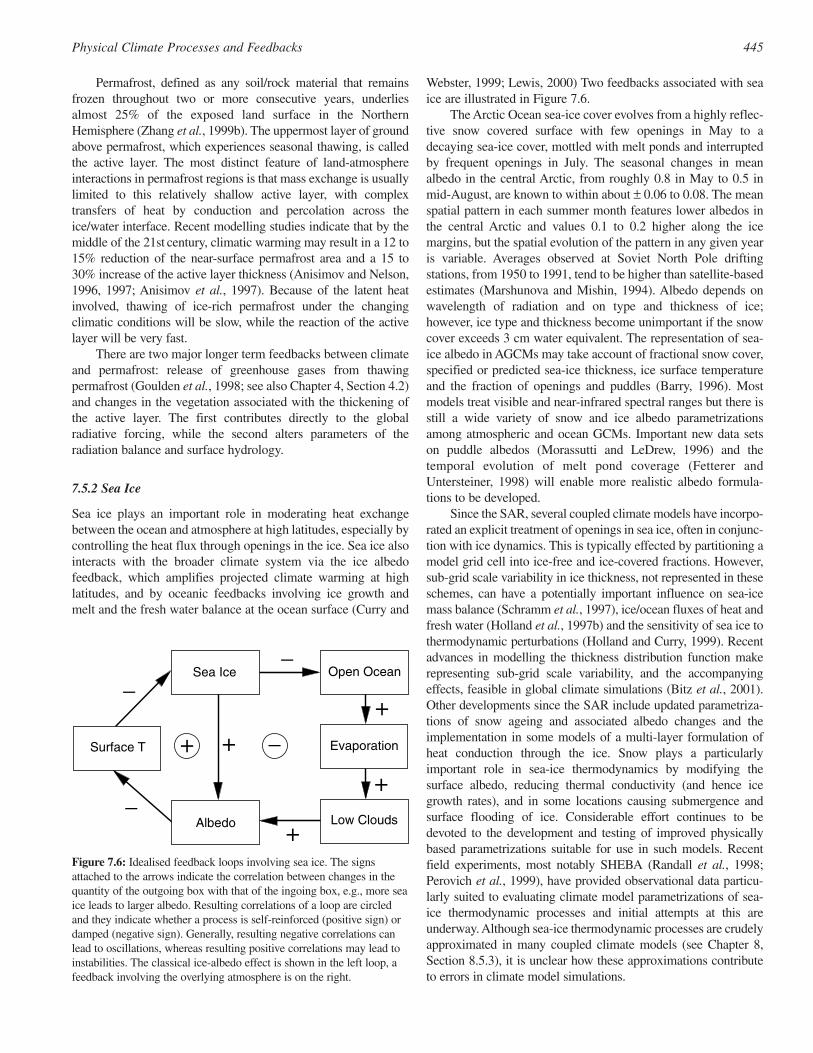
Permafrost, defined as any soil/rock material that remainsfrozen throughout two or more consecutive years, underliesalmost 25% of the exposed land surface in the NorthernHemisphere (Zhang et al., 1999b). The uppermost layer of groundabove permafrost, which experiences seasonal thawing, is calledthe active layer. The most distinct feature of land-atmosphereinteractions in permafrost regions is that mass exchange is usuallylimited to this relatively shallow active layer, with complextransfers of heat by conduction and percolation across theice/water interface. Recent modelling studies indicate that by themiddle of the 21st century, climatic warming may result in a 12 to15% reduction of the near-surface permafrost area and a 15 to30% increase of the active layer thickness (Anisimov and Nelson,1996, 1997; Anisimov et al., 1997). Because of the latent heatinvolved, thawing of ice-rich permafrost under the changingclimatic conditions will be slow, while the reaction of the activelayer will be very fast.

There are two major longer term feedbacks between climateand permafrost: release of greenhouse gases from thawingpermafrost (Goulden et al., 1998; see also Chapter 4, Section 4.2)and changes in the vegetation associated with the thickening ofthe active layer. The first contributes directly to the globalradiative forcing, while the second alters parameters of theradiation balance and surface hydrology.

7.5.2 Sea Ice

Sea ice plays an important role in moderating heat exchangebetween the ocean and atmosphere at high latitudes, especially bycontrolling the heat flux through openings in the ice. Sea ice alsointeracts with the broader climate system via the ice albedofeedback, which amplifies projected climate warming at highlatitudes, and by oceanic feedbacks involving ice growth andmelt and the fresh water balance at the ocean surface (Curry and

Webster, 1999; Lewis, 2000) Two feedbacks associated with seaice are illustrated in Figure 7.6.

The Arctic Ocean sea-ice cover evolves from a highly reflec-tive snow covered surface with few openings in May to adecaying sea-ice cover, mottled with melt ponds and interruptedby frequent openings in July. The seasonal changes in meanalbedo in the central Arctic, from roughly 0.8 in May to 0.5 inmid-August, are known to within about ± 0.06 to 0.08. The meanspatial pattern in each summer month features lower albedos inthe central Arctic and values 0.1 to 0.2 higher along the icemargins, but the spatial evolution of the pattern in any given yearis variable. Averages observed at Soviet North Pole driftingstations, from 1950 to 1991, tend to be higher than satellite-basedestimates (Marshunova and Mishin, 1994). Albedo depends onwavelength of radiation and on type and thickness of ice;however, ice type and thickness become unimportant if the snowcover exceeds 3 cm water equivalent. The representation of sea-ice albedo in AGCMs may take account of fractional snow cover,specified or predicted sea-ice thickness, ice surface temperatureand the fraction of openings and puddles (Barry, 1996). Mostmodels treat visible and near-infrared spectral ranges but there isstill a wide variety of snow and ice albedo parametrizationsamong atmospheric and ocean GCMs. Important new data setson puddle albedos (Morassutti and LeDrew, 1996) and thetemporal evolution of melt pond coverage (Fetterer andUntersteiner, 1998) will enable more realistic albedo formula-tions to be developed.

Since the SAR, several coupled climate models have incorpo-rated an explicit treatment of openings in sea ice, often in conjunc-tion with ice dynamics. This is typically effected by partitioning amodel grid cell into ice-free and ice-covered fractions. However,sub-grid scale variability in ice thickness, not represented in theseschemes, can have a potentially important influence on sea-icemass balance (Schramm et al., 1997), ice/ocean fluxes of heat andfresh water (Holland et al., 1997b) and the sensitivity of sea ice tothermodynamic perturbations (Holland and Curry, 1999). Recentadvances in modelling the thickness distribution function makerepresenting sub-grid scale variability, and the accompanyingeffects, feasible in global climate simulations (Bitz et al., 2001).Other developments since the SAR include updated parametriza-tions of snow ageing and associated albedo changes and theimplementation in some models of a multi-layer formulation ofheat conduction through the ice. Snow plays a particularlyimportant role in sea-ice thermodynamics by modifying thesurface albedo, reducing thermal conductivity (and hence icegrowth rates), and in some locations causing submergence andsurface flooding of ice. Considerable effort continues to bedevoted to the development and testing of improved physicallybased parametrizations suitable for use in such models. Recentfield experiments, most notably SHEBA (Randall et al., 1998;Perovich et al., 1999), have provided observational data particu-larly suited to evaluating climate model parametrizations of sea-ice thermodynamic processes and initial attempts at this areunderway. Although sea-ice thermodynamic processes are crudelyapproximated in many coupled climate models (see Chapter 8,Section 8.5.3), it is unclear how these approximations contributeto errors in climate model simulations.


+Surface T

–

+

+–

–Sea Ice

Albedo Low Clouds

Evaporation

Open Ocean

+

+ –

Figure 7.6: Idealised feedback loops involving sea ice. The signsattached to the arrows indicate the correlation between changes in thequantity of the outgoing box with that of the ingoing box, e.g., more seaice leads to larger albedo. Resulting correlations of a loop are circledand they indicate whether a process is self-reinforced (positive sign) ordamped (negative sign). Generally, resulting negative correlations canlead to oscillations, whereas resulting positive correlations may lead toinstabilities. The classical ice-albedo effect is shown in the left loop, afeedback involving the overlying atmosphere is on the right.


Box 7.1: Sea ice and climate change.

Sea-ice processes:Sea ice in the Arctic and around Antarctica responds directly to climate change and may, if properly monitored, become increas-ingly important for detecting climate change. Although sea ice covers only about 5% of the Earth’s surface, its extent andthickness have important influences in the coupled atmosphere-ocean system. Increasing the understanding of these processesand representing them more realistically in climate models is important for making more reliable climate change projections.Several processes associated with sea ice are climatically relevant. The sea-ice albedo effect is an important contributor to theamplification of projected warming at high latitudes. Albedo decreases if the extent of sea ice is reduced and more ocean surfaceis exposed, resulting in increased heat absorption and hence warming. Melting of snow and the formation of melt-water pondsalso reduces albedo and alters the radiation balance. Changes in sea-ice thickness and lead (open water) fraction modify the heattransfer from the ocean: thinner sea ice and more leads result in enhanced heat loss from the exposed ocean thus furtherwarming the atmosphere. Changes in cloud cover may influence how large this effect really is. A principal mechanism for densewater formation in the ocean around Antarctica and in shelf regions of the Arctic is the rejection of brine as sea water freezes.Changes in sea-ice formation alter the properties and formation rates of ocean deep water and therefore have an influence onthe water mass structure that reaches far beyond the area of sea ice. Finally, ice export from the Arctic represents an importantsouthward flux of fresh water which influences the density structure of the upper ocean in the Nordic, Labrador and IrmingerSeas.

Observations of sea ice:Observations of sea-ice extent and concentration (the fraction of local area covered by ice) are based primarily on satellite dataavailable since the late 1970s. Sea-ice thickness is also important in assessing possible changes in the amount of sea ice;however, thickness observations are more difficult to make. For the Arctic, thickness data come primarily from sonar measure-ments from submarines and a few oceanographic moorings. Although limited, the observations indicate statistically significantdecreases in ice extent and thickness over the past few decades, with Arctic sea-ice extent declining at a rate of about 3% perdecade since the late 1970s. Sea-ice retreat in the Arctic spring and summer over the last few decades is consistent with anincrease in spring temperature, and to a lesser extent, summer temperatures at high latitudes. Thickness data show a near 40%decrease in the summer minimum thickness of Arctic sea ice over approximately the last 30 years. Estimates using independentmethods for the winter, but over a much shorter period, also suggest thickness reductions, but at a markedly slower rate.However, due to limited sampling, uncertainties are difficult to estimate, and the influence of decadal to multi-decadalvariability cannot yet be assessed.

While Arctic sea-ice extent and thickness have clearly decreased in the last 20 years, changes in Antarctic sea-ice extent havebeen insignificant. The earlier part of the data set indicates somewhat greater ice extents in the early 1970s, and indirectevidence from historical records also points to more northerly sea-ice margins in the 1930s and 1940s. Warming over much ofAntarctica has only been about 0.5°C over the last 50 years with the notable exception of the Antarctic Peninsula where temper-atures have increased by about 2°C for reasons that remain unclear.

Sea-ice modelling and projection:Sea ice is particularly difficult to simulate in climate models because it is influenced directly by both the atmosphere (temper-ature, radiation, wind) and the ocean (heat transport and mixing, and surface currents), and because many of the relevantprocesses require high grid resolution or must be parametrized. Recent coupled climate models include a sea-ice componentthat incorporates openings in the ice, often in conjunction with ice dynamics (motion and deformation). Furthermore, updatedparametrizations of snow ageing and associated albedo changes and multi-layer formulations of heat conduction through the iceand overlying snow cover are being implemented in some models. Although many thermodynamic processes are crudelyapproximated, it is unclear how these approximations contribute to errors in climate model simulations. Sea-ice dynamics isimportant in determining local ice thickness and export of sea ice from the formation areas, but despite the rather mature statusof physically based sea-ice dynamics models, only a few of the current coupled climate models include such a component.Coupled model simulations of the seasonal cycle of sea-ice coverage in both hemispheres exhibit large deviations from thelimited observational data base, as illustrated in Chapter 8, and current research is aimed at improving model performance.

Coupled model projections of the future distribution of sea ice differ quantitatively from one to another as shown in Chapter9. However, they agree that sea-ice extent and thickness will decline over the 21st century as the climate warms. Box 7.1, Figure1 illustrates this with annual mean Arctic ice extent results from two coupled models. The simulations of ice extent decline overthe past 30 years are in good agreement with the observations, lending confidence to the subsequent projections which show asubstantial decrease of Arctic sea-ice cover leading to roughly 20% reduction in annual mean Arctic sea-ice extent by the year 2050.

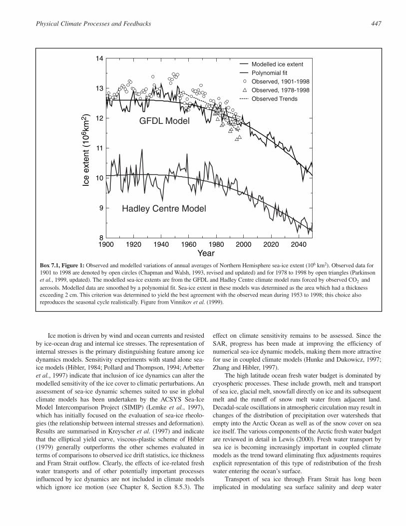
Ice motion is driven by wind and ocean currents and resistedby ice-ocean drag and internal ice stresses. The representation ofinternal stresses is the primary distinguishing feature among icedynamics models. Sensitivity experiments with stand alone sea-ice models (Hibler, 1984; Pollard and Thompson, 1994; Arbetteret al., 1997) indicate that inclusion of ice dynamics can alter themodelled sensitivity of the ice cover to climatic perturbations. Anassessment of sea-ice dynamic schemes suited to use in globalclimate models has been undertaken by the ACSYS Sea-IceModel Intercomparison Project (SIMIP) (Lemke et al., 1997),which has initially focused on the evaluation of sea-ice rheolo-gies (the relationship between internal stresses and deformation).Results are summarised in Kreyscher et al. (1997) and indicatethat the elliptical yield curve, viscous-plastic scheme of Hibler(1979) generally outperforms the other schemes evaluated interms of comparisons to observed ice drift statistics, ice thicknessand Fram Strait outflow. Clearly, the effects of ice-related freshwater transports and of other potentially important processesinfluenced by ice dynamics are not included in climate modelswhich ignore ice motion (see Chapter 8, Section 8.5.3). The

effect on climate sensitivity remains to be assessed. Since theSAR, progress has been made at improving the efficiency ofnumerical sea-ice dynamic models, making them more attractivefor use in coupled climate models (Hunke and Dukowicz, 1997;Zhang and Hibler, 1997).

The high latitude ocean fresh water budget is dominated bycryospheric processes. These include growth, melt and transportof sea ice, glacial melt, snowfall directly on ice and its subsequentmelt and the runoff of snow melt water from adjacent land.Decadal-scale oscillations in atmospheric circulation may result inchanges of the distribution of precipitation over watersheds thatempty into the Arctic Ocean as well as of the snow cover on seaice itself. The various components of the Arctic fresh water budgetare reviewed in detail in Lewis (2000). Fresh water transport bysea ice is becoming increasingly important in coupled climatemodels as the trend toward eliminating flux adjustments requiresexplicit representation of this type of redistribution of the freshwater entering the ocean’s surface.

Transport of sea ice through Fram Strait has long beenimplicated in modulating sea surface salinity and deep water


Box 7.1, Figure 1: Observed and modelled variations of annual averages of Northern Hemisphere sea-ice extent (106 km2). Observed data for1901 to 1998 are denoted by open circles (Chapman and Walsh, 1993, revised and updated) and for 1978 to 1998 by open triangles (Parkinsonet al., 1999, updated). The modelled sea-ice extents are from the GFDL and Hadley Centre climate model runs forced by observed CO2 andaerosols. Modelled data are smoothed by a polynomial fit. Sea-ice extent in these models was determined as the area which had a thicknessexceeding 2 cm. This criterion was determined to yield the best agreement with the observed mean during 1953 to 1998; this choice alsoreproduces the seasonal cycle realistically. Figure from Vinnikov et al. (1999).

1900 1920 1940 1960 1980 2000 2020 2040Year

8

9

10

11

12

13

14

Ice

exte

nt (

106 k

m2 )

Modelled ice extentPolynomial fitObserved, 1901-1998Observed, 1978-1998Observed Trends

GFDL Model

Hadley Centre Model

formation in the North Atlantic (Dickson et al., 1988; Belkin etal., 1998). Recent modelling studies show that wind forcingdominates the variability in ice outflow (Hakkinen, 1993; Harderet al., 1998; Hilmer et al., 1998) and suggest that decadal-scaleoscillations in atmospheric circulation are reflected in overall icetransport patterns (Proshutinsky and Johnson, 1997; Polyakov etal., 1999). Net export of ice from the Arctic Ocean to the NorthAtlantic amounts to an annual loss of roughly 0.4 m of freshwater (Vinje et al., 1998), which is offset by net ice growth. Thesalt released by this ice growth is in turn largely offset by inflowof fresher Pacific water, via the Bering Strait, and river runoff,maintaining a stable stratification. Changes in ice outflow, suchas might arise under a changing climate, could alter the distribu-tion of fresh water input to the Arctic and North Atlantic, withconsequences for ocean circulation, heat transport and carboncycling.

Around Antarctica, ice transport primarily exports freshwater from coastal regions where it is replaced by net ice growth.The salt released by this growth contributes directly to Antarcticdeep water production (Goosse et al., 1997; Legutke et al., 1997;Stössel et al., 1998; Goosse and Fichefet, 1999). However, thedetails of how salt released by freezing sea ice is distributed in thewater column can have a substantial impact on water massformation and circulation (Duffy and Caldeira, 1997; Legutke etal., 1997; Duffy et al., 1999) and hence on heat and carbonsequestration in a changing climate.

7.5.3 Land Ice

Ice stream instability, ice shelf break-up and switches in routingand discharge of glacial melt water present themselves asmechanisms for altering the surface salinity of oceans andinducing changes in the pattern and strength of the THC. Thereare positive and negative feedbacks associated with changingland ice masses (Figure 7.7). In coupled climate models, all thesecryospheric processes are represented simply as surface freshwater inputs to the ocean (see Chapter 8, Section 8.5.4.2).

Ice sheets are continental scale masses of fresh water iceformed by the burial and densification of snow. They can bedivided into areas that are grounded on the land surface, eitherbelow or above sea level, and areas that are afloat. Groundedparts of ice sheets exhibit slow and fast modes of flow. The slowsheet-flowing component is the more prevalent but the faststream-flowing component can account for most of the icedischarge. Switching between slow and fast modes of flow mayoccur thermally, mechanically or hydrologically and is sugges-tive of “surging”, a known cyclic instability of certain glaciers(Kamb et al., 1985; Bindschadler, 1997). The slow-flow processfor ice sheets is internal creep and the fast-flow processes relevantto ice streams are bottom sliding, enhanced creep and sub-glacialsediment deformation (Alley, 1989; Iken et al., 1993; Engelhardtand Kamb, 1998). The factors controlling onset, discharge andwidth of ice streams are subject to poorly understood geological,topographic, thermal and hydrological controls (Clarke andEchelmeyer, 1996; Anandakrishnan and Alley, 1997;Bindschadler, 1997; Anandakrishnan et al., 1998; Bell et al.,1998; Jacobson and Raymond, 1998).

Although in GCMs the albedo of land ice is typically fixed,satellite observations could be used to remove this limitation; themelt area, as identified from satellite passive microwave observa-tions (Mote et al., 1993; Abdalati and Steffen, 1995), andAVHRR-derived albedo estimates can now be mapped (Stroeveet al., 1997). Land ice dynamics and thermodynamics, ignored incurrent coupled GCMs, respond to changes in the temperatureand balance of accumulation and melt at upper and lowersurfaces. These boundary conditions involve couplings to theatmosphere, ocean and lithosphere. Ice sheet models typicallyrepresent atmospheric boundary conditions using simpleelevation-based parametrizations. However, results obtained forAntarctica using this approach (Huybrechts and Oerlemans,1990; Fastook and Prentice, 1994) compare favourably withthose using more comprehensive AGCM-derived boundaryconditions (Thompson and Pollard, 1997). Predictive models offuture evolution must incorporate past ice-mass variationsbecause ice sheets continue to respond to climate change forseveral thousand years. Time-scales complicate the inclusion ofland ice in existing coupled climate models, and it is usual inthese models to regard land ice as passive, providing only a staticboundary for the atmosphere. Models of ocean circulationseldom incorporate explicit treatments of melt water inputs fromland ice.

Models simulate the coupled evolution of ice sheet flow,form and temperature. The flow law in Glen (1955) is commonlyadopted but such models must employ a poorly justified flowenhancement factor to correctly capture the height-to-width ratiosof ice sheets. In general, these models perform well in inter-comparison exercises (Huybrechts et al., 1996; Payne et al.,2000), but there is uncertainty in the predicted thermal structureand bottom melting conditions. This constitutes a potentiallyserious shortcoming because several models of ice sheetinstability invoke thermal trigger mechanisms (MacAyeal, 1992).Ice stream flow models are limited by the current knowledge ofthe controlling physical processes. Outstanding issues involve therelative importance of bottom drag and lateral drag (Whillans and


Atlantic THC

SST

SSTSurface

Temperature

Land IceVolume

Snow FallN Hemisphere

–

Atlantic THC

+

+

+

+

+

+

++

–

+ +

Evaporation

Sea SurfaceSalinity

Figure 7.7: Feedback loops associated with land ice masses. Changesin their volume affect the salt balance at the sea surface and mayinfluence the thermohaline circulation (THC). While there is palaeo-climatic evidence that this has happened often during the last Ice Age,the above processes are unlikely to play a major role for futureclimate change.

van der Veen, 1993; MacAyeal et al., 1995) and the representationof fast-flow and water-transport processes (Fowler and Schiavi,1998; Hindmarsh, 1998; Tulaczyk et al., 1998). Recently, coupledmodels of the evolution of ice streams within ice sheets have beendeveloped (Marshall and Clarke, 1997) which incorporate thecrucial processes of ice stream onset (Bell et al., 1998) andmargin migration (van der Veen and Whillans, 1996).

Floating margins of ice sheets are called ice shelves, thelargest of which are found in West Antarctica and mediate thetransfer of ice between fast-flowing ice streams and the SouthernOcean. Break-up of one or both of the large West Antarctic iceshelves, either associated with ice stream instability orindependent of it, cannot be discounted and would be consider-ably more probable than complete disintegration of the WestAntarctic ice sheet (Bentley, 1998; see also Chapter 11, Section11.3.3). Such an event would be accompanied by a large increasein iceberg flux to the Southern Ocean and uncertain effects on theproduction of AABW and ocean circulation. Different ice shelfmodels compare well (MacAyeal et al., 1996); however, thestability of grounding lines remains an issue and could signifi-cantly influence the behaviour of numerical models (Hindmarsh,1993). The suggestion that the grounding line is inherentlyunstable (Thomas and Bentley, 1978) is not supported by morerecent modelling studies (Muszynski and Birchfield, 1987;Huybrechts and Oerlemans, 1990; Hindmarsh, 1993). However,this issue has yet to be resolved.

Megafloods of water stored beneath ice sheets have beenpostulated (Shaw et al., 1996) but the subject is controversial.The estimated total volume of lake water beneath Antarctica isequivalent to 10 to 35 mm of sea level rise (Dowdeswell andSiegert, 1999) but the simultaneous release of all this storedwater is unlikely. The timing would be unpredictable and climateimpacts, if any, would be associated with the effect of the freshwater pulse on AABW formation. Modelling such phenomena isbeyond the scope of existing ice dynamics models. Althoughprogress has been made in the understanding of ice streamprocesses, there are still many unanswered questions andrepresentation of ice stream and grounding line physics in land-ice dynamics models remains rudimentary.

7.6 Processes, Feedbacks and Phenomena in the Coupled System

This section deals with some of the processes and feedbacks inthe coupled atmosphere-ocean system; those involving land andthe cryosphere are dealt with in Sections 7.4 and 7.5, respectively.Increasingly, natural modes of variability of the atmosphere andthe atmosphere-ocean system are also understood to play keyroles in the climate system and how it changes, and thus theteleconnections which are believed to be most important forclimate change are briefly discussed.

7.6.1 Surface Fluxes and Transport of Heat and Fresh Water

Fundamental issues in the global climate system are the relativeamounts of heat and fresh water carried by the oceans and theatmosphere to balance the global heat and water budgets.

Because the top-of-the-atmosphere radiation largely determinesthe distribution of net energy on the Earth, the fluid componentsof the climate system, the atmosphere and ocean, transport heatand energy from regions of surplus to regions of deficit, with thetotal heat transport constrained. In the SAR a major problem withatmospheric models was that their surface fluxes with the oceanand the implied oceanic heat transports did not agree with thequite uncertain observational estimates and the biggest problemwas clearly with clouds. The result was that all coupled modelsof the current climate either had a bias in their simulation of themean state or that a “flux adjustment” was employed to keep themean state close to that observed. Although some recent coupledocean-atmosphere models (Boville and Gent, 1998; Gordon etal., 2000) do not have adjustments to the modelled surface heat,water and momentum fluxes (see Chapter 8, Section 8.4.2), thedrift in surface climate is small. This implies that the surface air-sea heat and water fluxes calculated by the model are reasonablyconsistent with the simulated ocean heat and fresh watertransports. However, only comparison with flux values of knownaccuracy can verify the predicted fluxes, and thereby increaseconfidence in the modelled physical processes.

The role of the oceans in maintaining the global heat andwater budgets may be assessed using bulk formulae, residual anddirect (hydrographic) methods. Direct measurements of thesensible and latent heat fluxes have led to improved parametriza-tions (Fairall et al., 1996; Weller and Anderson, 1996; Godfrey etal., 1998), but large 20 to 30% uncertainties amounting to severaltens of Wm−2 remain (DeCosmo et al., 1996; Gleckler and Weare,1997). Recent global air-sea flux climatologies based on ship dataand bulk formulae (da Silva et al., 1994; Josey et al., 1999) exhibitan overall global imbalance; on average the ocean gains heat at arate of about 30 Wm−2. This was adjusted by globally scaling theflux estimates (da Silva et al., 1994), but spatially uniform correc-tions are not appropriate (Josey et al., 1999). While satellites givedata over all ocean regions (e.g., Schulz and Jost, 1998; Curry etal., 1999), and precipitation estimates over the oceans are onlyviable using satellites (Xie and Arkin, 1997), their accuracy is stillunknown. Overall, surface evaporation minus precipitation (E–P)estimates are probably accurate to no better than about 30%.

In the residual method the atmospheric energy transport issubtracted from the top-of-the-atmosphere radiation budget toderive the ocean heat transport. Until fairly recently, theatmospheric poleward transport estimates were too small and ledto overestimates of the ocean transports. This has improved withlocal applications of global numerical atmospheric analysesbased on four dimensional data assimilation (Trenberth andSolomon, 1994; Keith, 1995). With reanalysis of atmosphericobservations, more reliable atmospheric transports are becomingavailable (Table 7.1). Sun and Trenberth (1998) show that largeinterannual changes in poleward ocean heat transports areinferred with El Niño events in the Pacific. The moisture budgetestimates of E–P are generally superior to those computeddirectly from E and P estimates from the model used in theassimilation (e.g., Trenberth and Guillemot, 1998) and areprobably to be preferred to bulk flux estimates, given the inaccu-racy of bulk estimates of P.

In the direct method the product of ocean velocity and


temperature measured over the boundaries is integrated todetermine the ocean heat transport divergence for the volume.While it deals with ocean circulation and the mechanisms ofocean heat transport, estimates could only be made at a fewlocations where high quality observations were available andassumptions, such as geostrophic velocity estimates, are reason-able. Most of the recent estimates are for the Atlantic Ocean (seeTable 7.1), for which there is general agreement that there isnorthward ocean heat transport at all latitudes. It is generallyunderstood that this northward heat transport is associated withthe THC in which NADW is formed in the polar and sub-polarNorth Atlantic and subsequently flows southward as a deepwestern boundary current into the Southern Ocean. In the NorthPacific Ocean at 10°N (Wijffels et al., 1996), the northward heatflux of 0.7 ± 0.5 PW (1 PetaWatt = 1 PW = 1015 W) is dueprimarily to a shallow Ekman upper thermocline cell. It isestimated that a 6 Sv change in Ekman transport, which iscomparable to the differences among existing climatologies,would cause a 0.4 PW change in meridional heat transport. Forthe South Pacific (Koshlyakov and Sazhina, 1996; Tsimplis et al.,1998) and Indian oceans (Robbins and Toole, 1997) the determi-nation of ocean heat transport is hampered by uncertainties in thesize of the Indonesian Throughflow and in the Agulhas Currenttransports (Beal and Bryden, 1997), and the estimates ofnorthward heat transport across 30°S in the Indian Ocean rangefrom –0.4 to –1.3 PW (Robbins and Toole, 1997; Macdonald,1998). Macdonald (1998) and Macdonald and Wunsch (1996)have made a global inverse analysis of selected high qualityhydrographic sections covering all ocean basins taken prior to theWorld Ocean Circulation Experiment (WOCE) observationalperiod to produce meridional heat transports (Table 7.1). For theheat fluxes, results from the methods are beginning to converge.While some new direct ocean fresh water transport measure-

ments (Saunders and King, 1995) indicate that the South Atlanticreceives adequate excess precipitation to supply the cross equato-rial flux of fresh water for North Atlantic excess evaporation, thisruns contrary to previous estimates (Wijffels et al., 1992) and therecent atmospheric moisture budget results (Trenberth andGuillemot, 1998).

The latest results of the zonal mean ocean heat transportscomputed from (i) observational data as residuals, (ii) models runwithout flux adjustments and (iii) direct measurements agreewithin error estimates (Table 7.1). This suggests that the modelsare now converging on the correct values for the zonally averagedheat fluxes. However, significant regional biases and compen-sating errors in the radiative and turbulent fluxes still exist(Doney et al., 1998; Gordon et al., 2000). The coupled modelfresh water flux estimates are more problematic. For example, theinter-tropical convergence zone may become skewed andspuriously migrate from one hemisphere to the other, seriouslydistorting the precipitation fields (e.g., Boville and Gent, 1998).

The compatibility and improvements of the ocean andatmospheric heat transports in models is evidently the primaryreason why coupled runs can now be made without flux adjust-ments (Gregory and Mitchell, 1997). This is due to a betterrepresentation of key processes in both atmosphere and oceancomponents of climate models, and improved spatial resolution.These key processes include, in the atmosphere, convection,boundary-layer physics, clouds, and surface latent heat fluxes(Hack, 1998), and in the ocean, boundary layer and mesoscaleeddy mixing processes (Doney et al., 1998; Large and Gent,1999). However, while simulated SSTs generally agree well withobservations (deviations of less than 2°C), there are large areaswhere consistent errors of SST occur in the models (e.g., too coldin the North Pacific; too warm in coastal upwelling regions, seeChapter 8, Figure 8.1a). These point to processes that must be


Table 7.1: Ocean heat transport estimates, positive northwards in PetaWatts (1 PetaWatt = 1 PW = 1015W), from analyses of individual hydrographicsections from pre WOCE sections (Macdonald, 1998), indirect methods (Trenberth et al., 2001), and years 81 to 120 of the HadCM3 (UKMO)coupled model (Gordon et al., 2000) and from the CSM 1.0 (NCAR) (Boville and Gent, 1998). Typical error bars are ±0.3 PW. For the Atlantic thesections are: 55°N (Bacon, 1997), 24°N (Lavin et al., 1998), 14°N (Klein et al., 1995), 11°S (Speer et al., 1996), and at 45°S (Saunders and King,1995). For the Pacific: 47°N (Roemmich and McCallister, 1989), 24°N (Bryden et al., 1991), 10°N (Wijffels et al., 1996). Because of the Indonesianthroughflow, South Pacific and Indian Ocean transports make most sense if combined.

Atlantic Sections Macdonald Trenberth HadCM3 CSM 1.055°N 0.28 − 0.29 − 0.6348°N − 0.65 0.41 0.54 0.8124°N 1.27 1.07 1.15 1.14 1.3114°N 1.22 − 1.18 − 1.2711°N − 1.39 1.15 1.12 1.2111°S 0.60 0.89 0.63 − 0.6523°S − 0.33 0.51 0.67 0.6145°S 0.53 − 0.62 0.64 −

Pacific47°N − 0.09 − 0.08 − 0.06 0.17 0.1124°N 0.76 0.45 0.73 0.50 0.6910°N 0.70 0.44 0.85 0.68 0.87

Pacific + Indian32°S − −1.34 −1.14 −1.19 −1.13

improved in future models. For instance, stratocumulus decks arenot well simulated in coupled models, resulting in significantdeviations of SST from the observed (see Chapter 8, Figure 8.1aand Section 8.4.2 for a discussion).

7.6.2 Ocean-atmosphere Interactions

There is no clear separation between the wind-driven circula-tion and the THC (see Section 7.3.6) because they interact witheach other on several time-scales. While there is a great deal ofempirical evidence that the ocean and sea surface temperaturesco-vary with the atmosphere, this may only indicate that theatmosphere forces the ocean, and it does not necessarily signifya feedback or a truly coupled process that contributes to thevariability. Moreover, it is very difficult to establish suchcoupling from observational studies. This topic was not dealtwith thoroughly by the SAR. In the tropics there is clearevidence of the ocean forcing the atmosphere, such as in ElNiño (see Section 7.6.5). In the extra-tropics much of what canbe seen is accountable through fairly random wind variations;essentially stochastic forcing of the ocean is converted into lowfrequency ocean variability and gives a red spectrum in oceanictemperatures and currents up to the decadal time-scale(Hasselmann, 1976; Hall and Manabe, 1997). Feedback to theatmosphere is not involved. In the spatial resonance concept(Frankignoul and Reynolds, 1983) there is still no feedbackfrom the ocean to the atmosphere, but oceanic quantities mayexhibit a spectral peak through an advective time-scale(Saravanan and McWilliams, 1998) or Rossby wave dynamicstime-scale (Weng and Neelin, 1998). In coupled air-sea modes,such as those proposed by Latif and Barnett (1996) for theNorth Pacific and by Groetzner et al. (1998) for the NorthAtlantic, there is a feedback from the ocean to the atmosphere.Spectral peaks are found in both the ocean and the atmosphere,and the period of the oscillation is basically determined by theadjustment time of the sub-tropical gyre to changes in the windstress curl.

Coupled models indicate that, in mid-latitudes, thepredominant process is the atmosphere driving the ocean asseen by the surface fluxes and as observed, yet when anatmospheric model is run with specified SSTs, the fluxes arereversed in sign, showing the forcing of the atmosphere fromthe now infinite heat capacity of the ocean (implied by specifiedSSTs). Recent ensemble results (Rodwell et al., 1999; Mehta etal., 2000) have been able to reproduce the decadal NorthAtlantic atmospheric variations from observed SSTs but withmuch reduced amplitude. Bretherton and Battisti (2000)suggest that this is consistent with a predominant stochasticdriving of the ocean by the atmosphere with some modestfeedback on the atmosphere, and that the signal only emergesthrough ensemble averaging.

In the extra-tropics, a key question remains the sensitivityof the mid-latitude atmosphere to surface forcing from sea iceand sea surface temperature anomalies. Different modellingstudies with similar surface conditions yield contradictoryresults (e.g., Robertson et al., 2000a,b). The crude treatment ofprocesses involving sea ice, oceanic convection, internal ocean

mixing and eddy-induced transports and the coarse resolutionof most coupled climate models, adds considerably to theuncertainty.

7.6.3 Monsoons and Teleconnections

The weather and climate around the world in one place isgenerally strongly linked to that in other places throughatmospheric linkages. In the tropics and sub-tropics, large-scaleoverturning in the atmosphere, which is manifested as theseasonal monsoon variations, links the wet summer monsoons tothe dry subsiding regions usually in the tropics and sub-tropics ofthe winter hemisphere. Throughout the world, teleconnectionslink neighbouring regions mainly through large-scale, quasi-stationary atmospheric Rossby waves. A direct consequence ofthese linkages is that some regions are wetter and/or hotter thanthe prevailing global scale changes, while half a wavelength awaythe regions may be dryer and/or cooler than the global pattern.Moreover, because of the way these patterns set up relative toland and ocean, they can alter the global mean changes. Inaddition, errors in models (such as in convection in the tropicalPacific) can be manifested non-locally through teleconnections,e.g., in the North Pacific SSTs (see Figure 8.1a), although otherprocesses are also involved.

The term “monsoon” is now generally applied to tropicaland sub-tropical seasonal reversals in both the atmosphericcirculation and associated precipitation. These changes arisefrom reversals in temperature gradients between continentalregions and the adjacent oceans with the progression of theseasons. The dominant monsoon systems in the world are theAsian-Australian, African and the American monsoons. As landheats faster than ocean in summer, heated air rises and drawsmoist low-level maritime air inland where convection and releaseof latent heat fuel the monsoon circulation. For the Asianmonsoon, a regional meridional temperature gradient extendingfrom the tropical Indian Ocean north to mid-latitude Asiadevelops prior to the monsoon through a considerable depth ofthe troposphere (Webster et al., 1998). To a first order, thestronger this meridional temperature gradient, the stronger themonsoon. Thus land-surface processes, such as soil moisture andsnow cover in Asia can influence the monsoon and, along withSST variations, may induce quasi-biennial variability (Meehl,1997). Additionally, large-scale forcing associated with tropicalPacific SSTs influences monsoon strength through the large-scaleeast-west overturning in the atmosphere. Anomalously cold(warm) Pacific SSTs often are associated with a strong (weak)monsoon, though these connections are somewhat intermittent.

Some teleconnections arise simply from natural preferredmodes of the atmosphere associated with the mean climate stateand the land-sea distribution. Several are directly linked to SSTchanges (Trenberth et al., 1998). The most prominent are thePacific-North American (PNA) and the North Atlantic Oscillation(NAO; see Section 7.6.4) in the Northern Hemisphere, and bothaccount for a substantial part of the pattern of northernhemispheric temperature change, especially in winter (Hurrell,1996), in part through the “cold ocean warm land” (COWL)pattern (Wallace et al., 1995; Hurrell and Trenberth, 1996) (see


Chapter 2). Although evidently a prominent mode of theatmosphere alone, the PNA is also influenced by changes inENSO (see Section 7.6.5). Thompson and Wallace (1998, 2000)suggest that the NAO may be the regional manifestation of anannular (zonally symmetric) hemispheric mode of variabilitycharacterised by a seesaw of atmospheric mass between thepolar cap and the middle latitudes in both the Atlantic andPacific Ocean basins and they call this the Arctic Oscillation(AO). A similar, even more zonal structure is dominant in theSouthern Hemisphere (Trenberth et al., 1998) (the SouthernAnnular Mode, sometimes called the Antarctic Oscillation,AAO). The vertical structure of both AO and AAO extends wellinto the stratosphere (Perlwitz and Graf, 1995; Thompson andWallace, 1998).

In the Atlantic, an important emerging coupled mode ofvariability is the so-called tropical Atlantic dipole, whichinvolves variations of opposite sign in the sea level pressurefield across the equatorial Atlantic and corresponding variationsin the ITCZ location. Given the background SST and windfields, anomalous SSTs of opposite sign across the equatorialregion are apt to alter the surface winds in such a way as toenhance or reduce evaporative cooling of the ocean andreinforce the original SST pattern (Carton et al., 1996; Chang etal., 1997). The ocean provides a decadal time-scale to thecoupled interactions.

Dominant large-scale patterns of ocean-atmosphereinteractions are also found in the tropical Indian Ocean (Saji etal., 1999; Webster et al., 1999). They have characteristicssimilar to El Niño and are associated with large east-west SSTchanges and a switch of the major tropical convection areasfrom Africa to Indonesia. There are indications that thisatmosphere-ocean process is somewhat independent of ENSOand represents a natural mode of the tropical Indian Ocean.

The vital processes for improved monsoon simulation inmodels are those associated with the hydrological cycle,especially in the tropics. These include convection, precipita-tion and other atmospheric processes (see Section 7.2) as wellas land surface processes (see Section 7.4), and interactions ofthe atmosphere with complex topography and with the ocean.The difficulties in assembling all of these elements togetherhas led to problems in simulating mean precipitation as well asinterannual monsoon variability, although improvements areevident (Webster et al., 1998, and see Chapter 8, Section8.7.3).

For teleconnections and regional climate patterns, not onlyare there demanding requirements on simulating the variationsin tropical SSTs that drive many of the interannual and longer-term fluctuations through latent heating in the associatedtropical precipitation, but results also depend on the mean stateof the atmosphere through which Rossby waves propagate.Feedbacks from changes in storm tracks, and thus momentumand heat transports by transient atmospheric disturbances, aswell as interactions with changed land-surface soil moisturefrom precipitation changes and interactions with extra-tropicaloceans are critical. While there is scope for further improve-ments, great strides have been made in modelling all theseaspects in the recent years.

7.6.4 North Atlantic Oscillation and Decadal Variability

The NAO is the dominant pattern of wintertime atmosphericcirculation variability over the extra-tropical North Atlantic(Hurrell, 1995), and has exhibited decadal variability and trends(see Chapter 2, Section 2.6). There is strong evidence indicatingthat much atmospheric circulation variability in the form of theNAO arises from internal atmospheric processes (Saravanan,1998; Osborn et al., 1999). During winters when the stratosphericvortex is stronger than normal, the NAO (and AO) tends to be ina positive phase suggesting an interaction and perhaps even adownward influence from the stratosphere to the troposphere (seeSections 7.2.5 and 7.6.3; Baldwin and Dunkerton, 1999). Therecent trend in the NAO/AO could possibly thus be related toprocesses which are known to affect the strength of the strato-spheric polar vortex such as tropical volcanic eruptions (Kodera,1994; Kelly et al., 1996), ozone depletion, and changes ingreenhouse gas concentrations resulting from anthropogenicforcing (Shindell et al., 1999b).

It has long been recognised that fluctuations in SST arerelated to the strength of the NAO, and Dickson et al. (1996,2000) have shown a link to the ocean gyre and thermohalinecirculations. The leading mode of SST variability over the NorthAtlantic during winter is associated with the NAO. During highNAO years anomalous SSTs form a tri-polar pattern with a coldanomaly in the sub-polar region, a warm anomaly in the middlelatitudes, and a cold sub-tropical anomaly (e.g., Deser andBlackmon, 1993), consistent with the spatial form of theanomalous surface fluxes associated with the NAO pattern(Cayan, 1992). This indicates that SST is responding toatmospheric forcing on seasonal time-scales (Deser and Timlin,1997). However, GCM simulations suggest that SST in the NorthAtlantic can, in turn, have a marked effect on NAO (see Section7.6.2). Winter SST anomalies were observed to spread eastwardalong the path of the Gulf Stream and North Atlantic Currentwith a transit time-scale of a decade (Sutton and Allen, 1997).These SST anomalies reflect anomalies in the heat content of thedeep winter mixed layers that when exposed to the atmosphere inwinter (Alexander and Deser, 1995) could affect the NAO,imprinting the advective time-scale of the gyre on the atmosphere(McCartney et al., 1996). Moreover, similar processes wereidentified in coupled GCM integrations (Groetzner et al., 1998;Timmermann et al., 1998; Delworth and Mann, 2000) wherechanges in SST due to oceanic processes (gyre advection orthermohaline circulation) affected the NAO. This, in turn, leadsto changes in heat and fresh water fluxes, and in wind stressforcing of the oceanic circulation. Oceanic response to suchchanges in the forcing produced a negative feedback loop,leading to decadal oscillations. However, the role of thesemechanisms is yet to be established.

Watanabe and Nitta (1999) have suggested that high latitudesnow cover on land is responsible for decadal changes in theNAO. Changes in sea-ice cover in both the Labrador andGreenland Seas as well as over the Arctic also appear to be wellcorrelated with the NAO (Deser et al., 2000). Such changes mayalso affect the atmosphere because of the large changes insensible and latent heat fluxes along the ice edge.


7.6.5 El Niño-Southern Oscillation (ENSO)

The strongest natural fluctuation of climate on interannualtime-scales is the El Niño-Southern Oscillation (ENSO)phenomenon, and ENSO-like fluctuations also dominatedecadal time-scales (sometimes referred to as the Pacificdecadal oscillation). ENSO originates in the tropical Pacific butaffects climate conditions globally. The importance of changesin ENSO as the climate changes and its potential role in

possible abrupt shifts have only recently been appreciated.Observations and modelling of ENSO are addressed inChapters 2, 8 and 9; here the underlying processes arediscussed. Observational and modelling results suggest thatmore frequent or stronger ENSO events are possible in thefuture. Because social and ecological systems are particularlyvulnerable to rapid changes in climate, for the next decades,these may prove of greater consequence than a gradual rise inmean temperature.


Box 7.2: Changes in natural modes of the climate system.

Observed changes in climate over the Northern Hemisphere in winter reveal large warming over the main continental areas andcooling over the North Pacific and North Atlantic. This “cold ocean – warm land” pattern has been shown to be linked to changesin the atmospheric circulation, and, in particular, to the tendency in the past few decades for the North Atlantic Oscillation (NAO)to be in its positive phase. Similarly, the Pacific-North American (PNA) teleconnection pattern has been in a positive phase inassociation with a negative Southern Oscillation index or, equivalently, the tendency for El Niño-Southern Oscillation (ENSO) toprefer the warm El Niño phase following the 1976 climate shift (Chapter 2). Because of the differing heat capacities of land andocean, the “cold ocean-warm land” pattern has amplified the Northern Hemisphere warming. A fingerprint of global warming fromclimate models run with increasing greenhouse gases indicates greater temperature increases over land than over the oceans, mainlyfrom thermodynamic (heat capacity and moisture) effects. This anthropogenic signal is therefore very similar to that observed,although an in-depth analysis of the processes involved shows that the dynamical effects from atmospheric circulation changes arealso important. In other words, the detection of the anthropogenic signal is potentially masked or modified by the nature of theobserved circulation changes, at least in the northern winter season. The detection question can be better resolved if other seasonsare also analysed (Chapter 12). Attribution of the cause of the observed changes requires improved understanding of the origin ofthe changes in atmospheric circulation. In particular, are the observed changes in ENSO and the NAO (and other modes) perhapsa consequence of global warming itself?

There is no simple answer to this question at present. Because the natural response of the atmosphere to warming (or indeedto any forcing) is to change large-scale waves, some regions will warm while others cool more than the hemispheric average, andcounterintuitive changes can be experienced locally. Indeed, there are preferred modes of behaviour of the atmospheric circulation,sometimes manifested as preferred teleconnection patterns (see this chapter) that arise from the planetary waves in the atmosphereand the distribution of land, high topography, and ocean. Often these modes are demonstrably natural modes of either theatmosphere alone or the coupled atmosphere-ocean system. As such, it is also natural for modest changes in atmospheric forcingto project onto changes in these modes, through changes in their frequency and preferred sign, and the evidence suggests thatchanges can occur fairly abruptly. This is consistent with known behaviour of non-linear systems, where a slow change in forcingor internal mechanisms may not evoke much change in behaviour until some threshold is crossed at which time an abrupt switchoccurs. The best known example is the evidence for a series of abrupt climate changes in the palaeoclimate record apparently partlyin response to slow changes in sea level and the orbit of the Earth around the Sun (Milankovitch changes, see Chapter 2). There isincreasing evidence that the observed changes in the NAO may well be, at least in part, a response of the system to observedchanges in sea surface temperatures, and there are some indications that the warming of tropical oceans is a key part of this (seethis chapter for more detail). ENSO is not simulated well enough in global climate models to have confidence in projected changeswith global warming (Chapter 8). It is likely that changes in ENSO will occur, but their nature, how large and rapid they will be,and their implications for regional climate change around the world are quite uncertain and vary from model to model (see thischapter and Chapter 9). On time-scales of centuries, the continuing increase of greenhouse gases in the atmosphere may cause theclimate system to cross a threshold associated with the Atlantic thermohaline circulation: beyond this threshold a permanent shut-down of the thermohaline circulation results (see this chapter and Chapter 9).

Therefore, climate change may manifest itself both as shifting means as well as changing preference of specific regimes, asevidenced by the observed trend toward positive values for the last 30 years in the NAO index and the climate “shift” in the tropicalPacific about 1976. While coupled models simulate features of observed natural climate variability such as the NAO and ENSO,suggesting that many of the relevant processes are included in the models, further progress is needed to depict these natural modesaccurately. Moreover, because ENSO and NAO are key determinants of regional climate change, and they can possibly result inabrupt changes, there has been an increase in uncertainty in those aspects of climate change that critically depend on regionalchanges.

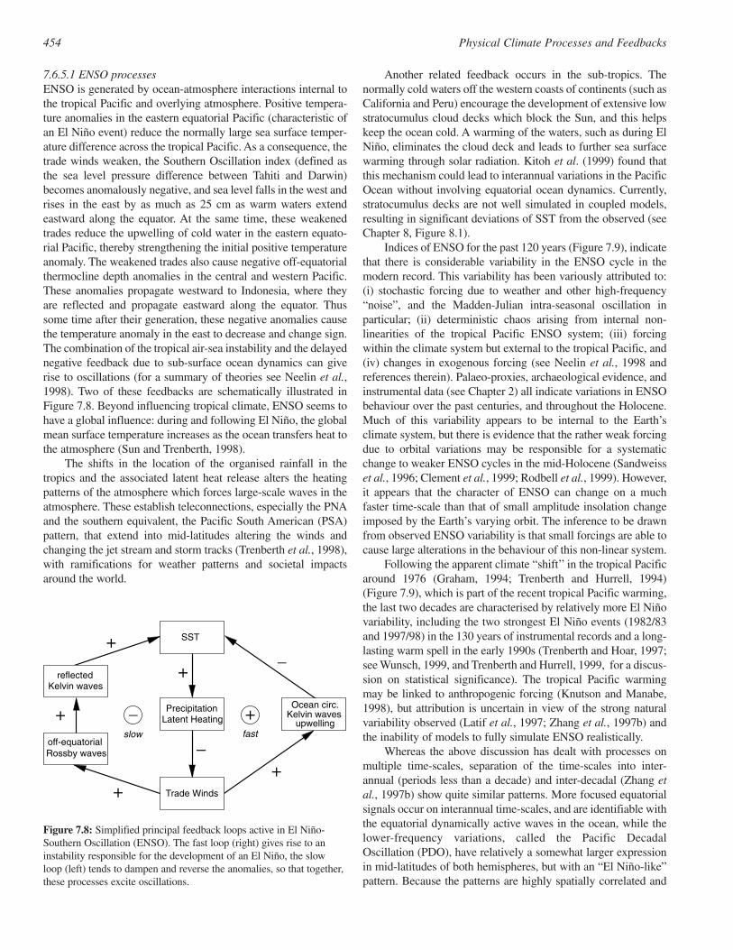
7.6.5.1 ENSO processesENSO is generated by ocean-atmosphere interactions internal tothe tropical Pacific and overlying atmosphere. Positive tempera-ture anomalies in the eastern equatorial Pacific (characteristic ofan El Niño event) reduce the normally large sea surface temper-ature difference across the tropical Pacific. As a consequence, thetrade winds weaken, the Southern Oscillation index (defined asthe sea level pressure difference between Tahiti and Darwin)becomes anomalously negative, and sea level falls in the west andrises in the east by as much as 25 cm as warm waters extendeastward along the equator. At the same time, these weakenedtrades reduce the upwelling of cold water in the eastern equato-rial Pacific, thereby strengthening the initial positive temperatureanomaly. The weakened trades also cause negative off-equatorialthermocline depth anomalies in the central and western Pacific.These anomalies propagate westward to Indonesia, where theyare reflected and propagate eastward along the equator. Thussome time after their generation, these negative anomalies causethe temperature anomaly in the east to decrease and change sign.The combination of the tropical air-sea instability and the delayednegative feedback due to sub-surface ocean dynamics can giverise to oscillations (for a summary of theories see Neelin et al.,1998). Two of these feedbacks are schematically illustrated inFigure 7.8. Beyond influencing tropical climate, ENSO seems tohave a global influence: during and following El Niño, the globalmean surface temperature increases as the ocean transfers heat tothe atmosphere (Sun and Trenberth, 1998).

The shifts in the location of the organised rainfall in thetropics and the associated latent heat release alters the heatingpatterns of the atmosphere which forces large-scale waves in theatmosphere. These establish teleconnections, especially the PNAand the southern equivalent, the Pacific South American (PSA)pattern, that extend into mid-latitudes altering the winds andchanging the jet stream and storm tracks (Trenberth et al., 1998),with ramifications for weather patterns and societal impactsaround the world.

Another related feedback occurs in the sub-tropics. Thenormally cold waters off the western coasts of continents (such asCalifornia and Peru) encourage the development of extensive lowstratocumulus cloud decks which block the Sun, and this helpskeep the ocean cold. A warming of the waters, such as during ElNiño, eliminates the cloud deck and leads to further sea surfacewarming through solar radiation. Kitoh et al. (1999) found thatthis mechanism could lead to interannual variations in the PacificOcean without involving equatorial ocean dynamics. Currently,stratocumulus decks are not well simulated in coupled models,resulting in significant deviations of SST from the observed (seeChapter 8, Figure 8.1).

Indices of ENSO for the past 120 years (Figure 7.9), indicatethat there is considerable variability in the ENSO cycle in themodern record. This variability has been variously attributed to:(i) stochastic forcing due to weather and other high-frequency“noise”, and the Madden-Julian intra-seasonal oscillation inparticular; (ii) deterministic chaos arising from internal non-linearities of the tropical Pacific ENSO system; (iii) forcingwithin the climate system but external to the tropical Pacific, and(iv) changes in exogenous forcing (see Neelin et al., 1998 andreferences therein). Palaeo-proxies, archaeological evidence, andinstrumental data (see Chapter 2) all indicate variations in ENSObehaviour over the past centuries, and throughout the Holocene.Much of this variability appears to be internal to the Earth’sclimate system, but there is evidence that the rather weak forcingdue to orbital variations may be responsible for a systematicchange to weaker ENSO cycles in the mid-Holocene (Sandweisset al., 1996; Clement et al., 1999; Rodbell et al., 1999). However,it appears that the character of ENSO can change on a muchfaster time-scale than that of small amplitude insolation changeimposed by the Earth’s varying orbit. The inference to be drawnfrom observed ENSO variability is that small forcings are able tocause large alterations in the behaviour of this non-linear system.

Following the apparent climate “shift’’ in the tropical Pacificaround 1976 (Graham, 1994; Trenberth and Hurrell, 1994)(Figure 7.9), which is part of the recent tropical Pacific warming,the last two decades are characterised by relatively more El Niñovariability, including the two strongest El Niño events (1982/83and 1997/98) in the 130 years of instrumental records and a long-lasting warm spell in the early 1990s (Trenberth and Hoar, 1997;see Wunsch, 1999, and Trenberth and Hurrell, 1999, for a discus-sion on statistical significance). The tropical Pacific warmingmay be linked to anthropogenic forcing (Knutson and Manabe,1998), but attribution is uncertain in view of the strong naturalvariability observed (Latif et al., 1997; Zhang et al., 1997b) andthe inability of models to fully simulate ENSO realistically.

Whereas the above discussion has dealt with processes onmultiple time-scales, separation of the time-scales into inter-annual (periods less than a decade) and inter-decadal (Zhang etal., 1997b) show quite similar patterns. More focused equatorialsignals occur on interannual time-scales, and are identifiable withthe equatorial dynamically active waves in the ocean, while thelower-frequency variations, called the Pacific DecadalOscillation (PDO), have relatively a somewhat larger expressionin mid-latitudes of both hemispheres, but with an “El Niño-like”pattern. Because the patterns are highly spatially correlated and


–slow fast

+

SST+

−

–

+

+Ocean circ.

Kelvin wavesupwelling

Trade Winds+

Rossby wavesoff-equatorial

reflectedKelvin waves

PrecipitationLatent Heating

+

Figure 7.8: Simplified principal feedback loops active in El Niño-Southern Oscillation (ENSO). The fast loop (right) gives rise to aninstability responsible for the development of an El Niño, the slowloop (left) tends to dampen and reverse the anomalies, so that together,these processes excite oscillations.

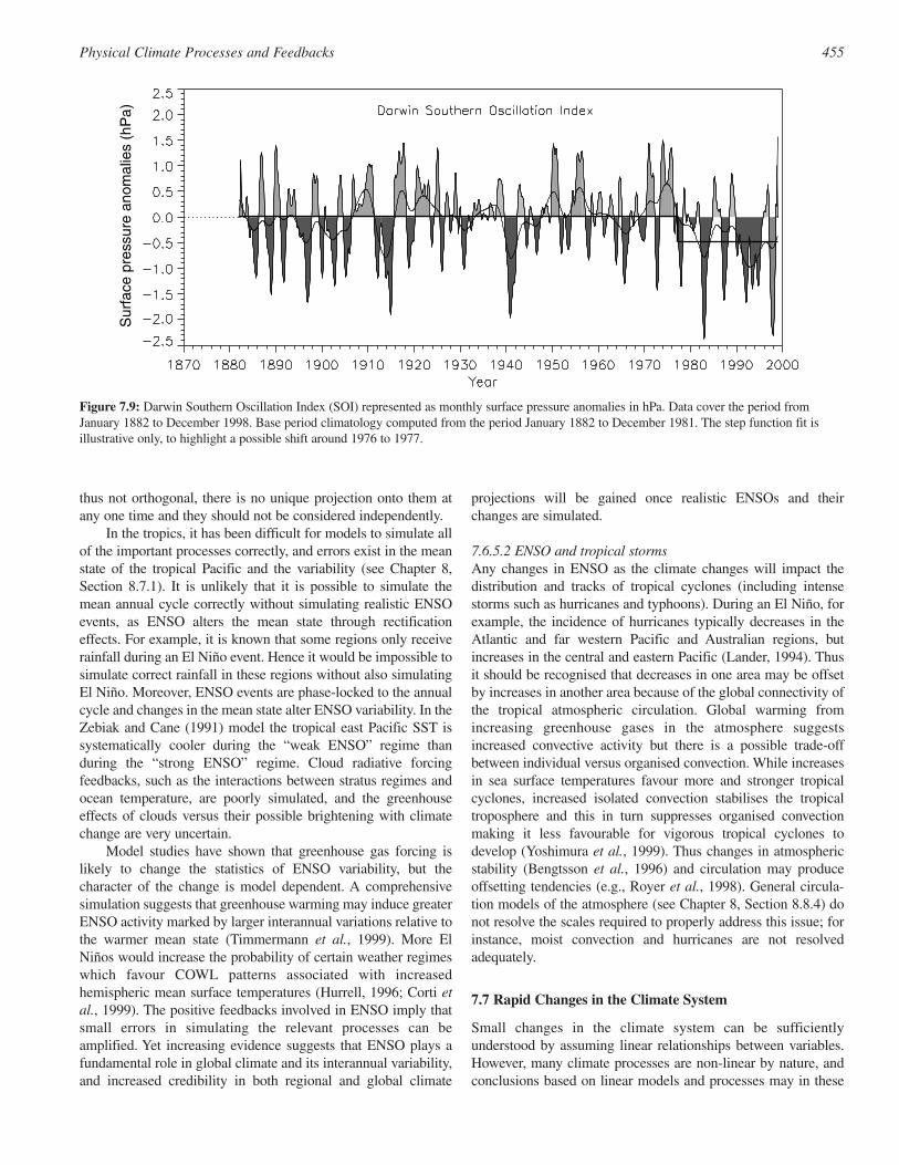
thus not orthogonal, there is no unique projection onto them atany one time and they should not be considered independently.

In the tropics, it has been difficult for models to simulate allof the important processes correctly, and errors exist in the meanstate of the tropical Pacific and the variability (see Chapter 8,Section 8.7.1). It is unlikely that it is possible to simulate themean annual cycle correctly without simulating realistic ENSOevents, as ENSO alters the mean state through rectificationeffects. For example, it is known that some regions only receiverainfall during an El Niño event. Hence it would be impossible tosimulate correct rainfall in these regions without also simulatingEl Niño. Moreover, ENSO events are phase-locked to the annualcycle and changes in the mean state alter ENSO variability. In theZebiak and Cane (1991) model the tropical east Pacific SST issystematically cooler during the “weak ENSO” regime thanduring the “strong ENSO” regime. Cloud radiative forcingfeedbacks, such as the interactions between stratus regimes andocean temperature, are poorly simulated, and the greenhouseeffects of clouds versus their possible brightening with climatechange are very uncertain.

Model studies have shown that greenhouse gas forcing islikely to change the statistics of ENSO variability, but thecharacter of the change is model dependent. A comprehensivesimulation suggests that greenhouse warming may induce greaterENSO activity marked by larger interannual variations relative tothe warmer mean state (Timmermann et al., 1999). More ElNiños would increase the probability of certain weather regimeswhich favour COWL patterns associated with increasedhemispheric mean surface temperatures (Hurrell, 1996; Corti etal., 1999). The positive feedbacks involved in ENSO imply thatsmall errors in simulating the relevant processes can beamplified. Yet increasing evidence suggests that ENSO plays afundamental role in global climate and its interannual variability,and increased credibility in both regional and global climate

projections will be gained once realistic ENSOs and theirchanges are simulated.

7.6.5.2 ENSO and tropical stormsAny changes in ENSO as the climate changes will impact thedistribution and tracks of tropical cyclones (including intensestorms such as hurricanes and typhoons). During an El Niño, forexample, the incidence of hurricanes typically decreases in theAtlantic and far western Pacific and Australian regions, butincreases in the central and eastern Pacific (Lander, 1994). Thusit should be recognised that decreases in one area may be offsetby increases in another area because of the global connectivity ofthe tropical atmospheric circulation. Global warming fromincreasing greenhouse gases in the atmosphere suggestsincreased convective activity but there is a possible trade-offbetween individual versus organised convection. While increasesin sea surface temperatures favour more and stronger tropicalcyclones, increased isolated convection stabilises the tropicaltroposphere and this in turn suppresses organised convectionmaking it less favourable for vigorous tropical cyclones todevelop (Yoshimura et al., 1999). Thus changes in atmosphericstability (Bengtsson et al., 1996) and circulation may produceoffsetting tendencies (e.g., Royer et al., 1998). General circula-tion models of the atmosphere (see Chapter 8, Section 8.8.4) donot resolve the scales required to properly address this issue; forinstance, moist convection and hurricanes are not resolvedadequately.

7.7 Rapid Changes in the Climate System

Small changes in the climate system can be sufficientlyunderstood by assuming linear relationships between variables.However, many climate processes are non-linear by nature, andconclusions based on linear models and processes may in these


Figure 7.9: Darwin Southern Oscillation Index (SOI) represented as monthly surface pressure anomalies in hPa. Data cover the period fromJanuary 1882 to December 1998. Base period climatology computed from the period January 1882 to December 1981. The step function fit isillustrative only, to highlight a possible shift around 1976 to 1977.

Sur

face

pre

ssur

e an

omal

ies

(hP

a)

cases no longer be valid. Non-linearity is a prerequisite for theexistence of thresholds in the climate system: small perturbationsor changes in the forcing can trigger large reorganisations ifthresholds are passed. The result is that atmospheric and oceaniccirculations may change from one regime to another. This couldpossibly be manifested as rapid climate change.

There is no clear definition of “rapid climate change”. Ingeneral, this notion is used to describe climate changes that are ofsignificant magnitude (relative to the natural variability) andoccur as a shift in the mean or variability from one level toanother. In order to distinguish such changes from “extremeevents”, a certain persistence of the change is required. Amongthe classical cases are spontaneous transitions from one preferredmode to another or transitions triggered by slowly varyingforcing. This occurs in non-linear systems which have multipleequilibria (Lorenz, 1993). Evidence for the possibility of suchtransitions can be found in palaeoclimatic records (see Chapter 2,Section 2.4; and Stocker, 2000), in observations of changes inlarge-scale circulation patterns from the instrumental record (seeSection 7.6.5.1), and contemporary observations of regionalweather patterns (e.g., Corti et al., 1999).

Here, we briefly summarise non-linear changes that havecaptured attention in the recent literature and that have beenassessed in this chapter:

• The Northern Hemispheric atmospheric circulation exhibitsdifferent regimes that are associated with the North AtlanticOscillation. Recent analyses of observations suggest thatrelatively rapid regime changes are possible (see Section 7.2.6)and that they may have happened frequently in the past(Appenzeller et al., 1998). Several studies suggest that therecent changes may be a response to anthropogenic forcing, butour understanding of the processes generating NAO is notsufficient to have confidence in whether this is the case.

• Observed variability of ENSO suggests that a transition to morefrequent El Niño occurred around 1976 (see Section 7.6.5.1).Current understanding of ENSO processes does not yet permita distinction as to the extent this is a response to anthropogenicforcing versus part of the long-term natural variability of thetropical atmosphere-ocean system, or both (see also Chapter 2,Section 2.6.2).

• Results from most climate models suggest that the Atlanticthermohaline circulation slows down in response to globalwarming; some models simulate a complete shut-down ifcertain thresholds are passed (see Section 7.3.6 and Chapter 9,

Section 9.3.4.3). Such a shut-down is in general not abrupt butevolves on a time-scale which is determined by the warming,i.e., a few decades to centuries. Processes for such an evolutionare increasingly understood. As model resolution increases andhigh latitude processes are better represented in these models(sea ice, topography), additional feedbacks influencing theAtlantic THC will be investigated and their relative importancemust be explored. This will lead to a better quantification of theoverall stability of the THC.

• Large polar ice masses, ice shelves or even complete ice sheetsmay be destabilised by sea level rise (see Section 7.5 andChapter 11, Section 11.3.3), thereby contributing to further sealevel rise.

• Warming in the high latitudes may lead to significant reductionsin sea ice and associated feedbacks may accelerate thisdevelopment (see Box 7.1).

• Large-scale and possibly irreversible changes in the terrestrialbiosphere and vegetation cover are thought to have occurred inthe past when anthropogenic perturbation was negligible (e.g.,the development of the Saharan desert, Claussen et al., 1999).These changes may be interpreted as non-linear changestriggered by slow changes in external forcing and thus cannotbe excluded to occur in the future. Knowledge on thesephenomena, however, is not advanced yet.

Reducing uncertainty in climate projections also requires abetter understanding of these non-linear processes which giverise to thresholds that are present in the climate system.Observations, palaeoclimatic data, and models suggest that suchthresholds exist and that transitions have occurred in the past. Theoccurrence of such transitions can clearly not be excluded in aclimate that is changing. On the contrary, model simulationsindicate that such transitions lie within the range of changes thatare projected for the next few centuries if greenhouse gas concen-trations continue to increase. A particular concern is the fact thatsome of these changes may even be irreversible due to theexistence of multiple equilibrium states in the climate system.

Comprehensive climate models in conjunction withsustained observational systems, both in situ and remote, are theonly tool to decide whether the evolving climate system isapproaching such thresholds. Our knowledge about theprocesses, and feedback mechanisms determining them, must besignificantly improved in order to extract early signs of suchchanges from model simulations and observations.


References

Abdalati, W. and K. Steffen, 1995: Passive microwave-derived snow-melt regions on the Greenland ice sheet. Geophys. Res. Lett., 22, 787-790.

Abdella, K. and N. McFarlane, 1997: A new second-order turbulenceclosure scheme for the planetary boundary layer. J. Atm. Sci., 54,1850-1867.

Albrecht, B., 1989: Aerosols, cloud microphysics and fractional cloudi-ness. Science, 245, 1227-1230.

Alexander, M.A. and C. Deser, 1995: A mechanism for the recurrence ofwinter time midlatitude SST anomalies. J. Phys. Oceanogr., 25, 122-137.

Allan, R.P., K.P. Shine, A. Slingo and J.A. Pamment, 1999: The depend-ence of clear-sky outgoing long-wave radiation on surface tempera-ture and relative humidity. Quart. J. Roy. Met. Soc., 125, 2103-2126.

Alley, R.B., 1989: Water-pressure coupling of sliding and bed deforma-tion: II. Velocity-depth profiles. J. Glaciol., 35, 119-129.

AMIP, 1995: Proceedings of the First International AMIP ScientificConference [Gates, W. L. (ed.)]. World Meteorological Organization,Geneva.

Anandakrishnan, S. and R.B. Alley, 1997: Stagnation of ice stream C,West Antarctica, by water piracy. Geophys. Res. Lett., 24, 265-268.

Anandakrishnan, S., D.D. Blankenship, R.B. Alley and P.L. Stoffa,1998: Influence of subglacial geology on the position of a WestAntarctic ice stream from seismic observations. Nature, 394, 62-65.

Andre, J.C., J.P. Goutorbe and A. Perrier, 1986: HAPEX/MOBILHY: Ahydrologic atmospheric experiment for the study of water budget andevaporation flux at the climate scales. Bull. Am. Met. Soc., 67, 138-144.

Andrews, D.G., J.R. Holton and C.B. Leovy, 1987: Middle AtmosphereDynamics. Academic Press, Florida. Chapter 2.

Anisimov, O.A. and F.E. Nelson, 1996: Permafrost distribution in thenorthern hemisphere under scenarios of climatic change. Glob.Planet. Change, 14, 59-72.

Anisimov, O.A. and F.E. Nelson, 1997: Permafrost zonation and climatechange: results from transient general circulation models. Clim.Change, 35, 241-258.

Anisimov, O.A., N.I. Shiklomanov and F.E. Nelson, 1997: Effects ofglobal warming on permafrost and active-layer thickness: resultsfrom transient general circulation models. Glob. Planet. Change, 61,61-77.

Appenzeller, C., T.F. Stocker and M. Anklin, 1998: North Atlanticoscillation dynamics recorded in Greenland ice cores. Science, 282,446-449.

Arakawa, A. and W.H. Schubert, 1974: Interaction of a cumulus cloudensemble with the large-scale environment. Part I. J. Atm. Sci., 31,674-701.

Arbetter, T.E., J.A. Curry, M.M. Holland and J.A. Maslanik, 1997:Response of sea-ice models to perturbations in surface heat flux. Ann.Glaciol., 25, 193-197.

Arkin, P.A. and P. Xie, 1994: The Global Precipitation ClimatologyProject: First algorithm intercomparison project. Bull. Am. Met. Soc.,75, 401-420.

Arking, A., M.-D. Chou and W.L. Ridgway, 1996: On estimating theeffects of clouds on atmospheric absorption based on flux observa-tions above and below cloud level. Geophys. Res. Lett., 23, 829-832.

Atlas, R.M. and N. Wolfson, 1993: The effect of SST and soil moistureanomalies on GLA model simulations of the 1988 U.S. summerdrought. J. Clim., 6, 2034-2048.

Avissar, R., 1998: Which type of soil-vegetation-atmosphere transferscheme is needed for general circulation models: a proposal for ahigher-order scheme. J. Hydrol., 212, 136-154.

Avissar, R. and T. Schmidt, 1998: An evaluation of the scale at whichground-surface heat flux patchiness affects the convective boundary

layer using large-eddy simulations. J. Atm. Sci., 55, 2666-2689. Avissar, R., E.W. Eloranta, K. Gurer and G.J. Tripoli, 1998: An evalua-

tion of the large-eddy simulation option of the regional atmosphericmodeling system in simulating a convective boundary layer: a FIFEcase study. J. Atm. Sci., 55, 1109-1130.

Ayotte, K.W., P.P. Sullivan, A. Andren, S.C. Doney, A.A.M. Holtslag,W.G. Large, J.C. McWilliams, C.-H. Moeng, M. Otte, J.J. Tribbia andJ.C. Wyngaard, 1996: An evaluation of neutral and convectiveplanetary boundary-layer parameterization relative to large eddysimulations. Bound.-Lay. Meteorol., 79, 131-175.

Bacon, S., 1997: Circulation and fluxes in the North Atlantic betweenGreenland and Ireland. J. Phys. Oceanogr., 27, 1420-1435.

Baldwin, M.P. and T.J. Dunkerton, 1999: Propagation of the ArcticOscillation from the stratosphere to the troposphere. J. Geophys.Res., 104, 30937-30946.

Baldwin, M.P., X. Cheng and T.J. Dunkerton, 1994: Observed correla-tions between winter-mean tropospheric and stratospheric circulationanomalies. Geophys. Res. Lett., 21, 1141-1144.

Baringer, M.O. and J.F. Price, 1997: Mixing and spreading of theMediterranean outflow. J. Phys. Oceanogr., 27, 1654-1677.

Barker, H.W. and Z. Li, 1997: Interpreting shortwave albedo-transmit-tance plots: True or apparent anomalous absorption. Geophys. Res.Lett., 24, 2023-2026.

Barry, R.G., 1996: The parameterization of surface albedo for sea ice andits snow cover. Prog. Phys. Geogr., 20, 63-79.

Bates, J.J. and D.L. Jackson, 1997: A comparison of water vapor observa-tions with AMIP 1 simulations. J. Geophys. Res., 102, 21837-21852.

Beal, L.M. and H.L. Bryden, 1997: Observations of an AgulhasUndercurrent. Deep-Sea Res. I, 44, 1715-1724.

Beckmann, A. and R. Döscher, 1997: A method for improved represen-tation of dense water spreading over topography in geopotential-coordinate models. J. Phys. Oceanogr., 27, 581-591.

Beljaars, A.C.M., P. Viterbo, M.J. Miller and A.K. Betts, 1996: Theanomalous rainfall over the United States during July 1993:Sensitivity to land-surface parameterization and soil-moistureanomalies. Mon. Wea. Rev., 124, 362-383.

Belkin, I.M., S. Levitus, J. Antonov and S.-A. Malmberg, 1998: “GreatSalinity Anomalies” in the North Atlantic. Prog. Oceanogr., 41, 1-68.

Bell, R.E., D.D. Blankenship, C.A. Finn, D.L. Morse, T.A. Scambos,J.M. Brozena and S.M. Hodge, 1998: Influence of subglacial geologyon the onset of a West Antarctic ice stream from aerogeophysicalobservations. Nature, 394, 58-62.

Bengtsson, L., M. Botzet and M. Esch, 1996: Will greenhouse gas-induced warming over the next 50 years lead to higher frequency andgreater intensity of hurricanes? Tellus, 48A, 57-73.

Bengtsson, L., E. Roeckner and M. Stendel, 1999: Why is the globalwarming proceeding much slower than expected. J. Geophys. Res.,104, 3865-3876.

Bentley, C.R., 1998: Rapid sea-level rise from a West Antarctic ice-sheetcollapse: a short-term perspective. J. Glaciol., 44, 157-163.

Betts, A.K., 1982: Saturation point analysis of moist convectiveoverturning. J. Atm. Sci., 39, 1484-1505.

Betts, A.K., J.H. Ball, A.C.M. Beljaars, M.J. Miller and P.A. Viterbo,1996: The land-surface atmosphere interaction: A review based onobservational and global modeling perspectives. J. Geophys. Res.,101, 7209-7225.

Betts, A.K., P. Viterbo, A.C.M. Beljaars, H.L. Pan, S.Y. Hong, M.Goulden and S. Wofsy, 1998: Evaluation of land-surface interactionin ECMWF and NCEP/NCAR reanalysis models over grassland(FIFE) and boreal forest (BOREAS). J. Geophys. Res., 103, 23079-23085.

Betts, R.A., P.M. Cox, S.E. Lee and F.I. Woodward, 1997: Contrastingphysiological and structural vegetation feedbacks in climate changesimulations. Nature, 387, 796-799.

Bindschadler, R., 1997: Actively surging West Antarctic ice streams and


their response characteristics. Ann. Glaciol., 24, 409-414. Bitz, C.M., M.M. Holland, A.J. Weaver and M. Eby, 2001: Simulating the

ice-thickness distribution in a coupled climate model. J. Geophys.Res., 106, 2441-2464.

Boening, C.W., W.R. Holland, F.O. Bryan, G. Danabasoglu and J.C.McWilliams, 1995: An overlooked problem in model simulations ofthe thermohaline circulation and heat transport in the Atlantic Ocean.J. Clim., 8, 515-523.

Bolle, H.-J., J.-C. Andre, J.L. Arrue, H.K. Barth, P. Bessemoulin, A.Brasa, H.A.R. de Bruin, J. Cruces, G. Dugdale, E.T. Engman, D.L.Evans, R. Fantechi, F. Fiedler, A. van de Griend, A.C. Imeson, A.Jochum, P. Kabat, T. Kratzsch, J.-P. Lagouarde, I. Langer, R. Llamas,E. Lopez-Baeza, J. Melia Miralles, L.S. Muniosguren, F. Nerry, J.Noilhan, H.R. Oliver, R. Roth, S.S. Saatchi, J. Sanchez Diaz, M. deSanta Olalla, W.J. Shuttleworth, H. Sogaard, H. Stricker, J. Thornes,M. Vauclin and D. Wickland, 1993: EFEDA: European field experi-ment in a desertification threatened area. Ann. Geophys., 11, 173-189.

Bonan, G.B., 1995: Land-atmosphere CO2 exchange simulated by a landsurface process model coupled to an atmospheric general circulationmodel. J. Geophys. Res., 100, 2817-2831.

Bonan, G.B., 1996: Sensitivity of a GCM simulation to subgrid infiltra-tion and surface runoff. Clim. Dyn., 12, 279-285.

Bonan, G.B., 1999: Frost followed the plow: Impacts of deforestation onthe climate of the United States. Ecol. Appl., 9, 1305-1315.

Bonan, G.B., D. Pollard and S.L. Thompson, 1992: Effects of borealforest vegetation on global climate. Nature, 359, 716-718.

Bony, S., J.-P. Duvel and H. Le Treut, 1995: Observed dependence of thewater vapor and clear-sky greenhouse effect on sea surface tempera-ture: comparison with climate warming experiments. Clim. Dyn., 11,307-320.

Bony, S., K.M. Lau and Y.C. Sud, 1997: Sea surface temperature andlarge-scale circulation influences on tropical greenhouse effect andcloud radiative forcing. J. Clim., 10, 2055-2077.

Boville, B.A., 1995: Middle atmosphere version of CCM2 (MACCM2):annual cycle and interannual variability. J. Geophys. Res., 100, 9017-9039.

Boville, B.A. and P.R. Gent, 1998: The NCAR climate system model,version one. J. Clim., 11, 1115-1130.

Braswell, W.D. and R.S. Lindzen, 1998: Anomalous short wave absorp-tion and atmospheric tides. Geophys. Res. Lett., 25, 1293-1296.

Breon, F., 1992: Reflectance of broken cloud fields: Simulation andparameterization. J. Atm. Sci., 49, 1221-1232.

Bretherton, C.S. and D.S. Battisti, 2000: An interpretation of the resultsfrom atmospheric general circulation models forced by the timehistory of the observed sea surface temperature distribution.Geophys. Res. Lett., 27, 767-770.

Bretherton, C.S., M.K. McVean, P. Bechtold, A. Chlond, W.R. Cotton, J.Cuxart, H. Cuijpers, M. Khairoutdinov, B. Kosovic, D. Lewellen, C.-H. Moeng, P. Siebesma, B. Stevens, D.E. Stevens, I. Sykes and M.C.Wyant, 1999: An intercomparison of radiatively-driven entrainmentand turbulence in a smoke cloud, as simulated by different numericalmodels. Quart. J. Roy. Met. Soc., 125, 391-423.

Broecker, W.S., 1997: Thermohaline circulation, the Achilles heel of ourclimate system: will man-made CO2 upset the current balance?Science, 278, 1582-1588.

Brubaker, K.L. and D. Entekhabi, 1996: Analysis of feedbackmechanisms in land-atmosphere interaction. Water Resour. Res., 32,1343-1357.

Brubaker, K.L., D. Entekhabi and P.S. Eagleson, 1993: Estimation ofcontinental precipitation recycling. J. Clim., 6, 1077-1089.

Bryan, F., 1986: High-latitude salinity effects and interhemisphericthermohaline circulations. Nature, 323, 301-304.

Bryden, H.L., D.H. Roemmich and J.A. Church, 1991: Ocean heattransport across 24N in the Pacific. Deep-Sea Res., 38, 297-324.

Butchart, N. and J. Austin, 1998: Middle atmosphere climatologies from

the troposphere-stratosphere configuration of the UKMO’s unifiedmodel. J. Atm. Sci., 55, 2782-2809.

Cahalan, R.F., W. Ridgeway, W.J. Wiscombe, S. Gollmer andHarshvardhan, 1994: Independent pixel and Monte Carlo estimatesof stratocumulus albedo. J. Atm. Sci., 51, 3776-3790.

Cao, K.K. and F.I. Woodward, 1998: Dynamic responses of terrestrialecosystem carbon cycling to global climate change. Nature, 393,249-252.

Carton, J.A., X. Cao, B.S. Giese and A.M. da Silva, 1996: Decadal andinterannual SST variability in the tropical Atlantic. J. Phys.Oceanogr., 26, 1165-1175.

Cayan, D.R., 1992: Latent and sensible heat flux anomalies over thenorthern oceans: the connection to monthly atmospheric circulation.J. Clim., 5, 354-369.

Cess, R.D., G.L. Potter, J.P. Blanchet, G.J. Boer, A.D.D. Genio, M.Deque, V. Dymnikov, V. Galin, W.L. Gates, S.J. Ghan, J.T. Kiehl,A.A. Lacis, H. Le Treut, Z.X. Li, X.-Z. Liang, B.J. McAvaney, V.P.Meleshko, J.F.B. Mitchell, J.-J. Morcrette, D.A. Randall, L. Rikus, E.Roeckner, J.F. Roer, U. Schlese, D.A. Sheinin, A. Slingo, A.P.Sokolov, K.E. Taylor, W.M. Washington, R.T. Wetherald, I. Yagai andM.-H. Zhang, 1990: Intercomparison and interpretation of climatefeedback processes in 19 atmospheric general circulation models. J.Geophys. Res., 95, 16601-16615.

Cess, R.D., M. Zhang, P. Minnis, L. Corsetti, E.G. Dutton, B.W. Forgan,D.P. Garber, W.L. Gates, J.J. Hack, E.F. Harrisson, X. Jing, J.T. Kiehl,C.N. Long, J.-J. Morcrette, G.L. Potter, V. Ramanathan, B. Subasilar,C.H. Whitlock, D.F. Young and Y. Zhou, 1995: Absorption of solarradiation by clouds: Observations versus models. Science, 267, 496-499.

Cess, R.D., M.H. Zhang, W.J. Ingram, G.L. Potter, V. Alekseev, H.W.Barker, E. Cohen-Solal, R.A. Colman, D.A. Dazlich, A.D. DelGenio, M.R. Dix, V. Dymnikov, M. Esch, L.D. Fowler, J.R. Fraser, V.Galin, W.L. Gates, J.J. Hack, J.T. Kiehl, H. LeTreut, K.K.-W. Lo, B.J.McAvaney, V.P. Meleshko, J.-J. Morcrette, D.A. Randall, E.Roeckner, J.-F. Royer, M.E. Schlesinger, P.V. Sporyshev, B. Timbal,E.M. Volodin, K.E. Taylor, W. Wang and R.T. Wetherald, 1996:Cloud feedback in atmospheric general circulation models: Anupdate. J. Geophys. Res., 101, 12791-12794.

Cess, R.D., M.H. Zhang, F.P.J. Valero, S.K. Pope, A. Bucholtz, B. Bush,C.S. Zender and J. Vitko, 1999: Absorption of solar radiation by thecloudy atmosphere: Further interpretations of collocated aircraftmeasurements. J. Geophys. Res., 104, 2059-2066.

Chang, P., L. Ji and H. Li, 1997: A decadal climate variation in thetropical ocean from thermodynamic air-sea interactions. Nature, 385,516-518.

Chapman, W.L. and J.E. Walsh, 1993: Recent variations of sea ice andair temperature in high latitudes. Bull. Am. Met. Soc., 74, 33-48.

Chou, C. and J.D. Neelin, 1999: Cirrus detrainment-temperaturefeedback. Geophys. Res. Lett., 26, 1295-1298.

Christensen, O.B., J.H. Christensen, B. Machenhauer and M. Botzet,1998: Very high-resolution regional climate simulations overScandinavia - Present climate. J. Clim., 11, 3204-3229.

Ciais, P., P.P. Tans, J.W.C. White, M. Trolier, R.J. Francey, J.A. Berry,D.R. Randall, P.J. Sellers, J.G. Collatz and D.S. Schimel, 1995:Partitioning of ocean and land uptake of CO2 as inferred by δ13Cmeasurements from the NOAA Climate Monitoring and DiagnosticsLaboratory Global Air Sampling Network. J. Geophys. Res., 100,5051-5070.

Ciais, P., A.S. Denning, P.P. Tans, J.A. Berry, D.A. Randall, G.J. Collatz,P.J. Sellers, J.W.C. White, M. Trolier, H.A.J. Meijer, R.J. Francey, P.Monfray and M. Heimann, 1997: A three-dimensional synthesisstudy of delta O-18 in atmospheric CO2. 1. Surface fluxes. J.Geophys. Res., 102, 5857-5872.

Cihlar, J., P.H. Carmori, P.H. Schuepp, R.L. Desjardins and J.I.Macpherson, 1992: Relationship between satellite-derived vegetation


indices and aircraft-based CO2 measurements. J. Geophys. Res., 97,18515-18521.

Ciret, C. and A. Henderson-Sellers, 1998: Sensitivity of global vegeta-tion models to present-day climate grassland simulated by globalclimate models. Glob. Biogeochem. Cyc., 11, 1141-1169.

Clarke, T.S. and K. Echelmeyer, 1996: Seismic-reflection evidence for adeep subglacial trough beneath Jakobshavns Isbrae, West Greenland.J. Glaciol., 43, 219-232.

Claussen, M., 1997: Modeling bio-geophysical feedbacks in the Africanand Indian monsoon region. Clim. Dyn., 13, 247-257.

Claussen, M., C. Kubatzki, V. Brovkin, A. Ganopolski, P. Hoelzmannand H.-J. Pachur, 1999: Simulation of an abrupt change in Saharanvegetation in the mid-Holocene. Geophys. Res. Lett., 26, 2037-2040.

Clement, A. and R. Seager, 1999: Climate and the tropical oceans. J.Clim., 12, 3383-3401.

Clement, A., R. Seager and M.A. Cane, 1999: Orbital controls ontropical climate. Paleoceanogr., 14, 441-455.

Colello, G.D., C. Grivet, P.J. Sellers and J.A. Berry, 1998: Modeling ofenergy, water and CO2 flux in a temperate grassland ecosystem withSiB2: May-October 1987. J. Atm. Sci., 55, 1141-1169.

Collatz, G.J., J.T. Ball, C. Grivet and J.A. Berry, 1991: Physiological andenvironmental regulation of stomatal conductance, photosynthesisand transpiration: A model that includes a laminar boundary layer.Agric. For. Meteorol., 54, 107-136.

Collatz, G.J., L. Bounoua, S.O. Los, D.A. Randall, I.Y. Fung and P.J.Sellers, 2000: A mechanism for the influence of vegetation on theresponse of the diurnal temperature range to a changing climate.Geophys. Res. Lett., 27, 3381-3384.

Collins, W.G., 1998: Complex quality control of significant levelrawinsonde temperature. J. Atmos. Oc. Tech., 15, 69-79.

Colman, R.A. and B.J. McAvaney, 1995: Sensitivity of the climateresponse of the atmospheric general circulation model to changes inconvective parameterization and horizontal resolution. J. Geophys.Res., 100, 3155-3172.

Corti, S., F. Molteni and T.N. Palmer, 1999: Signature of recent climatechange in frequencies of natural atmospheric circulation regimes.Nature, 398, 799-802.

Cubasch, U., J. Waszkewitz, G. Hegerl and J. Perlwitz, 1995: Regionalclimate changes as simulated in time-slice experiments. Clim.Change, 31, 273-304.

Cuijpers, J.W.M. and A.A.M. Holtslag, 1998: Impact of skewness andnonlocal effects on scalar and buoyancy fluxes in convectiveboundary layers. J. Atm. Sci., 55, 151-162.

Curry, J., C.A. Clayson, W.B. Rossow, R. Reeder, Y.-C. Zhang, P.J.Webster, G. Liu and R.-S. Sheu, 1999: High-resolution satellite-derived dataset of the surface fluxes of heat, freshwater, andmomentum for the TOGA COARE IOP. Bull. Am. Met. Soc., 80,2059-2080.

Curry, J.A. and P.J. Webster, 1999: Thermodynamics of Atmospheresand Oceans. Academic Press, 465.

da Silva, A.M., C.C. Young and S. Levitus, 1994: Atlas of Surface MarineData 1994 Volume 1: Algorithms and Procedures. In: NOAA AtlasNESDIS (6) . U.S. Department of Commerce, Washington D. C., 83.

Dai, A., F. Giorgi and K.E. Trenberth, 1999: Observed and model-simulated diurnal cycles of precipitation over the contiguous UnitedStates. J. Geophys. Res., 104, 6377-6402.

Dai, A.G. and I.Y. Fung, 1993: Can climate variability contribute to the“missing” CO2 sink? Global Biogeochemical Cycles, 7, 543-567.

Danabasoglu, G. and J.C. McWilliams, 1995: Sensitivity of the globalocean circulation to parameterizations of mesoscale tracer transports.J. Clim., 8, 2967-2987.

de Ruijter, W.P.M., A. Biastoch, S.S. Drijfhout, J.R.E. Lutjeharms, R.P.Matano, T. Pichevin, P.J. van Leeuwen and W. Weijer, 1999: Indian-Atlantic interocean exchange: dynamics, estimation and transport. J.Geophys. Res., 104, 20885-20910.

DeCosmo, J., K.B. Katsaros, S.D. Smith, R.J. Anderson, W. Oost, K.Bumke and H. Chadwick, 1996: Air-sea exchange of water vapor andsensible heat: The humidity exchange over the sea (HEXOS) results.J. Geophys. Res., 101, 12001-12016.

Del Genio, A.D., A.A. Lacis and R.A. Ruedy, 1991: Simulations of theeffect of a warmer climate on atmospheric humidity. Nature, 251,382-385.

Del Genio, A.D., W. Kovari and M.-S. Yao, 1994: Climatic implicationsof the seasonal variation of upper tropospheric water vapor. Geophys.Res. Lett., 21, 2701-2704.

Del Genio, A.D., M.-S. Yao, W. Kovari and K.K.W. Lo, 1996: Aprognostic cloud water parameterization for global climate models. J.Clim., 9, 270-304.

Delire, C. and J.A. Foley, 1999: Evaluating the performance of a landsurface/ecosystem model with biophysical measurements fromcontrasting environments. J. Geophys. Res., 104, 16895-16909.

Delworth, T.L. and M.E. Mann, 2000: Observed and simulatedmultidecadal variability in the Northern Hemisphere. Clim. Dyn., 16,661-676.

Denning, A.S., G.J. Collatz, C. Zhang, D.A. Randall, J.A. Berry, P.J.Sellers, G.D. Colello and D.A. Dazlich, 1996a: Simulations ofterrestrial carbon metabolism and atmospheric CO2 in a generalcirculation model. Part I: Surface carbon fluxes. Tellus, 48B, 521-542.

Denning, A.S., D.A. Randall, G.J. Collatz and P.J. Sellers, 1996b:Simulations of terrestrial carbon metabolism and atmospheric CO2 ina general circulation model. Part II: simulated CO2 concentrations.Tellus, 48B, 543-567.

Deser, C. and M.L. Blackmon, 1993: Surface climate variations over theNorth Atlantic Ocean during winter: 1900-1993. J. Clim., 6, 1743-1753.

Deser, C. and M.S. Timlin, 1997: Atmosphere-ocean interaction onweekly time scales in the North Atlantic and Pacific. J. Clim., 10,393-408.

Deser, C., J.E. Walsh and M.S. Timlin, 2000: Arctic sea ice variability inthe context of recent wintertime atmospheric circulation trends. J.Clim., 13, 617-633.

Desjardins, J., R.J. Hart, J.I. MacPherson, P.H. Schuepp and S.B. Verma,1992: Aircraft- and tower-based fluxes of carbon dioxide, latent, andsensible heat. J. Geophys. Res., 97, 18477-18485.

Dessler, A.E. and S.C. Sherwood, 2000: Simulations of tropical uppertropospheric humidity. J. Geophys. Res., 105, 20155-20163.

Dickinson, R.E., M. Shaikh, R. Bryant and L. Graumlich, 1998:Interactive canopies for a climate model. J. Clim., 11, 2823-2836.

Dickson, R.R., J. Lazier, J. Meincke, P. Rhines and J. Swift, 1996: Long-term coordinated changes in the convective activity of the NorthAtlantic. Prog. Oceanogr., 38, 241-295.

Dickson, R.R., J. Meincke, S.-A. Malmberg and A.J. Lee, 1988: The“Great Salinity Anomaly” in the northern North Atlantic 1968-1982.Prog. Oceanogr., 20, 103-151.

Dickson, R.R., T.J. Osborn, J.W. Hurrell, J. Meincke, J. Blindheim, B.Adlandsvik, T. Vinje, G. Alekseev and W. Maslowski, 2000: TheArctic Ocean response to the North Atlantic Oscillation. J. Clim., 13,2671-2696.

Dixon, K.W., T.L. Delworth, M.J. Spelman and R.J. Stouffer, 1999: Theinfluence of transient surface fluxes on North Atlantic overturning ina coupled GCM climate change experiment. Geophys. Res. Lett., 26,2749-2752.

Doney, S.C., W.G. Large and F.O. Bryan, 1998: Surface ocean fluxes andwater-mass transformation rates in the coupled NCAR ClimateSystem Model. J. Clim., 11, 1420-1441.

Döscher, R., C.W. Boening and P. Herrmann, 1994: Response of circula-tion and heat transport in the North Atlantic to changes in thermoha-line forcing in northern latitudes: A model study. J. Phys. Oceanogr.,24, 2303-2320.


Douville, H., J.F. Royer and J.F. Mahfouf, 1995: A new snow parameter-ization for the Meteo-France climate model. 1. Validation in stand-alone experiments. Clim. Dyn., 12, 21-35.

Dowdeswell, J.A. and M.J. Siegert, 1999: The dimensions andtopographic setting of Antarctic subglacial lakes and implications forlarge-scale water storage beneath continental ice sheets. Geology,111, 254-263.

Ducharne, A., K. Laval and J. Polcher, 1996: Sensitivity of the hydrolog-ical cycle to the parameterization of soil hydrology in a GCM. Clim.Dyn., 14, 307-327.

Duffy, P.B. and K. Caldeira, 1997: Sensitivity of simulated salinity in athree-dimensional ocean model to upper-ocean transport of salt fromsea-ice formation. Geophys. Res. Lett., 24, 1323-1326.

Duffy, P.B., M. Eby and A.J. Weaver, 1999: Effects of sinking of saltrejected during formation of sea ice on results of an ocean-atmosphere-sea ice climate model. Geophys. Res. Lett., 26, 1739-1742.

Dümenil, L., S. Hagemann and K. Arpe (eds.), 1997: Validation of thehydrological cycle in the Arctic using river discharge data, Workshopon Polar Processes in Global Climate, Cancun, Mexico.

Dunkerton, T.J., 1997: The role of gravity waves in the quasi-biennialoscillation. J. Geophys. Res., 102, 26053-26076.

Duvel, J.-P., S. Bony and H. Le Treut, 1997: Clear-sky greenhouse effectsensitivity to sea surface temperature changes: an evaluation of AMIPsimulations. Clim. Dyn., 13, 259-273.

Duynkerke, P.G., P.J. Jonker, A. Chlond, M.C. van Zanten, J. Cuxart, P.Clark, E. Sanchez, G. Martin, G. Lenderink and J. Teixeira, 1999:Intercomparison of three- and one-dimensional model simulationsand aircraft observations of stratocumulus. Bound.-Lay. Meteorol.,92, 453-488.

Eby, M. and G. Holloway, 1994: Sensitivity of a large-scale ocean modelto a parameterization of topographic stress. J. Phys. Oceanogr., 24,2577-2588.

Eluszkiewicz, J.E., R. Zurek, L. Elson, E. Fishbein, L. Froidevaux, J.Waters, R. Grainger, A. Lambert, R. Harwood and G. Peckham,1996: Residual circulation in the stratosphere and lower mesosphereas diagnosed from Microwave Limb Sounder data. J. Atm. Sci., 53,217-240.

Emanuel, K., 1991: A scheme for representing cumulus convection inlarge scale models. J. Atm. Sci., 48, 2313-2333.

Emanuel, K.A. and M. Zivkovic-Rothman, 1999: Development andevaluation of a convection scheme for use in climate models. J. Atm.Sci., 56, 1766-1782.

Engelhardt, H. and B. Kamb, 1998: Basal sliding of Ice Stream B, WestAntarctica. J. Glaciol., 44, 223-230.

Fairall, C.W., E.F. Bradley, D.P. Rogers, J.B. Edson and G.S. Young,1996: Bulk parametrization of air-sea fluxes for TOGA COARE. J.Geophys. Res., 101, 1295-1308.

Farquhar, G.D., S. von Caemmerer and J.A. Berry, 1980: A biochemicalmodel of photosynthetic CO2 fixation in leaves of C3 species. Planta,149, 78-90.

Fastook, J.L. and M. Prentice, 1994: A finite-element model ofAntarctica: sensitivity test for meteorological mass-balance relation-ship. J. Glaciol., 40, 167-175.

Fetterer, F. and N. Untersteiner, 1998: Observations of melt ponds onArctic sea ice. J. Geophys. Res., 103, 24821-24835.

Field, C.B. and I.Y. Fung, 1999: The not-so-big US carbon sink. Science,285, 544-545.

Field, C.B., J.T. Randerson and C.M. Malmstrong, 1995: Global netprimary production: combining ecology and remote sensing. Rem.Sens. Environ., 51, 74-88.

Findell, K.L. and E.A.B. Eltahir, 1997: An analysis of the soil moisture-rainfall feedback, based on direct observations from Illinois. WaterResour. Res., 33, 725-735.

Foley, J.A., I.C. Prentice, N. Ramankutty, S. Levis, D. Pollard, S. Sitch

and A. Haxeltine, 1996: An integrated biosphere model of landsurface processes, terrestrial carbon balance and vegetationdynamics. Glob. Biogeochem. Cyc., 10, 603-628.

Foley, J.A., S. Levis, I.C. Prentice, D. Pollard and S.L. Thompson, 1998:Coupling dynamic models of climate and vegetation. Glob. ChangeBiol., 4, 561-579.

Forster, P., R.S. Freckleton and K.P. Shine, 1997: On aspects of theconcept of radiative forcing. Clim. Dyn., 13, 547-560.

Fowler, A.C. and E. Schiavi, 1998: A theory of ice-sheet surges. J.Glaciol., 44, 104-118.

Fowler, A.M. and K.J. Hennessy, 1995: Potential impacts of globalwarming on the frequency and magnitude of heavy precipitation.Natural Hazards, 11, 283-304.

Fowler, L.D., D.A. Randall and S.A. Rutledge, 1996: Liquid and icecloud microphysics in the CSU general circulation model. Part I:Model description and simulated microphysical processes. J. Clim.,9, 489-529.

Francey, R.J., P.P. Tans, C.E. Allison, I.G. Enting, J.W.C. White and M.Troller, 1995: Changes in oceanic and terrestrial carbon uptake since1982. Nature, 373, 326-330.

Frankignoul, C. and R.W. Reynolds, 1983: Testing a dynamical modelfor mid-latitude sea surface temperature anomalies. J. Phys.Oceanogr., 13, 1131-1145.

Frei, C., C. Schär, D. Lüthi and H.C. Davies, 1998: Heavy precipitationprocesses in a warmer climate. Geophys. Res. Lett., 25, 1431-1434.

Fung, I.Y., C.B. Field, J.A. Berry, M.V. Thompson, J.T. Randerson, C.M.Malmstrom, P.M. Vitousek, G.J. Collatz, P.J. Sellers, D.A. Randall,A.S. Denning, F. Badeck and J. John, 1997: Carbon-13 exchangesbetween the atmosphere and biosphere. Glob. Biogeochem. Cyc., 11,507-533.

Gaffen, D.J., A. Robock and W.P. Elliott, 1992: Annual cycles of tropos-pheric water vapor. J. Geophys. Res., 97, 18185-18193.

Gamache, J.F. and R.A. Houze, 1983: Water budget of a meso-scaleconvective system in the tropics. J. Atm. Sci., 40, 1835-1850.

Gargett, A.E. and G. Holloway, 1992: Sensitivity of the GFDL oceanmodel to different diffusivities for heat and salt. J. Phys. Oceanogr.,22, 1158-1177.

Gash, J.H.C., C.A. Nobre, J.M. Robert and R.L. Victoria, 1996:Amazonian Deforestation and Climate. Wiley, Chichester, 595.

Gates, W.L., J.S. Boyle, C. Covey, C.G. Dease, C.M. Doutriaux, R.S.Drach, M. Fiorino, P.J. Gleckler, J.J. Hnilo, S.M. Marlais, T.J.Phillips, G.L. Potter, B.D. Santer, K.R. Sperber, K.E. Taylor and D.N.Williams, 1999: An overview of the results of the Atmospheric ModelIntercomparison Project (AMIP I). Bull. Am. Met. Soc., 80, 29-55.

Gent, P.R., J. Willebrand, T.J. McDougall and J.C. McWilliams, 1995:Parameterizing eddy-induced transports in ocean circulation models.J. Phys. Oceanogr., 25, 463-474.

Giorgi, F., L.O. Mearns, C. Shields and L. Mayer, 1996: A regionalmodel study of the importance of local versus remote controls of the1988 drought and the 1993 flood over the Central United States. J.Clim., 9, 1150-1162.

Giorgi, F., L.O. Mearns, C. Shields and L. McDaniel, 1998: Regionalnested model simulations of present day and 2 x CO2 climate overthe central plains of the US. Clim. Change, 40, 457-493.

Gleckler, P.J. and B.C. Weare, 1997: Uncertainties in global oceansurface heat flux climatologies derived from ship observations. J.Clim., 10, 2764-2781.

Glen, J.W., 1955: The creep of polycrystalline ice. Proc. Roy. Soc. Lond.A, 228, 519-538.

Godfrey, J.S., 1996: The effect of the Indonesian throughflow on oceancirculation and heat exchange with the atmosphere: a review. J.Geophys. Res., 101, 12217-12238.

Godfrey, J.S., R.A. Houze, R.H. Johnson, R. Lukas, J.-L. Redelsperger,A. Sumi and R. Weller, 1998: Coupled Ocean-Atmosphere ResponseExperiment (COARE): An interim report. J. Geophys. Res., 103,


14395-14450. Goosse, H. and T. Fichefet, 1999: Importance of ice-ocean interactions

for the global ocean circulation: a model study. J. Geophys. Res., 104,23337-23355.

Goosse, H., J.M. Campin, T. Fichefet and E. Deleersnijder, 1997: Theimpact of sea-ice formation on the properties of Antarctic BottomWater. Ann. Glaciol., 25, 276-281.

Goosse, H., E. Deleersnijder, T. Fichefet and M. England, 1999:Sensitivity of a global coupled ocean-sea ice model to the parameter-ization of vertical mixing. J. Geophys. Res., 104, 13681-13695.

Gordon, C., C. Cooper, C.A. Senior, H. Banks, J.M. Gregory, T.C. Johns,J.F.B. Mitchell and R.A. Wood, 2000: The simulation of SST, sea iceextents and ocean heat transports in a version of the Hadley Centrecoupled model without flux adjustments. Clim. Dyn., 16, 147-168.

Goulden, M., J. Munger, S.-M. Fan, B. Daube and S. Wofsy, 1996:Exchange of carbon dioxide by a deciduous forest: response tointerannual climate variability. Science, 271, 1576-1578.

Goulden, M., S. Wofsy, J. Harden, S. Trumbore, P. Crill, S. Gower, T.Fries, B. Daube, S. Fan, D. Sutton, A. Bazzaz and J. Munger, 1998:Sensitivity of boreal forest carbon balance to soil thaw. Science, 279,214-217.

Goutorbe, J.-P., 1994: HAPEX-Sahel: A large-scale study of land-atmosphere interactions in the semi-arid tropics. Ann. Geophys., 12,53-64.

Graham, N.E., 1994: Decadal-scale climate variability in the tropicaland North Pacific during the 1970s and 1980s: Observations andmodel results. Clim. Dyn., 10, 135-162.

Greenwald, T.J., G.L. Stephens, S.A. Christopher and T.H. Vonder Haar,1995: Observations of the global characteristics and regionalradiative effects of marine cloud liquid water. J. Clim., 8, 2928-2946.

Gregg, M.C., 1989: Scaling turbulent dissipation in the thermocline. J.Geophys. Res., 94, 9686-9698.

Gregory, J.M. and J.F.B. Mitchell, 1995: Simulation of daily variabilityof surface temperature and precipitation over Europe in the currentand 2xCO2 climates of the UKMO climate model. Quart. J. Roy.Met. Soc., 121, 1451-1476.

Gregory, J.M. and J.F.B. Mitchell, 1997: The climate response to CO2 ofthe Hadley Centre coupled AOGCM with and without flux adjust-ment. Geophys. Res. Lett., 24, 1943-1946.

Grenier, H. and C.S. Bretherton, 2001: A moist PBL parameterizationfor large-scale models and its application to subtropical cloud-toppedmarine boundary layers. Mon. Wea. Rev., 129, 357-377.

Griffies, S.M., A. Gnanadesikan, R.C. Pacanowski, V.D. Larichev, J.K.Dukowicz and R.D. Smith, 1998: Isoneutral diffusion in a z-coordi-nate ocean model. J. Phys. Oceanogr., 28, 805-830.

Groetzner, A., M. Latif and T.P. Barnett, 1998: A decadal climate cyclein the North Atlantic Ocean as simulated by the ECHO coupledGCM. J. Clim., 11, 831-847.

Gwarkiewicz, G. and D.C. Chapman, 1995: A numerical study of densewater formation and transport on a shallow, sloping continental shelf.J. Geophys. Res., 100, 4489-4507.

Hack, J.J., 1998: Analysis of the improvement in implied meridionalocean energy transport as simulated by the NCAR CCM3. J. Clim.,11, 1237-1244.

Hahmann, A.N. and R. Dickinson, 1997: RCCM2-BATS model overtropical South America: Application to tropical deforestation. J.Clim., 10, 1944-1964.

Haigh, J.D., 1996: The impact of solar variability on climate. Science,272, 981-983.

Hakkinen, S., 1993: An Arctic source for the Great Salinity Anomaly: Asimulation of the Arctic ice-ocean system for 1955-1975. J. Geophys.Res., 98, 16397-16410.

Hall, A. and S. Manabe, 1997: Can local linear stochastic theory explainsea surface temperature and salinity variability? Clim. Dyn., 13, 167-180.

Hall, A. and S. Manabe, 1999: The role of water vapor feedback inunperturbed climate variability and global warming. J. Clim., 12,2327-2346.

Hallberg, R., 2000: Time integration of diapycnal diffusion andRichardson number-dependent mixing in isopycnal coordinate oceanmodels. Mon. Wea. Rev., 128, 1402-1419.

Hansen, J.E., M. Sato and R. Ruedy, 1997: Radiative forcing and climateresponse. J. Geophys. Res., 102, 6831-6864.

Harder, M., P. Lemke and M. Hilmer, 1998: Simulation of sea icetransport through Fram Strait: Natural variability and sensitivity toforcing. J. Geophys. Res., 103, 5595-5606.

Harvey, L.D.D., 2000: An assessment of the potential impact of adownward shift of tropospheric water vapor on climate sensitivity.Clim. Dyn., 16, 491-500.

Hasselmann, K., 1976: Stochastic climate models. Part I: Theory. Tellus,28, 473-485.

Hasumi, H. and N. Suginohara, 1999: Effects of locally enhancedvertical diffusivity over rough bathymetry on the world ocean circula-tion. J. Geophys. Res., 104, 23367-23374.

Haynes, P.H., C.J. Marks, M.E. McIntyre, T.G. Shepherd and K.P. Shine,1991: On the downward control of extratropical diabatic circulationsby eddy-induced mean forces. J. Atm. Sci., 48, 651-678.

Hazeleger, W. and S.S. Drijfhout, 2000: Eddy subduction in a model ofthe subtropical gyre. J. Phys. Oceanogr., 30, 677-695.

Held, I.M. and B.J. Soden, 2000: Water vapor feedback and globalwarming. Ann. Rev. Energy Env., 25, 441-475.

Henderson-Sellers, A., H. Zhang and W. Howe, 1996: Human andphysical aspects of tropical deforestation. In: Climate Change:Developing Southern Hemisphere Perspectives [Giambelluca, T. W.and A. Henderson-Sellers (eds.)]. John Wiley & Sons, Chichester,259-292.

Hennessy, K.J., J.M. Gregory and J.F.B. Mitchell, 1997: Changes indaily precipitation under enhanced greenhouse conditions. Clim.Dyn., 13, 667-680.

Hense, A., P. Krahe and H. Flohn, 1988: Recent fluctuations of tropos-pheric temperature and water vapour content in the tropics.Meteorology and Atmospheric Physics, 38, 215-227.

Hibler, W.D., 1979: A dynamic thermodynamic sea ice model. J. Phys.Oceanogr., 9, 815-846.

Hibler, W.D., 1984: The role of sea ice dynamics in modeling CO2increases. In: Climate Processes and Climate Sensitivity [Hansen, J.E. and T. Takahashi (eds.)]. American Geophysical Union,Washington DC, 238-253.

Hilmer, M., M. Harder and P. Lemke, 1998: Sea ice transport: a highlyvariable link between Arctic and North Atlantic. Geophys. Res. Lett.,25, 3359-3362.

Hindmarsh, R.C.A., 1993: Qualitative dynamics of marine ice sheets. In:NATO ASI, I 12: Ice in the Climate System [Peltier, W. R. (ed.)]., 67-99.

Hindmarsh, R.C.A., 1998: The stability of a viscous till sheet coupledwith ice flow, considered at wavelengths less than the ice thickness.J. Glaciol., 44, 285-292.

Holland, E.A., B.H. Braswell, J.-F. Lamarque, A. Townsend, J. Sulzman,J.-F. Muller, F. Dentener, G. Brasseur, H. Levy, J.E. Penner and G.-U. Roelofs, 1997a: Variations in the predicted spatial distribution ofatmospheric nitrogen deposition and their impact on carbon uptakeby terrestrial ecosystems. J. Geophys. Res., 102, 15849-15866.

Holland, M.M. and J.A. Curry, 1999: The role of different physicalprocesses in determining the interdecadal variability of Central Arcticsea ice. J. Clim., 12, 3319-3330.

Holland, M.M., J.A. Curry and J.L. Schramm, 1997b: Modeling thethermodynamics of a sea ice thickness distribution. 2. Sea ice/oceaninteractions. J. Geophys. Res., 102, 23093-23107.

Holtslag, A.A.M. and P.G. Duynkerke, 1998: Clear and cloudy boundarylayers. Royal Netherlands Academy of Arts and Sciences, 372 pp.


Horinouchi, T. and S. Yoden, 1998: Wave-mean flow interaction associ-ated with a QBO like oscillation in a simplified GCM. J. Atm. Sci.,55, 502-526.

Houghton, R.A. and J.L. Hackler, 1999: Emissions of carbon fromforestry and land-use change in tropical Asia. Glob. Change Biol., 5,481-492.

Houze, R.A., 1993: Cloud Dynamics. Academic Press, San Diego, 570. Hu, H. and W.T. Liu, 1998: The impact of upper tropospheric humidity

from microwave limb sounder on the midlatitude greenhouse effect.Geophys. Res. Lett., 25, 3151-3154.

Hunke, E.C. and J.K. Dukowicz, 1997: An elastic-viscous-plastic modelfor sea ice dynamics. J. Phys. Oceanogr., 27, 1849-1867.

Hurrell, J.W., 1995: Decadal trends in the North Atlantic Oscillationregional temperatures and precipitation. Science, 269, 676-679.

Hurrell, J.W., 1996: Influence of variations in extratropical wintertimeteleconnections on Northern Hemisphere temperatures. Geophys.Res. Lett., 23, 665-668.

Hurrell, J.W. and K.E. Trenberth, 1996: Satellite versus surfaceestimates of air temperature since 1979. J. Clim., 9, 2222-2232.

Huybrechts, P. and J. Oerlemans, 1990: Response of the Antarctic IceSheet to future greenhouse warming. Clim. Dyn., 5, 93-102.

Huybrechts, P., A.J. Payne and EISMINT Intercomparison Group, 1996:The EISMINT benchmarks for testing ice-sheet models. Ann.Glaciol., 23, 1-12.

Iken, A., K. Echelmeyer, W. Harrison and M. Funk, 1993: Mechanism offast flow in Jakobshavns Isbrae, West Greenland: Part I.Measurements of temperature and water level in deep boreholes. J.Glaciol., 39, 15-25.

Imre, D.G., E.H. Abramson and P.H. Daum, 1996: Quantifying cloud-induced shortwave absorption: An examination of uncertainties andof recent arguments for large excess absorption. J. Appl. Met., 35,1991-2010.

Inamdar, A.K. and V. Ramanathan, 1998: Tropical and global scaleinteractions among water vapor, atmospheric greenhouse effect, andsurface temperature. J. Geophys. Res., 103, 32177-32194.

IPCC, 1990: Climate Change – The IPCC Scientific Assessment[Houghton, J.T., G.J. Jenkins and J.J. Ephraums (eds.)]. CambridgeUniversity Press, 365 pp.

IPCC, 1996: Climate Change 1995: The Science of Climate Change.Contribution of Working Group I to the Second Assessment Report ofthe Intergovernmental Panel on Climate Change [Houghton, J. T., L.G. Meira Filho, B. A. Callander, N. Harris, A. Kattenberg and K.Maskell (eds.)]. Cambridge University Press, 572 pp.

Iwashima, T. and R. Yamamoto, 1993: A statistical analysis of theextreme events: Long-term trend of heavy daily precipitation. J. Met.Soc. Japan, 71, 637-640.

Jacob, C. and S.A. Klein, 1999: The role of vertically varying cloudfraction in the parameterization of microphysical processes in theECMWF model. Quart. J. Roy. Met. Soc., 125, 941-965.

Jacobson, H.P. and C.F. Raymond, 1998: Thermal effects on the locationof ice stream margins. J. Geophys. Res., 103, 12111-12122.

Jones, R.G., J.M. Murphy and M. Noguer, 1995: Simulation of climatechange over Europe using a nested regional climate model. Part I:Assessment of control climate including sensitivity to location oflateral boundaries. Quart. J. Roy. Met. Soc., 121, 1413-1449.

Jones, R.G., J.M. Murphy, M. Noguer and A.B. Keen, 1997: Simulationof climate change over Europe using a nested regional climate model.Part II: Comparison of driving and regional model responses to adoubling of carbon dioxide. Quart. J. Roy. Met. Soc., 123, 265-292.

Joos, F., G.-K. Plattner, T.F. Stocker, O. Marchal and A. Schmittner,1999: Global warming and marine carbon cycle feedbacks on futureatmospheric CO2. Science, 284, 464-467.

Josey, S.A., E.C. Kent and P.K. Taylor, 1999: New insights into the oceanheat budget closure problem from analysis of the SOC air-sea fluxclimatology. J. Clim., 12, 2685-2718.

Kamb, B., C.F. Raymond, W.D. Harrison, H. Engelhardt, K.A.Echelmeyer, N. Humphrey, M.M. Brugman and T. Pfeffer, 1985:Glacier surge mechanism: 1982-1983 surge of Variegated Glacier,Alaska. Science, 227, 469-479.

Karl, T.R. and R.W. Knight, 1998: Secular trends of precipitationamount, frequency and intensity in the USA. Bull. Am. Met. Soc., 79,231-242.

Karl, T.R., R.W. Knight and N. Plummer, 1995: Trends in high-frequency climate variability in the twentieth century. Nature, 377,217-220.

Kato, S., T.P. Ackerman, E.E. Clothiaux and J.H. Mather, 1997:Uncertainties in modeled and measured clear-sky surface shortwaveirradiances. J. Geophys. Res., 102, 25881-25898.

Keeling, C.D., T.P. Whorf, M. Wahlen and M. van der Plicht, 1995:Interannual extremes in the rate of rise of atmospheric carbon dioxidesince 1980. Nature, 375, 666-670.

Keith, D.A., 1995: Meridional energy transport: Uncertainty in zonalmeans. Tellus, 47A, 30-44.

Kelly, P.M., P. Jia and P.D. Jones, 1996: The spatial response of theclimate system to explosive volcanic eruptions. Int. J. Clim., 16, 537-550.

Kicklighter, D.W., M. Bruno, S. Donges, G. Esser, M. Heimann, J.Helfrich, F. Ift, F. Joos, J. Kaduk, G.H. Kohlmaier, A.D. McGuire,J.M. Melillo, R. Meyer, B. Moore, A. Nadler, I.C. Prentice, W. Sauf,A.L. Schloss, S. Sitch, U. Wittenberg and G. Wurth, 1998: A first-order analysis of the potential role of CO2 fertilization to affect theglobal carbon budget: a comparison of four terrestrial biospheremodels. Tellus, 51B, 343-366.

Kiehl, J.T. and K.E. Trenberth, 1997: Earth’s annual global mean energybudget. Bull. Am. Met. Soc., 78, 197-208.

Kiehl, J.T., J.J. Hack, M.H. Zhang and R.D. Cess, 1995: Sensitivity of aGCM climate to enhanced shortwave absorption. J. Atm. Sci., 8,2200-2212.

Kiehl, J.T., J.J. Hack and J.W. Hurrell, 1998: The energy budget of theNCAR Community Climate Model CCM3. J. Clim., 11, 1151-1178.

Killworth, P.D., 1994: On reduced-gravity flow through sills. Geophys.Astrophys. Fluid Dyn., 75, 91-106.

Killworth, P.D., 1997: On the parametrization of eddy transfer. Part I:Theory. J. Mar. Res., 55, 1171-1197.

Killworth, P.D. and N.R. Edwards, 1999: A turbulent bottom boundarylayer code for use in numerical ocean models. J. Phys. Oceanogr., 29,1221-1238.

Kim, Y.J., 1996: Representation of subgrid-scale orographic effects in ageneral circulation model, 1: Impact on the dynamics of simulatedJanuary climate. J. Clim., 9, 2698-2717.

Kirk-Davidoff, D.B. and R.S. Lindzen, 2000: An energy balance modelbased on potential vorticity homogenization. J. Clim., 13, 431-448.

Kitoh, A., T. Motoi and H. Koide, 1999: SST variability and itsmechanism in a coupled atmosphere-mixed layer ocean model. J.Clim., 12, 1221-1239.

Klein, B., R.L. Molinari, T.J. Muller and G. Siedler, 1995: A transatlanticsection at 14.5N: Meridional volume and heat fluxes. J. Mar. Res., 53,929-957.

Kley, D., H.G.J. Smit, H. Vömel, H. Grassl, V. Ramanathan, P.J. Crutzen,S. Williams, J. Meywerk and S.J. Oltmans, 1997: Troposphericwater-vapour and ozone cross-sections in a zonal plane over thecentral equatorial Pacific Ocean. Quart. J. Roy. Met. Soc., 123, 2009-2040.

Klinger, B., J. Marshall and U. Send, 1996: Representation of convectiveplumes by vertical adjustment. J. Geophys. Res., 101, 18175-18182.

Knutson, T.R. and S. Manabe, 1998: Model assessment of decadalvariability and trends in the Tropical Pacific Ocean. J. Clim., 11,2273-2296.

Knutti, R. and T.F. Stocker, 2000: Influence of the thermohaline circula-tion on projected sea level rise. J. Clim., 13, 1997-2001.


Kodera, K., 1994: Influence of volcanic eruptions on the tropospherethrough stratospheric dynamical processes in the NorthernHemisphere winter. J. Geophys. Res., 99, 1273-1282.

Koltermann, K.P., A.V. Sokov, V.P. Tereschenkov, S.A. Dobroliubov, K.Lorbacher and A. Sy, 1999: Decadal changes in the thermohalinecirculation of the North Atlantic. Deep-Sea Res. II, 46, 109-138.

Kondratyev, K.Y., V.I. Bieneko and I.N. Melnikova, 1998: Absorption ofsolar radiation by clouds and aerosols in the visible wavelengthregion. Meteorology and Atmospheric Physics, 65, 1-10.

Koshlyakov, M.N. and T.G. Sazhina, 1996: Meridional volume and heattransport by large-scale geostrophic currents in the Pacific sector ofthe Antarctic. Oceanology, 35, 767-777.

Koster, R. and P.C.D. Milly, 1997: The interplay between transpirationand runoff formulations in land surface schemes used withatmospheric models. J. Clim., 10, 1578-1591.

Kreyscher, M., M. Harder and P. Lemke, 1997: First results of the Sea-Ice Model Intercomparison Project (SIMIP). Ann. Glaciol., 25, 8-11.

Labitzke, K. and H. van Loon, 1997: The signal of the 11-year sunspotcycle in the upper troposphere-lower stratosphere. Space SciencesReviews, 80, 393-410.

LabSea Group, 1998: The Labrador Sea deep convection experiment.Bull. Am. Met. Soc., 79, 2033-2058.

Lacis, A.A. and J.E. Hansen, 1974: A parameterization for the absorptionof solar radiation in the earth’s atmosphere. J. Atm. Sci., 31, 118-133.

Lander, M., 1994: An exploratory analysis of the relationship betweentropical storm formation in the Western North Pacific and ENSO.Mon. Wea. Rev., 122, 636-651.

Large, W.G. and P.R. Gent, 1999: Validation of vertical mixing in anequatorial ocean model using large eddy simulations and observa-tions. J. Phys. Oceanogr., 29, 449-464.

Large, W.G., G. Danabasoglu, S.C. Doney and J.C. McWilliams, 1997:Sensitivity to surface forcing and boundary layer mixing in a globalocean model: Annual-mean climatology. J. Phys. Oceanogr., 27,2418-2447.

Larson, K., D.L. Hartmann and S.A. Klein, 1999: The role of clouds,water vapor, circulation, and boundary layer structure in thesensitivity of the tropical climate. J. Clim., 12, 2359-2374.

Latif, M. and T.P. Barnett, 1996: Decadal climate variability over theNorth Pacific and North America: Dynamics and predictability. J.Clim., 9, 2407-2423.

Latif, M., R. Kleeman and C. Eckert, 1997: Greenhouse warming,decadal variability or El Niño: An attempt to understand theanomalous 1990s. J. Clim., 10, 2221-2239.

Latif, M., E. Roeckner, U. Mikolajewicz and R. Voss, 2000: Tropicalstabilization of the thermohaline circulation in a greenhouse warmingsimulation. J. Clim., 13, 1809-1813.

Lau, N.-C. and M.J. Nath, 1999: Observed and GCM-simulatedwestward-propagating, planetary-scale fluctuation with approxi-mately three-week periods. Mon. Wea. Rev., 127, 2324-2345.

Lavin, A., H.L. Bryden and G. Parrilla, 1998: Meridional transport andheat flux variations in the subtropical North Atlantic. Glob. Atm. Oc.Sys., 6, 269-293.

Le Treut, H. and Z.X. Li, 1991: The sensitivity of an atmospheric generalcirculation model to prescribed SST changes: Feedback effectsassociated with the simulation of cloud optical properties. Clim.Dyn., 5, 175-187.

Le Treut, H., Z.X. Li and M. Forichon, 1994: Sensitivity of the LMDgeneral circulation model to greenhouse forcing associated with 2different cloud-water parameterizations. J. Clim., 7, 1827-1841.

Le Treut, H. and B. McAvaney, 2000: Equilibrium climate change inresponse to a CO2 doubling: an intercomparison of AGCM simula-tions coupled to slab oceans. Technical Report, Institut Pierre SimonLaplace, 18, 20 pp.

Lean, J., C.B. Bunton, C.A. Nobre and P.R. Rowntree, 1996: Thesimulated impacts of Amazonian deforestation on climate using

measured ABRACOS vegetation characteristics. In: AmazonianDeforestation and Climate [Gash, J. H. C., C. A. Nobre, J. M. Robertand R. L. Victoria (eds.)]. Wiley, Chichester, 549-576.

Lean, J. and P. Rowntree, 1997: Understanding the sensitivity of a GCMsimulation of Amazonian deforestation to the specification of vegeta-tion and soil characteristics. J. Clim., 10, 1216-1235.

Ledwell, J.R., E.T. Montogmery, K.L. Polzin, L.C. St. Laurent, R.W.Schmitt and J.M. Toole, 2000: Evidence for enhanced mixing overrough topography in the abyssal ocean. Nature, 403, 179-181.

Ledwell, J.R., A.J. Watson and C.S. Law, 1993: Evidence for slowmixing across the pycnocline from an open-ocean tracer-releaseexperiment. Nature, 364, 701-703.

Lee, T.N., W. Johns, R. Zantopp and E. Fillenbaum, 1996: Mooredobservations of western boundary current variability and thermoha-line circulation at 26.5°N in the subtropical North Atlantic. J. Phys.Oceanogr., 26, 962-983.

Lee, W.-H., S.F. Iacobellis and R.C.J. Somerville, 1997: Cloud radiationforcings and feedbacks: general circulation model test and observa-tional validation. J. Clim., 10, 2479-2496.

Legg, S., J. McWilliams and G. Jianbo, 1998: Localization of deep oceanconvection by a mesoscale eddy. J. Phys. Oceanogr., 28, 944-970.

Legutke, S., E. Maier-Reimer, A. Stössel and A. Hellbach, 1997: Ocean-sea-ice coupling in a global ocean general circulation model. Ann.Glaciol., 25, 116-120.

Lemke, P., W.D. Hibler, G. Flato, M. Harder and M. Kreyscher, 1997: Onthe improvement of sea-ice models for climate simulations: the Sea-Ice Model Intercomparison Project. Ann. Glaciol., 25, 183-187.

Lenderink, G. and A.A.M. Holtslag, 2000: Evaluation of the kineticenergy approach for modelling fluxes in stratocumulus. Mon. Wea.Rev., 128, 244-258.

Levis, S., J.A. Foley and D. Pollard, 1999: Potential high-latitude vegeta-tion feedbacks on CO2-induced climate change. Geophys. Res. Lett.,26, 747-750.

Lewis, E.L., E.P. Jones, P. Lemke, T.D. Prowse, P. Wadhams (eds.), 2000:The Freshwater Budget of the Arctic Ocean. NATO Science Series 2-70. Kluwer Academic Publishers, 625.

Li, Z., 1998: Influence of absorbing aerosols on the inference of solarsurface radiation budget and cloud absorption. J. Clim., 11, 5-17.

Li, Z. and L. Moreau, 1996: Alteration of atmospheric solar absorptionby clouds: simulation and observation. J. Appl. Met., 35, 653-670.

Li, Z., H.W. Barker and L. Moreau, 1995: The variable effect of cloudson atmospheric absorption of solar radiation. Nature, 376, 486-490.

Li, Z., L. Moreau and A. Arking, 1997: On solar energy disposition: Aperspective from observation and modeling. Bull. Am. Met. Soc., 78,53-70.

Li, Z., A. Trishchenko, H.W. Barker, G.L. Stephens and P.T. Partain,1999: Analysis of Atmospheric Radiation Measurement (ARM)programs’s Enhanced Shortwave Experiment (ARESE) multiple datasets for studying cloud absorption. J. Geophys. Res., 104, 19127-19134.

Lindzen, R.S., M.-D. Chou and A. Hou, 2001: Does the earth have anadaptive iris? Bull. Am. Met. Soc., 82, 417-432.

Lohmann, U. and E. Roeckner, 1996: Design and performance of a newcloud microphysics scheme developed for the ECHAM generalcirculation model. Clim. Dyn., 12, 557-572.

Lohmann, G. and R. Gerdes, 1998: Sea ice effects on the sensitivity ofthe thermohaline circulation. J. Clim., 11, 2789-2803.

Lorenz, E.N., 1993: The Essence of Chaos. University of WashingtonPress, Seattle, USA, 227.

Loth, B., H.-F. Graf. and J.M. Oberhuber, 1993: Snow cover model forglobal climate simulations. J. Geophys. Res., 98, 10451-10464.

Lott, F. and M.J. Miller, 1997: A new subgrid-scale orographic dragparametrization: Its formulation and testing. Quart. J. Roy. Met. Soc.,123, 101-127.

Lüthi, D., A. Cress, H.C. Davies, C. Frei and C. Schär, 1996: Interannual


variability and regional climate simulations. Theor. Appl. Clim., 53,185-209.

Lynch-Stieglitz, M., 1994: The development and validation of a simplesnow model for the GISS GCM. J. Clim., 7, 1842-1855.

MacAyeal, D.R., 1992: Irregular oscillations of the West Antarctic IceSheet. Nature, 359, 29-32.

MacAyeal, D.R., R.A. Bindschadler and T.A. Scambos, 1995: Basalfriction of Ice Stream E, West Antarctica. J. Glaciol., 41, 247-262.

MacAyeal, D.R., V. Rommelaere, C.L. Hulbe, J. Determann and C. Ritz,1996: An ice-shelf model test based on the Ross Ice Shelf, Antarctica.Ann. Glaciol., 23, 46-51.

Macdonald, A.M., 1998: The global ocean circulation: a hydrographicestimate and regional analysis. Prog. Oceanogr., 41, 281-382.

Macdonald, A.M. and C. Wunsch, 1996: An estimate of global oceancirculation and heat fluxes. Nature, 382, 436-439.

Manabe, S. and R.J. Stouffer, 1988: Two stable equilibria of a coupledocean atmosphere model. J. Clim., 1, 841-866.

Manabe, S. and R.J. Stouffer, 1993: Century-scale effects of increasedatmospheric CO2 on the ocean-atmosphere system. Nature, 364, 215-218.

Manabe, S. and R.T. Wetherald, 1987: Large-scale changes of soilwetness induced by an increase in atmospheric carbon dioxide. J.Atm. Sci., 44, 1211-1235.

Manzini, E. and L. Bengtsson, 1996: Stratospheric climate andvariability from a general circulation model and observations. Clim.Dyn., 12, 615-639.

Marotzke, J., 1991: Influence of convective adjustment on the stability ofthe thermohaline circulation. J. Phys. Oceanogr., 21, 903-907.

Marotzke, J. and J. Willebrand, 1991: Multiple equilibria of the globalthermohaline circulation. J. Phys. Oceanogr., 21, 1372-1385.

Marshall, J. and F. Schott, 1999: Open-ocean convection: observations,theory and models. Rev. Geophys., 37, 1-64.

Marshall, S.J. and G.K.C. Clarke, 1997: A continuum mixture model ofice stream thermodynamics in the Laurentide Ice Sheet 1. Theory. J.Geophys. Res., 102, 20599-20613.

Marshunova, M.S. and A.A. Mishin, 1994: Handbook on the RadiationRegime of the Arctic Basin: Results from the Drift Stations. In: ArcticOcean Snow and Meteorological Observations from DriftingStations: University of Washington, Applied Physics Laboratory,Tech. Rep. APL-URW TR 9413 [Radionov, V. F. and R. Colony(eds.)]., 52. (Available on: Arctic Ocean Snow and MeteorologicalObservations from Drifting Stations, CD ROM, NSIDC, Universityof Colorado, 1996).

Mauritzen, C., 1996: Production of dense overflow waters feeding theNorth Atlantic across the Greenland-Scotland Ridge: Evidence for arevised circulation scheme. Deep-Sea Res., 43, 769-806.

Maxworthy, T., 1997: Convection into domains with open boundaries.Ann. Rev. Fluid Mech., 29, 327-371.

McCartney, M.S., R.G. Curry and H.F. Bezdek, 1996: North Atlantic’stransformation pipeline chills and redistributed subtropical water.Oceanus, 39, 19-23.

McGuffie, K., A. Henderson-Sellers, N. Holbrook, Z. Kothavala, O.Balachova and J. Hoekstra, 1999: Assessing simulations of dailytemperature and precipitation variability with global climate modelsfor present and enhanced greenhouse climates. Int. J. Clim., 19, 1-26.

McWilliams, J.C., P.P. Sullivan and C.-H. Moeng, 1997: Langmuirturbulence in the ocean. J. Fluid Mech., 334, 1-30.

Mearns, L.O., F. Giorgi, L. McDaniel and C. Shields, 1995: Analysis ofdaily variability of precipitation in a nested regional climate model:comparison with observations and doubled CO2 results. Glob. Planet.Change, 10, 55-78.

Meehl, G.A., 1997: The south Asian monsoon and the troposphericbiennial oscillation. J. Clim., 10, 1921-1943.

Meehl, G.A., W.D. Collins, B.A. Boville, J.T. Kiehl, T.M.L. Wigley andJ.M. Arblaster, 2000: Response of the NCAR Climate System Model

to increased CO2 and the role of physical processes. J. Clim., 13,1879-1898.

Mehta, V.M., M.J. Suarez, J.V. Manganello and T.L. Delworth, 2000:Oceanic influence of the North Atlantic Oscillation and associatedNorthern Hemisphere climate variations: 1959-1993. Geophys. Res.Lett., 27, 121-124.

Meleshko, V.M., Kattsov, P.V. Sporyshev, S.V. Vavulin and V.A.Govorkova, 2000: Feedback processes in climate system: cloudradiation and water vapour feedbacks interaction. Meteorologia iGidrologia (Russian Meteorology and Hydrology), 2, 22-45.

Merryfield, W.J. and G. Holloway, 1997: Topographic stress parameter-ization in a quasi-geostrophic barotropic model. J. Fluid Mech., 341,1-18.

Mikolajewicz, U. and E. Maier-Reimer, 1994: Mixed boundaryconditions in ocean general circulation models and their influence onthe stability of the model’s conveyor belt. J. Geophys. Res., 99,22633-22644.

Mikolajewicz, U. and R. Voss, 2000: The role of the individual air-seaflux components in CO2-induced changes of the ocean’s circulationand climate. Clim. Dyn., 16, 627-642.

Milly, P.C.D. and K.A. Dunne, 1994: Sensitivity of the global water cycleto the water-holding capacity of land. J. Clim., 7, 506-526.

Mitchell, J.F.B., C.A. Wilson and W.M. Cunnington, 1987: On CO2climate sensitivity and model dependence of results. Quart. J. Roy.Met. Soc., 113, 293-322.

Moeng, C.-H., D.H. Lenschow and D.A. Randall, 1995: Numericalinvestigations of the roles of radiative and evaporative feedbacks instratocumulus entrainment and breakup. J. Atm. Sci., 52, 2869-2883.

Moeng, C.-H., W.R. Cotton, C.S. Bretherton, A. Chlond, M.Khairoutdinov, S. Krueger, W.S. Lewellen, M.K.M. Vean, J.R.M.Pasquier, H.A. Rand, A.P. Siebesma, R.I. Sykes and B. Stevens,1996: Simulations of a stratocumulus-topped PBL: Intercomparisonamong different numerical codes. Bull. Am. Met. Soc., 77, 261-278.

Monahan, A.H., J.C. Fyfe and G.M. Flato, 2000: A regime view ofnorthern hemisphere atmospheric variability and change under globalwarming. Geophys. Res. Lett., 27, 1139-1142.

Morassutti, M.P. and E.F. LeDrew, 1996: Albedo and depth of meltponds on sea ice. Int. J. Clim., 16, 817-838.

Morcrette, J.-J. and C. Jakob, 2000: The response of the ECMWF modelto changes in cloud overlap assumption. Mon. Wea. Rev., 128, 1707-1732.

Mote, T.L., M.R. Anderson, K.C. Kuivinen and C.M. Rowe, 1993:Passive microwave-derived spatial and temporal variations ofsummer melt on the Greenland ice sheet. Ann. Glaciol., 17, 233-238.

Munk, W., 1966: Abyssal recipes. Deep-Sea Res., 13, 707-730. Munk, W. and C. Wunsch, 1998: Abyssal recipes II, energetics of tidal

and wind mixing. Deep-Sea Res., 45, 1977-2010. Murphy, J., 1999: An evaluation of statistical and dynamical techniques

for downscaling local climate. J. Clim., 12, 2256-2284. Muszynski, I. and G.E. Birchfield, 1987: A coupled marine ice-stream

ice-shelf model. J. Glaciol., 33, 3-15. Myneni, R.B., F.G. Hall, P.J. Sellers and A.L. Marshak, 1995: The

interpretation of spectral vegetation indexes. IEEE Trans. Geosci.Rem. Sens., 33, 481-486.

Myneni, R.B., C.D. Keeling, C.J. Tucker, G. Asrar and R.R. Nemani,1997: Increased plant growth in the northern high latitudes from1981-1991. Nature, 386, 698-701.

Neelin, J.D., D.S. Battisti, A.C. Hirst, F.-F. Jin, Y. Wakata, T. Yamagataand S.E. Zebiak, 1998: ENSO theory. J. Geophys. Res., 103, 14,261-14,290.

Nobre, C.A., P.J. Sellers and J. Shukla, 1991: Amazonian deforestationand regional climate change. J. Clim., 4, 957-988.

O’Hirok, W. and C. Gautier, 1998a: A three-dimensional radiativetransfer model to investigate the solar radiation within a cloudyatmosphere. Part I: Spatial effects. J. Atm. Sci., 55, 2162-2179.


O’Hirok, W. and C. Gautier, 1998b: A three-dimensional radiativetransfer model to investigate the solar radiation within a cloudyatmosphere. Part II: Spectral effects. J. Atm. Sci., 55, 3065-3076.

Oreopoulos, L. and H.W. Barker, 1999: Accounting for subgrid-scalecloud variability in a multi-layer 1D solar radiative transfer radiativealgorithm. Quart. J. Roy. Met. Soc., 125, 301-330.

Orsi, A., G. Johnson and J. Bullister, 1999: Circulation, mixing andproduction of Antarctic Bottom Water. Prog. Oceanogr., 43, 55-109.

Osborn, T.J., K.R. Briffa, S.F.B. Tett, P.D. Jones and R.M. Trigo, 1999:Evaluation of the North Atlantic oscillation as simulated by a coupledclimate model. Clim. Dyn., 15, 685-702.

Osborn, T.J. and M. Hulme, 1997: Development of a relationshipbetween station and grid-box rainday frequencies for climate modelevaluation. J. Clim., 10, 1885-1908.

Palmer, T.N., 1999: A nonlinear dynamical perspective on climateprediction. J. Clim., 12, 575-591.

Palmer, T.N., 2000: Predicting uncertainty in forecasts of weather andclimate. Rep. Prog. Phys., 63, 71-116.

Palmer, T.N. and D.A. Mansfield, 1986: A study of the wintertimecirculation anomalies during past El Niño events, using a high resolu-tion general circulation model. I. Influence of model climatology.Quart. J. Roy. Met. Soc., 112, 613-638.

Palmer, T.N., G.J. Shutts and R. Swinbank, 1986: Alleviation of asystematic westerly bias in general circulation and numerical weatherprediction models through an orographic gravity wave drag parame-trization. Quart. J. Roy. Met. Soc., 112, 1001-1039.

Paluszkiewicz, T. and R.D. Romea, 1997: A one-dimensional model forthe parameterization of deep convection in the ocean. Dyn. Atm.Ocean, 26, 95-130.

Pan, L., S. Solomon, W. Randel, J.F. Lamarque, P. Hess, J. Gille, E.W.Chiou and M.P. McCormick, 1997: Hemispheric asymmetries andseasonal variations of the lowermost stratospheric water vapor andozone derived from SAGE II data. J. Geophys. Res., 102, 28177-28184.

Parkinson, C.L., D.J. Cavalieri, P. Gloersen, H.J. Zwally and J.C.Comiso, 1999: Arctic sea ice extent, areas, and trends, 1978-1996. J.Geophys. Res., 104, 20837-20856.

Payne, A.J., P. Huybrechts, A. Abe-Ouchi, R. Calov, J.L. Fastook, R.Greve, S.J. Marshall, I. Marsiat, C. Ritz, L. Tarasov and M.P.A.Thomassen, 2000: Results from the EISMINT model intercompar-ison: the effects of thermomechanical coupling. J. Glaciol., 46, 227-238

Perlwitz, J. and H.-F. Graf, 1995: The statistical connection betweentropospheric and stratospheric circulation of the NorthernHemisphere in winter. J. Clim., 8, 2281-2295.

Perovich, D.K., E.L. Andreas, J.A. Curry, H. Eiken, C.W. Fairall, T.C.Grenfell, P.S. Guest, J. Intrieri, D. Kadko, R.W. Lindsay, M.G.McPhee, J. Morison, R.E. Moritz, C.A. Paulson, W.S. Pegau, P.O.G.Persson, R. Pinkel, J.A. Richter-Menge, T. Stanton, H. Stern, M.Sturm, W.B. Tucker III and T. Uttal, 1999: Year on ice gives climateinsights. EOS; Trans. Am. Geophys. Un., 80, 481-486.

Petroliagis, T., R. Buizza, A. Lanzinger and T.N. Palmer, 1996: Extremerainfall prediction using the European centre for medium-rangeweather forecasts ensemble prediction system. J. Geophys. Res., 101,26227-26236.

Pierrehumbert, R.T., 1995: Thermostats, radiator fins and the localrunaway greenhouse. J. Atm. Sci., 52, 1784-1806.

Pierrehumbert, R.T., 1999: Subtropical water vapor as a mediator ofrapid climate change. In: Geophysical Monograph: Mechanisms ofglobal climate change at millennial time scales (112) [Clark, P. U., R.S. Webb and L. D. Keigwin (eds.)]. American Geophysical Union,Washington, 339-361.

Pierrehumbert, R.T. and R. Roca, 1998: Evidence for control of Atlanticsubtropical humidity by large scale advection. Geophys. Res. Lett.,25, 4537-4540.

Pilewskie, P. and F.P.J. Valero, 1995: Direct observations of excessabsorption by clouds. Science, 267, 1626-1629.

Pinnock, S., M.D. Hurley, K.P. Shine, T.J. Wallington and T.J. Smyth,1995: Radiative forcing by hydrochlorofluorocarbons and hydrofluo-rocarbons. J. Geophys. Res., 100, 23227-23238.

Polcher, J., 1995: Sensitivity of tropical convection to land surfaceprocesses. J. Atm. Sci., 52, 3143-3161.

Pollard, D. and S.L. Thompson, 1994: Sea-ice dynamics and CO2sensitivity in a global climate model. Atm.-Oce., 32, 449-467.

Polyakov, I.V., A.Y. Proshutinsky and M.A. Johnson, 1999: Seasonalcycles in two regimes of Arctic climate. J. Geophys. Res., 104,25761-25788.

Polzin, K., J.M. Toole and R.W. Schmitt, 1995: Finescale parameteriza-tions of turbulent dissipation. J. Phys. Oceanogr., 25, 306-328.

Polzin, K.L. and E. Firing, 1997: Estimates of diapycnal mixing usingLADCP and CTD data from 18S. International WOCE Newsletter,29, 39-42.

Polzin, K.L., J.M. Toole, J.R. Ledwell and R.W. Schmitt, 1997: Spatialvariability of turbulent mixing in the abyssal ocean. Science, 276, 93-96.

Pope, S.K. and F.P.J. Valero, 2000: Observations and models of irradi-ance profiles, column transmittance, and column reflectance duringthe Atmospheric Radiation Measurements Enhanced ShortwaveExperiment. J. Geophys. Res., 105, 12521-12528.

Pratt, L.J. and M. Chechelnitsky, 1997: Principles for capturing theupstream effects of deep sills in low resolution ocean models. Dyn.Atm. Ocean, 26, 1-25.

Proshutinsky, A.Y. and M.A. Johnson, 1997: Two circulation regimes ofthe wind-driven Arctic Ocean. J. Geophys. Res., 102, 12493-12514.

Ramanathan, V. and W. Collins, 1991: Thermodynamic regulation ofocean warming by cirrus clouds deduced from observations of the1987 El Niño. Nature, 351, 27-32.

Ramanathan, V., B. Subasilar, G. Zhang, W. Conant, R.D. Cess, J.T.Kiehl, H. Grassl and L. Shi, 1995: Warm Pool heat budget andshortwave cloud forcing - A missing physics. Science, 267, 499-503.

Ramankutty, N. and J.A. Foley, 1998: Characterizing patterns of globalland use: an analysis of global croplands data. Glob. Biogeochem.Cyc., 12, 667-685.

Ramaswamy, V., M.D. Schwarzkopf and W. Randel, 1996: Fingerprintof ozone depletion in the spatial and temporal pattern of recent lower-stratospheric cooling. Nature, 382, 616-618.

Randall, D., J. Curry, D. Battisti, G. Flato, R. Grumbine, S. Hakkinen, D.Martinson, R. Preller, J. Walsh and J. Weatherly, 1998: Status andoutlook for large-scale modelling of atmosphere-ice-ocean interac-tions in the Arctic. Bull. Am. Met. Soc., 79, 197-219.

Randall, D.A., 1995: Parameterizing fractional cloudiness produced bycumulus detrainment. In: Technical Document: Workshop on CloudMicrophysics Parameterizations in Global Atmospheric GeneralCirculation Models (713) . World Meteorological Organization, 1-16.

Randall, D.A., P.J. Sellers, J.A. Berry, D.A. Dazlich, C. Zhang, C.J.Collatz, A.S. Denning, S.O. Los, C.B. Field, I. Fung, C.O. Justice andC.J. Tucker, 1996: A revised land surface parameterization (SiB2) foratmospheric GCMs. Part 3: The greening of the CSU GCM. J. Clim.,9, 738-763.

Randel, W.J. and F. Wu, 1999: Cooling of the Arctic and Antarctic polarstratosphere due to ozone depletion. J. Clim., 12, 1467-1479.

Randerson, J.T. and M.V. Thompson, 1999: Linking C-13 basedestimates of land and ocean sinks with predictions of carbon storagefrom CO2 fertilization of plant growth. Tellus, 51B, 668-678.

Randerson, J.T., M.V. Thompson, T.J. Conway, I. Fung and C.B. Field,1997: The contribution of terrestrial sources and sinks to trends in theseasonal cycle of atmospheric carbon dioxide. Glob. Biogeochem.Cyc., 11, 535-560.

Randerson, J.T., C.B. Field, I.Y. Fung and P.P. Tans, 1999: Increases inearly season ecosystem uptake explain recent changes in the seasonal


cycle of atmospheric CO2 at high northern latitudes. Geophys. Res.Lett., 26, 2765-2768.

Raval, A. and V. Ramanathan, 1989: Observational determination of thegreenhouse effect. Nature, 342, 758-761.

Rayner, P. and R. Law, 1999: The interannual variability of the globalcarbon cycle. Tellus, 51B, 210-212.

Ricard, J.-L. and J.-F. Royer, 1993: A statistical cloud scheme for use inan AGCM. Ann. Geophys., 11, 1095-1115.

Roads, J.O., S. Marshall, R. Oglesby and S.-C. Chen, 1996: Sensitivityof the CCM1 hydrological cycle to CO2. J. Geophys. Res., 101, 7321-7339.

Robbins, P.E. and J.M. Toole, 1997: The dissolved silica budget as aconstraint on the meridional overturning circulation of the IndianOcean. Deep-Sea Res. I, 44, 879-906.

Roberts, M. and D. Marshall, 1998: Do we require adiabatic dissipationschemes in eddy-resolving ocean models? J. Phys. Oceanogr., 28,2050-2063.

Roberts, M.J. and R.A. Wood, 1997: Topography sensitivity studies witha Bryan-Cox type ocean model. J. Phys. Oceanogr., 27, 823-836.

Robertson, A.W., M. Ghil and M. Latif, 2000a: Interdecadal changes inatmospheric low-frequency variability with and without boundaryforcing. J. Atm. Sci., 57, 1132-1140.

Robertson, A.W., C.R. Mechoso and Y.-J. Kim, 2000b: The influence ofAtlantic sea surface temperature anomalies on the North AtlanticOscillation. J. Clim., 13, 122-138.

Rodbell, D., G.O. Seltzer, D.M. Anderson, D.B. Enfield, M.B. Abbott andJ.H. Newman, 1999: A high-resolution 15,000 year record of El Niñodriven alluviation in southwestern Ecuador. Science, 283, 516-520.

Rodwell, M.J., D.P. Rowell and C.K. Folland, 1999: Oceanic forcing ofthe wintertime North Atlantic oscillation and European climate.Nature, 398, 320-323.

Roeckner, E., M. Rieland and E. Keup, 1991: Modeling of cloud andradiation in the ECHAM model. In: Procs. ECMWF/WCRPWorkshop on “Clouds, radiative transfer and the hydrological cycle”12-15 November 1990 . ECMWF, Reading, UK, 199-222.

Roeckner, E., K. Arpe, L. Bengtsson, M. Christoph, M. Claussen, L.Dümenil, M. Esch, M. Giorgetta, U. Schlese and U. Schulzweida,1996: The atmospheric general circulation model ECHAM-4: Modeldescription and simulation of present-day climate. Report 218, Max-Planck Institut für Meteorologie, Hamburg, 90 pp.

Roemmich, D. and T. McCallister, 1989: Large scale circulation of theNorth Pacific Ocean. Prog. Oceanogr., 22, 171-204.

Rosenlof, K.H., 1995: Seasonal cycle of the residual mean meridionalcirculation in the stratosphere. J. Geophys. Res., 100, 5173-5191.

Ross, R.J. and W.P. Elliot, 1996: Tropospheric water vapor climatologyand trends over North America: 1973-93. J. Clim., 9, 3561-3574.

Rotstayn, L.D., 1997: A physically based scheme for the treatment ofclouds and precipitation in large-scale models. I: Description andevaluation of the microphysical processes. Quart. J. Roy. Met. Soc.,123, 1227-1282.

Royer, J.-F., F. Chauvain, P. Timbal, P. Araspin and D. Grimal, 1998: AGCM study of the impact of greenhouse gas increase on thefrequency of occurrence of tropical cyclones. Clim. Change, 38, 307-343.

Saji, N.H., B.N. Goswami, P.N. Vinayachandran and T. Yamagata, 1999:A dipole mode in the tropical Indian Ocean. Nature, 401, 360-363.

Salathe, E.P. and D.L. Hartmann, 1997: A trajectory analysis of tropicalupper-tropospheric moisture and convection. J. Clim., 10, 2533-2547.

Sandweiss, D.H., J.B. Richardson, E.J. Reitz, H.B. Rollins and K.A.Maasch, 1996: Geoarchaeological evidence from Peru for a 5,000 BPonset of El Niño. Science, 273, 1531-1533.

SAR, see IPCC, 1996.Saravanan, R., 1998: Atmospheric low frequency variability and its

relationship to midlatitude SST variability: studies using the NCARClimate System Model. J. Clim., 11, 1386-1404.

Saravanan, R. and J.C. McWilliams, 1998: Advective ocean-atmosphereinteraction: An analytical stochastic model with implications fordecadal variability. J. Clim., 11, 165-188.

Saunders, P.M. and B.A. King, 1995: Oceanic fluxes on the WOCE A11section. J. Phys. Oceanogr., 25, 1942-1958.

Schär, C., D. Lüthi, U. Beyerle and E. Heise, 1999: The soil-precipitationfeedback: a process study with a regional climate model. J. Clim., 12,722-741.

Schiller, A., U. Mikolajewicz and R. Voss, 1997: The stability of theNorth Atlantic thermohaline circulation in a coupled ocean-atmosphere general circulation model. Clim. Dyn., 13, 325-347.

Schlosser, C.A., A.G. Slater, A.J. Pitman, A. Robock, K.Y. Vinnikov, A.Henderson-Sellers, N.A. Speranskaya, K. Mitchell, A. Boone, H.Braden, F. Chen, P. Cox, P. de Rosnay, C.E. Desborough, R.E.Dickinson,Y.-J. Dai, Q. Duan, J. Entin, P. Etchevers, N. Gedney,Y.M.Gusev, F. Habets, J. Kim, V. Koren, E. Kowalczyk, O.N. Nasonova, J.Noilhan, J. Schaake, A.B. Shmakin, T.G. Smirnova, D. Verseghy, P.Wetzel, Y. Xue and Z.-L. Yang, 2000: Simulations of a borealgrassland hydrology at Valdai, Russia: PILPS Phase 2(d). Mon. Wea.Rev., 128, 301-321.

Schmittner, A., C. Appenzeller and T.F. Stocker, 2000: EnhancedAtlantic freshwater export during El Niño. Geophys. Res. Lett., 27,1163-1166.

Schmittner, A. and T.F. Stocker, 1999: The stability of the thermohalinecirculation in global warming experiments. J. Clim., 12, 1117-1133.

Schneider, E.K., B.P. Kirtman and R.S. Lindzen, 1999: Troposphericwater vapor and climate sensitivity. J. Atm. Sci., 36, 1649-1658.

Schott, F., M. Visbeck and J. Fischer, 1993: Observations of verticalcurrents and convection in the central Greenland Sea during winter1988/89. J. Geophys. Res., 98, 14401-14421.

Schott, F., M. Visbeck, U. Send, J. Fischer, L. Stramma and Y. Desaubies,1996: Observations of deep convection in the Gulf of Lions, northernMediterranean, during the winter of 1991/92. J. Phys. Oceanogr., 26,505-524.

Schramm, J.L., M.M. Holland, J.A. Curry and E.E. Ebert, 1997:Modeling the thermodynamics of a sea ice thickness distribution. 1.Sensitivity to ice thickness resolution. J. Geophys. Res., 102, 23079-23091.

Schulz, J. and V. Jost (eds.), 1998: HOAPS: A Satellite-Derived WaterBalance Climatology, WOCE Conference, May, Halifax.

Sellers, P.J., J.A. Berry, G.J. Collatz, C.B. Field and F.G. Hall, 1992a:Canopy reflectance, photosynthesis and transpiration. Part III: Areanalysis using enzyme kinetics-electron transport models of leafphysiology. Rem. Sens. Environ., 42, 187-216.

Sellers, P.J., F.G. Hall, G. Asrar, D.E. Strebel and R.E. Murphy, 1992b:An overview of the First International Satellite Land SurfaceClimatology Project (ISLSCP) Field Experiment (FIFE). J. Geophys.Res., 97, 18345-18731.

Sellers, P.J., M.D. Heiser and F.G. Hall, 1992c: Relationship betweensurface conductance and spectral vegetation indices at intermediate(100 m2-15 km2) length scales. J. Geophys. Res., 97, 19033-19060.

Sellers, P.J., F.G. Hall, H. Margolis, B. Kelly, D. Baldocchi, J. denHartog,J. Cihlar, M. Ryan, B. Goodison, P. Crill, J. Ranson, D. Lettenmaierand D.E. Wickland, 1995: The Boreal Ecosystem-Atmosphere Study(BOREAS): an overview and early results from the 1994 field year.Bull. Am. Met. Soc., 76, 1549-1577.

Sellers, P.J., L. Bounoua, G.J. Collatz, D.A. Randall, D.A. Dazlich, S.O.Los, J.A. Berry, I. Fung, C.J. Tucker, C.B. Field and T.G. Jensen,1996a: Comparison of radiative and physiological effects of doubledatmospheric CO2 on climate. Science, 271, 1402-1406.

Sellers, P.J., B.W. Meeson, J. Closs, F. Corprew, D. Dazlich, F.G. Hall, Y.Kerr, R. Koster, S. Los, K. Mitchell, J. McManus, D. Myers, K.-J. Sunand P. Try, 1996b: The ISLSCP Initiative I Global Data Sets: Surfaceboundary conditions and atmospheric forcings for land-atmospherestudies. Bull. Am. Met. Soc., 77, 1987-2005.


Sellers, P.J., D.A. Randall, G.J. Collatz, J.A. Berry, C.B. Field, D.A.Dazlich, C. Zhang, G.D. Collelo and L. Bounoua, 1996c: A revisedland surface parameterization (SiB2) for atmospheric GCMs. Part I:Model formulation. J. Clim., 9, 676-705.

Sellers, P.J., R.E. Dickinson, D.A. Randall, A.K. Betts, F.G. Hall, J.A.Berry, G.J. Collatz, A.S. Denning, H.A. Mooney, C.A. Nobre, N.Sato, C.B. Field and A. Henderson-Sellers, 1997: Modeling theexchange of energy, water and carbon between continents and theatmosphere. Science, 275, 502-509.

Senior, C.A. and J.F.B. Mitchell, 1993: Carbon dioxide and climate: theimpact of cloud parameterization. J. Clim., 6, 393-418.

Shao, Y. and A. Henderson-Sellers, 1996: Validation of soil moisturesimulation in land surface parameterization schemes with HAPEXdata. Glob. Planet. Change, 13, 11-46.

Shaw, J., B. Rains, R. Eyton and L. Weissling, 1996: Laurentidesubglacial outburst floods: landform evidence from digital elevationmodels. Can. J. Earth Sci., 33, 1154-1168.

Shepherd, T.G., K. Semeniuk and J.N. Koshyk, 1996: Sponge layerfeedbacks in middle atmosphere models. J. Geophys. Res., 101,23447-23464.

Sherwood, S.C., 1996: Maintenance of the free-troposphere tropicalwater vapor distribution. Part II: Simulation by large-scale advection.J. Clim., 9, 2919-2934.

Shindell, D., D. Rind, N. Balachandran, J. Lean and P. Lonergan, 1999a:Solar cycle variability, ozone, and climate. Science, 284, 305-308.

Shindell, D.T., R.L. Miller, G.A. Schmidt and L. Pandolfo, 1999b:Simulation of recent northern winter climate trends by greenhouse-gas forcing. Nature, 399, 452-455.

Shine, K.P., 1993: The greenhouse effect and stratosheric change. In:NATO ASI I8: The role of the stratosphere in global change [Chanin,M.-L. (ed.)]. Springer-Verlag, Berlin, 285-300.

Shine, K.P. and P.M.F. Forster, 1999: The effect of human activity onradiative forcing of climate change: a review of recent developments.Glob. Planet. Change, 20, 205-225.

Shine, K.P., B. Briegleb, A. Grossman, D. Hauglustaine, H. Mao, V.Ramaswamy, D. Schwarzkopf, R.V. Dorland and W.-C. Wang, 1995:Radiative forcing due to changes in ozone: A comparison of differentcodes. In: NATO ASI I32: Atmospheric Ozone as a Climate Gas[Wang, W.-C. and I. Isaksen (eds.)]., 373-396.

Slater, A.G., A.J. Pitman and C.E. Desborough, 1998a: The simulation offreeze-thaw cycles in a GCM land surface scheme. J. Geophys. Res.,103, 11303-11312.

Slater, A.G., A.J. Pitman and C.E. Desborough, 1998b: The validation ofa snow parameterization designed for use in General CirculationModels. Int. J. Clim., 18, 595-617.

Slingo, J.M., K.R. Sperber, J.S. Boyle, J.P. Ceron, M. Dix, B. Dugas, W.Ebisuzaki, J. Fyfe, D. Gregory, J.F. Gueremy, J. Hack, A. Harzallah,P. Inness, A. Kitoh, W.K.M. Lau, B. McAvaney, R. Madden, A.Matthews, T.N. Palmer and C.K. Park, 1996: Intraseasonal oscilla-tions in 15 atmospheric general circulation models: results from anAMIP diagnostic subproject. Clim. Dyn., 12, 325-357.

Smith, R.D., M.E. Maltrud, F.O. Bryan and M.W. Hecht, 2000:Numerical simulation of the North Atlantic at 1/10°. J. Phys.Oceanogr., 30, 1532-1561.

Smith, R.N.B., 1990: A scheme for predicting layer clouds and theirwater content in a general circulation model. Quart. J. Roy. Met. Soc.,116, 435-460.

Soden, B.J., 1997: Variations in the tropical greenhouse effect during ElNiño. J. Clim., 10, 1050-1055.

Soden, B.J., 1998: Tracking upper tropospheric water vapor radiances: Asatellite perspective. J. Geophys. Res., 103, 17069-17081.

Soden, B.J., 2000: The sensitivity of the tropical hydrological cycle toENSO. J. Clim., 13, 538-549.

Soden, B.J. and R. Fu, 1995: A satellite analysis of deep convection,upper-tropospheric humidity, and the greenhouse effect. J. Clim., 8,

2333-2351. Solomon, S., R.W. Portmann, R.R. Garcia, L.W. Thomason, L.R. Poole

and M.P. McCormick, 1996: The role of aerosol variations in anthro-pogenic ozone depletion at northern midlatitudes. J. Geophys. Res.,101, 6713-6727.

Spall, M.A. and J.F. Price, 1998: Mesoscale variability in Denmark Strait:the PV outflow hypothesis. J. Phys. Oceanogr., 28, 1598-1623.

Spall, M.A., R.A. Weller and P. Furey, 2000: Modelling the three-dimensional upper ocean heat budget and subduction rate during theSubduction Experiment. J. Geophys. Res., 105, 26151-26166.

Speer, K.G., J. Holfort, T. Reynard and G. Siedler, 1996: South Atlanticheat transport at 11°S. In: The South Atlantic: Present and PastCirculation [Wefer, G., W. H. Berger, G. Siedler and D. J. Webb(eds.)]. Springer, 105-120.

Spencer, R.W. and W.D. Braswell, 1997: How dry is the tropical freetroposphere? Implications for global warming theory. Bull. Am. Met.Soc., 78, 1097-1106.

St. Laurent, L. and R.W. Schmitt, 1999: The contribution of salt fingersto vertical mixing in the North Atlantic Tracer Release Experiment. J.Phys. Oceanogr., 29, 1404-1424.

Stephens, G.L., 1996: How much solar radiation do clouds absorb?Science, 271, 1131-1133.

Stocker, T.F., 2000: Past and future reorganization in the climate system.Quat. Sci. Rev., 19, 301-319.

Stocker, T.F. and D.G. Wright, 1991: Rapid transitions of the ocean’sdeep circulation induced by changes in surface water fluxes. Nature,351, 729-732.

Stocker, T.F. and A. Schmittner, 1997: Influence of CO2 emission rateson the stability of the thermohaline circulation. Nature, 388, 862-865.

Stocker, T.F. and O. Marchal, 2000: Abrupt climate change in thecomputer: is it real? PNAS, 97, 1362-1365.

Stommel, H., 1961: Thermohaline convection with two stable regimes offlow. Tellus, 13, 224-230.

Stössel, A., S.-J. Kim and S.S. Drijfhout, 1998: The impact of SouthernOcean sea ice in a global ocean model. J. Phys. Oceanogr., 28, 1999-2018.

Stouffer, R.J. and S. Manabe, 1999: Response of a coupled ocean-atmosphere model to increasing atmospheric carbon dioxide:sensitivity to the rate of increase. J. Clim., 12, 2224-2237.

Stroeve, J., A.W. Nolin and K. Steffen, 1997: Comparison of AVHRR-derived and in situ surface albedo over the Greenland ice sheet. Rem.Sens. Environ., 62, 262-276.

Sud, Y.C. and G.K. Walker, 1999: Microphysics of clouds with therelaxed Arakawa-Schubert scheme (McRAS). Part I: design andevaluation with GATE phase III data. J. Atm. Sci., 56, 3196-3220.

Sud, Y.C., G.K. Walker, J.-H. Kim, G.E. Liston, P.J. Sellers and W.K.-M.Lau, 1996: Biogeophysical consequences of a tropical deforestationscenario: a GCM simulation study. J. Clim., 9, 3225-3247.

Sun, D.-Z. and K.E. Trenberth, 1998: Coordinated heat removal from thetropical Pacific during the 1986-87 El Niño. Geophys. Res. Lett., 25,2659-2662.

Suppiah, R. and K.J. Hennessy, 1998: Trends in the intensity andfrequency of heavy rainfall in tropical Australia and links with theSouthern Oscillation. Austr. Meteorol. Mag., 45, 1-17.

Sutton, R.T. and M.R. Allen, 1997: Decadal predictability of NorthAtlantic sea surface temperature and climate. Nature, 388, 563-567.

Takahashi, M., 1996: Simulation of the stratospheric quasi-biennialoscillation using a general circulation model. Geophys. Res. Lett., 23,661-664.

Takle, E.S., J. Gutowski, W. J., R.W. Arritt, Z. Pan, C.J. Anderson, R.R.da Silva, D. Caya, S.-C. Chen, F. Giorgi, J.H. Christensen, S.-Y.Hong, H.-M.H. Juang, J. Katzfey, W.M. Lapenta, R. Laprise, G.E.Liston, P. Lopez, J. McGregor, R.A. Pielke Sr. and J.O. Roads, 1999:GEWEX Continental-scale International Project (GCIP), Part 2:Project to intercompare regional climate simulations (PIRCS):


Description and initial results. J. Geophys. Res., 104, 19443-19462. Tans, P.P., I.Y. Fung and T. Takahashi, 1990: Observational constraints on

the global atmospheric CO2 budget. Science, 247, 1431-1438. Tett, S.F.B., J.F.B. Mitchell, D.E. Parker and M.R. Allen, 1996: Human

influence on the atmospheric vertical temperature structure: detectionand observations. Science, 274, 1170-1173.

Thomas, G. and P.R. Rowntree, 1992: The boreal forest and climate.Quart. J. Roy. Met. Soc., 118, 469-497.

Thomas, R.H. and C.R. Bentley, 1978: A model for Holocene retreat ofthe West Antarctic Ice Sheet. Quat. Res., 10, 150-170.

Thompson, D.W.J. and J.M. Wallace, 1998: The Arctic Oscillationsignature in the wintertime geopotential height and temperaturefields. Geophys. Res. Lett., 25, 1297-1300.

Thompson, D.W.J. and J.M. Wallace, 2000: Annular modes in the extrat-ropical circulation Part I: month-to-month variability. J. Clim., 13,1000-1016.

Thompson, S.L. and D. Pollard, 1995: A global climate model(GENESIS) with a land-surface transfer scheme (LSX). Part II CO2sensitivity. J. Clim., 8, 1104-1121.

Thompson, S.L. and D. Pollard, 1997: Greenland and Antarctic massbalances for present and doubled atmospheric CO2 from theGENESIS version-2 global climate model. J. Clim., 10, 871-900.

Tian, H., J.M. Melillo, D.W. Kicklighter, A.D. McGuire and J. Helfrich,1999: The sensitivity of terrestrial carbon storage to historical climatevariability and atmospheric CO2 in the United States. Tellus, 51B,414-452.

Tiedtke, M., 1993: Representation of clouds in large-scale models. Mon.Wea. Rev., 121, 3040-3061.

Timmermann, A., M. Latif, R. Voss and R.A. Grotzner, 1998: Northernhemispheric interdecadal variability: a coupled air-sea mode. J. Clim.,11, 1906-1931.

Timmermann, A., J.M. Oberhuber, A. Bacher, M. Esch, M. Latif and E.Roeckner, 1999: Increased El Niño frequency in a climate modelforced by future greenhouse warming. Nature, 398, 694-696.

Toggweiler, J.R. and B. Samuels, 1995: Effect of Drake Passage on theglobal thermohaline circulation. Deep-Sea Res. I, 42, 477-500.

Tompkins, A.M. and K.A. Emanuel, 2000: The vertical resolutionsensitivity of simulated equilibrium temerature and water vapourprofiles. Quart. J. Roy. Met. Soc., 126, 1219-1238.

Trenberth, K.E., 1998: Atmospheric moisture residence times andcycling: Implications for rainfall rates and climate change. Clim.Change, 39, 667-694.

Trenberth, K.E., 1999: Conceptual framework for changes of extremesof the hydrological cycle with climate change. Clim. Change, 42, 327-339.

Trenberth, K.E. and J.W. Hurrell, 1994: Decadal atmosphere-oceanvariations in the Pacific. Clim. Dyn., 9, 303-319.

Trenberth, K.E. and A. Solomon, 1994: The global heat balance: heattransports in the atmosphere and ocean. Clim. Dyn., 10, 107-134.

Trenberth, K.E. and T.J. Hoar, 1997: El Niño and climate change.Geophys. Res. Lett., 24, 3057-3060.

Trenberth, K.E. and C.J. Guillemot, 1998: Evaluation of the atmosphericmoisture and hydrological cycle in the NCEP/NCAR reanalyses.Clim. Dyn., 14, 213-231.

Trenberth, K.E. and J.W. Hurrell, 1999: Comments on “The interpreta-tion of short climate records with comments on the North Atlantic andSouthern Oscillations”. Bull. Am. Met. Soc., 80, 2721-2722.

Trenberth, K.E., G.W. Branstator, D. Karoly, A. Kumar, N.-C. Lau andC. Ropelewski, 1998: Progress during TOGA in understanding andmodeling global teleconnections associated with tropical sea surfacetemperatures. J. Geophys. Res., 103, 14291-14324.

Trenberth, K.E., J.M. Caron and D.P. Stepaniak, 2001: The atmosphericenergy budget and implications for surface fluxes and ocean heattransports. Clim. Dyn., 17, 259-276.

Tselioudis, G. and W.B. Rossow, 1994: Global, multiyear variations of

optical thickness with temperature in low and cirrus clouds. Geophys.Res. Lett., 21, 2211-2214.

Tselioudis, G., W. Rossow and D. Rind, 1992: Global patterns of cloudoptical thickness variation with temperature. J. Clim., 5, 1484-1495.

Tselioudis, G., A.D. Del Genio, W. Kowari Jr. and M.-S. Yao, 1998:Temperature dependence of low cloud optical thickness in the GISSGCM: Contributing mechanisms and climate implication. J. Clim.,11, 3268-3281.

Tselioudis, G., Y. Zhang and W.B. Rossow, 2000: Cloud and radiationvariations associated with northern midlatitude low and high sea levelpressure regimes. J. Clim., 13, 312-327.

Tsimplis, M.N., S. Bacon and H.L. Bryden, 1998: The circulation of thesub-tropical South Pacific derived from hydrographic data. J.Geophys. Res., 103, 21443-21468.

Tucker, C.J.B., I.Y. Fung, C.D. Keeling and R.H. Gammon, 1986:Relationship between atmospheric CO2 variation and a satellite-derived vegetation index. Nature, 319, 195-199.

Tulaczyk, S., B. Kamb, R.P. Scherer and H. Engelhardt, 1998:Sedimentary processes at the base of a West Antarctic ice stream:Constraints from textural and compositional properties of subglacialdebris. J. Sed. Res., 68, 487-496.

Twomey, S.A., 1974: Pollution and the planetary albedo. Atmos. Env., 8,1251-1256.

Tziperman, E., 2000: Proximity of the present-day thermohaline circula-tion to an instability threshold. J. Phys. Oceanogr., 30, 90-104.

Udelhofen, P.M. and D.L. Hartmann, 1995: Influence of tropical cloudsystems on the relative humidity in the upper troposphere. J. Geophys.Res., 100, 7423-7440.

Valero, F.P.J., R.D. Cess, M. Zhang, S.K. Pope, A. Bucholtz, B. Bush andJ. Vitko Jr., 1997: Absorption of solar radiation by clouds. J. Geophys.Res., 102, 29917-29927.

Valero, F.P.J., P. Minnis, S.K. Pope, A. Bucholtz, D.R. Doelling, W.L.Smith and X.Q. Dong, 2000: Absorption of solar radiation by theatmosphere as determined using satellite, aircraft, and surface dataduring the Atmospheric Radiation Measurement EnhancedShortwave Experiment (ARESE). J. Geophys. Res., 105, 4743-4758.

van der Veen, C.J. and I.M. Whillans, 1996: Model experiments on theevolution and stability of ice streams. Ann. Glaciol., 23, 129-137.

Verseghy, D.L., N.A. McFarlane and M. Lazare, 1993: CLASS - ACanadian land surface scheme for GCMs. II: Vegetation model andcoupled runs. Int. J. Clim., 13, 347-370.

Vinje, T., N. Nordlund and A. Kvambekk, 1998: Monitoring ice thicknessin Fram Strait. J. Geophys. Res., 103, 10437-10449.

Vinnikov, K.Y., A. Robock, R.J. Stouffer, J.E. Walsh, C.L. Parkinson,D.J. Cavalieri, J.F.B. Mitchell, D. Garrett and V.F. Zakharov, 1999:Global warming and Northern Hemisphere sea ice extent. Science,286, 1934-1937.

Visbeck, M., J. Fischer and F. Schott, 1995: Preconditioning theGreenland Sea for deep convection: Ice formation and ice drift. J.Geophys. Res., 100, 18489-18502.

Visbeck, M., J. Marshall, T. Haine and M. Spall, 1997: Specification ofeddy transfer coefficients in coarse-resolution ocean circulationmodels. J. Phys. Oceanogr., 27, 381-402.

Viterbo, P., A.C.M. Beljaars, J.-F. Mahfouf and J. Teixeira, 1999: Therepresentation of soil moisture and freezing and its impact on thestable boundary layer. Quart. J. Roy. Met. Soc., 125, 2401-2426.

Wallace, J.M., Y. Zhang and J.A. Renwick, 1995: Dynamic contributionto hemispheric mean temperature trends. Science, 270, 780-783.

Wang, W.-C., M.P. Dudek, X.-Z. Liang and J.T. Kiehl, 1991: Inadequacyof effective CO2 as a proxy in simulating the greenhouse effect ofother radiatively active gases. Nature, 350, 573-577.

Watanabe, M. and T. Nitta, 1999: Decadal changes in the atmosphericcirculation and associated surface climate variations in the NorthernHemisphere winter. J. Clim., 12, 494-510.

Watterson, I.G., M.R. Dix and R.A. Colman, 1999: A comparison of


present and doubled CO2 climates and feedbacks simulated by threegeneral circulation models. J. Geophys. Res., 104, 1943-1956.

Waugh, D.W., T.M. Hall, W.J. Randel, K.A. Boering, S.C. Wofsy, B.C.Daube, J.W. Elkins, D.W. Fahey, G.S. Dutton, C.M. Volk and P.Vohralik, 1997: Three-dimensional simulations of long-lived tracersusing winds from MACCM2. J. Geophys. Res., 102, 21493-21513.

Weare, B.C., 2000a: Insights into the importance of cloud verticalstructure in climate. Geophys. Res. Lett., 27, 907-910.

Weare, B.C., 2000b: Near-global observations of low clouds. J. Clim., 13,1255-1268.

Weare, B.C. and I.I. Mokhov, 1995: Evaluation of total cloudiness and itsvariability in the Atmospheric Model Intercomparison Project. J.Clim., 8, 2224-2238.

Weaver, A.J. and T.M.C. Hughes, 1994: Rapid interglacial climate fluctu-ations driven by North Atlantic ocean circulation. Nature, 367, 447-450.

Webster, P.J., V.O. Magaña, T.N. Palmer, J. Shukla, R.A. Tomas, M.Yanai and T. Yasunari, 1998: Monsoons: Processes, predictability andthe prospects for prediction. J. Geophys. Res., 103, 14451-14510.

Webster, P.J., A.M. Moore, J.P. Loschnigg and R.R. Leben, 1999:Coupled ocean-atmosphere dynamics in the Indian Ocean during1997-98. Nature, 401, 356-360.

Weller, R.A. and S.P. Anderson, 1996: Surface Meteorology and air-seafluxes in the western equatorial Pacific warm pool during the TOGACoupled Ocean-Atmosphere Experiment. J. Clim., 9, 1959-1990.

Weller, R.A. and J.F. Price, 1988: Langmuir circulation within theoceanic mixed layer. Deep-Sea Res., 35, 711-747.

Weng, W.J. and J.D. Neelin, 1998: On the role of ocean-atmosphereinteraction in midlatitude interdecadal variability. Geophys. Res. Lett.,25, 167-170.

Wentz, F.J. and M. Schabel, 2000: Precise climate monitoring usingcomplementary satellite data sets. Nature, 403, 414-416.

Wetherald, R.T. and S. Manabe, 1999: Detectability of summer drynesscaused by greenhouse warming. Clim. Change, 43, 495-511.

Whetton, P.H., A.M. Fowler and M.R. Haylock, 1993: Implications ofclimate change due to the enhanced greenhouse effect on floods anddraughts in Australia. Clim. Change, 25, 289-317.

Whillans, I.M. and C.J. van der Veen, 1993: New and improved determi-nations of velocity of Ice Streams B and C, West Antarctica. J.Glaciol., 39, 483-490.

Wijffels, S.E., R.W. Schmitt, H.L. Bryden and A. Stigebrandt, 1992:Transport of freshwater by the oceans. J. Phys. Oceanogr., 22, 155-162.

Wijffels, S.E., J.M. Toole, H.L. Bryden, R.A. Fine, W.J. Jenkins and J.L.Bullister, 1996: The water masses and circulation at 10N in thePacific. Deep-Sea Res., 43, 501-544.

Wild, M., A. Ohmura, H. Gilgen, E. Roeckner, M. Giorgetta and J.-J.Morcrette, 1998: The disposition of radiative energy in the globalclimate system: GCM-calculated versus observational estimates.Clim. Dyn., 14, 853-869.

Willebrand, J., B. Barnier, C. Böning, C. Dieterich, P. Killworth, C.LeProvost, Y. Jia, J.-M. Molines and A.L. New, 2001: Circulationcharacteristics in three eddy-permitting models of the North Atlantic.Prog. Oceanogr., in press,

Williamson, D.L. and P.J. Rasch, 1994: Water-vapor transport in theNCAR-CCM2. Tellus, 46A, 34-51.

Winton, M., 1995: Why is the deep sinking narrow? J. Phys. Oceanogr.,25, 997-1005.

WMO, 1999: Scientific Assessment of Ozone Depletion: 1998, GlobalOzone Research and Monitoring Project. Report WorldMeteorological Organization, Geneva, Chapter 5

Wood, E.F., D.P. Lettenmaier, X. Liang, D. Lohmann, A. Boone, S.Chang, F. Chen,Y. Dai, R.E. Dickinson, Q. Duan, M. Ek,Y.M. Gusev,F. Habets, P. Irannejad, R. Koster, K.E. Mitchel, O.N. Nasonova, J.Noilhan, J. Schaake, A. Schlosser, Y. Shao, A.B. Shmakin, D.

Verseghy, K. Warrach, P. Wetzel, Y. Xue, Z.-L. Yang and Q.-C. Zeng,1998: The Project for Intercomparison of Land-surfaceParameterization Schemes (PILPS) Phase 2(c) Red-Arkansas Riverbasin experiment: 1. Experiment description and summary intercom-parisons. Glob. Planet. Change, 19, 115-135.

Woodwell, G.M., F.T. Mackenzie, R.A. Houghton, M. Apps, E. Gorhamand E. Davidson, 1998: Biotic feedbacks in the warming of the Earth.Clim. Change, 40, 495-518.

Wu, X. and M.W. Moncrieff, 1999: Effects of sea surface temperature andlarge-scale dynamics on the thermodynamic equilibrium state andconvection over the tropical western Pacific. J. Geophys. Res., 104,6093-6100.

Wunsch, C., 1999: The interpretation of short climate records, withcomments on the North Atlantic and Southern Oscillations. Bull. Am.Met. Soc., 80, 245-256.

Xiao, X., J.M. Melillo, D.W. Kicklighter, A.D. McGuire, R.G. Prinn, C.Wang, P.H. Stone and A. Sokolov, 1998: Transient climate change andnet ecosystem production of the terrestrial biosphere. Glob.Biogeochem. Cyc., 12, 345-360.

Xie, P.P. and P.A. Arkin, 1997: Global precipitation: A 17-year monthlyanalysis based on gauge observations, satellite estimates, andnumerical model outputs. Bull. Am. Met. Soc., 78, 2539-2558.

Xu, K.M. and K.A. Emanuel, 1989: Is the tropical atmosphere condition-ally unstable? Mon. Wea. Rev., 117, 1471-1479.

Xue, Y., 1997: Biosphere feedback on regional climate in tropical northAfrica. Quart. J. Roy. Met. Soc., 123, 1483-1515.

Xue, Y. and J. Shukla, 1996: The influence of land surface properties onSahel climate. Part II: Afforestation. J. Clim., 9, 3260-3275.

Yang, G. and J. Slingo, 1998: The seasonal mean and diurnal cycle oftropical convection as inferred from CLAUS data and the UnifiedModel. UGAMP Tech. Rep., 47,(unpublished)

Yang, H. and R.T. Pierrehumbert, 1994: Production of dry air byisentropic mixing. J. Atm. Sci., 51, 3437-3454.

Yang, Z.-L., R.E. Dickinson, A. Robock and K.Y. Vinnikov, 1997:Validation of the snow sub-model of the biosphere-atmospheretransfer scheme with Russian snow cover and meteorologicalobservational data. J. Clim., 10, 353-373.

Yao, M.-S. and A.D. Del Genio, 1999: Effect of cloud parameterizationon the simulation of climate changes in the GISS GCM. J. Clim., 12,761-779.

Yoshimura, J., M. Sugi and A. Noda (eds.), 1999: Influence ofgreenhouse warming on tropical cyclone frequency simulated by ahigh-resolution AGCM., 23rd Conference on Hurricanes and TropicalCyclones, Dallas, TX, 10-15.

Zebiak, S.E. and M.A. Cane, 1991: Natural climate variability in acoupled model. In: Greenhouse Gas-Induced Climatic Change:Critical Appraisal of Simulations and Observations [Schlesinger, M.E. (ed.)]. Elsevier, 457-470.

Zender, C.S., B. Bush, S.K. Pope, A. Bucholtz, W.D. Collins, J.T. Kiehl,F.P.J. Valero and J. Vitko Jr., 1997: Atmospheric absorption during theAtmospheric Radiation Measurement (ARM) Enhanced ShortwaveExperiment (ARESE). J. Geophys. Res., 102, 29901-29915.

Zeng, N., J.D. Neelin, W.K.-M. Lau and C.J. Tucker, 1999: Enhancementof interdecadal climate variability in the Sahel by vegetation interac-tion. Science, 286, 1537-1539.

Zhai, P. and R.E. Eskridge, 1997: Atmospheric water vapor over China.J. Clim., 10, 2643-2652.

Zhang, G.J. and N.A. McFarlane, 1995: Sensitivity of climate simula-tions to the parameterization of cumulus convection in the CanadianClimate Centre general circulation model. Atm.-Oce., 33, 407-446.

Zhang, H., A. Henderson-Sellers, B. McAvaney and A. Pitman, 1997a:Uncertainties in GCM evaluations of tropical deforestation: Acomparison of two model simulations. In: Assessing Climate Change:Results from the Model Evaluation Consortium for ClimateAssessment [Howe, W. and A. Henderson-Sellers (eds.)]. Gordon and


Breach Science Publisher, Sydney, 418.Zhang, H., A. Henderson-Sellers and K. McGuffie, 1996a: Impacts of

tropical deforestation I: Process analysis of local climate change. J.Clim., 9, 1497-1517.

Zhang, H., K. McGuffie and A. Henderson-Sellers, 1996b: Impacts oftropical deforestation II: The role of large-scale dynamics. J. Clim., 9,2498-2521.

Zhang, J. and W.D. Hibler, 1997: On an efficient numerical method formodeling sea ice dynamics. J. Geophys. Res., 102, 8691-8702.

Zhang, J., R.W. Schmitt and R.X. Huang, 1998: Sensitivity of the GFDLModular Ocean Model to the parameterization of double-diffusiveprocesses. J. Phys. Oceanogr., 28, 589-605.

Zhang, J., R.W. Schmitt and R.X. Huang, 1999a: The relative influenceof diapycnal mixing and hydrologic forcing on the stability of thethermohaline circulation. J. Phys. Oceanogr., 29, 1096-1108.

Zhang, M.H., J.J. Hack, J.T. Kiehl and R.D. Cess, 1994: Diagnostic study

of climate feedback processes in atmospheric general circulationmodels. J. Geophys. Res., 99, 5525-5537.

Zhang, S., R.J. Greatbatch and C.A. Lin, 1993: A reexamination of thepolar halocline catastrophe and implications for coupled ocean-atmosphere modelling. J. Phys. Oceanogr., 23, 287-299.

Zhang, T., R.G. Barry, K. Knowles, J.A. Heginbottom and J. Brown,1999b: Statistics and characteristics of permafrost and ground icedistribution in the Northern Hemisphere. Polar Geogr., 23, 147-169.

Zhang,Y., J.M. Wallace and D.S. Battisti, 1997b: ENSO-like interdecadalvariability: 1900-93. J. Clim., 10, 1004-1020.

Zhou, J.Y., Y.C. Sud and K.M. Lau, 1996: Impact of orographicallyinduced gravity-wave drag in the GLA GCM. Quart. J. Roy. Met.Soc., 122, 903-927.

Zwiers, F.W. and V.V. Kharin, 1998: Changes in the extremes of theclimate simulated by CCC GCM2 under CO2 doubling. J. Clim., 11,2200-2222.


Documents

Physical Climate Processes and Feedbacks - UNFCCCunfccc.int/resource/cd_roms/na1/mitigation/Resource_materials/IPCC... · 7.1 Introduction 421 ... latitudes, and cooling and net precipitation