Long-range Energy Alternatives Planning System

TRAINING EXERCISES

May 2005: Updated for LEAP 2005

STOCKHOLMENVIRONMENTINSTITUTES E I

Boston Center, Tellus Institute11 Arlington Street, Boston, MA, 02116 USA

These exercises are for use with LEAP for Windows. Download the latest version of LEAP from http://forums.seib.org/leap before using these exercises.

TABLE OF CONTENTS

INTRODUCTION __________________________________________________________ 3

GETTING STARTED IN LEAP_________________________________________________ 4

EXERCISE 1: INTRODUCTION TO LEAP____________________________________ 8

1.1 OVERVIEW OF FREEDONIA_____________________________________________ 8 1.2 BASIC PARAMETERS _________________________________________________ 8 1.3 DEMAND __________________________________________________________ 9 1.4 TRANSFORMATION _________________________________________________ 16 1.5 EMISSIONS________________________________________________________ 23 1.6 A SECOND SCENARIO: DEMAND-SIDE-MANAGEMENT ______________________ 25

EXERCISE 2: DEMAND__________________________________________________ 27

2.1 INDUSTRY ________________________________________________________ 27 2.2 TRANSPORT _______________________________________________________ 29 2.3 COMMERCE: USEFUL ENERGY ANALYSIS ________________________________ 31 2.4 TOTAL FINAL DEMANDS _____________________________________________ 33

EXERCISE 3: TRANSFORMATION ________________________________________ 34

3.1 CHARCOAL PRODUCTION_____________________________________________ 34 3.2 ELECTRICITY GENERATION ___________________________________________ 34 3.3 OIL REFINING _____________________________________________________ 34 3.4 COAL MINING _____________________________________________________ 35

EXERCISE 4: ALTERNATIVE SCENARIOS AND POLICY MEASURES _________ 38

4.1 INSTRUCTIONS _____________________________________________________ 39 4.2 DATA FOR SCENARIO MEASURES ______________________________________ 40

EXERCISE 5: A TRANSPORTATION STUDY _______________________________ 46

5.1 BASIC PARAMETERS AND STRUCTURE___________________________________ 46 5.2 CURRENT ACCOUNTS DATA __________________________________________ 48 5.3 CURRENT ACCOUNTS EMISSIONS FACTORS_______________________________ 49 5.4 BUSINESS AS USUAL SCENARIO________________________________________ 52 5.5 POLICY SCENARIOS _________________________________________________ 54

2

TRAINING EXERCISES FOR LEAP

Introduction These training exercises will introduce you to LEAP, the Long-range Energy Alternatives Planning system, and how it can be applied to energy and environmental analysis. The exercises are normally used as part of LEAP training courses. They assume that you have some background in energy issues and familiarity with Windows-based software, including spreadsheets (such as Microsoft Excel). The training exercises are designed in a modular fashion. If you only have a few hours and want to get a general impression of how LEAP works then complete Exercise 1.

• Exercise 1 will introduce you to the basic elements of energy demand and supply analysis, of projecting energy requirements and calculating environmental loadings. You must complete Exercise 1 before beginning Exercise 2.

• Exercises 2 and 3 allow you to develop a basic energy (and emissions) analysis, to create

scenarios, and to evaluate a handful of individual policy and technical options, such as cogeneration, energy efficiency standards, and switching power plants from coal to natural gas. The exercises cover demand, supply, environmental loadings, and scenario analysis, and can be done individually or together. Altogether they will take about to 2 to 4 days to complete fully.

All of the exercises use the backdrop of a fictional country called “Freedonia”. The exercises present you with data that is similar to the information you will encounter in the real world. As in the real world, in some cases you will need to convert the data into a format suitable for entry into LEAP. We provide you with hints to assist you and to help ensure that your approaches are consistent. In order for the exercises to work well, exercises 1-3 have a “right answer”, and you will need to check your results against the provided “answer sheets”. Notice that your data structures can vary, but your projected energy requirements should match the answer sheets. You can import the results of individual exercises if you wish to skip them. For instance, users interested only in supply analysis (Exercise 3) can import a data set that corresponds to the results of Exercise 2 (demand analysis).

• Exercise 4 lets you explore alternative scenarios in an open-ended fashion (for which

there are no “answer sheets”). In this exercises, working groups adopt roles (e.g. energy supplier, environmental NGO, rural development agency) and use LEAP to construct, present, and defend energy policy scenarios that reflect different interests and perspectives.

• Exercise 5 lets you use LEAP’s transportation analysis features to construct a range of

scenarios that examine different policies for reducing fuel use and pollution emissions from cars and sport utility vehicles (SUVs). You can use Exercise 5 without having completed any of the previous exercises.

3

In order to complete these exercises you will need a Pentium class PC (400 MHz or higher clock speed recommended) with at least 64 MB of RAM with Microsoft Windows 98 or later running LEAP. You will also need pens, paper and a calculator, such as the one built-in to Windows.

Getting Started in LEAP If LEAP is installed, start LEAP from the Start/Programs/LEAP menu. If not, run the setup program on the CD-ROM or download and run LEAP from the Internet (http://forums.seib.org/leap), following the on-screen instructions. Once started, LEAP will display a title screen, then the main screen shown overleaf. NB: To complete these exercises you must be using a registered version of LEAP. The Evaluation version of LEAP does not allow you to save data and so cannot be used for these exercises. The main screen consists of 8 major “views”, each of which lets you examine different aspects of the software. The View Bar located on the left of the screen, displays an icon for each view. Click on one of the View Bar icons or use the View Menu to change views,

Hint: If you are working on a lower resolution screen, you may want to hide the View Bar to make more space on the screen. Use the menu option View: View Bar to do this. When the View Bar is hidden use the View menu to switch views.

• The Analysis View is where you enter or view data and construct your models and scenarios. • The Diagram View shows you your energy system depicted as a Reference Energy System

Diagram. • The Results View is where you examine the outcomes of the various scenarios as graphs and

tables. For information on the other views, click on Help. The Analysis View

The Analysis View (shown below) contains a number of controls apart from the view bar mentioned above. On the left is a tree in which you view or edit your data structures. On the right are two linked panes. At the top is a table in which you edit or

view data and create the modeling relationships. Below it is an area containing charts and tables that summarize the data you entered above. Above the data table is a toolbar that lets you select the data you want to edit. The topmost toolbar gives access to standard commands such as saving data, creating new areas, and accessing the supporting fuels, effects and references databases.

4

The main parts of the Analysis View are described in more detail below:

• Tree: The tree is the place where you organize your data for both the demand and supply (Transformation) analyses. In most respects the tree works just like the ones in standard Windows tools such as the Windows Explorer. You can rename branches by clicking once on them and typing, and you can expand and collapse the tree outline by clicking on the +/- symbols. Use the right-click menu to expand or collapse all branches or to set the outline level. To edit the tree, right-click on it and use the Add ( ), Delete ( ) and Properties ( ) buttons. All of these options are also available from the Tree menu option. You can

Data is organized in a tree.

The main menu and toolbar give access to major options.

Edit data by typing here.

Switch between views of the Area here.

Data can be reviewed in chart or table format.

The status bar notes the current Area and View.

5

move selected tree branches by clicking and dragging them, or you can copy parts of the tree by holding down the Ctrl key and then clicking and dragging branches. You can also copy and paste tree branches using the standard Windows Copy and Paste keyboard shortcuts: Ctrl-C and Ctrl-V. The tree contains different types of branches. The type of a branch depends on its context (for example whether it is part of your demand or Transformation data structure, or whether it is one of your own independent variables added under the “Key Variables” branch. Different branch icons indicate different types of branches. The main types of branches are listed below:

Category branches are used mainly for the hierarchical organization of

data in the tree. In a demand analysis, these branches only contain data on activity levels and costs. In a supply analysis, category branches are used to indicate the main energy conversion “modules” such as electric generation, oil refining and resource extraction, as well as groups of processes and output fuels. Technology branches contain data on the actual technologies that consume, produce and convert energy. In a supply analysis, technology branches are shown with the icon. They are used to indicate the particular processes within each module that convert energy (for example a particular power plant in an electric generation module). In a demand analysis, technology branches are associated with particular fuels and also normally have an energy intensity associated with them. Demand technology branches can appear in three different forms depending on the type of demand analysis methodology chosen. These methodologies are activity analysis ( ), stock analysis ( ) and transport analysis ( ). This latter methodology is described in more detail in Exercise 5.

Key Variable branches are where you create your own independent variables such as macroeconomic or demographic indictors.

Fuel branches are found under the Resources tree branch. They also

appear under each Transformation module, representing the Output Fuels produced by the module and the Auxiliary and Feedstock Fuels consumed by the module.

Environmental loading branches represent the various pollutants emitted by energy demand and transformation technologies. Effect branches are always the lowest level branches. In a demand analysis they appear underneath demand technologies, while in a transformation analysis they appear underneath the feedstock and auxiliary fuel branches. They can also optionally be created for non-energy sector emissions analyses.

• Data Table: The Analysis View contains two panes to the right of the tree. The top

pane is a table in which you can view and edit the data associated with the variables at

6

each branch in the tree. As you click on different branches in the tree, the data screen shows the data associated with branches at and immediately below the branch in the tree. Each row in the table represents data for a branch in the tree. For example, in the sample data set click on the “Demand” branch in the tree, and the data screen lists the sectors of your demand analysis, then click on “Households” in the tree and the data screen summarizes the household subsectors (in this case urban and rural).

At the top of the table is a set of “tabs” giving access to the different variables associated with each branch. The tabs you see depend on how you specified your data structures, and on what part of the tree you are working on. For example, when editing demand sectors you will normally see tabs giving access to “Activity Level” and “Demand Costs”; while at the lowest levels of the tree you will also see tabs for “Final Energy Intensity” and “Environmental Loading” data.

• Chart/Table/Notes: The lower pane summarizes the data entered above as a chart or a table. When viewing charts, use the toolbar on the right to customize the chart. Graphs can be displayed in various formats (bar, pie, etc.), printed, or copied to the clipboard for insertion into a report. The toolbar also allows you to export the data to Excel or PowerPoint.

• Scenario Selection Box: Above the data table is a selection box, which you can use to select between Current Accounts and any of the scenarios in an area. Current Accounts data is the data for the base year of your study. Different scenarios in LEAP all begin from the base year. This box also shows you the basic inheritance of each scenario. In LEAP, scenarios can inherit modeling expressions from other scenarios. All scenarios ultimately inherit expressions from the Current Accounts data set. In other words, unless you specifically enter scenario data for a variable, its value will be constant in the future.

To create a new scenario, click on Manage Scenarios ( ). When you create a new scenario, you can specify that it be based on (i.e. inherits from) another scenario. Until you change some expressions in the new scenario, it will give exactly the same results as its parent scenario. Expressions displayed in the data table are color-coded so you can tell if they were explicitly entered in the scenario (colored blue) or if they are inherited from the parent scenario (colored black).

7

Exercise 1: Introduction to LEAP

1.1 Overview of Freedonia In order to illustrate how LEAP can be used in a variety of contexts, we have structured the data in Freedonia to reflect the characteristics of both an industrialized, and developing country. For instance, Freedonia’s urban population is fully electrified and living at OECD standards, while its poorer rural population has limited access to modern energy services, and is heavily reliant on biomass fuels to meet basic needs. To simplify the exercises and reduce repetitive data entry, we have deliberately left out a number of common sectors and end uses. For example, exercise 1 considers only a partial residential sector: appliance energy use in Freedonia’s urban households, and cooking and electricity use for Freedonia’s rural residents. Similarly, in exercise 2, there is no agriculture sector, and the only energy used by commercial buildings is for space heating.

1.2 Basic Parameters Before beginning the exercises, set the basic parameters of your study. These include the standard energy unit for your study, the standard currency unit (including its base year), and basic monetary parameters. LEAP comes supplied with a completed Freedonia data set, so for the purpose of these exercises, we will make a new blank data set called “New Freedonia”. Start by creating a new area in LEAP called “New Freedonia” that is based only on default data (Area: New menu option). Review the General: Basic Parameters screen ( ) and set the base year and end year for the analysis. Choose 2000 as the base year and 2030 for the end year. Also enter 2030 as the only default year for time-series functions (this will save you time later on when specifying interpolated data). On the scope screen, you can initially leave all of the options unchecked since we will start by only conducting a demand analysis. All other options can be left at their default values.

8

1.3 Demand This preliminary demand analysis exercise considers only the energy used in Freedonia households. You will start by developing a set of “Current Accounts” that depict household energy uses in the most recent year for which data are available (2000). You will then construct a “Reference” scenario that examines how energy consumption patterns are likely to change in the coming years in the absence of any new policy measures. Finally, we will develop a “Policy” scenario that examines how energy consumption growth can be reduced by the introduction of energy efficiency measures.

1.3.1 Data Structures The first step in an energy analysis is to design your data structure. The structure will determine what kinds of technologies, policies, and alternative development paths you can analyze. It will be guided by the information you collect (data and assumptions) and by the relationships you assume. For instance, you might consider whether you want to include branches for all possible end-uses or only for major categories of residential energy consumption, you might consider whether residential energy intensities should be developed on a per capita (i.e. per person) or per household basis, or you might consider whether energy demand be a direct function of income or prices. (In this simple exercise we don’t include these factors). Before using the software, it is therefore important to plan the way you will enter data into the program. Read the following description of the relevant data (in sections 1.3.2 to 1.3.3) to get an idea of the types of data structures that are possible. Note that there is more than one branch structure that can be created with the data provided. It is a good idea to sketch the structure before entering it into LEAP. Use the blank spaces below for your sketch. If you are working as part of a training course, discuss your first sketch with your instructor and revise your drawing if needed.

9

First Sketch of Demand Tree

Second Sketch of Demand Tree

10

After reading though the following sections and finalizing a sketch of a demand tree, you should now be ready to create a demand tree structure in LEAP that reflects the organization of household demand data in Freedonia.

Hint: Make sure you have selected the Analysis view in the View Bar before proceeding and make sure you have selected Current Accounts in the scenario selection box. Note that you can only change the structure of the tree (and also select scaling factors, fuels and units) when editing Current Accounts data.

Create the tree structure using the Add, Delete and Properties commands available either by right clicking on the Tree, or on the Tree menu. In this exercise, you will create various sub-sectors, end-uses, and devices beneath the “Households” branch, but, for now, you can ignore the other demand sector branches labeled: Industry, Transportation, etc. Remember that most upper level branches will be categories ( ), while the lower level branches at which you select a fuel and enter an energy intensity will be technologies ( ).

1.3.2 Current Accounts In the year 2000, Freedonia’s 40 million people are living in about 8 million households. 30% of these are in urban areas. The key data is given below.

Urban Households• All of Freedonia’s urban residents are connected to the electric grid, and use

electricity for lighting and other devices. • 95% have refrigerators, which consume 500 KWh per year on average. • The average urban household annually consumes 400 KWh for lighting. • Other devices such as VCRs, televisions, and fans annually consume 800 KWh per

urban household. • 30% of Freedonia’s urban dwellers use electric stoves for cooking: the remainder use

natural gas stoves. All households have only one type of cooking device. • The annual energy intensity of electric stoves is 400 KWh per household, for natural

gas stoves it is 60 cubic meters.

Hint 1: in general you can enter the above data as simple numeric values in the “Current Accounts Expression” column. In the scale and units columns, select the units for the activity levels and energy intensities for each branch (scaling factors can be left blank). If you specify “shares” as the unit for stove type (natural gas or electric), then you need only type the percentage value for electric stoves. For gas stoves, enter “Remainder(100)”. LEAP will use this expression to calculate the households using gas stoves.

Hint 2: When selecting units for activity levels, it is important to select carefully between “saturations” and “shares”. Shares should be used only where activity levels for adjacent branches need to sum to 100%, as in the case above of stove fuel shares above. LEAP calculations require that shares always sum to 100% across immediately neighboring branches. Therefore, be

11

sure to use “saturation” for items such as refrigerator ownership that need not sum to 100% to avoid later error messages.

Rural Households• A recent survey of all rural households (both electrified and non-electrified) indicates

the following types of cooking devices are used:

Cooking in Rural Freedonia % Share of Energy Intensity Rural HH per HouseholdCharcoal Stove 30% 166 Kg LPG Stove 15% 59 Kg Wood 55% 525 Kg

Hint: If you choose to create two branches one for rural electrified households, and one for rural non-electrified households, then you can enter the above data only once and then copy and paste the group of branches from one subsector to the other. Do this by holding down by holding down the Ctrl key and then clicking and dragging branches. You can also copy and paste tree branches using the keys: Ctrl-C and Ctrl-V.

• Only 25% of rural households have access to grid-connected electricity. • 20% of the electrified rural households own a refrigerator, which consumes 500 KWh

per year on average. • All electrified rural households use electricity for lighting, which consumes 335 KWh

per household. 20% of these households also use kerosene lamps for additional lighting, using about 10 liters per year.

Hint: Use saturation for your activity level units here since some devices own more than one lighting device.

• Other electric devices (TV, radio, fans, etc.), account for 111 KWh per household per year.

• Non-electrified households rely exclusively on kerosene lamps for lighting, averaging 69 liters consumption per household per year.

Hint: This is a good place to save your data before going on. Do this by clicking the icon or by selecting Areas: Save. It is always a good idea to save your data often.

1.3.3 Reference Scenario You are now ready to create your first scenario, analyzing how household energy demands are likely to evolve over time in the Reference scenario. Click the Manage Scenarios button

12

( ) and use the Scenario Manager screen to add a first scenario. Give it the name “Reference” and the abbreviation “REF”. Add an explanatory note to describe the scenario, e.g., “business-as-usual development; official GDP and population projections; no new policy measures.” Exit the scenario manager and, if necessary, select the “Reference” scenario from the selection box at the top of the screen. Now enter the assumptions and predictions of the future data in Freedonia as described below.

Hint: If you wish to add branches or to edit the base year data you should return to Current Accounts.

First enter the basic demographic changes that are expected to take place in Freedonia. The number of households is expected to grow from 8 million in the year 2000 at 3% per year.

Hint: To enter a growth rate, press Ctrl-G or click on the button attached to the expression field and select “Growth Rate” (you must be in scenarios to see this option). You can also type “Growth(3%)” directly as the expression.

Urban Households • By 2030, 45% of Freedonia’s households will be in urban areas.

Hint: This is an example of a common situation in LEAP, one in which you wish to specify just a few data values (2000, implicitly, and 2030) and then have LEAP interpolate to calculate the values of all the years in-between. You can enter interpolated data in a number of different ways. The simplest way is to click on the button attached to the expression field and select “End Year Value”. Then simply type in the value 45. When you click OK, LEAP will enter an “Interp” function into your expression. You can also type the “Interp" function directly into the expression field as “Interp(2030, 45)”.

• Increased preference for electric stoves results in a 55% market share by 2030. • The energy intensity of electric and gas stoves is expected to decrease by half a

percent every year due to the penetration of more energy-efficient technologies. • As incomes rise and people purchase larger appliances, annual refrigeration intensity

increases to 600 kWh per household by 2030. • Similarly, annual lighting intensity increases to 500 kWh per household by 2030 • The use of other electricity-using equipment grows rapidly, at a rate of 2.5% per year.

Hint: To specify a decrease, simply enter a negative growth rate.

13

Rural Households • An ongoing rural electrification program is expected to increase the percentage of

rural households with electricity service to 28% in 2010 and 50% in 2030. • As incomes increase, the energy intensity of electric lighting is expected to increase

by 1% per year. • Refrigerator use in grid-connected rural homes is expected to increase to 40% in 2010,

and 66% in 2030. • Due to rural development activities the share of various cooking devices changes so

that by 2030, LPG stoves are used by 55% of households, and charcoal stoves by 25%. The remaining rural households use wood stoves.

Hint: Save your data before going on by pressing the Save button ( ).

1.3.4 Viewing Results Click on the Results view to see the results of the Reference scenario in either Chart or Table form.

14

To configure your results:

• On the Chart, use the selection boxes to select which types of data you want to see on the legend and X-axis of the chart. Typically you will select years as the X-axis for many charts and “fuels” or “branches” as the legend (see above).

• On the toolbar above the chart, select Result: “Net Final Fuel Demand”, then, using the Tree, select the demand branches you want to chart. Click on the “Demand” branch to display the total energy demands for Freedonia.

• Use the “units” selection box on the left axis to change the units of the report. You can further customize chart options using the toolbar on the right of the chart. Use the toolbar to select options such as the chart type (area, bar, line, pie, etc.) or whether the chart is stacked or not.

• Once you have created a chart, click on the Table tab to view the underlying results in table format. You can also save the chart configuration for future reference by saving it as a “Favorite” chart (click on the Favorites menu). This feature works much like the Favorite/Bookmark options in Internet browser tools such as Internet Explorer.

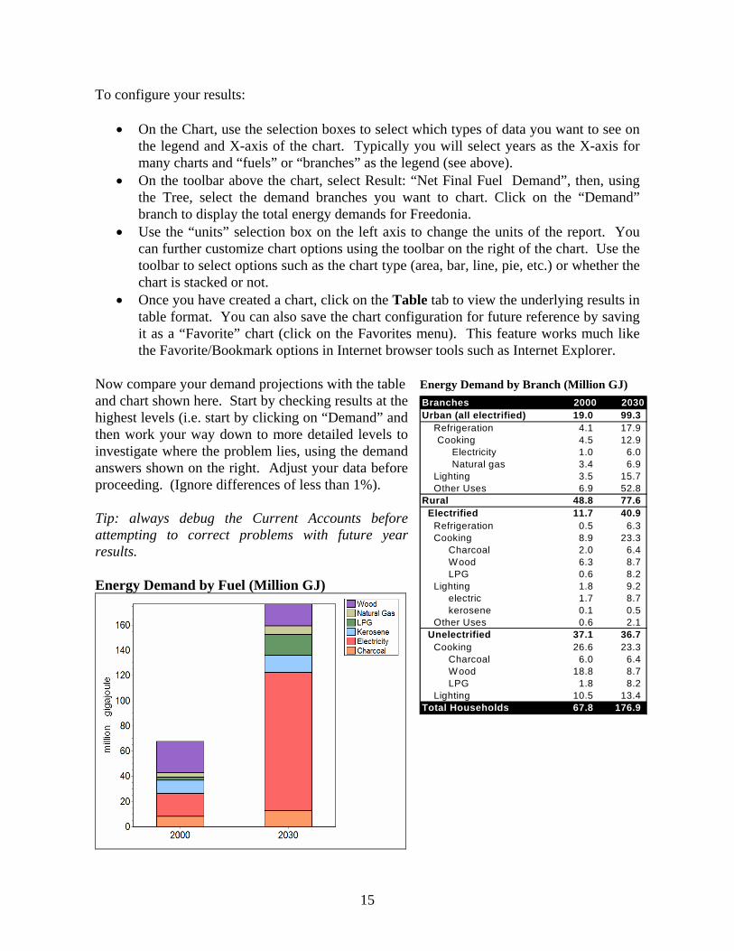
Now compare your demand projections with the table Energy Demand by Branch (Million GJ) and chart shown here. Start by checking results at the highest levels (i.e. start by clicking on “Demand” and then work your way down to more detailed levels to investigate where the problem lies, using the demand answers shown on the right. Adjust your data before proceeding. (Ignore differences of less than 1%).

Branches 2000 2030Urban (all electrified) 19.0 99.3 Refrigeration 4.1 17.9 Cooking 4.5 12.9 Electricity 1.0 6.0 Natural gas 3.4 6.9

Lighting 3.5 15.7 Other Uses 6.9 52.8 Rural 48.8 77.6 Electrified 11.7 40.9 Refrigeration 0.5 6.3 Cooking 8.9 23.3 Charcoal 2.0 6.4 Wood 6.3 8.7 LPG 0.6 8.2 Lighting 1.8 9.2 electric 1.7 8.7 kerosene 0.1 0.5 Other Uses 0.6 2.1 Unelectrified 37.1 36.7 Cooking 26.6 23.3 Charcoal 6.0 6.4 Wood 18.8 8.7 LPG 1.8 8.2 Lighting 10.5 13.4 Total Households 67.8 176.9

Tip: always debug the Current Accounts before attempting to correct problems with future year results. Energy Demand by Fuel (Million GJ)

15

1.4 Transformation The Transformation sector uses special branches called modules to model energy supply and conversion sectors such as electricity generation, refining, or charcoal production. Each module contains one or more processes, which represent an individual technology such as a particular type of electric plant or oil refinery, and produces one or more output fuels. These represent the energy products produced by the module. The basic structure of a module is shown below: LEAP Module Structure

OutputFuel

OutputFuel

OutputFuel

OutputFuel

ModuleDispatch

Process(efficiency)

Co-ProductFuel (e.g Heat)

Feedstock Fuel

Feedstock Fuel

Process(efficiency)

Feedstock Fuel

Feedstock Fuel

Process(efficiency)

Feedstock Fuel

Feedstock Fuel

Process(efficiency)

Feedstock Fuel

Feedstock Fuel

Process(efficiency)

Feedstock Fuel

Feedstock Fuel

OutputFuel

Auxiliary Fuel Use

Auxiliary Fuel Use

In this exercise you will develop a simplified model of the electricity transmission and generation sectors in Freedonia. This model will be the basis for the more detailed and realistic model you will create in Exercise 3. Return to the General: Basic Parameters screen ( ) and check the box marked Transformation & Resources, since we are now going to enter data for various Transformation modules.

16

1.4.1 Transmission and Distribution We will start by adding a simple module to represent electricity and transmission and distribution (T&D) losses and natural gas pipeline losses. Electricity T&D losses amount to 15% of the electricity generated in 2000. In the Reference scenario these are expected to decrease to 12% by 2030. Natural gas pipeline losses amount to 2% in 2000, and are expected to decrease to 1.5% by 2030 in the Reference scenario. To create a module, right-click on the Transformation branch on the Tree and select the Add command ( ). On the resulting Module properties screen (shown right), enter a name “Transmission and Distribution”, and use the checkboxes to indicate the types of data you will be entering. Check the box marked “simple, non-dispatched module”, and then mark that efficiencies will be entered as losses. When you click “OK” the module is added. Expand the branches beneath the newly created module and you will see some new branches marked Output Fuels and Processes. Click on Processes and first add a new process called “Electricity”. Select the feedstock fuel (electricity), and then enter percentage share of electricity losses on the Energy Losses tab. Repeat this process to add a process for natural gas then enter the data on natural gas pipeline losses.

Hint: Use the same features as in demand to enter time-varying data: switch to the Reference scenario and use the Interpolate function to specify how electric losses change over time.

17

1.4.2 Electricity Generation Next we simulate how electricity is generated in Freedonia. The module “Electricity Generation” should already appear on the list. If not you will need to add it. Make sure that the Electricity Generation module appears below the Transmission and Distribution module in the list of modules. You may need to use the up ( ) and down ( ) buttons to reorder modules. You will need to switch to Current Accounts before you can do this. The sequencing of modules reflects the flow of energy resources from primary/extraction (bottom of the list) to final use (top of the list). Electricity must be generated before it is transmitted and distributed. Similarly a module for mining of coal that feeds electricity generation would need to be added

wer down on the list. lo Make sure that you set correct properties ( ) for Electricity Generation module (see above). Since you will be specifying data on plant capacities, costs, efficiencies, and a system load urve, be sure that these items are checked off.

ation on some of the basic characteristics of these plants is supplied in the following ble:

c Next you will add x processes to represent the various power plants available in the region. Informta

Installed Thermal Dispatch MaximumPlant Type Capacity (MW) Efficiency (%) Merit Order Capacity FactorCoal Steam 1000 30 1 (base) 70Hydro 500 100 1 (base) 70Diesel Combustion Turbines 800 25 2 (peak) 80

us parameters that will allow LEAP to mulate the dispatch of power plants by merit order.

“in ascending merit order” for all processes. The les will be obeyed from 2001 onwards.

e from hydro plants. 15% from the Diesel CTs, and the remainder came from the coal plants.

In this exercise we are going to simulate base year operations in a special way, since for that year we have data describing known (historical) operation of power plants. In later future years, for which we do not have operational data, we will simulate the dispatch of different power plants by specifying a dispatch rule and variosi To enable this type of simulation we need to set a few process variables in Current Accounts. First, set the First Simulation Year to 2001 (the year after the Base Year) for all processes. Next, set the Process Dispatch Rules toru In the base year, total generation was 5970 GWhr. 29% cam

18

The electricity system operates with a minimum planning reserve margin of 35%, and the electric system currently has a low system load factor reflected in the system load curve shown below. The peak system demand in 2000 was 1383 MW.

1.4.2.1 The Reference Scenario

• No new power plants are currently being built in Freedonia.

• In the Reference scenario, several existing power plants are expected to be retired. 500 MW of existing coal-fired steam plants will be retired in 2010 and the remaining 500 MW are retired in 2020.

System Load Curve in 2000 Hours

Hint: To enter discrete changes, click on the 2001-2030 expression for capacity, and select the Step function in the Time Series Wizard. You can then enter the relevant remaining capacity amounts in the future. The resulting expression for coal capacity should appear as: Step(2010, 500, 2020, 0).

• In the future, to meet growing demands (and replace retired plants), new power plants are expected to consist of base load coal-fired steam plants (built in units of 500 MW, with a thermal efficiency of 35%) and new peak load fuel oil-fired combustion turbines (built in units of 300 MW with a thermal efficiency of 30%). Both types of plants have a life expectancy of 30 years and a maximum capacity factor of 80%.

Hint: Add new power plant types in Current accounts and then enter the information on endogenous capacity additions on the Endogenous Capacity tab (scenarios only). Remember to set the dispatch merit order of each process.

% of Peak

0 100 1000 98 2000 95 3000 70 4000 40 5000 25 6000 20 7000 15 8000 12 8760 10

19

Use the Diagram View (top icon of the View bar) to review the energy flows in the energy supply system you have created. Your diagram should show the modules you’ve created. Double-click on the electricity generation module and check that the diagram is similar to the one shown right. If it doesn’t look correct, check that you have specified all of the appropriate input fuels (specific to each process) and output fuels (specific to each module).

1.4.3 Viewing Results Click on the Results View to see the results of the Reference scenario. Select the Transformation: Electricity Generation branch and view the results for categories such as capacities, energy outputs, and module reserve margins. Compare your results to the tables and charts provided below.

20

Electricity Generation in Freedonia: Reference Scenario

Notes: base year = 5,970 GWhr, 2030 = 34,583 GWhr Hint: To get this chart, click on the Processes under the Electricity Generation module in the Tree, select Results: Transformation: Outputs. Next, choose Selected Years on the X-axis and choose every 2 years for results. On the chart legend select All Branches. Use the chart toolbar on the right to select a stacked bar chart. Finally, make sure units are set to Gigawatt-hours on the Y axis. To save all these settings for future reference, click on the Favorites menu and choose “Save Chart as Favorite”.

21

Electricity Generation Capacity (MW)

Notes: base year = 2300 MW, 2030 =11,400 MW Reserve Margin (%) Power Dispatched in 2030 (MW)

22

1.5 Emissions You will now use LEAP to estimate the emissions of major pollutants in the Reference scenario. To do this, return to Analysis View, select Current Accounts and then create links between each relevant technology branch (those marked with the

icon) and matching or similar technologies contained in the Technology and Environmental Database (TED). You create links to the data in TED by first selecting the Environmental Loading tab, and then clicking the TED button ( ). This will display the box shown on the right, from you For this exercise we will make use of the default emission factors suggested by the Intergovernmental Panel on Climate Change (IPCC). To create the links, first click on a technology branch and then select the Environment tab in the data screen. Then for each relevant demand-side and electric generation technology select the appropriate IPCC Tier 1 default technology, using the TED technology selection form (shown right). Make sure the input fuels to the TED technology are similar to fuels used by the LEAP technology. In some cases, the IPCC tier 1 technologies do not contain entries for all fuels. In this case you will need to pick the closest matching entry (e.g. the IPCC “Oil Residential” category can be linked to the LEAP “LPG stoves” category). You do NOT need to create links to TED for any demand-side devices that consume electricity, such as lights or refrigerators, since their environmental impacts occur upstream (e.g. in the power plants that produce the electricity).

23

1.5.1 Viewing Results Click on the Results View to see environmental results for the Reference scenario. Click on the top-level branch “Freedonia” and select the category Environmental Effects: Global Warming Potential. Compare your results to those shown below. Also check the results for other non-greenhouse gases, such as sulfur and nitrogen oxides. Global Warming Potential of Emissions from Freedonia Reference Scenario (all greenhouse gases)

Note: Base Year = 6.1, 2030 = 33.9 Million Tonnes CO2 EQ.

24

1.6 A Second Scenario: Demand-Side-Management We will now create a second scenario to explore the potential for electricity conservation in Freedonia. Use the Manage Scenarios ( ) option and use the Scenario Manager screen to add a new scenario. Add the scenario under the Reference scenario so that by default it inherits all of the Reference scenario assumptions and modeling expressions. Give the new scenario the name “Demand Side Management”, the abbreviation “DSM”, and add the following notes: “Efficient lighting, transmission and distribution loss reductions, and electric system load factor improvements”. Exit the scenario manager and select the “Demand Side Management” scenario on the main screen, and then edit the data for the scenario to reflect the following notes:

Hint: Remember you must be in Analysis View to change scenarios. Use the view bar to select it if you are not.

The DSM scenario consists of four policy measures:

1. Refrigeration: Proposed new efficiency standards for refrigerators are expected to cut the average energy intensities of refrigeration by 5% in 2010 compared to current account values, and by 20% in 2030.

Hint: You can enter this information in several ways.

• Use the time series wizard, select interpolation, and enter the values for refrigerator energy intensity in future years (calculate the values off-line), or

• Enter an expression which calculates the value for you, such as Interp(2010, BaseYearValue * 0.95, 2030, BaseYearValue * 0.8)

2. Lighting: A range of measures including new

lighting standards and utility demand-side-management programs are expected to reduce the energy intensity of electric lighting in urban households by 1% per year (-1%/year), and to reduce the expected growth in electric lighting intensity in rural areas from 1% (reference scenario) to 0.3% per year (+0.3%/year).

3. Transmission and Distribution: Under the

planned DSM program, electric transmission and distribution losses are expected to be reduced to 12% by 2015 and to 9% by 2030%.

4. Electric System Load Factor Improvements:

Various load-leveling measures in the DSM plan are expected to lead to gradual improvements in the

System Load Curve in 2030: DSM Scenario Hours % of Peak

0 100 1000 98 2000 95 3000 75 4000 60 5000 50 6000 45 7000 40 8000 35 8760 30 Tip: enter these values using an Interp function: NOT as single numbers.

25

system load factor, so that increases to about 64% in 2030. The expected annual cumulative system load curve in 2030 is shown here.

1.6.1 DSM Scenario Results Click on the Results View to see the results of the DSM scenario. Compare your results with those shown below:

Electricity Generation: Reference Scenario Compared to DSM Scenario Electricity Generation Process Capacities

Notes: generation in DSM scenario in 2030 = 29,160 Gw-hr, plant capacity = 7400 MW.

26

Exercise 2: Demand Exercise 2 further develops the demand analysis begun in Exercise 1 covering three other sectors: industry, transport, and commercial buildings. Use the information in section 2 to complete the tree structure, Current Accounts data and Reference scenario analysis for these sectors.

2.1 Industry

2.1.1 Current Accounts There are two principal energy-intensive industries in Freedonia: Iron & Steel and Pulp & Paper. All other industries can be grouped into a single category. The adjoining table shows the output of each subsector. Industrial energy analysis is typically done in either economic (e.g., value added) or physical (e.g. tonnes) terms. The choice generally depends on data availability and the diversity of products within a sub-sector. In this exercise, both methods are used.

Industrial Output (2000) Iron and Steel 600,000 Tonnes Pulp and Paper 400,000 Tonnes Other Industry 1.8 Billion US$

Hint: When adding the branch for “Industry”, set the activity level unit to “No data” (since for this sector you are specifying different activity level units for each subsector).

Energy use in the Iron & Steel and Pulp & Paper industries can be are divided into two end-uses: process heat and motive power. Iron and Steel

• Currently, process heat requirements average 24.0 GJ per tonne, and boilers using bituminous coal produce all of this.

• Each tonne of steel requires an average of 2.5 GJ of electricity use. Pulp and Paper

• Wood-fired boilers meet all process heat requirements of 40.0 GJ per tonne of products.

• Each tonne of pulp & paper requires 3 Megawatt-hours of electricity use. Other Industry

• Freedonia’s other industries consume 36 Million GJ of energy in 2000. • 40% of this energy was electricity and the remainder was residual fuel oil.

Hint: When adding the branch for “Other Industry”, set the branch type to “End-Use” (the icon). This indicates that you want to enter an aggregate energy intensity at this branch. You can then add two

27

more branches for electricity and fuel oil below this branch. These lower branches will only contain fuel shares, not energy intensities. Note also that you will also need to calculate the energy intensity in GJ/US Dollars using the total value added for the “Other” subsectors (see above).

2.1.2 Reference Scenario

Iron and Steel • Total output is not expected to change: all plants are operating at maximum capacity

and no new plants are planned within the analysis period. • Natural gas is expected to provide for 10% of process heat requirements by 2030. • Natural gas boilers are 10% more efficient than coal boilers.

Hint: You will need to switch back to Current Accounts to add a new branch for Natural gas. You can use the following simple expression to calculate natural gas energy intensity as a function of coal energy intensity:

Coal * 90%

Hint: Remember to use the “Interp” and “Remainder” functions to help you calculate boiler shares.

Pulp and Paper • Two new paper plants are

expected: one in 2005 and one in 2010. Each will add 100 thousand tonnes per year to the total output of this industry.

Hint: Use the Step Function in the Time Series Wizard to specify discrete changes in activity levels or other variables (see right).

Other Industry • Output of other industries is

expected to grow at a rate of 3.5% per year. • The fuel share of electricity is expected to rise to 55% by the year 2030.

28

2.1.3 Viewing Results Now review your results and compare to the answer sheet shown below. Industrial Energy Demand in Freedonia: Reference (Million Gigajoules) Fuels 2000 2030 Subsectors 2000 2030Coal (bituminous) 14.4 13.0 Iron and Steel 15.9 15.8 Electricity 20.2 63.6 Other 36.0 101.0 Natural Gas - 1.3 Pulp and Paper 20.3 30.5 Residual Fuel Oil 21.6 45.5 Wood 16.0 24.0 Industry 72.2 147.3 Industry 72.2 147.3

2.2 Transport

2.2.1 Current Accounts Passenger Transport • All passenger transportation in Freedonia is either by road (cars and buses) or rail.

(We ignore air and water transport for this exercise). • In the year 2000, cars were estimated to have traveled about 8 billion km; buses

traveled about 1 billion km. • Surveys also estimate that cars have a (distance-weighted) average number of

occupants (load factor) of 2.5 people, while the similar average for buses is 40 passengers.

Calculating Passenger-KmA Car Use (billion veh-km)B Load Factor (pass-km/veh-km) 2.5

C=A*B = Total Car Pass-km

D Bus Use (billion veh-km)E Load Factor (pass-km/veh-km) 40.0

F=D*E Total Bus Pass-km

G=F+C Road Passenger-kmH Rail Passenger-km

I=G+H Total Passenger-km

Calculating Energy IntensitiesJ Car Fuel Economy (veh-km/l) 12.0 K Load Factor (pass-km/veh-km) 2.5

L=1/(J*K) Energy Intensity (liters/pass-km)

M Bus Fuel Economy (veh-km/l) 3.0 N Bus Load Factor (pass-km/veh-km) 40.0

O=1/(M*N) Energy Intensity (liters/pass-km)

• Surveys have found that the current stock of cars has a fuel economy of about 12 km/liter (roughly 28 m.p.g.). Buses, in contrast, travel about 3 km/liter.

• The national railroad reports 15 billion passenger-km traveled in 2000.

Hint: You may wish to enter total population as the activity level at the sector level (see section 1.3 for population data).

Hint: use the information above to calculate the total number of passenger-kms, the percentage for each mode, and the average energy intensity (per passenger-km). Use the worksheet on the right to help you.

29

• 20% of rail transit is by electric trains, the remainder by diesel trains. The energy intensity of electric trains is 0.1 kilowatt-hours per passenger-km. The energy intensity of diesel trains is 25% higher than that of electric trains.

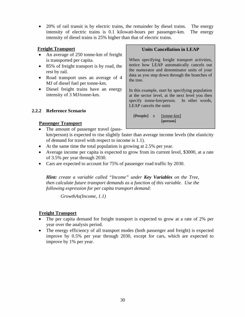
Freight Transport Units Cancellation in LEAP

When specifying freight transport activities, notice how LEAP automatically cancels out the numerator and denominator units of your data as you step down through the branches of the tree.

• An average of 250 tonne-km of freight is transported per capita.

• 85% of freight transport is by road, the rest by rail.

• Road transport uses an average of 4 MJ of diesel fuel per tonne-km.

In this example, start by specifying population at the sector level, at the next level you then specify tonne-km/person. In other words, LEAP cancels the units [People] x [tonne-km] [person]

• Diesel freight trains have an energy intensity of 3 MJ/tonne-km.

2.2.2 Reference Scenario

Passenger Transport • The amount of passenger travel (pass-

km/person) is expected to rise slightly faster than average income levels (the elasticity of demand for travel with respect to income is 1.1).

• At the same time the total population is growing at 2.5% per year. • Average income per capita is expected to grow from its current level, $3000, at a rate

of 3.5% per year through 2030. • Cars are expected to account for 75% of passenger road traffic by 2030.

Hint: create a variable called “Income” under Key Variables on the Tree, then calculate future transport demands as a function of this variable. Use the following expression for per capita transport demand:

GrowthAs(Income, 1.1)

Freight Transport • The per capita demand for freight transport is expected to grow at a rate of 2% per

year over the analysis period. • The energy efficiency of all transport modes (both passenger and freight) is expected

improve by 0.5% per year through 2030, except for cars, which are expected to improve by 1% per year.

30

2.2.3 Viewing Results Now switch to Results View and compare your results with the tables shown below. Transport Energy Demand in Freedonia: Reference (Million Gigajoules)

Bra nche s 2000 2030 Fue ls 2000 2030Fre ight 38.5 125.9 Diesel 56.5 182.6 Ra il 4.5 14.7 E lec tric ity 1.1 6.1 Roa d 34.0 111.2 Gasoline 22.1 240.1 Pa sse nge r 41.2 303.0 Ra il 6.5 36.4 Die se l 5.4 30.3 Ele ctric 1.1 6.1 Roa d 34.7 266.6 Die se l Buse s 12.6 26.5 Ga soline Ca rs 22.1 240.1 All Tra nsport 79.7 428.8 All Tra nsport 79.7 428.8

2.3 Commerce: Useful Energy Analysis This exercise considers space-heating uses in commercial buildings, and serves to introduce the application of useful energy analysis techniques. Useful energy analysis is particularly helpful where multiple combinations of fuels and technologies can provide a common service at (such as heating), and in situations where you want to independently model device efficiencies, and overall energy service requirements.

2.3.1 Current Accounts • Commercial buildings in Freedonia utilized a total of 100 million square meters of

floor space in 2000. • Total energy consumption for heating purposes was 20 million GJ in 2000. • Fuel oil and electricity each currently supply half of the total heating energy. Natural

gas is expected to be introduced in the near future

Hint: For this exercise, you need to setup an end-use branch for heating and check-off that you want to enter aggregate energy intensities AND conduct a useful energy analysis. Use the branch properties screen to set this up (see below).

31

• Electric heaters have an efficiency of nearly 100%, while fuel oil boiler efficiencies average 65%, and natural gas boilers have 80% efficiencies.

2.3.2 Reference Scenario • Floor space in the commercial sector is expected to grow at a rate of 3% per year. • Due to expected improvements in commercial building insulation standards, the useful

energy intensity (i.e. the amount of heat delivered per square meter1) is expected to decline by 1% per year. Until 2030.

• By 2030, natural gas boilers are expected to have reached a market penetration (i.e. share of floor space) of 25%, while fuel oil boilers are expected to decline to only a 10% market share. Electricity heating fills the remaining requirements. (Notice that these activity shares are different from the fuel shares you entered for Current Accounts).

• Finally, gradually improving energy efficiency standards for commercial boilers are expected to lead to improvements in the average efficiency of fuel oil and natural gas boilers. Fuel oil systems are expected to reach and efficiency of 75% by 2030, and natural gas systems are expected to reach an efficiency of 85% by 2030.

2.3.3 Viewing Results After entering the above data, switch to Results View and compare your results with the table shown below.

Commercial Space Heating: Reference Scenario

Fuels 2000 2030Electricity 10.0 19.3 Natural Gas - 8.7 Residual Fuel Oil 10.0 3.9 Total Commercial 20.0 31.9

1 As opposed to the final energy intensity: the amount of fuel used per square meter.

32

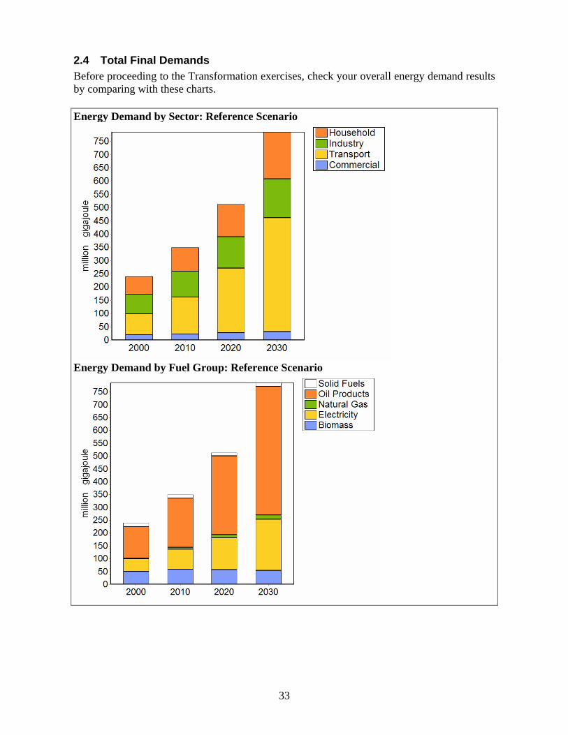
2.4 Total Final Demands Before proceeding to the Transformation exercises, check your overall energy demand results by comparing with these charts. Energy Demand by Sector: Reference Scenario

Energy Demand by Fuel Group: Reference Scenario

33

Exercise 3: Transformation In this fourth exercise we will further develop the simplified Transformation data set we constructed in Exercise 1. In this exercise we will add new modules to examine charcoal production, oil refining and coal mining.

3.1 Charcoal Production No charcoal is imported or exported. It is all produced by conversion from firewood. All charcoal in Freedonia is currently made using traditional earth mounds. These have a conversion efficiency (on an energy basis) of around 20%. In the future, more efficient “brick beehive” kilns are expected to be imported from Thailand. These kilns have a conversion efficiency of around 47%. They are expected to be used to meet 5% of total charcoal demand by 2010, 20% of charcoal demand by 2030.

Hint: You can link your LEAP data to the entry in TED for Thailand Brick Beehives. Use the “Add from TED” function to link the data on efficiencies and emissions to the TED technology:

“Energy Conversion\Biomass Conversion\Charcoal Making\Thailand\Brick Beehive”

3.2 Electricity Generation With the addition of the extra demand sectors in Exercise 2, the demand for electricity generation triples to around 16,200 GWhr. Thus, you now need to specify a larger and more realistic electric generation system to match the additional demand for electricity. Change the data you entered in Exercise 1 in Current Accounts for the Electricity Generation module to match those below: Plant Type Year 2000

Capacity (MW)Base Year Output

(% of GWhr) Hydro 1,000 34% Coal Steam 2,500 44% Oil Combustion Turbine 2,000 22% Total 5,500 100% (16,200 GWhr)

3.3 Oil Refining Oil refineries in Fredonia processed approximately 4 million tonnes of crude oil in the year 2000, which was well under their capacity of about 6 million tonnes of crude2. The efficiency of the refineries (on an energy basis) was about 97.0%. There are currently no plans to increase refining capacity. The refineries used only one feedstock fuel: crude oil, and produced seven types of products: gasoline, aviation gas, kerosene/jet fuel, diesel, residual/fuel oil, LPG, and lubricants. The 2 Note: you are limited to entering capacity data in basic energy units (tonnes of oil equivalent or tonnes of coal equivalent per year). For the purposes of this exercise, assume 1 tonne of coal = 1 TCE and 1 tonne of crude oil = 1 TOE.

34

refineries can be operated with sufficient flexibility that the mix of refinery products matches the mix of requirements for those products. Any oil product requirements that cannot be produced from the refinery are imported into Freedonia.

3.4 Coal Mining All coal mined in Freedonia is bituminous. In the base year, the country’s coal mines produced 4.7 million of coal, mining capacity stood at 6 million tonnes, and the efficiency of coal mining (including coal washing plants) was 80%. The Reference scenario assumes that coal mining capacity will increase as follows: 10 million tonnes by 2000, 14 million tonnes by 2010, and to 23 million tonnes by 2030. It is assumed that mine capacity will expand linearly in years between these data years. In spite of this expansion program, it is expected that sometime after 2020 additional imports of coal will be needed to meet domestic requirements. In the future, any coal requirements that cannot be produced from the nation’s coalmines are imported into Freedonia.

3.4.1 Viewing Results Before switching to results, review your energy system diagram and check that it looks similar to the one shown below: Energy System Diagram

Now switch to the Energy Balance View and check your base and end year energy balances against the following tables:

35

Energy Balance of Freedonia in 2000 (GJ)

Solid Fuels Natural Gas Crude Oil Hydropower Biomass Electricity Oil Products TotalProduction 125 0 0 20 81 0 0 226Imports 0 4 183 0 0 0 0 187Exports 0 0 0 0 0 0 0 0Total Primary Supply 125 4 183 20 81 0 0 413Coal Mining -25 0 0 0 0 0 0 -25Oil Refining 0 0 -183 0 0 0 174 -9Charcoal Making 0 0 0 0 -32 0 0 -32Transmission & Distribution 0 0 0 0 0 -9 0 -9Electricity Generation -86 0 0 -20 0 58 -51 -98Total Transformation -110 0 -183 -20 -32 50 123 -174Household 0 3 0 0 33 18 13 68Industry 14 0 0 0 16 20 22 72Transport 0 0 0 0 0 1 78 79Commercial 0 0 0 0 0 10 10 20Total Demand 14 3 0 0 49 50 123 239Unmet Demand 0 0 0 0 0 0 0 0

Energy Balance of Freedonia in 2030 (GJ)

Solid Fuels Natural Gas Crude Oil Hydropower Biomass Electricity Oil Products TotalProduction 546 0 0 12 105 0 0 663Imports 0 17 251 0 0 0 513 782Exports 0 0 0 0 0 0 0 0Total Primary Supply 546 17 251 12 105 0 513 1,445Coal Mining -109 0 0 0 0 0 0 -109Oil Refining 0 0 -251 0 0 0 239 -13Charcoal Making 0 0 0 0 -51 0 0 -51Electricity Generation -424 0 0 -12 0 225 -250 -459Transmission & Distribution 0 0 0 0 0 -27 0 -27Total Transformation -533 0 -251 -12 -51 198 -11 -660Household 0 7 0 0 30 110 30 177Industry 13 1 0 0 24 64 45 147Transport 0 0 0 0 0 6 423 429Commercial 0 9 0 0 0 19 4 32Total Demand 13 17 0 0 54 198 502 785Unmet Demand 0 0 0 0 0 0 0 0

36

Now switch to Results View and compare your results with the charts shown below. Electricity Generation: Reference Scenario

Notes: base year = 16, 200 GWhr, 2030 = 62,640 GWhr Electricity Generation Capacity: Reference Scenario

37

Exercise 4: Alternative Scenarios and Policy Measures In this final exercise you will be divided into teams, each of which will be given the task of constructing, presenting, and defending a separate policy scenario. Each team will take on the role of a different institution, and different institutions will have different perspectives on what they consider to be a “desirable” policy scenario. The following are suggested “scenario teams”, but feel free to adapt these to your local institutional context.

• Team 1: Freedonia Chamber of Commerce. You are representatives of major industrial and commercial concerns. You believe that energy supplies will be inadequate to support the 6%/year economic growth rate for Freedonia that you are aiming for. You want Freedonia to be a major steel producer, tripling production in the next 20 years to support a strong manufacturing sector. Other industries should grow at 6%/year. You want the government to invest in infrastructure so that freight transport tonnage can also grow at 6% per year. You will need to show the total financing requirements for this scenario (how much more capital will it require?), explain how it will be financed.

• Team 2: FreedoniaNET. You are a consortium of environmental and social interest

non-government organizations. Your goals are rural economic and social development and minimization of local air pollution, which is becoming a severe problem near coal plants in rural areas and in the major cities due to transportation. You are also concerned about the impacts of global climate change, and want proactive policies to develop markets for low-GHG technologies, but you don’t want to invest in GHG reduction at the expense of other goals.

• Team 3: MoE Freedonia. You are the Freedonia Ministry of Energy. You are

tasked with developing a National Energy Strategy to promote the economic and social goals of Freedonia. You also need to consider the interests of various groups within the country. You are concerned about the oil import bill and implications of the Reference scenario, as well as that of high growth policies such as those pushed by the Chamber of Commerce. You may wish to examine the implications of higher-than expected crude oil prices in the near term. You are also interested in developing an active market for greenhouse gas (GHG) credits, benefiting from international instruments such as the Clean Development Mechanism (CDM) and Global Environmental Facility (GEF), which in the near future may be available to finance projects that can demonstrate reductions in GHG emissions.

• Team 4: Global Development Bank. You are a representative of the global

development bank. You are tasked with promoting fiscal and regulatory reforms in the electric sector and are interested in studying the how the energy system might look if fuel price subsidies are reduced and the state-owned electric generation and oil refining sectors are deregulated and privatized. You expect that these reforms could lead to a significant boost to economic growth in the Freedonia, but they may also lead to widening gaps in income between rich and poor. In particular you would like

38

to identify least-cost configurations of the energy system as a way of identifying some of the benefits (and costs) of deregulation.

4.1 Instructions There are two main steps to this exercise: 1) working in groups to develop your scenarios, and 2) presenting your strategies to the wider group, followed by a debate.

4.1.1 Step 1: Strategy/Scenario Development. Work together as groups to use LEAP to construct your scenarios. In this step, we suggest that you confer for no more than an hour to a) define your overall group strategy; b) create a list of prospective “changes” to the reference case (e.g. from altering the growth rate for industrial value added to adding an efficiency program or developing renewable energy resources. Once you’ve listed these out, think about:

1. In what year will these changes begin? 2. What LEAP branches/sectors will this change/policy affect? Will you need to alter

the Freedonia data structure and/or add new branches? 3. If any new technologies are implicated, how will you represent them in the LEAP data

set? 4. What are your basic assumptions regarding:

• Rates of change, e.g. activity levels, energy intensities, penetration rate of new technologies

• Cost of resources and technologies 5. Will there be significant implementation costs (administrative or transaction costs)? If

so, how might you represent these in LEAP? To assist in the construction of scenarios, we provide a range of measures that you might want consider in section 4.2. Use the remaining time to develop the quantitative analysis of your scenario using LEAP. Once you’ve come to a reasonably good representation of your scenario (ideally with cost analysis included), develop a series of “favorite” reports and use the Overviews View to present them to the full group.

Hint: Create a separate “scenario” for each measure/change you create. Then you can combine these in different combinations using the Scenario manager tool, to come up with your “best” scenario.

4.1.2 Step 2: Presentations Each group will deliver a presentation of no more than 20 minutes, explaining the elements of and rationale for their proposed energy strategy, and using a computer screen projector if available, to present the quantitative results. Presentations can be followed by 5-10 minutes of questions.

39

4.2 Data for Scenario Measures To assist you in the construction of scenarios, we provide data for the following range of measures that you might want consider: Demand Options:

• Efficient Lighting for Households • Refrigerator Efficiency Standards • PV electrification program • Accelerated Rural Grid Electrification • Kerosene Stove Program • Biogas program • Transport Mode Switching • Natural Gas Bus Program

Supply Options

• Natural Gas Pipeline and Power Development • Wind Resource Development

Feel free to create any combination of these options. For comparability with other working groups and with the standard results, we recommend you model these options using the key assumptions outlined below. If you wish to change a key parameter for the options detailed below (e.g. fuel price, technology penetration rate, etc.), we recommend that you create sensitivities (alternative scenarios) after developing the original option. Also, feel free to introduce additional measures of your own. If you wish to conduct an economic (cost-benefit) analysis of these measures, begin by establishing a few general costing parameters: 1) Under General/Basic Parameters, set the boundary for cost-benefit analysis at the Electricity module (under Costing Methodology). As a result you will enter costs for refined petroleum products rather than crude oil. Also click to select the inclusion of environmental externality costs. 2) Under the Resources section of the tree, enter the following price trajectories:

Primary Resources: • Coal - $20/t in 2000, rising to $30/t in 2030 • Imported Natural gas - $0.1/m3 in 2000, rising to $0.2/m3 in 2030

Secondary Resources:

• Diesel - $250/t in 2000, rising to $300/t in 2030 • Gasoline, LPG, kerosene - $300/t in 2000, rising to $400/t in 2030 • Residual Fuel Oil - $200/t in 2000, rising to $250/t in 2030 • Electricity is not priced here since you are modeling electricity costs instead on

the basis of input fuel and power plant costs.

40

41

Costs for existing and future electric facilities: Capital

($/kW) Fixed O&M ($/kW-yr)

Variable O&M ($/MWh)

Existing Plants Coal $40 $3 Oil Steam $30 $0.5 Hydro --- $1 Combustion Turbine $10 $0.1 New Plants Coal $1000 $40 $3 Combustion Turbine $400 $10 $0.1 Combined Cycle See below Biomass $1500 $80 $0.1 Wind $800 $25 --

3) You can develop each of the measures below as distinct policy scenarios, and then combine them. To do this, add a new scenario under the Reference scenario entitled “Individual measures”. This will be where you “store” your measures. For the time being, you may wish to unclick the show results box (in Manage Scenarios) for these individual measures – this will speed up the calculations. 4) After you have created several measures, create a combined policy scenario. To do this, add another scenario under Reference, and use the inheritance box on the right side of the screen to pick the measures that your combined scenario will “inherit”. 5) When completed, view results to evaluate the impacts.

DEMAND-SIDE OPTIONS

Measure Notes LEAP tips Efficient Lighting for Households:

Begin by creating a new scenario for “household lighting program”. (Under your policy scenario)

• A program to install efficient lighting systems could reduce electricity consumed by 40% per urban household, using compact fluorescent (CFL) and other technologies.

Try entering a second lighting technology branch. Make its’ energy intensity 60% of the standard one. Use the expression builder, choose the LEAP branch tab, and select the branch energy intensity, adding “*.6” to complete the equation.

• Assume that the program starts in 2002 and is capable of reaching 40% of all households by 2007 and 50% by 2010. Assume the costs are equivalent to the added cost of a 15W CFL ($10 US, 5 year life) compared to a 60W incandescent bulb ($1, 1 year life).

Represent the program penetration rate at the activity level. Use the cost of saved energy (detailed) feature to enter

demand costs (for the program branch).

• Each CFL bulb runs for about 1000 hours, thus using 15kWh/year, a 45 kWh savings relative to the standard bulb. • Assume the administrative cost of the program adds $2 to the CFL cost.

Create a new scenario. Refrigerator Efficiency Standards

• An efficiency standards program would require that manufacturers produce refrigerators with a weighted average efficiency of 380 kWh/year beginning in the year 2004.

Add a new branch for efficient refrigerators and enter its’ energy intensity and penetration rate (activity level).

Trying using the device/activity cost feature to enter demand costs (for the program branch). • Assume that, with an average 10-year life, all

refrigerators will average the new efficiency level by 2014.

• The cost of improving refrigerator efficiency to 380kWh is approximately $30 US.

Create a new scenario. PV electrification program

• This program would provide PV electrification to 50% of all non-electrified homes by 2010 and 80% by 2015.

Add new branches (try creating a new rural subsector for PV electrified homes, copy the cooking and lighting end uses from rural non-electrified, and modify those branches) • 50 W PV systems cost $1000 today, expected to

decline to $500 by 2020. They are expected to last 20 years, with annual fixed O&M costs of $30/year.

Add a new fuel called “off-grid PV electricity”. (So that it is not counted in grid electricity generation requirements).

42

Consider relating the activity level for PV electrified to the share of non-electrified, e.g. PVElectrified = (1-RuralElectrified)*.5 for the 2010 value. (This allows the number of PV installations to vary with the amount of grid electrification, per below)

• Each system provides for DC lights that consume 70 kWh/year. As a result household kerosene consumption for lighting is only 15 liter/year. • Each system also provides 30kWh/year for the use of black and white televisions.

Assume a lifetime of 50 years on the connection. Accelerated Rural Grid Electrification

• This program would increase connections to 50% of rural households by 2010, 90% by 2020, and 99% by 2030. • The cost of a connection (including the required transmission and distribution lines) averages $3000 per household.

This programme targets all rural households, electrified and unelectrified. (If your data structure has cooking end-use under each, enter all data for the branch before copying the new kerosene branch and its data to other subsectors. It’s easiest to work in Current Accounts when adding multiple branches. )

Kerosene Stove Program

• To improve indoor air quality and reduce pressures on woodfuel resources, this program seeks to encourage the use of kerosene wick stoves in rural areas, aiming to replace 50% of woodfuel use by 2010. • Assume that kerosene stoves cost $15 and last 2 years. • Average annual consumption of kerosene for stoves is 80 liters. • Link to the environmental data for Indian kerosene wick stoves.

See note above for kerosene stoves. Biogas program • A biogas program aims to get 3% of all rural households using biogas as their main cooking fuel by 2010.

You will need to create a new Transformation module for biogas production. (Use the default properties, and be sure to set the input and output fuels correctly) • Assume that biogas burners cost $10 and last 4

years. • Average annual consumption of biogas for stoves is 3 GJ. • Link to the environmental data for Indian biogas stoves. • Biogas digesters are 20% efficient in converting animal wastes to biogas and cost $50 to build, $5 per year to run, and last about 10 years.

Transport Mode Switching

• Improved urban design, special bus lanes, etc reduce the share of private auto transport. As a result the share of private auto transport grows more slowly reaching only 50% by 2030.

43

If you are curious about NGVs, check out the detailed and fact filled web site of the International Association for NGVs at http://www.iangv.org/

Natural Gas Bus Program

• A policy to reduce urban air pollution targets the conversion of urban bus fleets to compressed natural gas (CNG). Assume that by 2008, 40% of all bus travel can be done by CNG buses rising to 60% by 2010.

• CNG buses cost an additional $20,000 per bus. Assume the average bus carries approximately 2 million pass-km per year. • Assume CNG buses have the same fuel efficiency as diesel buses (314kJ/pass-km) and last approximately 10 years.

SUPPLY OPTIONS

Enter capacity value on the “Properties” screen (right-click) for wind.

Wind Resource Development

• Wind resources development could contribute 100 MW by 2005 and 300 MW by 2010.

• See the above chart for costs • Assume its capacity value (contribution to meeting peak demands) equal to its maximum capacity factor of 30%.

3 Create a new module for the natural gas pipeline. And another module for the pipeline losses (suitably located in the tree).

Natural Gas Capacity Expansion

• A 10 billion m /year pipeline (8.17 million TOE/yr) will be operational by 2006 and it will supply imported natural gas for new power supply expansion. It will cost $300 million. Create a new fuel called “imported natural gas”, so you can

separately track it (prices, quantities, limits). • Assume that instead of a mix of coal and oil (as in the reference case), all new power plants thereafter (2006 and beyond) will be 400 MW natural gas combined cycle units.

• Use the cost (capital and O&M) and efficiency data found under TED for Natural gas/Combined Cycle/AEO99/Advanced Gas Combined Cycle. (Ignore the difference in currency years) • Assume 1% losses in the pipeline.

44

45

Exercise 5: A Transportation Study In exercise five you will use LEAP’s transportation analysis features to construct a range of scenarios that examine different policies for cars and sport utility vehicles (SUVs). SUVs are the kind of large energy-intensive vehicles, the popularity of which is causing rapidly growing fuel consumption and greenhouse gas emissions, especially in the USA. You will first use LEAP to construct a Current Accounts inventory of fuel use and selected emissions from these vehicles. Next, you will create a “Business and Usual” scenario that projects fuel use and emissions into the future under the assumption of no new policies to reduce fuel use and emissions. Finally you will create and compare a range of scenarios that examine measures designed to reduce fuel use and emissions. As with other exercises, we will start by creating an Area and then setting up the basic parameters of the study. Select menu option Area: New Area, or click on the New Area ( ) button on the main toolbar. Call the new area “Transportia” (or any other name you like!). Check the radio button to create the area from default data then click OK.

5.1 Basic Parameters and Structure Now go to General: Basic Parameters.

• On the Scope tab, make sure only the Energy Sector and Non-GHG environmental loadings boxes are checked. This study will not make use of Transformation and Resource data.

• On the Years tab, enter 2000 as the base year and 2020 as the end year. • Transportia uses U.S. measurement units rather than the International S.I. units, so you

will need to set different default units for your study. On the Defaults tab select Gallons of Gasoline Equivalent as the default energy unit, Miles as the default Distance unit, Pounds/Million BTU as the default energy-based emissions unit and grammes/Vehicle-Mile as the default transport-based emissions unit.

• On the Stocks tab, make sure both the Top-down data and Save Stock Vintages boxes are checked.

46

You are now ready to enter your tree structure. First, Make You will create two major categories, one for Cars and one for Sport Utility Vehicles (SUVs). To add each of these click on the Add button (

Hybrid-Electric Vehicles Hybrid vehicles combine a small internal combustion engine with an electric motor and battery to reduce fuel consumption and tailpipe emissions. Energy lost during braking is captured and returned to the battery in a process called "regenerative braking."

) above the tree and create each as a category branch ( ). Under each category create subcategories for conventional Internal Combustion Engine (ICE) vehicles and one for the new type of Hybrid-Electric Vehicles (see box).

Unlike other electric vehicles, hybrids have the distinct advantage that they do not need to be “plugged-in” to the electric supply. Hybrid engines operate more efficiently and produce less pollution than conventional internal combustion engines.

Under each of the conventional Internal Combustion Engines categories you will consider two alternative technologies, Gasoline and Diesel, so create two technologies. When adding these make, sure you create them as Transport Technology branches ( ), and select the correct fuel for each. Under the Hybrid categories you will only consider gasoline vehicles.

Hybrids should be competitively priced when all the costs over the life of the vehicle are included. This is because any cost premium is likely to be offset by fuel savings.

Your tree structure should look something like this:

By combining gasoline with electric power, hybrids will have the same or greater range than traditional combustion engines. Hybrids offer similar performance compared to conventional internal combustion engine vehicles.

The Toyota Prius: one of the new hybrid-electric cars.

47

5.2 Current Accounts Data Age (Years) % of Stock

0 01 11.262 11.043 10.604 95 96 87 78 69 5

10 4.5811 3.7512 3.0113 2.3714 1.8215 1.3816 1.0217 0.7418 0.5319 0.3720 0.2521 0.1722 0.27

.00

.99

.22

.34

.40

.43

.48

You are now ready to enter the following base year (Current Accounts) data for your analysis.

• There were 6 million cars and 4 million SUVs on the road in the base year (2000), not including new cars sold in that year.

• The existing stock of cars and SUVs is made up of vehicles of different ages (vintages). The percent share of each of these vintages is given in the table on the right.

Tip: Create a new lifecycle profile named “Existing Car Stocks” to represent the distribution of vintages within the base year stock. The Lifecycle Profiles screen is accessed under the General menu. First add a profile then enter the data shown on the right. The figure below shows how this information will look when entered into the lifecycle profile screen. Back in Analysis View, go to the Stock tab for each technology branch and in the final Stock Vintage Profile column, select the Existing Car Stocks profile.

Important: Note that LEAP requires that all stock vintage profiles have zero vehicles of age zero years. This is because the data you enter for base year stocks should not include those new vehicles sold in the base year. These vehicles are specified using the sales variable.

48

• In the base year, 0.8 million cars were sold, and 0.5 million SUVs. As these and other vehicles age they will gradually be retired from the vehicle stock (taken off-road). A survival profile describing this retirement of vehicles can be represented by an exponential function of the following type:

02.01

⋅− ⋅= t

tt eSS

Where S is the fraction of surviving vehicles, t is the age in years of the vehicle.

Tip: Create another lifecycle profile named “Car Survival” to represent the percent survival of vehicles as they get older. First add a profile then create an exponential curve with the constant parameter –0.02. Back in Analysis View, go to the Sales tab for each technology branch and in the Survival Profile column, select the Car Survival profile.

• Among internal combustion engine cars and SUVs, 2% of sales and 2% of the base year stock is diesel vehicles. The remainder was gasoline vehicles.

• 0.05% of the base year stock of cars is Hybrid vehicles. 0.5% of the cars sold in the base year were Hybrids.

• All new cars and new SUVs are assumed to be driven 15,000 miles in their first year on the road. As the age of vehicles increases they are driven less. This decrease in driving can be represented by an exponential function, similar to the one above, and also with the constant parameter –0.002.

• The base year fuel economy of the different types of vehicles is shown in the following table. Fuel economy is assumed to stay constant as a vehicle’s age increases.

Fuel Economy in 2000 (Miles Per Gallon)

Gasoline Diesel GasolineICE ICE Hybrid

Cars 25 28 40 SUVs 15 17 23

• No hybrid SUVs are currently available.

5.3 Current Accounts Emissions Factors Next, you will enter environmental loading tabs you will enter data describing some of the pollution loadings associated with the vehicles you are studying. To keep data entry to a minimum, for this short exercise we will examine only four pollutants: the greenhouse gas, Carbon Dioxide (CO2) and three pollutants contributing to local air pollution: Nitrogen Oxides (NOx), Carbon Monoxide (CO), and Particulate matter of size less than 10 microns (PM10). CO2 emissions from vehicles are dependent only on the type of fuel used and the efficiency (fuel economy) of the vehicle. Therefore they can be specified in terms of emissions per unit of energy consumed. The measurement units used are Pounds of CO2 per MMBTU of fuel consumed. Local air pollutants are much more dependent on the type of control technology used in the vehicle, and also tend to be regulated by the Government at certain levels. For this reason these emission factors tend to be specified per vehicle-mile traveled. The units used are

49

grammes of pollutant per Vehicle-Mile traveled. Because emissions of these pollutants depend critically on the performance of the catalytic converter or other control technology used in the vehicle, they can also be expected increase per vehicle-mile quite substantially as vehicles get older. For this reason, in addition to specifying the emission factors for new vehicles, you will also need to specify degradation factors for each pollutant that specify how emissions increase as vehicles get older. The Government is continually reviewing and improving its regulations for vehicle emissions, based on recommendations from its Environmental Protection Agency. Since 1990, the emissions standards for new vehicles have been tightened a number of times. The following table specifies how average emission factors for each type of new vehicle have evolved since 1990. Car Pollutant Units 1990 1995 2004 New Standard?Gasoline CO2 lbs/MMBTU 159.50

CO g/veh-mile 6.20 5.30 3.50 1.70 NOx g/veh-mile 0.44 0.35 0.04 0.03 PM10 g/veh-mile 0.40 0.30 0.20 0.05

Diesel CO2 lbs/MMBTU 161.00 CO g/veh-mile 1.05 0.54 0.20 NOx g/veh-mile 0.60 0.27 0.08 PM10 g/veh-mile 1.50 1.50 0.50 0.20

Data on emissions from hybrid vehicles are not yet available. However, because they area regulated in the same way as conventional internal combustion engine gasoline vehicles they are assumed to have the same emission factors as that type of vehicles.

50

One set of standards is due to come into force for vehicles manufactured in 2004, the Government is also considering introducing a new set of emissions regulations, with the proposed new emission factors, listed in the final column. This proposed set of regulations has not yet been approved and thus, the date when this will come into law and affect new vehicles being manufactured has not yet been decided. To enter the above data into LEAP you will first need to create a series of environmental loading branches ( ) under each of your technologies ( ). Go to the environmental loading tab, and use the Add button ( ) to add CO , CO, NO and PM2 x 10 effects. Once complete, your tree structure should appear as shown on the right. It is important to set the correct units for each pollutant. For CO2, set the Type to “of energy consumed” and then select units Pound/MMBTU. For the other pollutants select type “of transport” and then select units: grammes/vehicle-mile. Since the above data represent emissions standards that came into force governing the manufacture of new vehicles in a specific year, you will need to enter the data for 1990, 1995, and 2004 using a step function. Since the year for the new standard has not yet been decided you can specify that year using a Key Variable named “New Reg Year”. Set the value of this variable to 2050 so that the new standards will, in effect, not be used in any initial scenario calculations. So for example, you might create an expression to represent CO emissions from gasoline vehicles as follows:

Step(1990, 6.2, 1995, 5.3, 2004, 3.5, New Reg Year, 1.7) Finally for the three local air pollutants you will also need to specify how the emission factors increase over time, as each vintage of vehicles on the road gets older. To do this you will again need to go to the lifecycle profile screen (Alt-L) and create three named profiles to represent degradation of CO, NO and PMx 10. The degradation of these can each be represented by exponential curve with the following constant parameters: CO=0.006, NO =0.008, PMx 10=0.005. Back in Analysis View, go to the Environmental Loading tab for each technology branch and in the final Degradation Profile column, select the appropriate profiles.

51

Emissions of carbon dioxide (CO2) depend only on the amount of fuel burnt in the vehicle. Therefore a single constant emission factor can be used, and no degradation curve is required. Hence, for CO emission factors leave the Degradation Profile set to constant. 2

5.4 Business as Usual Scenario You are now ready to create a “Business and Usual” scenario (BAU) that projects fuel use and emissions into the future under the assumption of no new policies to reduce fuel use and emissions. Go to the Manage Scenarios screen ( ) and click the Add button ( ) to add a new a new scenario named “Business as Usual” (BAU). Then enter the following data:

• Sales of vehicles are expected to double, reaching 2 million vehicles/year in 2020. However all this growth is expected within the SUV market segment. Annual car sales remain at 0.8 million/year in 2020, while annual SUV sales more than double, reaching 1.2 million in 2020.

• Hybrid market penetration remains constant in the BAU scenario. No hybrid SUVs are introduced.

• In the absence of new standards, fuel economy of all vehicles remains unchanged in the future.

• Apart from the already-approved emissions regulations to be introduced in 2004, no new emissions standards are imposed.

52

You are now ready to view BAU results. Check your results against each of the following categories for the years 2000, 2010, and 2020. Stock of Vehicles (Millions) 2000 2010 2020Cars Internal Combustion Engine\Gasoline 6.7 6.9 6.9

Internal Combustion Engine\Diesel 0.1 0.1 0.1Hybrid\Gasoline 0.01 0.03 0.04

SUVs Internal Combustion Engine\Gasoline 4.4 5.9 8.9Internal Combustion Engine\Diesel 0.1 0.1 0.2

Total 11.3 13.1 16.2Annual Sales of Vehicles (Thousands)Cars Internal Combustion Engine\Gasoline 780 780 780

Internal Combustion Engine\Diesel 16 16 16 Hybrid\Gasoline 4 4 4

SUVs Internal Combustion Engine\Gasoline 490 833 1,176 Internal Combustion Engine\Diesel 10 17 24

Total 1,300 1,650 2,000 Annual Vehicle-Mileage (Billion Vehicle-Miles)Cars Internal Combustion Engine\Gasoline 94.8 98.2 99.1

Internal Combustion Engine\Diesel 1.9 2.0 2.0 Hybrid\Gasoline 0.1 0.5 0.5

SUVs Internal Combustion Engine\Gasoline 62.8 85.9 128.2 Internal Combustion Engine\Diesel 1.3 1.8 2.6

Total 160.9 188.3 232.5 Fuel Consumption (Million Gallons Gasoline Eq.)Cars Internal Combustion Engine\Gasoline 3,793 3,929 3,965

Internal Combustion Engine\Diesel 69 72 72Hybrid\Gasoline 3 12 13

SUVs Internal Combustion Engine\Gasoline 4,186 5,723 8,546 Internal Combustion Engine\Diesel 75 103 154

Total 8,125 9,838 12,750Pollution EmissionsCO2 (Millions of Tonnes) 70 85 110 CO (Thousand Tonnes) 1,079 882 930 PM10 (Thousand Tonnes) 69 52 54 NOx (Thousand Tonnes) 82 36 14

Tip: if your results differ by more than a few percent from those shown above, first check, and if necessary debug, your Current Accounts data. First eliminate the possibility of errors in your Current accounts data before trying to debug future values.

53

5.5 Policy Scenarios You are now ready to examine a series of policy scenarios. You will start by examining a range of different measures individually, and then later combine them into different combinations of integrated scenarios.

5.5.1 Improved Fuel Economy (IFE) The first policy being considered by the Government is to introduce stricter fuel economy standards for conventional (i.e. non-hybrid) internal combustion engine gasoline and diesel vehicles. The proposed new standard will require new cars and SUVs to increase their fuel economy by 5% in 2005, by 10% in 2010 and by 20% in 2020 (all values relative to the base year fuel economy). To model this policy, first go to the Manage Scenarios screen ( ), and then create a new scenario below the BAU scenario called “Improved Fuel Economy”. To reduce data entry, you may want to create a new Key Variable to represent the above improvements. For example, you could create a variable called “Target Economy”, set its Current Accounts value to 1 and then in the Improved Fuel Economy scenario, specify its future values using the following expression: Step(2005, 1.05, 2010, 1.1, 2015, 1.2) Next, go to the Fuel Economy tab for each appropriate vehicle type and enter the following expression for the Improved Fuel Economy scenario:

BaselineScenario*Target Economy

This will cause future fuel economy to be calculated as the product of the BAU fuel economy and the target fuel economy.

5.5.2 Increased Market Penetration of Hybrid-Electric Vehicles (HYB) A second policy being considered is to increase the market penetration of hybrid-electric vehicles. This is likely to be done through a range of consumer and producer tax incentives and subsidies. It is expected that with these incentives hybrids can increase their market penetration so that by 2020, 50% of the market for cars and SUVs is for hybrids. Hybrid fuel economy is expected to improve as the technology matures. Hybrid Gasoline cars reach a fuel economy of 60 MPG by 2020, while Hybrid SUVs reach 35 MPG. Create a new scenario called “Hybrids” and enter an Interp function to specify how the future sales of cars and SUVs will be split between conventional ICEs and Hybrids.

5.5.3 Increased Market Penetration of Diesel Cars and SUVs (DSL) Because of their higher efficiency and GHG benefits, the Government is also considering a policy to increase the market penetration of diesel cars and SUVs. However, it is not clear that whether these benefits are justified given that diesel vehicles have higher emissions of

54

local air pollutants, especially particulates. It is expected that with various incentives diesels could increase their market penetration to 30% of the market for conventional ICEs by 2020. Create a new scenario called “Diesel” and enter an Interp function to specify how the future sales of ICE cars and SUVs will be split between diesel and gasoline vehicles.

5.5.4 New Tailpipe Emissions Standards (TAIL) As noted above in section 5.3, the Government is also considering introducing a new and more stringent tailpipe emissions standard. The Government wants to see what the emissions reductions benefits will be of introducing this new standard in 2010, both as a standalone policy and also as part of a wider package of measures to reduce pollution and combat climate change.

Tip: Create a new scenario called “Tailpipe Standard” then simply edit the value of the Key Variable named “New Reg Year” that you created earlier for this new scenario. This variable represents the date when the new tailpipe emissions standard will be introduced. Change it to 2010.

5.5.5 Promotion of Cars over SUVs The Government is also considering a series of measures to discourage consumers from purchasing large and fuel-inefficient SUVs. With a series of policies such as fuel or carbon taxes, and motor vehicle insurance based on vehicle weight or fuel economy, it is expected that SUV sales in 2020 can be reduced by 500,000 while car sales will increase by a similar amount.

55

You are now ready to view the results of your scenarios. Compare the results you get to the charts on the following pages.

Scenario Fuel Consumption Minus the BAU scenario

Scenario CO Emissions Minus the BAU scenario 2

For these two charts, results for scenario “tailpipe emissions standard” are same as for BAU scenario.

56

Scenario PM10 Emissions Minus the BAU scenario

Notice that some scenarios result in environmental trade-offs. In particular, notice that increased use of diesel vehicles leads to reductions in CO2 emissions but to significant increased in PM10 and NO . x

You can try creating your own combinations of scenarios. Start by combing the following scenarios:

• Improved Fuel Efficiency Standards for Conventional Gasoline Vehicles. • Introduction of a new Tailpipe Emissions Standard. • Increased Market Penetration of Hybrid-Electric Vehicles. • Promotion of Cars over SUVs.

Go to the Manage Scenarios screen ( ) and create a new scenario named “Combined” that inherits from the BAU scenario. On the inheritance tab, click on the add button ( ) to add each of the above named scenarios to the area marked “Also Inherits From”. You do not need to enter new data for this scenario, as it will automatically inherit the data entry expressions used in each of the scenarios from which it inherits. Now compare the results for this new combined scenario to the individual policy scenarios and to the BAU scenario.

57

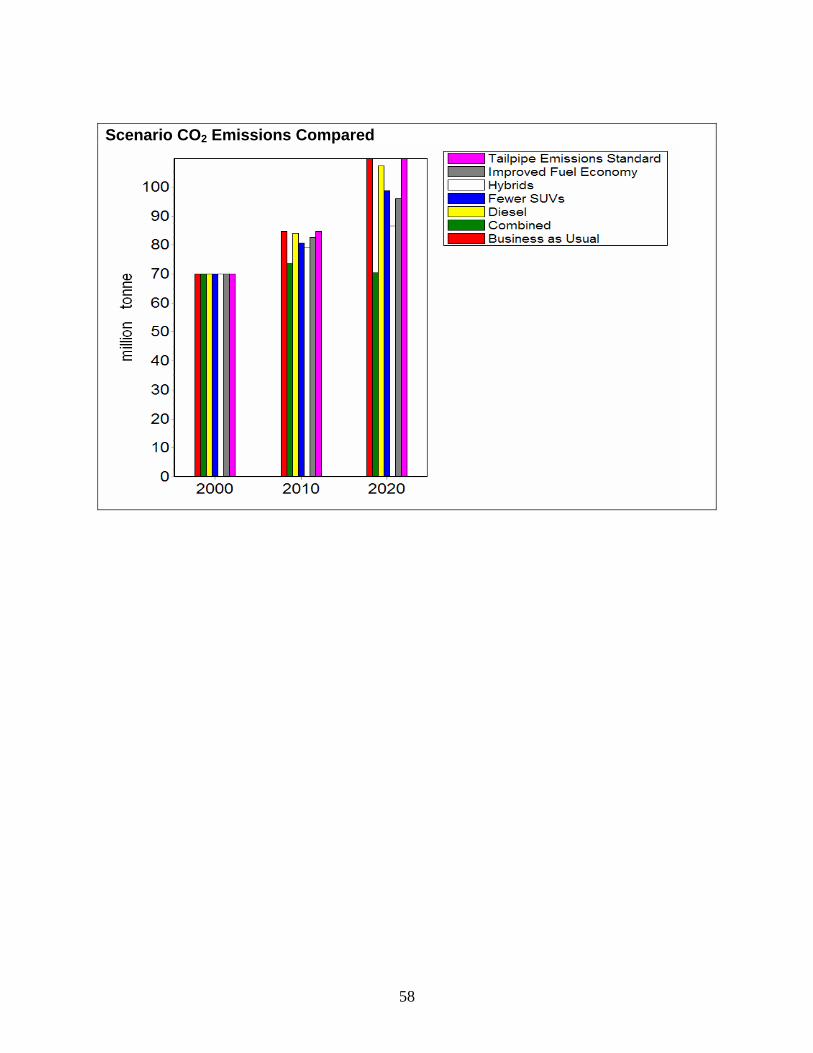
Scenario CO Emissions Compared 2

58

59