University of LatviaFaculty of Physics and Mathematics

Department of Mathematics

PhD Thesis

L-fuzzy valued measure and integral

by Vecislavs Ruza

Scientific supervisor: professor, Dr. Math.

Svetlana Asmuss

Riga, 2012

Abstract

In this thesis we develop the theory of measure and integral in the context of

L-sets, when L is a complete, completely distributive lattice with the minimum t-norm.

The main purpose of this thesis is to introduce the concept of measure and integral taking

values in the L-fuzzy real line. We suggest the construction of L-fuzzy valued measure

by extending the measure defined on σ-algebra of crisp sets to L-fuzzy valued measure

defined on the tribe of L-sets. We introduce the L-fuzzy valued integral over the L-set

with respect to an L-fuzzy valued measure, consider its properties and describe methods

of L-fuzzy valued integration. We define an L-fuzzy valued norm using the L-fuzzy

valued integral and apply it to estimate the error of approximation of real valued func-

tions on L-set.

MSC: 03E72, 28E10, 26E50, 28A05, 28A12, 28A20, 28A25.

Key words and phrases: L-set, L-fuzzy real number, L-fuzzy real measure, L-fuzzy

valued integral, L-fuzzy valued norm, approximation error.

1

Anotacija

Promocijas darba mera un integrala koncepcijas ir attıstıtas L-kopu teorijas kon-

teksta, kur L ir pilns, pilnıgi distributıvs režgis ar minimuma t-normu. Darba merkis

ir izstradat mera un integrala jedzienus gadıjuma, kad ne tikai kopas, bet arı mera un

integrala vertıbas ir L-nestriktas. Darba izstradata visparıga shema parasto kopu mera

turpinajumam lıdz L-kopu meram ar vertıbam L-nestriktaja realaja taisne. Ir definets

L-nestrikti vertıgs integralis pa merojamu L-kopu pec L-nestrikti vertıga mera, izpetıtas

ta ıpasıbas un aprakstıtas integresanas metodes. Izmantojot integrali ir uzdota L-nestrikti

vertıga norma, kura raksturo merojamas funkcijas L-kopas. Ir aprakstıti daži L-nestrikti

vertıgas normas lietojumi funkciju aproksimaciju teorija.

MSC: 03E72, 28E10, 26E50, 28A05, 28A12, 28A20, 28A25.

Atslegvardi: L-kopa, L-nestrikti reala taisne, L-nestrikti vertıgs mers, L-nestrikti

vertıgs integralis, aproksimacijas kluda.

2

Acknowledgements

First and foremost I would like to thank my mentor Svetlana Asmuss. It has been a great

honour to be her Ph.D. student. I appreciate a lot all her enormous contributions of time,

incredible ideas, and funding to make my Ph.D. experience productive and stimulating.

The joy and enthusiasm she got was contagious and motivational for me, even during

tough times in the Ph.D. pursuit. I am also thankful for the excellent example she has

provided as a successful woman mathematician and professor.

For the invaluable support I would like to thank my course-mate Olga Grigorenko,

as well as all participants of Prof. Alexander Sostak’s seminar – Julija Lebedinska,

Irina Zvina, Pavels Orlovs and others, for inspiration and memorable time spent in the

university classes and participating in several conferences.

I gratefully acknowledge the funding sources that made my Ph.D. work possible.

My work was partly supported by the European Social Fund (ESF) projects:

1. "Doktorantu un jauno zinatnieku atbalsts Latvijas Universitate" in 2007/2008 year,

2. "Atbalsts doktora studijam Latvijas Universitate" in 2010/2011 year.

3

Contents

Introduction 6

1 Preliminaries 131.1 Lattices and t-norms . . . . . . . . . . . . . . . . . . . . . . . . . . . 13

1.2 L-sets . . . . . . . . . . . . . . . . . . . . . . . . . . . . . . . . . . . 16

1.3 Classes of L-sets . . . . . . . . . . . . . . . . . . . . . . . . . . . . . 18

1.4 L-fuzzy real line . . . . . . . . . . . . . . . . . . . . . . . . . . . . . . 19

1.5 L-fuzzy valued functions . . . . . . . . . . . . . . . . . . . . . . . . . 21

2 Construction of L-fuzzy valued measure 222.1 L-fuzzy valued measures . . . . . . . . . . . . . . . . . . . . . . . . . 22

2.2 Construction of L-fuzzy valued elementary measure . . . . . . . . . . . 23

2.3 Measurable L-sets . . . . . . . . . . . . . . . . . . . . . . . . . . . . . 25

2.4 Construction of L-fuzzy valued measure . . . . . . . . . . . . . . . . . 28

3 L-fuzzy valued integral 343.1 Definition of L-fuzzy valued integral . . . . . . . . . . . . . . . . . . . 34

3.2 Properties of L-fuzzy valued integral . . . . . . . . . . . . . . . . . . . 37

3.3 Alternative definition of L-fuzzy valued integral . . . . . . . . . . . . . 40

3.4 Integration over measurable fuzzy sets . . . . . . . . . . . . . . . . . . 45

3.4.1 Integration over A(M,α) . . . . . . . . . . . . . . . . . . . . . 46

3.4.2 Integration over SNMF E . . . . . . . . . . . . . . . . . . . . 46

3.4.3 Integration over NMF E . . . . . . . . . . . . . . . . . . . . . 48

4 Applications of L-fuzzy valued integral in approximation theory 504.1 L-fuzzy valued norm . . . . . . . . . . . . . . . . . . . . . . . . . . . 50

4.2 Function approximation error on L-sets . . . . . . . . . . . . . . . . . 51

4

CONTENTS

4.2.1 Theoretical background . . . . . . . . . . . . . . . . . . . . . 51

4.2.2 Numerical example . . . . . . . . . . . . . . . . . . . . . . . . 52

4.3 Error of approximation on L-sets for classes of functions . . . . . . . . 55

4.3.1 Theoretical background . . . . . . . . . . . . . . . . . . . . . 55

4.3.2 Numerical example . . . . . . . . . . . . . . . . . . . . . . . . 58

Conclusions 65

List of conferences 66

Bibliography 68

Author’s publications 70

5

Introduction

The history of measure theory starts in the late 19th and early 20th centuries by the

works of E. Borel, H. Lebesgue, J. Radon and M. Frechet, among others. H. Lebesgue

is known as a person that stands in the very beginning of the measure and integral the-

ory foundation. In his "Lectures on integration and search for primitive functions" he

challenged the goal to find a (non-negative) measure on the real line that would have

existed for all bounded sets, and would satisfy three conditions: congruent sets have

equal measure (i.e. the measure is invariant under the symmetry operations and transfer),

measure is countably additive and measure of interval (0,1) is equal to 1. Lebesgue’s

studies have found a broad scientific response and were continued and developed by

many mathematicians: E. Borel, M. Riess, G. Vitali, M. Frechet etc.

The main applications of measures are in the foundations of the Lebesgue integral, in

A. Kolmogorov’s axiomatisation of probability theory and in ergodic theory. In integra-

tion theory, specifying a measure allows one to define integrals on spaces more general

than subsets of Euclidean space; moreover, the integral with respect to Lebesgue mea-

sure on Euclidean spaces is more general and has a richer theory than its predecessor, the

Riemann integral. Probability theory considers measures that assign to the whole set the

size 1, and considers measurable subsets to be events whose probability is given by the

measure. Ergodic theory considers measures that are invariant under, or arise naturally

from, a dynamical system.

Since the notion of measure was introduced the several ways to generalize this con-

cept where attempted. In certain purposes it is useful to have a "measure" whose values

are not restricted to the non-negative reals or infinity. For example, the countably ad-

ditive set function with values in the (signed) real numbers is called a signed measure,

while such a function with values in complex numbers is called a complex measure.

Measures that take values in Banach spaces have been studied extensively. A mea-

sure that takes values in the set of self-adjoint projections on a Hilbert space is called

a projection-valued measure; these are used in functional analysis for the spectral the-

6

orem. When it is necessary to distinguish the usual measures which take non-negative

values from generalizations, the term positive measure is used. Positive measures are

closed under conical combination but not general linear combination, while signed mea-

sures are the linear closure of positive measures. Another generalization is the finitely

additive measure, which are sometimes called contents. This is the same as a measure,

except that instead of requiring countable additivity we only require finite additivity.

As one can see all these ways to generalize the concept of measure in some sense is

just manipulation with the properties of measure as a mapping (σ-additivity, additivity)

and its domain (σ-algebra, algebra, semiring) or range (R+,R,R∪{∞}). Absolutely

new possibilities for generalization of measure and integral have been discovered when

the innovative theory of fuzzy sets were introduced.

Fuzzy mathematics forms a branch of mathematics related to fuzzy set theory and

fuzzy logic. The actual history of the fuzzy sets theory starts in 1965 when L. A. Zadeh

work [32] entitled "Fuzzy Sets" was published in the journal "Information and Control".

Then in 1968 J. A. Gogen in [6] has developed and improved Zadeh ideas by imple-

menting the concept of an L-set. L-set concept led to enormous interest, both among

mathematicians - academics, as well as between the professionals who use mathemati-

cal ideas, concepts and results of various real process modelling.

A fuzzy subset A of a set X is a function (also called a membership function)

A : X → L, where L is the interval [0,1]. This function is also called a membership

function. A membership function is a generalization of a characteristic function. More

generally, instead of [0,1] one can use a complete lattice L in a definition of L-fuzzy

subset A. Usually, a fuzzification of mathematical concepts is based on a generalization

of these concepts from characteristic functions to membership functions. For exam-

ple, having two fuzzy subsets: the intersection and union can be defined as min and

max of their membership functions. Instead of min and max one can use t-norm and

t-conorm, respectively, for example, min can be replaced by multiplication. A straight-

forward fuzzification is usually based on min and max operations because in this case

more properties of traditional mathematics can be extended to the fuzzy case.

The concept of an L-set creates applications in many other mathematical disciplines.

Among them are also the measure and integral theory. In real processes there are often

situations when the object is a set of "washed out" boundaries in the sense that a given

element may belong to a given set to a greater or lower degree. Integral theory, which

arose from this kind of practical tasks is rapidly evolving and increasingly is being suc-

7

cessfully implemented. One can find plenty of papers devoted to the concept of measure

and integral in the fuzzy context. Quite worthwhile approach to classify all types of

measures in fuzzy sense was introduced by E. P. Klement and S. Weber in the joint pa-

per called "Generalized measures" [17]. We just recall here some of the most important

definitions to highlight all the diversity of the measure concept in fuzzy context and

point out the area of possible widening to existing results.

We have already mentioned before that generalization process of measure by its na-

ture reminds a "game" where we are "playing" with the mapping properties, its domain

or range. As we see in [17] E. P. Klement and S. Weber put the "game rules" into

the following frames: having a σ-complete lattice as domain and σ-complete, lattice

ordered commutative semigroup as a range, the mapping satisfying boundary condi-

tion, valuation property and left-continuity can be considered as a generalized mea-

sure. Then for the different cases of domain and range the following examples of

generalized measure can be described: probability measures of fuzzy events ([33]), pos-

sibility measures ([24], [34], [35]), fuzzy probability measures ([10], [14]), fuzzy-valued

fuzzy measures ([12]), decomposable measures ([30]), measures of fuzzy sets ([29]).

Since the concept of integral comes along with the measure concept very closely, it

is worth to mention that diversity of the integral in the fuzzy context does not inferior to

the variety of measure concept. As examples of well known approaches to define fuzzy

integral Sugeno, Choquet and Sipos integrals should be mentioned. The tremendous

scope of papers devoted to the concept of fuzzy integral obviously requires proper clas-

sification. The concept of general and universal integrals that can be defined on arbitrary

measurable spaces introduced in [16] by E. P. Klement, R. Mesiar, E. Pap, obviously,

is a worthwhile attempt to clarify the overall picture in the entire diversity of multiple

integral definitions. For instance, the Choquet and the Sugeno integrals are well-known

examples of universal integrals.

Answering the question: "Should the measure of an L-set be a real number or it

should have a fuzzy nature same as the set that it characterizes?" we give a preference

to the second option. The same question can be addressed to the integral case. The fact

that the majority of papers deals with the measure or integral defined as a real valued

function we considered as a major lack.

To address this shortcoming, the work is intended to investigate measure and integral

as an L-fuzzy valued structure. At that point we had to choose one of the several (quite

different) approaches to the concept of an L-fuzzy real number. We decided in favour

8

of fuzzy real numbers, as they were first defined by B. Hutton [9], and then thoroughly

studied in a series of papers (see e.g. [21], [22], [23], [25]). The preference of using

this approach for defining L-fuzzy real numbers is motivated by our intention to develop

results on approximation from [1], [2].

Although, there are also some works where L-fuzzy valued measures and integral are

involved, they used an alternative (essentially different) definition of a fuzzy real num-

ber (see e.g. [5], [31]). As an exception we can mention the E. P. Klement’s approach

(see e.g. [12], [17]) where fuzzy-valued measures take values in the collection of all

probability distribution functions. The authors of the previously mentioned works

devoted to a concept of fuzzy measure are mainly interested in finding appropriate

definitions and studying the properties of this measures. As different from these works

our main interest is in presenting the construction for a measure as well as calculation

methods and possible applications for the integral.

I believe that this research work is very topical, because it combines the L-structure

study, which is traditional to Latvian mathematicians (see e.g. [26]), as well as mea-

sure and integral theory further development, which opens a very wide range of pack-

age options. L-sets and the associated objects research in Latvia is conducted from

the mid 80th leading by professor A. Šostak. These studies have gained international

recognition. It is anticipated that the thesis results will actively continue traditional

studies of Latvian mathematics in the theory of L-sets and also successfully develop this

theoretical mathematics perspective direction.

Goal and objectivesThe main objective of the doctoral thesis is to develop a theory of measure and

integral in the L-fuzzy context, to generalize the constructions of measure and integral

in the case when not only sets but also measure and integral take L-fuzzy values, where

L is a complete, completely distributive lattice with the minimum t-norm.

The tasks of the thesis are strongly correlated with its goal:

1. to suggest a general scheme for extension of a crisp measure to an L-fuzzy valued

measure taking values in the L-fuzzy real line,

2. to introduce the concept of an L-fuzzy valued integral of a real valued non-

negative measurable function over an L-set with respect to the L-fuzzy valued

measure,

9

3. to investigate the properties of an L-fuzzy valued integral and consider possible

calculation methods,

4. to introduce the concept of an L-fuzzy valued norm by using the concept of an

L-fuzzy valued integral,

5. to describe some possible applications of an L-fuzzy valued norm in the approxi-

mation theory.

Thesis structureThis thesis is structured in the following way.

Chapter 1 presents a general overview of necessary preliminaries. Starting with

some concepts from the lattice theory continuing with the definition of an L-set and

describing operations with L-sets by using concepts of triangular norm and conorm as

well as involution. Then considering the notion of L-fuzzy real numbers and operations

with them such as addition, countable addition and multiplication by a real number,

as well as infimum and supremum of a set of L-fuzzy real numbers. Next the classes

of L-sets introduced such as T-tribes, T-clans and T-semirings and also L-fuzzy valued

functions defined on classes of L-sets and taking values in the range of non-negative

L-fuzzy real numbers.

Chapter 2 contains the definitions of L-fuzzy valued measure, L-fuzzy valued

elementary measure and L-fuzzy valued exterior measure. The main aim of the

second chapter is to develop a construction of an L-fuzzy valued measure by extend-

ing a measure defined on a σ-algebra of crisp sets to an L-fuzzy valued measure defined

on a T-tribe of L-sets in the case when T is the minimum t-norm. In order to realize

the construction we consider the following steps: first, we describe the L-fuzzy valued

elementary measured construction, second, we develop an approach to build the L-fuzzy

valued exterior measure on the basis of the L-fuzzy valued elementary measure, then we

describe the T-tribe of L-sets that are measurable with respect to the L-fuzzy valued

exterior measure and, finally, we present the method of narrowing the L-fuzzy valued

exterior measure to the L-fuzzy valued measure defined on the T-tribe.

Chapter 3 presents the concept of an L-fuzzy valued integral of a real valued func-

tion over an L-set with respect to an L-fuzzy valued measure. The definition of integral

implemented stepwise: first considering the case when the integrand is a characteris-

tic function, then extending it to the case when the integrand is a simple non-negative

10

measurable function and, finally, the case with non-negative measurable function. Ba-

sic properties of an L-fuzzy valued integral are proved. Inspired by the fact from the

classical measure theory stating that an integral of a given non-negative function can be

considered as a measure we obtain two different approaches to define an L-fuzzy valued

integral. The second approach shows that an L-fuzzy valued integral can be obtained by

considering the measure ν f using a crisp measure ν and then extending it to the L-fuzzy

valued measure µ f according to the construction described in Chapter 2. Finally we

show that both approaches give us equivalent ways to define the L-fuzzy valued integral,

i.e. µ f = µ f . This result can be described by the following diagram:

ν −→ µ

↓ ↓ν f → µ f

The second approach to the definition gives us an opportunity to simplify calculations

of the L-fuzzy valued integral. Some special cases of integration for different types of

L-sets are described.

Chapter 4 shows some possible applications of an L-fuzzy valued integral in

approximation theory. For problems that can be solved only approximately, the no-

tion of the error of a method of approximation plays the fundamental role. In order to

estimate the quality of approximation on an L-fuzzy set, we need an appropriate L-fuzzy

analogue of a norm. We introduce an L-fuzzy valued norm defined by an L-fuzzy valued

integral with respect to an L-fuzzy valued measure µ. We describe the space L1(E,Σ,µ)

of an L-fuzzy integrable over a measurable L-set E ∈ Σ real valued functions. We also

show how the introduced L-fuzzy valued norm can be applied to estimate on E the error

of approximation of real valued functions f ∈L1(E,Σ,µ). And, finally, some numerical

examples are mentioned.

ApprobationThe results obtained in the process of thesis writing have been presented at 12 in-

ternational conferences: three EUSFLAT (European Society for Fuzzy Logic and

Technology) conferences in 2007, 2009 and 2011 ([C02], [C08], [C12]); three FSTA

(Fuzzy Set Theory and Applications) conferences in 2008, 2010 and 2012 ([C01], [C07],

[C10]); three MMA (Mathematical Modelling and Analysis) conferences in 2009, 2010

and 2011 ([C04], [C06], [C09]); AGOP (Aggregation Operators) conference in 2011

[C03]; APLIMAT (Applied Mathematics) conference in 2011 [C05], ICTAA (Interna-

11

tional Conference on Topological Algebras and Applications) conference in 2008 [C11];

at 5 domestic conferences: three Conferences of University of Latvia in 2007, 2008 and

2009 ([C13], [C15], [C16]); two Conferences of Latvian Mathematical Society in 2006

and 2008 ([C14], [C17]); and at 4 international seminars ([C18]–[C21]).

The main results of the research have been reflected in 7 scientific publications [P1]–

[P7] and 11 conference abstracts listed in p.72.

12

Chapter 1

Preliminaries

1.1 Lattices and t-norms

In matters where lattices are involved, our main sources of references are [3], [4]. How-

ever we reproduce here some definitions, notations and results.

Definition 1.1.1. A poset (L,≤) is a set L in which a binary relation≤ is defined, which

satisfies for all α,β,γ ∈ L the following conditions:

• α≤ α (reflexivity),

• if α≤ β and β≤ α, then α = β (antisymmetry),

• if α≤ β and β≤ γ, then α≤ γ (transitivity).

Definition 1.1.2. Let (L,≤) be a poset and A be a subset of L. An element α ∈ L is

called:

• upper bound of A iff β≤ α for all β ∈ A;

• join of A iff it is an upper bound of A and for every other upper bound γ of A it

holds that α≤ γ;

• lower bound of A iff α≤ β for all β ∈ A;

• meet of A iff it is a lower bound of A and for every other lower bound γ of A it

holds that γ≤ α.

Note that the join and meet of an arbitrary subset (if they exist) are unique. We write∨A and a∨b to denote the joins, and

∧A and a∧b to denote the meets.

13

Lattices and t-norms

Definition 1.1.3. A poset (L,≤) is called a lattice iff it is closed under finite joins and

meets.

For convenience, going forward we write L meaning lattice (L,≤).

Definition 1.1.4. A lattice L is called as a bounded lattice if it contains∨

L (the greatest

element or maximum) and∧

L (the least element or minimum), denoted 1L and 0L by

convenience.

Any lattice can be converted into a bounded lattice by adding a greatest and least ele-

ments, and every non-empty finite lattice is bounded, by taking the join (resp., meet) of

all elements.

Definition 1.1.5. A poset is called a complete lattice if all its subsets have both a join

and a meet.

In particular, every complete lattice is a bounded lattice.

Since lattices come with two binary operations, it is natural to ask whether one of them

distributes over the other.

Definition 1.1.6. A lattice L is called a distributive lattice if for any three elements

α,β,γ ∈ L one of the following axioms is satisfied:

• α∨ (β∧ γ) = (α∨β)∧ (α∨ γ),

• α∧ (β∨ γ) = (α∧β)∨ (α∧ γ).

In the mathematical area of order theory, a completely distributive lattice is a lattice in

which arbitrary joins distribute over arbitrary meets.

Definition 1.1.7. A lattice L is said to be completely distributive if for any doubly in-

dexed family {α jk| j ∈ J,k ∈ K j} ⊂ L, we have

∧j∈J

∨k∈K j

α jk =∨f∈F

∧j∈J

α j f ( j),

where F is the set of choice functions f choosing for each index j ∈ J some index

f ( j) ∈ K j.

Going forward we work only with lattices which are complete and completely distribu-

tive. Complete distributivity is a self-dual property, i.e. dualizing the above statement

14

Lattices and t-norms

yields the same class of complete lattices. Note that the unit interval [0,1], ordered in

the natural way, is a completely distributive lattice and the power set lattice for any set

X is a completely distributive lattice.

In order to describe the operations with L-sets, such as intersection, union and difference,

we consider functions defined in L× L, which satisfy such important properties like

associativity, commutativity and monotonicity. Such functions are known as triangular

norms and triangular conorms. Also, to describe the complementary of an L-set and

the difference between L-sets we need a concept of involution. Our sources for the

references regarding t-norms and t-conorms are [15], [27].

Definition 1.1.8. A function T : L×L→ L is called a triangular norm (t-norm for short)

if it satisfies the following conditions for all α,β,γ ∈ L:

• T (α,1L) = 1L,

• T (α,β)≤ T (α,γ) whenever β≤ γ,

• T (α,β) = T (β,α),

• T (α,T (β,γ)) = T (T (α,β),γ).

A function S : L×L→ L is called a triangular conorm (t-conorm for short) if it satisfies

the following conditions for all α,β,γ ∈ L:

• S(α,0L) = α,

• S(α,β)≤ S(α,γ) whenever β≤ γ,

• S(α,β) = S(β,α),

• S(α,S(β,γ)) = S(S(α,β),γ).

A function N : L→ L is called an order reversing involution if it satisfies the following

conditions for all α,β ∈ L:

• N(N(α)) = α,

• N(α)≥ N(β) whenever α≤ β.

15

L-sets

Note that N(0L) = 1L and N(1L) = 0L.

If a lattice L provided with a t-norm T and an involution N, then the corresponding

t-conorm is the function S : L×L→ L defined by

S(α,β) = N(T (N(α),N(β))).

It is easily seen that given a t-conorm S and an involution N, then T : L×L→ L, defined

by

T (α,β) = N(S(N(α),N(β)))

is a t-norm whose corresponding t-conorm is exactly the t-conorm S we started with.

Example 1.1.1.Some of the most important pairs of t-norms and its corresponding t-conorms are the

minimum TM and the maximum SM, the product TP and the probabilistic sum SP, the

Lukasiewicz t-norm TL and the Lukasievicz t-conorm SL given by, respectively:TM(α,β) = min(α,β), SM(α,β) = max(α,β),

TP(α,β) = α ·β, SP(α,β) = α+β−α ·β,

TL(α,β) = max(0,α+β−1), SL(α,β) = min(1,α+β).

Note that the Lukaciewicz t-norm and product t-norm are defined in case when L= [0,1],

but minimum t-norm we can define for arbitrary lattice.

1.2 L-sets

Given a (crisp) universe X and a complete, completely distributive lattice L, an L-fuzzy

subset A of X (or, briefly, an L-set A) is characterized by its membership function

A : X −→ L,

where for x ∈ X the value A(x) is interpreted as the degree of membership of x in the

L-set A. Thus, we do not make distinction between an L-set and its membership func-

tion. The class of all L-fuzzy subsets of X will be denoted LX . It is obvious that each

crisp subset of X is just a special case of an L-set.

Example 1.2.1. A very special role is played in this survey by the following example of

L-sets. For M ⊂ X, α ∈ L we define the L-set A(M,α) : X → L by

(A(M,α))(x) =

{α, x ∈M,

0L, x /∈M.

16

L-sets

Figure 1.1: L-set A(M,α)

The operations with L-sets A,B ∈ LX such as intersection, union and difference are de-

fined by using a triangular norm T , its corresponding triangular conorm S and an invo-

lution N:

(ATB)(x) = T (A(x),B(x)),

(ASB)(x) = S(A(x),B(x)),

(ADB)(x) = T (A(x),N(B(x))).

The operations for a sequence of L-sets (An)n∈N such as intersection and union are

defined in the following way:

(∞

Tn=1

An)(x) =∧

n∈N

nT

k=1An(x) =

∧n∈N

(A1(x)TA2(x)T ...TAn(x)),

(∞

Sn=1

An)(x) =∨

n∈N

nS

k=1An(x) =

∨n∈N

(A1(x)SA2(x)S ...SAn(x)).

Within this section all definitions are given for the case when T is an arbitrary t-norm.

We also describe a concept of T -disjointness.

Definition 1.2.1. A finite family of L-sets A1,A2, . . . ,An is said to be T -disjoint (see e.g.

[13]) iff for each k ∈ {1, . . . ,n}

(nS

j=1, j 6=kA j)TAk = /0.

A countable family of L-sets is said to be T -disjoint iff every finite subfamily of this

family is T -disjoint.

For the crisp sets such as /0 or X we do not distinct the set and its characteristic function.

For example, for all x ∈ R we have /0(x) = 0L.

17

Classes of L-sets

1.3 Classes of L-sets

In order to consider L-fuzzy valued functions we describe such classes of L-sets as

semirings, clans and tribes. We start with T -semirings (defined by analogy with the

classical case, see e.g. [7]).

Definition 1.3.1. A class℘⊂ LX is called a T -semiring on X iff the following properties

are satisfied:

• /0 ∈℘,

• for all A,B ∈℘we have ATB ∈℘,

• for all A,B ∈℘ there exist such T -disjoint L-sets A1,A2, ...,An ∈℘ that

ADB =nS

i=1Ai.

In matters where T-clans and T-tribes are involved, our main source of references is [13].

Definition 1.3.2. A class A⊂ LX is called a T -clan on X iff the following properties are

satisfied:

• /0 ∈A,

• for all A ∈A we have N(A) ∈A,

• for all A,B ∈A we have ATB ∈A.

Definition 1.3.3. A class Σ⊂ LX is called a T -tribe on X iff the following properties are

satisfied:

• /0 ∈ Σ,

• for all A ∈ Σ we have N(A) ∈ Σ,

• for all sequences (An)n∈N ⊂ Σ we have∞

Tn=1

An ∈ Σ.

Example 1.3.1. The class of L-sets from Example 1.2.1 forms a T -semiring:

℘= {A(M,α) |M ⊂ X and α ∈ L}.

18

L-fuzzy real line

1.4 L-fuzzy real line

For our purposes we use the L-fuzzy real numbers as they were first defined by B. Hut-

ton [9] and then studied thoroughly in a series of papers (see e.g. [18], [21], [22], [23]).

Definition 1.4.1. An L-fuzzy real number is a function z : R→ L such that

• z is non-increasing, i.e. t1 ≤ t2⇒ z(t1)≥ z(t2),

•∧t

z(t) = 0L,∨t

z(t) = 1L,

• z is left semi-continuous, i.e. for all t0 ∈ R we have∧

t<t0z(t) = z(t0).

In the original papers on this subject (see [9], [18], [21]) the L-fuzzy real numbers were

defined not as order reversing functions, but as equivalence classes of such functions.

However each class of equivalence has a unique left semi-continuous representative and

therefore an L-fuzzy real number can be identified with this representative.

The set of all L-fuzzy real numbers is called the L-fuzzy real line and it is denoted

by R(L). An L-fuzzy real number z is called non-negative if z(0) = 1L. We denote by

R+(L) the set of all non-negative L-fuzzy real numbers.

The ordinary real line R can be identified with the subspace {za | a ∈R} of R(L) by

assigning to a real number a ∈ R the fuzzy real number za defined by

za(t) =

{1L, if t ≤ a ,

0L, if t > a .

Operations with L-fuzzy real numbers such as addition ⊕ and multiplication by a

real positive number are defined as follows:

(z1⊕ z2)(t) =∨τ

{z1(τ)∧ z2(t− τ)}, (rz)(t) = z(tr).

The supremum and the infimum of a set of non-negative L-fuzzy numbers F ⊂R+(L) are defined by the formulas (see e.g. [1], [2]):

(In f F)(t) =∧{z(t) | z ∈ F}, t ∈ R,

Sup F = In f{z | z ∈ R(L),z≥ z′ for all z′ ∈ F}.

Due to F is bounded from below it is easy to see that In f F is an L-fuzzy real number.

In case F is bounded from above (i.e. there exists z0 ∈ R(L) such that z ≤ z0 for all

z ∈ F), Sup F is an L-fuzzy real number, otherwise the condition

19

L-fuzzy real line

∧t

SupF(t) = 0L

does not necessarily hold.

Going forward we will need also the countable addition of non-negative fuzzy real

numbers. Given a sequence of non-negative fuzzy real numbers (zn)n∈N ⊂ R+(L) we

consider the countable sum∞⊕

n=1

zn = Sup{z1⊕ z2⊕ ...⊕ zn | n ∈ N}.

In the case when ∧t(

∞⊕n=1

zn)(t) 6= 0L

the series∞⊕

n=1zn diverges.

Example 1.4.1. For a ∈ R+ and α ∈ L by z(a,α) we denote a special type of non-

negative L-fuzzy real numbers

(z(a,α))(t) =

1L, t ≤ 0,

α, 0 < t ≤ a,

0L, t > a,

that will play an important role in our work.

Figure 1.2: L-fuzzy real number z(a,α)

Note that:

• a1,a2 ∈ R+⇒ z(a1,α)⊕ z(a2,α) = z(a1 +a2,α);

• r ∈ R+⇒ rz(a,α) = z(ra,α);

• ai ∈ R+, i ∈ J and sup{ai | i ∈ J}<+∞⇒⇒ Sup{z(ai,α) | i ∈ J}= z(sup{ai | i ∈ J},α).

20

L-fuzzy valued functions

1.5 L-fuzzy valued functions

Let K be a class of L-sets. Within this section some basic properties of an L-fuzzy

valued function η : K→ R+(L) are considered.

Definition 1.5.1. An L-fuzzy valued function η is called

• T -additive

if for all A,B ∈K such that ATB = /0 and ASB ∈K it holds

η(ASB) = η(A)⊕η(B);

• countably T -additive

if for all (An)n∈N ⊂K such that (∀i, j ∈ N : i 6= j⇒ Ai TA j = /0) and∞

Sn=1

An ∈K

it holds

η(∞

Sn=1

An) =∞⊕

n=1

η(An);

• a T -valuation

if for all A,B ∈K such that ATB, ASB ∈K we have

η(ATB)⊕η(ASB) = η(A)⊕η(B);

• left T -continuous

if for all (An)n∈N ⊂K such that∞

Sn=1

An = A ∈K and ∀n ∈N : An ≤ An+1 we have

Sup{η(An) | n ∈ N}= η(A);

• countably T -semiadditive

if for all (An)n∈N ⊂K and for all A ∈K such that A≤∞

Sn=1

An we have

η(A)≤∞⊕

n=1

η(An).

Remark 1.5.1. If η is a T-valuation and η( /0) = 0L, then η is also T-additive, the con-

verse not being generally true (see e.g. [13]). It is obvious that countably T-additive

functions are always T-additive.

21

Chapter 2

Construction of L-fuzzy valuedmeasure

This section is devoted to an L-fuzzy valued generalization of the classical concept of

measure. Referring to the paper [17] that type of generalization is called a triangular

norm based measures.

We consider such L-fuzzy valued functions as T-measure, elementary T-measure and

exterior T-measure. We also suggest a construction that allows us to extend a measure

defined on a σ-algebra of crisp sets to the L-fuzzy valued TM-measure defined on the

TM-tribe.

2.1 L-fuzzy valued measures

Definition 2.1.1. An L-fuzzy valued function η : K→ R+(L) satisfying boundary con-

dition η( /0) = z(0,1L) is called

• an L-fuzzy valued T -measure

if K is a T -tribe and η is left T -continuous T -valuation;

• an L-fuzzy valued countably T-additive measure

if K is a T -tribe and η is countably T-additive T -valuation;

• an L-fuzzy valued elementary T -measure

if K is a T -semiring and η is T -additive;

• an L-fuzzy valued exterior T -measure

if K = LX and η is countably T -semiadditive.

22

Construction of L-fuzzy valued elementary measure

Remark 2.1.1. L-fuzzy valued measures are countably T-additive functions.

All main results of the thesis obtained in the case when T is the minimum t-norm, al-

though, some of them are true in the case of other t-norms as well. Going forward we

mean TM every time the t-norm concept is involved and we use ∧,∨ instead of T,S when

operations with L-sets are mentioned. Also for convenience, we say L-fuzzy valued mea-

sure meaning L-fuzzy valued TM-measure.

2.2 Construction of L-fuzzy valued elementary measure

Let Φ be a σ-algebra of "crisp" subsets of X and ν is a finite measure ν : Φ→ [0,+∞).

Our aim is to construct an L-fuzzy valued measure µ on a TM-clan by extension a crisp

measure ν. To achieve this we generalize the well known construction of "classic" mea-

sure theory (see e.g. [7]) to the L-fuzzy case.

To realize the construction we use the special type of L-sets with respect to σ-algebra

Φ of crisp sets on X (see Example 1.2.1). For M ∈Φ, α∈ L we consider L-sets A(M,α):

(A(M,α))(x) =

{α, x ∈M,

0L, x /∈M.

Proposition 2.2.1. The class of L-sets

℘= {A(M,α)|M ∈Φ and α ∈ L}

is a TM-semiring.

Proof.

For all A(M,α),B(K,β) ∈℘we have

A(M,α)∧B(K,β) =C(M∩K,α∧β) ∈℘

and

A(M,α)\B(K,β) = A1(M \K,α)∨A2(M∩K,α∧N(β)),

where

A1(M \K,α), A2(M∩K,α∧N(β)) ∈℘.

Taking into account that also /0 = A( /0,0L) ∈℘, it is proved that ℘ is a TM-semiring.

23

Construction of L-fuzzy valued elementary measure

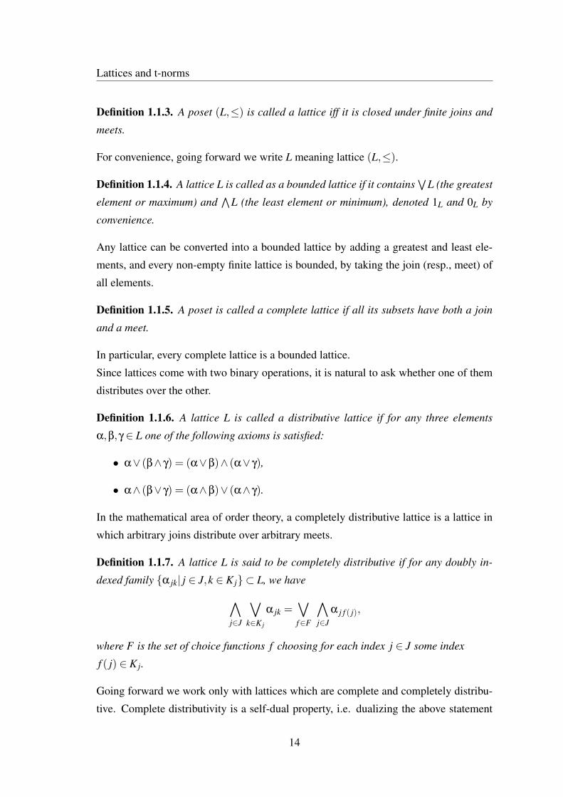
We define an L-fuzzy valued function m on the TM-semiring ℘ by the formula

m(A(M,α)) = z(ν(M),α), where

(z(ν(M),α))(t) =

1L, t ≤ 0,

α, 0 < t ≤ ν(M),

0L, t > ν(M),

is an L-fuzzy real number.

Proposition 2.2.2. m is an L-fuzzy valued elementary measure.

Proof.

It is easy to see that m( /0) = z(ν( /0),0L) = z0 and the equality

m(A(M,α))⊕m(B(K,β)) = m(A(M,α)∨B(K,β))

is true if A(M,α) = /0 or B(K,β) = /0.

Now let us consider A(M,α),B(K,β) ∈℘such that

A(M,α)∧B(K,β) = /0, A(M,α)∪B(K,β) ∈℘and α 6= 0L,β 6= 0L.

It follows that M∩K = /0 or α∧β = 0L. If M∩K = /0 then α = β and in this case

m(A(M,α))⊕m(B(K,α)) = z(ν(M),α)⊕ z(ν(K),α) =

= z(ν(M)+ν(K),α) = z(ν(M∪K),α) = m(A(M,α)∨B(K,α)).

If M ∩K 6= /0 then it is sufficient to consider the case when α∧ β = 0L. In this case

α and β are incomparable (due to the assumptions that α 6= 0L,β 6= 0L). Because of

A(M,α)∨B(K,β) =C1(M∩K,α∨β)∨C2(M \K,α)∨C3(K \M,β) ∈℘

we obtain that K \M = /0, M \K = /0 and hence M = K. Then

m(A(M,α))⊕m(B(M,β)) = z(ν(M),α)⊕ z(ν(M),β) =

= z(ν(M),α∨β) = m(C(M,α∨β)) = m(A(M,α)∨B(M,β)).

By this we prove that m is TM-additive.

24

Measurable L-sets

2.3 Measurable L-sets

For every E ∈ LX we define an L-fuzzy valued function m∗ : LX → R+(L) as follows

m∗(E) = In f{∞⊕

n=1

m(En) | (En)n∈N ⊂℘: E ≤∞∨

n=1

En}.

Remark 2.3.1.

• For every E ∈ LX there always exists a sequence (En)n∈N ⊂℘ : E ≤∞∨

n=1En. It is

enough to take E1(X ,1L). Thus, m∗ is bounded from above in the following sense:

m∗(E)≤ z(ν(X),1L) for all E ∈ LX .

• For all E ∈℘we have m∗(E) = m(E).

• Let us note that defining m∗(E) we can consider only TM-disjoint sequences

(En)n∈N.

Proposition 2.3.1. m∗ is a countably TM-semiadditive L-fuzzy valued function.

Proof. Let us consider a sequence (An)n∈N ⊂ LX and an L-set A ∈ LX such that

A≤∞

Sn=1

An . To prove the inequality

m∗(A)≤∞⊕

n=1

m∗(An)

we take sequences (Bnk)k∈N ∈℘such that

An ≤∞∨

k=1Bn

k ,n ∈ N. Then

A≤∞∨

n=1

An ≤∞∨

n=1

∞∨k=1

Bnk

and hence

m∗(A)≤∞⊕

n=1

∞⊕k=1

m(Bnk).

Taking into account that this inequality holds independent of the choice of sequences

(Bnk)k∈N we obtain

m∗(A)≤∞⊕

n=1

m∗(An).

This proposition means that m∗ is an L-fuzzy valued exterior measure.

25

Measurable L-sets

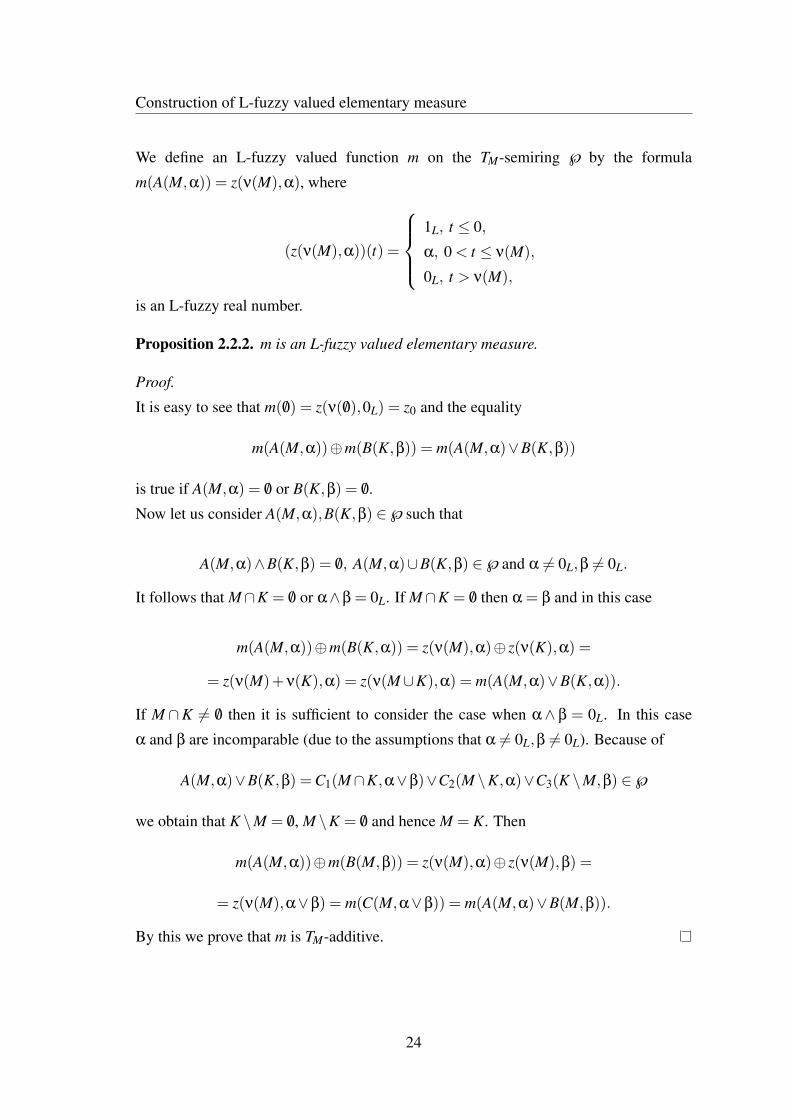
Proposition 2.3.2. For all A,B ∈ LX we have

m∗(A)⊕m∗(B)≥ m∗(A∧B)⊕m∗(A∨B).

Proof. For given L-sets A and B we consider two TM-disjoint sequences:

(Ci(Mi,αi))i∈N ⊂℘: A≤∞∨

i=1

Ci,

(D j(K j,β j)) j∈N ⊂℘: B≤∞∨

j=1

D j,

and define the following TM-disjoint sequence

(Hi j(Li j,γi j))i, j∈N, with Li j = Mi∩K j and γi j = αi∧βi.

Obviously, A∧B≤∨

i∈N

∨i∈N

Hi j.

As to L-set A∨B we can cover it with elements of three sequences:

(Hi j(Li j,λi j))i, j∈N with Li j = Mi∩K j, λi j = αi∨βi,

(Ci(Mi,αi))i∈N with Mi = Mi \⋃j∈N

K j,

(D j(K j,β j)) j∈N with K j = K j \⋃i∈N

Mi.

Now let us transform the sum∞⊕

i=1m∗(Ci)⊕

∞⊕j=1

m∗(D j). We use the following notation:

Fαi j (Li j,αi), Fβ

i j(Li j,β j), i, j ∈ N.

Because of σ-additivity of measure ν we get

ν(Mi) = ν(Mi)+∞

∑j=1

ν(Li j), i ∈ N,

ν(K j) = ν(K j)+∞

∑i=1

ν(Li j), j ∈ N.

It follows

m∗(Ci) = z(ν(Mi),αi) = z(ν(Mi)+∞

∑j=1

ν(Li j),αi) =

= z(ν(Mi),αi)⊕∞⊕

j=1

z(ν(Li j),αi) = m∗(Ci)⊕∞⊕

j=1

m∗(Fαi j ),

26

Measurable L-sets

m∗(D j) = z(ν(K j),β j) = z(ν(K j)+∞

∑i=1

ν(Li j),β j) =

= z(ν(K j),β j)⊕∞⊕

i=1

z(ν(Li j),β j) = m∗(D j)⊕∞⊕

i=1

m∗(Fβ

i j).

Now we obtain∞⊕

i=1

m∗(Ci)⊕∞⊕

j=1

m∗(D j) =

=∞⊕

i=1

(m∗(Ci)⊕∞⊕

j=1

m∗(Fαi j ))⊕

∞⊕j=1

(m∗(D j)⊕∞⊕

i=1

m∗(Fβ

i j)) =

=∞⊕

i=1

m∗(Ci)⊕∞⊕

j=1

m∗(D j)⊕∞⊕

i=1

∞⊕j=1

m∗(Fαi j )⊕

∞⊕j=1

∞⊕i=1

m∗(Fβ

i j) =

=∞⊕

i=1

m∗(Ci)⊕∞⊕

j=1

m∗(D j)⊕∞⊕

i=1

∞⊕j=1

(m∗(Fαi j )⊕m∗(Fβ

i j)).

Since

m∗(Fαi j )⊕m∗(Fβ

i j) = m∗(Hi j)⊕m∗(Hi j),

we continue∞⊕

i=1

m∗(Ci)⊕∞⊕

j=1

m∗(D j)⊕∞⊕

i=1

∞⊕j=1

(m∗(Fαi j )⊕m∗(Fβ

i j)) =

=∞⊕

i=1

m∗(Ci)⊕∞⊕

j=1

m∗(D j)⊕∞⊕

i=1

∞⊕j=1

m∗(Hi j)⊕∞⊕

i=1

∞⊕j=1

m∗(Hi j).

Now taking into account the fact that

A∧B≤∞∨

i=1

∞∨j=1

Hi j and A∨B≤ (∞∨

i=1

Ci)∨ (∞∨

j=1

D j)∨ (∞∨

i=1

∞∨j=1

Hi j),

we get∞⊕

i=1

m∗(Ci)⊕∞⊕

j=1

m∗(D j)⊕∞⊕

i=1

∞⊕j=1

m∗(Hi j)⊕∞⊕

i=1

∞⊕j=1

m∗(Hi j)≥

≥ m∗(A∧B)⊕m∗(A∨B).

So independent of the choice of sequences (Ci)i∈N, (D j) j∈N it holds

∞⊕i=1

m∗(Ci)⊕∞⊕

j=1

m∗(D j)≥ m∗(A∧B)⊕m∗(A∨B).

27

Construction of L-fuzzy valued measure

Finally, by taking the infimum we obtain

m∗(A)⊕m∗(B)≥ m∗(A∧B)⊕m∗(A∨B).

Next we define the concept of m∗-measurable L-sets. We generalize the concept of

measurability in the sense of Caratheodory (see e.g. [7]).

Definition 2.3.1. An L-set A ∈ LX is called a m∗-measurable L-set, if it satisfies the

following conditions for all L-sets E ∈ LX :

(i) m∗(A)⊕m∗(E) = m∗(A∧E)⊕m∗(A∨E),

(ii) m∗(N(A))⊕m∗(E) = m∗(N(A)∧E)⊕m∗(N(A)∨E).

We denote by Σ the class of all m∗-measurable L-sets. Some obvious properties of Σ:

• /0, X ∈ Σ,

• A ∈ Σ =⇒ N(A) ∈ Σ.

2.4 Construction of L-fuzzy valued measure

In this section we will prove that the class Σ of all m∗-measurable L-sets is a TM-tribe

and the restriction of m∗ to Σ is an L-fuzzy valued measure.

Proposition 2.4.1. Class Σ is a TM-clan.

Proof. For given L-sets A1,A2 ∈ Σ and E ∈ LX we will prove the equality

m∗(E)⊕m∗(A1∧A2) = m∗(E ∧ (A1∧A2))⊕m∗(E ∨ (A1∧A2)). (2.1)

Since A1 and A2 are m∗-measurable we have

m∗(A1)⊕m∗(A2) = m∗(A1∧A2)⊕m∗(A1∨A2),

m∗(A1∧E)⊕m∗(A1∨E) = m∗(A1)⊕m∗(E).

Now by summing up these two equalities we obtain

m∗(A1)⊕m∗(A2)⊕m∗(A1∧E)⊕m∗(A1∨E) =

= m∗(A1∧A2)⊕m∗(A1∨A2)⊕m∗(A1)⊕m∗(E).(2.2)

28

Construction of L-fuzzy valued measure

Let us transform now the left part of (2.2). To do this we use (2.3) and (2.4):

m∗(A1)⊕ [m∗(A2)⊕m∗(E ∧A1)] =

= m∗(A1)⊕ [m∗(E ∧A1∧A2)⊕m∗((E ∧A1)∨A2)] =

= m∗(E ∧A1∧A2)⊕m∗((E ∧A1)∨A2∨A1)⊕m∗(((E ∧A1)∨A2)∧A1) =

= m∗(E ∧A1∧A2)⊕m∗(A1∨A2)⊕m∗((E ∨A2)∧A1)

(2.3)

and

m∗(E ∨A1)⊕m(A1∧ (E ∨A2)) =

= m∗(E ∨ (A1∧A2)∨A1)⊕m∗(E ∨A1∧A2∧A1) =

= m∗(E ∨ (A1∧A2))⊕m∗(A1).

(2.4)

Next we substitute (2.3) and (2.4) in (2.2):

m∗(E ∧A1∧A2)⊕m∗(A1∨A2)⊕m∗(E ∨ (A1∧A2))⊕m∗(A1) =

= m∗(A1∧A2)⊕m∗(A1∨A2)⊕m∗(A1)⊕m∗(E).

Finally, we obtain (2.1).

By analogy it can be proved that

m∗(E)⊕m∗(A1∨A2) = m∗(E ∧ (A1∨A2))⊕m∗(E ∨ (A1∨A2)).

Taking into account that N(A1∨A2) = N(A1)∧N(A2) and N(A1∧A2) = N(A1)∨N(A2),

we get that A1∨A2 and A1∧A2 are m∗-measurable.

Proposition 2.4.2. m∗ is a TM-additive L-fuzzy valued function on Σ.

Proof. We will show that for TM - disjoint L-sets A1,A2, ...,An ∈ Σ it holds

m∗(n∨

i=1

Ai) =n⊕

i=1

m∗(Ai).

For n = 2 by using m∗-measurability and TM - disjointness of A1,A2 we obtain

m∗(A1)⊕m∗(A2) = m∗(A1∨A2)⊕m∗(A1∧A2) = m∗(A1∨A2)⊕m∗( /0) = m∗(A1∨A2).

Now we assume that the equality holds for a given n ∈ N and we prove it for n+ 1

TM-disjoint sets A1,A2, ...,An+1 ∈ Σ

m∗(n+1∨k=1

Ak) = m∗((n∨

k=1

Ak)∨An+1) = m∗(n∨

k=1

Ak)⊕m∗(An+1) =

=n⊕

k=1

m∗(Ak)+m∗(An+1) =n+1⊕k=1

m∗(Ak).

29

Construction of L-fuzzy valued measure

Theorem 2.4.1. For all TM-disjoint sequences of m∗-measurable L-sets (An)n∈N it holds

m∗(∞∨

n=1

An) =∞⊕

n=1

m∗(An).

Proof. To prove the equality we need to prove only one of the inequalities:

m∗(∞∨

n=1

An)≥∞⊕

n=1

m∗(An).

For a given n ∈ N we have

m∗(n∨

k=1

Ak)≤ m∗(∞∨

k=1

(Ak))

and

m∗(n∨

k=1

Ak)) =n⊕

k=1

m∗(Ak).

Hencen⊕

k=1

m∗(Ak)≤ m∗(∞∨

k=1

Ak).

Now by taking the supremum we obtain

∞⊕k=1

m∗(Ak)≤ m∗(∞∨

k=1

Ak).

Proposition 2.4.3. ℘⊂ Σ

Proof. First we will show that for a given A(H,α) ∈℘and all E ∈ LX it holds

m∗(A)⊕m∗(E) = m∗(A∨E)⊕m∗(A∧E).

Because of Proposition 2.3.2 it is sufficient to prove the inequality

m∗(A)⊕m∗(E)≤ m∗(A∨E)⊕m∗(A∧E).

We consider two TM-disjoint sequences (Ck(Mk,βk))k∈N ⊂℘ and (Dk(Kk,γk))k∈N ⊂℘

such that

A∨E ≤∞∨

k=1

Ck and A∧E ≤∞∨

k=1

Dk

and define two new sequences

(Fk(Mk \H,βk))k∈N and (Gk(H ∩Mk,βk))k∈N.

30

Construction of L-fuzzy valued measure

By TM-additivity of m it holds

m(Gk)⊕m(Fk) = m(Ck), k ∈ N.

Taking into account

A≤∞∨

k=1

Gk and E ≤ (∞∨

k=1

Fk)∨ (∞∨

k=1

Gk),

we obtain

m∗(A) = m(A)≤∞⊕

k=1

m(Gk),

m∗(E)≤∞⊕

k=1

m(Fk)⊕∞⊕

k=1

m(Dk).

Summing up

m∗(A)⊕m∗(E)≤∞⊕

k=1

m(Gk)⊕∞⊕

k=1

m(Fk)⊕∞⊕

k=1

m(Dk) =

=∞⊕

k=1

(m(Gk)⊕m(Fk))⊕∞⊕

k=1

m(Dk) =∞⊕

k=1

m(Ck)⊕∞⊕

k=1

m(Dk).

So independent of a choice of sequences (Ck)k∈N and (Dk)k∈N it holds

∞⊕k=1

m(Ck)⊕∞⊕

k=1

m(Dk)≥ m∗(A)⊕m∗(E).

Finally, by taking infimum we get

m∗(A)⊕m∗(E)≤ m∗(A∨E)⊕m∗(A∧E).

Since

N(A) = B1(H,N(α))∨B2(X \H,1L),

where B1(H,N(α)),B2(X \H,1L) ∈℘, the equality

m∗(N(A))⊕m∗(E) = m∗(N(A)∧E)⊕m∗(N(A)∨E)

can be proved by analogy.

Theorem 2.4.2. For all sequences of m∗-measurable L-sets (En)n∈N such that ∀n ∈ N :

En ≤ En+1 it holds

Sup{m∗(En) | n ∈ N}= m∗(∞∨

n=1

En).

31

Construction of L-fuzzy valued measure

Proof. It is obviously that

Sup{m∗(En) | n ∈ N} ≤ m∗(∞∨

n=1

En).

To prove the inverse inequality let us rewrite Sup{m∗(En) | n ∈ N} by using the defini-

tion of m∗(En),n ∈ N :

Sup{m∗(En) | n ∈ N}=

= Sup{In f{∞⊕

k=1

m(Bnk) | (B

nk)k∈N ⊂℘: En ≤

∞∨k=1

Bnk} | n ∈ N}=

= In f{Sup{∞⊕

k=1

m(Bnk) | n ∈ N} | (Bn

k)k∈N ⊂℘: En ≤∞∨

k=1

Bnk}.

Let us note that in this formula you can take only TM-disjoint sequences (Bnk)k∈N, n∈N,

such that∞∨

k=1

Bnk ≤

∞∨k=1

Bn+1k , n ∈ N.

Let us denote

An =∞∨

k=1

Bnk , n ∈ N, A =

∞∨n=1

An =∞∨

n=1

∞∨k=1

Bnk .

Then

m∗(An) =∞⊕

k=1

m(Bnk), n ∈ N,

and

Sup{m∗(En) | n ∈ N}= In f{Sup{m∗(An) | n ∈ N} | (Bnk)k∈N ⊂℘: En ≤

∞∨k=1

Bnk}.

It is clear that

m∗(A)≥ m∗(∞∨

n=1

En).

Let us prove that

Sup{m∗(An) | n ∈ N}= m∗(A).

For a given value α = m∗(A)(t0) we consider sets

Aα = {x ∈ X : A(x)> α}, Aαn = {x ∈ X : An(x)> α}, n ∈ N.

Taking into account that An =∞∨

k=1Bn

k ,n ∈ N, and Aα =∞∨

n=1Aα

n , we obtain that

Aαn ,A

α ∈Φ, n ∈ N, and t0 = ν(Aα) = limν(Aαn ).

Now the equality follows from the fact, that Sup{m∗(An) | n ∈ N} is left semi-

continuous at t0 = ν(Aα) and m∗(An)(ν(Aαn ))≥ α, n ∈ N.

32

Construction of L-fuzzy valued measure

Theorem 2.4.3. Class Σ is a TM-tribe.

Proof. Let us consider a sequence of m∗-measurable L-sets (En)n∈N⊂ Σ. First we notice

that

m∗(∞∨

n=1En) = Sup{m∗(

n∨i=1

Ei) | n ∈ N}.

Now taking into account thatn∨

i=1Ei is m∗-measurable we obtain that for all L-sets B∈ LX

and for all n ∈ N:

m∗(n∨

i=1Ei)⊕m∗(B) = m∗((

n∨i=1

Ei)∧B)⊕m∗((n∨

i=1Ei)∨B).

This means that for all n ∈ N

m∗(n∨

i=1Ei)⊕m∗(B)≤ m∗((

∞∨i=1

Ei)∧B)⊕m∗((∞∨

i=1Ei)∨B),

and hence

Sup{m∗(n∨

i=1Ei) | n ∈ N}⊕m∗(B)≤ m∗((

∞∨i=1

Ei)∧B)⊕m∗((∞∨

i=1Ei)∨B).

Finally we obtain

m∗(∞∨

n=1En)⊕m∗(B) = m∗((

∞∨n=1

En)∧B)⊕m∗((∞∨

n=1En)∨B).

By analogy the result can be proved for∞∧

n=1En.

Now let us denote by µ the restriction of m∗ to TM-tribe Σ:

µ : Σ→ R+(L), µ(E) = m∗(E) for all E ∈ Σ.

As the final result, by extension of a crisp measure ν we obtain L-fuzzy valued measure

µ : Σ→ R+(L) such that

• µ |℘= m,

• µ |Φ= ν.

The last equality means that for every M ∈Φ it holds µ(A(M,1L)) = zν(M).

33

Chapter 3

L-fuzzy valued integral

In this section we define an L-fuzzy valued integral by analogy with the classical

Lebesgue integral (see e.g. [7]). We consider the case when the integrand is a non-

negative real valued function that is driven by applications.

3.1 Definition of L-fuzzy valued integral

We consider an L-fuzzy valued integral ∫E

f dµ,

where

• E is a measurable L-set, i.e. E ∈ Σ,

• f : X → R is a non-negative measurable function with respect to σ-algebra Φ,

• µ is an L-fuzzy valued measure obtained by the construction described above.

By analogy with the classical case we define an L-fuzzy valued integral stepwise, first,

considering the case when integrand f is a characteristic function, then the case with

f as a simple non-negative function and, finally, the case when f is a non-negative

measurable function.

Case 1

f is a characteristic function:

f (x) = χC(x) =

{1L, x ∈C

0L, x /∈C, where C ∈Φ.

34

Definition of L-fuzzy valued integral

Integral defined as follows: ∫E

χCdµ = µ(E ∧C).

Note that µ(E ∧C) is an L-fuzzy real number and in the case when E ∈ 2X we get

µ(E ∧C)(t) =

{1L, t ≤ ν(E ∩C)

0L, t > ν(E ∩C).

Case 2

f is a simple non-negative measurable function (for short SNMF):∫E

(n

∑i=1

ciχCi) dµ =n⊕

i=1

ci µ(Ci∧E),

whenever

– ci ∈ R+, Ci ∈Φ for all i = 1, ...,n,

– χCi is the characteristic function of Ci , i = 1, ...,n,

– C1, ...,Cn are pairwise disjoint sets.

Case 3

f is a non-negative measurable function f (for short NMF):∫E

f dµ = Sup{∫E

g dµ | g≤ f and g is SNMF}.

For I f =∫E

f dµ due to properties of the supremum of a set of L-fuzzy numbers, we have

• I f is non-increasing, i.e. t1 ≤ t2⇒ I f (t1)≥ I f (t2),

•∨tI f (t) = 1L,

• I f is left semi-continuous, i.e. for all t0 ∈ R we have∧

t<t0I f (t) = I f (t0).

These are the properties of the L-fuzzy real numbers except one boundary condition that

we need to require additionally. As a result we come up with the following definition.

Definition 3.1.1. We say that a non-negative measurable function f is integrable over

L-set E iff ∧tI f (t) = 0L.

35

Definition of L-fuzzy valued integral

As known from the classical theory, a function considered as integrable when not only

the integral exists but it also has a finite value and that is why the definition of an inte-

grable function over an L-set looks natural to us.

Remark 3.1.1.

• Let us note that if f is non-negative integrable over X with respect to measure ν

then it is also L-fuzzy integrable over every E ∈ Σ.

• If a function f is integrable on the set SuppE with respect to measure ν then it is

also integrable on the L-set E with respect to L-fuzzy valued measure µ.

Proposition 3.1.1. For every crisp set M ∈Φ and α ∈ L it holds:∫M

f dµ = z(∫M

f dν,1L),

∫A(M,α)

f dµ = z(∫M

f dν,α).

Proof. The equality for the crisp set is obvious. We prove the equality for L-set A(M,α).

For f =n∑

i=1ciχCi we get

∫A(M,α)

n

∑i=1

ciχCidµ =n⊕

i=1

ci µ(Ci∧A(M,α)) =n⊕

i=1

ci z(ν(M∩Ci),α) =

= z(n

∑i=1

ci ν(M∩Ci),α) = z(∫M

f dν,α).

In the case when f is NMF we have

∫A(M,α)

f dµ = Sup{z(∫M

g dν,α) | g≤ f and g is SNMF}=

= z(sup{∫M

g dν,α | g≤ f and g is SNMF},α) = z(∫M

f dν,α).

36

Properties of L-fuzzy valued integral

3.2 Properties of L-fuzzy valued integral

In this section we consider properties of an L-fuzzy valued integral of L-fuzzy integrable

functions. Here L-sets E,En (n ∈ N) are measurable and functions f , fn (n ∈ N) are

integrable.

(I1) r ∈ R+⇒∫E

r f dµ = r∫E

f dµ

Proof. In the case when integrand f =n∑

i=1ciχCi is SNMF the equality follows from

n⊕i=1

(rci) µ(Ci∧E) = rn⊕

i=1

ci µ(Ci∧E).

Considering the case when f is NMF and r > 0 (if r = 0 then the equality is

obvious) we have

∫E

r f dµ = Sup{∫E

g dµ | g≤ r f , and g is SNMF}=

= rSup{∫E

gr

dµ | gr≤ f , and g is SNMF}= r

∫E

f dµ.

(I2) f1 ≤ f2⇒∫E

f1dµ≤∫E

f2dµ

Proof. From

{∫E

g dµ | g≤ f1 and g is SNMF} ⊂ {∫E

g dµ | g≤ f2 and g is SNMF}

it follows

Sup{∫E

g dµ | g≤ f1 and g is SNMF} ≤ Sup{∫E

g dµ | g≤ f2 and g is SNMF}.

(I3) E1 ≤ E2⇒∫E1

f dµ≤∫E2

f dµ

37

Properties of L-fuzzy valued integral

Proof. The inequality

Sup{∫E1

g dν | g≤ f and g is SNMF} ≤ Sup{∫E2

g dν | g≤ f and g is SNMF}

holds due to ∫E1

gdµ≤∫E2

gdµ, where g =n

∑i=1

ciχCi is SNMF.

The last inequality is equivalent to

n⊕i=1

ci µ(Ci∧E1)≤n⊕

i=1

ci µ(Ci∧E2),

that holds because of monotonicity of µ.

(I4) (Ek)k∈N : Ek ≤ Ek+1 and∨

k∈NEk = E⇒

∫E

f dµ = Sup{∫Ek

f dµ | k ∈ N}

Proof. We start with the case when f =n∑

i=1ciχCi is SNMF:

∫E

f dµ=n⊕

i=1

ci µ(Ci∧E) = Sup{n⊕

i=1

ci µ(Ci∧Ek) | k∈N}= Sup{∫Ek

f dµ | k∈N}.

Now to prove the equality when f is NMF we show both inequalities "≥" and

"≤".

The inequality∫E

f dµ≥∫Ek

f dµ for all k ∈ N implies the inequality

∫E

f dµ≥ Sup{∫Ek

f dµ | k ∈ N}.

Taking into account that for all functions g (g is SNMF and g≤ f ) we have

∫E

g dµ = Sup{∫Ek

g dµ | k ∈ N} ≤ Sup{∫Ek

f dµ | k ∈ N},

it follows that∫E

f dµ = Sup{∫E

g dµ | g is SNMF and g≤ f} ≤ Sup{∫Ek

f dµ | k ∈ N}.

(I5) ( fn)n∈N : fn ≤ fn+1 and limn→∞

fn = f ⇒ Sup{∫E

fn dµ | n ∈ N}=∫E

f dµ

38

Properties of L-fuzzy valued integral

Proof. To prove the equality we show that both inequalities "≤" and "≥".

The inequality

Sup{∫E

fn dµ | n ∈ N} ≤∫E

f dµ

holds due to property (I2). To show the opposite inequality by using a function g

(g is SNMF and g≤ f ) and a number c ∈ (0,1) we define

Mn = {x ∈ X | fn(x)≥ cg(x), c ∈ (0,1)} and En = E ∧Mn, n ∈ N.

Obviously, Mn ≤Mn+1 and⋃

n∈NMn = X . Now we have

∫E

fndµ≥∫

E∧Mn

fndµ≥∫

E∧Mn

cg dµ,

Sup{∫E

fn dµ | n ∈ N} ≥ c Sup{∫

E∧Mn

g dµ | n ∈ N}= c∫

∨n∈N

En

g dµ.

It follows

Sup{∫E

fn dµ | n ∈ N} ≥ c∫E

f dµ.

And finally,

Sup{∫E

fn dµ | n ∈ N} ≥∫E

f dµ.

(I6)∫E( f1 + f2)dµ =

∫E

f1dµ⊕∫E

f2dµ

Proof. Again we start with the case when integrands are SNMF:

f1 =n

∑i=1

ci χCi, f2 =k

∑j=1

b j χB j , f1 + f2 =p

∑l=1

al χAl .

We suppose thatn⋃

i=1Ci =

k⋃j=1

B j =p⋃

l=1Al = X . Then

∫E

( f1 + f2)dµ =m⊕

l=1

al µ(Al ∧E) =n⊕

i=1

k⊕j=1

m⊕l=1

al µ(Al ∧Ci∧B j∧E) =

=n⊕

i=1

k⊕j=1

m⊕l=1

(ci +b j) µ(Al ∧Ci∧B j∧E) =

39

Alternative definition of L-fuzzy valued integral

=n⊕

i=1

ci

k⊕j=1

m⊕l=1

µ(Al ∧Ci∧B j∧E))⊕k⊕

j=1

b j

n⊕i=1

m⊕l=1

µ(Al ∧Ci∧B j∧E)) =

=n⊕

l=1

(ci µ(Ci∧E))⊕k⊕

j=1

(b j µ(B j∧E)) =∫E

f1dµ⊕∫E

f2dµ.

Now we consider the case when integrands are NMF. Then we can find

non-increasing sequences of SNMF (gn)n∈N and (hn)n∈N: limn→∞

gn = f1 and

limn→∞

hn = f2.

Hence,

∫E

f1 dµ⊕∫E

f2 dµ = Sup{∫E

gn dµ | n ∈ N}⊕Sup{∫E

hn dµ | n ∈ N}=

= Sup{∫E

(gn +hn) dµ | n ∈ N}=∫E

( f1 + f2) dµ.

(I7) E1∧E2 = /0⇒∫

E1∨E2

f dµ =∫E1

f dµ⊕∫E2

f dµ

Proof. Again we start with the case when integrand f =n∑

i=1ci χCi is SNMF:

∫E1∨E2

f dµ =n⊕

i=1

ci µ(Ci∧ (E1∨E2)) =n⊕

i=1

ci (µ(Ci∧E1)⊕µ(Ci∧E2)) =

=n⊕

i=1

(ci µ(Ci∧E1))⊕n⊕

i=1

(ci µ(Ci∧E2)) =∫E1

f dµ⊕∫E2

f dµ.

To prove the equality when f is NMF we consider a non-increasing sequence of

SNMF (gn)n∈N such that limn→∞

gn = f and apply the technique described in the

proof of the previous property.

3.3 Alternative definition of L-fuzzy valued integral

From the classical measure theory (see e.g. [7]) it is known that having a measure ν and

non-negative measurable function f we can get a new measure ν f defined as following

ν f (M) =∫M

f dν, M ∈Φ.

40

Alternative definition of L-fuzzy valued integral

In this section we apply the same approach in the fuzzy case. For a given real valued non-

negative integrable over X function f we consider µ f : Σ→ R+(L) defined as follows:

µ f (E) =∫E

f dµ, E ∈ Σ.

Theorem 3.3.1. µ f is an L-fuzzy valued measure.

Proof. Due to the integral property µ f is left TM-continuous. We need to prove that µ f

is a TM-valuation, i.e.

µ f (E1∨E2)⊕µ f (E1∧E2) = µ f (E1)⊕µ f (E1) for all E1,E2 ∈ Σ.

Again we start with the case when integrand f =n∑

i=1ci χCi is SNMF and then continue

for the case when f is NMF by taking a non-increasing sequence of SNMF (gn)n∈N such

that limn→∞

gn = f .

As we can see L-fuzzy valued measure µ f was obtained by the following scheme:

• first extending crisp measure ν using the construction described in section 2.2 ;

• second defining a measure by using an integral with respect to L-fuzzy valued

measure µ .

We can also show that µ f can be obtained in another way described by the following

diagram:ν −→ µ

↓ ↓ν f → µ f

For a given σ-algebra Φ⊂ 2X and a finite measure ν : Φ→R+ we define measure ν f as

following:

ν f (M) =∫M

f dν, M ∈Φ.

Then an L-fuzzy valued measure µ f can be obtained by using the same scheme as in

section 2.2.

• We define an L-fuzzy valued function m f :℘→ R+(L) by

m f (A(M,α)) = z(ν f (M),α),

41

Alternative definition of L-fuzzy valued integral

and we extend it to the L-fuzzy valued function m∗f : LX → R+(L) as following:

m∗f (E) = In f {∞⊕

n=1

m f (En) | (En)n∈N ⊂℘: E ≤∞∨

n=1

En}.

• We denote by Σ f the class of all so called m∗f -measurable L-sets E ∈ LX such that

for all B ∈ LX it holds

m∗f (B)⊕m∗f (E) = m∗f (B∧E)⊕m∗f (B∨E),

m∗f (N(E))⊕m∗f (B) = m∗f (N(E)∧B)⊕m∗f (N(E)∨B).

• Finally, considering µ f as the restriction of m∗f to Σ f we obtain the L-fuzzy valued

measure: µ f (E) = m∗f (E), E ∈ Σ f .

To show the equivalence of both definitions of an L-fuzzy valued integral described

above we consider the following theorem.

Theorem 3.3.2. For all integrable non-negative functions f it holds:

(T1) Σ⊂ Σ f ,

(T2) for all E ∈ Σ we have µ f (E) = µ f (E).

To prove Theorem 3.3.2 we use the following Lemma.

Lemma 3.3.1. For all E ∈ LX it holds:

(L1) if f is SNMF (i.e. f =n∑

i=1ciχCi), then

m∗f (E) =n⊕

i=1

ci m∗(E ∧Ci);

(L2) if ( fn)n∈N is a sequence of SNMF such that

fn ≤ fn+1 and limn→∞

fn = f , then

m∗f (E) = Sup{m∗fn(E)|n ∈ N}.

Proof. (L1) First we show that equality holds for an L-set E = A(M,α) ∈℘. Taking

into account the properties of L-fuzzy real numbers we get:

m f (A(M,α)) = z(ν f (M),α) = z(∫M

f dν,α) =

42

Alternative definition of L-fuzzy valued integral

= z(∫M

n

∑i=1

ci χCi dν,α) = z(n

∑i=1

ci ν(M∧Ci),α) =

=n⊕

i=1

ci z(ν(M∧Ci),α) =n⊕

i=1

ci m(A(M,α)∧Ci).

Now for a TM-disjoint sequence of L-sets (Ek)k∈N ⊂℘such that E ≤∞∨

k=1Ek we obtain:

∞⊕k=1

m f (Ek) =∞⊕

k=1

n⊕i=1

ci m(Ek∧Ci) =n⊕

i=1

ci

∞⊕k=1

m(Ek∧Ci).

Finally, recalling the definition of m∗f :

m∗f (E) = In f {∞⊕

k=1

m f (Ek) | (Ek)k∈N ⊂℘: E ≤∞∨

k=1

Ek}=

=n⊕

i=1

ci In f {∞⊕

k=1

m(Ek∧Ci) | (Ek)k∈N ⊂℘: E ≤∞∨

k=1

Ek}=n⊕

i=1

ci m∗(E ∧Ci).

(L2) We start with an L-set E = A(M,α) ∈℘. Using the properties of L-fuzzy real

numbers we get:

Sup{m fn(A(M,α))|n ∈ N}= Sup{z(ν fn(M),α)|n ∈ N}=

= z(supn(ν fn(M)),α) = z(ν f (M),α) = m f (A(M,α)).

Now taking any E ∈ LX and the fact that L if completely distributive lattice we obtain:

Sup {m∗fn(E)|n ∈ N}=

= Sup{ In f {∞⊕

k=1

m fn(Ek) | (Ek)k∈N ⊂℘: E ≤∞∨

k=1

Ek}|n ∈ N}=

= In f{ Sup {∞⊕

k=1

m fn(Ek)|n ∈ N}|(Ek)k∈N ⊂℘: E ≤∞∨

k=1

Ek}=

= In f{∞⊕

k=1

m f (Ek)|(Ek)k∈N ⊂℘: E ≤∞∨

k=1

Ek}= m∗f (E).

Now coming back to theorem 3.3.2.

43

Alternative definition of L-fuzzy valued integral

Proof. (T1) We consider E ∈ Σ and start with the case when f - SNMF or f =n∑

i=1ciχCi .

For every i ∈ {1, ...,n} if E ∈ Σ then E ∧Ci ∈ Σ and following for all B ∈ LX we have

m∗(E ∧Ci)⊕m∗(B∧Ci) = m∗(E ∧B∧Ci)⊕m∗((E ∧Ci)∨ (B∧Ci)).

Now multiplying the equality by ci and summing up by i we obtain

∞⊕i=1

(ci m∗(E ∧Ci))⊕∞⊕

i=1

(ci m∗(B∧Ci)) =

=∞⊕

i=1

(ci m∗(E ∧B∧Ci))⊕∞⊕

i=1

(ci m∗((E ∧Ci)∨ (B∧Ci))).

And finally applying Lemma 3.3.1:

m∗f (E)⊕m∗f (B) = m∗f (E ∧B)⊕m∗f (E ∨B).

By analogy we can prove the second equality

m∗f (N(E))⊕m∗f (B) = m∗f (N(E)∧B)⊕m∗f (N(E)∨B).

In the case when f is NMF there exists a sequence of SNMF

( fn)n∈N : fn ≤ fn+1 and limn→∞

fn = f .

For all fn it holds

m∗fn(E)⊕m∗fn(B) = m∗fn(E ∧B)⊕m∗fn(E ∨B).

Now taking Sup we obtain

Sup{m∗fn(E)|n ∈ N}⊕Sup{m∗fn(B)|n ∈ N}=

= Sup{m∗fn(E ∧B)|n ∈ N}⊕Sup{m∗fn(E ∨B)|n ∈ N}.

And due to Lemma 3.3.1

m∗f (E)⊕m∗f (B) = m∗f (E ∧B)⊕m∗f (E ∨B).

The same logic can be used to prove the second equality.

(T2) We start again with SNMF f . Using Lemma 3.3.1 we see that

µ f (E) =∫E

f dµ =n⊕

i=1

ci µ(E ∧Ci) =n⊕

i=1

ci m∗(E ∧Ci) = m∗f (E) = µ f (E).

44

Integration over measurable fuzzy sets

In the case when f is NMF we use a sequence

( fn)n∈N : fn ≤ fn+1 and limn→∞

fn = f .

By using Lemma 3.3.1 and the fact, that for SNMF the equality µ fn = µ fn is true, we get:

µ f (E) =∫E

f dµ = Sup{∫E

fn dµ |n ∈ N}= Sup{µ fn(E) |n ∈ N}=

= Sup{µ fn(E) |n ∈ N}= m∗f (E) = µ f (E).

This result gives us an opportunity to define an L-fuzzy valued integral by applying the

following formula: ∫E

f dµ = µ f (E), E ∈ Σ.

Summarizing, we want to mention that both ways of defining the L-fuzzy val-

ued integral have their own motivation. The first approach has a theoretical founda-

tion, while the second approach gives us an opportunity to simplify calculations of the

L-fuzzy valued integral.

3.4 Integration over measurable fuzzy sets

In this section we suggest a method of calculation of the fuzzy valued integral over a

measurable fuzzy set E in the case when L = [0,1] and E is NMF (i.e. E is measurable

with respect to σ-algebra Φ). The main idea of the method is based on the following

reasoning. The fuzzy set we want to integrate over can be viewed as a non-negative

function. Let us assume that this function is measurable with respect to σ-algebra Φ.

It is known that every non-negative measurable function can be presented as a limit

of a non-decreasing sequence of SNMF. Obviously, every fuzzy set that is SNMF can

be presented as the union of TM-disjoint fuzzy sets from the class ℘. And the L-fuzzy

valued integral over an element from the class ℘can be easily calculated.

This observation gives a reason for the following theorem.

Theorem 3.4.1. If E : X → [0,1] is a measurable function with respect to σ-algebra Φ,

then fuzzy set E is measurable with respect to TM-tribe Σ.

45

Integration over measurable fuzzy sets

We describe the method gradually depending on the type of a fuzzy set E: first

considering the case when E is an element of the class ℘, then extend it to the case

when E is SNMF or a finite union of elements from the class ℘ and, finally, the case

when E is NMF.

3.4.1 Integration over A(M,α)

To show that for all A(M,α) ∈℘ it holds∫A(M,α)

f dµ = z(∫M

f dν,α),

we use some special properties of the addition of fuzzy numbers z(a,α) described in

subsection 1.4.1.

For f =n∑

i=1ciχCi we get

∫A(M,α)

n

∑i=1

ciχCidµ =n⊕

i=1

ci µ(Ci∧A(M,α)) =

=n⊕

i=1

ci z(ν(M∩Ci),α) = z(n

∑i=1

ci ν(M∩Ci),α) = z(∫M

f dν,α).

In the case when f is NMF we have

∫A(M,α)

f dµ = Sup{z(∫M

g dν,α) | g≤ f and g is SNMF}=

= z(sup{∫M

g dν,α | g≤ f and g is SNMF},α) = z(∫M

f dν,α).

3.4.2 Integration over SNMF E

If E is SNMF then E(R) = {α1, ...,αn}. We assume that

α1 > α2 > ... > αn and Mi = E−1(αi), i = 1, ...,n.

Then

• i 6= j⇒Mi∩M j = /0;

46

Integration over measurable fuzzy sets

Figure 3.1: Integral∫

A(M,α)

f dµ

•n⋃

i=1Mi = R;

• E =n∨

i=1A(Mi,αi);

• Eαi =i⋃

j=1M j, where Eαi is the αi-cut of fuzzy set E .

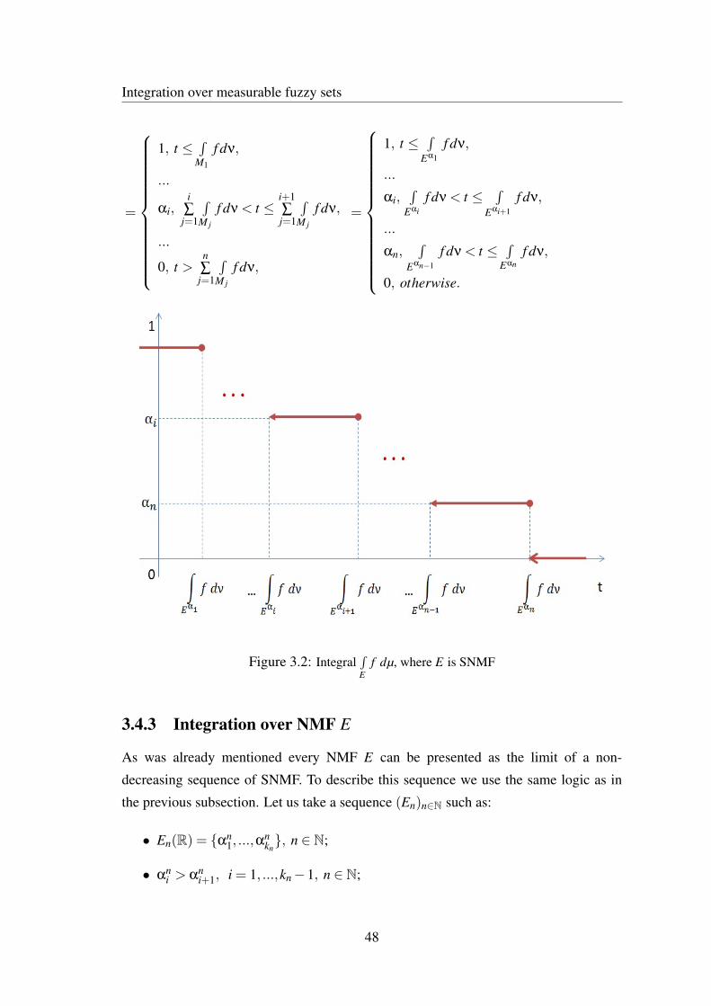
Taking into account the property of addition of fuzzy numbers:

(n⊕

i=1z(ai,αi))(t) =

1, t ≤ 0,

α1, 0 < t ≤ a1,

...

αi+1, a1 + ...+ai < t ≤ a1 + ...+ai+1,

...

0, t > a1 + ...+an,

we obtain

∫E

f dµ =n⊕

i=1

∫E(αi,Mi)

f dµ =n⊕

i=1

z(∫Mi

f dν,αi) =

47

Integration over measurable fuzzy sets

=

1, t ≤∫

M1

f dν,

...

αi,i

∑j=1

∫M j

f dν < t ≤i+1∑j=1

∫M j

f dν,

...

0, t >n∑j=1

∫M j

f dν,

=

1, t ≤∫

Eα1

f dν,

...

αi,∫

Eαi

f dν < t ≤∫

Eαi+1

f dν,

...

αn,∫

Eαn−1

f dν < t ≤∫

Eαnf dν,

0, otherwise.

Figure 3.2: Integral∫E

f dµ, where E is SNMF

3.4.3 Integration over NMF E

As was already mentioned every NMF E can be presented as the limit of a non-

decreasing sequence of SNMF. To describe this sequence we use the same logic as in

the previous subsection. Let us take a sequence (En)n∈N such as:

• En(R) = {αn1, ...,α

nkn}, n ∈ N;

• αni > αn

i+1, i = 1, ...,kn−1, n ∈ N;

48

Integration over measurable fuzzy sets

• Mn1 = {x | E(x) = αn

1},Mn

i = {x | αni ≤ E(x)< αn

i−1}, i = 2, ...,kn, , n ∈ N;

• En =kn∨

i=1E(αn

i ,Mni ), n ∈ N;

• E =∨n

En.

Denoting

I =∫E

f dµ and In =∫En

f dµ

we get

I = Sup{∫En

f dµ | n ∈ N}= Sup{In | n ∈ N}.

From the last equality we can get an approximate value of I by fixing n. Obviously, the

integral accuracy in this case will be dependent on n .

49

Chapter 4

Applications of L-fuzzy valued integralin approximation theory

4.1 L-fuzzy valued norm

For a given linear space Y by the analogy with the classical case we consider the concept

of a norm taking values in R+(L).

Definition 4.1.1.An L-fuzzy valued norm on a linear space Y is a function ‖ · ‖ : Y → R+(L) with the

following properties: for all r ∈ R and all y,y1,y2 ∈ Y it holds

• ‖y‖= z(0,1L)⇔ y = 0Y ,

• ‖ry‖= |r|‖y‖,

• ‖y1 + y2‖ ≤ ‖y1‖⊕‖y2‖.

For the space (A,Φ,ν) with a finite measure ν and A ∈ Φ we denote by F the linear

space of all real valued functions that are integrable over A with respect to the measure

ν. We suppose that F0 is the subspace of F that contains all functions which are equal to

0 almost everywhere. Then L1(A,Φ,ν) is the factor space F/F0. We do not distinguish

the functions of the space L1(A,Φ,ν) that are equal almost everywhere with respect to

the measure ν. The norm of a function f ∈L1(A,Φ,ν) is defined with

‖ f‖ν =∫A

| f | dν.

50

Function approximation error on L-sets

Generalizing to the fuzzy case we use an L-set E instead of a set A and consider the

space L1(E,Σ,µ) equipped with the L-fuzzy valued norm defined by the formula:

‖ f‖µ =∫E

| f | dµ,

where µ is an L-fuzzy valued measure and E ∈ Σ. We denote by L1(E,Σ,µ) the space

of all L-fuzzy integrable over E real valued functions.

It is easy to show that the function

‖ · ‖µ : L1(E,Σ,µ)→ R+(L)

defined above satisfies the conditions of an L-fuzzy valued norm:

• ‖ f‖µ = z(0,1L) iff f is equal to 0 almost everywhere,

• ‖r f‖µ =∫E|r f | dν = |r|

∫E| f | dν = |r|‖ f‖µ,

• ‖ f1 + f2‖µ =∫E| f1 + f2| dµ≤

∫E(| f1|+ | f2|) dµ =

=∫E| f1| dµ⊕

∫E| f2| dµ = ‖ f1‖µ⊕‖ f2‖µ.

4.2 Function approximation error on L-sets

For problems which can be solved only approximately the notion of the error of a method

of approximation plays the fundamental role. A classical task of the approximation

theory is to estimate the error of approximation for a given class of real valued functions

defined on a crisp set. For us it seems natural to consider the case when the set we

interpolate over is an L-set, meaning that our interest is more focused at some parts of

the set we approximate over and maybe not so much important on the rest part of the

set.

In order to estimate the quality of approximation on an L-fuzzy set, we need an

appropriate L-fuzzy analogue of a norm. In this section we apply the L-fuzzy norm

introduced above to investigate the error of approximation on an L-fuzzy set E of a real

valued function f .

4.2.1 Theoretical background

Let us suppose that E ∈ Σ and f ∈L1(suppE,Φ,ν) . We consider a method of approx-

imation described by

A : L1(suppE,Φ,ν)→U,

51

Function approximation error on L-sets

where U⊂L1(suppE,Φ,ν) is a finite-dimensional space of functions used for approx-

imation. For example, it could be a space of polynomials or splines.

Definition 4.2.1. The error of approximation A of a function f on an L-fuzzy set E is

defined as follows:

e( f ,A,E) = ‖ f −A f‖µ.

Notice that the error of approximation in this case is characterized by an L-fuzzy real

number which is obtained as the L-fuzzy valued integral over E. The introduced concept

allows us to develop the well known idea of an optimal error method of approximation

for this case. It is the method whose error is the infimum of the errors of all methods for

a given problem characterized by L-fuzzy numbers.

Definition 4.2.2. A method AOE is called an optimal error method iff

e( f ,AOE ,E) =

= In f {e( f ,A,E) |A : L1(suppE,Φ,ν)→U}.

This approach gives us a possibility to consider some extremal problems of approx-

imation on L-fuzzy sets in the context of [1], [2], but it is not the principal aim of this

paper. Our intention is to show how the most optimal decision can be taken when com-

paring several methods based on the error value.

4.2.2 Numerical example

In this subsection we illustrate with some numerical examples the dependence of the

error e( f ,A,E) on method A and set E. We suppose that L = [0,1], X = [0,1] and

ν is the Lebesgue measure, and we consider the errors of approximation of the given

function

f =1

1+25x2

(the Runge example) by two methods:

• approximation A1 by the Lagrange interpolation polynomial of degree 10 with

respect to the uniform mesh on [0,1],

• approximation A2 by the interpolation natural cubic spline with respect to the

same uniform mesh on [0,1],

52

Function approximation error on L-sets

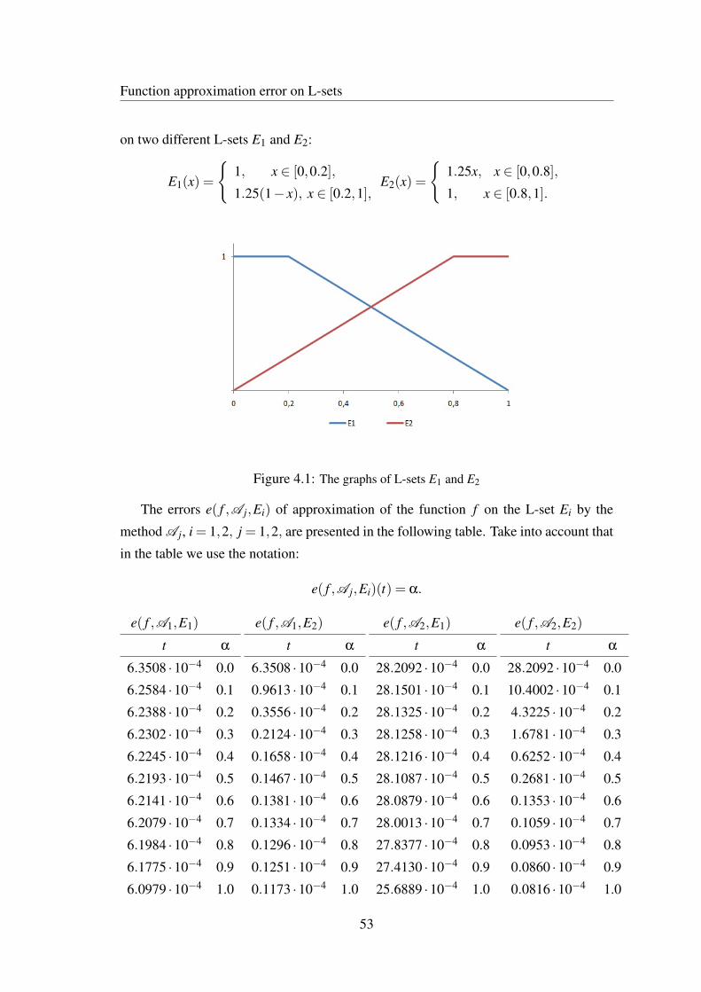
on two different L-sets E1 and E2:

E1(x) =

{1, x ∈ [0,0.2],

1.25(1− x), x ∈ [0.2,1],E2(x) =

{1.25x, x ∈ [0,0.8],

1, x ∈ [0.8,1].

Figure 4.1: The graphs of L-sets E1 and E2

The errors e( f ,A j,Ei) of approximation of the function f on the L-set Ei by the

method A j, i = 1,2, j = 1,2, are presented in the following table. Take into account that

in the table we use the notation:

e( f ,A j,Ei)(t) = α.

e( f ,A1,E1)

t α

6.3508 ·10−4 0.0

6.2584 ·10−4 0.1

6.2388 ·10−4 0.2

6.2302 ·10−4 0.3

6.2245 ·10−4 0.4

6.2193 ·10−4 0.5

6.2141 ·10−4 0.6

6.2079 ·10−4 0.7

6.1984 ·10−4 0.8

6.1775 ·10−4 0.9

6.0979 ·10−4 1.0

e( f ,A1,E2)

t α

6.3508 ·10−4 0.0

0.9613 ·10−4 0.1

0.3556 ·10−4 0.2

0.2124 ·10−4 0.3

0.1658 ·10−4 0.4

0.1467 ·10−4 0.5

0.1381 ·10−4 0.6

0.1334 ·10−4 0.7

0.1296 ·10−4 0.8

0.1251 ·10−4 0.9

0.1173 ·10−4 1.0

e( f ,A2,E1)

t α

28.2092 ·10−4 0.0

28.1501 ·10−4 0.1

28.1325 ·10−4 0.2

28.1258 ·10−4 0.3

28.1216 ·10−4 0.4

28.1087 ·10−4 0.5

28.0879 ·10−4 0.6

28.0013 ·10−4 0.7

27.8377 ·10−4 0.8

27.4130 ·10−4 0.9

25.6889 ·10−4 1.0

e( f ,A2,E2)

t α

28.2092 ·10−4 0.0

10.4002 ·10−4 0.1

4.3225 ·10−4 0.2

1.6781 ·10−4 0.3

0.6252 ·10−4 0.4

0.2681 ·10−4 0.5

0.1353 ·10−4 0.6

0.1059 ·10−4 0.7

0.0953 ·10−4 0.8

0.0860 ·10−4 0.9

0.0816 ·10−4 1.0

53

Function approximation error on L-sets

Let us note that

suppE1 = suppE2 = [0,1]

and

e( f ,A1, [0,1]) = 6.3509 ·10−4,

e( f ,A2, [0,1]) = 28.2092 ·10−4,

but it is easy to see that the error of approximation A j, j = 1,2, on the set E2 is essentially

less than the error on the set E1.

To compare both L-fuzzy values one can use Figure 4.2 left chart for approxima-

tion A1 (i.e. by the Lagrange interpolation polynomial) and Figure 4.2 right chart for

approximation A2 (i.e. by the interpolation natural cubic spline).

Figure 4.2: The graphs of errors α = e( f ,A1,E1)(t), α = e( f ,A1,E2)(t), α = e( f ,A2,E1)(t)

and α = e( f ,A2,E2)(t)

It is also interesting to see how both approximations A1 and A2 performing on the

L-set E2. As we can see from Figure 4.3 there is no obvious preference to any of two

Figure 4.3: The graphs of errors α = e( f ,A1,E2)(t) and α = e( f ,A2,E2)(t)

approximations, because they perform different on different levels.

54

Error of approximation on L-sets for classes of functions

Summarizing, we want to highlight that approximation error defined as an L-fuzzy

number gives us opportunity to develop a strategy for choosing most optimal approxi-

mation algorithm on an L-set. As was illustrated in the previous example avoiding the

"fuzziness" of the set we interpolate over and comparing the errors on the support of the

L-set, we can fail with the choice of the best strategy.

4.3 Error of approximation on L-sets for classes of func-

tions

As shown in the previous section, applying L-fuzzy valued integral to define the ap-

proximation error gives us a good tool to compare efficiency of different approximation

methods and helps us to make more accurate decisions when choosing the most optimal

approximation way on an L-set. Despite the numerical example 4.2.2 described above,

when it comes to real life our knowledge about the function we want to approximate is

rather limited, with some values maybe. That is why for us it seems natural to consider

estimation of the approximation error on classes of functions.

4.3.1 Theoretical background

In 4.2.1 the space L1 was mentioned. Now let us consider space Lp = Lp[0,1], where

1≤ p≤ ∞ with the norm ‖ · ‖p defined as follows:

‖ f‖p = (

1∫0

| f (x)|pdx)

1p

, where 1≤ p < ∞ ,

and

‖ f‖p = supx∈[0,1]

| f (x)| , where p = ∞ .

Also we consider the space L np of functions f that satisfy the following conditions:

• there exists (n−1) derivative f (n−1) and it is absolutely continuous on [0,1],

• f (n) ∈Lp.

In other words, L np is the set of n degree indefinite integrals from functions f ∈Lp.

55

Error of approximation on L-sets for classes of functions

Particularly, we observe the class containing functions f ∈ L np with bounded deriva-

tives. We denote by KW np (n = 1,2, ...;1 ≤ p ≤ ∞) the class of all functions f ∈ L n

p

satisfying

‖ f (n)‖p ≤ K, K ∈ R+.

We know that every function f ∈Lp can be represented as follows

f (x) =n−1

∑i=0

1i!

f (i)(0) xi +1

(n−1)!

1∫0

f (n)(u)(x−u)n−1+ du.

Let us denote

pn−1(x) =n−1

∑i=0

1i!

f (i)(0) xi

and

rn−1(x) =1

(n−1)!

1∫0

f (n)(u)ϕn−1(x,u)du,

where

ϕn−1(x,u) = (x−u)n−1+ =

{(x−u)n−1, x≥ u,

0, u > x.

Hence,

f (x) = pn−1(x)+ rn−1(x),

where

• pn−1 is the (n−1)-degree Taylor polynomial of f centred at 0,

• rn−1 is an integral form of the remainder.

Now we want to estimate the error of approximation A of function f . We do the follow-

ing assumptions regarding the choice of approximation method A:

• for all q ∈ Pn−1 we have Aq = q, where Pn−1 is the class of all polynomials with

degree at most (n−1);

• approximation A is linear;

• for r(x) =1∫0

g(u) h(x,u) du it holds

(A r)(x) =1∫

0

g(u) (A h(x,u))du,

where approximation A applied only to argument x of function h.

56

Error of approximation on L-sets for classes of functions

Taking into account these assumptions we obtain:

f −A f = (pn−1 + rn−1)−A (pn−1 + rn−1) =

= (pn−1−A pn−1)+(rn−1−A rn−1) = rn−1−A rn−1.

Coming back to initial notations:

f (x)− (A f )(x) = rn−1(x)− (A rn−1)(x) =

=1

(n−1)!

1∫0

f (n)(u)ϕn−1(x,u) du− 1(n−1)!

1∫0

f (n)(u)(A ϕn−1(x,u)) du =

=1

(n−1)!

1∫0

f (n)(u)(ϕn−1(x,u)−A ϕn−1(x,u)) du

We denote by Un−1(x,u) the kernel of the integral representation of the error f −A f

and define it as follows:

Un−1(x,u) =ϕn−1(x,u)−A ϕn−1(x,u)

(n−1)!.

Finally, we get

f (x)− (A f )(x) =1∫

0

f (r)(u)Un−1(x,u) du.

Now considering the error on an L-set E we obtain:

∫E

| f −A f | dµ≤∫E

(

1∫0

| f (n)(u)||Un−1(x,u)| du) dµ.

Having this estimation for the approximation error we can observe how it will be calcu-

lated for particular classes of functions.

• In the case when f ∈ KW n1 the norm of f (n) is bounded as follows

‖ f (n)‖1 =

1∫0

| f (n)(u)| du≤ K

and then ∫E

| f −A f | dµ≤∫E

(

1∫0

| f (n)(u)||Un−1(x,u)| du) dµ≤

57

Error of approximation on L-sets for classes of functions

≤∫E

(

1∫0

| f (n)(u)| supu∈[0,1]

|Un−1(x,u)| du) dµ =

=∫E

( supu∈[0,1]

|Un−1(x,u)|1∫

0

| f (n)(u)| du) dµ≤ K∫E

supu∈[0,1]

|Un−1(x,u)| dµ.

Hence,

‖ f −A f‖µ ≤ K∫E

supu∈[0,1]

|Un−1(x,u)| dµ.

• In the case when f ∈ KW n∞ the norm of f (n) is bounded as follows

‖ f (n)‖∞ = supu∈[0,1]

| f (n)(u)| ≤ K

and then ∫E

| f −A f | dµ≤∫E

(

1∫0

| f (n)(u)||Un−1(x,u)| du) dµ≤

≤ K∫E

(

1∫0

|Un−1(x,u)| du) dµ.

Hence,

‖ f −A f‖µ ≤ K∫E

(

1∫0

|Un−1(x,u)| du) dµ.

4.3.2 Numerical example

In this subsection we illustrate by some numerical examples how to use the technique

described above. We consider classes KW n1 and KW n

∞ when n = 1, i.e. the classes of

functions such that the first derivative is bounded: KW 11 and KW 1

∞.

We examine the approximation A by polygons (i.e. the first degree splines) with

respect to a mesh {x0,x1, ...,xk} on [0,1] over L-set E defined as follows:

E(x) =

{1− x, x ∈ [0,1],

0, otherwise.

In this case

ϕ0(x,u) =

{1, x≥ u,

0,x < u.

58

Error of approximation on L-sets for classes of functions

And if xi−1 < x < xi then

U0(x,u) =

xi−x

xi−xi−1, xi−1 < u < x,

− x−xi−1xi−xi−1

, x < u < xi,

0, u /∈ [xi−1,xi].

Class KW 1∞

Denoting

z∞ =∫E

(

1∫0

|U0(x,u)| du) dµ

for f ∈ KW 1∞ we have

‖ f −A f‖µ ≤ K z∞.

Considering the case when xi−1 < x < xi we obtain

1∫0

|U0(x,u)| du =

xi∫xi−1

|U0(x,u)| du =

x∫xi−1

xi− xxi− xi−1

du+xi∫

x

x− xi−1

xi− xi−1du =

= 2(xi− x)(x− xi−1)

xi− xi−1.

In the case of the uniform mesh {x0,x1, ...,xk} on [0,1] for every x ∈ [0,1] denoting

h = xi− xi−1 we have

1∫0

|U0(x,u)| du = 2h{x

h

}(1−{x

h

}),

going forward we mean by [r] the integer part and by {r} the fractional part of r ∈ R.

This integral for the uniform mesh with 11 (i.e. k = 10) knots is plotted on the Figure

4.4.

The next step is to integrate this function over the L-set E. Applying the calculation

method described in subsection 3.4.2 for all α ∈ [0,1] we obtain

z−1∞ (α) =

h2

3

([1−α

h

]+

{1−α

h

}2

(3−2{

1−α

h

})

).

Now by choosing α according to any mesh on the [0,1] we can get the integral value as

accurate as we want. For example, taking the uniform mesh of [0,1] with step 0.01:

α0 = 1,α1 = 0.99,α2 = 0.98, ...,α100 = 0,

59

Error of approximation on L-sets for classes of functions

Figure 4.4: The graph of integral1∫0|U0(x,u)| du

Figure 4.5: The graph of z∞

60

Error of approximation on L-sets for classes of functions

we obtain fuzzy real number z∞ plotted on Figure 4.5.

Changing from the uniform mesh to the following:

x0 = 0,x1 = 0.02,x2 = 0.03,x3 = 0.05,x4 = 0.1,x5 = 0.15,

x6 = 0.25,x7 = 0.35,x8 = 0.55,x9 = 0.75,x10 = 1.00,

we, obviously, obtain a different approximation error bound. On Figure 4.6 both ap-

proximation errors bounds are plotted with uniform and non-uniform meshes.

Figure 4.6: Comparison of the error bounds with the uniform and non-uniform meshes

In the crisp case we would give a preference for the method with the uniform mesh,

while in the fuzzy case the decision is not that obvious, meaning that on the higher

levels (α > 0.6) the method with the non-uniform mesh performing better.

Class KW 11

Taking into consideration that U0(x,u) = 0 when x ∈ [xi−1,xi], u ∈ [x j−1,x j] and i 6= j,

for class KW 11 we can get more accurate error estimation by the following reasoning.

Let us denote Ei = E ∧ [xi−1,xi], i = 1, ...,k. Then

‖ f −A f‖µ =k⊕

i=1

∫Ei

(

1∫0

| f ′(u)||U0(x,u)| du)dµ =

=k⊕

i=1

∫Ei

(

xi∫xi−1

| f ′(u)||U0(x,u)| du)dµ≤k⊕

i=1

∫Ei

( supu∈[xi−1,xi]

|U0(x,u)|xi∫

xi−1

| f ′(u)| du)dµ =

61

Error of approximation on L-sets for classes of functions

=k⊕

i=1

xi∫xi−1

| f ′(u)|du∫Ei

supu∈[xi−1,xi]

|U0(x,u)|dµ≤

≤ Sup{∫E j

supu∈[x j−1,x j]

|U0(x,u)|dµ | j = 1, ..,k}k

∑i=1

xi∫xi−1

| f ′(u)|du =

= Sup{∫E j

supu∈[x j−1,x j]

|U0(x,u)|dµ | j = 1, ..,k}1∫

0

| f ′(u)|du≤

≤ K Sup{∫E j

supu∈[x j−1,x j]

|U0(x,u)|dµ | j = 1, ..,k}.

Now denoting

wi =∫Ei

supu∈[x j−1,x j]

|U0(x,u)|dµ, i = 1, ...,k,

z1 = Sup{wi|i = 1, ...,k},

we have

‖ f −A f‖µ ≤ K z1.

Considering the case when xi−1 < x < xi we obtain

supu∈[xx−1,xi]

|U0(x,u)|=

{xi−x

xi−xi−1, xi−1 < x < xi−1+xi

2 ,

− x−xi−1xi−xi−1

, xi−1+xi2 < x < xi,

.

This function is plotted on the following graph:

Figure 4.7: The graph of supu∈[xi−1,xi]

|U0(x,u)|

62

Error of approximation on L-sets for classes of functions

Taking integral over Ei we get:

w−1i (α) =

1−α∫xi−1

supu∈[xi−1,xi]

|U0(x,u)|dx, when 1− xi ≤ α≤ 1− xi−1.

Hence,

w−1i (α) =

1−α− xi−1

2

(2− 1−α− xi−1

hi

), when xi−1 ≤ 1−α≤ xi−1 + xi

2,

and

w−1i (α) =

34

hi−xi− (1−α)

2

(2− xi− (1−α)

hi

), when

xi−1 + xi

2≤ 1−α≤ xi.

It is easy to see that

w−1i (1− xi−1) = 0 and w−1

i (1− xi) =34

hi.

In the case when t /∈ [0, 34hi] we have

wi(t) =

{1, t ≤ 0,

0, t > 34hi.

To obtain value z1 we take Sup of all fuzzy numbers wi, i = 1, ...,k.

These numbers as well as z1 for uniform mesh with 11 knots are plotted on Figure

4.8 (the dashed lines for wi, i = 1, ...,k and the even line for z1).

Figure 4.8: The graphs of wi and z1 in the case of the uniform mesh

Changing from the uniform mesh to the following:

x0 = 0,x1 = 0.02,x2 = 0.03,x3 = 0.05,x4 = 0.1,x5 = 0.15,

63

Error of approximation on L-sets for classes of functions

Figure 4.9: The graphs of wi and z1 in the case of non-uniform mesh

x6 = 0.25,x7 = 0.35,x8 = 0.55,x9 = 0.75,x10 = 1.00,

we obtain the integrals displayed on Figure 4.9.

To compare methods with the uniform and non-uniform meshes Figure 4.10 is pre-

sented. As we can see there is no obvious decision on what method is more preferable:

Figure 4.10: Comparison of the errors with the uniform and non uniform meshes

in the case when we are interested in points with the membership level close to 1 both

methods have the same error bound, while on points with the membership degree in

[0.5,0.98], obviously, the method with the non-uniform mesh is better, but on levels be-

low 0.5 the error of approximation significantly lower for the method with the uniform

mesh.

64

Conclusions

To conclude I would like to say that in my belief the overall goal of the thesis has been

achieved:

• the concept of an L-fuzzy valued measure defined on T-tribe and taking values in

the L-fuzzy real line is introduced, in the case when L is complete, completely

distributive lattice,

• construction for an L-fuzzy valued measure is developed by extending the crisp

finite measure,

• considered the concept of an L-fuzzy valued integral, the properties of integral are

investigated and calculations methods described,

• some possible applications of an L-fuzzy valued integral in the approximation

theory are suggested.

I believe that this research work is very relevant since it combines the L-structure

study, which is traditional to Latvian mathematicians, as well as measure and integral

theory further development. These studies could potentially contribute to Latvian re-

searches and investigations of many valued structures and subsequently develop this

perspective direction of theoretical mathematics.

65

List of conferences

International scientific conferences and congresses

C01 11th International Conference on Fuzzy Set Theory and Applications (FSTA

2012), January 30 - February 3, 2012, Liptovsky Jan, Slovak Republic.

C02 Joint 7th Conference of the European Society for Fuzzy Logic and Technology

(EUSFLAT-2011) and Les Rencontres Francophones sur la Logique Floue et ses

Applications (LFA-2011), July 18-22, 2011, Aix-Les-Bains, France.

C03 6th International Summer School on Aggregation Operators (AGOP 2011), July

11-15, 2011, Benevento, Italy.

C04 16th International Conference on Mathematical Modelling and Analysis (MMA

2011), May 25-28, 2011, Sigulda, Latvia.

C05 10th International Conference on Applied mathematics (APLIMAT 2011), Febru-

ary 1-4, 2011, Bratislava, Slovak Republic.

C06 15th International Conference on Mathematical Modelling and Analysis (MMA

2010), May 26-29, 2010, Druskininkai, Lithuania.

C07 10th International Conference on Fuzzy Set Theory and Applications (FSTA

2010), February 1-5, 2010, Liptovsky Jan, Slovak Republic.

C08 Joint 13th IFSA World Congress and 6th Conference of the European Society for

Fuzzy Logic and Technology (EUSFLAT 2009), July 20-24, 2009, Lisbon, Portu-

gal.

C09 14th International Conference on Mathematical Modelling and Analysis (MMA

2009), May 27-30, 2009, Daugavpils, Latvia.

66

Error of approximation on L-sets for classes of functions

C10 9th International Conference on Fuzzy Set Theory and Applications (FSTA 2008),

February 4-8, 2008, Liptovsky Jan, Slovak Republic.

C11 6th International Conference on Topological Algebras and Applications (ICTAA

2008), January 24-27, 2008, Tartu, Estonia.

C12 5th Conference of the European Society for Fuzzy Logic and Technology

(EUSFLAT 2007), Septemeber 11-14, 2007, Ostarva, Czech Republic.

Domestic scientific conferences

C13 67th Conference of University of Latvia, New scientist section, February 2, 2009,

Riga, Latvia.

C14 7th Conference of Latvian Mathematical Society, April 18-19, 2008, Rezekne,

Latvia.

C15 66th Conference of University of Latvia, New scientist section, February 21, 2008,

Riga, Latvia.

C16 65th Conference of University of Latvia, New scientist section, February 8, 2007,

Riga, Latvia.

C17 6th Conference of Latvian Mathematical Society, April 7-8, 2006, Liepaja, Latvia.

International seminars

C18 A.Šostak Spring Workshop, May 14, 2009, Riga, Latvia.

C19 1st Czech-Latvian Seminar Advanced Methods in Soft Computing, November 19-

22, 2008, Trojanovice, Czech Republic.

C20 International Seminar on Algebra and Applications, May 4-6, 2007, Ratnieki,

Latvia.

C21 International Latvian-Finnish Seminar on Algebra and Topology, November 8,

2006, Riga, Latvia.

67

Bibliography

[1] S. Asmuss and A. Šostak. Extremal problems of approximation theory in fuzzy

context. Fuzzy Sets and Systems, 105:249–257, 1999.

[2] S. Asmuss and A. Šostak. On central algorithms of approximation under fuzzy

information. Fuzzy Sets and Systems, 155:150–163, 2005.

[3] G. Birkhoff. Lattice theory. Colloquium Publications, 1948.

[4] B. A. Davey and H. A. Priestley. Introduction to Lattices and Order. Cambridge

University Press, 2002.

[5] C. Degang and Z. Liguo. Signed fuzzy-valued measure and Radon-Nikodym the-

orem of fuzzy-valued measurable functions. Southeaset Asian Bulletin of Mathe-

matics, 26:375–385, 2002.

[6] J. A. Goguen. L-fuzzy sets. Journal of Mathematical Analysis and Applications,

18:145–174, 1967.

[7] P. Halmos. Measure theory. Springer-Verlag, 1950.

[8] U. Hohle. Fuzzy real numbers as Dedekind cuts with respect to multiple-valued

logic. Fuzzy Sets and Systems, 24:263–278, 1987.

[9] B. Hutton. Normality in fuzzy topological spaces. Journal of Mathematical Anal-

ysis and Applications, 50:74–79, 1975.

[10] E. P. Klement. Characterization of finite fuzzy measures using Markoff-kernels.

Journal of Mathematical Analysis and Applications, 75:330–339, 1980.

[11] E. P. Klement. Fuzzy sigma-algebras and fuzzy measurable functions. Fuzzy Sets

and Systems, 4, 1980.

68

BIBLIOGRAPHY

[12] E. P. Klement. Fuzzy measures assuming their values in the set of fuzzy numbers.

Journal of Mathematical Analysis and Applications, 93:312–323, 1983.

[13] E. P. Klement and D. Butnariu. Triangular norm based measures. In Handbook of

Measure Theory, chapter 23, pages 947–1010. Elsevier, Amsterdam, 2002.

[14] E. P. Klement, R. Lowen, and W. Schwyhla. Fuzzy probability measures. Fuzzy

Sets and Systems, 5:21–30, 1981.

[15] E. P. Klement, R. Mesiar, and E. Pap. Triangular norms. Kluwer Academic Pub-

lishers, 2000.

[16] E. P. Klement, R. Mesiar, and E. Pap. A universal integral. New Dimensions

in Fuzzy Logic and Related Technologies. Proceedings of the 5th Conference of

the European Society for Fuzzy Logic and Technology (EUSFLAT 2007), Ostrava

(Czech Republic), pages 253–256, 2007.

[17] E. P. Klement and S. Weber. Generalized measures. Fuzzy Sets and Systems,

40:375–394, 1991.

[18] R. Lowen. On (R(L),⊕). Fuzzy Sets and Systems, 10:203–209, 1983.

[19] R. Mesiar. Fuzzy measures and integrals. Fuzzy Sets and Systems, 156:365–370,

2005.

[20] E. Pap. Handbook of Measure Theory. Elsevier, Amsterdam, 2002.

[21] S. E. Rodabaugh. Fuzzy addition and the L-fuzzy real line. Fuzzy Sets and Systems,

8:39–52, 1982.

[22] S. E. Rodabaugh. Complete fuzzy topological hyperfields and fuzzy multiplication

in the fuzzy real lines. Fuzzy Sets and Systems, 15:285–310, 1988.

[23] S. E. Rodabaugh. A theory of fuzzy uniformities with applications to fuzzy real

lines. J. Math. Anal. Appl., 129:37–70, 1988.

[24] M. Sugeno. Theory of Fuzzy Integrals and Its Applications. PhD thesis, Tokyo

Institute of Technology, 1974.

[25] R. C. Steinlage T. E. Gantner and R. H. Warren. Compactness in fuzzy topological

spaces. Journal of Mathematical Analysis and Applications, 62:547–562, 1978.

69

BIBLIOGRAPHY

[26] A. Šostak. Mathematics in the context of fuzzy sets: basic ideas, concepts, and

some remarks on the history and recent trends of development. Mathematical

Modelling and Analysis, 16(2):173–198, 2011.

[27] A. Šostaks. L-kopas un L-vertıgas strukturas. Latvijas Universitate, Rıga, 2003.

[28] Z. Wang and G. J. Klir. Fuzzy measure theory. Plenum Press, New York, 1992.

[29] S. Weber. Measures of fuzzy sets and measures of fuzziness. Fuzzy Sets and

Systems, 13:247–271, 1984.

[30] S. Weber. ⊥-decomposable measures and integrals for Archimedean t-conorms ⊥.

Journal of Mathematical Analysis and Applications, 101:114–138, 1984.

[31] H. C. Wu. Fuzzy-valued integrals of fuzzy-valued measurable functions with re-

spect to fuzzy-valued measures based on closed intervals. Fuzzy Sets and Systems,

87:65–78, 1997.

[32] L. A. Zadeh. Fuzzy sets. Information and Control, 8:338–353, 1965.

[33] L. A. Zadeh. Probability measures of fuzzy events. Journal of Mathematical

Analysis and Applications, 23:421–427, 1968.

[34] L. A. Zadeh. The concept of a linguistic variable and its application to approximate

reasoning I, II. Information Sciences, 8:199–249,301–357, 1975.

[35] L. A. Zadeh. The concept of a linguistic variable and its application to approximate

reasoning III. Information Sciences, 9:43–80, 1976.

70

BIBLIOGRAPHY

Author’s publications

P1 V. Ruzha, S. Asmuss. A construction of a fuzzy valued measure based on min-

imum t-norm. In: New Dimensions in Fuzzy Logic and Related Technologies.

Proceedings of the 5th Conference of the European Society for Fuzzy Logic and

Technology (EUSFLAT 2007), p. 175-178, Ostrava (Czech Republic), 2007. ISI

CPCI-S

P2 V. Ruzha, S. Asmuss. A construction of an L-fuzzy valued measure of L-fuzzy

sets. In: Proceedings of the Joint 13th IFSA World Congress and 6th Confer-

ence of the European Society for Fuzzy Logic and Technology (EUSFLAT 2009),

p. 1735-1739, Lisbon (Portugal), 2009. ISI CPCI-S

P3 V. Ruza. On an L-fuzzy valued integral with respect to an L-fuzzy valued TM-

measure. In: Proceedings of the 10th International Conference on Applied Math-

ematics (APLIMAT 2011), p. 605-614, Bratislava (Slovakia), 2011.

P4 V. Ruza. On an L-fuzzy valued integral with respect to an L-fuzzy valued TM-

measure. Paper is accepted for publication in the Journal of Applied Mathematics.

P5 V. Ruza, S. Asmuss. L-fuzzy valued measure and integral. In: Proceedings

of the 7th conference of the European Society for Fuzzy Logic and Technology

(EUSFLAT-2011) and LFA-2011, p. 127-131, Aix-Les-Bains (France), 2011.

P6 V. Ruza, S. Asmuss. On an L-fuzzy valued norm defined by an L-fuzzy valued

integral. In: Proceedings of the 6th International Summer School on Aggregation

Operators, p. 183-188, Benevento (Italy), 2011.

P7 V. Ruza, S. Asmuss. On another approach to the definition of an L-fuzzy valued

integral. In: Proceedings of the 2011 IEEE International Conference On Fuzzy

Systems, p. 1598-1602, Taipei (Taiwan), 2011. SCOPUS

71

BIBLIOGRAPHY

Author’s abstracts

T1 V. Ruza. On estimation of approximation error on fuzzy sets by means of fuzzy

valued integral. 11th International Conference on Fuzzy Set Theory and Applica-

tions (FSTA 2012), January 30 - February 3, 2012, Liptovsky Jan, Slovak Repub-

lic, p. 94.

T2 V. Ruza, S. Asmuss. An analysis of approximation on an L-fuzzy set based on L-

fuzzy valued integral. 16th International Conference on Mathematical Modelling

and Analysis (MMA 2011), May 25-28, 2011, Sigulda, Latvia, p. 109.

T3 V. Ruza. On an L-fuzzy valued integral with respect to an L-fuzzy valued

TM-measure. 10th International Conference on Applied mathematics (APLIMAT

2011), February 1-4, 2011, Bratislava, Slovak Republic, p. 173.

T4 V. Ruza. L-fuzzy valued measure and integral. 15th International Confer-

ence on Mathematical Modelling and Analysis (MMA 2010), May 26-29, 2010,

Druskininkai, Lithuania, p. 86.

T5 V. Ruza. A concept of a fuzzy valued integral over a fuzzy set with respect to a

fuzzy valued T-measure. 10th International Conference on Fuzzy Set Theory and

Applications (FSTA 2010), February 1-5, 2010, Liptovsky Jan, Slovak Republic,

p. 112.

T6 V. Ruza, S. Asmuss. On integration over fuzzy set with respect to fuzzy valued

measure. 14th International Conference on Mathematical Modelling and Analysis

(MMA 2009), May 27-30, 2009, Daugavpils, Latvia, p. 64.

T7 V. Ruza, S. Asmuss. On a fuzzy valued measure and integral. 1st Czech-Latvian

Seminar Advanced Methods in Soft Computing, November 19-22, 2008, Tro-

janovice, Czech Republic, p. 29.

T8 V. Ruzha, S. Asmuss. L-fuzzy valued T-measure of L-sets. Abstracts of the 7th

Latvian Mathematical Conference, April 18-19, Rezekne, Latvia, 2008, p. 40.

72

BIBLIOGRAPHY

T9 V. Ruza, S. Asmuss. On a construction of an L-fuzzy valued measure of L-sets.

9th International Conference on Fuzzy Set Theory and Applications (FSTA 2008),

February 4-8, 2008, Liptovsky Jan, Slovak Republic, p. 21.

T10 V. Ruza, S. Asmuss. On a concept of an L-fuzzy valued measure of L-sets. 6th In-

ternational Conference on Topological Algebras and Applications (ICTAA 2008),

January 24-27, 2008, Tartu, Estonia, p. 18.

T11 V. Ruza. On construction of an L-fuzzy valued T-measure. Abstracts of the 6th

Latvian Mathematical Conference, April 7-8, 2006, Liepaja, Latvia, p. 8.

73