PharmaSUG 2016 - Paper PO020 Using GTL … · Using GTL Generating Customized Kaplan-Meier Survival ... to generate a template named KMplot for KM graphs with KM estimate as step-plot

PharmaSUG 2016 - Paper PO020

Using GTL Generating Customized Kaplan-Meier Survival Plots

Joanne Zhou, GlaxoSmithKline, Collegeville, Pennsylvania, USA

ABSTRACT

In cardiovascular and oncology clinical trials time-to-event endpoints such as overall survival and progression-free survival are the main focal point of clinical interests and usually graphically displays of the Kaplan Meier (KM) curve plays a key role in presenting the key clinical results and importance. With advent of SAS Graph Template Language (GTL) and newer version of the LIFETEST procedure, generation of conventional KM curves becomes much easier. However, some adhoc requests for customized KM plots could be still quite a challenge. In this paper, I use SAS GTL, ODS and SAS macros along with other SAS statistical analysis procedures to overcome some of the challenges to generate the customized KM plots.

INTRODUCTION

For graphical presentation of cardiovascular and oncology clinical trial time-to-event results, the need to present the KM survival estimates, standard error of the KM estimates, risk sets and summary statistics in a single graph is very common. However, generation of such graphical presentations can be a quite challenge. In this paper I use Proc Template, Proc Lifetest, ODS, SAS macro language and Proc Sgrender to simplify such a task. I divide my programming effort into four parts: 1) Data preparation, 2) Style definition, 3) Statgraph definition and 4) Graph generation.

DATA PREPARATION

I use the data in SAS/STAT 9.2 User’s Guide Second Edition Example 49.2 for this paper. To make the graphs look simpler I convert the time to years by dividing the time by 365. ODS names ProductLimitEstimates, CensoredSummary and HomTests for Proc Lifetest are used to create datasets to store KM estimates, total number of subjects, number and percent of subjects with event and logrank test p-value respectively. In order to gain some efficiency, a macro called KM was created. The KM macro creates two datasets specified in macro variables KMout and Statout to store KM estimates and the summary statistics respectively. The last observation carry forward method is used to populate the KM estimates for censored patients. To create specified time points for risk sets and standard error bars (+/- stderr) for KM estimates, two dummy datasets are created and this provides the mechanism for risk sets and standard error presentation. There are two things worth mentioning. First, the appearance of the statistics in the graph is determined by the rows and columns in the summary statistics dataset. The values in each row and column are converted into macro variables in the KMplot macro and used by Gridded/Entry statements to create the summary statistics in the graph. This approach provides us flexibility to control the contents and the appearance in the graph for the summary statistics. Second, the two dummy datasets, one for risk sets and one for standard error bars provide us needed control at which time points to have the risk sets and/or standard error bars added to the KM plots. Detail reasons/logic for each data manipulation steps are self explanatory and are documented in the comments fields in the appendix SAS codes. Below are some brief codes to show how can the summary statistics from two cutoffs be combined and displayed in one survival graph and how the dummy datasets can be generated for risk sets and standard error bars at different time points.

* call KM macro to perform km analysis at Year 4;

%km(dsin=bmt4, kmout=plein4, censords=cs4, pvalue=pvalue4,statout=stat4);

* call KM macro to perform km analysis at Year 8;

%km(dsin=bmt, kmout=plein, censords=cs, pvalue=pvalue);

* create dataset allstat to store the descriptive summary statistics from year

4 and year 8 analyses;

data allstat;

retain Yearc;

set stat4 (in = b) stat (in = a);

Year = 4; if a then year = 8; yearc = put(year, 4.);

label yearc = 'Year';

run;

data allstat;

retain yearc groupc totalc event pvalue;

set allstat;

by yearc;

if first.yearc then do; output; end;

else do; yearc = ' '; output;

if last.yearc and year ne 8 then do;

yearc = ' '; groupc = ' '; totalc = ' '; event = ' '; pvalue = ' ';

output;

end;

end;

drop year;

run;

…

* create dataset atrisk to hold the timepoints for number of patients at risk.

This is approach is quite flexible. We can specify needed timepoints to display

the reskset, for example at timepoints 0, 1, 3, 5, 8.;

data atrisk;

do group = 1 to 3;

do t = 0 to 8;

*do t = 0, 1, 3, 5, 8;

output;

end;

end;

run;

* create dataset aterr to hold the timepoint for where surv +/- stderr will be

plotted. Again, this is a flexible approach to add the +/- stderr bars in the

graphs. We can for example specify timepoints 1, 4, 5 to display the stderr

bars;

data aterr;

do group = 1 to 3;

*do t = 0 to 8;

do t = 1, 4, 5;

output;

end;

end;

run;

STYLE DEFINITION

Proc template is used to create line style, line color and marker symbols for KM estimates plots. This provides users needed flexibility to generate customized graphical presentations. Details see macro style1 which generate a style name called style1.

STATGRAPH DEFINITION

A macro named KMplot is created to generate a template named KMplot for KM graphs with KM estimate as step-plot lines, censored patients as circles, legends for treatment group, risk sets at above x-axis and a table with summary statistics in graph. The step-plot lines are created by Stepplot statement; censored patients are plotted by Scatterplot statement, the legend is created by Mergedlegend/Discretelegend statement to put the legends for survival curves and censored patients into combined legends and risk sets are plotted by Blockplot statement along with Innermargin statement.

The summary statistics table is created by using Gridded/Entry statement and needs a bit more explanation. First, the summary statistics are passed into macro KMplot in a datasets through macro variable Statds. In the dataset, the variable labels are used to label the column headers in the statistics table. Second, the contents of the dataset are used for the cell values of an rxc table. For example, if a dataset contains 3 rows and 5 columns, the summary table

in the graph will be a 3x5 table and the values of each cell will be populated in the table. In macro KMplot, the labels for the variables and the values of the variables in dataset Statds are converted into macro variables: LBLc and Vrc, where r and c stand for row and column in dataset Statds respectively. The values of those macro variables are then used in Gridded/Entry statements for the summary statistics table. Since the statistics are stored in rows and columns in the Statds dataset, this in turn provides users needed flexibility.

GRAPH GENERATION

Once the input datasets, Style1 and KMplot templates are created, Proc sgrender is used to create the graph for the survival analysis results. Using ODS RTF we can generate survival graph in RTF format which can be easily used for MS powerpoint presentation for example.

GRAPH OUTPUT

Below are the different output generated by various macro calls.

Figure 1 is the KM estimates plots with number of subjects at risk and summary statistics. The summary statistics

include total number of patients, number and percent of patients with event and logrank test p-value for overall comparison. The numbers of patients at risk are populated above x-axis.

Figure 2 is the same KM estimates as Figure 1 with +/- standard error bars at years 1, 4 and 5 and statistics from two analysis time points, one at year 4 and one at year 8.

Figures 3 is the KM estimates with number of subjects at risk and hazard ratios, 95% CI for hazard ratios and p-values from Cox regression model.

Figure 4 is the same as Figure 3 without censored patients being plotted.

CONCLUSIONS

In this paper we developed some simple programming steps to facilitate the creation for graphs for KM estimates with various summary statistics to enhance the presentation of clinical results. The KMplot macro along with the dummy datasets and summary statistics dataset approaches gained programmers much needed flexibilities and versatility. With tight timeline and multiple tasks at the same time as usual, those methods can really make a difference.

REFERENCES

Warren F. Kuhfeld and Ying So. 2013. Creating and Customizing the Kaplan-Meier Survival Plot in PROC LIFETEST, SAS Global Forum 2013. SAS Institute Inc. 2015. SAS® 9.4 Graph Template Language: User's Guide, Fourth Edition. Cary, NC: SAS Institute Inc. Sanjay Matange. 2011. Tips and Tricks for Clinical Graphs using ODS Graphics. SAS Global Forum 2011.

CONTACT INFORMATION

Your comments and questions are valued and encouraged. Contact the author at:

Name: Joanne Zhou Work Phone: 610-917-2734 E-mail: [email protected]

SAS and all other SAS Institute Inc. product or service names are registered trademarks or trademarks of SAS Institute Inc. in the USA and other countries. ® indicates USA registration.

Other brand and product names are trademarks of their respective companies

APPENDIX

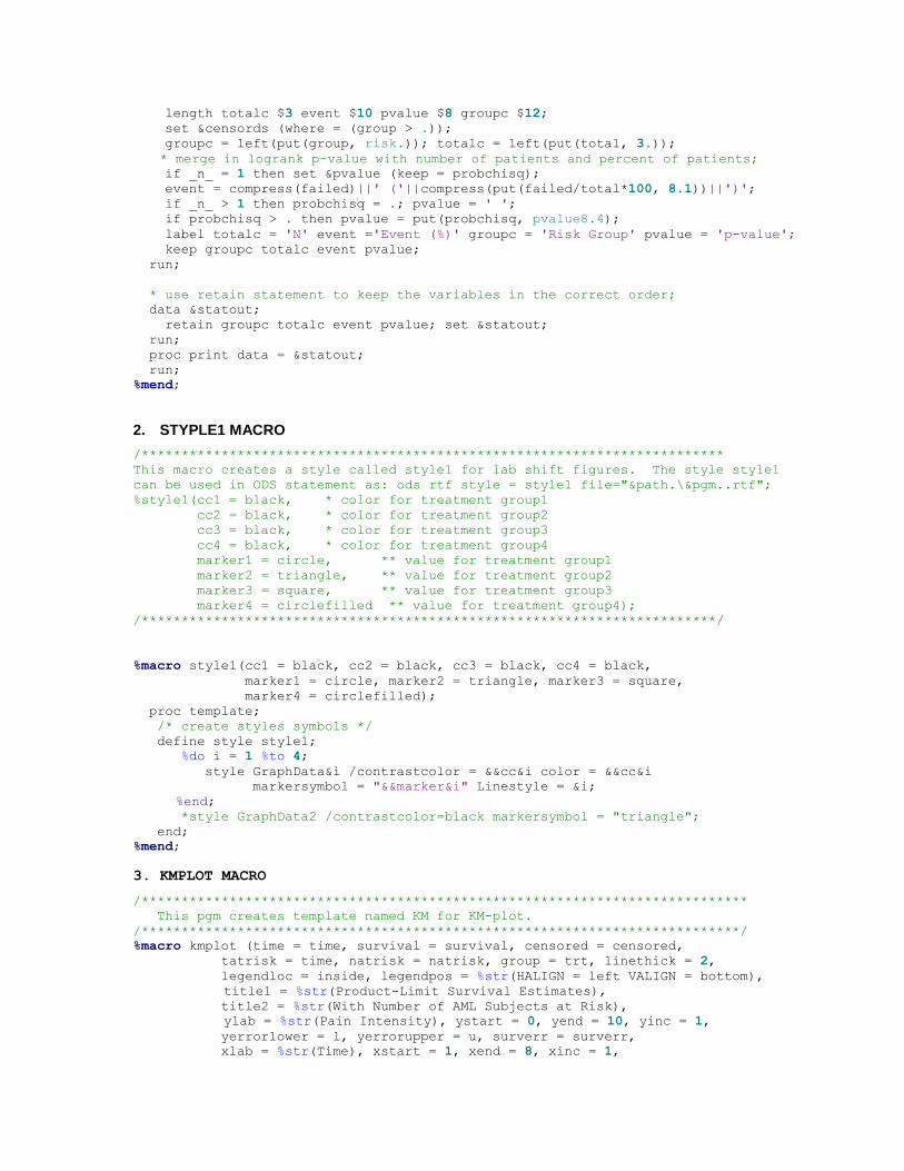
1. KM MACRO

/***************************************************************************

Function: This macro create datasets:

1) mkout - for km estimates, km estimates for censored patients, surv +/- sdteff. Since those values are not calculated for censored patients, the

LOCF method is used to fill the missing values for those censored

patients.

2) Statout – for total N, number (%) patients with event and log-rank pvalue for comparison for the survival curves.

/*************************************************************************/

%macro km(dsin = bmt, /* input time to event data */

timevar = t, /* time var in DSIN */

trt = group, /* trt = treat group */

censorvar = status, /* censorvar = censor variable */

censorval = 0, /* value for censored patients */

kmout = plein, /* output dataset to have KM estimate */

censords = cs, /* output dataset to have total number of patients,

number of events, number of censored per group */

pvalue = pvalue, /* output dataset to hold p-value */

statout = stat /* output dataset to hold summary stats */

);

ods output ProductLimitEstimates = &kmout CensoredSummary = &censords

HomTests = &pvalue;

proc lifetest data = &dsin ATRISK ;

time &Timevar * &censorvar(&censorval);

strata &trt/ test = logrank;

run;

ods output close;

/****************************************************************************

create variables

1) cesored = survival prob for censored patients;

2) atrisk = number of patients at risk for fixed time points.

/***************************************************************************/

proc sort data = &kmout;

by &trt &timevar;

run;

* create variable censored to hold the survival prob for censored patients;

data &kmout;

set &kmout;

where Observedevents is not missing;

by &trt &timevar;

Survival = Failure; retain surv stde;

if t = 0 then do; surv = survival; stde = 0;end;

if survival ne . then do; surv = survival; if stderr ne . then stde = stderr;end;

if censor = 1 then do; censored = surv; end;

l = surv - stde; u = surv + stde;

label T = 'Disease Free Time' l = 'Survival Est. - stderr'

u = 'Survival Est. + stderr';

run;

* find max time for each group;

proc sql;

create table &kmout as select *, max(&timevar) as maxt from &kmout

group by &trt order by &trt, &timevar;

run;

* all variables in statout dataset are character variables;

data &statout;

length totalc $3 event $10 pvalue $8 groupc $12;

set &censords (where = (group > .));

groupc = left(put(group, risk.)); totalc = left(put(total, 3.));

* merge in logrank p-value with number of patients and percent of patients;

if _n_ = 1 then set &pvalue (keep = probchisq);

event = compress(failed)||' ('||compress(put(failed/total*100, 8.1))||')';

if _n_ > 1 then probchisq = .; pvalue = ' ';

if probchisq > . then pvalue = put(probchisq, pvalue8.4);

label totalc = 'N' event ='Event (%)' groupc = 'Risk Group' pvalue = 'p-value';

keep groupc totalc event pvalue;

run;

* use retain statement to keep the variables in the correct order;

data &statout;

retain groupc totalc event pvalue; set &statout;

run;

proc print data = &statout;

run;

%mend;

2. STYPLE1 MACRO

/*************************************************************************

This macro creates a style called style1 for lab shift figures. The style style1

can be used in ODS statement as: ods rtf style = style1 file="&path.\&pgm..rtf";

%style1(cc1 = black, * color for treatment group1

cc2 = black, * color for treatment group2



marker1 = circle, ** value for treatment group1

marker2 = triangle, ** value for treatment group2

marker3 = square, ** value for treatment group3

marker4 = circlefilled ** value for treatment group4);

/************************************************************************/

%macro style1(cc1 = black, cc2 = black, cc3 = black, cc4 = black,

marker1 = circle, marker2 = triangle, marker3 = square,

marker4 = circlefilled);

proc template;

/* create styles symbols */

define style style1;

%do i = 1 %to 4;

style GraphData&i /contrastcolor = &&cc&i color = &&cc&i

markersymbol = "&&marker&i" Linestyle = &i;

%end;

*style GraphData2 /contrastcolor=black markersymbol = "triangle";

end;

%mend;

3. KMPLOT MACRO

/****************************************************************************

This pgm creates template named KM for KM-plot.

/***************************************************************************/

%macro kmplot (time = time, survival = survival, censored = censored,

tatrisk = time, natrisk = natrisk, group = trt, linethick = 2,

legendloc = inside, legendpos = %str(HALIGN = left VALIGN = bottom),

title1 = %str(Product-Limit Survival Estimates),

title2 = %str(With Number of AML Subjects at Risk),

ylab = %str(Pain Intensity), ystart = 0, yend = 10, yinc = 1,

yerrorlower = l, yerrorupper = u, surverr = surverr,

xlab = %str(Time), xstart = 1, xend = 8, xinc = 1,

statds = stat,statloc = %str(topright topleft bottomright bottomleft));

*** convert the variable labels, variable values into macro variable;

proc contents data = &statds noprint out = ct; run;

proc sort data = ct; by VARNUM; run;

/**********************************************************************

create variables

1) lblxx to hold variable labels for stat summary table headers

2) vNamexx to hold variable names

3) lxx to hold variable length

**********************************************************************/

data ct;

set ct end = e;

call symput('lbl'||compress(_n_), trim(label));

call symput('vNAME'||compress(_n_), trim(name));

call symput('l'||compress(_n_), compress(length));

* create nvar = number of variables in statds;

if e then do; call symput('nvar', compress(_n_)); end;

run;

data &statds;

set &statds end = e;

%do i = 1 %to &nvar;

call symput('v'||compress(_n_)||compress(&i), put(&&vNAME&i, $&&l&i...));

%end;

if e then do; call symput('nrow', compress(_n_)); end;

run;

/******************************************************

Create template kmplot for KM plot

/*****************************************************/

proc template;

define statgraph kmplot;

begingraph;

%if "&title1" ne "" %then %do; entrytitle "&title1"; %end;

%if "&title2" ne "" %then %do; entrytitle "&title2"/textattrs=(size=8); %end;

layout overlay/yaxisopts=(display= all label = "&ylab"

linearopts=(tickvaluepriority = true

tickvaluesequence = (start = &ystart end = &yend increment=&yinc) ))

xaxisopts=(label = "&xlab" linearopts=(tickvaluepriority = true

tickvaluesequence=(start = &xstart end = &xend increment = &xinc) ) );

** both stepplot and scatterplot are achieved by 1st lattice statement;

stepplot x = &time y = &survival / group = &group name='s'

LINEATTRS = (THICKNESS = &linethick);

%if "&censored" ne "" %then %do;

scatterplot x = &time y = &censored / markerattrs=(symbol = circle)

GROUP = &group name='c';

%end;

%if "&yerrorlower" ne "" and "&yerrorupper" ne "" %then %do;

scatterplot x = &time y = &surverr/ group = &group

yerrorlower = &yerrorlower

yerrorupper = &yerrorupper name = "x" markerattrs=(symbol = plus)

ERRORBARATTRS = (THICKNESS = &linethick);

%end;

* add summary stats;

layout gridded /rows = &nrow columns = &nvar border=true

columngutter = 5px autoalign=(&statloc);

* 1st row for the variable labels;

%do i = 1 %to &nvar; entry halign =

%if "&i" = "1" %then %do; left "&&lbl&i" %end;

%else %do; center "&&lbl&i" %end;

/textattrs=(size = 11);

%end;

* rest rows for summary stats;

%do j = 1 %to &nrow;

%do i = 1 %to &nvar; entry halign =

%if "&i" = "1" %then %do; left "&&v&j&i" %end;

%else %do; center "&&v&j&i" %end;/textattrs=(size = 10);

%end;

%end;

endlayout;

*** bottom at risk table – this is achieved by the lattice statement

with row = 2 (the 2nd row);

innermargin;

** tattisk is the time variable where n at risk will be presented;

** atrisk is variable with number of patients at risk;

blockplot x = &tatrisk block = &natrisk / class = &group

display=(values label) REPEATEDVALUES = true

EXTENDBLOCKONMISSING= true valuehalign = start

valueattrs=(size = 10) labelattrs=(size = 10);

/**

axistable x = &tatrisk value = &natrisk / class = &group display=(label)

colorgroup = &group valueattrs=(size=8) labelattrs=(size=8);

/**/

endinnermargin;

%if "&censored" ne "" %then %do;

MERGEDLEGEND 's' 'c'/border = false location = &legendloc &legendpos;

%end;

%else %do;

discretelegend 's' /border = false location = &legendloc &legendpos;

%end;

** add summary stat table here ?????;

endlayout; endgraph; end;

run;

%mend;

4. MAIN PROGRAM

/****************************************************************************

1) data preparation for graph generation

/***************************************************************************/

%let path = C:\PharmSUG\2016\SAS graphs;

%let pgm = KM Plots example 3;

proc format;

value risk 1='ALL' 2='Low Risk' 3='High Risk';run;

* example data from SAS/STAT ® 9.2 User’s Guide Second Edition Example 49.2;

data BMT;

input Group T Status @@; format Group risk.;

day = t; t = t/365; label T = 'Disease Free Time';

datalines;

1 2081 0 1 1602 0 1 1496 0 1 1462 0 1 1433 0

1 1377 0 1 1330 0 1 996 0 1 226 0 1 1199 0

1 1111 0 1 530 0 1 1182 0 1 1167 0 1 418 1

1 383 1 1 276 1 1 104 1 1 609 1 1 172 1

1 487 1 1 662 1 1 194 1 1 230 1 1 526 1

1 122 1 1 129 1 1 74 1 1 122 1 1 86 1

1 466 1 1 192 1 1 109 1 1 55 1 1 1 1

1 107 1 1 110 1 1 332 1 2 2569 1 2 2506 0

2 2409 0 2 2218 0 2 1857 0 2 1829 0 2 1562 0

2 1470 0 2 1363 0 2 1030 0 2 860 0 2 1258 0

2 2246 0 2 1870 0 2 1799 0 2 1709 0 2 1674 0

2 1568 0 2 1527 0 2 1324 0 2 957 0 2 932 0

2 847 0 2 848 0 2 1850 0 2 1843 0 2 1535 0

2 1447 0 2 1384 0 2 414 1 2 2204 1 2 1063 1

2 481 1 2 105 1 2 641 1 2 390 1 2 288 1

2 421 1 2 79 1 2 748 1 2 486 1 2 48 1

2 272 1 2 1074 1 2 381 1 2 10 1 2 53 1

2 80 1 2 35 1 2 248 1 2 704 1 2 211 1

2 219 1 2 606 1 3 2640 0 3 2430 0 3 2252 0

3 2140 0 3 2133 0 3 1238 0 3 1631 0 3 2024 0

3 1345 0 3 1136 0 3 845 0 3 422 1 3 162 1

3 84 1 3 100 1 3 2 1 3 47 1 3 242 1

3 456 1 3 268 1 3 318 1 3 32 1 3 467 1

3 47 1 3 390 1 3 183 1 3 105 1 3 115 1

3 164 1 3 93 1 3 120 1 3 80 1 3 677 1

3 64 1 3 168 1 3 74 1 3 16 1 3 157 1

3 625 1 3 48 1 3 273 1 3 63 1 3 76 1

3 113 1 3 363 1

;

run;

Proc print data =bmt;run;

* create analysis dataset at year 4: censor those whose t > 4 years;

data bmt4;

set bmt; if t > 4 then do; t = 4; Status = 0; end;

run;

* km analysis at Year 4;

%km(dsin=bmt4, kmout = plein4, censords = cs4, pvalue = pvalue4, statout = stat4);

* overall analysis;

%km(dsin = bmt, kmout = plein, censords = cs, pvalue = pvalue);

* Cox regression for HR, 95% CI for HR and pvalue;

ods output ParameterEstimates =ph1;

proc phreg data = bmt;

class group (ref = last); model t*status(0)=group /alpha = 0.05 rl ties=breslow;

run;

ods output close;

data ph1;

set ph1; groupc = ClassVal0;

run;

* merge phreg hr, ci and p-values into stat dataset to create stats dataset;

data stats;

merge stat (drop = pvalue) ph1 (keep = groupc HazardRatio HRLowerCL HRUpperCL

probchisq); by groupc;

run;

data stats;

set stats;

if probchisq > . then pvalue = put(probchisq, pvalue7.3);

if hazardratio > ' ' then hr = put (hazardratio, 4.2);

if HRLowerCL > ' ' then

lu = '('||compress(put(HRLowerCL, 4.2))||', '||compress(put(HRUpperCL,

4.2))||')';

label pvalue = 'p-value' hr = 'Hazard Ratio' lu = '95% CI';

keep groupc totalc event hr lu pvalue;

run;

* create stats dataset for HR stats;

data stats;

retain groupc totalc event hr lu pvalue; set stats;

run;

proc print data = stats; run;

* create dataset allstat to hold the descriptive summary for by-year summary;

data allstat;

retain Yearc;

set stat4 (in = b) stat (in = a);

year = 4; if a then year = 8; yearc = put(year, 4.); label yearc = 'Year';

run;

data allstat;

retain yearc groupc totalc event pvalue; set allstat; by yearc;

if first.yearc then do; output; end;

else do; yearc = ' '; output;

if last.yearc and year ne 8 then do;

yearc = ' '; groupc = ' '; totalc = ' '; event = ' '; pvalue = ' '; output;

end;

end;

drop year;

run;

* create dataset atrisk to hold the timepoint for number of patients at risk;

data atrisk;

do group = 1 to 3;

do t = 0 to 8; *do t = 0, 2, 3, 4, 6, 8; output; end;

end;

run;

* create dataset aterr to hold the timepoint for where surv +/- stderr will be

plotted;

data aterr;

do group = 1 to 3;

*do t = 0 to 8; do t = 1, 4, 5; output; end;

end;

run;

data ple;

merge ple atrisk (in = b) aterr (in = c);

by group t; if b then atr = 1; if c then aterr = 1;

run;

* create variable atrisk to hold # of patients at risk;

data ple;

set ple; by group t; retain atrisk mt;

if t = 0 then do; atrisk = numberatrisk; mt = maxt;end;

if numberatrisk ne . then atrisk = numberatrisk;

if maxt = . then maxt = mt; drop mt;

run;

* populate surv, l and u for the surv +/- error plots;

data ple;

set ple; by group t; retain sv ll uu;

if surv ne . then sv = surv; if surv = . and t <= maxt then surv = sv;

if l ne . then ll = l; if l = . and t <= maxt then l = ll;

if u ne . then uu = u; if u = . and t <= maxt then u = uu; drop sv ll uu;

run;

* use variable atr to set atrisk = missing or 0;

data ple;

set ple;

if atr ne 1 then atrisk = .; if atr = 1 and atrisk = . then atrisk = 0;

* set atrisk = 0 if t > maxt;

if t > maxt then atrisk = 0;

format atrisk 4.;

* create a new survival prob variable to have the stderr bar;

surverr = surv; if aterr ne 1 then do; surverr = .; l = .; u = .; end;

format atrisk 4.;

run;

* call style1 to define style1 to create colored version;

%style1(cc1 = blue, cc2 = red, cc3 = black, marker1 = circlefilled,

marker2 = trianglefilled, marker3 = square);

quit;

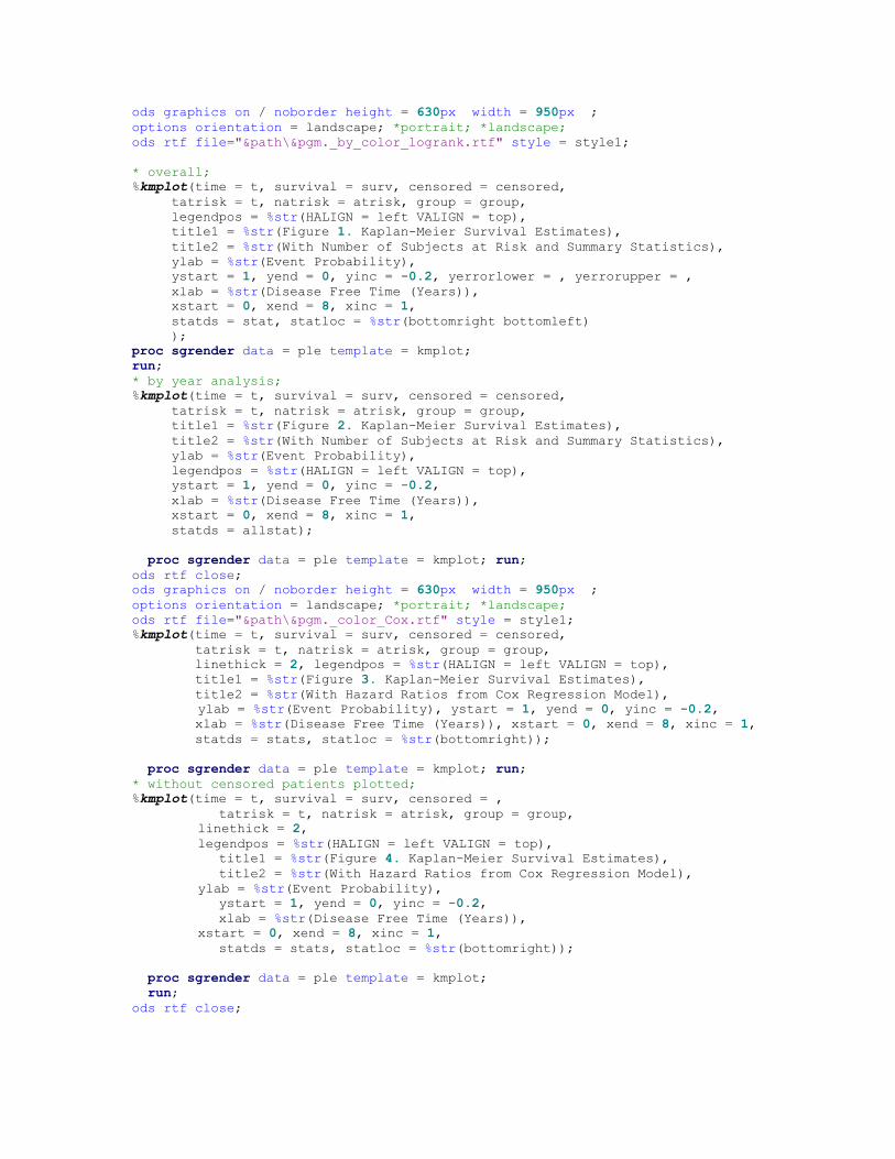
ods graphics on / noborder height = 630px width = 950px ;

options orientation = landscape; *portrait; *landscape;

ods rtf file="&path\&pgm._by_color_logrank.rtf" style = style1;

* overall;

%kmplot(time = t, survival = surv, censored = censored,

tatrisk = t, natrisk = atrisk, group = group,

legendpos = %str(HALIGN = left VALIGN = top),

title1 = %str(Figure 1. Kaplan-Meier Survival Estimates),

title2 = %str(With Number of Subjects at Risk and Summary Statistics),

ylab = %str(Event Probability),

ystart = 1, yend = 0, yinc = -0.2, yerrorlower = , yerrorupper = ,

xlab = %str(Disease Free Time (Years)),

xstart = 0, xend = 8, xinc = 1,

statds = stat, statloc = %str(bottomright bottomleft)

);

proc sgrender data = ple template = kmplot;

run;

* by year analysis;




title2 = %str(With Number of Subjects at Risk and Summary Statistics),



ystart = 1, yend = 0, yinc = -0.2,



statds = allstat);

proc sgrender data = ple template = kmplot; run;

ods rtf close;

ods graphics on / noborder height = 630px width = 950px ;

options orientation = landscape; *portrait; *landscape;

ods rtf file="&path\&pgm._color_Cox.rtf" style = style1;



linethick = 2, legendpos = %str(HALIGN = left VALIGN = top),


title2 = %str(With Hazard Ratios from Cox Regression Model),

ylab = %str(Event Probability), ystart = 1, yend = 0, yinc = -0.2,

xlab = %str(Disease Free Time (Years)), xstart = 0, xend = 8, xinc = 1,

statds = stats, statloc = %str(bottomright));

proc sgrender data = ple template = kmplot; run;

* without censored patients plotted;

%kmplot(time = t, survival = surv, censored = ,


linethick = 2,



title2 = %str(With Hazard Ratios from Cox Regression Model),


ystart = 1, yend = 0, yinc = -0.2,



statds = stats, statloc = %str(bottomright));

proc sgrender data = ple template = kmplot;

run;

ods rtf close;

Documents

PharmaSUG 2016 - Paper PO020 Using GTL … · Using GTL Generating Customized Kaplan-Meier Survival ... to generate a template named KMplot for KM graphs with KM estimate as step-plot