Petroleum Refineries New Source Performance Standards Ja

Regulatory Impact Analysis

Petroleum Refineries

New Source Performance Standards Ja

June 2012

U.S. Environmental Protection Agency

Office of Air and Radiation

Office of Air Quality Planning and Standards

Research Triangle Park, NC 27711

ii

CONTACT INFORMATION

This document has been prepared by staff from the Office of Air Quality Planning and

Standards, U.S. Environmental Protection Agency and RTI International. Questions related to

this document should be addressed to Alexander Macpherson, U.S. Environmental Protection

Agency, Office of Air Quality Planning and Standards, C445-B, Research Triangle Park, North

Carolina 27711 (email: [email protected]).

ACKNOWLEDGEMENTS

In addition to EPA staff from the Office of Air Quality Planning and Standards,

personnel from RTI International contributed significant data and analysis to this document

under contract number EP-D-06-003.

mailto:[email protected]

iii

TABLE OF CONTENTS

TABLE OF CONTENTS .................................................................................................................... III

LIST OF TABLES .............................................................................................................................. V

LIST OF FIGURES ........................................................................................................................... VI

1. EXECUTIVE SUMMARY ........................................................................................................ 1-1

1.1 INTRODUCTION ............................................................................................................................................ 1-1 1.2 RESULTS ...................................................................................................................................................... 1-2 1.3 REFERENCES ................................................................................................................................................ 1-6

2 INDUSTRY PROFILE ............................................................................................................. 2-1

2.1 INTRODUCTION ............................................................................................................................................ 2-1 2.2 THE SUPPLY SIDE ......................................................................................................................................... 2-1

2.2.1 Production Process, Inputs, and Outputs ........................................................................................... 2-1 2.2.2 Emissions and Controls in Petroleum Refining ................................................................................. 2-9 2.2.3 Costs of Production .......................................................................................................................... 2-10

2.3 THE DEMAND SIDE .................................................................................................................................... 2-15 2.3.1 Product Characteristics .................................................................................................................... 2-15 2.3.2 Uses and Consumers ........................................................................................................................ 2-15 2.3.3 Substitution Possibilities in Consumption ....................................................................................... 2-17

2.4 INDUSTRY ORGANIZATION ......................................................................................................................... 2-17 2.4.1 Market Structure .............................................................................................................................. 2-17 2.4.2 Characteristics of U.S. Petroleum Refineries and Petroleum Refining Companies ......................... 2-21

2.5 MARKETS ................................................................................................................................................... 2-30 2.5.1 U.S. Petroleum Consumption .......................................................................................................... 2-30 2.5.2 U.S. Petroleum Production .............................................................................................................. 2-36 2.5.3 International Trade ........................................................................................................................... 2-37 2.5.4 Market Prices ................................................................................................................................... 2-39 2.5.5 Profitability of Petroleum Refineries ............................................................................................... 2-41 2.5.6 Industry Trends ................................................................................................................................ 2-43

2.6 REFERENCES .............................................................................................................................................. 2-45

3 NSPS REGULATORY OPTIONS, COSTS AND EMISSION REDUCTIONS FROM COMPLYING

WITH THE NSPS .......................................................................................................................... 3-1

4 ECONOMIC IMPACT ANALYSIS: METHODS AND RESULTS ................................................. 4-1

4.1 INTRODUCTION………………………………………………………………………………………….4-1

4.2 COMPLIANCE COST ESTIMATES………………..…………………………………….………………4-1

4.3 SMALL BUSINESS IMPACT ANALYSIS……………………………………………………………….4-4

4.3.1 Small Entity Economic Impact Measures……………………………………………..…………….4-4

4.3.2 Small Entity Economic Impact Analysis…………………………………………………………….4-5

4.4 REFERENCES……………………………………………………………………………………………..4-8

5 EXECUTIVE ORDERS............................................................................................................ 5-1

5.1 UNFUNDED MANDATES ........................................................................................................................ 5-1 5.2 ENVIRONMENTAL JUSTICE .................................................................................................................. 5-1 5.3 SIGNIFICANT ENERGY ACTIONS ........................................................................................................ 5-1

6 HUMAN HEALTH BENEFITS OF EMISSIONS REDUCTIONS .................................................. 6-1

6.1 CALCULATION OF PM2.5-RELATED HUMAN HEALTH BENEFITS ................................................................... 6-1

iv

6.2 SOCIAL COST OF CARBON AND GREENHOUSE GAS BENEFITS .................................................................... 6-14 6.3 ENERGY DISBENEFITS ................................................................................................................................ 6-17 6.4 TOTAL MONETIZED BENEFITS .................................................................................................................... 6-18 6.5 UNQUANTIFIED BENEFITS .......................................................................................................................... 6-19

6.5.1 Additional SO2 and NO2 Benefits .................................................................................................... 6-19 6.5.2 Ozone Benefits ................................................................................................................................. 6-22 6.5.3 Visibility Impairment ....................................................................................................................... 6-22

6.6 CHARACTERIZATION OF UNCERTAINTY IN THE MONETIZED BENEFITS ...................................................... 6-23 6.7 REFERENCES .............................................................................................................................................. 6-28

7 COMPARISON OF BENEFITS AND COSTS ............................................................................. 7-1

APPENDIX A PARENT COMPANY INFORMATION FOR PETROLEUM REFINERIES ..................... A-1

v

LIST OF TABLES

Table 1-1 National Incremental Cost Impacts, Emission Reductions, and Cost Effectiveness for Petroleum

Refinery Flares Subject to Amended Standards Under 40 CFR part 60, subpart Ja (Fifth Year After

Effective Date of Final Rule Amendments) .................................................................................... 1-3

Table 1-2 Summary of the Monetized Benefits, Social Costs, and Net Benefits for the Final Petroleum Refineries NSPS in 2017………………………………………………………………...…………..1-5

Table 2-1. Types and Characteristics of Raw Materials used in Petroleum Refineries ....................................... 2-7 Table 2-2. Major Refinery Product Categories .................................................................................................... 2-9 Table 2-3. Labor, Material, and Capital Expenditures for Petroleum Refineries (NAICS 324110) .................. 2-12 Table 2-4. Costs of Materials Used in Petroleum Refining Industry ................................................................. 2-14 Table 2-5. Major Refinery Products .................................................................................................................. 2-16 Table 2-6. Market Concentration Measures of the Petroleum Refining Industry: 1985 to 2007 ....................... 2-20 Table 2-7. Number of Petroleum Refineries, by State ....................................................................................... 2-23 Table 2-8. Full Production Capacity Utilization Rates for Petroleum Refineries .............................................. 2-24 Table 2-9. Characteristics of Small Businesses in the Petroleum Refining Industry ......................................... 2-31 Table 2-10. Total Petroleum Products Supplied (millions of barrels per year) ................................................... 2-36 Table 2-11. U.S. Refinery and Blender Net Production (millions of barrels per year) ........................................ 2-36 Table 2-12. Value of Product Shipments of the Petroleum Refining Industry .................................................... 2-38 Table 2-13. Imports of Major Petroleum Products (millions of barrels per year) ................................................ 2-38 Table 2-14. Exports of Major Petroleum Products (millions of barrels per year) ................................................ 2-39 Table 2-15. Average Price of Major Petroleum Products Sold to End Users (cents per gallon) ......................... 2-40 Table 2-16. Producer Price Index Industry Data: 1995 to 2010 .......................................................................... 2-41 Table 2-17. Mean Ratios of Profit before Taxes as a Percentage of Net Sales for Petroleum Refiners, Sorted by

Value of Assets ................................................................................................................................. 2-42 Table 2-18. Net Profit Margins for Publicly Owned, Small Petroleum Refiners: 2010 ...................................... 2-43 Table 2-19. Forecasted Average Price of Major Petroleum Products Sold to End Users in 2009 Currency (cents

per gallon) ........................................................................................................................................ 2-44 Table 2-20. Total Petroleum Products Supplied (millions of barrels per year) ................................................... 2-44 Table 2-21. Full Production Capacity Utilization Rates for Petroleum Refineries .............................................. 2-45 Table 3-1. National Incremental Cost Impacts for Petroleum Refinery Flares Subject to Amended Standards

Under 40 CFR part 60, subpart Ja (Fifth Year After Effective Date of Final Rule Amendments) ..... 3-2 Table 3-2. National Incremental Emissions Reductions and Cost-Effectiveness for Petroleum Refinery Flares

Subject to Amended Standards Under 40 CFR part 60, subpart Ja (Fifth Year After Effective Date of

Final Rule Amendments) .................................................................................................................... 3-3

Table 4-1. Rates of Return on Investment for Refineries………………………………………………….…….4-2 Table 4-2. Impact Levels of Proposed NSPS Amendments on Small Firms………………………..……..……4-6

Table 4-3. Summary of Sales Ratios for Firms Affected by Proposed NSPS Amendments……………………4-7

Table 6-1. Human Health Effects of PM2.5 .......................................................................................................... 6-3 Table 6-2. General Summary of Monetized PM-Related Health Benefits Estimates for Petroleum Refineries

NSPS Reconsideration (millions of 2006$)* .................................................................................... 6-11

Table 6-3. Summary of Reductions in Health Incidences from PM2.5 Benefits for Petroleum Refineries NSPS

Reconsideration* .............................................................................................................................. 6-12 Table 6-4. All PM2.5 Benefits Estimates for the Final Petroleum Refineries NSPS Reconsideration at discount

rates of 3% and 7% in 2017 (in millions of 2006$)* ........................................................................ 6-13 Table 6-5. Social Cost of Carbon (SCC) Estimates (per tonne of CO2) for 2017

a ............................................. 6-16

Table 6-6. Monetized SCC-Derived Benefits of CO2 Emission Reductions in 2017 a,b

.................................... 6-17 Table 7-1. National Incremental Cost Impacts, Emission Reductions, and Cost Effectiveness for Petroleum

Refinery Flares Subject to Amended Standards Under 40 CFR part 60, subpart Ja (Fifth Year After

Effective Date of Final Rule Amendments) ....................................................................................... 7-2

Table 7-2. Summary of the Monetized Benefits, Social Costs, and Net Benefits for the Final Petroleum Refineries NSPS in 2017……………………………………………………………………………7-3

Table A-1. Parent Company Information for Petroleum Refineries .................................................................... A-2

vi

LIST OF FIGURES

Figure 2-1. Outline of the Refining Process ......................................................................................................... 2-3 Figure 2-2. Desalting Process ............................................................................................................................... 2-3 Figure 2-3. Atmospheric Distillation Process ....................................................................................................... 2-4 Figure 2-4. Vacuum Distillation Process .............................................................................................................. 2-5 Figure 2-5. Petroleum Refinery Expenditures .................................................................................................... 2-11 Figure 2-6. Employment Distribution of Companies Owning Petroleum Refineries (N=61) ............................ 2-25 Figure 2-7. Average Revenue of Companies Owning Petroleum Refineries by Employment (N=61) .............. 2-26 Figure 2-8. Revenue Distribution of Large Companies Owning Petroleum Refineries (N=25) ......................... 2-27

Figure 2-9. Revenue Distribution of Small Companies Owning Petroleum Refineries (N=36)……….………2-28

Figure 2-10. Total Petroleum Products Supplied (millions of barrels per year) ................................................... 2-35 Figure 6-1: Breakdown of Monetized PM2.5 Health Benefits using Mortality Function from Pope et al. (2002)6-10 Figure 6-2: Monetized PM2.5 Benefits of Final Petroleum Refineries Reconsideration in 2017......................... 6-14 Figure 6-3: Breakdown of Monetized Benefits for Final Petroleum Refineries NSPS Reconsideration by Pollutant

…………………………………………………………………………………………………...…6-18

Figure 6-4. Breakdown of Monetized Benefits for Final Petroleum Refineries NSPS Reconsideration by Requirement and Flare Size………………………………………………………………………..6-19

Figure 6-5. Percentage of Adult Population by Annual Mean PM2.5 Exposure in the Baseline ......................... 6-25 Figure 6-6. Cumulative Distribution of Adult Population by Annual Mean PM2.5 Exposure in the Baseline .... 6-26 Figure 7-1. Net Benefits for Final Petroleum Refineries NSPS Reconsideration at 3% discount rate* ............... 7-4 Figure 7-2. Net Benefits for Final Petroleum Refineries NSPS Reconsideration at 7% discount rate* ............... 7-5

1-1

1. EXECUTIVE SUMMARY

1.1 Introduction

On June 24, 2008, EPA promulgated amendments to the Standards of Performance for

Petroleum Refineries and new standards of performance for petroleum refinery process units

constructed, reconstructed, or modified after May 14, 2007. EPA subsequently received three

petitions for reconsideration of these final rules. On September 26, 2008, EPA granted

reconsideration and issued a stay for the issues raised in the petitions regarding process heaters

and flares. On December 22, 2008, EPA addressed those specific issues by proposing

amendments to certain provisions for process heaters and flares. This final regulation includes

emissions limits for new and modified/reconstructed sources, and these limits are set for sulfur

dioxide (SO2), nitrogen oxides (NOx), volatile organic compounds (VOC), and other pollutants.

The petroleum refining industry comprises establishments primarily engaged in refining

crude petroleum into refined petroleum. Examples of refined petroleum products include

gasoline, kerosene, asphalt, lubricants, solvents, and a variety of other products. Petroleum

refining falls under the North American Industrial Classification System (NAICS) 324110.

This regulatory impact analysis (RIA) was prepared in response to requirements under

Executive Order 12866. The RIA presents the results of analyses undertaken in support of this

final rule including compliance costs, benefits, economic impacts, and impacts to small

businesses. This RIA is organized as follows:

Section 1: Executive Summary,

Section 2 and an Appendix A: Profile of the Petroleum Refining Industry,

Section 3: NSPS Regulatory Alternatives, and Costs and Emission Reductions From

Complying with the NSPS,

Section 4: Economic Impact Analysis: Methods and Results,

Section 5: Executive Orders,

Section 6: Benefits of the NSPS, and

Section 7: Comparison of Benefits and Costs.

1-2

1.2 Results

EPA has characterized the facilities and companies potentially affected by the NSPS by

examining existing refineries and the companies that own them. EPA projects that new refineries

and processes will be similar to existing ones, and that the companies owning new sources will

also be similar to the companies owning existing refineries. EPA has collected data on 148

existing refineries, owned by 64 companies. Of the affected parent companies, thirty-six are

identified as small entities based on the Small Business Administration size standard criteria for

NAICS 324110, for they employ 1,500 or fewer employees.

The total annualized engineering compliance costs of the NSPS are estimated at $96

million. The total annual savings from offset natural gas purchases and product recovery credits

that arise as a result of complying with the rule are estimated at $180 million. EPA estimates

that complying with the final NSPS will yield an annualized cost savings of approximately $79

million per year (2006 dollars) in 2017. The estimated nationwide 5-year incremental emissions

reductions and cost impacts for the final standards are summarized in Table 1-1 below. Given

that there are cost savings, EPA anticipates that the NSPS will have no negative impacts on the

market for petroleum products. Based on sales data obtained for the affected small entities, as

well as expected annualized cost savings, EPA estimates that the NSPS will not result in a

SISNOSE (significant economic impact on a substantial number of small entities).

1-3

Table 1-1. National Incremental Cost Impacts, Emission Reductions, and Cost Effectiveness for Petroleum Refinery Flares Subject to

Amended Standards Under 40 CFR part 60, subpart Ja (Fifth Year After Effective Date of Final Rule Amendments)1

Subpart Ja

Requirements

Total

capital

cost

(millions)

Total

annual cost

without

credit

(millions/yr)

Natural

gas

offset/

product

recovery

credit

(millions)

Total

annual cost

(millions/yr)

Annual

emission

reductions

(tons

SO2/yr)

Annual

emission

reductions

(tons

NOX/yr)

Annual

emission

reductions

(tons

VOC/yr)

Cost

effective-

ness

($/ton

emissions

reduced)

Annual

emission

reductions

(metric

tons

CO2/yr)2

Monetized

Benefits

(millions, 3%

discount rate for

health and

climate benefits)

Monetized

Benefits

(millions, 3%

discount rate for

health and 7%

for climate

benefits)

Sm

all

Fla

res

Flare

Monitoring $72 $12 $0 $12 0 0 0 0 $0 to $0 $0 to $0

Flare gas

recovery $0 $0 $0 $0 0 0 0 0 $0 to $0 $0 to $0

Flare

Management $0 $0.79 $0 $0.79 0 0 270 $2,900 0 $0 to $0 $0 to $0

SO2 RCA/CA $0 $1.9 $0 $1.9 2,600 0 0 $760 0 $170 to $410 $150 to $370

Flowrate

RCA/CA $0 $0.90 -$6.7 -$5.8 3.4 50 390 -$13,000 98,000 $2.9 to $3.7 $2.9 to $3.6

Total $72 $16 -$6.7 $9.0 2,600 50 660 $2,700 98,000 $170 to $410 $150 to $370

Larg

e F

lare

s

Flare

Monitoring $12 $2.0 $0 $2.0 0 0 0 0 $0 to $0 $0 to $0

Flare gas

recovery $380 $78 -$170 -$90 380 1,100 2,700 -$22,000 1,800,000 $74 to $120 $71 to $110

Flare

Management $0 $0.088 $0 $0.088 0 0 30 $2,900 0 $0 to $0 $0 to $0

SO2 RCA/CA $0 $0.22 $0 $0.22 290 0 0 $760 0 $18 to $45 $17 to $41

Flowrate

RCA/CA $0 $0.10 -$0.74 -$0.64 0 6 43 -$13,000 11,000 $0 to $0 $0 to $0

Total $390 $81 -$170 -$88 660 1,100 2,800 -$20,000 1,800,000 $93 to $160 $88 to $150

All

Fla

res

Flare

Monitoring $84 $14 $0 $14 0 0 0 0 $0 to $0 $0 to $0

Flare gas

recovery $380 $78 -$170 -$90 380 1,100 2,700 -$22,000 1,800,000 $74 to $120 $71 to $110

Flare

Management $0 $0.88 $0 $0.88 0 0 300 $2,900 0 $0 to $0 $0 to $0

SO2 RCA/CA $0 $2.2 $0 $2.2 2,900 0 0 $760 0 $180 to $450 $170 to $410

Flowrate

RCA/CA $0 $1.00 -$7.4 -$6.4 3.4 56 430 -$13,000 110,000 $3.2 to $4.0 $3.1 to $3.9

Total $460 $96 -$180 -$79 3,200 1,100 3,400 -$10,000 1,900,000 $260 to $580 $240 to $520 1All estimates are for the implementation year (2017), and are rounded to two significant figures.

2 The emission reductions of CO2 reflect the anticipated emission increases associated with the energy disbenefits from additional electricity consumption.

1-4

EPA estimates that the total monetized benefits of the final NSPS are $260 million to

$580 million and $240 million to $520 million, at 3% and 7% discount rates, respectively (Table

1-2). All estimates are in 2006 dollars for the year 2017. Using alternate relationships between

PM2.5 and premature mortality supplied by experts, higher and lower benefits estimates are

plausible, but most of the expert-based estimates fall between these estimates. In addition, direct

exposure to SO2 and NOx benefits, ozone benefits, ecosystem benefits, and visibility benefits

have not been monetized in this analysis.

EPA estimates the net benefits of the final NSPS are $340 million to $660 million and

$320 million to $600 million, at 3% and 7% discount rates, respectively (Table 1-2). All

estimates are in 2006 dollars for the year 2017.

1-5

Table 1-2. Summary of the Monetized Benefits, Social Costs, and Net Benefits for the

Final Petroleum Refineries NSPS in 2017 (millions of 2006$)1

3% Discount Rate 7% Discount Rate

Final Major Source NSPS

Total Monetized Benefits2 $260 to $580 $240 to $520

Total Compliance Costs3 -$79 -$79

Net Benefits $340 to $660 $320 to $600

Non-monetized Benefits

Health effects from SO2, NO2, and ozone exposure

Health effects from PM exposure from VOCs

Ecosystem effects

Visibility impairment 1All estimates are for the implementation year (2017), and are rounded to two significant figures.

2 The total monetized benefits reflect the human health benefits associated with reducing exposure to PM2.5 through

reductions of PM2.5 precursors such as NOx and SO2 as well as CO2 benefits. It is important to note that the

monetized benefits do not include the reduced health effects from direct exposure to SO2 and NOx, ozone

exposure, ecosystem effects, or visibility impairment. Human health benefits are shown as a range from Pope et

al. (2002) to Laden et al. (2006). These models assume that all fine particles, regardless of their chemical

composition, are equally potent in causing premature mortality because the scientific evidence is not yet

sufficient to allow differentiation of effects estimates by particle type. The net present value of reduced CO2

emissions is calculated differently than other benefits. This table includes monetized climate benefits using the

global average social cost of carbon (SCC) estimated at a 3 percent discount rate because the interagency

workgroup deemed the SCC estimate at a 3 percent discount rate to be the central value. 3 The engineering compliance costs are annualized using a 7 percent discount rate.

Alternatively, if no refineries install flare gas recovery systems, EPA estimates the costs

would be $10.7 million with monetized benefits of $190 to $460 million and $170 to $410

million at a discount rates of 3% and 7% respectively. Thus, net benefits without flare gas

recovery systems would be $180 million to $450 million and $160 million to $400 million, at 3%

and 7% discount rates, respectively. All estimates are in 2006 dollars for the year 2017.

For small flares, we estimate the monetized benefits are $170 million to $410 million (3-

percent discount rate) and $150 million to $370 million (7% discount rate for health benefits and

3% discount rate for climate benefits). For large flares, we estimate the monetized benefits are

$93 million to $160 million (3% discount rate) and $88 million to $150 million (7% discount rate

for health benefits and 3-percent discount rate for climate benefits). All estimates are in 2006

dollars for the year 2017.

1-6

1.3 References

Laden, F., J. Schwartz, F.E. Speizer, and D.W. Dockery. 2006. Reduction in Fine Particulate Air

Pollution and Mortality. American Journal of Respiratory and Critical Care Medicine. 173:

667-672.

Office of Management and Budget. Circular A-4, September 17, 2003. Available on the

Internet at http://www.whitehouse.gov/omb/circulars_a004_a-4.

Pope, C.A., III, R.T. Burnett, M.J. Thun, E.E. Calle, D. Krewski, K. Ito, and G.D. Thurston.

2002. “Lung Cancer, Cardiopulmonary Mortality, and Long-term Exposure to Fine

Particulate Air Pollution.” Journal of the American Medical Association 287:1132-1141.

2-1

2. PROFILE OF THE PETROLEUM REFININGINDUSTRY

2.1 Introduction

This industry profile of the petroleum refining industry provides information that will

support this and subsequent regulatory impact analyses (RIAs) and economic impact analyses

(EIAs) that will assess the impacts of these standards.

At its core, the petroleum refining industry comprises establishments primarily engaged

in refining crude petroleum into finished petroleum products. Examples of these petroleum

products include gasoline, kerosene, asphalt, lubricants, and solvents, among others.

Firms engaged in petroleum refining are categorized under the North American Industry

Classification System (NAICS) code 324110. In 2010, 148 establishments owned by 64 parent

companies were refining petroleum in the continental United States. In 2009, the petroleum

refining industry shipped products valued at over $436 billion (U.S. Census Bureau, Sector 31:

2009 and 2008).

This industry profile report is organized as follows. Section 2.2 provides a detailed

description of the inputs, outputs, and processes involved in petroleum refining. Section 2.3

describes the applications and users of finished petroleum products. Section 2.4 discusses the

organization of the industry and provides facility- and company-level data. In addition, small

businesses are reported separately for use in evaluating the impact on small business to meet the

requirements of the Small Business Regulatory Enforcement and Fairness Act (SBREFA).

Section 2.5 contains market-level data on prices and quantities and discusses trends and

projections for the industry.

2.2 The Supply Side

Estimating the economic impacts of any regulation on the petroleum refining industry

requires a good understanding of how finished petroleum products are produced (the “supply

side” of finished petroleum product markets). This section describes the production process used

to manufacture these products as well as the inputs, outputs, and by-products involved. The

section concludes with a description of costs involved with the production process.

2.2.1 Production Process, Inputs, and Outputs

Petroleum pumped directly out of the ground, known as crude oil, is a complex mixture

of hydrocarbons (chemical compounds that consist solely of hydrogen and carbon) and various

impurities such as salt. To manufacture the variety of petroleum products recognized in everyday

2-2

life, this mixture must be refined and processed over several stages. This section describes the

typical stages involved in this process as well as the inputs and outputs.

2.2.1.1 The Production Process

The process of refining crude oil into useful petroleum products can be separated into two

phases and a number of supporting operations. These phases are described in detail in the

following section. In the first phase, crude oil is desalted and then separated into its various

hydrocarbon components (known as “fractions”). These fractions include gasoline, kerosene,

naphtha, and other products (EPA, 1995).

In the second phase, the distilled fractions are converted into petroleum products (such as

gasoline and kerosene) using three different types of downstream processes: combining,

breaking, and reshaping (EPA, 1995). An outline of the refining process is presented in Figure 2-

1.

Desalting. Before separation into fractions, crude oil is treated to remove salts,

suspended solids, and other impurities that could clog or corrode the downstream equipment.

This process, known as “desalting,” is typically done by first heating the crude oil, mixing it with

process water, and depositing it into a gravity settler tank. Gradually, the salts present in the oil

will be dissolved into the process water (EPA, 1995). After this takes place, the process water is

separated from the oil by adding demulsifier chemicals (a process known as chemical separation)

and/or by applying an electric field to concentrate the suspended water globules at the bottom of

the settler tank (a process known as electrostatic separation). The effluent water is then removed

from the tank and sent to the refinery wastewater treatment facilities (EPA, 1995). This process

is illustrated in Figure 2-2.

2-3

Figure 2-1 Outline of the Refining Process

Source: U.S. Department of Labor, Occupational Safety and Health Administration (OSHA). 2003. OSHA

Technical Manual, Section IV: Chapter 2, Petroleum Refining Processes. TED 01-00-015. Washington, DC: U.S.

DOL. Available at <http://www.osha.gov/dts/osta/otm/otm_iv/otm_iv_2.html>. As obtained on October 23, 2006.

Figure 2-2 Desalting Process




2-4

Atmospheric Distillation. The desalted crude oil is then heated in a furnace to 750°F and

fed into a vertical distillation column at atmospheric pressure. After entering the tower, the

lighter fractions flash into vapor and travel up the tower. This leaves only the heaviest fractions

(which have a much higher boiling point) at the bottom of the tower. These fractions include

heavy fuel oil and asphalt residue (EPA, 1995).

As the hot vapor rises, its temperature is gradually reduced. Lighter fractions condense onto

trays located at successively higher portions of the tower. For example, motor gasoline will

condense at higher portion of the tower than kerosene because it condenses at lower temperatures.

This process is illustrated in Figure 2-3. As these fractions condense, they will be drawn off their

respective trays and potentially sent downstream for further processing (OSHA, 2003; EPA, 1995).

Figure 2-3 Atmospheric Distillation Process




Vacuum Distillation. The atmospheric distillation tower cannot distill the heaviest

fractions (those at the bottom of the tower) without cracking under requisite heat and pressure.

So these fractions are separated using a process called vacuum distillation. This process takes

place in one or more vacuum distillation towers and is similar to the atmospheric distillation

process, except very low pressures are used to increase volatilization and separation. A typical

first-phase vacuum tower may produce gas oils or lubricating-oil base stocks (EPA, 1995). This

process is illustrated in Figure 2-4.

2-5

Figure 2-4 Vacuum Distillation Process




Downstream Processing. To produce the petroleum products desired by the market

place, most fractions must be further refined after distillation or “downstream” processes. These

downstream processes change the molecular structure of the hydrocarbon molecules by breaking

them into smaller molecules, joining them to form larger molecules, or shaping them into higher

quality molecules (EPA, 1995).

Downstream processes include thermal cracking, coking, catalytic cracking, catalytic

hydrocracking, hydrotreating, alkylation, isomerization, polymerization, catalytic reforming,

solvent extraction, merox, dewaxing, propane deasphalting and other operations (EPA, 1995).

2.2.1.2 Supporting Operations

In addition to the processes described above, there are other refinery operations that do

not directly involve the production of hydrocarbon fuels, but serve in a supporting role. Some of

the major supporting operations are described in this section.

Wastewater Treatment. Petroleum refining operations produce a variety of wastewaters

including process water (water used in process operations like desalting), cooling water (water

used for cooling that does not come into direct contact with the oil), and surface water runoff

(resulting from spills to the surface or leaks in the equipment that have collected in drains).

2-6

Wastewater typically contains a variety of contaminants (such as hydrocarbons,

suspended solids, phenols, ammonia, sulfides, and other compounds) and must be treated before

it is recycled back into refining operations or discharged. Petroleum refineries typically utilize

two stages of wastewater treatment. In primary wastewater treatments, oil and solids present in

the wastewater are removed. After this is completed, wastewater can be discharged to a publicly

owned treatment facility or undergo secondary treatment before being discharged directly to

surface water. In secondary treatment, microorganisms are used to dissolve oil and other organic

pollutants that are present in the wastewater (EPA, 1995; OSHA, 2003).

Gas Treatment and Sulfur Recovery. Petroleum refinery operations such as coking and

catalytic cracking emit gases with a high concentration of hydrogen sulfide mixed with light

refinery fuel gases (such as methane and ethane). Sulfur must be removed from these gases in

order to comply with the Clean Air Act’s SOx emission limits and to recover saleable elemental

sulfur.

Sulfur is recovered by first separating the fuel gases from the hydrogen sulfide gas. Once

this is done, elemental sulfur is removed from the hydrogen sulfide gas using a recovery system

known as the Claus Process. In this process, hydrogen sulfide is burned under controlled

conditions producing sulfur dioxide. A bauxite catalyst is then used to react with the sulfur

dioxide and the unburned hydrogen sulfide to produce elemental sulfur. However, the Claus

process only removes 90% of the hydrogen sulfide present in the gas stream, so other processes

must be used to recover the remaining sulfur (EPA, 1995).

Additive Production. A variety of chemicals are added to petroleum products to

improve their quality or add special characteristics. For example, ethers have been added to

gasoline to increase octane levels and reduce CO emissions since the 1970s.

Heat Exchangers, Coolers, and Process Heaters. Petroleum refineries require very

high temperatures to perform many of their refining processes. To achieve these temperatures,

refineries use fired heaters fueled by refinery or natural gas, distillate, and residual oils. This heat

is managed through heat exchangers, which are composed of bundles of pipes, tubes, plate coils,

and other equipment that surround heating or cooling water, steam, or oil. Heat exchangers

facilitate the indirect transfer of heat as needed (OSHA, 2003).

Pressure Release and Flare Systems. As liquids and gases expand and contract through

the refining process, pressure must be actively managed to avoid accident. Pressure-relief

systems enable the safe handling of liquids and gases that are released by pressure-relieving

2-7

devices and blow-downs. According to the OSHA Technical Manual, “pressure relief is an

automatic, planned release when operating pressure reaches a predetermined level. A blow-down

normally refers to the intentional release of material, such as blow-downs from process unit

startups, furnace blow-downs, shutdowns, and emergencies” (OSHA, 2003).

Blending. Blending is the final operation in petroleum refining. It is the physical mixture

of a number of different liquid hydrocarbons to produce final petroleum products that have

desired characteristics. For example, additives such as ethers can be blended with motor gasoline

to boost performance and reduce emissions. Products can be blended in-line through a manifold

system, or batch blended in tanks and vessels (OSHA, 2003).

2.2.1.3 Inputs

The inputs in the production process of petroleum products include general inputs such as

labor, capital, and water.1 The inputs specific to this industry are crude oil and the variety of

chemicals used in producing petroleum products. These two specific inputs are discussed below.

Crude Oil. Crude oils are complex, heterogeneous mixtures and contain many different

hydrocarbon compounds that vary in appearance and composition from one oil field to another.

An “average” crude oil contains about 84% carbon; 14% hydrogen; and less than 2% sulfur,

nitrogen, oxygen, metals, and salts (OSHA, 2003). The proportions of crude oil elements vary

over a narrow limit: the proportion of carbon ranges from 83 to 87 percent; hydrogen ranges

from 10 to 14 percent; nitrogen ranges from 0.1 to 2 percent; oxygen ranges from 0.5 to 1.5

percent; and sulfur ranges from 0.5 to 6 percent (Speight 2006).

In 2010, the petroleum refining industry used 5.4 billion barrels of crude oil in the

production of finished petroleum products (EIA 2010).2

Common Refinery Chemicals. In addition to crude oil, a variety of chemicals are used

in the production of petroleum products. The specific chemicals used will depend on specific

characteristics of the product in question. Table 2-1 lists the most common chemicals used by

petroleum refineries, their characteristics, and their applications.

Table 2-1 Types and Characteristics of Raw Materials used in Petroleum Refineries

1 Crude oil processing requires large volumes of water, a large portion of which is continually recycled. The amount

of water used by a refinery can vary significantly, depending on process configuration, refinery complexity,

capability for recycle, degree of sewer segregation, and local rainfall. In 1992, the average amount of water used in

refineries was estimated between 65 and 90 gallons per barrel of crude oil processed (OGJ 1992a). 2 A barrel is a unit of volume that is equal to 42 U.S. gallons.

2-8

Type Description

Crude Oil Heterogeneous mixture of different hydrocarbon compounds.

Oxygenates Substances which, when added to gasoline, increase the amount of oxygen in that

gasoline blend. Ethanol, ethyl tertiary butyl ether (ETBE), and methanol are

common oxygenates.

Caustics Caustics are added to desalting water to neutralize acids and reduce corrosion.

They are also added to desalted crude in order to reduce the amount of corrosive

chlorides in the tower overheads. They are used in some refinery treating processes

to remove contaminants from hydrocarbon streams.

Leaded Gasoline Additives Tetraethyl lead (TEL) and tetramethyl lead (TML) are additives formerly used to

improve gasoline octane ratings but are no longer in common use except in

aviation gasoline.

Sulfuric Acid and

Hydrofluoric Acid

Sulfuric acid and hydrofluoric acid are used primarily as catalysts in alkylation

processes. Sulfuric acid is also used in some treatment processes.




In 2010, the petroleum refining industry used 971 million barrels of natural gas liquids

and other liquids in the production of finished petroleum products (EIA 2010).

2.2.1.4 Types of Product Outputs

The petroleum refining industry produces a number of products that fall into one of three

categories: fuels, finished nonfuel products, and feedstock for the petrochemical industry. Table

2-2 briefly describes these product categories. A more detailed discussion of petroleum fuel

products can be found in Section 2.3.

2-9

Table 2-2 Refinery Product Categories

Product Category Description

Fuels Finished Petroleum products that are capable of releasing energy. These products

power equipment such as automobiles, jets, and ships. Typical petroleum fuel

products include gasoline, jet fuel, and residual fuel oil.

Finished nonfuel products Petroleum products that are not used for powering machines or equipment. These

products typically include asphalt, lubricants (such as motor oil and industrial

greases), and solvents (such as benzene, toluene, and xylene).

Feedstock

Sulfur

Many products derived from crude oil refining, such as ethylene, propylene,

butylene, and isobutylene, are primarily intended for use as petrochemical

feedstock in the production of plastics, synthetic fibers, synthetic rubbers, and other

products.

Commercial uses are primarily in fertilizers, because of the relatively high

requirement of plants for it, and in the manufacture of sulfuric acid, a primary

industrial chemical.




2.2.2 Emissions and Controls in Petroleum Refining

Petroleum refining results in emissions of hazardous air pollutants (HAPs), criteria air

pollutants (CAPs), and other pollutants. The HAPs include metals and toxic organic compounds;

the CAPs include carbon monoxide (CO), sulfur oxides (SOx), nitrogen oxides (NOx),

particulates, and volatile organic compounds (VOCs); and the other pollutants include spent

acids, gaseous pollutants, ammonia (NH3), and hydrogen sulfide (H2S).

2.2.2.1 Gaseous and VOC Emissions

As previously mentioned, CO, SOx, NOx, NH3, and H2S emissions are produced along

with petroleum products. Sources of these emissions from refineries include fugitive emissions

of the volatile constituents in crude oil and its fractions, emissions from the burning of fuels in

process heaters, and emissions from the various refinery processes themselves. Fugitive

emissions occur as a result of leaks throughout the refinery and can be reduced by purchasing

leak-resistant equipment and maintaining an ongoing leak detection and repair program (EPA,

1995).

The numerous process heaters used in refineries to heat process streams or to generate

steam (boilers) for heating or other uses can be potential sources of SOx, NOx, CO, and

hydrocarbons emissions. Emissions are low when process heaters are operating properly and

using clean fuels such as refinery fuel gas, fuel oil, or natural gas. However, if combustion is not

complete, or the heaters are fueled using fuel pitch or residuals, emissions can be significant

(EPA, 1995).

http://en.wikipedia.org/wiki/Fertilizer

http://en.wikipedia.org/wiki/Sulfuric_acid

2-10

The majority of gas streams exiting each refinery process contain varying amounts of

refinery fuel gas, H2S, and NH3. These streams are directed to the gas treatment and sulfur

recovery units described in the previous section. Here, refinery fuel gas and sulfur are recovered

using a variety of processes. These processes create emissions of their own, which normally

contain H2S, SOx, and NOx gases (EPA, 1995). For additional details on refinery fuel, or waste,

gas composition, see Table 12 of the January 25, 2012 Impact Estimates for Fuel Gas

Combustion Device and Flare Regulatory Options for Amendments to the Petroleum Refinery

NSPS available in the docket.

Emissions can also be created by the periodic regeneration of catalysts that are used in

downstream processes. These processes generate streams that may contain relatively high levels

of CO, particulate, and VOC emissions. However, these emissions are treated before being

discharged to the atmosphere. First, the emissions are processed through a CO boiler to burn CO

and any VOC, and then through an electrostatic precipitator or cyclone separator to remove

particulates (EPA, 1995).

2.2.2.2 Wastewater and Other Wastes

Petroleum refining operations produce a variety of wastewaters including process water

(water used in process operations like desalting), cooling water (water used for cooling that does

not come into direct contact with the oil), and surface water runoff (resulting from spills to the

surface or leaks in the equipment that have collected in drains). This wastewater typically

contains a variety of contaminants (such as hydrocarbons, suspended solids, phenols, NH3,

sulfides, and other compounds) and is treated in on-site facilities before being recycled back into

the production process or discharged.

Other wastes include forms of sludges, spent process catalysts, filter clay, and incinerator

ash. These wastes are controlled through a variety of methods including incineration, land filling,

and neutralization, among other treatment methods (EPA, 1995).

2.2.3 Costs of Production

Between 1995 and 2009, expenditures on input materials accounted for the largest cost to

petroleum refineries—amounting to 95% of total expenses (Figure 2-5). These material costs

included the cost of all raw materials, containers, scrap, and supplies used in production or repair

during the year, as well as the cost of all electricity and fuel consumed.

2-11

Average Percentage

(1995–2009)

Figure 2-5 Petroleum Refinery Expenditures

Sources: U.S. Department of Commerce, Bureau of the Census. 2007. 2006 Annual Survey of Manufactures.

Obtained through American Fact Finder Database

<http://factfinder.census.gov/home/saff/main.html?_lang=en>.

U.S. Department of Commerce, Bureau of the Census. 2006. 2005 Annual Survey of Manufactures.

M05(AS)-1. Washington, DC: Government Printing Office. Available at

<http://www.census.gov/prod/2006pubs/

U.S. Department of Commerce, Bureau of the Census. 2003a. 2001 Annual Survey of Manufactures.




M99(AS)-1 (RV). Washington, DC: Government Printing Office. Available at



M96(AS)-1 (RV). Washington, DC: Government Printing Office. Available at

<http://www.census.gov/prod/3/98pubs/



<http://www.census.gov/prod/2/manmin/

U.S. Census Bureau, American FactFinder; “Sector 31: Annual Survey of Manufactures:

General Statistics: Statistics for Industry Groups and Industries: 2009 and 2008 “ Release Date:

12/3/10; (Data accessed on 10/10/11). [Source for 2008 and 2009 numbers]

http://factfinder.census.gov/servlet/IBQTable?_bm=y&-NAICSASM=324110&-ds_name=

AM0931GS101&-ib_type=NAICSASM&-_industry=324110&-_lang=en

U.S. Census Bureau, American FactFinder; “Sector 31: Manufacturing: Industry Series:

Detailed Statistics by Industry for the United States: 2007” Release Date 10/30/09; (Data accessed

on 10/11/11). [Source for 2007 numbers] http://factfinder.census.gov/servlet/IBQTable?_bm=y&-

geo_id=01000US&-ds_name=EC0731I1&-NAICS2007=324110&-_lang=en

http://factfinder.census.gov/servlet/IBQTable?_bm=y&-NAICSASM=324110&-ds_name=AM0931GS101&-ib_type=NAICSASM&-_industry=324110&-_lang=en


http://factfinder.census.gov/servlet/IBQTable?_bm=y&-geo_id=01000US&-ds_name=EC0731I1&-NAICS2007=324110&-_lang=en


2-12

Labor and capital accounted for the remaining expenses faced by petroleum refiners.

Capital expenditures include permanent additions and alterations to facilities and machinery and

equipment used for expanding plant capacity or replacing existing machinery. A detailed

breakdown of how much petroleum refiners spent on each of these factors of production over

this 15-year period is provided in Table 2-3. A more exhaustive assessment of the costs of

materials used in petroleum refining is provided in Table 2-4.

Table 2-3 Labor, Material, and Capital Expenditures for Petroleum Refineries (NAICS 324110)

Payroll ($millions) Materials ($millions) Total Capital ($millions)

Year Reported 2005 Reported 2005 Reported 2005

1995 3,791 4,603 112,532 136,633 5,937 7,209

1996 3,738 4,435 132,880 157,658 5,265 6,247

1997 3,885 4,595 127,555 150,865 4,244 5,020

1998 3,695 4,415 92,212 110,187 4,169 4,982

1999 3,983 4,682 114,131 134,146 3,943 4,635

2000 3,992 4,509 180,568 203,967 4,685 5,292

2001 4,233 4,743 158,733 177,838 6,817 7,638

2002 4,386 4,947 166,368 187,646 5,152 5,811

2003 4,752 5,227 185,369 203,893 6,828 7,510

2004 5,340 5,635 251,467 265,369 6,601 6,966

2005 5,796 5,796 345,207 345,207 10,525 10,525

2006 5,984 5,751 396,980 381,546 11,175 10,741

2007 6,357 5,885 470,946 435,965 17,105 15,834

2008 6,313 5,415 649,784 557,380 17,660 15,148

2009 6,400 5,776 398,679 359,790 16,824 15,183

Note: Adjusted for inflation using the producer price index industry for total manufacturing industries (Table 5-6).


Obtained through American Fact Finder Database <http://factfinder.census.gov/home/saff/main.html?_lang=en>.

U.S. Department of Commerce, Bureau of the Census. 2006. 2005 Annual Survey of Manufactures. M05(AS)-1.

Washington, DC: Government Printing Office. Available at <http://www.census.gov/prod/2006pubs/

am0531gs1.pdf>. As obtained on October 23, 2007.

U.S. Department of Commerce, Bureau of the Census. 2003a. 2001 Annual Survey of Manufactures. M01(AS)-1.

Washington, DC: Government Printing Office. Available at <http://www.census.gov/prod/2003pubs/

m01as-1.pdf>. As obtained on October 23, 2006.

U.S. Department of Commerce, Bureau of the Census. 2001. 1999 Annual Survey of Manufactures. M99(AS)-1

(RV). Washington, DC: Government Printing Office. Available at <http://www.census.gov/prod/2001pubs/

m99-as1.pdf>. As obtained on October 23, 2006.

U.S. Department of Commerce, Bureau of the Census. 1998. 1996 Annual Survey of Manufactures. M96(AS)-1

(RV). Washington, DC: Government Printing Office. Available at <http://www.census.gov/prod/3/98pubs/

m96-as1.pdf>. As obtained on October 23, 2006.

U.S. Department of Commerce, Bureau of the Census. 1997. 1995 Annual Survey of Manufactures. M95(AS)-1.

Washington, DC: Government Printing Office. Available at <http://www.census.gov/prod/2/manmin/

asm/m95as1.pdf>. As obtained on October 23, 2006.

U.S. Census Bureau, American FactFinder; “Sector 31: Annual Survey of Manufactures: General Statistics:

Statistics for Industry Groups and Industries: 2009 and 2008 “ Release Date: 12/3/10; (Data accessed on

10/10/11). [Source for 2008 and 2009 numbers] http://factfinder.census.gov/servlet/IBQTable?_bm=y&-

NAICSASM=324110&-ds_name=AM0931GS101&-ib_type=NAICSASM&-_industry=324110&-_lang=en



2-13

U.S. Census Bureau, American FactFinder; “Sector 31: Manufacturing: Industry Series: Detailed Statistics by

Industry for the United States: 2007” Release Date 10/30/09; (Data accessed on 10/11/11). [Source for 2007

numbers] http://factfinder.census.gov/servlet/IBQTable?_bm=y&-geo_id=01000US&-ds_name=EC0731I1&-

NAICS2007=324110&-_lang=en



2-14

Table 2-4 Costs of Materials Used in Petroleum Refining Industry

2007 2002

Material

Delivered

Cost ($103)

Percentage

of Material

Costs

Delivered

Cost ($103)

Percentage

of Material

Costs

Petroleum Refineries NAICS 324110

Total materials 440,165,193 100.00% 157,415,200 100.00%

Domestic crude petroleum, including lease

condensate

133,567,383 30.3% 63,157,497 40.1%

Foreign crude petroleum, including lease

condensate

219,780,279 49.9% 69,102,574 43.9%

Foreign unfinished oils (received from

foreign countries for further processing)

D 2,297,967 1.5%

Ethane (C2) (80% purity or more) — D

Propane (C3) (80% purity or more) — 118,257 0.1%

Butane (C4) (80% purity or more) 7,253,910 1.7% 1,925,738 1.2%

Gas mixtures (C2, C3, C4) — 1,843,708 1.2%

Isopentane and natural gasoline 5,117,182 1.2% 810,530 0.5%

Other natural gas liquids, including plant

condensate

3,356,718 0.8% 455,442 0.3%

Toluene and xylene (100% basis) 1,801,972 0.4% 159,563 0.1%

Additives (including antioxidants,

antiknock compounds, and inhibitors)

D 40,842 0.0%

Other additives (including soaps and

detergents)

— 709 0.0%

Animal and vegetable oils — D

Chemical catalytic preparations D D

Fats and oils, all types, purchased 87,038 0.0% — —

Sodium hydroxide (caustic soda) (100%

NaOH)

209,918 0.1% 129,324 0.1%

Sulfuric acid, excluding spent (100%

H2SO4)

67,458 0.0% 189,912 0.1%

Metal containers D 9,450 0.0%

Plastics containers D D

Paper and paperboard containers 1,819 0.0% D

Cost of materials received from petroleum

refineries and lube manufacturers

20,951,741 4.8% 8,980,758 5.7%

All other materials and components, parts,

containers, and supplies

24,839,320 5.6% 5,722,580 3.6%

Materials, ingredients, containers, and

supplies

4,745,614 1.1% 576,175 0.4%

Sources: U.S. Department of Commerce, Bureau of the Census. 2004. 2002 Economic Census, Industry Series—

Shipbuilding and Repair. Washington, DC: Government Printing Office. Available at

<http://www.census.gov/prod/ec02/ec0231i324110.pdf>. As obtained on October 23, 2006.

U.S. Census Bureau, American FactFinder; “Sector 31: Manufacturing: Industry Series: Materials

Consumed by Kind for the United States: 2007” Release Date 10/30/09; (Data accessed on 10/11/11). [

Source for 2007 numbers] <http://factfinder.census.gov/servlet/IBQTable?_bm=y&-ds_name=EC0731I3&-

NAICS2007=324110&-ib_type=NAICS2007&-geo_id=&-_industry=324110&-_lang=en&-

fds_name=EC0700A1>

2-15

2.3 The Demand Side

Estimating the economic impact the regulation will have on the petroleum refining

industry also requires characterizing various aspects of the demand for finished petroleum

products. This section describes the characteristics of finished petroleum products, their uses and

consumers, and possible substitutes.

2.3.1 Product Characteristics

Petroleum refining firms produce a variety of different products. The characteristics these

products possess largely depend on their intended use. For example, the gasoline fueling our

automobiles has different characteristics than the oil lubricating the car’s engine. However, as

discussed in Section 2.1.4, finished petroleum products can be categorized into three broad

groups based on their intended uses (EIA, 1999a):

fuels—petroleum products that are capable of releasing energy such as motor

gasoline

nonfuel products—petroleum products that are not used for powering machines or

equipment such as solvents and lubricating oils

petrochemical feedstocks—petroleum products that are used as a raw material in the

production of plastics, synthetic rubber, and other goods

A list of selected products from each of these groups is presented in Table 2-5 along with a

description of each product’s characteristics and primary uses.

2.3.2 Uses and Consumers

Finished petroleum products are rarely consumed as final goods. Instead, they are used as

primary inputs in the creation of a vast number of other goods and services. For example, goods

created from petroleum products include fertilizers, pesticides, paints, thinners, cleaning fluids,

refrigerants, and synthetic fibers (EPA, 1995). Similarly, fuels made from petroleum are used to

run vehicles and industrial machinery and generate heat and electrical power. As a result, the

demand for many finished petroleum products is derived from the demand for the goods and

services they are used to create.

The principal end users of petroleum products can be separated into five sectors:

Residential sector—private homes and residences

Industrial sector—manufacturing, construction, mining, agricultural, and forestry

establishments

Transportation sector—private and public vehicles that move people and

commodities such as automobiles, ships, and aircraft

2-16

Commercial sector—nonmanufacturing or nontransportation business establishments

such as hotels, restaurants, retail stores, religious and nonprofit organizations, as well

federal, state, and local government institutions

Electric utility sector—privately and publicly owned establishments that generate,

transmit, distribute, or sell electricity (primarily) to the public; nonutility power

producers are not included in this sector

Table 2-5 Major Refinery Products

Product Description

Fuels

Gasoline A blend of refined hydrocarbons, motor gasoline ranks first in usage among petroleum

products. It is primarily used to fuel automobiles and lightweight trucks as well as

boats, recreational vehicles, lawn mowers, and other equipment. Other forms of

gasoline include Aviation gasoline, which is used to power small planes.

Kerosene Kerosene is a refined middle-distillate petroleum product that finds considerable use

as a jet fuel. Kerosene is also used in water heaters, as a cooking fuel, and in lamps.

Liquefied petroleum gas

(LPG) LPG consists principally of propane (C3H8) and butane (C4H10). It is primarily used

as a fuel in domestic heating, cooking, and farming operations.

Distillate fuel oil Distillate fuel oil includes diesel oil, heating oils, and industrial oils. It is used to

power diesel engines in buses, trucks, trains, automobiles, as well as other machinery.

Residual fuels Residual fuels are the fuels distilled from the heavier oils that remain after

atmospheric distillation; they find their primary use generating electricity in electric

utilities. However, residual fuels can also be used as fuel for ships, industrial boiler

fuel, and commercial heating fuel.

Petroleum coke Coke is a high carbon residue that is the final product of thermal decomposition in the

condensation process in cracking. Coke can be used as a low-ash solid fuel for power

plants.

Finished Nonfuel Products

Coke In addition to use as a fuel, petroleum coke can be used a raw material for many

carbon and graphite products such as furnace electrodes and liners.

Asphalt Asphalt, used for roads and roofing materials, must be inert to most chemicals and

weather conditions.

Lubricants Lubricants are the result of a special refining process that produce lubricating oil base

stocks, which are mixed with various additives. Petroleum lubricating products

include spindle oil, cylinder oil, motor oil, and industrial greases.

Solvents A solvent is a fluid that dissolves a solid, liquid, or gas into a solution. Petroleum

based solvents, such as Benzyme, are used to manufacture detergent and synthetic

fibers. Other solvents include toluene and xylene.

Feedstock

Ethylene Ethylene is the simplest alkene and has the chemical formula C2H4. It is the most

produced organic compound in the world and it is used in the production of many

products. For example, one of ethylene’s derivatives is ethylene oxide, which is a

primary raw material in the production of detergents.

Propylene Propylene is an organic compound with the chemical formula C3H6. It is primarily

used the production of polypropylene, which is used in the production of food

packaging, ropes, and textiles.

Sources: U.S. Department of Labor, Occupational Safety and Health Administration (OSHA). 2003. OSHA



U.S. Department of Energy, Energy Information Administration (EIA). 1999.

2-17

Of these end users, the transportation sector consumes the largest share of petroleum

products, accounting for 67% of total consumption in 2005 (EIA, 2006a). In fact, petroleum

products like motor gasoline, distillate fuel, and jet fuel provide virtually all of the energy

consumed in the transportation sector (EIA, 1999a).

Of the three petroleum product categories, end-users primarily consume fuel. Fuel

products account for 9 out of 10 barrels of petroleum used in the United States (EIA, 1999a). In

2005, motor gasoline alone accounted for 49% of demand for finished petroleum products (EIA,

2006a).

2.3.3 Substitution Possibilities in Consumption

A major influence on the demand for finished petroleum products is the availability of

substitutes. In some sectors, like the transportation sector, it is currently difficult to switch

quickly from one fuel to another without costly and irreversible equipment changes, but other

sectors can switch relatively quickly and easily (EIA, 1999a).

For example, equipment at large manufacturing plants often can use either residual fuel

oil or natural gas. Often coal and natural gas can be easily substituted for residual fuel oil at

electricity utilities. As a result, we would expect demand in these industries to be more sensitive

to price (in the short run) than in others (EIA, 1999a).

However, over time, demand for petroleum products could become more elastic. For

example, automobile users could purchase more fuel-efficient vehicles or relocate to areas that

would allow them to make fewer trips. Technological advances could also create new products

that compete with petroleum products that currently have no substitutes. An example of such a

technological advance would be the invention of ethanol (an alcohol produced from biomass),

which can substitute for gasoline in spark-ignition motor vehicles (EIA, 1999a).

2.4 Industry Organization

This section examines the organization of the U.S. petroleum refining industry, including

market structure, firm characteristics, plant location, and capacity utilization. Understanding the

industry’s organization helps determine how it will be affected by new emissions standards.

2.4.1 Market Structure

Market structure characterizes the level and type of competition among petroleum

refining companies and determines their power to influence market prices for their products. For

example, if an industry is perfectly competitive, then individual producers cannot raise their

2-18

prices above the marginal cost of production without losing market share to their competitors.

Understanding pricing behavior in the petroleum refining industry is crucial for performing

subsequent EIAs.

According to basic microeconomic theory, perfectly competitive industries are

characterized by unrestricted entry and exit of firms, large numbers of firms, and undifferentiated

(homogenous) products being sold. Conversely, imperfectly competitive industries or markets

are characterized by barriers to entry and exit, a smaller number of firms, and differentiated

products (resulting from either differences in product attributes or brand name recognition of

products). This section considers whether the petroleum refining industry is competitive, based

on these three factors.

2.4.1.1 Barriers to Entry

Firms wanting to enter the petroleum refining industry may face at least two major

barriers to entry. First, according to a 2004 Federal Trade Commission staff study, there are

significant economies of scale in petroleum refinery operations. This means that costs per unit

fall as a refinery produces more finished petroleum products. As a result, new firms that must

produce at relatively low levels will face higher average costs than firms that are established and

produce at higher levels, which will make it more difficult for these new firms to compete

(Nicholson, 2005). This is known as a technical barrier to entry.

Second, legal barriers could also make it difficult for new firms to enter the petroleum

refining industry. The most common example of a legal barrier to entry is patents—intellectual

property rights, granted by the government, that give exclusive monopoly to an inventor over his

invention for a limited time period. In the petroleum refining industry, firms rely heavily on

process patents to appropriate returns from their innovations. As a result, firms seeking to enter

the petroleum refining industry must develop processes that respect the novelty requirements of

these patents, which could potentially make entry more difficult for new firms (Langinier, 2004).

A second example of a legal barrier would be environmental regulations that apply only to new

entrants or new pollution sources. Such regulations would raise the operating costs of new firms

without affecting the operating costs of existing ones. As a result, new firms may be less

competitive.

Although neither of these barriers is impossible for new entrants to overcome, they can

make it more difficult for new firms to enter the market for manufactured petroleum products. As

a result, existing petroleum refiners could potentially raise their prices above competitive levels

with less worry about new firms entering the market to compete away their customers with lower

2-19

prices. It was not possible during this analysis to quantify how significant these barriers would be

for new entrants or what effect they would have on market prices. However, existing firms

would still face competition from each other. In an unconcentrated industry, competition among

existing firms would work to keep prices at competitive levels.

2.4.1.2 Measures of Industry Concentration

Economists often use a variety of measures to assess the concentration of a given

industry. Common measures include four-firm concentration ratios (CR4), eight-firm

concentration ratios (CR8), and Herfindahl-Hirschmann indexes (HHI). The CR4s and CR8s

measure the percentage of sales accounted for by the top four and eight firms in the industry. The

HHIs are the sums of the squared market shares of firms in the industry. These measures of

industry concentrated are reported for the petroleum refining industry (NAICS 324110) in Table

2-6 for selected years between 1985 and 2007.

Between 1990 and 2000, the HHI rose from 437 to 611, which indicates an increase in

market concentration over time. This increase is partially due to merger activity during this time

period. Between 1990 and 2000, over 2,600 mergers occurred across the petroleum industry;

13% of these mergers occurred in the industry’s refining and marketing segments (GAO, 2007).

From 2000 to 2007 the HHI rose again.

Unfortunately, there is no objective criterion for determining market structure based on

the values of these concentration ratios. However, accepted criteria have been established for

determining market structure based on the HHIs for use in horizontal merger analyses (U.S.

Department of Justice and the Federal Trade Commission, 1992). According to these criteria,

industries with HHIs below 1,000 are considered unconcentrated (i.e., more competitive);

industries with HHIs between 1,000 and 1,800 are considered moderately concentrated (i.e.,

moderately competitive); and industries with higher HHIs are considered heavily concentrated.

Based on this criterion, the petroleum refining industry continues to be unconcentrated even in

recent years.

A more rigorous examination of market concentration was conducted in a 2004 Federal

Trade Commission (FTC) staff study. This study explicitly accounted for the fact that a refinery

in one geographic region may not exert competitive pressure on a refinery in another region if

transportation costs are high. This was done by comparing HHIs across Petroleum

Administration for Defense Districts (PADDs). PADDs separate the United States into five

geographic regions or districts. They were initially created during World War II to help manage

2-20

the allocation of fuels during wartime. However, they have remained in use as a convenient way

of organizing petroleum market information (FTC, 2004).

Table 2-6 Market Concentration Measures of the Petroleum Refining Industry: 1985 to 2007

Measure 1985 1990 1996 2000 2001 2002 2003 2007

Herfindahl-Hirschmann Index

(HHI)

493 437 412 611 686 743 728 807

Four-firm concentration ratio (CR4) 34.4 31.4 27.3 40.2 42.5 45.4 44.4 47.5

Eight-firm concentration ratio

(CR8)

54.6 52.2 48.4 61.6 67.2 70.0 69.4 73.1

Sources: Federal Trade Commission (FTC). 2004. “The Petroleum Industry: Mergers, Structural Change, and

Antitrust Enforcement.” Available at <http://www.ftc.gov/opa/2004/08/oilmergersrpt.shtm>. As obtained on

February 6, 2007.

U.S. Census Bureau, American FactFinder; “Sector 31: Manufacturing: Subject Series: Concentration Ratios:

Share of Value of Shipments Accounted for by the 4, 8, 20, and 50 Largest Companies for Industries: 2007 “

Release Date 1/7/2011; (Data accessed on 10/12/11) [Source for 2007

numbers]<http://factfinder.census.gov/servlet/IBQTable?_bm=y&-ds_name=EC0731SR12&-

NAICS2007=324110&-ib_type=NAICS2007&-NAICS2007sector=*6&-industrySel=324110&-geo_id=&-

_industry=324110&-_lang=en>

This study concluded that these geographic markets were not highly concentrated.

PADDs I, II, and III (East Coast, Midwest, and Gulf Coast) were sufficiently connected that they

exerted a competitive influence on each other. The HHI for these combined regions was 789 in

2003, indicating a low concentration level. Concentration in PADD IV (Rocky Mountains) was

also low in 2003, with an HHI of 944. PADD V gradually grew more concentrated in the 1990s

after a series of significant refinery mergers. By 2003, the region’s HHI was 1,246, indicating a

growth to a moderate level of concentration (FTC, 2004).

2.4.1.3 Product Differentiation

Another way firms can influence market prices for their product is through product

differentiation. By differentiating one’s product and using marketing to establish brand loyalty,

manufacturers can raise their prices above marginal cost without losing market share to their

competitors.

While we saw in Section 3.3 that there are a wide variety of petroleum products with

many different uses, individual petroleum products are by nature quite homogenous. For

example, there is little difference between premium motor gasoline produced at different

refineries (Mathtech, 1997). As a result, the role of product differentiation is probably quite

small for many finished petroleum products. However, there are examples of relatively small

2-21

refining businesses producing specialty products for small niche markets. As a result, there may

be some instances where product differentiation is important for price determination.

2.4.1.4 Competition among Firms in the Petroleum Refining Industry

Overall, the petroleum industry is characterized as producing largely generic products for

sale in relatively unconcentrated markets. Although it is not possible to quantify how much

barriers to entry and other factors will affect competition among firms, it seems unlikely that

individual petroleum refiners would be able to significantly influence market prices given the

current structure of the market.

2.4.2 Characteristics of U.S. Petroleum Refineries and Petroleum Refining Companies

A petroleum refinery is a facility where labor and capital are used to convert material

inputs (such as crude oil and other materials) into finished petroleum products. Companies that

own these facilities are legal business entities that conduct transactions and make decisions that

affect the facility. The terms “facility,” “establishment,” and “refinery” are synonymous in this

report and refer to the physical location where products are manufactured. Likewise, the terms

“company” and “firm” are used interchangeably to refer to the legal business entity that owns

one or more facilities. This section presents information on refineries, such as their location and

capacity utilization, as well as financial data for the companies that own these refineries.

2.4.2.1 Geographic Distribution of U.S. Petroleum Refineries

There are approximately 148 petroleum refineries operating in the United States, spread

across 32 states. The number of petroleum refineries located in each of these states is listed in

Table 2-7. This table illustrates that a significant portion of petroleum refineries are located

along the Gulf of Mexico region. The leading petroleum refining states are Texas, Louisiana, and

California.

2.4.2.2 Capacity Utilization

Capacity utilization indicates how well current refineries meet demand. One measure of

capacity utilization is capacity utilization rates. A capacity utilization rate is the ratio of actual

production volumes to full-capacity production volumes. For example, if an industry is

producing as much output as possible without adding new floor space for equipment, the

capacity utilization rate would be 100 percent. On the other hand, if under the same constraints

the industry were only producing 75 percent of its maximum possible output, the capacity

utilization rate would be 75 percent. On an industry-basis, capacity utilization is highly variable

from year to year depending on economic conditions. It is also variable on a company-by-

2-22

company basis depending not only on economic conditions, but also on a company’s strategic

position in its particular industry. While some plants may have idle production lines or empty

floor space, others need additional space or capacity.

Table 2-8 lists the capacity utilization rates for petroleum refineries from 2000 to 2010. It

is interesting to note the declines in capacity utilization from 2007 to 2008 and again from 2008

to 2009. These declines seem counter intuitive because there does not appear to be evidence that

demand for petroleum products is dropping. To understand this better, it is important to realize

that the capacity utilization ratio in the petroleum industry represents the utilization of the

atmospheric crude oil distillation units. This ratio is calculated for the petroleum industry by

dividing the gross input to atmospheric crude oil distillation units (all inputs involved in

atmospheric crude oil distillation, such as crude oil) by the industry’s operational capacity.

2-23

Table 2-7 Number of Petroleum Refineries, by State

State Number of Petroleum Refineries

Alabama 3

Alaska 6

Arkansas 2

California 20

Colorado 2

Delaware 1

Georgia 1

Hawaii 2

Illinois 4

Indiana 2

Kansas 3

Kentucky 2

Louisiana 19

Michigan 1

Minnesota 2

Mississippi 3

Montana 4

Nevada 1

New Jersey 5

New Mexico 3

North Dakota 1

Ohio 4

Oklahoma 6

Pennsylvania 5

Tennessee 1

Texas 26

Utah 5

Virginia 1

Washington 5

West Virginia 1

Wisconsin 1

Wyoming 6

Total 148

Source: U.S. Energy Information Administration (EIA), Form EIA-820, “Annual Refinery Report. Table 1. Number

and Capacity of Operable Petroleum Refineries by PAD District and State as of January 1, 2011” Release

Date: June 24, 2011; (Data accessed on 10/12/11). [Source for 2011 numbers.]

http://www.eia.gov/petroleum/refinerycapacity/


2-24

Table 2-8 Full Production Capacity Utilization Rates for Petroleum Refineries

Year


Capacity Utilization Rates

(NAICS 324110)

Gross Input to Atmospheric

Crude Oil Distillation Units

(1,000s of barrels per day)

Operational Capacity


2000 92.6 15,299 16,525

2001 92.6 15,352 16,582

2002 90.7 15,180 16,744

2003 92.6 15,508 16,748

2004 93.0 15,783 16,974

2005 90.6 15,578 17,196

2006 89.7 15,602 17,385

2007 88.5 15,450 17,450

2008 85.3 15,027 17,607

2009 82.9 14,659 17,678

2010 86.4 15,177 17,575

Sources: U.S. Department of Energy, Energy Information Administration (EIA). 2007a. “Refinery Utilization and

Capacity.” Available at <http://tonto.eia.doe.gov/dnav/pet/ pet_pnp_unc_dcu_nus_m.htm>. As obtained on

January, 2007.

U.S. Energy Information Administration (EIA), “Refinery Utilization and Capacity.” Available at

http://www.eia.gov/dnav/pet/pet_pnp_unc_dcu_nus_a.htm; Release date: 7/28/11; (Data accessed on

10/11/11). [Source for 2007-2010 numbers]

From 2007 to 2008 operational capacity increased from 17,450,000 barrels per calendar

day to 17,607,000 barrels per calendar day at the same time gross inputs fell from 15,450,000

barrels per calendar day to 15,027,000 barrels per calendar day resulting in a 3.6 percent

decrease in utilization. Similarly, from 2008 to 2009 operational capacity increased from

17,607,000 barrels per calendar day to 17,678,000 barrels per calendar day at the same time

gross inputs fell from 15,027,000 barrels per calendar day to 14,659,000 barrels per calendar day

resulting in a 2.8 percent decrease in utilization.

2.4.2.3 Characteristics of Small Businesses Owning U.S. Petroleum Refineries

Under Small Business Administration (SBA) regulations, a small refiner is defined as a

refinery with no more than 1,500 employees.3 For this analysis we applied the small refiner

definition of a refinery with no more than 1,500 employees. For additional information on the

Agency’s application of the definition for small refiner, see the June 24, 2008 Federal Register

Notice for 40 CFR Part 60, Standards of Performance for Petroleum Refineries (Volume 73,

Number 122, page 35858).

As of January 2011, there were 148 petroleum refineries operating in the continental

United States and US territories with a cumulative capacity of processing over 17 million barrels

of crude per calendar day (EIA, 2011a). We identified 64 parent companies owning refineries in

3 See Table in 13 CFR 121.201, NAICS code 324110.

2-25

the United States and were able to collect employment and sales data for 61 (95%) of them. We

were not able to collect employment and sales data for Ten By Inc., PBF Holdings LLC, and

Northern Tier Energy LLC, representing 2.36% of refining capacity.

The distribution of employment across companies is illustrated in Figure 2-6. As this

figure shows, 36 companies (59% of the 61 total) employee fewer than 1,500 workers and would

be considered small businesses. These firms earned an average of $1.36 billion of revenue per

year, while firms employing more than 1,500 employees earned an average of $82.5 billion of

revenue per year (Figure 2-7). Distributions of the number of large and small firms earning

different levels of revenue are presented in Figures 2-8 and 2-9.

Figure 2-6 Employment Distribution of Companies Owning Petroleum Refineries (N=61)

Sources: Employment Data from Petroleum Refinery Emissions Information Collection, where available,

Component 1, OMB Control No. 2060-0657.

Hoovers 2011 Online Data, accessed through University of South Carolina’s Moore School of Business

Library. Hoovers 2011 Online Data reflects either actual data for 2010/2011 reported by companies,

estimated data for 2011, or occasionally 2009 values.

Million Dollar Database online, 2011, accessed through University of South Carolina’s Moore School of

Business Library. Million Dollar Online Data reflects either actual data for 2011 reported by companies or

estimated data for 2011.

Ward’s Business Directory of Public and Private Companies, 2011, accessed at James Branch Cabell

Library (Virginia Commonwealth University). Ward’s Business Directory compiles financial data from

several sources such as annual reports, company websites, and phone interviews. If financial data from

private companies is unavailable, Ward’s staff estimates the information.

Copyright 2011 Harte-Hanks Market Intelligence, Inc., All Rights Reserved. CI Technology Database,

September 2011.

Reference USA, accessed thru Jefferson Madison Regional Library, Charlottesville, Virginia.

14 firms

6 firms

9 firms

4 firms 3 firms

25 firms

0%

5%

10%

15%

20%

25%

30%

35%

40%

45%

<100 100-250 250-500 500-1,000 1,000-1,500 >1,500

Shar

e o

f fi

rms

(%)

Number of Employees

2-26

Copyright 2011 Experian Information Solutions, Inc., Experian Business Reports accessed through

LexisNexis at James Branch Cabell Library (Virginia Commonwealth University). Experian Business

Reports reflects the most recent data reported by a company, which may be 2010 or 2011.

Global Duns Market Identifiers, accessed through LexisNexis at University of Virginia’s Alderman

Library.

Figure 2-7 Average Revenue of Companies Owning Petroleum Refineries by Employment (N=61)














September 2011.






Library.

0

10,000

20,000

30,000

40,000

50,000

60,000

70,000

80,000

90,000

<100 100-250 250-500 500-1,000 1,000-1,500 >1,500

Average revenue ($ millions)

Number of Employees

2-27

Figure 2-8 Revenue Distribution of Large Companies Owning Petroleum Refineries (N=25)














September 2011.






Library.

1 firm 1 firm

23 firms

0%

10%

20%

30%

40%

50%

60%

70%

80%

90%

100%

<5 5-10 10-50 50-100 100-500 500-1,000 >1,000

Revenue ($milllions)

2-28

Figure 2-9 Revenue Distribution of Small Companies Owning Petroleum Refineries (N=36)














September 2011.






Library.

Employment, crude capacity, and location information are provided in Table 2-9 for each

refinery owned by a parent company employing 1,500 employees or less. Similar information

can be found for all 64 companies owning petroleum refineries in Appendix A.

5 firms

1 firm

8 firms

2 firms

7 firms

4 firms

9 firms

0%

5%

10%

15%

20%

25%

30%

<5 5-10 10-50 50-100 100-500 500-1,000 >1,000

Revenue ($millions)

2-29

In Section 3.4.2.1, we discussed how petroleum refining operations are characterized by

economies of scale—that the cost per unit falls as a refinery produces more finished petroleum

products. This means that smaller petroleum refiners face higher per unit costs than larger

refining operations because they produce fewer petroleum products. As a result, some smaller

firms have sought to overcome their competitive disadvantage by locating close to product-

consuming areas to lower transportation costs and serving niche product markets (FTC, 2004).

A good example of a firm locating close to prospective customers is Countrymark

Cooperative, Inc., which was started in the 1930s for the express purpose of providing farmers in

Indiana with a consistent supply of fuels, lubricants, and other products. A good example of a

firm producing niche products is Calumet Specialty Product Partners. The firm produces both

basic fuels like gasoline, diesel fuel and jet fuel and specialty products like lubricating oils,

solvents, waxes, and other petroleum products. However, the firm’s specialty products unit is its

largest unit (Hoovers, 2011 online). Also Arabian American Development Company’s South

Hampton Resources facility specializes in producing high purity solvents for the plastics and

foam industries.

However, recent developments are making these factors less important for success in the

industry. For example, the entry of new product pipelines is eroding the locational advantage of

smaller refineries (FTC, 2004). This trend can possibly be illustrated by the fact that most

refineries owned by small businesses tend to be located in relatively rural areas (see Table 2-9).

The median population density of counties occupied by small refineries is 103 people per square

mile. This could suggest that refineries do not rely on the population surrounding them to support

their refining operations.

Capacity information for the refineries owned by small businesses also suggests that

fewer small businesses are focusing on developing specialty products or serving local customers

as major parts of their business plan. For example, in 2006 29 small refineries had a collective

crude refining capacity of 778,920 barrels per calendar day or 857,155 barrels per stream day

(EIA, 2006c). Approximately 21% of this total capacity was devoted to producing specialty

products or more locally focused products such as aromatics, asphalt, lubricants, and petroleum

coke. The remaining 79% was used to produce gasoline, kerosene, diesel fuel, and liquefied

petroleum gases. Similarly, in 2011, approximately 20% of small businesses’ total capacity was

dedicated to producing specialty products and 80% was dedicated to producing fuel products.

As discussed in Section 3.4.1.3, fuel products tend to be quite homogenous (gasoline from one

refinery is not very different from gasoline from another refinery), and they are also normally

transported by pipeline.

2-30

2.5 Markets

This section provides data on the volume of petroleum products produced and consumed

in the United States, the quantity of products imported and exported, and the average prices of

major petroleum products. The section concludes with a discussion of future trends for the

petroleum refining industry.

2.5.1 U.S. Petroleum Consumption

Figure 2-10 illustrates the amount of petroleum products supplied between 2000 and

2010 (measured in millions of barrels of oil). These data represent the approximate consumption

of petroleum products because it measures the disappearance of these products from primary

sources (i.e., refineries, natural gas processing plants, blending plants, pipelines, and bulk

terminals).

2-3

1

Table 2-9 Characteristics of Small Businesses in the Petroleum Refining Industry

Parent Company

Parent

Company

Type

Cumulative

Crude

Capacity

(bbl/cd)

Parent

Company

Employment

(#) Facility Name

Facility

City

Facilit

y State Facility County

Facility

County

Population

Density (2000)

Facility

County

Population

Density (2010)

AGE Refining, Inc. Private 14,021 124 AGE Refining Inc San Antonio TX Bexar County 1,117 1,383

American Refining Group,

Inc.

Private 10,000 323 American

Refining Group

Inc

Bradford PA McKean County 47 44

Arabian American

Development Co

Public 0 145 South Hampton

Resources Inc.

Silsbee TX Hardin County 54 61

BTB Refining Private 0 37 Trigeant Ltd. Corpus

Christi

TX Nueces County 375 406

Calcasieu Refining Company Private 78,000 92 Calcasieu

Refining Co.

Lake

Charles

LA Calcasieu Parish 171 181

Calumet Specialty Products

Partners, L.P.

Public 57,000 654 Calumet

Shreveport LLC

Shreveport LA Caddo Parish 286 290


Partners, L.P.


Lubricants Co LP

Cotton

Valley

LA Caddo Parish 286 290


Partners, L.P.


Lubricants Co LP

Princeton LA Caddo Parish 286 290

CHS, Inc. Public 59,600 287 Cenex Harvest

States

Laurel MT Yellowstone

County

49 56

Connacher Oil and Gas,

Limited

Public 10,000 170 Montana Refining

Co.

Great Falls MT Cascade County 30 30

CVR Energy, Inc. Public 115,700 371 Coffeyville

Resources

Rfg&Mktg LLC

Coffeyville KS Montgomery

County

56 55

Countrymark Cooperative Private 26,500 425 Countrymark

Cooperative, Inc.

Mt. Vernon IN Posey County 66 63

Cross Oil Refining &

Marketing, Inc.

Private 7,500 110 Martin Midstream

Partners LP

Smackover AR Union County 44 40

Foreland Refining Corp. Private 2,000 27 Foreland Refining

Co.

Ely NV White Pine

County

1 1

Frontier Oil Corp. Private 47,000 723 Frontier Refining

Inc

Cheyenne WY Laramie County 30 34

(continued)

2-3

2

Table 2-9. Characteristics of Small Businesses in the Petroleum Refining Industry (continued)

Parent Company

Parent

Company

Type

Cumulative

Crude

Capacity

(bbl/cd)

Parent

Company

Employment

(#) Facility Name

Facility

City

Facilit


Facility

County

Population

Density (2000)

Facility

County

Population

Density (2010)

Frontier Oil Corp. Private 138,000 723 Frontier El

Dorado Refining

Co

El Dorado KS Butler County 42 46

Garco Energy Private 3,600 16 Garco Energy

LLC

Douglas WY Converse

County

3 3

Gary-Williams Energy

Corporation

Private 70,000 260 Wynnewood

Refining Co.

Wynnewood OK Garvin County 34 34

Goodway Refining, LLC Private 4,100 17 Goodway

Refining LLC

Atmore AL Escambia

County

41 41

Gulf Atlantic Operations

LLC

Private 32 Gulf Atlantic

Operations LLC

Mobile Bay AL Mobile County 324 336

Holly Corporation Public 25,050 1,321 Holly Refining &

Marketing Co

Woods

Cross

UT Davis County 785 1,026

Holly Corporation Public 105,000 1,321 Navajo Refining

Co.

Artesia NM Eddy County 12 13


Marketing Co

Tulsa East OK Tulsa County 988 1,058


Marketing Co

Tulsa West OK Tulsa County 988 1,058

Hunt Refining Co. Private 36,000 1,100 Hunt Refining Co. Tuscaloosa AL Tuscaloosa

County

125 147

Hunt Refining Co. Private 11,000 1,100 Hunt Southland

Refining Co

Sandersville MS Lamar County 79 112

Kern Oil & Refining Co. Private 26,000 346 Kern Oil &

Refining Co.

Bakersfield CA Kern County 81 103

Lion Oil Co. Private 75,000 350 Lion Oil Co. El Dorado AR Union County 44 40

National Cooperative

Refinery Association

Public 85,500 612 National

Cooperative

Refinery

Association

McPherson KS McPherson

County

33 33

NuStar Energy LP Public 70,000 1,492 Nustar Asphalt

Refining LLC

Paulsboro NJ Gloucester 784 895

NuStar Energy LP Public 28,000 1,492 Nustar Asphalt

Refining LLC

Savannah GA Chatham 530 622

(continued)

2-3

3


Parent Company

Parent

Company

Type

Cumulative

Crude

Capacity

(bbl/cd)

Parent

Company

Employment

(#) Facility Name

Facility

City

Facilit


Facility

County

Population

Density (2000)

Facility

County

Population

Density (2010)

Pasadena Refining Systems

Inc.

Private 120,000 348 Pasadena Refining

Systems Inc.

Pasadena TX Harris County 1967 2,402

Pelican Refining Co LLC Private 0 33 Pelican Refining

Co. LLC

Lake

Charles

LA Calcasieu Parish 171 181

Petro Star Inc. Private 19,700 400 Petro Star Inc. North Pole AK Fairbanks North

Star

11 13

Petro Star Inc. Private 55,000 400 Petro Star Inc. Valdez AK Valdez Cordova 0.3 0

Placid Refining Private 57,000 207 Placid Refining

Inc.

Port Allen LA West Baton

Rouge Parish

113 124

San Joaquin Refining Co. Private 15,000 108 San Joaquin

Refining Co., Inc.

Bakersfield CA Kern County 81 103

Santa Maria Refining

Company

Private 9,500 47 Greka Energy Santa Maria CA Santa Barbara

County

146 155

Silver Eagle Refining Inc. Private 3,000 60 Silver Eagle

Refining

Evanston WY Uinta County 10 10

Silver Eagle Refining Inc. Private 10,250 60 Silver Eagle

Refining

Woods

Cross

UT Davis County 785 1,026

Somerset Oil Inc. Private 5,500 11 Somerset Energy

Refinery LLC

Somerset KY Pulaski County 85 96

US Oil & Refining Co. Private 38,800 182 US Oil & Refining

Co.

Tacoma WA Pierce County 417 476

Ventura Refining &

Transmission, LLC

Private 12,000 37 Ventura Refining

& Transmission

LLC

Thomas OK Custer County 27 28

Western Refining, Inc. Public 122,000 636 Western Refining

Company LP

El Paso TX El Paso County 671 791


Yorktown Inc

Yorktown VA York County 533 625


Southwest Inc

Bloomfield NM San Juan County 21 24


Southwest Inc

Gallup NM McKinley

County

14 13

(continued)

2-3

4


Parent Company

Parent

Company

Type

Cumulative

Crude

Capacity

(bbl/cd)

Parent

Company

Employment

(#) Facility Name

Facility

City

Facility

State Facility County

Facility

County

Population

Density (2000)

Facility

County

Population

Density (2010)

World Oil Marketing Co. Private 8,500 65 Lunday-Thagard

Co.

South Gate CA Los Angeles

County

2,344 2,420

Wyoming Refining Co. Private 14,000 96 Wyoming

Refining Co

New Castle WY Weston County 3 3

Total 1,875,641 11,264 103

Sources: U.S. Census Bureau, American Fact Finder, “2010 Census Summary File 1 Population, Housing Units, Area & Density: 2010- County – Census Tract

100% Data 2010 Census” (Data accessed on 10/21/2011); http://factfinder2.census.gov/faces/tableservices/jsf/pages/productview.xhtml?ftp=table

Hoovers 2011 Online Data, accessed through University of South Carolina’s Moore School of Business Library. Hoovers 2011 Online Data reflects

either actual data for 2010/2011 reported by companies, estimated data for 2011, or occasionally 2009 values.

Million Dollar Database online, 2011, accessed through University of South Carolina’s Moore School of Business Library. Million Dollar Online Data

reflects either actual data for 2011 reported by companies or estimated data for 2011.

Ward’s Business Directory of Public and Private Companies, 2011, accessed at James Branch Cabell Library (Virginia Commonwealth University).

Ward’s Business Directory compiles financial data from several sources such as annual reports, company websites, and phone interviews. If financial

data from private companies is unavailable, Ward’s staff estimates the information.

Copyright 2011 Harte-Hanks Market Intelligence, Inc., All Rights Reserved. CI Technology Database, September 2011.


Copyright 2011 Experian Information Solutions, Inc., Experian Business Reports accessed through LexisNexis at James Branch Cabell Library

(Virginia Commonwealth University). Experian Business Reports reflects the most recent data reported by a company, which may be 2010 or 2011.

Global Duns Market Identifiers, accessed through LexisNexis at University of Virginia’s Alderman Library.

Employment Data from Petroleum Refinery Emissions Information Collection, where available, Component 1, OMB Control No. 2060-0657.

Energy Information Administration (EIA), Form EIA 820, “Annual Refinery Report,” Table 3. Capacity of Operable Petroleum Refineries by State and

Individual Refinery as of January 1, 2011 <http://www.eia.gov/petroleum/refinerycapacity/>

http://factfinder2.census.gov/faces/tableservices/jsf/pages/productview.xhtml?ftp=table

2- 35

Between 2000 and 2004, U.S. consumption of petroleum products increased by 5%.

Consumption leveled off by 2007 and dropped by 9% between 2007 and 2009 (Figure 2-10).

This reduced growth was primarily the result of less jet fuel, residual fuel, distillate fuel, and

other products being consumed in recent years. Consumption of all petroleum products, except

for motor gasoline, increased between 2009 and 2010, but the total consumption of petroleum

products did not reach 2000-2004 levels. The cumulative decrease in consumption over the 11

year period is 3% (Table 2-10).

Figure 2-10 Total Petroleum Products Supplied (millions of barrels per year)

Sources: U.S. Department of Energy. 2011 Energy Information Administration (EIA). 1996–2011. “Petroleum

Supply Annuals, Volume 1.” (Data accessed on February 23, 2012) [Source for 2000–2010 numbers.] <

http://www.eia.gov/dnav/pet/pet_cons_psup_dc_nus_mbbl_a.htm >.

6,400

6,600

6,800

7,000

7,200

7,400

7,600

7,800

2000 2001 2002 2003 2004 2005 2006 2007 2008 2009 2010

Millions of barrels per year

Year

2- 36

Table 2-10 Total Petroleum Products Supplied (millions of barrels per year)

Year

Motor

Gasoline Jet Fuel

Distillate

Fuel Oil

Residual

Fuel Oil

Liquefied

Petroleum Gases

Other

Products Total

2000 3,101 631 1,362 333 816 967 7,211

2001 3,143 604 1,404 296 746 978 7,172

2002 3,229 591 1,378 255 789 969 7,213

2003 3,261 576 1,433 282 757 1,003 7,312

2004 3,333 597 1,485 316 780 1,076 7,588

2005 3,343 613 1,503 336 741 1,057 7,593

2006 3,377 596 1,522 251 749 1,055 7,551

2007 3,389 592 1,532 264 761 1,011 7,548

2008 3,290 563 1,444 228 715 896 7,136

2009 3,284 509 1,325 187 749 799 6,852

2010 3,282 523 1,387 195 793 820 7,001

Sources: Annuals, Volume 1.” Available at <http://www.eia.doe.gov/oil_gas/petroleum/data_publications/

petroleum_supply_annual/psa_volume1/psa_volume1.html>. As obtained on October 31, 2007.

U.S. Department of Energy. 2011 Energy Information Administration (EIA). 1996–2011. “Petroleum

Supply Annuals, Volume 1.” (Data accessed on October 11, 2011) [Source for 2007–2010 numbers.]

<http://www.eia.gov/dnav/pet/pet_sum_snd_d_nus_mbbl_a_cur.htm>.

2.5.2 U.S. Petroleum Production

Table 2-11 reports the number of barrels of major petroleum products produced in the

United States between 2000 and 2010. U.S. production of petroleum products at refineries and

blenders grew steadily, resulting in a 7% cumulative increase for the period. However, in 2005

and 2009 production declined by slightly.

Table 2-11 U.S. Refinery and Blender Net Production (millions of barrels per year)

Year

Motor

Gasoline Jet Fuel

Distillate

Fuel Oil

Residual

Fuel Oil

Liquefied

Petroleum Gases

Other

Products Total

2000 2,910 588 1,310 255 258 990 6,311

2001 2,928 558 1,349 263 243 968 6,309

2002 2,987 553 1,311 219 245 990 6,305

2003 2,991 543 1,353 241 240 1,014 6,383

2004 3,025 566 1,396 240 236 1,057 6,520

2005 3,036 564 1,443 229 209 1,015 6,497

2006 3,053 541 1,475 232 229 1,032 6,561

2007 3,051 528 1,509 246 239 464 6,568

2008 3,129 546 1,572 227 230 950 6,641

2009 3,207 510 1,478 218 227 1,418 6,527

2010 3,306 517 1,542 213 240 1,747 6,735

Sources: U.S. Department of Energy, Energy Information Administration (EIA). 1996–2007. “Petroleum Supply

Annuals, Volume 1.” Available at <http://www.eia.doe.gov/oil_gas/petroleum/data_publications/

petroleum_supply_annual/psa_volume1/psa_volume1.html>. As obtained on October 31, 2007.

2- 37


Supply Annuals, Volume 1.” (Data accessed on October 7, 2011) [Source for 2007–2010 numbers.]

<http://www.eia.gov/dnav/pet/pet_pnp_refp_dc_nus_mbbl_a.htm>.

The 2005 decline in production (0.35%) was possibly the result of damage inflicted by

two hurricanes (Hurricane Katrina and Hurricane Rita) on the U.S. Gulf Coast—the location of

many U.S. petroleum refineries (Section 3.4.2). According to the American Petroleum Institute,

approximately 30% of the U.S. refining industry was shut down as a result of the damage (API,

2006). The 2009 decline in production (1.72%) was probably the result of the global economic

crisis. Additional production data are presented in Table 2-12, which reports the value of

shipments of products produced by the petroleum refining industry between 1997 and 2009.

2.5.3 International Trade

International trade trends are shown in Tables 2-13 and 2-14. Between 1995 and 2006,

imports and exports of petroleum products increased by 123% and 51% respectively. Between

1995 and 2006, while imports of most major petroleum products grew at approximately the same

rate, the growth of petroleum product exports was driven largely by residual fuel oil and other

petroleum products. More recently, between 2008 and 2010 exports of petroleum products such

as motor gasoline, jet fuel, distillate fuel oil and liquefied petroleum gases have also increased.

Since 2006, industry import and export trends have diverged significantly. Between 2006

and 2010 imports declined by 28%, returning close to 2001 levels. In 2010, U.S. net imports

were 98 million barrels, accounting for 10% of the country’s imports and around 1% of total

petroleum products consumed in that year. Exports grew at an average annual rate of 12% and in

2010 were 2.4 times the level of exports in 2001.

In 2011, U.S. net imports of crude oil, based on a four-week average, ranged from 8,138

to 9,474 thousand barrels per day. And while 2011 started out with the U.S. as a net importer of

total petroleum products, from July 2011 through December 2011 the U.S. became a net exporter

of total petroleum products. From July to December 2011, based on a four-week average, the

U.S. exported an average of 405,000 barrels per day with a maximum of 809,000 barrels per day

of total petroleum products (EIA 2012).4

4 Data for 2011 located on the Energy Information Administration’s website at

http://www.eia.gov/dnav/pet/pet_move_wkly_dc_NUS-Z00_mbblpd_4.htm.

2- 38

Table 2-12 Value of Product Shipments of the Petroleum Refining Industry

Year Millions of $Reported Millions of $2005

1997 152,756 180,671

1998 114,439 136,746

1999 140,084 164,651

2000 210,187 237,425

2001 195,898 219,476

2002 186,761 210,647

2003 216,764 238,425

2004 290,280 306,328

2005 419,063 419,063

2006 489,051 470,037

2007 551,997 510,996

2008 682,756 585,664

2009 436,974 394,348

Note: Numbers were adjusted for inflation using producer price index industry data for Total Manufacturing

Industries (Table 2-16).


Obtained through American Fact Finder Database


U.S. Department of Commerce, Bureau of the Census. 2003b. 2001 Annual Survey of Manufactures.


<http://www.census.gov/prod/2003pubs/m01as-2.pdf>. As obtained on March 4, 2008.

U.S. Department of Commerce, Bureau of the Census, FactFinder. 2011. 2009 Annual Survey of

Manufactures. 1996–2011. Obtained through American Fact Finder Database. (Data accessed on October

14, 2011.) [Source for 2007–2009 numbers] <http://factfinder.census.gov/servlet/

DatasetMainPageServlet?_lang=en&_ts=336651423017&_ds_name=AM0931GS101&_program=EAS>.

Table 2-13 Imports of Major Petroleum Products (millions of barrels per year)

Year

Motor

Gasoline Jet Fuel

Distillate

Fuel Oil

Residual

Fuel Oil

Liquefied

Petroleum Gases

Other

Products Total

1995 97 35 71 68 53 262 586

1996 123 40 84 91 61 322 721

1997 113 33 83 71 62 345 707

1998 114 45 77 101 71 324 731

1999 139 47 91 86 66 344 774

2000 156 59 108 129 79 343 874

2001 166 54 126 108 75 400 928

2002 182 39 98 91 67 396 872

2003 189 40 122 119 82 397 949

2004 182 47 119 156 96 520 1,119

2005 220 69 120 193 120 587 1,310

2006 173 68 133 128 121 687 1,310

2007 151 79 111 136 90 688 1,255

2008 110 38 78 128 93 700 1,146

2009 82 29 82 121 66 597 977

2010 49 36 83 134 56 584 942

Sources: U.S. Department of Energy, Energy Information Administration (EIA).1996–2007. “Petroleum Supply Annuals, Volume 1.” Available at <http://www.eia.doe.gov/oil_gas/petroleum/data_publications/ petroleum_supply_annual/psa_volume1/psa_volume1.html>. As obtained on October 31, 2007.

2- 39

U.S. Department of Energy. 2011 Energy Information Administration (EIA). 1996–2011. “Petroleum Supply Annuals, Volume 1.” (Data accessed on October 7, 2011.) [Source for 2007–2010 numbers.] http://www.eia.gov/dnav/pet/pet_move_imp_dc_NUS-Z00_mbbl_a.htm

Table 2-14 Exports of Major Petroleum Products (millions of barrels per year)

Year

Motor

Gasoline Jet Fuel

Distillate

Fuel Oil

Residual

Fuel Oil

Liquefied

Petroleum Gases

Other

Products Total

1995 38 8 67 49 21 128 312

1996 38 17 70 37 19 138 319

1997 50 13 56 44 18 147 327

1998 46 9 45 50 15 139 305

1999 40 11 59 47 18 124 300

2000 53 12 63 51 27 157 362

2001 48 10 44 70 16 159 347

2002 45 3 41 65 24 177 356

2003 46 7 39 72 20 186 370

2004 45 15 40 75 16 183 374

2005 49 19 51 92 19 183 414

2006 52 15 79 103 21 203 472

2007 46 15 98 120 21 213 513

2008 63 22 193 130 25 216 649

2009 71 25 214 152 36 224 723

2010 108 31 239 148 48 270 843

Sources: U.S. Department of Energy, Energy Information Administration (EIA). 1996–2007. “Petroleum Supply Annuals, Volume 1.” Available at <http://www.eia.doe.gov/oil_gas/petroleum/data_publications/ petroleum_supply_annual/psa_volume1/psa_volume1.html>. As obtained on October 31, 2007.

U.S. Department of Energy. 2011 Energy Information Administration (EIA). 1996–2011. “Petroleum Supply Annuals, Volume 1.” (Data accessed on October 7, 2011.) [Source for 2007–2010 numbers] <http://www.eia.gov/dnav/pet/pet_move_exp_dc_NUS-Z00_mbbl_a.htm>.

2.5.4 Market Prices

The average nominal prices of major petroleum products sold to end users are provided

for selected years in Table 2-15.5 As these data illustrate, nominal prices rose substantially

between 2005 and 2008. In 2009 there was a drop in prices, resulting in a return to 2005 price

levels for most products. In 2010 nominal prices increased. During the 2008–2010 period, the

most volatile price was jet fuel price: it declined by 44% in 2009 and increased by 29% in 2010.

5 Sales to end users are those made directly to the consumer of the product. This includes bulk consumers, such as

agriculture, industry, and utilities, as well as residential and commercial consumers.

http://www.eia.gov/dnav/pet/pet_move_imp_dc_NUS-Z00_mbbl_a.htm

2- 40

Table 2-15 Average Price of Major Petroleum Products Sold to End Users (cents per gallon)

Product 1995 2000 2005 2008 2009 2010

Motor gasoline 76.5 110.6 183 278 189 230

No. 1 distillate fuel 62.0 98.8 183 298 214 271

No. 2 distillate fuel 56.0 93.4 178 314 184 232

Jet fuel 54.0 89.9 174 305 170 220

Residual fuel oil 39.2 60.2 105 196 134 171

Note: Prices do not include taxes.

Sources: U.S. Department of Energy, Energy Information Administration (EIA). 2007b. “Refiner Petroleum Product

Prices by Sales Type.” Available at <http://tonto.eia.doe.gov/dnav/pet/pet_pri_refoth_dcu_nus_m.htm>. As

obtained on January 11, 2008.


Supply Annuals, Volume 1.” (Data accessed on October 7, 2011.) [Source for 2007–2010

numbers.]<http://www.eia.gov/dnav/pet/pet_pri_refoth_dcu_nus_a.htm>.

The nominal prices domestic petroleum refiners receive for their products have been

volatile, especially compared to prices received by other U.S. manufacturers. This trend is

demonstrated in Table 2-16 by comparing the producer price index (PPI) for the petroleum

refining industry against the index for all manufacturing industries. Between 1995 and 2010, prices

received by petroleum refineries for their products rose by 288%, while prices received by all

manufacturing firms rose by 41%. In 2009, both price indexes experienced a decline from 2008

levels, however the decrease was 36% for petroleum refineries and 5% for all manufacturing firms.

2- 41

Table 2-16 Producer Price Index Industry Data: 1995 to 2010

Petroleum Refining (NAICS 32411) Total Manufacturing Industries

Year PPI

Annual Percentage

Change in PPI PPI

Annual Percentage

Change in PPI

1995 74.5 3% 124.2 3%

1996 85.3 14% 127.1 2%

1997 83.1 −3% 127.5 0%

1998 62.3 −25% 126.2 −1%

1999 73.6 18% 128.3 2%

2000 111.6 52% 133.5 4%

2001 103.1 −8% 134.6 1%

2002 96.3 −7% 133.7 −1%

2003 121.2 26% 137.1 3%

2004 151.5 25% 142.9 4%

2005 205.3 36% 150.8 6%

2006 241.0 17% 156.9 4%

2007 266.9 11% 162.9 4%

2008 338.3 27% 175.8 8%

2009 217.0 −36% 167.1 −5%

2010 289.4 33% 175.4 5%

Sources: U.S. Bureau of Labor Statistics (BLS). 2007. “Producer Price Index Industry Data: Customizable Industry

Data Tables.” Available at <http://www.bls.gov/ppi/>. As obtained on October 11, 2007.

U.S. Bureau of Labor Statistics (BLS). 2011. “Producer Price Index Industry Data: Customizable Industry

Data Tables.” (Data accessed on October 11, 2011.) [Source for 2007–2010

numbers]<http://data.bls.gov/cgi-bin/dsrv?pc>.

2.5.5 Profitability of Petroleum Refineries

Estimates of the mean profit (before taxes) to net sales ratios for petroleum refiners are

reported in Table 2-17 for the 2006–2007 and 2009-2010 fiscal years. These ratios were

calculated by Risk Management Associates by dividing net income into revenues for 44 firms for

the 2006-2007 fiscal year and 43 firms for the 2009-2010 fiscal year. They are broken down

based on the value of assets owned by the reporting firms.

2- 42

Table 2-17 Mean Ratios of Profit before Taxes as a Percentage of Net Sales for Petroleum Refiners,

Sorted by Value of Assets

Fiscal Year

Total

Number of

Statements

0 to

500,000

500,000 to

2 Million

2 Million

to 10

Million

10 Million

to 50

Million

50 Million

to 100

Million

100 Million

to 250

Million

All

Firms

4/1/2006–

3/31/2007

44 — — 4.6 6.5 — — 6.7

4/1/2009–

3/31/2010

43 — — 5.5 — — — 4.1

Sources: Old Source: Risk Management Association (RMA). 2008. Annual Statement Studies 2007–2008.

Pennsylvania: RMA, Inc.

New Source: Risk Management Association (RMA). 2011. Annual Statement Studies 2010–2011.


As these ratios demonstrate, firms that reported a greater value of assets also received a

greater return on sales. For example, for the 2006–2007 fiscal year, firms with assets valued

between $10 and $50 million received a 6.5% average return on net sales, while firms with assets

valued between $2 and $10 million only received a 4.6% average return. Firms with assets

valued between $2 and 10 million received 5.5% average return between 2009 and 2010. The

data for other asset size categories is not shown for the fiscal year 2009–2010 because RMA

received fewer than 10 financial statements in those categories and RMA does not consider those

samples to be representative. The average return on sales for the entire industry was 6.7% during

the 2006–2007 fiscal year and declined to 4.1% during the 2009–2010 fiscal year.

Obtaining profitability information specifically for small petroleum refining companies

can be difficult as most of these firms are privately owned. However, some of the small,

domestic petroleum refining firms identified in Section 3.4.2.3 are publicly owned companies—

the Arabian American Development Co., CVR Energy Inc., Calumet Specialty Products

Partners, L.P., Holly Corporation, and Western Refining, Inc. Profit ratios were calculated for

these companies using data obtained from their publicly available 2010 income statements.

These ratios are presented in Table 2-18.

2- 43

Table 2-18 Net Profit Margins for Publicly Owned, Small Petroleum Refiners: 2010

Company

Net Income

($millions)

Total Revenue

($millions)

Net Profit Margin

(%)

Arabian American Development Co. 2.69 139.11 1.93%

Calumet Specialty Products Partners 16.70 2,190.80 0.76%

CVR Energy Inc. 14.30 4,079.80 0.35%

Holly Corporation 133.10 8,323.00 1.60%

Western Refining, Inc. −17.05 7,965.10 −0.21%

Sources: Holly Corporation, EDGAR database Holly Corporation 10K. February 25, 2011. 10K for year ended

December 31, 2010. (Data accessed on 10/23/11) [Source for 2010 numbers.]

http://files.shareholder.com/downloads/FTO/1428853845x0xS950123-11-18524/48039/filing.pdf>

Western Refining, Thomson Reuters Western Refining, Inc. 10K. March 8, 2011. 10K for year ended

December 31, 2010. (Data accessed on 10/23/11) [Source for 2010 numbers.] http://phx.corporate-

ir.net/phoenix.zhtml?c=194293&p=irol-sec>

Arabian American Develop Co., South Hampton Resources, Inc. Arabian American Development Co. Q4

& FY2010 Financial Results. (Data accessed on 10/21/11) [Source for 2010 numbers.]

http://www.arabianamericandev.com/images/uploads/investor/2010eoyearningspresentation.pdf>

Calumet Specialty Products Partners, Morningstar for Calumet Specialty Products Partners 10K. February

22, 2011. 10K for year ended December 31, 2010. (Data accessed on 10/21/11) [Source for 2010 numbers.]

http://quote.morningstar.com/stock-filing/Annual-Report/2010/12/31/t.aspx?t=XNAS:CLMT&ft=10-

K&d=c7dd2813722445ded56c7e3aefebf2ca>

CVR Energy Inc., EDGAR database for CVR Energy Inc. 10K. March 7, 2011. 10K for year ended

December 31, 2010. (Data accessed on 10/23/11) [Source for 2010 numbers.]

<http://www.sec.gov/Archives/edgar/data/1376139/000095012311022741/y90110e10vk.htm>

2.5.6 Industry Trends

The Energy Information Administration’s (EIA’s) 2011 Annual Energy Outlook provides

forecasts of average petroleum prices, petroleum product consumption, and petroleum refining

capacity utilization to the year 2035. Trends in these variables are affected by many factors that

are difficult to predict, such as energy prices, U.S. economic growth, advances in technologies,

changes in weather patterns, and future public policy decisions. As a result, the EIA evaluated a

wide variety of cases based on different assumptions of how these factors will behave in the

future. This section focuses on the EIA’s “reference case” forecasts, which assume that current

policies affecting the energy sector will remain unchanged throughout the projection period

(EIA, Form EIA-820).

According to the 2011 Annual Energy Outlook’s reference forecast, world oil prices

(defined as the average price of low-sulfur, light crude oil) are expected to steadily increase over

the next 10 years as the amount of oil demanded by non-OECD and OECD countries increases.

Since crude oil is the primary input in petroleum refining, an increase in its price would likewise

represent an increase in production costs of petroleum refiners. As a result, the prices of

petroleum products sold to end users are expected to rise over the same period (Table 2-19).

http://files.shareholder.com/downloads/FTO/1428853845x0xS950123-11-18524/48039/filing.pdf%3e

http://phx.corporate-ir.net/phoenix.zhtml?c=194293&p=irol-sec%3e%20

http://phx.corporate-ir.net/phoenix.zhtml?c=194293&p=irol-sec%3e%20

http://www.arabianamericandev.com/images/uploads/investor/2010eoyearningspresentation.pdf%3e

http://quote.morningstar.com/stock-filing/Annual-Report/2010/12/31/t.aspx?t=XNAS:CLMT&ft=10-K&d=c7dd2813722445ded56c7e3aefebf2ca

http://quote.morningstar.com/stock-filing/Annual-Report/2010/12/31/t.aspx?t=XNAS:CLMT&ft=10-K&d=c7dd2813722445ded56c7e3aefebf2ca

2- 44

Higher prices and tighter fuel efficiency standards (enlarged production of non-oil fuels) will

moderate the growth in petroleum products consumed by the recovering US economy (Table 2-

20). Between 2011 and 2019, the prices of major petroleum products are expected to rise

approximately from 32% to 49%, while consumption of all of those products is expected to rise

by 7%. In particular the price of the most supplied product, motor gasoline, is projected to rise

by 38% and its consumption is projected to slightly increase by 2%.

Table 2-19 Forecasted Average Price of Major Petroleum Products Sold to End Users in 2009 Currency

(cents per gallon)

Product 2011 2012 2013 2014 2015 2016 2017 2018 2019

Motor gasoline 286.1 291.3 312.3 326.9 342.1 353.6 369.5 382.9 395.5

Jet fuel 233.0 252.2 261.8 270.4 280.3 297.9 314.5 330.8 346.1

Distillate fuel 302.6 289.8 301.9 313.9 326.9 345.8 364.1 382.3 400.4

Residual fuel oil 186.2 183.1 191.3 202.9 213.6 225.9 236.8 249.1 259.9

LPGs 178.9 180.5 186.7 193.6 200.4 208 217 226.2 235.4

Sources: U.S. Department of Energy, Energy Information Administration (EIA). 2007c. “Annual Energy Outlook.”

Available at <http://www.eia.doe.gov/oiaf/archive/aeo07/pdf/0383(2007).pdf>. As obtained on January 21,

2007.

U.S. Department of Energy, Energy Information Administration (EIA). 2011. “Annual Energy Outlook.”;

(Data accessed on October 11, 2011) [Source for 2011–2019 numbers.]

<http://www.eia.gov/forecasts/aeo/pdf/0383(2011).pdf>.

Table 2-20 Total Petroleum Products Supplied (millions of barrels per year)

Year

Motor

Gasoline Jet Fuel

Distillate

Fuel Oil

Residual

Fuel Oil

Liquefied

Petroleum Gases

Other

Products Total

2011 3,317 515 1,367 199 768 806 6,972

2012 3,407 554 1,451 219 823 838 7,291

2013 3,424 555 1,501 218 835 866 7,400

2014 3,429 560 1,501 216 843 876 7,425

2015 3,432 564 1,509 217 848 888 7,459

2016 3,438 569 1,524 217 850 891 7,490

2017 3,416 575 1,538 218 850 891 7,487

2018 3,392 580 1,550 218 850 881 7,472

2019 3,371 585 1,563 218 850 876 7,463



2007.

U.S. Department of Energy, Energy Information Administration (EIA). 2011. “Annual Energy Outlook.”;

(Data accessed on October 11, 2011) [Source for 2016–2019 numbers.]

<http://www.eia.gov/forecasts/aeo/pdf/0383(2011).pdf>.

Overall, the EIA forecasts that U.S. operational capacity will decrease by a total of 5%

between 2011 and 2019 (Table 2-21). The rate of capacity utilization is projected to average 86%

during this period.

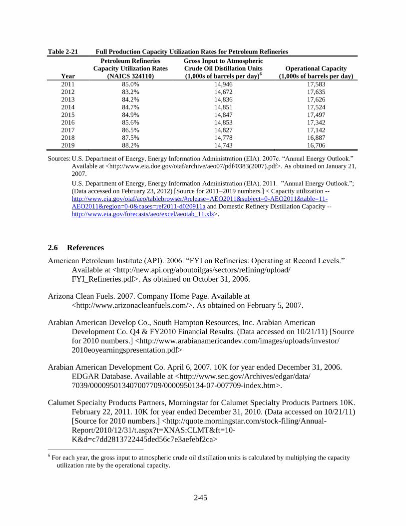
2- 45

Table 2-21 Full Production Capacity Utilization Rates for Petroleum Refineries

Year


Capacity Utilization Rates

(NAICS 324110)

Gross Input to Atmospheric

Crude Oil Distillation Units

(1,000s of barrels per day)6

Operational Capacity


2011 85.0% 14,946 17,583

2012 83.2% 14,672 17,635

2013 84.2% 14,836 17,626

2014 84.7% 14,851 17,524

2015 84.9% 14,847 17,497

2016 85.6% 14,853 17,342

2017 86.5% 14,827 17,142

2018 87.5% 14,778 16,887

2019 88.2% 14,743 16,706



2007.

U.S. Department of Energy, Energy Information Administration (EIA). 2011. ”Annual Energy Outlook.”;

(Data accessed on February 23, 2012) [Source for 2011–2019 numbers.] < Capacity utilization --

http://www.eia.gov/oiaf/aeo/tablebrowser/#release=AEO2011&subject=0-AEO2011&table=11-

AEO2011&region=0-0&cases=ref2011-d020911a and Domestic Refinery Distillation Capacity --

http://www.eia.gov/forecasts/aeo/excel/aeotab_11.xls>.

2.6 References

American Petroleum Institute (API). 2006. “FYI on Refineries: Operating at Record Levels.”

Available at <http://new.api.org/aboutoilgas/sectors/refining/upload/

FYI_Refineries.pdf>. As obtained on October 31, 2006.

Arizona Clean Fuels. 2007. Company Home Page. Available at

<http://www.arizonacleanfuels.com/>. As obtained on February 5, 2007.

Arabian American Develop Co., South Hampton Resources, Inc. Arabian American

Development Co. Q4 & FY2010 Financial Results. (Data accessed on 10/21/11) [Source

for 2010 numbers.] <http://www.arabianamericandev.com/images/uploads/investor/

2010eoyearningspresentation.pdf>

Arabian American Development Co. April 6, 2007. 10K for year ended December 31, 2006.

EDGAR Database. Available at <http://www.sec.gov/Archives/edgar/data/

7039/000095013407007709/0000950134-07-007709-index.htm>.

Calumet Specialty Products Partners, Morningstar for Calumet Specialty Products Partners 10K.

February 22, 2011. 10K for year ended December 31, 2010. (Data accessed on 10/21/11)

[Source for 2010 numbers.] <http://quote.morningstar.com/stock-filing/Annual-

Report/2010/12/31/t.aspx?t=XNAS:CLMT&ft=10-

K&d=c7dd2813722445ded56c7e3aefebf2ca>

6 For each year, the gross input to atmospheric crude oil distillation units is calculated by multiplying the capacity

utilization rate by the operational capacity.

http://www.eia.gov/oiaf/aeo/tablebrowser/#release=AEO2011&subject=0-AEO2011&table=11-AEO2011&region=0-0&cases=ref2011-d020911a

http://www.eia.gov/oiaf/aeo/tablebrowser/#release=AEO2011&subject=0-AEO2011&table=11-AEO2011&region=0-0&cases=ref2011-d020911a

http://www.eia.gov/forecasts/aeo/excel/aeotab_11.xls

2- 46

Calumet Specialty Products Partners. February 23, 2007. 10K for year ended December 31,

2006. EDGAR Database. Available at <http://www.sec.gov/Archives/edgar/data/

1340122/000095013407003992/h43776e10vk.htm>.

Copyright 2011 Experian Information Solutions, Inc., Experian Business Reports accessed

through LexisNexis at James Branch Cabell Library (Virginia Commonwealth

University).

Copyright 2011 Harte-Hanks Market Intelligence, Inc., All Rights Reserved. CI Technology

Database, September 2011.

CVR Energy Inc. 2006. Google Finance. Available at

<http://finance.google.com/finance?q=NYSE:CVI>. As obtained on February 28, 2008.

CVR Energy Inc., EDGAR database for CVR Energy Inc. 10K. March 7, 2011. 10K for year

ended December 31, 2010. (Data accessed on 10/23/11) [Source for 2010 numbers.]

<http://www.sec.gov/Archives/edgar/data/1376139/000095012311022741/y90110e10vk.

htm>

Dun & Bradstreet Small Business Solutions. Small Business Database. Available at

<http://smallbusiness.dnb.com/default.asp?bhcd2=1107465546>.

Dun & Bradstreet. 2007. 2007 D&B Million Dollar Directory. Pennsylvania: Dun & Bradstreet

Inc.

Energy Information Administration (EIA), Form EIA-820, “Annual Refinery Report.” Table 3.

Capacity of Operable Petroleum Refineries by State and Individual Refinery as of

January 1, 2011. (Data accessed on October 31, 2011.) [Source for 2009–2011 numbers.]

<http://www.eia.gov/petroleum/refinerycapacity/>

Federal Trade Commission (FTC). 2004. “The Petroleum Industry: Mergers, Structural Change,

and Antitrust Enforcement.” Available at <http://www.ftc.gov/opa/2004/08/

oilmergersrpt.shtm>. As obtained on February 6, 2007.

Gale Research Inc. 2007. Ward’s Business Directory of U.S. Private and Public Companies.

Detroit: Gale Research.

General Accounting Office (FTC). 2007. “Energy Markets: Factors That Influence Gasoline

Prices.” Available at <http://www.gao.gov/new.items/d07902t.pdf>. As obtained on

February 6, 2007.

Global Duns Market Identifiers, accessed through LexisNexis at University of Virginia’s

Alderman Library.

Holly Corporation. March 1, 2007. 10K for year ended December 31, 2006. EDGAR Database.

Available at <http://www.sec.gov/Archives/edgar/data/48039/000095013407004555/

d44106e10vk.htm>.

2- 47

Holly Corporation, EDGAR database for Holly Corporation 10K. February 25, 2011. 10K for

year ended December 31, 2010. (Data accessed on 10/23/11) [Source for 2010 numbers.]

<http://files.shareholder.com/downloads/FTO/1428853845x0xS950123-11-

18524/48039/filing.pdf>

Hoovers 2011 Online Data, accessed through University of South Carolina’s Moore School of

Business Library. Hoovers 2011 Online Data reflects either actual data for 2010/2011

reported by companies or estimated data for 2011.

Hoovers. 2007. Free Content, Company Information. Available at

<http://www.hoovers.com/free/>. As obtained on April 11, 2007.

Langinier, Corrine. 2004. “Are Patents Strategic Barriers to Entry?” Journal of Economics and

Business 56:349-361.

MathTech, Inc. 1997. “Industry Profile for the Petroleum Refinery NESHAP.” Available at

<http://www.epa.gov/ttnecas1/regdata/IPs/Petroleum%20Refinery%20

(Sulfur%20Recovery%20Units,%20Catalytic%20Crackin.pdf>. As obtained on October

31, 2006.

Million Dollar Database online, 2011, accessed through University of South Carolina’s Moore

School of Business Library. Million Dollar Online Data reflects either actual data for

2011 reported by companies or estimated data for 2011.

Nicholson, Walter. 2005. Microeconomic Theory: Basic Principles and Extensions. Mason, OH:

South-Western Publishing.

Oil & Gas Journal, September 21, 1992. K.S. Eble and J. Feathers, “Process Water Reuse, Part

I.” OGJ 1992a

Oil and Gas Journal, December 6, 2010

Petroleum Refinery Emissions Information Collection Request, Component 1, OMB Control No.

2060-0657


Oil and Gas Journal. April 7, 2008.Worldwide Construction Update.

Risk Management Association (RMA). 2008. Annual Statement Studies 2007-2008.


Risk Management Association (RMA). 2011. Annual Statement Studies 2010–2011.


2- 48

Reuters. July 19, 2007. “U.S. Refinery Expansion Plans.” Available at

<http://uk.reuters.com/article/oilRpt/idUKN199746120070719>. As obtained on

February 5, 2007.

Small Business Administration. 2011. Table of Small Business Size Standards. Available at <

http://www.sba.gov/sites/default/files/Size_Standards_Table.pdf>. As obtained October

2011.

Speight, James G. 2006. “The Chemistry and Technology of Petroleum.” 4th

Edition, page 178.

U.S. Bureau of Labor Statistics (BLS), 2011. “Producer Price Index Industry Data: Customizable

Industry Data Tables.” (Data accessed on October 11, 2011.) [Source for 2007–2010

numbers]<http://data.bls.gov/cgi-bin/dsrv?pc>.

U.S. Bureau of Labor Statistics (BLS). 2007. “Producer Price Index Industry Data: Customizable

Industry Data Tables.” Available at <http://www.bls.gov/ppi/>. As obtained on October

11, 2007.

U.S. Census Bureau, using American FactFinder; “Sector 31: Annual Survey of Manufacturers:

General Statistics: Statistics for Industry Groups and Industries: 2009 and 2008 “ Release

Date: 12/3/10 ; (Data accessed on 10/10/11). [Source for 2008 and 2009 numbers]

<http://factfinder.census.gov/servlet/IBQTable?_bm=y&-NAICSASM=324110&-

ds_name=AM0931GS101&-ib_type=NAICSASM&-_industry=324110&-_lang=en>

U.S. Census Bureau, using American FactFinder; “Sector 31: Manufacturing: Industry Series:

Detailed Statistics by Industry for the United States: 2007” Release Date 10/30/09; (Data

accessed on 10/11/11). [Source for 2007 numbers]

<http://factfinder.census.gov/servlet/IBQTable?_bm=y&-geo_id=01000US&-

ds_name=EC0731I1&-NAICS2007=324110&-_lang=en>

U.S. Census Bureau, using American FactFinder; “Sector 31: Manufacturing: Industry Series:

Materials Consumed by Kind for the United States: 2007” Release Date 10/30/09; (Data

accessed on 10/11/11). [Source for 2007 numbers] <http://factfinder.census.gov/

servlet/IBQTable?_bm=y&-ds_name=EC0731I3&-NAICS2007=324110&-

ib_type=NAICS2007&-geo_id=&-_industry=324110&-_lang=en&-

fds_name=EC0700A1>

U.S. Census Bureau, using American FactFinder; “Sector 31: Manufacturing: Subject Series:

Concentration Ratios: Share of Value of Shipments Accounted for by the 4, 8, 20, and 50

Largest Companies for Industries: 2007.” Release Date 1/7/2011; (Data accessed on

10/12/11) [Source for 2007 numbers]<http://factfinder.census.gov/

servlet/IBQTable?_bm=y&-ds_name=EC0731SR12&-NAICS2007=324110&-

ib_type=NAICS2007&-NAICS2007sector=*6&-industrySel=324110&-geo_id=&-

_industry=324110&-_lang=en>

2- 49

U.S. Department of Commerce, Bureau of the Census, FactFinder. 2011. 2009 Annual Survey of

Manufactures. 1996–2011. Obtained through American FactFinder Database. (Data

accessed on October 14, 2011.) [Source for 2007–2009 numbers]

<http://factfinder.census.gov/servlet/DatasetMainPageServlet?_lang=en&_ts=336651423

017&_ds_name=AM0931GS101&_program=EAS>.

U.S. Department of Commerce, Bureau of the Census. 1997. 1995 Annual Survey of

Manufacturers. M95(AS)-1. Washington, DC: Government Printing Office. Available at

<http://www.census.gov/prod/2/manmin/asm/m95as1.pdf>. As obtained on October 23,

2006.


Manufacturers. M96(AS)-1 (RV). Washington, DC: Government Printing Office.

Available at <http://www.census.gov/prod/3/98pubs/m96-as1.pdf>. As obtained on

October 23, 2006.

U.S. Department of Commerce, Bureau of the Census. 2000. “Population Density by County:

Census 2000 Summary File 1 (SF 1) 100-Percent Data”. Available through American

FactFinder <http://factfinder.census.gov/home/saff/main.html?_lang=en>. As obtained

on February 21, 2008.


Manufacturers. M99(AS)-1 (RV). Washington, DC: Government Printing Office.

Available at <http://www.census.gov/prod/2001pubs/m99-as1.pdf>. As obtained on

October 23, 2006.

U.S. Department of Commerce, Bureau of the Census. 2003a. 2001 Annual Survey of


<http://www.census.gov/prod/2003pubs/m01as-1.pdf>. As obtained on October 23, 2006.

U.S. Department of Commerce, Bureau of the Census. 2003b. 2001 Annual Survey of


<http://www.census.gov/prod/2003pubs/m01as-2.pdf. As obtained on March 4, 2008.

U.S. Department of Commerce, Bureau of the Census. 2004. 2002 Economic Census, Industry

Series—Petroleum Refineries. Washington, DC: Government Printing Office. Available

at <http://www.census.gov/prod/ec02/ec0231i324110.pdf>. As obtained on October 23,

2006.



<http://www.census.gov/prod/2005pubs/am0431gs1.pdf>. As obtained on October 23,

2006.


Manufacturers. Obtained through American Fact Finder Database


2- 50

U.S. Department of Energy, Energy Information Administration (EIA). 2012. “Petroleum &

Other Liquids, Weekly Imports & Exports.”

<http://www.eia.gov/dnav/pet/pet_move_wkly_dc_NUS-Z00_mbblpd_4.htm>.

U.S. Department of Energy, 2011 Energy Information Administration (EIA). 1996–2011.

“Petroleum Supply Annuals, Volume 1.” (Data accessed on October 7, 2011) [Source for

2007–2010 numbers.] <http://www.eia.gov/dnav/pet/pet_sum_snd_d_nus_

mbbl_a_cur.htm>.


“Petroleum Supply Annuals, Volume 1.” (Data accessed on October 7, 2011) [Source for

2007–2010 numbers.] <http://www.eia.gov/dnav/pet/pet_pnp_refp_dc_nus_

mbbl_a.htm>.


“Petroleum Supply Annuals, Volume 1.” (Data accessed on October 7, 2011.) [Source for

2007–2010 numbers.] <http://www.eia.gov/dnav/pet/pet_move_imp_dc_NUS-

Z00_mbbl_a.htm>



2007–2010 numbers] <http://www.eia.gov/dnav/pet/pet_move_exp_dc_NUS-

Z00_mbbl_a.htm>.



2007–2010 numbers.]<http://www.eia.gov/dnav/pet/pet_pri_refoth_dcu_nus_a.htm>.

U.S. Department of Energy, Energy Information Administration (EIA). 1996–2007. “Petroleum

Supply Annuals, Volume 1.” Available at <http://www.eia.doe.gov/oil_gas/

petroleum/data_publications/petroleum_supply_annual/psa_volume1/psa_

volume1.html>. As obtained on October 31, 2007.

U.S. Department of Energy, Energy Information Administration (EIA). 2006a. “A Primer on

Gasoline Prices.” Available at <http://www.eia.doe.gov/bookshelf/brochures/

gasolinepricesprimer/printerversion.pdf>. As obtained on October 31, 2007.

U.S. Department of Energy, Energy Information Administration (EIA). 1999a. “Petroleum: An

Energy Profile 1999.” DOE/EIA-0545(99). Available at <http://tonto.eia.doe.gov/

FTPROOT/petroleum/054599.pdf>. As obtained on October 23, 2006.

U.S. Department of Energy, Energy Information Administration (EIA). 2006b. “Refinery

Capacity Report 2006.” Available at <http://www.eia.doe.gov/oil_gas/petroleum/

data_publications/refinery_capacity_data/refcapacity.html/>. As obtained on October 23,

2006.

http://www.eia.gov/dnav/pet/pet_move_wkly_dc_NUS-Z00_mbblpd_4.htm

2- 51

U.S. Department of Energy, Energy Information Administration (EIA). 2006c. “Petroleum

Supply Annual 2005, Volume 1.” Available at <http://www.eia.doe.gov/pub/oil_gas/

petroleum/data_publications/petroleum_supply_annual/psa_volume1/historical/2005/psa

_volume1_2005.html>. As obtained on October 31, 2007.

U.S. Department of Energy, Energy Information Administration (EIA). 2007a. “Refinery

Utilization and Capacity.” Available at <http://tonto.eia.doe.gov/dnav/pet/

pet_pnp_unc_dcu_nus_m.htm>. As obtained on January 7, 2008.

U.S. Department of Energy, Energy Information Administration (EIA). 2007b. “Refiner

Petroleum Product Prices by Sales Type.” Available at <http://tonto.eia.doe.gov/

dnav/pet/pet_pri_refoth_dcu_nus_m.htm>. As obtained on January 11, 2008.

U.S. Department of Energy, Energy Information Administration (EIA). 2007c. “Annual Energy

Outlook.” Available at <http://www.eia.doe.gov/oiaf/archive/aeo07/pdf/0383(2007).pdf>.

As obtained on January 21, 2007.

U.S. Department of Energy, Energy Information Administration (EIA). 2010. “Petroleum Supply

Annual 2010, Volume 1.” Available at

http://www.eia.gov/petroleum/supply/annual/volume1/archive/2010/pdf/table15.pdf.

U.S. Department of Energy, Energy Information Administration (EIA). 2011, “Annual Energy

Outlook.” (Data accessed on October 11, 2011) [Source for 2011–2019

numbers.]<http://www.eia.gov/forecasts/aeo/pdf/0383(2011).pdf>.

U.S. Department of Justice and the Federal Trade Commission. 1992. Horizontal Merger

Guidelines. Available at <http://www.ftc.gov/bc/docs/horizmer.htm>. As obtained on

October 28, 2006.

U.S. Department of Labor, Occupational Safety and Health Administration (OSHA). 2003.

OSHA Technical Manual, Section IV: Chapter 2, Petroleum Refining Processes. TED 01-

00-015. Washington, DC: U.S. DOL. Available at <http://www.osha.gov/dts/osta/

otm/otm_iv/otm_iv_2.html>. As obtained on October 23, 2006.

U.S. Energy Information Administration (EIA), 2011a. “Refinery Utilization and Capacity.”

Available at http://www.eia.gov/dnav/pet/pet_pnp_unc_dcu_nus_a.htm; Release date:

7/28/11; (Data accessed on 10/11/11). [Source for 2007–2010 numbers]

U.S. Energy Information Administration (EIA), Form EIA-820, “Annual Refinery Report. Table

1. Number and Capacity of Operable Petroleum Refineries by PAD District and State as

of January 1, 2011” Release Date: June 24, 2011; (Data accessed on 10/12/11). [Source

for 2011 numbers.] <http://www.eia.gov/petroleum/refinerycapacity/>

U.S. Environmental Protection Agency. 1995. “EPA Office of Compliance Sector Notebook

Project: Profile of the Petroleum Refining Industry.” EPA/310-R-95-013. Washington,

DC: U.S. EPA. Available at <http://www.epa.gov/compliance/resources/

publications/assistance/sectors/notebooks/petrefsn.pdf>. As obtained on October 23,

2006.

http://www.eia.gov/petroleum/supply/annual/volume1/archive/2010/pdf/table15.pdf

2- 52

U.S. Environmental Protection Agency. 2006. “Proposed MHA Nation Clean Fuels Refinery.”

Available at <http://www.epa.gov/Region8/compliance/nepa/refinerydeis.html>. As

obtained on February 6, 2007.

Ward’s Business Directory of Public and Private Companies, 2011, accessed at James Branch

Cabell Library (Virginia Commonwealth University).

Western Refining, Inc. March 8, 2007. 10K for year ended December 31, 2006. EDGAR

Database. Available at <http://www.sec.gov/Archives/edgar/data/1339048/000095

013407005096/h44360e10vk.htm>.

Western Refining, Thomson Reuters Western Refining, Inc. 10K. March 8, 2011. 10K for year

ended December 31, 2010. (Data accessed on 10/23/11) [Source for 2010 numbers.]

<http://phx.corporate-ir.net/phoenix.zhtml?c=194293&p=irol-sec>

3- 1

3 NSPS REGULATORY OPTIONS, COSTS AND EMISSION REDUCTIONS

FROM COMPLYING WITH THE NSPS

The emissions reduction and cost impacts presented in this section for flares are revised

estimates for the impacts of the final requirements of 40 CFR part 60, subpart Ja for flares, as

amended by this action. The impacts are expressed as incremental differences between the

impacts of petroleum refinery process units complying with these final amendments to subpart Ja

and the final June 2008 NSPS requirements of 40 CFR part 60, subpart Ja (i.e., baseline). The

impacts are presented for petroleum refinery flares that commence construction, reconstruction

or modification over the next 5 years. We anticipate that there will be 400 affected flares over the

next 5 years and most of the flares would become affected due to the modification provisions for

flares in subpart Ja. For this analysis we assumed 90 percent of the flares would be modified or

reconstructed and 10 percent of the flares would be newly constructed.

Further, we estimate that 30 percent of the 400 affected flares, or 120 flares, either would

meet the definition of “emergency flare” in 40 CFR part 60, subpart Ja or would be equipped

with a flare gas recovery system such that robust sulfur and flow monitoring would not be

required. Therefore, the values presented in this section include the costs and emissions

reductions for 400 flares to comply with the flare management plan and root cause and corrective

action analyses requirements and for 280 flares to comply with the sulfur and flow monitoring

requirements. The cost and emissions reductions for the affected flares to comply with the short-

term H2S concentration of 162 ppmv in the fuel gas are included in the baseline rather than the

incremental impacts because this limit is unchanged from the requirements in subpart J. For

further detail on the methodology of these calculations, see the January 25, 2012 memorandum

entitled “Impact Estimates for Fuel Gas Combustion Device and Flare Regulatory Options for

Amendments to the Petroleum Refinery NSPS”, in Docket ID No. EPA-HQ-OAR-2007-0011.

We estimate that the final requirements for flares will reduce emissions of SO2 by 3,200

tons per year (tons/yr), NOx by 1,100 tons/yr, VOC by 3,400 tons/yr, and CO2 by 1,900,000

metric tons/yr from the baseline. The estimated annual cost, including annualized capital costs

for flare gas recovery systems, is $96 million (2006 dollars). The total annual savings from

offset natural gas purchases and product recovery credits that arise as a result of complying with

3- 2

the rule are estimated at $180 million. The estimated net annual cost is a cost savings of $79

million (2006 dollars). Note that not all refiners will realize a cost savings as only flare systems

with high waste gas flows (about 10% of all flares) are expected to install vapor recovery

systems. The overall cost effectiveness is a cost savings of about $10,000 per ton of combined

pollutants (excluding CO2) removed. The estimated nationwide 5-year incremental emissions

reductions and cost impacts for the final standards are summarized in Tables 3-1 and 3-2 below.

Table 3-1. National Cost Impacts for Petroleum Refinery Flares Subject to Amended

Standards Under 40 CFR part 60, subpart Ja (Fifth Year After the Effective Date of the

Final Rule Amendments)

Subpart Ja Requirements

Total capital

cost ($1,000)

Total annual

cost without

credit

($1,000/yr)

Natural gas

offset/ product

recovery credit

($1,000)

Total Annual

Cost ($1,000/

yr)

Estimates from June 2008 Final

Rule 40,000

(7,000)

Total for Revised Estimates for

Amendments 460,000 96,000 (180,000) (79,000)

Flare Monitoring 84,000 14,000 0 14,000

Flare Gas Recovery7 380,000 78,000 (170,000)

(90,000)

Flare Management Plans -- 880 -- 880

SO2 Root Cause

Analysis/Corrective Action -- 2,200 -- 2,200

Flow Rate Root Cause Analysis/ Corrective Action

-- 1,000 (7,400) (6,400)

Note: Costs presented in this table are estimated relative to the baseline used for the 2008 NSPS impacts analysis.

Additionally, totals may not sum due to independent rounding.

7 Forty flare systems are estimated to have sufficient waste gas to install recovery systems.

3- 3

Table 3-2. National Emission Reductions and Cost-Effectiveness for Petroleum Refinery

Flares Subject to Amended Standards Under 40 CFR part 60, subpart Ja (Fifth Year After

the Effective Date of the Final Rule Amendments)

Subpart Ja Requirements

Annual

emission

reductions

(tons SO2/yr)

Annual

emission

reductions

(tons NOx/yr)

Annual

emission

reductions

(tons

VOC/yr)

Cost

effectiveness

($/ton

emissions

reduced)

Annual

emission

reductions

(metric tons

CO2/yr)

Estimates from June 2008

Final Rule 80 6 200 (23,000)

--

Total for Revised Estimates

for Amendments 3,200 1,100 3,400 (10,000) 1,900,000

Flare Monitoring 0 0 0 -- --

Flare Gas Recovery 380 1,100 2,700 (22,000) 1,800,000

Flare Management Plans 0 0 300 2,900 --

SO2 Root Cause Analysis/Corrective Action

2,900 0 0 760 --

Flow Rate Root Cause Analysis/

Corrective Action 3.4 56 430 (13,000) 98,000

Alternatively, if no refineries install flare gas recovery systems, the final requirements for

flares would reduce emissions of SO2 by 2,820 tons/yr, NOx by 56 tons/yr, VOC by 730 tons/yr,

and CO2 by 98,000 metric tons/yr from the baseline. The estimated annual cost would be about

$10.7 million (2006 dollars).

The provisions for flares and other fuel gas combustion devices (i.e., process heaters and

boilers) from the final June 2008 standards were stayed. The analysis for this final rule includes

the same unit costs for the flare provisions as the final June 2008 rule but reflects recalculated

total costs using data collected in the March 2011 ICR to update the number of flares.8 Table 3-1

includes the recalculated cost estimates for flares, broken out by specific flare requirements,

based on the updated number of flares. For the other fuel gas combustion devices, the total

annualized costs for those provisions were estimated at $24 million (2006 dollars) in the June

2008 rule and remain the same. As discussed below, because there are no additional incremental

costs associated with the other fuel gas combustion device provisions, we consider those annual

costs accounted for in the final June 2008 standards. We are presenting them here again, even

8 For the June 2008 standards we estimated 40 flares. As indicated, for this analysis we anticipate that there will be

400 affected flares that will be subject to this final rule.

3- 4

though we estimate no changes to these costs, since these provisions will become effective upon

this final action to lift the stay on certain provisions in the June 2008 rule.

The cost, environmental and economic impacts for the final amendments to 40 CFR part

60, subpart Ja for process heaters are not expected to be different than those reported for the final

June 2008 standards. We expect owners and operators to install the same technology to meet

these final amendments that we anticipated they would install to meet the June 2008 final subpart

Ja requirements (i.e., ultra-low NOx burners). We did revise our emissions estimates based on the

type of process heater, creating separate impacts for forced draft process heaters and natural draft

process heaters. Dividing process heaters into separate subcategories, based on the draft type,

required us to develop new distributions of baseline emissions for each type of process heater.

The baseline emissions estimates for natural draft process heaters are slightly lower than those

developed for the existing subpart Ja requirements (per affected process heater), but the average

emission reduction achieved by ultra-low NOx burners was adjusted to 80 percent (rather than 75

percent used for generic process heaters). For forced draft process heaters, the baseline (i.e.,

uncontrolled) emissions rate for forced draft process heaters was revised slightly upward, based

on the available emissions data. Because of these differences, the mix of controls needed to meet

a 40 ppmv emissions limit was no longer cost effective for forced draft process heaters, but the

emission reductions associated with process heaters complying with the 60 ppmv standard were

higher than those previously estimated for generic process heaters. Thus, the creation of new

subcategories of process heaters with different emissions limits for each subcategory did not

impact the control or compliance methods used by the facilities (i.e., BSER in all cases was

based on the performance of advanced combustion monitoring controls in conjunction with ultra-

low NOx burners) and did not change the estimated compliance costs. As we do not have

adequate data regarding the prevalence of natural draft process heaters versus forced draft

process heaters that will become subject to the rule, we used the emission reductions estimated

for the two different types of process heaters as a means to bound the range of anticipated NOx

emission reductions to be from 7,100 to 8,600 tons/yr in the fifth year after promulgation (see

Revised NOx Impact Estimates for Process Heaters, in Docket ID No. EPA-HQ-OAR-2007-

0011). We estimated the emission reductions to be 7,500 tons/yr for the June 2008 final

standards, which falls well within the anticipated range of emissions reductions for the standards

3- 5

we are finalizing here. Given the uncertainty in the emissions estimates, as well as the

uncertainty in the relative number of natural draft process heaters versus forced draft process

heaters, we concluded that the impacts previously developed for subpart Ja accurately represent

the impacts for process heaters in these final amendments.

We note that, in the preamble to the June 2008 final standards, we estimated costs and

emissions reductions for 30 fuel gas combustion devices, but we subsequently determined that

those estimates did not fully account for the number of affected flares (which, at the time, were

considered a subset of fuel gas combustion devices). Therefore, in the preamble to the December

2008 proposed amendments, we presented revised emission reduction and cost estimates for

affected fuel gas combustion devices. Because these final amendments consider flares to be a

separate affected source, the emission reductions and costs for fuel gas combustion devices are

not affected by these final amendments and are not included in this action. Rather, the final

emission reduction and cost estimates for fuel gas combustion devices are very close to the

impacts presented in the June 2008 final rule; the details of the analysis and the final impacts are

presented in the January 25, 2012 memorandum entitled “Impact Estimates for Fuel Gas

Combustion Device and Flare Regulatory Options for Amendments to the Petroleum Refinery

NSPS”, in Docket ID No. EPA-HQ-OAR-2007-0011.

The final amendments to 40 CFR part 60, subpart J are technical corrections or

clarifications to the existing rule and should have no negative emissions impacts.

4-1

4 ECONOMIC IMPACT ANALYSIS: METHODS AND RESULTS

4.1 Introduction

The economic impact analysis (EIA) is designed to inform decision makers about the

potential economic consequences of a regulatory action. An economic welfare analysis

estimates the social costs and consumer and producer surplus changes associated with a

regulatory program. The welfare analysis identifies how the regulatory costs are distributed

across the two broad classes of stakeholders -- consumers and producers. As defined in EPA’s

(2010) Guidelines for Preparing Economic Analyses,9 social costs are the value of the goods and

services lost by society resulting from using resources to comply with and implement a

regulation. In addition, national engineering compliance cost estimates can be used to

approximate the welfare impacts of a regulatory program.

Because the proposed amendments apply to new or modifying sources, we are not able to

predict which specific sources will trigger applicability. Also, assuming no refineries install fuel

gas recovery systems, the estimated, incremental annual costs would be about $10.7 million

(2006 dollars), which represents substantially less than 0.001% of total refinery industry

revenues in 2010. If we assume a full cost pass through, we do not anticipate any resulting price

increases. As such, we did not employ a detailed economic model to estimate the social costs of

the proposed amendments, nor to estimate the social cost distribution across stakeholders. For

this rule, based on our analysis and an estimated annual cost savings of $79 million (2006

dollars) expected in the fifth year, no national-level negative economic impacts are expected.

The remainder of this section includes a discussion of why firms may consider installing flare

gas recovery systems, as well as the small business impact analysis.

4.2 Compliance Costs Estimates

As indicated in Section 3, we estimate there are approximately 500 flares industry-wide,

and about 80 percent, or 400 flares, would be subject to the proposed amendments over the next

five years. We further estimate that it would be cost-effective to install compressors and

9 These guidelines are currently under review by the Agency.

4-2

recovery systems at 10 percent of the 400 flares, or at approximately 40 flares. We assume that a

flare gas recovery system would be considered for flares with average releases greater than

500,000 scf per 24-hour period. And while we do not have current data on where all of the

potential 40 flares are located, data from the 2002 National Emissions Inventory indicate the

flares are likely located at large refineries.10

The total annualized engineering compliance costs are estimated at $96 million, and the

estimated annual savings from offset natural gas purchases and product recovery credits are

estimated at $180 million, giving rise to the net annual savings of $79 million discussed in

Section 3. These costs can be broken down into costs required by the rule and costs that are not

required by the rule. The annualized compliance costs for actions required by the rule are

estimated at $18 million, and the estimated savings from product recovery credits is $7.4 million.

Using these figures, we estimate the implied rate of return for actions required by the rule to be

about -60 percent. Meanwhile, the annualized compliance costs for actions not required by the

rule are estimated at $78 million, and the estimated savings from offset natural gas purchases is

$168 million. Using these figures, we estimate the implied rate of return for actions not required

by the rule to be about 120 percent and the overall rate of return to be about 90 percent. The

actual industry-level rate of return varies greatly over time because of industry and economic

factors. See Table 4-1 for refinery rates of return on investment from 2000 through 2009. It is

readily observed that the rate of return related to the pollution control equipment and activities

by this rule exceeds that of the rate of return associated with investments in the refining sector.

Table 4-1 Rates of Return on Investment for Refineries

2000 2001 2002 2003 2004 2005 2006 2007 2008 2009

Rate of Return on

Investment 9.6 14.5 (1.7) 9.3 18.4 23.2 25.3 21.2 2.4 (6.6)

(EIA 2009)

10

For details on where flares of this size were located as of the 2002 National Emissions Inventory, see Appendix A

of the January 25, 2012 memorandum entitled “Impact Estimates for Fuel Gas Combustion Device and Flare

Regulatory Options for Amendments to the Petroleum Refinery NSPS.”

4-3

Assuming financially rational producers, standard economic theory suggests that

refineries would incorporate all cost-effective improvements, which they are aware of, without

government intervention. The cost analysis of this RIA nevertheless is based on the observation

that process actions (i.e., installation of a flare gas recovery system) that appear to be profitable

in our analysis have not been widely adopted. One explanation for why there appears to be

negative cost control technologies that are not generally adopted is imperfect information. If

process improvements in the refining sector are not well understood, firms may underestimate

the potential financial returns to those improvements. Another explanation is the cost associated

with the irreversibility of implementing these process improvements is not reflected in the

engineering cost estimates. Because of the high volatility of natural gas prices, it is important to

recognize the value of flexibility taken away from firms when requiring them to install and use a

particular process technology.

If a firm has not adopted the technology on its own, then a regulation encouraging its use

means the firm may require reprioritizing other non-environmental investments. Although the

rule does not specifically require installation of flare gas recovery systems, we anticipate that

owners and operators of flares receiving high waste gas flows will conclude, upon installation of

monitors, implementation of their flare management plans, and implementation of root causes

analyses, that installing flare gas recovery would result in fuel savings by using the recovered

flare gas where purchased natural gas is now being used to fire equipment such as boilers and

process heaters. The flare management plan requires refiners to conduct a thorough review of

the flare system so that flare gas recovery systems are installed and used where these systems are

warranted. As part of the development of the flare management plan, refinery owners and

operators must provide rationale and supporting evidence regarding the flare waste gas reduction

options considered, the quantity of flare gas that would be recovered or prevented by the option,

the BTU content of the flare gas and the ability or inability of the reduction option to offset

natural gas purchases. In addition, regulatory requirements imply firms are unable to suspend

use of the technology if it becomes unprofitable in the future. Therefore, the true cost of the

regulation should include the lost option value, as well as the engineering costs. In the absence

of quantitative estimates of this option value, the costs presented in this RIA may underestimate

the full costs faced by the affected firms.

4-4

4.3 Small Business Impact Analysis

The Regulatory Flexibility Act (RFA) as amended by the Small Business Regulatory

Enforcement Fairness Act (SBREFA) generally requires an agency to prepare a regulatory

flexibility analysis of any rule subject to notice and comment rulemaking requirements under the

Administrative Procedure Act or any other statute, unless the agency certifies that the rule will

not have a significant economic impact on a substantial number of small entities. Small entities

include small businesses, small governmental jurisdictions, and small not-for-profit enterprises.

The petroleum refining industry (NAICS code 324110) does not include small governmental

jurisdictions or small not-for-profit enterprises. For this analysis we applied the Small Business

Administration’s small refiner definition of a refinery with no more than 1,500 employees (SBA,

2011). For additional discussion of the Agency’s application of the definition for small refiner,

see the June 24, 2008 Federal Register Notice for 40 CFR Part 60, Standards of Performance for

Petroleum Refineries (Volume 73, Number 122, page 35858).11

4.3.1 Small Entity Economic Impact Measures

The analysis provides EPA with an estimate of the magnitude of impacts that the

provisions of the proposed standards may have on the ultimate domestic parent companies that

own the small refineries. This section references the data sources used in the screening analysis

and presents the methodology we applied to develop estimates of impacts, the results of the

analysis, and conclusions drawn from the results.

The small business impacts analysis for Subpart Ja New Source Performance Standards

amendments rely upon data collected through the March 2011 Information Collection Request

(ICR -- OMB Control No. 2060-0657). Information collected through component 1 of the ICR

includes facility location, products produced, capacity, throughput, process and emissions, and

employment and sales receipt data. EPA performed a screening analysis for impacts on all

affected small refineries by comparing compliance costs to revenues at the parent company level.

This is known as the cost-to-revenue or cost-to-sales ratio, or the “sales test.” The “sales test” is

11

Refer to http://www.sba.gov/sites/default/files/Size_Standards_Table.pdf for more information on SBA small

business size standards.

4-5

the impact methodology EPA employs in analyzing small entity impacts as opposed to a “profits

test,” in which annualized compliance costs are calculated as a share of profits. The sales test is

frequently used because revenues or sales data are commonly available for entities impacted by

EPA regulations, and profits data normally made available are often not the true profit earned by

firms because of accounting and tax considerations. The use of a “sales test” for estimating

small business impacts for a rulemaking is consistent with guidance offered by EPA on

compliance with the RFA12 and is consistent with guidance published by the U.S. SBA’s Office

of Advocacy that suggests that cost as a percentage of total revenues is a metric for evaluating

cost increases on small entities in relation to increases on large entities (U.S. SBA, 2010).13

4.3.2 Small Entity Economic Impact Analysis

As discussed in Section 2 of this RIA, as of January 2011 there were 148 petroleum

refineries operating in the continental United States and US territories with a cumulative capacity

of processing over 17 million barrels of crude per calendar day (EIA, 2011b). Sixty-four (64)

parent companies own these refineries, and EPA has employment and sales data for 61 (95%) of

the parent companies. Thirty-six (36) companies (59% of the 61 total) employ fewer than 1,500

workers and are considered small businesses. These firms earned an average of $1.36 billion of

revenue per year, while firms employing more than 1,500 employees earned an average of $82.5

billion of revenue per year.14

12

The RFA compliance guidance to EPA rule writers regarding the types of small business analysis that should be

considered can be found at <http://www.epa.gov/sbrefa/documents/rfaguidance11-00-06.pdf> 13

U.S. SBA, Office of Advocacy. A Guide for Government Agencies, How to Comply with the Regulatory

Flexibility Act, Implementing the President’s Small Business Agenda and Executive Order 13272, June 2010. 14 The U.S. Census Bureau’s Statistics of U.S. Businesses include the following relevant definitions: (i)

establishment – a single physical location where business is conducted or where services or industrial operations

are performed; (ii) firm – a firm is a business organization consisting of one or more domestic establishments in the

same state and industry that were specified under common ownership or control. The firm and the establishment are

the same for single-establishment firms. For each multi-establishment firm, establishments in the same industry

within a state will be counted as one firm; and (iii) enterprise -- an enterprise is a business organization consisting

of one or more domestic establishments that were specified under common ownership or control. The enterprise and

the establishment are the same for single-establishment firms. Each multi-establishment company forms one

enterprise.

4-6

Based on data collected through the March 2011 ICR, EPA performed the sales test

analysis for impacts on affected small refineries. Four of the 36 small refiners were removed

from the analysis because we determined they were not major sources and would not be subject

to the rules, and one of the 36 small refiners (Gulf Atlantic Operations) was not analyzed

because we had no ICR and/or other publically available employment and sales data.

While we estimated the natural gas recovery offsets or credit at a national level and

believe that larger firms are more likely to offset natural gas purchases, the revenues from natural

gas recovery offsets might mask disproportionate impacts on small refiners. At present to better

identify disproportionate impacts, we examined the potential impacts on refiners based on a

scenario where no firms adopt flare gas recovery systems and comply with the NSPS through

flare monitoring and flare management and root cause analysis actions. Refer to Tables 3-1 and

3-2 in the prior Section for details on the costs and emissions reductions associated with each of

the potential compliance actions. Table 4-2 presents the distribution of estimated cost-to-sales

ratios for the small firms in our analysis. The incremental compliance costs imposed on small

refineries are not estimated to create significant impacts on a cost-to-sales ratio basis at the firm

level.

Table 4-2 Impact Levels of Proposed NSPS Amendments on Small Firms

Impact Level

Number of Small Firms in

Sample Estimated to be

Affected

% of Small Firms in

Sample Estimated to be

Affected

Cost-to-Sales Ratio less than 1% 31 100%

Cost-to-Sales Ratio 1-3% 0 --

Cost-to-Sales Ratio greater than 3% 0 --

For comparison, we calculated the cost-to-sales ratios for all of the affected refineries to

determine whether potential costs would have a more significant impact on small refineries. As

presented in Table 4-3, for all large firms, the average cost-to-sales ratio is less than 0.01

percent; the median cost-to-sales ratio is less than 0.01 percent; and the maximum cost-to-sales

ratio is 0.02 percent. For small firms, the average cost-to-sales ratio is about 0.06 percent, the

median cost-to-sales ratio is 0.02 percent, and the maximum cost-to-sales ratio is 0.63 percent.

While the potential costs show a somewhat larger impact on small refiners, the impacts on small

refiners are not significant. Because no small firms are expected to have cost-to-sales ratios

4-7

greater than one percent, we determined that the cost impacts for Subpart Ja New Source

Performance Standards amendments will not have a significant economic impact on a substantial

number of small entities (SISNOSE).

Table 4-3 Summary of Sales Test Ratios for Firms Affected by Proposed NSPS Amendments

Firm Size

No. of Known

Affected Firms

% of Total Known

Affected Firms

Mean Cost-to-Sales

Ratio

Median Cost-to-

Sales Ratio

Min.

Cost-to-

Sales

Ratio

Max. Cost-

to-Sales

Ratio

Small 31 55% 0.06% 0.02% <0.01% 0.63%

Large 25 45% <0.01% <0.01% <0.01% 0.02%

All 56 100% 0.02% <0.01% <0.01% 0.63%

4-8

4.4 References

U.S. Department of Energy, 2009 Energy Information Administration (EIA). “Performance

Profiles of Major Energy Producers 2009.” (Data accessed on March 5, 2012.)

<http://www.eia.gov/cfapps/frs/frstables.cfm?tableNumber=9>

U.S. Environmental Protection Agency, 2010. Guidelines for Preparing Economic Analyses,

EPA 240-R-10-001. <http://yosemite.epa.gov/ee/epa/eed.nsf/pages/Guidelines.html>

Accessed on: 11/14/11.

http://yosemite.epa.gov/ee/epa/eed.nsf/pages/Guidelines.html

5-

1

5 EXECUTIVE ORDERS

5.1 Unfunded Mandates

This rule does not contain a Federal mandate that may result in expenditures of $100

million or more for State, local, and tribal governments, in the aggregate, or the private sector in

any one year. The costs of the final amendments would not increase costs associated with the

final rule. Thus, this rule is not subject to the requirements of sections 202 or 205 of the

Unfunded Mandates Reform Act of 1995 (UMRA).

This rule is also not subject to the requirements of section 203 of UMRA because it

contains no regulatory requirements that might significantly or uniquely affect small

governments. The proposed amendments contain no requirements that apply to such

governments, and impose no obligations upon them.

5.2 Environmental Justice

Executive Order 12898 (59 FR 7629, February 16, 1994) establishes Federal executive

policy on environmental justice. Its main provision directs Federal agencies, to the greatest

extent practicable and permitted by law, to make environmental justice part of their mission by

identifying and addressing, as appropriate, disproportionately high and adverse human health or

environmental effects of their programs, policies, and activities on minority populations and low-

income populations in the United States.

EPA has determined that this final rule will not have disproportionately high and adverse

human health or environmental effects on minority or low-income populations because it

increases the level of environmental protection for all affected populations without having any

disproportionately high and adverse human health or environmental effects on any population,

including any minority or low-income population. This rule is a nationwide standard that will

yield reductions in various criteria pollutant emissions from new, modified, and reconstructed

process heaters and flares at petroleum refineries, thus decreasing the amount of such emissions

to which all affected populations are exposed.

5.3 Significant Energy Actions

These proposed amendments do not represent a “significant energy action” as defined in

Executive Order 13211, “Actions Concerning Regulations That Significantly Affect Energy

Supply, Distribution, or Use” (66 FR 28355 [May 22, 2001]) because they are not likely to have

5-

2

a significant adverse effect on the supply, distribution, or use of energy. Assuming no refineries

install a flare gas recovery system, the estimated annualized compliance costs for the proposed

requirements are substantially less than 0.001% of total refinery industry revenues in 2010.

Assuming a full cost pass through, we do not anticipate any resulting price increases, and we

estimate there will be no significant increase in our dependence on foreign energy supplies.

Finally, today’s action will have no adverse effect on crude oil supply, coal production,

electricity production, and energy distribution. Based on the findings from the analysis of

impacts on energy markets, we conclude that today’s action is not a “significant energy action”

as defined in Executive Order 13211.

6-1

6 HUMAN HEALTH BENEFITS OF EMISSIONS REDUCTIONS

Synopsis

In this section, we provide an estimate of the monetized benefits for the final Petroleum

Refineries NSPS Reconsideration associated with reducing exposure to ambient particulate

matter (PM) by reducing emissions of PM2.5 precursors including SO2, NOx, and VOCs, as well

as climate benefits associated with reducing emissions of CO2. SO2, NOx, and VOCs are

precursors to PM2.5, and NOx and VOCs are precursors to ozone. These estimates reflect the

monetized human health benefits of reducing cases of morbidity and premature mortality among

populations exposed to PM2.5 reduced by this reconsideration. We estimate the total monetized

benefits to be $260 million to $580 million at a 3% discount rate and $240 million to $520

million at a 7% discount rate. All estimates are in 2006$ in the year 2017.

These estimates reflect EPA’s most current interpretation of the scientific literature.

Higher or lower estimates of benefits are possible using other assumptions; examples of this are

provided in Figure 6-2 on page 6-14). Data, resource, and methodological limitations prevented

EPA from monetizing the benefits from several important benefit categories, including benefits

from reducing direct exposure to NO2 and SO2, ozone exposure, ecosystem effects, and visibility

impairment.

6.1 Calculation of PM2.5-Related Human Health Benefits

This final NSPS Reconsideration would reduce emissions of SO2, NOX, and VOCs.

Because these emissions are precursors to PM2.5, reducing these emissions would also reduce

PM2.5 formation, human exposure and the incidence of PM2.5-related health effects. Due to

analytical limitations, it was not possible to provide a comprehensive estimate of PM2.5-related

benefits or provide estimates of the health benefits associated with direct exposure to SO2 and

NOx or exposure to ozone. Instead, we used the “benefit-per-ton” approach to estimate these

benefits. The methodology employed in this analysis is similar to the work described in Fann,

Fulcher, and Hubbell (2009), but represents an improvement that EPA believes will provide

more reliable estimates of PM2.5-related health benefits for emissions reductions in specific

sectors. The key assumptions are described in detail below. These PM2.5 benefit-per-ton

estimates provide the total monetized human health benefits (the sum of premature mortality and

premature morbidity) of reducing one ton of PM2.5 from a specified source. EPA has used the

6-2

benefit per-ton technique in several previous RIAs, including the recent SO2 NAAQS RIA (U.S.

EPA, 2010).

The Integrated Science Assessment (ISA) for Particulate Matter (U.S. EPA, 2009b)

identified the human health effects associated with ambient PM2.5, which include premature

morality and a variety of morbidity effects associated with acute and chronic exposures. Table 6-

1 shows the quantified and unquantified benefits captured in those benefit-per-ton estimates, but

this table does not include entries for the unquantified health effects associated with exposure to

ozone, SO2, and NOx nor welfare effects such as ecosystem effects and visibility that are

described in section 6.2. It is important to emphasize that the list of unquantified benefit

categories is not exhaustive, nor is quantification of each effect complete.

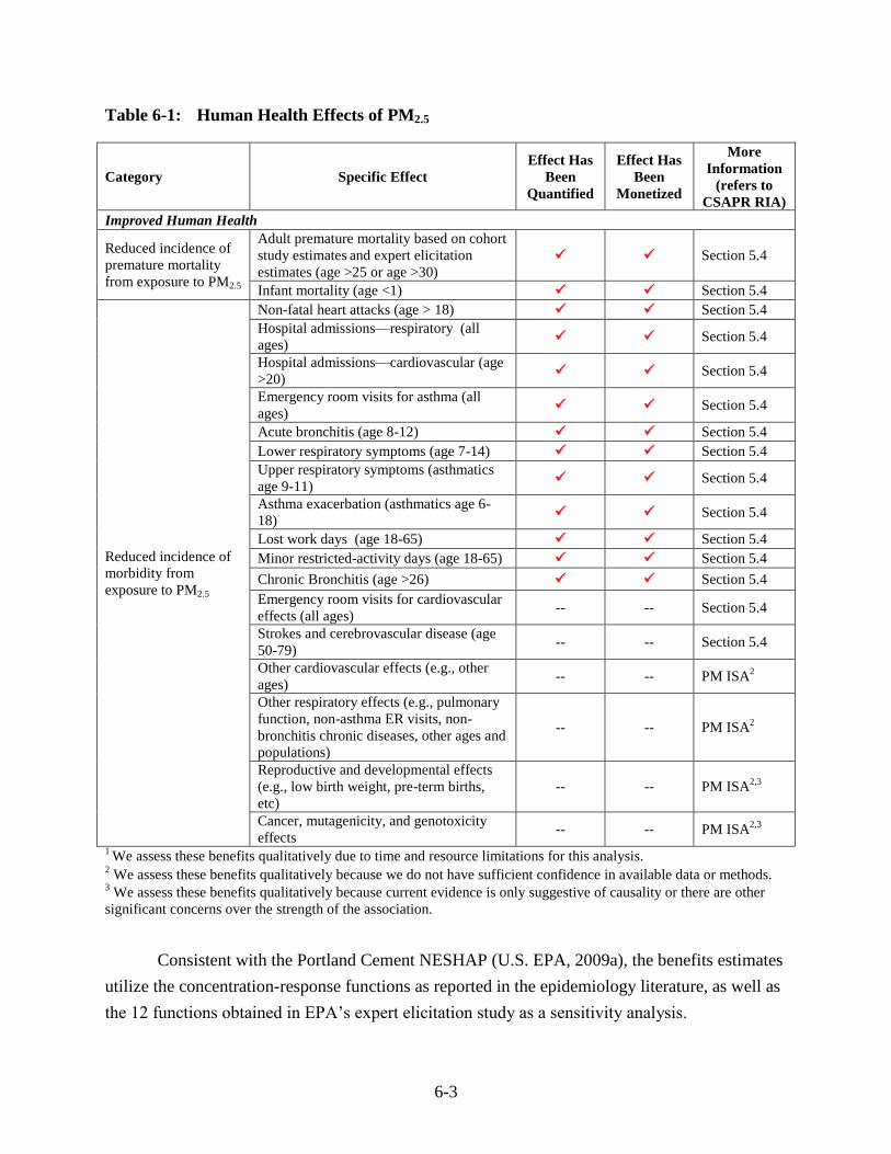
6-3

Table 6-1: Human Health Effects of PM2.5

Category Specific Effect

Effect Has

Been

Quantified

Effect Has

Been

Monetized

More

Information

(refers to

CSAPR RIA)

Improved Human Health

Reduced incidence of

premature mortality

from exposure to PM2.5

Adult premature mortality based on cohort

study estimates and expert elicitation

estimates (age >25 or age >30)

Section 5.4

Infant mortality (age <1) Section 5.4

Reduced incidence of

morbidity from

exposure to PM2.5

Non-fatal heart attacks (age > 18) Section 5.4

Hospital admissions—respiratory (all

ages) Section 5.4

Hospital admissions—cardiovascular (age

>20) Section 5.4

Emergency room visits for asthma (all

ages) Section 5.4

Acute bronchitis (age 8-12) Section 5.4

Lower respiratory symptoms (age 7-14) Section 5.4

Upper respiratory symptoms (asthmatics

age 9-11) Section 5.4

Asthma exacerbation (asthmatics age 6-

18) Section 5.4

Lost work days (age 18-65) Section 5.4

Minor restricted-activity days (age 18-65) Section 5.4

Chronic Bronchitis (age >26) Section 5.4

Emergency room visits for cardiovascular

effects (all ages) -- -- Section 5.4

Strokes and cerebrovascular disease (age

50-79) -- -- Section 5.4

Other cardiovascular effects (e.g., other

ages) -- -- PM ISA

2

Other respiratory effects (e.g., pulmonary

function, non-asthma ER visits, non-

bronchitis chronic diseases, other ages and

populations)

-- -- PM ISA2

Reproductive and developmental effects

(e.g., low birth weight, pre-term births,

etc)

-- -- PM ISA2,3

Cancer, mutagenicity, and genotoxicity

effects -- -- PM ISA

2,3

1 We assess these benefits qualitatively due to time and resource limitations for this analysis.

2 We assess these benefits qualitatively because we do not have sufficient confidence in available data or methods.

3 We assess these benefits qualitatively because current evidence is only suggestive of causality or there are other

significant concerns over the strength of the association.

Consistent with the Portland Cement NESHAP (U.S. EPA, 2009a), the benefits estimates

utilize the concentration-response functions as reported in the epidemiology literature, as well as

the 12 functions obtained in EPA’s expert elicitation study as a sensitivity analysis.

6-4

One estimate is based on the concentration-response (C-R) function developed from

the extended analysis of American Cancer Society (ACS) cohort, as reported in Pope

et al. (2002), a study that EPA has previously used to generate its primary benefits

estimate. When calculating the estimate, EPA applied the effect coefficient as

reported in the study without an adjustment for assumed concentration threshold of 10

µg/m3 as was done in recent (2006-2009) Office of Air and Radiation RIAs.

One estimate is based on the C-R function developed from the extended analysis of

the Harvard Six Cities cohort, as reported by Laden et al (2006). This study,

published after the completion of the Staff Paper for the 2006 PM2.5 NAAQS, has

been used as an alternative estimate in the PM2.5 NAAQS RIA and PM2.5 benefits

estimates in RIAs completed since the PM2.5 NAAQS. When calculating the

estimate, EPA applied the effect coefficient as reported in the study without an

adjustment for assumed concentration threshold of 10 µg/m3 as was done in recent

(2006-2009) RIAs.

Twelve estimates are based on the C-R functions from EPA’s expert elicitation study

(Roman et al., 2008) on the PM2.5 -mortality relationship and interpreted for benefits

analysis in EPA’s final RIA for the PM2.5 NAAQS. For that study, twelve experts

(labeled A through L) provided independent estimates of the PM2.5 -mortality

concentration-response function. EPA practice has been to develop independent

estimates of PM2.5 -mortality estimates corresponding to the concentration-response

function provided by each of the twelve experts, to better characterize the degree of

variability in the expert responses.

The effect coefficients are drawn from epidemiology studies examining two large

population cohorts: the American Cancer Society cohort (Pope et al., 2002) and the Harvard Six

Cities cohort (Laden et al., 2006).15 These are logical choices for anchor points in our

presentation because, while both studies are well designed and peer reviewed, there are strengths

and weaknesses inherent in each, which we believe argues for using both studies to generate

benefits estimates. Previously, EPA had calculated benefits based on these two empirical

studies, but derived the range of benefits, including the minimum and maximum results, from an

expert elicitation of the relationship between exposure to PM2.5 and premature mortality (Roman

15

These two studies specify multi-pollutant models that control for SO2, among other co-pollutants.

6-5

et al., 2008).16

Within this assessment, we include the benefits estimates derived from the

concentration-response function provided by each of the twelve experts to better characterize the

uncertainty in the concentration-response function for mortality and the degree of variability in

the expert responses. Because the experts used these cohort studies to inform their

concentration-response functions, benefits estimates using these functions generally fall between

results using these epidemiology studies (see Figure 6-2). In general, the expert elicitation

results support the conclusion that the benefits of PM2.5 control are very likely to be substantial.

Readers interested in reviewing the general methodology for creating the benefit-per-ton

estimates used in this analysis should consult the draft Technical Support Document (TSD) on

estimating the benefits per ton of reducing PM2.5 and its precursors from the petroleum refineries

sector specifically (U.S. EPA, 2012). The primary difference between the estimates used in this

analysis and the estimates reported in Fann, Fulcher, and Hubbell (2009) is the air quality

modeling data utilized. While the air quality data used in Fann, Fulcher, and Hubbell (2009)

reflects broad pollutant/source category combinations, such as all non-EGU stationary point

sources, the air quality modeling data used in this analysis is sector-specific. In addition, the

updated air quality modeling data reflects more recent emissions data (2005 rather than 2001)

and has a higher spatial resolution (12km rather than 36 km grid cells). As a result, the benefit-

per-ton estimates presented herein better reflect the geographic areas and populations likely to be

affected by this sector. The benefits methodology, such as health endpoints assessed, risk

estimates applied, and valuation techniques, applied did not change. As noted below in the

characterization of uncertainty, these updated estimates still have similar limitations as all

national-average benefit-per-ton estimates in that they reflect the geographic distribution of the

modeled emissions, which may not exactly match the emission reductions in this rulemaking,

and they may not reflect local variability in population density, meteorology, exposure, baseline

health incidence rates, or other local factors for any specific location. In this analysis, we apply

these national benefit-per-ton estimates calculated for this sector separately for SO2 and NOx and

multiply them by the corresponding emission reductions.

These models assume that all fine particles, regardless of their chemical composition, are

equally potent in causing premature mortality because the scientific evidence is not yet sufficient

to allow differentiation of effects estimates by particle type. SO2 and NOx are the primary PM2.5

precursors affected by this rule. Even though we assume that all fine particles have equivalent

16

Please see the Section 5.2 of the Portland Cement RIA in Appendix 5A for more information regarding the change

in the presentation of benefits estimates.

6-6

health effects, the benefit-per-ton estimates vary between precursors depending on the location

and magnitude of their impact on PM2.5 levels, which drive population exposure. The sector-

specific modeling does not provide estimates of the PM2.5-related benefits associated with

reducing VOC emissions, but these unquantified benefits are generally small compared to other

PM2.5 precursors (U.S. EPA, 2012).

The benefit-per-ton coefficients in this analysis were derived using modified versions of

the health impact functions used in the PM NAAQS Regulatory Impact Analysis (U.S. EPA,

2006). Specifically, this analysis uses the benefit-per-ton method first applied in the Portland

Cement NESHAP RIA (U.S. EPA, 2009a), which incorporated three updates: a new population

dataset, an expanded geographic scope of the benefit-per-ton calculation, and the functions

directly from the epidemiology studies without an adjustment for an assumed threshold.17

Removing the threshold assumption is a key difference between the method used in this analysis

of PM benefits and the methods used in RIAs prior to Portland Cement proposal, and we now

calculate incremental benefits down to the lowest modeled PM2.5 air quality levels.

Based on our review of the current body of scientific literature, EPA now estimates PM-

related mortality without applying an assumed concentration threshold. EPA’s Integrated

Science Assessment for Particulate Matter (U.S. EPA, 2009b), which was reviewed by EPA’s

Clean Air Scientific Advisory Committee (U.S. EPA-SAB, 2009a; U.S. EPA-SAB, 2009b),

concluded that the scientific literature consistently finds that a no-threshold log-linear model

most adequately portrays the PM-mortality concentration-response relationship while

recognizing potential uncertainty about the exact shape of the concentration-response function.

Consistent with this finding, we have conformed the previous threshold sensitivity

analysis to the current state of the PM science by incorporating a “Lowest Measured Level”

(LML) assessment, which is a method EPA has employed in several recent RIAs including the

Cross-State Air Pollution Rule (U.S. EPA, 2011b). This information allows readers to determine

the portion of population exposed to annual mean PM2.5 levels at or above the LML of each

study; in general, our confidence in the estimated PM mortality decreases as we consider air

quality levels further below the LML in major cohort studies that estimate PM-related mortality.

While an LML assessment provides some insight into the level of uncertainty in the estimated

17

The benefit-per-ton estimates have also been updated since the Portland Cement RIA to incorporate a revised

VSL, as discussed below.

6-7

PM mortality benefits, EPA does not view the LML as a threshold and continues to quantify PM-

related mortality impacts using a full range of modeled air quality concentrations. It is important

to emphasize that we have high confidence in PM2.5-related effects down to the lowest LML of

the major cohort studies, which is 5.8 µg/m3. Just because we have greater confidence in the

benefits above the LML, this does not mean that we have no confidence that benefits occur

below the LML. For a summary of the scientific review statements regarding the lack of a

threshold in the PM2.5-mortality relationship, see the Technical Support Document (TSD)

entitled Summary of Expert Opinions on the Existence of a Threshold in the Concentration-

Response Function for PM2.5-related Mortality (U.S. EPA, 2010b).

For this analysis, policy-specific air quality data is not available due to time or resource

limitations. For these rules, we are unable to estimate the percentage of premature mortality

associated with this specific rule’s emission reductions at each PM2.5 level. However, we believe

that it is still important to characterize the distribution of exposure to baseline air quality levels.

As a surrogate measure of mortality impacts, we provide the percentage of the population

exposed at each PM2.5 level using the source apportionment modeling used to calculate the

benefit-per-ton estimates for this sector. It is important to note that baseline exposure is only one

parameter in the health impact function, along with baseline incidence rates population, and

change in air quality. In other words, the percentage of the population exposed to air pollution

below the LML is not the same as the percentage of the population experiencing health impacts

as a result of a specific emission reduction policy. The most important aspect, which we are

unable to quantify for rules without rule-specific air quality modeling, is the shift in exposure

associated with this specific rule. Therefore, caution is warranted when interpreting the LML

assessment for this rule. The results of this analysis are provided in Section 6.3.

As is the nature of RIAs, the assumptions and methods used to estimate air quality

benefits evolve over time to reflect the Agency’s most current interpretation of the scientific and

economic literature. For a period of time (2004-2008), the Office of Air and Radiation (OAR)

valued mortality risk reductions using a value of statistical life (VSL) estimate derived from a

limited analysis of some of the available studies. OAR arrived at a VSL using a range of $1

million to $10 million (2000$) consistent with two meta-analyses of the wage-risk literature.

The $1 million value represented the lower end of the interquartile range from the Mrozek and

Taylor (2002) meta-analysis of 33 studies. The $10 million value represented the upper end of

6-8

the interquartile range from the Viscusi and Aldy (2003) meta-analysis of 43 studies. The mean

estimate of $5.5 million (2000$)18 was also consistent with the mean VSL of $5.4 million

estimated in the Kochi et al. (2006) meta-analysis. However, the Agency neither changed its

official guidance on the use of VSL in rulemakings nor subjected the interim estimate to a

scientific peer-review process through the Science Advisory Board (SAB) or other peer-review

group.

During this time, the Agency continued work to update its guidance on valuing mortality

risk reductions, including commissioning a report from meta-analytic experts to evaluate

methodological questions raised by EPA and the SAB on combining estimates from the various

data sources. In addition, the Agency consulted several times with the Science Advisory Board

Environmental Economics Advisory Committee (SAB-EEAC) on the issue. With input from the

meta-analytic experts, the SAB-EEAC advised the Agency to update its guidance using specific,

appropriate meta-analytic techniques to combine estimates from unique data sources and

different studies, including those using different methodologies (i.e., wage-risk and stated

preference) (U.S. EPA-SAB, 2007).

Until updated guidance is available, the Agency determined that a single, peer-reviewed

estimate applied consistently best reflects the SAB-EEAC advice it has received. Therefore, the

Agency has decided to apply the VSL that was vetted and endorsed by the SAB in the Guidelines

for Preparing Economic Analyses (U.S. EPA, 2000)19 while the Agency continues its efforts to

update its guidance on this issue. This approach calculates a mean value across VSL estimates

derived from 26 labor market and contingent valuation studies published between 1974 and

1991. The mean VSL across these studies is $6.3 million (2000$).20 The Agency is committed

to using scientifically sound, appropriately reviewed evidence in valuing mortality risk

reductions and has made significant progress in responding to the SAB-EEAC’s specific

recommendations.

In implementing these rules, emission controls may lead to reductions in ambient PM2.5

below the National Ambient Air Quality Standards (NAAQS) for PM in some areas and assist

18

After adjusting the VSL for a different currency year (2006$) and to account for income growth to 2015 of the

$5.5 million value, the VSL is $7.4 million. 19

In revised Economic Guidelines (U.S. EPA, 2010c), EPA retained the VSL endorsed by the SAB with the

understanding that further updates to the mortality risk valuation guidance would be forthcoming in the near future.

Therefore, this report does not represent final agency policy. 20

In this analysis, we adjust the VSL to account for a different currency year ($2006) and to account for income

growth to 2015. After applying these adjustments to the $6.3 million value, the VSL is $8.5 million.

6-9

other areas with attaining the PM NAAQS. Because the PM NAAQS RIAs also calculate PM

benefits, there are important differences worth noting in the design and analytical objectives of

each RIA. The NAAQS RIAs illustrate the potential costs and benefits of attaining a new air

quality standard nationwide based on an array of emission control strategies for different sources.

In short, NAAQS RIAs hypothesize, but do not predict, the control strategies that States may

choose to enact when implementing a NAAQS. The setting of a NAAQS does not directly result

in costs or benefits, and as such, the NAAQS RIAs are merely illustrative and are not intended to

be added to the costs and benefits of other regulations that result in specific costs of control and

emission reductions. However, some costs and benefits estimated in this RIA account for the

same air quality improvements as estimated in the illustrative PM2.5 NAAQS RIA.

By contrast, the emission reductions for implementation rules are from a specific class of

well-characterized sources. In general, EPA is more confident in the magnitude and location of

the emission reductions for implementation rules rather than illustrative NAAQS analyses.

Emission reductions achieved under these and other promulgated rules will ultimately be

reflected in the baseline of future NAAQS analyses, which would reduce the incremental costs

and benefits associated with attaining the NAAQS. EPA remains forward looking towards the

next iteration of the 5-year review cycle for the NAAQS, and as a result does not issue updated

RIAs for existing NAAQS that retroactively update the baseline for NAAQS implementation.

For more information on the relationship between the NAAQS and rules such as analyzed here,

please see Section 1.2.4 of the SO2 NAAQS RIA (U.S. EPA, 2010a).

6-10

Figure 6.1 illustrates the relative breakdown of the monetized PM2.5 health benefits.

Figure 6-1: Breakdown of Monetized PM2.5 Health Benefits using Mortality Function

from Pope et al. (2002)* *This pie chart breakdown is illustrative, using the results based on Pope et al. (2002) as an example. Using the

Laden et al. (2006) function for premature mortality, the percentage of total monetized benefits due to adult

mortality would be 97%. This chart shows the breakdown using a 3% discount rate, and the results would be similar

if a 7% discount rate was used.

Table 6-2 provides a general summary of the monetized PM-related health benefits by

precursor, including the emission reductions and benefit-per-ton estimates at discount rates of

3% and 7%.21 Table 6-3 provides a summary of the reductions in health incidences as a result of

the pollution reductions. In Table 6-4, we provide the benefits using our anchor points of Pope

et al. and Laden et al. as well as the results from the expert elicitation on PM mortality. Figure

21

To comply with Circular A-4, EPA provides monetized benefits using discount rates of 3% and 7% (OMB, 2003).

These benefits are estimated for a specific analysis year (i.e., 2017), and most of the PM benefits occur within

that year with two exceptions: acute myocardial infarctions (AMIs) and premature mortality. For AMIs, we

assume 5 years of follow-up medical costs and lost wages. For premature mortality, we assume that there is a

“cessation” lag between PM exposures and the total realization of changes in health effects. Although the

structure of the lag is uncertain, EPA follows the advice of the SAB-HES to assume a segmented lag structure

characterized by 30% of mortality reductions in the first year, 50% over years 2 to 5, and 20% over the years 6 to

20 after the reduction in PM2.5 (U.S. EPA-SAB, 2004). Changes in the lag assumptions do not change the total

number of estimated deaths but rather the timing of those deaths. Therefore, discounting only affects the AMI

costs after the analysis year and the valuation of premature mortalities that occur after the analysis year. As such,

the monetized benefits using a 7% discount rate are only approximately 10% less than the monetized benefits

using a 3% discount rate.

Adult Mortality - Pope et

al. 93%

Chronic Bronchitis 4%

AMI 2%

Acute Respiratory Symptoms 0.5%

Infant Mortality 0.4%

Work Loss Days 0.2%

Hospital Admissions, Cardio 0.2%

Hospital Admissions, Resp 0.04%

Asthma Exacerbation 0.01%

Acute Bronchitis 0.01%

Upper Resp Symp 0.00%Lower Resp Symp 0.00%

ER Visits, Resp 0.00%

Other 1%

Breakdown of Monetized PM2.5 Health Benefits using Pope et al. Mortality Function

6-11

6-2 provides a visual representation of the range of PM2.5-related benefits estimates using

concentration-response functions supplied by experts.

Table 6-2: General Summary of Monetized PM-Related Health Benefits Estimates for

Petroleum Refineries NSPS Reconsideration (millions of 2006$)*

Pollutant

Emissions

Reductions

(tons)

Benefit

per ton

(Pope,

3%)

Benefit

per ton

(Laden,

3%)

Benefit

per ton

(Pope,

7%)

Benefit

per ton

(Laden,

7%)

Total Monetized

Benefits (millions

of 2006$ at 3%)

Total Monetized

Benefits (millions

of 2006$ at 7%)

Small

Flares

PM2.5 Precursors

SO2 2,600 $65,000 $160,000 $58,000 $140,000 $170 to $410 $150 to $370

NOX 50 $6,400 $16,000 $5,700 $14,000 $.32 to $.79 $.29 to $.71

Total $170 to $410 $150 to $370

Large

Flares

PM2.5 Precursors

SO2 660 $65,000 $160,000 $58,000 $140,000 $43 to $100 $38 to $94

NOX 1,100 $6,400 $16,000 $5,700 $14,000 $6.80 to $17.00 $6.10 to $15.00

Total $49 to $120 $44 to $110

All

Flares

PM2.5 Precursors

SO2 3,200 $65,000 $160,000 $58,000 $140,000 $210 to $510 $190 to $460

NOX 1,100 $6,400 $16,000 $5,700 $14,000 $7.1 to $18.0 $6.4 to $16

Total $220 to $530 $190 to $480

* All estimates are for the analysis year (2017), and are rounded to two significant figures so numbers may not sum

across columns. It is important to note that the monetized benefits do not include reduced health effects from direct

exposure to SO2 and NOx, ozone exposure, ecosystem effects, or visibility impairment. These estimates do not

include CO2 benefits estimated at $46 million (3% discount rate). All fine particles are assumed to have equivalent

health effects, but the benefit per ton estimates vary because each ton of precursor reduced has a different propensity

to form PM2.5. The monetized benefits incorporate the conversion from precursor emissions to ambient fine

particles. Confidence intervals are unavailable for this analysis because of the benefit-per-ton methodology.

6-12

Table 6-3: Summary of Reductions in Health Incidences from PM2.5 Benefits for the Final

Petroleum Refineries NSPS Reconsideration*

Avoided Premature Mortality

Pope et al. 26

Laden et al. 66

Avoided Morbidity

Chronic Bronchitis 19

Emergency Department Visits, Respiratory 19

Hospital Admissions, Respiratory 5

Hospital Admissions, Cardiovascular 10

Acute Bronchitis 43

Lower Respiratory 550

Upper Respiratory 420

Minor Restricted Activity Days 23,000

Work Loss Days 3,800

Asthma Exacerbation 920

Acute Myocardial Infarction 27

* All estimates are for the analysis year (2017) and are rounded to whole numbers with two significant figures. All

fine particles are assumed to have equivalent health effects because the scientific evidence is not yet sufficient to

allow differentiation of effects estimates by particle type. Confidence intervals are unavailable for this analysis

because of the benefit-per-ton methodology.

6-13

Table 6-4: All PM2.5 Benefits Estimates for the Final Petroleum Refineries NSPS

Reconsideration at discount rates of 3% and 7% in 2017 (in millions of

2006$)*

3% 7%

Benefit-per-ton Coefficients Derived from Epidemiology Literature

Pope et al. $220 $190

Laden et al. $530 $480

Benefit-per-ton Coefficients Derived from Expert Elicitation

Expert A $560 $510

Expert B $430 $380

Expert C $430 $380

Expert D $300 $270

Expert E $700 $630

Expert F $390 $350

Expert G $260 $230

Expert H $320 $290

Expert I $420 $380

Expert J $350 $310

Expert K $83 $74

Expert L $290 $260

*All estimates are rounded to two significant figures. These estimates do not include CO2 benefits estimated at $49

million (3% discount rate). The benefits estimates from the Expert Elicitation are provided as a reasonable

characterization of the uncertainty in the mortality estimates associated with the concentration-response function.

Confidence intervals are unavailable for this analysis because of the benefit-per-ton methodology

6-14

Figure 6-2: Monetized PM2.5 Benefits of Final Petroleum Refineries Reconsideration in

2017 *This graph shows the estimated benefits at discount rates of 3% and 7% using effect coefficients derived from the

Pope et al. study and the Laden et al study, as well as 12 effect coefficients derived from EPA’s expert elicitation on

PM mortality. The results shown are not the direct results from the studies or expert elicitation; rather, the estimates

are based in part on the concentration-response function provided in those studies. These estimates do not include

CO2 benefits estimated at $46 million (3% discount rate).

6.2 Social Cost of Carbon and Greenhouse Gas Benefits

EPA has assigned a dollar value to reductions in carbon dioxide (CO2) emissions using

recent estimates of the “social cost of carbon” (SCC). The SCC is an estimate of the monetized

damages associated with an incremental increase in carbon emissions in a given year. It is

intended to include (but is not limited to) changes in net agricultural productivity, human health,

property damages from increased flood risk, and the value of ecosystem services due to climate

change. The SCC estimates used in this analysis were developed through an interagency process

that included EPA and other executive branch entities, and concluded in February, 2010. EPA

first used these SCC estimates in the benefits analysis for the final joint EPA/DOT Rulemaking

to establish Light-Duty Vehicle Greenhouse Gas Emission Standards and Corporate Average

Fuel Economy Standards; see the rule’s preamble for discussion about application of SCC (75

$0

$100

$200

$300

$400

$500

$600

$700

Pope et al.

Laden et al.

Mil

lio

ns

(20

06

$)

PM2.5 mortality benefits estimates derived from 2 epidemiology functions and 12 expert functions

Total Monetized Benefits for Final Petroleum Refineries NSPS Reconsideration by 2017*

3% DR

7% DR

6-15

FR 25324; 5/7/10). The SCC Technical Support Document (SCC TSD) provides a complete

discussion of the methods used to develop these SCC estimates.22

The interagency group selected four SCC values for use in regulatory analyses, which we

have applied in this analysis: $5, $21, $35, and $65 per metric ton of CO2 emissions23

in 2010, in

2007 dollars. The first three values are based on the average SCC from three integrated

assessment models, at discount rates of 2.5, 3, and 5 percent, respectively. SCCs at several

discount rates are included because the literature shows that the SCC is quite sensitive to

assumptions about the discount rate, and because no consensus exists on the appropriate rate to

use in an intergenerational context. The fourth value is the 95th percentile of the SCC from all

three models at a 3 percent discount rate. It is included to represent higher-than-expected impacts

from temperature change further out in the tails of the SCC distribution. Low probability, high

impact events are incorporated into all of the SCC values through explicit consideration of their

effects in two of the three models as well as the use of a probability density function for

equilibrium climate sensitivity. Treating climate sensitivity probabilistically results in more high

temperature outcomes, which in turn lead to higher projections of damages.

The SCC increases over time because future emissions are expected to produce larger

incremental damages as physical and economic systems become more stressed in response to

greater climatic change. Note that the interagency group estimated the growth rate of the SCC

directly using the three integrated assessment models rather than assuming a constant annual

growth rate. This helps to ensure that the estimates are internally consistent with other modeling

assumptions. The SCC estimates for the analysis years of 2014, in 2005 dollars are provided in

Table 6-5.

22

Docket ID EPA-HQ-OAR-2009-0472-114577, Technical Support Document: Social Cost of Carbon for

Regulatory Impact Analysis Under Executive Order 12866, Interagency Working Group on Social Cost of

Carbon, with participation by Council of Economic Advisers, Council on Environmental Quality, Department of

Agriculture, Department of Commerce, Department of Energy, Department of Transportation, Environmental

Protection Agency, National Economic Council, Office of Energy and Climate Change, Office of Management

and Budget, Office of Science and Technology Policy, and Department of Treasury (February 2010). Also

available at http://www.epa.gov/otaq/climate/regulations.htm 23

The interagency group decided that these estimates apply only to CO2 emissions. Given that warming profiles and

impacts other than temperature change (e.g., ocean acidification) vary across GHGs, the group concluded

“transforming gases into CO2-equivalents using GWP, and then multiplying the carbon-equivalents by the SCC,

would not result in accurate estimates of the social costs of non-CO2 gases” (SCC TSD, pg 13).

http://www.epa.gov/otaq/climate/regulations.htm

6-16

Table 6-5. Social Cost of Carbon (SCC) Estimates (per tonne of CO2) for 2017a

Discount Rate and Statistic SCC estimate (2006$)

5% (Average) $5.9

3% (Average) $24.1

2.5% (Average) $38.6

3% (95th

percentile) $73.9

a The SCC values are dollar-year and emissions-year specific. SCC values represent only a partial accounting of

climate impacts.

When attempting to assess the incremental economic impacts of carbon dioxide

emissions, the analyst faces a number of serious challenges. A recent report from the National

Academies of Science (NRC, 2009) points out that any assessment will suffer from uncertainty,

speculation, and lack of information about (1) future emissions of greenhouse gases, (2) the

effects of past and future emissions on the climate system, (3) the impact of changes in climate

on the physical and biological environment, and (4) the translation of these environmental

impacts into economic damages. As a result, any effort to quantify and monetize the harms

associated with climate change will raise serious questions of science, economics, and ethics and

should be viewed as provisional.

The interagency group noted a number of limitations to the SCC analysis, including the

incomplete way in which the integrated assessment models capture catastrophic and non-

catastrophic impacts, their incomplete treatment of adaptation and technological change,

uncertainty in the extrapolation of damages to high temperatures, and assumptions regarding risk

aversion. The limited amount of research linking climate impacts to economic damages makes

the interagency modeling exercise even more difficult. The interagency group hopes that over

time researchers and modelers will work to fill these gaps and that the SCC estimates used for

regulatory analysis by the Federal government will continue to evolve with improvements in

modeling. Additional details on these limitations are discussed in the SCC TSD.

In light of these limitations, the interagency group has committed to updating the current

estimates as the science and economic understanding of climate change and its impacts on

society improves over time. Specifically, the interagency group has set a preliminary goal of

revisiting the SCC values within two years or at such time as substantially updated models

become available, and to continue to support research in this area.

6-17

Applying the global SCC estimates to the estimated reductions in CO2 emissions for the

range of policy scenarios, we estimate the dollar value of the climate-related benefits captured by

the models for each analysis year. For internal consistency, the annual benefits are discounted

back to net present value (NPV) terms using the same discount rate as each SCC estimate (i.e.,

5%, 3%, and 2.5%) rather than 3% and 7%.24

These estimates are provided in Table 6-6.

Table 6-6. Monetized SCC-Derived Benefits of CO2 Emission Reductions in 2017 a,b

Discount Rate and Statistic

Monetized Climate Benefits with

flare gas recovery

(millions of 2006$)

Monetized Climate Benefits

without flare gas recovery

(millions of 2006$)

Tonnes of CO2 1,900,000 110,000

5% (Average) $11 $0.6

3% (Average) $46 $2.6

2.5% (Average) $73 $4.2

3% (95th

percentile) $140 $8.1

a All estimates have

been rounded to two significant digits. The SCC values are dollar-year and emissions-year

specific. SCC values represent only a partial accounting of climate impacts.

b The tonnes of CO2 emission reductions in this table reflect the anticipated emission increases associated with the

energy disbenefits described in section 6.3.

6.3 Energy Disbenefits

In this section, we provide an estimate of the energy disbenefits associated with the

increased emissions from additional energy usage.25 We estimate that electricity usage associated

with operation of the control devices would increase by 123 GWh/yr nationwide.26 This

electricity usage is anticipated to increase emissions of pollutants from electric utility boilers

(EGU boilers) that supply electricity to the non-EGU boiler facilities by 104,381 tonnes CO2. In

the calculation of CO2 benefits, we have already subtracted these CO2 emission increases

associated with increased electricity usage from the CO2 emission reductions associated with the

regulatory requirements in the benefits shown in Table 6-6.

24

It is possible that other benefits or costs of proposed regulations unrelated to CO2 emissions will be discounted at

rates that differ from those used to develop the SCC estimates. 25

As we use the term “energy disbenefits” in this analysis, we are not referring to the cost of purchasing additional

electricity or fuel, which are captured within the cost estimates. We use the term to refer to the increase in

emissions associated with additional energy use. 26

See Impact Estimates for Fuel Gas Combustion Device and Flare Regulatory Options for Amendments to the

Petroleum Refinery NSPS, in Docket ID No. EPA-HQ-OAR-2007-0011.

6-18

6.4 Total Monetized Benefits

The total monetized benefits of this rulemaking include both the PM-related health

benefits as well as the CO2-related climate benefits. We estimate the total monetized benefits to

be $260 million to $580 million at a 3% discount rate and $240 million to $520 million at a 7%

discount rate. All estimates are in 2006$ for the year 2017. Figures 6-3 and 6-4 provide a visual

representation of the breakdown of total monetized benefits by pollutant and requirement,

respectively.

Alternatively, if no refineries install flare gas recovery systems, EPA estimates the

monetized benefits of $190 to $460 million and $170 to $410 million at discount rates of 3% and

7% respectively. For small flares only, we estimate the monetized benefits are $170 million to

$410 million (3% discount rate) and $150 million to $370 million (7% discount rate for health

benefits and 3% discount rate for climate benefits). For large flares, we estimate the monetized

benefits are $93 million to $160 million (3% discount rate) and $88 million to $150 million (7%

discount rate for health benefits and 3-percent discount rate for climate benefits). All estimates

are in 2006 dollars for the year 2017.

Figure 6-3: Breakdown of Monetized Benefits for Final Petroleum Refineries NSPS

Reconsideration by Pollutant * This chart uses the results based on Pope et al. (2002) and a 3% discount rate as an example.

SO2 80%

NOX 3%

CO2 17%

6-19

Figure 6-4: Breakdown of Monetized Benefits for Final Petroleum Refineries NSPS

Reconsideration by Requirement and Flare Size

6.5 Unquantified Benefits

The monetized benefits estimated in this RIA only reflect a subset of benefits attributable

to the health effect reductions associated with ambient fine particles. Data, time, and resource

limitations prevented EPA from quantifying the impacts to, or monetizing the benefits from

several important benefit categories, including benefits from reducing direct exposure to SO2 and

NOx, ozone exposure, ecosystem effects, and visibility impairment. NOx and SO2 emissions

also contribute to adverse welfare effects, including acidic deposition in aquatic and terrestrial

ecosystems and visibility impairment.

6.5.1 Additional SO2 and NO2 Benefits

In addition to being a precursor to PM2.5, SO2 and NOx emissions are also associated with

a variety of respiratory health effects. Unfortunately, we were unable to estimate the health

benefits associated with reduced SO2 and NO2 exposure in this analysis because we do not have

air quality modeling data available. Therefore, this analysis only quantifies and monetizes the

PM2.5 benefits associated with the reductions in SO2 and NO2 emissions.

Following an extensive evaluation of health evidence from epidemiologic and laboratory

studies, the U.S. EPA has concluded that there is a causal relationship between respiratory health

Flare Gas

Recovery 28%

SO2 RCA/CA

71%

Flow Rate

RCA/CA 1.2%

Flare Monitoring 0%

Flare Management Plans 0%

Small flares 65%

Large flares 35%

6-20

effects and short-term exposure to SO2 (U.S. EPA, 2008b). According to summary of the ISA in

EPA’s risk and exposure assessment (REA) for the SO2 NAAQS, “the immediate effect of SO2

on the respiratory system in humans is bronchoconstriction” (U.S. EPA, 2009b). Asthmatics are

more sensitive to the effects of SO2 likely resulting from preexisting inflammation associated

with this disease. A clear concentration-response relationship has been demonstrated in

laboratory studies following exposures to SO2 at concentrations between 20 and 100 ppb, both in

terms of increasing severity of effect and percentage of asthmatics adversely affected. Based on

our review of this information, we identified four short-term morbidity endpoints that the SO2

ISA identified as a “causal relationship”: asthma exacerbation, respiratory-related emergency

department visits, and respiratory-related hospitalizations. The differing evidence and associated

strength of the evidence for these different effects is described in detail in the SO2 ISA. The SO2

ISA also concluded that the relationship between short-term SO2 exposure and premature

mortality was “suggestive of a causal relationship” because it is difficult to attribute the mortality

risk effects to SO2 alone. Although the SO2 ISA stated that studies are generally consistent in

reporting a relationship between SO2 exposure and mortality, there was a lack of robustness of

the observed associations to adjustment for pollutants.

Following an extensive evaluation of health evidence from epidemiologic and laboratory

studies, the Integrated Science Assessment (ISA) for Nitrogen Dioxide concluded that there is a

likely causal relationship between respiratory health effects and short-term exposure to NO2

(U.S. EPA, 2008c). Persons with preexisting respiratory disease, children, and older adults may

be more susceptible to the effects of NO2 exposure. Based on our review of this information, we

identified four short-term morbidity endpoints that the NO2 ISA identified as a “likely causal

relationship”: asthma exacerbation, respiratory-related emergency department visits, and

respiratory-related hospitalizations. The differing evidence and associated strength of the

evidence for these different effects is described in detail in the NO2 ISA. The NO2 ISA also

concluded that the relationship between short-term NO2 exposure and premature mortality was

“suggestive but not sufficient to infer a causal relationship” because it is difficult to attribute the

mortality risk effects to NO2 alone. Although the NO2 ISA stated that studies consistently

reported a relationship between NO2 exposure and mortality, the effect was generally smaller

than that for other pollutants such as PM.

SO2 and NOx emissions also contribute to a variety of adverse welfare effects, including

acidic deposition, visibility impairment, nutrient enrichment (NOx only) and enhanced mercury

methylation (SO2 only). Deposition of sulfur and nitrogen causes acidification, which can cause

a loss of biodiversity of fishes, zooplankton, and macro invertebrates in aquatic ecosystems, as

6-21

well as a decline in sensitive tree species, such as red spruce (Picea rubens) and sugar maple

(Acer saccharum) in terrestrial ecosystems. In the northeastern United States, the surface waters

affected by acidification are a source of food for some recreational and subsistence fishermen

and for other consumers and support several cultural services, including aesthetic and

educational services and recreational fishing. Biological effects of acidification in terrestrial

ecosystems are generally linked to aluminum toxicity, which can cause reduced root growth,

which restricts the ability of the plant to take up water and nutrients. These direct effects can, in

turn, increase the sensitivity of these plants to stresses, such as droughts, cold temperatures,

insect pests, and disease leading to increased mortality of canopy trees. Terrestrial acidification

affects several important ecological services, including declines in habitat for threatened and

endangered species (cultural), declines in forest aesthetics (cultural), declines in forest

productivity (provisioning), and increases in forest soil erosion and reductions in water retention

(cultural and regulating). (U.S. EPA, 2008d)

Deposition of nitrogen is also associated with aquatic and terrestrial nutrient enrichment.

In estuarine waters, excess nutrient enrichment can lead to eutrophication. Eutrophication of

estuaries can disrupt an important source of food production, particularly fish and shellfish

production, and a variety of cultural ecosystem services, including water-based recreational and

aesthetic services. Terrestrial nutrient enrichment is associated with changes in the types and

number of species and biodiversity in terrestrial systems. Excessive nitrogen deposition upsets

the balance between native and nonnative plants, changing the ability of an area to support

biodiversity. When the composition of species changes, then fire frequency and intensity can

also change, as nonnative grasses fuel more frequent and more intense wildfires. (U.S. EPA,

2008d)

Mercury is a highly neurotoxic contaminant that enters the food web as a methylated

compound, methylmercury (U.S. EPA, 2008d). The contaminant is concentrated in higher

trophic levels, including fish eaten by humans. Experimental evidence has established that only

inconsequential amounts of methylmercury can be produced in the absence of sulfate (U.S. EPA,

2008d). Current evidence indicates that in watersheds where mercury is present, increased

sulfate deposition very likely results in methylmercury accumulation in fish (Drevnick et al.,

2007; Munthe et al, 2007). The NOx/SOx Ecological ISA concluded that evidence is sufficient

to infer a casual relationship between sulfur deposition and increased mercury methylation in

wetlands and aquatic environments (U.S. EPA, 2008d).

Reducing SO2 and NOx emissions and the secondary formation of PM2.5 would improve

the level of visibility throughout the United States. Fine particles with significant light-

6-22

extinction efficiencies include sulfates, nitrates, organic carbon, elemental carbon, and soil

(Sisler, 1996). These suspended particles and gases degrade visibility by scattering and

absorbing light. Higher visibility impairment levels in the East are due to generally higher

concentrations of fine particles, particularly sulfates, and higher average relative humidity levels.

In fact, particulate sulfate is the largest contributor to regional haze in the eastern U.S. (i.e., 40%

or more annually and 75% during summer). In the western U.S., particulate sulfate contributes

to 20-50% of regional haze (U.S. EPA, 2009c). Visibility has direct significance to people’s

enjoyment of daily activities and their overall sense of wellbeing. Good visibility increases the

quality of life where individuals live and work, and where they engage in recreational activities.

6.5.2 Ozone Benefits

In the presence of sunlight, NOx and VOCs can undergo a chemical reaction in the

atmosphere to form ozone. Reducing ambient ozone concentrations is associated with

significant human health benefits, including mortality and respiratory morbidity (U.S. EPA,

2008a). Epidemiological researchers have associated ozone exposure with adverse health effects

in numerous toxicological, clinical and epidemiological studies (U.S. EPA, 2006c). These health

effects include respiratory morbidity such as fewer asthma attacks, hospital and ER visits, school

loss days, as well as premature mortality.

6.5.3 Visibility Impairment

Reducing secondary formation of PM2.5 would improve visibility throughout the U.S.

Fine particles with significant light-extinction efficiencies include sulfates, nitrates, organic

carbon, elemental carbon, and soil (Sisler, 1996). Suspended particles and gases degrade

visibility by scattering and absorbing light. Higher visibility impairment levels in the East are

due to generally higher concentrations of fine particles, particularly sulfates, and higher average

relative humidity levels. Visibility has direct significance to people’s enjoyment of daily

activities and their overall sense of wellbeing. Good visibility increases the quality of life where

individuals live and work, and where they engage in recreational activities. Previous analyses

(U.S. EPA, 2006; U.S. EPA, 2011a; U.S. EPA, 2011b) show that visibility benefits are a

significant welfare benefit category. Without air quality modeling, we are unable to estimate

visibility-related benefits, nor are we able to determine whether VOC emission reductions would

be likely to have a significant impact on visibility in urban areas or Class I areas.

6-23

6.6 Characterization of Uncertainty in the Monetized Benefits

In any complex analysis, there are likely to be many sources of uncertainty. Many inputs

are used to derive the final estimate of economic benefits, including emission inventories, air

quality models (with their associated parameters and inputs), epidemiological estimates of

concentration-response (C-R) functions, estimates of values, population estimates, income

estimates, and estimates of the future state of the world (i.e., regulations, technology, and human

behavior). For some parameters or inputs it may be possible to provide a statistical

representation of the underlying uncertainty distribution. For other parameters or inputs, the

necessary information is not available. As discussed in the PM2.5 NAAQS RIA (Table 5.5) (U.S.

EPA, 2006), there are a variety of uncertainties associated with these PM benefits. Therefore,

the estimates of annual benefits should be viewed as representative of the magnitude of benefits

expected, rather than the actual benefits that would occur every year.

It is important to note that the monetized benefit-per-ton estimates used here reflect

specific geographic patterns of emissions reductions and specific air quality and benefits

modeling assumptions. For example, these estimates do not reflect local variability in population

density, meteorology, exposure, baseline health incidence rates, or other local factors. Use of

these $/ton values to estimate benefits associated with different emission control programs (e.g.,

for reducing emissions from large stationary sources like EGUs) may lead to higher or lower

benefit estimates than if benefits were calculated based on direct air quality modeling. Great care

should be taken in applying these estimates to emission reductions occurring in any specific

location, as these are all based on national or broad regional emission reduction programs and

therefore represent average benefits-per-ton over the entire United States. The benefits-per-ton

for emission reductions in specific locations may be very different than the estimates presented

here.

PM2.5 mortality benefits are the largest benefit category that we monetized in this

analysis. To better characterize the uncertainty associated with mortality impacts that are

estimated to occur in areas with low baseline levels of PM2.5, we included the LML assessment.

For this analysis, policy-specific air quality data is not available due to time or resource

limitations, thus we are unable to estimate the percentage of premature mortality associated with

this specific rule’s emission reductions at each PM2.5 level. As a surrogate measure of mortality

impacts, we provide the percentage of the population exposed at each PM2.5 level using the

source apportionment modeling used to calculate the benefit-per-ton estimates for this sector. A

very large proportion of the population is exposed at or above the lowest LML of the cohort

studies (Figures 6-5 and 6-6), increasing our confidence in the PM mortality analysis. Figure 6-5

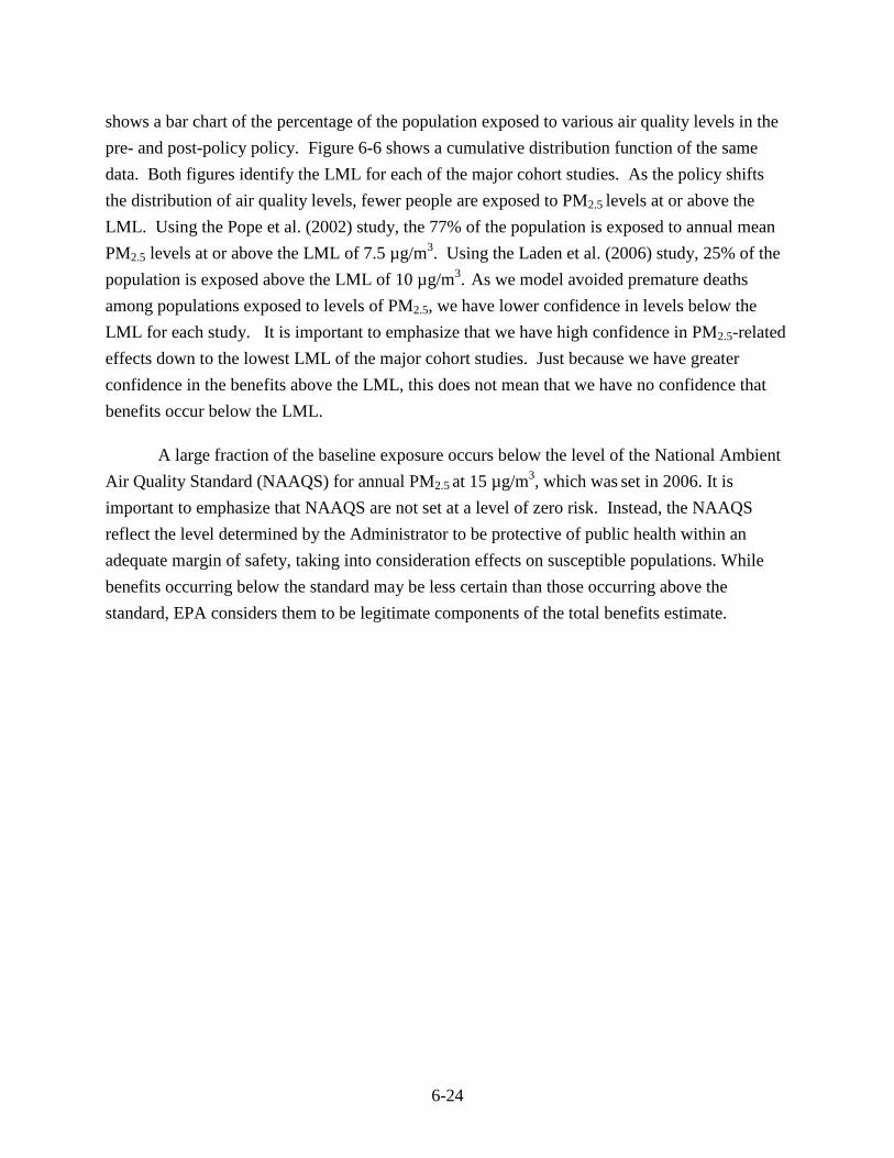
6-24

shows a bar chart of the percentage of the population exposed to various air quality levels in the

pre- and post-policy policy. Figure 6-6 shows a cumulative distribution function of the same

data. Both figures identify the LML for each of the major cohort studies. As the policy shifts

the distribution of air quality levels, fewer people are exposed to PM2.5 levels at or above the

LML. Using the Pope et al. (2002) study, the 77% of the population is exposed to annual mean

PM2.5 levels at or above the LML of 7.5 µg/m3. Using the Laden et al. (2006) study, 25% of the

population is exposed above the LML of 10 µg/m3. As we model avoided premature deaths

among populations exposed to levels of PM2.5, we have lower confidence in levels below the

LML for each study. It is important to emphasize that we have high confidence in PM2.5-related

effects down to the lowest LML of the major cohort studies. Just because we have greater

confidence in the benefits above the LML, this does not mean that we have no confidence that

benefits occur below the LML.

A large fraction of the baseline exposure occurs below the level of the National Ambient

Air Quality Standard (NAAQS) for annual PM2.5 at 15 µg/m3, which was

set in 2006. It is

important to emphasize that NAAQS are not set at a level of zero risk. Instead, the NAAQS

reflect the level determined by the Administrator to be protective of public health within an

adequate margin of safety, taking into consideration effects on susceptible populations. While

benefits occurring below the standard may be less certain than those occurring above the

standard, EPA considers them to be legitimate components of the total benefits estimate.

6-25

Figure 6-5. Percentage of Adult Population by Annual Mean PM2.5 Exposure in the

Baseline

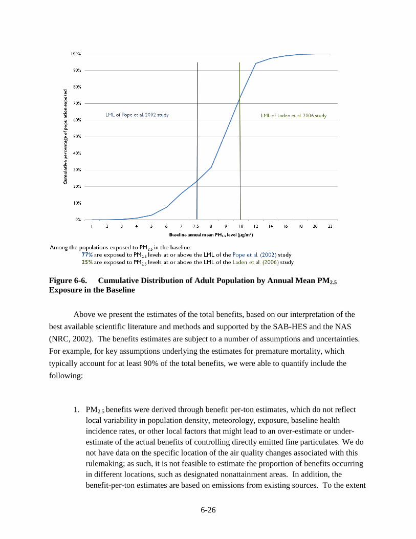
6-26

Figure 6-6. Cumulative Distribution of Adult Population by Annual Mean PM2.5

Exposure in the Baseline

Above we present the estimates of the total benefits, based on our interpretation of the

best available scientific literature and methods and supported by the SAB-HES and the NAS

(NRC, 2002). The benefits estimates are subject to a number of assumptions and uncertainties.

For example, for key assumptions underlying the estimates for premature mortality, which

typically account for at least 90% of the total benefits, we were able to quantify include the

following:

1. PM2.5 benefits were derived through benefit per-ton estimates, which do not reflect

local variability in population density, meteorology, exposure, baseline health

incidence rates, or other local factors that might lead to an over-estimate or under-

estimate of the actual benefits of controlling directly emitted fine particulates. We do

not have data on the specific location of the air quality changes associated with this

rulemaking; as such, it is not feasible to estimate the proportion of benefits occurring

in different locations, such as designated nonattainment areas. In addition, the

benefit-per-ton estimates are based on emissions from existing sources. To the extent

6-27

that the geographic distribution of the emissions reductions for this rule are different

than the modeled emissions, the benefits may be underestimated or overestimated. In

general, there is inherently more uncertainty for new sources, which may not be

included in the emissions inventory, than existing sources.

2. We assume that all fine particles, regardless of their chemical composition, are

equally potent in causing premature mortality. This is an important assumption,

because PM2.5 produced via transported precursors emitted from EGUs may differ

significantly from direct PM2.5 released from diesel engines and other industrial

sources, but no clear scientific grounds exist for supporting differential effects

estimates by particle type.

3. We assume that the health impact function for fine particles is linear down to the

lowest air quality levels modeled in this analysis. Thus, the estimates include health

benefits from reducing fine particles in areas with varied concentrations of PM2.5,

including both regions that are in attainment with fine particle standard and those that

do not meet the standard down to the lowest modeled concentrations.

4. To characterize the uncertainty in the relationship between PM2.5 and premature

mortality (which typically accounts for 85% to 95% of total monetized benefits), we

include a set of twelve estimates based on results of the expert elicitation study in

addition to our core estimates. Even these multiple characterizations omit the

uncertainty in air quality estimates, baseline incidence rates, populations exposed and

transferability of the effect estimate to diverse locations. As a result, the reported

confidence intervals and range of estimates give an incomplete picture about the

overall uncertainty in the PM2.5 estimates. This information should be interpreted

within the context of the larger uncertainty surrounding the entire analysis. For more

information on the uncertainties associated with PM2.5 benefits, please consult the

PM2.5 NAAQS RIA (Table 5.5).

This RIA does not include the type of detailed uncertainty assessment found in the PM

NAAQS RIA because we lack the necessary air quality input and monitoring data to run the

benefits model. In addition, we have not conducted any air quality modeling for this rule.

Moreover, it was not possible to develop benefit-per-ton metrics and associated estimates of

uncertainty using the benefits estimates from the PM RIA because of the significant differences

between the sources affected in that rule and those regulated here. However, the results of the

Monte Carlo analyses of the health and welfare benefits presented in Chapter 5 of the PM RIA

can provide some evidence of the uncertainty surrounding the benefits results presented in this

analysis.

6-28

6.7 References

Fann, N., C.M. Fulcher, B.J. Hubbell. 2009. “The influence of location, source, and emission

type in estimates of the human health benefits of reducing a ton of air pollution.” Air Qual

Atmos Health 2:169–176.

Kochi, I., B. Hubbell, and R. Kramer. 2006. “An Empirical Bayes Approach to Combining

Estimates of the Value of Statistical Life for Environmental Policy Analysis.”

Environmental and Resource Economics. 34: 385-406.

Krewski D, Jerrett M, Burnett RT, Ma R, Hughes E, Shi, Y, et al. 2009. Extended follow-up and

spatial analysis of the American Cancer Society study linking particulate air pollution and

mortality. HEI Research Report, 140, Health Effects Institute, Boston, MA.

Laden, F., J. Schwartz, F.E. Speizer, and D.W. Dockery. 2006. Reduction in Fine Particulate Air

Pollution and Mortality. American Journal of Respiratory and Critical Care Medicine. 173:

667-672.

Mrozek, J.R., and L.O. Taylor. 2002. “What Determines the Value of Life? A Meta-Analysis.”

Journal of Policy Analysis and Management 21(2):253-270.

National Research Council (NRC). 2002. Estimating the Public Health Benefits of Proposed Air

Pollution Regulations. Washington, DC: The National Academies Press.

National Research Council (NRC). 2009. Hidden Costs of Energy: Unpriced Consequences of

Energy Production and Use. National Academies Press. Washington, DC.

Office of Management and Budget (OMB). 2003. Circular A-4: Regulatory Analysis.

Washington, DC. Available on the Internet at

http://www.whitehouse.gov/omb/circulars/a004/a-4.html.

Pope, C.A., III, R.T. Burnett, M.J. Thun, E.E. Calle, D. Krewski, K. Ito, and G.D. Thurston.

2002. “Lung Cancer, Cardiopulmonary Mortality, and Long-term Exposure to Fine

Particulate Air Pollution.” Journal of the American Medical Association 287:1132-1141.

Roman, Henry A., Katherine D. Walker, Tyra L. Walsh, Lisa Conner, Harvey M. Richmond,

Bryan J. Hubbell, and Patrick L. Kinney. 2008. “Expert Judgment Assessment of the

Mortality Impact of Changes in Ambient Fine Particulate Matter in the U.S.” Environ. Sci.

Technol., 42(7):2268-2274.

Sisler, J.F. 1996. Spatial and seasonal patterns and long-term variability of the composition of

the haze in the United States: an analysis of data from the IMPROVE network. CIRA Report,

ISSN 0737-5352-32, Colorado State University.

http://www.whitehouse.gov/omb/circulars/a004/a-4.html

6-29

U.S. Environmental Protection Agency (U.S. EPA). 2000. Guidelines for Preparing Economic

Analyses. EPA 240-R-00-003. National Center for Environmental Economics, Office of

Policy Economics and Innovation. Washington, DC. September. Available on the Internet

at <http://yosemite.epa.gov/ee/epa/eed.nsf/webpages/Guidelines.html/$file/cover.pdf>.

U.S. Environmental Protection Agency. 2006. Regulatory Impact Analysis, 2006 National

Ambient Air Quality Standards for Particulate Matter, Chapter 5. Available at

<http://www.epa.gov/ttn/ecas/regdata/RIAs/Chapter%205--Benefits.pdf >.

U.S. Environmental Protection Agency. 2008a. Regulatory Impact Analysis, 2008 National

Ambient Air Quality Standards for Ground-level Ozone, Chapter 6. Available at

<http://www.epa.gov/ttn/ecas/regdata/RIAs/6-ozoneriachapter6.pdf>.

U.S. Environmental Protection Agency (U.S. EPA). 2008b. Integrated Science Assessment for

Sulfur Oxides—Health Criteria (Final Report). National Center for Environmental

Assessment, Research Triangle Park, NC. Available at

<http://cfpub.epa.gov/ncea/cfm/recordisplay.cfm?deid=198843>.

U.S. Environmental Protection Agency (U.S. EPA). 2008c. Integrated Science Assessment for

Oxides of Nitrogen - Health Criteria (Final Report). National Center for Environmental

Assessment, Research Triangle Park, NC. July. Available at at


U.S. Environmental Protection Agency (U.S. EPA). 2008d. Integrated Science Assessment for

Oxides of Nitrogen and Sulfur–Ecological Criteria National (Final Report). National Center

for Environmental Assessment, Research Triangle Park, NC. EPA/600/R-08/139. December.

Available at <http://cfpub.epa.gov/ncea/cfm/recordisplay.cfm?deid=201485>.

U.S. Environmental Protection Agency (U.S. EPA). 2009a. Regulatory Impact Analysis:

National Emission Standards for Hazardous Air Pollutants from the Portland Cement

Manufacturing Industry. Office of Air Quality Planning and Standards, Research Triangle

Park, NC. April. Available on the Internet at

<http://www.epa.gov/ttn/ecas/regdata/RIAs/portlandcementria_4-20-09.pdf >.

U.S. Environmental Protection Agency (U.S. EPA). 2009b. Integrated Science Assessment for

Particulate Matter (Final Report). EPA-600-R-08-139F. National Center for Environmental

Assessment – RTP Division. December. Available on the Internet at


U.S. Environmental Protection Agency (U.S. EPA). 2010a. Final Regulatory Impact Analysis

(RIA) for the SO2 National Ambient Air Quality Standards (NAAQS). Office of Air Quality

Planning and Standards, Research Triangle Park, NC. June. Available at

<http://www.epa.gov/ttn/ecas/ria.html>.

U.S. Environmental Protection Agency (U.S. EPA). 2010b. Technical Support Document:

Summary of Expert Opinions on the Existence of a Threshold in the Concentration-Response

http://yosemite.epa.gov/ee/epa/eed.nsf/webpages/Guidelines.html/$file/cover.pdf

http://www.epa.gov/ttn/ecas/regdata/RIAs/Chapter%205--Benefits.pdf

http://www.epa.gov/ttn/ecas/regdata/RIAs/6-ozoneriachapter6.pdf

http://www.epa.gov/ttn/ecas/regdata/RIAs/portlandcementria_4-20-09.pdf

6-30

Function for PM2.5-related Mortality. Research Triangle Park, NC. June. Available on the

Internet at <www.epa.gov/ttn/ecas/regdata/Benefits/thresholdstsd.pdf>.

U.S. Environmental Protection Agency (U.S. EPA). 2010c. Guidelines for Preparing Economic

Analyses. EPA 240-R-10-001. National Center for Environmental Economics, Office of

Policy Economics and Innovation. Washington, DC. December. Available on the Internet at

<http://yosemite.epa.gov/ee/epa/eerm.nsf/vwAN/EE-0568-50.pdf/$file/EE-0568-50.pdf>.

U.S. Environmental Protection Agency (U.S. EPA). 2011a. The Benefits and Costs of the Clean

Air Act from 1990 to 2020. Office of Air and Radiation, Washington, DC. March.

<http://www.epa.gov/air/sect812/feb11/fullreport.pdf>. Accessed March 30, 2011.

U.S. Environmental Protection Agency (U.S. EPA). 2011b. Regulatory Impact Analysis for the

Final Transport Rule. Office of Air Quality Planning and Standards, Research Triangle

Park, NC. June. Available at <http://www.epa.gov/airtransport/pdfs/FinalRIA.pdf>.

U.S. Environmental Protection Agency (U.S. EPA). 2012. Technical Support Document:

Estimating the Benefit per ton of Reducing PM2.5 Precursors from the Petroleum Refineries

Sector. Office of Air Quality Planning and Standards, Research Triangle Park, NC. January.

U.S. Environmental Protection Agency - Science Advisory Board (U.S. EPA-SAB). 2007. SAB

Advisory on EPA’s Issues in Valuing Mortality Risk Reduction. EPA-SAB-08-001. October.

Available on the Internet at

<http://yosemite.epa.gov/sab/sabproduct.nsf/4128007E7876B8F0852573760058A978/$File/

sab-08-001.pdf >.

U.S. Environmental Protection Agency - Science Advisory Board (U.S. EPA-SAB). 2009a.

Review of EPA’s Integrated Science Assessment for Particulate Matter (First External

Review Draft, December 2008). EPA-COUNCIL-09-008. May. Available on the Internet at

<http://yosemite.epa.gov/sab/SABPRODUCT.NSF/81e39f4c09954fcb85256ead006be86e/73

ACCA834AB44A10852575BD0064346B/$File/EPA-CASAC-09-008-unsigned.pdf>.

U.S. Environmental Protection Agency - Science Advisory Board (U.S. EPA-SAB). 2009b.

Consultation on EPA’s Particulate Matter National Ambient Air Quality Standards: Scope

and Methods Plan for Health Risk and Exposure Assessment. EPA-COUNCIL-09-009.

May. Available on the Internet at

<http://yosemite.epa.gov/sab/SABPRODUCT.NSF/81e39f4c09954fcb85256ead006be86e/72

3FE644C5D758DF852575BD00763A32/$File/EPA-CASAC-09-009-unsigned.pdf>.

U.S. Environmental Protection Agency - Science Advisory Board (U.S. EPA-SAB). 2010.

Review of EPA’s DRAFT Health Benefits of the Second Section 812 Prospective Study of the

Clean Air Act. EPA-COUNCIL-10-001. June. Available on the Internet at

<http://yosemite.epa.gov/sab/sabproduct.nsf/0/72D4EFA39E48CDB28525774500738776/$F

ile/EPA-COUNCIL-10-001-unsigned.pdf>.

Viscusi, V.K., and J.E. Aldy. 2003. “The Value of a Statistical Life: A Critical Review of

Market Estimates throughout the World.” Journal of Risk and Uncertainty 27(1):5-76.

http://yosemite.epa.gov/ee/epa/eerm.nsf/vwAN/EE-0568-50.pdf/$file/EE-0568-50.pdf

http://yosemite.epa.gov/sab/sabproduct.nsf/4128007E7876B8F0852573760058A978/$File/sab-08-001.pdf

http://yosemite.epa.gov/sab/sabproduct.nsf/4128007E7876B8F0852573760058A978/$File/sab-08-001.pdf

http://yosemite.epa.gov/sab/SABPRODUCT.NSF/81e39f4c09954fcb85256ead006be86e/73ACCA834AB44A10852575BD0064346B/$File/EPA-CASAC-09-008-unsigned.pdf

http://yosemite.epa.gov/sab/SABPRODUCT.NSF/81e39f4c09954fcb85256ead006be86e/73ACCA834AB44A10852575BD0064346B/$File/EPA-CASAC-09-008-unsigned.pdf

http://yosemite.epa.gov/sab/SABPRODUCT.NSF/81e39f4c09954fcb85256ead006be86e/723FE644C5D758DF852575BD00763A32/$File/EPA-CASAC-09-009-unsigned.pdf

http://yosemite.epa.gov/sab/SABPRODUCT.NSF/81e39f4c09954fcb85256ead006be86e/723FE644C5D758DF852575BD00763A32/$File/EPA-CASAC-09-009-unsigned.pdf

7-1

7 COMPARISON OF BENEFITS AND COSTS

EPA estimates the range of benefits of this reconsideration to be $260 million to $580

million at a 3% discount rate and $240 million to $520 million at a 7% discount rate in 2017.

The annualized costs are a cost savings of $79 million at a 7% interest rate. Thus, net benefits

are $340 million to $660 million at a 3% discount rate for the benefits and $320 million to $600

million at a 7% discount rate. All estimates are in 2006$.

Table 7-1 provides details, by flare size, of the monetized benefits and Table 7-2 shows a

summary of the monetized benefits, social costs, and net benefits. Figure 7-1 shows the full

range of net benefits estimates (i.e., benefits minus annualized costs) utilizing the 14 different

PM2.5 mortality functions at the 3% discount rate, and Figure 7-2 shows this information at a 7%

discount rate. EPA believes that the benefits of this rule are likely to exceed the costs by a

substantial margin even when taking into account uncertainties in the cost and benefit estimates.

Alternatively, if no refineries install flare gas recovery systems, EPA estimates the costs

would be $10.7 million with monetized benefits of $190 to $460 million and $170 to $410

million at a discount rates of 3% and 7% respectively. Thus, net benefits without flare gas

recovery systems would be $180 million to $450 million and $160 million to $400 million, at 3%

and 7% discount rates, respectively. All estimates are in 2006 dollars for the year 2017.

For small flares, we estimate the monetized benefits are $170 million to $410 million (3-

percent discount rate) and $150 million to $370 million (7% discount rate for health benefits and

3% discount rate for climate benefits). For large flares, we estimate the monetized benefits are

$93 million to $160 million (3% discount rate) and $88 million to $150 million (7% discount rate

for health benefits and 3-percent discount rate for climate benefits). All estimates are in 2006

dollars for the year 2017.

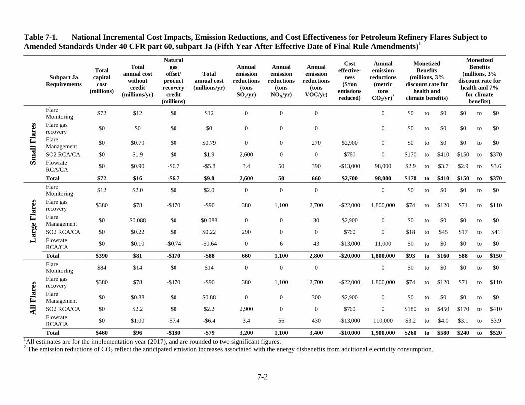
7-2

Table 7-1. National Incremental Cost Impacts, Emission Reductions, and Cost Effectiveness for Petroleum Refinery Flares Subject to

Amended Standards Under 40 CFR part 60, subpart Ja (Fifth Year After Effective Date of Final Rule Amendments)1

Subpart Ja

Requirements

Total

capital

cost

(millions)

Total

annual cost

without

credit

(millions/yr)

Natural

gas

offset/

product

recovery

credit

(millions)

Total

annual cost

(millions/yr)

Annual

emission

reductions

(tons

SO2/yr)

Annual

emission

reductions

(tons

NOX/yr)

Annual

emission

reductions

(tons

VOC/yr)

Cost

effective-

ness

($/ton

emissions

reduced)

Annual

emission

reductions

(metric

tons

CO2/yr)2

Monetized

Benefits

(millions, 3%

discount rate for

health and

climate benefits)

Monetized

Benefits

(millions, 3%

discount rate for

health and 7%

for climate

benefits)

Sm

all

Fla

res

Flare

Monitoring $72 $12 $0 $12 0 0 0 0 $0 to $0 $0 to $0

Flare gas

recovery $0 $0 $0 $0 0 0 0 0 $0 to $0 $0 to $0

Flare

Management $0 $0.79 $0 $0.79 0 0 270 $2,900 0 $0 to $0 $0 to $0

SO2 RCA/CA $0 $1.9 $0 $1.9 2,600 0 0 $760 0 $170 to $410 $150 to $370

Flowrate

RCA/CA $0 $0.90 -$6.7 -$5.8 3.4 50 390 -$13,000 98,000 $2.9 to $3.7 $2.9 to $3.6

Total $72 $16 -$6.7 $9.0 2,600 50 660 $2,700 98,000 $170 to $410 $150 to $370

Larg

e F

lare

s

Flare

Monitoring $12 $2.0 $0 $2.0 0 0 0 0 $0 to $0 $0 to $0

Flare gas

recovery $380 $78 -$170 -$90 380 1,100 2,700 -$22,000 1,800,000 $74 to $120 $71 to $110

Flare

Management $0 $0.088 $0 $0.088 0 0 30 $2,900 0 $0 to $0 $0 to $0

SO2 RCA/CA $0 $0.22 $0 $0.22 290 0 0 $760 0 $18 to $45 $17 to $41

Flowrate

RCA/CA $0 $0.10 -$0.74 -$0.64 0 6 43 -$13,000 11,000 $0 to $0 $0 to $0

Total $390 $81 -$170 -$88 660 1,100 2,800 -$20,000 1,800,000 $93 to $160 $88 to $150

All

Fla

res

Flare

Monitoring $84 $14 $0 $14 0 0 0 0 $0 to $0 $0 to $0

Flare gas

recovery $380 $78 -$170 -$90 380 1,100 2,700 -$22,000 1,800,000 $74 to $120 $71 to $110

Flare

Management $0 $0.88 $0 $0.88 0 0 300 $2,900 0 $0 to $0 $0 to $0

SO2 RCA/CA $0 $2.2 $0 $2.2 2,900 0 0 $760 0 $180 to $450 $170 to $410

Flowrate

RCA/CA $0 $1.00 -$7.4 -$6.4 3.4 56 430 -$13,000 110,000 $3.2 to $4.0 $3.1 to $3.9

Total $460 $96 -$180 -$79 3,200 1,100 3,400 -$10,000 1,900,000 $260 to $580 $240 to $520 1All estimates are for the implementation year (2017), and are rounded to two significant figures.

2 The emission reductions of CO2 reflect the anticipated emission increases associated with the energy disbenefits from additional electricity consumption.

7-3

Table 7-2. Summary of the Monetized Benefits, Social Costs, and Net Benefits for the

Final Petroleum Refineries NSPS in 2017 (millions of 2006$)1

3% Discount Rate 7% Discount Rate

Total Monetized Benefits2 $260 to $580 $240 to $520

Total Compliance Costs3 -$79 -$79

Net Benefits $340 to $660 $320 to $600

Non-monetized Benefits

Health effects from ozone, SO2, NO2 exposure

Health effects from PM2.5 exposure from VOCs

Ecosystem effects

Visibility impairment

1All estimates are for the implementation year (2017), and are rounded to two significant figures.

2 The total monetized benefits reflect the human health benefits associated with reducing exposure to PM2.5 through

reductions of PM2.5 precursors such as NOx and SO2 as well as CO2 benefits. It is important to note that the

monetized benefits do not include the reduced health effects from direct exposure to SO2 and NOx, ozone

exposure, ecosystem effects, or visibility impairment. Human health benefits are shown as a range from Pope et

al. (2002) to Laden et al. (2006). These models assume that all fine particles, regardless of their chemical

composition, are equally potent in causing premature mortality because the scientific evidence is not yet

sufficient to allow differentiation of effects estimates by particle type. The net present value of reduced CO2

emissions is calculated differently than other benefits. This table includes monetized climate benefits using the

global average social cost of carbon (SCC) estimated at a 3 percent discount rate because the interagency

workgroup deemed the SCC estimate at a 3 percent discount rate to be the central value. 3 The engineering compliance costs are annualized using a 7 percent discount rate.

7-4

Figure 7-1. Net Benefits for Final Petroleum Refineries NSPS Reconsideration at 3%

discount rate* *Net Benefits are quantified in terms of PM2.5 and CO2 benefits at a 3% discount rate for 2017. This graph shows 14

benefits estimates combined with the cost estimate. All fine particles are assumed to have equivalent health effects.

The monetized benefits incorporate the conversion from precursor emissions to ambient fine particles.

$0

$100

$200

$300

$400

$500

$600

$700

$800

$900

Pope et al.

Laden et al.

Mill

ion

s (2

00

6$

)

Cost estimate combined with total monetized benefits estimates derived from 2 epidemiology functions and 12 expert functions

7-5

Figure 7-2. Net Benefits for Final Petroleum Refineries NSPS Reconsideration at 7%

discount rate* *Net Benefits are quantified in terms of PM2.5 benefits at a 7% discount rate and CO2 benefits at a 3% discount rate

for 2017. This graph shows 14 benefits estimates combined with the cost estimate. All fine particles are assumed to

have equivalent health effects. The monetized benefits incorporate the conversion from precursor emissions to

ambient fine particles.

$0

$100

$200

$300

$400

$500

$600

$700

$800

Pope et al.

Laden et al.

Mill

ion

s (2

00

6$

)

Cost estimate combined with total monetized benefits estimates derived from 2 epidemiology functions and 12 expert functions

A-1

APPENDIX A

PARENT COMPANY INFORMATION FOR PETROLEUM REFINERIES

A-2

Table A-1. Parent Company Information for Petroleum Refineries

Facility Name City State

Capacity

(bbl/cd) Parent Company Name

Parent Company

Sales

Parent Company

Employment

AGE Refining Inc San Antonio TX 14,021 AGE Refining, Inc. 65.00 124

Alon Bakersfield

Operating Inc Bakersfield CA Alon Israel Oil Company

LTD 7,283.06 12,000

Alon Refining Krotz

Springs Inc Krotz Springs LA 80,000 Alon Israel Oil Company

LTD 7,283.06 12,000

Alon USA Energy Inc. Big Spring TX 67,000 Alon Israel Oil Company

LTD 7,283.06 12,000

American Refining Group

Inc Bradford PA 10,000 American Refining

Group, Inc. 737.19 323

Big West Oil Co. North Salt Lake UT 29,400 Flying J Oil & Gas Inc. 1,719.00 15,000

BP Exploration Alaska Inc Prudhoe Bay AK 12,780 BP PLC 297,107.00 12,633

BP Products North

America Inc Whiting IN 405,000 BP PLC 297,107.00 12,633

BP Products North

America Inc Texas City TX 406,570 BP PLC 297,107.00 12,633

BP West Coast Products

LLC Los Angeles CA 253,000 BP PLC 297,107.00 12,633

BP West Coast Products

LLC Ferndale WA 225,000 BP PLC 297,107.00 12,633

BP-Husky Refining LLC Toledo OH 131,400 BP PLC 297,107.00 12,633

Calcasieu Refining Co. Lake Charles LA 78,000 Calcasieu Refining

Company 291.74 92

Calumet Lubricants Co LP Cotton Valley LA 13,020 Calumet Specialty

Products Partners, L.P. 2,190.75 654

Calumet Lubricants Co LP Princeton LA 8,300 Calumet Specialty


Calumet Shreveport LLC Shreveport LA 57,000 Calumet Specialty


Cenex Harvest States Laurel MT 59,600 CHS, Inc. 23.30 287

Chalmette Refining LLC Chalmette LA 192,500 ExxonMobil Corp. 383,221.00 83,600

Chevron USA Inc. Perth Amboy NJ 80,000 Chevron Corporation 204,928.00 58,267

Chevron USA Inc. Salt Lake City UT 45,000 Chevron Corporation 204,928.00 58,267

Chevron USA Inc. Pascagoula MS 330,000 Chevron Corporation 204,928.00 58,267

Chevron USA Inc. El Segundo CA 273,000 Chevron Corporation 204,928.00 58,267

Chevron USA Inc. Richmond CA 245,271 Chevron Corporation 204,928.00 58,267

Chevron USA Inc. Honolulu HI 54,000 Chevron Corporation 204,928.00 58,267

Citgo Corpus Christi TX 163,000 CITGO Petroleum

Corporation 475.80 3,506

Citgo Petroleum Corp. Lake Charles LA 427,800 CITGO Petroleum

Corporation 475.80 3,506

Coffeyville Resources Rfg

& Mktg LLC Coffeyville KS 115,700 CVR Energy, Inc. 4,079.77 371

ConocoPhillips Sweeny TX 247,000 ConocoPhillips 198,655.00 29,700

ConocoPhillips Linden NJ 238,000 ConocoPhillips 198,655.00 29,700

ConocoPhillips Wilmington CA 139,000 ConocoPhillips 198,655.00 29,700

ConocoPhillips SF—Rodeo CA 120,200 ConocoPhillips 198,655.00 29,700

ConocoPhillips Belle Chasse LA 247,000 ConocoPhillips 198,655.00 29,700

ConocoPhillips Alaska Inc Prudhoe Bay AK 15,000 ConocoPhillips 198,655.00 29,700

ConocoPhillips Co Trainer PA 185,000 ConocoPhillips 198,655.00 29,700

(continued)

A-3

Table A-1. Parent Company Information for Petroleum Refineries (continued)


Capacity


Parent Company

Sales

Parent Company

Employment

ConocoPhillips Company Westlake LA 239,400 ConocoPhillips 198,655.00 29,700

ConocoPhillips Company Ponca City OK 198,400 ConocoPhillips 198,655.00 29,700

ConocoPhillips Company Billings MT 58,000 ConocoPhillips 198,655.00 29,700

ConocoPhillips Company Ferndale WA 100,000 ConocoPhillips 198,655.00 29,700

Countrymark Cooperative,

Inc. Mt. Vernon IN 26,500 Countrymark

Cooperative 862.97 425

Deer Park Refining LTD

Partnership Deer Park TX 327,000 Royal Dutch Shell, PLC 378,152.00 93,000

Delaware City Refining Co

LLC Delaware City DE 182,200 PBF Holdings LLC Not Listed Not Listed

Delek Refining Ltd Tyler TX 60,000 Delek US Holdings, Inc. 3,755.60 3,296

Equistar Chemicals LP Channelview TX Lyondell Basell

Industries N.V.

27,684.00 14,000

Ergon Refining Inc. Vicksburg MS 23,000 Ergon, Inc. 3,830.00 1,625

Ergon West Virginia Inc. Newell WV 20,000 Ergon, Inc. 3,830.00 1,625

Excel Paralubes Westlake LA Koch Industries Inc 9,182.50 62,544

ExxonMobil Corp. Beaumont TX 344,500 ExxonMobil Corp. 383,221.00 83,600

ExxonMobil Corp. Torrance CA 149,500 ExxonMobil Corp. 383,221.00 83,600

ExxonMobil Oil Corp Baytown TX 560,640 ExxonMobil Corp. 383,221.00 83,600

ExxonMobil Refining &

Supply Co Baton Rouge LA 502,000 ExxonMobil Corp. 383,221.00 83,600


Supply Co Billings MT 60,000 ExxonMobil Corp. 383,221.00 83,600


Supply Co Joliet IL 238,600 ExxonMobil Corp. 383,221.00 83,600

Flint Hills Resources Corpus Christi TX 290,078 Koch Industries Inc 9,182.50 62,544

Flint Hills Resources North Pole AK 219,500 Koch Industries Inc 9,182.50 62,544

Flint Hills Resources Saint Paul MN 262,000 Koch Industries Inc 9,182.50 62,544

Foreland Refining Co. Ely NV 2,000 Foreland Refining Corp. 12.55 27

Frontier El Dorado

Refining Co El Dorado KS 138,000 Frontier Oil Corp. 5,884.91 723

Frontier Refining Inc Cheyenne WY 47,000 Frontier Oil Corp. 5,884.91 723

Garco Energy LLC Douglas WY 3,600 Garco Energy 11.44 16

Goodway Refining LLC Atmore AL 4,100 Goodway Refining, LLC 2.00 17

Greka Energy Santa Maria CA 9,500 Santa Maria Refining

Company 2.80 47

Gulf Atlantic Operations Mobile Bay AL 20,000 Gulf Atlantic Operations

LLC 76.99 32

Hess Corporation Port Reading NJ Hess Corporation 34,613.00 13,800

Holly Refining &

Marketing Co Woods Cross UT 25,050 Holly Corporation 8,323.00 1,321

Holly Refining &

Marketing Co Tulsa East OK 70,300 Holly Corporation 8,323.00 1,321

Holly Refining &

Marketing Co Tulsa West OK 85,000 Holly Corporation 8,323.00 1,321

Houston Refining LP Houston TX 280,390 Lyondell Basell

Industries N.V. 27,684.00 14,000

Hunt Refining Co. Tuscaloosa AL 36,000 Hunt Refining Co. 4,871.00 346

Hunt Southland Refining

Co Sandersville MS 11,000 Hunt Refining Co. 4,871.00 1,100

(continued)

A-4



Capacity


Parent Company

Sales

Parent Company

Employment

Kern Oil & Refining Co. Bakersfield CA 26,000 Kern Oil & Refining Co. 282.00 105

Lima Refining Company Lima OH 155,000 Husky Energy, Inc. 18,174.36 4,491

Lion Oil Co. El Dorado AR 75,000 Lion Oil Co. 169.60 350

Little America Refining

Co. Evansville WY 24,500 Sinclair Co.’s 7,753.46 7,000

Lunday-Thagard Co. South Gate CA 8,500 World Oil Marketing Co. 35.40 65

Marathon Petroleum Co.

LLC Robinson IL 206,000 Marathon Oil Corp 73,621.00 29,677


LLC Catlettsburg KY 212,000 Marathon Oil Corp 73,621.00 29,677


LLC Detroit MI 106,000 Marathon Oil Corp 73,621.00 29,677


LLC Canton OH 78,000 Marathon Oil Corp 73,621.00 29,677


LLC Texas City TX 76,000 Marathon Oil Corp 73,621.00 29,677


LLC Garyville LA 464,000 Marathon Oil Corp 73,621.00 29,677

Martin Midstream Partners

LP Smackover AR 7,500 Cross Oil Refining &

Marketing, Inc. 265.00 110

Montana Refining Co. Great Falls MT 10,000 Connacher Oil and Gas,

Limited 574.19 265

Motiva Enterprises Port Arthur TX 285,000 Motiva Enterprises LLC 26,400.00 2,900

Motiva Enterprises LLC Norco LA 233,500 Motiva Enterprises LLC 26,400.00 2,900

Motiva Enterprises LLC Convent LA 235,000 Motiva Enterprises LLC 26,400.00 2,900

Murphy Oil USA Inc. Superior WI 34,300 Murphy Oil Corp 23,345.07 8,994

Murphy Oil USA Inc. Meraux LA 125,000 Murphy Oil Corp 23,345.07 8,994

National Cooperative


McPherson KS 85,500 National Cooperative


2,810.30 612

Navajo Refining Co. Artesia NM 105,000 Holly Corporation 8,323.00 1,321

Nustar Asphalt Refining

LLC Paulsboro NJ 70,000 NuStar Energy LP 4,403.06 1,492

Nustar Asphalt Refining

LLC Savannah GA 28,000 NuStar Energy LP 4,403.06 1,492

Paramount Petroleum Co Long Beach CA 31,500 Alon Israel Oil Company

LTD 7,283.06 12,000

Paramount Petroleum

Corp. Paramount CA 53,000 Alon Israel Oil Company

LTD 7,283.06 12,000

Pasadena Refining Systems

Inc. Pasadena TX 100,000 Pasadena Refining 31.00 348

Paulsboro Refining Co

LLC Paulsboro NJ 160,000 PBF Holding Company

LLC Not Listed Not Listed

PDV Midwest Refining Lemont IL 167,000 Petróleos de Venezuela

S.A. (PDVSA) 75.00 102,750

Pelican Refining Co. LLC Lake Charles LA Pelican Refining Co LLC 4.00 33

Petro Star Inc. North Pole AK 19,700 Petro Star Inc. 887.00 400

Petro Star Inc. Valdez AK 55,000 Petro Star Inc. 887.00 400

Placid Refining Inc. Port Allen LA 57,000 Placid Refining 3,351.84 207

Premcor Refining Group

Inc Memphis TN 180,000 Valero Energy 82,233.00 20,313

(continued)

A-5



Capacity


Parent Company

Sales

Parent Company

Employment

Premcor Refining Group

Inc Port Arthur TX 292,000 Valero Energy 82,233.00 20,313

San Joaquin Refining Co.,

Inc. Bakersfield CA 15,000 San Joaquin Refining Co. 3.50 108

Shell Chemical LP St. Rose LA 55,000 Royal Dutch Shell, PLC 378,152.00 93,000

Shell Chemical LP Saraland AL 80,000 Royal Dutch Shell, PLC 378,152.00 93,000

Shell Oil Products US Anacortes WA 145,000 Royal Dutch Shell, PLC 378,152.00 93,000

Shell Oil Products US Martinez CA 156,400 Royal Dutch Shell, PLC 378,152.00 93,000

Silver Eagle Refining Evanston WY 3,000 Silver Eagle Refining Inc. 225.87 60

Silver Eagle Refining Woods Cross UT 10,250 Silver Eagle Refining Inc. 225.87 60

Sinclair Wyoming

Refining Co Sinclair WY 74,000 Sinclair Co.’s 7,753.46 7,000

Somerset Energy Refinery

LLC Somerset KY 5,500 Somerset Oil Inc. 16.90 11

South Hampton Resources

Inc. Silsbee TX Arabian American

Development Co 139.11 145

St Paul Park Refining Co.

LLC Saint Paul MN 74,000 Northern Tier Energy

LLC Not listed Not Listed

Suncor Energy Inc. Commerce City

West CO 67,000 Suncor Energy Inc. 34,398.09 12,978

Suncor Energy Inc. Commerce City

East CO 36,000 Suncor Energy Inc. 34,398.09 12,978

Sunoco, Inc. Marcus Hook PA 178,000 Sunoco, Inc. 37,489.00 4,544

Sunoco, Inc. Toledo OH 160,000 Sunoco, Inc. 37,489.00 4,544

Sunoco, Inc. (R&M) Philadelphia PA 335,000 Sunoco, Inc. 37,489.00 4,544

Tenby Inc. Oxnard CA 2,800 Ten By Inc. NotListed NotListed

Tesoro Alaska Petroleum

Co Kenai AK 68,000 Tesoro Corp 20,583.00 5,261

Tesoro Hawaii Corp Ewa Beach HI 93,500 Tesoro Corp 20,583.00 5,261

Tesoro Refining &

Marketing Corporation Martinez CA 166,000 Tesoro Corp 20,583.00 5,261

Tesoro Refining &

Marketing Corporation Wilmington CA 94,300 Tesoro Corp 20,583.00 5,261

Tesoro West Coast Mandan ND 58,000 Tesoro Corp 20,583.00 5,261

Tesoro West Coast Salt Lake City UT 57,500 Tesoro Corp 20,583.00 5,261

Tesoro West Coast Anacortes WA 120,000 Tesoro Corp 20,583.00 5,261

Total Petrochemicals Inc Port Arthur TX 232,000 Total SA 186,158.80 92,855

Trigeant Ltd. Corpus Christi TX BTB Refining 5.00 37

United Refining Co. Warren PA 65,000 United Refining

Company 2,654.40 4,434

US Oil & Refining Co. Tacoma WA 38,800 US Oil & Refining Co. 26.90 182

Valero Energy Corporation Three Rivers TX 93,000 Valero Energy 82,233.00 20,313

Valero Energy Corporation Sunray TX 156,000 Valero Energy 82,233.00 20,313

Valero Refining Co

California Benicia CA 132,000 Valero Energy 82,233.00 20,313

Valero Refining Co

California

Wilmington

Asphalt Plant CA 6,300 Valero Energy 82,233.00 20,313

Valero Refining Co

California

Wilmington

Refinery CA 78,000 Valero Energy 82,233.00 20,313

Valero Refining Co

Oklahoma Ardmore OK 85,000 Valero Energy 82,233.00 20,313

(continued)

A-6



Capacity


Parent Company

Sales

Parent Company

Employment

Valero Refining Co Texas

LP Corpus Christi TX 142,000 Valero Energy 82,233.00 20,313


LP Houston TX 88,000 Valero Energy 82,233.00 20,313


LP Texas City TX 225,000 Valero Energy 82,233.00 20,313

Valero Refining New

Orleans LLC Norco LA 205,000 Valero Energy 82,233.00 20,313

Ventura Refining &

Transmission LLC Thomas OK 12,000 Ventura Refining &

Transmission, LLC 3.10 37

Western Refining

Company LP El Paso TX 122,000 Western Refining, Inc. 7,965.05 636

Western Refining

Southwest Inc

Bloomfield NM 16,800 Western Refining, Inc. 7,965.05 636

Western Refining

Southwest Inc Gallup NM 21,100 Western Refining, Inc. 7,965.05 636

Western Refining

Yorktown Inc Yorktown VA 66,300 Western Refining, Inc. 7,965.05 636

WRB Refining LLC Borger TX 146,000 ConocoPhillips 198,655.00 29,700

WRB Refining LLC Wood River IL 362,000 ConocoPhillips 198,655.00 29,700

Wynnewood Refining Co. Wynnewood OK 70,000 Gary-Williams Energy

Corporation 49.90 260

Wyoming Refining Co New Castle WY 14,000 Wyoming Refining Co. 125.00 96

Sources: Hoovers 2011 Online Data, accessed through University of South Carolina’s Moore School of Business











September 2011.






Library.

Oil & Gas Journal, December 6, 2010

Energy Information Administration (EIA), Form EIA-820, “Annual Refinery Report.” Table 3. Capacity of

Operable Petroleum Refineries by State and Individual Refinery as of January 1, 2011. (Data accessed on

October 31, 2011.) [Source for 2009–2011 numbers.] <http://www.eia.gov/petroleum/refinerycapacity/


United States

Environmental Protection

Agency

Office of Air and Radiation

Office of Air Quality Planning and Standards

Research Triangle Park, NC

June 2012

Documents

Petroleum Refineries New Source Performance Standards Ja