Perspectives on U.S. Monetary Policy Tools and Instruments*

James D. Hamilton

University of California at San Diego

May 9, 2019 Revised: June 14, 2019

ABSTRACT

The Federal Reserve characterizes its current policy decisions in terms of targets for the fed funds rate and the size of its balance sheet. The fed funds rate today is essentially an administered rate that is heavily influenced by regulatory arbitrage and divorced from its traditional role as a signal of liquidity in the banking system. The size of the Fed’s balance sheet is at best a very blunt instrument for influencing interest rates. In this paper I compare the current operating system with the historical U.S. system and the procedures of other central banks. I then examine strategies for transitioning from the current system to one that would give the Federal Reserve more accurate tools with which to achieve its strategic objective of influencing inflation and output.

*I thank Peter Ireland, Andrew Levin, and John Taylor for helpful suggestions.

1

1. Introduction.

This paper discusses the policy instruments that the central bank uses in pursuit of its

broader strategic objectives of influencing variables like inflation and output. For many decades,

the primary instrument of U.S. monetary policy was the federal funds rate, which is an interest

rate on overnight loans of Federal Reserve deposits between depository institutions. When this

rate fell essentially to zero in 2009, the Fed implemented massive purchases of Treasury

securities and mortgage-backed securities as an alternative policy instrument with which it hoped

to influence longer-term interest rates. Although the fed funds rate is no longer at the effective

lower bound, today the Fed continues to treat both the fed funds rate and its holdings of

securities as policy instruments.

I review the current operating procedures and conclude that neither instrument is well

suited for achieving the Fed’s broader strategic objectives. The fed funds rate has become a

largely administered rate that is heavily influenced by regulatory arbitrage and divorced from its

traditional role as a signal of liquidity in the banking system. To the extent that the size of the

Fed’s balance sheet matters today, it is primarily from the liabilities rather than the asset side of

the balance sheet, with the size of the balance sheet at best a very blunt tool for influencing

interest rates. I discuss alternative possible operating procedures such as a corridor system based

on repurchase agreements.

Section 2 reviews the effects of the Fed’s asset holdings on long-term interest rates over

2009 to 2019. I conclude that this instrument has less influence on interest rates than is

sometimes believed. Section 3 describes a traditional corridor system such as used by the

European Central Bank. Sections 4 and 5 discuss the discount rate and interest on excess

reserves, respectively, tools that could in principle operate like the ceiling and floor of a corridor

2

system but in U.S. practice have not. Section 6 discusses the reverse repo rate and argues that

this policy rate is the true floor on short-term interest rates in the current system. Section 7 notes

how the operation of the system changed in 2018. Section 8 concludes with some thoughts on

how the U.S. could transition to a system that would give the Federal Reserve more accurate

tools with which to influence inflation and output.

2. The effects of large-scale asset purchases.

Figure 1 displays the Fed’s holdings of Treasury and mortgage-backed securities. These

rose from $500 billion at the start of 2009 to $4.5 trillion by 2017. These purchases are

sometimes described as “quantitative easing,” and were implemented in three phases popularly

referred to as QE1, QE2, and QE3. In November of 2017, the Fed stopped some of its purchases

of new securities, allowing its holdings of securities to gradually decline to a level of $3.8 trillion

as of May 2019.

In many standard macroeconomic and finance models, if the nominal interest rate is zero,

purchases of securities by the central bank would have no effects on any real or nominal variable

of interest; see for example Eggertsson and Woodford (2003). As discussed by Hamilton (2018),

adding various financial frictions to the models can change that prediction; see among others

Cúrdia and Woodford (2011), Gertler and Karadi, (2011), Chen, Cúrdia and Ferrero (2012),

Hamilton and Wu (2012), Woodford (2012), Greenwood and Vayanos (2014), Eggertsson and

Proulx (2016), and Caballero and Farhi (2017). However, it is not clear from theory how large

the potential stimulus arising from these channels could be.

A number of empirical studies concluded that QE1-3 were successful in their goal of

bringing down long-term interest rates; for surveys of this literature see Williams (2014), Borio

3

and Zabai (2018), and Swanson (2018). It is useful to put these claims in perspective. Figure 2,

updated from Woodford (2012), plots the interest rate on 10-year Treasury bonds over this

period. On net this rate rose during QE1 when the Fed was trying to bring it down, fell when

QE1 ended, rose in QE2 when the Fed again resumed its efforts to lower long-term rates,

dropped after QE2 was halted, only to rise again in QE3. One can of course claim that, if the Fed

had not been purchasing bonds, the rate would have risen even more than it did during the QE1-3

episodes. But at a minimum we are forced to conclude that Fed purchases were only one of

many factors influencing bond yields during these episodes, and certainly not the most important

factor.

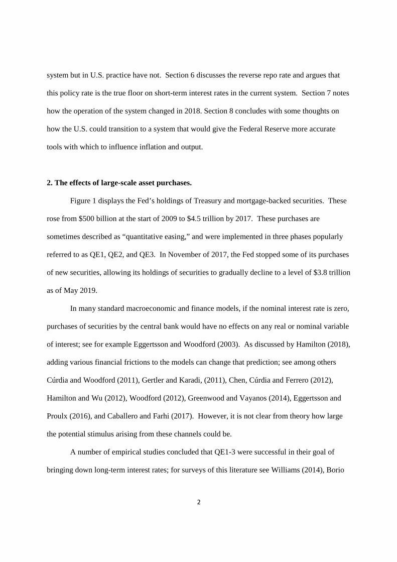
One way we might try to isolate the effects of Fed actions is to focus only on the

particular days when the FOMC issued a statement or released its minutes or when the Fed Chair

gave a speech on the economy or monetary policy. Figure 3, adapted from Greenlaw et al.

(2018), shows the cumulative change in the 10-year yield that occurred on those days alone.

Figure 3 turns out to show the same broad pattern as Figure 2—yields on average rose, not fell,

during QE1-3, even if we focus on just days in which the Fed made an announcement.

Many researchers have conducted event studies using a subset of days on which there

were particularly important announcements of the Fed’s intentions to implement additional

large-scale asset purchases. But the analysis of some of these days by Thornton (2017),

Hamilton (2018) and Levin and Loungani (2019) suggest that previous studies may have

overestimated the role of the purchases in moving interest rates. One key question is the extent

to which interest rates were responding to the Fed’s assessment of the economic situation rather

than to the purchases themselves. See Melosi (2016), Nakamura and Steinsson (2018), and

Miranda-Agrippino and Ricco (2018) for more discussion of this issue.

4

Regardless of one’s position on whether large-scale asset purchases are an important tool

when the traditional instrument of controlling the fed funds rate is unavailable, the case for its

importance in 2019 when short rates are significantly above zero is far from compelling. I

conclude below that the primary relevance of the size of the Fed’s balance sheet today for the

conduct of monetary policy comes from the liabilities side rather than any tangible consequences

of its asset holdings for long-term interest rates. But before returning to that issue, I first discuss

alternative monetary procedures for controlling the short-term interest rate.

3. The corridor system for controlling short-term interest rates.

The European Central Bank is one of many central banks that use a corridor system for

controlling interest rates. The ECB stands ready to lend banks as much as they want at a

particular rate �� that is set by policy. This sets a ceiling on short-term loans between banks.

Why should I pay more than �� to borrow from another bank when I can get all I want from the

ECB at ��? The ECB sets another rate �� on funds that are left on deposit with the ECB. One

can think of these as short-term loans from private banks to the ECB. The rate �� sets a floor on

the interest rate on interbank loans. Why should I lend to another bank for less than �� when I

can earn �� risk-free just by leaving my funds with the ECB? The policy instruments are the

ECB’s choices for �� and �� which define a corridor within which the interbank loan rate trades,

as seen in Figure 4. Since June 2014 the ECB has charged a fee rather than pay interest on

deposits (essentially a negative value for ��) which it has used to cause interest rates to become

negative.

It’s worth remembering that the core power that gives the central bank the ability to

specify �� and �� as instruments of policy is its ability to create new deposits of private banks

with the ECB. This is what enables the central bank to satisfy all demand for borrowing at the

5

chosen ��. By choosing particular values for �� and �� the ECB is implicitly committing to a

level and growth rate of the monetary base which may or may not be consistent with its broader

strategic inflation objective. Indeed, one could think of monetary policy equivalently either as a

decision for �� and �� or as a decision about monetary aggregates. Modern economic theory

(e.g., Woodford, 2003) and central bank practice usually adopt the former perspective,

essentially for reasons described by Poole (1970): the demand for monetary aggregates can be

very volatile, making targeting interest rates a more reliable tool than targeting monetary

aggregates for purposes of stabilizing inflation and real activity

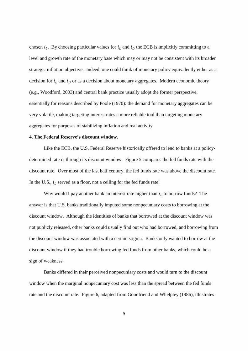
4. The Federal Reserve’s discount window.

Like the ECB, the U.S. Federal Reserve historically offered to lend to banks at a policy-

determined rate �� through its discount window. Figure 5 compares the fed funds rate with the

discount rate. Over most of the last half century, the fed funds rate was above the discount rate.

In the U.S., �� served as a floor, not a ceiling for the fed funds rate!

Why would I pay another bank an interest rate higher than �� to borrow funds? The

answer is that U.S. banks traditionally imputed some nonpecuniary costs to borrowing at the

discount window. Although the identities of banks that borrowed at the discount window was

not publicly released, other banks could usually find out who had borrowed, and borrowing from

the discount window was associated with a certain stigma. Banks only wanted to borrow at the

discount window if they had trouble borrowing fed funds from other banks, which could be a

sign of weakness.

Banks differed in their perceived nonpecuniary costs and would turn to the discount

window when the marginal nonpecuniary cost was less than the spread between the fed funds

rate and the discount rate. Figure 6, adapted from Goodfriend and Whelpley (1986), illustrates

6

how the fed funds rate was determined in this system. The Fed’s open-market operations

resulted in a certain level of nonborrowed reserves, which are deposits with the Fed that banks

would have even if they do no borrowing at the discount window. As the fed funds rate rises

above the discount rate, more banks would be willing to borrow at the discount window, thereby

increasing the total supply of nonborrowed plus borrowed reserves until supply equals demand.

Figure 7 compares the gap between the fed funds rate and the discount rate (top panel)

with the total volume of discount window borrowing (bottom panel), showing how the system

worked in practice. A higher value for the fed funds rate relative to the discount rate was

associated with a higher volume of borrowing. Indeed, some observers at the time thought of the

operating system as one of borrowed reserves targeting rather than fed funds rate targeting.

5. Interest on excess reserves.

Beginning in October 2008, the Federal Reserve began paying an interest rate on excess

reserves (IOER), akin to the interest rate �� in a corridor system. Figure 8 shows the recent

relation between the fed funds rate and IOER. Whereas �� acts as a floor in the traditional

corridor system, until very recently IOER seemed to be a ceiling on the fed funds rate! Indeed,

at times IOER looked like a deterministic ceiling. On most days, the average effective fed funds

rate would be exactly 9 basis points below the interest on excess reserves, though it would drop

significantly below on the last day of the month.

Why would anyone offer to lend at a fed funds rate below IOER if they could earn IOER

just by parking the funds with the Fed? The answer is that not all depository institutions can earn

IOER. Federal Home Loan Banks (FHLB) have deposits with the Fed but are not paid IOER, so

they have an incentive to lend to banks that can earn IOER. But why wouldn’t banks that can

earn IOER bid up the fed funds rate so as to earn the risk-free arbitrage from borrowing at the

7

fed funds rate and earning IOER? Part of the answer is on the supply side; individual Federal

Home Loan Banks set limits on to whom and how much they lend. Afonso, Armenter, and Lester

(2019) modeled these frictions using a search and matching model for the fed funds market.

Another factor is nonpecuniary costs on the demand side, as discussed by Klee, Senyuz, and

Yoldas (2016), Banegas and Tase (2017) and Anbil and Senyuz (2018). If a bank tries to

arbitrage by borrowing fed funds and holding fed deposits to earn IOER, it expands its balance

sheet. A larger level of assets exposes U.S. banks to higher fees from the Federal Deposit

Insurance Corporation. For this reason, foreign banks are a more natural counterparty than

domestic banks to borrow the fed funds from the FHLB. In addition, both domestic and foreign

banks are subject to complicated capital requirements, another source of nonpecuniary costs

associated with borrowing fed funds. A larger balance sheet may require the bank to make other

adjustments to meet capital requirements, which imposes another nonpecuniary cost on

arbitraging the IOER-fed funds spread. For European banks, the capital requirements are

primarily based on end-of-month assets. This explains why before 2018 there was usually a

sharp spike in the gap between IOER and the fed funds rate on the last day of a month; this was

the one day those banks didn’t want to borrow fed funds.

One can think about the determination of the fed funds rate in this setting as in Figure 9.

Banks differ in their marginal nonpecuniary costs of borrowing fed funds and would be willing

to borrow more the bigger the gap between IOER and fed funds. The apparent deterministic

nature of the IOER-fed funds gap in early 2017 arose from the fact that, on days other than the

last day of the month, and over the range of volume traded at that time, there was a sufficient

volume of borrowers with fixed nonpecuniary costs of 9 basis points. In other words, the

8

demand curve was flat over that range resulting in essentially a constant gap between IOER and

the fed funds rate.

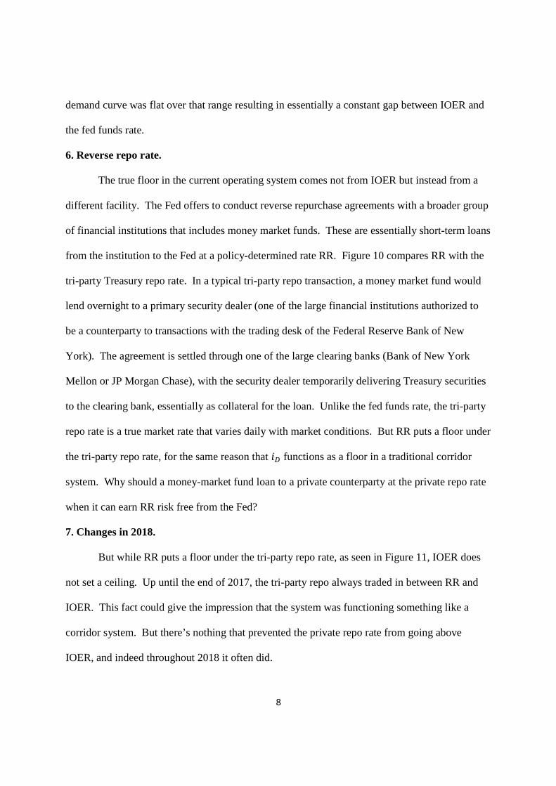
6. Reverse repo rate.

The true floor in the current operating system comes not from IOER but instead from a

different facility. The Fed offers to conduct reverse repurchase agreements with a broader group

of financial institutions that includes money market funds. These are essentially short-term loans

from the institution to the Fed at a policy-determined rate RR. Figure 10 compares RR with the

tri-party Treasury repo rate. In a typical tri-party repo transaction, a money market fund would

lend overnight to a primary security dealer (one of the large financial institutions authorized to

be a counterparty to transactions with the trading desk of the Federal Reserve Bank of New

York). The agreement is settled through one of the large clearing banks (Bank of New York

Mellon or JP Morgan Chase), with the security dealer temporarily delivering Treasury securities

to the clearing bank, essentially as collateral for the loan. Unlike the fed funds rate, the tri-party

repo rate is a true market rate that varies daily with market conditions. But RR puts a floor under

the tri-party repo rate, for the same reason that �� functions as a floor in a traditional corridor

system. Why should a money-market fund loan to a private counterparty at the private repo rate

when it can earn RR risk free from the Fed?

7. Changes in 2018.

But while RR puts a floor under the tri-party repo rate, as seen in Figure 11, IOER does

not set a ceiling. Up until the end of 2017, the tri-party repo always traded in between RR and

IOER. This fact could give the impression that the system was functioning something like a

corridor system. But there’s nothing that prevented the private repo rate from going above

IOER, and indeed throughout 2018 it often did.

9

Figure 11 also plots another market-determined short-term interest rate, the Treasury

general collateralized finance rate (GCF). These are also repurchase agreements collateralized

with Treasury securities that are cleared through a third party, in this case the Fixed Income

Clearing Corporation1. A typical transaction here would be a loan from a primary security dealer

to a nonprimary security dealer, again collateralized by Treasuries, with the primary dealer often

rehypothecating the Treasury securities for purposes of its own borrowing through tri-party

repos. The GCF rate is generally above the tri-party repo rate. It’s interesting to compare the

2018 portion of Figure 11 with Figure 8. GCF started to trade consistently above IOER at the

same time that IOER stopped being the de facto ceiling on the fed funds rate.

What changed in 2018? The elimination of the gap between IOER and fed funds could

have come from either a rightward shift of the demand curve in Figure 9—the nonpecuniary

costs of borrowing fed funds decreased, leading borrowing banks bid up the cost of fed funds—

or from a leftward shift of the supply curve—FHLB are less willing to lend fed funds. If the first

explanation was correct, we would expect to see an increase in the volume of fed funds lending,

whereas if the second, we would expect to see a decrease. Figure 12 plots the effective fed funds

rate together with the volume of borrowing. It shows that the disappearing gap between IOER

and fed funds coincided with a decreased volume of fed lending, favoring the second explanation

based on the supply side. Figure 13 plots selected assets held by the FHLB. It paints a picture of

the FHLB turning from lending fed funds to alternative ways of investing short-term funds that

presumably provide a higher yield.

8. Perspectives on the current and potential future operating systems.

I’ve described the current operating system as one with a floor but no ceiling. What then

is holding rates down? I think the answer is twofold. First, there has been weak demand for 1 For more details on GCF see Agueci et al. (2014).

10

investment both in the U.S. and around the world for some time. Second, there remains a huge

volume of reserves in the system. Figure 14 summarizes the implications of the Fed’s balance

sheet from the perspective of its liabilities. The large security purchases of Figure 1 were

primarily financed by an expansion of bank deposits with the Fed. Banks so far have been

willing to hold these reserves as a result of IOER. As the Fed’s balance sheet contracted (and as

demand for cash gradually climbed), excess reserves have slowly been coming down.

Another important development in 2018 was increasing demand for borrowed funds, in

part arising from an elevated level of borrowing by the U.S. Treasury to finance the federal

government budget deficit. This could be one of the factors that has driven GCF up in 2018 and

that pulled lending away from the fed funds market. As we look ahead, we should expect

demand for loans to continue to change. The Fed will want some more accurate policy tools to

respond to these changes.

One option would be to allow reserves to shrink until we are back in something like the

historical system in Figure 6. That system worked when fluctuations in the Treasury’s balance

with the Fed (which are a choice of the Treasury, not the Fed) were on the order of a few billion

dollars. But one sees in Figure 14 that fluctuations today are in the hundreds of billions. It’s

also far from clear how we would make a smooth transition from the current operating system to

something like Figure 6.

A more natural transition from the current system would begin by acknowledging that

something like the tri-party repo rate is currently a more relevant market measure than the fed

funds rate. The Fed could introduce an open repo facility from which the same institutions that

currently use the reverse repo facility could also use direct repos to borrow all the funds they

usually wanted at a chosen policy rate. This would establish a corridor system for controlling the

11

private repo rate. I specify “usually” here because it would not be necessary, or even desirable,

to fully smooth out the “window dressing” that one sees in the end-of-quarter spike in private

repo rates. The end-of-quarter spikes arise because some institutions do not want to

acknowledge the extent of their exposure to private counterparty repos in their publicly available

statements, which are only based on assets as of the last day of a quarter. There’s no compelling

policy reason why the Fed should accommodate that seasonal demand. Indeed, historically a

specified fed funds target was viewed as perfectly consistent with end-of-month spikes in the

effective fed funds rate above the target arising from such forces.

The drawback of such a system would be that it puts the Fed in the position of effectively

insuring a broader set of institutions than those over which it has regulatory authority. The

longer run goal should therefore be to return both the ceiling and the floor for the policy rate to

offers to lend or borrow from only regulated institutions. The Fed could initially implement a

repo corridor system with a broad range of counterparties at the same time that it continues to

reduce the volume of excess reserves. As we reach a level when banks are more actively

managing their reserve balances, the Fed could restrict access to both repo facilities to regulated

institutions. This could be a practical path toward the goal of replacing the discount window

with a stigma-free facility.

12

References

Afonso, Gara, Roc Armenter, and Benjamin Lester. “A model of the federal funds market: yesterday, today, and tomorrow.” Working paper, Federal Reserve Bank of Philadelphia, 2019. Agueci, Paul et al. “A primer on the GCF repo service,” Federal Reserve Bank of New York, 2014. Anbil, Sriya, and Zeynep Senyuz. “Window-dressing and the Fed’s RRP Facility in the repo market.” Finance and Economics Discussion Paper Series 2018-027 (2018). Banegas, Ayelen, and Manjola Tase. “Reserve balances, the federal funds market and arbitrage in the new regulatory framework.” Available at SSRN 3055299 (2017). Borio, Claudio, and Anna Zabai. “Unconventional monetary policies: a re-appraisal.” Research Handbook on Central Banking, pp. 398-444, edited by Peter Conti-Brown, and Rosa Maria Lastra, Cheltenham: Edward Elgar Publishing, 2018. Caballero, Ricardo, and Emmanuel Farhi. “The safety trap.” The Review of Economic Studies 85, no. 1 (2017): 223-274. Chen, Han, Vasco Cúrdia, and Andrea Ferrero. “The macroeconomic effects of large‐scale asset purchase programmes.” Economic Journal 122, no. 564 (2012). Cúrdia, Vasco, and Michael Woodford. “The central-bank balance sheet as an instrument of monetary policy.” Journal of Monetary Economics 58, no. 1 (2011): 54-79. Eggertsson, Gauti B., and Kevin Proulx. “Bernanke’s no-arbitrage argument revisited: Can Open Market Operations in Real Assets Eliminate the Liquidity Trap?” National Bureau of Economic Research working paper 22243, 2016. Eggertsson, Gauti B, and Michael Woodford. “Zero bound on interest rates and optimal monetary policy.” Brookings Papers on Economic Activity 2003, no. 1 (2003): 139-233.

Gertler, Mark, and Peter Karadi. “A model of unconventional monetary policy.” Journal of Monetary Economics 58, no. 1 (2011): 17-34. Goodfriend, Marvin, and William Whelpley. “Federal funds: instrument of Federal Reserve policy.” Federal Reserve Bank of Richmond Economic Review 72, no. 5 (1986): 3-11. Greenlaw, David, James D. Hamilton, Ethan Harris, and Kenneth D. West. “A skeptical view of the impact of the Fed’s balance sheet.” National Bureau of Economic Research working paper 24687, 2018. Greenwood, Robin, and Dimitri Vayanos. “Bond supply and excess bond returns.” The Review of Financial Studies 27, no. 3 (2014): 663-713.

13

Hamilton, James D. “The efficacy of large-scale asset purchases when the short-term interest rate is at its effective lower bound.” Brookings Papers on Economic Activity, Fall 2018. Hamilton, James D., and Jing Cynthia Wu. “The effectiveness of alternative monetary policy tools in a zero lower bound environment,” Journal of Money, Credit and Banking 44, no. s1 (2012): 3-46. Klee, Elizabeth, Zeynep Senyuz, and Emre Yoldas. “Effects of changing monetary and regulatory policy on overnight money markets.” Working paper, Federal Reserve Board (2016). Levin, Andrew, and Prakash Loungani. “Reassessing the benefits and costs of quantitative easing,” Working paper, Dartmouth University, 2019. Melosi, Leonardo. “Signalling effects of monetary policy.” The Review of Economic Studies 84, no. 2 (2016): 853-884. Miranda-Agrippino, Silvia, and Giovanni Ricco. “The Transmission of Monetary Policy Shocks,” working paper, Bank of England, 2018. Nakamura, Emi, and Jón Steinsson. “High frequency identification of monetary non-neutrality: the information effect.” Quarterly Journal of Economics 133, Issue 3: 1283-1330, 2018. Poole, William. “Optimal choice of monetary policy instruments in a simple stochastic macro model.” The Quarterly Journal of Economics 84, no. 2 (1970): 197-216. Swanson, Eric. “The Federal Reserve is not very constrained by the lower bound on nominal interest rates.” Brookings Papers on Economics Activity, Fall 2018. Thornton, Daniel L. “Effectiveness of QE: An assessment of event-study evidence.” Journal of Macroeconomics 52 (2017): 56-74. Williams, John C. “Monetary policy at the zero lower bound: putting theory into practice.” Brookings Institution, 2014. Woodford, Michael. Interest and Prices: Foundations of a Theory of Monetary Policy. Princeton: Princeton University Press, 2003. Woodford, Michael. “Methods of policy accommodation at the interest-rate lower bound.” The Changing Policy Landscape, Federal Reserve Bank of Kansas City, Jackson Hole Wyoming (2012): 185-288.

14

Figure 1. Federal Reserve holdings of securities, billions of dollars.

Notes to Figure 1. Weekly Fed holdings of Treasury securities, mortgage-backed securities and agency

debt, plus unamortized premiums minus unamorized discounts, Wednesday values, Jan 7, 2009 to Feb 6,

2019. Data source: Federal Reserve H.4.1 release. Shading dates for QE1: Mar 18, 2009 to Mar 24,

2010; QE2: Nov 3, 2010 to Jun 22, 2011; QE3: Nov 7, 2012 to Apr 30, 2014 (halfway through taper);

unwind: Nov 22, 2017 to present.

Figure 2. Interest rate on 10-year Treasury bond.

0

500

1000

1500

2000

2500

3000

3500

4000

4500

5000

2009 2010 2011 2012 2013 2014 2015 2016 2017 2018 2019

QE1-3 unwind securities

0

1

1

2

2

3

3

4

4

5

2009 2010 2011 2012 2013 2014 2015 2016 2017 2018 2019

QE1-3 unwind 10 year yield

15

Figure 3. Cumulative change in 10-year yield on Fed Days.

Notes to Figure 3. Cumulative change in interest rate on 10-year Treasury bond on FOMC meeting days,

days when FOMC minutes were released, or days with speech by Fed chair on economy or monetary

policy, Jan 1, 2009 to Dec 29, 2017. Data source: Greenlaw et al. (2018).

Figure 4. Corridor system for controlling interest rates used by the European Central Bank.

Notes to Figure 4. End-of-month values for ECB marginal lending rate (orange) and deposit facility (blue)

along with monthly average 3-month Euribor rate (gray), Jan 2001 to Jan 2016.

-50

0

50

100

150

200

Jan-

09

Jun-

09

Oct

-09

Mar

-10

Aug

-10

Jan-

11

Jun-

11

Oct

-11

Mar

-12

Aug

-12

Jan-

13

May

-13

Oct

-13

Mar

-14

Aug

-14

Jan-

15

Jun-

15

Oct

-15

Mar

-16

Aug

-16

Jan-

17

May

-17

Oct

-17

-1

0

1

2

3

4

5

6

7

deposit rate lending rate 3-month Euribor

16

Figure 5. Fed funds rate and discount rate.

Notes to Figure 5. Monthly average effective fed funds rate, Apr 1954 to Apr 2019 (blue) and discount

rate, Apr 1954 to Apr 2017 (red). Figure source: FRED Economic Data, Federal Reserve Bank of St. Louis.

Figure 6. Determination of fed funds rate in historical U.S. system.

17

Figure 7. Volume of borrowed reserves and gap between fed funds rate and discount rate.

Notes to Figure 7. Top panel: monthly average effective fed funds rate minus discount rate, Jan 1965 to

Dec 1975. Bottom panel: discount window borrowings of depository institutions from the Federal

Reserve, billions of dollars. Data source: FRED.

18

Figure 8. Fed funds rate and interest on excess reserves.

Notes to Figure 8. Daily effective fed funds rate (black) and interest on excess reserves (green), Dec 17

2015 to Apr 10, 2019. Data source: FRED.

19

Figure 9. Determination of the fed funds rate in 2017.

Figure 10. Tri-party repo rate and interest on excess reserves.

Notes to Figure 10. Daily interest rate on tri-party repurchase agreements based on Treasury securities

(black) and Fed reverse repo rate (blue), Dec 17 2015 to Apr 10, 2019. Vertical lines denote last day of a

quarter. Tri-party repo rates from Bank of New York Mellon

(https://repoindex.bnymellon.com/repoindex/).

20

Figure 11. GCF rate, tri-party repo rate, reverse repo rate, and interest on excess reserves.

Notes to Figure 11. Daily general collateralized finance rate for repurchase agreements based on

Treasury securities (dashed red), rate on tri-party repurchase agreements based on Treasury securities

(black), interest on excess reserves (green), and Fed reverse repo rate (blue), Dec 17 2015 to Apr 10,

2019. GCF data from DTCC (http://www.dtcc.com/charts/dtcc-gcf-repo-index#download).

21

Figure 12. Daily effective fed funds rate and volume of fed funds lending.

Notes to Figure 12. Figure source: Federal Reserve Bank of New York

(https://apps.newyorkfed.org/markets/autorates/fed%20funds).

Figure 13. Selected end-of-quarter assets of Federal Home Loan Banks (billions of dollars).

Notes to Figure 13. Data source: FHLB end-of-quarter financial reports (http://www.fhlb-

of.com/ofweb_userWeb/pageBuilder/fhlbank-financial-data-36).

0

10

20

30

40

50

60

70

80

90

100

2018:Q1 2018:Q2 2018:Q3 2018:Q4

fed funds lent interest-bearing deposits repos

22

Figure 14. Weekly Federal Reserve liabilities (billions of dollars).

Notes to Figure 14. Wednesday values. Dec 18, 2002 to Feb 6, 2019. Currency: currency in circulation;

rev repo: reverse repurchase agreements; treasury: U.S. Treasury general account plus supplementary

financing account; reserve balances: reserve balances with Federal Reserve Banks. Data source: Federal

Reserve H.4.1 release.

0

500

1000

1500

2000

2500

3000

3500

4000

4500

5000

20

02

20

03

20

04

20

05

20

06

20

07

20

08

20

09

20

10

20

11

20

12

20

13

20

14

20

15

20

16

20

17

20

18

currency rev repo term deposits treasury other reserve balances