Perspectives on Poverty Presented by John McPeak Department of Public Administration Syracuse University

Perspectives on Poverty

Presented by John McPeak

Department of Public Administration

Syracuse University

Why focus on poverty?

• This is increasingly a major goal of governments and donors.

• Eradicating Poverty For Stability And Peace• WASHINGTON, October 3, 2004 – Saying

that eradication of poverty is central to global stability and peace, World Bank Group President James D. Wolfensohn today issued an urgent call to action to make the planet more equitable and safe, through the three pillars of poverty reduction, environmental stewardship, and education of the youth of the world.

Why focus on poverty?Poverty reduction an explicit goal of development agencies.

Millennium Development Goals.

Poverty Reduction Strategy Papers for HIPC’s.

37 countries have completed full PRSPs, 48 have completed interim PRSPs.

Important documents for national planning and communicating needs to development partners.

What is poverty?

• If we want to reduce it, first we have to define what it is.

• How do we measure poverty?

• Do different measures tell us different things?

• Do these different messages have different policy implications?

Relative versus absolute poverty• First, we have to clarify whether we are

talking about absolute poverty or relative poverty.

• Usually the idea is absolute poverty.• “human” poverty as an index of

depravations (UNDP looks at low life expectancy, lack of basic educaton, lack of access to health services and clean water)

• Most concepts are based on the idea of income poverty

• Headcount or headcount index.

• Define a poverty line (say $1 per person per day as defined by PPP).

• Obtain information on people’s real income.

• Count those below the poverty line – a headcount of poverty.

• Report this as a fraction of the population – a headcount index or poverty incidence.

Static measures of absolute poverty


Country A Country B

Person 1 $0.50 $0.10

Person 2 $0.90 $0.15

Person 3 $0.95 $0.35

Person 4 $1.25 $1.50

Person 5 $1.50 $2.00

Person 6 $2.00 $3.00

Headcount in both countries is 3, Headcount index / poverty incidence is 50%. But it appears poverty is worse in Country B than in Country A. Same total income ($7.10) and same average income ($1.18).


• Poverty Gap measure.

• Country A: ($1-$0.50)+($1-$0.90)+($1-$0.95) = $0.65

• Country B: ($1-$0.10)+($1-$0.15)+($1-$0.35) = $2.40

• Can also calculate the average poverty gap by dividing the gap by the headcount.

• Country A: $0.22, Country B: $0.80.


• Note that this measure does not pick up differences in income distribution among the poor.

• Country B: ($1-$0.10)+($1-$0.15)+($1-$0.35) = $2.40

• Country B’: ($1-$0.05)+($1-$0.05)+($1-$0.50) = $2.40

A squared index is sometimes used to account for this, to penalize more heavily larger deviations from the poverty line.


• This can be done for various other measures.

• Useful from a planning perspective as a way to target poverty alleviation measures spatially.

• Can be overlaid with other GIS maps to uncover patterns (access to roads, markets, public services, school enrollment, cell phone coverage,…)

Dynamic measures of absolute poverty

• Krishna’s study.• 35 villages in five districts of Rajasthan.• Stages of progress exercise to establish

what constitutes poverty in each village.• First four stages: buying food to eat,

sending children to school, possessing clothes to wear outside the house, retiring debt in regular installments.

• Poverty is not being able to meet these four conditions.


• Select event 25 years ago (the national emergency).

• Discuss each household’s position at the time of the event and current position (ended up excluding education due to changes over time in the view of education).

• Men and women draw up different lists, reconcile at end, and follow up with households if outstanding differences exist.


Poor 25 years ago

Not poor 25 years ago.

Poor currently 17.8%

remained poor

7.9%

became poor

Not poor currently

11.1%

Escaped poverty

63.2%

remained non poor


• Falling into poverty

• No single factor, mostly a combination of factors. Not a single blow, but a series of blows.

• 85% of cases involve some combination of health problems and health related expenses, high interest private debt, and social and customary expenses.

• Drunkenness and laziness are mentioned in around 5% of cases.


• Escaping poverty.• Diversification of income sources – taking up

activities in addition to agriculture.• Often an urban link and information is critical.• Personal capability and enterprise, relatives

help.• Direct assistance from government departments,

NGOs, political parties less important.• Informal sector is main source of opportunities,

not formal full time employment.


• The Kenya study provides a similar story with a few variations.

• Policy implications?

• First, if we want to help people escape, we should first know what they do themselves?

• Second, if we want to help people avoid falling into poverty, we should understand the main factors that lead to a fall and target them.


• High healthcare costs, high interest consumption debt, social expenses on deaths and marriage.

• Escaping poverty can be improved by improved information (water tables for irrigation, disease control for health, contacts and jobs in the city).


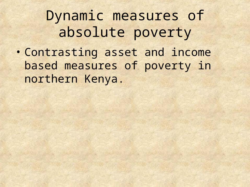
• Contrasting asset and income based measures of poverty in northern Kenya.

• In pastoral areas, the key asset is livestock.

This makes asset poverty simpler to analyze than in other settings, but there is broad applicability of this approach

• Asset poverty can be viewed as “structural poverty”.– the assets of a household are below a threshold that

generates expected income above some defined poverty line.

• Income poverty can be viewed as “transitory poverty”.– The observed income level is below a threshold in a

given time period.

• Vulnerability to these different types of poverty differs.

• Average household income is highly variable over time periods.

• Clear seasonality (1 is the long rains, 3 is the short rains, 2 and 4 are dry seasons).

• Slow upward shift of the cycle.

0

10

20

30

40

50

60

93-1 93-2 93-3 93-4 94-1 94-2 94-3 94-4 95-1 95-2 95-3 95-4 96-1 96-2 96-3 96-4 97-1

Time period

Inc

om

e p

er

pe

rso

n p

er

da

y in

US

c

en

ts

0.0

0.5

1.0

1.5

2.0

2.5

0 5 10 15 20 25

Average Herd Size per person

CV

of

ho

us

eh

old

in

co

me

0.0

0.5

1.0

1.5

2.0

2.5

0.1

4

0.1

7

0.2

0

0.2

3

0.2

6

0.2

8

0.2

9

0.3

0

0.3

2

0.3

4

0.3

5

0.3

8

0.4

6

0.5

0

0.5

7

0.6

5

0.7

7

0.9

5

Average Income per person per day in USD

CV

of

ho

use

ho

ld i

nco

me

Clearly, this is a highly variable production environment due to rainfall fluctuations.

Contrast households by income variability over time under the assumption that higher variability is “bad”.

CV of household income is a decreasing function of both average herd size and of average income level

• Herd dynamics play a critical role in household vulnerability.

• Average household herd size changed dramatically over time (35% increase to max, 55% decrease from max).

• The late 1996 loss to the average herd corresponds to a 34% drop in expected income.

0

2

4

6

8

10

12

93-1 93-2 93-3 93-4 94-1 94-2 94-3 94-4 95-1 95-2 95-3 95-4 96-1 96-2 96-3 96-4 97-1 97-2 97-3 97-4

Time period

Her

d si

ze p

er a

dult

equi

vale

nt

• Regression analysis allows us to trace out the relationship between herd size per adult equivalent and expected income.

• Threshold using a $0.50 per person per day poverty line: – wet season 6.5 animals– dry season 9.5 animals

Wet season

010203040

5060708090

0 1 2 3 4 5 6 7 8 9 10 11 12 13 14 15

Herd size per adult equivalent

$ in

com

e pe

r adu

lt eq

uiva

lent

pe

r day

Dry season

010

2030

4050

6070

8090

0 1 2 3 4 5 6 7 8 9 10 11 12 13 14 15

Herd size per adult equivalent

$ pe

r ad

ult e

quiv

alen

t per

da

y

Examples Structural Poverty Stochastic Poverty

Chronic Poverty

No animals String of bad luck

Transitory Poverty

Seasonal Escape /

Had temporary good luck

Drought

Definition Structural Poverty Stochastic Poverty

Chronic Poverty

Always income poor

Asset poor

Always income poor

Asset non-poor

Transitory Poverty

Sometimes income poor

Asset poor

Sometimes income poor

Asset non-poor

Percent of households over four years that were:

ASSET POVERTYLINE

Always below

Sometimes below

Never below

Dry Season

71% 27% 2%

Wet season

43% 46% 11%

INCOME POVETY LINE

Always below

Sometimes below

Never below

Dry Season

49% 45% 6%

Wet season

6% 85% 9%

Contrast income poverty with asset poverty.– 69% income poor in wet seasons and 77% in

dry seasons – 64% asset poor in wet seasons and 83% in

dry seasons– Households that are income poor but not

asset poor more common in the wet season.

0%

10%

20%

30%

40%

50%

60%

93-1 93-2 93-3 93-4 94-1 94-2 94-3 94-4 95-1 95-2 95-3 95-4 96-1 96-2 96-3 96-4 97-1

Season

% o

f H

H a

bo

ve

as

se

t p

ov

ert

y

line

Dry season line

Wet season line

0%

5%

10%

15%

20%

25%

30%

35%

40%

45%

50%

93-1 93-2 93-3 93-4 94-1 94-2 94-3 94-4 95-1 95-2 95-3 95-4 96-1 96-2 96-3 96-4 97-1

Time period

% a

bo

ve

in

co

me

po

ve

rty

lin

e

When you measure and how you measure poverty leads to different implications

The implications for development policy

• Sharp declines in aid flows over the 1990’s.

• Increasing share of this aid spent on humanitarian / emergency needs rather than structural development.

• Share on education, health, economic infrastructure, agricultural production technology fell from 47% of the total OECD flow in 1993 to 31% in 1999.


• With shrinking funds and a shrinking share of these funds spent on addressing structural poverty, risk is that we enter a cycle of humanitarian crisis after humanitarian crisis.

• Without changing underlying conditions, end up only providing temporary relief.

• Contrast food-for-work with food aid distribution if public goods constructed.


• Vulnerability to poverty may influence behavior as much as the state of poverty.

• Asset complementarities may be critical (and wealth may matter). Land plus irrigation as opposed to just land.

• Access to assets – who has access? Will markets alone allocate assets to allow people to climb out of poverty?

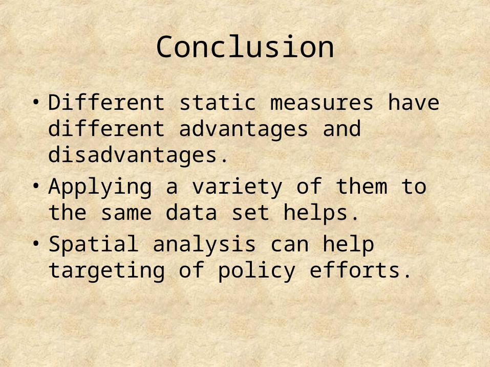
Conclusion

• Different static measures have different advantages and disadvantages.

• Applying a variety of them to the same data set helps.

• Spatial analysis can help targeting of policy efforts.

Conclusion

• Dynamic measures provide different types of information on poverty.– What do people identify as the causes of falling into

poverty?– What do people identify as the main paths out of

poverty?– What can government / NGOs do with this

information? – Policy to prevent falls (“safety nets”) may differ from

policy to allow escape (“cargo nets”).– Humanitarian is by nature targeted at transitory, crisis

relief. Does this crowd out longer term development assistance?

Conclusion

• Asset based poverty measures differ from income based poverty measures.

• Asset vulnerability may be important.

• Seasonality of income measures may be misleading.

Documents

Perspectives on Poverty Presented by John McPeak Department of Public Administration Syracuse University