Personal Response System (PRS). Revision session

Dr David Field

Do not turn your handset on yet!

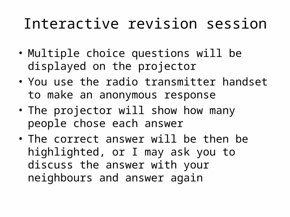
Interactive revision session

• Multiple choice questions will be displayed on the projector

• You use the radio transmitter handset to make an anonymous response

• The projector will show how many people chose each answer

• The correct answer will be then be highlighted, or I may ask you to discuss the answer with your neighbours and answer again

Interactive revision session

• The purpose of the session is to– allow you to find out how familiar you are with

the course material– give you practice for the Week 10 statistics

test– provide an opportunity for me to explain topics

further if there is confusion

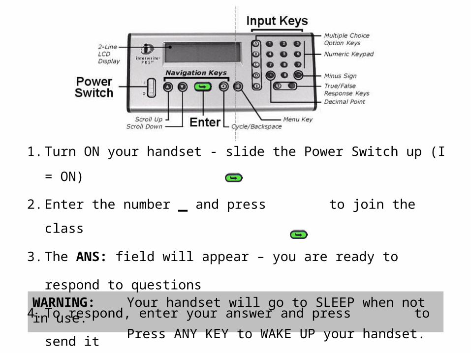
WARNING: Your handset will go to SLEEP when not in use. Press ANY KEY to WAKE UP your handset.

1. Turn ON your handset - slide the Power Switch up (I = ON)

2. Enter the number _ and press to join the class

3. The ANS: field will appear – you are ready to respond to questions

4. To respond, enter your answer and press to send it

5. You may change your mind by entering a new answer to replace your

original answer

Which of these variables has an ordinal level of measurement?

1) reaction time measured in seconds?2) place in class exam (e.g., 1st , 2nd, 3rd)3) gender4) percentage score in a maths exam

What is a dependent variable?

1) something which you measure in an experiment

2) something that varies which is continuous

3) something which you manipulate in an experiment

4) none of the above

Which of these is likely to have the largest SD?

1) The heights of a sample of men

2) The heights of a sample of men and women

3) The heights of a sample of women

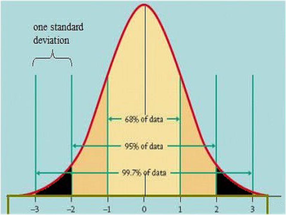
A person’s height is 2SD > the mean of a sample. What % of participants are shorter?

1) 68%2) 5%3) 2.5%4) 97.5%5) 95%

The formula for computing a z score is:

1. (score – mean) / standard deviation

2. (mean – score) / variance

3. mean / standard deviation

4. score / variance

If a frequency histogram shows a normal distribution, which of the following are true? To select multiple answers you enter the corresponding numbers in any order, without any separating spaces or commas.

1) The mean and the median will have similar values2) The tallest histogram bar shows the interval with more

scores in it than any other interval3) 95% of scores will fall within 1.96 * the SD of the mean4) 68% of scores will fall within 1 * the SD of the mean

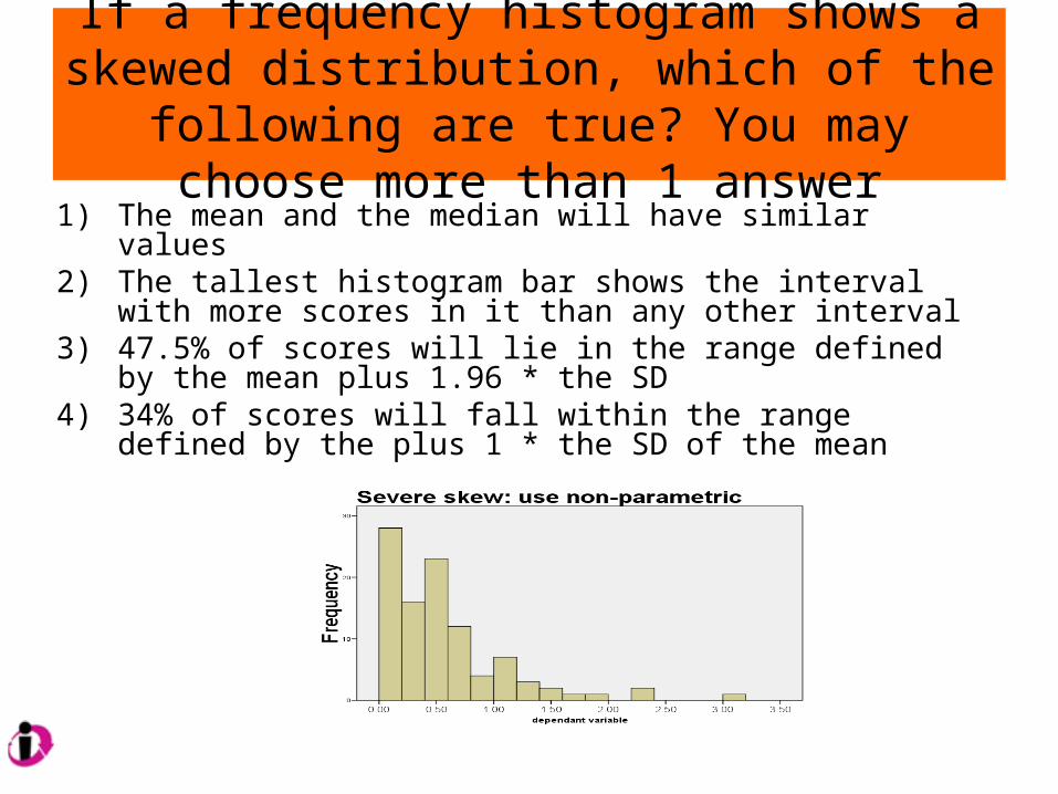
If a frequency histogram shows a skewed distribution, which of the following are true?

You may choose more than 1 answer1) The mean and the median will have similar values2) The tallest histogram bar shows the interval with more

scores in it than any other interval3) 47.5% of scores will lie in the range defined by the

mean plus 1.96 * the SD4) 34% of scores will fall within the range defined by the

plus 1 * the SD of the mean

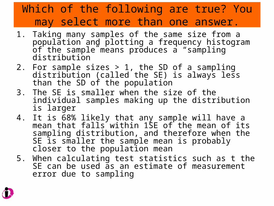
Which of the following are true? You may select more than one answer.

1. Taking many samples of the same size from a population and plotting a frequency histogram of the sample means produces a “sampling distribution”

2. For sample sizes > 1, the SD of a sampling distribution (called the SE) is always less than the SD of the population

3. The SE is smaller when the size of the individual samples making up the distribution is larger

4. It is 68% likely that any sample will have a mean that falls within 1SE of the mean of its sampling distribution, and therefore when the SE is smaller the sample mean is probably closer to the population mean

5. When calculating test statistics such as t the SE can be used as an estimate of measurement error due to sampling

A type I error is when…

1. We fail to reject the null hyp, but it is actually false in the population

2. We support the null hypothesis3. We reject the null hypothesis, but it is

actually true in the population4. the p value is > 0.05

Imaginary experiment

• 30 myopic volunteers undergo eye surgery– volunteers selected to have similar acuity pre surgery

• 15 are randomly selected to undergo modern laser surgery

• The other 15 undergo a traditional operation, in which the top of the cornea is removed with a knife– Which procedure produces better post-op vision?

• After recovery from surgery visual acuity is measured• Visual acuity is measured in normalised units of

“LogMAR”– after normalisation of the scale, the average score for young

adults with typical vision is 0– negative numbers indicate acuity worse than average– positive numbers indicate better than average acuity

Choose the type of research design and likely statistical test.

1) Repeated measures experiment - test the null hypothesis with an independent samples t test

2) Independent samples experiment - test the null hypothesis with a paired samples t test

3) Correlational design - test the null hypothesis with an independent samples t test

4) Independent samples experiment - test the null hypothesis with an independent samples t test

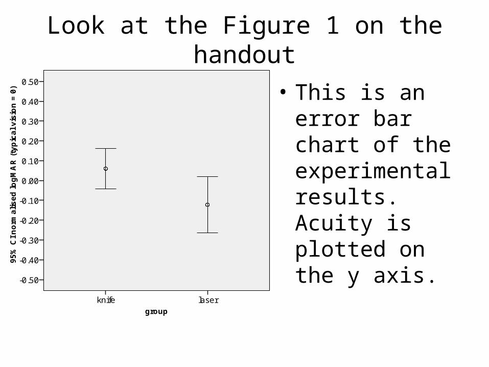
Look at the Figure 1 on the handout

• This is an error bar chart of the experimental results. Acuity is plotted on the y axis.

group

laserknife

95

% C

I n

orm

ali

se

d l

og

MA

R (

typ

ica

l v

isio

n =

0)

0.50

0.40

0.30

0.20

0.10

0.00

-0.10

-0.20

-0.30

-0.40

-0.50

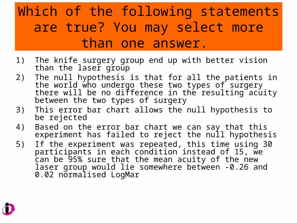
Which of the following statements are true? You may select more than one answer.

1) The knife surgery group end up with better vision than the laser group

2) The null hypothesis is that for all the patients in the world who undergo these two types of surgery there will be no difference in the resulting acuity between the two types of surgery

3) This error bar chart allows the null hypothesis to be rejected4) Based on the error bar chart we can say that this experiment has

failed to reject the null hypothesis5) If the experiment was repeated, this time using 30 participants in

each condition instead of 15, we can be 95% sure that the mean acuity of the new laser group would lie somewhere between -0.26 and 0.02 normalised LogMar

Look at the Figure 2 on the handout

Group Statistics

15 .0598 .18226 .04706

15 -.1225 .25629 .06617

groupknife

laser

normalised logMAR(typical vision = 0)

N Mean Std. DeviationStd. Error

Mean

Independent Samples Test

.826 .371 2.245 28 .033 .18227 .08120 .01594 .34861

2.245 25.277 .034 .18227 .08120 .01513 .34942

Equal variancesassumed

Equal variancesnot assumed

normalised logMAR(typical vision = 0)

F Sig.

Levene's Test forEquality of Variances

t df Sig. (2-tailed)Mean

DifferenceStd. ErrorDifference Lower Upper

95% ConfidenceInterval of the

Difference

t-test for Equality of Means

For this t test, you should report the df and Sig. from the “equal variance not assumed” row

1) True

2) False

The t test is statistically significant and the null hypothesis can be rejected

1) True

2) False

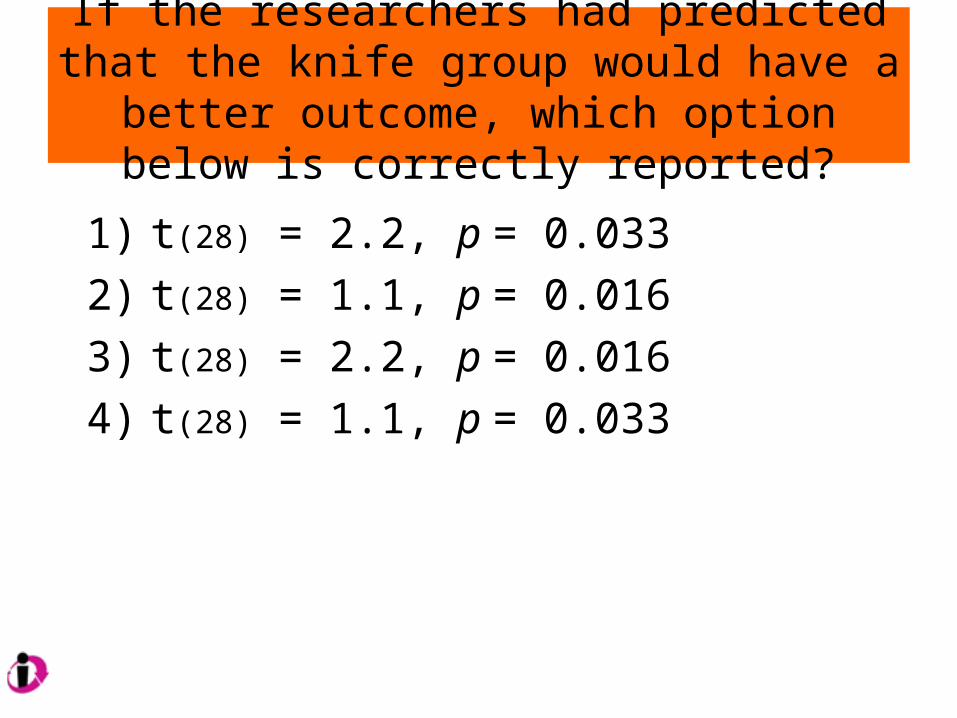
If the researchers had predicted that the knife group would have a better outcome, which option below is correctly reported?

1) t(28) = 2.2, p = 0.033

2) t(28) = 1.1, p = 0.016

3) t(28) = 2.2, p = 0.016

4) t(28) = 1.1, p = 0.033

What is the effect size?

1) 0.83

2) 0.24

3) 1.67

4) 0.56

5) none of the above

Effect size (Cohen’s d )

d =Condition 1 mean – Condition 2 mean

SD Condition 1 + SD condition 2

2

Effect size in the acuity experiment

d =(knife mean)0.06 – –0.12 (laser mean)

(Knife SD) 0.18 + 0.26 (laser SD)

2

Remember that two minuses make a plus!

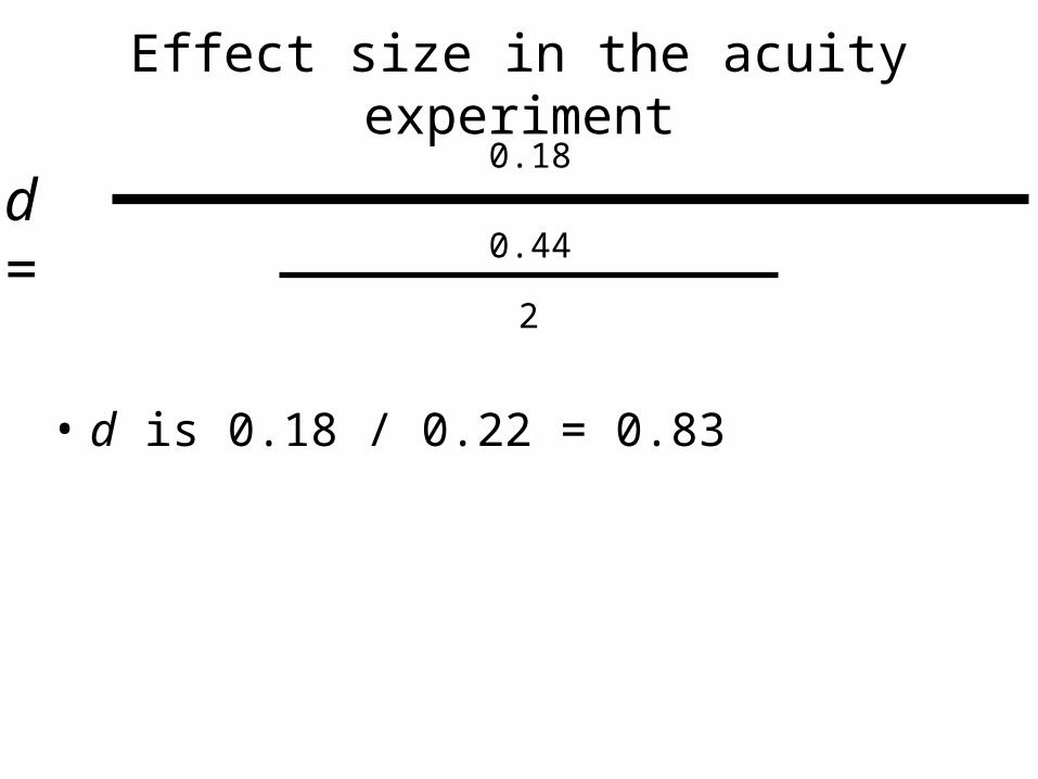
Effect size in the acuity experiment

• d is 0.18 / 0.22 = 0.83

d =0.18

0.44

2

Cohen (1988) would describe this effect size as…

1) enormous

2) significant

3) large

4) medium

5) small

Imaginary repeated measures experiment

• 15 participants have their reaction time measured in the afternoon and then again in the evening

• Half of them are tested in the afternoon and then the evening, and half vice versa

• Look at Figure 4 of the handout

Did it take longer to react in the afternoon or the evening?

1) It took longer in the evening

2) It took longer in the afternoon

Given a two-tailed hypothesis, can the null hypothesis of no time of day effects be rejected?

1) yes

2) no

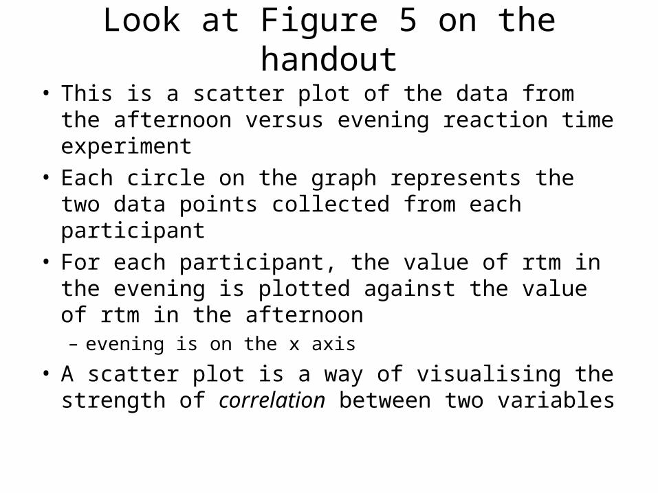
Look at Figure 5 on the handout

• This is a scatter plot of the data from the afternoon versus evening reaction time experiment

• Each circle on the graph represents the two data points collected from each participant

• For each participant, the value of rtm in the evening is plotted against the value of rtm in the afternoon– evening is on the x axis

• A scatter plot is a way of visualising the strength of correlation between two variables

Most of the variation in the scores on the scatter plot is determined by…

1) The difference in rtm between afternoon and evening

2) Differences between participants

3) Neither of the above

How helpful did you find this interactive PRS session?

1) Very helpful2) Helpful3) A bit helpful4) Not very helpful

Would you like more PRS sessions in the future (for statistics or other courses)?

1) Yes2) Maybe3) No

If the mean and the median of a variable are similar…

1) The data is probably measured on an interval or ratio scale

2) A frequency histogram of the variable probably will not show a normal distribution

3) The data is probably measured on an ordinal scale

4) A frequency histogram of the variable will probably show a normal distribution