Performance evaluation when non-discretionary factors correlate with technical efficiency

European Journal of Operational Research 159 (2004) 250–257

www.elsevier.com/locate/dsw

Interfaces with Other Disciplines

Performance evaluation when non-discretionaryfactors correlate with technical efficiency

John Ruggiero *

Department of Economics and Finance, University of Dayton, 517 Miriam Hall, Dayton, OH 45469-2251, USA

Received 15 April 2002; accepted 16 May 2003

Available online 11 September 2003

Abstract

The current data envelopment analysis (DEA) literature on non-discretionary inputs ignores the possibility that

efficiency may be correlated with the non-discretionary factors. This paper extends the literature by analyzing the effects

that such correlation has. It will be shown that if the true technical efficiency is negatively correlated with the non-

discretionary inputs, the existing DEA efficiency estimates will be biased upward. Using simulated data, the perfor-

mance of the existing model will be analyzed. In addition, a corrected model will be introduced to effectively handle the

problem. The resulting model is able to disentangle the two effects that the non-discretionary factor has on production.

� 2003 Elsevier B.V. All rights reserved.

Keywords: Data envelopment analysis; Non-discretionary factors

1. Introduction

The literature on the measurement of technical

efficiency has grown substantially since Farrell(1957) introduced an index based on the maximum

radial reduction in inputs consistent with observed

production. Based on Farrell�s work, Charneset al. (1978) introduced data envelopment analysis

(DEA), a linear programming approach to per-

formance evaluation when production is charac-

terized by constant returns to scale. Theoretical

contributions have been numerous, including al-lowing variable returns to scale (Banker et al.,

1984), non-radial performance evaluation (F€are

* Tel.: +1-937-229-2550; fax: +1-937-229-2477.

E-mail address: [email protected] (J. Ruggiero).

0377-2217/$ - see front matter � 2003 Elsevier B.V. All rights reserv

doi:10.1016/S0377-2217(03)00403-X

and Lovell, 1978; Zhu, 1996; Ruggiero and Bret-

schneider, 1998; Ruggiero, 2000), and non-discre-

tionary inputs (Banker and Morey, 1986; Ray,

1991; Ruggiero, 1996, 1998; Fried et al., 1999;Maital and Vaninsky, 2001). For an excellent

theoretical reference on non-parametric frontier

analysis, see F€are et al. (1994).Non-discretionary inputs play an important

role in public sector production applications. De-

cision making units (DMUs) tend to be heteroge-

nous, operating in different production

environments. For example, the amount of moneynecessary for police services to provide a given

level of public safety will differ among municipal-

ities depending on size and poverty. Similarly, we

would expect that fire service provision depends

on the age and structure of houses and that the

provision of educational services depends on the

ed.

mail to: [email protected]

J. Ruggiero / European Journal of Operational Research 159 (2004) 250–257 251

socio-economic environment of the students.Consequently, performance analyses need to con-

trol for non-discretionary factors.

There are three general approaches that have

been developed to control for non-discretionary

inputs. Banker and Morey (1986) provided the first

DEA model to do so; their model assumed con-

vexity with respect to both discretionary and non-

discretionary inputs. These classes of inputs weretreated differently, however, by not allowing radial

reduction in the non-discretionary inputs. Ruggi-

ero (1996) extended this model by dropping the

convexity constraint associated with the non-dis-

cretionary inputs. Rather, non-discretionary in-

puts were treated as shift factors leading to

multiple frontiers and restrictions were placed on

the weights to exclude DMUs with more favorablelevels of the non-discretionary factor.

The third approach, developed by Ray (1991),

excludes the non-discretionary inputs from the

DEA model in a first stage. The non-discretionary

inputs are controlled in a second stage regression,

allowing an adjusted measure of technical effi-

ciency. Ruggiero (1998) developed a hybrid model

with three stages to allow for multiple non-dis-cretionary inputs. Simulation analysis (Ruggiero,

1998) revealed that the multiple stage models of

Ray and Ruggiero were preferred to the Banker

and Morey model. Yu (1998) used simulation

analysis to compare the Banker and Morey model

with the stochastic frontier model with one exog-

enous variable. The cross-sectional stochastic

frontier approach has been shown by Ondrich andRuggiero (2001) to be of limited value since it does

not really allow measurement error. Yu�s otherresults are consistent with Ruggiero (1996).

These modified DEA models all assume that the

true level of efficiency is not correlated with the

non-discretionary factors. Suppose instead that

the non-discretionary inputs were correlated with

the true level of efficiency. In this case, non-dis-cretionary inputs would not only determine the

location of the frontier as an input in the pro-

duction process but would also influence the dis-

tance from the frontier as a correlate of efficiency.

And, existing models that control for non-discre-

tionary inputs will produce distorted efficiency

results because of the inability to separate the two

effects. Intuitively, we would expect the degree ofthe distortion to increase as the correlation be-

tween efficiency and non-discretionary inputs in-

crease.

The purposes of this paper are threefold. First,

the problem arising from a correlation between

non-discretionary inputs and efficiency will be il-

lustrated. Also, a revised model will be proposed

that will produce an undistorted efficiency mea-sure. Unfortunately, the revised model requires an

additional assumption on the production tech-

nology and parametric specification in a second

stage. However, the benefit is a new DEA model

that will prove useful for empirical public sector

applications. Finally, a simulation is performed to

facilitate comparison between the measures.

The rest of the paper is organized as follows.The next section reviews existing DEA models that

control for non-discretionary inputs. Also, the case

where the non-discretionary inputs effect efficiency

will be discussed and the distortion introduced into

measured efficiency will be illustrated. Simulated

data are used in Section 3 to facilitate comparison.

The last section concludes.

2. Data envelopment analysis

The production technology transforming inputsx ¼ ðx1; . . . ; xMÞ 2 RM

þ into outputs y ¼ ðy1; . . . ;ySÞ 2 RS

þ for j ¼ 1; . . . ; J firms given a non-dis-cretionary input z can be represented with by theproduction possibility set:

T ðzÞ ¼ fðx; yÞ is feasible given zg:Without loss of generality, we assume only onenon-discretionary input. Ruggiero (1998) allows

multiple non-discretionary inputs. It will be as-

sumed that the relationship between the non-dis-

cretionary input and production is given by

T ðzÞ � T ðz0Þ if z0 P z.The effect that the non-discretionary input has

on production is shown in Fig. 1, where it is as-

sumed that nine DMUs A–I produce one output yusing one discretionary input x given one non-discretionary input z. Two levels (z0 and z) of thenon-discretionary factor are assumed, where

z0 P z. Production possibilities A, B, C and I are

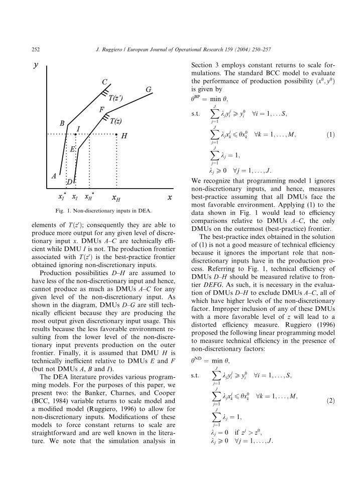
Fig. 1. Non-discretionary inputs in DEA.

252 J. Ruggiero / European Journal of Operational Research 159 (2004) 250–257

elements of T ðz0Þ; consequently they are able toproduce more output for any given level of discre-

tionary input x. DMUs A–C are technically effi-

cient while DMU I is not. The production frontierassociated with T ðz0Þ is the best-practice frontierobtained ignoring non-discretionary inputs.

Production possibilities D–H are assumed to

have less of the non-discretionary input and hence,cannot produce as much as DMUs A–C for any

given level of the non-discretionary input. As

shown in the diagram, DMUs D–G are still tech-

nically efficient because they are producing the

most output given discretionary input usage. This

results because the less favorable environment re-

sulting from the lower level of the non-discre-

tionary input prevents production on the outerfrontier. Finally, it is assumed that DMU H is

technically inefficient relative to DMUs E and F(but not DMUs A, B and I).The DEA literature provides various program-

ming models. For the purposes of this paper, we

present two: the Banker, Charnes, and Cooper

(BCC, 1984) variable returns to scale model and

a modified model (Ruggiero, 1996) to allow fornon-discretionary inputs. Modifications of these

models to force constant returns to scale are

straightforward and are well known in the litera-

ture. We note that the simulation analysis in

Section 3 employs constant returns to scale for-mulations. The standard BCC model to evaluate

the performance of production possibility ðx0; y0Þis given by

hBP ¼ min h;

s:t:XJ

j¼1kjy

ji P y0i 8i ¼ 1; . . . S;

XJ

j¼1kjx

jk 6 hx0k 8k ¼ 1; . . . ;M ;

XJ

j¼1kj ¼ 1;

kj P 0 8j ¼ 1; . . . ; J :

ð1Þ

We recognize that programming model 1 ignores

non-discretionary inputs, and hence, measures

best-practice assuming that all DMUs face the

most favorable environment. Applying (1) to the

data shown in Fig. 1 would lead to efficiency

comparisons relative to DMUs A–C, the onlyDMUs on the outermost (best-practice) frontier.

The best-practice index obtained in the solutionof (1) is not a good measure of technical efficiency

because it ignores the important role that non-

discretionary inputs have in the production pro-

cess. Referring to Fig. 1, technical efficiency of

DMUs D–H should be measured relative to fron-

tier DEFG. As such, it is necessary in the evalua-

tion of DMUs D–H to exclude DMUs A–C, all ofwhich have higher levels of the non-discretionaryfactor. Improper inclusion of any of these DMUs

with a more favorable level of z will lead to adistorted efficiency measure. Ruggiero (1996)

proposed the following linear programming model

to measure technical efficiency in the presence of

non-discretionary factors:

hND ¼ min h;

s:t:XJ

j¼1kjy

ji P y0i 8i ¼ 1; . . . ; S;

XJ

j¼1kjx

jk 6 hx0k 8k ¼ 1; . . . ;M ;

XJ

j¼1kj ¼ 1;

kj ¼ 0 if zj > z0;kj P 0 8j ¼ 1; . . . ; J :

ð2Þ


Model 2 prevents DMUs with a higher level of the

non-discretionary input into the reference set.

Ruggiero (1998) extended this model to allow

multiple non-discretionary factors by using re-

gression analysis to construct an overall index of

non-discretionary inputs. As shown in Ruggiero

(1996), this model performs well in measuring

technical efficiency.One key assumption in (2) is that true efficiency

is not correlated with the non-discretionary factor.

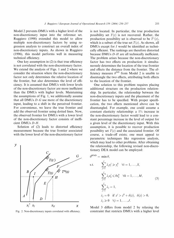
We extend the analysis of Figs. 1 and 2 where we

consider the situation where the non-discretionary

factor not only determines the relative location of

the frontier, but also determines the level of effi-

ciency. It is assumed that DMUs with lower levels

of the non-discretionary factor are more inefficientthan the DMUs with higher levels. Maintaining

the assumptions of Fig. 1, we additionally assume

that all DMUs D–G use more of the discretionaryinput, leading to a shift in the perceived frontier.

For convenience, we leave the true frontier and

add the observed frontier using dotted lines. Now,

the observed frontier for DMUs with a lower level

of the non-discretionary factor consists of ineffi-cient DMUs D–H .Solution of (2) leads to distorted efficiency

measurement because the true frontier associated

with the lower level of the non-discretionary factor

Fig. 2. Non-discretionary inputs correlated with efficiency.

is not located. In particular, the true productionpossibility set T ðzÞ is not recovered. Rather, theproduction possibility set is observed to be T �ðzÞ,which is a subset of the true set T ðzÞ. As shown, allDMUs except for I would be identified as techni-cally efficient. The rankings are therefore distorted

because DMUs D–H are all technically inefficient.

The problem arises because the non-discretionary

factor has two effects on production: it simulta-neously determines the location of the true frontier

and effects the distance from the frontier. The ef-

ficiency measure hND from Model 2 is unable to

disentangle the two effects, attributing both effects

to the location of the frontier.

One solution to this problem requires placing

additional structure on the production relation-

ship. In particular, the relationship between thenon-discretionary inputs and the placement of the

frontier has to be specified. With proper specifi-

cation, the two effects mentioned above can be

disentangled. For example, one could assume a

constant elasticity relationship: a 1% increase in

the non-discretionary factor would lead to a con-

stant percentage increase in the level of output for

a given level of the discretionary input. With thisassumption, it is possible to recover production

possibility set T ðzÞ and the associated frontier. Ofcourse, a trade-off exists; one must appeal to

parametric techniques like regression analysis,

which may lead to other problems. After obtaining

the relationship, the following revised non-discre-

tionary DEA model can be employed:

hRND ¼ min h;

s:t:XJ

j¼1kjy

ji P y0i 8i ¼ 1; . . . ; S;

XJ

j¼1kjx

jk 6 hx0k 8k ¼ 1; . . . ;M ;

XJ

j¼1kj ¼ 1;

kj ¼ 0 if zj > z0 þ dðzÞ; dðzÞ > 0;kj P 0 8j ¼ 1; . . . ; J :

ð3Þ

Model 3 differs from model 2 by relaxing the

constraint that restricts DMUs with a higher level


of the non-discretionary input from the reference

group. Now, DMUs with higher levels of the non-

discretionary input can be included as long as the

difference between non-discretionary levels is not

greater than dðzÞ. By relaxing this constraint,

DMUs with a more favorable environment can be

included in the referent set, which essentially

controls for the correlation between efficiency andthe non-discretionary environment. There are two

important features of this model. First, model 3 is

applicable for cases (like the one shown in Fig. 2)

where there exists a negative correlation between zand the true efficiency level. Implementation of

Model 3 requires specification of the relationship

between d and z. This is achieved by noting thatthe best-practice measure hBP from Model 1 willdecrease at higher rates when z decreases if theredoes exist a negative correlation between true ef-

ficiency and the level of z. Regression analysis willbe used to uncover this relationship in the simu-

lation analysis.

3. Simulation analysis

To illustrate the effects discussed above, a sim-

ulation was performed assuming two discretionary

inputs x1 and x2 are used to produce one output y.Additionally, it was assumed that production lev-els depended on one non-discretionary input z. Inparticular, constant returns to scale were assumed

with respect to the discretionary inputs with the

following production function:

y ¼ zx1=21 x1=22 :

Based on this technology, DMUs with a higherlevel of the non-discretionary input z can producemore output for given levels of the discretionary

inputs. Given that constant returns to scale prevail

for this technology, we employ constant returns to

scale versions of the programming models above.

The inputs were randomly generated from a

uniform distribution with 250 observations with

the following intervals:

x1; x2 : ð20; 40Þ and z : ð1; 2Þ:Given the generated inputs, the efficient level of

output was calculated according to the production

function above. Observed output was calculatedas

yo ¼ ð1� ciÞzx1=21 x1=22 ;

where ci is a measure of inefficiency in scenario i.Three different scenarios were considered based on

the correlation between the non-discretionary

input z and the true efficiency level. As such, in-efficiency was calculated with the following func-

tions:

Scenario 1: c1 ¼ c0,Scenario 2: c2 ¼ 0:6c1 � 0:1ðz� 2Þ,Scenario 3: c3 ¼ 0:4c1 � 0:15ðz� 2Þ,

where c0 was generated from a half-normal dis-

tribution:

c0 jNð0; 0:2036Þj:To allow efficient units, the value of c0 was furtherrestricted by setting c0 ¼ 0 if the generated valuewas greater than 0.30. Based on the generated

data, the correlation between the non-discretion-

ary input z and ci was )0.11, )0.54 and )0.80 forscenarios 1–3, respectively.

Based on the production function and the

generated data, the non-discretionary input effects

production in two ways. First, holding discre-

tionary inputs and efficiency constant, DMUs withhigher levels of z can produce more output (i.e.,they belong to a higher production frontier). Sec-

ond, given the negative correlations, higher levels

of z lead to lower levels of c; DMUs with lowerlevels of the non-discretionary input are relatively

more inefficient. Hence, the simulation was de-

signed to be consistent with Fig. 2.

All three programming models were used toevaluate the problem of biased measurement due

to the negative correlation of true but unobserved

efficiency and the non-discretionary input. Model

2, which includes the non-discretionary input as a

control variable, was the first one considered. We

expect that model 2 will perform well in scenario 1

where there is a low correlation between efficiency

and the non-discretionary input. We also expectthat the performance of model 2 will decline in

scenarios 2 and 3 where the negative correlation

between efficiency and z is moderate and strong,respectively.


Model 3 requires specification of the relation-ship between the best-practice frontier and the

non-discretionary input. In order to do so, we first

measure best-practice hBP by solving the constantreturns to scale version of model 1. We expect that

the model will not perform well in measuring ef-

ficiency given the non-discretionary input. How-

ever, we note that the negative correlation between

true but unobserved efficiency and the non-dis-cretionary will cause a non-linear inverse rela-

tionship between hBP and z. Given hBP, we estimatethe following regression for each scenario:

hBP ¼ a þ b1zþ b2ð1=zÞ þ e: ð4ÞIf b2 ¼ 0, the equation reduces to the linear rela-tionship between best-practice and the non-dis-cretionary factor where we would expect b1 > 0because DMUs with higher levels of the non-dis-

cretionary input will be closer to the best-practice

frontier, ceteris paribus. If there is a negative cor-

relation between the non-discretionary input and

efficiency, we should see hBP increase at an in-creasing rate as z increases. This relationshipclearly holds in (4) if z2 > b2=b1 and if b2 > 0based on the first and second derivatives.

Regression (4) was run for each model scenario

and the results are reported in Table 1. The ex-

pected result that hBP is increasing in z at an in-creasing rate holds true under scenarios 2 and 3

but not under scenario 1. We note that there was

not a negative correlation between the socio-eco-

nomic variable z and true efficiency under scenario1. Hence, the linear specification with b2 ¼ 0 is

Table 1

Regression resultsa (250 observations)

Scenario

1 2 3

Intercept )0.039 )0.353� )0.506��

(0.27) (0.17) (0.12)

z 0.494�� 0.629�� 0.694��

(0.09) (0.06) (0.04)

1=z )0.003 0.151 0.226��

(0.19) (0.12) (0.08)

R2 0.78 0.92 0.96

** (*) indicates significance at 99% (95%) level of confidence.a The dependent variable is hBP obtained by solving model 2.

appropriate for scenario 1. This implies that it isnot necessary to revise the non-discretionary

Model 2. The statistical results reported in Table 1

are not surprising. All equations are significant at

acceptable levels of confidence and the high R2 foreach model suggests a reasonable statistical fit. In

all cases, b1 > 0 was statistically significant at the99% level of confidence. However, at conventional

levels of confidence, b2 was not statistically dif-ferent from zero in model 2, even though the pa-

rameter has the correct sign and is of reasonable

magnitude based on the expectations discussed

above.

The purpose of linear program Model 1 and the

subsequent regression (4) was to provide a para-

metric specification of dðzÞ for the constraint in therevised non-discretionary linear programmingModel 3. Based on the regression results reported

in Table 1, we specify the following relationships

for dðzÞ:

Scenario 1: dðzÞ ¼ 0,Scenario 2: dðzÞ ¼ 0:151=z, andScenario 3: dðzÞ ¼ 0:226=z.

For scenario 1, since b2 was negative and notstatistically different from zero, there is no statis-

tical evidence that the distance from the best-

practice frontier can be attributed to the effect that

z has on the placement of the frontier. Hence, therevised model reduces to the regular non-discre-

tionary linear programming Model 2. For scenar-

ios 2 and 3, however, we see a systematicrelationship develop that DMUs with lower levels

of the non-discretionary input tend to be further

away from the best-practice frontier. As a result,

the correction factor dðzÞ used in Model (3) allowsDMUs with a more favorable environment into

the possible reference set. We note that the cor-

rection factor is decreasing in z, which is consistentwith the negative correlation assumed between zand the true efficiency.

In summary, all three models were used to

evaluate efficiency across scenarios 1 and 2. The

regression also revealed that the revised non-dis-

cretionary was not necessary for scenario 1, which

is consistent with the data generating process. The

results for these models are reported in Table 2.

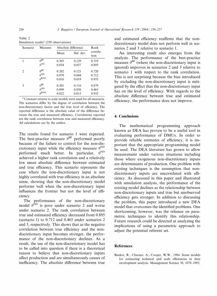
Table 2

Simulation resultsa (250 observations)

Scenario Measure Absolute difference Rank

correla-

tionMean Std. dev.

1 hBP 0.205 0.129 0.519

hND 0.034 0.037 0.895

2 hBP 0.202 0.121 0.720

hND 0.078 0.044 0.712

hRND 0.016 0.019 0.935

3 hBP 0.201 0.116 0.879

hND 0.099 0.050 0.465

hRND 0.022 0.015 0.932

aConstant returns to scale models were used for all measures.

The scenarios differ by the degree of correlation between the

non-discretionary factor and the true level of efficiency. The

reported difference is the absolute value of the difference be-

tween the true and measured efficiency. Correlations reported

are the rank correlation between true and measured efficiency.

All calculations are by the author.


The results found for scenario 1 were expected.The best-practice measure hBP performed poorlybecause of the failure to control for the non-dis-

cretionary input while the efficiency measure hND

performed much better. In particular, hND

achieved a higher rank correlation and a relatively

low mean absolute difference between estimated

and true efficiency. This scenario represents the

case where the non-discretionary input is nothighly correlated with true efficiency in an absolute

sense, showing that the non-discretionary model

performs well when the non-discretionary input

influences the frontier but not the level of effi-

ciency.

The performance of the non-discretionary

model hND is poor under scenario 2 and worse

under scenario 2. The rank correlation betweentrue and estimated efficiency decreased from 0.895

(scenario 1) to 0.712 and 0.465 under scenarios 2

and 3, respectively. This shows that as the negative

correlation between true efficiency and the non-

discretionary input becomes stronger, the perfor-

mance of the non-discretionary declines. As a

result, the use of the non-discretionary model has

to be called into question if there is a theoreticalreason to believe that non-discretionary inputs

affect production and are simultaneously causes of

inefficiency. The absolute difference between true

and estimated efficiency reaffirms that the non-discretionary model does not perform well in sce-

narios 2 and 3 relative to scenario 1.

An interesting result also emerges from the

analysis. The performance of the best-practice

measure hBP (where the non-discretionary input isignored) improves in scenarios 2 and 3 relative to

scenario 1 with respect to the rank correlation.

This is not surprising because the bias introducedby excluding the non-discretionary input is miti-

gated by the effect that the non-discretionary input

has on the level of efficiency. With regards to the

absolute difference between true and estimated

efficiency, the performance does not improve.

4. Conclusions

The mathematical programming approach

known as DEA has proven to be a useful tool in

evaluating performance of DMUs. In order to

provide reliable estimates of efficiency, it is im-

portant that the appropriate programming model

be used. The DEA literature has grown to allow

measurement under various situations includingthose where exogenous non-discretionary inputs

are determinants of production. One problem with

existing techniques is the assumption that non-

discretionary inputs are uncorrelated with effi-

ciency. As discussed in this paper and illustrated

with simulation analysis, the performance of the

existing model declines as the relationship between

non-discretionary inputs and true but unobservedefficiency gets stronger. In addition to discussing

the problem, this paper introduced a new DEA

model that overcomes the identified problems. One

shortcoming, however, was the reliance on para-

metric techniques to identify this relationship.

Future research could be directed at analyzing the

implications of using a parametric approach to

adjust the potential referent set.

References

Banker, R., Charnes, A., Cooper, W.W., 1984. Some models

for estimating technical and scale efficiencies in data

envelopment analysis. Management Science 30, 1078–1092.


Banker, R., Morey, R., 1986. Efficiency analysis for exoge-

nously fixed inputs and outputs. Operations Research 34,

513–521.

Charnes, A., Cooper, W.W., Rhodes, E., 1978. Measuring the

efficiency of decision making units. European Journal of

Operational Research 2, 429–444.

F€are, R., Lovell, C.A.K., 1978. Measuring the technical

efficiency of production. Journal of Economic Theory 19,

150–162.

F€are, R., Grosskopf, S., Lovell, C.A.K., 1994. Production

Frontiers. Cambridge University Press, New York.

Farrell, M.J., 1957. The measurement of productive efficiency.

Journal of the Royal Statistical Science Series A, General

120, 253–281.

Fried, H., Schmidt, S., Yaisawarng, S., 1999. Incorporating the

operating environment into a nonparametric measure of

technical efficiency. Journal of Productivity Analysis 4, 419–

432.

Maital, S., Vaninsky, A., 2001. Data envelopment analysis with

resource constraints: An alternative model with non-discre-

tionary factors. European Journal of Operational Research

128, 206–212.

Ondrich, J., Ruggiero, J., 2001. Efficiency measurement in the

Stochastic frontier model. European Journal of Operational

Research 129, 434–442.

Ray, S., 1991. Resource use efficiency in public schools. A study

of connecticut data. Management Science 37, 1620–1628.

Ruggiero, J., 1996. On the measurement of technical efficiency

in the public sector. European Journal of Operational

Research 90, 553–565.

Ruggiero, J., 1998. Non-discretionary inputs in data envelop-

ment analysis. European Journal of Operational Research

111, 461–469.

Ruggiero, J., 2000. Measuring technical efficiency. European

Journal of Operational Research 121, 138–150.

Ruggiero, J., Bretschneider, S., 1998. The weighted Russell

measure of technical efficiency. European Journal of Oper-

ational Research 108, 438–451.

Yu, C., 1998. The effects of exogenous variables in efficiency

measurement––A Monte Carlo study. European Journal of

Operational Research 105, 569–580.

Zhu, J., 1996. Data envelopment analysis with preference

structure. Journal of the Operational Research Society 47,

136–150.

Documents

Performance evaluation when non-discretionary factors correlate with technical efficiency