HAL Id: tel-03215137https://tel.archives-ouvertes.fr/tel-03215137

Submitted on 3 May 2021

HAL is a multi-disciplinary open accessarchive for the deposit and dissemination of sci-entific research documents, whether they are pub-lished or not. The documents may come fromteaching and research institutions in France orabroad, or from public or private research centers.

L’archive ouverte pluridisciplinaire HAL, estdestinée au dépôt et à la diffusion de documentsscientifiques de niveau recherche, publiés ou non,émanant des établissements d’enseignement et derecherche français ou étrangers, des laboratoirespublics ou privés.

Performance evaluation of green IT networksYoussef Ait El Mahjoub

To cite this version:Youssef Ait El Mahjoub. Performance evaluation of green IT networks. Networking and InternetArchitecture [cs.NI]. Université Paris-Saclay, 2021. English. NNT : 2021UPASG011. tel-03215137

Thès

e de

doc

tora

tN

NT

:202

1UPA

SG01

1

Performance evaluation of greenIT networks

Évaluation des performances pour des réseauxIT économes en énergie

Thèse de doctorat de l’université Paris-Saclay

École doctorale n 580, Sciences et technologies de l’information et de lacommunication (STIC)

Spécialité de doctorat: Réseaux, information et communicationsUnités de recherche: (1) Université Paris-Saclay, UVSQ, Données etAlgorithmes pour une ville intelligente et durable, 78035, Versailles,

France.(2) Institut Polytechnique de Paris, Télécom SudParis, Services Répartis,

Architectures, Modélisation, Validation, Administration des Réseaux,91000, Evry, France.

Référent: Université de Versailles-Saint-Quentin-en-Yvelines

Thèse présentée et soutenue à Paris-Saclay, le 18 mars 2021,par

Youssef AIT EL MAHJOUB

Composition du jury:Lynda Mokdad PrésidenteProfesseur des universités, Université Paris-EstOlivier Brun Rapporteur & examinateurDirecteur de recherche, LAAS-CNRSGérardo Rubino Rapporteur & examinateurDirecteur de recherche, INRIA/IRISAThomas Begin ExaminateurMaître de conférences HDR, UniversitéLyon1Anne-Cécile Orgerie ExaminatriceChargée de recherche et HDR, IRISAVéronique Vèque ExaminatriceProfesseur des universités, Université Paris-Sud

Direction de la thèseJean-Michel Fourneau DirecteurProfesseur, DAVID - UVSQHind Castel-Taleb Co-directriceProfesseur, SAMOVAR - Télécom SudParis

Emmanuel Hyon InvitéMaître de Conférences, Université Paris Nan-terre

Acknowledgments

It will be very difficult for me to thank everyone because it is thanks to the helpof many people that i was able to complete this thesis.

First of all, i would like to greatly thank my thesis director and co-director,Jean-Michel Fourneau and Hind Castel-Taleb, for their help. I am delighted to haveworked with them because in addition to their scientific support, they were alwaysthere to support and advise me during the development of this thesis.

I also thank the Labex DigiCosme which believed in my research project.Olivier Brun and Gérardo Rubino honored me by being the rapporteurs of my

thesis, they took the time to listen to me and to discuss with me. Their remarksallowed me to consider my work from another angle. For all that i thank them.

I would like to thank the members of the jury for having accepted to participatein my thesis committee and for their scientific participation as well as the time theydevoted to my research.

I thank the members of the DAVID laboratory for their kindness and our dis-cussions around a coffee in the hallways, especially the ”ALMOST” team in whichi developed my research during my thesis and my internships. A special thought toStefi Nouleho, Mael guiraud, Chen Wei, Thierry Mautor, Franck Quessette, SandrineVial, Yann Strozeski, Pierre Coucheney, Dominique Barth ...

I thank from the bottom of my heart for their support and their wisdom myparents, my uncle Brahim, my grandfather Mohamed. I thank my brothers Ayoub,Reda, and Anouar, my cousins. My family in Morocco and in France.

3

Related international conference papers

• Youssef Ait El Mahjoub, Jean-Michel Fourneau and Hind-Castel Taleb, ”En-ergy Packet Networks with general service time distribution”. A conferencepaper. In 28th International Symposium on Modeling, Analysis, and Simu-lation of Computer and Telecommunication Systems (MASCOTS), pp. 1-8.Nice, France, November 2020, DOI: 10.1109/MASCOTS50786.2020.9285965.

• Youssef Ait El Mahjoub, Jean-Michel Fourneau and Hind Castel-Taleb. ”Anal-ysis of Energy Consumption in Cloud Center with Tasks Migrations”. A con-ference paper. In: CN2019, International Conference on Computer Networks,pp 301−315. Kamień Śląski, Poland, July 2019. DOI: 10.1007/978−3−030−21952−9_23.

• Youssef Ait El Mahjoub, Jean-Michel Fourneau and Hind Castel-Taleb. ”Anumerical approach of the analysis of optical container filling”. A conferencepaper. In: VALUETOOLS 2019, the 12th EAI International Conference onPerformance Evaluation Methodologies and Tools, pp. 159-162. Palma, Spain,March 2019. DOI: doi .or g /10.1145/3306309.3306333.

• Youssef Ait El Mahjoub, Hind Castel-Taleb and Jean-Michel Fourneau. ”Per-formance and energy efficiency analysis in NGREEN optical network”. A con-ference paper. In: WIMOB 2018, 14th International Conference on Wirelessand Mobile Computing, Networking and Communications, pp. 1−9. Limassol,Cyprus, October 2018. DOI: 10.1109/Wi MOB.2018.8589144.

• Jean-Michel Fourneau, Youssef Ait El Mahjoub, Franck Quessette and Dim-itris Vekris. ”XBorne 2016: A Brief Introduction”. A Conference paper. In:ISCIS 2016, International Symposium on Computer and Information Sciences,vol. 659, pp. 134−141. Kraków, Poland, October 2016. DOI: 10.1007/978−3−319−47217−1_15.

Related journal paper

• Jean-Michel Fourneau and Youssef Ait El Mahjoub. ”Processor sharing G-queues with inert customers and catastrophes: A model for server aging andrejuvenation”. A journal paper. In: Probability in the Engineering and In-formational Sciences, vol. 31, no. 04, pp. 420−435, Cambridge, April 2017.DOI: 10.1017/S0269964817000092.

4

Contents

Contents 5

List of Figures 9

List of Tables 12

I Introduction 16

A. The context and problematics . . . . . . . . . . . . . . . . . . . . . . . . 17B. The organization of the document . . . . . . . . . . . . . . . . . . . . . . 18

II Numerical analysis of energy consumption and perfor-mance in networking and processing systems 21

1 State of the art of power management and optical networks 221.1 Power and energy consumption strategies . . . . . . . . . . . . . . . . 23

1.1.1 SPM, DPM and DVFS . . . . . . . . . . . . . . . . . . . . . . . 231.1.2 Virtualization . . . . . . . . . . . . . . . . . . . . . . . . . . . . 231.1.3 Scheduling – VM allocation/placement . . . . . . . . . . . . . 231.1.4 Consolidation . . . . . . . . . . . . . . . . . . . . . . . . . . . . 251.1.5 Thresholds strategies . . . . . . . . . . . . . . . . . . . . . . . . 25

1.2 Optical networks . . . . . . . . . . . . . . . . . . . . . . . . . . . . . . . 261.2.1 OTDM and WDM Multiplexing technologies . . . . . . . . . . 271.2.2 Optical Switching methods . . . . . . . . . . . . . . . . . . . . 27

2 XBorne the software tool 292.1 Introduction . . . . . . . . . . . . . . . . . . . . . . . . . . . . . . . . . . 302.2 Building a model with XBorne . . . . . . . . . . . . . . . . . . . . . . . 312.3 Numerical Resolution . . . . . . . . . . . . . . . . . . . . . . . . . . . . 332.4 Quasi-Lumpability . . . . . . . . . . . . . . . . . . . . . . . . . . . . . . 352.5 Birth-death process . . . . . . . . . . . . . . . . . . . . . . . . . . . . . 362.6 A numerical example in XBorne . . . . . . . . . . . . . . . . . . . . . 37

2.6.1 Presentation of Mitrani’s model . . . . . . . . . . . . . . . . . . 372.6.2 Variation of server’s activating time distribution . . . . . . . . 382.6.3 Variation of customers inter-arrival distribution . . . . . . . . 38

5

2.6.4 Numerical results . . . . . . . . . . . . . . . . . . . . . . . . . . 38

3 Dynamic Voltage and Frequency Scaling (DVFS) processor 423.1 Introduction . . . . . . . . . . . . . . . . . . . . . . . . . . . . . . . . . . 433.2 Model 1: A multi-core processor with one Pstate . . . . . . . . . . . . 44

3.2.1 Mean number of jobs and response time . . . . . . . . . . . . . 453.2.2 Power and energy consumption . . . . . . . . . . . . . . . . . . 463.2.3 Numerical comparison of the six Opteron Pstates . . . . . . . 49

3.2.3.1 Performance, power and Energy per job . . . . . . . 493.2.3.2 The appropriate Pstate in performance and energy

trade-off . . . . . . . . . . . . . . . . . . . . . . . . . . 493.2.3.3 Condition verification for power and energy com-

parison . . . . . . . . . . . . . . . . . . . . . . . . . . . 493.3 Model 2: A multi-core processor with N = 2 Pstates . . . . . . . . . . 53

3.3.1 Closed form for the steady-state distribution . . . . . . . . . . 533.3.2 Mean number of jobs and response time . . . . . . . . . . . . . 543.3.3 Power and energy consumption . . . . . . . . . . . . . . . . . . 553.3.4 Optimization of energy consumption and response time . . . 563.3.5 Numerical results . . . . . . . . . . . . . . . . . . . . . . . . . . 59

3.3.5.1 Performance optimization . . . . . . . . . . . . . . . 593.3.5.2 Energy per job optimization . . . . . . . . . . . . . . 60

3.4 Model 3: A multi-core processor with all Pstates . . . . . . . . . . . . 613.4.1 Closed form for the steady-state distribution . . . . . . . . . . 613.4.2 Mean number of jobs and response time . . . . . . . . . . . . . 623.4.3 Power and energy consumption . . . . . . . . . . . . . . . . . . 633.4.4 Numerical results . . . . . . . . . . . . . . . . . . . . . . . . . . 64

4 Performance and energy efficiency analysis in NGREEN opticalnetwork 664.1 Introduction . . . . . . . . . . . . . . . . . . . . . . . . . . . . . . . . . . 674.2 Model for optical container filling . . . . . . . . . . . . . . . . . . . . . 68

4.2.1 Markov Chain model . . . . . . . . . . . . . . . . . . . . . . . . 684.2.2 Numerical Analysis . . . . . . . . . . . . . . . . . . . . . . . . . 724.2.3 A more realistic example with Ethernet and TCP SDUs . . . 76

4.2.3.1 Model 1 . . . . . . . . . . . . . . . . . . . . . . . . . . 764.2.3.2 Model 2 . . . . . . . . . . . . . . . . . . . . . . . . . . 78

4.3 Generalization to non stationary arrivals . . . . . . . . . . . . . . . . . 814.3.1 Replacement of Step 6) in our algorithm . . . . . . . . . . . . 834.3.2 Algorithm Comparison . . . . . . . . . . . . . . . . . . . . . . . 85

4.3.2.1 NCD matrix . . . . . . . . . . . . . . . . . . . . . . . 864.3.2.2 General modulating matrix . . . . . . . . . . . . . . 87

4.3.3 Example . . . . . . . . . . . . . . . . . . . . . . . . . . . . . . . 884.4 Modeling the container insertion on the optical ring . . . . . . . . . . 89

4.4.1 Scenario A : latency with opportunistic insertion mode . . . 914.4.2 Scenario B : guarantee latency with slot reservation insertion

mode . . . . . . . . . . . . . . . . . . . . . . . . . . . . . . . . . 954.5 Energy efficiency and latency analysis . . . . . . . . . . . . . . . . . . 98

6

III Analytic analysis of power consumption in a cloudcenter 100

5 State of the art 1015.1 Load balancing of tasks . . . . . . . . . . . . . . . . . . . . . . . . . . . 1035.2 Server’s power consumption . . . . . . . . . . . . . . . . . . . . . . . . 104

6 Analysis of power consumption in cloud/data center with tasksmigrations 1066.1 Introduction . . . . . . . . . . . . . . . . . . . . . . . . . . . . . . . . . . 1076.2 Power consumption model . . . . . . . . . . . . . . . . . . . . . . . . . 1076.3 Jackson network model for task migrations . . . . . . . . . . . . . . . 108

6.3.1 Analytic results for the queues . . . . . . . . . . . . . . . . . . 1096.3.2 Systems comparison . . . . . . . . . . . . . . . . . . . . . . . . . 1116.3.3 Optimization of power consumption . . . . . . . . . . . . . . . 1136.3.4 Generalization to larger scale systems . . . . . . . . . . . . . . 116

6.3.4.1 Heuristic 1 . . . . . . . . . . . . . . . . . . . . . . . . 1176.3.4.2 Heuristic 2 . . . . . . . . . . . . . . . . . . . . . . . . 117

6.4 Numerical results . . . . . . . . . . . . . . . . . . . . . . . . . . . . . . . 1206.4.1 A data center with two physical servers . . . . . . . . . . . . 1206.4.2 A data center with N physical servers . . . . . . . . . . . . . . 124

6.4.2.1 Experiment 1 . . . . . . . . . . . . . . . . . . . . . . . 1246.4.2.2 Experiment 2 . . . . . . . . . . . . . . . . . . . . . . . 125

IV Analytical analysis of EPN networks and G-networks127

7 State of the art 1287.1 Energy packet networks . . . . . . . . . . . . . . . . . . . . . . . . . . 1297.2 The evolution of G-networks . . . . . . . . . . . . . . . . . . . . . . . . 131

8 Energy Packet Networks with general service time distribution 1358.1 Introduction . . . . . . . . . . . . . . . . . . . . . . . . . . . . . . . . . . 1368.2 Model Description and Markov chain analysis . . . . . . . . . . . . . . 136

8.2.1 Markov chain analysis . . . . . . . . . . . . . . . . . . . . . . . 1378.2.2 Product form of the EPN network . . . . . . . . . . . . . . . . 1398.2.3 Existence of a fixed point solution . . . . . . . . . . . . . . . . 143

8.3 Performance and Energy evaluation . . . . . . . . . . . . . . . . . . . 1448.3.1 Loss rate of energy packets . . . . . . . . . . . . . . . . . . . . 1458.3.2 Waiting time and total number of data packets . . . . . . . . 146

8.4 Solar panel assignment . . . . . . . . . . . . . . . . . . . . . . . . . . . 1488.4.1 Case of a tree EPN topology . . . . . . . . . . . . . . . . . . . 148

8.4.1.1 Optimization problem . . . . . . . . . . . . . . . . . . 1508.4.1.2 A collecting sensor network of N = 7 cells . . . . . . 1538.4.1.3 A collecting sensor network of N = 20 cells . . . . . . 155

8.4.2 A star EPN topology . . . . . . . . . . . . . . . . . . . . . . . . 1598.4.2.1 Optimization problem . . . . . . . . . . . . . . . . . . 159

7

8.4.2.2 A star sensor network of N = 10 cells . . . . . . . . . 161

9 Processor Sharing G-queues with inert customers and catastro-phes: a model for server aging and rejuvenation 1659.1 Introduction . . . . . . . . . . . . . . . . . . . . . . . . . . . . . . . . . . 1669.2 Model and product-form steady-state distribution . . . . . . . . . . . 1679.3 Stability . . . . . . . . . . . . . . . . . . . . . . . . . . . . . . . . . . . . 1709.4 Partial rejuvenation . . . . . . . . . . . . . . . . . . . . . . . . . . . . . 171

A Proof of product form solution for the steady state distribution 175

V Conclusion and perspectives 178

A. Synthesis . . . . . . . . . . . . . . . . . . . . . . . . . . . . . . . . . . . . . 179B. Perspectives . . . . . . . . . . . . . . . . . . . . . . . . . . . . . . . . . . . 180

Résumé substantiel 195

8

List of Figures

1 Chapters overview . . . . . . . . . . . . . . . . . . . . . . . . . . . . . . 20

2.1 Mitrani’s model. Steady-state for the queue size (the first figure inabove). Sample path of the state of the servers (the second figure inabove). . . . . . . . . . . . . . . . . . . . . . . . . . . . . . . . . . . . . . 33

2.2 Mitrani’s model. Directed graph of the chain (left). Mean powerconsumption (right). . . . . . . . . . . . . . . . . . . . . . . . . . . . . . 35

2.3 Mitrani’s queuing system . . . . . . . . . . . . . . . . . . . . . . . . . . 372.4 Poissonian arrivals and Erlang servers activation: Mean power con-

sumption (a) vs Loss probability (in log10) (b) . . . . . . . . . . . . 402.5 Poissonian arrivals and Exponential servers activation: Mean power

consumption (a) vs Loss probability (in log10) (b) . . . . . . . . . . 402.6 Poissonian arrivals and Hyper-Exponential servers activation: Mean

power consumption (a) vs Loss probability (in log10) (b) . . . . . . 412.7 SBBP arrivals and Erlang servers activation: Mean power consump-

tion (a) vs Loss probability (in log10) (b) . . . . . . . . . . . . . . . . 41

3.1 Pstates Support in AMD Opteron Processor [Inc05]. . . . . . . . . . . 433.2 Mean number of jobs (left) and mean response time (right). Param-

eters: C = 20 servers, server’s rate (i.e. core’s speed) in each Pstateis depicted in Fig. 3.1. . . . . . . . . . . . . . . . . . . . . . . . . . . . . 50

3.3 Idle power consumption (left) and total power consumption (right).Parameters are the same as in Fig. 3.2. . . . . . . . . . . . . . . . . . 51

3.4 Energy per job consumption (left) and response time as a functionof mean power consumption. Parameters are the same as in Fig. 3.2. 51

3.5 The mean power consumption as a function of the threshold. . . . . 573.6 Objective function: c1 = 200, c2 = 1 (left) and c1 = 500, c2 = 1

(Right). For instance, in the left heatmap, the optimal thresholdfor the entry i = 2, j = 3 is th = 2 with a total cost of Ω = 140.6. Inthe right heatmap, for the same entry, the optimal threshold is th = 1with a total cost of Ω= 290.4. . . . . . . . . . . . . . . . . . . . . . . . 60

3.7 Objective function: c1 = 1, c2 = 10 (left) and c1 = 1, c2 = 50 (Right).For instance, in left heatmap for the entry i = 1, j = 4. The optimalthreshold is th = 84 with a total cost function of Ω= 324.2, while inthe right heatmap th = 100 and Ω= 1610.1 . . . . . . . . . . . . . . . 61

3.8 Mean number of jobs (left) and Mean response time (right). . . . . 653.9 Mean power consumption (left) and Energy per job consumption

(right) . . . . . . . . . . . . . . . . . . . . . . . . . . . . . . . . . . . . . 65

9

4.1 Container filling and insertion. . . . . . . . . . . . . . . . . . . . . . . 694.2 ToyModel: The Markov chain for J= 8, C= 8, and arrivals of 0, 1 or

3 SDU per slot. . . . . . . . . . . . . . . . . . . . . . . . . . . . . . . . . 714.3 ToyModel: Distribution of the steady-state probability for (X,H) for

the simple model. Non reachable states are depicted in white. . . . 734.4 ToyModel: Distribution of the container size (in chunks of 1500 bytes)

at release time. . . . . . . . . . . . . . . . . . . . . . . . . . . . . . . . 734.5 ToyModel: Distribution of the Timer at release time. . . . . . . . . . 754.6 ToyModel: Distribution of inter-PDU release time. . . . . . . . . . . 754.7 Model1: Distribution of the PDU size at release time (in chunks of

50 bytes) . . . . . . . . . . . . . . . . . . . . . . . . . . . . . . . . . . . 764.8 Model1: Distribution of the Timer at release time. . . . . . . . . . . 774.9 Model1: Distribution of inter-PDU release time. . . . . . . . . . . . . 774.10 Model1: Distribution of the Timer at release time VS deadline, for

different threshold ratios . . . . . . . . . . . . . . . . . . . . . . . . . . 784.11 Model2: Distribution of the PDU size at release time (in chunks of

50 bytes). . . . . . . . . . . . . . . . . . . . . . . . . . . . . . . . . . . . 794.12 Model2: Distribution of the Timer at release time. . . . . . . . . . . 794.13 Model2: Distribution of inter-PDU release time. . . . . . . . . . . . . 804.14 ModelSBBP: Distribution of the PDU size at release time (chunks of

50 bytes). . . . . . . . . . . . . . . . . . . . . . . . . . . . . . . . . . . . 884.15 ModelSBBP: Distribution of the Timer at release time. . . . . . . . 894.16 The optical conversion at the insertion at a NGREEN node (from [D

C17]). . . . . . . . . . . . . . . . . . . . . . . . . . . . . . . . . . . . . . 904.17 Average ring occupancy versus number of stations. . . . . . . . . . . 904.18 I : Distribution of the insertion time (in slots) for the first station of

22 stations. . . . . . . . . . . . . . . . . . . . . . . . . . . . . . . . . . . 924.19 I : Distribution of the insertion time (in slots) for the first station of

28 stations. . . . . . . . . . . . . . . . . . . . . . . . . . . . . . . . . . . 934.20 Ring occupancy versus simulation time. . . . . . . . . . . . . . . . . . 934.21 E2E: distribution of the end to end delay, case of 22 stations. . . . . 944.22 E2E: distribution of the end to end delay, case of 28 stations. . . . . 944.23 Loss probability & Distribution of the optical containers in the buffer 964.24 I : Distribution of the insertion time (in slots) for the first station of

22 stations. . . . . . . . . . . . . . . . . . . . . . . . . . . . . . . . . . . 974.25 I : Distribution of the insertion time (in slots) for the first station of

28 stations. . . . . . . . . . . . . . . . . . . . . . . . . . . . . . . . . . . 974.26 Energy efficiency versus deadline. . . . . . . . . . . . . . . . . . . . . 984.27 End to end delays versus deadline. . . . . . . . . . . . . . . . . . . . . 99

5.1 Statistics of electricity consumption in France, 2015 (Source: [dec]). 102

6.1 Power consumption under γ2,1 variation . . . . . . . . . . . . . . . . . 1216.2 The mean number of ativated VMs under γ2,1 variation . . . . . . . . 1226.3 Power consumption in optimal case, under pm variation . . . . . . . 1226.4 Power gain in optimal case, under pm variation . . . . . . . . . . . . 123

10

7.1 Bibliographic taxonomy of EPNs, [Ray19]. . . . . . . . . . . . . . . . 1307.2 G−network with positive and negative customers . . . . . . . . . . . . 131

8.1 An EPN network with three cells. . . . . . . . . . . . . . . . . . . . . 1378.2 Cox process with K phases. . . . . . . . . . . . . . . . . . . . . . . . . 1378.3 A tree EPN topology of N = 7 cells. . . . . . . . . . . . . . . . . . . . . 1538.4 Mean waiting time of a DP in a tree EPN of N = 7 cells: Heuristic

solution Vs Gradient descent solution . . . . . . . . . . . . . . . . . . . 1548.5 Loss rate of EPs in a tree EPN of N = 7 cells: Heuristic solution Vs

Gradient descent solution . . . . . . . . . . . . . . . . . . . . . . . . . . 1548.6 A tree EPN topology of N = 20 cells. . . . . . . . . . . . . . . . . . . . 1568.7 Mean waiting time of a DP in a tree EPN of N = 20 cells: Heuristic

solution Vs Gradient descent solution . . . . . . . . . . . . . . . . . . . 1578.8 Loss rate of EPs in a tree EPN of N = 20 cells: Heuristic solution Vs

Gradient descent solution . . . . . . . . . . . . . . . . . . . . . . . . . . 1578.9 A star EPN topology of N = 10 cells. . . . . . . . . . . . . . . . . . . . 1628.10 Mean waiting time of a DP in a star EPN of N = 10 cells: Heuristic

solution Vs Gradient descent solution . . . . . . . . . . . . . . . . . . . 1638.11 Loss rate of EPs in a star EPN of N = 10 cells: Heuristic solution Vs

Gradient descent solution . . . . . . . . . . . . . . . . . . . . . . . . . . 163

9.1 Sample-paths for a queue with catastrophes and customers (usual inblue, inert in red). Parameters: λI = 0.1, λS = 0.01, λU = 1.0, µ= 1.0. 166

9.2 Two PS-queue with usual customers (white boxes), inert customers(grey boxes) and catastrophe signals. . . . . . . . . . . . . . . . . . . 167

9.3 Sample-paths for the effective capacity for a queue with catastrophesand both types of customers. Same parameters as in Fig. 9.1. . . . . 170

11

List of Tables

1.1 Comparison of related surveys . . . . . . . . . . . . . . . . . . . . . . . 24

3.1 The examination of the condition of Lemma 3.2.5 for all pairs ofPstates (i,j) where µi ≤ µ j . Note that µi and pi are obtained fromthe AMD table in Fig. 3.1. . . . . . . . . . . . . . . . . . . . . . . . . . 52

4.1 Parameters for the batch distribution. . . . . . . . . . . . . . . . . . . 864.2 Computation time in seconds and number of iterations for NCD chains. 864.3 Computation time in seconds and number of iterations for modulat-

ing matrix M1. . . . . . . . . . . . . . . . . . . . . . . . . . . . . . . . . 874.4 Computation time in seconds and number of iterations for modulat-

ing matrix M2. . . . . . . . . . . . . . . . . . . . . . . . . . . . . . . . . 87

5.1 Server’s power modeling. . . . . . . . . . . . . . . . . . . . . . . . . . . 105

6.1 Experiment1, Heuristic1: Load and power consumption in each serverduring iterations ’k’. The power gain = 14.21%. . . . . . . . . . . . . 124

6.2 Experiment1, Heuristic2, ϵ = 10−2: Load and power consumption ineach server during iterations ’k’. The power gain = 6.2% . . . . . . . 124

6.3 Experiment2, Heuristic1: Load and power consumption in each serverduring iterations ’k’. The power gain = 22.33% . . . . . . . . . . . . . 125

6.4 Experiment2, Heuristic2, ϵ = 10−2: Load and power consumption ineach server during iterations ’k’. The power gain = 7.4% . . . . . . . 125

7.1 Related G−networks models. . . . . . . . . . . . . . . . . . . . . . . . . 133

8.1 Distribution of ∆ panels using Heuristic and Gradient descent algo-rithm, N = 7 cells. . . . . . . . . . . . . . . . . . . . . . . . . . . . . . . 155

8.2 Distribution of ∆ panels using Heuristic and Gradient descent algo-rithm, N = 20 cells. . . . . . . . . . . . . . . . . . . . . . . . . . . . . . . 158

8.3 Distribution of ∆ panels using Heuristic and Gradient descent algo-rithm, N = 10 cells. . . . . . . . . . . . . . . . . . . . . . . . . . . . . . . 164

12

List of Algorithms

1 Purchasing the best threshold for each two-pstates Opteron system . 58

2 Computation of the steady-state distribution: Robertazzi’s algorithm 743 Computation of the steady-state distribution: KMS-BGS algorithm . 824 Replacement of step 6) for KMS+R algorithm . . . . . . . . . . . . . . 855 Discrete time simulator . . . . . . . . . . . . . . . . . . . . . . . . . . . 91

6 Heuristic 1: Computing the power consumption in a data center withN > 2 physical servers . . . . . . . . . . . . . . . . . . . . . . . . . . . . 118

7 Heuristic 2: Computing the power consumption in a data center withN > 2 physical servers . . . . . . . . . . . . . . . . . . . . . . . . . . . . 118

8 Heuristic: Panels assignment algorithm . . . . . . . . . . . . . . . . . . 1519 Gradient descent: Panels assignment algorithm . . . . . . . . . . . . . 152

13

List of abbreviations

ACPI Advanced Configuration and Power Interface

AMD Advanced Micro Devices

BBU Base-Band Unit

BFS Breadth-First Search

BGS Block Gauss Seidel

CRAN Cloud Radio Access Network

CTMC Continuous-Time Markov Chain

DP Data Packet

DPM Dynamic Power Management

DTMC Discrete-Time Markov Chain

DVFS Dynamic Voltage and Frequency Scaling

EP Energy Packet

EPN Energy Packet Network

ES Energy Storage

FCFS First Come First Serve

GBE Global Balance Equation

GPU Graphics Processing Unit

GTH Grassmann, Taksar and Heymann

IAAS Infrastructure as a Service

ICT Information and communications technology

IoT Internet of Things

IP Internet Protocol

14

IT Information Technology

KMS Koury, McAllister and Stewart

LB Load Balancing

LORA Long Range

LPWAN Low Power Wide Area Network

MDP Markov decision process

MTU Maximum Transmission Unit

NCD Near Completely Decomposable

OBS Optical Burst Switching

OCS Optical Circuit Switching

OPM Optimized Power Management

OPS Optical Packet Switching

OSS Optical Slot Switching

OTDM Optical Time Division Multiplexing

PDU Protocol Data Unit

PEPA Performance Evaluation Process Algebra

PIT Propagation of Instantaneous Transitions

PS Processor Sharing

RCAT Reversed Compound Agent Theorem

RRH Remote Radio Head

SBBP Switched Bernouilli Batch Process

SDU Service Data Unit

SOR Successive Over-Relaxation

SPM Static Power Management

TCP Transmission Control Protocol

VM Virtual Machine

VMM Virtual Machine Monitor

WDM Wavelength Division Multiplexing

WSN Wireless Sensor Network

15

Part I

Introduction

16

A. The context and problematics

The IT sector has a very high contribution on the increase of the overall energyconsumption. Hence a CO2 emissions increase. Many methods to reduce consump-tion in other industries or services results in more IT and telecommunications (the”Green by IT” approach [CIG17] ) and therefore in an increase of consumption inIT domains. Green by IT concept aims to reduce the economic, ecological andsocial footprint of the company’s activities (a product or a service) through digitaltechnologies. Several themes can be explored: smart grids, mobility and smart trans-portation, environmental and urban monitoring, dematerialization, remote work andvideo-conferencing, intelligent buildings and eco-design software.

In the processing and the networking domain, energy optimization is mainlybased on an adaptation of the architecture and the resources employed according tothe traffic flows to be transported (or processed) and the promised quality of serviceQoS. We therefore seek to adapt resources to demand, which results in a dynamicdimensioning adapted to the load. This is by nature different from the worst-casedimensioning commonly used. In terms of technology, this requires network equip-ment to have ”sleep”, ”deep sleep”, or ”hibernate” modes (the terminology variesamong suppliers), but all of these modes are associated with the same concept:putting the equipment in sleep mode to reduce its energy consumption. The deci-sion for switching modes is not trivial, for instance putting down or in sleep modea device for a very short period of time could be not efficient due to the restartingor awakening power for an eventual use. For a relevant performance/energy trade-off, it is important to use energy consumption formulas obtained from the networkresource utilization and devices.

The methods we used in this document are based on the queueing network the-ory, Markov chain analysis and stochastic comparison theory. We first determinethe queueing system (or Markovian process) to analyze, and then we investigate theanalytical solution for the steady-state distribution (if it exists). A semi-closed solu-tion is suggested in Chapter 3 and product-form solutions are proposed in Chapter6, 8, and 9. According to the nature of the system, we also perform a numerical reso-lution using: the GTH algorithm, one of the algorithms implemented in the XBornetool in Chapter 2), is a very precise direct method that does not benefit from thechain structure, the Power (Block-Power), the Gauss-Seidel (Block-Gauss-Seidel)which are classical iterative algorithms. Block-resolution versions are efficient if theMarkov chain exhibits a block structure. The resolution of multiple blocks and theircoupling works efficiently and faster than the resolution of a large block. In thatway, we have proposed a new resolution algorithm for the ”Near Completely De-composable (NCD)” Markov chains. This algorithm is derived from Robertazzi’salgorithm which assumes a specific behaviour of the Markov chain (more details inChapter 4). After obtaining the steady-state distribution probability of the system,we can derive various performance measures we call ’rewards’. The main advantageof the product form solution of a network of queues is that the rewards can beobtained separately for each queue, which facilitate the calculations. Also we canconduct an optimization of the rewards based on a cost function that combines sev-eral measures. We were particularly interested in efficient analytical solutions and

17

fast numerical algorithms in order to conduct an optimization of the rewards forlarge scale systems. Some of the rewards we have derived are: the mean number ofjobs, the mean response time, the emptiness probability of the system, the lost rateof jobs (for example, if the queue is finite), the probability of servers switching state(for example, from ”IDLE” to ”AWAKE” state), the mean power (and IDLE power)consumption of the system, the energy per job consumption. The mean power andenergy consumption are derived from an energetic equation that should considerall the states of the system. This equation varies from one model to another, anddepends on the components and features of the system.

In the application level, we have addressed several issues:

• At processing level;

– The Dynamic Voltage and Frequency Scaling (DVFS) in a processor’scores, The processor adapts its core’s speed to the current workload. Inorder to optimize the resource utilization.

– The migration of tasks between physical servers in a cloud center. TheOver-loaded servers share a part of their workload with less-loaded serversin order to minimize overall energy consumption and performance.

• At networking level;

– The dimensionning of an optical network by studying the resident timeof packets which is the sum of the gathering time of packets in opticalcontainers, the insertion time of containers in the optical network, andthe transport time of packets in the network.

– The assignment of energy packets in a sensor network (as LoRa network),where each sensor gets energy packets from photo-voltaic solar panels andthe energy flow is stored in sensor’s battery.

B. The organization of the documentThe document is composed of 5 parts (see Fig. 1). In each part, with the exceptionof the introduction and perspectives, we present the state of the art of the incomingworks. In next, we give a brief review of chapters.

In the first part, a general introduction is made which covers all the chapters.In the second part, we have brought together all the studies that have involved thenumerical analysis of Markov chains, in particular, a numerical resolution for steady-state distribution. Whether using a classical resolution algorithm, or by proposinga new resolution algorithm:

• Chapter 1 (state of the art): We point out some power management techniques,and optical network technologies.

• Chapter 2 : We present the last version of XBorne a software tool for theprobabilistic modeling with Markov chains. The numerical analysis of Markov

18

chains always deals with a trade-off between complexity and accuracy. There-fore we need tools to compare the approaches, the codes and some well-definedexamples to use as a test-bed

• Chapter 3 : We proposed a comparative numerical study for a DVFS processor.In particular, for the AMD Opteron processor. Using a global cost function, wederive the performance and power consumption per task for different processorconfigurations. In that way, we show how to determine the best configurationfor a given set of input parameters.

• Chapter 4 : Here, we collaborated on the NGREEN project that aims todesign and validate a versatile network architecture with a scalable capacity,low cost and low energy consumption. In this work, we studied two parts ofthe network. The first one, is the mechanism used to fill the optical containerwith the electronic packets (i.e. Internet Protocol (IP) or Ethernet) and thesecond one is the insertion node where the flows of optical containers arequeued before being emitted on the ring.

In part III, we present an analytical analysis for the energy consumption in acloud/data center

• Chapter 5 (state of the art) : In this chapter we recall some load balancing oftasks strategies. Also, we have listed many power equations related to physicalservers consumption.

• Chapter 6 : In this work, we study how to optimally minimize the powerconsumption using an exact analysis of the queueing network with customersmigration. We use the multi-server Jackson network to represent the behaviorof the cloud center.

In part IV, we conduct an analytical study on Energy Packet Networks (EPNs)and G-Networks (also called Gelenbe-Networks).

• Chapter 7 (state of the art) : We discuss the previous models of the EnergyPacket Networks (EPNs) and G-networks and their resolution techniques.

• Chapter 8 : In this work, we give the proof of the product form of the steady-state distribution of an EPN model we propose. We focus on performanceevaluation and energy losses rate. We also show how to optimize a sensornetwork with a solar panels harvesting capacity. This illustrates one of themain advantages of EPNs models. Based on its closed form solution, it ispossible to conduct an optimization of the systems utilities (rewards).

• Chapter 9 : Here, we present a proof of the product form of the steady-statedistribution of a G-network model. The proposed model is about the agingand rejuvenation of servers. The aging of servers is triggered by a internal orexternal catastrophe signal.

Finally in Part V, we examine the perspectives to further improve of our works.

19

Figure 1: Chapters overview

20

Part II

Numerical analysis of energyconsumption and performance in

networking and processing systems

21

Chapter 1

State of the art of powermanagement and optical networks

Contents1.1 Power and energy consumption strategies . . . . . . . . . . 23

1.1.1 SPM, DPM and DVFS . . . . . . . . . . . . . . . . . . . . . . 231.1.2 Virtualization . . . . . . . . . . . . . . . . . . . . . . . . . . . 231.1.3 Scheduling – VM allocation/placement . . . . . . . . . . . . 231.1.4 Consolidation . . . . . . . . . . . . . . . . . . . . . . . . . . . 251.1.5 Thresholds strategies . . . . . . . . . . . . . . . . . . . . . . . 25

1.2 Optical networks . . . . . . . . . . . . . . . . . . . . . . . . . . 261.2.1 OTDM and WDM Multiplexing technologies . . . . . . . . 271.2.2 Optical Switching methods . . . . . . . . . . . . . . . . . . . 27

22

1.1 Power and energy consumption strategiesTable 1.1 presents multiple surveys on energy and power consumption in differentareas of Information and communications technology (ICT): computing, storage,data management, network, infrastructure. These surveys are mainly derived from[DWF16], we have added new ones especially for data centres.

Technologies, methods or approaches which are used to minimize the power/energyconsumption of ICT equipment are known as Power Management Techniques [Bel+11].In the following we will present several methods, that are widely cited in the litera-ture ([Bel+11; OAL14; Zak18]):

1.1.1 SPM, DPM and DVFSThe energy consumption of a device (servers, disks, routers ...) is the power con-sumption needed for the device to operate for a period of time. So in order tominimize the energy, either the device needs less power to operate, or simply switchit off when it is not in use. However, a switched off device is unavailable to performany task and might take considerable time to become available. Therefore, hard-ware designers implement other capabilities to devices such as Dynamic Voltageand Frequency Scaling (DVFS) so that energy can be minimized if the device is notin use [OAL14]. Static Power Management (SPM) are techniques where system’sbehavior does not change. SPM makes the hardware suitable for Dynamic PowerManagement (DPM) if the hardware has a certain capability such as DVFS, thenDPM techniques make it possible to use that hardware capability. DPM includesmethods for run-time adaptation of the system behaviour according to resource de-mand. DPM relates to application level resource management techniques, which isconsidered more energy efficient than SPM both in single server and large systems[Bel+11].

1.1.2 VirtualizationVirtualization means to create a virtual version of a device or resource, such as aserver, storage device, network or even an operating system where the frameworkdivides the resource into one or more execution environments. In terms of cloudcomputing and data-centers, virtualisation is considered as the most promising ap-proach to save energy, which increases resource utilization. For different types ofworkload scheduled on a virtualized and physical (non-virtualized) servers, the studyin [LA12] suggests that a virtualized server (running two VMs) can save up to 51.7%more energy as compared to two physical servers (non-virtualized) treating the sametype of workload.

1.1.3 Scheduling – VM allocation/placementA virtualized host can accommodate several vms and it is possible that a numberof hosts could run the VM with variations in energy use due to resource hetero-geneity – it may take more, or less, energy to run the same VM’s work on differenthosts. A cluster scheduler is responsible to allocate hosts for VMs inside a cluster or

23

Year Contributors Area of focus2005 Venkatachalam et al.

[VF05]Power consumption of micropro-cessor systems

2011 Beloglazov et al.[Bel+11]

Energy-efficient design of datacenters and cloud computing sys-tems

2011 Wang et al. [Wan+11] Energy-saving techniques for datamanagement

2012 Reda et al. [RN12] Power modeling and characteriza-tion for processors

2012 Sekhar et al. [SJD12] Servers consolidation with Vir-tual Machine (VM) live migration

2013 Ge et al. [GSW13] Energy efficiency of data centersand content delivery networks

2013 Bostoen et al.[BMB13]

Power reduction techniques fordata-center storage systems

2014 Orgerie et al. [OAL14] Energy efficiency of computingand network resources

2014 Mittal [SMi14] Energy efficiency in embeddedcomputing systems

2014 Mittal et al. [SV14] GPU energy efficiency2014 Hammadi et al.

[HM14a], Bilal et al.[al14; BKZ13]

Data center networks and theirenergy efficiency

2014 Ebrahimi et al.[EJF14]

Data center cooling technology

2014 Rahman et al.[RLK14], Mittal[Mit14]

Data center power management

2014 Gu et al. [GHJ14] VM power metering2014 Kong et al. [KL14] Renewable energy usage and/or

carbon emission in data centers2015 Mastelic et al.

[Mas+15]Energy efficiency in ICT technol-ogy

2016 Shuja et al. [al16] Data center energy efficiency2018 Zakarya [Zak18] Different approaches to make

data-centers greener

Table 1.1: Comparison of related surveys .

data-center [Ver+15]. Therefore, to reduce the energy consumption and guaranteethe desired level of performance, it is essential to allocate energy and performanceefficient resources. There are many of scheduling and VM placement (optimal,

24

heuristics and approximate) algorithms available in the literature [Bel+11; Ver+15;TNR11; VAN08; BKB07].

1.1.4 ConsolidationVirtualization allows gathering several virtual machines into a single physical serverusing a technique called VM consolidation. VM consolidation can provide signif-icant benefits to cloud computing by facilitating better use of the available datacenter resources [Abd+14]. It can be performed either statically or dynamically. Instatic VM consolidation, the Virtual Machine Monitor (VMM) allocates the physicalresources to the VMs based on peak load demand. This leads to resource wastagebecause the workloads are not always at peak. In case of dynamic VM consolidation,the VMM adapts the VM capacities according to the current workload demands (re-sizing). This helps in utilizing the data centers resources efficiently. In [Rei+12]the authors suggest that in Google’s cluster, hosts are not highly utilized, and somepower might be saved through consolidation. Studies [Rei+15; Cou14] also suggestthat approximately 30% of the running servers in US datacenters are idle and theothers are under-utilized, making it possible to save energy and money by using VMconsolidation to reduce the number of hosts in use.

1.1.5 Thresholds strategiesStochastic methods and queuing theory together provide a valuable approach toanswer important questions about data centre systems, in particular performanceand power/energy consumption. In [Mit11] Mitrani proposed a dynamic operatingpolicy where a subset of the available servers is designated as ’reserve’. The stateof the reserves is controlled by two thresholds: they are powered up when the num-ber of jobs in the system becomes sufficiently high, and are powered down whenthat number becomes sufficiently low. For analytic study, Mitrani uses generatingfunctions to solve system’s balance equations. Then he expressed losses (R) andserver’s energy consumption (S) in a single function C = c1R+ c2S. Using heuristicsthis function is minimized and optimal values of thresholds are derived. In chapter2 we studied two variations of this model using XBorne tool (a software tool forthe probabilistic modeling with Markov chains). Authors In [MD15] used only onethreshold. It could be seen as an particular case of Mitrani’s model when the twothresholds are equal. But the queue has only one server and many server’s stateare considered (LOW, SETUP, BUSY, IDLE, OFF). Other well-known thresholdstrategy is the hysteresis queueing system [LG99; Sho+15; Tou+]. This k serversmodel uses k−1 thresholds to power on (F1,F2, . . . ,Fk−1) or power off (R1,R2, . . . ,Rk−1)the servers. For instance, when a customer arrives to an empty system, it is servedby a single server. Whenever the number of customers exceeds a forward thresholdFi , a server is added to the system. Whenever the number of customer falls be-low a reverse threshold Ri , a server is removed from the system. Using stochasticcomplement many variation of this model (as (1) homogeneous servers with Poissonarrivals, (2) homogeneous servers with bulk (Poisson) arrivals and (3) heterogeneousservers with Poisson arrivals ) is studied in [LG99]. Also in [Tou+] authors propose

25

effective optimization methods (heuristics and Markov chain aggregation) for thesearch for threshold values that minimize an overall cost function that considersperformances and resource use. These thresholds strategies could be very efficient ifthe powering on/off of servers is instantaneous (which is not often verified in server’sdata center).

Many communication networks and computer systems use load balancing to im-prove performance and resource utilization. The ability to efficiently divide servicerequests among system resources can have a significant effect on performance andenergy consumption. Static [SM91; Sou+12] load balancing mainly based on theinformation about the average of the system work load. It does not take the ac-tual current system status into account. In [AD85] static load balancing algorithmsaim at finding optimal customer routing to optimize the throughput and other per-formance indices under certain constraints. Dynamic or adaptive load balancingpolicies are the most efficient ones. The system reacts dynamically to the networkstate and traffic is directed to routes with less load or extra load, depending on acost function. Dynamic load balancing algorithms are usually classified into twofamilies: receiver-initiated and sender-initiated [DEJ86]. In the first case, an over-loaded node decides to send some of its job to another node that receives them andtries to process or reallocate them elsewhere. In the latter case, it is the receiver thatdecides when it can poll another node to import some of its jobs. In [DEJ86] also in[RDJ90] for heterogeneous systems, authors compare sender- and receiver-initiatedstrategies and conclude that, under heavy load, receiver-initiated algorithms givelower expected response time than sender-initiated one. Also In [ASJ17], authorsaddress the problem of dynamic load balancing for networks with open topologywhere an arbitrary number of nodes implement a receiver-initiated dynamic loadbalancing algorithm. The algorithm’s point is to compute the polling rates amongthe network stations that ensure both the network to be in product-form and thatthe sets of specified stations have their load balanced.

Regarding the literature on product-form analysis (see e.g. [SJH13; SA13; GM15;Gar+16] ) for some works in the field, Load Balancing (LB) networks present im-portant particularities. Compared to the literature on signals in G−networks andsimilar models ([XMM99; Gel93a; Gel93b; Gel93d; FV95; AB12]), LB networkshave the property that the network population is preserved by node interactions. InChapter 6, we present a study based on the load balancing between physical servers,in order to reduce energy consumption of the system.

1.2 Optical networksIn order to respond to the continued growth in data traffic, new technologies andnetwork structures must be implemented. For example, with the evolution of com-munication materials, electrical cables have been replaced by optical fibres, whichhas made it possible to increase the bandwidth of communication channels fromKbit/s to Tbit/, thanks to new multiplexing technologies such as Wavelength Divi-sion Multiplexing (WDM). In optical networks The two leading multiplexing tech-nologies are: Optical Time Division Multiplexing (OTDM) and WDM .

26

1.2.1 OTDM and WDM Multiplexing technologiesIn OTDM, lower bit rate optical streams are assigned to different time slots onthe multiplexed channel [TEK88]. In other words, it’s practical to combine a setof low-bit-rate streams, each with a fixed and pre-defined bit rate, into a singlehigh-speed bit stream that can be transmitted over a single channel. In contrastto WDM, OTDM only uses one wavelength. WDM technology is very similar tocan allow multiple non-overlapping wavelength channels to transmit in the sameoptical fibre link. Each of these channels can operate at a different data rate.Essentially, the bandwidth capacity of the optical fibre is multiplied by the number ofwavelengths multiplexed onto it. Each wavelength being an independent channel cantransmit data at a different rate [Don12]. This parallelism mechanism increases thebandwidth, consequently reduces the optical fibre cable cost and use of equipment.

1.2.2 Optical Switching methodsAn optical switch is a multi-port network bridge which connects multiple optic fibersto each other and controls data packets routing between inputs and outputs. Someoptical switches convert light to electrical data before forwarding it and converting itinto a light signal again. The main objectives of optical switching are (a) increasingbandwidth (b) reducing protocol issues and density of the network. For that purpose,in below we present briefly the three main optical switching techniques:

• Optical Circuit Switching (OCS), was the first optical switching technique usedin optical networks. In OCS the network is configured to establish a circuit,from an entry to an exit node, by adjusting the optical cross connect circuits inthe core routers in a manner that the data signal, in an optical form, can travelin an all-optical manner from the entry to the exit node. Ideally, the packetsthat enter the network should be transported from the ingress to the egresspoint in an all-optical form. The technology needed to process the headersof the packets using only optics is not yet available, and thus, the packetsneed to be converted to electrical form so that current electronic integratedcircuits can interpret the header and make the convenient routing decisions[11b]. This approach suffers from all the disadvantages of circuit switchingi.e. the circuits require time to set up and to destroy, and while the circuitis established, the resources will not be efficiently used to the unpredictablenature of network traffic.

• Optical Packet Switching (OPS), in OPS the payload is switched optically.OPS can be faster, and also cheaper to purchase and maintain than traditionalswitching [SZC09]. OPS hardware could lower power requirements, dissipateless heat and take less space compared to electronic equipment [31]. We canexpect OPS to eventually replace traditional electronic switching, becauseoptical network equipment is cheaper to maintain, more reliable and consumeless energy [Ram06] then their electronic counterparts.

• Optical Burst Switching (OBS) is used in core networks, and viewed as afeasible compromise between the existing Optical Circuit Switching OCS and

27

the yet not viable Optical Packet Switching OPS [11a]. In OBS, the packetsare aggregated in the entry node, for a very short period of time. This allowsthat packets that have the same constraints (the same destination, the samequality of service requirements...) are sent together as a burst of data. Whenthe burst arrives at the exit node, it is disassembled and gathered packets arerouted to their destination.

28

Chapter 2

XBorne the software tool

Contents2.1 Introduction . . . . . . . . . . . . . . . . . . . . . . . . . . . . . 302.2 Building a model with XBorne . . . . . . . . . . . . . . . . . 312.3 Numerical Resolution . . . . . . . . . . . . . . . . . . . . . . . 332.4 Quasi-Lumpability . . . . . . . . . . . . . . . . . . . . . . . . . 352.5 Birth-death process . . . . . . . . . . . . . . . . . . . . . . . . 362.6 A numerical example in XBorne . . . . . . . . . . . . . . . 37

2.6.1 Presentation of Mitrani’s model . . . . . . . . . . . . . . . . 372.6.2 Variation of server’s activating time distribution . . . . . . 382.6.3 Variation of customers inter-arrival distribution . . . . . . . 382.6.4 Numerical results . . . . . . . . . . . . . . . . . . . . . . . . . 38

29

2.1 IntroductionWe present the last version (2016) of XBorne a software tool for the probabilisticmodeling with Markov chains. The tool which has been developed initially as a test-bed for the algorithmic stochastic comparisons of stochastic matrices and Markovchains, is now a general purpose framework which can be used for the Markovianmodelling in education and research.

The numerical analysis of Markov chains always deals with a trade-off betweencomplexity and accuracy. Therefore we need tools to compare the approaches, thecodes and some well-defined examples to use as a test-bed. After many years ofdevelopment of exact or bounding algorithms for stochastic matrices, we have gath-ered the most efficient into XBorne, our numerical analysis tool [Fou+03]. Typicallyusing XBorne, one can easily build models with tens of millions of states. Note thatsolving any questions with this size of models is a challenging issue. XBorne wasdeveloped with the following key ideas:

1. Build one software tool dedicated to only one function and let the tools com-municate with file sharing

2. If another tool already exists for free and is sufficiently efficient, use it andwrite the export tool (only create tools you cannot find easily).

3. Allow to recompile the code to include new models.

4. Separate the data and the description of the data.

As a consequence, we have chosen to avoid the creation of a new modelling language.The models are written in C and included as a set of 4 functions to be compiled bythe model generator. This aspect of the tool will be emphasized in section 2 withthe presentation of an example (a queue with hysteresis). The tool decompositionapproach will also be illustrated in the study.

XBorne is now a part of the French project MARMOTE which aims to build aset of tools for the analysis of Markovian models. It is based on PSI3 to performperfect simulation (i.e. Coupling from the past) of monotone systems and theirgeneralizations [Bus+10], MarmoteCore to provide an object interface to Markovobjects and associated methods, and XBorne that we will present in this study. Theaim of XBorne (and the other tools developed in the MARMOTE project) is notto replace older modeling tools but to be included into a larger framework wherewe can share tools and models developed in well-specified frameworks which can betranslated into one another. XBorne will be freely available upon request.

The technical part of this work is as follows: in section 2.2, we present how wecan build a new model. We show in section 2.3 how it can be solved and we presentsome numerical results. In section 2.4, we consider the quasi-lumpability technique.We modify the Tarjan and Paige approach used for the detection of macro-statesfor aggregation or bi-simulation [VF10] to relax the assumption on the creation ofmacro states and accommodate a quasi-lumpable partition of the state space. Insection 2.5 we show how to build, solve and extract some rewards in a Birth-deathprocess . Section 2.6 is devoted to the study of performance and power consumptionin a threshold queuing system using XBorne.

30

2.2 Building a model with XBorneXBorne can be used to generate a sparse matrix representation of a Discrete TimeMarkov Chain (DTMC) from a high level description provided in C. Continuous-timemodels can be considered after uniformization (see the example in the following).Like many other tools, the formalism used by XBorne is based on the descriptionof the states and the transitions. All the information concerning the states and thetransitions are provided by the modeler using 2 files (1 for the constants and one forthe code, respectively denoted as ”const.h” and ”fun.c”). States belong to a hyper-rectangle the dimension of which is given by the constant NEt. The bounds of thehyper-rectangle must be given by function ”InitEtendue()”. The states belong tothe hyper-rectangle and they are found by a Breadth-First Search (BFS) visit froman initial state given by the modeler through function ”EtatInitial()”.

The transitions are given in a similar manner. The constant ”NbEvtsPossibles”is the number of events which provoke a transition. The idea is that an event isa mapping applied to a state (not necessarily a one to one mapping). Each eventhas a probability given by function ”Probabilite()” and its value may depend onthe state description. The mapping realized by an event is described by function”Equation()”. To conclude, it is sufficient to describe 4 functions in C and somedefinitions and recompile the model generator to obtain a new code which buildsthe transition probability matrix.

#define NEt 2 #define NbEvtsPossibles 4#define AlwaysOn 10 #define BufferSize 20#define OnAndOff 5 #define UPandDOWN 0#define WARMING 1 #define ALL_UP 2#define UP 10 #define DOWN 5

We now present an example for the various definitions and functions which arewritten in the files ”const.h” and ”fun.c” to describe the model developed by Mitraniin [Mit11] to study the tradeoff between power consumption and quality of service ina data-center. It is a model of a M/M/(a+b) queue with hysteresis and impatience.We have slightly changed the assumptions as follows: the queue is finite with size”BufferSize”. The arrivals still follow a Poisson process with rate ”Lambda”. Theservices are exponential with rate ”Mu”. Initially only ”AlwaysOn” servers areavailable. Once the number of customers in the queue is larger than ”UP”, anotherset (with size OnAndOff) of servers is switched on. The switching time has anexponential duration with rate ”Nu”. If the number of customers becomes smallerthan ”DOWN”, this set of servers is switched off. This action is immediate. AsNEt=2, a state is a two dimension vector. The first dimension is the number ofcustomers and the second dimension encodes the state of the servers. The initialstate is an empty queue with the extra block of servers which is not activated.

void InitEtendue()

Min[0] = 0; Max[0] = BufferSize; Min[1] = UPandDOWN; Max[1] = ALL_UP;void EtatInitial(E)

31

int *E;

E[0] = 0; E[1] = UPandDOWN;double Probabilite(int indexevt, int *E)

double p1, Delta;int nbServer, inserv;nbServer = AlwaysOn;if (E[1]==ALL_UP) nbServer += OnAndOff;inserv = min(E[0], nbServer);Delta = Lambda + Nu + Mu*(AlwaysOn + OnAndOff);switch (indexevt)

case ARRIVAL: p1 = Lambda/Delta; break;case SERVICE: p1 = (inserv)*Mu/Delta; break;case SWITCHINGON: p1 = Nu/Delta; break;case LOOP: p1 = Mu*(AlwaysOn + OnAndOff - inserv)/Delta; break;

return(p1);

The model is in continuous time. Thus we build an uniformized version of themodel adding a new event to generate the loops in the transition graph which arecreated during the uniformization. After this process we have 4 events: ARRIVAL,SERVICE, SWITCHINGON, LOOP. In all the functions, E and F are states. Thegeneration tool creates 3 files: one contains the transition matrix in sparse rowformat, the second gives information on the number of states and transitions andthe third one stores the encoding of the states. Indeed the states are found duringthe BFS visit of the graph and they are ordered by this visit algorithm. Thus, wehave to store in a file the mapping between the state number given by the algorithmand the state description needed by the modeler and some algorithms.

void Equation(int *E, int indexevt, int *F, int *R)

F[0] = E[0]; F[1] = E[1];switch (indexevt)

case ARRIVAL: if (E[0]<BufferSize) F[0]++;if ((E[0]>=UP) && (E[1]==UPandDOWN)) F[1]=WARMING;break;

case SERVICE: if (E[0]>0) F[0]--;if ((F[0]==DOWN) && (E[1]>UpandDOWN)) F[1]=UPandDOWN;break;

case SWITCHINGON: if (E[1]==WARMING) F[1]=ALL_UP;break;

case LOOP: break;

Once the steady-state distribution is obtained with some numerical algorithms,the marginal distributions and some rewards are computed using the description

32

of the states obtained by the generation method and comes codes provided (andcompiled) by the modeler to specify the rewards (see in the left part of Fig. 2.1 themarginal distribution for the queue size).

5 10 15 20

0.00

0.02

0.04

0.06

0.08

0.10

Index

V2

0 200 400 600 800 1000

0.0

0.5

1.0

1.5

2.0

Index

V3

Figure 2.1: Mitrani’s model. Steady-state for the queue size (the first figure in above).Sample path of the state of the servers (the second figure in above).

2.3 Numerical ResolutionIn XBorne, we have developed some well-known numerical algorithms to computethe steady-state distribution (Grassmann, Taksar and Heymann (GTH) for small

33

matrices), Over-Relaxation (SOR) and Gauss Seidel for large sparse matrices butwe have chosen to export the matrices into MatrixMarket format to use state of theart solvers which are now available on the web. But we also provide new algorithmsfor the stochastic bounds or the element-wise bound of the matrices, the stochasticbound or the entry-wise bounds of the steady-state distribution. These bounds arebased on the algorithmic stochastic comparison of Discrete Time Markov Chain(see [FP02] for a survey) where stochastic comparison relations are mitigated withstructural constraints on the bounding chains. More precisely, the following methodsare available:

• Lumpability: to enforce the bounding matrix to be ordinary lumpable. Thus,we can aggregate the chain [FLQ04].

• Pattern based: to enforce the bounding matrix to follow a pattern whichprovides an ad-hoc numerical algorithm (think at a upper Hessenberg matrixfor instance) [BF05].

• Censored Markov chain: only the useful part of the chain is censored andwe provide bounds based on this partial representation of the chain [DPY06;BDF12].

Other techniques for entry-wise bounds of the steady state distribution have alsobeen derived and implemented [BF11]. They allow in some particular cases to dealwith infinite state space (otherwise not considered in XBorne).

More recently, we have developed a new low rank decomposition for a stochasticmatrix [BFB14]. This decomposition is adapted to stochastic matrices because itprovides an approximation which is still a stochastic matrix while singular valuedecomposition gives a low rank matrix which is not stochastic anymore. Our lowrank decomposition allows to compute the steady-state distribution and the tran-sient distribution with a lower complexity which takes into account the matrix rank.For instance, for a matrix of rank k and size N, the computation of the steady-statedistribution requires O(Nk2) operations. We also have derived algorithms to providestochastic bounds with a given rank for any stochastic matrix (see [BFB14]).

Note that the integration with other tools we mention previously is not limitedto numerical algorithms provided by statistical package like R. We also use theirgraphic capabilities and the layout algorithms. We illustrate these two aspects inFig. 2.2. In the left part we have drawn the layout of the Markov chain associatedwith Mitrani’s model for a small buffer size (i.e. 20). We have developed a toolwhich reads the Markov chains description and write it as a labelled directed graphin ”tgf” format. With this graph description, we use the graph editors availableon the web to obtain a layout of the chain and to visualize the states and theirtransitions. On the right part of the figure, we have depicted a heat diagram forthe mean power consumption associated to Mitrani’s model for all the values of thethresholds U and D.

34

Power Consuming

U

D

10

20

30

40

10 20 30 40

10

11

12

13

14

Figure 2.2: Mitrani’s model. Directed graph of the chain (left). Mean power consumption(right).

2.4 Quasi-LumpabilityQuasi-Lumpability testing has been recently added into XBorne to analyze verylarge matrices. The numerical algorithms which have been developed are also usedto analyze stochastic matrices which are not completely specified. It is well-knownnow that Tarjan’s algorithm can be used to obtain the coarsest partition of the statespace of a Markov chain which is ordinary lumpable and which is consistent with aninitial partition provided by the modeler. Lumpable matrix can be aggregated toobtain a smaller matrix, easier to analyze. Logarithmic reduction in size are oftenreported in the literature. We define quasi-lumpability of partition A1, A2, . . . , Ak withthreshold ϵ of stochastic matrix M as follows: for all macro-states Ai and A j we have

maxl1,l 2∈Ai

| ∑k∈A j

M(l1,k)− ∑k∈A j

M(l2,k)| = E(i , j ) ≤ ϵ. (2.1)

When ϵ = 0 we obtain the definition of ordinary lumpability. We have modifiedTarjan’s algorithm to obtain a partition which is quasi-lumpable given an initialpartition and a maximum threshold ϵ. The output of the algorithm is the coarsestpartition consistent with the initial partition and the real threshold needed in thealgorithm (which can be smaller than ϵ). Note that the algorithm always returns apartition. However the partition may be useless as it may have a large number ofnodes. The next step is to lump matrix M according to the partition found by themodified Tarjan’s algorithm. If the real threshold needed is equal to 0, the matrixis lumpable and the aggregated matrix is stochastic. It is solved with classicalmethods.

If the threshold needed is positive, we obtain two aggregated matrices Up andLo: one where the transition probability between macro states Ai and A j is equal tomaxl∈Ai

∑k∈A j

M(l ,k) and one where it is equal to minl∈Ai

∑k∈A j

M(l ,k). Up is super-stochastic while Lo is sub-stochastic. These two bounding matrices also appear whenthe Markov chains are not completely specified and transitions are associated withintervals of probability. We have implemented Courtois and Semal algorithm [CS85]to obtain entry-wise bounds on the steady-state distribution of all matrices betweenUp and Lo. We are still conducting new research to improve this algorithm.

35

2.5 Birth-death processBirth-death processes have been used in many applications including ecology, pop-ulation genetics, epidemiology, and queuing theory. Here we are interested in birth-death processes that generate the same state transition rate after a given state (suchas a M/M/C queue). For example, to study the average response time of a dataprocessing server, birth transitions will represent the arrival of tasks and death tran-sitions represent the processing of tasks. For this type of system, the resolution ofthe steady-state is half numerical (from state 0 to the given state) and half analyti-cal (for all states after the given state). The steady-state algorithm we use (C code)requires three description files and generates two output files. The input files are

• ”Model.Rank” this file must contain two integers R1 and R2 separated by ablank space or a line break. R1 represents the state at which all arrivals ratetransitions occur at the same rate, R1 must be a positive integer (R1 ≥ 0).Also, R2 is the triggering rate of the service transitions, R2 must be a non-zeropositive integer (R2 > 0).

• ”Model.Lambda” file must contain R1+1 numbers that represents arrival rateat each state in 0, . . . ,R1.

• ”Model.Mu” must include service rate at each state in 1, . . . ,R2.

The generated files are ”Model.pi” that contains the steady-state distribution, and”Model.rewards” that will contain the mean number of tasks in the server and themean response time.For example, the three files representing a M/M/4 queue:

"MM4.Rank" "MM4.Lambd a" "MM4.Mu"0 5 24 4

68

The sequence of service rates in file ”MM4.Mu” reports that in state 1 the service rateis 2 tasks per unit of time, in state 2 the service rate is 4, in state 3 the service rateis 6, and for all state x ≥ 4 the service rate is 8. ”MM4.Lambda” claims that arrivalrate of tasks is the same (5 tasks per unit of time) for all the states. The resultsobtained from this will automatically be stored in ”MM4.pi” and ”MM4.rewards”.Also note that ”Model.pi” and ”Model.rewards” will not be generated if the birth-death system considered is not stable (i.e. the last transition in ”MM4.Lambda” fileis strictly lower than the last transition in ”MM4.Mu” file). In the next chapter, westudy some variations of the M/M/C queue in order to investigate the performance,and the power and energy consumption of the so-called ”Opteron processor”. TheOpteron processor uses six configurations for it’s cores speed. We have performedthe C code of this section to compare the different configurations (more details inChapter 3).

36

2.6 A numerical example in XBorne

To study performance and power consumption, we looked at Mitrani’s model [Mit11](as briefly presented in the last section). Mitrani offers a multi-server thresholdmodel with an analytical form that combines performance and mean power con-sumption in a single function. This model is based on thresholds, i. e. if the num-ber of customers exceeds the threshold ”UP” then reserve servers will be switchedon and conversely after a ”DOWN” threshold the reserve servers will be switchedoff. Note that the servers switching-on time is not instantaneous but follows anexponential distribution. We were interested in studying the power consumptionand then the performance of the system (separately) according to different server’sactivating time distributions. More specifically, does the variation of activation timedistribution (while keeping the same average rate) influence the performance/powerconsumption of the system.

2.6.1 Presentation of Mitrani’s model

Mitrani’s model (Fig. 2.3) is presented as follows: Arrivals are ”Poissonian”, switch-ing on servers and service times are ”Exponential”, the queue is infinite, the serversare homogeneous, a server can be either ”OFF” or on ”WARMING” or ”ON”(resp. ”UPandDOWN”, ”WARMING” and ”ALL_UP” in the ”C” code in section2.2) , the queue contains ”N” servers of which ”n” are always running and N-n ”re-serve servers” which turn on and off according to the threshold policy. The reserveservers are set to ”UPandDOWN” if the number of customers is below a threshold”DOWN” and vice versa, they are set to ”WARMING” if the number of customersis above a threshold ”UP ”. The servers stop instantly and can be shut down evenif they are in the WARMING state, a customer cannot wait indefinitely, at the endof a deadline the customer leaves the queue without being served (abandonment ofa customer), the deadline of a customer follows the exponential distribution. TheContinuous-Time Markov Chain (CTMC) that describes this model is (X, Y) whereX is the number of customers with X ∈[0, +∞] and Y is the state of the reserveservers with Y ∈ 0 (UPandDOWN), 1 (WARMING), 2 (ALL_UP) .

λ

U D Common serversState : ON

Reserve serversState : OFF/WARMING/ON

Figure 2.3: Mitrani’s queuing system

37

2.6.2 Variation of server’s activating time distributionIn this model, we consider that the queue is finite in order to make Mitrani’s modelmore realistic. Thus we are no longer talking about customer abandonment butrather customer losses that are caused by the arrival of a customer when the queueis full. The other changes concern the distribution of servers activating time. Westudied three activation times distributions with the same average rate and dif-ferent coefficient of variation. The three distributions are: the ”Exponential”with a coefficient of variation r = 1, the ” Er l ang (k) ” with r = 1

k < 0 when k > 1,and the ” Hyper-Exponential ” with a coefficient r > 0. For this new model, wekeep the same Markov chain (X,Y) but the description of X and Y has changed.X the number of customers is finite ( X ∈ [0, BufferSize]) and Y depends on thenumber of transitions before activating the reserve block. In ”Erlang(k)” case wehave Y ∈ [0,k].

2.6.3 Variation of customers inter-arrival distributionIn this model, we are investigating the variation in customers inter-arrival timedistribution. We studied the Poisson distribution and the Poisson distribution undera 2-states modulating chain (i.e. Switched Bernouilli Batch Process (SBBP)), whilekeeping the same average. the modulating chain has 2 states, i.e. if the chain is instate 0 (resp. state 1) then we expect an arrival of customers of Poisson type witha low intensity rate (resp. or high intensity rate). this model requires additionalinformation which is the phase or state of the modulating chain. The Markov chaindescribing the system is (X,Y,Z) where X is the number of customers in the queue( X ∈ [0, BufferSize]), Y is the state of the reserve servers which depends on theservers activation distribution and Z is the state of the modulating chain (Z ∈ 0, 1).

2.6.4 Numerical resultsIn all the experiments below, we consider 10 servers always UP and 5 reserve serversand a queue capacity of 50 customers. For each server, the service rate is one cus-tomer per time unit and the activating rate is 0.2. The arrivals rate is 9 customersper time unit. An active switched on server consumes one Watt, an idle server con-sumes 0.6 Watts, the switching on of a server consumes 1.5 Watts, and the switchingoff does not consumes power. Note that, we are studying different distributions forthe arrivals of customers and the activating time of servers, but the mean ratesremains the same.

Below (Figures 2.4, 2.5 and 2.6) we present some numerical results on the meanpower consumed and the loss rate of customers for each type of activation dis-tribution. We keep the same arrival distribution, Poisson, for all three figures.The x-axis represents the UP threshold and y-axis the Down threshold. It shouldbe remembered that the UP and DOWN thresholds play a crucial role in perfor-mance. It is these two parameters that regulate the activation/deactivation of thereserve servers whatever the variation of the Mitrani model studied. It is by turn-ing OFF or ON the servers that the system consumes less or more. The power

38

consumption equation we considered takes into account the power consumed by anactive powered server PON, idle server PIDL = PON ∗0.6 and the power required forthe activation PWARMING = PON + PON

2 and POFF = 0. The point is to minimize thelosses as well as the power consumption of the system, it is clear that there is acompromise and that we should find the right equilibrium between these two per-formance indicators. The ”UP” and ”DOWN” thresholds must comply with theBu f f er Si ze > UP ≥ DOWN >0 condition. The graphs below illustrate the powerconsumption/performance trade-off. It can be seen that when the power consumedis low (the purple area in Fig. 2.4-a) the average probability of customers loss in-creases (the green to yellow and light brown areas in Fig. 2.4-b). So the equilibriumarea is the blue area in both figures in Fig. 2.4. Therefore, for an ecological andefficient use of the system, in the case of Erlang distribution, the value of the UP andDOWN thresholds should be chosen at the intersection of the intervals delimited bythe two blue zones so around DOWN = 10 and UP = 20. The blank field in figuresis the case where DOWN > UP, which is not allowed since the activation thresholdmust always be greater than (or equal to) the deactivation threshold.

Concerning the variation of the ignition distribution (Erlang(3) Fig. 2.4, Ex-ponential Fig. 2.5, and HyperExponential(2) Fig. 2.6) it has been observed thatErlang’s distribution provides better results in both power and performance in con-trast to HyperExponential. This is particularly important in cases of thresholdsthat trigger server behavior change. For example, if one takes a high enough DOWNthreshold, the servers will be practically all the time off and therefore the activationprocess that one wants to study is not present enough. Therefore, the more the ac-tivation time distribution is varying (high coefficient of variation), the less efficientthe system is, and so the more steady the time distribution is, the better the systembehaves.

In order to compare the power consumption for each activation time distribution,one should observe figures 2.4-a, 2.5-a and 2.6-a. Also comparing system lossesmeans comparing 2.4-b, 2.5-b and 2.6-b. The losses are expressed in log10 sincewe are comparing very small probabilities, and the power consumption in units ofWatts.

In Fig. 2.7 we represents the results for an SBBP arriving time distribution withan Erlang(3) distribution for the ignition of servers. We observe the same behaviorfor the trade-off between power consumption and losses rate. Also, comparing thisfigure with Fig. 2.4 which considers Poissonian arrivals and also Erlang activatingservers. We conclude that the Poissonian configuration for the arrivals behavesbetter than the SBBP one for both rewards.

We deduce from these numerical results that the system performs better with lesspower consumption when considering low coefficient of variation for the distributionof inter-arrivals and servers activation time.

39

Power Consuming (W)

U

D

10

20

30

40

10 20 30 40

9

10

11

12

13

14

15

16

(a)

Costumers loss probability (in log10)

UD

10

20

30

40

10 20 30 40

−9

−8

−7

−6

−5

−4

−3

(b)

Figure 2.4: Poissonian arrivals and Erlang servers activation: Mean power consumption(a) vs Loss probability (in log10) (b)

Power Consuming (W)

U

D

10

20

30

40

10 20 30 40

9

10

11

12

13

14

15

16

(a)

Costumers loss probability (in log10)

U

D

10

20

30

40

10 20 30 40

−9

−8

−7

−6

−5

−4

−3

(b)

Figure 2.5: Poissonian arrivals and Exponential servers activation: Mean power consump-tion (a) vs Loss probability (in log10) (b)

40

U

D

10

20

30

40

10 20 30 40

10

11

12

13

14

15

(a)

UD

10

20

30

40

10 20 30 40

−6.0

−5.5

−5.0

−4.5

−4.0

−3.5

−3.0

(b)

Figure 2.6: Poissonian arrivals and Hyper-Exponential servers activation: Mean powerconsumption (a) vs Loss probability (in log10) (b)

Power Consuming (W)

U

D

10

20

30

40

10 20 30 40

9

10

11

12

13

14

15

16

(a)

Costumers loss probability (in log10)

U

D

10

20

30

40

10 20 30 40

−10

−9

−8

−7

−6

−5

−4

−3

−2

−1

(b)

Figure 2.7: SBBP arrivals and Erlang servers activation: Mean power consumption (a) vsLoss probability (in log10) (b)

41

Chapter 3

Dynamic Voltage and FrequencyScaling (DVFS) processor

Contents3.1 Introduction . . . . . . . . . . . . . . . . . . . . . . . . . . . . . 433.2 Model 1: A multi-core processor with one Pstate . . . . . 44

3.2.1 Mean number of jobs and response time . . . . . . . . . . . 453.2.2 Power and energy consumption . . . . . . . . . . . . . . . . . 463.2.3 Numerical comparison of the six Opteron Pstates . . . . . . 49

3.3 Model 2: A multi-core processor with N = 2 Pstates . . . . 533.3.1 Closed form for the steady-state distribution . . . . . . . . . 533.3.2 Mean number of jobs and response time . . . . . . . . . . . 543.3.3 Power and energy consumption . . . . . . . . . . . . . . . . . 553.3.4 Optimization of energy consumption and response time . . 563.3.5 Numerical results . . . . . . . . . . . . . . . . . . . . . . . . . 59

3.4 Model 3: A multi-core processor with all Pstates . . . . . 613.4.1 Closed form for the steady-state distribution . . . . . . . . . 613.4.2 Mean number of jobs and response time . . . . . . . . . . . 623.4.3 Power and energy consumption . . . . . . . . . . . . . . . . . 633.4.4 Numerical results . . . . . . . . . . . . . . . . . . . . . . . . . 64

42

3.1 IntroductionThe AMD Opteron processor [Inc05] has a well-deserved reputation for high perfor-mance and low power consumption. Its industry-leading dynamic power manage-ment solution, AMD PowerNow technology, first became available in June 2000. Infact, AMD was the first company to introduce dynamic voltage and frequency scal-ing (DVFS) support capability in x86-based processors. This technology, which hasbeen continually refined, delivers performance on demand and greatly reduces powerconsumption when full CPU performance is not needed. In its latest, most advancedform, AMD PowerNow technology with OPM (Optimized Power Management) al-lows the processor to run at multiple frequencies and voltages without changing thememory/front-side bus speed, under industry-standard ACPI (Advanced Configu-ration and Power Interface) program control. The multiple frequencies and voltagesof processors are called ”Pstates” (see Fig. 3.1). ACPI was originally developedfor power management on notebook computers, but in its latest iteration, it hasbecome an operating system-independent power management scheme with inherentmultiprocessor support that can tailor each processor’s power consumption level toits workload when the platform supports multiple Pstates. The highest Pstate runsthe processor at full clock speed and full voltage. But during off-peak conditions,the clock can drop all the way back to a 1GHz “idle,” saving as much as 75 percentof the full-speed power (See the original paper [Inc05] for more details).

1.0 1.5 2.0 2.5

2040

6080

100

Frequency (GHz)

Pow

er (

Wat

t)

Pstates power (see Table in left) Two−point extrapolation of the power

Figure 3.1: Pstates Support in AMD Opteron Processor [Inc05].

Fig. 3.1 represents the frequency (in GHz) that corresponds to the number ofprocessor’s instruction per time unit ’t’. This table is obtained from AMD paper[Inc05]. We notice that the power consumption increases with the frequency of anOpteron processor in a non-linear approach. The Pstates power is a super-linearlyfunction of the frequency.

43

Here, we suppose that Opteron processor’s Pstates only depends on the tasksit performs. so the higher the workload, the higher the processor’s speed. We alsoassume that:

• Task scheduling discipline is FCFS (First Come, First Served).

• External arrivals of tasks follow independent Poisson process with rate λ.

• Service rates are distributed according to exponential distributions,

• Tasks arriving into a processor may require ’a’ instructions (with a > 0). So theservice rate (i.e. the number of tasks executed per time unit by a processor’score), is f (Pst atei )

a where ’f’ is the frequency.

• The service rate will depends on the model considered. In Model 1 the servicerate is fixed to the frequency of the Pstate considered, while in Model 2 andModel 3 the service rate changes and depends on the current workload inprocessors.

The aim of this work is to evaluate the response time and energy per job con-sumed in three distinct processor configurations. In the first configuration, whichwe call Model 1, a single Pstate is used. In Model 2, we consider two OpteronPstates. We have proposed a closed form for steady-state distribution and we de-rived a cost function that uses both performance and energy consumption. We alsoshow, through an algorithm we suggest, the best combination of Pstates and thresh-olds that minimizes the cost function. In the last section we investigate the case ofan Opteron processor that uses all Pstates. Note that all steady-state distributionsin this chapter are obtained using the birth-death resolution in Section 2.5.

3.2 Model 1: A multi-core processor with onePstate

In this section, we consider that an Opteron processor has only one Pstate ’i’. Thus,a classical M/M/C queue can represent this model. The servers speed rate µi > 0 isfixed and only depends on the chosen Pstate ’i’. We denote such a system Si . We willstudy the performance and power consumption in each Pstate separately. Steady-state distribution and rewards as mean response time, mean number of tasks in thesystem are well known in the literature. Here, we show how to calculate, analytically,the mean power consumption and energy per job/task in the system.

We first recall some definitions about the ’st’ comparison between probabilityvectors and CTMCs processes. In the following, we will use it to compare the meannumber of jobs and the mean response time between different systems.

Definition 3.2.1 (Comparison of probability vectors [Sto83])Let p and q be two probability vectors of size M (each entry is a positive real suchthat the sum of entries is equal to 1), then

p≤st q i f fM∑

j=kp[j] ≤

M∑j=k

q[j] , ∀k ∈ 1,2, . . . ,M. (3.1)

44

Definition 3.2.2 (Comparison of CTMCs [Sto83])Let Xt

1, t ≥ 0 and Xt2, t ≥ 0 be the two CTMCs, then

Xt1, t ≥ 0 ≤st Xt

2, t ≥ 0,

iffX0

1 ≤st X02 ⇒ ∀ t > 0 , Xt

1 ≤st Xt2. (3.2)

Lemma 3.2.1 (Comparison of steady-state distributions [Sto83])Let Xt

1, t ≥ 0 and Xt2, t ≥ 0 be two CTMCs. Hence, if the steady-state distribution

Π1 (r esp. Π2) exists, thenXt

1, t ≥ 0 ≤st Xt2, t ≥ 0 ⇒ Π1 ≤st Π2.

Theorem 3.2.1 (Comparison of birth-death processes [Sto83])Stoyan theorem states that: considering two homogeneous birth-death processesXt

1, t ≥ 0 and Xt2, t ≥ 0 with Poisson arrivals rate λ

(S1)x and λ

(S2)x , and Expo-

nential service rates µ(S1)x and µ

(S2)x . Note that arrivals rate and service rate depends

on the state x. If∀ st ate x ≥ 0 µ

(S1)x ≥µ

(S2)x and λ

(S1)x ≤ λ

(S2)x ,

thenXt

1, t ≥ 0 ≤st Xt2, t ≥ 0.

3.2.1 Mean number of jobs and response timeLet (x) be the number of jobs in the system. Under the classical assumptionswe mention in Section 3.1, Xt

i , t ≥ 0 is the CTMC that describes the system Si .If the system is stable, then the steady-state distribution exists. Let Πi be thisdistribution, and E[Xi ] (resp. Ti ) be the mean number of jobs (resp. the meanresponse time). So

E[Xi ] =∞∑

x=0xΠi (x) and Ti = E[Xi ]

λ(Li t t le ′s l aw). (3.3)

Corollary 3.2.1 We consider N = 6 stable systems (corresponding to the sixthPstates in Fig. 3.1). Each system denoted by Si represent a multi-core Opteronprocessor with the Pstate ’i’. Let µ1,µ2, . . . ,µ6 be processor’s speed (i.e. servicerate of cores in each system). Let ∀ t ≥ 0 Xt

1, Xt2, . . . , Xt

6 be the Markov chain,and Π1,Π2, . . . ,Π6 the steady-state distribution for each stable multi-core Opteronprocessor, then

µ1 ≤µ2, . . . ,≤µ6 ⇒ Π6 ≤st Π5, . . . ,≤st Π1. (3.4)

Proof. The proof is directly derived from Theorem 3.2.1 and Lemma 3.2.1.In our systems we have the same arrivals rate λ in every system S1,S2, . . . ,S6 and

it does not depend on the state of the system. Then for all the states ’x’, λ(S1)x =

λ(S2)x =, . . . ,= λ

(S6)x = λ. Also from the assumption, we have for all state x, µ

(S1)x ≤

µ(S2)x ≤, . . . ,≤ µ

(S6)x as a consequence of µ

(Si )x = µi , then all conditions are satisfied to

apply the theorem cited above, therefore we get ∀ t ≥ 0, Xt6 ≤st Xt

5 ≤st , . . . ,≤st Xt1.

Finally, since the systems are stable, then from Lemma 3.2.1 we conclude thatΠ6 ≤st Π5, . . . ,≤st Π1.

45

Property 3.2.1 Let E[X1],E[X2], . . . ,E[X6] (resp. T1,T2, . . . ,T6) be the mean numberof jobs (resp. the mean response time) for stable multi-core Opteron processorsS1,S2, . . . ,S6 that uses one Pstate, then

Π6 ≤st Π5, . . . ,≤st Π1 ⇒

E[X1] ≥ E[X2], . . . ,≥ E[X6]

T1 ≥ T2, . . . ,≥ T6.(3.5)

Proof. The systems are supposed to be stable, therefore the steady-state distributionexists. Let f (x) = x : N→N be an increasing function, then

Π6 ≤st Π5, . . . ,≤st Π1 ⇒ ∑x≥0

xΠ1(x) ≥ ∑x≥0

xΠ2(x) ≥, . . . ,≥ ∑x≥0

xΠ6(x),

and using Equation (3.3) , we get

Π6 ≤st Π5, . . . ,≤st Π1 ⇒ E[X1] ≥ E[X2], . . . ,≥ E[X6].

Mean response time is obtained using Little’s law for the jobs in the system (seeEquation (3.3)). Since the systems receive the same traffic rate λ then we onlyhave to divide the mean number of jobs E[Xi ] by λ to get the mean response time.Therefore

Π6 ≤st Π5, . . . ,≤st Π1 ⇒ T1 ≥ T2, . . . ,≥ T6.

Corollary 3.2.2 The result of this proposition is the conjunction of Corollary 3.2.1and Corollary 3.2.1. Under stability condition of systems, we state that a higherspeed of the Opteron processors (so higher Pstates) implies a less mean number ofjobs and response time.If

µ1 ≤µ2, . . . ,≤µ6,

then E[X1] ≥ E[X2], . . . ,≥ E[X6]

T1 ≥ T2, . . . ,≥ T6.(3.6)

No proof is needed since Equation (3.6) is the result of the conjunction of Equation(3.4) and Equation (3.5).

3.2.2 Power and energy consumptionLet p1, ..., p6 be the power consumption corresponding to the systems S1, ...,S6 (seeFig. 3.1). A server (i.e. core) in the idle state provides a power gain of 75%. Letpi (r esp. pi ,Id ) for i ∈ 1, . . . ,6 be the Opteron Pstate power (resp. Pstate idle power)used by a core in a system Si , then

pi ,Id = αpi , (3.7)

precisely α= 0.25 in AMD features.

46

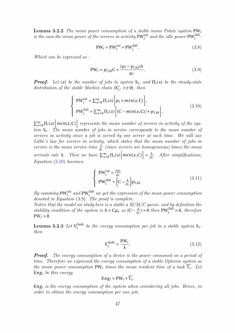
Lemma 3.2.2 The mean power consumption of a stable mono Pstate system PWi

is the sum the mean power of the servers in activity PW(a)i and the idle power PW(Id)

i :

PWi = PW(a)i +PW(Id)

i . (3.8)

Which can be expressed as :

PWi = pi ,Id C+ (pi −pi ,Id )λ

µi. (3.9)

Proof. Let (x) be the number of jobs in system Si , and Πi (x) be the steady-statedistribution of the stable Markov chain Xt

i , t ≥ 0, thenPW(a)

i =∑∞x=0Πi (x)

[pi ∗mi nx,C

],

PW(Id)i =∑∞

x=0Πi (x)

[(C−mi nx,C)∗pi ,Id

].

(3.10)

∑∞x=0Πi (x)

[mi n(x,C)

]represents the mean number of servers in activity of the sys-

tem Si . The mean number of jobs in service corresponds to the mean number ofservers in activity since a job is served by one server at each time. We will useLittle’s law for servers in activity, which states that the mean number of jobs inservice is the mean service time 1

µi(since servers are homogeneous) times the mean

arrivals rate λ. Then we have ∑∞x=0Πi (x)

[mi n(x,C)

]= λ

µi. After simplifications,

Equation (3.10) becomes: PW(a)

i = λpiµi

PW(Id)i =

(C− λ

µi

)pi ,Id

(3.11)

By summing PW(a)i and PW(Id)

i we get the expression of the mean power consumptiondenoted in Equation (3.9). The proof is complete.Notice that the model we study here is a stable a M/M/C queue, and by definition thestability condition of the system is λ< Cµi so (C− λ

µi) > 0 then PW(Id)

i > 0, thereforePWi > 0.

Lemma 3.2.3 Let E(Job)i be the energy consumption per job in a stable system Si .

then

E(Job)i = PWi

λ. (3.12)

Proof. The energy consumption of a device is the power consumed on a period oftime. Therefore we expressed the energy consumption of a stable Opteron system asthe mean power consumption PWi times the mean resident time of a task Ti . LetEngi be this energy

Engi = PWi ∗Ti .

Engi is the energy consumption of the system when considering all jobs. Hence, inorder to obtain the energy consumption per one job,

47

E(Job)i = Engi

E[Xi ].

Using Little’s law for the mean number of jobs in a steady-state system (E[Xi ] = λTi ),then by substitution we get Equation (3.12), the proof is complete.

Lemma 3.2.4 Let E(Job)i (resp. E(Job)

j ) be the energy consumption per job of a stablesystem Si (resp. S j ). Also let PWi (resp. PW j ) be the corresponding mean powerconsumption. In below, we present a sufficient and necessary condition for thecomparison of the mean power and the energy per job consumption:

pi

p j≤ µi g (µ j )

µ j g (µi )⇐⇒

PWi ≤ PW j

E(Job)i ≤ E(Job)

j

(3.13)

whereg (µi ) = αµi C+ (1−α)λ. (3.14)

Proof. From equation (3.9) we have

PWi = pi ,Id C+ (pi −pi ,Id )λ

µi,

and using pi ,Id = αpi we get

PWi =(αµi C+ (1−α)λ

µi

)pi .

then

E(Job)i ≤ E(Job)

j ⇔ PWi ≤ PW j ⇔ pi

p j≤ (αµ j C+ (1−α)λ)µi

(αµi C+ (1−α)λ)µ j(3.15)

and using Equation (3.14) the proof is complete.

Lemma 3.2.5 In this lemma we present a sufficient condition for the comparisonof the mean power and the energy per job consumption in two stable systems Si andS j (with i ≤ j):

µi ≤µ j andpi

p j≤ µi

µ j=⇒

PWi ≤ PW j

E(Job)i ≤ E(Job)

j .(3.16)

Proof. Equation (3.13) in Lemma 3.2.4 presents a sufficient and necessary condi-tion. Therefore:

pi

p j≤ αµiµ j C+ (1−α)λµi

αµiµ j C+ (1−α)λµ j⇒

PWi ≤ PW j

E(Job)i ≤ E(Job)

j .(3.17)

48

Hence, We only have to verify that

µi

µ j≤ αµiµ j C+ (1−α)λµi

αµiµ j C+ (1−α)λµ j. (3.18)

Equation (3.18) can be expressed as

αµ2i µ j C+ (1−α)λµiµ j ≤ αµiµ

2j C+ (1−α)λµiµ j .

After simplification of terms we obtain

µi ≤µ j ,

which is the assumption stated in the presentation of this lemma. Hence, fromEquation (3.17) and (3.18) we obtain Equation (3.16), and the proof is complete.

3.2.3 Numerical comparison of the six Opteron PstatesWe consider here six systems S1, . . . ,S6, each system has C = 20 cores. The speedof the servers (i.e. cores) depends on the Pstate performed. Also, here we supposethat each task requires one core’s instruction a = 1, therefore µi = fi .

3.2.3.1 Performance, power and Energy per job

In Fig. 3.2 we observe that, (a) by increasing the task’s arrivals load, the systemfills up more and the waiting time in the queue increases. (b) In stable cases ofeach system, Pstate6 (contrary to Pstate1) presents the best results in terms ofperformance i.e. mean number of tasks and waiting time in the network, but requiresthe highest power consumption (see Fig. 3.3). In the left figure in Fig. 3.3 we observethat Idle power decreases by increasing the load in the system, but active power willincrease (since the servers will be activated as depicted in the right figure). Thesenumerical results are clearly matching with our analytical results (Corollary 3.2.2,Lemma 3.2.4 and Lemma 3.2.5). The left figure of Fig. 3.4 represents the energyper job consumption when increasing the traffic. This consumption clearly decreaseswith an increase in the load (see Lemma 3.2.3).

3.2.3.2 The appropriate Pstate in performance and energy trade-off

In the right figure, we presented the mean waiting time as a function of the meanpower consumption. This figure give us various information: as the minimal and themaximal power consumption requirement if using any Pstate and the correspondingdelay. Also for a given delay (resp. power consumption value) we can derive thePstate that consumes the least power consumption (resp. delay) as the goal is tominimize both of performance and mean power (resp. energy per job) consumption.

3.2.3.3 Condition verification for power and energy comparison

In Table 3.1, we show a verification of the condition cited in Lemma 3.2.5. Thiscondition is based on the Pstates configurations of an Opteron processor (see Fig.

49

3.1). Note that in Lemma 3.2.5, we only need the core’s speed and core’s power con-sumption to make a comparison of the mean power consumption and the energy perjob consumption between two single-Pstate Opteron processors. This comparison issufficient and not necessary, which means that when µi ≤µ j and pi

p j≤ µi

µ jis verified,

then Pstate ’i’ consumes less mean power and energy per job consumption than thesystem with Pstate ’j’. Otherwise, we don’t dispose of much information to comparethe two systems. In that case, we can use Lemma 3.2.4, which, additionally, includestraffic arrivals rate and other parameters.

For the verified cases in Table 3.1, Lemma 3.2.5 ensures that PWi ≤ PW j andE( j ob)

i ≤ E( j ob)j . Otherwise, we use Lemma 3.2.4. This Lemma considers λ the arrivals

rate (which is supposed to be the same in both systems). The non-verified cases forLemma 3.2.5 are the couple of Pstates i = 1, j = 2 and i = 5, j = 6. For i = 1, j = 2,Lemma 3.2.4 ensures PW1 ≤ PW2 (and E( j ob)

1 ≤ E( j ob)2 ) for all values of λ that makes

both systems stable. But for the case of i = 5 and j = 6 the behavior of the meanpower and energy per job changes with the value of λ. Hence, when applying Lemma3.2.4 with λ≤ 34 we obtain PW5 ≤ PW6 (and E(Job)

5 ≤ E(Job)6 ). Also, when λ> 34 then

PW6 < PW5. That explains the crossover behavior between the red and the greencurve in the right figure of Fig. 3.3.

0 10 20 30 40 50

010

2030

4050

6070

Lambda

Mea

n nu

mbe

r of j

obs

Pstate1Pstate2Pstate3Pstate4Pstate5Pstate6

0 10 20 30 40 50

0.0

0.5

1.0

1.5

2.0

Lambda

Mea

n re

spon

se ti

me

Pstate1Pstate2Pstate3Pstate4Pstate5Pstate6

Figure 3.2: Mean number of jobs (left) and mean response time (right).Parameters: C = 20 servers, server’s rate (i.e. core’s speed) in each Pstate is depicted inFig. 3.1.

50

0 10 20 30 40 50

050

010

0015

0020

00

Lambda

Idle

pow

er c

onsu

mpt

ion

(Wat

t)

Pstate1Pstate2Pstate3Pstate4Pstate5Pstate6

0 10 20 30 40 50

050

010

0015

0020

00

Lambda

Pow

er c

onsu

mpt

ion

(Wat

t)

Pstate1Pstate2Pstate3Pstate4Pstate5Pstate6

Figure 3.3: Idle power consumption (left) and total power consumption (right). Parame-ters are the same as in Fig. 3.2.

0 10 20 30 40 50

010

020

030

040

050

060

0

Lambda

Ene

rgy

per

job

(Wat

t/job

)

Pstate1Pstate2Pstate3Pstate4Pstate5Pstate6

0 500 1000 1500 2000

0.0

0.5

1.0

1.5

2.0

Average power consumption (Watt)

Mea

n re

spon

se ti

me

Pstate1Pstate2Pstate3Pstate4Pstate5Pstate6

Figure 3.4: Energy per job consumption (left) and response time as a function of meanpower consumption. Parameters are the same as in Fig. 3.2.

51

Pstate ’i’ Pstate ’j’ pip j

≤ µiµ j

1 1 Verified1 2 Not verified1 3 Verified1 4 Verified1 5 Verified1 6 Verified2 2 Verified2 3 Verified2 4 Verified2 5 Verified2 6 Verified3 3 Verified3 4 Verified3 5 Verified3 6 Verified4 4 Verified4 5 Verified4 6 Verified5 5 Verified5 6 Not verified6 6 Verified

Table 3.1: The examination of the condition of Lemma 3.2.5 for all pairs of Pstates (i,j)where µi ≤µ j . Note that µi and pi are obtained from the AMD table in Fig. 3.1.

52

3.3 Model 2: A multi-core processor with N = 2Pstates

In this model we consider a birth-death process with two Pstates ’i’ and ’j’ (N = 2).We suppose that Pstate ’j’ consumes more power than Pstate ’i’ i.e. Pstate ’j’executes instructions faster than Pstate ’i’ (see Fig. 3.1). Servers speed rate dependson the number of tasks in the system. It means that if the number of tasks is belowa certain threshold ’th’, then servers (cores) speed corresponds to µi otherwise, it issupposed that the queue is well loaded therefore servers speed rate are fixed to µ j .We denote such a system S(i , j , th) and we suppose the i ≤ j . Stability condition ofthis model, that verifies the existence of a steady-state distribution, is λ< Cµ j .

3.3.1 Closed form for the steady-state distributionThe processor contains C cores. Therefore mi nC, x task are in service and (x −mi nC, x)+ are queued. Under the classical assumptions we mention in Section 3.1,Xt

i , j ,th , t ≥ 0 is a Markov chain, and the transitions are as follows :

(x) → (x +1) with rate λ,(x) → (max0, x −1), with rate mi nx,C·µ(x).

and service rate µ(x) is expressed as :

µ(x) =

µi = fi

ai f (x ≤ th),

µ j = f j

ai f (x > th).

(3.19)

fi is the frequency (GHz) given in Fig. 3.1.

Theorem 3.3.1 The transition diagram of this Markov chain is a birth-death pro-cess. Then, under stability condition (i.e. λ < Cµ j ), we can derive Πi , j ,th(x) thesteady-state probability of the two Pstates Opteron processor S(i , j , th).Let

Ψ(x) =x∏

k=1mi nk,Cµ(k),

andR = maxC, th, (3.20)

then

Πi , j ,th(x) =

λx

Ψ(x)Πi , j ,th(0) ∀ 0 < x ≤ R,

λx[

(Cµ j )x−RΨ(R)]−1

Πi , j ,th(0) ∀ x > R,

(3.21)

where

Πi , j ,th(0) =[

1+ λR+1

(Cµ j −λ)Ψ(R)+

R∑x=1

λx

Ψ(x)

]−1

. (3.22)

53

Proof. The Markov chain we consider is a birth-death process. We also set ’R’(Equation (3.20)) the threshold at which the system maintains it’s service rate (whichis Cµ j ). This simplifies the calculation of the steady state distribution. Hence, wehave divided the calculation of Πi , j ,th(x) into two parts. States from 1 to ’R’ andstates from ’R’ to +∞. From classical equations in a birth-death process, we deducethat:

Πi , j ,th(x) =

λ

mi nx,Cµ(x)Πi , j ,th(x −1) ∀ 0 < x ≤ R,

(λ

Cµ j

)x−RΠi , j ,th(R) ∀ x > R.

(3.23)

After simple substitutions in Equation (3.23) (i.e. to write Πi , j ,th(x) as a functionof Πi , j ,th(0) for all x ∈ [1,+∞[), we get Equation (3.21). Finally, as the system issupposed to be stable, then Equation (3.22) is obtained after the normalization ofprobabilities ( ∑+∞

x=0Πi , j ,th(x) = 1).

3.3.2 Mean number of jobs and response timeHere we seek to compare the mean number of jobs and mean response time betweentwo stable systems S(i , j , th1) with i ≤ j and S(k, l , th2) with k ≤ l . Note that, tocalculate the mean number of jobs E[Xi , j ,th] and mean response time Ti , j ,th, we usethe same approach as in Equation (3.3).

Corollary 3.3.1 We consider the two stable systems described above, then for anythresholds th1 and th2, we have:

j ≤ k ⇒

E[Xk,l ,th2] ≤ E[Xi , j ,th1]

Tk,l ,th2 ≤ Ti , j ,th1.(3.24)

Proof. Let Xti , j ,th1, t ≥ 0 (resp. Xt

k,l ,th2, t ≥ 0) the Markov chain of the stablesystem S(i , j , th1) (resp. S(k, l , th2)). Also, let Πi , j ,th1 and Πk,l ,th2 be the steady-statedistributions of both systems. Let λ

S(i , j ,th1)x , λS(k,l ,th2)

x (resp. µS(i , j ,th1)x , µS(k,l ,th2)

x )be the arrivals rate (resp. service rate) generated at the state ’x’ in the systemS(i , j , th1) and S(k, l , th2).

• We first derive the ’st’ comparison between the two systems. The arrivals rateλ is supposed the same. Then for all the states ’x’, λ

S(i , j ,th1)x = λS(k,l ,th2)

x = λ.Also, we have j ≤ k from the assumption, and i ≤ j and k ≤ l from the definitionof systems, then i ≤ j ≤ k ≤ l . It means that, for any values of ’th1’ and ’th2’,services rates in S(k, l , th2) are always greater than the ones in S(i , j , th1), soµS(k,l ,th2)

x ≥µS(i , j ,th1)x . From Theorem 3.2.1 we deduce that

Xtk,l ,th2, t ≥ 0 ≤st Xt

i , j ,th1, t ≥ 0.

• Both systems are supposed stable, then using Lemma 3.2.1, we have

Xtk,l ,th2, t ≥ 0 ≤st Xt

i , j ,th1, t ≥ 0 ⇒Πk,l ,th2 ≤st Πi , j ,th1.

54

• Finally, the same approach of property 3.2.1 is used to get

Πk,l ,th2 ≤st Πi , j ,th1 ⇒

E[Xk,l ,th2] ≤ E[Xi , j ,th1]

Tk,l ,th2 ≤ Ti , j ,th1.

By combining the three last equations we obtain Equation (3.24), that concludes theproof.

Corollary 3.3.2 In this corollary, we use another assumption, that concerns twostable systems using the same Pstates and different thresholds S(i , j , th1) and S(i , j , th2).We have:

th1 ≤ th2 ⇒

E[Xi , j ,th1] ≤ E[Xi , j ,th2]

Ti , j ,th1 ≤ Ti , j ,th2.(3.25)

Proof. The approach of the proof is similar to the one in Corollary 3.3.1.

• Arrivals rate λ is identical in both systems, then for all the states ’x’, λS(i , j ,th1)x =

λS(k,l ,th2)x = λ. Also, we have from the assumption of the corollary that th1 ≤

th2. It means that Opteron system S(i , j , th1) will activate the higher Pstate’j’ earlier than system S(i , j , th2). And as shown in Fig. 3.1, server’s (core’s)speed is an increasing function of the Pstates. Hence, for all states ’x’,µ

S(i , j ,th1)x ≥µ

S(i , j ,th2)x . From Theorem 3.2.1 we deduce that

Xti , j ,th1, t ≥ 0 ≤st Xt

i , j ,th2, t ≥ 0.

• Using Lemma 3.2.1, and Property 3.2.1 for two Pstates systems. We obtainEquation (3.25), and the proof is complete.

3.3.3 Power and energy consumptionLet pi (resp. p j ) be the power consumption corresponding to Pstate i (resp. Pstatej) (see Fig. 3.1), with i ≤ j . The power consumed by the processor depends on thespeed of its cores, which is a function of the number of tasks assigned to it. Let(x) be the number of tasks in the processor, then the power consumed by each core,when hosting x tasks, is :

pi i f (x ≤ th),p j i f (x > th).

(3.26)

Lemma 3.3.1 Let (x), with x ∈ [0,+∞[, be the number of jobs in the system.Xt

i , j ,th , t ≥ 0 is an CTMC that under stability condition (mentioned in the de-scription section of this model) admits a steady-state distribution Πi , j ,th(x). LetPWi , j ,th be the mean power consumption of the system S(i , j , th), then

PWi , j ,th = pi (1−α)[

pi∑th

x=0 mi n(x,C)Πi , j ,th(x)+p j∑+∞

x=th+1 mi n(x,C)Πi , j ,th(x)]

+αC[

p j + (pi −p j )∑th

x=0Πi , j ,th(x)]

.

(3.27)

55

Proof. Let PW(a)i , j ,th (resp. PW(Id)

i , j ,th) be the mean power consumption of the serversin activity state (resp. Idle state). Hence, as in Lemma 3.2.2, we have

PWi , j ,th = PW(a)i , j ,th +PW(Id)

i , j ,th , (3.28)

wherePW(a)

i , j ,th = pi∑th

x=0 mi n(x,C)Πi , j ,th(x)+p j∑+∞

x=th+1 mi n(x,C)Πi , j ,th(x),

PW(Id)i , j ,th = pi ,Id

∑thx=0(C−mi n(x,C))Πi , j ,th(x)+p j ,Id

∑+∞x=th+1(C−mi n(x,C))Πi , j ,th(x).

(3.29)After simple simplifications using Equation (3.7) in Equation (3.29). Also by the

substitution of PW(a)i , j ,th and PW(Id)

i , j ,th. Then Equation (3.28) is expressed as Equation(3.27) and the proof is complete.

Notice that Lemma 3.2.3 for energy consumption per job still hold for this model.Let E(Job)

i , j ,th be this energy, therefore

E(Job)i , j ,th = PWi , j ,th

λ. (3.30)

.

3.3.4 Optimization of energy consumption and response time• From Corollary 3.3.2, we conclude that when comparing two stable systems

S(i , j , th1) and S(i , j , th2) with th1 ≤ th2 then Ti , j ,th1 ≤ Ti , j ,th2. Therefore, themean response time (and mean number of jobs) is an increasing function ofthe threshold. Hence, to minimize the mean response time in a two-Pstatessystem, th = 1 is the optimal threshold to use.

• The ’st’ comparison does not hold for the mean power consumption (resp.energy per job) function. The function is not monotone. In Fig. 3.5 we showthe evolution of the mean power consumption with the increase of thresholds.In that example we consider λ= 30, C = 20 servers, i = 5, j = 6, and µi = 2.4,µ j = 2.6 (see Fig. 3.1). Note that, specially in that example the mean powerfunction behaves as a convex function. This behavior is not always true.

• So in order to optimize the mean power consumption (resp. energy consump-tion), we shall consider an exhaustive algorithm looking for the best threshold.

In the following, we suggest merging the mean response time Ti , j ,th and theenergy per job consumption E( j ob)

i , j ,th in a single function to minimize. Let c1 (resp.c2) be the cost of the mean response time (resp. energy per job consumption). LetΩ be the total cost to minimize. Ω is normalized through costs c1 and c2.

Ω= Ti , j ,th ∗ c1+E( j ob)i , j ,th ∗ c2 (3.31)

56

Figure 3.5: The mean power consumption as a function of the threshold.

To analyze Equation (3.31), we propose the algorithm below. This algorithm,under stability constraint, generates the best threshold (in the range [1, . . . ,THMAX])to use for each couple of Pstates (i,j). Given the input parameters: number of serversC, services rate (inspired from Fig. 3.1), an upper bound THMAX for the thresholds,arrival rate of tasks λ, and the rewards costs c1 and c2.

57

Algorithm 1: Purchasing the best threshold for each two-pstates Opteronsystem

Input : Number of servers C, arrivals rate λ, rewards cost c1, c2, and avalue of THMAX.

Output: Threshold that minimizes cost function Ω for each couple ofPstates (i , j ).

1 for (i , j ) with 1 ≤ i ≤ j ≤ 6 do2 if λ< Cµ j then // The system is stable3 initiate ’th∗’;4 for th ← 1 to THMAX do5 1) Calculate the steady-state distribution (Equation (3.21) and

(3.22)) for the system S(i , j , th) ;6 2) Derive the mean response time Ti , j ,th (Equation (3.3)) and

energy per job consumption E( j ob)i , j ,th (Equation (3.30));

7 3) Calculate the cost function Equation (3.31) ;8 4) Update ’th∗’ if the current cost function is lower than the cost

function for the previous iteration.9 end

10 Print ”The best threshold for the couple of Pstates (i,j) is ’th∗’ ;11 else12 Print ”The system is not stable for the couple of Pstates (i,j)”;13 end14 end

58

3.3.5 Numerical resultsIn Fig. 3.6 and Fig. 3.7 we investigate the influence of cost values c1 and c2 onpstates (i,j) and their optimal thresholds. We considered the following parameters:arrivals rate λ= 20, number of servers C = 20, and the maximal threshold to purchaseis THMAX = 100. Services rate are inspired from Fig. 3.1 with a = 1 (see Equation(3.19)). We present here two experiments:

• In the first experiment (Fig, 3.6), we consider higher costs c1 for the responsetime and lower costs c2 for the energy per job. In particular, c1 = 200 andc2 = 1 in the left heat-map of Fig. 3.6, we also took c1 = 500 and c2 = 1 in theright heat-map.

• In the second experiment (Fig. 3.7) we focus on the energy per job consump-tion, by adopting higher costs c2 for the energy and lower costs c1 for theresponse time. In the left heat-map of Fig. 3.7 we take c1 = 1 and c2 = 10,and in the right one c1 = 1 and c2 = 50.

Note that, the following results are derived from Algorithm 1. In both figures below,white areas are due to the relation i ≤ j which is an assumption of a two-Pstates(i,j) system. Colored square areas are the values of the objective function (Equation(3.31)). Blue integer in colored areas is the value of the optimal threshold weobtained (in the range [1, . . . ,THMAX]) that minimizes the objective function for thecorresponding couple of Pstates (i,j). Case of i = j the threshold has no meaningsince the system remains in the same Pstate, that explains the ’-’ entry in the figures.

3.3.5.1 Performance optimization

By promoting the mean response time costs. We observe in Fig. 3.6, that to optimizecost function:

• We should consider higher Pstates for the Pstate j, in particular j = 6. Thesystem opts for high Pstates to reduce the response time component in the costfunction. The best couple of Pstates to use is in the green column (i ∈ 1, . . . ,6, j = 6).

• The blue integer in each colored square area,is the optimal threshold, it’s avery small value. It shows that the Opteron processor switches quickly itscores to the higher Pstate ’j’ , i.e. after having 1,2,3,4, or 5 jobs in the systemdepicted in the left heat-map, or after having 1 job in the system as shown inthe right heat-map.

• The impact of Pstate ’i’ is not relevant (in contrast to Pstate ’j’). Smallthresholds here are usually exceeded. That explains the almost similar colorin each column.

• When increasing c1 cost, to the value of 500, and still taking c2 = 1. Weobserve that the best threshold for all configurations is th = 1. Energy perjob cost is irrelevant with regard to the response time’s cost. Therefore, the

59

system behaves as there is no optimization for the energy per job. In thatcase, we have proved (as a consequence of Corollary 3.3.2) that response timefunction increases with the threshold.

3.3.5.2 Energy per job optimization

For the case of the enhancement of energy per job cost’s. We observe in Fig. 3.6,that:

• The energy per job consumption increases with the value of Pstate ’i’. There-fore, the best couples of Pstates minimizing the objective function are in thegreen range (i = 1, j ∈ 2, . . . ,6). The system opts for low Pstates, in order toreduce the energy consumption.

• In contrast to the response time results, the optimal thresholds (blue integersin the colored squares) for the energy per job, achieves the highest levels (upto th = THMAX = 100). Notice that the aim is to minimize the energy per job,then it is consistent that the system switches ’lately’ to the higher Pstate ’j’which consumes more. The system remains mostly all the time in Pstate ’i’.That explains the unnoticed modifications of cost function when changing thePstate ’j’.

Pstate j

Pst

ate

i

1

2

3

4

5

6

2 3 4 5 6

1

−

1

2

−

1

3

3

−

2

4

4

5

−

2

3

3

3

1

−

130

135

140

145

Pstate j

Pst

ate

i

1

2

3

4

5

6

2 3 4 5 6

1

−

1

1

−

1

1

1

−

1

1

1

1

−

1

1

1

1

1

−

240

250

260

270

280

290

300

310

Figure 3.6: Objective function: c1 = 200, c2 = 1 (left) and c1 = 500, c2 = 1 (Right).For instance, in the left heatmap, the optimal threshold for the entry i = 2, j = 3 is th = 2with a total cost of Ω = 140.6. In the right heatmap, for the same entry, the optimalthreshold is th = 1 with a total cost of Ω= 290.4.

60

Pstate j

Pst

ate

i

1

2

3

4

5

6

2 3 4 5 6

56

−

73

86

−

84

86

74

−

96

84

73

66

−

91

86

73

65

13

−

350

400

450

500

Pstate j

Pst

ate

i

1

2

3

4

5

6

2 3 4 5 6

100

−

100

86

−

100

86

74

−

100

84

73

64

−

100

86

73

64

13

−

1600

1800

2000

2200

2400

2600

Figure 3.7: Objective function: c1 = 1, c2 = 10 (left) and c1 = 1, c2 = 50 (Right).For instance, in left heatmap for the entry i = 1, j = 4. The optimal threshold is th = 84with a total cost function of Ω= 324.2, while in the right heatmap th = 100 and Ω= 1610.1

3.4 Model 3: A multi-core processor with all PstatesIn this section, we also represent the Opteron processor by a birth-death process.We consider all (N = 6) Pstates of the Opteron processor. Servers rates (i.e. coresspeed) depends on the number of tasks in the queue. Let Γ = [th1, th2, . . . , th5] bethe vector of the triggering thresholds (see Equation (3.33)). The existence of thesteady-state distribution in this model is subject to the condition λ < Cµ6. Wesuppose that all the systems we study are stable. We denote SΓ such a system.

We first recall the ’el’ comparison between vectors of thresholds.

Definition 3.4.1 Let Γ1 and Γ2 be integer vectors of size M, then

Γ1 ≤el Γ2 ⇒ Γ1( j ) ≤ Γ2( j ) ∀ j ∈ 1, . . . ,M. (3.32)

3.4.1 Closed form for the steady-state distribution

The processors contains C cores. Therefore mi n(C, x) tasks are in service, and(x−mi nC, x)+ are queued. Under the classical assumptions we mention in Section3.1, Xt

Γ, t ≥ 0 is a Markov chain, and the transitions are as follows :

(x) → (x +1) with rate λ,(x) → (max0, x −1), with rate mi nx,C·µ(x).

61

and service rate µ(x) is expressed as :

µ(x) =

µ1 = f1a

i f (x ≤ th1),

µ2 = f2a

i f (th1 < x ≤ th2),

µ3 = f3a

i f (th2 < x ≤ th3),

.

.

µ6 = f6a

i f (x > th5).

(3.33)

fi is the frequency (GHz) given in Fig. 3.1.

Theorem 3.4.1 The Markov chain is a birth-death process. Then, under stabilitycondition (i.e. λ< Cµ6) we can derive ΠΓ(x) the steady-state probability.Let

Ψ(x) =x∏

k=1mi nk,Cµ(k),

andR = maxC, th5, (3.34)

then

ΠΓ(x) =

λx

Ψ(x)ΠΓ(0) ∀ 0 < x ≤ R,

λx[Ψ(R)(Cµ6)x−R

]−1ΠΓ(0) ∀ x > R.

(3.35)

where

ΠΓ(0) =[

1+ λR+1

(Cµ6 −λ)Ψ(R)+

R∑x=1

λx

Ψ(x)

]−1

. (3.36)

Proof. In Equation (3.37), we present the classical birth-death equations for thesteady-state distribution of that model.

ΠΓ(x) =

λ

mi nx,Cµ(x)ΠΓ(x −1) ∀ 0 < x ≤ th5,

(λ

Cµ6

)x−th5ΠΓ(th5) ∀ x > th5.

(3.37)

The rest of the proof is similar to the one used in Theorem 3.3.1 for N = 2 Pstates.

3.4.2 Mean number of jobs and response timeNote that all Pstates are used and the system adapts the speed of its servers ac-cording to the number of pending jobs in the queue.

62

Corollary 3.4.1 This corollary is the extension of Corollary 3.3.2 to N = 6 Pstates.The same approach is used. Let Xt

Γ1, t ≥ 0 (resp. XtΓ2, t ≥ 0) be the Markov chain

of the stable system SΓ1(r esp. SΓ2) with the thresholds vector Γ1 (resp. Γ2). LetE[XΓ1], E[XΓ2] (resp. TΓ1,TΓ2) be the mean number of tasks (resp. mean responsetime) in system SΓ1 resp. SΓ2. Therefore

Γ1 ≤el Γ2 ⇒

E[XΓ1] ≤ E[XΓ2]

TΓ1 ≤ TΓ2

(3.38)

Proof. Let µ(SΓ1)x = mi nx,Cµ(x) (the same for µ

(SΓ2)x ) be the services rate transition

generated at state x in system SΓ1 (resp. SΓ2) then

Γ1 ≤el Γ2 ⇒ µ(SΓ1)x ≥µ

(SΓ2)x ∀ st ate x,

also forall x, we have λ(S1)x = λ

(S2)x = λ . From Theorem 3.2.1 we have

XtΓ1, t ≥ 0 ≤st Xt

Γ2, t ≥ 0.

Using Lemma 3.2.1 for two stable systems, we get ΠΓ16 ≤st Π

Γ26 , therefore we conclude

from Property 3.2.1 that E[XΓ1] ≤ E[XΓ2] and TΓ1 ≤ TΓ2.

3.4.3 Power and energy consumptionLet p1, ..., p6 be the power consumption corresponding to Pstates 1, . . . ,6 (see Ta-ble3.1). Cores speed depends on the number of tasks affected to the Opteron pro-cessor. Let (x) be the number of tasks in the processor, then the power consumedby each core when hosting x tasks in the system is :

p1 i f (x ≤ th1),p2 i f (th1 < x ≤ th2),p3 i f (th2 < x ≤ th3),..p6 i f (th5 < x).

(3.39)

As in previous models. Let pi (r esp. pi ,Id ) for i ∈ 1, . . . ,6 be the Opteron Pstatepower (resp. Pstate idle power) used by a core in Pstate ’i’ so pi ,Id = αpi .

Lemma 3.4.1 Let PWΓ be the total power consumption of a stable Opteron system.For the simplicity of the power consumption equation, we fix th0 =−1 and th6 =∞(effective thresholds are th1, th2, . . . th5). Let PW(a)

Γ (resp. PW(Id)Γ ) be the mean

power consumption of the servers in activity states (resp. Idle states). Let x ∈ [0,+∞[be the number of jobs in the system. Xt

Γ, t ≥ 0 is an CTMC and, under stabilityconstraint, admits a steady-state distribution ΠΓ(x). Then, similarly to Lemma 3.2.2we have :

PWΓ = PW(a)Γ +PW(Id)

Γ , (3.40)

63

where PW(a)

Γ =∑5s=0

[∑ths+1x=ths+1ΠΓ(x)

(mi n(x,C)ps+1

)],

PW(Id)Γ =∑5

s=0

[∑ths+1x=ths+1ΠΓ(x)

(C−mi n(x,C)

)ps+1,Id

].

(3.41)

then

PWΓ =5∑

s=0

[ ths+1∑x=ths+1

ΠΓ(x)

(Cps+1,Id +

(ps+1 −ps+1,Id

)mi n(x,C)

)]. (3.42)

Notice that Lemma 3.2.3 for energy consumption per job still hold for this model.Let E(Job)

Γ be this energy, thenE(Job)Γ = PWΓ

λ. (3.43)

.In next section, we do not proceed to develop Algorithm 1 for the case of N = 6

Pstates.The number of systems to analyze can be up to 4∗106 (with THMAX = 100).Note that in each system, we derive the steady-state distribution and the rewards(mean response time and energy per job). The steady state’s calculation is, however,very fast with a complexity of O(R) (see Equation (3.34)). Hence, for numericalresults in all Pstates Opteron system, we will show how the rewards evolves withthresholds vectors.

3.4.4 Numerical resultsIn the following, we present results of an Opteron processor with C = 20 cores. ThisOpteron processor uses all the Pstates N = 6 (as stated in the description section ofthis model). We decided to compare the results for two systems. The first systemuses Γ1 = 3,6,12,24,48 as a distribution of thresholds. In that system thresholdsrange is growing exponentially, while in the second system, we consider a regularthresholds range Γ2 = 10,20,30,40,50.

In Fig. 3.8 we observe that, for all values of λ where the system is stable(λ < Cµ6), mean number of jobs and response time is lower in the system with Γ1thresholds. This result is justified in Corollary 3.4.1. In Fig. 3.9 it is noted that themean power consumption and energy per job consumption is lower in the systemwith Γ2 thresholds. This result can be seen as a consequence of the results in Fig.3.8. Here Γ1 ≤el Γ2, then it is apparent that the system with Γ1 thresholds, wouldconsume more power (and energy per job), since high Pstates are quickly reached.However, we can’t yet, offer an analytical proof for this result.

64

10 20 30 40 50

020

4060

8010

0

Lambda

Mea

n nu

mbe

r of

jobs

Γ1 = 3,6,12,24,48Γ2 = 10,20,30,40,50

10 20 30 40 50

0.0

0.5

1.0

1.5

Lambda

Mea

n re

spon

se ti

me

Γ1 = 3,6,12,24,48Γ2 = 10,20,30,40,50

Figure 3.8: Mean number of jobs (left) and Mean response time (right).

10 20 30 40 50

500

1000

1500

Lambda

Pow

er c

onsu

mpt

ion

(Wat

t)

Γ1 = 3,6,12,24,48Γ2 = 10,20,30,40,50

10 20 30 40 50

2030

4050

6070

80

Lambda

Ene

rgy

per

job

(Wat

t/job

)

Γ1 = 3,6,12,24,48Γ2 = 10,20,30,40,50

Figure 3.9: Mean power consumption (left) and Energy per job consumption (right)

65

Chapter 4

Performance and energy efficiencyanalysis in NGREEN opticalnetwork

Contents4.1 Introduction . . . . . . . . . . . . . . . . . . . . . . . . . . . . . 674.2 Model for optical container filling . . . . . . . . . . . . . . . 68

4.2.1 Markov Chain model . . . . . . . . . . . . . . . . . . . . . . . 684.2.2 Numerical Analysis . . . . . . . . . . . . . . . . . . . . . . . . 724.2.3 A more realistic example with Ethernet and TCP SDUs . . 76

4.3 Generalization to non stationary arrivals . . . . . . . . . . 814.3.1 Replacement of Step 6) in our algorithm . . . . . . . . . . . 834.3.2 Algorithm Comparison . . . . . . . . . . . . . . . . . . . . . . 854.3.3 Example . . . . . . . . . . . . . . . . . . . . . . . . . . . . . . 88

4.4 Modeling the container insertion on the optical ring . . . 894.4.1 Scenario A : latency with opportunistic insertion mode . . 914.4.2 Scenario B : guarantee latency with slot reservation inser-

tion mode . . . . . . . . . . . . . . . . . . . . . . . . . . . . . . 954.5 Energy efficiency and latency analysis . . . . . . . . . . . . 98

66

4.1 IntroductionThe fifth generation of mobile networks technology represents wireless communica-tion systems related with the enormous growth of data traffic, due to the numberof connected devices and the popularity of some applications as video streaming,augmented and virtual reality, cloud gaming, smart homes, connected cars, and re-mote control of machines [GK15]. These applications have strict constraints such asultra-low latency, ultra-high bandwidth, to ensure the delivery of real-time services.These requirements can be met by efficiently integrating heterogeneous wireless andoptical network segments and massive computing and storage services, delivered bymeans of cloud computing.

The Cloud Radio Access Network (CRAN) has been recently proposed [Ase+16].Because of the stringent requirements (latency in the order of tens of milliseconds) ofthe several interfaces needed in C-RAN and the maturity and evolution of differentoptical network technologies, optical networks have been proposed to support inter-faces between Remote Radio Head (RRH) and Base-Band Unit (BBU) (front-haulnetwork), among BBUs and between BBUs and their peering point in the mobilecore network (back-haul network).

The NGREEN network takes advantages of several improvements of optical tech-nology [D C17; Chi17a; Chi17b; WC17]. First, for metro networks, it is now possibleto synchronize entire networks up to nanoseconds. This enables architectures basedon Optical Slot Switching (OSS) where packets circulate on specific time slots. Sec-ond, the use of WDM (Wavelength Division Multiplexing) packets allows some kindof optical parallelism. The introduction of parallelism in the optical processing hasbeen considered as a powerful approach to reduce cost and energy consumption foroptical systems.

The NGREEN project aims to design and validate a versatile network archi-tecture with a scalable capacity, low cost and low energy consumption. For theperformance point of view, we expect low latency and high utilization of the opticalcapacity. In OSS networks, the delay is due to the optical container constructionand its insertion into the optical ring. Once the container has been emitted, it isnever converted to electronic nor queued until its arrival to destination. The trans-portation time is only related to the distance (i.e. the length of the optical link)between source and destination.

In this work, we study two parts of the network. The first one, is the mechanismused to fill the optical container with the electronic packets (i.e. Internet Proto-col (IP) or Ethernet) and the second one is the insertion node where the flows ofoptical containers are queued before being emitted on the ring. Here, we evaluatemathematically both mechanisms and the results from the filling process are used asan input parameter for the analysis of the insertion. Thus we do not need to makethe typical assumption about Poisson arrivals of optical containers to the insertionnode. The discrete distribution for the inter-arrivals of container is obtained throughnumerical analysis of the Markov chain and we found that it is quite different froma Poisson process.

The aggregation of several data units into optical container must have a deadlineto avoid that some information wait too long during this first step. Adding a deadline

67

which is triggered when the container begins to fill will help to keep the delay shorter.However it makes the container filling incomplete because the Protocol Data Unit(PDU) moves to the insertion node when the deadline occurs. This movementcan also be triggered if the filling is larger than a threshold. Thus we have twomechanisms to study the trade-off between latency and energy consumption. Indeed,the energy needed is the same irrespective of the number of Service Data Units(SDUs) carried by the PDU, the optical container has a fixed size and padding isadded after the filling to complete the PDU. Thus a shorter deadline and a smallerthreshold make the container less energy efficient and reduce the delay. For theinsertion of the PDU into the ring we analyze both the opportunistic and reservationmode, in order to compare the delays. In [Gra+18], two mathematical models havebeen proposed to compare these two insertion modes, by considering Poisson arrivalsfor the PDU. In our work, we compute the distribution of inter-arrival time of thePDUs obtained from the filling process, in order to evaluate delays for the differentinsertion modes. We compute both insertion delays and end to end delays fromSDU arrival to its depart from the optical ring.

This work is organized as follows. First, in section 4.2, we present the model ofa container filling with stationary batch arrivals of service data units which arriveaccording to a stationary batch process. We derive a Discrete Time Markov Chain(DTMC in the following) to represent the remaining time and the number of servicedata units still present in the container. We prove that this chain satisfies a propertyalready studied by Robertazzi in [Rob89]. All the directed cycles of the DTMC gothrough a single state. This property allows to compute the steady-state distributionvery efficiently. We obtain the distribution of the PDU size when it is inserted on thering and the distribution of the delay to fill a container and the delay between therelease of two successive containers. Through these models we get the distributionof the delay between two successive arrivals of container at the insertion point onthe optical ring which are used in Section 4.4 to perform extensive simulations ofthe ring. In section 4.3 we extend the model to a non stationary batch of arrivals. Insection 4.5 We compare distributions of delays for both opportunistic and reservationinsertion mode, and we study the trade off between energy efficiency and delays. Atthe end, we finish with some remarks.

4.2 Model for optical container fillingWe first model the filling process (Fig. 4.1) to obtain the distribution of the numberof bytes (aggregated in chunks) in an optical container (also denoted as PDU) andthe distribution of time between two successive releases of PDU. We fill a containerby aggregating various SDUs like Ethernet frames or Transmission Control Proto-col (TCP) packets. We release a container either due to a deadline or a minimaloccupancy.

4.2.1 Markov Chain modelWe consider a discrete time model the time unit of which is the WDM slot duration.We assume that the arrivals follow a stationary batch process (we will change this

68

SDU

Optical Container

N-Green Ring

Figure 4.1: Container filling and insertion.

assumption in the next section), called A. We also assume independence betweenthe successive batches of arrivals. The optical container size is 12500 bytes for theNGreen architecture [Chi17a; WC17] and the container size is associated with a slotequal to 10µs.

The arrivals may represent SDU or chunks with a constant number of bytes de-pending of the granularity needed by the model. For the example below, we assumethat all the SDU (also equal to a chunk in this example) have the same size equal to1500 bytes like an Ethernet MTU. Thus, the PDU can contain at most 8 chunks andwe can depict the chain (see for instance Fig. 4.2). This assumption is only neededhere for the sake of readability of the figure. Let An be the number of chunks whicharrives at time n, An=st A. The support of A is an upper bounded subspace of N.We only assume that 0 ≤ An ≤ MaxAr r i val . This value (i.e. MaxArrival) dependson the number of incoming lines connected to the station.

We design a discrete time Markov chain with two components: the occupancy ofthe container and the clock. The timer is initially equal to 0 and it jumps to 1 whenthe first SDU arrives in the buffer. It is then increased during each time unit untilthe buffer is released. Let Hn be the value of the timer and let Xn be the number ofchunks in the buffer at time n. The system evolves based of the following events attime n:

• a batch of An chunks arrives and they are added into the buffer (i.e. An maybe 0),

• the timer is increased if the number of Data Units in the container is positive,

• if the timer is equal to the deadline, or if the buffer is sufficiently filled, thebuffer is released into an optical container to be inserted on the ring. Then,we begin the filling again.

Assume that chunks have a size equal to Y. Let Z be the size of the PDU. Let J beZ/Y be the number of chunks which can be included into the container. Let C be

69

the deadline and Thr be the utilization ratio of the buffer which triggers the releaseof the container.

Xn+1 = mi n(Xn +An , J)IF Xn+1 > 0 Hn+1 = mi n(Hn +1,C)I f (Hn+1 = C) Cont ai ner Read yI f (Xn+1 ≥ Thr ∗ J) Cont ai ner Read y

Once the ”Container Ready” event occurs, we make the following transitions at thenext step : Xn = 0 and Hn = 0.

Clearly, due to the independence and stationary assumption, (Xn ,Hn) is a finitediscrete time Markov chain the state space of which is included into [0, J]×[0,C]. Anexample of such a chain for small parameters C and J and three possible batches ofarrivals with size 0, 1 and 3 is displayed in Fig. 4.2. The Markov chain is built withthe XBorne tool [Fou+16].

70

Figure 4.2: ToyModel: The Markov chain for J= 8, C= 8, and arrivals of 0, 1 or 3 SDUper slot.

71

4.2.2 Numerical AnalysisThe numerical analysis of the chain takes into account its structural properties.

Property 4.2.1 Assume that E[An] > 0 (positive arrival) and that J∗Thr+MaxAr r i val ≤J (no loss), the chain has the following properties:

• All the nodes in [0, J]× [0,C] are not reachable. Let S be the set of reachablestates reachable from state (0,0).

• The chain consists in many directed trees rooted at (0,0) with back edges fromthe tree leaves returning to (0,0).

• Therefore the matrix of the Markov chain (say P) can be decomposed into anupper diagonal matrix plus a matrix whose first column is positive and all theother entries are equal to 0.

Proof. To prove the first point, we just mention that state (0,2) is not reachablefrom state (0,0) because the clock jumps out of state 0 only with the first arrival. Letus now consider the graph of the Markov chain. Let b be a node of S . Assume thatb 6= (0,0). By definition there is an oriented path from 0 to b in S . During all thetransitions out of b, the component Hn increases when Xn > 0 and the component Xn

does not decrease. Therefore, after some transitions, the components Hn is equal toC or the component Xn is larger than J∗Thr . The next transition leads to state (0,0).Therefore there is also a path from b to (0,0). Thus, for every state b in S , state(0,0) is in at least one cycle going through b. Clearly, during all transitions (exceptthe loop in state (0,0)), component Hn always increases. Therefore all the directedcycles of the chain are going through state (0,0). The last point follows directly fromthe property on the cycles.

Property 4.2.2 If Thr ≤ J+1−MaxAr r i valJ , no SDU are lost. The PDU is released

before it is sufficiently filled.

Indeed, this assumption implies that J∗Thr −1+MaxAr r i val ≤ J, and J∗Thr −1 isthe largest buffer occupancy which does not trigger the emission of the container.

The first property allows that one can use a very efficient algorithm proposed byRobertazzi [Rob89] to compute the steady-state distribution (say π()).

Such an algorithm has a complexity which is linear in the number of non zeroentries in matrix of the Markov chain while the Gaussian elimination for a fullmatrix has a complexity cubic in the number of states. Thus, solving the steady-state distribution only requires few seconds.

Once the steady-state distribution is obtained (typical results are represented inFig. 4.3 as a heatmap to illustrate the bivariate nature of the chain), one can derivethe distribution of the timer when the container is released. We have two conditionsto release a container: the buffer occupancy Xn is larger than J∗Thr or the clock Hn isequal to C. Let S 1 be the set of states which satisfy one of these constraints. We firstcompute the probability of S 1 Pr (S 1) = ∑

(X,H)∈S 1π(X,H). Then, the distributionof the clock at a release instant are obtained after conditioning.

PrH(t ) = 1

Pr (S 1)

∑(X,H)∈S 1

Pr (X,H)1H=t

72

Parametres: J=8, A(n)=0,1,3, J*0.75 = 6 and C = 8X

H

0

2

4

6

8

0 2 4 6 8

0.00

0.05

0.10

0.15

0.20

Figure 4.3: ToyModel: Distribution of the steady-state probability for (X,H) for the simplemodel. Non reachable states are depicted in white.

0 1 2 3 4 5 6 7 8

x : Number of SDUs in PDU

PrX

(x)

0.0

0.1

0.2

0.3

0.4

probabilityThreshold

Figure 4.4: ToyModel: Distribution of the container size (in chunks of 1500 bytes) atrelease time.

73

Algorithm 2: Computation of the steady-state distribution: Robertazzi’salgorithm

Input : Matrix P.Output: Steady-state distribution π(x, y).Step 1) Initialize π(0,0) = 1.Step 2) Compute all the values of π(x, y) along the trees using the globalbalance Equation (in a tree, a node has only one predecessor, thereforesolving the balance Equation is trivial).Step 3) When the probability for all the leaves have been obtained,compute the sum of the probability S.

Step 4) Normalize: divide each probability by S to obtain a sum equal to1.0.

Let D be this distribution of time needed for filling a PDU. Note that it has abounded support: the upper bound is C while the lower bound is bJ∗Thr /MaxAr r i valc.

One can also compute the distribution of the buffer size when the PDU is re-leased.

PrX(x) = 1

Pr (S 1)

∑(X,H)∈S 1

Pr (X,H)1X=x

See Fig. 4.4 for this distribution for the model depicted in Fig. 4.2.Once we have obtained the distribution of the timer at a release instant, we have

to add the time period when the buffer is empty. As the arrivals are independentand stationary, the duration of time between the release of the container and thearrival of the SDU has a geometric distribution with rate (1−Pr (An = 0)) and itssupport is N. Let E be this distribution of the empty period. The time between twosuccessive releases of a container is the sum of the empty period and the durationto fill a container (i.e. D) As the arrivals are independent, the distribution of thetimer at release time and the distribution of the empty period for the buffer arealso independent. Therefore the distribution of time between successive releases ofa container is the convolution of D and E . We compute a truncation of F =D⊗E .Note that we must truncate the distribution because the support of E is not upperbounded. This distribution F can be used an input parameter of the simulation ofNGREEN optical ring.

In Fig. 4.4, Fig. 4.5 and Fig. 4.6, we have depicted typical results for thesedistributions. These results were obtained for arrivals of Ethernet Maximum Trans-mission Units (MTUs) with full size. Therefore, the container size is 8. We haveconsider a deadline equal to 8 and the threshold ratio for occupancy is 75% leadingto an integer threshold equal to 6. We have assumed that the batch of arrivals maycontain between 0, 1 or 3 SDU with respective probability: 0.5, 0.4, and 0.1. Thusthe expected number of SDU per time slot is 0.7.

74

0 1 2 3 4 5 6 7 8 9 10 11 12 13 14 15 16 17 18

t

PrH

(t)

0.0

0.1

0.2

0.3

0.4

0.5 probability

Timer deadline

Figure 4.5: ToyModel: Distribution of the Timer at release time.

0 1 2 3 4 5 6 7 8 9 10 11 12 13 14 15 16 17 18

t

PrH

_G(t)

0.0

0.1

0.2

0.3

0.4

0.5 probability

Figure 4.6: ToyModel: Distribution of inter-PDU release time.

75

4.2.3 A more realistic example with Ethernet and TCP SDUsWe model the arrivals of several types of SDU (short SDU of 50 bytes like TCPacknowledgments, and larger SDU of 1500 bytes like Ethernet frames). We alsoconsider some others SDUs which will describe in the following. As the gcd of 50and 1500 is 50 we describe the buffer occupancy by chunks of 50 bytes. TCP acksconsist in one chunk while a Ethernet MTU is modeled by 30 chunks. The bufferoccupancy varies from 0 to J = 250 chunks. To keep this representation of the buffer,we assume that the sizes of the other SDUs are also a multiple of 50 bytes.

4.2.3.1 Model 1

In that model we consider three possible batches : 1 for the TCP packets, 30 for theEthernet frames, and 0 for no arrivals. Their respective probabilities are assumedto be 0.4, 0.2 and 0.4.

1 13 27 41 55 69 83 97 113 131 149 167 185 203

x : Number of SDUs in PDU

PrX(

x)

0.00

0.05

0.10

0.15

probabilityThreshold

Figure 4.7: Model1: Distribution of the PDU size at release time (in chunks of 50 bytes)

Thus the average number of bytes arriving per slot is 320 (i.e. 6.4 chunks of50 bytes). We first chose a deadline equal to 40 and a threshold ratio equal to75% leading to an integer threshold equal to 190. We obtain a Markov chain with5200 states and roughly 15000 transitions, the steady-state distribution of which isobtained after 0.01s of computation time. The PDU contains an average payloadof 971 bytes (i.e. 194.37 chunks of 50 bytes obtained from the expectation of thedistribution depicted in Fig. 4.7). The average time to fill a container is 29.7 slots(see the distribution in Fig. 4.8), and the average inter-arrival time 31.3 slots (seethe distribution depicted in Fig. 4.9).

We now study the effect of the deadline and the threshold ratio. In Fig. 4.10, wepresent the mean time to fill a container for various threshold ratios (0.60,0.70,0.80,0.90).

76

0 3 6 9 13 17 21 25 29 33 37 41 45 49 53 57 61

t

PrH

(t)

0.00

0.05

0.10

0.15

0.20

probabilityTimer deadline

Figure 4.8: Model1: Distribution of the Timer at release time.

0 3 6 9 13 17 21 25 29 33 37 41 45 49 53 57 61

t

PrH_G

(t)

0.00

0.05

0.10

0.15

0.20

probability

Figure 4.9: Model1: Distribution of inter-PDU release time.

77

The analysis shows that the deadline is useful when it is small. After a boundaryvalue depicted by small dots in Fig. 4.10, the deadline has a weaker impact on thetime needed to fill the containers. They are mostly released because they have theminimal size required. Obviously, the mean time to fill a container increases withthe threshold ratio.

10 20 30 40 50 60

5

10

15

20

25

30

35

40

C

Mea

n tim

e of

PD

U's

filli

ng

Thr = 90%Thr = 80%Thr = 70%Thr = 60%

Figure 4.10: Model1: Distribution of the Timer at release time VS deadline, for differentthreshold ratios

We will use this model for the insertion of PDUs by the stations in the opticalring (see Section 4.4).

4.2.3.2 Model 2

In this model we consider five possible batches : 1 for the TCP packets, 30 for theEthernet frames, 4 and 9 chunks for various SDUs and 0 for no arrivals. Theirrespective probabilities are 0.2, 0.15, 0.2, 0.1 and 0.35.

Thus, the average number of bytes arriving per slot is 320 (i.e. 6.4 chunksof 50 bytes). The threshold ratio and the deadline are the same as in the lastmodel. Clearly this model will generate a bigger Markov chain since there is morebatches of arrivals. We obtain a Markov chain with 7670 states and more than33500 transitions, the steady-state distribution of which is obtained after 0.03s ofcomputation time. Clearly our approach is extremely efficient.

The container contains an average payload of 980.5 bytes (i.e. 196.1 chunks of50 bytes for the expectation of the distribution depicted in Fig. 4.11). The averagetime to fill a container is 30.1 slots (see the distribution in Fig. 4.12). and theaverage inter-arrival time of containers is 31.6 slots (the distribution is depicted in

78

0 20 40 60 80 100 120 140 160 180 200 220

x : Number of chunks in PDU

PrX(

x)

0.00

0.02

0.04

0.06

0.08 probability

Threshold

Figure 4.11: Model2: Distribution of the PDU size at release time (in chunks of 50 bytes).

0 5 10 15 20 25 30 35 40 45 50 55

t

PrH

(t)

0.00

0.05

0.10

0.15

probabilityTimer deadline

Figure 4.12: Model2: Distribution of the Timer at release time.

79

0 5 10 15 20 25 30 35 40 45 50 55

t

PrH_G

(t)

0.00

0.05

0.10

0.15

probability

Figure 4.13: Model2: Distribution of inter-PDU release time.

Fig. 4.13). We will use this model in the next section where we generalize theresolution to wider non stationary arrivals.

80

4.3 Generalization to non stationary arrivalsWe now assume that the arrival process is not stationary. More precisely we considera Switched Bernoulli Batch Process (SBBP): the size of the batch is modulated byan auxiliary discrete time finite Markov chain [HTS91]. Let Φn be the modulatingMarkov chain, N be its number of states, M its transition matrix and ψ its transitionfunction [Duf97]. When this chain is in state k, the batch of arrivals is distributedfollowing distribution Bk. The arrivals are still independent but the distributiondepends on phase Φn at time n. Clearly, using the same notation as in previoussection, (Φn ,Xn ,Hn) is a DTMC whose transition is described by:

Φn =ψ(U,Φn−1)Xn+1 = mi n(Xn +An , J) wi th An=st BΦn−1

IF Xn+1 > 0 Hn+1 = mi n(Hn +1,C)I f (Hn+1 = C) Cont ai ner Read yI f (Xn+1 ≥ Thr ∗ J) Cont ai ner Read y

where U is uniform random. Again, once the ”Container Ready” event occurs, wemake the following transitions at the next step : Xn = 0 and Hn = 0 but the value ofΦ does not change.

Due to these assumptions we can reorder the Markov chain of the model toexhibit a block structure:

P =

P11 P12 . . . P1N

P21 P22 . . . P2N... ... ... . . .

PN1 PN2 . . . PNN

, (4.1)

where block Pi ,i describes the transitions when modulating chain Φ remains in statei while Pi , j models the transitions when modulating chain Φ moves from state i tostate j . Matrix Pi , j has size ni ×n j . We have for all value i and j of Φ, and all valuek and l of (X,H):

Pi , j [k, l ] = M[i , j ]Qi [k, l ], (4.2)

where Qi [k, l ] describes the transition from state k = (Xn−1,Hn−1) to l = (Xn ,Hn)when the phase is i at the beginning of the transition. Thus the Markov chain canbe described as a generalized tensor product and some algorithms take advantageof this block decomposition [FPS98; GDF01; Ben+04].

Remember that the NGreen container size is associated with a slot equal to 10µs.Thus, if the evolution of the phase is much slower, we also have that (i.e M(i , j ) <<M(i , i ), for all i 6= j ) and the Markov chain is Near Completely Decomposable (NCD).

Definition 4.3.1 P is NCD if P is decomposed as in Equation (4.1) such that forall i 6= j , ||Pi , j ||∞ << 1.

Proposition 4.3.1 If M(i , j ) << M(i , i ), for all i 6= j , the DTMC (Φn ,Xn ,Hn) isNCD.

81

This is a simple consequence of the multiplicative form in Equation (4.2).There exist many algorithms which takes into account the block structure or the

NCD property to compute the steady-state distribution [Ste95] after a decomposi-tional analysis and the coupling of the sub-problems. Elimination algorithms arerather inefficient due to the complexity and the spectral properties of NCD matricesforbid to use iterative algorithms like Gauss Seidel or the Power method. We firstuse a decompositional method (more precisely Iterative Aggregation/Disaggregationalgorithm) because our matrix exhibits a block structure decomposition: Koury,McAllister and Stewart (KMS). More precisely we begin with the KMS-BGS ver-sion described in [Ste95] (see also Algorithm 3) where a Block Gauss Seidel (BGS) isperformed at each iteration (Step 6) in Algorithm 3. The steady-state distributionπ is decomposed into sub-vectors πi . Sub-vector πi has size ni and n =∑N

i=1 ni is thesize of the Markov chain of the model. All vectors in the following are row vectors.e is a row vector whose entries are all equal to 1 and eT is the transpose of e.

Algorithm 3: Computation of the steady-state distribution: KMS-BGSalgorithm

Input : Matrix P.Output: Steady-state distribution π(x, y).Step 1) Choose an initial probability distribution π(0)

i for each sub-problemi , typically, the uniform distribution: π(0)[m] = 1/n for all m. Decomposeπ(0) into sub-vectors π(0)

i .Step 2) Compute the conditional probabilities at iteration k knowing thatwe are in subset i :

ϕ(k)i = π(k)

i

||π(k)i ||1

.

Step 3) Compute coupling matrix A(k): A(k)[i , j ] =ϕ(k)i Pi , j eT.

Step 4) Compute the dominant eigenvector of matrix A(k): ψ(k) =ψ(k)A(k),and ψ(k)eT = 1.

Step 5) Obtain a new approximation of the solution based on thedecomposition and the law of total probability:

z(k) = (ψ(k)[1]ϕ(k)1 ,ψ(k)[2]ϕ(k)

2 , . . . ,ψ(k)[N]ϕ(k)N ).

Step 6) Perform an iteration of block Gauss Seidel to find a betteriteration for π(k+1)

i

π(k+1)i (Id −Pi ,i ) = ∑

j<iπ(k+1)

j P j ,i +∑j>i

z(k)j P j ,i .

Step 7) Conduct a test for convergence between π(k)i and π(k−1)

i . If theaccuracy is sufficient, then build solution π from sub-vectors π(k)

i .Otherwise set k = k +1 and go to step 2).

Unfortunately, Step 6) requires to compute exactly (or to give an approximation)

82

of (Id −Pi ,i )−1 to perform the block Gauss Seidel iteration. Even if this matrix hasto be computed once for all the iterations of the algorithm, it needs a large amountof time. As Pi ,i is transient, (Id−Pi ,i )−1 is the fundamental matrix associated to Pi ,i .The computation of the fundamental matrix is known to be numerically unstableand we use an elimination algorithm proposed by Sheskin [She95] due to its stability.Such an algorithm is also time consuming and we also use a version of KMS wherethe block Gauss Seidel iteration is replaced by an iteration of the Power method.This version (called KMS-Pwr) is known to need a larger number of iterations butan iteration of the Power method does not require to compute (Id −Pi ,i )−1 and istherefore much faster. In KMS-Pwr algorithm, Step 6) is replaced by

π(k+1)i =∑

jz(k)

j P j ,i .

Computing the steady-state distribution is really time consuming as it can be seenin Table 3.1 for KMS-BGS while the numbers of iterations increase with KMS-Pwr.Thus we develop a new algorithm which combines the mains ideas of KMS algorithm(decomposition and coupling) and Robertazzi method (simple elimination due to thegraph structure). In this new algorithm (called KMS+R) we replace Step 6) of KMSalgorithm and we obtain a much more efficient method as it is based on the cyclesof the graph.

4.3.1 Replacement of Step 6) in our algorithmAs we state the complexity of this new algorithm, we need some notation and someassumptions about the storage of matrix P.

• Matrix P is stored by column.

• Matrix P is decomposed into blocks called Pi , j for i = 1..N, and j = 1..N. Di-agonal block i (i.e. Pi ,i ) contains ni nodes and mi non zero elements.

• Furthermore n =∑i ni . Let m the number of non zero transitions in P.

• πki represents the value of sub-vector π for subset i at iteration k. It is a vector

of size ni .

• Diagonal block Pi ,i has the following structure (see previous results): Pi ,i =Ci +Ui , where:

– Ci is a matrix whose first column is positive and all the other entries areequal to 0.

– Ui is a strictly upper diagonal matrix.– Pi ,i [1,1] = 0.

Instead of computing matrices (I−Pi ,i )−1 for each index i , we solve the followingsystem of linear equations, at each iteration k and for each index i , taking intoaccount the properties of the matrices.

π(k+1)i (Id −Pi ,i ) = ∑

j<iπ(k+1)

j P j ,i +∑j>i

z(k)j P j ,i .

83

Note that the right part can be computed before solving the linear system. Letb(k)

i be the right hand side. The Equation becomes: π(k)i = π(k)

i Pi ,i +b(k)i . Using the

decomposition, we get:π(k)

i =π(k)i (Ci +Ui )+b(k)

i (4.3)Taking into account the structure, we get for p = 2 to ni

π(k)i [p] = ∑

q<pπ(k)

i [q]Ui [q, p]+b(k)i [p]

andπ(k)

i [1] =∑qπ(k)

i [q]Ci [q,1]+b(k)i [1]

We prove in the following lemma a constructive formula for π(k)i [q] for all index

i and node q.

Lemma 4.3.1 For all q > 1 and i in 1..b, we have:

π(k)i [q] = αi [q]π(k)

i [1]+β(k)i [q] (4.4)

where αi [q] and βi [q] are defined by the following induction:

αi [q] = ∑p<q

αi [p]Pi ,i [p, q], (4.5)

with the following initializations: αi [2] = Pi ,i [1,2], and αi [1] = 1. Moreover

β(k)i [q] = b(k)

i [q]+ ∑p<q

β(k)i [p]Pi ,i [p, q], (4.6)

with β(k)i [2] = b(k)

i [2], and β(k)i [1] = 0. Furthermore, we have

π(k)i [1](1− ∑

p>1αi [p]Pi ,i [p,1]) = b(k)

i [1]+ ∑p>1

β(k)i [p]Pi ,i [p,1] (4.7)

Note that vector αi does not change with iteration number k unlike vector β(k)i . Thus

it can be computed once.

Proof: First, we prove the induction.

1. For p = 2, from Equation (4.3), we clearly have: π(k)i [2] =π(k)

i [1]Pi [1,2]+b(k)i [2],

because node 1 if the only predecessor of node 2. We clearly get the values forαi [2] and βi [2].

2. For an arbitrary p > 2, assume the induction holds until p −1. We have:

π(k)i [p] = ∑

q<pπ(k)

i [q]Pi ,i [q, p]+b(k)i [p].

Using the induction for π(k)i [q] with q < p, we get:

π(k)i [p] = ∑

q<p(αi [q]π(k)

i [1]+β(k)i [q])Pi ,i [q, p]+b(k)

i [p],

from which one can readily obtained the induction.

84

Finally, we compute π(k)i [1] using Equation (4.3):

πki [1] = b(k)

i [1]+ ∑p>1

β(k)i [p]Pi ,i [p,1]+ ∑

p>1αi [p]Pi ,i [p,1])

This concludes the proof and we can now derive the algorithm (called KMS+R as itmixed the KMS approach of block structured matrices with Robertazzi algorithm).

Algorithm 4: Replacement of step 6) for KMS+R algorithmInput : KMS+R algorithm.Output: Steady-state distribution π(x, y).Step 6.1) Compute the terms of the right hand side to obtain bk

i .Step 6.2) Using Equations 4.5 and 4.6, we get the values of αi [p] andβ(k)

i [p] for p > 1.Step 6.3) Using Equation (4.7), we get the value of π(k)

i [1].Step 6.4) We obtain π(k)

i [p] for all p > 1 using the last two steps and theinduction.

Let turn to the complexity of this approach for replacing Step 6). The compu-tation of bk

i requires at most m products and m additions to obtain the values ofbk

i for all i (it is a block Gauss Seidel iteration) during Step 6.1). At Step 6.2) theloop iterates on p from 2 to ni and iteration p has a complexity equal to two timesthe number of non zero elements in column p of matrix Pi ,i . Step 6.3) requires mul-tiplication by the first column of Pi ,i (twice). Finally for Step 6.4) we only need ni

multiplications and ni additions. Steps 6.2 and 6.3 requires o(mi ) operations whileStep 6.4) needs o(ni ). This is much more efficient that our version of KMS-BGSwhich computes the fundamental matrix of an arbitrary transient Markov chain (i.e.(I−Pi ,i )−1) [She95] which has a complexity in o(n3

i ). Note however that we only needto compute (I−Pi ,i )−1 once.

4.3.2 Algorithm ComparisonWe now compare the time needed to solve the model using a standard numericalalgorithm with a cubic complexity (GTH proposed by Grassmann, Taksar and Hey-mann ) which does not take into account the structure of the matrix, and with twoversions of the algorithm for block structured chains Markov chains (including NCDchains). GTH is a very accurate direct method. A detailed presentation of thisalgorithm can be found in [Ste95].

KMS-BGS, KMS-Pwr and KMS+R algorithms are iterative. To stop the processwe use the same condition as Stewart [Ste95] (i.e. ‖π−πP‖2 ≤ ϵ with a precision ϵ

equal to 10−15). We check the algorithms for NCD and non NCD matrices associatedwith the same model for the buffer and various modulating Markov chains for thephase of the arrivals. We assume without loss of generality that the modulatingMarkov chain has only two phases. We check our algorithm for NCD and non NCDmatrices.

85

4.3.2.1 NCD matrix

We have assumed the following matrix for modulation of the arrival:

M =(

0.9 0.10.001 0.999

)(4.8)

Clearly, such a matrix makes the Markov chain of the model near completely de-composable. The batches of arrival have the same support (with size equal to 4)but different probabilities for the two phases (see Table 4.1).

Batch size 0 1 2 3Probability Phase 1 0.1 0.15 0.25 0.50Probability Phase 2 0.5 0.25 0.15 0.1

Table 4.1: Parameters for the batch distribution.

We present in the following table a comparison of the execution time of the fouralgorithms. The computations have been performed on a multicore PC with 8 Xeonprocessors at 2.4 GHz with 12Go RAM. We report the results in Table 4.2. Thecomputations are performed 30 times to obtain the 95% confidence intervals for thecomputation times. We only report the CPU usage and we do not take into accountthe IO. The numbers of iterations needed by the KMS-BGS and KMS+R algorithmsare extremely low (4 to 6 iterations on most of the examples we solved) when thematrix is NCD, as already reported in [Ste95]. KMS-Pwr is less efficient for thiscriterion.

Size 1000 1500KMS+R [0.018, 0.020]s 5 [0.019, 0.022] s 5

KMS-Pwr [0.056 , 0.062]s 18 [0.076 , 0.079]s 18KMS-BGS [20.21, 20.58]s 5 [62.96, 63.90]s 5

GTH [4.07, 4.39]s [13.41, 13.78]sSize 2000 5500

KMS+R [0.039, 0.057]s 5 [0.15, 0.16]s 6KMS-Pwr [0.12, 0.15]s 17 [0.37 , 0.38]s 16KMS-BGS [154.68, 155.25]s 5 [2956.70, 2965.16]s 6

GTH [33.34, 33.72]s [629,67, 632.32]s

Table 4.2: Computation time in seconds and number of iterations for NCD chains.

86

4.3.2.2 General modulating matrix

We now consider two modulating matrices which make the matrix non NCD.

M1 =(

0.8 0.20.1 0.9

), M2 =

(0.7 0.30.4 0.6

)Our approach is again very fast as it could be seen in Table 4.3 and Table 4.4. Thenumbers of iterations increase for general matrices compared to NCD matrices.

Size 1000 1500KMS+R [0.049, 0.054]s 18 [0.082, 0.091]s 21

KMS-Pwr [0.074 , 0.081]s 32 [0.190 , 0.194]s 36KMS-BGS [20.24, 20.62]s 18 [63.00, 63.99]s 21

GTH [4.04,4.35]s [13.31,13.74]sSize 2000 5500

KMS+R [0.23, 0.29]s 25 [0.89, 0.91]s 41KMS-Pwr [0.29 , 0.30]s 41 [1.38 , 1.41]s 64KMS-BGS [155.11, 155.75]s 25 [2975.93, 2985.47]s 41

GTH [33.42, 33.84]s [630.99, 634.26]s

Table 4.3: Computation time in seconds and number of iterations for modulating matrixM1.

1000 1500KMS+R [0.23, 0.25]s 66 [0.50, 0.51]s 88

KMS-Pwr [0.36 , 0.39]s 92 [0.71 , 0.73]s 118KMS-BGS [20.48, 20.84]s 66 [64.12, 65.20]s 88

GTH [4.12, 4.47]s [13.73, 13.99]s2000 5500

KMS+R [0.82, 0.94]s 113 [5.54, 5.57]s 252KMS-Pwr [1.13 , 1.14]s 145 [6.86 , 6.92 ]s 305KMS-BGS [157.16, 157.77]s 113 [2998.26, 3011.79]s 252

GTH [33.37, 33.75] s [633.92, 638.27]s

Table 4.4: Computation time in seconds and number of iterations for modulating matrixM2.

The usual version of KMS-BGS is not efficient because the problem is not bal-anced: we consider a problem with two large blocks. Our implementation of KMS-BGS begins with the computation of the blocks (I−Pi ,i )−1, a task which is very timeconsuming for our problem. The numerical results show that the time needed bythe KMS-BGS algorithm slowly increase with the number of iterations. This is dueto this constant time needed to compute the fundamental matrices associated withthe diagonal blocks.

87

The KMS+R and KMS-Pwr algorithm have a different timing behavior. Whenthe matrix size is constant, the times increases almost linearly with the numberof iterations. This is consistent with the complexity of the problem. Howeverour algorithm (KMS+R) requires less iterations and less computation times untilconvergence.

4.3.3 ExampleWe now consider an application to a more realistic traffic. We still assume two phasesfor the modulating Markov chain. During phase 1 the traffic is the same than theone we consider in section 4.2.3.2 while during phase 2 we assume heavier batchesof arrivals. More precisely we keep the same support for the batch distribution butnow the probability distribution is (0.15,0.1,0.2,0.3,0.25). We still assume that thebuffer size is 250 chunks of 50 bytes. We consider a deadline equal to 40 and thesame threshold as in section 2.3. Note that due to the more frequent arrival of largebatches, the average size of the batches is 11.1 chunks. The modulating chain isNCD and equal to

(0.999 0.0010.001 0.999

).

The chain has 15340 states and 135160 transitions. The steady state distributionis computed by KMS+R using 4 iterations and 0.37s. We observe from the distri-bution that the average size of the container is 10093 bytes (i.e. 201.86 chunks) andthe mean inter arrival time of the containers at the insertion node is 19.18 time slots.The average time to fill a container is 18.009 slots. The distributions are depictedin Fig. 4.14 and Fig. 4.15. Due to the heavy arrivals in phase 2 the containers aremuch more filled.

0 20 40 60 80 100 120 140 160 180 200 220

x : Number of chunks in PDU

PrX(

x)

0.00

0.02

0.04

0.06

0.08 probability

Threshold

Figure 4.14: ModelSBBP: Distribution of the PDU size at release time (chunks of 50bytes).

88

0 5 10 15 20 25 30 35 40 45 50 55

t

PrH

(t)

0.00

0.01

0.02

0.03

0.04

0.05

0.06

0.07 probability

timer deadline

Figure 4.15: ModelSBBP: Distribution of the Timer at release time.

4.4 Modeling the container insertion on the opti-cal ring

We first explain some constraints due to the technology we used to design theNGREEN network. First, the network is an optical ring where optical contain-ers are inserted by stations. The ring network is synchronized and divided into timeslots. The communication mode is the so-called Broadcast and Select. Under thismode, the optical container may contain SDU destined to various stations. All thestations copy the container to be converted to electronic packets. The only sta-tion which can free the slot on the ring from the container is the sending station.Therefore a container moving on the ring makes one turn and is copied by all thestations.

The third important feature already mentioned in the introduction is the use ofWDM packets. The NGREEN network is built on slots: 1-µs long in the time domainand covering 10 WDM channels in the spectral domain. The optical container has10µs long time duration (i.e. 12500 bytes, for an emission at 10 Gbs). The containeris filled by aggregating different service data units and the optical container is spreadover the 10 wavelengths. Thus, the WDM packet has a duration which is 10 timessmaller than the optical container previously filled (this is illustrated in Fig. 4.16).

The slot assignment to containers may be opportunistic or based on a reservation[Gra+18]. Next, we analyze these two insertion modes and give numerical results ofthe delays. The container once it has been released by the filling mechanism waitsfor an empty slot on the ring. It must also wait 10 slots after the last insertion onthe ring. This is a consequence of the conversion of a 10µs PDU into a WDM packet

89

Figure 4.16: The optical conversion at the insertion at a NGREEN node (from [D C17]).

of 1µs. Remember that the slot is freed by the node which has used it for emission,after one turn of the ring. A container can be immediately inserted at its arrival ifthe conditions of insertions are respected. We consider two scenarios which differby the kind of the insertion mode of the PDU into the ring : opportunistic or slotreservation. We first begin with the opportunistic insertion mode, by a simulationon the ring to find the number of stations which makes the network stable withdistribution of PDU inter-arrival time given in Fig.4.9. The results are depicted inFig. 4.17.

12 14 16 18 20 22 24 26 28 30 32 34 36

60

80

100

120

140

Number of stations

Num

ber

of fi

lled

slot

s

Figure 4.17: Average ring occupancy versus number of stations.

We also check with the number of containers waiting for insertion. Clearly, thesystem is stable up to 30 stations. In the following we will study a network with 22stations (when the load on the ring is low) and a network with 28 stations whichprovide a high load to the ring.

90

4.4.1 Scenario A : latency with opportunistic insertion modeWe build a discrete time simulation engine to study the insertion delay for a containerto enter the optical ring. As we model an Optical Slot Switching system, a simulatorbased on discrete time is easier to build and to use than a continuous event engine.The main loop of the simulator proceeds as described in Algorithm 5.

Algorithm 5: Discrete time simulatorInput : The number of stations, and the inter-arrival distribution of

containers.Output: Statistics on the ring occupancy, and insertion time distribution.

1 Initiate the simulation time t ← 0;2 while !(simulator stop condition) do3 //−−− Make the ring turn a slot −−−4 Increase the global clock t ← t +1;5 for all the stations do6 1) Free the slot in front of the station if it was occupied by the

station for a container;7 2) If the slot is empty and if ∆= 0, and if there is a container waiting

for insertion, then: put the container on the ring, remove the PDUfor the queue, perform some statistics on the insertion delay, andlet ∆= 10;

8 3) If an arrival of a fresh PDU occurs, then compute the next arrivalinstant using an inverse transform method based on the discretedistribution obtained in section 4.2;

9 4) Perform some statistics on the queue occupancy ;10 5) Let ∆=∆−1;11 end12 end13 Derive some statistics as the mean insertion delay for all stations, and the

ring occupancy.

We assume that all the nodes receive the same traffic which obeys the samemodel studied in section 4.2.3.1. We suppose initially that 22 insertion nodes areconnected to the ring. The distribution of the time between two arrivals of containeris given by the distribution depicted in Fig. 4.9.

In Fig. 4.18, we show the distribution of the insertion time in slots for the firststation. The number of containers waiting for insertion is extremely small: duringthe simulation we observe between 0 and 1 containers waiting. Note that due tothe scheduling used in the simulation a container may be inserted immediately atits arrival. The probability to observe 2 containers waiting is less that 10−4 witha confidence interval of 95%. Thus a very small buffer will be sufficient in the linecard. The utilisation of the ring is depicted in Fig. 4.20. After a small transientperiod, the ring occupancy has small oscillations around 105 used slots (rememberthat the ring contains 150 optical slots). We remove the first part of the sample path(typically for time smaller than 1000 slots) to avoid the transient phenomenon. The

91

simulations are long enough to reach steady-state. We propose now to increase thenumber of insertion nodes to 28, and we see in Fig. 4.19, the probability distributionreachs higher insertion delays due to a higher load, typically around 135 used slotsamong 150. For this case, the number of containers waiting is up to 6 and theprobability to observe 6 containers waiting is about 10−2.

0 1 2 3 4 5 6 7 8 9 10 12 14 16

Insertion Delay

Pro

babi

lity

0.0

0.1

0.2

0.3

0.4

Figure 4.18: I : Distribution of the insertion time (in slots) for the first station of 22stations.

We now compute E 2E the distribution of the end to end delay. Rememberthat the duration to fill a PDU is D. As the arrivals of SDU are supposed to beindependent, the arrival instants of optical containers are independent. Thereforethe distribution of end to end delay for a PDU is the convolution of D, I (theinsertion delay) and T (the transportation delay on the ring). Transportation delayis upper bounded by the size of the ring as we do not make any assumption on thespatial distribution on insertion stations along the ring. See Fig. 4.21 and Fig. 4.22for E 2E distribution in case of 22 (resp. 28) stations in the ting..

E 2E =D⊗I ⊗T

92

0 5 11 18 25 32 39 46 53 60 67 74 81 88 102 124

Insertion Delay

Pro

babi

lity

0.00

0.01

0.02

0.03

0.04

0.05

0.06

Figure 4.19: I : Distribution of the insertion time (in slots) for the first station of 28stations.

0e+00 2e+04 4e+04 6e+04 8e+04 1e+05

050

100

150

time

Fill

ed s

lots

Figure 4.20: Ring occupancy versus simulation time.

93

150 156 162 168 174 180 186 192 198 204 210 216 222

End to End Delay

Prob

abilit

y

0.00

0.01

0.02

0.03

0.04

0.05

Figure 4.21: E2E: distribution of the end to end delay, case of 22 stations.

150 165 180 195 210 225 240 255 270 285 300 315 330

End to End Delay

Pro

babi

lity

0.00

0.01

0.02

0.03

0.04

0.05

Figure 4.22: E2E: distribution of the end to end delay, case of 28 stations.

94

Next, we propose to analyze another insertion mode, allowing a greater stabilitywhen the number of insertion nodes increases.

4.4.2 Scenario B : guarantee latency with slot reservationinsertion mode

We model the slot reservation mode. A station can only use the slots that areperiodically reserved for it. We assume that a slot is reserved every D slots on thering. The arrivals are independent and the inter-arrivals of containers follow therandom process, the distribution of which was computed in Section II-C.

We consider a discrete time model, the time unit of which is the WDM slotduration. The model is based on two clocks: H1 to model the arrival of a reservedslot on the ring and H2 to model the inter-arrival of an optical container. Bothclocks are synchronized. However clock H1 makes a deterministic jump of lengthD after the arrival of the reserved slot while clock H2 makes a random jump afteran arrival of a container. The length of the jump is a random variable distributionof which is given by the steady-state distribution computed in Section 4.2.3.1 (Fig.4.9).

We also take into account the fact that an arriving container may be insertedimmediately if the reserved slot is available. This is modeled by the schedulingused in the dynamics of the clock (i.e. H2 first). We assume that the arrival of acontainer or a slot on the ring are modeled by the transition of the clocks out of 0.The model also contains the population of container waiting for insertion. Let X bethis random variable. We assume that the buffer size is B. Clearly (H1,H2,X)n isa Discrete Time Markov Chain. More precisely the dynamics are the following ateach time slot.

• First, if Clock H2 is positive, then it is decreased, otherwise as it is equal to 0,it jumps to state K−1 while component X is increased if it is not equal to B.If an arrival occurs while the buffer size is reached, the incoming customer islost. This probability will be computed in the following. K is the inter-arrivaldelay. It is distributed as F .

• Second, if Clock H1 is positive, then it is decreased, otherwise it is equal to0 and it jumps to state D−1. During the same transition, component X isdecreased by 1 if is not 0.

The model is generated using XBorne and it is solved numerically using a standardnumerical technique (i.e. Sparse version of the Grassman, Taksar and HeymanAlgorithm [Wil94]). As the matrix is very sparse, the computations only requirea few seconds for a matrix of size 8500. Once we have obtained the steady stateprobability (say Pr (H1,H2,X)), one can numerically compute the following quantity:

• The loss probability for a container :

PLoss =∑

iPr (i ,0,B) (4.9)

95

• The buffer population :

E[X] =∑i

∑j

X Pr (i , j ,X) (4.10)

• The distribution of the insertion time for an arriving container: when a con-tainer arrives at state ( j ,0,Y) (with Y < B, otherwise it is lost), it has to wait(Y ∗D+ j ) time units. Note that we must consider in the distribution theconditional probabilities knowing that a new container arrives :

Pr ( j ,0,Y)∑i∑

X<B Pr (i ,0,X)(4.11)

The Markov chains are solved for the same traffic assumptions we already use forthe simulation. Furthermore the parameter D is supposed to be equal to the numberof stations to share equally the bandwidth among the stations. The buffer size issupposed to be small. We consider a buffer which can contain up to 4 containers.The numerical analysis show that this buffer is sufficient to avoid losses (see Tablesin Fig. 4.23).

#Stations 22 28

Losses 10−17 10−8

Optical containers 0 1 2 3 4

22 Stations 0.65 0.34 10−3 10−7 10−12

28 Stations 0.46 0.50 0.03 10−4 10−5

Figure 4.23: Loss probability & Distribution of the optical containers in the buffer

In the case of the slot reservation insertion mode, we can see in Fig.4.24 (resp.Fig. 4.25 ), the distribution of the insertion delays of the first station for 22 (resp.28) nodes. If we compare with the opportunistic insertion mode in Fig. 4.18 and Fig.4.19, we can remark that insertion delays are smaller in the opportunistic insertionmode, for 22 nodes, and higher for 28 nodes. In fact, for 28 stations, the numberof containers waiting in the node is up to 6 in the opportunistic insertion mode,against up to 4 in the slot reservation mode. So the slot reservation insertion modeis really interesting when the number of nodes increases.

96

0 3 6 9 12 15 18 21 24 27 30 33 36 39 42 45 48 51

Insertion Delay

Pro

babi

lity

0.00

0.02

0.04

0.06

0.08

Figure 4.24: I : Distribution of the insertion time (in slots) for the first station of 22stations.

0 5 11 18 25 32 39 46 53 60 67 74 81 88 95 102 110

Insertion Delay

Pro

babi

lity

0.00

0.02

0.04

0.06

0.08

Figure 4.25: I : Distribution of the insertion time (in slots) for the first station of 28stations.

97

4.5 Energy efficiency and latency analysisWe consider a scenario with 10 stations, with the opportunistic insertion mode intothe ring, and we try to analyze both end to end delays, and energy efficiency. Inthe NGREEN project, the energy consumed with respect to the different equipmentcrossed is 0.8 nJoule/bit. For the transmission of an optical packet of 12500 byteswe need 12500∗8∗0.8 nJoules, so the energy efficiency represents the ratio between80 µJoules and the payload of the PDU which depends on the filling. We give theenergy efficiency as

Cont ai ner Capaci t y ∗8∗0.8∗10−9 (Joules)

Cont ai ner occupanc y (bi t )= 80∗10−6 (Joules)

Cont ai ner occupanc y (bi t ).

In Fig. 4.26, we have represented energy efficiency for different filling ratios anddeadlines. Obviously, the larger the thresholds and the deadlines, the larger theoccupancy of the container, then the smaller (and better) the energy efficiency. Wehave also represented in Fig. 4.27, the end to end delays according to the deadlinesand the thresholds ratios, in order to analyze the impact of the traffic aggregationon the end to end performances. So we can see that the higher threshold ratio (0.90)gives the higher end to end delay due to the high delays to fill the PDU (as shown inFig.4.10), but the lowest and the best energy efficiency. These results are obtainedfor the opportunistic insertion mode, and allow to provide the thresholds and thedeadlines which guarantee both energy efficiency and end to end delays. In the caseof the slot reservation insertion mode, the energy efficiency will be the same as itdepends essentially on the parameters of the filling process (threshold and deadline).The insertion delays will be higher as the number of stations is small.

10 20 30 40 50 60

0.5

1.0

1.5

2.0

2.5

3.0

C

Ene

rgy

effic

ienc

y (n

Joul

e/bi

t)

Thr = 90%Thr = 80%Thr = 70%Thr = 60%

Figure 4.26: Energy efficiency versus deadline.

98

20 30 40 50 60

160

170

180

190

200

C

Mea

n S

ejou

rn T

ime

Thr = 90%Thr = 80%Thr = 70%Thr = 60%

Figure 4.27: End to end delays versus deadline.

RemarkThe optical container filling model considered in this work is much wider. The modelsupports any filling system subject to a global clock. For instance, the charging ofa battery with energy packets.

99

Part III

Analytic analysis of powerconsumption in a cloud center

100

Chapter 5

State of the art

Contents5.1 Load balancing of tasks . . . . . . . . . . . . . . . . . . . . . . 1035.2 Server’s power consumption . . . . . . . . . . . . . . . . . . . 104

101

Half of the power consumption of a data center is due solely to the cooling ofcomputer devices, particularly servers. The need to reduce the energy consumedby servers is constantly increasing. Servers consume 60% of their maximum energyby being inactive. Turning on an off server consumes even more energy. Mostcompanies are reluctant to shut down inactive servers because the cost of poweringthem up is very high, typically 200sec, while at most one task is processed in 1second ([Kri10] and [DeC07]). So before making the right decision, studies must bedone to obtain an estimate of costs, energy, losses and other performance indicators.

In 2015, in France, digital technology consumed approximately 56 TWh of elec-tricity out of a total of 476 TWh, i.e. about 12% of the country’s electricity con-sumption. According to [dec] calculations, since electricity accounts for approxi-mately 25% of final energy consumption in France, digital technology now accountsfor approximately 3% of the country’s final energy consumption. Details are in Fig.5.1.

Figure 5.1: Statistics of electricity consumption in France, 2015 (Source: [dec]).

In order to reduce high operating costs, as well as CO2 emissions, one of thegreatest future challenges is the improvement of energy efficiency in data centers.In [A+17], the authors analyze using traces some shutdown policies in order tostudy their impact on energy saving. Shutdown policies are often combined withconsolidation algorithms that gather the load on a few servers to favor the shutdownof the others. The resources (servers, Virtual Machines (VMs)) can be in one ofthe following states: OFF, ON, and the ON state is divided into two sub-states:Idle or Run. The power consumption for OFF state is low (sometimes consideredzero), but in the Idle state as the resource is powered On, then the consumptioncould reach half of its maximum consumption when it is in activity. In the Runstate, the consumption increases with the resource utilization. Moreover, energyconsumption for turning ON, and turning OFF is not negligible and has to be takeninto account for the shutdown policies. So turning OFF resources could be energysaving only if the idle periods are long enough to make the transitions ON/OFF

102

and OFF/ON. Migration of tasks or VMs can also be used in order to balance theload between overused servers to unused servers [LA10]. This helps to preserve thenodes from overheating and to prevent overused nodes to have technical problemsprematurely. It is linked to the principle that it is better to have a working nodethan a turned ON node which is doing nothing. Several papers have addressedthe problem of load balancing in distributed networks to avoid server overload, andto improve the response time [ASJ17; JJ06; MN91]. Another approach, is to useconsolidation [A13] in order to overload some servers and to shut down others. Itcould be efficient for long shut down periods. In [A+15] this approach is used withPIKA simulation framework aiming at reducing the brown energy consumption (i.e.from non-renewable energy sources), and improving the usage of renewable energyfor small mono-site data centers. Simulators as ”CloudSim, SimGrid, ns-2 and ns-3,ecofen (for wired networks) [AC+17] ...” have been widely used in the last decade toevaluate cloud performance and energy consumption. Virtualization in cloud datacenters allows one to create several VMs on a physical server, and therefore, reducethe amount of hardware in use and improve the utilization of resources. Manystudies as consolidation algorithms, load balancing algorithms, power saving underperformance/power budget/CO2 emission constraints are discussed in [A13][A+15].

5.1 Load balancing of tasksLoad balancing technique consists on Balancing the workload among different servers,in order to (i) achieve some equilibrium load between servers so that no servers arein Idle state, this solution clearly increases the performance and could be energyefficient depending on the energetic equation considered. (ii) Another concern ofthe load balancing is the consolidation, it could be efficient to gather the workloadinto a single physical server in order to shutdown the sending load servers for a longperiod. In [KR13] authors presents an energy conscious, power aware load balanc-ing strategy based on adaptive migration of VMs. This strategy will be applied tovirtual machines on cloud, considering higher and lower thresholds for migration ofVMs on the servers also they consider RAM and Bandwidth for better performanceand load balancing. Load balancing is very common in queueing theory [ASJ17;JJ06].

Many communication networks and computer systems use load balancing to im-prove performance and resource utilization. The ability to efficiently divide servicerequests among system resources can have a significant effect on performance andenergy consumption. Static [SM91; Sou+12] load balancing mainly based on theinformation about the average of the system work load. It does not take the ac-tual current system status into account. In [AD85] static load balancing algorithmsaim at finding optimal customer routing to optimize the throughput and other per-formance indices under certain constraints. Dynamic or adaptive load balancingpolicies are the most efficient ones. The system reacts dynamically to the networkstate and traffic is directed to routes with less load or extra load, depending on acost function. Dynamic load balancing algorithms are usually classified into twofamilies: receiver-initiated and sender-initiated [DEJ86]. In the first case, an over-loaded node decides to send some of its job to another node that receives them and

103

tries to process or reallocate them elsewhere. In the latter case, it is the receiver thatdecides when it can poll another node to import some of its jobs. In [DEJ86] also in[RDJ90] for heterogeneous systems, authors compare sender- and receiver-initiatedstrategies and conclude that, under heavy load, receiver-initiated algorithms givelower expected response time than sender-initiated one. Also In [ASJ17], authorsaddress the problem of dynamic load balancing for networks with open topologywhere an arbitrary number of nodes implement a receiver-initiated dynamic loadbalancing algorithm. The algorithm’s point is to compute the polling rates amongthe network stations that ensure both the network to be in product-form and thatthe sets of specified stations have their load balanced.

Regarding the literature on product-form analysis (see e.g. [SJH13; SA13; GM15;Gar+16] ) for some works in the field, LB networks present important particularities.Compared to the literature on signals in G−networks and similar models ([XMM99;Gel93a; Gel93b; Gel93d; FV95; AB12]), LB networks have the property that thenetwork population is preserved by node interactions. In Chapter 6, we presenta study based on the load balancing between physical servers, in order to reduceenergy consumption of the system.

5.2 Server’s power consumptionThe power consumption of a server depends on the server’s components. It is wellknown that a server has a basic or static consumption (consumed even when theserver is in an idle state), and a dynamic consumption. Dynamic power consumptionis the power needed by a server to execute a task. Static and dynamic consumptiondepends on the configuration of the server, for instance, for a physical server thepower consumption will depend on the number of VMs hosted, the number of coresin an single VMs, cores speed, cores/VMs states considered, and the VMs migrationcost if this technique is considered. The power consumption of a server is generallyrelated to its workload. When the server is not virtualized and the applicationsit runs are known, the term server load has a meaning relative to the applicationspresent. For example, the load of a web server can be defined as the number ofrequests it receives per second. While the literature does not provide a generalmodel of servers consumption, it does, however, provide different approaches someof them are presented in Table 5.1.

104

Works Characteristics.[Gao+13; BAB12; Bas+11] Linear power model.[BBA10; Lim+11] Non linear power model based on mathemat-

ical integration.[GNS11; MD15] Non linear model based on queueing theory.[WTB10; Inc05] Non linear model based on the CPU utiliza-

tion[G14] Quadratic power model.[Zha+13] Cubic polynomial power model

Table 5.1: Server’s power modeling.

105

Chapter 6

Analysis of power consumption incloud/data center with tasksmigrations

Contents6.1 Introduction . . . . . . . . . . . . . . . . . . . . . . . . . . . . . 1076.2 Power consumption model . . . . . . . . . . . . . . . . . . . . 1076.3 Jackson network model for task migrations . . . . . . . . . 108

6.3.1 Analytic results for the queues . . . . . . . . . . . . . . . . . 1096.3.2 Systems comparison . . . . . . . . . . . . . . . . . . . . . . . 1116.3.3 Optimization of power consumption . . . . . . . . . . . . . . 1136.3.4 Generalization to larger scale systems . . . . . . . . . . . . . 116

6.4 Numerical results . . . . . . . . . . . . . . . . . . . . . . . . . . 1206.4.1 A data center with two physical servers . . . . . . . . . . . 1206.4.2 A data center with N physical servers . . . . . . . . . . . . 124

106

6.1 IntroductionIn this study, we use the load balancing as a resource management, in order tosee the impact on the power consumption. We use Jackson multi-server networkto model the servers of the data center. Queueing theory and Mean Field analysishave already been used for performance analysis of clouds. Models include M/M/Cqueues to study the minimum of resources required for the performance [G+16] orthe reliability of the cloud [B+09]. Infrastructure as a service (IAAS) clouds havebeen modeled by M/G/m/m+k queues in [X+16]. Mean Field approximation havebeen proposed for the asymptotic analysis of large scale load balancing network withgeneral distribution [RLK15]. Dealing with general arrivals and services processes,one can also use a diffusion approximation ([W04],[T+09]). Such an approach waspublished recently to build a model which explicitly represent energy and data insensor networks with energy harvesting [HE16].

In this work, we study how to optimaly minimize the mean power consumptionusing an exact analysis of the queueing network with customer migration. We usethe multi-server Jackson network to represent the behavior of the data center. Eachphysical server is represented by a multi-server station, and the VM (Virtual ma-chines) are the servers of the stations. The routing between the stations representsthe task migrations. The exact distribution provided by Jakson model allows tocompute the optimal migration rate. An extension of this work consists in using thenew product form result published by Gelenbe and his colleagues ([EE15],[EE16]).This model explicitly represents the energy needed by data transfer and computa-tion.

The chapter is organized as follows: next, we give the power consumption equa-tions computed in a data center, then in section 6.3 we derive the mathematicalformula of the mean power consumption and we give the upper bound of the mi-gration power which reduces the global power consumption. We give the migrationrate which minimizes the mean power consumption. In section 6.4, we show with anumerical example how to choose the parameters (power migration, migration rates)in order to minimize the power consumption.

6.2 Power consumption modelIn a data center, the power consumption can be divided into static and dynamicparts. The static parts are the base costs of running the data center when being idleand the dynamic costs depend on the current usage [MAA16]. For the data centerwith n servers, we denote si the power consumption of server i , for i = 1, . . . ,n. Eachserver hosts a set of (VMs) Virtual Machines that perform tasks, and m representsthe number of VMs hosted by a server.

Let Pwrtot al be the total power consumed in the data center, and Pwr (si ) thepower consumed by a physical server. From [G14] we have:

Pwrtot al =n∑

i=1Pwr (si ).

The power consumed by a server is the sum of static power (δ) when the server

107

is powered ON (and idle) and the dynamic part (β and α) depends on the CPUresource utilization of the VMs hosted in the server when they are performing tasks.As the CPU is one of the highest power consumers on a node, in many studies thisis the most considered (compared to the RAM or disk). In [G14], the consumptionof a server is defined as a polynomial function of degree two of the CPU load of thisserver. It is therefore an extension of the linear model, which is a polynomial ofdegree one.

Pwr (si ) = δ+CPU(si )∗β+CPU2(si )∗α, (6.1)

We consider that CPU(si ) is the CPU utilization ratio of the server i , which isdivided between each VM of the server:

CPU(si ) =m∑

j=1CPU(vm j ),

where CPU(vm j ) is the CPU ratio allocated to the vm j . We suppose that all thevirtual machines are homogeneous in terms of CPU utilization [X+16; R+13]. Thatmeans that the physical resources allocated to each VM are of the same capacityand type. We consider a single-task policy, each job or task is served by one virtualmachine, so the mean number of activated VMs corresponds to the mean numberof tasks in service. As the virtual machines are homogeneous, then CPU(vm j ) =CPU(vm), for all j. And if E(ns,i ) is the mean number of tasks in service (or activatedVMs), then:

CPU(si ) = E(ns,i )∗CPU(vm).

As an example, if we consider a data center with 2 physical servers, then Equation(6.1) gives, for i ∈ 1,2:

Pwr (si ) = δ+E(ns,i )∗CPU(vm)∗β+ (E(ns,i )∗CPU(vm))2 ∗α.

The consumption of a physical server is upper bounded by δ+β+α : let’s m be thenumber of VMs in a physical server, CPU(vm) = 1

m since the VMs are all homo-geneous and receive the same utilisation ratio as mentioned above. As E(ns,i ) ≤ mthen we deduce that δ+β+α is an upper bound of Pwr (si ).

We note that in this section, we have not considered migrations of tasks andtherefore power consumption due to migrations, but it will be added in the following.Next, we compute analytically the power consumption in a data center using multi-server Jackson network with task migrations for load balancing.

6.3 Jackson network model for task migrationsWe consider a data center system with two physical servers. We suppose now thatthe system performs migrations from overloaded to unloaded server in order to avoidto shutdown the unloaded servers. We model the system with a Jackson network.Each station represents a physical server, where tasks are either waiting in thequeue, or in activity (in service or in migration). This limitation to system withtwo servers is due to the optimization process detailed in section 6.3.3. Of course

108

the queueing model can accommodate larger systems. In section 6.4 we extend thestudy to models with N > 2 physical servers.

A task can migrate from one station to another one. We assume that for eachstation i (i = 1, 2), the external arrivals of tasks follow independent Poisson processeswith rate λi . We also assume that the services and the migration durations areindependent and distributed according to exponential distributions with rate µi

(i = 1, 2) and γi , j (i , j = 1, 2, and i 6= j ) for the task migration from station i tostation j .

We suppose that each physical server is associated to m logical servers (VMs)as in [G+16]. If the number of tasks is larger than m, then they wait in the queue,and only m among them are in service or involved in a migration. We also assumethat the queueing capacity is infinite. No task can be rejected at its arrival.

The logical service rate in a queue could be a real service or a migration. As bothactivities are independent and exponentially distributed, their parallel compositioncan be seen as an exponential duration with rate µi +γi , j (i , j = 1, 2 and j 6= i). Afterthis logical service, a task can leave the system (being stopped) or stochasticallyroute to the other queue (migrate). This is typically a race condition between twoevents as in a stochastic Petri net. The probabilities of these events are given inLemma 6.3.1.

6.3.1 Analytic results for the queuesThe state of station i is xi , which represents the number of tasks waiting or inactivity. The task scheduling discipline is FCFS (First Come First Serve). Weassume that both stations contain m logical servers. Therefore mi n(m, xi ) taskare in service or in a migration activity while (xi −m)+ are queued. Each queuein isolation can be seen as a M/M/m queue, using Kendall notations. Under theclassical assumptions we mention earlier, Xt = (x1, x2)t is a Markov chain, and thetransitions are as follows:

(x1, x2) → (x1 +1, x2) with rate λ1,→ (x1, x2 +1), with rate λ2,→ (max0, x1 −1, x2), with rate mi nx1,m·µ,→ (max0, x1 −1, x2 +1), with rate mi nx1,m ·γ1,2,→ (x1, max0, x2 −1)with rate mi nx2,m ·µ,→ (x1 +1, max0, x2 −1)with rate mi nx2,m ·γ2,1 .

We know that under ergodicity conditions, Jackson networks have a steady-statedistribution Π(x1, x2) =Π1(x1)Π2(x2) which has a product form [Jai92]. Π1(x1) andΠ2(x2) are steady-state distributions of two M/M/m queues the parameters of whichare given by the flow equations between traffic intensities ρ1 and ρ2.Theorem 6.3.1 Let (x)t be the Markov chain that represents a M/M/m queue. xis the number of tasks in the station. Let ρ< 1 be the traffic intensity and Π(x) thesteady-state distribution. Then from [Jai92], we have:

Π(x) =

Π(0) (mρ)x

x! , x < m

Π(0)ρx mm

m! , x ≥ m

(6.2)

109

and

Π(0) =[

1+ (mρ)m

m!(1−ρ)+

m−1∑x=1

(mρ)x

x!

]−1

. (6.3)

It remains to write the flow Equation for our model.

Lemma 6.3.1 In the networks we consider, the fresh arrivals at station i (i =1, 2) follow Poisson processes with rate λi . The parallel composition of serviceand migration results in an activity with an exponential duration with rate µi +γi , j

(i , j = 1, 2 and i 6= j), followed by a departure with probability µiµi+γi , j

(i , j = 1, 2, i 6= j)or a migration with probability γi , j

µi+γi , j(i , j = 1, 2, i 6= j). Using the flow equations

for Jackson networks, we get:

ρ1 =λ1 +m(µ2+γ2,1)ρ2

γ2,1(µ2+γ2,1)

m(µ1+γ1,2), ρ2 =

λ2 +m(µ1+γ1,2)ρ1γ1,2

(µ1+γ1,2)

m(µ2+γ2,1).

And after simplifications we obtain the flow Equation of the model with migration:

ρ1 =λ1 +mρ2γ2,1

m(µ1+γ1,2)and ρ2 =

λ2 +mρ1γ1,2

m(µ2+γ2,1). (6.4)

We now define some notations we will use in the following of the study. Considera task in a station, it is either served or implied in a migration to another station.Let P1 (resp. P2) be the probability of service and 1-P1 (resp. 1-P2) the probabilityof migration:

P1 = µ1

µ1 +γ1,2, P2 = µ2

µ2 +γ2,1. (6.5)

In order to compute power consumption of the system using the relations men-tioned in the previous section, we need the mean number of tasks in service whichcorrespond to the mean number of active VMs. Since our system has a productform solution, the rewards will be calculated separately for each station. Let E(ns,1)(resp. E(ns,2)) be the mean number of tasks in service in station 1 (resp. station 2).It is well-known that (see for instance [Jai92] for a proof):

E(ns,1) = mρ1, and E(ns,2) = mρ2. (6.6)

Lemma 6.3.2 The total power is the summation of the power consumed by eachstation plus the power Pm needed for the migrations:

PwrJackson = Pwr (s1)+Pwr (s2)+Pm.

Combining the power model (in Equation 6.1), the value of the average queue size(Equation 6.6) and the probability of serving (resp. migrating) (Equation 6.5), weobtain for physical server i ∈ 1,2:

Pwr (si ) = δ+E(ns,i )∗CPU(vm)∗P1 ∗β+ (E(ns,i )∗CPU(vm)∗P1)2α, (6.7)

110

while for the power consumed by the migration:

Pm = pmE(ns,1)(1−P1)+pmE(ns,2)(1−P2), (6.8)

where pm is the migration power for a task.Combining Equations 6.7, and 6.8, we finally obtained after summation:

PwrJackson = 2δ+ [P1E(ns,1)+P2E(ns,2)

]CPU(vm)β+ [

E(ns,1)2P21 +

E(ns,2)2P22)

]CPU(vm)2α+Pm.

Remember that, CPU(vm) = 1m since the VMs are supposed homogeneous as already

mentioned in section 2. Then, we get:

PwrJackson = 2δ+ (ρ1P1 +ρ2P2

)β+ [

(ρ1P1)2 + (ρ2P2)2]α

+ mpmρ1(1−P1)+mpmρ2(1−P2).(6.9)

Corollary 6.3.1 The system without migration is modeled with migration ratesequal to 0:

γ1,2 = γ2,1 = 0.

Each physical server is an independent M/M/m queue. Let ri be the trafficintensity of station i (i ∈ 1,2) in the system without migration, then :

ri = λi

mµi, (6.10)

And the mean number of tasks in service are E(ns,i ) = mri . Since γ1,2 = γ2,1 = 0,we get P1 = P2 = 1 (see Equation (6.5)) and the power consumption of this systemwithout migration is:

PwrMMm = 2δ+ (r1 + r2)β+ [r 2

1 + r 22

]α. (6.11)

6.3.2 Systems comparisonIn this section we compare the power consumption in both models. Clearly if mi-gration cost is very high, there is no benefit to perform migration.

Assumption 6.3.1 We consider that the two physical servers have different trafficintensities. More precisely and without loss of generality, we assume a heavy trafficin station 2 and a low traffic in server 1: r1 < r2 < 1. To minimize the powerconsumption, we assume that the migrations only occur from the heavy traffic station(station 2) to the low traffic one (station 1). Thus, γ1,2 = 0.

Lemma 6.3.3 Under this assumption, we have P1 = 1 and P2 = ρ2r2

.

Proof. As P1 = µ1µ1+γ1,2

the assumptions clearly implies that P1 = 1. Furthermore wehave the following relations:

P2 = µ2

µ2 +γ2,1, r2 = λ2

mµ2, ρ2 = λ2

m(µ2+γ2,1), ρ1 =

λ1 +mρ2γ2,1

m(µ1). (6.12)

Clearly P2 = ρ2r2

holds.

111

Lemma 6.3.4 Assume that VMs are homogeneous and the servers are equivalent(i.e. µ1 =µ2 =µ), then the sum of the mean number of activated VMs in each modelis a constant value.

mρ1 +mρ2 = mr1 +mr2 = mK, wher e K ∈ [0,2]. (6.13)

Proof. By solving the Equation system in Equation (6.4) and using γ1,2 = 0, weget:

ρ1 =λ2γ2,1 +λ1(µ+γ2,1)

mµ(µ+γ2,1), and ρ2 = λ2

m(µ+γ2,1). (6.14)

So:

⇒ ρ1 +ρ2 =λ2γ2,1 +λ1(µ+γ2,1)+λ2µ

mµ(µ+γ2,1)= λ2(µ+γ2,1)+λ1(µ+γ2,1)

mµ(µ+γ2,1).

⇒ ρ1 +ρ2 =λ2(µ+γ2,1)+λ1(µ+γ2,1)

mµ(µ+γ2,1).

⇒ ρ1 +ρ2 = λ2 +λ1

mµ= λ1

mµ+ λ2

mµ.

⇒ ρ1 +ρ2 = r1 + r2.

Lemma 6.3.5 Assuming that γ2,1 ≥ 0 then the following relations hold:

ρ2 ≤ r2 and ρ1 ≥ r1.

Proof. From Equation (6.10) and (6.14) we have:

ρ1 − r1 =λ2γ2,1 +λ1(µ+γ2,1)

mµ(µ+γ2,1)− λ1

mµ= λ2γ2,1

mµ(µ+γ2,1)≥ 0,

ρ2 − r2 = λ2

m(µ+γ2,1)− λ2

mµ= −λ2γ2,1

mµ(µ+γ2,1)≤ 0.

Lemma 6.3.6 Under Assumption 6.3.1, if the following relation on the power fora migration holds,

0 ≤ pm ≤[

(r2 + r2P2)(2α+αP22)−2Kα+P2β

mP2

], (6.15)

thenf (ρ1,ρ2)− g (r1,r2) ≤ 0.

This gives an upper bound on the power needed for a migration which reduces theglobal power consumption.

Proof. Let f (ρ1,ρ2) (resp. g (r1,r2)) be the power consumption function in the taskmigration model (resp. no task migration model). From Equation (6.9) and (6.11)and Assumption 6.3.1 we obtain:[

g (r1,r2) = 2δ+ (r1 + r2)β+ [r 2

1 + r 22

]α,

f (ρ1,ρ2) = 2δ+ (ρ1 +ρ2P2

)β+ [

ρ21 + (ρ2P2)2

]α+mpmρ2(1−P2).

(6.16)

112

Using P2 = ρ2r2

and r1 + r2 = ρ1 +ρ2 = K (see Lemma (6.3.4)) then:

f (ρ1,ρ2)− g (r1,r2) = P2(ρ2 − r2)β+(ρ4

2−r 42

r 22

)α

+ (r2 −ρ2)[(2K−ρ2 − r2)α+mpmP2

].

After factorization:

f (ρ1,ρ2)− g (r1,r2) = (r2 −ρ2)

∗[

mpmP2 + (2K−ρ2 − r2)α−P2β− (ρ2+r2)(ρ22+r 2

2 )α

r 22

].

Remember that ρ2 ≤ r2 (see Lemma 6.3.5) and after some algebraic manipulations,the proof is complete.

Remark that the best case is when pm = 0 but it’s not realistic, as migration oftasks costs power.

6.3.3 Optimization of power consumptionNext, we study the optimal solution of the equation describing power consumptionfor the model with tasks migrations (see Equation (6.9)). We know that ρ1 = K−ρ2

(see Lemma (6.3.4) ), P2 = ρ2r2

and P1 = 1 (see Lemma 6.3.3). Then we can expressEquation (6.9) as a function of one variable ρ2. Let f () be this function:

f (ρ2) = 2δ+ (K−ρ2 +ρ2P2

)β+ (

(K−ρ2)2 + (ρ2P2)2)α+mpmρ2(1−P2).

After some algebraic manipulations, we get the expression of f () as a degree 4polynomial:

f (ρ2) =(α

r 22

)ρ4

2 +(αr2 −mpm +β

r2

)ρ2

2 + (mpm −β−2αK)ρ2 +K2α+Kβ+2δ. (6.17)

Let us now study the domain of definition (the possible values of ρ2). The set ofpossible values for (ρ1,ρ2) comes from all the constraints we got:

ρ1 ≤ 1,ρ1 ≥ r1 ≥ 0,ρ2 ≥ 0,ρ2 ≤ r2 ≤ 1,ρ1+ρ2 = K = r1 + r2.

Let S be this set. It is a compact set of R2. Let D be its projection for the secondcomponent. By construction D is a compact of R. Depending of the value of K, Dcan be: [0,K] i f 0 < K < 1,

[0,1] i f K = 1,[K−1,1] i f K > 1.

113

Theorem 6.3.2 As a polynomial function, f is continuous and it takes value from acompact set D to the real numbers. According to Weierstrass extreme value theorem,it has a minimal and a maximal values on the compact set. Therefore it exists avalue of ρ2 in the domain of definition which minimizes the power consumption.

Lemma 6.3.7 If the following condition on the parameters of the power functionholds:

mpm −β−αr2 ≤ 6α

r2((K−1)+)2, (6.18)

then, f is convex on D.

Proof. The first and second derivative of f are:

f ′(ρ2) =(

4α

r 22

)ρ3

2 +(

2αr2 −2mpm +2β

r2

)ρ2 +

(mpm −β−2αK

),

and,

f ′′(ρ2) =(

12α

r 22

)ρ2

2 +(

2αr2 −2mpm +2β

r2

),

whilef ′′′(ρ2) =

(24α

r 22

)ρ2.

Function f ′′() is a degree 2 polynomial which is increasing on D as f ′′′() is positiveon R+ and D⊂ R+. To prove that f ′′(ρ2) ≥ 0 on D, we just have to compute f ′′(ρ2)for the smallest element of D. We have two cases:

• if K ≤ 1, the minimal element of D is 0. We obtain the following condition

mpm −β−αr2 ≤ 0,

which is consistent with our claim, as (K−1)+ = 0 in that condition.

• if K > 1, the minimal element is K−1 and we get:

mpm −β−αr2 ≤ 6α

r2(K−1)2,

which is equivalent to our claim as (K−1)+ = K−1 when K > 1.

And the proof is complete.

Let us state how we can obtain the optimal solution for the power consumptionby looking at function f ′() and its zero. We look for the value of ρ2 which satisfiesthe following equation:

ρ32 +

((αr2 −mpm +β)r2

2α

)ρ2 +

((mpm −β−2αK)r 2

2

4α

)= 0 , (6.19)

Let x (resp. y) be the minimal (resp. maximal) value on D: i f (k ≤ 1) then x = 0and y = K, else x = K - 1 and y = 1.

114

• If this Equation has no solution in D then:

ρ2,opt = ρ′2 wher e f (ρ

′2) = mi n( f (x), f (y)).

• Otherwise, Let ρ2, j wi th j ∈ 0,1,2 (at most the three solutions are in D) besolutions that satisfies ρ2, j ∈D and let define ρ2,t such as:

f (ρ2,t ) = mi n( f (ρ2, j )) ∀ j ∈ 0,1,2,

then:ρ2,opt = ρ

′2

wheref (ρ

′2) = mi n( f (x), f (y), f (ρ2,t )).

Lemma 6.3.8 When K ≤ 1 and f is convex, then the global minimum of the powerfunction (Equation (6.17)) is unique.

Proof. Using Cardan formula, to solve Equation (6.19), we first compute ∆:

∆=−[

4

((αr2 −mpm +β)r2

2α

)3

+27

((mpm −β−2αK)r 2

2

4α

)2].

Theorem 6.3.2 assures that f admits at least one global minimum on D. Conditionin Lemma 6.3.7 states that f is convex and that ∆ ≤ 0. f is convex guaranties thatglobal minimum is not on the reachable bounds of D and ∆< 0 implies that f’ admitsone real solution. We conclude that the unique solution of f ′ is the global minimumof f.

Now we can deduce γ2,opt the migrations rate that optimizes power consumption.So we have:

γ2,opt = max(0,

λ2

mρ2,opt−µ

)wi th ρ2,opt ∈D, (6.20)

is the optimal solution of:

f (γ2,1) = 2δ+(K− λ2

m(µ+γ2,1)+

(λ2

m(µ+γ2,1)

)2

r−12

)β +((

K− λ2

m(µ+γ2,1)

)2

+(

λ2

m(µ+γ2,1)

)4

r−22

)α +

mpm

(λ2

m(µ+γ2,1)−

(λ2

m(µ+γ2,1)

)2

r−12

). (6.21)

Notice that ρ2,opt = 0 could be possible (in theory), since γ2,1 ∈ [0,+∞[.

Corollary 6.3.2 Equation (6.20) shows that if λ2mρ2,opt

< µ then the migration oftasks will only increase power consumption of the data center. Therefore the opti-mal solution is to not perform the migration (γ2,opt = 0) under the current powerparameters. Otherwise, it means that an optimal solution that acutely reduce powerconsumption exists and its value is λ2

mρ2,opt−µ.

115

6.3.4 Generalization to larger scale systemsIn this section, we study the general case of migrations between servers. Eachserver i ∈ [1,N] can serve a task (resp. Migrate the task to a server j ∈ [1,N]) with aprobability Pi (resp. 1−Pi ). Let γi , j be the migration rate from the physical serveri to the physical server j .

Pi = µi

µi +∑Nj=1γi , j

.

First, we notice that Lemma. 6.3.4 still holds for N servers.

Lemma 6.3.9 When VMs are homogeneous, then the sum of the mean number ofactivated VMs in each model is a constant value (property of the conservation of thesum of the workload).

∀ i ∈ [1,N] , µi =µ ⇒ mN∑

i=1ρi = m

N∑i=1

ri = mK (6.22)

Proof. Equation (6.4) for each server i ∈ [1,N] :

∀ i , ρi =λi +∑N

j=1 mρ jγ j ,i

m(u +∑Nj=1γi , j )

⇒ µmρi +mρi

N∑j=1

γi , j = λi +N∑

j=1mρ jγ j ,i

⇒ ρi = λi

mµ+

∑Nj=1 mρ jγ j ,i

mµ−

∑Nj=1 mρiγi , j

mµ

⇒N∑

i=1ρi =

N∑i=1

λi

mµ+

∑Ni=1

∑Nj=1ρ jγ j ,i −∑N

i=1

∑Nj=1ρiγi , j

µ

⇒N∑

i=1ρi =

N∑i=1

ri

Lemma 6.3.10 Let f (ρ1,ρ2, . . . ,ρN) (resp. g (r1,r2, . . . ,rN)) the energetic function forthe model with task migration (resp. model without migration of tasks). We proposea sufficient condition on em,i the migration cost of the sending queues :

f (ρ1, . . . ,ρN)− g (r1, . . . ,rN) ≤ 0

⇒N∑

i=1(ρi Pi − ri )β+

N∑i=1

[(ρi Pi )2 − r 2

i

]α+m

N∑i=1

ρi em,i (1−Pi ) ≤ 0

If : ∀i , em,i = pm then:

pm ≤∑N

i=1(ri −ρi Pi )(β+ riα+ρi Piα)

m∑N

i=1ρi (1−Pi )(6.23)

116

If the energetic cost per task migrated is the same for all physical servers, then thecondition (Equation (6.23)) must be checked to reduce power consumption in thedata center. Otherwise, in the Equation (6.24) we propose a sufficient condition oneach physical server migration cost :

∀i , em,i ≤ (ri −ρi Pi )(β+ riα+ρi Piα)

mρi (1−Pi )(6.24)

Next we propose two heuristics that improve data center consumption duringtask migrations for N physical servers. The heuristics are based on the optimizationprocess detailed in section 6.3.

6.3.4.1 Heuristic 1

• We propose an iterative algorithm (Algorithm 6) that reduces power con-sumption step by step. At each iteration, we optimize the power consumptionbetween the physical server that consumes the most power and the one thatconsumes the least.

• A physical server can be either a transmitter, a receiver or ”not defined yet”during the algorithm.

• A sending server sends part of its load to a receiving server or to a serverwhose status has not yet been defined.

• The algorithm stops if the maximum load of the transmitters is lower than theminimum load of the receivers, or if the selected couple (Max_Transmitters,Min_Receivers) has already been processed in the last iterations.

6.3.4.2 Heuristic 2

• In this algorithm (Algorithm 7), at each iteration, the most consuming physicalserver distributes part of its load to a group of servers with a minimal load.This group includes servers whose load is lower than the total average load.

• The load is distributed in order to obtain the average load for each of theservers in the group (starting with those with low load in the group).

• The transmitter sends the load from the least loaded in the group to the mostloaded.

• A server in the group does not receive tasks if the sender no longer has tasksto migrate.

• The algorithm stops when all the transmitters performed the migration.

117

Algorithm 6: Heuristic 1: Computing the power consumption in a datacenter with N > 2 physical servers

Input : pm , γ, β, α and ri ∀i ∈ 1, . . . ,N.Output: Pwrtot al and ρi ∀i ∈ 1, . . . ,N.Step 1) Initialization : k = 0 , S=; and ∀ i ρi = ri , computing ofPwri (ρi ,γ,β,α) and St atei = N.Step 2) Select ρi ,max (resp. ρi ,mi n) the maximum (resp. minimum) serversconsumption which state St atei ∈ E,N (resp. St atei ∈ R,N).Step 3) If (Si ,max ,Si ,mi n) ∉S, then perform the optimal migration betweenthe server Si ,max and Si ,mi n, and put St atei ,max = E, St atei ,mi n = R andS=S∪ (Si ,max ,Si ,mi n). Otherwise the algorithm stops.Step 4) After performing the migration, we update ρi ,max , ρi ,mi n,Pwri ,max , Pwri ,mi n and Pwrtot al e =

∑Ni=1 Pwri (ρi ,γ,β,α).

Step 5) Do ρi ,max = ρi ,maxPi ,max where Pi ,max is the probability ofexecuting a task in the server Si ,max .Step 6) Print (ρi , Pwri ) for each server i in 1, . . . ,N.Step 7) If the maximal load of the transmitters is less than the minimalload of the receivers and that this couple (Max_Transmitters,Min_Receivers)∉S, then k++ and go to step 3). Otherwise, the algorithmstops.

Algorithm 7: Heuristic 2: Computing the power consumption in a datacenter with N > 2 physical servers

Input : pm , γ, β, α, θ and ri ∀i ∈ 1, . . . ,N.Output: Pwrtot al and ρi ∀i ∈ 1, . . . ,N.Step 1) Initialization : k = 0 and ∀ i ρi = ri , computing ofPwri (ρi ,γ,β,α) and let Et ati = N.Step 2) Computation of the average load m =∑N

i=1ρiN .

Step 3) Do St atei = E for each server Si with ρi > m +ϵ. Let T be thenumber of these servers.Step 4) Do S=; and select ρi ,max the maximum’s servers consumptionwith St atei = E which has not performed the migration yet.Step 5) Do S=S∪S j for each server S j which ρ j +θ< m andSt ate j ∈ N,R.Step 6) For all S j ∈S, starting with low loaded servers ρ j . Ifρi ,max − (m −ρ j −θ) > 0, then perform the migration of m −ρ j −θ fromSi ,max to S j , which means, put ρi ,max = ρi ,max − (m −ρ j −ϵ) andρ j = ρ j +m −ρ j −ϵ.Step 7) Do St ate j = R for each server S j ∈S receiving tasks.Step 8) Updating Pwri ,max , Pwr j ∀S j ∈S and Pwrtot al e .Step 9) Print (ρi , Pwri ) for each server i in 1,…,N.Step 10) The algorithm stops if k < T, otherwise k++ and go to step 3).

118

Remark 6.3.1 In heuristics 1, for each pair (transmitter, receiver) we optimize themigration, i.e. if the transmitter is very loaded and the receiver is almost empty, thetransmitter sends part of its load to the receiver. In heuristics 2, we considered thata transmitter distributes the load to be sent to a group of low receivers and not onlyto a single receiver.

119

6.4 Numerical resultsLet’s consider the following power parameters: δ = 95W, β = 25W, α = 100W sothe maximal power that can be consumed by a physical server without migrationis 220W. These power consumption parameters are inspired from Taurus server[MAA16] consumption. We use the total power given by Equation (6.11) for thesystem without migration, while for the system with migrations we have also toconsider the migration power Em given by Equation (6.8), so it results Equation(6.9).

6.4.1 A data center with two physical serversWe suppose that m = 20 VMs on each physical server so the CPU ratio of eachVM is CPU(vm) = 1

20 = 0.05. Arrival rate in server1 (resp. server2) is λ1 = 2 (resp.λ2 = 17), and service rate is µ = 1. So traffic intensity is r2 = 0.85 and r1 = 0.1.Migration of tasks will only be performed from server2 to server1 (see Assumption6.3.1 ) so γ1,2 = 0. When γ2,1 = 0, then no migrations are performed in the system(see Corollary 6.3.1).

Taking pm = 3W and varying γ2,1, we can see in Fig. 6.1 that data center powerconsumption (green curve, circle points) is a convex function since numerical param-eters satisfies condition in Lemma 6.3.7. The behavior of black curve (rectangularpoints) and red curve (star points) clearly shows the effect of tasks migrations fromserver 2 to server 1, also shown in Fig. 6.2. Migration rate should be cleverly chosenin order to reduce data center consumption. Let’s analyze optimal case: using Car-dan formula to solve Equation (6.19) that becomes ρ3

2+0.2125ρ2−0.2799 = 0, we have∆≤ 0, then we obtain one solution ρ2,opt = 0.5305 in [0 , 0.95] so γ2,opt = 0.553 whichcorresponds to an power consumption of 249.20W instead of an power consumptionof 287W in the model without migrations. Then power gain is 13.16%. Notice that,in Fig. 6.2, the load of expected number of activated VMs in server2 (10.94) is notequal to the expected number of activated VMs in server1 (8.05), when the totalpower consumption is minimized.

In Fig. 6.3, we have calculated optimal power consumption for several value ofpm. We can see that the data center consumption increases with migration costuntil some point (pm = 18) where the migration is no more efficient, then ∀ pm ≥ 18optimal solution of Equation (6.21) is γ2,opt = 0. The best case, but not realistic, iswhen the migration does not cost power then we achieve an power gain of 17.31%and the worst case is when the power is costly but in that case no migrations areperformed so the power gain is 0% as shown in Fig. 6.3 and Fig. 6.4.

120

Figure 6.1: Power consumption under γ2,1 variation

121

0.0 0.5 1.0 1.5 2.0

05

1015

2025

Migration rate

Mea

n nu

mbe

r of a

ctiva

ted

VMs

(0 , 17)

(0 , 2)

(0.55 , 10.94)

(0.55 , 8.05)

Server 2Server 1

Figure 6.2: The mean number of ativated VMs under γ2,1 variation

Figure 6.3: Power consumption in optimal case, under pm variation

122

Figure 6.4: Power gain in optimal case, under pm variation

123

6.4.2 A data center with N physical serversNext we fix the parameters : pm = 1W and ∀ i ∈ [1 . . .N] µi = 1.

6.4.2.1 Experiment 1

We consider a data center with N = 5 physical servers and m = 50 VMs per physicalserver. The arrival rates are λ= 49,1,1,1,1 respectively in server S1 . . .S5.

S1 S2 S3 S4 S5 Pw rt ot al e

k = 0 0.98 215.54 0.02 95.54 0.02 95.54 0.02 95.54 0.02 95.54 597.70

k = 1 0.35 128.51 0.40 121.77 0.02 95.54 0.02 95.54 0.02 95.54 536.91

k = 2 0.14 104.87 0.40 121.77 0.15 101.02 0.02 95.54 0.02 95.54 518.75

k = 3 0.079 99.01 0.40 121.77 0.15 101.02 0.05 96.77 0.02 95.54 514.12

k = 4 0.071 97.49 0.40 121.77 0.15 101.02 0.05 96.77 0.024 95.65 512.72

Table 6.1: Experiment1, Heuristic1: Load and power consumption in each server duringiterations ’k’. The power gain = 14.21%.

S1 S2 S3 S4 S5 Pw rt ot al e

k = 0 0.98 215.54 0.02 95.54 0.02 95.54 0.02 95.54 0.02 95.54 597.70

k = 1 0.25 144.05 0.202 104.13 0.202 104.13 0.202 104.13 0.202 104.13 560.57

Table 6.2: Experiment1, Heuristic2, ϵ= 10−2: Load and power consumption in each serverduring iterations ’k’. The power gain = 6.2%

The table 6.1 represents the power consumption and load in each server duringheuristic 1. The k = 0 line represents the data center without migration. The mi-gration process starts from k = 1 and in each line we have the load ρi ∗Pi (the actualload in a Si server after the optimization process, see Step 5) in Algorithm 8) andthe power consumed by the corresponding server. We can see that the data center’spower consumption decreases (column Pwrtot al ) until it reaches an power gain of11.34 %. The table 6.2 represents the actual load ρi in a server after migration (nooptimization process is considered here) and the power consumed. The algorithmstops after an iteration since there is only one transmitter S1. In the following ex-ample, we will increase the number of physical servers and transmitter servers tosee the impact on heuristics 2.

124

6.4.2.2 Experiment 2

Now, we consider a data center with N = 7 physical servers, we keep m = 50 VMsper physical server. The arrival rates are λ= 49,49,49,1,1,1,1 respectively in serverS1 . . .S7.

k = 0 k = 1 k = 2 k = 3 k = 4 k = 5 k = 6

S1 0.98 215.54 0.35 128.51 0.35 128.51 0.35 128.51 0.14 104.87 0.14 104.87 0.14 104.87

S2 0.98 215.54 0.98 215.54 0.35 128.51 0.35 128.51 0.35 128.51 0.20 107.46 0.20 107.46

S3 0.98 215.54 0.98 15.54 0.98 215.54 0.35 128.51 0.35 128.51 0.35 128.51 0.23 09.26

S4 0.02 95.54 0.40 121.77 0.40 121.77 0.40 121.77 0.40 121.77 0.40 121.77 0.40 121.77

S5 0.02 95.54 0.02 95.54 0.40 121.77 0.40 121.77 0.40 121.77 0.40 121.77 0.40 121.77

S6 0.02 95.54 0.02 95.54 0.02 95.54 0.40 121.77 0.40 121.77 0.40 121.77 0.40 121.77

S7 0.02 95.5 0.02 95.54 0.02 95.54 0.02 95.54 0.15 101.02 0.24 106.76 0.30 112.10

E 1028.78 967.99 907.20 846.42 828.26 812.95 799.03

Table 6.3: Experiment2, Heuristic1: Load and power consumption in each server duringiterations ’k’. The power gain = 22.33%

k = 0 k = 1 k = 2 k = 3

S1 0.98 215.54 0.39 149.53 0.39 149.53 0.39 149.53

S2 0.98 215.54 0.98 215.54 0.40 150.07 0.40 150.07

S3 0.98 215.54 0.98 215.54 0.98 215.54 0.54 159.77

S4 0.02 95.54 0.02 95.54 0.42 123.29 0.42 123.29

S5 0.02 95.54 0.02 95.54 0.19 103.81 0.42 123.29

S6 0.02 95.54 0.20 104.46 0.20 104.46 0.42 123.29

S7 0.02 95.54 0.42 123.29 0.42 123.29 0.42 123.29

E 1028.78 999.46 970.03 952.57

Table 6.4: Experiment2, Heuristic2, ϵ= 10−2: Load and power consumption in each serverduring iterations ’k’. The power gain = 7.4%

We can see in the tables 6.1, 6.2, 6.3 and 6.4 that heuristic 1 gives better results.The power gain reaches 22.33% in the table 6.3 which could be very significant in ahuge data center. Of course the results depend on the initial load in the servers and

125

the power parameters. The power of heuristic1 is that it could admit that some dataare actually migrating (see the optimization process in Section 6.3) and then costonly the cost of migration which is normally quite lower than the cost of service. Inheuristics 2, the tasks are either in the transmitter server or in the receiver serverand the migration cost is also included in the energetic function.

126

Part IV

Analytical analysis of EPNnetworks and G-networks

127

Chapter 7

State of the art

Contents7.1 Energy packet networks . . . . . . . . . . . . . . . . . . . . . 1297.2 The evolution of G-networks . . . . . . . . . . . . . . . . . . 131

128

7.1 Energy packet networksEnergy Packet Networks (EPNs) were recently introduced by Gelenbe and his col-leagues [Gel11; Gel12; Gel14a; GC15]. They are used to study interactions betweenIT devices consuming energy like sensors, cpu, storage systems and networking ele-ments and the flow of intermittent sources of energy like batteries and solar or windbased generators.

Energy Packet Networks [EC16] model energy packets (EPs) as discrete units (asimplified version of the actual continuous flow of energy) of energy, e.g. X Joulesor Watts, which is represented as arriving in “one chunk”. An energy storage unit(ES) such as a battery is modelled as a queue of EPs that are waiting to be used.The ES is replenished by a flow of EPs from some external source including anenergy harvesting unit, and it can be depleted both when energy is forwarded toa consumer, and through losses that represent leakage. The sources of power, theESs and the consumers are interconnected by Power Switches, which dynamicallyconnects the sources of power to the ESs, and the sources of power and ESs tothe consumers. The consumers will request for EPs from either a power switchor an energy storage, and these requests will typically be intermittent, since theyare a function of the work that these consumers accomplish with the energy. Atypical example of such consumers are ICT systems which intermittently receivecomputational work to accomplish, and which in turn require energy to accomplishthis work.

Some EP Networks (EPN in the following) are linked to the theory of G-networks(more details are in the next section) of queues and signals, which was introduced bythe seminal papers by Gelenbe on networks of queues with positive and negative cus-tomers [Gel91]. Since then, many networks of queues with various signals (Triggersfor one the first papers [Gel93a] and Adders for a recent one [FG17]) where provedto have a product form for the steady-state distribution of positive customers in thequeues under some classical assumptions. From the product form of the steady-statedistribution a closed form function can be derived for optimization purposes. In sur-vey article [Ray19], authors have provided a bibliographic taxonomy on EPNs andtheir domain of application. The EPN model was thus proposed to formulate andoptimize the dynamic behavior of energy consumption by the ICT-based infrastruc-tures as Wireless Sensor Networks (WSNs), wired networks, servers, managementof energy/Renewable energy in clouds/IOTs (more details in Fig. 7.1).

129

Figure 7.1: Bibliographic taxonomy of EPNs, [Ray19].

130

7.2 The evolution of G-networksThe theory of queues with signals (or G−networks) have received a considerableattention since the seminal papers on positive and negative customers [Gel91; Gel89]published by Gelenbe more than 20 years ago. The G−networks are motivatedby neural networks where each queue represents a neuron, and excitation signalsrepresents the movement of positive customers from a queue to another. Negativecustomers represents inhibition signals. In Fig. 7.2 a simple G−network of threequeues is depicted. P(i , j ) (resp. E(i , j )) is the routing probability from a queue ito a queue j for positive (resp. negative) customers. di is the departure probabilityof a customer from a queue i . Let N be number of queues, then for all i ∈ 1 . . .N:di +∑N

j=1 P(i , j )+E(i , j ) = 1.

λ1

λ2

λ3

E(1,2)

P(2,1)

d2

P(3,2)E(3,1)

d3

µ1 µ2

µ3

E(2,3)

Figure 7.2: G−network with positive and negative customers

Traditional queueing networks models are used to represent contention amongcustomers for a set of resources. Customers move from server to server where theywait for service according to a scheduling discipline. Apart this competition, theydo not interact among themselves.

In a network of queues with signals, signals interact at their arrival into a queuewith the queue or with customers already backlogged. Signals are never queued. Attheir arrival, they try to interact immediately. After their trial of interaction, theydisappear irrespective of their failure or success or they can migrate to another queue.Furthermore, customers are allowed to change into signals at the completion of theirservice. This mechanism allows to model complex interaction between customers inseveral queues.

Despite this deep modification of the classical queueing network model, G-networks still preserve the product form property for the steady-state distributionof some Markovian queueing networks under some technical conditions on the pro-cesses involved (Poisson arrivals for signals and customers from the outside, expo-nential service times for customers, Markovian routing of customers and signals,open topology, independence).

The first type of signal was introduced as negative customers in [Gel91]. Anegative customer deletes a positive customer at its arrival at a non empty queue.

131

Positive customers are usual customers which are queued and receive service or aredeleted by negative customers. It must be clear that the results are more complexthan Jackson’s networks. The G-networks flow equations exhibit some uncommonproperties: they are neither linear as in closed queueing networks nor contracting asin Jackson queueing networks. Therefore the existence of a solution had to be proved[GS92] by new techniques from the theory of fixed point equation and numericalalgorithms had to be proved to solve the flow equations [Fou91; FQ06]. Many typesof signal have been studied and they all lead to product form solution: triggers whichredirect other customers among the queues [Gel93a], catastrophes which flush all thecustomers out of a queue and batches of deletion [Gel93b], resets [GF02]. Extensionswith multiple classes of customers have also been derived [GL98].

G-networks had also motivated many new important results in the theory ofqueues. As negative customers lead to customer deletions, the original descriptionof quasi-reversibility by arrivals and departures does not hold anymore and a newversion had been proposed by Chao and his co-authors in [CMP99]. A differentapproach, based on Stochastic Process Algebra, was proposed by Harrison [Har03;Har04]. The main results (CAT and RCAT theorems and their extensions [BHM10;Har03; Har04]) give some sufficient conditions for product form stationary distri-butions. This technique clearly has a different range of applications as it allows torepresent component based models which are much more general and more detailedthan networks of queues.

Network of positive and negative customers were introduced to model neuralnetworks where neurons exchange inhibitory and exciting signals [Gel94; GF99]. G-networks and Random Neural Networks were also used in the design of the learningprocess for Cognitive Packet Networks [GLX01] or application of the Random NeuralNetworks to quality of service [MRV04] or to model the interaction between energyand the Data plane in telecom networks [Gel14b; GC16]. Currently there are severalhundred references devoted to the subject and two books [GM10; CMP99] provideinsight into some of the research issues, developments and applications in the areaof networks of queues with customers and signals.

Most of single class G−networks have a product-form [MAR16] which is basedon the product of the marginal geometric distributions of the single queues. In Table7.1 we present a chronological listing about G−networks. The analytical methodsinvolved depend on the nature and complexity of the G−network, and the existenceof a product-form for the steady-state distribution are subject to assumptions. Astandard approach consists in guessing the expression of the equilibrium distribu-tion and verifying that it satisfies the system of global balance equations (GBEs) ingeneral this method does not require introducing formalism to specify the synchro-nizations [JF06; HM14b] of the stations of the queueing network. In Chapter 9 wepropose a product form solution for a G−network with processor sharing and catas-trophes signals, our analytical approach is based on guessing/verifying the GBEs.Other approaches based on a description formalism of the network are proposed inthe literature: ” RCAT ” Reversed Compound Agent Theorem introduced by Har-rison [HM14b; Har03] which rely on the verification of some sufficient conditions forthe product-form, ”PEPA ” Performance Evaluation Process Algebra introduced byHillston in [Hil94], ” PITs ” Propagation of Instantaneous Transitions for synchro-

132

nizations in G−networks [HM14b].

Year Works Characteristics.1989, 1991 Gelenbe [Gel91; Gel89] First apparition of G−networks, in those

works Gelenbe proposed a product formsolution for networks with positive andnegative customers.

1993 [Gel93c] G−networks with triggered customermovement.

1993 [Gel93a] G−networks with instantaneous customermovement.

1993 [Gel93b] G−networks witch batch removal.1994 [Gel94] G−networks with unifying a model for

queuing networks and neural networks.1995, 1999 [JLF95; XMM99] G−networks with catastrophe’s signals.1996, 1998 [FGS96; GL98] G−networks with multiple classes of sig-

nals and positive/negative customers.2000 [JLF00; JLD00] G−networks with multiple class and it-

erated (resp. list-oriented) probabilisticdeleting mechanism.

2002, 2004, 2007 [EJ02; PG04; Fou07] G−networks with resets.2006 [JF06] G−networks with synchronized partial

flushing.2014 [HM14b] G−networks with multi-way (chains of

pairwise [Kel87; Mun72]) synchronisa-tions.

Table 7.1: Related G−networks models.

Below we recall some definitions related to networks topology. We are using thesedefinitions in the following chapters in order to reflect the features of the network inquestion. By ”node” we refer to: a DP-queue for EPNs (Chapter 8), or a PS queuewhen dealing with G-networks (Chapter 9), or .

Definition 7.2.1 Let A be a binary operator which represents a network’s (G-network or EPN network) connectivity . We note by i A j the existence of a directedpath from node i to node j .

Definition 7.2.2 We use ’0’ to indicate an external source/destination. A networkis open iff each node i verifies i A0 and 0Ai .

Definition 7.2.3 Let P(i , j ) be the routing matrix of usual costumers when dealingwith G-networks, or routing matrix of data packets when dealing with EPNs. Then,a network with routing matrix P is connected if for all couple of nodes (i , j ), i A j orj Ai is verified. Hence, we say that P is irreducible.

133

Remark 7.2.1 The topology reported in Definition 7.2.3 is not the only topologyfor interconnected G-networks, the queues can also be connected through signals.

134

Chapter 8

Energy Packet Networks withgeneral service time distribution

Contents8.1 Introduction . . . . . . . . . . . . . . . . . . . . . . . . . . . . . 1368.2 Model Description and Markov chain analysis . . . . . . . 136

8.2.1 Markov chain analysis . . . . . . . . . . . . . . . . . . . . . . 1378.2.2 Product form of the EPN network . . . . . . . . . . . . . . . 1398.2.3 Existence of a fixed point solution . . . . . . . . . . . . . . . 143

8.3 Performance and Energy evaluation . . . . . . . . . . . . . 1448.3.1 Loss rate of energy packets . . . . . . . . . . . . . . . . . . . 1458.3.2 Waiting time and total number of data packets . . . . . . . 146

8.4 Solar panel assignment . . . . . . . . . . . . . . . . . . . . . . 1488.4.1 Case of a tree EPN topology . . . . . . . . . . . . . . . . . . 1488.4.2 A star EPN topology . . . . . . . . . . . . . . . . . . . . . . . 159

135

8.1 IntroductionIn the literature, product form results were obtained under classical assumptions:Poisson arrivals of packets (both EP and data), exponential duration for serviceand leakage, independence, Markovian routing. Other stochastic processes, likeInterrupted Poisson Process [Fou20], have been considered to model energy packetgeneration variation during a day. Here, we extend the results to general service timedistribution. We assume that the service times of the Energy Packets which triggerthe data processing follow a Coxian distribution. Since all non-negative distributionscan be arbitrarily closely approximated by Coxian distributions [Bar76], we canuse them to model EP networks with general service times for both the energyconsumption of energy packets and data packets processing

The technical part of this work is as follows. In section 8.2, we describe the EPNmodel. We give the proof of the product form steady-state distribution. We alsostudy the existence of a solution to the flow equations. In Section 8.3, we focus onperformance evaluation and energy losses rate. Finally, in section 8.4, we show howto optimize a sensor network with a solar panels harvesting capacity and we presenttwo methods to distribute the panels among the stations to optimize the averagedelay. This illustrates one of the main advantages of EP networks models. Basedon its closed form solution, it is possible to conduct an optimization of the systemsbased on some utility function like mean response time or loss rates [GC15; FMB16;GZ19; GA18].

8.2 Model Description and Markov chain analysisWe consider a distributed system (as a fog [DF19] or a sensor system) consumingenergy provided by intermittent sources. It is represented by an EPN (see Fig.8.1) which is an open network with N cells, where each of the cells is representedby one queue that stores DPs (Data Packets) and one battery that stores EPs(Energy Packets). Both EP and DP queues have an infinite capacity. DPs arriveto each cell i following a Poisson distribution with parameter λi , and EPs arriveto cell i following also a Poisson distribution with rate αi > 0. We suppose thatqueuing discipline is Processor Sharing, and the service is applied on EP queuesand follows the Cox probability distribution law with K phases (see Fig. 8.2). Eachphase n ∈ 1, . . . ,K of cell i ∈ 1, . . . ,N generates a transition with an exponentialdistribution with parameter µi ,n > 0. At each phase n there is a probability pi ,n

that the corresponding exponential transition occurred, and a probability 1− pi ,n

that the process ends. Also note that pi ,K = 0 and we suppose that 0 ≤ pi ,n ≤ 1 forall n ∈ 1, . . . ,K−1. The process could reach the last phase K that generates the lasttransition µi ,k . We consider that there are energy leakages with exponential timesand only occur in the first phase of the Cox process. Let γi > 0 be the leakage rateof one EP in the battery of cell i .

The service takes place in EP queues, and is described as follows for the cell iand at each phase n (0 ≤ n < K):

• With rate µi ,n(1−pi ,n) an EP packet is consumed and a data packet is sent;

136

• With rate µi ,n pi ,n the EP service continues, to go to the next phase.

Note that the triggered data packet either goes outside (with probability di ) or isrouted to another cell j (1 ≤ j ≤ N) with probability P(i , j ) of a DP. Hence, for all i(1 ≤ i ≤ N):

di +N∑

j=1P(i , j ) = 1. (8.1)

Figure 8.1: An EPN network with three cells.

Figure 8.2: Cox process with K phases.

We consider an EPN where the EPs initiates the transfer. This means that,upon service in cell i, an EP is sent from the battery to the DP queue of the samecell. If the DP queue is empty, the energy packet is lost. If no EPs are present in thebattery of a cell then DPs are blocked in the queue until the next external arrivalof an EP. This model represents two important features of the model: first withoutenergy, the data packets are not served, and second even if there is no data packetsin the server, there is still some energy consumption.

8.2.1 Markov chain analysisIn this section we propose to analyse the system with a Markov chain model. Foreach cell i we have the following components:

137

• Xi is the number of data packets at the DP queue of cell i ;

• Yi ,n is the number of energy packets in phase n at the battery of cell i .

Let us note by X = (X1, . . . ,XN) and Yn = (Y1,n , . . . ,YN,n). Under the assumptions aboutthe arrivals and the services, (X,Y1, . . . ,YK)t , t ≥ 0 is a continuous-time Markov chainwhere:

• on X component, transitions are due to (i) external arrivals of DPs, (ii) servicedeparture of a DP in phase n (n ∈ 1, . . . ,K) EP, and (iii) transit of DPs afterrouting between the cells;

• on Y1 component, transitions are caused by (i) external arrivals of EPs, (ii)Leakage of an EP, (iii) transformation to phase 2 of an EP after a service, and(iiii) the triggering (departure/routing) of a DP after a service;

• on Yn for all 2 ≤ n ≤ K−1 components, transitions are due to (i) arrivals of EPsby transformation from phase n−1, (ii) the transformation of an EP to phasen+1 after a service, and (iii) the triggering (departure/routing) of a DP aftera service.

• on YK component, transitions are (i) arrivals of EPs by transformation fromphase K−1, and (ii) the triggering of a DP (departure/routing) after a service.

In the next theorem, we prove that the Markov chain (X,Y1, . . . ,YK)t , t ≥ 0 has aproduct form steady-state distribution if the flow equations have a solution whichsatisfies the stability constraints. Let us first introduce the flow equations, for alli ∈ 1, . . . ,N:

βi ,1 = αi

γi +µi ,1, βi ,n =

(pi ,n−1µi ,n−1

µi ,n

)βi ,n−1 (8.2)

which is equivalent to

βi ,1 = αi

γi +µi ,1, ∀n ∈ 2, . . . ,K βi ,n = µi ,1βi ,1

µi ,n

n−1∏r=1

pi ,r .

Also we have

ρi =λi +∑K

n=1∑N

j=1(1−p j ,n)µ j ,nρ jβ j ,nP( j , i )∑Kn=1(1−pi ,n)µi ,nβi ,n

. (8.3)

Lemma 8.2.1 Energy packets are cell unique contrary to DP that are routed toother cells. So the equation flow of EPs in each cell i is

γiβi ,1 +K∑

n=1(1−pi ,n)µi ,nβi ,n = αi . (8.4)

Where the l.h.s of the equation represents the total rate for the departure of an EPfrom a cell i and the r.h.s stands for the arrivals rate of an EP to cell i .

138

Proof. By developing the second term of the l.h.s of Equation (8.4), we have

γiβi ,1 +∑Kn=1(1−pi ,n)µi ,nβi ,n = γiβi ,1 +µi ,1βi ,1

−pi ,1µi ,1βi ,1 +µi ,2βi ,2 −pi ,2µi ,2βi ,2 +·· ·+µi ,K−1βi ,K−1 −pi ,K−1µi ,K−1βi ,K−1 +µi ,Kβi ,K

−pi ,Kµi ,Kβi ,K.

By substituting using Equation (8.2) and using that pi ,K = 0

γiβi ,1 +∑Kn=1(1−pi ,n)µi ,nβi ,n = βi ,1(γi +µi ,1)

−pi ,1µi ,1βi ,1 +pi ,1µi ,1βi ,1 −pi ,2µi ,2βi ,2 +·· ·+pi ,K−2µi ,K−2βi ,K−2 −pi ,K−1µi ,K−1βi ,K−1+pi ,K−1µi ,K−1βi ,K−1.

All r.h.s terms of the last equation are eliminated except the first one, so

γiβi ,1 +∑Kn=1(1−pi ,n)µi ,nβi ,n = βi ,1(γi +µi ,1) = αi .

The proof is complete.

8.2.2 Product form of the EPN network

Theorem 8.2.1 Assume that Markov chain (X,Y1, . . . ,YK)t is ergodic. If the flowequations (8.2) and (8.3) have a fixed point solution (ρi ,βi ,1, . . . ,βi ,K) such that ρi < 1and ∑K

n=1βi ,n < 1 , then the steady-state distribution is

π(X,Y1, . . . ,YK) = GN∏

i=1(ρi )Xi ||Yi ||!

K∏n=1

(βi ,n)Yi ,n

Yi ,n !(8.5)

where ||Yi || =∑Kn=1 Yi ,n. See Lemma 8.2.2 for the value of G.

Proof. The proof of this theorem is based on the analysis of the global balanceequation. First let us introduce some notations. As usual ei will denote a vectorwhose components are all 0 except component with index i which is 1. Moreover 1c

be the step function equal to 1 when condition C is true and 0 otherwise. Let us nowwrite the Chapman-Kolmogorov equation at steady-state:

π(X,Y1, . . . ,YK)

[ N∑i=1

(λi +αi +γi

Yi ,1

||Yi ||1||Yi ||>0 +

K∑n=1

µi ,nYi ,n

||Yi ||1||Yi ||>0

)](8.6)

139

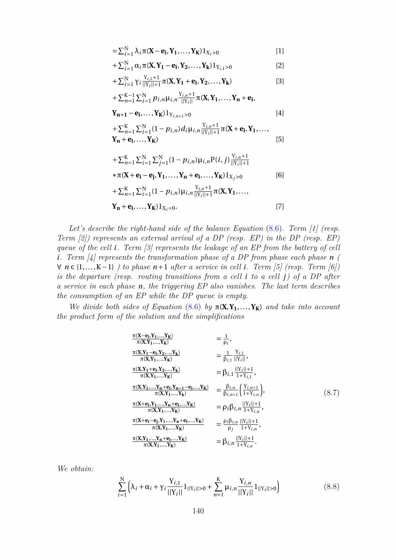
=∑Ni=1λiπ(X−ei,Y1, . . . ,YK)1Xi>0 [1]

+∑Ni=1αiπ(X,Y1 −ei,Y2, . . . ,Yk)1Yi ,1>0 [2]

+∑Ni=1γi

Yi ,1+1||Yi ||+1π(X,Y1 +ei,Y2, . . . ,Yk) [3]

+∑K−1n=1

∑Ni=1 pi ,nµi ,n

Yi ,n+1||Yi || π(X,Y1, . . . ,Yn +ei,

Yn+1 −ei, . . . ,YK)1Yi ,n+1>0 [4]

+∑Kn=1

∑Ni=1(1−pi ,n)diµi ,n

Yi ,n+1||Yi ||+1π(X+ei,Y1, . . . ,

Yn +ei, . . . ,YK) [5]

+∑Kn=1

∑Ni=1

∑Nj=1(1−pi ,n)µi ,nP(i , j )

Yi ,n+1||Yi ||+1

∗π(X+ei −ej,Y1, . . . ,Yn +ei, . . . ,YK)1X j>0 [6]

+∑Kn=1

∑Ni=1(1−pi ,n)µi ,n

Yi ,n+1||Yi ||+1π(X,Y1, . . . ,

Yn +ei, . . . ,YK)1Xi=0. [7]

Let’s describe the right-hand side of the balance Equation (8.6). Term [1] (resp.Term [2]) represents an external arrival of a DP (resp. EP) in the DP (resp. EP)queue of the cell i . Term [3] represents the leakage of an EP from the battery of celli . Term [4] represents the transformation phase of a DP from phase each phase n (∀ n ∈ 1, . . . ,K−1 ) to phase n+1 after a service in cell i . Term [5] (resp. Term [6])is the departure (resp. routing transitions from a cell i to a cell j) of a DP aftera service in each phase n, the triggering EP also vanishes. The last term describesthe consumption of an EP while the DP queue is empty.

We divide both sides of Equation (8.6) by π(X,Y1, . . . ,YK) and take into accountthe product form of the solution and the simplifications

π(X−ei,Y1,...,YK)π(X,Y1,...,YK) = 1

ρi,

π(X,Y1−ei,Y2,...,Yk)π(X,Y1,...,YK) = 1

βi ,1

Yi ,1||Yi || ,

π(X,Y1+ei,Y2,...,Yk)π(X,Y1,...,YK) = βi ,1

||Yi ||+11+Yi ,1

,

π(X,Y1,...,Yn+ei,Yn+1−ei,...,YK)π(X,Y1,...,Yk) = βi ,n

βi ,n+1

(Yi ,n+11+Yi ,n

),

π(X+ei,Y1,...,Yn+ei,...,YK)π(X,Y1,...,YK) = ρiβi ,n

||Yi ||+11+Yi ,n

,

π(X+ei−ej,Y1,...,Yn+ei,...,YK)π(X,Y1,...,YK) = ρiβi ,n

ρ j

||Yi ||+11+Yi ,n

,

π(X,Y1,...,Yn+ei,...,YK)π(X,Y1,...,YK) = βi ,n

||Yi ||+11+Yi ,n

.

(8.7)

We obtain:N∑

i=1

(λi +αi +γi

Yi ,1

||Yi ||1||Yi ||>0 +

K∑n=1

µi ,nYi ,n

||Yi ||1||Yi ||>0

)(8.8)

140

=∑Ni=1

λiρi

1Xi>0 [1]

+∑Ni=1

αiβi ,1

Yi ,1||Yi ||1||Yi ||>0 [2]

+∑Ni=1γiβi ,1 [3]

+∑K−1n=1

∑Ni=1

pi ,nµi ,nβi ,nβi ,n+1

Yi ,n+1||Yi || 1||Yi ||>0 [4]

+∑Kn=1

∑Ni=1(1−pi ,n)diµi ,nρiβi ,n [5]

+∑Kn=1

∑Ni=1

∑Nj=1

(1−pi ,n )µi ,nρiβi ,n P(i , j )ρ j

1X j>0 [6]

+∑Kn=1

∑Ni=1(1−pi ,n)µi ,nβi ,n1Xi=0. [7]

In Term [4] of the r.h.s of Equation (8.8), we apply an index change on n. InTerm [7], we substitute 1Xi = 0 with 1−1Xi>0 and we move the negative terms in thel.h.s. To get: ∑N

i=1

(λi +αi +

(γi

Yi ,1||Yi || +

∑Kn=1µi ,n

Yi ,n||Yi ||

)1||Yi ||>0

+∑Kn=1(1−pi ,n)µi ,nβi ,n1Xi > 0

)= ∑N

i=1λiρi

1Xi>0

+∑Ni=1γiβi ,1 +∑N

i=1αiβi ,1

Yi ,1||Yi ||1||Yi ||>0

+∑Kn=2

∑Ni=1

pi ,n−1µi ,n−1βi ,n−1βi ,n

Yi ,n||Yi ||1||Yi ||>0

+∑Kn=1

∑Ni=1(1−pi ,n)diµi ,nρiβi ,n

+∑Kn=1

∑Ni=1(1−pi ,n)µi ,nβi ,n

+∑Kn=1

∑Ni=1

∑Nj=1

(1−pi ,n )µi ,nρiβi ,n P(i , j )ρ j

1X j>0.

(8.9)

We decompose Equation (8.9) into three equation systems based on the stepfunctions they expose:

∑Ni=1

∑Kn=1(1−pi ,n)µi ,nβi ,n1Xi>0 =∑N

i=1

(λiρi

+∑Kn=1

∑Nj=1(1−pi ,n)µ j ,nP( j , i )

ρ jβ j ,n

ρi

)1Xi>0

(8.10)

and

[∑Ni=1γi

(Yi ,1||Yi ||

)+∑N

i=1µi ,1

(Yi ,1||Yi ||

)+∑K

n=2∑N

i=1µi ,n

(Yi ,n||Yi ||

) ]1||Yi ||>0 =

[∑Ni=1

αiβi ,1

(Yi ,1||Yi ||

)+∑K

n=2∑N

i=1pi ,n−1µi ,n−1βi ,n−1

βi ,n

(Yi ,n||Yi ||

) ]1||Yi ||>0

(8.11)

and [ ∑Ni=1(λi +αi ) =∑K

n=1∑N

i=1(1−pi ,n)diµi ,nρiβi ,n

+∑Kn=1

∑Ni=1(1−pi ,n)µi ,nβi ,n +∑N

i=1γiβi ,1.(8.12)

The values of (ρi ,βi ,1, . . . ,βi ,K) we are looking for have to satisfy the three equations(8.10),(8.11) and (8.12).

141

First by the factorisation of ρi in Equation (8.10) we get, for all i

ρi =λi +∑K

n=1∑N

j=1(1−p j ,n)µ j ,nρ jβ j ,nP( j , i )∑Kn=1(1−pi ,n)µi ,nβi ,n

. (8.13)

Next we decompose Equation (8.11), into two equations. And we verify that twoequations are satisfied. This decomposition:

∑Ni=1(γi +µi ,1)

(Yi ,1||Yi ||

)1||Yi ||>0 =∑N

i=1αiβi ,1

(Yi ,1||Yi ||

)1||Yi ||>0,

and∑Kn=2

∑Ni=1µi ,n

(Yi ,n||Yi ||

)1||Yi ||>0 =∑K

n=2∑N

i=1pi ,n−1µi ,n−1βi ,n−1

βi ,n

(Yi ,n||Yi ||

)1||Yi ||>0.

By the elimination of the multiplicative terms on both sides of the equations. We getin the first equation for all i ∈ 1, . . . ,N

βi ,1 = αi

γi +µi ,1, (8.14)

and in the second equation for all i ∈ 1, . . . ,N and n ∈ 2, . . . ,K

βi ,n = pi ,n−1µi ,n−1βi ,n−1

µi ,n. (8.15)

Finally, we only have to check that the values of (ρi ,βi ,1, . . . ,βi ,K) in Equation(8.13), (8.14) and (8.15) also satisfies Equation (8.12).

For Equation (8.12). We use Lemma 8.2.1 and Equation (8.1) (which states that∀i di = 1−∑N

j=1 P(i , j )). By moving negative terms to the l.h.s, Equation (8.12) isreduced to 0 = 0. Therefore, all equations that constitute the global balance equationat steady-state are satisfied and the proof of the theorem is complete.

Lemma 8.2.2 The normalization constant is equal to

G =N∏

i=1Gi . (8.16)

WhereGi = (1−ρi )(1−

K∑n=1

βi ,n). (8.17)

Proof. We compute the value of G using that ∑X,Y1,...,YK π(X,Y1, . . . ,YK) = 1 and

Equation (8.5), we get that

∑X,Y1,...,YK

GN∏

i=1(ρi )Xi ||Yi ||!

K∏n=1

(βi ,n)Yi ,n

Yi ,n != 1

⇒ GN∏

i=1

∑Xi ,Yi ,1,...,Yi ,K

(ρi )Xi ||Yi ||!K∏

n=1

(βi ,n)Yi ,n

Yi ,n != 1

⇒ GN∏

i=1

∑Xi

(ρi )Xi∑

Yi ,1,...,Yi ,K

||Yi ||!K∏

n=1

(βi ,n)Yi ,n

Yi ,n != 1.

142

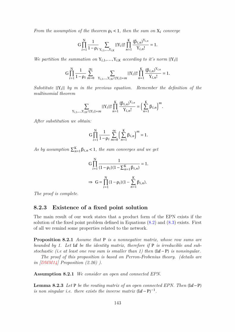
From the assumption of the theorem ρi < 1, then the sum on Xi converge

GN∏

i=1

1

1−ρi

∑Yi ,1,...,Yi ,K

||Yi ||!K∏

n=1

(βi ,n)Yi ,n

Yi ,n != 1.

We partition the summation on Yi ,1, . . . ,Yi ,K according to it’s norm ||Yi ||

GN∏

i=1

1

1−ρi

∞∑m=0

∑Yi ,1,...,Yi ,K/||Yi ||=m

||Yi ||!K∏

n=1

(βi ,n)Yi ,n

Yi ,n != 1.

Substitute ||Yi || by m in the previous equation. Remember the definition of themultinomial theorem

∑Yi ,1,...,Yi ,K/||Yi ||=m

||Yi ||!K∏

n=1

(βi ,n)Yi ,n

Yi ,n !=

( K∑n=1

βi ,n

)m.

After substitution we obtain:

GN∏

i=1

1

1−ρi

∞∑m=0

( K∑n=1

βi ,n

)m = 1.

As by assumption ∑Kn=1βi ,n < 1, the sum converges and we get

GN∏

i=1

1

(1−ρi )(1−∑Kn=1βi ,n)

= 1.

⇒ G =N∏

i=1(1−ρi )(1−

K∑n=1

βi ,n).

The proof is complete.

8.2.3 Existence of a fixed point solutionThe main result of our work states that a product form of the EPN exists if thesolution of the fixed point problem defined in Equations (8.2) and (8.3) exists. Firstof all we remind some properties related to the network.

Proposition 8.2.1 Assume that P is a nonnegative matrix, whose row sums arebounded by 1. Let Id be the identity matrix, therefore if P is irreducible and sub-stochastic (i.e at least one row sum is smaller than 1) then (Id −P) is nonsingular.

The proof of this proposition is based on Perron-Frobenius theory. (details arein [DMM14] Proposition (2.26) ).

Assumption 8.2.1 We consider an open and connected EPN.

Lemma 8.2.3 Let P be the routing matrix of an open connected EPN. Then (Id−P)is non singular i.e. there exists the inverse matrix (Id −P)−1.

143

Proof. An open and connected EPN ensures that (a) it exists at least one celli in the network such that di > 0 (a data packet in cell i leaves the system withprobability di ). Therefore, for at least one cell i we have ∑N

j=1 P(i , j ) < 1. Thatproves that P is substochastic. (b) The EPN is connected as defined in Definition7.2.3 then P is irreducible. From Statements (a) and (b) we have that routing matrixP is substochastic and irreducible, we conclude (using Proposition 8.2.1) that (Id−P)is nonsingular.

Lemma 8.2.4 For all i and j in 1, . . . ,N and n in 1, . . . ,K, we have βi ,n definedin Equation (8.2) and θ j exists i.e. βi ,n > 0 and θ j > 0. Note that

θ j =K∑

n=1(1−p j ,n)µ j ,nβ j ,n . (8.18)

Proof. By definition, we have for all i ∈ 1, . . . ,N and n ∈ 1, . . . ,K, µi ,n > 0, αi > 0and γi > 0, then βi ,n expressed in Equation (8.2) exists and βi ,n > 0.θ j > 0 since (i) µ j ,n > 0 , (ii) β j ,n > 0 and (iii) we know that at least the last term(1−p j ,K)µ j ,Kβ j ,K > 0 as p j ,K = 0.

Lemma 8.2.5 Equation (8.3) that represents flow equations of data packets in eachcell i , has a fixed point ρi .

Proof. By substitution using Equation (8.18), then Equation (8.3) becomes ∀ i ∈1, . . . ,N

ρi =λi +∑N

j=1θ jρ j P( j , i )

θi, (8.19)

⇒ ρiθi −N∑

j=1θ jρ j P( j , i ) = λi . (8.20)

Which represents the flow equations in Jackson networks [CY01].Let ρθ = (ρ1θ1, . . . ,ρNθN), λ = (λ1, . . . ,λN) and Id the identity matrix, then Equation(8.20) for vectors

ρθ (Id −P) = λ. (8.21)Using Lemma 8.2.3, (Id - P) admits an inverse

⇒ ρθ = λ(Id −P)−1.

This proves the existence of the vector ρθ therefore ρi exists since θi exists as statedin Lemma 8.2.4. The proof is complete.

8.3 Performance and Energy evaluationIn this section, we compute both energy and performance measures. Since oursystem has a product form solution, the measures can be computed as expectationsof rewards separately on each cell. Note that Equation (8.5) can be expressed as

π(X,Y1, . . . ,YK) =N∏

i=1π(Xi ,Yi ,1, . . . ,Yi ,K), (8.22)

144

andπ(Xi ,Yi ,1, . . . ,Yi ,K) =π(Xi )π(Yi ,1, . . . ,Yi ,K)

where, by the substitution of Gi

π(Xi ) = (1−ρi )(ρi )Xi , π(0) = (1−ρi ) (8.23)

andπ(Yi ,1, . . . ,Yi ,K) = (1−

K∑n=1

βi ,n)||Yi ||!K∏

n=1

(βi ,n)Yi ,n

Yi ,n !. (8.24)

8.3.1 Loss rate of energy packetsFor each cell in the EPN, energy packets are lost either when there is no data packetsin the DP queue, or due to battery leaks which occur in phase 1 of the Cox process.

Lemma 8.3.1 Let LossT be the total loss rate of EPs in the network, then:

LossT =N∑

i=1

∑||Yi ||>0

π(Yi ,1, . . . ,Yi ,K)[π(0)r1(Yi ,1, . . . ,Yi ,K)

+∑Xi

π(Xi )r2(Yi ,1, . . . ,Yi ,K)]

. (8.25)

Where r1(Yi ,1, . . . ,Yi ,K) (resp. r2(Yi ,1, . . . ,Yi ,K) ) is described in Equation (8.29) (resp.Equation (8.32)).

Proof. Let Loss(i ) be the loss rate of EPs in cell i . As the EPN network has aproduct-form solution, then :

LossT =N∑

i=1Loss(i ). (8.26)

Let Loss(i )1 (resp. Loss(i )

2 ) be the loss rate of EPs due to emptiness of DP queue(resp. battery leakage) in cell i , then:

Loss(i ) = Loss(i )1 +Loss(i )

2 . (8.27)

States that correspond to Loss(i )1 , in Equation (8.28), are those where, Xi =0 and

at least one EP in the battery is ready to trigger a DP. This explains the sum on||Yi || >0. Also, for each state, we multiply by the appropriate reward r1(Yi ,1, . . . ,Yi ,K).The reward in this case, Equation (8.29), represents the rate at which a DP istriggered in each phase of the Cox process. So

Loss(i )1 = ∑

Yi ,1,...,Yi ,K/||Yi ||>0π(0,Yi ,1, . . . ,Yi ,K)r1(Yi ,1, . . . ,Yi ,K), (8.28)

wherer1(Yi ,1, . . . ,Yi ,K) =

K∑n=1

Yi ,n

||Yi ||(1−pi ,n)µi ,n . (8.29)

145

Using the separation simplifications in Equation (8.22), (8.23) and (8.24), Loss(i )1

can be expressed as

Loss(i )1 =π(0)

∑||Yi ||>0

π(Yi ,1, . . . ,Yi ,K)r1(Yi ,1, . . . ,Yi ,K). (8.30)

For Loss(2)i , we use the same approach as for Loss(1)

i . This means that we multiplythe steady state probability of the appropriate states by the corresponding rewardsr2(Yi ,1, . . . ,Yi ,K). In this case, we are interested in the rate of EP loss due to batteryleakage that occurs in the first phase of the Cox process with the rate Yi ,1

||Yi ||γi . Notethat we can use either the summation with ||Yi || >0 or Yi ,1 >0, the final result ofLoss(i )

2 remains the same. We use ||Yi || > 0 for simplification purposes. So

Loss(i )2 = ∑

Xi ,Yi ,1,...,Yi ,K/||Yi ||>0π(Xi ,Yi ,1, . . . ,Yi ,K)r2(Yi ,1, . . . ,Yi ,K), (8.31)

wherer2(Yi ,1, . . . ,Yi ,K) = Yi ,1

||Yi ||γi . (8.32)

Also, using the separation simplifications in Equation (8.22), (8.23) and (8.24) then

Loss(i )2 =∑

Xi

π(Xi )∑

||Yi ||>0π(Yi ,1, . . . ,Yi ,K)r2(Yi ,1, . . . ,Yi ,K), (8.33)

Finally, by the substitution of Loss(i )1 and Loss(i )

2 in Equation (8.27). And usingEquation (8.26), we obtain Equation (8.25) and the proof is complete.

8.3.2 Waiting time and total number of data packetsLemma 8.3.2 Let E[X] be the total number of data packets in the system, then

E[X] =N∑

i=1

[ λi +∑Nj=1θ jρ j P( j , i )

θi − (λi +∑Nj=1θ jρ j P( j , i ))

]. (8.34)

See Equation (8.18) for the value of θi .

Proof. We first calculate E[Xi ] the mean number of data packets in cell i . As theEPN network has a product form solution, then

E[X] =N∑

i=1E[Xi ]. (8.35)

From Equation (8.23) we can deduce that

E[Xi ] = ρi

1−ρi. (8.36)

Then by substitution of ρi (see Equation (8.3)) and using Equation (8.18), we get

E[Xi ] =λi +∑N

j=1θ jρ j P( j , i )

θi − (λi +∑Nj=1θ jρ j P( j , i ))

. (8.37)

146

Note that E[Xi ] > 0 since from stability conditions (see Theorem 8.2.1), we have forall i , ρi < 1 then θi > λi +∑N

j=1θ jρ j P( j , i ). Finally, using Equation (8.35) we obtainEquation (8.34) and the proof is complete.

Lemma 8.3.3 Let E[Ti ] be the mean waiting time of a data packet in cell i , then

E[Ti ] = 1

θi − (λi +∑Nj=1θ jρ j P( j , i ))

. (8.38)

Proof. Let Λi be the overall arrival rate to DP queue of cell i , including bothexternal arrivals and internal transitions

Λi = λi +K∑

n=1

N∑j=1

(1−p j ,n)µ j ,nρ jβ j ,nP( j , i ). (8.39)

Then from Little’s law for data packets in the cell i

E[Ti ] = E[Xi ]

Λi. (8.40)

By substitution, using Equation (8.36)

E[Ti ] = ρi

Λi (1−ρi ). (8.41)

Also using Equation (8.3) to substitute ρi , Equation (8.39) to substitute Λi andEquation (8.18), we obtain after simplifications

E[Ti ] = 1

θi − (λi +∑Nj=1θ jρ j P( j , i ))

.

As for E[Xi ] we have E[Ti ] > 0 since the denominator is a strictly positive value, andthe proof is complete.

Lemma 8.3.4 Let E[T] be the mean waiting time of a data packet in the EPNnetwork, then

E[T] =N∑

i=1

[ λi +∑Nj=1θ jρ j P( j , i )

θi − (λi +∑Nj=1θ jρ j P( j , i ))

][ N∑i=1

λi

]−1. (8.42)

Proof. Let χ = ∑Ni=1λi be the total arrival rate of data packets incoming from

outside the network. Then from Little’s law

E[T] = E[X]

χ.

Therefore using Lemma 8.3.2, we obtain Equation (8.42).

147

8.4 Solar panel assignmentWe are now studying an EPN sensor network that collects information in a backbonenetwork. Each sensor gets energy packets from photo-voltaic solar panels, energyflow is stored in sensor’s battery. The aim is to obtain an optimal distribution of ∆solar panels over the N sensors (∆ and N being a non-zero positive integers). Moreprecisely, we are looking for an assignment of the solar panels that minimizes theaverage end to end delay of data packets in the network. Also we considered thefollowing constraints: (a) A solar panel could be assigned to only one sensor, buta sensor receives energy from at least one panel. We consider identical panels (i.ethe panels generates the same rate of energy) (b) Stability constraints as describedin Theorem 8.2.1. The EPs stability condition provides an upper bound on thenumber of panels to use, while DPs’ condition of stability gives a lower bound ofthe quantity of panels.

Lemma 8.4.1 Let Φi be the number of solar panels affected to a cell i . Then, underEPs stability conditions of the EPN, for all i ∈ 1, . . . ,N

Φi <γi +µi ,1

α

(1+

K∑n=2

µi ,1

µi ,n

n−1∏r=1

pi ,r

)−1, (8.43)

where α> 0 is the rate of energy packets generated by a solar panel (which is supposedto be the same since the panels are identical).

Proof. In this lemma we are interested in the stability condition of EPs (i.e. forall i ∈ 1, . . . ,N, ∑K

n=1βi ,n < 1).

K∑n=1

βi ,n < 1 ⇒ βi ,1 +K∑

n=2βi ,n < 1.

By substitution using Equation (8.2)

⇒ αi

γi +µi ,1

(1+

K∑n=2

µi ,1

µi ,n

n−1∏r=1

pi ,r

)< 1. (8.44)

The rate of energy packets coming into a cell’s battery αi is a function of the numberof solar panels assigned to the cell. Then

αi =Φiα. (8.45)

By the substitution of αi in Equation (8.44), we obtain Equation (8.43). The proofis complete.

8.4.1 Case of a tree EPN topologyLet us now simplify the DPs flow equations due to the tree topology (see Fig. 8.3and Fig. 8.6).

148

Lemma 8.4.2 Let i be an arbitrary node of the tree, A(i ) will denote the set ofnodes in the sub-tree rooted at i (including i). Then, the flow equations of DPqueues (Equation (8.3)) can be simplified as

ρi =∑

j∈A(i )λ j∑Kn=1(1−pi ,n)µi ,nβi ,n

. (8.46)

Proof. by induction on the node number. We assume that the nodes are numberedaccording to a topological ordering of the tree.

• i = 1: node 1 is a leaf because it has no predecessor. Therefore A(1) = 1. Thus

ρ1 = λ1∑Kn=1(1−p1,n)µ1,nβ1,n

,

and it is also equal to∑

j∈A(1)λ j∑Kn=1(1−p1,n )µ1,nβ1,n

. Thus the property is established fori = 1.

• arbitrary i . Let us now assume that the property is established for all j < i .Thus we have:

ρ j

K∑n=1

(1−p j ,n)µ j ,nβ j ,n = ∑k∈A( j )

λk .

Let Γ−(i ) be the set of predecessor of i . Remember that routing matrix Pencodes the tree topology. Therefore P( j , i ) = 1 if j is a predecessor of i (i.e.in Γ−(i )) and 0 otherwise. Consider the numerator of the flow equation forDP in station i :

λi +∑

j ∈Γ−(i )

K∑n=1

(1−p j ,n)µ j ,nβ j ,n .

Applying the induction, the numerator becomes:

λi +∑

j ∈Γ−(i )

∑k∈A( j )

λk .

Due to the recursive construction of any tree, we get:

λi +∑

j ∈Γ−(i )

∑k∈A( j )

λk = ∑j∈A(i )

λ j .

And the proof is complete.

Lemma 8.4.3 The DPs stability condition is ρi < 1 for all i . Then, in a tree EPN,We have for all i ∈ 1, . . . ,N

Φi >(γi +µi ,1)

αµi ,1

∑j∈A(i )

λ j . (8.47)

149

Proof. From Lemma 8.2.1 we have for all i ∈ 1, . . . ,N, ∑Kn=1(1− pi ,n)µi ,nβi ,n =

αi −γiβi ,1 and by the substitution of βi ,1 and αi (Equation (8.45)) we obtain

K∑n=1

(1−pi ,n)µi ,nβi ,n = αΦiµi ,1

γi +µi ,1. (8.48)

Using Equation (8.48) in Equation (8.46), we get

ρi =γi +µi ,1

αΦiµi ,1

∑j∈A(i )

λ j . (8.49)

DPs stability conditions are ∀ i ∈ 1, . . . ,N, ρi < 1. Hence, by combining Equation(8.49) and that ρi < 1 we obtain Equation (8.47), and the proof is complete.

8.4.1.1 Optimization problem

Let us now study the domain of definition. The set of possible values for (Φ1, . . . ,ΦN)comes from all the constraints we got (particularly Lemma 8.4.1, Lemma 8.4.3) :∀i ∈ 1, . . . ,N Φi < γi+µi ,1

α

(1+∑K

n=2µi ,1µi ,n

∏n−1r=1 pi ,r

)−1,

Φi > (γi+µi ,1)αµi ,1

∑j∈A(i )λ j > 0,∑N

i=1Φi =∆.

Using ρi in Equation (8.49), and the expression of the total mean waiting timeE[X] = ∑N

i=1ρi

1−ρi. Then, according to Little’s law, we derive the mean response

time function, which is equal to E[X]∑Ni=1λi

, by substitution we obtain the function tominimize:

f (Φ1, . . . ,ΦN) =N∑

i=1

(γi +µi ,1)∑

j∈A(i )λ j

αΦiµi ,1 − (γi +µi ,1)∑

j∈A(i )λ j

( N∑i=1

λi

)−1. (8.50)

Function in Equation (8.50) can be expressed as f (Φ1, . . . ,ΦN) = ∑Ni=1 f (Φi ). As f

is decreasing in each Φi , then to minimize Equation (8.50) we should increase Φi .Therefore, the optimal solution is the upper bound (excluded) for each cell i if ∆ is atleast equal to sum of upper bounds (excluded). Otherwise, we suggest an heuristic(Algorithm 8) and a Gradient descent algorithm (Algorithm 9).

Note that the aim is to propose a distribution of ∆ panels over the N cells. Theheuristic algorithm consists of 3 steps. In step 1) we calculate the bounds of thesolution domain for each cell. In Step 2) we verify that the domain has at least onesolution and that ∆ is at least equal to the sum of the lower bound of cells. Alsoif ∆ is equal to or greater than the sum of the upper bound of the cells, then thesolution is the upper bound of the panels in each cell. In step 3) we know that thesolution is between the lower (included) and the upper (excluded) bounds. So westart with a first solution which corresponds to the lower bound of panels in eachcell (Lemma 8.4.3), then at each iteration we add a panel in the most loaded cellthat has not reached its upper bound. The algorithm stops when we have reached∆ panels in the network. Note that the algorithm may stop in step 2) due to invalidparameters or an empty set for the solution.

150

In Algorithm 8, we decide to assign the new panel to the most loaded cell,while in Algorithm 9 (Gradient descent) the new panel is assigned to the cell thatwill minimize the most Equation (8.50). Therefore, the main difference betweenthe heuristic and the Gradient descent is the decision made in step 3.2). Gradientdescent algorithm performs the optimal local decision at each step. We have verifiednumerically that it achieves the optimal global distribution of panels. But we donot have a theoretical proof of this optimality.

Algorithm 8: Heuristic: Panels assignment algorithmInput : ∆ the number of panels.Output: An assignment of the ∆ panels.Step 1) Calculation of lower and upper bound of Φi for each cell i .(Lemma 8.4.1 and 8.4.3).

Step 2) Verification of bounds:Step 2.1) If there is a cell whose upper bound of the number of panels islower than the lower bound, then print ”No solution for such parameters”,the algorithm stops. Otherwise go to Step 2.2).Step 2.2) If ∆ is strictly lower than the sum of all lower bounds, thenprint ”∆ is too low”, the algorithm stops. Otherwise go to Step 2.3).Step 2.3) If ∆ is equal or greater than the sum of all upper bounds, thenthe solution is the upper bound (Lemma 8.4.1) of each cell, the algorithmstops. Otherwise, go to step 3).

Step 3) Constructing progressively the solution:Step 3.1) We construct a first solution, which corresponds to the lowerbound of each cell.Step 3.2) We add a panel in the most loaded cell that can receive a panel.Step 3.3) If we achieved ∆ panels in the network, then the algorithmstops. Otherwise go to Step 3.2).

Step 4) Return the solution and the corresponding delay.

151

Algorithm 9: Gradient descent: Panels assignment algorithmInput : ∆ the number of panels.Output: An optimal assignment of the ∆ panels.Step 1) and Step 2) are the same as in Algorithm 8.

Step 3) Constructing progressively the solution:Step 3.1) We construct a first solution, which corresponds to the lowerbound of each cell.Step 3.2) We add a panel in a cell that can receive a panel and thatminimizes the objective function (Equation (8.50)) the most.Step 3.3) If we achieved ∆ panels in the network, than the algorithmstops. Otherwise go to Step 3.2).

Step 4) Return the solution and the corresponding delay.

152

8.4.1.2 A collecting sensor network of N = 7 cells

We consider a tree EPN topology with N = 7 cells (Fig. 8.3) and K = 4 phases.Cells 1,2,3 and 4 are leaf cells, 5 and 6 are inter-cellular cells and the root cell is7. All cells point towards the root. Service time is an Erlang process (i.e. ∀i ∈1, . . . ,N µi ,n =µi and ∀n ∈ 1, . . . ,K−1 pi ,n = 1 and pi ,K = 0). We suppose that onlyleaf cells receives DPs from outside the network, arrivals rate of DPs in each cell,are respectively, 1,2,3,4,0,0,0. Also, the service rate and leakage rate of EPs ineach cell is ∀ i ,µi = 50 and γi = 5. EPs rate generated by a single solar panel is α= 2and the number of panels is ∆ = 41. We made sure to consider valid parameters(21 ≤∆≤ 41) in order to perform step 3) which is the main part of both algorithms.All parameters and rewards are expressed for a unit of time.

1 432

7

65

Out

λ1 = 1 λ2 = 2 λ3 = 3 λ4 = 4

Figure 8.3: A tree EPN topology of N = 7 cells.

Fig. 8.4 illustrates the evolution of the mean waiting time of a DP in the networkwhile increasing the number of panels ∆. The mean waiting time was calculatedusing the solution proposed by the two algorithms. We first observe that the meanwaiting time decreases with the increase in the number of panels in the network (asthe number of panels is at the denominator of the function to minimize i.e. Equation(8.50) ). We also notice that the solutions proposed by the two methods are quasisimilar. In particular, for this example we have 22 experiments (from ∆ = 20 to∆ = 41) of which 16 experiments generate the same solution (solutions details arein Table 8.1). In the 6 other experiments (∆ = 29,31,32,35,36,39) the delay ofthe heuristic is around 10−3 and 10−4 above the Gradient descent. In Table 8.1we present the solutions proposed by both algorithms for some values of ∆. In thistable, an entry ’x1&x2’ means that the heuristic answers x1 panels while Gradientdescent proposes x2 while a single number (say ’x’) means that both algorithmsassign the same number of panels x to the corresponding cell.

Fig. 8.5 illustrates the loss rate of EPs (see Equation (8.25)) generated by bothalgorithms. We notice that the loss rate increases in most cases by increasing thenumber of panels in the network. Also, we observe that the heuristic gives betterresults for the energy loss, as the Gradient algorithm only cares about the waitingtime. Therefore, the best configuration of the panels for the waiting time is obviouslynot the same for energy losses.

153

It is worthy to note that both methods are very fast. We have also verifiednumerically that the gradient descent algorithm generates the optimal solution, i.e.by comparing its solution to an exhaustive algorithm. Since the exhaustive methodis exponential in execution time, then we can perform this exhaustive analysis upto ∆= 50 panels.

Figure 8.4: Mean waiting time of a DP in a tree EPN of N = 7 cells: Heuristic solution VsGradient descent solution .

Figure 8.5: Loss rate of EPs in a tree EPN of N = 7 cells: Heuristic solution Vs Gradientdescent solution .

154

∆ Φ1 Φ2 Φ3 Φ4 Φ5 Φ6 Φ7

20 1 2 2 3 2 4 621 1 2 2 3 2 5 622 1 2 3 3 2 5 623 1 2 3 3 3 5 624 1 2 3 3 3 6 625 1 2 3 4 3 6 626 2 2 3 4 3 6 627 2 3 3 4 3 6 628 2 3 4 4 3 6 629 2 3 4 5 & 4 3 & 4 6 630 2 3 4 5 4 6 631 2 3 4 6 & 5 4 & 5 6 632 2 3 5 6 & 5 4 & 5 6 633 2 3 5 6 5 6 634 2 4 5 6 5 6 635 2 & 3 4 6 & 5 6 5 6 636 2 & 3 4 6 6 6 & 5 6 637 3 4 6 6 6 6 638 3 5 6 6 6 6 639 3 & 4 6 & 5 6 6 6 6 640 4 6 6 6 6 6 641 5 6 6 6 6 6 6

Table 8.1: Distribution of ∆ panels using Heuristic and Gradient descent algorithm, N = 7cells.

8.4.1.3 A collecting sensor network of N = 20 cells

In this example (Fig. 8.6), we consider a wider tree EPN network (N = 20 cells),where the graph’s structure is less regular. The service is still an Erlang process withK = 4 phases. We suppose that not only leaf cells receives data packets from outsidethe network. Cells that receive data packets are 1,2,3,4,5,6,7,8,9,10,18. Arrival rateof DPs, respectively in each cell, are 1, 1, 1, 1, 2, 2, 3, 3, 3, 1, 0, 0, 0, 0, 0, 0, 0,1, 0, 0. We suppose that service rate is ∀ i ,µi = 85, also leakage rate of EPs is∀ i ,γi = 5. EPs rate generated by a single solar panel is α = 2. Notice that usingthese parameters the total number of panels to use in this topology should be in51,220. That means when ∆ ≤ 50 then the number of panels to distribute is notenough therefore both algorithms will stop in Step 2.2). And when ∆≥ 220 thereforethe best solution correspond to the upper bound of Φi in each cell, as stated in Step2.3) in both algorithms. Hence, for this example we consider ∆= 90 panels.

As in the model with N = 7 cells, we observe in Fig. 8.7 that the mean waitingtime of a DP decreases when increasing the number of panels in the system. AsDPs are triggered using energy parquets, otherwise they wait. Therefore, it is evi-dent that the mean waiting time of a DP decreases when increasing the sources of

155

incoming energy in the network. Also, we observe that Gradient descent algorithmperforms better than the heuristic algorithm. Nevertheless, heuristic gives almostthe same results as the gradient, which is the optimal solution (verified numericallyby comparing it to an exhaustive algorithm).

Fig. 8.8 illustrates the total loss rate of EPs in the network. To note that lossesof EPs are due to battery leakages and emptiness of DP queue. Hence, the morepanels we add, the less DPs are waiting in the queues, then, the more the queuesare empty. Also the mean leakage rates in the system will increase while increasingthe number of panels. That explains the increasing histograms in Fig. 8.8. Wealso observe that the Gradient descent is worse than heuristic algorithm, when itconcerns total loss rate of EPs, that result is only an observation, as both algorithmsaims to optimize the waiting time of a DP. Hence, we can deduce that optimizingthe waiting time, will unfortunately, not optimize the total loss rate of EPs. InTable 8.2 we show the distribution of ∆= 51,60,70,80,90 panels over the network,using both algorithms.

20

17 1918

10 5 12 13 1416

6 7 8 915 41

2 11

3

λ1 = 1

λ3 = 1

λ2 = 1

λ4 = 1 λ6 = 2 λ7 = 3 λ8 = 3

λ5 = 2

λ9 = 3

λ10 = 1

λ18 = 1

Out

Figure 8.6: A tree EPN topology of N = 20 cells.

156

Figure 8.7: Mean waiting time of a DP in a tree EPN of N = 20 cells: Heuristic solutionVs Gradient descent solution .

Figure 8.8: Loss rate of EPs in a tree EPN of N = 20 cells: Heuristic solution Vs Gradientdescent solution .

157

∆ 51 60 70 80 90

Φ1 1 1 2 2 2Φ2 1 1 2 2 2Φ3 1 1 2 2 2Φ4 1 1 2 2 2Φ5 2 2 2 3 3Φ6 2 2 2 3 3Φ7 2 3 3 4 5Φ8 2 3 3 4 4 & 5Φ9 2 3 3 4 4 & 5Φ10 2 2 2 3 3Φ11 1 1 1 & 2 2 2Φ12 2 2 2 3 3Φ13 2 3 3 4 4 & 5Φ14 4 5 6 7 & 6 8 & 7Φ15 2 2 2 2 & 3 3Φ16 2 3 3 3 & 4 4 & 5Φ17 3 4 5 5 7 & 6Φ18 3 4 5 5 7 & 6Φ19 5 6 9 & 8 9 & 8 11 & 10Φ20 11 11 11 11 11

Table 8.2: Distribution of ∆ panels using Heuristic and Gradient descent algorithm, N = 20cells.

158

8.4.2 A star EPN topologyLow Power Wide Area Network (LPWAN) technologies are characterized by longrange links (several kilometers) and have star network topologies [Van+15]. Thesesystems do not focus on enabling high data rates per device or on minimizing latency.Rather, the key metrics concerned are energy efficiency, scalability and wide-areacoverage, which comes with minimum power consumption and maintenance costs[Son+17]. In LPWAN family, the most widely used technology is Long Rang (LoRa).This in mainly due to the utilization of unlicensed bands. As a result, the LoRanetworks is easy to deploy over a range of several kilometers [Son+17]. The LoRasystem’s architecture consists of three main components [Van+15]:

• End-Devices: sensors/actuators are devices that are connected via LoRa radiointerface to one or more Lora Gateways;

• Gateways: are concentrators that connect end-devices to the LoRa NetServer;

• NetServer: The network server is the central element of the network’s archi-tecture. The NetServer controls the whole network (resource management,admission control, security, etc).

LoRa is a low energy network with a battery which may be used several years.Adding an energy harvesting possibility will increase her availability. This harvestingis modelled by an EPN. In the following, we use an EPN network to model a LoRasensor network with solar panels in order to study both energy losses of EPs and thewaiting time of a DP. As depicted in Fig. 8.9, we considered a star EPN network ofN = 10 cells. Cells 1,2, . . . ,N−1 are end-devices, while cell N is the LoRa gateway,also the LoRa NetServer is represented by the ”Out” cell. The main difference withthe first model is the topology. Here we assume that the topology is a star withsymmetric directed edges as the communication between the nodes and the gatewaytakes place in both directions (see Fig. 8.9).

8.4.2.1 Optimization problem

Before presenting the optimization problem, we first have to adapt Lemma 8.4.2 andLemma 8.4.3 that do not hold for the star topology:

Lemma 8.4.4 Let i be an arbitrary node in a star EPN network. Then, the flowequations of DP queues (Equation (8.3)) can be simplified as, ∀ i ∈ 1, . . . ,N

ρi =C(i )

∑Nj=1λ j

θi (1−∑Nj=1 P(N, j ))

+ λi

θi1i<N (8.51)

whereC(i ) =

[P(N, i ) i f i ∈ 1, . . . ,N−11 i f i = N.

(8.52)

Proof. Note that we are considering a star topology with 1,2, . . . ,N cells. Themiddle cell is cell N, which transmit data to the NetServer (i.e. dN > 0). Then

159

we have ∀i ∈ 1, . . . ,N−1,P(i ,N) = 1 and ∑Ni=1 P(N, i ) < 1 as dN > 0. By using these

typology’s features in the flow Equation (8.3), we obtain:

∀ i ∈ 1, . . . ,N−1, ρi = λi +ρNθNP(N, i )

θi(8.53)

and

ρN =λN +∑K

n=1∑N

j=1(1−p j ,n)µ j ,nρ jβ j ,nP( j ,N)

θN. (8.54)

By substitution, using Equation (8.53), Equation (8.54) becomes:

ρNθN

(1−

N∑j=1

P(N, j ))=

N∑j=1

λi

⇒ ρN =∑N

j=1λi

θN(1−∑Nj=1 P(N, j ))

. (8.55)

Finally by substitution of Equation (8.55), Equation (8.53) becomes

∀ i ∈ 1, . . . ,N−1, ρi =P(N, i )

∑Nj=1λ j

θi (1−∑Nj=1 P(N, j ))

+ λi

θi(8.56)

We have defined C(i) in Equation (8.52) in order to express Equation (8.55) and(8.56) in a single equation for all i ∈ 1, . . . ,N, which is Equation (8.51). The proofis complete.

Lemma 8.4.5 The DPs stability condition is ρi < 1 for all i . Then, in a star EPN,we have for all i ∈ 1, . . . ,N

Φi >(γi +µi ,1)

αµi ,1

[ C(i )∑N

j=1λ j

1−∑Nj=1 P(N, j )

+λi 1i<N

]. (8.57)

Proof. Recall that ∀ i ∈ 1, . . . ,N, θi = ∑Kn=1(1− pi ,n)µi ,nβi ,n (see Lemma 8.2.4).

Also from Lemma 8.2.1 we have for all i ∈ 1, . . . ,N, ∑Kn=1(1−pi ,n)µi ,nβi ,n = αi−γiβi ,1.

Therefore θi = αi −γiβi ,1. By the substitution of βi ,1 and αi (Equation (8.45)), weobtain

θi =αΦiµi ,1

γi +µi ,1. (8.58)

Using Equation (8.58) in Equation (8.51), we get

ρi =γi +µi ,1

αΦiµi ,1

[ C(i )∑N

j=1λ j

1−∑Nj=1 P(N, j )

+λi 1i<N

]. (8.59)

DPs stability conditions are ∀ i ∈ 1, . . . ,N, ρi < 1. Hence, by combining Equation(8.59) and that ρi < 1, we obtain Equation (8.57), and the proof is complete.

160

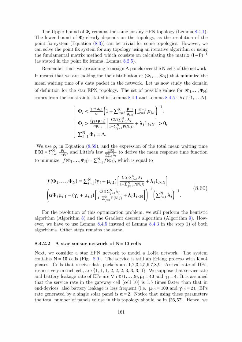
The Upper bound of Φi remains the same for any EPN topology (Lemma 8.4.1).The lower bound of Φi clearly depends on the topology, as the resolution of thepoint fix system (Equation (8.3)) can be trivial for some topologies. However, wecan solve the point fix system for any topology using an iterative algorithm or usingthe fundamental matrix method which consists on calculating the matrix (I−P)−1

(as stated in the point fix lemma, Lemma 8.2.5).Remember that, we are aiming to assign ∆ panels over the N cells of the network.

It means that we are looking for the distribution of (Φ1, . . . ,ΦN) that minimize themean waiting time of a data packet in the network. Let us now study the domainof definition for the star EPN topology. The set of possible values for (Φ1, . . . ,ΦN)

comes from the constraints stated in Lemma 8.4.1 and Lemma 8.4.5 : ∀i ∈ 1, . . . ,NΦi < γi+µi ,1

α

(1+∑K

n=2µi ,1

µi ,n

∏n−1r=1 pi ,r

)−1,

Φi > (γi+µi ,1)αµi ,1

[ C(i )∑N

j=1λ j

1−∑Nj=1 P(N, j )

+λi 1i<N

]> 0,∑N

i=1Φi =∆.

We use ρi in Equation (8.59), and the expression of the total mean waiting timeE[X] = ∑N

i=1ρi

1−ρi, and Little’s law E[X]∑N

i=1λito derive the mean response time function

to minimize: f (Φ1, . . . ,ΦN) =∑Ni=1 f (ϕi ), which is equal to

f (Φ1, . . . ,ΦN) =∑Ni=1(γi +µi ,1)

[ C(i )∑N

j=1λ j

1−∑Nj=1 P(N, j )

+λi 1i<N

](αΦiµi ,1 − (γi +µi ,1)

[ C(i )∑N

j=1λ j

1−∑Nj=1 P(N, j )

+λi 1i<N

])−1(∑Ni=1λi

)−1.

(8.60)

For the resolution of this optimization problem, we still perform the heuristicalgorithm (Algorithm 8) and the Gradient descent algorithm (Algorithm 9). How-ever, we have to use Lemma 8.4.5 instead of Lemma 8.4.3 in the step 1) of bothalgorithms. Other steps remains the same.

8.4.2.2 A star sensor network of N = 10 cells

Next, we consider a star EPN network to model a LoRa network. The systemcontains N = 10 cells (Fig. 8.9). The service is still an Erlang process with K = 4phases. Cells that receive data packets are 1,2,3,4,5,6,7,8,9. Arrival rate of DPs,respectively in each cell, are 1, 1, 1, 2, 2, 2, 3, 3, 3, 0. We suppose that service rateand battery leakage rate of EPs are ∀ i ∈ 1, . . . ,9,µi = 40 and γi = 4. It is assumedthat the service rate in the gateway cell (cell 10) is 1.5 times faster than that inend-devices, also battery leakage is less frequent (i.e. µ10 = 100 and γ10 = 2). EPsrate generated by a single solar panel is α= 2. Notice that using these parametersthe total number of panels to use in this topology should be in 26,57. Hence, we

161

suppose that ∆ = 40 panels. The non-zero transition probabilities in the routingmatrix P are ∀i ∈ 1, . . . ,9 P(i ,N) = 1 and P(N, i ) = 0.01.

The trend in the results for the mean waiting time of a DP (Fig. 8.10) and thetotal loss rate of EPs (Fig. 8.11) remains the same as in the previous examples. Thismeans that the mean waiting time decreases and the total loss rate of EPs increases,while increasing the amount of energy affected to the batteries. Furthermore, theheuristic and Gradient descent algorithm shows nearly the same distribution for thepanels. Three different distributions (∆= 27,28,29) out of 15 (see Table 8.3). Andthe difference in waiting time in these cases does not exceed 10−4. Note, however,that the Gradient descent algorithm provides the optimal panel distribution. (i.e. wehave numerically verified the solution of the Gradient descent with an exhaustivealgorithm). The verifications go up to ∆ = 50 since the exhaustive algorithm isexponential.

10

3

2

1

8

7

6

4

5

9

Out

λ6 = 2

λ1 = 1

λ2 = 1

λ5 = 2

λ4 = 2

λ3 = 1

λ9 = 3

λ8 = 3

λ7 = 3

Figure 8.9: A star EPN topology of N = 10 cells.

162

Figure 8.10: Mean waiting time of a DP in a star EPN of N = 10 cells: Heuristic solutionVs Gradient descent solution .

Figure 8.11: Loss rate of EPs in a star EPN of N = 10 cells: Heuristic solution Vs Gradientdescent solution .

163

∆ Φ1 Φ2 Φ3 Φ4 Φ5 Φ6 Φ7 Φ8 Φ9 Φ10

26 1 1 1 2 2 2 2 2 2 1127 1 1 1 2 2 2 2 & 3 2 2 12 & 1128 1 1 1 2 2 2 3 2 & 3 2 12 & 1129 1 1 1 2 2 2 3 3 2 & 3 12 & 1130 1 1 1 2 2 2 3 3 3 1231 2 1 1 2 2 2 3 3 3 1232 2 2 1 2 2 2 3 3 3 1233 2 2 2 2 2 2 3 3 3 1234 2 2 2 3 2 2 3 3 3 1235 2 2 2 3 3 2 3 3 3 1236 2 2 2 3 3 3 3 3 3 1237 2 2 2 3 3 3 4 3 3 1238 2 2 2 3 3 3 4 4 3 1239 2 2 2 3 3 3 4 4 4 1240 2 2 2 3 3 3 5 4 4 12

Table 8.3: Distribution of ∆ panels using Heuristic and Gradient descent algorithm, N = 10cells.

164

Chapter 9

Processor Sharing G-queues withinert customers and catastrophes:a model for server aging andrejuvenation

Contents9.1 Introduction . . . . . . . . . . . . . . . . . . . . . . . . . . . . . 1669.2 Model and product-form steady-state distribution . . . . 1679.3 Stability . . . . . . . . . . . . . . . . . . . . . . . . . . . . . . . . 1709.4 Partial rejuvenation . . . . . . . . . . . . . . . . . . . . . . . . 171

165

9.1 Introduction

In this study, we consider a G-network with Processor Sharing (PS) queues withinert customers and signals. Inert customers were introduced by Dao Thi and herco-authors in [DFT13]. Inert customers are customers which do not use the servicecapacity but they stay in the queue until they interact with the signal. More pre-cisely, in a PS queue, the service is shared among all the customers whatever theyare usual customers or inert customers. But the inert customers do not use theserver and this part of the service capacity is wasted. The signal is a catastrophe ora disaster: it removes all the customers (both inert or usual). Note that the arrivalrate of signal must be positive to obtain a stationary system. Indeed, the signal isthe only possibility to let the inert customers leave the queue. We depict in Fig. 9.1a typical sample-path for a queue with both usual and inert customers obtained bythe simulation tool in XBorne [Fou+16]. We will see that the queue is less and lessefficient with aging until it is refreshed by the signal.

0 200 400 600 800 1000

010

2030

40

Time

customers

0 200 400 600 800 1000

010

2030

40

0 200 400 600 800 1000

010

2030

40

Figure 9.1: Sample-paths for a queue with catastrophes and customers (usual in blue,inert in red). Parameters: λI = 0.1, λS = 0.01, λU = 1.0, µ= 1.0.

This work is organized as follows. In Section 9.2, we introduce networks withinert customers and catastrophes signals. We state that the steady-state distribu-tion has a product form if the chain is ergodic (the proof based on the analysis ofthe Kolmogorov equation at steady-state in postpone in Appendix A for the sakeof readability). In Section 9.3, we prove that under some technical assumptions,the flow equations have a solution. We present in Section 9.4 , a more complexcatastrophe signal which only deletes the inert customers (some of them).

166

9.2 Model and product-form steady-state distri-bution

We consider an open network with N processor sharing queues and two types ofcustomers: usual customer and inert customers. Furthermore, the queues can receivesignals from the outside or sent by another queue at the completion of service foran usual customer (see Fig. 9.2).

Both types of customers arrive from the outside at queue i according to Poissonprocesses with rate λU

i for usual customers and λIi for inert ones. Usual customers

receive service at queue i with a exponentially distributed duration with rate µi .Inert customers have a service rate equal to 0: they do not receive service. Howevera part of the service capacity of the server is given to inert customers according tothe PS discipline. Therefore it is wasted.

1

2

Figure 9.2: Two PS-queue with usual customers (white boxes), inert customers (greyboxes) and catastrophe signals.

At the completion of its service at queue i , an usual customer may join queuej either as an usual customer (routing matrix P(i , j )), or a signal (routing matrixC(i , j )) or an inert customer (routing matrix E(i , j )), or it can leave the networkwith probability di . Of course we have for all i ,

di +N∑

j=1P(i , j )+

N∑j=1

E(i , j )+N∑

j=1C(i , j ) = 1.

We also assume that there is no loop in the routing matrices: for all i

P(i , i ) = 0, E(i , i ) = 0, C(i , i ) = 0.

Signals may also arrive from the outside following Poisson processes of rate λSi for

queue i . A signal entering queue i deletes all the customers present in the queueirrespective of their types. A signal is never queued. It disappear immediately afterits arrival. Such a signal has been previously studied in the literature [FKQ95;

167

KA00; DK01]. It is a particular case of the batch deletion of customers proposed in[Gel93b].

Note that the open topology is mandatory because in a closed queuing networkwith catastrophes, the customers disappear and all the queues are empty at steady-state with probability one.

We consider an open network with N queues. The state of queue i is xi =(xU

i , xIi ). Under the classical assumptions we have presented, (x)t = (x1, ..., xi , ...xN)t

is a Markov chain.Let us first introduce some notation. Let:

• ||xi || = xUi +xI

i .

• eUi is a vector whose all entries are equal to 0 except entry (i ,U) which is equal

to 1.

• Similarly, eIi is a vector whose all entries are equal to 0 except entry (i , I) which

is equal to 1.

Theorem 9.2.1 Assume that the Markov chain (x)t = (x1, ..., xi , ...xN)t is ergodic. Ifthe following flow equations have a solution such that ρU

i +ρIi < 1 for all i ,

ρUi =

λUi +∑

j µ jρUj P( j , i )

µi + (λSi +

∑j µ jρ

Uj C( j , i ))Ri

, (9.1)

and

ρIi =

λIi +

∑j µ jρ

Uj E( j , i )

(λSi +

∑j µ jρ

Uj C( j , i ))Ri

, (9.2)

whereRi =

∞∑k=0

(ρUi +ρI

i )k = (1−ρUi +ρI

i )−1, (9.3)

then the steady state distribution has a product form solution:

π(x) =N∏

i=1(1−ρU

i −ρIi )

||xi ||!xU

i ! xIi !

(ρUi )xU

i (ρIi )xI

i (9.4)

The proof is based on the analysis of the global balance equation. The Kol-mogorov equation at steady-state is:

π(x)

(∑i (λU

i +λIi +λS

i )+∑i

xUi µi

||xi || 1||xi ||>0

)= ∑

i π(x −eUi )λU

i 1xUi >0

+ ∑i π(x −eI

i )λIi 1xI

i>0

+ ∑i π(x +eU

i )(xU

i +1)µi

||xi+eUi || di

+ ∑i∑

j π(x +eUi −eU

j )(xU

i +1)µi

||xi+eUi || P(i , j )1xU

j >0

+ ∑i∑

j π(x +eUi −eI

j )(xU

i +1)µi

||xi+eUi || E(i , j )1xI

j>0

+ ∑i λ

Si

∑a≥0

∑b≥0π(x +eU

i a +eIi b)1||xi ||=0

+ ∑i µi

∑j C(i , j )

∑a≥0

∑b≥0π(x +eU

i +eUj a +eI

j b)1||x j ||=0

168

Remark that this equation includes null transitions, on both sides of the equation,when the queue size is 0. For the sake of readability the proof is postponed toAppendix A.

These queues exhibit a very interesting behavior which is depicted in Fig. 9.3. Asmentioned earlier, the part of the capacity given by the servers to the inert customersis lost, thus one can observe a waste of the server power. At state (xU, xI), the lostpart is xI

xU+xI . In Fig. 9.3, we have depicted a sample path of the remaining part ofthe service capacity. When xU+xI = 0, we have set this lost part to 0 (or equivalently,the remaining part is equal to 1). The service capacity evolves with time with adecreasing trend which is due to the increasing number of inert customers. Clearly,the remaining service which is equal to xU

xU+xI decreases with the number of inertcustomers (i.e. xI). As the number of inert customers increases with time untilthe next catastrophe, we obtain a queue where the service capacity decreases withage until a rejuvenation (i.e. the catastrophe) refreshes the server and its capacity.The small fluctuations are due to the number of usual customers which increases ordecreases as a result of arrivals and departures. Finally at time 144, a signal occursand all the customers are deleted. Another signal arrives at time 217 and also clearsthe queue. However these two signals do not have exactly the same effect on thefuture of the sample-path.

The signal arriving at time 144 empties the queue. But the next event is anarrival of an inert customer and the remaining capacity of service jumps to 0 as thequeue only contains one inert customer. When an usual customer arrives, the ca-pacity jumps at 0.5 as the queue population is now one inert and one usual customersharing the capacity.

At time 217, the signal is followed by the arrival of several usual customers (i.e.exactly 3). Thus the capacity stays at 1 for a short period of time before decreasingwhen the first inert customer arrives.

Note that even if these queues exhibit a very unusual behavior, they are still PSqueues with a well-known steady-state distribution. The only difference is describedby the flow equation, not by the distribution. Therefore the usual formulas for PSqueues are still valid and we obtain the average number of usual customers at queuei by:

E[Ni ] = ρUi +ρI

i

1−ρUi −ρI

i

.

169

0 50 100 150 200 250

0.0

0.2

0.4

0.6

0.8

1.0

Power

Time

Figure 9.3: Sample-paths for the effective capacity for a queue with catastrophes and bothtypes of customers. Same parameters as in Fig. 9.1.

9.3 StabilityClearly Equations 9.1 to 9.3 define a non linear fixed point system. Due to the nonlinearity, existence of a fixed point solution is not a trivial question and must beaddressed. Furthermore one may expect that the arrival of catastrophes make thequeueing process stationary.

Theorem 9.3.1 Assume that the chain is ergodic. If λSi > 0 and λU

i > 0 for all queuei , then the solution of the fixed point exists and ρU

i +ρIi < 1 for all i .

Proof. We first prove the existence with Brouwer’s theorem. Let us define operatorF on (R+)2N by its components FU

i and FIi :

• if FUi +FI

i < 1

FUi (F) =

λUi +∑

j µ j FUj P( j , i )

µi + (λSi +

∑j µ j FU

j C( j , i ))Ri,

FIi (F) =

λIi +

∑j µ j FU

j E( j , i )

(λSi +

∑j µ j FU

j C( j , i ))Ri

andRi = (1−FU

i −FIi )−1

• and FUi = FI

i = 0 otherwise

170

We investigate the fixed points of F. Remark that the system of flow equations andF define the same system when ρU

i +ρIi < 1. We now define a new operator, say G,

on (R+)2N by its components:

GUi (F) =

λUi +∑

j µ j FUj P( j , i )

µi,

and

GIi (F) =

λIi +

∑j µ j FU

j E( j , i )

λSi

Clearly, F ¹ G. It is sufficient to take into account that µ j > 0, FUj ≥ 0, C( j , i ) ≥ 0,

and Ri ≥ 0 or Ri ≥ 1 in Equations 9.1 and 9.2.Furthermore, operator G is non negative, contracting, continuous and (GU

i ) isassociated with a classical Jackson network. Thus, G has a fixed point f .

Now, we define S as a subset of (R+)2N as follows:

S = q ∈ (R+)2N : 0 ¹ q ¹ f .

Clearly, S is compact and convex. Since for all j , λUj > 0, we have f  0 and

then interior of S is not empty.As mentioned earlier, F(q) ¹ G(q). Furthermore G is non-decreasing in S , so for

all q in S we have G(q) ¹ G( f ). Combining these inequalities and the fixed point,we get:

F(q) ¹ G(q) ¹ G( f ) = f

and then F(S ) ⊆S .S is compact convex and has a non empty interior, F is continuous and F(S ) ⊆

S . F satisfies assumptions of Brouwer’s theorem [GZ81]. Thus, F has a fixed point.This sufficient condition of existence of fixed point of F is also a sufficient con-

dition for system of Equations 9.1, 9.2 and 9.3 to have a fixed point.Finally we prove that ρU

i +ρIi < 1. Clearly, if a fixed point exist with ρU

i +ρIi > 1

for some i , then FUi = 0. But FU

i cannot be equal to 0 for a fixed point. Indeed FUi > 0

as λUi > 0 for all queue i .

Theorem 9.3.2 If λSi > 0 and λU

i > 0 for all queue i , then the chain is ergodic.

Proof. As the rates are bounded, the chain is uniformizable and we consider theembedded Markov chain. Remember that N is the number of queues. At any time,there is a positive probability that the next N events are signals sent to the N queuesand which empty all the queues. Therefore the chain is ergodic.

9.4 Partial rejuvenationWe now assume that the effect of the signal is to delete some of the inert customerspresent in the queue. However, it does not delete all of them with probability1. The probability of deletion is state dependent. It depends on the number of

171

inert customers and the number of usual customers. Let the state be (xU, xI), theprobability of a deletion of m customer is given by the following probability:

Pr (m del eti ons g i ven st ate(xU, xI)) = β(xU, xI,m) (9.5)

Of course this is only defined for m ≤ xI and we have: ∑xI

m=0β(xU, xI,m) = 1. Weprove, in the following theorem, that for a well defined distribution β, the steady-state distribution has a multiplicative form. For the sake of readability, we assumethat matrix C is zero and the signals only arrive from the outside.

Theorem 9.4.1 Assume that for all queue, the effect of the signal on inert cus-tomers is given by probability:

β(xU, xI +m,m) = xU

xU +xI(

m∏k=1

xI +k

xU +xI +k) = xU

xU +xI

(xI +m)!(xU +xI)!

(xU +xI +m)!xI!)1||x||>0, (9.6)

and β(0,0,0) = 1. Assume that the Markov chain (x)t = (x1, ..., xi , ...xN)t is ergodic. Ifthe following flow equations have a solution such that ρU

i +ρIi < 1 for all i ,

ρUi =

λUi +∑

j µ jρUj P( j , i )

µi +λSi

, (9.7)

and

ρIi =

λIi +

∑j µ jρ

Uj E( j , i )

λSi

1−ρIi

, (9.8)

then the steady state distribution has a product form solution:

π(x) =N∏

i=1(1−ρU

i −ρIi )

||xi ||!xU

i ! xIi !

(ρUi )xU

i (ρIi )xI

i (9.9)

Proof. Once again, the proof is based on the analysis of the Kolmogorov equationat steady-state:

π(x)

(∑i (λU

i +λIi +λS

i )+∑i

xUi µi

||xi || 1||xi ||>0

)= ∑

i π(x −eUi )λU

i 1xUi >0

+ ∑i π(x −eI

i )λIi 1xI

i>0

+ ∑i π(x +eU

i )(xU

i +1)µi

||xi+eUi || di

+ ∑i∑

j π(x +eUi −eU

j )(xU

i +1)µi

||xi+eUi || P(i , j )1xU

j >0

+ ∑i∑

j π(x +eUi −eI

j )(xU

i +1)µi

||xi+eUi || E(i , j )1xI

j>0

+ ∑i λ

Si

∑m≥0π(x +eI

i m)β(xUi , xI

i +m,m)

Once again this equation includes null transitions, on both sides of the equation,when the queue size is 0. We use the same arguments as in the previous proof of

172

product form.

∑i (λU

i +λIi +λS

i )+∑i

xUi µi

||xi || 1||xi ||>0 = ∑i λ

Ui

xUi

ρUi ||xi ||1||xi ||>0

+ ∑i λ

Ii

xIi

ρIi ||xi ||1||xi ||>0

+ ∑i ρ

Ui µi di

+ ∑i∑

j µiρUi

xUj

ρUj ||x j ||P(i , j )1||x j ||>0

+ ∑i∑

j µiρUi

xIj

ρIj ||x j ||E(i , j )1||x j ||>0

+ ∑i λ

Si

∑m≥0(ρI

i )m (||xi ||+m)!xIi !

||xi ||! (xIi+m)!

β(xUi , xI

i +m,m)

We use the definition of the distribution β. After substitution, we obtain:

∑i (λU

i +λIi +λS

i )+∑i

xUi µi

||xi || 1||xi ||>0 = ∑i λ

Ui

xUi

ρUi ||xi ||1||xi ||>0

+ ∑i λ

Ii

xIi

ρIi ||xi ||1||xi ||>0

+ ∑i ρ

Ui µi di

+ ∑i∑

j µiρUi

xUj

ρUj ||x j ||P(i , j )1||x j ||>0

+ ∑i∑

j µiρUi

xIj

ρIj ||x j ||E(i , j )1||x j ||>0

+ ∑i λ

Si

xUi

||xi ||∑

m≥0(ρIi )m1||xi ||>0

+ ∑i λ

Si

∑m≥0(ρI

i )m1||xi ||=0

As ρIi < 1, ∑

m≥0(ρIi )m = (1− ρI

i )−1. We make the same decomposition of λSi into

λSi

xUi

||xi || +λSi

xIi

||xi || . Furthermore, xUi

||xi || = 1− xIi

||xi || and we move the negative part to theleft hand side.

∑i (λU

i +λIi +λS

i )+∑i

λSi

1−ρIi

xIi

||xi ||1||xi ||>0 +∑i

xUi (µi+λS

i )||xi || 1||xi ||>0 = ∑

i λUi

xUi

ρUi ||xi ||1||xi ||>0

+ ∑i λ

Ii

xIi

ρIi ||xi ||1||xi ||>0

+ ∑i ρ

Ui µi di

+ ∑i∑

j µiρUi

xUj

ρUj ||x j ||P(i , j )1||x j ||>0

+ ∑i∑

j µiρUi

xIj

ρIj ||x j ||E(i , j )1||x j ||>0

+ ∑i λ

Si

11−ρI

i1||xi ||>0

+ ∑i λ

Si

11−ρI

i1||xi ||=0

The last two terms of the r.h.s are gathered and we cancel the term λSi which is

173

present on both sides on the equation.

∑i (λU

i +λIi )+∑

iλS

i

1−ρIi

xIi

||xi ||1||xi ||>0 +∑i

xUi (µi+λS

i )||xi || 1||xi ||>0 = ∑

i λUi

xUi

ρUi ||xi ||1||xi ||>0

+ ∑i λ

Ii

xIi

ρIi ||xi ||1||xi ||>0

+ ∑i ρ

Ui µi di

+ ∑i∑

j µiρUi

xUj

ρUj ||x j ||P(i , j )1||x j ||>0

+ ∑i∑

j µiρUi

xIj

ρIj ||x j ||E(i , j )1||x j ||>0

+ ∑i λ

Si

ρIi

1−ρIi

We decompose into three equations:

∑i

(λUi +λI

i ) =∑iρU

i µi di +∑

iλS

i

ρIi

1−ρIi

(9.10)

∑i

λSi

1−ρIi

xIi

||xi ||1||xi ||>0 =

∑iλI

i

xIi

ρIi ||xi ||

1||xi ||>0 +∑

i

∑jµiρ

Ui

xIj

ρIj ||x j ||

E(i , j )1||x j ||>0 (9.11)

∑i

xUi (µi +λS

i )

||xi ||1||xi ||>0 =

∑iλU

i

xUi

ρUi ||xi ||

1||xi ||>0 +∑

i

∑jµiρ

Ui

xUj

ρUj ||x j ||

P(i , j )1||x j ||>0 (9.12)

The second and third equations are satisfied due to the definition of ρIi (Equation

(9.8)) and ρUi (Equation (9.7)). It remains to prove that the first equation is a global

flow equation between the network and the outside. We consider Equation (9.8) andwe multiply by the denominator:

λSi

1−ρIi

ρIi = λI

i +∑

jµ jρ

Uj E( j , i ).

We proceed the same way for Equation (9.7):

µiρUi = λU

i +∑jµ jρ

Uj P( j , i ).

We sum for all queue index i and we add the two equalities:

∑iµiρ

Ui +∑

i

λSi

1−ρIi

ρIi =

∑iλU

i +∑i

∑jµ jρ

Uj P( j , i )+∑

iλI

i +∑

i

∑jµ jρ

Uj E( j , i ).

Taking into account that for all i , ∑j P(i , j )+∑

j E(i , j ) = 1−di , as matrix C is zero,we get: ∑

iµiρ

Ui di +

∑i

λSi

1−ρIi

ρIi =

∑iλU

i +∑iλI

i .

And we find the first flow equation and that concludes the proof.

174

Appendix A

Proof of product form solution forthe steady state distribution

We assume that the solution as a product form solution and each queue has distri-bution at steady-state given by Equation 9.4. After simplification, and exchangingindices i and j in the last term of the r.h.s., we get:

∑i (λU

i +λIi +λS

i )+∑i

xUi µi

||xi || 1||xi ||>0 = ∑i λ

Ui

xUi

ρUi ||xi ||1||xi ||>0

+ ∑i λ

Ii

xIi

ρIi ||xi ||1||xi ||>0

+ ∑i ρ

Ui µi di

+ ∑i∑

j µiρUi

xUj

ρUj ||x j ||P(i , j )1||x j ||>0

+ ∑i∑

j µiρUi

xIj

ρIj ||x j ||E(i , j )1||x j ||>0

+ ∑i λ

Si

∑a≥0

∑b≥0(ρU

i )a(ρIi )b1||xi ||=0

+ ∑j µ jρ

Uj

∑i C( j , i )

∑a≥0

∑b≥0

(a+b)!(ρUi )a (ρI

i )b

a!b! 1||xi ||=0

First let us consider the double summation in the last two terms of the r.h.s:(a+b)!(ρU

i )a (ρIi )b

a!b! . It is well-known that, if ρUi +ρI

i < 1, then:

∑a≥0

∑b≥0

(a +b)!(ρUi )a(ρI

i )b

a!b!= (1−ρU

i −ρIi )−1.

175

Thus, this double summation is equal to Ri . On the r.h.s, we now write 1||xi ||=0 =1−1||xi ||>0 and the move the negative terms on the l.h.s. to factorize.

∑i (λU

i +λIi +λS

i )+∑i

xUi µi

||xi || 1||xi ||>0 +∑i (λS

i +∑

j µ jρUj C( j , i ))Ri 1||xi ||>0

= ∑i λ

Ui

xUi

ρUi ||xi ||1||xi ||>0

+ ∑i λ

Ii

xIi

ρIi ||xi ||1||xi ||>0

+ ∑i ρ

Ui µi di

+ ∑i∑

j µiρUi

xUj

ρUj ||x j ||P(i , j )1||x j ||>0

+ ∑i∑

j µiρUi

xIj

ρIj ||x j ||E(i , j )1||x j ||>0

+ ∑i (λS

i +∑

j µ jρUj C( j , i ))Ri

Now we decompose Ri into RixU

i||xi || +Ri

xIi

||xi || and we substitute in the l.h.s. Aftersubstitution, factorization and exchanging indices i and j in the fifth and sixthterms of the r.h.s., we get:

∑i (λU

i +λIi +λS

i )+∑i (µi + (λS

i +∑

j µ jρUj C( j , i ))Ri )

xUi

||xi ||1||xi ||>0+∑i (λS

i +∑

j µ jρUj C( j , i ))Ri

xIi

||xi ||1||xi ||>0 =

∑i λ

Ui

xUi

ρUi ||xi ||1||xi ||>0

+∑i λ

Ii

xIi

ρIi ||xi ||1||xi ||>0

+∑i ρ

Ui µi di

+∑i∑

j µ jρUj

xUi

ρUi ||xi ||P( j , i )1||xi ||>0

+∑i∑

j µ jρUj

xIi

ρIi ||xi ||E( j , i )1||xi ||>0

+∑i (λS

i +∑

j µ jρUj C( j , i ))Ri

which can be decomposed into three parts:∑i

(λUi +λI

i +λSi ) =∑

iρU

i µi di +∑

i(λS

i +∑

jµ jρ

Uj C( j , i ))Ri

∑i

(µi + (λSi +

∑jµ jρ

Uj C( j , i ))Ri )

xUi

||xi ||1||xi ||>0 =

∑i

(λUi +∑

jµ jρ

Uj P( j , i ))

xUi

ρUi ||xi ||

1||xi ||>0

and

∑i

(λSi +

∑jµ jρ

Uj C( j , i ))Ri

xIi

||xi ||1||xi ||>0 =

∑i

(λIi +

∑jµ jρ

Uj E( j , i ))

xIi

ρIi ||xi ||

1||xi ||>0

And the last two equations hold because of the flow equations (i.e. Equations 9.1and 9.2). It remains to prove that the first equation is consistent with Equations

176

9.1 and 9.2 and describes the flow between the network and the outside. From theseequations, we obtain:

ρUi µi +ρU

i Ri (λSi +

∑jµ jρ

Uj C( j , i )) = λU

i +∑jµ jρ

Uj P( j , i )

and(λS

i +∑

jµ jρ

Uj C( j , i ))Riρ

Ii = λI

i +∑

jµ jρ

Uj E( j , i )

Thus, adding the two equalities:

ρUi µi + (ρU

i +ρIi )Ri (λS

i +∑

jµ jρ

Uj C( j , i )) = λU

i +λIi +

∑jµ jρ

Uj (P( j , i )+E( j , i ))

But Ri (ρUi +ρI

i ) = Ri −1. After substitution and summation on i , we get:∑iρU

i µi +∑

i(λS

i +∑

jµ jρ

Uj C( j , i ))(Ri −1) =∑

i(λU

i +λIi )+∑

jµ jρ

Uj

∑i

(P( j , i )+E( j , i ))

Moving the negative terms on the r.h.s., we get:∑iρU

i µi+∑

i(λS

i +∑

jµ jρ

Uj C( j , i ))Ri =

∑i

(λUi +λI

i+λSi )+∑

jµ jρ

Uj

∑i

(P( j , i )+E( j , i )+C( j , i ))

Remember that due to the normalization, we have for all i

di +∑

jP(i , j )+∑

jE(i , j )+∑

jC(i , j ) = 1.

Therefore, after cancellation of terms, we get:∑i

(λUi +λI

i +λSi ) =∑

iρU

i µi di +∑

i(λS

i +∑

jµ jρ

Uj C( j , i ))Ri

This concludes the proof.

177

Part V

Conclusion and perspectives

178

A. SynthesisWe have considered in this document the problem of the trade-off between powerconsumption and performance in IT networks. Motivated by the ”Green by IT”concept, we have proposed analytical and numerical analysis for several subjects.

• For numerical studies we used the XBorne tool (Chapter 2). The numericalanalysis of Markov chains always deals with a trade-off between complexity andaccuracy. After many years of development of exact or bounding algorithmsfor stochastic matrices, we have gathered the most efficient into XBorne. Typ-ically using XBorne, one can easily build models with tens of millions of states.Note that solving any questions with this size of models is a challenging issue.

• We first proposed, in Chapter 3, a numerical study for a multi-core DVFSprocessor. The processor adapts its speed (i.e. its frequency) to the work-load. We used birth-death processes to generate closed forms for steady-statedistribution, performance and energy measures (power and energy per job).We also used stochastic order to compare the performance of different proces-sor configurations (one Pstate, two Pstates and all Pstates). For the energymeasures in one Pstate configuration, we proposed sufficient conditions forthe systems comparison. In a two Pstates configuration, the stochastic orderfor the energy measures does not fit. There is no monotony when changingthe system’s thresholds (monotony remains valid for performance measureswith assumptions on the considered Pstates). Therefore we have proposed analgorithm that optimizes a cost function derived from both measures. Thecomparison of energy measures in all Pstates configuration is more complexand we intend to use an MDP algorithm in future works.

• In the following work (Chapter 4), we treated the problematic of performanceand energy in networking level. With the deployment of new services relatedto the Internet of Things (IoT), a large quantities of data will be generatedand processed in real time. Optical networks will represent the most efficientsolution for high speed transmission in communication networks. NGREENsolution is based on a ring topology and new advances on optical technologywhich allows to design OSS. Thus the routing problem does not exist anymoreand we only have to deal with the access to the ring, by the filling of theoptical container and the insertion mode (opportunistic or slot reservation).In this work, we developed mathematical models in order to analyze aggre-gation efficiency and end to end delays taking into account some constraints.The goal is to propose a trade-off between energy efficiency and delays. Weproposed a discrete-time Markov chain to model the packet aggregation in theoptical container. This model is efficiently solved by a numerical algorithmbased on the structure of the chain. This new numerical technique we devel-oped and proved combines two previously proposed algorithms. Note that theKMS-BGS algorithm would have been much faster if we have been able todecompose the problem into many smaller problems. Nevertheless, the com-plexity analysis and the numerical results showed that our approach is the bestone (among the ones we check) for the problem we consider and more generally

179

for DTMC with a block structure such that the diagonal blocks exhibit somestructural properties for the directed cycles. Note that this property is notnumerically based, it only takes into account the graph. From the resolutionof this Markov chain, we compute the inter-arrival PDUs which are used forinsertion delay analysis in both opportunistic and reservation slot modes. An-other important contribution of this study is to propose efficient mathematicalmethods to decide which values of parameters (thresholds, parameters) andinsertion modes to choose in order to guarantee both energy efficiency anddelays.

• In Chapter 6, we have modelled a data center with a multi-server Jacksonnetwork in order to represent the resources (physical servers, VMs), and taskactivities (services and migrations) between the servers. We studied task mi-grations between overloaded servers to unloaded servers in order to see theeffect on power consumption. Using a closed form solution for the steady-state probability, we derived analytic formulas for the power consumption. Sowe can compute bounds on migration power in order to reduce overall powerconsumption, also we gave the migration rate minimizing power consumptionin the case of two servers. We have also extended the work to larger scale datacenters by proposing and comparing two heuristics that significantly reducepower consumption.

• In Chapter 8, we analyzed mathematically an Energy Packet Network (EPN)using Markov chains and balance equations. We proved the product formsolution for the stationary probability from which we compute the end to enddelays and energy packet loss rates. We also proved the existence of a solutionfor the fixed point problem for any open and connected EPN’s topology. Inorder to optimize end to end delays , we proposed and compare an heuristicand a Gradient descent algorithm for different sensor network architectures.The algorithms we proposed are designed to optimize the assignment of ∆

solar panels over the sensor network.

• In the last chapter, we presented a new types of G-networks with a new type ofcustomers. Typically, we represented an age-dependent server, with a servicecapacity which decreases with time until a rejuvenation takes place. We hopethat such a theoretical result will help to develop new models for G-networksin the performability domain. It is possible to extend this result for a moregeneral partial rejuvenation with a more complex state dependent distributionof destruction.

B. PerspectivesIn this section, we propose further perspectives for some of our works. In Chapter3 we proposed a comparison study for different configurations of a DVFS processorwith one Pstate. We derived an optimization algorithm with the aim of choosingthe best configuration for a two Pstates model. We can also extend the optimizationstudy to a model with several Pstates (> 2), by proposing an heuristic that gives the

180

best distribution of thresholds that optimize the cost function according to the inputparameters. Another approach is to integrate the reinforcement learning [Wan+18].This provides a representation of the states in an environment by taking actionsand receiving rewards. One of the features of reinforcement learning is learning theoptimal strategy by exploring unknown environments. From this perspective, threecomponents are required with careful treatment, namely agents, rewards, and poli-cies. We can derive a Markovian decision process (MDP) algorithm that optimizesthe cost function and generate the thresholds directly from traces. The advantageis that this approach will be based on real input parameters, therefore the system”learns” an optimal policy. However, convergence time may be rather significant.

In Chapter 4 the mathematical model proposed for the filling of an optical con-tainer can be used for a variety of other applications. Any system that receives dataand subject to a global clock can be considered. For instance the loading of sensor’sbatteries with energy packets in a sensor network.

In Chapter 6 we manage to derive an MDP algorithm for the load balancing prob-lem between physical servers in order to minimize power consumption/performance.The state environment would be the number of tasks in each physical server, andthe actions involved are ”migrate” or ”do not migrate” from one physical serverto another. We can also extend the problem by considering that logical servers ofphysical servers support the DVFS mechanism which will further complicate thetask migration decision.

We also seek to obtain more accurate and realistic energy models as in [Out+15]where authors compare some well known cloud simulation tools as CloudSim, Green-Cloud, SimGrid, and iCanCloud. We can use theses simulators to get realistic powerand energy consumption for our numerical results. In particular, the power consump-tion related to servers (logical and physical) in several states ”IDLE”, ”AWAKE”,”SWITCHING ON”, ”SWITCHING OFF”, ”HIBERNATE” ... , also the powerconsumption when migrating a single task from a physical server to another. Theserecords are often difficult to acquire from other sources than simulation.

The development of the fifth-generation 5G cellular network technologies createsthe possibility to deploy enormous sensors in the framework of the IoT and to processmassive data. In Chapter 8 we proposed an analytical study of an energy packetnetwork (EPN), this model is later used to the analysis of the assignment of solarpanels over a sensor network where each sensor carries a rechargeable battery. Wehave supposed that the inter-arrival rate of energy packet that are generated bysolar panels is Poissonian. However, we can extend this work to a more general andrealistic distribution as the amount of energy generated by solar panels depends onthe time of day and the weather. For instance, in [AJ20] authors propose a newmodel for stochastic sources of solar energy. This can be the next step of our EPNanalysis study.

181

Bibliography

[Mun72] R.R. Muntz. “Poisson departure processes and queueing networks”. In:Technical Report. IBM Research Report RC4145 (1972).

[Bar76] A. D. Barbour. “Networks of Queues and the Method of Stages”. In:Advances in Applied Probability 8.3 (1976), pp. 584–591.

[GZ81] C. D. Garcia and W. I. Zangwill. Pathways to solutions, fixed points,and equilibria. Prentice-Hall, Englewood Cliffs, N.J., 1981.

[Sto83] D. Stoyan. Comparaison Methods for Queues and Other Stochastic Mod-els. Berlin: John Wiley and Sons, 1983.

[AD85] Tantawi A. and Towsley D. “Optimal static load balancing in dis-tributed computer systems”. In: ACM 32 (1985), pp. 445–465.

[CS85] P.-J. Courtois and P. Semal. “On polyhedra of Perron-Frobenius eigen-vectors”. In: Linear Algebra and Applications 65 (1985), pp. 157–170.

[DEJ86] Eager D.L., Lazowska E.D., and Zahorjan J. “A comparison of receiver-initiated and sender-initiated adaptive load sharing”. In: Perform. Eval6.1 (1986), pp. 53–68.

[Kel87] F. P. Kelly. Reversibility and Stochastic Networks. J. Wiley, 1987.[TEK88] R. S. Tucker, G. Eisenstein, and S. K. Korotky. “Optical time-division

multiplexing for very high bit-rate transmission”. In: Journal of Light-wave Technology 6.11 (1988), pp. 1737–1749.

[Gel89] E. Gelenbe. “Random neural networks with negative and positive signalsand product form solution”. In: Neural Computation 4.1 (1989), pp. 502–510.

[Rob89] T.G. Robertazzi. “Recursive solution of a class of non-product formprotocol models”. In: INFOCOM. 1989.

[RDJ90] Mirchandaney R., Towsley D., and Stankovic J.A. “Adaptive load shar-ing in heterogeneous distributed systems”. In: Parallel Distrib. Comput.9.4 (1990), pp. 331–346.

[Fou91] J-M. Fourneau. “Computing the steady-state distribution of networkswith positive and negative customers”. In: 13t h IMACS World Congresson Computation and Applied Mathematics, Dublin. 1991.

[Gel91] E. Gelenbe. “Product-form queuing networks with negative and positivecustomers”. In: Journal of Applied Probability 28 (1991), pp. 656–663.

182

[HTS91] O. Hashida, Y. Takahaski, and S. Shimogawa. “Switched Batch BernoulliProcess (SBBP) and the Discrete-Time SBBP/G/1 Queue with Applica-tion to Statistical Multiplexer Performance”. In: IEEE JSAC 9.3 (1991),pp. 394–401.

[MN91] Squillante M.S. and R.D Nelson. “Analysis of task migration in shared-memory multiprocessor scheduling”. In: ACM SIGMETRICS Perfor-mance Evaluation Review 19.1 (1991), pp. 143–155. doi: 107972.107987.

[SM91] E. de Souza e Silvia and M.Gerla. “Queueing network models for loadbalancing in distributed systems”. In: Journal of Parallel and DistributedComputing (May 1991).

[GS92] E. Gelenbe and R. Schassberger. “Stability of G-Networks”. In: Proba-bility in the Engineering and Informational Sciences 6 (1992), pp. 271–276.

[Jai92] R. Jain. THE ART OF COMPUTER SYSTEMS PERFORMANCEANALYSIS, Techniques for Experimental Design Measurement, Simu-lation and Modeling. Wiley professional computing, 1992.

[Gel93a] E. Gelenbe. “G-networks with instantaneous customer movement”. In:Journal of Applied Probability 30.3 (1993), pp. 742–748.

[Gel93b] E. Gelenbe. “G-Networks with signals and batch removal”. In: Proba-bility in the Engineering and Informatonal Sciences 7 (1993), pp. 335–342.

[Gel93c] E. Gelenbe. “G-networks with triggered customer movement”. In: Jour-nal of Applied Probability 30 (1993), pp. 742–748.

[Gel93d] E. Gelenbe. “Learning in the recurrent random network”. In: NeuralComputation 5 (1993), pp. 154–164.

[Gel94] E. Gelenbe. “G-networks: An unifying model for queuing networks andneural networks”. In: Annals of Operations Research 48.1–4 (1994),pp. 433–461.

[Hil94] J. Hillston. “A compositional approach to Performance Modeling.” PhDthesis. University of Edinburgh, 1994.

[Wil94] William J. Stewart. Introduction to the numerical solution of MarkovChains. 1994.

[FKQ95] J-M. Fourneau, L. Kloul, and F. Quessette. “Multiple Class G-Networkswith Jumps back to Zero”. In: MASCOTS ’95: Proceedings of the 3rdInternational Workshop on Modeling, Analysis, and Simulation of Com-puter and Telecommunication Systems. Washington, DC, USA: IEEEComputer Society, 1995, pp. 28–32.

[FV95] J-M. Fourneau and D. Verchere. “G-networks with triggered batch state-dependent movement”. In: MASCOTS ’95: Proc. of the Third Int. Work-shop on Modeling, Analysis and Simulation on Computer and Telecom-munication Systems (1995), pp. 33–37.

183

[JLF95] Fourneau J-M., Kloul L., and Quessette F. “G-networks with jumpsback to zero”. In: In Proceedings of ACM/IEEE MASCOTS (1995),pp. 28–32.

[She95] Theordore Sheskin. “Computing the fundamental matrix for a reducibleMarkov chain”. In: Mathematics magazine 68.5 (1995), pp. 391–398.

[Ste95] W.J. Stewart. Introduction to the numerical Solution of Markov Chains.New Jersey: Princeton University Press, 1995.

[FGS96] J-M. Fourneau, E. Gelenbe, and R. Suros. “G-networks with multipleclasses of positive and negative customers”. In: Theoretical ComputerScience 155 (1996), pp. 141–156.

[Duf97] M. Duflo. Random iterative models. Berlin, Germany: Springer Verlag.,1997.

[FPS98] P. Fernandes, B. Plateau, and W. J. Stewart. “Efficient Descriptor-Vector Multiplications in Stochastic Automata Networks”. In: J. Acm45.3 (1998), pp. 381–414.

[GL98] Erol Gelenbe and Ali Labed. “G-networks with multiple classes of sig-nals and positive customers”. In: European Journal of Operations Re-search 108 (1998), pp. 293–305.

[CMP99] X. Chao, M. Miyazawa, and M. Pinedo. Queueing Networks Customers,Signals and Product Form solutions. John Wiley and Sons, 1999.

[GF99] E. Gelenbe and J-M. Fourneau. “Random Neural Networks with Mul-tiple Classes of Signals”. In: Neural Computation 11.4 (1999), pp. 953–963.

[LG99] John C. S. Lui and L. Golubchik. “Stochastic Complement Analysisof Multi-Server Threshold Queues with Histeresis”. In: Perform. Eval.35.1-2 (1999), pp. 19–48.

[XMM99] Chao X., Miyazawa M., and Pinedo M. “Queueing Networks: Cus-tomers, Signals and Product Form Solutions”. In: Wiley (1999).

[JLD00] Fourneau J-M., Kloul L., and Verchere D. “Multiple class G-networkswith list-oriented deletions”. In: European Journal of Operational Re-search 126.2 (2000), pp. 250–272.

[JLF00] Fourneau J-M., Kloul L., and Quessette F. “Multiple class G-networkswith iterated deletions”. In: Performance Evaluation 42.1 (2000), pp. 1–20.

[KA00] B. Krishna Kumar and D. Arivudainambi. “Transient solution of anM/M/1 queue with catastrophes”. In: Computers and Mathematics WithApplications 40.10-11 (2000), pp. 1233–1240.

[CY01] H. Chen and D. Yao. “Jackson Networks”. In: Fundamentals of Queue-ing Networks. Stochastic Modelling and Applied Probability 46 (2001),pp. 15–35.

184

[DK01] Alexander N. Dudin and A. V. Karolik. “BMAP/SM/1 queue withMarkovian input of disasters and non-instantaneous recovery”. In: Per-form. Eval. 45.1 (2001), pp. 19–32.

[GLX01] Erol Gelenbe, Ricardo Lent, and Zhiguang Xu. “Design and performanceof cognitive packet networks”. In: Perform. Eval. 46.2-3 (2001), pp. 155–176.

[GDF01] O. Gusak, T. Dayar, and J. Fourneau. “Stochastic Automata Networksand Near Complete Decomposability”. In: SIAM Journal on MatrixAnalysis and Applications 23.2 (2001), pp. 581–599.

[EJ02] Gelenbe E. and Fourneau J-M. “G-networks with resets”. In: Perfor-mance Evaluation 49 (2002), pp. 179–191.

[FP02] J-M. Fourneau and N. Pekergin. “An Algorithmic Approach to Stochas-tic Bounds”. In: Performance Evaluation of Complex Systems: Tech-niques and Tools, Performance 2002, Tutorial Lectures. Vol. 2459. LNCS.Springer, 2002, pp. 64–88.

[GF02] E. Gelenbe and J-M. Fourneau. “G-Networks with resets”. In: Perform.Eval. 49.1-4 (2002), pp. 179–191.

[Fou+03] J-M. Fourneau et al. “An open tool to compute stochastic bounds onsteady-state distributions and rewards”. In: 11th Int. Conf. on Modeling,Analysis, and Simulation of Computer and Telecommunication Systems,Orlando. IEEE Computer Society, 2003.

[Har03] P.G. Harrison. “Turning back time in Markovian process algebra”. In:Theoretical Computer Science 290.3 (2003), pp. 1947–1986.

[Ben+04] A. Benoit et al. “On the benefits of using functional transitions andKronecker algebra”. In: Perform. Eval. 58.4 (2004), pp. 367–390.

[FLQ04] J-M. Fourneau, M. Le Coz, and F. Quessette. “Algorithms for an irre-ducible and lumpable strong stochastic bound”. In: Linear Algebra andApplications 386 (2004), pp. 167–185.

[Har04] Peter G. Harrison. “Compositional reversed Markov processes, with ap-plications to G-networks”. In: Perform. Eval. 57.3 (2004), pp. 379–408.

[MRV04] Samir Mohamed, Gerardo Rubino, and Martın Varela. “Performanceevaluation of real-time speech through a packet network: a random neu-ral networks-based approach”. In: Perform. Eval. 57.2 (2004), pp. 141–161.

[PG04] Harrison P.G. “Compositional reversed Markov processes, with applica-tions to G-networks”. In: Performance Evaluation 57.3 (2004), pp. 379–408.

[W04] Whitt W. “A Diffusion Approximation for the G/GI/n/m Queue”. In:Operations Research 52.6 (2004), pp. 922–941. doi: 10.1287/opre.1040.0136.

185

[BF05] A. Busic and J-M. Fourneau. “A Matrix Pattern Compliant StrongStochastic Bound”. In: 2005 IEEE/IPSJ International Symposium onApplications and the Internet Workshops (SAINT Workshops), Italy.IEEE Computer Society, 2005, pp. 260–263.

[Inc05] Advanced Micro Devices (AMD) Inc. POWER AND COOLING INTHE DATA CENTER - Addressing today’s and tomorrow’s challengeswith the AMD Opteron TM processor and AMD PowerNow TM technol-ogy with Optimized Power Management (OPM). Tech. rep. Mar. 2005,pp. 1–8.

[VF05] V. Venkatachalam and M. Franz. “Power reduction techniques for mi-croprocessor systems”. In: ACM Comput 37.3 (Sept. 2005), pp. 195–237.

[DPY06] T. Dayar, N. Pekergin, and S. Younès. “Conditional steady-state boundsfor a subset of states in Markov chains”. In: Structured Markov Chain(SMCTools) workshop in VALUETOOLS. ACM, 2006.

[FQ06] J-M. Fourneau and F. Quessette. “Computing the Steady-State Distri-bution of G-networks with Synchronized Partial Flushing”. In: Com-puter and Information Sciences - ISCIS 2006, 21th International Sym-posium, Istanbul, Turkey, November 1-3, 2006, Proceedings. Ed. by Al-bert Levi et al. Vol. 4263. Lecture Notes in Computer Science. Springer,2006, pp. 887–896.

[JF06] Fourneau J-M and Quessette F. “Computing the steady-state distribu-tion of G-networks with synchronized partial flushing”. In: Proceedingsof ISCIS, 21th International Symposium (2006), pp. 887–896.

[JJ06] Leino J. and Virtamo J. “Insensitive load balancing in data networks”.In: Computer Networks 50.8 (2006), pp. 1059–1068. doi: 10.1016/j.comnet.2005.09.009.

[Ram06] R. Ramaswami. “Optical networking technologies: what worked andwhat didn’t”. In: IEEE Communications Magazine 44.9 (2006), pp. 132–139.

[BKB07] Norman Bobroff, Andrzej Kochut, and Kirk Beaty. “Dynamic placementof virtual machines for managing SLA violations”. In: International sym-posium on integrated network management (2007), pp. 119–128.

[DeC07] DeCandia G, Hastorun D, Jampani M, kakulapati G, Lakshman A,Pilchin A, Sivasubramanian S, Vosshall P, Vogels W. “Amazon’s highlyavailable key-value store”. In: Proceedings of twenty-first ACM SIGOPSSymposium on Operating Systems Principles (2007), 205–220.

[Fou07] J-M. Fourneau. “Closed G-networks with resets: product form solution”.In: In Proceedings of QEST (2007), pp. 287–296.

[VAN08] Akshat Verma, Puneet Ahuja, and Anindya Neogi. “pmapper: powerand migration cost aware application placement in virtualized systems”.In: Springer Middleware 2008 (2008), pp. 243–264.

186

[B+09] Yang B. et al. “Performance Evaluation of Cloud Service ConsideringFault Recovery”. In: First International Conference, Cloud Computing5931 (2009), pp. 571–576. doi: 10.1007/s11227-011-0551-2.

[SZC09] IRENEUSZ SZCZESNIAK. “Overview of optical packet switching”. In:heoretical and Applied Informatics 21.3-4 (2009), pp. 167–180.

[T+09] Czachórski T. et al. “Diffusion Approximation Model of Multi-serverStations with Losses”. In: Electr. Notes Theor. Comput. Sci 232 (2009),pp. 125–143. doi: 10.1016/j.entcs.2009.02.054.

[BHM10] Simonetta Balsamo, Peter G. Harrison, and Andrea Marin. “A unifyingapproach to product-forms in networks with finite capacity constraints”.In: SIGMETRICS 2010, Proceedings of the 2010 ACM SIGMETRICSInternational Conference on Measurement and Modeling of ComputerSystems, New York. Ed. by Vishal Misra, Paul Barford, and Mark S.Squillante. ACM, 2010, pp. 25–36.

[Bus+10] A. Busic et al. “PSI2: Envelope Perfect Sampling of Non Monotone Sys-tems”. In: QEST 2010, Seventh Int. Conf. on the Quantitative Evalua-tion of Systems, Virginia, USA. IEEE Computer Society, 2010, pp. 83–84.

[BBA10] R. Buyya, A. Beloglazov, and J. H. Abawajy. “Energy-efficient manage-ment of data center resources for cloud computing: A vision, architec-tural elements, and open challenges”. In: CoRR abs/1006.0308 (2010).

[GM10] Erol Gelenbe and Isi Mitrani. Analysis and Synthesis of Computer Sys-tems. Imperial College Press, 2010.

[Kri10] Krioukov A, Mohan P,Alspaugh S, Keys L, Culler D, Katz R. “NapSAC:design and Implementation of a power-proportional web cluster”. In:Green Networking: Proceendings of the first ACM SIGCOMM Workshopon Green Networking (2010), 15–22.

[LA10] Lefevre L. and Orgerie A.C. “Designing and evaluating an energy effi-cient cloud”. In: Journal of Supercomputing 51.3 (2010), pp. 352–373.

[VF10] A. Valmari and G. Franceschinis. “Simple O(m logn) Time MarkovChain Lumping”. In: 16th Int. Conf. on Tools and Algorithms for theConstruction and Analysis of Systems, in Joint European Conferenceson Theory and Practice of Software, ETAPS, Cyprus. Ed. by J. Es-parza and R. Majumdar. Vol. 6015. Lecture Notes in Computer Science.Springer, 2010, pp. 38–52.

[WTB10] Z. Wang, N. Tolia, and C. Bash. “Opportunities and challenges to unifyworkload, power, and cooling management in data centers”. In: SIGOPSOper. Syst. Rev. 44.3 (2010), pp. 41–46.

[Bas+11] R. Basmadjian et al. “A methodology to predict the power consumptionof servers in data centres”. In: Proc. 2nd Int. Conf. e-Energy-EfficientComput. Netw. (2011), pp. 1–10.

187

[Bel+11] A. Beloglazov et al. “A taxonomy and survey of energy-efficient datacenters and cloud computing systems”. In: Adv. in Comput. 82.11 (2011),pp. 47–111.

[BF11] A. Busic and J-M. Fourneau. “Iterative component-wise bounds for thesteady-state distribution of a Markov chain”. In: Numerical Linear Al-gebra with Applications 18.6 (2011), pp. 1031–1049.

[Gel11] E. Gelenbe. “Energy Packet Networks: ICT based energy allocation andstorage (invited paper)”. In: GreenNets. 2011, pp. 186–195.

[GNS11] V. Gupta, R. Nathuji, and K. Schwan. “An analysis of power reductionin datacenters using heterogeneous chip multiprocessors”. In: SIGMET-RICS Perform. Eval. Rev. 39.3 (2011), pp. 87–91.

[11a] https://www.techopedia.com/definition/25332/optical-burst-switching-obs.2011.

[11b] https://www.techopedia.com/definition/27135/optical-circuit-switching-ocs. 2011.

[Lim+11] S.-H. Lim et al. “A dynamic energy management scheme for multi-tierdata centers”. In: Proc. IEEE ISPASS (2011), pp. 257–266.

[Mit11] I. Mitrani. “Service center trade-offs between customer impatience andpower consumption”. In: Perform. Eval. 68.11 (2011), pp. 1222–1231.

[TNR11] Marco A.S.Netto Tiago C.Ferreto, Rodrigo N.Calheiros, and César A.F.DeRose. “Server consolidation with migration control for virtualized datacenters”. In: Future Generation Computer Systems 27.8 (Oct. 2011),pp. 1027–1034.

[Wan+11] J. Wang et al. “A survey on energy efficient data management”. In:SIGMOD Rec 40.2 (Sept. 2011), pp. 17–23.

[AB12] Marin A. and Harrison P.G. Balsamo S. “Analysis of stochastic Petrinets with signals”. In: Perform. Eval. 69.11 (2012), pp. 551–572.

[BAB12] A. Beloglazov, J. Abawajy, and R. Buyya. “Energy-aware resource al-location heuristics for efficient management of data centers for cloudcomputing”. In: Future Gener. Comput. Syst. 28.5 (2012), pp. 755–768.

[BDF12] A. Busic, H. Djafri, and J-M. Fourneau. “Bounded state space trunca-tion and censored Markov chains”. In: 51st IEEE Conf. on Decision andControl (CDC 2012). 2012.

[Don12] Xiaowen Dong. “Green Optical Networks”. PhD thesis. The Universityof Leeds School of Electronic and Electrical Engineering, Nov. 2012.

[Gel12] Erol Gelenbe. “Energy packet networks: smart electricity storage tomeet surges in demand”. In: International ICST Conference on Simu-lation Tools and Techniques, SIMUTOOLS ’12, Sirmione-Desenzano,Italy, March 19-23, 2012. ICST/ACM, 2012, pp. 1–7.

[LA12] Osama Masfary Lu Liu and Nick Antonopoulos. “Energy PerformanceAssessment of Virtualization Technologies Using Small EnvironmentalMonitoring Sensors”. In: Sensors 12.5 (May 2012), pp. 6610–6628.

188

[RN12] S. Reda and A. N. Nowroz. “Power modeling and characterization ofcomputing devices: A survey”. In: Found. Trends Electron. Des. Autom.6.2 (Feb. 2012), pp. 121–216.

[Rei+12] Charles Reiss et al. “Towards understanding heterogeneous clouds atscale: Google trace analysis”. In: ISTC-CC-TR-12-101 (Apr. 2012).

[SJD12] Jyothi Sekhar, Getzi Jeba, and S. Durga. “A SURVEY ON ENERGYEFFICIENT SERVER CONSOLIDATION THROUGH VM LIVE MI-GRATION”. In: International Journal of Advances in Engineering andTechnology 5.1 (Nov. 2012), pp. 515–525.

[Sou+12] P Beaulah Soundarabai et al. “COMPARATIVE STUDY ON LOADBALANCING TECHNIQUES IN DISTRIBUTED SYSTEMS”. In: In-ternational Journal of Information Technology and Knowledge Manage-ment 6.1 (Dec. 2012), pp. 53–60.

[A13] Beloglazov A. “Energy-Efficient Management of Virtual Machines inData Centers for Cloud Computing”. PhD thesis. Department of Com-puting and Information Systems, the university of Melbourne, 2013.

[BKZ13] K. Bilal, S. Khan, and A. Zomaya. “Green data center networks: Chal-lenges and opportunities”. In: Proc. 11th Int. Conf. FIT. (Dec. 2013),pp. 229–234.

[BMB13] T. Bostoen, S. Mullender, and Y. Berbers. “Power-reduction techniquesfor data-center storage systems”. In: ACM Comput. 45.3 (July 2013),33:1–33:38.

[DFT13] Thu-Ha Dao-Thi, J-M. Fourneau, and Minh-Anh Tran. “Network ofqueues with inert customers and signals”. In: 7th International Confer-ence on Performance Evaluation Methodologies and Tools, ValueTools’13, Italy. ICST/ACM, 2013, pp. 155–164.

[Gao+13] Y. Gao et al. “Quality of service aware power management for virtual-ized data centers”. In: J. Syst. Architect. 59.4/5 (2013), pp. 245–259.

[GSW13] C. Ge, Z. Sun, and N. Wang. “A survey of power-saving techniques ondata centers and content delivery networks”. In: IEEE Commun. 15.3(2013), pp. 1334–1354.

[KR13] Maurya Khushbu and Sinha Richa. “Energy conscious dynamic provi-sioning of virtual machines using adaptive migration thresholds in clouddata center”. In: International Journal of Computer Science and MobileComputing 3.2 (2013), pp. 74–82.

[R+13] Ghosh R. et al. “Modeling and performance analysis of large scaleIaaS Clouds”. In: Future Generation Computer Systems 29.5 (2013),pp. 1216–1234. doi: 10.1016/j.future.2012.06.005.

[SA13] Balsamo S. and Marin A. “Separable solutions for Markov processesin random environments”. In: European J. Oper. Res. 229.2 (2013),pp. 391–403.

189

[SJH13] Haddad S., Mairesse J., and Nguyen H.-T. “Synthesis and analysis ofproduct-form petri nets”. In: Fund. Inform. 1-2.122 (2013), pp. 147–172.

[Zha+13] Xiao Zhang et al. “A high-level energy consumption model for hetero-geneous data centers”. In: Simulation Modelling Practice and Theory 39(2013), pp. 41–55.

[Abd+14] Amany Abdelsamea et al. “Virtual Machine Consolidation Challenges:A Review”. In: International Journal of Innovation and Applied StudiesISSN 8.4 (Oct. 2014), pp. 1504–1516.

[al14] K. Bilal et al. “A taxonomy and survey on green data center networks”.In: Future Gener. Comput. Syst. 36 (July 2014), pp. 189–208.

[BFB14] A. Busic, J-M. Fourneau, and M. Ben Mamoun. “Stochastic Boundswith a Low Rank Decomposition”. In: Stochastic Models, Special Is-sue with selected papers from the Eighth Int. Conf. on Matrix-AnalyticMethods in Stochastic Models 30.4 (2014), pp. 494–520.

[Cou14] Natural Resources Defense Council. “America’s data centers are wastinghuge amounts of energy: critical action needed to save billions of dollarsand kilowatts”. In: NRDC Issue Brief, IB:14-08-A (2014), pp. 1–6.

[DMM14] C. Dellacherie, S. Martinez, and J. san Martin. Inverse M-matrices andUltrametric Matrices. Springer International Publishing Switzerland,2014.

[EJF14] K. Ebrahimi, G. F. Jones, and A. S. Fleischer. “A review of data centercooling technology and operating conditions and the corresponding lowgrade waste heat recovery opportunities”. In: Renew. Sustain. EnergyRev. 31 (Mar. 2014), pp. 622–638.

[G14] Le Louët G. “Maîtrise énergétique des centres de données virtualisés:D’un scénario de charge à l’optimisation du placement des calculs”. PhDthesis. École nationale supérieure des mines de Nantes, 2014.

[Gel14a] E. Gelenbe. “A sensor node with energy harvesting”. In: SIGMETRICSPerformance Evaluation Review 42.2 (2014), pp. 37–39.

[Gel14b] E. Gelenbe. “Adaptive Management of Energy Packets”. In: IEEE 38thAnnual Computer Software and Applications Conference, COMPSACWorkshops, IEEE Computer Society, 2014, pp. 1–6.

[GHJ14] C. Gu, H. Huang, and X. Jia. “Power metering for virtual machinein cloud computing-challenges and opportunities”. In: IEEE Access 2(Sept. 2014), pp. 1106–1116.

[HM14a] A. Hammadi and L. Mhamdi. “A survey on architectures and energyefficiency in data center networks”. In: Comput. Commun. 40 (Mar.2014), pp. 1–21.

[HM14b] P.G. Harrison and A. Marin. “Product-forms in multi-way synchroniza-tions”. In: Comp. J. 57.11 (2014), pp. 1693–1710.

[KL14] F. Kong and X. Liu. “A survey on green-energy-aware power manage-ment for datacenters”. In: ACM Comput. 47.2 (Nov. 2014), 30:1–30:38.

190

[Mit14] S. Mittal. “Power management techniques for data centers: A survey”.In: CoRR. abs/1404.6681 (2014).

[OAL14] A.-C. Orgerie, M. D. de Assuncao, and L. Lefevre. “A survey on tech-niques for improving the energy efficiency of large-scale distributed sys-tems”. In: ACM Comput. 46.4 (Mar. 2014), 47:1–47:31.

[RLK14] A. Rahman, X. Liu, and F. Kong. “A survey on geographic load bal-ancing based data center power management in the smart grid environ-ment”. In: IEEE Commun. 16.1 (2014), pp. 214–233.

[SMi14] S.Mittal. “A survey of techniques for improving energy efficiency in em-bedded computing systems”. In: arXiv preprint arXiv:1401.0765 (2014).

[SV14] S.Mittal and J. S. Vetter. “A survey of methods for analyzing and im-proving GPU energy efficiency”. In: ACM Comput. 47.2 (Aug. 2014),19:1–19:23.

[A+15] Benoit A. et al. “Opportunistic Scheduling in Clouds Partially Poweredby Green energy”. In: IEEE International Conference on Green Com-puting and Communications (GreenCom) (2015). doi: 10.1109/DSDIS.2015.80.

[EE15] Gelenbe E. and Ceran E.T. “Central or distributed energy storage forprocessors with energy harvesting”. In: Sustainable Internet and ICT forSustainability, SustainIT (2015), pp. 1–3. doi: 10.1109/SustainIT.2015.7101380.

[GC15] E. Gelenbe and E. Tugce Ceran. “Central or distributed energy storagefor processors with energy harvesting”. In: 2015 Sustainable Internetand ICT for Sustainability, SustainIT. IEEE, 2015, pp. 1–3.

[GM15] E. Gelenbe and A. Marin. “Interconnected Wireless Sensors with En-ergy Harvesting”. In: Analytical and Stochastic Modelling Techniquesand Applications - 22nd International Conference, ASMTA. Ed. by M.Gribaudo, D. Manini, and A. Remke. Vol. 9081. Lecture Notes in Com-puter Science. Springer, 2015, pp. 87–99.

[GK15] A Gupta and R Khumar Jha. “A survey of 5G network: architectureand emerging technologies”. In: IEEE Access (2015), pp. 1206–1232.

[MD15] V.J. Maccio and D.G. Down. “On optimal policies for energy-awareservers”. In: Performance Evaluation 90 (Apr. 2015), pp. 36–52.

[Mas+15] Toni Mastelic et al. “Cloud computing: survey on energy efficiency”. In:ACM Computing Surveys, Association for Computing Machinery 47.2(2015), pp. 1–36.

[Out+15] E. Outin et al. “Enhancing Cloud Energy Models for Optimizing Data-centers Efficiency”. In: 2015 International Conference on Cloud and Au-tonomic Computing. 2015, pp. 93–100. doi: 10.1109/ICCAC.2015.10.

[RLK15] Aghajani R., Xingjie L., and Ramanan K. “Mean-field Dynamics ofLoad-Balancing Networks with General Service Distributions”. In: (2015).

191

[Rei+15] Charles Reiss et al. “Energy Efficiency Techniques in Cloud Computing:A Survey and Taxonomy”. In: ACM Computing Surveys (Oct. 2015).

[Sho+15] S.Y. Shorgin et al. “Threshold-based queuing system for performanceanalysis of cloud computing system with dynamic scaling”. In: AIP Con-ference Proceedings (2015).

[Van+15] Vangelista et al. “Long-Range IoT Technologies: The Dawn of LoRa™”.In: Sept. 2015, pp. 51–58. isbn: 978-3-319-27071-5. doi: 10.1007/978-3-319-27072-2_7.

[Ver+15] Abhishek Verma et al. “Large-scale cluster management at Google withBorg”. In: Proceedings of the tenth European conference on computersystems - EuroSys 15 (2015), pp. 1–17.

[al16] J. Shuja et al. “Survey of techniques and architectures for designingenergy-efficient data centers”. In: IEEE Syst. Journal 10.2 (June 2016),pp. 507–519.

[Ase+16] A Asensio et al. “Study of the Centralization Level of Optical Network-Supported Cloud RAN”. In: 20th International Conference on OpticalNetwork Design and Modeling (ONDM 2016), Cartagena, Spain. IEEE.2016, pp. 1–6.

[DWF16] Miyuru Dayarathna, Yonggang Wen, and Rui Fan. “Data Center EnergyConsumption Modeling: A Survey”. In: IEEE COMMUNICATIONSSURVEYS and TUTORIALS 18.1 (2016), pp. 74–82.

[EE16] Gelenbe E. and Ceran E.T. “Energy Packet Networks With Energy Har-vesting”. In: IEEE Access 4 (2016). DOI: 10.1109/ACCESS.2016.2545340,pp. 1321–1331.

[EC16] IEEE) EROL GELENBE (Fellow and ELIF TUGÇE CERAN. “EnergyPacket Networks With Energy Harvesting”. In: IEE Access, SPECIALSECTION ON SMART GRIDS: A HUB OF INTERDISCIPLINARYRESEARCH (Mar. 2016).

[FMB16] J-M. Fourneau, A. Marin, and S. Balsamo. “Modeling Energy Pack-ets Networks in the Presence of Failures”. In: 24th IEEE InternationalSymposium on Modeling and Analysis and Simulation of Computer andTelecommunication Systems and MASCOTS. 2016, pp. 144–153.

[Fou+16] J-M. Fourneau et al. “XBorne 2016: A Brief Introduction”. In: Computerand Information Sciences - 31st International Symposium, ISCIS 2016,Krakow, Poland. Ed. by T. Czachórski et al. Vol. 659. Communicationsin Computer and Information Science. Springer, 2016.

[G+16] Huang G. et al. “Auto Scaling Virtual Machines for Web Applicationswith Queueing Theory”. In: ICSAI The 3rd International Conference onSystems and Informatics (2016).

[Gar+16] K. Gardner et al. “The power of d choices for redundancy”. In: ACMSIGMETRICS International Conference on Measurement and Modelingof Computer Science (2016), pp. 409–410.

192

[GC16] E. Gelenbe and E. T. Ceran. “Energy Packet Networks With EnergyHarvesting”. In: IEEE Access 4 (2016), pp. 1321–1331.

[HE16] Omer H.A. and Gelenbe E. “A Diffusion Model for Energy HarvestingSensor Nodes”. In: 24th IEEE International Symposium on Modeling,Analysis and Simulation of Computer and Telecommunication Systems,MASCOTS (2016), pp. 154–158.

[MAA16] Kurpiez Ma., Orgerie A.C., and Sobe A. “How Much Does a VM Cost?Energy-Proportional Accounting in VM-Based Environments”. In: PDPEuromicro International Conference on Parallel, Distributed, and Network-Based Processing (2016), p. 8. doi: 10.1109/PDP.2016.70.

[MAR16] ANDREA MARIN. “PRODUCT-FORM IN G-NETWORKS”. In: Prob-ability in the Engineering and Informational Sciences 30 (2016), pp. 345–360.

[X+16] Chang X. et al. “Modeling Active Virtual Machines on IaaS CloudsUnsing an M/G/m/m+k Queue”. In: IEEE Transactions on servicescomputing 9.3 (2016), pp. 408–420. doi: 10.1109/TSC.2014.2376563.

[A+17] Benoit A. et al. “Reducing the energy consumption of large scale com-puting systems through combined shutdown policies with multiple con-straints”. In: International Journal of high performance computing ap-plications 32.1 (2017). doi: 10.1177/1094342017714530.

[ASJ17] Marin A., Balsamo S., and Fourneau J.M. “LB-networks: A model fordynamic load balancing in queueing networks”. In: Performance Evalu-ation 115 (2017). doi: 10.1016/j.peva.2017.06.004.

[AC+17] Orgerie A.C. et al. “Simulation Toolbox for Studying energy Consump-tion in Wired Networks”. In: CNSM International Conference on Net-work and Service Management (2017). hal-01630226.

[Chi17a] D. Chiaroni. “ANR N-GREEN project: Eco-designed solutions for agreener ICT in high sensitive network segments”. In: Workshop GreenDays@Sophia. Sophia-Antipolis, 2017.

[Chi17b] D. Chiaroni. “Network Energy: Problematic and solutions towards sus-tainable ICT”. In: ICO 24. Tokyo, Japan, 2017.

[CIG17] CIGREF. ”Du Green IT au Green by IT, Exemples d’applications dansles Grandes Entreprises”. Tech. rep. 2017. url: https://www.cigref.fr/wp/wp-content/uploads/2017/01/CIGREF-Du-Green-IT-au-Green-by-IT-2017.pdf.

[D C17] B. Uscumlic D. Chiaroni. “Potential of WDM packets”. In: 2017. doi:10.23919/ONDM.2017.7958521.

[FG17] J-M. Fourneau and E. Gelenbe. “G-Networks with Adders”. In: FutureInternet 9.3 (2017), p. 34.

[Son+17] Yonghua Song et al. “An Internet of Energy Things Based on WirelessLPWAN”. In: Engineering 3.4 (2017), pp. 460–466. issn: 2095-8099. doi:https://doi.org/10.1016/J.ENG.2017.04.011.

193

[WC17] C. Ware and D. Chiaroni. “Towards WDM Slot switching for aggrega-tion access and metropolitan applications: the ANR N-GREEN project”.In: ICTON. 2017.

[GA18] E. Gelenbe and O. H. Abdelrahman. “An Energy Packet Network modelfor mobile networks with energy harvesting”. In: Nonlinear Theory andIts Applications and IEICE 9.3 (2018), pp. 322–336.

[Gra+18] Annie Gravey et al. “Modelling packet insertion on a WSADM ring”.In: 2018 International Conference on Optical Network Design and Mod-eling, ONDM 2018, Dublin, Ireland, May 14-17, 2018. Ed. by MarcoRuffini et al. IEEE, 2018, pp. 82–87.

[Wan+18] D. Wang et al. “From IoT to 5G I-IoT: The Next Generation IoT-BasedIntelligent Algorithms and 5G Technologies”. In: IEEE Communica-tions Magazine 56.10 (2018), pp. 114–120. doi: 10.1109/MCOM.2018.1701310.

[Zak18] Muhammad Zakarya. “Energy, performance and cost efficient datacen-ters: A survey”. In: Renewable and Sustainable Energy Reviews 94 (Oct.2018), pp. 363–385.

[DF19] J. Doncel and J-M. Fourneau. “Balancing Energy Consumption andLosses with Energy Packet Network Models”. In: IEEE InternationalConference on Fog Computing and ICFC. 2019, pp. 59–68.

[GZ19] E. Gelenbe and Y. Zhang. “Performance optimization with energy pack-ets”. In: IEEE Systems Journal 13.4 (2019), pp. 3770–3780.

[Ray19] Partha Pratim Ray. “Energy Packet Networks: an Annotated Bibliog-raphy”. In: SN Computer Science 1.6 (2019). doi: 10.1007/s42979-019-0008-x.

[AJ20] Sara Alouf and Alain Jean-Marie. “Short-Scale Stochastic Solar EnergyModels: A Datacenter Use Case”. In: MDPI Mathematics 8.12 (2020).doi: doi.org/10.3390/math8122127.

[Fou20] J-M. Fourneau. “Modeling Green Data-Centers and Jobs Balancing withEnergy Packet Networks and Interrupted Poisson Energy Arrivals”. In:SN Comput. Sci. 1.1 (2020), 28:1–28:6.

[dec] decrypterlenergie.org. La révolution numérique fera-t-elle exploser nosconsommations d’énergie ? Published on December 7, 2017 and modifiedon February 10, 2020.

[Tou+] T. Tournaire et al. “Génération de seuils optimaux dans une file hys-térésis : application à un modèle de cloud”. In: (). url: https://hal.archives-ouvertes.fr/hal-02126493/document.

194

Résumé substantiel

Contexte et problématiquesLe secteur de l’informatique et des télécommunications (IT) contribue très forte-ment à l’accroissement de la consommation globale d’énergie. Par conséquent, lesémissions de CO2 augmentent. Nombre de méthodes de réduction de la consomma-tion, dans d’autres industries ou services, se traduisent par une augmentation de laconsommation dans le secteur IT (approche ”Green by IT” [CIG17]). Le concept”Green by IT” vise à réduire les impacts économiques et écologiques des activités deproduction des entreprises (produits ou services), grâce aux technologies numériques.Divers thèmes peuvent être explorés: les réseaux intelligents (smart grids), la mobil-ité et les transports intelligents , la surveillance environnementale et urbaine (urbanmonitoring), la dématérialisation, le travail à distance et la vidéo-conférence, lesbâtiments intelligents et les logiciels d’éco-conception.

Dans le domaine du traitement (processing) et de la mise en réseau, l’optimisationénergétique repose principalement sur une adaptation de l’architecture et des moyensmis en œuvre en fonction des flux de trafic à transporter ou à traiter, ainsi que surla qualité de service promise (QoS). On cherche donc à adapter les ressources àla demande, ce qui se traduit par un dimensionnement dynamique approprié à lacharge. Ce dernier est, par nature, différent du dimensionnement ”dans le pire descas” le plus couramment utilisé. Sur le plan technologique, cette démarche impliqueque les équipements de réseau disposent de modes ”sommeil”, ”sommeil profond”ou ”hibernation” (la terminologie varie selon les fournisseurs); tous ces modes sontassociés au même concept: mettre l’équipement en mode ”sommeil”, afin de réduiresa consommation d’énergie. La décision de passer d’un mode à l’autre n’est pas an-odine: par exemple, mettre un appareil en mode ”sommeil” pendant une très courtepériode pourrait ne pas être efficace, en raison de la consommation de redémarrageou de réactivation. Pour un compromis performance/énergie pertinent, il est impor-tant de faire appel à des formules de consommation d’énergie obtenues à partir del’utilisation des ressources du réseau et de ses équipements.

Travaux conduitsLes méthodes utilisées dans cette thèse sont fondées sur la théorie des réseaux de filesd’attente, l’analyse numérique et analytique de chaînes de Markov, et sur la théoriede la comparaison stochastique. Face aux problématiques traitées, nous détermi-nons d’abord le réseau de files d’attentes (ou processus markovien) le plus adéquat

195

pour modéliser l’interconnectivité des systèmes. Nous proposons ensuite une solu-tion analytique de la distribution stationnaire (si elle existe), sous forme produitou forme ”close”. En exploitant certaines propriétés des graphes markoviens, nousavons également proposé de nouveaux algorithmes numériques rapides, notammenten améliorant la complexité temporelle.

Ce document se divise en cinq parties. La première (resp. deuxième) est con-sacrée à l’introduction générale (resp. conclusion et perspectives). Chacune desautres parties s’ouvre sur un état des connaissances afférentes aux études qui y sontprésentées. On trouvera ci-dessous un récapitulatif des différents travaux:

• En premier lieu (Chapitre 2), nous avons proposé la dernière version de l’outilXBorne. L’analyse numérique des chaînes de Markov traite systématiquementd’un compromis entre complexité et précision. Après de nombreuses années dedéveloppement d’algorithmes exacts ou de bornes pour les matrices stochas-tiques, nous avons rassemblé les plus efficaces dans XBorne. À l’aide de celogiciel, on peut facilement construire des modèles contenant des dizaines demillions d’états. On notera que la résolution numérique de toute probléma-tique, avec des modèles de cette taille, représente un vrai défi.

• Au Chapitre 3, nous avons proposé une étude numérique d’un processeur mul-ticœur (DVFS). Ce dernier adapte sa vitesse (i.e. sa fréquence) à la chargede travail. Nous avons utilisé des processus de naissance et de mort pourgénérer des formes ”closes” pour la distribution stationnaire, ainsi que desmesures de performance et d’énergie (puissance et énergie par tâche). Nousavons également employé l’ordre stochastique pour comparer les performancesde différentes configurations de processeurs (un Pstate, deux Pstates, tous lesPstates). Un Pstate correspond à un palier de vitesse et de consommation.Les plus hauts Pstates génèrent des vitesses supérieures, mais consomment da-vantage. Pour les mesures d’énergie dans une configuration à un Pstate, nousavons proposé des conditions suffisantes sur les paramètres, afin de comparerles systèmes. Dans une configuration à deux Pstates, l’ordre stochastique pourles mesures énergétiques ne convient pas. On ne constate pas de monotonielorsque l’on modifie les seuils du système; en revanche, la monotonie restevalable pour les mesures de performance avec des hypothèses sur les Pstatesconsidérés. Nous avons donc suggéré un algorithme qui optimise une fonctionde coût dérivée des deux mesures. Dans un modèle multi-Pstates (> 2), la com-paraison des mesures énergétiques est plus complexe: nous avons l’intentiond’utiliser un algorithme MDP pour nos travaux futurs.

• Dans l’étude suivante (Chapitre 4), nous avons abordé la problématique dela performance et de l’énergie dans un réseau optique. Avec le déploiementde nouveaux services liés à l’internet des objets (IoT), de grandes quantitésde données seront générées et traitées en temps réel. Les réseaux optiquesreprésenteront la solution la plus efficace pour la transmission à haut débitdans les réseaux de communication. La solution NGREEN est basée sur unetopologie en anneau et sur de nouvelles avancées en technologie optique per-mettant de concevoir des OSS (Optical Slots Switching). Ainsi, le problème

196

du routage n’existe plus: il suffit de régler l’accès à l’anneau par le remplis-sage du conteneur optique et le mode d’insertion (opportuniste ou réservationde créneau). Dans ce travail, nous avons développé des modèles mathéma-tiques, afin d’analyser l’agrégation efficace et les délais de bout en bout, entenant compte de certaines contraintes. L’objectif est de proposer un com-promis entre l’efficacité énergétique et les délais. Nous avons proposé unechaîne de Markov à temps discret, afin de modéliser l’agrégation des paquetsdans le conteneur optique. Ce modèle est résolu efficacement par un algo-rithme numérique basé sur la structure de la chaîne. Cette nouvelle techniquenumérique, que nous avons développée et prouvée, combine deux algorithmesexistants. On notera que l’algorithme KMS-BGS eût été beaucoup plus rapidesi nous avions été capable de décomposer le graphe du système en plusieurssous-matrices de petite taille. Néanmoins, l’analyse de la complexité et lesrésultats numériques ont montré que notre approche est la meilleure (parmicelles que nous avons vérifiées) pour le problème que nous considérons et, plusgénéralement, pour les DTMC comportant une structure en blocs tels que lesblocs diagonaux présentent certaines propriétés structurelles pour les cyclesdirigés. Vous remarquerez que cette propriété n’est pas numérique et qu’ellene prend en compte que le graphe de la chaîne. À partir de la résolution decette chaîne de Markov, nous calculons la distribution des inter-arrivées desPDUs et l’utilisons ensuite pour l’analyse du délai d’insertion dans les créneauxopportunistes ou avec réservation. Une autre contribution importante de cetteétude est de proposer des méthodes mathématiques pour décider des valeursdes paramètres (notamment les seuils) et des modes d’insertion à choisir, afinde garantir à la fois efficacité énergétique et délais.

• Au Chapitre 6, nous avons modélisé un centre de données avec un réseau deJackson multi-serveurs, afin de représenter les ressources (serveurs physiques,VM) et les activités des tâches (services et migrations) entre les serveurs.Nous avons étudié les migrations de tâches entre des serveurs surchargés etdes serveurs délestés, afin d’analyser l’effet sur la consommation d’énergie. Enutilisant une solution à forme produit de la distribution stationnaire, nousavons obtenu des formules analytiques pour la consommation d’énergie. Noussommes ainsi parvenu à calculer une borne supérieure de la puissance de migra-tion, afin de réduire la consommation énergétique globale. Nous avons égale-ment déterminé le taux de migration optimal minimisant la consommationénergétique, dans le cas de deux serveurs. Nous avons, par ailleurs, étendul’étude à des centres de données à plus grande échelle, en proposant et encomparant deux heuristiques qui réduisent considérablement la consommationd’énergie.

• Au Chapitre 8, nous avons analysé mathématiquement un réseau de paquetsénergétiques (EPN) en utilisant les chaînes de Markov et les équations debalance. Nous avons proposé et prouvé la solution sous forme produit de laprobabilité stationnaire, à partir de laquelle nous calculons le délai de bouten bout et les taux de perte de paquets d’énergie. Nous avons égalementdémontré l’existence d’une solution pour le problème du point fixe comprenant

197

toute topologie ouverte et connectée de l’EPN. Afin d’optimiser les délais debout en bout, nous avons proposé et comparé un algorithme heuristique et unalgorithme de descente de gradient, pour différentes architectures de réseauxde capteurs. Les algorithmes établis sont conçus pour optimiser l’affectationd’un certain nombre de panneaux solaires dans un réseau de capteurs.

• Dans le dernier chapitre, nous avons présenté un nouveau modèle de G-réseauxavec un nouveau type de clients. Plus spécialement, nous avons représenté unserveur dont le taux d’utilisation dépend de l’âge. La capacité de servicediminue avec le temps, jusqu’à ce qu’un rajeunissement ait lieu. Nous es-pérons que ce résultat théorique aidera à développer de nouveaux modèlesde G-réseaux dans le domaine des performances. Avec une distribution pluscomplexe dépendant de l’état de destruction, il serait possible d’étendre cerésultat à un rajeunissement partiel plus général.

198

Titre: Évaluation des performances pour des réseaux IT économes en énergie

Mots clés: Consommation énergétique et performances. Réseaux de files d’attente. Chaînesde Markov. Forme produit pour la distribution stationnaire. Centre de données.

Résumé: L’économie d’énergie dans lesréseaux de télécommunication poursuit un ob-jectif majeur: réduire la consommation glob-ale. La part du domaine IT est déjà trèsélevée et tend à augmenter. En effet, de nom-breuses techniques destinée à réduire la consom-mation dans d’autres industries ou services setraduisent par davantage de traitements infor-matiques et de télécommunications (l’approche”Green by IT”); en bref, par une augmentationde la consommation dans les domaines IT. Il estdonc important, d’un point de vue économique,de parvenir à réduire la consommation énergé-tique par bit transmis ou calculé (l’approche”Green by IT”, au coeur de nos travaux). Dansle domaine des réseaux, l’optimisation énergé-tique repose essentiellement sur une adaptationde l’architecture et des ressources employées, enfonction des flux à transporter et de la qualitéde service promise. En conséquence, on cherchedonc à adapter les ressources à la demande, cequi se traduira par un dimensionnement dy-namique et adapté à la charge. Ce procédéest, par nature, différent d’un dimensionnement”au pire cas” que l’on utilise généralement. Surle plan technologique, il sera nécessaire queles équipements de réseaux disposent de modes

”sommeil”, ”sommeil profond” ou ”hibernation”(terminologie variable selon les fournisseurs) ;tous ces modes sont associés au même con-cept: mettre en sommeil l’équipement afin deréduire sa consommation d’énergie. Pour quele compromis performance/énergie soit perti-nent, il parait important d’employer des for-mules de consommation énergétiques obtenues àpartir de l’utilisation des ressources du réseau.Les méthodes que nous proposons relèvent dela théorie des réseaux de files d’attente, del’analyse des chaînes de Markov (analytique-ment, en proposant de nouvelles formes produit, numériquement, en suggérant de nouveaux al-gorithmes de résolution), et de la théorie de lacomparaison stochastique. Au niveau des ap-plications, nous avons abordé diverses problé-matiques: les mécanismes de DVFS avec unchangement de vitesse des processeurs; la migra-tion de tâche entre serveurs physiques dans uncentre de données (équilibre de charge, consol-idation); les réseaux optiques avec un remplis-sage efficace des conteneurs (optiques); la dis-tribution d’énergie intermittente dans un réseaude capteurs (et réseau LORA). À cette fin, nousproposons un nouveau modèle des réseaux à pa-quets d’énergie (EPNs).

Maison du doctorat de l’Université Paris-Saclay2ème étage aile ouest, Ecole normale supérieure Paris-Saclay4 avenue des Sciences,91190 Gif sur Yvette, France

199

Title: Performance evaluation of green IT networks

Keywords: Energy/Power consumption. Performance evaluation. Queueing networks. Markovchains analysis. Product Form for equilibrium distribution. Data center.

Abstract: Energy saving in telecommunica-tion networks is a major objective to reduceoverall consumption. The IT sector already hasa very high contribution to this increase. In-deed, many techniques to reduce consumptionin other industries or services results in moreIT and telecommunications (the ”Green by IT”approach) and therefore in an increase of con-sumption in IT domains. It is therefore impor-tant from an economical point of view to reducethe energy consumption per transmitted or cal-culated bit (the ”Green by IT” concept). In thenetworks domain, energy optimization is mainlybased on an adaptation of the architecture andthe resources employed according to the trafficflows to be transported and the promised qual-ity of service. We therefore seek to adapt re-sources to demand, which results in a dynamicdimensioning adapted to the load. This is bynature different from the worst-case dimension-ing commonly used. In terms of technology, thisrequires network equipment to have ”sleep”,

”deep sleep” or ”hibernate” modes (terminol-ogy varies among suppliers); all these modes areassociated with the same concept: putting theequipment to sleep to reduce its energy con-sumption. For the performance/energy trade-off to be relevant, it seems important to use en-ergy consumption formulas obtained from thenetwork resource utilization. The approacheswe propose are based on the theory of queuingnetworks, Markov chain analysis (analyticallyby proposing new product forms and numeri-cally by suggesting new resolution algorithms)and the theory of stochastic comparison. Atthe application level we have addressed variousissues: DVFS mechanisms with a change of pro-cessors speed; task migration between physicalservers in a data center (load balancing, consoli-dation); optical networks with efficient filling ofoptical containers; intermittent power distribu-tion in a sensor network (and LoRa network),including a new model of Energy Packet Net-works (EPNs).

Maison du doctorat de l’Université Paris-Saclay2ème étage aile ouest, Ecole normale supérieure Paris-Saclay4 avenue des Sciences,91190 Gif sur Yvette, France

200