Embed Size (px)
Citation preview
Performance Analysis of Attitude Determination Algorithms for Low CostAttitude Heading Reference Systems
by
Karthik Narayanan
A dissertation submitted to the Graduate Faculty ofAuburn University
in partial fulfillment of therequirements for the Degree of
Doctor of Philosophy
Auburn, AlabamaAugust 9, 2010
Keywords: attitude estimation, quaternion, nonlinear observer
Copyright 2010 by Karthik Narayanan
Approved by:
Michael E. Greene, Chair, Professor Emeritus of Electrical and Computer EngineeringThomas Denney, Associate Professor of Electrical and Computer Engineering
John E. Cochran, Jr., Professor and Head of Aerospace Engineering
Abstract
Development of micro-electro mechanical system (MEMS) and micro-electro optical
mechanical system (MEOMS) inertial sensors has been driven by the need for inexpensive
sensing solutions in military and commercial applications. In addition to traditional attitude
estimation and automobile applications, the reduced cost of MEMS/MEOMS inertial sensors
has spurred new applications in personal navigation, pose estimation, audio visualization,
cueing, etc. Electromechanical inertial sensors are also increasingly used in low cost attitude
heading reference systems (AHRS) and backup attitude indicators, when the required accu-
racies are not too stringent. With the current performance levels of MEMS sensors, AHRS
systems using electromechanical sensors rely on some form of external aiding to generate
a better attitude solution. External aiding could come from an air data computer, global
positioning system (GPS), etc., but the aiding comes at an increased cost. Aiding sources
have their own set of errors and may not be available at all times. For example, air data
sources suffer from problems such as icing, blocked pressure ports etc., and GPS integrity
can be compromised due to interference. This dissertation addresses the problem of low cost
attitude estimation using a triad of MEMS gyros and accelerometers for fixed wing and ro-
tary wing aircrafts, under conditions when external aiding is unavailable or not useful. Using
angular rate, acceleration and magnetic measures, a unit quaternion algorithm is formulated
by combining a non linear attitude estimator with fuzzy logic concepts. Static and dynamic
conditions of the aircraft are exploited to adaptively alter gains in correction loops used to
correct input rate measures. Standard tests are simulated to assess the performance of the
formulated algorithm. Real world flight data is used to compare the results of the proposed
algorithm with an extended Kalman filter, and the error analysis is presented. It is shown
that the fuzzy non linear estimator algorithm can be used to compute a reasonably accurate
ii

attitude solution using inexpensive MEMS sensors, even when external sources of aiding are
unavailable.
iii

Acknowledgments
I would like to thank my advisor Dr. Michael Greene for his guidance through this long
effort. Without his periodic reminders and and encouragement this dissertation would not
have been possible. Dr. Greene’s breadth of knowledge in many areas has been a continued
source of inspiration to me. I would like to thank the advisory committee members Dr.
Denney, Dr. Cochran, and Dr. Sinclair for their suggestions to improve this dissertation.
Special thanks are due to Mr. Victor Trent, my supervisor at Archangel Systems, for his
enormous encouragement and help. I am very thankful to Archangel Systems for letting me
use measurement sensors and flight test data. I am indebted to my closest of friends who
have helped me through some tough times. Finally, I thank my family for their support
during my graduate studies.
iv
Table of Contents
Abstract . . . . . . . . . . . . . . . . . . . . . . . . . . . . . . . . . . . . . . . . . . . ii
Acknowledgments . . . . . . . . . . . . . . . . . . . . . . . . . . . . . . . . . . . . . . iv
List of Figures . . . . . . . . . . . . . . . . . . . . . . . . . . . . . . . . . . . . . . . viii
1 Introduction . . . . . . . . . . . . . . . . . . . . . . . . . . . . . . . . . . . . . . 1
1.1 Overview . . . . . . . . . . . . . . . . . . . . . . . . . . . . . . . . . . . . . . 1
1.2 The Case for MEMS Inertial Sensing . . . . . . . . . . . . . . . . . . . . . . 2
1.3 Thesis Contributions and Organization . . . . . . . . . . . . . . . . . . . . . 3
2 Attitude Estimation and Fuzzy Logic . . . . . . . . . . . . . . . . . . . . . . . . 5
2.1 Overview . . . . . . . . . . . . . . . . . . . . . . . . . . . . . . . . . . . . . . 5
2.2 Attitude Representations . . . . . . . . . . . . . . . . . . . . . . . . . . . . . 5
2.2.1 Euler Angles . . . . . . . . . . . . . . . . . . . . . . . . . . . . . . . . 6
2.2.2 Direction Cosine Matrix . . . . . . . . . . . . . . . . . . . . . . . . . 7
2.2.3 Axis-Angle . . . . . . . . . . . . . . . . . . . . . . . . . . . . . . . . . 8
2.2.4 Quaternions . . . . . . . . . . . . . . . . . . . . . . . . . . . . . . . . 10
2.2.5 Rodrigues Parameters . . . . . . . . . . . . . . . . . . . . . . . . . . 13
2.3 Survey of Attitude Estimation . . . . . . . . . . . . . . . . . . . . . . . . . . 13
2.4 Complementary filtering . . . . . . . . . . . . . . . . . . . . . . . . . . . . . 15
2.5 SO(3) complementary filtering . . . . . . . . . . . . . . . . . . . . . . . . . . 17
2.6 Fuzzy logic . . . . . . . . . . . . . . . . . . . . . . . . . . . . . . . . . . . . 20
3 MEMS Sensor Modeling and Calibration . . . . . . . . . . . . . . . . . . . . . . 23
3.1 Overview . . . . . . . . . . . . . . . . . . . . . . . . . . . . . . . . . . . . . . 23
3.2 Operation of MEMS Gyroscopes . . . . . . . . . . . . . . . . . . . . . . . . . 23
3.3 MEMS Gyro Error Sources . . . . . . . . . . . . . . . . . . . . . . . . . . . . 24
v
3.3.1 Angle Random Walk . . . . . . . . . . . . . . . . . . . . . . . . . . . 25
3.3.2 Bias Instability . . . . . . . . . . . . . . . . . . . . . . . . . . . . . . 27
3.3.3 Rate Random Walk . . . . . . . . . . . . . . . . . . . . . . . . . . . . 28
3.3.4 Exponentially Correlated Noise . . . . . . . . . . . . . . . . . . . . . 28
3.3.5 MEMS Gyroscope Model . . . . . . . . . . . . . . . . . . . . . . . . . 30
3.3.6 Determination of Stochastic Model Parameters . . . . . . . . . . . . . 31
3.3.7 Gyro Model Verification . . . . . . . . . . . . . . . . . . . . . . . . . 35
3.4 MEMS Accelerometer Model . . . . . . . . . . . . . . . . . . . . . . . . . . . 36
3.5 Magnetic Sensors . . . . . . . . . . . . . . . . . . . . . . . . . . . . . . . . . 41
3.5.1 Magnetometer Model . . . . . . . . . . . . . . . . . . . . . . . . . . . 42
3.5.2 Magnetometer Calibration . . . . . . . . . . . . . . . . . . . . . . . . 44
4 Attitude Estimation Algorithm Formulation . . . . . . . . . . . . . . . . . . . . 49
4.1 Introduction . . . . . . . . . . . . . . . . . . . . . . . . . . . . . . . . . . . . 49
4.2 Motivation . . . . . . . . . . . . . . . . . . . . . . . . . . . . . . . . . . . . . 50
4.3 Proposed algorithm . . . . . . . . . . . . . . . . . . . . . . . . . . . . . . . . 53
4.4 Fuzzy Controller Parameters . . . . . . . . . . . . . . . . . . . . . . . . . . . 58
5 Performance Studies . . . . . . . . . . . . . . . . . . . . . . . . . . . . . . . . . 63
5.1 Overview . . . . . . . . . . . . . . . . . . . . . . . . . . . . . . . . . . . . . . 63
5.2 Simulation Studies . . . . . . . . . . . . . . . . . . . . . . . . . . . . . . . . 63
5.3 Flight Test Studies . . . . . . . . . . . . . . . . . . . . . . . . . . . . . . . . 68
5.3.1 Performance with airspeed aiding . . . . . . . . . . . . . . . . . . . . 69
5.3.2 Performance under loss of aiding . . . . . . . . . . . . . . . . . . . . 72
6 Conclusions . . . . . . . . . . . . . . . . . . . . . . . . . . . . . . . . . . . . . . 77
6.1 Overview . . . . . . . . . . . . . . . . . . . . . . . . . . . . . . . . . . . . . . 77
6.2 Future Work . . . . . . . . . . . . . . . . . . . . . . . . . . . . . . . . . . . . 78
Bibliography . . . . . . . . . . . . . . . . . . . . . . . . . . . . . . . . . . . . . . . . 79
A Kalman Filter Formulation . . . . . . . . . . . . . . . . . . . . . . . . . . . . . . 82
vi

A.1 Overview . . . . . . . . . . . . . . . . . . . . . . . . . . . . . . . . . . . . . . 82
A.2 Extended Kalman Filter . . . . . . . . . . . . . . . . . . . . . . . . . . . . . 82
vii
List of Figures
1.1 Inertial Sensors Comparison . . . . . . . . . . . . . . . . . . . . . . . . . . . 2
2.1 Coordinates Frames . . . . . . . . . . . . . . . . . . . . . . . . . . . . . . . . 6
2.2 Complementary filter . . . . . . . . . . . . . . . . . . . . . . . . . . . . . . . 16
2.3 Fuzzy Control Building Blocks . . . . . . . . . . . . . . . . . . . . . . . . . . 20
2.4 Fuzzy Membership Function . . . . . . . . . . . . . . . . . . . . . . . . . . . 21
3.1 Comparison of Allan Variance of Simulated White Noise Sources . . . . . . . 27
3.2 Allan Variance of simulated Gauss-Markov processes - Constant Tau . . . . . 29
3.3 Allan Variance of simulated Gauss-Markov processes - Constant Variance . . 30
3.4 ADXRS150 Allan Deviation . . . . . . . . . . . . . . . . . . . . . . . . . . . 32
3.5 Experimental Autocorrelation . . . . . . . . . . . . . . . . . . . . . . . . . . 34
3.6 Exponential fit for autocorrelation . . . . . . . . . . . . . . . . . . . . . . . . 35
3.7 Gyro Allan Variance Comparison . . . . . . . . . . . . . . . . . . . . . . . . 36
3.8 Allan deviation of ADXL210 MEMS accelerometers . . . . . . . . . . . . . . 39
3.9 ADXL210 Experimental Readings . . . . . . . . . . . . . . . . . . . . . . . . 40
3.10 Computed Autocorrelation of accelerometers . . . . . . . . . . . . . . . . . . 40
3.11 Autocorrelation fit for accelerometers . . . . . . . . . . . . . . . . . . . . . . 41
3.12 Hard Iron Effect . . . . . . . . . . . . . . . . . . . . . . . . . . . . . . . . . . 44
3.13 Compass Swing . . . . . . . . . . . . . . . . . . . . . . . . . . . . . . . . . . 46
3.14 Heading Error Post-Calibration . . . . . . . . . . . . . . . . . . . . . . . . . 48
4.1 Take-off Maneuver . . . . . . . . . . . . . . . . . . . . . . . . . . . . . . . . 51
viii

4.2 Sinusoidal Motion Roll Angle - Constant Gain . . . . . . . . . . . . . . . . . 52
4.3 Coordinated Turn Roll Angle - Constant Gain . . . . . . . . . . . . . . . . . 53
4.4 Proposed Attitude Estimator . . . . . . . . . . . . . . . . . . . . . . . . . . 54
4.5 Injected and Estimated Gyro Bias . . . . . . . . . . . . . . . . . . . . . . . . 58
4.6 Roll Angle Convergence . . . . . . . . . . . . . . . . . . . . . . . . . . . . . 60
4.7 Gain Profile for Roll Attitude . . . . . . . . . . . . . . . . . . . . . . . . . . 61
4.8 Gain Profile for Pitch Attitude . . . . . . . . . . . . . . . . . . . . . . . . . . 61
5.1 Static Simulation . . . . . . . . . . . . . . . . . . . . . . . . . . . . . . . . . 65
5.2 Sinusoidal Roll Motion . . . . . . . . . . . . . . . . . . . . . . . . . . . . . . 66
5.3 Sinusoidal Pitch Motion . . . . . . . . . . . . . . . . . . . . . . . . . . . . . 67
5.4 Roll Attitude During Coordinated Turn . . . . . . . . . . . . . . . . . . . . . 68
5.5 Aided Roll angle comparison between IKF and proposed algorithm . . . . . 70
5.6 Takeoff pitch angle comparison between IKF and proposed algorithm . . . . 71
5.7 Approach to hover . . . . . . . . . . . . . . . . . . . . . . . . . . . . . . . . 72
5.8 Unaided Roll Angle Comparison . . . . . . . . . . . . . . . . . . . . . . . . . 73
5.9 Unaided Pitch Angle Comparison . . . . . . . . . . . . . . . . . . . . . . . . 74
5.10 Pitch Estimate and Airspeed . . . . . . . . . . . . . . . . . . . . . . . . . . . 75
5.11 Takeoff Maneuver . . . . . . . . . . . . . . . . . . . . . . . . . . . . . . . . . 76
ix
Chapter 1
Introduction
1.1 Overview
Attitude and Heading Reference Systems are used as a part of electronic flight informa-
tion systems to provide aircraft pitch, roll and heading angles. In addition to delta angles
and delta velocities provided by inertial measurement units, AHRS provide estimates of
platform attitude. These inertial sensing systems use a triad of gyroscopes, accelerometers
and a magnetometer to measure angular rates, linear accelerations and the earth’s magnetic
field. Target applications have traditionally been in navigation, guidance and control to pro-
vide body rates, accelerations and attitude to flight control systems (FCS), primary flight
displays (PFD) and autopilot systems. Until recently, technologies like ring laser (RLG)
and fiber optic gyros (FOG) have been the preferred choices given their performance and
reliability. The associated costs of these sensor systems coupled with restrictions on export-
ing the enabling technologies have led to the rapid development of micro-eletromechanical
(MEMS) technology aimed at reducing unit size and cost. MEMS sensors are usually clas-
sified as automotive-grade - as opposed to navigation grade, due to the difference in their
performance. For example, as illustrated in Figure 1.1[6], current automotive grade MEMS
gyroscopes have bias drifts of the order of 50-100 deg/hour, compared to 0.01 deg/hour with
a navigation-grade gyro.
1
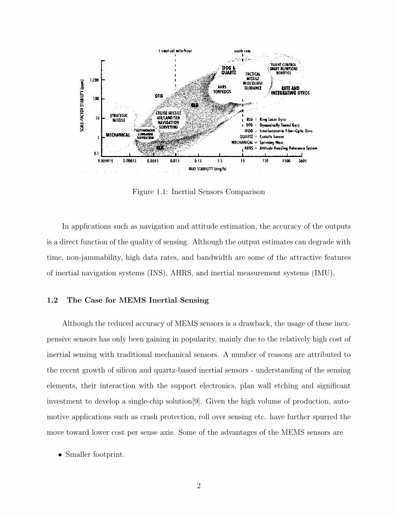
Figure 1.1: Inertial Sensors Comparison
In applications such as navigation and attitude estimation, the accuracy of the outputs
is a direct function of the quality of sensing. Although the output estimates can degrade with
time, non-jammability, high data rates, and bandwidth are some of the attractive features
of inertial navigation systems (INS), AHRS, and inertial measurement systems (IMU).
1.2 The Case for MEMS Inertial Sensing
Although the reduced accuracy of MEMS sensors is a drawback, the usage of these inex-
pensive sensors has only been gaining in popularity, mainly due to the relatively high cost of
inertial sensing with traditional mechanical sensors. A number of reasons are attributed to
the recent growth of silicon and quartz-based inertial sensors - understanding of the sensing
elements, their interaction with the support electronics, plan wall etching and significant
investment to develop a single-chip solution[9]. Given the high volume of production, auto-
motive applications such as crash protection, roll over sensing etc. have further spurred the
move toward lower cost per sense axis. Some of the advantages of the MEMS sensors are
• Smaller footprint.
2

• Lower weight and power consumption.
• Higher volume of production at a lower cost.
• Lower part counts resulting in lower maintenance.
While navigation applications still require accuracies not currently met by MEMS sen-
sors, other areas such as AHRS, personal navigation, crash testing, graphics, etc. have helped
sustain the growth. A major factor that has contributed to the penetration of MEMS sensors
is the idea of external aiding. Aiding sources like air data systems, Doppler sensors, global
positioning system (GPS) signals etc. help alleviate the reduced acuracy of the MEMS sen-
sors, by providing independent measures. While an improvement in position and velocity
accuracy is a direct result of external aiding, attitude estimates in an AHRS, for example,
also improve. Aiding sources, not surprisingly, are far from perfect and suffer from problems
such as low update rates, jammability, interference etc. For example, GPS signals suffer
from interference and the obtained velocity estimates are noisy at low speeds. Air data from
static and pitot sources suffer from installation specific errors that are difficult to model.
Processing algorithms have been devised to account for aiding errors, but this in turn in-
creases the development cost of the system. In applications such as hover on point, aiding
sources such as GPS do not provide adequate information. Given the costs and problems
associated with aiding, fixed-wing and rotary wing aircrafts in the general aviation market
require reasonable attitude accuracies, in the event of a loss or absence of aiding. With re-
dundant systems, for example two or three AHRS, per aircraft, the cost of attitude sensing
becomes more important.
1.3 Thesis Contributions and Organization
The focus of this dissertation is on the development of an attitude estimation algorithm
using low cost MEMS sensors for an AHRS application. Emphasis is placed on using the
minimum sensing package needed to achieve an acceptable accuracy. The performance of
3

the attitude estimation algorithm with aiding is compared with other estimators to verify
baseline performance. The achievable accuracy, under loss of aiding, is determined through
flight test studies and compared with an Euler angle estimation algorithm with no aiding.
The following are the contributions of this dissertation:
• Development of an algorithm that can provide reasonable attitude estimates without
aiding when required.
• Use of sensor models to design the proposed algorithm.
• Comparison of algorithm results with those achieved using a traditional Kalman filter.
• Evaluation of the algorithm with simulated and real world sensor data.
To meet these objectives, this dissertation is organized as follows. Chapter 2 details
the attitude representations and explores previous work in attitude estimation. Chapter 3
details the sensor models and calibration techniques for the MEMS sensors. Sensor model
parameters are determined from experimental data to understand the performance limita-
tions and determine the the extent of augmentation necessary. For example, information
from Allan Variance plots of a MEMS gyro is used as an aid in choosing correction gains to
reduce attitude error growth. Chapter 4 covers the development of the attitude estimation
algorithm based on the quaternion formulation of a complementary filter in the special or-
thogonal group. Chapter 5 presents the results of tests with simulated and real world data,
and compares them to those obtained using a Kalman filter attitude estimator with air data
aiding. Chapter 6 provides conclusions and presents some ideas for future work.
4
Chapter 2
Attitude Estimation and Fuzzy Logic
2.1 Overview
Attitude estimation has received considerable attention in the literature. Traditional
AHRS used gimballed mechanical gyros that remained to sense attitude with respect to an
inertial frame. Modern strapdown systems measure angular rates and linear accelerations
of a body-fixed frame with respect to a non rotating inertial frame and demand higher
dynamic ranges from the sensors. The measurements of angular rates and specific forces
are coordinatized in a body fixed frame. This chapter presents some of the representations
of platform attitude, along with their advantages and drawbacks, and surveys the attitude
estimation techniques in literature. An overview of classical complementary filtering in the
s-domain is also presented, followed by a review of work on SO(3) complementary filtering.
A review of fuzzy logic concepts is given to conclude the chapter.
2.2 Attitude Representations
The attitude estimation problem is formulated using two reference frames - a non-
rotating (inertial) frame and a rotating (body-fixed) frame and . Let A and B represent the
inertial reference frame and the rotating frame respectively. Depending on the set chosen,
the orientation of B with respect to A can be represented using several different sets of
parameters. In the following sections and chapters, the frame aligned with the magnetic
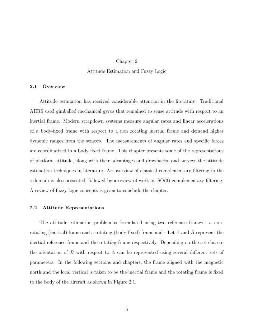
north and the local vertical is taken to be the inertial frame and the rotating frame is fixed
to the body of the aircraft as shown in Figure 2.1.
5
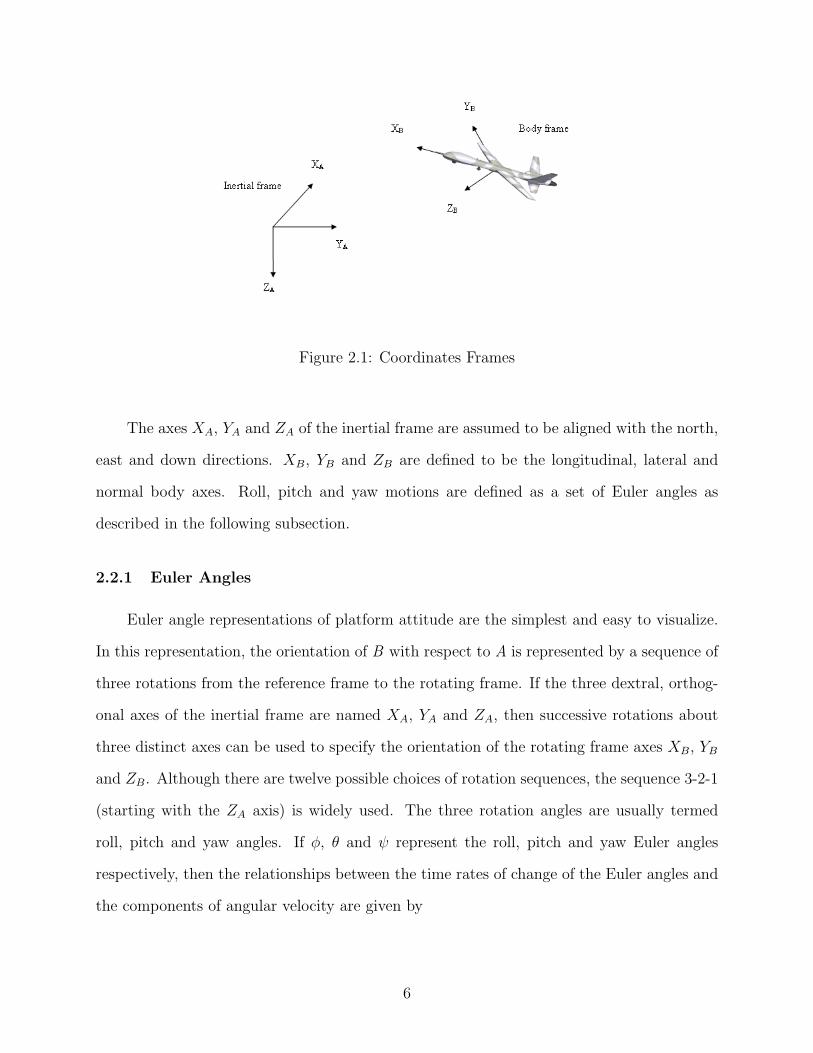
Figure 2.1: Coordinates Frames
The axes XA, YA and ZA of the inertial frame are assumed to be aligned with the north,
east and down directions. XB, YB and ZB are defined to be the longitudinal, lateral and
normal body axes. Roll, pitch and yaw motions are defined as a set of Euler angles as
described in the following subsection.
2.2.1 Euler Angles
Euler angle representations of platform attitude are the simplest and easy to visualize.
In this representation, the orientation of B with respect to A is represented by a sequence of
three rotations from the reference frame to the rotating frame. If the three dextral, orthog-
onal axes of the inertial frame are named XA, YA and ZA, then successive rotations about
three distinct axes can be used to specify the orientation of the rotating frame axes XB, YB
and ZB. Although there are twelve possible choices of rotation sequences, the sequence 3-2-1
(starting with the ZA axis) is widely used. The three rotation angles are usually termed
roll, pitch and yaw angles. If φ, θ and ψ represent the roll, pitch and yaw Euler angles
respectively, then the relationships between the time rates of change of the Euler angles and
the components of angular velocity are given by
6
φ
θ
ψ
=
1 sinφ tan θ cosφ tan θ
0 cosφ − sinφ
0sinφ
cos θ
cosφ
cos θ
ωx
ωy
ωz
(2.1)
Here ωx, ωy and ωz are the x, y and z-axis components of the body frame angular velocities.
The Euler angles can be obtained by integrating the above equations. It is important to
note that φ, θ and ψ represent the angular rates of intermediate frames and do not form
a vector. Euler angles are conceptually easy to visualize but suffer from singularity at
θ = nπ2, n = ±1,±3,±5 etc., for the 3-2-1 rotation sequence. The attitude propagation
equations for each choice of rotation sequence contain a similar singularity.
2.2.2 Direction Cosine Matrix
Another representation of relative orientation between two coordinate frames is the
direction cosine matrix. A vector ~ui in the non-rotating reference frame can be transformed
to a vector ~ub in the body frame using the orthogonal rotation matrix Cbi .
~ub = Cbi ~ui (2.2)
The elements of the direction cosine matrix (DCM) represent the projections of unit
vectors in the non-rotating reference frame onto the rotating frame. For example, element
12 of the DCM represents the cosine of the angle between the XA axis of the reference frame
and the YB axis of the rotating frame. Similar to the attitude rate equations, the attitude
propagation equation is given by the time rate of change of the rotation matrix
Cbi = −ΩibC
bi (2.3)
7
Ωib =
0 −ωz ωy
ωz 0 −ωx
−ωy ωx 0
(2.4)
where again ωx, ωy and ωz are the x, y and z components of angular velocity of the
rotating frame with respect to the reference frame. With a known initial orientation and
measurements of ωx, ωy and ωz from gyroscopes, the above differential equation can be
integrated to determine the current orientation. Direction cosine matrices obtained using
numerical integration lose their orthonormal properties due to numerical errors and require
re-orthogonalization. The re-orthogonalization is usually performed at a much slower rate
when compared to the integration interval. The relationship between the rotation matrix
and Euler angles is given by
Cbi =
cos θ cosψ cos θ sinψ − sin θ
− cosφ sinψ + sinφ sin θ cosψ cosφ cosψ + sinφ sin θ sinψ sinφ cos θ
sinφ sinψ + cosφ sin θ cosψ − sinφ cosψ + cosφ sin θ sinψ cosφ cos θ
(2.5)
To compute the Euler angles φ, θ and ψ from the rotation matrix, the following equations
are used:
φ = tan−1 C23
C33
(2.6)
θ = sin−1C13 (2.7)
ψ = tan−1 C12
C11
(2.8)
2.2.3 Axis-Angle
The orientation between the two reference frames can also be represented using the
axis-angle representation. This representation is based on Euler’s rotation theorem that two
8

orthogonal frames can be made to coincide by performing a right-handed rotation about a
space-fixed axis. Although the axis of rotation and the angle are not obvious, this represen-
tation is still useful in some applications such as tracking. If Rn(φ) is the rotation matrix
used to align the non-rotating reference frame with the rotating frame, the angle of rotation
is φ and the direction of rotation axis is specified by ~n, the rotation matrix can be written
as
Rn(φ) = (1− cosφ)nnT + cosφI3 + sinφn (2.9)
with n is the skew-symmetric matrix given by
n =
0 −n3 n2
n3 0 −n1
−n2 n1 0
(2.10)
For the rotation operator Cbi , the axis of rotation ~n is the eigenvector corresponding to the
eigenvalue of +1. Therefore, the unit vector ~n can be determined using
[Cbi − I
]~n = 0 (2.11)
The angle of rotation φ can be determined using the equation
φ = cos−1 Tr(Cbi )− 1
2(2.12)
where Tr(Cbi ) is the trace of the rotation matrix. Although the axis-angle representation
reduces the number of independent variables to four - the rotation angle and the three
elements of the rotation axis, the rotation metrix Rn(φ) still needs to be constructed to
apply a rotation. As a result, problems such as loss of orthogonality in direction cosine
matrices still exist in the axis-angle representation.
9
2.2.4 Quaternions
Sir William R.Hamilton invented the hypercomplex numbers of rank 4 and termed them
quaternions. Hamilton defined quaternions as 4-tuples of real numbers
q = (q0, q1, q2, q3) (2.13)
Here q0 is the scalar part of the quaternion and q = (q1, q2, q3) is the vector part constructed
using the standard basis vectors ~i, ~j and ~k. Quaternions, being hypercomplex numbers of
rank greater than 2, do not satisfy field properties of real numbers - quaternion products
are, in general, not commutative. The norm of a quaternion is defined as
||q|| =√q2
0 + q21 + q2
2 + q23 (2.14)
If the norm of the quaternion is unity, it is referred to as a unit quaternion. Just like the
rotation matrix, a unit quaternion (or any quaternion in general) can be used to rotate a
vector from a non-rotating reference frame to a rotating frame. For a vector ~u, the rotation
operator in terms of quaternion is expressed as [19]
L(q) = q∗ ⊗ u⊗ q (2.15)
where
q∗ =
q0
−q
(2.16)
is the inverse of the unit quaternion q and ⊗ denotes a quaternion product. L(q) can be
interpreted as an operator that rotates the reference frame A into the rotating frame B. In
terms of the axis-angle rotation, if the unit quaternion q is represented as
q = cosφ+ ~u sinφ (2.17)
10

the quaternion operator L(q) rotates the frame through an angle of 2θ. In terms of the Euler
angles φ, θ and ψ, the component quaternions can be represented as
~qφ =
cos φ2
sin φ2
0
0
(2.18)
~qθ =
cos θ2
0
sin θ2
0
(2.19)
~qψ =
cos ψ2
0
0
sin ψ2
(2.20)
The quaternion q for the rotation operator L(q) can be derived from the component quater-
nions as
~q = ~qψ ⊗ ~qθ ⊗ ~qφ (2.21)
The elements of q can be represented in terms of the Euler angles as
q0 = cosψ
2cos
θ
2cos
φ
2+ sin
ψ
2sin
θ
2sin
φ
2(2.22)
q1 = cosψ
2cos
θ
2sin
φ
2− sin
ψ
2sin
θ
2cos
φ
2(2.23)
q2 = cosψ
2sin
θ
2cos
φ
2+ sin
ψ
2cos
θ
2sin
φ
2(2.24)
11

q3 = sinψ
2cos
θ
2cos
φ
2− cos
ψ
2sin
θ
2sin
φ
2(2.25)
Poisson’s kinematic equation in quaternion form that relates the rate of change of the attitude
quaternion to the angular rate of the body frame with respect to inertial frame is given by:
q =1
2q ⊗ ωib (2.26)
In matrix form this equation can be written as
q =1
2∗
q0 −q
q q0I3 + S(q)
0
ωib
(2.27)
where S(q) is the skew-symmetric matrix
S(q) =
0 −q3 q2
q3 0 −q1
−q2 q1 0
(2.28)
If q1 and q2 are two quaternions, the relative orientation or the error quaternion between
the two is given by
q = q1 ⊗ q∗2 (2.29)
Two frames whose attitude quaternions with respect to a reference frame are q1 and q2
coincide if:
s = 1 (2.30)
v = 0 (2.31)
where s and v are the real and vector parts of the quaternion error. Regardless of the
magnitude of the quaternion error, v = 0 is a sufficient condition for the two frames to
coincide.
12

2.2.5 Rodrigues Parameters
Another attitude representation related to quaternions is the Rodrigues vector, also
called Gibbs vector. The parameter set is defined as [24]:
~ρ =~q
q0
= tan
(θ
2
)n (2.32)
The components(ρ1, ρ2, ρ3
)are referred to as the Rodrigues parameters and the quaternion
in terms of these parameters is given by
q =1√
1 + |ρ|2
1
~ρ
(2.33)
Rodrigues vector is a minimum parameter set for attitude representation but rotations pass-
ing through π cannot be represented as |ρ| → ∞.
2.3 Survey of Attitude Estimation
Attitude estimation has been studied extensively. Different sensor sets and techniques
have been developed to estimate vehicle attitude, both online and offline. The basic sensor
measurements used are
• Gyroscopes.
• Accelerometers.
• Magnetometers.
• Air data sensors.
• GPS.
• Combinations of these.
13
In strapdown systems attitude estimation involves estimating the orientation of a body-fixed,
rotating frame with respect to an inertial frame. Wahba [27] proposed that, given measure-
ments of two non-colinear vectors, one in a body fixed frame vb, and one in an inertial frame,
vi, a least-squares estimate of the rotation matrix can be computed by reducing the error
between the reference vector set and the rotated vector set from the body-fixed frame. The
objective in this case is to find the orthogonal matrix M such that
n∑i=1
||vi −Mvb||2
is minimized.
Various algorithms and methods that use inertial sensors are available in the literature.
A simple attitude estimation scheme for a small autonomous helicopter utilizing a two-axis
inclinometer, triad of rate gyros and a compass is proposed in [3]. The inclination and the
integrated outputs are combined with a complementary filter and the bandwidth of the fil-
ters are tuned to match the bandwidth of interest. A gyro-free system using non-colinear
vector measurements to compute the attitude quaternion is proposed in [10]. Body frame
measurements obtained from accelerometers and magnetometers are combined with the ref-
erence magnetic and gravity vectors using least-squares and a time-varying Kalman filter.
The magnetic model requires the current position from a GPS and the gravitational field
of the earth is assumed to be a constant and pointing down in the local vertical frame. In
[11], GPS is used to determine the attitude solution using an ultra short-baseline in a triple
antenna configuration, with the resulting attitude uncertainties being less than 0.5 deg. This
carrier phase detection algorithm requires precise initialization to account for integer am-
biguities and is sensitive to noise. It is also shown that reducing the spacing degrades the
accuracy of the computed attitude solution. To coast through GPS outages and get a higher
bandwidth output, inertial aiding using solid-state rate gyros is also explored. A drawback
of a GPS-based attitude determination is the susceptibility to interference and loss of lock
requiring reinitialization. Two recursive algorithms to solve the vector-matching problem
14
by determining the minimum variance estimate of the attitude quaternion are presented in
[5]. An extended Kalman filter is used to estimate the difference between the true attitude
quaternion and the estimate. A similar recursive scheme to solve the two-vector problem
using Euler angles is presented in [4].
A novel approach is taken in [20], wherein, instead of carrier phase measurements from GPS,
signal-to-noise (SNR) measurements are used to determine three-axis attitude. The SNR
measurements and the gain pattern of the antenna are used to compute the orientation of
the platform. When compared to the conventional carrier-phase estimation, this method has
the advantage of requiring no reinitialization. However, the sensitvity in yaw is dependent
on the antenna geometry and hence the possibility of combining the standard carrier-phase
method with the SNR measurements is also explored.
Another approach, utilizing GPS velocity signals to generate a ’pseudo-attitude’ for general
aviation applications, is presented in [13]. Velocity measurements from a single GPS antenna
are used to synthesize flight path angle relative to the local horizontal plane and the roll
angle about the velocity vector, assuming non slipping turns. It is shown that the body axes
and the wind axes are closely oriented, and the synthesized attitude is closely related to the
conventional pitch and roll angles. The computed ’pseudo-attitude’ is suitable for backup
attitude indicators. A fast estimation algorithm to solve the vector matching problem using
quaternions is proposed in [21]. Complementary filtering schemes that take advantage of
the short-term stability of the gyros and the long-term stability of accelerometers are also
popular. A fuzzy logic signal processing approach to adaptively adjust the filter bandwidths
to correct the gyro bias is proposed in [22].
2.4 Complementary filtering
Complementary filtering is a technique used to combine measurements from two or more
sources with different spectral characteristics with minimal distortion in the signal output.
15
The measurement sources usually have different frequency regions where the measurement
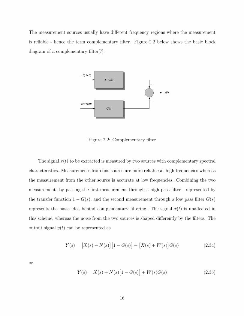
is reliable - hence the term complementary filter. Figure 2.2 below shows the basic block
diagram of a complementary filter[7].
Figure 2.2: Complementary filter
The signal x(t) to be extracted is measured by two sources with complementary spectral
characteristics. Measurements from one source are more reliable at high frequencies whereas
the measurement from the other source is accurate at low frequencies. Combining the two
measurements by passing the first measurement through a high pass filter - represented by
the transfer function 1− G(s), and the second measurement through a low pass filter G(s)
represents the basic idea behind complementary filtering. The signal x(t) is unaffected in
this scheme, whereas the noise from the two sources is shaped differently by the filters. The
output signal y(t) can be represented as
Y (s) =[X(s) +N(s)
][1−G(s)
]+[X(s) +W (s)
]G(s) (2.34)
or
Y (s) = X(s) +N(s)[1−G(s)
]+W (s)G(s) (2.35)
16

With this scheme, the problem reduces to determining the transfer function G(s) to shape
the spectral characteristics of the two sources to provide the best estimate of x(t). The idea
can be extended to include more than two sources by making the transfer function of one
path the complement of the sum of the other two transfer functions. As an application of
complementary filtering to single-axis attitude estimation - given measurements y1 and y2
from an inclinometer and a rate gyroscope respectively, the estimate for the tilt θ(t) can be
written as
θ(t) = G(s)Y1(s) +[1−G(s)
]Y2(s) (2.36)
2.5 SO(3) complementary filtering
The term SO(3) refers to the special orthogonal group - the group of all orthogonal ma-
trices that represent a rotation in 3D space. The principles of complementary filtering have
been extended by various authors to design nonlinear controller/observers in rigid bodies.
An earlier work by [25] presents a design of a nonlinear velocity and angular momentum
observer for rigid bodies using Euler quaternions and energy functions. Angular velocity
estimates are generated using torque and orientation measures and the exponential conver-
gence of the observer is demonstrated. Reference [14] extends the nonlinear angular velocity
observer to estimate bias, scale factor and misalignment errors in gyros and accelerometers.
The residual bias errors in the gyro measurements are assumed to decay exponentially. The
angular velocity observer presented in [25] and [14] requires a true attitude quaternion and
the residual bias, scale factor errors etc. are estimated using the observed attitude errors.
The observer proposed in [14] is of the form
q0
q
=1
2
−q0T
q0I + S(q)
[(I + ∆ωimu + b+Ksgn(s)v
](2.37)
˙b = −βb+
1
2sgn(s)v (2.38)
17

where b is the estimated gyro bias, [q0 q] is the estimate of the attitude quaternion
and [s v] are the real and the vector parts of the quaternion error.
The angular velocity observer in [14] is shown to be exponentially stable with the equilib-
rium points (0, 0, 0) and (±1, 0, 0, 0) for the bias errors and attitude quaternion respectively.
[18] proposes a similar algorithm to estimate a constant bias in angular velocity measures.
The bias estimates are used as part of a nonlinear algorithm for spacecraft attitude control.
The observer proposed for gyro bias is of the form
˙q =1
2Q(q(t))RT (s)
[ω(t) + ksgn(s(t))v(t)
](2.39)
˙b(t) = −1
2sgn(s(t))v(t) (2.40)
[12] proposes a complementary filter design using rotation matrices, instead of attitude
quaternion, for control of unmanned aerial vehicles. A cost function Et of
Et =1
2tr(I − R) = 2 sin2(
θ
2) (2.41)
is used to show exponential convergence. The proposed observer kinematics is of the form
˙R = (RΩ + Rω(R, R))xR (2.42)
where
ω = kestvex(πa(R)) (2.43)
with vex() defined as the operation to convert the skew-symmetric rotation error matrix R
into an error vector. This operation is the inverse of the operation below that converts a
18

vector ~ω to a skew-symmetric matrix Ωx.
~ω × ~a = Ωx~a (2.44)
In the above equations R is the true attitude matrix obtained from another source -
accelerometers and magnetometers, for example. Using the corrected attitude matrix R to
transform Ω simplifies the observer equation to
˙R = R(Ω + ω)x (2.45)
with ω again given by
ω = kestvex(πa(R)) (2.46)
If R is the reference attitude matrix and R is the last known estimate of the filter, the
attitude error required to compute ω can be computed as the relative orientation between
the two frames:
R = RTR (2.47)
The ω term in the above equations can be viewed as the rate correction in the body frame
necessary for the attitude matrix R to track the true attitude R. For a constant gyro bias,
the observer kinematic equation using a quaternion representation is written as [12]
˙q =1
2q ⊗ p(Ω− b+ ω) (2.48)
with
˙b = −kbsv (2.49)
and
ω = kestsv (2.50)
19
where s and v are the real and the vector parts of the quaternion error.
2.6 Fuzzy logic
Fuzzy logic provides a method to represent control strategies as if it were implemented by
a human. Fuzzy control methods attempt to implement a human being’s intuitive knowledge
to achieve the desired controlled outputs. Reference [23] provides an excellent reference on
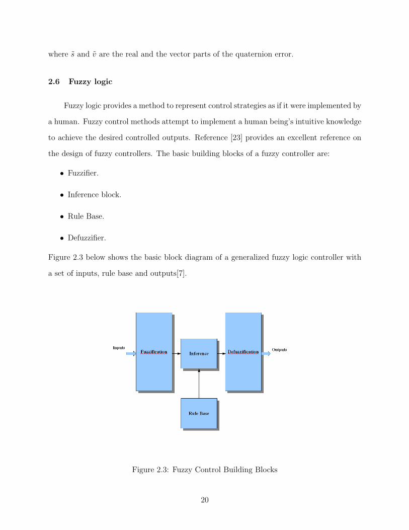
the design of fuzzy controllers. The basic building blocks of a fuzzy controller are:
• Fuzzifier.
• Inference block.
• Rule Base.
• Defuzzifier.
Figure 2.3 below shows the basic block diagram of a generalized fuzzy logic controller with
a set of inputs, rule base and outputs[7].
Figure 2.3: Fuzzy Control Building Blocks
20

As shown in the above figure, external inputs are converted by the fuzzifier, using a set
of if-then rules, into different input classes such as ‘negative large’, ‘negative small’, ‘positive
small’ etc., to create the input membership function set. Each input - usually an ‘error’
measure e(t) and a ‘rate of change of error’ measure e(t), is processed by the fuzzifier. For
example, triangular membership functions for an ‘error’ input e(t) are shown in Figure 2.4.
Figure 2.4: Fuzzy Membership Function
The set of physical values that an input can assume is referred to as the ‘universe of
discourse’ for the input parameter. Each triangular membership function has a center(c)
and a width(w) that determine the probability that a given input belongs that membership
function. For example, an input error of 1.5 in Figure 2.4 would belong to both “positive
small” and “positive medium” membership functions. The fuzzifier determines the certainty
(a measure of probability) that the input belongs to a group of membership functions or the
certainty that a particular rule is applicable. If u is the input, the certainty for the triangular
membership functions with center(c) and a width(w) can be determined using the following
21

equations [23]:
Left Triangular Membership Function
y =
1.0 if u ≤ c
max(1− u−c
0.5w, 0)
if u > c
Right Triangular Membership Function
y =
max(1 + u−c
0.5w, 0)
if u ≤ c
1.0 if u > c
Center Triangular Membership Function
y =
max(1 + u−c
0.5w, 0)
if u ≤ c
max(1− u−c
0.5w, 0)
if u > c
Once the applicability of all the input rules is determined, a ‘confidence matrix’ for
all combinations of inputs is generated. For example, if µe is the certainty associated with
‘error’ and µe is the certainty associated with ‘rate of error’, then the combined certainty
that both the rules apply is given by
µ = µe × µe (2.51)
The rule base matrix is a set of rules that specify the output values for each input
combination. The confidence matrix is scaled element-by-element with the rule base in the
defuzzification step and the entries are summed to generate the controller output.
22

Chapter 3
MEMS Sensor Modeling and Calibration
3.1 Overview
Usage of MEMS sensors in inertial sensing relies heavily on characterizing the behavior
of the sensor and developing compensation techniques to correct the device outputs. De-
pending on the application, the compensation can be applied in real-time or offline. This
chapter describes the sensor models used in this work for MEMS gyros, accelerometers and
magnetometers and an overview of calibration methods to reduce the deterministic errors.
Stochastic models of gyros and accelerometers are developed to understand the performance
limits of the sensors and the underlying noise characteristics. The parameters from the
stochastic models are used in the development of an extended Kalman filter. In addition,
the parameters are used as an aid to determine the correction gains in the proposed algo-
rithm.
3.2 Operation of MEMS Gyroscopes
Angular rate MEMS sensors use the Coriolis effect on a proof mass to sense angular
motion. A vibrating proof mass with a linear velocity of ~v which is subjected to an angular
rate of Ω experiences a Coriolis acceleration given by
Ac = −2(~Ω× ~v) (3.1)
The acceleration is perpendicular to the rotational axis and the velocity. For example,
ADXRS150 is a vibratory MEMS gyro that uses the Coriolis effect. Angular rate measure-
ment range of several thousand degrees per second has been achieved with this technology.
23
Quartz-based and resonant ring MEMS gyroscopes are other MEMS gyro technologies that
use similar vibratory elements. MEMS accelerometers rely on sensing the displacement of a
proof mass leading to a change in capacitance or a change in frequency of a vibrating beam
subjected to a linear acceleration. The advantages of silcon sensors outweigh the drawbacks
that accompany reduction in size such as decreased sensitivity, resolution, increased noise
and thermal sensitivity etc.[9].
3.3 MEMS Gyro Error Sources
MEMS gyroscopes have a number of errors that corrupt the angular rate measurement.
The errors can be classified as deterministic and stochastic. Deterministic errors that corrupt
a gyro measurement include:
• Scale factor errors.
• Thermal variation of bias.
• Linear acceleration sensitivity.
The scale factor (Sf ) of a MEMS gyro can exhibit variation with temperature as well
as applied angular rate. The g-sensitivity term indicates that the output of the sensor
can change as a function of linear acceleration. The g-sensitivity term manifests as a bias
shift at the output of the sensor. The deterministic terms - scale factor errors, thermal
variation of bias and g-sensitivity, can be characterized through carefully designed calibration
methods. The deterministic terms in the MEMS gyroscope measurement equation - Sf ,
O(T ), and g(A), can be computed using standard offline calibration techniques. For an
orthogonal triad of gyroscopes, sensor readings collected at different temperatures with a
null input angular rate can be used to determine the variation of bias with temperature.
MEMS gyroscopes usually provide a sensor core temperature output and this can be used
to compensate bias variation with temperature. A polynomial fit of the readings against
the recorded temperature can compensate for the variation. The scale factor matrix can
24
be determined by spinning the orthogonal triad at different temperatures. A 2D surface fit
of the collected readings against rate and temperature gives the scale factor matrix. If the
scale factor dependence on temperature is minimal, a curve fit will suffice. G-sensitivity
matrix can be determined by subjecting the gyroscope to linear accelerations along the
three orthogonal axes. Gravitational acceleration can be used as the input to determine the
g-sensitivity coefficients.
The stochastic errors that corrupt a gyroscope measurement can be classified into the
following categories:
• Angle Random Walk
• Bias Instability.
• Rate Random Walk.
• Exponentially Correlated Noise.
In addition to the above errors, a random constant turn-on bias can also corrupt the
measurement. The turn-on bias can be estimated at startup by averaging a long sequence
(typically 1 to 3 minutes) of gyro measurements. To characterize the other stochastic er-
rors, techniques like Allan Variance and autocorrelation are used. Allan Variance is a time
domain data analysis technique developed by David Allan to study the frequency stability
of oscillators[2]. The analysis has since been extended to study random processes in data
sets and can be used to identify noise sources. The following sections briefly describe the
stochastic errors and the methods to estimate them.
3.3.1 Angle Random Walk
Angle random walk(ARW) is a measure of the wideband noise η with correlation time
shorter than the sampling period. MEMS gyroscopes are usually bandlimited with a pre-
sampling filter and hence the wideband noise spectrum can be assumed to be ‘white’ when
25
compared to the device bandwidth. Wideband noise at the output of the sensor causes the
integrated attitude solution to exhibit a ‘random walk’ behavior. Random walk is character-
ized by a standard deviation that increases with√t. The rate noise power spectral density
as a function of frequency f can be represented by [1]
Sω(f) = N2 (3.2)
where N is the angular random walk coefficient. The relationship between the Allan
Variance of wideband noise and the ARW coefficient is given by
σ2(τ) =N2
τ(3.3)
where τ is the averaging time. The above equation indicates that at τ = 1, the ARW
coefficient is equal to σ(τ) and a log-log plot of σ(τ) versus τ will have a slope of -1/2.
Figure 3.1 shows a comparison of Allan variance of simulated noise sources with variances -
0.1, 0.25 and 0.5. An increase in the noise variance moves the log-log plot upward resulting
in a higher ARW coefficient, indicating that the random walk in the integrated output will
be higher. The ARW coefficient is usually expressed in deg/√hr.
26
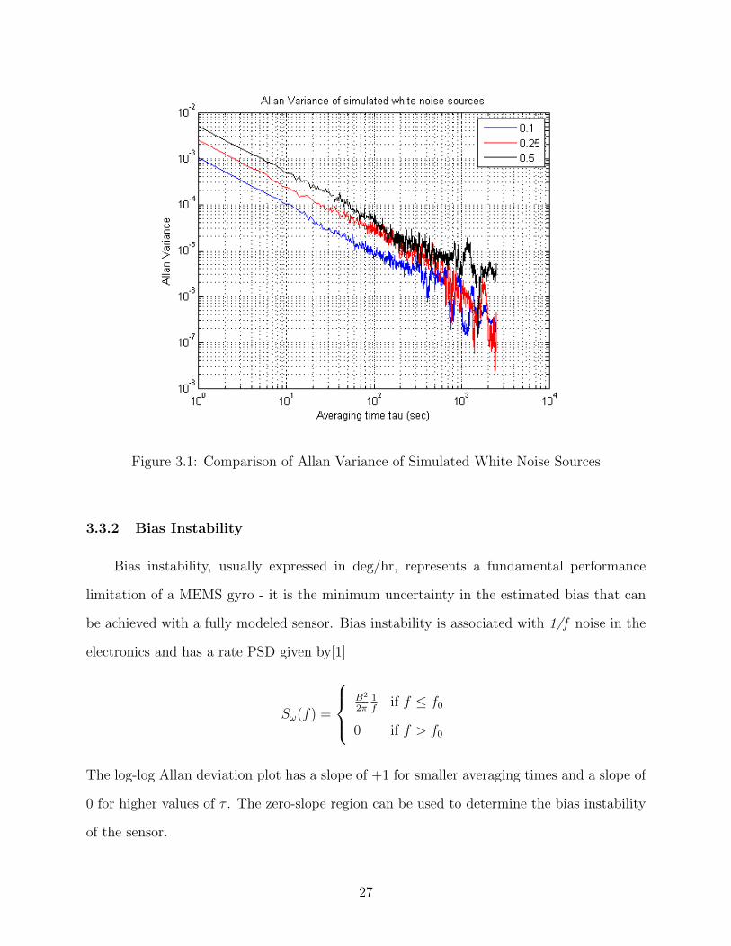
Figure 3.1: Comparison of Allan Variance of Simulated White Noise Sources
3.3.2 Bias Instability
Bias instability, usually expressed in deg/hr, represents a fundamental performance
limitation of a MEMS gyro - it is the minimum uncertainty in the estimated bias that can
be achieved with a fully modeled sensor. Bias instability is associated with 1/f noise in the
electronics and has a rate PSD given by[1]
Sω(f) =
B2
2π1f
if f ≤ f0
0 if f > f0
The log-log Allan deviation plot has a slope of +1 for smaller averaging times and a slope of
0 for higher values of τ . The zero-slope region can be used to determine the bias instability
of the sensor.
27
3.3.3 Rate Random Walk
Rate random walk is associated with 1/f 2 noise with the rate PSD given by:
Sω(f) =K
2π
2 1
f 2(3.4)
with K being the rate random walk coefficient. The Allan deviation plot shows a slope of
+1/2. In a similar fashion, the rate ramp and quantization errors show slopes of +1 and
-1 respectively. Rate random walk and rate ramp indicate processes that have increasing
variance and are physically unrealizable.
3.3.4 Exponentially Correlated Noise
An exponentially correlated (or Gauss-Markov) process is a stationary process with an
exponentially decaying autocorrelation. The rate PSD of a Gauss-Markov process
S(ω) =2σ2β
ω2 + β2(3.5)
where σ2 and 1/β are mean-square value and the time constant of the process.
The autocorrelation of the process is given by:
R(τ) = σ2e−β|τ | (3.6)
The Allan Variance of a Gauss-Markov process converges to that of ARW for averaging
times much greater than 1/β. For averaging times much smaller than 1/β, the Allan variance
approaches a rate random walk. A Gauss-Markov process is usually used as an approximation
for a rate random walk. A Gauss-Markov sequence is generated using the equation:
Xk+1 = e−βδtXk +Wk (3.7)
28
where Wk is the driving white noise sequence with zero mean and variance equal to σ2[1 −
e−2β∆t],
σ2 is the variance of the Gauss Markov process,
β = 1/τ ,
and ∆t is the sampling period
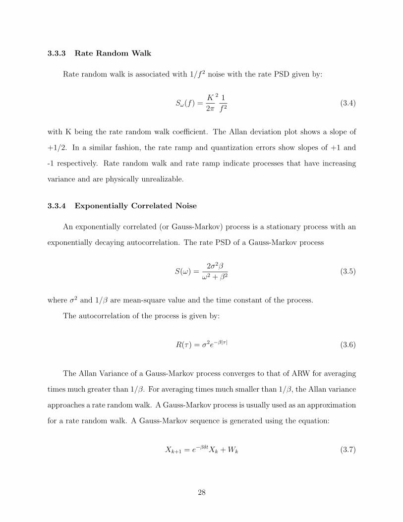
Figure 3.2 shows the comparison plot of Allan variance of three simulated Gauss-Markov
processes with a time constant of 1000 seconds and different variances. As shown in the figure,
increasing the variance of the exponential process shifts the Allan variance plot toward lower
correlation times.
Figure 3.2: Allan Variance of simulated Gauss-Markov processes - Constant Tau
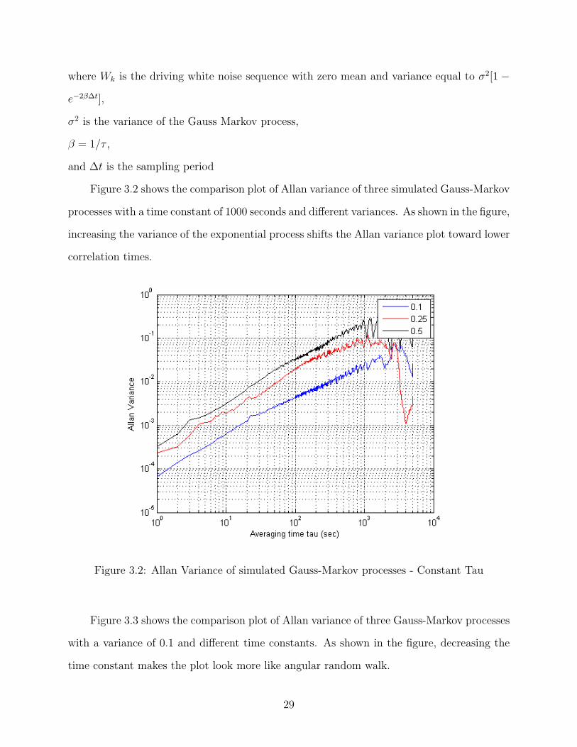
Figure 3.3 shows the comparison plot of Allan variance of three Gauss-Markov processes
with a variance of 0.1 and different time constants. As shown in the figure, decreasing the
time constant makes the plot look more like angular random walk.
29
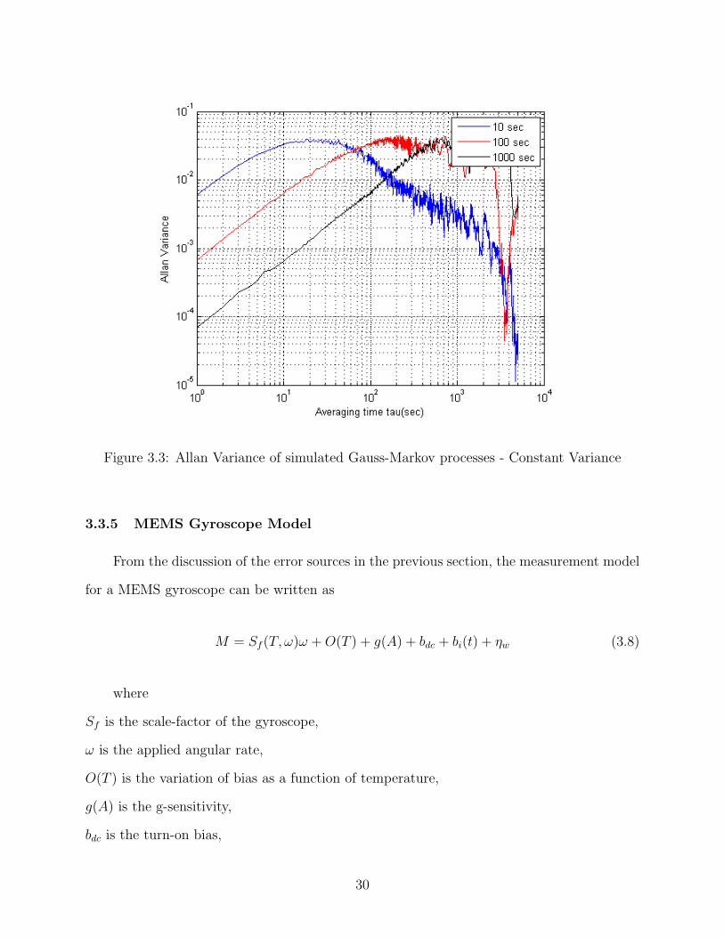
Figure 3.3: Allan Variance of simulated Gauss-Markov processes - Constant Variance
3.3.5 MEMS Gyroscope Model
From the discussion of the error sources in the previous section, the measurement model
for a MEMS gyroscope can be written as
M = Sf (T, ω)ω +O(T ) + g(A) + bdc + bi(t) + ηw (3.8)
where
Sf is the scale-factor of the gyroscope,
ω is the applied angular rate,
O(T ) is the variation of bias as a function of temperature,
g(A) is the g-sensitivity,
bdc is the turn-on bias,
30
bi is the time varying bias,
η is the wideband noise
For a triad of orthogonally mounted gyroscopes, the above equation can be written as
Mx
My
Mz
=
Sxx Sxy Sxz
Syx Syy Syz
Szx Szy Szz
ωx
ωy
ωz
+
Ox(Tx)
Oy(Ty)
Oz(Tz)
+
gxx gxy gxz
gyx gyy gyz
gzx gzy gzz
Ax
Ay
Az
+
bxdc
bydc
bzdc
+
bx(t)
by(t)
bz(t)
+
ηx
ηy
ηz
(3.9)
where the scale factor Sf is expanded to include misalignment terms and the g-sensitivity
term is expanded to include sensitivity to applied acceleration in x, y and z axes.
An exponentially correlated process model is assumed for the bias variation bi(t) with
time:
bi =−1
τbi + ηw (3.10)
where τ is the time constant of the process and ηw is the driving noise.
3.3.6 Determination of Stochastic Model Parameters
To estimate the stochastic errors and the model parameters, the Allan deviation of
ADXRS150 is computed with readings collected from the device at a constant temperature.
The sensor readings are sampled at 100 Hz and decimated to 10 Hz. The Allan deviation of
three ADXRS150 gyroscopic sensors used to generate data for this dissertation is shown in
Figure 3.4.
31

Figure 3.4: ADXRS150 Allan Deviation
The following observations are made from the Allan deviation plot:
• The ARW can be determined from this plot as the Allan deviation corresponding to
τ = 1sec - approximately 0.035 deg/sec or an ARW of 2.1 deg/√hr.
• The bias stability of the gyro is the minimum Allan deviation - approximately 0.0075
deg/sec or 28 deg/hr.
• For τ > 100 sec, the process can be approximated with an exponentially correlated
process.
To estimate the parameters σ2 and β of the exponentially correlated process, the auto-
correlation of a lengthy time sequence of sensor readings is used. A major consideration in
32
computing the autocorrelation is the amount of experimental data required to achieve the
required accuracy. The variance of the experimental autocorrelation satisfies[7]
VarVx(τ) ≤ 4
T
∫ ∞0
Rx2(τ)d(τ) (3.11)
For a Gauss-Markov process with exponential autocorrelation this reduces to
VarVx(τ) ≤ 2σ4
βT(3.12)
Accurate determination of the autocorrelation parameters is very difficult in practice. It
is shown in [7] that for a 10% accuracy, the experimental data required is 200 times the
time constant of the Gauss-Markov process. Since the Allan deviation plot of ADXRS150
only showed that the time constant of the underlying process is much greater than 100 sec,
determining the model parameters σ2 and β requires a very large data set.
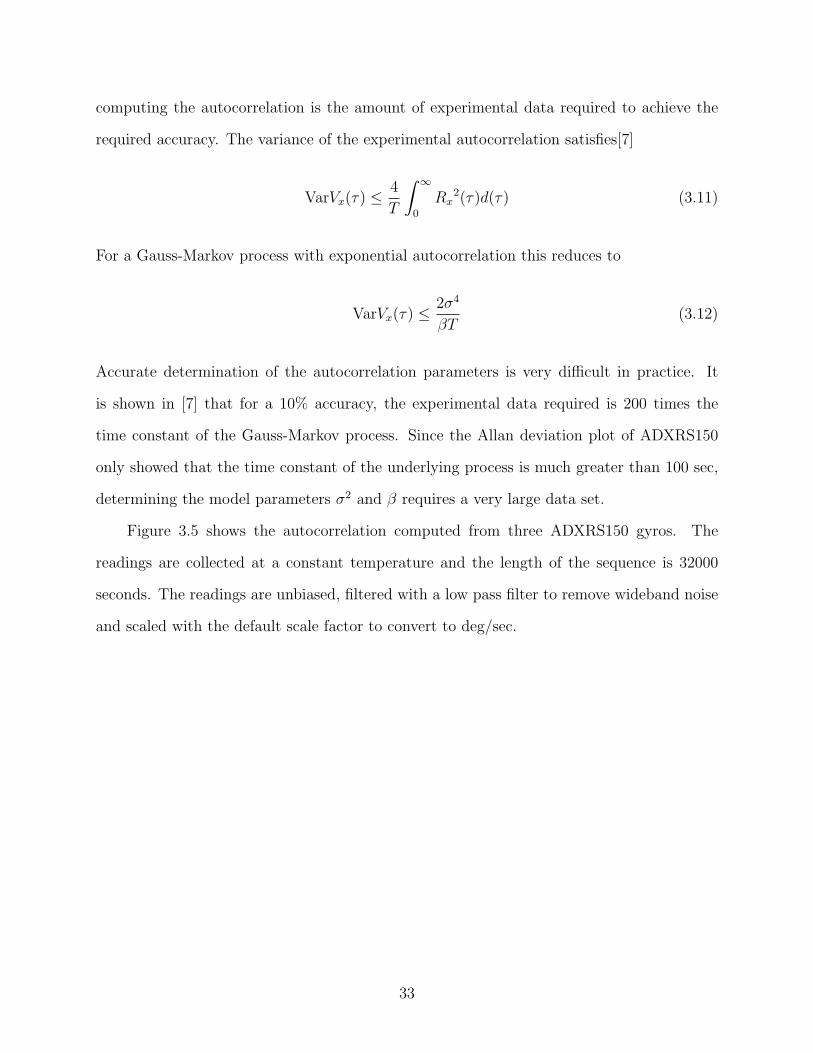
Figure 3.5 shows the autocorrelation computed from three ADXRS150 gyros. The
readings are collected at a constant temperature and the length of the sequence is 32000
seconds. The readings are unbiased, filtered with a low pass filter to remove wideband noise
and scaled with the default scale factor to convert to deg/sec.
33

Figure 3.5: Experimental Autocorrelation
The variability in the computed autocorrelation can be seen in the above figure. To
generate the model parameters σ2 and β, an exponential fit is made on the experimental
autocorrelation as shown in Figure 3.6.
34
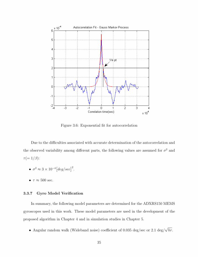
Figure 3.6: Exponential fit for autocorrelation
Due to the difficulties associated with accurate determination of the autocorrelation and
the observed variability among different parts, the following values are assumed for σ2 and
τ(= 1/β):
• σ2 ≈ 3× 10⁻⁴[deg/sec
]2.
• τ ≈ 500 sec.
3.3.7 Gyro Model Verification
In summary, the following model parameters are determined for the ADXRS150 MEMS
gyroscopes used in this work. These model parameters are used in the development of the
proposed algorithm in Chapter 4 and in simulation studies in Chapter 5.
• Angular random walk (Wideband noise) coefficient of 0.035 deg/sec or 2.1 deg/√hr.
35
• Bias Instability ≈ 28 deg/hr.
• Gauss Markov variance of 3× 10⁻⁴[deg/sec
]2.
• Gauss Markov time constant of 500 sec.
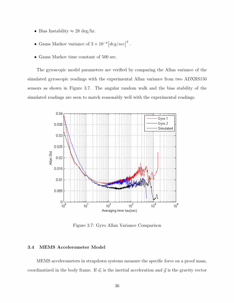
The gyroscopic model parameters are verified by comparing the Allan variance of the
simulated gyroscopic readings with the experimental Allan variance from two ADXRS150
sensors as shown in Figure 3.7. The angular random walk and the bias stability of the
simulated readings are seen to match reasonably well with the experimental readings.
Figure 3.7: Gyro Allan Variance Comparison
3.4 MEMS Accelerometer Model
MEMS accelerometers in strapdown systems measure the specific force on a proof mass,
coordinatized in the body frame. If ~ai is the inertial acceleration and ~g is the gravity vector
36
then the specific force is given by:
~f = ~ai − ~g (3.13)
The measured specific force is the component along the sensitive direction of the ac-
celerometer and is coordinatized in the body frame.
Like gyros, MEMS accelerometers have a number of error sources that corrupt the
specific force measurement. The measurement model for a MEMS accelerometer, assuming
that the turn-on bias is negligible, can be written as
fb = Sf (T )A+O(T ) + bdc + bi(t) + ηf (3.14)
where
Sf is the scale-factor of the accelerometer.
A is the applied specific force.
O(T ) is the variation of bias as a function of temperature.
bdc is the turn on bias.
bi is the bias variation as a function of time.
ηf is the wideband noise.
The deterministic terms - scale factor errors, thermal variation of bias and misalignment,
can be characterized through calibration methods. For an orthogonal triad of accelerome-
ters, sensor readings collected at different temperatures on a leveled surface can be used to
determine the variation of bias with temperature. A measure of the sensor core temperature
output can be used to compensate for the bias variation. The scale factor matrix can be
determined by using gravity as the excitation or by using a centrifuge.
Turn on bias bdc in an accelerometer, if not estimated, manifests as an attitude initial-
ization error during system alignment. For small angles, the tilt errors in the roll and pitch
37
axes introduced by the accelerometer biases [9] can be expressed as
δα =−By
g(3.15)
δβ =Bx
g(3.16)
where δα is the initialization error in roll angle, δβ is the initialization error in pitch
angle and Bx, By are the biases of the x and y-axis accelerometers respectively. In an
attitude heading reference system the gravity vector derived from the accelerometers is used
as a reference, the accelerometer biases cannot be estimated without an external aiding
source. In this attitude estimation study, the turn-on bias in accelerometers is assumed to
be negligible.
The methods to estimate the stochastic errors in MEMS accelerometers are analogous
to MEMS gyros, with the velocity random walk(VRW), bias instability and exponentially
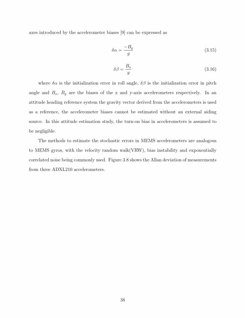
correlated noise being commonly used. Figure 3.8 shows the Allan deviation of measurements
from three ADXL210 accelerometers.
38
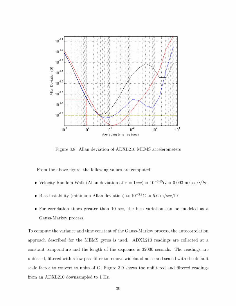
Figure 3.8: Allan deviation of ADXL210 MEMS accelerometers
From the above figure, the following values are computed:
• Velocity Random Walk (Allan deviation at τ = 1sec) ≈ 10−3.65G ≈ 0.093 m/sec/√hr.
• Bias instability (minimum Allan deviation) ≈ 10−3.8G ≈ 5.6 m/sec/hr.
• For correlation times greater than 10 sec, the bias variation can be modeled as a
Gauss-Markov process.
To compute the variance and time constant of the Gauss-Markov process, the autocorrelation
approach described for the MEMS gyros is used. ADXL210 readings are collected at a
constant temperature and the length of the sequence is 32000 seconds. The readings are
unbiased, filtered with a low pass filter to remove wideband noise and scaled with the default
scale factor to convert to units of G. Figure 3.9 shows the unfiltered and filtered readings
from an ADXL210 downsampled to 1 Hz.
39
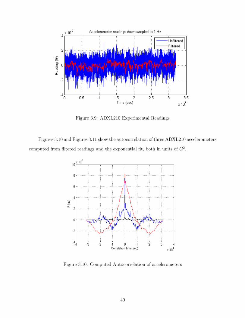
Figure 3.9: ADXL210 Experimental Readings
Figures 3.10 and Figures 3.11 show the autocorrelation of three ADXL210 accelerometers
computed from filtered readings and the exponential fit, both in units of G2.
Figure 3.10: Computed Autocorrelation of accelerometers
40

Figure 3.11: Autocorrelation fit for accelerometers
From the exponential fit Figures 3.11, the following autocorrelation parameters are
computed for accelerometers:
• Gauss Markov process variance σ2 (peak value of autocorrelation) ≈ 7× 10⁻⁷G2.
• Gauss Markov process time constant τ (time value corresponding to 1e× peak value)
≈ 500 sec.
3.5 Magnetic Sensors
Three-axis attitude solution requires integrating the output of the rate gyros with a
known initial attitude. Initial values of roll and pitch attitudes can be obtained from the
gravity reference, whereas the initial heading requires a magnetic sensor or a GPS. Further-
more, to prevent an unbounded growth in attitude errors, some form of reinitialization is
always required. A magnetic sensor is used in this work to compute the reference magnetic
41

heading. Single-chip magnetic sensors, like Honeywell HMC105X, are magnetoresistive sen-
sors that sense a change in resistance due to an applied magnetic field. Magnetoresistive
sensors have the following advantages when compared to the traditional flux-gate sensors:
• Low cost and size.
• High sensitivity
• Low temperature sensitivity
Three orthogonally aligned magnetic sensors can sense the Earth’s magnetic field in the body
frame. If Hx, Hy and Hz are the components of the Earth’s field in the magnetic north, east
and the local vertical directions, then the magnetic field sensed is given by:
~B = CφCθ ~H (3.17)
where Cφ and Cθ are the rotation matrices along the reference y and x axes respectively.
Given the current roll and pitch attitudes, the measurement vector ~B can be transformed
into the reference frame and the magnetic heading can be computed as:
ψ = arctan
[−Hy
Hx
](3.18)
3.5.1 Magnetometer Model
Magnetic sensors measure the Earth’s magnetic field at the mounted location and are
thus susceptible to a number of error sources. For navigation over small distances close to
the earth’s surface the magnetic field vector ~H can be assumed to be constant, and the basic
measurement model for a magnetic sensor can be written as:
~Bb = SsiSsfCib ~H + ~δBb (3.19)
42

where
~H is vector[HxHyHz
]T,
Cib is the direction cosine matrix from local horizontal reference frame to the body frame,
Ssi is the matrix representing soft-iron errors,
Ssf is the matrix representing on and off-axis scale factors,
~Bb is the vector of measures from the magnetic sensors,
~δBb is the vector of hard-iron offsets.
The matrix Cib represents the difference in orientation between the local level reference
frame and the body frame. The matrix Cib is not an error source but is still required
to accurately transform measures between the two frames. Ssi is the matrix representing
installation-dependent soft-iron errors. Soft-iron errors are caused by time-varying magnetic
fields, fields that depend on the orientation of the aircraft etc. Soft-iron errors are very
difficult to compensate due to their time-varying nature. Ssf is the matrix containing scale
factors for applied fields along the sensitive axis and off axes. ~δBb is the vector of biases
introduced due to hard-iron effects. Hard-iron errors are caused due to permanent magnetic
fields that are fixed with respect to the sensor. These sources introduce a fixed offset in the
magnetic sensor measures and can be compensated. Figure 3.12 shows x and y-axis readings
collected from a solid state magnetometer with and without distortion. A piece of ferrous
metal is placed close to the sensor to introduce the distortion. It can be seen that the center
of ellipse containing the x and y readings is offset, in the presence of distortion.
43
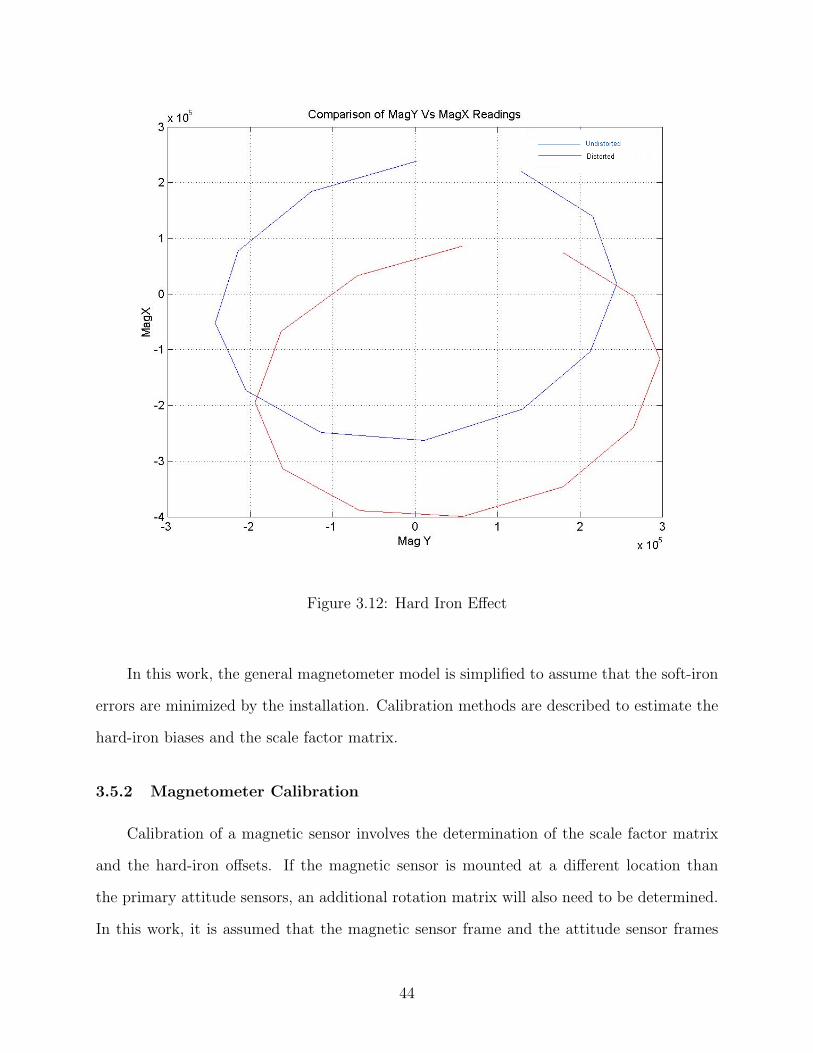
Figure 3.12: Hard Iron Effect
In this work, the general magnetometer model is simplified to assume that the soft-iron
errors are minimized by the installation. Calibration methods are described to estimate the
hard-iron biases and the scale factor matrix.
3.5.2 Magnetometer Calibration
Calibration of a magnetic sensor involves the determination of the scale factor matrix
and the hard-iron offsets. If the magnetic sensor is mounted at a different location than
the primary attitude sensors, an additional rotation matrix will also need to be determined.
In this work, it is assumed that the magnetic sensor frame and the attitude sensor frames
44

coincide. Also, it is assumed that the soft-iron errors are negligible and the magnetic sensor
can be leveled or a means is available to determine the inclination of the magnetic sensor
with respect to the local level. The measurement equation can be rewritten as:
Bx
By
Bz
=
Sxx Sxy Sxz
Syx Syy Syz
Szx Szy Szz
c11 c12 c13
c21 c22 c23
c31 c32 c33
Hx
Hy
Hz
+
δBx
δBy
δBz
(3.20)
Assuming that the rotation matrix Cib is known, applying an input magnetic field along
the z-axis in the positive and negative direction gives the set of equations:
Bx1
By1
Bz1
=
SxzHz
SyzHz
SzzHz
+
δBx
δBy
δBz
(3.21)
and Bx2
By2
Bz2
=
−SxzHz
−SyzHz
−SzzHz
+
δBx
δBy
δBz
(3.22)
where Hz is the applied field along the z-axis of the sensor. The scale factor column vector[SxzSyzSzz
]Tcan be determined from the above equations. The rest of the scale factor
matrix can be determined in a similar fashion, but the installation magnetic environment
is very likely to alter the scale factors. It is best to estimate the remaining elements of the
scale factor matrix and the hard-iron biases through a compass swing calibration method,
with the sensor mounted on the aircraft. A compass swing procedure involves rotating the
aircraft through a circle to collect readings along reference heading directions as shown in
Figure 3.13 [17].
45
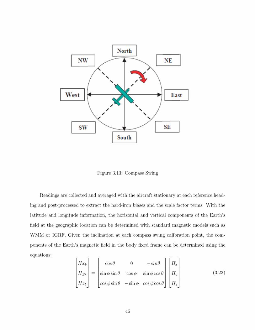
Figure 3.13: Compass Swing
Readings are collected and averaged with the aircraft stationary at each reference head-
ing and post-processed to extract the hard-iron biases and the scale factor terms. With the
latitude and longitude information, the horizontal and vertical components of the Earth’s
field at the geographic location can be determined with standard magnetic models such as
WMM or IGRF. Given the inclination at each compass swing calibration point, the com-
ponents of the Earth’s magnetic field in the body fixed frame can be determined using the
equations: Hxb
Hyb
Hzb
=
cos θ 0 −sinθ
sinφ sin θ cosφ sinφ cos θ
cosφ sin θ − sinφ cosφ cos θ
Hx
Hy
Hz
(3.23)
46
If N is the number of calibration points around the circle, this leads to a set of N linear
equations in x,y and z:
Hxb Hyb 1
......
...
Sxx
Sxy
δBx
=
Bx1 − Sxz ×Hzb
Bx2 − Sxz ×Hzb...
(3.24)
Hxb Hyb 1
......
...
Syx
Syy
δBy
=
By1 − Syz ×Hzb
By2 − Syz ×Hzb...
(3.25)
Hxb Hyb 1
......
...
Szx
Szy
δBz
=
Bz1 − Szz ×Hzb
Bz2 − Szz ×Hzb...
(3.26)
The above equations are solved using least-squares to determine Sxx, Sxy, Syx, Syy
and the hard-iron biases δBx,δBy and δBz. Figure 3.14 below shows the post-calibration
heading error in degrees at each compass swing point. The distorted data set generated to
demonstrate hard-iron biases is post-processed to generate these results.
47
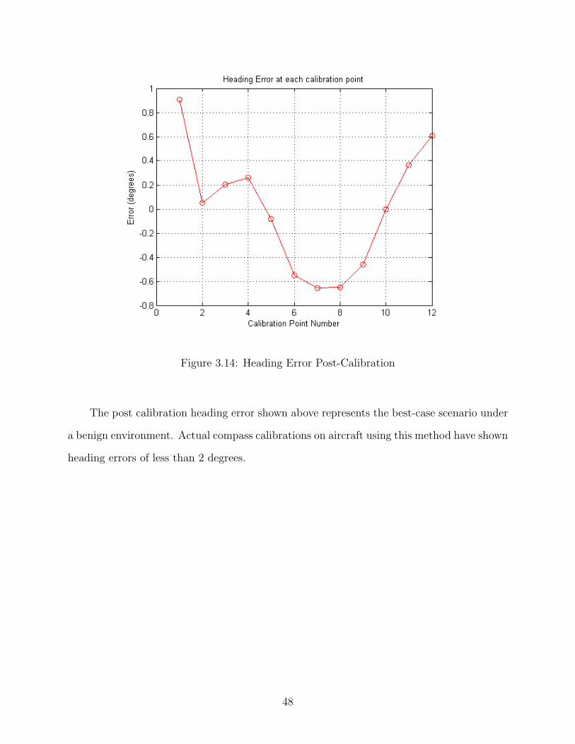
Figure 3.14: Heading Error Post-Calibration
The post calibration heading error shown above represents the best-case scenario under
a benign environment. Actual compass calibrations on aircraft using this method have shown
heading errors of less than 2 degrees.
48

Chapter 4
Attitude Estimation Algorithm Formulation
4.1 Introduction
This chapter describes the proposed algorithm using rotational quaternions to estimate
3-DOF attitude using low cost MEMS gyros, accelerometers and magnetometers. The atti-
tude estimation algorithm proposed in this chapter is based on the quaternion formulation
of SO(3) complementary filtering [12] reviewed in Chapter 2. The algorithm combines the
quaternion formulation with fuzzy logic concepts to build a stable attitude estimation sys-
tem. The motivation for the modification to [12] is given followed by the formulation of
the proposed algorithm. Model parameters for gyros and accelerometers determined in the
previous chapter are used in the development of the algorithm to select the fuzzy controller
parameters.
In formulating the attitude estimation algorithm, the following assumptions are made:
• Measurements from a triad of MEMS gyros, accelerometers and magnetometers are
available.
• MEMS gyroscope outputs are calibrated to minimize scale factor and misalignment
errors.
• MEMS accelerometer outputs are calibrated to minimize scale factor and misalignment
errors.
• Magnetometer is calibrated using the compass swing procedure described earlier to
minimize hard-iron and scale factor errors. Soft-iron errors are assumed to be negligible.
49
• Startup alignment time of 2 minutes to capture the random turn-on bias of the MEMS
gyros. The residual bias in the gyros are corrected by augmentation with accelerometers
and magnetometers.
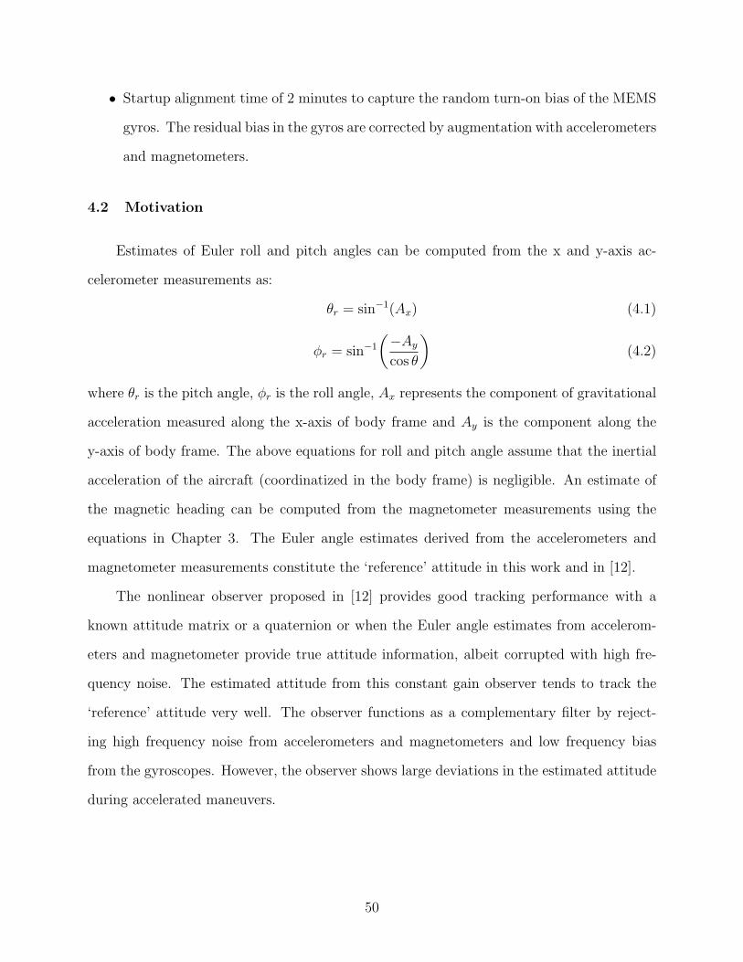
4.2 Motivation
Estimates of Euler roll and pitch angles can be computed from the x and y-axis ac-
celerometer measurements as:
θr = sin−1(Ax) (4.1)
φr = sin−1
(−Aycos θ
)(4.2)
where θr is the pitch angle, φr is the roll angle, Ax represents the component of gravitational
acceleration measured along the x-axis of body frame and Ay is the component along the
y-axis of body frame. The above equations for roll and pitch angle assume that the inertial
acceleration of the aircraft (coordinatized in the body frame) is negligible. An estimate of
the magnetic heading can be computed from the magnetometer measurements using the
equations in Chapter 3. The Euler angle estimates derived from the accelerometers and
magnetometer measurements constitute the ‘reference’ attitude in this work and in [12].
The nonlinear observer proposed in [12] provides good tracking performance with a
known attitude matrix or a quaternion or when the Euler angle estimates from accelerom-
eters and magnetometer provide true attitude information, albeit corrupted with high fre-
quency noise. The estimated attitude from this constant gain observer tends to track the
‘reference’ attitude very well. The observer functions as a complementary filter by reject-
ing high frequency noise from accelerometers and magnetometers and low frequency bias
from the gyroscopes. However, the observer shows large deviations in the estimated attitude
during accelerated maneuvers.
50
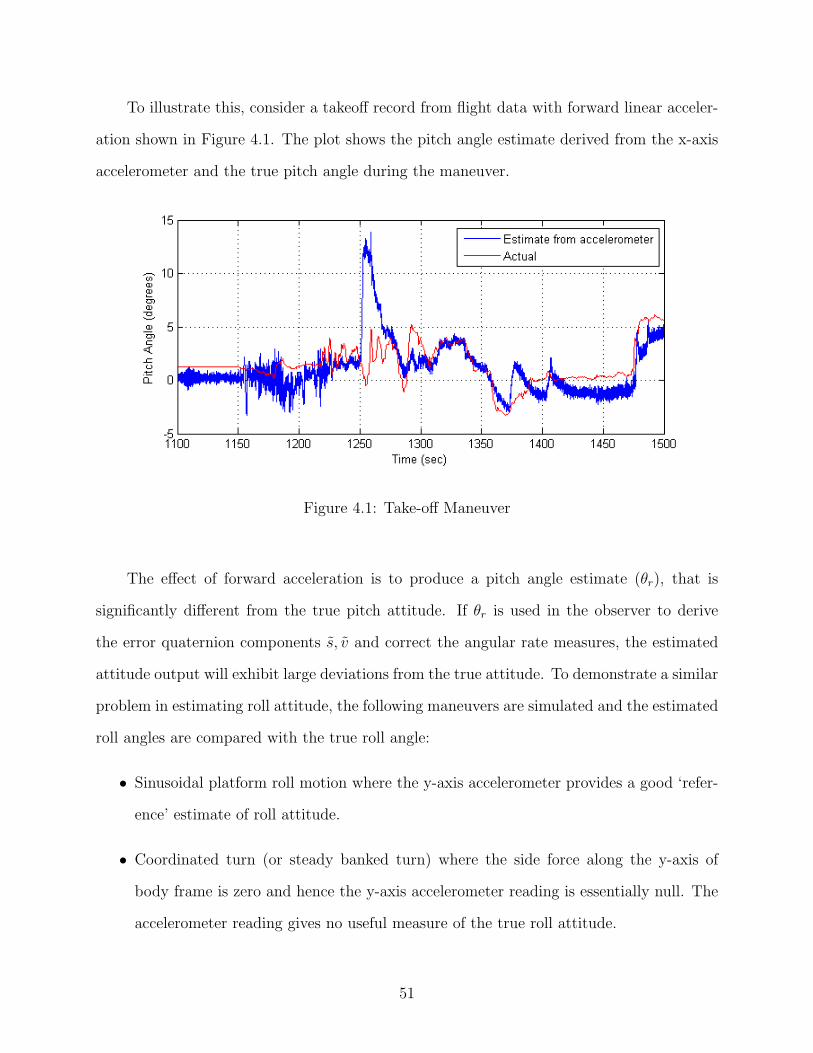
To illustrate this, consider a takeoff record from flight data with forward linear acceler-
ation shown in Figure 4.1. The plot shows the pitch angle estimate derived from the x-axis
accelerometer and the true pitch angle during the maneuver.
Figure 4.1: Take-off Maneuver
The effect of forward acceleration is to produce a pitch angle estimate (θr), that is
significantly different from the true pitch attitude. If θr is used in the observer to derive
the error quaternion components s, v and correct the angular rate measures, the estimated
attitude output will exhibit large deviations from the true attitude. To demonstrate a similar
problem in estimating roll attitude, the following maneuvers are simulated and the estimated
roll angles are compared with the true roll angle:
• Sinusoidal platform roll motion where the y-axis accelerometer provides a good ‘refer-
ence’ estimate of roll attitude.
• Coordinated turn (or steady banked turn) where the side force along the y-axis of
body frame is zero and hence the y-axis accelerometer reading is essentially null. The
accelerometer reading gives no useful measure of the true roll attitude.
51
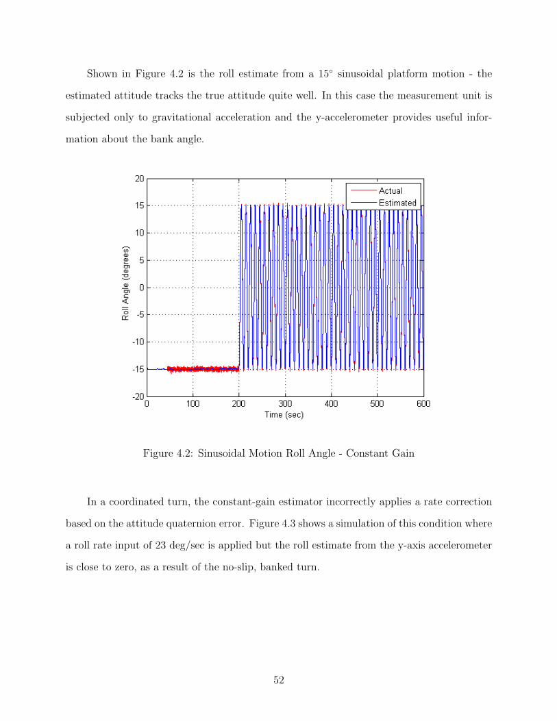
Shown in Figure 4.2 is the roll estimate from a 15 sinusoidal platform motion - the
estimated attitude tracks the true attitude quite well. In this case the measurement unit is
subjected only to gravitational acceleration and the y-accelerometer provides useful infor-
mation about the bank angle.
Figure 4.2: Sinusoidal Motion Roll Angle - Constant Gain
In a coordinated turn, the constant-gain estimator incorrectly applies a rate correction
based on the attitude quaternion error. Figure 4.3 shows a simulation of this condition where
a roll rate input of 23 deg/sec is applied but the roll estimate from the y-axis accelerometer
is close to zero, as a result of the no-slip, banked turn.
52
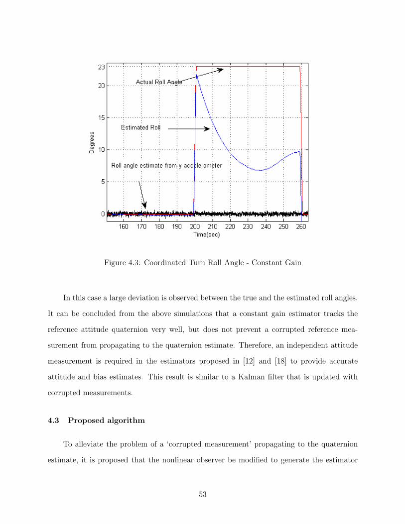
Figure 4.3: Coordinated Turn Roll Angle - Constant Gain
In this case a large deviation is observed between the true and the estimated roll angles.
It can be concluded from the above simulations that a constant gain estimator tracks the
reference attitude quaternion very well, but does not prevent a corrupted reference mea-
surement from propagating to the quaternion estimate. Therefore, an independent attitude
measurement is required in the estimators proposed in [12] and [18] to provide accurate
attitude and bias estimates. This result is similar to a Kalman filter that is updated with
corrupted measurements.
4.3 Proposed algorithm
To alleviate the problem of a ‘corrupted measurement’ propagating to the quaternion
estimate, it is proposed that the nonlinear observer be modified to generate the estimator
53
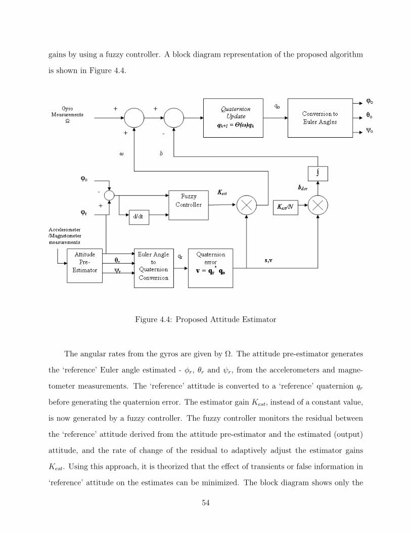
gains by using a fuzzy controller. A block diagram representation of the proposed algorithm
is shown in Figure 4.4.
Figure 4.4: Proposed Attitude Estimator
The angular rates from the gyros are given by Ω. The attitude pre-estimator generates
the ‘reference’ Euler angle estimated - φr, θr and ψr, from the accelerometers and magne-
tometer measurements. The ‘reference’ attitude is converted to a ‘reference’ quaternion qr
before generating the quaternion error. The estimator gain Kest, instead of a constant value,
is now generated by a fuzzy controller. The fuzzy controller monitors the residual between
the ‘reference’ attitude derived from the attitude pre-estimator and the estimated (output)
attitude, and the rate of change of the residual to adaptively adjust the estimator gains
Kest. Using this approach, it is theorized that the effect of transients or false information in
‘reference’ attitude on the estimates can be minimized. The block diagram shows only the
54
roll angle ‘error’ and ‘rate of error’ inputs to the fuzzy controller. A similar controller is im-
plemented for pitch attitude using the pitch angle ‘error’ and ‘rate of error’. To demonstrate
the behavior of the fuzzy - non linear estimator the sinusoidal motion and the coordinated
turn simulations in the previous sub-section are revisited in Chapter 5. The formulation of
the attitude estimation equations is given below:
The quaternion observer kinematics proposed by [12] is restated here for completeness:
˙q =1
2q ⊗ p(Ω− b+ ω) (4.3)
with
˙b = −kbsv (4.4)
and
ω = kestsv (4.5)
where Ω is the measured angular rate, b is the estimated bias and ω is the angular rate
correction. For the proposed algorithm, these equations can be rewritten as
˙q =1
2q ⊗ p(Ω− b+ ω) (4.6)
with
ω = kest(t)sgn(s)v (4.7)
and
˙b = −kb(t)sgn(s)v (4.8)
where b is the bias estimate that is initialized with the bias estimates from alignment
and kest(t) and kb(t) are time-dependent values generated by a fuzzy controller.
Trapezoidal integration method is used to integrate and estimate qk+1 from the corrected
body rates, and the components of the updated attitude quaternion are renormalized to
55
maintain a unity norm.
qk+1 = qk +T
4
(Qk∆k +Qk−1∆k−1
)(4.9)
with ∆k = Ω− b+ ω and Qk is the 4x4 matrix given by
Qk =
q0 −q1 −q2 −q3
q1 q0 −q3 q2
q2 q3 q0 −q1
q3 −q2 q1 q0
(4.10)
The estimated attitude quaternion qk+1 at each integration step is converted to Euler angles
for output. The rate and bias correction equations can be viewed as the proportional and
integral paths of a correction loop for attitude and bias errors. Since the vector part of the
attitude quaternion is analogous to a rotation axis, the rate correction terms ωx, ωy and ωz
derived from the quaternion error can be viewed as corrections to the angular velocity vector
and allow the estimated quaternion to track the reference quaternion dynamics. The bias
estimate terms bx, by and bz track the gyro bias under quiescent conditions. The angular
rate corrections for x, y and z-axis gyros are updated using the equations:
ωx = kx(t)sgn(s)vx (4.11)
ωy = ky(t)sgn(s)vy (4.12)
ωz = kz(t)sgn(s)vz (4.13)
Following the exponentially correlated bias model in [14], the modified bias estimate
update equations can be written as:
˙b =−1
τb+
kestN
sv (4.14)
56
where N is a scaling constant and τ is the time constant of the first-order Gauss Markov
process. The gain kb is chosen as a scaled version of kest to sufficiently decouple the bias
update equations from attitude errors. Also, under dynamic conditions, the fuzzy controller
lowers the estimator gain kest and choosing
kb =kestN
(4.15)
ensures that the bias update equation preserves the last bias estimate. The time constant τ
of the exponentially correlated bias model was determined from experimental autocorrelation
data to be 500 seconds. Since τ >> 1 sec, a first order approximation of the bias update
equation gives
bk+1 = bk + TskestN
sv (4.16)
Since the gyro biases are slowly varying, the bias estimation gain kb is picked to be 100 times
smaller than kest. For a constant gyro bias, convergence to the true bias is assured [12] if
kb >2b(0)
2− E(0)(4.17)
where E(0) is the initial value of the cost function and b(0) is the initial bias error. In
this case, the alignment step produces an initial estimate of gyro bias by averaging the rate
sensor readings and hence b(0) is small - a typical value being 0.01 deg/sec. Also, if the
accelerometer bias is negligible, the initial quaternion estimate is assumed to be equal to the
‘reference’ quaternion - the body and reference frames are coincident, and the initial cost
function is zero.
To verify that the bias estimator tracks the gyro bias drift with these gain settings,
static gyro readings are generated with a random turn-on bias, first order Gauss Markov
source and white noise with the characteristics determined from sensor models in Chapter
57
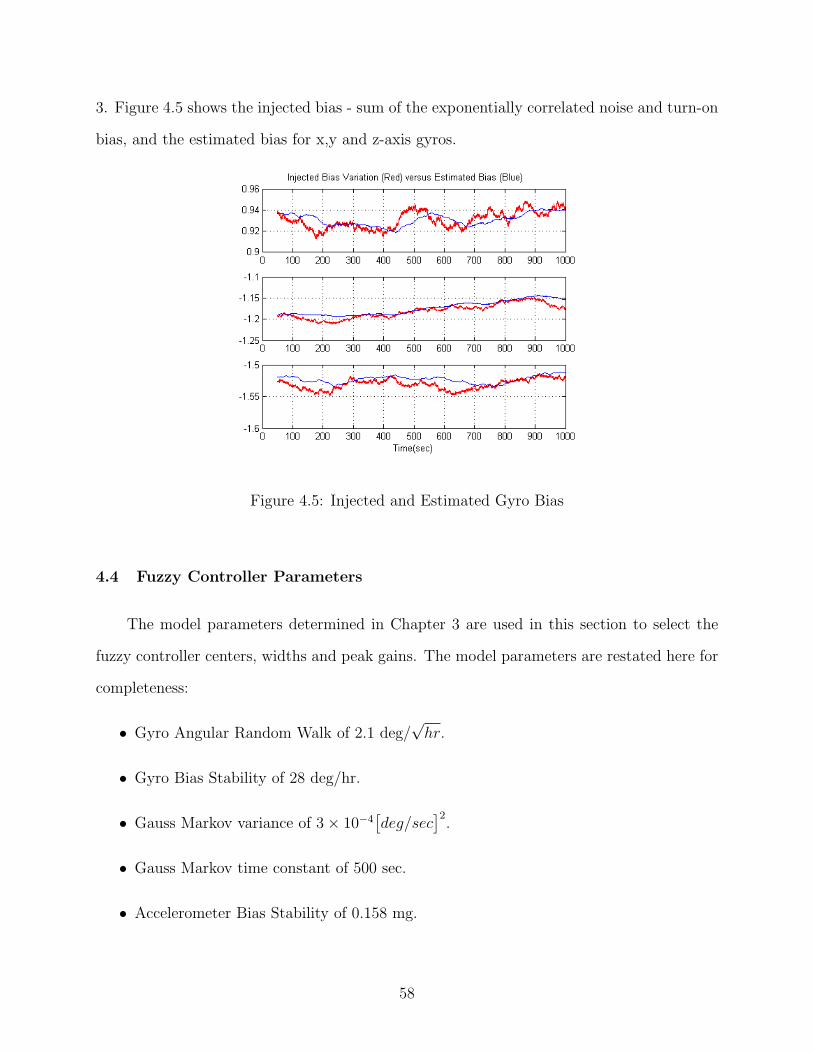
3. Figure 4.5 shows the injected bias - sum of the exponentially correlated noise and turn-on
bias, and the estimated bias for x,y and z-axis gyros.
Figure 4.5: Injected and Estimated Gyro Bias
4.4 Fuzzy Controller Parameters
The model parameters determined in Chapter 3 are used in this section to select the
fuzzy controller centers, widths and peak gains. The model parameters are restated here for
completeness:
• Gyro Angular Random Walk of 2.1 deg/√hr.
• Gyro Bias Stability of 28 deg/hr.
• Gauss Markov variance of 3× 10⁻⁴[deg/sec
]2.
• Gauss Markov time constant of 500 sec.
• Accelerometer Bias Stability of 0.158 mg.
58
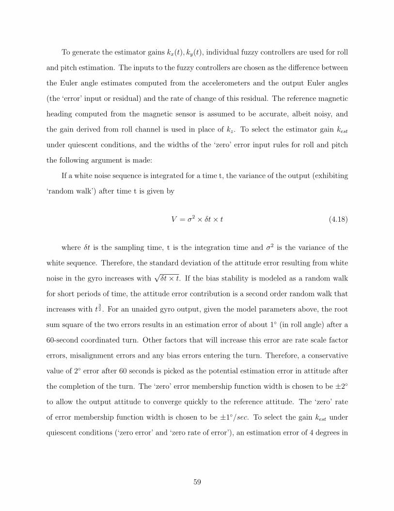
To generate the estimator gains kx(t), ky(t), individual fuzzy controllers are used for roll
and pitch estimation. The inputs to the fuzzy controllers are chosen as the difference between
the Euler angle estimates computed from the accelerometers and the output Euler angles
(the ‘error’ input or residual) and the rate of change of this residual. The reference magnetic
heading computed from the magnetic sensor is assumed to be accurate, albeit noisy, and
the gain derived from roll channel is used in place of kz. To select the estimator gain kest
under quiescent conditions, and the widths of the ‘zero’ error input rules for roll and pitch
the following argument is made:
If a white noise sequence is integrated for a time t, the variance of the output (exhibiting
‘random walk’) after time t is given by
V = σ2 × δt× t (4.18)
where δt is the sampling time, t is the integration time and σ2 is the variance of the
white sequence. Therefore, the standard deviation of the attitude error resulting from white
noise in the gyro increases with√δt× t. If the bias stability is modeled as a random walk
for short periods of time, the attitude error contribution is a second order random walk that
increases with t32 . For an unaided gyro output, given the model parameters above, the root
sum square of the two errors results in an estimation error of about 1 (in roll angle) after a
60-second coordinated turn. Other factors that will increase this error are rate scale factor
errors, misalignment errors and any bias errors entering the turn. Therefore, a conservative
value of 2 error after 60 seconds is picked as the potential estimation error in attitude after
the completion of the turn. The ‘zero’ error membership function width is chosen to be ±2
to allow the output attitude to converge quickly to the reference attitude. The ‘zero’ rate
of error membership function width is chosen to be ±1/sec. To select the gain kest under
quiescent conditions (‘zero error’ and ‘zero rate of error’), an estimation error of 4 degrees in
59

roll angle is artificially introduced with the true roll attitude set to zero as shown in Figure
4.6.
Figure 4.6: Roll Angle Convergence
The maximum gain kest is set to 0.5 rad/sec to get a time constant of approximately 20
seconds. Since kest > 0, the stability of the estimator for this gain setting follows from [12].
With the center and widths of the ‘zero error’ and ‘zero rate of error’ picked, the centers
and widths of ‘negative small’, ‘positive small’, ‘negative medium’ etc., are picked to be
equally spaced with identical widths. The output gains corresponding to these membership
functions are picked to decrease by a factor of 2, as the ‘error’ or ‘rate of error’ increases.
The gain profiles used by the fuzzy controller for roll and pitch channels are shown in Figures
4.7 and 4.8.
60
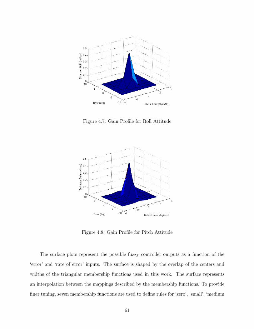
Figure 4.7: Gain Profile for Roll Attitude
Figure 4.8: Gain Profile for Pitch Attitude
The surface plots represent the possible fuzzy controller outputs as a function of the
‘error’ and ‘rate of error’ inputs. The surface is shaped by the overlap of the centers and
widths of the triangular membership functions used in this work. The surface represents
an interpolation between the mappings described by the membership functions. To provide
finer tuning, seven membership functions are used to define rules for ‘zero’, ‘small’, ‘medium
61
and ‘large’ positive and negative error. Similarly, seven membership functions are used for
the rate of error input. The centers and widths of the input rules are picked to be symmetric
on either side of the ’zero’ rule. Thus, the ‘negative small’ error rule is centered at −2, the
‘negative medium’ rule is centered at −4 etc. Under level flight conditions, when the error
e and the rate of change of error e are ‘zero’, the output attitude quaternion converges to
the reference quaternion qr and the output Euler angle estimates converge to the reference
angles. Under dynamic flight conditions, as the error e or e increases, the rate correction
and the bias integration gains are lowered by the fuzzy controller so that transients in qr can
be rejected.
62
Chapter 5
Performance Studies
5.1 Overview
This chapter presents a description of simulation studies and the results obtained using
the proposed attitude estimation algorithm to demonstrate compliance with some of the
requirements for an Attitude Heading Reference System. The sinusoidal motion and coor-
dinated turn simulations from Chapter 4 are exercised to highlight the effect of introducing
the fuzzy controller and to compare the results from the constant gain estimator. Real
world flight test inputs from an inexpensive inertial measurement unit are used to assess the
performance in flight and the results are compared with those from an aided Kalman filter
algorithm and outputs from a reference attitude estimator. The robustness of the proposed
algorithm is studied by evaluating the performance with no external aiding.
5.2 Simulation Studies
Depending on the operating modes that are supported, attitude heading reference sys-
tems are required to meet a minimum set of performace tests per various Technical Standard
Orders (TSO). For example, a settling error of less than 2 degrees after one hour of sinu-
soidal motion is required to be compliant with TSOC4c Bank and Pitch Instruments[15].
If a directional gyro heading mode is supported, the system is required to meet TSOC5e
Direction Instrument[16]. The simulation studies presented in this section were conducted
to obtain results for a few of these standard tests and assess the performance of the proposed
algorithm. The following tests are simulated by generating time series data in Simulink for
body frame gyroscopic rates, accelerations and magnetic field components:
63
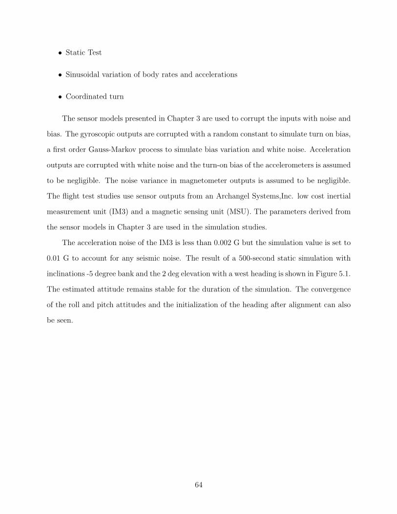
• Static Test
• Sinusoidal variation of body rates and accelerations
• Coordinated turn
The sensor models presented in Chapter 3 are used to corrupt the inputs with noise and
bias. The gyroscopic outputs are corrupted with a random constant to simulate turn on bias,
a first order Gauss-Markov process to simulate bias variation and white noise. Acceleration
outputs are corrupted with white noise and the turn-on bias of the accelerometers is assumed
to be negligible. The noise variance in magnetometer outputs is assumed to be negligible.
The flight test studies use sensor outputs from an Archangel Systems,Inc. low cost inertial
measurement unit (IM3) and a magnetic sensing unit (MSU). The parameters derived from
the sensor models in Chapter 3 are used in the simulation studies.
The acceleration noise of the IM3 is less than 0.002 G but the simulation value is set to
0.01 G to account for any seismic noise. The result of a 500-second static simulation with
inclinations -5 degree bank and the 2 deg elevation with a west heading is shown in Figure 5.1.
The estimated attitude remains stable for the duration of the simulation. The convergence
of the roll and pitch attitudes and the initialization of the heading after alignment can also
be seen.
64

Figure 5.1: Static Simulation
The simulated sinusoidal platform motion is an angular motion with an amplitude of
15 degrees and a frequency of 0.1 Hz. The motion is imparted such that the roll and pitch
motion are 90 degrees out-of-phase and the roll and yaw motion are in-phase. Figure 5.2 and
Figure 5.3 show convergence of the estimated roll and pitch attitude to the static attitude
after 3000 seconds of sinusoidal motion.
65
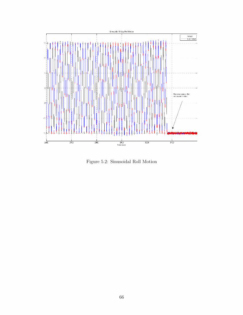
Figure 5.2: Sinusoidal Roll Motion
66
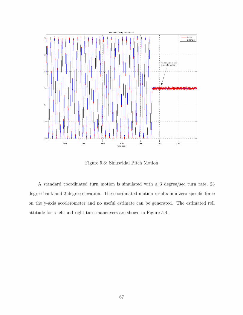
Figure 5.3: Sinusoidal Pitch Motion
A standard coordinated turn motion is simulated with a 3 degree/sec turn rate, 23
degree bank and 2 degree elevation. The coordinated motion results in a zero specific force
on the y-axis accelerometer and no useful estimate can be generated. The estimated roll
attitude for a left and right turn maneuvers are shown in Figure 5.4.
67
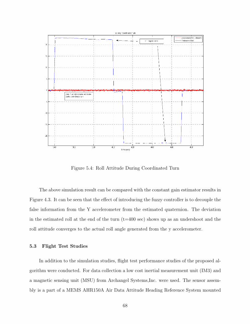
Figure 5.4: Roll Attitude During Coordinated Turn
The above simulation result can be compared with the constant gain estimator results in
Figure 4.3. It can be seen that the effect of introducing the fuzzy controller is to decouple the
false information from the Y accelerometer from the estimated quaternion. The deviation
in the estimated roll at the end of the turn (t=400 sec) shows up as an undershoot and the
roll attitude converges to the actual roll angle generated from the y accelerometer.
5.3 Flight Test Studies
In addition to the simulation studies, flight test performance studies of the proposed al-
gorithm were conducted. For data collection a low cost inertial measurement unit (IM3) and
a magnetic sensing unit (MSU) from Archangel Systems,Inc. were used. The sensor assem-
bly is a part of a MEMS AHR150A Air Data Attitude Heading Reference System mounted
68
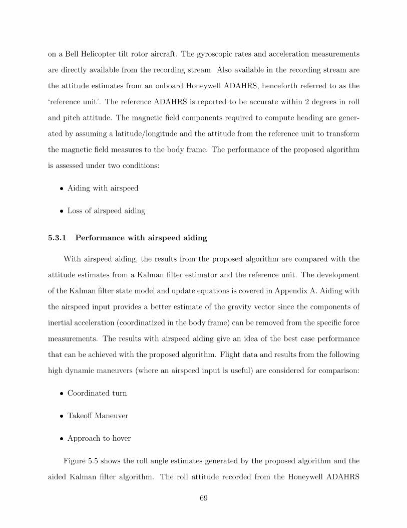
on a Bell Helicopter tilt rotor aircraft. The gyroscopic rates and acceleration measurements
are directly available from the recording stream. Also available in the recording stream are
the attitude estimates from an onboard Honeywell ADAHRS, henceforth referred to as the
‘reference unit’. The reference ADAHRS is reported to be accurate within 2 degrees in roll
and pitch attitude. The magnetic field components required to compute heading are gener-
ated by assuming a latitude/longitude and the attitude from the reference unit to transform
the magnetic field measures to the body frame. The performance of the proposed algorithm
is assessed under two conditions:
• Aiding with airspeed
• Loss of airspeed aiding
5.3.1 Performance with airspeed aiding
With airspeed aiding, the results from the proposed algorithm are compared with the
attitude estimates from a Kalman filter estimator and the reference unit. The development
of the Kalman filter state model and update equations is covered in Appendix A. Aiding with
the airspeed input provides a better estimate of the gravity vector since the components of
inertial acceleration (coordinatized in the body frame) can be removed from the specific force
measurements. The results with airspeed aiding give an idea of the best case performance
that can be achieved with the proposed algorithm. Flight data and results from the following
high dynamic maneuvers (where an airspeed input is useful) are considered for comparison:
• Coordinated turn
• Takeoff Maneuver
• Approach to hover
Figure 5.5 shows the roll angle estimates generated by the proposed algorithm and the
aided Kalman filter algorithm. The roll attitude recorded from the Honeywell ADAHRS
69

reference unit is also shown. The deviations in the roll estimates between the three outputs
are less than 2 degrees.
Figure 5.5: Aided Roll angle comparison between IKF and proposed algorithm
Figure 5.6 shows the pitch angle estimates during a takeoff maneuver with sustained
linear acceleration. The estimate from the proposed algorithm tracks the pitch angle from
the other two sources within 2 degrees.
70
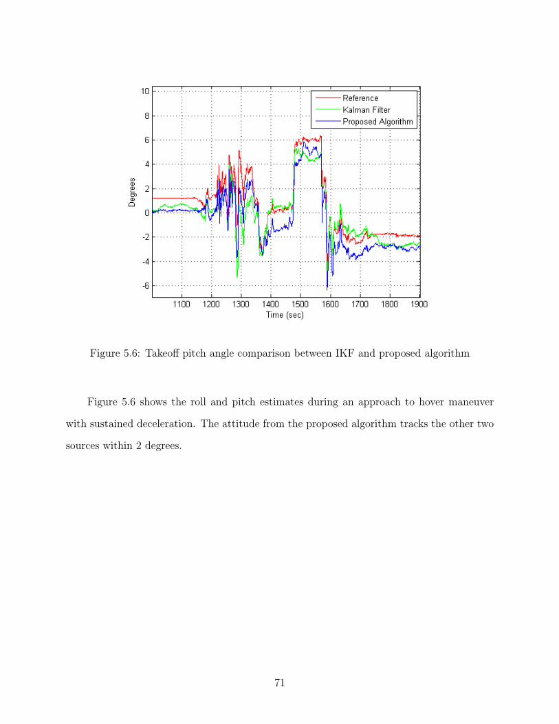
Figure 5.6: Takeoff pitch angle comparison between IKF and proposed algorithm
Figure 5.6 shows the roll and pitch estimates during an approach to hover maneuver
with sustained deceleration. The attitude from the proposed algorithm tracks the other two
sources within 2 degrees.
71
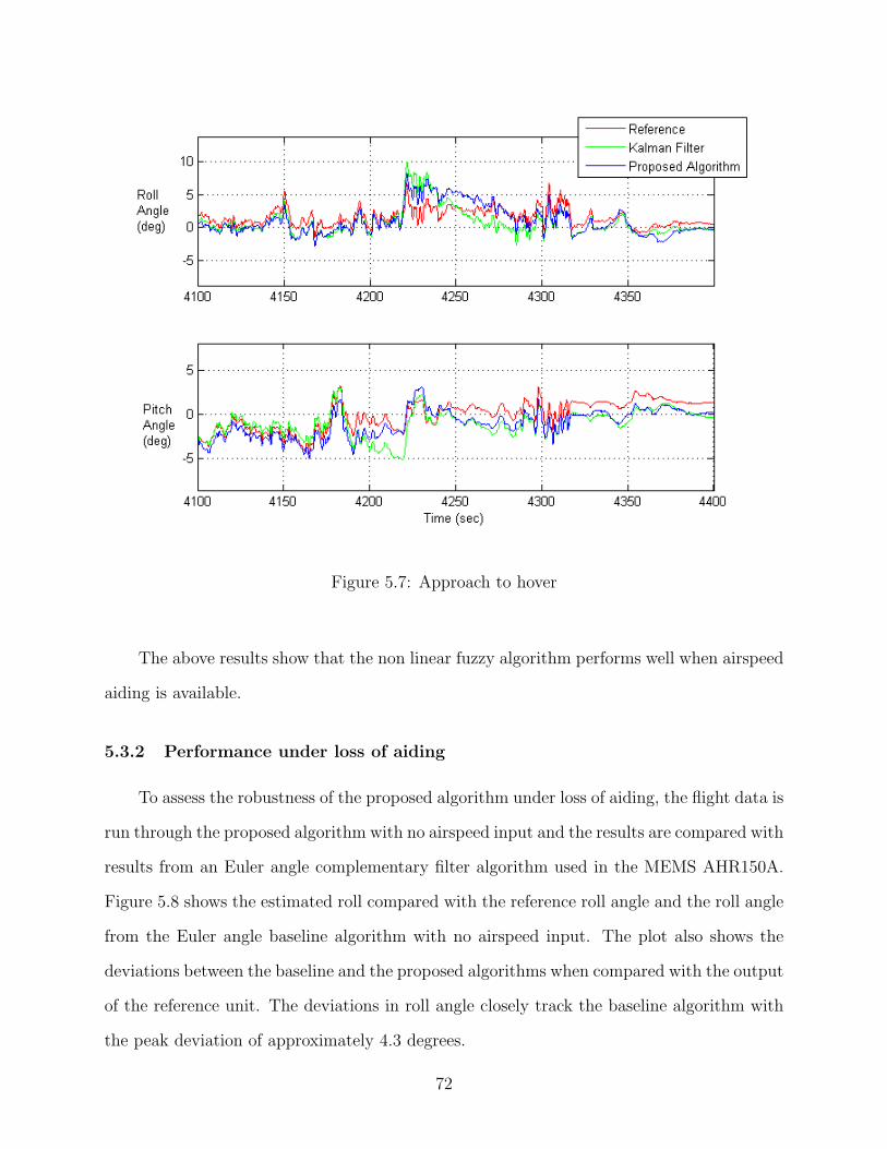
Figure 5.7: Approach to hover
The above results show that the non linear fuzzy algorithm performs well when airspeed
aiding is available.
5.3.2 Performance under loss of aiding
To assess the robustness of the proposed algorithm under loss of aiding, the flight data is
run through the proposed algorithm with no airspeed input and the results are compared with
results from an Euler angle complementary filter algorithm used in the MEMS AHR150A.
Figure 5.8 shows the estimated roll compared with the reference roll angle and the roll angle
from the Euler angle baseline algorithm with no airspeed input. The plot also shows the
deviations between the baseline and the proposed algorithms when compared with the output
of the reference unit. The deviations in roll angle closely track the baseline algorithm with
the peak deviation of approximately 4.3 degrees.
72

Figure 5.8: Unaided Roll Angle Comparison
Figure 5.9 shows the pitch angle comparison with the reference and the Euler angle
baseline algorithm with no airspeed input. The plot also shows the deviations between the
baseline and the proposed algorithms. The deviations in pitch angle match up well with the
baseline results.
73
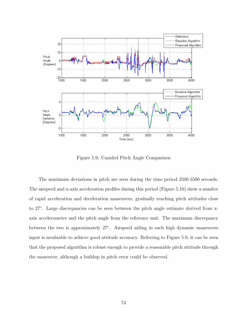
Figure 5.9: Unaided Pitch Angle Comparison
The maximum deviations in pitch are seen during the time period 2500-3500 seconds.
The airspeed and x-axis acceleration profiles during this period (Figure 5.10) show a number
of rapid acceleration and deceleration maneuvers, gradually reaching pitch attitudes close
to 27. Large discrepancies can be seen between the pitch angle estimate derived from x-
axis accelerometer and the pitch angle from the reference unit. The maximum discrepancy
between the two is approximately 27. Airspeed aiding in such high dynamic maneuvers
input is invaluable to achieve good attitude accuracy. Referring to Figure 5.9, it can be seen
that the proposed algorithm is robust enough to provide a reasonable pitch attitude through
the maneuver, although a buildup in pitch error could be observed.
74
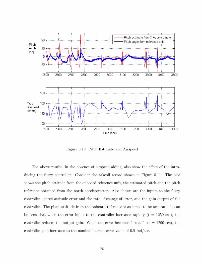
Figure 5.10: Pitch Estimate and Airspeed
The above results, in the absence of airspeed aiding, also show the effect of the intro-
ducing the fuzzy controller. Consider the takeoff record shown in Figure 5.11. The plot
shows the pitch attitude from the onboard reference unit, the estimated pitch and the pitch
reference obtained from the north accelerometer. Also shown are the inputs to the fuzzy
controller - pitch attitude error and the rate of change of error, and the gain output of the
controller. The pitch attitude from the onboard reference is assumed to be accurate. It can
be seen that when the error input to the controller increases rapidly (t = 1250 sec), the
controller reduces the output gain. When the error becomes ”‘small”’ (t = 1290 sec), the
controller gain increases to the nominal ”zero”’ error value of 0.5 rad/sec.
75
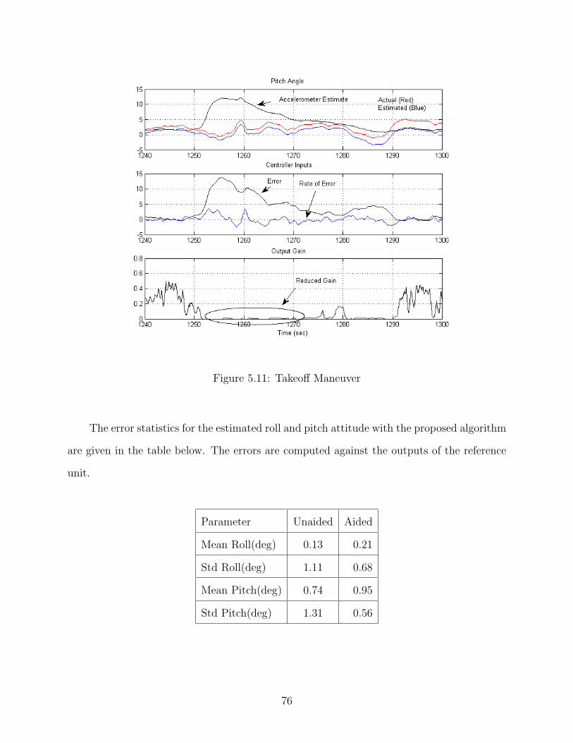
Figure 5.11: Takeoff Maneuver
The error statistics for the estimated roll and pitch attitude with the proposed algorithm
are given in the table below. The errors are computed against the outputs of the reference
unit.
Parameter Unaided Aided
Mean Roll(deg) 0.13 0.21
Std Roll(deg) 1.11 0.68
Mean Pitch(deg) 0.74 0.95
Std Pitch(deg) 1.31 0.56
76
Chapter 6
Conclusions
6.1 Overview
This dissertation presented a robust attitude estimation algorithm combining non linear
observer techniques with an adaptive fuzzy logic controller for attitude and heading reference
systems. The proposed estimation algorithm is an extension of the recent work on non linear
attitude observers proposed by various authors for spacecraft applications. These observers,
however, required an independent measurement of platform attitude to estimate the attitude
error and the gyro bias and do not perform well when the augmentation sources provide false
information. In the effort to address this problem, this dissertation reviewed some of the
attitude representation and estimation techniques including non linear estimation techniques
that operate in SO(3) and quaternion spaces. Sensors models for the low cost MEMS sensors
used were presented and the model verification was performed by using techniques such as
Allan Variance. Model parameters were used to develop the fuzzy logic-quaternion estimation
algorithm that relies on gravity and magnetic vectors to derive the reference attitude. Flight
test data were used to compare the estimation performance of the proposed algorithm with
baseline results. In the presence of airspeed aiding, the algorithm was shown to provide
attitude estimates comparable to other attitude estimators such as an extended Kalman filter.
The robustness of the algorithm was shown by evaluating the performance from takeoff to
landing with no external aiding sources like air data systems, GPS etc. The results of offline
processing showed that, under loss of external aiding, the proposed algorithm performed
reasonably well even through some dynamic maneuvers involving rapid accelerations. The
overall performance of the proposed algorithm makes it ideal for implementation as part
77

of an inexpensive backup attitude estimation system that can continue to provide attitude
estimates when aiding sources are unavailable.
6.2 Future Work
Improving the estimation accuracy during high dynamic maneuvers, when no external
aiding is available, is an obvious area for improvement in the adaptive correction scheme pro-
posed in this work. Adding more fuzzy controller input rules could help in better predicting
the conditions to engage and disengage augmentation. However, when the augmentation
sources cannot be trusted, the bias stability of the gyro limits the achievable attitude ac-
curacy and the growth of error. The proposed algorithm could be extended to fuse inputs
from multiple aiding sources, for example GPS and an air data system, to provide attitude
estimates and inertial velocity estimates for a hover-on-point application.
78
Bibliography
[1] IEEE Std 952-1997. IEEE standard specication format guide and test procedure for
single-axis interferometric fiber optic gyros. IEEE Standards Board, 1997.
[2] D.W Allan. Statistics of atomic frequency standards. Proceedings of the IEEE, Vol.54,
No.2, 1966.
[3] Albert-Jan Baerveldt and Robert Klang. A low-cost and low-weight attitude estimation
system for an autonomous helicopter. Intelligent Engineering Systems, 1997.
[4] I.Y. Bar-Itzhack and M. Idan. Recursive attitude determination from vector obser-
vations: Euler angle estimation. AIAA Journal of Guidance Control and Navigation,
1987.
[5] I.Y. Bar-Itzhack and Y. Oshman. Attitude determination from vector observations:
Quaternion estimation. IEEE Transactions on Aerospace and Electronic Systems, 1985.
[6] Neil Barbour and George Schmidt. Inertial sensor technology trends. IEEE Sensors
Journal, 2001.
[7] Robert Grover Brown and Patrick Y.C. Hwang. Introduction to Random Signals and
Applied Kalman Filtering. The American Institute of Aeronautics and Astronautics,
1997.
[8] C.Moler and G.Van Loan. Nineteen dubious ways to compute the exponential of a
matrix. SIAM review, Vol 20, No.4, 1978.
[9] D.H.Titterton and J.L.Weston. Strapdown Inertial Navigation Technology. The Ameri-
can Institute of Aeronautics and Astronautics, 2004.
79
[10] Demoz Gebre-Egziabher et al. A gyro-free quaternion-based attitude determination
system for implementation using low cost sensors. Proceedings of the IEEE Position
Location and Navigation Symposium, 2000.
[11] R.C.Hayward et al. Inertially aided GPS based attitude heading reference system(ahrs)
for general aviation aircraft. Proceedings of ION-GPS, 1997.
[12] Robert Mahony et al. Complementary filter design on the special orthogonal group
SO(3). Proceedings of the 44th IEEE Conference on Decision and Control, 2005.
[13] R.P.Kornfeld et al. Single antenna GPS based aircraft attitude determination. J.
Institute of Navigation, 1998.
[14] B.Vik et.al. Nonlinear observer design for integration of DGPS and INS. New Directions
in Nonlinear Observer Design,ser. Lecture Notes in Control and Information Sciences,
1999.
[15] FAA. Tso-c4c bank and pitch instruments. Federal Aviation Administration, 1959.
[16] FAA. Tso-c5e direction instrument, non-magnetic(gyroscopically stabilized). Federal
Aviation Administration, 1989.
[17] Demoz Gebre-Egziabher. Design and Analysis of Performance Analysis of a low-cost
aided dead reckoning navigator. Stanford University, 2004.
[18] J.Thienel and R.M.Sanner. A coupled nonlinear spacecraft attitude controller and ob-
server with an unknown constant gyro bias and gyro noise. IEEE Transactions on
Automatic Control, 2003.
[19] Jack B. Kuipers. Quaternions and Rotation Sequences. Princeton University Press,
1999.
80
[20] E.Glenn Lightsey and Jared Madsen. Three-axis attitude determination using global
positioning system signal strength measurements. J. Guidance, Control and Dynamics,
2003.
[21] F. Landis Markley. Fast quaternion attitude estimation from two vector measurements.
J. Guidance, Control and Dynamics, 2002.
[22] M.Greene and V.Trent. Software algorithms in air data attitude heading reference
systems. Aircraft Engineering and Aerospace Technology, 2003.
[23] Kevin M.Passino and Stephen Yurkovich. Fuzzy Control. Addison Wesley, 1998.
[24] Malcolm D. Shuster. A Survey of Attitude Representations. Journal of Astronautical
Sciences, 1993.
[25] S.Salcudean. A globally convergent angular velocity observer for rigid body motion.
IEEE Transactions on Automatic Control, 1991.
[26] Nikolas Trawny and Stergios I.Roumeliotis. Indirect Kalman Filter for 3D attitude
estimation. A Tutorial for Quaternion Algebra, 2005.
[27] Grace Wahba. A least-squares estimate of spacecraft attitude. SIAM Review, 1965.
81
Appendix A
Kalman Filter Formulation
A.1 Overview
The development of an extended Kalman filter for quaternion attitude estimation is
addressed in the following sections. The Kalman filter is used to estimate errors in the
attitude quaternion and gyro bias. The development of a state-space model for the Kalman
filter is based on [26].
A.2 Extended Kalman Filter
The following data inputs are used in the Kalman filter algorithm:
• Triad of gyroscopic rates
• Triad of accelerations
• Triad of magnetic measures
• True airspeed computed by an air data system
Using true airspeed as an aiding input allows compensation for linear accelerations in deter-
mining the reference attitude quaternion. The state-space model for the filter can be written
by starting with the gyro measurement model, assuming that the deterministic errors have
been calibrated. If the deterministic errors in gyros are assumed to be calibrated, the gyro
model can be written as
ωm = ωT + b + ηr (A.1)
82
where ωm and ωT are the measured and the true angular rates, b is the bias and ηr is the
rate noise and assumed to be white. If the estimated rate is ω, then
ω = ωm − b (A.2)
ω = ω − δb− ηr (A.3)
where b is the estimated bias and δb is the bias error. If the estimated attitude quaternion
is represented by q and the true attitude quaternion by q, then the quaternion error can be
represented as the incremental rotation δq necessary to rotate the estimated quaternion to
align with the true quaternion.
q = δq ⊗ q (A.4)
The true and estimated attitude quaternion dynamics are given by the equations
q =1
2
0
ω
⊗ q (A.5)
˙q =1
2
0
ω
⊗ q (A.6)
The quaternion error dynamics can be derived from the above equations as
δq = −Θ(ω)δq − 1
2δb− 1
2nr (A.7)
The bias error dynamics are modeled as a first order Gauss Markov process as
δb = −βδb+ nw (A.8)
83
where nw is the driving noise process of the Gauss Markov process and Θ(ω) is the skew-
symmetric matrix
Θ(ω) =
0 −ωz ωy
ωz 0 −ωx
−ωy ωx 0
(A.9)
The continuous-time state and measurement equations for the quaternion and bias errors is
given by δqδb
=
−S(ω) −12I3x3
03x3 −βI3x3
δqδb
+
−12I3x3 0
0 I3x3
nrnw
(A.10)
z =
[I3x3 03x3
]δqδb
+
v1
v2
v3
(A.11)
In formulating the above equations, the attitude errors are assumed to be small and
only the vector components of the quaternion are considered. The process noise covariance
and the measurement noise covariance matrices are given by
Q =
σ2gI3x3 03x3
03x3 σ2gmI3x3
(A.12)
R = σ2aI3x3 (A.13)
where σ2g is the rate noise covariance, σ2
gm is the covariance of the Gauss Markov process
modeled using experimental autocorrelation, and σ2a is the measurement noise covariance.
The discretized versions of the matrices are given by [7]:
A = exp(F∆t) (A.14)
Qd = GQGT (A.15)
84
Rd =R
∆t(A.16)
where F is the system matrix in the state equation. The computation of the state transition
matrix A is performed by using a Taylor’s series approximation for the exponential, following
the treatment in [8]. The difficulty in accurately calculating the noise variances, especially
for gyro bias drift modeled as an exponentially correlated process, introduces errors in the
initialization values for the covariance matrices Q and R. As a result, optimality of the
Kalman filter is difficult to achieve in practice. Therefore, the error covariance Pk at each
step is updated using the generalized update equation that holds for any Kalman gain -
optimal or otherwise [7]:
Pk = (I −KkHk)Pk−(I −KkHk)
T +KkRkKTk (A.17)
The reference attitude quaternion is derived from acceleration and magnetometer mea-
surements, along with the true air speed. Since the y-axis accelerometer does not provide
any information about the roll attitude during a non-slipping turn, true airspeed and inertial
yaw rate are used to derive the reference roll attitude using the equation:
tan(φ) =UΨ
G(A.18)
where U is the true air speed in meters per second, Ψ is the Euler yaw rate in rad/sec in the
local reference frame and G is the acceleration due to gravity. The measurement input for
the Kalman filter is the quaternion error between the reference and the quaternion updated
using the current body rates and bias estimates.
85