Attitude Determination Algorithms through Accelerometers

Research ArticleAttitude Determination Algorithms through Accelerometers,GNSS Sensors, and Gravity Vector Estimator

Raúl de Celis and Luis Cadarso

European Institute for Aviation Training and Accreditation (EIATA), Rey Juan Carlos University, 28943 Fuenlabrada, Spain

Correspondence should be addressed to Raúl de Celis; [email protected]

Received 6 October 2017; Accepted 29 November 2017; Published 4 February 2018

Academic Editor: Linda L. Vahala

Copyright © 2018 Raúl de Celis and Luis Cadarso. This is an open access article distributed under the Creative CommonsAttribution License, which permits unrestricted use, distribution, and reproduction in any medium, provided the original workis properly cited.

Aircraft and spacecraft navigation precision is dependent on the measurement system for position and attitude determination.Rotation of an aircraft can be determined measuring two vectors in two different reference systems. Velocity vector can bedetermined in the inertial reference frame from a GNSS-based sensor and by integrating the acceleration measurements in thebody reference frame. Estimating gravity vector in both reference frames, and combining with velocity vector, determinesrotation of the body. A new approach for gravity vector estimations is presented and employed in an attitude determinationalgorithm. Nonlinear simulations demonstrate that using directly the positioning and velocity outputs of GNSS sensors andstrap-down accelerometers, aircraft attitude determination is precise, especially in ballistic projectiles, to substitute preciseattitude determination devices, usually expensive and forced to bear high solicitations as for instance G forces.

1. Introduction

Obtaining precise attitude information is essential fornavigation and control. The effectiveness of navigation andcontrol is determined by the degree of precision of navigationand control systems, including inertial measurement units[1]. There is an extensive body of literature regarding attitudeestimation using various sensor inputs [2].

Traditionally, in order to obtain accurate values fordetermining attitude, expensive and/or weighty units, suchas laser or fiber optic gyroscopes and accelerometers, or theirMEMS equivalent must be employed. Moreover, when high-demanding maneuvers are performed, this equipment maybecome extremely expensive.

Other methods, based on very precise and advancedcarrier-phase single-frequency GNSS attitude determinationalgorithms or multi-GNSS developments of integratingGNSS systems for attitude determination, are not possibleto be applied on these artillery devices due the small spaceavailable on the vehicle. At present, the best carrier-phase-based method for GNSS attitude determination is the multi-variate constrained MC-LAMBDA method. This method is

currently the best performing attitude determination methodas was demonstrated in land, sea, and air experiments. Exam-ple publications describing such actual real-world GNSS-attitude determination results can be found in [3–6]. Theunderlying theory and advanced algorithms for much ofthe above-referred integer-ambiguity-resolved carrier-phaseGNSS attitude determination methods can be found in[7–9]. Multi-GNSS developments of integrating GNSS sys-tems for attitude determination are stated in [10, 11].

It is well known that the attitude of an aero-vehicle can bedetermined, starting from an initial condition, by integratingthe angular rates (pitch, roll, and yaw rates) of the vehicle andpropagating them forward time. Nevertheless, accuracyrequirements usually cannot be satisfied by using inexpensivesensors [1]. This problem becomes even more importantwhen the vehicle cannot be reused: low-cost attitude determi-nation systems are of key importance for these applications.For example, Gebre-Egziabher et al. [12] describe an attitudedetermination system that is based on two measurements ofnonzero, noncollinear vectors. Using the Earth’s magneticfield and gravity as the two measured quantities, a low-costattitude determination system is proposed. Gebre-Egziabher

HindawiInternational Journal of Aerospace EngineeringVolume 2018, Article ID 5394057, 14 pageshttps://doi.org/10.1155/2018/5394057

http://orcid.org/0000-0002-7940-8097

http://orcid.org/0000-0002-5382-2927

https://doi.org/10.1155/2018/5394057

et al. [13] develop an inexpensive attitude heading referencesystem for general aviation applications by fusing low-costautomotive-grade inertial sensors with GPS. The inertial sen-sor suit consists of three orthogonally mounted solid-state-rate gyros. Eure et al. [14] describe an attitude estimationalgorithm derived by postprocessing data from a small low-cost inertial navigation system recorded during the flight ofa subscale commercial off-the-shelf UAV. Estimates of theUAV attitude are based on MEMS gyro, magnetometer,accelerometer, and pitot tube inputs.

Henkel and Iafrancesco [15] state that low-cost GNSSreceivers and antennas can provide a precise attitude anddrift-free position information, but accuracy is not continu-ous. Inertial sensors are robust to GNSS signal interruptionand very precise over short time frames, which enables a reli-able cycle slip correction, but low-cost inertial sensors sufferfrom a substantial drift. The authors propose a tightlycoupled position and attitude determination method fortwo low-cost GNSS receivers, a gyroscope and an accelerom-eter, and obtain a heading with an accuracy of 0.25°/baselinelength (m) and an absolute position with an accuracy of 1m.Similar developments may be found within space vehicles,for example, in [16]. In [17], the use of an inertial navigationsystem (INS) and a multiple GPS antenna system for attitudedetermination of an off-road vehicle is developed, and in[18], attitude determination using the GPS carrier phasehas been applied successfully to aircrafts in experiments bya number of researchers.

Also, improved algorithms for estimating attitude incase of failures have been proposed in the literature. Forexample, Soken and Hajiyev [19] introduce algorithmswith filter gain correction for the case of measurementmalfunctions. Two different algorithms are proposed andapplied for the attitude estimation process of a pico satel-lite. The results of these algorithms are compared for dif-ferent types of measurement faults in different estimationscenarios, and recommendations about their applicationsare given. Another example is exposed in [20]. This algo-rithm is based on interacting multiple models (IMM)extended Kalman filters (EKF) using a star sensor and gyro-scope data. In Liu et al. 2011, a computationally efficient non-linear attitude estimation strategy is based on the vectorobservations for satellites.

However, as stated in [21], many of the presentedmethods such as those employing local magnetic field vectorsare only valid for estimating the orientation of a slow-rotation body. On the other hand, for high spin rate bodies,electromagnetic interactions degrade magnetic measure-ments. In the research described in this paper, two measuredquantities are used to obtain attitude information for highdynamic and high spin rate vehicles: speed and gravity vec-tors. They are obtained in two different reference framesusing a GNSS sensor and a strap-down accelerometer.

1.1. Contributions. The main contributions of this paperare twofold. First is the development of a novel algorithmwhich avoids the use of gyroscopes for attitude determina-tion. This is purposed to decrease costs in attitude sensorsand even to improve attitude determination by applying

filtering techniques, especially for artillery device applica-tions, where high acceleration conditions increase the priceof precise attitude determination devices such as gyroscopes.Second is the development of an estimation method in orderto obtain the gravity vector in body axes. This estimator ismotivated by the need of having two vectors expressed intwo different triads in order to determine attitude changes.Flight nonlinear simulations are performed to determinereal attitude and compare it to the estimated attitudeobtained from the algorithms. The applicability of the pro-posed solution for aircraft flight navigation, guidance, andcontrol or for ballistic rocket terminal guidance, whereattack and side-slip angles or total angle of yaw are rela-tively small, is also demonstrated.

This paper is organized as follows. Section 2 describes theproblem in detail. Section 3 is devoted to the estimation ofthe gravity vector. The attitude determination algorithm isdetailed in Section 4. Flight dynamics and sensor modelsare briefly described in Section 5. Section 6 shows simulationresults. Conclusions and references follow.

2. Problem Description

Attitude determination is a fundamental field in aircraft engi-neering, as maneuvers in order to change vehicle trajectoriesare governed by aerodynamic forces, which depend directlyon ship orientation angles. Furthermore, attitude in the artil-lery rocket terminal phase is vital as it determines factors aspenetrability of payload or avoidability of countermeasuresfor the artillery rocket. Therefore, developing algorithms toimprove attitude determination is a cornerstone in preciseguidance, navigation, and control research.

One of the techniques to determine attitude is to calculateit from the director cosine matrix (DCM) which determinescompletely the rotation of a body between two referenceframes. In order to obtain this DCM, a geometrical planedefined in both reference triads must be obtained. Every geo-metrical plane is defined by two vectors, and therefore, know-ing the same two vectors expressed in the two referenceframes, DCM may be calculated.

2.1. Triad Definition. Two axis systems are defined in order toexpress forces and moments: north-east-down (NED) axesand body (B) axes. NED axes are defined by subindex NED.xNED is pointing north, zNED is perpendicular to xNED andpointing nadir, and yNED is forming a clockwise trihedron.Body axes are defined by subindex B. xB is pointing forwardand contained in the plane of symmetry of the rocket, zB isperpendicular to xB pointing down and contained in theplane of symmetry of the rocket, and yB is forming a clock-wise trihedron. The origin of body axes is located at the cen-ter of mass of the rocket.

2.2. Involved Vector Determination. If a GNSS sensordevice is equipped on the aircraft, velocity vector can bedirectly expressed from the sensor velocity output on theNED triad. Expression for velocity in NED is defined in(1), where vxNED , vyNED , and vzNED are the components ofthis velocity in NED axes.

2 International Journal of Aerospace Engineering

vNED = vxNED , vyNED , vzNEDT

1

The same velocity vector expressed in body triad can beobtained from a set of accelerometers equipped on the ship,one on each of the axes. These devices are able to measureacceleration. After integration of each of the componentsalong time, velocity vector is obtained, which is expressedin (2), where axB , ayB , and azB are the components of the

acceleration in body axes and ωb describes angular velocityexpressed in body axes.

vB = vB t=0 + axB , ayB , azBT+ ωB × vB dt 2

Another vector expressed in two bases is required inorder to define the rotation. Gravity vector is very simpleto determine in NED triad as it is always parallel tozNED, as it is shown in (3), where g is the gravity acceler-ation, which is fixed constant in this model (9.81m/s2).Note that precision may be increased using more compli-cated models, that is, it can be modeled depending on latitudeand longitude of the aircraft.

gNED = g 0, 0, 1 T 3

The keystone of the presented attitude determinationmethod is determining gravity vector in body axes.Methods to calculate this gravity vector are developed in[22]. For example, by determining the constant compo-nent of the measured acceleration employing a low passfilter, where jerk in body axes is calculated by derivationof acceleration, then, it is integrated in order to obtain thenonconstant component of acceleration, and, by subtract-ing this nonconstant component from the measured accel-eration, gravity vector is estimated. However, this methodis not valid when the aircraft rotates. Another method toobtain gravity vector is by integrating the mechanizationequations [23] and manipulating consequently the resultingequations. Again, gyros are needed in order to implementthis method.

In the next section, a new estimation method, which isvalid for nonrotating and rotating aircrafts and which doesnot need gyros, is presented.

3. Gravity Vector Estimation

The gravity vector estimation method presented heredepends on the aerial platform on which it will be employed.This means that the method must be adjusted for the aircraftof interest. Without loss of generality, the estimation methoddetailed in this section (and also Sections 5 and 6) is particu-larized for a four-canard-controlled spinning rocket. But,using the applicable flight mechanics equations, it may beapplied to other aircraft.

The estimated gravity vector may be expressed as in (4),where its components in body axes are shown.

gB = gxB, gyB , gzB

T4

In order to describe the estimator, the gravity vector mustbe modeled as a subtraction between accelerations measuredby accelerometers in body axes ( AB ) and an estimation ofthe aerodynamic and control forces expressed also in bodyaxes. Equation (5) describes this estimator as a particulariza-

tion of Newton-Euler equations, where Fai describes aerody-

namic and inertial forces, Fcontrol describes control forces,and m describes aircraft mass.

gB = AB −1m

Fai + Fcontrol 5

In order to compute gB, Fai , Fcontrol, and ωB must beestimated exclusively from data obtained from GNSS sensorsand accelerometers. First of all, the Mach number (M) andangle of attack (α), which are shown in (6), are estimatedfrom accelerometer data. This hypothesis is completely validfor small angles of attack, which is the case for the flightsdescribed in this paper. The Mach number and angle ofattack must be calculated in order to estimate forces andmoments involved on aircraft flight. Speed of sound isobtained as a function of altitude (a zNED ) employing theInternational Standard Atmosphere (ISA) model. This alti-tude is directly obtained from the GNSS positioning outputof the sensor.

M =vB

a zNED,

α = a cosvB ⋅ xBvB

6

Passive aerodynamic and inertial forces ( Fai ) are calcu-lated according to

Fai = D + L + MF + P + C , 7

where D is the drag force, L is the lift force, MF is the

Magnus force, P is the pitch damping force, and C is theCoriolis force.

Each of these forces is estimated by the expressions in (8),where ρ zNED is the air density as a function of altitudeusing the ISA model, d is the rocket caliber, CD0

M is thedrag force linear coefficient, CDa2

M is the drag force squarecoefficient, CLa

M is the lift force linear coefficient, CLa3M

is the lift force cubic coefficient, Cmf M is the Magnus forcecoefficient, Ix and Iy are the rocket inertia moments in bodyaxes, CNq M is the pitch damping force coefficient, and Ω isthe earth angular velocity vector. Note that aerodynamiccoefficients are dependent of the Mach number, which wascalculated in (6).

3International Journal of Aerospace Engineering

D = −π

8d2ρ zNED CD0

M + CDα2M α2 vB vB,

L = −π

8d2ρ zNED CLα

M α + CLα3M α2

⋅ vB2 ⋅ xB − xB ⋅ vB vB ,

MF = −π

8d3ρ zNED

Cmf MIx

Ix ωB ⋅ xB xB + IyxB × ωB × xB ⋅ xB xB × vB ,

P = −π

8d3ρ zNED

CNq M

IyvB

2

⋅ Ix ωB ⋅ xB xB + IyxB × ωB × xB × xB ,

C = −2mΩ × vB8

In order to estimate the required forces to estimate thegravity vector, angular velocity is required. Newton-Eulerequations are used in order to estimate angular velocity(see (9)), where IB is the rocket inertia tensor defined in

(10), Mai are the passive aerodynamic moments which actu-

ate on the projectile, andMcontrol are the moments generatedby control surfaces. Passive aerodynamic moments are

defined in (11), where O is the overturn moment, PM is

the pitch damping moment, MM is the Magnus moment,

and S is the spin damping moment.

ωB = I−1B Mai +Mcontrol − ωB × IB ωB dt, 9

IB =Ix 0 0

0 Iy 0

0 0 Iy

,

I−1B =

1Ix

0 0

01Iy

0

0 01Iy

,

10

Mai = O + PM +MM + S 11

Each of the aerodynamic moments is estimated in (12),where CMα

M is the overturning moment linear coefficient,CMα3

M is the overturning moment cubic coefficient,CMq

M is the pitch damping moment coefficient, Cmm M

is the Magnus moment coefficient, and Cspin M is the spindamping moment coefficient.

O = π

8d3ρ zNED CMα

M α + CMα3M α2

⋅ vB2 vB × xB ,

PM = π

8d3ρ zNED

1IyCMq

M vB

⋅ Ix ωB ⋅ xB xB + IyxB × ωB × xB

− Ix ωB ⋅ xB xB + IyxB × ωB × xB ⋅ xB xB ,

MM =π

8d4ρ zNED

1IyCmm M

⋅ Ix ωB ⋅ xB xB + IyxB

× ωB × xB ⋅ xB ⋯ vB ⋅ xB xB − vB ,

S =π

8d4ρ zNED

1IyCspin M vB

⋅ Ix ωB ⋅ xB xB + IyxB × ωB × xB ⋅ xB xB

12

Similarly, control forces and moments in body axes foreach of the four fins must be estimated. For this purpose,the similar model as defined in [24] is employed, but withsome modifications in the aerodynamics. The first modifica-tion is that the effective incidence aerodynamic speed on eachof the four fins must be estimated.

The mathematical expressions for incidence aerody-namic speed decomposition are defined in

vef f xi= vB − vB ⋅ ubi ubi , ∀i ∈ 1, 2, 3, 4 ,

vef f yi= vB − vB ⋅ ubi ubi

− vB − vB ⋅ ubi ubi ⋅ xb xb , ∀i ∈ 1, 2, 3, 4 ,13

where i denotes the fin and vef f xiand vef f yi

are the aero-

dynamic speed minus the fin-span component of theaerodynamic speed and the perpendicular component ofvef f xi

to xb, respectively, ub1 = 0, 0, −1 , ub2 = 0, −1, 0 ,

ub3 = 0, 0, 1 , and ub4 = 0, 1, 0 .The effective angle of attack for each fin (αef f i ) may be

expressed for each fin as the sum of the local angle of attack,αi, and fin deflection, δi (see the following equation).

αef f i = αi + δi = sin vef f yi⋅ uFNi

⋅ a cosvef fxivef fxi

⋅ xb + δi, ∀i ∈ 1, 2, 3, 4 ,

14

where uFN1= 0, 1, 0 , uFN2

= 0, 0, −1 , uFN3= 0, −1, 0 , and

uFN4= 0, 0, 1 .


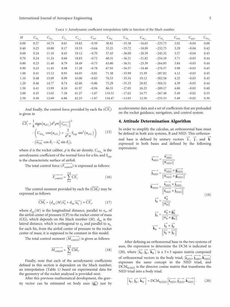
And finally, the control force provided by each fin (CFi)is given in

CFi =18sign αef f i d

2ρπ vef fxi

2

CNαwcos αef f i +

2d2π

Sexp sin2 αef f i

uFNicos δi − xb sin δi ,

15

where d is the rocket caliber, ρ is the air density, CNαwis the

aerodynamic coefficient of the normal force for a fin, and Sexpis the characteristic surface of airfoil.

The total control force (Fcontrol) is expressed as follows:

Fcontrol = 〠i=4

i=1CFi 16

The control moment provided by each fin (CMi) may beexpressed as follows:

CMi = dax M xb + dlat ubi × CFi , 17

where dax M is the longitudinal distance, parallel to xb, ofthe airfoil center of pressure (CP) to the rocket center of mass(CG), which depends on the Mach number (M). dlat is thelateral distance, which is orthogonal to xb and parallel to ubifor each fin, from the airfoil center of pressure to the rocketcenter of mass; it is supposed to be constant in this model.

The total control moment Mcontrol is given as follows:

Mcontrol = 〠i=4

i=1CMi 18

Finally, note that each of the aerodynamic coefficientsdefined in this section is dependent on the Mach number;an interpolation (Table 1) based on experimental data forthe geometry of the rocket analyzed is provided next.

After this previous mathematical development, the grav-ity vector can be estimated on body axes (gB) just by

accelerometer data and a set of coefficients that are preloadedon the rocket guidance, navigation, and control system.

4. Attitude Determination Algorithm

In order to simplify the calculus, an orthonormal base mustbe defined in both axis systems, B and NED. This orthonor-

mal base is defined by unitary vectors i , j , and kexpressed in both bases and defined by the followingexpressions:

iNED =vNEDvNED

,

jNED =vNED × gNEDvNED × gNED

,

kNED =iNED × jNEDiNED × jNED

,

iB =vBvB

,

jB =vB × gBvB × gB

,

kB =iB × jBiB × jB

19

After defining an orthonormal base in the two systems ofaxes, the expression to determine the DCM is indicated in

(20), where iB , jB , kB is a 3× 3 square matrix composed

of orthonormal vectors in the body triad, iNED, jNED, kNEDexpresses the same concept in the NED triad, andDCMB,NED is the director cosine matrix that transforms theNED triad into a body triad.

iB , jB , kB = DCMB,NED iNED, jNED, kNED 20

Table 1: Aerodynamic coefficient interpolation table in function of the Mach number.

M CD0CDα2

CLαCLα3

Cmf CNq CMαCMα3

CMqCmm Cspin CNαw

0.00 0.27 10.74 8.01 19.82 −0.59 50.81 −35.58 −16.65 −225.73 3.02 −0.04 0.00

0.40 0.25 10.88 8.17 19.55 −0.64 53.25 −35.72 −18.09 −232.75 3.29 −0.04 0.42

0.60 0.24 11.10 8.43 19.12 −0.70 57.43 −36.00 −20.39 −245.32 3.57 −0.04 0.43

0.70 0.24 11.24 8.60 18.83 −0.72 60.31 −36.21 −21.82 −254.10 3.71 −0.03 0.44

0.80 0.23 11.40 8.79 18.49 −0.75 63.80 −36.51 −23.39 −264.85 3.84 −0.03 0.44

0.90 0.23 11.45 8.98 17.28 −0.78 67.93 −36.57 −18.48 −276.57 3.98 −0.03 0.45

1.00 0.41 15.12 8.93 44.05 −0.81 71.38 −35.99 15.39 −287.82 4.12 −0.03 0.45

1.10 0.48 15.09 8.99 43.00 −0.83 76.53 −35.54 19.12 −302.58 4.25 −0.03 0.45

1.20 0.46 14.77 8.74 42.60 −0.86 75.29 −35.33 28.92 −304.31 4.39 −0.03 0.44

1.50 0.41 13.99 8.10 41.97 −0.94 86.55 −27.05 26.25 −289.17 4.80 −0.03 0.40

2.00 0.35 13.02 7.28 41.27 −1.07 110.51 −17.62 24.77 −267.48 5.49 −0.02 0.35

2.50 0.30 12.69 6.86 42.25 −1.07 134.47 −13.03 12.50 −255.33 5.49 −0.02 0.30


The DCM matrix can be solved from (20) as it isshown in (21). Note that employing an orthonormal basesimplifies the calculation of the inverse matrix as it is thetransposed matrix.

After obtaining the director cosine matrix, the rotationmust be characterized. The most suitable method toexpress this rotation is through quaternions, as they avoid

any possible singularities on the poles of rotation. Thematrix equation that relates DCMB,NED and quaternionsis shown in (22), where qi for i = 0, 3 are the quater-nions and Mj,k for j = 1, 3 and k = 1, 3 are the DCMmatrix coefficients.

The expressions in (23) may be used in order to solvequaternions.

DCMB,NED = iB , jB , kB iNED, jNED, kNED−1= iB , jB , kB iNED, jNED, kNED

T, 21

DCMB,NED =

M1,1 M1,2 M1,3

M2,1 M2,2 M2,3

M3,1 M3,2 M3,3

=

q20 + q21 − q22 − q23 2 q1q2 + q0q3 2 q1q3 − q0q2

2 q1q2 − q0q3 q20 − q21 + q22 − q23 2 q2q3 + q0q1

2 q1q3 + q0q2 2 q2q3 − q0q1 q20 − q21 − q22 + q23

, 22

q0 =

12

1 + Tr, if Tr > 0,

12C1 M2,3 −M3,2 , if Tr ≤ 0 andM1,1 ≥M2,2 andM1,1 ≥M3,3,

12C2 M3,1 −M1,3 , if Tr ≤ 0 andM2,2 >M1,1 andM2,2 >M3,3,

12C3 M1,2 −M2,1 , if Tr ≤ 0 andM3,3 >M2,2 andM3,3 >M1,1,

q1 =

12C0 M2,3 −M3,2 , if Tr > 0,

12

1 +M1,1 −M2,2 −M3,3, if Tr ≤ 0 andM1,1 ≥M2,2 andM1,1 ≥M3,3,

12C2 M1,2 +M2,1 , if Tr ≤ 0 andM2,2 >M1,1 andM2,2 >M3,3,


q2 =

12C0 M3,1 −M1,3 , if Tr > 0,

12C1 M1,2 +M2,1 , if Tr ≤ 0 andM1,1 ≥M2,2 andM1,1 ≥M3,3,

12

1 +M2,2 −M1,1 −M3,3, if Tr ≤ 0 andM2,2 >M1,1 andM2,2 >M3,3,


q3 =

12C0 M1,2 −M2,1 , if Tr > 0,

12C1 M3,1 +M1,3 , if Tr ≤ 0 andM1,1 ≥M2,2 andM1,1 ≥M3,3,


12

1 +M3,3 −M1,1 −M2,2, if Tr ≤ 0 andM3,3 >M2,2 andM3,3 >M1,1,

23


where Tr, C0, C1, C2, and C3 are defined in (24).

It is known that quaternions themselves are enough toexpress rotations without singularities, but it is also knownthat conceptually, they are difficult to be visualized. An easiermanner to define these rotations is by means of Euler angles.Concretely, the most common aeronautical rotation isdefined by the roll (ϕ), pitch (θ), and yaw (ψ) angles. Theexpressions that relate quaternions with Euler angles aredefined by (25).

ϕ = a tan2 q2q3 + q0q1q20 − q21 − q22 + q23

,

θ = a sin −2 q1q3 − q0q2 ,

ψ = a tan2 q1q2 + q0q3q20 + q21 − q22 − q23

25

These Euler angles obtained from measurements may beused to characterize rotations and angular velocities in navi-gation guidance and control algorithms.

5. Flight Dynamics and Sensor Model

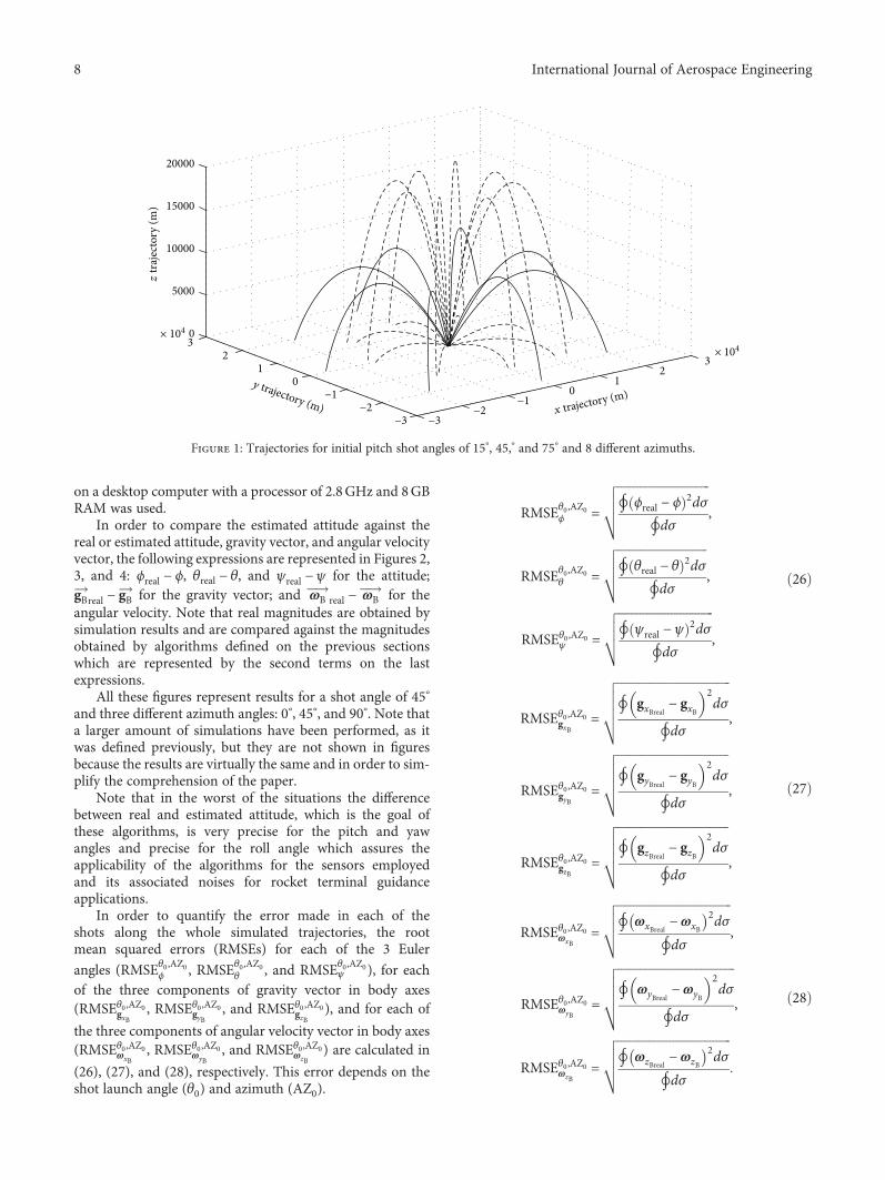
The flight dynamics model in [24] is employed. The equa-tions of motion are integrated using a fixed time stepRunge-Kutta scheme of fourth order to obtain a single flighttrajectory. A set of ballistic simulated shots, with no windperturbations, is performed varying shot angles from 15° to75° taking 1° steps and also varying initial azimuth anglesfrom 0° to 360° taking 45° steps. An example of these trajec-tories for a maximum range of 45°, minimum range of 15°,

and maximum height of 75° for the whole set of azimuthshots is shown in Figure 1.

GNSS sensors are modeled, based on a u-blox series 7sensor, adding a white noise of null average and maximumabsolute value ofmp=3m for position values and for velocityof mv=0.01m/s to the simulated position and velocityobtained from the model.

Accelerometers are modeled as second-order systems,based on MTi 1-series accelerometer, with a natural fre-quency of 300Hz and a damping factor of 0.7. A whitenoise of null average and maximum absolute value ofma=10

−3m/s2 and a bias of 10−3m/s2 is added. Note thataccelerometers will provide acceleration in body axes, whichwill be employed on the determination of the velocity vectorin body axes.

The modeling of the sensors has been based on relativelylow-cost equipment. This fact will induce significant errorson measurements, which will determine the suitability ofthe attitude calculation method. However, as it is shown inthe following section, the results are accurate enough for ter-minal guidance tasks in artillery.

6. Simulation Results

Simulation results are presented using the nonlinear flightdynamics model [24] in order to demonstrate suitabilityof attitude determination algorithm. A set of ballistic sim-ulated shots was performed as defined in the previoussection, in order to compare real (denoted with subindex“real”) and estimated attitudes. MATLAB/Simulink R2016a

Tr =M1,1 +M2,2 +M3,3,

C0 =1

1 + Tr, if 1 + Tr > 0,

0, else,

C1 =1

1 +M1,1 −M2,2 −M3,3, if 1 +M1,1 −M2,2 −M3,3 > 0,

0, else,

C2 =1

1 +M2,2 −M1,1 −M3,3, if 1 +M2,2 −M1,1 −M3,3 > 0,

0, else,

C3 =1

1 +M3,3 −M1,1 −M2,2, if 1 +M3,3 −M1,1 −M2,2 > 0,

0, else

24


on a desktop computer with a processor of 2.8GHz and 8GBRAM was used.

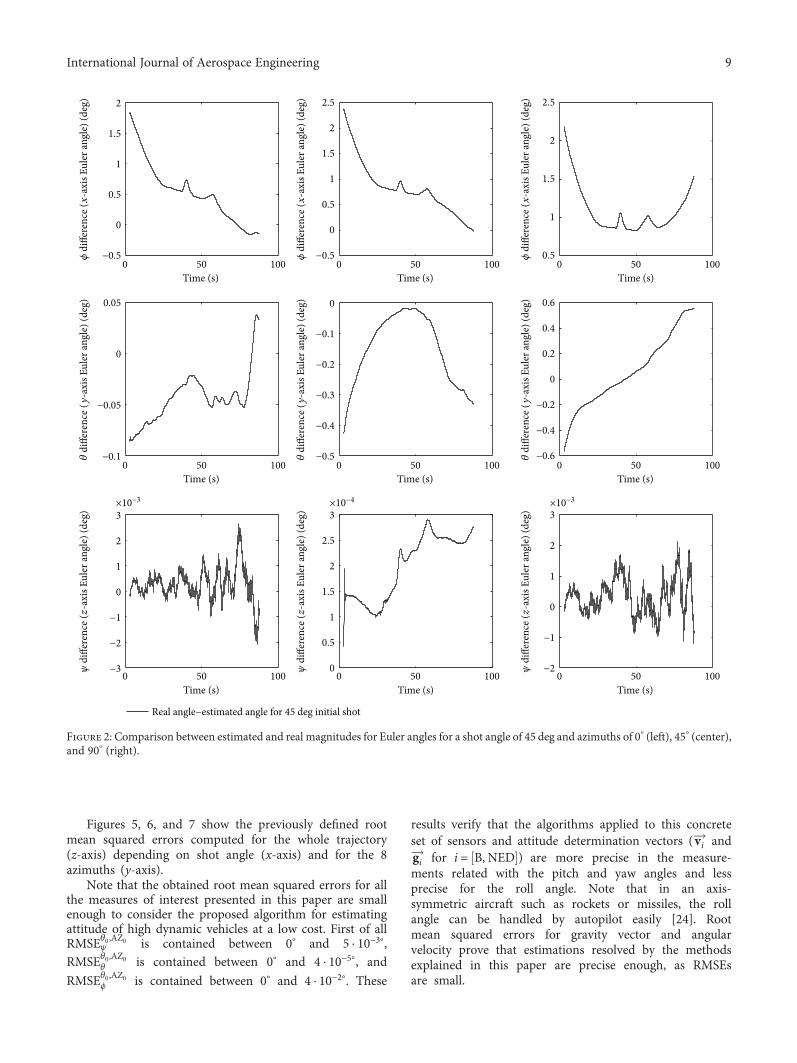
In order to compare the estimated attitude against thereal or estimated attitude, gravity vector, and angular velocityvector, the following expressions are represented in Figures 2,3, and 4: ϕreal − ϕ, θreal − θ, and ψreal − ψ for the attitude;gBreal − gB for the gravity vector; and ωB real − ωB for theangular velocity. Note that real magnitudes are obtained bysimulation results and are compared against the magnitudesobtained by algorithms defined on the previous sectionswhich are represented by the second terms on the lastexpressions.

All these figures represent results for a shot angle of 45°

and three different azimuth angles: 0°, 45°, and 90°. Note thata larger amount of simulations have been performed, as itwas defined previously, but they are not shown in figuresbecause the results are virtually the same and in order to sim-plify the comprehension of the paper.

Note that in the worst of the situations the differencebetween real and estimated attitude, which is the goal ofthese algorithms, is very precise for the pitch and yawangles and precise for the roll angle which assures theapplicability of the algorithms for the sensors employedand its associated noises for rocket terminal guidanceapplications.

In order to quantify the error made in each of theshots along the whole simulated trajectories, the rootmean squared errors (RMSEs) for each of the 3 Euler

angles (RMSEθ0,AZ0ϕ , RMSEθ0,AZ0

θ , and RMSEθ0,AZ0ψ ), for each

of the three components of gravity vector in body axes(RMSEθ0,AZ0gxB

, RMSEθ0,AZ0gyB, and RMSEθ0,AZ0gzB

), and for each of

the three components of angular velocity vector in body axes(RMSEθ0,AZ0

ωxB, RMSEθ0,AZ0

ωyB, and RMSEθ0,AZ0

ωzB) are calculated in

(26), (27), and (28), respectively. This error depends on theshot launch angle (θ0) and azimuth (AZ0).

RMSEθ0,AZ0ϕ =

∮ ϕreal − ϕ 2dσ

∮dσ,

RMSEθ0,AZ0θ =

∮ θreal − θ 2dσ

∮dσ,

RMSEθ0,AZ0ψ =

∮ ψreal − ψ 2dσ

∮dσ,

26

RMSEθ0,AZ0gxB=

∮ gxBreal − gxB2dσ

∮dσ,

RMSEθ0,AZ0gyB=

∮ gyBreal − gyB2dσ

∮dσ,

RMSEθ0,AZ0gzB=

∮ gzBreal − gzB2dσ

∮dσ,

27

RMSEθ0,AZ0ωxB

=∮ ωxBreal

−ωxB2dσ

∮dσ,

RMSEθ0,AZ0ωyB

=∮ ωyBreal

−ωyB

2dσ

∮dσ,

RMSEθ0,AZ0ωzB

=∮ ωzBreal

− ωzB2dσ

∮dσ

28

03

5000

21 3

10000

z tr

ajec

tory

(m)

2

15000

× 104

y trajectory (m)

0 1

x trajectory (m)0

20000

−2−1 −1

−2−3 −3

× 104

Figure 1: Trajectories for initial pitch shot angles of 15°, 45,° and 75° and 8 different azimuths.


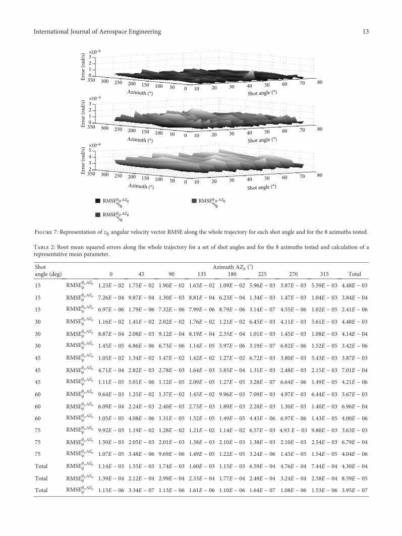
Figures 5, 6, and 7 show the previously defined rootmean squared errors computed for the whole trajectory(z-axis) depending on shot angle (x-axis) and for the 8azimuths (y-axis).

Note that the obtained root mean squared errors for allthe measures of interest presented in this paper are smallenough to consider the proposed algorithm for estimatingattitude of high dynamic vehicles at a low cost. First of allRMSEθ0,AZ0

ψ is contained between 0° and 5 ⋅ 10−3°,RMSEθ0,AZ0

θ is contained between 0° and 4 ⋅ 10−5°, and

RMSEθ0,AZ0ϕ is contained between 0° and 4 ⋅ 10−2°. These

results verify that the algorithms applied to this concreteset of sensors and attitude determination vectors (vi andgi for i = B, NED ) are more precise in the measure-ments related with the pitch and yaw angles and lessprecise for the roll angle. Note that in an axis-symmetric aircraft such as rockets or missiles, the rollangle can be handled by autopilot easily [24]. Rootmean squared errors for gravity vector and angularvelocity prove that estimations resolved by the methodsexplained in this paper are precise enough, as RMSEsare small.

Time (s)

−0.5

0

0.5

1

1.5

2

𝜙 d

iffer

ence

(x-a

xis E

uler

angl

e) (d

eg)

𝜙 d

iffer

ence

(x-a

xis E

uler

angl

e) (d

eg)

𝜙 d

iffer

ence

(x-a

xis E

uler

angl

e) (d

eg)

Time (s)

−0.1

−0.05

0

0.05

𝜃 d

iffer

ence

(y-a

xis E

uler

angl

e) (d

eg)

𝜃 d

iffer

ence

(y-a

xis E

uler

angl

e) (d

eg)

𝜃 d

iffer

ence

(y-a

xis E

uler

angl

e) (d

eg)

Time (s)

−3

−2

−1

0

1

2

3

𝜓 d

iffer

ence

(z-a

xis E

uler

angl

e) (d

eg)

𝜓 d

iffer

ence

(z-a

xis E

uler

angl

e) (d

eg)

𝜓 d

iffer

ence

(z-a

xis E

uler

angl

e) (d

eg)

0 50 1000 50 1000 50 100

0 50 1000 50 1000 50 100

0 50 1000 50 1000 50 100

Time (s)

0.5

1

1.5

2

2.5

Time (s)

−0.6

−0.4

−0.2

0

0.2

0.4

0.6

Time (s)

−2

−1

0

1

2

3×10−3×10−4×10−3

Time (s)

−0.5

0

0.5

1

1.5

2

2.5

Time (s)

−0.5

−0.4

−0.3

−0.2

−0.1

0

Time (s)

0

0.5

1

1.5

2

2.5

3

Real angle−estimated angle for 45 deg initial shot

Figure 2: Comparison between estimated and real magnitudes for Euler angles for a shot angle of 45 deg and azimuths of 0° (left), 45° (center),and 90° (right).


Table 2 shows the root mean squared errors for the 3Euler angles for different shot angles and azimuths, whichis basically the numerical values of Figure 5. The first columnshows the shot angle and the second one the displayed error(RMSEθ0,AZ0

ϕ , RMSEθ0,AZ0θ , and RMSEθ0,AZ0

ψ ). The rest of thecolumns show the numerical values of the errors for differ-ent azimuths. In order to present a significant result for thewhole method, root mean squared errors have been calcu-lated for the values shown on the surface represented byFigure 5. In order to accomplish this task, the last column,named total, shows the root mean squared errors for theset of azimuths represented on the same row. Similarly, thelast three rows represent the root mean squared errors for

the set of shot angles represented on the same column.Finally, the three values of the bottom-right corner can beconsidered as an estimation of the whole error of the attitudecalculation algorithms.

7. Conclusions

A novel low-cost approach for estimating attitude ofaerial platforms has been proposed. This approach isbased on the measurement of two different vectors:speed and gravity vectors. They are measured and esti-mated in two different reference frames using a GNSSsensor and a set of accelerometers. A new estimation

Time (s)

−5

0

5

10

15

20

x-b

ody-

axis

grav

ityve

ctor

diff

eren

ce (m

/s2 )

x-b

ody-

axis

grav

ityve

ctor

diff

eren

ce (m

/s2 )

x-b

ody-

axis

grav

ityve

ctor

diff

eren

ce (m

/s2 )

y-b

ody-

axis

grav

ityve

ctor

diff

eren

ce (m

/s2 )

y-b

ody-

axis

grav

ityve

ctor

diff

eren

ce (m

/s2 )

y-b

ody-

axis

grav

ityve

ctor

diff

eren

ce (m

/s2 )

z-b

ody-

axis

grav

ityve

ctor

diff

eren

ce (m

/s2 )

z-b

ody-

axis

grav

ityve

ctor

diff

eren

ce (m

/s2 )

z-b

ody-

axis

grav

ityve

ctor

diff

eren

ce (m

/s2 )

× 10−3 × 10−3 × 10−3

−0.05

0

0.05

0.1

0.15

0.2

0.25

−0.01

−0.005

0

0.005

0.01

0.015

0.02

−5

0

5

10

15

20

0.05

0.1

0.15

0.2

0.25

0.3

0.02

0.04

0.06

0.08

0.1

0.12

0.14

0 50 100Time (s)

0 50 100Time (s)

0 50 100

Time (s)0 50 100

Time (s)0 50 100

Time (s)0 50 100

Time (s)0 50 100

Time (s)0 50 100

Time (s)0 50 100

−5

0

5

10

15

20

−0.1

0

0.1

0.2

0.3

−0.1

−0.05

0

0.05

0.1

Real angel−estimated angel for 45 deg initial shot

Figure 3: Comparison between estimated and real magnitudes for gravity vector for a shot angle of 45 deg and azimuths of 0° (left), 45°

(center), and 90° (right).


method for obtaining the gravity vector in body axes hasalso been presented.

The presented algorithm is of special interest for highdynamic vehicles where other low-cost approaches, such asthe ones using magnetometers, especially in ballistic rocketsor unmanned air vehicles are not suitable due electronicinterferences with other electronic equipment.

Nonlinear simulations based on ballistic rocketlaunches are performed to obtain ideal attitude and com-pare it to the attitude obtained by the proposed approach.

Computational results show that errors are small enoughto consider the presented algorithm as a good candidatefor use within a control algorithm. Concretely, the totalroot mean square errors defined in Table 2 are below10−2° for the three attitude angles in the totality of testedcases. It is demonstrated that through the attitude deter-mination algorithm proposed, precision is maintained.Note that the needed low-cost components make thisapproach highly interesting for nonreusable vehicles suchas ballistic rockets.

−1

0

1

2

3

4

x-b

ody-

axis

angu

lar

velo

city

vec

tor d

iffer

ence

(rad

/s)

−8

−6

−4

−2

0

2

4

y-b

ody-

axis

angu

lar

velo

city

vec

tor d

iffer

ence

(rad

/s)

1

2

3

4

5

z-b

ody-

axis

angu

lar

velo

city

vec

tor d

iffer

ence

(rad

/s)

× 10−4 × 10−4 × 10−4

× 10−5 × 10−4 × 10−5

× 10−15 × 10−15 × 10−15

0 50 100Time (s)

0 50 100Time (s)

0 50 100Time (s)

0 50 100Time (s)

0 50 100Time (s)

0 50 100Time (s)

0 50 100Time (s)

0 50 100Time (s)

0 50 100Time (s)

−4

−3

−2

−1

0

1

2

x-b

ody-

axis

angu

lar

velo

city

vec

tor d

iffer

ence

(rad

/s)

−20

−15

−10

−5

0

5

y-b

ody-

axis

angu

lar

velo

city

vec

tor d

iffer

ence

(rad

/s)

1

2

3

4

5z

-bod

y-ax

is an

gula

rve

loci

ty v

ecto

r diff

eren

ce (r

ad/s

)

−4

−2

0

2

4

x-b

ody-

axis

angu

lar

velo

city

vec

tor d

iffer

ence

(rad

/s)

−1

0

1

2

3

y-b

ody-

axis

angu

lar

velo

city

vec

tor d

iffer

ence

(rad

/s)

−1

0

1

2

3

4

5

z-b

ody-

axis

angu

lar

velo

city

vec

tor d

iffer

ence

(rad

/s)

Real angel−estimated component for 45 deg initial shot

Figure 4: Comparison between estimated and real magnitudes for aircraft angular velocity for a shot angle of 45 deg and azimuths of 0° (left),45° (center), and 90° (right).


1350 300

2

80250 70

3

200 60Azimuth (°)

150 50Shot angle (°)

Azimuth (°) Shot angle (°)


4

40100 3050 200 10

0350 300 80250

2

70200 60150 50

4

40100 3050 200 10

0350 300 80250

1

Erro

r (m/s

2 )Er

ror (m

/s2 )

Erro

r (m/s

2 )

×10−3

×10−3

×10−5

70200 60150 50

2

40100 3050 200 10

RMSE𝜃0, AZ0gxBRMSE𝜃0, AZ0gzB

RMSE𝜃0, AZ0gyB

Figure 6: Representation of gravity vector RMSE along the whole trajectory for each shot angle and for the 8 azimuths tested.

0350 300

0.01

80250

Erro

r (°)

70

0.02

200 60Azimuth (°)

150 50Shot angle (°)



0.03

40100 3050 200 10

0350 300

2

80250

Erro

r (°)

70

4

200 60150 50

6

40100 3050 200 10

0350 300

1

80250

×10−5

×10−3

Erro

r (°)

70

2

200 60150 50

3

40100 3050 200 10

RMSE𝜃 0,AZ0𝜓

RMSE𝜃0,AZ0𝜃

RMSE𝜃0, AZ0𝜙

Figure 5: Representation of Euler angle RMSE along the whole trajectory for each shot angle and for the 8 azimuths tested.


−6

−6

−6

𝜃0, AZ0wzB

yB

𝜃 0, AZ0wxB

𝜃0,AZ0w

0350 300

1

80250Erro

r (ra

d/s)

70

2

200 60150 50

3

40100 3050 200 10

0350 300

1

80250Erro

r (ra

d/s)

70

2

200 60150 50

3

40100 3050 200 10

2350 300

3

80250Erro

r (ra

d/s)

×10

×10

×10

70

4

200 60150 50




5

40100 3050 200 10

RMSE RMSE

RMSE

Figure 7: Representation of zB angular velocity vector RMSE along the whole trajectory for each shot angle and for the 8 azimuths tested.

Table 2: Root mean squared errors along the whole trajectory for a set of shot angles and for the 8 azimuths tested and calculation of arepresentative mean parameter.

Shotangle (deg)

Azimuth AZ0 (°)

0 45 90 135 180 225 270 315 Total

15 RMSEθ0,AZ0ϕ 1.23E − 02 1.75E − 02 1.90E − 02 1.63E − 02 1.09E − 02 5.96E − 03 3.87E − 03 5.59E − 03 4.48E − 03

15 RMSEθ0,AZ0θ 7.26E − 04 9.87E − 04 1.30E − 03 8.81E − 04 6.23E − 04 1.34E − 03 1.47E − 03 1.04E − 03 3.84E − 04

15 RMSEθ0,AZ0ψ 6.97E − 06 1.79E − 06 7.32E − 06 7.99E − 06 8.79E − 06 3.14E − 07 4.55E − 06 1.02E − 05 2.41E − 06










75 RMSEθ0,AZ0φ 9.92E − 03 1.19E − 02 1.28E − 02 1.21E − 02 1.14E − 02 6.57E − 03 4.93 E − 03 9.80E − 03 3.63E − 03



Total RMSEθ0,AZ0ϕ 1.14E − 03 1.55E − 03 1.74E − 03 1.60E − 03 1.15E − 03 6.59E − 04 4.76E − 04 7.44E − 04 4.30E − 04

Total RMSEθ0,AZ0θ 1.39E − 04 2.12E − 04 2.99E − 04 2.33E − 04 1.77E − 04 2.48E − 04 3.24E − 04 2.58E − 04 8.59E − 05

Total RMSEθ0,AZ0ψ 1.13E − 06 3.34E − 07 1.13E − 06 1.61E − 06 1.10E − 06 1.64E − 07 1.08E − 06 1.53E − 06 3.95E − 07


Conflicts of Interest

The authors declare that there is no conflict of interestregarding the publication of this paper.

Acknowledgments

The authors would like to thank Lieutenant Colonel JesúsSánchez (NMT) and “Instituto Tecnológico La Marañosa”of the National Institute for Aerospace Technology (INTA)for the solid modeling of the concept.

References

[1] D.-M. Ma, J.-K. Shiau, I.-C. Wang, and Y.-H. Lin, “Attitudedetermination using a mems-based flight information mea-surement unit,” Sensors, vol. 12, no. 1, pp. 1–23, 2012.

[2] J. L. Crassidis, F. L. Markley, and Y. Cheng, “Survey of nonlin-ear attitude estimation methods,” Journal of Guidance, Con-trol, and Dynamics, vol. 30, no. 1, pp. 12–28, 2007.

[3] L. Cong, E. Li, H. Qin, K. V. Ling, and R. Xue, “A performanceimprovement method for low-cost land vehicle GPS/MEMS-INS attitude determination,” Sensors, vol. 15, no. 3,pp. 5722–5746, 2015.

[4] C. Eling, L. Klingbeil, and H. Kuhlmann, “Real-time single-frequency GPS/MEMS-IMU attitude determination of light-weight UAVs,” Sensors, vol. 15, no. 10, pp. 26212–26235, 2015.

[5] G. Giorgi, P. J. Teunissen, S. Verhagen, and P. J. Buist, “Testinga new multivariate GNSS carrier phase attitude determinationmethod for remote sensing platforms,” Advances in SpaceResearch, vol. 46, no. 2, pp. 118–129, 2010.

[6] P. J. Teunissen, G. Giorgi, and P. J. Buist, “Testing of a newsingle-frequency GNSS carrier phase attitude determinationmethod: land, ship and aircraft experiments,” GPS Solutions,vol. 15, no. 1, pp. 15–28, 2011.

[7] G. Giorgi, P. J. Teunissen, and T. P. Gourlay, “Instantaneousglobal navigation satellite system (GNSS)-based attitude deter-mination for maritime applications,” IEEE Journal of OceanicEngineering, vol. 37, no. 3, pp. 348–362, 2012.

[8] P. J. Teunissen, “Integer least-squares theory for the GNSScompass,” Journal of Geodesy, vol. 84, no. 7, pp. 433–447, 2010.

[9] P. J. G. Teunissen, “The affine constrained GNSS attitudemodel and its multivariate integer least-squares solution,”Journal of Geodesy, vol. 86, no. 7, pp. 547–563, 2012.

[10] N. Nadarajah, P. J. Teunissen, and N. Raziq, “InstantaneousGPS–Galileo attitude determination: single-frequency perfor-mance in satellite-deprived environments,” IEEE Transactionson Vehicular Technology, vol. 62, no. 7, pp. 2963–2976, 2013.

[11] N. Nadarajah and P. J. G. Teunissen, “Instantaneous GPS/Galileo/QZSS/SBAS attitude determination: a single-frequency (L1/E1) robustness analysis under constrained envi-ronments,” Navigation, vol. 61, no. 1, pp. 65–75, 2014.

[12] D. Gebre-Egziabher, G. H. Elkaim, J. Powell, and B.W. Parkin-son, “A gyro-free quaternion-based attitude determinationsystem suitable for implementation using low cost sensors,”in IEEE 2000. Position Location and Navigation Symposium(Cat. No.00CH37062), San Diego, CA, USA, March 2000.

[13] D. Gebre-Egziabher, R. C. Hayward, and J. D. Powell, “A low-cost GPS/inertial attitude heading reference system (AHRS)for general aviation applications,” in IEEE 1998 Position

Location and Navigation Symposium (Cat. No.98CH36153),Palm Springs, CA, USA, April 1998.

[14] K. W. Eure, C. C. Quach, S. L. Vazquez, E. F. Hogge, and B. L.Hill, “An application of uav attitude estimation using a low-cost inertial navigation system,” 2013, https://ntrs.nasa.gov/archive/nasa/casi.ntrs.nasa.gov/20140002398.pdf.

[15] P. Henkel and M. Iafrancesco, “Tightly coupled position andattitude determination with two low-cost gnss receivers,” in2014 11th International Symposium on Wireless Communica-tions Systems (ISWCS), Barcelona, Spain, August 2014.

[16] J. C. Springmann and J. W. Cutler, “Flight results of a low-costattitude determination system,” Acta Astronautica, vol. 99,pp. 201–214, 2014.

[17] D. M. Bevly, A. Rekow, and B. Parkinson, “Comparison of INSvs. carrier-phase DGPS for attitude determination in the con-trol of off-road vehicles,” Navigation, vol. 47, no. 4, pp. 257–266, 2000.

[18] C. E. Cohen, B. W. Parkinson, and B. D. McNally, “Flight testsof attitude determination using GPS compared against an iner-tial navigation unit,” Navigation, vol. 41, no. 1, pp. 83–97,1994.

[19] H. E. Soken and C. Hajiyev, “Pico satellite attitude estimationvia robust unscented Kalman filter in the presence of measure-ment faults,” ISA Transactions, vol. 49, no. 3, pp. 249–256,2010.

[20] H. Bolandi, F. F. Saberi, and A. M. Eslami, “Design of anextended interacting multiple models adaptive estimator forattitude determination of a stereoimagery satellite,” Interna-tional Journal of Aerospace Engineering, vol. 2011, Article ID890502, 19 pages, 2011.

[21] X. Yun, E. R. Bachmann, and R. B. McGhee, “A simplifiedquaternion-based algorithm for orientation estimation fromearth gravity and magnetic field measurements,” IEEE Trans-actions on Instrumentation and Measurement, vol. 57, no. 3,pp. 638–650, 2008.

[22] D. Mizell, “Using gravity to estimate accelerometer orienta-tion,” in Seventh IEEE International Symposium on WearableComputers, 2003. Proceedings, vol. 252, White Plains, NY,USA, October 2003.

[23] P. G. Savage, Strapdown Analytics, vol. 2, Strapdown Associ-ates Maple Plain, MN, 2000.

[24] R. de Celis, L. Cadarso, and J. Sánchez, “Guidance and Controlfor High Dynamic Rotating Artillery Rockets,” AerospaceScience and Technology, vol. 64, pp. 204–212, 2017.


https://ntrs.nasa.gov/archive/nasa/casi.ntrs.nasa.gov/20140002398.pdf

https://ntrs.nasa.gov/archive/nasa/casi.ntrs.nasa.gov/20140002398.pdf

International Journal of

AerospaceEngineeringHindawiwww.hindawi.com Volume 2018

RoboticsJournal of

Hindawiwww.hindawi.com Volume 2018


Active and Passive Electronic Components

VLSI Design



Shock and Vibration


Civil EngineeringAdvances in

Acoustics and VibrationAdvances in



Electrical and Computer Engineering

Journal of

Advances inOptoElectronics

Hindawiwww.hindawi.com

Volume 2018

Hindawi Publishing Corporation http://www.hindawi.com Volume 2013Hindawiwww.hindawi.com

The Scientific World Journal

Volume 2018

Control Scienceand Engineering

Journal of


Hindawiwww.hindawi.com

Journal ofEngineeringVolume 2018

SensorsJournal of



RotatingMachinery


Modelling &Simulationin EngineeringHindawiwww.hindawi.com Volume 2018


Chemical EngineeringInternational Journal of Antennas and

Propagation




Navigation and Observation


Hindawi

www.hindawi.com Volume 2018

Advances in

Multimedia

Submit your manuscripts atwww.hindawi.com

https://www.hindawi.com/journals/ijae/

https://www.hindawi.com/journals/jr/

https://www.hindawi.com/journals/apec/

https://www.hindawi.com/journals/vlsi/

https://www.hindawi.com/journals/sv/

https://www.hindawi.com/journals/ace/

https://www.hindawi.com/journals/aav/

https://www.hindawi.com/journals/jece/

https://www.hindawi.com/journals/aoe/

https://www.hindawi.com/journals/tswj/

https://www.hindawi.com/journals/jcse/

https://www.hindawi.com/journals/je/

https://www.hindawi.com/journals/js/

https://www.hindawi.com/journals/ijrm/

https://www.hindawi.com/journals/mse/

https://www.hindawi.com/journals/ijce/

https://www.hindawi.com/journals/ijap/

https://www.hindawi.com/journals/ijno/

https://www.hindawi.com/journals/am/

https://www.hindawi.com/

https://www.hindawi.com/

Documents

Attitude Determination Algorithms through Accelerometers