lable at ScienceDirect

Energy 35 (2010) 718–728

Contents lists avai

Energy

journal homepage: www.elsevier .com/locate/energy

Performance analysis of a CO2 heat pump water heating system under a dailychange in a standardized demand

Ryohei Yokoyama a,*, Tetsuya Wakui a, Junya Kamakari a, Kazuhisa Takemura b

a Department of Mechanical Engineering, Osaka Prefecture University, 1-1 Gakuen-cho, Naka-ku, Sakai, Osaka 599-8531, Japanb Research and Development Department, Kansai Electric Power Co., Inc., 3-11-20 Nakoji, Amagasaki, Hyogo 661-0974, Japan

a r t i c l e i n f o

Article history:Received 25 October 2008Received in revised form5 November 2009Accepted 6 November 2009Available online 26 November 2009

Keywords:Heat pumpCO2

Water heaterThermal storageSystem performanceNumerical simulation

* Corresponding author. Tel.: þ81 72 254 9229; faxE-mail address: yokoyama@me.osakafu-u.ac.jp (R.

0360-5442/$ – see front matter � 2009 Elsevier Ltd.doi:10.1016/j.energy.2009.11.008

a b s t r a c t

Air-to-water heat pumps using CO2 as a natural refrigerant have been developed and commercialized.They are expected to contribute to energy saving in residential hot water supply. The objective of theresearch is to analyze the performance of a water heating system composed of a CO2 heat pump and a hotwater storage tank by numerical simulation. In this paper, the system performance is analyzed undera daily change in a standardized hot water demand, and some features of the temperature distribution inthe storage tank and the system performance criteria such as coefficient of performance, storage andsystem efficiencies, and volumes of stored and unused hot water are investigated. It turns out that thedaily change in the hot water demand does not significantly affect the daily averages of the COP, andstorage and system efficiencies, while it significantly affects not only the daily change in the volume ofhot water unused after the tapping mode, but also that in the volume of hot water stored after thecharging mode. The influence of the daily change in the hot water demand on the volumes of stored andunused hot water is clarified quantitatively.

� 2009 Elsevier Ltd. All rights reserved.

1. Introduction

Air-to-water heat pumps using CO2 as a natural refrigerant havebeen developed and commercialized. They are expected tocontribute to energy saving in residential hot water supply [1].

Many theoretical and experimental studies have beenconducted for the performance analysis only on CO2 heat pumps[2–10]. The recent technological development has enhanced theperformance of CO2 heat pumps remarkably. However, a residentialwater heating system is composed of a CO2 heat pump and a hotwater storage tank so that it can supply hot water even in the caseof a sudden increase in hot water demand, and its performance isaffected significantly not only by instantaneous air and feed watertemperatures but also by hourly changes in the heat pump opera-tion, hot water demand, and their resultant temperature distribu-tion in the storage tank. Therefore, it is necessary to conduct theperformance analysis on water heating systems in consideration ofthese items. It takes much time to do it under various conditions byexperiment, and it is expected that numerical simulation enablesone to do it very efficiently.

: þ81 72 254 9904.Yokoyama).

All rights reserved.

Some studies have been conducted for the performance analysison water heating systems [11,12]. However, few studies have beenconducted in consideration of hourly changes in the heat pumpoperation, hot water demand, and their resultant temperaturedistribution in the storage tank [13–15]. First in these studies,simulation models have been proposed, and results obtained bynumerical simulation have been compared with those by experi-ment. Then, the influence of ambient conditions such as air and feedwater temperatures on the system performance has been clarified.In addition, the influence of operation conditions such as the outletwater temperature during the heat pump operation and the inletwater temperature for the heat pump shutdown on the systemperformance has been clarified. However, the system performancehas been investigated under the condition without any daily changein a standardized hot water demand. The hot water demand maychange daily actually, which may affect the system performancesignificantly. Therefore, it is also important to investigate the systemperformance under a daily change in the hot water demand.

In this paper, the performance of a CO2 heat pump water heatingsystem is analyzed under a daily change in a hot water demand bynumerical simulation. Here, an hourly change in a standardized hotwater demand is adopted as the first step of the research, and themagnitude for the hot water flow rates is changed daily. Theinfluence of the daily change in the standardized hot water demandon the system performance is investigated. Especially, features of

Fig. 2. Model of CO2 heat pump.

_WHP ¼�

a1 þ b1Ta þ g1Ta2��

a2 þ b2THPi þ g2T2HPi

���

a3 þ b3THPo þ g3T2HPo

�hHP ¼

�a4 þ b4Ta þ g4Ta2

��a5 þ b5THPi þ g5T2

HPi

���

a6 þ b6THPo þ g6T2HPo

�

9>>>>>>>=>>>>>>>;

(3)

R. Yokoyama et al. / Energy 35 (2010) 718–728 719

the temperature distribution in the storage tank and the systemperformance criteria such as coefficient of performance (COP),storage and system efficiencies, and volumes of stored and unusedhot water are investigated.

2. CO2 heat pump water heating system

Fig.1 shows the configuration of the CO2 heat pump water heatingsystem investigated in this paper. This system is composed of a CO2

heat pump and a hot water storage tank. The CO2 heat pump iscomposed of a compressor, a gas cooler, an expansion valve, and anevaporator. The system is equipped with a fan, a pump, and motorsM1–M3 as auxiliary machinery. Here, inlet and outlet water is definedas water at the inlet and outlet of the gas cooler, respectively. Thesystem heats water using the refrigeration cycle of the CO2 heat pump,stores hot water in the storage tank, and supplies it to a tapping site.

3. Numerical simulation

3.1. Simulation model

3.1.1. Modeling of CO2 heat pumpA simplified static model is adopted for the CO2 heat pump [13]:

i.e., although the CO2 heat pump includes the aforementioned fourcomponents, they are not taken into account explicitly, and it isexpressed by one model. The mass flow rates and temperatures ofwater at the inlet and outlet, COP, heat output, power consumption,and air temperature are adopted as basic variables whose values areto be determined. The mass and energy balance relationships aswell as the energy input and output relationship are adopted asbasic equations to be satisfied. The remaining equations to beconsidered are approximate functions of the power consumptionand COP, and they are expressed in relation to the air and inlet/outlet water temperatures.

The model of the CO2 heat pump is shown in Fig. 2. The massand energy balance relationships are expressed by

_mHPi ¼ _mHPo_mHPi cTHPi þ _QHP ¼ _mHPocTHPo

�(1)

where _mHP and THP are the mass flow rate and temperature ofwater, respectively, and these variables at the inlet and outlet are

Fig. 1. Configuration of CO2 heat

denoted by the subscripts i and o, respectively. In addition, _QHP isthe heat output, and c is the specific heat of water, which isassumed to be constant. The energy input and output relationshipis expressed by

_QHP ¼ hHP_WHP (2)

where _WHP is the power consumption, and hHP is the COP. Theapproximate functions of the power consumption and COP areexpressed by quadratic functions with respect to the air and inlet/outlet water temperatures as follows:

where Ta is the air temperature, and a1wa6, b1wb6, and g1wg6 arethe coefficients of the quadratic functions, whose values are to beidentified based on measured data for an existing device. Themodeling results in a set of nonlinear algebraic equations.

3.1.2. Modeling of storage tankA detailed dynamic model is adopted for the storage tank

[13,14]. To consider the one-dimensional vertical temperature

pump water heating system.

Fig. 3. Model of storage tank.

R. Yokoyama et al. / Energy 35 (2010) 718–728720

distribution in the storage tank, it is vertically divided into manycontrol volumes with the same volume, in each of which the watertemperature is assumed to be uniform. It is also assumed that theheat transfer occurs by water flow and heat conduction as well asheat loss from the tank surface. The mass flow rates and temper-atures of water for each control volume are adopted as basic vari-ables whose values are to be determined. In addition, the mass flowrates and temperatures of water at the inlet and outlet of the topand bottom of the storage tank are adopted as variables. The massand energy balance relationships for each control volume areadopted as basic equations to be satisfied.

The model of the storage tank is shown in Fig. 3. For each of Jcontrol volumes, the mass balance relationship of water isexpressed by

_mtSTi ¼ _mST1 þ _mt

STo_mSTj�1 ¼ _mSTj ðj ¼ 2;3; ::: ; J � 1Þ_mb

STi þ _mSTJ�1 ¼ _mbSTo

9>=>; (4)

where the mass flow rate of water which flows downward from thejth to (jþ 1)th control volumes is denoted by _mSTj, and _mSTj � 0 and_mSTj < 0 when water flows downward and upward, respectively.

The variables at the top and bottom inlet/outlet are denoted bythe superscripts t and b, respectively, and at the inlet and outlet bythe subscripts i and o, respectively. For each control volume, theenergy balance relationship of water is expressed by

Fig. 4. Model of mixing valve.

rcVST=JðdTST1=dtÞ ¼ _mtSTicTt

STi � _mtSTocTt

STo_QST1

�l1SSTJ=HSTðTST1 � TST2Þ � USTðAST þ 2SSTÞ=J�TST1 � Ta

�rcVST=J

�dTSTj=dt

�¼ � _QSTj þ lj�1SSTJ=HST

�TSTj�1 � TSTj

��ljSSTJ=HST

�TSTj � TSTjþ1

�� USTðAST þ 2SSTÞ=J

�TSTj � Ta

�ðj ¼ 2;3; ::: ; J � 1Þ

rcVST=J�dTSTJ=dt

�¼ _mb

STicTbSTi � _mb

STocTbSTo

_QSTJ

þlJ�1SSTJ=HST�TSTJ�J � TSTJ

�� USTðAST þ 2SSTÞ=J

�TSTJ � Ta

�

9>>>>>>>>>>>=>>>>>>>>>>>;

(5)

where the water temperature in the jth control volume is denoted byTSTj. r and l are the density and heat conductivity of water, respec-tively, r is assumed to be constant, and l is assumed to depend ontemperature, which is denoted by the subscript j. HST, VST, SST, and AST

are the height, volume, horizontal sectional area, and cylindricalsurface area of the storage tank, respectively. In addition, UST is theoverall heat transfer coefficient, and _QSTj is the rate of heat transferby water flow, which is expressed by

_QST1 ¼ _mST1cTST1_QSTj ¼ � _mSTj�1cTSTj þ _mSTjcTSTj ð j ¼ 2;3; ::: ; J� 1Þ_QSTJ ¼ � _mSTJ�1cTSTJ�1

9=; (6)

and

_QST1 ¼ _mST1cTST2_QSTj ¼ � _mSTj�1cTSTj þ _mSTjcTSTjþ1 ð j ¼ 2;3; ::: ; J� 1Þ_QSTJ ¼ � _mSTJ�1cTSTJ

9=; (7)

when _mSTj � 0 and _mSTj < 0, respectively. The water temperaturesat the top and bottom outlets of the storage tank are expressed by

TtSTo ¼ TST1

TbSTo ¼ TSTJ

)(8)

The modeling results in a set of nonlinear differential equations.

3.1.3. Modeling of mixing valveA static model is adopted for the mixing valve. The mass flow

rates and temperatures of water at the inlets and outlet areconsidered as basic variables, and the mass and energy balancerelationships are considered as basic equations.

The model of the mixing valve is shown in Fig. 4. The mass andenergy balance relationships are expressed by

_mMVi1 þ _mMVi2 ¼ _mMVo_mMVi1cTMVi1 þ _mMVi2cTMVi2 ¼ _mMVocTMVo

�(9)

where mMV and TMV are the mass flow rate and temperature ofwater, respectively, and these variables at the inlet and outlet aredenoted by the subscripts i and o, respectively. In addition, theinlets for hot water from the storage tank and feed water aredenoted by the subscripts 1 and 2, respectively. The modelingresults in a set of linear algebraic equations.

3.1.4. Modeling of systemAt the connection points among the CO2 heat pump, storage

tank, and mixing valve, connection conditions are taken intoaccount to equalize the values of the corresponding variables. Theoutlet water temperature is given as a control condition. The feedwater temperature as well as the mass flow rate and temperature ofhot water to the tapping site are given as boundary conditions. Theair temperature is given as an ambient condition.

The aforementioned modeling for the performance analysis bynumerical simulation is conducted by a building block approach asfollows: The component models for the CO2 heat pump, storagetank, and mixing valve, and the substance model for water aredefined independently; The system model is composed of the

R. Yokoyama et al. / Energy 35 (2010) 718–728 721

component and substance models as well as the connection,control, boundary, and ambient conditions.

The equations for the CO2 heat pump and mixing valve arestatic, while those for the storage tank are dynamic. Therefore, themodeling results in the following set of nonlinear differentialalgebraic equations:

f�xðtÞ; _xðtÞ; yðtÞ; t

�¼ 0

xðt0Þ ¼ x0

�(10)

where f is the vector for all the equations, x is the vector for thevariables with their derivatives: i.e., the temperatures of water forall the control volumes of the storage tank, y is the vector for all theother variables without their derivatives, _x is the derivative of xwith respect to time t, and x0 is the initial value of x at the initialtime t0.

3.2. Solution method

The set of nonlinear differential algebraic equations expressedby Eq. (10) is solved numerically by a hierarchical combination ofthe Runge–Kutta and Newton–Raphson methods. A concretesolution algorithm is shown here.

For a value of the sampling time interval Dt, the Runge–Kuttamethod is used to derive the values of y(t) and x(tþ Dt) from that ofx(t) at any time t. A common formula for this purpose is as follows:

f�

xðtÞ þ _x½r�k½rþ1�Dt; _x½rþ1�ðtÞ; y½rþ1�ðtÞ; t þ k½rþ1�Dt�¼ 0

ðr ¼ 0; 1; 2; ::: Þ ð11Þ

where k is the constant, and the subscript [r] denotes the number ofapplications of the formula. For example, k[1]¼ 0, k[2]¼ 1/2, k[3]¼ 1/2,and k[4] ¼ 1 according to the Runge–Kutta formula considering thefourth order of Dt. For each application, the values of _x½rþ1� and y[rþ1]

are derived using the following equation based on the Newton–Raphson method:

�_x½rþ1�ðsþ1ÞðtÞy½rþ1�ðsþ1ÞðtÞ

�¼�

_x½rþ1�ðsÞðtÞy½rþ1�ðsþ1ÞðtÞ

�

�hvf�

xðtÞþ _x½r�k½rþ1�Dt; _x½rþ1�ðsÞðtÞ;y½rþ1�ðsÞðtÞ; tþk½rþ1�Dt�.

v _x½rþ1�;vf�

xðtÞþ _x½r�k½rþ1�Dt; _x½rþ1�ðsÞðtÞ;y½rþ1�ðsÞðtÞ; tþk½rþ1�Dt�.

vy½rþ1�

i�1

�f�

xðtÞþ _x½r�k½rþ1�Dt; _x½rþ1�ðsÞðtÞ;y½rþ1�ðsÞðtÞ; tþk½rþ1�Dt�ðr¼0;1;2;::: Þ

(12)

where the subscript (s) denotes the number of repeats for theconvergence calculation. After the first application of the formula, thevalue of y(t) is derived as y[1]. In addition, after all the applications,the value of x(t þ Dt) is derived from those of x(t) and _x½rþ1� (r ¼ 0, 1,2,...). For example, xðt þ DtÞ ¼ xðtÞ þ ð _x½1� þ 2 _x½2� þ 2 _x½3� þ _x½4�ÞDt=6according to the Runge–Kutta formula.

3.3. Validation of simulation model

In advance of its application to a numerical study, the simulationmodel has been validated as follows:

3.3.1. Validity of one-dimensional numerical simulationAn important thing is to investigate the validity of the one-

dimensional simulation model for the storage tank. The three-dimensional numerical simulation has also been conducted foranother study [16]. The temperature distribution obtained by theone-dimensional numerical simulation has been different locally

from that obtained by the three-dimensional one, especially nearthe inlet and outlet of the top and bottom of the storage tank.However, since the flow rate of water through the storage tank issmall enough, the temperature distribution obtained by the one-dimensional numerical simulation has coincided well globally withthat obtained by the three-dimensional one.

An example of the comparison between the temperaturedistributions obtained by the one- and three-dimensionalnumerical simulations is shown here. The one- and three-dimensional numerical simulations are conducted by supposinghot water supply to bath for 900 s in the tapping mode. Theinitial temperature distribution in the storage tank is set to be assame as the calculated one at the beginning of the tapping modein Section 3.3.2. Hot water flows into the pipe with a diameter of0.0216 m located in the center at the top of the storage tank, andfeed water flows out of the pipe with the same diameter locatedin the center at the bottom. The volumetric flow rate is 0.0983 L/s.Fig. 5(a) and (b) shows the velocity and temperature distribu-tions in the storage tank, respectively, after 300, 600, and 900 sobtained by the three-dimensional numerical simulation. Fig. 6compares the temperature distributions after 300, 600, and 900 sobtained by the one- and three-dimensional numerical simula-tions. Here, the temperature by the three-dimensional numericalsimulation is the one averaged at each horizontal cross section.After 300 s, the temperature distribution is two-dimensional nearthe bottom, because feed water enters into hot water and itdiffuses toward the up and radial directions. As a result, thetemperature near the bottom by the three-dimensional numericalsimulation is higher than that by the one-dimensional one. After900 s, however, the temperature distribution is almost one-dimensional, or the temperature is almost stratified. These resultsindicate that the temperature distribution obtained by the one-dimensional numerical simulation coincides well globally withthat obtained by the three-dimensional one.

In addition, the temperature distribution obtained by the one-dimensional numerical simulation has coincided well globally with

that obtained by the experiment, as described below. Therefore, theone-dimensional simulation model has been validated.

3.3.2. Number of control volumes for storage tankIt is also important to determine the number of control

volumes for the storage tank appropriately in relation to thesampling time interval for the Runge–Kutta method, so that thehourly change in the temperature distribution in the storage tankdue to the heat transfer by water flow and heat conductionindicates an actual one. For this purpose, the number of controlvolumes has been set at 120, 200, and 240 for the sampling timeinterval of 10 s, and the hourly change in the temperaturedistribution obtained by the numerical simulation has beencompared with that by the experiment. It has been concludedthat the hourly changes in the temperature distribution for thenumbers of control volumes of 200 and 240 are in good agree-ment with each other as well as that by the experiment, and thenumber of control volumes of 200 has been used in the previous

Fig. 5. Results by three-dimensional numerical simulation. (a) Velocity distributions, (b) Temperature distributions.

Fig. 6. Comparison between one- and three-dimensional numerical simulations.

R. Yokoyama et al. / Energy 35 (2010) 718–728722

study on the comparison between the numerical simulation andexperiment [13].

An example of the comparison between the temperaturedistributions obtained by the numerical simulation and experi-ment is shown here. The numerical simulation and experimentare conducted for three days under the standardized hot waterdemand prescribed by the Japan Refrigeration and Air Condi-tioning Industry Association (JRA) and other appropriate condi-tions. Fig. 7(a) and (b) compares calculated and measuredtemperature distributions at some representative times in thecharging and tapping modes, respectively, on the third day. Thecalculated and measured ones are denoted by continuous curvesand discrete points, respectively. It turns out that the calculatedand measured temperature distributions are also in goodagreement.

Fig. 7. Comparison between numerical simulation and experiment (a) Charging mode,(b) Tapping mode.

Fig. 8. Performance characteristics of CO2 heat pump.

R. Yokoyama et al. / Energy 35 (2010) 718–728 723

3.3.3. Solution of nonlinear differential algebraic equationsAnother important thing is to solve the set of nonlinear differ-

ential algebraic equations accurately. As aforementioned, theRunge–Kutta method is adopted at the upper level to solve thedifferential equations. This method has the fourth order accuracy ifit adopts the Runge–Kutta formula. In addition, the Newton–Raphson method is adopted at the lower level to satisfy thenonlinear algebraic equations accurately at each sampling time.Therefore, it is concluded that this solution method for the set ofnonlinear differential algebraic equations has high accuracy.

4. Numerical study

4.1. Calculation conditions

A numerical study is conducted for several days in mid-seasonon each of which an hourly change in a standardized hot water

Table 1Specifications of CO2 heat pump water heating system.

Equipment Specification Value

CO2 heat pump Rated heat output 4.50 kWVolume 370 LHeight 143 m

Hot water storage tank Diameter 0.56 mOverall heat transfer coefficient 0.80 W/(m2 �C)Number of control volumes 200

demand is assumed. This is because it takes several days untila periodic steady state appears.

The following are the calculation conditions used in thenumerical study:

4.1.1. SystemTable 1 shows the specifications of the CO2 heat pump water

heating system. The values of model parameters included in theequations are estimated based on measured data for existingdevices.

The rated heat output of the CO2 heat pump is set at 4.5 kW.As an example, Fig. 8 shows measured values and approximatefunctions for the power consumption, COP, and their resultant heatoutput of the CO2 heat pump in relation to the inlet watertemperature for the air and outlet water temperatures of 16 and85 �C, respectively. Here, each value is relative to its rated one forthe air and inlet/outlet water temperatures of 16, 17, and 65 �C,respectively.

The volume of the hot water storage tank is set at 370 L. Thenumber of control volumes for the storage tank is set at 200, andthe sampling time interval for the Runge–Kutta method is set at10 s, as described previously.

4.1.2. Ambient conditionsThe air and feed water temperatures are set at 16 and 17 �C,

respectively, which is prescribed as the ambient conditions in mid-season by JRA [17]. These values are assumed to be constantthroughout the days.

4.1.3. Hot water demandThe hourly changes in the flow rate and temperature of the

standardized hot water demand are given as shown in Fig. 9, whichis also prescribed by JRA [17]. Here, the height of each vertical line

Fig. 9. Hourly change in standardized hot water demand.

R. Yokoyama et al. / Energy 35 (2010) 718–728724

means the flow rate, as indicated. The temperature is shown aboveeach vertical line. In addition, the thickness of each vertical linemeans the duration. The heat for the total hot water demandis 46.15 MJ/d for the aforementioned feed water temperature inmid-season.

In order to investigate the influence of a daily change in the hotwater demand on the system performance, the following four casesare studied:

Case A: The standardized hot water demand is used every day.Case B: Half of the standardized hot water demand is used everyday.Case C: Double of the standardized hot water demand is usedevery day.Case D: Half and double of the standardized hot water demandare used alternately every two days.

Fig. 10. Hourly change in temperature distribution in storage tank (8th day in case A)(a) Charging mode, (b) Tapping mode.

Fig. 11. Hourly change in temperature distribution in storage tank (8th day in case B)(a) Charging mode, (b) Tapping mode.

4.1.4. OperationThe system is assumed to be operated in the charging and

tapping modes independently during the nighttime and daytime,respectively. In the charging mode, the outlet water temperature ofthe CO2 heat pump is set at 85 �C. In addition, the CO2 heat pump isstarted up at 2:00 and is shut down with a shutdown conditionsatisfied at an appropriate time before 7:00. The shutdown condi-tion is that the inlet water temperature of the CO2 heat pumpattains 30 �C.

As the initial condition, the temperature of water in all thecontrol volumes of the storage tank is set at 17 �C at 0:00 on the 1stday.

4.2. Results and discussion

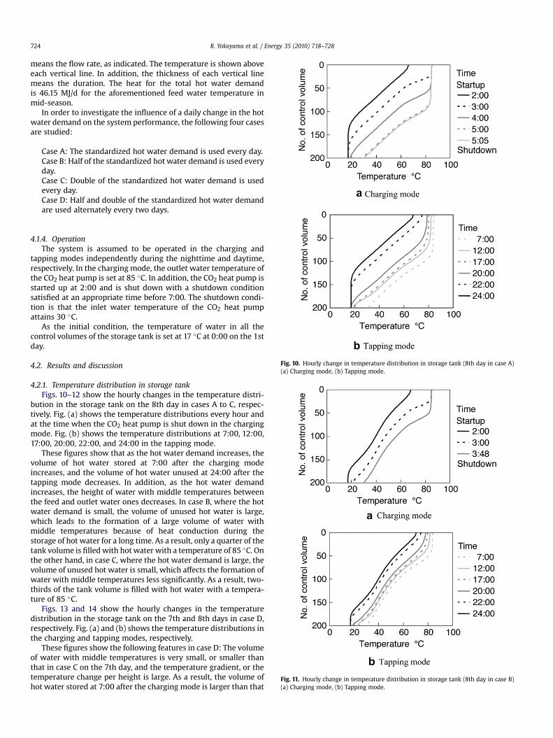
4.2.1. Temperature distribution in storage tankFigs. 10–12 show the hourly changes in the temperature distri-

bution in the storage tank on the 8th day in cases A to C, respec-tively. Fig. (a) shows the temperature distributions every hour andat the time when the CO2 heat pump is shut down in the chargingmode. Fig. (b) shows the temperature distributions at 7:00, 12:00,17:00, 20:00, 22:00, and 24:00 in the tapping mode.

These figures show that as the hot water demand increases, thevolume of hot water stored at 7:00 after the charging modeincreases, and the volume of hot water unused at 24:00 after thetapping mode decreases. In addition, as the hot water demandincreases, the height of water with middle temperatures betweenthe feed and outlet water ones decreases. In case B, where the hotwater demand is small, the volume of unused hot water is large,which leads to the formation of a large volume of water withmiddle temperatures because of heat conduction during thestorage of hot water for a long time. As a result, only a quarter of thetank volume is filled with hot water with a temperature of 85 �C. Onthe other hand, in case C, where the hot water demand is large, thevolume of unused hot water is small, which affects the formation ofwater with middle temperatures less significantly. As a result, two-thirds of the tank volume is filled with hot water with a tempera-ture of 85 �C.

Figs. 13 and 14 show the hourly changes in the temperaturedistribution in the storage tank on the 7th and 8th days in case D,respectively. Fig. (a) and (b) shows the temperature distributions inthe charging and tapping modes, respectively.

These figures show the following features in case D: The volumeof water with middle temperatures is very small, or smaller thanthat in case C on the 7th day, and the temperature gradient, or thetemperature change per height is large. As a result, the volume ofhot water stored at 7:00 after the charging mode is larger than that

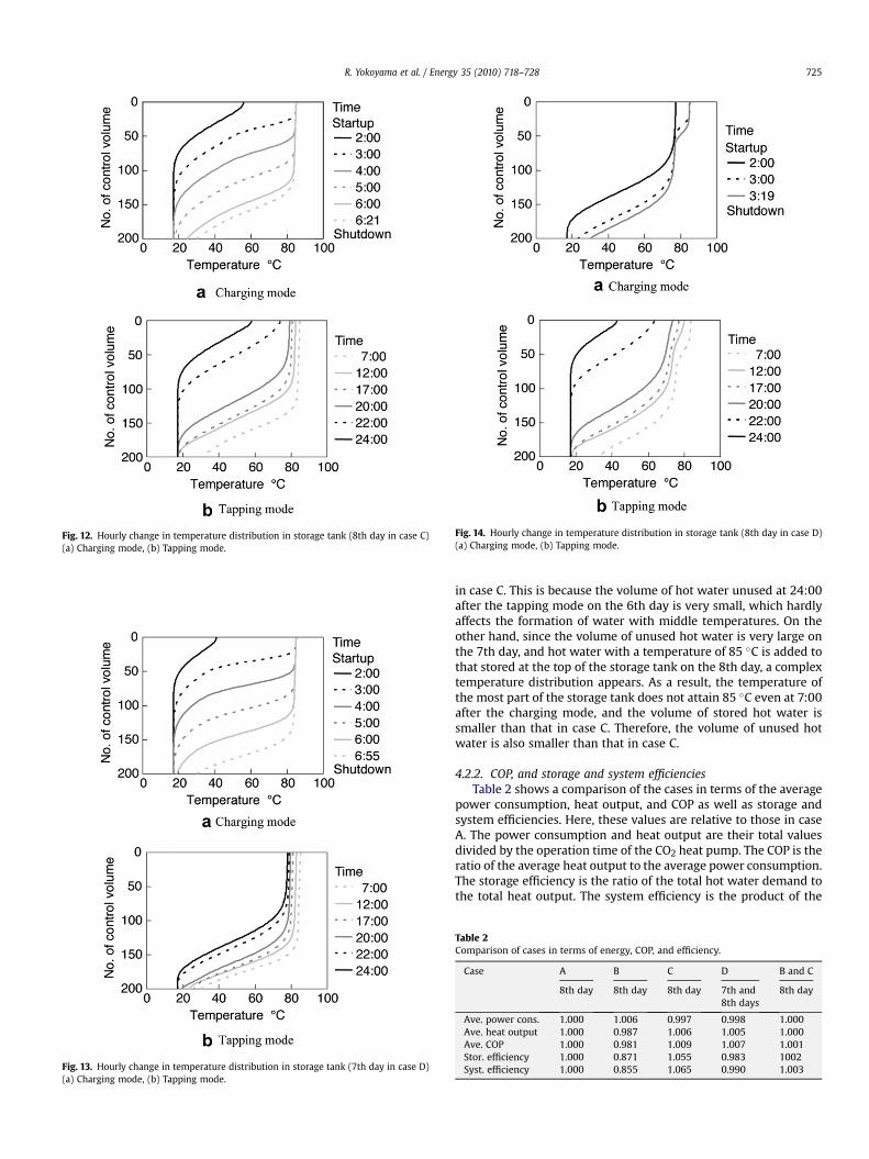
Fig. 13. Hourly change in temperature distribution in storage tank (7th day in case D)(a) Charging mode, (b) Tapping mode.

Fig. 14. Hourly change in temperature distribution in storage tank (8th day in case D)(a) Charging mode, (b) Tapping mode.

Fig. 12. Hourly change in temperature distribution in storage tank (8th day in case C)(a) Charging mode, (b) Tapping mode.

R. Yokoyama et al. / Energy 35 (2010) 718–728 725

in case C. This is because the volume of hot water unused at 24:00after the tapping mode on the 6th day is very small, which hardlyaffects the formation of water with middle temperatures. On theother hand, since the volume of unused hot water is very large onthe 7th day, and hot water with a temperature of 85 �C is added tothat stored at the top of the storage tank on the 8th day, a complextemperature distribution appears. As a result, the temperature ofthe most part of the storage tank does not attain 85 �C even at 7:00after the charging mode, and the volume of stored hot water issmaller than that in case C. Therefore, the volume of unused hotwater is also smaller than that in case C.

4.2.2. COP, and storage and system efficienciesTable 2 shows a comparison of the cases in terms of the average

power consumption, heat output, and COP as well as storage andsystem efficiencies. Here, these values are relative to those in caseA. The power consumption and heat output are their total valuesdivided by the operation time of the CO2 heat pump. The COP is theratio of the average heat output to the average power consumption.The storage efficiency is the ratio of the total hot water demand tothe total heat output. The system efficiency is the product of the

Table 2Comparison of cases in terms of energy, COP, and efficiency.

Case A B C D B and C

8th day 8th day 8th day 7th and8th days

8th day

Ave. power cons. 1.000 1.006 0.997 0.998 1.000Ave. heat output 1.000 0.987 1.006 1.005 1.000Ave. COP 1.000 0.981 1.009 1.007 1.001Stor. efficiency 1.000 0.871 1.055 0.983 1002Syst. efficiency 1.000 0.855 1.065 0.990 1.003

Fig. 16. Cumulative distribution of temperature in storage tank throughout day (8thday in case A, and cases B and C; 7th and 8th days in case D).

R. Yokoyama et al. / Energy 35 (2010) 718–728726

average COP and storage efficiency. The values in cases A–C arecalculated on the 8th day, and those in case D are calculated on the7th and 8th days. The values in cases B and C calculated on the 8thday are added for reference. These values are obtained under thesituation that cases B and C are continued for many daysindependently.

First, the differences in the average COP are discussed. Cases A–Chave meaningfully different values of the average COP. Case C hasthe largest value, while case B has the smallest one. This is due tothe aforementioned differences in the temperature distributions inthe storage tank. In case C, since the height of water with middletemperatures is smaller, the ratio of the time with lower COP to thetotal operation time is smaller. In case B, vice versa. However, theinlet water temperature for shutdown of the CO2 heat pump is30 �C, the time when the CO2 heat pump is operated with the inletwater temperature of about 17 �C is dominant, and the COP doesnot significantly decrease. As a result, the differences in the averageCOP among cases A–C are less than 3%. On the other hand, thedifferences in the average COP among case A, case D, and cases Band C are only less than 1%. To confirm whether these slightdifferences are meaningful or not, the cumulative distributions ofthe inlet water temperature during the heat pump operation areinvestigated. Fig. 15 shows them on the 8th day in case A, the 7thand 8th days in case D, and the 8th day in cases B and C. Here, eachfrequency in case A is doubled for the comparison purpose. Thediscrete width of temperature is 0.5 �C. The distributions are almostsimilar among the cases. In addition, the frequency for the inletwater temperature of 16.5–17.0 �C is dominant in all the cases.However, the cases have slightly different values. Case D has thelargest value, which corresponds to the largest value of the averageCOP in Table 2. Although cases B and C have the second largestvalue, and case A has the smallest value, the difference in theaverage COP between case A, and cases B and C is very small. Thismay be affected by the frequencies for the inlet water temperaturehigher than 17.0 �C.

Next, the differences in the storage efficiency are discussed. Thedifferences in the storage efficiency among cases A–C are more than5%. Case C has the largest value, while case B has the smallest one.As the hot water demand increases, the storage efficiency increases.This is because although the total heat output increases with thehot water demand, the heat loss from the tank surface does notsignificantly increase. On the other hand, the differences in thestorage efficiency among case A, case D, and cases B and C are only

Fig. 15. Cumulative distribution of inlet water temperature during heat pump opera-tion (8th day in case A, and cases B and C; 7th and 8th days in case D).

less than 2%. However, case D has a small value. To confirm whetherthis small value is meaningful or not, the cumulative distributionsof the temperature in the storage tank throughout the day areinvestigated. Fig. 16 shows them on the 8th day in case A, the 7thand 8th days in case D, and the 8th day in cases B and C. Here, eachfrequency in case A is doubled for the comparison purpose. Thediscrete width of temperature is 1 �C. It is clear that the frequenciesof higher temperatures in case D are larger than those in case A, andcases B and C, and that the frequencies of lower temperatures incase D are smaller than those in case A, and cases B and C. This isbecause the height of temperature with middle temperatures in thestorage tank in case D is kept small even when the hot waterdemand is small. As a result, the storage efficiency in case D issmaller than those in case A, and cases B and C.

From the aforementioned discussions, the differences in thesystem efficiency among cases A to C are larger than those in theaverage COP and storage efficiency, and are more than 6%.However, the system efficiency in cases B and C is almost equal tothat in case A. In addition, the difference in the system efficiencyin cases D and A is averaged between those in the average COPand storage efficiency, and is only 1%. This result shows that thedaily change in the hot water demand does not significantlyaffect the daily averages of the COP, and storage and systemefficiencies.

4.2.3. Volumes of stored and unused hot waterTable 3 shows a comparison of the cases in terms of the

volumes of hot water stored at 7:00 after the charging mode andunused at 24:00 after the tapping mode. Here, these values arerelative to the volume of stored hot water in case A. The volume ofhot water is the one with a temperature of 42 �C obtained bymixing the hot water with temperatures higher than 42 �C and thefeed water with a temperature of 17 �C. The values in cases A–C arecalculated on the 8th day, and those in case D are calculated on the7th and 8th days.

Table 3Comparison of cases in terms of volumes of stored and unused hot water.

Case A B C D

8th day 8th day 8th day 7th day 8th day

Stored hot water 1.000 0.781 1.157 1.226 1.066Unused hot water 0.267 0.371 0.105 0.783 0.011

R. Yokoyama et al. / Energy 35 (2010) 718–728 727

The volumes of stored and unused hot water are differentamong the cases. This is because there are differences in thetemperature distributions in the storage tank, as shown previously.In case B, since the hot water demand is small, the volume ofunused hot water is large. However, since the volume of water withmiddle temperatures is large, the volume of stored hot water issmall. On the contrary, in case C, since the hot water demand islarge, the volume of unused hot water is small. However, since thevolume of water with middle temperatures is small, the volume ofstored hot water is large. In case D, the volumes of stored andunused hot water change daily, and especially the latter changesdrastically. On the 7th day, since the volume of stored hot water ismuch larger than that in case B, the volume of unused hot water isalso very large. On the other hand, on the 8th day, since the volumeof stored hot water is less than that in case C, the volume of unusedhot water is very small.

This result shows that the daily change in the hot water demandsignificantly affects not only the daily change in the volume of hotwater unused after the tapping mode, but also that in the volume ofhot water stored after the charging mode. As a result, it makes theminimum for the volume of unused hot water smaller. Therefore,under a daily change in the hot water demand, the CO2 heat pumpshould be operated in consideration of a higher possibility ofshortage in hot water supply.

5. Conclusions

The influence of a daily change in a standardized hot waterdemand on the performance of a CO2 heat pump water heatingsystem has been analyzed by numerical simulation. Especially,features of the temperature distribution in the storage tank and thesystem performance criteria such as COP, storage and system effi-ciencies, and volumes of stored and unused hot water have beeninvestigated.

A numerical study has been conducted on a water heatingsystem composed of a CO2 heat pump with a heat output of 4.5 kWand a hot water storage tank with a volume of 370 L. The followingare the main results obtained in the study:

(1) The daily change in the hot water demand does not signifi-cantly affect the daily averages of the COP, and storage andsystem efficiencies.

(2) The daily change in the hot water demand significantly affectsnot only the daily change in the volume of hot water unusedafter the tapping mode, but also that in the volume of hot waterstored after the charging mode. The influence of the dailychange in the hot water demand on the volumes of stored andunused hot water is clarified quantitatively.

As the first step of the research, the system performance hasbeen investigated under limited ambient and operation conditionsas well as a daily change in the standardized hot water demand. Asa subsequent subject, it should be done under other ambient andoperation conditions as well as an actual daily change in the hotwater demand. In addition, the values of model parameters esti-mated based on measured data for existing devices have been usedin this study. As another subsequent subject, the influence of thevalues of model parameters on the system performance should beinvestigated.

Acknowledgements

A part of this work was supported by the JSPS Grant-in-Aid forScientific Research (C) No. 19560850.

References

[1] Saikawa M. CO2 heat pump water heater. Energy and Resources2004;25(2):101–5 [in Japanese].

[2] Hwang Y, Radermacher R. Theoretical evaluation of carbon dioxide refrigera-tion cycle. International Journal of Heating, Ventilating, Air-Conditioning andRefrigerating Research 1998;4(3):1–20.

[3] Nekså P, Rekstad H, Zakeri R, Schiefloe PA. CO2-heat pump water heater:characteristics, system design and experimental results. International Journalof Refrigeration 1998;21(3):172–9.

[4] Saikawa M, Hashimoto K, Hasegawa H, Iwatsubo T. Study on efficiency andcontrol method of CO2 heat pump, report no. W98004. Central ResearchInstitute of Electric Power Industry; 1999 [in Japanese].

[5] Saikawa M, Hashimoto K. Evaluation on efficiency of CO2 heatpump cycle for hot water supplydevaluation on theoretical efficiencyand characteristics. Transactions of the JSRAE 2001;18(3):217–23 [inJapanese].

[6] Nekså P. CO2 heat pump systems. International Journal of Refrigeration2002;25(4):421–7.

[7] White SD, Yarrall MG, Cleland DJ, Hedley RA. Modelling the performance ofa transcritical CO2 heat pump for high temperature heating. InternationalJournal of Refrigeration 2002;25(4):479–86.

[8] Skaugen G, Nekså P, Pettersen J. Simulation of trans-critical CO2 vapourcompression systems. In: Proceedings of the 5th IIR-Gustav LorentzenConference on Natural Working Fluids, Guangzhou; 2002. p. 82–9.

[9] Richter MR, Song SM, Yin JM, Kim MH, Bullard CW, Hrnjak PS. Experimentalresults of transcritical CO2 heat pump for residential application. Energy2003;28(10):1005–19.

[10] Yokoyama R, Shimizu T, Takemura K, Ito K. Performance analysis of a hot watersupply system with a CO2 heat pump by numerical simulation (1st report,modeling and analysis of heat pump). JSME International Journal Series B2006;49(2):541–8.

[11] Cecchinato L, Corradi M, Fornasieri E, Zamboni L. Carbon dioxide as refrigerantfor tap water heat pumps: a comparison with the traditional solution. Inter-national Journal of Refrigeration 2005;28(8):1250–8.

[12] Stene J. Residential CO2 heat pump system for combined space heatingand hot water heating. International Journal of Refrigeration 2005;28(8):1259–65.

[13] Yokoyama R, Okagaki S, Ito K, Takemura K. Performance analysis of a CO2 heatpump water heating system by numerical simulation with a simplified model.In: Proceedings of the 19th International Conference on Efficiency, Cost,Optimization, Simulation and Environmental Impact of Energy Systems, AghiaPelagia; 2006. p. 1353–60.

[14] Yokoyama R, Shimizu T, Ito K, Takemura K. Influence of ambient temperatureson performance of a CO2 heat pump water heating system. Energy2007;32(4):388–98.

[15] Yokoyama R, Okagaki S, Wakui T, Takemura K. Influence of operationtemperatures on performance of a CO2 heat pump water heating system.Journal of Environment and Engineering 2008;3(1):61–73.

[16] Wakui T, Yokoyama R, Kamakari J. Analysis of temperature distribution ina storage tank of a CO2 heat pump water heating system (analysis ofextraction of medium temperature water). In: Proceedings of the JSME2007 Symposium on Environmental Engineering, Osaka, 2007; p. 261–4[in Japanese].

[17] Residential heat pump water heaters, standard no. JRA 4050: 2007R.Japan Refrigeration and Air Conditioning Industry Association; 2007[in Japanese].

Nomenclature

A: cylindrical surface area of hot water storage tank [m2]c: specific heat of water [J/(kg$�C)]f: vector for equationsH: height of hot water storage tank [m]J: number of control volumesk: constant of formula by Runge–Kutta method_m: mass flow rate [kg/s]_Q: heat flow rate [W]S: horizontal sectional area of hot water storage tank [m2]T: temperature [�C]t: time [s]Dt: sampling time interval [s]U: overall heat transfer coefficient [W/(m2 �C)]V: volume of hot water storage tank [m3]_W: power consumption [W]

x: vector for variables with their derivativesy: vector for variables without their derivativesa, b, g: coefficients of quadratic functionsh: coefficient of performance (COP)l: heat conductivity of water [W/(m �C)]r: density of water [kg/m3]ð�Þ: derivative with respect to time

R. Yokoyama et al. / Energy 35 (2010) 718–728728

SubscriptsHP: CO2 heat pumpi: inletj: index for control volumesMV: mixing valveo: outlet[r]: number of applications of formula by Runge–Kutta methodST: hot water storage tank

(s): number of repeats for convergence calculation by Newton–Raphson method0: initial state

Superscriptsa: airb: bottomt: top