PERFECTLY MATCHED

LAYERS AND THE ART

OF CLOAKING

SECOND PRESENTATION

7/19/2013

Brett Sneed, Rose-Hulman Institute of Technology

Mentor : Dr. Vogelius, Rutgers University

Outline

I. Wave Equation

II. Perfectly Matched Layers (PML)

III. Wave Equation in 1st order form with PML

IV. Wave Equation in 2nd order form with PML

V. Polar Wave Equation with PML

VI. Analysis of One Dimensional Case

VII. Stability of Finite Difference Methods (FDM)

VIII. Results

IX. References

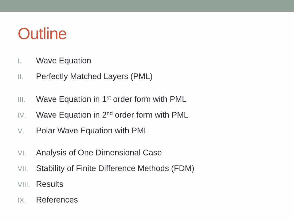
Wave Equation

• The wave equation is the following partial differential

equation (PDE) :

𝑢𝑡𝑡 = 𝑐2 𝛻 ⋅ 𝛻𝑢

• In Cartesian coordinates:

𝑢𝑡𝑡 = 𝑐2 𝑢𝑥𝑥, for 𝑢 𝑡, 𝑥

𝑢𝑡𝑡 = 𝑐2 𝑢𝑥𝑥 + 𝑢𝑦𝑦 , for 𝑢 𝑡, 𝑥, 𝑦

• In polar coordinates:

𝑢𝑡𝑡 = 𝑐2 1

𝑟 𝑟 𝑢𝑟 𝑟 +

1

𝑟2 𝑢𝜃𝜃

• These equations produce the familiar traveling wave

solutions.

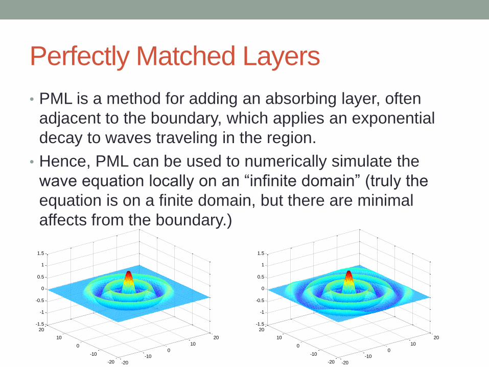
Perfectly Matched Layers

• PML is a method for adding an absorbing layer, often

adjacent to the boundary, which applies an exponential

decay to waves traveling in the region.

• Hence, PML can be used to numerically simulate the

wave equation locally on an “infinite domain” (truly the

equation is on a finite domain, but there are minimal

affects from the boundary.)

-20

-10

0

10

20

-20

-10

0

10

20-1.5

-1

-0.5

0

0.5

1

1.5

-20

-10

0

10

20

-20

-10

0

10

20-1.5

-1

-0.5

0

0.5

1

1.5

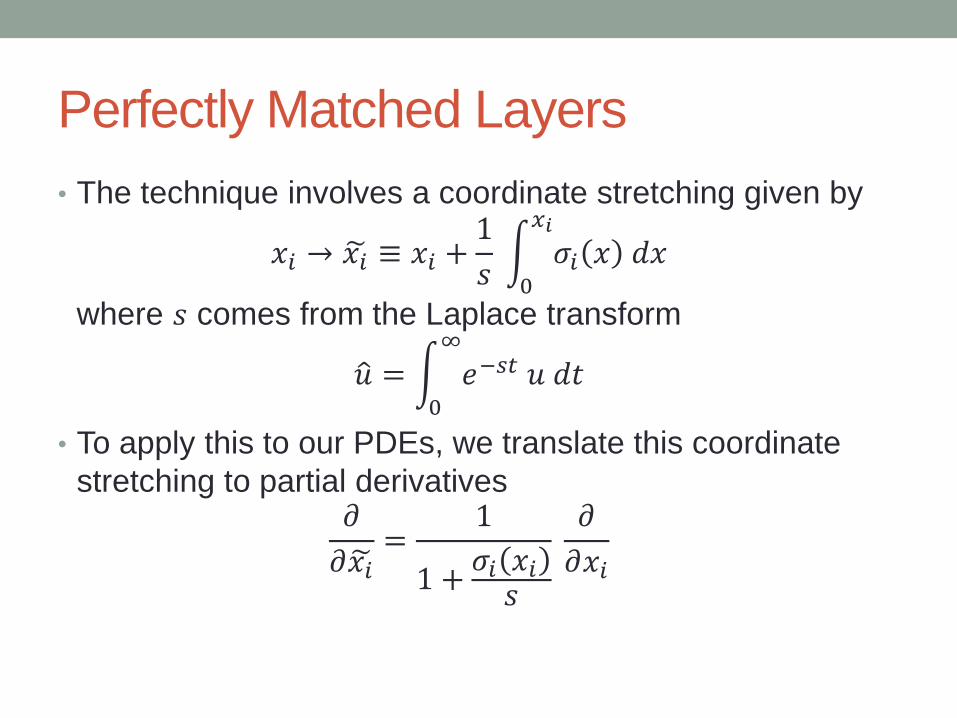
Perfectly Matched Layers

• The technique involves a coordinate stretching given by

𝑥𝑖 → 𝑥𝑖 ≡ 𝑥𝑖 +1

𝑠 𝜎𝑖 𝑥 𝑑𝑥

𝑥𝑖

0

where 𝑠 comes from the Laplace transform

𝑢 = 𝑒−𝑠𝑡 𝑢 𝑑𝑡∞

0

• To apply this to our PDEs, we translate this coordinate

stretching to partial derivatives 𝜕

𝜕𝑥𝑖 =

1

1 +𝜎𝑖 𝑥𝑖𝑠

𝜕

𝜕𝑥𝑖

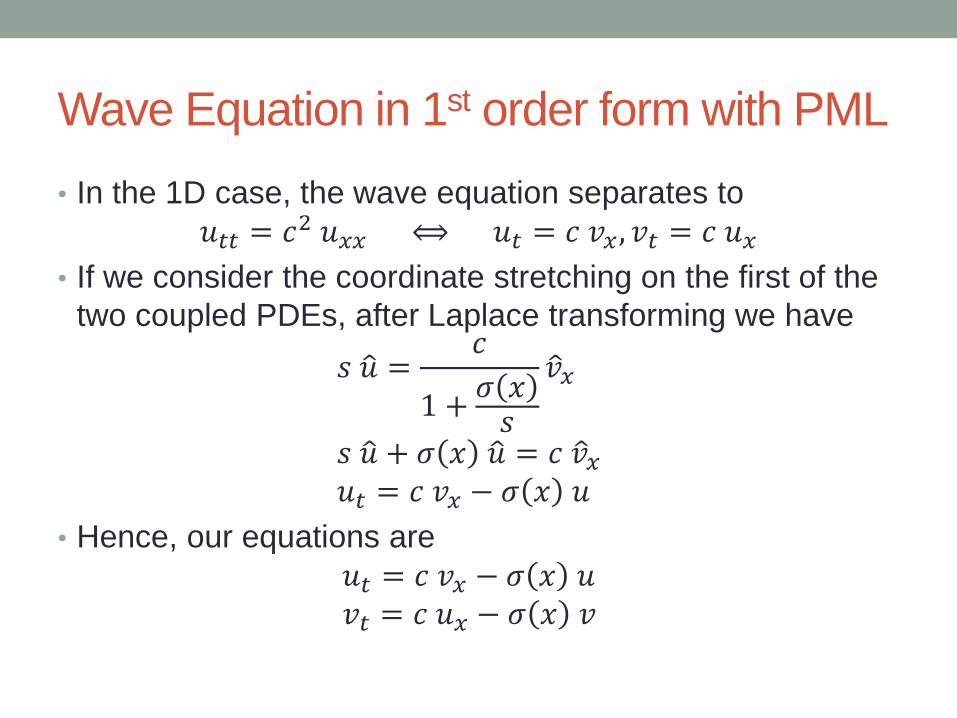
Wave Equation in 1st order form with PML

• In the 1D case, the wave equation separates to

𝑢𝑡𝑡 = 𝑐2 𝑢𝑥𝑥 ⟺ 𝑢𝑡 = 𝑐 𝑣𝑥 , 𝑣𝑡 = 𝑐 𝑢𝑥

• If we consider the coordinate stretching on the first of the

two coupled PDEs, after Laplace transforming we have

𝑠 𝑢 =𝑐

1 +𝜎 𝑥𝑠

𝑣 𝑥

𝑠 𝑢 + 𝜎 𝑥 𝑢 = 𝑐 𝑣 𝑥

𝑢𝑡 = 𝑐 𝑣𝑥 − 𝜎 𝑥 𝑢

• Hence, our equations are

𝑢𝑡 = 𝑐 𝑣𝑥 − 𝜎 𝑥 𝑢

𝑣𝑡 = 𝑐 𝑢𝑥 − 𝜎 𝑥 𝑣

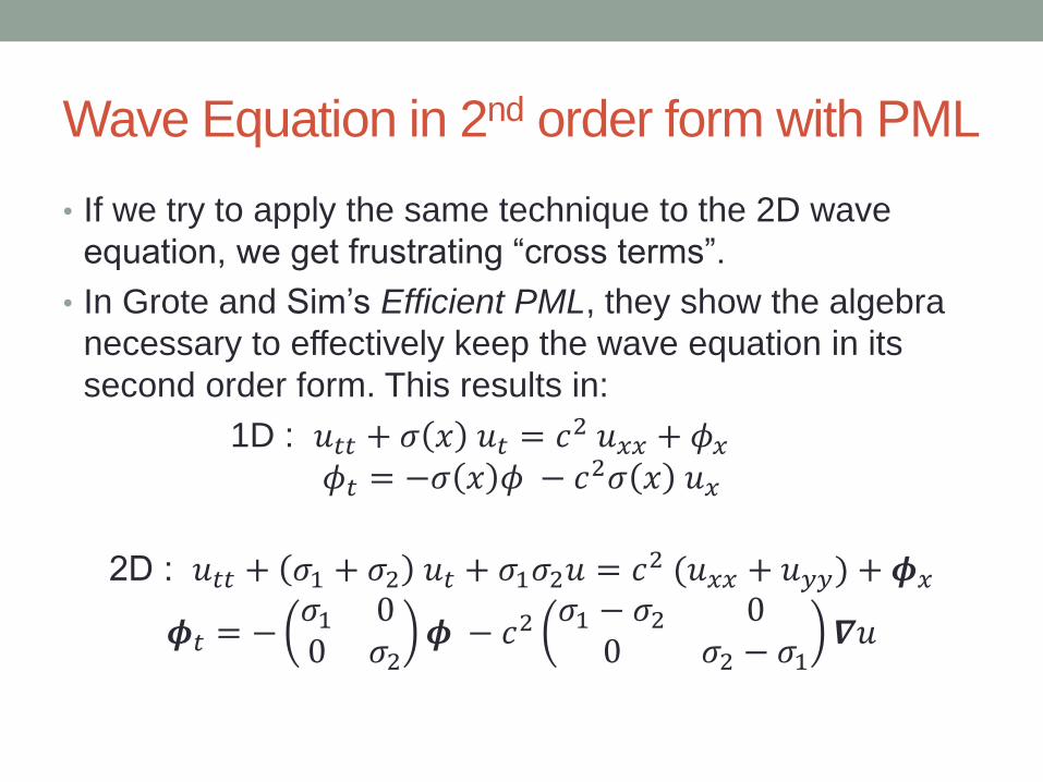
Wave Equation in 2nd order form with PML

• If we try to apply the same technique to the 2D wave

equation, we get frustrating “cross terms”.

• In Grote and Sim’s Efficient PML, they show the algebra

necessary to effectively keep the wave equation in its

second order form. This results in:

1D : 𝑢𝑡𝑡 + 𝜎 𝑥 𝑢𝑡 = 𝑐2 𝑢𝑥𝑥 + 𝜙𝑥 𝜙𝑡 = −𝜎 𝑥 𝜙 − 𝑐2𝜎 𝑥 𝑢𝑥

2D : 𝑢𝑡𝑡 + 𝜎1 + 𝜎2 𝑢𝑡 + 𝜎1𝜎2𝑢 = 𝑐2 (𝑢𝑥𝑥 + 𝑢𝑦𝑦) + 𝝓𝑥

𝝓𝑡 = −𝜎1 00 𝜎2

𝝓 − 𝑐2𝜎1 − 𝜎2 0

0 𝜎2 − 𝜎1𝜵𝑢

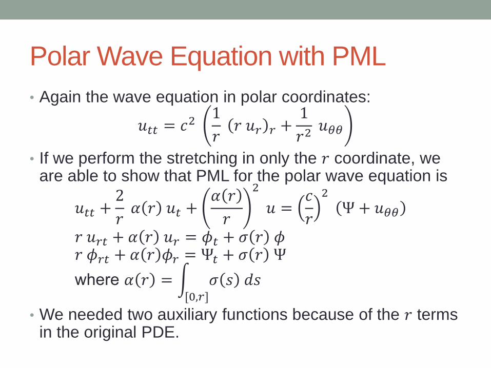
Polar Wave Equation with PML

• Again the wave equation in polar coordinates:

𝑢𝑡𝑡 = 𝑐2 1

𝑟 𝑟 𝑢𝑟 𝑟 +

1

𝑟2 𝑢𝜃𝜃

• If we perform the stretching in only the 𝑟 coordinate, we are able to show that PML for the polar wave equation is

𝑢𝑡𝑡 +2

𝑟 𝛼 𝑟 𝑢𝑡 +

𝛼 𝑟

𝑟

2

𝑢 =𝑐

𝑟

2

Ψ + 𝑢𝜃𝜃

𝑟 𝑢𝑟𝑡 + 𝛼 𝑟 𝑢𝑟 = 𝜙𝑡 + 𝜎 𝑟 𝜙 𝑟 𝜙𝑟𝑡 + 𝛼 𝑟 𝜙𝑟 = Ψ𝑡 + 𝜎 𝑟 Ψ

where 𝛼 𝑟 = 𝜎 𝑠 𝑑𝑠[0,𝑟]

• We needed two auxiliary functions because of the 𝑟 terms in the original PDE.

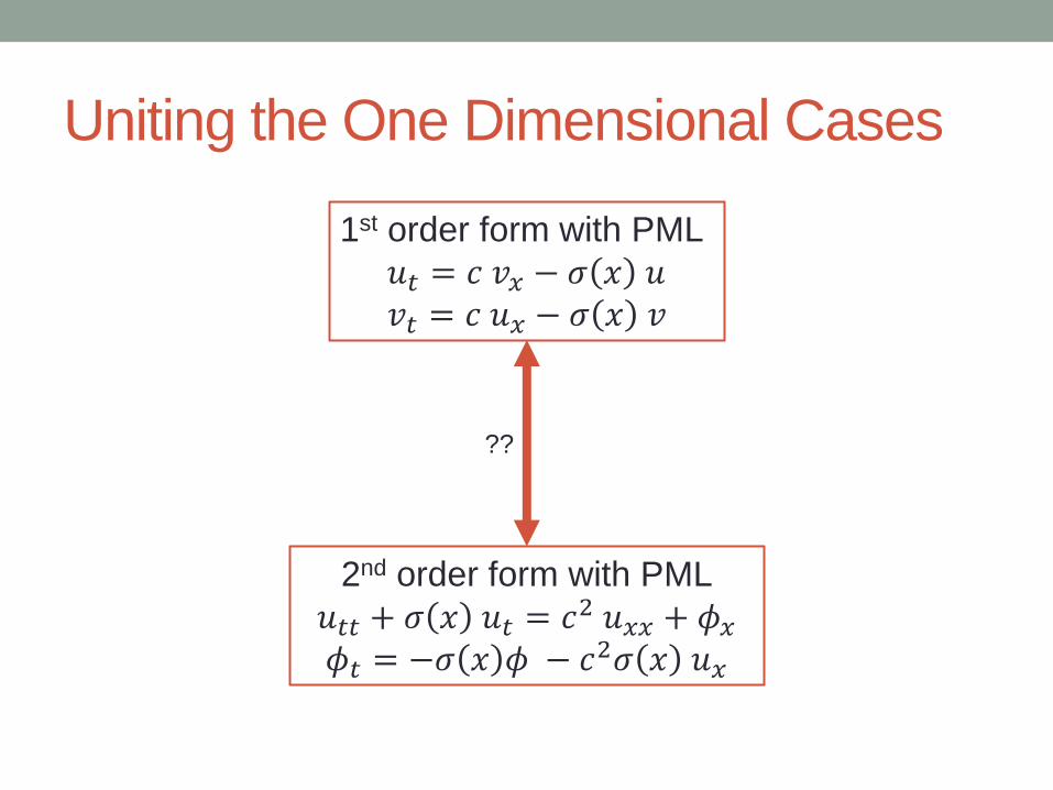
Uniting the One Dimensional Cases

1st order form with PML

𝑢𝑡 = 𝑐 𝑣𝑥 − 𝜎 𝑥 𝑢 𝑣𝑡 = 𝑐 𝑢𝑥 − 𝜎 𝑥 𝑣

2nd order form with PML

𝑢𝑡𝑡 + 𝜎 𝑥 𝑢𝑡 = 𝑐2 𝑢𝑥𝑥 + 𝜙𝑥

𝜙𝑡 = −𝜎 𝑥 𝜙 − 𝑐2𝜎 𝑥 𝑢𝑥

??

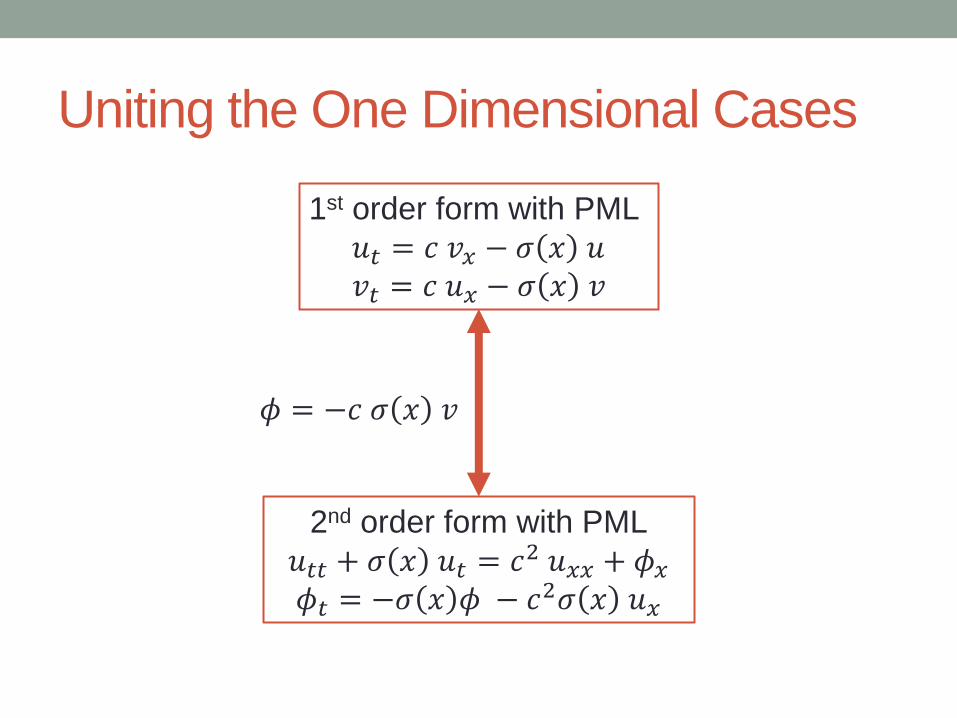
Uniting the One Dimensional Cases

1st order form with PML

𝑢𝑡 = 𝑐 𝑣𝑥 − 𝜎 𝑥 𝑢 𝑣𝑡 = 𝑐 𝑢𝑥 − 𝜎 𝑥 𝑣

2nd order form with PML

𝑢𝑡𝑡 + 𝜎 𝑥 𝑢𝑡 = 𝑐2 𝑢𝑥𝑥 + 𝜙𝑥

𝜙𝑡 = −𝜎 𝑥 𝜙 − 𝑐2𝜎 𝑥 𝑢𝑥

𝜙 = −𝑐 𝜎 𝑥 𝑣

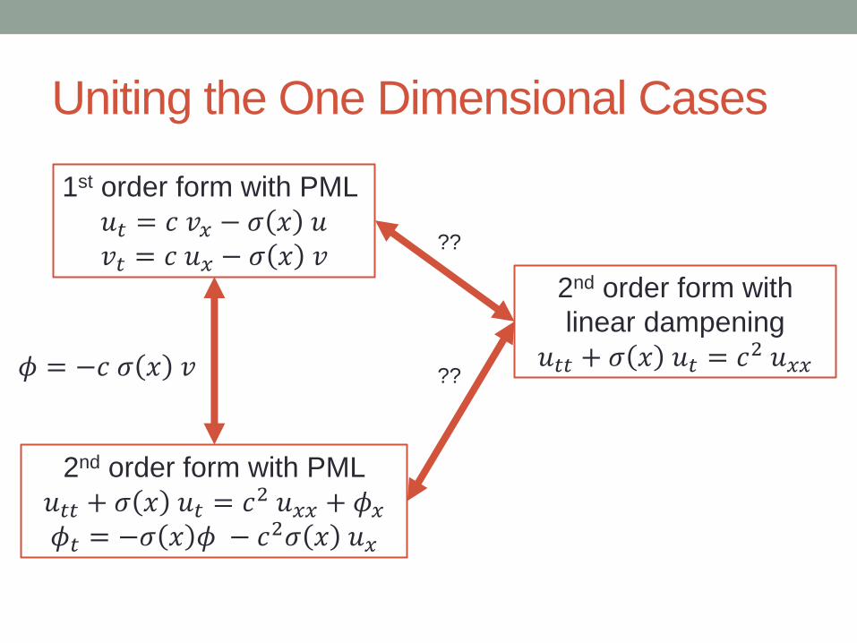
Uniting the One Dimensional Cases

1st order form with PML

𝑢𝑡 = 𝑐 𝑣𝑥 − 𝜎 𝑥 𝑢 𝑣𝑡 = 𝑐 𝑢𝑥 − 𝜎 𝑥 𝑣

2nd order form with PML

𝑢𝑡𝑡 + 𝜎 𝑥 𝑢𝑡 = 𝑐2 𝑢𝑥𝑥 + 𝜙𝑥

𝜙𝑡 = −𝜎 𝑥 𝜙 − 𝑐2𝜎 𝑥 𝑢𝑥

𝜙 = −𝑐 𝜎 𝑥 𝑣

2nd order form with

linear dampening

𝑢𝑡𝑡 + 𝜎 𝑥 𝑢𝑡 = 𝑐2 𝑢𝑥𝑥

??

??

Uniting the One Dimensional Cases

1st order form with PML

𝑢𝑡 = 𝑐 𝑣𝑥 − 𝜎 𝑥 𝑢 𝑣𝑡 = 𝑐 𝑢𝑥 − 𝜎 𝑥 𝑣

2nd order form with PML

𝑢𝑡𝑡 + 𝜎 𝑥 𝑢𝑡 = 𝑐2 𝑢𝑥𝑥 + 𝜙𝑥

𝜙𝑡 = −𝜎 𝑥 𝜙 − 𝑐2𝜎 𝑥 𝑢𝑥

𝜙 = −𝑐 𝜎 𝑥 𝑣

1st order form with

linear dampening

𝑢𝑡 = 𝑐 𝑣𝑥 − 𝜎 𝑥 𝑢 𝑣𝑡 = 𝑐 𝑢𝑥

Drop

a

term

2nd order form with

linear dampening

𝑢𝑡𝑡 + 𝜎 𝑥 𝑢𝑡 = 𝑐2 𝑢𝑥𝑥

Soliton Solution to One Dimensional Case

• A Soliton is a traveling wave solution to a wave-like PDE. Typical examples include the Korteweg-deVries equation which describes water waves in a trough or canal.

• If we take our 1D 1st order wave equation with PML, 𝑢𝑡 = 𝑐 𝑣𝑥 − 𝜎 𝑥 𝑢 𝑣𝑡 = 𝑐 𝑢𝑥 − 𝜎 𝑥 𝑣, 𝑥 ∈ −∞,∞ , 𝑡 ∈ 0,∞

𝑢 𝑡 = 0, 𝑥 = 𝑓 𝑥 , 𝑢𝑡 𝑡 = 0, 𝑥 = 0

• And assume the form 𝑢 = 𝐹 𝑥 + 𝑐 𝑡 𝑔(𝑥). Then after some algebra we find our solution is

𝑢 𝑡, 𝑥 =𝑓(𝑥 + 𝑐 𝑡)

𝑏 𝑥 + 𝑐 𝑡 +1

𝑏 𝑥 + 𝑐 𝑡

𝑏 𝑥 +𝑓 𝑥 − 𝑐 𝑡

𝑏 𝑥 − 𝑐 𝑡 +1

𝑏(𝑥 − 𝑐 𝑡)

1

𝑏(𝑥)

where 𝑏 𝑥 = exp 𝜎 𝑠

𝑐 𝑑𝑠

0,𝑥.

Stability of Finite Difference Methods

• I chose to use second order FDMs to discretize PDEs.

• Suppose we are considering the problem

𝑢𝑡𝑡 + 𝜎 𝑥 𝑢𝑡 = 𝑐2 𝑢𝑥𝑥 + 𝜙𝑥

𝜙𝑡 = −𝜎 𝑥 𝜙 − 𝑐2𝜎 𝑥 𝑢𝑥

• We define our mesh by Δ𝑥, Δ𝑡 such that

𝑈𝑗𝑖 ≈ 𝑢 𝑖 ∆𝑡, 𝑗 ∆𝑥 and 𝜙𝑗

𝑖 ≈ 𝜙 𝑖 ∆𝑡, 𝑗 ∆𝑥

for 𝑖 = 0,… , 𝑛 − 1, 𝑗 = 0,… ,𝑚 − 1.

• The standard discretization of the second equation

however, is unstable (𝜙 explodes)

𝜙𝑗𝑖+1 − 𝜙𝑗

𝑖−1

2 𝑑𝑡= −𝜎𝑗 𝜙𝑗

𝑖 − 𝑐2 𝜎𝑗𝑢𝑗+1𝑖 − 𝑢𝑗−1

𝑖

2 𝑑𝑥

Stability of Finite Difference Methods

• We can experimentally observe that the instability in begins in 𝜙 before affecting 𝑢. Hence for stability concerns we can consider just

𝜙𝑡 = −𝜎(𝑥0) 𝜙

• Which is very easy to analyze with Von Neumann Stability analysis, to show that

𝜙𝑖+1 − 𝜙𝑖−1

2 𝑑𝑡= −𝜎 𝜙𝑖

accrues error with each step on the order of

𝑔 = 𝑑𝑡 𝜎 + 𝑑𝑡 𝜎 2 + 1

• However, if we use 𝜙𝑖+1 − 𝜙𝑖−1

2 𝑑𝑡= −𝜎

𝜙𝑖 + 𝜙𝑖+1

2

then our error remains fairly constant (𝑔 = 1).

• Each PDE has a term which needs this substitution for stability.

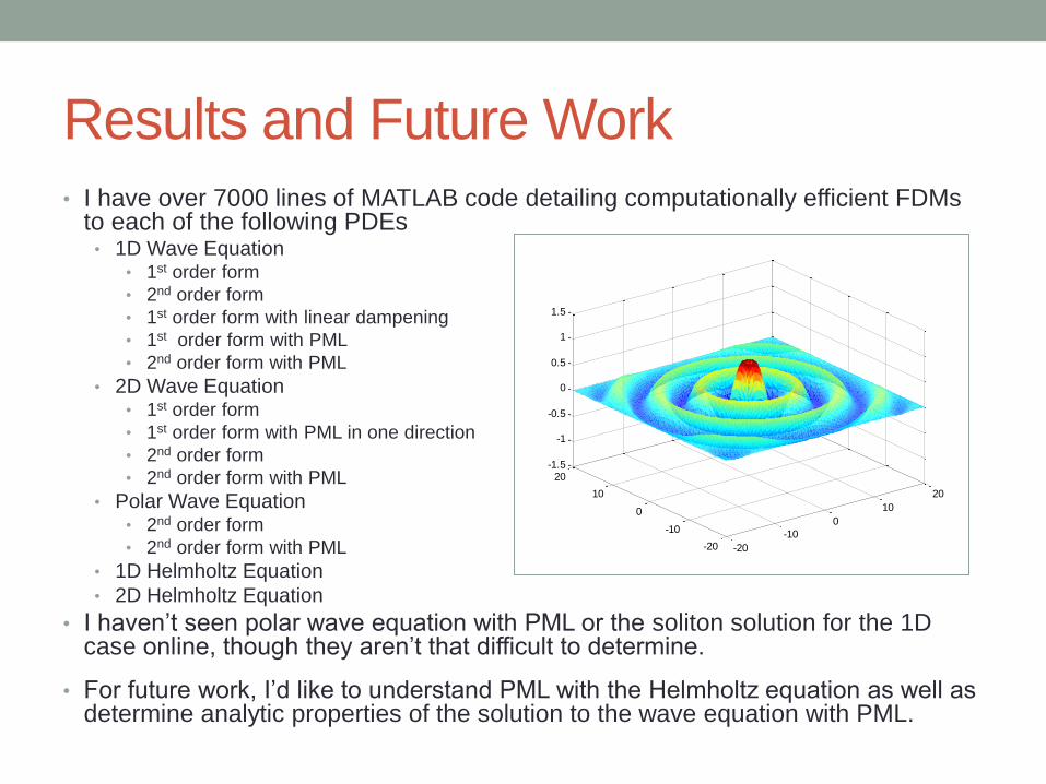
Results and Future Work • I have over 7000 lines of MATLAB code detailing computationally efficient FDMs

to each of the following PDEs • 1D Wave Equation

• 1st order form

• 2nd order form

• 1st order form with linear dampening

• 1st order form with PML

• 2nd order form with PML

• 2D Wave Equation • 1st order form

• 1st order form with PML in one direction

• 2nd order form

• 2nd order form with PML

• Polar Wave Equation • 2nd order form

• 2nd order form with PML

• 1D Helmholtz Equation

• 2D Helmholtz Equation

• I haven’t seen polar wave equation with PML or the soliton solution for the 1D case online, though they aren’t that difficult to determine.

• For future work, I’d like to understand PML with the Helmholtz equation as well as determine analytic properties of the solution to the wave equation with PML.

-20

-10

0

10

20

-20

-10

0

10

20-1.5

-1

-0.5

0

0.5

1

1.5

References

I. J.-P. Bérenger, “A perfectly matched layer for the absorption of

electromagnetic waves,” J. Comput. Phys., vol. 114, no. 1, pp.

185–200, 1994.

II. M. Grote & I. Sim, “Efficient PML for the wave equation,” Jan.

2010. arXiv:1001.0319 [math.NA]

III. S. Johnson, “Notes on Perfectly Matched Layers (PML),” Aug.

2007. math.mit.edu/~stevenj/18.369/pml.pdf

IV. M. Lassas & E. Somersalo, “On the existence and convergence of

the solution of PML equations,” J. Computing, vol. 60, Issue 3, pp.

229-241, 1998.