Embed Size (px)
Citation preview

INTERNATIONAL JOURNAL FOR NUMERICAL METHODS IN ENGINEERINGInt. J. Numer. Meth. Engng 2004; 59:1039–1074 (DOI: 10.1002/nme.896)
Perfectly matched layers for transient elastodynamicsof unbounded domains
Ushnish Basu and Anil K. Chopra∗,†
Department of Civil and Environmental Engineering, University of California, Berkeley, CA 94720, U.S.A.
SUMMARY
One approach to the numerical solution of a wave equation on an unbounded domain uses a boundeddomain surrounded by an absorbing boundary or layer that absorbs waves propagating outward fromthe bounded domain. A perfectly matched layer (PML) is an unphysical absorbing layer model forlinear wave equations that absorbs, almost perfectly, outgoing waves of all non-tangential angles-of-incidence and of all non-zero frequencies. In a recent work [Computer Methods in Applied Mechanicsand Engineering 2003; 192:1337–1375], the authors presented, inter alia, time-harmonic governingequations of PMLs for anti-plane and for plane-strain motion of (visco-)elastic media. This paperpresents (a) corresponding time-domain, displacement-based governing equations of these PMLs and(b) displacement-based finite element implementations of these equations, suitable for direct transientanalysis. The finite element implementation of the anti-plane PML is found to be symmetric, whereasthat of the plane-strain PML is not. Numerical results are presented for the anti-plane motion of asemi-infinite layer on a rigid base, and for the classical soil–structure interaction problems of a rigidstrip-footing on (i) a half-plane, (ii) a layer on a half-plane, and (iii) a layer on a rigid base. Theseresults demonstrate the high accuracy achievable by PML models even with small bounded domains.Copyright � 2004 John Wiley & Sons, Ltd.
KEY WORDS: perfectly matched layers (PML); absorbing boundary; scalar wave equation; elasticwaves; transient analysis; finite elements (FE)
1. INTRODUCTION
The solution of the elastodynamic wave equation over an unbounded domain finds applications
in soil–structure interaction analysis [1] and in the simulation of earthquake ground motion [2].The need for realistic models often compels a numerical solution using a bounded domain, along
with an artificial absorbing boundary or layer that simulates the unbounded domain beyond.
∗Correspondence to: Anil K. Chopra, Department of Civil and Environmental Engineering, 707 Davis Hall,University of California, Berkeley, CA 94720, U.S.A.
†E-mail: [email protected]
Contract/grant sponsor: Waterways Experiment Station, U.S. Army Corps of Engineers; contract/grant number:DACW39-98-K-0038
Received 18 December 2002
Revised 25 April 2003
Copyright � 2004 John Wiley & Sons, Ltd. Accepted 28 May 2003

1040 U. BASU AND A. K. CHOPRA
Of particular importance are absorbing boundaries that allow transient analysis, facilitating
incorporation of non-linearity within the bounded domain.
Classical approximate absorbing boundaries [3–6], although local and cheaply computed,
may require large bounded domains for satisfactory accuracy, since typically they absorb inci-
dent waves well only over a small range of angles-of-incidence. For satisfactory performance,
approximate absorbing layer models [7, 8] require careful formulation and implementation to
eliminate spurious reflections from the interface to the layer. The superposition boundary [9]is cumbersome and expensive to implement, and infinite elements [10, 11] typically require
problem-dependent assumptions on the wave motion. Rigorous absorbing boundaries are typ-
ically formulated in the frequency domain [12–14]; corresponding time-domain formulations
[15–17] may be computationally expensive and may not be applicable to all problems of interest.
The difficulty in obtaining a sufficiently accurate, yet not-too-expensive model of the un-
bounded domain directly in the time domain has led to the use of traditional frequency-domain
models towards time-domain analysis. One such method uses hybrid frequency–time-domain
analysis [1, 18], iterating between the frequency and time domains in order to account for
non-linearity in the bounded domain; this computationally demanding method requires care-
ful implementation to ensure stability. Another approach replaces the non-linear system by
an equivalent linear system [19] whose stiffness and damping values are compatible with the
effective strain amplitudes in the system. A third approach [20–22] approximates the frequency-
domain DtN map of a system by a rational function and uses this approximation to obtain a
time-domain system that is temporally local. Although this approach is conceptually attractive,
computation of an accurate rational-function approximation may be expensive.
A perfectly matched layer (PML) is an absorbing layer model for linear wave equations that
absorbs, almost perfectly, propagating waves of all non-tangential angles-of-incidence and of
all non-zero frequencies. First introduced in the context of electromagnetic waves [23, 24], the
concept of a PML has been applied to other linear wave equations [25–27], including the
elastodynamic wave equation [28, 29]. In a recent work [30], the authors have developed
the concept of a PML in the context of frequency-domain elastodynamics, utilising insights
obtained from PMLs in electromagnetics, and illustrated it using the one-dimensional rod on
elastic foundation and the anti-plane motion of a two-dimensional continuum, governed by the
Helmholtz equation. Extending the PML concept to the displacement formulation of plane-strain
and three-dimensional motion, they have also presented a novel displacement-based, symmetric
finite element implementation of such a PML.
The objective of this paper is to present (a) time-domain, displacement-based, equations
of the PMLs for anti-plane and for plane-strain motion of a (visco-)elastic medium, and (b)
displacement-based finite element (FE) implementations of these equations. The frequency-
domain PML equations from Reference [30] are first transformed into the time domain by a
special choice of the co-ordinate-stretching functions, and then these time-domain equations are
implemented numerically by a straightforward finite element approach. Time-domain numerical
results are presented for the anti-plane motion of a semi-infinite layer on rigid base and for
the classical soil–structure interaction problems of a rigid strip-footing on (i) a half-plane, (ii)
a layer on a half-plane, and (iii) a layer on a rigid base. Additionally, the adequacy of the
special choice of the stretching functions towards attenuating evanescent waves is investigated
through numerical results in the frequency domain. This paper presents only a brief explanation
of the concept of a PML; a detailed development, and the derivation of the frequency-domain
equations are presented in Reference [30].
Copyright � 2004 John Wiley & Sons, Ltd. Int. J. Numer. Meth. Engng 2004; 59:1039–1074

TRANSIENT ELASTODYNAMICS OF UNBOUNDED DOMAINS 1041
Tensorial and indicial notation will be used interchangeably in this paper; the summation
convention will be assumed unless an explicit summation is used or it is mentioned otherwise.
An italic boldface symbol will represent a vector, e.g. x, an upright boldface symbol will
represent a tensor or its matrix in a particular orthonormal basis, e.g. D, and a sans-serif
boldface symbol will represent a fourth-order tensor, e.g. C; the corresponding lightface symbols
with Roman subscripts will denote components of the tensor, matrix or vector. An overbar over
a symbol, e.g. u, denotes a time-harmonic quantity; such distinguishing notation was not
employed in Reference [30] because the entire analysis was in the frequency domain.
2. ANTI-PLANE MOTION
2.1. Elastic medium
Consider a two-dimensional homogeneous isotropic elastic continuum undergoing only anti-
plane displacements in the absence of body forces. For such motion, if the x3-direction is
taken to point out of the plane, only the 31- and 32-components of the three-dimensional
stress and strain tensors are non-zero. The displacements u(x, t) are governed by the following
equations (i ∈ {1, 2}):
∑
i
��i
�xi
= �u (1a)
�i = �εi (1b)
εi = �u
�xi
(1c)
where � is the shear modulus of the medium and � its mass density; �i and εi represent the
3i-components of the stress and strain tensors.
On an unbounded domain, Equation (1) admits plane shear wave solutions [31] of the form
u(x, t) = exp[−iksx·p] exp(i�t) (2)
where ks = �/cs is the wavenumber, with wave speed cs = √�/�, and p is a unit vector
denoting the propagation direction.
2.2. Perfectly matched layer
The discussion of PML presented here is a synopsis of the corresponding development in
Reference [30]. The summation convention is abandoned in this section.
Consider a wave of the form in Equation (2) propagating in an unbounded elastic domain,
the x1–x2 plane, governed by Equation (1). The objective of defining a perfectly matched layer
(PML) is to simulate such wave propagation by using a corresponding bounded domain.
The governing equations of a PML are most naturally defined in the frequency domain,
through frequency-dependent, complex-valued co-ordinate stretching. Assuming harmonic time-
dependence of the displacement, stress and strain, e.g. u(x, t) = u(x) exp(i�t), with � the
Copyright � 2004 John Wiley & Sons, Ltd. Int. J. Numer. Meth. Engng 2004; 59:1039–1074
1042 U. BASU AND A. K. CHOPRA
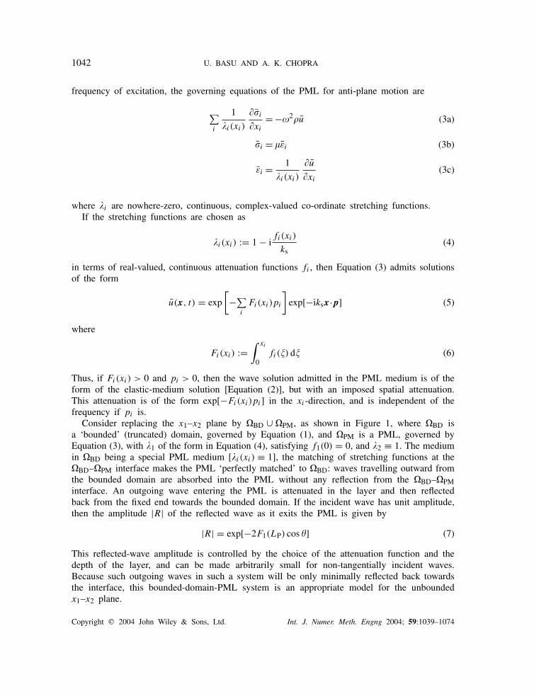
frequency of excitation, the governing equations of the PML for anti-plane motion are
∑
i
1
�i(xi)
��i
�xi
= −�2�u (3a)
�i = �εi (3b)
εi = 1
�i(xi)
�u
�xi
(3c)
where �i are nowhere-zero, continuous, complex-valued co-ordinate stretching functions.
If the stretching functions are chosen as
�i(xi) := 1 − ifi(xi)
ks(4)
in terms of real-valued, continuous attenuation functions fi , then Equation (3) admits solutions
of the form
u(x, t) = exp
[
−∑
i
Fi(xi)pi
]
exp[−iksx·p] (5)
where
Fi(xi) :=∫ xi
0
fi(�) d� (6)
Thus, if Fi(xi) > 0 and pi > 0, then the wave solution admitted in the PML medium is of the
form of the elastic-medium solution [Equation (2)], but with an imposed spatial attenuation.
This attenuation is of the form exp[−Fi(xi)pi] in the xi-direction, and is independent of the
frequency if pi is.
Consider replacing the x1–x2 plane by �BD ∪ �PM, as shown in Figure 1, where �BD is
a ‘bounded’ (truncated) domain, governed by Equation (1), and �PM is a PML, governed by
Equation (3), with �1 of the form in Equation (4), satisfying f1(0) = 0, and �2 ≡ 1. The medium
in �BD being a special PML medium [�i(xi) ≡ 1], the matching of stretching functions at the
�BD–�PM interface makes the PML ‘perfectly matched’ to �BD: waves travelling outward from
the bounded domain are absorbed into the PML without any reflection from the �BD–�PM
interface. An outgoing wave entering the PML is attenuated in the layer and then reflected
back from the fixed end towards the bounded domain. If the incident wave has unit amplitude,
then the amplitude |R| of the reflected wave as it exits the PML is given by
|R| = exp[−2F1(LP) cos �] (7)
This reflected-wave amplitude is controlled by the choice of the attenuation function and the
depth of the layer, and can be made arbitrarily small for non-tangentially incident waves.
Because such outgoing waves in such a system will be only minimally reflected back towards
the interface, this bounded-domain-PML system is an appropriate model for the unbounded
x1–x2 plane.
Copyright � 2004 John Wiley & Sons, Ltd. Int. J. Numer. Meth. Engng 2004; 59:1039–1074

TRANSIENT ELASTODYNAMICS OF UNBOUNDED DOMAINS 1043
Figure 1. A PML adjacent to a ‘bounded’ (truncated) domain attenuates and reflectsback an outgoing plane wave.
2.3. Time-domain equations for the PML
Consider two rectangular Cartesian co-ordinate systems for the plane as follows: (1) an {xi}system, with respect to an orthonormal basis {ei}, and (2) an {x′
i} system, with respect to
another orthonormal basis {e′i}, with the two bases related by the rotation-of-basis matrix Q,
with components Qij := ei · e′j . Equation (3) can be re-written in terms of the co-ordinates x′
i
by replacing xi by x′i throughout, representing a medium wherein waves are attenuated in the
e′1 and e′
2 directions, rather than in the e1 and e2 directions as in Equation (3). This resultant
equation can be transformed to the basis {ei} to obtain [30]
∇ · (��) = −�2�[�1(x′1)�2(x
′2)]u (8a)
� = �(1 + 2ia0�)� (8b)
� = �(∇u) (8c)
where
� :={
�1
�2
}
, � :={
ε1
ε2
}
, ∇ :=
�
�x1
�
�x2
(9)
Copyright � 2004 John Wiley & Sons, Ltd. Int. J. Numer. Meth. Engng 2004; 59:1039–1074

1044 U. BASU AND A. K. CHOPRA
and
� = Q�′QT, � = Q�
′QT (10)
with
�′ :=
[
�2(x′2) ·
· �1(x′1)
]
, �′ :=
[
1/�1(x′1) ·
· 1/�2(x′2)
]
(11)
Equation (8) explicitly incorporates Voigt material damping through the correspondence principle
in terms of a damping ratio � and a non-dimensional frequency a0 = ksb, where b is a
characteristic length of the physical problem. This damping model is chosen over the traditional
hysteretic damping model because the latter is non-causal [32]; implementation of a causal
hysteretic model in a PML formulation is beyond the scope of this paper.
Because multiplication or division by the factor i� in the frequency domain corresponds to
a derivative or an integral, respectively, in the time domain, time-harmonic equations are easily
transformed into corresponding equations for transient motion if the frequency-dependence of
the former is only a simple dependence on this factor. Therefore, the stretching functions are
chosen to be of the form
�i(x′i) := [1 + f e
i (x′i)] − i
fpi (x′
i)
ks(12)
where, the functions f ei serve to attenuate evanescent waves whereas the functions f
pi serve
to attenuate propagating waves. For �i as in Equation (12), the stretch tensors � and � can
be written as
� = Fe + 1
i�Fp, � =
[
Fe + 1
i�Fp
]−1
(13)
where
Fe = QFe′QT, Fp = QFp′QT, Fe = QFe′QT, Fp = QFp′QT (14)
with
Fe′ :=[
1 + f e2 (x′
2) ·
· 1 + f e1 (x′
1)
]
, Fp′ :=[
csfp
2 (x′2) ·
· csfp
1 (x′1)
]
(15a)
and
Fe′ :=[
1 + f e1 (x′
1) ·
· 1 + f e2 (x′
2)
]
, Fp′ :=[
csfp
1 (x′1) ·
· csfp
2 (x′2)
]
(15b)
Equation (8c) is premultiplied by i��−1, Equations (12) and (13) are substituted into Equa-
tion (8), and the inverse Fourier transform is applied to the resultant to obtain the time domain
equations for the PML:
∇ · � = �fmu + �csfcu + �fku (16a)
Copyright � 2004 John Wiley & Sons, Ltd. Int. J. Numer. Meth. Engng 2004; 59:1039–1074

TRANSIENT ELASTODYNAMICS OF UNBOUNDED DOMAINS 1045
� = �
(
� + 2�b
cs�
)
(16b)
Fe� + Fp
� = ∇u (16c)
where
� := Fe� + Fp
�, with � :=∫ t
0
� d (17)
and
fm := [1 + f e1 (x′
1)][1 + f e2 (x′
2)]
fc := [1 + f e1 (x′
1)]fp
2 (x′2) + [1 + f e
2 (x′2)]f
p
1 (x′1)
fk := fp
1 (x′1)f
p
2 (x′2)
(18)
The application of the inverse Fourier transform to obtain � assumes that �(� = 0) = 0. The
presence of the time-integral of � in the governing equations, although unconventional from
the point-of-view of continuum mechanics, is not unnatural in a time-domain implementation
of a PML obtained without field-splitting [33].
2.4. Finite element implementation
Equation (16) is implemented using a standard displacement-based finite element approach
[34]. The weak form of Equation (16a) is derived by multiplying it with an arbitrary weighting
function w residing in an appropriate admissible space, and then integrating over the entire
computational domain � using integration-by-parts and the divergence theorem to obtain∫
�
�fmwu d� +∫
�
�csfcwu d� +∫
�
�fkwu d� +∫
�
∇w · � d� =∫
�
w � · n d� (19)
where � := �� is the boundary of � and n is the unit normal to �. The weak form is first
spatially discretized by interpolating u and w element-wise in terms of nodal quantities using
appropriate nodal shape functions. This leads to the system of equations
md + cd + kd + pint = pext (20)
where m, c and k are the mass, damping and stiffness matrices, respectively, d is a vector of
nodal displacements, pint is a vector of internal force terms, and pext is a vector of external
forces. These matrices and vectors are assembled from corresponding element-level matrices and
vectors. In particular, the element-level constituent matrices of m, c and k are, respectively,
me =∫
�e�fmNTN d�, ce =
∫
�e�csfcN
TN d�, ke =∫
�e�fkN
TN d� (21a)
and the element-level internal force term is
pe =∫
�eBT
� d� (21b)
Copyright � 2004 John Wiley & Sons, Ltd. Int. J. Numer. Meth. Engng 2004; 59:1039–1074
1046 U. BASU AND A. K. CHOPRA
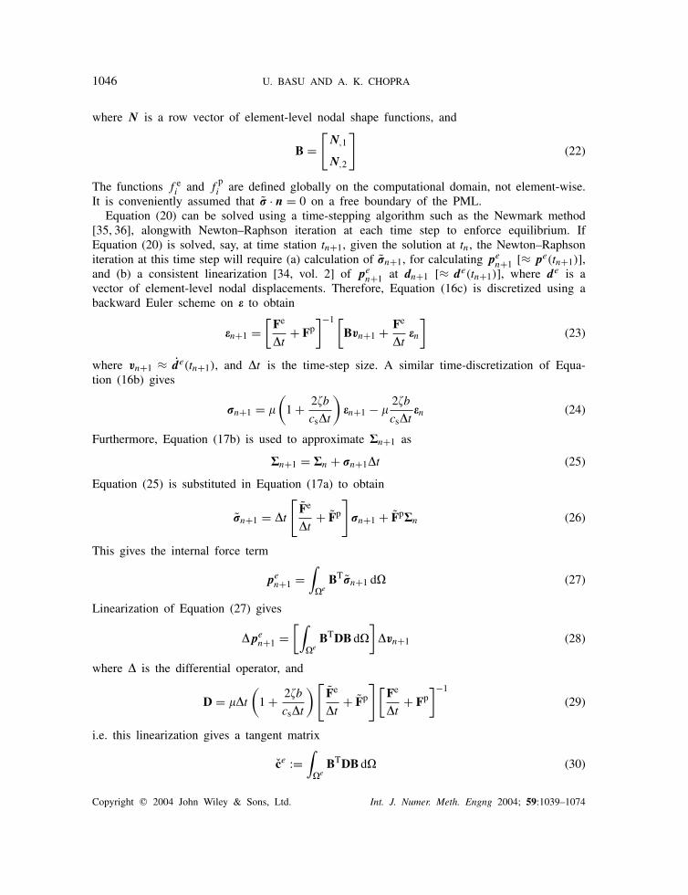
where N is a row vector of element-level nodal shape functions, and
B =[
N,1
N,2
]
(22)
The functions f ei and f
pi are defined globally on the computational domain, not element-wise.
It is conveniently assumed that � · n = 0 on a free boundary of the PML.
Equation (20) can be solved using a time-stepping algorithm such as the Newmark method
[35, 36], alongwith Newton–Raphson iteration at each time step to enforce equilibrium. If
Equation (20) is solved, say, at time station tn+1, given the solution at tn, the Newton–Raphson
iteration at this time step will require (a) calculation of �n+1, for calculating pen+1 [≈ pe(tn+1)],
and (b) a consistent linearization [34, vol. 2] of pen+1 at dn+1 [≈ de(tn+1)], where de is a
vector of element-level nodal displacements. Therefore, Equation (16c) is discretized using a
backward Euler scheme on � to obtain
�n+1 =[
Fe
�t+ Fp
]−1 [
Bvn+1 + Fe
�t�n
]
(23)
where vn+1 ≈ de(tn+1), and �t is the time-step size. A similar time-discretization of Equa-
tion (16b) gives
�n+1 = �
(
1 + 2�b
cs�t
)
�n+1 − �2�b
cs�t�n (24)
Furthermore, Equation (17b) is used to approximate �n+1 as
�n+1 = �n + �n+1�t (25)
Equation (25) is substituted in Equation (17a) to obtain
�n+1 = �t
[
Fe
�t+ Fp
]
�n+1 + Fp�n (26)
This gives the internal force term
pen+1 =
∫
�eBT
�n+1 d� (27)
Linearization of Equation (27) gives
�pen+1 =
[∫
�eBTDB d�
]
�vn+1 (28)
where � is the differential operator, and
D = ��t
(
1 + 2�b
cs�t
)
[
Fe
�t+ Fp
]
[
Fe
�t+ Fp
]−1
(29)
i.e. this linearization gives a tangent matrix
ce :=∫
�eBTDB d� (30)
Copyright � 2004 John Wiley & Sons, Ltd. Int. J. Numer. Meth. Engng 2004; 59:1039–1074

TRANSIENT ELASTODYNAMICS OF UNBOUNDED DOMAINS 1047
Box I. Computing effective force and stiffness for anti-plane PML element.
(1) Compute system matrices me, ce and ke [Equation (21a)].(2) Compute internal force pe
n+1[Equations (27)].
Use �n+1 [Equation (23)], �n+1 [Equation (24)] and �n+1 [Equation (26)].(3) Compute tangent matrix ce [Equation (30)] using D [Equation (29)].
(4) Compute effective internal force pen+1
and tangent stiffness ke:
pen+1 = mean+1 + cevn+1 + kedn+1 + pe
n+1
ke = kke + c
(
ce + ce)
+ mme
where an+1 ≈ de(tn+1), and, for example,
k = 1, c = �
��t, m = 1
��t2
for the Newmark method.
Note: The tangent stiffness ke is independent of the solution, and thus has to be computed onlyonce. However, the internal force pe
n+1has to be re-computed at each time-step because it is
dependent on the solution at past times.
which may be incorporated into the effective tangent stiffness used in the time-stepping
algorithm.
A skeleton of the algorithm for computing the element-level effective internal force and
tangent stiffness is given in Box I. The matrix ce is symmetric because D is symmetric by
the virtue of the coaxiality of the constituent matrices. The other system matrices, m, c and
k are clearly symmetric by Equation (21a). Moreover, because all these matrices are of the
same form as the system matrices for an elastic medium, the effective tangent stiffness (say,
as found in the Newmark scheme) of the entire computational domain will be positive definite
if f ei and f
pi are positive and if the boundary restraints are adequate. Furthermore, since all
the system matrices, m, c, c and k that constitute the tangent stiffness are independent of d,
this is effectively a linear model.
2.5. Numerical results
Consider a homogeneous isotropic semi-infinite layer of depth d on a rigid base, as shown in
Figure 2(a), whose anti-plane motion is governed by Equation (1) with the following boundary
conditions:
u(x, t) = 0 at x2 = 0, ∀x1 > 0, ∀t
�2 = 0 at x2 = d, ∀x1 > 0, ∀t
u(x, t) = u1(t)N1(x2/d) + u2(t)N2(x2/d) at x1 = 0, ∀x2 ∈ [0, d](31)
and a radiation condition for x1 → ∞, where u1 and u2 are the displacements at nodes 1 and
2, and N1 and N2 are shape functions defined as
N1(�) = 4�(1 − �), N2(�) = �(2� − 1), � ∈ [0, 1] (32)
Copyright � 2004 John Wiley & Sons, Ltd. Int. J. Numer. Meth. Engng 2004; 59:1039–1074

1048 U. BASU AND A. K. CHOPRA
Figure 2. (a) Homogeneous isotropic (visco-)elastic semi-infinite layer of depth d ona fixed base; and (b) a PML model.
-1
0
1
0 10 20 30 40 50
u0
(t)
t(a)
0
2
4
6
8
0 2 4 6 8 10
|− u0
(ω)|
ω(b)
Figure 3. Plot of typical: (a) input displacement with td = 20; and (b) amplitude of itsFourier transform, with �f = 2.
The wave motion in this system is similar to Love wave motion: it is dispersive, and consists
of not only propagating modes but also an infinite number of evanescent modes, with the
propagation (and decay) in the x1-direction [37, Appendix A.3].The time-domain response of this system may be studied through the reactions at nodes 1
and 2 due to any combination of nodal displacements u1(t) and u2(t). Employed here is a
time-limited cosine wave, bookended by cosine half-cycles so that the initial displacement and
velocity as well as the final displacement and velocity are zero. This imposed displacement
is characterized by two parameters: the duration td and the dominant forcing frequency �f ; a
typical waveform and its Fourier transform are shown in Figure 3, and a detailed description
of the waveform is given in Appendix A. The displacement u0(t) is imposed on the two nodes
individually, i.e. two cases are considered: (1) u1(t) = u0(t), u2(t) ≡ 0, and (2) u1(t) ≡ 0,
u2(t) = u0(t), and the two nodal reactions are computed for each of the two displacements.
This semi-infinite layer is modelled using the bounded-domain-PML model shown in
Figure 2(b), composed of a bounded domain �BD and a PML �PM, with the attenuation
functions in Equation (12) chosen as f e1 = f
p
1 = f , where f is linear in the PML, and
f e2 = f
p
2 = 0. A uniform finite element mesh of four-node bilinear isoparametric elements is
used to discretize the entire bounded domain. The mesh is chosen to have nd elements per
Copyright � 2004 John Wiley & Sons, Ltd. Int. J. Numer. Meth. Engng 2004; 59:1039–1074

TRANSIENT ELASTODYNAMICS OF UNBOUNDED DOMAINS 1049
-2
-1
0
1
2
0 10 20 30 40 50
P11
ExactPMLDashpots
-2
-1
0
1
2
0 10 20 30 40 50
P11
Extd. meshPMLDashpots
-1
-0.5
0
0.5
1
0 10 20 30 40 50
P12
-1
-0.5
0
0.5
1
0 10 20 30 40 50P
12
-0.5
0
0.5
0 10 20 30 40 50
P22
t
-0.5
0
0.5
0 10 20 30 40 50
P22
t(a) (b)
Figure 4. Nodal reactions of (visco-)elastic semi-infinite layer on fixed base, due to imposednodal displacements; L = d/2, LP = d, nb = np = 15, nd = 15, f1(x1) = 10〈x1 − L〉/LP;td = 30, �f = 2.5 for all cases except for P11 and P22 for elastic layer, where �f = 2.75:
(a) elastic layer, � = 0; and (b) visco-elastic layer, � = 0.05.
unit d, nb elements per unit L/d across the width of �BD, and np elements per unit LP/d
across �PM, with choices for nd, nb and np indicated along with the numerical results. For
comparison, the layer is also modelled using viscous dashpots [4], with consistent dashpots
placed at the edge x1 = L + LP, and the entire domain �BD ∪ �PM taken to be (visco-)elastic.
Thus, the domain size and mesh size are comparable to those in the PML model.
Figure 4(a) presents the nodal reactions computed for an elastic medium using the PML
model and the dashpot model against the exact reactions computed using convolution of the
excitation and the exact impulse response function in Reference [37], where Pij denotes
the reaction at node i due to a non-zero displacement at node j . Based on a comparison
of the frequency-domain responses of the PML and the viscous dashpot models, the values of
�f were chosen as the excitation frequencies where the two responses are significantly differ-
ent. The results obtained from the PML model are virtually indistinguishable from the exact
results, even though the domain is small enough that the viscous-dashpot boundary generates
Copyright � 2004 John Wiley & Sons, Ltd. Int. J. Numer. Meth. Engng 2004; 59:1039–1074
1050 U. BASU AND A. K. CHOPRA
spurious reflections, manifested in the higher response amplitudes. Moreover, these accurate
results from the PML model are obtained at a low computational cost: the cost of the PML
model is observed to be approximately 1.3 times that of the dashpot model, which itself is
extremely inexpensive. Figure 4(b) presents similar results for a visco-elastic layer, with results
from an extended-mesh model used as a benchmark in the absence of analytical solutions; this
extended-mesh model is a viscous-dashpot model of depth d and length 10d from the edge
x1 = 0, with consistent dashpots at x1 = 10d and visco-elastic material within the domain. The
results from the PML model are highly accurate; due to the material damping in the medium,
the inaccuracies of the dashpot model are significantly lesser than in the elastic case.
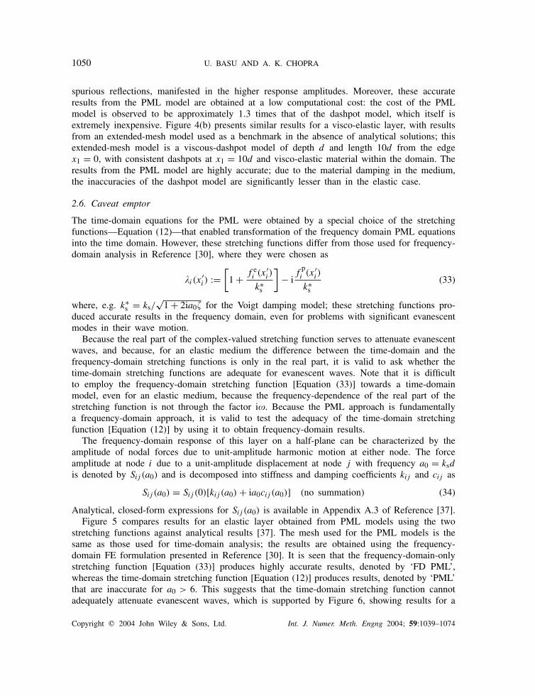
2.6. Caveat emptor
The time-domain equations for the PML were obtained by a special choice of the stretching
functions—Equation (12)—that enabled transformation of the frequency domain PML equations
into the time domain. However, these stretching functions differ from those used for frequency-
domain analysis in Reference [30], where they were chosen as
�i(x′i) :=
[
1 +f e
i (x′i)
k∗s
]
− if
pi (x′
i)
k∗s
(33)
where, e.g. k∗s = ks/
√1 + 2ia0� for the Voigt damping model; these stretching functions pro-
duced accurate results in the frequency domain, even for problems with significant evanescent
modes in their wave motion.
Because the real part of the complex-valued stretching function serves to attenuate evanescent
waves, and because, for an elastic medium the difference between the time-domain and the
frequency-domain stretching functions is only in the real part, it is valid to ask whether the
time-domain stretching functions are adequate for evanescent waves. Note that it is difficult
to employ the frequency-domain stretching function [Equation (33)] towards a time-domain
model, even for an elastic medium, because the frequency-dependence of the real part of the
stretching function is not through the factor i�. Because the PML approach is fundamentally
a frequency-domain approach, it is valid to test the adequacy of the time-domain stretching
function [Equation (12)] by using it to obtain frequency-domain results.
The frequency-domain response of this layer on a half-plane can be characterized by the
amplitude of nodal forces due to unit-amplitude harmonic motion at either node. The force
amplitude at node i due to a unit-amplitude displacement at node j with frequency a0 = ksd
is denoted by Sij (a0) and is decomposed into stiffness and damping coefficients kij and cij as
Sij (a0) = Sij (0)[kij (a0) + ia0cij (a0)] (no summation) (34)
Analytical, closed-form expressions for Sij (a0) is available in Appendix A.3 of Reference [37].Figure 5 compares results for an elastic layer obtained from PML models using the two
stretching functions against analytical results [37]. The mesh used for the PML models is the
same as those used for time-domain analysis; the results are obtained using the frequency-
domain FE formulation presented in Reference [30]. It is seen that the frequency-domain-only
stretching function [Equation (33)] produces highly accurate results, denoted by ‘FD PML’,
whereas the time-domain stretching function [Equation (12)] produces results, denoted by ‘PML’
that are inaccurate for a0 > 6. This suggests that the time-domain stretching function cannot
adequately attenuate evanescent waves, which is supported by Figure 6, showing results for a
Copyright � 2004 John Wiley & Sons, Ltd. Int. J. Numer. Meth. Engng 2004; 59:1039–1074

TRANSIENT ELASTODYNAMICS OF UNBOUNDED DOMAINS 1051
0
0.5
1
0 2 4 6 8 10
k 11(a
0)
ExactPMLFD PML
0
0.2
0.4
0 2 4 6 8 10
c 11(a
0)
0
0.5
1
1.5
2
0 2 4 6 8 10
k 12(a
0)
a0
0
0.2
0.4
0.6
0.8
0 2 4 6 8 10
−c 1
2(a
0)
a0
Figure 5. Dynamic stiffness coefficients of elastic semi-infinite layer on fixed base computed usingPML models with two different forms of the stretching function: ‘PML’ from a stretching functionthat can be implemented in the time domain, and ‘FD PML’ from a stretching function that is moreaccurate but is only suitable for the frequency domain; L = d/2, LP = d, nb = np = 15, nd = 15,
f1(x1) = 10〈x1 − L〉/LP; ‘Exact’ results from Reference [37].
visco-elastic layer obtained using a PML model with the time-domain stretching function: the
material damping attenuates the evanescent modes, and the results are now highly accurate.
Thus, for undamped systems with severely-constricted geometries—typically, waveguides such
as the layer on a rigid base—the time domain results from a PML model may not be accurate
if the excitation is primarily in a frequency band where evanescent modes are not adequately
attenuated. Such a conclusion is echoed in electromagnetics literature [38, 39], where alternative
choices of the stretching function have been considered for attenuating evanescent waves.
3. PLANE-STRAIN MOTION
3.1. Elastic medium
Consider a homogeneous isotropic elastic medium undergoing plane-strain motion in the absence
of body forces. The displacements u(x, t) of such a medium are governed by the following
Copyright � 2004 John Wiley & Sons, Ltd. Int. J. Numer. Meth. Engng 2004; 59:1039–1074

1052 U. BASU AND A. K. CHOPRA
-1
0
1
0 2 4 6 8 10
k 11(a
0)
ExactPML
0.2
0.4
0 2 4 6 8 10
c 11(a
0)
1
1.5
2
0 2 4 6 8 10
k 12(a
0)
a0
-0.2
0
0.2
0.4
0 2 4 6 8 10
−c 1
2(a
0)
a0
Figure 6. Dynamic stiffness coefficients of visco-elastic semi-infinite layer on fixed base computedusing a PML model with a stretching function that can be implemented in the time domain; L = d/2,LP = d, nb = np = 15, nd = 15, f1(x1) = 10〈x1 − L〉/LP; � = 0.05; ‘Exact’ results using the
correspondence principle on results from Reference [37].
equations (i, j, k, l ∈ {1, 2}):
∑
j
��ij
�xj
= �ui (35a)
�ij =∑
k,l
Cijkl εkl (35b)
εij = 1
2
[
�ui
�xj
+ �uj
�xi
]
(35c)
where Cijkl written in terms of the Kronecker delta ij is
Cijkl = (� − 23�) ij kl + �( ik j l + il jk) (36)
�ij and εij are the components of � and �, the stress and infinitesimal strain tensors, Cijkl are
the components of C, the material stiffness tensor; � is the bulk modulus, � the shear modulus,
and � the mass density of the medium. Equation (35) also describes plane-stress motion if �
is re-defined appropriately.
Copyright � 2004 John Wiley & Sons, Ltd. Int. J. Numer. Meth. Engng 2004; 59:1039–1074

TRANSIENT ELASTODYNAMICS OF UNBOUNDED DOMAINS 1053
On an unbounded domain, Equation (35) admits body-wave solutions [31] in the form of
(1) P waves:
u(x, t) = q exp[−ikpx·p] exp(i�t) (37a)
where kp = �/cp, with cp =√
(� + 4�/3)/� the P-wave speed, p is a unit vector denoting the
propagation direction, and q = ±p the direction of particle motion, and (2) S waves:
u(x, t) = q exp[−iksx·p] exp(i�t) (37b)
where ks = �/cs, with cs = √�/� the S-wave speed, and q·p = 0.
3.2. Perfectly matched layer
The discussion presented here is a synopsis of the corresponding development in Reference
[30]. The summation convention is abandoned in this section.
A PML for plane-strain motion is defined naturally in the frequency domain as
∑
j
1
�j (xj )
��ij
�xj
= −�2�ui (38a)
�ij =∑
k,l
Cijkl εkl (38b)
εij = 1
2
[
1
�j (xj )
�ui
�xj
+ 1
�i(xi)
�uj
�xi
]
(38c)
where �i are nowhere-zero, continuous, complex-valued co-ordinate stretching functions. Be-
cause the constitutive relation Equation (38b) is the same as for the elastic medium, Equa-
tion (38) also describes a PMM for plane-stress motion if � is re-defined appropriately.
Equation (38) assumes harmonic time-dependence of the displacement, stress and strain, e.g.
u(x, t) = u(x) exp(i�t), where � is the frequency of excitation.
If the stretching functions are chosen as in Equation (4), then Equation (38) admits solutions
of the form
u(x) = exp
[
− cs
cp
∑
i
Fi(xi)pi
]
q exp[−ikpx·p] (39a)
with q = ±p, and
u(x) = exp
[
−∑
i
Fi(xi)pi
]
q exp[−iksx·p] (39b)
with q·p = 0, and Fi defined as in Equation (6). Thus, if Fi(xi) > 0 and pi > 0, then the
wave solutions admitted in the PML medium are P-type and S-type waves, but with a spatial
attenuation imposed upon them.
As in the case of anti-plane motion, an appropriately defined PML may be placed adjacent
to a bounded domain (Figure 1) in order to simulate an unbounded domain. A wave travelling
outward from the bounded domain is absorbed into the PML without any reflection from the
bounded-domain-PML interface. This wave is then attenuated in the layer and reflected back
Copyright � 2004 John Wiley & Sons, Ltd. Int. J. Numer. Meth. Engng 2004; 59:1039–1074
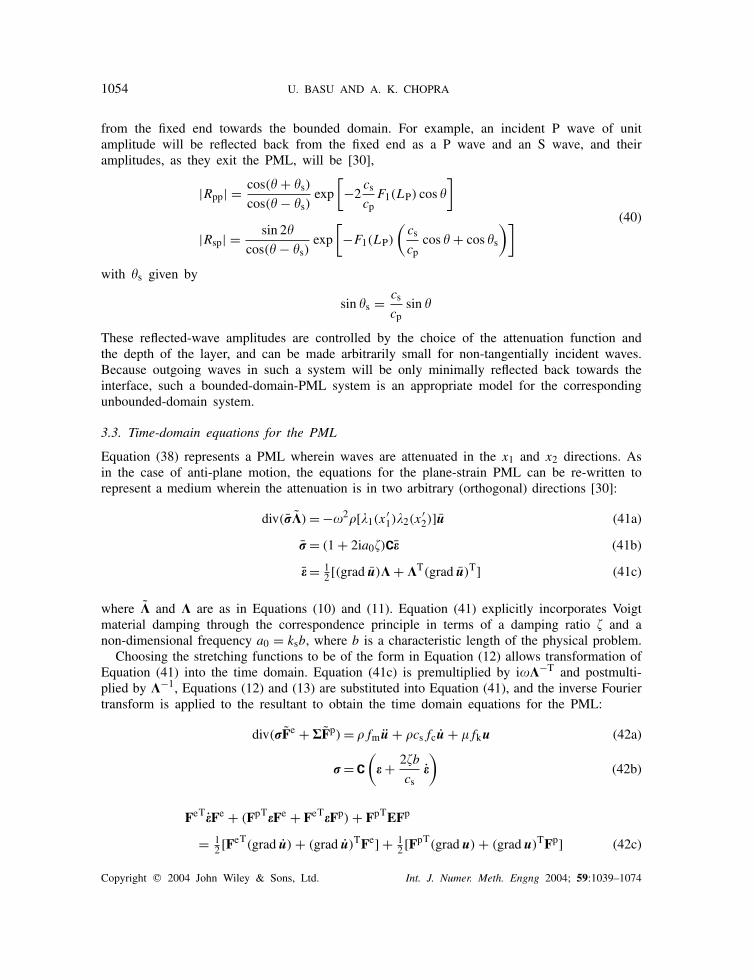
1054 U. BASU AND A. K. CHOPRA
from the fixed end towards the bounded domain. For example, an incident P wave of unit
amplitude will be reflected back from the fixed end as a P wave and an S wave, and their
amplitudes, as they exit the PML, will be [30],
|Rpp| = cos(� + �s)
cos(� − �s)exp
[
−2cs
cpF1(LP) cos �
]
|Rsp| = sin 2�
cos(� − �s)exp
[
−F1(LP)
(
cs
cpcos � + cos �s
)]
(40)
with �s given by
sin �s = cs
cpsin �
These reflected-wave amplitudes are controlled by the choice of the attenuation function and
the depth of the layer, and can be made arbitrarily small for non-tangentially incident waves.
Because outgoing waves in such a system will be only minimally reflected back towards the
interface, such a bounded-domain-PML system is an appropriate model for the corresponding
unbounded-domain system.
3.3. Time-domain equations for the PML
Equation (38) represents a PML wherein waves are attenuated in the x1 and x2 directions. As
in the case of anti-plane motion, the equations for the plane-strain PML can be re-written to
represent a medium wherein the attenuation is in two arbitrary (orthogonal) directions [30]:
div(��) = −�2�[�1(x′1)�2(x
′2)]u (41a)
� = (1 + 2ia0�)C� (41b)
� = 12[(grad u)� + �
T(grad u)T] (41c)
where � and � are as in Equations (10) and (11). Equation (41) explicitly incorporates Voigt
material damping through the correspondence principle in terms of a damping ratio � and a
non-dimensional frequency a0 = ksb, where b is a characteristic length of the physical problem.
Choosing the stretching functions to be of the form in Equation (12) allows transformation of
Equation (41) into the time domain. Equation (41c) is premultiplied by i��−T and postmulti-
plied by �−1, Equations (12) and (13) are substituted into Equation (41), and the inverse Fourier
transform is applied to the resultant to obtain the time domain equations for the PML:
div(�Fe + �Fp) = �fmu + �csfcu + �fku (42a)
� = C
(
� + 2�b
cs�
)
(42b)
FeT�Fe + (FpT
�Fe + FeT�Fp) + FpT
EFp
= 12[FeT
(grad u) + (grad u)TFe] + 12[FpT
(grad u) + (grad u)TFp] (42c)
Copyright � 2004 John Wiley & Sons, Ltd. Int. J. Numer. Meth. Engng 2004; 59:1039–1074

TRANSIENT ELASTODYNAMICS OF UNBOUNDED DOMAINS 1055
where Fe, Fp, Fe and Fp are as in Equations (14) and (15), fm, fc and fk are as in Equa-
tion (18), and
� :=∫ t
0
� d, E :=∫ t
0
� d (43)
Application of the inverse Fourier transform to obtain � and E assumes that �(� = 0) = 0
and �(� = 0) = 0.
3.4. Finite element implementation
Equation (42) is implemented using a standard displacement-based finite element approach
[34]. The weak form of Equation (42a) is derived by taking its inner product with an arbitrary
weighting function w residing in an appropriate admissible space, and then integrating over the
entire computational domain � using integration-by-parts and the divergence theorem to obtain
∫
�
�fmw · u d� +∫
�
�csfcw · u d� +∫
�
�fkw · u d�
+∫
�
�e : � d� +
∫
�
�p : � d� =
∫
�
w · (�Fe + �Fp)n d� (44)
where � := �� is the boundary of � and n is the unit normal to �. The symmetry of � and
� is used to obtain the last two integrals on the left-hand side, with
�e := 1
2[(grad w)Fe + FeT(grad w)T], �
p := 12[(grad w)Fp + FpT(grad w)T] (45)
The weak form is first spatially discretized by interpolating u and w element-wise in terms of
nodal quantities using appropriate nodal shape functions. This leads to a system of equations
as in Equation (20), but with the mass, damping and stiffness matrices given in terms of their
IJ th nodal submatrices as, respectively,
meIJ =
∫
�e�fmNINJ d� I, ce
IJ =∫
�e�csfcNINJ d�I, ke
IJ =∫
�e�fkNINJ d�I (46a)
where NI is the shape function for node I and I is the identity matrix of size 2 × 2. The
element-level internal force term is given by
pe =∫
�eBeT
� d� +∫
�eBpT
� d� (46b)
where Be and Bp are given in terms of their nodal submatrices as
BeI :=
NeI1 ·
· NeI2
NeI2 Ne
I1
, BpI :=
Np
I1 ·
· Np
I2
Np
I2 Np
I1
(47)
Copyright � 2004 John Wiley & Sons, Ltd. Int. J. Numer. Meth. Engng 2004; 59:1039–1074

1056 U. BASU AND A. K. CHOPRA
with
NeI i := F e
ijNI,j and NpI i := F
pijNI,j (48)
and
� :=
�11
�22
�12
(49)
with � the time-integral of �. Note that the above vector representation of the tensor � assumes
its symmetry, which requires a minor symmetry of C; because the PML medium is unphysical,
a physically-motivated axiom—the balance of angular momentum—cannot be employed to
show the symmetry of �. The attenuation functions f ei and f
pi are defined globally on the
computational domain, not element-wise. It is conveniently assumed that there is no contribution
to pext from a free boundary of the PML.
Solution of the equations of motion [Equation (20)] using a time-stepping algorithm requires
calculating �n+1 and �n+1 at tn+1, to calculate pen+1, and also a consistent linearization of
pen+1 at dn+1. Towards this, the approximations
�(tn+1) ≈ �n+1 − �n
�t, E(tn+1) ≈ En + �n+1�t (50)
are used in Equation (42c) to obtain
�n+1 = 1
�t
[
Bεvn+1 + B�dn+1 + 1
�tFε
�n − F�En
]
(51)
where
� :=
ε11
ε22
2ε12
(52)
and E is the time-integral of �. The matrices Bε, B�, Fε and F� in Equation (51) are defined
in Appendix B.
The use of Equation (50a) in the constitutive equation [Equation (42b)] gives
�n+1 =(
1 + 2�b
cs�t
)
D�n+1 − 2�b
cs�tD�n (53)
where
D :=
� + 4�/3 � − 2�/3 ·� − 2�/3 � + 4�/3 ·
· · �
(54)
Copyright � 2004 John Wiley & Sons, Ltd. Int. J. Numer. Meth. Engng 2004; 59:1039–1074

TRANSIENT ELASTODYNAMICS OF UNBOUNDED DOMAINS 1057
Furthermore, �n+1 is approximated as
�n+1 = �n + �n+1�t (55)
Substituting Equation (55) into Equation (46b) gives
pen+1 =
∫
�eBT
�n+1 d� +∫
�eBpT
�n d� (56)
where
B := Be + �tBp (57)
Linearization of Equation (56) gives, on using Equation (53) alongwith Equation (51),
�pen+1 =
[∫
�eBTDBε d�
]
�vn+1 +[∫
�eBTDB� d�
]
�dn+1 (58)
where
D = 1
�t
(
1 + 2�b
cs�t
)
D (59)
i.e. this linearization gives tangent matrices
ce :=∫
�eBTDBε d�, ke :=
∫
�eBTDB� d� (60)
which may be incorporated into the effective tangent stiffness used in the time-stepping algo-
rithm. Unfortunately, these matrices are not symmetric. However, since all the system matrices
are independent of d, this is effectively a linear model. Note that the attenuation functions,
representing the co-ordinate-stretching, affect the various compatibility matrices, e.g. Be, Bε
etc. but not the material moduli matrix D. Consequently, this plane-strain FE formulation can
be applied to plane-stress problems by re-defining � appropriately.
The profusion of notation and equations in this section cries out for a synopsis of the
algorithm for computing the element-level effective internal force and tangent stiffness; this is
presented in Box II.
3.5. Numerical results
Numerical results are presented for the classical soil–structure interaction problems of a rigid
strip-footing on (i) a half-plane, (ii) a layer on a half-plane, and (iii) a layer on a rigid base.
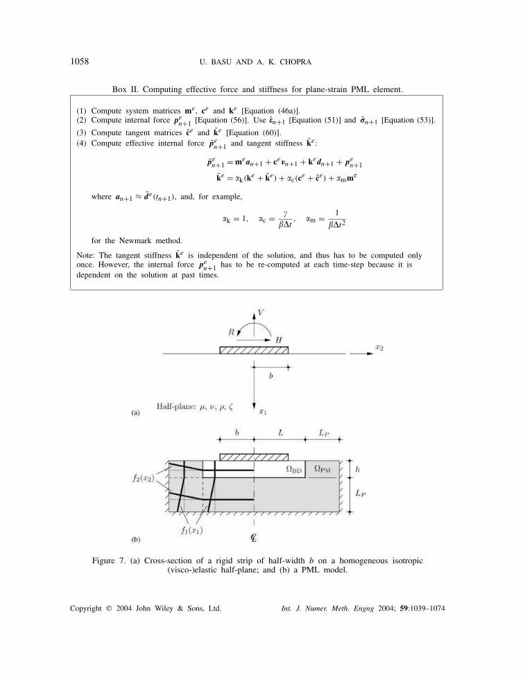
Figure 7(a) shows a cross-section of a rigid strip-footing of half-width b with its three
degrees-of-freedom (DOFs) identified—vertical (V ), horizontal (H ), and rocking (R)—supported
by a homogeneous isotropic (visco-)elastic half-plane with shear modulus �, mass density �,
Poisson’s ratio �, and Voigt damping ratio � for the visco-elastic medium. The time-domain
response of this system is studied through the reactions along the three DOFs due to an imposed
displacement along any of the three DOFs; the imposed displacement is chosen to be of the
form of Equation (A3) and the reaction along DOF i due to an imposed displacement along
j is denoted by Pij , with i, j ∈ {V, H, R}.
Copyright � 2004 John Wiley & Sons, Ltd. Int. J. Numer. Meth. Engng 2004; 59:1039–1074
1058 U. BASU AND A. K. CHOPRA
Box II. Computing effective force and stiffness for plane-strain PML element.
(1) Compute system matrices me, ce and ke [Equation (46a)].(2) Compute internal force pe
n+1[Equation (56)]. Use �n+1 [Equation (51)] and �n+1 [Equation (53)].
(3) Compute tangent matrices ce and ke [Equation (60)].
(4) Compute effective internal force pen+1
and tangent stiffness ke:
pen+1 = mean+1 + cevn+1 + kedn+1 + pe
n+1
ke = k(ke + ke) + c(ce + ce) + mme
where an+1 ≈ de(tn+1), and, for example,
k = 1, c = �
��t, m = 1
��t2
for the Newmark method.
Note: The tangent stiffness ke is independent of the solution, and thus has to be computed onlyonce. However, the internal force pe
n+1has to be re-computed at each time-step because it is
dependent on the solution at past times.
Figure 7. (a) Cross-section of a rigid strip of half-width b on a homogeneous isotropic(visco-)elastic half-plane; and (b) a PML model.
Copyright � 2004 John Wiley & Sons, Ltd. Int. J. Numer. Meth. Engng 2004; 59:1039–1074

TRANSIENT ELASTODYNAMICS OF UNBOUNDED DOMAINS 1059
-5
-2.5
0
2.5
5
0 20 40 60
PVV
-5
-2.5
0
2.5
5
0 20 40 60
PVV
Extd. meshPMLDashpots
-4
-2
0
2
4
0 20 40 60
PHH
-4
-2
0
2
4
0 20 40 60PHH
-3
-1.5
0
1.5
3
0 20 40 60
PRR
t
-3
-1.5
0
1.5
3
0 20 40 60
PRR
t(a) (b)
Figure 8. Reactions of a rigid strip on (visco-)elastic half-plane due to imposed displacements;L = 3b/2, h = b/2, LP = b, f1(x1) = 10〈x1 − h〉/LP, f2(x2) = 10〈|x2| − L〉/LP; 〈x〉 := (x + |x|)/2;� = 1, � = 0.25; td = 30, �f = 1.00 for vertical excitation, 0.75 for horizontal excitation and 1.25
for rocking excitation: (a) elastic half-plane, � = 0; and (b) visco-elastic half-plane, � = 0.05.
This unbounded-domain system is modelled using the bounded-domain-PML model shown
in Figure 7(b), composed of a bounded domain �BD and a PML �PM, with the attenuation
functions in Equation (12) chosen as f ei = f
pi = fi , with fi chosen to be linear in the
PML. A finite element mesh of four-node bilinear isoparametric elements are used to discretize
the entire bounded domain. The mesh chosen is reasonably dense and is graded to capture
sharp variations in stresses near the footing. For comparison, the half-plane is also modelled
using a viscous-dashpot model [3], wherein the entire domain �BD ∪ �PM is taken to be
(visco-)elastic and consistent dashpot elements replace the fixed outer boundary; thus the mesh
used for the dashpot model is comparable to that used for the PML model. Because of the
dearth of analytical results in the time domain, the half-plane is modelled using an extended
mesh; the results from this mesh will serve as a benchmark. From the center of the footing,
this mesh extends to a distance of 35b downwards and laterally; the entire domain is taken to
be (visco-)elastic, and viscous dashpots are placed on the outer boundary.
Copyright � 2004 John Wiley & Sons, Ltd. Int. J. Numer. Meth. Engng 2004; 59:1039–1074

1060 U. BASU AND A. K. CHOPRA
0
0.2
0.4
0.6
0.8
1
0 0.5 1 1.5
Re F V
VExactPML
0
0.2
0.4
0.6
0.8
1
0 0.5 1 1.5
− I
m FVV
0
0.2
0.4
0.6
0.8
1
0 0.5 1 1.5
Re FHH
0
0.2
0.4
0.6
0.8
1
0 0.5 1 1.5
− I
m FHH
0
0.2
0.4
0.6
0.8
1
0 0.5 1 1.5
Re FRR
a0
0
0.2
0.4
0.6
0.8
1
0 0.5 1 1.5
− I
m FRR
a0
Figure 9. Dynamic flexibility coefficients of rigid strip on elastic half-plane computedusing a PML model with stretching functions suitable for time-domain analysis; L = 3b/2,h = b/2, LP = b, f1(x1) = 10〈x1 − h〉/LP, f2(x2) = 10〈|x2| − L〉/LP; � = 1, � = 0.25;
‘Exact’ results from Reference [40].
Figure 8(a) compares the reactions computed for an elastic medium using the PML model
and the dashpot model with results from the extended mesh. Note that the bounded domain
for the PML and the dashpot models is small, extending only upto b/2 on either side of the
footing and below it, and the PML width equal to b, the half-width of the footing. Based
on a comparison of the frequency-domain responses of the PML and the viscous dashpot
models, the values of �f were chosen as the excitation frequencies where the two responses
are significantly different. The results obtained from the PML model follow the extended mesh
results closely, even though the domain is small enough for the dashpots to reflect waves back
to the footing, as manifested in the higher response amplitudes. The computational cost of
Copyright � 2004 John Wiley & Sons, Ltd. Int. J. Numer. Meth. Engng 2004; 59:1039–1074
TRANSIENT ELASTODYNAMICS OF UNBOUNDED DOMAINS 1061
0
0.2
0.4
0.6
0.8
1
0 1 2 3 4
Re FVV
FD PMLPML
0
0.2
0.4
0 1 2 3 4
− I
m F
VV
0
0.2
0.4
0.6
0.8
1
0 1 2 3 4
Re FHH
0
0.2
0.4
0 1 2 3 4
− I
m F
HH
0
0.2
0.4
0.6
0 1 2 3 4
Re FRR
a0
0
0.2
0.4
0 1 2 3 4
− I
m F
RR
a0
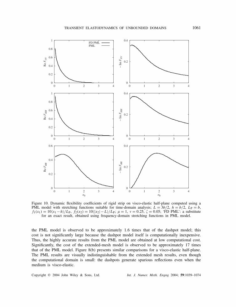
Figure 10. Dynamic flexibility coefficients of rigid strip on visco-elastic half-plane computed using aPML model with stretching functions suitable for time-domain analysis; L = 3b/2, h = b/2, LP = b,f1(x1) = 10〈x1 −h〉/LP, f2(x2) = 10〈|x2|−L〉/LP; � = 1, � = 0.25, � = 0.05; ‘FD PML’: a substitute
for an exact result, obtained using frequency-domain stretching functions in PML model.
the PML model is observed to be approximately 1.6 times that of the dashpot model; this
cost is not significantly large because the dashpot model itself is computationally inexpensive.
Thus, the highly accurate results from the PML model are obtained at low computational cost.
Significantly, the cost of the extended-mesh model is observed to be approximately 17 times
that of the PML model. Figure 8(b) presents similar comparisons for a visco-elastic half-plane.
The PML results are visually indistinguishable from the extended mesh results, even though
the computational domain is small: the dashpots generate spurious reflections even when the
medium is visco-elastic.
Copyright � 2004 John Wiley & Sons, Ltd. Int. J. Numer. Meth. Engng 2004; 59:1039–1074

1062 U. BASU AND A. K. CHOPRA
Figure 11. (a) Cross-section of the rigid strip of half-width b on a homogeneous isotropic (visco-)elasticlayer on half-plane; and (b) a PML model.
Figures 9 and 10 present frequency-dependent flexibility coefficients Fij (a0) for the rigid
strip-footing on a half-plane computed using a PML model employing the time-domain stretch-
ing functions in Equation (12). The flexibility coefficients are defined as the displacement
amplitudes along DOF i due to a unit-amplitude harmonic force along DOF j . Results for
the elastic half-plane are compared in Figure 9 against available analytical results [40]. Owing
to the dearth of analytical solutions for the strip on a Voigt visco-elastic half-plane, the re-
sults obtained from the (possibly less accurate) time-domain stretching functions are compared
in Figure 10 to results from a PML model employing the frequency-domain-only stretching
functions [Equation (33)], denoted by ‘FD PML’ in the figures. The rationale behind this ap-
proach is that the frequency-domain stretching functions produce highly accurate results for
hysteretic damping [30] and, hence, can be expected to also produce excellent results for Voigt
damping. The results demonstrate that the time-domain stretching functions indeed produce ac-
curate results as expected, because the wave motion in the half-plane consists primarily of prop-
agating modes, which are adequately attenuated even by the time-domain stretching functions.
Figure 11(a) shows a cross-section of the rigid strip supported by a layer on a half-plane, and
Figure 11(b) shows a corresponding PML model with the attenuation functions in Equation (12)
Copyright � 2004 John Wiley & Sons, Ltd. Int. J. Numer. Meth. Engng 2004; 59:1039–1074

TRANSIENT ELASTODYNAMICS OF UNBOUNDED DOMAINS 1063
-5
-2.5
0
2.5
5
0 20 40 60
PVV
-5
-2.5
0
2.5
5
0 20 40 60
PVV
Extd. meshPMLDashpots
-4
-2
0
2
4
0 20 40 60
PHH
-4
-2
0
2
4
0 20 40 60PHH
-3
-1.5
0
1.5
3
0 20 40 60
PRR
t
-3
-1.5
0
1.5
3
0 20 40 60
PRR
t(a) (b)
Figure 12. Reactions of a rigid strip on (visco-)elastic layer on half-plane, due to imposed displace-ments; L = 3b/2, LP = b, h = b/2, f1(x1) = 10〈x1 − (d +h)〉/LP, f2(x2) = 10〈|x2|−L〉/LP; d = 2b,�l = 1, �h = 4�l , � = 0.4; td = 30, �f = 1.00 for vertical excitation, 0.75 for horizontal excitation
and 1.75 for rocking excitation: (a) elastic media, � = 0; and (b) visco-elastic media, � = 0.05.
chosen as f ei = f
pi = fi , with fi chosen to be linear in the PML. The elastic moduli for the
PMLs employed for the layer and the half-plane are set to the moduli for the corresponding
elastic media. For comparison, a viscous-dashpot model is also employed, where the entire
bounded domain is taken to be (visco-)elastic and consistent dashpots replace the fixed outer
boundary. An extended-mesh model, with viscous dashpots at the outer boundary, is taken as a
benchmark model for the layer on a half-plane; this mesh extends to a distance of 40b laterally
and downwards from the center of the footing.
Figure 12 shows the reactions of the rigid strip on a layer-on-half-plane due to imposed
displacements. The PML results typically follow the results from the extended mesh, even
though the domain is small enough for the viscous dashpots to generate spurious reflections.
The computational cost of the PML model is not significantly large: it is observed to be
approximately 1.5 times that of the dashpot model. Significantly, the extended-mesh results
show some spurious reflections for vertical motion of the footing: the P-wave speed in the
Copyright � 2004 John Wiley & Sons, Ltd. Int. J. Numer. Meth. Engng 2004; 59:1039–1074

1064 U. BASU AND A. K. CHOPRA
0
0.2
0.4
0.6
0 1 2
Re FVV
FD PMLPML
0
0.2
0.4
0.6
0 1 2
− I
m FVV
0
0.2
0.4
0.6
0 1 2
Re FHH
0
0.2
0.4
0.6
0 1 2
− I
m FHH
0
0.2
0.4
0.6
0 1 2
Re FRR
a0
0
0.2
0.4
0.6
0 1 2
− I
m FRR
a0
Figure 13. Dynamic flexibility coefficients of rigid strip on elastic layer on half-plane computedusing a PML model with stretching functions suitable for time-domain analysis; L = 3b/2, LP = b,h = b/2, f1(x1) = 10〈x1 − (d +h)〉/LP, f2(x2) = 10〈|x2|−L〉/LP; d = 2b, �l = 1, �h = 4�l , � = 0.4,
a0 = �b/√
�l/�; ‘FD PML’: a substitute for an exact result, obtained using frequency-domainstretching functions in PML model.
half-plane is high enough that the depth of the extended mesh is not adequate for the time
interval in the analysis; the cost of the extended-mesh model is observed to be approximately
18 times that of the PML model. Figures 13 and 14 demonstrate that the time-domain stretching
functions provide frequency-dependent flexibility coefficients that closely match those obtained
using the frequency-domain-only stretching functions.
Figure 15(a) shows a cross-section of the rigid strip supported by a layer on a rigid base, and
Figure 15(b) shows a corresponding PML model where f ei = f
pi = fi in Equation (12), with
Copyright � 2004 John Wiley & Sons, Ltd. Int. J. Numer. Meth. Engng 2004; 59:1039–1074

TRANSIENT ELASTODYNAMICS OF UNBOUNDED DOMAINS 1065
0
0.2
0.4
0.6
0 1 2
Re FVV
FD PMLPML
0
0.2
0.4
0.6
0 1 2
− I
m FVV
0
0.2
0.4
0.6
0 1 2
Re FHH
0
0.2
0.4
0.6
0 1 2
− I
m FHH
0
0.2
0.4
0.6
0 1 2
Re FRR
a0
0
0.2
0.4
0.6
0 1 2
− I
m FRR
a0
Figure 14. Dynamic flexibility coefficients of rigid strip on visco-elastic layer on half-plane computedusing a PML model with stretching functions suitable for time-domain analysis; L = 3b/2, LP = b,h = b/2, f1(x1) = 10〈x1 − (d + h)〉/LP, f2(x2) = 10〈|x2| − L〉/LP; d = 2b, �l = 1, �h = 4�l ,
� = 0.4, � = 0.05, a0 = �b/√
�l/�; ‘FD PML’: a substitute for an exact result, obtained usingfrequency-domain stretching functions in PML model.
f1(x1) = 0 and f2(x2) linear in the PML. The corresponding viscous-dashpot model includes
the entire bounded domain as (visco-)elastic, with viscous dashpots replacing the fixed lateral
boundaries. The extended-mesh model is also a viscous-dashpot model, but extending to 40b
on either side from the center of the footing. Figure 16 demonstrates the high accuracy of the
PML model, as well as the small size of the computational domain through the inadequacy of
the dashpot model. These results from the PML model are obtained at a cost approximately
Copyright � 2004 John Wiley & Sons, Ltd. Int. J. Numer. Meth. Engng 2004; 59:1039–1074

1066 U. BASU AND A. K. CHOPRA
Figure 15. (a) Cross-section of the rigid strip of half-width b on a homogeneous isotropic (visco-)elasticlayer on rigid base; and (b) a PML model.
1.2 times that of the dashpot model, i.e. the computational cost is not significantly large. The
cost of the extended-mesh model is observed to be approximately 3 times that of the PML
model; it is relatively cheaper here than in the previous two cases because the extension of
the mesh is only in the lateral directions, not downwards.
Figure 17 demonstrates that for a rigid strip on an elastic layer on rigid base, the frequency-
dependent flexibility coefficients obtained using the time-domain stretching functions do not
always closely follow those from the frequency-domain-only stretching functions; this is pre-
sumably due to the presence of evanescent modes in the system. However, this apparent
inadequacy of the time-domain stretching functions is not reflected in the time domain results
in Figure 16(a). The time-domain stretching functions provide accurate results for a rigid strip
on a visco-elastic layer, as demonstrated in Figure 18.
4. CONCLUSIONS
Building on recent formulations for corresponding time-harmonic PMLs [30], this paper has
presented displacement-based, time-domain equations for the PMLs for anti-plane and for plane-
strain motion of a two-dimensional (visco-)elastic continuum. These equations are obtained by
selecting stretching functions in the PML that have a simple dependence on the factor i�,
which facilitates transformation of the time-harmonic equations into the time domain. In the
interest of obtaining a realistic model of the unbounded domain, material damping is introduced
into the PML equations in the form of a Voigt damping model in the constitutive relation for
Copyright � 2004 John Wiley & Sons, Ltd. Int. J. Numer. Meth. Engng 2004; 59:1039–1074

TRANSIENT ELASTODYNAMICS OF UNBOUNDED DOMAINS 1067
-20
-10
0
10
20
0 20 40 60
PVV
-20
-10
0
10
20
0 20 40 60
PVV
Extd. meshPMLDashpots
-5
-2.5
0
2.5
5
0 20 40 60
PHH
-5
-2.5
0
2.5
5
0 20 40 60PHH
-3
-1.5
0
1.5
3
0 20 40 60
PRR
t
-3
-1.5
0
1.5
3
0 20 40 60
PRR
t
Figure 16. Reactions of a rigid strip on (visco-)elastic layer on rigid base, due to imposed displace-ments; L = 3b/2, LP = b, f1(x1) = 0, f2(x2) = 20〈|x2| − L〉/LP; d = 2b, � = 1, � = 0.4; td = 30,�f = 2.75 for vertical excitation, 1.25 for horizontal excitation and 1.75 for rocking excitation:
(a) elastic layer, � = 0; and (b) visco-elastic layer, � = 0.05.
the PML; this model is chosen instead of the traditional hysteretic damping model because the
latter is non-causal.
These PML equations have been implemented numerically by a straightforward finite ele-
ment approach. As is conventional, the ‘equilibrium’ equations are discretized in time by a
traditional integrator, such as the Newmark method; the equilibrium equations are solved at
each time-station using a Newton–Raphson iteration scheme. Because the tangent stiffness ma-
trix employed in the Newton–Raphson scheme is independent of the solution, it is computed
only once at the start of the analysis. This property of the tangent makes the PML model
effectively a linear model. The tangent stiffness of the anti-plane PML is found to be sym-
metric. Furthermore, it is argued that if the attenuation functions are positive-valued, and if
the boundary restraints on the whole domain are adequate, then the tangent stiffness of the
entire computational domain will be positive definite. Unfortunately, the tangent stiffness of
the plane-strain PML turns out to be unsymmetric. The system matrices of both PML models
retain the sparsity structure associated with corresponding matrices for an elastic medium.
Copyright � 2004 John Wiley & Sons, Ltd. Int. J. Numer. Meth. Engng 2004; 59:1039–1074

1068 U. BASU AND A. K. CHOPRA
-1.5
-1
-0.5
0
0.5
1
0 1 2
Re FVV
FD PMLPML
-0.4
-0.2
0
0.2
0.4
0.6
0 1 2
− I
m FVV
-0.5
0
0.5
1
1.5
0 1 2
Re FHH
-0.5
0
0.5
1
1.5
2
0 1 2
− I
m FHH
0
0.2
0.4
0.6
0.8
0 1 2
Re FRR
a0
0
0.2
0.4
0.6
0.8
0 1 2
− I
m FRR
a0
Figure 17. Dynamic flexibility coefficients of rigid strip on elastic layer on rigid base computedusing a PML model with stretching functions suitable for time-domain analysis; L = 3b/2, LP = b,f1(x1) = 0, f2(x2) = 20〈|x2| − L〉/LP; d = 2b, � = 1, � = 0.4; ‘FD PML’: a substitute for an exact
result, obtained using frequency-domain stretching functions in PML model.
These FE implementations of the PMLs are employed to solve the canonical problem of
the anti-plane motion of a semi-infinite layer on a rigid base and the classical soil-structure
interaction problems of a rigid strip-footing on (i) a half-plane, (ii) a layer on a half-plane,
and (iii) a layer on a rigid base. Highly accurate results were obtained from PML models
with small bounded domains at low computational costs. The bounded domains employed for
these problems were small enough that comparable viscous-dashpot models typically generated
spurious reflections within the time-interval of the analysis, even if the domain was visco-
elastic. The computational costs of the PML models were not significantly large: based on the
Copyright � 2004 John Wiley & Sons, Ltd. Int. J. Numer. Meth. Engng 2004; 59:1039–1074

TRANSIENT ELASTODYNAMICS OF UNBOUNDED DOMAINS 1069
0
0.2
0 1 2
Re FVV
FD PMLPML
0
0.2
0.4
0 1 2
− I
m FVV
0
0.2
0.4
0.6
0.8
1
0 1 2
Re FHH
0
0.2
0.4
0.6
0.8
1
0 1 2
− I
m FHH
0
0.2
0.4
0.6
0 1 2
Re FRR
a0
0
0.2
0.4
0.6
0 1 2
− I
m FRR
a0
Figure 18. Dynamic flexibility coefficients of rigid strip on visco-elastic layer on rigid base computedusing a PML model with stretching functions suitable for time-domain analysis; L = 3b/2, LP = b,f1(x1) = 0, f2(x2) = 20〈|x2| −L〉/LP; d = 2b, � = 1, � = 0.4, � = 0.05; ‘FD PML’: a substitute for
an exact result, obtained using frequency-domain stretching functions in PML model.
relative expense of the PML and the viscous dashpot models, and also on the relative number
of PML elements and elastic elements in a PML model, it was estimated that the cost of an
anti-plane PML element is approximately 1.5 times the corresponding elastic element, and that
of a plane-strain PML element is approximately 1.75 times the corresponding elastic element.
Frequency-domain results suggest that the time-domain results may not be accurate for
an elastic system if the excitation is primarily in a frequency-band where evanescent modes
are not adequately attenuated. If the excitation is broadband, however, and evanescent modes
are not sufficiently attenuated only in a narrow frequency-band, then the time-domain results
can be expected to be accurate. Moreover, the results are accurate for a visco-elastic system
Copyright � 2004 John Wiley & Sons, Ltd. Int. J. Numer. Meth. Engng 2004; 59:1039–1074

1070 U. BASU AND A. K. CHOPRA
because the evanescent modes are attenuated by damping. Issues about inaccuracies due to
evanescent modes are of concern primarily in waveguide systems—such as the layer on a rigid
base—because of their severely-constricted geometries; evanescent modes are of less concern in
half-plane or full-plane problems. Note that this issue arises in the time-domain model of the
PML because the special choice of stretching functions is not always adequate for attenuating
evanescent modes. An alternate choice of the stretching function for a frequency-domain PML
model produces accurate results even for waveguide systems with significant evanescent modes
[30]; however, it is difficult to employ such a frequency-domain stretching function in a direct
time-domain analysis.
This paper presented time-domain PML models for isotropic, homogeneous or discretely-
inhomogeneous media only. However, the constitutive relation for the PML is the same as that
for the elastic medium. This suggests that the PML formulations presented in this paper may
be extended to anisotropic, continuously-inhomogeneous elastic media with at most minimal
modifications, mirroring similar developments in electromagnetics [41].
NOMENCLATURE
Roman symbols
a0 non-dimensional frequency
a nodal accelerations
b half-width of footing
B, Be, Bp, Bε, B� compatibility matrices
cp, cs compressional and shear wave velocities
cij damping coefficient of nodal dynamic stiffness of layer on rigid base
ce, ce, c, c element-level and global damping matrices
C, Cijkl material stiffness tensor
d depth of layer
d nodal displacements
D material moduli matrix
{ei} standard orthonormal basis
E, E time integral of �, �
fm, fc, fk see Equation (18)
f ei , f
pi attenuation functions
Fe, Fp, Fe, Fp attenuation tensors; Equation (14)
Fij flexibility coefficient of rigid strip-footing, with i, j ∈ {V, H, R}H (in subscript) horizontal DOF of rigid strip-footing
i =√
−1 unit imaginary number
Im imaginary part of a complex number
I identity matrix
ks, k∗s , kp wavenumbers for S and P waves
kij stiffness coefficient of nodal dynamic stiffness of layer on rigid base
ke, ke, k element-level and global stiffness matrices
LP depth of PML
me, m element-level and global mass matrices
nc number of full cycles in imposed displacement
Copyright � 2004 John Wiley & Sons, Ltd. Int. J. Numer. Meth. Engng 2004; 59:1039–1074
TRANSIENT ELASTODYNAMICS OF UNBOUNDED DOMAINS 1071
n unit normal to a surface
N , NI nodal shape functions
p, pi direction of wave propagation
pe element-level internal force term
q direction of particle motion
Q, Qij rotation-of-basis matrix
R (in subscript) rocking DOF of rigid strip-footing
|R|, |Rpp|, |Rsp| amplitude(s) of wave(s) reflected from the PML
Re real part of a complex number
Sij component of dynamic stiffness matrix of layer on rigid base
td duration of imposed displacement
Tf dominant forcing period of imposed displacement
u, u displacement(s)
v nodal velocities
V (in subscript) vertical DOF of rigid strip-footing
w, w arbitrary weighting function in weak form
x, xi , x co-ordinate(s)
Greek symbols
ij Kronecker delta
� differential operator
�t time-step size
ε, εi , εij , �, � strain quantities
� damping ratio for visco-elastic medium
� angle of incidence of outgoing wave on PML
� bulk modulus
�i complex co-ordinate stretching function
�, � stretch tensors
� shear modulus
� Poisson ratio
� mass density
�, �i , �ij , �, �, � stress quantities
�, � time-integral of �, �
� excitation frequency
�f dominant forcing frequency of imposed displacement
� entire bounded domain used for computation
�e element domain
�BD bounded domain
�PM perfectly matched layer
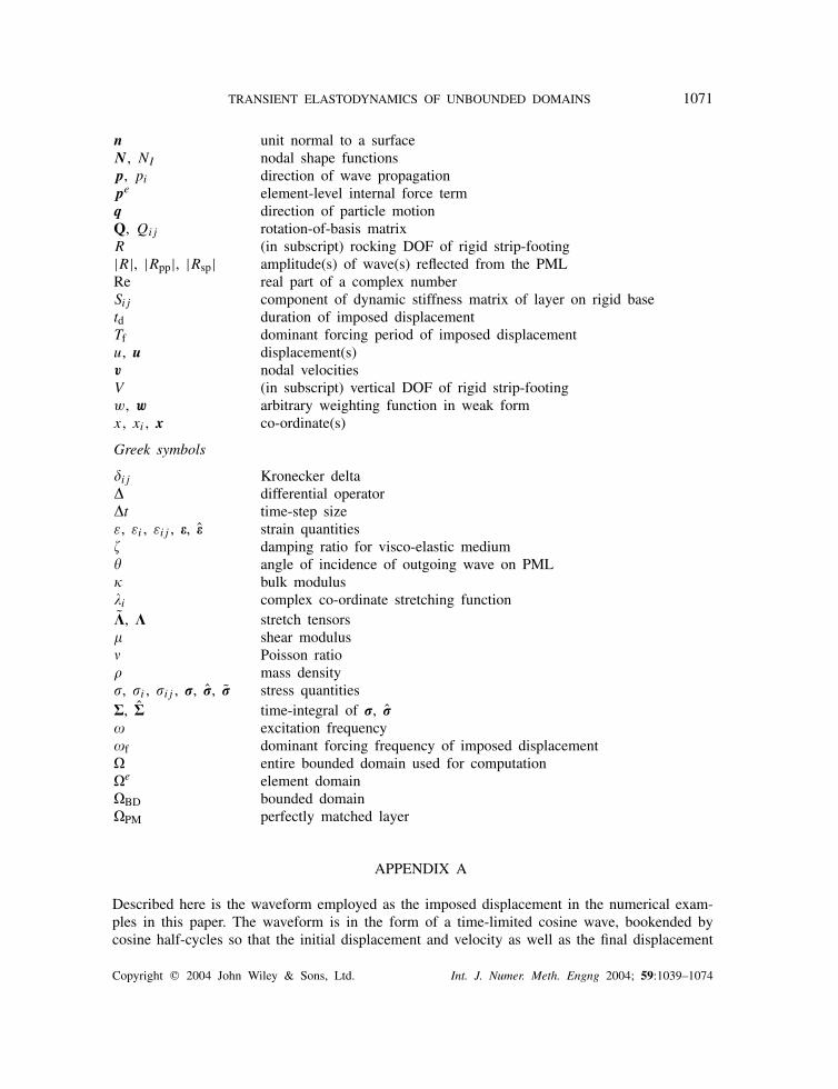
APPENDIX A
Described here is the waveform employed as the imposed displacement in the numerical exam-
ples in this paper. The waveform is in the form of a time-limited cosine wave, bookended by
cosine half-cycles so that the initial displacement and velocity as well as the final displacement
Copyright � 2004 John Wiley & Sons, Ltd. Int. J. Numer. Meth. Engng 2004; 59:1039–1074

1072 U. BASU AND A. K. CHOPRA
and velocity are zero. It is characterized by two parameters: the duration td and the dominant
forcing frequency �f ; the dominant forcing period is then
Tf = 2�
�f
and the number of full cycles, nc, in the excitation is calculated as
nc =[
td
Tf
− 1
2
]
(A1)
where the 12
accounts for the cosine half-cycle used to end the excitation. For consistency, the
forcing period is adjusted to
Tf := td
nc + 1/2(A2)
The excitation is then defined as
u0(t) = 1
2
[
1 − cos
(
2�t
Tf
)]
t ∈ [0, Tf/2)
= cos
(
2�t − Tf/2
Tf
)
t ∈ [Tf/2, ncTf)
= 1
2
[
1 − cos
(
2�t − ncTf
Tf
)]
− 1 t ∈ [ncTf , td]
= 0 t ∈ (td, ∞)
(A3)
A typical waveform and its Fourier transform are shown in Figure 3. The Fourier transform
shows a dominant frequency, as expected; the bandwidth of the peak at this frequency varies
inversely with td, but is largely independent of �f .
APPENDIX B
The matrices Bε, B�, Fε and F� used in Equation (51) in Section 3.4 are defined as follows.
Define
F™ :=[
Fe
�t+ Fp
]−1
, Fε := FeF™, F� := FpF™ (B1)
Then Bε is defined in terms of nodal submatrices as
Bε
I :=
F ε
11N™
I1 F ε
21N™
I1
F ε
12N™
I2 F ε
22N™
I2
F ε
11N™
I2 + F ε
12N™
I1 F ε
21N™
I2 + F ε
22N™
I1
(B2)
Copyright � 2004 John Wiley & Sons, Ltd. Int. J. Numer. Meth. Engng 2004; 59:1039–1074

TRANSIENT ELASTODYNAMICS OF UNBOUNDED DOMAINS 1073
where
N ™
I i := F ™ijNI,j (B3)
The matrix B� is defined similarly, with F� replacing Fε throughout. Furthermore,
Fε :=
(
F ε
11
)2 (
F ε
21
)2F ε
11Fε
21
(
F ε
12
)2 (
F ε
22
)2F ε
12Fε
22
2F ε
11Fε
12 2F ε
21Fε
22 F ε
11Fε
22 + F ε
12Fε
21
(B4)
and F� is defined similarly, with F� replacing Fε throughout.
ACKNOWLEDGEMENTS
This research investigation is funded by the Waterways Experiment Station, U.S. Army Corps ofEngineers, under Contract DACW39-98-K-0038; this financial support is gratefully acknowledged. Theauthors are also grateful to Prof. Robert L. Taylor, Prashanth K. Vijalapura and Prof. Fernando L.Teixeira for their helpful advice and comments, and to Claire Johnson for editing the manuscript.
REFERENCES
1. Wolf JP. Soil-Structure-Interaction Analysis in Time Domain. Prentice-Hall: Englewood Cliffs, NJ, 1988.
2. Bao H, Bielak J, Ghattas O, Kallivokas LF, O’Hallaron DR, Shewchuck JR, Xu J. Large-scale simulation
of elastic wave propagation in heterogeneous media on parallel computers. Computer Methods in Applied
Mechanics and Engineering 1998; 152(1–2):85–102.
3. Lysmer J, Kuhlemeyer RL. Finite dynamic model for infinite media. Journal of the Engineering Mechanics
Division (ASCE) 1969; 95(EM4):859–877.
4. Clayton R, Engquist B. Absorbing boundary conditions for acoustic and elastic wave equations. Bulletin of
the Seismological Society of America 1977; 67(6):1529–1540.
5. Higdon RL. Absorbing boundary conditions for elastic waves. Geophysics 1991; 56(2):231–241.
6. Liao ZP, Wong HL. A transmitting boundary for the numerical simulation of elastic wave propagation. Soil
Dynamics and Earthquake Engineering 1984; 3(4):174–183.
7. Cerjan C, Kosloff D, Kosloff R, Reshef M. A nonreflecting boundary-condition for discrete acoustic and
elastic wave-equations. Geophysics 1985; 50(4):705–708.
8. Sochaki J, Kubichek R, George J, Fletcher WR, Smithson S. Absorbing boundary conditions and surface
waves. Geophysics 1987; 52(1):60–71.
9. Smith WD. A nonreflecting plane boundary for wave propagation problems. Journal of Computational Physics
1974; 15(4):492–503.
10. Yerli HR, Temel B, Kiral E. Transient infinite elements for 2D soil-structure interaction analysis. Journal
of Geotechnical and Geoenvironmental Engineering 1998; 124(10):976–988.
11. Kim DK, Yun CB. Time-domain soil-structure interaction analysis in two-dimensional medium based on
analytical frequency-dependent infinite elements. International Journal for Numerical Methods in Engineering
2000; 47(7):1241–1261.
12. Manolis GD, Beskos DE. Boundary Element Methods in Elastodynamics. Unwin Hyman: London, 1988.
13. Givoli D, Keller JB. Non-reflecting boundary conditions for elastic waves. Wave Motion 1990; 12(3):261–279.
14. Song C, Wolf JP. The scaled boundary finite-element method—alias consistent infinitesimal finite-element
cell method—for elastodynamics. Computer Methods in Applied Mechanics and Engineering 1997; 147(3–4):
329–355.
15. Israil ASM, Banerjee PK. Advanced time-domain formulation of BEM for two-dimensional transient
elastodynamics. International Journal for Numerical Methods in Engineering 1990; 29(7):1421–1440.
Copyright � 2004 John Wiley & Sons, Ltd. Int. J. Numer. Meth. Engng 2004; 59:1039–1074

1074 U. BASU AND A. K. CHOPRA
16. Grote MJ, Keller JB. Exact nonreflecting boundary condition for elastic waves. SIAM Journal on Applied
Mathematics 2000; 60(3):803–819.
17. Wolf JP, Song C. Consistent infinitesimal finite-element cell method: in-plane motion. Computer Methods in
Applied Mechanics and Engineering 1995; 123(1–4):355–370.
18. Kawamoto JD. Solution of nonlinear dynamic structural systems by a hybrid frequency–time-domain approach.
Research Report R 83-5, Department of Civil Engineering, Massachusetts Institute of Technology, Cambridge,
MA, 1983.
19. Seed HB, Idriss IM. Influence of soil conditions on ground motions during earthquakes. Journal of the Soil
Mechanics and Foundations Division (ASCE) 1969; 94(SM1):99–137.
20. Wolf JP. Consistent lumped-parameter models for unbounded soil: physical representation. Earthquake
Engineering and Structural Dynamics 1991; 20(1):11–32.
21. Feltrin G. Absorbing boundaries for the time-domain analysis of dam-reservoir-foundation systems. IBK Bericht
No. 232, Institute of Structural Engineering, Swiss Federal Institute of Technology Zürich, Birkhaüser Verlag,
Basel, 1997.
22. Ruge P, Trinks C, Witte S. Time-domain analysis of unbounded media using mixed-variable formulations.
Earthquake Engineering and Structural Dynamics 2001; 30(6):899–925.
23. Bérenger JP. A perfectly matched layer for the absorption of electromagnetic waves. Journal of Computational
Physics 1994; 114(2):185–200.
24. Chew WC, Weedon WH. A 3D perfectly matched medium from modified Maxwell’s equations with stretched
co-ordinates. Microwave and Optical Technology Letters 1994; 7(13):599–604.
25. Qi Q, Geers TL. Evaluation of the perfectly matched layer for computational acoustics. Journal of
Computational Physics 1998; 139(1):166–183.
26. Hu FQ. On absorbing boundary conditions for linearized Euler equations by a perfectly matched layer.
Journal of Computational Physics 1996; 129(1):201–219.
27. Zeng YQ, He JQ, Liu QH. The application of the perfectly matched layer in numerical modeling of wave
propagation in poroelastic media. Geophysics 2001; 66(4):1258–1266.
28. Chew WC, Liu QH. Perfectly matched layers for elastodynamics: a new absorbing boundary condition.
Journal of Computational Acoustics 1996; 4(4):341–359.
29. Collino F, Tsogka C. Application of the perfectly matched absorbing layer model to the linear elastodynamic
problem in anisotropic heterogeneous media. Geophysics 2001; 66(1):294–307.
30. Basu U, Chopra AK. Perfectly matched layers for time-harmonic elastodynamics of unbounded domains:
theory and finite-element implementation. Computer Methods in Applied Mechanics and Engineering 2003;
192(11–12):1337–1375.
31. Graff KF. Wave Motion in Elastic Solids. Dover: NY, 1975.
32. Makris N. Causal hysteretic element. Journal of Engineering Mechanics (ASCE) 1997; 123(11):1209–1214.
33. Zhao L, Cangellaris AC. A general approach for the development of unsplit-field time-domain implementations
of perfectly matched layers for FDTD grid truncation. IEEE Microwave and Guided Wave Letters 1996;
6(5):209–211.
34. Zienkiewicz OC, Taylor RL. The Finite Element Method (5th edn). Butterworth-Heinemann: New York, 2000.
35. Newmark NM. A method of computation for structural dynamics. Journal of the Engineering Mechanics
Division (ASCE) 1959; 85(EM3):67–94.
36. Chopra AK. Dynamics of Structures: Theory and Applications to Earthquake Engineering (2nd edn). Prentice-
Hall: Englewood Cliffs, NJ, 2001.
37. Wolf JP, Song C. Finite-Element Modelling of Unbounded Media. Wiley: Chichester, 1996.
38. De Moerloose J, Stuchly MA. Behaviour of Bérenger’s ABC for evanescent waves. IEEE Microwave and
Guided Wave Letters 1995; 5(10):344–346.
39. Bérenger JP. Application of the CFS PML to the absorption of evanescent waves in waveguides. IEEE
Microwave and Wireless Components Letters 2002; 12(6):218–220.
40. Luco JE, Westmann RA. Dynamic response of a rigid footing bonded to an elastic half space. Journal of
Applied Mechanics (ASME) 1972; 39(2):527–534.
41. Teixeira FL, Chew WC. A general approach to extend Bérenger’s absorbing boundary condition to anisotropic
and dispersive media. IEEE Transactions on Antennas and Propagation 1998; 46(9):1386–1387.
Copyright � 2004 John Wiley & Sons, Ltd. Int. J. Numer. Meth. Engng 2004; 59:1039–1074

INTERNATIONAL JOURNAL FOR NUMERICAL METHODS IN ENGINEERINGInt. J. Numer. Meth. Engng 2004; 61:156–157 (DOI: 10.1002/nme.1137)
ERRATUM
Erratum to ‘Perfectly matched layers for transient elastodynamicsof unbounded domains’
(Int. J. Numer. Meth. Engng 2004; 59:1039–1074)
Ushnish Basu and Anil K. Chopra∗ , †
Department of Civil and Environmental Engineering, University of California, Berkeley, CA 94720, U.S.A.
The PML equations presented in the paper are valid only for b = 1, where b is a characteristic
length of the physical problem. For proper dimensionalisation of the PML equations and their FE
implementations, Equation (12) should be corrected to
�i(x′i) := [1 + f e
i (x′i)] − i
fpi (x′
i)
a0(12)
with a0 = ksb replacing ks in the original equation. This characteristic length b carries over to
Equations (15), (16a) and (42a) in an obvious way. Corrected versions of these equations are as
follows:
Fe′ :=
[
1 + f e2 (x′
2) ·
· 1 + f e1 (x′
1)
]
, Fp′ :=
[
fp2 (x′
2)cs/b ·
· fp1 (x′
1)cs/b
]
(15a)
Fe′
:=
[
1 + f e1 (x′
1) ·
· 1 + f e2 (x′
2)
]
, Fp′
:=
[
fp1 (x′
1)cs/b ·
· fp2 (x′
2)cs/b
]
(15b)
∇ · � = �fmu + �cs
bfcu +
�
b2fku (16a)
div(�Fe + �F
p) = �fmu + �cs
bfcu +
�
b2fku (42a)
∗ Correspondence to: A. K. Chopra, Department of Civil and Environmental Engineering, 707 Davis Hall,University of California, Berkeley, CA 94720, U.S.A.
† E-mail: [email protected]
Copyright � 2004 John Wiley & Sons, Ltd.

ERRATUM 157
The last two equations affect Equations (19), (21a), (44) and (46a), which should be corrected as
follows:∫
�
�fmwu d� +
∫
�
�cs
bfcwu d� +
∫
�
�
b2fkwu d� +
∫
�
∇w · � d� =
∫
�
w � · n d� (19)
me =
∫
�e�fmN
TN d�, c
e =
∫
�e�
cs
bfcN
TN d�, k
e =
∫
�e
�
b2fkN
TN d� (21a)
∫
�
�fmw · u d� +
∫
�
�cs
bfcw · u d� +
∫
�
�
b2fkw · u d�
+
∫
�
�e: � d� +
∫
�
�p: � d� =
∫
�
w · (�Fe + �F
p)n d� (44)
meIJ =
∫
�e�fmNINJ d� I, c
eIJ =
∫
�e�
cs
bfcNINJ d� I, k
eIJ =
∫
�e
�
b2fkNINJ d� I
(46a)
The authors apologise for any confusion this may have caused. The numerical results presented in
the paper are unaffected because they were computed for b = 1.
Copyright � 2004 John Wiley & Sons, Ltd. Int. J. Numer. Meth. Engng 2004; 61:156–157