10. Natural Gas - US EPA 10. Natural Gas This chapter describes how natural gas supply, demand, and costing are modeled in EPA Base Case v.5.13. Section 0 indicates that natural gas

10-1

10. Natural Gas

This chapter describes how natural gas supply, demand, and costing are modeled in EPA Base Case v.5.13. Section 0 indicates that natural gas supply dynamics are directly (i.e., endogenously) modeled in the base case. Section 10.2 gives an overview of the new natural gas module. Sections 10.3 and 10.4 describe the very detailed process-engineering model and data sources used to characterize North American conventional and unconventional natural gas resources and reserves and to derive all the cost components incurred in bringing natural gas from the ground to the pipeline. These sections also discuss resource constraints affecting production and the assumptions (in the form of cost indices) used to depict expected changes in costs over the 2016-2050 modeling time horizon.

Section 10.5 describes how liquefied natural gas (LNG) imports are represented in the natural gas module. The section covers the assumptions regarding liquefaction facilities, LNG supply, regasification capacity, and related costs. Section 10.6 turns to demand-side issues, in particular, how non-power sector residential, commercial, and industrial consumer demand is represented. This section also describes the use of the gas demand sub-module to model LNG exports. Section 10.7 describes the detailed characterization of the natural gas pipeline network, the pipeline capacity expansion logic, and the assumptions and procedures used to capture pipeline transportation costs. Section 10.8 treats issues related to natural gas storage: capacity characterization and expansion logic, injection/withdrawal rates, and associated costs. Section 10.9 describes the crude oil and natural gas liquids (NGL) price projections that are exogenous inputs in the natural gas module. They figure in the modeling of natural gas because they are a source of revenue which influence the exploration and development of hydrocarbon resources. The chapter concludes in Section 10.10 with a discussion of key gas market parameters in the natural gas report of EPA Base Case v.5.13.

10.1 Overview of IPM’s Natural Gas Module

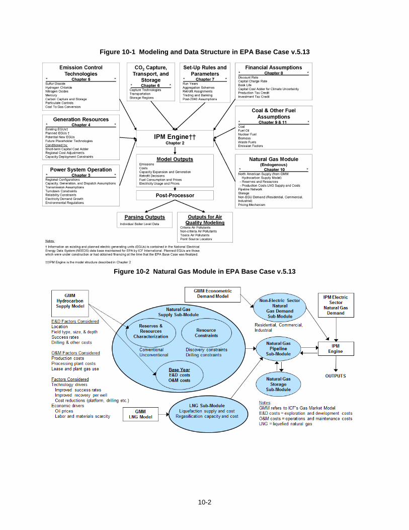
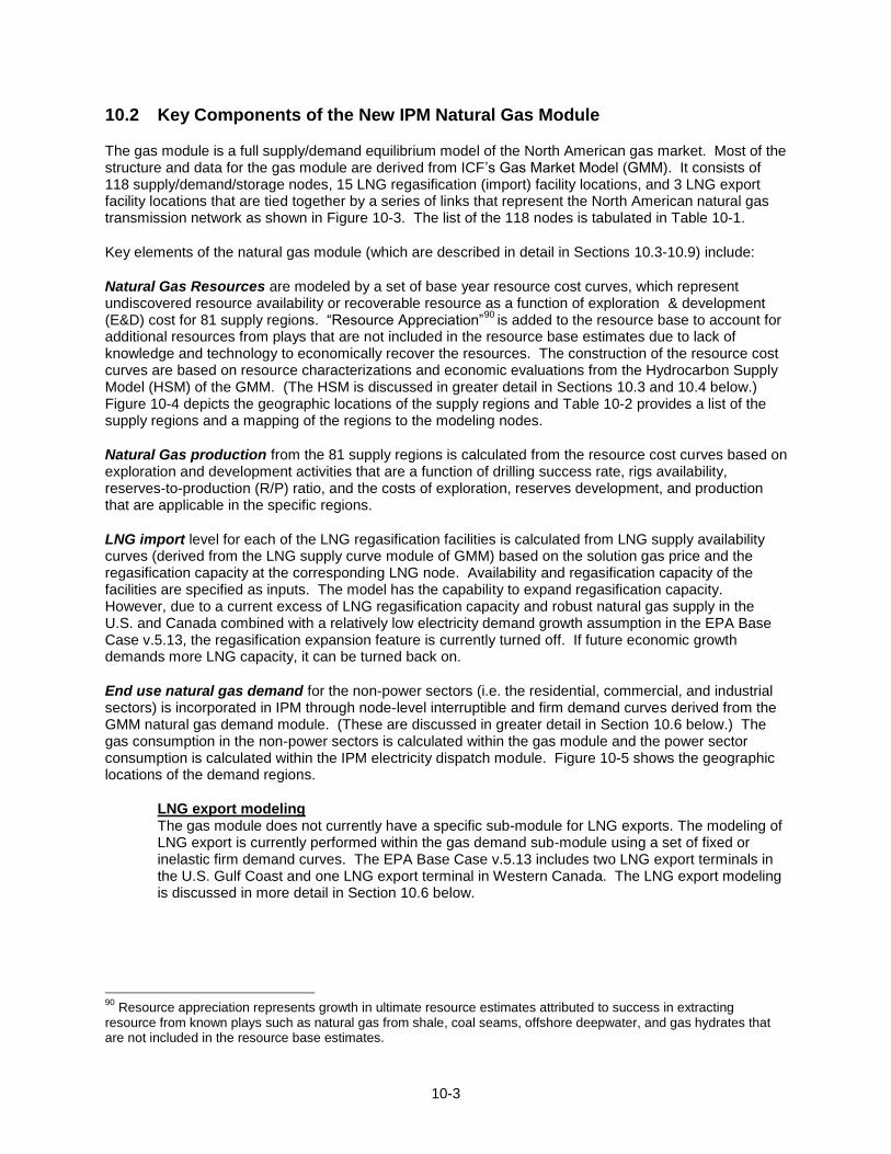
In EPA Base Case v.5.13 natural gas supply, demand, transportation, storage, and related costs are modeled directly in IPM through the incorporation of a natural gas module. Natural gas supply curves are generated endogenously for each region, and the balance between the natural gas supply and demand is solved in all regions simultaneously. Figure 10-1 and Figure 10-2 illustrate the integration of the natural gas module in IPM. The integration allows direct interaction between the electric and the gas modules and captures the overall gas supply and demand dynamic.

To a certain extent, the design and assumptions of the new natural gas module are similar to those in ICF International’s private practice Gas Market Model (GMM) which has been used extensively for forecasting and market analyses in the North American natural gas market. To provide these new natural gas modeling capabilities within IPM and still maintain an acceptable model size and solution time, however, simplifications of some of the GMM design and assumptions were made.

Seasonality in the gas module is made consistent with that in IPM and is currently modeled with two seasons (summer and winter), each with up to six IPM load periods that correspond to the IPM electric sector load duration curve (LDC) segments. The gas module also employs a similar run year concept as in IPM where, in order to manage model size, individual calendar years over the entire modeling period are mapped to a lesser number of run years. In the current version, both modules use the same run year mapping.

10-2

Figure 10-1 Modeling and Data Structure in EPA Base Case v.5.13

Figure 10-2 Natural Gas Module in EPA Base Case v.5.13

10-3

10.2 Key Components of the New IPM Natural Gas Module

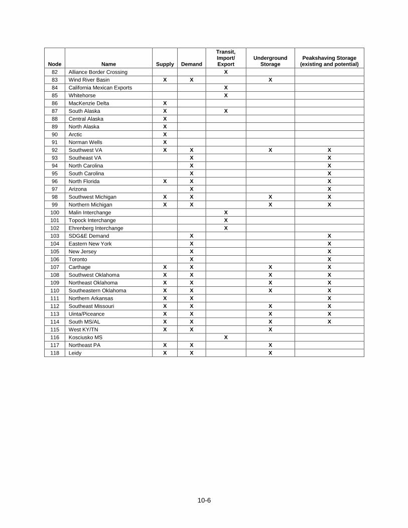
The gas module is a full supply/demand equilibrium model of the North American gas market. Most of the structure and data for the gas module are derived from ICF’s Gas Market Model (GMM). It consists of 118 supply/demand/storage nodes, 15 LNG regasification (import) facility locations, and 3 LNG export facility locations that are tied together by a series of links that represent the North American natural gas transmission network as shown in Figure 10-3. The list of the 118 nodes is tabulated in Table 10-1.

Key elements of the natural gas module (which are described in detail in Sections 10.3-10.9) include:

Natural Gas Resources are modeled by a set of base year resource cost curves, which represent undiscovered resource availability or recoverable resource as a function of exploration & development (E&D) cost for 81 supply regions. “Resource Appreciation”

90 is added to the resource base to account for

additional resources from plays that are not included in the resource base estimates due to lack of knowledge and technology to economically recover the resources. The construction of the resource cost curves are based on resource characterizations and economic evaluations from the Hydrocarbon Supply Model (HSM) of the GMM. (The HSM is discussed in greater detail in Sections 10.3 and 10.4 below.) Figure 10-4 depicts the geographic locations of the supply regions and Table 10-2 provides a list of the supply regions and a mapping of the regions to the modeling nodes.

Natural Gas production from the 81 supply regions is calculated from the resource cost curves based on exploration and development activities that are a function of drilling success rate, rigs availability, reserves-to-production (R/P) ratio, and the costs of exploration, reserves development, and production that are applicable in the specific regions.

LNG import level for each of the LNG regasification facilities is calculated from LNG supply availability curves (derived from the LNG supply curve module of GMM) based on the solution gas price and the regasification capacity at the corresponding LNG node. Availability and regasification capacity of the facilities are specified as inputs. The model has the capability to expand regasification capacity. However, due to a current excess of LNG regasification capacity and robust natural gas supply in the U.S. and Canada combined with a relatively low electricity demand growth assumption in the EPA Base Case v.5.13, the regasification expansion feature is currently turned off. If future economic growth demands more LNG capacity, it can be turned back on.

End use natural gas demand for the non-power sectors (i.e. the residential, commercial, and industrial sectors) is incorporated in IPM through node-level interruptible and firm demand curves derived from the GMM natural gas demand module. (These are discussed in greater detail in Section 10.6 below.) The gas consumption in the non-power sectors is calculated within the gas module and the power sector consumption is calculated within the IPM electricity dispatch module. Figure 10-5 shows the geographic locations of the demand regions.

LNG export modeling The gas module does not currently have a specific sub-module for LNG exports. The modeling of LNG export is currently performed within the gas demand sub-module using a set of fixed or inelastic firm demand curves. The EPA Base Case v.5.13 includes two LNG export terminals in the U.S. Gulf Coast and one LNG export terminal in Western Canada. The LNG export modeling is discussed in more detail in Section 10.6 below.

90

Resource appreciation represents growth in ultimate resource estimates attributed to success in extracting resource from known plays such as natural gas from shale, coal seams, offshore deepwater, and gas hydrates that are not included in the resource base estimates.

10-4

Figure 10-3 Gas Transmission Network Map

Table 10-1 List of Nodes

Node Name Supply Demand

Transit, Import/ Export

Underground Storage

Peakshaving Storage (existing and potential)

1 New England X X

2 Everett TRANS X

3 Quebec X X X

4 New York City X X

5 Niagara X X X X

6 Southwest PA X X X X

7 Cove Point TRANS X

8 Georgia X X

9 Elba Is TRANS X

10 South Florida X X

11 East Ohio X X X X

12 Maumee/Defiance X X X

13 Lebanon X X X

14 Indiana X X X X

15 South Illinois X X X X

16 North Illinois X X X X

17 Southeast Michigan X X X X

18 East KY/TN X X X X

19 MD/DC/Northern VA X X

20 Wisconsin X X X

21 Northern Missouri X X X

22 Minnesota X X X X

23 Crystal Falls X X X

24 Ventura X X X X

25 Emerson Imports X

26 Nebraska X X X

27 Great Plains X

28 Kansas X X X X

29 East Colorado X X X X

10-5



Underground Storage


30 Opal X X X X

31 Cheyenne X X X

32 San Juan Basin X X X

33 EPNG/TW X X X

34 North Wyoming X X X

35 South Nevada X X X

36 SOCAL Area X X X X

37 Enhanced Oil Recovery Region X X

38 PGE Area X X X X

39 Pacific Offshore X

40 Monchy Imports X

41 Montana/North Dakota X X X X

42 Wild Horse Imports X

43 Kingsgate Imports X

44 Huntingdon Imports X

45 Pacific Northwest X X X X

46 NPC/PGT Hub X X

47 North Nevada X X X

48 Idaho X X X

49 Eastern Canada Offshore X

50 Atlantic Offshore X

51 Reynosa Imp/Exp X

52 Juarez Imp/Exp X

53 Naco Imp/Exp X

54 North Alabama X X X X

55 Alabama Offshore X

56 North Mississippi X X X X

57 East Louisiana Shelf X

58 Eastern Louisiana Hub X X X X

59 Viosca Knoll/Desoto/Miss Canyon X

60 Henry Hub X X X X

61 North Louisiana Hub X X X X

62 Central and West Louisiana Shelf X

63 Southwest Texas X X X

64 Dallas/Ft Worth X X X X

65 E. TX (Katy) X X X X

66 S. TX X X X

67 Offshore Texas X

68 NW TX X X X

69 Garden Banks X

70 Green Canyon X

71 Eastern Gulf X

72 North British Columbia X X X

73 South British Columbia X X X

74 Caroline X X X X

75 Empress X

76 Saskatchewan X X X X

77 Manitoba X X X

78 Dawn X X X X

79 Philadelphia X X

80 West Virginia X X X X

81 Eastern Canada Demand X X

10-6



Underground Storage


82 Alliance Border Crossing X

83 Wind River Basin X X X

84 California Mexican Exports X

85 Whitehorse X

86 MacKenzie Delta X

87 South Alaska X X

88 Central Alaska X

89 North Alaska X

90 Arctic X

91 Norman Wells X

92 Southwest VA X X X X

93 Southeast VA X X

94 North Carolina X X

95 South Carolina X X

96 North Florida X X X

97 Arizona X X

98 Southwest Michigan X X X X

99 Northern Michigan X X X X

100 Malin Interchange X

101 Topock Interchange X

102 Ehrenberg Interchange X

103 SDG&E Demand X X

104 Eastern New York X X

105 New Jersey X X

106 Toronto X X

107 Carthage X X X X

108 Southwest Oklahoma X X X X

109 Northeast Oklahoma X X X X

110 Southeastern Oklahoma X X X X

111 Northern Arkansas X X X

112 Southeast Missouri X X X X

113 Uinta/Piceance X X X X

114 South MS/AL X X X X

115 West KY/TN X X X

116 Kosciusko MS X

117 Northeast PA X X X

118 Leidy X X X

10-7

Figure 10-4 Gas Supply Regions Map

Table 10-2 List of Gas Supply Regions

Supply Region Number Node Number Region Name

1 5 Niagara

2 6 Southwest PA

3 96 Florida

4 11 East Ohio

5 12 Maumee/ Defiance

6 13 Lebanon

7 14 Indiana

8 15 South Illinois

9 16 North Illinois

10 17 Southeast Michigan

11 18 Eastern KY/TN

12 92 SW Virginia

13 20 Wisconsin

14 21 Northern Missouri

15 22 Minnesota

16 23 Crystal Falls

17 24 Ventura

18 26 Nebraska

19 28 Kansas

20 29 East Colorado

21 30 Opal

22 31 Cheyenne

23 32 San Juan Basin

24 33 EPNG/TW

25 34 North Wyoming

26 97 Arizona

27 36 SOCAL Area

28 38 PGE Area

10-8


29 39 California Offshore

30 41 Montana/ North Dakota

31 45 Pacific Northwest

32 47 North Nevada

33 48 Idaho

34 49 Eastern Canada Offshore

35 50 Atlantic Offshore

36 54 North Alabama

37 55 Alabama Offshore

38 56 North Mississippi

39 57 East Louisiana Shelf

40 58 Eastern Louisiana Hub

41 59 Viosca Knoll S./ Desoto Canyon/Mississippi Canyon

42 60 Henry Hub

43 61 North Louisiana Hub

44 62 Central and West Louisiana Shelf

45 63 Southwest Texas

46 64 Dallas/Fort Worth

47 65 E. TX (Katy)

48 66 S. TX

49 67 Offshore Texas

50 68 NW TX

51 69 Garden Banks

52 70 Green Canyon

53 71 Florida off-shore moratorium area

54 72 North British Columbia

55 74 Caroline

56 76 Saskatchewan

57 77 Manitoba

58 78 Dawn

59 80 West Virginia

60 83 Wind River Basin

61 86 McKenzie Delta

62 87 Southern Alaska

63 88 Central Alaska

64 89 Northern Alaska

65 90 Arctic

66 91 Norman Wells

67 37 Enhanced Oil Recovery Region

68 98 Southwest Michigan

69 99 Central Michigan

70 107 Carthage

71 108 Southwest Oklahoma

72 109 Northeast Oklahoma

73 110 Southeastern Oklahoma

74 111 Northern Arkansas

75 112 Southeast Missouri

76 113 Uinta/Piceance

77 114 South MS/AL

10-9


78 115 Western KY/TN

79 3 Eastern Canada Onshore

80 117 NE PA/SC NY

81 118 Leidy

Figure 10-5 Gas Demand Regions Map

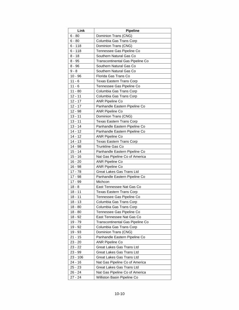
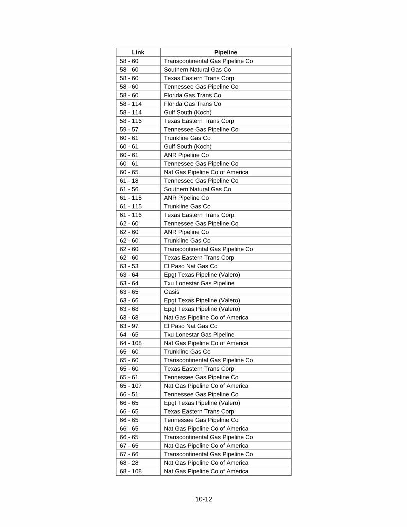
Natural gas pipeline network is modeled by 380 transmission links or segments (excluding pipeline connections with LNG import nodes) that represent major interstate transmission corridors throughout North America (Figure 10-3). The pipeline corridors represent a group of interstate pipelines along the corridor. The list of key interstate pipelines by links is tabulated in Table 10-3. Each of the links has an associated discount curve (derived from GMM natural gas transportation module), which represents the marginal value of gas transmission on that pipeline segment as a function of the pipeline’s load factor.

91

Starting year of operation and transmission capacity (in units of BBtu/day) are specified as inputs and the model allows for capacity expansions.

Table 10-3 List of Key Pipelines

Link Pipeline

1 - 4 Iroquois Pipeline Co

1 - 104 Tennessee Gas Pipeline Co

1 - 104 Algonquin Gas Trans Co





6 - 5 National Fuel Gas Supply Co

6 - 11 Dominion Trans (CNG)

6 - 11 Columbia Gas Trans Corp


6 - 79 Texas Eastern Trans Corp

91

In this context “load factor” refers to the percentage of the pipeline capacity that is utilized at a given time.

10-10

Link Pipeline





8 - 18 Southern Natural Gas Co

8 - 95 Transcontinental Gas Pipeline Co



10 - 96 Florida Gas Trans Co





12 - 17 ANR Pipeline Co

12 - 17 Panhandle Eastern Pipeline Co








14 - 98 Trunkline Gas Co


15 - 16 Nat Gas Pipeline Co of America



17 - 78 Great Lakes Gas Trans Ltd


17 - 99 Michcon

18 - 8 East Tennessee Nat Gas Co






18 - 92 East Tennessee Nat Gas Co












27 - 24 Williston Basin Pipeline Co

10-11

Link Pipeline






28 - 29 Colorado Interstate Gas



28 - 109 Southern Star Central (Williams)


30 - 48 Northwest Pipeline Corp




32 - 33 El Paso Nat Gas Co

32 - 33 Transwestern Pipeline Co








34 - 31 Wyoming Interstate Co

36 - 37 Socal Gas

36 - 103 Socal Gas

37 - 38 Pacific Gas & Electric

40 - 41 Northwest Energy


43 - 73 Terasen (BC Gas)












56 - 58 Gulf South (Koch)








10-12

Link Pipeline


























63 - 64 Epgt Texas Pipeline (Valero)

63 - 64 Txu Lonestar Gas Pipeline

63 - 65 Oasis






















10-13

Link Pipeline


78 - 106 Union Gas

















101 - 36 Socal Gas

101 - 37 Pacific Gas & Electric


102 - 36 Socal Gas






105 - 104 Algonquin Gas Trans Co




107 - 61 Centerpoint Energy (Reliant)














113 - 30 Wyoming Interstate Co




10-14

Link Pipeline











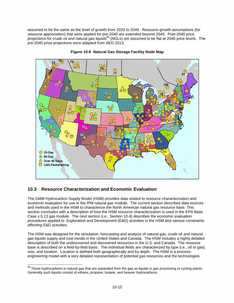
Natural gas storage is modeled by 190 underground and LNG peak shaving

92 storage facilities that are

linked to individual nodes. The underground storage is grouped into three categories based on storage “Days Service”

93: (1) 20-day for high deliverability

94 storage such as salt caverns, (2) 80-day for

depleted95

and aquifer96

reservoirs, and (3) over 80 days mainly for depleted reservoirs. The level of gas storage withdrawals and injections are calculated within the supply and demand balance algorithm based on working gas

97 levels, gas prices, and extraction/injection rates and costs. Starting year of operation

and working gas capacity (in units of BBtu) are specified as inputs and the model allows for capacity expansions. The location of the storage facilities is shown in Figure 10-6.

Natural gas prices are market clearing prices derived from the supply and demand balance at each of the model’s nodes for each segment of IPM’s electricity sector’s seasonal load duration curve (LDC). On the supply-side, prices are determined by production and storage price curves that reflect prices as a function of production and storage utilization. Prices are also affected by the “pipeline discount” curves discussed earlier, which represent the marginal value of gas transmission as a function of a pipeline’s load factor and result in changes in basis differential. On the demand-side, the price/quantity relationship is represented by demand curves that capture the fuel-switching behavior of end-users at different price levels. The model balances supply and demand at all nodes and yields market clearing prices determined by the specific shape of the supply and demand curves at each node.

10.2.1 Note on the Modeling Time Horizon and Pre- and Post-2040 Input Assumptions

The time horizon of the EPA’s Base Case v.5.13 extends through 2050. Projections through the year 2040 in EPA’s Base Case v.5.13 are based on a detailed bottom-up development of natural gas assumptions from available data sources. Beyond 2040, where detailed data are not readily available, various technically plausible simplifying assumptions were made. For example, natural gas demand growth from 2040 to 2050 for the non-power sectors (i.e. residential, commercial, and industrial) is

92

LNG peak shaving facilities supplement deliveries of natural gas during times of peak periods. LNG peak shaving facilities have a regasification unit attached, but may or may not have a liquefaction unit. Facilities without a liquefaction unit depend upon tank trucks to bring LNG from nearby sources. 93

“Days Service” refers to the number of days required to completely withdraw the maximum working gas inventory associated with an underground storage facility. 94

High deliverability storage is depleted reservoir storage facility or Salt Cavern storage whose design allows a relatively quick turnover of the working gas capacity. 95

A gas or oil reservoir that is converted for gas storage operations. Its economically recoverable reserves have usually been nearly or completely produced prior to the conversion. 96

The underground storage of natural gas in a porous and permeable rock formation topped by an impermeable cap rock, the pore space of which was originally filled with water. 97

The term “working gas” refers to natural gas that has been injected into an underground storage facility and stored therein temporarily with the intention of withdrawing it. It is distinguished from “base (or cushion) gas” which refers to the volume of gas that remains permanently in the storage reservoir in order to maintain adequate pressure and deliverability rates throughout the withdrawal season.

10-15

assumed to be the same as the level of growth from 2020 to 2040. Resource growth assumptions (for resource appreciation) that were applied for pre-2040 are extended beyond 2040. Post-2040 price projections for crude oil and natural gas liquids

98 (NGLs) are assumed to be flat at 2040 price levels. The

pre-2040 price projections were adapted from AEO 2013.

Figure 10-6 Natural Gas Storage Facility Node Map

10.3 Resource Characterization and Economic Evaluation

The GMM Hydrocarbon Supply Model (HSM) provides data related to resource characterization and economic evaluation for use in the IPM natural gas module. The current section describes data sources and methods used in the HSM to characterize the North American natural gas resource base. This section concludes with a description of how the HSM resource characterization is used in the EPA Base Case v.5.13 gas module. The next section (i.e., Section 10.4) describes the economic evaluation procedures applied to Exploration and Development (E&D) activities in the HSM and various constraints affecting E&D activities.

The HSM was designed for the simulation, forecasting and analysis of natural gas, crude oil and natural gas liquids supply and cost trends in the United States and Canada. The HSM includes a highly detailed description of both the undiscovered and discovered resources in the U.S. and Canada. The resource base is described on a field-by-field basis. The individual fields are characterized by type (i.e., oil or gas), size, and location. Location is defined both geographically and by depth. The HSM is a process-engineering model with a very detailed representation of potential gas resources and the technologies

98

Those hydrocarbons in natural gas that are separated from the gas as liquids in gas processing or cycling plants. Generally such liquids consist of ethane, propane, butane, and heavier hydrocarbons.

10-16

with which those resources can be proven99

and produced. The degree and timing by which resources are proven and produced are determined in the model through discounted cashflow analyses of alternative investment options and behavioral assumptions in the form of inertial and cashflow constraints, and the logic underlying producers' market expectations (e.g., their response to future gas prices).

Supply results from the HSM model include undeveloped resource accounting and detailed well, reserve addition, decline rate, and financial results. These results are utilized to provide estimates of base year economically recoverable natural gas resources and remaining reserves as a function of E&D cost for the 81 supply regions in the IPM natural gas module. The HSM also provides other data such as the level of remaining resource that could be discovered and developed in a year, exploration and development drilling requirements, production operation and maintenance (O&M) cost, resource share of crude oil and natural gas liquids, natural gas reserves to production ratio, and natural gas requirement for lease and plant use.

100

10.3.1 Resource and Reserves101

Assessment

Data sources: The HSM uses the U.S. Geological Survey (USGS), Minerals Management Service (MMS), and Canadian Gas Potential Committee (CGPC) play-level

102 resource assessments as the

starting point for the new field/new pool103

assessments. Beyond the resource assessment data, ICF has access to numerous databases that were used for the HSM model development and other analysis. Completion-level production is based on IHS Energy completion level oil and gas production databases for the U.S. and Canada. The U.S. database contains information on approximately 300,000 U.S. completions. A structured system is employed to process this information and add certain ICF data (region, play, ultimate recovery, and gas composition) to each record. ICF also performs extensive quality control checks using other data sources such as the MMS completion and production data for Outer Continental Shelf (OCS) areas and state production reports.

In the area of unconventional gas104

, ICF has worked for many years with the Gas Research Institute (GRI)/Gas Technology Institute (GTI) to develop a database of tight gas, coalbed methane, and Devonian Shale reservoirs in the U.S. and Canada. Along with USGS assessments of continuous plays, the

99

The term “proven” refers to the estimation of the quantities of natural gas resources that analysis of geological and engineering data demonstrate with reasonable certainty to be recoverable in future years from known reservoirs under existing economic and operating conditions. Among the factors considered are drilling results, production, and historical trends. Proven reserves are the most certain portion of the resource base. 100

As discussed more fully in Section 10.4, natural gas for “lease and plant use” refers to the gas used in well, field, and lease operations (such as gas used in drilling operations, heaters, dehydrators, and field compressors) and as fuel in gas processing plants. 101

When referring to natural gas a distinction is made between “resources” and “reserves.” “Resources” are concentrations of natural gas that are or may become of potential economic interest. “Reserves” are that part of the natural gas resource that has been fully evaluated and determined to be commercially viable to produce. 102

A “play” refers to a set of known or postulated natural gas (or oil) accumulations sharing similar geologic, geographic, and temporal properties, such as source rock, migration pathway, timing, trapping mechanism, and hydrocarbon type. 103

A “pool” is a subsurface accumulation of oil and other hydrocarbons. Pools are not necessarily big caverns. They can be small oil-filled pores. A “field” is an accumulation of hydrocarbons in the subsurface of sufficient size to be of economic interest. A field can consist of one or more pools. 104

Unconventional gas refers to natural gas found in geological environments that differ from conventional hydrocarbon traps. It includes: (a) “tight gas,” i.e., natural gas found in relatively impermeable (very low porosity and permeability) sandstone and carbonate rocks; (b) “shale gas,” i.e., natural gas in the joints, fractures or the matrix of shales, the most prevalent low permeability low porosity sedimentary rock on earth; and (c) “coal bed methane,” which refers to methane (the key component of natural gas) found in coal seams, where it was generated during coal formation and contained in the microstructure of coal. Unconventional natural gas is distinguished from conventional gas which is extracted using traditional methods, typically from a well drilled into a geological formation exploiting natural subsurface pressure or artificial lifting to bring the gas and associated hydrocarbons to the wellhead at the surface.

10-17

database was used to help develop the HSM’s “cells”, which represent resources in a specific geographic area, characterizing the unconventional resource in each basin, historical unconventional reserves estimates and typical decline curves.

105 ICF has recently revised the unconventional gas resource

assessments based on new gas industry information on the geology, well production characteristics, and costs. The new assessments include major shale units such as the Fort Worth Barnett Shale, the Marcellus Shale, the Haynessville Shale, and Western Canada shale plays. ICF has built up a database on gas compositions in the United States and has merged that data with production data to allow the analysis of net versus raw gas production.

106

In Canada, gas composition data are obtained from provincial agencies. These data were used to develop dry gas

107 production/reserves by region and processing costs in the HSM and to characterize

ethane rejection108

by regions. Information on oil and gas fields and pools in the U.S. come originally from Dwight’s Energydata (now IHS Energy) TOTL reservoir database. ICF has made extensive modifications to the database during the creation of the Gas Information System (GASIS) database for the U.S. Department of Energy (DOE) and other projects. Field and reservoir data for Canada comes from the provincial agency databases. These data are used to estimate the number and size of undiscovered fields or pools and their rate of discovery per increment of exploratory drilling. Additional data were obtained from the Significant Field Data Base of NRG Associates.

Methodology and assumptions: Resources in the HSM model are divided into three general categories: new fields/new pools, field appreciation, and unconventional gas. The methodology for resource characterization and economic evaluation differs for each.

Conventional resource – new fields/new pools: The modeling of conventional resource is based on a modified “Arps Roberts” equation

109 to estimate the rate at which new fields are discovered. The

fundamental theory behind the find-rate methodology is that the probability of finding a field is proportional to the field's size as measured by its area extent, which is highly correlated to the field's level of reserves. For this reason, larger fields tend to be found earlier in the discovery process than smaller fields. Finding that the original Arps-Roberts equation did not replicate historical discovery patterns for many of the smaller field sizes, ICF modified the equation to improve its ability to accurately track discovery rates for mid- to small-size fields. Since these are the only fields left to be discovered in many mature areas of the U.S. and Western Canada Sedimentary Basin (WCSB), the more accurate find-rate representation is an important component in analyzing the economics of exploration activity in these areas. An economic evaluation is made in the model each year for potential new field exploration programs using a standard discounted after-tax cash flow (DCF) analysis. This DCF analysis takes into account how many fields of each type are expected to be found and the economics of developing each.

105

A decline curve is a plot of the rate of gas production against time. Since the production rate decline is associated with pressure decreases from oil and gas production, the curve tends to smoothly decline from a high early production rate to lower later production rate. Exponential, harmonic, and hyperbolic equations are typically used to represent the decline curve. 106

Raw gas production refers to the volumes of natural gas extracted from underground sources, whereas net gas production refers to the volume of purified, marketable natural gas leaving the natural gas processing plant. 107

Natural gas is a combustible mixture of hydrocarbon gases. Although consisting primarily of methane, the composition of natural gas can vary widely to include propane, butane, ethane, and pentane. Natural gas is referred to as 'dry' when it is almost pure methane, having had most of the other commonly associated hydrocarbons removed. When other hydrocarbons are present, the natural gas is called 'wet'. 108

Ethane rejection occurs when the ethane component in the natural gas stream is not recovered in a gas processing plant but left in the marketable natural gas stream. Ethane rejection is deployed when the value of ethane is worth more in the gas stream than as an a separate commodity or as a component of natural gas liquids (NGL), which collectively refers to ethane, propane, normal butane, isobutane, and pentanes in processed and purified finished form. Information that characterizes ethane rejection by region can play a role in determining the production level and cost of natural gas by region. 109

“Arps-Roberts equation” refers to the statistical model of petroleum discovery developed by J. J. Arps, and T. G. Roberts, T. G., in the 1950’s.

10-18

Conventional resource – field appreciation: The model maintains inventories of potential resources that can be proved from already discovered fields. These inventories are referred to as appreciation, growth-to-known or “probables.” As the model simulation proceeds, these probables inventories are drawn down as the resources are proved. At the same time, the inventories of probables are increased due to future year appreciation of new fields that are added to the discovered fields’ data set during the model simulation.

Unconventional resource: Originally, the assessments of the unconventional resources were based on the Enhanced Recovery Module (or ERM) within the HSM. The ERM covers that portion of the resource base which falls outside the scope of the "conventional" oil and gas field discovery process dealt with elsewhere in the model. The ERM includes coalbed methane, shale gas, and tight gas. These resources generally correspond to the “continuous plays” designated by the USGS in its resource assessments. The ERM is organized by "cells", which represent resources in a specific geographic area. A cell can represent any size of area ranging from the entire region/depth interval to a single formation in a few townships of a basin. Each cell is evaluated in the model using the same discounted cashflow analysis used for new and old field investments. The ERM cells also are subject to the inertial and cashflow constraints affecting the other types of investment options in the model. The model reports total wells drilled, reserve additions, production, and dollars invested for each type of ERM cell (e.g., coalbed methane) within a region.

As described earlier, ICF has recently revised the unconventional gas resource assessments based on new gas industry information on the geology, well production characteristics, and costs. The new assessment method is a “bottom-up” approach that first generates estimates of unrisked and risked gas-in-place (GIP) from maps of depth, thickness, organic content, and thermal maturity. Then ICF uses a reservoir simulator to estimate well recoveries and production profiles. Unrisked GIP is the amount of original gas-in-place determined to be present based upon geological factors without risk reductions. Risked GIP includes a factor to reduce the total gas volume on the basis of proximity to existing production and geologic factors such as net thickness (e.g., remote areas, thinner areas, and areas of high thermal maturity have higher risk). ICF calibrates well recoveries with specific geological settings to actual well recoveries by using a rigorous method of analysis of historical well data.

10.3.2 Frontier Resources (Alaska and Mackenzie Delta)

Besides the three general categories of resources described above, the handling of frontier resources in the HSM is worth noting. Frontier resources such as Alaska North Slope and Mackenzie Delta are subject to similar resource assessment and economic evaluation procedures as applied to other regions. However, unlike other regions, the resources from these regions are stranded to date due to lack of effective commercial access to markets. In fact, 6-8 Bcf/d of gas that is currently produced as part of the oil activities in the Alaska North Slope is re-injected back into the Slope’s oil reservoirs as part of the pressure maintenance programs. Several development proposals have been put forward for bringing this Alaska North Slope and Mackenzie Delta gas to market.

In developing the gas resource assumptions for EPA Base Case v.5.13, two gas pipeline projects were identified for bringing the two frontier gas supply resources to the markets in the U.S. and Canada. However, due to uncertainties in the economics and the timing of these pipeline projects, they are not included in the EPA Base Case v.5.13.

10.3.3 Use of the HSM resource and reserves data in EPA Base Case using IPM v.5.13 Natural Gas Module

The base year for the integrated gas-electricity module in EPA Base Case using IPM v.5.13 is 2016. Having a base year in the future has implications on how the model is run and how the gas reserves and resources data are set up. The IPM run begins with a gas module only run for year 2015 to provide beginning of year (BOY) 2016 reserves and resources as the starting point for the integrated run from 2016 onward. This in turn requires the reserves and resources data to be provided for the BOY 2015. Since the data from the HSM are as of BOY 2011, adjustments have to be made to account for reserves

10-19

development, production, and also resource appreciation between 2011 and 2014. In the EPA Base Case using IPM v.5.13, these adjustments are made based on a four-year production and reserves development forecast using the GMM and a set of resource appreciation growth assumptions. The resource growth assumptions are discussed in “Undiscovered Resource Appreciation” section below.

Table 10-4 provides a snapshot of the starting natural gas resource and reserve assumptions for the EPA Base Case v.5.13. In this table, undiscovered resources represent the economic volume of dry gas that could be discovered and developed with current technology through exploration and development at a specified maximum wellhead gas price. Since the IPM natural gas module differentiates conventional gas from unconventional gas, these are shown separately in Table 10-4. The conventional gas is subcategorized into non-associated gas from gas fields and associated gas

110 from oil fields. The

unconventional gas is subdivided into coalbed methane (CBM), shale gas, and tight gas. In Table 10-4, the shale gas resource availability in the Northeast region is constrained by as assumption of limited access in accordance with current permitting procedures mostly affecting the Marcellus play. The full resource is about 925 Tcf.

The reserves are remaining dry gas volumes to be produced from existing developed fields. For EPA Base Case v.5.13 the maximum wellhead price for the resource cost curves is capped at $16/MMBtu (in real 2011 dollars). The ultimate potential undiscovered resources available are actually higher than those presented in Table 10-4 but it would cost more than $16/MMBtu to recover them. (It is important to note that this price is for wet

111 gas at the wellhead in the production nodes. The dry gas price at the receiving

nodes can be higher than $16/MMBtu which depends on the share of dry gas, lease and plant use, gas processing cost, production O&M cost, and pipeline transportation costs.) The approach used in the HSM to derive these costs is described more fully in section 10.4 below.

Table 10-4 U.S. and Canada Natural Gas Resources and Reserves

Region

Beginning of Year 2015

Undiscovered Dry Gas Resource (Tcf) Dry Gas Reserves (Tcf)

Lower 48 Onshore Non Associated 2,049 325

Conventional (includes tight) 566 101

Northeast 49 9

Gulf Coast 144 18

Midcontinent 48 16

Southwest 19 13

Rocky Mountain 288 46

West Coast 18 0

Shale Gas 1,408 212

Northeast 647 79

Gulf Coast 492 89

Midcontinent 151 22

Southwest 67 15

Rocky Mountain 50 8

West Coast 0 -

Coalbed Methane 75 11

Northeast 10 1

Gulf Coast 4 1

110

Associated gas refers to natural gas that is produced in association with crude oil production, whereas non-associated gas is natural gas that is not in contact with significant quantities of crude oil in the reservoir. 111

A mixture of hydrocarbon compounds and small quantities of various non-hydrocarbons existing in the gaseous phase or in solution with crude oil in porous rock formations at reservoir conditions. The principal hydrocarbons normally contained in the mixture are methane, ethane, propane, butane, and pentane. Typical non-hydrocarbon gases that may be present in reservoir natural gas are water vapor, carbon dioxide, hydrogen sulfide, nitrogen and trace amounts of helium.

10-20

Region

Beginning of Year 2015

Undiscovered Dry Gas Resource (Tcf) Dry Gas Reserves (Tcf)

Midcontinent 10 1

Southwest - -

Rocky Mountain 50 9

West Coast 1 -

Lower 48 Offshore Non Associated 85 6

Gulf of Mexico 85 6

Pacific - 0

Atlantic - -

Associated-Dissolved Gas 116 13

Alaska 51 10

Total U.S. 2,300 355

Canada Non Associated 858 59

Conventional and Tight 104 30

Shale Gas 723 24

Coalbed Methane 31 5

Canada Associated-Dissolved Gas 4 3

Total Canada 862 62

Total U.S and Canada 3,162 416

Figure 10-7 presents dry gas resource cost curves for the BOY 2015 initializing gas assumptions for EPA Base Case v.5.13. The resource cost curves show the undiscovered recoverable dry gas resources at different price levels. The curves do not include dry gas reserves. Separate resource cost curves are shown for conventional, shale, coalbed methane (CBM), and tight gas. The recoverable resources shown at maximum wellhead prices in these graphs are those tabulated in Table 10-4 under “Undiscovered Dry Gas Resource” column. The y-axis of the resource cost curves shows the cost at the wellhead of bringing the volume of undiscovered resource indicated on the x-axis into the reserves category. Figure 10-8 diagrams the exploration & development and production processes and the associated costs required to bring undiscovered resource into reserves and production.

10-21

Figure 10-7 Resource Cost Curves at the Beginning of Year 2015

10.3.4 Undiscovered Resource Appreciation

Undiscovered resource appreciation is additional resources from hydrocarbon plays that were not included in the resource base estimates. It differs from field appreciation or reserves appreciation category discussed above which comes from already discovered fields. Natural gas from shales, coal seams, offshore deepwater, and gas hydrates may not be included in the resource base assessments due to lack of knowledge and technology to economically recover the resource. As new technology becomes available, these untapped resources can be produced economically in the future. One example is the advancements in horizontal drilling and hydraulic fracture technologies to produce gas from shale formations. For EPA Base Case, the undiscovered gas resource is assumed to grow at 0.2% per year for conventional gas and 0.75% per year for unconventional gas. The BOY 2015 undiscovered recoverable gas resources in Table 10-4 and Figure 10-7 include resource appreciation between 2011 and 2014.

10-22

Figure 10-8 Exploration & Development and Production Processes and Costs to Bring Undiscovered Resource into Reserves and Production

10.4 Exploration, Development, and Production Costs and Constraints

10.4.1 Exploration and Development Cost

Exploration and development (E&D) cost or resource cost is the expenditure for activities related to discovering and developing hydrocarbon resources. The E&D cost for natural gas resources is a function of many factors such as geographic location, field type, size, depth, exploratory success rates, and platform, drilling and other costs. The HSM contains base year cost for wells, platforms, operating costs and all other relevant cost items. In addition to the base year costs, the HSM contains cost indices that adjust costs over time. These indices are partly a function of technology drivers such as improved exploratory success rates, cost reductions in platform, drilling and other costs, improved recovery per well, and partly a function of regression-based algorithms that relate cost to oil and gas prices and industry activity. As oil and gas prices and industry activity increase, the cost for seismic, drilling & completion services, casing and tubing and lease equipment goes up.

Other technology drivers affect exploratory success rates and reduce the need to drill exploratory wells. A similar adjustment is made to take into account changes over time in development success rates, but the relative effect is much smaller because development success rates are already rather high. The technology drivers that increase recovery per well are differentiated in the HSM by region and by type of gas. Generally, the improvements are specified as being greater for unconventional gas because their recovery factors are much lower than those of conventional gas.

The HSM model provides estimates of E&D cost and the level of economically viable gas resource by region as a function of E&D cost. The HSM increased recovery as a function of technology improvement by region is converted to E&D and production technology improvement over time in the form of cost reduction factors by onshore, offshore shelf, and offshore deepwater as shown in Figure 10-9. The average cost reduction factors for onshore, offshore shelf, and offshore deepwater E&D activities are -0.9% per year, -0.7% per year, and -0.4% per year, respectively. These factors are predominantly affected by the level of E&D investments in the regions. The expected aggressive onshore E&D activities to find and produce unconventional gas resources, such as shale gas, will lead to more research in horizontal drilling and hydraulic fracturing technologies to improve productions and lower the costs. This is reflected in higher cost reduction factors for the onshore regions.

10-23

Figure 10-9 E&D and Production Technology Improvement Factor

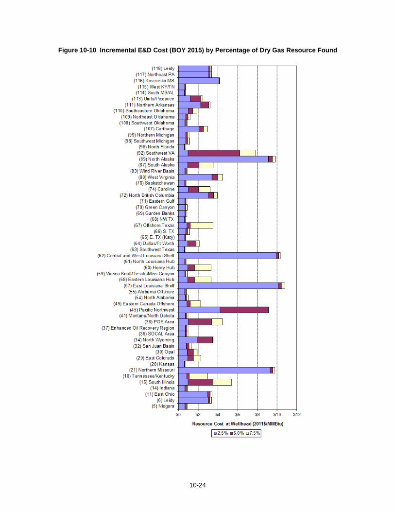
Figure 10-10 shows E&D cost needed to discover and develop 2.5%, 5%, and 7.5% of the remaining undiscovered resource in BOY 2015 by natural gas supply region.

10-24

Figure 10-10 Incremental E&D Cost (BOY 2015) by Percentage of Dry Gas Resource Found

10-25

10.4.2 Resource Discovery and Drilling Constraints

As mentioned above the simulation in HSM also provides other data such as resource discovery factors which describe the maximum share of remaining undiscovered resource that could be discovered and developed in a year and drilling requirements which describe the drilling required for successful exploration and development. These two parameters are constraints to the development of the resource and their values are not time dependent. The resource discovery constraint is the same for all regions and is assumed to be 6% of the remaining undiscovered resource (column 4 in Table 10-5). The drilling requirement constraint (column 5 in Table 10-5) varies from 2,500 feet for every billion cubic feet of incremental resource discovered (feet/Bcf) for offshore U.S. and between 3,000 feet/Bcf to 10,000 feet/Bcf for onshore regions and offshore Canada.

Table 10-5 Exploration and Development Assumptions for EPA Base Case v.5.13

Region

Fraction of Hydrocarbons

that are Natual Gas

Liquids (NGLs)


that are Crude Oil

Max Share of Resources that can be Developed per Year

Exploration, Development

Drilling Required

Lease and Plant Use

(Fraction) (Fraction) (Fraction) (Ft/Bcf) (Fraction)

(5) Niagara 0.02 0.12 0.06 10,000 0.05

(6) Leidy 0.01 0.02 0.06 4,556 0.03

(11) East Ohio 0.10 0.01 0.06 9,400 0.01

(14) Indiana 0.00 0.99 0.06 10,000 0.02

(15) South Illinois 0.00 0.96 0.06 10,000 0.30

(16) North Illinois 0.00 1.00 0.06 10,000 0.30

(18) Tennessee/Kentucky 0.11 0.02 0.06 10,000 0.04

(21) Northern Missouri 0.11 0.00 0.06 10,000 0.04

(28) Kansas 0.12 0.25 0.06 7,454 0.04

(29) East Colorado 0.11 0.03 0.06 9,349 0.05

(30) Opal 0.08 0.29 0.06 4,862 0.05

(32) San Juan Basin 0.11 0.04 0.06 6,323 0.13

(34) North Wyoming 0.11 0.00 0.06 3,688 0.05

(36) SOCAL Area 0.08 0.56 0.06 9,320 0.13

(37) Enhanced Oil Recovery Region 0.04 0.74 0.06 10,000 0.13

(38) PGE Area 0.08 0.61 0.06 9,376 0.13

(41) Montana/North Dakota 0.05 0.64 0.06 10,000 0.13

(45) Pacific Northwest 0.14 0.00 0.06 10,000 0.02

(49) Eastern Canada Offshore 0.03 0.00 0.06 10,000 0.06

(54) North Alabama 0.07 0.04 0.06 6,099 0.03

(55) Alabama Offshore 0.01 0.84 0.06 2,500 0.03

(57) East Louisiana Shelf 0.04 0.74 0.06 2,500 0.04

(58) Eastern Louisiana Hub 0.13 0.24 0.06 6,884 0.04

(59) Viosca Knoll/Desoto/Miss Canyon 0.07 0.56 0.06 2,500 0.04

(60) Henry Hub 0.13 0.25 0.06 6,927 0.04

(61) North Louisiana Hub 0.11 0.01 0.06 9,823 0.04

(62) Central and West Louisiana Shelf 0.04 0.74 0.06 2,500 0.04

(63) Southwest Texas 0.17 0.36 0.06 7,925 0.05

(64) Dallas/Ft Worth 0.06 0.05 0.06 4,510 0.05

(65) E. TX (Katy) 0.14 0.42 0.06 8,819 0.05

(66) S. TX 0.12 0.24 0.06 7,596 0.05

(67) Offshore Texas 0.09 0.31 0.06 2,500 0.05

(68) NW TX 0.22 0.08 0.06 7,584 0.05

(69) Garden Banks 0.07 0.49 0.06 2,500 0.04

(70) Green Canyon 0.07 0.53 0.06 2,500 0.04

(71) Eastern Gulf 0.04 0.71 0.06 2,500 0.04

10-26

Region


that are Natual Gas

Liquids (NGLs)


that are Crude Oil

Max Share of Resources that can be Developed per Year

Exploration, Development

Drilling Required

Lease and Plant Use

(Fraction) (Fraction) (Fraction) (Ft/Bcf) (Fraction)

(72) North British Columbia 0.01 0.00 0.06 9,948 0.08

(74) Caroline 0.04 0.04 0.06 9,752 0.10

(76) Saskatchewan 0.01 0.54 0.06 10,000 0.07

(80) West Virginia 0.06 0.00 0.06 3,539 0.05

(83) Wind River Basin 0.11 0.01 0.06 7,013 0.05

(86) MacKenzie Delta 0.00 1.00 0.06 10,000 0.08

(87) South Alaska 0.05 0.59 0.06 10,000 0.08

(89) North Alaska 0.04 0.62 0.06 10,000 0.99

(90) Arctic 0.00 1.00 0.06 10,000 0.08

(92) Southwest VA 0.00 0.00 0.06 5,787 0.02

(96) North Florida 0.01 0.94 0.06 9,937 0.21

(98) Southwest Michigan 0.08 0.09 0.06 10,000 0.04

(99) Northern Michigan 0.05 0.21 0.06 7,946 0.04

(107) Carthage 0.07 0.02 0.06 3,228 0.05

(108) Southwest Oklahoma 0.15 0.06 0.06 6,905 0.04

(109) Northeast Oklahoma 0.16 0.03 0.06 9,089 0.04

(110) Southeastern Oklahoma 0.16 0.02 0.06 4,445 0.04

(111) Northern Arkansas 0.00 0.05 0.06 4,437 0.04

(113) Uinta/Piceance 0.10 0.13 0.06 7,715 0.05

(114) South MS/AL 0.06 0.16 0.06 7,012 0.03

(115) West KY/TN 0.11 0.06 0.06 10,000 0.04

(116) Kosciusko MS 0.11 0.00 0.06 10,000 0.04

(117) Northeast PA 0.01 0.01 0.06 3,394 0.04

(118) Leidy 0.01 0.01 0.06 3,993 0.04

Other drilling constraints include rig capacity, rig retirement, rig growth, and drilling speed. Values for the constraints are specified for each of the three drilling category: (1) onshore, (2) offshore shelf, and (3) offshore deepwater. The drilling rig capacity constraint shows the number of drilling rigs initially available in the BOY 2015. The initial rig counts are 4,050 rigs for onshore, 125 rigs for offshore shelf, and 125 rigs for offshore deepwater and the numbers can change over time controlled by rig retirement and rig growth constraints. The drilling rig retirement constraint is the share of rig capacity that can retire in a year. The drilling rig growth constraint is the maximum increase of total rig count in a year. The drilling retirement and growth are assumed to be the same for all drilling category and the constraints are set to 0.5% per year and 3.5% per year, respectively.

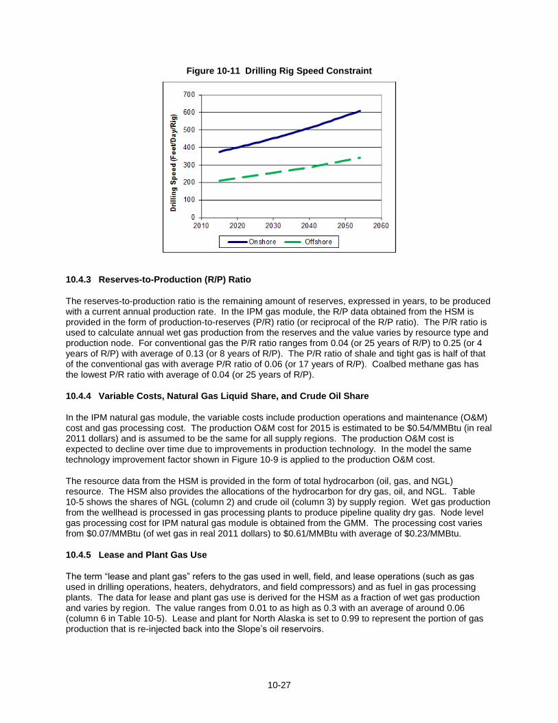
Another growth constraint, minimum drilling capacity increase, is implemented to force the rig count to grow by at least one rig in each drilling category. The drilling speed constraint is the required speed in feet/day/rig for successful exploration and development. The drilling speed required for successful E&D grows over time, as shown in Figure 10-11 and differs for onshore and offshore (which in this case includes both shelf and deep shelf).

10-27

Figure 10-11 Drilling Rig Speed Constraint

10.4.3 Reserves-to-Production (R/P) Ratio

The reserves-to-production ratio is the remaining amount of reserves, expressed in years, to be produced with a current annual production rate. In the IPM gas module, the R/P data obtained from the HSM is provided in the form of production-to-reserves (P/R) ratio (or reciprocal of the R/P ratio). The P/R ratio is used to calculate annual wet gas production from the reserves and the value varies by resource type and production node. For conventional gas the P/R ratio ranges from 0.04 (or 25 years of R/P) to 0.25 (or 4 years of R/P) with average of 0.13 (or 8 years of R/P). The P/R ratio of shale and tight gas is half of that of the conventional gas with average P/R ratio of 0.06 (or 17 years of R/P). Coalbed methane gas has the lowest P/R ratio with average of 0.04 (or 25 years of R/P).

10.4.4 Variable Costs, Natural Gas Liquid Share, and Crude Oil Share

In the IPM natural gas module, the variable costs include production operations and maintenance (O&M) cost and gas processing cost. The production O&M cost for 2015 is estimated to be $0.54/MMBtu (in real 2011 dollars) and is assumed to be the same for all supply regions. The production O&M cost is expected to decline over time due to improvements in production technology. In the model the same technology improvement factor shown in Figure 10-9 is applied to the production O&M cost.

The resource data from the HSM is provided in the form of total hydrocarbon (oil, gas, and NGL) resource. The HSM also provides the allocations of the hydrocarbon for dry gas, oil, and NGL. Table 10-5 shows the shares of NGL (column 2) and crude oil (column 3) by supply region. Wet gas production from the wellhead is processed in gas processing plants to produce pipeline quality dry gas. Node level gas processing cost for IPM natural gas module is obtained from the GMM. The processing cost varies from $0.07/MMBtu (of wet gas in real 2011 dollars) to $0.61/MMBtu with average of $0.23/MMBtu.

10.4.5 Lease and Plant Gas Use

The term “lease and plant gas” refers to the gas used in well, field, and lease operations (such as gas used in drilling operations, heaters, dehydrators, and field compressors) and as fuel in gas processing plants. The data for lease and plant gas use is derived for the HSM as a fraction of wet gas production and varies by region. The value ranges from 0.01 to as high as 0.3 with an average of around 0.06 (column 6 in Table 10-5). Lease and plant for North Alaska is set to 0.99 to represent the portion of gas production that is re-injected back into the Slope’s oil reservoirs.

10-28

10.5 Liquefied Natural Gas (LNG) Imports

As described earlier, most of the data related to North American LNG imports is derived from the GMM LNG model. Based on a comprehensive database of existing and potential liquefaction and regasification facilities and worldwide LNG import/export activities, the model uses a simulation procedure to create the BOY 2015 North American LNG supply curves and projections of regasification capacity and costs.

Key elements of the LNG model are described below.

10.5.1 Liquefaction Facilities and LNG Supply

The supply side of the GMM LNG model takes into account capacities from existing as well as potential liquefaction facilities. The lower and upper boundaries of supply capacity allocated for each North American regasification facility are set by available firm contracts and swing supplies. Three point LNG supply curves are generated within this envelope where: (1) the lower point is the amount of firm LNG supply, (2) the upper bound is the firm imports plus the maximum swing imports available for that facility, and (3) the midpoint is the average of the minimum and maximum values. Prices for the minimum and maximum points are tied to Refiner Acquisition Cost of Crude (RACC) price.

112 The minimum price

represents minimum production cost for liquefaction facilities and is set at 0.5 of RACC price and the maximum price is set at 1.5 of RACC price. The prices are then shifted up for winter months and shifted down in the summer months to represent the seasonal variation in competition from Asian and European LNG consumers.

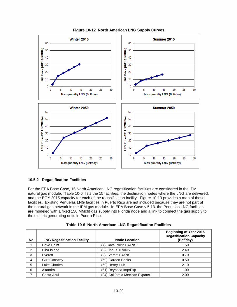
The individual LNG supply curves from the GMM LNG model are aggregated to create total North American LNG supply curves describing LNG availability serving the North American regasification facilities. The three point curves are converted to six points by linear interpolation to provide more supply steps in the IPM natural gas module. Two LNG supply curves, one for winter and one for summer, are specified for each year starting from 2015 until 2054 to capture growth as well as seasonal variation of the LNG supplies. Figure 10-12 shows the North American LNG supply curves for the winters and summers of 2015 and 2050.

112

Refiner Acquisition Cost of Crude Oil (RACC) is a term commonly use in discussing crude oil. It is the cost of crude oil to the refiner, including transportation and fees. The composite cost is the weighted average of domestic and imported crude oil costs.

10-29

Figure 10-12 North American LNG Supply Curves

10.5.2 Regasification Facilities

For the EPA Base Case, 15 North American LNG regasification facilities are considered in the IPM natural gas module. Table 10-6 lists the 15 facilities, the destination nodes where the LNG are delivered, and the BOY 2015 capacity for each of the regasification facility. Figure 10-13 provides a map of these facilities. Existing Penuelas LNG facilities in Puerto Rico are not included because they are not part of the natural gas network in the IPM gas module. In EPA Base Case v.5.13. the Penuelas LNG facilities are modeled with a fixed 150 MMcfd gas supply into Florida node and a link to connect the gas supply to the electric generating units in Puerto Rico.

Table 10-6 North American LNG Regasification Facilities

No LNG Regasification Facility Node Location

Beginning of Year 2015 Regasification Capacity

(Bcf/day)

1 Cove Point (7) Cove Point TRANS 1.50

2 Elba Island (9) Elba Is TRANS 2.40

3 Everett (2) Everett TRANS 0.70

4 Gulf Gateway (69) Garden Banks 0.50

5 Lake Charles (60) Henry Hub 2.10

6 Altamira (51) Reynosa Imp/Exp 1.00

7 Costa Azul (84) California Mexican Exports 2.00

10-30

No LNG Regasification Facility Node Location

Beginning of Year 2015 Regasification Capacity

(Bcf/day)

8 Cameron LNG (60) Henry Hub 1.50

9 Freeport LNG (65) E. TX (Katy) 1.50

10 Golden Pass (65) E. TX (Katy) 2.00

11 Canaport (81) Eastern Canada Demand 1.00

12 Sabine Pass (60) Henry Hub 2.60

13 Gulf LNG Energy LLC (114) South MS/AL 1.00

14 Northeast Gateway (1) New England 0.80

15 Manzanillo (51) Reynosa Imp/Exp 0.75

Figure 10-13 North American LNG Regasification Facilities Map

10.5.3 LNG Regasification Capacity Expansions

The IPM natural gas module has two constraints for the regasification capacity expansion: (1) minimum LNG regasification facility capacity expansion and (2) maximum LNG regasification facility capacity expansion. The values are specified for each facility and year where the minimum constraint is used to force the model to add regasification capacity and the maximum constraint is the upper bound for the capacity expansion.

The decision of whether to expand regasification capacity is controlled by the two constraints and by a levelized capital cost for regasification capacity expansion. The BOY 2015 levelized capital cost for capacity expansion (in real 2011 dollars per MMBtu of capacity expansion) is specified for each facility. A cost multiplier can be applied to represent the increase in levelized capital cost over time. The

10-31

constraints for the capacity expansion can be used to turn on or off the regasification capacity expansion feature in the model. Setting both constraints to zero will deactivate this feature.

If the regasification capacity is allowed to expand, the model can add capacity to a facility within the minimum and maximum constraints if the cost of the regasification expansion contributes to the optimal solution, i.e., minimizes the overall costs to the power sector, including the capital cost for adding new regasification capacity less their revenues. The model takes into account all possible options/projects (including regasification capacity expansions) in any year that do not violate the constraints and selects the combination of options/projects that provide the minimum objective function value. In this way, regasification capacity expansion projects will compete with each other and even with other projects such as pipeline expansions, storage expansions, etc.

Due to excess LNG regasification capacity already in the system, the regasification capacity expansion feature is not deployed in EPA Base Case v.5.13. EPA scenario results show very low total LNG utilizations throughout the projection period because of robust natural gas supply in the U.S. and Canada combined with a relatively low electricity demand growth assumption. The results suggest the base year LNG regasification capacity is already high and requires no expansion.

10.6 End Use Demand

Non-power sector demand (i.e. the residential, commercial, and industrial) is modeled in the new gas module in the form of node-level firm and interruptible demand curves

113. The firm demand curves are

developed and used for residential, commercial, and some industrial sources, while the interruptible demand curves are developed and used exclusively for industrial sources.

A three step process is used to prepare these curves for use in the IPM gas module. First, GMM is used to develop sector specific econometric models representing the non-power sector demand. Since the GMM econometric models are functions of weather, economic growth, price elasticity, efficiency and technology improvements, and other factors, these drivers, in effect, are embedded in the resulting IPM natural gas module demand curves. Second, projections are made using the GMM econometric models and assembled into monthly gas demand curves by sector and demand node. Third, using a second model, seasonal and load segment specific demand curves are derived from the monthly gas demand curves. The sections below describe each of these steps in further detail.

10.6.1 Step 1: Developing Sector Specific Econometric Models of Non-Power Sector Demand

Residential/Commercial Sector

The GMM econometric models of residential and commercial demand are based on regression analysis of historical data for 41 regions and are adjusted to reflect conservation, efficiency, and technology changes over time. The regional data is allocated to the node level based on population data and information from the Energy Information Administration’s “Annual Report of Natural and Supplemental Gas Supply & Disposition” (EIA Form-176). Specifically, the econometric models used monthly Department of Energy/Energy Information Administration (DOE/EIA) data from January 1984 through December 2002 for the U.S. and monthly Statistics Canada data from January 1988 through December 2000 for Canada.

The GMM econometric models showed node-level residential and commercial gas demand to be a function of heating degree days, elasticity of gas demand relative to GDP, and elasticity of gas demand relative to gas price. The GDP elasticity was generally about 0.4 for the residential sector and 0.6 for the commercial sector. The gas price elasticity was generally less than 0.1 for both sectors. Since gas demand in these sectors is relatively inelastic, GDP and price changes have small effects on demand.

113

“Firm” refers to natural gas demand that is not subject to interruptions from the supplier, whereas “interruptible” refers to natural gas demand that is subject to curtailment or cessation by the supplier.

10-32

U.S. Industrial Sector

The GMM econometric model of U.S. industrial gas demand employed historical data for 11 census-based regions and ten industry sectors, focusing on gas-intensive industries such as:

Food

Pulp and Paper

Petroleum Refining

Chemicals

Stone, Clay and Glass

Iron and Steel

Primary Aluminum

Other Primary Metals

Other Manufacturing

Non-Manufacturing

For each of these sectors three end-use categories (process heat, boilers, and other end uses) are modeled separately:

Process heat: This includes all uses of gas for direct heating as opposed to indirect heating (e.g., steam production). The GMM econometric modeling indicated that forecasts for process heat for each industrial sector are a function of growth in output, the energy intensity trend, and the price elasticity. Growth in output over time for most industries is controlled by industrial production indices. Energy intensity is a measure of the amount of gas consumed per unit of output. Energy intensity tends to decrease over time as industries become more efficient.

Boilers: This category includes natural gas-fired boilers whose purpose is to meet industrial steam demand. GMM econometric models indicated that gas demand for boilers is a function of the growth in industrial output and the amount of gas-to-oil switching. Industry steam requirements grow based on industrial production growth. A large percentage of the nominally “dual-fired” boilers cannot switch due to environmental and technical constraints.

Other end uses: This category includes all other uses for gas, including non-boiler cogeneration, on-site electricity generation, and space heating. Like the forecasts for process heat, the GMM econometric modeling showed “other end uses” for each industrial sector to be a function of growth in output, the energy intensity trend, and the price elasticity.

In addition to these demand models, a separate regression model was use to characterize the chemicals sector’s demand for natural gas as a feedstock for ammonia, methanol, and non-refinery hydrogen. Growth in the chemicals industry is represented by a log-linear regression model that relates the growth to GDP and natural gas prices. As GDP growth increases, chemical industry production increases; and as gas prices increase, chemical industry production decreases.

The GMM econometric models for the U.S. industrial sector used DOE/EIA monthly data from January 1991 through December 2000.

Canada Industrial Sector

The industrial sector in Canada is modeled in less detail. Canada is divided into 6 regions based on provincial boundaries. The approach employs a regression fit of historic data similar to that used in the residential/commercial sectors. Sub-sectors of Canadian industrial demand are not modeled separately. The Canadian industrial sector also includes power generation gas demand. The model used Statistics Canada monthly data from January 1991 through December 2000.

10-33

10.6.2 Step 2: Use projections based on the GMM econometric models to produce monthly gas demand curves by sector and demand node

The regression functions resulting from the econometric exercises described in Step 1 are used to create monthly sector- and nodal-specific gas demand curves. To do this the functions are first populated with the macroeconomic assumptions that are consistent with those used in EPA Base Case v.5.13. Then, a range of natural gas prices are fed into the regression functions. At each gas price the regression functions report out projected monthly demand by sector and node. These are the GMM’s nodal demand curves.

10.6.3 Step 3: Develop non-electric sector natural gas demand curves that correspond to the seasons and segments in the load duration curves used in IPM

A second model, the Daily Gas Load Model (DGLM), is used to create daily gas load curves based on the GMM monthly gas demand curves obtained in Step 2. The DGLM uses the same gas demand algorithms as the GMM, but uses a daily temperature series to generate daily variations in demand, in contrast to the seasonal variations in gas demand that are obtained from the GMM.

The resulting daily nodal demand data for each non-power demand sector are then re-aggregated into the two gas demand categories used in the IPM gas module: all of the residential and commercial demand plus 10% of the industrial demand is allocated to the firm gas demand curves, and the remaining 90% of the industrial demand is allocated to the interruptible gas demand curves.

IPM, the power sector model, has to take into account natural gas demand faced by electric generating units that dispatch in different segments of the load duration curves, since demand for natural gas and its resulting price may be very different for units dispatching in the peak load segment than it is for units dispatching in the base, high shoulder, mid shoulder, or low shoulder load segments. In addition, since seasonal differences in demand can be significant, IPM requires separate load segment demand data for each season that is modeled. In EPA Base Case v.5.13, there are two seasons: Summer (May 1 – September 30) and winter (October 1 – April 30). Therefore, the firm and interruptible daily gas demand and associated prices are allocated to the summer and winter load segment based on the applicable season and prevailing load conditions to produce the final non-electric sector gas demand curves that are used in IPM.

In EPA Base Case v.5.13, each of the summer and winter periods uses 6 load segments for pre-2030 and 4 load segments for post-2030 as shown in Table 10-7. The “Peak” load segment in post-2030 is an aggregate of “Needle Peak“ and “Near Peak” load segments in the pre-2030. The “High Shoulder” load segment in post-2030 is an aggregate of “High Shoulder“ and “Middle Shoulder” load segments in the pre-2030. The same definitions of “Low Shoulder” and “Base” load segments are applied to both pre-2030 and post-2030. Input data for firm and interruptible demand curves are specified for all six load segments listed in the pre-2030 column of Table 10-7.

Table 10-7 Summer and Winter Load Segments in EPA Base Case v.5.13

Pre 2030 Post 2030

1 Needle Peak 1 Peak

2 Near Peak

3 High Shoulder 2 High Shoulder

4 Middle Shoulder

5 Low Shoulder 3 Low Shoulder

6 Base 4 Base

Aggregation of summer and winter load segments from six in the pre-2030 to four in the post-2030 is performed endogenously in the model.

10-34

The non-electric sector demand curves (firm and interruptible) are generated based on GMM regressions described above with macroeconomic assumptions consistent with those of EPA Base Case v.5.13. A set of firm and interruptible gas demand curves is generated for each node and year. Examples of node-specific firm and interruptible demand curves, for summer and winter load segments are shown in Figure 10-14 and Figure 10-15. Figure 10-14 is very inelastic; only a small fraction of demand is shed as prices increase. The interruptible gas demand in the peak segments is also very inelastic as expected with higher elasticities in the shoulder and base load segments.

It is important to note that the non-electric gas demand curves provided to the IPM/Gas model are static inputs. The implied elasticities in the curves represent short-term elasticities based on EPA Base Case v.5.13 macroeconomic assumptions. Long-term elasticity is not factored into the gas demand curves. In other words, changes in the assumptions that affect the price/volume solutions have no effect to the long-term gas demand elasticity assumed here.

Figure 10-14 Examples of Firm Demand Curves by Electric Load Segment

Figure 10-15 Examples of Interruptible Demand Curves by Electric Load Segment

10-35

10.6.4 The Use of Firm Gas Demand to Represent LNG Exports

As described earlier, the gas module does not currently have a specific sub-module for LNG exports. In the EPA Base Case v.5.13, the LNG exports are treated as firm demand in the form of fixed or inelastic firm demand curves. Three additional demand nodes are added to represent the three LNG export terminals, two in the U.S. Gulf Coast and one in Western Canada. The U.S. Gulf Coast LNG nodes are linked to nodes (60) Henry Hub and (65) E. TX (Katy) and the Western Canada LNG export node is linked to node (72) North British Columbia. The assumptions for LNG exports from the U.S. Gulf Coast, starting from 2016, are adapted from AEO 2013. The assumptions for LNG exports from Western Canada, starting from 2017, are derived from GMM LNG Model. Figure 10-16 shows LNG exports projection from the U.S. and Canada.

Figure 10-16 LNG Export Assumptions in EPA Base Case v.5.13.

10.7 Pipeline Network

10.7.1 Network Structure

The pipeline network in the IPM natural gas module represents major transmission corridors (not individual pipelines) throughout North America. It contains 380

114 gas pipeline corridors (including bi-

directional links) between the 118 nodes (Figure 10-3). Each corridor is characterized by maximum capacity and a “value of service” (discount curve) relationship that determines the market value of capacity as a function of load factor.

115 The node structure is developed to reflect points of change or

influence on the pipeline system such as:

Major demand and supply centers

Pipeline Hubs and market centers

Points of divergence in pipeline corridors

To illustrate the relationship of corridors and pipelines, Figure 10-17 shows the flow and capacity of five pipeline corridors in New England in 2020. Gas flows into New England along three pipeline corridors

114

Excluding LNG import Terminal nodes and their pipeline connections. 115

See footnote 88 above for a definition of “load factor.”

10-36

(indicated in Figure 10-17 by 3 of the 4 arrows that point into the region) representing a total of seven pipeline systems (indicated by name labels in Figure 10-17). New England also receives gas via the Everett LNG terminal (indicated in Figure 10-17 by the 4th arrow that points into the region). Also, some of the gas that flows into New England on the Iroquois system flows through the region and back to downstate New York; this is represented on the map as an export from New England (indicated in Figure 10-17 by the arrow that points away from the region).

Figure 10-17 New England Pipeline Corridors in 2020

10.7.2 Pipeline Transportation Costs

In the IPM natural gas module, the natural gas moves over the pipeline network at variable cost. The variable cost as a function pipeline throughput (or pipeline discount curve) is used to determine transportation basis

116 (i.e., the market value of capacity) for each period in the forecast for each pipeline

link. The 4-point pipeline discount curves in the IPM natural gas module are simplified forms of the more robust continuous discount curves from the GMM pipeline module. The GMM pipeline discount curves have been derived in the course of extensive work to calibrate the model to actual history. The curves have been fit to basis differentials observed from actual gas prices and to annual load factors from pipeline electronic bulletin boards via Lippman Consulting, Inc.

The GMM continuous discount curves are converted to 4-point linear curves for the IPM natural gas module capturing deflection points in the GMM discount curves. Figure 10-18 depicts the BOY 2015 discount curve for the pipeline corridor connecting nodes (61) North Louisiana Hub and (18) Tennessee/Kentucky. Cost growth factors shown in

116

In natural gas discussions “basis” refers to differences in the price of natural gas in two different geographical locations. In the marketplace “basis” typically means the difference between the NYMEX futures price at the Henry Hub and the cash price at other market points. In the modeling context “basis” means the difference in natural gas prices between any two nodes at the same instance in time.

10-37

Figure 10-19 are applied to the pipeline discount curves to reflect cost increase over time. The cost is assumed to grow at an average rate of 0.5 percent per year.

Figure 10-18 Example Pipeline Discount Curve

Figure 10-19 Pipeline Cost Growth Factor

10.7.3 Pipeline Capacity Expansion Logic

Initial pipeline capacity, derived from GMM, includes existing capacities and planned capacities that are expected to be operational from the beginning of 2015. The IPM natural gas module has the capability to endogenously expand the pipeline capacity. The decision of whether to expand pipeline capacity is controlled by two constraints, which stipulate minimum and maximum capacity additions and by the levelized capital cost of expanding pipeline capacity in the specific corridor and year. The minimum capacity addition constraint forces the model to add capacity in a specified corridor and year. The

10-38

maximum capacity constraint is the upper bound on capacity additions in a specified corridor and year. For most pipeline corridors there is no minimum or maximum capacity requirement, and so they are assigned a value of zero as their minimum capacity addition requirement and infinity

117 as their maximum

capacity addition requirement. Where this occurs, the pipeline expansion is only controlled by the pipeline capital cost.

The model is allowed to add capacity to a pipeline corridor within the minimum and maximum capacity addition constraints if the cost of the pipeline expansion contributes to the optimal solution, i.e., minimizes the overall costs to the power sector, including the capital cost for pipeline capacity expansion, less their revenues. The model takes into account all possible options/projects including capacity additions for pipeline corridors in any year that do not violate the constraints and selects the combination of options/projects that provide the minimum objective function. In this way, pipeline corridor expansion projects will compete with each other and even with other projects such as LNG regasification capacity expansions, storage expansions, etc.

For EPA Base Case v.5.13, pipeline corridors connecting North Alaska (node 89) and Mackenzie Delta (node 86) to North British Columbia (node 72) have the minimum and maximum capacity addition constraints. Due to uncertainties of these pipeline projects as discussed in Section 3, the North Alaska and Mackenzie Delta pipeline projects are not made available throughout the projection. Both capacity addition constraints for North Alaska and Mackenzie delta pipeline corridors are set to zero.

Expansions in other pipeline corridors are not restricted. The model is allowed to build capacity to any pipeline corridors at any time as long as it contributes to minimization of the objective function.

The BOY 2015 levelized pipeline capital cost (in real 2011 dollars per MMBtu/Day of pipeline capacity addition) is specified for each of the 380 pipeline links. The cost growth factors shown in

Figure 10-19 are applied to derive the cost increase over time. The average levelized capital cost for pipeline capacity expansion for 2015 is $165 per MMBtu/Day.

10.8 Gas Storage

The IPM natural gas module has 118 underground storage facilities that are linked to 51 nodes. The underground storage is grouped into three categories based on storage “Days Service.”

118

“20-Day” high deliverability storage – 37 storage facilities

“80-Day” depleted/aquifer reservoirs – 41 storage facilities

“Over 80 Days” depleted/aquifer reservoirs – 40 storage facilities

The model also includes existing and potential LNG peak shaving storage facilities. The existing facilities are linked to 24 nodes with allocations based on historical capacity data. There are 48 other nodes that are linked to LNG peakshaving storage. These facilities do not currently have capacity but are included in the storage database for the purpose of future expansion. The map of storage facility locations is shown in Figure 10-6 and the list of storage facility nodes is shown in

Table 10-8.

In

Table 10-8 an X in columns 2 (“20-Day”), 3 (“80-Day”), or 4 (“Over 80-Days”) represents an underground storage facility. There are 118 such X’s which correspond to the 118 underground storage facilities noted

117

In the model this is achieved by assigning a large number, e.g., 100 Bcfd, for every year where there is no constraint on maximum capacity. 118

See footnote 90 above for a definition of “Days Service.”

10-39

in the previous paragraph. These 118 X’s appear in 51 rows, which represent the linked nodes noted in the previous paragraph. The identities of these nodes are found in column 1 (“Node”). Similarly, 24 X’s in columns 5 (“Existing”) represent the 24 existing LNG peakshaving facilities and 48 X’s in column 6 (“Potential”) represent the 48 prospective LNG storage facilities.

Table 10-8 List of Storage Nodes

Node

Underground Storage Facility LNG Peakshaving Facility

20-Day 80-Day Over 80 Days Existing Potential

(1) New England X

(3) Quebec X X X

(4) New York City X

(5) Niagara X X X X

(6) Southwest PA X X X X

(8) Georgia X

(10) South Florida X

(11) East Ohio X X X X

(12) Maumee/Defiance X

(13) Lebanon X

(14) Indiana X X X

(15) South Illinois X X X X

(16) North Illinois X X X X

(17) Southeast Michigan X X X

(18) East KY/TN X X X X

(19) MD/DC/Northern VA X

(20) Wisconsin X

(21) Northern Missouri X

(22) Minnesota X X

(23) Crystal Falls X

(24) Ventura X X X

(26) Nebraska X X

(28) Kansas X X X X

(29) East Colorado X X X X

(30) Opal X X X X

(31) Cheyenne X X

(32) San Juan Basin X

(33) EPNG/TW X

(34) North Wyoming X

(35) South Nevada X

(36) SOCAL Area X X X

(38) PGE Area X X X X

(41) Montana/North Dakota X X X

(45) Pacific Northwest X X X

(46) NPC/PGT Hub X

(47) North Nevada X

(48) Idaho X

(54) North Alabama X X X X

(56) North Mississippi X X X

(58) Eastern Louisiana Hub X X X

(60) Henry Hub X X X X

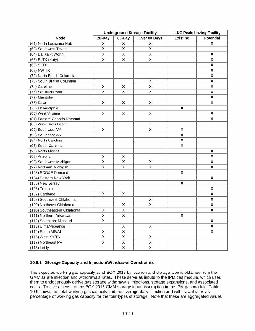
10-40

Node

Underground Storage Facility LNG Peakshaving Facility

20-Day 80-Day Over 80 Days Existing Potential

(61) North Louisiana Hub X X X X

(63) Southwest Texas X X X

(64) Dallas/Ft Worth X X X X

(65) E. TX (Katy) X X X X

(66) S. TX X

(68) NW TX X

(72) North British Columbia X

(73) South British Columbia X X

(74) Caroline X X X X

(76) Saskatchewan X X X X

(77) Manitoba X

(78) Dawn X X X X

(79) Philadelphia X

(80) West Virginia X X X X

(81) Eastern Canada Demand X

(83) Wind River Basin X

(92) Southwest VA X X X

(93) Southeast VA X

(94) North Carolina X

(95) South Carolina X

(96) North Florida X

(97) Arizona X X X

(98) Southwest Michigan X X X X

(99) Northern Michigan X X X X

(103) SDG&E Demand X

(104) Eastern New York X

(105) New Jersey X

(106) Toronto X

(107) Carthage X X X

(108) Southwest Oklahoma X X

(109) Northeast Oklahoma X X X

(110) Southeastern Oklahoma X X X

(111) Northern Arkansas X X X

(112) Southeast Missouri X X

(113) Uinta/Piceance X X X

(114) South MS/AL X X X

(115) West KY/TN X X X

(117) Northeast PA X X X

(118) Leidy X X

10.8.1 Storage Capacity and Injection/Withdrawal Constraints

The expected working gas capacity as of BOY 2015 by location and storage type is obtained from the GMM as are injection and withdrawals rates. These serve as inputs to the IPM gas module, which uses them to endogenously derive gas storage withdrawals, injections, storage expansions, and associated costs. To give a sense of the BOY 2015 GMM storage input assumption in the IPM gas module, Table 10-9 shows the total working gas capacity and the average daily injection and withdrawal rates as percentage of working gas capacity for the four types of storage. Note that these are aggregated values

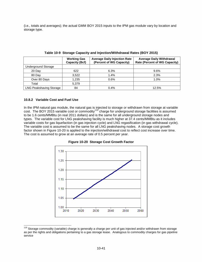
10-41

(i.e., totals and averages); the actual GMM BOY 2015 inputs to the IPM gas module vary by location and storage type.

Table 10-9 Storage Capacity and Injection/Withdrawal Rates (BOY 2015)

Working Gas Capacity (Bcf)

Average Daily Injection Rate (Percent of WG Capacity)

Average Daily Withdrawal Rate (Percent of WG Capacity)

Underground Storage

20 Day 622 6.3% 9.6%

80 Day 3,522 1.4% 2.3%

Over 80 Days 1,235 0.6% 1.0%

Total 5,379

LNG Peakshaving Storage 84 0.4% 12.5%

10.8.2 Variable Cost and Fuel Use

In the IPM natural gas module, the natural gas is injected to storage or withdrawn from storage at variable cost. The BOY 2015 variable cost or commodity

119 charge for underground storage facilities is assumed

to be 1.6 cents/MMBtu (in real 2011 dollars) and is the same for all underground storage nodes and types. The variable cost for LNG peakshaving facility is much higher at 37.4 cents/MMBtu as it includes variable costs for gas liquefaction (in gas injection cycle) and LNG regasification (in gas withdrawal cycle). The variable cost is assumed to be the same for all LNG peakshaving nodes. A storage cost growth factor shown in Figure 10-20 is applied to the injection/withdrawal cost to reflect cost increase over time. The cost is assumed to grow at an average rate of 0.5 percent per year.

Figure 10-20 Storage Cost Growth Factor

119

Storage commodity (variable) charge is generally a charge per unit of gas injected and/or withdrawn from storage as per the rights and obligations pertaining to a gas storage lease. Analogous to commodity charges for gas pipeline service

10-42

Fuel use for injection and withdrawal for underground storage is 1% of the gas throughput. The withdrawal fuel use for the LNG peakshaving storage is also 1% but the injection fuel use is much higher at 11% of the injection gas as it includes fuel use for gas liquefaction.

10.8.3 Storage Capacity Expansion Logic

The endogenous modeling decision of whether to expand working gas storage capacity is controlled by two constraints, which stipulate minimum and maximum capacity additions for each storage facility and year, and by the levelized capital cost of the storage expansion. The two constraints are specified as input data for each storage facility and year. The minimum constraint forces the model to add working gas capacity to the specified facility and year and the maximum constraint is the cap for the expansion. Figure 10-21 shows projected maximum storage expansion constraints for the “80-day” category storage facility in supply area Katy, Texas.

Figure 10-21 Example Maximum Storage Capacity Expansion

The model is allowed to add working gas capacity to a storage facility within the two constraints if the cost of storage expansion contributes to the optimal solution, i.e., minimizes the overall costs to the power sector, including the capital cost for working gas capacity expansion less their revenues. The model takes into account all possible options/projects including working gas capacity additions for storage facilities in any year that do not violate the constraints and selects the combination of options/projects that provide the minimum objective function value. In this way, storage capacity expansion projects will compete with each other and even with other projects such as LNG regasification capacity expansions, pipeline expansions, etc.

The BOY 2015 levelized storage capital cost (in real 2011 dollars per MMBtu of storage capacity addition) is specified for each of the 190 storage facilities. Table 10-10 lists the average BOY 2015 levelized storage capital cost for the four types of storage facility. Amongst the underground storage facilities the higher capital costs represent more storage cycles

120 that could be achieved in a year. On average, the

capital costs for the “80-Day” and “20-Day” storage facilities are assumed to be about 20 percent and 40

120

One storage cycle is the theoretical time required to completely inject and withdraw the working gas quantity for any given underground gas storage facility or the turnover time for the working gas capacity rating of the facility. The cycle rate of any storage facility is usually expressed in cycles per year and is the number of times the working gas volumes can theoretically be turned over each storage year. The cycle rating for Porous Storage varies from 1 to 6 per year while that for Salt Cavern Storage are as high as 12 per year.

10-43

percent, respectively, higher than that of the “Over 80 Days” storage facility. The levelized capital cost for LNG peakshaving storage is much higher due to higher capital cost for the liquefaction unit. The cost growth factors shown in Figure 10-20 are applied to the capital cost to derive the cost increase over time. The capital cost is assumed to grow at an average rate of 0.5 percent per year.

Table 10-10 Base Year 2015 Average Levelized Storage Capital Cost

Storage Type

Average Levelized Storage Capital Cost

(2011 $/MMBtu)

Underground Storage

20-Day 1.19

80-Day 0.99

Over 80 Days 0.83

LNG Peakshaving Storage 5.34

10.9 Fuel Prices

10.9.1 Crude Oil and Natural Gas Liquids Prices

Since a fraction of the hydrocarbons produced in the natural gas exploration and development process are crude oil and NGLs (see columns 2 and 3 in Table 10-5), revenues from crude oil and NGL production play a key role in determining the extent of exploration and development for natural gas. To take into account these revenues, crude oil and NGL price projections are provided as inputs to the IPM natural gas module and factored into the calculation of costs in the IPM objective function.

The crude oil and NGL price projections used in the IPM natural gas module are shown in Figure 10-22. These price projections were adapted from AEO 2013. No attempt was made to project prices beyond 2040 other than to assume that prices remain at their 2040 levels. The projected prices shown in Figure 10-22 are expressed in units of 2011$ per MMBtu. Using a crude oil Btu content of 5.8 MMBtu/Bbl, the projected crude oil prices in Figure 10-22 can be translated into the more familiar units of dollars per barrel (Bbl), in which case, prices in this figure are equivalent to $93/Bbl in 2015, $102/Bbl in 2020, $126/Bbl in 2020, and constant at $155/Bbl from 2040 (in real 2011 dollars) onward.

Figure 10-22 Crude Oil and NGL Prices

10-44

10.9.2 Natural Gas Prices

Node-level natural gas prices are outputs of the model and are obtained from the optimal solution of the combined IPM electric power sector and natural gas linear programming (LP) model. From a technical modeling standpoint, the node gas prices are what are called “shadow prices” or “dual variable values” associated with the node mass balance constraints at the optimal LP solution.

10.10 Outputs and Glossary of Terms

10.10.1 Outputs from the IPM Natural Gas Module

The EPA Base Case v.5.13 reports natural gas consumption (in TBtu), Henry Hub and delivered natural gas prices (in $/MMBtu). It also reports natural gas supply (in Tcf), disposition (in Tcf), prices (in $/MMBtu), production (in Tcf) by supply region, end-of-year reserves and annual reserve additions (in Tcf), imports and exports (in Tcf), consumption by end-use sector and census division (in Tcf), prices by census division (in $/MMBtu), and inter-regional pipeline flows and LNG imports (in Bcf).

10.10.2 Glossary of Terms Used in this Section

For ease of reference Table 10-11 assembles in one table terms that have been defined in footnotes throughout this chapter.

Table 10-11 Glossary of Natural Gas Terms Used in Documentation

Term Definition

Arps-Roberts equation “Arps-Roberts equation” refers to the statistical model of petroleum discovery developed by J. J. Arps, and T. G. Roberts, T. G., in the 1950’s.

Associated gas Associated gas refers to natural gas that is produced in association with crude oil production, whereas non-associated gas is natural gas that is not in contact with significant quantities of crude oil in the reservoir.

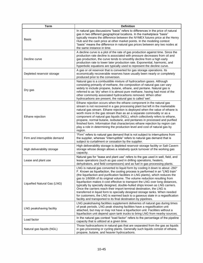
10-45

Term Definition

Basis

In natural gas discussions “basis” refers to differences in the price of natural gas in two different geographical locations. In the marketplace “basis” typically means the difference between the NYMEX futures price at the Henry Hub and the cash price at other market points. In the modeling context “basis” means the difference in natural gas prices between any two nodes at the same instance in time.

Decline curve

A decline curve is a plot of the rate of gas production against time. Since the production rate decline is associated with pressure decreases from oil and gas production, the curve tends to smoothly decline from a high early production rate to lower later production rate. Exponential, harmonic, and hyperbolic equations are typically used to represent the decline curve.

Depleted reservoir storage A gas or oil reservoir that is converted for gas storage operations. Its economically recoverable reserves have usually been nearly or completely produced prior to the conversion.

Dry gas

Natural gas is a combustible mixture of hydrocarbon gases. Although consisting primarily of methane, the composition of natural gas can vary widely to include propane, butane, ethane, and pentane. Natural gas is referred to as 'dry' when it is almost pure methane, having had most of the other commonly associated hydrocarbons removed. When other hydrocarbons are present, the natural gas is called 'wet'.

Ethane rejection

Ethane rejection occurs when the ethane component in the natural gas stream is not recovered in a gas processing plant but left in the marketable natural gas stream. Ethane rejection is deployed when the value of ethane is worth more in the gas stream than as an a separate commodity or as a component of natural gas liquids (NGL), which collectively refers to ethane, propane, normal butane, isobutane, and pentanes in processed and purified finished form. Information that characterizes ethane rejection by region can play a role in determining the production level and cost of natural gas by region.

Firm and interruptible demand “Firm” refers to natural gas demand that is not subject to interruptions from the supplier, whereas “interruptible” refers to natural gas demand that is subject to curtailment or cessation by the supplier.

High deliverability storage High deliverability storage is depleted reservoir storage facility or Salt Cavern storage whose design allows a relatively quick turnover of the working gas capacity.

Lease and plant use Natural gas for “lease and plant use” refers to the gas used in well, field, and lease operations (such as gas used in drilling operations, heaters, dehydrators, and field compressors) and as fuel in gas processing plants.

Liquefied Natural Gas (LNG)

LNG is natural gas converted to liquid form by cooling it down to about -260° F. Known as liquefaction, the cooling process is performed in an “LNG train” (the liquefaction and purification facilities in LNG plants), which reduces the gas to 1/600th of its original volume. The volume reduction resulting from liquefaction makes it cost effective to transport the LNG over long distances, typically by specially designed, double-hulled ships known as LNG carriers. Once the carriers reach their import terminal destination, the LNG is transferred in liquid form to specially designed storage tanks. When needed for customers, the LNG is warmed back to a gaseous state in a regasification facility and transported to its final destination by pipelines.

LNG peakshaving facility

LNG peakshaving facilities supplement deliveries of natural gas during times of peak periods. LNG peak shaving facilities have a regasification unit attached, but may or may not have a liquefaction unit. Facilities without a liquefaction unit depend upon tank trucks to bring LNG from nearby sources.

Load factor In the natural gas context “load factor” refers to the percentage of the pipeline capacity that is utilized at a given time.

Natural gas liquids (NGL) Those hydrocarbons in natural gas that are separated from the gas as liquids in gas processing or cycling plants. Generally such liquids consist of ethane, propane, butane, and heavier hydrocarbons.

10-46

Term Definition

Play

A “play” refers to a set of known or postulated natural gas (or oil) accumulations sharing similar geologic, geographic, and temporal properties, such as source rock, migration pathway, timing, trapping mechanism, and hydrocarbon type.

Pool

A “pool” is a subsurface accumulation of oil and other hydrocarbons. Pools are not necessarily big caverns. They can be small oil-filled pores. A “field” is an accumulation of hydrocarbons in the subsurface of sufficient size to be of economic interest. A field can consist of one or more pools.

Proven (or proved)

The term “proven” refers to the estimation of the quantities of natural gas resources that analysis of geological and engineering data demonstrate with reasonable certainty to be recoverable in future years from known reservoirs under existing economic and operating conditions. Among the factors considered are drilling results, production, and historical trends. Proven reserves are the most certain portion of the resource base.

RACC price

Refiner Acquisition Cost of Crude Oil (RACC) is a term commonly use in discussing crude oil. It is the cost of crude oil to the refiner, including transportation and fees. The composite cost is the weighted average of domestic and imported crude oil costs.

Raw gas Raw gas production refers to the volumes of natural gas extracted from underground sources, whereas net gas production refers to the volume of purified, marketable natural gas leaving the natural gas processing plant.

Reserves-to-production (R/P) ratio Reserves-to-production ratio is the remaining amount of reserves, expressed in years, to be produced with a current annual production rate.

Resource and reserves

When referring to natural gas a distinction is made between “resources” and “reserves.” “Resources” are concentrations of natural gas that are or may become of potential economic interest. “Reserves” are that part of the natural gas resource that has been fully evaluated and determined to be commercially viable to produce.

Resource appreciation

Resource appreciation represents growth in ultimate resource estimates attributed to success in extracting resource from known plays such as natural gas from shales, coal seams, offshore deepwater, and gas hydrates that are not included in the resource base estimates.

Storage "Days Service" Storage “Days Service” refers to the number of days required to completely withdraw the maximum working gas inventory associated with an underground storage facility.

Storage commodity charge

Storage commodity (variable) charge is generally a charge per unit of gas injected and/or withdrawn from storage as per the rights and obligations pertaining to a gas storage lease. Analogous to commodity charges for gas pipeline service

Storage cycle

One storage cycle is the theoretical time required to completely inject and withdraw the working gas quantity for any given underground gas storage facility or the turnover time for the working gas capacity rating of the facility. The cycle rate of any storage facility is usually expressed in cycles per year and is the number of times the working gas volumes can theoretically be turned over each storage year. The cycle rating for Porous Storage varies from 1 to 6 per year while that for Salt Cavern Storage are as high as 12 per year.

10-47

Term Definition

Unconventional gas

Unconventional gas refers to natural gas found in geological environments that differ from conventional hydrocarbon traps. It includes: (a) “tight gas,” i.e., natural gas found in relatively impermeable (very low porosity and permeability) sandstone and carbonate rocks; (b) “shale gas,” i.e., natural gas in the joints, fractures or the matrix of shales, the most prevalent low permeability low porosity sedimentary rock on earth; and (c) “coal bed methane,” which refers to methane (the key component of natural gas) found in coal seams, where it was generated during coal formation and contained in the microstructure of coal. Unconventional natural gas is distinguished from conventional gas which is extracted using traditional methods, typically from a well drilled into a geological formation exploiting natural subsurface pressure or artificial lifting to bring the gas and associated hydrocarbons to the wellhead at the surface.

Underground storage The underground storage of natural gas in a porous and permeable rock formation topped by an impermeable cap rock, the pore space of which was originally filled with water.

Wet gas

A mixture of hydrocarbon compounds and small quantities of various nonhydrocarbons existing in the gaseous phase or in solution with crude oil in porous rock formations at reservoir conditions. The principal hydrocarbons normally contained in the mixture are methane, ethane, propane, butane, and pentane. Typical nonhydrocarbon gases that may be present in reservoir natural gas are water vapor, carbon dioxide, hydrogen sulfide, nitrogen and trace amounts of helium.

Working gas

The term “working gas” refers to natural gas that has been injected into an underground storage facility and stored therein temporarily with the intention of withdrawing it. It is distinguished from “base (or cushion) gas” which refers to the volume of gas that remains permanently in the storage reservoir in order to maintain adequate pressure and deliverability rates throughout the withdrawal season.

Documents

10. Natural Gas - US EPA 10. Natural Gas This chapter describes how natural gas supply, demand, and costing are modeled in EPA Base Case v.5.13. Section 0 indicates that natural gas