Model predictions and comparisons for three toxicokinetic models

for the systemic transport of trichloroethylene

H.T. Banks� and Laura K. Pottery

Center for Research in Scienti�c Computation

North Carolina State University

Raleigh, NC 27695-8205

September 6, 2001

Abstract

In this paper we present and compare three physiologically based pharmacokinetic models for thesystemic transport of trichloroethylene (TCE), a common environmental toxicant. Of particular interestis the disposition of TCE in the adipose tissue, where TCE is known to accumulate. The �rst twosystemic models utilize standard ODE-based adipose compartments that assume rapid equilibrium anduniformity. The third model includes a PDE-based axial dispersion model that is designed to capturethe heterogeneous physiology of adipose tissue and the expected transport of TCE there.

Using numerical methods and model simulations, we compare the predicted concentration pro�les ofTCE in the adipose tissue for the three systemic models. Our results suggest that the dispersion-basedadipose compartmental model is best able to capture the physiological heterogeneities of adipose tissueand their expected e�ects on TCE adipose concentrations.

1 Introduction

Trichloroethylene (TCE) is a solvent that has been used widely in industry as a metal-degreasing agent.This highly lipophilic chemical is now a common soil and groundwater contaminant, and can be found atSuperfund sites and Department of Defense facilities across the United States [21]. Numerous studies havelinked TCE and several of its metabolites to toxic e�ects in humans and animals. Acute exposure to TCE isassociated with fatigue, headaches, dizziness and drowsiness [12], while chronic exposure has been linked todevelopmental defects and kidney, liver and lung tumors [6, 7, 8, 13, 15, 20]. TCE is highly soluble in lipids,and is known to accumulate in the adipose (fat) tissue of humans and animals. This important characteristicof TCE has major implications on its dynamics inside the organs and tissues, and on the overall amount oftime it takes for TCE to be eliminated from the body.

Physiologically based pharmacokinetic (PBPK) models are used to describe the systemic transport be-havior of compounds such as TCE. These compartmental models are useful in determining the e�ectivedosage level received by each of the organs and tissues, and are an important part of the overall processof determining a compound's toxicity in humans and animals. PBPK models usually involve a system ofcoupled algebraic and di�erential equations, where each equation represents the transport of the compoundthrough a given organ or tissue. The standard compartmental equations are based on assumptions of rapidequilibrium and uniformity in concentrations within that particular tissue.

These \well-mixed" assumptions may not be appropriate for highly lipophilic chemicals such as TCEinside the adipose tissue, as several studies have demonstrated large degrees of physiological heterogeneitiesin fat tissue. These heterogeneities include wide variations in fat cell size, metabolic activity, blood ow ratesand cell membrane permeabilities [9, 10, 14, 19]. Moreover, it is known that there are varying amounts of

�Author to whom correspondence should be addressed.yCurrent address: National Health and Environmental E�ects Research Laboratory, U.S. Environmental Protection Agency,

Research Triangle Park, NC.

1

lipid in each fat cell, which leads to an uneven distribution of lipid throughout the adipose tissue [14]. Thisuneven lipid distribution together with the other heterogeneous properties of adipose tissue strongly suggestthat TCE and other lipophilic compounds are likely to have spatially varying concentrations in the adiposetissue. Therefore a spatially varying model may be most appropriate for the transport of TCE within thefat.

To test this hypothesis, we have developed three PBPK models for the systemic transport of TCE, whereeach model has a di�erent submodel for the adipose tissue compartment [1, 17]. The �rst two adiposecompartmental models are based on the standard \well-mixed" assumptions used in PBPK modeling. Thethird systemic model is a PBPK-hybrid model with an axial dispersion-based compartmental model for theadipose tissue. This spatially varying submodel is based speci�cally on the physiology of adipose tissue andthe expected transport of TCE within the tissue.

In this paper we present and compare these three PBPK whole-body models for TCE. Using modelsimulations, we demonstrate that the hybrid model with the spatially varying adipose compartment is mostappropriate for this case and is best able to predict the expected transport of TCE inside the adipose tissue.

2 A PBPK model for TCE with a perfusion-limited adipose tissue

compartment

First we present a standard PBPK model proposed in [1, 17] which has a perfusion-limited adipose tissuecompartment. This model is based on experimental and computational work carried out by Evans et al. [11],who developed a PBPK model for inhaled TCE in Long-Evans rats. The compartments included in themodel are: lung, arterial blood, venous blood, brain, kidney, liver, muscle, fat and remaining tissue. SeeFigure 1 for a geometrical representation of the model.

Each of these compartments except for the lung and blood compartments is modeled as a \perfusion-limited" compartment, in which the blood ow rate to the tissue is assumed to be much slower than the rateof di�usion of TCE across cell membranes within that particular tissue [16]. The liver compartment has anadditional sink term that represents the metabolism of TCE via Cytochrome P450, which is modeled withMichaelis-Menten kinetics. The lung model is based on a steady-state assumption that leads to an algebraicequation for the concentration of TCE in the arterial blood [16], and the venous blood compartment ismodeled as a di�erential equation that is based on mass balance.

The coupled system of model equations is given by

VfdCfdt

= Qf (Ca �CfPf

) (1)

VvdCvdt

= Qm

CmPm

+Qt

CtPt

+Qf

CfPf

+Qbr

CbrPbr

+Ql

ClPl

+Qk

CkPk

�QcCv (2)

Ca =QcCv +QpCc

Qc +Qp

Pb

(3)

VbrdCbrdt

= Qbr(Ca �CbrPbr

) (4)

VkdCkdt

= Qk(Ca �CkPk

) (5)

VldCldt

= Ql(Ca �ClPl

)�vmaxCl

kMPl + Cl(6)

VmdCmdt

= Qm(Ca �CmPm

) (7)

VtdCtdt

= Qt(Ca �CtPt

): (8)

The subscripts denote the following speci�c tissues:

f , Fat

2

pQ C i pQ C x

kv

mv

kQ C a

fv

lv

tv

vbr

Lung Blood

Alveolar Space

Kidney

Muscle

Fat

Brain

Liver

Remaining Tissue

MetabolismKm

m

br

l

t

k

m

f

br

l

t

Venous

Blood

PBPK Model for Inhaled TCE

c cQ C aQ C v

Q C

Q C aQ C

afQ C Q C

Q C a Q C

Q C a Q C

Q C Q Ca

Figure 1: PBPK model for inhaled TCE with a perfusion-limited compartment for adipose tissue. TCEconcentrations are denoted by C and blood ow rates are denoted by Q.

3

0 5 10 150

5

10

15

20

25

30

35

40

45

Time (hours)

TC

E c

once

ntra

tion

(mg/

liter

)

TCE concentration in adipose tissue

Figure 2: Model simulation: Concentration in time of unbound TCE inside the perfusion-limited fat com-partment.

v , Venous blood

a , Arterial blood

br , Brain

k , Kidney

l , Liver

m , Muscle

t , Remaining non-fat tissue.

Total concentrations (in mg/liter) in each of the speci�c tissues are denoted by C, volumes (in liters) by V ,and ow rates (liters/hour) are denoted by Q, each with subscripts corresponding to the speci�c tissue. Theparameters P are the blood/tissue partition coeÆcients for the respective tissues. See [1, 17] for a completedescription of the model equations and parameters. A list of the model parameters is given in the appendix.

Model simulations for (1) { (8) were generated in Matlab using code and model parameters from [11].For this simulation we chose the forcing function to simulate inhaled TCE as in the experiments carried outby Evans et al. [11]. Speci�cally, we de�ned the chamber air concentration Cc(t) to be 2000 parts per millionTCE for one hour, followed by fourteen hours of zero TCE concentration.

Figure 2 depicts simulated unbound TCE concentrations in the perfusion-limited adipose tissue compart-ment. Note the rapid, exponential decay of TCE concentrations following the hour-long exposure period.This simulation illustrates that the perfusion-limited compartmental model may not be able to predict theexpected slow accumulation and release of TCE within the adipose tissue. Furthermore, this model may leadto an over-prediction of TCE blood concentrations, as well as an under-prediction of the overall clearancerate for TCE.

3 A PBPK model for TCE with a di�usion-limited adipose tissue

compartment

A second type of standard PBPK compartmental model is the di�usion-limited compartment. This modelis based on the assumption that the blood ow rate to the tissue is much faster than the transport of

4

0 5 10 150

20

40

60

80

100

120

140

160

180

Time (hours)

TC

E c

once

ntra

tion

(mg/

liter

)

Concentration of TCE in adipose extracellular space

µ = 1 µ = 0.1 µ = 0.01 µ = 0.001

Figure 3: Model simulation: Total concentration of TCE in time in the extracellular subcompartment of thedi�usion-limited fat compartment for various values of the permeability coeÆcient �.

solute (in this case, TCE) across cell membranes in the tissue [16]. The di�usion-limited compartment isdivided into two subcompartments: the intracellular space and the extracellular space, which includes thevascularization and the interstitial uid. Within each of these subcompartments, rapid equilibrium anduniformity are assumed. The di�usion of solute across the cell membranes is modeled using Fick's �rst lawof di�usion.

In [1, 17] we modi�ed the original PBPK model (1) { (8) for TCE by replacing the perfusion-limitedadipose tissue compartment with a di�usion-limited compartment. A new PBPK whole-body model is thenformed by coupling the equations (2) { (8) with the following di�erential equations corresponding to thedi�usion-limited adipose tissue compartment:

VfedCfedt

= Qf (Ca �CfePf

) + �(Cfi � Cfe) (9)

VfidCfidt

= �(Cfe � Cfi); (10)

where Cfe and Cfi denote TCE concentrations in the extracellular and intracellular subcompartments ofthe adipose tissue, respectively. The parameter � is the cell membrane permeability coeÆcient for TCE, andhas units liters/hour. See the appendix for a list of parameter values.

Model simulations were computed as before for varying values of the permeability coeÆcient �. See Fig-ures 3 and 4 for simulations of intracellular and extracellular adipose TCE concentrations, respectively. Notethat the response in the intracellular subcompartment for � = 1 is similar to the response in the perfusion-limited adipose tissue compartment (Figure 2). Moreover, as � decreases, the peak concentration of unboundTCE in the intracellular subcompartment also decreases and the post-exposure decay of concentrations isless rapid.

Although this model has greater exibility than the perfusion-limited model in predicting various con-centration pro�les, it is important to note that the di�usion-limited model may not be appropriate for TCEin adipose tissue. TCE has a low molecular weight and is highly lipophilic, so that it di�uses rapidly acrosscell membranes. Therefore the di�usion rate of TCE is likely to be much greater than the rate of blood owto the adipose tissue and hence the di�usion-limited model may not be physically appropriate in this case.

5

0 5 10 150

5

10

15

20

25

30

35

40

45

Time (hours)

TC

E c

once

ntra

tion

(mg/

liter

)

Concentration of TCE in adipose intracellular space

µ = 1 µ = 0.1 µ = 0.01 µ = 0.001

Figure 4: Model simulation: Concentrations of unbound TCE in time in the intracellular subcompartmentof the di�usion-limited fat compartment for various values of the permeability coeÆcient �.

4 A PBPK-hybrid model for TCE with an axial dispersion-based

adipose tissue compartment

In this section we present a PBPK-hybrid model for TCE with a spatially varying compartment for theadipose tissue. As detailed in [1, 17], we have developed an axial dispersion-type model for the transportof TCE inside the adipose tissue, which is designed to account for the physiological heterogeneities seenin the fat. This compartmental model is then coupled with the remaining tissue compartments to createa whole-body PBPK-hybrid model. The dispersion-based compartmental model for the adipose tissue isbased on the model of Roberts and Rowland [18] for disposition in the liver, and is adapted for the speci�cphysiology of fat tissue.

A key feature of the dispersion model is that it utilizes a single representative \cell" to capture thetransport behavior in a large collection of similar \cells" which have varying properties. The variabilityamong cells is modeled with an axial dispersion term, which has a coeÆcient known as the axial dispersionnumber. The axial dispersion number is a model parameter that measures the variability that occurs acrossthe population of cells. See [17, 18] for a detailed discussion of the dispersion model.

In the case of adipose tissue, we choose the representative \cell" to be an adipocyte (fat cell) togetherwith a neighboring capillary, which are both surrounded by the interstitial uid. This \cell" represents afunctional unit within the adipose tissue, as it is well known that each adipocyte is in contact with one ormore capillaries [24]. See Figure 5 for an illustration of an adipocyte{capillary unit.

4.1 Model geometry and assumptions

The geometry for the axial dispersion model is based on the structure of the adipocyte{capillary unit. Wedivide the adipose compartment into three subcompartments which represent the adipocyte, capillary andinterstitial space. The adipocyte region (A) is represented by a sphere, and is adjacent to the capillary orblood region (B) that is represented as a circular cylinder which curves around the surface of the adipocyte(see Figure 6). Each of these two regions is surrounded by the interstitial region (I). Although not indicatedby the geometry, we assume that the capillary and adipocyte are in direct contact at areas of membranecontinuity between the capillary endothelium and the adipocyte plasma membrane. Several studies haveindicated the existence of these \interfacial continua" [3, 4, 5, 22], and we include them in the model as animportant route of TCE transport within the adipose tissue (see [17]).

6

Figure 5: Representation of an adipocyte and capillary, surrounded by interstitial uid.

Arterial blood

Venous blood

B

A x y

z

φ

θ

r

I

Figure 6: Adipose tissue represented geometrically: the adipocyte region (A) is a sphere, surrounded by theinterstitial space (I). The capillary or blood region (B) is a cylindrical tube that wraps around the capillary.Coordinates are in spherical coordinates (r; �; �).

7

We assume that blood and TCE ow from the arterial blood compartment into the capillary region of theadipose compartment. As it ows through the capillary, TCE di�uses across the capillary endothelium intoand out of the interstitial uid, as well as into and out of the adipocyte at areas of membrane continuity.At the exit to the capillary, TCE and blood ow from the adipose compartment into the venous bloodcompartment.

TCE enters and exits the interstitial uid via the capillary at the location � = �0, "1 < � < "2, andfrom the adipocyte at all points 0 � � � 2�, 0 � � � �. The nonuniform interface between the capillaryand interstitial space (with respect to �) results in di�usion of TCE through the interstitial uid. Similarconditions occur in the adipocyte region.

In the capillary region our set of assumptions results in a partial di�erential equation that depends onlyon time and on the spatial variable �. In the other two subcompartments, our assumptions lead to PDEs thatdepend on time and on the spatial variables � and �. See [1, 17] for detailed descriptions and justi�cationsof our model geometry and assumptions.

4.2 Model equations

The resulting model equations for the capillary, interstitial uid and adipocyte subcompartments are givenby

VB@CB@t

=VB

r2 sin�

@

@�

�sin�

�DB

r2

@CB@�

� vCB

��

+ �I�BI (fICI(�0)� fBCB)

+ �A�BA(fACA(�0)� fBCB) (11)

�DB

r2

@CB@�

(t; �) + vCB(t; �)

�����="1

=Qc

1000AB

Ca(t) (12)

�DB

r2

@CB@�

(t; �) + vCB(t; �)

�����=��"2

=Qc

1000AB

Cv(t) (13)

VI@CI@t

=VIDI

r21

�1

sin2 �

@2CI@�2

+1

sin�

@

@�

�sin�

@CI@�

��

+ �0(�)�B(�)�I�BI(fBCB � fICI )

+ �IA(fACA � fICI ) (14)

CI(t; �; �) = CI(t; � + 2�; �) (15)

@CI@�

(t; �; �) =@CI@�

(t; � + 2�; �) (16)

CI(t; �; 0) < 1 (17)

CI(t; �; �) < 1 (18)

VA@CA@t

=VADA

r20

�1

sin2 �

@2CA@�2

+1

sin�

@

@�

�sin�

@CA@�

��

+ �0(�)�B(�)�A�BA(fBCB � fACA)

+ �IA(fICI � fACA) (19)

CA(t; �; �) = CA(t; � + 2�; �) (20)

@CA@�

(t; �; �) =@CA@�

(t; � + 2�; �) (21)

CA(t; �; 0) < 1 (22)

CA(t; �; �) < 1; (23)

where CB , CI and CA denote the concentrations of TCE in the capillary, interstitial uid and adipocyteregions, respectively. The two boundary conditions (12) and (13) for the capillary region are based on ux

8

balance principles, while the periodic boundary conditions (15), (16) and (20), (21) with respect to � in theother two regions are based on the geometry of the sphere. The conditions of �niteness (17), (18) and (22),(23) with respect to � in the interstitial and adipocyte regions result from the singularity that occurs at thepoles of the sphere. A complete derivation of the adipose dispersion model and an explanation of the modelparameters are presented in [1, 17].

We combine the adipose compartmental model equations (11) { (23) with the whole-body model equa-tions (2) { (8) to obtain a PBPK-hybrid model for TCE. Issues of well-posedness for this nonlinear systemof partial di�erential equations have been addressed in [2, 17]. Speci�cally, we used a variational formulationand Galerkin methods to establish the existence of a unique weak solution for an abstract class of nonlinearparabolic systems that includes the TCE PBPK-hybrid model as a special case. Moreover, we have provedthe theoretical convergence of the Galerkin scheme that we utilize in our numerical model simulations thatwe present in Section 4.3, and we have addressed theoretical issues related to the associated parameterestimation problem (see [2, 17]).

4.3 Numerical methods

In this section we present results related to the numerical approximation of the PBPK-hybrid TCE model. Weuse a �nite element method to discretize the partial di�erential equations in the model and we implement ouralgorithm in Matlab. Moreover, we demonstrate the theoretically guaranteed convergence of our numericalapproximation scheme.

Our numerical method utilizes a weak or variational formulation for the PBPK-hybrid TCE model,which is obtained by multiplying each di�erential equation (11), (14), (19), (2) { (8) by a function from anappropriate class of test functions and then integrating with respect to the spatial variable. The resultingweak formulation has the form

h _y(t); iV�;V + �(y(t); ) + hg(y(t)); i = hf(t); iV�;V (24)

for all 2 V , wherey = [CB ; CI ; CA; Cv ; Cbr ; Ck; Cl; Cm; Ct]

T;

� is given a sesquilinear form on the space V � V , g is a speci�ed nonlinear function and f is the forcingfunction (for details see [2, 17]. The state space V is de�ned by

V = H1(�B)�H1per(

�IA)�H1per(

�IA)� R6 ;

whereH1per(

�IA) = fu = u(�; �) 2 �IA : u(�; �) = u(� + 2�; �)g;

and h�; �iV�;V is the standard duality product detailed in [25]. The sets �B and �IA are the domains for thecapillary region and the interstitial and adipocyte regions, respectively, and are given by �B = ("1; � � "2)and �IA = [0; 2�]� [0; �]. See [17] for a complete description and a derivation of the weak form (24).

4.3.1 Finite element formulation

The capillary equation is one-dimensional in space, and we choose uniform subintervals of ["1; �� "2] for ourdiscretization nodes in that region. Both the interstitial space and adipocyte equations are two-dimensionalin space, and for those regions we choose squares for our discretization meshes.

Using squares in the interstitial and adipocyte regions will allow us to match up the grid points in the� variable with the nodal points in the capillary in a simple and systematic way. Moreover, we can takeadvantage of the one-dimensional matrix structure for the capillary region to build the matrices for the othertwo regions using tensors. This leads to a computationally simple and fast implementation in Matlab, (TheMathworks Inc., Natick, MA) which is the programming language we use for our computational work.

Recall that our solution spaces are H1(�B) for the capillary region and H1per(�IA) for the interstitial

and adipocyte regions. Based on the smoothness of these spaces, we choose piecewise linear splines for ourbasis functions in both the � and � variables. That is, in the capillary region we use piecewise linear splinesand for the other two regions we use piecewise bilinear functions.

9

Note that the solutions CI and CA for the interstitial and adipocyte regions respectively are 2�-periodicwith respect to �, as required by the boundary conditions (15) and (20). This suggests that Fourier elementsmay be chosen instead as basis functions in the � variable. The Æ function with respect to � that appearsin the PDEs (14) and (19) for the interstitial and adipocyte regions, however, suggests that piecewise linearsplines may be more appropriate than the global Fourier elements. We tested this hypothesis by implementingand comparing piecewise linear splines with sine/cosine functions as basis functions in the � variable. Thesolutions generated with the piecewise linear splines were better able to capture the localized behavior of theÆ function around � = �0 than the solutions generated with sine and cosine basis functions. Here we reporton our results related to the piecewise linear basis functions.

For any positive integer N and for some discretization �1; : : : ; �N+1, we de�ne basis functions BNj (�) by

BNj (�) =

8>>>>><>>>>>:

���j�1�j��j�1

if �j�1 � � � �j

�j+1��

�j+1��jif �j � � � �j+1

0 otherwise

(25)

for j = 2; : : : ; N and

BN1 (�) =

8<:

�2���2��1

if �1 � � � �2

0 otherwise

(26)

BNN+1(�) =

8<:

���N�N+1��N

if �N � � � �N+1

0 otherwise.

(27)

In each of the three regions of the adipose tissue compartment, we specify N and �1; : : : ; �N+1 in orderto generate a discretization that includes the capillary boundary points "1 and � � "2, and so that thediscretization points in each of the three regions are aligned. Speci�cally, we set "1 = "2 = �=8 and N� = 8�for some positive integer � � 1, and we de�ne

NB = N� � 2�

NI = N�

NA = N�:

Moreover, we de�ne the discretization in the capillary region by

�Bj = "1 +(� � "2 � "1)(j � 1)

NB

(28)

for j = 1; : : : ; NB + 1. Therefore the basis functions in the capillary are given by (25){(27) where we setN = NB and �j = �Bj as in (28) for j = 1; : : : ; NB + 1.

In the interstitial and adipocyte regions respectively, we de�ne the discretizations with respect to � by

�Ij =�(j � 1)

NI

; j = 1; : : : ; NI + 1 (29)

�Aj =�(j � 1)

NA

; j = 1; : : : ; NA + 1: (30)

Our basis functions are then given by (25){(27) with N = NI and �j = �Ij , j = 1; : : : ; NI + 1 as in (29) for

the interstitial space, and with N = NA and �j = �Aj , j = 1; : : : ; NA +1 as in (30) for the adipocyte region.

Note that by design we have �Bj = �Ij+� = �Aj+� for j = 1; : : : ; NB + 1.In the interstitial and adipocyte regions we also require basis functions with respect to �. For each

positive integerM we de�ne �j = 2�(j�1)=M for j = 1; : : : ;M +1, and we de�ne the basis functions Mj (�)

10

Capillary regiondiscretization

φ = ε1

φ = π − ε 2

φ = 0θ = 2π

φ = π

θ = 0

Interstitial space and adipocyte region discretizations

θ = π

Figure 7: Schematic of an example �nite element discretization with N� = 16 (� = 2). The interstitial andadipocyte regions are each represented by the large rectangle and the capillary region is represented by thesmaller rectangle.

to be standard linear splines for j = 1; : : : ;M + 1. In the interstitial region we set M = MI = 2N� and inthe adipocyte region we set M =MA = 2N�. See Figure 7 for a schematic of the discretizations for each ofthe three regions with N� = 16 (� = 2). We denote the total number of variables by Ntot, which is given by

Ntot = (NB + 1) + (NI + 1)(MI + 1) + (NA + 1)(MA + 1) + 6:

Now let V NB = spanfBNB

k gNB+1k=1 , and

VM;NI = spanf MI

j BNI

k g

VM;NA = spanf MA

j BNA

k g

for j = 1; : : : ;MI +1, k = 1; : : : ; NI +1 and for j = 1; : : : ;MA+1, k = 1; : : : ; NA+1 respectively. Note thatV NB � H1(�B), V

M;NI � H1

per(�IA) and VM;NA � H1

per(�IA). We de�ne the �nite-dimensional state space

VM;N byVM;N = V N

B � V M;NI � V M;N

A � R6 � V :

This space is the subspace of V that we use for our �nite dimensional approximations.We now de�ne the following approximation functions:

CNB (t; �) =

NB+1Xn=1

un(t)BNB

n (�) (31)

CM;NI (t; �; �) =

NI+1Xn=1

MI+1Xm=1

vmn(t) MI

m (�)BNI

n (�) (32)

CM;NA (t; �; �) =

NA+1Xn=1

MA+1Xm=1

wmn(t) MAm (�)BNA

n (�): (33)

These approximation functions (31) { (33) are then inserted into the weak form (24) with 2 VM;N toobtain the matrix-vector equation

MM;N _yM;N(t) = AM;NyM;N (t) + G(yM;N (t)) +F(t) (34)

yM;N (0) = yM;N0 : (35)

11

The matricesMM;N and AM;N have dimension Ntot �Ntot, and the vector-valued functions G and F havedimension Ntot. A complete description and derivation of the weak form (34) { (35) is presented in [17].

In the interstitial and adipocyte regions, there are singularities in the weak form at the poles � = 0 and� = �. To remove these singularities, we utilize the �niteness boundary conditions (17), (18) and (22), (23).This results in the elimination of the endpoints � = 0, � = � in the conventional way with the requirementthat vm;1(t) � vm;(NI+1)(t) � 0. Similarly, we require wm;1(t) � wm;(NA+1)(t) � 0.

4.3.2 Implementation

In this section we outline the procedure used to solve numerically the semi-discrete problem for the PBPK-hybrid model. As discussed in [2, 17], the solutions to our semi-discrete problem theoretically will convergeto the solution of the in�nite-dimensional model as M;N !1:

The integrals in the matrices MM;N and AM;N were evaluated analytically, as described in [17]. Theform for the forcing function F(t) was chosen to simulate one hour of exposure to a constant concentrationof TCE in the chamber air, followed by tf � 1 hours with zero concentration of TCE, where tf is the �naltime of the simulation. That is, we de�ne Cc(t), the chamber air concentration of TCE, by

Cc(t) =

8<:

0 if t = 0K if 0 < t � 10 if 1 < t � tf

(36)

where K = 200, 2000 or 4000 parts per million. Note that this leads to a discontinuous forcing functionF 2 L2(0; tf ). In these simulations we set the initial condition y0 to be identically zero. This simulates anexperiment where each of the animals is assumed to have no TCE in its system before being exposed to TCEduring the experiment.

The computer code was written and implemented in Matlab, using Versions 6.0.0.88 (Release 12) and 5.3.Computations were conducted on Sun Ultra 5 and Ultra 10 workstations, a Windows ME-based personalcomputer with a 1.5 GHz Pentium 4 processor, and a Windows 98-based personal computer with a 400 MHzPentium II processor.

We solved the semi-discrete problem (34), (35) using the Matlab ordinary di�erential equation solverode15s. This variable order, variable time step solver is designed to solve both sti� and non-sti� systemseÆciently, and is based on numerical di�erentiation formulas [23]. The sti�ness of our system of equa-tions (34), (35) varies as a function of the model parameters, which suggests that ode15s is an appropriatesolver for this model and the associated parameter estimation problems. We set the relative and absoluteerror tolerances for ode15s to 10�3. Moreover, we supplied the solver with the analytic Jacobian, resultingin reduced computational time, especially for parameter sets which led to a sti� system.

4.3.3 Convergence of the numerical scheme

In [2, 17] we established the theoretical convergence of solutions for the system of �nite dimensional Galerkinapproximations to the solution for our in�nite dimensional model system of equations. This convergencecan be demonstrated in practice by solving the semi-discrete problem with �xed parameters for increasingvalues of N and M .

As previously outlined in Section 4.3.1, we set N = N� = 8� and M = MI = MA = 2N�, where � is apositive integer. To test the convergence of our numerical scheme, we ran simulations for tf = 5 hours with� ranging from one to �ve, resulting in the values N� = 8; 16; 24; 32; 40. For values of � greater than 5 (i.e.,N� > 40 and Ntot > 6679), Matlab ran out of memory and was unable to complete the computation.

Figures 8 { 11 illustrate the convergence of the numerical scheme in each of the adipose subcompartments.Concentrations of TCE at the exit to the capillary region and entrance to the venous blood (� = �� "2) areshown in Figure 8. See Figure 9 for unbound TCE concentrations at the point � = �0 = �, � = �=2, whichis the point on the \equator" of the interstitial space nearest the interface with capillary. Both of these plotssuggest convergence of the approximate solutions, with concentrations at the exit to the capillary appearingto be nearly independent of the grid size.

Figure 10 depicts unbound TCE concentrations at the point � = �0, � = �=2 in the adipocyte region, andunbound concentrations at the point � = �0, � = �=8 = "1 in the adipocyte region are given in Figure 11.

12

0 0.5 1 1.5 2 2.5 3 3.5 4 4.5 50

50

100

150

200

250

300

Time (hours)

TC

E c

onc.

(m

g/lit

er)

TCE concentrations at the exit to the capillary region

Nφ = 8

Nφ = 16

Nφ = 24

Nφ = 32

Nφ = 40

Figure 8: Model simulations at the exit of the capillary region of the adipose tissue for N = 8; 16; 24; 32; 40.

Each of these plots also suggests convergence of the numerical scheme, although the solutions appear todi�er more signi�cantly for varying values of N than in the other two regions.

As seen in Figure 11, the concentrations in the adipocyte region at � = �0, � = "1 appear to beconverging most slowly. This point in the adipocyte region is located at the interface with the capillarywhere the capillary joins with the arterial blood system, and is also located near the pole � = 0. Recall fromSection 4.3.1 that the boundary conditions

CA(t; �; 0) <1; CA(t; �; �) <1

require that the coeÆcients wm;1(t) � wm;MA+1(t) � 0 for all m = 1; : : : ; NA +1 and t � 0. This e�ectivelyimposes zero boundary conditions at each of the poles in the adipocyte region. Similar boundary conditionsapply in the interstitial space.

The continuity of the basis functions dictates that these zero boundary conditions have a major in uenceon the shape of concentration curves near the poles, especially for small values of N . In general, whenN = 8�, there are � � 1 grid points between the pole � = 0 and the point � = �0, � = "1. Therefore, as �and N increase, the solutions at the point � = "1 become less \dependent" on the values at the pole and atthe grid points immediately adjacent to the pole. This results in the increasing levels of TCE concentrationsat the point (�0; "1) as N becomes large.

4.4 Model simulations

4.4.1 Predicted adipose tissue concentrations

Model simulations were generated for tf = 5 hours with a forcing function chosen to simulate 2000 ppmTCE in the chamber air for one hour, followed by four hours of no exposure. We set N� = 32 for our�nite element discretization, leading to an overall system of Ntot = 4064 di�erential equations. See [17] fora detailed description of model parameters and the appendix for a list of parameter values used for thesesimulations.

Simulations of capillary TCE concentrations at the points � = �=8; �=4, �=2, 3�=4 and 7�=8 are givenin Figure 12. These concentration pro�les are similar in shape to the concentrations of TCE in the venousblood, shown in Figure 13. In each of these two �gures, the concentrations increase sharply during exposureto TCE and then decrease at an exponential rate following exposure. The similarity of behavior in thecapillary region and the venous blood compartment is a consequence of the ux boundary condition (13),

13

0 0.5 1 1.5 2 2.5 3 3.5 4 4.5 50

50

100

150

200

250

300

Time (hours)

TC

E c

onc.

(m

g/lit

er)

TCE concentrations in the interstitial space at θ=π, φ=π/2

Nφ = 8

Nφ = 16

Nφ = 24

Nφ = 32

Nφ = 40

Figure 9: Model simulations in the interstitial region of the adipose tissue for N = 8; 16; 24; 32; 40.

0 0.5 1 1.5 2 2.5 3 3.5 4 4.5 50

10

20

30

40

50

60

70

80

Time (hours)

TC

E c

onc.

(m

g/lit

er)

TCE concentrations in the adipocyte region at θ=π, φ=π/2

Nφ = 8

Nφ = 16

Nφ = 24

Nφ = 32

Nφ = 40

Figure 10: Model simulations in time at the point � = �0 = �, � = �=2 in the adipocyte region of the adiposetissue for N = 8; 16; 24; 32; 40.

14

0 0.5 1 1.5 2 2.5 3 3.5 4 4.5 50

5

10

15

20

25

30

35

40

Time (hours)

TC

E c

onc.

(m

g/lit

er)

TCE concentrations in the adipocyte region at θ=π, φ=π/8

Nφ = 8

Nφ = 16

Nφ = 24

Nφ = 32

Nφ = 40

Figure 11: Model simulations in time at the point � = �0 = �, � = "1 = �=8 in the adipocyte region of theadipose tissue for N = 8; 16; 24; 32; 40.

0 0.5 1 1.5 2 2.5 3 3.5 4 4.5 50

500

1000

1500

2000

2500

3000

3500

Time (hours)

TC

E c

onc.

(m

g/lit

er)

TCE capillary concentrations

φ = π/8φ = π/4φ = π/2φ = 3π/4φ = 7π/8

Figure 12: Model simulations: TCE concentrations in time inside the capillary region of the adipose tissueat � = �=8; �=4, �=2, 3�=4 and 7�=8.

15

0 5 10 150

50

100

150

200

250

300

Time (hours)

TC

E c

onc.

(m

g/lit

er)

TCE venous blood concentrations

Figure 13: Model simulations: TCE concentrations in time in the venous blood compartment.

and is also consistent with the idea that the dynamics of TCE in the venous blood would be similar (butnot necessarily identical) to the dynamics in the capillary.

Figure 14 depicts unbound TCE concentrations in the interstitial region of the adipose tissue at pointsalong the \equator," where � = �=2 and � = 0, �=4, �=2, 3�=4 and �. These concentrations are similarto those in the venous blood compartment and the capillary region, with less-pronounced peaks. Note thatthe concentration pro�le with the largest magnitude is at the point � = � = �0, which is closest in locationto the capillary region. Moreover, the concentration pro�le with the smallest magnitude corresponds to thepoint � = 0, which is the furthest point on the \equator" from the capillary region. Note the delay betweenthe maximal value at the point � = � and the maximal value at � = 0, which occurs because the TCE mustdi�use from the region nearest the capillary around to areas in the interstitial space that are further awayfrom the capillary.

Time snapshots of TCE concentrations on the spherical domain of the interstitial space with tf = 3 canbe seen in Figures 15 { 16. Each individual plot has a color scheme that is scaled between the minimumand maximum values for that point in time, with red representing the highest concentrations and bluerepresenting the lowest concentrations at that time. The colorbar to the right of each plot indicates theconcentration levels that correspond to the color scheme.

The location in the interstitial space nearest the capillary (� = �0 = �) can be seen clearly as the areawith the highest concentrations. As time progresses past the hour of TCE exposure, the di�usion term inthe model becomes more predominant and the concentrations begin to level out with respect to � and �,although the highest concentrations remain near the capillary interface.

Figures 17 { 18 depict time snapshots of concentrations in the adipocyte region. Note that the dynamicsare similar to those seen in Figures 15 { 16 for the interstitial space, although the di�usion term seemsto be less dominant in the adipocyte region compared to the interstitial space. This is likely an e�ect ofthe di�ering values of the partition coeÆcients for each of these two regions, which were estimated usingparameter values from [11]. Speci�cally, the partition coeÆcient in the adipocyte region is larger than thepartition coeÆcient in interstitial region since TCE is highly soluble in lipids.

See Figure 19 for a simulation in time of TCE concentrations inside the adipocyte region at the points� = �=2 and � = 0, �=4, �=2, 3�=4 and �. The rate of decay of concentrations in the adipocyte region isslower than the decay rate in the other two adipose regions, which is also a re ection of the higher partitioncoeÆcient in the adipocyte region. Note that these concentration pro�les look similar to those for thedi�usion-limited model in Figure 3.

An important di�erence between the di�usion-limited model simulations and the dispersion model simu-lations is that all of the concentration pro�les in Figure 19 were generated with �xed permeability coeÆcients

16

0 0.5 1 1.5 2 2.5 3 3.5 4 4.5 50

50

100

150

200

250

300

Time (hours)

TC

E c

onc.

(m

g/lit

er)

TCE interstitial space concentrations along φ = π/2

θ = 0θ = π/4θ = π/2θ = 3π/4θ = π

Figure 14: Model simulations: Unbound TCE concentrations in time in the interstitial region of the adiposetissue at the points � = �=2 and � = 0, �=4, �=2, 3�=4 and �.

�BA, �BI and �IA for each of the three regions and with observations taken at various locations, while thoseshown in Figure 3 were generated with varying values of the permeability coeÆcient �. By design, thedispersion model accounts for spatial variation in concentrations within each region of the adipose tissue,and can be used to predict various concentration pro�les within the fat.

A simulation for the mean concentration of TCE in the adipocyte region is given in Figure 20. The meanconcentration was calculated by taking the average unbound concentration over the discretization points forthe �nite element approximations:

E [CMI ;N�

A (ti; �; �)] =1

(N� + 1)(MI + 1)

MI+1Xj=1

N�+1Xk=1

fACMI ;N�

A (ti; �j ; �k) (37)

where in this case we have N� = 32 and MI = 64, and �j , �k are given by

�j =2�

MI

(j � 1); j = 1; : : : ;MI + 1

�k =�

N�

(k � 1); k = 1; : : : ; N� + 1:

This type of simulation is useful in comparing model predictions with experimental data that are collectedfrom homogenized tissue samples. The data gathered by Evans et al. [11], for example, include unboundTCE concentrations in homogenized samples of liver, brain and fat tissues. Calculating the mean TCEconcentration in the adipocyte region allows a comparison of the dispersion model predictions with theseexperimental data. We have made extensive use of this type of simulation in a study of several parameterestimation problems for our model with simulated data (see [17]).

Note that the predicted concentration pro�le in Figure 20 is similar to the expected behavior of TCE inadipose tissue (based on experimental data provided to us by M. Evans), with a slow rate of decay followingthe exposure period. Indeed, the predicted mean TCE adipocyte concentration appears to be more closelymatched to this expected transport behavior than the prediction generated by the perfusion-limited adiposetissue compartment. Although the di�usion-limited model yields concentrations similar to those seen for thedispersion model, the di�usion-limited model is based on rate-limiting assumptions that seem incompatiblewith the transport of TCE in the adipose tissue. As discussed in Section 3, TCE is easy transported acrossbiological membranes, which suggests that the di�usion-limited model may be inappropriate for TCE. The

17

−1

−0.8

−0.6

−0.4

−0.2

0

0.2

0.4

0.6

0.8

1

−1

−0.5

0

0.5

1

−1

−0.5

0

0.5

1

−1

−0.5

0

0.5

1

t = 0

0

1

2

3

4

5

6

7

8

9

−1

−0.5

0

0.5

1

−1

−0.5

0

0.5

1

−1

−0.5

0

0.5

1

t = 0.05

0

10

20

30

40

50

60

70

−1

−0.5

0

0.5

1

−1

−0.5

0

0.5

1

−1

−0.5

0

0.5

1

t = 0.25

20

40

60

80

100

120

140

160

−1

−0.5

0

0.5

1

−1

−0.5

0

0.5

1

−1

−0.5

0

0.5

1

t = 0.5

0

50

100

150

200

250

−1

−0.5

0

0.5

1

−1

−0.5

0

0.5

1

−1

−0.5

0

0.5

1

t = 0.9

50

100

150

200

250

−1

−0.5

0

0.5

1

−1

−0.5

0

0.5

1

−1

−0.5

0

0.5

1

t = 1

Figure 15: Time snapshots from t = 0 to 1 hour of TCE concentrations in the interstitial space.

18

50

100

150

200

250

−1

−0.5

0

0.5

1

−1

−0.5

0

0.5

1

−1

−0.5

0

0.5

1

t = 1.1

0

20

40

60

80

100

120

140

160

180

200

−1

−0.5

0

0.5

1

−1

−0.5

0

0.5

1

−1

−0.5

0

0.5

1

t = 1.3

0

20

40

60

80

100

120

140

160

−1

−0.5

0

0.5

1

−1

−0.5

0

0.5

1

−1

−0.5

0

0.5

1

t = 1.5

0

10

20

30

40

50

60

70

80

90

100

−1

−0.5

0

0.5

1

−1

−0.5

0

0.5

1

−1

−0.5

0

0.5

1

t = 1.9

0

5

10

15

20

25

30

35

40

45

50

−1

−0.5

0

0.5

1

−1

−0.5

0

0.5

1

−1

−0.5

0

0.5

1

t = 2.5

5

10

15

20

25

30

35

−1

−0.5

0

0.5

1

−1

−0.5

0

0.5

1

−1

−0.5

0

0.5

1

t = 3

Figure 16: Time snapshots from t = 1 to 3 hours of TCE concentrations in the interstitial space.

19

−1

−0.8

−0.6

−0.4

−0.2

0

0.2

0.4

0.6

0.8

1

−1

−0.5

0

0.5

1

−1

−0.5

0

0.5

1

−1

−0.5

0

0.5

1

t = 0

0

0.2

0.4

0.6

0.8

1

1.2

1.4

−1

−0.5

0

0.5

1

−1

−0.5

0

0.5

1

−1

−0.5

0

0.5

1

t = 0.05

2

4

6

8

10

12

14

−1

−0.5

0

0.5

1

−1

−0.5

0

0.5

1

−1

−0.5

0

0.5

1

t = 0.25

0

5

10

15

20

25

30

35

−1

−0.5

0

0.5

1

−1

−0.5

0

0.5

1

−1

−0.5

0

0.5

1

t = 0.5

10

20

30

40

50

60

70

−1

−0.5

0

0.5

1

−1

−0.5

0

0.5

1

−1

−0.5

0

0.5

1

t = 0.9

0

10

20

30

40

50

60

70

−1

−0.5

0

0.5

1

−1

−0.5

0

0.5

1

−1

−0.5

0

0.5

1

t = 1

Figure 17: Time snapshots from t = 0 to 1 hour of TCE concentrations in the adipocyte region.

20

0

10

20

30

40

50

60

70

80

−1

−0.5

0

0.5

1

−1

−0.5

0

0.5

1

−1

−0.5

0

0.5

1

t = 1.1

0

10

20

30

40

50

60

70

−1

−0.5

0

0.5

1

−1

−0.5

0

0.5

1

−1

−0.5

0

0.5

1

t = 1.3

0

10

20

30

40

50

60

70

−1

−0.5

0

0.5

1

−1

−0.5

0

0.5

1

−1

−0.5

0

0.5

1

t = 1.5

0

10

20

30

40

50

60

−1

−0.5

0

0.5

1

−1

−0.5

0

0.5

1

−1

−0.5

0

0.5

1

t = 1.9

0

5

10

15

20

25

30

35

40

45

−1

−0.5

0

0.5

1

−1

−0.5

0

0.5

1

−1

−0.5

0

0.5

1

t = 2.5

5

10

15

20

25

30

35

40

−1

−0.5

0

0.5

1

−1

−0.5

0

0.5

1

−1

−0.5

0

0.5

1

t = 3

Figure 18: Time snapshots from t = 1 to 3 hours of TCE concentrations in the adipocyte region.

21

0 0.5 1 1.5 2 2.5 3 3.5 4 4.5 50

10

20

30

40

50

60

70

80

Time (hours)

TC

E c

onc.

(m

g/lit

er)

TCE adipocyte concentrations along φ = π/2

θ = 0θ = π/4θ = π/2θ = 3π/4θ = π

Figure 19: Model simulations: Unbound TCE concentrations in time in the adipocyte region of the adiposetissue at the points � = �=2 and � = 0, �=4, �=2, 3�=4 and �.

0 5 10 150

2

4

6

8

10

12

14

Time (hours)

TC

E c

onc.

(m

g/lit

er)

Mean TCE concentration in the adipocyte region

Figure 20: Model simulations: Mean unbound TCE concentration in time in the adipocyte region of theadipose tissue.

22

axial dispersion-based compartmental model for TCE is based speci�cally on the heterogeneous physiology ofthe adipose tissue, and the simulations presented here suggest that this model may be well-suited to predictthe adipose and systemic transport of TCE using parameter estimation techniques and experimental data.

5 Concluding remarks

In this paper we have presented three PBPK models for the systemic transport of TCE, each with a dif-ferent adipose tissue compartment. The �rst two models are standard PBPK models which are based onassumptions of uniformity and rapid equilibrium within tissue compartments and subcompartments. Theperfusion-limited compartmental model yields a rapidly decaying concentration pro�le of TCE in the adi-pose tissue, which is likely not a good approximation of TCE's transport and accumulation in the fat. Thedi�usion-limited compartmental model, which does allow for slower rates of decay and various concentrationcurves, is not appropriate for this case since TCE is known to di�use rapidly across cell membranes.

The third PBPK model for TCE includes an axial dispersion-type model for the fat compartment, andis based speci�cally on the physiology of the adipose tissue. In particular, this spatially varying modelwas designed to account for the well-established physiological heterogeneities in fat tissue and the expectedtransport of TCE based on experimental data. Simulations demonstrate the ability of this model to predictTCE concentration pro�les in the adipose tissue that are a reasonable match to the expected transport ofTCE there. Moreover, this PBPK-hybrid model appears to be well-suited for predicting actual tissue TCEconcentrations using parameter estimation techniques and experimental data.

Acknowledgments

This research was supported in part by the U.S. Air Force OÆce of Scienti�c Research under grants AFOSRF49620-98-1-0430, AFOSR F49620-98-1-0180, AFOSR F49620-01-1-0026, and in part by an NSF-GRT fel-lowship (grant GER-9454175) and a P.E.O. Scholar Award to L.K.P. The authors gratefully acknowledgeDr. Marina Evans of the National Health and Environmental E�ects Research Laboratory at the U.S. En-vironmental Protection Agency for her insight and helpful suggestions regarding the TCE models, and forproviding us access to experimental TCE data.

Appendix: Model parameters

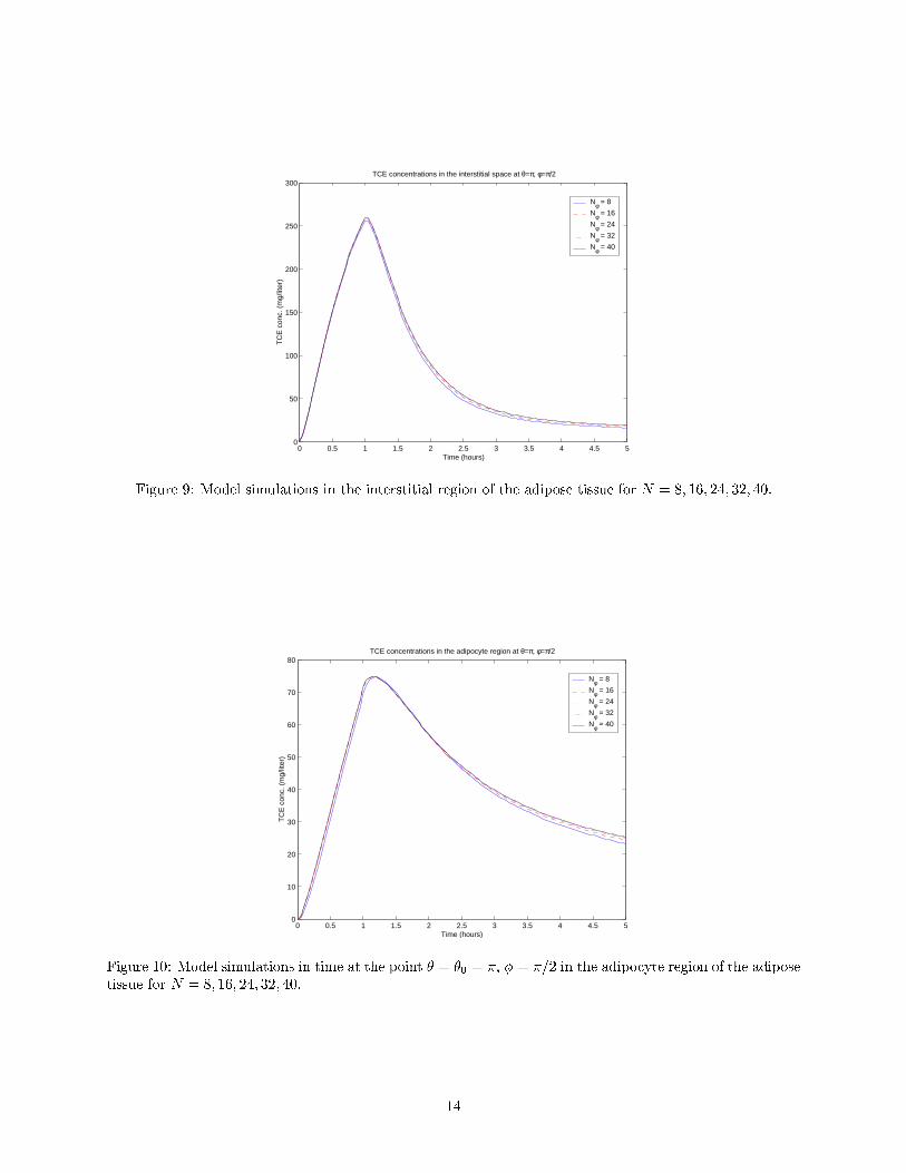
Parameters for whole-body PBPK model with a perfusion-limited fat compartment.Source: [11].

Model parameter Abbr. Estimated value

Body weight (kg) bw 0.437Tissue volumes (liters)Blood Vv 0.0393Brain Vbr 0.0026Fat Vf 0.0336Kidney Vk 0.002Liver Vl 0.017Muscle Vm 0.3277Remaining tissue Vt 0.0146

Blood ow rates (liters/hr)Cardiac output Qc 7.6322Brain Qbr 0.1755Fat Qf 0.6106Kidney Qk 0.6182

23

Liver Ql 1.1448Muscle Qm 2.4423Remaining tissue Qt 2.6407

Ventilation rate (liters/hr) Qp 7.6322

Blood/air partition coeÆcient Pb 21.9

Tissue/blood partition coeÆcientsBrain Pbr 0.7671Fat Pf 26.26Kidney Pk 1.01Liver Pl 1.041Muscle Pm 0.541Remaining tissue Pt 1.041

Michaelis-Menten constant (mg/liters) kM 0.18Metabolic constant (mg/hour) vmax 2.8997

Parameters for di�usion-limited fat compartment.

Model parameter Abbr. Estimated value

Volumes (liters)Intracellular space Vfi 0.0269Extracellular space Vfe 0.0067

Permeability coeÆcient (liters/hr) � 0.1Blood ow rate to fat (liters/hr) Qf 0.6106Blood/fat partition coeÆcient Pf 26.26

Parameters for adipose dispersion model.

Model parameter Abbr. Estimated value

VolumesCapillary VB 0.0084Interstitial space VI 0.0118Adipocyte VA 0.0135

Unbound fractionCapillary fB 1Interstitial space fI 0.6667Adipocyte fA 0.0381

Permeability coeÆcients (liters/hr)Capillary { Interstitial space �BI 0.02Capillary { Adipocyte �BA 0.03Interstitial space { Adipocyte �IA 0.025

Fraction of transport between the capillary and the other two adipose regionsCapillary { Interstitial space �I 0.6Capillary { Adipocyte �A 0.4

24

Dispersivity coeÆcient for capillary (m2/hr) DB 1

Di�usion coeÆcients (m2/hr)Interstitial space DI 0.01Adipocyte DA 0.001

Cross-sectional area of capillary (m2) AB 5� 10�5

Radius of adipocyte (m) r1 0.08Velocity of blood in capillary (m/hr) v 0.9769Reverse Fahraeus-Lindquist parameter F 0.08Location (in �) of capillary central axis �0 �

Points of interface (in �) between capillary and blood compartmentsCapillary { Arterial blood "1 �=8Capillary { Venous blood � � "2 7�=8

References

[1] R. A. Albanese, H. T. Banks, M. V. Evans, and L. K. Potter. Physiologically based pharma-cokinetic models for the transport of trichloroethylene in adipose tissue. Tech. Rep. CRSC-TR01-03, Center for Research in Scienti�c Computation, North Carolina State University, January 2001(www.ncsu.edu/crsc/reports.html); Bulletin of Mathematical Biology, submitted.

[2] H. T. Banks and L. K. Potter. Well-posedness results for a class of toxicokinetic models. Tech. Rep.CRSC-TR01-18, Center for Research in Scienti�c Computation, North Carolina State University, July2001 (www.ncsu.edu/crsc/reports.html); Discrete and Continuous Dynamical Systems, submitted.

[3] E. J. Blanchette-Mackie and R. O. Scow. Lipolysis and lamellar structures in white adipose tissue ofyoung rats: Lipid movement in membranes. Journal of Ultrastructure Research, 77:295{318, 1981.

[4] E. J. Blanchette-Mackie and R. O. Scow. Membrane continuities within cells and intercellular contactsin white adipose tissue of young rats. Journal of Ultrastructure Research, 77:277{294, 1981.

[5] E. J. Blanchette-Mackie and R. O. Scow. Continuity of intracellular channels with extracellular spacein adipose tissue and liver: Demonstrated with tannic acid and lanthanum. The Anatomical Record,203:205{219, 1982.

[6] H. Brauch, G. Weirich, M. A. Hornauer, S. St�orkel, T. W�ohl, and T. Br�uning. Trichloroethyleneexposure and speci�c somatic mutations in patients with renal cell carcinoma. Journal of the NationalCancer Institute, 91:854{861, 1999.

[7] J. V. Bruckner, B. D. Davis, and J. N. Blancato. Metabolism, toxicity, and carcinogenicity oftrichloroethylene. Critical Reviews in Toxicology, 20:31{50, 1989.

[8] R. J. Bull. Mode of action of liver tumor induction by trichloroethylene and its metabolites, trichloroac-etate and dichloroacetate. Environmental Health Perspectives, 108 Suppl. 2:241{260, 2000.

[9] D. Crandall and M. DiGirolamo. Hemodynamic and metabolic correlates in adipose tissue: Pathophys-iologic considerations. FASEB, 4:141{147, 1990.

[10] D. Crandall, G. J. Hausman, and J. G. Kral. A review of the microcirculation of adipose tissue:anatomic, metabolic, and angiogenic perspectives. Microcirculation, 4:211{232, 1997.

[11] M. V. Evans, W. K. Boyes, P. J. Bushnell, J. H. Raymer, and J. E. Simmons. A physiologically basedpharmacokinetic model for trichloroethylene (TCE) in Long-Evans rats. Personal communication, 1999.

25

[12] A. R. Goeptar, J. N. M. Commandeur, B. van Ommen, P. J. van Bladeren, and N. P. E. Vermeulen.Metabolism and kinetics of trichloroethylene in relation to toxicity and carcinogenicity. relevance of themercapturic acid pathway. Chemical Research in Toxicology, 8:3{21, 1995.

[13] T. Green. Pulmonary toxicity and carcinogenicity of trichloroethylene: Species di�erences and modesof action. Environmental Health Perspectives, 108 Suppl. 2:261{264, 2000.

[14] G. J. Hausman. The comparative anatomy of adipose tissue. In New Perspectives in Adipose Tissue:Structure, Function and Development. Butterworths, London, 1985.

[15] L. H. Lash, J. C. Parker, and C. S. Scott. Modes of action of trichloroethylene for kidney tumorigenesis.Environmental Health Perspectives, 108 Suppl. 2:225{240, 2000.

[16] M. A. Medinsky and C. D. Klaassen. Toxicokinetics. In Casarett and Doull's Toxicology: The BasicScience of Poisons. McGraw-Hill, Health Professions Division, New York, 5th edition, 1996.

[17] L. K. Potter. Physiologically based pharmacokinetic models for the systemic transport of trichloroethy-lene. PhD thesis, North Carolina State University, Raleigh, NC, August 2001.

[18] M. S. Roberts and M. Rowland. A dispersion model of hepatic elimination: 1. Formulation of the modeland bolus considerations. Journal of Pharmacokinetics and Biopharmaceutics, 14:227{260, 1986.

[19] S. Rosell and E. Belfrage. Blood circulation in adipose tissue. Physiological Reviews, 59:1078{1104,1979.

[20] A. M. Saillenfait, I. Langonne, and J. P. Sabate. Developmental toxicity of trichloroethylene, tetra-chloroethylene and four of their metabolites in rat whole embryo culture. Archives of Toxicology,70:71{82, 1995.

[21] C. S. Scott and V. J. Cogliano. Trichloroethylene health risks{state of the science. EnvironmentalHealth Perspectives, 108 Suppl. 2:159{160, 2000.

[22] R. O. Scow, E. J. Blanchette-Mackie, and L. C. Smith. Transport of lipid across capillary endothelium.Federation Proceedings, 39:2610{2617, 1980.

[23] L.F. Shampine and M.W. Reichelt. The MATLAB ODE suite. SIAM Journal on Scienti�c Computing,18:1{22, 1997.

[24] B. G. Slavin. The morphology of adipose tissue. In New Perspectives in Adipose Tissue: Structure,Function and Development. Butterworths, London, 1985.

[25] J. Wloka. Partial Di�erential Equations. Cambridge University Press, Cambridge, 1987.

26