Galerkin Methods for Incompressible Flow Simulation

Paul FischerMathematics and Computer Science DivisionArgonne National Laboratory

Example: Vascular Flow Simulations Loth, Bassiouny, F (UIC/U Akron / UC / ANL)

Seeking to understand hemodynamics & vascular disease:Combined in vivo, in vitro, numerical studies of AV graftsValidated code in a complex geometry using LDA measurementsIdentified mechanisms for low Re transition to turbulence in AV grafts

Coherent structures in AV graft at Re=1200; λ2 criterion of Jeong & Hussein (JFM95)

Outline of Lectures

Lecture 1: IntroductionNavier Stokes EquationsQuick overview of some relevant timestepping issuesGalerkin methods

Introduction1D examples (2D…?)

Lecture 2: Galerkin methods cont’d2D / 3D examples Solvers

IterativeFast diagonalization methods

Lecture 3: Putting it all together: Unsteady Navier-Stokes SolverUnsteady Stokes / spatial discretization (velocity/pressure spaces)System solversExamples: natural convection / driven cavity / Kovasznay flowExtensions to 3D

Objectives

Enable solution of NS in a simple domain

Develop understanding of costs/benefits of FEM/SEM/spectral methodsDifferences between low/high order, FEM/FD

Importance of pressure treatment

Stability of Various Timesteppers

Derived from model problem

Stability regions shown in the λΔt plane

Fornberg’s Polynomial Interpolant/Derivative Code

Code available in f77 and matlab – short, stable, fast

Lagrange Polynomials: Good and Bad Nodal Point Distributions

N=4

N=7

φ2 φ4

N=8

Uniform Gauss-Lobatto-Legendre

Spectral Element Convergence: Exponential with N

Exact Navier-Stokessolution due toKovazsnay(1948):

Lagrangian Bases: Piecewise Linear and Quadratic

Linear case results in A being tridiagonal (b.w. = 1)

Q: What is matrix bandwidth for piecewise quadratic case?

Modal Basis Example

Bad basis choice: xi, i=1,…,N

Aij = ij / (i+j-1)

Condition number of A grows exponentially with N

Long-Time Integration: Plane Rotation of Gaussian Pulse

N=33

N=43

N=53

Spectral Element Discretization

Convection-Diffusion Equation:

Weighted Residual Formulation:

Inner products – integrals replaced by Gaussian quadrature:

2D basis function, N=10

Spectral Element Basis Functions

Nodal basis:

ξj = Gauss-Lobatto-Legendre quadrature points:

- stability ( not uniformly distributed points )- allows pointwise quadrature (for most operators…)- easy to implement BCs and C0 continuity

Stable Lagrange Interpolants

GLL Nodal Basis good conditioning, minimal round-off

Monomials: xk

Uniform Points

GLL Points ~ N 3

Accuracy+

Costs

Spectral Element Convergence: Exponential with N

Exact Navier-Stokessolution due toKovazsnay(1948):

Influence of Scaling on Discretization

Large problem sizes enabled by peta- and exascale computers allow propagation of small features (size λ) over distances L >> λ.

Dispersion errors accumulate linearly with time:

~|correct speed – numerical speed| * t ( for each wavenumber )

errort_final ~ ( L / λ ) * | numerical dispersion error |

For fixed final error εf, require: numerical dispersion error ~ (λ / L)εf, << 1

High-order methods most efficiently deliver small dispersion errors(Kreiss & Oliger 72, Gottlieb et al. 2007)

Excellent transport properties, even for non-smooth solutions

Convection of non-smooth data on a 32x32 grid (K1 x K1 spectral elements of order N). (cf. Gottlieb & Orszag 77)

N=10

N=4

Costs

Cost dominated by iterative solver costs, proportional toiteration countmatrix-vector product + preconditioner cost

Locally-structured tensor-product forms:

minimal indirect addressing

fast matrix-free operator evaluation

fast local operator inversion via fast diagonalization method (FDM)( Approximate, when element deformed. )

Tensor-Product Forms: Matrix-Matrix Based Derivative Evaluation

Local tensor-product form (2D),

allows derivatives to be evaluated as matrix-matrix products:

Memory access scales only as O(n) Work scales as N*O(n), but CPU time is weakly dependent on N (WHY?)

mxm

hi (r)

For a deformed spectral element, Ω k,

Operation count is only O (N 4) not O (N 6) [Orszag ‘80 ]Memory access is 7 x number of points (Grr ,Grs, etc., are diagonal )Work is dominated by (fast) matrix-matrix products involving Dr , Ds , etc.

Local “Matrix-Free” Stiffness Matrix in 3D

9

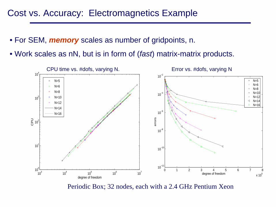
• For SEM, memory scales as number of gridpoints, n.

• Work scales as nN, but is in form of (fast) matrix-matrix products.

103

104

105

106

107

100

101

102

103

104

degree of freedom

CP

U

N=5

N=6

N=8

N=10

N=12

N=14

N=16

Periodic Box; 32 nodes, each with a 2.4 GHz Pentium Xeon

0 1 2 3 4 5 6 7 8

x 106

10−12

10−10

10−8

10−6

10−4

10−2

degree of freedom

err

ors

N=5N=6N=8N=10N=12N=14N=16

CPU time vs. #dofs, varying N. Error vs. #dofs, varying N

Cost vs. Accuracy: Electromagnetics Example

Stability

Stabilizing High-Order Methods

In the absence of eddy viscosity, some type of stabilization is generally required at high Reynolds numbers.

Some options:

high-order upwinding (e.g., DG, WENO)bubble functionsspectrally vanishing viscosityfilteringdealiasing

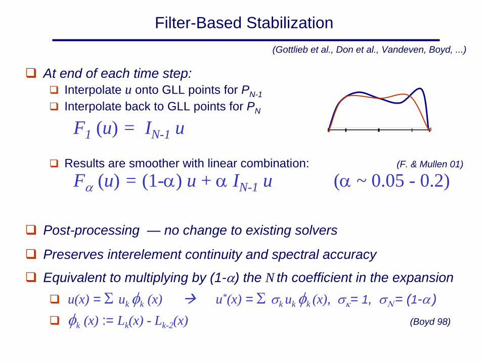
Filter-Based Stabilization

At end of each time step:Interpolate u onto GLL points for PN-1Interpolate back to GLL points for PN

F1 (u) = IN-1 u

Results are smoother with linear combination: (F. & Mullen 01)

Fα

(u) = (1-α) u + α

IN-1 u (α

~ 0.05 - 0.2)

Post-processing — no change to existing solvers

Preserves interelement continuity and spectral accuracy

Equivalent to multiplying by (1-α) the N th coefficient in the expansionu(x) = Σ uk φk (x) u*(x) = Σ σk uk φk (x), σκ= 1, σΝ = (1-α )φk (x) := Lk(x) - Lk-2(x) (Boyd 98)

(Gottlieb et al., Don et al., Vandeven, Boyd, ...)

Numerical Stability Test: Shear Layer Roll-Up (Bell et al. JCP 89, Brown & Minion, JCP 95, F. & Mullen, CRAS 2001)

2562

2562

1282 2562

25621282

Spatial and Temporal Convergence (F. & Mullen, 01)

Base velocity profile and perturbation streamlines

Error in Predicted Growth Rate for Orr-Sommerfeld Problem at Re=7500 (Malik & Zang 84)

Filtering permits Reδ99 > 700 for transitional boundary layer calculations

blow up

Re = 700

Re = 1000

Re = 3500

Why Does Filtering Work ? ( Or, Why Do the Unfiltered Equations Fail? )

Double shear layer example:

OkHigh-strain regionsare troublesome…

Why Does Filtering Work ? ( Or, Why Do the Unfiltered Equations Fail? )

Consider the model problem:

Weighted residual formulation:

Discrete problem should never blow up.

Why Does Filtering Work ? ( Or, Why Do the Unfiltered Equations Fail? )

Weighted residual formulation vs. spectral element method:

This suggests the use of over-integration (dealiasing) to ensure that skew-symmetry is retained

Aliased / Dealiased Eigenvalues:

Velocity fields model first-order terms in expansion of straining and rotating flows.For straining case,

Rotational case is skew-symmetric.

Filtering attacks the leading-order unstable mode.

N=19, M=19 N=19, M=20

c = (-x,y)

c = (-y,x)

Stabilization Summary

Filtering acts like well-tuned hyperviscosity

Attacks only the fine scale modes (that, numerically speaking, shouldn’t have energy anyway…)

Can precisely identify which modes in the SE expansion to suppress (unlike differential filters)

Does not compromise spectral convergence

Dealiasing of convection operator recommended for high Reynolds number applications to avoid spurious eigenvalues

Can run double shear-layer roll-up problem forever with

– ν = 0 ,

– no filtering

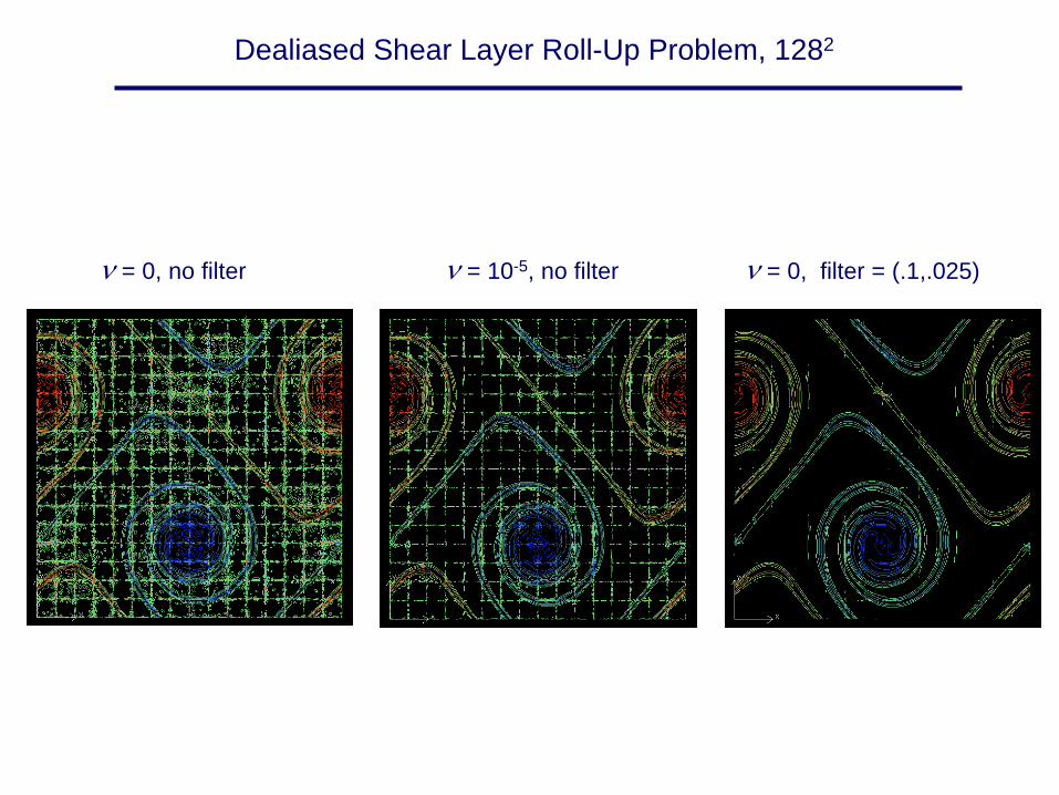
Dealiased Shear Layer Roll-Up Problem, 1282

ν = 0, no filter ν = 10-5, no filter ν = 0, filter = (.1,.025)

Linear Solvers

Linear Solvers for Incompressible Navier-Stokes

Navier-Stokes time advancement:

Nonlinear term: explicit k th-order backward difference formula / extrapolation characteristics (Pironneau ’82, MPR ‘90)

Stokes problem: pressure/viscous decoupling:3 Helmholtz solves for velocity (“easy” w/ Jacobi-precond. CG)(consistent) Poisson equation for pressure (computationally dominant)

PN - PN-2 Spectral Element Method for Navier-Stokes (MP 89)

Gauss-Lobatto Legendre points(velocity)

Gauss Legendre points(pressure)

Velocity, u in PN , continuousPressure, p in PN-2 , discontinuous

—

Navier-Stokes Solution Strategy

Semi-implicit: explicit treatment of nonlinear term.Leads to Stokes saddle problem, which is algebraically split

MPR 90, Blair-Perot 93, Couzy 95

E - consistent Poisson operator for pressure, SPDStiffest substep in Navier-Stokes time advancementMost compute-intensive phase Spectrally equivalent to SEM Laplacian, A