Embed Size (px)
Citation preview
Patterns formation in axially symmetricLandau-Lifshitz-Gilbert-Slonczewski equations
September 26, 2013
C. Melcher1 & J.D.M. Rademacher2
Abstract
The Landau-Lifshitz-Gilbert-Slonczewski equation describes magnetization dynamicsin the presence of an applied field and a spin polarized current. In the case of axialsymmetry and with focus on one space dimension, we investigate the emergence of space-time patterns in the form of coherent structures, whose profiles asymptote to wavetrains.In particular, we give a complete existence and stability analysis of wavetrains and proveexistence of various coherent structures, including soliton- and domain wall-type solutions.Decisive for the solution structure is the size of anisotropy compared with the differenceof field intensity and current intensity normalized by the damping.
1 Introduction
This paper concerns the analysis of spatio-temporal pattern formation for the axially sym-metric Landau-Lifshitz-Gilbert-Slonczeweski equation in one space dimension
∂tm = m×[
α∂tm− ∂2xm+ (µm3 − h)e3 + βm× e3
]
(1)
as a model for the magnetization dynamics m = m(x, t) ∈ S2 (i.e. m is a direction field)
driven by an external fields h = he3 and currents j = βe3. The parameters α > 0 and µ ∈ R
are the Gilbert damping factor and the anisotropy constant, respectively. A brief overviewof the physical background and interpretation of terms is given below in Section 2. Whilethe combination of field and current excitations gives rise to a variety of pattern formationphenomena, see e.g. [5, 12, 13, 16], not much mathematically rigorous work is available sofar, in particular for the dissipative case α > 0 that we consider. The case of axial symmetryis not only particularly convenient from a technical perspective. It offers at the same timevaluable insight in the emergence of space-time patterns and displays strong similarities tobetter studied dynamical systems such as real and complex Ginzburg-Landau equations. Inthis framework we examine the existence and stability of wavetrain solutions of (1), i.e.,solutions of the form
m(x, t) = eiϕ(kx−ωt)m0,
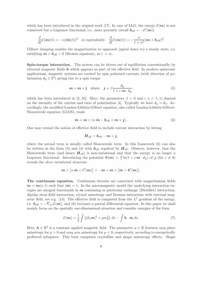
where the complex exponential acts on m0 ∈ S2 by rotation about the e3-axis (cf. Figure 1
for an illustration). We give a complete characterization of wavetrains and their L2-stability.We also investigate the existence of their spatial connections, i.e. coherent structures of theform
m(x, t) = eiϕ(x,t)m0(x− st) where ϕ(x, t) = φ(x− st) + Ωt
1Lehrstuhl I fur Mathematik and JARA-FIT, RWTH Aachen University, 52056 Aachen, Germany,[email protected]
2Fachbereich 3 – Mathematik, Universitat Bremen, Postfach 33 04 40, 28359 Bremen, Germany,[email protected]
1
ff
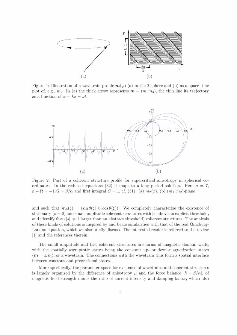
(a) (b)
Figure 1: Illustration of a wavetrain profile m(ϕ) (a) in the 2-sphere and (b) as a space-timeplot of, e.g., m2. In (a) the thick arrow represents m = (m,m3), the thin line its trajectoryas a function of ϕ = kx− ωt.
10 20 30 40 50 60x
-0.5
0.5
m2
-0.6 -0.4 -0.2 0.2 0.4 0.6 0.8m2
-0.8
-0.6
-0.4
-0.2
0.2
0.4m1
(a) (b)
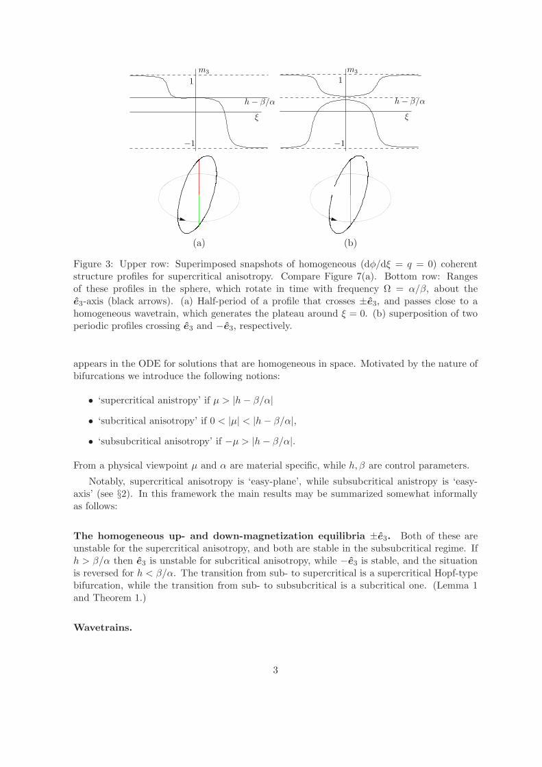
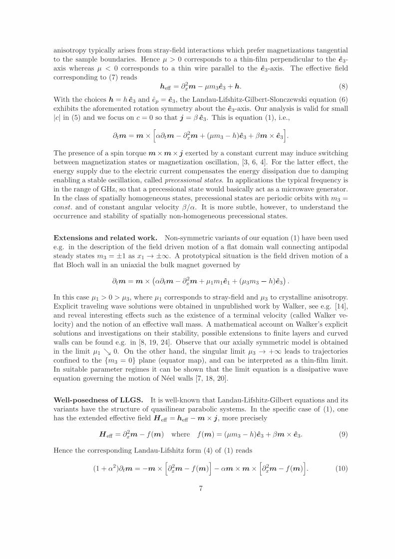
Figure 2: Part of a coherent structure profile for supercritical anisotropy in spherical co-ordinates. In the reduced equations (32) it maps to a long period solution. Here µ = 7,h− Ω = −1,Ω = β/α and first integral C = 1, cf. (31). (a) m2(x), (b) (m1,m2)-plane.
and such that m0(ξ) = (sin θ(ξ), 0, cos θ(ξ)). We completely characterize the existence ofstationary (s = 0) and small amplitude coherent structures with |s| above an explicit threshold,and identify fast (|s| ≫ 1 larger than an abstract threshold) coherent structures. The analysisof these kinds of solutions is inspired by and bears similarities with that of the real Ginzburg-Landau equation, which we also briefly discuss. The interested reader is referred to the review[1] and the references therein.
The small amplitude and fast coherent structures are forms of magnetic domain walls,with the spatially asymptotic states being the constant up- or down-magnetization states(m = ±e3), or a wavetrain. The connections with the wavetrain thus form a spatial interfacebetween constant and precessional states.
More specifically, the parameter space for existence of wavetrains and coherent structuresis largely organized by the difference of anisotropy µ and the force balance |h − β/α|, ofmagnetic field strength minus the ratio of current intensity and damping factor, which also
2
−1
ξ
h− β/α
m3
1
−1
ξ
h− β/α
m3
1
(a) (b)
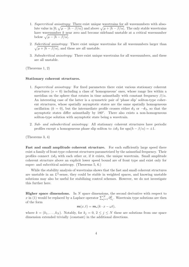
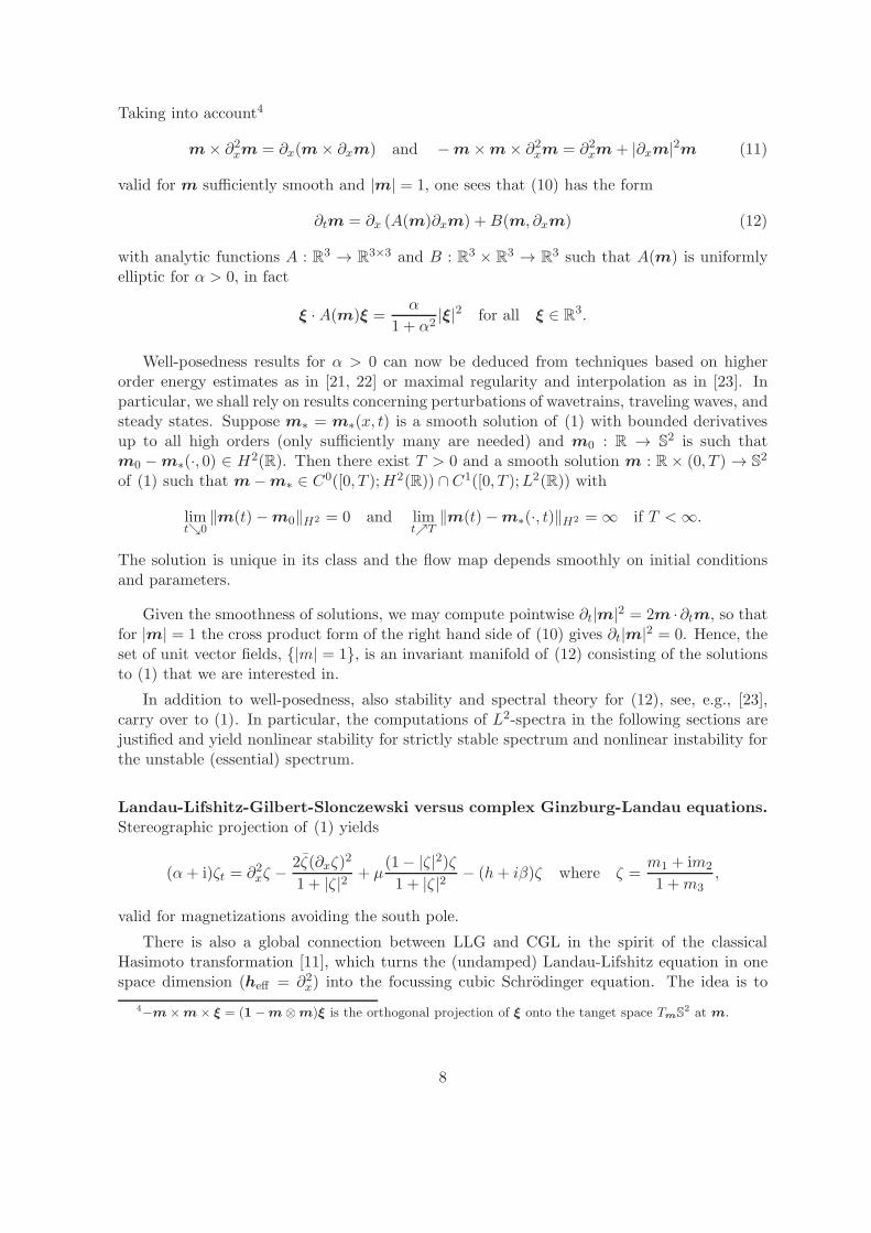
Figure 3: Upper row: Superimposed snapshots of homogeneous (dφ/dξ = q = 0) coherentstructure profiles for supercritical anisotropy. Compare Figure 7(a). Bottom row: Rangesof these profiles in the sphere, which rotate in time with frequency Ω = α/β, about thee3-axis (black arrows). (a) Half-period of a profile that crosses ±e3, and passes close to ahomogeneous wavetrain, which generates the plateau around ξ = 0. (b) superposition of twoperiodic profiles crossing e3 and −e3, respectively.
appears in the ODE for solutions that are homogeneous in space. Motivated by the nature ofbifurcations we introduce the following notions:
• ‘supercritical anistropy’ if µ > |h− β/α|
• ‘subcritical anisotropy’ if 0 < |µ| < |h− β/α|,
• ‘subsubcritical anisotropy’ if −µ > |h− β/α|.
From a physical viewpoint µ and α are material specific, while h, β are control parameters.
Notably, supercritical anisotropy is ‘easy-plane’, while subsubcritical anistropy is ‘easy-axis’ (see §2). In this framework the main results may be summarized somewhat informallyas follows:
The homogeneous up- and down-magnetization equilibria ±e3. Both of these areunstable for the supercritical anisotropy, and both are stable in the subsubcritical regime. Ifh > β/α then e3 is unstable for subcritical anisotropy, while −e3 is stable, and the situationis reversed for h < β/α. The transition from sub- to supercritical is a supercritical Hopf-typebifurcation, while the transition from sub- to subsubcritical is a subcritical one. (Lemma 1and Theorem 1.)
Wavetrains.
3
1. Supercritical anisotropy: There exist unique wavetrains for all wavenumbers with abso-lute value in [0,
√
µ− |h− β/α|) and above√
µ+ |h− β/α|. The only stable wavetrainshave wavenumber k near zero and become sideband unstable at a critical wavenumberbelow
√
µ− |h− β/α|.
2. Subcritical anisotropy: There exist unique wavetrains for all wavenumbers larger than√
µ+ |h− β/α|, and these are all unstable.
3. Subsubcritical anisotropy: There exist unique wavetrains for all wavenumbers, and theseare all unstable.
(Theorems 1, 2)
Stationary coherent structures.
1. Supercritical anisotropy: For fixed parameters there exist various stationary coherentstructures (s = 0) including a class of ‘homogeneous’ ones, whose range lies within ameridian on the sphere that rotates in time azimuthally with constant frequency β/α.An interesting case of the latter is a symmetric pair of ‘phase slip’ soliton-type coher-ent structures, whose spatially asymptotic states are the same spatially homogeneousoscillation (k = 0), but the intermediate profile crosses either e3 or −e3, so that theasymptotic states differ azimuthally by 180. There also exists a non-homogeneoussoliton-type solution with asymptotic state being a wavetrain.
2. Sub- and subsubcritical anisotropy: All stationary coherent structures have periodicprofiles except a homogeneous phase slip soliton to ±e3 for sgn(h− β/α) = ±1.
(Theorems 3, 4)
Fast and small amplitude coherent structure. For each sufficiently large speed thereexist a family of front-type coherent structures parametrized by the azimuthal frequency. Theirprofiles connect ±e3 with each other or, if it exists, the unique wavetrain. Small amplitudecoherent structure above an explicit lower speed bound are of front type and exist only forsuper- and subcritical anistropy. (Theorems 5, 6.)
While the stability analysis of wavetrains shows that the fast and small coherent structuresare unstable in an L2-sense, they could be stable in weighted spaces, and knowing unstablesolutions may also be useful for stabilizing control schemes. However, we do not investigatethis further here.
Higher space dimensions. In N space dimensions, the second derivative with respect tox in (1) would be replaced by a Laplace operator
∑Nj=1 ∂
2xj. Wavetrain type solutions are then
of the formm(x, t) = m∗(k · x− ωt),
where k = (k1, . . . , kN ). Notably, for kj = 0, 2 ≤ j ≤ N these are solutions from one spacedimension extended trivially (constant) in the additional directions.
4
Conveniently, the rotation symmetry (gauge invariance in the Ginzburg-Landau context),means that the analyses of ±e3 and these wavetrains is already covered by that of the one-dimensional case: the linearization is space-independent and therefore there is no symmetrybreaking due to different kj. Indeed, all relevant quantities are rotation symmetric, depending
only on k2 =∑N
j=1 k2j or ℓ2 =
∑Nj=1 ℓ
2j , where ℓ = (ℓ1, . . . , ℓN ) is the Fourier wavenumber
vector of the linearization. In particular, the only nontrivial stability boundary are sidebandinstabilities, which occur simultaneously for all directions.
Concerning coherent structures, (27) turns into an elliptic PDE in general so that theanalysis in this paper only allows for the trivial extension into higher dimensions.
This article is organized as follows. In Section 2, the terms in the model equation (1) andits well-posedness are discussed. Section 3 concerns the stability of the trivial steady states±e3 and in §4 existence and stability of wavetrains are analyzed. Section 5 is devoted tocoherent structures.
Acknowledgement. JR has been supported in part by the NDNS+ cluster of the DutchScience Fund (NWO).
2 Landau-Lifshitz equations
The classical equation of magnetization dynamics, the conservative Landau-Lifshitz equation[17], corresponds to a torque balance for the magnetic moment, represented by a unit vectorfield m = m(t) ∈ S
2,m+ γm× heff = 0.
It features a free precession of m about the effective field heff = −E ′(m), i.e., minus thevariation of the underlying interaction energy E = E(m), which is conserved in time. Thegyromagnetic ratio γ > 0 is a parameter which appears as the typical precession frequency.By rescaling time, one can always assume γ = 1. Adding a dissipative counter-field, which isproportional to the velocity m, yields the Landau-Lifshitz-Gilbert equation (LLG) [10, 14]
m = m× (α m− heff) . (2)
The Gilbert damping factor α > 0 is a constant that can be interpreted dynamically as theinverse of the typical relaxation time. It is useful to take into account that there are severalequivalent forms of LLG. Carrying out another cross multiplication of (2) by m from the leftand taking into account that −m×m× ξ = ξ − (m · ξ)m is the orthonormal projection tothe tangent plane of S2 at m, one obtains
α m+m× m = −m×m× heff , (3)
where the right hand side can also be written as heff − (m ·heff)m. Multiplying this equationby α and adding it to the original one, one obtains the dissipative Landau-Lifshitz equation3,i.e.
(1 + α2)m = −m× (αm× heff + heff) , (4)
3original form m = −m× heff − λm×m× heff with Landau-Lifshitz damping λ > 0
5
which has been introduced in the original work [17]. In case of LLG, the energy E(m) is notconserved but a Liapunov functional, i.e., more precisely (recall heff = −E ′(m))
d
dtE(m(t)) = −α‖m(t)‖2 or equivalently
d
dtE(m(t)) = −
α
1 + α2‖m× heff‖
2.
Gilbert damping enables the magnetization to approach (spiral down to) a steady state, i.e.satisfying m× heff = 0 (Browns equation), as t → ∞.
Spin-torque interaction. The system can be driven out of equilibrium conventionally byexternal magnetic fields h which appears as part of the effective field. In modern spintronicapplications, magnetic systems are excited by spin polarized currents (with direction of po-larization ep ∈ S
2) giving rise to a spin torque
m×m× j where j = βep
1 + c m · ep, (5)
which has been introduced in [2, 25]. Here, the parameters β > 0 and c ∈ (−1, 1) dependon the intensity of the current and ratio of polarization [4]. Typically we have ep = e3. Ac-cordingly, the modified Landau-Lifshitz-Gilbert equation, also called Landau-Lifshitz-Gilbert-Slonczewski equation (LLGS), reads
m = m× (α m− heff +m× j) . (6)
One may extend the notion of effective field to include current interaction by letting
Heff = heff −m× j,
where the second term is usually called Slonczewski term. In this framework (6) can alsobe written in the form (3) and (4) with heff repalced by Heff . Observe, however, that theSlonczewski term (and hence Heff) is non-variational and that the energy is no longer aLiapunov functional. Introducing the potential Ψ(m) = β
c ln(1 + cm · ep) of j (for c 6= 0)reveals the skew variational structure
m×[
α m+ E ′(m)]
= −m×m×[
m+Ψ′(m)]
.
The continuum equation. Continuum theories are concerned with magnetization fieldsm = m(x, t) such that |m| = 1. In the micromagnetic model the underlying interaction en-ergies are integral functionals in m containing in particular exchange (Dirichlet) interaction,dipolar stray-field interaction, crystal anisotropy and Zeeman interaction with external mag-netic field, see e.g. [14]. The effective field is computed from the L2 gradient of the energy,i.e. heff = −∇L2E(m), and (6) becomes a partial differential equation. In this paper we shallmainly focus on the spatially one-dimensional situation and consider energies of the form
E(m) =1
2
∫
(
|∂xm|2 + µm23
)
dx−
∫
h ·m dx. (7)
Here, h ∈ R3 is a constant applied magnetic field. The parameter µ ∈ R features easy plane
anisotropy for µ > 0 and easy axis anisotropy for µ < 0, respectively, according to energeticallypreferred subspaces. This term comprises crystalline and shape anisotropy effects. Shape
6
anisotropy typically arises from stray-field interactions which prefer magnetizations tangentialto the sample boundaries. Hence µ > 0 corresponds to a thin-film perpendicular to the e3-axis whereas µ < 0 corresponds to a thin wire parallel to the e3-axis. The effective fieldcorresponding to (7) reads
heff = ∂2xm− µm3e3 + h. (8)
With the choices h = h e3 and ep = e3, the Landau-Lifshitz-Gilbert-Slonczewski equation (6)exhibits the aforemented rotation symmetry about the e3-axis. Our analysis is valid for small|c| in (5) and we focus on c = 0 so that j = β e3. This is equation (1), i.e.,
∂tm = m×[
α∂tm− ∂2xm+ (µm3 − h)e3 + βm× e3
]
.
The presence of a spin torque m×m× j exerted by a constant current may induce switchingbetween magnetization states or magnetization oscillation, [3, 6, 4]. For the latter effect, theenergy supply due to the electric current compensates the energy dissipation due to dampingenabling a stable oscillation, called precessional states. In applications the typical frequency isin the range of GHz, so that a precessional state would basically act as a microwave generator.In the class of spatially homogeneous states, precessional states are periodic orbits with m3 =const. and of constant angular velocity β/α. It is more subtle, however, to understand theoccurrence and stability of spatially non-homogeneous precessional states.
Extensions and related work. Non-symmetric variants of our equation (1) have been usede.g. in the description of the field driven motion of a flat domain wall connecting antipodalsteady states m3 = ±1 as x1 → ±∞. A prototypical situation is the field driven motion of aflat Bloch wall in an uniaxial the bulk magnet governed by
∂tm = m×(
α∂tm− ∂2xm+ µ1m1e1 + (µ3m3 − h)e3
)
.
In this case µ1 > 0 > µ3, where µ1 corresponds to stray-field and µ3 to crystalline anisotropy.Explicit traveling wave solutions were obtained in unpublished work by Walker, see e.g. [14],and reveal interesting effects such as the existence of a terminal velocity (called Walker ve-locity) and the notion of an effective wall mass. A mathematical account on Walker’s explicitsolutions and investigations on their stability, possible extensions to finite layers and curvedwalls can be found e.g. in [8, 19, 24]. Observe that our axially symmetric model is obtainedin the limit µ1 ց 0. On the other hand, the singular limit µ3 → +∞ leads to trajectoriesconfined to the m3 = 0 plane (equator map), and can be interpreted as a thin-film limit.In suitable parameter regimes it can be shown that the limit equation is a dissipative waveequation governing the motion of Neel walls [7, 18, 20].
Well-posedness of LLGS. It is well-known that Landau-Lifshitz-Gilbert equations and itsvariants have the structure of quasilinear parabolic systems. In the specific case of (1), onehas the extended effective field Heff = heff −m× j, more precisely
Heff = ∂2xm− f(m) where f(m) = (µm3 − h)e3 + βm× e3. (9)
Hence the corresponding Landau-Lifshitz form (4) of (1) reads
(1 + α2)∂tm = −m×[
∂2xm− f(m)
]
− αm×m×[
∂2xm− f(m)
]
. (10)
7
Taking into account4
m× ∂2xm = ∂x(m× ∂xm) and −m×m× ∂2
xm = ∂2xm+ |∂xm|2m (11)
valid for m sufficiently smooth and |m| = 1, one sees that (10) has the form
∂tm = ∂x (A(m)∂xm) +B(m, ∂xm) (12)
with analytic functions A : R3 → R3×3 and B : R3 × R
3 → R3 such that A(m) is uniformly
elliptic for α > 0, in fact
ξ ·A(m)ξ =α
1 + α2|ξ|2 for all ξ ∈ R
3.
Well-posedness results for α > 0 can now be deduced from techniques based on higherorder energy estimates as in [21, 22] or maximal regularity and interpolation as in [23]. Inparticular, we shall rely on results concerning perturbations of wavetrains, traveling waves, andsteady states. Suppose m∗ = m∗(x, t) is a smooth solution of (1) with bounded derivativesup to all high orders (only sufficiently many are needed) and m0 : R → S
2 is such thatm0 −m∗(·, 0) ∈ H2(R). Then there exist T > 0 and a smooth solution m : R× (0, T ) → S
2
of (1) such that m−m∗ ∈ C0([0, T );H2(R)) ∩C1([0, T );L2(R)) with
limtց0
‖m(t)−m0‖H2 = 0 and limtրT
‖m(t)−m∗(·, t)‖H2 = ∞ if T < ∞.
The solution is unique in its class and the flow map depends smoothly on initial conditionsand parameters.
Given the smoothness of solutions, we may compute pointwise ∂t|m|2 = 2m ·∂tm, so thatfor |m| = 1 the cross product form of the right hand side of (10) gives ∂t|m|2 = 0. Hence, theset of unit vector fields, |m| = 1, is an invariant manifold of (12) consisting of the solutionsto (1) that we are interested in.
In addition to well-posedness, also stability and spectral theory for (12), see, e.g., [23],carry over to (1). In particular, the computations of L2-spectra in the following sections arejustified and yield nonlinear stability for strictly stable spectrum and nonlinear instability forthe unstable (essential) spectrum.
Landau-Lifshitz-Gilbert-Slonczewski versus complex Ginzburg-Landau equations.Stereographic projection of (1) yields
(α+ i)ζt = ∂2xζ −
2ζ(∂xζ)2
1 + |ζ|2+ µ
(1− |ζ|2)ζ
1 + |ζ|2− (h+ iβ)ζ where ζ =
m1 + im2
1 +m3,
valid for magnetizations avoiding the south pole.
There is also a global connection between LLG and CGL in the spirit of the classicalHasimoto transformation [11], which turns the (undamped) Landau-Lifshitz equation in onespace dimension (heff = ∂2
x) into the focussing cubic Schrodinger equation. The idea is to
4−m×m× ξ = (1−m⊗m)ξ is the orthogonal projection of ξ onto the tanget space TmS
2 at m.
8
disregard the customary coordinates representation and to introduce instead a pull-back frameon the tangent bundle along m. In the case of µ = β = h = 0, i.e. heff = ∂xm, this leads to
(α+ i)Dtu = D2xu (13)
where u = u(x, t) is the complex coordinate of ∂xm in the moving frame representation,and Dx and Dt are covariant derivatives in space and time giving rise to cubic and quinticnonlinearities, see [21, 22] for details.
3 Hopf instabilities of the steady states m = ±e3
As a starting point and to motivate the subsequent analysis of more complex patterns, let usconsider the stability of the constant magnetizations ±e3. Substituting m = ±e3+ δn+ o(δ),where n = (n, 0) ∈ TmS
2, into (1) gives, at order δ, the linear equation
∂tn = (±µ− h)n × e3 ± e3 × (α∂tn− ∂2xn+ βn× e3),
which may be written in complex form as
∂tn± βn = i(
α∂tn− ∂2xn− (h∓ µ)n
)
.
Its eigenvalue problem diagonalizes in Fourier space (for x) and yields the matrix eigenvalueproblem
∣
∣
∣
∣
±β − λ Λ−Λ ±β − λ
∣
∣
∣
∣
= 0,
where Λ = ±µ− h∓ αλ∓ ℓ2 with ℓ the Fourier wave number. The determinant reads
(±β − λ)2 = −Λ2 ⇔ ±β − λ = σiΛ, σ ∈ ±1.
Considering real and imaginary parts this leads to
(1 + α2)ℜ(λ) = ±β − α(ℓ2 ± h− µ) = α(µ ∓ (h− β/α)− ℓ2)
ℑ(λ) = σ(∓ℜ(λ) + β/α),
so that the maximal real part has ℓ = 0. At criticality, where ℜ(λ) = 0 the imaginary parts are±β/α, which corresponds to a Hopf-instability of the spectrum, and we expect the emergenceof oscillating solutions whose frequency at onset is β/α.
The formulas for real- and imaginary parts immediately give the results mentioned in §1and
Lemma 1 The constant magnetizations m = ±e3 are (strictly) L2-stable if and only if theanisotropy is subsubcritical (−µ > |h− β/α|), and both are unstable if and only if it is super-critical (µ > |h− β/α|). The instabilities are of Hopf-type with frequency β/α.
Remark 1 The result extends to the more general situation of (5) with |c| < 1. In fact,linearization leads to the analogous equation
∂tn = (±µ− h)n× e3 ± e3 × (α∂tn− ∂2xn+ β±n× e3)
with β± = β/(1± c) at m3 = ±1, respectively.
9
4 Wavetrains
To exploit the roation symmetry about the e3-axis, we change to polar coordinates in theplanar components m = (m1,m2) of the magnetization m = (m,m3). With m = r exp(iϕ)equation (1) changes to
(
α −11 α
)(
r2∂tϕ∂tm3
)
=
(
∂x(r2∂xϕ)
∂2xm3 + |∂xm|2m3
)
+ r2(
βh− µm3
)
, (14)
where|∂xm|2 = (∂xr)
2 + r2(∂xϕ)2 + (∂xm3)
2 and r2 +m23 = 1.
This can be seen as follows. In view of (3), with heff replaced by the extended effective fieldHeff = heff −m× j as is (9) and taking into account (11), (1) reads
α∂tm+m× ∂tm = ∂2xm+ (h− µm3)e3 +
(
|∂xm|2 + µm23 − hm3
)
m− βm× e3.
The third component of the above equation is the second component of (14), whereas the firstcomponent of (14) is obtained upon inner multiplication by m⊥ = (m⊥, 0) = (ieiϕ, 0) andtaking into account that m× e3 = −m⊥.
The rotation symmetry has turned into the shift symmetry ϕ 7→ ϕ + const. In full spherical
coordinates m =(eiϕ sin θ
cos θ
)
, (14) further simplifies to
(
α −11 α
)(
sin θ∂tϕ−∂tθ
)
=
(
2 cos θ∂xθ ∂xϕ+ sin θ∂2xϕ
−∂2xθ + sin θ cos θ(∂xϕ)
2
)
+ sin θ
(
βh− µ cos θ
)
. (15)
4.1 Existence of wavetrains
Wavetrains are solutions of the form m(x, t) = m∗(kx − ωt), where k is referred to as thewavenumber and ω as the frequency. A natural type of wavetrains are relative equilibria withrespect to the phase shift symmetry for which ϕ = kx−ωt andm3, r are constant. See Figure 1for an illustration.
Substituting this ansatz into (15) yields the algebraic equations
(
α −11 α
)(
− sin(θ)ω0
)
=
(
0sin(θ) cos(θ)k2
)
+ sin(θ)
(
βh− µ cos(θ)
)
.
Thus either θ ≡ 0 mod π or
−αω = β
−ω = (k2 − µ)m3 + h.
In the first case we have r = 0, which corresponds to the constant upward or downwardmagnetizations, (r,m3) = (0,±1) with unspecified k and ω.
In the second case, first notice that absence of dissipation (α = 0) implies absence of mag-netic field (β = 0) and there is a two-parameter set of wavetrains given by the second equation.
10
-4 -2 0 2 40
1
2
3
4
5
6
k
Θ
-4 -2 0 2 40
1
2
3
4
5
6
k
Θ
-4 -2 0 2 40
1
2
3
4
5
6
k
Θ
(a) (b) (c)
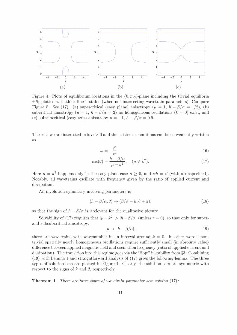
Figure 4: Plots of equilibrium locations in the (k,m3)-plane including the trivial equilibria±e3 plotted with thick line if stable (when not intersecting wavetrain parameters). CompareFigure 5. See (17). (a) supercritical (easy plane) anisotropy (µ = 1, h − β/α = 1/2), (b)subcritical anisotropy (µ = 1, h − β/α = 2) no homogeneous oscillations (k = 0) exist, and(c) subsubcritical (easy axis) anisotropy µ = −1, h− β/α = 0.9.
The case we are interested in is α > 0 and the existence conditions can be conveniently writtenas
ω = −β
α(16)
cos(θ) =h− β/α
µ− k2, (µ 6= k2). (17)
Here µ = k2 happens only in the easy plane case µ ≥ 0, and αh = β (with θ unspecified).Notably, all wavetrains oscillate with frequency given by the ratio of applied current anddissipation.
An involution symmetry involving parameters is
(h− β/α, θ) → (β/α− h, θ + π), (18)
so that the sign of h− β/α is irrelevant for the qualitative picture.
Solvability of (17) requires that |µ− k2| > |h−β/α| (unless r = 0), so that only for super-and subsubcritical anisotropy,
|µ| > |h− β/α|, (19)
there are wavetrains with wavenumber in an interval around k = 0. In other words, non-trivial spatially nearly homogeneous oscillations require sufficiently small (in absolute value)difference between applied magnetic field and oscillation frequency (ratio of applied current anddissipation). The transition into this regime goes via the ‘Hopf’ instability from §3. Combining(19) with Lemma 1 and straightforward analysis of (17) gives the following lemma. The threetypes of solution sets are plotted in Figure 4. Clearly, the solution sets are symmetric withrespect to the signs of k and θ, respectively.
Theorem 1 There are three types of wavetrain parameter sets solving (17):
11
supercritical
subcritical
subsubcritical−|h− β/α|
|h− β/α|
σe3 stable
±e3 unstable
±e3 stable
µ
k
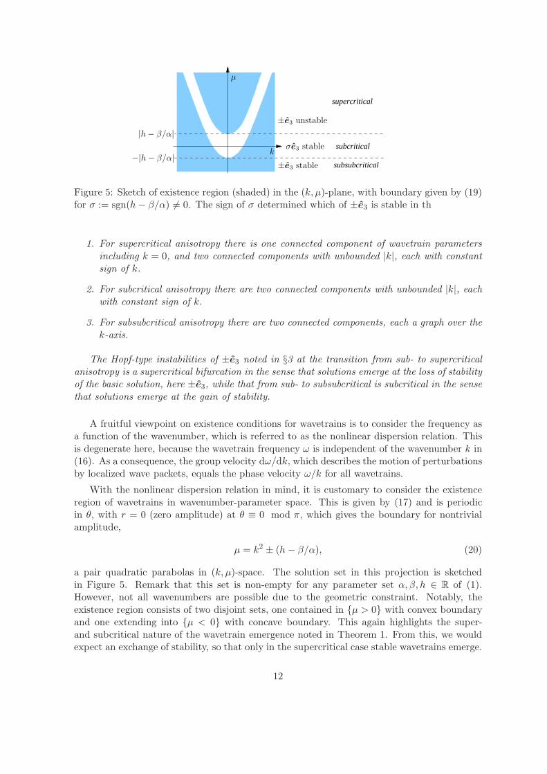
Figure 5: Sketch of existence region (shaded) in the (k, µ)-plane, with boundary given by (19)for σ := sgn(h− β/α) 6= 0. The sign of σ determined which of ±e3 is stable in th
1. For supercritical anisotropy there is one connected component of wavetrain parametersincluding k = 0, and two connected components with unbounded |k|, each with constantsign of k.
2. For subcritical anisotropy there are two connected components with unbounded |k|, eachwith constant sign of k.
3. For subsubcritical anisotropy there are two connected components, each a graph over thek-axis.
The Hopf-type instabilities of ±e3 noted in §3 at the transition from sub- to supercriticalanisotropy is a supercritical bifurcation in the sense that solutions emerge at the loss of stabilityof the basic solution, here ±e3, while that from sub- to subsubcritical is subcritical in the sensethat solutions emerge at the gain of stability.
A fruitful viewpoint on existence conditions for wavetrains is to consider the frequency asa function of the wavenumber, which is referred to as the nonlinear dispersion relation. Thisis degenerate here, because the wavetrain frequency ω is independent of the wavenumber k in(16). As a consequence, the group velocity dω/dk, which describes the motion of perturbationsby localized wave packets, equals the phase velocity ω/k for all wavetrains.
With the nonlinear dispersion relation in mind, it is customary to consider the existenceregion of wavetrains in wavenumber-parameter space. This is given by (17) and is periodicin θ, with r = 0 (zero amplitude) at θ ≡ 0 mod π, which gives the boundary for nontrivialamplitude,
µ = k2 ± (h− β/α), (20)
a pair quadratic parabolas in (k, µ)-space. The solution set in this projection is sketchedin Figure 5. Remark that this set is non-empty for any parameter set α, β, h ∈ R of (1).However, not all wavenumbers are possible due to the geometric constraint. Notably, theexistence region consists of two disjoint sets, one contained in µ > 0 with convex boundaryand one extending into µ < 0 with concave boundary. This again highlights the super-and subcritical nature of the wavetrain emergence noted in Theorem 1. From this, we wouldexpect an exchange of stability, so that only in the supercritical case stable wavetrains emerge.
12
Before proving this, let us briefly discuss the origins of this expectation. The fact thatfrequencies are constant means that in co-rotating (‘detuned’) coordinates θ = ϕ − β
α t thewavetrains have frequency zero and are thus stationary. The situation is then reminiscent ofthe (cubic) real Ginzburg-Landau equation mentioned in the introduction,
∂tA = ∂2xA+ µA∓A|A|2, A(x, t) ∈ C, (21)
which describes the dynamics near pattern forming Turing instabilities and possesses thegauge-symmetry A → eiϕA. The solution A = 0 becomes unstable as µ becomes positive,which is the analogue of ±e3 losing stability as µ crosses ±(h− β/α).
Concerning wavetrains, the analogue of the symmetry group ansatz above is A = rekx−ωt,r ∈ R the amplitude, which yields
ω = 0, µ = k2 ± r2.
In particular, all these wavetrains are stationary and the existence region, bounded by r =0, is a parabola in (k, µ)-space, convex in the ‘+’-case and concave otherwise. A stabilityanalysis of these wavetrains (which we omit) shows that only in the convex (supercritical)case stable wavetrains emerge, and these lie in the socalled Eckhaus region µ ≥ 3k2. Hence,the aforementioned expectation, which is fully justified in the next section. The overall picturefor (1) is thus a combination of the scenarios from a supercritical (µ > 0) and a subcritical(µ < 0) real Ginzburg-Landau equation, connected in parameter space via µ.
We have only considered the special case of (5) with c = 0, for otherwise (16) and (17) giverise to a quadratic equation for m3. For a parameter set away from special points, however,there exists for 0 < |c| ≪ 1 a unique solution m3 which is compatible with the geometricconstraint. In this generic situation the considerations on spectral stability to be carried outin Section 4.2 hold true by continuous differentiability.
4.2 Stability of wavetrains
In this section spectral stability of wavetrains is determined. For convenience, the comovingframe y = x− cpht is considered with cph = ω/k the wavespeed. In this variable the wavetrainis an equilibrium of (14). Again for convenience, time is rescaled to t = (1+α2)τ . The explicitformulation of (14) then reads
∂τ
(
ϕm3
)
=
(
α(∂y(r2∂yϕ)/r
2 + β) + (∂2ym3 + |∂ym|2m3)/r
2 + h− µm3 + cph∂yϕ
α(∂2ym3 + |∂ym|2m3 + r2(h− µm3))− ∂y(r
2∂yϕ)− r2β + cph∂ym3
)
,
(22)where r2 = 1−m2
3.
Let F = (F1,F2)t denote the right hand side of (22). Wavetrains have constant r and m3
so that quadratic terms in their derivatives can be discarded for the linearization L of F in a
13
wavetrain, and from |∂ym|2 only r2(∂yϕ)2 is relevant. The components of L are
∂ϕF1 = α∂2y + cph∂y + 2km3∂y
∂m3F1 = r−2∂2
y + k2 − µ− 2αkm3r−2∂y
∂ϕF2 = 2αkm3r2∂y − r2∂2
y
∂m3F2 = α∂2
y + αr2(k2 − µ) + cph∂y − 2αm3(m3k2 + h− µm3) + 2m3(k∂y + β)
= α∂2y + αr2(k2 − µ) + cph∂y + 2m3k∂y,
where the last equation is due to (17). Since all coefficients are constant, the eigenvalueproblem
Lu = λu
is solved by the characteristic equation arising from an exponential ansatz u = exp(νy)u0,which yields the matrix
A(ν, cph) :=
(
αν2 + (cph + 2km3)ν −r−2ν(−ν + 2αkm3) + k2 − µr2ν(−ν + 2αkm3) αν2 + (cph + 2km3)ν + αr2(k2 − µ)
)
.
The characteristic equation then reads
dcph(λ, ν) := |A(ν, cph)− λ| = |A(ν, 0) − (λ− iνcph)| = d0(λ− cphν, ν)
d0(λ, ν) = λ2 − trA(ν, 0)λ+ detA(ν, 0) (23)
with trace and determinant of A(ν, 0)
trA(ν, 0) = 2ν(αν + 2km3) + αr2(k2 − µ)
detA(ν, 0) = (1 + α2)ν2(ν2 + 4k2m23 + r2(k2 − µ))
= (1 + α2)ν2(
ν2 + (3k2 + µ)(β/α − h)2
(k2 − µ)2+ k2 − µ
)
.
In the last equation (17) was used.
The characteristic equation is also referred to as the complex dispersion relation. Thespectrum of L, for instance in L2(R), consists of solutions for ν = iℓ and is purely essentialspectrum (in the sense that λ−L is not a Fredholm operator with index zero). Indeed, settingν = iℓ corresponds to Fourier transforming in y with Fouriermode ℓ. Note that the solutiond(0, 0) = 0 stems from spatial translation symmetry in y.
The real part of solutions λ of (23) does not depend on cph, which means that spectralstability is independent of cph and is therefore completely determined by d0(λ, iℓ) = 0.
First note the eigenvalues A(0, 0) are 0 and αr2(k2−µ) so that in the easy axis case µ < 0all wavetrains are unstable. In the easy plane case µ > 0 the wavetrains for k2 ≤ µ have achance to be spectrally stable. In the following we therefore restrict to µ > 0 and k2 < µ andcheck the possible marginal stability configurations case by case.
14
Sideband instability. A sideband instability occurs when the curvature of the curve ofessential spectrum attached to the origin changes sign so that the essential spectrum extendsinto positive real parts. Let λ0(ℓ) denote the curve of spectrum of A(iℓ, 0) attached to theorigin, that is λ0(0) = 0, and let ′ denote the differentiation with respect to ℓ. Derivatives ofλ0 can be computed by implicit differentiation of
det(A(iℓ, 0) − λ) = detA(iℓ, 0) + λ2 − tr(A(iℓ, 0))λ = 0.
Since ∂ν detA(0, 0) = 0 we have λ′0(0) = 0 and therefore
λ′′0(0) = −
∂2ν detA(0, 0)
trA(0, 0)=
1 + α2
αr2(µ − k2)C,
where D = (3k2 + µ) (β/α−h)2
(k2−µ)2 + k2 − µ.
At k = 0 (which means µ > β/α − h) we have D = (β/α − h)2/µ − µ = (m23 − 1)µ < 0
so that λ′′0(0) < 0, which implies stable sideband. Since k2 6= µ, sideband instabilities are sign
changes of
f(K) := (K − µ)2D = (3K + µ)(β/α − h)2 + (K − µ)3
= K3 − 3µK2 + 3(µ2 + (β/α− h)2)K + µ(−µ2 + (β/α − h)2),
where K = k2.
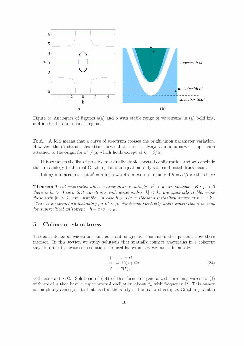
For µ > 0, f is monotone increasing for positive K: f ′(0) > 0 and f ′ 6= 0 for real K bydirect calculation. Since f(0) < 0 and f(µ) > 0 (recall µ > β/α − h for existence) there isprecisely one real root to f(k2) = 0 in k2 < µ. Therefore, for all µ > 0 precisely one sidebandinstability occurs in k2 < µ for increasing k2 from zero. In Figure 6 we plot the resultingstability region.
For later purposes note that the non-zero solutions ν to
d0(0, ν) = detA(ν, 0) = (1 + α2)ν2(ν2 +D) = 0
change at the sideband instability D = 0 from positive and negative real to a complex conju-gate pair.
Hopf instability. A Hopf instability occurs when the essential spectrum touches the imag-inary axis at nonzero values, that is, there is γ 6= 0 so that d0(iγ, iℓ) = 0. The imaginary partreads (−2αℓ2 + αr2(k2 − µ))γ = 0 and γ 6= implies 2ℓ2 = r2(k2 − µ). Hence, there is no Hopfinstability in the range k2 < µ. Recall that wavetrains with k2 > µ are already unstable.
Turing instability. A Turing instability occurs when the spectrum touches the origin fornonzero ℓ, that is, there is ℓ 6= 0 so that d0(0, iℓ) = 0, which means detA(iℓ, 0) = 0. Touchingthe origin means in addition ∂ℓ detA(iℓ) = 0. However, detA(iℓ, 0) = (1 + α2)ℓ2(ℓ2 −D) forD 6= 0 away from sideband instabilities. Since ℓ2 = D > 0 implies unstable sideband there areno relevant solutions.
15
-4 -2 0 2 40
1
2
3
4
5
6
k
Θ supercritical
subcritical
subsubcritical
µ
k
(a) (b)
Figure 6: Analogues of Figures 4(a) and 5 with stable range of wavetrains in (a) bold line,and in (b) the dark shaded region.
Fold. A fold means that a curve of spectrum crosses the origin upon parameter variation.However, the sideband calculation shows that there is always a unique curve of spectrumattached to the origin for k2 6= µ, which holds except at h = β/α.
This exhausts the list of possible marginally stable spectral configuration and we concludethat, in analogy to the real Ginzburg-Landau equation, only sideband instabilities occur.
Taking into account that k2 = µ for a wavetrain can occurs only if h = α/β we thus have
Theorem 2 All wavetrains whose wavenumber k satisfies k2 > µ are unstable. For µ > 0there is k∗ > 0 such that wavetrains with wavenumber |k| < k∗ are spectrally stable, whilethose with |k| > k∗ are unstable. In case h 6= α/β a sideband instability occurs at k = ±k∗.There is no secondary instability for k2 < µ. Nontrivial spectrally stable wavetrains exist onlyfor supercritical anisotropy, |h− β/α| < µ.
5 Coherent structures
The coexistence of wavetrains and constant magnetizations raises the question how theseinteract. In this section we study solutions that spatially connect wavetrains in a coherentway. In order to locate such solutions induced by symmetry we make the ansatz
ξ = x− stϕ = φ(ξ) + Ωtθ = θ(ξ),
(24)
with constant s,Ω. Solutions of (14) of this form are generalized travelling waves to (1)with speed s that have a superimposed oscillation about e3 with frequency Ω. This ansatzis completely analogous to that used in the study of the real and complex Ginzburg-Landau
16
equations. See, e.g., the review [1]. As for the existence and stability of wavetrains the resultsin this section near the instabilities of ±e3 are analogous to those for the real Ginzburg-Landauequation. However, this is not the case globally.
Substituting ansatz (24) into (15) with ′ = d/dξ and q = φ′ gives, after division by sin(θ),the ODEs(
α −11 α
)(
sin(θ)(Ω− sq)−sθ′
)
=
(
2 cos(θ)θ′q + sin(θ)q′
−θ′′ + sin(θ) cos(θ)q2
)
+ sin(θ)
(
βh− µ cos(θ)
)
,
(25)on the cylinder (θ, q) ∈ S1 × R, which is the same as (m3, r, q) ∈ R
3 : m23 + r2 = 1.
Wavetrains. Steady states with vanishing ξ-derivative correspond to the wavetrains dis-cussed in §4 which have constant wavenumber k = q = dφ/dξ, frequency ω = sq − Ω andamplitude r inm-space. Notably, for s 6= 0, steady states of (25) have the selected wavenumberq given by
q =Ω− β/α
s. (26)
The θ-value of steady states solves sin(θ) = 0, i.e., r = 0, or cos(θ)(q2 − µ) + h − β/α = 0,where the latter is the same as the wavetrain existence condition (17) with k replaced by q.
In other words, the ansatz (24) for s 6= 0 removes all equilibria with wavenumber k 6= Ω−β/αs .
Coherent structure ODEs. Writing (25) as an explicit ODE gives
θ′ = pp′ = sin(θ)
(
h+ (q2 − µ) cos(θ)− (Ω− sq))
+ αsp
q′ = α(Ω − sq)− β +s− 2 cos(θ)q
sin(θ)p,
(27)
whose study is the subject of the following sections. For later use we also note the ‘desingu-larization’ by the (singular) coordinate change p = sin(θ)p so that p′ = p′/ sin(θ)− p2 cos(θ),which gives
θ′ = sin(θ)pp′ = h+ (q2 − µ) cos(θ)− (Ω − sq) + αsp− cos(θ)p2
q′ = α(Ω − sq)− β + (s− 2 cos(θ)q)p.(28)
Hence, (27) is equivalent to (28) except at zeros of sin(θ). In particular, for p = 0 theequilibria of (28) are those of (27), but θ = nπ, n ∈ Z are invariant subspaces which maycontain equilibria with p 6= 0.
5.1 Stationary coherent structures (s = 0)
In this section we consider the case s = 0 (which does not imply time-independence), whereequations (27) reduce to
θ′′ = sin(θ)(
h− Ω+ (q2 − µ) cos(θ))
q′ = αΩ − β − 2 cot(θ)θ′q,(29)
where cot(θ) = cos(θ)sin(θ) .
17
0 1 2 3 4 5 6
-2
-1
0
1
2
0 1 2 3 4 5 6
-2
-1
0
1
2
0 1 2 3 4 5 6
-2
-1
0
1
2
0 1 2 3 4 5 6
-2
-1
0
1
2
(a) (b) (c) (d)
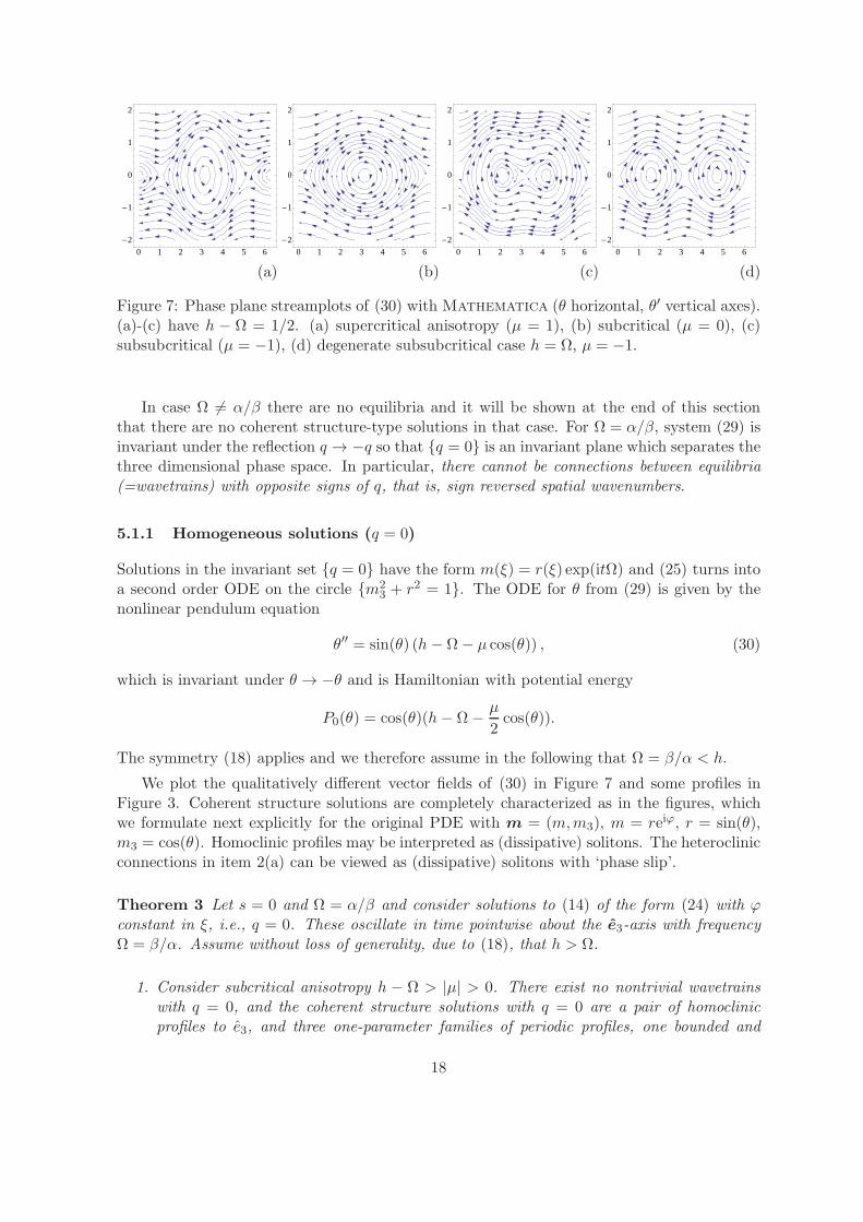
Figure 7: Phase plane streamplots of (30) with Mathematica (θ horizontal, θ′ vertical axes).(a)-(c) have h − Ω = 1/2. (a) supercritical anisotropy (µ = 1), (b) subcritical (µ = 0), (c)subsubcritical (µ = −1), (d) degenerate subsubcritical case h = Ω, µ = −1.
In case Ω 6= α/β there are no equilibria and it will be shown at the end of this sectionthat there are no coherent structure-type solutions in that case. For Ω = α/β, system (29) isinvariant under the reflection q → −q so that q = 0 is an invariant plane which separates thethree dimensional phase space. In particular, there cannot be connections between equilibria(=wavetrains) with opposite signs of q, that is, sign reversed spatial wavenumbers.
5.1.1 Homogeneous solutions (q = 0)
Solutions in the invariant set q = 0 have the form m(ξ) = r(ξ) exp(itΩ) and (25) turns intoa second order ODE on the circle m2
3 + r2 = 1. The ODE for θ from (29) is given by thenonlinear pendulum equation
θ′′ = sin(θ) (h− Ω− µ cos(θ)) , (30)
which is invariant under θ → −θ and is Hamiltonian with potential energy
P0(θ) = cos(θ)(h− Ω−µ
2cos(θ)).
The symmetry (18) applies and we therefore assume in the following that Ω = β/α < h.
We plot the qualitatively different vector fields of (30) in Figure 7 and some profiles inFigure 3. Coherent structure solutions are completely characterized as in the figures, whichwe formulate next explicitly for the original PDE with m = (m,m3), m = reiϕ, r = sin(θ),m3 = cos(θ). Homoclinic profiles may be interpreted as (dissipative) solitons. The heteroclinicconnections in item 2(a) can be viewed as (dissipative) solitons with ‘phase slip’.
Theorem 3 Let s = 0 and Ω = α/β and consider solutions to (14) of the form (24) with ϕconstant in ξ, i.e., q = 0. These oscillate in time pointwise about the e3-axis with frequencyΩ = β/α. Assume without loss of generality, due to (18), that h > Ω.
1. Consider subcritical anisotropy h − Ω > |µ| > 0. There exist no nontrivial wavetrainswith q = 0, and the coherent structure solutions with q = 0 are a pair of homoclinicprofiles to e3, and three one-parameter families of periodic profiles, one bounded and
18
two semi-unbounded. The homoclinic profiles each cross once through −e3 in oppositeθ-directions. The limit points of the bounded curve of periodic profiles are −e3 andthe union of homoclinic profiles. Each of the homoclinics is the limit point of one ofthe semi-unbounded families, each of which has unbounded θ-derivatives. The profilesfrom the bounded family each cross −e3 once during a half-period, the profiles of theunbounded family cross both ±e3 during one half-period.
2. Suppose super- or subsubcritical anisotropy |µ| > h − Ω. There exists a wavetrain withk = 0, which is stable in the supercritical case (µ > 0) and unstable in the subsubcriticalcase (µ < 0). In (30) this appears in the form of two equilibria being the symmetric pairof intersection points of the wavetrain orbit and a meridian on the sphere, phase shiftedby π in ϕ-direction. Details of the following can be read off Figure 7 analogous to item1.
(a) In the supercritical case (µ > h − Ω) the coherent structure solutions with q = 0are two pairs of heteroclinic connections between the wavetrain and its phase shift,and four curves of periodic profiles; two bounded and two semi-unbounded.
(b) In the subsubcritical case (µ < h−Ω) the coherent structure solutions with q = 0 aretwo pairs of homoclinic connections to ±e3, respectively, and five curves of periodicprofiles, three bounded and two semi-unbounded.
3. The degenerate case h = Ω, µ < 0 is the only possibility for profiles of stationary coherentstructures to connect between ±e3, which then come in a pair as in the correspondingpanel of Figure 7. The remaining coherent structures with q = 0 are analogous to thesupercritical case with ±e3 and the pair of wavetrain and its phase shift interchanged.
Proof. As for wavetrains discussed in §4, the condition cos(θ) = (h−Ω)/µ yields the existencecriterion |h − Ω| < |µ| for an equilibrium to (30) in (0, π). The derivative of the right handside of (30) at θ = 0 is h − Ω − µ, which dictates the type of all equilibria and only saddlesgenerate heteroclinic or homoclinic solutions.
It remains to study the connectivity of stable and unstable manifolds of saddles, which isgiven by the difference in potential energy P0(θ). Since P0(0) − P0(π) = 2(h − Ω) the claimsfollow.
5.1.2 Non-homogeneous solutions (q 6= 0)
In order to study (29) for q 6= 0, we note the following first integral. Since Ω = β/α, theequation for q can be written as
(log |q|)′ = −2(log | sin(θ)|)′,
and therefore explicitly integrated. With integration constant C = sin(θ(0))2|q(0)| this gives
q =C
sin(θ)2. (31)
Substituting this into the equation for θ yields the nonlinear pendulum
θ′′ = sin(θ) (h− Ω− µ cos(θ)) + C2 cos(θ)
sin(θ)3, (32)
19
-4 -2 0 2 4
0
1
2
3
4
5
6
k
Θ1 2 3 4 5 6
-1.0
-0.8
-0.6
-0.4
-0.2
0.0
0.2
0.4
1 2 3 4 5 6
-0.6
-0.4
-0.2
0.0
0.2
0.4
(a) (b)
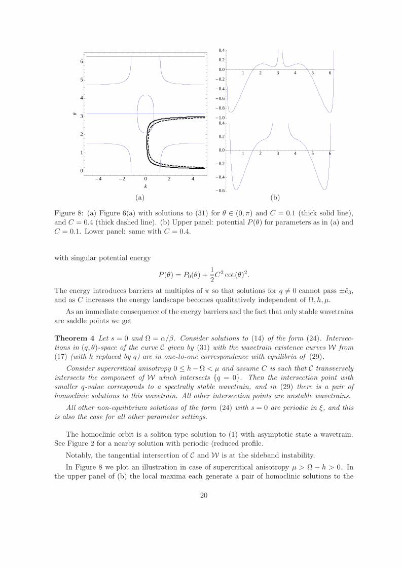
Figure 8: (a) Figure 6(a) with solutions to (31) for θ ∈ (0, π) and C = 0.1 (thick solid line),and C = 0.4 (thick dashed line). (b) Upper panel: potential P (θ) for parameters as in (a) andC = 0.1. Lower panel: same with C = 0.4.
with singular potential energy
P (θ) = P0(θ) +1
2C2 cot(θ)2.
The energy introduces barriers at multiples of π so that solutions for q 6= 0 cannot pass ±e3,and as C increases the energy landscape becomes qualitatively independent of Ω, h, µ.
As an immediate consequence of the energy barriers and the fact that only stable wavetrainsare saddle points we get
Theorem 4 Let s = 0 and Ω = α/β. Consider solutions to (14) of the form (24). Intersec-tions in (q, θ)-space of the curve C given by (31) with the wavetrain existence curves W from(17) (with k replaced by q) are in one-to-one correspondence with equilibria of (29).
Consider supercritical anisotropy 0 ≤ h−Ω < µ and assume C is such that C transverselyintersects the component of W which intersects q = 0. Then the intersection point withsmaller q-value corresponds to a spectrally stable wavetrain, and in (29) there is a pair ofhomoclinic solutions to this wavetrain. All other intersection points are unstable wavetrains.
All other non-equilibrium solutions of the form (24) with s = 0 are periodic in ξ, and thisis also the case for all other parameter settings.
The homoclinic orbit is a soliton-type solution to (1) with asymptotic state a wavetrain.See Figure 2 for a nearby solution with periodic (reduced profile.
Notably, the tangential intersection of C and W is at the sideband instability.
In Figure 8 we plot an illustration in case of supercritical anisotropy µ > Ω − h > 0. Inthe upper panel of (b) the local maxima each generate a pair of homoclinic solutions to the
20
stable wavetrain it represents. The values of q that it visits lie on the bold curve in (a), whoseintersections with the curve of equilibria are the local maxima and minima. The lower panelin (b) has C = 0.4 and the local maxima disappeared. All solutions are periodic and lie onthe thick dashed curve in (a).
5.1.3 Absence of wavetrains (Ω 6= α/β)
In this case the first integral Q = log(|q| sin(θ)2) is monotone,
Q′ =Ω− α/β
q6= 0,
and therefore |q| is unbounded as ξ → ∞ or ξ → −∞. In view of (32), we also infer that θoscillates so that there are no relevant solutions of the form (24).
5.2 Moving coherent structures
Using the desingularized system (28), we prove existence of some non-stationary coherentstructures.
5.2.1 Fast front-type coherent structures (|s| ≫ 1)
In this section we prove existence of fast front-type coherent structures with at least oneasymptotic state of the profile being the constant up- or down-magnetization ±e3.
As a first step, it is convenient to consider such solutions in the desingularized system (28).
Theorem 5 For any bounded set of (α, β, µ,Ω0,Ω1) there exists s0 > 0 and neighborhoodU of M0 := θ ∈ [0, π], p = q − Ω1 = 0 such that for all |s| ≥ s0 the following holds for(28) with Ω = Ω0 + Ω1s. There exists a pair of heteroclinic trajectories (θ±h, p±h, q±h)(ξ)in U with d
dξ θh(ξ) = O(s−1), and limξ→−∞ θ−h(τξ) = 0, limξ→∞ θ+h(τξ) = π, where τ =sgn(s(h− β/α − µ)).
The local wavenumbers are always nontrivial, q±h 6≡ 0, and the heteroclinics form a smoothfamily in s−1 with
lim|ξ|→∞
q±h(ξ) =1
s
(
h+ αβ ∓ µ
1 + α2− Ω
)
+O(s−2).
On the spatial scale η = ξ/s the heteroclinics solve, to leading order in s−1, the ODE
d
dηθ =
α
1 + α2sin(θ)
(
h−β
α+ (Ω2
1 − µ) cos(θ)
)
. (33)
Before the proof we note the consequences of this for coherent structures in (27).
Corollary 1 The heteroclinic solutions of Theorem 5 are in one-to-one correspondence withheteroclinic solutions to (27) that lie in U and connect θ = 0, π and/or the possible equilibriumat θ1 := arccos((h−β/α)/µ). For θ ∈ (0, π) all properties carry over to (27) with the bijectiongiven by p = sin(θ)p.
21
Some remarks are in order.
• The ODE (33) is the spatial variant of the temporal heteroclinic connection in (15):setting all space derivatives to zero, the θ-equation of (15) reads
−∂tθ =α
1 + α2sin(θ)
(
h−β
α− µ cos(θ)
)
,
which is (33) with µ replaced by Ω21−µ and up to possible direction reversal. Since Ω1 = q
on the slow manifold (i.e. at leading order), the reduced flow equilibria reproduce thewavetrain existence condition (17). This kind of relation between temporal dynamics andfast travelling waves formally holds for any evolution equation in one space dimension.
• For increasing speeds these solutions are decreasingly localized, hence far from a sharptransition. For Ω1 6= 0 the azimuthal frequency increases with s.
• The uniqueness statement is limited, since in the (θ, p, q)-coordinates the neighborhoodU from the theorem is ‘pinched’ near θ = 0, π: a uniform neighborhood in (θ, p) has asinus boundary in (θ, p).
Concerning stability, we infer from Lemma 1 and Theorem 2 that none of these fronts canbe stable in an L2-sense: always one of the asymptotic states is unstable. In the supercriticalcase ±e3 are unstable, in the subcritical case one of ±e3 is unstable and in the subsubcriticalcase the wavetrain with θ = θ1 ∈ (0, π) is unstable. However, it is not ruled out that thesefronts are stable in a suitable weighted sense as invasion fronts into an unstable state, whichwe do not pursue further in this paper.
Proof (Theorem 5) Let us set s = ε−1 so that the limit to consider is ε → 0. Since we willrescale space with ε and ε−1 this means sign changes of s reflect the directionality of solutions.
The existence proof relies on a geometric singular perturbation argument and we shall usethe terminology from this theory, see [9, 15], and also sometimes suppress the ε-dependenceof θ, p, q.
Upon multiplying the p- and q-equations of (28) by ε we obtain the, for ε 6= 0 equivalent,‘slow’ system
θ′ = sin(θ)p
εp′ = αp+ q − Ω1 + ε(h+ (q2 − µ) cos(θ)− Ω0 − cos(θ)p2)
εq′ = p− α(q − Ω1) + ε(αΩ0 − β − 2 cos(θ)qp).
(34)
Setting ε = 0 gives the algebraic equations
A
(
pq
)
= −Ω1
(
−1α
)
, A =
(
α 11 −α
)
.
Since detA = −(1+α2) < 0 the unique solution is p = q−Ω1 = 0 and thus the ‘slow manifold’is M0 as defined in the theorem, with ‘slow flow’ given by
θ′ = sin(θ)p.
22
Since p = 0 at ε = 0, M0 is a manifold (a curve) of equilibria at ε = 0, so that the slowflow is in fact ‘superslow’ and will be considered explicitly below. Since the slow manifold isone-dimensional (and persists for ε > 0 as shown below) it suffices to consider equilibria forε > 0. These lie on the one hand at θ = θ0 ∈ 0, π, if
A
(
pq
)
+Ω1
(
−1α
)
+ εF (p, q) = 0 , F (p, q) :=
(
h+ σ(q2 − µ)−Ω0 − σp2
αΩ0 − β − 2σqp
)
,
where σ = cos(θ0) ∈ −1, 1. Since detA = −(1 + α2) < 0 the implicit function theoremprovides a locally unique curve of equilibria (pε, qε) for sufficiently small ε, where
d
dε
∣
∣
∣
∣
ε=0
(
pεqε
)
= −A−1F (0, 0) = −A−1
(
h− σµ −Ω0
αΩ0 − β
)
.
This proves the claimed location of asymptotic states.
On the other hand, for θ 6= 0 system (28) is equivalent to (27). From the previous consid-erations of equilibria (=wavetrains) we infer that the unique equilibria in an ε-neighborhoodof M0 are those at θ = θ0, (p, q) = (pε, qε) together with the single solution θ1 to (17), if itexists, with k replaced by q = ε(Ω0 − β/α).
Towards the persistence of M0 as a perturbed invariant manifold for |ε| > 0, let us switchto the ‘fast’ system by rescaling the time-like variable to ζ = ξ/ε. With θ = dθ/dζ etc., thisgives
θ = ε sin(θ)p
˙p = αp+ q − Ω1 + ε(h + (q2 − µ) cos(θ)− Ω0 − cos(θ)p2)
q = p− α(q − Ω1) + ε(αΩ0 − β − 2 cos(θ)qp).
(35)
Note that M0 is (also) a manifold of equilibria at ε = 0 in this system and the linearizationof (35) in M0 for transverse directions to M0 is given by A. Since the eigenvalues of A,±√
(1 + α2), are off the imaginary axis, M0 is normally hyperbolic and therefore persists asan ε-close invariant one-dimensional manifold Mε, smooth in ε and unique in a neighborhoodof M0. See [9]. The aforementioned at least two and at most three equilibria lie in Mε, and,Mε being one-dimensional, these must be connected by heteroclinic orbits.
For the connectivity details it is convenient to derive an explicit expression of the leadingorder flow. We thus switch to the superslow time scale η = εξ and set p = p/ε, q = (q−Ω1)/ε,which changes (34) to (subdindex η means d/dη)
θη = sin(θ)p
εpη = αp+ q + h+ (Ω21 − µ) cos(θ)− Ω0 + ε cos(θ)(ε(q2 − p2) + 2qΩ1)
εqη = p− αq + αΩ0 − β − 2ε cos(θ)(εqp+Ω1p).
(36)
At ε = 0, solving the algebraic equations for p provides the flow for θ given by
A−1
(
h+ (Ω21 − µ) cos(θ)− Ω0
αΩ0 − β
)
=1
1 + α2
(
αh− α(Ω21 − µ) cos(θ)− β
h− (Ω21 − µ) cos(θ)− (1 + α2)Ω0 + αβ.
)
so that the leading order superslow flow on the invariant manifold is given by (33).
Proof (Corollary 1) Recall that (28) and (27) are equivalent for θ ∈ (0, π). Next, wenote that the limit of the vector field of (27) along such a heteroclinic from (28) is zero byconstruction. Hence, for each of the heteroclinic orbits in (28) of Theorem 5, there exist aheteroclinic orbit in (27) in the sense of the corollary statement.
23
5.2.2 Small amplitude moving coherent structures
In this section we consider all possible small amplitude coherent structures for speeds
s2 >4q2
1 + α2, (37)
where q 6= 0 is an equilibrium q-value (26). Small amplitude means q must lie near a bifurcationpoint, which are the intersection points of the solution curves from (17) with θ = θ0 = 0, π.This gives
cos(θ0)(
q2 − µ)
=β
α− h (38)
and is only possible for super- and subcritical anisotropy.
We show that such coherent structures must be of front-type. Recall that for s = 0there are also coherent structures with periodic and homoclinic (soliton-type) profiles. Inthe previous section we found front-type solutions when h − β/α enters (−µ, µ), that is, theanisotropy changes from subcritical to super- or subsubcritical, and when the speed s is abovea theoretical threshold. In this section, we give an explicit bound for this threshold in the smallamplitude limit. We shall prove that for speeds satisfying (37), these points are pitchfork-type bifurcations in (28), which give rise to front-type coherent structures. As in the previoussection, we locate such solutions in (27) from an analysis of (28). Remark that in the PDE (1)the pitchfork-type bifurcation corresponds to a Hopf-type bifurcation due to the superimposedoscillation about the e3-axis.
Theorem 6 Let Sε = (αε, βε, hε, µε,Ωε, sε) be a curve in the parameter space of (28) withε ∈ (−ε0, ε0) for some ε0 > 0 sufficiently small such that αε > 0 and qε, S(ε) solve (26), (38)with qε strictly monotone increasing in ε, and at ε = 0.
Then (28) with parameters Sε has equilibria at (θ, p, q) = (θ0, 0, qε) and at ε = 0 thefollowing occur.
1. There is a pitchfork-type bifurcation in case q0 6= µ0 and θ0 = 0 or π: If q0 > µ0
(q0 < µ0) two equilibria bifurcate as ε changes from negative to positive (positive tonegative), which are connected to (θ0, 0, qε) by a heteroclinic connection, respectively.These are unique in a neighborhood U of (θ0, 0, q0).
The heteroclinics converge to (θ0, 0, qε) as sgn(s(q2 − µ))ξ → ∞ so that a bifurcation inq2 < µ is supercritical and subcritical in q2 > µ.
These bifurcations are not generic in the coordinates of (28), because its linearizationin equilibria with θ = 0 or π always has a kernel.
2. There is no local bifurcation in case q0 − µ0 = h0 − β0/α0 = 0 and θ0 = π/2: for ε 6= 0there is at most one equilibrium and there are no small amplitude solutions to (27) inits vicinity.
Analogous to Corollary 1 we have
Corollary 2 The heteroclinic solutions of Theorem 6 are in one-to-one correspondence withheteroclinic solutions to (27), connecting to θ = 0 or θ = π in U . Bounded solutions forθ 6∈ 0, π are also in one-to-one correspondence.
24
Proof (Theorem 6) The existence analysis of equilibria already implies the emergence oftwo symmetric equilibria under the stated conditions in item (1), and that there is at most onein item (2). Hence, it remains to show that the center manifold associated to the bifurcationis one-dimensional and to obtain the directionality of heteroclinics.
For the former it suffices to show that the linearization at the bifurcation point has onlya simple eigenvalue on the imaginary axis, namely at zero. The linearization of (28) in anypoint with p = 0 (in particular for all relevant equilibria) gives the 3× 3 matrix
A =
0 sin(θ) 0
(µ− q2) sin(θ)0
B
, B =
(
αs 2q cos(θ)− ss− 2q cos(θ) αs
)
.
In particular, for θ = θ0 = 0, π and for µ0 = q20, the matrix A has a kernel with eigenvector(1, 0, 0)t. The remaining eigenvalues are those of B. SinceB has vanishing trace, its eigenvaluesare either a complex conjugate pair (for detB > 0) or a pair of sign reversed real numbers (fordetB < 0) or a double zero (detB = 0). Since detB = 4q2 cos(θ0)
2−(1+α2)s2 the constraintsin the theorem statement imply a simple zero eigenvalue and no further eigenvalues on theimaginary axis.
The simple eigenvalue on the imaginary axis implies existence of a one-dimensional centermanifold that includes all equilibria near (θ0, 0, q0) for nearby parameters.
In case (1) the uniqueness of bifurcating equilibria on either side of the symmetry axesand invariance of the one-dimensional center manifold implies presence and local uniquenessof the claimed heteroclinic connections. In order to determine the directionality of these, wecompute the leading order correction to the eigenvalues of A for θ = θ0+δ. The straightforwardcalculation yields the eigenvalue of the bifurcation branch as
α
(1 + α2)s(q2 − µ)δ2 +O(δ4),
which gives the claimed directionality.
References
[1] Aranson, I., and Kramer, L. The world of the complex Ginzburg-Landau equation.Rev. Mod. Phys. 74 (2002), 99–143.
[2] Berger, L. Emission of spin waves by a magnetic multilayer traversed by a current.Phys. Rev. B 54, 13 (Oct. 1996), 9353–9358.
[3] Berkov, D., and Miltat, J. Spin-torque driven magnetization dynamics: Micromag-netic modeling. J. Magn. Magn. Mat. 320, 7 (April 2008), 1238–1259.
[4] Bertotti, G. Spin-transfer-driven magnetization dynamics.
[5] Bertotti, G., Bonin, R., d’Aquino, M., Serpico, C., and Mayergoyz, I. Spin-wave instabilities in spin-transfer-driven magnetization dynamics. IEEE Magnetics letters1 (2010), 3000104.
25
[6] Bertotti, G., Serpico, C., Mayergoyz, I. D., Magni, A., d’Aquino, M., and
Bonin, R. Magnetization switching and microwave oscillations in nanomagnets drivenby spin-polarized currents. Phys. Rev. Lett. 94 (Apr 2005), 127206.
[7] Capella, A., Melcher, C., and Otto, F. Wave-type dynamics in ferromagnetic thinfilms and the motion of Neel walls. Nonlinearity 20, 11 (2007), 2519–2537.
[8] Carbou, G. Stability of static walls for a three-dimensional model of ferromagneticmaterial. J. Math. Pures Appl. (9) 93, 2 (2010), 183–203.
[9] Fenichel, N. Geometric singular perturbation theory for ordinary differential equations.J. Differ. Equations 31 (1979), 53–98.
[10] Gilbert, T. A phenomenological theory of damping in ferromagnetic materials. Mag-netics, IEEE Transactions on 40, 6 (nov. 2004), 3443 – 3449.
[11] Hasimoto, H. A soliton on a vortex filament. J. Fluid Mech 51, 3 (1972), 477–485.
[12] Hoefer, M., Ablowitz, M., Ilan, B., Pufall, M., and Silva, T. Theory of mag-netodynamics induced by spin torque in perpendicularly magnetized thin films. Physicalreview letters 95, 26 (2005), 267206.
[13] Hoefer, M., Sommacal, M., and Silva, T. Propagation and control of nanoscalemagnetic-droplet solitons. Phys. Rev. B. 85 (2012), 214433.
[14] Hubert, A., and Schafer, R. Magnetic Domains: The Analysis of Magnetic Mi-crostructures. Springer, August 1998.
[15] Jones, C. K. Geometric singular perturbation theory. Johnson, Russell (ed.), Dynamicalsystems. Lectures given at the 2nd session of the Centro Internazionale Matematico Estivo(CIME) held in Montecatini Terme, Italy, June 13-22, 1994. Berlin: Springer-Verlag. Lect.Notes Math. 1609, 44-118 (1995)., 1995.
[16] Kravchuk, V. P., Volkov, O. M., Sheka, D. D., and Gaididei, Y. Periodicmagnetization structures generated by transverse spin current in magnetic nanowires.Physical Review B 87, 22 (2013), 224402.
[17] Landau, L., and Lifshitz, E. On the theory of the dispersion of magnetic permeabilityin ferromagnetic bodies. Phys. Z. Sovietunion 8 (1935), 153–169.
[18] Melcher, C. The logarithmic tail of Neel walls. Arch. Ration. Mech. Anal. 168, 2(2003), 83–113.
[19] Melcher, C. Domain wall motion in ferromagnetic layers. Phys. D 192, 3-4 (2004),249–264.
[20] Melcher, C. Thin-film limits for Landau-Lifshitz-Gilbert equations. SIAM J. Math.Anal. 42, 1 (2010), 519–537.
[21] Melcher, C. Global solvability of the cauchy problem for the Landau-Lifshitz-Gilbertequation in higher dimensions. Indiana Univ. Math. J., to appear (2011).
26
[22] Melcher, C., and Ptashnyk, M. Landau-Lifshitz-Slonczewski equations: global weakand classical solutions. SIAM J. Math. Anal. 45, 1 (2013), 407–429.
[23] Meyries, M., Rademacher, J. D., and Siero, E. Quasilinear parabolic reaction-diffusion systems: user’s guide to well-posedness, spectra and stability of travelling waves.submitted, ArXiv 1305.3859 .
[24] Podio-Guidugli, P., and Tomassetti, G. On the evolution of domain walls in hardferromagnets. SIAM J. Appl. Math. 64, 6 (2004), 1887–1906 (electronic).
[25] Slonczewski, J. C. Current-driven excitation of magnetic multilayers. Journal ofMagnetism and Magnetic Materials 159, 11 (1996), L1–L7.
27