Embed Size (px)
Citation preview

Motivation Modeling Existence Semiclassical limit
Semiclassical limit of theSchrödinger-Poisson-Landau-Lifshitz-Gilbert
system
Lihui Chai
Department of MathematicsUniversity of California, Santa Barbara
Joint work withCarlos J. García-Cervera, and Xu Yang
YRW 2016, Duke

Motivation Modeling Existence Semiclassical limit
Outline
1 Motivation and introduction
2 The Schrödinger-Poisson-Landau-Lifshitz-Gilber system
3 Existence of weak solutions
4 Semiclassical limit of SPLLG

Motivation Modeling Existence Semiclassical limit
Outline
1 Motivation and introduction
2 The Schrödinger-Poisson-Landau-Lifshitz-Gilber system
3 Existence of weak solutions
4 Semiclassical limit of SPLLG

Motivation Modeling Existence Semiclassical limit
Magnetic devicesMagnetic recording devices and computer storagesSpinvalues1
Magnetic random accessmemory
Domain walls 2
Racetrackmemories
1Science@Berkeley Lab: The Current Spin on Spintronics2http://www2.technologyreview.com/article/412189/tr10-racetrack-
memory/

Motivation Modeling Existence Semiclassical limit
Methodology for detecting the orientationTunnel magnetoresistance 3
Julliere’s model:Constant tunnelingmatrix
Giant magnetoresistance 4
Albert Fert & Peter Grünberg:2007 Nobel Prize in Physics
3http://unlcms.unl.edu/cas/physics/tsymbal/reference/4http://unlcms.unl.edu/cas/physics/tsymbal/reference/

Motivation Modeling Existence Semiclassical limit
Methodology for rotating the orientation
Spin transfer torque (STT) 5
Two layers of differentthickness: different switchingfields
The thin film is switched, andthe resistance measured
5http://www.wpi-aimr.tohoku.ac.jp/mizukami_lab/

Motivation Modeling Existence Semiclassical limit
Micromagnetics: Landau-Lifshitz-Gilbert model
Basic quantity of interest:
m : Ω −→ R3; |m| = Ms
Landau-Lifshitz energy functional:
F [m] =
∫Ωφ
(mMs
)dx +
AM2
s
∫Ω|∇m|2 dx
− µ0
2
∫Ω
Hs ·m dx − µ0
∫Ω
He ·m dx

Motivation Modeling Existence Semiclassical limit
φ(
mMs
): Anisotropy Energy: Penalizes deviations from the
easy directions. For uniaxial materialsφ(m) = Ku
((m2/Ms)2 + (m3/Ms)2).
AM2
s|∇m|2: Exchange energy: Penalizes spatial variations.
−µ0He ·m: External field (Zeeman) energy.−µ0
2 Hs ·m: Stray field (self-induced) energy.The stray field, Hs = −∇u is obtained by solving themagnetostatic equation:
∆u = div m, x ∈ Ω, ∆u = 0, x ∈ Ωc,
with jump boundary conditions
[u]∂Ω = 0,[∂u∂ν
]∂Ω
= −m · ν.

Motivation Modeling Existence Semiclassical limit
φ(
mMs
): Anisotropy Energy: Penalizes deviations from the
easy directions. For uniaxial materialsφ(m) = Ku
((m2/Ms)2 + (m3/Ms)2).
AM2
s|∇m|2: Exchange energy: Penalizes spatial variations.
−µ0He ·m: External field (Zeeman) energy.
−µ02 Hs ·m: Stray field (self-induced) energy.
The stray field, Hs = −∇u is obtained by solving themagnetostatic equation:
∆u = div m, x ∈ Ω, ∆u = 0, x ∈ Ωc,
with jump boundary conditions
[u]∂Ω = 0,[∂u∂ν
]∂Ω
= −m · ν.

Motivation Modeling Existence Semiclassical limit
φ(
mMs
): Anisotropy Energy: Penalizes deviations from the
easy directions. For uniaxial materialsφ(m) = Ku
((m2/Ms)2 + (m3/Ms)2).
AM2
s|∇m|2: Exchange energy: Penalizes spatial variations.
−µ0He ·m: External field (Zeeman) energy.−µ0
2 Hs ·m: Stray field (self-induced) energy.
The stray field, Hs = −∇u is obtained by solving themagnetostatic equation:
∆u = div m, x ∈ Ω, ∆u = 0, x ∈ Ωc,
with jump boundary conditions
[u]∂Ω = 0,[∂u∂ν
]∂Ω
= −m · ν.

Motivation Modeling Existence Semiclassical limit
φ(
mMs
): Anisotropy Energy: Penalizes deviations from the
easy directions. For uniaxial materialsφ(m) = Ku
((m2/Ms)2 + (m3/Ms)2).
AM2
s|∇m|2: Exchange energy: Penalizes spatial variations.
−µ0He ·m: External field (Zeeman) energy.−µ0
2 Hs ·m: Stray field (self-induced) energy.The stray field, Hs = −∇u is obtained by solving themagnetostatic equation:
∆u = div m, x ∈ Ω, ∆u = 0, x ∈ Ωc,
with jump boundary conditions
[u]∂Ω = 0,[∂u∂ν
]∂Ω
= −m · ν.

Motivation Modeling Existence Semiclassical limit
Landau-Lifshitz-Gilbert equation
∂m∂t
= −γm × H + αm × ∂m∂t
,
where H = − δFδm and the second is Gilbert damping term.
γ = 1.76× 10¹¹ T−1s−1
α << 1: Damping coefficient
With the injection of spin current
∂m∂t
= −γm × (H + Js) + αm × ∂M∂t
,
where s is the spin procession and J is the couplingstrength between spin and magnetization

Motivation Modeling Existence Semiclassical limit
How to describe the spin dynamics?
Quantum (Schrödinger equation in spinor form)
i~∂ψ
∂t=
((− ~2
2m∇2
x + V (x))
I − µBω
2σ ·m(x , t)
)ψ.
Kinetic (Boltzmann equation)
∂tW (x ,v , t) + v · ∇xW (x ,v , t)− em
E · ∇v W (x ,v , t)
− i2~
[µBωσ ·m(x , t),W (x ,v , t)] = −W − Wτ
− 2τsf
(W − I2
TrC2W )
Hydrodynamic (Diffusion equation)
∂s∂t
= −div Js − 2D0(x)sλ2
sf− 2D0(x)
s ×mλ2
J,
Js =βµB
eJn ⊗m − 2D0(x) [∇s − ββ′ (∇s ·m)⊗m] .

Motivation Modeling Existence Semiclassical limit
How to describe the spin dynamics?Quantum (Schrödinger equation in spinor form)
i~∂ψ
∂t=
((− ~2
2m∇2
x + V (x))
I − µBω
2σ ·m(x , t)
)ψ.
Kinetic (Boltzmann equation)
∂tW (x ,v , t) + v · ∇xW (x ,v , t)− em
E · ∇v W (x ,v , t)
− i2~
[µBωσ ·m(x , t),W (x ,v , t)] = −W − Wτ
− 2τsf
(W − I2
TrC2W )
Hydrodynamic (Diffusion equation)
∂s∂t
= −div Js − 2D0(x)sλ2
sf− 2D0(x)
s ×mλ2
J,
Js =βµB
eJn ⊗m − 2D0(x) [∇s − ββ′ (∇s ·m)⊗m] .

Motivation Modeling Existence Semiclassical limit
Outline
1 Motivation and introduction
2 The Schrödinger-Poisson-Landau-Lifshitz-Gilber system
3 Existence of weak solutions
4 Semiclassical limit of SPLLG

Motivation Modeling Existence Semiclassical limit
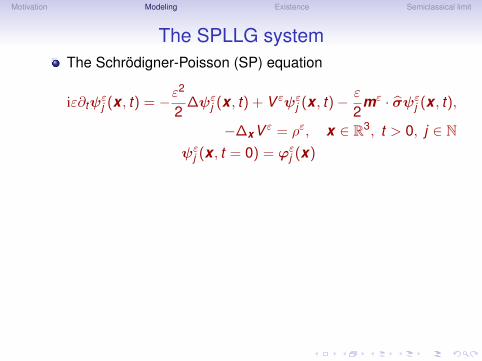
The SPLLG system
The Schrödigner-Poisson (SP) equation
iε∂tψεj (x , t) = −ε
2
2∆ψεj (x , t) + V εψεj (x , t)− ε
2mε · σψεj (x , t),
−∆xV ε = ρε, x ∈ R3, t > 0, j ∈ Nψεj (x , t = 0) = ϕεj (x)
The Landau-Lifshitz-Gilbert (LLG) equation
∂tmε = −mε × Hεeff + αmε × ∂tmε,
|mε(x , t)| = 1, x ∈ Ω, t > 0∂mε
∂ν= 0 on ∂Ω
mε(x , t = 0) = m0
Motivation Modeling Existence Semiclassical limit
The SPLLG systemThe Schrödigner-Poisson (SP) equation
iε∂tψεj (x , t) = −ε
2
2∆ψεj (x , t) + V εψεj (x , t)− ε
2mε · σψεj (x , t),
−∆xV ε = ρε, x ∈ R3, t > 0, j ∈ Nψεj (x , t = 0) = ϕεj (x)
The Landau-Lifshitz-Gilbert (LLG) equation
∂tmε = −mε × Hεeff + αmε × ∂tmε,
|mε(x , t)| = 1, x ∈ Ω, t > 0∂mε
∂ν= 0 on ∂Ω
mε(x , t = 0) = m0

Motivation Modeling Existence Semiclassical limit
The occupation numbers λεj > 0 satisfy that there existC > 0 such that∞∑
j=1
λεj + ε2∞∑
j=1
λεj ‖∇ϕεj ‖2L2(R3) + ε−3∞∑
j=1
(λεj )2 ≤ C
Physical observables
ρε(x , t) =∞∑
j=1
λεj |ψεj (x , t)|2,
jε(x , t) = ε
∞∑j=1
λεj Im(ψεj†(x , t)∇xψ
εj (x , t)
),
sε(x , t) =∞∑
j=1
λεj TrC2
(σ(ψεj (x , t)ψεj
†(x , t)))

Motivation Modeling Existence Semiclassical limit
The Landau-Lifshitz-Gilbert energy
FLL =
∫Ω
(12|∇mε|2 − 1
2Hε
s ·mε − ε
2sε ·mε
)dx ,
The the effective field
Hεeff = −δFLL
δmε= ∆mε + Hε
s +ε
2sε
The stray field
Hεs(x) = −∇
∫Ω∇N (x − y) ·mε(y) dy ,
with N (x) = − 14πx .

Motivation Modeling Existence Semiclassical limit
The Landau-Lifshitz-Gilbert energy
FLL =
∫Ω
(12|∇mε|2 − 1
2Hε
s ·mε − ε
2sε ·mε
)dx ,
The the effective field
Hεeff = −δFLL
δmε= ∆mε + Hε
s +ε
2sε
The stray field
Hεs(x) = −∇
∫Ω∇N (x − y) ·mε(y) dy ,
with N (x) = − 14πx .

Motivation Modeling Existence Semiclassical limit
The Landau-Lifshitz-Gilbert energy
FLL =
∫Ω
(12|∇mε|2 − 1
2Hε
s ·mε − ε
2sε ·mε
)dx ,
The the effective field
Hεeff = −δFLL
δmε= ∆mε + Hε
s +ε
2sε
The stray field
Hεs(x) = −∇
∫Ω∇N (x − y) ·mε(y) dy ,
with N (x) = − 14πx .

Motivation Modeling Existence Semiclassical limit
The Landau-Lifshitz-Gilbert energy
FLL =
∫Ω
(12|∇mε|2 − 1
2Hε
s ·mε − ε
2sε ·mε
)dx ,
The the effective field
Hεeff = −δFLL
δmε= ∆mε + Hε
s +ε
2sε
The stray field
Hεs(x) = −∇
∫Ω∇N (x − y) ·mε(y) dy ,
with N (x) = − 14πx .

Motivation Modeling Existence Semiclassical limit
The Wigner-Poisson equation
The Wigner transformation
W ε(x ,v) =1
(2π)3
∫R3
y
∞∑j=1
λεj ψεj
(x +
εy2
)ψεj†(
x − εy2
)eiv ·y dy .
The Wigner equation
∂tW ε + v · ∇xW ε −(
Θε[V ε] +i2
Γε[mε]
)W ε = 0,

Motivation Modeling Existence Semiclassical limit
The Wigner-Poisson equation
The Wigner transformation
W ε(x ,v) =1
(2π)3
∫R3
y
∞∑j=1
λεj ψεj
(x +
εy2
)ψεj†(
x − εy2
)eiv ·y dy .
The Wigner equation
∂tW ε + v · ∇xW ε −(
Θε[V ε] +i2
Γε[mε]
)W ε = 0,

Motivation Modeling Existence Semiclassical limit
The Wigner-Poisson equation
The Wigner transformation
W ε(x ,v) =1
(2π)3
∫R3
y
∞∑j=1
λεj ψεj
(x +
εy2
)ψεj†(
x − εy2
)eiv ·y dy .
The Wigner equation
∂tW ε + v · ∇xW ε −(
Θε[V ε] +i2
Γε[mε]
)W ε = 0,

Motivation Modeling Existence Semiclassical limit
where the operator Θε is given by
Θε[V ε]W ε(x ,v)
=1
(2π)3
∫∫1iε
[V ε(
x − εy2
)− V ε
(x +
εy2
)]W ε(x ,v ′)
× ei(v−v ′)·y dy dv ′,
and the operator Γε is given by
Γε[mε]W ε(x ,v)
=1
(2π)3
∫∫ [Mε(
x − εy2
)W ε(x ,v ′)−W ε(x ,v ′)Mε
(x +
εy2
)]× ei(v−v ′)·y dy dv ′,
where the matrix Mε = σ ·mε.

Motivation Modeling Existence Semiclassical limit
Outline
1 Motivation and introduction
2 The Schrödinger-Poisson-Landau-Lifshitz-Gilber system
3 Existence of weak solutions
4 Semiclassical limit of SPLLG

Motivation Modeling Existence Semiclassical limit
Consider the case ε = 1.
The Schrödinger equations
i∂tψj = −12
∆ψj + Vψj −12
m · σψj , x ∈ K , j ∈ N, t > 0,
ψj(t = 0,x) = ϕj(x), x ∈ K
ψj(t ,x) = 0, x ∈ ∂K
The Landau-Lifschitz-Gilbert equation
∂tm = −m × H + αm × ∂tm, (x , t) ∈ Ω× R+,
m(t = 0,x) = m0(x), x ∈ Ω,
∂νm = 0, (x , t) ∈ ∂Ω× R+,
The Poisson potential V = −N ∗ ρThe effective field H = ∆m + Hs + 1
2s, andHs = −∇(∇N ∗ ·m),

Motivation Modeling Existence Semiclassical limit
Consider the case ε = 1.The Schrödinger equations
i∂tψj = −12
∆ψj + Vψj −12
m · σψj , x ∈ K , j ∈ N, t > 0,
ψj(t = 0,x) = ϕj(x), x ∈ K
ψj(t ,x) = 0, x ∈ ∂K
The Landau-Lifschitz-Gilbert equation
∂tm = −m × H + αm × ∂tm, (x , t) ∈ Ω× R+,
m(t = 0,x) = m0(x), x ∈ Ω,
∂νm = 0, (x , t) ∈ ∂Ω× R+,
The Poisson potential V = −N ∗ ρ
The effective field H = ∆m + Hs + 12s, and
Hs = −∇(∇N ∗ ·m),

Motivation Modeling Existence Semiclassical limit
Consider the case ε = 1.The Schrödinger equations
i∂tψj = −12
∆ψj + Vψj −12
m · σψj , x ∈ K , j ∈ N, t > 0,
ψj(t = 0,x) = ϕj(x), x ∈ K
ψj(t ,x) = 0, x ∈ ∂K
The Landau-Lifschitz-Gilbert equation
∂tm = −m × H + αm × ∂tm, (x , t) ∈ Ω× R+,
m(t = 0,x) = m0(x), x ∈ Ω,
∂νm = 0, (x , t) ∈ ∂Ω× R+,
The Poisson potential V = −N ∗ ρThe effective field H = ∆m + Hs + 1
2s, andHs = −∇(∇N ∗ ·m),

Motivation Modeling Existence Semiclassical limit
Existence of weak solution
Denote Ψ = ψjj∈N and Φ = ϕjj∈N.Introduce the summation Hilbert space Hr
λ(K ) by defined‖Ψ‖2Hr
λ(K ) :=∑∞
j=1 λj‖ψj‖2H r (K ).
Theorem:
Given any initial conditions with Φ ∈ H1λ(R3) and
m0 ∈ H1(Ω), |m0| = 1, a.e. . Then there existsΨ ∈ L∞([0,∞),H1
λ(R3)) and m ∈ C([0,∞),H1(Ω)),|m| = 1, a.e. , such that the SPLLG system hold weakly.
We prove this theorem first in a bounded domain K andthen let K → R3 .

Motivation Modeling Existence Semiclassical limit
Existence of weak solution
Denote Ψ = ψjj∈N and Φ = ϕjj∈N.
Introduce the summation Hilbert space Hrλ(K ) by defined
‖Ψ‖2Hrλ(K ) :=
∑∞j=1 λj‖ψj‖2H r (K ).
Theorem:
Given any initial conditions with Φ ∈ H1λ(R3) and
m0 ∈ H1(Ω), |m0| = 1, a.e. . Then there existsΨ ∈ L∞([0,∞),H1
λ(R3)) and m ∈ C([0,∞),H1(Ω)),|m| = 1, a.e. , such that the SPLLG system hold weakly.
We prove this theorem first in a bounded domain K andthen let K → R3 .

Motivation Modeling Existence Semiclassical limit
Existence of weak solution
Denote Ψ = ψjj∈N and Φ = ϕjj∈N.Introduce the summation Hilbert space Hr
λ(K ) by defined‖Ψ‖2Hr
λ(K ) :=∑∞
j=1 λj‖ψj‖2H r (K ).
Theorem:
Given any initial conditions with Φ ∈ H1λ(R3) and
m0 ∈ H1(Ω), |m0| = 1, a.e. . Then there existsΨ ∈ L∞([0,∞),H1
λ(R3)) and m ∈ C([0,∞),H1(Ω)),|m| = 1, a.e. , such that the SPLLG system hold weakly.
We prove this theorem first in a bounded domain K andthen let K → R3 .

Motivation Modeling Existence Semiclassical limit
Existence of weak solution
Denote Ψ = ψjj∈N and Φ = ϕjj∈N.Introduce the summation Hilbert space Hr
λ(K ) by defined‖Ψ‖2Hr
λ(K ) :=∑∞
j=1 λj‖ψj‖2H r (K ).
Theorem:Given any initial conditions with Φ ∈ H1
λ(R3) andm0 ∈ H1(Ω), |m0| = 1, a.e. . Then there existsΨ ∈ L∞([0,∞),H1
λ(R3)) and m ∈ C([0,∞),H1(Ω)),|m| = 1, a.e. , such that the SPLLG system hold weakly.
We prove this theorem first in a bounded domain K andthen let K → R3 .

Motivation Modeling Existence Semiclassical limit
Galerkin approximations in a bounded domain
Assume K ⊂ R3 bounded.Construct solutions by Galerkin approximations:
Let θnn∈N be the normalized eigenfunctions of−∆θ = µθ in K , θ|∂K = 0.
Let ωnn∈N be the normalized eigenfunctions of−∆ω = µω in Ω, ∂νω|∂Ω
= 0.We seek the approximate solutionsψj N
(x , t) =∑N
n=1αjn(t)θn(x), andmN(x , t) =
∑Nn=1 βn(t)ωn(x),
and satisfy the initial conditionsψjN(·,0) = ΠK
Nϕj , and mN(·,0) = ΠΩNm0,
where ΠKN and ΠΩ
N is the orthogonal projections toSpanθnN
n=1 and SpanωnNn=1, resp..

Motivation Modeling Existence Semiclassical limit
Galerkin approximations in a bounded domain
Assume K ⊂ R3 bounded.
Construct solutions by Galerkin approximations:
Let θnn∈N be the normalized eigenfunctions of−∆θ = µθ in K , θ|∂K = 0.
Let ωnn∈N be the normalized eigenfunctions of−∆ω = µω in Ω, ∂νω|∂Ω
= 0.We seek the approximate solutionsψj N
(x , t) =∑N
n=1αjn(t)θn(x), andmN(x , t) =
∑Nn=1 βn(t)ωn(x),
and satisfy the initial conditionsψjN(·,0) = ΠK
Nϕj , and mN(·,0) = ΠΩNm0,
where ΠKN and ΠΩ
N is the orthogonal projections toSpanθnN
n=1 and SpanωnNn=1, resp..

Motivation Modeling Existence Semiclassical limit
Galerkin approximations in a bounded domain
Assume K ⊂ R3 bounded.Construct solutions by Galerkin approximations:
Let θnn∈N be the normalized eigenfunctions of−∆θ = µθ in K , θ|∂K = 0.
Let ωnn∈N be the normalized eigenfunctions of−∆ω = µω in Ω, ∂νω|∂Ω
= 0.We seek the approximate solutionsψj N
(x , t) =∑N
n=1αjn(t)θn(x), andmN(x , t) =
∑Nn=1 βn(t)ωn(x),
and satisfy the initial conditionsψjN(·,0) = ΠK
Nϕj , and mN(·,0) = ΠΩNm0,
where ΠKN and ΠΩ
N is the orthogonal projections toSpanθnN
n=1 and SpanωnNn=1, resp..

Motivation Modeling Existence Semiclassical limit
Galerkin approximations in a bounded domain
Assume K ⊂ R3 bounded.Construct solutions by Galerkin approximations:
Let θnn∈N be the normalized eigenfunctions of−∆θ = µθ in K , θ|∂K = 0.
Let ωnn∈N be the normalized eigenfunctions of−∆ω = µω in Ω, ∂νω|∂Ω
= 0.
We seek the approximate solutionsψj N
(x , t) =∑N
n=1αjn(t)θn(x), andmN(x , t) =
∑Nn=1 βn(t)ωn(x),
and satisfy the initial conditionsψjN(·,0) = ΠK
Nϕj , and mN(·,0) = ΠΩNm0,
where ΠKN and ΠΩ
N is the orthogonal projections toSpanθnN
n=1 and SpanωnNn=1, resp..

Motivation Modeling Existence Semiclassical limit
Galerkin approximations in a bounded domain
Assume K ⊂ R3 bounded.Construct solutions by Galerkin approximations:
Let θnn∈N be the normalized eigenfunctions of−∆θ = µθ in K , θ|∂K = 0.
Let ωnn∈N be the normalized eigenfunctions of−∆ω = µω in Ω, ∂νω|∂Ω
= 0.We seek the approximate solutionsψj N
(x , t) =∑N
n=1αjn(t)θn(x), andmN(x , t) =
∑Nn=1 βn(t)ωn(x),
and satisfy the initial conditionsψjN(·,0) = ΠK
Nϕj , and mN(·,0) = ΠΩNm0,
where ΠKN and ΠΩ
N is the orthogonal projections toSpanθnN
n=1 and SpanωnNn=1, resp..

Motivation Modeling Existence Semiclassical limit
Galerkin approximations in a bounded domain
Assume K ⊂ R3 bounded.Construct solutions by Galerkin approximations:
Let θnn∈N be the normalized eigenfunctions of−∆θ = µθ in K , θ|∂K = 0.
Let ωnn∈N be the normalized eigenfunctions of−∆ω = µω in Ω, ∂νω|∂Ω
= 0.We seek the approximate solutionsψj N
(x , t) =∑N
n=1αjn(t)θn(x), andmN(x , t) =
∑Nn=1 βn(t)ωn(x),
and satisfy the initial conditionsψjN(·,0) = ΠK
Nϕj , and mN(·,0) = ΠΩNm0,
where ΠKN and ΠΩ
N is the orthogonal projections toSpanθnN
n=1 and SpanωnNn=1, resp..

Motivation Modeling Existence Semiclassical limit
Galerkin solutions
Let ψjN and mN be the solutions of
ΠKN
(i∂tψj N
= −12
∆ψj N+ VNψj N
− 12
mN · σψj N
),
ΠΩN(−α∂tmN = mN × ∂tmN − HN + k(|mN |2 − 1)mN
), 6
where HN = ∆mN +(HsN + 1
2sN).
Estimates then are based the following conservation
ddt
∫K
∞∑j=1
λj |∇ψjN |2 +ddt
∫K|∇VN |2
+ddt
∫Ω|∇mN |2 +
ddt
∫R3|HsN |2
+k2
ddt
∫Ω
(|mN |2 − 1
)2+ 2α
∫Ω|∂tmN |2 =
ddt
∫Ω
sN ·mN .
6F. Alouges & A. Soyeur 1992

Motivation Modeling Existence Semiclassical limit
Limits as N →∞
Then we have the convergence w.r.t. corresponding topology:
ΨNN→∞−−−−→ Ψ k ∈ L∞(R+,H1
λ(K )), weak * ,
∂tΨNN→∞−−−−→ ∂tΨ
k ∈ L∞(R+,H−1λ (K )), weak * ,
mNN→∞−−−−→ mk ∈ L∞(R+,H1(Ω)), weak * ,
∂tmNN→∞−−−−→ ∂tmk ∈ L2(R+,L2(Ω)), weakly ,
|mN |2 − 1 N→∞−−−−→ |mk |2 − 1 ∈ L∞(R+,L2(Ω)), weak* ,

Motivation Modeling Existence Semiclassical limit
Weak Solutions to the penalized problem
Lemma
For all χ ∈ H1([0,T ]×Ω) and η ∈ C([0,T ],H1(K )), it holds that
i∫ T
0
∫K∂tψj
kη =12
∫ T
0
∫K∇ψj
k · ∇η +
∫ T
0
∫K
V kψjkη
− 12
∫ T
0
∫K
mk · σψjkη,∫ T
0
∫Ωα∂tmkχ = −
∫ T
0
∫Ω
(mk × ∂tmk − Hs
k − 12
sk)χ
+
∫ T
0
∫Ω
k(|mk |2 − 1
)mkχ+∇mk · ∇χ.

Motivation Modeling Existence Semiclassical limit
Weak Solutions to the SPLLG
Ψ k k→∞−−−→ Ψ ∈ L∞(R+,H1λ(K )) weak* ,
∂tΨk k→∞−−−→ ∂tΨ ∈ L∞(R+,H−1
λ (K )) weak* ,
mk k→∞−−−→ m ∈ L∞(R+,H1(Ω)) weak* ,∂tmk k→∞−−−→ ∂tm ∈ L2(R+,L2(Ω)) weakly ,|mk |2 − 1 k→∞−−−→ 0 ∈ L2([0,T ]× Ω) weakly and a.e. ,
Take χ = mk × ξ with ξ ∈ C∞([0,T ]× Ω) in the penalizedLLG equation and obtain∫ T
0
∫Ω∂tm · ξ =
∫ T
0
∫Ω
(m ×
(α∂tm − Hs −
12
s))· ξ
+
∫ T
0
∫Ω
m ×∇m · ∇ξ.Since |m| = 1 a.e. , by a density argument, we also obtainthe above equation holds for all ξ ∈ H1([0,T ]× Ω).

Motivation Modeling Existence Semiclassical limit
Weak Solutions to the SPLLG
Ψ k k→∞−−−→ Ψ ∈ L∞(R+,H1λ(K )) weak* ,
∂tΨk k→∞−−−→ ∂tΨ ∈ L∞(R+,H−1
λ (K )) weak* ,
mk k→∞−−−→ m ∈ L∞(R+,H1(Ω)) weak* ,
∂tmk k→∞−−−→ ∂tm ∈ L2(R+,L2(Ω)) weakly ,|mk |2 − 1 k→∞−−−→ 0 ∈ L2([0,T ]× Ω) weakly and a.e. ,
Take χ = mk × ξ with ξ ∈ C∞([0,T ]× Ω) in the penalizedLLG equation and obtain∫ T
0
∫Ω∂tm · ξ =
∫ T
0
∫Ω
(m ×
(α∂tm − Hs −
12
s))· ξ
+
∫ T
0
∫Ω
m ×∇m · ∇ξ.Since |m| = 1 a.e. , by a density argument, we also obtainthe above equation holds for all ξ ∈ H1([0,T ]× Ω).

Motivation Modeling Existence Semiclassical limit
Weak Solutions to the SPLLG
Ψ k k→∞−−−→ Ψ ∈ L∞(R+,H1λ(K )) weak* ,
∂tΨk k→∞−−−→ ∂tΨ ∈ L∞(R+,H−1
λ (K )) weak* ,
mk k→∞−−−→ m ∈ L∞(R+,H1(Ω)) weak* ,∂tmk k→∞−−−→ ∂tm ∈ L2(R+,L2(Ω)) weakly ,
|mk |2 − 1 k→∞−−−→ 0 ∈ L2([0,T ]× Ω) weakly and a.e. ,
Take χ = mk × ξ with ξ ∈ C∞([0,T ]× Ω) in the penalizedLLG equation and obtain∫ T
0
∫Ω∂tm · ξ =
∫ T
0
∫Ω
(m ×
(α∂tm − Hs −
12
s))· ξ
+
∫ T
0
∫Ω
m ×∇m · ∇ξ.Since |m| = 1 a.e. , by a density argument, we also obtainthe above equation holds for all ξ ∈ H1([0,T ]× Ω).

Motivation Modeling Existence Semiclassical limit
Weak Solutions to the SPLLG
Ψ k k→∞−−−→ Ψ ∈ L∞(R+,H1λ(K )) weak* ,
∂tΨk k→∞−−−→ ∂tΨ ∈ L∞(R+,H−1
λ (K )) weak* ,
mk k→∞−−−→ m ∈ L∞(R+,H1(Ω)) weak* ,∂tmk k→∞−−−→ ∂tm ∈ L2(R+,L2(Ω)) weakly ,|mk |2 − 1 k→∞−−−→ 0 ∈ L2([0,T ]× Ω) weakly and a.e. ,
Take χ = mk × ξ with ξ ∈ C∞([0,T ]× Ω) in the penalizedLLG equation and obtain∫ T
0
∫Ω∂tm · ξ =
∫ T
0
∫Ω
(m ×
(α∂tm − Hs −
12
s))· ξ
+
∫ T
0
∫Ω
m ×∇m · ∇ξ.Since |m| = 1 a.e. , by a density argument, we also obtainthe above equation holds for all ξ ∈ H1([0,T ]× Ω).

Motivation Modeling Existence Semiclassical limit
Weak Solutions to the SPLLG
Ψ k k→∞−−−→ Ψ ∈ L∞(R+,H1λ(K )) weak* ,
∂tΨk k→∞−−−→ ∂tΨ ∈ L∞(R+,H−1
λ (K )) weak* ,
mk k→∞−−−→ m ∈ L∞(R+,H1(Ω)) weak* ,∂tmk k→∞−−−→ ∂tm ∈ L2(R+,L2(Ω)) weakly ,|mk |2 − 1 k→∞−−−→ 0 ∈ L2([0,T ]× Ω) weakly and a.e. ,
Take χ = mk × ξ with ξ ∈ C∞([0,T ]× Ω) in the penalizedLLG equation and obtain
∫ T
0
∫Ω∂tm · ξ =
∫ T
0
∫Ω
(m ×
(α∂tm − Hs −
12
s))· ξ
+
∫ T
0
∫Ω
m ×∇m · ∇ξ.Since |m| = 1 a.e. , by a density argument, we also obtainthe above equation holds for all ξ ∈ H1([0,T ]× Ω).

Motivation Modeling Existence Semiclassical limit
Weak Solutions to the SPLLG
Ψ k k→∞−−−→ Ψ ∈ L∞(R+,H1λ(K )) weak* ,
∂tΨk k→∞−−−→ ∂tΨ ∈ L∞(R+,H−1
λ (K )) weak* ,
mk k→∞−−−→ m ∈ L∞(R+,H1(Ω)) weak* ,∂tmk k→∞−−−→ ∂tm ∈ L2(R+,L2(Ω)) weakly ,|mk |2 − 1 k→∞−−−→ 0 ∈ L2([0,T ]× Ω) weakly and a.e. ,
Take χ = mk × ξ with ξ ∈ C∞([0,T ]× Ω) in the penalizedLLG equation and obtain∫ T
0
∫Ω∂tm · ξ =
∫ T
0
∫Ω
(m ×
(α∂tm − Hs −
12
s))· ξ
+
∫ T
0
∫Ω
m ×∇m · ∇ξ.
Since |m| = 1 a.e. , by a density argument, we also obtainthe above equation holds for all ξ ∈ H1([0,T ]× Ω).

Motivation Modeling Existence Semiclassical limit
Weak Solutions to the SPLLG
Ψ k k→∞−−−→ Ψ ∈ L∞(R+,H1λ(K )) weak* ,
∂tΨk k→∞−−−→ ∂tΨ ∈ L∞(R+,H−1
λ (K )) weak* ,
mk k→∞−−−→ m ∈ L∞(R+,H1(Ω)) weak* ,∂tmk k→∞−−−→ ∂tm ∈ L2(R+,L2(Ω)) weakly ,|mk |2 − 1 k→∞−−−→ 0 ∈ L2([0,T ]× Ω) weakly and a.e. ,
Take χ = mk × ξ with ξ ∈ C∞([0,T ]× Ω) in the penalizedLLG equation and obtain∫ T
0
∫Ω∂tm · ξ =
∫ T
0
∫Ω
(m ×
(α∂tm − Hs −
12
s))· ξ
+
∫ T
0
∫Ω
m ×∇m · ∇ξ.Since |m| = 1 a.e. , by a density argument, we also obtainthe above equation holds for all ξ ∈ H1([0,T ]× Ω).

Motivation Modeling Existence Semiclassical limit
Weak solutions in whole space R3 7
For each R fixed, there exist weak solutions to the SPLLGin K = B(0,R).Conservation law and energy dissipation.The energy estimates does not depend on the radius R.There exit subsequences of solutions converge as R →∞.The limit satisfy the SPLLG weakly in R3.
7F. Brezzi & P.A. Markowich 1991

Motivation Modeling Existence Semiclassical limit
Weak solutions in whole space R3 7
For each R fixed, there exist weak solutions to the SPLLGin K = B(0,R).
Conservation law and energy dissipation.The energy estimates does not depend on the radius R.There exit subsequences of solutions converge as R →∞.The limit satisfy the SPLLG weakly in R3.
7F. Brezzi & P.A. Markowich 1991

Motivation Modeling Existence Semiclassical limit
Weak solutions in whole space R3 7
For each R fixed, there exist weak solutions to the SPLLGin K = B(0,R).Conservation law and energy dissipation.
The energy estimates does not depend on the radius R.There exit subsequences of solutions converge as R →∞.The limit satisfy the SPLLG weakly in R3.
7F. Brezzi & P.A. Markowich 1991

Motivation Modeling Existence Semiclassical limit
Weak solutions in whole space R3 7
For each R fixed, there exist weak solutions to the SPLLGin K = B(0,R).Conservation law and energy dissipation.The energy estimates does not depend on the radius R.
There exit subsequences of solutions converge as R →∞.The limit satisfy the SPLLG weakly in R3.
7F. Brezzi & P.A. Markowich 1991

Motivation Modeling Existence Semiclassical limit
Weak solutions in whole space R3 7
For each R fixed, there exist weak solutions to the SPLLGin K = B(0,R).Conservation law and energy dissipation.The energy estimates does not depend on the radius R.There exit subsequences of solutions converge as R →∞.
The limit satisfy the SPLLG weakly in R3.
7F. Brezzi & P.A. Markowich 1991

Motivation Modeling Existence Semiclassical limit
Weak solutions in whole space R3 7
For each R fixed, there exist weak solutions to the SPLLGin K = B(0,R).Conservation law and energy dissipation.The energy estimates does not depend on the radius R.There exit subsequences of solutions converge as R →∞.The limit satisfy the SPLLG weakly in R3.
7F. Brezzi & P.A. Markowich 1991

Motivation Modeling Existence Semiclassical limit
Outline
1 Motivation and introduction
2 The Schrödinger-Poisson-Landau-Lifshitz-Gilber system
3 Existence of weak solutions
4 Semiclassical limit of SPLLG

Motivation Modeling Existence Semiclassical limit
The WPLLG system in the semiclassical regime.
The Wigner equation∂tW ε + v · ∇xW ε −
(Θε[V ε] + i
2Γε[mε])
W ε = 0The Landau-Lifshitz-Gilbert (LLG) equation∂tmε = −mε × Hε
eff + αmε × ∂tmε
The Poisson potential V ε = −N ∗ ρε
The effective field Hεeff = ∆m + Hε
s + 12sε and
Hεs = −∇(∇N ∗ ·mε)
The behavior of the solution (W ε,mε) in the semiclassicallimit ε→ 0.

Motivation Modeling Existence Semiclassical limit
The WPLLG system in the semiclassical regime.
The Wigner equation∂tW ε + v · ∇xW ε −
(Θε[V ε] + i
2Γε[mε])
W ε = 0
The Landau-Lifshitz-Gilbert (LLG) equation∂tmε = −mε × Hε
eff + αmε × ∂tmε
The Poisson potential V ε = −N ∗ ρε
The effective field Hεeff = ∆m + Hε
s + 12sε and
Hεs = −∇(∇N ∗ ·mε)
The behavior of the solution (W ε,mε) in the semiclassicallimit ε→ 0.

Motivation Modeling Existence Semiclassical limit
The WPLLG system in the semiclassical regime.
The Wigner equation∂tW ε + v · ∇xW ε −
(Θε[V ε] + i
2Γε[mε])
W ε = 0The Landau-Lifshitz-Gilbert (LLG) equation∂tmε = −mε × Hε
eff + αmε × ∂tmε
The Poisson potential V ε = −N ∗ ρε
The effective field Hεeff = ∆m + Hε
s + 12sε and
Hεs = −∇(∇N ∗ ·mε)
The behavior of the solution (W ε,mε) in the semiclassicallimit ε→ 0.

Motivation Modeling Existence Semiclassical limit
The WPLLG system in the semiclassical regime.
The Wigner equation∂tW ε + v · ∇xW ε −
(Θε[V ε] + i
2Γε[mε])
W ε = 0The Landau-Lifshitz-Gilbert (LLG) equation∂tmε = −mε × Hε
eff + αmε × ∂tmε
The Poisson potential V ε = −N ∗ ρε
The effective field Hεeff = ∆m + Hε
s + 12sε and
Hεs = −∇(∇N ∗ ·mε)
The behavior of the solution (W ε,mε) in the semiclassicallimit ε→ 0.

Motivation Modeling Existence Semiclassical limit
Main theorem: The semiclassical limitThere exists a subsequence of solutions (W ε, mε) to theWPLLG system such thatW ε ε→0−−−→W in L∞((0,T ); L2(R3
x × R3v )) weak ∗
mε ε→0−−−→ m in L∞((0,T ); H1(Ω)) weak ∗and (W ,m) is a weak solution of the following VPLLG system,
∂tW = −v · ∇xW +∇xV · ∇vW +i2
[σ ·m, W ],
∂tm = −m × Heff + αm × ∂tm,
V (x) =1
4π
∫R3
x
∫R3
v
W (y ,v , t)|x − y |
dv dy ,
Heff = ∆m + Hs,
Hs(x) = −∇(
14π
∫Ω
∇ ·m(y)
|x − y |dy).

Motivation Modeling Existence Semiclassical limit
Conservation quantities.
Conservation of the total mass.∫R3
x
ρε(x , t) dx =
∫R3
x
∫R3
v
TrC2
(W ε(x ,v , t)
)dv dx
=
∫R3
x
ρε(x ,0) dx =∞∑
j=1
λεj .
Conservation of the L2-norm of W ε.
‖W ε(t)‖2L2(R3x×R3
v ):=
∫R3
x
∫R3
v
TrC2
[W ε(x ,v , t)
]2 dv dx
=‖W εI ‖2L2(R3
x×R3v )
=2
(4πε)3
∞∑j=1
(λεj )2.
Conservation in the magnetization.
|mε(x , t)| = |m0(x)| ≡ 1;
‖mε(x , t)‖L2(Ω) = ‖m0(x)‖L2(Ω) = |Ω|.

Motivation Modeling Existence Semiclassical limit
Conservation quantities.Conservation of the total mass.∫
R3x
ρε(x , t) dx =
∫R3
x
∫R3
v
TrC2
(W ε(x ,v , t)
)dv dx
=
∫R3
x
ρε(x ,0) dx =∞∑
j=1
λεj .
Conservation of the L2-norm of W ε.
‖W ε(t)‖2L2(R3x×R3
v ):=
∫R3
x
∫R3
v
TrC2
[W ε(x ,v , t)
]2 dv dx
=‖W εI ‖2L2(R3
x×R3v )
=2
(4πε)3
∞∑j=1
(λεj )2.
Conservation in the magnetization.
|mε(x , t)| = |m0(x)| ≡ 1;
‖mε(x , t)‖L2(Ω) = ‖m0(x)‖L2(Ω) = |Ω|.

Motivation Modeling Existence Semiclassical limit
Energy dissipation.
Schrödinger-Poisson energy
FSP = Eεkin +
12
∫R3
x
|∇V ε|2 dx
The Landau-Lifschitz energy
FLL =
∫Ω
(12|∇mε|2 +
12|Hε
s|2 −ε
2sε ·mε
)dx
The energy dissipation
ddt
(FLL + FSP) + α
∫R3
x
|∂tmε(x , t)|2 dx ≤ 0

Motivation Modeling Existence Semiclassical limit
Energy dissipation.
Schrödinger-Poisson energy
FSP = Eεkin +
12
∫R3
x
|∇V ε|2 dx
The Landau-Lifschitz energy
FLL =
∫Ω
(12|∇mε|2 +
12|Hε
s|2 −ε
2sε ·mε
)dx
The energy dissipation
ddt
(FLL + FSP) + α
∫R3
x
|∂tmε(x , t)|2 dx ≤ 0

Motivation Modeling Existence Semiclassical limit
Energy dissipation.
Schrödinger-Poisson energy
FSP = Eεkin +
12
∫R3
x
|∇V ε|2 dx
The Landau-Lifschitz energy
FLL =
∫Ω
(12|∇mε|2 +
12|Hε
s|2 −ε
2sε ·mε
)dx
The energy dissipation
ddt
(FLL + FSP) + α
∫R3
x
|∂tmε(x , t)|2 dx ≤ 0

Motivation Modeling Existence Semiclassical limit
Energy dissipation.
Schrödinger-Poisson energy
FSP = Eεkin +
12
∫R3
x
|∇V ε|2 dx
The Landau-Lifschitz energy
FLL =
∫Ω
(12|∇mε|2 +
12|Hε
s|2 −ε
2sε ·mε
)dx
The energy dissipation
ddt
(FLL + FSP) + α
∫R3
x
|∂tmε(x , t)|2 dx ≤ 0

Motivation Modeling Existence Semiclassical limit
Energy dissipation. Cont.
Using the estimate∣∣∣∣∫Ω
sε ·mε dx∣∣∣∣ ≤ ∫
Ω|sε ·mε| dx ≤
∫R3
x
|sε| dx ≤ C
we get there exists a constant C independent of ε, such that8∫Ω|∇mε(t)|2 dx + Eε
kin(t) +12
∫R3
x
|∇V ε(x , t)|2 dx + α
∫ t
0
∫R3
x
|∂tm|2 dxdt
≤C + FLL(0) + Eεkin(0) +
∫R3
x
|∇V ε(x ,0)|2 dx
≤C.
8Brezzi & Markowich 1991, Arnold 1996

Motivation Modeling Existence Semiclassical limit
Boundedness
From the conservation equations and the energy dissipation weget the following boundedness
Eεkin(t) =
∫R3
x
∫R3
v
|v |2TrC2
(W ε(x ,v , t)
)dv dx ≤ C,
‖V ε‖L∞((0,∞),L6(R3x )) + ‖∇V ε‖L∞((0,∞),L2(R3
x )) ≤ C.
‖W ε‖L2(R3x×R3
v ) + ‖mε(t)‖L2(Ω) + ‖∇mε(t)‖L2(Ω) ≤ C,
and‖∂tmε‖L2([0,T ],L2(R3)) ≤ C.

Motivation Modeling Existence Semiclassical limit
From the interpolation lemma9
LemmaLet 1 ≤ p ≤ ∞, q = (5p − 3)/(3p − 1), s = (5p − 3)/(4p − 2),and θ = 2p/(5p − 3). Then ∃C > 0 s.t.‖ρε‖Lq ≤ C|λε|θp
(ε−2Eε
kin)1−θ, ‖jε‖Ls ≤ C|λε|θp
(ε−2Eε
kin)1−θ,
where |λε|p =(∑∞
j=1 |λεj |p)1/p
under the assumption |λε|2 ≤ C we get the estimats
‖ρε‖L∞((0,∞),Lq(R3x )) + ‖sε‖L∞((0,∞),Lq(R3
x )) ≤ C, q ∈ [1,6/5] ,
‖jε‖L∞((0,∞),Ls(R3x )) + ‖Jεs‖L∞((0,∞),Ls(R3
x )) ≤ C, s ∈ [1,7/6] .
9Arnold 1996

Motivation Modeling Existence Semiclassical limit
Convergence subsequences.
W ε ε→0−−−→W in L∞((0,∞); L2(R3x × R3
v )) weak ∗ ,
ρεε→0−−−→ ρ in L∞((0,∞); Lq(R3
x )) weak ∗ ,q ∈ [1,6/5]
sε ε→0−−−→ s in L∞((0,∞); Lq(R3x )) weak ∗ ,q ∈ [1,6/5]
mε ε→0−−−→ m in L∞((0,∞); H1(Ω)) weak ∗ ,
mε ε→0−−−→ m in L2([0,T ],L2(R3x )) strongly.
Hεsε→0−−−→ H in L∞((0,∞); L2(Ω)) weak ∗ ,
V ε ε→0−−−→ V in L∞((0,∞); L6(R3x )) weak ∗ ,
∇V ε ε→0−−−→ ∇V in L∞((0,∞); L2(R3x )) weak ∗ .

Motivation Modeling Existence Semiclassical limit
Passing to the limit of the Wigner equation
We study the weak formulation of the Wigner equation∫∫∫ [W ε(∂tφ+ v · ∇xφ) +
(Θε[V ε] +
i2
Γε[mε]
)W εφ
]= 0.
limε→0
∫∫∫W ε(∂tφ+ v · ∇xφ) =
∫∫∫W (∂tφ+ v · ∇xφ).
10 limε→0
∫∫∫Θε[V ε]W εφ = −
∫∫∫W∇xV · ∇vφ
limε→0
∫∫∫Γε[mε]W εφ
?=
∫∫∫[m · σ,W ]φ
10Markowich & Mauser 1993

Motivation Modeling Existence Semiclassical limit
Recall that the operator Θε is given by
Θε[V ε]W ε(x ,v)
=1
(2π)3
∫∫1iε
[V ε(
x − εy2
)− V ε
(x +
εy2
)]W ε(x ,v ′)
× ei(v−v ′)·y dy dv ′,
and the operator Γε is given by
Γε[mε]W ε(x ,v)
=1
(2π)3
∫∫ [Mε(
x − εy2
)W ε(x ,v ′)−W ε(x ,v ′)Mε
(x +
εy2
)]× ei(v−v ′)·y dy dv ′,
where the matrix Mε = σ ·mε.
Motivation Modeling Existence Semiclassical limit
limε→0 Γε[mε]W ε
If mε ∈ H1(R3), we can prove (by Taylor’s theorem)
limε→0
∫∫∫Γε[mε]W εφ =
∫∫∫[m · σ,W ]φ
But mε /∈ H1(R3), since |mε| ≡ 1 in Ω, mε ≡ 0 in Ωc
Let mε,β = mε ∗x ϕβ, and then mε = (mε −mε,β) + mε,β,where ϕβ(x) = ϕ(x/β) and ϕ is a positive mollifier.
∣∣∣∣∫∫∫ (Γε[mε]W ε − [M,W ])φ dx dv dt
∣∣∣∣≤∣∣∣∣∫∫∫ Γε
[mε −mε,β
]W εφ dx dv dt
∣∣∣∣+
∣∣∣∣∫∫∫ (Γε [mε,β]
W ε −[Mβ ,W
])φ dx dv dt
∣∣∣∣+
∣∣∣∣∫∫∫ [Mβ −M,W]φ dx dv dt
∣∣∣∣ ,where M = σ ·m and Mβ = M ∗x ϕβ.

Motivation Modeling Existence Semiclassical limit
limε→0 Γε[mε]W ε Cont.
For the second integral, since mε,β ∈ H1(R3) andmε,β → m ∗x ϕβ strongly in L2([0,T ]× R3), we have
limε→0
∫∫∫ (Γε[mε,β]W ε − [Mβ,W ]
)φ = 0.
For the third integral we have∣∣∣∣∫∫∫ [Mβ −M,W]φ dx dv dt
∣∣∣∣ ≤ Cβ → 0, as β → 0.
For the first integral, we use triangle inequality to get∣∣∣∣∫∫∫ Γε[mε −mε,β
]W εφ dx dv dt
∣∣∣∣≤C‖mε −m‖L2([0,T ]×R3
x ) + C‖mβ −mε,β‖L2([0,T ]×R3x )
+ C‖m −mβ‖L2([0,T ]×R3x )
≤C‖mε −m‖L2([0,T ]×R3x ) + C‖m −mβ‖L2([0,T ]×R3
x ),

Motivation Modeling Existence Semiclassical limit
limε→0 Γε[mε]W ε Cont.For the second integral, since mε,β ∈ H1(R3) andmε,β → m ∗x ϕβ strongly in L2([0,T ]× R3), we have
limε→0
∫∫∫ (Γε[mε,β]W ε − [Mβ,W ]
)φ = 0.
For the third integral we have∣∣∣∣∫∫∫ [Mβ −M,W]φ dx dv dt
∣∣∣∣ ≤ Cβ → 0, as β → 0.
For the first integral, we use triangle inequality to get∣∣∣∣∫∫∫ Γε[mε −mε,β
]W εφ dx dv dt
∣∣∣∣≤C‖mε −m‖L2([0,T ]×R3
x ) + C‖mβ −mε,β‖L2([0,T ]×R3x )
+ C‖m −mβ‖L2([0,T ]×R3x )
≤C‖mε −m‖L2([0,T ]×R3x ) + C‖m −mβ‖L2([0,T ]×R3
x ),

Motivation Modeling Existence Semiclassical limit
limε→0 Γε[mε]W ε Cont..
Then
limε→0
∣∣∣∣∫∫∫ Γε[mε −mε,β
]W εφ dx dv dt
∣∣∣∣ ≤ Cβ.
And Then
limε→0
∣∣∣∣∫∫∫ (Γε[mε]W ε − [M,W ])φ dx dv dt
∣∣∣∣ ≤ Cβ.
But the left hand side of above inequality is independent ofβ, we then have
limε→0
∣∣∣∣∫∫∫ (Γε[mε]W ε − [M,W ])φ dx dv dt
∣∣∣∣ = 0.

Motivation Modeling Existence Semiclassical limit
limε→0 Γε[mε]W ε Cont..Then
limε→0
∣∣∣∣∫∫∫ Γε[mε −mε,β
]W εφ dx dv dt
∣∣∣∣ ≤ Cβ.
And Then
limε→0
∣∣∣∣∫∫∫ (Γε[mε]W ε − [M,W ])φ dx dv dt
∣∣∣∣ ≤ Cβ.
But the left hand side of above inequality is independent ofβ, we then have
limε→0
∣∣∣∣∫∫∫ (Γε[mε]W ε − [M,W ])φ dx dv dt
∣∣∣∣ = 0.

Motivation Modeling Existence Semiclassical limit
Passing to the limit of the LLG equationThe weak formulation of the LLG equation∫∫
mε ∂tφ =
∫∫mε × Hε
eff φ− α∫∫
mε × ∂tmε φ.
Since mε → m in L2([0,T ],L2(Ω)) strongly, we have
limε→0
∫∫mε∂tφ =
∫∫m∂tφ.
Since ∂tmε → ∂tmε in L2([0,T ],L2(Ω)) weakly, we have
limε→0
∫∫mε × ∂tmε∂tφ =
∫∫m × ∂tm∂tφ.
∫∫mε × Hε
eff φ dx dt =−∫∫
mε ×∇mε · ∇φ dx dt
+
∫∫mε × Hε
sφ dx dt
+ε
2
∫∫mε × sεφ dx dt .

Motivation Modeling Existence Semiclassical limit
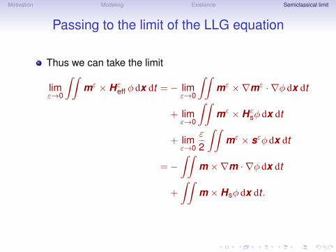
Passing to the limit of the LLG equation
Thus we can take the limit
limε→0
∫∫mε × Hε
eff φ dx dt =− limε→0
∫∫mε ×∇mε · ∇φ dx dt
+ limε→0
∫∫mε × Hε
sφ dx dt
+ limε→0
ε
2
∫∫mε × sεφ dx dt
=−∫∫
m ×∇m · ∇φ dx dt
+
∫∫m × Hsφ dx dt .
Motivation Modeling Existence Semiclassical limit
Passing to the limit of the LLG equation
Thus we can take the limit
limε→0
∫∫mε × Hε
eff φ dx dt =− limε→0
∫∫mε ×∇mε · ∇φ dx dt
+ limε→0
∫∫mε × Hε
sφ dx dt
+ limε→0
ε
2
∫∫mε × sεφ dx dt
=−∫∫
m ×∇m · ∇φ dx dt
+
∫∫m × Hsφ dx dt .

Motivation Modeling Existence Semiclassical limit
The limit of the WPLLG system
(W ,m) is a weak solution of the following VPLLG system,
∂tW = −v · ∇xW +∇xV · ∇vW +i2
[σ ·m, W ],
∂tm = −m × Heff + αm × ∂tm,
V (x) =1
4π
∫R3
x
∫R3
v
W (y ,v , t)|x − y |
dv dy ,
Heff = ∆m + Hs,
Hs(x) = −∇(
14π
∫Ω
∇ ·m(y)
|x − y |dy).

Motivation Modeling Existence Semiclassical limit
Summary
Use the Schödinger-Poisson-Landau-Lifshitz-Gilbertsystem to model the spin-magnetization coupling.Prove the existence of H1 solutions.Use Wigner transformation to get the kinetic description.In the semiclassical limit, the spin-magnetization couplingdynamics can be described by aVlasov-Poisson-Landau-Lifshitz system.

Motivation Modeling Existence Semiclassical limit
Summary
Use the Schödinger-Poisson-Landau-Lifshitz-Gilbertsystem to model the spin-magnetization coupling.
Prove the existence of H1 solutions.Use Wigner transformation to get the kinetic description.In the semiclassical limit, the spin-magnetization couplingdynamics can be described by aVlasov-Poisson-Landau-Lifshitz system.

Motivation Modeling Existence Semiclassical limit
Summary
Use the Schödinger-Poisson-Landau-Lifshitz-Gilbertsystem to model the spin-magnetization coupling.Prove the existence of H1 solutions.
Use Wigner transformation to get the kinetic description.In the semiclassical limit, the spin-magnetization couplingdynamics can be described by aVlasov-Poisson-Landau-Lifshitz system.

Motivation Modeling Existence Semiclassical limit
Summary
Use the Schödinger-Poisson-Landau-Lifshitz-Gilbertsystem to model the spin-magnetization coupling.Prove the existence of H1 solutions.Use Wigner transformation to get the kinetic description.
In the semiclassical limit, the spin-magnetization couplingdynamics can be described by aVlasov-Poisson-Landau-Lifshitz system.

Motivation Modeling Existence Semiclassical limit
Summary
Use the Schödinger-Poisson-Landau-Lifshitz-Gilbertsystem to model the spin-magnetization coupling.Prove the existence of H1 solutions.Use Wigner transformation to get the kinetic description.In the semiclassical limit, the spin-magnetization couplingdynamics can be described by aVlasov-Poisson-Landau-Lifshitz system.

Motivation Modeling Existence Semiclassical limit
THANKS FOR YOUR ATTENTION!