Patterns of Response Times and Response Choices to Science

Cognitive Science (2014) 1–42Copyright © 2014 Cognitive Science Society, Inc. All rights reserved.ISSN: 0364-0213 print / 1551-6709 onlineDOI: 10.1111/cogs.12166

Patterns of Response Times and Response Choicesto Science Questions: The Influence of Relative

Processing Time

Andrew F. Heckler,a Thomas M. Scaifeb

aDepartment of Physics, Ohio State UniversitybDepartment of Chemistry and Engineering Physics, University of Wisconsin—Platteville

Received 18 September 2011; received in revised form 31 December 2013; accepted 4 January 2014

Abstract

We report on five experiments investigating response choices and response times to simple sci-

ence questions that evoke student “misconceptions,” and we construct a simple model to explain

the patterns of response choices. Physics students were asked to compare a physical quantity rep-

resented by the slope, such as speed, on simple physics graphs. We found that response times of

incorrect answers, resulting from comparing heights, were faster than response times of correct

answers comparing slopes. This result alone might be explained by the fact that height was typi-

cally processed faster than slope for this kind of task, which we confirmed in a separate experi-

ment. However, we hypothesize that the difference in response time is an indicator of the cause(rather than the result) of the response choice. To support this, we found that imposing a 3-s delay

in responding increased the number of students comparing slopes (answering correctly) on the

task. Additionally a significant proportion of students recognized the correct written rule (compare

slope), but on the graph task they incorrectly compared heights. Finally, training either with repet-

itive examples or providing a general rule both improved scores, but only repetitive examples had

a large effect on response times, thus providing evidence of dual paths or processes to a solution.

Considering models of heuristics, information accumulation models, and models relevant to the

Stroop effect, we construct a simple relative processing time model that could be viewed as a kind

of fluency heuristic. The results suggest that misconception-like patterns of answers to some sci-

ence questions commonly found on tests may be explained in part by automatic processes that

involve the relative processing time of considered dimensions and a priority to answer quickly.

Keywords: Response time; Fluency; Heuristics; Dual processes; Stroop effect; Science

misconceptions; Graph comprehension; Science concepts

Correspondence should be sent to Andrew F. Heckler, Department of Physics, Ohio State University,

191 W. Woodruff Ave, Columbus, OH 43210. E-mail: [email protected]

1. Introduction

One of the most important empirical findings of science education research in the last

half century is the fact that, when asked simple scientific questions, people often get them

wrong in regular, patterned ways. More specifically, thousands of empirical studies have

established that when conceptual questions about simple natural phenomena are posed to

students, their answers are often contrary to scientists’ answers, remarkably similar to

those of other students, and resistant to traditional instruction (see compilations in Kind,

2004; McDermott & Redish, 1999; Pfundt & Duit, 2000). For example, students often

believe, even after traditional instruction, that an upward traveling ball must have a net

upward force acting on it (Clement, 1982). These patterns of “incorrect” answers to sci-

ence questions permeate virtually every aspect of science education.

While patterns in response choices to science concept questions have been well-stud-

ied, the extent to which there are also corresponding patterns in other response metrics,

such as response times, is relatively unknown. This additional information about response

times is potentially important because it may help to gain insight into mechanisms con-

tributing to the pervasive phenomenon of incorrect answering patterns to science ques-

tions.

Therefore, this study is aimed at investigating two questions. First, are there interesting

patterns in response times that correspond to specific response choices to simple concep-

tual science questions known to commonly evoke incorrect responses? Experiments 1 and

2 provide strong evidence that such patterns exist. This finding leads to the second ques-

tion: What can response time data reveal about the mechanisms involved in generating

patterns of incorrect responses? Through a variety of contextual and instructional manipu-

lations in Experiments 3–5, we investigate this question and argue that implicit, automatic

processes involving relative processing time of different solution paths (as measured by

response time) may play a significant role in generating response choice patterns to at

least some science questions typically used in testing and instruction.

We will propose a simple model of incorrect answer patterns based on relative process-

ing time of different solution paths. This model will emerge from the introductory discus-

sions on dual process theories, heuristics, and response time models for simple tasks, and

in the course of the experiments. The model is explicitly introduced in Experiment 3.

Finally, we summarize the empirical results, discuss how they compare to the simple

model we introduce in this study, discuss other prevalent related models and phenomena,

and discuss the multiple points of significance of our findings.

1.1. Response patterns and dual process models

Cognitive psychologists have long noted that for a variety of tasks there appears to be

two distinct ways to arrive at a response, and in many cases these two paths lead to dif-

ferent responses (cf. the Criterion S of Sloman, 1996) that may be associated with differ-

ent response times. One kind of response tends to be fast, implicit, intuitive, automatic,

2 A. F. Heckler, T. M. Scaife / Cognitive Science (2014)

relatively effortless and is ascribed to being a result of System 1 processes. The other

response tends to be slower, explicit, and controlled and is thought to come from a Sys-

tem 2 process (e.g., Evans, 2008; Kahneman & Frederick, 2002; Stanovich & West,

2000). Interestingly, studies tended to concentrate on cases in which the fast implicit

response was the incorrect response. Classic examples used to study the possible exis-

tence of such dual processes include optical illusions, the Stroop task (e.g., MacLeod,

1991), the Wason selection task (e.g., Evans, Newstead, & Byrne, 1993), and answers to

simple questions involving statistical inference (Tversky & Kahneman, 1974). Note that

the Stroop task is of particular relevance to this study and will be discussed in more

detail in the final discussion section at the end of the paper.

Can dual process theories help to explain response patterns to science concept ques-

tions? The general idea that implicit and explicit processes are at work in the answering

of science questions related to physical phenomena has been proposed and investigated in

the past, though such studies (which are relatively scarce) have focused more on the for-

mat of the question or the type of response rather than the speed of the response to deter-

mine the implicit or explicit nature of the processes involved in responding (cf.

Kozhevnikov & Hegarty, 2001). For example, differences in answering on verbal tasks

compared to equivalent physical tasks have been attributed to the utilization of a higher-

level conceptual system compared to a lower level perceptual system based on every day

perceptual experience (Oberle, McBeath, Madigan, & Sugar, 2006; Piaget, 1976). Simi-

larly, differences in predictions of motion using static versus dynamic diagrams has been

attributed to explicit reasoning versus perceptual knowledge that is based on common

experience (Kaiser, Proffitt, & Anderson, 1985; Kaiser, Proffitt, Whelan, & Hecht, 1992;

Rohrer, 2003; however, see also Thaden-Koch, Dufresne, & Mestre, 2006). Another

example is representational momentum, in which the image of an apparently moving

object is recalled in a position shifted forward (Freyd, 1987; Freyd & Finke, 1984a; Hub-

bard, 1998). The observers are not aware of the distortion; thus, their response is consid-

ered as originating in implicit knowledge. Kozhevnikov and Hegarty (2001) found that

even physics experts’ implicit knowledge as measured by representational momentum is

non-Newtonian. They proposed that implicit knowledge may affect explicit answering

under certain constraints such as time limitations.

In this study, we will measure the relative response times for correct and incorrect

responses which can provide further evidence for faster more automatic and implicit pro-

cesses at work (cf. De Neys, 2006). Perhaps more important, such measurements can also

help to identify specific mechanisms underlying such automatic implicit processes. This

will be discussed in the following sections on heuristics and response time models.

1.2. Response patterns and heuristics

Based on work by Simon (1955), judgment and choice have been explained in terms

of bounded rationality, namely, that people make rational decisions that automatically

include real-world constraints such as limited time and limited access to information. This

idea has led to the hypothesis that people use fast and efficient heuristics to make

A. F. Heckler, T. M. Scaife / Cognitive Science (2014) 3

choices. While heuristics are often quite successful in achieving tasks, in other cases heu-

ristics can lead to biases that cause systematic errors. For reviews of the topic of heuris-

tics and biases, see Gigerenzer (2008), Kahneman (2003), and Gilovich and Griffin

(2002).

The heuristics explanation is related to the dual system perspective in that heuristics

tend to be regarded as an automatic, bottom-up process rather than an analytic explicit

reasoning process (e.g., Evans, 2008; Kahneman, 2003; Stanovich & West, 2000). Heuris-

tics are an attempt to more carefully model automatic, fast and efficient processes. How-

ever, as pointed out by Gigerenzer (2008), early attempts at characterizing specific

heuristics lacked sufficient specificity necessary for rigorous theoretical consistency and

empirical testing. For example, the availability heuristic was first described by Tversky

and Kahneman (1973) as the fast heuristic by which people judge the probability of

events by their “availability.” Kahneman (2003) later discussed the related notion of

accessibility or “ease with which particular mental contents come to mind” as being a

critical factor in determining which dimensions are used in making judgments, though he

also acknowledged that this was not a sufficiently detailed theoretical account.

There has been some progress in establishing testable predictions from models of

heuristics that bolster the scientific usefulness of the heuristics hypothesis (Gigerenzer &

Brighton, 2009). In fact, response time data can provide crucial evidence for distinguishing

between the use of automatic processes such as heuristics as opposed to more deliberate

reasoning processes (e.g., De Neys, 2006; Evans, 1996). Bergert and Nosofsky (2007)

recently modeled response choices and response times for a generalized version of the

well-studied Take-the-Best heuristic (Gigerenzer & Goldstein, 1996) and a prevailing

generalized model of (explicit) rational decision making for a multi-attribute decision task

and compared the results to participant data. They found that both models yielded similar

response choices, but the response times were more closely matched to the Take-the-Best

heuristic.

1.3. A heuristic using processing time as a factor

Much of the work on explicit and implicit processes discusses the response time as

being a result or output of the process employed. However, the notion of heuristics versus

deliberate reasoning is partially motivated by the hypothesis that heuristics are used

because they are faster. Therefore, we would like to consider the possibility that process-

ing time is part of the input in the decision mechanism itself because value is implicitly

placed on answering quickly.

Such a mechanism might be viewed as a way to define the notion of accessibility: Thesmaller the processing time, the more accessible the dimension. A similar approach focus-

ing on processing time has been taken by Schooler and Hertwig (2005) in their work on

the fluency heuristic (see also Hertwig, Herzog, Schooler, & Reimer, 2008). For a two-choice task, the fluency heuristic can be stated as follows: If one of two objects is more

fluently processed, then infer that this object has the higher choice value. Schooler and


Hertwig, whose work focused on memory retrieval, interpreted fluency via processing

time; therefore, this heuristic effectively chooses the option that is processed the fastest.

Here, we are interested in considering a similar version of the fluency heuristic by

applying the idea of relative processing time to explain response patterns to simple sci-

ence concept questions. The framework of the model (described in more detail in Experi-

ment 3) is the following: Accumulate information from the two dimensions available in

the question (even though one happens to be relevant, and the other irrelevant), and base

the response on the dimension processed first. This relative processing time model is

rooted in the priority to answer quickly. Note that if both dimensions are processed

before the choice is made and the dimensions lead to different responses, then some other

decision process must be used to choose between the responses. In Experiments 3–5, wewill consider this relative processing time model as a kind of fluency heuristic to explain

response patterns.

1.4. Response time models

Response time models may provide an avenue to delve yet deeper into basic mecha-

nisms behind automatic processes (such as manifest by the fluency heuristic) contributing

to answering patterns. One can consider two classes of response time models, roughly

distinguished by either involving more rule-based, multiple processes with large response

times on the order of seconds, or more automatic, single processes with small response

times < 2–3 s. At least some of the longer timescale multistep processes are likely com-

prised of a collection of shorter time scale processes, but how they might be unified into

one model is still an open question. Multi-step models are exemplified by the highly suc-

cessful model Active Control of Thought-Rational (ACT-R; Anderson, 1993; Anderson &

Lebiere, 1998), which is a well-developed cognitive architecture that includes both proce-

dural (rule-based) and declarative tasks. It has been used to model response choices and

response times for a wide range of tasks (e.g. Anderson, Fincham, & Douglass, 1999),

including for graph reading tasks (Peebles & Cheng, 2003).

Complex model and cognitive architectures such as ACT-R may ultimately be best

suited to coherently model the overall results of this study and address the fact that the

task of answering science concept questions may involve several steps and take at least

several seconds to answer. However, it is the second, finer-grain class of models, those

relevant to single processes and short reaction times that are currently better suited to

more carefully characterize and explain the response time data in this study. For exam-

ple, with only a small number of parameters these short timescale models can character-

ize and predict the shape of the response time distributions for simple tasks, which may

carry important information not described by the mean (Balota & Yap, 2011; Heathcote,

Popiel, & Mewhort, 1991; Ratcliff & Murdock, 1976).

Over the last 50 years, there have been a large number of such quantitative response

time models for simple two-choice or multichoice tasks, largely motivated to explain the

well-known speed-accuracy tradeoff phenomenon (Brown & Heathcote, 2008; Luce,

1986; Ratcliff & McKoon, 2008; Townsend & Ashby, 1983; Usher & McClelland,


2001). We may rule out one category of these models: the simple fast-guess model. This

model assumes that responding is governed by two processes: guessing, which is fast and

random, or stimulus-controlled, which is slower (Ollman, 1966). For the science concept

question studies here, student responses are not dominated by guessing. We will show

that students responding correctly or incorrectly tend to respond consistently and not ran-

domly.

Another category of simple-task models, namely information accumulation models or

“sequential sampling models” (e.g., Brown & Heathcote, 2008; Ratcliff & McKoon,

2008; Usher & McClelland, 2001) may be relevant to simple multiple-choice science

questions like the one used in this study, especially after students answer many similar

questions in a row, possibly allowing the answering process to become more simplified

and automated. In these models, once the question is presented, a stochastic (e.g., Ratcliff

& McKoon, 2008; Usher & McClelland, 2001) or steady (e.g., Brown & Heathcote,

2008) accumulation of information occurs until the accumulation has reached a predeter-

mined critical level for a response. Most of these have been able to accurately model

with a relatively small number of parameters a wide range of response time phenomena

including the speed accuracy tradeoff, the shape of the response time distribution, and

response times for correct versus incorrect responses. Furthermore, these models may be

more than just phenomenological. They are consistent with some neural models and data

(Ratcliff & McKoon, 2008).

The most relevant single-task response time models for the task in this study are

those in which there are n information accumulators (one for each response choice) and

each accumulator has its own average information accumulation rate, decision boundary

value, and average starting point. The accumulator that reaches its boundary first (i.e.,

“wins”) is the one chosen for the response, analogous to a race. An example of simple

model is that of Brown & Heathcote, 2008. Note that different response choices are

likely to have different response time distributions, reflecting different average accumu-

lation rates, initial conditions, and final boundaries. Also note that this model is consis-

tent with the fluency heuristic mentioned in the previous section. This includes the fact

that accumulator models must resort to some other decision mechanism to mediate a

“tie.” We will consider general features of the information accumulation model

throughout the paper, including in the construction of a simple model outlined in

Experiment 3.

1.5. Response patterns and science education

While studies in cognitive psychology have devoted significant attention to automatic

and implicit processes when considering patterns of incorrect responses, this is not the

case in the field of science education (see also Heckler, 2011). Perhaps the most com-

mon explanation for incorrect answering patterns in science education stems from the

inference that the patterns are caused by relatively “higher level” mental structures such

as concepts, schemas, mental models, or loose collections of pieces of knowledge (e.g.,

Carey, 2009; Driver & Erickson, 1983; McCloskey, 1983; Novak, 2002; Smith, diSessa,


and Roschelle (1993); Stavy & Tirosh, 2000; Vosniadou, 1994; Wellman & Gelman,

1992). One prevalent explanation is that the answering patterns arise from somewhat

coherent and generally applied “misconceptions” or “na€ıve theories” cued by the

question and constructed by students from their everyday experience. A student, for

example, may answer that an upward moving ball must have a net upward force

because he/she has developed a coherent “impetus” theory (i.e., misconception) that all

moving objects must have a force in the direction of their motion (e.g., Halloun &

Hestenes, 1985).

The key issue here is that many of these approaches tend to infer that incorrect

answering patterns are primarily a result of some relatively high order mental structure

such as a na€ıve theory or concept. Clearly it is reasonable to conclude that if studentsheld coherent, incorrect theories (i.e., misconceptions), then they would likely answer rel-

evant questions in patterned incorrect ways, assuming the misconception is applied con-

sistently (cf. Keil, 2010). However, this is not necessarily the case: Patterns of incorrect

answers may also be due to other causes. Thus, we will often refer to patterns of incor-

rect answering as misconception-like answers, because the patterns may not be due to

misconceptions per se.

Here we investigate the possibility that misconception-like answers could also stem

from or at least be significantly influenced by implicit, automatic processes involving rel-

ative processing time that direct the student toward “undesired” answers in regular ways,

and sometimes may have little to do with consistently applied explicit concepts (see also

Heckler, 2011). These automatic processes may help people to function in the everyday

world (e.g., answer quickly), but they may present barriers for answering scientific ques-

tions and acquiring scientific knowledge.

It is important to note that our focus on implicit, automatic processes as a significant

influence on answering patterns to science questions is to be seen as complementary to

(rather than in conflict with) most existing explanations in science education research

which primarily focus on top-down, higher level mental structures or processes. Further-

more, knowledge of the role of bottom-up mechanisms may also prove useful for inter-

preting student responses to science questions typically used in testing and instruction

and for designing instruction to improve student performance on difficult science ques-

tions.

1.6. The science concept questions used in this study

The set science concept questions used in this study is based on a well-known student

difficulty with interpreting graphs commonly used in math and physics courses at the

high school and introductory university level (Beichner, 1994; Kozhevnikov, Motes, &

Hegarty, 2007; Mcdermott, Rosenquist, & van Zee, 1987; Mokros & Tinker, 1987). Stu-

dents often interpret graphs as a physical picture and commonly confuse the physical

meaning of height and slope at a point on a line. When a variable of interest corresponds

to the slope of a line at a given point, students instead often attend to the value (i.e., the

height) of the point on the line rather than the slope at that point. For example, when


students are presented with a position versus time graph for an object and asked “At

which point does the object have a higher speed?”, many incorrectly and consistently

answer according to the higher point rather than the greater slope (Mcdermott et al.,

1987).

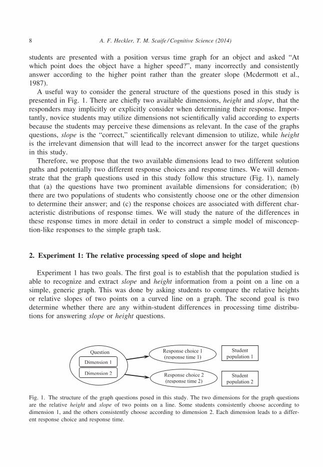
A useful way to consider the general structure of the questions posed in this study is

presented in Fig. 1. There are chiefly two available dimensions, height and slope, that theresponders may implicitly or explicitly consider when determining their response. Impor-

tantly, novice students may utilize dimensions not scientifically valid according to experts

because the students may perceive these dimensions as relevant. In the case of the graphs

questions, slope is the “correct,” scientifically relevant dimension to utilize, while heightis the irrelevant dimension that will lead to the incorrect answer for the target questions

in this study.

Therefore, we propose that the two available dimensions lead to two different solution

paths and potentially two different response choices and response times. We will demon-

strate that the graph questions used in this study follow this structure (Fig. 1), namely

that (a) the questions have two prominent available dimensions for consideration; (b)

there are two populations of students who consistently choose one or the other dimension

to determine their answer; and (c) the response choices are associated with different char-

acteristic distributions of response times. We will study the nature of the differences in

these response times in more detail in order to construct a simple model of misconcep-

tion-like responses to the simple graph task.

2. Experiment 1: The relative processing speed of slope and height

Experiment 1 has two goals. The first goal is to establish that the population studied is

able to recognize and extract slope and height information from a point on a line on a

simple, generic graph. This was done by asking students to compare the relative heights

or relative slopes of two points on a curved line on a graph. The second goal is two

determine whether there are any within-student differences in processing time distribu-

tions for answering slope or height questions.

Student population 1

Student population 2

Response choice 1(response time 1)

Response choice 2(response time 2)

Dimension 1

Question

Dimension 2

Fig. 1. The structure of the graph questions posed in this study. The two dimensions for the graph questions

are the relative height and slope of two points on a line. Some students consistently choose according to

dimension 1, and the others consistently choose according to dimension 2. Each dimension leads to a differ-

ent response choice and response time.


2.1. Method

2.1.1. ParticipantsEighteen undergraduates enrolled in an undergraduate calculus-based introductory

physics class participated, receiving partial credit for participation.

2.1.2. Materials, design, and procedureTesting was presented to individual participants on a computer screen in a quiet room.

Participants were presented with examples depicting various position time curves for a

car (e.g., Appendix A). For each graph, two points on the curve were marked, indicating

the position and time of the car at two different times. Participants were asked to deter-

mine as quickly as they could without making a mistake either which point was higher,

or at which point the slope was greater. The test was administered in blocks of nine ques-

tions of the same type (compare height or compare slope). Question type blocks were

presented in an alternating sequence, with two blocks for each question type, for a total

of four blocks (36 questions), each with a set but random order of questions.

2.2. Results and discussion

Students successfully answered both slope and height questions. The mean score for the

compare-height and the compare-slope questions was >97% for both types. Because the

response times in the first two blocks were initially relatively high and decayed to an

asymptote within 3–4 questions and the times were near a steady asymptote in the final

two blocks, we only compared the response times in the third and forth blocks. The mean

response time was significantly lower for the compare-height questions (M = 788 ms) ver-

sus the compare-slope questions (M = 1,216 ms), paired-sample t(17) = 7.04, p < .001,

d = 1.28.

In order to more carefully parameterize the shape of the response time distributions for

each condition by more than just the mean, we fit the curves to an ex-Gaussian function,

which has been demonstrated to be a useful fit to response time curves for a variety of

tasks (Balota & Yap, 2011; Heathcote et al., 1991; Ratcliff & Murdock, 1976). This

method will allow us to disambiguate factors that contribute to the shape of the curve as

well as quantitatively parameterize and compare curves. The ex-Gaussian function is a

combination of a Gaussian and exponential decay function:

f t; l; s; rð Þ ¼ er2

2s2�t�l

s

� �s

ffiffiffiffiffiffi2p

pZ t�l

r �rs

�1e�

y2

2 dy

The parameter l can be thought of as the peak of the distribution, s as the decay con-

stant for the tail of the distribution, and r as contributing to the width. For data that per-

fectly fits the ex-Gaussian distribution, the mean, M, is given by M = l + s, and the

variance by s2= r2 + s2.


We applied maximum likelihood methods to the observed response times to find esti-

mates of the three parameters, presented in Table 1. Standard errors of the parameter esti-

mates were computed using the Fisher information matrix (Lehman & Casella, 1998).

The results in Fig. 2 and Table 1 provide a clear indication that the peak, variance,

decay and mean times are larger for the slope comparison task compared to the height

comparison task. In sum, the results establish that the participants are able to compare

slopes and heights of points on a simple graph, but in this context it takes significantly

longer to compare the slopes at two points on a line than to compare the heights.

2.3. Caveat for data analysis

There is one important caveat to the ex-Gaussian fitting employed for all of the

response time data in this paper. Typically, parameters are fit for a single participant indi-

vidually, and this is the usual assumption of response time models, such as information

accumulation models. Here, we will determine parameters for populations of students,

Table 1

Experiments 1, 2, 4, and 5 response time results, in milliseconds (SE in parentheses)

Group Response Mean

MLE of ex-Gauss. Parameters

l s r

Experiment 1

Compare height Correct 727 (21) 553 (10) 175 (18) 37 (8)

Compare slope Correct 1,140 (30) 877 (43) 262 (46) 205 (30)

Experiment 2

Math Incorrect – – – –Math Correct 2,949 (80) 1,360 (47) 1,566 (82) 316 (38)

Kinematics Incorrect 3,457 (203) 946 (82) 2,418 (192) 259 (65)

Kinematics Correct 3,826 (101) 1,711 (71) 2,081 (115) 528 (57)

Elec. potential Incorrect 2,553 (180) 631 (26) 1,890 (143) 35 (23)

Elec. potential Correct 3,662 (208) 1,168 (149) 2,425 (230) 464 (135)

Experiment 4

Control Incorrect 3,053 (171) 453 (63) 2,508 (162) 222 (52)

Control Correct 3,215 (138) 1,139 (98) 2,041 (150) 593 (75)

Example tr. Incorrect 1,295 (106) 510 (54) 764 (102) 49 (55)

Example tr. Correct 2,077 (89) 963 (37) 1,099 (82) 145 (30)

Experiment 5

Control Incorrect 2,922 (161) 609 (37) 2,248 (131) 157 (27)

Control Correct 4,482 (146) 1,574 (69) 2,825 (158) 332 (58)

Example tr. Incorrect 1,620 (147) 712 (26) 799 (109) 35 (55)

Example tr. Correct 2,202 (96) 1,018 (48) 1,159 (97) 159 (42)

Rule tr. Incorrect 2,829 (368) 863 (118) 1,831 (333) 104 (104)

Rule tr. Correct 3,213 (166) 1,414 (83) 1,751 (154) 281 (70)

Note. The small number of incorrect responses in the Experiment 2 Math condition resulted in inconclusive

values for the parameters shown.


assuming that this measures average values for response time parameters. Ratcliff (1979)

describes a way to “Vincent average” response time curves for groups of students which

has the advantage of tending to preserve the functional shape of the curve and having

group parameter values which are the averages of the parameter values of individual par-

ticipants. However, the number of trials per student (8) in this study makes this method

marginal at best. Therefore, we simply pooled the data in order to have a large enough

set to reliably perform maximum likelihood estimations. Naturally, simple pooling of

response time data will have some confounding effect on the shape and the parameter

values determined. Nonetheless, most of the differences in response time curves in the

experiments here are large enough to maintain confidence in the ultimately qualitative

conclusions made from this study. Cleary, improvements to this study would include

increasing the number of within-student trials so that techniques such as Vincent averag-

ing would decrease the uncertainty in parameter values.

3. Experiment 2: Response choices and response times to physics graph questions

Experiment 2 consists of a preliminary Experiment 2a and the main Experiment 2b,

which were designed to achieve three goals. The first goal is to demonstrate misconcep-

tion-like response patterns relating to the well-known slope-height confusion for a set of

physics graph questions. That is, the goal is to demonstrate that a significant subpopula-

tion of students consistently answer a given set of similar graph questions according to

height when the correct response requires answering according to slope.The second and most important goal of this experiment is to determine whether there

are patterns of response times associated with patterns in response choices. Specifically,

were response times corresponding to incorrect responses faster or slower than correct

response times?

0.0

0.1

0.2

0.3

0.4

0 1000 2000 3000

Prop

ortio

n of

reps

onse

s

Response time (ms)

Height comparison dataSlope comparison dataHeight comp. ex-Gauss fitSlope comp. ex-Gauss fit

Fig. 2. Experiment 1 response time distributions for height and slope comparison tasks. Maximum likelihood

fits to an ex-Gaussian function for each task is included.


The third goal is to examine the extent to which student familiarity with the question

influences the response choices and the response times. Experiment 1 demonstrated that

when students were asked to compare either “slopes” or “heights” on a line on a simple

graph, they had no difficulty. And yet it is well-documented that students have a slope-

height confusion with physics graph questions; therefore, lack of familiarity may play a role

in the confusion. For an unfamiliar question context, students may fail to recognize that the

quantity of interest (such as speed) is associated with slope on the graph, and instead base

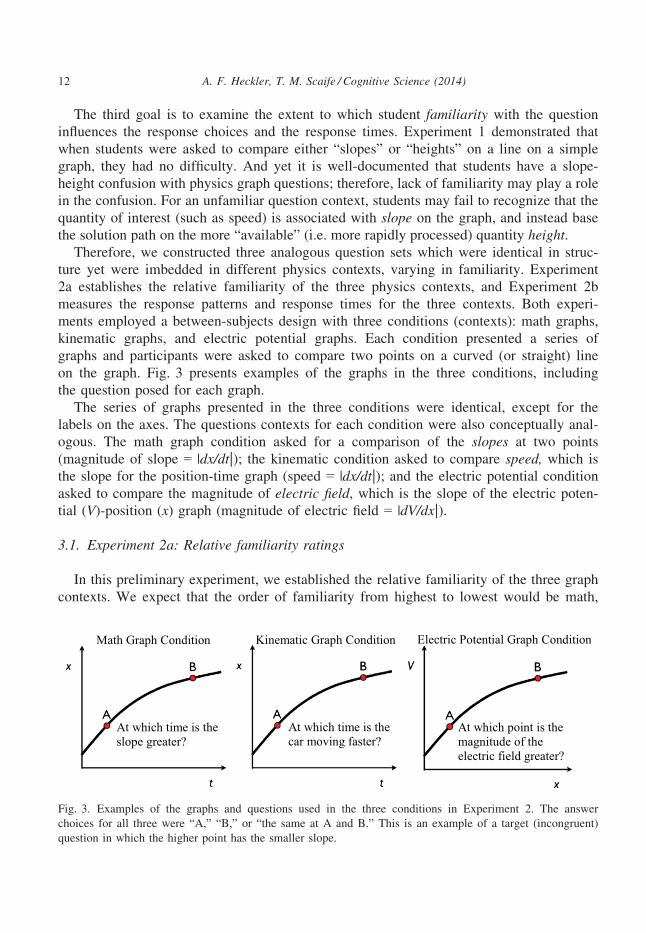
the solution path on the more “available” (i.e. more rapidly processed) quantity height.Therefore, we constructed three analogous question sets which were identical in struc-

ture yet were imbedded in different physics contexts, varying in familiarity. Experiment

2a establishes the relative familiarity of the three physics contexts, and Experiment 2b

measures the response patterns and response times for the three contexts. Both experi-

ments employed a between-subjects design with three conditions (contexts): math graphs,

kinematic graphs, and electric potential graphs. Each condition presented a series of

graphs and participants were asked to compare two points on a curved (or straight) line

on the graph. Fig. 3 presents examples of the graphs in the three conditions, including

the question posed for each graph.

The series of graphs presented in the three conditions were identical, except for the

labels on the axes. The questions contexts for each condition were also conceptually anal-

ogous. The math graph condition asked for a comparison of the slopes at two points

(magnitude of slope = |dx/dt|); the kinematic condition asked to compare speed, which is

the slope for the position-time graph (speed = |dx/dt|); and the electric potential condition

asked to compare the magnitude of electric field, which is the slope of the electric poten-

tial (V)-position (x) graph (magnitude of electric field = |dV/dx|).

3.1. Experiment 2a: Relative familiarity ratings

In this preliminary experiment, we established the relative familiarity of the three graph

contexts. We expect that the order of familiarity from highest to lowest would be math,

At which time is the slope greater?

Math Graph Condition

At which time is the car moving faster?

Kinematic Graph Condition

At which point is the magnitude of the electric field greater?

Electric Potential Graph Condition

Fig. 3. Examples of the graphs and questions used in the three conditions in Experiment 2. The answer

choices for all three were “A,” “B,” or “the same at A and B.” This is an example of a target (incongruent)

question in which the higher point has the smaller slope.


kinematic, and electric potential graphs. Math graphs are likely to be most familiar

because such generic graphs and the concept of slope are commonly introduced in stan-

dard curricula before and throughout high school and in college math. Next, kinematic

graphs are typically introduced in high school physical science courses and used frequently

in the prerequisite university-level physics course (mechanics). Finally, electric potential

graphs would likely be the least familiar, since most participants likely saw them for the

first time in the physics course in which they were enrolled at the time of the study.

Sixty-three students enrolled in the second course of introductory calculus-based phys-

ics (electromagnetism) were randomly assigned to one of three graph contexts, receiving

partial credit for participation. In a pencil and paper task, students were asked to answer

one of three graphs questions in Fig. 3. Next, they were asked, “How would you rank

your familiarity with the question above?” and given a scale of 1 (Not at all familiar) to

5 (Very familiar).

The familiarity ratings are presented in Table 2, and the trends follow the expected pat-

tern, with math graph rated as the most familiar and electric potential graphs rated as least

familiar. The three familiarity ratings are significantly different, F(2, 62) = 27.8, p < .001,

and a post hoc Bonferroni adjusted comparison reveals significant differences between the

mean familiarity rating of the electric potential graphs and the math graphs (p < .001,

d = 2.3) and between electric potential graphs and the kinematic graphs (p < .001,

d = 1.4); however, there was no reliable difference between mean rating of math graphs

and the kinematic graphs (p = .40, d = .5), though the means followed the expected trend.

In addition, in the electric potential graph condition a comparison of the mean famil-

iarity ratings according to score on the question (about 70% answered correctly) revealed

a significant difference in the familiarity ratings of students answering correctly

(M = 3.3) versus students answering incorrectly (M = 2.3), t(20) = .005, d = 1.4. In the

other two conditions, <10% of students answered incorrectly, preventing any meaningful

comparison; however, these few that answered incorrectly also chose the lowest familiar-

ity rating recorded in their condition. These results indicate that students answering incor-

rectly (consistent with answering according to height rather than slope) tend to be those

who are least familiar with the question.

3.2. Experiment 2b: Response choices and response times

3.2.1. ParticipantsThe participants were primarily engineering majors enrolled in one of two undergradu-

ate calculus-based introductory physics courses that comprise a sequence covering

Table 2

Mean familiarity ratings of the three studied question contexts

Condition Mean (SE) Familiarity Rating n

Math graph 4.71 (0.12) 21

Kinematic graph 4.35 (0.18) 20

Electric potential graph 3.05 (0.19) 22


classical mechanics and electromagnetism. Participants received partial course credit for

participation which was >95% of all students enrolled in course (about 350 each course).

Only some of these students, chosen randomly, participated in this particular study.

Participants were assigned to one of three conditions. For the math graphs condition,

28 participants were chosen from the mechanics course and 49 from the electromagnetism

course, for a total of 77 participants. For the kinematics graphs condition, 94 participants

were chosen from the mechanics course. For the electric potential graphs condition, 38

students were chosen from the electromagnetism course.

3.2.2. Procedure, materials, and designAll testing was presented to individual participants on a computer screen in a quiet

room. They proceeded through testing at their own pace, and their response choices and

response times were electronically recorded.

In each condition participants were presented with a series of graphs and asked to

compare the slopes, speed, or electric field at two points on each graph, such as in Fig. 3.

Participants were given no feedback as to the correctness of their answers. Once they

answered a question, the next question was immediately displayed on the screen.

The question set contained 16 graphs with various line shapes on which two points

were placed for the comparison task (see Appendix B). Each graph could be placed in

one of four categories. First, there were 10 graphs of various shapes in which the higher

point had a lower slope. These are the “incongruent” target questions, and are of the most

interest because they represent the archetypical difficult question, where the relative

slopes and heights conflict. Second, there were two graphs in which the higher point had

a higher slope (“congruent” questions). Students might be expected to answer these cor-

rectly since relative slope and height are in accord. Third, there were two graphs in which

both points had the same slope but different heights, and finally there were two graphs in

which the two points had the same height but different slopes. These last two graph types

could be considered special cases of “incongruent” questions. The response choices and

response times for these last two question types were similar to the target questions, but

for purposes of focusing on the target question type, were not included in the analysis

below. All four kinds of graphs were included to provide some variety in the graphs and

the responses, and to mimic more closely a natural test environment.

The 16 graphs were placed in a fixed random order for all participants in all condi-

tions. Experiment 4 uses a design to counterbalance for order, with similar results to

Experiment 2. Therefore, we are confident that the results here are not an artifact of ques-

tion order. The graphs were constructed such that the correct response was sometimes

“A” or “B” or “Equal,” and the correct answer was not always the lower or higher point

or the point on the right or left.

3.2.3. Results: Analysis of response choicesWe will focus on the performance on the “incongruent” target questions, namely those

graphs in which the higher point has a lower slope. These type of questions are important


for investigating graph difficulties, since the correct answer choice is opposite of the com-

mon “misconception” that, for example, “the higher point has greater speed.”

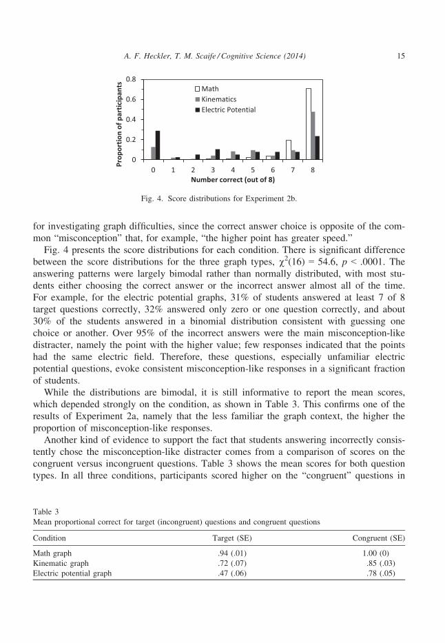
Fig. 4 presents the score distributions for each condition. There is significant difference

between the score distributions for the three graph types, v2(16) = 54.6, p < .0001. The

answering patterns were largely bimodal rather than normally distributed, with most stu-

dents either choosing the correct answer or the incorrect answer almost all of the time.

For example, for the electric potential graphs, 31% of students answered at least 7 of 8

target questions correctly, 32% answered only zero or one question correctly, and about

30% of the students answered in a binomial distribution consistent with guessing one

choice or another. Over 95% of the incorrect answers were the main misconception-like

distracter, namely the point with the higher value; few responses indicated that the points

had the same electric field. Therefore, these questions, especially unfamiliar electric

potential questions, evoke consistent misconception-like responses in a significant fraction

of students.

While the distributions are bimodal, it is still informative to report the mean scores,

which depended strongly on the condition, as shown in Table 3. This confirms one of the

results of Experiment 2a, namely that the less familiar the graph context, the higher the

proportion of misconception-like responses.

Another kind of evidence to support the fact that students answering incorrectly consis-

tently chose the misconception-like distracter comes from a comparison of scores on the

congruent versus incongruent questions. Table 3 shows the mean scores for both question

types. In all three conditions, participants scored higher on the “congruent” questions in

0

0.2

0.4

0.6

0.8

0 1 2 3 4 5 6 7 8

Prop

ortio

n of

par

ticip

ants

Number correct (out of 8)

MathKinematicsElectric Potential

Fig. 4. Score distributions for Experiment 2b.

Table 3

Mean proportional correct for target (incongruent) questions and congruent questions

Condition Target (SE) Congruent (SE)

Math graph .94 (.01) 1.00 (0)

Kinematic graph .72 (.07) .85 (.03)

Electric potential graph .47 (.06) .78 (.05)


which the relative slopes and heights led to the same (correct answer), compared to the

incongruent questions in which the relative slopes led to the correct answer and the

heights led to the incorrect answer (paired t-tests, ps < .003). These results and the ques-

tion types are similar in structure to the Stroop task and will be discussed in the General

Discussion.

3.2.4. Results: Analysis of response timesWe present the response time results in two ways. First, to provide a picture of the

scale and dynamics of the response times, we present trial-by-trial median response times

for each condition in Fig. 5. As expected, the figure shows a typical and expected rapid

decrease in response times for the first few questions, followed by a slow decrease (on

average) for the remaining questions. Roughly speaking, the median response times range

between 7 and 15 s for the few two responses, and range between 2 and 4 s for the last

13 questions. To characterize a central value of the distributions, we use the median time

to reduce effects of outliers (Ratcliff, 1993). Fig. 5 demonstrates that the evolution of the

median response times for the three conditions were roughly similar in shape and magni-

tude. However, there was a difference in averages of the median response times for the

last 13 questions between the three conditions, F(2) = 10.4, p < .001. Specifically, a post

hoc analysis reveals that the median response times are smaller for the electric potential

graph condition (M = 2,305 ms) compared to the kinematic graph condition

(M = 3,311 ms), Bonferroni adjusted p < .001, d = 1.8 and compared to the math graphs

condition (M = 3,091 ms), Bonferroni adjusted p = .006, d = 1.6. Therefore, averaged

over all responses, the least familiar question type was answered the most rapidly.

Since both the scores and the familiarity ratings of electric potential graph questions

were significantly lower compared to the other two graph question types, this suggests

that the lower average response times for this condition may be due to the possibility that

incorrect responses had faster response times. Therefore, we analyzed the response time

data a second way: By comparing the response times of correct versus incorrect answers

for the last 8 of 10 target questions (when the response times are “settled” into roughly

0

4000

8000

12000

16000

1 2 3 4 5 6 7 8 9 10

Med

ian

Resp

onse

Tim

e (m

s)

Question number

Math GraphsKinematic GraphsElectric Pot. Graphs

Fig. 5. Experiment 2b median response times for the first 10 questions. The response times leveled off

quickly after 2 questions.


asymptotic means). Fig. 6 presents the distribution of these response times for each con-

dition, separated out by response times for correct and incorrect responses. In addition,

Table 1 presents the three fitted response curve parameters (l, s, r) and the means for

correct and incorrect responses for each graph type.

The most important result from the data presented in Fig. 6 and Table 1 is that

response times for incorrect answers are faster than response times for correct answers

for the kinematic and electric potential graphs conditions (Mann–Whitney U test used

because of long tails in distribution, ps < .0001). This difference is highlighted via the

peaks of the distributions, as measured by l in Table 1. The peaks of the distributions for

correct answers are around 1,100–1,700 ms. For incorrect answers, the peaks are around

600–900 ms; hence, the incorrect answers are about 500–700 ms earlier than for the cor-

rect answers. There are so few incorrect responses for the math graphs that no reliable

comparisons can be made for that case. Interestingly, unlike the score results, there does

not appear to be any large or systematic trends in correct and incorrect response times

that correlate the familiarity ratings.

0

0.05

0.1

0.15

0.2

0.25

0 2000 4000 6000 8000 10000

Prop

ortio

n of

resp

onse

s

Correct MathIncorrect Math

0

0.05

0.1

0.15

0 2000 4000 6000 8000 10000

Prop

ortio

n of

resp

onse

s

Correct Kinematics

Incorrect Kinematics

0

0.05

0.1

0.15

0.2

0 2000 4000 6000 8000 10000

Prop

ortio

n of

resp

onse

s

Response time (ms)

Correct Electric Potential

Incorrect Electric Potential

Fig. 6. Experiment 2b response time distributions for correct and incorrect answers to target questions for all

three question contexts. The total number of correct or incorrect answers for each condition is proportional to

the area under each curve.


Note the caveat mentioned earlier that the response times for both between student and

within student data were pooled together. Since the majority of students answered virtu-

ally all questions either correctly or incorrectly, one could interpret the difference

between the correct and incorrect response times in two (nonmutually exclusive) ways.

First, the difference may be due to some fundamental difference between the two popula-

tions in processing speeds for the two solution paths. Second, the populations may have

similar solution path processing speeds, but they are simply utilizing different solution

paths. While we will not rule out the first possibility, we provide evidence supporting the

second and assume this interpretation is valid. For example, Experiment 1 demonstrated

that all students can compare slopes and heights, and that, within-student, processing

height is faster than slope (for this task). In addition, Fig. 2 does not show any evidence

of two populations, such as bimodal peaks. Other evidence will come from experiments

3–5 which will demonstrate that changing the question context or kind of training

changes the response choices and response times in ways that are consistent with the

assumption that there is not a fundamental difference in slope and height processing

speeds between student populations.

4. Experiment 3: Imposing a delay in responding

The results of Experiments 1 and 2 demonstrate that response times of misconception-

like responses were shorter than those of correct responses, and the underlying task nec-

essary for determining the misconception-like response (comparing heights) took less time

than the task necessary for determining the correct response (comparing slopes). Further-

more, as familiarity with graph context decreased, the misconception-like response pat-

terns increased. A simple explanation for these results is that students who are unfamiliar

with a particular graph context use height as the default dimension to base a response,

and because height happens to be processed faster, the response times are relatively short.

However, we propose a more causal rather than coincidental relationship between the

response choice and the relative processing time of the available dimensions. That is, let

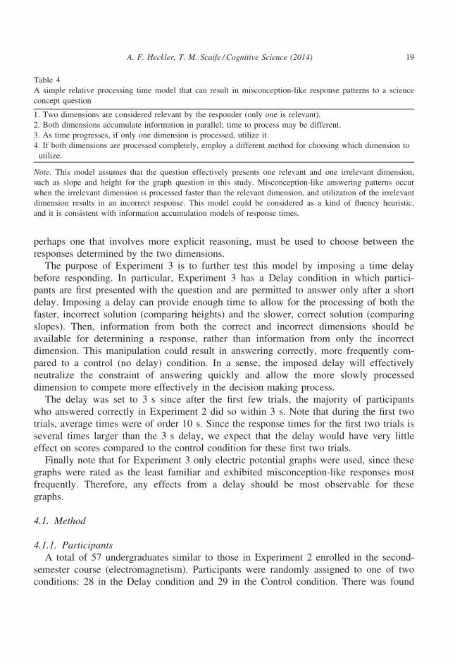
us consider the relative processing time model discussed in the introduction as the causeof the incorrect response choices. The outline of this model is shown in Table 4. In this

model, we assume an implicit goal to answer quickly. For the task in this study, we pro-

pose that students unfamiliar with the question context will implicitly consider both

height and slope as sufficiently plausible dimensions for determining the answer. The

model assumes separate information accumulators for each dimension. Experiment 1 sug-

gests that the height accumulator reaches its critical boundary faster than the slope accu-

mulator (for the graph questions studied). Since the height is processed faster, the

responder (who is biased to answer rapidly) will tend to base the response on height,

which is incorrect. As for the slope dimension, this information requires more time to

process, and the response may often be already completed before the slope accumulator

reaches its critical level and is thus excluded from the response. If for some reason both

processes are completed before the response is set, then some other decision process,


perhaps one that involves more explicit reasoning, must be used to choose between the

responses determined by the two dimensions.

The purpose of Experiment 3 is to further test this model by imposing a time delay

before responding. In particular, Experiment 3 has a Delay condition in which partici-

pants are first presented with the question and are permitted to answer only after a short

delay. Imposing a delay can provide enough time to allow for the processing of both the

faster, incorrect solution (comparing heights) and the slower, correct solution (comparing

slopes). Then, information from both the correct and incorrect dimensions should be

available for determining a response, rather than information from only the incorrect

dimension. This manipulation could result in answering correctly, more frequently com-

pared to a control (no delay) condition. In a sense, the imposed delay will effectively

neutralize the constraint of answering quickly and allow the more slowly processed

dimension to compete more effectively in the decision making process.

The delay was set to 3 s since after the first few trials, the majority of participants

who answered correctly in Experiment 2 did so within 3 s. Note that during the first two

trials, average times were of order 10 s. Since the response times for the first two trials is

several times larger than the 3 s delay, we expect that the delay would have very little

effect on scores compared to the control condition for these first two trials.

Finally note that for Experiment 3 only electric potential graphs were used, since these

graphs were rated as the least familiar and exhibited misconception-like responses most

frequently. Therefore, any effects from a delay should be most observable for these

graphs.

4.1. Method

4.1.1. ParticipantsA total of 57 undergraduates similar to those in Experiment 2 enrolled in the second-

semester course (electromagnetism). Participants were randomly assigned to one of two

conditions: 28 in the Delay condition and 29 in the Control condition. There was found

Table 4

A simple relative processing time model that can result in misconception-like response patterns to a science

concept question

1. Two dimensions are considered relevant by the responder (only one is relevant).

2. Both dimensions accumulate information in parallel; time to process may be different.

3. As time progresses, if only one dimension is processed, utilize it.

4. If both dimensions are processed completely, employ a different method for choosing which dimension to

utilize.

Note. This model assumes that the question effectively presents one relevant and one irrelevant dimension,

such as slope and height for the graph question in this study. Misconception-like answering patterns occur

when the irrelevant dimension is processed faster than the relevant dimension, and utilization of the irrelevant

dimension results in an incorrect response. This model could be considered as a kind of fluency heuristic,

and it is consistent with information accumulation models of response times.


no significant difference between the average course grades of participants in the Delay

(M = 2.13) versus Control (M = 2.21) conditions, t(53) = .45, p = .66, d = .08.

4.1.2. Procedure, materials, and designThe procedure was similar to Experiment 2b. Participants in both conditions were pre-

sented with the same graphs as in the electric potential graph condition in Experiment 2b.

However, in the Delay condition participants were presented a screen with the following

message: “On each slide, you will see a question with a message at the bottom of the

screen.” At first the message will read: “Take a moment to determine your answer.”

While this message is displayed, you will not be able to answer the question. After a cou-

ple of seconds, the message will change and prompt you for an answer. Please press the

key that corresponds to your answer at that time.” Participants were then given a simple

math-fractions problem as an example of the delay, and they proceded to the graph ques-

tions. Participants in the Control condition also received the initial practice simple math

fractions problem, but with no delay. In sum, the Control and Delay conditions were pre-

sented with the same questions as in Experiment 2b, but the students in the delay condi-

tion were required to wait 3 s before responding.


Similar to Experiment 2, we report here the results of the target incongruent questions.

Since there is a significant change in response times for the first couple of questions (e.g.

see Fig. 5), we analyzed the scores for the first two questions, which had an average

response time of approximately 16 s for both the control and delay condition (including

the 3 s delay), and the remaining 8 target questions which had an average response time

of approximately 4 s for both conditions, including the 3-s delay.

For the first two questions, there was a small but unreliable difference between the

scores in the Delay condition (M = 48%) and the Control (M = 40%), Mann–Whitney

U(55) = 366, Z = .76, p = .46, d = .19, as expected.

However, for the remaining questions participants in the Delay condition (M = 70%)

scored significantly higher than those in the Control condition (M = 47%), Mann–Whit-

ney test U(55) = 247, Z = 2.24, p = .025, d = .64. The score distribution for the two con-

ditions is shown in Fig. 7. Therefore, the delay had little if any effect for the first two

questions when the response times were much larger than the delay time, but the delay

did affect student responses once the response times were comparable to the delay time.

The difference in score between the Delay and Control conditions implies that a signif-

icant fraction of students were able to answer correctly if they were constrained to wait

before responding, but without this constraint, these students would choose the common,

fast misconception-like response. The improved score of the Delay condition provides

support for the hypothesis that misconception-like answers are influenced by a bias to

answer quickly, utilizing the dimension that is processed the fastest, to the exclusion of

more slowly processed dimensions.


One might also interpret the difference in answering between the conditions as due

some other cause. For example, in the Delay condition, the delay and the cue “take a

moment to determine your answer” might motivate the students to exert more effort in

finding the correct solution. However, if this explanation were valid, one would then

expect a significant increase in performance in the Delay condition for the first two ques-

tions as well, but this was not the case.

5. Experiment 4: Including repetitive training

In Experiment 3, the score improved when a short delay in responding was imposed.

This was interpreted as providing time for both fast-incorrect and slow-correct dimensions

to be processed, allowing the two dimensions to compete for the response. In Experiment

4, we improve scores a different way: by providing training prior to the test. The question

then becomes, if training improves scores, does it also change the relative response times

between correct and incorrect answering? According to the relative processing time model,

one way to improve scores would be to decrease the processing time of the correct response

relative to the processing time of the incorrect response. According to the model, one might

reasonably expect that training has the effect of speeding up the processing of the dimen-

sion associated with the correct response so that it may better compete with the dimension

associated with the incorrect response. Experiment 4 investigates this possibility.

Therefore Experiment 4 has two main goals. First, it is to replicate the results of Experi-

ment 3, namely that an imposed delay improves scores. Second, it is to determine whether

training that improves scores also decreases the relative response times (from which we

infer processing times) of correct versus incorrect answers compared to no training.

5.1. Method

5.1.1. ParticipantsA total of 138 undergraduates similar to the population in Experiment 3. Participants

were randomly assigned to one of three conditions: 35 in the Example training condition,

0

0.1

0.2

0.3

0.4

0.5

0 1 2 3 4 5 6 7 8

Prop

ortio

n of

Par

ticip

ants

Number correct (out of 8)

ControlDelay

Fig. 7. Experiment 3 score distribution for the last eight target questions, when average response times were

of the same order as the 3s delay.


37 in the Delay condition, and 35 in the Control condition. There was no significant dif-

ference between the average course grades of participants in the Example training

(M = 2.66), Delay (M = 2.82), and Control (M = 2.64) conditions, F(2, 135) = .37,

p = .69.

5.1.2. Procedure, materials, and designThe procedure was similar to Experiment 3, with two exceptions. First, we added a

condition that included training prior to the test. Second, in order to address a concern in

the design of Experiments 2 and 3, we counterbalanced the test for question order by

having two (random) test orders. The two test orders were the same for each condition.

A critical goal of the Example training condition was to improve the scores on the tar-

get questions by providing multiple practice trials with feedback on simple examples sim-

ilar to the target questions. This training condition was based on some of our related pilot

studies in which this training sequence was found to be effective in improving scores on

the target questions. In the Example training condition participants were presented a ser-

ies of 32 graph questions with immediate feedback (providing the correct answer) after

each response (see Appendix C). The training questions were similar to the target (incon-

gruent) test questions in that the text of the question is the same as the test question (At

which point is the electric field greater?), but the graphs were slightly different. The train-

ing questions consisted of graphs with two points (on a curved line) at the same height

but different slopes and graphs with two points on a curve line, with one point higher

and having a higher slope. The average score for the entire training condition was 86%,

indicating they learned the task, and the average time to complete training was approxi-

mately 2 min. Between training and the test was an unrelated task lasting between 5 and

10 min.


5.2.1. Analysis of scoresAs done in Experiment 3, we will separately consider the scores for the first two ques-

tions and for the last eight. Similar to Experiment 3, as expected, the average score for

the Delay condition (M = 60%) was not reliably higher than for the Control (M = 51%),

Mann–Whitney test U(103) = 1,351, Z = .99, Bonferroni adjusted p = .68, d = .21. How-

ever, there was a larger difference between the Example training (M = 71%) and Control

(M = 51%) scores for the first two questions, Mann–Whitney test U(101) = 862,

Z = 2.25, Bonferroni adjusted p = .05, d = .5. This is also expected, since the training

should improve scores on all of the test questions.

The score distributions for the remaining target questions reveal that the scores of the

three conditions were different, Kruskal–Wallis K(2) = 10.2, p = .006. In a replication of

Experiment 3, the Delay condition (M = 70%) scored higher than those in the Control

condition (M = 51%), Mann–Whitney test U(103) = 1,527, Z = 2.18, Bonferroni adjusted

p = .06, d = .48. Furthermore, the Train condition (M = 75%) scored higher than the

Control (M = 51%), Mann–Whitney test U(101) = 771, Z = 2.87, Bonferroni adjusted


p = .008, d = .6. In sum, the increase in scores due to an imposed delay in responding

was replicated, and there was also an increase in scores due to repetitive example prac-

tice, as expected.

5.2.2. Analysis of response timesThe response time distributions and the ex-Gaussian fitted parameters for the two con-

ditions are presented in Fig. 8 and Table 1. The Fisher matrix estimates of the standard

errors as well as visual inspection of the graphical distributions allow us to make reason-

ably reliable inferences about trends in the data. For example, the data reveal that training

had a clear overall effect of reducing the mean response times by over 1 s compared to

the Control condition. An examination of the fitted parameters reveals that this reduction

was predominantly in the reduction of the “decay” times s for both correct and incorrect

responses, and there was also a small reduction in the “width” r.However, the result of most interest to this study arises from the peaks of the distribu-

tions, as parameterized by l. The data indicate that training did not significantly change

the peak response time for the incorrect responses, but training did significantly decrease

the peak response time for correct responses. The difference between the peak times for

incorrect responses for the Example training (l = 510 ms) and Control (l = 453 ms)

conditions is 57 ms, which is within the pooled standard error of the peak times for

incorrect responses (59 ms). However, the peak-time difference for correct responses for

0

0.05

0.1

0.15

0.2

0 2000 4000 6000 8000 10000

Prop

. of r

espo

nses

Control correctControl incorrect

0

0.1

0.2

0.3

0.4

0 2000 4000 6000 8000 10000

Prop

. of r

espo

nses

Response time (ms)

Example train correctExample train incorrect

Fig. 8. Experiment 4 response time for the Control and Examples training conditions. Training reduced the

difference in incorrect versus correct response times compared to control.


the Example training (l = 963 ms) and Control (l = 1,139 ms) is 176 ms, which is more

than twice as large as the pooled standard error for correct responses (74 ms).

In other words, training decreased the difference in the peak response times between

correct and incorrect responses (453 ms) compared to the difference for control (686 ms).

This reduction in the difference between the peak-times for the correct versus incorrect

responses is also evident from the response time distributions in Fig. 8.

In sum, the data provide support for the relative processing time model in that training

not only improved scores, but it also reduced the relative peak response time between the

correct and incorrect responses. In particular, the incorrect peak times did not change, but

the correct peak times were reduced by training. These results strengthen the idea that

this particular kind of training resulted in more correct responses by reducing the process-

ing time of the dimension associated with the correct response, thereby allowing it to bet-

ter compete with the dimension associated with the incorrect answer choice.

6. Experiment 5: Repetitive training versus rule training

The relative processing time model (Table 4) proposes that incorrect responders con-

sider both the relevant and irrelevant dimensions and utilize the irrelevant dimension

because it is processed faster. How does the model account for correct responders?

Experiment 4 demonstrated that one way to increase the score is to decrease the process-

ing time of the relevant dimension via repetitive training such that the relevant dimension

competes better with the irrelevant dimension. In Experiment 5 we will investigate

another way implied by the relative processing model to increase the score, namely to

remove the irrelevant dimension from consideration for the response.

The irrelevant dimension will be suppressed from consideration by providing an expli-

cit general rule stating that only the relevant dimension must be used to respond cor-

rectly. The result should be an increase in score. However, one might not expect any

change in response time compared to control, since it is not clear that an explicit rule can

affect the processing time of the automatically processed relevant and irrelevant dimen-

sions. Both may still be processed, but only one is now considered for the response.

In addition, as noted in the discussion in Experiment 3, the improved scores in the

delay condition suggest that some student understand the task and may “know” the cor-

rect answer, but somehow do not choose it, perhaps because they have a priority to

answer quickly. We would like to test this possibility in another way by providing the

students with an explicit task to determine whether they can identify the correct (written)

rule for finding the answer. Experiments 3 and 4 suggest that there may be students who

can identify the correct written rule but do not use this rule in the graph task, perhaps

because they choose the faster-processed dimension instead of the correct, slower pro-

cessed dimension.

Therefore, Experiment 5 has three main goals. First, it is to replicate the results of

repetitive examples training in Experiment 4 to improve our confidence in the results.

Second, Experiment 5 will compare response times for repetitive example training with


explicit rule-based training to determine if the results agree with our relative processing

time model. Both kinds of training are expected to improve the average score. However,

as seen in Experiment 4 repetitive example training is expected to decrease the response

time of correct responses compared to control, yet rule training may not. Third, it is to

determine whether students who are answering incorrectly can nonetheless recognize the

correct written rule, thus supporting our hypothesis that something other than explicit

knowledge of the rule is playing a role in their response.

6.1. Method

6.1.1. ParticipantsA total of 71 undergraduates similar to the population Experiment 3. Participants were

randomly assigned to one of three conditions: 25 in the repetitive Example training condi-

tion, 22 in the Rule training condition, and 24 in the Control condition.

6.1.2. Procedure, materials, and designThe procedure was similar to Experiment 4, with the addition of a condition that

included Rule training prior to the test. The Rule training condition consisted of a simple

rule stating that the electric field can be determined from the slope of the electric poten-

tial versus position graph followed two multiple-choice comprehension questions with

corrective feedback (see Appendix D for the actual text used). This sequence was then

repeated once to better ensure learning of the rule. All students in this condition indi-

cated “yes” when prompted whether they understood the rule, with average score was

91% on the two multiple-choice questions, indicating that the student successfully

learned the rule. Testing on the target questions followed directly after training on the

rule.

We also added a multiple-choice question at the end of the graphs tasks which asked

students to choose which explicit rule would determine the correct response. This ques-

tion was used to determine whether students had some level of explicit understanding of

the graph tasks and could identify the correct rule, namely that a comparison of slopesdetermines the correct response.


6.2.1. Analysis of scoresThe score distributions on the (last eight) target questions for all three conditions are

shown in Fig. 9. As expected, both training conditions improved the average score. The

Example training condition (M = 78%) scored higher than those in the Control condition

(M = 53%), Mann–Whitney test U(71) = 178, Z = 2.6, Bonferroni adjusted p = .018,

d = .58. Furthermore, the Rule training condition (M = 83%) scored higher than the Con-

trol (M = 53%), Mann–Whitney test U(71) = 144.5, Z = 2.8, Bonferroni adjusted

p = .012, d = .75.


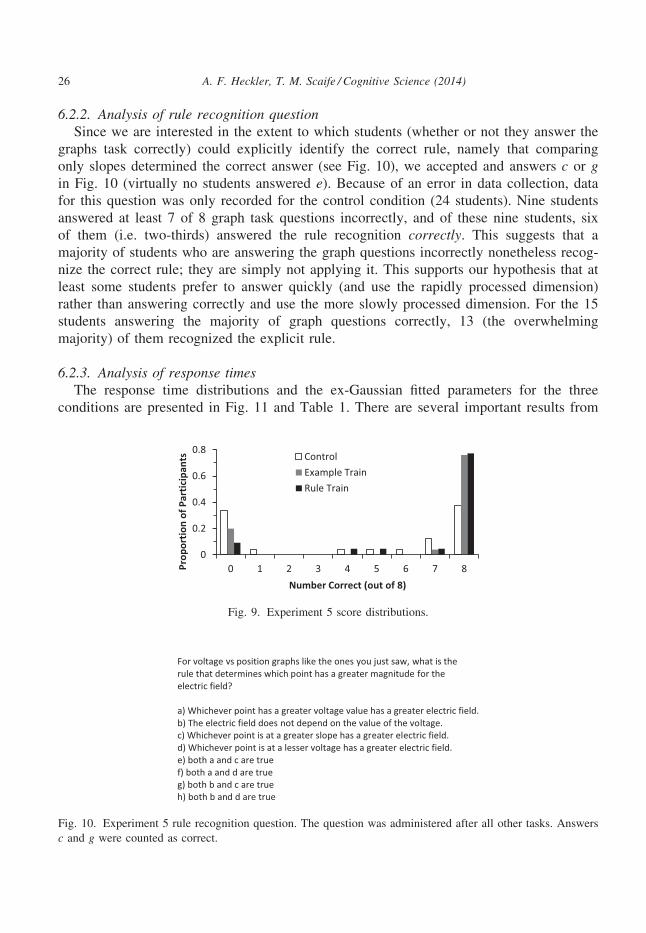
6.2.2. Analysis of rule recognition questionSince we are interested in the extent to which students (whether or not they answer the

graphs task correctly) could explicitly identify the correct rule, namely that comparing

only slopes determined the correct answer (see Fig. 10), we accepted and answers c or gin Fig. 10 (virtually no students answered e). Because of an error in data collection, data

for this question was only recorded for the control condition (24 students). Nine students

answered at least 7 of 8 graph task questions incorrectly, and of these nine students, six

of them (i.e. two-thirds) answered the rule recognition correctly. This suggests that a

majority of students who are answering the graph questions incorrectly nonetheless recog-

nize the correct rule; they are simply not applying it. This supports our hypothesis that at

least some students prefer to answer quickly (and use the rapidly processed dimension)

rather than answering correctly and use the more slowly processed dimension. For the 15

students answering the majority of graph questions correctly, 13 (the overwhelming

majority) of them recognized the explicit rule.

6.2.3. Analysis of response timesThe response time distributions and the ex-Gaussian fitted parameters for the three

conditions are presented in Fig. 11 and Table 1. There are several important results from

0

0.2

0.4

0.6

0.8

0 1 2 3 4 5 6 7 8Prop

ortio

n of

Par

ticip

ants

Number Correct (out of 8)

ControlExample TrainRule Train

Fig. 9. Experiment 5 score distributions.

For voltage vs position graphs like the ones you just saw, what is the rule that determines which point has a greater magnitude for the electric field?

a) Whichever point has a greater voltage value has a greater electric field.b) The electric field does not depend on the value of the voltage.c) Whichever point is at a greater slope has a greater electric field.d) Whichever point is at a lesser voltage has a greater electric field.e) both a and c are truef) both a and d are trueg) both b and c are trueh) both b and d are true

Fig. 10. Experiment 5 rule recognition question. The question was administered after all other tasks. Answers

c and g were counted as correct.


this data. First, a comparison of the peak times for the Control and Example training con-

ditions reveals results similar to Experiment 4. While there is a small difference (103 ms)

between the peak times for incorrect responses for the two conditions, there is a larger

and significant decrease of 556 ms in the peak time for the correct responses. This differ-

ence is much larger than the pooled standard error of the peak times (59 ms) for correct

responses of these two conditions. In other words, similar to Experiment 4, there was

reduction in the difference between correct and incorrect peak times for Example training

(306 ms) compared to the difference for the Control (965 ms).

The second and more important result is that Rule training affected the peak response

times less than the Example training. There are two ways to see this. First, Rule training

did not reduce the peak time for correct answers nearly as much as Examples training

did. For correct answers the peak for Rule training was only 160 ms less than Control,

which is only about twice the pooled standard error (76 ms) and is thus only marginally

significant. As stated above, Example training reduced the peak time by 556 ms, which is

much larger, about ten times the pooled standard error (59 ms). Second, Rule training did

not reduce the difference between correct and incorrect peak times as much as Example

training did. For Rule training, the difference between correct and incorrect peak times is

551 ms, which is larger than the 315 ms difference for Example training (though it is still

smaller than the 965 ms difference for Control).

In sum, while Rule and Example training both increased scores on target questions to

the same extent, they did not affect the response times similarly. In a replication of

Experiment 4, we found that Example training significantly reduced the peak response

time for correct answers and the difference between peak correct and incorrect times

compared to Control. In contrast, Rule training at most only marginally reduced the peak

times for correct responses and consequently did not reduce the difference between peak

correct and incorrect response time as much as Example training. These results are also

supported by inspecting the response time distributions in Fig. 11.

The results of the comparison between Examples and Rule training support our relative

processing time model, namely that Rule-based training increases the score by affecting

the dimensions considered for the response, but does not appear to significantly affect the

0

0.1

0.2

0.3

0 2000 4000 6000 8000 10000Prop

or�o

n of

Res

pons

es

Response �me (ms)

Control correctExample training correctRule training correct

Fig. 11. Experiment 5 response time distributions. Note that example training significantly reduces response

times while rule training only marginally reduces response times compared to control.


relative processing time, and the Example-based training does significantly affect the rela-

tive processing time, and this in turn affects the response choice.

7. General discussion and conclusions

There were two main objectives of this study. The first was empirical: to determine, in

various testing contexts, whether there may be interesting patterns of response times cor-

responding to response choices for science questions known to exhibit patterns of incor-

rect responses (i.e., misconception-like responses). The second was more theoretical: to

analyze the empirical results in light of existing response time explanations and mecha-

nisms and to test a simple model for misconception-like response choices and response

times that emerged in the course of the experimental results. The results are discussed

below.

7.1. Empirical results

All experiments in the study were administered after the relevant physics instruction to

students enrolled in an introductory physics class. The main empirical results of this study

are as follows:

1. When asked to compare “heights” or “slopes” on a simple graph, all students were

successful, and response times for comparing heights were faster than times for

comparing slopes (within student). (Experiment 1)

2. For a set of physics graph questions which asked for a comparison of a quantity rep-

resented by the slope, most students consistently either compared heights on the

graph (incorrect) or they compared slopes on the graph (correct). (Experiments 2–5)3. The lower the familiarity of the question context, the more likely a student would

consistently compare heights (incorrect) rather than slopes. (Experiments 2a, 2b)

4. The response times for the incorrect responses were faster than the correct

responses. (Experiments 2–5)5. Imposing a delay on the response increased the accuracy. (Experiments 3 and 4).

6. Example training increased accuracy and significantly decreased the difference

between correct and incorrect answer response times. (Experiments 4 and 5)

7. Explicit rule training increased accuracy but only marginally decreased time of cor-

rect response, still leaving a large difference between correct and incorrect response

times. (Experiment 5)

8. The majority of students answering the graphs task incorrectly could nonetheless

identify the correct explicit rule for determining the correct answer. (Experiment 5)

In sum, we have found interesting patterns in response times that correspond to

response choices to the simple but standard science concept question used in this study.

Note that the response times in this study are short, on the order of 1–3 s. These empiri-

cal results indicate that the relative processing time of relevant available dimensions may


play an important role in response patterns to science concept questions, and some stu-

dents appear to know the correct answer (or the correct rule) but answer incorrectly

because answering quickly is a high priority. Furthermore, these results highlight an inter-

esting difference between the effect of rule versus example training. While both kinds of

training increase the score, example training reduces the difference in processing time of

incorrect and correct responses more than rule training.

7.2. Explanations of empirical results

We have constructed a simple relative processing time model to help explain the mis-

conception-like patterns of incorrect answers and the corresponding response times to a

simple science concept question. The most important components of the model (see

Table 4) are (a) many students at least implicitly consider both relevant and irrelevant

dimensions available in the question, (b) as time progresses, if one and only one of these

dimensions is processed, then students will utilize this dimension, and (c) if more than

one dimension is processed, then some other mechanism must be used to choose between

them. This relative processing time model may be a result of an implicit priority to

respond quickly. As demonstrated in Experiments 3 and 4, some students are able to

respond accurately, but instead answer rapidly, even when there is no explicit constraint

or reason to do so. This is further supported in Experiment 5, in which it was demon-

strated that the majority of students answering incorrectly nonetheless recognized the cor-

rect explicit rule, but they simply were not applying it in this context in which a rapidly

processed but incorrect dimension is competing with a slower processed correct dimen-

sion.

7.2.1. The relative processing time model as a heuristicThis relative processing time model can be regarded as a kind of fluency heuristic

(Hertwig et al., 2008; Schooler & Hertwig, 2005) and is a more specific version of the

general idea of an availability heuristic (Kahneman, 2003; Tversky & Kahneman, 1973).

The core idea of the fluency heuristic is to place high value on speed, thus favoring the

solution that is processed the fastest. However, to fully explain misconception-like

answering, it is also necessary to assume that students will consider incorrect solution

paths and that these paths are faster than the correct paths. Furthermore, the fastest pro-

cessed solution is not always the one to be chosen, as evidenced by the improved scores

when a delay in responding was imposed. This result can be explained in terms of com-

petition. If at the time a solution is processed there are no other solutions processed, then

there is no competition, and this first-processed solution is utilized. However, if more

than one solution is processed before an answer is chosen, then these solutions must com-

pete, and the outcome of this competition must be determined via some other mechanism

(e.g., another heuristic). In a sense, the imposed delay might be interpreted as a kind of

forced disfluency (e.g., Alter, 2013), inducing the participant to use some other perhaps

more explicit process.


Besides imposing a delay in responding, this model implies two other ways to improve

scores, which we investigated in Experiments 4 and 5. The first is to speed up the pro-

cessing of the correct solution path via repeated practice. The second was employ explicit

rule training to remove the incorrect solution path from the student’s consideration, thus

denying the initial assumption of the model that both incorrect and correct solutions paths

are considered. This might therefore be seen as a demonstration of the dual processes or

two paths to the same solution (fast and automatic versus slow and controlled).

7.2.2. The relative processing time model as an information accumulation modelThe relative processing time model is also consistent with the general structure and

assumptions of more fine-grained information accumulation models often used to explain

and describe response time data, as discussed in the introduction. From this perspective,

information about the relevant and irrelevant dimension accumulates simultaneously, and

the accumulator that reaches its critical boundary first wins. Such models predict within-

student ex-Gaussian-like response time shapes, and they can describe the fairly compli-

cated phenomenon of response times for simple tasks with only a few parameters. Clearly

these response time models are at a fine grain level and would need to be adapted to the

more complex (e.g., multi-step) science question task studied here. This includes the need

to explain how decisions are made when both accumulators have reached the boundary.

7.3. Do students “Just not understand the task or the topic”?

The term understand is often poorly specified in education and the learning sciences.

For the science topics in this study, is understanding demonstrated by correctly answering

the graphs tasks in this study? Is it identifying the correct rule? Is it providing a detailed

verbal explanation? It is being able to answer quickly? All of these meaning are useful in

different circumstances. In educational practice, understanding is determined via instruc-

tors, who make inferences about “understanding” (e.g., the achievement of an instruc-

tional goal) based on student performance on an assigned task. Therefore it is important

to carefully characterize how students respond to typical test questions, such as the ones

in this study.

One might attempt to “explain” incorrect responses by saying that the incorrect

responders do not understand the task or the topic. However, this ambiguous statement

does not explain why there are patterns to their incorrect answers, or why incorrect

responders can identify the correct rule for the task, but do not apply it. In contrast, for

the relative processing time model explored here, the less familiar a student is with the

graph task, the more the relative processing time matters, and this is what produces the

pattern of incorrect answering. This model is consistent with other models in cognitive

psychology that explain incorrect answering pattern phenomena such as the Stroop effect.

Note that in such experiments, one does not speak of participants “not understanding”

Stroop-like tasks, rather the patterns are influenced by automatic processing time issues.

Therefore, the implication of the influence of bottom-up processes on answering

patterns is to call into question what is practically meant by understanding. If the


performance on science question tasks is inevitably influenced by unconscious, automatic,

bottom-up processes, then our characterization of understanding a science concept must

include both explicit reasoning and automatic, bottom-up processes. One might say that

both “System 1” and “System 2” are a necessary part of what we operationally mean by

understanding a science concept, as they both may influence performance on any task rel-

evant to the science concept. Indeed, a significant portion of expert science knowledge

may be implicit (cf. Evans, Clibbins, Cattani, Harris, & Dennis, 2003).

Furthermore, if bottom-up processes do play an important role in what is meant by

understanding of a science concept, then this suggests that one should utilize methods of

instruction that align these process with goals of explicit reasoning. For example, students

may be better able to understand the meaning of tangent slopes on a graph if they can

process them as quickly as positions on a graph. This idea of aligning instruction with

automatic processes has been explored by a number of researchers (e.g., Brace, Morton,

& Munakata, 2006; Goldstone, Landy, & Son, 2010; Kellman, Massey, & Son, 2010).

7.4. Comparison to the Stroop task

The Stroop effect has held a long-established importance in building models of

responses to tasks. In the prototypical Stroop task, participants are asked to name the

color of the letters comprising a color word name. Incongruent trials consist of colored

ink that does not match the color word, such as the word “blue” in red ink, and congruent

trials consist of ink that does match the word. Response times are typically higher and

accuracy is typically lower (though often close to perfect) in incongruent versus congru-

ent trials. Furthermore, response times for color naming on incongruent trials are typically

longer than for “control” trials in which the word is not the name of a color (for reviews,

see MacLeod, 1991; MacLeod & MacDonald, 2000).

This increased response time and reduced accuracy are typically interpreted as interfer-ence of the word-reading process on the color naming process (note that color does not

interfere with word reading). There have been two prevalent and possibly related explana-

tions for the Stroop effect interference. The first explanation is based on relative process-

ing time. Since it was well established that word reading is faster than color naming, it

was hypothesized that word reading “interferes” with color naming in the incongruent tri-

als (e.g., Dunbar & MacLeod, 1984; Dyer, 1973). The idea is that, during decision, when

the two dimensions provide conflicting responses, time is needed to resolve the conflict.

However, the relative processing time explanation is unable to account for all of the

Stroop task data. For example, manipulation of the processing time of the fast or slow

dimensions via training or change in format does not always lead to an expected reversal

or disappearance of the Stroop effect (Dunbar & MacLeod, 1984; Macleod & Dunbar,

1988).

While the speed of processing model explains many Stroop effect observations, the

data as a whole appears to be better explained by the related concept of relative auto-

maticity and relative strength of processing pathways (Cohen, Dunbar, & McClelland,

1990; Macleod & Dunbar, 1988; MacLeod & MacDonald, 2000). In this account,


processes are considered to be on a continuum from automatic (and usually faster) to

controlled and slower. The more automatic processes tend to interfere with the more

controlled processes, but the controlled processes do not tend to influence the automatic

processes. Cohen et al. (1990) have built a parallel distributed processing connectionist

model to account for much of the Stroop effect data. In this model, the relative strength

of processing pathways determines the outcome of competing responses. The relative

strength also determines the relative automaticity and roughly the response time of the

process.

7.4.1. Is the graph task a Stroop task?There are a number of points to consider for this question.

1. The structure of the graph task in this study is similar to the Stroop task. There are

incongruent questions (i.e., the target questions of this study) in which two dimen-

sions (slope and height) provide conflicting answers, and there are congruent ques-

tions in which the slope and height provide the same answer. Furthermore, the

irrelevant dimension (height) is processed faster than the relevant dimension.

2. While the structure may be similar to a Stroop task, it is not clear whether all of

the response data of this study are similar. On one hand, the scores for incongruent

trials are lower than for congruent trials, like the Stroop task. However, post hoc,

we analyzed the response times for Experiments 1 and 2b and found no significant

difference between congruent and incongruent trials. It should be noted that these

experiments were not designed to measure response time differences between con-

gruent and incongruent trials. For example, there were only two congruent trials in

the test in Experiment 2b, compared to 10 incongruent trials. Thus, at most we can

conclude that the response time differences, if any, were not large. Note also that

Stroop effects can be strongly influenced by the proportion of congruent to incon-

gruent trials.

3. The concept that response times are longer for incongruent trials because of inter-

ference (i.e., competition) is not an explicit part of the relative processing time

model in this paper, though some accumulation models such as by Usher and McC-

lelland (2001) do include competition between accumulators. Stroop effect models

would explain the observed longer processing time of slope compared to height on

incongruent trials in this study as due to interference from the conflicting height

and slope dimensions. If the interference explanation is correct, a modification of

our model, which assumes that processing slope (in this context) takes inherently

longer to process than height, would be required. The interference explanation

could be tested by determining whether correct responses for congruent trials are

reliably faster than incongruent trials. As mentioned in the previous point, we have

found no such evidence in our study, but further experiments are needed.

4. The increase in accuracy on incongruent questions with familiarity in Experiment

2b and with repetitive training in Experiments 4 and 5 is consistent with the rela-

tive processing time and the relative automaticity model of the Stoop effect.


5. One way to directly challenge the relative processing time model would be to find

an instance in which the incorrect dimension was processed slower than the correct

dimension yet there were still significant numbers of incorrect responses. Such

cases were found for the Stroop effect (e.g., Dunbar & MacLeod, 1984), and these

counterexamples were one reason for the evolution of the Stroop explanation to the

idea of relative automaticity and relative strength of processing pathways rather

than a simple relative processing time model. If the graph task is a kind of Stroop

task, then a more general model should include relative automaticity rather than

only relative processing time.

6. If the graph task and other similar science concept questions are to be considered

as a Stroop task, then it is one in which the accuracy is zero for a significant num-

ber of students and 100% for another significant fraction. Typically in Stroop tasks,

the accuracy is very high, often close to 100% for all students. Therefore the graph

task probes a potentially interesting region of parameter space.

In sum, the graph task appears to be closely related (if not isomorphic) to the Stroop

task, and the relative automaticity and relative processing strength model of Stroop task

may be another model to consider as an explanation for the graph task in this study. The

prevalent Stroop effect models do not appear to have major fundamental contradictions

with information accumulation models or the fluency heuristic model. In fact the relative

processing time concept used in this study is still an important part of Stroop effect

explanations and matches well with many aspects of the relative automaticity model. Per-

haps the Stroop models, fluency heuristic, and information accumulation models may be

incorporated or seen as manifestations of a unified model for a wide range of tasks in

which there are patterns of incorrect answers or delays in responding for incongruent

questions.

7.5. Relevance to research on processing of visual-spatial displays

Since the science concept questions in this study involved graphs, it is important to

consider related research and models on graph perception and comprehension. Certainly

there is a considerable amount of research on visual-spatial displays, particularly on two

dimensional graphs (for a review see Hegarty, 2011). For example, there has been work

on understanding the interaction between top-down versus bottom-up in processing of

graphs (e.g., Shah & Freedman, 2011), and animations of visual displays (e.g., Kriz &

Hegarty, 2007).

We discuss two points regarding the relation of previous work on visual displays to

this study. First, we presume that the relative processing model discussed in this study

and its consequences is not necessarily unique to tasks involving graphs or other visual-

spatial displays. While the graph question used here certainly highlights the importance

of the relative processing speed of certain graphical features, other tasks involving, for

example, written or spoken words may also be influenced by relative processing speed

and the general idea of fluency or availability.


That being said, our second point is that our findings and the relative processing model

do not appear to be fundamentally inconsistent with the very general and flexible models

of visual display comprehension such as proposed by Kriz and Hegarty (2007). Further-

more, our findings and methods of experimentation may help to expand and refine such

models. While there have been studies modeling response time as a parameter itself,

(e.g., Gillan & Lewis, 1994; Peebles & Cheng, 2003), here we model response time as a

causal factor that determines which dimensions are utilized. That is, the faster processed

dimension will be utilized, even at the cost of accuracy. One might interpret this

approach as a model of saliency, in that relative saliency might be operationally defined

in terms of relative processing time, and the more salient features dominate utilization.

However, in models of visual display comprehension, saliency is also determined in terms

of relative amount of attention captured, which is not the same parameter as relative pro-

cessing time. Therefore, including the relative processing time of dimensions may be

another important measure in models of visual display comprehension.

7.6. Significance of the findings

From a broad perspective, this study investigated the important domain of misconcep-

tion-like responses to a simple science concept question, one that might be found on a

typical classroom or standardized test. We present novel findings of patterns in response

times on the few-second time scale that correspond to either consistently correct or incor-

rect response choices to a science concept question.

This finding on response times has led to the identification of a basic processing

time mechanism and a simple model that may at least partially explain the origins of

incorrect answer patterns to some science questions. Specifically, the response patterns

suggest that automatic processes involving relative processing time of competing rele-

vant and irrelevant dimensions plays a significant role in misconception-like response

patterns for the graph question studied here and perhaps for a large class of science

concept questions.

The identification of an automatic mechanism involving relative processing times for

science concept questions is significant for three main reasons. First, the data and pro-

posed model are consistent with the general framework and models of several different

areas in cognitive psychology in which response time plays a critical role, namely heuris-

tics, sequential sampling models of response times, and the Stroop effect. It also indicates

that models of visual display comprehension may need to more explicitly include relative

processing time as a factor. The results here may further help to develop a unified model

which explains response choices and response times for a wide variety of tasks. Second,

much of science education has focused on explicit reasoning when investigating and

addressing the topic of incorrect response patterns to science questions. The results here

indicate that the study of the influence of automatic, implicit processes involving relative

processing time on responses to science questions may also yield important results. Third,

the elaboration of mechanisms underlying student responding to science questions may be

of practical use for instruction and assessment. In other words, understanding basic


mechanisms may help in more first-principled design of instructional materials and

assessments for understanding science concepts.

For example, in addition to the observation of patterns in response times, this study

also found that imposing a small delay in responding can significantly improve student

scores; perhaps this is a kind of disfluency effect. This improvement implies a kind of

false positive, namely that students may in fact explicitly know the correct answer, but

implicitly they place higher value on answering quickly. In addition, we provide evidence

that many students who answer incorrectly can identify the correct rule, but they are not

applying it. These results call into question how scores on this and other similar questions

should be interpreted. If student answering is a sensitive function of response time, how

does this affect how assessments should be designed and administered? As mentioned in

a previous section, what does this mean about how we define and measure the meaning

of understanding of a particular topic?

Finally, the results of Experiments 4 and 5 highlight interesting differences between

the results of instruction involving repetitive practice examples with simple corrective

feedback versus instruction on an explicit rule. Both appear to be effective in improving

scores, yet the difference in response times between the two kinds of training indicates

that the repetitive training results in a speed-up of the processing of correct response so

that it better competes with the incorrect response, and the benefit is purely a change in

automatic processing. In contrast, the results suggest that the rule training does not speed

up the processing of the correct answer, rather explicitly removes the incorrect answer

from the competition. Which result is a more desirable outcome may depend on the

instructional goals; what is interesting is that the response times provide evidence that the

different kinds of instruction can affect explicit and implicit mechanisms in different

ways. Better knowledge of these mechanisms may help us to design instruction to

improve student understanding of science concepts.

Acknowledgments

We thank Jeffrey Asch, Rebecca Rosenblatt, and Eleanor Sayre for assistance with

data acquisition. This research is supported by the Institute of Education Sciences, U.S.

Department of Education, through grant R305H050125.

References

Alter, A. L. (2013). The benefits of cognitive disfluency. Current Directions in Psychological Science, 22(6),437–442.

Anderson, J. R. (1993). Rules of the mind. Hillsdale, NJ: Erlbaum.

Anderson, J. R., Fincham, J. M., & Douglass, S. (1999). Practice and retention: A unifying analysis. Journalof Experimental Psychology: Learning, Memory, and Cognition, 25, 1120–1136.

Anderson, J. R., & Lebiere, C. (1998). The atomic components of thought. Mahwah, NJ: Erlbaum.


Balota, D. A., & Yap, M. J. (2011). Moving beyond the mean in studies of mental chronometry: The power

of response time distributional analyses. Current Directions in Psychological Science, 20, 160–166.Beichner, R. J. (1994). Testing student interpretation of graphs. American Journal of Physics, 62, 750–

762.

Bergert, F. B., & Nosofsky, R. M. (2007). A response-time approach to comparing generalized rational and

take-the-best models of decision making. Journal of Experimental Psychology: Learning, Memory, andCognition, 33, 107–129.

Brace, J. J., Morton, J. B., & Munakata, Y. (2006). When actions speak louder than words: Improving

children’s flexibility in a card-sorting task. Psychological Science, 17, 665–669.Brown, S. D., & Heathcote, A. (2008). The simplest complete model of choice response time: Linear ballistic

accumulation. Cognitive Psychology, 57, 153–178.Carey, S. (2009). The origin of concepts. New York: Oxford University Press.

Clement, J. (1982). Students’ preconceptions in introductory mechanics. American Journal of Physics, 50,66–71.

Cohen, J. D., Dunbar, K., & McClelland, J. L. (1990). On the control of automatic processes: A parallel

distributed processing account of the Stroop effect. Psychological Bulletin, 97, 332–361.De Neys, W. (2006). Dual processing in reasoning: Two systems but one reasoned. Psychological Science,

17, 428–433.Driver, R., & Erickson, G. (1983). Theories-in-action: Some theoretical and empirical issues in the study of

students’ conceptual frameworks in science. Studies in Science Education, 10, 37–60.Dunbar, K. N., & MacLeod, C. M. (1984). A horse race of a different color: Stroop interference patterns

with transformed words. Journal of Experimental Psychology: Human Perception and Performance, 10,622–639.

Dyer, F. N. (1973). The Stroop phenomenon and its use in the study of perceptual, cognitive, and response

processes. Memory and Cognition, 1, 106–120.Evans, J. St. B. T. (1996). Deciding before you think: Relevance and reasoning in the selection task. British

Journal of Psychology, 87, 223–240.Evans, J. St. B. T. (2008). Dual-processing accounts of reasoning, judgment, and social cognition. Annual

Review of Psychology, 59, 255–278.Evans, J. St. B. T., Clibbins, J., Cattani, A., Harris, A., & Dennis, I. (2003) Explicit and implicit processes in

multicue judgment. Memory and Cognition, 31, 608–618.Evans, J. St. B. T., Newstead, S. E., & Byrne, R. M. J. (1993). Human reasoning: The psychology of

deduction. Hove, England: Erlbaum.

Freyd, J. J. (1987). Dynamic mental representations. Psychological Review, 94, 427–438.Freyd, J. J., & Finke, R. A. (1984). Representational momentum. Journal of Experimental Psychology:

Learning, Memory, & Cognition, 10, 126–132.Gigerenzer, G. (2008). Why heuristics work. Perspectives on Psychological Science, 3, 20–29.Gigerenzer, G., & Brighton, H. (2009). Homo heuristicus: Why biased minds make better inferences. Topics

in Cognitive Science, 1, 107–143.Gigerenzer, G., & Goldstein, D. G. (1996). Reasoning the fast and frugal way: Models of bounded

rationality. Psychological Review, 103, 650–669.Gillan, D. J., & Lewis, R. (1994). A componential model of human interaction with graphs: 1. Linear

regression modeling. Human Factors, 36, 419–440.Gilovich, T., & Griffin, D. W. (2002). Heuristics and biases then and now. In T. Gilovich, D. W. Griffin, &

D. Kahneman (Eds.), The psychology of intuitive judgment: Heuristic and biases (pp. 1–18). Cambridge,

England: Cambridge University Press.

Goldstone, R. L., Landy, D. H., & Son, J. Y. (2010). The education of perception. Topics in CognitiveScience, 2, 265–284.

Halloun, I. A., & Hestenes, D. (1985). Common-sense concepts about motion. American Journal of Physics,53, 1056–1065.


Heathcote, A., Popiel, S. J., & Mewhort, D. J. K. (1991). Analysis of response time distributions: An

example using the Stroop task. Psychological Bulletin, 109, 340–347.Heckler, A. F. (2011). The ubiquitous patterns of incorrect answers to science questions: The role of

automatic, bottom-up processes. In J. P. Mestre, & B. H. Ross (Eds.), Cognition in education. Vol. 55(pp. 227–268). Oxford, England: Academic Press.

Hegarty, M. (2011). The cognitive science of visual-spatial displays: Implications for design. Topics inCognitive Science, 3, 446–474.

Hertwig, R., Herzog, S. M., Schooler, L. J., & Reimer, T. (2008). Fluency heuristic: A model of how the

mind exploits a by-product of information retrieval. Journal of Experimental Psychology: Learning,Memory and Cognition, 34, 1191–1206.

Hubbard, T. L. (1998). Representational momentum and other displacement in memory as evidence for

nonconscious knowledge of physical principles. In S. Hameroff, A. Kaszniak, & A. Scott (Eds.), Towarda science of consciousness: II. The 1996 Tucson discussion and debates (pp. 505–512). Cambridge, MA:

MIT Press.

Kahneman, D. (2003). A perspective on judgment and choice: Mapping bounded rationality. AmericanPsychologist, 58, 697–720.

Kahneman, D., & Frederick, S. (2002). Representativeness revisited: Attribute substitution in intuitive

judgement. In T. Gilovich, D. Griffin, & D. Kahneman (Eds.), Heuristics and biases: The psychology ofIntuitive Judgment (pp. 49–81). Cambridge, England: Cambridge University Press.

Kaiser, M. K., Proffitt, D. R., & Anderson, K. A. (1985). Judgments of natural and anomalous trajectories in

the presence and absence of motion. Journal of Experimental Psychology: Learning, Memory, andCognition, 11, 795–803.

Kaiser, M. K., Proffitt, D. R., Whelan, S. M., & Hecht, H. (1992). Influence of animation on dynamical

judgments. Journal of Experimental Psychology: Human Perception & Performance, 18, 669–689.Kellman, P. J., Massey, C. M., & Son, J. Y. (2010). Perceptual learning modules in mathematics:

Enhancing students’ pattern recognition, structure extraction, and fluency. Topics in Cognitive Science, 2,285–305.

Keil, F. C. (2010). The feasibility of folk science. Cognitive science, 34(5), 826–862.Kind, V. (2004). Beyond appearances: students’ misconceptions about basic chemical ideas: A report

prepared for the Royal Society of Chemistry, London: Education Division, Royal Society of Chemistry

(2nd ed.). Available at http://www.rsc.org/images/Misconceptions_update_tcm18-188603.pdf. Accessed

September 12, 2011.

Kozhevnikov, M., & Hegarty, M. (2001). Impetus beliefs as default heuristics: Dissociation between explicit

and implicit knowledge about motion. Psychonomic Bulletin & Review, 8, 439–453.Kozhevnikov, M., Motes, M. A., & Hegarty, M. (2007). Spatial visualization in physics problem solving.

Cognitive Science, 31, 549–579.Kriz, S., & Hegarty, M. (2007). Top-down and bottom-up influences on learning from animations.

International Journal of Human-Computer Studies, 65, 911–930.Lehman, E. L., & Casella, G. (1998). Theory of point estimation. New York: Springer-Verlag.

Luce, R. D. (1986). Response Times: Their Role in Inferring Elementary Mental Organization (No. 8). New

York: Oxford University Press.

MacLeod, C. M. (1991). Half a century of research on the Stroop effect: An integrative review.

Psychological Bulletin, 109, 163–203.Macleod, C. M., & Dunbar, K. (1988). Training and stroop-like interference: Evidence for a continuum of

automaticity. Journal of Experimental Psychology: Learning, Memnory and Cognition, 14, 126–135.MacLeod, C. M., & MacDonald, P. A. (2000). Interdimensional interference in the Stroop effect: Uncovering

the cognitive and neural anatomy of attention. Trends in Cognitive Science, 4, 383–391.McCloskey, M. (1983). Naive theories of motion. In D. Gentner & A. L. Stevens (Eds.), Mental models (pp.

299–324). Hillsdale, NJ: Lawrence Erlbaum Associates Inc.


McDermott, L. C., & Redish, E. F. (1999). Resource Letter: PER-1 Physics Education Research, AmericanJournal of Physics, 67, 755–767.

Mcdermott, L. C., Rosenquist, M. L., & van Zee, E. (1987). Student difficulties in connecting graphs and

physics: Examples from kinematics. American Journal of Physics, 55, 503.Mokros, J. R., & Tinker, R. F. (1987). The impact of microcomputer-based labs on children’s ability to

interpret graphs. Journal of Research in Science Teaching, 24, 369–383.Novak, J. D. (2002). Meaningful learning: The essential factor for conceptual change in limited or

inappropriate propositional hierarchies leading to empowerment of learners. Science Education, 86, 548–571.

Oberle, C. D., McBeath, M. K., Madigan, S. C., & Sugar, T. G. (2006). The Galileo bias: A naive conceptual

belief that influences people’s perceptions and performance in a ball-dropping task. Journal ofExperimental Psychology: Learning, Memory, and Cognition, 31, 643–653.

Ollman, R. T. (1966). Fast guesses in choice reaction time. Psychonomic Science, 6, 155–156.Peebles, D., & Cheng, P. C. (2003). Modeling the effect of task and graphical representation on response

latency in a graph reading task. Human Factors, 45, 28–45.Pfundt, H., & Duit, R. (2000). Bibliogaphy: Students’ alternative frameworks and science education (5th ed).

Kiel, Germany: Institute for Education Science.

Piaget, J. (1976). The grasp of consciousness (S. Wedgwood, Trans.). Cambridge, MA: Harvard University

Press. (Original work published 1974).

Ratcliff, R. (1979). Group reaction time distributions and an analysis of distribution statistics. PsychologicalBulletin, 86, 446–461.

Ratcliff, R. (1993). Methods for dealing with reaction time outliers. Psychological Bulletin, 114, 510–532.Ratcliff, R., & McKoon, G. (2008). The diffusion decision model: Theory and data for two-choice decision

tasks. Neural Computation, 20, 873–922.Ratcliff, R., & Murdock, B. B., Jr (1976). Retrieval processes in recognition memory. Psychological Review,

83, 190–214.Rohrer, D. (2003). The natural appearance of unnatural incline speed. Memory and Cognition, 31, 816–826.Schooler, L. J., & Hertwig, R. (2005). How forgetting aids heuristic inference. Psychological Review, 112,

610–628.Shah, P., & Freedman, E. G. (2011). Bar and line graph comprehension: An interaction of top-down and

bottom-up processes. Topics in Cognitive Science, 3, 560–578.Simon, H. A. (1955). A behavioral model of rational choice. Quarterly Journal of Economics, 69, 99–

118.

Sloman, S. A. (1996). The empirical case for two systems of reasoning. Psychological Bulletin, 119, 3–22.

Smith, J. P., diSessa, A. A., & Roschelle, J. (1993). Misconceptions reconceived: A constructivist analysis of

knowledge in transition. Journal of the Learning Sciences, 3, 115–163.Stanovich, K. E., & West, R. F. (2000). Individual differences in reasoning: Implications for the rationality

debate. Behavioral and Brain Sciences, 23, 645–665.Stavy, R., & Tirosh, D. (2000). How students (Mis-) understand science and mathematics: intuitive rules.

New York: Teachers College Press.

Thaden-Koch, T. C., Dufresne, R. J., & Mestre, J. P. (2006). Coordination of knowledge in judging animated

motion. Physical Review Special Topics–Physics Education Research, 2, 020107-1–020107-11.Townsend, J. T., & Ashby, F. G. (1983). Stochastic modeling of elementary psychological processes. New

York: Cambridge University Press.

Tversky, A., & Kahneman, D. (1973). Availability: A heuristic for judging frequency and probability.

Cognitive Psychology, 5, 207–232.Tversky, A., & Kahneman, D. (1974). Judgment under uncertainty: Heuristics and biases. Science, 185,

1124–1131.


Usher, M., & McClelland, J. L. (2001). On the time course of perceptual choice: The leaky competing

accumulator model. Psychological Review, 108, 550–592.Vosniadou, S. (1994). Capturing and modeling the process of change. Learning and Instruction, 4, 45–69.Wellman, H. M., & Gelman, S. A. (1992). Cognitive development: Foundational theories of core domains.

Annual Review of Psychology, 43, 337–375.

Appendix A

Fig. A1. Four example graphs presented for Experiment 1. Participants were asked, “Which point is higher”

or “Which point has a steeper slope?” They were asked to press “A” or “B” on the keyboard as fast as they

can without making a mistake.


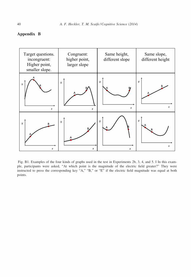
Appendix B

Fig. B1. Examples of the four kinds of graphs used in the test in Experiments 2b, 3, 4, and 5. I In this exam-

ple, participants were asked, “At which point is the magnitude of the electric field greater?” They were

instructed to press the corresponding key “A,” “B,” or “E” if the electric field magnitude was equal at both

points.

Target questions. incongruent: Higher point, smaller slope.

Congruent: higher point, larger slope

Same height, different slope

Same slope, different height


Appendix C

Fig. C1. Examples of the two kinds of Example training graphs used for Experiments 4 and 5. Participants

were asked, “At which point is the magnitude of the electric field greater?”. They were provided with feed-

back as to the correct answer immediately after each question.

Appendix D: Explicit Rule training slides

Participants in the Rule training condition in Experiment 5 were presented with the fol-

lowing slides on a computer screen.

Slide 1

There is a very simple rule which will tell you where electric field is greater:

The electric field, E, depends on the slope of a line on a voltage, V, versus x plot.

Press ‘y’ if you understand the rule. Press ‘n’ if you do not understand the rule.

Congruent: higher point, larger slope

Same height, different slope


Slide 2

Which of the following rules was given on the previous slide?

a. The electric field is equal to the value of the voltage on a V versus x plot.

b. The voltage depends on the slope of a line on an E versus x plot.

c. The electric field depends on position on a V versus x plot.

d. The electric field depends on the slope of a line on a V versus x plot.

Slide 3

Answer d is correct.

You were told,

“The electric field, E, depends on the slope of a line on a V vs. x plot.”

Press the space bar to continue.

Slide 4

True or False:

The electric field, E, does not depend on the slope of a line on a V versus x plot.

Press “t” for true and “f ” for false.

Slide 5

FALSE

The electric field, E, DOES depend on the slope of a line on a V versus x plot.


Documents

Patterns of Response Times and Response Choices to Science