Find us at www.keysight.com Page 1

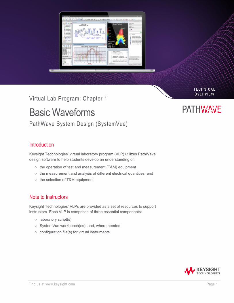
Virtual Lab Program: Chapter 1

Basic Waveforms PathWave System Design (SystemVue)

Introduction Keysight Technologies’ virtual laboratory program (VLP) utilizes PathWave design software to help students develop an understanding of:

o the operation of test and measurement (T&M) equipment o the measurement and analysis of different electrical quantities; and o the selection of T&M equipment

Note to Instructors Keysight Technologies’ VLPs are provided as a set of resources to support instructors. Each VLP is comprised of three essential components:

o laboratory script(s) o SystemVue workbench(es); and, where needed o configuration file(s) for virtual instruments

Find us at www.keysight.com Page 2

The first component of the VLP, the script (such as this), is self-contained, thus allowing instructors to use it fully (as it stands) or partially (together with other material). Each script is tagged with a set of identifiers that include references to the: level of difficulty; experiment number; stimulus number; objective; and virtual instrument to be used. A summary of these identifiers with cross-references to the scripts and workbenches is given in the instructors’ overview at the end of this section.

The second component of the VLP is a SystemVue workbench. This can be thought of as a signal generator and is arranged in such a way that the student can select predefined signal characteristics using a simple top-level interface. Beneath this, SystemVue code blocks interpret the students’ input selection and correspondingly configure the parameters of schematic components. Upon execution of the simulation, SystemVue generates the required signal which can then analyzed and visualized in the third component of the VLP, the virtual instrument, and/or in SystemVue. In addition to the pre-configured settings, the instructor may adapt the parameter settings in order to provide alternative configurations. The instructor may also choose to adapt the supplied SystemVue workbenches according to their specific requirements and teaching objectives.

Software Versions The workspaces included in this VLP were developed in Keysight PathWave System Design (SystemVue) 2021 and were tested using Keysight PathWave Vector Signal Analysis (89600 VSA) Version 2020. These software packages are recommended as the basis for the VLP.

Instructors’ Overview The SystemVue workspace “Basic waveforms.wsv”—summarized in the table below—has been designed to provide the instructor with a total of 3 x 2 x 5 x 4 x 4 = 480 experiments.

Parameter Index #1 Index #2 Index #3 Index #4 Index #5

Waveforms sinewave triangular square - -

Inversions 0 1 - - -

Offsets [V] -0.1 -0.001 0 0.5 10

Amplitudes [V] 0.1 0.5 1.0 10 -

Frequencies [kHz] 1 25 50.1 100.2 -

Find us at www.keysight.com Page 3

Downloading VLP Packages There are several different VLP packages available for download. To download the various packages, go to www.Keysight.com/find/PathWave-System-Design-Virtual-Labs. This landing page contains links to the PDF lab scripts, workspaces, and configuration files.

Technical and Sales Support PathWave System Design (SystemVue) Technical Support

PathWave System Design (SystemVue) Sales Support

Background for Students In this set of exercises, you will create a variety of signals and visualize them in both the time and frequency domain using Keysight PathWave System Design (SystemVue). A common SystemVue workspace is used for all of the exercises. This is conceptually similar to a laboratory workbench comprised of a signal generator (the source) and signal analyzers (the sinks). The latter includes a time domain data sink which can be thought of as an oscilloscope and a frequency domain sink which is similar to a spectrum analyzer.

To begin with the exercises, it is assumed that you have a PC or laptop on which the suitable software has been installed and that you have access to the relevant workspace which forms part of the VLP.

Find us at www.keysight.com Page 4

Prerequisites In order to work through Keysight Technologies’ VLP (either fully or partly), a basic level of competence with SystemVue is required. This should include the ability to:

o open a workspace; o navigate through the workspace tree and view its components; o execute simulations; o adjust workspace parameter settings (mainly by using pre-configured sliders); and

visualize simulation results.

Students who are unfamiliar with any of the above aspects of SystemVue should take advantage of the on-line resources provided in Table 1—a Keysight account might be required.

Table 1. An overview of on-line training resources.

Resource Description On-line link SystemVue video library available

A collection of SystemVue instructional videos presented by Keysight Technologies

https://bit.ly/3cck4vW

Learn SystemVue in 5 mins

A collection of SystemVue instructional videos presented by Anurag Bhargava Tutorial-1: What is Pathwave System Design (SystemVue) Tutorial-2: Understanding SystemVue Design Environment Tutorial-3: Getting Started with Data Flow Simulation in SystemVue Tutorial-4: Working with Graphs in SystemVue Tutorial-8: Vector Modulation Analysis using VSA in SystemVue

Blog: http://abhargava.wordpress.com T1: https://youtu.be/UHh_0RVGI58 T2: https://youtu.be/oRy9suFdB7c T3: https://youtu.be/ZWtJ84oLhF0 T4: https://youtu.be/S0MhwflXM3A T5: https://youtu.be/5cDdl9ohJnM

SystemVue Essentials & Intro to Phased Array Beam Forming and 5GNR Library

This workshop is intended to get you up to speed on SystemVue essentials. After learning the basics, this workshop covers Phased Array, Beamforming, and 5G NR integration. Data analysis in PathWave VSA is also covered.

Keysight Knowledge Center

Vector Signal Analysis Basics

This application note serves as a primer on performing vector signal analysis using the 89600 VSA software to measure and manipulate complex data.

Keysight website (5990-7451)

Digital Modulation in Communication Systems

Understand concepts of digital modulation and learn new digital modulation techniques in communication systems to make informed decisions to optimize your systems.

Keysight website (5965-7160)

Find us at www.keysight.com Page 5

Spectrum Analysis Basics (App Note 150)

Spectrum Analysis Basics teaches the fundamentals of spectrum analyzers and spectrum analysis including the latest advances in spectrum analyzer capabilities.

Keysight website (5952-0292)

Signal Analyzer Fundamentals (What the RF)

This course covers when and how to use different applications and capabilities of signal/spectrum analyzers to make various RF measurements.

Keysight website

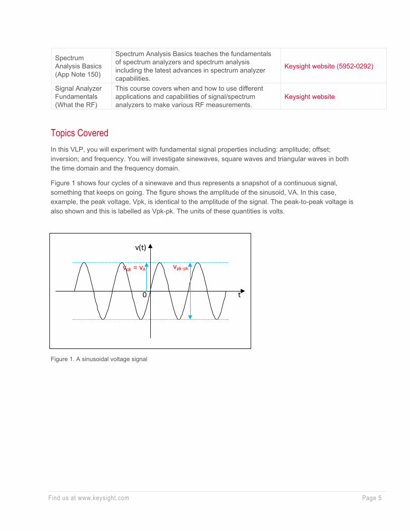
Topics Covered In this VLP, you will experiment with fundamental signal properties including: amplitude; offset; inversion; and frequency. You will investigate sinewaves, square waves and triangular waves in both the time domain and the frequency domain.

Figure 1 shows four cycles of a sinewave and thus represents a snapshot of a continuous signal, something that keeps on going. The figure shows the amplitude of the sinusoid, VA. In this case, example, the peak voltage, Vpk, is identical to the amplitude of the signal. The peak-to-peak voltage is also shown and this is labelled as Vpk-pk. The units of these quantities is volts.

Figure 1. A sinusoidal voltage signal

t

v(t)

vpk = vA vpk-pk

0

Find us at www.keysight.com Page 6

Figure 2. A sinusoidal voltage signal which is inverted with respect to that shown in Figure 1.

Figure 2 is identical to Figure 1 with the exception that the signal is said to be inverted.

Figure 3 is identical to Figure 1 with the exception that the signal period is labelled with the lower-case Greek letter tau, τ. This represents the duration or period of one cycle of the sinusoid and is the reciprocal of the signal’s frequency. The units of period are seconds while those of frequency are hertz (note that up until 1960, the units of cycles per second [c/s] were used instead of hertz1).

Figure 3. A sinusoidal voltage signal showing its amplitude, peak-to-peak voltage and period.

1 See for example https://www.edn.com/cycles-per-second-a-historical-perspective/

t

v(t)

vpk = vA vpk-pk

0

t

v(t)

τ= 1/f

vpk = vA vpk-pk

0

Find us at www.keysight.com Page 7

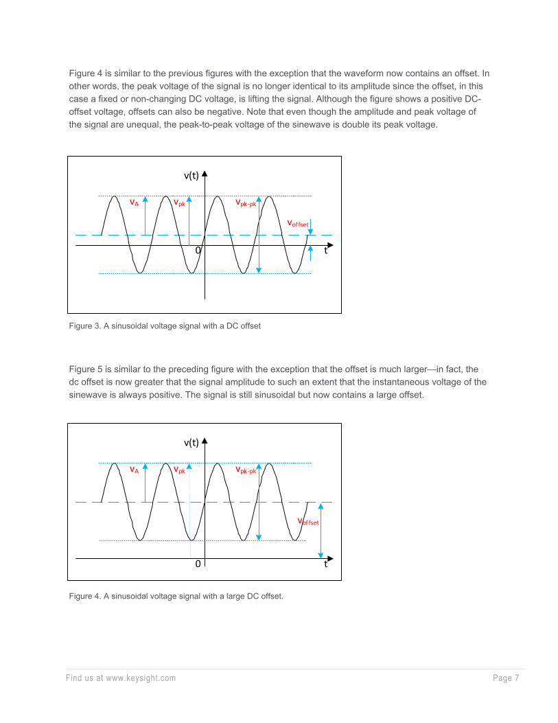
Figure 4 is similar to the previous figures with the exception that the waveform now contains an offset. In other words, the peak voltage of the signal is no longer identical to its amplitude since the offset, in this case a fixed or non-changing DC voltage, is lifting the signal. Although the figure shows a positive DC-offset voltage, offsets can also be negative. Note that even though the amplitude and peak voltage of the signal are unequal, the peak-to-peak voltage of the sinewave is double its peak voltage.

Figure 3. A sinusoidal voltage signal with a DC offset

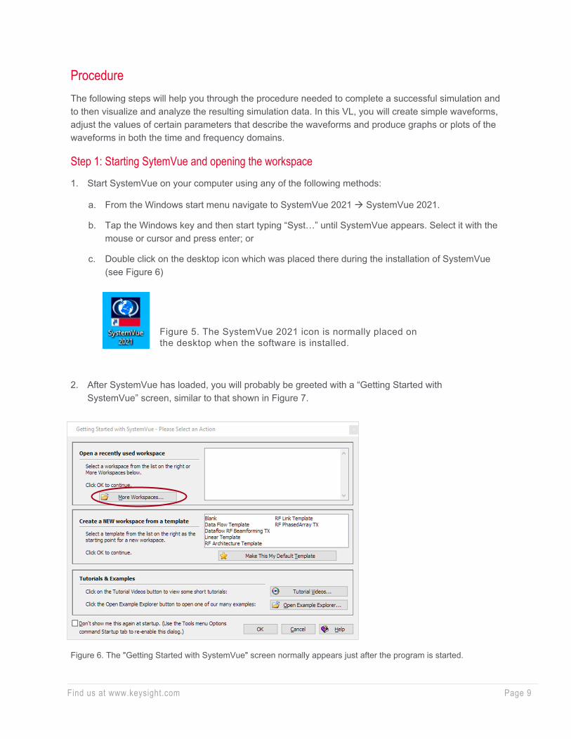
Figure 5 is similar to the preceding figure with the exception that the offset is much larger—in fact, the dc offset is now greater that the signal amplitude to such an extent that the instantaneous voltage of the sinewave is always positive. The signal is still sinusoidal but now contains a large offset.

Figure 4. A sinusoidal voltage signal with a large DC offset.

t

v(t)

vpk vpk-pk

0

voffset

vA

t

v(t)

vpk vpk-pk

0

voffset

vA

Find us at www.keysight.com Page 8

Overview Level 1 Experiment reference number 01 Stimulus reference number 001-480 Objective number 1 (Basic simulation, visualization and analysis) Instrument SystemVue

Learning Objective In this Virtual Laboratory (VL), students will use Keysight PathWave System Design (SystemVue) electronic system-level design software to explore and measure signals. This VL will assist students in their understanding of signal analysis with the following learning objective(s):

o Observe a signal in the time domain and identify its: amplitude; peak voltage; peak-to-peak voltage; DC offset voltage; and period. Calculate the frequency from the signal’s period.

o Observe a signal in the frequency domain and identify its amplitude and frequency and its DC offset if present.

Student Outcomes Upon successful completion of this VL exercise, students will:

o Be familiar with the principle of the VLP. o Understand how to execute a SystemVue simulation, change parameter settings and

collect data. o Analyze and measure signals in the time and frequency domains using SystemVue.

Find us at www.keysight.com Page 9

Procedure The following steps will help you through the procedure needed to complete a successful simulation and to then visualize and analyze the resulting simulation data. In this VL, you will create simple waveforms, adjust the values of certain parameters that describe the waveforms and produce graphs or plots of the waveforms in both the time and frequency domains.

Step 1: Starting SytemVue and opening the workspace 1. Start SystemVue on your computer using any of the following methods:

a. From the Windows start menu navigate to SystemVue 2021 SystemVue 2021.

b. Tap the Windows key and then start typing “Syst…” until SystemVue appears. Select it with the mouse or cursor and press enter; or

c. Double click on the desktop icon which was placed there during the installation of SystemVue (see Figure 6)

Figure 5. The SystemVue 2021 icon is normally placed on the desktop when the software is installed.

2. After SystemVue has loaded, you will probably be greeted with a “Getting Started with SystemVue” screen, similar to that shown in Figure 7.

Figure 6. The "Getting Started with SystemVue" screen normally appears just after the program is started.

Find us at www.keysight.com Page 10

In the top panel, click on More Workspaces and using the file explorer, navigate your way to the workspace “Basic waveforms.wsv”. This workspace (and perhaps others too) might have already been installed on the machine you are using or on a network drive to which you have access. It is recommended that you save a local copy of the workspace and use that version to work with. This will allow you to revert to the original version with its default settings should the need arise.

Step 2: Understanding the SystemVue window 1. After you have successfully opened the workspace, your screen should be similar to that shown in

Figure 8.

Figure 7. The default view of the “Basic Waveforms” workspace in SystemVue.

2. The default view of the Basic Waveforms workspace comprises a number of panels or windows. These are listed below together with links to the relevant parts of the user manual:

a) The workspace tree – see: Home > Users Guide > Environment > Design Environment > Workspace Tree SystemVue 2021: qthelp://systemvue.2021/doc/users/Workspace_Tree.html

b) The design – see: Home > Users Guide > Using PathWave System Design > Designs SystemVue 2021: qthelp://systemvue.2021/doc/users/Designs.html

c) A graph (for time domain analysis) – see: Home > Users Guide > Using PathWave System Design (SystemVue) > Graphs SystemVue 2021: qthelp://systemvue.2021/doc/users/Graphs.html

a

b

d

e

f g

c

h

Find us at www.keysight.com Page 11

d) A graph (for frequency domain analysis) – see: Home > Users Guide > Using PathWave System Design (SystemVue) > Graphs SystemVue 2021: qthelp://systemvue.2021/doc/users/Graphs.html

e) The tune window – see: Home > Users Guide > Environment > Design Environment > Tune Window SystemVue 2021: qthelp://systemvue.2021/doc/users/Tune_Window.html

f) The autorecalc window– see: Home > Users Guide > Environment > Design Environment > Tune Window SystemVue 2021: qthelp://systemvue.2021/doc/users/Tune_Window.html

g) The error, messages and status window – see: Home > Users Guide > Environment > Design Environment > Error Log SystemVue 2021: qthelp://systemvue.2021/doc/users/Error_Log.html

The command prompt – see: Home > Users Guide > Environment > Design Environment > Command Prompt SystemVue 2021: qthelp://systemvue.2021/doc/users/Command_Prompt.html

1. Referring to list item ‘b’ above, the design window of the Basic Waveforms looks like that shown in Figure 9.

Figure 8. The “Basic waveforms” design window showing source, sink and waveform settings.

a b

c

Find us at www.keysight.com Page 12

3. The design window shows an apparently very simple schematic diagram which has been arranged into three main areas:

a) A signal source which is configured using predefined parameter values selectable thru the use of sliders. In this step and the next, it is recommended to leave the sliders set to their default positions. The source parameters are grouped into five sets:

i. Waveform_Selection – this slider allows the student to select one of the following waveforms: sinewave (1); triangular wave (2); and square wave (3).

ii. Inversion_Selection – this slider allows the student to leave the waveforms non-inverted (0) or inverted (1).

iii. Offset_Selection – the student can use this slider to select a DC offset (including 0V). Five presets are available.

iv. Amplitude_Selection – the student can set the waveform amplitude from four defined values.

v. Frequency_Selection – this allows the student to select the frequency of the waveform. Four settings are predefined.

b) An area showing three different sinks. These are used in SystemVue to collect data during a data flow simulation. In this step and the next, it is recommended to leave the sliders set to their default positions. The sinks shown are:

i. TimeSink, this is used to visualize and analyze the signal in the time domain. By default, the sink is activated (1). It can be controlled using the slider useTimeSink – see: Home > Part Catalog > Algorithm Design Library > Sinks Category > Sink Part > Sink (Data Sink) SystemVue 2021: qthelp://systemvue.2021/doc/algorithm/Sink.html

ii. SpectrumSink, this is used to visualize and analyze the signal in the frequency domain. By default, the sink is activated (1). It can be controlled using the slider useSpectrumSink – see: Home > Part Catalog > Algorithm Design Library > Sinks Category > SpectrumAnalyzer Part SystemVue 2021: qthelp://systemvue.2021/doc/algorithm/SpectrumAnalyzer_Part.html

An area that presents a textual summary of the parameter settings used for the signal source showing the type of waveform, whether or not it is inverted, its offset voltage, its amplitude and its frequency.

Find us at www.keysight.com Page 13

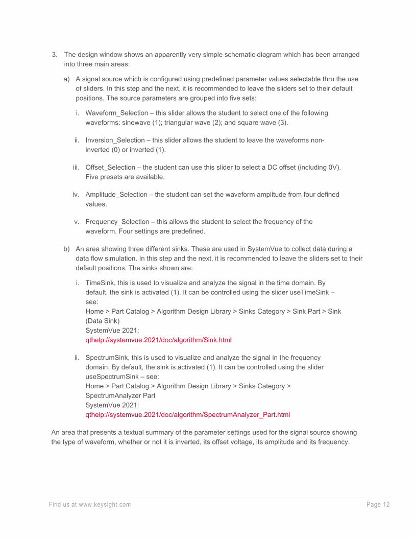
Step 3: Executing the simulation with default parameter settings 1. Using the default settings for both the source parameter values and the sink activation controls (see

Figure 9), execute the simulation by using anyone of the following methods:

a) Click on the green Run Analyses arrow shown below:

Figure 9. A closeup view of the menu bar and main toolbar showing the green Run Analyses button.

b) On the menu bar, go to Action -> Run All Out-of-Date Analyses and Sweeps; or

c) Press F5 on your keyboard.

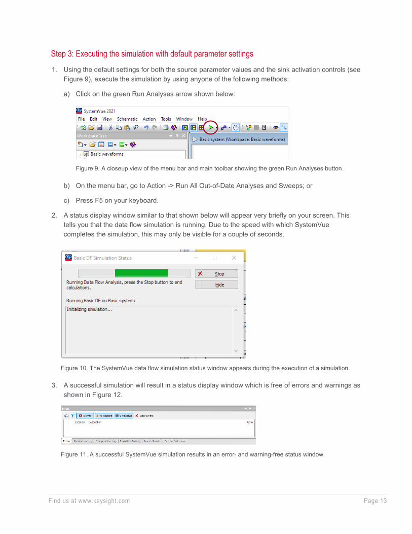
2. A status display window similar to that shown below will appear very briefly on your screen. This tells you that the data flow simulation is running. Due to the speed with which SystemVue completes the simulation, this may only be visible for a couple of seconds.

Figure 10. The SystemVue data flow simulation status window appears during the execution of a simulation.

3. A successful simulation will result in a status display window which is free of errors and warnings as shown in Figure 12.

Figure 11. A successful SystemVue simulation results in an error- and warning-free status window.

Find us at www.keysight.com Page 14

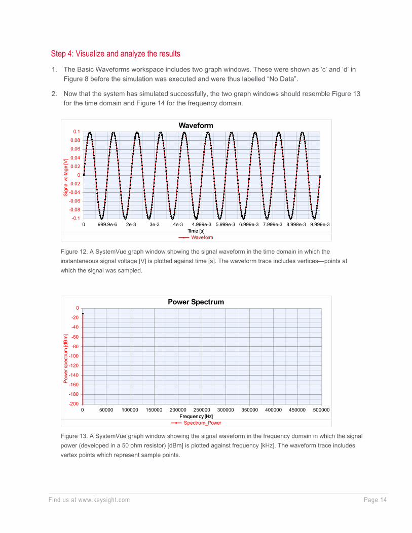
Step 4: Visualize and analyze the results 1. The Basic Waveforms workspace includes two graph windows. These were shown as ‘c’ and ‘d’ in

Figure 8 before the simulation was executed and were thus labelled “No Data”.

2. Now that the system has simulated successfully, the two graph windows should resemble Figure 13 for the time domain and Figure 14 for the frequency domain.

Figure 12. A SystemVue graph window showing the signal waveform in the time domain in which the instantaneous signal voltage [V] is plotted against time [s]. The waveform trace includes vertices—points at which the signal was sampled.

Figure 13. A SystemVue graph window showing the signal waveform in the frequency domain in which the signal power (developed in a 50 ohm resistor) [dBm] is plotted against frequency [kHz]. The waveform trace includes vertex points which represent sample points.

Time [s]

Sig

nal v

olta

ge [V

]

-0.1

-0.08

-0.06

-0.04

-0.02

0

0.02

0.04

0.06

0.08

0.1

Time [s]0 999.9e-6 2e-3 3e-3 4e-3 4.999e-3 5.999e-3 6.999e-3 7.999e-3 8.999e-3 9.999e-3

Waveform

Waveform

Frequency [Hz]

Pow

er s

pect

rum

[dB

m]

-200

-180

-160

-140

-120

-100

-80

-60

-40

-20

0

Frequency [Hz]0 50000 100000 150000 200000 250000 300000 350000 400000 450000 500000

Power Spectrum

Spectrum_Power

Find us at www.keysight.com Page 15

3. SystemVue graphs enable you to explore and examine your data in many different ways. The user manual provides detailed instructions that include:

d) An overview – see: Home > Users Guide > Using PathWave System Design (SystemVue) > Graphs SystemVue 2021: qthelp://systemvue.2021/doc/users/Graphs.html

e) Zooming a graph – see: Home > Users Guide > Using PathWave System Design (SystemVue) > Graphs > Zooming Graphs SystemVue 2021: qthelp://systemvue.2021/doc/users/Zooming_Graphs.html

f) Using markers on graphs – see: Home > Users Guide > Using PathWave System Design (SystemVue) > Graphs > Using Markers on Graphs SystemVue 2021: qthelp://systemvue.2021/doc/users/Using_Markers_on_Graphs.html

g) Annotate a graph – see: Home > Users Guide > Using PathWave System Design (SystemVue) > Graphs > Annotating Graphs SystemVue 2021: qthelp://systemvue.2021/doc/users/Annotating_Graphs.html

h) Copying and saving a graph – see: Home > Users Guide > Using PathWave System Design (SystemVue) > Graphs > Copying and Saving Graphs SystemVue 2021: qthelp://systemvue.2021/doc/users/Creating_Graphs.html#CreatingGraphs-CopyingandSavingGraphs

Creating a graph – see: Home > Users Guide > Using PathWave System Design (SystemVue) > Graphs > Creating Graphs SystemVue 2021: qthelp://systemvue.2021/doc/users/Creating_Graphs.html

Find us at www.keysight.com Page 16

Step 5: Explore parameter settings 1. Now that you have completed your first simulation and have viewed and analyzed the results

obtained, you should be ready to investigate what happens when other waveform parameter settings are used.

2. Your instructor might provide you with a list of configuration settings to explore. If not, you are encouraged to make small changes to the settings, re-simulate and observe the changes. For example, now that you have analyzed the sinewave, you might like to visualize what happens to the sinewave when you:

a) Turn inversion on and off;

b) Change the signal amplitude;

c) Change the signal frequency; and

d) Change the DC offset.

3. Referring to the section “Topics covered”, you should make sure that you understand the relationship of ‘a’ to ‘d’ above and their effect on the signal waveform. In addition, you should also be familiar with:

a) Measuring signal quantities from plots and calculating the frequency of a periodic from an estimation of its period in the time domain.

b) Using graph markers.

c) The relationship between signal amplitude and signal power.

d) Decibels and the unit dBm.

Review Congratulations, you have now completed your first virtual laboratory and have:

o Observed a signal in the time domain and identified its: amplitude; peak voltage; peak-to-peak voltage; DC offset voltage; and period. Calculated the frequency from the signal’s period;

o Observed a signal in the frequency domain and identified its amplitude and frequency and its DC offset if present;

o Become familiar with the principle of the VLP; o Understood how to execute a SystemVue simulation, change parameter settings and

collect data; and o Analyzed and measured signals in the time and frequency domains using SystemVue.

Find us at www.keysight.com Page 17 This information is subject to change without notice. © Keysight Technologies, 2021, Published in USA, August 4, 2021, 3121-1265.EN

Learn more at: www.keysight.com For more information on Keysight Technologies’ products, applications or services, please contact your local Keysight office. The complete list is available at: www.keysight.com/find/contactus

Suggested Exercises In addition to the tasks assigned to you by your instructor, here are some exercises that you might like to try:

1. How does the type of waveform affect its spectrum?

2. How does a waveform’s offset and amplitude affect its spectrum?

3. Using a sinusoidal waveform (any frequency and amplitude):

a) understand how the amplitude and frequency relate to the signal in both the time and frequency domains;

b) set the DC offset to zero and note the spectrum. Then set the DC offset to the lowest non-zero zero value. Compare the two spectra and describe what changed. Again, increase the DC offset and describe the change to the spectrum;

c) experiment with markers in both the time and frequency domain. Use them to measure amplitude, offset, power, period and frequency. Compare the results obtained in the time and frequency domain and explain the relationship—be careful to describe the units carefully; and

d) what can be said about the spectrum of a sinusoidal waveform in terms of its bandwidth?

4. Choose a non-sinusoidal waveform (any frequency and amplitude), remove the DC offset and then compare its spectrum with that of a sinusoid. Describe the differences.

5. Choose any waveform and any frequency and amplitude, remove the DC offset and observe the signal in the time and frequency domains. Invert the signal and describe what happens in each domain.

Acknowledgement Keysight would like to thank Dr. Paul Leather at Technische Hochschule Rosenheim for his help in developing these lab guides