Path dependent option pricing under Lévy processes

Applied to Bermudan options

Conall O’Sullivan1

University College Dublin

December 2004

A model is developed that can price path dependent options when the under-lying process is an exponential Lévy process with closed form conditional charac-teristic function. The model is an extension of a recent quadrature option pricingmodel so that it can be applied with the use of Fourier and Fast Fourier trans-forms. Thus the model possesses nice features of both Fourier and quadratureoption pricing techniques since it can be applied for a very general set of under-lying Lévy processes and can handle exotic path dependent features. The modelis applied to European and Bermudan options for geometric Brownian motion, ajump-di¤usion process, a variance gamma process and a normal inverse Gaussianprocess. However it must be noted that the model can also price other pathdependent exotic options such as lookback and Asian options.

Key words: Fast Fourier transform, recursive, path dependent option pricing.

1All comments welcome and encouraged.Contact info.: Tel: +353 1 716 8836, email: conall.osullivan@ucd.ie

1. Introduction

Existing Fourier and Fast Fourier transform option pricing models are essentiallyclosed form option pricing formula that can be applied to a wide range of underly-ing stochastic processes. Fourier and Fast Fourier transform models (hereafter re-ferred to collectively as transform models) can handle general stochastic processesand can also be applied to exotic versions of the Black Scholes (BS) option pric-ing formula2 such as barrier options, digital options etc. They cannot be appliedrecursively so this limits their applicability when an option includes certain exoticfeatures, for example, if an option has a changing barrier, if an option is exercis-able on a number of dates or if there is a discrete dividend during the life of theoption. Pioneering articles on the application of transform techniques to optionpricing include Stein and Stein (1991), Heston (1993), Bates (1996), Du¢e, Panand Singleton (2001), Carr and Madan (1999), Backshi and Madan (2000), Lewis(2000) and Lee (2004).

Existing quadrature option pricing models have been developed for a restric-tive class of underlying processes, namely geometric Brownian motion, howeverthey are recursive models and so they can accurately price options with exoticfeatures. Option pricing using numerical integration methods was …rst introducedby Parkinson (1997) but because of the discontinuities involved in option pricingthis has been one of the least used option pricing methods. Sullivan (2000) didsuccessfully apply quadrature routines to price American options under geometricBrownian motion. One of the most recent of these numerical integration schemesspeci…cally deals with the non-linearity error introduced by the discontinuities inoption prices, see Andricopoulos, Widdicks, Duck and Newton (2003). In their ar-ticle it was recognised that options could be priced accurately using a discountedintegration of the payo¤ provided the payo¤ is segmented so the integral is onlycarried out over continuous segments of the payo¤. They run a quadrature rou-tine (QUAD) to estimate each section of the segmented integral. In this way thequadrature routine is only applied to functions that are continuous and have con-tinuous higher order derivatives and thus the routine retains its accuracy. If thereis more than one time step needed to price the option, an asset price lattice isset up and the price at each point in the lattice at time t is calculated recursivelyfrom the prices at time t+ 1 using the quadrature routine. Thus, for example, in

2Transform models can also price exotic options that cannot be priced in the BS framework,for example, Asian options where the average is taken over the entire life of the option, seeBackshi and Madan (2000).

2

a plain vanilla call option only one time step is needed and the payo¤ is split intotwo continuous regions, the segment that is greater than zero and the segmentthat is zero. As another example, a single barrier at time t can be included byworking backwards from maturity to …nd the prices on the lattice at time t andthen applying the barrier condition. The option price prior to time t is calculatedrecursively from the time t prices which are split into two continuous regions, oneon either side of the barrier.

In this article the qaudrature option pricing model developed by Andricopouloset al. (2003) is extended so that it can be applied with the use of Fourier and FastFourier transform (FFT) techniques originated by Heston (1993) and Carr andMadan (1999) respectively. This model allows transform option pricing modelsto be applied recursively resulting in a model that can incorporate exotic featuresand can be applied for a wide range of stochastic processes, speci…cally thosestochastic processes that result in a process with independent increments3 andwhose conditional characteristic function is known in closed form. Many Lévyprocesses fall into this category. Examples of …nite activity Lévy processes includethe jump-di¤usion process of Merton (1976), and the double exponential jump-di¤usion model of Kou (2002). Examples of in…nite activity Lévy processes (Lévyprocesses whose jump arrival rate is in…nite) include the variance gamma processof Madan and Seneta (1990), Madan and Milne (1991) and Madan, Carr andChang (1998), and the normal inverse Gaussian model of Barndor¤-Nielsen (1998).See Geman (2002) and Carr and Wu (2004) and references therein for more onthese models and other Lévy processes. The model developed in this paper can beconsidered as a simple alternative model to current numerical pricing methods forpath dependent options under Lévy processes, such as the …nite di¤erence methodof Hirsa and Madan (2004), the lattice method of Kellizi and Webber (2003) andthe multinomial tree method of Maller, Solomon and Szimayer (2004).

To demonstrate the accuracy of the model European options are priced andcompared to existing prices under a number of di¤erent processes. These processesinclude geometric Brownian motion (GBM) for benchmarking purposes, Merton’sjump-di¤usion (JD) process as an example of a …nite activity Lévy process, avariance gamma (VG) and a normal inverse Gaussian (NIG) process as exam-ples of in…nite activity Lévy processes. In the GBM case American options are

3The model developed in this paper can be used with processes that do not have independentincrements, for example options can be priced under Heston’s (1993) stochastic volatility process.However the model becomes slower than competing methods as the integrations must run overtwo dimensions: the asset price and the variance.

3

approximately priced using extrapolation techniques and compared with pricesfrom existing American option pricing models to demonstrate the ability of themodel to price path dependent options. For the remaining processes Bermudanoptions are priced for benchmarking purposes, however extrapolation techniquescan be applied to approximate American prices. The remaining article is organ-ised as follows. Section 2 covers the methodology by …rst examining the existingQUAD model and then extending it so that transform techniques can be applied inconjunction with the quadrature routine. Section 3 contains the implementationdetails for both the Fourier and the FFT approach. Section 4 contains results forEuropean and American options priced under GBM, and European and Bermudanoptions priced under JD, VG and NIG processes. Section 5 concludes.

2. Methodology

2.1. Qaudrature model

Let us start by considering the quadrature model of Andricopoulos et al. (2003).Assume the underlying process is geometric Brownian motion. The notation is asfollows: St is the stock price, E is the exercise price, r is the constant risk freerate, q is the dividend yield and ¾ is the volatility. Let T = t+¢t be the time atwhich the payo¤ (or option price) is known, noting that the model is recursive.De…ne the transformed prices as x = log (St=E) and y = log (St+¢t=E). Theoption price at time t can be written as

V (x; t) = e¡r¢tEQt [V (y; t+ ¢t)] (2.1)

where the expectation is a risk neutral (RN) expectation and where V (y; t+¢t)is the time t+ ¢t known payo¤ (or option price) at a transformed price y. ThisRN expectation can be written as

V (x; t) = e¡r¢tZ 1

¡1V (y; t+¢t) f (y jx )dy (2.2)

where f (y jx ) is the conditional RN probability density of attaining y given x. Ifthe stock price process is geometric Brownian motion then y is normally distrib-uted and

f (y jx ) = 1p2¼¾2¢t

exp

0B@¡

³y ¡x ¡

³r ¡ q ¡ 1

2¾2´¢t

´2

2¾2¢t

1CA (2.3)

4

and

V (x; t) =e¡r¢tp2¼¾2¢t

Z 1

¡1V (y; t +¢t) exp

0B@¡

³y¡ x ¡

³r ¡ q ¡ 1

2¾2´¢t

´2

2¾2¢t

1CA dy

=1p

2¼¾2¢tA (x)

Z 1

¡1V (y; t+ ¢t)B (x; y) dy

=1p

2¼¾2¢tA (x)

Z 1

¡1F (x; y) dy (2.4)

where

A (x) =1p

2¼¾2¢texp

µ¡12kx¡ 1

8k2¾2¢t¡ r¢t

¶

F (x; y) = V (y; t+ ¢t)B (x; y)

B (x; y) = exp

á(y ¡x)22¾2¢t

+1

2ky

!

k = 2µr ¡ q¾2

¶¡ 1 (2.5)

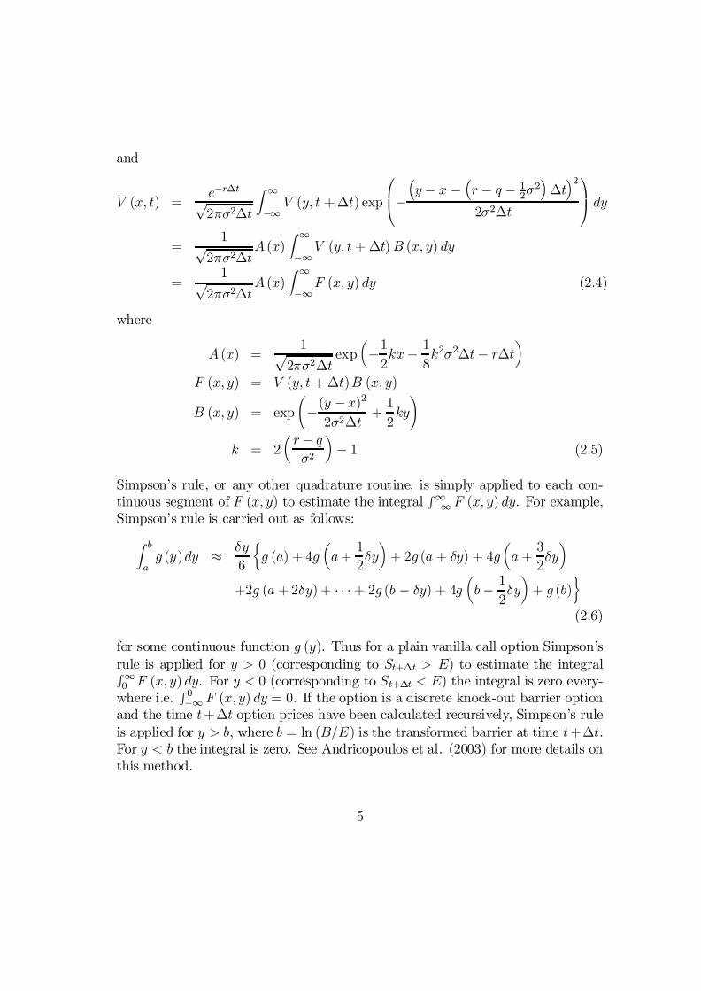
Simpson’s rule, or any other quadrature routine, is simply applied to each con-tinuous segment of F (x; y) to estimate the integral

R1¡1 F (x; y) dy. For example,

Simpson’s rule is carried out as follows:

Z b

ag (y)dy ¼ ±y

6

½g (a) + 4g

µa+

1

2±y

¶+ 2g (a + ±y) + 4g

µa +

3

2±y

¶

+2g (a +2±y) + ¢ ¢ ¢+ 2g (b ¡ ±y) + 4gµb¡ 1

2±y

¶+ g (b)

¾

(2.6)

for some continuous function g (y). Thus for a plain vanilla call option Simpson’srule is applied for y > 0 (corresponding to St+¢t > E) to estimate the integralR10 F (x; y) dy. For y < 0 (corresponding to St+¢t < E) the integral is zero every-

where i.e.R 0¡1 F (x; y) dy = 0. If the option is a discrete knock-out barrier option

and the time t+¢t option prices have been calculated recursively, Simpson’s ruleis applied for y > b, where b = ln (B=E) is the transformed barrier at time t+¢t.For y < b the integral is zero. See Andricopoulos et al. (2003) for more details onthis method.

5

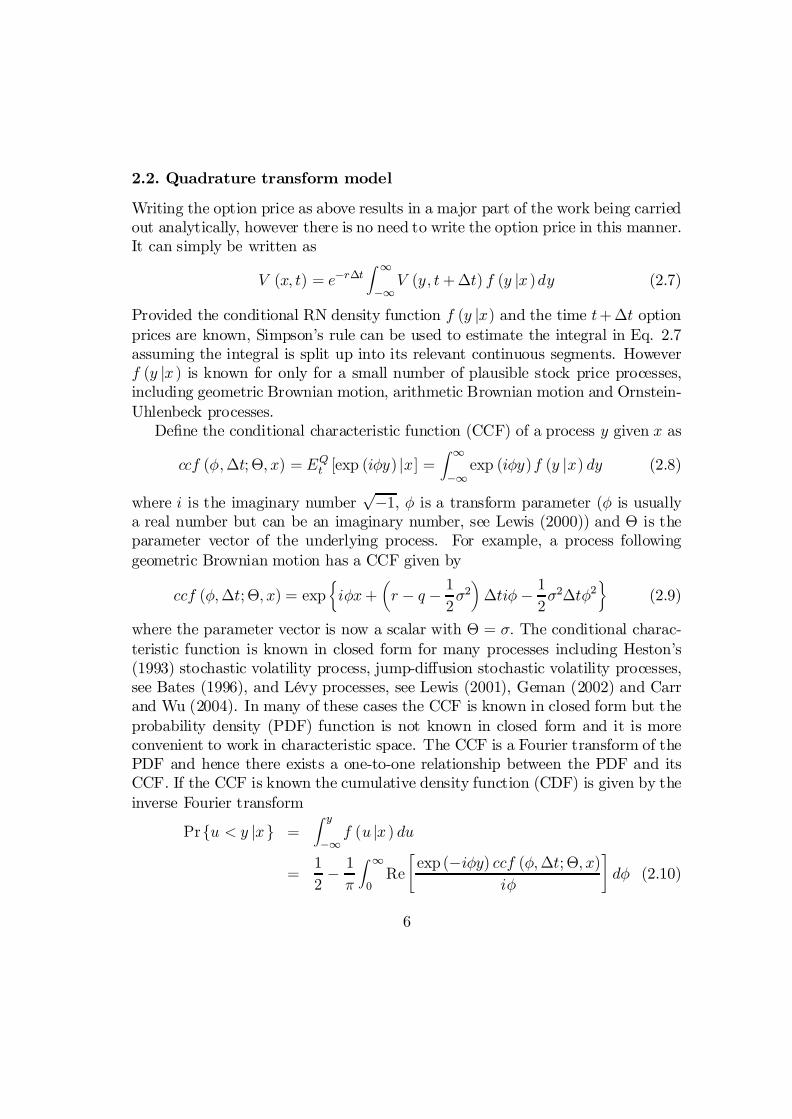
2.2. Quadrature transform model

Writing the option price as above results in a major part of the work being carriedout analytically, however there is no need to write the option price in this manner.It can simply be written as

V (x; t) = e¡r¢tZ 1

¡1V (y; t+¢t) f (y jx )dy (2.7)

Provided the conditional RN density function f (y jx) and the time t+¢t optionprices are known, Simpson’s rule can be used to estimate the integral in Eq. 2.7assuming the integral is split up into its relevant continuous segments. Howeverf (y jx ) is known for only for a small number of plausible stock price processes,including geometric Brownian motion, arithmetic Brownian motion and Ornstein-Uhlenbeck processes.

De…ne the conditional characteristic function (CCF) of a process y given x as

ccf (Á;¢t; £; x) = EQt [exp (iÁy) jx] =Z 1

¡1exp (iÁy)f (y jx) dy (2.8)

where i is the imaginary numberp

¡1, Á is a transform parameter (Á is usuallya real number but can be an imaginary number, see Lewis (2000)) and £ is theparameter vector of the underlying process. For example, a process followinggeometric Brownian motion has a CCF given by

ccf (Á;¢t; £; x) = exp½iÁx+

µr ¡ q ¡ 1

2¾2

¶¢tiÁ ¡ 1

2¾2¢tÁ2

¾(2.9)

where the parameter vector is now a scalar with £ = ¾: The conditional charac-teristic function is known in closed form for many processes including Heston’s(1993) stochastic volatility process, jump-di¤usion stochastic volatility processes,see Bates (1996), and Lévy processes, see Lewis (2001), Geman (2002) and Carrand Wu (2004). In many of these cases the CCF is known in closed form but theprobability density (PDF) function is not known in closed form and it is moreconvenient to work in characteristic space. The CCF is a Fourier transform of thePDF and hence there exists a one-to-one relationship between the PDF and itsCCF. If the CCF is known the cumulative density function (CDF) is given by theinverse Fourier transform

Prfu < y jxg =Z y

¡1f (u jx ) du

=1

2¡ 1

¼

Z 1

0Re

"exp (¡iÁy) ccf (Á;¢t; £; x)

iÁ

#dÁ (2.10)

6

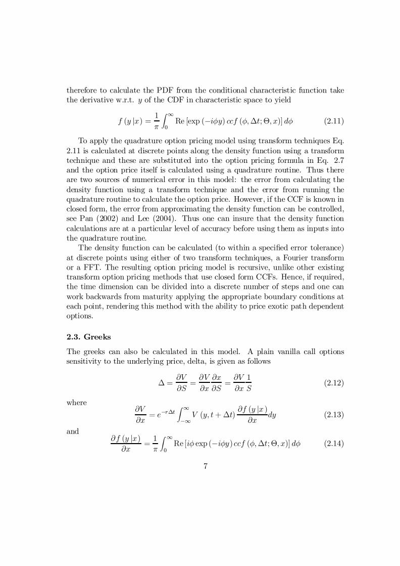
therefore to calculate the PDF from the conditional characteristic function takethe derivative w.r.t. y of the CDF in characteristic space to yield

f (y jx) = 1

¼

Z 1

0Re [exp (¡iÁy) ccf (Á;¢t; £; x)] dÁ (2.11)

To apply the quadrature option pricing model using transform techniques Eq.2.11 is calculated at discrete points along the density function using a transformtechnique and these are substituted into the option pricing formula in Eq. 2.7and the option price itself is calculated using a quadrature routine. Thus thereare two sources of numerical error in this model: the error from calculating thedensity function using a transform technique and the error from running thequadrature routine to calculate the option price. However, if the CCF is known inclosed form, the error from approximating the density function can be controlled,see Pan (2002) and Lee (2004). Thus one can insure that the density functioncalculations are at a particular level of accuracy before using them as inputs intothe quadrature routine.

The density function can be calculated (to within a speci…ed error tolerance)at discrete points using either of two transform techniques, a Fourier transformor a FFT. The resulting option pricing model is recursive, unlike other existingtransform option pricing methods that use closed form CCFs. Hence, if required,the time dimension can be divided into a discrete number of steps and one canwork backwards from maturity applying the appropriate boundary conditions ateach point, rendering this method with the ability to price exotic path dependentoptions.

2.3. Greeks

The greeks can also be calculated in this model. A plain vanilla call optionssensitivity to the underlying price, delta, is given as follows

¢ =@V

@S=@V

@x

@x

@S=@V

@x

1

S(2.12)

where@V

@x= e¡r¢t

Z 1

¡1V (y; t+ ¢t)

@f (y jx )@x

dy (2.13)

and@f (y jx)@x

=1

¼

Z 1

0Re [iÁ exp (¡iÁy)ccf (Á;¢t; £; x)] dÁ (2.14)

7

Thus the delta is calculated in same manner as the option price itself.Suppose £i 2 £ is a parameter of the model. The options sensitivity to £i is

given by@V

@£i= e¡r¢t

Z 1

¡1V (y; t+ ¢t)

@f (y jx )@£i

dy (2.15)

where@f (y jx )@£i

=1

¼

Z 1

0Re

"exp (¡iÁy) @ccf

@£i

#dÁ (2.16)

and the options sensitivity to £i is calculated in same manner as the option priceitself.

3. Implementation

In this section the implementation details are outlined for setting up the lattice,and for applying the two di¤erent methods of calculating the density functionusing transform techniques.

3.1. Lattice model

The model is implemented in a similar fashion to Andricopoulos et al. (2003).First the asset price lattice is constructed. Suppose x0 is the initial transformedprice at time t. The transformed prices at time t+ ¢t are given by the vector

y = fy0; y1; : : : ; yN¡1g0

= fx0 ¡ q¤; x0 ¡ q¤ +¢y; : : : ; x0 + q¤ ¡¢y; x0 + q¤g0

where¢y = 2q¤=N , q¤ = L£ vol (¢t) and vol (¢t) is the volatility of the process4

over the time interval ¢t, so in the geometric Brownian motion case vol (¢t) =¾p¢t. This means that the PDF is calculated L standard deviations either side

of x0 and should result in su¢cient accuracy if L = 10 (this of course can beadjusted downwards). For i = 0; : : : ; N ¡ 1 each discrete point of the densityfunction f (yi jx0 ) can be calculated using a Fourier transform or the entire vectorof discrete points f (y jx0 ) can be calculated using one FFT.

4This volatilty can be computed for stochastic processes whose CCF is known with

vol (¢t) =p

var (¢t); var (¢t) =1

i2Á2

@2ccf

@Á2

¯̄¯̄Á=0

8

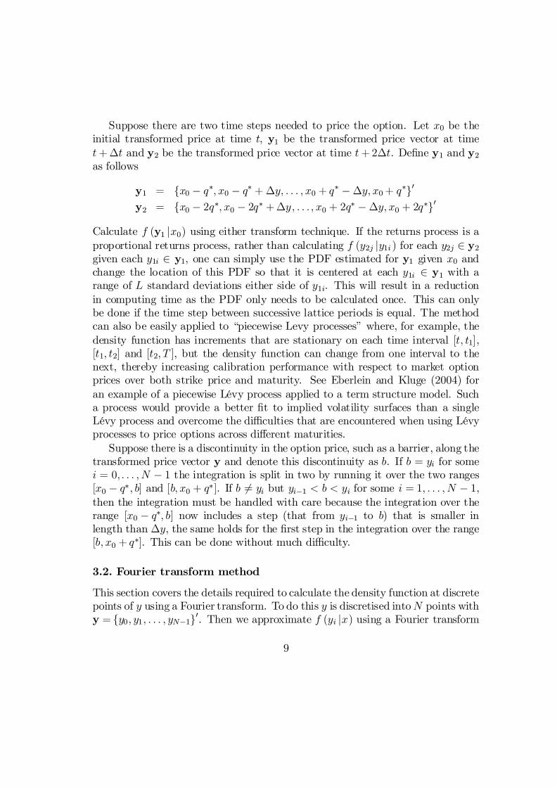
Suppose there are two time steps needed to price the option. Let x0 be theinitial transformed price at time t, y1 be the transformed price vector at timet+¢t and y2 be the transformed price vector at time t+2¢t. De…ne y1 and y2as follows

y1 = fx0 ¡ q¤; x0 ¡ q¤ + ¢y; : : : ; x0 + q¤ ¡¢y; x0+ q¤g0

y2 = fx0 ¡ 2q¤; x0 ¡ 2q¤ +¢y; : : : ; x0 + 2q¤ ¡¢y; x0 + 2q¤g0

Calculate f (y1 jx0) using either transform technique. If the returns process is aproportional returns process, rather than calculating f (y2j jy1i ) for each y2j 2 y2given each y1i 2 y1, one can simply use the PDF estimated for y1 given x0 andchange the location of this PDF so that it is centered at each y1i 2 y1 with arange of L standard deviations either side of y1i. This will result in a reductionin computing time as the PDF only needs to be calculated once. This can onlybe done if the time step between successive lattice periods is equal. The methodcan also be easily applied to “piecewise Levy processes” where, for example, thedensity function has increments that are stationary on each time interval [t; t1],[t1; t2] and [t2; T ], but the density function can change from one interval to thenext, thereby increasing calibration performance with respect to market optionprices over both strike price and maturity. See Eberlein and Kluge (2004) foran example of a piecewise Lévy process applied to a term structure model. Sucha process would provide a better …t to implied volatility surfaces than a singleLévy process and overcome the di¢culties that are encountered when using Lévyprocesses to price options across di¤erent maturities.

Suppose there is a discontinuity in the option price, such as a barrier, along thetransformed price vector y and denote this discontinuity as b. If b = yi for somei = 0; : : : ; N ¡ 1 the integration is split in two by running it over the two ranges[x0 ¡ q¤; b] and [b; x0 + q¤]. If b 6= yi but yi¡1 < b < yi for some i = 1; : : : ; N ¡ 1,then the integration must be handled with care because the integration over therange [x0 ¡ q¤; b] now includes a step (that from yi¡1 to b) that is smaller inlength than ¢y, the same holds for the …rst step in the integration over the range[b; x0 + q¤]. This can be done without much di¢culty.

3.2. Fourier transform method

This section covers the details required to calculate the density function at discretepoints of y using a Fourier transform. To do this y is discretised intoN points withy = fy0; y1; : : : ; yN¡1g0. Then we approximate f (yi jx) using a Fourier transform

9

for i = 0; : : : ; N ¡ 1. The PDF in Eq. 2.11 can be discretised as follows

f (yi jx ) =1

¼

Z 1

0Re [exp (¡iÁyi) ccf (Á;¢t; £; x)] dÁ

' 1

¼

T¡1X

j=0

Rehexp

³¡iÁjyi

´ccf

³Áj;¢t; £; x

´i¢Á (3.1)

where the transform parameterÁ is discretised into a vector with Á=nÁ0; : : : ; ÁT¡1

o0,

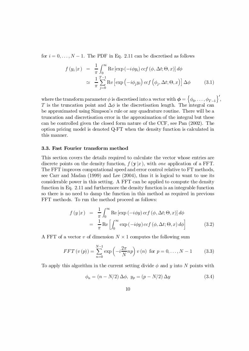
T is the truncation point and ¢Á is the discretisation length. The integral canbe approximated using Simpson’s rule or any quadrature routine. There will be atruncation and discretisation error in the approximation of the integral but thesecan be controlled given the closed form nature of the CCF, see Pan (2002). Theoption pricing model is denoted Q-FT when the density function is calculated inthis manner.

3.3. Fast Fourier transform method

This section covers the details required to calculate the vector whose entries arediscrete points on the density function, f (y jx ), with one application of a FFT.The FFT improves computational speed and error control relative to FT methods,see Carr and Madan (1999) and Lee (2004), thus it is logical to want to use itsconsiderable power in this setting. A FFT can be applied to compute the densityfunction in Eq. 2.11 and furthermore the density function is an integrable functionso there is no need to damp the function in this method as required in previousFFT methods. To run the method proceed as follows:

f (y jx ) =1

¼

Z 1

0Re [exp (¡iÁy) ccf (Á;¢t; £; x)] dÁ

=1

¼Re

·Z 1

0exp (¡iÁy)ccf (Á;¢t; £; x) dÁ

¸(3.2)

A FFT of a vector v of dimension N £ 1 computes the following sum

FFT (v (p)) =N¡1X

n=0

expµ¡i2¼Nnp

¶v (n) for p = 0; : : : ; N ¡ 1 (3.3)

To apply this algorithm in the current setting divide Á and y into N points with

Án = (n¡N=2)¢Á; yp = (p ¡N=2)¢y (3.4)

10

for n; p = 0; 1; : : : ; N ¡ 1. Write the density function as

f (y jx) »= 1

¼Re

"N¡1X

n=0

exp (¡iÁnyp) ccf (Án;¢t; £; x) ¢Á#

=1

¼(¡1)pRe

"N¡1X

n=0

exp (¡i¢Á¢ynp) (¡1)n ccf (Án;¢t; £; x) ¢Á#

(3.5)

Provided ¢Á and ¢y are restricted so that ¢Á £ ¢y = 2¼=N the FFT can beapplied with

f (y jx ) = 1

¼(¡1)pRe [FFT (v (p))] (3.6)

wherev (n) = (¡1)n ccf (Án;¢t; £; x) ¢Á (3.7)

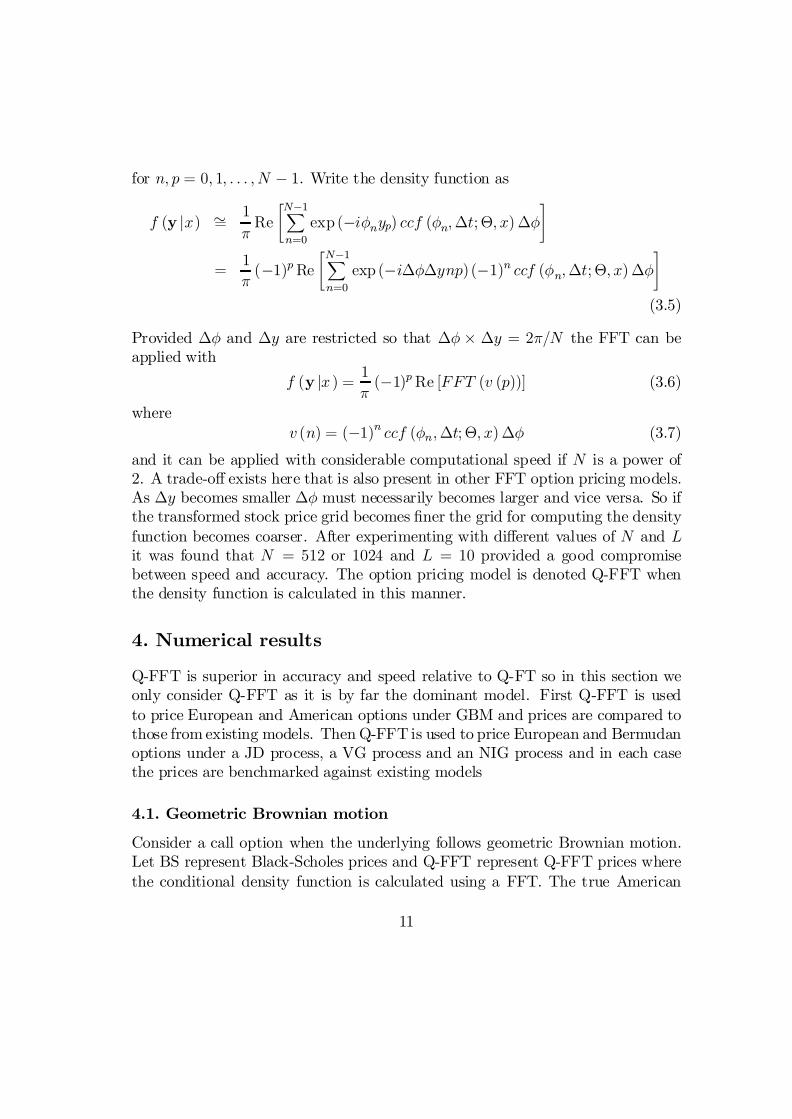
and it can be applied with considerable computational speed if N is a power of2. A trade-o¤ exists here that is also present in other FFT option pricing models.As ¢y becomes smaller ¢Á must necessarily becomes larger and vice versa. So ifthe transformed stock price grid becomes …ner the grid for computing the densityfunction becomes coarser. After experimenting with di¤erent values of N and Lit was found that N = 512 or 1024 and L = 10 provided a good compromisebetween speed and accuracy. The option pricing model is denoted Q-FFT whenthe density function is calculated in this manner.

4. Numerical results

Q-FFT is superior in accuracy and speed relative to Q-FT so in this section weonly consider Q-FFT as it is by far the dominant model. First Q-FFT is usedto price European and American options under GBM and prices are compared tothose from existing models. Then Q-FFT is used to price European and Bermudanoptions under a JD process, a VG process and an NIG process and in each casethe prices are benchmarked against existing models

4.1. Geometric Brownian motion

Consider a call option when the underlying follows geometric Brownian motion.Let BS represent Black-Scholes prices and Q-FFT represent Q-FFT prices wherethe conditional density function is calculated using a FFT. The true American

11

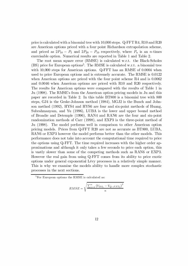
price is calculated with a binomial tree with 10,000 steps. Q-FFTR4, R10 and R20are American options priced with a four point Richardson extrapolation scheme,and priced as 2P10 ¡ P5 and 2P20 ¡ P10 respectively, where Pn is an n-timesexercisable option. Numerical results are reported in Table 1 and Table 2.

The root mean square error (RMSE) is calculated w.r.t. the Black-Scholes(BS) price for European options5. The RMSE is calculated w.r.t. a binomial treewith 10,000 steps for American options. Q-FFT has an RMSE of 0.0004 whenused to price European options and is extremely accurate. The RMSE is 0.0122when American options are priced with the four point scheme R4 and is 0.0062and 0.0046 when American options are priced with R10 and R20 respectively.The results for American options were compared with the results of Table 1 inJu (1998). The RMSE’s from the American option pricing models in Ju and thispaper are recorded in Table 2. In this table BT800 is a binomial tree with 800steps, GJ4 is the Geske-Johnson method (1984), MGJ2 is the Bunch and John-son method (1992), HYS4 and HYS6 are four and six-point methods of Huang,Subrahmanyam, and Yu (1996), LUBA is the lower and upper bound methodof Broadie and Detemple (1996), RAN4 and RAN6 are the four and six-pointrandomization methods of Carr (1998), and EXP3 is the three-point method ofJu (1998). The model performs well in comparison to other American optionpricing models. Prices from Q-FFT R20 are not as accurate as BT800, LUBA,RAN6 or EXP3 however the model performs better than the other models. Thisperformance does not take into account the computational time required to pricethe options using Q-FFT. The time required increases with the higher order ap-proximations and although it only takes a few seconds to price each option, thisis vastly slower than some of the competing methods such as RAN6 or EXP3.However the real gain from using Q-FFT comes from its ability to price exoticoptions under general exponential Lévy processes in a relatively simple manner.This is why we examine the models ability to handle more complex stochasticprocesses in the next sections.

5For European options the RMSE is calculated as:

RMSE =

sPnj=1

¡VBSj ¡ VQ¡F FTj

¢2

n

12

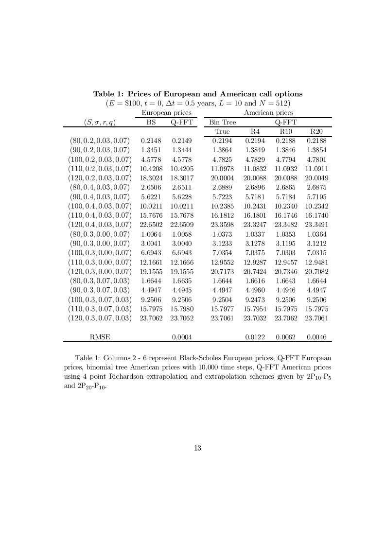
Table 1: Prices of European and American call options(E = $100, t = 0, ¢t = 0:5 years, L = 10 and N = 512)

European prices American prices(S; ¾; r; q) BS Q-FFT Bin Tree Q-FFT

True R4 R10 R20(80; 0:2; 0:03; 0:07) 0.2148 0.2149 0.2194 0.2194 0.2188 0.2188(90; 0:2; 0:03; 0:07) 1.3451 1.3444 1.3864 1.3849 1.3846 1.3854(100; 0:2; 0:03; 0:07) 4.5778 4.5778 4.7825 4.7829 4.7794 4.7801(110; 0:2; 0:03; 0:07) 10.4208 10.4205 11.0978 11.0832 11.0932 11.0911(120; 0:2; 0:03; 0:07) 18.3024 18.3017 20.0004 20.0088 20.0088 20.0049(80; 0:4; 0:03; 0:07) 2.6506 2.6511 2.6889 2.6896 2.6865 2.6875(90; 0:4; 0:03; 0:07) 5.6221 5.6228 5.7223 5.7181 5.7184 5.7195(100; 0:4; 0:03; 0:07) 10.0211 10.0211 10.2385 10.2431 10.2340 10.2342(110; 0:4; 0:03; 0:07) 15.7676 15.7678 16.1812 16.1801 16.1746 16.1740(120; 0:4; 0:03; 0:07) 22.6502 22.6509 23.3598 23.3247 23.3482 23.3491(80; 0:3; 0:00; 0:07) 1.0064 1.0058 1.0373 1.0337 1.0353 1.0364(90; 0:3; 0:00; 0:07) 3.0041 3.0040 3.1233 3.1278 3.1195 3.1212(100; 0:3; 0:00; 0:07) 6.6943 6.6943 7.0354 7.0375 7.0303 7.0315(110; 0:3; 0:00; 0:07) 12.1661 12.1666 12.9552 12.9287 12.9457 12.9481(120; 0:3; 0:00; 0:07) 19.1555 19.1555 20.7173 20.7424 20.7346 20.7082(80; 0:3; 0:07; 0:03) 1.6644 1.6635 1.6644 1.6616 1.6643 1.6644(90; 0:3; 0:07; 0:03) 4.4947 4.4945 4.4947 4.4960 4.4946 4.4947(100; 0:3; 0:07; 0:03) 9.2506 9.2506 9.2504 9.2473 9.2506 9.2506(110; 0:3; 0:07; 0:03) 15.7975 15.7980 15.7977 15.7954 15.7975 15.7975(120; 0:3; 0:07; 0:03) 23.7062 23.7062 23.7061 23.7032 23.7062 23.7061

RMSE 0.0004 0.0122 0.0062 0.0046

Table 1: Columns 2 - 6 represent Black-Scholes European prices, Q-FFT Europeanprices, binomial tree American prices with 10,000 time steps, Q-FFT American pricesusing 4 point Richardson extrapolation and extrapolation schemes given by 2P10-P5and 2P20-P10.

13

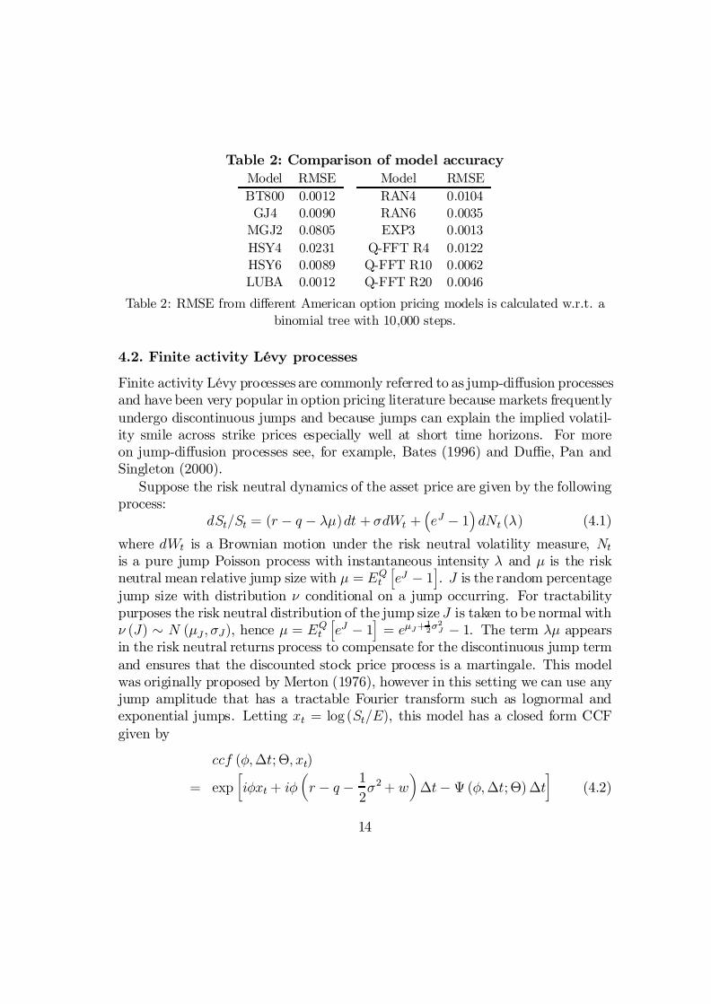
Table 2: Comparison of model accuracyModel RMSE Model RMSEBT800 0.0012 RAN4 0.0104GJ4 0.0090 RAN6 0.0035

MGJ2 0.0805 EXP3 0.0013HSY4 0.0231 Q-FFT R4 0.0122HSY6 0.0089 Q-FFT R10 0.0062LUBA 0.0012 Q-FFT R20 0.0046

Table 2: RMSE from di¤erent American option pricing models is calculated w.r.t. abinomial tree with 10,000 steps.

4.2. Finite activity Lévy processes

Finite activity Lévy processes are commonly referred to as jump-di¤usion processesand have been very popular in option pricing literature because markets frequentlyundergo discontinuous jumps and because jumps can explain the implied volatil-ity smile across strike prices especially well at short time horizons. For moreon jump-di¤usion processes see, for example, Bates (1996) and Du¢e, Pan andSingleton (2000).

Suppose the risk neutral dynamics of the asset price are given by the followingprocess:

dSt=St = (r ¡ q ¡ ¸¹)dt + ¾dWt +³eJ ¡ 1

´dNt (¸) (4.1)

where dWt is a Brownian motion under the risk neutral volatility measure, Ntis a pure jump Poisson process with instantaneous intensity ¸ and ¹ is the riskneutral mean relative jump size with ¹ = EQt

heJ ¡ 1

i. J is the random percentage

jump size with distribution º conditional on a jump occurring. For tractabilitypurposes the risk neutral distribution of the jump size J is taken to be normal withº (J) » N (¹J ; ¾J), hence ¹ = EQt

heJ ¡ 1

i= e¹J+

12¾

2J ¡ 1. The term ¸¹ appears

in the risk neutral returns process to compensate for the discontinuous jump termand ensures that the discounted stock price process is a martingale. This modelwas originally proposed by Merton (1976), however in this setting we can use anyjump amplitude that has a tractable Fourier transform such as lognormal andexponential jumps. Letting xt = log (St=E), this model has a closed form CCFgiven by

ccf (Á;¢t; £; xt)

= exp·iÁxt + iÁ

µr ¡ q ¡ 1

2¾2+ w

¶¢t¡ª (Á;¢t; £)¢t

¸(4.2)

14

whereª (Á;¢t; £) =

1

2¾2Á2 ¡¸

³eiÁ¹J¡

12Á

2¾2J ¡ 1´

(4.3)

andw = ¡¸¹= ¡¸

³e¹J¡

12 Á

2¾2J ¡ 1´

(4.4)

ª is the characteristic exponent and w is risk neutral compensator6 that ensuresthat the discounted stock price follows a martingale. Note that the parametervector is given by £ = f¾; ¸; ¹J ; ¾Jg0 and that the CCF is conditioned only onthe observable transformed stock price xt.

Let us consider a put option in the jump-di¤usion case. Let FT representprices using the standard Fourier transform techniques and Q-FFT represent Q-FFT prices. Let FT2 represent twice-exercisable option prices using a FT ap-proach extended to the case of two exercise dates7 and let Q-FFT2 representtwice-exercisable option prices using Q-FFT. In each twice-exercisable option the…rst exercise date is t + 1

2¢t and the second exercise date is t + ¢t. The bench-

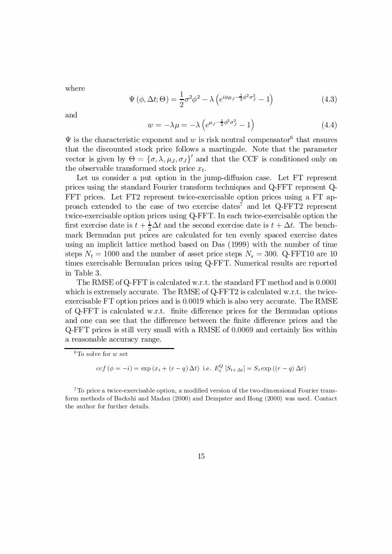
mark Bermudan put prices are calculated for ten evenly spaced exercise datesusing an implicit lattice method based on Das (1999) with the number of timesteps Nt = 1000 and the number of asset price steps Ns = 300. Q-FFT10 are 10times exercisable Bermudan prices using Q-FFT. Numerical results are reportedin Table 3.

The RMSE of Q-FFT is calculated w.r.t. the standard FT method and is 0:0001which is extremely accurate. The RMSE of Q-FFT2 is calculated w.r.t. the twice-exercisable FT option prices and is 0:0019 which is also very accurate. The RMSEof Q-FFT is calculated w.r.t. …nite di¤erence prices for the Bermudan optionsand one can see that the di¤erence between the …nite di¤erence prices and theQ-FFT prices is still very small with a RMSE of 0:0069 and certainly lies withina reasonable accuracy range.

6To solve for w set

ccf (Á = ¡i) = exp (xt + (r ¡ q)¢t) i.e. EQt [St+¢t ] = St exp ((r ¡ q) ¢t)

7To price a twice-exercisable option, a modi…ed version of the two-dimensional Fourier trans-form methods of Backshi and Madan (2000) and Dempster and Hong (2000) was used. Contactthe author for further details.

15

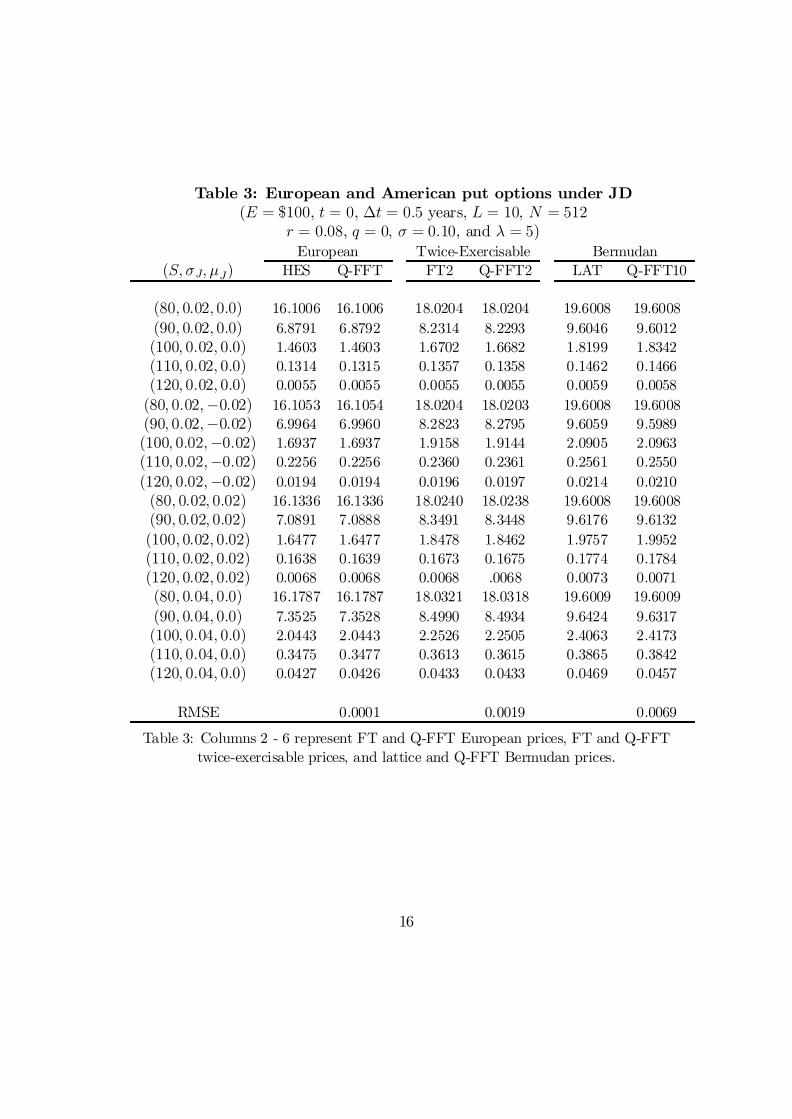
Table 3: European and American put options under JD(E = $100, t = 0, ¢t = 0:5 years, L = 10, N = 512

r = 0:08, q = 0, ¾ = 0:10, and ¸ = 5)European Twice-Exercisable Bermudan

(S; ¾J; ¹J) HES Q-FFT FT2 Q-FFT2 LAT Q-FFT10

(80; 0:02; 0:0) 16.1006 16.1006 18.0204 18.0204 19.6008 19.6008(90; 0:02; 0:0) 6.8791 6.8792 8.2314 8.2293 9.6046 9.6012(100; 0:02; 0:0) 1.4603 1.4603 1.6702 1.6682 1.8199 1.8342(110; 0:02; 0:0) 0.1314 0.1315 0.1357 0.1358 0.1462 0.1466(120; 0:02; 0:0) 0.0055 0.0055 0.0055 0.0055 0.0059 0.0058(80; 0:02;¡0:02) 16.1053 16.1054 18.0204 18.0203 19.6008 19.6008(90; 0:02;¡0:02) 6.9964 6.9960 8.2823 8.2795 9.6059 9.5989(100; 0:02;¡0:02) 1.6937 1.6937 1.9158 1.9144 2.0905 2.0963(110; 0:02;¡0:02) 0.2256 0.2256 0.2360 0.2361 0.2561 0.2550(120; 0:02;¡0:02) 0.0194 0.0194 0.0196 0.0197 0.0214 0.0210(80; 0:02; 0:02) 16.1336 16.1336 18.0240 18.0238 19.6008 19.6008(90; 0:02; 0:02) 7.0891 7.0888 8.3491 8.3448 9.6176 9.6132(100; 0:02; 0:02) 1.6477 1.6477 1.8478 1.8462 1.9757 1.9952(110; 0:02; 0:02) 0.1638 0.1639 0.1673 0.1675 0.1774 0.1784(120; 0:02; 0:02) 0.0068 0.0068 0.0068 .0068 0.0073 0.0071(80; 0:04; 0:0) 16.1787 16.1787 18.0321 18.0318 19.6009 19.6009(90; 0:04; 0:0) 7.3525 7.3528 8.4990 8.4934 9.6424 9.6317(100; 0:04; 0:0) 2.0443 2.0443 2.2526 2.2505 2.4063 2.4173(110; 0:04; 0:0) 0.3475 0.3477 0.3613 0.3615 0.3865 0.3842(120; 0:04; 0:0) 0.0427 0.0426 0.0433 0.0433 0.0469 0.0457

RMSE 0.0001 0.0019 0.0069

Table 3: Columns 2 - 6 represent FT and Q-FFT European prices, FT and Q-FFTtwice-exercisable prices, and lattice and Q-FFT Bermudan prices.

16

4.3. In…nite activity Lévy processes

In…nite activity Lévy processes are those Lévy processes with an in…nite jumparrival rate, that is an in…nite number of jumps can occur in a …nite time horizon.They have become increasingly popular in …nance because of their ability to …tasset return processes and option prices across strike prices in a parsimoniousmanner. The fact that on very small time scales market dynamics undergo a largenumber of very small discrete jumps is another theoretically appealing propertyof in…nite activity Lévy processes.

4.3.1. Variance gamma process

The variance gamma process for asset returns was …rst proposed by Madan andSeneta (1990), and extended by Madan and Milne (1991), Madan, Carr and Chang(1998) and Carr, Geman, Madan and Yor (2003). The process is an arithmeticBrownian motion with drift evaluated at a random time change that follows agamma process thus the VG process is a pure jump process. European optionsunder VG can be priced in terms of special functions. Methods for pricing pathdependent options under VG processes include the …nite di¤erence method ofHirsa and Madan (2004), the lattice methods of Kellizi and Webber (2003) andthe multinomial tree method Maller, Solomon and Szimayer (2004).

Denote an arithmetic Brownian motion with drift µ and volatility ¾ as follows:

b (t; µ; ¾) = µt+ ¾W (t) (4.5)

Then a VG process has a log stock price process given by

X (t;¾; º; µ) = b (T vt ; µ; ¾) (4.6)

where T vt = ° (t; 1; º) is a gamma process with unit mean and variance º. Lettingxt = ln (St=E) this model has a simple closed form CCF given by

ccf (Á;¢t; £; xt) = exp [iÁxt + iÁ(r ¡ q + w)¢t ¡ª(Á;¢t; £)¢t] (4.7)

whereª (Á;¢t; £) =

1

ºln

·1 ¡ iµºÁ + 1

2¾2ºÁ2

¸(4.8)

andw =

1

ºln

·1¡ µº ¡ 1

2¾2º

¸(4.9)

17

As before ª is the characteristic exponent and w is the risk neutral compensator.The parameter vector is given by £ = f¾; µ; ºg0 and the CCF is conditioned onlyon the observable transformed stock price xt.

Option prices from Q-FFT are compared to those from Kellezi and Webber(2003), denoted as KW, to benchmark Q-FFT with results available in the lit-erature. Table 4 contains results for European call options and Bermudan putoptions with 10 evenly spaced exercise dates. The parameter vector is given by£ = f0:12;¡0:14; 0:2g0, the current stock price is St = 100 and the exercise pricetakes on values E = f90; 95; : : : ; 110g0.

Table 4: European and Bermudan options under VG(t = 0, ¢t = 1 year, r = 0:10, q = 0, L = 10 and N = 1024)

European call prices European and Bermudan put pricesE Analytical KW Q-FFT Q-FFT KW Q-FFT10

(Euro) (Berm) (Berm)90 19.09935 19.09936 19.09937 0.53474 0.76115 0.7578795 15.07047 15.07048 15.07049 1.03005 1.52574 1.53866100 11.37002 11.37002 11.37003 1.85377 2.88152 2.87782105 8.11978 8.11978 8.11986 3.12779 5.17036 5.19537110 5.42960 5.42960 5.42963 4.96175 9.04064 9.06040115 3.36543 3.36544 3.36523 7.42153 13.87623 13.89456120 1.92110 1.92110 1.92078 10.50127 18.80965 18.82561

RMSE 6.5£10¡6 1.5£10¡4 0.01603

Table 4: Columns 2 - 6 represent analytical, KW and Q-FFT European call prices,Q-FFT European put prices, KW and Q-FFT Bermudan put prices

The RMSE of KW and Q-FFT are calculated w.r.t. the analytical prices forthe European call prices. Both models are very accurate with KW more accuratethan Q-FFT. The RMSE of Q-FFT for the Bermudan put prices is calculatedw.r.t. the KW prices and is reasonably accurate. The Bermudan prices fromboth models are relatively close as can be seen from the table. The surface plotin …gure 1 is a plot of Bermudan put prices in the VG model versus number ofexercise dates, M , and exercise price, E . The plot uses the put option parametersgiven in table 4 with M now varying from 1 to 10. As can be seen from thisplot the early exercise premium for in-the-money puts grows at a much faster ratethan the premium for out-of-the-money puts.

18

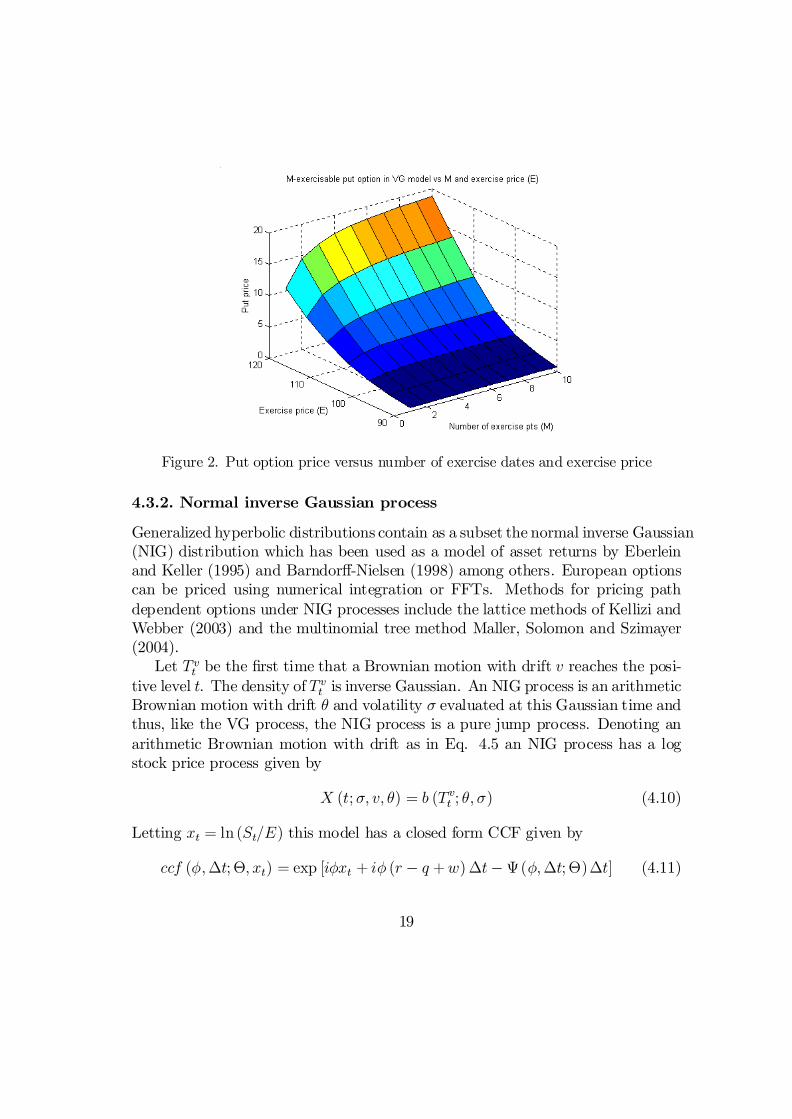
Figure 2. Put option price versus number of exercise dates and exercise price

4.3.2. Normal inverse Gaussian process

Generalized hyperbolic distributions contain as a subset the normal inverse Gaussian(NIG) distribution which has been used as a model of asset returns by Eberleinand Keller (1995) and Barndor¤-Nielsen (1998) among others. European optionscan be priced using numerical integration or FFTs. Methods for pricing pathdependent options under NIG processes include the lattice methods of Kellizi andWebber (2003) and the multinomial tree method Maller, Solomon and Szimayer(2004).

Let T vt be the …rst time that a Brownian motion with drift v reaches the posi-tive level t. The density of T vt is inverse Gaussian. An NIG process is an arithmeticBrownian motion with drift µ and volatility ¾ evaluated at this Gaussian time andthus, like the VG process, the NIG process is a pure jump process. Denoting anarithmetic Brownian motion with drift as in Eq. 4.5 an NIG process has a logstock price process given by

X (t;¾; v; µ) = b (T vt ; µ; ¾) (4.10)

Letting xt = ln (St=E) this model has a closed form CCF given by

ccf (Á;¢t; £; xt) = exp [iÁxt + iÁ (r ¡ q +w) ¢t¡ª(Á;¢t; £)¢t] (4.11)

19

whereª (Á;¢t; £) = ±

µq®2 ¡ (¯ + iÁ)2 ¡

q®2¡ ¯2

¶(4.12)

andw = ±

µq®2 ¡ (¯ + 1)2 ¡

q®2¡ ¯2

¶(4.13)

As before ª is the characteristic exponent and w is the risk neutral compensator.The parameter vector is written as £ = f®; ¯; ±g0 to conform with conventionalnotation, where the relationship with the parameters f¾; v; µg0 is given as follows

®2 =v2

¾2+µ2

¾4; ¯ =

µ

¾2; ± = ¾ (4.14)

The CCF is conditioned only on the observable transformed stock price xt.To benchmark results option prices from Q-FFT are compared to those from

Kellezi and Webber (2003). Table 5 contains results for European call optionsand Bermudan put options with 10 evenly spaced exercise dates. The parametervector is given by £ = f28:42141;¡15:08623; 0:31694g0 8, the current stock priceis St = 100 and the exercise price takes on values E = f90; 95; : : : ; 110g0.

As with the VGcase the European options from Q-FFT are extremely accurateand the Bermudan prices are very close to the prices from Kellezi and Webber.

Table 5: European and Bermudan options under NIG(t = 0, ¢t = 1 year, r = 0:10, q = 0, L = 10 and N = 1024)

European call prices European and Bermudan put pricesE Reference KW Q-FFT Q-FFT KW Q-FFT10

(Euro) (Berm) (Berm)90 19.09330 19.09330 19.09321 0.52858 0.74482 0.7300095 15.06077 15.06077 15.06061 1.02017 1.49554 1.47900100 11.35994 11.35993 11.35969 1.84343 2.84445 2.82777105 8.11561 8.11561 8.11537 3.12330 5.17297 5.15981110 5.43723 5.43724 5.43691 4.96902 9.03395 9.02806115 3.38474 3.38475 3.38418 7.44048 13.86529 13.86170120 1.94359 1.94359 1.94296 10.52345 18.80693 18.80320

RMSE

Table 5: Columns 2 - 6 represent analytical, KW and Q-FFT European call prices,Q-FFT European put prices, KW and Q-FFT Bermudan put prices

8These parameters were chosen by Kellezi and Webber so that the density function of theNIG process has the same …rst four moments as the density function from the VG process.

20

5. Conclusion

A model is developed that can be used to price path dependent options on Lévyprocesses. The model combines two existing models: the Fourier transform andquadrature option pricing models, retaining nice features of both models. Themodel is very general in terms of the underlying processes, with the only constraintbeing that the log stock price process has to have a closed form conditional char-acteristic function. The model is also very general in terms of the type of exoticoption being priced. It is easy to adjust the model to price other path dependentoptions such as barrier options, Asian options etc. The model can easily handlein…nite activity Lévy processes since a characteristic function based approach isused thus avoiding any problems other lattice based approaches encounter whenusing the Lévy measure in a neighbourhood of zero.

There are many possible avenues of future research. The accuracy and speedof the model can be improved by using more re…ned quadrature routines and byconstructing trees that are bounded. However I am more interested in applyingthe model to Lévy processes that incorporate stochastic volatility as a continuoustime stochastic process or as a regime switching volatility model. The model inthis paper can also be extended to incorporate “piecewise Lévy processes” where,for example, the density function has increments that are stationary on each timeinterval [t; t1], [t1; t2] and [t2; t+¢t], but the density function can change fromone interval to the next, thereby increasing calibration performance with respectto option prices over both strike price and maturity.

References

[1] Andricopoulos, A.D., M. Widdicks, P.W. Duck and D.P. Newton (2003).Universal option valuation using quadrature methods. Journal of FinancialEconomics 67, 447-471.

[2] Bakshi, G.C., and D.B. Madan (2000). Spanning and derivative-security val-uation. Journal of Financial Economics 55, 205-38.

[3] Barndor¤-Nielsen, O.E. (1998). Processes of normal inverse Gaussian type.Finance and Stochastics 2, 41-68.

[4] Bates, D. (1996). Jumps and stochastic volatility: exchange rate processesimplicit in Deutsche mark options. Review of Financial Studies 9, 67-107.

21

[5] Broadie, M. and J. Detemple (1996). American option valuation: new bounds,approximations, and a comparison of existing methods. Review of FinancialStudies 9, 1211-1250.

[6] Bunch, D. and H. Johnson (1992). A simple and numerically e¢cient valu-ation method for American puts using a modi…ed Geske-Johnson approach.Journal of Finance 47, 809-16.

[7] Carr, P. (1998). Randomization and the American put. Review of FinancialStudies 11, 597-626.

[8] Carr, P. and D.B. Madan (1999). “Option Valuation Using the Fast FourierTransform” Journal of Computational Finance 2.

[9] Carr, P. and L. Wu (2004). Time-changed Lévy processes and option pricing.Journal of Financial Economics 71, 113-141.

[10] Das, S.R. (1997). Discrete-time bond and option pricing for jump-di¤usionprocesses. Review of Derivatives Research 1, 211-43.

[11] Dempster, M., and S. Hong (2000). Spread option valuation and the FastFourier transform. Research Paper in Management Studies. The Judge Insti-tute of Management Studies.

[12] Du¢e, D., J. Pan, and K. Singleton (2000). Transform analysis and assetpricing for a¢ne jump-di¤usions. Econometrica 68, 1343-76.

[13] Eberlein, E. and U. Keller (1995). Hyperbolic distributions in …nance.Bernoulli 1, 281-299.

[14] Eberlein, E. and W. Kluge (2004). Exact pricing formulae for caps and swap-tions in a Lévy term structure model. Preprint Nr. 86, Freiburg Center forData Analysis and Modelling, University of Freiburg.

[15] Geman, H. (2002). Pure jump Lévy processes for asset price modelling. Jour-nal of Banking and Finance 26, 1297-1316.

[16] Geske, R., and H.E. Johnson (1984). The American put option valued ana-lytically. Journal of Finance 34, 1511-24.

22

[17] Heston, S. (1993). A closed-form solution of options with stochastic volatilitywith applications to bond and currency options. Review of Financial Studies6, 327-43.

[18] Hirsha, A. and D.B. Madan (2004). Pricing American options under variancegamma. Journal of Computational Finance 7.

[19] Huang, J., M. Subrahmanyam and G. Yu (1996). Pricing and hedging Amer-ican options: a recursive integration method. Review of Financial Studies 9,277-300.

[20] Ju, N. (1998). Pricing an American option by approximating its early exerciseboundary as a multipiece exponential function. Review of Financial Studies11, 627-46.

[21] Kellezi, E. and N. Webber (2003). Valuing Bermudan options when assetreturns are Lévy processes. Quantitative Finance 4, 87-100.

[22] Kou, S.G. (2002). A jump-di¤usion model for option pricing. ManagementScience 48, 1086-1101.

[23] Lee, R.W. (2004). Option pricing by transform methods: extensions, uni-…cation, and error control. Working paper, Stanford University. Journal ofComputational Finance 7.

[24] Lewis, A. (2000). Option pricing under stochastic volatility. Finance Press,California.

[25] Lewis, A. (2001). A simple option formula for general jump-di¤usion andother exponential Lévy process. Working paper. OptionCity.net.

[26] Madan, D.B. and E. Seneta. (1990). The variance gamma (VG) model forshare market returns. Journal of Business 63, 511-524.

[27] Madan, D.B. and F. Milne. (1991). Option pricing with VG martingale com-ponents. Mathematical Finance 1, 39-56.

[28] Madan, D.B., P. Carr and E.C. Chang. (1998). The variance gamma processand option pricing. European Finance Review 2, 79-105.

[29] Maller, R.A., D.H. Solomon and A. Szimayer (2004). A multinomial approx-imation of American option prices in a Lévy process model. Working paper.

23

[30] Merton, R.C. (1976). Option pricing when underlying stock returns are dis-continuous. Journal of Financial Economics 3, 125-44.

[31] Pan, J. (2002). The jump-risk premia implicit in options: evidence from anintegrated time-series study. Journal of Financial Economics 63, 3–50.

[32] Parkinson, M. (1977). Option pricing: the American put. Journal of Business50, 21-36.

[33] Stein, E.M., and J.C. Stein (1991). Stock price distributions with stochasticvolatility: an analytic approach. Review of Financial Studies 4, 725-52.

[34] Sullivan, M.A. (2000). Valuing American put options using Gaussian quadra-ture. Review of Financial Studies 13, 75-94.

24