Particle Identification in ALICE: a Bayesian approach · Particle Identiﬁcation (PID) provides information about the mass and ﬂavour composition of particle production in high-energy

EUROPEAN ORGANIZATION FOR NUCLEAR RESEARCH

CERN-EP-2016-02302 February 2016

c© 2016 CERN for the benefit of the ALICE Collaboration.Reproduction of this article or parts of it is allowed as specified in the CC-BY-4.0 license.

Particle identification in ALICE: a Bayesian approach

ALICE Collaboration∗

Abstract

We present a Bayesian approach to particle identification (PID) within the ALICE experiment. Theaim is to more effectively combine the particle identification capabilities of its various detectors. Af-ter a brief explanation of the adopted methodology and formalism, the performance of the BayesianPID approach for charged pions, kaons and protons in the central barrel of ALICE is studied. PID isperformed via measurements of specific energy loss (dE/dx) and time-of-flight. PID efficiencies andmisidentification probabilities are extracted and compared with Monte Carlo simulations using high-purity samples of identified particles in the decay channels K0

S→ π−π+, φ →K−K+, and Λ→ pπ−

in p–Pb collisions at√

sNN = 5.02TeV. In order to thoroughly assess the validity of the Bayesianapproach, this methodology was used to obtain corrected pT spectra of pions, kaons, protons, and D0

mesons in pp collisions at√

s = 7 TeV. In all cases, the results using Bayesian PID were found tobe consistent with previous measurements performed by ALICE using a standard PID approach. Forthe measurement of D0→ K−π+, it was found that a Bayesian PID approach gave a higher signal-to-background ratio and a similar or larger statistical significance when compared with standard PIDselections, despite a reduced identification efficiency. Finally, we present an exploratory study of themeasurement of Λ+

c → pK−π+ in pp collisions at√

s = 7 TeV, using the Bayesian approach for theidentification of its decay products.

∗See Appendix A for the list of collaboration members

arX

iv:1

602.

0139

2v2

[ph

ysic

s.da

ta-a

n] 2

6 M

ay 2

016

http://creativecommons.org/licenses/by/4.0

Particle identification in ALICE: a Bayesian approach ALICE Collaboration

1 Introduction

Particle Identification (PID) provides information about the mass and flavour composition of particleproduction in high-energy physics experiments. In the context of ALICE (A Large Ion Collider Experi-ment) [1], identified particle yields and spectra give access to the properties of the state of matter formedat extremely high energy densities in ultra-relativistic heavy-ion collisions. Modern experiments usuallyconsist of a variety of detectors featuring different PID techniques. Bayesian approaches to the problemof combining PID signals from different detectors have already been used by several experiments, e.g.NA27 [2], HADES [3] and BESII [4]. This technique was proposed for ALICE during its early planningstages [5] and then used extensively to prepare the ALICE Physics Performance Report [6, 7]. An anal-ogous method is also used to combine the PID signals from the different layers of the ALICE TransitionRadiation Detector.

The ALICE detector system is composed of a central part that covers the mid-rapidity region |η |< 1 (the‘central barrel’), and a muon spectrometer that covers the forward rapidity region −4 < η <−2.5. Thecentral barrel detectors that have full coverage in azimuth (ϕ) are, from small to large radii, the InnerTracking System (ITS), the Time Projection Chamber (TPC), the Transition Radiation Detector (TRD)1

and the Time Of Flight system (TOF). Further dedicated PID detectors with limited acceptance in ϕ andη are also located in the central barrel. These are the Electromagnetic Calorimeter (EMCal), the PhotonSpectrometer (PHOS), and a Cherenkov system for High-Momentum Particle Identification (HMPID).

The central barrel detectors provide complementary PID information and the capability to separate parti-cle species in different momentum intervals. At low momenta (p . 3–4GeV/c), a track-by-track separa-tion of pions, kaons and protons is made possible by combining the PID signals from different detectors.At higher momenta, statistical unfolding based on the relativistic rise of the TPC signal can be performedfor PID. Given the wide range of momenta covered, ALICE has the strongest PID capabilities of any ofthe LHC experiments. More details about the identification possibilities of the single detectors can befound in [1].

Several different PID methods were applied for analyses of data collected by ALICE during the RUN 1data taking period of the LHC (2009–2013). A non-exhaustive list of examples of PID in ALICE is givenin the following. Results were published on the transverse momentum (pT) distributions of charged pion,kaon and proton production [8, 9, 10] in different collision systems and centre-of-mass energies using theITS, TPC, TOF and HMPID detectors. Electron measurements from semileptonic heavy-flavour hadrondecays took advantage of the TPC, TOF, TRD and EMCal detectors [11, 12]. Neutral pion productionwas studied via photon detection in the PHOS and the detection of e+e− pairs from gamma conversionsin the TPC. PID detectors were also used extensively to improve the signal-to-background ratios whenstudying the production of certain particles based on the reconstruction of their decay products, such asD mesons [13], φ and K∗ resonances [14]; in studies of particle correlations, such as femtoscopy [15];and to identify light nuclei [16]. In all analyses where PID was used, selections were applied based onindividual detector signals and later combined.

In this paper we describe results obtained during RUN 1 in pp collisions at√

s = 7TeV, Pb–Pb collisionsat√

sNN = 2.76TeV and p–Pb collisions at√

sNN = 5.02TeV. In particular, we focus on the hadronidentification capabilities of the central barrel detectors that had full azimuthal coverage during RUN 1.These are the ITS, TPC and TOF detectors, which are described in more detail below. The other centralbarrel detectors are not discussed here.

The ITS is formed of six concentric cylindrical layers of silicon detectors: two layers each of SiliconPixel (SPD), Silicon Drift (SDD) and Silicon Strip Detectors (SSD). The SDD and the SSD provide aread-out of the signal amplitude, and thus contribute to the PID by measuring the specific energy loss

1The TRD was completed during the first Long Shutdown phase (2013–2015) and only had partial ϕ coverage during theRUN 1 data taking period (2009–2013).

2


(dE/dx) of the traversing particle. A truncated mean of the (up to) four signals is calculated, resulting ina relative dE/dx resolution of approximately 12% [1].

The TPC [17] is the main tracking device of ALICE. Particle identification is performed by measuringthe specific energy loss (dE/dx) in the detector gas2 in up to 159 read-out pad rows. A truncated meanthat rejects the 40% largest cluster charges is built, resulting in a Gaussian dE/dx response. The dE/dxresolution ranges between 5–8% depending on the track inclination angle and drift distance, the energyloss itself, and the centrality in p–Pb and Pb–Pb collisions due to the differing detector occupancy.

The TOF detector [18] is based on Multigap Resistive Plate Chamber technology. It measures the flighttimes of particles with an intrinsic resolution of ∼80 ps. The expected flight time for each particlespecies is calculated during the reconstruction, and then PID is performed via a comparison between themeasured and expected times.

Other forward-rapidity detectors are also relevant to the data analyses presented in this paper. The V0plastic scintillator arrays, V0A (covering 2.8 < η < 5.1) and V0C (−3.7 < η < −1.7), are required inthe minimum-bias trigger. The V0 signals are also used to determine the centrality of p–Pb and Pb–Pbcollisions. The T0 detector is a quartz Cherenkov detector that is used for start-time estimation with aresolution of ∼40 ps in pp collisions and 20–25 ps in Pb–Pb collisions.

A thorough understanding of the detector response is crucial for any particle identification method. In thecase of dE/dx, this means a well parameterised description of the average energy loss (according to theBethe-Bloch formula [19]) and a reliable estimate of the signal resolution. For the TOF measurement,the start-time information, start-time resolution, track reconstruction resolution, and intrinsic detectorresolution need to be known [18].

Combining the PID signals of the individual detectors using a Bayesian approach [20] makes effectiveuse of the full PID capabilities of ALICE. However, using combined probabilities to perform particleidentification may result in unintuitive, non-trivial track selections. It is therefore important to benchmarkthe Bayesian PID method, compare efficiencies in data and Monte Carlo, and validate that this techniquedoes not introduce a systematic bias with respect to previously published results. This paper focuses onthe verification of the Bayesian PID approach on the basis of various data analyses.

Section 2 describes the Bayesian approach (2.1), the definitions of efficiency and contamination in thecontext of PID (2.2), the extraction and application of prior distributions (2.3), and different strategies forusing the resulting probabilities (2.4). Section 3 presents benchmark analyses of high-purity samples ofpions, kaons, and protons from the two-prong decays of K0

S mesons, φ mesons and Λ baryons. Section 4presents validations of the Bayesian approach for two full analyses: the measurement of the transversemomentum spectra of pions, kaons and protons (4.1), and the analysis of D0→ K−π+ (4.2). Section 5illustrates the application of the Bayesian PID approach to maximise the statistical significance whenanalysing the production of Λ+

c baryons. Finally, a conclusion and outlook are given in Section 6.

2 Bayesian PID in ALICE

Simple selections based on the individual PID signals of each detector do not take full advantage of thePID capabilities of ALICE. An example of this is illustrated in Fig. 1, which shows the separation ofthe expected TPC and TOF signals for pions, kaons and protons with transverse momenta in the range2.5 < pT < 3 GeV/c. Clearly, the separation in the two-dimensional plane (the peak-to-peak distance)of e.g. pions and kaons is larger than the separation of each individual one-dimensional projection. Anatural way of combining the information of independent detectors is to express the signals in terms ofprobabilities. An additional advantage of this method is that detectors with non-Gaussian responses canalso be included in a straightforward way. A Bayesian approach makes use of the full PID capabilities

2 A Ne-CO2-based gas mixture of ∼90m3 in RUN 1.

3


(arb. units)π

⟩x/dEd⟨ − x/dEd30 20 10 0 10 20

(ps)

π⟩T

OF

t⟨ −

TO

Ft

400

200

0

200

400

600

800

1000

1200

1400

1

10

210

310

410ALICE

= 2.76 TeVNN

sPb −Pb

| < 0.8η10% centrality, |−0c < 3.0 GeV/

Tp2.5 <

p

K

π

Fig. 1: Combined particle identification in the TPC and TOF for data from Pb–Pb collisions at√

sNN = 2.76TeV,shown as a two-dimensional plot. The PID signals are expressed in terms of the deviation from the expectedresponse for pions in each detector.

by folding the probabilities with the expected abundances (priors) of each particle species. This sectionoutlines the standard ‘nσ ’ PID approach, before presenting the method used to combine the signals fromthe different detectors when adopting a Bayesian PID approach.

2.1 PID signals in ALICE

The response of each detector can be expressed in terms of its raw signal, S. One of the simplest waysof performing PID is to directly select based on S. Examples of S include the flight-time informationfrom the TOF detector, tTOF, and the specific energy loss dE/dx in detector gas or silicon, respectivelymeasured by the TPC and the ITS. A more advantageous approach would be to use a discriminatingvariable, ξ , which makes use of the expected detector response R:

ξ = f (S,R), (1)

where R can have functional dependences on the properties of the particle tracks, typically the mo-mentum p, the charge Z, or the track length L. The detector response functions are usually complexparameterisations expressing an in-depth knowledge of subtle detector effects.

For a detector with a Gaussian response, R is given by the expected average signal S(Hi) for a givenparticle species Hi and the expected signal resolution σ . The index i usually refers to electrons, muons,pions, kaons or protons, but may also include light nuclei such as deuterons, tritons, 3He nuclei and4He nuclei. The most commonly used discriminating variable for PID is the nσ variable, defined as thedeviation of the measured signal from that expected for a species Hi, in terms of the detector resolution:

nσ i

α=

Sα − S(Hi)α

σ iα

, (2)

where α = (ITS,TPC, ...). The resolution is given here as σ iα , as it depends both on the detector and the

species being measured. In the following, σ iα is simply referred to as ‘σ ’.

The nσ PID approach corresponds to a ‘true/false’ decision on whether a particle belongs to a givenspecies. A certain identity is assigned to a track if this value lies within a certain range around the

4


expectation (typically 2 or 3σ ). Depending on the detector separation power, a track can be compatiblewith more than one identity.

For a given detector α with a Gaussian response, it is possible to define the conditional probability thata particle of species Hi will produce a signal S as

P(S|Hi) =1√

2πσe−

12 nσ

2=

1√2πσ

e−(S−S(Hi))

2

2σ2 . (3)

In the case of a non-Gaussian response, the probability is described by an alternative parameterisationappropriate to the detector. The advantage of using probabilities is that the probabilities from differentdetectors, Pα , with and without Gaussian responses, can then be combined as a product:

P(~S|Hi) = ∏α=ITS,TPC,...

Pα(Sα |Hi), (4)

where ~S = (SITS,STPC, ...).

The probability estimate P(~S|Hi) (either for a single detector, or combined over many) can be interpretedas the conditional probability that the set of detector signals ~S will be seen for a given particle speciesHi. However, the variable of interest is the conditional probability that the particle is of species Hi,given some measured detector signal (i.e. P(Hi|~S)). The relation between the two for a combined set ofdetectors can be expressed using Bayes’ theorem [20]:

P(Hi|~S) =P(~S|Hi)C(Hi)

∑k=e,µ,π,... P(~S|Hk)C(Hk). (5)

Here, C(Hi) is an a priori probability of measuring the particle species Hi, also known as the prior, andthe conditional probability P(Hi|~S) is known as the posterior probability.

The priors (which are discussed in more detail in Section 2.3) serve as a ‘best guess’ of the true particleyields per event. When such a definition is adopted for the priors, a selection based on the Bayesianprobability calculated with Eq. 5 then corresponds to a request on the purity (defined as the ratio betweenthe number of correctly identified particles and the total selected). Additionally, priors can be used toreject certain particle species that are not relevant to a given analysis. Most commonly in the context ofthe ALICE central barrel, the prior for muons is set to zero. Due to the similarity between the pion andmuon mass, the two species are almost indistinguishable over a broad momentum range; the efficiencyof detecting a pion would thus be reduced if muons were not neglected. At the same time, this influencesthe number of particles wrongly identified as pions, since the true abundance of muons (roughly 2% ofall particles, estimated using Monte Carlo simulations) is neglected. This case is further discussed in thefollowing sections.

2.2 PID efficiency and contamination

In order to obtain the physical quantity of interest (typically a cross section or a spectrum) from a rawyield, it is necessary to (a) compute the efficiency due to other selections applied before PID, and (b)compute the efficiency of the PID strategy. The PID efficiency is defined as the proportion of particlesof a given species that are identified correctly by the PID selections. Both kinds of efficiency are usuallyestimated via Monte Carlo techniques. To precisely compute the efficiency of a given PID strategy, it isof utmost importance that an accurate description of the actual signals present in the data is provided bythe Monte Carlo simulation. Special care must be given to the ‘tuning’ of Monte Carlo simulations toreproduce all of the features and dependences observed in data for PID signals.

5


It is possible to define a εPID matrix that contains the probability to identify a species i as a species j. Ifonly pions, kaons and protons are considered, the 3×3 εPID matrix is defined as

εPID =

εππ επK επpεKπ εKK εKpεpπ εpK εpp

, (6)

where the diagonal elements εii are the PID efficiencies, and the non-diagonal elements (εi j, i 6= j)represent the probability of misidentifying a species i as a different species j.

The abundance vectors for pions, kaons and protons are defined as

~Ameas =

πmeasKmeaspmeas

and ~Atrue =

πtrueKtrueptrue

, (7)

where the elements of ~Ameas (~Atrue) represent the measured (true) abundances of each species. Thediagonal elements εii of the PID matrix are then defined as

εii =Ni identified as i

Aitrue

. (8)

Techniques to estimate the matrix elements are discussed in Section 3. The abundance vectors ~Ameas and~Atrue are linked by the following relation:

πmeasKmeaspmeas

=

εππ επK επpεKπ εKK εKpεpπ εpK εpp

ᵀ

·

πtrueKtrueptrue

. (9)

Inverting the εᵀPID matrix, the physical quantities are then extracted via:

~Atrue = (εᵀPID)

−1×~Ameas. (10)

The εPID matrix elements have functional dependences on many variables, primarily pT and collisionsystem. Other second-order dependences (for example pseudorapidity, event multiplicity, and centrality)can also be studied depending on the specific track selections and PID strategies applied.

The contamination of the species j due to a different species i (c ji) is the number of particles belongingto species i that are wrongly identified as j (Ni identified as j), divided by the total number of identified jparticles (A j

meas) [7]:

c ji =Ni identified as j

A jmeas

, i 6= j. (11)

Contamination should not be confused with the misidentification probabilities defined in Eq. 6, which donot depend on the real abundances. The connection between contamination and misidentification is:

c ji =εi jAi

true

ε j jAjtrue +∑ j 6=k ε jkAk

true

. (12)

6


There is usually a trade-off between efficiency and contamination. Both depend on the PID strategy (e.g.choice of detectors), the detector response, and the priors used, all of which are momentum-dependent.The contamination is additionally driven by the real abundances.

An accurate estimate of the contamination c ji depends on the real abundances, and it must be determinedwith data-driven techniques (or with Monte Carlo simulations with abundances corresponding to what isfound in the data).

Although the PID matrix elements are independent of the real abundances, they still depend on thechoice of priors. They are therefore evaluated consistently as long as the same set of priors is usedboth in the data analysis and for the Monte Carlo simulations, provided that the detector responses aresimulated correctly. In addition, a choice of priors that lies closer to the true abundances allows thebest compromise to be found between the maximisation of the efficiency and the minimisation of thecontamination probabilities. Considering that any systematic uncertainties in the detector response willbe amplified if the efficiency is low or if the contamination probabilities are large, the method becomesmore effective as the priors tend closer to reality. An extreme example of this would be the identificationof pions and muons using equal priors for all species, as the two species are difficult to distinguish fromeach other (εππ ≈ εµµ ≈ 0.5 and επµ ≈ εµπ ≈ 0.5). In such a case, even a small discrepancy in thedescription of the detector response in Monte Carlo would cause a fluctuation in εi j, leading to a largeuncertainty in the estimate of the pion yield; a choice of priors corresponding to the true abundanceswould prevent this from happening.

In cases where the detector responses are well separated between different species, the priors do notneed to correspond to the true abundances, and could even be flat. The differences between differentchoices can then be used to provide an estimate of the systematic uncertainties depending on the currentknowledge of the detector response. The influence of the choice of priors is further discussed as part ofthe analyses presented in Section 4.

The combination of probabilities can also be used to identify and reduce the level of unphysical back-ground that may arise in PID analyses due to track misassociation between detectors. For example, thefraction of TPC tracks that are not correctly associated with the corresponding TOF hit increases withthe multiplicity of the event, and depends on the spatial matching window used in the reconstruction toassociate a TOF hit to a track. In ALICE this effect only plays a role in Pb–Pb and p–Pb collisions,and even in the most central Pb–Pb collisions it remains below 10% for tracks with momentum above1 GeV/c. In these cases, a mismatch probability can be defined based on e.g. the measured flight timebeing uncorrelated with the track reconstructed with the ITS and TPC due to the TOF hit being producedby another particle.

2.3 Priors in ALICE

As discussed in Section 2.1, an analysis using the Bayesian approach is expected to be moderatelydependent on the choice of priors. Separate sets of priors were evaluated for each collision system.They were evaluated by means of an iterative procedure on data taken in 2010 and 2013 from pp, Pb–Pb,and p–Pb collisions at

√s = 7TeV,

√sNN = 2.76TeV and

√sNN = 5.02 TeV, respectively, and were

computed as a function of transverse momentum. Priors were also determined as a function of centralityfor Pb–Pb collisions, and of the multiplicity class (based on the signal in the V0A detector) for p–Pb data.All of the priors were obtained at mid-rapidity, |η |< 0.8.

The absolute normalisation of the priors is arbitrary, and was chosen so as to normalise all of the priors tothe abundance of pions. The value of the priors for pions is thereby set to unity for all pT. Flat priors (i.e.1 for all species) are applied at the beginning of the iterative procedure. Bayesian posterior probabilitiesPn(Hi|S) are computed using the priors obtained in step n, as defined in Eq. 5. These probabilities arethen used in turn as weights to fill identified pT spectra Y (Hi, pT) for the step n+ 1 starting from the

7


inclusive (unidentified) measured pT spectra:

Yn+1(Hi, pT) = ∑S

Pn(Hi|S), (13)

where the summation is performed for all signals S induced by particles of a given pT in the sample. It isthen possible to obtain a new set of priors Cn+1 from the relative ratios of the identified spectra accordingto

Cn+1(Hi, pT) =Yn+1(Hi, pT)

Yn+1(Hπ , pT). (14)

The procedure is then iterated, and the extracted prior values converge progressively with each iteration.The values of the priors are shown in the left panel of Fig. 2 for the K/π ratio obtained using data fromp–Pb collisions. The convergence of this procedure is illustrated in the right-hand panel, as a ratio of thepriors for successive steps. A satisfactory convergence is obtained after 6–7 iterations.

)c (GeV/T

p

0 2 4 6 8 10

πK

/

0.2

0.4

0.6

0.8

1.0

Step 0 = equal priorsStep 1Step 2Step 3Step 4Step 5, 6, 7

ALICE priors

= 5.02 TeVNN

sPb −p

20% V0A multiplicity−10

)c (GeV/T

p

0 2 4 6 8 10

1 −

nste

p

)π

/ (

K/

nste

p

)π

(K/

0.2

0.4

0.6

0.8

1.0

1.2

= 1n

= 2n

= 3n

= 4n

= 5n

= 6n

= 7n

ALICE priors

= 5.02 TeVNN

sPb −p

20% V0A multiplicity−10

Fig. 2: An example of the iterative prior extraction procedure for p–Pb data (for the 10–20% V0A multiplicityclass). The extracted K/π ratio of the priors is shown as a function of pT at each step of the iteration (left) and asa ratio of the value between each successive step (right). Step 0 refers to the initial ratio, which is set to 1.

A set of priors was obtained for global tracks, defined as tracks reconstructed in both the ITS and TPC.This set is referred to in the following as C(Hi)TPC (the “standard priors”). This set of priors is thenpropagated to other detectors using “propagation factors” Fα , which are detector-specific and dependenton transverse momentum. In some cases these multiplicative factors can also be charge-dependent (thisis true for EMCal, for example). Fα , which is obtained for each detector via Monte Carlo, takes intoaccount the particles reaching the outer detectors, as well as the acceptances of the outer detectors andtheir corresponding energy thresholds. The abundances measured by TOF and TPC will differ due tothese effects. The requirement of a given detector therefore changes the priors. For an outer detector α ,the priors for a track with momentum pT are determined as

C(Hi)α(pT) = Fα(pT)×C(Hi)TPC(pT). (15)

Priors are currently propagated for TRD, TOF, EMCal and HMPID. Priors were also generated for tracksthat are obtained using only ITS hits. These were used for the spectrum analysis at low momentum [9].

8


In the analyses presented in this paper, the propagation procedure of priors from TPC to TOF was testedextensively.

Since the priors correspond to relative particle abundances, it is possible to directly compare the priorsobtained from the iterative procedure with the abundances measured by ALICE [8, 10, 21]. Comparisonsbetween the priors and the measured p/π and K/π ratios are shown in Fig. 3 for pp and Pb–Pb collisionsat√

s = 7 TeV and√

sNN = 2.76 TeV, respectively, and in Fig. 4 for p–Pb collisions at√

sNN = 5.02 TeV.In some cases the priors cover a larger range than the measurements made by ALICE.

In order to make these comparisons, the priors were corrected by several factors to take into account thedifferent selections used in the physics analyses and in the priors computation. Since the standard priorsare provided for the TPC case, only the tracking efficiency correction was applied. Additional conver-sions from pseudorapidity intervals (used for the priors) to rapidity intervals (used for the measurement)were also applied, as well as an average feed-down correction derived from the Pb–Pb analysis [10].This feed-down mainly applies to protons from the decays of Λ baryons.

The priors (open symbols) and the measured abundances (filled symbols) are consistent with one anotherwithin roughly 10% over a wide momentum range for all centrality ranges (for Pb–Pb collisions) andV0A multiplicity classes (for p–Pb collisions). The choice to use feed-down corrections evaluated ina given system leads to better agreement at low momenta in Pb–Pb collisions than in p–Pb collisions.However, at high momenta, where the PID performance is better exploited, the results are independent ofthis correction. The overall level of agreement is satisfactory, as the priors represent a realistic descriptionof the various particle abundances.

0.5 1 1.5 2 2.5 3 3.5 4

Spectr

a r

atio

0.0

0.2

0.4

0.6

0.8

1.0 πp/ ALICE = 2.76 TeV

NNsPb −Pb

= 7 TeVspp

0.5 1 1.5 2 2.5 3 3.5 4

Ra

tio

to

prio

rs

0.8

1.0

1.20.5 1.0 1.5 2.0 2.5 3.0 3.5 4.0

0.0

0.2

0.4

0.6

0.8

1.0 πK/ 5%− 040%− 3080%− 60

pp

open: Bayesian priors

closed: published spectra

)c (GeV/T

p

0.5 1 1.5 2 2.5 3 3.5 4

0.8

1

1.2

Fig. 3: The proton/pion ratio (left) and kaon/pion ratio (right), as measured by ALICE [8, 10] using TPC andTOF (filled symbols), compared with the standard priors as described in the text (open symbols) for Pb–Pb andpp collisions. For Pb–Pb, the results are reported for different centrality classes. Particle ratios are calculated formid-rapidity, |y|< 0.5. The double ratios (the measured abundances divided by the Bayesian priors) are shown inthe lower panels.

It is also important to test whether there is any dependence of the final result on the set of priors used. Toperform these tests, it is possible to use alternative sets of priors as well as flat priors, which essentiallycombine the probabilities from the different detectors without weighting them with Bayesian priors.Slightly different sets of priors can be obtained by varying the track selection parameters. An example

9


0.5 1 1.5 2 2.5 3 3.5 4

Spectr

a r

atio

0.0

0.2

0.4

0.6

0.8πp/ ALICE

= 5.02 TeVNN

sPb −p

0.5 1 1.5 2 2.5 3 3.5 4

Ra

tio

to

prio

rs

0.8

1.0

1.20.5 1.0 1.5 2.0 2.5 3.0 3.5 4.0

0.0

0.2

0.4

0.6

0.8πK/ 5%− 0

40%− 2080%− 60

open: Bayesian priors

closed: published spectra

)c (GeV/T

p

0.5 1 1.5 2 2.5 3 3.5 4

0.8

1

1.2

Fig. 4: The proton/pion ratio (left) and kaon/pion ratio (right), as measured by ALICE [21] using TPC andTOF (filled symbols), compared with the standard priors obtained with an iterative procedure (open symbols) forp–Pb collisions for different V0A multiplicity classes. Particle ratios are calculated for mid-rapidity, |y|< 0.5 withrespect to the centre-of-mass system. The double ratios (the measured abundances divided by the Bayesian priors)are shown in the lower panels.

of a systematic check on the dependence on varying the set of priors is discussed in Section 4.2 for theD0 case.

2.4 Bayesian PID strategies

Once the Bayesian probability for each species (p, K, π , etc.) has been calculated for a given track, thePID selection may be applied with a variety of selection criteria. The three criteria applied in this paperare:

– Fixed threshold: The track is accepted as belonging to a species if the probability for this is greaterthan some pre-defined value. As an example, the choice of a 50% threshold means that a particlewill only be accepted as a kaon if its Bayesian probability of being a kaon is greater than 50%. Notethat this strategy is not necessarily exclusive, as a threshold of less than 50% could lead to multiplepossible identities. As already discussed, a selection on the Bayesian probability corresponds to apurity requirement of the signal if the priors reflect the true particle abundances.

– Maximum probability: The track is accepted as the most likely species (i.e. the species with thehighest probability).

– Weighted: All tracks reaching the PID step of the analysis are accepted, with a weight differentfrom unity applied to their yield. The weight is defined as the product of the Bayesian probabilitiesobtained for the tracks involved (e.g. in D0→ K−π+, this is the kaon probability of the negativetrack multiplied by the pion probability of the positive track). The final result is corrected for theaverage weight determined in Monte Carlo simulations in the same way as is done for the PIDefficiency in other methods.

The fixed threshold method is compared with nσ PID as part of the benchmark analysis (see Section 3).The maximum probability method is used in the single-particle spectrum analysis described in Sec-

10


tion 4.1 and for the Λ+c baryon analysis in Section 5. Finally, all three of the aforementioned methods

are tested for the analysis of D0→ K−π+ in Section 4.2.

3 Benchmark analysis on two-prong decay channels

High-purity samples of identified particles were selected via the study of specific decay channels. Thesesamples served as a baseline for validating the Monte Carlo tools that are normally used to estimatethe efficiencies and misidentification probabilities (i.e. the εPID matrix discussed in Section 2) of theBayesian PID approach. The methodology developed in this section was also applied to the nσ PIDapproach, providing an important cross-check.

3.1 Description of the method

The following decays were used to obtain high-purity samples of three different species:

– K0S→ π−π+ to study charged pions;

– Λ→ pπ− (and respective charge conjugates) to study protons; and

– φ → K−K+ to study charged kaons.

The first two cases are true V0 decays, comprising two charged prongs originating from a secondaryvertex displaced from the interaction point, whereas the daughters of the φ meson originate from theprimary interaction vertex due to its shorter lifetime. For conciseness, all of these are referred to as V0

decays in this paper.

Here we report results based on the p–Pb data set, testing the PID method using both TPC and TOF. Thep–Pb data sample is less affected by background uncertainties than the Pb–Pb sample when perform-ing fits of the invariant mass spectra, due to the smaller amount of combinatorial background. This isespecially true for the φ analysis.

Different track selection criteria were applied in order to select daughter particles coming either from theprimary vertex (for the φ case) or from a secondary vertex (for the K0

S and Λ cases). For a given V0, afit of the combinatorial invariant mass distribution allows the background to be subtracted and the yieldof V0 decays to be extracted. The estimated yield is considered to be a pure sample of a given species(a precise measurement of the total number of particles of a given species in a given data set). Thisestimation was done without applying any PID selections. Then the exercise was repeated applying PIDselections on each of the two prongs, selecting between pions, kaons and protons. The comparison withthe number of positively identified secondary prongs determines the efficiency and the misidentificationwith respect to the values estimated when not applying PID.

Figure 5 shows examples of the fitting procedure for the K0S invariant masses for 2< pπ

T < 3GeV/c. Fromleft to right, the panels show the analysis without PID and then requiring the identification of a positivepion, kaon, or proton, respectively. The K0

S signal (and background) fitted in the latter three cases,compared with the results without applying PID, allow the extraction of the identification efficiency andmisidentification probabilities.

In order to reduce the background for the φ analysis, before starting the procedure, one of the two decaytracks was ‘tagged’ using a PID selection requiring compatibility with the kaon hypothesis and then thePID selection under study is applied on the other track. The tagging was performed with a 2σ selectionon a combination of the TPC and TOF signals.

The TPC and TOF signals are combined as |nCombσ ( j)|=

√(nTPC

σ ( j)2 +nTOFσ ( j)2)/2. The same method

was also applied on the simulated sample in order to check the agreement between Monte Carlo and data

11


0.46 0.48 0.5 0.52

2c

En

trie

s /

80

0 k

eV

/

1

10

210

310

No PID

0.46 0.48 0.5 0.52

1

10

) > 0.2π(+π

P

0.46 0.48 0.5 0.52

1

10

(K) > 0.2+π

P

)2c) (GeV/−

π+

πInvariant mass (

0.46 0.48 0.5 0.52

1

10

2

3

ALICE

= 5.02 TeVNN

sPb −p

)c < 3 GeV/+

π

Tp (2 < −

π+

π → s0

K

(p) > 0.2+π

P

Fig. 5: V0 fits to extract the yield and background for K0S→ π−π+ in p–Pb collisions at

√sNN = 5.02 TeV. From

left to right: no PID selections applied and selecting pions, kaons and protons using a specific PID strategy (here,Bayesian probability > 0.2). The yield estimated from the second plot from the left (compared with the no-PIDyield result) gives a measure of the PID efficiency for the pions, while the remaining ones give information aboutmisidentification.

on the estimated quantities. This serves as a validation for the Monte Carlo estimation of the efficiencyof a given PID strategy, as well as for the subsequent corrections required in order to extract physicsresults.

3.2 Comparison of PID efficiencies between data and Monte Carlo

The PID matrix elements obtained for different Bayesian probability thresholds are presented here. Anexample for the highest purity case considered in this work (Bayesian probability greater than 80%) isshown in Fig. 6. Each plot represents a row of the εPID matrix for a given species i, with the i = j pointscorresponding to the PID efficiencies (εii) and the i 6= j points corresponding to the misidentificationprobabilities (εi j). The matrix was evaluated separately for positively and negatively charged tracks.As no difference was found between the two cases, the results shown here were averaged over bothcharges. For Monte Carlo, the PID hypothesis was tested both via the true particle identity available inthe simulation and by applying the same procedure as for the data.

0.5 1 1.5 2 2.5 3 3.5 4

(i,j)

PID

ε

0.0

0.2

0.4

0.6

0.8

1.0

±πi =

ALICE

= 5.02 TeVNNsPb −p

(j) > 0.8P

0.5 1 1.5 2 2.5 3 3.5 40

0.2

0.4

0.6

0.8

1

±i = K

±πj = ±j = K

pj = p,

)c (GeV/T

p0.5 1 1.5 2 2.5 3 3.5 4

0

0.2

0.4

0.6

0.8

1

pi = p,

Data

MC

Fig. 6: εPID matrix elements in p–Pb collisions after selection with a Bayesian probability greater than 80%.Comparisons with Monte Carlo (open symbols) are also shown.

As can be seen from Fig. 6, the efficiencies and misidentification probabilities can be evaluated veryprecisely. The agreement between data and Monte Carlo is good, both in shape and absolute value.

12


0.5 1 1.5 2 2.5 3 3.5 4

(i,j)

PID

ε

0.0

0.2

0.4

0.6

0.8

1.0

±πi =

ALICE

= 5.02 TeVNNsPb −p

(j)| < 2Comb

σ|n

0.5 1 1.5 2 2.5 3 3.5 40

0.2

0.4

0.6

0.8

1

±i = K

±πj = ±j = K

pj = p,

)c (GeV/T

p

0.5 1 1.5 2 2.5 3 3.5 40

0.2

0.4

0.6

0.8

1

pi = p,

Data

MC

Fig. 7: εPID matrix elements in p–Pb collisions after selection with a 2σ selection on the combined TPC and TOFsignal. Comparisons with Monte Carlo (open symbols) are also shown.

The general features of the PID strategies are also described well, and behave as expected: using ahigh threshold maximises the purity, but also sharply reduces the efficiency. Nevertheless, even forP ≥ 80%, where the efficiency estimate is more sensitive to the description of the detector responses inthe simulations, the agreement with Monte Carlo remains within 5% below 3 GeV/c.

The analysis was repeated using 2σ and 3σ selections on the combined TOF and TPC signals, as dis-cussed above, to identify the three hadron species. The result is shown in Fig. 7 for the 2σ case. Asexpected, the εPID matrix elements have different values from the 80% Bayesian probability threshold(given that the nComb

σ selection is somewhat more inclusive), and the probability of misidentification in-creases accordingly. The agreement between Monte Carlo and data for the misidentification probabilitiesis worse in the nσ case than in the Bayesian case for kaons misidentified as pions. However, there remainsa good agreement between Monte Carlo and data overall. The efficiencies are below the values expectedfrom a perfectly Gaussian signal; a Monte Carlo or data-driven evaluation of the PID strategy efficiencyis therefore mandatory. The non-Gaussian tail of the TOF signal [18], caused by charge induction onpairs of neighbouring readout pads, plays a significant role in this discrepancy. The mismatch fraction isalso not negligible in p–Pb collisions, being ∼2% above 1 GeV/c.

0.5 1 1.5 2 2.5 3 3.5 4

Eff

icie

ncy r

atio

(d

ata

/MC

)

0.8

0.9

1.0

1.1

1.2±π

ALICE = 5.02 TeV

NNsPb −p

0.5 1 1.5 2 2.5 3 3.5 4

0.8

0.9

1

1.1

1.2±K

P > 0.2 P > 0.4

P > 0.6 P > 0.8

)c (GeV/T

p

0.5 1 1.5 2 2.5 3 3.5 4

0.8

0.9

1

1.1

1.2

pp,

Fig. 8: Data/Monte Carlo ratios of PID efficiencies for pions, kaons and protons in p–Pb collisions, extracted usingdifferent Bayesian probability thresholds.

13


0.5 1 1.5 2 2.5 3 3.5 4

Eff

icie

ncy r

atio

(d

ata

/MC

)

0.8

0.9

1.0

1.1

1.2

ALICE = 5.02 TeV

NNsPb −p

±π

0.5 1 1.5 2 2.5 3 3.5 4

0.8

0.9

1

1.1

1.2

| < 2Comb

σ|n

| < 3Comb

σ|n

±K

)c (GeV/T

p

0.5 1 1.5 2 2.5 3 3.5 4

0.8

0.9

1

1.1

1.2

pp,

Fig. 9: Data/Monte Carlo ratios of PID efficiencies for pions, kaons and protons in p–Pb collisions, extracted using2- and 3σ selections on the combined TPC and TOF signal.

For a more detailed comparison, the ratios between data and Monte Carlo are presented in Figs. 8 and 9for efficiencies obtained using different Bayesian probability thresholds, and a 2σ or 3σ PID selection,respectively. The agreement is very similar (within ∼5%) for both methods. A larger difference isseen for kaons when using a very high Bayesian probability threshold (corresponding to a “high purity”strategy). However, such an approach could still be beneficial in physics analyses where an efficiencycorrection is not needed (such as analyses investigating Bose-Einstein correlations [15] or the flow ofidentified particles [22]). The uncertainties reported in these plots are purely statistical. Apart from thecase of kaons extracted from φ decays, the statistical uncertainties on the Monte Carlo simulations givethe largest contribution to the uncertainties shown here. The φ -meson invariant mass plots are affected bya larger combinatorial background in the data sample when PID is not requested (i.e. in the denominatorof the efficiency). As the ratios of data to Monte Carlo for both Bayesian and nσ PID are close to unityin Figs. 8 and 9, it can be concluded that the systematic uncertainties from the PID procedure are wellunder control in both cases.

In summary, the V0 analysis technique described in this section serves not only as a validation of thequality of the Monte Carlo description of the various detector responses, but can also be used in data andsimulations to validate different PID strategies and track selections for any kind of analysis. Finally, itprovides a tool to investigate the systematic uncertainties that arise due to the PID selection.

4 Bayesian approach applied to physics analyses

In this section we present validations of the Bayesian PID approach for two analyses already publishedby the ALICE Collaboration in pp collisions at

√s = 7 TeV: identified pion, kaon and proton spectra [8]

and D0 → K−π+ [13]. While the previous papers remain the proper references for the extraction ofthe physical quantities such as cross sections, and for theory comparisons, this paper shows the resultsobtained by applying the Bayesian approach to the PID part of those analyses.

4.1 Identified hadron spectra

The consistency of the Bayesian PID technique was tested using the tools described in the previoussections to obtain the pT spectra of pions, kaons and protons. This analysis used a data sample of1.2×108 inelastic pp collisions at

√s = 7 TeV that was collected in 2010.

The results are compared here with similar measurements that were already reported in [8]. In the quotedpaper, different PID techniques were used depending on the detectors involved in different pT ranges (nσ

for ITS only and for the combined TPC and TOF signals, and unfolding techniques for TOF and HMPID

14


separately). Charged kaon spectra were also measured via the identification of their decays (measurementof the kink topology). Full details of the original analysis, including the event selection criteria (whichwere also used here) and the procedure used to merge the various PID techniques and detectors, can befound in [8].

The efficiency, detector acceptance, and other correction factors, were estimated using Monte Carlosamples that simulated the detector conditions run-by-run. The simulation was based on the PYTHIA6.4event generator [23] using the Perugia0 tune [24], with events propagated through the detector usingGEANT3 [25].

Only the TPC and TOF detectors were used for PID. The particle species were identified using the max-imum probability method outlined in Section 2.4. The identification of charged hadrons used differentdetector combinations in different momentum ranges, as shown in Table 1. Although a Bayesian ap-proach does not necessarily require such a division, it was chosen in order to make a closer comparisonwith the analysis presented in [8]. In particular, the TOF efficiency drops very steeply at low momentumdue to the acceptance, meaning that the systematic uncertainty on the TOF efficiency would becomedominant and make the comparison difficult.

Hadron TPC TPC–TOFπ 0.2 ≤ pT ≤ 0.5 0.5 ≤ pT ≤ 2.5K 0.3 ≤ pT ≤ 0.45 0.45 ≤ pT ≤ 2.5p 0.5 ≤ pT ≤ 0.8 0.8 ≤ pT ≤ 2.5

Table 1: PID detectors and transverse momentum ranges (in GeV/c) used for the analysis of identified hadronspectra.

The PID efficiency is higher than 95% for pions and protons, while for kaons it begins to decrease from100% at 1 GeV/c to 75% at 2.5 GeV/c. The misidentification percentage is below 5% for pions andprotons for all pT, and reaches 20% for kaons at pT = 2.5GeV/c. In order to avoid the dependenceof the corrections on the relative abundances of each hadron species in the event generator, the spectrawere corrected for their respective PID efficiencies and for contamination using the εPID matrix methoddescribed in Section 2.2. A 4×4 matrix (also including electrons) was defined for each pT interval. Thesematrices were then inverted and used in Eq. 10 in order to obtain the spectra. In addition, the spectrawere corrected for the tracking, TPC–TOF matching and primary vertex determination efficiencies. Thecontributions from secondary particles that were not removed by a selection based on the distance ofclosest approach to the vertex were determined using a data-driven method, as explained in [8], and weresubtracted from the final spectra.

Figure 10 compares the minimum-bias charged hadron spectra from pp collisions at√

s= 7 TeV obtainedfrom this analysis with the published result. A very good agreement within the uncertainties can beobserved between the pT spectra obtained using these different approaches. For this comparison, thestatistical uncertainties are shown for both analyses, while the systematic uncertainties that are not onlyrelated to PID were only considered for the results published in [8]. The ratios of the spectra, presentedin the lower panels of Fig. 10, show an agreement within ±5% for all species.

A further check was performed testing the stability of the method against the priors used. The analysiswas repeated using flat priors, i.e. equal probabilities for the four particle species that are included inthe PID matrix (electrons, pions, kaons and protons). The muon priors were set to zero, their percentagebeing negligible (with standard priors, they are estimated to be less than 2% with respect to all otherparticle species). Despite considering quite an extreme case here in terms of varying the priors, thepion and proton abundances were consistent with the result obtained with standard priors within 3%. Adecrease in the estimated pion abundance at pT > 1GeV/c resulted in a variation of up to 10% for kaonsin some pT intervals. The observed variations can be interpreted as being due to remaining uncertainties

15


1− )

c (

Ge

V/

Tp

dy

/dN

2 d

ev (

INE

L)

N1

/

210

110

1

10

Bayesian analysis

ALICE [EPJ C75 (2015) 226]

±π

0.5 1 1.5 2 2.5

Ra

tio

to

Ba

ye

sia

n

0.8

0.9

1.0

1.1

1.2

210

110

Uncertainty

statistical

systematic

±K

0.5 1 1.5 2 2.50.8

0.9

1.0

1.1

1.2

210

110

ALICE = 7 TeVspp

pp,

)c(GeV/T

p0.5 1 1.5 2 2.5

0.8

0.9

1.0

1.1

1.2

Fig. 10: Identified particle spectra from the Bayesian analysis, compared with the measurement reported by ALICEin pp collisions at 7 TeV [8].

in the detector response; a naive set of priors, such as a set of flat priors, is generally expected to amplifysuch effects.

4.2 Analysis of D0→ K−π+

This section presents a comprehensive overview of a variety of Bayesian PID strategies applied to theanalysis of D0→K−π+ (and charge conjugates) in pp collisions at

√s = 7 TeV. The analysis was based

on a data sample of roughly 3× 108 events collected during RUN 1. The geometrical selections on thedisplaced decay vertex topology matched those used in the ALICE measurement of D0→ K−π+ in ppcollisions reported in [13].

In order to make a detailed assessment of the Bayesian method, this analysis compares the results ob-tained using each of the PID strategies outlined in Section 2.4. In each case, the PID method relied onselecting an oppositely charged pair of tracks corresponding to a kaon and a pion. The TPC and TOFdetectors were used in conjunction with one another. For tracks without TOF information, the PID wasbased on information from the TPC only.

For the fixed-threshold method, probability thresholds of 40%, 50%, 70%, and 80% were tested. Notethat in the case of the 40% threshold, there is the possibility that a daughter track may be compatiblewith both the kaon and pion hypothesis; in such cases, the track was accepted as possibly belonging toeither species. For the maximum-probability and fixed-threshold methods, once the daughter tracks wereanalysed, the candidate was accepted or rejected according to the following criteria:

– if both daughters were identified as possible kaons, the candidate was accepted both as a D0 and aD0;

– if one daughter was identified as a kaon and the other as a pion, the candidate was accepted as aD0 if the negative track was a kaon and the positive track was a pion, and vice-versa for D0;

– if neither daughter was identified as a kaon, the candidate was rejected;

16


– if either daughter was not compatible with the kaon or the pion hypothesis, the candidate wasrejected.

The weighted method was implemented as defined in Section 2.4, whereby the invariant mass distribu-tions were filled for each candidate with weights Wi. These weights are defined as

WD0 = PK−×Pπ+ , and

WD0 = PK+×Pπ− ,

(16)

where Pi corresponds to the Bayesian probability assigned to each track for a given species i. In this case,the PID efficiency from Monte Carlo corresponded to the average weight that was assigned to simulatedD0 mesons in each pT interval.

Once the invariant mass distributions in each pT interval had been obtained, the yields were fitted using aGaussian function for the signal and an exponential function to estimate the background. The raw signalwas extracted according to the integral of the fit to the signal distribution. In order to ensure the stabilityof the fitting procedure, the width and mean of the Gaussian functions were kept the same in each pTinterval for all PID methods. To do this, the fit parameters were first determined for the nσ PID methodin each pT interval, and then fixed to those values in the fitting procedure for each other PID method.

Example invariant mass distributions obtained without PID, with nσ PID, and with Bayesian PID usingthe maximum-probability strategy are shown in Fig. 11, with a logarithmic scale on the vertical axis.There is a clearly visible increase in the signal-to-background ratio when using nσ PID as compared tothe analysis without PID, and a further increase when applying a Bayesian selection with the maximum-probability strategy. Due to the large background and low statistical significance, it was not possible toextract a stable yield for 1 < pT < 2 GeV/c without PID. For this reason, the results obtained withoutPID are excluded for this pT interval in the following comparisons.

)2c)(GeV/πInvariant mass (K

1.7 1.8 1.9 2 2.1

2c

Entr

ies / 1

5 M

eV

/

410

510

189 ±) 1722 σS (3

83±) 50980 σB (3

) 0.0338 σS/B (3

116 ±) 1264 σS (3

46±) 18093 σB (3

) 0.0699 σS/B (3

+π

−

K→0

D

and charge conjugates

c < 2 GeV/T

p1 <


1.7 1.8 1.9 2 2.1

2c

Entr

ies / 1

5 M

eV

/

310

410 195 ±) 1988 σS (3

87±) 53086 σB (3

) 0.0375 σS/B (3

73 ±) 1126 σS (3

29±) 5957 σB (3

) 0.1890 σS/B (3

124 ±) 1763 σS (3

56±) 19977 σB (3

) 0.0883 σS/B (3

c < 3 GeV/T

p2 <

No PID PIDσn

Bayesian (max)


1.7 1.8 1.9 2 2.1

2c

Entr

ies / 1

5 M

eV

/

310

95 ±) 1595 σS (3

43±) 10555 σB (3

) 0.1511 σS/B (3

58 ±) 1079 σS (3

23±) 3220 σB (3

) 0.3350 σS/B (3

137±) 1817 σS (3

64±) 24187 σB (3

) 0.0751σS/B (3

ALICE

= 7 TeVspp

c < 4 GeV/T

p3 <

Fig. 11: A comparison of the invariant mass distributions in three pT intervals for D0 candidates obtained withoutPID, with nσ PID, and with Bayesian PID using the maximum probability condition. Due to the low statisticalsignificance, it was not possible to extract a stable signal without PID for 1 < pT < 2GeV/c, therefore this fit andits results are not shown.

Full comparisons of the signal-to-background ratio and significance obtained for different PID strategiesare shown in Fig. 12. The statistical significance is defined as the signal divided by the square root ofthe sum of the signal and background. The signal-to-background ratio increases significantly for all pT

17


when using the nσ PID approach, as compared to not making a PID selection. A similar increase, of afactor of at least 2, was seen in each of the Bayesian methods when compared with nσ PID.

As expected, the statistical significance of the signal was higher for the nσ PID than when no PIDselection was applied. At low pT, all but the strictest Bayesian selections (i.e. 80% probability threshold)gave a further increase in significance over the nσ PID method, while at higher pT the significance ofthese methods became similar to that of nσ PID. The 80% probability threshold yielded a lower statisticalsignificance than nσ PID for pT > 3GeV/c, whereas the performance of the two methods is equivalentfor pT ≤ 3GeV/c.

)c (GeV/T

p0 2 4 6 8 10 12 14 16

Sig

nalto

backgro

und r

atio

0

0.5

1

1.5

2

2.5

3 PIDσn

Bayesian (weighted)Bayesian (40%)Bayesian (50%)Bayesian (80%)Bayesian (max)No PID

= 7 TeVsALICE pp,

+π

−

K→0D


)c (GeV/T

p0 2 4 6 8 10 12 14 16

Sig

nific

ance

0

2

4

6

8

10

12

14

16

18

PIDσn Bayesian (40%)Bayesian (50%) Bayesian (80%)Bayesian (max) Bayesian (weighted)No PID

= 7 TeVsALICE pp,

and charge conjugates+π

−

K→0

D

Fig. 12: (Left) Signal-to-background ratio and (right) statistical significance as a function of pT for various methodsof particle identification. Note that the increase in significance at 8 < pT < 12GeV/c is an effect of the width ofthe pT interval increasing from 1 to 4 GeV/c.

The efficiencies for each particle identification method were obtained using charm-enriched Monte Carlosimulations, as described in [13]. The PID efficiency was defined as the proportion of simulated Dmesons that passed the PID selection criteria, having already passed the other selections. In the caseof the weighted Bayesian PID method, as previously mentioned, the PID efficiency corresponded to anaverage weight for true D0 candidates, and for the purposes of corrections was used in the same way asthe other PID efficiencies. The PID efficiencies obtained for each method are shown in Fig. 13.

)c (GeV/T

p0 2 4 6 8 10 12 14 16

PID

effic

iency

0

0.5

1

PIDσ

n Bayesian (40%) Bayesian (50%) Bayesian (70%) Bayesian (80%) Bayesian (max) Bayesian (weighted)

ALICE = 7 TeVspp

+π

−

K→0D


Fig. 13: A comparison of the PID efficiencies for D0→K−π+ obtained using various PID strategies, as a functionof pT.

When a stricter PID selection was applied (for example, an 80% probability threshold as compared toa 70% threshold), the PID efficiency fell correspondingly. All of the Bayesian methods gave a lower

18


PID efficiency than the nσ method. The observed significances and efficiencies highlight a benefit anda potential drawback in using a strict Bayesian PID strategy: while a tighter PID selection gives a yieldof higher purity, it also requires a greater reliance on the Monte Carlo simulation to give an accuratecorrection due to the reduced PID efficiency. However, it is important to note that this is not necessarilyinherent to the Bayesian PID method. For example, a very narrow nσ selection (e.g. at 0.5σ ) would alsoyield a lower efficiency, leading to a similar degree of reliance on the Monte Carlo simulations; even a2σ selection reduces the PID efficiency to 80%.

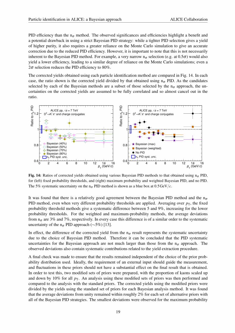
The corrected yields obtained using each particle identification method are compared in Fig. 14. In eachcase, the ratio shown is the corrected yield divided by that obtained using nσ PID. As the candidatesselected by each of the Bayesian methods are a subset of those selected by the nσ approach, the un-certainties on the corrected yields are assumed to be fully correlated and so almost cancel out in theratio.

)c (GeV/T

p0 2 4 6 8 10 12 14 16

PID

σR

atio to n

0.6

0.8

1

1.2

Bayesian (40%)

Bayesian (50%)Bayesian (70%)

Bayesian (80%) PID syst. unc.σn

= 7 TeVsALICE pp,


−

K→0

D

)c (GeV/T

p0 2 4 6 8 10 12 14 16

PID

σR

atio to n

0.6

0.8

1

1.2

Bayesian (max)

Bayesian (weighted)

No PID

PID syst. unc.σn

= 7 TeVsALICE pp,


−

K→0

D

Fig. 14: Ratios of corrected yields obtained using various Bayesian PID methods to that obtained using nσ PID,for (left) fixed probability thresholds, and (right) maximum probability and weighted Bayesian PID, and no PID.The 5% systematic uncertainty on the nσ PID method is shown as a blue box at 0.5GeV/c.

It was found that there is a relatively good agreement between the Bayesian PID method and the nσ

PID method, even when very different probability thresholds are applied. Averaging over pT, the fixedprobability threshold methods give a systematic difference between 5 and 9%, increasing for the lowerprobability thresholds. For the weighted and maximum-probability methods, the average deviationsfrom nσ are 3% and 7%, respectively. In every case this difference is of a similar order to the systematicuncertainty of the nσ PID approach (∼5%) [13].

In effect, the difference of the corrected yield from the nσ result represents the systematic uncertaintydue to the choice of Bayesian PID method. Therefore it can be concluded that the PID systematicuncertainties for the Bayesian approach are not much larger than those from the nσ approach. Theobserved deviations also contain systematic contributions related to the yield extraction procedure.

A final check was made to ensure that the results remained independent of the choice of the prior prob-ability distribution used. Ideally, the requirement of an external input should guide the measurement,and fluctuations in these priors should not have a substantial effect on the final result that is obtained.In order to test this, two modified sets of priors were prepared, with the proportion of kaons scaled upand down by 10% for all pT. An analysis using these modified sets of priors was then performed andcompared to the analysis with the standard priors. The corrected yields using the modified priors weredivided by the yields using the standard set of priors for each Bayesian analysis method. It was foundthat the average deviations from unity remained within roughly 2% for each set of alternative priors withall of the Bayesian PID strategies. The smallest deviations were observed for the maximum probability

19


and weighted methods, and for lower fixed probability thresholds.

In conclusion, since the corrected yield is largely independent of the choice of PID method, and consid-ering the improvement in signal-to-background ratio and (at low pT) significance, we conclude that theBayesian PID method is a valid choice for the analysis of D0→ K−π+. However, it must be noted thatalthough the stricter Bayesian methods give a purer signal, they also create an increased reliance on theMonte Carlo simulations to correct for the lower efficiencies, as well as introducing a greater dependenceon the choice of priors in those pT intervals that have lower statistical significance.

5 Application of Bayesian PID for Λ+c analysis

In this section we present an exploratory study of Λ+c → pK−π+ in pp collisions at

√s = 7 TeV using

a Bayesian PID approach. This decay channel suffers from a high level of combinatorial background,even in the relatively low-multiplicity environment of a pp collision. Due to the short decay length ofthe Λ+

c (cτ = 59.9 µm [26]) and current limitations in the spatial resolution of the ITS, topological andgeometrical selections alone are not sufficient to reduce this background and extract a signal. This meansthat a robust PID strategy is required to select Λ+

c candidates.

Here we compare analyses of Λ+c → pK−π+ using the nσ approach, a Bayesian approach using the

maximum-probability criterion, and an alternative “minimum-σ” approach that mimics the Bayesianstrategy. This analysis used ∼3×108 events from pp collisions at

√s = 7TeV collected during RUN 1.

Both the TPC and TOF responses were used for the nσ approach. A 3σ selection was applied on the TOFsignal for kaons, pions and protons at all pT, while in the TPC a pT-dependent nσ selection (between 2and 3σ ) was applied for protons and kaons, and a 3σ selection was applied for pions at all pT. If thetrack had a valid TOF signal, only this was used for the PID; otherwise the TPC response was used. Forthe Bayesian PID method, the TPC and TOF responses were combined; in cases where the TOF signalwas not available, only the TPC response was used.

The minimum-σ strategy serves as a middle ground between the nσ analysis and the Bayesian approach.It is also based on the deviation from the expected detector signal, but in this case only the speciesresulting in the smallest nσ value is chosen for each track, making this an exclusive selection. TheTPC and TOF responses are combined by adding their respective nσ values in quadrature. The potentialbenefit of this approach is that it uses similar logic to the Bayesian approach, without requiring the inputof any priors.

In order to build Λ+c candidates, triplets of tracks were reconstructed and selected, based on PID and

topological selections. Pairs of oppositely charged tracks were reconstructed from the set of selectedtracks, and a secondary (decay) vertex was computed. Selections were applied to each pair based onthe distance of closest approach between the two tracks, and the distance between the primary and thesecondary vertex of the reconstructed pair. A third track was then associated to each selected pair to forma triplet. The secondary vertex of the triplet was calculated and the Λ+

c candidates were selected using:

– the quality of the reconstructed vertex, which was determined using the quadratic sum of thedistances of the single tracks from the calculated secondary vertex;

– the distance between the primary and the secondary vertex of the triplet (decay length); and

– the cosine of the pointing angle. The pointing angle is the angle between the momentum vectorof the reconstructed Λ+

c candidate and the Λ+c flight line reconstructed from the line joining the

primary and secondary vertices.

The invariant mass plots for pKπ candidates with 2 < pT < 6 GeV/c are shown in the left-hand panelof Fig. 15 for the standard nσ PID approach (top), the alternative minimum-σ approach (middle) and

20


)2

c) (GeV/πInvariant mass (pK

2.2 2.22 2.24 2.26 2.28 2.3 2.32 2.34 2.36

2c

En

trie

s /

4 M

eV

/

410

510

965 ±) 4226 σS (3

391±B 929955 ) 0.0045σS/B (3

c < 6 GeV/T

p2 < ALICE = 7 TeVspp

PIDσn

PIDσMinimum

Bayesian PID (maximum probability)

495 ±) 2578 σS (3

184±) 254122 σB (3

) 0.0101σS/B (3

403 ±) 2145 σS (3

136±) 127250 σB (3

) 0.0169σS/B (3

)2

c) (GeV/πInvariant mass (pK

2.2 2.22 2.24 2.26 2.28 2.3 2.32 2.34 2.36

2c

En

trie

s /

4 M

eV

/310

410

c < 4 GeV/T

p3 <

PIDσn

PIDσMinimum

Bayesian PID (maximum probability)

and c.c.+π

−

pK→ c+

Λ

235 ±) 628 σS (3

100±) 53445 σB (3

) 0.0117σS/B (3

146 ±) 600 σS (3

55±) 17828 σB (3

) 0.0337σS/B (3

Fig. 15: Invariant mass spectra of Λ+c → pK−π+ using nσ PID, minimum-σ PID and Bayesian PID for (left)

2 < pT < 6 GeV/c and (right) 3 < pT < 4 GeV/c. Due to the low statistical significance, it was not possible toextract a stable signal for nσ PID for 3 < pT < 4GeV/c, therefore this fit and its results are not shown.

Bayesian PID (bottom). Over this pT interval, the statistical significance determined from the yieldextraction (as defined in Section 4.2) is 4.4±1.0 for nσ PID, 5.1±1.0 for minimum-σ PID and 6.0±1.1for Bayesian PID. In addition, the signal-to-background ratio is three times higher in the Bayesian casethan for nσ PID, with a background that is reduced by a factor of approximately seven. On the otherhand, the Bayesian PID method yields fewer Λ+

c candidates in the peak, indicating a lower selectionefficiency.

The equivalent invariant mass distributions for 3 < pT < 4 GeV/c are shown in the right-hand panelof Fig. 15. In this case, the nσ PID approach yields an insufficient statistical significance to extract astable yield. As with the pT-integrated case, the statistical significance improves when using the othertwo methods (2.7± 1.0 for minimum-σ and 4.4± 1.1 for Bayesian PID), and we again find a markedimprovement in the signal-to-background ratio for these two approaches. From this we conclude thatthe Bayesian approach represents the best candidate PID method for future measurements of the Λ+

cproduction cross section.

6 Conclusions and outlook

A Bayesian method for particle identification has been presented and validated for a variety of analy-ses. A comparison between different PID selection methods in ALICE was performed, with a focuson testing the suitability of Bayesian PID techniques. A selection based on the Bayesian probabilitycan be interpreted as a request on the purity, and therefore the main benefit of these techniques is thatthey increase the purity of the extracted signal by combining information from different detectors via arelatively simple technique.

The iterative procedure used to extract the prior probabilities (corresponding to the relative particle abun-dances) was outlined for pp collisions at

√s = 7TeV, p–Pb collisions at

√sNN = 5.02TeV and Pb–Pb

21


collisions at√

sNN = 2.76TeV. In each collision system, and for every centrality and multiplicity classstudied in Pb–Pb and p–Pb collisions, the extracted priors were found to be consistent with the trueparticle abundances seen in data.

The ability of Monte Carlo simulations to compute efficiencies and misidentification probabilities wastested via high-purity samples of pions, kaons and protons from the two-prong decays K0

S → π−π+,Λ → pπ−, and φ → K−K+ in p–Pb collisions at

√sNN = 5.02TeV. Equivalent analyses were also

performed using nσ PID. It was found that the variation in the result when using Bayesian PID as opposedto nσ PID was on the order of 5% in each case.

Comparisons between the Bayesian approach and PID methods used in measurements already publishedby ALICE in pp collisions at

√s = 7TeV were performed for the analysis of the pT-differential yields of

identified pions, kaons and protons. In this case, the previous analysis used a combination of nσ PID, un-folding methods and spectra obtained with kinks. A simple maximum-probability Bayesian PID methodwas used in this analysis. When compared, the results from nσ PID and Bayesian PID were found to beconsistent with one another within uncertainties.

A detailed comparison of different Bayesian PID strategies was performed for the analysis of D0 →K−π+ in pp collisions at

√s = 7TeV. Through the use of different probability thresholds, the trade-off

between selecting a purer sample and having a stronger dependence on the description of the detectorsin Monte Carlo simulations was demonstrated. An increase in the signal-to-background ratio over thenσ PID method was seen for all pT for all of the tested Bayesian strategies. The statistical significancewas found to be similar or greater than nσ PID for all of the Bayesian methods other than a strict 80%probability threshold. In every case, the corrected yield was found to be stable against the choice of PIDmethod when comparing with the nσ PID method used for D0 mesons. The dependence on the choiceof priors was also investigated, and it was found that the uncertainty on the corrected yield due to thechoice of priors was within ∼2%. We conclude that the systematic uncertainties arising from the choiceof Bayesian PID method are of a similar order to those of the nσ approach.

In summary, a good level of consistency is seen in both of the full analyses considered in Sections 4.1and 4.2 with respect to previously reported results. Because of this, we conclude that the validity of theBayesian PID approach has been successfully assessed.

Furthermore, the improved performance of the Bayesian PID approach in certain scenarios will provebeneficial for future analyses. The case of the Λ+

c baryon was presented as an example where a simple nσ

approach is unable to yield a stable signal, while the Bayesian approach is able to combine informationfrom the different detectors effectively without the need to develop a complex variable-σ selection. Thispresents a promising option for a more comprehensive study of the Λ+

c production cross section in ppand p–Pb collisions.

The analyses presented here are currently limited to charged hadrons detected in the TPC and TOFdetectors. However, the method can be extended to other particle species and detectors within the ALICEcentral barrel, and we expect to further test and refine these techniques in future. In particular, it will bepossible to examine the performance of the Bayesian approach for electron identification with the TRDat full azimuthal coverage in RUN 2.

Acknowledgements

The ALICE Collaboration would like to thank all its engineers and technicians for their invaluable con-tributions to the construction of the experiment and the CERN accelerator teams for the outstandingperformance of the LHC complex. The ALICE Collaboration gratefully acknowledges the resourcesand support provided by all Grid centres and the Worldwide LHC Computing Grid (WLCG) collab-oration. The ALICE Collaboration acknowledges the following funding agencies for their support in

22


building and running the ALICE detector: State Committee of Science, World Federation of Scientists(WFS) and Swiss Fonds Kidagan, Armenia; Conselho Nacional de Desenvolvimento Cientıfico e Tec-nologico (CNPq), Financiadora de Estudos e Projetos (FINEP), Fundacao de Amparo a Pesquisa doEstado de Sao Paulo (FAPESP); National Natural Science Foundation of China (NSFC), the ChineseMinistry of Education (CMOE) and the Ministry of Science and Technology of China (MSTC); Min-istry of Education and Youth of the Czech Republic; Danish Natural Science Research Council, theCarlsberg Foundation and the Danish National Research Foundation; The European Research Councilunder the European Community’s Seventh Framework Programme; Helsinki Institute of Physics andthe Academy of Finland; French CNRS-IN2P3, the ‘Region Pays de Loire’, ‘Region Alsace’, ‘RegionAuvergne’ and CEA, France; German Bundesministerium fur Bildung, Wissenschaft, Forschung undTechnologie (BMBF) and the Helmholtz Association; General Secretariat for Research and Technology,Ministry of Development, Greece; National Research, Development and Innovation Office (NKFIH),Hungary; Department of Atomic Energy and Department of Science and Technology of the Governmentof India; Istituto Nazionale di Fisica Nucleare (INFN) and Centro Fermi - Museo Storico della Fisicae Centro Studi e Ricerche “Enrico Fermi”, Italy; Japan Society for the Promotion of Science (JSPS)KAKENHI and MEXT, Japan; Joint Institute for Nuclear Research, Dubna; National Research Foun-dation of Korea (NRF); Consejo Nacional de Cienca y Tecnologia (CONACYT), Direccion General deAsuntos del Personal Academico(DGAPA), Mexico, Amerique Latine Formation academique - Euro-pean Commission (ALFA-EC) and the EPLANET Program (European Particle Physics Latin AmericanNetwork); Stichting voor Fundamenteel Onderzoek der Materie (FOM) and the Nederlandse Organisatievoor Wetenschappelijk Onderzoek (NWO), Netherlands; Research Council of Norway (NFR); NationalScience Centre, Poland; Ministry of National Education/Institute for Atomic Physics and National Coun-cil of Scientific Research in Higher Education (CNCSI-UEFISCDI), Romania; Ministry of Educationand Science of Russian Federation, Russian Academy of Sciences, Russian Federal Agency of AtomicEnergy, Russian Federal Agency for Science and Innovations and The Russian Foundation for Basic Re-search; Ministry of Education of Slovakia; Department of Science and Technology, South Africa; Centrode Investigaciones Energeticas, Medioambientales y Tecnologicas (CIEMAT), E-Infrastructure sharedbetween Europe and Latin America (EELA), Ministerio de Economıa y Competitividad (MINECO) ofSpain, Xunta de Galicia (Consellerıa de Educacion), Centro de Aplicaciones Tecnolgicas y DesarrolloNuclear (CEADEN), Cubaenergıa, Cuba, and IAEA (International Atomic Energy Agency); SwedishResearch Council (VR) and Knut & Alice Wallenberg Foundation (KAW); Ukraine Ministry of Edu-cation and Science; United Kingdom Science and Technology Facilities Council (STFC); The UnitedStates Department of Energy, the United States National Science Foundation, the State of Texas, and theState of Ohio; Ministry of Science, Education and Sports of Croatia and Unity through Knowledge Fund,Croatia; Council of Scientific and Industrial Research (CSIR), New Delhi, India; Pontificia UniversidadCatolica del Peru.

References

[1] ALICE Collaboration, B. Abelev et al., “Performance of the ALICE Experiment at the CERNLHC,” Int. J. Mod. Phys. A29 (2014) 1430044, arXiv:1402.4476 [nucl-ex].

[2] LEBC-EHS Collaboration, M. Aguilar-Benitez et al., “Inclusive particle production in 400 GeV/cpp interactions,” Z. Phys. C50 (1991) 405–426.

[3] HADES Collaboration, G. Agakishiev et al., “Measurement of charged pions in 12C + 12Ccollisions at 1A GeV and 2A GeV with HADES,” Eur. Phys. J. A40 (2009) 45–59,arXiv:0902.4377 [nucl-ex].

[4] X. Ye, H. Jian, and G. Kai-En, “Applying Bayesian neural networks to identify pion, kaon andproton in BESII,” Chin. Phys. C 32 (2008) 201–204.

[5] I. Belikov, P. Hristov, M. Ivanov, T. Kuhr, and K. Safarik, “Bayesian approach for particle

23

http://dx.doi.org/10.1142/S0217751X14300440

http://arxiv.org/abs/1402.4476

http://dx.doi.org/10.1007/BF01551452

http://dx.doi.org/10.1140/epja/i2008-10746-7


http://dx.doi.org/10.1088/1674-1137/32/3/008


identification in ALICE experiment at LHC,” in Computing in High Energy Physics and NuclearPhysics. Proceedings of CHEP04 Conference, Interlaken, Switzerland, 2004. 2005.

[6] ALICE Collaboration, F. Carminati et al., “ALICE: Physics performance report, volume I,” J.Phys. G30 (2004) 1517–1763.

[7] ALICE Collaboration, B. Alessandro et al., “ALICE: Physics performance report, volume II,” J.Phys. G32 (2006) 1295–2040.

[8] ALICE Collaboration, B. Abelev et al., “Measurement of pion, kaon and proton production inproton-proton collisions at

√s = 7 TeV,” Eur. Phys. J. C75 (2015) 226, arXiv:1504.00024

[nucl-ex].[9] ALICE Collaboration, B. Abelev et al., “Production of charged pions, kaons and protons at large

transverse momenta in pp and Pb–Pb collisions at√

sNN = 2.76 TeV,” Phys. Lett. B736 (2014)196–207, arXiv:1401.1250 [nucl-ex].

[10] ALICE Collaboration, B. Abelev et al., “Pion, Kaon, and Proton Production in Central Pb–PbCollisions at

√sNN = 2.76 TeV,” Phys. Rev. Lett. 109 (2012) 252301, arXiv:1208.1974

[hep-ex].[11] ALICE Collaboration, B. Abelev et al., “Measurement of electrons from beauty hadron decays in

pp collisions at√

s = 7 TeV,” Phys. Lett. B721 (2013) 13–23, arXiv:1208.1902 [hep-ex].[12] ALICE Collaboration, B. Abelev et al., “Measurement of electrons from semileptonic

heavy-flavor hadron decays in pp collisions at√

s = 2.76 TeV,” Phys. Rev. D91 (2015) 012001,arXiv:1405.4117 [nucl-ex].

[13] ALICE Collaboration, B. Abelev et al., “Measurement of charm production at central rapidity inproton-proton collisions at

√s = 7 TeV,” JHEP 1201 (2012) 128, arXiv:1111.1553 [hep-ex].

[14] ALICE Collaboration, B. Abelev et al., “K∗(892)0 and φ(1020) production in Pb–Pb collisions at√sNN = 2.76 TeV,” Phys. Rev. C91 (2015) 024609, arXiv:1404.0495 [nucl-ex].

[15] ALICE Collaboration, J. Adam et al., “Two-pion femtoscopy in p–Pb collisions at√

sNN = 5.02TeV,” Phys. Rev. C91 (2015) 034906, arXiv:1502.00559 [nucl-ex].

[16] ALICE Collaboration, J. Adam et al., “Precision measurement of the mass difference betweenlight nuclei and anti-nuclei,” Nature Phys. 11 (2015) 811–814, arXiv:1508.03986 [nucl-ex].

[17] ALICE Collaboration, “Technical Design Report of the Time Projection Chamber.” CERN/LHCC2000-001, 2000. https://edms.cern.ch/document/398930/1.

[18] A. Akindinov et al., “Performance of the ALICE Time-Of-Flight detector at the LHC,” Eur. Phys.J. Plus 128 (2013) 44.

[19] W. Blum and L. Rolandi, Particle Detection with Drift Chambers. Springer-Verlag, 1994.[20] P. Gregory, Bayesian Logical Data Analysis for the Physical Sciences. Cambridge University

Press, 2005.[21] ALICE Collaboration, B. Abelev et al., “Multiplicity Dependence of Pion, Kaon, Proton and

Lambda Production in p–Pb Collisions at√

sNN = 5.02 TeV,” Phys. Lett. B728 (2014) 25–38,arXiv:1307.6796 [nucl-ex].

[22] ALICE Collaboration, B. Abelev et al., “Elliptic flow of identified hadrons in Pb–Pb collisions at√sNN = 2.76 TeV,” JHEP 06 (2015) 190, arXiv:1405.4632 [nucl-ex].

[23] T. Sjostrand, S. Mrenna, and P. Z. Skands, “PYTHIA 6.4 Physics and Manual,” JHEP 05 (2006)026, arXiv:hep-ph/0603175 [hep-ph].

[24] P. Z. Skands, “Tuning Monte Carlo Generators: The Perugia Tunes,” Phys. Rev. D82 (2010)074018, arXiv:1005.3457 [hep-ph].

[25] R. Brun, F. Carminati, and S. Giani, “GEANT Detector Description and Simulation Tool,” Tech.Rep. CERN-W5013, CERN, 1994.

[26] Particle Data Group Collaboration, K. A. Olive et al., “Review of Particle Physics,” Chin. Phys.

24

http://dx.doi.org/10.1088/0954-3899/30/11/001

http://dx.doi.org/10.1088/0954-3899/30/11/001

http://dx.doi.org/10.1088/0954-3899/32/10/001

http://dx.doi.org/10.1088/0954-3899/32/10/001

http://dx.doi.org/10.1140/epjc/s10052-015-3422-9



http://dx.doi.org/10.1016/j.physletb.2014.07.011



http://dx.doi.org/10.1103/PhysRevLett.109.252301





http://dx.doi.org/10.1103/PhysRevD.91.012001


http://dx.doi.org/10.1007/JHEP01(2012)128


http://dx.doi.org/10.1103/PhysRevC.91.024609


http://dx.doi.org/10.1103/PhysRevC.91.034906


http://dx.doi.org/10.1038/nphys3432


https://edms.cern.ch/document/398930/1

http://dx.doi.org/10.1140/epjp/i2013-13044-x

http://dx.doi.org/10.1140/epjp/i2013-13044-x



http://dx.doi.org/10.1007/JHEP06(2015)190


http://dx.doi.org/10.1088/1126-6708/2006/05/026

http://dx.doi.org/10.1088/1126-6708/2006/05/026

http://arxiv.org/abs/hep-ph/0603175




http://dx.doi.org/10.1088/1674-1137/38/9/090001

http://dx.doi.org/10.1088/1674-1137/38/9/090001


C38 (2014) 090001.

25

http://dx.doi.org/10.1088/1674-1137/38/9/090001

http://dx.doi.org/10.1088/1674-1137/38/9/090001


A The ALICE Collaboration

J. Adam39, D. Adamova84, M.M. Aggarwal88, G. Aglieri Rinella35, M. Agnello110, N. Agrawal47,Z. Ahammed132, S. Ahmad19, S.U. Ahn68, S. Aiola136, A. Akindinov58, S.N. Alam132, D.S.D. Albuquerque121,D. Aleksandrov80, B. Alessandro110, D. Alexandre101, R. Alfaro Molina64, A. Alici104,12, A. Alkin3,J.R.M. Almaraz119, J. Alme37, T. Alt42, S. Altinpinar18, I. Altsybeev131, C. Alves Garcia Prado120,C. Andrei78, A. Andronic97, V. Anguelov94, T. Anticic98, F. Antinori107, P. Antonioli104, L. Aphecetche113,H. Appelshauser53, S. Arcelli27, R. Arnaldi110, O.W. Arnold36,93, I.C. Arsene22, M. Arslandok53, B. Audurier113,A. Augustinus35, R. Averbeck97, M.D. Azmi19, A. Badala106, Y.W. Baek67, S. Bagnasco110, R. Bailhache53,R. Bala91, S. Balasubramanian136, A. Baldisseri15, R.C. Baral61, A.M. Barbano26, R. Barbera28, F. Barile32,G.G. Barnafoldi135, L.S. Barnby101, V. Barret70, P. Bartalini7, K. Barth35, J. Bartke117, E. Bartsch53,M. Basile27, N. Bastid70, S. Basu132, B. Bathen54, G. Batigne113, A. Batista Camejo70, B. Batyunya66,P.C. Batzing22, I.G. Bearden81, H. Beck53, C. Bedda110, N.K. Behera50, I. Belikov55, F. Bellini27,H. Bello Martinez2, R. Bellwied122, R. Belmont134, E. Belmont-Moreno64, V. Belyaev75, P. Benacek84,G. Bencedi135, S. Beole26, I. Berceanu78, A. Bercuci78, Y. Berdnikov86, D. Berenyi135, R.A. Bertens57,D. Berzano35, L. Betev35, A. Bhasin91, I.R. Bhat91, A.K. Bhati88, B. Bhattacharjee44, J. Bhom128,117,L. Bianchi122, N. Bianchi72, C. Bianchin134, J. Bielcık39, J. Bielcıkova84, A. Bilandzic81,36,93, G. Biro135,R. Biswas4, S. Biswas4,79, S. Bjelogrlic57, J.T. Blair118, D. Blau80, C. Blume53, F. Bock74,94, A. Bogdanov75,H. Bøggild81, L. Boldizsar135, M. Bombara40, J. Book53, H. Borel15, A. Borissov96, M. Borri83,124,F. Bossu65, E. Botta26, C. Bourjau81, P. Braun-Munzinger97, M. Bregant120, T. Breitner52, T.A. Broker53,T.A. Browning95, M. Broz39, E.J. Brucken45, E. Bruna110, G.E. Bruno32, D. Budnikov99, H. Buesching53,S. Bufalino35,26, P. Buncic35, O. Busch94,128, Z. Buthelezi65, J.B. Butt16, J.T. Buxton20, J. Cabala115,D. Caffarri35, X. Cai7, H. Caines136, L. Calero Diaz72, A. Caliva57, E. Calvo Villar102, P. Camerini25,F. Carena35, W. Carena35, F. Carnesecchi27, J. Castillo Castellanos15, A.J. Castro125, E.A.R. Casula24,C. Ceballos Sanchez9, J. Cepila39, P. Cerello110, J. Cerkala115, B. Chang123, S. Chapeland35, M. Chartier124,J.L. Charvet15, S. Chattopadhyay132, S. Chattopadhyay100, A. Chauvin93,36, V. Chelnokov3, M. Cherney87,C. Cheshkov130, B. Cheynis130, V. Chibante Barroso35, D.D. Chinellato121, S. Cho50, P. Chochula35,K. Choi96, M. Chojnacki81, S. Choudhury132, P. Christakoglou82, C.H. Christensen81, P. Christiansen33,T. Chujo128, S.U. Chung96, C. Cicalo105, L. Cifarelli12,27, F. Cindolo104, J. Cleymans90, F. Colamaria32,D. Colella59,35, A. Collu74,24, M. Colocci27, G. Conesa Balbastre71, Z. Conesa del Valle51, M.E. ConnorsII,136,J.G. Contreras39, T.M. Cormier85, Y. Corrales Morales110, I. Cortes Maldonado2, P. Cortese31, M.R. Cosentino120,F. Costa35, P. Crochet70, R. Cruz Albino11, E. Cuautle63, L. Cunqueiro54,35, T. Dahms93,36, A. Dainese107,M.C. Danisch94, A. Danu62, D. Das100, I. Das100, S. Das4, A. Dash79, S. Dash47, S. De120, A. DeCaro30,12, G. de Cataldo103, C. de Conti120, J. de Cuveland42, A. De Falco24, D. De Gruttola12,30, N. DeMarco110, S. De Pasquale30, A. Deisting97,94, A. Deloff77, E. DenesI,135, C. Deplano82, P. Dhankher47,D. Di Bari32, A. Di Mauro35, P. Di Nezza72, M.A. Diaz Corchero10, T. Dietel90, P. Dillenseger53,R. Divia35, Ø. Djuvsland18, A. Dobrin82,62, D. Domenicis Gimenez120, B. Donigus53, O. Dordic22,T. Drozhzhova53, A.K. Dubey132, A. Dubla57, L. Ducroux130, P. Dupieux70, R.J. Ehlers136, D. Elia103,E. Endress102, H. Engel52, E. Epple136, B. Erazmus113, I. Erdemir53, F. Erhardt129, B. Espagnon51,M. Estienne113, S. Esumi128, J. Eum96, D. Evans101, S. Evdokimov111, G. Eyyubova39, L. Fabbietti93,36,D. Fabris107, J. Faivre71, A. Fantoni72, M. Fasel74, L. Feldkamp54, A. Feliciello110, G. Feofilov131,J. Ferencei84, A. Fernandez Tellez2, E.G. Ferreiro17, A. Ferretti26, A. Festanti29, V.J.G. Feuillard15,70,J. Figiel117, M.A.S. Figueredo124,120, S. Filchagin99, D. Finogeev56, F.M. Fionda24, E.M. Fiore32, M.G. Fleck94,M. Floris35, S. Foertsch65, P. Foka97, S. Fokin80, E. Fragiacomo109, A. Francescon35,29, U. Frankenfeld97,G.G. Fronze26, U. Fuchs35, C. Furget71, A. Furs56, M. Fusco Girard30, J.J. Gaardhøje81, M. Gagliardi26,A.M. Gago102, M. Gallio26, D.R. Gangadharan74, P. Ganoti89, C. Gao7, C. Garabatos97, E. Garcia-Solis13, C. Gargiulo35, P. Gasik93,36, E.F. Gauger118, M. Germain113, A. Gheata35, M. Gheata35,62,P. Ghosh132, S.K. Ghosh4, P. Gianotti72, P. Giubellino110,35, P. Giubilato29, E. Gladysz-Dziadus117,P. Glassel94, D.M. Gomez Coral64, A. Gomez Ramirez52, A.S. Gonzalez35, V. Gonzalez10, P. Gonzalez-Zamora10, S. Gorbunov42, L. Gorlich117, S. Gotovac116, V. Grabski64, O.A. Grachov136, L.K. Graczykowski133,

26


K.L. Graham101, A. Grelli57, A. Grigoras35, C. Grigoras35, V. Grigoriev75, A. Grigoryan1, S. Grigoryan66,B. Grinyov3, N. Grion109, J.M. Gronefeld97, J.F. Grosse-Oetringhaus35, R. Grosso97, F. Guber56, R. Guernane71,B. Guerzoni27, K. Gulbrandsen81, T. Gunji127, A. Gupta91, R. Gupta91, R. Haake35, Ø. Haaland18,C. Hadjidakis51, M. Haiduc62, H. Hamagaki127, G. Hamar135, J.C. Hamon55, J.W. Harris136, A. Harton13,D. Hatzifotiadou104, S. Hayashi127, S.T. Heckel53, E. Hellbar53, H. Helstrup37, A. Herghelegiu78, G. Her-rera Corral11, B.A. Hess34, K.F. Hetland37, H. Hillemanns35, B. Hippolyte55, D. Horak39, R. Hosokawa128,P. Hristov35, T.J. Humanic20, N. Hussain44, T. Hussain19, D. Hutter42, D.S. Hwang21, R. Ilkaev99,M. Inaba128, E. Incani24, M. Ippolitov75,80, M. Irfan19, M. Ivanov97, V. Ivanov86, V. Izucheev111, N. Jacazio27,P.M. Jacobs74, M.B. Jadhav47, S. Jadlovska115, J. Jadlovsky115,59, C. Jahnke120, M.J. Jakubowska133,H.J. Jang68, M.A. Janik133, P.H.S.Y. Jayarathna122, C. Jena29, S. Jena122, R.T. Jimenez Bustamante97,P.G. Jones101, A. Jusko101, P. Kalinak59, A. Kalweit35, J. Kamin53, J.H. Kang137, V. Kaplin75, S. Kar132,A. Karasu Uysal69, O. Karavichev56, T. Karavicheva56, L. Karayan97,94, E. Karpechev56, U. Kebschull52,R. Keidel138, D.L.D. Keijdener57, M. Keil35, M. Mohisin KhanIII,19, P. Khan100, S.A. Khan132, A. Khanzadeev86,Y. Kharlov111, B. Kileng37, D.W. Kim43, D.J. Kim123, D. Kim137, H. Kim137, J.S. Kim43, M. Kim137,S. Kim21, T. Kim137, S. Kirsch42, I. Kisel42, S. Kiselev58, A. Kisiel133, G. Kiss135, J.L. Klay6, C. Klein53,J. Klein35, C. Klein-Bosing54, S. Klewin94, A. Kluge35, M.L. Knichel94, A.G. Knospe118,122, C. Kobdaj114,M. Kofarago35, T. Kollegger97, A. Kolojvari131, V. Kondratiev131, N. Kondratyeva75, E. Kondratyuk111,A. Konevskikh56, M. Kopcik115, P. Kostarakis89, M. Kour91, C. Kouzinopoulos35, O. Kovalenko77,V. Kovalenko131, M. Kowalski117, G. Koyithatta Meethaleveedu47, I. Kralik59, A. Kravcakova40, M. Krivda59,101,F. Krizek84, E. Kryshen86,35, M. Krzewicki42, A.M. Kubera20, V. Kucera84, C. Kuhn55, P.G. Kuijer82,A. Kumar91, J. Kumar47, L. Kumar88, S. Kumar47, P. Kurashvili77, A. Kurepin56, A.B. Kurepin56,A. Kuryakin99, M.J. Kweon50, Y. Kwon137, S.L. La Pointe110, P. La Rocca28, P. Ladron de Guevara11,C. Lagana Fernandes120, I. Lakomov35, R. Langoy41, C. Lara52, A. Lardeux15, A. Lattuca26, E. Laudi35,R. Lea25, L. Leardini94, G.R. Lee101, S. Lee137, F. Lehas82, R.C. Lemmon83, V. Lenti103, E. Leogrande57,I. Leon Monzon119, H. Leon Vargas64, M. Leoncino26, P. Levai135, S. Li7,70, X. Li14, J. Lien41, R. Lietava101,S. Lindal22, V. Lindenstruth42, C. Lippmann97, M.A. Lisa20, H.M. Ljunggren33, D.F. Lodato57, P.I. Loenne18,V. Loginov75, C. Loizides74, X. Lopez70, E. Lopez Torres9, A. Lowe135, P. Luettig53, M. Lunardon29,G. Luparello25, T.H. Lutz136, A. Maevskaya56, M. Mager35, S. Mahajan91, S.M. Mahmood22, A. Maire55,R.D. Majka136, M. Malaev86, I. Maldonado Cervantes63, L. MalininaIV,66, D. Mal’Kevich58, P. Malzacher97,A. Mamonov99, V. Manko80, F. Manso70, V. Manzari103,35, M. Marchisone126,65,26, J. Mares60, G.V. Margagliotti25,A. Margotti104, J. Margutti57, A. Marın97, C. Markert118, M. Marquard53, N.A. Martin97, J. MartinBlanco113, P. Martinengo35, M.I. Martınez2, G. Martınez Garcıa113, M. Martinez Pedreira35, A. Mas120,S. Masciocchi97, M. Masera26, A. Masoni105, A. Mastroserio32, A. Matyja117, C. Mayer117, J. Mazer125,M.A. Mazzoni108, D. Mcdonald122, F. Meddi23, Y. Melikyan75, A. Menchaca-Rocha64, E. Meninno30,J. Mercado Perez94, M. Meres38, Y. Miake128, M.M. Mieskolainen45, K. Mikhaylov66,58, L. Milano35,74,J. Milosevic22, A. Mischke57, A.N. Mishra48, D. Miskowiec97, J. Mitra132, C.M. Mitu62, N. Mohammadi57,B. Mohanty79,132, L. Molnar113,55, L. Montano Zetina11, E. Montes10, D.A. Moreira De Godoy54, L.A.P. Moreno2,S. Moretto29, A. Morreale113, A. Morsch35, V. Muccifora72, E. Mudnic116, D. Muhlheim54, S. Muhuri132,M. Mukherjee132, J.D. Mulligan136, M.G. Munhoz120, R.H. Munzer93,36,53, H. Murakami127, S. Murray65,L. Musa35, J. Musinsky59, B. Naik47, R. Nair77, B.K. Nandi47, R. Nania104, E. Nappi103, M.U. Naru16,H. Natal da Luz120, C. Nattrass125, S.R. Navarro2, K. Nayak79, R. Nayak47, T.K. Nayak132, S. Nazarenko99,A. Nedosekin58, L. Nellen63, F. Ng122, M. Nicassio97, M. Niculescu62, J. Niedziela35, B.S. Nielsen81,S. Nikolaev80, S. Nikulin80, V. Nikulin86, F. Noferini104,12, P. Nomokonov66, G. Nooren57, J.C.C. Noris2,J. Norman124, A. Nyanin80, J. Nystrand18, H. Oeschler94, S. Oh136, S.K. Oh67, A. Ohlson35, A. Okatan69,T. Okubo46, L. Olah135, J. Oleniacz133, A.C. Oliveira Da Silva120, M.H. Oliver136, J. Onderwaater97,C. Oppedisano110, R. Orava45, M. Oravec115, A. Ortiz Velasquez63, A. Oskarsson33, J. Otwinowski117,K. Oyama94,76, M. Ozdemir53, Y. Pachmayer94, D. Pagano26, P. Pagano30, G. Paic63, S.K. Pal132, J. Pan134,A.K. Pandey47, V. Papikyan1, G.S. Pappalardo106, P. Pareek48, W.J. Park97, S. Parmar88, A. Passfeld54,V. Paticchio103, R.N. Patra132, B. Paul100, H. Pei7, T. Peitzmann57, H. Pereira Da Costa15, D. Peresunko80,75,C.E. Perez Lara82, E. Perez Lezama53, V. Peskov53, Y. Pestov5, V. Petracek39, V. Petrov111, M. Petrovici78,

27


C. Petta28, S. Piano109, M. Pikna38, P. Pillot113, L.O.D.L. Pimentel81, O. Pinazza104,35, L. Pinsky122,D.B. Piyarathna122, M. Płoskon74, M. Planinic129, J. Pluta133, S. Pochybova135, P.L.M. Podesta-Lerma119,M.G. Poghosyan85,87, B. Polichtchouk111, N. Poljak129, W. Poonsawat114, A. Pop78, S. Porteboeuf-Houssais70, J. Porter74, J. Pospisil84, S.K. Prasad4, R. Preghenella104,35, F. Prino110, C.A. Pruneau134,I. Pshenichnov56, M. Puccio26, G. Puddu24, P. Pujahari134, V. Punin99, J. Putschke134, H. Qvigstad22,A. Rachevski109, S. Raha4, S. Rajput91, J. Rak123, A. Rakotozafindrabe15, L. Ramello31, F. Rami55,R. Raniwala92, S. Raniwala92, S.S. Rasanen45, B.T. Rascanu53, D. Rathee88, K.F. Read85,125, K. Redlich77,R.J. Reed134, A. Rehman18, P. Reichelt53, F. Reidt94,35, X. Ren7, R. Renfordt53, A.R. Reolon72, A. Reshetin56,K. Reygers94, V. Riabov86, R.A. Ricci73, T. Richert33, M. Richter22, P. Riedler35, W. Riegler35, F. Riggi28,C. Ristea62, E. Rocco57, M. Rodrıguez Cahuantzi11,2, A. Rodriguez Manso82, K. Røed22, E. Rogochaya66,D. Rohr42, D. Rohrich18, F. Ronchetti72,35, L. Ronflette113, P. Rosnet70, A. Rossi35,29, F. Roukoutakis89,A. Roy48, C. Roy55, P. Roy100, A.J. Rubio Montero10, R. Rui25, R. Russo26, E. Ryabinkin80, Y. Ryabov86,A. Rybicki117, S. Saarinen45, S. Sadhu132, S. Sadovsky111, K. Safarık35, B. Sahlmuller53, P. Sahoo48,R. Sahoo48, S. Sahoo61, P.K. Sahu61, J. Saini132, S. Sakai72, M.A. Saleh134, J. Salzwedel20, S. Sambyal91,V. Samsonov86, L. Sandor59, A. Sandoval64, M. Sano128, D. Sarkar132, N. Sarkar132, P. Sarma44, E. Scapparone104,F. Scarlassara29, C. Schiaua78, R. Schicker94, C. Schmidt97, H.R. Schmidt34, S. Schuchmann53, J. Schukraft35,M. Schulc39, Y. Schutz35,113, K. Schwarz97, K. Schweda97, G. Scioli27, E. Scomparin110, R. Scott125,M. Sefcık40, J.E. Seger87, Y. Sekiguchi127, D. Sekihata46, I. Selyuzhenkov97, K. Senosi65, S. Senyukov3,35,E. Serradilla10,64, A. Sevcenco62, A. Shabanov56, A. Shabetai113, O. Shadura3, R. Shahoyan35, M.I. Shahzad16,A. Shangaraev111, A. Sharma91, M. Sharma91, M. Sharma91, N. Sharma125, A.I. Sheikh132, K. Shigaki46,Q. Shou7, K. Shtejer9,26, Y. Sibiriak80, S. Siddhanta105, K.M. Sielewicz35, T. Siemiarczuk77, D. Silvermyr33,C. Silvestre71, G. Simatovic129, G. Simonetti35, R. Singaraju132, R. Singh79, S. Singha79,132, V. Singhal132,B.C. Sinha132, T. Sinha100, B. Sitar38, M. Sitta31, T.B. Skaali22, M. Slupecki123, N. Smirnov136, R.J.M. Snellings57,T.W. Snellman123, J. Song96, M. Song137, Z. Song7, F. Soramel29, S. Sorensen125, R.D.de Souza121,F. Sozzi97, M. Spacek39, E. Spiriti72, I. Sputowska117, M. Spyropoulou-Stassinaki89, J. Stachel94, I. Stan62,P. Stankus85, E. Stenlund33, G. Steyn65, J.H. Stiller94, D. Stocco113, P. Strmen38, A.A.P. Suaide120,T. Sugitate46, C. Suire51, M. Suleymanov16, M. SuljicI,25, R. Sultanov58, M. Sumbera84, S. Sumowidagdo49,A. Szabo38, A. Szanto de ToledoI,120, I. Szarka38, A. Szczepankiewicz35, M. Szymanski133, U. Tabassam16,J. Takahashi121, G.J. Tambave18, N. Tanaka128, M. Tarhini51, M. Tariq19, M.G. Tarzila78, A. Tauro35,G. Tejeda Munoz2, A. Telesca35, K. Terasaki127, C. Terrevoli29, B. Teyssier130, J. Thader74, D. Thakur48,D. Thomas118, R. Tieulent130, A.R. Timmins122, A. Toia53, S. Trogolo26, G. Trombetta32, V. Trubnikov3,W.H. Trzaska123, T. Tsuji127, A. Tumkin99, R. Turrisi107, T.S. Tveter22, K. Ullaland18, A. Uras130,G.L. Usai24, A. Utrobicic129, M. Vala59, L. Valencia Palomo70, S. Vallero26, J. Van Der Maarel57,J.W. Van Hoorne35, M. van Leeuwen57, T. Vanat84, P. Vande Vyvre35, D. Varga135, A. Vargas2, M. Vargyas123,R. Varma47, M. Vasileiou89, A. Vasiliev80, A. Vauthier71, V. Vechernin131, A.M. Veen57, M. Veldhoen57,A. Velure18, E. Vercellin26, S. Vergara Limon2, R. Vernet8, M. Verweij134, L. Vickovic116, G. ViestiI,29,J. Viinikainen123, Z. Vilakazi126, O. Villalobos Baillie101, A. Villatoro Tello2, A. Vinogradov80, L. Vinogradov131,Y. VinogradovI,99, T. Virgili30, V. Vislavicius33, Y.P. Viyogi132, A. Vodopyanov66, M.A. Volkl94, K. Voloshin58,S.A. Voloshin134, G. Volpe32,135, B. von Haller35, I. Vorobyev36,93, D. Vranic97,35, J. Vrlakova40, B. Vulpescu70,B. Wagner18, J. Wagner97, H. Wang57, M. Wang7,113, D. Watanabe128, Y. Watanabe127, M. Weber35,112,S.G. Weber97, D.F. Weiser94, J.P. Wessels54, U. Westerhoff54, A.M. Whitehead90, J. Wiechula34, J. Wikne22,G. Wilk77, J. Wilkinson94, M.C.S. Williams104, B. Windelband94, M. Winn94, H. Yang57, P. Yang7,S. Yano46, Z. Yasin16, Z. Yin7, H. Yokoyama128, I.-K. Yoo96, J.H. Yoon50, V. Yurchenko3, I. Yushmanov80,A. Zaborowska133, V. Zaccolo81, A. Zaman16, C. Zampolli104,35, H.J.C. Zanoli120, S. Zaporozhets66,N. Zardoshti101, A. Zarochentsev131, P. Zavada60, N. Zaviyalov99, H. Zbroszczyk133, I.S. Zgura62, M. Zhalov86,H. Zhang18, X. Zhang74,7, Y. Zhang7, C. Zhang57, Z. Zhang7, C. Zhao22, N. Zhigareva58, D. Zhou7,Y. Zhou81, Z. Zhou18, H. Zhu18, J. Zhu7,113, A. Zichichi27,12, A. Zimmermann94, M.B. Zimmermann54,35,G. Zinovjev3, M. Zyzak42

28


Affiliation Notes

I DeceasedII Also at: Georgia State University, Atlanta, Georgia, United StatesIII Also at Department of Applied Physics, Aligarh Muslim University, Aligarh, IndiaIV Also at: M.V. Lomonosov Moscow State University, D.V. Skobeltsyn Institute of Nuclear, Physics,Moscow, Russia

Collaboration Institutes

1 A.I. Alikhanyan National Science Laboratory (Yerevan Physics Institute) Foundation, Yerevan, Arme-nia2 Benemerita Universidad Autonoma de Puebla, Puebla, Mexico3 Bogolyubov Institute for Theoretical Physics, Kiev, Ukraine4 Bose Institute, Department of Physics and Centre for Astroparticle Physics and Space Science (CAPSS),Kolkata, India5 Budker Institute for Nuclear Physics, Novosibirsk, Russia6 California Polytechnic State University, San Luis Obispo, California, United States7 Central China Normal University, Wuhan, China8 Centre de Calcul de l’IN2P3, Villeurbanne, France9 Centro de Aplicaciones Tecnologicas y Desarrollo Nuclear (CEADEN), Havana, Cuba10 Centro de Investigaciones Energeticas Medioambientales y Tecnologicas (CIEMAT), Madrid, Spain11 Centro de Investigacion y de Estudios Avanzados (CINVESTAV), Mexico City and Merida, Mexico12 Centro Fermi - Museo Storico della Fisica e Centro Studi e Ricerche “Enrico Fermi”, Rome, Italy13 Chicago State University, Chicago, Illinois, USA14 China Institute of Atomic Energy, Beijing, China15 Commissariat a l’Energie Atomique, IRFU, Saclay, France16 COMSATS Institute of Information Technology (CIIT), Islamabad, Pakistan17 Departamento de Fısica de Partıculas and IGFAE, Universidad de Santiago de Compostela, Santiagode Compostela, Spain18 Department of Physics and Technology, University of Bergen, Bergen, Norway19 Department of Physics, Aligarh Muslim University, Aligarh, India20 Department of Physics, Ohio State University, Columbus, Ohio, United States21 Department of Physics, Sejong University, Seoul, South Korea22 Department of Physics, University of Oslo, Oslo, Norway23 Dipartimento di Fisica dell’Universita ’La Sapienza’ and Sezione INFN Rome, Italy24 Dipartimento di Fisica dell’Universita and Sezione INFN, Cagliari, Italy25 Dipartimento di Fisica dell’Universita and Sezione INFN, Trieste, Italy26 Dipartimento di Fisica dell’Universita and Sezione INFN, Turin, Italy27 Dipartimento di Fisica e Astronomia dell’Universita and Sezione INFN, Bologna, Italy28 Dipartimento di Fisica e Astronomia dell’Universita and Sezione INFN, Catania, Italy29 Dipartimento di Fisica e Astronomia dell’Universita and Sezione INFN, Padova, Italy30 Dipartimento di Fisica ‘E.R. Caianiello’ dell’Universita and Gruppo Collegato INFN, Salerno, Italy31 Dipartimento di Scienze e Innovazione Tecnologica dell’Universita del Piemonte Orientale and GruppoCollegato INFN, Alessandria, Italy32 Dipartimento Interateneo di Fisica ‘M. Merlin’ and Sezione INFN, Bari, Italy33 Division of Experimental High Energy Physics, University of Lund, Lund, Sweden34 Eberhard Karls Universitat Tubingen, Tubingen, Germany

29


35 European Organization for Nuclear Research (CERN), Geneva, Switzerland36 Excellence Cluster Universe, Technische Universitat Munchen, Munich, Germany37 Faculty of Engineering, Bergen University College, Bergen, Norway38 Faculty of Mathematics, Physics and Informatics, Comenius University, Bratislava, Slovakia39 Faculty of Nuclear Sciences and Physical Engineering, Czech Technical University in Prague, Prague,Czech Republic40 Faculty of Science, P.J. Safarik University, Kosice, Slovakia41 Faculty of Technology, Buskerud and Vestfold University College, Vestfold, Norway42 Frankfurt Institute for Advanced Studies, Johann Wolfgang Goethe-Universitat Frankfurt, Frankfurt,Germany43 Gangneung-Wonju National University, Gangneung, South Korea44 Gauhati University, Department of Physics, Guwahati, India45 Helsinki Institute of Physics (HIP), Helsinki, Finland46 Hiroshima University, Hiroshima, Japan47 Indian Institute of Technology Bombay (IIT), Mumbai, India48 Indian Institute of Technology Indore, Indore (IITI), India49 Indonesian Institute of Sciences, Jakarta, Indonesia50 Inha University, Incheon, South Korea51 Institut de Physique Nucleaire d’Orsay (IPNO), Universite Paris-Sud, CNRS-IN2P3, Orsay, France52 Institut fur Informatik, Johann Wolfgang Goethe-Universitat Frankfurt, Frankfurt, Germany53 Institut fur Kernphysik, Johann Wolfgang Goethe-Universitat Frankfurt, Frankfurt, Germany54 Institut fur Kernphysik, Westfalische Wilhelms-Universitat Munster, Munster, Germany55 Institut Pluridisciplinaire Hubert Curien (IPHC), Universite de Strasbourg, CNRS-IN2P3, Strasbourg,France56 Institute for Nuclear Research, Academy of Sciences, Moscow, Russia57 Institute for Subatomic Physics of Utrecht University, Utrecht, Netherlands58 Institute for Theoretical and Experimental Physics, Moscow, Russia59 Institute of Experimental Physics, Slovak Academy of Sciences, Kosice, Slovakia60 Institute of Physics, Academy of Sciences of the Czech Republic, Prague, Czech Republic61 Institute of Physics, Bhubaneswar, India62 Institute of Space Science (ISS), Bucharest, Romania63 Instituto de Ciencias Nucleares, Universidad Nacional Autonoma de Mexico, Mexico City, Mexico64 Instituto de Fısica, Universidad Nacional Autonoma de Mexico, Mexico City, Mexico65 iThemba LABS, National Research Foundation, Somerset West, South Africa66 Joint Institute for Nuclear Research (JINR), Dubna, Russia67 Konkuk University, Seoul, South Korea68 Korea Institute of Science and Technology Information, Daejeon, South Korea69 KTO Karatay University, Konya, Turkey70 Laboratoire de Physique Corpusculaire (LPC), Clermont Universite, Universite Blaise Pascal, CNRS–IN2P3, Clermont-Ferrand, France71 Laboratoire de Physique Subatomique et de Cosmologie, Universite Grenoble-Alpes, CNRS-IN2P3,Grenoble, France72 Laboratori Nazionali di Frascati, INFN, Frascati, Italy73 Laboratori Nazionali di Legnaro, INFN, Legnaro, Italy74 Lawrence Berkeley National Laboratory, Berkeley, California, United States75 Moscow Engineering Physics Institute, Moscow, Russia76 Nagasaki Institute of Applied Science, Nagasaki, Japan77 National Centre for Nuclear Studies, Warsaw, Poland78 National Institute for Physics and Nuclear Engineering, Bucharest, Romania79 National Institute of Science Education and Research, Bhubaneswar, India

30


80 National Research Centre Kurchatov Institute, Moscow, Russia81 Niels Bohr Institute, University of Copenhagen, Copenhagen, Denmark82 Nikhef, Nationaal instituut voor subatomaire fysica, Amsterdam, Netherlands83 Nuclear Physics Group, STFC Daresbury Laboratory, Daresbury, United Kingdom84 Nuclear Physics Institute, Academy of Sciences of the Czech Republic, Rez u Prahy, Czech Republic85 Oak Ridge National Laboratory, Oak Ridge, Tennessee, United States86 Petersburg Nuclear Physics Institute, Gatchina, Russia87 Physics Department, Creighton University, Omaha, Nebraska, United States88 Physics Department, Panjab University, Chandigarh, India89 Physics Department, University of Athens, Athens, Greece90 Physics Department, University of Cape Town, Cape Town, South Africa91 Physics Department, University of Jammu, Jammu, India92 Physics Department, University of Rajasthan, Jaipur, India93 Physik Department, Technische Universitat Munchen, Munich, Germany94 Physikalisches Institut, Ruprecht-Karls-Universitat Heidelberg, Heidelberg, Germany95 Purdue University, West Lafayette, Indiana, United States96 Pusan National University, Pusan, South Korea97 Research Division and ExtreMe Matter Institute EMMI, GSI Helmholtzzentrum fur Schwerionen-forschung, Darmstadt, Germany98 Rudjer Boskovic Institute, Zagreb, Croatia99 Russian Federal Nuclear Center (VNIIEF), Sarov, Russia100 Saha Institute of Nuclear Physics, Kolkata, India101 School of Physics and Astronomy, University of Birmingham, Birmingham, United Kingdom102 Seccion Fısica, Departamento de Ciencias, Pontificia Universidad Catolica del Peru, Lima, Peru103 Sezione INFN, Bari, Italy104 Sezione INFN, Bologna, Italy105 Sezione INFN, Cagliari, Italy106 Sezione INFN, Catania, Italy107 Sezione INFN, Padova, Italy108 Sezione INFN, Rome, Italy109 Sezione INFN, Trieste, Italy110 Sezione INFN, Turin, Italy111 SSC IHEP of NRC Kurchatov institute, Protvino, Russia112 Stefan Meyer Institut fur Subatomare Physik (SMI), Vienna, Austria113 SUBATECH, Ecole des Mines de Nantes, Universite de Nantes, CNRS-IN2P3, Nantes, France114 Suranaree University of Technology, Nakhon Ratchasima, Thailand115 Technical University of Kosice, Kosice, Slovakia116 Technical University of Split FESB, Split, Croatia117 The Henryk Niewodniczanski Institute of Nuclear Physics, Polish Academy of Sciences, Cracow,Poland118 The University of Texas at Austin, Physics Department, Austin, Texas, USA119 Universidad Autonoma de Sinaloa, Culiacan, Mexico120 Universidade de Sao Paulo (USP), Sao Paulo, Brazil121 Universidade Estadual de Campinas (UNICAMP), Campinas, Brazil122 University of Houston, Houston, Texas, United States123 University of Jyvaskyla, Jyvaskyla, Finland124 University of Liverpool, Liverpool, United Kingdom125 University of Tennessee, Knoxville, Tennessee, United States126 University of the Witwatersrand, Johannesburg, South Africa127 University of Tokyo, Tokyo, Japan

31


128 University of Tsukuba, Tsukuba, Japan129 University of Zagreb, Zagreb, Croatia130 Universite de Lyon, Universite Lyon 1, CNRS/IN2P3, IPN-Lyon, Villeurbanne, France131 V. Fock Institute for Physics, St. Petersburg State University, St. Petersburg, Russia132 Variable Energy Cyclotron Centre, Kolkata, India133 Warsaw University of Technology, Warsaw, Poland134 Wayne State University, Detroit, Michigan, United States135 Wigner Research Centre for Physics, Hungarian Academy of Sciences, Budapest, Hungary136 Yale University, New Haven, Connecticut, United States137 Yonsei University, Seoul, South Korea138 Zentrum fur Technologietransfer und Telekommunikation (ZTT), Fachhochschule Worms, Worms,Germany

32

Documents

Particle Identification in ALICE: a Bayesian approach · Particle Identiﬁcation (PID) provides information about the mass and ﬂavour composition of particle production in high-energy