Embed Size (px)
Citation preview
Particle and Astroparticle Physics
© 2008 by Taylor & Francis Group, LLC
Series in High Energy Physics, Cosmology, and Gravitation
Series Editors: Brian Foster, Oxford University, UKEdward W Kolb, Fermi National Accelerator Laboratory, USA
This series of books covers all aspects of theoretical and experimental high energy physics, cosmology and gravitation and the interface between them. In recent years the fields of particle physics and astrophysics have become increasingly interdependent and the aim of this series is to provide a library of books to meet the needs of students and researchers in these fields.
Other recent books in the series:
Joint Evolution of Black Holes and GalaxiesM Colpi, V Gorini, F Haardt, and U Moschella (Eds.)
Gravitation: From the Hubble Length to the Planck Length I Ciufolini, E Coccia, V Gorini, R Peron, and N Vittorio (Eds.)
Neutrino PhysicsK Zuber
The Galactic Black Hole: Lectures on General Relativity and AstrophysicsH Falcke, and F Hehl (Eds.)
The Mathematical Theory of Cosmic Strings: Cosmic Strings in the Wire ApproximationM R Anderson
Geometry and Physics of BranesU Bruzzo, V Gorini and, U Moschella (Eds.)
Modern CosmologyS Bonometto, V Gorini and, U Moschella (Eds.)
Gravitation and Gauge SymmetriesM Blagojevic
Gravitational WavesI Ciufolini, V Gorini, U Moschella, and P Fré (Eds.)
Classical and Quantum Black HolesP Fré, V Gorini, G Magli, and U Moschella (Eds.)
Pulsars as Astrophysical Laboratories for Nuclear and Particle PhysicsF Weber
The World in Eleven Dimensions: Supergravity, Supermembranes and M-TheoryM J Duff (Ed.)
Particle AstrophysicsRevised paperback editionH V Klapdor-Kleingrothaus, and K Zuber
Electron-Positron Physics at the ZM G Green, S L Lloyd, P N Ratoff, and D R Ward
© 2008 by Taylor & Francis Group, LLC
Series in High Energy Physics, Cosmology, and Gravitation
Utpal SarkarPhysical Research Laboratory
Ahmedabad, India
New York London
Taylor & Francis is an imprint of theTaylor & Francis Group, an informa business
Particle and Astroparticle Physics
© 2008 by Taylor & Francis Group, LLC
CRC Press
Taylor & Francis Group
6000 Broken Sound Parkway NW, Suite 300
Boca Raton, FL 33487-2742
© 2008 by Taylor & Francis Group, LLC
CRC Press is an imprint of Taylor & Francis Group, an Informa business
No claim to original U.S. Government works
Printed in the United States of America on acid-free paper
10 9 8 7 6 5 4 3 2 1
International Standard Book Number-13: 978-1-58488-931-1 (Hardcover)
This book contains information obtained from authentic and highly regarded sources. Reprinted
material is quoted with permission, and sources are indicated. A wide variety of references are
listed. Reasonable efforts have been made to publish reliable data and information, but the author
and the publisher cannot assume responsibility for the validity of all materials or for the conse-
quences of their use.
Except as permitted under U.S. Copyright Law, no part of this book may be reprinted, reproduced,
transmitted, or utilized in any form by any electronic, mechanical, or other means, now known or
hereafter invented, including photocopying, microfilming, and recording, or in any information
storage or retrieval system, without written permission from the publishers.
For permission to photocopy or use material electronically from this work, please access www.
222 Rosewood Drive, Danvers, MA 01923, 978-750-8400. CCC is a not-for-profit organization that
provides licenses and registration for a variety of users. For organizations that have been granted a
photocopy license by the CCC, a separate system of payment has been arranged.
Trademark Notice: Product or corporate names may be trademarks or registered trademarks, and
are used only for identification and explanation without intent to infringe.
Library of Congress Cataloging-in-Publication Data
Sarkar, U. (Utpal)
Particle and astroparticle physics / Utpal Sarkar.
p. cm. -- (Series in high energy physics, cosmology and gravitation)
Includes bibliographical references and index.
ISBN-13: 978-1-58488-931-1
ISBN-10: 1-58488-931-4
1. Particles (Nuclear physics) 2. Nuclear astrophysics. I. Title.
QC793.S27 2008
539.7’2--dc22 2007046150
Visit the Taylor & Francis Web site at
http://www.taylorandfrancis.com
and the CRC Press Web site at
http://www.crcpress.com
© 2008 by Taylor & Francis Group, LLC
copyright.com (http://www.copyright.com/) or contact the Copyright Clearance Center, Inc. (CCC)
Preface
Our knowledge of elementary particles and their interactions has reached an exciting
juncture. We have learned that there are four fundamental interactions: strong, weak,
electromagnetic and gravitational. The weak and the electromagnetic interactions
are low energy manifestations of the electroweak interaction. The standard model
of particle physics is the theory of the strong and the electroweak interactions, while
general theory of relativity is the theory of the gravitational interaction. We now
believe that at higher energies these forces may unify, yielding yet another unified
theory. In this quest, many new possible theories beyond the standard model have
been proposed in recent times and attempts are being made to unify these theories
with gravity.
To name a few, the grand unified theories would unify three of the four forces, su-
persymmetry would unify fermions with bosons, Kaluza–Klein theories would unify
gravity with internal gauge symmetries with extra dimensions, superstring gives us
hope of unifying all of these concepts into an ultimate theory of everything. There
have also been very fascinating developments with extra dimensions, e.g., gravity
could become strong at very low energy, the geometry is warped leading to new phe-
nomenology, or the occurrence of electroweak symmetry breaking from boundary
conditions in higher dimensions. In parallel, newer activities are coming up in the ar-
eas of astroparticle physics, which studies the cosmological consequences of particle
physics and relates them with astrophysical observations. Some topics in cosmology,
such as dark matter, dark energy or cosmological constant, matter–antimatter asym-
metry and models of inflation are also concerns of particle physics models and may
expose themselves through some low energy phenomenology.
While delivering talks or discussing with colleagues at different places in the
world, I realized the need for a book that provides an introduction to such wide vari-
eties of topics in one place. The main motivation of this book is to present the recent
developments in these diverse areas of particle physics and astroparticle physics in a
coherent manner, providing the required background materials. Since many of these
newer results may change with future findings, a major part of the book covers the
essential ingredients in a systematic and concise manner, which can help the readers
to follow any other related developments in the field.
The book is divided into five parts. The first part provides a working knowledge
of group theory and field theory. The second part summarizes the standard model of
particle physics including some extensions such as the neutrino physics and CP vio-
lation. The next part contains an introduction to grand unification and supersymme-
try. In the fourth part of the book, an introduction to the general theory of relativity,
iii
© 2008 by Taylor & Francis Group, LLC
iv Particle and Astroparticle Physics
higher dimensional theories of gravity and superstring theory are discussed. Then
the various newer ideas and models with extra dimensions including low scale grav-
ity are introduced. The last part of the book deals with astroparticle physics, which
studies the interplay between particle physics and cosmology. After an introduction
to cosmology, some specialized topics such as baryogenesis, dark matter and dark
energy and models of extra dimensions are introduced.
Efforts of many people went into the book directly or indirectly. I would first re-
member my collaboration with the late Prof. Abdus Salam, whose teachings changed
the course of my scientific career. Some other senior collaborators, E. Ma, E.A.
Paschos, J.C. Pati and A. Raychaudhuri, influenced me very much. I earnestly thank
my collaborators from all over the world, from whom I have learned many things
that have enriched the book to a large extent. I owe sincere thanks to Prof. H.V.
Klapdor-Kleingrothaus, MPI, Heidelberg, who inspired me to join him in writing a
book, which however did not materialize. I profusely thank the Alexander von Hum-
boldt Foundation for their support to visit places in Germany at different times and
acknowledge hospitality at the Institut fur physik at Universitat Dortmund, DESY at
Hamburg, Max-Planck-Institut fur Kernphysik at Heidelberg and the University of
California at Riverside, where parts of the book were written.
I have included references, which are directly related and contain details. Some
original articles have also been referenced. The list is by no means complete. I
tried to be as careful as possible with the contents of the book, but some errors may
still remain. I would appreciate if the readers would bring them to my notice, so
I can make them available at http://www.prl.res.in/˜utpal/books. At this site I shall
also keep a glossary, writeups of any new developments in the field and additional
references that I think may help the readers. While writing the book I realized that I
could continue to add more materials and improve the book indefinitely. So, I had to
conclude at one point with the hope of providing further inputs in this link.
Ahmedabad Utpal SarkarDecember 2007
© 2008 by Taylor & Francis Group, LLC
Contents
Preface iii
Introduction ix
I Formalism 1
1 Particles and Fields 31.1 Action Principle . . . . . . . . . . . . . . . . . . . . . . . . . . 4
1.2 Scalar, Spinor and Gauge Fields . . . . . . . . . . . . . . . . . . 10
1.3 Feynman Diagrams . . . . . . . . . . . . . . . . . . . . . . . . . 20
1.4 Scattering Processes and Cross-Section . . . . . . . . . . . . . . 29
2 Renormalization 412.1 Divergences . . . . . . . . . . . . . . . . . . . . . . . . . . . . . 41
2.2 Radiative Corrections . . . . . . . . . . . . . . . . . . . . . . . . 46
2.3 Renormalization of QED . . . . . . . . . . . . . . . . . . . . . . 56
2.4 Renormalization in φ 4 Theory . . . . . . . . . . . . . . . . . . . 60
3 Group Theory 653.1 Matrix Groups . . . . . . . . . . . . . . . . . . . . . . . . . . . 65
3.2 Lie Groups and Lie Algebras . . . . . . . . . . . . . . . . . . . . 69
3.3 SU(2), SU(3) and SU(n) Groups . . . . . . . . . . . . . . . . . . 74
3.4 Group Representations . . . . . . . . . . . . . . . . . . . . . . . 84
3.5 Orthogonal Groups . . . . . . . . . . . . . . . . . . . . . . . . . 90
II Standard Model and Beyond 95
4 Symmetries in Nature 974.1 Discrete Symmetries . . . . . . . . . . . . . . . . . . . . . . . . 97
4.2 Continuous Symmetries . . . . . . . . . . . . . . . . . . . . . . 102
4.3 Symmetry Breaking . . . . . . . . . . . . . . . . . . . . . . . . 106
4.4 Local Symmetries . . . . . . . . . . . . . . . . . . . . . . . . . 111
v
© 2008 by Taylor & Francis Group, LLC
vi Particle and Astroparticle Physics
5 The Standard Model 1215.1 Quantum Chromodynamics . . . . . . . . . . . . . . . . . . . . 122
5.2 V −A Theory . . . . . . . . . . . . . . . . . . . . . . . . . . . . 125
5.3 Electroweak Theory . . . . . . . . . . . . . . . . . . . . . . . . 129
5.4 Fermion Masses and Mixing . . . . . . . . . . . . . . . . . . . . 134
6 Neutrino Masses and Mixing 1396.1 Dirac and Majorana Neutrinos . . . . . . . . . . . . . . . . . . . 140
6.2 Models of Neutrino Masses . . . . . . . . . . . . . . . . . . . . 146
6.3 Neutrino Oscillations . . . . . . . . . . . . . . . . . . . . . . . . 156
6.4 Summary of Experiments . . . . . . . . . . . . . . . . . . . . . . 164
7 CP Violation 1797.1 CP Violation in the Quark Sector . . . . . . . . . . . . . . . . . . 1797.2 StrongCP Problem . . . . . . . . . . . . . . . . . . . . . . . . . 188
7.3 Peccei–Quinn Symmetry . . . . . . . . . . . . . . . . . . . . . . 191
7.4 CP Violation in the Leptonic Sector . . . . . . . . . . . . . . . . 198
III Grand Unification and Supersymmetry 203
8 Grand Unified Theory 2058.1 SU(5) Grand Unified Theories . . . . . . . . . . . . . . . . . . . 206
8.2 Particle Spectrum . . . . . . . . . . . . . . . . . . . . . . . . . . 209
8.3 Proton Decay . . . . . . . . . . . . . . . . . . . . . . . . . . . . 212
8.4 Coupling Constant Unification . . . . . . . . . . . . . . . . . . . 215
8.5 SO(10) GUT . . . . . . . . . . . . . . . . . . . . . . . . . . . . 220
9 Supersymmetry 2319.1 Why Supersymmetry . . . . . . . . . . . . . . . . . . . . . . . . 231
9.2 Formalism . . . . . . . . . . . . . . . . . . . . . . . . . . . . . 235
9.3 Gauge Theory . . . . . . . . . . . . . . . . . . . . . . . . . . . . 243
9.4 Supersymmetry Breaking . . . . . . . . . . . . . . . . . . . . . . 247
10 Supersymmetric Models 25110.1 Minimal Supersymmetric Standard Model . . . . . . . . . . . . . 251
10.2 Supersymmetry Breaking Models . . . . . . . . . . . . . . . . . 261
10.3 R-Parity Violation . . . . . . . . . . . . . . . . . . . . . . . . . . 26610.4 Supersymmetry and L Violation . . . . . . . . . . . . . . . . . . 267
10.5 Grand Unified Theories . . . . . . . . . . . . . . . . . . . . . . . 270
© 2008 by Taylor & Francis Group, LLC
Table of Contents vii
IV Extra Dimensions 275
11 Extended Gravity 27711.1 Gravity in Four Dimensions . . . . . . . . . . . . . . . . . . . . 277
11.2 Gravity in Higher Dimensions . . . . . . . . . . . . . . . . . . . 288
11.3 Supergravity . . . . . . . . . . . . . . . . . . . . . . . . . . . . 294
11.4 Extended Supergravity . . . . . . . . . . . . . . . . . . . . . . . 300
12 Introduction to Strings 30512.1 Bosonic Strings . . . . . . . . . . . . . . . . . . . . . . . . . . . 306
12.2 Superstrings . . . . . . . . . . . . . . . . . . . . . . . . . . . . . 310
12.3 Heterotic String . . . . . . . . . . . . . . . . . . . . . . . . . . . 318
12.4 Superstring Phenomenology . . . . . . . . . . . . . . . . . . . . 323
12.5 Duality and Branes . . . . . . . . . . . . . . . . . . . . . . . . . 328
13 Extra Dimensions and Low-Scale Gravity 33913.1 Large Extra Dimensions . . . . . . . . . . . . . . . . . . . . . . 340
13.2 Phenomenology of Large Extra Dimensions . . . . . . . . . . . . 346
13.3 TeV Scale GUTs . . . . . . . . . . . . . . . . . . . . . . . . . . 349
13.4 Neutrino Masses and Strong CP Problem . . . . . . . . . . . . . . 35713.5 Warped Extra Dimensions . . . . . . . . . . . . . . . . . . . . . 365
14 Novelties with Extra Dimensions 37114.1 Noncompact Warped Dimensions . . . . . . . . . . . . . . . . . 371
14.2 Orbifold Grand Unified Theories . . . . . . . . . . . . . . . . . . 375
14.3 Split Supersymmetry . . . . . . . . . . . . . . . . . . . . . . . . 378
14.4 Higgsless Models . . . . . . . . . . . . . . . . . . . . . . . . . . 381
V Astroparticle Physics 387
15 Introduction to Cosmology 38915.1 The Standard Model of Cosmology . . . . . . . . . . . . . . . . 390
15.2 Evolution of the Universe . . . . . . . . . . . . . . . . . . . . . 395
15.3 Primordial Nucleosynthesis . . . . . . . . . . . . . . . . . . . . 405
15.4 Cosmic Microwave Background Radiation . . . . . . . . . . . . 411
15.5 Formation of Large Scale Structures . . . . . . . . . . . . . . . . 415
15.6 Cosmic Microwave Background Anisotropy . . . . . . . . . . . . 419
15.7 Inflation . . . . . . . . . . . . . . . . . . . . . . . . . . . . . . . 423
© 2008 by Taylor & Francis Group, LLC
viii Particle and Astroparticle Physics
16 Baryon Asymmetry of the Universe 42916.1 Baryogenesis . . . . . . . . . . . . . . . . . . . . . . . . . . . . 429
16.2 Leptogenesis . . . . . . . . . . . . . . . . . . . . . . . . . . . . 441
16.3 Models of Leptogenesis . . . . . . . . . . . . . . . . . . . . . . . 445
16.4 Leptogenesis and Neutrino Masses . . . . . . . . . . . . . . . . . 453
16.5 Generic Constraints . . . . . . . . . . . . . . . . . . . . . . . . . 458
17 Dark Matter and Dark Energy 46117.1 Dark Matter and Supersymmetry . . . . . . . . . . . . . . . . . . 462
17.2 Models of Dark Matter . . . . . . . . . . . . . . . . . . . . . . . 466
17.3 Dark Matter Searches . . . . . . . . . . . . . . . . . . . . . . . . 469
17.4 Dark Energy and Quintessence . . . . . . . . . . . . . . . . . . . 471
17.5 Neutrino Dark Energy . . . . . . . . . . . . . . . . . . . . . . . 476
18 Cosmology and Extra Dimensions 47918.1 Bounds on Extra Dimensions . . . . . . . . . . . . . . . . . . . . 480
18.2 Brane Cosmology . . . . . . . . . . . . . . . . . . . . . . . . . . 483
18.3 Dark Energy in a Brane World . . . . . . . . . . . . . . . . . . . 486
Epilogue 489
Bibliography 491
References 497
© 2008 by Taylor & Francis Group, LLC
Introduction
At present our knowledge of elementary particles and their interactions is passing
through an interesting phase. We believe that there are four fundamental interactions:
the strong, the weak, the electromagnetic and the gravitational. The standard model
of particle physics explains the three gauge interactions: the strong, weak and the
electromagnetic interactions, which originate from some internal symmetries. The
gravitational interaction originates from space–time symmetry and is described by
the general theory of relativity.
The standard model has two parts: the strong interaction and the electroweak in-
teraction. The strong interaction, which is experienced by the quarks, is a gauge
theory and the carriers of the interaction are eight massless gluons. There are eigh-
teen quarks that come in six flavors: up, down, charm, strange, top and bottom, and
each of these flavored quarks comes in three colors: red, green and blue. A gauge
theory originates from gauge invariance, i.e., any symmetry of the state vectors in
some internal space. The state vectors represent the particles that undergo the par-
ticular interaction. In this case the state vectors correspond to the quarks of different
colors and the interaction is the strong interaction. The carriers (the gluons) of the
interaction ensure that the gauge transformations at two different points in space do
not destroy the invariance of the Lagrangian. These carriers are spin-1 bosons, called
the gauge bosons. Since the exchange of these gauge bosons gives rise to the partic-
ular interaction, one may say that the interaction is mediated by the gauge bosons.
The range of the force is restricted by the mass of the gauge bosons; for massless
gauge bosons, the force has infinite range.
The electroweak interaction is a spontaneously broken gauge theory, acting on
both quark flavors and leptons. Every state has two particles: two quarks with dif-
ferent flavors or two leptons. There are four gauge bosons, three of which W±,Zbecome massive after the spontaneous symmetry breaking and the fourth one γ (pho-ton) remains massless. The electromagnetic interaction is mediated by the photon
and any charged particle undergoes electromagnetic interaction. The spontaneous
symmetry breaking means that the Lagrangian is invariant under the symmetry trans-
formation of the state vectors, but the vacuum or the minimum energy state does not
respect this symmetry. For any gauge theory, spontaneous symmetry breaking makes
the mediating gauge bosons massive.
While talking about the gauge interactions, we mentioned quarks and leptons.
These are the elementary or fundamental particles, which are the building blocks of
all matter. They are spin-1/2 fermions. There are three quarks with charge +2/3(u,c, t) and three quarks with charge −1/3 (d,s,b). Each of them carries a colorquantum number which can have three values. These eighteen quarks interact with
ix
© 2008 by Taylor & Francis Group, LLC
x Particle and Astroparticle Physics
each other through the strong interaction. They also experience the weak, electro-
magnetic and gravitational forces, but these forces are negligible compared with the
strong force. It is not possible to see a free quark because they are confined. They
may exist as baryons, which are composed of three quarks so the quarks carry a
baryon number 1/3, or as mesons, which are quark–antiquark pairs. The most com-mon baryons are the nucleons (protons and neutrons) that reside in the nucleus. A
proton is made of uud quarks and a neutron is made of udd quarks. The strong nu-clear force between the nucleons can be derived from the strong interaction that acts
on the quarks.
The three negatively charged particles, e−,µ−,τ−, and the corresponding neutri-nos, νe,νµ ,ντ , together are called leptons. While the charged leptons undergo weak,electromagnetic and gravitational interactions, the neutral leptons or the neutrinos
undergo only weak and gravitational interactions. The gravitational interaction is
too weak compared with other interactions at our present energy. The leptons do not
take part in the strong interaction.
We now come to the fourth interaction, the gravitational interaction. The gravi-
tational interaction is described by the general theory of relativity, which is based
on the equivalence principle. The basic idea of the theory is to draw an equivalence
between the gravitational force due to a massive object and some curvature in space.
In other words, the gravitational interaction can be viewed as a theory originating
from the space–time symmetry. The gravitational interaction is mediated by spin-2
bosons, the gravitons. Although this is the weakest of all the interactions, it governs
the motion of the stars, planets and also the falling bodies on Earth.
This completes our brief discussion about the standard model and the general
theory of relativity as the theory of the strong, weak, electromagnetic and gravita-
tional interactions. Although we have very little experimental evidence for any new
physics, there are many theoretical considerations that make us believe that there
should be new horizons that are waiting for us to explore. We shall now mention
some of the exciting ideas that will be discussed later in this book.
The success of the electroweak theory makes us think that at very high energies all
the three interactions could become part of a single theory, called the grand unified
theory. The coupling constants of the strong, weak and the electromagnetic interac-
tions evolve with energy and seem to meet at a point at very high energy. At higher
energies all three interactions will be described by only one theory, the grand unified
theory, with only one interaction strength. Although the idea of grand unification is
highly interesting, it has not yet been established experimentally. Our accelerators
can only reach the electroweak unification scale and verify the standard model be-
yond doubt. But our quest for theories beyond the standard model continues since
it may not be possible to search for any new physics unless we know what we are
looking for.
Several theoretically fascinating ideas have evolved over the past couple of decades
for physics beyond the standard model. Since the grand unification scale is about 14
orders of magnitude higher than the electroweak symmetry breaking scale, this gives
rise to a new theoretical inconsistency called the gauge hierarchy problem. As a so-
lution to this problem supersymmetry has been proposed. Supersymmetry is a sym-
© 2008 by Taylor & Francis Group, LLC
Introduction xi
metry between a fermion and a boson. As a result, all the known particles will have
their superpartners in the supersymmetric standard model of strong and electroweak
interactions. Since a solution of the gauge hierarchy problem requires all these par-
ticles to be as light as 100 GeV to few TeV, these particles should be observed in the
next generation accelerators.
One of the most important theoretical challenges is to unify gravity with the stan-
dard model. This leads to higher dimensional theories near the Planck scale, where
gravity needs to be quantized. The criterion for any higher dimensional theories is to
reproduce the standard model and the general theory of relativity at energies below
the Planck scale. The theory should also have the known fermions at low energies.
Finally the theory should be consistent and free from any unwanted infinities such as
the anomalies that can make the theory unstable. Taking all these points into consid-
eration the ten dimensional superstring theory emerged as the most promising theory
for unifying the strong, electroweak and the gravitational interactions. Superstring
theory also appears to be the most consistent theory of quantum gravity. Although
it may not be possible to establish the superstring theory from experiments, an enor-
mous amount of theoretical effort went into the development of the subject.
Another interesting idea predicts new extra space-dimensions at around the elec-
troweak symmetry breaking scale, which are seen only by gravity and not the other
interactions. This became possible as a consequence of the duality conjecture and
the brane solutions. This class of models with extra dimensions allows a low Planck
scale and also predicts new physics in the next generation accelerators. Grand uni-
fication and all new physics should also become accessible to the next generation
accelerators in this class of theories. All these theories tend to solve the cosmolog-
ical problems from a different approach and hence some of these results could also
be verified by astrophysical observations.
There are also results from cosmology that require new physics beyond the stan-
dard model. It has been established that a large fraction of the matter in the universe
is in the form of dark energy and dark matter. Only a small fraction of the matter is
the visible matter. The required dark matter candidate has to come from some new
physics. It could be the lightest supersymmetric particle or some new particle. The
explanation of the dark energy of the universe is also a challenging question for par-
ticle physics. Models with extra dimensions provide some hope to this problem, so
any indication of dimensions beyond the usual four space–time dimensions is most
welcome. The baryon asymmetry of the universe also requires new physics beyond
the standard model. The lepton number violation required for the neutrino masses
seems to provide a natural explanation to this problem.
One thus studies the possible theoretical extensions of the standard model and
then considers its cosmological consequences and looks for consistency. Although
we have been enriching our theoretical concepts very rapidly, we may not be able to
verify them in the laboratory. Then cosmology remains to be the only testing ground
for these theories. According to the big-bang theory, the universe was extremely hot
at early times. So, the new physics at very high energy may have some signatures im-
printed in our present day cosmological observations. Thus, the interplay of particle
physics and cosmology has opened up a new era of astroparticle physics.
© 2008 by Taylor & Francis Group, LLC
xii Particle and Astroparticle Physics
In this book an attempt is made to introduce these new concepts in a coherent
approach. First, we shall provide some background on field theory and group theory,
which form the backbone for modern particle physics. In the second part, we discuss
the standard model of particle physics. We discuss the neutrino physics and CPviolation in some detail, since there are some new discoveries in these topics during
the past few years and these topics play a crucial role in astroparticle physics. In
the next part, we discuss grand unification and supersymmetry. Then we introduce
general theory of relativity and extend it to higher dimensions and to supergravity.
All these concepts are then used in developing superstring theory. The new ideas with
extra dimensions are then introduced. Since each of these ideas has many virtues
and limitations, an attempt is made to explain the concepts, which will be useful to
readers even if these models are modified by future findings. In the last part of the
book, we provide an introduction to cosmology including the recent results. Some of
the topics in astroparticle physics are then discussed in the subsequent chapters. Most
of the discussions in earlier chapters may have application to these topics. Finally
© 2008 by Taylor & Francis Group, LLC
we conclude with a brief epilogue.
Part I
Formalism
© 2008 by Taylor & Francis Group, LLC
1Particles and Fields
To understand the nature of interactions of any particles at very high energies, one
needs to treat the particles as quantum fields and study them in Quantum field theory
(QFT), which started as an elegant theory of relativistic quantum electrodynamics
(QED) [1, 2, 3]. Although the beauty of the theory was plagued with all kinds of
apparent infinities, the QFT was accepted because of its predictability. The infinities
are accepted as our inability to deal with interactions at very high energies, not as a
problem with the theory. Proper mathematical prescriptions, called renormalization,
to take care of the infinities are then introduced to maintain the predictive power of
the theory even at high energies. So far no discrepancy between the predictions of
QFT and experiments has been noticed, which makes it one of the building blocks
for our present knowledge of particle physics.
In the first two chapters we present a brief introduction to quantum field theory
and renormalization. We shall try to present the basic idea and some key points,
which may help in understanding some of the concepts we shall be discussing in
later chapters. For details, the readers may consult any textbooks on quantum field
theory.
We follow the convention of natural units, that the Plancks constant h = 1 and the
velocity of light is c = 1. The Boltzmann constant is also chosen to be kB = 1. In
general one should be careful in applying these units. To go to the classical limit
from the domain of quantum mechanics one takes the limit h → 0, which becomes
difficult with natural units. Similarly for going from relativistic to nonrelativistic
limits one has to be careful in working with the natural units. By fixing the Boltz-
mann constant, one has to be careful while applying microscopic theory of statistical
mechanics to macroscopic quantities. Fortunately, in particle physics we are mostly
concerned about interactions at very high energies and at very short distances, where
we can safely apply the relativistic and quantum mechanical formalism, which is
the quantum field theory. The Boltzmann constant appears in cosmology, where we
restrict ourselves only to macroscopic quantities such as temperature. This justifies
the choice of natural units in particle physics. The main consequence of the natural
units is to have a unifying unit for length, time, mass, temperature and energy:
[length] = [time] = [mass]−1 = [temperature]−1 = [energy]−1.
Masses of the particles are thus given by their rest energy (mc2) in units of eV or
inverse Compton wavelength (mc/h) in units of cm−1.
3
© 2008 by Taylor & Francis Group, LLC
The books we consulted, while writing this chapter, are listed in the bibli-
ography.
4 Particle and Astroparticle Physics
1.1 Action PrincipleTo study the time development of any particle one may start from the action principle,
which states that in classical mechanics, the motion of any particle is determined
uniquely by minimizing the action
δS = δ∫ t2
t1L(qi, qi) dt = 0, (1.1)
where L(qi, qi) is the Lagrangian. In quantum mechanics one needs to sum over all
possible paths that are allowed by the uncertainty principle.
The classical equations of motion can be obtained by taking the variation of both
the position qi and the velocity qi and applying the boundary conditions δqi(t1) = 0
and δqi(t2) = 0. The minimization of the action then results in the Euler–Lagrange
equations of motionδLδqi
− ddt
δLδ qi
= 0. (1.2)
For a particle moving under the influence of a potential energy V (qi), the Lagrangian
can be written as
L(qi, qi) =1
2m q2
i −V (qi), (1.3)
so the classical equations of motion become
md2qi
dt2 = −∂V (qi)∂qi
. (1.4)
In this Lagrangian formalism the positions qi and the velocities qi are considered as
independent variables that identify the particle.
In the Hamiltonian formalism, one defines the momentum pi = δL/δ qi and then
the Hamiltonian as
H(qi, pi) = piqi −L(qi, qi). (1.5)
The Hamiltonian corresponding to the Lagrangian of equation 1.3 then becomes
H(qi, pi) =p2
i2m
+V (qi). (1.6)
The first term gives the kinetic energy, the second term is the potential energy and
the total energy is given by the Hamiltonian for the system. The equations of motion
in terms of the Hamiltonian are given by
dqi
dt=
δHδ pi
, and − d pi
dt=
δHδqi
. (1.7)
The time variation of any field F is given by
dFdt
=∂F∂ t
+H,F (1.8)
© 2008 by Taylor & Francis Group, LLC
Particles and Fields 5
where the Poisson bracket for the two fields A and B is defined as
A,B =∂A∂ pi
∂B∂qi
− ∂A∂qi
∂B∂ pi
.
The transition to quantum mechanics is possible in many ways, which are all equiv-
alent.
The main conceptual difference between classical and quantum mechanics is the
uncertainty principle:
∆qi∆pi ∼ h. (1.9)
Mathematical equivalence of the uncertainty principle is the replacement of fields
with their corresponding operators, so the Poisson bracket may be replaced by the
commutator of two operators
A,B→ ih[A,B].
Thus, the commutation relation between pi and qi is given by
[pi,q j] = −ihδi j. (1.10)
This can be done either by considering matrix representations of these operators or
by defining the operators:
pi →−ih∂
∂qiand E → ih
∂∂ t
,
which acts on the wave function or the state vector of the particle, ψ , to give the
eigenvalue of the operator. The wave function of the particle can be obtained by
solving the Schrodinger equation
Hψ = Eψ =⇒(− h2
2m∂ 2
∂q2i
+V (qi))
ψ =(
ih∂∂ t
)ψ. (1.11)
Then ρ = |ψ|2 is interpreted as the probability of finding the particle at any given
point qi with momentum pi, where the experimental error in measuring qi and pisatisfies the uncertainty principle.
For a relativistic free particle represented by φ , satisfying
E2 = p2 +m2,
(in natural units, h = c = 1), the corresponding equation of motion becomes
∂ 2φ∂ t2 −∇2φ +m2φ = 0 or ∂µ ∂ µ φ +m2φ = 0. (1.12)
This is known as the Klein–Gordon equation [4]. The derivatives are defined as
∂µ =(
∂∂ t
,∂
∂xi
)and ∂ µ = gµν ∂ν =
(∂∂ t
,− ∂∂xi
)(1.13)
© 2008 by Taylor & Francis Group, LLC

6 Particle and Astroparticle Physics
where the metric is given by
gµν = gµν =
1 0 0 0
0 −1 0 0
0 0 −1 0
0 0 0 −1
. (1.14)
For a free particle with wave function φ = Ne−ipµ xµ, the probability density and the
energy eigenvalues are then given by
ρ = |N|2E and E = ±(p2 +m2)1/2. (1.15)
This appears to be inconsistent. The negative energy with negative probability den-
sity cannot represent any physical system, and hence, this extension to relativistic
quantum mechanics was abandoned.
At this point a relativistic equation, linear in xi and t, was proposed by Dirac [5]:
(iγµ ∂ µ −m)ψ = 0, (1.16)
where γµ are 4×4 matrices given by
γ0 = γ0 =(
1 00 −1
)γ i = −γi =
(0 σ i
−σ i 0
), (1.17)
where each of the elements are 2×2 matrices: 1 =(
1 0
0 1
), 0 =
(0 0
0 0
)and σ i
are the Pauli Matrices, given by
σ1 =(
0 1
1 0
)σ2 =
(0 −ii 0
)σ3 =
(1 0
0 −1
). (1.18)
The γ-matrices satisfy the anticommutation relations
γµ ,γν = γµ γν + γν γµ = 2gµν (1.19)
and the Pauli matrices satisfy the commutation relation
[σ i,σ j] = iε i jkσ k, (1.20)
where ε i jk is the totally antisymmetric tensor with ε123 = 1. For completeness we
also define
γ5 = γ5 = iγγ1γ2γ3 = − i4!
εµνρσ γµ γν γρ γσ =(
0 11 0
), (1.21)
where εµνρσ = −εµνρσ is the totally antisymmetric tensor with ε0123 = 1. The γ5
matrix satisfies (γ5)† = γ5, (γ5)2 = 1 and γ5,γµ = 0.
© 2008 by Taylor & Francis Group, LLC
Particles and Fields 7
The Dirac equation could explain particles with spin-1/2 and there is no negative
probability density. However, the energy of any particle could be positive or neg-
ative. The negative energy solution was then interpreted by the hole theory, which
assumes an infinite sea of negative energy states, which are all filled up. Thus, any
positive energy particles cannot usually go into these states due to the Pauli exclu-
sion principle. However, when any negative energy particle with mass m absorbs a
photon of energy more than 2m, the negative energy particle can come out of the
negative energy sea and propagate as a positive energy particle creating a hole in the
negative energy sea. The propagation of the hole will then appear as an antiparticle
with mass m and positive energy, whose quantum numbers are opposite to those of
the particle. The process of a photon of energy greater than 2m creating a particle and
an antiparticle is called the pair creation. Similarly, any particle can fall into the hole
in the negative energy sea releasing energy. In this process of particle–antiparticle
annihilation, the particle and the antiparticle corresponding to the hole will disap-
pear, releasing a photon with energy 2m or more depending on the kinetic energy of
the particle.
Later the Klein–Gordon equation was also revived with the suggestion to multiply
the probability density by electric charge and define it as charge density, which could
be negative. The second problem of negative energy of the Klein–Gordon equation
could not be solved by the concept of holes because it is not possible to saturate any
negative energy states by bosons because there is no exclusion principle for bosons.
Nevertheless, it would be possible to interpret the negative energy states as positive
energy antiparticles even in this case.
Thus, we have the Dirac equation to explain the motion of any relativistic spin-1/2
fermions and the Klein–Gordon equation to explain the motion of any relativistic
integer spin bosons. At the level of quantum mechanics both of these equations
are consistent and describe the motion of any single relativistic particle. However,
these equations suffer from other problems and lead to inconsistency, which could
be solved in quantum field theory.
The main problem with the relativistic quantum mechanics to describe a relativis-
tic particle is that the creation of particle–antiparticle pairs from vacuum cannot be
taken care of. Even when the energy of the particles is less than the energy required
for pair creation, it is possible to have virtual pair creation and annihilation which
will influence the motion of the particle. The virtual particle–antiparticle pairs can
exist for a short period of time, allowed by the uncertainty principle. Thus, any single
particle equation of motion is inadequate to explain any quantum relativistic theory.
Another problem encountered by any relativistic quantum mechanics is the vio-
lation of causality. In both nonrelativistic and relativistic quantum mechanics, it is
possible for a state to propagate between two points separated by space-like inter-
vals, violating causality. In quantum field theory the propagation of any particle in
a space-like interval would appear as propagation of an antiparticle in the opposite
direction. Thus, the amplitudes of a particle and an antiparticle propagating between
two points, separated by space-like interval, will cancel each other making the theory
consistent.
© 2008 by Taylor & Francis Group, LLC
8 Particle and Astroparticle Physics
Classical Field Theory
We start our discussion with classical field theory, which describes a system with
infinite degrees of freedom. In field theories any interaction can be treated as colli-
sion while the initial and final states are treated as fields of free particles with infinite
degrees of freedom at each space–time point. The ensemble of free particles are
described by fields φ(x) with infinite degrees of freedom. The Lagrangian of the
system depends on both of the fields as well as their space–time derivatives ∂µ φ(x)and can be written as spatial integral of a Lagrangian density, so the action is given
by
S =∫
L dt =∫
L (φ ,∂µ φ)d4x. (1.22)
The principle of least action would then give us the Euler–Lagrange equations of
motion. Taking the variation of the action, if we apply the boundary condition that
the variations of the fields vanish at the end-points, we get the equations of motion
∂µδL
δ∂µ φ− δL
δφ= 0. (1.23)
In the Hamiltonian formalism the conjugate momentum is defined as
p(x) =∂L
∂ φ(x)=
∂∂ φ(x)
∫L d3x =
∫π(x)d3x, (1.24)
where π(x) = ∂L /∂ φ(x) is called the momentum density. The Hamiltonian is then
defined as
H =∫ (
π(x)φ(x)−L)
d3x =∫
H d3x. (1.25)
Explicit Lorentz invariance makes the Lagrangian formalism more convenient com-
pared with the Hamiltonian formalism in many problems of quantum field theory.
Noether’s Theorem
The symmetry of the action determines the conserved quantities in the theory. The
Noether’s theorem states that corresponding to any symmetry of the action, there
exists a conserved current and, hence, a conserved charge [6]. We are familiar with
the invariance of the action under space–time translation that ensures conservation of
momentum and energy, while the conservation of angular momentum is an outcome
of rotational symmetry of the action. There could be other internal symmetries of
the action, which would give us some new conservation laws.
Consider the infinitesimal continuous transformation of the field
φ(x) → φ ′(x) = φ(x)+αδφ(x),
where α is an infinitesimal parameter and δφ is some variation of the field configu-
ration. The variation of the action due to this transformation of the field is then given
© 2008 by Taylor & Francis Group, LLC
Particles and Fields 9
by
δS =∫
d4x(
δL
δφαδφ +
δL
δ (∂µ φ)αδ (∂µ φ)
)=
∫d4xα∂µ
(δL
δ∂µ φδφ)
. (1.26)
We used the Euler–Lagrange equations of motion to arrive at the last expression. The
invariance of the action with respect to the variation of the field configuration implies
invariance of the Lagrangian up to a 4-divergence
L (x) → L (x)+α∂µ tµ(x),
where tµ is some 4-vector. Combining the two we get the conservation of current as
a result of invariance of the action
∂µ jµ = 0, where jµ =δL
δ∂µ φδφ − tµ . (1.27)
The conservation law also implies that the corresponding charge
Q =∫
d3x j0 (1.28)
is a constant in time dQ/dt = 0. Thus, the symmetry of the action implies a conser-
vation principle.
To obtain the conservation principle corresponding to a space–time translation,
consider the infinitesimal translation
xµ → xµ +aµ
and, hence,
δφ(x) = φ(x+a)−φ(x) = aµ ∂µ φ(x).
The Lagrangian, being a scalar, transforms the same way
L → L +aν ∂µ(δ µν L ),
which gives an additional term. Variation of the action then gives the conserved
current
T µν =
δL
δ∂µ φ∂ν φ −L δ µ
ν , with ∂µ T µν = 0, (1.29)
which is the energy-momentum tensor. The energy–momentum 4-vector Pµ ≡ (E,Pi)can then be defined as
Pµ =∫
d3x T µ0, (1.30)
which is conserved as dPµ/dt = 0, if the action is invariant under space–time trans-
lation. Pi is the physical momentum carried by the field and E is the energy.
© 2008 by Taylor & Francis Group, LLC
10 Particle and Astroparticle Physics
Let us now consider a generalized Lorentz transformation:
δxµ → εµν xν .
The field and the Lagrangian will transform as
δφ(x) = εµν xν ∂µ φ(x)
δL = εµν xν ∂µL , (1.31)
and the conserved current becomes
M ρ,µν = T ρν xµ −T ρµ xν , with ∂ρM ρ,µν = 0 . (1.32)
The corresponding conserved charge
Mµν =∫
d3x M 0,µν ,
with dMµν/dt = 0, generates the Lorentz group. The 3-dimensional rotational in-
variance of the action thus give us the conservation of angular momentum.
1.2 Scalar, Spinor and Gauge FieldsThe purpose of field theory is to understand the behaviour of particles and their
interactions. So, we start with the descriptions of scalar, spinor and gauge fields, then
discuss how they are quantized, and finally write down the free-field propagators.
Klein–Gordon Fields
Although we have not seen any fundamental scalar particles with spin-0, because
of simplicity we start our discussions about quantum field theory with scalar field
theory. The Lagrangian for a real scalar field φ is given by
L =1
2(∂µ φ)2 − 1
2m2φ 2, (1.33)
where m is the mass of the particle. The Euler–Lagrange equation then gives us
the Klein–Gordon equation (see equation (1.12)). The corresponding Hamiltonian is
given by
H =∫
d3xH =∫
d3x[1
2π2 +
1
2(∇φ)2 +
1
2m2φ 2], (1.34)
where
π(x) =δL
δ φ(x)= φ(x)
© 2008 by Taylor & Francis Group, LLC
Particles and Fields 11
is the canonical momentum density conjugate to φ . The theory is quantized by de-
manding the commutation relation among the conjugate fields
[φ(x, t),π(y, t)] = iδ 3(x−y), (1.35)
while φ(x) and π(x) commute with themselves.
A free-particle solution to the Klein–Gordon equation may be written as
φ(x) =∫ d3k
(2π)3/2
1√2ωk
[a(k)e−ik·x +a†(k)eik·x
]π(x) =
∫ d3k(2π)3/2 (−i)
√ωk
2
[a(k)e−ik·x −a†(k)eik·x
], (1.36)
where k ·x = kµ xµ = (Et −k ·x), ωk =√
k2 +m2, and ak and a†k are the annihilation
and creation operators satisfying the commutation relation[a(k),a†(k′)
]= δ 3(k−k′), (1.37)
so [φ(x, t),π(x′, t)] = iδ 3(x−x′). In terms of the ladder operators, the Hamiltonian
H and the momentum p are given by
H =∫
d3kωk
[a†(k) a(k)+
1
2
]p =
∫d3kk
[a†(k) a(k)+
1
2
]. (1.38)
The factor 1/2 in both energy and momentum is divergent. This divergent part cor-
responding to the zero-point energy is taken out for consistency. In the x space
this corresponds to moving the creation operator to the left of annihilation operator,
which is done by normal-ordering
: φ1φ2 : ≡ a†(k1)a†(k2)+a†(k1)a(k2)+a†(k2)a(k1)+a(k1)a(k2).
This normal-ordering or dropping out the factor of 1/2 in the momentum space will
remove the infinities.
The vacuum can be defined as
a(k)|0〉 = 0 (1.39)
so all other states can be obtained from this state. A single-particle state can be
written as
a†(k)|0〉 = |k〉. (1.40)
Similarly we can construct multiparticle states
a†(k1)a†(k2) · · ·a†(kN)|0〉 = |k1,k2, · · ·kN〉. (1.41)
© 2008 by Taylor & Francis Group, LLC
12 Particle and Astroparticle Physics
In general, a multiparticle state can have n(ki) number of particles with momentum
ki. The number operator, defined as
N =∫
d3ki a†(ki) a(ki), (1.42)
gives the number n(ki), when it acts on a multiparticle state
N|n(k1)n(k2) · · ·n(km)〉 = N
[m
∏i=1
(a†(ki)
)n(ki)√n(ki)!
]|0〉
=
(m
∑i=1
n(ki)
)|n(k1)n(k2) · · ·n(km)〉. (1.43)
If we define 〈k| = 〈0|a(k) with 〈0|0〉 = 1, then the norm should be positive 〈k|k′〉 =δ 3(k−k′) for any physical state. There could be ghost states with negative norms,
but these should cancel out to maintain the unitarity of the theory.
In case of a charged scalar, we combine two real scalars to form a complex field
φ =1√2(φ1 + iφ2), (1.44)
which satisfies the action given by the Lagrangian density
L = ∂µ φ †∂ µ φ −m2φ †φ . (1.45)
For a free field we can expand in terms of its Fourier components as
φ(x) =∫ d3k
(2π)3/2
1√2ωk
(a(k)e−ik·x +b†(k)eik·x)
φ †(x) =∫ d3k
(2π)3/2
1√2ωk
(a†(k)eik·x +b(k)e−ik·x). (1.46)
These operators satisfy the Bose commutation relation
[a(k),a†(k′)] = [b(k),b†(k′)] = δ 3(k−k′). (1.47)
All other pairs of operators commute.
This theory has a symmetry
φ → eiθ φ , and φ † → e−iθ φ †,
and the corresponding Noether current and charge are respectively given by
Jµ = iφ †∂µ φ − i∂µ φ †φ
Q =∫
d3k[a†(k)a(k)−b†(k)b(k)] = Na −Nb, (1.48)
© 2008 by Taylor & Francis Group, LLC
Particles and Fields 13
where N(a) and N(b) are the number operators for a and b type oscillators. This
theory leads to negative probability if j0 is the probability making it apparently in-
consistent. A proper interpretation [7] is that a(k) and b(k) are annihilation operators
for particles and antiparticles (with opposite charge), respectively, while a†(k) and
b†(k) are the corresponding creation operators.
After describing the states, we now proceed to describe how these particles prop-
agate in space–time. We first introduce a source term j(x) in the Klein–Gordon
equation (1.12)
∂µ ∂ µ φ +m2φ = j(x) (1.49)
which corresponds to the Lagrangian
L =1
2(∂µ φ)2 − 1
2m2φ 2 + j(x)φ(x). (1.50)
In the absence of the source term, the field can be described by equation (1.36). In
the presence of the source term, the solution of the Klein–Gordon equation can be
constructed using retarded Green’s function
φ(x) = φ0(x)−∫
d4x∆F(x− y) j(y), (1.51)
where φ0(x) is the free-particle wave function, which satisfies Klein–Gordon equa-
tion in the absence of the source term and the propagator ∆F(x− y) satisfies
(∂µ ∂ µ +m2)∆F(x− y) = −δ 4(x− y). (1.52)
To solve for the propagator, we take the Fourier transformation
∆F(x− y) =∫ d4k
(2π)4 e−ik(x−y)∆F(k) (1.53)
and solve for ∆F(k). The solution does not allow us to perform the integral over k at
the points k2µ = m2. One prescription to resolve this ambiguity is to shift the poles
by iε , which corresponds to proper boundary conditions. Then we can write
∆F(k) =1
k2 −m2 + iε. (1.54)
We would like to relate this propagator with the correlation functions. First we define
the θ -function which will allow us to define the time-ordered product and interpret
the particles and antiparticles properly. We define the θ -function as
θ(x0 − y0) = − limε→0
1
2πi
∫ ∞
−∞
e−iω(x0−y0)dωω + iε
=
1 if x0 > y0
0 otherwise. (1.55)
© 2008 by Taylor & Francis Group, LLC
14 Particle and Astroparticle Physics
We can then write the expression for the propagator as
i ∆F(x− y) = θ(x0 − y0)∫ d3k e−ik(x−y)
(2π)32ωk+θ(y0 − x0)
∫ d3k eik(x−y)
(2π)32ωk
= θ(x0 − y0)〈0|φ(x)φ(y)|0〉+θ(y0 − x0)〈0|φ(y)φ(x)|0〉
≡ 〈0| T φ(x)φ(y) |0〉, (1.56)
where the time-ordered operator T is defined as
T φ(x)φ(y) =
φ(x)φ(y) if x0 > y0
φ(y)φ(x) if y0 > x0(1.57)
so it ensures that the operators follow in order, the one with the latest time component
appearing to the left. The boundary conditions now imply that the positive energy
solution is moving forward in time, while the negative energy solution is moving
backward in time. Since the quantum numbers of any antiparticle is opposite to
the particle, the negative energy solution moving backward can be interpreted as
an antiparticle moving forward in time. The boundary conditions considered also
ensure that the propagator vanishes for any space-like separations, satisfying the
microscopic causality.
Dirac Fields
A Dirac field [5] represents a spin-1/2 particle and satisfies the Dirac equation (see
equation (1.16)). The corresponding Lorentz invariant Lagrangian is given by
L = ψ(iγµ ∂µ −m)ψ, (1.58)
where ψ = ψ†γ0, so variation with respect to ψ gives equation 1.16. The field ψ is
a 4-dimensional spinor and can be expressed in terms of the basis spinors
u1(0) =
1
0
0
0
; u2(0) =
0
1
0
0
; v1(0) =
0
0
1
0
; v2(0) =
0
0
0
1
. (1.59)
These basis states may be acted upon by the Lorentz boost matrix
S(Λ) =√
E +m(
1 σ ·pE+mσ ·p
E+m 1
)(1.60)
to get the momentum dependent spinors
uα(p) = S(Λ)uα(0)vα(p) = S(Λ)vα(0). (1.61)
© 2008 by Taylor & Francis Group, LLC
Particles and Fields 15
These spinors satisfy the equations of motion
(/p−m)u(p) = 0; (/p+m)v(p) = 0;
u(p)(/p−m) = 0; v(p)(/p+m) = 0.(1.62)
where /p = γ · p = γµ pµ . The u spinors represent particles with positive energy and
moving forward in time, while the v spinors represent particles with negative energy
and moving backward in time, which is an antiparticle moving forward in time.
A spinor with a spin s may be represented by us(p) and vs(p), where the spin-
vector sµ ≡ (0,s) satisfies the Lorentz invariant conditions
s2µ = −1 and pµ sµ = 0. (1.63)
The spin projection operator may then be defined as
Ps =1+ γ5 /s
2, (1.64)
where /s = sµ γµ , so the spinors satisfy
Psus(p) = us(p), Psvs(p) = vs(p)
P−sus(p) = P−svs(p) = 0. (1.65)
We normalized these spinors as
ur(p)us(p) = 2mδ rs
vr(p)vs(p) = −2mδ rs. (1.66)
Then they satisfy certain completeness conditions
∑s
usα(p)us
β (p)− vsα(p)vs
β (p) = 2mδαβ
∑s
usα(p)us
β (p) = (/p+m)αβ = [Λ+(p)]αβ
∑s
vsα(p)vs
β (p) = (/p−m)αβ = −[Λ−(p)]αβ . (1.67)
We defined two operators [Λ±(p)]αβ , which project out the positive and negative
solutions and satisfy Λ2± = 2mΛ±, Λ+Λ− = 0 and Λ+ +Λ− = 2m.
To quantize the theory, we define the conjugate momentum
π(x) = δL /δ ψ(x) = iψ†,
and to satisfy the spin-statistics postulate, we define equal time anticommutation
relations
ψa(x),ψ†b (y) = δ 3(x−y)δab
ψa(x),ψb(y) = ψ†a (x),ψ†
b (y) = 0. (1.68)
© 2008 by Taylor & Francis Group, LLC
16 Particle and Astroparticle Physics
We can now expand the Dirac fields in terms of ladder operators
ψ(x) =∫
1√2Ep
d3 p(2π)3/2 ∑
s
(bs(p)us(p)e−ipx +ds†(p)vs(p)eipx
)ψ(x) =
∫1√2Ep
d3 p(2π)3/2 ∑
s
(bs†(p)us(p)eipx +ds(p)vs(p)e−ipx
). (1.69)
The four terms represent annihilation of particles [bsus], creation of antiparticles
[ds†vs], creation of particles [bs†us] and annihilation of antiparticles [dsvs]. These
creation and annihilation operators satisfy the anticommutation relations
ar(p),as†(p′) = br(p),bs†(p′) = δ rsδ 3(p−p′), (1.70)
and all other anticommutators vanish. The Hamiltonian and the momentum are now
given by
H =∫
d3 p p0 ∑s[bs†(p)bs(p)+ds†(p)ds(p)]
p =∫
d3 p p∑s[bs†(p)bs(p)+ds†(p)ds(p)]. (1.71)
We have normal-ordered the operators to remove the zero-point energy, which also
removed the negative energy eigenvalues of the Hamiltonian since the ladder opera-
tors anticommute.
The Dirac Lagrangian has a symmetry ψ → eiθ ψ and ψ → ψe−iθ , and the cor-
responding current jµ = ψγµ ψ is conserved. The associated normal-ordered charge
becomes
Q =∫
d3x : ψ†ψ : =∫
d3 p∑s[bs†(p)bs(p)−ds†(p)ds(p)]. (1.72)
Since antiparticles have opposite charges compared with particles, the negative sign
gives proper explanation. The anticommutation of the ladder operator also ensures
Pauli exclusion principle, since ds†(k)ds†(k)|0〉= 0. Any multiparticle state, created
by any operator satisfying anticommutation relation, will be of the form
N
∏i=1
dri †(pi)M
∏j=1
br j †(p j) |0〉. (1.73)
Thus, two particles with same quantum numbers cannot be in any single quantum
state [8].
To define a Dirac propagator, we introduce a source term j(x) in the Dirac equation
(i /∂ −m)ψ(x) = j(x). (1.74)
The Dirac propagator then satisfies
(i /∂ −m)SF(x− y) = δ 4(x− y). (1.75)
© 2008 by Taylor & Francis Group, LLC
Particles and Fields 17
Using Fourier transformation we can solve for the propagator
SF(x− y) =∫ d4 p
(2π)4 e−ip(x−y) /p+mp2 −m2 + iε
. (1.76)
Proceeding in the same way as for the Klein–Gordon fields, we can write
iSF(x− y) = 〈0|T ψ(x)ψ(y)|0〉. (1.77)
While taking time-ordered products of fermions, interchanging the fields would in-
troduce an additional negative sign.
Quantum Electrodynamics
We started with quantization of spin-0 scalar particles and then discussed the spin-
1/2 fermions. We complete this discussion with spin-1 electromagnetic fields. We
start with the Maxwell’s equation in the relativistic form
∂µ Fµν = jν , (1.78)
where the four-vector current jν ≡ (ρ, j) satisfies the current conservation equation
∂µ jµ = 0. (1.79)
The electromagnetic field tensor F µν is defined in terms of the electric (E) and the
magnetic (B) fields or the the scalar (φ ) and the vector (A) potentials Aµ ≡ (φ ,A) as
Fµν =
0 −E1 −E2 −E3
E1 0 −B3 B2
E2 B3 0 −B1
E3 −B2 B1 0
= ∂µ Aν −∂ν Aµ . (1.80)
The electric and the magnetic fields can then be defined in terms of the potentials as
F0i = −E i, and F i j = −ε i jkBk, (1.81)
where ε i jk is the totally antisymmetric tensor. The Lagrangian that gives the Max-
well’s equation as the Euler–Lagrange equation of motion is given by
L = −1
4Fµν Fµν +Aν jν . (1.82)
We shall again discuss this Lagrangian and its origin as a U(1) gauge theory in
section 4.4.
Quantization of the Maxwell’s equation has to be done by properly taking care
of gauge invariance. Let us consider the interaction of a fermion ψ with the elec-
tromagnetic field Aµ . The four-vector current with the fermions can be written as
jµ = eψγµ ψ , which is conserved because of the symmetry ψ → eiθ ψ . If we pro-
mote θ(x) to a local variable, then invariance of the Lagrangian requires
∂µ → Dµ = ∂µ + ieAµ ,
© 2008 by Taylor & Francis Group, LLC
18 Particle and Astroparticle Physics
where Aµ → Aµ − ∂µ θ(x). The freedom to add ∂µ θ(x) to Aµ does not allow us to
construct any propagator. We, thus, work in a particular gauge to avoid this problem
of infinite redundancy. This is conveniently done either by constraining the field Aµor by adding a term − 1
2α (∂µ Aµ)2 for arbitrary α in the Lagrangian.
While working in a particular gauge, existence of θ should be verified. For ex-
ample, in the Landau gauge ∂µ Aµ = 0, there should be θ which allows this gauge
condition, which is
θ = − 1
∂ 2 ∂µ Aµ .
Similarly for the Coulomb gauge ∆ ·A = 0, there should be a θ that satisfies ∆ ·A′ =∆ · (A+∆θ) = 0, which is given by
θ = −∫ d3x′
4π|x−x′|∆′ ·A(x′).
In the Coulomb gauge only the physical states are allowed to propagate by extract-
ing the longitudinal modes of the field from the beginning. So we shall work in the
Coulomb gauge. The A0 is eliminated by the equations of motion, and the longitudi-
nal mode is gauged away leaving the two transverse modes of the photons.
We can then write down the modified canonical commutation relations, which
takes care of the fact that Ai is divergence free. This is given by
[Ai(x, t),π j(y, t)] = −iδi j(x−y), (1.83)
where we modified the delta function to make it transverse
δi j(x−y) =∫ d3k
(2π)3 eik·(x−y)(
δi j − kik j
k2
). (1.84)
We can then write down the decomposition of the fields in terms of their Fourier
modes as
A(x) =∫ d3k
(2π)3/2√
2k0
2
∑λ=1
ελ (k)[aλ (k)e−ik·x +aλ †
(k)eik·x], (1.85)
where the polarization vector ελ (k) satisfies
ελ ·k = 0
ελ (k) · ελ ′(k) = δ λλ ′
. (1.86)
The polarization vector thus ensures that the fields have only the transverse modes.
The Fourier moments then satisfy
[aλ (k),aλ ′†(k′)] = δ λλ ′
δ 3(k−k′). (1.87)
© 2008 by Taylor & Francis Group, LLC
Particles and Fields 19
Thus, there are only positive norm states in the Coulomb gauge. The Hamiltonian
and the momentum are given by
H =1
2
∫d3x(E2 +B2) =
∫d3k ω
2
∑λ=1
[aλ †(k)aλ (k)]
P =∫
d3x(: E×B :) =∫
d3k k2
∑λ=1
[aλ †(k)aλ (k)]. (1.88)
We have positive definite energy after normal-ordering. The propagator is now given
by
iDtrF (x− y)µν = 〈0|TAµ(x)Aν(y)|0〉 = i
∫ d4k(2π)4
e−ik·(x−y)
k2 + iε ∑λ
ελµ (k)ελ
ν (k). (1.89)
The main difference between the propagators for scalars or fermions and the gauge
bosons is the presence of the polarization tensor. This propagator is not Lorentz
invariant, although by working in the Coulomb gauge we had the advantage that
all states are physical. However, this is not a problem since the Lorentz invariance
violating part will vanish from the full S-matrix. The sum over the polarization
vectors can be expressed as
∑λ
ελµ (k)ελ
ν (k) = −gµν +(Lorentz noninvariant part). (1.90)
The Lorentz noninvariant part will vanish from any scattering amplitude as a conse-
quence of gauge invariance. Thus, we can write the propagator as
iDtrF (x− y)µν = 〈0|TAµ(x)Aν(y)|0〉 =
∫ d4k(2π)4 e−ik·(x−y) −igµν
k2 + iε. (1.91)
This form of the propagator will be used for all calculations.
We shall now discuss the Gupta–Bleuler covariant quantization method [9]. In
this case the theory remains Lorentz invariant explicitly although gauge invariance is
broken by the Lagrangian
L = −1
4Fµν Fµν − 1
2α(∂µ Aµ)2 (1.92)
for arbitrary α . Then it is possible to get the propagator
Dµν = −[gµν − (1−α)∂µ ∂ν/∂ 2]/∂ 2, (1.93)
which has the propagating ghost states violating unitarity. In the Feynman gauge,
α = 1, the equation of motion reads ∂ 2Aµ = 0 and the conjugate field now becomes
a four-vector πµ(x) = Aµ(x), so the commutation relations becomes
[Aµ(x),πν(y)] = iδ νµ δ 3(x−y). (1.94)
© 2008 by Taylor & Francis Group, LLC
20 Particle and Astroparticle Physics
The Fourier decomposition of the field can be given in terms of the polarization
four-vector ελµ as
Aµ(x) =∫ d3k
(2π)3/2√
2ωk
[aλ (k)ελ
µ (k)e−ik·x +aλ †(k)ελ
µ (k)eik·x]. (1.95)
The ladder operators now satisfy the commutation relation
[aλ (k),aλ ′†(k)] = −gλλ ′
δ 3(k−k′) (1.96)
and the propagator becomes
〈0|TAµ(x)Aν(y)|0〉 = −igµν ∆F(x− y), (1.97)
where ∆F is the propagator for a massless scalar field. This is the same as that given
in equation (1.91). In this formalism one needs to remove the ghosts or the negative
norm states that appear because the metric has both signs. This can be achieved by
acting on the physical states by the destruction part of the constraint,
(∂µ Aµ)+|Ψ〉 = 0.
This is equivalent to the condition kµ aµ(k)|ψ〉 = 0. This ensures that the negative
norm ghost states are explicitly removed from the system.
1.3 Feynman DiagramsAfter describing how the scalars, fermions and electromagnetic fields propagate in
free space, we would like to know how they interact with each other and give graphi-
cal representations of different interactions in terms of Feynman diagrams. We men-
tioned about the interactions of fermions with electromagnetic fields through the term
eψγµ ψ . Similarly, there could be interactions of fermions with scalars (gψψφ ) or
of fermions with pseudo-scalars (gψγ5ψφ ) or of scalars with electromagnetic fields
(eAµ φ ∗∂φ or e2|φ |2Aµ Aµ ) or self interactions of the fields (φ 4orA4). To preserve
causality we consider interactions of fields at the same space–time point.
Interaction picture
We represent the interaction part of the Hamiltonian by
HInt =∫
d3xHInt [φ(x)] = −∫
d3xLInt [φ(x)]. (1.98)
For a φ 4 theory the interaction Lagrangian would be L = (λ/4!)φ 4(x). The com-
plete Hamiltonian will have the Klein–Gordon Hamiltonian and the interaction part
H = H0 +HInt =∫
d3x[1
2φ 2 +
1
2(∇φ)2 +
1
2m2φ 2 +
λ4!
φ 4(x)].
© 2008 by Taylor & Francis Group, LLC
Particles and Fields 21
Starting from the propagator of the free theory
〈0|T φ(x)φ(y)|0〉 f ree = i∆F(x− y) =∫ d4k
(2π)4i e−ik(x−y)
k2 −m2 + iε,
we would like to find the two-point correlation function or the two-point Green’s
function
〈Ω|T φ(x)φ(y)|Ω〉,where |Ω〉 is the vacuum state in the presence of the interaction, which is different
from |0〉. This analysis can then be generalized to correlation functions with several
field operators.
It is not easy to solve the problem in a most general way. We thus assume that
the interactions are not too strong, so one can treat them as small perturbations.
This means that instead of taking the interactions at all the points simultaneously,
to the leading order we shall treat them as instantaneous interactions and consider
the particles as free particles propagating in space–time for the rest of the time. So,
the initial and the final states are always free-particle states. This will give us the
leading order term. The next term in the perturbation series will treat the interactions
at two different points, again instantaneously. Summing over all such terms would
then give us the complete two-point function, which can then be generalized to the
formalism of Feynman diagrams.
The mathematical description of this notion of treating the interaction as perturba-
tion series was provided by Dyson’s generalization of the Heisenberg’s formalism.
Consider a matrix element in the Heisenberg picture
〈ψ2|O(t)|ψ1〉 = 〈ψ2|eiHtO(0)e−iHt |ψ1〉,
where the state vectors are constant in time and the field operators obey the Heisen-
berg’s equation of motion
O(t) = −i[O(t),H].
Dyson considered the time evolution of the operators O as
OI(t) = −i[OI(t),H0], so that OI(t) = eiH0(t−t0)O(t0)e−iH0(t−t0). (1.99)
This will allow us to treat the time evolution of the field operators as free-fields so
we can construct the field for any instant of time in this interaction picture as
φI(x, t) = eiH0(t−t0)φ(x, t0)e−iH0(t−t0)
=∫ d3k
(2π)3/2
1√2ωk
[a(k)e−ik·x +a†(k)eik·x
]x0=t−t0
. (1.100)
To preserve the matrix elements, the state vectors will now become time dependent
〈ψ2|O(t)|ψ1〉 = I〈ψ2|OI(t)|ψ1〉I . (1.101)
© 2008 by Taylor & Francis Group, LLC
22 Particle and Astroparticle Physics
The state vectors in the Heisenberg picture and the interaction picture are related by
the unitary time-evolution operator U(t, t0):
|ψ(t)〉I = U(t, t0)|ψ(t0)〉 = eiH0(t−t0)e−iH(t−t0)|ψ〉 , (1.102)
which obeys the initial condition U(t0, t0) = 1 and its time evolution is given by
i∂∂ t
U(t, t0) = eiH0(t−t0)(H −H0)e−iH(t−t0) = HI(t)U(t, t0) , (1.103)
where
HI(t) = eiH0(t−t0)HInte−iH0(t−t0) =∫
d3xλ4!
φ 4I
is the interaction Hamiltonian in the interaction picture.
The time evolution of the interaction picture propagator can be written in the form
of an integral equation as
U(t, t0) = 1+(−i)∫ t
t0dt1HI(t1)U(t1, t0). (1.104)
Successive iterations can then give us an expression for the time-evolution operator
as a power series in the coupling constant λ
U(t, t0) = 1+(−i)∫ t
t0dt1HI(t1)+(−i)2
∫ t
t0dt1
∫ t1
t0dt2HI(t1)HI(t2)
+(−i)3∫ t
t0dt1
∫ t1
t0dt2
∫ t2
t0dt3HI(t1)HI(t2)HI(t3)+ · · · . (1.105)
This expression can be simplified using the time-ordering symbol since HI(t) enters
in time-ordered sequence, which allows us to write
∫ t
t0dt1
∫ t1
t0dt2 · · ·
∫ tn−1
t0dtnHI(t1)HI(t2) · · ·HI(tn)
=1
n!
∫ t
t0dt1dt2 · · ·dtnTHI(t1)HI(t2) · · ·HI(tn) (1.106)
so we can express the interaction picture propagator in a compact form:
U(t, t0) = 1+(−i)∫ t
t0dt1HI(t1)+
(−i)2
2!
∫ t
t0dt1dt2THI(t1)HI(t2)
≡ T
exp
[−i
∫ t
t0dt ′HI(t ′)
], (1.107)
which satisfies U(t1, t2)U(t2, t3) = U(t1, t3) and U(t1, t3)U†(t2, t3) = U(t1, t2).We shall now discuss the ground state |Ω〉 of the Hamiltonian H. If En are the
eigenvalues of H, we can write
e−iHT |0〉 = e−iE0T |Ω〉〈Ω|0〉+ ∑n =0
e−iEnT |n〉〈n|0〉, (1.108)
© 2008 by Taylor & Francis Group, LLC
Particles and Fields 23
where E0 = 〈Ω|H|Ω〉 and 〈0|H0|0〉 = 0. Since En > E0, we can eliminate all terms
with n = 0 on the right by taking the limit T → ∞(1− iε). This will then give
|Ω〉 = limT→∞(1−iε)
[e−iE0(t0−(−T ))〈Ω|0〉
]−1U(t0,−T )|0〉. (1.109)
Since T is very large we shift by a constant amount t0 to get this expression. The
two-point correlation function can then be given by
〈Ω|φ(x)φ(y)|Ω〉 = limT→∞(1−iε)
〈0|U(T,x0)φI(x)U(x0,y0)φI(y)U(y0,−T )|0〉〈0|U(T,−T )|0〉 .
(1.110)
Taking the time-ordered product we can express the correlation function as
〈Ω|T [φ(x)φ(y)]|Ω〉 = limT→∞(1−iε)
〈0|T[φI(x)φI(y)e−i
∫ T−T dtHI(t)
]|0〉
〈0|T[e−i
∫ T−T dtHI(t)
]|0〉
.
(1.111)
This formula can be generalized to any higher correlation function with arbitrary
numbers of field operators. In practice we may expand the exponential function in
power series and consider only the first few terms as long as the perturbation theory
holds because higher order terms are suppressed by powers of the coupling constant.
Wick’s Theorem
We have defined two types of ordering, normal-ordered products that takes care of
the infinities originating from the zero-point energy and the time-ordered product
that enters in the propagators of the free-fields. The Wick’s theorem relates these
two types of ordering with the Feynman propagators [10]. We demonstrate this with
scalar fields, although the theorem is applicable for fermions also. In case of fermion
field operators, the ordering that requires interchange of two fermions will introduce
a negative sign.
Let us decompose a scalar field in terms of its positive and negative frequency
components:
φ(x) = φ+(x)+φ−(x)
φ+(x) =∫ d3k
(2π)3/2
1√2ωk
a(k)e−ik·x
φ−(x) =∫ d3k
(2π)3/2
1√2ωk
a†(k)eik·x. (1.112)
These fields satisfy φ+(x)|0〉 = 0 and 〈0|φ−(x) = 0. The normal-ordering means all
negative frequency components appear to the left,
: φ(x)φ(y) := φ+(x)φ+(y)+φ−(x)φ+(y)+φ−(y)φ+(x)+φ−(x)φ−(y)],
© 2008 by Taylor & Francis Group, LLC
24 Particle and Astroparticle Physics
so the vacuum expectation value (vev) of a normal-ordered product vanishes
〈0| : φ(x)φ(y) : |0〉 = 0.
Let us define the contraction of two fields as C[φ(x)φ(y)], which is a c-number. For
two particles, the Wick’s theorem states
T [φ(x)φ(y)] =: φ(x)φ(y) : + C[φ(x)φ(y)]. (1.113)
Taking the vev on both sides, the c-number can be identified with the propagator
C[φ(x)φ(y)] = 〈0|T [φ(x)φ(y)]|0〉 = i∆F(x− y)
so we can write
T [φ(x)φ(y)] =: φ(x)φ(y) : +i∆F(x− y). (1.114)
For the time-ordered product of n fields, the Wick’s theorem reads
T [φ(x1)φ(x2) · · ·φ(xn)]
=: φ(x1)φ(x2) · · ·φ(xn) : + : all possible contractions : (1.115)
Let us explain with one example. We shall simplify notation as φ(xi) ≡ φi and
i∆F(xi − x j) = ∆i j. For n = 4 we then have
T [φ1φ2φ3φ4] = : φ1φ2φ3φ4 : +∆12 : φ3φ4 : +∆13 : φ2φ4 : +∆14 : φ2φ3 :
+∆23 : φ1φ4 : +∆24 : φ1φ3 : +∆34 : φ1φ2 :
+∆12∆34 +∆13∆24 +∆14∆23. (1.116)
This theorem can be proved by method of induction. Since the vev of any normal-
ordered product vanishes, we can denote the expression
〈0|T [φ1φ2φ3φ4]|0〉 = ∆12∆34 +∆13∆24 +∆14∆23
by a sum of products of Feynman propagators.
Feynman’s Diagrams
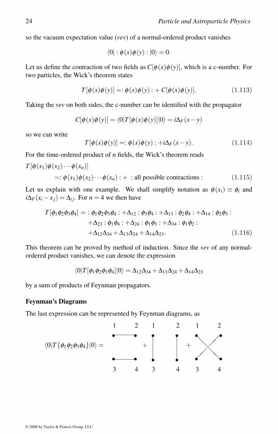
The last expression can be represented by Feynman diagrams, as
〈0|Tφ1φ2φ3φ4|0〉 =
1
3
2
4
• •
• •+
1
3
2
4
• •
• •+
1
3
2
4
• •
• •
© 2008 by Taylor & Francis Group, LLC
Particles and Fields 25
These diagrams show particles created at a point and annihilated at another point,
which can happen in three different ways shown by separate diagrams. Total ampli-
tude for the process will be summed over all the diagrams. In this case since all the
diagrams give same amplitudes, there will be a factor of 3, which is the symmetry
factor.
Let us now discuss a slightly more involved case when there are interactions given
by the fields at the same points. Consider a theory with the interaction Hamiltonian
HI(t) =∫
d3x(λ/4!)φ 4(x). We are interested in evaluating the two-point correlation
function 〈Ω|Tφ(x)φ(y)|Ω〉. As we shall see later, the numerator can be factored
out into two parts: one with propagators connected to external points x and y, called
the connected diagrams, and the other part that is not connected to external legs,
called the disconnected diagrams. The denominator comprises only the disconnected
part of the diagrams, so the two-point correlation function may be evaluated by sum-
ming over only the connected diagrams. For the present we shall discuss only the
numerator, given by
〈0|T
φ(x)φ(y)+φ(x)φ(y)[−i
∫dtHI(t)
]+ · · ·
|0〉. (1.117)
The first term in the series is the free-particle propagator 〈0|T φ(x)φ(y)|0〉= i∆F(x−y). The second term contains the interactions at only one point and is the leading
term in the perturbation series representing the interactions. We can express this
term in terms of propagators using the Wick’s theorem as
〈0|T
φ(x)φ(y)(−iλ
4!
)∫d4zφ(z)φ(z)φ(z)φ(z)
|0〉
= 3 ·(−iλ
4!
)∆xy
∫d4z∆zz∆zz +12 ·
(−iλ4!
)∫d4z∆xz∆yz∆zz (1.118)
Previously we introduced the notation, i∆F(x− y) = ∆xy. The factors 3 and 12 are
the symmetry factors, which are the different possible contractions that can give the
same diagrams. As discussed above, for the four φi three possible contractions are
possible. The propagators ∆zz represent loops, since the starting and end points are
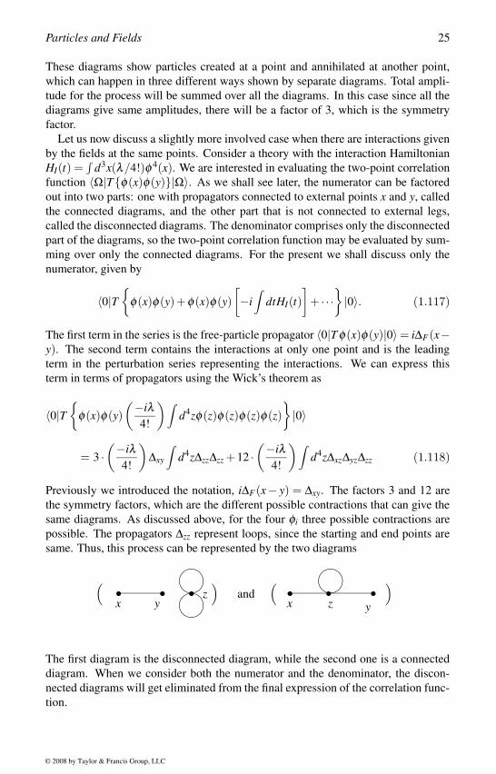
same. Thus, this process can be represented by the two diagrams
( )
x yz• • •
( )and
• • •x z y
The first diagram is the disconnected diagram, while the second one is a connected
diagram. When we consider both the numerator and the denominator, the discon-
nected diagrams will get eliminated from the final expression of the correlation func-
tion.
© 2008 by Taylor & Francis Group, LLC
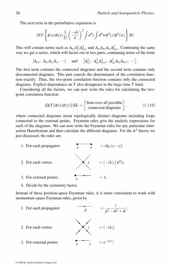
26 Particle and Astroparticle Physics
The next term in the perturbative expansion is
〈0|T
φ(x)φ(y)1
2!
(−iλ4
)2 ∫d4z
∫d4wφ 4(z)φ 4(w)
|0〉.
This will contain terms such as ∆xy∆2zz∆2
ww and ∆xz∆yz∆zz∆2ww. Continuing the same
way we get a series, which will factor out in two parts, containing terms of the form
[∆xy; ∆xz∆yz∆zz · · ·] and[∆2
zz; ∆2zz∆
2ww; ∆2
zw∆zz∆ww; · · ·] .The first term contains the connected diagrams and the second term contains only
disconnected diagrams. This part cancels the denominator of the correlation func-
tion exactly. Thus, the two-point correlation function contains only the connected
diagrams. Explicit dependence on T also disappears in the large time T limit.
Considering all the factors, we can now write the rules for calculating the two-
point correlation function:
〈Ω|Tφ(x)φ(y)|Ω〉 =[
Sum over all possible
connected diagrams
], (1.119)
where connected diagrams mean topologically distinct diagrams including loops
connected to the external points. Feynman rules give the analytic expressions for
each of the diagrams. We can now write the Feynman rules for any particular inter-
action Hamiltonian and then calculate the different diagrams. For the φ 4 theory we
just discussed, the rules are
1. For each propagator: • •x y = i∆F(x− y);
2. For each vertex:
• x = (−iλ )∫
d4x;
3. For external points:•
x = 1;
4. Divide by the symmetry factor.
Instead of these position-space Feynman rules, it is more convenient to work with
momentum-space Feynman rules, given by
1. For each propagator:
p =i
p2 −m2 + iε;
2. For each vertex:
• z = (−iλ );
3. For external points:•
x y = e−ip·x;
© 2008 by Taylor & Francis Group, LLC
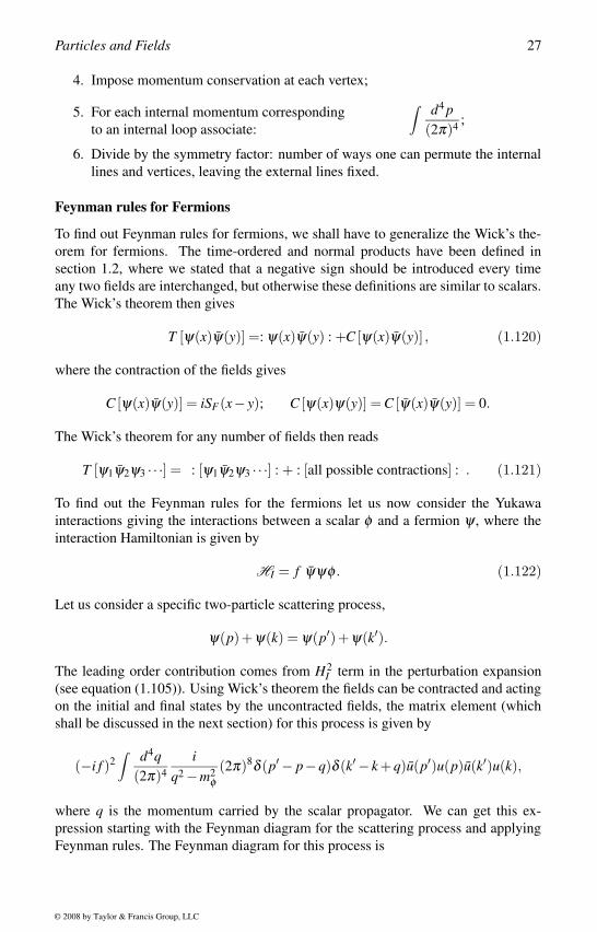
Particles and Fields 27
4. Impose momentum conservation at each vertex;
5. For each internal momentum corresponding
to an internal loop associate:
∫ d4 p(2π)4 ;
6. Divide by the symmetry factor: number of ways one can permute the internal
lines and vertices, leaving the external lines fixed.
Feynman rules for Fermions
To find out Feynman rules for fermions, we shall have to generalize the Wick’s the-
orem for fermions. The time-ordered and normal products have been defined in
section 1.2, where we stated that a negative sign should be introduced every time
any two fields are interchanged, but otherwise these definitions are similar to scalars.
The Wick’s theorem then gives
T [ψ(x)ψ(y)] =: ψ(x)ψ(y) : +C [ψ(x)ψ(y)] , (1.120)
where the contraction of the fields gives
C [ψ(x)ψ(y)] = iSF(x− y); C [ψ(x)ψ(y)] = C [ψ(x)ψ(y)] = 0.
The Wick’s theorem for any number of fields then reads
T [ψ1ψ2ψ3 · · ·] = : [ψ1ψ2ψ3 · · ·] : + : [all possible contractions] : . (1.121)
To find out the Feynman rules for the fermions let us now consider the Yukawa
interactions giving the interactions between a scalar φ and a fermion ψ , where the
interaction Hamiltonian is given by
HI = f ψψφ . (1.122)
Let us consider a specific two-particle scattering process,
ψ(p)+ψ(k) = ψ(p′)+ψ(k′).
The leading order contribution comes from H2I term in the perturbation expansion
(see equation (1.105)). Using Wick’s theorem the fields can be contracted and acting
on the initial and final states by the uncontracted fields, the matrix element (which
shall be discussed in the next section) for this process is given by
(−i f )2∫ d4q
(2π)4i
q2 −m2φ(2π)8δ (p′− p−q)δ (k′− k +q)u(p′)u(p)u(k′)u(k),
where q is the momentum carried by the scalar propagator. We can get this ex-
pression starting with the Feynman diagram for the scattering process and applying
Feynman rules. The Feynman diagram for this process is
© 2008 by Taylor & Francis Group, LLC
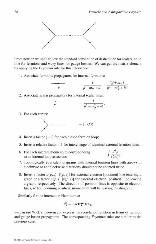
28 Particle and Astroparticle Physics
From now on we shall follow the standard convention of dashed line for scalars, solid
line for fermions and wavy lines for gauge bosons. We can get the matrix element
by applying the Feynman rule for this interaction:
1. Associate fermions propagators for internal fermions:
p =
i/p−mψ + iε
=i(/p+mψ)
p2 −m2ψ + iε
;
2. Associate scalar propagators for internal scalar lines:
p =
ip2 −m2
φ + iε;
3. For each vertex:
= (−i f );
4. Insert a factor (−1) for each closed fermion loop;
5. Insert a relative factor −1 for interchange of identical external fermion lines.
6. For each internal momentum corresponding
to an internal loop associate:
∫ d4 p(2π)4 ;
7. Topologically equivalent diagrams with internal fermion lines with arrows in
clockwise or anticlockwise directions should not be counted twice.
8. Insert a factor u(p,s) [v(p,s)] for external electron [positron] line entering a
graph or a factor u(p,s) [v(p,s)] for external electron [positron] line leaving
a graph, respectively. The direction of positron lines is opposite to electron
lines, so for incoming positron, momentum will be leaving the diagram.
Similarly for the interaction Hamiltonian
HI = −ieψγµ ψAµ ,
we can use Wick’s theorem and express the correlation function in terms of fermion
and gauge boson propagators. The corresponding Feynman rules are similar to the
previous case:
© 2008 by Taylor & Francis Group, LLC
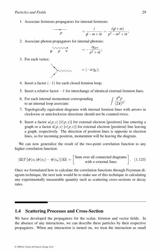
Particles and Fields 29
1. Associate fermions propagators for internal fermions:
p =
i/p−m+ iε
=i(/p+m)
p2 −m2 + iε;
2. Associate photon propagators for internal photons:µ p ν = − igµν
p2 + iε;
3. For each vertex:
= (−ieγµ);
4. Insert a factor (−1) for each closed fermion loop;
5. Insert a relative factor −1 for interchange of identical external fermion lines.
6. For each internal momentum corresponding
to an internal loop associate:
∫ d4 p(2π)4 ;
7. Topologically equivalent diagrams with internal fermion lines with arrows in
clockwise or anticlockwise directions should not be counted twice.
8. Insert a factor u(p,s) [v(p,s)] for external electron [positron] line entering a
graph or a factor u(p,s) [v(p,s)] for external electron [positron] line leaving
a graph, respectively. The direction of positron lines is opposite to electron
lines, so for incoming positron, momentum will be leaving the diagram.
We can now generalize the result of the two-point correlation function to any
higher correlation function:
〈Ω|Tφ(x1)φ(x2) · · ·φ(xn)|Ω〉 =[
Sum over all connected diagrams
with n external lines
]. (1.123)
Once we formulated how to calculate the correlation functions through Feynman di-
agram technique, the next task would be to make use of this technique in calculating
any experimentally measurable quantity such as scattering cross-sections or decay
rates.
1.4 Scattering Processes and Cross-SectionWe have developed the propagators for the scalar, fermion and vector fields. In
the absence of any interactions, we can describe these particles by their respective
propagators. When any interaction is turned on, we treat the interaction as small
© 2008 by Taylor & Francis Group, LLC
30 Particle and Astroparticle Physics
perturbations to the free propagator assuming that the interactions are not strong.
To the first order this amounts to treating the interaction to be instantaneous, so
for the rest of the time the free propagators can describe these particles. At higher
orders, several instantaneous interactions are taken into consideration. As long as
the strength of the interaction is small, higher order contributions will be smaller and
we shall be able to describe the nature of interaction taking the first few terms in the
perturbation expansions.
Cross-Section
Different experiments measure the cross-section of various processes, which can be
compared with measurements in different environments with differing beam sizes
and intensity. Simply speaking the cross-section measures an effective size of the
target particle. If ρB,T are the number densities of the incident beam of particles of
type B and of the target particles of type T , which are at rest, B,T are the lengths of
the bunches of these particles; A is the cross-sectional area, then the cross-section is
defined as
σ ≡ Number of scattering events
ρB B ρT T A. (1.124)
The total number of events (N) will then be given by
N = σ B T
∫d2x ρB(x) ρT (x).
Since the beam density is not constant in practice, one needs to integrate over the
beam area. When we are interested in the cross-section with definite momenta, we
have to work with differential cross-section dσ/d3 p1 · · ·d3 pn. Integrating over the
small regions of momentum–space gives us the final-state cross-section for scattering
into that region of final-state momentum–space.
For the decays of any unstable particles (X), we define the decay rate as
Γ ≡ Number of decays per unit time
Number of decaying particles (X) present. (1.125)
The lifetime τX (half-life τ · ln2) of the particle is then
τX ≡ 1
∑Γ(X → all possible final states).
In a scattering experiment, an unstable particle shows up as a resonance. Near the
resonance, the scattering amplitude is given by the Breit–Wigner formula
f (E) ∝1
E −E0 + iΓ/2. (1.126)
The cross-section has a resonance peak σ ∝ 1/((E −E0)2 +Γ2/4), whose width
gives the decay rate of the unstable state. In relativistic quantum mechanics, the
Breit–Wigner formula can be generalized to 1/(p2 −m2 + imΓ).
© 2008 by Taylor & Francis Group, LLC
Particles and Fields 31
To calculate the cross-section, we introduce the S-matrix
S f i = 〈 f |S|i〉 = δ f i − i(2π)4δ 4(Pf −Pi)T f i , (1.127)
where δ f i corresponds to no interactions and T f i is the transition matrix between the
initial state |i〉 and the final state | f 〉 in the presence of interactions. The initial and fi-
nal states are collections of free asymptotic states at t →−∞ and t → ∞, respectively.
The S-matrix is unitary.
The differential cross-section is then given by
dσ =1
J|S f i|2dN f
V T
=1
J(2π)4δ 4(Pf −Pi)|T f i|2dN f , (1.128)
where V T = (2π)4δ 4(0), J is the flux of incident particles, and
dN f =N f
∏i=1
Vd3 p
(2π)3
is the number of states with momentum between p and p+δp.
For a scattering process 1 + 2 → 3 + 4 + · · ·, the incident flux J can be given in
the center of mass frame (p1 = −p2) as J = [(p1 · p2)2 −m21m2
2]1/2/(V E1E2), so the
differential cross-section is given by
dσ =(2π)4|M f i|2δ 4(Pf −Pi)
(2E1)(2E2)|v1 − v2| ∏f
d3 p f
(2π)32Ep f
=(2π)4|M f i|2δ 4(Pf −Pi)4[(p1.p2)2 −m2
1m22]1/2 ∏
f
d3 p f
(2π)32Ep f
(1.129)
in a collinear frame where T f i = ∏Nj=1(2Ep jV )−1/2M f i. For two final-state particles,
we can simplify this formula to(dσdΩ
)CM
=1
(2E1)(2E2)|v1 − v2||p1|
(2π)44ECM|M (p1, p2 → p3, p4)|2. (1.130)
The matrix elements may be read from the Feynman diagram.
The probability of the decay of a single particle can then be evaluated in the same
way:
Ptot = ∑f
∫dN f |S f i|2 = ∑
f
∫dN f |T f i|2[(2π)4δ 4(Pf −Pi)]2, (1.131)
so after proper normalization the final differential decay rate becomes
dΓ(i → f) =(2π)4
2mi∏
f
d3 p f
(2π)32E f|M f i|2δ 4(Pf −Pi). (1.132)
It is assumed that the decaying particle is at rest, so we could replace (2Ei)−1 by
(2mi)−1. The lifetime of the particle will be τ = 1/Γ. In this formalism the main
task is then to evaluate the matrix elements M f i for any given Feynman diagram.
© 2008 by Taylor & Francis Group, LLC

32 Particle and Astroparticle Physics
LSZ Reduction
A direct connection between the scaterring matrix and the correlation function was
given by Lehmann, Symanzik and Zimmermann [11], and is known as the LSZ re-
duction formula. This will allow us to calculate any physical scattering process by
calculating the correlation functions using Feynman rules.
Consider a scalar free-field whose two-point function in momentum space is given
by the propagator
∫d4xeipx〈Ω|T [φ(x)φ(0)]|Ω〉 =
ip2 −m2 + iε
.
This also represents the asymptotic state of the scalar field at time t →±∞ and has a
simple pole at the mass of the one-particle state.
If we are interested in calculating the S-matrix element for a ni-body −→ n f -body
scattering process, we start with a correlation function with ni +n f Heisenberg fields.
If we Fourier transform the correlation function with respect to any one of the ni +n ffields, it will be possible to factor out a term with a pole, which represents a free-
field and may be associated with the asymptotic propagator of the corresponding
field. Continuing in the same way it will be possible to write the (ni +n f )-point cor-
relation function as a product of asymptotic states corresponding to all the (ni +n f )fields. The S-matrix element of our interest will then be given by the coefficient of
these asymptotic states. This can be expressed as
ni
∏i=1
∫d3xieipi·xi
n f
∏j=1
∫d3y jeik j ·y j〈Ω|T [φ(x1) · · ·φ(xni)φ(y1) · · ·φ(yn f )]|Ω〉
=ni
∏i=1
ip2
i −m2 + iε
n f
∏j=1
ik2
j −m2 + iεS f i. (1.133)
The momenta of the incoming particles are denoted by pi and those of the outgoing
particles as k j and S f i is the S-matrix for the scattering process. Effects of renormal-
ization have not been included in this discussion but will be considered in the next
chapter.
Optical Theorem
We shall now discuss one more important aspect of field theory, how to deal with
unstable particles. Since the asymptotic states cannot be defined for any unstable
states, LSZ reduction is not possible for any decaying particles. This is solved by
using the optical theorem in conjunction with the Cutkowsky rules [12]. In this
approach the decays of any unstable particle are related to the imaginary part of the
two-point correlation function of the decaying particles with all possible intermediate
states, so Feynman rules can be used to calculate the decay rate.
Consider a process, a1 + a2 → [ fi] → b1 + b2, which can go through several in-
termediate channels, where [ fi] denotes different multiparticle intermediate states.
The optical theorem states that the imaginary part of the amplitude for the forward
© 2008 by Taylor & Francis Group, LLC
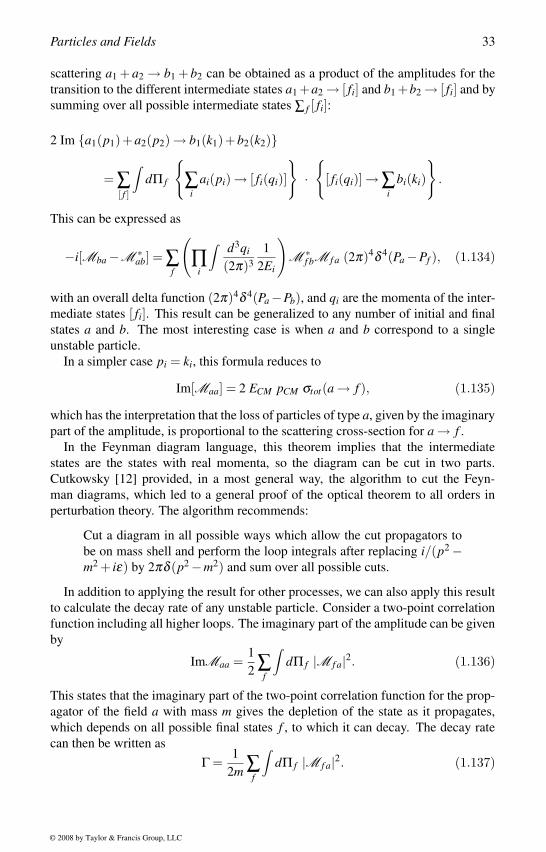
Particles and Fields 33
scattering a1 + a2 → b1 + b2 can be obtained as a product of the amplitudes for the
transition to the different intermediate states a1 +a2 → [ fi] and b1 +b2 → [ fi] and by
summing over all possible intermediate states ∑ f [ fi]:
2 Im a1(p1)+a2(p2) → b1(k1)+b2(k2)
= ∑[ f ]
∫dΠ f
∑
iai(pi) → [ fi(qi)]
·
[ fi(qi)] → ∑i
bi(ki)
.
This can be expressed as
−i[Mba −M ∗ab] = ∑
f
(∏
i
∫ d3qi
(2π)31
2Ei
)M ∗
f bM f a (2π)4δ 4(Pa −Pf ), (1.134)
with an overall delta function (2π)4δ 4(Pa −Pb), and qi are the momenta of the inter-
mediate states [ fi]. This result can be generalized to any number of initial and final
states a and b. The most interesting case is when a and b correspond to a single
unstable particle.
In a simpler case pi = ki, this formula reduces to
Im[Maa] = 2 ECM pCM σtot(a → f ), (1.135)
which has the interpretation that the loss of particles of type a, given by the imaginary
part of the amplitude, is proportional to the scattering cross-section for a → f .
In the Feynman diagram language, this theorem implies that the intermediate
states are the states with real momenta, so the diagram can be cut in two parts.
Cutkowsky [12] provided, in a most general way, the algorithm to cut the Feyn-
man diagrams, which led to a general proof of the optical theorem to all orders in
perturbation theory. The algorithm recommends:
Cut a diagram in all possible ways which allow the cut propagators to
be on mass shell and perform the loop integrals after replacing i/(p2 −m2 + iε) by 2πδ (p2 −m2) and sum over all possible cuts.
In addition to applying the result for other processes, we can also apply this result
to calculate the decay rate of any unstable particle. Consider a two-point correlation
function including all higher loops. The imaginary part of the amplitude can be given
by
ImMaa =1
2∑
f
∫dΠ f |M f a|2. (1.136)
This states that the imaginary part of the two-point correlation function for the prop-
agator of the field a with mass m gives the depletion of the state as it propagates,
which depends on all possible final states f , to which it can decay. The decay rate
can then be written as
Γ =1
2m ∑f
∫dΠ f |M f a|2. (1.137)
© 2008 by Taylor & Francis Group, LLC
34 Particle and Astroparticle Physics
This is the result given in equation (1.132). Thus, although the asymptotic states for
any unstable particle cannot be defined, it is possible to calculate the decay rate of
the particle by calculating the two-point function using Feynman diagrams.
Møller Scattering
p1
p′1
p2
p′2
p1
p′1
p2
p′2
FIGURE 1.1Møller scattering of two electrons
We shall work out the cross-section for the electron–electron scattering. To the
lowest order there are two Feynman graphs contributing to the process, which are
shown in figure 1.4. Using the Feynman rules we can write the matrix element for
these diagrams as
iM f i = (−ie)2u(p′1)γµ u(p1)−igµν
(p′1 − p1)2 u(p′2)γν u(p2)
and
iM f i =ie2gµν
(p1 − p′2)2 u(p′2)γµ u(p1)u(p′1)γν u(p2).
To write the matrix element squared, we shall use the relation
|u(p′)Γu(p)|2 = [u(p′)Γu(p)][u†(p)Γ†u†(p′)]
= [u(p′)Γu(p)][u(p)γ0Γ†γ0u(p′)]
= Tr[(/p ′ +m) Γ (/p+m)γ0Γ†γ0
], (1.138)
where uα(p)uβ (p) = (/p+m)αβ . In the center of mass frame (p1 = −p2), the differ-
ential cross-section will then be given by
dσ =(2π)4δ 4(p′1 + p′2 − p1 − p2)
4[(p1 · p2)2 −m4]1/2
∫ d3 p′1(2π)32E ′
1
d3 p′2(2π)32E ′
2|M f i|2 (1.139)
© 2008 by Taylor & Francis Group, LLC
Particles and Fields 35
with the matrix element squared given by
|M f i|2 =e4
4
[Tr[γµ(/p1 +m)γν(/p1
′ +m)] Tr[γµ(/p2 +m)γν(/p2′ +m)]
(p′1 − p1)2(p′1 − p1)2
− Tr[γµ(/p1 +m)γν(/p2′ +m)] Tr[γµ(/p2 +m)γν(/p1
′ +m)](p′1 − p1)2(p′2 − p2)2
+ (p′1 ↔ p′2)]. (1.140)
In this expression contributions from both the diagrams have been included. To take
the trace of the gamma matrices, we can make use of the following identities:
γµ γµ = 4
γσ γµ γσ = −2γµ
γσ γµ γν γσ = 4gµν
γσ γµ γν γρ γσ = −2γρ γν γµ . (1.141)
We shall also make use of the trace operations:
Tr [γ5γµ ] = Tr [σ µν ] = Tr [γµ γν γ5] = 0
Tr [γµ γν ] = 4gµν
Tr [γµ γν γρ γσ ] = 4[gµν gρσ −gµρ gνσ +gµσ gνρ ]Tr [γ5γµ γν γρ γσ ] = 4iεµνρσ . (1.142)
Trace of any odd numbers of γ-matrices vanishes. These relations can be applied to
products of /a = aµ γµ , for example,
Tr [/a /b] = 4(a ·b)Tr [/a /b /c /d] = 4[(a ·b)(c ·d)− (a · c)(b ·d)+(a ·d)(b · c)].
After taking the trace we work in the center of mass frame and choose p1 and p2to be along the z-axis. If the scattered particles make an angle θ with the incident
particles, then we can express products of all the momenta in terms of the center of
mass energy E, electron momentum p and θ as
p1 · p2 = 2E2 −m2
p1 · p′1 = E2(1− cosθ)+m2 cosθp1 · p′2 = E2(1+ cosθ)−m2 cosθ (1.143)
The differential cross-section for the electron–electron scattering per unit of solid
angle is then given by [13]
dσdΩ
=α2
4E2
[(2E2 −m2)2
(E2 −m2)2
(4
sin4 θ− 3
sin2 θ
)+(
1+4
sin4 θ
)], (1.144)
© 2008 by Taylor & Francis Group, LLC
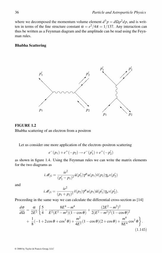
36 Particle and Astroparticle Physics
where we decomposed the momentum volume element d3 p = dΩp2d p, and is writ-
ten in terms of the fine structure constant α = e2/4π = 1/137. Any interaction can
thus be written as a Feynman diagram and the amplitude can be read using the Feyn-
man rules.
Bhabha Scattering
p1
p′1
p2
p′2
p1
p′1
p2
p′2
FIGURE 1.2Bhabha scattering of an electron from a positron
Let us consider one more application of the electron–positron scattering
e−(p1)+ e+(−p2) → e−(p′1)+ e+(−p′2)
as shown in figure 1.4. Using the Feynman rules we can write the matrix elements
for the two diagrams as
iM f i =ie2
(p′1 − p1)2 u(p′1)γµ u(p1)v(p2)γµ v(p′2)
and
iM f i =ie2
(p1 + p2)2 v(p2)γµ u(p1)u(p′1)γµ v(p′2).
Proceeding in the same way we can calculate the differential cross-section as [14]
dσdΩ
=α
2E2
5
4− 8E4 −m4
E2(E2 −m2)(1− cosθ)+
(2E2 −m2)2
2(E2 −m2)2(1− cosθ)2
+1
8(−1+2cosθ + cos2 θ)+
m2
4E2 (1− cosθ)(2+ cosθ)+m4
8E4 cos2 θ
.
(1.145)
© 2008 by Taylor & Francis Group, LLC
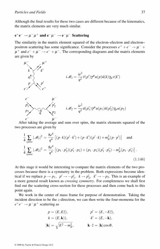
Particles and Fields 37
Although the final results for these two cases are different because of the kinematics,
the matrix elements are very much similar.
e+e− → µ−µ+ and e−µ− → e−µ− Scattering
The similarity in the matrix element squared of the electron–electron and electron–
positron scattering has some significance. Consider the processes e+ + e− → µ− +µ+ and e− + µ− → e− + µ−. The corresponding diagrams and the matrix elements
are given by
e− e+p p′
µ− µ+
k k′
q
iM1 =ie2
q2 v(p′)γµ u(p)u(k)γµ v(k′)
e− µ−
p1
p′1
e− µ−
p2
p′2
q
iM2 =ie2
q2 u(p′1)γµ u(p1)u(p′2)γµ u(p2)
After taking the average and sum over spins, the matrix elements squared of the
two processes are given by
1
4∑
spins|M1|2 =
8e4
q4
[(p · k)(p′ · k′)+(p · k′)(p′ · k)+m2
µ(p · p′)]
and
1
4∑
spins|M2|2 =
8e4
q4
[(p1 · p′2)(p′1 · p2)+(p1 · p2)(p′1 · p′2)−m2
µ(p1 · p′1)].
(1.146)
At this stage it would be interesting to compare the matrix elements of the two pro-
cesses because there is a symmetry in the problem. Both expressions become iden-
tical if we replace p → p1, p′ →−p′1, k → p′2, k′ →−p2. This is an example of
a more general result known as crossing symmetry. For completeness we shall first
find out the scattering cross-section for these processes and then come back to this
point again.
We work in the center of mass frame for purpose of demonstration. Taking the
incident direction to be the z-direction, we can then write the four-momenta for the
e+e− → µ−µ+ scattering as
p = (E,Ez), p′ = (E,−Ez),
k = (E,k)), k′ = (E,−k),
|k| =√
E2 −m2µ , k · z = |k|cosθ ,
© 2008 by Taylor & Francis Group, LLC
38 Particle and Astroparticle Physics
so the relevant quantities for the calculation of the squared matrix elements are
q2 = (p+ p′)2 = 4E2, p · p′ = 2E2,
p · k = p′ · k′ = E2 −E|k|cosθ , p · k′ = p′ · k = E2 +E|k|cosθ .
The final squared matrix element is then given by
1
4∑
spins|M |2 = e4
[(1+
m2µ
E2
)+
(1− m2
µ
E2
)cos2 θ
]
and the differential scattering cross-section for the unpolarized e+e− → µ−µ+ scat-
tering in the center of mass frame is given by
dσdΩ
=α2
4E2CM
(1− m2
µ
E2
)1/2[(1+
m2µ
E2
)+
(1− m2
µ
E2
)cos2 θ
], (1.147)
where the center of mass energy ECM = 2E.
In the case of e−µ− → e−µ− scattering, we can choose the four-momenta for the
initial and final states as
p1 = (k,kz), p2 = (E,−kz),
p′1 = (k,k)), p′2 = (E,−k),
E2 = k2 +m2µ , k · z = k cosθ ,
with the center of mass energy ECM = E + k. The final differential cross-section for
unpolarized electron–muon scattering is given by
dσdΩ
=α2
2k2E2CM(1− cosθ)2 [E2
CM +(E + k cosθ)2 −m2µ(1− cosθ)]. (1.148)
The cross-sections for the two processes are, thus, much different.
Crossing Symmetry and Mandelstam Variables
We notice the similarity between the matrix elements for the processes e+e− →µ−µ+ and e−µ− → e−µ− in equation (1.146) under the exchange p → p1, p′ →−p′1, k → p′2, k′ →−p2. This is a more general result known as the crossing sym-metry, which states that the S-matrices for any two processes become equal (to be
precise, can be analytically continued to each other), if these processes are identical
except for the exchange of a particle with momentum p in the initial state with an
antiparticle in the final state with momentum k = −p. This can be expressed by
M [φ(p)+ · · · → ·· ·] = M [· · · → φ(k)+ · · ·],where φ(k = −p) is the antiparticle of φ(p). However, the kinematics for the two
cases are different. This is a consequence of
∑u(p)u(p) =/p+m = −(/k−m) = −∑v(k)v(k).
© 2008 by Taylor & Francis Group, LLC
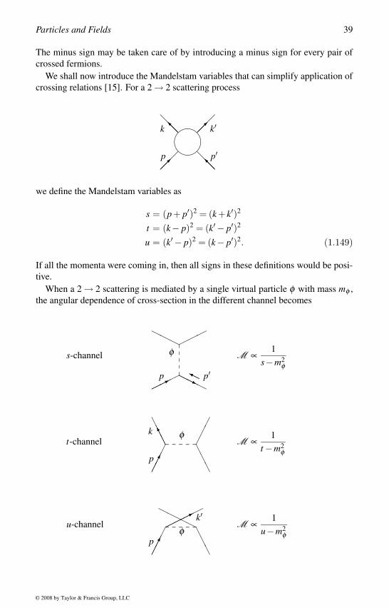
Particles and Fields 39
The minus sign may be taken care of by introducing a minus sign for every pair of
crossed fermions.
We shall now introduce the Mandelstam variables that can simplify application of
crossing relations [15]. For a 2 → 2 scattering process
p
p′
k
k′
we define the Mandelstam variables as
s = (p+ p′)2 = (k + k′)2
t = (k− p)2 = (k′− p′)2
u = (k′− p)2 = (k− p′)2. (1.149)
If all the momenta were coming in, then all signs in these definitions would be posi-
tive.
When a 2 → 2 scattering is mediated by a single virtual particle φ with mass mφ ,
the angular dependence of cross-section in the different channel becomes
s-channel
p
φ
p′
M ∝1
s−m2φ
t-channel
p
φk
M ∝1
t −m2φ
u-channel
pφ
k′
M ∝1
u−m2φ
© 2008 by Taylor & Francis Group, LLC
40 Particle and Astroparticle Physics
In the massless limit of e+e− → µ+µ− scattering, the Mandelstam variables are
s = (p+ p′)2 = q2, t = −2p · k = −2p′ · k′ and u = −2p · k′ = −2p′ · k, which give
1
4∑
spins|M |2 =
2e4
s2 (t2 +u2).
Let us now consider the massless limit of the e−µ− → e−µ− scattering. The crossing
relations p → p1, p′ → −p′1, k → p′2, k′ → −p2 would imply that the s and tvariables of the e+e− → µ+µ− process have become t and s variables, respectively,
with u remaining the same. So, for the process e−µ− → e−µ− we now have
1
4∑
spins|M |2 =
2e4
t2 (s2 +u2).
Some processes may receive contributions from more than one type channel. We
noticed, Møller scattering received contributions from t- and u-channel diagrams,
while Bhabha scattering received contributions from s- and t-channel diagrams.
In the center of mass frame for particles of mass m, we can write
p = (E, pz), p′ = (E,−pz),k = (E,p)), k′ = (E,−p),
so the Mandelstam variables becomes
s = (2E)2, t = −2p2(1− cosθ), u = −2p2(1+ cosθ).
Thus, t → 0 as θ → 0, while u → 0 as θ → π . Another useful identity with the
Mandelstam variables is
s+ t +u =4
∑i=1
m2i . (1.150)
The sum extends over all 4-external particles.
So far we restricted ourselves to only tree-level or the lowest order Feynman dia-
grams for the different processes. In the next chapter we shall consider higher-order
radiative corrections and discuss how to take care of such divergences to make the
theory consistent.
© 2008 by Taylor & Francis Group, LLC
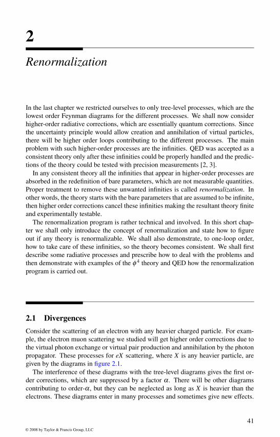
2Renormalization
In the last chapter we restricted ourselves to only tree-level processes, which are the
lowest order Feynman diagrams for the different processes. We shall now consider
higher-order radiative corrections, which are essentially quantum corrections. Since
the uncertainty principle would allow creation and annihilation of virtual particles,
there will be higher order loops contributing to the different processes. The main
problem with such higher-order processes are the infinities. QED was accepted as a
consistent theory only after these infinities could be properly handled and the predic-
tions of the theory could be tested with precision measurements [2, 3].
In any consistent theory all the infinities that appear in higher-order processes are
absorbed in the redefinition of bare parameters, which are not measurable quantities.
Proper treatment to remove these unwanted infinities is called renormalization. In
other words, the theory starts with the bare parameters that are assumed to be infinite,
then higher order corrections cancel these infinities making the resultant theory finite
and experimentally testable.
The renormalization program is rather technical and involved. In this short chap-
ter we shall only introduce the concept of renormalization and state how to figure
out if any theory is renormalizable. We shall also demonstrate, to one-loop order,
how to take care of these infinities, so the theory becomes consistent. We shall first
describe some radiative processes and prescribe how to deal with the problems and
then demonstrate with examples of the φ 4 theory and QED how the renormalization
program is carried out.
2.1 DivergencesConsider the scattering of an electron with any heavier charged particle. For exam-
ple, the electron muon scattering we studied will get higher order corrections due to
the virtual photon exchange or virtual pair production and annihilation by the photon
propagator. These processes for eX scattering, where X is any heavier particle, are
given by the diagrams in figure 2.1.
The interference of these diagrams with the tree-level diagrams gives the first or-
der corrections, which are suppressed by a factor α . There will be other diagrams
contributing to order-α , but they can be neglected as long as X is heavier than the
electrons. These diagrams enter in many processes and sometimes give new effects.
41
© 2008 by Taylor & Francis Group, LLC
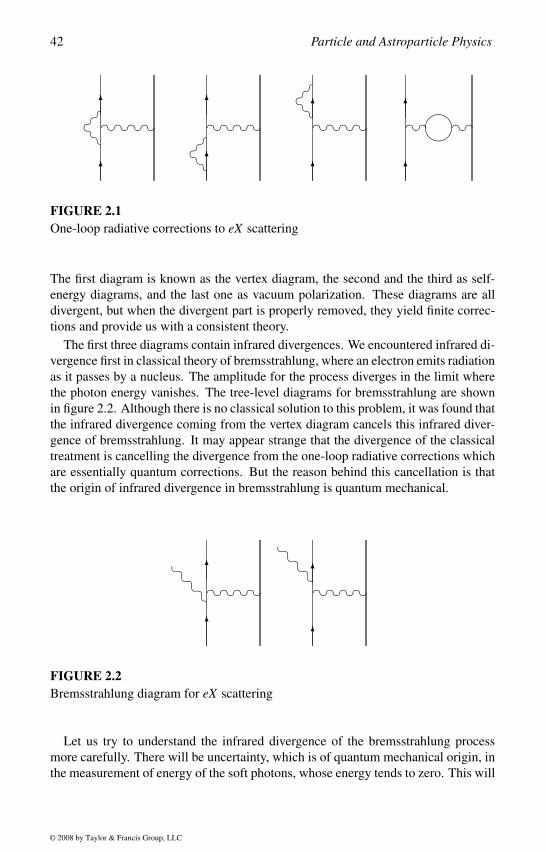
42 Particle and Astroparticle Physics
FIGURE 2.1One-loop radiative corrections to eX scattering
The first diagram is known as the vertex diagram, the second and the third as self-
energy diagrams, and the last one as vacuum polarization. These diagrams are all
divergent, but when the divergent part is properly removed, they yield finite correc-
tions and provide us with a consistent theory.
The first three diagrams contain infrared divergences. We encountered infrared di-
vergence first in classical theory of bremsstrahlung, where an electron emits radiation
as it passes by a nucleus. The amplitude for the process diverges in the limit where
the photon energy vanishes. The tree-level diagrams for bremsstrahlung are shown
in figure 2.2. Although there is no classical solution to this problem, it was found that
the infrared divergence coming from the vertex diagram cancels this infrared diver-
gence of bremsstrahlung. It may appear strange that the divergence of the classical
treatment is cancelling the divergence from the one-loop radiative corrections which
are essentially quantum corrections. But the reason behind this cancellation is that
the origin of infrared divergence in bremsstrahlung is quantum mechanical.
FIGURE 2.2Bremsstrahlung diagram for eX scattering
Let us try to understand the infrared divergence of the bremsstrahlung process
more carefully. There will be uncertainty, which is of quantum mechanical origin, in
the measurement of energy of the soft photons, whose energy tends to zero. This will
© 2008 by Taylor & Francis Group, LLC
Renormalization 43
allow all the photons with energy lower than the uncertainty in energy measurement
to emit without being detected. Since photons are massless, there could be an infinite
number of photons below any given momentum. This infinite number of photons
gives us the divergence even in a classical treatment. Since these soft photons cannot
be detected, these processes have to be included in the cross-sections for scattering
without radiation, which includes the vertex diagram. In other words, the uncertainty
principle will not allow us to determine if these soft photons are real or virtual. So, by
calculating the vertex correction and the bremsstrahlung together, we can eliminate
this divergence.
Bremsstrahlung
The bremsstrahlung process has two parts: an elastic scattering of an electron from
a nucleus and the emission of photons from the electron during the interaction. The
matrix element for the bremsstrahlung process (shown in figure 2.2) can, thus, be
written using the Feynman rules as
iM = −ieu(p′)(
M0(p′, p− k)i
/p− /k−m+ iεγµ ε∗µ(k)
+ γµ ε∗µ(k)i
/p ′+ /k−m+ iεM0(p′ + k, p)
)u(p).
In this expression M0 includes the interaction of the electrons with the external field,
which is essentially the contribution from the elastic scattering. In our discussion we
shall not specify this part of the interaction, which is finite.
In our notation p is the momentum of the incoming electron, k is the momentum
carried by the photon, and p′ is the momentum of the outgoing electron. For soft
photons |k| |p′−p|, we can approximate
M0(p′, p− k) = M0(p′ + k, p) = M0(p′, p)
and simplify
1
/p− /k−m+ iεγµ ε∗µ(k)u(p) =
−1
p · k pµ ε∗µ(k)u(p)
u(p)γµ ε∗µ(k)1
/p ′+ /k−m+ iε= u(p)
1
p′ · k p′µ ε∗µ(k),
so the amplitude in the soft-photon approximation becomes
iM = e u(p′)M0(p′, p)u(p)(
p′ · ε∗p′ · k − p · ε∗
p · k)
. (2.1)
The cross-section also factors out as the cross-section for the elastic scattering (with-
out bremsstrahlung) times a factor coming from soft bremsstrahlung:
dσ(p → p′ + γ) = dσ(p → p′)∫ d3k
(2π)3e2
2k ∑λ
∣∣∣∣ p′ · ε(λ )p′ · k − p · ε(λ )
p · k∣∣∣∣2 . (2.2)
© 2008 by Taylor & Francis Group, LLC
44 Particle and Astroparticle Physics
We sum over the two photon polarization states λ = 1,2 and perform the integral
up to the energy |q| = |p−p′|, at which time the soft-photon approximation breaks
down. The theory is consistent for the upper limit, but the integral diverges at the
lower limit, which is the infrared divergence we discussed. To see the nature of
divergence and to compare with other diagrams, we introduce a small photon mass
µ and write down the final form of the cross-section as [16]
dσ(p → p′ + γ) ≈ dσ(p → p′)απ
log
(−q2
µ2
). log
(−q2
m2
), (2.3)
where q2 = (p′− p)2. The q2 dependence, known as the Sudakov double logarithm,
is physical. The problem with µ → 0 is the infrared divergence of the bremsstrahlung
process, which will be solved when we include vertex corrections to the elastic scat-
tering.
This infrared divergence problem is generic to any process in which massless par-
ticles are emitted from an initial or final leg that is on mass shell. If a soft photon of
momentum k is emitted from an on-shell electron with momentum p, the momentum
integration diverges. Since k is small and p2 = m2, the propagator
1
(p− k)2 −m2 + iε∼ 1
−2p · kgives the infrared divergence. However, this infrared divergence is not really a prob-
lem, since it cancels with divergences in the radiative diagrams.
Degree of Divergence and Renormalizability
The main problem with higher order processes is the ultraviolet divergences. One
may look at the problem from the point of view that at higher momentum the theory
may not remain the same and, hence, our lack of knowledge of very high energy
interactions may be manifesting as the unknown ultraviolet divergences, which we
eliminate by extracting the infinite contribution from the finite contribution by means
of some regularization and then by redefining some bare parameters to remove the
infinite contributions. In some theories it is not possible to absorb all the infinities
in the bare parameters. Renormalizable theories are ones that allow us to remove the
infinities. We shall now give some broad descriptions of the types of divergences one
may encounter and when the theory is renormalizable.
We try to understand the type of divergences by counting the powers of momenta pin any Feynman graph and calculating the degree of divergence D. We count the de-
gree of divergence D by counting (i) boson propagators, each contributing p−2; (ii)
fermion propagators, each contributing p−1; (iii) loop integrals, contributing loop
integration with p4; and (iv) every vertex with n derivatives contributing at most npowers of p. If D is 0 or positive, then the graph diverges. D = 0 gives to loga-
rithmically divergent, D = 1 gives linearly divergent, and D = 2 gives quadratically
divergent integrals.
We now state a criterion for the renormalizability of any theory.
© 2008 by Taylor & Francis Group, LLC
Renormalization 45
If any theory allows graphs, whose degree of divergence D depends only
on the external legs (internal loops do not contribute), we can collect all
N-point loop graphs into one term. In such theories, if there are finite
numbers of classes of divergent N-point graphs which can be absorbed
in the bare parameters of the theory, the theory is renormalizable.
In a super-renormalizable theory, adding internal loops decreases D. The degree
of divergence of any theory is determined in terms of the mass dimensions of the
various fields and coupling constants. We start with a dimensionless action. The
volume element d4x has dimension [M]−4 (or equivalently [L]4 in the natural unit
system h = 1 and c = 1). Thus, the Lagrangian should have a dimension [M]4 to
keep the action dimensionless. The kinetic energy term of a scalar field, (∂µ φ)2 then
means φ has a dimension [M] since the derivative ∂µ has a dimension [M]. Similarly
the kinetic energy term of a gauge field Fµν Fµν would give us the dimension of a
vector field or a gauge boson to be [M]. The kinetic energy term of a fermion ψi /∂ψwould give us the dimension of any fermion [M]3/2.
In any renormalizable theory coupling constants do not have anymass-dimensions.
In a d-dimensional theory (space–time dimension d), the fields will have different
mass dimensions. Since the action should be dimensionless and the integration is
over a d-dimensional space ddx, it would mean that
[φ ] = [M](d−2)/2; [ψ] = [M](d−1)/2 and [Aµ ] = [M](d−2)/2. (2.4)
This also includes the mass-dimensions in four space–time dimensions.
Let us consider a non-renormalizable theory, which allows an interaction LI with
coupling constant [g] = [M]−n, n > 0. For n = 2, the interaction could be a four-
fermion interaction g(ψaψb)(ψcψd) or a six-scalar interaction of the form gφ 6. Let
us consider an N-point function in this theory. If we insert the interaction LI , the N-
point function will have one extra coupling constant g, which will reduce the mass-
dimension of the N-point function. To maintain the mass-dimension of the graph,
every coupling constant g should be accompanied by kn, which makes the graph
more divergent by a factor of kn. Thus, by going to higher orders in perturbation
theory, we make the graph arbitrarily divergent.
Gravity, supergravity, four-fermion interactions and massive vector theory with
non-Abelian gauge group are thus, examples of non-renormalizable theories. A
φ 4 model, Yukawa interactions, gauge theories, massive vector Abelian theory and
spontaneously broken gauge theories are examples of renormalizable theories. In
addition, there are super-renormalizable theories, in which the degree of divergence
goes down so the theory has only a few divergent graphs. φ 3 theory is an example
of super-renormalizable theory. Finally, there are finite theories such as the super
Yang–Mills theory and the superstring theory, which are free of any divergences to
all orders.
© 2008 by Taylor & Francis Group, LLC
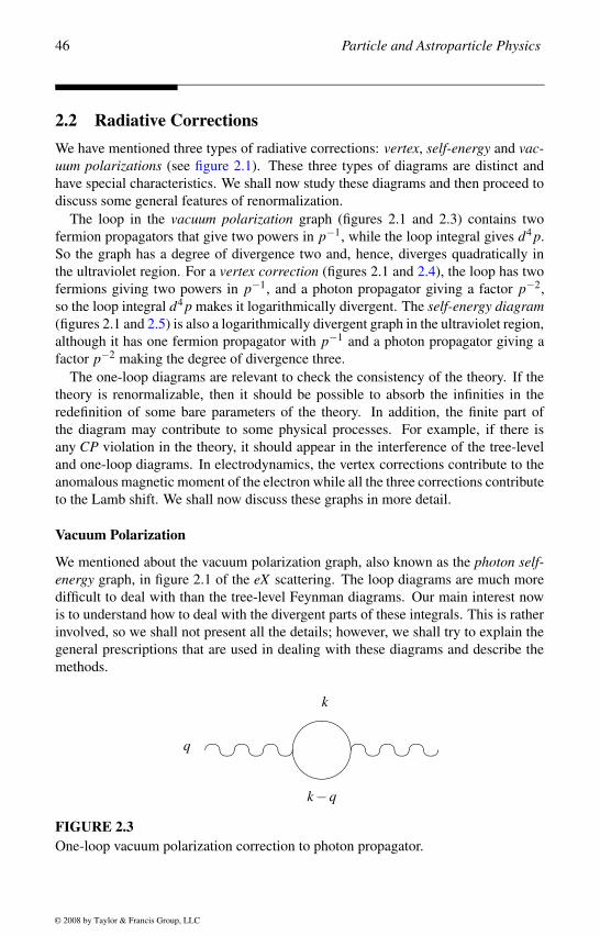
46 Particle and Astroparticle Physics
2.2 Radiative CorrectionsWe have mentioned three types of radiative corrections: vertex, self-energy and vac-uum polarizations (see figure 2.1). These three types of diagrams are distinct and
have special characteristics. We shall now study these diagrams and then proceed to
discuss some general features of renormalization.
The loop in the vacuum polarization graph (figures 2.1 and 2.3) contains two
fermion propagators that give two powers in p−1, while the loop integral gives d4 p.
So the graph has a degree of divergence two and, hence, diverges quadratically in
the ultraviolet region. For a vertex correction (figures 2.1 and 2.4), the loop has two
fermions giving two powers in p−1, and a photon propagator giving a factor p−2,
so the loop integral d4 p makes it logarithmically divergent. The self-energy diagram(figures 2.1 and 2.5) is also a logarithmically divergent graph in the ultraviolet region,
although it has one fermion propagator with p−1 and a photon propagator giving a
factor p−2 making the degree of divergence three.
The one-loop diagrams are relevant to check the consistency of the theory. If the
theory is renormalizable, then it should be possible to absorb the infinities in the
redefinition of some bare parameters of the theory. In addition, the finite part of
the diagram may contribute to some physical processes. For example, if there is
any CP violation in the theory, it should appear in the interference of the tree-level
and one-loop diagrams. In electrodynamics, the vertex corrections contribute to the
anomalous magnetic moment of the electron while all the three corrections contribute
to the Lamb shift. We shall now discuss these graphs in more detail.
Vacuum Polarization
We mentioned about the vacuum polarization graph, also known as the photon self-energy graph, in figure 2.1 of the eX scattering. The loop diagrams are much more
difficult to deal with than the tree-level Feynman diagrams. Our main interest now
is to understand how to deal with the divergent parts of these integrals. This is rather
involved, so we shall not present all the details; however, we shall try to explain the
general prescriptions that are used in dealing with these diagrams and describe the
methods.
q
k
k−q
FIGURE 2.3One-loop vacuum polarization correction to photon propagator.
© 2008 by Taylor & Francis Group, LLC
Renormalization 47
The relevant part of the diagram for understanding the divergent character is shown
in figure 2.3. This diagram will add contributions to the photon propagator. We shall
now discuss only the divergent part of the process and, therefore, not include the
external photon lines. The loop contribution of the process is given by
iΠµν ,m(q) = e2∫ d4k
(2π)4 tr
[γµ
i/k−m+ iε
γνi
/k− /q−m+ iε
]= 4e2
∫ d4k(2π)4
ik2 −m2 + iε
i(k−q)2 −m2 + iε
×[kµ(k−q)ν + kν(k−q)µ −gµν(k2 − k ·q−m2)]. (2.5)
This integral is quadratically divergent.
One can regularize the divergent integrals by different methods, which essentially
means that we add new contributions to the integral, which allows us to evaluate
the integral, and then take the limit in which the new contributions vanish. This
will allow us to take out the finite part from the infinite part of the integral. In
this chapter we shall present two popular approaches of regularization, the Pauli–
Villars method and the dimensional regularization method, to evaluate the different
divergent integrals. In this present case we shall use the Pauli–Villars method [17],
which introduces new fictitious ghost fermions in the theory with mass M. This will
allow us to treat the integral in a covariant manner, since we are treating the fictitious
particles in the same way as the ordinary particles. Introduction of the new particles
will provide us a cut-off for the divergences and allow us to perform the integration
in terms of the new mass parameters M. At the end we take infinite M limit to remove
these new states.
Before introducing the Pauli–Vilars regulator fields, we simplify the integration
by introducing auxiliary variables
ik2 −m2 + iε
=∫ ∞
0dαeiα(k2−m2+iε) . (2.6)
To simplify Πµν ,m, we thus replace the electron propagators by two additional inte-
grals with the new auxiliary fields α1 and α2. A more convenient approach to deal
with these kinds of integrals is by using Feynman variables, which we shall discuss
while evaluating other divergent integrals. The integration over the momenta can
then be easily performed using
∫ d4 p(2π)4 eip2β =
−i16π2β 2
∫ d4 p(2π)4 pµ pν eip2β =
gµν
32π2β 3 , (2.7)
where β = α1 +α2 and p = k−qα2/β . The amplitude can then be written as
iΠµν ,m = (q2gµν −qµ qν) iΠ1 +gµν iΠ2, (2.8)
© 2008 by Taylor & Francis Group, LLC
48 Particle and Astroparticle Physics
where
Π1 = − e2
2π2
∫ ∞
0
∫ ∞
0
α1α2 dα1dα2
β 4 e f (α1,α2)
Π2 = − e2
4π2
∫ ∞
0
∫ ∞
0idα1dα2
β 3 [ f (α1,α2)−1]e f (α1,α2) (2.9)
with f (α1,α2) = −i(m2 − iε)β + iq2α1α2/β . We can now add a similar expression
for the Pauli–Villars regulator Πµν ,M , so in the modified amplitude
Πµν = Πµν ,m −Πµν ,M
the quadratically divergent parts coming from Πµν ,m and Πµν ,M cancel for fixed Mand one can show that Π2 in Πµν ,m cancels the Π2 in Πµν ,M and Π2 = 0 in Πµν .
To perform the Π1 integral, we use
∫ ∞
0
dρρ
δ(
1− βρ
)= 1 (2.10)
and after some manipulation obtain
Π1 = − e2
2π2
∫ ∞
0
∫ ∞
0dα1dα2α1α2δ (1−β )
∫ ∞
0
dρρ
eiρ(−a(m)+iε) , (2.11)
where a(m) = m2 − q2α1α2. The a(m) independent terms, including the uncon-
trollable divergent part, cancels out with the contributions from the Pauli–Villars
contributions. Finally, we arrive at the expression for the divergent part in the limit
q2 → 0:
Π1 = − α3π
logM2
m2 (2.12)
where α = e2/4π . This is equivalent to saying that the tree-level photon propagator
has been corrected by an infinite factor
−igµν
q2 −→−igµν
q2
(1− α
3πlog
M2
m2
)= −i(Z3)
gµν
q2 , (2.13)
when one-loop vacuum polarization corrections are included. This infinite factor
can be absorbed in the redefinition of the charge of the electron. Since the photon
couples with two external electrons with coupling strength e0 (we denote the bare
unrenormalized coupling with a subscript 0), the factor Z3 can be absorbed in the
redefinition of the bare coupling constant. Thus, to the first order, the renormalized
charge of electron is given by
e = e0√
Z3. (2.14)
The infinities in the bare coupling e0 cancel the infinities coming from the loop-
diagram, giving us a finite renormalized charge e. The energy dependence of the fine
structure constant is given by
α−1e f f (M) = α−1 − 1
3πlog
M2
m2 . (2.15)
© 2008 by Taylor & Francis Group, LLC
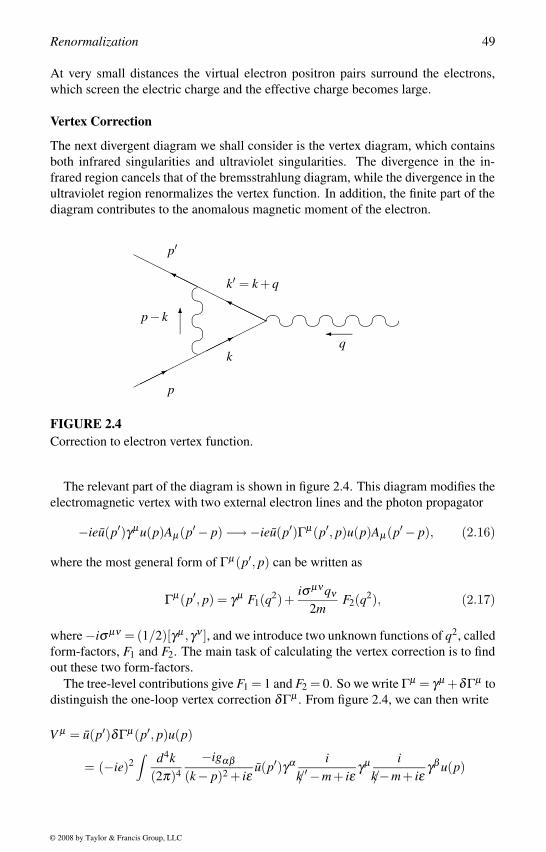
Renormalization 49
At very small distances the virtual electron positron pairs surround the electrons,
which screen the electric charge and the effective charge becomes large.
Vertex Correction
The next divergent diagram we shall consider is the vertex diagram, which contains
both infrared singularities and ultraviolet singularities. The divergence in the in-
frared region cancels that of the bremsstrahlung diagram, while the divergence in the
ultraviolet region renormalizes the vertex function. In addition, the finite part of the
diagram contributes to the anomalous magnetic moment of the electron.
p− k
q
p′
p
k′ = k +q
k
FIGURE 2.4Correction to electron vertex function.
The relevant part of the diagram is shown in figure 2.4. This diagram modifies the
electromagnetic vertex with two external electron lines and the photon propagator
−ieu(p′)γµ u(p)Aµ(p′− p) −→−ieu(p′)Γµ(p′, p)u(p)Aµ(p′− p), (2.16)
where the most general form of Γµ(p′, p) can be written as
Γµ(p′, p) = γµ F1(q2)+iσ µν qν
2mF2(q2), (2.17)
where −iσ µν = (1/2)[γµ ,γν ], and we introduce two unknown functions of q2, called
form-factors, F1 and F2. The main task of calculating the vertex correction is to find
out these two form-factors.
The tree-level contributions give F1 = 1 and F2 = 0. So we write Γµ = γµ +δΓµ to
distinguish the one-loop vertex correction δΓµ . From figure 2.4, we can then write
V µ = u(p′)δΓµ(p′, p)u(p)
= (−ie)2∫ d4k
(2π)4
−igαβ
(k− p)2 + iεu(p′)γα i
/k ′−m+ iεγµ i
/k−m+ iεγβ u(p)
© 2008 by Taylor & Francis Group, LLC
50 Particle and Astroparticle Physics
= 2ie2∫ d4k
(2π)4u(p′)[ /k γµ /k ′ +m2γµ −2m(k + k′)µ ]u(p)
((k− p)2 + iε)(k′2 −m2 + iε)(k2 −m2 + iε). (2.18)
This logarithmically divergent integral is difficult to calculate. We shall present some
crucial steps and then the final result.
The first step is to put the three factors in the denominator into one. This is con-
veniently done with the Feynman parameters, which are some auxiliary parameters
that are to be integrated out. For a factor of two terms, we can use the identity
1
ab=
∫ 1
0dx
1
[ax+b(1− x)]2=
∫ 1
0dxdyδ (x+ y−1)
1
(ax+by)2 . (2.19)
This is a simpler case of a more general identity
1
a1a2 · · ·an=
∫ 1
0dx1 · · ·dnn δ
(∑xi −1
) (n−1)![∑aixi]n
. (2.20)
This will allow us to write the denominator of V µ as
1
((k− p)2 + iε)(k′2 −m2 + iε)(k2 −m2 + iε)=
∫ 1
0dxdydzδ (x+ y+ z−1)
2
D3 ,
where
D = 2 −∆+ iε; ≡ k + yq− zp; and ∆ ≡−xyq2 +(1− z)2m2.
To simplify the numerator we use the identities
∫ d4
(2π)4µ
D3 = 0
∫ d4
(2π)4µν
D3 =∫ d4
(2π)42 gµν
4 D3 , (2.21)
which states that the integral depends only on the magnitude of . So we can write
the numerator only in terms of 2. We further use the Ward identity [18], which is an
extension of the charge conservation and reads qµ Γµ = 0. The vertex contribution
then simplifies to
V µ = 2ie2∫ d4
(2π)4
∫ 1
0dx dy dz δ (x+ y+ z−1)
2
D3 u(p′)[
γµ · (−2
2+A)+
iσ µν qν2m
·B]
u(p), (2.22)
with A = (1− x)(1− y)q2 + (1− 4z + z2)m2 and B = 2m2z(1− z). We shall then
perform the momentum integral.
To evaluate the integral, we make use of Wick’s rotation trick and work with Eu-
clidian four-momentum variable E , where
0 ≡ i0E ; and = E , (2.23)
© 2008 by Taylor & Francis Group, LLC
Renormalization 51
so 0E varies between −∞ to ∞. The integral then becomes
∫ d4
(2π)41
(2 −∆)m =i
(−1)m
∫ d4E
(2π)41
(2E +∆)m . (2.24)
One can then work in four-dimensional spherical coordinate to evaluate the integral.
However, for divergent integrals we have to adopt some regularization technique to
deal with the integral.
The integral is divergent, and hence, we introduce the Pauli–Villars regulators. We
shall replace the photon propagator with
1
(k− p)2 + iε−→ 1
(k− p)2 + iε− 1
(k− p)2 +Λ2 + iε.
Here Λ is the large mass of the fictitious heavy photons. The denominator will then
be replaced by
∆ −→ ∆Λ = −xyq2 +(1− z)2m2 + zΛ2.
This will make the momentum integral finite for any fixed value of Λ. We can then
perform the integral after making Wick’s rotation
∫ d4
(2π)4
(2
(2 −∆)3 − 2
(2 −∆Λ)3
)=
i(4π)2 log
(∆Λ∆
). (2.25)
Any Λ dependent contribution to the finite part of the integral is ignored. Finally we
arrive at
V µ =α2π
∫ 1
0dx dy dz δ (x+ y+ z−1)
u(p′)[
γµ
∆(log(zΛ2)+A
)+
iσ µν qν2m
B∆
]u(p). (2.26)
This gives the one-loop correction to the form-factors. The first form-factor F1 con-
tains both the infrared and ultraviolet divergences. The infrared divergence comes
out to be exactly the same as the infrared divergence in the bremsstrahlung pro-
cess and they cancel each other. The ultraviolet divergence appears in δF1(q2 = 0),where δF1 is the one-loop vertex correction to F1. F1(q2 = 0)+ δF1(q2 = 0) gives
the charge of the electron in units of e and, hence, should be 1. We know that the
tree-level contribution is F1(q2 = 0) = 1, so we normalize the vertex function by
δF1(q2) → δF1(q2)−δF1(q2 = 0), (2.27)
which eliminates the ultraviolet divergent contribution. Since the electric charge is
the only parameter entering in the vertex function, this infinite contribution cancels
the infinity of the bare charge. We shall come back to this point again when we
discuss renormalization of QED.
The second form-factor F2(q2) is finite, and for zero momentum it is
F2(q2 = 0) =α2π
. (2.28)
© 2008 by Taylor & Francis Group, LLC
52 Particle and Astroparticle Physics
The magnetic moment of the electron is given by
µ = g( e
2m
)S, (2.29)
where the Lande g-factor is given by
g = 2[F1(q2 = 0)+F2(q2 = 0)]. (2.30)
At the tree-level F1 = 1 and F2 = 0; hence, g = 2. At the one-loop level, the normal-
ization gives F1(q2 = 0) = 1. The correction to the g-factor thus comes only from the
correction F2(q2 = 0), which gives the anomalous magnetic moment of the electron
[19]
ae ≡ g−2
2=
α2π
= 0.0011614. (2.31)
This anomalous magnetic moment has been measured experimentally ae(expt) =0.0011597.
The first form-factor F1(q2) also contains the infrared divergence. In the limit of
q2 → 0, we have
∫ 1
0dx dy dzδ (x+ y+ z−1)
1−4z+ z2
∆(q2 = 0)=
∫ 1
0dz
−2
m2(1− z)+ · · · .
While discussing the bremsstrahlung process, we have seen that the infrared diver-
gence appears because photons are massless. If we assign a small mass µ to the
photon, this problem may be tackled, since it adds a term zµ2 to ∆. After a tedious
calculation, one can write the contribution from F1 of the vertex diagram to the scat-
tering cross-section to be
dσdΩ
≈(
dσdΩ
)0
[1− α
πlog
(−q2
µ2
). log
(−q2
m2
)]. (2.32)
Comparing equation (2.32) with the scattering cross-section for the bremsstrahlung
process given in equation (2.3), it is clear that the infrared divergent parts of the two
diagrams cancel out when the cross-sections for the two processes are added together.
Although the processes appear to be different, since it is not possible to distinguish
the virtual and real soft photons experimentally due to quantum uncertainty principle,
we have to add these processes, and then the final result becomes free of any infrared
divergences.
Self-Energy Correction
We shall now discuss the self-energy diagram. This diagram in figure 2.5 gives
correction to the free-fermion propagator i/(/p−m0 + iε). Since the bare parameter
in the fermion propagator is the fermion mass, it renormalizes the fermion mass.
We shall, therefore, denote the bare electron mass as m0 to distinguish it from the
renormalized physical mass m.
© 2008 by Taylor & Francis Group, LLC
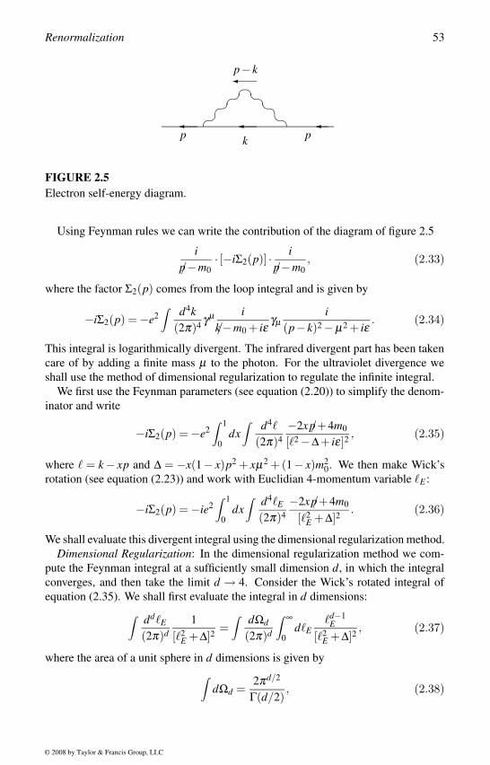
Renormalization 53
p pk
p− k
FIGURE 2.5Electron self-energy diagram.
Using Feynman rules we can write the contribution of the diagram of figure 2.5
i/p−m0
· [−iΣ2(p)] · i/p−m0
, (2.33)
where the factor Σ2(p) comes from the loop integral and is given by
−iΣ2(p) = −e2∫ d4k
(2π)4 γµ i/k−m0 + iε
γµi
(p− k)2 −µ2 + iε. (2.34)
This integral is logarithmically divergent. The infrared divergent part has been taken
care of by adding a finite mass µ to the photon. For the ultraviolet divergence we
shall use the method of dimensional regularization to regulate the infinite integral.
We first use the Feynman parameters (see equation (2.20)) to simplify the denom-
inator and write
−iΣ2(p) = −e2∫ 1
0dx
∫ d4
(2π)4−2x /p+4m0
[2 −∆+ iε]2, (2.35)
where = k− xp and ∆ = −x(1− x)p2 + xµ2 +(1− x)m20. We then make Wick’s
rotation (see equation (2.23)) and work with Euclidian 4-momentum variable E :
−iΣ2(p) = −ie2∫ 1
0dx
∫ d4E
(2π)4−2x /p+4m0
[2E +∆]2
. (2.36)
We shall evaluate this divergent integral using the dimensional regularization method.
Dimensional Regularization: In the dimensional regularization method we com-
pute the Feynman integral at a sufficiently small dimension d, in which the integral
converges, and then take the limit d → 4. Consider the Wick’s rotated integral of
equation (2.35). We shall first evaluate the integral in d dimensions:
∫ ddE
(2π)d1
[2E +∆]2
=∫ dΩd
(2π)d
∫ ∞
0dE
d−1E
[2E +∆]2
, (2.37)
where the area of a unit sphere in d dimensions is given by
∫dΩd =
2πd/2
Γ(d/2), (2.38)
© 2008 by Taylor & Francis Group, LLC
54 Particle and Astroparticle Physics
where Γ(1/2) =√
π and Γ(n+1) = nΓ(n).The second factor can be integrated out exactly in terms of beta function by sub-
stituting z = ∆/(2 +∆) and is given by
∫ ∞
0dE
d−1E
[2E +∆]2
=1
2∆(d−4)/2Γ
(2− d
2
)Γ(
d2
). (2.39)
The behavior near d = 4 can be expressed in terms of a variable ε = 4−d in the limit
ε → 0. For the Γ-function one can approximate it as
limd→4
Γ(
2− d2
)= lim
d→4
1(2− d
2
)Γ(
3− d2
)= lim
ε→0
2
ε.
However, a more appropriate procedure will be to consider a power series expansion
of the Γ-function and then take the limit. This form of the approximation gives
limε→0
Γ(ε/2) =2
ε− γ +O(ε), (2.40)
where γ ≈ 0.5772 is the Euler–Mascheroni constant. Then the leading terms come
from
limε→0
Γ(ε2)∆−ε/2 = lim
ε→0Γ(
ε2)e−(ε/2) log∆ =
2
ε− log∆+ · · · .
Only the first term is relevant for understanding the divergent nature of the integral.
Finally we can write the integral as
limd→4
∫ ddE
(2π)d1
[2E +∆]2
=1
(4π)2
[2
ε− log∆− γ + log(4π)+O(ε)
]. (2.41)
If we compare this result with the Pauli–Villars method, the pole 1/ε in dimensional
regularization corresponds to a logarithmic divergence logΛ2.
For using dimensional regularization one can use some more general formulae:
∫ ddE
(2π)d1
[2E +∆]n
=1
(4π)d/2 ∆(d−2n)/2 Γ(n− d
2
)Γ(n)
(2.42)
∫ ddE
(2π)d2
E
[2E +∆]n
=1
(4π)d/2
d2
∆(d+2−2n)/2 Γ(n− d
2 −1)
Γ(n). (2.43)
There are d gamma matrices γ µ satisfying
γµ ,γν = 2gµν , trI = 4 , gµν gµν = d.
We replace µν → 2gµν/d for any numerator of a symmetric integrand. The con-
traction identities in d = 4− ε will become
γµ γν γµ = −(2− ε)γν
γµ γν γρ γµ = 4gνρ − εγν γρ
γµ γν γρ γσ γµ = −2γσ γρ γν + εγν γρ γσ .
© 2008 by Taylor & Francis Group, LLC
Renormalization 55
We list these results for completeness although they will not be needed for the self-
energy diagram.
The required result for the self-energy contribution can, therefore, be expressed as
Σ2(p) =α4π
∫ 1
0dx(2m0 − x /p)
[2
ε− log∆− γ + log(4π)+O(ε)
]. (2.44)
Unlike the vertex or the vacuum polarization contributions, we cannot renormalize
any bare coupling constant with this one-loop contribution of the self-energy dia-
gram. We have to consider all other related diagrams to see how this infinite contri-
bution can be absorbed by any bare coupling constant. In this case, the mass of the
electron is renormalized.
We first define a one-particle irreducible (1PI) diagram, which is a diagram with
more than one part, each connected by only a single fermion line. In other words,
by removing any single fermion line, if the diagram cannot be split in two parts, we
call this a 1PI diagram. Let the contribution of sum over all 1PI diagrams be Σ. A
self-energy diagram is a 1PI diagram to leading order, and hence, Σ = Σ2 to order α .
Consider the Fourier transform of a two-point function, it can be written as a series
+ 1PI +
1PI 1PI + · · · .
(2.45)
We shall now compute the series to order α . The total contribution of the series will
be given by
i/p−m
=i
/p−m0+
i/p−m0
· [−iΣ2(p)] · i/p−m0
+i
/p−m0· [−iΣ2(p)] · i
/p−m0· [−iΣ2(p)] · i
/p−m0+ · · ·
=i
/p−m0 −Σ2(/p), (2.46)
where m is the renormalized mass after taking care of all the infinities coming from
the series 2.45. Thus, although the infinity in the self-energy diagram cannot be
absorbed in any bare parameter, the sum of the series 2.45 relates the infinite con-
tribution of the self-energy diagram with the bare mass of the electron. The shift in
mass is then given by
δm = m−m0 = Σ2(/p = m) ≈ Σ2(/p = m0), (2.47)
which can be obtained from equation (2.44) as
δm = limε→0
αm0
4π
∫ 1
0dx(2− x)
[2
ε− log(
∆4π
)− γ +O(ε)]
=3α4πε
m0 . (2.48)
© 2008 by Taylor & Francis Group, LLC
56 Particle and Astroparticle Physics
This is the correction to the bare mass coming from the self-energy diagrams to order
α . In general the 1PI blobs in the series 2.45 should include all the 1PI diagrams to
all orders. In that case, we can replace Σ2(p) by Σ(p), which is the sum of all the
1PI diagrams with two external fermions. In that case the mass renormalization will
include contributions from diagrams to all orders. Comparing with the results from
Pauli–Villars regularization, the divergence is found to be logarithmic and not linear.
This is because the diagram is proportional to the mass of the electron. Since the
diagram vanishes if electrons are massless, the symmetry ensures that one of the
momentum in the numerator does not contribute to the divergence.
2.3 Renormalization of QEDWe demonstrated how to deal with the infinities in quantum field theory and how
some of the infinities can be cancelled with the infinities of the bare parameters of
any theory, which cannot be measured. The next task will be to construct a renormal-
izable theory, in which all the divergences have been taken care of properly through
a prescribed renormalization program. The steps one follows for such construction
are
• Find out all the divergent diagrams order by order in perturbation theory. Su-
perficial power counting method may be adopted for the purpose.
• Use some regularization technique to evaluate the infinite integrals in terms of
some large parameters Λ. After completion of the renormalization, we take
the infinite limit of the parameter Λ and verify that the theory is consistent.
• Take care of the infinities by redefining the bare parameters in the theory [2, 3],
as we did with the mass and charge of electron after evaluating the vertex and
self-energy diagrams.
• Another equivalent, more appropriate, approach introduces counterterms (de-
veloped by Bogoliubov, Parasiuk, Hepp and Zimmerman [20]) also known as
the BPHZ approach. In this approach we add counterterms to the Lagrangian,
whose coefficients are chosen so they cancel the divergences to that order.
These counterterms are proportional to the original action. Any renormaliz-
able theory has finite numbers of counterterms. In this approach one can pro-
ceed with renormalized perturbation calculations with the new set of Feynman
rules.
• At the end of these exercises one can verify by method of induction that the
theory is renormalizable to all higher orders. This can be done using Wein-
berg’s theorem [21] that any graph converges if the degree of divergence of
the graph and all its subgraphs is negative.
© 2008 by Taylor & Francis Group, LLC
Renormalization 57
Ultraviolet Divergences and Power Counting
The main problem in field theory is the ultraviolet divergence, which needs to be
regularized and then absorbed in some bare coupling through renormarlization. So,
the first task is to find the nature of divergences in any graph, which is done by
power counting or by counting the superficial degree of divergence D. Since every
fermion line enters with k−1, the boson line contributes k−2 and a loop integral d4k;
by counting the overall power of k, we can tell if any diagram diverges for large k.
Let us explain this for QED.
Although we shall be discussing QED with only electrons and photons, we can
as well generalize it to any other charged fermions interacting with photons. If we
denote the numbers of external fermions [photons] by E f [Eγ ], numbers of fermion
photon] propagators by Pf [Pγ ], number of vertices by V , and number of loops by L,
then the superficial degree of divergence is given by
D = 4L−Pf −2Pγ . (2.49)
This simply means that in a given loop there are L loop integrals, each giving a factor
d4k and, hence, 4L numbers of k in the numerator; Pf internal fermion propagators
i/(/k−m+ iε), each contributing one k in the denominator; and Pγ numbers of photon
propagators −igµν/(k2 + iε), each contributing two powers of k in the denominator.
I f D is 0 or positive, the graph diverges.
In general, the graph with positive D diverges as ΛD, where Λ is some large parame-
ter, although there are exceptions. For D = 0 the graph diverges logarithmically. For
the vacuum polorization diagram, D = 2, and hence, it is quadratically divergent;
for vertex function diagram, D = 0 and it is logarithmically divergent; while for the
self-energy diagram, D = 1 and it is linearly divergent. However, actual calculations
show that all three graphs are logarithmically divergent. For the vacuum polarization
graph, the Ward–Takahashi identity reduces the degree of divergence. For the self-
energy graph the Lorentz invariance and chiral symmetry ensures that the diagram
is proportional to electron mass, so there is one extra momentum in the denominator
making it logarithmically divergent. On the other hand, if any diagram has some
subdiagrams, then the actual divergence could be worse than predicted by D, and for
a tree-level diagram with D = 0, there are no divergences.
Any vertex can have two fermions and a photon, so the number of vertices can be
given in terms of numbers of internal propagators and external lines:
V = 2Pγ +Eγ =1
2(2Pf +E f ),
since only one end of an external line connects to a vertex. Any loop will have an
independent momentum, which is the same as the number of internal propagators
minus the delta function appearing at the vertices modulo the overall momentum
conservation. Thus, we can write
L = Pf +Pγ −V +1.
© 2008 by Taylor & Francis Group, LLC
58 Particle and Astroparticle Physics
With these relations we can express the superficial degree of divergence as
D = 4− 3
2E f −Eγ . (2.50)
Thus, for QED we can characterize all the divergent diagrams from the number of
external lines:
No external lines (D = 4): These diagrams do not contribute to any scattering pro-
cesses.
One external photon (D = 3): Vanishes due to symmetries.
Two external photons (D = 2): Vacuum polarization diagrams that were discussed
earlier. Ward–Takahashi identity softens the divergence and makes it logarith-
mically divergent.
Three external photons (D = 1): These are called anomaly diagrams, which can
come with three fermion lines forming a triangle with the photons attached
to the vertices. Such diagrams are divergent for chiral theories only. Since
QED has no axial couplings, this diagram vanishes. For QED there will be
loops with fermion momenta flowing in one direction, which cancels a similar
diagram with momenta flowing in the opposite direction.
Four external photons (D = 0): This diagram also vanishes by gauge symmetry.
Two external fermions (D = 1): This is the self-energy diagram. The diagram is
proportional to fermion masses, and is logarithmically divergent.
Two external fermions and an external photon (D = 0): This is the logarithmically
divergent vertex diagram.
After characterizing the divergent diagrams the next task is to take care of them,
which is done through renormalization.
Renormalization
After identifying the divergent graphs, first we have to regularize the integrals and
express the divergent part in terms of some large scale. We demonstrated this with
the Pauli–Villars method and the dimensional regularization method for the vacuum
polarization, the vertex correction and the self-energy diagrams. One has to ensure
that the different regularization schemes give the same result.
Once the regularization is done the large scale dependent divergent contributions
have to be absorbed into the Lagrangian by rescaling the fields. Then we can write
the Lagrangian in two parts, the renormalized Lagrangian and the counterterms, with
all the divergences included in the counterterms. The next step will be to write the
physical renormalized masses and coupling constant and write the Feynman rules
in terms of new renormalized quantities and the new parameters. Any amplitude at
this order will then be finite. At higher orders there will be additional divergences,
© 2008 by Taylor & Francis Group, LLC
Renormalization 59
which can again be removed by adjusting the counterterms because renormalizability
ensures that there are only a finite number of counterterms.
We start with the QED Lagrangian with bare parameters
L = −1
4(Fµν)2 + ψ(i /∂ −m0)ψ − e0 ψγµ ψAµ . (2.51)
Let us study the contributions of the divergent diagrams. Consider the self-energy
diagram that we calculated and the final result given by equation (2.44). This is the
leading order contribution to any 1PI diagrams with two external fermions. The sum
of contributions from all such 1PI diagrams to leading order is given in equation
(2.46), which can be generalized to higher orders, and the complete propagator can
be written as
iS′F = iSF(/p)+ iSF(/p)[−iΣ(/p)]iSF(/p)+ · · · = i/p−m0 −Σ(/p)+ iε
. (2.52)
Σ(/p) is the sum over 1PI graphs with two external electrons, which can be Taylor
expanded around the renormalized mass m as
Σ(/p) = Σ(m)+(/p−m)Σ′ + Σ(/p), (2.53)
where the renormalized mass m is defined in the same way as equations (2.47) and
(2.48):
m = m0 +Σ(m).
Then the renormalized propagator is given by
iS′F =iZ2
/p−m−Z2Σ(/p)+ iε=
iZ2
/p−m+ iε+ · · · , (2.54)
where Z2 = 1/[1−Σ′(m)] contains the divergence in the propagator of a electron.
The vacuum polarization graph contributes to the propagator of the photon, which
is expressed as in equation (2.13):
−igµν
q2 −→−i(Z3)gµν
q2 .
We can then renormalize the electron and photon wave functions as
ψ →√Z2 ψr and Aµ →
√Z3 Aµ
r , (2.55)
so the S-matrix does not contain any of these infinities. The bare Lagrangian of
equation (2.51) will now be modified to
L = −1
4Z3(Fµν
r )2 +Z2ψr(i /∂ −m0)ψr − e0Z2Z1/23 ψrγµ ψrArµ . (2.56)
Let us now consider the vertex corrections. We normalized the form factor F1(q2) in
equation (2.27) to eliminate the infinite contribution. This is equivalent to redefining
the vertex function, defined in equation (2.17), as
Γµ(p, p′) = γµ F1(q2)+iσ µν qν
2mF2(q2) −→ 1
Z1Γµ(p, p′) . (2.57)
© 2008 by Taylor & Francis Group, LLC
60 Particle and Astroparticle Physics
This will then give the renormalized electric charge
e = Z2Z1/23 Z−1
1 e0. (2.58)
With these renormalized parameters, we can now write the Lagrangian in two parts:
L = Lr +Lct ,
where the renormalized Lagrangian Lr and the Lagrangian with the counterterms
Lct are given by
Lr = −1
4(Fµν
r )2 + ψr(i /∂ −m)ψr − e ψrγµ ψrArµ
Lct = −1
4δ3(Fµν
r )2 + ψr(iδ2 /∂ −δm)ψr − eδ1 ψrγµ ψrArµ , (2.59)
where δ3 = Z3 − 1, δ2 = Z2 − 1, δm = Z2m0 −m, and δ1 = Z1 − 1. If we write
the Lagrangian to order α , then the renormalized Lagrangian will not contain any
infinities to this order. The new Feynman rules for this Lagrangian will be given in
terms of the renormalized mass and electric charge of the electron. If we calculate
correlation functions with the renormalized Feynman rules, then to one-loop order
there will not be any divergences. However, at higher orders there will be new cor-
rections which can be taken care of by adjusting the parameters of the counterterms
again.
The most important feature of this procedure is that the same counterterms can
cancel divergences to all orders and no new counterterms have to be introduced. In
any nonrenormalizable theories, we have to introduce new counterterms at all orders
of perturbation, which makes the theory unpredictable. Moreover, the original sym-
metry of the theory will not be preserved by the new counterterms. For any renor-
malizable theory all counterterms respect the symmetry of the original Lagrangian,
and hence, the symmetry is preserved to all orders of perturbation theory.
2.4 Renormalization in φ 4 TheoryWe shall now discuss the renormalization in φ 4 theory. The simplicity of the model
clarifies certain points, which are not transparent in QED. The bare Lagrangian is
given by
L =1
2(∂µ φ)2 − 1
2m2
0φ 2 − λ0
4!φ 4. (2.60)
There are two bare parameters in the model, m0 and λ0.
We shall first find the divergent diagrams in this case. If there are E number of
external lines, P number of propagators, V vertices, and L loops in a diagram, then
we get the relations
L = P−V +1 and 4V = E +2P .
© 2008 by Taylor & Francis Group, LLC
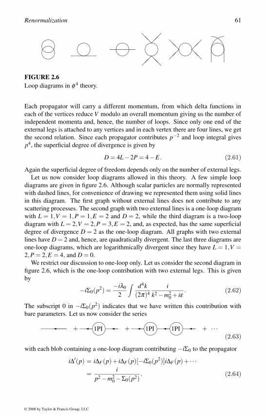
Renormalization 61
FIGURE 2.6Loop diagrams in φ 4 theory.
Each propagator will carry a different momentum, from which delta functions in
each of the vertices reduce V modulo an overall momentum giving us the number of
independent momenta and, hence, the number of loops. Since only one end of the
external legs is attached to any vertices and in each vertex there are four lines, we get
the second relation. Since each propagator contributes p−2 and loop integral gives
p4, the superficial degree of divergence is given by
D = 4L−2P = 4−E. (2.61)
Again the superficial degree of freedom depends only on the number of external legs.
Let us now consider loop diagrams allowed in this theory. A few simple loop
diagrams are given in figure 2.6. Although scalar particles are normally represented
with dashed lines, for convenience of drawing we represented them using solid lines
in this diagram. The first graph without external lines does not contribute to any
scattering processes. The second graph with two external lines is a one-loop diagram
with L = 1,V = 1,P = 1,E = 2 and D = 2, while the third diagram is a two-loop
diagram with L = 2,V = 2,P = 3,E = 2, and, as expected, has the same superficial
degree of divergence D = 2 as the one-loop diagram. All graphs with two external
lines have D = 2 and, hence, are quadratically divergent. The last three diagrams are
one-loop diagrams, which are logarithmically divergent since they have L = 1,V =2,P = 2,E = 4, and D = 0.
We restrict our discussion to one-loop only. Let us consider the second diagram in
figure 2.6, which is the one-loop contribution with two external legs. This is given
by
−iΣ0(p2) =−iλ0
2
∫ d4k(2π)4
ik2 −m2
0 + iε. (2.62)
The subscript 0 in −iΣ0(p2) indicates that we have written this contribution with
bare parameters. Let us now consider the series
+ 1PI +
1PI 1PI + · · ·
(2.63)
with each blob containing a one-loop diagram contributing −iΣ0 to the propagator
i∆′(p) = i∆F(p)+ i∆F(p)[−iΣ0(p2)]i∆F(p)+ · · ·=
ip2 −m2
0 −Σ0(p2). (2.64)
© 2008 by Taylor & Francis Group, LLC
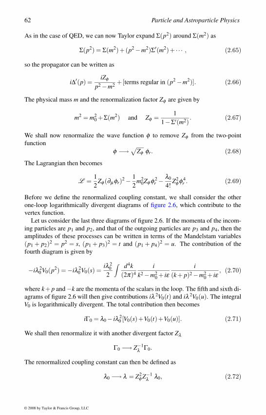
62 Particle and Astroparticle Physics
As in the case of QED, we can now Taylor expand Σ(p2) around Σ(m2) as
Σ(p2) = Σ(m2)+(p2 −m2)Σ′(m2)+ · · · , (2.65)
so the propagator can be written as
i∆′(p) =iZφ
p2 −m2 +[terms regular in (p2 −m2)]. (2.66)
The physical mass m and the renormalization factor Zφ are given by
m2 = m20 +Σ(m2) and Zφ =
1
1−Σ′(m2). (2.67)
We shall now renormalize the wave function φ to remove Zφ from the two-point
function
φ −→√Zφ φr. (2.68)
The Lagrangian then becomes
L =1
2Zφ (∂µ φr)2 − 1
2m2
0Zφ φ 2r −
λ0
4!Z2
φ φ 4r . (2.69)
Before we define the renormalized coupling constant, we shall consider the other
one-loop logarithmically divergent diagrams of figure 2.6, which contribute to the
vertex function.
Let us consider the last three diagrams of figure 2.6. If the momenta of the incom-
ing particles are p1 and p2, and that of the outgoing particles are p3 and p4, then the
amplitudes of these processes can be written in terms of the Mandelstam variables
(p1 + p2)2 = p2 = s, (p1 + p3)2 = t and (p1 + p4)2 = u. The contribution of the
fourth diagram is given by
−iλ 20 V0(p2) = −iλ 2
0 V0(s) =iλ 2
02
∫ d4k(2π)4
ik2 −m2
0 + iεi
(k + p)2 −m20 + iε
, (2.70)
where k+ p and −k are the momenta of the scalars in the loop. The fifth and sixth di-
agrams of figure 2.6 will then give contributions iλ 2V0(t) and iλ 2V0(u). The integral
V0 is logarithmically divergent. The total contribution then becomes
iΓ0 = λ0 − iλ 20 [V0(s)+V0(t)+V0(u)]. (2.71)
We shall then renormalize it with another divergent factor Zλ
Γ0 −→ Z−1λ Γ0.
The renormalized coupling constant can then be defined as
λ0 −→ λ = Z2φ Z−1
λ λ0, (2.72)
© 2008 by Taylor & Francis Group, LLC
Renormalization 63
so this takes care of the infinities in the vertex function as well as from the Lagrangian
after wave function renormalization.
We shall now eliminate the bare mass and coupling constant and write the La-
grangian with the counterterms
L = Lr +Lct
Lr =1
2(∂µ φr)2 − 1
2m2φ 2
r −λ4!
φ 4r
Lct =1
2δZ(∂µ φr)2 − 1
2δmφ 2
r −δλλ4!
φ 4r , (2.73)
where δZ = Zφ − 1, δm = m20Zφ −m2, and δλ = Zλ − 1. Thus, as per the BPHZ
formalism, we constructed the counterterms to one-loop order. We shall now evaluate
the one-loop diagrams with the renormalized parameters and new Feynman rules and
confirm that the theory has no divergences to first order.
Let us first consider the second diagram of figure 2.6. The physical mass m is now
identified as the pole in the propagator, and the amplitude for the process will be
−iΣ(p2) =−iλ
2
∫ d4k(2π)4
ik2 −m2 + iε
+ i(p2δZ −δm). (2.74)
The last term comes from the counterterm that contributes to the amplitude. To
evaluate this integral, we go to Euclidean system and then use dimensional reduction
method and get
−iΣ(p2) = −λ2
∫ d4kE
(2π)4i
k2E +m2 + i(p2δZ −δm)
= − limd→4
iλ(4π)d/2
∫dkE
kd−1E
k2E +m2 + i(p2δZ −δm)
= − iλm2
2(4π)2 limd→4
Γ(
1− d2
)+ i(p2δZ −δm). (2.75)
The divergence of the integral can be seen after taking the approximation
limd→4
Γ(
1− d2
)= lim
d→4
Γ(3− d
2
)(2− d
2
)(1− d
2
) = − limε→0
2
ε,
where ε = 4−d. Since the integral does not depend on p2, we set
δZ = 0 and δm = − λm2
2(4π)2 limd→4
Γ(
1− d2
), (2.76)
which makes the the one-loop contribution vanish.
The one-loop integrals with four external lines should also vanish. If we decide to
set λ to be the magnitude of scattering at zero momentum, then the vertex should be
© 2008 by Taylor & Francis Group, LLC
64 Particle and Astroparticle Physics
−iλ at s = 4m2, t = u = 0. This will then dictate us to choose, following equation
(2.71),
δλ = iλ [V (4m2)+2V (0)].
We shall now ensure that
iΓ = λ − iλ 2[V (s)+V (t)+V (u)]+λδλ (2.77)
remains finite. We shall use dimensional regularization for evaluating the divergent
integral V .
To compute V , we shall use Feynman parameters x, shift the variables to =k+xp, Wick rotate to Euclidian space, and then perform dimensional regularization:
V (p2) =1
2
∫ d4k(2π)4
1
k2 −m2 + iε1
(k + p)2 −m2 + iε
=i2
∫ 1
0dx lim
d→4
∫ ddE
(2π)d1
[2E − x(1− x)p2 +m2]2
=i2
limd→4
Γ(2− d
2
)(4π)d/2
∫ 1
0dx
1
[m2 − x(1− x)p2]2−d/2 . (2.78)
Thus, the counterterm becomes
δλ = −λ2
limd→4
Γ(2− d
2
)(4π)d/2
1
m4−d
∫ 1
0dx(
2+1
[1−4x(1− x)]2−d/2
). (2.79)
If we now substitute these two expressions in equation 2.77, the divergent contribu-
tions that appear in the limit d → 4 cancel out and the finite part is given by
iΓ = λ
1+λ
32π2
∫ 1
0dx log
(f (s) · f (t) · f (u)[1−4x(1− x)]
), (2.80)
where f (q) = [m2 − x(1− x)q]/m2, with q = s, t,u.
We have demonstrated the general principle of dealing with the infinities in field
theory with explicit examples of one-loop diagrams for QED and φ 4 theory. At
higher loops the complications will be much more. But at least we understand the
theory now, and the predictions are verified with an extremely high degree of preci-
sion.
© 2008 by Taylor & Francis Group, LLC
3Group Theory
Symmetry plays the most important role in our understanding of nature. Many di-
verse phenomena may be explained by a single theory if there is some symmetry
behind these phenomena. If two particles behave the same way in an environment,
one can postulate that some symmetry is relating these similar behaviors. Group the-
ory is the mathematical tool to study a set of objects, which have some underlying
symmetry.
In particle physics it is now impossible to understand the modern developments
without some basic understanding of group theory. The strong, the weak and the
electromagnetic interactions are explained by gauge theories based on different sym-
metry groups and extensions of the standard model of electroweak interaction are
often based on some extended symmetry groups. Although discrete groups are also
used, the continuous groups are more frequently used in particle physics. I shall,
therefore, restrict our discussions to continuous groups keeping in mind the applica-
tions we encounter in studying models of particle physics. In this short chapter, only
a working knowledge on some aspects of group theory that are required for the rest
of the book will be provided.
3.1 Matrix Groups
In this section we present the basics of group theory and different types of matrix
groups. We shall concentrate on continuous groups and our emphasis will be on
aspects of group theory that have applications in particle physics.
Definition of a Group
A group (G) is a collection of elements A,B,C, ..., on which a product operation
(•) is defined that combines different elements satisfying the four group postulates:
1. Closure: The product of two elements of the group corresponds to a unique
element of the group:
A•B ⊂ G. (3.1)
65
© 2008 by Taylor & Francis Group, LLC
66 Particle and Astroparticle Physics
2. Identity: One of the elements (I) of the group, known as the identity element,
satisfies
A• I = I •A = A (3.2)
for any A belonging to G.
3. Inverses: For any element A in G, there exists an inverse element A−1 in G,
such that
A•A−1 = I. (3.3)
4. Associativity: The product of three or more elements of G should not depend
on the order of product
A• (B•C) = (A•B)•C = A•B•C. (3.4)
Discrete and Continuous Groups
When there are finite numbers of elements in the group, the group is called a finitegroup. If there are denumerable infinite numbers of elements, an infinite discretegroup is formed. When the elements form a continuum, the group is said to be a
continuous group.
1. The elements ±1,±i form a finite group Z4 when the product operation is
multiplication.
2. The additive group of the integers is formed by the set of integers when the
product operation is addition. The zero corresponds to the identity element of
the group.
3. The infinite set of matrices
(cosθ sinθ−sinθ cosθ
)produced by the continuous
variations of θ from 0 to 2π forms a continuous group.
As an example, a theory invariant under the Z4 symmetry means that the La-
grangian is invariant under the operation of this group. If any complex scalar field φtransforms under the operation of this symmetry group as φ →−iφ , then the allowed
interaction terms in the Lagrangian will be given by
L = m2φ †φ +λ (φ †φ)2 +λ ′(φ 4 +φ †4). (3.5)
The quadratic (φ 2) and cubic (φ 3) couplings are not allowed by the Z4 symmetry.
If there are two fields φ1 and φ2 transforming under Z4 as φ1 → iφ1 and φ2 →−iφ2,
then the quadratic terms allowed by the symmetry will be φ1φ2 +φ †1 φ1 +φ †
2 φ2. There
will also be quartic interactions, but all trilinear couplings will be forbidden.
© 2008 by Taylor & Francis Group, LLC
Group Theory 67
Matrix Groups
Any set of n×n square matrices can form a regular matrix group; if the matrices are
nonsingular, the matrix multiplication satisfies associative law and the set contains
all the elements required for closure including the identity matrix
I = diag[1,1,1, ...] =
1 0 0 · · ·0 1 0 · · ·0 0 1 · · ·...
......
. . .
. (3.6)
Regular matrix groups could be finite or infinite, discrete or continuous. A matrix
A(n) of degree n can have real (R) or complex (C) elements, and it can act on an
n-dimensional real vector space Rn spanned by the vector x ≡ (x1,x2, ...,xn) or on an
n-dimensional complex vector space Cn spanned by the vector z≡ (z1,z2, ...,zn). The
action of the matrix A(n) on the real or complex vectors produces the transformations
x → x′ or z → z′, respectively.
Let us consider a continuous matrix group of degree 2. The elements of the group
A =(
a11 a12a21 a22
)will be restricted by the nonsingular condition det A = 0, and writing the matrix ele-
ments as ai j = δi j +αi j, the identity matrix would correspond to αi j = 0. Continuous
variations of the parameter αi j, which are otherwise unbounded and limited only by
the nonsingular condition, will then generate the continuous matrix group with el-
ements parameterized by αi j. For different types of continuous matrix groups, the
number of parameters can be different. In general, the elements of a continuous
matrix group can be represented by matrices of degree n:
An ≡ An(α1, ...,αr) , (3.7)
which depends on r parameters αi, i = 1, ...,r. The identity element would corre-
spond to An(0, ...,0) = I.
The matrix groups can be of different types, depending on whether the group
elements areSymmetric A = AT
Skew–Symmetric A+AT = 0
Orthogonal AT = A−1
Unitary A† = A−1
Real A = A∗Imaginary A = −A∗Hermitian A = A†
Skew–Hermitian A = −A†.
(3.8)
The matrix elements could be real or imaginary. Some of the important continuous
matrix groups are:
© 2008 by Taylor & Francis Group, LLC
68 Particle and Astroparticle Physics
General Linear Group GL(n,C): The elements of the complex general linear groupare n×n invertible matrices with complex elements. Any matrix is character-
ized by n2 complex elements and, hence, 2n2 real parameters. If the matrix
elements are real, we get the subgroup GL(n,R) of GL(n,C).
Special Linear Group SL(n,C): Restricting the determinants of the group elements
of GL(n,C) to +1, we get the complex special linear group SL(n,C). When
the elements are real, the group becomes SL(n,R) so SL(n,R) ⊂ SL(n,C) ⊂GL(n,C) and SL(n,R) ⊂ GL(n,R).
Unitary Groups U(n): The Hermitian form z1z∗1 +z2z∗2 + · · ·+znz∗n remains invariant
under the action of the elements of an n2-parameter unitary group U(n) formed
by the unitary matrices A of degree n. The elements ai j of the unitary matrices
A are bounded |ai j|2 ≤ 1 because of the unitarity condition A†A = I or aika∗k j =δi j.
The unitary matrices that leave the Hermitian f orm − z1z∗1 − · · · − zpz∗p +zp+1z∗p+1 + · · ·+ zp+qz∗p+q invariant are denoted as U(p,q), so that U(n,0) =U(0,n) = U(n).
Special Unitary Groups SU(n): When the determinant of a unitary group is re-
stricted to +1, the resulting (n2 −1)-parameter group is called special unitarygroup SU(n). Similarly, SU(p,q) groups are obtained by restricting the ele-
ments of U(p,q) groups to have determinant +1.
Orthogonal Groups O(n): The group O(n,C) is formed by the complex orthogonalmatrices A of degree n, which has n(n−1) complex parameters. The orthog-
onality condition AT A = I implies |A| = ±1, and hence, there are two dis-
connected pieces of the group. Special complex orthogonal groups SO(n,C)are formed by the orthogonal matrices of determinant +1, which leaves the
quadratic form z21 + · · ·+ z2
n invariant and SO(n,C) ⊂ O(n,C).
Special Orthogonal Groups SO(n): The n(n− 1)-parameter group formed by real
orthogonal matrices of determinant +1 is called the special orthogonal groupSO(n,R) or simply SO(n), which leaves the real quadratic form x2
1 + · · ·+ x2n
invariant and SO(n) ⊂ O(n,R). The SO(p,q) group ensures invariance of the
quadratic form −x21 −· · ·− x2
p + x2p+1 + · · ·+ x2
p+q.
Symplectic Groups Sp(2n): Given two vectors x = (x1, ...,xn,x′1, ...,x′n) and y =
(y1, ...,yn,y′1, ...,y′n) (in general, xi and yi are complex numbers) the nonde-
generate skew–symmetric bilinear form ∑n1=1(xiy′i − x′iyi) is left invariant by
the symplectic group Sp(2n,C) formed by the 2n(2n + 1)-parameter complex
matrices. The n(2n+1)-parameter Sp(2n,R) groups are formed with real ma-
trices. The unitary subset of the group Sp(2n,C) is called the unitary symplec-tic group Sp(2n) = U(2n)∩Sp(2n,C), which is also the n(2n+1)-parameter
group.
© 2008 by Taylor & Francis Group, LLC
Group Theory 69
To study group properties with matrices, we need the exponential function of a
matrix, which is defined as
eA = I +A+A2
2!+
A3
3!+ · · · =
∞
∑p=0
Ap
p!, (3.9)
where A0 = I. This series is convergent when the elements (ai j) of the matrix A are
bounded from above |ai j| ≤ µ . For the exponential matrices, it can be shown that
• eA+B = eAeB when A and B commutes,
• BeAB−1 = eBAB−1,
• eA∗= (eA)∗,
• eAT= (eA)T ,
• eA†= (eA)†,
• e−A = (eA)−1, and
• deteA = etr A.
• If λ1, ...,λn are characteristic roots of A, then the characteristic roots of eA are
eλ1 , ...,eλn .
• eA is orthogonal when A is skew–symmetric, and
• eA is unitary when A is skew–Hermitian.
3.2 Lie Groups and Lie AlgebrasLie groups and Lie algebras are widely used in particle physics. In this section we
give a brief introduction to the subject and proceed to discuss unitary groups that will
be used afterwards.
Lie Groups
In equation (3.7) the element A of a continuous group G was expressed in terms of rcontinuous parameters
A(α) ≡ An(α1, ...,αr) , (3.10)
which includes the identity element A(0). The closure of the group requires
A(γ) = A(α)A(β ) ≡ A( f (α,β )) =⇒ γ = f (α,β ) ,
© 2008 by Taylor & Francis Group, LLC
70 Particle and Astroparticle Physics
where γ should be a continuously differentiable function of α and β , and satisfy γ =f (γ,0) = f (0,γ). The inverse element A(α)−1 = A(α ′) exists if α ′ is a continuously
differentiable function of α . The continuous group under consideration is referred to
as a Lie group, if the associative condition
A(α)(B(β )C(γ)) ≡ (A(α)B(β ))C(γ) =⇒ f [α, f (β ,γ)] = f [ f (α,β ),γ] (3.11)
is also satisfied.
Let us now consider an infinitesimal transformation in the neighbourhood of the
identity element. We can write any element of the group A(α) lying near the identity
element by Taylor expansion
A(α) = A(0)+αi
(∂A∂αi
)αi=0
+1
2αiα j
(∂A∂αi
)αi=0
(∂A∂α j
)α j=0
+O(α3)
= A(0)+αiXi +1
2αiα jXiX j +O(α3), (3.12)
where sum over repeated indices are implied and Xi = (∂A/∂αi)αi=0 are the infinites-imal group generators of the group G. For a group parameterized by r continuous
parameters αi, i = 1, ...,r, there are r generators Xi. The group is then called an
r-parameter Lie group. The inverse element can be expanded as
A(α)−1 = A(0)−αiXi +1
2αiα jXiX j +O(α3) , (3.13)
so A(α)−1A(α) = A(0)+O(α2).We now define the commutator A(β ,γ) of two group elements A(β ) and A(γ) near
the identity. The combined group action A(β )−1 and then A(β ) brings the state to
its identity element. Similarly, the action A(γ)−1 and then A(γ) is equivalent to the
action A(0). However, if the group actions A(β ) and A(γ) do not commute near the
identity, then the commutator can be defined as
A(β ,γ) = A(β )−1A(γ)−1A(β )A(γ) = A(0)+βiγ j[Xi,X j] , (3.14)
where [Xi,X j] = XiX j −X jXi is the commutator of the group generators. Since the
commutator takes the state to another neighbourhood of the identity element, we can
write
A(β ,γ) = A(α) = A(0)+αkXk + ... , (3.15)
and then comparing terms, we get
[Xi,X j] = Cki jXk , (3.16)
where αk = Cki jβiγ j and Ck
i j are the structure constant of the infinitesimal Lie group.
The structure constants satisfy
Cki j = −Ck
ji , (3.17)
© 2008 by Taylor & Francis Group, LLC
Group Theory 71
and the Jacobi identity
[[Xi,X j],Xm]+ [[X j,Xm],Xi]+ [[Xm,Xi],X j] = 0 (3.18)
implies
Cki jC
lmn +Ck
jmClin +Ck
miCljn = 0. (3.19)
For finite group transformations, the group generators and the structure constants
also remain the same.
We now consider generation of finite group elements, which can be done by re-
peated application of infinitesimal group transformations. Any group elements that
are connected to the identity element through continuous transformations can be ex-
pressed as
A(α) = eα iXi . (3.20)
The sum over repeated index i = 1, ...,r is implied for an r-parameter group gener-
ated by the generators Xi. This generalization to finite group transformation can be
verified by expanding the exponential function and comparing it with the leading or-
der terms of the infinitesimal transformation, or can be verified with some example.
Lie Algebras
An r-parameter Lie group can be generated by r generators Xi, which span an r-
dimensional vector space characterized by αiXi, where αi are real numbers. The
algebra of the r-parameter vector space is governed by the properties of the gener-
ators given in equations (3.16), (3.17) and (3.19). Thus, Xi form the Lie algebra of
the corresponding Lie group. If αi are finite and bounded, the group is compact. All
complex Lie algebras are noncompact.A Lie algebra may be defined for an r-dimensional vector space A over a field
K by the condition that for a pair of vectors X and Y , there corresponds a vector
Z = [X ,Y ] such that
[αX +βY,Z] = α[X ,Z]+β [Y,Z] (3.21)
[X ,Y ]+ [Y,X ] = 0 (3.22)
[X , [Y,Z]]+ [Y, [Z,X ]]+ [Z, [X ,Y ]] = 0 (3.23)
for all α,β , ...∈ K and all X ,Y,Z, ...,∈ A. Under a transformation of basis X ′k = al
kXl ,
where alk is a nonsingular matrix, the structure function transforms as
C′ mkl = ap
k aql Cn
pq(anm)−1 . (3.24)
The algebraic property of the generators is more frequently used to understand the
symmetry properties in particle physics.
A mapping p of A into A′ is homomorphism of A into A′ if
p(αX +βY ) = α pX +β pY for any (X ,Y ∈ A, α,β ∈ K)
© 2008 by Taylor & Francis Group, LLC
72 Particle and Astroparticle Physics
and
p[X ,Y ] = [p(X), p(Y )] for any (X ,Y ∈ A).
If the mapping is one to one, then p is an isomorphism of A into A′. The Lie algebrasof two different Lie groups could be locally isomorphic and have the same structure
constant. In this case the groups are called locally isomorphic in the neighbourhood
of the identity element.
We now summarize a few properties of the Lie groups:
When all the elements of a Lie group commute with each other, it is called an
Abelian group. Generators of an Abelian group also commute with each other.
A subgroup H of G contains elements of G which satisfy the group postulates by
themselves. A subalgebra is Abelian if all generators of the subalgebra com-
mute with each other.
An ideal or invariant subalgebra of A is formed by a subset P if the commutators
of the generators Xa ∈ P with any other generators Xi ∈ A are also generators
of P, i.e., [Xa,Xi] ∈ P or [Xa,Xi] = CbaiXb, (a,b ∈ P, i ∈ A). For a proper ideal,
A must contain elements that do not belong to P.
A Lie algebra A can be split into a direct sum of Lie subalgebras A = A1 ⊕A2 ⊕·· ·⊕An, if any pair of subalgebras is orthogonal to each other Ai ∩A j = 0. In
this case, the group G split into a direct product group G = G1⊗G2⊗·· ·⊗Gn,
where the subalgebras Ai correspond to the simple groups Gi.
A simple Lie algebra contains no proper ideals, while a semi-simple Lie algebracontains no Abelian ideals except the null element 0. A semi-simple Liealgebra A can be written as a direct sum A = A1 ⊕A2 ⊕·· ·⊕An of its ideals
Ai, which also form simple Lie algebras.
A metric tensor or Killing form is a symmetric tensor defined for any Lie group as
gmn = gnm = CkmlC
lnk. (3.25)
The condition det |gmn| = 0 ensures that the Lie algebra is semi-simple.
The Casimir operator of a Lie algebra is defined as
C = gmnXmXn, (3.26)
which commutes with all the elements of the Lie algebra. The Casimir opera-tor is defined for any semi-simple Lie algebra.
Representations of Groups
In a physical system any transformation is associated with an operator, which, acting
on the state vector, transforms into another state vector. In quantum mechanics these
operators are unitary operators or are represented by matrices. The symmetry group
© 2008 by Taylor & Francis Group, LLC
Group Theory 73
of the state vectors is, thus, mapped into a set of operators that gives a realization
of the group. The mapping of the elements of a group (X ∈ G) to a set of operators
(D(X)) would imply that the mapping preserves the multiplication law
D(X)D(Y ) = D(X ·Y ) ∀(X ,Y ∈ G).
D(X) is then a representation of the element X of the group G.
An r-parameter Lie group is determined by r matrices Dp, which satisfies
[Dk,Dl ] = CmklDm, (3.27)
where Cmkl is the structure function of the group.
The operators D(X) now represent linear transformations on a vector space Vspanned by the state vectors. The basis vectors of this vector space V form the fun-
damental representation of the group, which is also the lowest dimensional nontriv-
ial representation of the group. If the fundamental representation is N-dimensional,
then the operators are N×N matrices. In other words, if V is a N-dimensional vector
space, then the operators D(X) are N×N matrices. The dimension of the representa-
tion is given by the number of rows or columns of the matrix D(X). Two representa-
tions D(X) and E(X) are equivalent if MD(X)M−1 = E(X) for any constant matrix
M.
An important representation is the adjoint representation of the Lie algebra ad(X).The adjoint representation defines a linear transformation of the Lie algebra A onto
itself:
ad(X) : Z → [X ,Z] ∀ (Z ∈ A).
This means that for any K ∈ A,
[ad(Y ),ad(Z)]K = ad([Y,Z])K.
For any SU(n) group, the n× n matrices representing the generators of the group
belong to the adjoint representation of the group, which acts on the fundamentalrepresentations of n-dimensions.
An irreducible representation does not have any invariant subspaces of V apart
from the identity. Any reducible representation can be expressed as the direct sum
of irreducible subrepresentations. If any representation D(X) is reducible, we can
express D(X) as
MD(X)M−1 =
D1(X) 0 · · ·0 D2(X) · · ·...
.... . .
∀ X ∈ G,
where M is a nonsingular matrix.
The complex conjugate D∗(X) of D(X) is also a representation of G, and it is
irreducible if D(X) is irreducible. If D(X) and D∗(X) are not equivalent, then D(X)is complex. If they are equivalent
D(X) = CD∗(X)C−1,
© 2008 by Taylor & Francis Group, LLC
74 Particle and Astroparticle Physics
then D(X) is real positive or real if the constant matrix is symmetric (C = CT ), or
else D(X) is real negative or pseudo-real if the constant matrix is antisymmetric
(C = −CT ). For real D(X) there exists a transformation R(X) = UD(X)U−1, such
that R(X) = R∗(X). This is not possible for a pseudo-real D(X). However, there
exists a transformation R(X) = UD(X)U−1, such that ZR(X) = R∗(X)Z where Z =A 0 · · ·0 A · · ·...
.... . .
with A =(
0 −1
1 0
)as the diagonal entries and all other entries are
equal to 0.
Since we are familiar with unitary operators in Hilbert space, we shall now discuss
some of the group properties when the operators are unitary. It is convenient to write
equation (3.20) as
A(θ) = eiθ kZk (3.28)
with real parameters θ k, so the infinitesimal group generators are related by Zk =−iXk and Zk = −i(∂A/∂θk)θk=0 are Hermitian. The generators now satisfy the Lie
algebra
[Zk,Zl ] = iCpklZp , (3.29)
where Cpkl is the structure constant. We can now define a matrix representation of
the group, where the structure constants generate the adjoint representation Tk of the
algebra
Cpkl = i (Tk)
pl , (3.30)
which satisfies
[Tk,Tl ] = iCpklTp . (3.31)
For a semi-simple group, we normalize the generators as
tr(TkTl) = λδkl . (3.32)
Once the generators are normalized for the fundamental representation, the value of
λ for all other irreducible representations is determined uniquely. For any represen-
tations R, λ (R) is called the index for the representation. In this basis the structure
constant becomes
Cpkl = −iλ−1tr(T p[Tk,Tl ]) , (3.33)
implying it is completely antisymmetric in all three indices.
3.3 SU(2), SU(3) and SU(n) GroupsSpecial unitary groups are the most common groups used in particle physics. The
standard model requires knowledge of SU(2) and SU(3), while grand unified theo-
ries requires knowledge of SU(5). There are other extensions of the standard model
that require knowledge of special unitary groups.
© 2008 by Taylor & Francis Group, LLC
Group Theory 75
SU(n) is a continuous matrix group. The group is generated by n× n matrices,
which are in the adjoint representation of the group and acts on the n-dimensional
fundamental representation of the group. There are (n − 1) diagonal generators,
which determine the rank of the group to be (n− 1). It is an (n2 − 1)-parameter
group with elements
U = eiαkTk , (3.34)
where sum over repeated index k = 1, . . . ,n2−1 is implied. The n2 −1 generators Tkof the group are n×n traceless Hermitian matrices.
SU(2) Group
We start our discussions with the simplest non-Abelian group SU(2). It is the group
of 2×2 unitary matrices with determinant +1. Thus, the generators are 2×2 trace-
less Hermitian matrices. Out of the 8 elements of a 2×2 complex matrix, Hermiticity
eliminates 4 elements and traceless condition leaves 3 independent elements. Thus,
SU(2) is a 3-parameter group. Only one of the generators is diagonal, so the rank of
the group is 1.
A convenient choice for the generators of the group is
Ja =1
2τa a = 1,2,3, (3.35)
where τa are the Pauli matrices
τ1 =(
0 1
1 0
), τ2 =
(0 −ii 0
), τ3 =
(1 0
0 −1
). (3.36)
The generators satisfy the commutation relation
[Ja,Jb] = i fabcJc , (3.37)
where fabc = εabc is the totally antisymmetric Levi–Civita symbol with ε123 = 1.
The complex conjugates J∗a of the generators Ja are related to each other by the
transformations
MJ∗a M−1 = −Ja, where M = iτ2 = εi j =(
0 1
−1 0
).
Thus, all representations of SU(2) are pseudo-real.This Lie algebra is the same as that of the angular momentum, and hence, we shall
assume some results from our experience with angular momentum. The quadraticCasimir invariant of the group corresponds to the total angular momentum operator
J2 = J21 + J2
2 + J23 , (3.38)
which commutes with all other generators of the group.
© 2008 by Taylor & Francis Group, LLC
76 Particle and Astroparticle Physics
The fundamental representation of the group is a 2-dimensional representation,
doublet, on which the generators Ja act. The two basis states are
u+ =(
1
0
)and u− =
(0
1
), (3.39)
so the diagonal generator, J3, acting on these states, gives eigenvalues +1/2 and
−1/2, respectively. Any state ψ that transforms as a doublet under the group SU(2)can be written as
ψ = ψ1u+ +ψ2u− =(
ψ1ψ2
). (3.40)
In case of angular momentum, the states u± are written in terms of their total angular
momentum and their eigenvalues, u+ = |1/2, +1/2〉 and u− = |1/2, −1/2〉.The index λ of the fundamental representation is λ = tr(JaJa) = 1/2 for all a (not
sum over a). This gives the normalization of the operators. In fact, we shall follow
the convention that for any SU(n) the generator of the fundamental representation is
normalized to 1/2. This will imply that the index for the adjoint representation of
SU(n) is n.
The raising and lowering operators can be defined as
J+ = (J1 + i J2) =(
0 1
0 0
)(3.41)
and
J− = (J1 − i J2) =(
0 0
1 0
), (3.42)
respectively, so
J+u+ = 0, J−u+ = u−,
J+u− = u+, J−u− = 0.
In terms of the raising and lowering operators, the commutation relations become
[J+,J−] = 2J3 [J±,J3] = ∓J±. (3.43)
The raising and lowering operators commute with the quadratic Casimir invariantor the total angular momentum operator.
It is possible to construct any state vector of the higher-dimensional representa-
tions starting from the fundamental representation by taking direct products of the
states. Consider two doublet states
ψ = ψ1u+ +ψ2u−
φ = φ1u+ +φ2u−. (3.44)
If we take a direct product of these states, different combinations of these states
will belong to different irreducible representations. We would like to find out which
© 2008 by Taylor & Francis Group, LLC
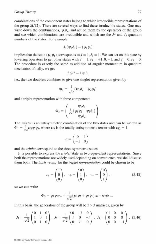
Group Theory 77
combinations of the component states belong to which irreducible representations of
the group SU(2). There are several ways to find these irreducible states. One may
write down the combinations, ψiφ j, and act on them by the operators of the group
and see which combinations are irreducible and which are the J2 and J3 quantum
numbers of the states. For example,
J3(ψ1φ1) = (ψ1φ1)
implies that the state (ψ1φ1) corresponds to J = 1,J3 = 1. We can act on this state by
lowering operators to get other states with J = 1,J3 = +1,0,−1, and J = 0,J3 = 0.
The procedure is exactly the same as addition of angular momentum in quantum
mechanics. Finally, we get
2⊗2 = 1⊕3,
i.e., the two doublets combines to give one singlet representation given by
Φ1 ≡ 1√2(ψ1φ2 −ψ2φ1)
and a triplet representation with three components
Φ3 ≡ ψ1φ1
1√2(ψ1φ2 +ψ2φ1)
ψ2φ2
.
The singlet is an antisymmetric combination of the two states and can be written as
Φ1 = 1√2εi jψiφ j, where εi j is the totally antisymmetric tensor with ε12 = 1
ε =(
0 1
−1 0
),
and the triplet correspond to the three symmetric states.
It is possible to express the triplet state in two equivalent representations. Since
both the representations are widely used depending on convenience, we shall discuss
them both. The basis vector for the triplet representation could be chosen to be
v+ =
1
0
0
, v0 =
0
1
0
, v− =
0
0
1
, (3.45)
so we can write
Φ3 = ψ1φ1v+ +1√2(ψ1φ2 +ψ2φ1)v0 +ψ2φ2v−.
In this basis, the generators of the group will be 3×3 matrices, given by
J1 =1√2
0 1 0
1 0 1
0 1 0
, J2 =1√2
0 −i 0
i 0 −i0 i 0
, J3 =
1 0 0
0 0 0
0 0 −1
, (3.46)
© 2008 by Taylor & Francis Group, LLC
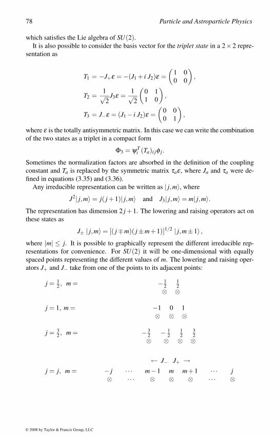
78 Particle and Astroparticle Physics
which satisfies the Lie algebra of SU(2).It is also possible to consider the basis vector for the triplet state in a 2×2 repre-
sentation as
T1 = −J+ε = −(J1 + i J2)ε =(
1 0
0 0
),
T2 =1√2
J3ε =1√2
(0 1
1 0
),
T3 = J−ε = (J1 − i J2)ε =(
0 0
0 1
),
where ε is the totally antisymmetric matrix. In this case we can write the combination
of the two states as a triplet in a compact form
Φ3 = ψTi (Ta)i jφ j.
Sometimes the normalization factors are absorbed in the definition of the coupling
constant and Ta is replaced by the symmetric matrix τaε , where Ja and τa were de-
fined in equations (3.35) and (3.36).
Any irreducible representation can be written as | j,m〉, where
J2| j,m〉 = j( j +1)| j,m〉 and J3| j,m〉 = m| j,m〉.The representation has dimension 2 j +1. The lowering and raising operators act on
these states as
J± | j,m〉 = [( j∓m)( j±m+1)]1/2 | j,m±1〉 ,where |m| ≤ j. It is possible to graphically represent the different irreducible rep-
resentations for convenience. For SU(2) it will be one-dimensional with equally
spaced points representing the different values of m. The lowering and raising oper-
ators J+ and J− take from one of the points to its adjacent points:
j = 12 , m = − 1
212⊗ ⊗
j = 1, m = −1 0 1
⊗ ⊗ ⊗
j = 32 , m = − 3
2 − 12
12
32⊗ ⊗ ⊗ ⊗
← J− J+ →j = j, m = − j · · · m−1 m m+1 · · · j
⊗ ·· · ⊗ ⊗ ⊗ ·· · ⊗
© 2008 by Taylor & Francis Group, LLC
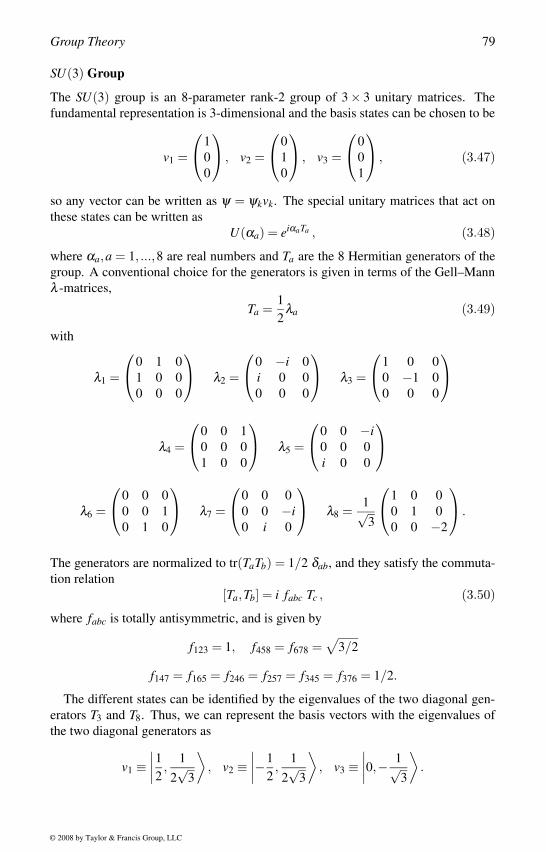
Group Theory 79
SU(3) Group
The SU(3) group is an 8-parameter rank-2 group of 3× 3 unitary matrices. The
fundamental representation is 3-dimensional and the basis states can be chosen to be
v1 =
1
0
0
, v2 =
0
1
0
, v3 =
0
0
1
, (3.47)
so any vector can be written as ψ = ψkvk. The special unitary matrices that act on
these states can be written as
U(αa) = eiαaTa , (3.48)
where αa,a = 1, ...,8 are real numbers and Ta are the 8 Hermitian generators of the
group. A conventional choice for the generators is given in terms of the Gell–Mann
λ -matrices,
Ta =1
2λa (3.49)
with
λ1 =
0 1 0
1 0 0
0 0 0
λ2 =
0 −i 0
i 0 0
0 0 0
λ3 =
1 0 0
0 −1 0
0 0 0
λ4 =
0 0 1
0 0 0
1 0 0
λ5 =
0 0 −i0 0 0
i 0 0
λ6 =
0 0 0
0 0 1
0 1 0
λ7 =
0 0 0
0 0 −i0 i 0
λ8 =1√3
1 0 0
0 1 0
0 0 −2
.
The generators are normalized to tr(TaTb) = 1/2 δab, and they satisfy the commuta-
tion relation
[Ta,Tb] = i fabc Tc , (3.50)
where fabc is totally antisymmetric, and is given by
f123 = 1, f458 = f678 =√
3/2
f147 = f165 = f246 = f257 = f345 = f376 = 1/2.
The different states can be identified by the eigenvalues of the two diagonal gen-
erators T3 and T8. Thus, we can represent the basis vectors with the eigenvalues of
the two diagonal generators as
v1 ≡∣∣∣∣12 ,
1
2√
3
⟩, v2 ≡
∣∣∣∣−1
2,
1
2√
3
⟩, v3 ≡
∣∣∣∣0,− 1√3
⟩.
© 2008 by Taylor & Francis Group, LLC
80 Particle and Astroparticle Physics
For a complex conjugate state the corresponding basis vectors would be
v∗1 ≡∣∣∣∣−1
2,− 1
2√
3
⟩, v∗2 ≡
∣∣∣∣12 ,− 1
2√
3
⟩, v∗3 ≡
∣∣∣∣0,1√3
⟩.
Any higher-dimensional representations can be constructed from products of these
basis vectors.
The generators
T1 ≡ I1, T2 ≡ I2, T3 ≡ I3
form an SU(2) subalgebra. Two more SU(2) embeddings are also possible in SU(3)with the generators
T4 ≡V1, T5 ≡V2, (√
3T8 +T3) ≡V3
and
T6 ≡U1, T7 ≡U2, (√
3T8 −T3) ≡U3,
but they are not orthogonal to each other. For each of these SU(2) embeddings one
can construct the raising and lowering operators and with these generators construct
the different irreducible states. We, thus, define
I± = T1 ± iT2 = I1 ± iI2, V± = T4 ±T5 = V1 ±V2,
U± = T6 ±T7 = U1 ±U2.
To compare between different notations, we further define
H1 = T3 and H2 =2√3
T8.
The generators I± interchange the states v1 and v2 and change the I3 quantum number
by ±1. Similarly, V± interchange the states v1 and v3, U± interchange between v2and v3.
Since any state can be identified by the two quantum numbers given by the eigen-
values x and y of the generators H1 and H2, it is possible to plot every state in an
irreducible representation in the H1 −H2 plane. In terms of the (x,y) quantum num-
bers, the three basis vectors correspond to the points
v1(1/2,1/3), v2(−1/2,1/3), v3(0,−2/3) ,
and the conjugate states correspond to the points
v∗1(−1/2,−1/3), v∗2(1/2,−1/3), v∗3(0,2/3).
Since the I,V,U raising and lowering operators relate the different basis states, the
action of these operators can be given by
I+ : (x → x+1, y → y);
V+ : (x → x−1/2, y → y+1);
U+ : (x → x+1/2, y → y+1) .
© 2008 by Taylor & Francis Group, LLC
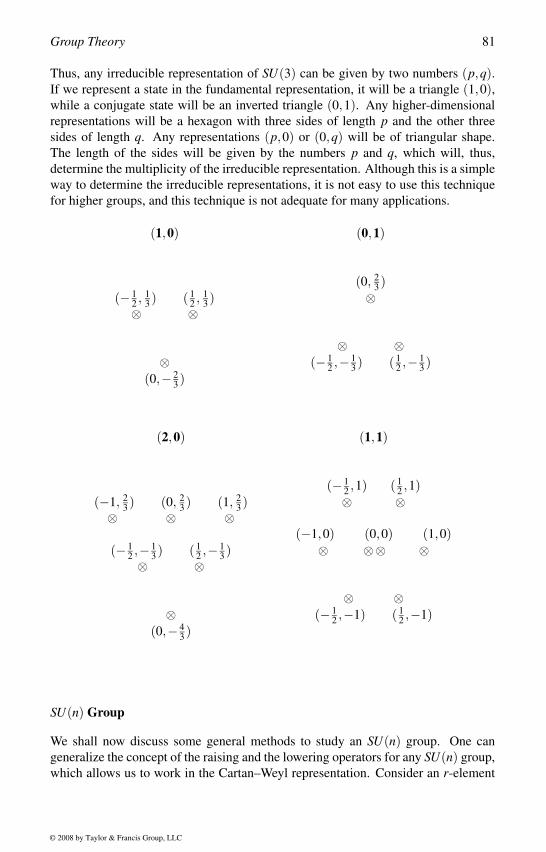
Group Theory 81
Thus, any irreducible representation of SU(3) can be given by two numbers (p,q).If we represent a state in the fundamental representation, it will be a triangle (1,0),while a conjugate state will be an inverted triangle (0,1). Any higher-dimensional
representations will be a hexagon with three sides of length p and the other three
sides of length q. Any representations (p,0) or (0,q) will be of triangular shape.
The length of the sides will be given by the numbers p and q, which will, thus,
determine the multiplicity of the irreducible representation. Although this is a simple
way to determine the irreducible representations, it is not easy to use this technique
for higher groups, and this technique is not adequate for many applications.
(1,0) (0,1)
(0, 23 )
(− 12 , 1
3 ) ( 12 , 1
3 ) ⊗⊗ ⊗
⊗ ⊗⊗ (− 1
2 ,− 13 ) ( 1
2 ,− 13 )
(0,− 23 )
(2,0) (1,1)
(− 12 ,1) ( 1
2 ,1)(−1, 2
3 ) (0, 23 ) (1, 2
3 ) ⊗ ⊗⊗ ⊗ ⊗
(−1,0) (0,0) (1,0)(− 1
2 ,− 13 ) ( 1
2 ,− 13 ) ⊗ ⊗⊗ ⊗
⊗ ⊗
⊗ ⊗⊗ (− 1
2 ,−1) ( 12 ,−1)
(0,− 43 )
SU(n) Group
We shall now discuss some general methods to study an SU(n) group. One can
generalize the concept of the raising and the lowering operators for any SU(n) group,
which allows us to work in the Cartan–Weyl representation. Consider an r-element
© 2008 by Taylor & Francis Group, LLC
82 Particle and Astroparticle Physics
Lie algebra of rank-l. There will be l generators that commute with each other,
which we denote as Hs,s = 1, ..., l. Hs will then span an l-dimensional subspace Cof the r-dimensional vector space. The set Hs is called the Cartan subalgebra C. If
the generators Hs of the Cartan subalgebra is diagonalized in the basis |µ,D〉 for the
irreducible representation D, then we can write
Hs|µ,D〉 = µs|µ,D〉 , (3.51)
where µ is the weight vector with components µs.
For an SU(n) group there could be l = n−1 commuting generators that form the
subspace C. For SU(3), there are two: H1 and H2. The remaining r− l = n(n− 1)even number of generators that span the n(n− 1)-dimensional vector subspace can
be written as raising and lowering operators. In the adjoint representation the states
|Xa〉 correspond to the generators (Xa) and the action of the generators on these states
is
Xa|Xb〉 = |[Xa,Xb]〉.The states belonging to the Cartan subalgebra commute with each other, and hence,
these are the states with weight zero Hs|Hl〉 = 0. Diagonalizing the remaining n(n−1)-dimensional space gives the n(n−1)/2 states |Ta〉 that satisfies
Hs|Ta〉 = as|Ta〉, (3.52)
and the corresponding generators would satisfy the commutation relation
[Hs,Ta] = asTa . (3.53)
These weights as are called roots. These generators are not Hermitian T †a = T−a.
They are the lowering and raising operators.
For every nonvanishing raising operator Ta, there is a corresponding nonvanishing
lowering operator T−a, which can be rephrased as: if Ta is a raising operator and Tbis the corresponding lowering operator, then a+b = 0. In this basis, the commutator
relations of the generators are given by
[Hs,Hl ] = 0 for s, l ∈C
[Hs,Ta] = fsaaTa = asTa for s ∈C
[Ta,Tb] = ∑s∈C
fabsHs = ∑s∈C
asHs for (a+b) = 0
[Ta,Tb] =
faba+bTa+b if (a+b) = 0 is a root .0 otherwise
(3.54)
Application of Ta on the state |µ,D〉 with weight vector µ and irreducible dimensions
D would raise one of the weights µi. Repeated application of Ta or T−a will, thus,
eventually make it vanish. If p repeated action of Ta or q repeated action of T−aannihilates the state, we can write
Ta|µ + pa,D〉 = 0, T−a|µ −qa,D〉 = 0
© 2008 by Taylor & Francis Group, LLC
Group Theory 83
for positive integers p and q. Operating on these states with raising and lowering
operators, we can obtain the entire spectrum of the irreducible representations.
We shall next study the tensor method in SU(n). Let us consider a vector in the
fundamental representation of the group ψk = ψ1, ...,ψn, which can be mapped
into another vector in the same vector space by the unitary transformations generated
by the generators of the group given in equation (3.34. Writing the transformation
matrix as Ukl , the transformation can be written as
ψk → ψ ′k = Uklψl . (3.55)
The fundamental representation of dimension n is also referred to as simply n. Simi-
larly for a conjugate representation ψ∗k , which is referred to as n∗, the corresponding
transformation becomes
ψ∗k → ψ ′∗
k = U∗klψ
∗l = ψ∗
l U†lk. (3.56)
For a representation with both regular as well as conjugate indices, it becomes diffi-
cult to distinguish the different indices. It is, thus, convenient to use a convention
ψk ≡ ψ∗k , Uk
l ≡Ukl and Ukl = U∗
kl .
In this notation
ψk → ψ ′k = Uk
lψl ψk → ψ ′k = Uklψ l . (3.57)
Higher rank tensors can be formed with the upper and lower indices, which would
correspond to higher-dimensional representations formed from the fundamental rep-
resentation and its conjugate.
We now define the Kronecker delta function as
δkl = δkl =
1 if k = l0 otherwise.
(3.58)
The unitarity condition then translates into
Ukl U l
m = δ km and δ k
l = Ukm Un
l δ mn.
Thus, the Kronecker delta function is an invariant tensor. The product of a vector ψkand its conjugate ψk will, in general, be a 3× 3 matrix, from which the trace will
form a separate 1-dimensional representation, which is invariant under any SU(n)transformations. The singlet state can be projected out with the Kronecker delta
function, which defines the SU(n) invariant scalar product
(ψ,φ) = ψk φl δ lk = ψkφk. (3.59)
In general, the Kronecker delta function can contract indices reducing the rank of a
tensor
ψabc..pqr.. δ p
a = ψbc..qr.. .
© 2008 by Taylor & Francis Group, LLC
84 Particle and Astroparticle Physics
When all the indices of any tensor are contracted, the tensor becomes invariant under
any group transformations. It is then said to be a singlet of the group SU(n).We shall now define the Levi–Civita symbol for the group SU(n) as
εk1..kn = εk1..kn =
1 for (k1..kn) ≡ (1..n) or even permutations
−1 for (k1..kn) to be odd permutations of (1..n)0 otherwise.
(3.60)
It is an invariant tensor and can be used to relate the regular states with conjugate
states
ψkr ...kn = εk1k2...knφk1k2...kr−1 .
The Levi–Civita symbol allows contraction of indices, and when it contracts all the
indices of a tensor, it results in an invariant singlet.
3.4 Group RepresentationsIn this section we shall try to explain how to find the dimensions of any irreducible
representations and the decomposition of products of any two representations in
terms of irreducible representations. We shall then discuss how these representa-
tions may be related to the representations of any semi-simple subgroup.
Irreducible Representations
Any group representations are formed by combining the regular states and conjugate
states as direct products. If we write a composite state with several indices, in gen-
eral, the state will be reducible. First we identify the properties of the composite
states that make them reducible.
Consider first the case of SU(3), and then we shall generalize the result to other
groups. There are two invariant tensors in SU(3), the Kronecker delta δ kl and the
Levi–Civita symbol ε i jk = εi jk. Thus, if any two upper or two lower indices of a
tensor are antisymmetric, then we can contract them with the Levi–Civita symbol.
For example, the antisymmetric tensor ψi j can be written as φ k = ε i jkψi j, which is a
conjugate vector. Similarly since all states are traceless, the trace of any tensor can
be written with the delta function, which is equivalent to contracting the indices with
the delta function.
With this introduction we can now work out the product decompositions for the
group SU(3) and find the irreducible representations. Let us start with two vectors
ψk and φk belonging to the fundamental representations 3. We can write the product
as
ψiφ j =1
2(ψiφ j +ψ jφi)+
1
2(ψiφ j −ψ jφi) = Ψi j +Φk.
Thus, the product can be written as a rank-2 symmetric tensor with two symmetric
lower indices Ψi j and another conjugate vector state Φk = 12 ε i jkψiφ j. This product
© 2008 by Taylor & Francis Group, LLC
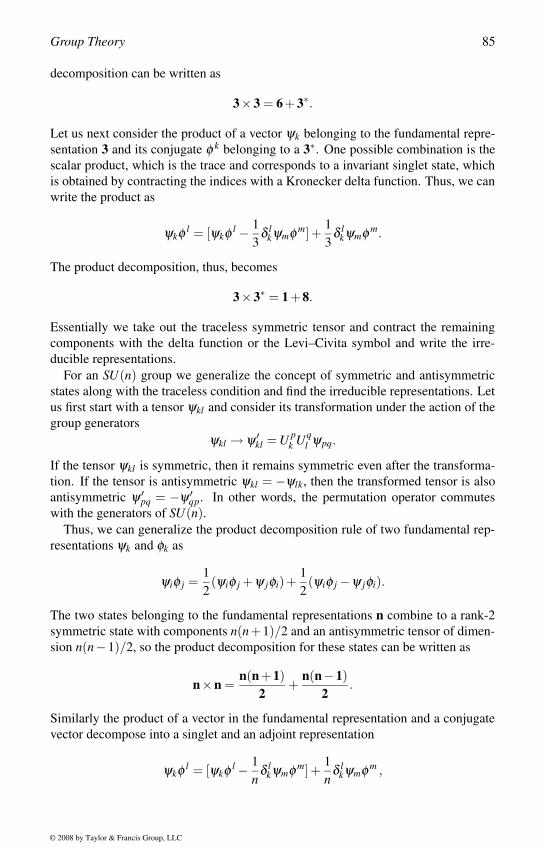
Group Theory 85
decomposition can be written as
3×3 = 6+3∗.
Let us next consider the product of a vector ψk belonging to the fundamental repre-
sentation 3 and its conjugate φ k belonging to a 3∗. One possible combination is the
scalar product, which is the trace and corresponds to a invariant singlet state, which
is obtained by contracting the indices with a Kronecker delta function. Thus, we can
write the product as
ψkφ l = [ψkφ l − 1
3δ l
kψmφ m]+1
3δ l
kψmφ m.
The product decomposition, thus, becomes
3×3∗ = 1+8.
Essentially we take out the traceless symmetric tensor and contract the remaining
components with the delta function or the Levi–Civita symbol and write the irre-
ducible representations.
For an SU(n) group we generalize the concept of symmetric and antisymmetric
states along with the traceless condition and find the irreducible representations. Let
us first start with a tensor ψkl and consider its transformation under the action of the
group generators
ψkl → ψ ′kl = U p
k Uql ψpq.
If the tensor ψkl is symmetric, then it remains symmetric even after the transforma-
tion. If the tensor is antisymmetric ψkl = −ψlk, then the transformed tensor is also
antisymmetric ψ ′pq = −ψ ′
qp. In other words, the permutation operator commutes
with the generators of SU(n).Thus, we can generalize the product decomposition rule of two fundamental rep-
resentations ψk and φk as
ψiφ j =1
2(ψiφ j +ψ jφi)+
1
2(ψiφ j −ψ jφi).
The two states belonging to the fundamental representations n combine to a rank-2
symmetric state with components n(n+1)/2 and an antisymmetric tensor of dimen-
sion n(n−1)/2, so the product decomposition for these states can be written as
n×n =n(n+1)
2+
n(n−1)2
.
Similarly the product of a vector in the fundamental representation and a conjugate
vector decompose into a singlet and an adjoint representation
ψkφ l = [ψkφ l − 1
nδ l
kψmφ m]+1
nδ l
kψmφ m ,
© 2008 by Taylor & Francis Group, LLC
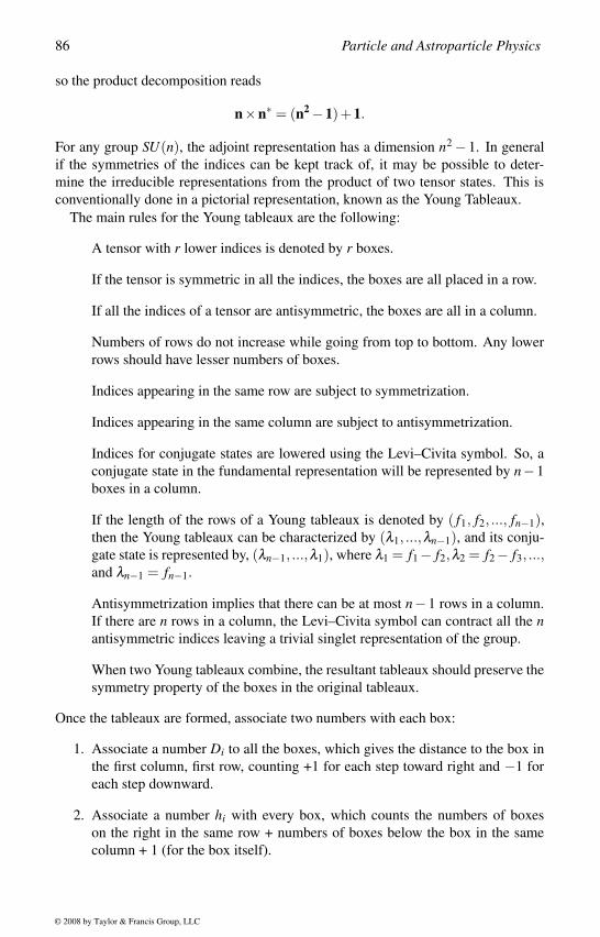
86 Particle and Astroparticle Physics
so the product decomposition reads
n×n∗ = (n2 −1)+1.
For any group SU(n), the adjoint representation has a dimension n2 −1. In general
if the symmetries of the indices can be kept track of, it may be possible to deter-
mine the irreducible representations from the product of two tensor states. This is
conventionally done in a pictorial representation, known as the Young Tableaux.
The main rules for the Young tableaux are the following:
A tensor with r lower indices is denoted by r boxes.
If the tensor is symmetric in all the indices, the boxes are all placed in a row.
If all the indices of a tensor are antisymmetric, the boxes are all in a column.
Numbers of rows do not increase while going from top to bottom. Any lower
rows should have lesser numbers of boxes.
Indices appearing in the same row are subject to symmetrization.
Indices appearing in the same column are subject to antisymmetrization.
Indices for conjugate states are lowered using the Levi–Civita symbol. So, a
conjugate state in the fundamental representation will be represented by n−1
boxes in a column.
If the length of the rows of a Young tableaux is denoted by ( f1, f2, ..., fn−1),then the Young tableaux can be characterized by (λ1, ...,λn−1), and its conju-
gate state is represented by, (λn−1, ...,λ1), where λ1 = f1− f2,λ2 = f2− f3, ...,and λn−1 = fn−1.
Antisymmetrization implies that there can be at most n−1 rows in a column.
If there are n rows in a column, the Levi–Civita symbol can contract all the nantisymmetric indices leaving a trivial singlet representation of the group.
When two Young tableaux combine, the resultant tableaux should preserve the
symmetry property of the boxes in the original tableaux.
Once the tableaux are formed, associate two numbers with each box:
1. Associate a number Di to all the boxes, which gives the distance to the box in
the first column, first row, counting +1 for each step toward right and −1 for
each step downward.
2. Associate a number hi with every box, which counts the numbers of boxes
on the right in the same row + numbers of boxes below the box in the same
column + 1 (for the box itself).
© 2008 by Taylor & Francis Group, LLC
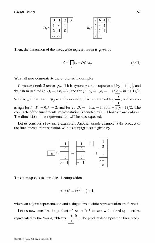
Group Theory 87
Di :
0 1 2 3
-1 0 1
-2 -1 0
-3 -2
hi :
7 6 4 1
5 4 2
4 3 1
2 1
Then, the dimension of the irreducible representation is given by
d = ∏i
(n+Di)/hi. (3.61)
We shall now demonstrate these rules with examples.
Consider a rank-2 tensor ψi j. If it is symmetric, it is represented by i j , and
we can assign for i : Di = 0,hi = 2; and for j : Di = 1,hi = 1, so d = n(n + 1)/2.
Similarly, if the tensor ψi j is antisymmetric, it is represented byi
j, and we can
assign for i : Di = 0,hi = 2; and for j : Di = −1,hi = 1, so d = n(n− 1)/2. The
conjugate of the fundamental representation is denoted by n−1 boxes in one column.
The dimension of the representation will be n as expected.
Let us consider a few more examples. Another simple example is the product of
the fundamental representation with its conjugate state given by
n ×
1
2
...
n−1
=
1 n
2
...
n−1
+
1
2
...
n−1
n
This corresponds to a product decomposition
n×n∗ = (n2 −1)+1,
where an adjoint representation and a singlet irreducible representation are formed.
Let us now consider the product of two rank-3 tensors with mixed symmetries,
represented by the Young tableauxa b
c. The product decomposition then reads
© 2008 by Taylor & Francis Group, LLC
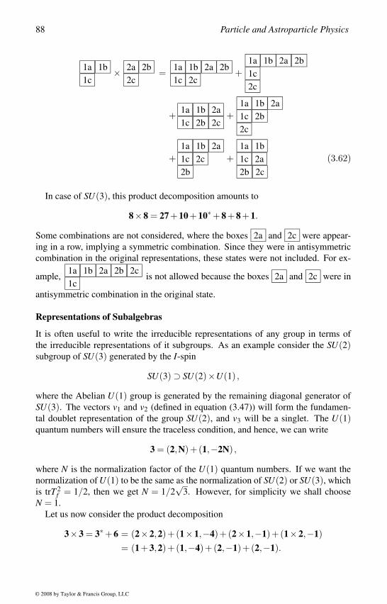
88 Particle and Astroparticle Physics
1a 1b
1c× 2a 2b
2c=
1a 1b 2a 2b
1c 2c+
1a 1b 2a 2b
1c
2c
+1a 1b 2a
1c 2b 2c+
1a 1b 2a
1c 2b
2c
+1a 1b 2a
1c 2c
2b
+1a 1b
1c 2a
2b 2c
(3.62)
In case of SU(3), this product decomposition amounts to
8×8 = 27+10+10∗ +8+8+1.
Some combinations are not considered, where the boxes 2a and 2c were appear-
ing in a row, implying a symmetric combination. Since they were in antisymmetric
combination in the original representations, these states were not included. For ex-
ample,1a 1b 2a 2b 2c
1cis not allowed because the boxes 2a and 2c were in
antisymmetric combination in the original state.
Representations of Subalgebras
It is often useful to write the irreducible representations of any group in terms of
the irreducible representations of it subgroups. As an example consider the SU(2)subgroup of SU(3) generated by the I-spin
SU(3) ⊃ SU(2)×U(1) ,
where the Abelian U(1) group is generated by the remaining diagonal generator of
SU(3). The vectors v1 and v2 (defined in equation (3.47)) will form the fundamen-
tal doublet representation of the group SU(2), and v3 will be a singlet. The U(1)quantum numbers will ensure the traceless condition, and hence, we can write
3 = (2,N)+(1,−2N) ,
where N is the normalization factor of the U(1) quantum numbers. If we want the
normalization of U(1) to be the same as the normalization of SU(2) or SU(3), which
is trT 2f = 1/2, then we get N = 1/2
√3. However, for simplicity we shall choose
N = 1.
Let us now consider the product decomposition
3×3 = 3∗ +6 = (2×2,2)+(1×1,−4)+(2×1,−1)+(1×2,−1)= (1+3,2)+(1,−4)+(2,−1)+(2,−1).
© 2008 by Taylor & Francis Group, LLC
Group Theory 89
Since the sextet is symmetric and the antitriplet is antisymmetric, the sextet should
contain the SU(2) triplet, a symmetric combination of the two states (2,−1) and
(1,−4), while the antitriplet will contain the SU(2) antisymmetric singlet and an
antisymmetric combination of the two SU(2) doublets
6 = (3,2)+(2,−1)+(1,−4) 3∗ = (2,−1)+(1,2).
Similarly taking the product of 3 and 3∗, we can get the decomposition of the octet
8 = (3,0)+(1,0)+(2,−3)+(2,3).
This tells us how the generators of SU(3) decompose under the SU(2) subgroup.
The (3,0) corresponds to the three generators I±, I3 which generate the group SU(2)and (1,0) corresponds to the diagonal generator T8 that generates the Abelian group
U(1). The raising and lowering operators U± and V± are doublets under SU(2) and
have definite T8 eigenvalues ±3, so they correspond to the states (2,±3).These results can be generalized for any group SU(n), and the decompositions
of the irreducible representations in terms of its SU(n−1)×U(1) subgroup can be
written
n = (n−1,1)+(1,−(n−1)),n∗ = ((n−1)∗,−1)+(1,n−1)
n(n+1)/2 = (n(n−1)/2,2)+(n−1,−n+2)+(1,−2n+2),n(n−1)/2 = ((n−1)(n−2)/2,2)+(n−1,−n+2)
n2 −1 = (n(n−2),0)+(1,0)+(n−1,n)+((n−1)∗,−n) . (3.63)
We shall also present the decompositions of the irreducible representations of SU(n)under the subgroup SU(n−m)×SU(m)×U(1):
n = (n−m,1,m)+(1,m,−(n−m))n∗ = ((n−m)∗,1,−m)+(1,m∗,(n−m))
n(n+1)2
=(
(n−m)(n−m+1)2
,1,2m)
+(
1,m(m+1)
2,−2(n−m)
)+(n−m,m,−n+2m)
n(n−1)2
=(
(n−m)(n−m−1)2
,1,2m)
+(
1,m(m−1)
2,−2(n−m)
)+(n−m,m,−n+2m)
n2 −1 = ((n−m)2 −1,1,0)+(1,m2 −1,0)+(1,0)+ (n−m,m∗,n)+((n−m)∗,m,−n) . (3.64)
We have not considered the normalization of the group U(1), which is a multiplica-
tive factor for all the U(1) quantum numbers. The decomposition of the fundamental
© 2008 by Taylor & Francis Group, LLC
90 Particle and Astroparticle Physics
representation under the subgroup SU(n−m)× SU(m)×U(1) means that a vector
ψk,k = 1, ...,n can be written as a direct sum ψa ⊕ψp,a ∈ SU(n−m), p ∈ SU(m).The relative U(1) quantum numbers ensure traceless condition. The generators in
the adjoint representation (n2 −1) of SU(n) now include generators of the subgroups
SU(n−m), SU(m) and U(1) and the lowering and raising operators that take a state
ψa ∈ SU(n−m) to a state ψp ∈ SU(m), which transforms nontrivially under both the
groups.
The decompositions of the irreducible representations in terms of its subgroup can
also be useful in determining the invariants for the different representations. Let us
first determine the index for the irreducible representations of the group SU(2). For
any irreducible representation denoted by the quantum numbers | j,m〉 and hence of
dimension n = 2 j +1, the index is given by
λ (n) = j2 +( j−1)2 + · · ·+(− j +1)2 +(− j)2.
So, the index for some of the representations is
λ (2) =1
2, λ (3) = 2, λ (4) = 5, λ (5) = 10.
We can now write the index for any irreducible representations of SU(3) with our
knowledge of the index for representations of SU(2). We follow the prescription
that the index for any irreducible representations Rn of SU(n) can be obtained in
terms of the irreducible representations Rmn−1 of SU(n− 1) as λ (Rn) = ∑m λ (Rm
n−1)if Rn = ∑m Rm
n−1. Let us consider the example of SU(3). Ignoring the U(1) quantum
numbers, we can write the decomposition of SU(3) representations in terms of the
SU(2) representations as
3 = 2+1, 6 = 3+2+1, 8 = 3+2+2+1.
Then the index for the SU(3) representations will be λ (3) = λ (2)+ λ (1) = 1/2 +0 = 1/2, as expected, since for all SU(n) groups, fundamental representations are
normalized to 1/2. The SU(3) index for 6 and 8 are thus
λ (6) = λ (3)+λ (2)+λ (1) = 2+1/2+0 = 5/2
and λ (8) = λ (3)+λ (2)+λ (2)+λ (1) = 3. (3.65)
As expected, for the adjoint representations of SU(n), the index is λ (n2 − 1) = n.
Similarly the group factor for the triangle anomaly for any representations of any
group can be obtained in terms of the anomaly or index of the representations of its
subgroup.
3.5 Orthogonal GroupsAny groups generated by orthogonal matrices
OT O = 1 or Oi jOk j = δik
© 2008 by Taylor & Francis Group, LLC
Group Theory 91
are called the orthogonal groups. For orthogonal groups there are two disconnected
vector spaces, which correspond to detO = ±1. We restrict our discussions to only
detO = +1, which is called the special orthogonal group.
We are familiar with orthogonal groups in many ways. Consider a 2-dimensional
rotation group O(2) generated by
O = eiσ2θ =(
cosθ sinθ−sinθ cosθ
),
where σ2 =(
0 −ii 0
)is the Pauli matrix. This is a 1-parameter group; the generator
commutes with itself, and hence, it is equivalent to the Abelian group U(1).The group SO(3) is the rotation group in 3-dimensional space with determinant
+1. The group transformations on the 3-vectors xi, i = 1,2,3, given by
xi → x′i = Oi jx j
leave the real quadratic form x21 + x2
2 + x23 invariant and preserve the distance. The
group elements are generated by the three angular momentum operators
O(θa) = eJaθa ,
where the generators are real antisymmetric matrices and can be given by
J1 =
0 1 0
−1 0 0
0 0 0
, J2 =
0 0 −1
0 0 0
1 0 0
, J3 =
0 0 0
0 0 1
0 −1 0
.
These generators satisfy the commutation relation
[Ja,Jb] = fabcJc,
where the structure function fabc is a completely antisymmetric tensor. Thus, the Lie
algebra satisfied by the generators of SO(3) is the same as that of the generators of
the group SU(2), so these two groups are locally isomorphic.
Another convention is to replace Ja by iTa and write Ta as imaginary antisymmetric
matrices; however, we shall restrict ourselves to the present convention with Ja. Let
us now consider the group SO(4), which is locally isomorphic to the Lorentz group
O(3,1). The Lorentz group SO(3,1) preserves the distance x2 + y2 + z2 − t2 and,
hence, allows disconnected regions in space–time because of the relative sign in the
metric, which is not present in the SO(4) group which preserves x2 +y2 +z2 +t2. But
locally they satisfy the same Lie algebra. The group SO(4) is isomorphic to the semi-
simple group SU(2)× SU(2), which we shall discuss later. Another isomorphism
between orthogonal and unitary groups is that the groups SO(6) and SU(4) are also
isomorphic to each other.
Let us write the operator, generating the SO(n) group, as
O(θa) = eθabMab ,
© 2008 by Taylor & Francis Group, LLC
92 Particle and Astroparticle Physics
where θab is antisymmetric and the generators are real antisymmetric matrices Mab =−Mba given by
[Mab]i j = δaiδb j −δbiδa j , (3.66)
and they satisfy the commutation relation
[Mab,Mcd ] = δbcMad −δacMbd −δbdMac +δadMbc. (3.67)
The commuting generators could be chosen to be M2 j−1,2 j, j = 1,2, ...,N for both the
groups SO(2N +1) and SO(2N).The Lorentz group is locally isomorphic to the SO(4) group. The generators of
the Lorentz group are
Mµν ≡ Lµν = xµ pν − xν pµ ,
which satisfy the same algebra as the SO(n) group generators. There are six genera-
tors of the group SO(4) that are given by
Ma = εabcMbc Na = M0a ,
where εabc is the totally antisymmetric invariant tensor of the group. These genera-
tors satisfy the algebra
[Ma,Mb] = εabcMc [Na,Nb] = εabcMc
[Ma,Na] = 0 [Ma,Nb] = εabcNc.
In another basis these generators can be written as direct sum of two SU(2) algebras,
which are
Ja =1
2(Ma +Na), and Ka =
1
2(Ma −Na). (3.68)
These generators now satisfy the commutation relation
[Ja,Jb] = εabcJc, [Ka,Kb] = εabcKc and [Ka,Jb] = 0. (3.69)
Ja and Ka then generates two distinct SU(2) groups, which are direct product groups,
and hence, SO(4) ⊃ SU(2)×SU(2).In terms of the SU(2)× SU(2) subgroup of SO(4), the different representations
are given by
S ≡ (0,0) V ≡ (1/2,1/2) Γ ≡ (1/2,0)+(0,1/2).
A doublet under the group SU(2) is represented by its quantum number 1/2. The
scalars (S) transform trivially under the group. There is a vector representation (V )
of dimension 4, which is the fundamental representation of the group. The four-
momentum belongs to the vector representation. There is also a 4-dimensional spinor
representation of the group Γ, which has two distinct parts. The usual γ5 matrix
projects out these two states, and they correspond to the left-handed spinor and the
right-handed spinor.
© 2008 by Taylor & Francis Group, LLC
Group Theory 93
All representations of SU(n) can be constructed as products of the fundamental
representations. However, for the orthogonal groups SO(n), there are two distinct
representations, the usual vector representations of dimension n and a spinor repre-
sentation of dimension 2N−1 for both n = 2N and n = 2N −1. To discuss the spinor
representations let us introduce the Clifford algebra, which entails the anticommuta-
tion relations (X ,Y = XY +Y X)
Γi,Γ j = 2δi j, i, j = 1,2, ...,n (3.70)
satisfied by the set of N matrices Γi. These matrices can give us a representation of
the group SO(n)
Mab =1
4[Γa,Γb], (3.71)
such that Mab satisfy the SO(n) algebra and
[Mab,Γc] = δbcΓa −δacΓb (3.72)
The Γ-matrices form a set of n tensors that transform according to vector represen-
tation of SO(n).Let us first consider the case n = 2N. It is possible to find a complex spinorial
representation of dimension 2N . But it is possible to define a generator
Γn+1 = Γ1Γ2...Γn , (3.73)
which commutes with all the generators, that projects out two components of the 2N
spinor. We can define the projection operators as
P− =1
2(1−Γn+1) P+ =
1
2(1+Γn+1) ,
which obey P2± = P± and P−+P+ = 1. That leaves two independent 2N−1 component
spinors in an SO(n = 2N) group. The main difference between the groups SO(2N)and SO(2N + 1) is that the two spinors of different helicity of the group SO(2N)transform like one spinor representation of the group SO(2N + 1), and hence, the
spinor of SO(2N + 1) is of dimension 2N . This is because the generator Γn+1 satis-
fies a similar anticommutation relation with other generators, and it belongs to the
group SO(2N + 1). It is the 2N + 1-th element of the SO(2N + 1) vector. Thus,
all representations of the group SO(2N + 1) are vector-like, and it is not possible to
distinguish the left-handed fermions from the right-handed fermions. For example,
the SO(10) group has a 10-dimensional vector representation and a 16-dimensional
spinor representation. The left-handed fermions and antifermions belong to the 16-
dimensional representation and the right-handed fermions and antifermions belong to
the 16∗-dimensional representation. However, in SO(11) this is not possible, because
both the 16 and 16∗ representations of SO(10) are part of the same 32-dimensional
representation of SO(11).Construction of the irreducible representations of any SO(n) group is not as simple
as that of the SU(n) groups. We shall, thus, discuss only a few simple representa-
tions. Consider the rotation group SO(3) in 3-dimensions, with which we are most
© 2008 by Taylor & Francis Group, LLC
94 Particle and Astroparticle Physics
familiar. There is a 3-dimensional vector representation ψk,k = 1,2,3. One can com-
bine two vectors to construct higher dimensional representations. For this purpose
we shall make use of the invariants of the group, εi jk and δi j. The product of two
vectors can then be decomposed as
ψiφ j = [1
2(ψiφ j +ψ jφi)− 1
3δi jψiφ j]+
1
2εi jkψiφ j +
1
3δi jψiφ j
= Ti j +Vk +S ,
where Ti j is the symmetric traceless rank-2 tensor; Vk is a vector, which comes from
the cross product of two vectors; and S is a scalar, which comes from the scalar
product of two vectors. The adjoint representation belongs to the antisymmetric
representation of dimension-3.
Let us now consider the case of SO(10). The vector belongs to a 10-dimensional
representation. When two vectors combine, it gives a scalar, an antisymmetric tensor
in the adjoint representation and a symmetric rank-2 tensor. The product decompo-
sition then becomes
10×10 = 1+45+54.
The product decomposition of the spinors does not have any analogy with lower-
dimensional groups. It is given by
16×16 = 10+120+126 16×16∗ = 1+45+210.
The adjoint representation is a 45-dimensional representation.
Construction of the irreducible representations of any SO(n) group is not as simple
as that of the SU(n) groups. Because of this it is convenient to study the orthogonal
groups in terms of their unitary subgroups. We shall discuss the SO(10) group in
some more detail in terms of its subgroup while discussing the SO(10) grand unified
theories.
© 2008 by Taylor & Francis Group, LLC
Part II
Standard Model and Beyond
© 2008 by Taylor & Francis Group, LLC
4Symmetries in Nature
If we do not try to find any correlation between different phenomena, then for every
event we have to find a different law. But if we can correlate these events, then
we find that only a very few laws can explain most of these phenomena. These
correlations lead us to the concept of symmetry. Consider a spherical ball. One
can visualize it by taking its projection from all orientations, which will give us an
infinite set of data. However, if we consider its spherical symmetry, we can visualize
it from only one direction and get all the infinite projections from all orientations by
making spherical transformations. Children develop such a notion of symmetry in
their mind just by observing. But they will not try to understand that the spherical
symmetry of the object means that this object has the minimum surface area and any
loop on the surface of the sphere can be contracted to a point. Neither do they try
to find out the meaning of spherical transformations. So, the concept of symmetry
can be understood at different levels and can have different applications as well. The
mathematical tool to study symmetries is the group theory which we discussed in
chapter 3.
We encounter several types of symmetries in nature. These symmetries could be
continuous or discrete and global or local. All fundamental interactions can origi-
nate from local continuous symmetries and can be explained by gauge theories. On
the other hand, it is very common to have global symmetries in nature. Interesting
possibilities emerge, when any symmetry of the Lagrangian is not respected by the
vacuum, leading to spontaneous symmetry breaking. All these notions form the basis
for the standard model of particle physics.
4.1 Discrete Symmetries
When a system remains invariant under a finite or denumerable infinite number of
transformations, the system is said to possess discrete symmetry. A term x2 is sym-
metric under a Z2 symmetry generated by x → −x; x3 is symmetric under Z3 sym-
metry x → ωx, where ω is the cube root of unity ω3 = 1 and 1 + ω + ω2 = 0; and
x4 is invariant under x → ix, which is a Z4 symmetry. In particle physics such simple
discrete symmetries are very common, although in some cases more complex dis-
crete symmetries including non-Abelian discrete symmetries, whose generators do
97
© 2008 by Taylor & Francis Group, LLC
98 Particle and Astroparticle Physics
not commute, are also used.
Let us consider a simple example of Z2 discrete symmetry. When a scalar field
φ(x) transforms under a Z2 symmetry as φ → −φ , the Lagrangian L (φ) will re-
main invariant under this Z2 transformation if the system is invariant under this Z2discrete symmetry. Thus, the most general scalar interactions in the Lagrangian can
be written as
Ls =1
2m2
φ φ 2 +1
4!λφ 4. (4.1)
The cubic term will not be allowed by the Z2 symmetry. Similarly the discrete sym-
metry can be extended to several fields, each of which will transform under the dis-
crete symmetry in a specified manner and any term in the Lagrangian should be
invariant under the given discrete symmetry. As an example consider a Z3 symme-
try, under which the scalar fields φ1 and φ2 transform as φ1 → ωφ1 and φ2 → ω2φ2.
The Z3 invariant scalar interactions in the Lagrangian will be given by
Ls = m2φ1φ2 + µ1φ 31 + µ2φ 3
2 +λφ 21 φ 2
2 . (4.2)
Several interactions that are allowed otherwise are now forbidden by the Z3 symme-
try.
We now discuss some important discrete symmetries:
parity P : (x, t) → (−x, t)charge conjugation C : e →−etime− reversal T : (x, t) → (x,−t)
and products of these symmetries. In weak interactions, C and P are maximally
broken, but CP and T are weakly broken. However, the product CPT is always
conserved for consistency of the quantum field theory.
Parity P
We shall study the transformations of scalars, spinors and vectors under the parity
operation. We start with a complex scalar field φ(x), which can be expressed as
φ(x) =∫ d3k
(2π)3/2
1√2ωk
(a(k)e−ik·x +b†(k)eik·x), (4.3)
in terms of the operators a(k) and b(k), which satisfy
[a(k),a†(k′)] = [b(k),b†(k′)] = δ 3(k−k′), (4.4)
and all other pairs of operators commute. Under parity operation, a(k) → ±a(−k)and b(k) →±b(−k) and the scalar field transforms as
P : φ(r, t) →±φ(−r, t), (4.5)
for which we need to change the summation variable k →−k.
© 2008 by Taylor & Francis Group, LLC
Symmetries in Nature 99
The transformation of a fermion ψ(x, t) under the operation of parity is given by
Pψ(x, t)P† = ηpγ0ψ(−x, t), (4.6)
where |ηp| = 1 is a phase. The left-handed field ψL = 12 (1− γ5)ψ and the right-
handed field ψR = 12 (1+ γ5)ψ transform into each other under parity
1
2(1− γ5)ψ = ψL P−→ ψR =
1
2(1+ γ5)ψ
1
2(1− γ5)ψc = (ψc)L = (ψR)c P−→ (ψL)c = (ψc)R =
1
2(1+ γ5)ψc. (4.7)
The charge conjugations of the fields ψ are defined as ψ C−→ ψc = CψT = Cγ0ψ∗,
where C = −iγ2γ0. A left-handed field transforms under parity into a right-handed
field, so left-handed and right-handed fields are treated the same way if any interac-
tion conserves parity.
A vector field Aµ and the momentum vector Pµ transform under parity operation
as
Aµ(x, t),Pµ P−→ Aµ(−x, t),Pµ. (4.8)
This can be seen from the transformation of the source term jµ . The charge distri-
bution ρ remains unchanged but j →−j under parity since the current flows in the
opposite direction. Thus,
jµ , ψ(x, t)γµ ψ(x, t) P−→ jµ , ψ(−x, t)γµ ψ(−x, t). (4.9)
An axial vector field will transform with a negative sign. Strong and electromagnetic
interactions are invariant under parity, but weak interaction violates parity strongly.
Charge Conjugation C
Under charge conjugation, C, a particle transforms into an antiparticle. For a scalar
particle, charge conjugation implies interchange of the creation and annihilation op-
erators for particles and antiparticles
a(k) ↔ b(k) a†(k) ↔ b†(k), (4.10)
so the scalar field transforms under charge conjugation as
C : φ(r, t) →±φ †(r, t). (4.11)
The transformation of a fermion can be derived from the invariance of the Dirac
equation. Since the electric charge changes sign under charge conjugation, the in-
variance of the Dirac equation dictates that the charge conjugation of a fermion field
should be
ψ C−→ ψc = CψT = Cγ0ψ∗, where C = −iγ2γ0 (4.12)
© 2008 by Taylor & Francis Group, LLC
100 Particle and Astroparticle Physics
and
C ψ(x, t)C † = ηcCψT (x, t), (4.13)
where |ηc| = 1 is another phase. The transformations of the left-handed and right-
handed fermions are given by
ψL C−→ ψcL = (ψR)c and
ψR C−→ ψcR = (ψL)c . (4.14)
Finally the transformations of the four-momenta Pµ , vector field Aµ(x, t), source
current jµ(x), and the current ψ(x, t)γµ ψ are given by
Pµ ,Aµ(x, t) C−→ Pµ ,−Aµ(x, t) jµ , ψ(x, t)γµ ψ(x, t) C−→ − jµ ,−ψ(x, t)γµ ψ(x, t). (4.15)
Under weak interaction, both P and C are violated strongly, although CP remains
almost conserved. On the other hand, the strong, the electromagnetic, and the gravi-
tational interactions conserve both P and C independently.
Under CP operation, the various fields transform as
ψL C P−→ ψcR = (ψL)c
ψR C P−→ ψcL = (ψR)c
Pµ ,Aµ(x, t) C P−→ Pµ ,−Aµ(−x, t)ψ(x, t)γµ ψ(x, t) C P−→ −ψ(−x, t)γµ ψ(−x, t). (4.16)
Thus, CP operation relates all the interaction terms to their Hermitian conjugates,
except for the coupling constants. As a result, CP violation can come from the
imaginary part of the couplings. Consider the Yukawa coupling of a fermion field ψwith a scalar φ and the mass term
L = mψLψR +m∗ψRψL + f ψLψRφ + f ∗ψRψLφ † . (4.17)
We have written the Hermitian conjugate terms explicitly, the second and the fourth
terms. Under the operation of CP, ψLψR → ψRψL, and φ → φ †, CP invariance
implies m = m∗ and f = f ∗. Any complex phase in the Yukawa couplings or in the
mass or the scalar potential then implies CP violation.
CP violation was first observed in K −K oscillations [22], where strangeness
changes by 2 units. Since Kaons are produced through the strong interactions, they
carry definite strangeness quantum numbers, which allows us to distinguish between
a K(≡ ds with S = 1) and its antiparticle K(≡ sd with S =−1). But the decays of
the kaons are through the weak interaction, violating strangeness quantum number.
This allows K and K to decay into two or three pions, which are even or odd under
CP, respectively. Virtual pion exchange will then convert the K into a K
[K,K] ↔ [2π or 3π] ↔ [K,K]. (4.18)
© 2008 by Taylor & Francis Group, LLC
Symmetries in Nature 101
Strangeness number is changed by two units in K −K oscillations, although K-
decays violate strangeness by one unit.
The CP transformation takes K → K, so we can define the states with definite
CP eigenvalues
|K1〉 =1√2[|K〉+ |K〉] CP = +1 (4.19)
|K2〉 =1√2[|K〉− |K〉] CP = −1. (4.20)
Since pions are odd under CP, the CP even state |K1〉 can decay only to 2π while the
CP odd state |K2〉 can decay only to 3π .
If there is CP violation in the weak interaction Hamiltonian appearing as a com-
plex phase in the Yukawa couplings, a small fraction of CP-even state |K1〉 can evolve
into |K2〉. The physical states that evolve with time are then given by
|KS〉 =1√
1+ |ε|2 [|K1〉+ ε|K2〉] (4.21)
|KL〉 =1√
1+ |ε|2 [|K2〉+ ε|K1〉]. (4.22)
The amount of CP violation is characterized by the parameter ε . These states have
definite lifetimes of 0.9×10⁻¹⁰ s and 0.5×10⁻⁷ s, respectively.
Time-Reversal T
The time-reversal symmetry implies that any reaction rate in the forward direction
(in time) should be the same as in the backward direction. Thus, the time-reversal
operator is defined as
T ψ(x, t)T † = ηT T ψ∗(x,−t) (4.23)
with the phase ηT = ±1 and T = iγ1γ3 = −iγ5C. Since time-reversal implies the
exchange of positive and negative energy solutions, particles have to be interchanged
with antiparticles. In the spinor space, this is done with T , which satisfies T γ µ T−1 =γT
µ = γµ ∗ and T = T † = T−1 = −T ∗. Strong and electromagnetic interactions are
invariant under the T transformation, but the time-reversal symmetry is broken in the
weak interaction very weakly.
The time-reversal operator T has the unique property that it is antiunitary. Con-
sider the operation of T on the time-evolution operator
T eiH(t1−t2)T −1 = e−iH(t1−t2). (4.24)
This implies that the Hamiltonian does not commute with the operation T and it
should be antiunitary, i.e., for any two states φ and ψ , the time-reversal operator
satisfies
< T φ |T ψ >=< ψ|φ > .
© 2008 by Taylor & Francis Group, LLC
102 Particle and Astroparticle Physics
The time-reversal transformation of a scalar field is defined as
T : φ(r, t) →±φ †(r,−t). (4.25)
Under time-reversal, the annihilation operators transform into creation operators as
a(k) → ±a†(−k) and b(k) → ±b†(−k). The vector field transforms under T as
Aµ(x, t) T−→ Aµ(x,−t).The product of all the discrete symmetries, CPT , is a foundation stone in quantum
field theory and it is always conserved. Under the CPT transformation, a fermion
transforms as
(C PT ) ψ(x, t) (CPT )† = iγ5ψ(−x,−t), (4.26)
implying that a positive frequency particle could be replaced by a negative frequency
antiparticle with their momenta reversed and multiplied by iγ5. For a scalar field the
CPT transformation reads
φ(r, t) = +φ(−r,−t). (4.27)
Since this relation can be obtained by redefining the summation variables k → −kand ε →−ε , this implies a(k)→ b†(k) and b(k)→ a†(k), i.e., interchange of particle
and antiparticle.
The Lagrangian and the Hamiltonian of any system transform under C PT as
(C PT ) L (x) (C PT )−1 = L (−x)(C PT ) H (x) (C PT )−1 = H (−x). (4.28)
This general invariance is stated by the CPT theorem [23] that under the combined
transformation of parity, charge conjugation and time-reversal, any system remains
invariant. CPT and local Lorentz invariance may, thus, be considered as the most
sacred symmetries in nature, and they are the two foundation stones of quantum field
theory.
4.2 Continuous SymmetriesContinuous symmetries are very common in particle physics. When a new result is
observed, one tries to extend the existing model with some new particles and impos-
ing additional symmetries. If the extended model explains the result, one tries to find
predictions of the new model and then test them. When some of these predictions are
verified and few of these predictions cannot be explained by other similar models,
the model is accepted. However, our limitations with high energy accelerators does
not allow us to test all these models, and we have to study several alternative models
simultaneously to look for their testable signatures in the upcoming accelerators or
cosmology.
A continuous symmetry consists of an infinite number of states that are related
by some continuous transformations of a parameter in a finite range. For example,
© 2008 by Taylor & Francis Group, LLC
Symmetries in Nature 103
a state vector |ψ(θ)〉 could be symmetric under rotation, so by varying the angle of
rotation θ continuously in the range 0 to 2π , we can relate all the infinite set of state
vectors parameterized by θ .
Any continuous symmetry of any system implies some conserved quantity. On
the other hand, if there is any conserved quantity, it is also possible to associate with
it some symmetry of nature. Consider a system described by the Hamiltonian H. If
there is a conserved quantity, the corresponding operator O will commute with the
Hamiltonian H, HO = OH, and it will be possible to obtain a complete set of eigen-
functions ψi, which are simultaneous eigenstates of both O and H. The operator
O, acting on a state ψi, will give the corresponding conserved quantity Oψi = qiψi.
Since the time evolution of the state ψi is governed by the Hamiltonian, in the ab-
sence of any new interaction, this state cannot evolve into another state ψ j with a
different quantum number Oψ j = q jψ j.
In field theory, the symmetry principle and its connection with conserved quanti-
ties is stated by the Noether theorem [6]. It states that if a Lagrangian density (L ) is
invariant under any symmetry of the fields φi → φi +δφi, there is always a conserved
current Jµ , which is called the Noether current. The corresponding charge is given
by
Q =∫
d3xJ0(x) , (4.29)
which satisfiesdQdt
= 0. (4.30)
This gives the corresponding conservation laws.
We are familiar with the local Lorentz invariance, which is a manifestation of
the space–time symmetry and the corresponding conserved quantities are energy,
momentum and angular momentum. There are also internal symmetries in nature,
which are the symmetries of the system under the transformations of some internal
degrees of freedom. Any space–time independent continuous symmetries of the state
vectors are called global symmetries. When such continuous symmetries depend on
the space–time coordinate of the state vector, it is called a local symmetry and the
corresponding theory is called the gauge theory. In this section we shall restrict
ourselves to only global symmetries.
Let us consider a particle, represented by a wave function ψ(x, t), at a position xand time t. This function ψ(x) satisfies the Schrodinger equation[
− 1
2m∂ 2
∂x2 +V (x)]
ψ(x, t) = i∂∂ t
ψ(x, t). (4.31)
Consider a symmetry transformation on the wave function
ψ(x, t) → e−iqα ψ(x, t), (4.32)
where α is the parameter defining the symmetry. If α is independent of x and the
potential V (x) is invariant under this transformation, then this theory possesses a
© 2008 by Taylor & Francis Group, LLC
104 Particle and Astroparticle Physics
global symmetry generated by the parameter α . In general, there could be several
states ψi, i = 1, . . . ,n and the transformations of these states,
ψ(x, t) → e−iq(α·T )ψ(x, t), (4.33)
could be generated by more than one parameters αi, and the generators of the trans-
formation Ti j could be noncommuting. When the generators of any transformation
commute, it corresponds to an Abelian symmetry. When the symmetry is generated
by a set of noncommuting generators, the system possesses a non-Abelian global
continuous symmetry.
We shall first consider an Abelian U(1) symmetry. If there exists a complex scalar
field φ(x), which transforms under the U(1) group as
φ → φ ′ = eiα φ , (4.34)
we can write the U(1) invariant Lagrangian as
L = (∂µ φ ∗)(∂ µ φ)−µ2(φ ∗φ)−λ (φ ∗φ)2. (4.35)
Both φ and φ ∗ or the real and the imaginary components of φ ,
φ ≡ 1√2[φr + iφi] ,
will have equal masses as long as the U(1) symmetry is exact. In terms of the
components, the Lagrangian becomes
L =1
2
[(∂µ φr)2 +(∂µ φi)2]− 1
2µ2(φ 2
r +φ 2i )− λ
4(φ 2
r +φ 2i )2. (4.36)
The O(2) symmetry corresponding to the transformation of the components, which
is equivalent to this U(1) symmetry, is given by
φr → φ ′r = φr cosα −φi sinα
φi → φ ′i = φr sinα +φi cosα. (4.37)
The U(1) or the O(2) symmetry of the Lagrangian would imply the same conserved
currents
Jµ = i[(∂µ φ ∗)φ − (∂µ φ)φ ∗]
= −(∂µ φr)φi +(∂µ φi)φr. (4.38)
We now extend this model with more particles.
Consider two complex scalar fields φi, i = 1,2 and a couple of fermions ψp, p =1,2. The transformations of these fields under the U(1) symmetry is given by
φi → φ ′i = eiqsiα φi
ψp → ψ ′p = eiq f pα ψp. (4.39)
© 2008 by Taylor & Francis Group, LLC
Symmetries in Nature 105
The U(1) charges or the U(1) quantum numbers qsi and q f p could be positive or
negative integers. For simplicity, we assume that both the left-handed and the right-
handed fermions carry the same U(1) charges although, in general, they can be dif-
ferent. The U(1) invariant Lagrangian will contain the kinetic energy terms for all
the fields
L = ∑i=1,2
[(∂µ φ ∗
si)(∂ µ φsi)]+ ∑
p=1,2
[ψ f p iγµ ∂µ ψ f p
], (4.40)
and the interaction terms will depend on the U(1) charges of the fields. Let us explain
with an example. The charge assignment of the fields qs1 = 1,qs2 = 2, q f 1 = 1 and
q f 2 = 2 would give us the U(1) invariant interaction Lagrangian
Lint = −µ21 (φ ∗
1 φ1)−µ22 (φ ∗
2 φ2)−Mφ1φ1φ ∗2 −λ1(φ ∗
1 φ1)2 −λ2(φ ∗2 φ2)2
+m1ψ1ψ1 +m2ψ2ψ2 +hψ1ψ2φ ∗1 +H.c. (4.41)
Invariance under U(1) implies that the sum of the U(1) charges must vanish for any
allowed terms. The sum of the charges for the term ψ1ψ2φ ∗1 is −q f 1 +q f 2 −qs1 = 0,
so under the U(1) symmetry transformation
ψ1ψ2φ ∗1 → e−iα · e2iα · e−iα ψ1ψ2φ ∗
1 = ψ1ψ2φ ∗1 ,
this term remains invariant.
We now consider an example of a non-Abelian symmetry SU(2). Particles can
belong to any of the representations of the group. A scalar field φs(x) transforming
as singlet under SU(2) will have one component and will transform to itself φs → φs.
A scalar field φd(x) belonging to a doublet representation of SU(2) will have two
components
φd =(
φ+φ−
),
and it will transform under the operation of SU(2) group as
φd → φ ′d = eiαaτa
i j φd .
τa, a = 1,2,3 are the Pauli matrices. Any representation of the group is characterized
by the number of its components, so a singlet is 1 and a doublet is 2, etc. The
components of φd are characterized by their τ2 and τ3 eigenvalues. Thus, φ+ ≡[2,+1/2] and φ− ≡ [2,−1/2].
Let us consider a model with one complex doublet scalar field φ and a real triplet
scalar field T :
doublet φ ≡(
φ+φ−
)triplet T ≡
T+T0T−
.
In addition to the kinetic energy terms for these fields, the interaction part of the
Lagrangian or the scalar potential is given by
V = µ2φ φ †φ + µ2
T T 2 +M (φφ +φ †φ †) T +λφ (φ †φ)2 −λT T 4
+λφT (φ †φ)T 2 + λφT (φ †T )(φT ). (4.42)
© 2008 by Taylor & Francis Group, LLC
106 Particle and Astroparticle Physics
A singlet combination of φφ vanishes because this term is symmetric under the ex-
change of the two fields while an antisymmetric combination of the two doublets
makes a singlet. Similarly a triplet combination of T ·T also vanishes. All compo-
nents of a field belonging to a particular representation of the SU(2) group always
have the same mass. SU(2) invariance also implies that the sum of the τ3 quantum
numbers of the component fields in any allowed interaction term must vanish. For
example without going into the details, one can directly infer that φ+φ+T− is allowed
( j3 = 1/2+1/2−1), but φ+φ−T− is forbidden.
4.3 Symmetry Breaking
The symmetries we observe in nature could be exact or broken. Symmetries aris-
ing from the Lorentz invariance are exact, which implies conservation of energy and
momentum. There are also some approximate global symmetries in nature corre-
sponding to baryon number, lepton number, strangeness numbers, etc. Strangeness
numbers are respected by the strong interaction but not by the weak interaction,
while baryon and lepton numbers are broken by some new interactions at very high
energies.
If any symmetry of the Lagrangian is exact, the corresponding charge will be
exactly conserved. When any symmetry is broken, there will be violation of the
corresponding charge. When one part of the Lagrangian is invariant under a given
symmetry operation, but some other parts of the Lagrangian do not respect the sym-
metry, the symmetry is said to be explicitly broken. The constant coefficients or the
coupling constants of these symmetry breaking terms dictate the amount of symme-
try breaking. In other words, some of the interactions are invariant under the given
symmetry, while some interactions violate the symmetry. In addition to the explicit
symmetry breaking, it is also possible that all the terms in the Lagrangian are in-
variant under a given symmetry, but the minimum energy states do not respect the
symmetry. In other words, the zero-point energy or the vacuum state is not invari-
ant under the symmetry of the Lagrangian. As a result, the physical states will not
experience this symmetry of the Lagrangian. This is called spontaneous symmetry
breaking. The phenomenology of the explicit and the spontaneous symmetry break-
ing are different, and hence, they are applicable to different scenarios.
Consider a Lagrangian with the symmetry φ → −φ . This symmetry will not al-
low any trilinear scalar interaction term µφ 3, where µ is some parameter of mass
dimension 1. If we now write the Lagrangian including this trilinear term, the sym-
metry of the Lagrangian will be explicitly broken. In this case the theory ceases to
be renormalizable, which means that all interaction terms that are not protected by
this symmetry will be radiatively generated. These infinite contributions may not be
absorbed by redefining any bare parameters because the original theory did not have
such bare parameters. Thus, large symmetry breaking interactions cannot be elimi-
© 2008 by Taylor & Francis Group, LLC
Symmetries in Nature 107
nated naturally in these theories, except by fine tuning of parameters. We shall next
discuss some of the features of the spontaneous symmetry breaking.
Spontaneous Symmetry Breaking
In the case of spontaneous symmetry breaking, the symmetry of the Lagrangian is
not the symmetry of the vacuum state or the minimum energy state. If the vacuum
state corresponds to a nonvanishing value v of any field φ (〈φ〉= v), then any physical
field can be written as φ phys = φ − v. v is called the vacuum expectation value (vev)
of the field φ . Although the physical field φ phys will no longer have the symmetry of
the field φ and, hence, the original symmetry of the Lagrangian will not be reflected
in the interactions of the physical field, the theory remains renormalizable. Any new
interaction terms that are not allowed by the symmetry of the original Lagrangian
may not be generated radiatively, and hence, all the infinite contributions coming
after including the radiative corrections can be absorbed by redefining some bare
parameter of the theory. If the vev of any field is not invariant under any symmetry,
that symmetry will be spontaneously broken. Since we do not want to break the
Lorentz group, the field should not transform nontrivially under the Lorentz group.
So only a scalar field can have nonvanishing vev.
We now discuss an example of a spontaneous symmetry breaking. Consider a
theory with a scalar field φ , which is invariant under a discrete symmetry Z2 under
which φ →−φ . The Z2 invariant scalar potential for this scalar field is given by
V (φ) =µ2
2φ 2 +
λ4
φ 4 (4.43)
with positive definite λ . Depending on the sign of the µ2 term, the minimum of this
potential would correspond to
< φ 2 > = 0 when µ2 > 0
< φ 2 > = v2 =−µ2
λ> 0 when µ2 < 0 . (4.44)
The second case with µ2 < 0 represents the spontaneous symmetry breaking, since
the vacuum now corresponds to a nonvanishing value of φ . If the vacuum corre-
sponds to any one of the minima, +v or −v, then any field residing on this vacuum
will not find the theory invariant under the Z2 symmetry, although the Lagrangian is
still symmetric. When the vacuum picks up a value < φ >= v, this is termed as the
vacuum expectation value (vev) of φ . Once the field φ acquires a vev, the physical
field φphys can be expanded around its vev as
φphys = φ − v. (4.45)
The potential V (φ) will now have cubic term when written in terms of the physical
field φphys, and hence, the Z2 symmetry φ →−φ will be spontaneously broken. So,
although the Lagrangian is symmetric under the Z2 symmetry φ →−φ , the vacuum
© 2008 by Taylor & Francis Group, LLC
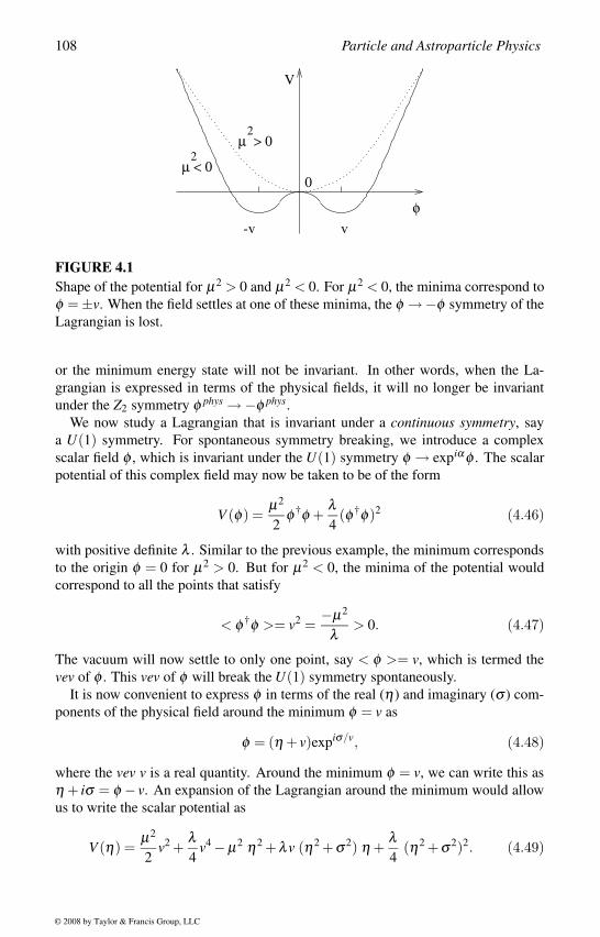
108 Particle and Astroparticle Physics
v
V
φ
0
2
2µ < 0
µ > 0
-v
FIGURE 4.1Shape of the potential for µ2 > 0 and µ2 < 0. For µ2 < 0, the minima correspond to
φ =±v. When the field settles at one of these minima, the φ →−φ symmetry of the
Lagrangian is lost.
or the minimum energy state will not be invariant. In other words, when the La-
grangian is expressed in terms of the physical fields, it will no longer be invariant
under the Z2 symmetry φ phys →−φ phys.
We now study a Lagrangian that is invariant under a continuous symmetry, say
a U(1) symmetry. For spontaneous symmetry breaking, we introduce a complex
scalar field φ , which is invariant under the U(1) symmetry φ → expiα φ . The scalar
potential of this complex field may now be taken to be of the form
V (φ) =µ2
2φ †φ +
λ4
(φ †φ)2 (4.46)
with positive definite λ . Similar to the previous example, the minimum corresponds
to the origin φ = 0 for µ2 > 0. But for µ2 < 0, the minima of the potential would
correspond to all the points that satisfy
< φ †φ >= v2 =−µ2
λ> 0. (4.47)
The vacuum will now settle to only one point, say < φ >= v, which is termed the
vev of φ . This vev of φ will break the U(1) symmetry spontaneously.
It is now convenient to express φ in terms of the real (η) and imaginary (σ ) com-
ponents of the physical field around the minimum φ = v as
φ = (η + v)expiσ/v, (4.48)
where the vev v is a real quantity. Around the minimum φ = v, we can write this as
η + iσ = φ − v. An expansion of the Lagrangian around the minimum would allow
us to write the scalar potential as
V (η) =µ2
2v2 +
λ4
v4 −µ2 η2 +λv (η2 +σ 2) η +λ4
(η2 +σ 2)2. (4.49)
© 2008 by Taylor & Francis Group, LLC
Symmetries in Nature 109
The U(1) symmetry η → expiα η is then spontaneously broken by the physical field.
One important feature of the spontaneous symmetry breaking is that the field σ re-
mains massless and is called the Nambu–Goldstone boson [24] or the Goldstoneboson. In case of µ2 > 0, the minimum is at φ = 0 and the mass term reads
µ2
2φ †φ =
µ2
2[(Re φ)2 +(Im φ)2],
and hence, both Re φ and Im φ have the same mass. But for µ2 < 0, the mass term
φ †φ can never include the field σ , and hence, it remains massless. It is also clear
from these discussions that the Nambu–Goldstone boson can have only derivative
couplings.
When the original theory is non-Abelian, the residual symmetry after spontaneous
symmetry breaking will be determined by the representation to which the scalar field
belongs and which component of the scalar field acquires a vev. Consider an SU(3)gauge symmetry, in which the scalar field that acquires a vev belongs to the funda-
mental triplet representation. If the third component of the triplet Higgs (T ) acquires
a vev
v =<
0
0
T3
>, (4.50)
the vacuum will not be able to distinguish between the states 1 and 2 even after the
symmetry breaking, although it distinguishes the third state from others. As a result,
the SU(2) subgroup (whose fundamental representation contains the states 1 and 2)
still remains unbroken, although the SU(3) symmetry of the Lagrangian is now bro-
ken. Out of the 8 generators of the SU(3) group λ i, i = 1, . . . ,8, the first three gener-
ators λ i =(
σi 0
0 0
), i = 1,2,3 correspond to the residual symmetry group SU(2).
Corresponding to the remaining five generators λ 4,5,6,7,8, there will be 5 Nambu–
Goldstone bosons. The triplet complex scalar field T has six real components, out of
which one will remain as the physical field η
T =
0
0
η + v
,
while all other 5 real components will become Nambu–Goldstone bosons.
This is a generic feature of any global symmetry breaking that gives rise to mass-
less Nambu–Goldstone bosons. Consider any theory with a global symmetry G1,
which is generated by N1 generators. Let this theory be spontaneously broken, and
after symmetry breaking the theory remains invariant under a global symmetry G2,
which is generated by N2 generators. Then there will be N1 −N2 Nambu–Goldstone
bosons.
Massless Nambu–Goldstone bosons could be a problem for some theories from
phenomenological considerations, particularly since it would imply a long range
force in classical physics. However, their spin dependence would make detection
© 2008 by Taylor & Francis Group, LLC
110 Particle and Astroparticle Physics
very difficult [25], and they can solve some other problems. A very special and inter-
esting case corresponds to models with pseudo-Nambu–Goldstone bosons (pNGB),
when the Nambu–Goldstone bosons receive a tiny but calculable mass.
Let us consider a model with global symmetry G , (i.e., the Lagrangian is invariant
under G ). If we now introduce a new interaction term in the Lagrangian, which
breaks this symmetry G explicitly, then that term will make the Nambu–Goldstone
boson massive. To see this, consider an example of a model with a scalar field φ and a
U(1) global symmetry φ → expiα φ . The scalar potential is given by equation (4.46).
If µ2 < 0, then the U(1) symmetry will be spontaneously broken and there will be a
massless Nambu–Goldstone boson, which is the imaginary part of the physical field.
If we now introduce an explicit symmetry breaking term
m2(φφ +φ ∗φ ∗),
then the Nambu–Goldstone boson will no longer remain massless even for µ 2 < 0.
We can expand the field φ around its vev 〈φ〉 = v as
φ = (η + v)expiσ/v ≈ η + v+ iσ − σ2
2v,
and find the mass of σ that comes out to be m2. The field σ is now called a pseudo-
Nambu–Goldstone boson (pNGB). If the explicit symmetry breaking term has a di-
mension less than 4, then radiative corrections cannot destabilize any result that is
derived from the symmetry argument. For example the mass of the pNGB remains
finite. These are called soft symmetry breaking terms. On the other hand, if the
explicit symmetry breaking terms have dimension 4, then they introduce infinite ra-
diative corrections to the mass of the pNGB and destabilize the theory.
Soft symmetry breaking terms appear in many models of particle physics. They
may have origin in some higher symmetric theory. For example, any spontaneous
gauge symmetry breaking can give rise to some soft terms. The advantage with the
soft terms is that they do not introduce new divergences in the theory, and hence,
the renormalizability of the original theory is not jeopardized. Any term in the
Lagrangian with coefficients having mass dimension is a soft term. For example,
m2φ †1 φ2 and mψψ are soft terms, but ψψφ and φ 4 are not soft terms, since the mass-
dimension of the scalar fields is 1 while the mass-dimension of the fermion fields is
3/2.
In case of local symmetry, the spontaneous symmetry breaking plays a different
role. When any local symmetry is broken spontaneously by the vev of a scalar field,
the Nambu–Goldstone boson no longer remain massless. One of the massless gauge
bosons of the symmetric theory makes the Nambu–Goldstone boson its longitudinal
mode and becomes massive [26]. Thus, the massless gauge bosons of the symmetric
theory can become massive during any spontaneous symmetry breaking. Since the
starting Lagrangian is invariant under the local symmetry, the theory remains renor-
malizable even after spontaneous symmetry breaking. From the name of one of the
inventors, the scalar field that breaks the symmetry is called a Higgs scalar [27].
© 2008 by Taylor & Francis Group, LLC
Symmetries in Nature 111
4.4 Local SymmetriesWhen a symmetry transformation depends on the space–time position, it is called
a local symmetry and the theory is called a gauge theory. Since a particle at one
point transforms in a different way in comparison with another particle located at a
different point, a new gauge particle is introduced to make the theory invariant under
the local symmetry transformation. Lorentz invariance requires this particle to have
spin-1 and this vector particle is called a gauge boson.
If the local symmetry is generated by n generators, there will be n gauge bosons.
If the different generators commute with each other, it is called an Abelian gauge
theory. When the generators of the local symmetry do not commute with each other,
it is called a non-Abelian gauge theory. All gauge theories are renormalizable and
the gauge bosons are massless. As a result the range of these interactions is extended
to infinity. When a gauge theory is spontaneously broken by the vacuum expectation
value of a Higgs scalar, whose minimum energy state does not respect the symme-
try although the Lagrangian is still symmetric, the theory remains renormalizable
although the gauge bosons become massive. The renormalizability of the gauge the-
ory or the spontaneously broken gauge theory makes these theories predictable, since
the parameters of these theories are finite and calculable and, hence, can be compared
with experiments. Although these theories are consistent classically, consistency of
these theories at the quantum level requires that these theories should be free from
anomalies [28]. Anomalies are one-loop diagrams with fermions in the loop and
gauge bosons attached at the vertices. In four dimensions, an anomaly is a triangle
diagram and it depends on the fermion contents of the theory. As a result, appropriate
choice of the fermion representations allows us to make a theory anomaly free. The
strong, weak and electromagnetic interactions can be explained by renormalizable
spontaneously broken gauge theories.
Abelian Gauge Theory
An Abelian gauge theory is invariant under a local symmetry transformation gener-
ated by Abelian or commuting generators. The interactions among the fermions and
scalars are mediated by massless gauge bosons in this theory. There are as many
gauge bosons as the number of generators of the local symmetry group. Consider a
local symmetry transformation,
ψ ′i (x) = exp−igOα(x)ψi(x), (4.51)
where α(x) depends on the space–time coordinate x, g sets the unit of the charge,
and the operator O gives the quantum number in units of g (i.e., Oψi = qiψi). Since
the fields ψ(x1) and ψ(x2) will have different transformations, the invariance of the
theory would require gauge fields that can communicate between these two points x1and x2.
© 2008 by Taylor & Francis Group, LLC
112 Particle and Astroparticle Physics
As an example, let us start with the Lagrangian density for the fermion field ψi:
L (ψ,∂ψ) = i∑i
ψiγµ ∂µ ψi +∑i, j
mi jψiψ j. (4.52)
We assume the condition mi j = 0 for i = j, which will guarantee that the system is
invariant under the transformation generated by O . The Lagrangian transforms as
L O−→ L ′ = i∑i
ψiγµ ∂µ ψi +gO∂µ α(x)∑i
ψiγµ ∂µ ψi +∑i
miiψiψi. (4.53)
This Lagrangian is not invariant under the transformation generated by O , since
∂µ α(x) does not vanish. To compensate for this additional contribution, we introduce
a new vector field Aµ , which transforms as
Aµ(x) O−→ A′µ(x) = Aµ(x)+∂µ α(x). (4.54)
We can then define an invariant derivative,
Dµ ψi(x) =[∂µ + igOAµ(x)
]ψi(x), (4.55)
so i∑i ψiγµ Dµ ψi transforms to itself. If we now replace the ordinary derivatives
from all the terms with the invariant derivative, the Lagrangian becomes invariant.
Since the derivative of the wave function (∂ψi) corresponds to the change in the wave
function at two different space–time points, the introduction of the gauge field (Aµ )
implies that this gauge field carries this information about the gauge transformation
from one point to the other. In other words, when two fields are transformed at two
different points, the gauge fields carry this information from one particle to the other
and compensate the difference, making the theory invariant under this transforma-
tion. Since the gauge fields convey this information to all points including the points
at infinity, this field cannot have any mass. From the transformations of the gauge
fields it is also possible to verify that the mass term m2Aµ Aµ for this field is not
invariant under the gauge symmetry. Thus, in all unbroken gauge theories, gauge
bosons are massless.
The gauge invariance will allow those terms in the Lagrangian that are invariant
under the gauge transformation. The final gauge invariant Lagrangian includes the
kinetic energy term for the gauge fields, making the gauge field a dynamical variable
and is given by
L = i∑i
ψiγµ Dµ ψi +∑i
miiψiψi − 1
4Fµν Fµν . (4.56)
The field–strength tensor is defined by
Fµν = ∂µ Aν −∂ν Aµ , (4.57)
which satisfies the equation of motion
Dµ Fµν = jν (4.58)
© 2008 by Taylor & Francis Group, LLC
Symmetries in Nature 113
and the identity
Dµ Fνλ +Dν Fλ µ +Dλ Fµν = 0, (4.59)
with the external current jν satisfying Dµ jµ = 0.
The simplest and most common gauge theory is the quantum electrodynamics
(QED). It is an Abelian U(1) gauge theory with only one generator O . In this case
|g|= e is the charge of the electron, and O acting on the wave function of any particle
gives the charge of the particle. Aµ is the usual four-vector potential and Fµν is the
field–strength tensor. The field equations and the identity give the four Maxwell
equations. There is only one gauge boson corresponding to the generator of the
theory, which is the massless photon.
Non-Abelian Gauge Theory
In a non-Abelian gauge theory the symmetry is generated by more than one gen-
erator, which do not commute with each other [30]. The operators generating the
symmetry are now associated with the generators of a non-Abelian group. Consider
a non-Abelian group SU(2), generated by the three Pauli matrices τi, i = 1,2,3, sat-
isfying
[τi,τ j] = iεi jkτk, (4.60)
where εi jk is the Levi–Civita symbol (+1 for even permutation of 123; −1 for odd
permutation; 0 if any two indices are the same). Let the particles u and d belong to
the two-dimensional fundamental representation of the group
Ψ =(
ud
),
and the state vector transform as
Ψ ≡(
ud
)→ exp−igτiαi(x)
(ud
). (4.61)
It is now convenient to write the generators of the group in the Cartan–Weyl basis
[τ+,τ−,τ3], where τ± = τ1 ± iτ2 are the two raising and lowering generators, so the
covariant derivative may be defined as
Dµ = ∂µ + ig∑i
τiAiµ = ∂µ + ig(τ+A+
µ + τ−A−µ + τ3A0
µ), (4.62)
where we define A±µ = A1
µ ∓ iA2µ and A0
µ = A3µ . As with the Abelian gauge theory,
we now replace all derivatives with the covariant derivatives and can write the La-
grangian including the kinetic energy terms of the gauge fields as
L[Ψ,∂µ Ψ
]−→ L[Ψ,Dµ Ψ
]− 1
4Fµν iF i
µν , (4.63)
with the field–strength tensor
Fµν i = Dµ Aν i −Dν Aµi + iεi jkA jµ Ak
ν (4.64)
© 2008 by Taylor & Francis Group, LLC
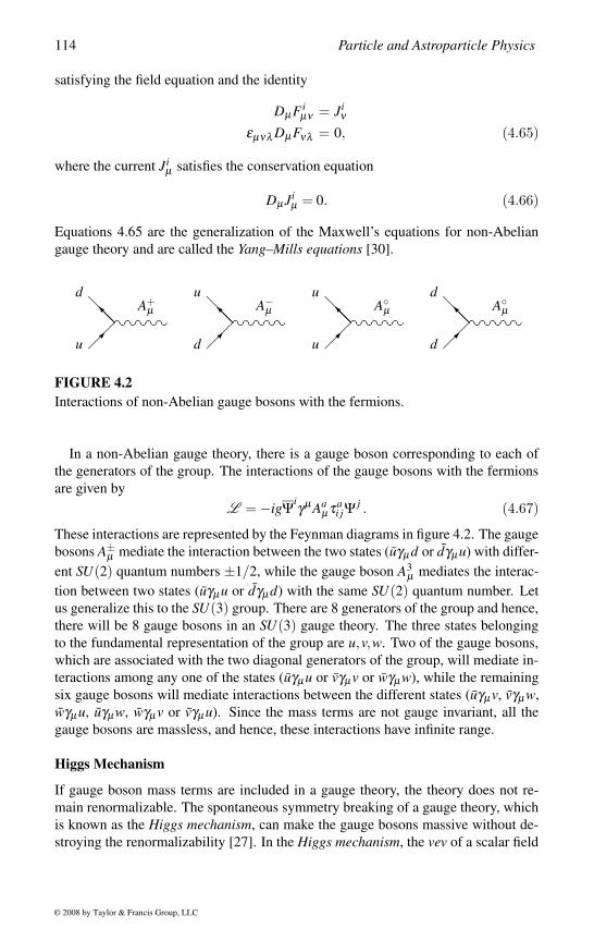
114 Particle and Astroparticle Physics
satisfying the field equation and the identity
Dµ F iµν = Ji
ν
εµνλ Dµ Fνλ = 0, (4.65)
where the current Jiµ satisfies the conservation equation
Dµ Jiµ = 0. (4.66)
Equations 4.65 are the generalization of the Maxwell’s equations for non-Abelian
gauge theory and are called the Yang–Mills equations [30].
d
u
A+µ
u
d
A−µ
u
u
Aµ
d
d
Aµ
FIGURE 4.2Interactions of non-Abelian gauge bosons with the fermions.
In a non-Abelian gauge theory, there is a gauge boson corresponding to each of
the generators of the group. The interactions of the gauge bosons with the fermions
are given by
L = −igΨiγµ Aaµ τa
i jΨj . (4.67)
These interactions are represented by the Feynman diagrams in figure 4.2. The gauge
bosons A±µ mediate the interaction between the two states (uγµ d or dγµ u) with differ-
ent SU(2) quantum numbers ±1/2, while the gauge boson A3µ mediates the interac-
tion between two states (uγµ u or dγµ d) with the same SU(2) quantum number. Let
us generalize this to the SU(3) group. There are 8 generators of the group and hence,
there will be 8 gauge bosons in an SU(3) gauge theory. The three states belonging
to the fundamental representation of the group are u,v,w. Two of the gauge bosons,
which are associated with the two diagonal generators of the group, will mediate in-
teractions among any one of the states (uγµ u or vγµ v or wγµ w), while the remaining
six gauge bosons will mediate interactions between the different states (uγµ v, vγµ w,
wγµ u, uγµ w, wγµ v or vγµ u). Since the mass terms are not gauge invariant, all the
gauge bosons are massless, and hence, these interactions have infinite range.
Higgs Mechanism
If gauge boson mass terms are included in a gauge theory, the theory does not re-
main renormalizable. The spontaneous symmetry breaking of a gauge theory, which
is known as the Higgs mechanism, can make the gauge bosons massive without de-
stroying the renormalizability [27]. In the Higgs mechanism, the vev of a scalar field
© 2008 by Taylor & Francis Group, LLC
Symmetries in Nature 115
breaks the gauge symmetry spontaneously. Although the interactions of the Higgs
scalar are invariant under the gauge symmetry, the minimum of the scalar potential
does not respect the gauge symmetry. Since the Lagrangian is gauge invariant, the
theory remains renormalizable, but the vacuum breaks the gauge symmetry allowing
a mass term for the gauge boson.
We shall consider a U(1) gauge theory, in which the fermion ψ transforms locally
as
ψ(x) → ψ ′(x) = exp−igOq(x)ψ(x).
The corresponding Lagrangian will be given by
L = iψγµ Dµ ψ +mψψ − 1
4Fµν Fµν , (4.68)
where
Dµ = ∂µ + igOAµ(x)
is the covariant derivative and
Fµν = ∂µ Aν −∂ν Aµ
is the field–strength tensor that satisfies the equation of motion
∂µ Fµν = jν .
The mass term for the gauge boson Aµ is not allowed by the gauge symmetry; hence,
it remains massless and hence the range of this interaction is infinity.
We now introduce a scalar field in the theory φ(x) that transforms as
φ(x) → φ ′(x) = exp−igOq(x)φ(x).
The gauge invariant Lagrangian is given by
L (φ) = Dµ φ †(x)Dµ φ(x)− 1
2µ2φ †φ − 1
4λ (φ †φ)2. (4.69)
When µ2 < 0, the scalar potential will have a continuum of minima satisfying
〈φ †φ〉 = v2 = −µ2/λ > 0.
The vacuum will pick up any one of these minima and the field will acquire a vev〈φ〉 = v. If we now expand the physical field η around the vev of the scalar field v
φ = (η + v)expiσ/v,
the kinetic energy term for the scalar field will contain a mass term for the gauge
boson,
g2v2Aµ Aµ ⊂ Dµ φ †Dµ φ .
© 2008 by Taylor & Francis Group, LLC
116 Particle and Astroparticle Physics
Unlike the case of spontaneous global symmetry breaking, in this case there is no
physical Nambu–Goldstone boson. The imaginary part of the scalar field (σ ) has
now become the longitudinal mode of the gauge boson Aµ .
In case of non-Abelian gauge symmetry, it is possible to introduce the proper
Higgs scalar field with appropriate interactions, leaving a residual gauge symmetry
that we require after the spontaneous symmetry breaking. The gauge bosons corre-
sponding to the generators of the coset space of the original symmetry group and the
residual symmetry group will now become massive. In other words, if the original
theory has a symmetry G1 (with n1 generators), which breaks down to a lower sub-
group G2 ⊂ G1 (with n2 generators) by the vev of a scalar field φ , there will be n1−n2massive gauge bosons, while n2 number of gauge bosons will still remain massless.
Let us consider some examples of symmetry breaking. If we want to break an
SU(n) group to its subgroup SU(n−1), we should consider a scalar field belonging
to n representation of the group SU(n). The gauge bosons corresponding to the
coset space SU(n)/SU(n−1) will now become massive after the symmetry breaking.
When the vev of a scalar field belonging to the adjoint representation of the gauge
group induces the spontaneous symmetry breaking, the rank of the residual gauge
group is not changed. If we start with an SU(n) gauge group, the residual group
will be SU(n−1)×U(1) or SU(n−m)×SU(m)×U(1). For example, a scalar field
φ belonging to the adjoint representation of the group SU(5) can break the SU(5)symmetry into its subgroup
SU(5) → SU(4)×U(1) or SU(5) → SU(3)×SU(2)×U(1)
if the vev of the scalar field is of the form
〈φ〉 =
1 0 0 0 0
0 1 0 0 0
0 0 1 0 0
0 0 0 1 0
0 0 0 0 −4
or
1 0 0 0 0
0 1 0 0 0
0 0 1 0 0
0 0 0 − 32 0
0 0 0 0 − 32
,
respectively. Depending on the components of the scalar fields, the phenomenology
of the spontaneous symmetry breaking may also change. In the case of electroweak
symmetry breaking, if the symmetry breaking is done only by a triplet Higgs scalar,
the ρ parameter will not be consistent. It is also possible to put constraint on the
mass of the triplet Higgs scalar from such consideration.
Anomalies
An anomaly is a quantum effect that breaks the classical symmetry of any theory. In
the language of field theory, anomalies are loop diagrams with infinite contributions
so the renormalizability of the theory is lost. Consider a chiral gauge theory, in
which the bare mass terms of any fermions are prevented and, hence, axial currents
are conserved. In any chiral gauge theories, there are divergent one-loop triangle
diagrams (see figure 4.3), which are divergent and are known as Adler–Bardeen–
Jackiw anomalies [28]. The anomaly diagrams involve fermions in the triangle loop.
© 2008 by Taylor & Francis Group, LLC
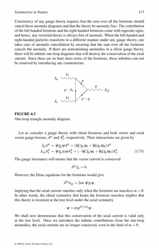
Symmetries in Nature 117
Consistency of any gauge theory requires that the sum over all the fermions should
cancel these anomaly diagrams and that the theory be anomaly free. The contribution
of the left-handed fermions and the right-handed fermions come with opposite signs,
and hence, any vectorial theory is always free of anomaly. When the left-handed and
right-handed particles transform in a different manner under any gauge theory, one
takes care of anomaly cancellation by ensuring that the sum over all the fermions
cancels the anomaly. If there are nonvanishing anomalies in a chiral gauge theory,
there will be infinite one-loop diagrams that will destroy the conservation of the axial
current. Since there are no bare mass terms of the fermions, these infinities can not
be removed by introducing any counterterms.
Jν
Jµ
J5λ
k2
k1
qp− k1
p−q
p
FIGURE 4.3One-loop triangle anomaly diagram.
Let us consider a gauge theory with chiral fermions and both vector and axial
vector gauge bosons, Aµ and Aµ5 , respectively. Their interactions are given by
Jµ Aµ = ψγµ ψAµ = (ψLγµ ψL +ψRγµ ψR)Aµ
J5µ Aµ5 = ψγµ γ5ψAµ
5 = (−ψLγµ ψL +ψRγµ ψR)Aµ5 . (4.70)
The gauge invariance will ensure that the vector current is conserved
∂ µ Jµ = 0.
However, the Dirac equations for the fermions would give
∂ µ J5µ = 2im ψγ5ψ,
implying that the axial current vanishes only when the fermions are massless m = 0.
In other words, the chiral symmetry that keeps the fermions massless implies that
this theory is invariant at the tree level under the axial symmetry
ψ = expiε(x)γ5ψ.
We shall now demonstrate that this conservation of the axial current is valid only
at the tree level. Once we introduce the infinite contributions from the one-loop
anomalies, the axial currents are no longer conserved, even in the limit of m = 0.
© 2008 by Taylor & Francis Group, LLC
118 Particle and Astroparticle Physics
The matrix element for the one-loop triangle anomaly diagram of figure 4.3 is
given by
Tµνλ (k1,k2,q) = −∫ d4 p
(2π)4 Tr
[i
/p−mγλ γ5
i/p− /q−m
γνi
/p− /k1 −mγµ
]+[k1 ↔ k2; µ ↔ ν ] . (4.71)
Simple power counting would tell us that the integral is linearly divergent. This will
complicate certain manipulation of the integral. For example, usually any shift of
variables x+a → x does not modify an integral:
I(a) =∫ +∞
−∞dx [ f (x+a)− f (x)] = 0 . (4.72)
However, when the integral diverges linearly, this difference does not vanish and
instead it is given by
I(a) =∫ +∞
−∞dx[
a f ′(x)+a2
2f ′′(x)+ · · ·
]= a [ f (∞)− f (−∞)]+ · · · . (4.73)
We shall now calculate certain identities without including the I(a) contributions due
to the shift in the variables of integration, and then see how the results are modified
by including these infinities.
Starting from the matrix element for the anomaly, it is possible to derive the Ward
identities
kµ1 Tµνλ = 0
kν2 Tµνλ = 0
qλ Tµνλ = 2 m Tµν , (4.74)
where
Tµν(k1,k2,q) = −∫ d4 p
(2π)4 Tr
[i
/p−mγ5
i/p− /q−m
γνi
/p− /k1 −mγµ
]+[k1 ↔ k2; µ ↔ ν ] . (4.75)
We make use of the identities
/ki = (/p−m)− (/p− /ki −m) = (/p+ /ki −m)− (/p−m) (i = 1,2)/qγ5 = (/p−m)γ5 − (/p− /q−m)γ5 = (/p−m)γ5 − γ5(/p− /q−m)−2mγ5 (4.76)
and shift the variables of integration from (/p− /k1) →/p or (/p− /q) to arrive at the Ward
identities.
It is possible to take care of the infinities in any of the standard ways. In the
Pauli–Villars method, the infinite integrals I(a) are regularized by subtracting similar
© 2008 by Taylor & Francis Group, LLC
Symmetries in Nature 119
integrals with very large fermion mass M and then taking the limit M → ∞. In the
Ward identity, this prescription modifies to
2 m Tµν(m) → 2 M Tµν(M).
Tµν(M) can now be evaluated by ignoring k1 and k2 in the integrand, and finally we
obtain the anomaly in the axial vector current
qλ Tµνλ = 2 m Tµν − 1
2π2 εµνρσ kρ1 kσ
2 . (4.77)
In the coordinate space the axial vector anomaly is expressed as
∂ µ J5µ = 2i m ψγ5ψ +g2
8π2 Fµν Fµν , (4.78)
where Fµν = 12 εµνρσ Fρσ and g is the gauge coupling constant. There is no contri-
bution from anomaly to the vector currents.
The anomalies make any theory nonrenormalizable and, hence, unpredictable.
Thus, any consistent gauge theory must be free of all anomalies. If fermions couple
to the gauge fields through the current
Jaµ = ψRγµ T a
R ψR + ψLγµ T aL ψL ,
where T a defines the matrix representations for the fermions, then every fermion will
be associated with a group factor
A = Tr[(T a
L T bL +T b
L T aL )T c
L − (T aR T b
R +T bR T a
R )T cR
]. (4.79)
The trace is over all the fermions in each representations. The condition for cancel-
lation of anomalies is then given by
∑A = 0,
where the sum is extended over all fermion representations, since anomalies do not
depend on the masses of the fermions.
We now present a simple algorithm to calculate anomalies in 4 and higher dimen-
sions [29]. If the fermions belong to a representation Rr of G in 4 dimensions, the
group factor contributing to the triangle anomaly will be
3A = tr [T a(Rr)T b(Rr)T c(Rr)], (4.80)
where T a(R1) are the generators of the representation. In 2d dimensions, the anomaly
will have n fermions in the loop, where n = d +1, so we need to calculate an anomaly
nA = tr [T a1(Rr)T a2(Rr) · · · T an(Rr)].
In odd dimensions, there is no anomaly, since there are no chiral fermions. For some
representations in higher dimensions, there are additional factorized contributions of
© 2008 by Taylor & Francis Group, LLC
120 Particle and Astroparticle Physics
the form(tr [T a1(Rr)T a2(Rr) · · ·]
)2, but we shall not discuss these reducible group
factors separately.
Consider the subgroup G1 ×G2 ⊂ G , where G2 = U(1) is an Abelian subgroup of
G . We can then decompose any representations of G under G1 ×G2 subgroup as
R = ∑i(ri, fi) , (4.81)
where fi represents the G2 ≡U(1) quantum numbers. fi is normalized so the anomaly
for the fundamental representation of any group is 1. The decomposition of the fun-
damental m-dimensional representation of SU(m) under SU(m−1)×U(1) will then
become m = (m− 1,1)+ (1,−m + 1). The product decomposition rules then give
the decompositions of the other representations.
We can then use the formulas
3A (R) = ∑i
λ (ri) · fi 4A (R) = ∑i
3A (ri) · fi
nA (R) = ∑i
(n−1)A (ri) · fi (4.82)
to calculate the anomalies for the representation R of the group G in terms of the
invariants of the subgroup G1 ×G2. Here λ (ri) is the index for the representation riof G1 (discussed in section 3.4). For verification of the calculated anomaly, one can
use the relation
nA (R) = ∑i
nA (ri). (4.83)
For completeness we also present a couple of useful relations
nA (R1 +R2) = nA (R1)+ nA (R2)
nA (R1 ×R2) = nA (R1)D(R2)+ nA (R2)D(R1). (4.84)
Thus, by writing the decomposition of any representation under its subgroup contain-
ing a properly normalized U(1) factor, it will be possible to calculate the irreducible
group factor entering into the expression for anomalies.
As an example, let us calculate the anomaly of 6-dimensional representation of
the group SU(3), which decomposes under SU(2)×U(1) as 6 = (3,2)+ (1,−4)+(2,−1). Then the required anomaly will be 3A (6) = λ (3) ·2+λ (2) · (−1) = 7. For
the cancellation of anomalies in any theory, we require only this factor, and hence,
these results will be extremely useful while building models in many extensions of
the standard model.
© 2008 by Taylor & Francis Group, LLC
5The Standard Model
The standard model of particle physics is the theory of the strong, the electromag-
netic and the weak interactions. The strong interaction is the interaction among the
quarks of different colors (there are three colors) and flavors (six flavors u,c, t,d,s,b),
and they are mediated by eight gluons. It is an SU(3) gauge theory, called quantum
chromodynamics (QCD), and the three colored states of every flavor belong to the
triplet representation of the SU(3)c. The gluons are the eight gauge bosons corre-
sponding to the generators of the group SU(3)c. Colored states are confined, and
hence, only color singlet states can exist in nature as free particles. Known color sin-
glet states are baryons (made of three quarks) or mesons (made of quark–antiquark
pairs). The strong nuclear force is the force between the protons and neutrons, which
is a manifestation of the underlying SU(3)c interactions among the quarks, although
with our present knowledge of the many-body problem it is almost impossible to
derive the nuclear potential starting from QCD without any assumption.
Interactions of charged particles are governed by electromagnetic interaction. It
is described by quantum electrodynamics (QED), which is a U(1)Q gauge theory,
where Q corresponds to the electric charge. Electromagnetic interaction is mediated
by the photon, which is the gauge boson corresponding to the generator of the U(1)Qgroup.
The weak interaction describes nuclear beta decay, and at low energy it is given
by an effective four fermion interaction. Since the effective operator has dimension
6, the coupling constant has inverse mass-squared dimension. This effective theory
fails at higher energies but is found to emerge from another renormalizable theory,
the electroweak interaction, which unifies both the weak and the electromagnetic
interactions.
The electroweak theory is described by an SU(2)L ×U(1)Y interaction, which is
spontaneously broken down to U(1)Q at around 100 GeV. The spontaneous symme-
try breaking makes three of the gauge bosons W±,Z heavy, leaving only one gauge
boson massless, which is the photon. Since the W±,Z bosons are massive, at low en-
ergies they appear as internal propagators in the effective four fermion interactions.
Under the SU(2)L group, the left-handed quarks and leptons are doublets, while the
right-handed fields are singlets. Thus, the mass terms for the fermions are forbidden
before the electroweak symmetry breaking. However, after the electroweak phase
transition, the vevs of the Higgs scalar that breaks the electroweak symmetry give
masses to the quarks and leptons. The problem of neutrino mass is somewhat differ-
ent, which we shall discuss in the next chapter. With this introduction we shall now
describe the standard model.
121
© 2008 by Taylor & Francis Group, LLC
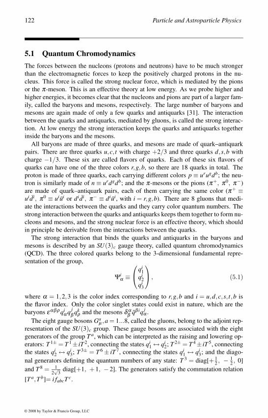
122 Particle and Astroparticle Physics
5.1 Quantum ChromodynamicsThe forces between the nucleons (protons and neutrons) have to be much stronger
than the electromagnetic forces to keep the positively charged protons in the nu-
cleus. This force is called the strong nuclear force, which is mediated by the pions
or the π-meson. This is an effective theory at low energy. As we probe higher and
higher energies, it becomes clear that the nucleons and pions are part of a larger fam-
ily, called the baryons and mesons, respectively. The large number of baryons and
mesons are again made of only a few quarks and antiquarks [31]. The interaction
between the quarks and antiquarks, mediated by gluons, is called the strong interac-
tion. At low energy the strong interaction keeps the quarks and antiquarks together
inside the baryons and the mesons.
All baryons are made of three quarks, and mesons are made of quark–antiquark
pairs. There are three quarks u,c, t with charge +2/3 and three quarks d,s,b with
charge −1/3. These six are called flavors of quarks. Each of these six flavors of
quarks can have one of the three colors r,g,b, so there are 18 quarks in total. The
proton is made of three quarks, each carrying different colors p ≡ urugdb; the neu-
tron is similarly made of n ≡ urdgdb; and the π-mesons or the pions (π+, π0, π−)
are made of quark–antiquark pairs, each of them carrying the same color (π+ ≡uidi, π0 ≡ uiui or didi, π− ≡ diui, with i = r,g,b). There are 8 gluons that medi-
ate the interactions between the quarks and they carry color quantum numbers. The
strong interaction between the quarks and antiquarks keeps them together to form nu-
cleons and mesons, and the strong nuclear force is an effective theory, which should
in principle be derivable from the interactions between the quarks.
The strong interaction that binds the quarks and antiquarks in the baryons and
mesons is described by an SU(3)c gauge theory, called quantum chromodynamics
(QCD). The three colored quarks belong to the 3-dimensional fundamental repre-
sentation of the group,
Ψiα ≡
qi1
qi2
qi3
, (5.1)
where α = 1,2,3 is the color index corresponding to r,g,b and i = u,d,c,s, t,b is
the flavor index. Only the color singlet states could exist in nature, which are the
baryons εαβρ qiα q j
β qkρ and the mesons δ α
β qβ iq jα .
The eight gauge bosons Gaµ ,a = 1...8, called the gluons, belong to the adjoint rep-
resentation of the SU(3)c group. These gauge bosons are associated with the eight
generators of the group T a, which can be interpreted as the raising and lowering op-
erators: T 1± = T 1± iT 2, connecting the states qi1 ↔ qi
2; T 2± = T 4± iT 5, connecting
the states qi2 ↔ qi
3; T 3± = T 6 ± iT 7, connecting the states qi1 ↔ qi
3; and the diago-
nal generators defining the quantum numbers of any state: T 3 = diag[+ 12 , − 1
2 , 0]
and T 8 = 12√
3diag[+1, +1, −2]. The generators satisfy the commutation relation
[T a,T b]= i fabcT c.
© 2008 by Taylor & Francis Group, LLC
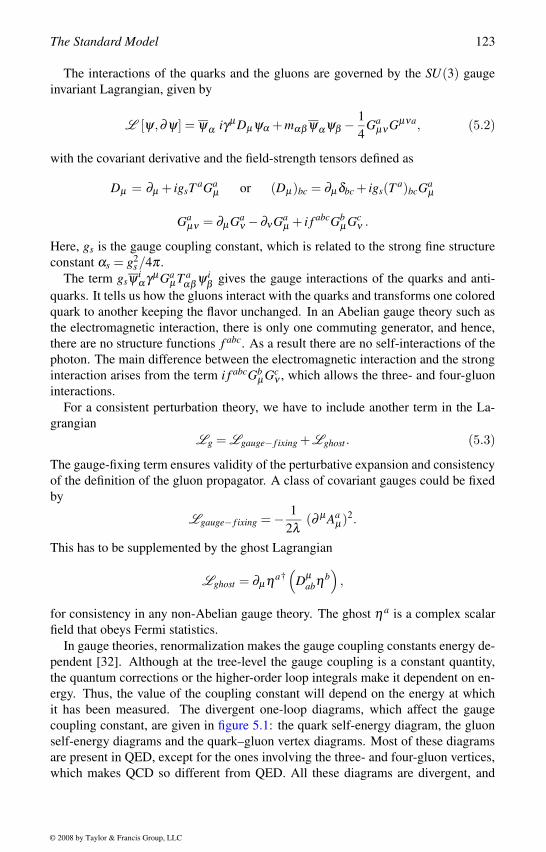
The Standard Model 123
The interactions of the quarks and the gluons are governed by the SU(3) gauge
invariant Lagrangian, given by
L [ψ,∂ψ] = ψα iγµ Dµ ψα +mαβ ψα ψβ − 1
4Ga
µν Gµνa, (5.2)
with the covariant derivative and the field-strength tensors defined as
Dµ = ∂µ + igsT aGaµ or (Dµ)bc = ∂µ δbc + igs(T a)bcGa
µ
Gaµν = ∂µ Ga
ν −∂ν Gaµ + i f abcGb
µ Gcν .
Here, gs is the gauge coupling constant, which is related to the strong fine structure
constant αs = g2s /4π .
The term gsψ iα γµ Ga
µ T aαβ ψ i
β gives the gauge interactions of the quarks and anti-
quarks. It tells us how the gluons interact with the quarks and transforms one colored
quark to another keeping the flavor unchanged. In an Abelian gauge theory such as
the electromagnetic interaction, there is only one commuting generator, and hence,
there are no structure functions f abc. As a result there are no self-interactions of the
photon. The main difference between the electromagnetic interaction and the strong
interaction arises from the term i f abcGbµ Gc
ν , which allows the three- and four-gluon
interactions.
For a consistent perturbation theory, we have to include another term in the La-
grangian
Lg = Lgauge− f ixing +Lghost . (5.3)
The gauge-fixing term ensures validity of the perturbative expansion and consistency
of the definition of the gluon propagator. A class of covariant gauges could be fixed
by
Lgauge− f ixing = − 1
2λ(∂ µ Aa
µ)2.
This has to be supplemented by the ghost Lagrangian
Lghost = ∂µ ηa†(
Dµabηb
),
for consistency in any non-Abelian gauge theory. The ghost η a is a complex scalar
field that obeys Fermi statistics.
In gauge theories, renormalization makes the gauge coupling constants energy de-
pendent [32]. Although at the tree-level the gauge coupling is a constant quantity,
the quantum corrections or the higher-order loop integrals make it dependent on en-
ergy. Thus, the value of the coupling constant will depend on the energy at which
it has been measured. The divergent one-loop diagrams, which affect the gauge
coupling constant, are given in figure 5.1: the quark self-energy diagram, the gluon
self-energy diagrams and the quark–gluon vertex diagrams. Most of these diagrams
are present in QED, except for the ones involving the three- and four-gluon vertices,
which makes QCD so different from QED. All these diagrams are divergent, and
© 2008 by Taylor & Francis Group, LLC
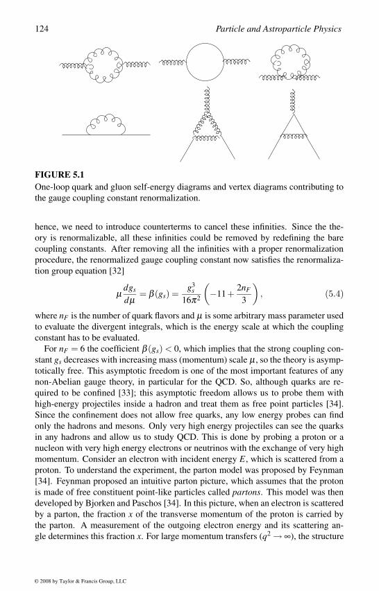
124 Particle and Astroparticle Physics
FIGURE 5.1One-loop quark and gluon self-energy diagrams and vertex diagrams contributing to
the gauge coupling constant renormalization.
hence, we need to introduce counterterms to cancel these infinities. Since the the-
ory is renormalizable, all these infinities could be removed by redefining the bare
coupling constants. After removing all the infinities with a proper renormalization
procedure, the renormalized gauge coupling constant now satisfies the renormaliza-
tion group equation [32]
µdgs
dµ= β (gs) =
g3s
16π2
(−11+
2nF
3
), (5.4)
where nF is the number of quark flavors and µ is some arbitrary mass parameter used
to evaluate the divergent integrals, which is the energy scale at which the coupling
constant has to be evaluated.
For nF = 6 the coefficient β (gs) < 0, which implies that the strong coupling con-
stant gs decreases with increasing mass (momentum) scale µ , so the theory is asymp-
totically free. This asymptotic freedom is one of the most important features of any
non-Abelian gauge theory, in particular for the QCD. So, although quarks are re-
quired to be confined [33]; this asymptotic freedom allows us to probe them with
high-energy projectiles inside a hadron and treat them as free point particles [34].
Since the confinement does not allow free quarks, any low energy probes can find
only the hadrons and mesons. Only very high energy projectiles can see the quarks
in any hadrons and allow us to study QCD. This is done by probing a proton or a
nucleon with very high energy electrons or neutrinos with the exchange of very high
momentum. Consider an electron with incident energy E, which is scattered from a
proton. To understand the experiment, the parton model was proposed by Feynman
[34]. Feynman proposed an intuitive parton picture, which assumes that the proton
is made of free constituent point-like particles called partons. This model was then
developed by Bjorken and Paschos [34]. In this picture, when an electron is scattered
by a parton, the fraction x of the transverse momentum of the proton is carried by
the parton. A measurement of the outgoing electron energy and its scattering an-
gle determines this fraction x. For large momentum transfers (q2 → ∞), the structure
© 2008 by Taylor & Francis Group, LLC
The Standard Model 125
functions of the proton become a scale-invariant function depending only on the frac-
tion x, which is given by the ratio x = (q2/2mE). This is known as Feynman scaling.
Further studies of this scaling phenomenon identified these partons as quarks.
At higher energies, the probing electrons scatter from the three valence quarks of
the proton, and also the sea quarks and the gluons. Quantum fluctuations will create
pairs of quarks and antiquarks and also gluons, which forms the sea of quarks and
antiquarks and the gluons. As the energy increases, more sea quark–antiquark pairs
are formed. These sea partons, coming from quantum corrections or higher order
effects, appear as a screening and lead to small scaling violation, which has also been
tested experimentally to a fairly good accuracy. In all experiments a large uncertainty
is introduced because of our lack of complete understanding of QCD. The formation
of hadrons, the confinement mechanism, and the scaling violation are among the
few less understood problems in QCD. There could also be some nonperturbative
effects introducing more complications. Thus, in many measurements the largest
uncertainty comes from hadronic corrections. Moreover, the theoretical calculations
of higher-order corrections are also very difficult.
5.2 V −A TheoryThe weak interaction has brought many surprises. The first one is the existence of
this interaction. If this interaction were not present at all, maybe nothing would have
changed at least at the macroscopic level. We can explain all matter around us and
their interactions in terms of the electromagnetic and the gravitational interactions,
and strong interaction explains why protons could stay together inside the nucleus in
spite of the electromagnetic repulsive force. The first evidence of weak interaction
appeared in the beta decay, in which a neutron converts into a proton and an electron
is emitted – a simple, but fairly puzzling, process. A neutrino associated with this
decay was postulated, but the neutrino was discovered much later. The mass of the
neutrinos was discovered after more than sixty years. We still do not know if the
neutrinos are Dirac or Majorana particles.
In the beginning the weak interaction could be explained by an effective four-
point interaction at low energies [35]. It was not a renormalizable theory. Consider
for example, the neutron decay n → p + e− + νe. Fermi generalized the concept of
electrodynamics to explain this interaction. In the coupling of a vector current to the
radiation field, Ψγµ ΨAµ , the 4-vector potential of the radiation field Aµ is replaced
by another vector current. This leads to Fermi’s β decay Lagrangian for an effective
four-fermion interaction
Lβ =GF√
2[Ψpγµ Ψn] [Ψeγµ Ψν ]. (5.5)
Since this effective interaction has four fermions and mass dimension six, the ef-
© 2008 by Taylor & Francis Group, LLC
126 Particle and Astroparticle Physics
fective coupling has an inverse mass-squared dimension and it is determined experi-
mentally to be GF = 1.17×10⁻⁵ GeV−2.
The four-fermion could explain many observed characteristics of the beta decay,
but some modifications were needed to explain several other weak interactions. For
this purpose this interaction was then generalized to include all possible forms of the
interactions,
Lβ =GF√
2∑
i=S,P,V,A,TCi[ΨpΓiΨn] [ΨeΓiΨν ]. (5.6)
The interactions could now be scalar (S, Γi = 1), pseudo-scalar (P, Γi = γ5), vector (V,
Γi = γµ ), axial-vector (A, Γi = γµ γ5), or tensor (T, Γi = σµν ). The coupling constants
have to be determined from experiments. For example, for the Fermi transitions,
[∆J = 0], the interaction could be S or T , while for the Gamow–Teller transitions,
[∆J = 0, ± 1, but J = 0 −→/ J = 0], the interaction could be A or T . Although this
phenomenological Lagrangian could explain the nuclear beta decays at low energies,
this is far from the actual theory of the weak interaction.
The next major step in the history of weak interactions was the discovery of parity
nonconservation. The two particles τ and θ with the same mass, charge, spin (0) and
lifetime were found to decay into states with odd and even parity, respectively,
τ → π+π+π− and θ → π+π0.
This was known as the τ −θ puzzle. As an explanation to this puzzle the possibility
of parity nonconservation was suggested, so both particles (τ and θ ) could be iden-
tified as one particle K+ [36]. Possible tests of parity violation were also proposed
in other weak interactions. Soon parity violation was observed [37] through a mea-
surement of the asymmetry in the beta decay of the polarized 60Co nuclei and later
in π decays.
The parity violation would then require a pseudoscalar term in the four-fermion
Lagrangian of the form C′i [ΨΓiΨ] [ΨΓiγ5Ψ]. Including this parity violating term, the
Lagrangian can be written in the form
Lβ =GF√
2∑
i=S,P,V,A,T[ΨpΓiΨn] [ΨeΓi(Ci −C′
iγ5)Ψν ]. (5.7)
The coefficients Ci and C′i were determined through a series of observations and
analysis of different weak interaction processes. Finally the Lagrangian for the weak
interaction was given a simple form
Lβ =GF√
2[Ψpγµ(1−λγ5)Ψn] [Ψeγµ(1− γ5)Ψν ], (5.8)
where λ = 1.25 was determined experimentally. The deviation from 1 can be at-
tributed to strong interaction effects, and for the weak interactions, a V −A form of
the interaction was established [38].
The V −A theory [38] could successfully explain all weak interactions. All charged
processes such as beta decay, muon decay or charged pion decay could be explained
© 2008 by Taylor & Francis Group, LLC
The Standard Model 127
in the V −A theory by an effective Lagrangian density in which a charged weak
current Jα is coupled to its Hermitian conjugate at a single point,
Lβ = − GF
2√
2[Jα Jα † + Jα †Jα ]. (5.9)
The charged weak current is universal in nature and contains two parts,
Jα = Jα + Jqα ,
where the leptonic part contains interactions among the leptons
Jα = Ψeγα(1− γ5)Ψνe + Ψµ γα(1− γ5)Ψνµ + Ψτ γα(1− γ5)Ψντ , (5.10)
and the hadronic part of the current contains the charged weak interactions among
the hadrons.
The weak hadronic interactions are also of the V −A form, except for the hadronic
corrections. The deviation from the V −A form due to the strong hadronic corrections
is parameterized by λ . The hadronic part of the beta decay includes conversion of a
neutron (udd) into a proton (uud), which is equivalent to a down-quark converting
into a up-quark, so the transition Ψpγα(1− γ5)Ψn can be equivalently written as
Ψuγα(1− γ5)Ψd . The charged weak hadronic current is then given by
Jqα = Ψdγα(1− γ5)Ψu + Ψsγα(1− γ5)Ψc + Ψbγα(1− γ5)Ψt . (5.11)
The states Ψd , Ψs and Ψb are admixtures of different mass eigenstates of d,s and b,
which will give rise to quark mixing. We shall come back to this discussion of quark
mixing later.
The V −A structure of the interaction implies that only the left-handed fermions
take part in the interaction, and hence, both the parity and the charge conjugation are
explicitly broken. This can be seen from
1
2Ψ1γα(1− γ5)Ψ2 =
(1− γ5)2
Ψ1γα (1− γ5)2
Ψ2 = Ψ1Lγα Ψ2L.
The CPT would imply that the Hermitian conjugate term will involve the CP conju-
gate states of the left-handed fermions (ΨL)c = (Ψc)R in the weak interactions, but
the right-handed fields ΨR and their charge conjugate states (ΨR)c = (Ψc)L should
not enter in the V −A theory.
Although the V − A theory was a highly successful, effective low-energy the-
ory, at higher energies the theory becomes inconsistent. Consider the νe + e− →νe + e− scattering, the V −A theory gives a differential cross-section (dσ/dΩ) =(G2
F/π2)ω2, where ω is the neutrino energy in the center of mass frame. How-
ever, if we expand the scattering amplitude in partial waves, f (θ) = ω−1 ∑∞J=0(J +
1/2)MJPJ(cosθ), then for the Fermi contact interaction of zero range, we obtain
the differential cross-section to be (dσ/dΩ) = (1/2ω)2|M0|2, where only the J =0 partial wave enters. Conservation of probability then gives the unitarity bound
© 2008 by Taylor & Francis Group, LLC
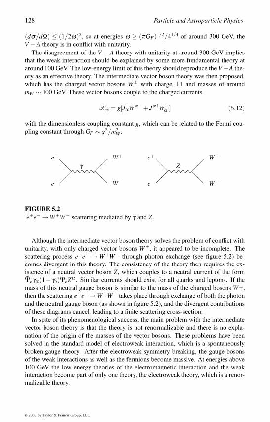
128 Particle and Astroparticle Physics
(dσ/dΩ) ≤ (1/2ω)2, so at energies ω ≥ (πGF)1/2/41/4 of around 300 GeV, the
V −A theory is in conflict with unitarity.
The disagreement of the V −A theory with unitarity at around 300 GeV implies
that the weak interaction should be explained by some more fundamental theory at
around 100 GeV. The low-energy limit of this theory should reproduce the V −A the-
ory as an effective theory. The intermediate vector boson theory was then proposed,
which has the charged vector bosons W± with charge ±1 and masses of around
mW ∼ 100 GeV. These vector bosons couple to the charged currents
Lcc = g[JαW α− + Jα †W+α ] (5.12)
with the dimensionless coupling constant g, which can be related to the Fermi cou-
pling constant through GF ∼ g2/m2W .
e+
e−
W+
W−
γ
e+
e−
W+
W−
Z
FIGURE 5.2e+e− →W+W− scattering mediated by γ and Z.
Although the intermediate vector boson theory solves the problem of conflict with
unitarity, with only charged vector bosons W±, it appeared to be incomplete. The
scattering process e+e− → W+W− through photon exchange (see figure 5.2) be-
comes divergent in this theory. The consistency of the theory then requires the ex-
istence of a neutral vector boson Z, which couples to a neutral current of the form
Ψeγα(1− γ5)ΨeZα . Similar currents should exist for all quarks and leptons. If the
mass of this neutral gauge boson is similar to the mass of the charged bosons W±,
then the scattering e+e− →W+W− takes place through exchange of both the photon
and the neutral gauge boson (as shown in figure 5.2), and the divergent contributions
of these diagrams cancel, leading to a finite scattering cross-section.
In spite of its phenomenological success, the main problem with the intermediate
vector boson theory is that the theory is not renormalizable and there is no expla-
nation of the origin of the masses of the vector bosons. These problems have been
solved in the standard model of electroweak interaction, which is a spontaneously
broken gauge theory. After the electroweak symmetry breaking, the gauge bosons
of the weak interactions as well as the fermions become massive. At energies above
100 GeV the low-energy theories of the electromagnetic interaction and the weak
interaction become part of only one theory, the electroweak theory, which is a renor-
malizable theory.
© 2008 by Taylor & Francis Group, LLC
The Standard Model 129
5.3 Electroweak TheoryThe electromagnetic and the weak interactions become unified at around 100 GeV
into the electroweak theory. The electroweak theory [39] is a spontaneously broken
gauge theory with the symmetry breaking pattern
SU(2)L ×U(1)Y −→U(1)Q,
where Q is the electric charge and Y is called the hypercharge and they are related by
Q = T3L +Y, (5.13)
where T3L is the diagonal generator of the group SU(2)L. The components of any
SU(2)L representation differ in their T3L quantum number by ±1; thus, the raising
and the lowering generators carry electric charge ±1. This implies that the three
gauge bosons of the group SU(2)L have electric charges ±1,0. The gauge boson
corresponding to the U(1)Y hypercharge is also electrically neutral. Before the sym-
metry breaking, all the four gauge bosons were massless, but after the symmetry
breaking, three of these gauge bosons become massive. After the symmetry break-
ing, only a combination of the two neutral gauge bosons remains massless, which is
the photon. The residual U(1)Q gauge theory can, thus, be identified with the elec-
tromagnetic interaction. The three gauge bosons corresponding to the broken gauge
symmetry become massive, and they allow effective four-fermion weak interactions,
which is the V −A theory. At energies above the symmetry breaking phase tran-
sition, the electroweak theory is an SU(2)L ×U(1)Y gauge theory. All left-handed
fermions are doublets under the SU(2)L group while all right-handed fermions are
singlets. Only after the symmetry breaking could they combine to give masses to the
fermions.
Particle Content
In the standard model, the quarks and the leptons are the only fermions. In addition
to these fermions, there are the gauge bosons corresponding to the symmetry group
SU(2)L ×U(1)Y of the electroweak interactions. In the standard model, one writes
the interactions including the strong interaction, so the symmetry group becomes
SU(3)c ×SU(2)L ×U(1)Y .
Only the left-handed fermions transform under the group SU(2)L, while the right-
handed fermions are all singlets. The electric charge of the different particles deter-
mines their hypercharge quantum numbers, once we assign the SU(2)L transforma-
tion. The left-handed up (uαL) and down (dαL) quarks form a doublet QiαL. These
fields carry an SU(3)c quantum number α = 1,2,3 since the quarks take part in
strong interactions. The weak interactions do not distinguish between the three gen-
erations, and hence, under the weak interactions, all three generations of particles
behave in the same way. Thus, the left-handed charm quark (cαL) and the strange
© 2008 by Taylor & Francis Group, LLC
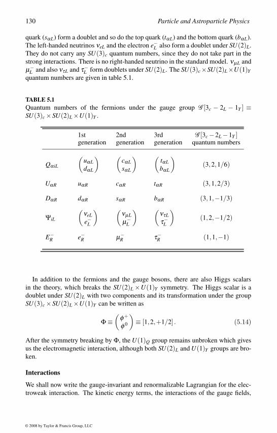
130 Particle and Astroparticle Physics
quark (sαL) form a doublet and so do the top quark (tαL) and the bottom quark (bαL).
The left-handed neutrinos νeL and the electron e−L also form a doublet under SU(2)L.
They do not carry any SU(3)c quantum numbers, since they do not take part in the
strong interactions. There is no right-handed neutrino in the standard model. νµL and
µ−L and also ντL and τ−L form doublets under SU(2)L. The SU(3)c×SU(2)L×U(1)Y
quantum numbers are given in table 5.1.
TABLE 5.1Quantum numbers of the fermions under the gauge group G [3c − 2L − 1Y ] ≡SU(3)c ×SU(2)L ×U(1)Y .
1st 2nd 3rd G [3c −2L −1Y ]generation generation generation quantum numbers
QαiL
(uαLdαL
) (cαLsαL
) (tαLbαL
)(3,2,1/6)
UαR uαR cαR tαR (3,1,2/3)
DαR dαR sαR bαR (3,1,−1/3)
ΨiL
(νeLe−L
) (νµLµ−
L
) (ντLτ−L
)(1,2,−1/2)
E−R e−R µ−
R τ−R (1,1,−1)
In addition to the fermions and the gauge bosons, there are also Higgs scalars
in the theory, which breaks the SU(2)L ×U(1)Y symmetry. The Higgs scalar is a
doublet under SU(2)L with two components and its transformation under the group
SU(3)c ×SU(2)L ×U(1)Y can be written as
Φ ≡(
φ+
φ 0
)≡ [1,2,+1/2] . (5.14)
After the symmetry breaking by Φ, the U(1)Q group remains unbroken which gives
us the electromagnetic interaction, although both SU(2)L and U(1)Y groups are bro-
ken.
Interactions
We shall now write the gauge-invariant and renormalizable Lagrangian for the elec-
troweak interaction. The kinetic energy terms, the interactions of the gauge fields,
© 2008 by Taylor & Francis Group, LLC
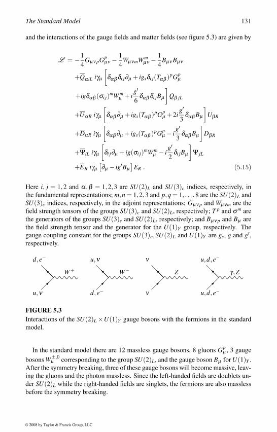
The Standard Model 131
and the interactions of the gauge fields and matter fields (see figure 5.3) are given by
L = −1
4Gµν pGp
µν −1
4WµνmW m
µν −1
4Bµν Bµν
+QαiL iγµ
[δαβ δi j∂µ + igsδi j(Tαβ )pGp
µ
+igδαβ (σi j)mW mµ + i
g′
6δαβ δi jBµ
]Qβ jL
+UαR iγµ
[δαβ ∂µ + igs(Tαβ )pGp
µ +2ig′
3δαβ Bµ
]UβR
+DαR iγµ
[δαβ ∂µ + igs(Tαβ )pGp
µ − ig′
3δαβ Bµ
]DβR
+ΨiL iγµ
[δi j∂µ + ig(σi j)mW m
µ − ig′
2δi jBµ
]Ψ jL
+ER iγµ[∂µ − ig′Bµ
]ER . (5.15)
Here i, j = 1,2 and α,β = 1,2,3 are SU(2)L and SU(3)c indices, respectively, in
the fundamental representations; m,n = 1,2,3 and p,q = 1, . . . ,8 are the SU(2)L and
SU(3)c indices, respectively, in the adjoint representations; Gµν p and Wµνm are the
field strength tensors of the groups SU(3)c and SU(2)L, respectively; T p and σ m are
the generators of the groups SU(3)c and SU(2)L, respectively; and Bµν p and Bµ are
the field strength tensor and the generator for the U(1)Y group, respectively. The
gauge coupling constant for the groups SU(3)c,SU(2)L and U(1)Y are gs, g and g′,respectively.
d,e−
u,ν
W+
u,ν
d,e−
W−
ν
ν
Z
u,d,e−
u,d,e−
γ,Z
FIGURE 5.3Interactions of the SU(2)L ×U(1)Y gauge bosons with the fermions in the standard
model.
In the standard model there are 12 massless gauge bosons, 8 gluons Gpµ , 3 gauge
bosons W±,0µ corresponding to the group SU(2)L, and the gauge boson Bµ for U(1)Y .
After the symmetry breaking, three of these gauge bosons will become massive, leav-
ing the gluons and the photon massless. Since the left-handed fields are doublets un-
der SU(2)L while the right-handed fields are singlets, the fermions are also massless
before the symmetry breaking.
© 2008 by Taylor & Francis Group, LLC
132 Particle and Astroparticle Physics
Symmetry Breaking
An explicit symmetry breaking can give masses to the gauge bosons and the fermions,
but that will make the theory nonrenormalizable. So, the symmetry is broken spon-
taneously by giving a vacuum expectation value to the Higgs scalar φ . We shall first
write the scalar potential so the vacuum is no longer invariant under the symmetry
groups. This will then break the symmetry spontaneously. The spontaneous symme-
try breaking maintains the renormalizability of the theory and will give masses to the
gauge bosons as well as to the fermions.
The Lagrangian involving the Higgs field can be written as
L (φ) = LφKE +LYuk −V (φ), (5.16)
where the first term contains the kinetic energy and gauge interaction of the Higgs
scalar field φ ,
LφKE =∣∣∣∣∂µ φ + igσ mW m
µ φ + ig′
2Bµ φ
∣∣∣∣2 ; (5.17)
the second term contains the Yukawa couplings
LYuk = huab QLaURb φ +hd
ab QLaDRb φ+he
ab ΨLaERb φ +H.c. , (5.18)
where a,b = 1,2,3 is the generation index; and the last term is the scalar potential
V (φ) = −µ2
2φ †φ +
λ4
(φ †φ)2. (5.19)
In the above we defined
φ = iτ2φ ∗ =(
φ ∗0
−φ−
)≡ [1,2,−1
2]. (5.20)
Since all SU(2) representations are pseudo-real (2 = 2), both φ and φ transform
under SU(2)L as doublets. However, they carry opposite U(1)Y quantum numbers.
The mass parameter of the Higgs scalar µ2 is taken to be positive-definite, so there
is a vacuum expectation value (vev) of the Higgs scalar at the stationary point of the
Lagrangian
〈φ †φ〉 = v2 =µ2
λ. (5.21)
We now perform an SU(2)L ×U(1)Y gauge transformation to a unitary gauge in
which φ+ = 0 and φ is real, with a positive vev
〈φ+〉 = 0 and 〈φ 〉 = v > 0. (5.22)
This vev will then break the groups SU(2)L and U(1)Y . However, an Abelian sub-
group, which is generated by a linear combination of T3L and Y , will remain invariant.
Since φ is electrically neutral, it leaves the U(1)Q group unbroken, which generates
quantum electrodynamics.
© 2008 by Taylor & Francis Group, LLC
The Standard Model 133
Gauge Bosons and Their Couplings
The interactions of the scalar φ with the gauge bosons W±,0µ and Bµ make the gauge
bosons corresponding to the broken groups massive. The two charged components
of the SU(2)L gauge bosons
W±µ =
1√2(W 1
µ ∓W 2µ ) (5.23)
get masses
mW =vg2
, (5.24)
and one combination of the neutral gauge bosons, given by
Zµ = cosθwW 3µ − sinθwBµ , (5.25)
gets mass
mZ =v√
g2 +g′2
2. (5.26)
These particles W± and Z have been discovered in the proton–antiproton collider
[40]. The remaining physical gauge boson, the photon,
Aµ = sinθwW 3µ + cosθwBµ , (5.27)
remains massless along with the gluons and becomes the gauge boson corresponding
to the unbroken U(1)Q and SU(3)c gauge symmetries.
The weak mixing angle θw is defined to relate the coupling constant of the SU(2)Land U(1)Y gauge theories with that of U(1)Q by
sinθw =eg
=g′
(g2 +g′2)1/2 , (5.28)
where |e| is the charge of an electron. Comparison of the four-fermion interaction of
the muon decay in this theory with the (V −A) theory gives
g2/m2W = 4
√2GF . (5.29)
Using the value of the Fermi constant GF = 1.16639(1)×10−5 GeV−2, we can now
get the value of the vev of φ to be
v =2mW
g= 2−1/4G−1/2
F = 246 GeV. (5.30)
In addition to the symmetry breaking, this vev gives masses to the fermions.
The interactions of the fermions with the physical gauge bosons can now be writ-
ten as
Lgauge = − g√2(Jµ
CCW+µ + Jµ
CC†W−
µ )− gg′
eJµ
NCZµ − eJµQAµ , (5.31)
© 2008 by Taylor & Francis Group, LLC
134 Particle and Astroparticle Physics
where the charged current, the neutral current and the electromagnetic current are
given by
JµCC = ψLγµ 1
2(σ1 + iσ2)ψL
JµNC = ψγµ 1
2(cV − cAγ5)ψ
JµQ = ψγµ Qψ, (5.32)
respectively, where cV = T3L − 2Qsin2 θw and cA = T3L. The right-handed charged
fermions also take part in the neutral current interactions, since the neutral current
contains couplings of the hypercharge gauge boson Bµ .
We now introduce another important parameter, the ρ parameter,
ρ =m2
W
m2Z cos2 θw
. (5.33)
For a doublet Higgs scalar, ρ = 1, which is the case in the standard model. If the
symmetry group is broken by a triplet, the ρ parameter would have been different
from unity. The precision measurements gave ρ = 1.0109±0.0006 for mt = 175±5
GeV and the Higgs mass around mZ , which constrains the possible vev of a triplet
Higgs scalar to be less than ∼ O(1) GeV.
5.4 Fermion Masses and MixingThe standard model does not allow any fermion mass terms since the left-handed
fermions are doublets while the right-handed fields are singlets, so the mass terms
are not invariant under SU(2)L. However, after the symmetry breaking, the Yukawa
couplings (equation (5.18)) can give fermion masses when the Higgs scalar field φacquires a vev
LYuk = huabQLaURb
(< φ ∗
0 >= v< φ− >= 0
)+(
hdabQLaDRb +he
abΨLaERb
)(< φ+ >= 0
< φ 0 >= v
)+H.c.
= muabULaURb +md
abDLaDRb +meabLaERb +H.c. , (5.34)
where
QLa =(
ULaDLa
)=(
uL,cL, tLdL,sL,bL
)ΨLa =
(νLaLa
)=(
νe,νµ ,ντeL,µL,τL
)
© 2008 by Taylor & Francis Group, LLC
The Standard Model 135
URa = (uR,cR, tR )
DRa = (dR,sR,bR )
ERa = (eR,µR,τR ) ; (5.35)
and the up, down and the charged lepton masses are
muab = hu
abv; mdab = hd
abv; meab = he
abv. (5.36)
Since there are no right-handed neutrinos in the theory and there are no Higgs triplet
that can induce a Majorana mass term mMψLcψL, neutrinos are massless in the stan-
dard model. We shall discuss the neutrino masses at length in the next chapter.
In general, the quark and lepton masses are not diagonal. In the case of leptons
we can make unitary transformations on both the neutrino fields and the charged
lepton fields and make the charged lepton mass matrix diagonal. Since neutrinos
are massless in this model, this transformation will not affect the charged current
interactions. So, it is convenient to work in the basis where the charged lepton masses
are diagonal.
Quark Mixing Matrix
In general, the up and the down quark mass matrices muab and md
ab are not diagonal.
If we now diagonalize the mass matrices, in terms of the quark states with definite
masses, which are the physical eigenstates, the charged current interaction will not
be diagonal. If we define the physical states or the mass eigenstates U ′[L,R] and D′
[L,R],
these states will be distinct from the weak eigenstates U[L,R] and D[L,R], which enter
in the charged current interaction.
In the matrix form, the quark masses can be written as
LM = ULMuUR +DLMdDR, (5.37)
where U[L,R] and D[L,R] are the matrix forms of Ua[L,R] and Da[L,R] and the 3×3 mass
matrix M[u,d] has the elements m[u,d]ab . As mentioned earlier, the mass matrices Mu
and Md are not diagonal in this weak basis, in which the charged current interactions
of the quarks are given by
L qcc =
g√2
[UmLγµ DmLW+
µ +DmLγµUmLW−µ]. (5.38)
We shall now diagonalize the mass matrices Mu and Md to get the physical eigen-
states.
The masses Mu and Md are not Hermitian and, hence, cannot be diagonalized by
unitary transformations. However, they can always be diagonalized by bi-unitary
transformations,
U †uLMuUuR = Mu
U †dLMdUdR = Md , (5.39)
© 2008 by Taylor & Francis Group, LLC
136 Particle and Astroparticle Physics
where Mu and Md are diagonal matrices and the left-transformation matrices UL and
the right-transformation matrices UR can be obtained by solving
U †ALMAM†
AUAL = MAM†A
U †ARM†
AMAUAR = M†AMA, (5.40)
where A means either up (u) or down (d) quarks for the entire equations. The mass
eigenstates are now given in terms of the weak eigenstates by
U ′[L,R] = Uu[L,R]U[L,R]
D′[L,R] = Ud[L,R]D[L,R]. (5.41)
The mass eigenstates are the physical states with definite mass eigenvalues
LM = U ′LMuU ′R +D′LMdD′
R. (5.42)
In any weak interaction, particles are created in the weak basis, but they will evolve
with time as physical eigenstates. For example, a down quark could be produced
in any weak interaction, but if the physical states are mixtures of down and strange
quarks, then during its propagation the original down quark may become a strange
quark.
The charged-current interactions can now be written in the mass basis as
L qcc =
g√2
[U ′aLγµVaiD′
iLW+µ +D′iLγµV ∗
aiU′aLW−
µ], (5.43)
where the unitary mixing matrix
Vai = [UuL]am[U †dL]im (5.44)
is called the Cabibbo–Kobayashi–Maskawa (CKM) mixing matrix [41]. The CKM
matrix Vai is a product of the two unitary matrices, one entering in the diagonalization
of the up quark and the other in the down quark mass matrix. The right transforma-
tion matrices do not enter in the charged current interactions. Thus, the CKM matrix
Vai will appear in interaction vertices where a down-quark is annihilated and an up-
quark is created and the opposite for V ∗ai. The neutral-current interaction is diagonal
in both the weak basis and the physical basis, since the mixing matrices of the same
field appear in the interaction. Similarly the neutral Higgs couplings are also diago-
nal. So, there are no flavor-changing neutral currents in the standard model [42].
Parameterization of the CKM Matrix
The mixing matrix appearing in the charged current interactions can be interpreted
in several ways. One convention is to consider the mass eigenstates and the physical
eigenstates of the up quarks to be the same, let us denote them as u,c, t. Let us now
denote the physical down quark eigenstates as d,s,b, which have definite masses.
The CKM mixing matrix will imply that in any charged current weak interaction of
© 2008 by Taylor & Francis Group, LLC
The Standard Model 137
an up quark, say u, a combination of d,s,b will appear. If the CKM matrix were
diagonal, then only d would have appeared, but due to the quark mixing, both s and
b will also mix with the d quark in the interactions of u. The weak eigenstate will be
an admixture of all three mass eigenstates d,s,b.
There are four independent parameters in the three generation CKM mixing ma-
trix, three mixing angles and a complex phase, which gives rise to CP violation. In
general all the elements of the CKM matrix could be complex, but phase transforma-
tions of the quark fields could remove most of these phases, except one for a three
generation scenario. In general, for an N generation scenario, V can be expressed by
N(N −1)/2 rotation angles and (N −1)(N −2)/2 independent phases, after remov-
ing (2N −1) phases by rephasing the quark fields.
The CKM matrix could be parameterized in several ways for convenience of
studying certain physical observables. One such parameterization, suggested by
Kobayashi and Maskawa, can be written as
V =
c1 −s1c3 −s1s3s1c2 c1c2c3 − s2s3expiδ c1c2s3 + s2c3expiδ
s1s2 c1s2c3 + c2s3expiδ c1s2s3 − c2c3expiδ
, (5.45)
where, s1 = sinθi,ci = cosθi(i = 1,2,3) are the three mixing angles and δ is a CPviolating phase. Wolfenstein proposed another phenomenological parameterization
[43], in which the matrix elements are expanded in terms of a small parameter, the
Cabibbo mixing angle λ = sinθc and unitarity is used to determine the remaining
elements
V =
1− 12 λ 2 λ Aλ 3(ρ − iη)
−λ 1− 12 λ 2 Aλ 2
Aλ 3(1−ρ − iη) −Aλ 2 1
. (5.46)
This matrix is approximately unitary and there are four parameters A,λ ,ρ and η .
The most accurately determined quark mixing parameter is the Cabibbo angle
λ [44]. From the measurement of the hyperon decay and K → πeν decay, we
have |Vus| = λ = 0.2196 ± 0.0023. Combined analysis [44] of inclusive and ex-
clusive B decays gives |Vcb| = 0.0402± 0.0019, which implies A = 0.819± 0.035.
End-point lepton energy spectra in the semi-leptonic decays B → Xuν and exclu-
sive semileptonic decays B → πν or ρν give |Vub/Vcb| = 0.090±0.025 yielding√ρ2 +η2 = 0.423±0.064 [45].
Some combination of parameters could be constrained by the unitarity conditions
of the CKM matrix. This is very useful for an understanding of the CP violation. Let
us consider one of the unitarity conditions of the CKM matrix
VudV ∗ub +VcdV ∗
cb +VtdV ∗tb = 0. (5.47)
The form of equation (5.46) then allows us to write this equation as
V ∗ub
λVcb+
Vtd
λVcb= 1. (5.48)
© 2008 by Taylor & Francis Group, LLC
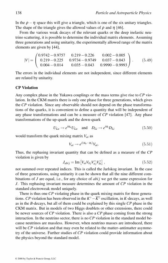
138 Particle and Astroparticle Physics
In the ρ −η space this will give a triangle, which is one of the six unitary triangles.
The shape of the triangle gives the allowed values of ρ and η [46].
From the various weak decays of the relevant quarks or the deep inelastic neu-
trino scattering, it is possible to determine the individual matrix elements. Assuming
three generations and using unitarity, the experimentally allowed range of the matrix
elements are given by [44],
|V | =0.9742−0.9757 0.219−0.226 0.002−0.005
0.219−0.225 0.9734−0.9749 0.037−0.043
0.004−0.014 0.035−0.043 0.9990−0.9993
. (5.49)
The errors in the individual elements are not independent, since different elements
are related by unitarity.
CP Violation
Any complex phase in the Yukawa couplings or the mass terms give rise to CP vio-
lation. In the CKM matrix there is only one phase for three generations, which gives
the CP violation. Since any observable should not depend on the phase transforma-
tions of the quarks, it is convenient to define a quantity that will be independent of
any phase transformations and can be a measure of CP violation [47]. Any phase
transformations of the up-quark and the down-quark
ULa → eiαaULa and DLi → eiαi DLi (5.50)
would transform the quark mixing matrix Vai as
Vai → ei(αa−αi)Vai. (5.51)
Thus, the rephasing invariant quantity that can be defined as a measure of the CPviolation is given by
Jabi j = Im[VaiVb jV ∗
a jV∗bi], (5.52)
not summed over repeated indices. This is called the Jarlskog invariant. In the case
of three generations, using unitarity it can be shown that all the nine different com-
binations of J are equal, i.e., for any choice of abi j we get the same expression for
J. This rephasing invariant measure determines the amount of CP violation in the
standard electroweak model uniquely.
There is thus one CP violating phase in the quark mixing matrix for three genera-
tions. CP violation has been observed in the K−K oscillation, in K-decays, as well
as in the B-decays, but all of them could be explained by this single CP phase in the
CKM matrix. But in models of two Higgs doublets or other extensions, there could
be newer sources of CP violation. There is also a CP phase coming from the strong
interaction. In the neutrino sector, there is no CP violation in the standard model be-
cause neutrinos are massless. However, when neutrino masses are introduced, there
will be CP violation and that may even be related to the matter–antimatter asymme-
try of the universe. Further studies of CP violation could provide information about
the physics beyond the standard model.
© 2008 by Taylor & Francis Group, LLC
6Neutrino Masses and Mixing
In a nuclear beta decay, a neutron decays into a proton, an electron and a neutrino. In
the beginning neutrinos were not observed in the beta decay; they were postulated to
satisfy conservation laws. Since the electrons emitted in a beta decay are not mono-
energetic, energy and momentum conservation ruled out the possibility of a two-
body decay of neutrons into a proton and an electron. Pauli postulated [48] the new
particle, the neutrino, to explain the energy distribution of electrons. Conservation
of angular momentum implied that the neutrinos are spin-1/2 fermions.
Neutrinos are neutral particles with very tiny mass. They interact with matter
only through weak and gravitational interactions and, hence, very weakly. Since
the strength of gravitational interaction is too small compared with the weak inter-
action, neutrinos interact with matter mostly through weak interactions and, hence,
play a very special role in particle physics. Although detection of neutrinos is ex-
tremely difficult, experiments with neutrinos brought many surprises. The tiny mass
of the neutrinos could be established almost sixty years after the discovery of the
neutrinos. On the other hand, the neutrinos could travel a very long distance in the
universe without interacting with anything else and, hence, play an important role
in astrophysics and cosmology. If we understand all the properties of neutrinos, it
may be possible to say how they contributed to nucleosynthesis. Neutrinos could
have been instrumental in generating a baryon asymmetry of the universe, explain-
ing the problem of the cosmological constant or contributing to the dark matter of
the universe.
During the past few years, many new developments have taken place with neutri-
nos. The atmospheric and the solar neutrino deficits established that the neutrinos
have very small mass, and neutrinos of one flavor oscillate into another kind dur-
ing their propagation in space. There are three types of active neutrinos and two of
the mixing angles are large while the third one is small. These results have been
confirmed by laboratory experiments. However, we have yet to answer many more
questions about the neutrinos. For example, we do not know if neutrinos are Dirac
or Majorana particles, what their absolute mass is, what the value of the third mixing
angle is, if there is CP violation in the leptonic sector, and what makes the neutrinos
so light compared with charged fermions. These questions become more interesting
in many extensions of the standard model, such as the supersymmetric theories or
the models with extra dimensions.
139
© 2008 by Taylor & Francis Group, LLC
140 Particle and Astroparticle Physics
6.1 Dirac and Majorana NeutrinosOne of the most important question for the neutrinos is whether they are Dirac or
Majorana particles. All charged particles are Dirac particles, but a neutral particle
like a neutrino could be either a Dirac or a Majorana particle. If neutrinos are Ma-
jorana particles [49], this could naturally explain why they are much lighter than
any charged fermions. Lepton number will be violated if neutrinos are Majorana
particles, which may have several interesting consequences in cosmology.
The main difference between Dirac and Majorana neutrinos lies in their lepton
number violation. If neutrinos are Dirac particles, lepton number will be conserved,
while for a Majorana neutrino, lepton number is violated by two units since they
are their own antiparticles. Any gauge interactions in the standard model conserve
lepton number. Only the mass term in the Lagrangian can distinguish between a
Dirac and a Majorana particle.
A Dirac particle is a spin-1/2 particle that satisfies the Dirac equation (equation
(1.16))
iγµ ∂µ ψD −mDψD = 0. (6.1)
Here ψD is the Dirac spinor and has four complex components. This 4-dimensional
spinor representation of the Lorentz group O(3,1), which is locally isomorphic to
O(4), can be decomposed under its subgroup SU(2)L ×SU(2)R as
4 = (2,1)+(1,2).
The chiral projection operator (1±γ5)/2 can project the left-handed and right-handed
components of the spinor representations, which are the (2,1) and (1,2) representa-
tions, respectively:
ψL =1
2(1− γ5)ψD ⊂ (2,1) and ψR =
1
2(1+ γ5)ψD ⊂ (1,2).
These states satisfy γ5ψL =−ψL and γ5ψR = ψR and the identitites ψLψR = ψcLψR =
ψLψLc = 0. Under charge conjugation (C ) and CP conjugation (CP), these com-
ponents transform as
ψL C−→ ψcL ψL C P−→ ψc
R = (ψL)c
ψR C−→ ψcR ψR C P−→ ψc
L = (ψR)c. (6.2)
Out of the four states (ψL,ψR,ψcL and ψc
R), only two of the states are independent.
CPT invariance implies that any theory will contain both the particles and their CPTmirror images, which are the CP conjugates. So, if any theory contains a ψL, then
CPT invariance would imply the existence of ψ cR = ψL
c as well.
In terms of the chiral components of the Dirac field ψD, the Dirac equation can be
reduced to two coupled equations
iγµ ∂µ ψL −mDψR = 0
iγµ ∂µ ψR −mDψL = 0. (6.3)
© 2008 by Taylor & Francis Group, LLC
Neutrino Masses and Mixing 141
These follow from the Lagrangian
L = LKE +LD, (6.4)
where the kinetic energy term is
LKE = iψDγµ ∂µ ψD = iψLγµ ∂µ ψL + iψRγµ ∂µ ψR. (6.5)
The kinetic energy term, thus, treats the left-handed and the right-handed fields in-
dependently, while the Dirac mass term connects the left-handed fields to the right-
handed fields. When mD = 0, the left-handed and the right-handed components of
ψD, i.e., the Weyl spinors [50] ψL and ψR, can be treated as independent.
A Lagrangian with a nonzero mD, which is the Dirac mass term, represents a
Dirac particle. Since massive particles propagate more slowly than light, a left-
handed Dirac particle will become a right-handed particle in another frame moving
faster than the particle. Thus, all four states (ψL, ψR, and their C P conjugate states)
should be present in any theory if any particle is a Dirac particle.
There are four independent solutions of the Dirac equation (two positive energy
up,±s and two negative energy solutions vp,±sdetails)
ψD(x) = ∑p,s
1√2ε(apsupsexp−ipx +b†
psvpsexpipx)ψD(x) = ψ†
Dγ0 = ∑p,s
1√2ε(a†
psupsexpipx +bpsvpsexp−ipx) , (6.6)
where s2 = −1 is the covariant spin vector, u = u†γ0, v = v†γ0 and the bispinors upsand vps are suitably normalized. The coefficients aps and bps are the annihilation
operators, and the coefficients a†ps and b†
ps are the creation operators for the particles
and antiparticles, respectively.
The Dirac mass term comes from the Lagrangian
LD = −mDψDψD = −mDψRψL −mDψLψR, (6.7)
where the second term is the Hermitian conjugate (H.c.) of the first term in the last
expression. In the standard model it is convenient to work with the states ψL and
ψR as independent states; CPT invariance will then include the states ψ cR and ψc
L.
However, in grand unified theories it is convenient to consider the states ψL and ψcL
as independent states, so they can be put into a single representation of the grand
unification group
ΨL ≡(
ψψc
)L.
CPT invariance will then include the CP conjugate states in the theory, which are the
right-handed particles
ΨR ≡(
ψc
ψ
)R.
© 2008 by Taylor & Francis Group, LLC
), so we may write (see section 1.2 for
142 Particle and Astroparticle Physics
The states ΨL and ΨR can then belong to the representations R(G ) and R(G ), re-
spectively, of any unifying group G that commutes with the Lorentz group. One can
then write the Dirac masses as
LD = −mDψRψL +H.c. = mDψTL C−1ψc
L +H.c. (6.8)
For CPT conservation, the Hermitian conjugate of every mass term (containing the
right-handed fields) will always be present. From now on we shall not mention them
explicitly, except when we discuss CP violation. A more general form of the Dirac
mass term is
LD =1
2(ψL ψc
L )T C−1(
0 mDmD 0
)(ψLψc
L
)=
1
2ΨT
LC−1MDΨL, (6.9)
where ΨTL = (ψ ψc )T
L . Thus, the Dirac mass term combines the two Weyl spinors,
ψL and ψcL (or ψR) to form a Dirac particle.
It is also possible to write the mass terms for each of the Weyl spinors keeping the
mass matrix diagonal, as
LD =1
2(ψL ψc
L )T C−1(
mL 0
0 mR
)(ψLψc
L
), (6.10)
which gives two massive states, ψL with mass mL and ψcL (or ψR) with mass mR:
LL = −1
2mLψLcψL =
1
2mLψT
L C−1ψL = −1
2mLψRψR
c
LR = −1
2mRψRcψR =
1
2mRψT
R C−1ψR = −1
2mRψLψL
c. (6.11)
The two masses mL and mR are now independent. These states will not be part of
one Dirac particle; instead they will become two Majorana particles [49], satisfying
the Majorana conditions
ψLc = ψc
R = ηLCψL and ψRc = ψc
L = ηRCψR , (6.12)
where ηLC and ηRC are two new phases, called the creation phases or the Majorana
phases. The overall phase can be chosen to be real, but the relative phase gives rise
to a new source of CP violation. For any number of Majorana particles, the overall
phase can always be chosen to be real. Since the Majorana condition relates the
charge conjugate state of the particle with itself, it corresponds to a real spinor and,
hence, has four real components. Thus, a Dirac particle can be formed from two
Majorana particles, which are combined by the Dirac mass term.
For a Majorana particle, the creation and the annihilation operators for the particles
and antiparticles are related by the Majorana condition, aps = bps = fps and a†ps =
b†ps = f †
ps. A Majorana field can then be written as
ψM(x) = ∑p,s
1√2ε(
fpsupsexp−ipx +η∗C f †
psvpsexpipx) . (6.13)
© 2008 by Taylor & Francis Group, LLC
Neutrino Masses and Mixing 143
It can then be checked that ψcMγµ ψc
M =−ψMγµ ψM , and hence, there is no vector cur-
rent for any Majorana particle. The number operator also vanishes,∫
d3xψMγ0ψM =0 for the Majorana particles, so there is no conservation of the number of particles.
The Majorana mass terms combine a left-handed particle ψL to its CP conjugate
state ψcR and a right-handed particle ψR to its CP conjugate state ψc
L. A particle
with Majorana mass will also move with a velocity less than the speed of light. So,
an observer moving with a higher velocity than a Majorana particle will see a left-
handed particle ψL to be a right-handed antiparticle ψcR.
A real four-component Majorana particle can be written in the Weyl basis as
ψM = ψL +η∗Cψc
R, (6.14)
where |ηC|2 = 1 is the Majorana phase, discussed earlier. A Majorana mass term can
be written as
LM = −1
2mMψc
MψM =1
2mMψT
MC−1ψM. (6.15)
If the fields carry any U(1) quantum number, the Majorana mass term for these
fields breaks the U(1) symmetry by two units. The neutrinos carry lepton number,
and hence, any Majorana mass terms for the neutrinos break lepton number by two
units.
In general, the mass matrix for a system comprised of both the left-handed and the
right-handed particles can be written as
Lmass =1
2(ψ ψc )T
L C−1(
mL mDmD mR
)(ψψc
)L
=1
2ΨT
LC−1MΨL, (6.16)
where ΨTL = (ψ ψc )T
L and M is a 2×2 symmetric mass matrix:
ΨTLC−1MΨL = ΨT
L MT (CT )−1ΨL = ΨTLC−1MT ΨL. (6.17)
If the particle carries any U(1) charge which is not broken, such as electric charge,
this matrix M can only have nonvanishing off-diagonal terms. This will then corre-
spond to a Dirac particle. Thus, any charged particles are Dirac particles.
For neutrinos the diagonal terms in the mass matrix can be nonvanishing [51],
which breaks lepton number since neutrinos and antineutrinos carry opposite lepton
numbers. Thus, this general mass matrix will correspond to two independent Ma-
jorana particles, which are two independent combinations of ψL and ψcL (or ψR).
Only when the diagonal elements vanish will this matrix represent a single Dirac
particle. Thus, depending on the structure of the mass matrix, one can say whether
these two particles combine to form a Dirac particle or represent two Majorana par-
ticles. This discussion can be generalized to any number of particles. If there are nnumber of Majorana particles ΨiL, (i = 1, · · · ,n) (some of which could be antiparti-
cles ψmL = χcmL, i.e., ψm = χc
m), one can write the mass matrix for these particles
as
Lmass =1
2ΨT
iLC−1Mi jΨ jL, (6.18)
© 2008 by Taylor & Francis Group, LLC
144 Particle and Astroparticle Physics
where ΨTL = (ψ1 · · · ψn )T
L and Mi j is a n×n symmetric mass matrix. In this case,
some of the states could pair up to form Dirac particles, while the remaining ones
remain as physical Majorana particles.
Let us elaborate this point with an example of three Majorana neutrinos ΨiL ≡(νe νµ ντ )L with a mass matrix:
Lmass =1
2ΨT
iLC−1
0 m 0
m 0 0
0 0 M
Ψ jL. (6.19)
The states νeL and νµL will combine to form a Dirac particle, while the state ντLwill correspond to a Majorana particle. The physical left-handed and right-handed
components of the Dirac particle correspond to
χL = νeL and χcL = νµL or χR = (νµL)c , (6.20)
so an observer from a faster moving frame will see the left-handed electron neu-
trino (νeL) to be a right-handed muon antineutrino (ν cµR). The τ-neutrino will be a
Majorana particle.
Let us now come back to the case of n Majorana neutrinos. The kinetic energy
terms or any other interactions will treat these states as n independent Majorana
states. Only the mass terms can tell us if the states correspond to different phys-
ical Majorana neutrinos, some of the states combine to give a Dirac neutrino, or
if they correspond to pseudo-Dirac neutrinos or some combinations of these states
[52, 53]. We shall again elaborate this point with the example of ψL and ψcL. The
real symmetric 2× 2 mass matrix MT = M can be diagonalized by the orthogonal
transformations O:
Md = OT MO =(
m1 0
0 m2
), (6.21)
where
m1,2 =1
2
[mL +mR ∓
√(mR −mL)2 +4m2
D
](6.22)
and Md is diagonal. In this diagonal basis ΨTdL = ΨT
L O = (ψ1L ψ2L ), the La-
grangian can be written as
Lmass =1
2ΨT
L C−1MΨL =1
2ΨT
dL C−1MdΨdL. (6.23)
The transformation relates the weak interaction basis ΨL to the diagonal physical
mass basis ΨdL through
ΨdL =(
ψ1ψ2
)L
= OT ΨL =(
cosθ −sinθsinθ cosθ
)(ψψc
)L, (6.24)
with the mixing angle tan2θ = 2mD/(mR −mL) .
© 2008 by Taylor & Francis Group, LLC
Neutrino Masses and Mixing 145
The values of mL, mR and mD determine if the physical particles are Majorana,
Dirac or pseudo-Dirac particles. For m1 = m2, the mass term becomes
Lmass =1
2m1ψT
1L C−1ψ1L +1
2m2ψT
2L C−1ψ2L. (6.25)
This corresponds to two physical Majorana particles ψ(1,2)L with masses m1,2. A
special case of this is mD = 0, when the physical states are
ψ1L = ψL and ψ2L = ψcL. (6.26)
In this case the two Majorana particles are the left-handed and the right-handed neu-
trinos. When mD = 0, the two physical Majorana particles ψ(1,2)L become combina-
tions of the left-handed particle and the antiparticle.
The mass matrix with mL = mR = 0 represents one physical Dirac particle
Lmass =1
2mDψT
1LC−1ψ1L − 1
2mDψT
2LC−1ψ2L = mDψTL C−1ψc
L, (6.27)
with the mass eigenvalues m1 = −m2 = mD. The states are now related by
ψL =1√2[ψ1L +ψ2L] and ψc
L =1√2[ψ1L −ψ2L]. (6.28)
Since the diagonal terms of the mass matrix vanish, all the U(1) charges carried by
these particles are conserved. In a more general case, if any U(1) symmetry of the
weak eigenstates is not broken by the mass matrix and if two of the mass eigenvalues
are equal with opposite sign, then they form a Dirac particle.
When the mass eigenvalues are equal but any symmetry of the weak eigenstates
is violated by the mass matrix, the two Majorana states combine to form a Dirac
particle at the tree-level; but one-loop corrections would break the degeneracy, and
these states will behave as two Majorana particles. This is the case corresponding to
mL = mR = m and mD = 0. The mass eigenstates are equal, m1 = m2 = m and we
can write the mass term as
Lmass =1
2mψT
1LC−1ψ1L +1
2mψT
2LC−1ψ2L = mχTL C−1χc
L, (6.29)
where
χL =1√2[ψ1L − iψ2L] and χc
L =1√2[ψ1L + iψ2L]. (6.30)
Then the particle χL appears as a Dirac particle and if it carries any U(1) charge, it
is conserved. However, if the fields ψ1L and ψ2L carry any U(1) charges, they are
not conserved. So, these particles are different from the usual Dirac particles and are
called pseudo-Dirac particles. Consider the case of neutrinos. The neutrinos carry
lepton number. But if they are pseudo-Dirac particles, the physical state will be an
admixture of a lepton and an antilepton and, hence, will not carry any definite lepton
number. So, lepton number will be violated. In this case there will be one-loop
© 2008 by Taylor & Francis Group, LLC
146 Particle and Astroparticle Physics
self-energy type diagrams with the charged leptons in the loop. The corrections to
the masses of the two states ψ1L and ψ2L will be proportional to the corresponding
mass squared of the charged leptons e1 and e2, and hence, the mass degeneracy will
be broken leading to two Majorana particles. However for a Dirac particle, the U(1)symmetry of the weak eigenstates guarantees the equality of the masses of the two
states even when higher order corrections are included.
A pseudo-Dirac particle is, thus, a Dirac particle at the tree-level, but after in-
cluding radiative corrections it becomes two almost degenerate Majorana particles.
Since Dirac, Majorana, or pseudo-Dirac neutrinos have almost similar gauge inter-
actions, modulo some small lepton-number violating components for the Majorana
and pseudo-Dirac neutrinos, it is not possible to distinguish between a pseudo-Dirac
and two almost degenerate Majorana particles. The neutrinoless double beta decay
experiment will be able to tell us if the neutrinos are Majorana or pseudo-Dirac par-
ticles and if there is lepton number violation in nature.
6.2 Models of Neutrino MassesThe atmospheric and the solar neutrinos have now established that neutrinos have
tiny masses, orders of magnitude smaller than the masses of the charged fermions.
Combined with some laboratory experiments we have a fairly good understanding of
two of the mass squared differences and two large mixing angles. For the absolute
mass scale of the neutrino mass matrix and the third mixing angles, only upper limit
exists.
In the standard model, neutrinos are massless. The left-handed neutrinos νiL, i =e,µ,τ transform under the standard model gauge group SU(3)c × SU(2)L ×U(1)Yas (1,2,−1). Thus, it is not possible to write a Majorana mass term for the neutrinos.
On the other hand, there are no right-handed neutrinos in the standard model, which
would allow a Dirac neutrino. If we introduce right-handed neutrinos νiR transform-
ing as (1,1,0), then it will be possible to write the Yukawa couplings that can give a
Dirac mass to the neutrinos:
Lmass =1
2fi jψiLψ jRφ . (6.31)
When the scalar doublet field φ acquires a vev, 〈φ〉 = v, neutrinos get a Dirac mass
mDi j = fi jv. Since all the charged fermions receive mass in the same way, it is natural
that this mass term is also of the same order of magnitude. Then what makes them
so light?
A natural explanation for the tiny neutrinos mass is seeded into the standard model.
Consider the most general dimension-5 effective lepton-number violating operator in
the standard model that can contribute to the Majorana masses of the neutrinos [54]
LMa j = Λ−1(νφ − eφ+)2. (6.32)
© 2008 by Taylor & Francis Group, LLC
Neutrino Masses and Mixing 147
Here Λ is some lepton-number violating heavy scale in the theory coming from some
extensions of the standard model, and φ is the usual Higgs doublet scalar. At this
stage we do not specify the origin of this term. We expect some extensions of the
standard model will generate this effective low-energy term. The electroweak sym-
metry breaking then induces a Majorana mass to the neutrinos:
LMa j = mν νTiL C−1ν jL, (6.33)
with mν = v2/Λ. Thus, a large lepton-number violating scale Λ would explain nat-
urally why mν is much smaller than the charged fermion masses. This also sug-
gests that a Majorana mass of the neutrinos is more natural than a Dirac mass. The
lepton number violation at very high scale may have interesting cosmological con-
sequences, which we shall discuss later. We shall now briefly discuss some of the
generic mechanisms of realizing the effective dimension-5 lepton-number violating
operators that can give us tiny Majorana neutrino mass naturally in some extensions
of the standard model.
See-Saw Mechanism
The see-saw mechanism of neutrino masses is the first and most popular generic
mechanism of obtaining a tiny neutrino mass in an extension of the standard model
with right-handed neutrinos [55]. Three right-handed neutrinos NiR, i = 1,2,3 are
included, which are singlets under the standard model gauge group and electrically
neutral. Inclusion of the right-handed neutrinos will allow the Yukawa couplings
LYuk = hiα NRi φ Lα , (6.34)
where Lα ,α = 1,2,3 are the left-handed leptons, φ is the standard model Higgs
doublet and hαi are the Yukawa couplings. In general, the Yukawa couplings could
be complex giving rise to CP violation. This CP violation can contribute to the gen-
eration of a lepton asymmetry of the universe and can be observed in the neutrino
oscillation experiments. For the present we shall assume hαi to be real. After the
electroweak symmetry breaking by the vev of the Higgs doublet, this Yukawa cou-
pling will induce a Dirac mass term like the charged fermions
mDαi = hαi〈φ〉. (6.35)
This Dirac mass will be of the same order of magnitude as that of the charged
fermions, which is unacceptable.
If we now allow all possible interactions of the singlet right-handed neutrinos and
do not impose lepton number conservation, then we can write the Majorana mass
term of the right-handed neutrinos
LMa j = Mi j (NRi)c NR j = Mi j NTiRC−1N jR = Mi j NcT
iL C−1 NcjL. (6.36)
Since the right-handed neutrinos are singlets under the standard model, the Majorana
masses Mi j of the right-handed neutrinos are not protected by any symmetry and it
© 2008 by Taylor & Francis Group, LLC
148 Particle and Astroparticle Physics
could be large. The conservation of lepton number in the Yukawa couplings of the
neutrinos implies that the right-handed neutrinos carry lepton number +1, and hence,
the Majorana mass term has a lepton number +2 breaking lepton number explicitly.
Combining the Dirac and Majorana mass matrices for both the left-handed and right-
handed neutrinos, we can write
Lmass = mDαi νTLα C−1 Nc
iL +Mi NcTiL C−1 Nc
iL +H.c.
= (να Nci )T
L C−1(
0 mDαimDiα Mi
) (ναNc
i
)L. (6.37)
Without loss of generality we assume that the Majorana mass matrix of the right-
handed neutrinos is real and diagonal (Mi j = Miδi j). Since the right-handed neutrinos
are sterile with respect to the standard model interactions, it is possible to diagonalize
the right-handed neutrino mass matrix without affecting any of the left-handed inter-
actions. There could be new sources of CP violation in the Majorana mass matrix,
but for the present discussion we shall ignore them.
The indices i = 1,2,3 and α = 1,2,3 correspond to the right-handed and left-
handed neutrinos, respectively. The mass matrix is thus a 6 × 6 matrix, and the
physical masses can be obtained by diagonalizing this mass matrix. Without any
knowledge of the Dirac neutrino mass matrix mD, it is not possible to study this
matrix in a general way. However, we are now interested in some general features,
which can be extracted in a simple way. Consider a 2×2 mass matrix of the similar
form
Mν =(
0 mDmD M
). (6.38)
When there is no mixing or very small mixing between the different generations, for
every generation there will be a mass matrix of this form. We can now diagonalize
this matrix with the assumption mD M, and the eigenvalues are given by
m1 = −m2D
Mand m2 = M. (6.39)
The sign of the neutrino masses can be absorbed in the phases of the physical fields.
Although the overall sign does not matter, for the three generations the relative signs
can play an important role in deciding the mass matrix.
The physical states corresponding to the two eigenvalues are now given by(ψ1ψ2
)=(
cosθ −sinθsinθ cosθ
)(ν
Nc
), (6.40)
where tanθ = 2mD/M. For every generations there are now two physical Majorana
particles: ψ1 with mass m1 and ψ2 with mass m2 and m1 m2. The lighter particle is
mostly the left-handed neutrino with a tiny admixture of the right-handed neutrino,
while the heavy particle is mostly the right-handed neutrino. If we now assume
M ∼ 109 GeV and the Dirac masses mD are of the order of a few GeV, the two
© 2008 by Taylor & Francis Group, LLC
Neutrino Masses and Mixing 149
mass eigenvalues become of the order of m1 ∼ 1 eV and m2 ∼ 109 GeV. Thus, by
increasing the large mass scale, we can make the left-handed neutrinos much lighter
than the Dirac masses of the charged fermions. This mechanism is called the see-sawmechanism.
Since the neutrinos are Majorana particles in this mechanism, they will violate
total lepton number and, hence, contribute to the neutrinoless double beta decay. Al-
though both the states will contribute to the neutrinoless double beta decay, the con-
tributions of the heavier states vanish because of a phase space factor in the nuclear
matrix element. The effective mass < m >= mee = ∑2i=1 U2
eimiF(mi,A) contributing
to the neutrinoless double beta decay has the factor from the nuclear matrix element
F(mi,A), which vanishes for large mi, and hence, we get < m >∼ m1. For three
generations, we have to block diagonalize the neutrino mass matrix and consider
only the light neutrino masses in calculating the amount of neutrinoless double beta
decay.
In a three generation scenario, the see-saw mechanism gives three light neutrino
state only when the determinant of the right-handed neutrinos are nonvanishing. If
any of the right-handed neutrino Majorana mass eigenvalue vanishes, the determi-
nant of the right-handed neutrino mass matrix will also vanish. In this case some
of the left-handed neutrinos will combine with the right-handed neutrinos to form
Dirac neutrinos. The number of Dirac neutrinos will depend on the rank of the mass
matrix M. For n generations, if the rank of M is r, then there will be 2r Majorana
neutrinos and n− r Dirac neutrinos. The magnitude of the Dirac neutrino masses is
expected to be of the order of the charged fermion masses, while there will be r light
Majorana neutrinos. The heavy Dirac and Majorana neutrinos with masses mD and
M, respectively, will not contribute to the neutrinoless double beta decay.
Triplet Higgs Model
Another realization of the effective operator (6.32) to give neutrino mass utilizes a
triplet Higgs scalar field. The standard model is now extended to include an SU(2)Ltriplet Higgs scalar ξ ≡ [ξ ++, ξ +, ξ 0], which transforms under SU(3)c ×SU(2)L ×U(1)Y as [1,3,+1]. We assume that there is no right-handed neutrino in the model;
it contains just the minimal particle content of the standard model and one triplet
Higgs scalar ξ .
The couplings of the triplet Higgs scalar with the left-handed doublet leptons i ≡[νi, li], given by
LYuk = fi j ξ i j = fi j[ξ νiν j +ξ +(νil j +ν jli)+ξ ++lil j
], (6.41)
can give Majorana masses to the neutrinos if ξ acquires a nonzero tiny vev 〈ξ 〉= u.
Since the vev of the ξ affects the ρ-parameter of the precision electroweak tests, its
vev should be less than a few GeV, but otherwise there is no constraint on u. u does
not affect any other charged fermions, so it can be as small as possible.
The minimal extension of the standard model to accommodate a triplet Higgs
scalar may or may not have a global lepton number symmetry. In the original triplet
Higgs model [56], lepton number was assumed to be a global symmetry as in the
© 2008 by Taylor & Francis Group, LLC
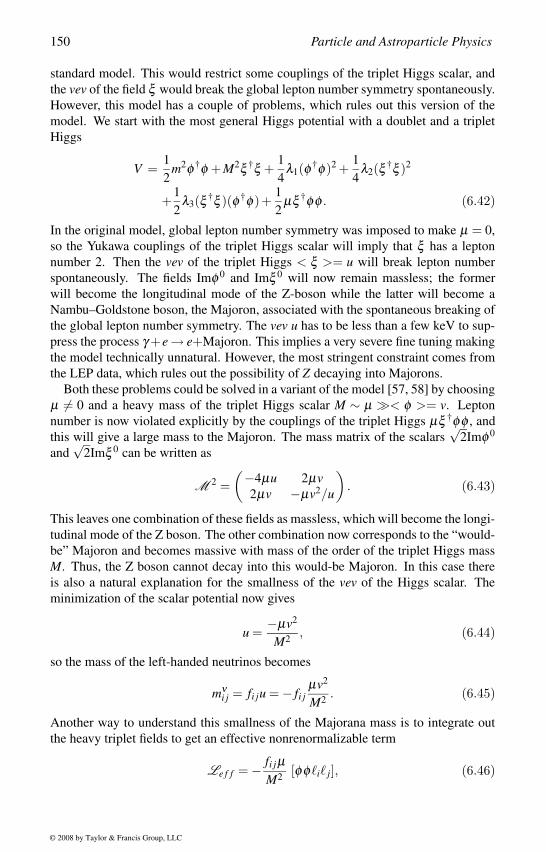
150 Particle and Astroparticle Physics
standard model. This would restrict some couplings of the triplet Higgs scalar, and
the vev of the field ξ would break the global lepton number symmetry spontaneously.
However, this model has a couple of problems, which rules out this version of the
model. We start with the most general Higgs potential with a doublet and a triplet
Higgs
V =1
2m2φ †φ +M2ξ †ξ +
1
4λ1(φ †φ)2 +
1
4λ2(ξ †ξ )2
+1
2λ3(ξ †ξ )(φ †φ)+
1
2µξ †φφ . (6.42)
In the original model, global lepton number symmetry was imposed to make µ = 0,
so the Yukawa couplings of the triplet Higgs scalar will imply that ξ has a lepton
number 2. Then the vev of the triplet Higgs < ξ >= u will break lepton number
spontaneously. The fields Imφ 0 and Imξ 0 will now remain massless; the former
will become the longitudinal mode of the Z-boson while the latter will become a
Nambu–Goldstone boson, the Majoron, associated with the spontaneous breaking of
the global lepton number symmetry. The vev u has to be less than a few keV to sup-
press the process γ +e → e+Majoron. This implies a very severe fine tuning making
the model technically unnatural. However, the most stringent constraint comes from
the LEP data, which rules out the possibility of Z decaying into Majorons.
Both these problems could be solved in a variant of the model [57, 58] by choosing
µ = 0 and a heavy mass of the triplet Higgs scalar M ∼ µ < φ >= v. Lepton
number is now violated explicitly by the couplings of the triplet Higgs µξ †φφ , and
this will give a large mass to the Majoron. The mass matrix of the scalars√
2Imφ 0
and√
2Imξ 0 can be written as
M 2 =(−4µu 2µv
2µv −µv2/u
). (6.43)
This leaves one combination of these fields as massless, which will become the longi-
tudinal mode of the Z boson. The other combination now corresponds to the “would-
be” Majoron and becomes massive with mass of the order of the triplet Higgs mass
M. Thus, the Z boson cannot decay into this would-be Majoron. In this case there
is also a natural explanation for the smallness of the vev of the Higgs scalar. The
minimization of the scalar potential now gives
u =−µv2
M2 , (6.44)
so the mass of the left-handed neutrinos becomes
mνi j = fi ju = − fi j
µv2
M2 . (6.45)
Another way to understand this smallness of the Majorana mass is to integrate out
the heavy triplet fields to get an effective nonrenormalizable term
Le f f = − fi jµM2 [φφi j], (6.46)
© 2008 by Taylor & Francis Group, LLC
Neutrino Masses and Mixing 151
which then gives the neutrino mass through the vev of the Higgs doublet φ . The
lepton-number violating scale can now be as high as 109 GeV or preferably more to
give an eV neutrino naturally, which is also the correct scale for leptogenesis in this
model [57, 58] (see section 16.3).
There are many advantages of the triplet Higgs model of neutrino masses. The
neutrino mass matrix is now directly proportional to the Yukawa couplings fi j. This
will mean that by finding the Yukawa couplings, we can find the neutrino mass ma-
trix. In models with extra dimensions or models where one explains the cosmological
constant, the triplet Higgs scalar has a mass of around a few TeV. In these models
the same-sign dilepton signals with negligible standard model background in the col-
liders can detect the triplet Higgs scalar. Then the decays of the triplet Higgs will
give us all the Yukawa couplings, and from the collider experiments it will be pos-
sible to determine the neutrino mass matrix. This may also help us understand the
matter–antimatter asymmetry through leptogenesis.
Although the see-saw mechanism and the triplet Higgs mechanism are two differ-
ent extensions of the standard model, if one extends the standard model to make it
left–right symmetric, both of these mechanisms get embedded in the model. How-
ever, the realizations of these mechanisms are different. In the left–right symmetric
model B− L is a local gauge symmetry. Hence, lepton number violation requires
breaking of this local B−L symmetry spontaneously. Thus, all lepton-number vio-
lating effects enter through the breaking of this local symmetry.
Left–right Symmetric models
The low-energy observed parity violation is accommodated in the standard model by
treating the left-handed particles preferentially. A natural extension of the standard
model should treat the left-handed and the right-handed fermions in the same way.
With this motivation the left–right symmetric extension of the standard model was
proposed.
The left–right symmetric extensions of the standard model gauge group is ex-
tended to a gauge group SU(2)L ×SU(2)R ×U(1)B−L [59, 60]. The SU(2)R ×U(1)group is broken at some high energy, giving our low-energy electroweak theory with
only unbroken SU(2)L ×U(1)Y . The left-handed fermions are now doublets under
SU(2)L, while the right-handed fermions are doublets under SU(2)R. The extra U(1)group quantum numbers come out to be the same as the B−L quantum numbers of
the usual quarks and leptons. The transformations of the quarks and the leptons are
given by
QL =(
uLdL
)≡ [3,2,1,
1
3] QR =
(uRdR
)≡ [3,1,2,
1
3]
L =(
νLeL
)≡ [1,2,1,−1] R =
(νReR
)≡ [1,1,2,−1]. (6.47)
The electric charge and the U(1)Y hypercharge are related to the quantum numbers
© 2008 by Taylor & Francis Group, LLC
152 Particle and Astroparticle Physics
of the U(1)(B−L) and the SU(2)R groups through the relations
Q = T3L +Y = T3L +T3R +B−L
2. (6.48)
Thus, B−L is now a local gauge symmetry, so any B−L violating phenomenon such
as the neutrino mass or the neutron–antineutron oscillation would be possible only
after this symmetry is broken spontaneously.
The left–right symmetric models have an added attractive feature of breaking the
parity symmetry spontaneously. The SU(2)L gauge bosons WL and the SU(2)R gauge
bosons WR are not parity eigenstates, but under parity transformation WL ↔ WR.
Since left-handed and right-handed fermions are related by the parity operation, a
discrete Z2 symmetry relating the group SU(2)L ↔ SU(2)R can now be identified
with the parity operator of the Lorentz group. Thus, the spontaneous breaking of
the left–right symmetry will also break parity spontaneously. The invariance of the
Lagrangian under the parity symmetry will ensure that the gauge coupling constants
for the two SU(2) groups are the same before the SU(2)R group is broken at a scale
MR,
gL(M > MR) = gR(M > MR). (6.49)
After the left–right symmetry breaking, the gauge coupling constants for the two
SU(2) groups can be different. In some left–right symmetric models parity is broken
explicitly, while in other models parity is broken spontaneously before the left–right
symmetry breaking.
The choice of the Higgs scalars that break the left–right symmetry determines
some of its phenomenology. We shall first consider the most popular choice of the
Higgs scalar and later mention some other combinations of Higgs scalars and the
corresponding phenomenology. The conventional choice of Higgs scalar breaks the
group in two stages [61, 62]:
SU(3)c ×SU(2)L × SU(2)R ×U(1)(B−L) [≡ GLR]MR→ SU(3)c ×SU(2)L ×U(1)Y [≡ Gstd ]mW→ SU(3)c ×U(1)Q [≡ Gem].
In this case the same Higgs that breaks the left–right symmetry can give masses
to the neutrinos. The SU(2)R symmetry is now broken by a triplet Higgs scalar
(∆R), which transforms under GLR as [1,1,3,−2]. The discrete symmetry Z2 will
imply the existence of another triplet scalar (∆L), which transforms under Gstd as
[1,3,1,−2]. However, the vev of the left-handed triplet ∆L is constrained by the
precision measurement to be less than a few eV. Both triplet scalars have one doubly
charged component, one singly charged component, and a neutral component, ∆ ≡[∆++ ∆+ ∆0]. Only the neutral components can acquire vevs,
< ∆0R >= vR ∼ MR < ∆0
L >= vL mW . (6.50)
Although we have already assumed vR vL, this comes naturally from the mini-
mization of the scalar potential.
© 2008 by Taylor & Francis Group, LLC
Neutrino Masses and Mixing 153
The electroweak symmetry can be broken by a SU(2)L doublet [1,2,0,1], but
this cannot give masses to the fermions. So, a bi-doublet Higgs scalar Φ, which
transforms under GLR as [1,2,2,0] is considered for electroweak symmetry breaking.
There are two neutral components of Φ, both of which acquire nonzero vevs v and
v′. Without loss of generality we assume for simplicity v v′ and neglect v′, which
takes care of the flavor changing neutral currents.
To see the condition for minimization of the scalar potential, we now write the
scalar potential with all of these fields replaced by their vevs and then minimize to
find the condition on the vevs of the various fields:
V (vL,vR,v) = −µ2v2 −m2∆(v2
L + v2R)+ρ1(v4
L + v4R)
+ρ2v2Lv2
R +λv4 +αv2(v2L + v2
R)+βv2vLvR. (6.51)
The last term is the most crucial one. This term allows the breaking of discrete parity
symmetry and the SU(2)R without breaking the SU(2)L group.
The minimization of this potential with respect to vL and vR gives
−2m2∆vL +4ρ1v3
L +2ρ2vLv2R +2αv2vL +βv2vR = 0
−2m2∆vR +4ρ1v3
R +2ρ2vRv2L +2αv2vR +βv2vL = 0. (6.52)
These equations can be combined to get the condition
(v2L − v2
R)[(4ρ1 −2ρ2)vLvR −βv2] = 0. (6.53)
This has two solutions: the first one is a parity conserving, vL = vR, which cannot
explain the parity violation at low energies. The other solution is
vL =βv2
(4ρ1 −2ρ2)vR. (6.54)
In this case if SU(2)R and the left–right parity are broken at a very large scale vR v,
we get vL v. Thus, the parity violating solution gives a natural explanation of the
hierarchy vR v vL.
The Yukawa couplings of the fermions will have two parts; the first part will con-
tain terms with the bi-doublets while the second part has the couplings with the triplet
Higgs scalars. The first part will give the Dirac masses while the second part gives
the Majorana masses. The complete Yukawa couplings can be written as
LYuk = LDir +LMa j , (6.55)
with LDir = hia QLiQRa Φ+ fia LiRa Φ, (6.56)
and LMa j = fLi jTLiC
−1L j∆L + fRabTRaC−1Ra∆R, (6.57)
where i, j = 1,2,3 are the indices for the three left-handed generations and a,b =1,2,3 are the indices for the three right-handed generations. This indicates that the
neutrino Dirac masses are of the same order of magnitude as the charged lepton
© 2008 by Taylor & Francis Group, LLC
154 Particle and Astroparticle Physics
masses mD ∼ me ∼ fi jv. The neutrino mass matrix can now be written including
both the Dirac and Majorana mass contributions in the basis (νLi νRac ) as
Mν =(
mL mDmD MN
)=(
fLi j vL fia vfia v fRab vR
). (6.58)
If the determinant of the heavy right-handed neutrino mass matrix is nonvanish-
ing, this mass matrix gives three heavy Majorana fields with masses of the order
of ∼ O(vR), which are mostly the right-handed neutrinos. The other three neutrinos
remain light with masses
mνLi j = mL − m2D
MN=(
β fLi j
4ρ1 −2ρ2− f 2
iafRab
)v2
vR. (6.59)
These light states are mostly the left-handed neutrinos with a small admixture of
the right-handed neutrinos. There are now two contributions to the light neutrino
masses, one coming from the vev of the SU(2)L triplet Higgs scalar ∆L and the other
coming from the see-saw contribution. The second term is also called type I see-
saw, which is the usual see-saw contribution, while the first term coming from the
vev of the triplet Higgs scalar is called type II see-saw. Sometimes type II see-saw
includes both the contributions. The minimization of the potential ensures that both
the contributions are of the same order of magnitude.
We shall consider one more combination of the Higgs scalars, which can give us
the required symmetry breaking. In this case there are no triplet Higgs scalars, all
Higgs scalars are doublets under the SU(2) groups [63, 64]. The SU(2)R ×U(1)B−Lgroup is broken by a right-handed Higgs doublet χR ≡ [1,1,2,+1], which acquires
a vev 〈χR〉 = vR. The left–right parity then ensures that there is another left-handed
doublet Higgs scalar field χL ≡ [1,2,1,+1], which acquires a small vev 〈χL〉 = vL.
We retain the bi-doublet scalar Φ to give masses to the charged fermions.
The scalars χL,R break lepton number by one unit, so they cannot contribute to the
masses to the neutrinos. However, with these fields we can write effective dimension-
5 terms, which can contribute to the neutrino masses,
Lν =hL
MhLLχLχL +
hR
MLRRχRχR. (6.60)
Mh is some new scale, which could be around the left–right symmetry breaking scale
vR. This effective operator may be realized by introducing a singlet fermion S ≡[1,1,1,0] with mass MS. The neutrino masses can then be generated by the Yukawa
couplings of the neutrinos and the singlet fermion S
LS = fiaLiRaΦ fiLLiSχL + faRRaSχR +MSSS. (6.61)
When the scalars acquire vevs, they contribute to the neutrino mass matrix, which
can be written in the basis (νLi νRac S ) as
Mν =
0 fiav fiLvLfiav 0 faRvR
fiLvL faRvR MS
. (6.62)
© 2008 by Taylor & Francis Group, LLC
Neutrino Masses and Mixing 155
The right-handed neutrinos get an effective Majorana mass of MN ∼ f 2aRv2
R/MS, while
the left-handed neutrinos remain light,
mν i j = − fia fiLvvL
faRvR+
fia f jb
faR fbR
MSv2
v2R
. (6.63)
The second term is the so-called double see-saw contribution, which looks like the
usual see-saw contribution when the expression for MN is substituted.
The first term is distinct from the see-saw mechanisms and is independent of MS.
This contribution has some interesting phenomenology and is called the type III see-
saw mechanism [64]. Although for simplicity we considered only one singlet S,
in any realistic model three singlet neutrinos Sp (p = 1,2,3) are required to have
a rank-3 light neutrino mass matrix. In this model parity could be spontaneously
broken by a singlet Higgs scalar or explicitly broken by giving different masses to
χL and χR, to get the required solution from minimization of the potential. A natural
assumption for the mass scales is vL <∼ v, since v breaks the electroweak symmetry
and gives masses to the fermions, and both vR and MS are heavy. If MS < vR, then
some of the heavy neutrinos become naturally almost degenerate, which may have
some interesting consequences.
There are now three additional gauge bosons in the theory. The two charged
right-handed gauge bosons become massive MWR ∼ vR. One combination of the
neutral gauge bosons corresponding to SU(2)R and U(1)B−L also becomes heavy
MZR ∼ vR. Although low-energy phenomenology gives a bound on these gauge
bosons of around 1 TeV [44], most models of neutrino masses and leptogenesis re-
quire the left–right symmetry breaking scale to be around vR ∼ 109 GeV or above. In
some grand unified theories this scale cannot be lower than 1014 GeV. The left–right
symmetric models have many interesting phenomenology. We shall discuss some of
the consequences of the B−L violation in section 8.5.
Radiative Models
Radiative models of neutrino masses were proposed to explain the smallness of the
neutrino masses without invoking a very large scale in the theory. Several radiative
models can naturally explain the smallness of the neutrino mass with only TeV scale
new particles. Since the scale of lepton number violation in this case is around a
few TeV, all new physics is now in the next generation accelerator energy range.
For example, the new Higgs scalars of these models could be observed in the near
future. However, these models suffer from a serious drawback that they allow very
fast lepton number violation, which can then erase any matter–antimatter asymmetry
in the universe.
In a radiative model with minimal extension of the standard model, one extends
the standard model with a singlet charged Higgs scalar η+, which transforms as
[1,1,+1] [65]. This model is known as the Zee model, which requires two doublet
Higgs scalars, φ1 and φ2, for explicit lepton number violation. The Yukawa couplings
of the singlet scalar then violate lepton number:
L∆L =0 = fi j iL jL η+ + µεab φaφb η†+, (6.64)
© 2008 by Taylor & Francis Group, LLC
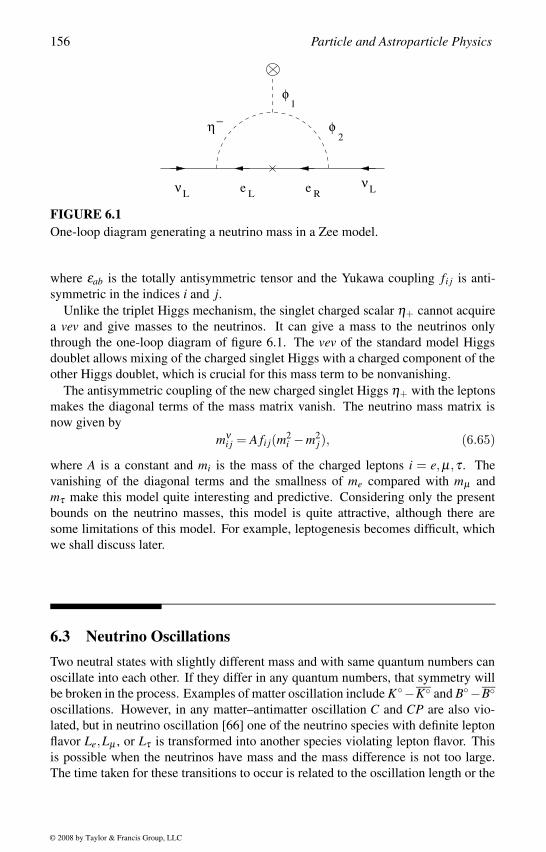
156 Particle and Astroparticle Physics
φ
φ
1
νν
η
ee
_
L LR
2
L
FIGURE 6.1One-loop diagram generating a neutrino mass in a Zee model.
where εab is the totally antisymmetric tensor and the Yukawa coupling fi j is anti-
symmetric in the indices i and j.Unlike the triplet Higgs mechanism, the singlet charged scalar η+ cannot acquire
a vev and give masses to the neutrinos. It can give a mass to the neutrinos only
through the one-loop diagram of figure 6.1. The vev of the standard model Higgs
doublet allows mixing of the charged singlet Higgs with a charged component of the
other Higgs doublet, which is crucial for this mass term to be nonvanishing.
The antisymmetric coupling of the new charged singlet Higgs η+ with the leptons
makes the diagonal terms of the mass matrix vanish. The neutrino mass matrix is
now given by
mνi j = A fi j(m2
i −m2j), (6.65)
where A is a constant and mi is the mass of the charged leptons i = e,µ,τ . The
vanishing of the diagonal terms and the smallness of me compared with mµ and
mτ make this model quite interesting and predictive. Considering only the present
bounds on the neutrino masses, this model is quite attractive, although there are
some limitations of this model. For example, leptogenesis becomes difficult, which
we shall discuss later.
6.3 Neutrino OscillationsTwo neutral states with slightly different mass and with same quantum numbers can
oscillate into each other. If they differ in any quantum numbers, that symmetry will
be broken in the process. Examples of matter oscillation include K−K and B−Boscillations. However, in any matter–antimatter oscillation C and CP are also vio-
lated, but in neutrino oscillation [66] one of the neutrino species with definite lepton
flavor Le,Lµ , or Lτ is transformed into another species violating lepton flavor. This
is possible when the neutrinos have mass and the mass difference is not too large.
The time taken for these transitions to occur is related to the oscillation length or the
© 2008 by Taylor & Francis Group, LLC
Neutrino Masses and Mixing 157
distance that a neutrino species can travel without getting changed to another species.
The uncertainty principle relates the oscillation time and the mass squared difference
between the two states. Another crucial requirement for the neutrino oscillations is
the violation of neutrino flavors through mixing of mass eigenstates [67].
The neutrinos of definite flavor are produced in any charged-current interaction. If
any process involves an electron, we know that a νe has been produced. When this
neutrino propagates, it is the physical state that propagates with time, and after some
time it has a probability to be partly in a different flavor state, say, νµ or ντ . If we
detect this neutrino at a distance, we may find a neutrino with a different flavor.
If the two states have the same masses, then both of them will propagate the same
way and there will not be any oscillation. If the two states have different masses but
the flavor states are the same as the physical states (no mixing), then the flavor states
will have definite evolution and they will not change to the other state. Thus, the
main criteria for the neutrino oscillation are that there should be a mass difference
between the different neutrino states and that the mass eigenstates are different from
the flavor eigenstates, which is given by the neutrino mixing matrix.
Neutrino Mixing
Let us assume that in some extensions of the standard model, neutrinos have masses,
which are given by
Lmass = miνTiLC−1νiL ≡ miνiLνiL, (6.66)
where νiL are the physical states with Majorana mass mi. We shall not worry about
the origin of this mass in this discussion.
In general, the physical states are not the weak eigenstates that appear in the
charged current and neutral current interactions of the neutrinos
LCC = − g√2
∑α=e,µ,τ
ναLγρ lαLW ρ
LNC = − g2cosθw
∑α=e,µ,τ
ναLγρ ναLZρ , (6.67)
where the lαL are physical charged leptons with masses mα . So, the ναL are the
neutrinos that have definite lepton flavor α .
The weak eigenstates are related to the physical or mass eigenstates by
ναL =3
∑i=1
UαiνiL. (6.68)
Uαi is called the PMNS (Pontecorvo–Maki–Nakagawa–Sakata) mixing matrix [67].
The mass matrix in the flavor basis, i.e., the basis in which the charged lepton mass
matrix is diagonal, is then given by
Mναβ = UαiM
diagi j UT
β j, (6.69)
© 2008 by Taylor & Francis Group, LLC
158 Particle and Astroparticle Physics
where Mdiagi j = miδi j. It is convenient to parameterize this mixing matrix Uαi in terms
of 3 mixing angles
U =
c1c3 −s1c3 −s3s1c2 − c1s2s3 c1c2 + s1s2s3 −c3s2s1s2 + c1c2s3 c1s2 − s2c2s3 c2c3
, (6.70)
where si = sinθi and ci = cosθi. If there is CP violation, there will be complex
phases in this matrix. This mixing is crucial for neutrino oscillations which violate
lepton flavors (Le,Lµ ,Lτ ).
Two Generation Vacuum Oscillation
We shall now discuss the neutrino oscillations. First we shall assume a two neutrino
scenario for simplification. Let us consider two weak eigenstates |νe > and |νµ >.
But the mass matrix in this basis is not diagonal. After diagonalizing the mass matrix,
we can write the two physical eigenstates as ν1 and ν2 with masses m1 and m2. The
two weak eigenstates or the flavor eigenstates can now be expressed in terms of the
mass eigenstates as( |νe >|νµ >
)=(
cosθ sinθ−sinθ cosθ
)( |ν1 >|ν2 >
)=(
c s−s c
)( |ν1 >|ν2 >
), (6.71)
where we defined for the mixing angles c = cosθ and s = sinθ . In this section we
shall assume that there is no CP violation, and hence, the mixing matrices are real
and orthogonal.
The physical states will evolve with time as
|ν1,2(t) >= exp−iE1,2t |ν1,2(0) >, (6.72)
where for the ultra-relativistic neutrinos with momentum (pi mi), the energy can
be approximated as
Ei = pi +m2
i2pi
. (6.73)
If we start with a νe beam at time t = 0, after a time t = t, both νe and νµ will be
present in the beam.
After a time t, the weak eigenstates will evolve into( |νe(t) >|νµ(t) >
)=(
c s−s c
)(exp−iE1t |ν1(0) >exp−iE2t |ν2(0) >
)=(
c s−s c
)(exp−iE1t 0
0 exp−iE2t
)(c −ss c
)( |νe(0) >|νµ(0) >
).(6.74)
If we thus start with |νe(0) >, after a time t, we shall have a beam |νe(t) >. The
probability of |νµ(0) > in this beam of |νe(t) > is the probability of finding a νµafter a time t, starting with a νe beam, which is
Pνe→νµ = | < νµ(0)|νe(t) > |2 = sin2(2θ)sin2(
∆m2L4E
), (6.75)
© 2008 by Taylor & Francis Group, LLC
Neutrino Masses and Mixing 159
where ∆m2 =∣∣m2
2 −m21
∣∣, E is the average energy of the neutrino beam, and L is the
length traversed by the beam before a νµ detection was taking place. Similarly the
survival probabilities for a νe(νµ) to be detected in a νe(νµ) beam after a time t are
Pνe→νe = Pνµ→νµ = 1− sin2(2θ)sin2(
∆m2L4E
). (6.76)
Thus, the two parameters sin2(2θ) and ∆m2 determine the oscillation probability.
The oscillation length can be defined as
L0 = 2.47E (GeV)
∆m2 (eV2)km, (6.77)
which is the distance, after which the neutrino returns to the initial state, i.e., the
phase becomes 2π . We can also write equation 6.75 in a more convenient form
Pνe→νµ = sin2(2θ) sin2(
1.27∆m2(eV2) L(km)
E(GeV)
)= sin2(2θ)sin2
(πLL0
). (6.78)
Most of the neutrino oscillation experiments analyze and present their results in terms
of the parameters of a two neutrino oscillation in one of the above forms, assuming
that the dominant mixing is between these two neutrinos.
The distance L at which a significant oscillation can be seen should be close to the
oscillation length L ∼ L0. For any shorter distance, the neutrinos will not get enough
time to oscillate. On the other hand, if the source to detector distance is too large,
L L0, many oscillations will take place within this distance and we get an average
value
Pνe→νµ (L) =1
2sin2(2θ). (6.79)
In neutrino oscillations neutrino flavor is violated but the total lepton number is con-
served. If there is helicity flip in the oscillation, total lepton numbers can be violated,
but such ∆L = 2 neutrino oscillation processes (originally proposed in [66]) will be
highly suppressed by a factor of mν/E. This is the so-called neutrino–antineutrino
oscillation, which is impossible to see with our present detectors.
In a neutrino oscillation experiment the distance between the source and the de-
tector L and the energy of the neutrino beam E determines what is the lowest mass-
squared difference that can be measured in the experiment
∆m2 ∼ EL
. (6.80)
The sensitivity ranges of the different experiments are presented in table 6.1.
© 2008 by Taylor & Francis Group, LLC
160 Particle and Astroparticle Physics
TABLE 6.1Neutrino sources and an estimate of their sensitivity for neutrino oscillations. SBL
and LBL correspond to short baseline and long baseline.
Source Energy E Distance L ∆m2
GeV km eV2
Reactor SBL 10−3 0.1 0.01
Reactor LBL 10−3 1 10−3
Accelerators SBL 1 1 1
Accelerators LBL 1 103 10−3
Atmosphere 1 104 10−4
Sun 10−3 108 10−11
Three Generation Scenario
There are at least three light neutrinos. So, in any detail analysis one has to con-
sider a three generation scenario. We shall thus generalize our previous discussion
to include the third neutrino. We start with the general relation between the mass
eigenstates and the flavor eigenstates of equation (6.68). The physical states |νi(t) >,
which are the states with masses mi, evolve with time as
|νi(t) >= exp−iEit |νi(0) > . (6.81)
The states |νi > have momentum pi and energy Ei = pi +m2i /(2pi), assuming pi
mi. After a time t, the weak eigenstates will evolve into
|να(t) > = ∑i
Uαiexp−iEit |νi(0) >
= ∑i
Uαiexp−iEitU∗β i|νβ (0) > . (6.82)
As in the earlier case, the oscillation probability of a νβ to be found in a neutrino
beam of να after a time t will then be given by
Pνα→νβ =∣∣< νβ (0)|να(t) >
∣∣2= ∑
i j
∣∣∣UαiU∗β iU
∗α jUβ j
∣∣∣cos[(Ei −E j)t −φαβ i j], (6.83)
where φαβ i j = arg[UαiU∗β iU
∗α jUβ j] is a phase, which vanishes when there is no CP
violation. The oscillation length can be defined as
L0i j =
4πE∆m2
i j= 2.47
E(GeV)∆m2
i j(eV2)km, (6.84)
© 2008 by Taylor & Francis Group, LLC
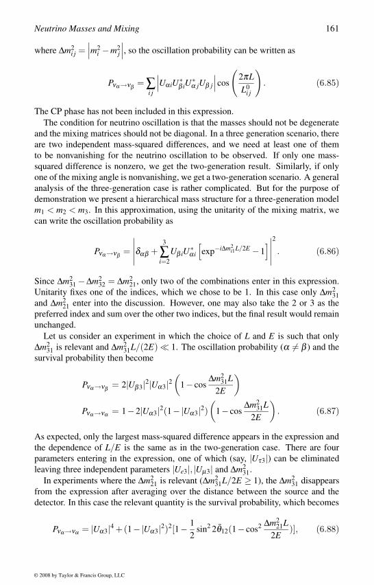
Neutrino Masses and Mixing 161
where ∆m2i j =
∣∣∣m2i −m2
j
∣∣∣, so the oscillation probability can be written as
Pνα→νβ = ∑i j
∣∣∣UαiU∗β iU
∗α jUβ j
∣∣∣cos
(2πLL0
i j
). (6.85)
The CP phase has not been included in this expression.
The condition for neutrino oscillation is that the masses should not be degenerate
and the mixing matrices should not be diagonal. In a three generation scenario, there
are two independent mass-squared differences, and we need at least one of them
to be nonvanishing for the neutrino oscillation to be observed. If only one mass-
squared difference is nonzero, we get the two-generation result. Similarly, if only
one of the mixing angle is nonvanishing, we get a two-generation scenario. A general
analysis of the three-generation case is rather complicated. But for the purpose of
demonstration we present a hierarchical mass structure for a three-generation model
m1 < m2 < m3. In this approximation, using the unitarity of the mixing matrix, we
can write the oscillation probability as
Pνα→νβ =
∣∣∣∣∣δαβ +3
∑i=2
Uβ iU∗αi
[exp−i∆m2
i1L/2E −1]∣∣∣∣∣
2
. (6.86)
Since ∆m231 −∆m2
32 = ∆m221, only two of the combinations enter in this expression.
Unitarity fixes one of the indices, which we chose to be 1. In this case only ∆m231
and ∆m221 enter into the discussion. However, one may also take the 2 or 3 as the
preferred index and sum over the other two indices, but the final result would remain
unchanged.
Let us consider an experiment in which the choice of L and E is such that only
∆m231 is relevant and ∆m2
31L/(2E) 1. The oscillation probability (α = β ) and the
survival probability then become
Pνα→νβ = 2|Uβ3|2|Uα3|2(
1− cos∆m2
31L2E
)Pνα→να = 1−2|Uα3|2(1−|Uα3|2)
(1− cos
∆m231L
2E
). (6.87)
As expected, only the largest mass-squared difference appears in the expression and
the dependence of L/E is the same as in the two-generation case. There are four
parameters entering in the expression, one of which (say, |Uτ3|) can be eliminated
leaving three independent parameters |Ue3|, |Uµ3| and ∆m231.
In experiments where the ∆m221 is relevant (∆m2
31L/2E ≥ 1), the ∆m231 disappears
from the expression after averaging over the distance between the source and the
detector. In this case the relevant quantity is the survival probability, which becomes
Pνα→να = |Uα3|4 +(1−|Uα3|2)2[1− 1
2sin2 2θ12(1− cos2 ∆m2
21L2E
)], (6.88)
© 2008 by Taylor & Francis Group, LLC
162 Particle and Astroparticle Physics
where
sin2 θ12 =|Uα2|2
∑2i=1 |Uαi|2
. (6.89)
The only common parameter between this probability and the previous one is |Ue3|2.
Since experimentally |Ue3|2 has been constrained by CHOOZ [68] to be extremely
small and the mass-squared differences required to explain the solar and atmospheric
neutrino problems do not overlap, these two experiments could thus be treated inde-
pendently for an order of magnitude estimate. However, for a detailed analysis one
needs to study a three-generation case for the allowed range of |Ue3|2.
Neutrino Oscillation in Matter
The neutrino oscillation depends on the mass-squared difference and the mixing an-
gle. For the present let us restrict ourselves to only two generations. Then there
are only one mass-squared difference and one mixing angle. It was noticed that the
mass of one of the neutrinos could vary while propagating through matter, due to its
interaction with the media. For example, if a beam of νe and νµ is propagating in
matter with varying density, the νe will interact with matter through charged-current
interactions and its mass can vary while νµ will not have any effect. The mass-square
difference can then vary, and this can lead to an interesting phenomenon of resonant
oscillation, called the Mikheyev–Smirnov–Wolfenstein (MSW) effect, which is re-
quired to solve the solar neutrino problem [69]. The matter effect was first pointed
out by Wolfenstein, but some factors were corrected and the resonance effect was no-
ticed by others [70]. Later this effect was applied to the solar neutrinos by Mikheyev
and Smirnov.
While propagating in matter, the νe interacts with matter through charged-current
interaction. This contributes an additional potential to the electron neutrinos, pro-
portional to the electron number density Ne,
V =√
2GF Ne. (6.90)
This will contribute to the energy of the electron neutrinos, generating an effective
mass of νem2
e → m2e +A = m2
e +2√
2 GF Ne E. (6.91)Now consider a simple situation with two neutrinos νe and one other neutrino νX ,
where X could be µ,τ or some other light neutrinos that do not interact through the
weak interaction, are singlets under SU(2)L, and are called the sterile neutrinos.
We shall now study the effect of this potential on the neutrino masses. If the
effective mass eigenvalues are m1 and m2 and the mass eigenstates are related to the
weak eigenstates through the orthogonal mixing matrix
O =(
cosθ sinθ−sinθ cosθ
), (6.92)
the mass-squared matrix of νe and νX can be written as
M2ν = OT (Mdiag
ν )2O+(
A 0
0 0
), (6.93)
© 2008 by Taylor & Francis Group, LLC
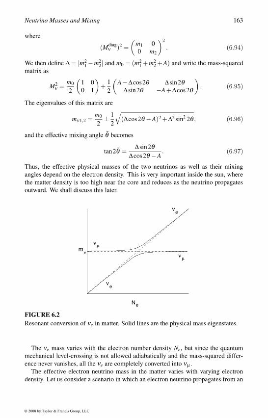
Neutrino Masses and Mixing 163
where
(Mdiagν )2 =
(m1 0
0 m2
)2
. (6.94)
We then define ∆ = |m21 −m2
2| and m0 = (m21 + m2
2 + A) and write the mass-squared
matrix as
M2ν =
m0
2
(1 0
0 1
)+
1
2
(A−∆cos2θ ∆sin2θ
∆sin2θ −A+∆cos2θ
). (6.95)
The eigenvalues of this matrix are
mν1,2 =m0
2± 1
2
√(∆cos2θ −A)2 +∆2 sin2 2θ , (6.96)
and the effective mixing angle θ becomes
tan2θ =∆sin2θ
∆cos2θ −A. (6.97)
Thus, the effective physical masses of the two neutrinos as well as their mixing
angles depend on the electron density. This is very important inside the sun, where
the matter density is too high near the core and reduces as the neutrino propagates
outward. We shall discuss this later.
µ
νµ
νe
νe
νmν
Ne
FIGURE 6.2Resonant conversion of νe in matter. Solid lines are the physical mass eigenstates.
The νe mass varies with the electron number density Ne, but since the quantum
mechanical level-crossing is not allowed adiabatically and the mass-squared differ-
ence never vanishes, all the νe are completely converted into νµ .
The effective electron neutrino mass in the matter varies with varying electron
density. Let us consider a scenario in which an electron neutrino propagates from an
© 2008 by Taylor & Francis Group, LLC
164 Particle and Astroparticle Physics
extremely dense media, such as the core of the sun, to rarer media such as the surface
of the sun. Let us also assume that near the core of the sun, the νe effective mass is
higher than the effective mass of νµ . Since both νe and νµ are combinations of the
mass eigenstates m1 and m2, one cannot talk about the mass of νe or νµ . However, if
the mixing angle is small, νe can be identified mostly with ν1 with a small admixture
of ν2, and then one can say that the effective mass of νe is m1. As νe comes out from
the core of the sun to the surface, the νe mass varies with the electron number density
Ne. When the νe mass approaches the νµ mass and the mass-squared difference
approaches the point ∆cos2θ , a resonant oscillation takes place at A ∼ ∆cos2θ . At
this point, the two masses are supposed to be the same and equal to ∆sinθ , so they
cross each other. But in quantum mechanics the phenomenon of level crossing does
not allow two quantum levels to cross adiabatically. If we now minimize the mass-
squared difference with respect to A, we find that the minimum never vanishes and
the two levels never cross each other. So, a total conversion of levels takes place and
all the νe become νµ . If there are any small numbers of νµ , they may get converted
to νe.
The minimum corresponds to a point
A = ∆cos2θ , (6.98)
where a total conversion of the states take place. Since A depends on both matter
density and the energy of the neutrinos, any νe with energy higher than a critical
value, will be completely converted into a νµ during its propagation inside the sun
and will come out as νµ . This is the MSW effect, demonstrated in figure 6.2. As
the νe propagate inside the sun from the dense core to its surface with very low
matter density, the effective mass of νe reduces until it approaches the cross-over
point. Near this point all of these νe are completely converted into νµ . Since the
mass of νµ does not depend on the matter density, it remains constant. All of the νµwill also be completely converted into νe near the cross-over point. We explained
the MSW effect with adiabatic approximation and with only two neutrinos for pur-
pose of demonstration. In practice one needs to consider the nonadiabatic region of
the parameter space and all the neutrino species, which makes it more complicated.
However, the basic idea remains the same.
6.4 Summary of ExperimentsExperiments with neutrinos are extremely difficult since they interact with matter
very weakly. Almost sixty years after its discovery we discovered that the neutrinos
have small masses. First the electron neutrino flux from the sun was observed to
be lower than the predictions in the chlorine experiment. Although this result had
several uncertainties, it initiated further activities in the field. Subsequently a defi-
ciency in the atmospheric muon neutrino flux was observed, which established that
© 2008 by Taylor & Francis Group, LLC
Neutrino Masses and Mixing 165
the neutrinos have tiny masses. Solar neutrino experiments as well as laboratory
experiments then confirmed this result.
We shall now present a brief summary of the results and then provide a few details
about some of the important results. The atmospheric neutrino results imply that νµoscillates into ντ with a mass-squared difference and mixing angle [71]:
∆m2atm (1.5−3.4)×10−3 eV2, sin2 2θatm > 0.92, (6.99)
with a best fit of ∆m2atm = 2.1×10⁻³ eV2 with sin2 2θatm = 1. A global fit to all the
solar neutrino experiments, combined with the KamLAND result [72], implies that
νe oscillates into a combination of the states νµ and ντ with
∆m2 = 7.9+0.6−0.5 ×10⁻⁵ eV2 and tan2 θ = 0.40+0.10
−0.07. (6.100)
These results also prefer a three-generation solution, although a sterile neutrino is
not yet ruled out.
If we assume that there are three left-handed Majorana neutrinos and the physical
neutrinos νi, i = 1,2,3 with masses mi are related to the weak eigenstates να , α =e,µ,τ by the mixing matrix Uαi , then the mixing matrix can be parameterized as
U =
c1c3 −s1c3 −s3s1c2 − c1s2s3 c1c2 + s1s2s3 −c3s2s1s2 + c1c2s3 c1s2 − s2c2s3 c2c3
, (6.101)
where si = sinθi and ci = cosθi. Nonobservation of oscillations of νe to some other
neutrinos at the CHOOZ experiment provided strong constraint on the third mixing
angle s3. For a mass-squared difference of 7×10⁻⁴ eV2 or more, the CHOOZ bound
[68] on the mixing angle is sin2 θ13 < 0.1. The WMAP constraint [73] on the sum of
all three neutrino masses is ∑mi < 0.69 eV, which may be softened in some cases.
The Heidelberg–Moscow neutrinoless double beta decay experiment [74] reported
mee = 0.1−0.9 eV, but this result is yet to be confirmed. The first positive indication
of neutrino oscillation was reported by LSND collaboration [75] that there is νµ → νe
oscillation with mass-squared difference ∆m2 > 0.2 eV and sin2 θ ∼ (0.001−0.04).This result would have required at least one sterile neutrino. But this result has been
ruled out by the MiniBOONE experiment at Fermilab [76]. After this brief summary
we shall now discuss some of these experiments.
Atmospheric Neutrinos
The neutrinos produced in our atmosphere mostly from pion and subsequent muon
decays,
π → µ + νµ and µ → e+ νe +νµ ,
were measured at Kamiokande and super-Kamiokande detectors. Although these
detectors could distinguish between νµ and νe, since the absolute flux of atmospheric
νµ and νe are not well-known, these experiments measured a double ratio
R =(Nµ/Ne)obs
(Nµ/Ne)MC. (6.102)
© 2008 by Taylor & Francis Group, LLC
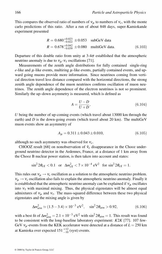
166 Particle and Astroparticle Physics
This compares the observed ratio of numbers of νµ to numbers of νe, with the monte
carlo predictions of this ratio. After a run of about 848 days, super-Kamiokande
experiment presented
R = 0.680+0.023−0.022 ±0.053 subGeV data
R = 0.678+0.042−0.039 ±0.080 multiGeV data. (6.103)
Departure of this double ratio from unity at 3-4σ established that the atmospheric
neutrino anomaly is due to νµ -ντ oscillations [71].
Measurements of the zenith angle distributions for fully contained single-ring
e-like and µ-like events, multiring µ-like events, partially contained events, and up-
ward going muons provide more information. Since neutrinos coming from verti-
cal direction travel less distance compared with the horizontal directions, the strong
zenith angle dependence of the muon neutrinos confirms oscillation of muon neu-
trinos. The zenith angle dependence of the electron neutrinos is not so prominent.
Similarly the up–down asymmetry is measured, which is defined as
A =U −DU +D
, (6.104)
U being the number of up-coming events (which travel about 13000 km through the
earth) and D is the down-going events (which travel about 20 km). The multiGeV
muon events show an asymmetry of
Aµ = 0.311±0.043±0.010, (6.105)
although no such asymmetry was observed for νe.
CHOOZ result [68] on nonobservation of νe disappearance in the Chooz under-
ground neutrino detector in the Ardennes, France, at a distance of 1 km away from
the Chooz B nuclear power station, is then taken into account and states:
sin2 2θeX < 0.1 or ∆m2eX < 7×10⁻⁴ eV2 for sin2 2θeX = 1.
This rules out νµ → νe oscillation as a solution to the atmospheric neutrino problem.
νµ → νs oscillation also fails to explain the atmospheric neutrino anomaly. Finally it
is established that the atmospheric neutrino anomaly can be explained if νµ oscillates
into ντ with maximal mixing. Thus, the physical eigenstates will be almost equal
admixtures of νµ and ντ . The mass-squared difference between these two physical
eigenstates and the mixing angle is given by
∆m2atm (1.5−3.4)×10−3 eV2, sin2 2θatm > 0.92, (6.106)
with a best fit of ∆m2atm = 2.1×10⁻³ eV2 with sin2 2θatm = 1. This result was found
to be consistent with the long-baseline laboratory experiment: K2K [77]. 107 few-
GeV νµ -events from the KEK accelerator were detected at a distance of L = 250 km
at Kamioka over expected 151 +12−10 (syst) events.
© 2008 by Taylor & Francis Group, LLC
Neutrino Masses and Mixing 167
Solar Neutrinos
The first indication of neutrino oscillation was obtained from solar neutrinos, when
the solar model predictions of νe flux were found to differ from the observed νe flux
in the chlorine experiment. It is now established that the νe coming from the sun
oscillates into a combination of νµ and ντ with fairly large mixing angles. This also
confirms that the source of energy in the sun and other stars is nuclear fusion.
There are two methods of hydrogen fusion into helium inside the sun, the pp-cycleand the CNO-cycle, which produce energy and release neutrinos
4p → 4He+2e+ +2νe +26.73 MeV. (6.107)
The dominant contribution comes from the pp-cycle:
Reactions % Eν in MeV
p+ p → 2H+ e+ +νe 99.6 % pp ≤ 0.42
p+ e− + p → 2H+νe 0.4 % pep 1.44
2H+ p → 3He+ γ3He+ 3He → 4He+2 p 85 %
3He+ p → 4He+ e+ +νe 2×10⁻⁵% hep ≤ 18.77
3He+ 4He+ → 7Be+ γ 15 %
7Be+ e− → 7Li+νe 99.87 % 7Be 0.861
7Li+ p → 2 4He
7Be+ p → 8B+ γ 0.13 %
8B → 8Be∗ + e+ +νe8B ≤ 14.06
8Be∗ → 2 4He
Only about 1.6% of the energy in the sun comes from the CNO-cycle:
12C+ p → 13N+ γ13N → 13C+ e+ +νe (Eν ≤ 1.2 MeV)
13C+ p → 14N+ γ14N+ p → 15O+ γ
15O → 15N+ e+ +νe (Eν ≤ 1.73 MeV)15N+ p → 12C+α15N+ p → 16O+ γ16O+ p → 17F+ γ
17F → 17O+ e+ +νe (Eν ≤ 1.74 MeV)17O+ p → 14N+α.
© 2008 by Taylor & Francis Group, LLC
168 Particle and Astroparticle Physics
Here C, N and O act as catalysts to fuse the hydrogen into helium.
The predictions of the solar neutrino flux are based on the so-called standard solarmodel. Using the basic equations of stellar evolution (hydrodynamic equilibrium is
assumed), the energy produced by the nuclear reactions given above is transported
by radiation and convection. The main uncertainties in the input parameters comes
from some nuclear cross-sections and the core temperature of the sun. The standard
solar models predict fluxes of electron neutrinos νe on earth of about 1010 cm−2 s−1
[78]. But since the detection of the neutrinos is extremely difficult because of their
very small cross-section, this flux leads to very few events in the detectors. With a
cross-section of about 10−45 cm2, about 1030 target atoms are required to produce
one event per day. So a very large physical size of the detectors is required to detect
the solar neutrinos.
It took many years to understand the solar neutrino problem. In the first experi-
ment at Homestake gold mine [79], chlorine was used to detect the neutrinos through
the reaction37Cl+νe → 37Ar+ e−. (6.108)
By measuring its radioactivity, 37Ar is detected. This reaction cannot detect the ppneutrinos, since it has a threshold of 0.814 MeV. This experiment reported, from
their 20 years of measurement, an average counting rate of 2.56±0.16±0.16 SNU
(solar neutrino unit), which is less than the predictions of the standard solar model
of 7.7± 1.2 SNU [80]. One SNU is defined as 10−36 captures per target atom per
sec. This was the first experiment to report the solar neutrino problem, indicating
the possibility of neutrino oscillations. The detection of neutrinos in this experiment
from the sun also established that the energy source of sun is nuclear fusion which is
associated with neutrino emission.
The solar neutrino experiments, the Kamiokande and the super-Kamiokande, used
water Cerenkov detectors [81], which are real-time detectors and can also measure
the zenith angle dependence of the events. They measure all the flavors of neu-
trinos, but for the νµ and ντ , the scattering rate is 6 times smaller than the νe − escattering cross-section. The threshold of these experiments is rather high, 7.0 MeV
and 5.5 MeV, respectively, but the statistics compensates for this and they expect
about 20 to 30 signals every day, which are mostly the 8B neutrinos. The observed
flux at Kamiokande and super-Kamiokande is (2.80± 0.19± 0.33)× 106 cm−2s−1
and (2.44± 0.05 +0.09−0.07 )× 106 cm−2s−1 as opposed to the theoretical predictions of
(5.15+1.00−0.72 )×106 cm−2s−1. The large statistics at the super-Kamiokande experiment
coming from 11,240 events in about 825 days allow the measurement of the energy
spectrum of the recoil electrons and also the day/night asymmetry.
The most sensitive and advanced solar neutrino experiment is the Sudbury neu-
trino observatory [82], which is an imaging water Cerenkov detector, filled with an
ultra pure D2O target in an acrylic vessel and surrounded by photo-multiplier tubes.
This is then shielded by ultra-pure H2O and construction material, which acts as a
cosmic ray veto. By using a D2O target, the SNO detector can detect electron neu-
trinos (νe) through charged current (CC) interactions, whereas through the neutral
current (NC) interactions and elastic scattering (ES), it can simultaneously measure
© 2008 by Taylor & Francis Group, LLC
Neutrino Masses and Mixing 169
the flux of all active neutrinos (νx, x = e,µ,τ) from 8B decay in the sun:
νe +d → p+ p+ e (charged current),νx +d → νx + p+n (neutral current),νx + e → νx + e (elastic scattering) (6.109)
The neutrino fluxes deduced from the CC, NC and ES interactions are [82]
ΦCC = 1.59+0.08−0.07 (stat) +0.06
−0.08(syst)×106 cm−2 s−1 (6.110)
ΦNC = 5.21±0.27(stat)±0.38(syst)×106 cm−2 s−1 (6.111)
ΦES = 2.21+0.31−0.26 (stat)±0.10(syst)×106 cm−2 s−1. (6.112)
The difference between the CC and ES fluxes is (0.62±0.40)×106 cm−2 s−1, which
is about 1.6σ . The discrepancy is more prominent in the CC data, when compared
with the NC data. The ratio of the two fluxes is [82]
ΦCC
ΦNC = 0.306±0.026(stat)±0.024(syst). (6.113)
This ratio is expected to be 1 if all the neutrinos from the sun are νe. The observed de-
viation thus establishes the fact that a fraction of νe from the sun has reached us as νx(νX could be νµ or ντ ). An estimate of the νe flux and the fluxes of the nonelectron-
neutrino component then implies neutrino oscillation at a 5σ c.l. SNO is the only
solar neutrino experiment which proves in a solar-model independent way that solar
neutrinos undergo oscillations. Comparing the day–night energy spectra, day–night
asymmetries of different classes of events are also estimated. No substantial distor-
tion of the neutrino energy spectrum compared with the theoretical expectation has
been found.
The simplest explanation for the deficiency in the number of detected solar elec-
tron neutrinos is neutrino oscillations. Unlike for the atmospheric neutrinos, for the
solar neutrinos there could be two distinct solutions. The first possibility involves
the electron neutrinos coming from the sun oscillating into a νµ or a ντ during their
passage to Earth. This is called the vacuum oscillation. All the experiments together
rule out this explanation.
The second possibility involves resonant matter effect (MSW effect, discussed
in section 6.3). When the neutrinos come out from the core of the sun, they pass
through varying matter density. The matter density at the core is maximum and on the
surface almost zero. As the νe from the core pass through this varying density, their
effective mass reduces due to their interaction with matter. However, as they reach
the νµ mass, a total conversion takes place and all the νe become νµ , since quantum
mechanical level crossing is forbidden. The lighter νe continue without any such
conversion, although they may oscillate during their passage to Earth. This is called
the MSW solution of the solar neutrino problem. All present results indicate that this
is the solution to the solar neutrino problem with the parameter space specified by
© 2008 by Taylor & Francis Group, LLC
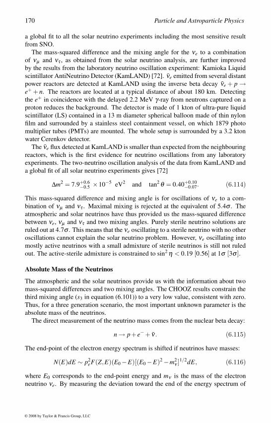
170 Particle and Astroparticle Physics
a global fit to all the solar neutrino experiments including the most sensitive result
from SNO.
The mass-squared difference and the mixing angle for the νe to a combination
of νµ and ντ , as obtained from the solar neutrino analysis, are further improved
by the results from the laboratory neutrino oscillation experiment: Kamioka Liquid
scintillator AntiNeutrino Detector (KamLAND) [72]. νe emitted from several distant
power reactors are detected at KamLAND using the inverse beta decay νe + p →e+ + n. The reactors are located at a typical distance of about 180 km. Detecting
the e+ in coincidence with the delayed 2.2 MeV γ-ray from neutrons captured on a
proton reduces the background. The detector is made of 1 kton of ultra-pure liquid
scintillator (LS) contained in a 13 m diameter spherical balloon made of thin nylon
film and surrounded by a stainless steel containment vessel, on which 1879 photo
multiplier tubes (PMTs) are mounted. The whole setup is surrounded by a 3.2 kton
water Cerenkov detector.
The νe flux detected at KamLAND is smaller than expected from the neighbouring
reactors, which is the first evidence for neutrino oscillations from any laboratory
experiments. The two-neutrino oscillation analysis of the data from KamLAND and
a global fit of all solar neutrino experiments gives [72]
∆m2 = 7.9+0.6−0.5 ×10⁻⁵ eV2 and tan2 θ = 0.40+0.10
−0.07. (6.114)
This mass-squared difference and mixing angle is for oscillations of νe to a com-
bination of νµ and ντ . Maximal mixing is rejected at the equivalent of 5.4σ . The
atmospheric and solar neutrinos have thus provided us the mass-squared difference
between νe, νµ and ντ and two mixing angles. Purely sterile neutrino solutions are
ruled out at 4.7σ . This means that the νe oscillating to a sterile neutrino with no other
oscillations cannot explain the solar neutrino problem. However, νe oscillating into
mostly active neutrinos with a small admixture of sterile neutrinos is still not ruled
out. The active-sterile admixture is constrained to sin2 η < 0.19 [0.56] at 1σ [3σ ].
Absolute Mass of the Neutrinos
The atmospheric and the solar neutrinos provide us with the information about two
mass-squared differences and two mixing angles. The CHOOZ results constrain the
third mixing angle (s3 in equation (6.101)) to a very low value, consistent with zero.
Thus, for a three generation scenario, the most important unknown parameter is the
absolute mass of the neutrinos.
The direct measurement of the neutrino mass comes from the nuclear beta decay:
n → p+ e− + ν. (6.115)
The end-point of the electron energy spectrum is shifted if neutrinos have masses:
N(E)dE ∼ p2eF(Z,E)(E0 −E)[(E0 −E)2 −m2
ν ]1/2dE, (6.116)
where E0 corresponds to the end-point energy and mν is the mass of the electron
neutrino νe. By measuring the deviation toward the end of the energy spectrum of
© 2008 by Taylor & Francis Group, LLC
Neutrino Masses and Mixing 171
the electrons in a tritium beta decay, the present upper limit on the mass of the νe is
obtained: mνe < 2.8 eV [44]. For the νµ and the ντ the corresponding bounds from
accelerator experiments are mνµ < 190 keV and mντ < 18.2 MeV [44].
This bound can be improved by the neutrinoless double beta decay experiment,
if neutrinos are Majorana particles. Any positive result in neutrinoless double beta
decay would also imply that there is lepton number violation in nature, which is a
fundamental question. Lepton number is conserved in all gauge interactions. Since
the Majorana mass of the neutrinos has to be very small, it is extremely difficult to
find out if there is lepton number violation in nature from any other experiment. On
the other hand, if the neutrinoless double beta decay can confirm that neutrinos are
Majorana particles, this will have many interesting consequences in particle physics
and cosmology. Even the constraints from the neutrinoless double beta decay can
provide us with strong bounds on many lepton-number violating processes.
In a neutrinoless double beta decay, the proton number of the decaying nucleus
changes by two units, keeping the mass number unchanged and two electrons (or
positrons) are emitted. This is an extremely rare process and the measurement is
extremely difficult. During beta decay, an even-even nucleus would go to an odd-
odd nucleus. When the binding energy of the odd–odd nuclei is smaller than that of
the parent nuclei, ordinary beta decay is forbidden energetically. However, a 2νββdecay, in which an even-even nucleus decays to another even-even nucleus, may still
be allowed:
(A,Z) → (A,Z +2)+ e− + e− + ν + ν. (6.117)
This second order process is extremely weak and is called two-neutrino double beta
decay (2νββ ). There are about 35 candidates for double beta decay, but only about
ten cases have so far been observed [44]. This process conserves lepton number and
is allowed in the standard model. On the other hand, if the neutrinos are Majorana
particles, a neutrinoless double beta decay is possible (0νββ ):
(A,Z) → (A,Z +2)+ e− + e−, (6.118)
in which two neutrons decay into two electrons without any neutrinos
n+n → p+ p+ e− + e−. (6.119)
This process violates lepton number by ∆L = 2 and directly measures the amount
of total lepton number violation. The total kinetic energies of the two electrons is
constant and is given by the Q value of the decay in the case of 0νββ decay. This
measurement does not have any background from the 2νββ decay or 2Mββ decay
(where M represents Majorons in models of spontaneously broken lepton number),
since in the 2νββ decay the total kinetic energy of the electrons have a distribution
because neutrinos or the Majorons carry away part of the energy.
In the standard model, the 0νββ decay is forbidden since neutrinos are massless.
However, in extensions of the standard model, neutrinos may have masses and Majo-
rana neutrinos are more natural than the Dirac neutrinos. If neutrinos have Majorana
masses, the measurement of the 0νββ decay will be able to measure this mass.
© 2008 by Taylor & Francis Group, LLC
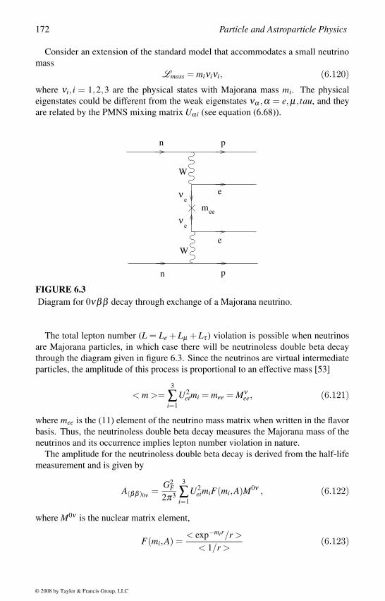
172 Particle and Astroparticle Physics
Consider an extension of the standard model that accommodates a small neutrino
mass
Lmass = miνiνi, (6.120)
where νi, i = 1,2,3 are the physical states with Majorana mass mi. The physical
eigenstates could be different from the weak eigenstates να ,α = e,µ, tau, and they
are related by the PMNS mixing matrix Uαi (see equation (6.68)).
n
W
ν
νm
e
e
ee
W
n p
e
e
p
FIGURE 6.3Diagram for 0νββ decay through exchange of a Majorana neutrino.
The total lepton number (L = Le + Lµ + Lτ ) violation is possible when neutrinos
are Majorana particles, in which case there will be neutrinoless double beta decay
through the diagram given in figure 6.3. Since the neutrinos are virtual intermediate
particles, the amplitude of this process is proportional to an effective mass [53]
< m >=3
∑i=1
U2eimi = mee = Mν
ee, (6.121)
where mee is the (11) element of the neutrino mass matrix when written in the flavor
basis. Thus, the neutrinoless double beta decay measures the Majorana mass of the
neutrinos and its occurrence implies lepton number violation in nature.
The amplitude for the neutrinoless double beta decay is derived from the half-life
measurement and is given by
A(ββ )0ν =G2
F2π3
3
∑i=1
U2eimiF(mi,A)M0ν , (6.122)
where M0ν is the nuclear matrix element,
F(mi,A) =< exp−mir/r >
< 1/r >(6.123)
© 2008 by Taylor & Francis Group, LLC
Neutrino Masses and Mixing 173
is the phase space factor, r is the distance between the two neutrons within the nu-
cleus, and R ≥ r/2 is the radius of the initial nucleus. The average is with respect to
the two-nucleon correlation function appropriate to a nucleus of atomic number A.
F(mi,A) can be approximated by a step function [83],
F(mi,A) = 1 for mi 10 MeV
F(mi,A) = 0 for mi 10 MeV. (6.124)
Thus, any heavy physical states will not contribute to the amplitude of the neutri-
noless double beta decay. In the case of the see-saw mechanism the right-handed
neutrinos are heavy and cannot cancel the contribution of the light left-handed neu-
trinos to the neutrinoless double beta decay. As a result, it is sufficient to work with
the effective Majorana mass matrices of the light left-handed neutrinos to study the
neutrinoless double beta decay.
The most sensitive double beta decay experiment is the Heidelberg–Moscow dou-
ble beta decay experiment in the Gran Sasso underground laboratory which was run-
ning for over a decade. The experiment operated five enriched (to 86%) high purity76Ge detectors, with a total mass of 11.5 kg, the active mass of 10.96 kg being equiv-
alent to a source strength of 125.5 mol 76Ge nuclei. It looked for the decay mode
76Ge → 76Se + 2 e− + (2 ν).
The high resolution of the Ge detector (3− 4 keV) leads to no background from
the 2νββ decay, in which the total energy carried by the two electrons is less than
the Q value. The Q value for this decay is known from earlier measurements with
high precision to be Qββ = 2039.006 (50) keV. This is very useful in identifying the
experimental signature of the 0νββ decay mode, which is a peak at the Q-value of
the decay.
The data from this experiment was accumulated in the five enriched detectors over
the period August 1990 through May 2003. An analysis of this data identified a line
at Qββ , with 29 events in the full spectrum corresponding to a 4.2σ evidence (> 5σfor the pulse shape selected spectrum) for the neutrinoless double beta decay [74].
The half-life for the 0νββ decay is reported to be
T 0ν1/2 = 1.19+0.37
−0.23 ×1025 y (1 σ) . (6.125)
Including the uncertainty in the nuclear matrix elements, this corresponds to an ef-
fective Majorana neutrino mass of the neutrino
< m >= (0.1−0.9) eV (99.73% c.l.). (6.126)
This is the first reported evidence for lepton number violation in nature. However,
this result relies on a very few events that could not be reproduced, and hence, needs
to be confirmed by future experiments.
Since the neutrinoless double beta decay measures the amount of lepton number
violation, the present upper bound on the lifetime of the 0νββ decay can constrain
© 2008 by Taylor & Francis Group, LLC
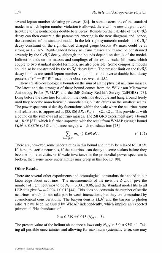
174 Particle and Astroparticle Physics
several lepton-number violating processes [84]. In some extensions of the standard
model in which lepton number violation is allowed, there will be new diagrams con-
tributing to the neutrinoless double beta decay. Bounds on the half-life of the 0νββdecay can then constrain the parameters entering in the new diagrams and, hence,
the extensions of the standard model. In the left–right symmetric models, the 0νββdecay constraint on the right-handed charged gauge bosons WR mass could be as
strong as 1.2 TeV. Right-handed heavy neutrino masses could also be constrained
severely by the 0νββ decay, although the bounds depend on details of the model.
Indirect bounds on the masses and couplings of the exotic scalar bilinears, which
couple to two standard model fermions, are also possible. Some composite models
could also be constrained by the 0νββ decay limit. The present limit on the 0νββdecay implies too small lepton number violation, so the inverse double beta decay
process e−e− →W−W− may not be observed even at ILC.
There are also cosmological bounds on the sum of all the physical neutrino masses.
The latest and the strongest of these bound comes from the Wilkinson Microwave
Anisotropy Probe (WMAP) and the 2dF Galaxy Redshift Survey (2dFGRS) [73].
Long before the structure formation, the neutrinos decouple and hang around freely
until they become nonrelativistic, smoothening out structures on the smallest scales.
The power spectrum of density fluctuations within the scale when the neutrinos were
still relativistic is suppressed as [85, 86] ∆Pm/Pm ≈−8Ων/Ωm. This provide us with
a bound on the sum over all neutrino masses. The 2dFGRS experiment gave a bound
of 1.8 eV [87], which is further improved with the result from WMAP giving a bound
Ων h2 < 0.0076 (95% confidence range), which translates into [73]
∑i=e,µ,τ
mνi ≤ 0.69 eV. (6.127)
There are, however, some uncertainties in this bound and it may be relaxed to 1.0 eV.
If there are sterile neutrinos, if the neutrinos can decay to some scalars before they
become nonrelativistic, or if scale invariance in the primordial power spectrum is
broken, then some more uncertainties may creep in this bound [88].
Other Results
There are several other experiments and cosmological constraints that added to our
knowledge about neutrinos. The measurements of the invisible Z-width give the
number of light neutrinos to be Nν = 3.00±0.06, and the standard model fits to all
LEP data give Nν = 2.994±0.012 [44]. This does not constrain the number of sterile
neutrinos, which do not take part in weak interactions, but they are constrained by
cosmological considerations. The baryon density Ωbh2 and the baryon to photon
ratio η have been measured by WMAP independently, which implies an expected
primordial 4He abundance of
Y = 0.249±0.013 (Ne f f −3).
The present value of the helium abundance allows only Ne f f < 3.0 at 95% c.l. Tak-
ing all possible uncertainties and allowing for maximum systematic error, one may
© 2008 by Taylor & Francis Group, LLC
Neutrino Masses and Mixing 175
stretch this number to 3.4, but a fourth neutrino with large mixing with other active
neutrinos is not allowed when WMAP results are combined with other measurements
including the big-bang nucleosynthesis.
There is one result from the Liquid Scintillator Neutrino Detector (LSND) [75] at
the Los Alamos National Laboratory, which claimed a mass-squared difference of
∆m2 > 0.2 eV with small mixing (sin2 2θ ∼ 0.001−0.04) between νe and νµ . When
combined with other neutrino oscillation results, this result would imply existence
of a fourth neutrino. However, this result has been ruled out by the MiniBOONE
experiment at Fermilab [76].
Another source of information about neutrinos is supernovae [89]. During a su-
pernovae explosion neutrinos are released. The typical energy of escaping neutrinos
is ∼ 10 to 15 MeV, and about 1056 neutrinos are released in a few milliseconds. The
neutrinos released from SN1987A have been monitored by several experiments in-
volved in detecting proton decay [90]. Supernova SN1987A is a type II supernova,
observed in the Large Magellanic Cloud at a distance of about 50 kpc (about 1021
m) with a mass of about 20 M. The detection of neutrinos from a type II supernova
is the first proof that the cores of massive stars collapse to neutron star densities.
Since the neutrinos traveled over 50 kpc in 5×10⁵ y, one can derive a bound on their
lifetime, which rules out an explanation of the solar neutrino deficit as neutrino de-
cay. There is also bound on the sum of the masses, magnetic moment and charge of
the neutrinos coming from supernovae. Supernovae results could be used to derive
constraints on axion coupling and mass, any new force coupling to neutrinos and the
characteristic scale of any new extra dimensions.
Implications
All the results now suggest that there are three active neutrinos that undergo weak
interactions. There may be sterile neutrinos that do not interact with other charged
fermions, but their mixing with the active neutrinos should be small. We shall not
include such sterile neutrinos in the following discussion. The atmospheric and the
solar neutrinos provide us with two mass-squared differences and two mixing angles.
The third mixing angle is severely constrained by the CHOOZ data. The absolute
mass of the neutrinos is still not determined, although the WMAP and the neutrino-
less double beta decay result give strong constraints. Although none of these results
provide us with any clue about the origin of the neutrino masses, at the phenomeno-
logical level we shall be able to talk about the three generation neutrino mass matrix
fairly well.
Without loss of generality, we shall work in the basis in which the charged lepton
mass matrix is diagonal. The weak eigenstates of the neutrinos να , α = e,µ,τ ,
are then defined as the states with diagonal charged current interactions. When the
neutrino mass matrix is written in this basis, the mass matrix is not diagonal. We
can then diagonalize the neutrino mass matrix and define the physical neutrino states
νi, i = 1,2,3 as the states with masses mi. In general, mi could be complex when
there is CP violation, otherwise they could be positive or negative. Due to neutrino
mixing, these states are not the weak eigenstates. A solution to the atmospheric
© 2008 by Taylor & Francis Group, LLC
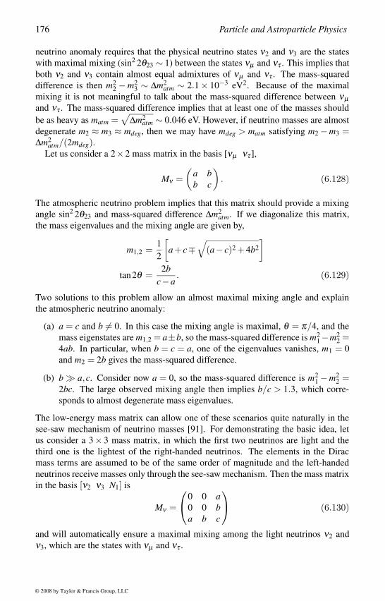
176 Particle and Astroparticle Physics
neutrino anomaly requires that the physical neutrino states ν2 and ν3 are the states
with maximal mixing (sin2 2θ23 ∼ 1) between the states νµ and ντ . This implies that
both ν2 and ν3 contain almost equal admixtures of νµ and ντ . The mass-squared
difference is then m22 −m2
3 ∼ ∆m2atm ∼ 2.1× 10⁻³ eV2. Because of the maximal
mixing it is not meaningful to talk about the mass-squared difference between νµand ντ . The mass-squared difference implies that at least one of the masses should
be as heavy as matm =√
∆m2atm ∼ 0.046 eV. However, if neutrino masses are almost
degenerate m2 ≈ m3 ≈ mdeg, then we may have mdeg > matm satisfying m2 −m3 =∆m2
atm/(2mdeg).Let us consider a 2×2 mass matrix in the basis [νµ ντ ],
Mν =(
a bb c
). (6.128)
The atmospheric neutrino problem implies that this matrix should provide a mixing
angle sin2 2θ23 and mass-squared difference ∆m2atm. If we diagonalize this matrix,
the mass eigenvalues and the mixing angle are given by,
m1,2 =1
2
[a+ c∓
√(a− c)2 +4b2
]tan2θ =
2bc−a
. (6.129)
Two solutions to this problem allow an almost maximal mixing angle and explain
the atmospheric neutrino anomaly:
(a) a = c and b = 0. In this case the mixing angle is maximal, θ = π/4, and the
mass eigenstates are m1,2 = a±b, so the mass-squared difference is m21−m2
2 =4ab. In particular, when b = c = a, one of the eigenvalues vanishes, m1 = 0
and m2 = 2b gives the mass-squared difference.
(b) b a,c. Consider now a = 0, so the mass-squared difference is m21 −m2
2 =2bc. The large observed mixing angle then implies b/c > 1.3, which corre-
sponds to almost degenerate mass eigenvalues.
The low-energy mass matrix can allow one of these scenarios quite naturally in the
see-saw mechanism of neutrino masses [91]. For demonstrating the basic idea, let
us consider a 3× 3 mass matrix, in which the first two neutrinos are light and the
third one is the lightest of the right-handed neutrinos. The elements in the Dirac
mass terms are assumed to be of the same order of magnitude and the left-handed
neutrinos receive masses only through the see-saw mechanism. Then the mass matrix
in the basis [ν2 ν3 N1] is
Mν =
0 0 a0 0 ba b c
(6.130)
and will automatically ensure a maximal mixing among the light neutrinos ν2 and
ν3, which are the states with νµ and ντ .
© 2008 by Taylor & Francis Group, LLC
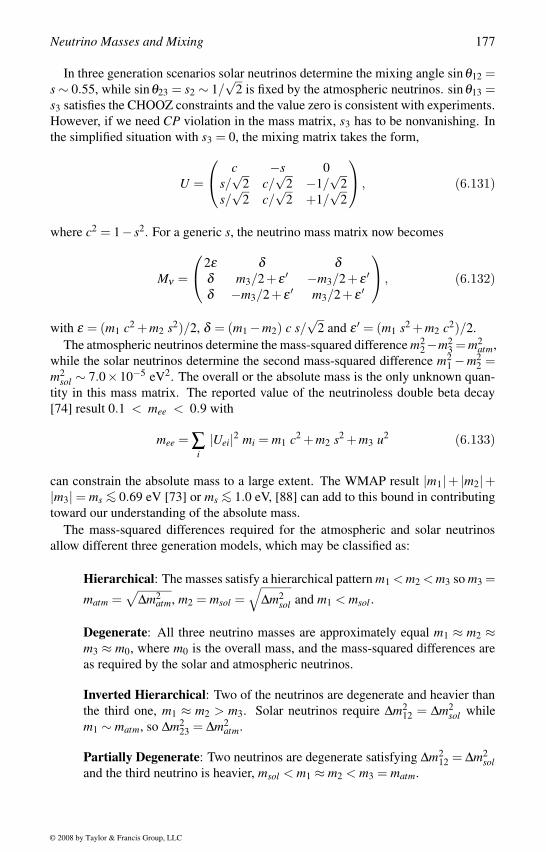
Neutrino Masses and Mixing 177
In three generation scenarios solar neutrinos determine the mixing angle sinθ12 =s ∼ 0.55, while sinθ23 = s2 ∼ 1/
√2 is fixed by the atmospheric neutrinos. sinθ13 =
s3 satisfies the CHOOZ constraints and the value zero is consistent with experiments.
However, if we need CP violation in the mass matrix, s3 has to be nonvanishing. In
the simplified situation with s3 = 0, the mixing matrix takes the form,
U =
c −s 0
s/√
2 c/√
2 −1/√
2
s/√
2 c/√
2 +1/√
2
, (6.131)
where c2 = 1− s2. For a generic s, the neutrino mass matrix now becomes
Mν =
2ε δ δδ m3/2+ ε ′ −m3/2+ ε ′δ −m3/2+ ε ′ m3/2+ ε ′
, (6.132)
with ε = (m1 c2 +m2 s2)/2, δ = (m1 −m2) c s/√
2 and ε ′ = (m1 s2 +m2 c2)/2.
The atmospheric neutrinos determine the mass-squared difference m22−m2
3 = m2atm,
while the solar neutrinos determine the second mass-squared difference m21 −m2
2 =m2
sol ∼ 7.0×10⁻⁵ eV2. The overall or the absolute mass is the only unknown quan-
tity in this mass matrix. The reported value of the neutrinoless double beta decay
[74] result 0.1 < mee < 0.9 with
mee = ∑i|Uei|2 mi = m1 c2 +m2 s2 +m3 u2 (6.133)
can constrain the absolute mass to a large extent. The WMAP result |m1|+ |m2|+|m3| = ms <∼ 0.69 eV [73] or ms <∼ 1.0 eV, [88] can add to this bound in contributing
toward our understanding of the absolute mass.
The mass-squared differences required for the atmospheric and solar neutrinos
allow different three generation models, which may be classified as:
Hierarchical: The masses satisfy a hierarchical pattern m1 < m2 < m3 so m3 =
matm =√
∆m2atm, m2 = msol =
√∆m2
sol and m1 < msol .
Degenerate: All three neutrino masses are approximately equal m1 ≈ m2 ≈m3 ≈ m0, where m0 is the overall mass, and the mass-squared differences are
as required by the solar and atmospheric neutrinos.
Inverted Hierarchical: Two of the neutrinos are degenerate and heavier than
the third one, m1 ≈ m2 > m3. Solar neutrinos require ∆m212 = ∆m2
sol while
m1 ∼ matm, so ∆m223 = ∆m2
atm.
Partially Degenerate: Two neutrinos are degenerate satisfying ∆m212 = ∆m2
soland the third neutrino is heavier, msol < m1 ≈ m2 < m3 = matm.
© 2008 by Taylor & Francis Group, LLC
178 Particle and Astroparticle Physics
All the four scenarios mentioned above are solutions of the solar and atmospheric
neutrino problems. WMAP cannot differentiate among these solutions [92], while
the neutrinoless double beta decay [74] allows only the degenerate case. In other
words, if the mass range reported by the Heidelberg–Moscow neutrinoless double
beta decay experiment is confirmed, all the solutions except for the degenerate neu-
trino solution will be ruled out. However, obtaining a degenerate mass matrix with
the required mixing angle is more difficult compared with hierarchical mass matrix.
In summary, the atmospheric and the solar neutrinos have provided us with the
most crucial information that neutrinos are massive. With more information from
these experiments and laboratory experiments, we have almost determined the neu-
trino mass matrix for a three generation scenario. Although a small admixture of a
sterile neutrino with the active neutrinos is not completely ruled out, a sterile neu-
trino is not required to explain any of the existing experimental results. If we restrict
to only a three generation scenario, the unknown parameters remaining to be de-
termined would be the third mixing angle (Ue3, which should be very small to be
consistent with the CHOOZ data), the CP phases, and the absolute mass of the neu-
trinos.
© 2008 by Taylor & Francis Group, LLC
7CP Violation
The charge conjugation (C), the parity (P), and the time-reversal (T ) are the three
important discrete symmetries in nature. These symmetries are exactly conserved in
the electromagnetic, the strong and the gravitational interactions, although they are
violated in the weak interaction. It is also known that the consistency of the field
theory requires that the product CPT should be conserved in any theory. Another
product CP plays a special role in particle physics and cosmology.
In the weak interaction, CP is not conserved, and in 1964 CP violation was ob-
served [22] in the K−K oscillation. During the past few years, evidence of CPviolation has been observed in the K-decays [93] as well as in the B-decays [94].
Although CP violation has not been observed in the strong interaction, theory pre-
dicts a large CP violation which needs to be suppressed; this is known as the strong
CP problem. There could be CP violation in the leptonic sector, which may have
its origin in the Majorana nature of the neutrinos. Since CP violation implies an
asymmetry between particles and antiparticles, the fact that there is more matter in
the universe compared with antimatter requires CP violation in the early universe.
In the standard model it is possible to accommodate a CP phase that can explain
all the observed CP violation in the K-system as well as in the B-system. But any
extensions of the standard model could provide newer sources of CP violation. The
strong CP problem requires a new dynamical origin of CP violation that predicts a
new particle, the axion. There are additional sources of CP violation in the leptonic
sector if neutrinos are Majorana particles. The CP violation required to explain the
baryon asymmetry of the universe could have a completely different origin.
7.1 CP Violation in the Quark Sector
As discussed in section 5.4, when the up-quark and the down-quark mass matrices
are diagonalized, one complex phase in the charge–current interaction cannot be
removed. This complex phase manifests itself as CP violation in decays of heavy
mesons. CP violation was first observed in K −K oscillations and recently it has
been observed in the K-decays and also in the B-meson system. In this section we
review some salient features of CP violation in the K-system as well as in the B-
system.
179
© 2008 by Taylor & Francis Group, LLC
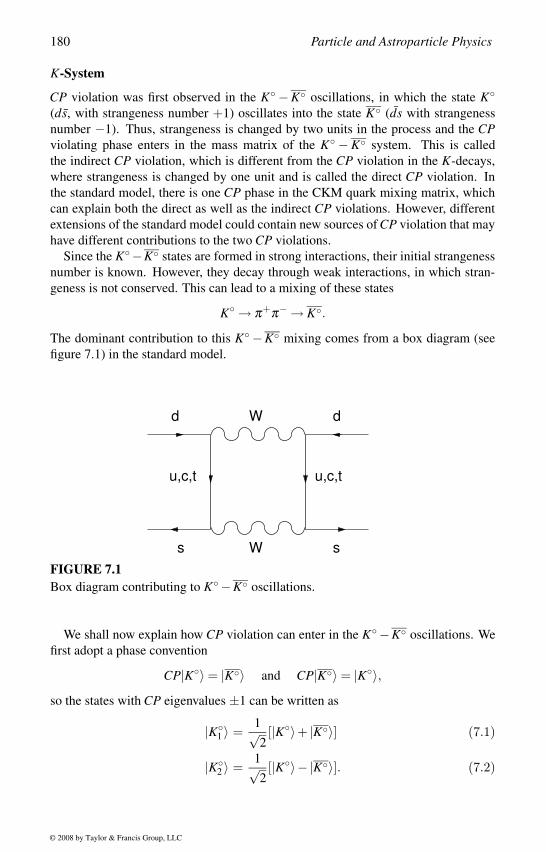
180 Particle and Astroparticle Physics
K-System
CP violation was first observed in the K −K oscillations, in which the state K(ds, with strangeness number +1) oscillates into the state K (ds with strangeness
number −1). Thus, strangeness is changed by two units in the process and the CPviolating phase enters in the mass matrix of the K − K system. This is called
the indirect CP violation, which is different from the CP violation in the K-decays,
where strangeness is changed by one unit and is called the direct CP violation. In
the standard model, there is one CP phase in the CKM quark mixing matrix, which
can explain both the direct as well as the indirect CP violations. However, different
extensions of the standard model could contain new sources of CP violation that may
have different contributions to the two CP violations.
Since the K−K states are formed in strong interactions, their initial strangeness
number is known. However, they decay through weak interactions, in which stran-
geness is not conserved. This can lead to a mixing of these states
K → π+π− → K.
The dominant contribution to this K−K mixing comes from a box diagram (see
figure 7.1) in the standard model.
s
d W d
u,c,t u,c,t
s W
FIGURE 7.1Box diagram contributing to K−K oscillations.
We shall now explain how CP violation can enter in the K−K oscillations. We
first adopt a phase convention
CP|K〉 = |K〉 and CP|K〉 = |K〉,so the states with CP eigenvalues ±1 can be written as
|K1 〉 =
1√2[|K〉+ |K〉] (7.1)
|K2 〉 =
1√2[|K〉− |K〉]. (7.2)
© 2008 by Taylor & Francis Group, LLC
CP Violation 181
These states can decay through weak interactions into the states containing pions,
which have odd parity P|π±,π0〉 = −|π±,π0〉. The pions transform under charge
conjugation as C|π±,π0〉 = |π∓,π0〉, and hence, a two pion state (π0π0 or π+π−)
has positive CP eigenvalue. A CP = +1 state K1 will thus decay into two pions,
while the CP = −1 state K2 will decay into three pions and more complex decay
modes if CP is conserved. K2 will have much shorter half-life than K
1 , since the
phase space consideration will suppress the three-body decays compared with the
two-body decays. There will also be a small mass difference between the two states
K−K , which has been observed, due to the different intermediate states to which
they can make virtual transitions.
We shall now write the time development of the K−K system, which is deter-
mined by an effective Hamiltonian containing the masses (Mi j) and the decay widths
(Γi j) of these states, in the basis K, K :
Hi j = Mi j − i2
Γi j. (7.3)
The mass matrix and the decay width are constrained by the Hermiticity, CPT and
CP conservation:
Mi j = M∗ji, Γi j = Γ∗
ji
M11 = M22 Γ11 = Γ22
M12 = M21 Γ12 = Γ21.
Since we are interested in the CP violation, we consider both M and Γ to be complex.
Then the physical eigenstates can be obtained by diagonalizing the Hamiltonian,
which can be parameterized by a measure of the CP violation ε and is given by
|KS〉 =1√
2(1+ |ε|2) [(1+ ε)|K〉+(1− ε)|K〉] (7.4)
|KL〉 =1√
2(1+ |ε|2) [(1+ ε)|K〉− (1− ε)|K〉]. (7.5)
The CP violating parameter ε enters in the mass matrix of the K−K system and
is given by
ε =√
H12 −√
H21√H12 +
√H21
=iImM12 + 1
2 ImΓ12
(ML −MS)− i2 (ΓL −ΓS)
. (7.6)
The CP violation also introduces nonorthogonality between the states KS and KL:
〈KS|KL〉 =2 Re ε1+ |ε|2 . (7.7)
The states K1 and K
2 have definite CP eigenstates with eigenvalues ±1 and are or-
thogonal to each other. If there is no CP violation, the state KL will become identical
to K2 and can decay into only three pions or more complex states. If there is CP
© 2008 by Taylor & Francis Group, LLC
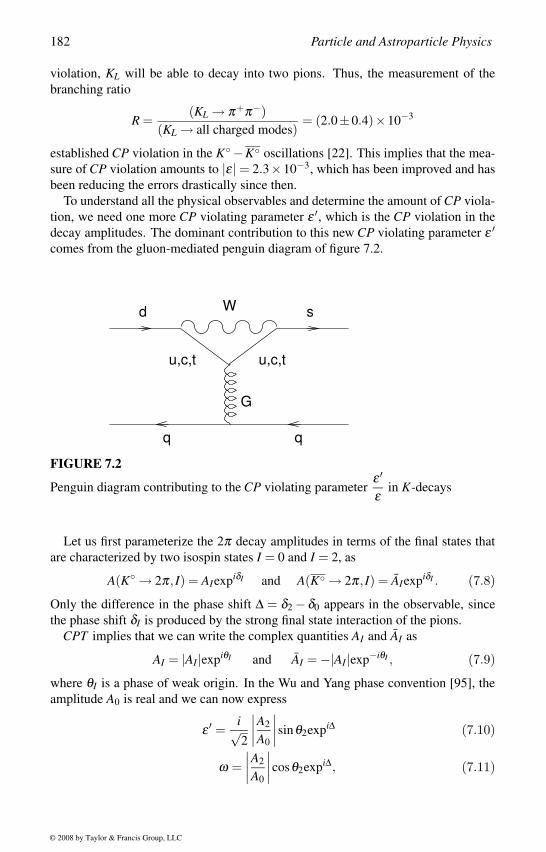
182 Particle and Astroparticle Physics
violation, KL will be able to decay into two pions. Thus, the measurement of the
branching ratio
R =(KL → π+π−)
(KL → all charged modes)= (2.0±0.4)×10−3
established CP violation in the K−K oscillations [22]. This implies that the mea-
sure of CP violation amounts to |ε| = 2.3×10⁻³, which has been improved and has
been reducing the errors drastically since then.
To understand all the physical observables and determine the amount of CP viola-
tion, we need one more CP violating parameter ε ′, which is the CP violation in the
decay amplitudes. The dominant contribution to this new CP violating parameter ε ′comes from the gluon-mediated penguin diagram of figure 7.2.
q
d sW
u,c,tu,c,t
G
q
FIGURE 7.2
Penguin diagram contributing to the CP violating parameterε ′
εin K-decays
Let us first parameterize the 2π decay amplitudes in terms of the final states that
are characterized by two isospin states I = 0 and I = 2, as
A(K → 2π, I) = AIexpiδI and A(K → 2π, I) = AIexpiδI . (7.8)
Only the difference in the phase shift ∆ = δ2 − δ0 appears in the observable, since
the phase shift δI is produced by the strong final state interaction of the pions.
CPT implies that we can write the complex quantities AI and AI as
AI = |AI |expiθI and AI = −|AI |exp−iθI , (7.9)
where θI is a phase of weak origin. In the Wu and Yang phase convention [95], the
amplitude A0 is real and we can now express
ε ′ =i√2
∣∣∣∣A2
A0
∣∣∣∣sinθ2expi∆ (7.10)
ω =∣∣∣∣A2
A0
∣∣∣∣cosθ2expi∆, (7.11)
© 2008 by Taylor & Francis Group, LLC
CP Violation 183
where ω is not related to CP violation.
The CP violating quantities that are directly related to the physical observables
can now be defined as
η+− = |η+−|expiφ+− =A(KL → π+π−)A(KS → π+π−)
(7.12)
η00 = |η00|expiφ00 =A(KL → π0π0)A(KS → π0π0)
(7.13)
δ =Γ(KL → π−+ν)−Γ(KL → π+−ν)Γ(KL → π−+ν)+Γ(KL → π+−ν)
, (7.14)
which are related to the CP violating parameters ε and ε ′ and the parameter ωthrough the relations
η+− = ε +ε ′
1+ ω√2
(7.15)
η00 = ε −2ε ′
1−√2ω
(7.16)
δ =2Reε
1+ |ε|2 . (7.17)
These quantities have been measured and found to be nonvanishing, confirming CPviolation in both K−K oscillations as well as in K-decays. The above discussions
are also valid for other neutral meson systems such as B−B or D−D, although
the short lifetime of the heavy mesons complicates the analysis much more.
The experimental values of the KL and KS mass differences and the decay width
differences are fairly precise [44]
∆MK ≡ ML −MS = 3.48×10⁻¹⁵ GeV
∆ΓK ≡ ΓL −ΓS = −7.37×10⁻¹⁵ GeV . (7.18)
Taking these numbers it is possible to arrive at an empirical relation within about 5%
error,
∆MK = −1
2∆ΓK . (7.19)
The interference of the KL and KS states allows a measurement of the CP violating
parameter ε from the measurement of the parameters
|η+−| = (2.276±0.017)×10−3
φ+− = (43.3±0.5)
|η00| = (2.262±0.017)×10−3
φ00 = (43.2±1.0)
δ = (3.27±0.12)×10−3. (7.20)
© 2008 by Taylor & Francis Group, LLC
184 Particle and Astroparticle Physics
The value of ε comes out to be [44]
|ε| = (2.271±0.017)×10−3
φ(ε) ≈ tan−1 2(ML −MS)ΓL −ΓS
= (43.49±0.08). (7.21)
The phase of εK is obtained by applying CPT and unitarity.
Using the experimental input of Γ12 ≈ 0, we simplify the relations
∆MK = 2ReM12,
∆ΓK = 2ReΓ12 ,
|ε| = 1√2
ImM12
∆MK=
1
2√
2
ImM12
ReM12.
The CP violating observables can also be simplified
η+− ≈ ε + ε ′, η00 ≈ ε −2ε ′, δ ≈ 2Re ε. (7.22)
The measurements of the CP violating parameters then give [93]
Re(ε ′
ε) =
ε ′
ε= (2.1±0.5)×10−3
φ(ε ′) = δ2 −δ0 +π4≈ (48±4). (7.23)
The predictions of the standard model for the CP parameters are so far consistent
with all measurements and there are no indications of new physics coming from
these measurements [96].
B-System
During the past few years the B-physics has made much progress. The CP violation
in the B-system has also been established in the B-factories. The new generation of B-
factory experiments intensified activities in B-physics. One of the main expectations
from these experiments is to discover whether there are any signals of new physics
beyond the standard model. Earlier experiments at LEP and SLD collected bb events
operating at the Z-resonance. But in the current experiments B-decays are studied
near their production threshold at the ϒ(4S) resonance [44]. Thus, heavier states
such as Bs (sb) or B+
c (cb) and b-flavored baryons are not produced. In the ϒ(4S)decays only equal amounts of B(db)B(db) and B+(ub)B−(ub) pairs are expected.
The short half-life of the B-mesons makes the analysis of B-system different from
that of the K-system. In addition, there are two neutral B − B meson systems,
Bd (db) and B
s (sb). For the heavy quarks the calculation of the hadronic matrix
elements is also different.
Let us consider the evolution of the flavor state B or B. The effective Hamilto-
nian in the basis [B B]
H = M− i2
Γ
© 2008 by Taylor & Francis Group, LLC
CP Violation 185
will govern the evolution of these states B or B. Here M and Γ are the mass and
decay width. Similar to the K-system, we shall write the eigenstates of this effective
Hamiltonian
|B±〉 = p|B〉±q|B〉, (7.24)
where
qp
=1− ε1+ ε
=
√M∗
12 − i2 Γ∗
12
M12 − i2 Γ12
. (7.25)
These states |B±〉 are not orthogonal. If CP is conserved, these states will have defi-
nite CP eigenvalues CP|B±〉=±|B±〉, where we considered the convention CP|B〉=|B〉 and Re (q/p) > 0.
We now consider the time development of any general state, which is a superposi-
tion of physical states. At a given time t, it is given by
|ψ(t)〉 = C1exp−i(M1−iΓ1/2)t |B+〉+C2exp−i(M2−iΓ2/2)t |B−〉∝(
C1exp−i(M1−iΓ1/2)t +C2exp−i(M2−iΓ2/2)t)|B〉
+qp
(C1exp−i(M1−iΓ1/2)t −C2exp−i(M2−iΓ2/2)t
)|B〉.
In the two cases C1 = ±C2 = 1, which corresponds to the initial states to be pure Band B states, the time evolutions are given by
|B(t)〉 = g+(t)|B〉+ qp
g−(t)|B〉
|B(t)〉 = g+(t)|B〉+ qp
g−(t)|B〉, (7.26)
where
g±(t) =1
2
(exp−i(M1−iΓ1/2)t ± exp−i(M2−iΓ2/2)t
). (7.27)
This gives the time-dependent probabilities for the flavor oscillations.
In the B−B oscillations, decays to flavor specific final states are studied. We
write the decay amplitudes
A f = 〈 f |H|B〉 and A f = 〈 f |H|B〉 (7.28)
for the B decay into a final state f and B decays into f , respectively. Although
the instantaneous decay amplitudes A f = 〈 f |H|B〉 and A f = 〈 f |H|B〉 vanish, the
B−B mixing allows B to decay into f and B to decay into f . We thus consider
the time-integrated mixing probability [44]
χB→Bf =
∫ ∞0 |〈 f |H|B(t)〉|2 dt∫ ∞
0 |〈 f |H|B(t)〉|2 +∫ ∞
0 |〈 f |H|B(t)〉|2 . (7.29)
If there is no CP violation, a simplified expression follows
χB→Bf = χB→B
f = χ =x2 + y2
2(x2 +1), (7.30)
© 2008 by Taylor & Francis Group, LLC
186 Particle and Astroparticle Physics
where
x =∆MΓ
, y =∆Γ2Γ
(7.31)
and ∆M and ∆Γ are given by
∆M = −2Re[qp(M12 − i
2Γ12)] ≈−2|M12|
∆Γ = −4Im[qp(M12 − i
2Γ12)] ≈ 2|Γ12|cosζ , (7.32)
where Γ12/M12 = r expiζ . Since r ∼ 10−3, we neglect higher order terms. Experi-
ments confirm the B−B oscillation [97], and the amount of mixing is given by
χd = 0.174±0.009 . (7.33)
However, flavor specific final states cannot be studied to look for CP violation in the
B-system [98].
It is convenient to look for some common nonleptonic decay channels of B and
B, which are also CP eigenstates, say, CP| f±〉 = ±| f±〉. Thus, if CP is conserved, a
CP positive state B can decay only into | f+〉. If we now start with N+(N−) numbers
of B+(B−) mesons, after a time t, there will be a different combination of B and Bmesons, denoted as B(t), whose decay rate into the state | f+〉 will be
Γ(B(t) → f+) =N+
N+ +N−Γ(B+(t) → f+). (7.34)
However, when there is CP violation, the time evolution of this decay rate will be
different from pure exponential.
Since both B and B can decay into a final state | f+〉 when there is CP violation,
the time-dependent decay rates are given by [44]
Γ(B(t) → f ) ∝|A f |2
|g+(t)|2 + |g−(t)|2 |ξ ( f )|2 +2Re[g−(t)g∗+(t)ξ ( f )
]Γ(B(t) → f ) ∝
exp−Γ1t |A f |2|g+(t)|2 + |g−(t)|2 |ξ ( f )|−2 +2Re
[g−(t)g∗+(t)
ξ ( f )
], (7.35)
where ξ ( f ) = (q/p) (A f /A f ). ∆Γ/Γ is significant only for Bs decays, but it can be
neglected for the Bd decays. We can, thus, define an asymmetry in the wrong-sign
semi-leptonic B-decays as a measure of indirect CP violation as
aSL(B) =Γ(B(t) → +X)−Γ(B(t) → −X)Γ(B(t) → +X)+Γ(B(t) → −X)
=|p/q|2 −|q/p|2|p/q|2 + |q/p|2 = rB sinζB. (7.36)
© 2008 by Taylor & Francis Group, LLC
CP Violation 187
Standard model predicts a tiny asymmetry, so any large asymmetry would imply new
physics beyond the standard model.
Since |A f | = |A f |, measurement of the rate asymmetries for CP conjugate decays
can tell us about direct CP violation. If the final state f for two amplitudes (Ai), with
different strong phases (δi) coming from final state interaction effects and different
weak phases (ξi), which contribute to the same decay, has different flavor content
than its CP conjugate, the asymmetry is given by
a =2A1A2 sin(ξ1 −ξ2)sin(δ1 −δ2)
A21 +A2
2 +2A1A2 cos(ξ1 −ξ2)cos(δ1 −δ2). (7.37)
Any difference between the CP asymmetries for B-decays to flavor eigenstates can
also allow measurement of direct CP violation, provided the weak decay phase in
A f /A f is not cancelled by the mixing weak phase in q/p.
Measurement of the decays of B and B to CP eigenstates provides the golden
mode for observing CP violation. When the initial states are B or B only, the time-
dependent decay rates to the same final state f with definite CP eigenvalue will be
different and the corresponding CP asymmetry is given by [44]
a f (t) =Γ(B(t) → f )−Γ(B(t) → f )Γ(B(t) → f )+Γ(B(t) → f )
. (7.38)
For the final state f = (cc)K with CP eigenvalue η f , the asymmetry becomes
a f (t) = −η f sin2φ1 sin∆Mt, (7.39)
for nonvanishing A f and A f and when weak mixing phase is different from the weak
decay phase. φ1 is one of the three internal angles of the unitary triangle, defined as
φ1 = π − arg
(−V ∗tbVtd
−V ∗cbVcd
).
This mode has the advantage that the decays of the final state (cc)K have very little
contribution from direct CP violation and there is no ambiguity due to strong inter-
actions [98]. This reduces the uncertainty in interpreting the data and has recently
been studied at the KEKB asymmetric-energy e+e− collider by the Belle detector.
They reported the first evidence for CP violation in the B-system from an analysis
of the asymmetry in the distribution of the time intervals between the two B meson
decay points
sin2φ1 = 0.99±0.14(stat)±0.06(syst). (7.40)
The large positive value for sin2φ1 is consistent with the CP violation coming from
the CKM phase in the standard model.
© 2008 by Taylor & Francis Group, LLC
188 Particle and Astroparticle Physics
7.2 Strong CP Problem
After discussing the question of CP violation in K- and B-decays, which have been
observed and could be explained consistently in the context of standard model, we
now come to another question of CP violation in the standard model, the strong
CP problem. While we try to study the weak decays to find if this can provide us
any information of physics beyond the standard model, in the strong CP problem
we try to solve a more theoretical problem. The strong interaction predicts a large
CP violation within the context of standard model, which has not been observed,
and hence, we should find some underlying theoretical justification to explain the
smallness of the prediction for CP violation.
To understand the problem, let us consider the limit when the u and d quarks
are massless. The QCD Lagrangian then has a chiral symmetry, U(2)L ×U(2)R,
which is spontaneously broken resulting in four massless Nambu–Goldstone bosons,
η meson and the pions. If we now introduce nonvanishing quark masses, they will
break the chiral symmetry explicitly, and hence, the Nambu–Goldstone bosons will
pick up small masses satisfying the relation mη ≤√3 mπ , which is inconsistent with
the actual masses of these mesons [99]. It was then pointed out [100] that the QCD
Lagrangian is invariant under a U(1)A transformation
qi → expiαγ5qi and m j → exp−2iα m j,
which is broken by the axial anomaly of the U(1)A current and the instanton effect,
which gives a mass to the η meson even for massless quarks. So, the pions are the
only Nambu–Goldstone bosons in the problem, which remains light after the quarks
are given masses.
Although the axial anomaly of the U(1)A current solves this problem, it makes
the QCD vacuum complex [101]. This CP violating term in the QCD Lagrangian
is parameterized by a phase Θ, which can take any values between 0 and π , but its
experimental bound is Θ ≤ 10−9. From naturalness consideration we should expect
the value of Θ to be of the order of 1, so the smallness of Θ becomes a problem,
which is called the strong CP problem.
There are suggestions to solve this problem, but none of the suggestions could
be verified so far. The most popular and interesting solution for the problem makes
the Θ parameter of QCD vanish dynamically through the Peccei–Quinn mechanism
[102]. A global U(1) symmetry, called the Peccei–Quinn symmetry, ensures that the
Lagrangian conserves CP and Θ = 0. This symmetry is then broken spontaneously at
a very high scale and the corresponding Nambu–Goldstone boson, called the axion,
picks up small mass due to instanton effects. The most interesting aspect of this
theory is that it predicts the new particle axion, which is being detected.
© 2008 by Taylor & Francis Group, LLC
CP Violation 189
CP Violation in Strong Interactions
The strong coupling constant of QCD makes the nonperturbative effects important.
Among other interesting effects, the transition matrix elements split up into a family
of disconnected sectors due to some static field configurations [101]. These dis-
connected sectors are topologically distinct and labelled by a topological quantum
number n, called the winding number. In a temporal gauge A0a = 0, these distinct
vacuum states |n〉 are specified by demanding that at spatial infinity the gauge fields
should vanish. The vacuum states are labelled by the winding numbers n, which are
topological numbers arising due to instanton effects, defined by
n =g2
32π2
∫d4xFa
µν Fµνa, (7.41)
where
Faµν = ∂µ Aa
ν −∂ν Aaµ +g f abcAµbAνc
Faµν =
1
2εµναβ Fαβa.
n is an integer number for any pure gauge, characterizing the QCD vacuum. Since
for an instanton n = 1, it is possible to transform |n〉 → |n + 1〉 in the presence of
an instanton. Any gauge transformations cannot take back a generated field to a
zero field smoothly. When any gauge transformation takes a generated field to a
definite vacuum state |n〉, the corresponding gauge fields are denoted as Ain. Except
for quantum tunnelling due to instanton effects, no gauge transformations can take
one vacuum to another.
The Θ vacua are gauge invariant vacuum states of QCD, which are constructed as
|Θ〉 = ∑n
exp−inΘ|n〉. (7.42)
Different Θ correspond to distinct theories, which are not connected by any gauge
transformations.
A Green’s function in QCD gives the vacuum to vacuum transition in the presence
of an external source. In the temporal gauge this gives the transition between the pure
gauge configurations Ain → Ai
m at t = ∞. In addition to the usual QCD vacuum, this
Green’s function will have an additional phase expiνΘ coming due to the transition
Ain → Ai
m, where winding number is changed by ν = m−n in a particular Θ vacuum.
This additional phase is associated with an additional term in the QCD Lagrangian
LΘ =g2
32π2 Θ Faµν Fµνa. (7.43)
This gives a new source of CP violation in QCD. There is no CP violation for Θ =0,π , and from current algebra consideration Θ = π is not allowed [101].
This term also has its origin in the U(1)A axial current
Jµ5 =
N f
∑i=1
qiγµ γ5qi, (7.44)
© 2008 by Taylor & Francis Group, LLC
190 Particle and Astroparticle Physics
which is classically conserved for massless quarks and is generated by a conserved
charge
Q5 =∫
d3xJ05 . (7.45)
The anomaly introduces an one-loop divergent contribution
∂µ Jµ5 = 2N f
(g2
32π2 Faµν Fµνa
)= 2N f
(g2
32π2 ∂ µ Kµ
), (7.46)
where N f is the number of flavors and
Kµ =1
2εµαβγ Aα
a [Fβγa − g
3εabcAβ
b Aγc ].
The conserved current has an additional contribution from the anomaly term
Jµ5 = Jµ
5 −2N f
(g2
32π2 Kµ)
. (7.47)
The associated charge Q5 =∫
d3xJ05 is time independent, but not gauge invariant.
Any gauge transformation, where winding number is changed by 1, transforms Q5 →Q5 +2N f . Thus, a chiral rotation changes the Θ vacuum to
expiαQ5 |Θ〉 = |Θ+2N f α〉. (7.48)
In short, the anomaly made the chiral current divergent. Absence of any associated
conserved charge implies there is no Nambu–Goldstone boson, and hence, the ηmeson becomes massive. But the new conserved current is no longer gauge invariant.
This generates the disconnected sectors of the vacuum and, hence, introduces the Θterm in the QCD Lagrangian.
If the quarks are massless, a chiral transformation can take one Θ vacuum to an-
other, and hence, it is possible to choose a chiral rotation that takes to Θ = 0. How-
ever, since quarks are not massless, this cannot be the solution to this strong CPproblem.
The CP violation in the weak interactions coming from a complex phase in the
quark mass matrices can also contribute to the Θ term of the QCD Lagrangian. In
general the quark mass matrices could be complex. A chiral rotation to the quark
fields transforms the Θ vacuum by an amount
Θ → Θ = Θ+Arg[det M].
Thus, any chiral rotation can make one of the two terms vanishing but cannot make
both of them vanish simultaneously. When quarks are not massless, it will not be
possible to apply any chiral rotations that can make the Θ term vanish.
Let us now consider the effect of the Θ term in the QCD Lagrangian. For simplic-
ity we consider a one generation example, where the Θ term can be explicitly given
by the expression
LΘ = imumd sinΘ√
m2u +m2
d +2mumd cosΘ(uγ5u+ dγ5d). (7.49)
© 2008 by Taylor & Francis Group, LLC
CP Violation 191
This predicts a nonvanishing electric dipole moment of the neutron in the range of
[103]
4×10⁻¹⁷ Θe.cm < dn < 2×10⁻¹⁵ Θe.cm,
which is much larger than the present experimental limit [44]
dn < 0.63×10⁻²⁵e.cm,
unless the Θ parameter is very small,
Θ = Θ+Arg[det M] < 10−10. (7.50)
Why Θ is so small and not of the order of 1 is the strong CP problem. Standard
model does not provide any solution to this problem. We shall now discuss some
extensions of the standard model that can provide a solution to this problem.
7.3 Peccei–Quinn SymmetryThe strong CP problem has its origin in the topological structure of the QCD vacuum.
The nonperturbative effects predict a large CP violation originating from the QCD
Lagrangian, but the experimental constraints require that this parameter be extremely
small. Higher order corrections will again predict large corrections, so the counter
terms have to be fine tuned to many decimal points to keep this parameter small to
all orders in perturbation theory and explain the experimental constraints. This fine
tuning is unnatural and known as the strong CP problem.
The first possibility one considers is that at least one of the quarks is massless,
say, the u-quark. The different Θ vacua states are now connected by chiral rotations,
and hence, it is possible to consider a Θ vacuum which solves the U(1)A problem.
Since all the vacuum states are equivalent, there is no CP violation. But none of
the quarks are massless, and hence, one starts with a massless u-quark and tries to
generate an effective u quark mass through instanton effects [104]. Although this
solution is definitely a reasonable possibility, this does not explain why the u-quark
mass is vanishing to start with.
In another possible solution to the strong CP problem, the theory allows a very
small arg[det M], estimates the Θ term, and shows that it is small. But the constraints
from the CP violation in the K- and the B-system do not allow a small enough strong
CP term, as required.
The most popular solution to the strong CP problem is the one suggested by Peccei
and Quinn [102], which provides a dynamical solution. One introduces a global
U(1)PQ symmetry under which the quark mass terms are forbidden, but they come
from the vev of the Higgs fields. The chiral transformation of the Peccei–Quinn
U(1)PQ global symmetry ensures that Θ vanishes dynamically. The vev of the Higgs
fields break the Peccei–Quinn symmetry spontaneously, but the axial anomaly also
© 2008 by Taylor & Francis Group, LLC
192 Particle and Astroparticle Physics
breaks this symmetry explicitly, giving a small mass to the corresponding Nambu–
Goldstone boson, the axion [105].
Under the Peccei–Quinn U(1)PQ symmetry, the left-handed and right-handed
quarks carry different charges, so the mass terms are forbidden. However, the trans-
formations of the Higgs scalar ensure that the Yukawa couplings, which can give
masses to the quarks after the Higgs scalars acquire vevs, are allowed. The chiral
nature of the symmetry will introduce a new anomaly term, given by
LPQ =ava
ξg2
32π2 Faµν Fµνa, (7.51)
where a is the axion field, the scale of the U(1)PQ breaking is va, and ξ is a parameter
which depends on how the PQ charges are assigned to the fermions. This anomaly
term provides a potential for the axion field and gives it a vacuum expectation value
〈a〉 = 〈Θ|a|Θ〉 = −Θ1
ξva. (7.52)
The physical axion can then be written as aphys = a−〈a〉, so the axion eliminates the
unwanted Θ term in the Lagrangian and replaces it with the physical axion field
Le f f = Θg2
32π2 Faµν Fµνa +
ava
ξg2
32π2 Faµν Fµνa
=aphys
vaξ
g2
32π2 Faµν Fµνa. (7.53)
The axion is the Nambu–Goldstone boson corresponding to the global U(1)PQ sym-
metry breaking, and hence, the effective Lagrangian contains only derivative cou-
plings
La = −1
2∂µ a∂ µ a+L (∂µ a,ψ), (7.54)
where the second term gives the interactions of the axions with the fermions, which
are determined by the structure of the U(1)PQ symmetry. The vacuum expectation
value of the axion conspires to cancel the Θ term exactly, and the axion gets a small
mass with its coupling determined by the scales of symmetry breaking.
Models of the Axion
The minimal extension of the standard model to accommodate a chiral symmetry re-
quires at least two Higgs doublets φ1 and φ2 carrying the same U(1)PQ charges. The
transformations of the quarks, the leptons and the Higgs scalars under the U(1)PQPeccei–Quinn symmetry can be defined as
q, L → exp−iαq, L
u,d,eR → expiαu,d,eR
φ1,2 → exp−2iα φ1,2.
© 2008 by Taylor & Francis Group, LLC
CP Violation 193
The usual Yukawa couplings that can give masses to the quarks and leptons after the
Higgs doublets φ1 and φ2 acquire vevs are now given by
LY = huqLuRφ2 +hd qLdRφ1 +heLeRφ1 +H.c. (7.55)
The vevs of the Higgs doublets 〈φi〉 = vi/√
2 break the U(1)PQ symmetry at a scale
v =√
v21 + v2
2. These Higgs scalars also break the electroweak symmetry and give
masses to the quarks and leptons. In the simplest model the scale of U(1)PQ sym-
metry breaking scale is the same as the electroweak symmetry breaking scale. Since
the axion couples to matter directly, these are called the visible axion models.
Corresponding to the two Higgs doublets, there are now four physical Higgs
scalars and four Nambu–Goldstone modes. Three of the Nambu–Goldstone modes
will give masses to the W±,Z bosons and the remaining one becomes the axion field
a =1
v(v1Imφ 0
1 − v2Imφ 02 ).
Since the U(1)PQ symmetry is spontaneously broken, the corresponding Nambu–
Goldstone boson, the axion, will be massless. But the QCD gluon anomaly will
break this symmetry explicitly, and hence, the axion will become a pseudo-Nambu–
Goldstone boson with a small mass, given by
ma =fπ mπ
vNg
(v1
v2+
v2
v1
) √mumd
mu +md, (7.56)
where fπ is the pion decay constant.
In the visible axion models, when the axion mass is less than the electron mass,
the axions can decay into two photons. The nonderivative interaction of the axion to
the electromagnetic field comes from loops containing the right-handed fermions
Laγγ =aphys
fπ
ma
mπ
√mu
md
e2
16π2 Fµνem Fem µν , (7.57)
and hence, the axion becomes long-lived. When the axion mass is more than the
electron mass, it can decay rapidly into two electrons and become short-lived
τ(a → e+e−) =8πv2v2
2
m2ev2
1
√m2
a −4m2e. (7.58)
But experiments ruled out both these possibilities. The strongest constraint comes
from the nonobservation of the K-decays to axions [106]
Br(K+ → π+ + nothing) ≤ 3.8×10⁻⁸, (7.59)
where (nothing) in the decay products includes long-lived axions, which would es-
cape detection. The quarkonium decay QQ → aγ measures the coupling of axions to
heavy quarks [107]. Nonobservation of such processes [44, 108]
Br(ϒ → aγ) < 3×10⁻⁴
Br(J/Ψ → aγ) < 1.4×10⁻⁵
© 2008 by Taylor & Francis Group, LLC
194 Particle and Astroparticle Physics
rules out the long-lived axions. The short-lived axions are ruled out from a measure-
ment of the process
Br(π+ → ae+νe) < 10−10. (7.60)
This rules out the short-lived axions that couple to matter directly.
In the visible axion model the Peccei–Quinn symmetry was broken along with the
electroweak symmetry and the axion couples to matter directly. Since this model
is ruled out, an extension of the model was considered, where the scale of U(1)PQsymmetry breaking is much higher. The couplings of the axion to the ordinary matter
are then suppressed by the ratio of the vevs of the electroweak symmetry breaking
scale to the U(1)PQ symmetry breaking scale. Such weak coupling of the axion
would allow it to evade existing experimental searches, and hence, this invisible
axion model is allowed by present experiments.
In the simplest extension [109] of the visible axion model a standard model singlet
scalar σ is added, which transforms under the U(1)PQ as σ → exp2iα σ . This field
interacts with the fermions only through its mixing with the usual Higgs scalars
V (φ1,φ2,σ) = V (φ1,φ2)+V (σ)+(a|φ1|2 +b|φ2|2)|σ |2 + cφ1φ2σ2.
The U(1)PQ symmetry is broken by the vev of the singlet Higgs 〈σ〉 = vσ at a scale
much higher than the electroweak symmetry breaking scale va = vσ v.
The axion field is now a combination of the fields Imφ 01 , Imφ 0
2 , and Imσ and is
given by
a =1
v(v2v2σ +4v2
1v22)1/2 [2v1v2(v1Imφ 0
1 + v2Imφ 02 )− v2vσ Imσ ]. (7.61)
In the limit of very large vσ , the mass of the axion becomes
ma ≈ fπ mπvσ
∼ (0.2 GeV)2
vσ, (7.62)
and the axion decay constant becomes fa ∼ vσ /2. This makes the axion very light
with derivative coupling to ordinary matter, which is suppressed by v/vσ . Axions
can now decay into only two photons.
The main criterion of the Peccei–Quinn mechanism is that the fermions with
nontrivial transformation under SU(3)c should have chiral transformation under the
Peccei–Quinn symmetry, so the symmetry is broken explicitly by the SU(3) anomaly.
This criterion is exploited in another version of the invisible axion model where
new heavy quarks were introduced [110]. The quarks, the leptons and the usual
Higgs doublets are singlets under the U(1)PQ group. Only the new heavy quarks
and the singlet Higgs scalar σ have nontrivial transformation under U(1)PQ. SU(3)canomaly cancellation require both left- and right-handed heavy quarks XL and XR.
Under the Peccei–Quinn symmetry the masses of the heavy fermions should not be
invariant, which is satisfied by the transformation
X[L,R] → expiγ5α X[L,R]. (7.63)
© 2008 by Taylor & Francis Group, LLC
CP Violation 195
A singlet, transforming under this U(1)PQ symmetry as
σ → e−2iα σ ,
can then have the required Yukawa coupling XLXRσ , which can give mass to the
heavy quarks when the singlet σ acquires a vev, 〈σ〉 = vσ .
Since the heavy quarks transform nontrivially under SU(3)c, a γ5 rotation of the
heavy quark fields can contribute to the QCD axial anomaly and change the Θ term
by an amount α . Since anomaly does not depend on the mass of the particles, the
new heavy quark fields XL,R can make the Θ term vanish dynamically. There will be
terms in the scalar potential that would mix the singlet Higgs with the Higgs doublet,
and the axion will be given by
a =1
(v2 + v2σ )1/2 [vImφ 0 + vσ Imσ ], (7.64)
where v is the vev of the standard model Higgs doublet φ , and va = vσ is the U(1)PQsymmetry breaking scale. The axion mass is given by
ma =fπmπ2va
√mumd
mu +md, (7.65)
with the decay constant fa = va/2. The axion now decays into two photons with
a very long lifetime. There is no direct coupling of the axion with the electrons,
except a tiny coupling at the one-loop level through its coupling to photons. A highly
suppressed coupling of the axion to ordinary matter follows from its couplings with
pions and η mesons.
In another variant of the invisible axion model, the role of the heavy quarks is re-
placed by the gluinos in supersymmetric theories, which are heavy colored fermions.
Replacing the µ term in the superpotential, the R-parity could be uplifted to a global
U(1)R symmetry which is then identified with the U(1)PQ symmetry. This symmetry
is then broken at a large scale without breaking supersymmetry, solving the strong
CP problem [111].
There is another solution in N = 1 supergravity models [112], where the R-parity
in supersymmetric models is considered as the Peccei–Quinn symmetry. In this the-
ory R-symmetry is broken by the soft terms in supergravity theories, and hence, there
is no axion. There are also interesting solutions to the strong CP problem originat-
ing from superstring theories. The pseudoscalar moduli fields in D = 10 superstring
theories contain a pseudoscalar field in four dimensions. This 4-dimensional pseu-
doscalar field could become the axion and the Yang–Mills Chern–Simmons form
could introduce an anomaly term and remove the Θ term from the QCD Lagrangian
[113]. In this case the heavy scale is the Planck scale or the compactification scale,
and hence, the axion is superlight with a large decay constant. This model has an-
other problem with a new source of the Θ term coming from the requirement of a
hidden sector confining force for supersymmetry breaking.
© 2008 by Taylor & Francis Group, LLC
196 Particle and Astroparticle Physics
Status of Axion Search
The most natural solution to the strong CP problem is the Peccei–Quinn mechanism,
which predicts a new light particle, the axion, with very weak coupling to ordinary
matter. This is the invisible axion model, in which the scale of Peccei–Quinn sym-
metry breaking is very high and the coupling of the axion is suppressed by this large
scale. Although this new particle has not yet been discovered, the allowed range of
parameters is highly constrained from astrophysical and cosmological considerations
and also from laboratory measurements.
The effective couplings that are relevant for the invisible axion searches are its
couplings with electrons gae+e− , nucleons gaNN , and photons gaγγ . Although these
quantities are model dependent, they can be expressed in terms of some known pa-
rameters and the inverse of the Peccei–Quinn symmetry breaking scale va, which
also determines the only free parameter of the theory, the mass of the axion
ma =√
z1+ z
Nfπ mπ
va, (7.66)
where N is the color-anomaly of the Peccei–Quinn symmetry, which is model de-
pendent and z = mu/md . Thus, all the astrophysical and cosmological bounds could
be translated to a bound on the axion mass.
The emission of axions could affect the stellar dynamics, which constrains the
mass of the axion. In models, in which electrons couple to axions directly through
derivative couplings [109], the axion emission occurs through the Compton axion
production, γ + e− → a + e−, and the axion bremsstrahlung, e− + Z → e− + Z + a.
On the other hand, in hadronic models [110] where the axions couple to the electrons
very weakly, the main axion production mechanism is through the Primakoff process:
γ + Z (or e−) → a + Z (or e−). So the emission rate is substantially reduced,
weakening the bound on axion mass.
The cooling of stars due to axion emission gives a bound on the axion mass to be
around 1 eV [114], while for the hadronic axions it is about 20 eV. These bounds
are applicable up to an axion mass of about 10 keV, since the production of such
axions will be suppressed at higher energies. The suppression of helium ignition
due to the axions in low-mass red giants [115] gives a constraint on the axion mass
to be less than 10−2 eV and for the hadronic axions around 2 eV. Nonobservation
of shortening of the neutrino emission from the supernovae SN1987a rules out any
axion mass within the range of 2 eV to 10−2 eV [116]. These bounds translate to a
lower bound on the scale of the Peccei–Quinn symmetry breaking of va > 109 GeV.
We now discuss the upper bound on va coming from the cosmological consider-
ations. Below the Peccei–Quinn symmetry breaking scale T = va, the axion field
takes some arbitrary value and appears as a massless Nambu–Goldstone particle, but
after the QCD phase transition it again picks up a mass
ma(T ) = 0.1 ma(T = 0)(
λQCD
T
)3.7
. (7.67)
© 2008 by Taylor & Francis Group, LLC
CP Violation 197
The vev will now adjust and start oscillating to its final dynamical value correspond-
ing to Θ = 0. The upper bound on va comes from the requirement that the energy
density stored in the oscillating axion field should not be larger than the energy den-
sity of the universe [117].
The vev of the axion field satisfies the equation of motion
d2〈a〉dt2 +3H(t)
d〈a〉dt
+m2a(t)〈a〉 = 0, (7.68)
where H is the Hubble constant and t ∼ T−2. In a fast expanding universe H(t) ma(t), and the expectation value of 〈a〉 remains approximately constant. But when
the mass attains equilibrium ma(t) H(t) and changes adiabatically (dma/dt m2
a(t)), the value of 〈a〉 will oscillate around its true expectation value corresponding
to the vanishing Θ parameter and is given by
〈a〉 ≈ A√ma(t)R3(t)
cosma(t)t, (7.69)
where A is a constant. The energy stored in this axion field
ρa(t) =1
2m2
a(t)〈a〉2 +1
2
(d〈a〉dt
)2
=1
2
A2ma(t)R3(t)
(7.70)
should not be more than the total energy of the universe
ρa ≤ ρcrit .
The axion density today ρa(t) can be estimated in terms of the density ρa(tosc) at the
time tosc when 〈a〉 started oscillating
ma(tosc) ∼ Λ2QCD/MPl
and
ρa(tosc) ∼ 1
2m2
a(tosc)(C va)2,
where C is some number O(1). The fact that the axion density should not overclose
the universe gives a lower bound on the mass of the axion to be around 10−5 eV
[117]. Combining this estimate of the cosmological bound with the astrophysical
bound, we are left with a small range of symmetry breaking scale
109 GeV < va < 1012 GeV (7.71)
and, hence, a small window of axion mass in the range of 10−2 eV > ma > 10−5 eV.
Several experiments are going on to detect the axions with mass in this allowed
range. In a novel detection mechanism virtual photons are produced in a strong
magnetic field, which should interact with the axion in the magnetic field releasing
a single mono-energetic photon [118]. There are also experiments where axions are
first produced in the laboratory through the axion–photon mixing [119], and then
they are detected. The axion searches have not provided any positive information
so far. However, if axions are detected, it will be a very important result for our
understanding of the physics beyond the standard model.
© 2008 by Taylor & Francis Group, LLC
198 Particle and Astroparticle Physics
7.4 CP Violation in the Leptonic SectorThe CP violation in the leptonic sector is different from the quark sector, mainly
because of the Majorana nature of the neutrinos. Since we expect the neutrinos to be
Majorana particles to explain why the neutrino masses are so much lower than the
charged fermion masses, the freedom of phase rotation of the right-handed fermions
is lost. In the quark sector it is possible to absorb some of the phases by the right-
handed fields. On the other hand, there are new Majorana CP phases contributing to
the neutrinos.
In general all the Yukawa couplings could be complex giving rise to CP viola-
tion. This will make the elements of the charged lepton mass matrix be complex.
The Majorana mass matrices of the left-handed and right-handed neutrinos and the
Dirac mass matrix of the neutrinos could also be complex. It is possible to make the
charged lepton mass matrix real and diagonal, particularly because of the freedom
of transforming the right-handed charged leptons without affecting other observable
parameters of the standard model. For the neutrino sector, we can integrate out the
effects of the heavy right-handed neutrinos and work in the basis of the effective
light neutrinos, which are dominantly left-handed neutrinos with very little or no
admixtures of right-handed neutrinos. In the rest of this section we shall denote
these effective light neutrinos, which are also the flavor eigenstates, by the states
να ,α = e,µ,τ .
We restrict our discussion to three generations, since the cosmological, astrophysi-
cal and laboratory constraints favor three generations of neutrinos at present. Without
referring to the origin of the neutrino mass, we shall only introduce a neutrino mass
term in the standard model. We start with the Lagrangian containing the charged
current interaction, charged lepton masses and the neutrino Majorana mass terms
L =g√2
lmL γµ νmL W−µ − lmL Mlmn lnR −νT
mL C−1 Mνmn νnL. (7.72)
The charged lepton mass matrix can be diagonalized by a bi-unitary transformation
E†αmRMlmnEnβL = Mlα δαβ , where α,β = e,µ,τ are the physical states and m,n =
1,2,3 are the states where the charged leptons are not diagonal. Thus, it is convenient
to work in the basis in which the charged lepton mass matrix is real and diagonal.
In this basis the neutrinos can be identified with the corresponding physical charged
leptons and are called the flavor basis.
In the flavor basis the charged current interactions and the lepton masses can be
written as
L =g√2
lαL γµ ναL W−µ − lαL Mdiag
lα lαR −νTαL C−1 Mναβ νβL. (7.73)
The flavor neutrino eigenstates ναL are given by
ναL = E†αmLνmL. (7.74)
© 2008 by Taylor & Francis Group, LLC
CP Violation 199
The symmetric neutrino mass matrix can be diagonalized by a single unitary matrix
Uαi through
UTiα MναβUβ j = K2
i Mν iδi j, (7.75)
where Mν i is a real diagonal matrix and K is a diagonal phase matrix. The unitary
transformation Uαi relates the flavor neutrino states to the neutrino mass eigenstates
(equation (6.68))
ναL = ∑i
UαiνiL. (7.76)
The mixing matrix Uαi is called the PMNS (Pontecorvo–Maki–Nakagawa–Sakata)
mixing matrix [67].
If there is CP violation, the Yukawa couplings will be complex. Some of these
phases could be removed by redefining the fermions, but some of the phases will
remain and show up in physical processes. To find out which phases cannot be
removed, it is convenient to construct some rephasing invariant quantities [120, 121],
in the same way the Jarlskog invariants were constructed for the quark CKM mixing
matrix (see equation (5.52)).
Any phase transformation of the physical neutrinos νi → expiδiνi should not af-
fect the charged current interactions and the Majorana mass matrix, and hence, the
mixing matrix U and the phase matrix K should transform as
Uαi,Ki→ exp−iδiUαi,Ki.This will allow us to remove the overall phase of K leaving two independent phases
for three generations. For the mixing matrix U , all other phases except for one could
be eliminated with this transformation for three generations. Appropriate rephasing
of the neutrinos may make K real and have all three phases in U , but it will not be
possible to reduce the numbers of phases to less than 3 by any rephasing.
The rephasing of the neutrinos transforms both U and K, but the physical processes
are independent of the rephasing of the neutrinos. Thus, U and K must enter in any
physical observables in the rephasing invariant combinations
sαi j = Im[Uαi U∗α j K∗
i K j]tαiβ j = Im[Uαi Uβ j U∗
α j U∗β i]. (7.77)
All of the sαi j and tαiβ j are not independent, for example,
tαiβ j = sαi j · sβ ji. (7.78)
We now look for a minimal set of these invariant measures of CP violation. For
three generations, if none of the elements of the mixing matrix vanishes, one possi-
bility is to work with the three independent sαi j. But a more useful set of minimal
independent rephasing invariant quantities is
JCP = tαi13; J1 = s113; J2 = s123. (7.79)
If any of the elements of U vanish, this argument fails. For example, if U13 = 0, all
these J’s will vanish, although s112 and s123 will still remain nonvanishing.
© 2008 by Taylor & Francis Group, LLC
200 Particle and Astroparticle Physics
This choice of the minimal set JCP,J1,J2 has the advantage that it interprets
JCP to be equivalent to the Jarlskog invariant in the quark sector. JCP can appear in
all processes, but the two CP violating measures J1 and J2 enter only in the lepton-
number violating interactions. However, some combinations of J1 and J2 may enter
in some higher order lepton-number conserving processes as well. If there are loops
containing lepton-number violating processes, although the final states are CP con-
serving, there may exist intermediate lepton-number violating vertices where J1 and
J2 will appear. In this case the CP violating phases J1 and J2 may contribute to the
amplitude of the CP conserving processes [122].
Let us now consider the case of neutrino oscillations. If a neutrino of one flavor
oscillates into another flavor of neutrino, lepton number is not violated. These are the
conventional neutrino oscillations we usually discuss. If JCP is nonvanishing, these
oscillations will be affected. It is also possible that a neutrino will oscillate into
an antineutrino, violating lepton number. This is the neutrino oscillation that was
proposed originally by Pontecorvo. In this case CP violation can come from J1, J2,
or JCP. However, this type of neutrino oscillation is not possible to observe, since the
amplitude for the process is highly suppressed from the phase–space consideration.
We shall now discuss only the CP violation in the lepton-number conserving neu-
trino oscillations. We use the convention that the probability of any neutrino oscilla-
tion from one flavor α to another flavor β is denoted by Pνα→νβ . The CPT invariance
relates the transition probabilities [123]
Pνα→νβ = Pνβ→να . (7.80)
It is then convenient to define a measure of CP violation
∆CPeµ = Pνe→νµ −Pνe→νµ = Pνµ→νe −Pνe→νµ , (7.81)
in terms of the difference between transition probabilities of CP conjugate channels.
Unitarity implies that for three generation there is only one such measure
∆CP = ∆CPeµ = ∆CP
µτ = ∆CPeτ , (7.82)
which is proportional to JCP. The CP measures J1 and J2 cannot enter in these ex-
pressions for lepton-number conserving processes.
In case of lepton-number violating neutrino oscillations, the CP measures are de-
fined as
∆CPαβ (∆L = 2) = Pνα→νβ −Pνα→νβ . (7.83)
The different measures ∆CPeµ (∆L = 2), ∆CP
µτ (∆L = 2) and ∆CPeτ (∆L = 2) will depend on
all the CP violating measures.
Let us now consider a particular parmetrization of the mixing matrix U for three
generations including all the three CP violating phases:
U =
c1c3 s1c3eη s3eρφ(−s1c2 − c1s2s3eφ )e−η c1c2 − s1s2s3eφ s2c3eρη(s1s2 − c1c2s3eφ )e−ρ (−c1s2 − s1c2s3eφ )eηρ c2c3
, (7.84)
© 2008 by Taylor & Francis Group, LLC
CP Violation 201
where ci = cosθi, si = sinθi, eα = expiα , eαβ = expi(α−β ), and α,β = η ,δ ,φ are
the three CP violating phases. The corresponding three CP violating measures are
JCP = −c1c2c23s1s2s3 sinφ (7.85)
J1 = −c1c3s3 sin(ρ −φ) (7.86)J2 = −s1c3 sin(ρ −φ −η) . (7.87)
For a special case, ρ = φ and η = 0, both J1 and J2 vanishes, but there can be CPviolation in any processes. On the other hand, for φ = 0 the CP violating measure
JCP vanishes, implying there is no CP violation in any lepton-number conserving
processes like neutrino oscillations. We can rewrite this parameterization by defining
the masses of the neutrinos with Majorana phases
m1 = m1 m2 = exp2iη m2 m3 = exp2i(ρ−φ)m3 (7.88)
and then write the mixing matrix U with one complex phase φ like the mixing matrix
in the quark sector
U =
c1c3 s1c3 s3e−φ−s1c2 − c1s2s3eφ c1c2 − s1s2s3eφ s2c3s1s2 − c1c2s3eφ −c1s2 − s1c2s3eφ c2c3
. (7.89)
The CP invariant measures remain the same in both cases.
There is another major difference between the CP violation in the quark sector
and the lepton sector. In case of leptons, in the flavor basis it is possible to find
a measure of the CP violation only in terms of the elements of the effective light
neutrino Majorana mass matrix [121]. This is possible because the mass matrix can
be diagonalized by only one mixing matrix and, hence, contains all the information
available in the mixing matrix. Any rephasing of the charged leptons E →XE, where
X is the phase transformation to the charged leptons, can introduce phases in the
mixing matrix U → X∗U . This transformation can be interpreted as a transformation
to the mass matrix, M → X∗MX∗.
Under the rephasing of the charged leptons and the neutrinos the effective light
neutrino mass matrix transforms as
να → eiδα να
α → eiηα α
Mναβ → ei(δα+δβ−ηα−ηβ )Mναβ . (7.90)
While the mixing matrix is unitary, the mass matrix is symmetric. Writing the ele-
ments of the mass matrix Mν as mαβ , we shall construct rephasing invariant measures
in terms of mαβ .
Any rephasing invariant quadratic terms are of the form m∗αβ mαβ = |mαβ |2 and,
hence, real. Thus, the simplest rephasing invariant measure we can consider is quar-
tic terms
Iαβηφ = mαβ mηφ m∗αφ m∗
ηβ . (7.91)
© 2008 by Taylor & Francis Group, LLC
202 Particle and Astroparticle Physics
Any n×n symmetric matrix has n(n+1)/2 independent phases. But by appropriate
rephasing, n independent phases can be removed leaving n(n− 1)/2 independent
phases.
To find the minimal set of the rephasing invariants, we make use of the transitive
and conjugation properties
Iαβρφ Iρβηφ = |mρβ mρφ |2Iαβηφ
IαβηρIαρηφ = |mαρ mηρ |2Iαβηφ
and
Iαβηφ = I ∗αφηβ = Iηφαβ = I ∗
ηβαφ . (7.92)
Using these relations we can express any of the measures in terms of the invariants
Iηφαα as
Iρβηφ =IρβααIηφααI ∗
φρααI ∗ηβαα
|mαα |4|mρα mβα mηα mφα |2 , (7.93)
where ρ,β ,η ,φ = α and α = 1,2, ...,n, where n is the number of generations. We
can also express any quartics of the form Iρφαα in terms of quartics such as Iββααas
Im [Iρφαα ] = −Im [Iρααφ ] = − Im[Iρραα ·Iααφφ ·Iρρφφ ]Re [Iρααφ ] (|mρρ |2 |mφφ |2) . (7.94)
When there are texture zeroes, this analysis has to be extended to include some other
quartics. In the absence of any zeroes, the CP violating measures can be defined as
Iαβ = Im [Iααββ ] = Im [mαα mββ m∗αβ m∗
βα ], (α < β ) (7.95)
For a given neutrino mass matrix, we can infer if there is CP violation by just ob-
serving it. Since
Iαβ = Iβα and Iαα = 0,
we can conclude that there are n(n−1)/2 independent measures for n generations.
The rephasing invariants Iαβ gives the total numbers of CP violating measures,
including both Dirac and Majorana type phases. If we now define the mass-squared
matrix
M = (M†ν Mν) = (Mν M†
ν)∗, (7.96)
with mαβ as its element, then
Ji jk = Im[mi j m jk mki
](i = j = k) (7.97)
is the measure of CP violation that tells us if any lepton number conserving pro-
cesses can have CP violation. This quantity Ji jk vanishes when JCP vanishes, and
in this case, there is no CP violation in lepton-number conserving processes such as
neutrino oscillations.
© 2008 by Taylor & Francis Group, LLC
Part III
Grand Unification andSupersymmetry
© 2008 by Taylor & Francis Group, LLC
8Grand Unified Theory
The standard model of the strong and the electroweak interactions is a spontaneously
broken gauge theory with at least 18 parameters. During the electroweak phase tran-
sition, the Higgs doublet φ acquires a vev breaking the symmetry group
SU(3)c ×SU(2)L ×U(1)YmW−→ SU(3)c ×U(1)Q .
The gauge coupling constants corresponding to the three groups, g3,g2 and gY are
three parameters of the theory. Other parameters include the six quark masses, three
mixing angles, and one CP violating phase in the quark mixing matrix appearing in
the charged currents, three charged lepton masses and the mass and the quartic cou-
pling constant of the Higgs scalar. When the standard model is extended to include
neutrino masses, the number of free parameters becomes 27. The additional parame-
ters are three neutrino masses, three mixing angles, and one CP phase in the leptonic
sector. If neutrinos are Majorana particles, there will be two additional Majorana CPphases.
One natural extension of the standard model is to consider a grand unified theory,
in which all three groups will be unified [124]. There will be only one unified gauge
group with only one coupling constant [125]. At some higher energy, which is the
scale of unification MU , the grand unified group will break down to the standard
model
GUMU−→ SU(3)c ×SU(2)L ×U(1)Y .
At the unification scale, the gauge coupling constant of the unified group will be the
same as the gauge coupling constants of the standard model. As we come down to
lower energies, the three gauge coupling constants evolve differently, and we arrive
at the standard model near the electroweak symmetry breaking scale. This gauge
coupling evolution determines the scale of unification.
Another motivation for grand unification is to treat the quarks and leptons in the
same footing at higher energies by putting them in the same representation of the
unification group. In the first attempt of unification, lepton was considered as a
fourth color in a partially unified SU(4)c × SU(2)L × SU(2)R gauge theory. This
quark–lepton unification implies baryon and lepton number violation and, hence,
predicts proton decay [59]. The quark–lepton unified theory breaks down to the
standard model through Higgs mechanism at some high scale MX . Another inter-
esting symmetry at higher energies could be the left–right symmetric theory with
the gauge group SU(3)c ×SU(2)L ×SU(2)R ×U(1)B−L. In the left–right symmetric
models, parity could be made an exact symmetry. Thus, spontaneous breaking of
205
© 2008 by Taylor & Francis Group, LLC
206 Particle and Astroparticle Physics
the left–right symmetry could also be associated with spontaneous breaking of par-
ity [59, 60]. Another interesting feature of the left–right symmetric models is that
the difference between the baryon and lepton number becomes a gauge symmetry.
Thus, neutrino masses or the matter–antimatter asymmetry in the universe could also
be related to the left–right symmetry breaking.
There are several possible grand unified theories depending on the unification
gauge group and the symmetry breaking pattern with differing predictions. While
some of the possibilities are ruled out by present experiments, none of the predic-
tions has been verified so far. One major uncertainty with all grand unified theories
is that the scale of unification is close to the Planck scale when gravity becomes
strong. Thus, nonrenormalizable interactions coming from gravity can modify many
of the predictions. However, general features of the grand unified theories remain
unaffected.
8.1 SU(5) Grand Unified TheoriesOur main purpose in constructing a grand unified theory is to unify the semi-simple
gauge group of the standard model SU(3)c × SU(2)L ×U(1)Y into a simple gauge
group G , so the theory contains only one gauge coupling constant gU corresponding
to the unified gauge group. At the unification scale (MU ) we have
g3(MU ) = g2(MU ) = g1(MU ) = gU (MU ).
The rank of the standard model gauge group is 4, so the unification group G must
have at least 4 diagonal generators. The simplest grand unified theory with the rank
of the unification group G to be more than 4, which can accommodate all the known
fermions, is based on a gauge group SU(5) [124].
In the standard model the first generation contains 15 fermions, the left-handed up
and down quarks of three flavors (u1,2,3L and d1,2,3
L ), the right-handed up and down
quarks of three flavors (u1,2,3R and d1,2,3
R ), the left-handed neutrinos (νeL), and the
left-handed and right-handed electrons (eL,eR). All of these particles have to be put
in some representations of the group SU(5).Since the unification group G must commute with the Lorentz group, the left-
handed and right-handed particles should belong to different representations of the
group. In any grand unified theory, it is thus convenient to include the left-handed
particles (ψL) and the CP conjugates of the right-handed particles, which are the left-
handed antiparticles (ψcL = ψR
c) in any particular representation R, so the conjugate
representation R contains the CP conjugates of the left-handed particles, which are
the right-handed antiparticles (ψcR = ψL
c) and the right-handed particles (ψR). In
case the left-handed fermions belong to R = R1 + R2, the right-handed fermions
will belong to R = R1 + R2. We shall now specify the representation R containing
all the fermions of one generation. The second and third generation fermions will
© 2008 by Taylor & Francis Group, LLC
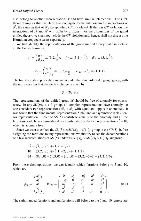
Grand Unified Theory 207
also belong to another representation R and have similar interactions. The CPTtheorem implies that the Hermitian conjugate terms will contain the interactions of
R, the same as that of R, except when CP is violated. If there is CP violation, the
interactions of R and R will differ by a phase. For the discussions of the grand
unified theory, we shall not include the CP violation and, hence, shall not discuss the
Hermitian conjugate terms separately.
We first identify the representations of the grand unified theory that can include
all the known fermions:
qL =(
ud
)L≡ (3,2,
1
6); uc
L ≡ (3,1,−2
3); dc
L ≡ (3,1,1
3);
L =(
νe−
)L≡ (1,2,−1
2); ec
L = e+L ≡ (1,1,1).
The transformation properties are given under the standard model gauge group, with
the normalization that the electric charge is given by
Q = T3L +Y.
The representations of the unified group R should be free of anomaly for consis-
tency. In any SU(n), n > 3 group, all complex representations have anomaly, so
one considers two representations R1 +R2 with equal and opposite anomalies. It
was found that the fundamental representation 5-plet and antisymmetric rank 2 ten-
sor representation 10-plet of SU(5) contribute equally to the anomaly and all the
fermions could be accommodated in a combination of the two representations 5+10,
which is anomaly free.
Since we want to embed the SU(3)c×SU(2)L×U(1)Y group in the SU(5), before
assigning the fermions to any representations we first try to see the decompositions
of a few representations of SU(5) under its SU(3)c ×SU(2)L ×U(1)Y subgroup:
5 = (3,1,1/3)+(1,2,−1/2)10 = (3,2,1/6)+(3,1,−2/3)+(1,1,1)24 = (8,1,0)+(1,3,0)+(1,1,0)+(3,2,−5/6)+(3,2,5/6) .
From these decompositions, we can identify which fermions belong to 5 and 10,
which are
ψ5L =
dc
1dc
2dc
3νee−
L
ψ10L =
0 uc
3 −uc2 −u1 −d1
−uc3 0 uc
1 −u2 −d2
uc2 −uc
1 0 −u3 −d3
u1 u2 u3 0 −e+
d1 d2 d3 e+ 0
L
. (8.1)
The right-handed fermions and antifermions will belong to the 5 and 10 representa-
© 2008 by Taylor & Francis Group, LLC
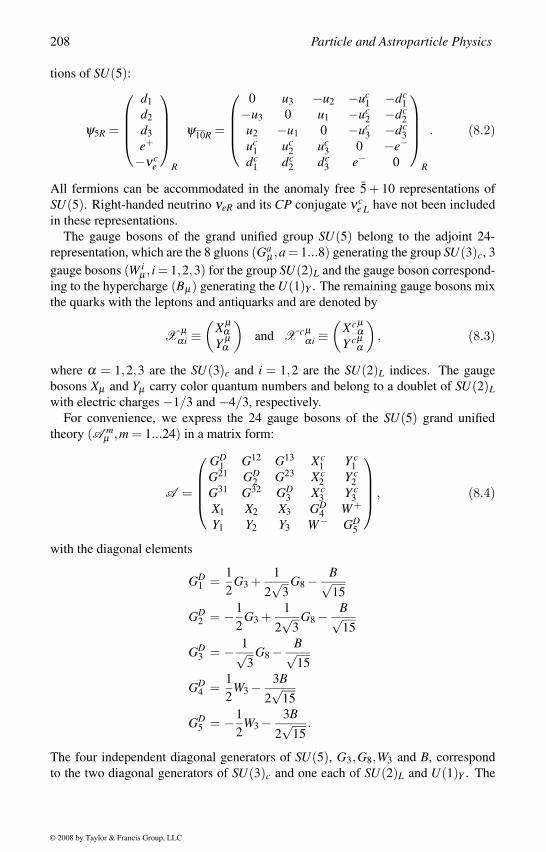
208 Particle and Astroparticle Physics
tions of SU(5):
ψ5R =
d1d2d3e+
−νce
R
ψ10R =
0 u3 −u2 −uc
1 −dc1
−u3 0 u1 −uc2 −dc
2u2 −u1 0 −uc
3 −dc3
uc1 uc
2 uc3 0 −e−
dc1 dc
2 dc3 e− 0
R
. (8.2)
All fermions can be accommodated in the anomaly free 5 + 10 representations of
SU(5). Right-handed neutrino νeR and its CP conjugate νce L have not been included
in these representations.
The gauge bosons of the grand unified group SU(5) belong to the adjoint 24-
representation, which are the 8 gluons (Gaµ ,a = 1...8) generating the group SU(3)c, 3
gauge bosons (W iµ , i = 1,2,3) for the group SU(2)L and the gauge boson correspond-
ing to the hypercharge (Bµ) generating the U(1)Y . The remaining gauge bosons mix
the quarks with the leptons and antiquarks and are denoted by
X µαi ≡
(X µ
αY µ
α
)and X cµ
αi ≡(
Xcµα
Y cµα
), (8.3)
where α = 1,2,3 are the SU(3)c and i = 1,2 are the SU(2)L indices. The gauge
bosons Xµ and Yµ carry color quantum numbers and belong to a doublet of SU(2)Lwith electric charges −1/3 and −4/3, respectively.
For convenience, we express the 24 gauge bosons of the SU(5) grand unified
theory (A mµ ,m = 1...24) in a matrix form:
A =
GD
1 G12 G13 Xc1 Y c
1G21 GD
2 G23 Xc2 Y c
2G31 G32 GD
3 Xc3 Y c
3X1 X2 X3 GD
4 W+
Y1 Y2 Y3 W− GD5
, (8.4)
with the diagonal elements
GD1 =
1
2G3 +
1
2√
3G8 − B√
15
GD2 = −1
2G3 +
1
2√
3G8 − B√
15
GD3 = − 1√
3G8 − B√
15
GD4 =
1
2W3 − 3B
2√
15
GD5 = −1
2W3 − 3B
2√
15.
The four independent diagonal generators of SU(5), G3,G8,W3 and B, correspond
to the two diagonal generators of SU(3)c and one each of SU(2)L and U(1)Y . The
© 2008 by Taylor & Francis Group, LLC
Grand Unified Theory 209
gauge bosons Xµ and X cµ are the raising and lowering operators connecting the
leptons (antileptons) with the antiquarks (quarks) or the quarks with the antiquarks.
Their interactions are shown diagrammatically in figure 8.1, which can lead to new
processes such as proton decay. This is prediction of any quark–lepton unification.
uc
u,d
(X,Y)c
(X ,Y )c
e, νu,d
e+
dc c
(X ,Y )c
FIGURE 8.1Interactions of Xµ and Yµ gauge bosons in SU(5) grand unified theory.
8.2 Particle SpectrumThe choice of Higgs scalar and the components that acquire vev determine the phe-
nomenology in any grand unified theory. A conventional choice of symmetry break-
ing pattern in SU(5) grand unified theory can be written as
SU(5)MU−→ SU(3)c ×SU(2)L ×U(1)YMW−→ SU(3)c ×U(1)Q . (8.5)
At the unification scale MU , the symmetry breaking does not change the rank of the
group, and this symmetry breaking could be achieved by a Higgs scalar in the adjoint
representation Σ 24.
The scalar potential for the field Σ, which acquires a vacuum expectation value
(vev), can be written as
V [Σ] = −1
2m2
ΣTr Σ2 +1
4a(Tr Σ2)2 +
1
2bTr Σ4, (8.6)
where m2Σ > 0. The expected symmetry breaking pattern requires that the standard
model singlet component of the 24-plet Higgs scalar acquires a vev
< Σ >= v0
1 0 0 0 0
0 1 0 0 0
0 0 1 0 0
0 0 0 − 32 0
0 0 0 0 − 32
. (8.7)
© 2008 by Taylor & Francis Group, LLC
210 Particle and Astroparticle Physics
This vev commutes with the generators of SU(3) that act on the first three elements
and commutes with the generators of SU(2) that act on the last two elements and
one U(1) subgroup of the SU(5). Gauge bosons corresponding to these three groups
remain massless, and the remaining gauge bosons become superheavy with mass
MX ≈MU . From the quantum numbers of the different states, it is possible to identify
the three groups with the standard model gauge groups. The normalization of the
group U(1) has to be suitably defined to identify it with the U(1)Y .
The electroweak symmetry breaking requires a standard model Higgs doublet
field, which can now belong to a 5-plet of SU(5), φ 5, whose scalar potential
can be written as
V [φ ] = −1
2m2
φ φ †φ +1
4λ (φ †φ)2. (8.8)
〈m2φ 〉 > 0 ensures a vev of this field, given by
< φ >=v√2
0
0
0
0
1
. (8.9)
Similar to the standard model, this Higgs scalar also gives masses to the fermions.
The usual mass term for the fermions comes from Yukawa coupling
LY = fi jψLψRφ +H.c. (8.10)
When the scalar field φ acquires a vev, this gives the fermion masses
mi jψLψRφ +H.c. with mi j = fi j〈φ〉.
Since the left-handed and right-handed fermions belong to the conjugate represen-
tations Ψ and Ψ, respectively, in grand unified theories, it is convenient to use the
following form of the Yukawa coupling for the fermion masses
LY = fi jψTL C−1ψc
Lφ +H.c. (8.11)
where C is the charge conjugation matrix acting on the spinor space. Since the left-
handed particles ψL and their CP conjugate left-handed antiparticles ψ cL belong to
the same representations Ψ of any grand unified theories, the Yukawa coupling terms
can be written as
LY = fi jΨTLC−1ΨLΦ+H.c. (8.12)
where C acts on both the spinor space as well as on the grand unified group space.
Although this form of the Yukawa coupling appears to be similar to the Majorana
mass terms, since both left-handed particles and antiparticles belong to the same
representation Ψ, this Yukawa coupling includes both the Dirac and Majorana mass
terms, if any.
© 2008 by Taylor & Francis Group, LLC
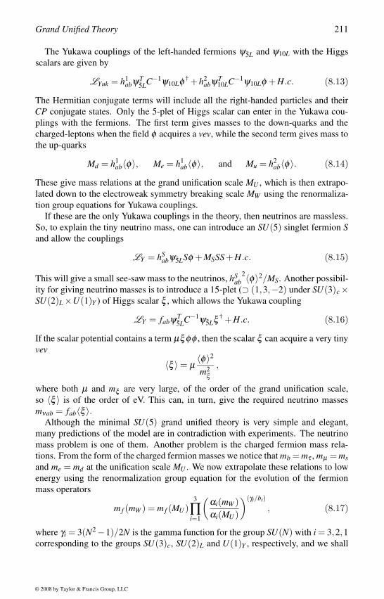
Grand Unified Theory 211
The Yukawa couplings of the left-handed fermions ψ5L and ψ10L with the Higgs
scalars are given by
LYuk = h1abψT
5LC−1ψ10Lφ † +h2abψT
10LC−1ψ10Lφ +H.c. (8.13)
The Hermitian conjugate terms will include all the right-handed particles and their
CP conjugate states. Only the 5-plet of Higgs scalar can enter in the Yukawa cou-
plings with the fermions. The first term gives masses to the down-quarks and the
charged-leptons when the field φ acquires a vev, while the second term gives mass to
the up-quarks
Md = h1ab〈φ〉, Me = h1
ab〈φ〉, and Mu = h2ab〈φ〉. (8.14)
These give mass relations at the grand unification scale MU , which is then extrapo-
lated down to the electroweak symmetry breaking scale MW using the renormaliza-
tion group equations for Yukawa couplings.
If these are the only Yukawa couplings in the theory, then neutrinos are massless.
So, to explain the tiny neutrino mass, one can introduce an SU(5) singlet fermion Sand allow the couplings
LY = hSabψ5LSφ +MSSS +H.c. (8.15)
This will give a small see-saw mass to the neutrinos, hSab
2〈φ〉2/MS. Another possibil-
ity for giving neutrino masses is to introduce a 15-plet (⊃ (1,3,−2) under SU(3)c ×SU(2)L ×U(1)Y ) of Higgs scalar ξ , which allows the Yukawa coupling
LY = fabψT5LC−1ψ5Lξ † +H.c. (8.16)
If the scalar potential contains a term µξ φφ , then the scalar ξ can acquire a very tiny
vev
〈ξ 〉 = µ〈φ〉2
m2ξ
,
where both µ and mξ are very large, of the order of the grand unification scale,
so 〈ξ 〉 is of the order of eV. This can, in turn, give the required neutrino masses
mνab = fab〈ξ 〉.Although the minimal SU(5) grand unified theory is very simple and elegant,
many predictions of the model are in contradiction with experiments. The neutrino
mass problem is one of them. Another problem is the charged fermion mass rela-
tions. From the form of the charged fermion masses we notice that mb = mτ , mµ = msand me = md at the unification scale MU . We now extrapolate these relations to low
energy using the renormalization group equation for the evolution of the fermion
mass operators
m f (mW ) = m f (MU )3
∏i=1
(αi(mW )αi(MU )
)(γi/bi)
, (8.17)
where γi = 3(N2−1)/2N is the gamma function for the group SU(N) with i = 3,2,1corresponding to the groups SU(3)c, SU(2)L and U(1)Y , respectively, and we shall
© 2008 by Taylor & Francis Group, LLC
212 Particle and Astroparticle Physics
define the beta functions later in equation (8.37). Although the low energy prediction
for the ratio mb/mτ is consistent, the conditions for the first and second generations
mµ = ms and me = md at the scale MU are badly in contradiction with low-energy
mass ratios.
The main reason for the fermion mass problem is that the vevs of φ do not distin-
guish between quarks and leptons. An interesting mechanism to solve this problem
includes a 45 Higgs scalar (χ i jk , antisymmetric in i, j) [126]. It is then possible to
give vev to the component
〈χ i5k 〉 =
v45√2(δ i
k −4δ i4δk4)
of χ i jk , which gives unequal contributions for the quarks and the leptons. Including
this field the additional Yukawa interactions are given by
LYuk = f 1abψ5Lψ10Lχ† + f 2
abψ10Lψ10Lχ +H.c. (8.18)
Taking the vevs of φ and χ , discussed above, the down quark and charged lepton
masses become√
2Md = h1abv+ f 1
abv45, and√
2M = h1abv−3 f 1
abv45, (8.19)
where a,b = 1,2,3 are generation indices. When only f22,h12 and h33 are nonvan-
ishing, the down quark and charged lepton mass matrices will be given by
√2Md =
0 h112v 0
h112v f 1
22v45 0
0 0 h133v
,√
2M =
0 h112v 0
h112v −3 f 1
22v45 0
0 0 h133v
, (8.20)
which can be diagonalized to get the relations
mb = mτ , mµ = 3ms and 3me = md (8.21)
at the grand unification scale. When extrapolated to low energies for comparison
with experimental numbers, these relations turns out to be very good. The factors 3
enter, where they should be, which comes from the choice of the vev of 45-plet. Since
χ i5k is traceless and antisymmetry requires i = 5, the quarks get equal contributions
and the leptons get a contribution equal to the number of quarks, which is 3. This
nice mechanism can be implemented in other grand unified theories such as SO(10)and the factor will always come out to be 3, because there are 3 colors of quarks.
8.3 Proton DecayUnification of the standard model gauge groups to a grand unified theory implies
unification of quarks and leptons as well. There will then be new interactions be-
tween the quarks and the leptons, to be mediated by new gauge bosons at the grand
© 2008 by Taylor & Francis Group, LLC
Grand Unified Theory 213
unification scale. This is a generic feature of any grand unified theory, which leads
to proton decay and baryon number violation. In SU(5) grand unified theory the
interactions of these gauge bosons Xµ and X cµ are given by
L = g5DcαLγµ ΨiLX cµ
αi +g5EcLγµ QαiLX cµ
αi
+g5UcαLγµ Qβ iLX µ
γi εαβγ +H.c., (8.22)
where g5 is the SU(5) gauge coupling constant and εαβγ is a totally antisymmetric
SU(3)c tensor with ε123 = 1. In general, the new interactions between the quarks
and leptons are mediated by three types of gauge bosons; leptoquarks interact with
a quark and a lepton, diquarks interact with a quark and an antiquark, and dileptonsineract with a lepton and an antilepton. In the SU(5) grand unified theory, dileptons
are absent, while the leptoquarks and diquarks are the same fields and mediate proton
decay, as shown in figure 8.2.
π0
e+
cd
d
u
u
d
X
p
µ
FIGURE 8.2Example of gauge bosons mediating proton decay p → e+π.
The new gauge bosons Xµ belong to SU(5)/SU(3)c × SU(2)L ×U(1)Y and are
superheavy with mass of the order of the unification scale (MX ≈ MU ). Since these
heavy bosons appear in the propagator, the amplitude for proton decay of the above
form (p → e+π0) will be given by
A (p → e+π0) =α5
M2X
, (8.23)
where the SU(5) gauge coupling constant α5 is given by
α5 =g2
54π
. (8.24)
The proton lifetime is then given by
τp ≈ M4X
α25 m5
p, (8.25)
© 2008 by Taylor & Francis Group, LLC
214 Particle and Astroparticle Physics
where mp is the mass of the proton. The unification scale and the coupling con-
stant at the unification scale can be obtained from an analysis of the evolution of
the gauge coupling constants using the renormalization group equations and apply-
ing the boundary condition of coupling constant unification. We shall discuss this in
the next section. For the minimal SU(5) grand unified theory, the prediction for the
proton lifetime (for the decay mode p → e+π0) comes out to be [125]
1030 years < τp < 1031 years , (8.26)
which is ruled out by the present experimental limit of τp > 1.6× 1033 years on
the proton lifetime [127]. However, some extensions such as inclusion of gravity
effects or the supersymmetric version of the model may still be consistent, so we
shall continue with the discussions with SU(5) grand unified theory.
In order to study different aspects of proton decay, including various decay modes
and the choice of Higgs scalars, we need to know more about the grand unified the-
ories and the interactions of the Higgs scalars. There is also an elegant formalism to
study these details starting from our knowledge of the standard model. It is possi-
ble to construct effective higher-dimensional operators, consistent with the standard
model, which can provide us some important information about the proton decays
[54] without any knowledge about the grand unified theories. We only assume that
the origin of these operators lies in the grand unified theories, and they are obtained
after integrating out all the heavy degrees of freedom in the theory.
A baryon-number violating operator must contain quarks (denoted by Q here)
and the SU(3)c invariance with nonzero baryon number would require at least three
quarks (QQQ). Lorentz invariance allows only even number of fermions, so the
simplest form of the operators is QQQL or QQQLc, where L represents a lepton.
These nonrenormalizable four-fermion effective operators have mass-dimension six
and hence they must have effective coupling constant suppressed by a factor of M−2,
where M is the heavy mass scale in the theory of the order of the grand unification
scale M ∼ MU . The proton lifetime, thus, comes out to be
τp ≈ Const.M4
m5p, (8.27)
which is similar to the one obtained in the SU(5) model.
There are six possible form of the dimension-six baryon-number violating oper-
ators, which are allowed by the standard model and Lorentz invariance. They are
given by [54]
O1abcd = (Dc
aαRUbβR)(QcciγLΨd jL)εαβγ εi j
O2abcd = (Qc
aiαLQb jβL)(UccγREdR)εαβγ εi j
O3abcd = (Qc
aiαLQb jβL)(QcckγLΨdlL)εαβγ εi jεkl
O4abcd = (Qc
aiαLQb jβL)(QcckγLΨdlL)εαβγ(τmε)i j(τmε)kl
© 2008 by Taylor & Francis Group, LLC
Grand Unified Theory 215
O5abcd = (Dc
aαRUbβR)(UccγREdR)εαβγ
O6abcd = (Uc
aαRUbβR)(DccγREdR)εαβγ . (8.28)
Here, α,β ,γ = 1,2,3 are SU(3)c indices; i, j = 1,2 are SU(2)L doublet indices;
m = 1,2,3 is a SU(2)L triplet index; and a,b,c,d = 1,2,3 are generation indices.
We exploioted the Fierz transformations to transform the vector and tensor operators
into these forms.
All of these operators are of the form QQQL, and hence, B−L is conserved, since
quarks carry baryon number 1/3 and leptons carry lepton number L = 1. To the
lowest order only the B−L conserving baryon number violation will be allowed in
all grand unified theories. The B− L violating baryon number violating operators
are of the form QQQLφ , where φ is the standard model Higgs doublet scalar. This
operator will have an additional suppression factor of 〈φ〉/M and the decay mode of
the proton will be suppressed by about 25 orders of magnitude. These operators will
not allow processes where an s-quark state is created, implying that processes such
as p → e+K0or n → e+K−
with ∆S = ∆B are forbidden. These operators also relate
several decay channels of the proton.
At this stage we have not included any intermediate scale in the theory, which is
valid for the SU(5) grand unified theory. But in grand unified theories with larger
gauge groups such as SO(10), there are intermediate symmetry breaking scales,
which may allow some of the higher-dimensional operators to dominate over the
dimension-6 operators. For example, an operator of the form QQQL∆ may be sup-
pressed by M−3I , where MI is some intermediate symmetry breaking scale and it is
also possible that 〈∆〉 ∼ MI . There are no such processes, but SO(10) grand uni-
fied theory allows B− L violating neutron–antineutron oscillations [61] and B− Lviolating three lepton decay modes of proton [128] that are comparable with B−Lconserving proton decays [129].
8.4 Coupling Constant UnificationIn grand unified theories the strong, the weak and the electromagnetic interactions
are unified into a single unified theory. So, the three gauge coupling constants g3,g2and g1, corresponding to the groups SU(3)c, SU(2)L and U(1)Y , also should get
unified at the unification scale MU , and we should have
g3(MU ) = g2(MU ) = g1(MU ) = g5(MU ). (8.29)
If we now use the renormalization group equations to study the evolution of the
different gauge coupling constants, it will be possible to estimate the unification
scale MU and the gauge coupling constant at the unification scale g5.
© 2008 by Taylor & Francis Group, LLC
216 Particle and Astroparticle Physics
When the symmetry breaking takes place at the scale of grand unification, the
standard model gauge group emerges from the unified SU(5) group. This requires
normalization of the generators of the different groups in the same way:
Tr [TiTj] = Nδi j, (8.30)
where N is a constant, which has to be the same for the unification group and all of
its subgroups. We choose N = 1/2 for the fundamental representation of any SU(n)group and then normalize the U(1) subgroup by comparing its normalization with
any complete representations of SU(5).Consider the 5 representation of SU(5), which contains the down antiquarks dc
Lwith hypercharge Y = 1/3 and the lepton doublets containing eL and νL with Y =−1/2. The U(1)Y normalization YN must be the same as the normalization of 5,
which is N = 12 . Writing the normalizations of the components of 5
Tr (Y 2) =[3×Y 2
dc +×Y 2e +Y 2
ν]=[
3× Y 2N9
+2× Y 2N4
]=
5
6Y 2
N , (8.31)
we can get the U(1)Y normalization to be
YN =
√3
5. (8.32)
The corresponding normalization of the U(1)Y coupling constant becomes
g′2 =3
5g2
1. (8.33)
At the unification scale the weak mixing angle then becomes
sin2 θw =g′2
g22 +g′2
=3
8. (8.34)
We shall now demonstrate how the different gauge coupling constants evolve with
energy and how we arrive at the gauge coupling unification.
We start with the experimental values of sin2 θW and αs at the electroweak scale
mW , obtained from the measurements of the Z-mass and Z-width at LEP and also the
jet cross-sections and energy–energy correlations. Using the fine structure constant
at the electroweak scale αem(mW ) = 1/127.9, along with the values of sin2 θ(mW ) =.2334 and α3(mW ) = .118 from the high precision LEP data, we can write the values
of the three coupling constants at mW as
α−11 (mW ) ≡ 3
5α−1(mW )cos2 θw(mW ) = 58.83
α−12 (mW ) ≡ α−1(mW )sin2 θw(mW ) = 29.85
α−13 (mW ) ≡ α−1
s (mW ) = 8.47, (8.35)
© 2008 by Taylor & Francis Group, LLC
Grand Unified Theory 217
where αi = g2i /4π . The evolution of these coupling constants with energy is gov-
erned by the renormalizable group equations
µdgi
dµ= βi(gi) = bi
g3i
16π2 , (8.36)
where gi, i = 3,2,1 are the gauge coupling constants for the groups SU(3)c, SU(2)Land U(1)Y , respectively. The one-loop beta functions are given by
βi(gi) =g3
i16π2
[−11
3Tr [T 2
a ]+2
3∑
fTr [T 2
f ]+1
6∑s
Tr [T 2s ]
], (8.37)
where T ’s are generators of different representations of the groups, to which the
gauge bosons, fermions and scalars belong. The quadratic Casimir invariants Tr [T 2i ]
are given by equation (8.30). The gauge boson contribution vanishes for any U(1)group, but for an SU(n) group it is Tr [T 2
a ] = n since the gauge bosons belong to the
adjoint representation of the group.
There are four quarks, the left-handed and right-handed up and down quarks,
which belong to the fundamental triplet representation of SU(3)c. For the funda-
mental representations of any SU(n) group, Tr [TiTi] = 1/2. Since the leptons do
not contribute to the SU(3)c beta function, the total contribution of the fermions to
the SU(3)c beta function is 2. Similarly, for the SU(2)L contribution to the beta
function, we consider all the SU(2)L doublets, which are three colored left-handed
quarks and the left-handed leptons. Since the contributions of the fundamental dou-
blet representation is 1/2, the total SU(2)L contribution to the beta function is also
2. If we now consider the normalization of the U(1)Y group as discussed above, the
total contribution again comes out to be 2.
If we include the contribution of the nh numbers of standard model doublet Higgs
scalars to the beta function, which are 0, nh and 3nh/5 for the groups SU(3)c, SU(2)Land U(1)Y , we can write the solutions to the renormalizable group equations in the
one-loop approximation as
α−13 (M2
U ) = α−13 (m2
W )+(11− 4
3 ng)4π
log
(M2
U
m2W
)α−1
2 (M2U ) = α−1
2 (m2W )+
( 223 − 4
3 ng − 16 nh)
4πlog
(M2
U
m2W
)α−1
1 (M2U ) = α−1
1 (m2W )+
(− 43 ng − 1
10 nh)4π
log
(M2
U
m2W
), (8.38)
where ng = 3 is the number of generations of fermions.
The evolution of the three gauge coupling constants α−11 ,α−1
2 and α−13 are plotted
as a function of energy in figure 8.3. They do not meet at a point, even including
the errors in the measurements of the coupling constants. This result is valid even
when the two-loop contributions are included and hence there is no grand unification
© 2008 by Taylor & Francis Group, LLC
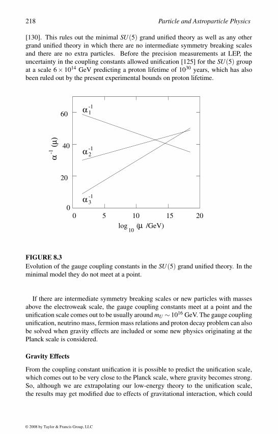
218 Particle and Astroparticle Physics
[130]. This rules out the minimal SU(5) grand unified theory as well as any other
grand unified theory in which there are no intermediate symmetry breaking scales
and there are no extra particles. Before the precision measurements at LEP, the
uncertainty in the coupling constants allowed unification [125] for the SU(5) group
at a scale 6× 10¹⁴ GeV predicting a proton lifetime of 1030 years, which has also
been ruled out by the present experimental bounds on proton lifetime.
0 105 15
α
(µ)
20
20
0
40
60
10log ( /GeV)µ
1
2
3
α
α
α -1
-1
-1
-1
FIGURE 8.3Evolution of the gauge coupling constants in the SU(5) grand unified theory. In the
minimal model they do not meet at a point.
If there are intermediate symmetry breaking scales or new particles with masses
above the electroweak scale, the gauge coupling constants meet at a point and the
unification scale comes out to be usually around mU ∼ 1016 GeV. The gauge coupling
unification, neutrino mass, fermion mass relations and proton decay problem can also
be solved when gravity effects are included or some new physics originating at the
Planck scale is considered.
Gravity Effects
From the coupling constant unification it is possible to predict the unification scale,
which comes out to be very close to the Planck scale, where gravity becomes strong.
So, although we are extrapolating our low-energy theory to the unification scale,
the results may get modified due to effects of gravitational interaction, which could
© 2008 by Taylor & Francis Group, LLC
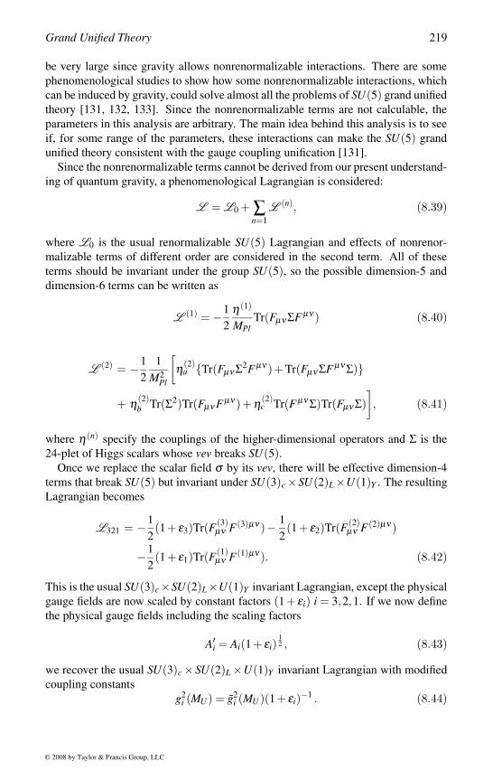
Grand Unified Theory 219
be very large since gravity allows nonrenormalizable interactions. There are some
phenomenological studies to show how some nonrenormalizable interactions, which
can be induced by gravity, could solve almost all the problems of SU(5) grand unified
theory [131, 132, 133]. Since the nonrenormalizable terms are not calculable, the
parameters in this analysis are arbitrary. The main idea behind this analysis is to see
if, for some range of the parameters, these interactions can make the SU(5) grand
unified theory consistent with the gauge coupling unification [131].
Since the nonrenormalizable terms cannot be derived from our present understand-
ing of quantum gravity, a phenomenological Lagrangian is considered:
L = L0 + ∑n=1
L (n), (8.39)
where L0 is the usual renormalizable SU(5) Lagrangian and effects of nonrenor-
malizable terms of different order are considered in the second term. All of these
terms should be invariant under the group SU(5), so the possible dimension-5 and
dimension-6 terms can be written as
L (1) = −1
2
η(1)
MPlTr(Fµν ΣFµν) (8.40)
L (2) = −1
2
1
M2Pl
[η(2)
a Tr(Fµν Σ2Fµν)+Tr(Fµν ΣFµν Σ)
+ η(2)b Tr(Σ2)Tr(Fµν Fµν)+η(2)
c Tr(Fµν Σ)Tr(Fµν Σ)], (8.41)
where η (n) specify the couplings of the higher-dimensional operators and Σ is the
24-plet of Higgs scalars whose vev breaks SU(5).Once we replace the scalar field σ by its vev, there will be effective dimension-4
terms that break SU(5) but invariant under SU(3)c ×SU(2)L ×U(1)Y . The resulting
Lagrangian becomes
L321 = −1
2(1+ ε3)Tr(F(3)
µν F(3)µν)− 1
2(1+ ε2)Tr(F(2)
µν F(2)µν)
−1
2(1+ ε1)Tr(F(1)
µν F(1)µν). (8.42)
This is the usual SU(3)c×SU(2)L×U(1)Y invariant Lagrangian, except the physical
gauge fields are now scaled by constant factors (1+ εi) i = 3,2,1. If we now define
the physical gauge fields including the scaling factors
A′i = Ai(1+ εi)
12 , (8.43)
we recover the usual SU(3)c ×SU(2)L ×U(1)Y invariant Lagrangian with modified
coupling constants
g2i (MU ) = g2
i (MU )(1+ εi)−1 . (8.44)
© 2008 by Taylor & Francis Group, LLC
220 Particle and Astroparticle Physics
We measure the coupling constants at low energy gi, and they then evolve with en-
ergy and, get scaled gi by the nonrenormalizable interactions near the unification
scale. The boundary condition at the unification scale now reads
g23 = g2
2 = g21 = g2
0 . (8.45)
So the coupling constants that are unified are not the same as the low-energy con-
stants we measure. When we evolved the low energy gauge couplings, even if they
do not meet at a point, that may not be interpreted as lack of unification.
It is possible to include the dimension-5 and dimension-6 terms and achieve uni-
fication at a scale as high as 1017 GeV. Thus, the problem of gauge unification and
proton decay are simultaneously solved in the minimal SU(5) grand unified theory
in the presence of gravity induced terms [132]. The fermion mass relations as well
as the neutrino mass problem can also be solved if gravity effects are included [133].
Consider the fermion mass problem where it is possible to have an effective gravity
induced term (1/MPl)ψLψRφΣ, which contains an effective 45-plet (⊂ 5× 24) of
Higgs scalar and can solve the fermion mass relations. The small Majorana neutrino
mass can come from an effective term φφ/MPl . The quantum gravity effects can,
in principle, cure all the problems of the minimal SU(5) grand unified theory. On
the other hand, predictions of any grand unified theory could get modified due to the
gravity effects.
8.5 SO(10) GUTThe grand unified theory based on the gauge group SO(10) has several new interest-
ing features [134] compared with the SU(5) grand unified theory. An SO(10) group
is a rank-5 group, and there is one additional diagonal generator, which allows some
interesting intermediate symmetry breaking stages before the group reduces to the
standard model gauge group SU(3)c ×SU(2)L ×U(1)Y . One of the most interesting
intermediate symmetries is the left–right symmetry, in which parity is broken sponta-
neously [59, 60]. The difference between the baryon and lepton number B−L is also
a gauge symmetry [129] in the theory and hence B−L is also spontaneously broken.
As a result, there are new B−L violating processes, which may have observable pre-
dictions such as neutron–antineutron oscillations, neutrinoless double beta decay or
B−L violating proton decay modes, making the model even more interesting. Tiny
neutrino masses are naturally explained and gauge coupling constants meet at a point
for some range of the intermediate symmetry breaking scale.
The SO(10) group can descend to the standard model through different interme-
diate symmetries, and depending on the choice of Higgs scalars, many versions of
the theory are possible. If the group SO(10) breaks down to the standard model di-
rectly at the scale of grand unification, the model will inherit some of the problems
of the SU(5) grand unified theory. We shall discuss only some salient features of
© 2008 by Taylor & Francis Group, LLC
Grand Unified Theory 221
the SO(10) grand unified theory, with one or two intermediate symmetry breaking
scales.
The Model
The SO(10) group is an orthogonal group with a 10-dimensional fundamental or vec-
tor representation. The generators of the group are 10× 10 antisymmetric matrices
of dimension 45. There is a 16-dimensional spinor representation with opposite he-
licity compared with its conjugate 16 spinor representation. All the known fermions
that belong to 5+10 of SU(5) and the CP conjugate of the right-handed neutrino that
could be accommodated in a singlet of SU(5), can be accommodated in the spinor
representation of SO(10):
ΨL =(
u1 u2 u3 νed1 d2 d3 e−
)L+(
uc1 uc
2 uc3 νc
edc
1 dc2 dc
3 e+
)L
. (8.46)
The right-handed fermions can then be identified with the components of a 16 repre-
sentation
ΨR =(
uc1 uc
2 uc3 νc
edc
1 dc2 dc
3 e+
)R+(
u1 u2 u3 νed1 d2 d3 e−
)R
. (8.47)
We have written this particular form with a motivation. The leptons can now be
identified as a fourth color of quarks after including the right-handed neutrino, which
means that we can extend the group SU(3)c ×SU(2)L ×U(1)Y ≡ G [3c −2L −1Y ] to
SU(4)c × SU(2)L × SU(2)R ≡ G [4c − 2L − 2R] and have quark–lepton unification
[59]. This partially unified group G [4c − 2L − 2R] has rank 5 and is the maximal
subgroup of SO(10). The decomposition of the 16-spinor containing the fermions
under the group G [4c −2L −2R] can be written as
16 = (4,2,1)+(4,1,2) and 16 = (4,2,1)+(4,1,2). (8.48)
One of the popular and interesting intermediate symmetry breaking chain of SO(10)group is via the partially unified group and then the left–right symmetric group
SO(10)MU−→ SU(4)c ×SU(2)L ×SU(2)R G [4c −2L −2R]M1−→ SU(3)c ×SU(2)L ×SU(2)R ×U(1)(B−L)
G [3c −2L −2R −1(B−L)]MR−→ SU(3)c ×SU(2)L ×U(1)Y . G [3c −2L −1Y ]mW−→ SU(3)c ×U(1)Q G [3c −1Q] .
The partially unified group
G [4c −2L −2R] ≡ GPS
is also called the Pati–Salam group and we denote the left–right symmetric group as
G [3c −2L −2R −1(B−L)] ≡ GLR
© 2008 by Taylor & Francis Group, LLC
222 Particle and Astroparticle Physics
and the standard model symmetry group as
G [3c −2L −1Y ] ≡ Gstd and G [3c −1Q] ≡ GQ.
The U(1) subgroup of SU(4)c has been identified with the B−L quantum number
[129], which is true for all the known fermions. But for scalars or some new exotic
fermions this may not be true. However for the present discussion this identification
is consistent.
B−L is a gauge symmetry in the conventional left–right symmetric model. In
these models the hypercharge and the electric charge are related to the B−L and the
SU(2)R quantum number by the relation
Q = T3L +T3R +B−L
2= T3L +Y. (8.49)
Thus, any B−L violating process can occur only after the B−L symmetry is spon-
taneously broken.
The gauge bosons belong to the adjoint 45-dimensional antisymmetric represen-
tation of SO(10), which transform under the left–right symmetric model GLR as
45 = (8,1,1,0)+(1,3,1,0)+(1,1,3,0)+(1,1,1,0)
+(3,2,2,−2
3)+(3,2,2,
2
3)+(3,1,1,
4
3)+(3,1,1,−4
3) . (8.50)
The gauge bosons corresponding to the first line are the ones that generate the left–
right symmetry group and remain massless until the left–right symmetry breaking
scale. The remaining fields given in the second line, which are the leptoquark and
diquark gauge bosons, become massive at the scale of grand unification. These gauge
bosons can mediate proton decay as in the SU(5) grand unified theory. However, in
all these interactions B−L is conserved, since it is a gauge symmetry and broken only
after the left–right symmetry breaking. During the left–right symmetry breaking, the
charged components W±R of the gauge bosons (1,1,3,0) and a combination of the
neutral component W 3R of (1,1,3,0) and WBL corresponding to (1,1,1,0) become
massive, leaving the standard model gauge bosons massless.
Symmetry Breaking and Fermion Masses
As we discussed earlier, in any grand unified theory the Higgs scalars are very im-
portant in deciding the symmetry breaking pattern, giving mass to the fermions, evo-
lution of the gauge coupling constants, and mediating exotic processes through their
interactions. In the SO(10) grand unified theory several Higgs scalars are required,
since there are now intermediate symmetry breaking scales. Moreover, the rank of
the group has to be reduced, so it can descend to the standard model.
There are many combinations of the Higgs scalars that can allow the different sym-
metry breaking chains. Each of these combinations can have different phenomeno-
logical implications. In addition to the Higgs scalars that are required for any sym-
metry breaking, there could be additional scalars, which only contribute in solving
© 2008 by Taylor & Francis Group, LLC
Grand Unified Theory 223
some problems such as fermion mass relations, neutrino mass, or baryon number
nonconservation. In supersymmetric theories there are more possibilities and some
Higgs scalars are required to allow symmetry breaking without breaking supersym-
metry. We shall discuss a few of these issues and concentrate on the generic features
of the SO(10) grand unified theory.
We shall consider the symmetry breaking chain
SO(10)MU−→ GLR
MLR−→ GstdMW−→ GQ .
We have not included the Pati–Salam subgroup in the discussion, since the renor-
malization group analysis of the gauge coupling evolution does not allow the GPSto be much lower than the unification scale. Moreover, the GPS intermediate sym-
metry does not allow the new phenomenology that we plan to discuss. However, to
identify different components of the scalars, we shall write the decomposition of the
various fields in terms of their decomposition under the group GPS. We start with the
decomposition of some of the scalar fields:
210 = (1,1,1)+(6,2,2)+(15,3,1)+(15,1,3)+(15,1,1)+(10,2,2)+(10,2,2)
54 = (1,1,1)+(1,3,3)+(20′,1,1)+(6,2,2)45 = (1,3,1)+(1,1,3)+(15,1,1)+(6,2,2)
126 = (15,2,2)+(10,1,3)+(10,3,1)+(6,1,1)120 = (1,2,2)+(10,1,1)+(10,1,1)+((6,1,3)
+(6,3,1)+(15,2,2)16 = (4,2,1)+(4,1,2)10 = (6,1,1)+(1,2,2). (8.51)
The SO(10) breaking to the left–right symmetric group GLR could be achieved by a
210-dimensional field or a combination of the fields 45+54. We shall consider only
the scalar belonging to the 210 representation, when two of its components (1,1,1)and (15,1,1) acquire vev. Another alternative of this symmetry breaking is when
the (1,1,1) component of 210 or 45 acquires vev and breaks SO(10) → GPS and
subsequently the (15,1,1) of 210 or 54 acquires vev and breaks GPS → GLR.
The next stage of symmetry breaking is more interesting from phenomenologi-
cal point of view. The left–right symmetry breaking can take place when the Higgs
scalar belongs to a 126-dimensional representation or a 16-dimensional representa-
tion of SO(10). The studies with these two choices of the Higgs scalar have widely
different consequences. The next stage of symmetry breaking requires a Higgs scalar
10,120,126 or a 16 of SO(10). Since the fermion masses come from the vev of these
scalars, different choices of the Higgs would give different fermion mass relations.
In the simplest version of the SO(10) grand unified theory the left–right symmetry
breaking also breaks the parity spontaneously. This is an interesting feature of the
theory that explains the origin of the low-energy parity violation. In the scalar sector,
parity could be broken even before the left–right symmetry is broken. When SO(10)
© 2008 by Taylor & Francis Group, LLC
224 Particle and Astroparticle Physics
is broken to GPS by the vev of (1,1,1) belonging to a 45 or a 210 of SO(10), parity
is also broken since the field is odd under parity [135]. This can then cause mass
splitting between scalars that are related to each other under SU(2)L ↔ SU(2)R.
This is referred to as D-parity to distinguish it from the parity of the Lorentz group.
Another interesting feature associated with the left–right symmetric model is that
the B−L symmetry is gauged. Thus, B−L violating interactions can appear only
after this symmetry is broken spontaneously. Since B − L symmetry breaking is
required for giving neutrino masses and explaining the baryon asymmetry of the uni-
verse, different choices of Higgs scalars for the B−L breaking can lead to different
consequences. The fermion mass relations can also be affected by the B−L sym-
metry breaking. Although the left–right symmetry could be broken with the B−Lsymmetry, it is also possible to break the left–right symmetry at a much higher scale
than the B−L symmetry breaking scale. It is also possible to associate the D-parity
violating scale with the neutrino masses, decoupling it from the B− L symmetry
breaking.
In the popular version of the SO(10) grand unified theory, a 126 representation of
SO(10) breaks the left–right symmetry along with the U(1)B−L. There is an SU(2)Rtriplet Higgs scalar transforming as ∆R ≡ (1,1,3,−2) under GLR, whose neutral com-
ponent acquires a vev. Left-right D-parity then implies the existence of a left-handed
triplet Higgs scalar ∆L ≡ (1,3,1,−2) under GLR belonging to a 126 representation
of SO(10). For a choice of parameters in the scalar potential, it is possible to give
vev to ∆R but not to ∆L. However, after the electroweak symmetry breaking, ∆L will
receive an induced vev, which is extremely small.
At the left–right symmetry breaking scale MR, we have
GLR〈∆R〉−→ Gstd ,
so 〈∆R〉 ∼ MR. The electroweak symmetry is then broken by the bi-doublet Higgs
scalar Φ10 ≡ (1,2,2,0) belonging to a 10-plet of SO(10), which is doublet under both
SU(2)L and SU(2)R. This field also gives masses to the fermions. At the electroweak
symmetry breaking scale MW , we thus have
Gstd〈Φ10〉−→ GQ .
As in the SU(5) grand unified theory, this scalar gives the wrong fermion mass re-
lations. Therefore, we need another component of 126-plet Higgs, which is also a
bi-doublet Φ126 ≡ (15,2,2,0), to contribute to the fermion masses. The 15-plet of
SU(4)c contains a component, which is a singlet under SU(3)c ×U(1)B−L and has
the form diag[1,1,1,−3], which can then give the correct fermion mass relations.
The minimization of the scalar potential would now give us the relation
〈∆L〉 = const.〈Φ10〉2
〈∆R〉 , (8.52)
where the constant (const.) includes parameters in the scalar potential.
© 2008 by Taylor & Francis Group, LLC
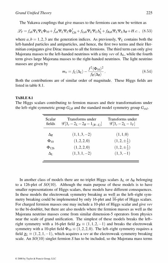
Grand Unified Theory 225
The Yukawa couplings that give masses to the fermions can now be written as
LY = fabΨLΨLΦ10 + fabΨLΨLΦ†126 + fLabΨLΨL∆†
L + fRabΨLΨL∆R +H.c. , (8.53)
where a,b = 1,2,3 are the generation indices. As previously, ΨL contains both the
left-handed particles and antiparticles, and hence, the first two terms and their Her-
mitian conjugates give Dirac masses to all the fermions. The third term can only give
Majorana masses to the left-handed neutrinos with a tiny vev of ∆L, while the fourth
term gives large Majorana masses to the right-handed neutrinos. The light neutrino
masses are given by
mν = fL〈∆L〉− f 2〈Φ10〉2
fR〈∆R〉 . (8.54)
Both the contributions are of similar order of magnitude. These Higgs fields are
listed in table 8.1.
TABLE 8.1The Higgs scalars contributing to fermion masses and their transformations under
the left–right symmetric group GLR and the standard model symmetry group Gstd .
Scalar Transforms under Transforms underfields G [3c −2L −2R −1(B−L)] G [3c −2L −1Y ]
∆R (1,1,3,−2) (1,1,0)
Φ10 (1,2,2,0) (1,2,± 12 )
Φ126 (1,2,2,0) (1,2,± 12 )
∆L (1,3,1,−2) (1,3,−1)
In another class of models there are no triplet Higgs scalars ∆L or ∆R belonging
to a 126-plet of SO(10). Although the main purpose of these models is to have
smaller representations of Higgs scalars, these models have different consequences.
In these models the electroweak symmetry breaking as well as the left–right sym-
metry breaking could be implemented by only 16-plet and 16-plet of Higgs scalars.
For charged fermion masses one may include a 10-plet of Higgs scalar and give vevto the bi-doublet, but there are also models where the fermion masses as well as the
Majorana neutrino masses come from similar dimension-5 operators from physics
near the scale of grand unification. The simplest of these models breaks the left–
right symmetry with a 16-plet field χR ≡ (1,1,2,−1) and breaks the electroweak
symmetry with a 10-plet field Φ10 ≡ (1,2,2,0). The left–right symmetry requires a
field χL ≡ (1,2,1,−1), which acquires a vev at the electroweak symmetry breaking
scale. An SO(10) singlet fermion S has to be included, so the Majorana mass terms
© 2008 by Taylor & Francis Group, LLC
226 Particle and Astroparticle Physics
of S can generate the see-saw Majorana masses to the left-handed and right-handed
neutrinos. The fermion mass relations can also be explained by the higher order
radiative contributions in these models.
B−L Violating Interactions
We shall now discuss some of the consequences of spontaneous B−L violation in the
SO(10) grand unified theories. We shall first consider the triplet Higgs models, where
the left–right symmetry GLR is broken by the Higgs scalar ∆R ≡ (1,1,3,−2). The
vev of ∆R can then mediate B−L violating processes such as neutron–antineutron
oscillations [61] or three-lepton decays of the proton [128] and give Majorana masses
to the right-handed neutrinos. We shall demonstrate how processes such as neutron–
antineutron oscillations take place in the SO(10) grand unified theory.
The leptoquark and diquark gauge bosons can take part in the baryon-number
violating processes, but they have masses of the order of MU , and their dominant
contribution will be to B− L conserving proton decays. In SO(10) grand unified
theory the left–right symmetry breaking Higgs scalar ∆†R belongs to 126 of SO(10).
Although the component ∆R only acquires vev, several other components of the same
representation 126 remain light, which includes the diquarks ∆qq and the leptoquarks
∆lq. Since the mixing between ∆qq and ∆lq is strongly suppressed, these scalars will
not mediate proton decay. If we now represent a 126 representation by ∆, then a
quartic coupling of ∆ can allow B−L violating processes, when ∆R acquires vev.
Consider a coupling ∆3qq∆†
R, where the diquarks take right-handed quarks to right-
handed antiquarks. When ∆R acquire a vev, the effective operator ∆3qq would take
three quarks into three antiquarks leading to neutron–antineutron oscillations. We
can write the relevant interactions as
L = f ∆3qq∆R + fqQR
cQR∆qq + fRLRcLR∆R, (8.55)
where we have adopted the convention that
QR =(
URDR
)and LR =
(NRER
), (8.56)
and NR are the right-handed neutrinos. From these interactions it is now possible
to allow a transition from a neutron to an antineutron as shown in figure 8.4. The
amplitude for this neutron–antineutron oscillation is given by [136]
δmn = Af f 3
q vR
m6∆qq
, (8.57)
where A ∼ 10−4 is a correction factor due to renormalization [137, 138], wave func-
tion at the origin [138, 139] and nuclear effects [140].
The neutron–antineutron oscillation requires an effective six quark dimension-9
effective operator QQQQQQ. The amplitude for the process has a suppression factor
M−5, whereas the lowest-dimensional proton decay operator has dimension-6 and is
© 2008 by Taylor & Francis Group, LLC
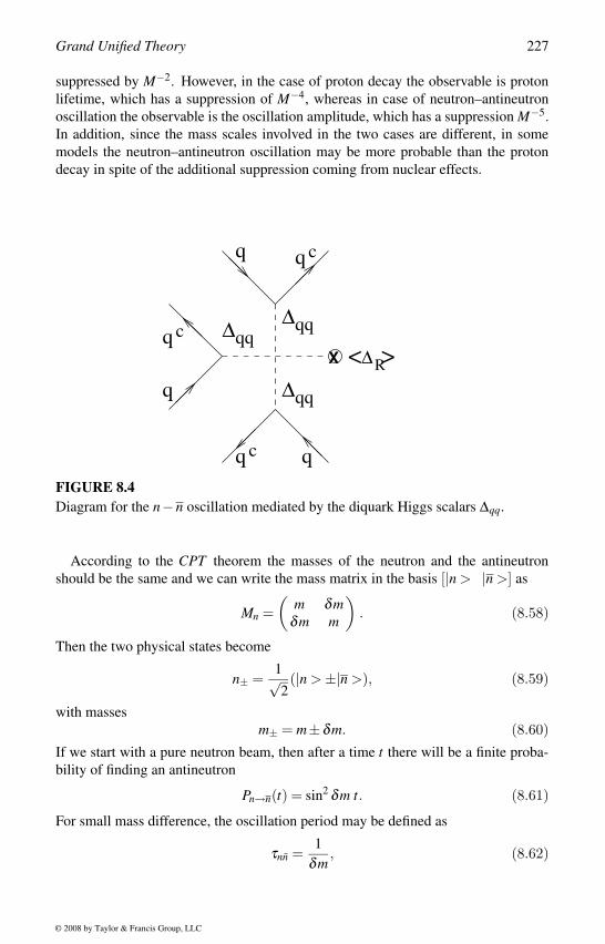
Grand Unified Theory 227
suppressed by M−2. However, in the case of proton decay the observable is proton
lifetime, which has a suppression of M−4, whereas in case of neutron–antineutron
oscillation the observable is the oscillation amplitude, which has a suppression M−5.
In addition, since the mass scales involved in the two cases are different, in some
models the neutron–antineutron oscillation may be more probable than the proton
decay in spite of the additional suppression coming from nuclear effects.
c
q c
q c
qq∆
qq∆qq∆
∆R< >q
q
X
q
q
FIGURE 8.4Diagram for the n−n oscillation mediated by the diquark Higgs scalars ∆qq.
According to the CPT theorem the masses of the neutron and the antineutron
should be the same and we can write the mass matrix in the basis [|n > |n >] as
Mn =(
m δmδm m
). (8.58)
Then the two physical states become
n± =1√2(|n > ±|n >), (8.59)
with masses
m± = m±δm. (8.60)
If we start with a pure neutron beam, then after a time t there will be a finite proba-
bility of finding an antineutron
Pn→n(t) = sin2 δm t. (8.61)
For small mass difference, the oscillation period may be defined as
τnn =1
δm, (8.62)
© 2008 by Taylor & Francis Group, LLC
228 Particle and Astroparticle Physics
so the probability of finding the antineutron in the pure neutron beam becomes
Pn→n(t) =(
tτnn
). (8.63)
Experiments could not detect any antineutrons in a neutron beam at a distance, from
which a bound on the neutron–antineutron oscillation period [141] is established
τnn > 0.86 × 10⁸ secs, corresponding to a baryon-number violating lifetime of a
physical neutron to be τ+ > 1032 years [127].
Gauge Coupling Unification
We demonstrated that in SU(5) grand unified theory, coupling constant unification is
not possible. We also commented that the result is valid for any grand unified theory
with no intermediate symmetry breaking scales. We shall now show how the problem
is solved and the coupling constant unification can be achieved in SO(10) grand
unified theory with intermediate symmetry breaking scales. Consider the symmetry
breaking pattern
SO(10)MU−→ GPS
MI−→ GLRMR−→ Gstd
MW−→ GQ .
To study the evolution of the gauge coupling constants, we shall apply boundary
conditions at the different symmetry breaking scales and then evolve the couplings
to the next symmetry breaking scales.
The contribution of the Higgs scalars can be large when there are intermediate
symmetry breaking scales, since several Higgs scalars take part in the symmetry
breaking and giving fermion masses. Moreover the Higgs representations are also
large compared with SU(5). In considering the Higgs contributions to the renor-
malization group equation, we shall assume the decoupling theorem. Following this
theorem, we shall assume that the components of any Higgs scalars that are not pro-
tected by any symmetry are heavy.
Let us start with a symmetry group G and consider the symmetry breaking pattern
GM1→ G1
M2→ G2. (8.64)
Consider a representation R of G, which decomposes under the different subgroups
G1 and G2 as
R → ∑n
Rn → ∑m
[∑n
Rnm
]. (8.65)
Any representation Ri of G1 can be decomposed under G2 as ∑m Rim. According to
the decoupling theorem, if any component Rkl ⊂ Rk ⊂ R acquires a vev at the scale
M2, then until M1, only the component Rk will contribute to the evolution of the
gauge coupling constants, and above M1, the entire representation R will contribute.
After the component Rkl of G2 acquires a vev at a scale M2, the G1 symmetry above
M2 ensures that all the components of the representation Rk of G2 have mass less
than M2. Similarly, above the scale M1 the symmetry group is G and it implies that
© 2008 by Taylor & Francis Group, LLC
Grand Unified Theory 229
all components of the representation R should have mass less than the symmetry
breaking scale M1.
We shall now start with the values of the couplings at the electroweak scale mW ,
whose central values are
α1(mW ) = 0.01699
α2(mW ) = 0.0335
α3(mW ) = 0.118 . (8.66)
We shall evolve these couplings to the left–right symmetry breaking scale MR and
then apply the boundary conditions at MR
α−11Y (MR) =
3
5α−1
2R (MR)+2
5α−1
1(B−L)(MR)
α−12L (MR) = α−1
2R (MR). (8.67)
For simplicity we assume MI = MU , so the next matching condition is at the unifica-
tion scale MU . The evolution equations then become
α−11Y (mW ) = α−1
10 (MU )+(
6
5b2R +
4
5b4
)MU1
+(
6
5b2R +
4
5b1(B−L)
)M1R +2b1Y MRW
α−12L (mW ) = α−1
10 (MU )+2b2LMU1 +2b2LM1R +2bew2LMRW
α−13c (mW ) = α−1
10 (MU )+2b4MU1 +2b3cM1R +2b3cMRW , (8.68)
where Mi j ≡ 4π ln(Mi/M j) and the beta function coefficients, bi’s, are given as
b1(B−L) =1
(4π)23
2; b1Y =
1
(4π)22
5; b2L = b2R = − 1
(4π)220
3;
bew2L = − 1
(4π)241
6; b3 = − 1
(4π)2 11. (8.69)
Here we have taken the number of fermion families n f = 3. The gauge coupling
constants now meet at a point as long as we consider MR > 1011 GeV. This scale
of left–right symmetry breaking is also interesting from the point of view of neu-
trino masses and generating a baryon asymmetry of the universe. We shall elaborate
on these points at a later stage. Now depending on the intermediate scale MI , the
unification scale can be MU > 1015 GeV. The proton lifetime also comes out to be
consistent with present experiments. Proper fermion mass relations require the ex-
istence of a 126-plet of Higgs field, which is also present in the theory. Most of the
inconsistencies of the minimal SU(5) grand unified theory are solved in the SO(10)grand unified theory.
The popular version of the SO(10) grand unified theory is the one with supersym-
metry above the symmetry breaking scale. Another advantage of the supersymmetric
© 2008 by Taylor & Francis Group, LLC
230 Particle and Astroparticle Physics
models is that it is possible to calculate the evolution of the fermion masses. Among
supersymmetric models, one interesting class of models is the minimal supersym-
metric SO(10) grand unified theory, in which the number of parameters is chosen to
be minimal, although it was subsequently proved to be inconsistent with the coupling
constant unification.
Nonsupersymmetric extensions of the SO(10) grand unified theory have also been
studied with some motivations. The baryon asymmetry of the universe adds more
constraint to the models. One of the main motivations of the grand unified theo-
ries was to explain the baryon asymmetry of the universe. Later it was found that
the baryon asymmetry generated in the grand unified theories were B−L conserv-
ing, which is washed out by the sphaleron transition before the electroweak phase
transition. At present the most popular explanation of the baryon asymmetry of the
universe comes from the lepton number violation. The B−L violating interactions
that generate the neutrino masses can also generate a lepton asymmetry, which gets
converted to a baryon asymmetry of the universe before the electroweak phase tran-
sition by the sphaleron transition.
We discussed some generic features of the grand unified theories and it appears
that some of the grand unified theories can solve all the problems. But once we start
probing them in details, more and more problems start creeping up. One of the most
important constraints comes from the gauge coupling unification. Other constraints
include the fermion mass relations, neutrino masses, proton decay, doublet–triplet
splitting, baryon asymmetry of the universe, gravitino problem, and more. The arbi-
trariness of the symmetry breaking patterns are also of concern. Some new variants
of the grand unified theories have also been studied in the recent times. The orbifold
grand unified theories were proposed to solve the doublet–triplet splitting problem.
The models with large extra dimensions opened up the possibility of grand unifica-
tion at the TeV scale. Some of these issues will be discussed later.
© 2008 by Taylor & Francis Group, LLC
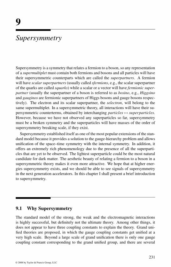
9Supersymmetry
Supersymmetry is a symmetry that relates a fermion to a boson, so any representation
of a supermultiplet must contain both fermions and bosons and all particles will have
their supersymmetric counterparts which are called the superpartners. A fermion
will have scalar superpartners (usually called sfermions, e.g., the scalar superpartner
of the quarks are called squarks) while a scalar or a vector will have fermionic super-partner (usually the superpartner of a boson is referred to as bosino, e.g., Higgsinoand gauginos are fermionic superpartners of Higgs bosons and gauge bosons respec-
tively). The electron and its scalar superpartner, the selectron, will belong to the
same supermultiplet. In a supersymmetric theory, all interactions will have their su-
persymmetric counterterms, obtained by interchanging particles ↔ superparticles.
However, because we have not observed any superparticles so far, supersymmetry
must be a broken symmetry and the superparticles will have masses of the order of
supersymmetry breaking scale, if they exist.
Supersymmetry established itself as one of the most popular extensions of the stan-
dard model because it provides a solution to the gauge-hierarchy problem and allows
unification of the space–time symmetry with the internal symmetry. In addition, it
offers an extremely rich phenomenology due to the presence of all the superparti-
cles that are yet to be observed. The lightest superparticle could be the most natural
candidate for dark matter. The aesthetic beauty of relating a fermion to a boson in a
supersymmetric theory makes it even more attractive. We hope that at higher ener-
gies supersymmetry exists, and we should be able to see signals of supersymmetry
in the next generation accelerators. In this chapter I shall present a brief introduction
to supersymmetry.
9.1 Why Supersymmetry
The standard model of the strong, the weak and the electromagnetic interactions
is highly successful, but definitely not the ultimate theory. Among other things, it
does not appear to have three coupling constants to explain the theory. Grand uni-
fied theories are proposed, in which the gauge coupling constants get unified at a
very high scale. Beyond a large scale of grand unification there is only one gauge
coupling constant corresponding to the grand unified group, and there are several
231
© 2008 by Taylor & Francis Group, LLC
232 Particle and Astroparticle Physics
interesting predictions of these theories that make them highly attractive. However,
the grand unified theories suffer from a serious gauge hierarchy problem. The scale
of grand unification is about 14 orders of magnitude higher than the electroweak
symmetry breaking scale. The interactions of the Higgs scalars that break the grand
unified group at the grand unification scale will interact with the electroweak sym-
metry breaking scalars and will introduce quadratic divergent corrections to the light
particles. To keep the electroweak symmetry breaking scale low, counterterms have
to be introduced that can cancel these divergent corrections to 14 decimal points.
Fine tuning of parameters to all orders is unnatural technically and this is the gauge
hierarchy problem.
Consider an SU(5) grand unified theory, where the SU(5) symmetry is broken by
a 24-plet Higgs field Σ and the electroweak symmetry is broken by a 5-plet Higgs
field φ . The scalar potential can be written as
V = V [Σ]+V [φ ]+V [Σ,φ ], (9.1)
where the first two terms contain the usual quadratic and quartic terms
V [Σ] = −1
2m2
ΣTr Σ2 +1
4a(Tr Σ2)2 +
1
2bTr Σ4
V [φ ] = −1
2m2
φ φ †φ +1
4λ (φ †φ)2. (9.2)
In addition there are the dangerous cross terms
V [Σ,φ ] = αφ †φ Tr Σ2 +βφ †Σ2φ . (9.3)
If we now write the Higgs scalar fields around their vevs, 〈Σ〉 = v0 and 〈φ〉 = v,
the cross terms will contribute to the masses of φ of the order of v0. If we introduce
counterterms to eliminate these cross terms, they will again be generated at all orders
of perturbation through loop diagrams. So, we need to introduce counterterms at all
orders.
Let us take the complete potential and get the condition for the minimum by sub-
stituting the vevs of the scalar fields
m2Σ =
1
2(15a+7b)v2
0 +(α +3
10β )v2 (9.4)
m2φ =
1
2λv2 +(15α +
9
2β )v2
0. (9.5)
The vev of the 5-plet Higgs scalar v will receive contributions proportional to the
vev of the 24-plet Higgs scalar v0. So, to prevent such large corrections we have to
fine tune parameters to all orders of perturbation with increasing precision, which
is technically unnatural. Any theory with two widely different mass scales, origi-
nating from the vevs of some scalar fields, always requires unnatural fine tuning of
parameters at all orders of perturbation theory. This is known as the gauge hierarchyproblem and is present in all grand unified theories.
© 2008 by Taylor & Francis Group, LLC
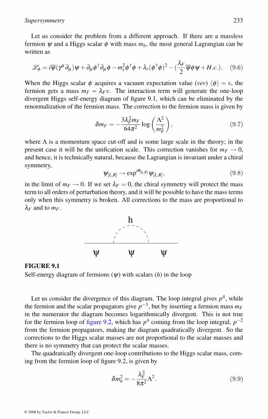
Supersymmetry 233
Let us consider the problem from a different approach. If there are a massless
fermion ψ and a Higgs scalar φ with mass mh, the most general Lagrangian can be
written as
Lφ = iψ(γµ ∂µ)ψ +∂µ φ †∂µ φ −m2s φ †φ +λs(φ †φ)2 − (
λF
2ψφψ +H.c.). (9.6)
When the Higgs scalar φ acquires a vacuum expectation value (vev) 〈φ〉 = v, the
fermion gets a mass mF = λF v. The interaction term will generate the one-loop
divergent Higgs self-energy diagram of figure 9.1, which can be eliminated by the
renormalization of the fermion mass. The correction to the fermion mass is given by
δmF = −3λ 2F mF
64π2 log
(Λ2
m2F
), (9.7)
where Λ is a momentum space cut-off and is some large scale in the theory; in the
present case it will be the unification scale. This correction vanishes for mF → 0,
and hence, it is technically natural, because the Lagrangian is invariant under a chiral
symmetry,
ψ[L,R] → expiθ[L,R]ψ[L,R], (9.8)
in the limit of mF → 0. If we set λF = 0, the chiral symmetry will protect the mass
term to all orders of perturbation theory, and it will be possible to have the mass terms
only when this symmetry is broken. All corrections to the mass are proportional to
λF and to mF .
h
ψ ψ ψFIGURE 9.1Self-energy diagram of fermions (ψ) with scalars (h) in the loop
Let us consider the divergence of this diagram. The loop integral gives p4, while
the fermion and the scalar propagators give p−3, but by inserting a fermion mass mFin the numerator the diagram becomes logarithmically divergent. This is not true
for the fermion loop of figure 9.2, which has p4 coming from the loop integral, p−2
from the fermion propagators, making the diagram quadratically divergent. So the
corrections to the Higgs scalar masses are not proportional to the scalar masses and
there is no symmetry that can protect the scalar masses.
The quadratically divergent one-loop contributions to the Higgs scalar mass, com-
ing from the fermion loop of figure 9.2, is given by
δm2h = − λ 2
F8π2 Λ2. (9.9)
© 2008 by Taylor & Francis Group, LLC
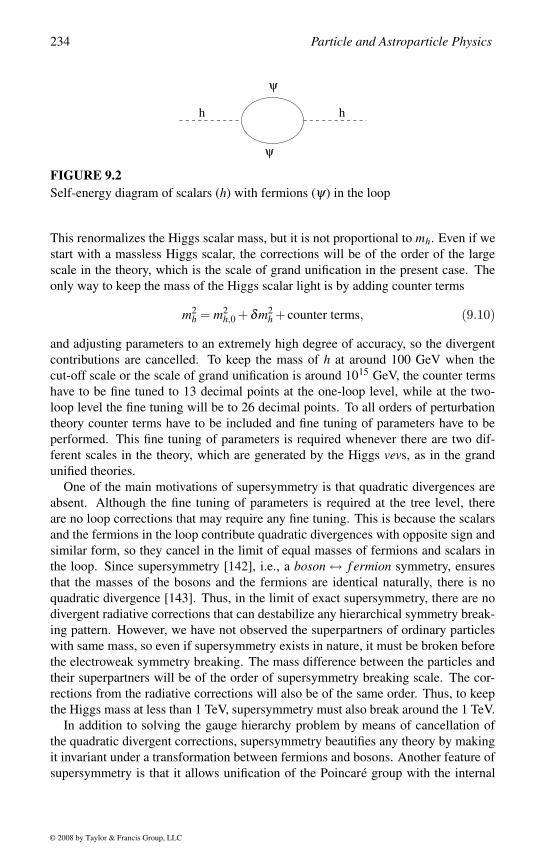
234 Particle and Astroparticle Physics
ψ
ψ
h h
FIGURE 9.2Self-energy diagram of scalars (h) with fermions (ψ) in the loop
This renormalizes the Higgs scalar mass, but it is not proportional to mh. Even if we
start with a massless Higgs scalar, the corrections will be of the order of the large
scale in the theory, which is the scale of grand unification in the present case. The
only way to keep the mass of the Higgs scalar light is by adding counter terms
m2h = m2
h,0 +δm2h + counter terms, (9.10)
and adjusting parameters to an extremely high degree of accuracy, so the divergent
contributions are cancelled. To keep the mass of h at around 100 GeV when the
cut-off scale or the scale of grand unification is around 1015 GeV, the counter terms
have to be fine tuned to 13 decimal points at the one-loop level, while at the two-
loop level the fine tuning will be to 26 decimal points. To all orders of perturbation
theory counter terms have to be included and fine tuning of parameters have to be
performed. This fine tuning of parameters is required whenever there are two dif-
ferent scales in the theory, which are generated by the Higgs vevs, as in the grand
unified theories.
One of the main motivations of supersymmetry is that quadratic divergences are
absent. Although the fine tuning of parameters is required at the tree level, there
are no loop corrections that may require any fine tuning. This is because the scalars
and the fermions in the loop contribute quadratic divergences with opposite sign and
similar form, so they cancel in the limit of equal masses of fermions and scalars in
the loop. Since supersymmetry [142], i.e., a boson ↔ f ermion symmetry, ensures
that the masses of the bosons and the fermions are identical naturally, there is no
quadratic divergence [143]. Thus, in the limit of exact supersymmetry, there are no
divergent radiative corrections that can destabilize any hierarchical symmetry break-
ing pattern. However, we have not observed the superpartners of ordinary particles
with same mass, so even if supersymmetry exists in nature, it must be broken before
the electroweak symmetry breaking. The mass difference between the particles and
their superpartners will be of the order of supersymmetry breaking scale. The cor-
rections from the radiative corrections will also be of the same order. Thus, to keep
the Higgs mass at less than 1 TeV, supersymmetry must also break around the 1 TeV.
In addition to solving the gauge hierarchy problem by means of cancellation of
the quadratic divergent corrections, supersymmetry beautifies any theory by making
it invariant under a transformation between fermions and bosons. Another feature of
supersymmetry is that it allows unification of the Poincare group with the internal
© 2008 by Taylor & Francis Group, LLC
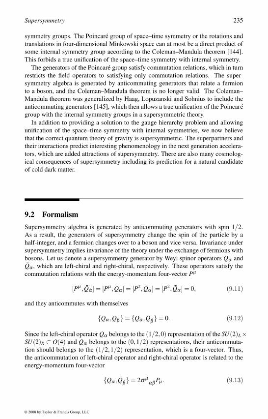
Supersymmetry 235
symmetry groups. The Poincare group of space–time symmetry or the rotations and
translations in four-dimensional Minkowski space can at most be a direct product of
some internal symmetry group according to the Coleman–Mandula theorem [144].
This forbids a true unification of the space–time symmetry with internal symmetry.
The generators of the Poincare group satisfy commutation relations, which in turn
restricts the field operators to satisfying only commutation relations. The super-
symmetry algebra is generated by anticommuting generators that relate a fermion
to a boson, and the Coleman–Mandula theorem is no longer valid. The Coleman–
Mandula theorem was generalized by Haag, Lopuzanski and Sohnius to include the
anticommuting generators [145], which then allows a true unification of the Poincare
group with the internal symmetry groups in a supersymmetric theory.
In addition to providing a solution to the gauge hierarchy problem and allowing
unification of the space–time symmetry with internal symmetries, we now believe
that the correct quantum theory of gravity is supersymmetric. The superpartners and
their interactions predict interesting phenomenology in the next generation accelera-
tors, which are added attractions of supersymmetry. There are also many cosmolog-
ical consequences of supersymmetry including its prediction for a natural candidate
of cold dark matter.
9.2 FormalismSupersymmetry algebra is generated by anticommuting generators with spin 1/2.
As a result, the generators of supersymmetry change the spin of the particle by a
half-integer, and a fermion changes over to a boson and vice versa. Invariance under
supersymmetry implies invariance of the theory under the exchange of fermions with
bosons. Let us denote a supersymmetry generator by Weyl spinor operators Qα and
Qα , which are left-chiral and right-chiral, respectively. These operators satisfy the
commutation relations with the energy-momentum four-vector Pµ
[Pµ , Qα ] = [Pµ ,Qα ] = [P2,Qα ] = [P2, Qα ] = 0, (9.11)
and they anticommutes with themselves
Qα ,Qβ = Qα , Qβ = 0. (9.12)
Since the left-chiral operator Qα belongs to the (1/2,0) representation of the SU(2)L×SU(2)R ⊂ O(4) and Qα belongs to the (0,1/2) representations, their anticommuta-
tion should belongs to the (1/2,1/2) representation, which is a four-vector. Thus,
the anticommutation of left-chiral operator and right-chiral operator is related to the
energy-momentum four-vector
Qα , Qβ = 2σ µαβ Pµ . (9.13)
© 2008 by Taylor & Francis Group, LLC
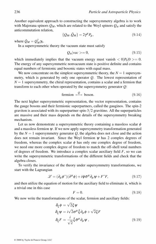
236 Particle and Astroparticle Physics
Another equivalent approach to constructing the supersymmetry algebra is to work
with Majorana spinors QM , which are related to the Weyl spinors Qα and satisfy the
anticommutation relation,
QM, QM = 2γµ Pµ , (9.14)
where QM = Q†Mγ0.
In a supersymmetric theory the vacuum state must satisfy
Qα |vac >= 0, (9.15)
which immediately implies that the vacuum energy must vanish < 0|P0|0 >= 0.
The energy of any supersymmetric nonvacuum state is positive definite and contains
equal numbers of fermionic and bosonic states with equal mass.
We now concentrate on the simplest supersymmetric theory, the N = 1 supersym-
metry, which is generated by only one operator Q. The lowest representation of
N = 1 supersymmetry, the chiral representation, contains a scalar and a fermion that
transform to each other when operated by the supersymmetry generator Q:
fermionQ←→ boson. (9.16)
The next higher supersymmetric representation, the vector representation, contains
the gauge bosons and their fermionic superpartners, called the gauginos. The spin-2
graviton is associated with its superpartner spin-3/2 gravitino. All the superparticles
are massive and their mass depends on the details of the supersymmetry breaking
mechanism.
Let us now demonstrate a supersymmetric theory containing a massless scalar φand a massless fermion ψ . If we now apply supersymmetry transformation generated
by the N = 1 supersymmetry generator Q, the algebra does not close and the action
does not remain invariant. Since the Weyl fermion ψ has 2 complex degrees of
freedom, whereas the complex scalar φ has only one complex degree of freedom,
we need one more complex degree of freedom to match the off-shell total numbers
of degrees of freedom. We introduce a complex scalar auxiliary field F , so we can
write the supersymmetric transformations of the different fields and check that the
algebra closes.
To verify the invariance of the theory under supersymmetry transformations, we
start with the Lagrangian
L = (∂µ φ ∗)(∂ µ φ)+ iψσ µ ∂µ ψ +F∗F, (9.17)
and then utilize the equation of motion for the auxiliary field to eliminate it, which is
a trivial one in this case
F = 0. (9.18)
We now write the transformations of the scalar, fermion and auxiliary fields:
δξ φ =√
2ξ ψ
δξ ψ = i√
2σ µ ξ ∂µ φ +√
2ξ F
δξ F =i√2
ξ σ µ ∂µ ψ , (9.19)
© 2008 by Taylor & Francis Group, LLC
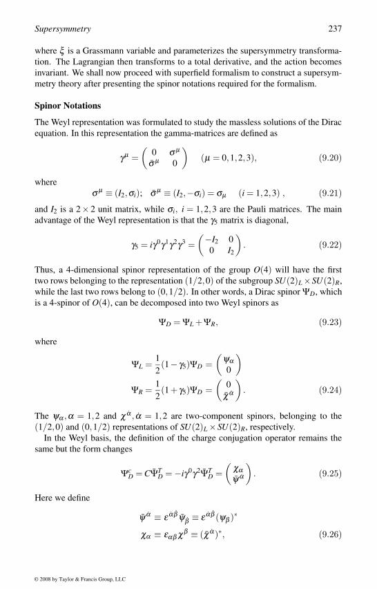
Supersymmetry 237
where ξ is a Grassmann variable and parameterizes the supersymmetry transforma-
tion. The Lagrangian then transforms to a total derivative, and the action becomes
invariant. We shall now proceed with superfield formalism to construct a supersym-
metry theory after presenting the spinor notations required for the formalism.
Spinor Notations
The Weyl representation was formulated to study the massless solutions of the Dirac
equation. In this representation the gamma-matrices are defined as
γµ =(
0 σ µ
σ µ 0
)(µ = 0,1,2,3), (9.20)
where
σ µ ≡ (I2,σi); σ µ ≡ (I2,−σi) = σµ (i = 1,2,3) , (9.21)
and I2 is a 2× 2 unit matrix, while σi, i = 1,2,3 are the Pauli matrices. The main
advantage of the Weyl representation is that the γ5 matrix is diagonal,
γ5 = iγ0γ1γ2γ3 =(−I2 0
0 I2
). (9.22)
Thus, a 4-dimensional spinor representation of the group O(4) will have the first
two rows belonging to the representation (1/2,0) of the subgroup SU(2)L×SU(2)R,
while the last two rows belong to (0,1/2). In other words, a Dirac spinor ΨD, which
is a 4-spinor of O(4), can be decomposed into two Weyl spinors as
ΨD = ΨL +ΨR, (9.23)
where
ΨL =1
2(1− γ5)ΨD =
(ψα0
)ΨR =
1
2(1+ γ5)ΨD =
(0
χ α
). (9.24)
The ψα ,α = 1,2 and χ α , α = 1,2 are two-component spinors, belonging to the
(1/2,0) and (0,1/2) representations of SU(2)L ×SU(2)R, respectively.
In the Weyl basis, the definition of the charge conjugation operator remains the
same but the form changes
ΨcD = CΨT
D = −iγ0γ2ΨTD =
(χαψ α
). (9.25)
Here we define
ψ α ≡ ε αβ ψβ ≡ ε αβ (ψβ )∗
χα ≡ εαβ χβ ≡ (χ α)∗, (9.26)
© 2008 by Taylor & Francis Group, LLC
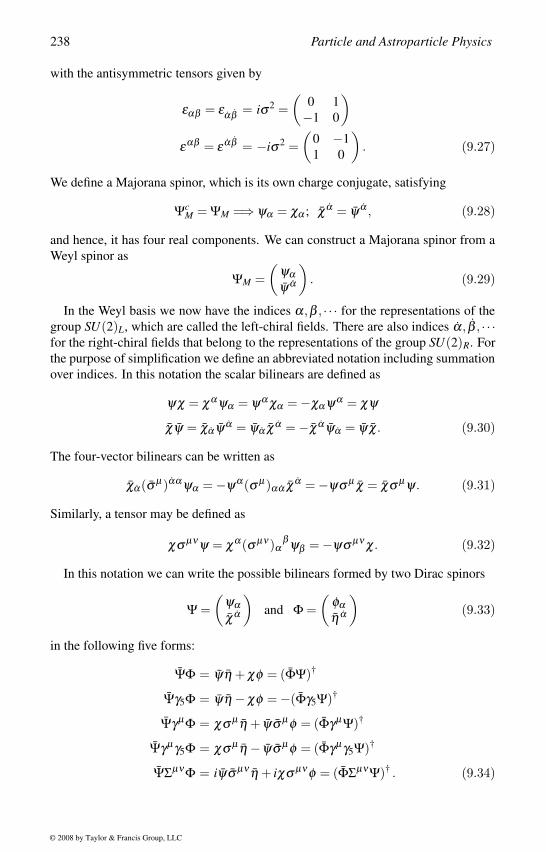
238 Particle and Astroparticle Physics
with the antisymmetric tensors given by
εαβ = εαβ = iσ 2 =(
0 1
−1 0
)εαβ = ε αβ = −iσ 2 =
(0 −1
1 0
). (9.27)
We define a Majorana spinor, which is its own charge conjugate, satisfying
ΨcM = ΨM =⇒ ψα = χα ; χ α = ψ α , (9.28)
and hence, it has four real components. We can construct a Majorana spinor from a
Weyl spinor as
ΨM =(
ψαψ α
). (9.29)
In the Weyl basis we now have the indices α,β , · · · for the representations of the
group SU(2)L, which are called the left-chiral fields. There are also indices α, β , · · ·for the right-chiral fields that belong to the representations of the group SU(2)R. For
the purpose of simplification we define an abbreviated notation including summation
over indices. In this notation the scalar bilinears are defined as
ψχ = χα ψα = ψα χα = −χα ψα = χψ
χψ = χα ψ α = ψα χ α = −χ α ψα = ψ χ. (9.30)
The four-vector bilinears can be written as
χα(σ µ)αα ψα = −ψα(σ µ)αα χ α = −ψσ µ χ = χσ µ ψ. (9.31)
Similarly, a tensor may be defined as
χσ µν ψ = χα(σ µν)αβ ψβ = −ψσ µν χ. (9.32)
In this notation we can write the possible bilinears formed by two Dirac spinors
Ψ =(
ψαχ α
)and Φ =
(φαη α
)(9.33)
in the following five forms:
ΨΦ = ψη + χφ = (ΦΨ)†
Ψγ5Φ = ψη −χφ = −(Φγ5Ψ)†
Ψγµ Φ = χσ µ η + ψσ µ φ = (Φγµ Ψ)†
Ψγµ γ5Φ = χσ µ η − ψσ µ φ = (Φγµ γ5Ψ)†
ΨΣµν Φ = iψσ µν η + iχσ µν φ = (ΦΣµν Ψ)† . (9.34)
© 2008 by Taylor & Francis Group, LLC
Supersymmetry 239
The five forms are the scalar, pseudo-scalar, vector, axial-vector and tensor.
Starting with the two Majorana spinors
ΨM =(
ψαψ α
)and ΦM =
(φαφ α
), (9.35)
we write the five bilinears:
ΨMΦM = ψφ +ψφ = ΦMΨM = (ΨMΦM)†
ΨMγ5ΦM = ψφ −ψφ = ΦMγ5ΨM = −(ΨMγ5ΦM)†
ΨMγµ ΦM = ψσ µ φ + ψσ µ φ = −ΦMγµ ΨM = −(ΨMγµ ΦM)†
ΨMγµ γ5ΦM = ψσ µ φ − ψσ µ φ = ΦMγµ γ5ΨM = (ΨMγµ γ5ΦM)†
ΨMΣµν ΦM = iψσ µν φ + iψσ µν φ = −ΦMΣµν ΨM
= −(ΨMΣµν ΦM)†. (9.36)
With this brief introduction we shall now proceed to construct superspace forlamisn.
Superspace Formalism
It is highly convenient to develop superspace formalism, in order to construct a super-
symmetric theory. The first ingredient for this purpose is the introduction of Grass-
mann parameters. In the Weyl representation two independent constant anticommut-
ing Grassmann numbers θα (α = 1,2) and θα , (α = 1, 2) belong to the (1/2,0)and (0,1/2) representations of the group SU(2)L × SU(2)R ⊂ O(4). In the Majo-
rana representation we need to introduce the anticommuting Grassmann numbers
εa (a = 1,2,3,4), where ε satisfies the Majorana condition. We shall now continue
with the Weyl representation.
The anticommutation relations of the Grassmann numbers are given by
θα ,θβ = θα , θβ = θα ,θβ = 0 . (9.37)
The only possible bilinears that can be formed with these Grassmann variables are
θθ = θα θ α = θα θβ εαβ
θ θ = θα θ α = θα θβ εαβ
θσ µ θ = −θσ µ θ = θα(σ µ)αβ θβ = −θ α(σ µ)αβ θ β . (9.38)
There are no cubic or higher products of θ or θ ,
θθθ = θθθθ = · · · = θ θ θ = θ θ θ θ = · · · = 0.
The only cubic and quadratic terms possible are
(θθ)θα , (θ θ)θα and (θθ)(θ θ).
© 2008 by Taylor & Francis Group, LLC
240 Particle and Astroparticle Physics
We complete this discussion by defining the derivatives with respect to the Grass-
mann variables, where ∂/∂θ α satisfies
∂∂θ α θ β = δα
β ;∂
∂θαθβ = δ α
β ;∂
∂θ β θα = εαβ . (9.39)
The derivative ∂/∂ θα satisfies analogous formulas.
A superspace is constructed with the variables (xµ ,θ , θ), so a superfield can be
defined as S(xµ ,θ , θ). The action of the generators,
Pµ = i∂µ
iQα =∂
∂θ α − iσ µαα θ α ∂µ
iQα = − ∂∂ θ α + iθ α σ µ
αα ∂µ , (9.40)
then gives the supersymmetry algebra.
We would now like to classify the different superfields and find the irreducible
representations of the superalgebra. We start with defining the fermionic derivatives
or the covariant derivatives for superfields
Dα =∂
∂θ α + iσ µαα θ α ∂µ
Dα = − ∂∂ θ α − iθ α σ µ
αα ∂µ , (9.41)
which satisfy the anticommutation relations
Dα ,Dβ = Dα , Dβ = 0 and Dα , Dα = 2iσ µαα ∂µ . (9.42)
The fermioninc derivatives also anticommute with the generators of the supersym-
metry algebra
Dα ,Qβ = Dα ,Qβ = Dα , Qβ = Dα , Qβ = 0. (9.43)
Thus, these covariant derivatives are invariant under supersymmetry transformations.
The covariant derivatives can project out superfields into two chiral representa-
tions. We define the left-chiral superfields satisfying
Dα Φ = 0 (9.44)
and the right-chiral superfields satisfying
Dα Φ = 0. (9.45)
This becomes transparent when we make the transformations of the variable
yµ = xµ + iθσ µ θ , (9.46)
© 2008 by Taylor & Francis Group, LLC
Supersymmetry 241
which satisfies
Dα yµ = 0. (9.47)
It terms of the new coordinates, any superfields satisfying the condition for left-
chiral superfield of equation (9.44) will have explicit dependence only in θ , while
the superfields satisfying equation (9.45) can be expressed only in terms of θ .
We can expand any left-chiral superfield satisfying equation 9.44 in powers of θand yµ as
Φ(yµ ,θ) = φ(y)+√
2θψ(y)+θθF(y) , (9.48)
while we can expand a right-chiral superfield that satisfies equation 9.45 in powers
of θ and yµ as
Φ†(yµ , θ) = φ(y)+√
2θψ(y)+ θ θF(y). (9.49)
The right-chiral superfields are called the conjugate superfields. The left-handed
particles and antiparticles belong to the left-chiral superfields, while the right-handed
particles and antiparticles belong to the right-chiral superfields.
The supersymmetric transformations of the component fields φ , ψ and F , given in
equation (9.19), can be retrieved by defining the infinitesimal supersymmetry trans-
formation of the superfield Φ as
Φ → Φ+δΦ = Φ+ i(ξ Q+ ξ Q)Φ . (9.50)
In terms of the superfields we can write the Lagrangian that is invariant under the
supersymmetry transformation as
Lsusy = ∑i[Φ†
i Φi]D +([W (Φ)]F +H.c.) . (9.51)
The second term is called the F-term and contains only left-chiral superfields. The
superpotential W (Φ) can be written in terms of 1,θ and θθ . Only the coefficient of
θθ transforms into total derivative under a supersymmetry transformation and this
coefficient is invariant under supersymmetry. This coefficient of θθ in the superpo-
tential W (Φ) is denoted as the F-term, [W (Φ)]F . The F-term in expansion of the
left-chiral superfields contains only the left-handed particles and antiparticles. The
right-handed particles and antiparticles are included in the Hermitian conjugate term,
which is the coefficient of θ θ in the superpotential W (Φ†) with the right-chiral su-
perfields. The first term contains products of left-chiral and right-chiral superfields,
so it contains all powers of θ and θ . The D-term, which is the coefficient of θθ θ θ ,
is invariant under supersymmetry transformation. All the kinetic energy terms are
included in the D-term.
We now demonstrate with an example with superfields Φi. We write the most
general superpotential
W (Φ) =1
2mi jΦiΦ j +
1
3λi jkΦiΦ jΦk. (9.52)
© 2008 by Taylor & Francis Group, LLC
242 Particle and Astroparticle Physics
Taking the D-term of ∑i Φ†i Φi and the F-term of the superpotential we can write the
Lagrangian as
L = ∂µ φ †i ∂ µ φi + iψiσ µ ∂µ ψi +F†
i Fi
+mi jφiFj − 1
2mi jψiψ j
+λi jkφiφ jFk −λi jkψiψ jφk +H.c. (9.53)
The first line comes from the D-terms and the rest from F-terms. We use the equa-
tions of motion for the auxiliary fields Fi:
F†i = − ∂W (φ)
∂φi
∣∣∣∣F
= −mi jφ j −λi jkφ jφk (9.54)
and eliminate them to write the Lagrangian in terms of physical fields as
L = LKE +LYuk +V (φi) , (9.55)
where the kinetic energy, Yukawa interactions including the fermion mass terms, and
the scalar potential are given by
LKE = ∂µ φ †i ∂ µ φi + iψiσ µ ∂µ ψi
LYuk = −1
2mi jψiψ j −λi jkψiψ jφk +H.c..
V (φi) = F†i Fi =
∣∣∣∣−[∂W (φ)∂φi
]F
∣∣∣∣2 =∣∣−mi jφ j −λi jkφ jφk
∣∣2 . (9.56)
The right-handed fermions and their antiparticles are included in the Hermitian con-
jugate term. The equality of the fermion and scalar masses is manifest in the con-
struction and vanishing of the quadratically divergent radiative corrections is guar-
anteed.
Any internal symmetry breaking can be implemented in supersymmetric theories
by giving vacuum expectation values to the scalar partners of any superfield. How-
ever, as long as the F-terms and D-terms do not acquire any vevs, supersymmetry
remains unbroken. Consider one example of internal symmetry breaking without
breaking supersymmetry. Let us start with two superfields X and Y , whose interac-
tions are represented by the superpotential
W (X ,Y ) = f X(Y 2 −M2) , (9.57)
where f and M are two parameters in the theory with mass dimensions 0 and 1,
respectively. In general, it is possible to start with a superpotential of the form we
require in a supersymmetric theory, because there are no radiative corrections that
can generate any new terms. We may need to fine tune some parameters at the tree
level, but since there are no higher order corrections, we do not require any further
fine tuning.
© 2008 by Taylor & Francis Group, LLC

Supersymmetry 243
The F-terms corresponding to this superpotential are
FX =[
∂W∂φX
]F
= f (φ 2Y −M2) and FY = 2 f φX φY ,
which vanish at the minima preserving supersymmetry when the vevs of the scalar
components of X and Y are given by
〈φX 〉 = 0 〈φY 〉 = M. (9.58)
The nonvanishing of the vev of Y can now break any internal symmetry at the scale
M if Y transforms nontrivially under the internal group.
9.3 Gauge TheoryWe shall now develop supersymmetric theories with local internal symmetries. Since
our ultimate goal is to construct supersymmetric standard model at energies above
the electroweak symmetry breaking scale, we shall discuss both Abelian as well as
non-Abelian gauge theories.
Abelian Gauge Theory
So far we have been working with chiral superfields, which include a scalar and a
fermion. Introduction of local symmetries would require covariant derivatives in-
cluding the vector fields, which should replace the ordinary derivatives in the kinetic
energy term. We should introduce vector superfields, which should be linked with
the D-term and depend on both θ and θ . A vector superfield V ≡ V (x,θ , θ) can be
written as
V = C(x)+ iθ χ(x)− iθ χ(x)+i2[θθG(x)− θ θG∗(x)]
+θσ µ θVµ(x)+ iθθ θ [λ (x)+i2
σ µ ∂µ χ(x)]
−iθ θθ [λ (x)+i2
σ µ ∂µ χ(x)]
+1
2θθθ θ [D(x)− 1
2∂µ ∂ µC(x)], (9.59)
where Vµ is the vector field; G = M + iN and C,M,N,D are real scalar fields and
χ,λ are Weyl spinors.
To construct an Abelian gauge theory, we start with two complex chiral superfields
X± with the U(1) charges ±1, which transform under the U(1) gauge symmetry as
X± → X ′± = exp∓[2iqΛ(x)]X±. (9.60)
© 2008 by Taylor & Francis Group, LLC
244 Particle and Astroparticle Physics
We introduce a vector superfield V (x,θ , θ), which transforms under the U(1) gauge
symmetry as
V →V ′ = V + i(Λ−Λ†). (9.61)
In order to write the gauge kinetic energy term we define a supersymmetric field
strength, which is a chiral superfield, constructed from this vector superfield as
Wα = D2DαV , (9.62)
so
DαWα = 0. (9.63)
This chiral superfield can be expanded as
Wα(y,θ) = 4iλα(y)+4D(y)θα +2i(σ µν θ)α Fµν(y)+4θθ(σ µ ∂µ λ )α , (9.64)
where λ is the gaugino and Fµν is the field strength tensor. The gaugino can be
expressed as a four-component Majorana spinor:
ΛM =(
λαλ α
). (9.65)
We can then write the gauge-invariant Lagrangian in terms of the superfields as
L =1
32[W αWα ]F +[X†
+exp2qV X+ +X†−exp−2qV X−]D
+m[X+X−]F +H.c. (9.66)
The first term contains the kinetic energy for the gauge boson and the gaugino, the
second term gives the interaction of the gauge superfields with the fermions, and the
scalar potential is given in the second line. Only a mass term is allowed by the gauge
symmetry for the chiral superfields X±, which combine the two Majorana spinors to
form a Dirac spinor
Ψ =(
ψX+αψ α
X−
). (9.67)
The physical fields in this theory includes the Dirac spinor Ψ, the corresponding
scalars φX+ and φX− , the vector boson Vµ , and the gaugino ΛM . Eliminating the
auxiliary fields, the Lagrangian becomes
L = iΨγµ Dµ Ψ−mΨΨ
+(Dµ φX+)†(Dµ φX+)+(Dµ φX†−)†(Dµ φX†
−)
−m2(φ †X+
φX+ +φ †X−φX−)− q2
2(φ †
X+φX+ −φ †
X−φX−)2
+q√2[ΛMΨ(φ †
X++φX−)− ΛMiγ5Ψ(φ †
X+−φX−)
−ΨΛM(φX+ +φ †X−)− Ψiγ5ΛM(φX+ −φ †
X−)]
−1
4VµνV µν +
i2
ΛMγµ ∂µ ΛM . (9.68)
© 2008 by Taylor & Francis Group, LLC

Supersymmetry 245
The covariant derivative is given by
Dµ = ∂ µ + iqV µ . (9.69)
The interactions in this theory are similar to the nonsupersymmetric case, except the
new interactions involving the superparticles. These new interactions can be obtained
simply by replacing any two of the particles at any vertex by their corresponding
superpartners.
Non-Abelian Gauge Theory
We generalize the supersymmetric gauge theory to include non-Abelian gauge group.
Any chiral superfield Φ transforms as
Φ → Φ′ = exp−2igT aΛaΦ, (9.70)
where T a,a = 1...N are the N generators of the non-Abelian gauge group. Gauge
invariance would now require N vector superfields V a and corresponding N Majorana
gauginos. The gauge bosons will interact with two fermions or two scalars, but the
gauginos can interact with only a fermion and a scalar.
Corresponding to any fermions or any scalars in a nonsupersymmetric theory, we
now have to include chiral superfields Φi. The superpotential will be a function of all
of these fields. Depending on the transformations of the fields under the non-Abelian
gauge group and any other discrete symmetries in the theory, the superpotential will
be determined. The superpotential will contain all of the left-chiral superfields, while
its Hermitian conjugate will contain all of the right-chiral superfields. The Yukawa
couplings and the scalar potential will then be contained in
Lint = [W (Φi)+H.c.]F . (9.71)
The scalar potential is obtained by eliminating the auxiliary fields. The superpo-
tential contains terms of mass-dimension 3 only. The F-term implies an integration∫d2θ or
∫d2θ , which adds one mass-dimension. However, the scalar quartic inter-
actions can enter in the scalar potential.
The spinor field strength superfield can now be defined as
W aα = D2DαV a + ig f abcD2(DαV b)V c
= 4iλ aα +[4δ β
α Da(y)+2i(σ µ σν)αβV a
µν(y)]θβ
+4θ 2σ µααDµ λ aα(y). (9.72)
The field-strength tensor corresponding to the gauge bosons is given by
V aµν = ∂µV a
ν −∂νV aµ − ig f abcV b
µV cν , (9.73)
where f abc is the structure function of the group, which defines the commutation
relations of the generators [T a,T b] = i f abcT c. The covariant derivative can then be
defined as
Dµ λ aα = ∂µ λ aα −g f abcV bµ λ cα . (9.74)
© 2008 by Taylor & Francis Group, LLC
246 Particle and Astroparticle Physics
The gauge invariant supersymmetric Lagrangian will now contain the kinetic energy
terms of the vector superfields
LV =1
64
[(W aαW a
α )+(W aα
†)(W aα †)]
F
= −1
4V a
µνV aµν + iλ aσ µDµ λ a +1
2DaDa (9.75)
and the D-term containing the interactions of the chiral superfields with the gauge
superfields
LD = [Φ†exp2gT aV aµ Φ]D
= (Dµ φ)†(Dµ φ)+ iψσ µD†µ ψ +F†F
+i√
2g(φ †T aλ aψ − ψT aλ aφ)+gφ †T aDaφ . (9.76)
The gauge covariant derivative is given by
Dµ = ∂µ + igT aV aµ . (9.77)
Finally we eliminate the auxiliary fields by using their equations of motion, given by
F†i = −∂W
∂φiand Da = −∑
igφ †
i T ai φi, (9.78)
where T ai is the generator of the representations of φi of the group. The effective
scalar potential now becomes
V (φi) = ∑i
∣∣∣∣∂W∂φi
∣∣∣∣2 +1
2g2 ∑
a
(∑
iφ †
i T ai φi
)2
. (9.79)
There is an additional contribution coming from the D-term in this case.
It is possible to break the gauge symmetry without breaking supersymmetry in the
same way we discussed earlier. Consider the superpotential
W (X ,Y ) = f X(Y 2 −M2), (9.80)
where X is a singlet under the gauge group but Y transforms nontrivially. The min-
imization of this superpotential will lead to vanishing of the F-terms preserving su-
persymmetry with nonvanishing vev of Y , which will break the group. This will
provide mass to the gauge bosons. Since supersymmetry is unbroken, the gaugi-
nos will also get mass equal to the mass of the gauge bosons. After supersymmetry
breaking the masses of the gauge bosons and the gauginos will differ and the mass
difference will be determined by the supersymmetry breaking mechanism and the
scale.
There are now chiral superfields corresponding to the fermions as well as to the
scalars. To distinguish the fermions from scalars, in some cases a discrete matter
parity is imposed to distinguish the two types of chiral superfields. A schematic
chart of the superfields corresponding to the ordinary particles of the standard model
is depicted in figure 9.3.
© 2008 by Taylor & Francis Group, LLC
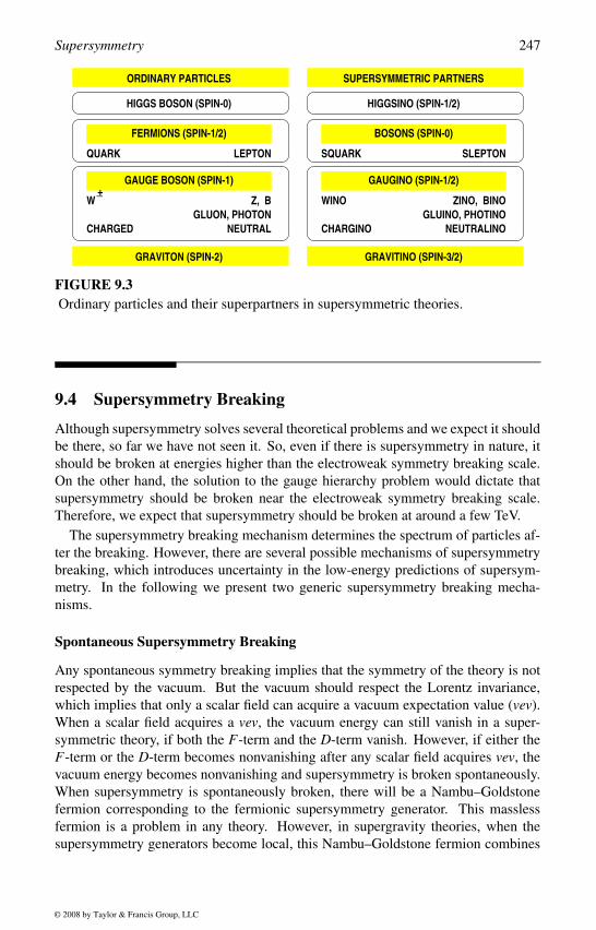
Supersymmetry 247
BOSONS (SPIN-0)
LEPTON SQUARK SLEPTON
GAUGE BOSON (SPIN-1) GAUGINO (SPIN-1/2)
GLUINO, PHOTINOW
NEUTRALCHARGED CHARGINO NEUTRALINO
GRAVITON (SPIN-2) GRAVITINO (SPIN-3/2)
FERMIONS (SPIN-1/2)
QUARK
WINOZ, B ZINO, BINO
HIGGSINO (SPIN-1/2)HIGGS BOSON (SPIN-0)
ORDINARY PARTICLES SUPERSYMMETRIC PARTNERS
GLUON, PHOTON
+_
FIGURE 9.3Ordinary particles and their superpartners in supersymmetric theories.
9.4 Supersymmetry Breaking
Although supersymmetry solves several theoretical problems and we expect it should
be there, so far we have not seen it. So, even if there is supersymmetry in nature, it
should be broken at energies higher than the electroweak symmetry breaking scale.
On the other hand, the solution to the gauge hierarchy problem would dictate that
supersymmetry should be broken near the electroweak symmetry breaking scale.
Therefore, we expect that supersymmetry should be broken at around a few TeV.
The supersymmetry breaking mechanism determines the spectrum of particles af-
ter the breaking. However, there are several possible mechanisms of supersymmetry
breaking, which introduces uncertainty in the low-energy predictions of supersym-
metry. In the following we present two generic supersymmetry breaking mecha-
nisms.
Spontaneous Supersymmetry Breaking
Any spontaneous symmetry breaking implies that the symmetry of the theory is not
respected by the vacuum. But the vacuum should respect the Lorentz invariance,
which implies that only a scalar field can acquire a vacuum expectation value (vev).
When a scalar field acquires a vev, the vacuum energy can still vanish in a super-
symmetric theory, if both the F-term and the D-term vanish. However, if either the
F-term or the D-term becomes nonvanishing after any scalar field acquires vev, the
vacuum energy becomes nonvanishing and supersymmetry is broken spontaneously.
When supersymmetry is spontaneously broken, there will be a Nambu–Goldstone
fermion corresponding to the fermionic supersymmetry generator. This massless
fermion is a problem in any theory. However, in supergravity theories, when the
supersymmetry generators become local, this Nambu–Goldstone fermion combines
© 2008 by Taylor & Francis Group, LLC
248 Particle and Astroparticle Physics
with the gravitino and the gravitino becomes massive.
We shall present simple examples where the F-term and the D-term can become
nonvanishing after any scalar field acquires vev. We discussed spontaneous symme-
try breaking in supersymmetric theories, where some scalars can acquire vev, break-
ing the internal symmetry group but preserving supersymmetry. We now consider an
example, which will not allow any minima that correspond to the vanishing of all the
F-terms, and supersymmetry will be spontaneously broken after the scalars acquire
vev. This is known as the O’Raifeartaigh mechanism [146]. Let us consider three
superfields A,B,C, which could even be singlets under any internal gauge symmetry.
If the superpotential is given by
W (A,B,C) = mAB+ fC(B2 −µ2), (9.81)
where f ,g are couplings and m and µ are some mass parameters, the F-terms are
given by
F†A =
∂W∂A
= mB
F†B =
∂W∂B
= mA+2 fCB
F†C =
∂W∂C
= f (B2 −µ2). (9.82)
It is clear that all the F-terms cannot be made to vanish simultaneously. Since the
scalar potential V = ∑i |Fi|2 vanishes only when all the F-terms vanish, the minimum
energy now corresponds to nonvanishing of the potential. Thus, supersymmetry is
broken spontaneously with this superpotential.
The minima of the potential correspond to a nonvanishing F-term, which is√
f µand determines the scale of supersymmetry breaking. The corresponding Nambu–
Goldstone fermion, ψC, remains massless and there is a mass splitting among the
bosonic and fermionic components of B. The mass splitting is of the order of super-
symmetry breaking scale.
To demonstrate the D-term supersymmetry breaking [147], consider a U(1) gauge
theory with chiral superfields Φi with charge e. Any term proportional to the vector
superfield (V ) may be added to the Lagrangian without breaking the gauge symmetry
or Lorentz invariance
L =1
32(W aWa)F +(Φ†exp2eV Φ)D +ξ (V )D, (9.83)
where ξ is a constant. The D-term is now given by
D = −(ξ + eφ †φ). (9.84)
When the two terms have opposite sign, i.e., ξ e < 0, the minimum of the potential
will correspond to 〈φ〉 = 0 but the D-term vanishes, whereas for ξ e > 0 the minimum
would correspond to < φ >= 0 and V = D2/2. In the latter case the gauge symmetry
© 2008 by Taylor & Francis Group, LLC
Supersymmetry 249
remains unbroken but breaks supersymmetry spontaneously, and the mass splitting
between particles and their superpartners becomes√
eξ .
Although both the F- and D-term spontaneous supersymmetry breaking looks at-
tractive and allows mass-splitting between the particles and their superpartners, it
is not possible to get a phenomenologically acceptable mass spectrum. One of the
two bosonic superpartners of any fermions always comes out to be lighter than the
fermions. Since we have not observed any superpartners of the known fermions in
nature, we need to make these bosonic superpartners heavier than the electroweak
symmetry breaking scale. Because of this, both the spontaneous supersymmetry
mechanisms have been abandoned in their simplest form. We now expect that the
supersymmetry breaking will come from some hidden sector and at low energy it
will appear as some kind of explicit symmetry breaking by soft terms.
Explicit Supersymmetry Breaking by Soft Terms
One solution to the problem of light bosonic superpartner is to introduce soft mass
terms for the superpartners, which breaks supersymmetry explicitly. Although in the
low-energy theory we introduce these explicit supersymmetry breaking soft terms,
we expect that these terms will originate from some definite supersymmetry breaking
mechanism at some high scale. In fact, in some simple N = 1 supergravity theory,
such soft supersymmetry breaking terms do emerge after the supersymmetry break-
ing in the hidden sector and are communicated to the observable sector through grav-
ity interactions. In any explicit symmetry breaking the main concern is the renormal-
izability of the original theory, which is protected if the explicit symmetry breaking
terms are all soft terms with mass dimension less than 4. If the symmetry breaking
terms have dimension 4 or more, then the higher order corrections will introduce
divergent terms which will destroy the symmetries of the original theory. However,
if the symmetry breaking terms are only the soft terms, the renormalizability of the
original theory will not be lost.
The mass terms for the scalars, the gauginos, and the bilinear and trilinear scalar
interactions could be the possible soft terms that break supersymmetry:
Lso f t = −1
2Ma
λ λ aλ a − 1
2(m2)i jφiφ ∗
j
−1
2(BM)i jφiφ j − 1
6(Ay)i jkφiφ jφk +H.c. (9.85)
The bilinear and the trilinear terms are referred to as A- and B-terms, respectively.
The mass parameters in the soft supersymmetry breaking terms could be of the order
of the supersymmetry breaking scale. Although the soft terms could introduce mass
terms for the gauginos, the mass terms for the gauge bosons are not allowed by
requirement of gauge invariance. We hope that a complete theory will also provide
an understanding of the origin of these soft terms. But for phenomenological studies
we shall include all possible soft terms allowed by the symmetries of the theory.
In the next chapter we shall make use of the supersymmetric formalism presented
so far and construct supersymmetric models. We shall first supersymmetrize the
© 2008 by Taylor & Francis Group, LLC
250 Particle and Astroparticle Physics
standard model and then add all possible supersymmetry breaking soft terms, which
becomes the so-called minimal supersymmetric standard model with the gauge group
SU(3)c × SU(2)L ×U(1)Y . Below the electroweak symmetry breaking, this theory
gives us the nonsupersymmetric standard model. We then consider possible super-
symmetry breaking mechanisms, which may restrict the allowed soft terms and re-
duce the numbers of parameters in the minimal supersymmetric standard model.
In these phenomenologically interesting models, supersymmetry breaking scale is
taken to be around a few TeV, so the electroweak symmetry breaking scalar mass is
protected. This will also allow these models to be tested in the next generation ac-
celerators. The lightest supersymmetric particle could also become the dark matter
candidate.
© 2008 by Taylor & Francis Group, LLC
10Supersymmetric Models
Supersymmetry provides a solution to the gauge hierarchy problem and promises
a unified theory of Poincare group with the internal symmetry groups. It is also a
beautiful theory by itself, since it unifies the concept of fermions and bosons and
keeps them in the same supermultiplets. Since supersymmetry has not been ob-
served in nature, it must be broken at some higher energies, if it exists. So, the phe-
nomenology of supersymmetry will depend strongly on the supersymmetry breaking
mechanism, while to see any signature of supersymmetry we need to consider a
supersymmetry breaking mechanism. To overcome this problem, some supersym-
metry breaking mechanism has been proposed from theoretical considerations and
then the predictions are generalized to study their phenomenological consequences.
For example, supergravity induced supersymmetry breaking gives us the soft super-
symmetry breaking terms. But there is no unique theory of supergravity that can be
used to calculate the possible soft supersymmetry breaking terms at low energy. So,
in a phenomenological model of supergravity induced supersymmetry breaking, all
possible soft terms will be included with proper constraints.
With this general concept of supersymmetric models, we shall now discuss a few
phenomenological models of supersymmetry and their consequences. We start with
the simplest supersymmetric extension of the standard model of particle physics,
called the minimal supersymmetric standard model (MSSM). These phenomeno-
logical models of supersymmetry have several interesting predictions for the next
generation accelerators.
10.1 Minimal Supersymmetric Standard Model
The minimal supersymmetric standard model, also referred to as MSSM, is an ex-
tension of the standard model of electroweak theory, where all particles and interac-
tions are made supersymmetric and all possible supersymmetry breaking soft terms,
whose origin is not specified, are included. The uncertainty in determining the soft
terms comes from our lack of knowledge about the supersymmetry breaking mech-
anism. R-parity invariance is imposed to eliminate fast baryon and lepton-number
violating terms. This ensures that at any vertex, superpartners of the standard model
particles should appear in pairs. We shall discuss the R-parity and some of the sym-
251
© 2008 by Taylor & Francis Group, LLC
252 Particle and Astroparticle Physics
metry breaking mechanisms at the end.
In this chapter, we follow the conventions:
We use the same notation for the superfields and the usual particles. In the
superpotential any field would correspond to a superfield, while in the scalar
potential or usual interaction terms the same field would correspond to the
usual particles of the standard model;
The superpartners are denoted by a tilde, for example, W± for the fermionic
superpartner of the charged gauge bosons W±.
Particle Contents
The gauge symmetry of the minimal supersymmetric standard model is the same as
the standard model gauge group SU(3)c × SU(2)L ×U(1)Y . So there are massless
gauge bosons, namely, 8 gluons corresponding to the group SU(3)c, 3 gauge bosons
corresponding to the group SU(2)L, and one generator of the group U(1)Y . Since
these gauge bosons belong to vector superfields, there will also be the corresponding
supersymmetric partners, the gauginos. They are 8 gluinos, 2 charged Winos, and 2
neutralinos. These neutralinos are now neutral fermions, which mix with the neutral
components of the Higgs scalars. As a result, they cannot be treated independently of
the superpartners of the neutral Higgs bosons. There are two Higgs scalars, H1 and
H2, which transform under SU(3)c×SU(2)L×U(1)Y as (1,2,−1/2) and (1,2,1/2),respectively. The two Higgs scalars are required, since the superpartners of the Higgs
scalars are fermions and contribute to the axial anomaly. So, anomaly cancellation
requires the presence of both scalars. The two Higgs scalars are also required for
giving mass to the up and the down quarks. Unlike the nonsupersymmetric theories,
one Higgs scalar alone cannot give mass to both the up and the down quarks. So there
will be four neutralinos which are combinations of two gauginos and two Higgsinos.
The supersymmetry breaking scale is assumed to be around the TeV scale to en-
sure that the electroweak symmetry breaking scale is not destabilized by the quadratic
divergences coming from some high scale. So, at the time of electroweak symmetry
breaking, this model appears to be similar to the nonsupersymmetric model. How-
ever, the couplings are now restricted by the requirement of supersymmetry. For
example, the same Higgs field cannot couple to the up and the down quarks even
after the symmetry breaking, and we need at least two Higgs scalars to give masses
to the up and the down quarks. Soft supersymmetry breaking terms are added to
give masses to the gauginos, while keeping the gauge bosons massless, since the
supersymmetry breaking can introduce mass splitting of the order of supersymme-
try breaking. Such soft supersymmetry breaking terms may have their origin from
supergravity, in which case they are naturally of the order of the supersymmetry
breaking scale. Other allowed soft terms are also included in the model.
We include the quarks and the leptons of three generations in the minimal super-
symmetric standard model. Since they are components of supersymmetry multiplets,
the scalar superpartners squarks and sleptons will also be present in the theory. They
transform under the gauge group SU(3)c ×SU(2)L ×U(1)Y in the same way as the
© 2008 by Taylor & Francis Group, LLC
Supersymmetric Models 253
quarks and leptons. The sfermions transform as scalars under the Lorentz group
and handedness does not make any sense. But in supersymmetric models the left-
handed fermions ψL are included in left-chiral superfields ΨL, while the right-handed
fermions ψR are replaced by their CP conjugates ψcL and belong to the conjugate
superfield ΨcL. To distinguish the partner of ψL from the partner of ψc
R, we use the
subscripts [L,R] for the scalar partners and denote them as φL ⊂ ΨL and φR ⊂ ΨcR,
although φL and φR transform in the same way under the Lorentz group.
The supersymmetry breaking soft terms that gives masses to the sfermions and
are proportional to the supersymmetry breaking scale are also included; hence, the
sfermions will have masses around the same scale. The hierarchy in the masses of the
sfermions is not large, since they all have masses within the range of a few GeV to a
few TeV. As a result, if supersymmetry is observed, we expect to see a proliferation of
new particles given by all of these new superparticles and their couplings to ordinary
matter in the planned next generation accelerators at LHC and ILC. At present these
soft terms are arbitrary, and we are not in a position to predict these masses. But if
they are observed in experiments, we can study their phenomenology.
The fermion masses come from the couplings of the fermion superfields with the
Higgs scalars. The superpotential containing the Yukawa couplings of the up and the
down quarks can be written as
W = hd QH1Dc +huQH2Uc +H.c. (10.1)
The F-term of this superpotential will give the Yukawa couplings which can give
masses to the up and the down quarks after the Higgs scalars H1 and H2 acquire vevs.
The conjugate of the Higgs superfields H1† and H2
† are right-chiral superfields and
will enter in the Hermitian conjugate part of this superpotential. Both Higgs scalars
H1† and H2
† are required for anomaly cancellation. All particles of the minimal
supersymmetric standard model are listed in table 10.1.
Interactions in the MSSM
The minimal supersymmetric standard model contains the usual quarks and leptons,
gauge bosons corresponding to the standard model gauge group, and two Higgs
scalars. The superpartners of all these particles are also present, although the mass
splitting between the ordinary particles and the superpartners is of the order of su-
persymmetry breaking scale and coming from the soft terms.
The supersymmetric Lagrangian also contains all the interactions of the standard
model with some restrictions coming from supersymmetry. The main constraints
are in the scalar potential. We write the supersymmetric Lagrangian in terms of the
superfields, which will contain all the interactions [148].
To write the gauge interactions, we first define the spinor field-strength tensors for
the three groups as
Gaα = D2Dα Ga + igs f abcD2(Dα Gb)Gc
W iα = D2DαW i + igε i jkD2(DαW j)W k
Bα = D2Dα B, (10.2)
© 2008 by Taylor & Francis Group, LLC
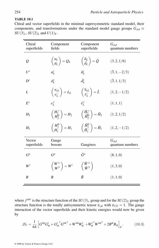
254 Particle and Astroparticle Physics
TABLE 10.1Chiral and vector superfields in the minimal supersymmetric standard model, their
components, and transformations under the standard model gauge groups Gstd ≡SU(3)c, SU(2)L and U(1)Y .
Chiral Component Component Gstdsuperfields fields superfields quantum numbers
Q(
uLdL
)= QL
(uLdL
)= Q (3,2,1/6)
Uc ucL uc
L (3,1,−2/3)
Dc dcL dc
L (3,1,1/3)
L(
νeLe−L
)= LL
(νeLe−L
)= L (1,2,−1/2)
Ec e+L e+
L (1,1,1)
H2
(H+
2H0
2
)= H2
(H+
2H0
2
)= H2 (1,2,1/2)
H1
(H0
1H−
1
)= H1
(H0
1H−
1
)= H1 (1,2,−1/2)
Vector Gauge Gstdsuperfields bosons Gauginos quantum numbers
Ga Ga Ga (8,1,0)
W i(
W±W 3
)= W i
(W±W 3
)(1,3,0)
B B B (1,1,0)
where f abc is the structure function of the SU(3)c group and for the SU(2)L group the
structure function is the totally antisymmetric tensor εi jk with ε123 = 1. The gauge
interaction of the vector superfields and their kinetic energies would now be given
by
LV =1
64
[Giα Gi
α +Giα
†Giα † +W iαW i
α +W iα
†W iα † +2Bα Bα
]F
. (10.3)
© 2008 by Taylor & Francis Group, LLC
Supersymmetric Models 255
The interactions of the gauge multiplets with the chiral superfields are contained in
the D-term where both the chiral superfields and the conjugate superfields will enter
in addition to the vector superfields. The D-term in the Lagrangian is given by
LD =[
Q†exp2(
gsT pGp+gσmW m+ g′6 B
)Q
+ Uc†exp2(
gsT pGp− 2g′3 B
)Uc +Dc†exp
2(
gsT pGp+ g′3 B
)Dc
+ L†exp2(
gσmW m− g′2 B
)L+Ec†exp2(g′B)Ec
+ H†2 exp
2(
gσmW m+ g′2 B
)H2 +H†
1 exp2(
gσmW m− g′2 B
)H1
]D
. (10.4)
Here, T p and σ m are the generators of the groups SU(3)c and SU(2)L, respectively
and we have suppressed the generation and group indices in the different chiral fields.
This Lagrangian will include all the interactions of the gauge bosons and the gaugi-
nos with the fermions and the scalars.
The superpotential contains the scalar interactions, Yukawa couplings, and the
interactions of the superpartners of the chiral superfields
WF = [huQH2Uc +hdQH1Dc +heLH1Ec + µH2H1]F . (10.5)
Generation indices are suppressed. The F-term of the superpotential includes the
Yukawa coupling terms. When the Higgs fields acquire vevs they give masses to the
fermions through these terms.
The most general potential includes more terms, which violate baryon and lepton
numbers very strongly [149]. To avoid these catastrophic terms in the minimal su-
persymmetric standard model, an additional discrete symmetry is imposed, which is
known as the R-parity and defined as [150, 151]
R = (−1)3(B−L)+2S or R = (−1)3B+L+2S, (10.6)
where S is the spin of the particle and B and L are the baryon and lepton numbers.
Both the definitions have the same consequences. R-parity implies that all ordinary
particles will have even R-parity, while the superpartners will have odd R-parity. The
R-parity conservation then implies
(i) The renormalizable baryon and lepton-number violating terms are absent.
(ii) In any vertex, superparticles will enter in pairs. So, when a superparticle de-
cays, the decay products contain at least one superparticle.
(iii) The lightest of the superparticles cannot decay and must be absolutely stable.
This lightest supersymmetric particle (LSP) could be a dark matter candidate.
The LSP is neutral and color singlet and it interacts with other particles very
weakly.
© 2008 by Taylor & Francis Group, LLC
256 Particle and Astroparticle Physics
In the minimal supersymmetric standard model R-parity conservation simplifies the
analysis substantially. In some extensions of the minimal supersymmetric standard
model R-parity violation is considered, which will be discussed later.
We write all the possible soft supersymmetry breaking terms that are allowed by
the standard model gauge symmetry and R-parity:
−Lso f t = m21|H1|2 +m2
2|H2|2 −Bµ(H1H2 +H.c.)
+M2Q(u∗LuL + d∗
LdL)+M2u u∗RuR +M2
d d∗RdR
+M2L(e∗LeL + ν∗
L νL)+M2e e∗ReR
+1
2
[M3 ¯gg+M2 ¯ω iωi +M1
¯bb]
+g√
2MW
[Md
cosβAdH1Qd∗
R +Mu
sinβAuH2Qu∗R
+Me
cosβAeH1Le∗R +H.c.
], (10.7)
where the angle tanβ = v2/v1 is the ratio of the vevs of the two Higgs doublets H1 and
H2. The soft terms contain the masses of the superpartners of the ordinary fermions
and gauge bosons, the trilinear A-terms that allow mixing of the scalar partners of
the left-handed and right-handed fermions when the Higgs scalars acquire vev and
the B-terms that mix the scalar components of the two Higgs doublets. Our lack of
knowledge about the origin of the soft terms increases the unknown parameters in
the model. In spite of that, the minimal supersymmetric standard model provides us
with very rich phenomenology.
Higgs Potential and Electroweak Symmetry Breaking
We can now write the complete Lagrangian for the minimal supersymmetric standard
model as
L = LV +LD +LF +Lso f t , (10.8)
where the different parts of the Lagrangian are given in equations (10.3), (10.4),
(10.5) and (10.7). The different terms give the gauge interactions, the interactions
of the gauge bosons with the fermions and scalars and also the kinetic energy terms
for the superfields, the Yukawa interactions and the scalar interactions, and the su-
persymmetry breaking soft terms, which also provide the mass splitting between the
ordinary particles and their superpartners.
Let us now write the scalar potential containing the masses and self interactions
of the Higgs scalars
V =g2
2|H∗
1 H2|2 +g2 +g′2
8
(|H2|2 −|H1|2)2
+|µ|2 (|H1|2 + |H2|2)
+m21|H1|2 +m2
2|H2|2 +BµH1H2 +H.c. (10.9)
© 2008 by Taylor & Francis Group, LLC
Supersymmetric Models 257
The terms in the first line with couplings g and g′ come from the D-terms correspond-
ing to the SU(2)L and U(1)Y gauge groups, and the terms in the second line are the
F-terms. The terms in the last line are the soft supersymmetry breaking masses and
the bilinear B-term. In terms of the SU(2)L components, these terms can be written
as
|H1|2 = |H01 |2 + |H−
1 |2|H2|2 = |H+
2 |2 + |H02 |2
H1H2 = H01 H0
2 +H−1 H+
2 . (10.10)
The sneutrino can also mix with the Higgs scalars and can even acquire vev in some
cases, which is constrained by phenomenology [151].
The parameters of the potential are more restrictive than in the standard model.
In the standard model with two Higgs doublets, there are six free parameters and a
phase, whereas for the minimal supersymmetric standard model there are only three
independent combinations of parameters
|µ|2 +m21, |µ|2 +m2
2, and µB, (10.11)
and there is no CP phase in V . When these parameters satisfy the relations
(µB)2 > (|µ|2 +m21)(|µ|2 +m2
2)
|µ|2 +m2
1 +m22
2> |µB|, (10.12)
the Higgs fields acquire vevs
< H01,2 >= v1,2, (10.13)
where v1,2 can be given in terms of the three independent parameters mentioned
above and can be chosen to be positive. This breaks the electroweak symmetry, and
the W bosons get a mass
M2W =
g2
2(v2
1 + v22). (10.14)
The experimental value of the W boson mass eliminates one free parameter.
The three components of the Higgs scalars will become the longitudinal modes of
the massive gauge bosons W±,Z leaving five other degrees of freedom of the two
complex Higgs doublets H1 and H2. These five components are
(i) a CP-odd neutral pseudoscalar Higgs boson A,
(ii) two CP-even Higgs fields h and H, with Mh < MH and
(iii) the charged Higgs bosons H±.
© 2008 by Taylor & Francis Group, LLC
258 Particle and Astroparticle Physics
The masses of the physical Higgs scalars are given by
M2A =
2 | µB |sin2β
M2h,H =
1
2
M2
A +M2Z ∓(
(M2A +M2
Z)2 −4M2ZM2
A cos2 2β)1/2
M2H± = M2
W +M2A, (10.15)
where the angle β is defined as
tanβ =v2
v1. (10.16)
The angle β lies in the range 0 ≤ β ≤ π/2 because v1,2 are positive. In terms of the
mass eigenstates the Higgs fields are given by
H1 =(
v1 + 1√2(H cosα −hsinα + iAsinβ )
H− sinβ
)
H2 =(
H+ cosβv2 + 1√
2(H sinα +hcosα + iAcosβ )
), (10.17)
where the Higgs mixing angle α is given by
tan2α = tan2β[
M2H +M2
h
M2A −m2
Z
]. (10.18)
We can now choose two of the parameters as free parameters and determine all others
only in terms of these two parameters. In one convention tanβ and MA are considered
as the free parameters and all other quantities are expressed in terms of these two
parameters.
These expressions can be combined to predict
MH+ > MW , MH > MZ , Mh < MA, and Mh < MZ |cos2β |. (10.19)
These relations are tree-level predictions and loop corrections will modify them. For
example, loop corrections make the lightest Higgs h heavier than the Z boson because
of the corrections from the top and the squarks. However, this does not change the
predictions too drastically. Including all corrections and taking a large tanβ , the
limit on the lightest of the neutral Higgs comes out to be [152]
Mh < 130GeV, (10.20)
which is definitely within the reach of LHC.
The Higgs sector is described by two parameters Mh and tanβ , although a certain
region of this parameter space has been ruled out by experiments. Experimental
bound on the supersymmetric Higgs mass [153] for all values of tanβ is less stringent
than the nonsupersymmetric Higgs bound due to suppression of their couplings to the
© 2008 by Taylor & Francis Group, LLC
Supersymmetric Models 259
vector bosons. In some models this bound becomes weaker since there are invisible
decay modes such as h,A → χ01 χ0
1 with significant branching ratios.
One of the main aims of LHC is to look for the Higgs scalars. Since the mass of the
lightest Higgs scalar in the supersymmetric models is constrained to be lower than
135 GeV, it is expected that LHC will be able to find the Higgs. One can complicate
the model and go beyond the minimal supersymmetric standard model, but in any
extensions the lightest neutral Higgs cannot be made heavier than 150 GeV, which is
also within the reach of LHC. If the neutral Higgs is not seen at this energy then the
supersymmetric models will be in trouble.
Spectrum of Superparticles
The masses of the fermions come from the Yukawa terms. One can now invert the
problem to get the Yukawa couplings in equation (10.5) in terms of the fermion
masses,
he,d =gme,d√
2MW cosβhu =
gmu√2MW sinβ
, (10.21)
where g is the SU(2)L gauge coupling constant. The Higgs boson couplings to
fermions are now determined in terms of the two parameters MA and tanβ , which
leaves only µ as a free parameter in the superpotential.
The gauge coupling constants give the interactions of the Higgs bosons to the
gauge bosons. To lowest order, the neutral Higgs boson couplings to fermions are
specified in terms of the two variables MA and tanβ :
L = − gmu
2MW sinβ(cosα uuh+ sinα uuH + cosβ uγ5uA)
− gmd
2MW cosβ(sinα ddh+ cosα ddH + sinβ dγ5dA)
− gme
2MW cosβ(sinα eeh+ cosα eeH + sinβ eγ5eA). (10.22)
The dependence on the squark masses and the mixing parameters cannot be neglected
when radiative corrections are included. For large MA (of the order of 300GeV or
higher), the Higgs couplings become close to the nonsupersymmetric standard model
couplings.
The masses of the superpartners come mainly from the soft mass terms, which de-
pend on the scale of supersymmetry breaking. The trilinear A-terms give the mixing
between the scalar partners of the left-handed and right-handed fermions. To see the
spectrum of the superpartners, we can write the mass matrices for the scalar partners
of the up and the down quarks and the charged leptons in the basis [ fL fR],
M2u =
(M2
Q +m2u +m2
1u mu(Au −µ cotβ )mu(Au −µ cotβ ) M2
u +m2u +m2
2u
)
M2d =
(M2
Q +m2d +m2
1d md(Ad −µ tanβ )md(Ad −µ tanβ ) M2
d +m2d +m2
2d
)
© 2008 by Taylor & Francis Group, LLC
260 Particle and Astroparticle Physics
M2e =
(M2
L +m2e +m2
1e me(Ae −µ tanβ )me(Ae −µ tanβ ) M2
e +m2e +m2
2e
), (10.23)
where we defined
m21a = M2
Z(T a3L −Qa sin2 θW )cos2β
m22a = QaM2
Z sin2 θW cos2β (a = u,d,e), (10.24)
with T a3L and Qa as the SU(2)L quantum numbers and electric charges of a = uL,dL
and eL. The various mixings depend on the soft parameters Ai and tanβ . For large
tanβ the mixings in the down quark sector and the charged lepton sector are large.
Depending on the parameters Ai, when the mixing is large the lightest squark will be
a stop. The requirement that the stop mass does not become negative, and hence the
stop acquire a vev, dictates a condition |At | < MQ,u.
The superpartners of the charged SU(2)L gauge bosons W± and the physical
charged Higgs H± are the four charged Majorana fermions called the charginos.
They mix with each other and the mass term for these charginos is given by
Mch = −1
2(W− H− )
(m2
√2MW cosβ√
2MW sinβ µ
)(W+
H+
). (10.25)
A bi-unitary transformation (similar to the quark masses) can diagonalize this matrix
to give two physical Dirac charginos with masses
m2χ±
1,2=
1
2
[m2
2 +2M2W + µ2 ∓ [(m2
2 −µ2)2 +4M4W cos2 2β
+4M2W (m2
2 + µ2 +2m2µ sin2 β )] 1
2
]. (10.26)
The usual convention is Mχ1 < Mχ2 .
The chargino mass vanishes for µ → 0. So, to keep the charginos heavier than
the electroweak symmetry breaking scale, we need µ = 0. On the other hand the Z-
boson mass is related to the µ-parameter through
m2Z = 2
[M2
h −M2H tan2 β
tan2 β −1
]−2µ2. (10.27)
The correct Z mass needs a cancellation of the term containing the Higgs mass with
the µ term quite accurately. This fine tuning of the parameter µ is called the µ-problem.
Finally we shall discuss the mass spectrum of the neutral fermions. There are four
of them: the fermion superpartners of the neutral gauge bosons B and W 3 denoted by
b and ω3, respectively and the fermion superpartners of the Higgs bosons, h01 and h0
2.
All four mix with each other and the mass matrix is given in the basis [b ω h01 h0
2]
© 2008 by Taylor & Francis Group, LLC
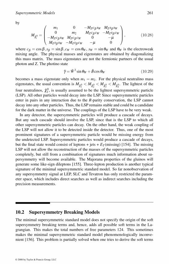
Supersymmetric Models 261
by
Mχ0i
=
m1 0 −MZcβ sW MZsβ sW0 m2 MZcβ cW −MZsβ cW
−MZcβ sW MZcβ cW 0 −µMZsβ sW −MZsβ cW −µ 0
, (10.28)
where cβ = cosβ ,sβ = sinβ ,cW = cosθW , sW = sinθW and θW is the electroweak
mixing angle. The physical masses and eigenstates are obtained by diagonalizing
this mass matrix. The mass eigenstates are not the fermionic partners of the usual
photon and Z. The photino state
γ = W 3 sinθW + BcosθW (10.29)
becomes a mass eigenstate only when m1 = m2. For the physical neutralino mass
eigenstates, the usual convention is Mχ01
< Mχ02
< Mχ03
< Mχ04. The lightest of the
four neutralinos, χ01 , is usually assumed to be the lightest supersymmetric particle
(LSP). All other particles would decay into the LSP. Since supersymmetric particles
enter in pairs in any interaction due to the R-parity conservation, the LSP cannot
decay into any other particles. Thus, the LSP remains stable and could be a candidate
for the dark matter in the universe. The couplings of the LSP have to be very weak.
In any detector, the supersymmetric particles will produce a cascade of decays.
But any such cascade should involve the LSP, since that is the LSP to which all
other supersymmetric particles can decay. On the other hand, the weak coupling of
the LSP will not allow it to be detected inside the detector. Thus, one of the most
prominent signatures of a supersymmetric particle would be missing energy from
the undetected LSP. Supersymmetric particles would produce a cascade of decays,
but the final state would consist of leptons + jets + ET (missing) [154]. The missing
LSP will not allow the reconstruction of the masses of the supersymmetric particles
completely, but still from a combination of signatures much information about su-
persymmetry will become available. The Majorana properties of the gluinos will
generate some like-sign dileptons [155]. Three-lepton production is another typical
signature of the minimal supersymmetric standard model. So far nonobservation of
any supersymmetry signal at LEP, SLC and Tevatron has only restricted the param-
eter space, which includes direct searches as well as indirect searches including the
precision measurements.
10.2 Supersymmetry Breaking ModelsThe minimal supersymmetric standard model does not specify the origin of the soft
supersymmetry breaking terms and, hence, adds all possible soft terms in the La-
grangian. This makes the total numbers of free parameters 124. This sometimes
makes the minimal supersymmetric standard model phenomenologically inconve-
nient [156]. This problem is partially solved when one tries to derive the soft terms
© 2008 by Taylor & Francis Group, LLC
262 Particle and Astroparticle Physics
from some other theory. For example, when supersymmetry is broken in the hidden
sector of any supergravity theory, it is possible to obtain the soft masses. In this case
the mass of the gravitino sets the mass scale in the theory and all mass parameters
get related to the same mass scale at some high energy scale of grand unification. Al-
though it is not possible to derive the complete theory from any supergravity theory,
a phenomenological theory may be constructed in which the constraints that could
come from the supergravity models on the soft terms of the minimal supersymmetric
standard model are imposed. This reduces the numbers of free parameters and makes
the theory more predictable in this supergravity inspired model or in the constrained
minimal supersymmetric standard model. In other words, one assumes some hid-den world where supersymmetry is broken, which then induces the soft terms. From
the nature of the hidden world and how the supersymmetry breaking information is
communicated to the ordinary world, we get some constraints on the minimal super-
symmetric standard model parameters.
Supergravity-Inspired Models
The most popular scenario of supersymmetry breaking comes from the supergravity
models. We shall discuss in the next chapter some formal aspects of the supergrav-
ity theory and how the soft terms originate in these theories. The requirement of
unification of several parameters constrains some of the parameters of the minimal
supersymmetric standard model. These theories are called the constrained minimal
supersymmetric standard model (CMSSM) or the supergravity-inspired minimal su-
persymmetric standard model or sometimes mSUGRA model [157].
In the supergravity-inspired models, one conjectures that it is natural that some of
the parameters were unified at very large scale without specifying the actual model.
For example, along with the gauge coupling unification, one assumes that the gaug-
ino masses (Mi) were also unified at the scale of grand unification (MU ),
Mi(MU ) = m1/2. (10.30)
The renormalization group equations then predict how they descend to low energy
dMi
dt= −biαiMi/4π, (10.31)
where bi are the usual beta functions and αi = g2i
4π is related to the gauge coupling
constants. The evolution of the parameters then gives the low-energy masses of the
gauge fermions to be
M2(MW ) =(
α(MW )αs(MW )sin2 θW (MW )
)M3(MW )
M1(MW ) =5
3tan2 θW (MW )M2(MW ), (10.32)
which makes the gluino the heaviest of the gaugino masses.
© 2008 by Taylor & Francis Group, LLC
Supersymmetric Models 263
It is also assumed that there is a common scalar mass at the unification scale (MU ),
m21 = m2
2 = M2Q = M2
u = M2d = M2
L = M2e = m2
0, (10.33)
which gives M2h,H(MU ) = m2
0 + µ2. Since the evolution of the squarks has some
contribution from the SU(3)c gauge bosons, the squarks become heavier than the
sleptons at low energy,
M2q(MW ) > M(MW ). (10.34)
In this picture it is assumed that the supersymmetry will be broken at some interme-
diate scale in the hidden sector, which will be communicated to the observable sector
through gravity interactions [158]. Since the hidden sector and how the supersym-
metry breaking is communicated cannot distinguish the components of any multiplet
of the gauge groups, any contribution coming from the hidden sector should be inde-
pendent of the gauge transformation properties of the fields. In N = 1 supergravity
models supersymmetry is broken at some intermediate scale MS ∼ m ∼ 1011 GeV
and all the soft terms are generated with the same mass, which is the gravitino mass
m3/2 (see section 11.3)
m3/2 ∼ Mso f t ∼ M2S
MPl∼ 1TeV. (10.35)
All A-parameters are also equal at the unification scale, independent of the fields.
This assumption leads to only 5 input parameters at the grand unification scale MU[155], which are, m0,m1/2,A0,µ and the Higgs mixing parameter B. At low energy
we then have only a few parameters from which the Z mass restricts |µB| and makes
tanβ a free parameter instead of B, so we have the new set of parameters
m0,m1/2,A0, tanβ ,sign(µ). (10.36)
One variation of this model assumes nonuniversal scalar masses at the unification
scale, changing the low-energy phenomenology of the model. Theoretical consider-
ations also suggest that the universality is not generic [159].
Gauge-Mediated Supersymmetry Breaking
There is a variant of the supergravity-inspired model called the gauge-mediated su-persymmetry breaking model. Supersymmetry is again broken in the hidden sector,
but the connection between the hidden sector and the low-energy phenomenology
is now through a messenger chiral superfield, which transforms under the SU(3)c ×SU(2)L ×U(1)Y group nontrivially. When supersymmetry is broken by a gauge sin-
glet superfield in the hidden sector, the messenger gauge nonsinglet chiral superfield
obtains a mass Λ, and the supersymmetry breaking effect is communicated to the
minimal supersymmetric standard model particles through gauge interaction [160].
The mass parameter Λ is chosen to be of the order of
Λ ∼ 104 −105GeV, (10.37)
© 2008 by Taylor & Francis Group, LLC
264 Particle and Astroparticle Physics
so the soft terms in the Lagrangian are of the order of a few TeV. The messenger
gauge nonsinglet chiral superfield couples to the ordinary particles, which then com-
municate the supersymmetry breaking effect through the soft terms.
One-loop contributions give masses to the gauginos,
Mi ∼ αi
4πΛ, (10.38)
and scale in the same way as the corresponding gauge coupling constants at low
energy. The scalar superpartners of the minimal supersymmetric standard model
obtain mass at the two-loop level from diagrams involving the gauge fields and the
messenger fields. The scalar masses are
M2 ∼(
Λ4π
)2α2
s C3 +α22C2 +α2
1C1
, (10.39)
where Ci are the quadratic Casimir operators of the gauge groups SU(3)c×SU(2)L×U(1)Y .
One of the problems with the minimal supersymmetric standard model is that the
mass splitting of the squarks and sleptons does not allow GIM type cancellation
and gives large flavor-changing neutral current (FCNC). However, by assuming that
the masses of the squarks and sleptons are almost degenerate, the FCNC problem
is reduced. In the gauge-mediated supersymmetric model the near degeneracy of
the squarks and the sleptons comes out naturally, which reduces the FCNC problem
somewhat. The µ and B parameters are model dependent and are not predicted in
this scenario.
One characteristic feature of the gauge-mediated supersymmetry breaking is that
it predicts a very tiny gravitino mass [160, 161]
m3/2 ∼Λ2
MPl∼ 10−10GeV , (10.40)
which is the LSP. All other supersymmetric particles will first decay into the next-to-
lightest supersymmetric particle (NLSP), which is heavier than the LSP but lighter
than all other superparticles, since the coupling with the gravitino is small. This
NLSP then decays into the LSP (gravitino) very weakly resulting in a very definite
signature of the gauge-mediated supersymmetry breaking models. Since the NLSP
can eventually decay, it can also be a charged particle. The most likely candidates
for NLSP are χ01 and τ±R . For both of these NLSPs, the decays contain a gravitino
χ01 → γ G3/2 and χ0
1 → Z G3/2 or τ±R → τ± G3/2. (10.41)
Since the gravitino cannot be detected, the energy carried away by the gravitino
gives a distinctive signal for supersymmetry of missing transverse momentum with
model-dependent lifetimes and phenomenologies.
The minimal gauge-mediated supersymmetry breaking scenario has fewer param-
eters compared with the supergravity inspired models, but the gauge-mediated mod-
els are somewhat less compelling compared with the supergravity-inspired models.
© 2008 by Taylor & Francis Group, LLC
Supersymmetric Models 265
The minimal gauge-mediated supersymmetry breaking model predicts an upper limit
on the lightest Higgs mass Mh < 124 GeV for a top quark mass of mt = 175 GeV
[161]. But this minimal model is by no means complete, and even the more com-
plicated models are not fully satisfactory. Finally the arbitrariness in the messenger
sector of the gauge-mediated supersymmetry breaking makes it less attractive.
Anomaly-Mediated Supersymmetry Breaking
We shall now consider another supersymmetry breaking mechanism with different
phenomenology, which has its origin in the superstring theory [162]. Superstring the-
ories are defined in 10 dimensions. The extra six dimensions are then compactified
to get the low-energy effective 4-dimensional theory. In some of the compactifica-
tion scheme it is possible that the resulting 4-dimensional effective theory has some
low-energy anomalous U(1) gauge group. Since the original theory is anomaly free,
the effective theory also should be free of anomalies. To have anomaly cancellation
in the effective theory, one needs to introduce an additional complex chiral super-
field, whose scalar partner is the dilaton field, which should then acquire a vev for
consistency. This vev of the dilaton field then introduces a D-type term, which in
turn breaks supersymmetry. This supersymmetry breaking also introduces the soft
mass terms. One drawback of the model is that it predicts too low gaugino mass.
However, since the A and the B terms are also likely to be small in this model, this
may not be so bad from a phenomenological point of view. However, this model has
not been studied in detail so far.
Another related supersymmetry breaking mechanism is based on the supergravity
model [163]. It has been observed that a supergravity-coupled gauge theory has a
conformal invariance in the absence of mass terms. When the parameters are evolved
with energy using renormalization group equations, the renormalization process will
break the conformal symmetry by introducing the mass scale in the theory. This will
break the conformal symmetry generating conformal anomaly in the theory leading
to soft terms with a very definite pattern. In fact, all soft terms become proportional
to the gravitino mass. So, the gravitino mass needs to be around 10 to 100 TeV.
The sfermion masses come out to be nearly degenerate as in the gauge-mediated
supersymmetry breaking, which helps to solve the FCNC problem. But there is one
serious problem with this scenario, namely, that it leads to tachyonic mass for the
color singlet superpartners. This negative mass squared term for the sleptons will
induce a vev to the sleptons, which is unacceptable. Any further consideration of
this scenario will depend on solving this issue. One attempt toward this end is to
extend the minimal supersymmetric standard model by an extra U(1), where the
Fayet–Illiopoulos D-terms solve the negative-mass squared problem [164].
© 2008 by Taylor & Francis Group, LLC
266 Particle and Astroparticle Physics
10.3 R-Parity ViolationAlthough we have not seen any signals for supersymmetry, we expect that the super-
symmetric particles have masses close to the electroweak symmetry breaking scale.
To ensure that we do not miss any signals for supersymmetry, there are attempts to
study some extensions of the minimal supersymmetric standard model, which may
have some testable predictions. One such extension is the R-parity violating models.
The renormalizable baryon and lepton-number violating couplings have been pre-
vented in the minimal supersymmetric standard model by imposing R-parity [149]
R = (−1)3(B−L)+2S or R = (−1)3B+L+2S. (10.42)
Otherwise the theory would mediate unacceptably fast proton decay. This implies
that at any vertex there have to be at least two supersymmetric particles. Thus, decays
of any supersymmetric particle should have one more supersymmetric particle, and
the LSP becomes stable.
Although it is a sufficient condition for suppressing proton decay to have R-parity
conservation, this is not necessary. From phenomenological considerations R-parity
violating models were considered, in which either B or L, but not both, is conserved
to prevent proton decay. Since proton decay requires violation of both baryon and
lepton numbers, we do not require both B and L conservation to prevent fast proton
decay. These R-parity violating theories with either B or L violation have several
predictions which are different from the minimal supersymmetric standard model.
In the R-parity violating extension of the minimal supersymmetric standard model,
one starts with the Lagrangian
L = LMSSM +[WR]F , (10.43)
where the second term contains the new R-parity violating interactions [149, 150]
and is given by the superpotential,
WR = W LR +W B
R
W BR =
1
2λ ′′
i jkUci Dc
jDck
W LR =
1
2λi jkLiL jEc
k +λ ′i jkLiQ jDc
k + µiLiH2, (10.44)
where i, j,k are flavor indices. The first part of these interactions W BR contains only
one term that violates baryon number but conserves lepton number. This term is
antisymmetric in j,k, and hence, λ ′′i jk has nine components.
The second part of the R-parity violating interactions W LR contains three terms that
violate lepton number but conserve baryon number. The first of these terms is anti-
symmetric in i, j. λi jk has nine components, while λ ′i jk has 27 components. The last
term of W LR is the bilinear term, which can be absorbed in the µ-term in the superpo-
tential of the minimal supersymmetric standard model by suitable transformations of
© 2008 by Taylor & Francis Group, LLC
Supersymmetric Models 267
the superfield H1. But removing this term at some energy does not ensure its removal
at all energies. Moreover, one should ensure that this does not lead to a nonvanishing
vev of the sneutrino, < νi >= 0. In general, this bilinear term will be present in most
cases of R-parity violation. So, counting these three bilinear couplings, in total 48
R-parity violating couplings are allowed, 9 B violating terms in W BR and 39 L violat-
ing terms in W LR . Since there is no motivation for B violation, while L violation is
required for neutrino masses, in most R-parity violating models one assume, W BR is
absent and only W LR is nonvanishing.
Any R-parity violating models have the characteristics that they allow the trilinear
R-parity violating terms in which there is only one supersymmetric particle. Thus,
a supersymmetric particle will be allowed to decay into two ordinary particles. This
would mean that the LSP can decay into ordinary particles and there is no stable
LSP. This will change the phenomenology of supersymmetric particles. The search
strategy for supersymmetry will also change accordingly. While the R-parity con-
serving scenarios would find a missing pT due to the energy carried by the LSP, the
R-parity violating scenarios may have, for example, dilepton signals as more definite
indication of supersymmetry.
The bilinear terms in the models of R-parity violation give rise to a mixing of the
neutralinos with the neutrinos. In the simplest scenario with one of the neutrinos, say,
τ neutrino, mixing with the neutralinos, the LSP can decay through its mixing with
the ντ to ordinary particles. This also enriches the phenomenology of supersymmetry
[165, 166]. Moreover, this lepton-number violating mixing of the neutralinos with
the neutrinos can contribute to the Majorana neutrino masses.
The parameters in the R-parity violating interactions can be constrained [167] by
the processes that these interactions allow, such as the baryon and lepton-number vi-
olating processes including proton decay, neutron–antineutron oscillations and Ma-
jorana neutrino masses. There are also constraints coming from charged current
universality, e−µ −τ universality, νe−e scattering, atomic parity violation, νe deep
inelastic scattering, quark mixing, K+ → π+νν or D0 − D0 mixing, τ-decays, D-
decays and LEP precision measurements. Astrophysical constraints can also be se-
vere for some parameters. Since there are no predictions for the R-parity violating
interactions, using these bounds for the R-parity violating parameters, possible ob-
servable signals are studied.
10.4 Supersymmetry and L Violation
There could be some new sources of lepton number violation in supersymmetric
models. The minimal supersymmetric standard model extends the standard model,
so there are no right-handed neutrinos and no lepton number violation, and hence,
neutrinos are massless. However, any of the extensions of the standard model that
give a Majorana mass to the neutrinos can be implemented into some extensions of
© 2008 by Taylor & Francis Group, LLC
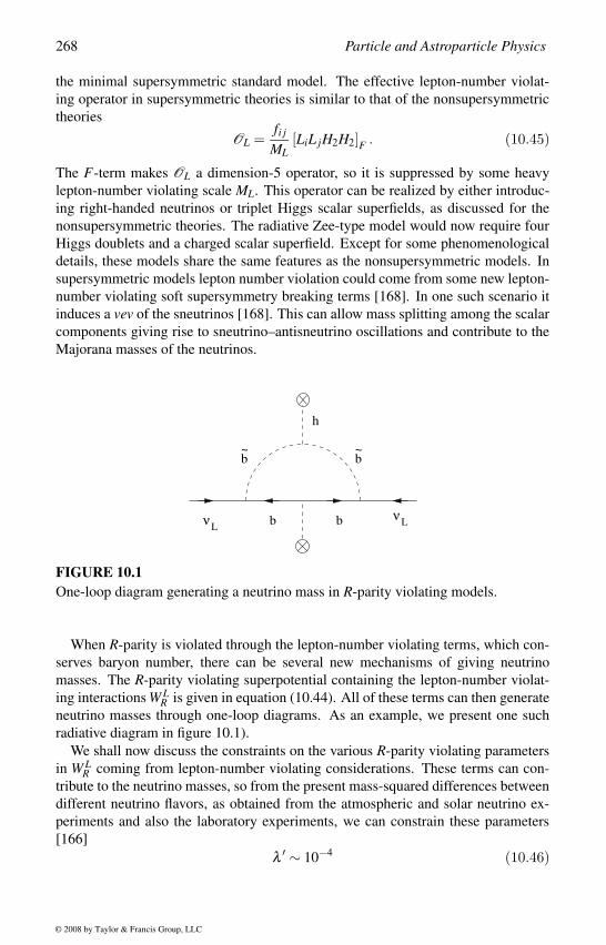
268 Particle and Astroparticle Physics
the minimal supersymmetric standard model. The effective lepton-number violat-
ing operator in supersymmetric theories is similar to that of the nonsupersymmetric
theories
OL =fi j
ML[LiL jH2H2]F . (10.45)
The F-term makes OL a dimension-5 operator, so it is suppressed by some heavy
lepton-number violating scale ML. This operator can be realized by either introduc-
ing right-handed neutrinos or triplet Higgs scalar superfields, as discussed for the
nonsupersymmetric theories. The radiative Zee-type model would now require four
Higgs doublets and a charged scalar superfield. Except for some phenomenological
details, these models share the same features as the nonsupersymmetric models. In
supersymmetric models lepton number violation could come from some new lepton-
number violating soft supersymmetry breaking terms [168]. In one such scenario it
induces a vev of the sneutrinos [168]. This can allow mass splitting among the scalar
components giving rise to sneutrino–antisneutrino oscillations and contribute to the
Majorana masses of the neutrinos.
b~
b~
h
νν bb LL
FIGURE 10.1One-loop diagram generating a neutrino mass in R-parity violating models.
When R-parity is violated through the lepton-number violating terms, which con-
serves baryon number, there can be several new mechanisms of giving neutrino
masses. The R-parity violating superpotential containing the lepton-number violat-
ing interactions W LR is given in equation (10.44). All of these terms can then generate
neutrino masses through one-loop diagrams. As an example, we present one such
radiative diagram in figure 10.1).
We shall now discuss the constraints on the various R-parity violating parameters
in W LR coming from lepton-number violating considerations. These terms can con-
tribute to the neutrino masses, so from the present mass-squared differences between
different neutrino flavors, as obtained from the atmospheric and solar neutrino ex-
periments and also the laboratory experiments, we can constrain these parameters
[166]
λ ′ ∼ 10−4 (10.46)
© 2008 by Taylor & Francis Group, LLC
Supersymmetric Models 269
with the supersymmetry breaking scale to be around 200 GeV. Similarly, the require-
ment for λ is also of the same order of magnitude to explain the neutrino masses.
These general constraints will hardly allow direct detection of these R-parity violat-
ing interactions, although a more rigorous analysis may still allow some interesting
phenomenology.
The bilinears and the lepton-number violating soft terms in the potential together
allow vevs for the sneutrinos. This will then allow mixing of the neutralinos with the
neutrinos, which in turn will introduce a mass to the neutrinos. Given the present
constraints on the parameters, these contributions from the bilinears alone are not
enough to explain all neutrino experiments, and one needs to consider the trilinears
together with the bilinears. The origin of the bilinears could be from the usual holo-
morphic terms, or from the nonholomorphic terms. When all of these terms are taken
together, these models explain the neutrino masses and also generate a baryon asym-
metry of the universe. However, none of the simple models with only one source of
lepton number violation could explain all the present results in neutrino masses and
mixing [165]. These models also fail to solve the problem of baryon asymmetry of
the universe.
In addition to the neutrino oscillation experiments, the present bound on the neu-
trinoless double beta decay (0νββ decay) can also constrain several lepton-number
nonconserving parameters of the supersymmetric theories. The lepton number vi-
olation coming from soft supersymmetry breaking, which gives rise to sneutrino–
antisneutrino oscillations, contributes to the amplitude of the 0νββ decay. These
supersymmetry breaking soft terms will then be constrained by the present bound
on the 0νββ decay [168], and the bound on the effective lepton-number violating
MSSM parameter is η susy < 1× 10⁻⁸(msusy/100 GeV)5. Assuming all superpar-
ticles to have a common mass msusy ∼ 100 GeV, this amounts to a bound for the
Majorana-like B−L violating sneutrino mass
mM < (2−11) GeV . (10.47)
This lepton-number violating mass mM corresponds to the mass difference between
a sneutrino and an antisneutrino.
All the R-parity violating interactions given by W LR in equation (10.44) would im-
ply Majorana masses to the neutrinos and contribute to the neutrinoless double beta
decay. As a result these couplings are constrained by the present bound on the neu-
trinoless double beta decay [169]. For the first generation this bound is
λ ′111 < 3.3×10⁻⁴
( mq
100 GeV
)2( mg
100 GeV
)1/2, (10.48)
assuming equal mass for the up-squark and the down-squark. If both R-parity vi-
olating interaction and the neutrino mass contribute to the neutrinoless double beta
decay, we get bounds on the products of two couplings
λ ′112λ ′
121 < 1.1×10⁻⁶(
Λsusy
100 GeV
)3
© 2008 by Taylor & Francis Group, LLC
270 Particle and Astroparticle Physics
λ ′113λ ′
131 < 3.8×10⁻⁸(
Λsusy
100 GeV
)3
(10.49)
for supersymmetric mass parameters of the order of 100 GeV.
Indirect constraints on the R-parity violating couplings come from the K −Koscillations, B−B mixing, D−D mixing, or lepton flavor changing processes.
Some of the bounds are even stronger, such as the bound from K−K oscillations
λ ′i12λ ′
i21 < 1×10⁻⁹ or the bound from B−B mixing λ ′i13λ ′
i31 < 8×10⁻⁸, both for
me = 100 GeV.
It is also possible to constraint the elements of the neutrino mass matrix from a
combined fit to the neutrino oscillation results, the bound on the neutrinoless double
beta decay, and WMAP constraints on the total mass of the three neutrinos. This, in
turn, can give bounds on the products of the standard couplings [169, 170]
λ ′i33λ ′
i′33 < 3.6×10⁻⁸, λ ′i32λ ′
i′23 < 8.9×10⁻⁷,
λ ′i22λ ′
i′22 < 2.2×10⁻⁵, λ ′i33λ ′
i33 < 6.3×10⁻⁷,
λ ′i32λ ′
i23 < 1.1×10⁻⁵, λ ′i22λ ′
i22 < 1.7×10⁻⁴. (10.50)
For this representative set of constraints the masses of the scalar superpartners are
assumed to be around 100 GeV. In the hierarchical scenario the bounds on the R-
parity violating couplings would be stronger than in the degenerate case.
10.5 Grand Unified TheoriesSupersymmetry was originally proposed as an interesting symmetry of nature that
relates fermions to bosons and unifies space–time symmetry with internal symme-
tries. However, it became popular only when it could provide a solution to the gauge
hierarchy problem of the grand unified theories. There are two widely different mass
scales separated by the great desert in any grand unified theories. To protect the light
Higgs scalars against quadratic divergences coming from the radiative corrections,
severe fine tuning is required at all orders. This problem is solved in supersymmetric
theories, where the divergent diagrams are cancelled by equivalent diagrams with
supersymmetric particles. Thus, it is natural to construct a supersymmetric version
of the grand unified theories.
Let us first consider a supersymmetric version of the SU(5) grand unified theory.
We first incorporate the fermions in chiral superfields, and the gauge bosons are
included in vector superfields belonging to the adjoint 24-dimensional representation
of SU(5). Thus, the two chiral superfields, ψ and T , belonging to the 5 and 10-
dimensional representations of SU(5), respectively, will contain the usual fermions
and their scalar superpartners. The vector superfield will contain the 24 gauge bosons
and the gauginos.
© 2008 by Taylor & Francis Group, LLC
Supersymmetric Models 271
We consider the Higgs scalars belonging to a 24-dimensional scalar superfield Σ,
which breaks the SU(5) group. The adjoint representation is the minimal choice for
the purpose, since we do not want to break the rank of the group. For the electroweak
symmetry breaking and for giving masses to the up and the down quarks and the
leptons, we introduce two Higgs doublets, H1, belonging to the representation 5
and H2, belonging to the representation 5 of SU(5). The two Higgs doublets are
also required to cancel chiral anomaly, since the fermions in the scalar superfields
contribute to anomaly.
Once the particle spectrum is determined, the gauge interactions and the kinetic
energy terms are determined. We shall now write the superpotential that can give us
the required symmetry breaking
SU(5)Σ24−→ SU(3)c ×SU(2)L ×U(1)Y
H15,H25−→ SU(3)c ×U(1)Q
and give masses to the fermions. To give TeV scale masses to the superpartners
coming from supersymmetry breaking, soft supersymmetry breaking terms are in-
troduced as in the minimal supersymmetric standard model. We shall not discuss
them here.
One possible choice of the superpotential containing the Higgs scalars is
W = huT T H2 +hdT ψH1 +λ2X(TrΣ2 −M2Σ)
+λ1H2H1Σ+ µH1H2, (10.51)
where we have introduced one singlet chiral field X to write this superpotential.
We assume that all supersymmetry breaking effect should be included in the soft
terms, so the minima of this superpotential should not break supersymmetry at the
unification scale. The vanishing of the F-terms
FX =∂W∂X
= TrΣ2 −M2Σ = 0
FΣ =∂W∂Σ
= 2λ2XΣ
now gives vevs of the fields
< Σ >= MΣdiag(1 1 1 −3/2 −3/2) and < X >= 0. (10.52)
There are two other degenerate vacua in which different components of Σ acquire
vevs, which will break SU(5) → SU(4)×U(1) or preserve SU(5). However, we as-
sume that supergravity effects will remove this degeneracy and SU(3)c ×SU(2)L ×U(1)Y will become the absolute minimum. Although we presented one particular su-
perpotential for demonstration, there could be many more possibilities for the super-
potential. Moreover, to write a particular superpotential one needs to impose certain
discrete symmetries, all of these complicate the theory. In addition, there are now
© 2008 by Taylor & Francis Group, LLC
272 Particle and Astroparticle Physics
new problems in the theory which require newer solutions. Some of the problems of
the nonsupersymmetric grand unified theories, such as the fermion mass problem or
the neutrino mass problem, are also present in the supersymmetric models. Again
gravitational corrections could also solve some of these problems. There is another
problem, called the doublet–triplet splitting problem, which we shall mention below.
The µ-problem is also difficult to solve in supersymmetric grand unified theories.
At present there is no standard supersymmetric SU(5) grand unified theory, which
is fully consistent and can provide solution to all of these problems. But all of them
have a generic structure, which is similar.
The vevs of the scalars H1 and H2 break the electroweak symmetry. These fields
also give masses to the fermions. In the effective SU(3)c ×SU(2)L ×U(1)Y , invari-
ant superpotential for the fermion masses will be exactly the same as the minimal
supersymmetric standard model, and hence, we shall not write them here. How-
ever, the triplet components of these scalars can in general mediate very fast proton
decay. This requires that there has to be some mechanism that makes the SU(3)ctriplet components as heavy as the grand unification scale, while keeping the doublet
component light. This is the so-called doublet–triplet splitting problem of the grand
unified theories.
Similar to the minimal supersymmetric standard model we shall impose R-parity
to forbid fast proton decay by forbidding the renormalizable baryon-number violat-
ing terms. The proton decay now comes from a dimension-5 operator,
O =f
MU[QQQL]F , (10.53)
where MU is the unification scale and f is the effective coupling constant. The scalar
superfields have mass dimension 1 and the F-term adds one more mass dimension.
This gives us an interaction vertex, violating baryon and lepton numbers, in which
two fermions and two scalars enter. Although the operator is suppressed by only one
power of MU , this is still acceptable since the coupling constants are now the Yukawa
couplings and could be smaller than the gauge couplings and the unification scale is
also large. This operator implies that the decay modes of the proton are different from
those of the nonsupersymmetric case. In this case the dominant proton decay mode
is µ+K0, which violates strangeness number. This comes because of the symmetry
property of the operator.
We shall now discuss the evolution of the gauge coupling constants in supersym-
metric theories. All of the superpartners of the ordinary particles contribute to the
renormalization group equation. This changes the coefficients of the beta function in
the following way. In the nonsupersymmetric case a gauge boson contribution to the
beta function comes with a coefficient −11/3, while a Weyl or Majorana fermion
contributes an amount 2/3 and a scalar an amount 1/6 (see equation (8.36)). In the
supersymmetric case a vector multiplet has a gauge boson, which contributes −11/3
and the corresponding gaugino, which is a Majorana fermion, contributes 2/3. So,
a vector multiplet contributes an amount −3 to the beta function. For a chiral mul-
tiplet there is a Majorana fermion contributing 2/3 and the corresponding complex
scalar superpartner contributing 1/3. So for a chiral superfield, the contribution is
© 2008 by Taylor & Francis Group, LLC
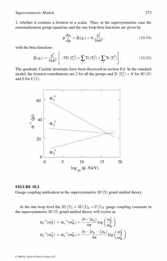
Supersymmetric Models 273
1, whether it contains a fermion or a scalar. Thus, in the supersymmetric case the
renormalization group equations and the one-loop beta functions are given by
µdgi
dµ= βi(gi) = bi
g3i
16π2 , (10.54)
with the beta functions
βi(gi) =g3
i16π2
[−3Tr [T 2
a ]+∑f
Tr [T 2f ]+∑
sTr [T 2
s ]
]. (10.55)
The quadratic Casimir invariants have been discussed in section 8.4. In the standard
model, the fermion contributions are 2 for all the groups and Tr [T 2a ] = N for SU(N)
and 0 for U(1).
0 105 15
α
(µ)
20
20
0
40
60
10log ( /GeV)µ
1
2
3
α
α
α -1
-1
-1
-1
FIGURE 10.2Gauge coupling unification in the supersymmetric SU(5) grand unified theory.
At the one-loop level the SU(3)c × SU(2)L ×U(1)Y gauge coupling constants in
the supersymmetric SU(5) grand unified theory will evolve as
α−13 (m2
X ) = α−13 (m2
W )+(9−2ng)
4πlog
(m2
X
m2W
)α−1
2 (m2X ) = α−1
2 (m2W )+
(6−2ng − 12 nh)
4πlog
(m2
X
m2W
)
© 2008 by Taylor & Francis Group, LLC
274 Particle and Astroparticle Physics
α−11 (m2
X ) = α−11 (m2
W )+(−2ng − 3
10 nh)4π
log
(m2
X
m2W
), (10.56)
where ng = 3 is the number of generations of fermions. We have included the effect
of nh Higgs doublets. Starting with the gauge coupling constants at the electroweak
scale, as obtained from the precision measurements, we evolve them to the grand
unification scale and find that all three meet at a point around 1016 GeV, as shown in
figure 10.2. In practice, one considers the uncertainty in the measured couplings and
then varies the supersymmetry breaking scale, below which the superparticles will
not contribute to the renormalization group equation. The best fit that corresponds
to coupling constant unification comes for the supersymmetry breaking scale to be
around a TeV [130, 171]. The present values of the precision results again disfavor
the single stage unification.
The supersymmetric SO(10) grand unified theories with some intermediate sym-
metry breaking scales are thus more likely unified theory, which can have solution
to many of the problems present in the minimal SU(5) grand unified theory. Some
of the problems that could be addressed naturally in an SO(10) grand unified theory
are correct neutrino mass, solution to strong CP problem, left–right symmetry break-
ing, leptogenesis, gravitino problem and inflation. Gauge coupling unification also
prefers theories with intermediate symmetry breaking scale.
Supersymmetric theories are more interesting than the nonsupersymmetric grand
unified theories, but N = 1 supergravity models are even more interesting. Starting
with the Higgs masses to be m20 + µ2 and the squarks and sleptons masses to be m0
at the unification scale MU , if we evolve downward to the electroweak scale, we
find one very interesting phenomenon. The squark and the slepton masses remain
positive, but the lighter Higgs mass-squared becomes negative M2h < 0 around the
electroweak scale. This will imply a vev for the Higgs scalar, which then breaks the
electroweak symmetry and gives masses to the fermions. Thus, the negative mass-
squared term required for the Higgs mechanism in the standard model comes out
naturally in supergravity theories [172].
Starting from the unification scale, as we evolve the top quark mass with energy it
reaches a fixed point value, beyond which it stops evolving. This means that the final
value of the top quark mass is independent of the initial values of the couplings at
the unification scale and the observed top quark mass is predicted for tanβ ∼ 1−3.
Supersymmetric theories have many advantages, but there are also some disadvan-
tages. The superpartners and the constraints in the couplings sometimes create new
problems. But considering all aspects we now believe that supersymmetry should
be present at high energies. In addition to the phenomenological considerations dis-
cussed in this chapter, it may play an important role in unifying the gauge interactions
with gravity.
© 2008 by Taylor & Francis Group, LLC
Part IV
Extra Dimensions
© 2008 by Taylor & Francis Group, LLC
11Extended Gravity
The gravitational interaction plays the most important role in the evolution of the
universe although this is the weakest of all the forces. However, at very high energies
gravity should become as strong as any other interaction. Since the strong, the weak
and the electromagnetic interactions are gauge theories and could be unified in a
grand unified theory, we envisage an ultimate theory at higher energies in which
gravity will be unified with all other interactions. At higher energies we expect
our theory to be supersymmetric to solve the gauge hierarchy problem and allow
unification of Poincare group with the internal symmetry groups. So, we must also
formulate a supersymmetric theory of gravity, which is the supergravity.
The strong, the weak and the electromagnetic interactions could be explained by
theories arising from symmetries in some internal degree of freedom, whereas grav-
ity originates from space–time symmetry. So the obvious choice would be to think
of considering the internal degrees of freedom that give rise to the different gauge
interactions to be some new space dimensions. This concept of extending gravity to
unify it with other gauge interactions at higher dimensional theories makes us think
that there are extra space dimensions beyond the four space–time dimensions we ex-
perience at present. Of course in all these theories, one needs to explain why the
extra dimensions have not yet shown up in any of our experiments. There are also
some new ideas leading to accessibility of the extra dimensions in the next genera-
tion accelerators. In the next few chapters we shall review the basics and mention
some of these recent developments. Although it will not be possible to go into any
details of these theories, we shall try to convey the excitements in the field.
11.1 Gravity in Four Dimensions
All matter attracts each other through gravitational interaction, and hence, we experi-
ence gravity in our daily life more than any other force. The next common interaction
is the electromagnetic interaction, which is the interaction among charged particles.
Both interactions follow an inverse square law, but the origin of the two forces are
completely different. While the electromagnetic interaction originates from some
internal symmetry, the gravitational interaction originates from the space–time sym-
metry.
277
© 2008 by Taylor & Francis Group, LLC
278 Particle and Astroparticle Physics
Unlike the electromagnetic interaction, the gravitational interaction is mediated
by spin-2 boson, the graviton, and hence, the theory is not renormalizable. Although
we do not understand the gravitational interaction at the quantum level, we have a
well-established classical theory of gravity, which is the general theory of relativity.
We hope that at very high energy we shall be able to embed the general theory of
relativity in a consistent renormalizable quantum theory of gravity. At present the
superstring theory is emerging as the most consistent theory of quantum gravity,
which also promises to unify gravity with other interactions. We start here with the
general theory of relativity, which has been an extremely successful theory as far as
our present observations are concerned.
General Theory of Relativity
The general theory of relativity is based on the hypothesis that any massive object
leaves an imprint in the space–time geometry around the object and any theory of
gravity must deal with this geometry of space–time. The equivalence between the
gravitational interaction of the object and the space–time geometry it created is for-
mulated in the equivalence principle, which is the foundation stone of the general
theory of relativity. The equivalence principle originates from the observation of
equivalence between the gravitational mass and the inertial mass.
The equivalence principle identifies the mass of a particle we measure on the
surface of the Earth with the mass of the particle that enters in the gravitational
interaction between Earth and that body. This equivalence between the inertial mass
and the gravitational mass can be stated in another form. Inside a freely falling lift
it will not be possible to experience the gravitational force under which the lift is
falling. This implies that any test body will appear to be massless inside the freely
falling lift, which is the locally accelerated space–time frame. Thus, we can replace
any gravitational interaction locally by an equivalent accelerated frame of reference
over a small interval of time. This is the essence of the weak equivalence principle.
This can be generalized to include effects of other interactions in the strong equiv-alence principle, which states that any physical interaction other than the gravity
behaves in a locally inertial frame as if gravitation were absent. Since gravity is
the only interaction that can be understood in terms of space–time geometry, the
Maxwell’s equations or any other interactions must remain the same in any locally
inertial frame.
To compare the weak and the strong equivalence principle, let us come back to the
example of the freely falling lift. According to the weak equivalence principle, the
curvature created by the mass of the Earth will not be felt by any test body inside
a freely falling lift. That is, any measurement of the mass of the test body will
not reveal any difference between the gravitational interaction of the Earth and the
accelerating frame of the lift. The strong equivalence principle states that not only
any measurement of the mass, which is experienced only by gravity, but any other
measurements that involve other kinds of interactions will also fail to reveal any
difference between the locally accelerating frame and the gravitational interaction of
the Earth.
© 2008 by Taylor & Francis Group, LLC
Extended Gravity 279
The equivalence principle will imply that we can study the gravitational inter-
action by studying an equivalent geometry of the space–time. To study any other
interactions in the presence of gravity, we can simply study these interactions in the
curved background space–time. The background curvature or the metric is deter-
mined by the background gravitational interaction. Let us consider an example of
bending of light. If there is a massive object between two space–time points, the
light will not travel in straight line while going from one of these points to the other.
The Maxwell’s equations will find the background metric to be curved because of
the massive object, and hence, light will travel along the curved space–time.
In the absence of matter, two points in space–time are connected by straight lines.
But if there are some massive objects in the neighbourhood, those will introduce
curvature to the background space–time metric. The effects of any massive object or
any gravitational interaction can be studied by replacing the object with an equivalent
curvature in space–time.
As an example, consider a flat wire mesh whose end-points are fixed at the bound-
ary. The wires are stretched along straight lines. If a massive ball is placed at a point,
the wires will become curved (see figure 11.1). If we now place any test particle on
the wire mesh, the test particle will role down toward the massive ball. If we take out
the massive ball, but by pressing keep the curvature of the wire mesh same, the test
particle will not see any difference and will be attracted toward the point where the
massive object was placed.
In a similar way, any massive object makes the space–time around the object
curved. If a test particle is placed near the massive object, it will experience the
gravitational attraction of the massive object. According to the equivalence princi-
ple, the test particle cannot distinguish whether a massive object is attracting it or the
background metric is curved causing it to be pulled in that direction. With this dis-
cussion of the equivalence principle we now proceed to develop the general theory
of relativity.
Before we explain how to relate the gravitational interactions to the curvature of
space–time, we shall first develop some mathematical tools to study the geometry of
space–time. We shall introduce the notion of covariant transformations in ordinary
space–time, starting with some discussions on local Lorentz transformations and
general coordinate transformations.
In a flat inertial space, the distance between two space–time points is given by
ds2 = dt2 −dx2 −dy2 −dz2 = gµν dxµ dxν . (11.1)
From now on we shall imply summation over repeated indices, unless otherwise
specified. The coefficient gµν is a function of the space–time coordinate xµ and is
called the metric. The metric gµν takes the simple form diag [1,−1,−1,−1] for
inertial flat space, but in a curved space–time the metric contains all the information
about the geometry of space–time. As we shall discuss, all the information about any
gravitational interaction will be contained in the metric.
We now introduce quantities that are invariant under any coordinate transforma-
tions. The distance between two points on the surface of a sphere and the distance
© 2008 by Taylor & Francis Group, LLC
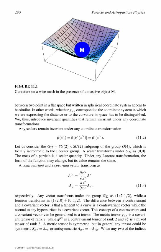
280 Particle and Astroparticle Physics
M
FIGURE 11.1Curvature on a wire mesh in the presence of a massive object M.
between two point in a flat space but written in spherical coordinate system appear to
be similar. In other words, whether gµν correspond to the coordinate system in which
we are expressing the distance or to the curvature in space has to be distinguished.
We, thus, introduce invariant quantities that remain invariant under any coordinate
transformations.
Any scalars remain invariant under any coordinate transformation
φ(xµ) = φ [xµ(x′ν)] = φ ′(x′ν). (11.2)
Let us consider the G22 = SU(2)× SU(2) subgroup of the group O(4), which is
locally isomorphic to the Lorentz group. A scalar transforms under G22 as (0,0).
The mass of a particle is a scalar quantity. Under any Lorentz transformation, the
form of the function may change, but its value remains the same.
A contravariant and a covariant vector transform as
A′µ =∂x′µ
∂xν Aν
A′µ =
∂xν
∂x′µAν , (11.3)
respectively. Any vector transforms under the group G22 as (1/2,1/2), while a
fermion transforms as (1/2,0) + (0,1/2). The difference between a contravariant
and a covariant vector is that a tangent to a curve is a contravariant vector while the
normal to any hypersurface is a covariant vector. This concept of a contravariant and
a covariant vector can be generalized to a tensor. The metric tensor gµν is a covari-
ant tensor of rank 2, while gµν is a contravariant tensor of rank 2 and gµν is a mixed
tensor of rank 2. A metric tensor is symmetric, but in general any tensor could be
symmetric Sµν = Sνµ or antisymmetric Aµν = −Aνµ . When any two of the indices
© 2008 by Taylor & Francis Group, LLC
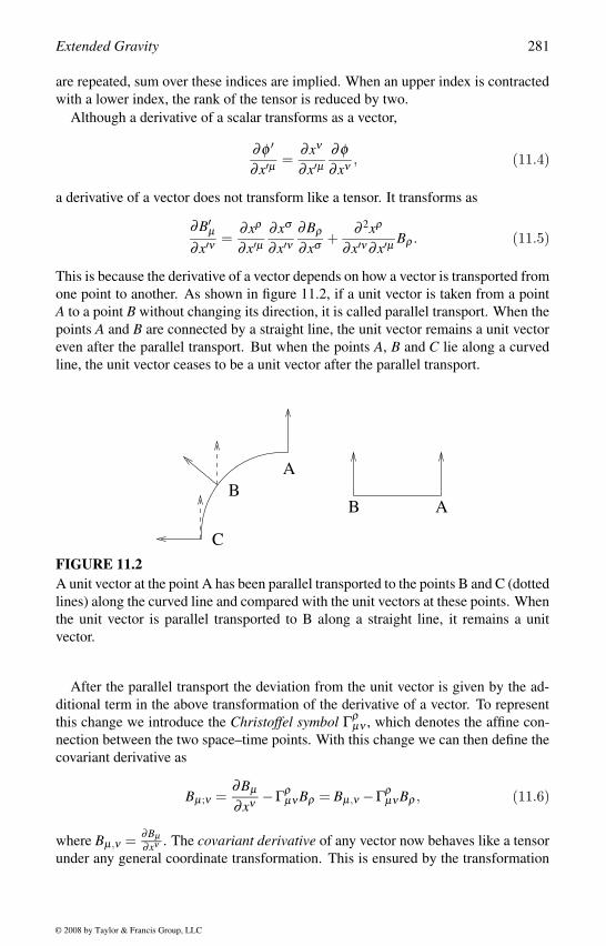
Extended Gravity 281
are repeated, sum over these indices are implied. When an upper index is contracted
with a lower index, the rank of the tensor is reduced by two.
Although a derivative of a scalar transforms as a vector,
∂φ ′
∂x′µ=
∂xν
∂x′µ∂φ∂xν , (11.4)
a derivative of a vector does not transform like a tensor. It transforms as
∂B′µ
∂x′ν=
∂xρ
∂x′µ∂xσ
∂x′ν∂Bρ
∂xσ +∂ 2xρ
∂x′ν ∂x′µBρ . (11.5)
This is because the derivative of a vector depends on how a vector is transported from
one point to another. As shown in figure 11.2, if a unit vector is taken from a point
A to a point B without changing its direction, it is called parallel transport. When the
points A and B are connected by a straight line, the unit vector remains a unit vector
even after the parallel transport. But when the points A, B and C lie along a curved
line, the unit vector ceases to be a unit vector after the parallel transport.
B
C
B
A
A
FIGURE 11.2A unit vector at the point A has been parallel transported to the points B and C (dotted
lines) along the curved line and compared with the unit vectors at these points. When
the unit vector is parallel transported to B along a straight line, it remains a unit
vector.
After the parallel transport the deviation from the unit vector is given by the ad-
ditional term in the above transformation of the derivative of a vector. To represent
this change we introduce the Christoffel symbol Γρµν , which denotes the affine con-
nection between the two space–time points. With this change we can then define the
covariant derivative as
Bµ;ν =∂Bµ
∂xν −Γρµν Bρ = Bµ,ν −Γρ
µν Bρ , (11.6)
where Bµ,ν = ∂Bµ∂xν . The covariant derivative of any vector now behaves like a tensor
under any general coordinate transformation. This is ensured by the transformation
© 2008 by Taylor & Francis Group, LLC
282 Particle and Astroparticle Physics
of the Christoffel symbol:
Γ′µνρ =
∂x′µ
∂xδ∂xσ
∂x′ν∂xπ
∂x′ρΓδ
σπ +∂ 2xπ
∂xν ∂xρ∂x′µ
∂xπ . (11.7)
The covariant derivatives of a contravariant vector and the covariant derivative of the
metric tensor are then given by
Aµ;ν =
∂Aµ
∂xν +Γµρν Aρ = Aµ
,ν +Γµρν Aρ ,
gµν ;ρ =∂gµν
∂xρ −Γσµρ gσν −Γσ
νρ gµσ . (11.8)
We can simplify these relations by working in a Riemannian space, in which it is
possible to have a locally inertial frame at any given point. Here we have
gµν ;ρ ≡ 0. (11.9)
The Christoffel symbol can now be expressed in terms of the metric tensor and of
ordinary derivatives of the metric tensor as
Γρµν =
1
2gρσ (gσ µ,ν +gσν ,µ −gµν ,σ
). (11.10)
The advantage of working in a Riemannian space is that it is always possible to go to
a locally inertial reference frame. This means that we can always go to a coordinate
system in the neighborhood of any point P, in which all the Christoffel symbols
vanish. At the point P the metric is given by the metric of a flat Minkowski space
ηmn = diag(+1,−1,−1,−1) . (11.11)
We now define another useful quantity, the vierbeins enµ , which relates the unit
vectors in the local inertial coordinate system with the unit vectors of the general
coordinate system. The metrics in the two coordinate systems are related by the
vierbeins through the relation
gµν emµ en
ν = ηmn. (11.12)
The inverse vierbeins emν is defined with the property
emµ em
ν = δ µν , (11.13)
so the inverse coordinate transformations become possible
gµν = emµ en
ν ηmn. (11.14)
All the information of a metric is, thus, contained in the vierbeins.
The vierbeins connect the general coordinate system to the locally flat inertial
coordinates, so they carry indices from both the coordinate system. We have to
define a new covariant derivative for the vierbeins
Dµ emν = em
ν ,µ −Γλµν em
λ +ωµm
nenν . (11.15)
© 2008 by Taylor & Francis Group, LLC
Extended Gravity 283
The covariant derivative now contain the spin-connection ωµm
n, which is a vec-
tor under the general coordinate transformations and also associated with the local
Minkowski space.
These spin-connections have some similarity with the gauge fields in gauge theo-
ries (Aiµ ). A gauge boson is a vector field that carries an index of the internal group.
For the spin-connection, the internal group is substituted by the local Lorentz group,
and hence, the indices m,n of the spin-connection replaces the group index i of the
gauge fields. We, thus, define a tensor under the general coordinate transformations,
analogous to the field-strength tensor of gauge theories
Rµνmn = ∂µ ων
mn −∂ν ωµmn +ωµ
mkων
kn −ωνm
kωµkn, (11.16)
where ωνmnηkn = ων
mk. This tensor is antisymmetric in µ,ν , so the symmetric
Christoffel symbols Γλµν = Γλ
νµ do not enter into this definition.
Various contractions of this tensor allow us to define some important tensors:
(a) Riemann–Christoffel curvature tensor:
Rµνρσ = Rµνmnemρ enσ , (11.17)
satisfying the symmetry relations
Rµνλρ = −Rνµλρ = −Rµνρλ = Rλρµν (11.18)
and
Rµνλρ +Rµρνλ +Rµλρν = 0. (11.19)
The curvature tensor also satisfies the Bianchi identity
Rµνλρ;σ +Rµνσλ ;ρ +Rµνρσ ;λ = 0. (11.20)
The important characteristics of the Riemann–Christoffel tensor is that it van-
ishes everywhere when the space–time is flat.
(b) Ricci tensor:
Rµν = Rλνmnen
λ emµ = gλρ Rλ µνρ = Rλµνλ
= ∂ν Γλµλ −∂λ Γλ
µν −Γσµν Γλ
σλ +Γλµσ Γσ
νλ . (11.21)
This is the only possible rank-2 tensor that could be constructed from the
Riemann–Christoffel tensor.
(c) Scalar curvature:
R = Rµνmnem
ν enµ = gµν Rµν = Rµ
µ . (11.22)
The scalar curvature appears in the equation of motion of the metric tensor.
© 2008 by Taylor & Francis Group, LLC
284 Particle and Astroparticle Physics
(d) Einstein tensor:
Gµν = Rµν − 1
2gµν R. (11.23)
The Bianchi identity implies vanishing of the covariant derivative of the Ein-
stein tensor
Gµν ;λ = 0 (11.24)
implying the Einstein tensor is divergence free.
Einstein Equation
The Einstein equation determines the metric and is given by the vanishing of the
Einstein tensor [173]
Gµν = Rµν − 1
2gµν R = 0. (11.25)
The corresponding Einstein action is given by [174]
S(E) =∫
d4x L (E) = −∫
d4xeR2κ2 , (11.26)
where
e = det(emλ ) = [det(em
λ )]−1 = [−det(gµν)]1/2, (11.27)
and κ2 = 8πGN , where GN = 6.67259(85)×10−11m3kg−1s−2 is the Newton’s grav-
itational constant.
In this form of the Einstein equation we have not included matter, which needs an
additional term proportional to the energy-momentum tensor Tµν . This will act as
a source in the Einstein equation. One more term could be included in the Einstein
equation: a constant may be added to the scalar curvature. This term has important
cosmological consequences, and hence, this constant Λ is called the cosmologicalconstant. Including all the terms the final form of the Einstein equation in the pres-
ence of matter and cosmological constant is given by
Gµν +Λgµν = Rµν − 1
2gµν R+Λgµν = −8πGNTµν . (11.28)
This is the most general equation that determines the metric or the geometry of
space–time in the presence of matter. The cosmological constant term does not af-
fect the gravitational interactions between two objects and hence this term was not
included in the original equation. Later Einstein included this term to find a static so-
lution of the universe. Although the observation of expanding universe ruled out the
possibility of static universe, we may still need the cosmological constant. Present
observations require about 70% of the total matter in the universe in the form of dark
energy or cosmological constant.
© 2008 by Taylor & Francis Group, LLC
Extended Gravity 285
Schwarzschild Solution
To understand the implications of the Einstein equation, we need to find exact solu-
tions with some ansatz. One of the interesting solutions of the Einstein equation, the
Schwarzschild solution [175], is used for many practical purposes. The space–time
geometry outside a spherical distribution of matter of mass M is given in the form of
a line element
ds2 =(
1− 2GNMR
)dt2 −
(1− 2GNM
R
)−1
dR2 −R2(dθ 2 + sin2 θ dφ 2). (11.29)
This line element determines the metric and hence the geometry of space–time out-
side the mass distribution.
This solution provides us with several interesting aspects of the general theory
of relativity. The characteristic scale of the general theory of relativity is given by
the Schwarzschild radius Rs = 2GNM, which is an important parameter in the the-
ory. The Schwarzschild radius Rs shows a singularity in the solution for any given
mass. For any compact object with radius smaller than Rs, the Schwarzschild solu-
tion shows that near the surface of such object the geometry is strongly curved and
even photons will be trapped inside such objects. Such objects are called black holes.
Another implication of the Schwarzschild radius is that it determines the scale
of quantum gravity. When the Schwarzschild radius becomes comparable to the
Compton wavelength of λ ∼ 1M , quantum effects cannot be neglected. This is called
the Planck scale, when the characteristic scales of the quantum theory (λ ) and the
general theory of relativity (R) become comparable,
MPl ∼ 1√GN
∼ 1019 GeV.
The corresponding length, the Planck length, and the time, the Planck time, are de-
fined as
LPl ∼√
GN ∼ 10−33 cm
tPl ∼√
GN ∼ 5×10−44 s.
To probe a distance scale smaller than the Planck length, the required kinetic energy
of the test particle should be greater than the Planck scale. At this scale, gravity
becomes strong and quantum uncertainty comes into the picture. This introduces a
restriction in our study of the early universe. Our lack of understanding of quan-
tum gravity does not allow us to understand the evolution of the universe before the
Planck time.
Tests of General Relativity
The general theory of relativity have been successfully tested by many experiments.
The simplest prediction is the bending of light. Since light propagates along a straight
line, if there is curvature in space due to a massive body, light will travel along the
© 2008 by Taylor & Francis Group, LLC
286 Particle and Astroparticle Physics
curved trajectory. This has been verified with differing accuracy at different times
[176, 177].
Newtonian mechanics also predicts a bending of light in a gravitational field. The
angle of deflection comes out to be
∆φN ≈ 2/e ≈ 2GM/c2rm,
where e is the eccentricity of the deflected path. For the light grazing the sun, this
gives φN = 0.875′′. On the other hand, for the light grazing the sun the general theory
of relativity predicted the deflection of light to be ∆φ = 1.75′′. Since light follows
the null geodesics, special theory of relativity does not predict any deflection of light.
During total eclipse of the sun, a measurement of positions of about 400 stars gives
an average deflection of light φ = 1.9′′.The gravitational red-shift of spectral lines measurement also supports the general
theory of relativity. Another important observation in support of the general theory
of relativity is the precession of the perihelion of Mercury [178]. According to the
Newtonian gravity, Mercury follows an elliptical path around the sun. But due to
other planets and stars, the orbit precesses. The Newtonian mechanics predicted
the precession of the perihelion (when the distance between the sun and Mercury is
minimum) of Mercury to be ∆φN = (5557.62± 0.20)′′ while the observed value is
∆φobs = (5600.73± 0.40)′′. The discrepancy of ∆φdis = (43.11± 0.45)′′ could be
explained by the general theory of relativity, which predicted ∆φ gtrdis = 43.03′′ for the
discrepancy.
Gravitational Radiation
The general theory of relativity describes the the gravitational interaction, and the
solution of the Einstein equation (equation (11.28)) gives the metric or the geometry
of space–time that contains the information about the gravitational interaction. The
traceless symmetric metric tensor gµν also includes the gravitational radiation, but
this is not transparent in the Einstein action as the quadratic kinetic energy term is not
present explicitly. For this purpose we shall now work with the action for linearized
Einstein gravity [179]. We first make the weak field approximation, which states
that the space is almost flat and the metric contains small fluctuations around the
Minkowski metric ηµν . This is expressed as
gµν = ηµν + k hµν , (11.30)
where |hµν | 1 and the factor k indicates that the mass dimension of hµν is 1. For
convenience we set k = 1. In one formulation, quantization of gravity makes similar
weak field approximation with the Minkowski metric as the vacuum and the pertur-
bation hµν corresponding to the quantum field mediating gravitational interaction–
the graviton.
Since the perturbation hµν is small, we keep only first order terms in hµν . This
will allow us to contract or raise or lower indices using ηµν . The linearized Einstein
© 2008 by Taylor & Francis Group, LLC
Extended Gravity 287
action can then be given by
S(E)L = −1
2
∫d4x(RL
µν −1
2ηµν RL)hµν , (11.31)
with the linearized Ricci tensor and the linearized curvature scalar given by
RLµν =
1
2
(∂ 2hµν
∂xλ ∂xλ− ∂ 2hλ
ν
∂xµ ∂xλ − ∂ 2hλµ
∂xν ∂xλ +∂ 2hλ
λ∂xµ ∂xν
)RL = ηµν RL
µν , (11.32)
where we retained terms only up to first order in hµν . The linearized Einstein equa-
tion including the cosmological constant and the energy-momentum tensor (Tµν ) for
the matter fields then becomes
RLµν −
1
2ηµν RL +Ληµν = −8πGNTµν . (11.33)
Since Tµν is independent of hµν to first order, it satisfies the condition
∂∂xµ T µ
ν = 0. (11.34)
We now demand that general coordinate transformations of any weak field should
leave the field weak, so after the general coordinate transformation the metric should
remain close to the Minkowski metric. This restricts the allowed general coordinate
transformations to the form
xµ → x′µ = xµ + εµ(x), (11.35)
where O(∂εµ/∂xν) <∼ hµν . This ensures that after the coordinate transformation, the
new fluctuation
h′µν = hµν − ∂εµ
∂xν − ∂εν∂xµ (11.36)
is also a solution, where εµ = εν ηµν are some small arbitrary functions of xµ .
We now work in the harmonic coordinate system utilizing the gauge freedom of
the linearized Einstein equation (11.33), which is defined as
gµν Γλµν = 0. (11.37)
The field equation then becomes
∂ 2hµν
∂xλ ∂xλ= −16πGN(Tµν − 1
2ηµν T λ
λ ) = −16πGNSµν , (11.38)
where Sµν is the source for the gravitational field hµν and the solution is a retarded
potential
hµν(x, t) = −4πGN
∫d3x′
Sµν(x′, t −|x−x′|)|x−x′| . (11.39)
© 2008 by Taylor & Francis Group, LLC
288 Particle and Astroparticle Physics
This is the gravitational radiation produced by the source Sµν , having two longi-
tudinal degrees of freedom like the photon, corresponding to the helicity ±2. The
quantum of the gravitational radiation, the graviton, can interact with itself due to
the nonlinearity in the Einstein equation making the general theory of relativity more
complex than any gauge theories.
If there is any radiation coming from infinity, that will satisfy the equations
∂ 2hµν
∂xλ ∂xλ= 0
∂∂xµ hµ
ν =1
2
∂∂xν hµ
µ (11.40)
and can be given by the plane wave solution
hµν(x) = eµν expikλ xλ+ e∗µν exp−ikλ xλ
, (11.41)
where the symmetric matrix eµν is the polarization tensor. This solution will add to
the retarded potential due to the source Sµν . The energy and momentum carried by
this plane wave coming from infinity is
tµν =1
8πGN[R(2)
µν −ηµν ηλρ R(2)λρ ], (11.42)
where R(2)µν is the second order term in the Ricci tensor in h2
µν . The first order terms
in h2µν cancel out since they satisfy the Einstein equation.
The Mach’s principle seeded the idea of gravitational radiation by stating that
the motions of local bodies are not independent of the influence from the rest of
the universe [180]. Analogy of gravitation and electromagnetism then implies that
the acceleration of the distant cosmic objects should produce gravitational waves
that will affect the motion of local matter. The Einstein equation demonstrates this
gravitational radiation mathematically and point out that this radiation carry energy.
Detection of gravitational radiation has been going on since its inception, but so far
we have not been able to detect the radiation. Earlier experiments tried to use small
mechanical or hydrodynamical resonant quadrupole antennas with natural mode of
free oscillation, while the present generations of detectors take into account possible
sources of the radiation and make use of the advancements in space technology.
11.2 Gravity in Higher DimensionsUnification of the gravitational interaction with the strong, weak and electromag-
netic interactions is the ultimate goal we have been aspiring. In this direction the
first consistent theory was the Kaluza–Klein theory [181]. In the Kaluza–Klein the-
ory the space–time dimensions have been extended to 5-dimensions with the ex-
pectation that the metric in 5-dimensions should contain the 4-dimensional metric
© 2008 by Taylor & Francis Group, LLC
Extended Gravity 289
as well as the gauge boson of the electromagnetic interaction. Since we know that
there are only four noncompact dimensions for consistency, the fifth dimension has
been assumed to be compact. The radius of compactification of the fifth dimension
is assumed to be extremely small, so our present energy probes will not be able to
see this extra dimensions. In this 5-dimensional theory of the general theory of rel-
ativity, the Einstein action describes all the interactions. After compactification the
effective theory will have the Einstein equation in 4-dimensions and the extra de-
grees of freedom of the 5-dimensional metric will contain the photon or the gauge
field corresponding to the U(1)Q gauge theory in 4-dimensions, which is the theory
of electromagnetic interaction. Higher-dimensional theories are required to accom-
modate the non-Abelian gauge interactions.
The Kaluza–Klein theory was not considered seriously for many years. However,
now we cannot think of unifying gravity with other interactions without extending
our theory to include new extra dimensions. Thus, the Kaluza–Klein theory now
forms the basis of many recent developments in the field.
Kaluza–Klein Theory
In the Kaluza–Klein theory [181] one starts with the theory of gravity in more than
three space and one time dimensions. The simplest case is a five-dimensional space–
time, where the fifth dimension is assumed to be a compact extra space dimension.
Since we have not seen the fifth dimension, we assume that it is compact with a
very small radius. The distance to which we could probe with our present energy
accelerators is larger than the radius of the compact fifth dimension and that is why
we have not been able to resolve the fifth dimension. In most theories we expect
the radius of the compact dimensions to be close to the Planck length of l ∼ GN ∼10−35m, so we may resolve them only when we reach the Planck energy scale of
MPl ∼ 1019 GeV.
The energy scale corresponding to the radius of the compact dimensions is also
called the scale of compactification. At energies below the compactification scale, it
will not be possible to resolve the extra dimensions and hence they will only appear
as points. However, the scaling invariance along the extra dimensions will mani-
fest itself as gauge invariance in some internal symmetry space. In general, when
we work in a (4 + n)-dimensional space, it correspond to a M4 ×K space, where
M4 is the usual 4-dimensional Minkowski space–time and K is the compactified n-
dimensional space [182]. In the present example, K is a one-dimensional space de-
noted by the coordinate y and the coordinate of the usual 4-dimensional Minkowski
space is represented by x. Since the fifth dimension is compact, the coordinate of the
fifth dimension must satisfy the boundary condition
y = y+2πr, (11.43)
where r is the radius of compactification, which gives the size of the compact space.
Although the simplest form of the compact space is a circle with radius r, in general
the shape of the compact space is irrelevant. As long as this boundary condition is
satisfied, the space is compact and its size is specified by r.
© 2008 by Taylor & Francis Group, LLC
290 Particle and Astroparticle Physics
This boundary condition will imply that any scalar field φ(x) should satisfy
φ(x,y) = φ(x,y+2πr) , (11.44)
which would then allow a Fourier series expansion of the field
φ(x,y) =∞
∑n=−∞
φn(x)expiny/r. (11.45)
The fact that the φn(x)expiny/r should be single-valued under y → y + 2πr implies
that the y component of the momentum of any state φn will be quantized and is of
the order of ∼ O(|n|/r). In 4-dimensions these states will represent physical states
or quantized excitations with momentum O(|n|/r).The physical spectrum of particles will now contain a zero-mode φ0, which cor-
responds to n = 0, and remain massless at this stage. All other states will be very
massive with mass of the order of 1/r ∼ Mc, where Mc is the compactification scale.
In the conventional theories this is taken to be around the Planck scale MPl ∼ 1019
GeV. Higher order excitations will have mass in multiples of the Planck mass. Thus,
all the particles we experience at present energies will have corresponding infinite
towers of Kaluza–Klein excitations above the compactification scale of Mc if the
theory originates from any higher-dimensional theories.
In any realistic Kaluza–Klein theory, the zero modes must contain the standard
model fermions, gauge bosons and the graviton. We shall now demonstrate that the
5-dimensional theory of gravity contains both the 4-dimensional graviton and a 4-
dimensional gauge boson corresponding to quantum electrodynamics. Let us start
with a line element in 5 dimensions:
ds2 = gMNdxMdxN = gµν dxµ dxν − (dy−κAµ(x)dxµ)2, (11.46)
where gMN ,M,N = 0,1,2,3,4 is the 5-dimensional metric; gµν ,µ,ν = 0,1,2,3 is
the 4-dimensional metric; and Aµ is a four vector. Any coordinate transformation in
the y direction will now appear as a gauge transformation that leaves the line element
invariant
xµ → xµ
y → y+Λ(x)gµν → gµν
Aµ(x) → Aµ(x)+1
κ∂µ Λ. (11.47)
Let us now include a complex scalar field (Φ) with mass µ . We assume that the field
satisfies the constraint
∂yΦ =ir
Φ . (11.48)
As we shall see, this would imply that the field behaves as a charged scalar, where
the charge is given in units of the couplings in the fifth dimension.
© 2008 by Taylor & Francis Group, LLC
Extended Gravity 291
The Lagrangian for the field is now given by
LΦ = e[
gµν Dµ ΦnDν Φn − (µ2 +n2
r2 )|Φn|2]
, (11.49)
where we define the gauge covariant derivative as
Dµ = ∂µ − iκr
Aµ . (11.50)
As mentioned earlier, the electromagnetic interaction comes out from the fifth di-
mension. Comparing with the usual gauge transformations of the quantum electro-
dynamics, we can see that the electric charge is given by
Qn =κr
, (11.51)
and the coordinate transformations in the fifth dimension become equivalent to a
U(1) gauge transformation in 4-dimensions.
The mass of the different Kaluza–Klein states are given by
m2n ∼ µ2 +
(nr
)2. (11.52)
Here µ 1/r is the mass parameter and gives the mass of the zero mode. If we start
with µ = 0, we find that the zero mode remains massless, while all other Kaluza–
Klein excitations have picked up mass in multiples of n/r. For any fermions, if the
zero modes belong to any chiral representations, only then can they remain massless
and protected by the chiral symmetry. Otherwise all the left-handed and right-handed
components would combine to make them massive with mass of the order of O(1/r).We now discuss the zero modes of the gauge fields and the metric.
We first assume∂gMN
∂y= 0 (11.53)
to get the zero modes of the metric and their field equations in 4-dimensions. The
Fourier transform of the 5-dimensional metric gMN can be written as
gMN(x,y) = ∑n
g(n)MN(x)expiny/r. (11.54)
Since the 4-dimensional metric gµν and the 4-dimensional gauge boson Aµ should
remain massless, they should belong to the zero mode of the 5-dimensional metric
g(0)MN . We parameterize the zero mode of the 5-dimensional metric g(0)
MN in terms of
gµν , Aµ and a scalar field φ as
g(0)MN = φ−1/3
(gµν +φAµ Aν φAµ
φAν φ
). (11.55)
© 2008 by Taylor & Francis Group, LLC
292 Particle and Astroparticle Physics
The field φ is called a dilaton field, since it appears as a scaling parameter in the
fifth dimension. Any higher-dimensional theory of gravity contains the dilaton field,
which may have some interesting phenomenological consequence as well.
If we now start with the Einstein’s action in 5-dimensions
S(5)(E) = − 1
κ25
∫d4xdye(5)R(5), (11.56)
in 4-dimensions the zero modes contain the 4-dimensional Einstein’s action, field
equations of the gauge fields, and the kinetic energy term of the dilaton field
S(5)(E) = S(E) −
e2κ2
∫d4x[
1
4φFµν Fµν +
1
6φ 2 ∂ µ φ∂µ φ]. (11.57)
Here Fµν is the field-strength tensor and κ is the four-dimensional gravitational
constant
Fµν = ∂µ Aν −∂ν Aµ
κ2 =κ2
5(2πr)
. (11.58)
The zero mode gauge fields Aµ remain massless due to the gauge invariance. Thus,
after integrating out all the heavy degrees of freedom from the theory, at low ener-
gies we find the 4-dimensional metric satisfying the Einstein equation, the massless
gauge bosons satisfying the field equations and maintaining gauge invariance of elec-
trodynamics, and the scalar dilaton field satisfying the Klein–Gordon equation. In
addition, if there are zero modes of scalars and fermions, they satisfy the usual field
equations.
Non-Abelian Gauge Theory in Higher Dimension
In the simplest Kaluza–Klein theory the general theory of relativity is extended to a
5-dimensional theory. The extra space dimension is then assumed to be compact so
5-dimensional metric can be expanded in terms of its harmonics. The zero mode of
the metric then contains the regular massless graviton, or the 4-dimensional metric
satisfying the Einstein equation. In addition the metric contains the vector bosons of
a U(1) gauge theory and a scalar field, the dilaton. Any translation along the fifth
dimension appears as a U(1) gauge transformation in 4-dimensions.
The next step in this approach is to consider more than 5-dimensions, so the com-
pactification leads to larger gauge groups, including non-Abelian gauge theories.
When the zero modes of the higher-dimensional metric are decomposed in terms
of the zero modes of the four-dimensional metric, the zero modes of the remain-
ing components become the gauge fields in four dimensions. For any non-Abelian
gauge theory, the gauge fields Aaµ ,a = 1, · · · ,n require 4m components of the higher-
dimensional metric, where m is determined by the isometry group, and the metric
of the compactified space depends on n as well. This will be possible in a 4 + m-
dimensional space.
© 2008 by Taylor & Francis Group, LLC
Extended Gravity 293
Let us consider a D = 4 + d-dimensional space M 4 ⊗K , where K is the com-
pact d-dimensional space and M 4 is the 4-dimensional Minkowski space. If the
radius of compactification is so small that an observer cannot resolve it, the observer
will find the space around him to be locally a Minkowski space M 4 and given by
a flat metric ηµν , µ,ν = 0,1,2,3. He will not know the existence of the extra di-
mensions. To ensure the validity of the equivalence principle, any transformations
in the local coordinate system should not affect the extra dimensions. On the other
hand, any fluctuations in the extra dimensions should not perturb our locally flat
space M 4. This means that K is orthogonal to M 4 and is a compact d-dimensional
manifold given by a metric gαβ (y), where the indices α,β = 4, · · · ,D run over the
d-dimensional space coordinates y ensuring causality. We can, thus, write the metric
of the D-dimensional space as
gMN =(
ηµν(x) 0
0 gαβ (y)
), (11.59)
where M,N are the D = 4+d-dimensional indices in the space M 4 ⊗K .
We now identify any transformations along the extra dimensions with the gauge
transformations in four dimensions, which will be restricted by the metric on K .
Given a particular manifold K in the d-dimensional space, the symmetry group for
the gauge transformations that can be generated in 4-dimensions is called the isome-try group of the manifold K . The isometry group is the group of transformations of
the coordinates yα , generated by the Killing vectors Kαa (y) of the manifold K , that
leave the metric of K unchanged.
Consider a group of transformations generated by the Killing vectors Kαa (y)
yα → y′α = yα +nk
∑a=1
εa(x)Kαa (y), (11.60)
where nk < d(d + 1) is the dimension of the isometry group of K . The Killing
vectors satisfy the Killing equations
∇α Kβa +∇β Kα
a = 0. (11.61)
The D-dimensional metric can then be parameterized as
gMN =
(gµν +gαβ Kα
a Aaµ Kβ
b Abν gαβ Kα
a Aaµ
gαβ Kβa Aa
ν gαβ
). (11.62)
Since any transformations generated by the Killing vectors should leave the metric
of the manifold invariant, the gauge bosons must transform as
Aaµ → Aa
µ +∂µ εa(x). (11.63)
These gauge bosons mediate the gauge interactions in 4-dimensions.
If we now try to get the standard model gauge groups from compactification of
some extra dimensions, then the isometry group of the required manifold K must
© 2008 by Taylor & Francis Group, LLC
294 Particle and Astroparticle Physics
contain the SU(3)c × SU(2)L ×U(1)Y gauge group. The lowest-dimensional man-
ifold that can have such isometry group to accommodate the standard model is a
7-dimensional manifold [183]. Thus, we need at least an 11-dimensional space to
accommodate the standard model gauge group. However, when we try to include the
quarks and leptons in any 11-dimensional theory, we encounter new problems.
In any odd-dimensional space, all fermion representations are vector-like, and af-
ter compactification they all acquires a mass of the order of the scale of compactifi-
cation, which is around the Planck scale. It can be proved in a general way that in
odd dimensions it is not possible to have any zero modes and there are no massless
fermions. This makes it difficult to construct any 11-dimensional Kaluza–Klein the-
ory, which can accommodate the standard model gauge group and the chiral fermions
that can give us the particle spectrum of the standard model.
Although the 11-dimensional Kaluza–Klein theory could not accommodate the
standard model, it demonstrated that higher-dimensional theories can treat gravity
and other gauge interactions in the same way. One natural extension of the theory
is to supersymmetrize the theory. In a supersymmetric theory of gravity, the super-gravity, all the gauge and scalar fields will have their fermionic superpartners, which
can remain massless after compactification. With this motivation, theories of super-
gravity were constructed in four and higher dimensions. We shall now discuss the
simplest case of N = 1 supergravity theory in four dimensions.
11.3 SupergravityWe discussed supersymmetry in chapter 9, where we did not consider the parameters
of supersymmetry transformation to be local. We also restricted ourselves to N = 1
supersymmetry generated by one spinorial operator Q. The minimal supersymmet-
ric standard model, which is also based on the N = 1 global supersymmetry, was
then discussed in chapter 10. However, if we intend to combine gravity with super-
symmetry, then we have to consider local supersymmetry or supergravity, where the
coefficients of the generators in the supersymmetry transformations are space–time
dependent [158].
We shall discuss only N = 1 supergravity generated by one spinorial operator Q.
The generators of supersymmetry now vary from point to point, generate local coor-
dinate system at different space–time points, and should include the general theory
of relativity. We first supersymmetrize the Einstein equation (equation (11.28)) of
the general theory of relativity. We include the fermionic superpartner Ψµ of the
spin-2 graviton, which is described by a traceless symmetric tensor gµν . The kinetic
energy for this spin-3/2 gravitino or the Rarita–Schwinger field Ψµ , which is a spinor
carrying a vector index, satisfies the Rarita–Schwinger Lagrangian [184],
LRS = −1
2εµνρσ Ψµ γ5γν Dρ Ψσ , (11.64)
© 2008 by Taylor & Francis Group, LLC
Extended Gravity 295
where εµνρσ is the totally antisymmetric tensor, with ε0123 = 1. The covariant
derivative (Dµ ) includes terms quadratic in the Rarita–Schwinger fields and is de-
fined by
Dµ = ∂µ − i4
ωµmnσmn, (11.65)
where
ωµmn = ωµmn +iκ2
4(Ψµ γmΨn + Ψmγµ Ψn − Ψµ γnΨm). (11.66)
To get the field equations of the gravitons, we expand the metric gµν around a flat
metric ηµν as
gµν = ηµν +κhµν , (11.67)
where κ makes the mass dimension of hµν to be 1, so it can describe the bosonic field
graviton. This expansion will linearize Einstein gravity [179], the Einstein action is
now replaced by the linearized Einstein action, and the vierbein is expressed in terms
of the graviton hµν .
The Lagrangian corresponding to this linearized Einstein action is now given by
L(E) = − eR2κ2 = − e
κ2 Rµνmnem
ν enµ . (11.68)
When this Lagrangian is combined with the Rarita–Schwinger Lagrangian of equa-
tion (11.64)
Lsugra = LRS +L(E), (11.69)
it becomes invariant under the on-shell local supersymmetry transformations,
δξ Ψµ =1
κDµ ξ (x) (11.70)
δξ emµ = − i
2κξ (x)γmΨµ . (11.71)
The spinorial field ξ (x) generates local supersymmetry.
We now introduce the auxiliary fields to close the algebra off-shell since the de-
grees of freedom for the fields emµ and Ψµ are different. These fields are: a scalar
S, a pseudoscalar P and an axial vector Aµ . These auxiliary fields will be eliminated
by the equations of motion. We can then define the complete Lagrangian as
L = LRS +L(E)−e3(S2 +P2 −A2
m), (11.72)
where Am = emµ Aµ . This completes the discussion on the supersymmetric gravity
multiplet.
To include the matter multiplet [158, 185], we start with the Wess–Zumino model
(equation (9.17)) and write the on-shell supersymmetric Lagrangian of a scalar φ and
a fermion ψ , given by
L = (∂µ φ ∗)(∂ µ φ)+ iψσ µ ∂µ ψ. (11.73)
© 2008 by Taylor & Francis Group, LLC
296 Particle and Astroparticle Physics
Under local supersymmetry transformation this Lagrangian is not invariant and there
is one additional term proportional to ∂µ ξ (x). This can be compensated by including
the Rarita–Schwinger field in combination with the energy-momentum tensor T µν .
But this is still not complete and the graviton field has to be included to compensate
the transformation of the Rarita–Schwinger field. After including all of these terms,
the final Lagrangian can be made invariant under local supersymmetry transforma-
tion, which is given by
L = − 1
2κ2 eR− 1
2εµνρσ Ψµ γ5γν Dρ Ψσ + e(∂µ φ ∗)(∂ µ φ)
+i2
eΨγµ Dµ Ψ− κ2
eΨµ φ(A− iγ5B)γµ Ψ
− iκ2
4εµνρσ Ψµ γν Ψρ A
↔Dσ B− κ2
4eΨγ5γµ ΨA
↔Dµ B
+four fermion quartic interaction terms, (11.74)
where the complex scalar φ has been written in terms of two real scalars,
φ =1√2(A+ iB). (11.75)
This is the local supersymmetric Lagrangian corresponding to the Wess–Zumino
model.
We can now follow the same procedure to construct a Lagrangian for the chiral
(Φ) and vector (V ) superfields, which is given by
L = LB +L ′ +LF , (11.76)
where the first term includes the interactions of the scalar fields and the kinetic energy
terms of the scalars and the gauge bosons; the second term includes the kinetic energy
terms for the Rarita–Schwinger spinor, the fermions, the gauginos and some non-
renormalizable terms; and the last term contains fermion Yukawa couplings, gaugino
couplings and all other remaining nonrenormalizable interactions.
For an explicit form of the Lagrangian, we first define the Kahler potential
G(φ ∗,φ) = J(φ ∗,φ)+ ln |W |2, (11.77)
where
J(φ ∗,φ) = −3ln(−K/3). (11.78)
Here K ≡ K(Φ†exp2gV ,Φ) is an arbitrary function of the chiral superfields (Φ) and
their conjugates (Φ†) and appears in the global supersymmetric Lagrangian. Since
gravity can induce nonrenormalizable terms, the global supersymmetric Lagrangian
is not necessarily renormalizable in any supergravity theory and is given by
LG = [K(Φ†exp2gV ,Φ)]D +[W (Φ)]F +[ fab(Φ)W αa Wαb]F +H.c. , (11.79)
where Waα = D2DαV a is the gauge field strength superfield and fab(Φ) = f R + i f I is
an arbitrary function of the superfields (with f Rab = Re fab; f I
ab = Im fab). Both K and
© 2008 by Taylor & Francis Group, LLC
Extended Gravity 297
f can now include nonrenormalizable terms. Interactions of the gauge bosons with
the chiral fields enter through the terms involving the vector superfield V .
Before we write the complete Lagrangian, we define the derivatives of the Kahler
potential as
Gi =∂G∂φi
Gi =∂G
∂φ i∗
Gij =
∂ 2G∂φi∂φ j∗ (11.80)
and define the inverse
(G−1)ijG
jk = δ i
k. (11.81)
In the unit of κ = 1 (which means all masses are in units of the Planck mass), the
different terms in the Lagrangian are then given by
LB
e= −1
2R+Gi
jDµ φiDµ φ j∗ + expG (3−Gi(G−1)ijG
j)−1
4f RabFaµν Fµν
b +i4
f IabFaµν Fµν
b
−g2
2(Re f−1
ab )Gi(Ta)i jφ jGk(Tb)klφl . (11.82)
L ′
e=
1
2eεµνσρ Ψµ γ5γν Dρ Ψσ +
1
4eΨµ γν Ψρ(GiDµνρ φi −GiDµνρ φ i∗)
+(
i2
GijΨiLγµ Dµ Ψ j
L +i2
ΨiLγµ Dµ φ jΨkL(−Gi jk +
1
2Gi
kG j)
+1√2
GijΨµLγν Dν φ i∗γµ Ψ jR
)− 1
2
∂ fab
∂φiΨiRσ µν Faµν λbL
+1
4f Rab(λaγµ Dµ λb + λaγµ σνρ Ψµ Fbνρ +GiDµ φiλaLγµ λbL)
− i8
f IabDµ(eλaγ5γµ λb)+H.c. (11.83)
LF
e=
1
2expG/2
(iΨµ σ µν Ψν − (Gi j +GiG j −Gi j
k (G−1)kl Gl)ΨiLΨ jR
+ i√
2GiΨµLγµ ψiL +1
2
∂ f ∗ab
∂φ j∗ (G−1) jkGkλaλb
)− i
2g(Gi(Ta)i jφ jΨµLγµ λaL −4Gi
j(Ta)ikφkλaRΨiL
+ Re f−1ab
∂ fbc
∂φkGi(Ta)i jφ jψkRλcL
)+H.c.
+four fermion quartic interaction terms, (11.84)
© 2008 by Taylor & Francis Group, LLC
298 Particle and Astroparticle Physics
where ψL and ψR are the left and right chiral components of the Majorana spinors
and we defined εαβγδ Dδ = Dαβγ . Although we presented the Lagrangian for com-
pleteness, it is too complicated to explain every term in details.
The global supersymmetric Lagrangian LG contains most of the low-energy in-
teractions. When supersymmetry is broken in the hidden sector, supersymmetry
breaking soft terms are introduced into the Lagrangian (see chapter 10) leaving the
low-energy theory renormalizable. This will ensure that there are no quadratic diver-
gent corrections even after supersymmetry breaking.
Although supersymmetry may be broken in the hidden sector at some intermediate
symmetry breaking scale, the scale of soft terms (µsusy) is of the order of TeV. As a
result the mass splitting among the superpartners is of the order of the µsusy and any
low-energy supersymmetry breaking effect will be of the same order of magnitude.
In any supergravity theory, when supersymmetry is broken the gravitino gets a mass,
m3/2 = expG/2. (11.85)
This sets the effective supersymmetry breaking scale at low-energy µsusy, and all soft
terms have the same mass parameter µsusy [158].
We shall now explain how the superHiggs mechanism breaks local supersymmetry
giving us the low-energy effective theory [158]. Consider a simple form of the Kahler
potential
G(φi,φ ∗i ) = φ iφ ∗
i + ln |W (φi)|2. (11.86)
The potential contained in the Lagrangian 11.82
V = expG[Gi(G−1)ijG
j −3] (11.87)
then becomes
V = expφ iφ∗i
[∣∣∣∣∂W∂φ i +φ ∗
i W∣∣∣∣2 −3|W |2
]. (11.88)
Since we are working in units of κ = 1, all masses are in units of Planck mass.
Any terms with mass dimension greater than 4 will be suppressed by powers of the
Planck mass. Neglecting these small terms this potential will reduce to the global
supersymmetric potential V = |∂W/∂φ i|2.
The hidden sector supersymmetry breaking through the superHiggs mechanism
introduces a chiral multiplet z, which is governed by the Polonyi potential [186]
W (z) = m2(z+β ) = m2z′. (11.89)
This potential breaks supersymmetry since V = |∂W/∂ z|2 = 0. To study the effect of
this supersymmetry breaking in the hidden sector on the ordinary matter, we consider
a superpotential involving the hidden sector field z and the matter field φi to be of the
form
W (z,φ i) = Wh(z)+Wo(φ i) .
© 2008 by Taylor & Francis Group, LLC
Extended Gravity 299
This gives the potential
V = exp(|z|2+|φi|2)
m4(∣∣1+ z′z∗
∣∣2 −3|z′|2)
+∣∣∣∣∂Wo
∂φ i +φ ∗i Wo
∣∣∣∣2 −3|Wo|2
.
(11.90)If we now assume that the vanishing of the cosmological constant before supersym-
metry breaking in the observable sector, the minimum of V must occur at V = 0.
This determines the vacuum expectation values z = a, Wo = bm2, and
m3/2 = expG/2 = |Wo|expz2/2 = bm2expa2/2. (11.91)
For Wo = 0, when ordinary matter is not included, a =√
3−1, b = 1, β = 2−√3,
and m ≈ (m3/2MPl)1/2 ≈ 1011 GeV for m3/2 ∼ 1 TeV.
To get the low-energy contributions we neglect all terms that are suppressed by
the Planck scale and then substituting the vevs of the hidden sector field z and hidden
sector superpotential Wh, we get
Ve f f = Pm4 +
∣∣∣∣∣∂Wo
∂φ i
∣∣∣∣∣2
+Vso f t , (11.92)
where P = [(1 + ab)2 − 3b2]expa2and Wo = expa2/2Wo. The cosmological constant
vanishes (not counting the contribution of the electroweak symmetry breaking scale)
for P = 0. The second term is the scalar potential coming from the global super-
symmetric theory, and the third term contains all the low-energy soft supersymmetry
breaking terms
Vso f t = m23/2|φ i|2 +m3/2
(∂Wo
∂φ i φ i +(a2 +ab−3)Wo +H.c.
). (11.93)
The soft terms contain only one mass parameter µsusy = m3/2. In this model of su-
pergravity, supersymmetry is broken in the hidden sector by the Polonyi potential,
which is communicated to the observable sector through supergravity interactions at
the Planck scale. Thus, the soft term has suppression by the Planck scale. At present
there does not exist any supersymmetry breaking mechanism in the observable sector
that is phenomenologically consistent. So, all the models that are studied at present
break supersymmetry in the hidden sector and the predictions of these models de-
pend on how the supersymmetry breaking in the hidden sector is mediated to the
observable sector. In all of these models low-energy theory contains only the soft
supersymmetry breaking contributions.
© 2008 by Taylor & Francis Group, LLC
300 Particle and Astroparticle Physics
11.4 Extended SupergravityThe gravitational interactions we encounter at present energies could be explained
by the general theory of relativity. All other known interactions could be explained
by the standard model, which is a gauge theory. One natural extension of gravity
to include the standard model interactions is the Kaluza–Klein theory, which is the
theory of gravity at higher dimensions. In the Kaluza–Klein theory, after compact-
ification of the extra dimensions, the higher-dimensional metric contains the usual
4-dimensional metric and also the gauge fields that can generate the gauge interac-
tions. Any translation in the extra dimensions would appear as gauge transforma-
tions in 4-dimensions. The isometry group of the compact manifold determines the
gauge groups in 4-dimensions. To accommodate the standard model gauge group
we require at least 11-dimensional space. However, in 11-dimensional space it is not
possible to have massless fermions after compactification because all representations
are vectorial. It is also extremely difficult to reproduce the standard model particle
spectrum starting from any 11-dimensional Kaluza–Klein theory.
The next step in this direction was to extend gravity to make it supersymmetric.
We start with a N = 1 local supersymmetric theory or a N = 1 supergravity theory.
All representations contain both fermions and bosons, and hence, accommodating
fermions is no longer a problem in this theory. All the soft terms have the same
origin, and gravitino mass is the only mass parameter that determines all supersym-
metry breaking effects. However, all the interactions are put in by hand and there is
no geometric origin of the interactions.
Considering the problems of the higher-dimensional Kaluza–Klein theory and 4-
dimensional N = 1 supergravity theory, one can now think of two possible exten-
sions of these theories. One possibility is to have a N = 1 supergravity theory in
11-dimensions, while the other alternative is to have N = n supersymmetry in 4-
dimensions. As we shall discuss later, both approaches lead to the same result. But
for the present let us discuss the two possibilities separately.
In an N = 1 supergravity theory in 11-dimensions, we start with only the graviton
supermultiplet. The fields in this theory are the components of the gravity supermul-
tiplet, which are the symmetric tensor gMN with 44 degrees of freedom, Rarita–
Schwinger spinor ψM with 128 degrees of freedom and an antisymmetric tensor
AMNP with 84 degrees of freedom. The 4-dimensional massless fermions can come
from the Rarita–Schwinger spinor fields in 11-dimensions. This theory has several
interesting features including the possibility of spontaneous compactification of D =11 to M 4 ⊗K . While the standard model gauge group SU(3)c × SU(2)L ×U(1)Ycan be extracted from the isometry group of a manifold if the manifold has at least
7-dimensions, another study of the extended supersymmetry reveals that for more
than 7 compact extra dimensions, the theory becomes inconsistent. Thus, the 11-
dimensional supergravity theory becomes a unique choice for higher dimensional
supersymmetric theory of gravity.
We will discuss in detail the N = 1 supersymmetry, which is generated by one
© 2008 by Taylor & Francis Group, LLC
Extended Gravity 301
spinorial operator Qα and its conjugate Qα . In general there could be more gener-
ators of supersymmetry Qaα ,a = 1, · · · ,n and their conjugates Qa
α ,a = 1, · · · ,n and
accordingly N = n supersymmetric theories may be constructed by these generators.
Let us now consider an N = 2 supersymmetric theory generated by two generators
Q1 and Q2 and their conjugates. These operators satisfy the algebra
Qaα ,Qb
β = εabεαβ Z
Qaα , Qb
β = δab(σ µ)αβ Pµ , (11.94)
where Z is called the central charge and commutes with Qaα , Qa
α and Pµ . We shall
discuss the simple case with Z = 0.
The lowest-dimensional multiplet of the N = 2 supersymmetry will contain more
particles than the lowest-dimensional multiplet of an N = 1 supersymmetry. Con-
sider a multiplet of an N = 2 supersymmetry. There will be a left-chiral N = 1
supermultiplet (Φ) and its conjugate right-chiral N = 1 supermultiplet (Φ), both be-
longing to the same representation of the N = 2 supermultiplet. If the components
of these superfields are written as
Φ ≡(
φψL
)and Φ ≡
(φ
ψR
),
then the generator of the N = 1 supersymmetry Q1 will transform these fields as
φ Q1↔ ψL, and φ Q1
↔ ψR. (11.95)
In the N = 2 supersymmetry the second spinor operator Q2 will act on the other
combinations
φ Q2↔ ψR, and φ Q2
↔ ψL, (11.96)
so the N = 1 superfields Φ and Φ become components of the same N = 2 scalar
superfield.
The lowest representation of the N = 2 supersymmetry contains both the left-chiral
and right-chiral superfields of the N = 1 supersymmetry. A scalar superfield of the
N = 2 supersymmetry contains both the left-handed fermions and the right-handed
fermions and their corresponding scalars, and there are no chiral multiplets. A vector
superfield of the N = 2 supersymmetry contains a vector and a scalar superfield of the
N = 1 supersymmetry. While the components of the vector and the scalar superfields
are related by Q1, the second supersymmetry generator of the N = 2 supersymmetry
Q2 relates the components of the vector superfield to the components of the scalar
superfield. Thus, the vector superfield of the N = 2 supersymmetry contains a vector,
two fermions and a scalar. The representations of the N = 2 supersymmetry are
The next higher supersymmetry is the N = 4 supersymmetry, which is generated
by four spinor operators, Qaα ,a = 1,2,3,4, and their conjugates. Let us consider
N = 2 superfields generated by the operators Q1 and Q2. A vector and a scalar N = 2
© 2008 by Taylor & Francis Group, LLC
depicted in figure 11.3.
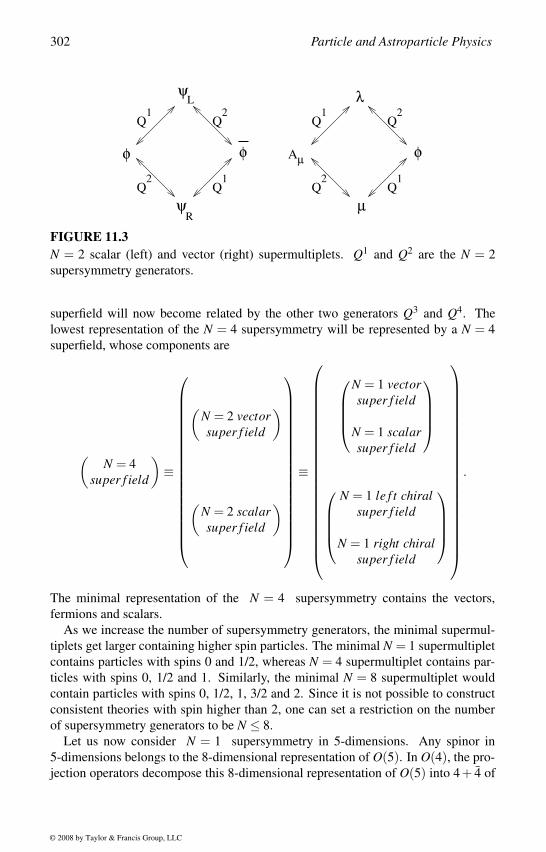
302 Particle and Astroparticle Physics
1
Q1
2Q
2Q
ψR
Q1
Q1
2Q
2Q
Q
L λ
Aµ
µ
φφφ
ψ
FIGURE 11.3N = 2 scalar (left) and vector (right) supermultiplets. Q1 and Q2 are the N = 2
supersymmetry generators.
superfield will now become related by the other two generators Q3 and Q4. The
lowest representation of the N = 4 supersymmetry will be represented by a N = 4
superfield, whose components are
(N = 4
super f ield
)≡
(N = 2 vectorsuper f ield
)
(N = 2 scalarsuper f ield
)
≡
N = 1 vectorsuper f ield
N = 1 scalarsuper f ield
N = 1 le f t chiral
super f ield
N = 1 right chiralsuper f ield
.
The minimal representation of the N = 4 supersymmetry contains the vectors,
fermions and scalars.
As we increase the number of supersymmetry generators, the minimal supermul-
tiplets get larger containing higher spin particles. The minimal N = 1 supermultiplet
contains particles with spins 0 and 1/2, whereas N = 4 supermultiplet contains par-
ticles with spins 0, 1/2 and 1. Similarly, the minimal N = 8 supermultiplet would
contain particles with spins 0, 1/2, 1, 3/2 and 2. Since it is not possible to construct
consistent theories with spin higher than 2, one can set a restriction on the number
of supersymmetry generators to be N ≤ 8.
Let us now consider N = 1 supersymmetry in 5-dimensions. Any spinor in
5-dimensions belongs to the 8-dimensional representation of O(5). In O(4), the pro-
jection operators decompose this 8-dimensional representation of O(5) into 4+ 4 of
© 2008 by Taylor & Francis Group, LLC
Extended Gravity 303
O(4). After compactification of the 5-dimensional space, the spinor operator of N =1 supersymmetry in 5-dimensions becomes two spinor operators in 4-dimensions
generating N = 2 supersymmetry. This implies that there is one-to-one correspon-
dence between a 4-dimensional N = 2 supersymmetry and a 5-dimensional N = 1 su-
persymmetry. In a more general way it has been shown that an 11-dimensional N = 1
supergravity theory has one-to-one correspondence with a 4-dimensional N = 8 su-
pergravity theory [187]. Since N > 8 supersymmetry is not consistent, D = 11 is the
highest-dimensional consistent supersymmetric theory. On the other hand, to accom-
modate the standard model gauge group, D = 11 is the lowest-dimensional theory.
This makes the 11-dimensional N = 1 supergravity theory unique.
As we mentioned earlier, one of the drawbacks of the 11-dimensional theory is
that it does not allow any chiral representations. The simplest modification to this
theory is to consider a 10-dimensional theory, which allows chiral representations.
However, by going to 10-dimensions we have to relax the condition of obtaining
the standard model gauge groups from the metric itself. The isometry group of the
10-dimensional theory does not allow the standard model gauge groups to emerge
from the 10-dimensional metric alone. In 10-dimensions, the graviton multiplet
now contains the metric gMN with 35 degrees of freedom, the 56-component left-
handed Majorana Rarita–Schwinger spinor ΨM , the 28-component antisymmetric
tensor BMN , the right-handed Majorana spinors λ with 8 degrees of freedom, and the
scalar dilaton field φ . The vector multiplet in 4-dimensions contains only 8 gauge
fields and 8 left-handed spinors, and the standard model gauge group cannot be in-
cluded. This problem has been addressed by introducing chiral and vector fields in
the 10-dimensional N = 1 supergravity theory. The vector fields in 10-dimensional
N = 1 supergravity theory will contain both the gauge bosons and the massless chiral
fermions in 4-dimensions, which can reproduce the standard model gauge group and
also the standard model particle spectrum.
Although this prescription to include the 10-dimensional gauge bosons in the the-
ory solves the problem of accommodating the standard model, the theory now con-
tains 10-dimensional gauge as well as gravitational anomalies. The hexagon loops
with fermions in the loop and gravitons at all the six external legs give the divergent
gravitational anomalies, while the gauge fermions in the loop introduce the gauge
anomalies. So, although the theory is consistent at the classical level, one-loop quan-
tum corrections will make it inconsistent. This problem of anomaly could be solved
in the superstring theory [188].
In a 10-dimensional superstring theory with the gauge group E8 ×E8 or a gauge
group SO(32), the gauge and the gravitational anomalies cancel. After compactifi-
cation in certain manifolds with SU(3) holonomy, these theories contain all known
fermions as the zero modes of the d=10 superstring theory [189]. Thus, the theory
reproduces the standard model interactions and the phenomenologically consistent
particle spectrum [190] and in some cases the Yukawa couplings could also be cal-
culated [191]. In addition to these phenomenological consistencies, the superstring
theory has many virtues. In recent times the duality conjectures and brane solutions
provided us many new possibilities. However, the most important feature of the su-
perstring theory is that it is now emerging as a successful theory of quantum gravity.
© 2008 by Taylor & Francis Group, LLC
304 Particle and Astroparticle Physics
KKSUGRAGUT
Gauge
Hierarchy
Problem
SUSY
Gravity
Extra
Dimensions
Standard
SUPERSTRING
Model
FIGURE 11.4Development of the superstring theory.
In summary, we started with the gauge theories of the standard model and the
general theory of relativity in 4-dimensions. To unify gauge interactions with grav-
ity, higher-dimensional Kaluza–Klein theory was developed. Unification of all the
gauge interactions could be achieved in the grand unified theories. The gauge hier-
archy problem of the grand unified theories could be solved by making the theory
supersymmetric, which also allows us to unify the Poincare group with the internal
symmetry groups. Gravity could be incorporated in these theories by making super-
symmetry transformations local, which is the supergravity theory. All of these con-
cepts of grand unification, Kaluza–Klein theory and supergravity could then be con-
sistently incorporated into the 10-dimensional superstring theory (see figure 11.4).
© 2008 by Taylor & Francis Group, LLC
12Introduction to Strings
There are four fundamental interactions in nature: the strong, weak, electromagnetic
and gravitational interactions. The first three of these interactions are explained as
gauge theories while the gravitational interaction is explained by the general theory
of relativity, classically. The superstring theory promises to be a unified theory of all
of these interactions at very high energy, when all the interactions become strong. It
is also emerging as a consistent quantum theory of gravity, which would ensure that
the ultimate unified theory is also a quantum theory of all the interactions.
The string theory replaces the point particles by objects, extended along one inter-
nal direction. Depending on the boundary conditions at the end-points of the strings,
there will be different vibrational modes of these strings. If the string tension is
too high about the Planck scale, the higher excited states cannot be created with our
present available energy. The infinite towers of particles corresponding to every par-
ticle we see are similar to the Kaluza–Klein excited states and decouple from our
low-energy world. Only the different massless zero modes of vibration will become
available to us as almost point particles. Let us draw an analogy with the musical
instruments for purpose of illustration. There are infinite towers of octaves. The first
diatonic scale may be identified with the massless zero modes, while the octaves will
correspond to excitations with mass of the order of the Planck scale. The different
tones in the diatonic scale will correspond to different particles we see at low energy.
Consider an ordinary string that is moving around us with its different points repre-
senting points in some internal degree of freedom. The two end-points should satisfy
certain boundary conditions. In an open string the end-points are fixed like the usual
musical instruments, while for a closed string the two end-points are identified with
each other. String theory can be consistently developed only in higher dimensions
that are also compactified near the Planck scale. At our present energies, all string
excitations as well as the Kaluza–Klein excitations will also disappear and we shall
be left with only a 4-dimensional theory with the standard model interactions.
Superstring theory is developing very fast and it is not possible to give any details
in this short chapter. So the idea of presenting this chapter is to provide familiarity
with some basic aspects of the theory, which will allow the reader to follow what is
going on in the subject, the phenomenological applications including the recent de-
velopments of models with extra dimensions, and some cosmological consequences.
305
© 2008 by Taylor & Francis Group, LLC
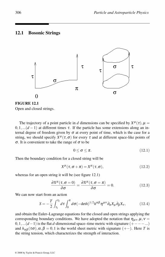
306 Particle and Astroparticle Physics
12.1 Bosonic Strings
0π
τ
σ
τ
τ
σ
στ
FIGURE 12.1Open and closed strings.
The trajectory of a point particle in d dimensions can be specified by X µ(τ),µ =0,1, ...(d − 1) at different times τ . If the particle has some extensions along an in-
ternal degree of freedom given by σ at every point of time, which is the case for a
string, we should specify X µ(τ,σ) for every τ and at different space-like points of
σ . It is convenient to take the range of σ to be
0 ≤ σ ≤ π. (12.1)
Then the boundary condition for a closed string will be
X µ(τ,σ +π) = X µ(τ,σ), (12.2)
whereas for an open string it will be (see figure 12.1)
∂X µ(τ,σ = 0)∂σ
=∂X µ(τ,σ = π)
∂σ= 0. (12.3)
We can now start from an action
S = −T2
∫ τ2
τ1
dτ∫ π
0dσ(−deth)1/2hαβ ηµν ∂α Xµ ∂β Xν , (12.4)
and obtain the Euler–Lagrange equations for the closed and open strings applying the
corresponding boundary conditions. We have adopted the notation that ηµν ,µ,ν =0,1, ...(d−1) is the flat d-dimensional space–time metric with signature (+−−− ...)and hαβ (τσ),α,β = 0,1 is the world sheet metric with signature (+−). Here T is
the string tension, which characterizes the strength of interaction.
© 2008 by Taylor & Francis Group, LLC
Introduction to Strings 307
Under the reparametrization (τ,σ) → (τ ′,σ ′) this action remains invariant and
we can exploit this freedom to choose our gauge to be a conformal gauge and then
use the Lorentz invariance and scale invariance to make hαβ = ηαβ , where ηαβ =diag(1, −1). We can write the equation of motion by varying the action with respect
to X µ and hαβ and applying boundary conditions to eliminate the surface terms. In
this covariant gauge the equation of motion becomes
∂σ ∂ σ X µ =(
∂ 2
∂τ2 − ∂ 2
∂σ2
)X µ = 0. (12.5)
In addition we have to satisfy a constraint equation given by the vanishing of the
energy-momentum tensor of the scalar fields X µ . In the conformal gauge the com-
ponents of the constraint equations are
T00 = T11 = −1
2(∂τ X µ ∂τ Xµ +∂σ X µ ∂σ Xµ) = 0
T01 = T10 = −∂τ X µ ∂σ Xµ = 0, (12.6)
where the indices 0 and 1 refer to τ and σ , respectively.
The general solutions for these wave equations can be expanded in terms of oscil-
lator coefficients, which can then be quantized for two different boundary conditions
of the closed and the open strings. The solution for the closed string can be separated
into two parts:
left-mover: where all terms depend on τ +σ
right-mover: where all terms depend on τ −σ .
The general solution then contains both the left-movers and the right-movers
X µ(τ,σ) = X µR (τ −σ)+X µ
L (τ +σ), (12.7)
where
X µR (τ −σ) =
1
2xµ +
1
2l2 pµ(τ −σ)+
i2
l ∑n=0
1
nαµ
n exp−2in(τ−σ)
X µL (τ +σ) =
1
2xµ +
1
2l2 pµ(τ +σ)+
i2
l ∑n=0
1
nαµ
n exp−2in(τ+σ) (12.8)
and l is the fundamental length scale, defined in terms of the string tension T by
l = (πT )−1/2.
The commutation relation for the center-of-mass coordinates (xµ ) and the momen-
tum (pµ ) of the string is given by
[xµ , pν ] = −iηµν . (12.9)
Similarly, commutation relation satisfied by the oscillators are
[αµm ,αν
n ] = −mδm+n,0ηµν
[αµm , αν
n ] = −mδm+n,0ηµν
[αµm , αν
n ] = 0. (12.10)
© 2008 by Taylor & Francis Group, LLC
308 Particle and Astroparticle Physics
The Hamiltonian in the covariant gauge
H = −T2
∫ π
0dσ(∂τ X µ ∂τ Xµ +∂σ X µ ∂σ Xµ) (12.11)
may now be expressed in terms of the oscillator coefficients in the mode expansion
as
H = −1
2∑n=0
(αµ−nαµn + αµ
−nαµn)− l2
2pµ pµ . (12.12)
We shall now discuss the constraint equations.
The independent constraints equations can be written by defining the new combi-
nations
T±± ≡ 1
2(T00 ±T01) = −1
4(∂τ X µ ±∂σ X µ)(∂τ Xµ ±∂σ Xµ) = 0, (12.13)
where T++ depends only on X µL (τ + σ), while T−− depends only on X µ
L (τ −σ). If
we now Fourier transform these quantities, we can write the Virasoro operators as
Lm =T2
∫ π
0dσ exp2im(τ−σ)T−− = −1
2
∞
∑n=−∞
αµm−nαµn
Lm =T2
∫ π
0dσ exp2im(τ+σ)T++ = −1
2
∞
∑n=−∞
αµm−nαµn,
where we defined αµ0 = αµ
0 = (l/2)pµ .
Acting on the physical states, these constraint equations give the conditions
Lm|φ〉 = Lm|φ〉 = 0 m > 0, (12.14)
and for m = 0, these conditions become
L0|φ〉 = 0 =⇒[−1
2αµ
0 αµ0 −∞
∑n=1
αµ−nαµn
]|φ〉 = a|φ〉
L0|φ〉 = 0 =⇒[−1
2αµ
0 αµ0 −∞
∑n=1
αµ−nαµn
]|φ〉 = a|φ〉 .
(12.15)
The constant a is infinite, but proper renormalization will allow us to choose a = 1.
The algebra satisfied by the Virasoro operators Lm is known as the Virasoro alge-bra
[Lm,Ln] = (m−n)Lm+n +b(m)δm+n,0, (12.16)
where the constant b(m) is called the conformal anomaly and is obtained by normal-
ordering when m+n = 0. Similarly the left-mover part of the Virasoro algebra comes
out to be exactly similar with Lm replaced by Lm. The algebra is completed by
[Lm, Ln] = 0. (12.17)
© 2008 by Taylor & Francis Group, LLC
Introduction to Strings 309
The conformal anomaly comes out to be b(m) = (D/12)m(m2 − 1). This theory
becomes consistent in D = 26 and a = 1.
The Hamiltonian is now given by the Virasoro operator L0
H = L0,
and the masses of the physical states are then obtained from the condition L0|φ〉 = 0
and are given in units of l = 1 by
1
4M2
R = −∞
∑n=1
αµ−nαµn −a
1
4M2
L = −∞
∑n=1
αµ−nαµn −a
M2 = M2L +M2
R = 2M2L = 2M2
R . (12.18)
The masses of the different states receive equal contributions from the left-movers
and the right-movers because L0|φ〉 = L0|φ〉.For the open string the general solution to the wave equation is given by
X µ(τ,σ) = xµ + l2 pµ(τ)+ il ∑n=0
1
nαµ
n exp−inτ cos(nσ). (12.19)
In this case the decomposition into left-movers or right-movers is not justified. The
nonzero commutators are now given by
[xµ , pν ] = −iηµν
[αµm ,αν
n ] = −mδm+n,0ηµν . (12.20)
The Hamiltonian now takes the form,
H = −1
2∑n=0
αµ−nαµn − l2
2pµ pµ . (12.21)
We can now construct the Virasoro algebra from the equation of constraints, follow-
ing the same prescription as in the case of closed strings.
Proceeding in the same way we can now write the masses of the physical states in
units of l = 1, which are
1
2M2 = −
∞
∑n=1
αµ−nαµn −a. (12.22)
As previously the infinite contribution a is chosen to be 1, after proper renormaliza-
tion. Exploiting the remaining freedom, we work in the light cone gauge. In this
gauge it is possible to find an expression for a, which after regularization gives
a =d −2
24. (12.23)
© 2008 by Taylor & Francis Group, LLC
310 Particle and Astroparticle Physics
For the choice of a = 1, we then get d = 26. In a more rigorous treatment it can
be shown that the consistency of the quantum theory also requires that the bosonic
strings are formulated in 26-dimensions only. In any other dimensions the confor-
mal invariance and the Lorentz invariance will be destroyed by an anomaly in the
quantum theory [188].
12.2 SuperstringsIn the superstring theory, we extend the bosonic string theory to include the fermions
and then ensure supersymmetry in the world sheet. Similar to the d-dimensional
scalar field X µ we include a d component two-dimensional Majorana spinor field
Ψµ in the action. Observing that the scalar X µ couples to two-dimensional gravity,
we expect that the spinor Ψµ would form a world-sheet supersymmetry that can then
couple to two-dimensional supergravity. This is possible with the Lagrangian
S = − 1
2π
∫dτdσ(−deth)1/2(hαβ ∂α X µ ∂β Xµ + iΨµ ρα ∂α Ψµ), (12.24)
where α = 0,1 are the world-sheet coordinates. The world-sheet gamma matrices
are given by
ρ0 =(
0 −ii 0
)ρ1 =
(0 ii 0
)and ρα ,ρβ = 2ηαβ I, (12.25)
where ηαβ = diag(+1, −1) and I is the 2×2 unit matrix. This Lagrangian possesses
a world-sheet supersymmetry, generated by
δX µ = ξ Ψµ
δΨµ = −iρα ∂α X µ ξ , (12.26)
but there is no space–time supersymmetry. However, in the final consistent theory
when the problem of tachyonic states is solved by applying projections of the states,
the theory possesses space–time supersymmetry.
To include gravity we now make the supersymmetry transformation local ξ ≡ξ (τ,σ). The algebra will close only after we include the supergravity gravitino
χα and the graviton hαβ fields, define their transformation properties, and include
their action in the Lagrangian. This world-sheet supergravity theory can be consis-
tently defined only in d = 10, satisfying the criterion of cancellation of the conformal
anomaly.
We proceed in the same way as in the bosonic strings. Making use of the confor-
mal invariance and reparametrization invariance to choose hαβ = ηαβ , we can write
the Euler–Lagrange equations as
∂α ∂ α X µ = 0
iρα ∂α Ψµ = 0. (12.27)
© 2008 by Taylor & Francis Group, LLC
Introduction to Strings 311
We now give the boundary conditions for the open and closed strings independently.
For the open strings the boundary conditions for the fermions are
ΨµL (τ,σ = 0) = Ψµ
R(τ,σ = 0)Ψµ
L (τ,σ = π) = ±ΨµR(τ,σ = π), (12.28)
where we have written
Ψµ =(
ΨµR(τ −σ)
ΨµL (τ +σ)
). (12.29)
The components satisfy the equations(∂
∂τ+
∂∂σ
)Ψµ
R = 0(∂
∂τ− ∂
∂σ
)Ψµ
L = 0. (12.30)
These boundary conditions ensure that the surface terms vanish to give us the equa-
tions of motion. In addition we have to consider the constraints coming from the
vanishing of the energy-momentum tensor Tαβ for X µ and Ψµ and the world-sheet
supercurrent Jα , where
Tαβ = −∂α X µ ∂β Xµ − i4
Ψµ(ρα ∂β +ρβ ∂α)Ψµ
+ηαβ
2(∂ γ X µ ∂γ Xµ +
i2
Ψµ ργ ∂γ Ψµ)
Jα =1
2ρβ ρα Ψµ ∂β Xµ . (12.31)
Similar to the Virasoro algebra, the Fourier transforms of certain combinations of
these quantities define the super-Virasoro algebra.
The boundary conditions for the closed strings can now be defined as
ΨµL,R(τ,σ +π) = ±Ψµ
L,R(τ,σ). (12.32)
We can now choose the boundary conditions for the left-movers and right-movers
independently. For both left-movers and right-movers we can have two choices of
periodic and antiperiodic boundary conditions. The periodic boundary condition,
given by +, is called the Ramond boundary conditions [192] (denoted by R) and the
antiperiodic boundary condition, given by −, is called the Neveu–Schwarz boundary
conditions [193] (denoted by NS).
We shall now concentrate mostly on the closed strings, which are phenomeno-
logically more promising. However, since some recent developments with brane
solutions make use of the open strings, we shall also mention the open strings in
the beginning. The mode expansions for the left- and the right-movers of the open
strings are not independent of each other. Both the left-movers and the right-movers
should be either periodic (R) or antiperiodic (NS) over a range 0 to π of σ . For the
© 2008 by Taylor & Francis Group, LLC
312 Particle and Astroparticle Physics
periodic (R) and antiperiodic (NS) boundary conditions, the mode expansions for the
open strings are given by
ΨµRL(R) =
1√2
∑n
dµn exp−in(τ∓σ)
ΨµRL(NS) =
1√2
∑r
bµr exp−ir(τ∓σ), (12.33)
where n = 1,2, ... are integers and r = 1/2,3/2, ... are half-integers. The anticom-
mutation relations of the fermions now give the quantization conditions
dµm,dν
n = −δm+n,0ηµν
bµr ,bν
s = −δr+s,0ηµν , (12.34)
where m,n are integers and r,s are half-integers. The superstring Hamiltonian for the
Ramond (R) and Neveu–Schwarz (NS) boundary conditions can now be written as
H(R) = −1
2pµ pµ − 1
2∑n=0
αµ−nαµn − 1
2∑n
ndµ−ndµn
H(NS) = −1
2pµ pµ − 1
2∑n=0
αµ−nαµn − 1
2∑r
rbµ−rbµr. (12.35)
Finally we can write the mass-squared operators
1
2M2(R) =
∞
∑n=1
ndµ−ndnµ −aR
1
2M2(NS) =
∞
∑r=1/2
rbµ−rbrµ −aNS, (12.36)
which contain the bosonic part and the fermionic part for the R and the NS boundary
conditions. The constant aR vanishes for the R sector because there is exact cancella-
tion of the fermionic and the bosonic contributions. For the NS sector, it comes out to
be aNS = (d−2)/16. For the cancellation of conformal anomaly and the consistency
of the quantum theory, the superstring theory can be defined only in d = 10, so we
get aNS = 1/2.
The left-movers and the right-movers for a closed string are distinct, and we have
to write the mode expansion for each of them separately for the periodic and antiperi-
odic boundary conditions, which are
ΨµR(R) = ∑
ndµ
n exp−2in(τ−σ)
ΨµR(NS) = ∑
r=n+1/2bµ
r exp−2ir(τ−σ)
ΨµL (R) = ∑
ndµ
n exp−2in(τ+σ)
ΨµL (NS) = ∑
r=n+1/2bµ
r exp−2ir(τ+σ), (12.37)
© 2008 by Taylor & Francis Group, LLC
Introduction to Strings 313
where n are integers and r are half-integers. The anticommutation relations of the
fermionic oscillators for the left-movers and right-movers are given by
dµm,dν
n = dµm, dν
n = −δm+n,0ηµν
bµr ,bν
s = bµr , bν
s = −δr+s,0ηµν . (12.38)
The Hamiltonians for the Ramond and the Neveu–Schwarz boundary conditions can
be given in terms of the fermionic oscillators of the mode expansions by
H(R) = −1
2pµ pµ − ∑
n=0(αµ
−nαµn + αµ−nαµn)
−∑n
n(dµ−ndµn + dµ
−ndµn)
H(NS) = −1
2pµ pµ − ∑
r =0(αµ
−rαµr + αµ−rαµr)
−∑r
r(bµ−rbµr + bµ
−rbµr). (12.39)
Vanishing of the energy-momentum tensor T αβ and the world sheet supercurrent
Jα will then give the constraint equations and the mass spectrum. These constraint
equations can be written in the covariant gauge as
T00 = T11 = 0, T10 = T01 = 0, J0 = 0 and J1 = 0.
The 0 and 1 in the subscript correspond to the σ and τ directions. We can now write
the independent constraint equations as
T±± =1
2(T00 ±T01) = −∂±X µ
LR
∂±Xµ LR− i
2Ψµ
LR
∂±Ψµ LR
= 0
J± = ΨµLR
∂±Xµ LR
= 0, (12.40)
with ∂± = (∂τ ±∂σ )/2.
The super-Virasoro operators can now be defined by taking the Fourier transforms
of T∓∓ as
Lm =1
2π
∫ π
0dσ exp2im(τ−σ) T−− m = 0
Lm =1
2π
∫ π
0dσ exp2im(τ+σ) T++ m = 0 . (12.41)
For the R sector we can Fourier transform J∓ and define
Fm =1
2π
∫ π
0dσ exp2im(τ−σ) J− m = 0
Fm =1
2π
∫ π
0dσ exp2im(τ+σ) J+ m = 0, (12.42)
© 2008 by Taylor & Francis Group, LLC
314 Particle and Astroparticle Physics
where m is an integer. Similarly we define for the NS sector
Gr =1
2π
∫ π
0dσ exp2ir(τ−σ) J−
Gr =1
2π
∫ π
0dσ exp2ir(τ+σ) J+, (12.43)
where r is half-integer.
These quantities can now be expressed in terms of the oscillators of the mode
expansion for the periodic and antiperiodic boundary conditions separately. For the
right-mover fermionic degrees of freedom, these operators are given for the NS and
R sectors by
Lm(NS) = −1
2∑n
αµm−nαµn +
1
2∑r
(m2− r)bµ
m−rbµr m = 0
Lm(R) = −1
2∑n
αµm−nαµn +
1
2∑n
(m2−n)dµ
m−ndµn m = 0
Gr(NS) = −1
2∑n
bµr−nαµn
Fm(R) = −1
2∑n
dµm−nαµn, (12.44)
where r is half integer and n is integer. For the left-movers these quantities are
obtained by replacing all of the operators with their corresponding tilde operators,
including the oscillators of the mode expansion.
For m = 0 we define for the right-movers and the left-movers
L0 =1
2π
∫ π
0dσ T−− and L0 =
1
2π
∫ π
0dσ T++. (12.45)
For the right-movers these operators can be written in terms of the mode expansion
oscillators in the NS and R sectors as
L0(NS) = −1
2∑n
αµ−nαµn − 1
2∑r
rbµ−rbµr
L0(R) = −1
2∑n
αµ−nαµn − 1
2∑n
ndµ−ndµn. (12.46)
In the same way we can write these operators for the left-movers by replacing the
operators and the oscillators with their corresponding tilde operators and oscillators.
The super-Virasoro algebra, given by the commutation relations of the Virasoro
operators, for the right-movers in the NS sector is given by
[Lm,Ln] = (m−n)Lm+n +D8
(m3 −m)δm+n,0
[Lm,Gr] = (m2− r)Gm+r
Gr,Gs = 2Lr+s +D8
(r2 − 1
4)δr+s,0 . (12.47)
© 2008 by Taylor & Francis Group, LLC
Introduction to Strings 315
For the right-movers in the R sector it is
[Lm,Ln] = (m−n)Lm+n +D8
m3δm+n,0
[Lm,Fn] = (m2−n)Fm+n
Fm,Fn = 2Lm+n +D8
m2δm+n,0. (12.48)
We are not writing the super-Virasoro algebra for the left-movers, which can be
obtained by replacing the operators by the tilde operators.
We can now write the Hamiltonian as
H = 2(L0 + L0). (12.49)
The physical states for both the NS and R sectors should now satisfy the constraint
equations
Lm|φ〉 = 0 for (m > 0) and L0|φ〉 = 0. (12.50)
The NS and R sectors should also satisfy further constraints
Gr|φ〉 = 0 (r > 0) Fm|φ〉 = 0 (m > 0). (12.51)
There exist similar constraints for the left-movers.
The mass-squared operators turn out to be the same for the left-movers and for the
right-movers. From these constraints we can write the mass-squared operators as
M2 = M2L +M2
R = 2M2L = 2M2
R. (12.52)
For the Ramond and Neveu–Schwarz boundary conditions, the mass-squared opera-
tors for the left-movers and right-movers are given by
1
4M2
R(NS) = −∞
∑n=1
αµ−nαµn −
∞
∑r=1/2
rbµ−rbrµ −aNS
1
4M2
R(R) = −∞
∑n=1
αµ−nαµn −
∞
∑n=1
ndµ−ndnµ −aR
1
4M2
L(NS) = −∞
∑n=1
αµ−nαµn −
∞
∑r=1/2
rbµ−rbrµ −aNS
1
4M2
L(R) = −∞
∑n=1
αµ−nαµn −
∞
∑n=1
ndµ−ndnµ −aR . (12.53)
Similar to the open strings the consistency condition for the cancellation of the
conformal anomaly requires d = 10 and the constants then become aR = 0 and
aNS = 1/2.
In the covariant gauge, where the world-sheet gravitino has been gauged away, it
is still possible to eliminate some more degrees of freedom utilizing the freedom to
© 2008 by Taylor & Francis Group, LLC
316 Particle and Astroparticle Physics
reparameterize the world-sheet and local Weyl scaling. This will finally give us the
physical states. For this purpose we work in the light-cone gauge, where we choose
X+(τ,σ) =1√2(X0 +XD−1) = x+ + p+τ, (12.54)
where x+ and p+ are constants. For the fermionic fields we consider the world-sheet
supersymmetry transformation, which allows us to choose
Ψ+ =1√2(Ψ0 +ΨD−1) = 0. (12.55)
The field
X−(τ,σ) =1√2(X0 −XD−1) and Ψ− =
1√2(Ψ0 −ΨD−1)
can then be expressed in terms of the transverse degrees of freedom X i and Ψi, i =1,2, ...,(D−2), leaving only the X i and Ψi as the physical degrees of freedom.
We now consider only the physical fields to write the mass-squared operators.
In terms of the mode expansion parameters of the physical fields the mass-squared
operators are now given by
M2 = M2R +M2
L = 2M2L = 2M2
R
1
4M2
R(R) =∞
∑n=1
α i−nα i
n +∞
∑n=1
ndi−ndi
n
1
4M2
L(R) =∞
∑n=1
α i−nα i
n +∞
∑n=1
ndi−ndi
n
1
4M2
R(NS) =∞
∑n=1
α i−nα i
n +∞
∑r=1/2
rbi−rb
ir −
1
2
1
4M2
L(NS) =∞
∑n=1
α i−nα i
n +∞
∑r=1/2
rbi−rb
ir −
1
2, (12.56)
where i = 1,2, ...8. As previously, R and NS correspond to the Ramond and Neveu–
Schwarz boundary conditions.
The physical states in the light-cone gauge are now given by α i−ndi−n|0 >R or
α i−nbi−r|0 >R for the right-movers, multiplied by α i−ndi−n|0 >L or α i−nbi−r|0 >L for
the left-movers. Combining the left-movers and right-movers, there are now four
types of states:
(R)− (R) : α i−ndi
−n|0 >R α i−ndi
−n|0 >L
(R)− (NS) : α i−ndi
−n|0 >R α i−nbi
−r|0 >L
(NS)− (R) : α i−nbi
−r|0 >R α i−ndi
−n|0 >L
(NS)− (NS) : α i−nbi
−r|0 >R α i−nbi
−r|0 >L . (12.57)
© 2008 by Taylor & Francis Group, LLC
Introduction to Strings 317
The ground state for the (R)− (R) case is a massless boson state, while for the
(NS)−(NS) case the ground state is a tachyon and original supersymmetry is broken.
The ground states for the mixed states have massless spinors.
The (NS)− (NS) Neveu–Schwarz sector ground state now becomes tachyonic,
since M2L = M2
R = −1/2. We can now apply the GSO projection (due to Gliozzi,
Scherk and Olive [194]) to the states of the theory, remove the problem of tachy-
onic states, and simultaneously restore d = 10 supersymmetry. The GSO projection
operators are given by
PNS =(1+(−1)FNS+1)
2
PR =(1+η(−1)FR+1)
2, (12.58)
where the number operators for the left- and right-movers in the Neveu–Schwarz and
the Ramond sectors are given by,
FLNS =
∞
∑r=1/2
bi−rb
ir
FRNS =
∞
∑r=1/2
bi−rb
ir
FLR =
∞
∑n=1
di−ndi
n
FRR =
∞
∑n=1
di−ndi
n. (12.59)
In terms of the GSO projections there are now three types of string theories, which
are classified as:
Type IIA: This is a closed string theory and has opposite values of η for the left- and
right-movers in the definition of the GSO projection operator for the Ramond
sector PR. The theory has N = 2 supersymmetry and the ground state contains
an N = 2 supermultiplet. There are no chiral multiplets. The massless particles
include an N = 2 supergravity multiplet at 10 dimensions.
Type IIB: This is also a closed string theory, but has the same value of η for the
left- and right-movers in the definition of the GSO projection operator PR.
The theory has N = 2 supersymmetry, but the massless states contain chiral
multiplets.
Type I: This contains both closed and open strings and have some similarity with
type IIB. However, in this case the string is not orientable, i.e., it is symmetri-
cal under the exchange σ →−σ . In this case the theory has only N = 1 super-
symmetry and the massless states contain chiral multiplets and the graviton.
© 2008 by Taylor & Francis Group, LLC
318 Particle and Astroparticle Physics
The vector multiplets come from the closed and open string sectors, respec-
tively. Perturbation is more complicated in this case, since it is unoriented and
breakable.
None of these three types of the string theories can accommodate any internal
gauge groups in addition to the multiplets they contain. Since the N = 1 and N =2 supergravity multiplets in 10-dimensions are insufficient to include the particle
spectrum of the standard model as well as the standard model gauge group, attempt
is made to construct heterotic strings [195]. In the heterotic strings it will be possible
to include a gauge group at 10-dimensions.
12.3 Heterotic StringThe heterotic string theory uses the right-movers of type II superstring theory and
the left-movers of closed bosonic strings [195]. The right-movers then become 10-
dimensional, whereas the left-movers become 26-dimensional. To match the two di-
mensions, the 16-extra dimensions of the left-movers are compactified, which gives
the stringy gauge fields and generates the non-Abelian gauge group. Once the new
gauge symmetry is generated, the superpartners of the corresponding gauge bosons,
the gauginos, will participate in the gauge and gravitational anomaly. The cancel-
lation of the gauge and the gravitational anomalies then restricts the gauge group to
either an SO(32) or an E8 ×E8. The latter group is found to be phenomenoloically
more attractive [190].
Compactification of Closed Bosonic Strings
We shall first discuss about some relevant features of compactification of closed
bosonic strings and then come back to the construction of a heterotic string theory.
We start with a closed bosonic string and compactify one of the dimensions on a
circle of radius R along the direction d = 25. The mode expansions of the left-movers
and the right-movers of the usual noncompact 25 dimensions X µ ,µ = 0,1, ..24 are
X µR (τ −σ) =
1
2xµ +
1
2pµ(τ −σ)+
i2
l ∑n=0
1
nαµ
n exp−2in(τ−σ)
X µL (τ +σ) =
1
2xµ +
1
2pµ(τ +σ)+
i2
l ∑n=0
1
nαµ
n exp−2in(τ+σ). (12.60)
For the compactified dimension d = 25, the compactification condition
xd = xd +2πR (12.61)
will modify the boundary condition and introduce two integers, one corresponding to
the Kaluza–Klein mode expansion and the second corresponding to winding number
of the string around the compact dimension.
© 2008 by Taylor & Francis Group, LLC
Introduction to Strings 319
The compactification condition will constrain the center of mass momentum pd
by the requirement that exp(ipdxd) should be single-valued, implying
pd = m/R (12.62)
for any integer m. The momentum is now quantized and the integer m defines the
Kaluza–Klein modes in the theory. Since the strings can wind around the compact
dimensions any number of times, in string compactification a new quantization re-
sults from the winding of the strings. If the strings wind around the extra dimensions
n times without changing the boundary conditions, the periodic boundary condition
of a closed string modifies to
X d(τ,σ +π) = X d(τ,σ)+2πRn. (12.63)
The boundary conditions will modify the mode expansion of the compactified di-
mensions along left-movers and right-movers to
X dR (τ −σ) = xd
R + pdR(τ −σ)+
i2
l ∑n=0
1
nα d
n exp−2in(τ−σ)
X dL (τ +σ) = xd
L + pdL(τ +σ)+
i2
l ∑n=0
1
nα d
n exp−2in(τ+σ), (12.64)
where
xd = xdL + xd
R
pdR =
1
2(pd −2nR)
pdL =
1
2(pd +2nR). (12.65)
The momentum now depends on the Kaluza–Klein state m with momentum pd and
also on the string winding number n.
The masses of the physical states can now be obtained by working in the light-cone
gauge defined by the equation (12.54). Since d = 25 is the compactified dimension,
we define
X± = (X0 ±X24), (12.66)
which gives us the physical degrees of freedom to be X i, i = 1,2, ...,23. From the
mass shell condition
M2 = −24
∑µ=0
pµ pµ , (12.67)
and the constraints (see equation (12.13)) T++ = 0 and T−− = 0, we finally obtain
the mass spectrum for the physical states
M2R = 4
(m2r
− nr
)2+8N −8
M2L = 4
(m2r
+nr
)2+8N −8, (12.68)
© 2008 by Taylor & Francis Group, LLC
320 Particle and Astroparticle Physics
where
N =∞
∑n=1
(α i−nαin +α d
−nαdn)
N =∞
∑n=1
(α i−nαin + α d
−nαdn). (12.69)
The level matching condition M2L = M2
R then implies that N− N = mn. This condition
has interesting implications for the duality between the numbers n and m. The mass-
squared operator now becomes
1
8M2 =
n2R2
2+
m2
8R2 +N2
+N2−1. (12.70)
The integer m denotes the Kaluza–Klein state and gives the momentum in the com-
pactified dimension, while the integer n is the winding number of the compactified
manifold and its contribution to mass is given in the first term. In ordinary Kaluza–
Klein theories there are the momenta of the compactified dimensions, but there is no
analogue of the first term arising from string winding. We can now denote these two
types of superheavy states as the string excited states and the Kaluza–Klein excited
states.
The 25-dimensional theory, resulting after the compactification of one of the di-
mensions in a circle, has the physical states: the graviton; the dilaton; the 25-dimen-
sional rank-2 tensor, α i−1|0 >R α j
−1|0 >L, which can be decomposed to the trace; the
traceless symmetric tensor; and the antisymmetric part. In addition to these states,
the compactification now provides new massless vector particles
V i = α i−1|0 >R α d
−1|0 >L and V i = α d−1|0 >R α i
−1|0 >L . (12.71)
They correspond to gauge fields of a U(1)×U(1) gauge symmetry. In the Kaluza–
Klein compactification, there are massless vector states, where one index belongs
to the compactified dimension (g5µ = Aµ). In string theory there are now two such
states, (V i ± V i)/√
2, and the evolved gauge group is larger than the Kaluza–Klein
compactification because of the topological property associated with the winding
number n of the compactified dimension.
The target space also has a scalar α d−1|0 >R α d
−1|0 >L. In addition there are all the
excited states with Kaluza–Klein and winding numbers m and n. For some special
values of R, some of these states with nonzero m and n can also remain massless
satisfying the mass shell condition M2L = M2
R = 0. Consider, for example, the special
case with
R2 =1
2= α ′. (12.72)
In earlier equations we set l = (πT )−1/2 =√
2α ′ = 1. This is one of the most
interesting solutions for the massless particles. If we interchange n → m and R →α ′/R, the spectrum of particles remains the same and is called T-duality. We shall
© 2008 by Taylor & Francis Group, LLC
Introduction to Strings 321
come back to duality in the last section of this chapter. Corresponding to the different
values of m,n,N and N, there are now six massless vectors and nine massless scalars.
We include the states with vanishing winding number and Kaluza–Klein number in
this counting. The six massless vector states now combine into an SU(2)× SU(2)gauge field whereas the scalars belong to a (3,3) representation of this group. In this
special case of R2 = 1/2, the gauge symmetry has been enhanced to a SU(2)×SU(2)gauge symmetry, without changing the rank of the group.
Construction of Heterotic Strings
We shall now construct the heterotic strings, whose right-movers are the ordinary
closed superstrings. The bosonic degrees of freedom X µR (τ −σ) and the fermionic
degrees of freedom ΨµR(τ−σ) of the right-movers satisfy the usual mode expansions
X µR (τ −σ) =
1
2xµ +
1
2pµ(τ −σ)+
i2
l ∑n=0
1
nαµ
n exp−2in(τ−σ)
ΨµR(R) = ∑
ndµ
n exp−2in(τ−σ)
ΨµR(NS) = ∑
rbµ
r exp−2ir(τ−σ), (12.73)
where n is integers and r is half-integers and µ = 0,1, ...,9. (R) and (NS) correspond
to the Ramond (periodic) and the Neveu–Schwarz (antiperiodic) boundary condi-
tions, respectively.
The left-movers are the bosonic strings, which are formulated in 26 dimensions.
The first 10 dimensions (µ = 0,1, ...,9) have their right-mover superstring counter-
parts and the usual mode expansion
X µL (τ +σ) =
1
2xµ +
1
2pµ(τ +σ)+
i2
l ∑n=0
1
nαµ
n exp−2in(τ+σ). (12.74)
The coefficients satisfy the usual commutator and anticommutator relations and
[xµ , pν ] = −iηµν . (12.75)
For the remaining 16 dimensions (I = 1,2, ...,16) there is no corresponding right-
mover counterpart. We, thus, compactify these 16 dimensions to get the resulting
10-dimensional heterotic strings. We shall expand these bosonic operators X IL(τ +σ)
as
X IL(τ +σ) =
1
2xI
L +1
2pI
L(τ +σ)+i2
l ∑n=0
1
nαµ
n exp−2in(τ+σ). (12.76)
In this case, there are no corresponding right-movers, and hence, there is a factor of
1/2 in the commutation relation,
[xIL, pI
L] = − i2
η IJ . (12.77)
© 2008 by Taylor & Francis Group, LLC
322 Particle and Astroparticle Physics
We compactify the 16-dimensional space (I = 1,2, ...,16) on a torus by identifying
xIL = xI
L +√
2π16
∑a=1
naRaeIa, (12.78)
where eIa,a = 1,2, ...,16 defines the basis vectors of the lattice Γ, which defines the
16-dimensional torus with radii Ra, whose length is chosen to be√
2. The single-
valuedness of the momentum corresponding to the compactification condition intro-
duces 16 integer numbers ma that specify the Kaluza–Klein states with momenta
pIL =
1√2
16
∑a=1
ma
Rae∗I
a, (12.79)
where the dual e∗Ia of the basis vector eI
a is defined by
eIae∗I
b = δab. (12.80)
In the light-cone gauge the mass-squared operator is now given by
M2 = M2R +M2
L, (12.81)
where1
4M2
R = N and1
4M2
L =1
2
16
∑I=1
(pIL)2 + N −1, (12.82)
with
N(R) =∞
∑n=1
α i−nα i
n +∞
∑n=1
ndi−ndi
n
N(NS) =∞
∑n=1
α i−nα i
n +∞
∑r=1/2
rbi−rb
ir −
1
2
N =∞
∑n=1
α i−nα i
n +∞
∑n=1
α I−nα I
n. (12.83)
Here, the sum over i extends from 1 to 8, while that over I extends from 1 to 16.
The physical states satisfy the condition M2R = M2
L. The massless states correspond
to M2R = M2
L = 0, which includes the vector bosons generating a gauge symmetry
at d = 10. The modular invariance of the strings ensures cancellation of gauge and
gravitational anomaly, which dictates two possible solutions in 16 dimensions with
M2L = 0. These two solutions correspond to the gauge groups SO(32) and E8 ×E8.
There are no tachyonic states in this case, so there is no necessity to enforce GSO
projections. The massless states now contain the superstring right-movers in the NSand R sectors and bosonic string left-movers with M2
R = 0 and M2L = 0; they are
(NS) : bi−1/2|0 >R α j
−1|0 >L i, j = 1,2, ...,8
(R) : |0 >R α j−1|0 >L j = 1,2, ...,8, (12.84)
© 2008 by Taylor & Francis Group, LLC
Introduction to Strings 323
which includes a massless graviton, a scalar field (dilaton), and an antisymmetric
tensor in the (NS) sector and a gravitino and an eight-component ten-dimensional
spinor. Together they form a complete 10-dimensional N = 1 supergravity multiplet.
In addition, there are now the gauge bosons corresponding to the groups SO(32) or
E8 ×E8 and the gauginos coming from the compactification.
12.4 Superstring Phenomenology
The goal of superstring theory is to unify gauge interactions with the gravitational
interaction. Since these interactions will become strong at large scale, the unified
theory should also be the theory of quantum gravity, should incorporate supersym-
metry to solve the gauge hierarchy problem and unify Poincare group with internal
gauge groups, and should incorporate the standard model gauge group and the par-
ticle spectrum. Among the five possible superstring theories, namely, type I, type
IIA, type IIB, heterotic strings with gauge group SO(32), and heterotic strings with
gauge group E8 ×E8, the E8 ×E8 heterotic string emerges as the most promising
candidate to accommodate all these requirements. When the extra 6 dimensions
are compactified in the Calabi–Yau manifold, the residual low-energy 4-dimensional
theory could retain the N = 1 supersymmetry and the standard-model gauge group
SU(3)c × SU(2)L ×U(1)Y with proper low-energy particle spectrum [189, 196]. It
is also possible to calculate the Yukawa couplings in some of these models [197],
which can at least confirm the consistency of the theory, although at this stage there
may not be any predictions.
The N = 1 supergravity Lagrangian in 10 dimensions with the physical particle
spectrum of the 10-dimensional heterotic string with the gauge group E8 ×E8, as
presented in table 12.1, will be almost equivalent to the heterotic string Lagrangian
and will have the same low-energy limit. The next step is to obtain the 4-dimensional
theory by compactifying the extra 6 dimensions, which preserves the required low-
energy aspects of the theory, such as unbroken supersymmetry and the low-energy
gauge group SU(3)c×SU(2)L×U(1)Y with its particle content. We should first find
some six-dimensional manifold, which is orthogonal to our locally flat Minkowski
space and satisfy the following criteria:
(i) The geometry of the 10-dimensional space should be M 4 ×K , where M 4
is the 4-dimensional flat Minkowski space–time and K is a 6-dimensional
compact space.
(ii) N = 1 supersymmetry should be unbroken in four dimensions at the time of
compactification. We should break supersymmetry around the electroweak
scale through some other mechanism so the quadratic divergences are pre-
vented until the electroweak symmetry breaking scale.
© 2008 by Taylor & Francis Group, LLC
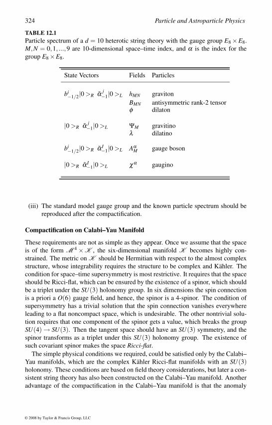
324 Particle and Astroparticle Physics
TABLE 12.1Particle spectrum of a d = 10 heterotic string theory with the gauge group E8 ×E8.
M,N = 0,1, ...,9 are 10-dimensional space–time index, and α is the index for the
group E8 ×E8.
State Vectors Fields Particles
bi−1/2|0 >R α j
−1|0 >L hMN graviton
BMN antisymmetric rank-2 tensorφ dilaton
|0 >R α j−1|0 >L ΨM gravitino
λ dilatino
bi−1/2|0 >R α I
−1|0 >L AαM gauge boson
|0 >R α I−1|0 >L χα gaugino
(iii) The standard model gauge group and the known particle spectrum should be
reproduced after the compactification.
Compactification on Calabi–Yau Manifold
These requirements are not as simple as they appear. Once we assume that the space
is of the form M 4 ×K , the six-dimensional manifold K becomes highly con-
strained. The metric on K should be Hermitian with respect to the almost complex
structure, whose integrability requires the structure to be complex and Kahler. The
condition for space–time supersymmetry is most restrictive. It requires that the space
should be Ricci-flat, which can be ensured by the existence of a spinor, which should
be a triplet under the SU(3) holonomy group. In six dimensions the spin connection
is a priori a O(6) gauge field, and hence, the spinor is a 4-spinor. The condition of
supersymmetry has a trivial solution that the spin connection vanishes everywhere
leading to a flat noncompact space, which is undesirable. The other nontrivial solu-
tion requires that one component of the spinor gets a value, which breaks the group
SU(4) → SU(3). Then the tangent space should have an SU(3) symmetry, and the
spinor transforms as a triplet under this SU(3) holonomy group. The existence of
such covariant spinor makes the space Ricci-flat.The simple physical conditions we required, could be satisfied only by the Calabi–
Yau manifolds, which are the complex Kahler Ricci-flat manifolds with an SU(3)holonomy. These conditions are based on field theory considerations, but later a con-
sistent string theory has also been constructed on the Calabi–Yau manifold. Another
advantage of the compactification in the Calabi–Yau manifold is that the anomaly
© 2008 by Taylor & Francis Group, LLC
Introduction to Strings 325
cancellation gives a condition that the spin connection has to be identified with the
gauge connection. This is done by associating the SU(3) holonomy group with the
SU(3) subgroup of one of the E8 gauge group of the E8 ×E8 heterotic strings [189].
This breaks the gauge group E8 spontaneously to E6, which contains the right par-
ticle spectrum of the standard model and has already been considered as a possible
grand unified group [198]. There are also some discrete symmetries of the manifold,
which ensure that the group E6 is further broken during compactification to one of
its subgroups, leaving the correct particle spectrum.
Compactification on a Calabi–Yau manifold thus gives chiral fermion in the fun-
damental representation of the group E6 automatically. The number of generations of
chiral representations is determined by the Euler characteristics χ , which is a topo-
logical quantity of the manifold. The Euler characteristics are related to the number
of superfields n27 in the fundamental representation 27 and the number of superfields
n27 in the conjugate representation 27 by the relation
χ = n27 −n27. (12.85)
There will be n27 numbers of 27 + 27 superfields, which will be the Higgs scalars.
Thus, the required numbers of fermions and scalars come out from the geometry of
the compact space. Since the compactification breaks the E6 gauge group also, only
the 27 and 27 Higgs scalars are required for any symmetry breaking or giving masses
to the fermions, which are also present in the theory.
The particle content of the 10-dimensional N = 1 supergravity theory originat-
ing from superstring theory includes the massless graviton, gravitino, dilaton, di-
latino and an antisymmetric rank-2 tensor. In addition there are the gauge fields AαM
and their superpartners, the gauginos χα in 10 dimensions that generate the group
E8 ×E8. After compactification some of the components of these gauge superfields
can only contribute to the chiral zero modes in 4 dimensions. In the following we
shall assume α to be the index for only one of the E8 group and the other E8 index
remains as a hidden sector index, which could contribute to low-energy supersym-
metry breaking.
The gauginos and the gauge bosons belong to the 248-dimensional representation
of the group E8. Under its maximal subgroup SU(3)×E6, these fields transform as
248 = (8,1)+(1,78)+(3,27)+(3,27). (12.86)
On the other hand, the 10-dimensional vector VM has a decomposition
VM = Vµ +Va +Va, (12.87)
where M = 0,1, ...,9 is the index of the 10 dimensions, while µ = 0,1,2,3 denotes
the four dimensions. Under the SU(3) holonomy group, the compact 6 dimensions
now split into 6 = 3+ 3, which corresponds to the indices a = 1,2,3 and a = 1,2,3.
So, their transformation is governed by the spin connection of the Calabi–Yau man-
ifold. When these SU(3) spin connections are identified with the gauge connections
of the SU(3) subgroup of E8, we contract the index a with the SU(3) index in the
© 2008 by Taylor & Francis Group, LLC
326 Particle and Astroparticle Physics
triplet representation. If we now write the E8 index as α ≡ (η ,m), where η is an E6index and m is an SU(3) index, then the 10-dimensional vectors would contain
V αM ⊃V (η78,m1)
µ ⊕V (η27,m3)a δ a
m3⊕V
(η f ,m3)a δ a
m3. (12.88)
The first term represents the gauge bosons of the group E6 in 4-dimensions, while the
second and the third terms are the scalar superfields in 4-dimensions, containing all
the fermions and Higgs scalars. Thus, for the field AαM , when we identify these two
SU(3) groups, the 27 and 27 representations acquire the topological property that
their numbers get related to some topological quantum numbers of the manifold,
which are the Hodge numbers. The low-lying states become blind to the second E8group, and hence, it does not affect any low-energy phenomenology. The gauginos
corresponding to this second E8 group can form condensates at very low energy and
can break supersymmetry in the hidden sector. For our discussions of the observable
sector phenomenology, we shall ignore this second E8 group.
Three-Generation Superstring Model
Without going into the details, we shall present an example of a Calabi–Yau mani-
fold, which gives three generations of fermions [196]. We demonstrate the discrete
symmetries in such manifold using algebraic geometry methods, which can restrict
some of the couplings of the fermions and make the theory consistent with low-
energy phenomenology [197].
Let us consider a complex space C n+1, described by (n + 1) complex numbers
(z0,z1, . . . ,zn) with the origin removed C n+1 −0. A complex projective space
C Pn of dimension n is defined by associating a scaling invariance or a projec-
tion, (z0,z1, ...,zn) = λ (z0,z1, ...,zn) on C n+1 −0, where λ is any nonzero com-
plex number. The coordinates (z0,z1, ...,zn) are called homogeneous coordinates of
C Pn, which is a complex Kahler manifold. A Calabi–Yau manifold is a hyper-
surface on a C P3 ×C P3 space with the homogeneous coordinates xi and yi, i =0,1,2,3, which is defined by the zeros of the polynomials
∑x3i +a1x0x1x2 +a2x0x1x3 +a3x0x2x3 +a4x1x2x3 = 0
∑y3i +b1y0y1y2 +b2y0y1y3 +b3y0y2y3 +b4y1y2y3 = 0
∑ci jxiy j = 0, (12.89)
with c00 = 1. These are the most general polynomials and have 23 parameters
ai,bi,ci j, which define the metric of the Calabi–Yau space. There are now 23 in-
dependent superfields belonging to the 27 representations, which can be represented
by the 23 independent monomials, as given in table 12.2.
We shall now act on this space by a Z3 discrete symmetry
Z3 : (x0,x1,x2,x3)× (y0,y1,y2,y3)−→ (x0,α2x1,αx2,αx3)× (y0,αy1,α2y2,α2y3), (12.90)
where α = exp[2πi/3], so α3 = 1. After the action of the discrete symmetry, this
Calabi–Yau space has an Euler characteristic 3 and gives a three-generation model.
© 2008 by Taylor & Francis Group, LLC
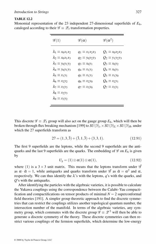
Introduction to Strings 327
TABLE 12.2Monomial representation of the 23 independent 27-dimensional superfields of E6,
cataloged according to their G ≡ Z3 transformation properties.
G (1) G (α) G (α2)
λ1 ≡ x0x1x2 q1 ≡ x1x2x3 Q1 ≡ x0x2x3
λ2 ≡ x0x1x3 q2 ≡ y0y2y3 Q2 ≡ y1y2y3
λ3 ≡ y0y1y2 q3 ≡ x0y1 Q3 ≡ x0y2
λ4 ≡ y0y1y3 q4 ≡ x1y2 Q4 ≡ x0y3
λ5 ≡ x1y1 q5 ≡ x1y3 Q5 ≡ x1y0
λ6 ≡ x2y2 q6 ≡ x2y0 Q6 ≡ x2y1
λ7 ≡ x3y3 q7 ≡ x3y0 Q7 ≡ x3y1
λ8 ≡ x2y3
λ9 ≡ x3y2
This discrete G ≡ Z3 group will also act on the gauge group E6, which will then be
broken through flux breaking mechanism [199] to SU(3)c×SU(3)L×SU(3)R, under
which the 27 superfields transform as
27 = (1,3, 3)+(3,1, 3)+(3,3,1). (12.91)
The first 9 superfields are the leptons, while the second 9 superfields are the anti-
quarks and the last 9 superfields are the quarks. The embedding of G on E6 is given
by
Ug = (1)⊗α(1)⊗α(1), (12.92)
where (1) is a 3× 3 unit matrix. This means that the leptons transform under Gas α · α = 1, while antiquarks and quarks transform under G as α = α2 and α ,
respectively. We can thus identify the λ ’s with the leptons, q’s with the quarks, and
Q’s with the antiquarks.
After identifying the particles with the algebraic varieties, it is possible to calculate
the Yukawa couplings using the correspondence between the Calabi–Yau compacti-
fication and compactifications on tensor products of minimal N = 2 superconformal
field theories [191]. A simpler group theoretic approach to find the discrete symme-
tries that can restrict the couplings utilizes another topological quantum number, the
intersection number of the manifold. In terms of the algebraic varieties, any sym-
metry group, which commutes with the discrete group G ≡ Z 3 will then be able to
generate a discrete symmetry of the theory. These discrete symmetries can then re-
strict various couplings of the fermion superfields, which determine the low-energy
© 2008 by Taylor & Francis Group, LLC

328 Particle and Astroparticle Physics
phenomenology. These calculations could establish the consistency of the theory, al-
though there are no unique phenomenological predictions of the superstring theory.
A large class of low-energy phenomenology of the superstring theory means only
superstring-inspired phenomenology [190]. In the superstring-inspired phenomenol-
ogy, a phenomenological model is considered taking the particle spectrum from the
superstring theory. One assumes that the theory contains fermions belonging only to
the 27-plet representation of E6 and the Higgs scalars belonging to the superfields in
the 27 or 27 representations. The Lagrangian is the N = 1 supergravity Lagrangian
with an arbitrary superpotential, constructed based on the problem under consid-
eration. For the soft terms one needs to assume string-motivated supersymmetry
breaking mechanisms.
It is also possible to construct four-dimensional superstring models. Here one does
not have to first take the field theoretical limit and then compactify. The compactifi-
cation takes place at the string level, which makes these theories more complicated.
Moreover, heterotic strings are no longer the unique possibility. The string scale
could also be lower than the Planck scale. The intersecting branes open up another
new aspect of the superstring phenomenology. All these newer developments are
changing the concept of superstring phenomenology very fast [200]. Whether or not
superstring theory can predict our low-energy world, the fact that it can accommodate
the standard model consistently with all the known fermions and their interactions
without any contradiction is already an achievement. This also supports our belief
that superstring theory can be the theory of all the basic interactions. Which solution
is preferred is difficult to decide from our present knowledge, but it is established
that the superstring theory can provide consistent low-energy phenomenology.
12.5 Duality and Branes
The superstring theory has been emerging as the most consistent theory of quan-
tum gravity, which can also unify gauge interactions with gravitational interaction
and have built-in supersymmetry. The low-energy standard model gauge group and
the standard model particle spectrum also could be accommodated in the theory. The
heterotic strings with E8×E8 gauge group in 10-dimensions with the extra six dimen-
sions compactified on a three-generation Calabi–Yau manifold appeared to be the
only possibility that could give us the low-energy phenomenology in 4-dimensions
consistently. But with newer developments this uniqueness is lost and we observe
many interesting results.
There is a general prescription for compactifying the extra dimensions by replac-
ing six of the target space dimensions with a conformal field theory with the desired
charge. Compactification on a Calabi–Yau manifold with SU(3) holonomy in the
field theory limit is only one of the solutions of this more general prescription. The
coordinates of the compact Calabi–Yau space will then belong to a conformal field
© 2008 by Taylor & Francis Group, LLC
Introduction to Strings 329
theory with a consistent central charge. Techniques such as F-theory provide new
classes of 4-dimensional N = 1 string vacua [201]. These developments with newer
solutions for the low-energy world are making the superstring theory appear less
unique, but more interesting [200]. Some recent advances in the field are revert-
ing our idea about nonuniqueness of the string vacua and giving indications that the
different low-energy theories may emerge from one ultimate theory [202].
Many of the newer developments in the field started when the string theory went
through a major breakthrough following the proposition of the duality conjectures.
These conjectures relate a theory with strong couplings to a theory with weak cou-
plings, which allows us to study some strongly coupled theories at least partially.
One of the significant results from such developments is the calculation of the black
hole entropy. While other approaches to the problem end up with a puzzle, string
theory could approach the problem from a microscopic point of view and provide a
partial solution.
Another interesting outcome of the duality conjecture is the brane solutions, which
now allow us to construct string theory at a scale as low as a few TeV. These theories
have many interesting features, some of which will be mentioned in the next two
chapters. The brane solutions also have other implications as well in connection
with the studies of duality conjectures and construction of new phenomenological
models.
Information Loss Puzzle
The string theory met with triumph in explaining the information loss puzzle in black
holes [203]. Since other competing theories of quantum gravity could not provide
any explanation for this puzzle, string theory is now accepted as the most consistent
theory of quantum gravity.
Black holes are classical solutions, in which the matter density and the space–time
curvature is so high that when any particle or even light reaches a certain distance
near the black hole, called the event horizon, it is pulled inside increasing the size
of the black hole. Since nothing can come out of the black hole once it is inside the
event horizon, it can be considered as a perfect blackbody. The black holes could be
formed by collapse of matter under its own gravitational pull or could be primordial.
When quantum effects are considered, the event horizon cannot be sharply defined.
Thus, the spread of the wave function of a particle falling inside the event horizon
allows the particle to leave from near the event horizon. Hawking radiation [204]
can now be viewed as pair creation near the event horizon, where some particles
may combine with the ensemble of particles. The remaining particles are pulled
back into the black hole. Black holes could as well evaporate radiating particles that
are near its event horizon. In quantum theory it is expected that the black holes emit
thermal blackbody radiation and carry entropy. Consider an ensemble of particles in
a pure state near the event horizon of a black hole. Hawking radiation will imply that
the state leaving the black hole will carry some information about the initial state,
and the wave functions of the particles that combine with the ensemble will make it
a mixed state. Since the Hawking radiation is thermal, although the ensemble started
© 2008 by Taylor & Francis Group, LLC
330 Particle and Astroparticle Physics
as pure state, most of the information about the initial state is lost.
Any consistent quantum theory of gravity should explain this information loss
puzzle from a microscopic description of the radiation from the black holes. Among
several other competing theories, only the string theory could at least partially solve
this problem. In a special class of black holes, the string theory could count the
number of quantum states of black holes and relate this number with the entropy of
the black holes. If N is the degeneracy of states with a certain quantum number of
these black holes, then the Bekenstein–Hawking entropy of a black hole is given by
SBH = ln (N). (12.93)
It is also possible in this microscopic approach of the string theories to calculate the
Hawking radiation from these black holes due to quantum scattering processes inside
the black hole [203].
The classical theory of gravity is explained by the general theory of relativity.
Although the theory has been extremely successful at low energies, the theory is
nonrenormalizable since it is described by a spin-2 particle, the graviton. In field
theory, the graviton exchange in the loop will have infinite contributions, which can-
not be removed by ordinary renormalization prescriptions. These quantum correc-
tions, coming from the loop diagrams, cannot be dealt with any techniques of or-
dinary point-particle field theory. On the other hand the quantum string theory has
no ultraviolet divergences, and since the particle spectrum of string theory contains
a massless spin-2 particle which can be interpreted as the graviton, it appears to be
a consistent theory of quantum gravity. The solution to the information loss puz-
zle now puts string theory ahead of all other approaches to a consistent theory of
quantum gravity.
String Duality
One of the major results in the string theory is the duality conjecture [205], which
establishes an equivalence between two or more apparently distinct string theo-
ries. This has many consequences in string theory as well as several fascinating
phenomenological applications. The duality conjectures started with reducing the
nonuniqueness of the string theory. We mentioned the five different superstring the-
ories: type I superstring theory, type IIA superstring theory, type IIB superstring
theory, heterotic string theory with gauge group E8 ×E8 and heterotic string theory
with gauge group SO(32). These theories are defined in 10 dimensions and have con-
sistent weak-coupling perturbation expansions, so they can be described by N = 1
supergravity theory in 10-dimensions.
The new era in string theory or the second string revolution started when some
of these theories could be shown to be equivalent by the duality symmetries of the
string theories. These duality symmetries were proposed as conjectures, which pro-
vided many mathematical identities. When these mathematical identities could be
eventually proved through rigorous calculations, these conjectures were established.
The main problem of proving these conjectures directly is that these duality conjec-
tures show equivalence between a weakly coupled string theory to a strongly coupled
© 2008 by Taylor & Francis Group, LLC
Introduction to Strings 331
string theory and we do not have any tools to calculate anything in the strongly cou-
pled string theories.
Before we discuss any of the recent developments, let us explain the duality con-
cept that was already known, the T-duality. Consider a 10-dimensional string theory
in which one of the dimensions has been compactified on a circle, so the space is now
R9×S1. We now consider two different types of string theories with compactification
radius R1 and R2 in this compactified space R9 ×S1, with the condition,
R1R2 = l2s , (12.94)
where ls is the fundamental string length scale, with tension
T =1
2πl2s
= 2πm2s , (12.95)
where ms is the fundamental string mass scale. The T-duality implies that the two
types of string theories under consideration are identical, if for R1 → 0, the dual
theory decompactifies and R2 → ∞. While compactifying the bosonic strings we
encountered two quantum numbers: string winding number n, which denotes the
number of times a string can wind the compactified dimension and the Kaluza–Klein
mode m, which comes from the single-valuedness of expipx requiring p = m/R. Both
these quantum numbers contribute to the mass-squared operator
1
8M2 =
N2
+N2−1+
n2R2
2+
m2
8R2 . (12.96)
Under T-duality, the last two terms exchange their roles [206]. If we interchange the
string winding number (n) with the quantum number associated with the quantized
Kaluza–Klein momentum modes (m) and simultaneously invert the compactification
radius R → 1/R, the spectrum remains invariant.
In superstring theories, type IIA and type IIB are T-dual. So, if the nonchiral type
IIA theory is compactified on S1 with almost vanishing radius to get a 9-dimensional
theory, it becomes equivalent to a chiral type IIB theory in 10 dimensions. The
radius of the IIA theory is equivalent to the vev of a scalar field. When this vevvanishes, the scalar field appears as one of the components of the 10-dimensional
metric tensor. Thus, these two theories are not independent and are two limiting
points in a continuous moduli space of quantum vacua in 10 dimensions. Similarly,
the two heterotic strings are also T-dual.
To elaborate this let us consider a type II superstring theory in ten dimensions
and then compactify its tenth dimension on a circle S1. Then consider the T-duality
transformation
m ↔ n R ↔ α ′
R,
where the string coupling constant is given by
α ′ =1
2πT=
1
2l2 =
1
2.
© 2008 by Taylor & Francis Group, LLC
332 Particle and Astroparticle Physics
This can be achieved for type II strings by assigning X 9 = X9L −X9
R instead of X9 =X9
L +X9R and reversing the sign of the right-movers but still combining the left-movers
with the right-movers. The corresponding changes in the fermionic sector, following
the same prescription for the T-duality, would take us from a type IIA superstring
to a type IIB superstring. Thus, a type IIA superstring compactified on a circle
with radius R is equivalent to a type IIB superstring compactified on a circle with
radius α ′/R. This is consistent with the observation that when type IIA and type
IIB superstrings are compactified on a circle, the mass spectra of these two theories
come out to be the same.
We shall now discuss a new class of duality, where one conjectures equivalence of
two different string theories [207] and the duality maps an elementary particle to a
composite particle depending on which string theory we use. This duality conjecture
could not be proved but has undergone many consistency checks and provided sev-
eral major important results. It maps a closed-string excitation to an open-string ex-
citation and also maps a strongly coupled theory to a weakly coupled theory through
gg = 1. A perturbation expansion in one type of string theory contains informa-
tion about the nonperturbative results of the other that describes the full quantum
string theory. Our lack of knowledge about calculations in a strongly coupled theory
makes it difficult to prove the conjecture more rigorously. In simple language this
establishes a duality between gravity and field theory in the context of branes, which
is also known as AdS/CFT correspondence. This conjecture establishes an equiva-
lence between a type IIB string theory on S5 ×AdS5 and an N = 4 superconformal
SU(N) gauge theory in 4-dimensions [207, 208].
We first define a few terms and then discuss the duality conjecture. An S5 is a
5-dimensional sphere embedded in a 6-dimensional space with its radius defined by
R2 = ∑6i=1 y2
i . We can define an antideSitter space (AdSp+2) of dimension p + 2 as
a hypersurface on a 2 + p + 1-dimensional flat space with signature (−−+ + +),whose size is given by
R2 = −X2−1 −X2
0 +p+1
∑i=1
X2α . (12.97)
Solving this equation one can get the metric in the AdSp+2 space as
ds2 =U2
R2 ηi jdxidx j +R2 dU2
U2 , (12.98)
where U = X−1 + Xp+1 and xi = RXi/U (i = 0, ..p) parameterize the hypersurface
satisfying the condition X−1 −Xp+1 = x2U/R2 + R2/U with x2 = ηi jxix j. All 10
dimensions in S5 ×AdS5 are assumed to have the same radius R. A type IIB string
theory in S5×AdS5 is related to an N = 4 superconformal SU(N) Yang–Mills theory.
An N = 4 superconformal field theory has four supersymmetric generators, which
relate four Majorana fermions and six bosons with each of the gauge bosons. There
is only one gauge coupling constant (gY ) for the entire SU(N) gauge group and all of
their N = 4 supersymmetric partners. In addition there is one more parameter, which
is the vacuum angle θ .
© 2008 by Taylor & Francis Group, LLC
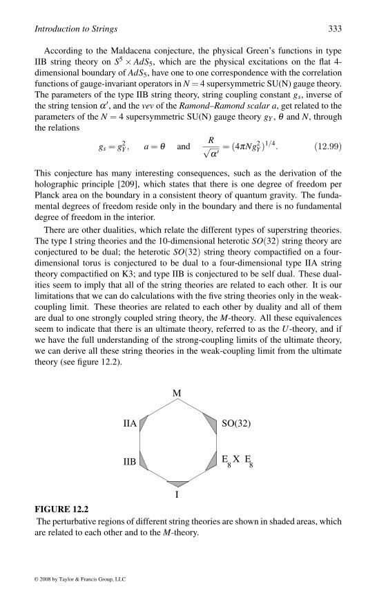
Introduction to Strings 333
According to the Maldacena conjecture, the physical Green’s functions in type
IIB string theory on S5 × AdS5, which are the physical excitations on the flat 4-
dimensional boundary of AdS5, have one to one correspondence with the correlation
functions of gauge-invariant operators in N = 4 supersymmetric SU(N) gauge theory.
The parameters of the type IIB string theory, string coupling constant gs, inverse of
the string tension α ′, and the vev of the Ramond–Ramond scalar a, get related to the
parameters of the N = 4 supersymmetric SU(N) gauge theory gY , θ and N, through
the relations
gs = g2Y , a = θ and
R√α ′ = (4πNg2
Y )1/4. (12.99)
This conjecture has many interesting consequences, such as the derivation of the
holographic principle [209], which states that there is one degree of freedom per
Planck area on the boundary in a consistent theory of quantum gravity. The funda-
mental degrees of freedom reside only in the boundary and there is no fundamental
degree of freedom in the interior.
There are other dualities, which relate the different types of superstring theories.
The type I string theories and the 10-dimensional heterotic SO(32) string theory are
conjectured to be dual; the heterotic SO(32) string theory compactified on a four-
dimensional torus is conjectured to be dual to a four-dimensional type IIA string
theory compactified on K3; and type IIB is conjectured to be self dual. These dual-
ities seem to imply that all of the string theories are related to each other. It is our
limitations that we can do calculations with the five string theories only in the weak-
coupling limit. These theories are related to each other by duality and all of them
are dual to one strongly coupled string theory, the M-theory. All these equivalences
seem to indicate that there is an ultimate theory, referred to as the U-theory, and if
we have the full understanding of the strong-coupling limits of the ultimate theory,
we can derive all these string theories in the weak-coupling limit from the ultimate
theory (see figure 12.2).
SO(32)
8 8IIB
IIA
E X E
M
I
FIGURE 12.2The perturbative regions of different string theories are shown in shaded areas, which
are related to each other and to the M-theory.
© 2008 by Taylor & Francis Group, LLC
334 Particle and Astroparticle Physics
At present the only information we have about the nonperturbative region of the
moduli space, except for the duality conjectures, is about the M-theory, which is a
well-defined quantum theory residing in 11 dimensions. In the low-energy limit it re-
duces to an 11-dimensional N = 1 supergravity theory, which allows us to get some
insight into M-theory. Other string theories approach the M-theory in the strong-
coupling limit. The strong-coupling limits of all the string theories in 10 dimensions
become 11-dimensional, since the coupling constant manifests itself as an extra di-
mension in the strong-coupling limit. As a result, the 11-dimensional M-theory does
not have any coupling constant and until now there does not exist any systematic
procedure to do calculations in M-theory, except for the low-energy limit.
The field equations of the 11-dimensional supergravity describe a supermembrane
(or M2-brane), where the particles have two space-like internal extensions and they
are defined on a (2+1)-dimensional world-sheet in 11 dimensions. When one of
the world-sheet space-like dimensions wraps around one space–time dimension, it
is also compactified and gives the type IIA superstring world-volume action in 10
dimensions. Thus, type IIA superstring theory is an M2-brane of M-theory with one
of its dimensions wrapped around the circular spatial dimension. Truncation to zero
modes is not required. The matrix theory is another attempt to give a nonperturba-
tive description of the M-theory. In the infinite-momentum limit, the M-theory is
described by a quantum system with N ×N matrices as the fundamental degrees of
freedom. The appropriate correlation functions then give the scattering amplitudes
of the M-theory in the limit N → ∞, which reproduce the low-energy 11-dimensional
N = 1 supergravity results.
We now understand the five weakly coupled superstring theories at 10 dimensions,
which are not independent and also related to the strongly coupled M-theory in 11
dimensions, whose low-energy limit correspond to the 11-dimensional N = 1 super-
gravity theory. However, we expect that all these theories should emerge from yet
another ultimate theory or the U-theory, which is also a strongly coupled theory in
11 dimensions. There are attempts to understand the U-theory by studying the five
weakly coupled theories as well as the strongly coupled M-theory. Although we are
yet to understand the U-theory, all these studies start giving us hope for an ultimate
theory of everything.
Branes
Brane solutions have several interesting consequences in string theory. They are
useful in deriving gauge theory results from string theories [210]. Observations from
branes lead to several duality conjectures. The branes solutions allow lowering of the
Planck scale, which leads to interesting low-energy phenomenology. Brane solutions
also allow new phenomenological models, in which only gravity propagates along
the extra dimensions while the gauge interactions are localized on a boundary brane
(which will be discussed in the next chapter) [211, 212].
Branes are static classical solutions in string theories [213]. A p-brane denotes
a static configuration which extends along p spatial directions and is localized in
all other directions. Such solutions are invariant under translation in the transverse
© 2008 by Taylor & Francis Group, LLC
Introduction to Strings 335
directions. Strings are equivalent to 1-brane, membranes are 2-brane, particles are
0-brane, and a p-brane is described by a (p+1)-dimensional gauge field theory.
Two kinds of boundary conditions are frequently used for the open strings. We
constructed open strings with the Neumann boundary condition
∂X µ(τ,σ = 0)∂σ
=∂X µ(τ,σ = π)
∂σ= 0, (12.100)
which states that the variations of the coordinates X µ are arbitrary at the boundary
and no momentum can flow out of the end of the open string. The other one is the
Dirichlet-boundary condition
Xa(τ,σ = 0) = Xa(τ,σ = π) = ca, (12.101)
where ca is a constant vector. The boundaries are now frozen, so the variation of the
coordinates vanishes although the momentum can now leave the boundaries.
The p-branes, which are extended solitons in string theory, are dynamical objects
and can move independently of the size of the d-dimensional compact manifold in
which they reside. The (p+1)-coordinates X i, i = 0,1,2, ..., p now satisfy the Neu-
mann boundary conditions, so no momentum can leave the boundaries along these
p + 1 dimensions. The remaining coordinates X a, a = p + 1, ...,d − 1 satisfy the
Dirichlet boundary conditions, so momentum can flow out of these boundaries to
a (d − p− 1)-dimensional surface, called the D-brane and extend along the p + 1
dimensions, whose positions are fixed at the end of the open strings.
We now discuss these solutions for superstrings. We have to impose opposite
boundary conditions for the Neumann and Dirichlet directions to maintain space–
time supersymmetry. In our convention the Neumann condition is
ΨiL(τ,σ = 0) = Ψi
R(τ,σ = 0)Ψi
L(τ,σ = π) = ±ΨiR(τ,σ = π), (12.102)
so the Dirichlet condition would be
ΨaL(τ,σ = 0) = −Ψa
R(τ,σ = 0)Ψa
L(τ,σ = π) = ±ΨaR(τ,σ = π). (12.103)
The advantage of this convention is that using a doubling trick it is possible to re-
late the Dirichlet and Neumann boundary conditions to the periodic and antiperiodic
boundary conditions for closed strings. We can then classify the open strings in the
same way as the R or NS types. When both the ends satisfy Dirichlet [Neumann]
conditions, the corresponding bosonic string is called DD [NN] and is related to a
periodic boundary condition. In this case, for the NS (antiperiodic fermionic) sector
we take the boundary conditions at σ = π to be
ΨiL = −Ψi
R and ΨaL = Ψa
R, (12.104)
and for the R (periodic fermionic) sector we take
ΨiL = Ψi
R and ΨaL = −Ψa
R. (12.105)
© 2008 by Taylor & Francis Group, LLC
336 Particle and Astroparticle Physics
When the opposite ends of the bosonic string satisfy different boundary conditions
DN [ND], it is related to the antiperiodic boundary condition in the bosonic sector.
In this case the fermionic sector is periodic in the NS sector and antiperiodic in the
R sector.
Let us now discuss the case of single D-brane, which is DD in the transverse
direction and NN in the longitudinal direction. Then X µ is always periodic, and Ψµ
is periodic in the R sector and antiperiodic in the NS sector. We can now write the
Neumann boundary conditions in the bosonic sector in terms of the mode expansion
oscillators as
α in = α i
n,
and those for the Dirichlet direction are
xa = ca, pa = 0, αan = −αa
n .
So the bosonic modes are given by
X i = xi + piτ + i ∑n =0
1
nα i
n exp−inτ cosnσ
Xa = ca − ∑n=0
1
nαa
n exp−inτ sinnσ . (12.106)
The mode expansion for the fermionic sector is given by
ΨiRL(R) =
1√2
∑n
dinexp−in(τ∓σ)
ΨaRL(R) = ± 1√
2∑n
danexp−in(τ∓σ)
ΨiRL(NS) =
1√2
∑r
birexp−ir(τ∓σ)
ΨaRL(NS) = ± 1√
2∑r
bar exp−ir(τ∓σ), (12.107)
where n = 1,2, ... are integers and r = 1/2,3/2, ... are half-integers. The commu-
tation relations of the bosonic oscillators and the anticommutation relations of the
fermions are the same as previously.
The left-movers are not independent of the right-movers. We work in the light
cone gauge and eliminate two directions, the time-like Neumann direction and one
space-like Neumann direction x1. The mass-squared operators for the R and the NSsectors now become
1
2M2(R) =
∞
∑n=1
α i−nα i
n +∞
∑n=1
ndµ−ndnµ −aR
1
2M2(NS) =
∞
∑n=1
α i−nα i
n +∞
∑r=1/2
rbµ−rbrµ −aNS. (12.108)
© 2008 by Taylor & Francis Group, LLC
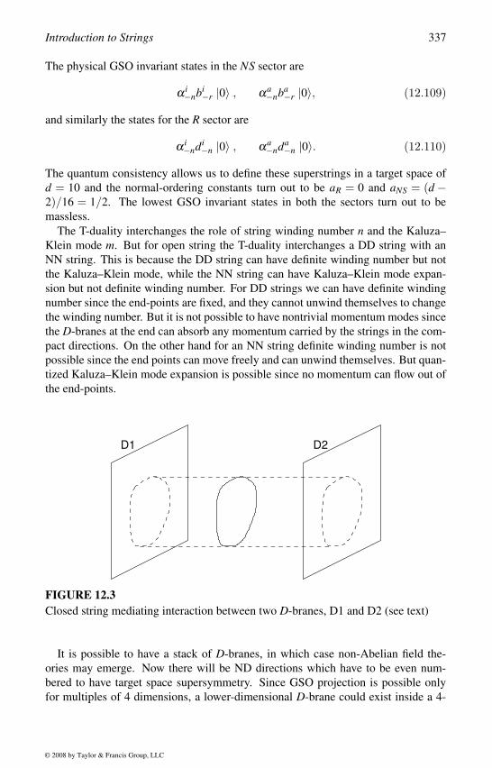
Introduction to Strings 337
The physical GSO invariant states in the NS sector are
α i−nbi
−r |0〉 , αa−nba
−r |0〉, (12.109)
and similarly the states for the R sector are
α i−ndi
−n |0〉 , αa−nda
−n |0〉. (12.110)
The quantum consistency allows us to define these superstrings in a target space of
d = 10 and the normal-ordering constants turn out to be aR = 0 and aNS = (d −2)/16 = 1/2. The lowest GSO invariant states in both the sectors turn out to be
massless.
The T-duality interchanges the role of string winding number n and the Kaluza–
Klein mode m. But for open string the T-duality interchanges a DD string with an
NN string. This is because the DD string can have definite winding number but not
the Kaluza–Klein mode, while the NN string can have Kaluza–Klein mode expan-
sion but not definite winding number. For DD strings we can have definite winding
number since the end-points are fixed, and they cannot unwind themselves to change
the winding number. But it is not possible to have nontrivial momentum modes since
the D-branes at the end can absorb any momentum carried by the strings in the com-
pact directions. On the other hand for an NN string definite winding number is not
possible since the end points can move freely and can unwind themselves. But quan-
tized Kaluza–Klein mode expansion is possible since no momentum can flow out of
the end-points.
D2D1
FIGURE 12.3Closed string mediating interaction between two D-branes, D1 and D2 (see text)
It is possible to have a stack of D-branes, in which case non-Abelian field the-
ories may emerge. Now there will be ND directions which have to be even num-
bered to have target space supersymmetry. Since GSO projection is possible only
for multiples of 4 dimensions, a lower-dimensional D-brane could exist inside a 4-
© 2008 by Taylor & Francis Group, LLC
338 Particle and Astroparticle Physics
or 8-dimensional D-brane. It is also possible to construct sets of parallel Dp-branes;
which have p space-like and one time-like dimensions. Consider two parallel Dp-
branes, the separation in the transverse direction can now take any values. There
are now two strings stretching between the two branes with opposite orientation, so
a U(1)×U(1) gauge symmetry would emerge, each U(1) residing on each of the
branes. The interaction of the D-branes takes place through exchange of closed type
IIA (B) strings (see figure 12.3). This allows a mapping of a Dp-brane with even p
to a Dq-brane with odd q under T-duality, which implies that under T-duality along
one circle type IIA interchanges with type IIB strings.
© 2008 by Taylor & Francis Group, LLC
13Extra Dimensions and Low-Scale Gravity
We are familiar with the four space–time dimensions, which are noncompact. But
from theoretical considerations we believe that there could be more than four space–
time dimensions. The simplest possibility is to consider the extra dimensions to
be compact with very small radius, so only the probes with energy close to the
Planck energy (MPl ∼ 1019 GeV) could see these extra dimensions. Then the Newto-
nian gravity in our effective four-dimensional space–time would remain unaffected.
When the dimensions higher than four are compactified, the components of the met-
ric corresponding to the extra compact dimensions will become gauge fields in four
dimensions. Any translation along the extra dimensions would then appear as gauge
transformations in four dimensions. The graviton in higher dimensions would de-
compose into the graviton and gauge bosons in four dimensions (see section 11.2).
With the advent of the brane solutions and duality, a new scenario of low effec-
tive Planck scale opened up. According to this possibility only gravity propagates
in the extra dimensions, while all other interactions are confined in the four dimen-
sions. As a result, gravity could be very strong in the extra dimensions, although due
to small overlap of the extra dimensions with our brane, we experience very weak
gravitational interaction. At higher energies all of the dimensions will open up and
gravity will become strong in all the dimensions. The possibility of models with low
Planck scale opens up new venues for extra dimensions. Several new scenarios have
been proposed since then, some of which have rich phenomenological implications,
while others have some shortcomings. But all of these models have their own merits,
which are worth investigating in details.
We shall now discuss a few selected topics in this new area of research. It will
not be possible to include all the interesting topics and there will be bias in selecting
these topics, but I hope this presentation will at least provide some feeling about
these developments and motivate the readers to follow the developments in more
details from the references. Some related exciting works will be reviewed in the
next chapter. Since this field of research is still developing many of the results may
be changed, but I hope the basic concepts that I try to emphasize here will remain
useful.
339
© 2008 by Taylor & Francis Group, LLC
340 Particle and Astroparticle Physics
13.1 Large Extra DimensionsAny higher-dimensional theories must give us four space–time dimensions with the
standard model interactions at energies below the electroweak symmetry breaking
scale. Any Kaluza–Klein excited states, which enter the theory after compactifica-
tion of the extra dimensions, should decouple from the low-energy theory. Thus, the
compactification scale, determined by the inverse radius of compactification, must
be much heavier than the electroweak scale. This implies that the radius of com-
pactification should be much smaller than the nuclear size. Thus, the possibility of
large extra dimension [211], with the radius of compactification of the order of mm,
became so drastically different from the usual higher-dimensional theories.
The main difference between the models of large extra dimensions and the con-
ventional higher-dimensional theories is that the large extra dimensions are blind to
the all interactions except gravity. Thus, although the extra dimensions are large, the
gauge interactions are not affected by their presence. Only gravitational interaction
will have some effect because of these large extra dimensions, which we shall discuss
later.
Another key issue for considering a large extra dimension [211] is that the funda-
mental scale of gravity need not be the Planck scale, MPl ∼ 1019 GeV. Gravitational
interaction can become strong even at a few TeV in theories with extra dimensions.
In a (4 + d)-dimensional space, gravity becomes strong at an energy M∗ of about
a few TeV, which is the fundamental scale in the theory. Below this scale ordinary
matter fields start decoupling from the extra dimensions and get confined to only
four space–time dimensions, although gravity continues to propagate along all di-
mensions. As a result the coupling of gravity with ordinary matter is suppressed by
the large volume of the extra dimensions. Thus, the effective Planck scale MPl that
we see today is due to the fact that the four-dimensional effective coupling to gravity
is suppressed by the volume of the extra dimensions at present energies.
Branes
The construction of theories of large extra dimensions or low-scale gravity relies on
the brane solutions in string theory (see section 12.5). The branes are static classical
solutions in string theories [213]. A p-brane extends along p spatial directions and
is localized in all other directions. The p + 1 coordinates now satisfy the Neumann
boundary conditions, so no momentum can flow out at the end-points and the par-
ticles residing in this p-brane are explained by the (p + 1)-dimensional gauge field
theory.
If a p-brane is embedded in a d-dimensional space, the remaining (d− p−1) coor-
dinates satisfy the Dirichlet boundary condition so the end-points are frozen although
momentum can leave the boundary (see section 12.5). These directions constitute
the bulk of the entire space–time. The p-branes are sitting only at the boundaries
(a p+1-dimensional wall with thickness M−1∗ ). The Neumann boundary conditions
© 2008 by Taylor & Francis Group, LLC
Extra Dimensions and Low-Scale Gravity 341
would imply that no momentum can flow out of the boundaries of these walls, so
the particles are confined in these branes. However, the Dirichlet condition would
allow momentum flow along the boundaries of the bulk, which are absorbed by the
p-branes at the boundary. So, particles moving in the bulk can enter or leave these
p-branes at the boundary. Moreover, such solutions are invariant under translation
in the transverse directions, so any particles residing in the p-branes cannot feel the
extra dimensions.
As an example consider a higher-dimensional theory, in which ordinary standard
model particles are residing on a 3-brane at one of the boundaries. These particles in
the 3-brane are described by the usual 4-dimensional gauge field theory. Only gravity
resides in the n-dimensional bulk, and the strength of gravitational interaction in the
bulk is very high. In addition, there could be other particles also in the bulk, which
do not have interactions with the standard model gauge bosons. The standard model
particles can experience gravity only when the gravitons enter our 3-brane, so the
gravity coupling in our 3-brane will be suppressed by the total volume of the bulk.
Essentially the interaction will be determined by the probability of the gravitons to
be in the p-brane. As a result, although the actual gravitational interaction strength
in the bulk is strong, the effective gravitational strength that we feel today in our
3-brane is weak.
At higher energies, all the dimensions were treated equally by all interactions
and even the particles confined in our 3-brane would have felt strong gravitational
interactions. So, the scale M∗ at which gravity becomes strong and quantum gravity
becomes effective, is the fundamental scale in the theory and can be as low as a few
TeV. At this scale the string action would treat the gravity and the ordinary particles
equally, which is now the string scale. Even the compactification scale has to be of
the same order of magnitude, implying that all the new physics we mentioned in the
context of higher dimensions would open up at this scale. The new Kaluza–Klein
excited states would make the evolution of the gauge coupling constants very fast,
and grand unification would also take place around this scale [214].
Low Planck Scale
We start with the simplest Kaluza–Klein theory in 5 dimensions, whose extra one
dimension is compactified on a circle (see section 11.2). After compactification,
the four-dimensional effective gravitational coupling constant κ is related to the 5-
dimensional gravitational constant κ5 by
κ2 =κ2
52πR
, (13.1)
where R is the radius of compactification of the fifth dimension. In a more gen-
eral case, when the space is a (4+d)-dimensional pseudo-Euclidean space, E4+d =M4×K (K is a d-dimensional compact space), the effective four-dimensional grav-
itational constant is given by
κ2 =κ2
4+d
Vd, (13.2)
© 2008 by Taylor & Francis Group, LLC
342 Particle and Astroparticle Physics
where Vd is the volume of the space of extra dimensions and κ4+d is the gravitational
coupling constant in E4+d . So the smallness of the effective four-dimensional grav-
itational constant could be due to a large volume (or the radius of compactification)
of the extra dimensions.
Let us now consider a 4 + d-dimensional space, the M 4 ×K space. The fun-
damental scale M∗ gives the gravitational potential between two test particles with
masses m1 and m2 in K separated by a distance r R,
V (r) ∼ m1m2
Md+2∗
1
rd+1 . (13.3)
When these test particles are separated by large distance r R, the gravitational flux
cannot penetrate the extra dimensions and hence the potential would be
V (r) ∼ m1m2
Md+2∗ Rd
1
r. (13.4)
In our four-dimensional world, the effective potential would be
V (r) ∼ m1m2
M2Pl
1
r, (13.5)
which relates the true Planck scale M∗ in the higher-dimensional theories, which
is the fundamental scale in the theory and the effective Planck scale MPl of our 4-
dimensional space M 4 through
M2Pl = M2+d
∗ Rd . (13.6)
Using the observed Planck scale in 4 dimensions, we can get an estimate of the radius
of compactification of the extra dimensions to be
R ∼ M−1∗
(MPl
M∗
)2/d
∼ 10(32−17d)/d ×(
1 TeVM∗
)(d+2)/2
cm. (13.7)
We now assume that the fundamental scale is of the order of a few TeV from phe-
nomenological considerations. If we now demand that M∗ is of the order of TeV,
then d = 1 is not allowed since it requires a deviation from the Newtonian gravity at
a distance R ∼ 1013 cm, which is about the distance scale of the solar system.
Since the large extra dimensions imply deviation from Newton’s law, improved
experiments were performed to verify Newton’s law to shorter distances. The new
experiments have now verified Newton’s law down to a distance of 0.2 mm [215].
This means that if the fundamental scale is in the TeV range, any value of d ≥ 2 is
allowed. In fact, any value of d ≥ 2 with TeV scale new physics will imply deviation
from Newton’s law at 1− 10 µm. In all earlier theories the compactification scale
was assumed to be the same as the Planck scale, but now it is possible to make M∗ to
be around a few TeV scale, making it experimentally testable.
Once the possibility of a fundamental scale of TeV with large extra dimensions
with compactified radius R ∼ 1−10 µm is considered, the problem comes with the
© 2008 by Taylor & Francis Group, LLC
Extra Dimensions and Low-Scale Gravity 343
ordinary particles. When the extra dimensions are compactified to a radius of R, it
would mean that all particles in these extra dimensions would have the Kaluza–Klein
excited states with mass ∼ n/R, where n is some integer number and n = 0 corre-
sponds to the zero modes. All the Kaluza–Klein excited states will have the same
quantum numbers as the zero mode. In the usual Kaluza–Klein compactification
only the zero modes could remain light and all the excited modes have masses of the
order of the Planck scale. Now we have a compactification radius R ∼ 1− 10 µm,
which corresponds to a scale of about a few eV. So, we shall get the infinite tower
of Kaluza–Klein excited states corresponding to each of the particles in the extra
dimensions with mass starting at eV. For gravitons this is not a problem, rather the
Kaluza–Klein states of the graviton make gravity strong at high energy that may
have interesting phenomenology. But for ordinary particles this is a problem. Since
none of the Kaluza–Klein excited states corresponding to the ordinary quarks, lep-
tons and gauge bosons have been observed so far, the only possibility is that the
ordinary particles do not see the extra dimensions. The standard model particles
and the SU(3)c × SU(2)L ×U(1)Y gauge interactions should be confined to our 4-
dimensional world. Although such solutions are provided by branes, let us consider
here the possibility of a classical solution providing us with localized matter [216].
Localized Matter
Let us consider a real scalar field φc in 5 dimensions. There is a classical kink
solution φc(y) depending on its fifth coordinate y, whose asymptotic forms are
φc(y → +∞) = +v and φc(y →−∞) = −v. (13.8)
This can be achieved starting with an action where the scalar potential V (φ) has two
degenerate minima at φ = ±v,
Sφ =∫
d4xdy[
1
2(∂Aφc)2 −V (φc)
]= 0. (13.9)
A ≡ x,y are the coordinates of the five dimensions. φc now describes a domain
wall separating two classical vacua along the y-direction, which breaks translational
invariance in this direction.
The action for a fermion Ψ in this model can be written as
SΨ =∫
d4xdy(iΨΓA∂AΨ−hφcΨΨ
). (13.10)
ΓA ≡ γµ ,−iγ5 are five-dimensional gamma matrices. In the domain wall back-
ground the Dirac equation becomes[iΓA∂A −hφc(y)
]Ψ = 0. (13.11)
The Poincare invariance along 4 dimensions is now unbroken and there is a zero
mode of the fermion characterized by
γµ pµ Ψ0 = 0 and γ5∂5Ψ0 = hφc(y)Ψ0. (13.12)
© 2008 by Taylor & Francis Group, LLC
344 Particle and Astroparticle Physics
In four dimensions this fermion is left-handed γ5Ψ0 = Ψ0 and has the form
Ψ0 = exp
[−
∫ y
0dy′hφc(y′)
]ψL(p), (13.13)
where ψL(p) satisfies the 4-dimensional Weyl equation.
This fermion is massless at the domain wall (near y = 0) and is localized near
y = 0. At large |y| it decays exponentially, Ψ0 ∝ exp[−m5|y| ]. At the scalar vacuum
φ = ±v, the 5-dimensional fermion acquires a mass m5 = hv, and hence, there are
continuum states starting with masses m5 in the 5 dimensions which are not bound
to the domain wall and could escape to |y| = ∞.
At low energy compared with v, the zero mode fermions are confined to 4 dimen-
sions and they form the ordinary matter around us. At energies above v, the zero
modes could produce the massive modes (m5) of the continuum and particles could
escape to the fifth dimension. This mimics the brane world, where the fermions are
confined to the 3-brane and only at higher energies do the extra dimensions open up.
This construction could be generalized to higher dimensions by considering topo-
logical defects such as Abrikosov–Nielsen–Olsen vortex or ’t Hooft–Polyakov
monopole. In some cases the index theorem ensures the zero modes. However it
is very difficult to localize the gauge fields. In one mechanism [217] a gauge theory
has been considered which is in confinement phase in the bulk but not in the brane.
Then the electric field of a charge residing on the brane will not penetrate the bulk.
On the other hand, all states propagating in the bulk are heavy, and light particles
carrying gauge charges are bound to the brane.
We have demonstrated the possibility of confining the ordinary particles in the
3-brane and allowing gravitons to propagate in the bulk. The gravity coupling in
the bulk is not so weak, but in 4 dimensions it is suppressed by the volume of extra
dimensions and would appear to be weak. There are all the Kaluza–Klein excited
modes of the graviton in the bulk, all of which couple weakly with the ordinary
matter. The long range gravitational force is due to the massless graviton exchange.
The fundamental scale M∗ is now about a TeV, when ordinary particles could transfer
momentum to the bulk. In addition to the gravitons, there could be singlet scalars
residing in the bulk.
Four-Dimensional Interactions
Let us now consider the interactions in our 4-dimensional world. For simplicity we
assume that the 3-brane is located at y = 0. For 4-dimensional fermions ψi(x) and
scalars φa(x), the action will be simply
Sψ =∫
d4xdyL (ψi,φa)δ (y) =∫
d4xL [ψi(x),φa(x)] . (13.14)
If we now consider a singlet scalar χ(x,y) in the bulk, the Yukawa interaction of this
field with the fermions in the 3-brane will be given by
Sint =∫
d4xdyfi j√M∗
ψi(x)ψ j(x)χ(x,y = 0)δ (y). (13.15)
© 2008 by Taylor & Francis Group, LLC
Extra Dimensions and Low-Scale Gravity 345
Here the Yukawa coupling fi j is dimensionless. If the mass dimension of a field
in 4 dimensions is D4, then its mass dimension in d dimensions would be D4 +d/2. Because of this the above 5-dimensional interaction term contains the mass
parameter (M∗), which is the fundamental scale in the theory.
Since the extra dimensions are compact with large radius R, the bulk field can be
expressed as the zero mode χ0 and Kaluza–Klein excited modes χn with masses n/R.
In four dimensions the effective interactions with the zero modes and the Kaluza–
Klein excited modes of χ will then be given by
Sint ≈∫
d4xM∗MPl
fi jψiψ j
(χ0 +
√2
∞
∑n=1
χn
). (13.16)
Thus, any coupling between the bulk fields and the ordinary matter is suppressed by
a factor M∗/MPl .
Bulk Matter
A generic features of any higher-dimensional theories is that the higher-dimensional
graviton must include the 4-dimensional graviton and a 4-dimensional scalar field,
the radion. The higher-dimensional gravitons would give us the zero mode of the
graviton G0µν , the Kaluza–Klein excited modes of the graviton Gn
µν , (n > 0) with
masses n/R, and zero mode and Kaluza–Klein excited modes of a scalar field, the
radion bn, (n ≥ 0). Their couplings with ordinary matter in 4 dimensions reduce to
L = − 1
MPl∑n
(Gn
µν −κ3
bnηµν
)Tµν . (13.17)
Here κ is a parameter of order 1. The zero mode of the radion b0 usually picks up
a mass from the stabilization mechanism [218]. The interaction with the zero mode
of the graviton is generally responsible for the gravitational interactions, and the
Newton constant in our world remains the same, GN ∼ M−2Pl to leading order. Due
to the effects of the excited gravitons there is a small correction at short distances,
which is being tested in experiments.
It is possible to introduce singlet fermions in the bulk. The free action for the
massless field in 5 dimensions will contain the free action for the 4-dimensional left-
and right-chiral fermions as well as the Dirac mass term, making all the Kaluza–
Klein states massive with mass n/R. However, one can add a Majorana mass term
in 5 dimensions in the action forbidding the Dirac mass term using an orbifold com-
pactification. In this case it is possible to have chiral fermions in four dimensions.
However, if gauge fields are introduced in the bulk, the Kaluza–Klein modes be-
come massive leaving the zero mode massless in 4 dimensions. But these gauge
fields should not be the gauge fields of the standard model, otherwise their coupling
to ordinary matter will be highly suppressed.
Let us now summarize the salient features of the model. Ordinary particles are
confined in the 3-brane at the boundary of the main higher-dimensional bulk. All
© 2008 by Taylor & Francis Group, LLC
346 Particle and Astroparticle Physics
interactions in the 3-brane are described by usual 4-dimensional gauge field the-
ory. Only gravity propagates in the bulk. The gravity coupling to ordinary matter is
suppressed by the volume of the extra dimensions, and we find it weak. The extra
dimensions are compactified with very large radius, and the Kaluza–Klein modes of
the graviton get masses of the order of eV. Near the fundamental scale of about TeV,
all dimensions become equal and gravity and ordinary matter are treated similarly.
All excited modes now show up, gravity becomes strong in all directions, and all
matter can propagate along any directions.
13.2 Phenomenology of Large Extra Dimensions
The models with extra dimensions that can allow low scale strong gravity can be
broadly classified into two classes, the models with large extra dimensions or those
with small extra dimensions. In the large extra dimensions the standard model inter-
actions are confined in a 3-brane and only gravity propagates in the bulk, whereas in
models with small extra dimensions, the geometry is warped. Since the phenomenol-
ogy of the models with large extra dimensions is comparatively easy to explain, we
shall restrict ourselves to the phenomenological studies of the large extra dimensions,
except for some comments on small extra dimensions.
There are many fascinating predictions of these models, but in constructing a
model, many new problems creep up due to the lack of any high scales. Expla-
nation of these new issues requires new physics from the extra dimensions. All these
new ideas for model building and new phenomenological predictions, assuming that
the new fundamental scale is of the order of TeV, started a new era in high energy
physics phenomenology. We shall try to give a brief introduction to this vast new
field.
Among the major predictions of these models with extra dimensions, the gravita-
tional force law should change from 1/r2 to 1/r4 for distances ∼ O(10−4 −1) mm.
For any hard collisions of energy greater than the fundamental scale E > M∗, some
of the momentum could be carried away by the bulk particles in the extra dimensions
and escape from our 4-dimensional world. However, no quantum numbers could be
lost, since the standard model particles reside only in our 4 dimensions. The new
particles and the large extra dimensions will modify cosmological predictions. Since
there are no large scales in the theory, solutions to the neutrino mass problem, strong
CP problem, and other problems require new physics from extra dimensions.
When supersymmetry is broken by compactification at the TeV scale, the particle
spectrum and the evolution of the gauge and Yukawa couplings are much different.
The squarks and sleptons are naturally an order of magnitude lighter than gauginos.
The sparticle spectrum now depends on only two new parameters. The Higgsino
mass is automatically generated when supersymmetry is broken. All this new phe-
nomenology promises new testable signatures in the next generation accelerators
© 2008 by Taylor & Francis Group, LLC
Extra Dimensions and Low-Scale Gravity 347
along with the signatures of new Kaluza–Klein states.
The models of extra dimensions will be most attractive if the fundamental scale
turns out to be close to the TeV scale [219]. In that case all the new physics we have
been mentioning could be accessible to the next generation accelerators. Since grav-
ity will become strong at this scale, we can expect many new signals that could be
beyond our imagination at present. However, so far there is no experimental evidence
that supports this idea, and hence, in reality it could be possible that the fundamental
scale is several orders of magnitude higher than TeV and we will not see anything in
the next generation laboratory experiments. So, none of the consequences we shall
be discussing can be truly considered as predictions of these models, but they are the
possibilities one should look for to test if the fundamental scale is really of the order
of TeV.
All of these new rich phenomenological and astrophysical consequences have
made this new idea of TeV scale extra dimensions extremely attractive. If signatures
of any of these predictions such as deviation from Newton’s law at a distance of µm
or signatures of new particles in the colliders are seen, then we have to understand
physics at the TeV scale in a different way than we see now.
Deviation from Newton’s Law
The first prediction of the models with large extra dimensions is deviation from New-
tonian gravity at short distances. Until recently Newton’s law was tested up to a dis-
tance of about a mm. But if gravity propagates in the bulk with strong coupling and
the fundamental scale is about TeV, then for d = 2, a deviation of the inverse squared
law of gravity was predicted at the submillimeter distances. So new experiments
were performed to test gravity in the mm range. These experiments now improved
the bound to a distance of about 0.2 mm.
Missing Energy
At low energy there are no new particles in the models with extra dimensions. But
at higher energies all the Kaluza–Klein excited states of the ordinary particles will
become accessible in the colliders. But even at lower energies there are some distinct
signals of the models with extra dimensions.
In all models of extra dimensions, the gravitons and some scalars propagate in
the bulk. In our 3-brane or the 4-dimensional world, there will be all the Kaluza–
Klein excited states of the graviton with masses given by the inverse radius of the
extra dimensions. All these gravitons can, in principle, interact with the ordinary
particles giving rise to new signals. When these excited gravitons interact with ordi-
nary particles, they can carry some transverse momentum of the ordinary particles.
The probability of such processes increases as we approach the fundamental scale at
which gravity becomes strong. So, the most distinct signals of these models with ex-
tra dimensions are to emit Kaluza–Klein gravitons into the bulk which we visualize
as missing energy.
Each of the Kaluza–Klein gravitons interact with matter in our world with 4-
dimensional gravitational strength. If there are d extra dimensions with large radius
© 2008 by Taylor & Francis Group, LLC
348 Particle and Astroparticle Physics
R, then (√
sR)d Kaluza–Klein excited gravitons will be produced during a collision
of center of mass energy√
s. When we write the interaction of the gravitons with
ordinary matter in 4 dimensions, the integration over the extra dimensions gives a
volume factor suppression, which makes these couplings suppressed as (s/M2Pl). The
total effect will be a missing energy of the order of
(√
sR)d
M2Pl
∼ 1
s
(√s
M∗
)d+2
. (13.18)
Thus, even though the coupling of every Kaluza–Klein state with matter is weak,
the total emission rate of Kaluza–Klein gravitons increases due to the large number
of states. The produced Kaluza–Klein gravitons will appear as missing energy and
there will be processes such as
e+ e− → γ + missing energy
q q → jet + missing energy
gluons + gluons → missing energy. (13.19)
The cross-section for the e+ e− process can be estimated as
σ ∼ αM2
Pl(ER)d ∼ α
E2
(E
M∗
)d+2
. (13.20)
Hence, the cross-section increases rapidly with energy, and near the fundamental
scale M∗, it becomes comparable to the electromagnetic cross-section. Detection of
these processes at LHC, ILC as well as in Tevatron could probe the fundamental scale
up to several TeV. There are also the indirect signals of extra dimensional origin of
some specific model, such as low-energy grand unification or existence of dileptons
in the TeV range and simultaneously lepton number violation.
Supernova
At present the most severe constraints for the fundamental scale come from super-
novae of about 30 TeV. The productions of the Kaluza–Klein gravitons will carry
away energy from inside the stars and sun, which will cause fast cooling and change
the evolution of the stars and sun. This gives strong bound on the fundamental scale
of any models with extra dimensions.
There are other comparable constraints coming from cosmology since all the
Kaluza–Klein states of the graviton will be produced at high temperature in the early
universe which could change the evolution of the universe or the present composition
of the universe. The evolution of the universe also gets modified in these models. We
shall discuss the astrophysical constraints and cosmological issues in more detail in
chapter 18.
© 2008 by Taylor & Francis Group, LLC
Extra Dimensions and Low-Scale Gravity 349
13.3 TeV Scale GUTsSince there are no large scales in the theories with large extra dimension, the concept
of grand unification has to be changed. Apparently the new Kaluza–Klein excited
states change the evolution of the gauge coupling constants and allow unification of
the strong, the weak and the electromagnetic interactions at the TeV scale.
In conventional theories the gauge coupling constants evolve with energy follow-
ing a logarithmic behavior. All the known fermions contribute to this evolution
through loop diagrams. The gauge coupling constants α3, α2 and α1 correspond-
ing to the groups SU(3)c, SU(2)L and U(1)Y now evolve in different ways, but all
three gauge couplings meet at a point. In the conventional grand unified theories
the gauge coupling constants are unified at around MU ∼ 1016 GeV, which is the
unification scale. Above this energy all the interactions will be explained by one
unified gauge symmetry. All fermions would then belong to some representations
of this grand unified symmetry group. The fact that the quarks and leptons belong
to the same representation of the group would imply that some of these new gauge
bosons will mediate proton decay. Again the present limit on the proton lifetime
requires the unification scale to be about the same value as predicted by the gauge
coupling unification. At the unification scale the unified gauge group is broken to its
low-energy subgroup by the Higgs mechanism. Some Higgs scalars belonging to the
representations of the unified group acquire a vev at the unification scale and break
the group. This Higgs has a mass and vev of the order of MU . In the scalar potential,
these heavy Higgs scalars will have mixing with the light Higgs scalar, which breaks
the electroweak symmetry. The vev of the heavy Higgs would then induce large mass
to the light Higgs, which has to be protected by means of fine tuning at all orders of
perturbation theory, giving rise to the gauge hierarchy problem.
Theories with large extra dimensions do not require any large scale for grand uni-
fication. Above the fundamental scale of a few TeV, new physics takes over and
grand unification is possible in these theories with extra dimensions slightly above
the fundamental scale and there is no hierarchy problem [214]. This means that all
the nice features of grand unification would now be accessible to the next generation
accelerators. At the fundamental scale all the Kaluza–Klein excited modes start in-
fluencing the evolution of the gauge coupling constants. Above some scale µ0 the
Kaluza–Klein excited states of the ordinary particles would contribute to the gauge
coupling running. This would modify the evolution of the gauge coupling constants
and they would start evolving much faster. The evolution of the gauge coupling will
then follow a power law behavior, instead of the usual logarithmic behavior. As a
result of the fast evolution of the gauge coupling constants above the TeV scale, the
grand unification will be achieved within tens of TeV.
Above the fundamental scale, all the Kaluza–Klein excitations of the ordinary par-
ticles will be produced and will not be localized in the brane. So they will be able
to propagate along the extra dimensions. As a result all the dimensions will open
up to the standard model particles around the fundamental scale. Since supersym-
© 2008 by Taylor & Francis Group, LLC
350 Particle and Astroparticle Physics
metric models become nonrenormalizable at dimensions higher than four, the nice
logarithmic behavior of the evolution of the gauge coupling constant will be lost.
The fundamental scale M∗ will become the ultraviolet cut-off scale for the higher-
dimensional supersymmetric standard model. So, for a consistent grand unification,
the gauge coupling constants have to evolve fast enough beyond the scale µ0 by the
influence of the Kaluza–Klein states, so unification can be achieved below M∗. As
we shall see, this is indeed the case and all three gauge coupling constants meet at
a point leading to grand unification just below the fundamental scale M∗ of tens of
TeV for µ0 to be around TeV. So the gauge hierarchy problem is solved. The proton
decay then becomes a problem, which we shall discuss shortly.
We demonstrate a simple case of gauge coupling unification with d extra dimen-
sions. Although this result is true for d = 1,2, it may be extended to higher dimen-
sions without loss of generality. We assume all the dimensions to have the same
radius R = µ−10 , but this can also be generalized. All the standard model particles
will now have the Kaluza–Klein excited states with mass
m2n = m2
0 +d
∑i=1
n2i
R2 . (13.21)
Since the evolution of the gauge coupling constants will be studied from the Z bo-
son mass, the zero mode masses of the ordinary particles can be neglected in the
following considerations.
Let us first consider only the gauge and Higgs boson contributions. At ener-
gies above µ0, all the Kaluza–Klein towers of particles will show up and then the
states can be identified with representations of N = 2 supersymmetry. At each of
the Kaluza–Klein mass levels n, the particle content of the supersymmetric standard
model is augmented by an N = 2 supermultiplet. An N = 2 vector supermultiplet
appears for each of the gauge bosons (Aµ ) and an N = 2 hyper-multiplet for each
of the two Higgs multiplets (H1 and H2). Consider an N = 2 supersymmetry gener-
ated by two spinorial generators Q1 and Q2. In an N = 2 hyper-multiplet of the nth
Kaluza–Klein mode, they relate the two scalars to left- and right-chiral spinors
Hn1
Q1↔ ψn
L , and Hn2
Q1↔ ψn
R
Hn1
Q2↔ ψn
R, and Hn2
Q2↔ ψn
L .
This is the minimal representation of N = 2 supersymmetry which is also a vectorial
(contains both left- and right-chiral fermions with same quantum numbers) represen-
tation. So, if we include fermions in our simple discussion, there have to be mirrorfermions in the theory. We assume that the brane solution is constructed in such a
way that only chiral fermions come out as zero modes, and we neglect effects of
Kaluza–Klein towers for the fermions. For the vector multiplet the transformations
are
Anµ
Q1↔ λ n, and φ n Q1
↔ χn
Anµ
Q2↔ χn, and φ n Q2
↔ λ n.
© 2008 by Taylor & Francis Group, LLC
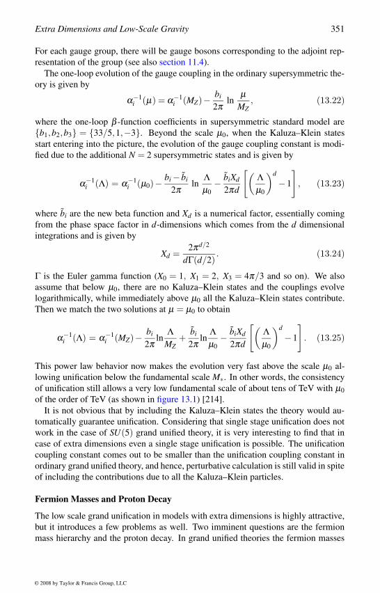
Extra Dimensions and Low-Scale Gravity 351
For each gauge group, there will be gauge bosons corresponding to the adjoint rep-
resentation of the group (see also section 11.4).
The one-loop evolution of the gauge coupling in the ordinary supersymmetric the-
ory is given by
α−1i (µ) = α−1
i (MZ)− bi
2πln
µMZ
, (13.22)
where the one-loop β -function coefficients in supersymmetric standard model are
b1,b2,b3 = 33/5,1,−3. Beyond the scale µ0, when the Kaluza–Klein states
start entering into the picture, the evolution of the gauge coupling constant is modi-
fied due to the additional N = 2 supersymmetric states and is given by
α−1i (Λ) = α−1
i (µ0)− bi − bi
2πln
Λµ0
− biXd
2πd
[(Λµ0
)d
−1
], (13.23)
where bi are the new beta function and Xd is a numerical factor, essentially coming
from the phase space factor in d-dimensions which comes from the d dimensional
integrations and is given by
Xd =2πd/2
dΓ(d/2). (13.24)
Γ is the Euler gamma function (X0 = 1, X1 = 2, X3 = 4π/3 and so on). We also
assume that below µ0, there are no Kaluza–Klein states and the couplings evolve
logarithmically, while immediately above µ0 all the Kaluza–Klein states contribute.
Then we match the two solutions at µ = µ0 to obtain
α−1i (Λ) = α−1
i (MZ)− bi
2πln
ΛMZ
+bi
2πln
Λµ0
− biXd
2πd
[(Λµ0
)d
−1
]. (13.25)
This power law behavior now makes the evolution very fast above the scale µ0 al-
lowing unification below the fundamental scale M∗. In other words, the consistency
of unification still allows a very low fundamental scale of about tens of TeV with µ0
It is not obvious that by including the Kaluza–Klein states the theory would au-
tomatically guarantee unification. Considering that single stage unification does not
work in the case of SU(5) grand unified theory, it is very interesting to find that in
case of extra dimensions even a single stage unification is possible. The unification
coupling constant comes out to be smaller than the unification coupling constant in
ordinary grand unified theory, and hence, perturbative calculation is still valid in spite
of including the contributions due to all the Kaluza–Klein particles.
Fermion Masses and Proton Decay
The low scale grand unification in models with extra dimensions is highly attractive,
but it introduces a few problems as well. Two imminent questions are the fermion
mass hierarchy and the proton decay. In grand unified theories the fermion masses
© 2008 by Taylor & Francis Group, LLC
of the order of TeV (as shown in figure 13.1) [214].
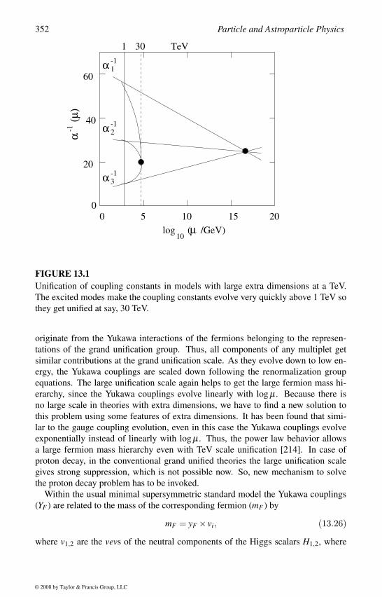
352 Particle and Astroparticle Physics
α -1
2α -1
1α -1
3
TeV
0 105 15 20
20
0
40
60
10log ( /GeV)µ
-1α
(µ
)
301
FIGURE 13.1Unification of coupling constants in models with large extra dimensions at a TeV.
The excited modes make the coupling constants evolve very quickly above 1 TeV so
they get unified at say, 30 TeV.
originate from the Yukawa interactions of the fermions belonging to the represen-
tations of the grand unification group. Thus, all components of any multiplet get
similar contributions at the grand unification scale. As they evolve down to low en-
ergy, the Yukawa couplings are scaled down following the renormalization group
equations. The large unification scale again helps to get the large fermion mass hi-
erarchy, since the Yukawa couplings evolve linearly with log µ . Because there is
no large scale in theories with extra dimensions, we have to find a new solution to
this problem using some features of extra dimensions. It has been found that simi-
lar to the gauge coupling evolution, even in this case the Yukawa couplings evolve
exponentially instead of linearly with log µ . Thus, the power law behavior allows
a large fermion mass hierarchy even with TeV scale unification [214]. In case of
proton decay, in the conventional grand unified theories the large unification scale
gives strong suppression, which is not possible now. So, new mechanism to solve
the proton decay problem has to be invoked.
Within the usual minimal supersymmetric standard model the Yukawa couplings
(YF ) are related to the mass of the corresponding fermion (mF ) by
mF = yF × vi, (13.26)
where v1,2 are the vevs of the neutral components of the Higgs scalars H1,2, where
© 2008 by Taylor & Francis Group, LLC
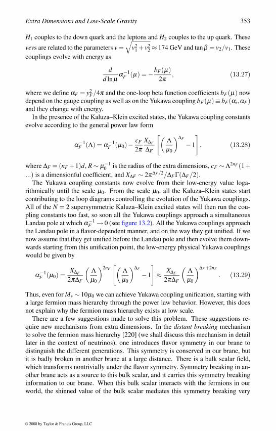
Extra Dimensions and Low-Scale Gravity 353
H1 couples to the down quark and the leptons and H2 couples to the up quark. These
vevs are related to the parameters v =√
v21 + v2
2 ≈ 174 GeV and tanβ = v2/v1. These
couplings evolve with energy as
dd ln µ
α−1F (µ) = −bF(µ)
2π, (13.27)
where we define αF = y2F/4π and the one-loop beta function coefficients bF(µ) now
depend on the gauge coupling as well as on the Yukawa coupling bF(µ)≡ bF(αi,αF)and they change with energy.
In the presence of the Kaluza–Klein excited states, the Yukawa coupling constants
evolve according to the general power law form
α−1F (Λ) = α−1
F (µ0)− cF
2πX∆F
∆F
[(Λµ0
)∆F
−1
], (13.28)
where ∆F = (nF +1)d, R ∼ µ−10 is the radius of the extra dimensions, cF ∼ Λ2nF (1+
...) is a dimensionful coefficient, and X∆F ∼ 2π∆F /2/∆F Γ(∆F/2).The Yukawa coupling constants now evolve from their low-energy value loga-
rithmically until the scale µ0. From the scale µ0, all the Kaluza–Klein states start
contributing to the loop diagrams controlling the evolution of the Yukawa couplings.
All of the N = 2 supersymmetric Kaluza–Klein excited states will then run the cou-
pling constants too fast, so soon all the Yukawa couplings approach a simultaneous
Landau pole at which α−1F → 0 (see figure 13.2). All the Yukawa couplings approach
the Landau pole in a flavor-dependent manner, and on the way they get unified. If we
now assume that they get unified before the Landau pole and then evolve them down-
wards starting from this unification point, the low-energy physical Yukawa couplings
would be given by
α−1F (µ0) =
X∆F
2π∆F
(Λµ0
)2nF[(
Λµ0
)∆F
−1
]≈ X∆F
2π∆F
(Λµ0
)∆F +2nF
. (13.29)
Thus, even for M∗ ∼ 10µ0 we can achieve Yukawa coupling unification, starting with
a large fermion mass hierarchy through the power law behavior. However, this does
not explain why the fermion mass hierarchy exists at low scale.
There are a few suggestions made to solve this problem. These suggestions re-
quire new mechanisms from extra dimensions. In the distant breaking mechanism
to solve the fermion mass hierarchy [220] (we shall discuss this mechanism in detail
later in the context of neutrinos), one introduces flavor symmetry in our brane to
distinguish the different generations. This symmetry is conserved in our brane, but
it is badly broken in another brane at a large distance. There is a bulk scalar field,
which transforms nontrivially under the flavor symmetry. Symmetry breaking in an-
other brane acts as a source to this bulk scalar, and it carries this symmetry breaking
information to our brane. When this bulk scalar interacts with the fermions in our
world, the shinned value of the bulk scalar mediates this symmetry breaking very
© 2008 by Taylor & Francis Group, LLC
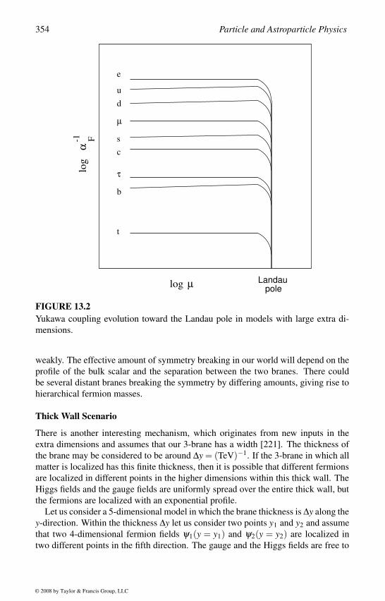
354 Particle and Astroparticle Physics
pole
log
αF-1
log µ
e
u
d
µ
τ
s
c
b
t
Landau
FIGURE 13.2Yukawa coupling evolution toward the Landau pole in models with large extra di-
mensions.
weakly. The effective amount of symmetry breaking in our world will depend on the
profile of the bulk scalar and the separation between the two branes. There could
be several distant branes breaking the symmetry by differing amounts, giving rise to
hierarchical fermion masses.
Thick Wall Scenario
There is another interesting mechanism, which originates from new inputs in the
extra dimensions and assumes that our 3-brane has a width [221]. The thickness of
the brane may be considered to be around ∆y = (TeV)−1. If the 3-brane in which all
matter is localized has this finite thickness, then it is possible that different fermions
are localized in different points in the higher dimensions within this thick wall. The
Higgs fields and the gauge fields are uniformly spread over the entire thick wall, but
the fermions are localized with an exponential profile.
Let us consider a 5-dimensional model in which the brane thickness is ∆y along the
y-direction. Within the thickness ∆y let us consider two points y1 and y2 and assume
that two 4-dimensional fermion fields ψ1(y = y1) and ψ2(y = y2) are localized in
two different points in the fifth direction. The gauge and the Higgs fields are free to
© 2008 by Taylor & Francis Group, LLC
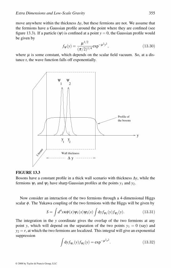
Extra Dimensions and Low-Scale Gravity 355
move anywhere within the thickness ∆y, but these fermions are not. We assume that
the fermions have a Gaussian profile around the point where they are confined (see
figure 13.3). If a particle (ψ) is confined at a point y = 0, the Gaussian profile would
be given by
fψ(y) =µ1/2
(π/2)1/4 exp−µ2y2, (13.30)
where µ is some constant, which depends on the scalar field vacuum. So, at a dis-
tance r, the wave function falls off exponentially.
ψ1
ψ2
y1
Profile of
the bosons
Wall thickness
3-br
ane
yy2
∆ y
FIGURE 13.3Bosons have a constant profile in a thick wall scenario with thickness ∆y, while the
fermions ψ1 and ψ2 have sharp Gaussian profiles at the points y1 and y2.
Now consider an interaction of the two fermions through a 4-dimensional Higgs
scalar φ . The Yukawa coupling of the two fermions with the Higgs will be given by
S =∫
d4xκφ(x)ψ1(x)ψ2(x)∫
dy fψ1(y) fψ2(y). (13.31)
The integration in the y coordinate gives the overlap of the two fermions at any
point y, which will depend on the separation of the two points y1 = 0 (say) and
y2 = r, at which the two fermions are localized. This integral will give an exponential
suppression ∫dy fψ1(y) fψ2(y) = exp−µ2r2
. (13.32)
© 2008 by Taylor & Francis Group, LLC
356 Particle and Astroparticle Physics
This is a generic feature of this mechanism of localizing fermions at different points.
For µr ∼ 1 this gives no suppression, which is required for the top mass, while for
µr ∼ 5 this gives a suppression of about 10−6, which can explain the electron mass.
The low-scale grand unification eliminates the gauge hierarchy problem, since the
ratio of the Planck scale (or the grand unification scale) to the electroweak scale
is only about 2 to 3 orders of magnitude. This will apparently imply that there is
no need for supersymmetry. However, the original theory is most likely the super-
string theory for consistency with quantum gravity and the brane solution, which is
supersymmetric. Because of this most of the analysis is done in the context of the
supersymmetric standard model.
Proton Decay
We now turn to the question of proton decay. In the ordinary grand unified theo-
ries the scale of unification is required to be above about 1016 GeV to explain the
present experimental limit on the proton lifetime. In theories with extra dimensions
the required unified value of the gauge coupling constant is slightly lower. Since the
gauge coupling enters in the proton lifetime as fourth power, this would mean that
the proton lifetime would give a constraint of 1014 GeV. So, a unification scale of
about TeV is too low to explain the proton decay.
A solution to this problem should come from some new mechanisms in the extra
dimensions. There are several suggestions made to solve this problem. In one of
them the higher-dimensional theory is compactified on a Z2 orbifold. The higher-
dimensional fields Φ(x) are then decomposed into even and odd functions of these
extra coordinates Φ±(x) [214]. The grand unified scale is close to the fundamental
scale, but the scale of compactification µ0 is one order of magnitude smaller. So, we
assume that at the time of compactification we can classify the particles belonging
to the minimal supersymmetric standard model as ΨMSSM and all the new particles
coming from the grand unification can be represented by ΨGUT . It is then clear that
all the new physics including proton decay are caused by the particles belonging to
ΨGUT .
We now assume that the particles ΨGUT are odd with respect to the compactified
coordinates yi, so after compactification we do not see them at low energy. They
become the bulk particles and their interactions with the ordinary matter is sup-
pressed by the effective Planck scale MPl . The usual minimal supersymmetric stan-
dard model particles ΨMSSM are even with respect to the yi coordinates, and the zero
modes of these particles remain massless at the compactification scale. These are
all the particles present in our 3-brane at low energy. They pick up mass at the time
of electroweak symmetry breaking. This mechanism also ensures the doublet–triplet
splitting mechanism, since the triplet now belongs to ΨGUT and becomes heavy nat-
urally, while the doublets belong to ΨMSSM and remain light.
Another interesting proposition to suppress proton decay comes from the idea of
delocalizing the fermions [221]. As we discussed while explaining the fermion mass
hierarchy, this mechanism localizes different fermions at different points in the thick
wall of our brane. The gauge and Higgs bosons can propagate anywhere in this thick
© 2008 by Taylor & Francis Group, LLC
Extra Dimensions and Low-Scale Gravity 357
wall, which is again confined to a point in the fifth dimension.
Let us now consider the operator for proton decay. In any proton decay operator
baryon number is violated by 1, which requires presence of three quarks. For Lorentz
invariance even numbers of fermions have to be present, so the simplest operator is a
four-fermion operator with three quarks and one lepton. Let us denote it by QQQL,
where these fields are all 5-dimensional (the corresponding operator in 4 dimensions
will be qqq). Now assume that all the quarks are localized at y = 0 and all leptons
are localized at y = r. Then the proton decay operator will be
S ∼ 1
M3
∫d5x(QQQL). (13.33)
In 4 dimensions, in terms of the zero modes quark and lepton fields, this will become
S ∼ 1
M2
∫d4xλ (qqq), (13.34)
where λ ∼ exp[−3µ2r2/4] comes from the overlap of the wave functions of quarks
and leptons along the y direction. For a separation of µr ∼ 10 we obtain λ ∼ 10−33
which can safely explain the present limit on the proton lifetime in a theory with TeV
scale grand unification.
In the earlier explanation, it was assumed that all the new particles responsible
for proton decay have to be heavier than the compactification scale and they become
bulk fields. So, the leptoquarks and diquarks will both reside in the bulk. But in this
case, localizing quarks and leptons in different points in extra dimensions implies
that diquarks and leptoquarks both can be there at low energy residing in our 3-
brane. But the leptoquark coupling to quarks and leptons will have an exponential
wave function overlap suppression. So, in this scenario it may be possible to see
diquarks in the next generation colliders, but leptoquarks should not be observed.
13.4 Neutrino Masses and Strong CP ProblemThe neutrino masses are the only evidence we have about physics beyond the stan-
dard model. This tiny mass is naturally explained by introducing a large lepton-
number violating scale. On the other hand the strong CP problem can be dynamically
explained by introducing a new Peccei–Quinn symmetry at some high scale. Since
there is no large scale in models of extra dimensions, these two problems have to be
explained with some new physics. We shall now discuss some of these proposals.
Neutrino Masses
In the standard model neutrinos are massless, but recent experiments confirm a
nonzero mass of the neutrinos. This requires new physics beyond the standard model.
© 2008 by Taylor & Francis Group, LLC
358 Particle and Astroparticle Physics
One simple way to understand the smallness of the neutrino mass is to write an ef-
fective operator for the neutrino masses in terms of the standard model particles.
Since there are no right-handed neutrinos in the standard model, one can only write
an operator for a Majorana mass. There is only one such effective operator, which
has dimension-5 and is given by [54]
LMa j =fe f f
M(νφ − eφ+)2, (13.35)
where M is some large mass indicating the scale of lepton number violation and fe f fis the effective coupling constant, which is determined by the details of the model.
This effective operator could be realized in different extensions of the standard
model. The most popular ones are to extend the standard model with right-handed
neutrinos NR or triplet Higgs scalars ξ . In models with right-handed neutrinos, there
is a Dirac mass term coming from the vev of the usual Higgs doublet and there is a
large Majorana mass term of the NR. The smallness of the Majorana mass is naturally
explained by considering the lepton-number violating scale to be of the order of
1010 GeV. In the triplet Higgs models the scalar potential contains a lepton-number
violating coupling of ξ with a large mass scale of about 1010 GeV that induces a
small vev to ξ , which in turn gives the tiny Majorana mass to the neutrinos naturally.
In models with extra dimensions there is no scale above the fundamental scale of
the theory, which is only tens of TeV. In the above operator, if we take the vev of
φ to be around 100 GeV, then for M ∼ 10 TeV we require an effective coupling
constant of fe f f ∼ 10−10, which is highly unnatural.
Bulk Singlet
In models with large extra dimensions it is possible to have a tiny Dirac neutrino mass
exploiting the special features of the extra dimensions. In addition to the standard
model particles in our 3-brane and graviton in bulk, we now introduce right-handed
neutrinos in the bulk, which are singlet fermions [222, 223]. Since the bulk field
interacts with particles in the 3-brane very weakly (suppressed by the volume of the
extra dimensions), we can write a Dirac mass of the neutrinos, which is very small. It
is also possible to generate a Majorana mass but the mass will be highly suppressed
in that case.
As an example consider a 5-dimensional theory with a right-handed neutrino NRin the bulk, which is a singlet under all gauge interactions. Writing the 8×8 gamma
matrices of the 5 dimensions in the Weyl basis as
Γµ =(
0 σ µ
σ µ 0
)and Γ5 =
(i 0
0 −i
), (13.36)
where σ µ = γ,γ i and σ µ = γ,−γ i, we can decompose the Dirac spinor as
Ψ ≡(
NRNcR
). (13.37)
© 2008 by Taylor & Francis Group, LLC
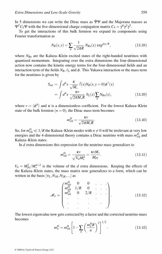
Extra Dimensions and Low-Scale Gravity 359
In 5 dimensions we can write the Dirac mass as ΨΨ and the Majorana masses as
ΨTC5Ψ with the five-dimensional charge conjugation matrix C5 = γ0γ2γ5.
To get the interactions of this bulk fermion we expand its components using
Fourier transformation as
NR(x,y) = ∑n
1√2πR
NRn(x) expiny/R, (13.38)
where NRn are the Kaluza–Klein excited states of the right-handed neutrinos with
quantized momentum. Integrating over the extra dimensions the four-dimensional
action now contains the kinetic energy terms for the four-dimensional fields and an
interaction term of the fields NR, L and φ . This Yukawa interaction or the mass term
for the neutrinos is given by
Sint =∫
d4xκ√M∗
(x)NR(x,y = 0)φ †(x)
=∫
d4xκv√
2πM∗RνL(x)∑
nNRn(x), (13.39)
where v = 〈φ 0〉 and κ is a dimensionless coefficient. For the lowest Kaluza–Klein
state of the bulk fermion (n = 0), the Dirac mass term becomes
mDν0 =
κv√2πM∗R
. (13.40)
So, for mDν0 1/R the Kaluza–Klein modes with n = 0 will be irrelevant at very low
energies and the 4-dimensional theory contains a Dirac neutrino with mass mDν0 and
Kaluza–Klein states.
In d extra dimensions this expression for the neutrino mass generalizes to
mDν0 =
κv√VdMd∗
=κvM∗MPl
. (13.41)
Vd = M2Pl/Md+2∗ is the volume of the d extra dimensions. Keeping the effects of
the Kaluza–Klein states, the mass matrix now generalizes to a form, which can be
written in the basis [νL,N1R,N2R, ...] as
Mν =
mD
ν0 0 0 . . .mD
ν0 1/R 0 . . .mD
ν0 0 2/R . . .. . . .. . . .. . . .
. (13.42)
The lowest eigenvalue now gets corrected by a factor and the corrected neutrino mass
becomes
mDν = mD
ν0
[1−∑
n
(mD
ν Rn
)2]1/2
. (13.43)
© 2008 by Taylor & Francis Group, LLC
360 Particle and Astroparticle Physics
This sum is well behaved for d > 2, which is also required for phenomenological
considerations.
Thus, making the singlet sterile neutrino to be a bulk fermion, we could suppress
the neutrino Dirac mass. For M∗ ∼ 1 TeV, the neutrino mass comes out to be mDν =
10−4 κ eV, which is too low. A trivial solution is to make M∗ ∼ 1000 TeV and
keep κ ∼ 1 for the heaviest neutrino. In this scenario it is possible to include a
lepton-number violating Majorana mass term for the right-handed neutrinos in 5
dimensions. But this will give a light Majorana neutrino with mass of the order of
10−11 eV.
The phenomenology of the right-handed neutrino in the bulk has been extensively
studied [223]. Since the right-handed neutrinos are bulk matter, they will also have
all the Kaluza–Klein excited states such as the graviton. There will be an infinite
tower of states starting at a scale of about eV. Since they interact with ordinary matter
very weakly, this is consistent with all present constraints. However, the existence
of the Kaluza–Klein states gives rise to some new features of the model, which are
mixing of neutrinos of different flavors with the Kaluza–Klein states. They induce
neutrino oscillations which are distinct and future experiments may distinguish them
from the usual 4-dimensional mechanisms of neutrino mass.
There is another suggestion to adjust the suppression factor without increasing
the fundamental scale or the 5-dimensional Yukawa coupling constant κ . Here one
assumes that the right-handed neutrino does not reside on the entire d-dimensional
bulk space. Instead it can move on an m-dimensional subspace. This can arise if our
brane is situated at the intersection of two or more branes, of which at least one brane
has m+3 spatial dimensions. Without going into the details of how such a scenario
may arise, let us consider the effect of such construction. Now the Kaluza–Klein
mode expansion of this field is
NR(x,y) =1√Vm
∑l
NRl(x) exp
[−2πil ·y(Vm)1/m
]. (13.44)
Using this Fourier expansion of the field and integrating over the extra dimensions
we get the Dirac neutrino mass to be
mDν = kv
[1−∑
n
(mD
ν Rn
)2]1/2(
M∗MPl
)m/d
. (13.45)
In this case the suppression factor is√
VmMm∗ ∼√(RM∗)m. Using the relation M2Pl =
RdMd+2∗ , the suppression factor becomes (M∗/MPl)m/d . Thus, with suitable choice
of m and d, it is possible to get the required neutrino masses.
Triplet Higgs
In models with extra dimensions it is possible to get naturally small neutrino masses
with triplet Higgs scalars in the distant breaking mechanism, which has some inter-
esting phenomenological consequences [222, 224]. In this scenario lepton number
© 2008 by Taylor & Francis Group, LLC
Extra Dimensions and Low-Scale Gravity 361
L is assumed to be conserved in our brane at P(y = 0), but broken spontaneously
by the vev of a scalar η (L = 2) in another brane P ′(y = y∗) at a distance r = |y∗|away from our brane in the extra dimension. This field η couples to a bulk scalar
χ(x,y) (L = −2), through the interaction [224]
Sother =∫
P ′d4x′ µ2 η(x′)χ(x′,y = y∗), (13.46)
where µ is a mass parameter. This will induce an effective vev to χ breaking lepton
number in the bulk, which in turn induces a tiny lepton number violation in our brane
through 〈χ〉:〈χ(x,y = 0)〉 = ∆d(r)〈η(x,y = y∗)〉, (13.47)
where 〈η〉 acts as a point source and ∆d(r) is the Yukawa potential in d transverse
dimensions. For mχ r 1, and d > 2, the Yukawa potential takes an interesting form
so the asymptotic form of the profile of χ becomes
〈χ〉 ≈ Γ( d−22 )
4π d2
M∗(M∗r)d−2 , (13.48)
which is the amount of lepton number violation in our world and is suitably small
for large r. Let us now introduce a triplet Higgs scalar [224] in our brane ξ , whose
quantum numbers are defined by its interaction
Sξ =∫
d4x fi jξ (x)i(x) j(x), (13.49)
then the shinned value of 〈χ〉 will induce explicit lepton number violation in our
brane
Sχ = h∫
Pd4x ξ †(x)φ(x)φ(x)χ(x,y = 0)
= h 〈χ〉∫
Pd4x ξ †(x)φ(x)φ(x). (13.50)
This lepton number violation will then give a neutrino mass
(Mν)i j ≈Γ( d−2
2 )
2π d2
h fi j〈φ〉2 M∗
m2ξ
(M∗MPl
)(2−4/d)
. (13.51)
For d = 3, M∗ ∼ 2 TeV, mξ <∼ 1 TeV and h ∼ fi j ∼ 0.5, we get (Mν)33 ∼ 0.24 eV,
which is of the right magnitude.
Explanation of the present experiments on neutrino mass requires that the triplet
Higgs mass has to be around TeV. Thus, this model predicts a triplet Higgs scalar in
the detectable range [224]. Since the same-sign dilepton signals of the triplet Higgs
are very clean, they should be observed in LHC or Tevatron or ILC if this is the true
mechanism of neutrino mass. Again the branching fractions of ξ ++ into same-sign
charged leptons l+i l+j determine directly the Yukawa coupling | fi j|, which in turn
© 2008 by Taylor & Francis Group, LLC
362 Particle and Astroparticle Physics
gives us the elements of the neutrino mass matrix modulo an overall scale factor.
This is a unique feature of this model. If this happens to be the model of neutrino
mass, then we can get all the information about the neutrino mass from collider
experiments.
There are a few other suggestions to explain the smallness of neutrino masses with-
out invoking a large lepton-number violating scale [222, 225]. While these models
have some interesting features, they do not involve any new mechanisms of the extra
dimensions. The model with bulk singlet right-handed neutrino can be implemented
in theories with warped compactification (small extra dimensions) [226]. Although
it has some differences in its construction, the basic idea is similar to that of a bulk
singlet mechanism of the large extra dimensions. However, the model has no new
predictions at low energy. It is difficult to implement the other models of neutrino
masses in models with small extra dimensions.
Strong CP Problem
The solution to the U(1)A problem through breaking of the chiral symmetry intro-
duced CP violation in the QCD Lagrangian. The coefficient Θ in the CP violating
term
Leff = LQCD + Θg2
32π2 Fµνa Fµνa (13.52)
is experimentally constrained to be very small. To explain why this number is so
small naturally, a dynamical mechanism has been proposed which predicts a new
light particle, the axion.
The mass of the axion ma is constrained to be very low from astrophysical and
cosmological considerations. The mass is given by the inverse of its decay constant
fa. In conventional theories the decay constant turns out to be the scale va at which
the Peccei–Quinn symmetry is broken and the bound on the axion mass implies
109 GeV < fa < 1012 GeV. It is a typical characteristics of any pseudo-Nambu–
Goldstone boson that its coupling is determined by the vevs of the Higgs scalars in
the theory and there is no extra parameter which can be tuned to suppress its coupling
to matter. A large scale is required so its coupling to matter can be suppressed.
In theories with extra dimensions there is no large scale in our world. So, the
global U(1) Peccei–Quinn symmetry cannot be broken at some high scale. If the
U(1) symmetry is broken at a scale below the fundamental scale, the axion coupling
to matter would be very strong which is ruled out. Then the natural possibility would
be to suppress the axion coupling to matter with some mechanisms involving extra
dimensions.
The obvious choice to suppress the axion coupling to matter would be to make the
axions a bulk field [227]. Then similar to the suppression of the coupling of matter to
gravity, the axion coupling will be suppressed by the ratio of the fundamental scale
to the Planck scale in 5 dimensions (M∗/MPl). If the symmetry breaking scale is
around M∗, the decay constant would be ∼ O(MPl). This suppression of the coupling
constant can be viewed as effectively raising the scale of va to the Planck scale,
which is again very large. The axion coupling will then be too small and fail to
© 2008 by Taylor & Francis Group, LLC
Extra Dimensions and Low-Scale Gravity 363
satisfy the cosmological constraint. Following the discussions for neutrino mass, the
natural choice is then to consider the axion to be a bulk field only along some (m-
dimensions) of the directions and not all (d-dimensions) the extra dimensions, so the
coupling to matter has a suppression (M∗/Mm/dPl ). This will make the axion coupling
to be the right amount.
Let us now discuss how a higher-dimensional Peccei–Quinn mechanism works.
Consider an example of a 5-dimensional space in which a complex scalar field φtransforms nontrivially under the U(1)PQ Peccei–Quinn symmetry. The vev of the
scalar breaks this symmetry at around the fundamental scale 〈φ〉 = va = fa/√
2 ∼M∗. The Nambu–Goldstone boson, the axion a, corresponding to the U(1)PQ sym-
metry breaking would translate under the U(1)PQ symmetry making it massless. We
now assume that our 3-brane is located at y = 0 and the field a interacts with the
gluons in our brane at the boundary, which gives a small mass to the axion. The
effective action of the 5-dimensional axion is given by
Seff =∫
d4x dy[
1
2M∗ ∂Aa∂ Aa +
ξfa
g2
32π2 aFµνa Fµνa δ (y)
], (13.53)
where ξ is a model dependent parameter.
We now Fourier expand the axion field assuming an orbifold compactification on a
Z2 under which the axion is assumed to be symmetric. In terms of the Kaluza–Klein
modes the axion decomposes as
a(x,y) =1√V
∞
∑n=0
an(x) cos(ny
R
), (13.54)
where V = 2πR is the volume of the extra dimension. Now only the zero mode
translates under the U(1)PQ symmetry and remains massless in the absence of the
anomaly term, but the other Kaluza–Klein modes become massive. This can be seen
from the effective 4-dimensional effective action
Leff =1
2
∞
∑n=0
(∂µ an)2 − 1
2
∞
∑n=1
n2
R2 a2n
+ξfa
g2
32π2
(a0 +
∞
∑n=1
√2an
)Fµν
a Fµνa , (13.55)
where we defined the new effective decay constant as fa = (V M∗)1/2 fa. For d extra
dimensions this becomes
fa =√
VdMd∗ fa =MPl
M∗fa. (13.56)
The Kaluza–Klein excited modes will have masses proportional to the inverse of
the radius of compactification man ∼ n/R and only the zero mode becomes the true
axion, which picks up a tiny effective mass from the anomaly term, proportional to
© 2008 by Taylor & Francis Group, LLC
364 Particle and Astroparticle Physics
the inverse of the decay constant. Since fa ∼ MPl is very large, an approximate form
of the axion can be given by
ma =√
2 fπ mπfa
∼ (0.3 GeV)2
fa. (13.57)
This expression is strictly valid in the limit R → 0. For large R, the effect of the
Kaluza–Klein modes is felt by the zero mode by decreasing its effective mass. For
very large R, the mass of the zero mode becomes ma ∼ R−1 and the mass of the axion
gets bounded by the inverse radius of compactification.
The axion coupling to ordinary matter comes from the
Saψψ ∼∫
d4x1
fa(∂µ a|y=0)(ψγµ γ5ψ) . (13.58)
In terms of Kaluza–Klein components this becomes
Saψψ ∼ 1
fa
∫d4x(∂µ a0 +
√2
∞
∑n=1
∂µ an)(ψγµ γ5ψ). (13.59)
Although only the zero mode could have a derivative coupling with matter, now
all the Kaluza–Klein modes have derivative coupling with matter suppressed by the
effective decay constant fa.
The effective decay constant fa ∼ MPl makes the axion mass unacceptably small
in this scenario. As we mentioned earlier, if we now consider a scenario in which
the axion propagates in the m-dimensional subspace of the d-dimensional bulk, the
effective decay constant becomes
fa =√
VmMm∗ fa =(
MPl
M∗
)m/d
fa. (13.60)
Suitable choice of m and d then makes the axion mass and, hence, the decay constant
consistent with present constraints.
In this scenario there are now new constraints on the axion coupling coming from
the coupling of matter with the Kaluza–Klein states with equal strength. The main
constraints are from cosmological considerations [228]. There are constraints from
the consideration of evolution of stars, mainly supernovae. This gives the strongest
lower bound. Then there are bounds coming from big-bang nucleosynthesis, overclo-
sure of the universe, cosmic microwave background radiation, and diffused photon
background. We shall discuss these details in chapter 18.
In another possible higher-dimensional solution to the axion mass problem, a
U(1)PQ symmetry is introduced in our brane, but broken in another brane at a dis-
tance [229]. This distant breaking of U(1)PQ then induces a small coupling of axion
to ordinary matter. Here one introduces heavy quarks with another anomalous low-
energy U(1) gauge symmetry (expecting that this symmetry will be anomaly free
at high energy). The details of the mechanism are similar to the distant breaking
mechanism for neutrino masses.
© 2008 by Taylor & Francis Group, LLC
Extra Dimensions and Low-Scale Gravity 365
There is a somewhat different suggestion to have quasi-localized gluons in higher
dimensions [230]. The vacuum structure then turns out to be trivial. At large dis-
tances the gluons would then behave as higher-dimensional, which does not support
finite action instantonic configurations. Then the Θ term vanishes on higher dimen-
sions and there is no CP problem in such scenario.
13.5 Warped Extra DimensionsSo far all the discussions we made about higher dimensions are based on the fact
that our 4-dimensional metric does not depend on the space–time points in the extra
dimensions. We usually consider higher-dimensional theories based on the fact that
the higher-dimensional metric is factorizable and can be written as a direct product of
the noncompact four space–time dimensions and the compact space of extra dimen-
sions. If the space–time geometry is warped, i.e., the 4-dimensional metric depends
on its position in the extra dimension, then it is possible to construct a consistent
theory of small extra dimensions that can allow a TeV scale strong gravity [231].
Several interesting features of the theories with large extra dimensions are shared
by theories with the small extra dimensions or the Randall–Sundrum model. This
theory with small extra dimensions promises a true solution to the gauge hierarchy
problem. In theories with large extra dimension, although the large Planck scale is
not present, there exists a very small scale corresponding to the distance of a few
microns, at which the law of gravity is modified. Since the extra dimensions are
compactified and the radius of compactification is of the order of a few microns, there
will be Kaluza–Klein excited states with masses starting from eV, corresponding to
all the particles in the bulk. Hence, in the bulk there is another scale of eV in addition
to the fundamental scale of a few TeV. For example, when the (4+d)-dimensional
Planck scale or the fundamental scale M∗ is related to the effective four-dimensional
Planck scale MPl by the volume of the compact space Vd ,
M2Pl = Md+2
∗ Vd , (13.61)
the corresponding compactification scale
µc ∼(
1
Vd
)1/d
(13.62)
is much smaller than the electroweak scale. Although there is no hierarchy between
the Planck scale of M∗ to the electroweak scale in theories with large extra dimen-
sions, a large hierarchy between the electroweak scale and the compactification scale
of order eV still exists.
In theories with small extra dimensions, the warped geometry relates the Planck
scale in our brane to the exponentially large Planck scale in another brane. So the
© 2008 by Taylor & Francis Group, LLC
366 Particle and Astroparticle Physics
new parameters appear only in the exponent, eliminating any hierarchy of scales. The
metric is not factorizable in this case, rather the four-dimensional metric is multiplied
by a warp factor, which is a rapidly changing function of an additional dimension.
Let us consider an example of such warped geometry, provided by a nonfactorizable
metric that respects the four-dimensional Poincare invariance,
ds2 = exp−2krc|φ | ηµν dxµ dxν + r2c dφ 2, (13.63)
where k is a scale of the order of the Planck scale and xµ are the four-dimensional co-
ordinates for constant φ . The extra dimension is considered to be an S1/Z2 orbifold,
whose coordinate is y = rc φ , where rc is the radius of a compact fifth dimension
and the angular coordinate φ has the periodicity in the range −π ≤ φ ≤ π . φ may be
rescaled to absorb rc, but that will alter the periodicity of φ .
The S1/Z2 orbifold may be viewed as a circle S1, whose two sides are identified
with each other by the Z2 mapping. If every point in the upper half of the circle
is identified with some points in the lower half of the circle, we get only a half-
circle. If some current was flowing through the circle, then at each point in this
half-circle the current flowing in two directions will cancel each other, except for
the two end-points. These two end-points then become the two singular fixed points
in this orbifold. The Z2 relates the points (x,φ) and (x,−φ), so there are now two
3-branes extending along the xµ directions and localized at the two fixed points in
the fifth dimension. We call the fixed point at φ = π the visible brane and the other at
φ = 0 the hidden sector brane. Both the branes couple to the purely four-dimensional
components of the bulk metric
gvisµν = Gµν(xµ ,φ = π)
ghidµν = Gµν(xµ ,φ = 0), (13.64)
where GMN (M,N = µ,4) is the five-dimensional metric. The curvature parameter
k relates the Planck scale in the hidden sector brane MPl to the fundamental scale
in our visible brane M∗ through the exponential warp factor of the five dimensional
spacetime,
M2Pl =
M3∗k
[1− exp−2krcπ
]. (13.65)
The bulk space connecting the visible sector brane and the hidden sector brane is a
slice of AdS5 space. The standard model particles are confined in our brane, while
gravity propagates in the bulk.
Four-Dimensional Interactions
We can now define an effective metric gµν(x) and express the metric in the visible
and hidden sector branes in terms of this effective metric as
gvisµν = exp−2σ gµν
ghidµν = gµν , (13.66)
© 2008 by Taylor & Francis Group, LLC
Extra Dimensions and Low-Scale Gravity 367
where σ = krcπ . The effective four-dimensional action can now be written in terms
of this effective metric gµν(x). The total action now splits into
S = Sbulk +Svis +Shid , (13.67)
where the bulk action now contains the 5-dimensional gravity including the cosmo-
logical constant term
Sbulk =∫
d4x∫ π
−πdφ
√−G(2M3∗R−Λ). (13.68)
By properly normalizing the fields we can determine the physical masses. Consider
a Higgs field H containing one symmetry breaking mass parameter v0,
Svis ⊃∫
d4x√−gvis
gµν
vis Dµ H†Dν H −λ (|H|2 − v20)
2 . (13.69)
We then write the action in terms of the effective metric gµν(x) and renormalize the
wave functions as
ψvis(φ = π) → exp3σ/2ψvis(φ = π)Hvis(φ = π) → expσ Hvis(φ = π)ψhid(φ = 0) → ψhid(φ = 0)Hhid(φ = 0) → Hhid(φ = 0) (13.70)
and obtain
Se f f =∫
d4x√−g
gµν Dµ H†Dν H −λ
(|H|2 − exp−2σ v20)2
. (13.71)
The mass scale (in general, any mass scale) in the visible sector 3-brane will corre-
spond to a physical mass
v0,m0phys = exp−σ v0,m0. (13.72)
Since all operators get rescaled by their four-dimensional conformal weight, the ef-
fective metric appears in the four-dimensional Einstein action. Hence, all mass scales
in the visible sector brane will be rescaled to the physical mass. In other words, the
Planck mass scale MPl in the distant brane now scales down to the M∗ scale in our
world (see figure 13.4).
By considering expσ to be of the order of 1015, this mechanism produces TeV
scale physics. In other words, for krc ≈ 10, all the mass parameters in the theory
v0,m0,k,M, and µc ∼ O(1/rc) become of the same order of magnitude, which is
close to the effective Planck scale of 103 GeV.
Similar to the models of large extra dimensions, in our brane the physical mass
scales in the theory are of the TeV scale. All the Kaluza–Klein modes and their
couplings are also determined by the TeV scale physics. This gives rise to a distinct
and rich phenomenology for the next generation accelerators. For an observer in the
© 2008 by Taylor & Francis Group, LLC
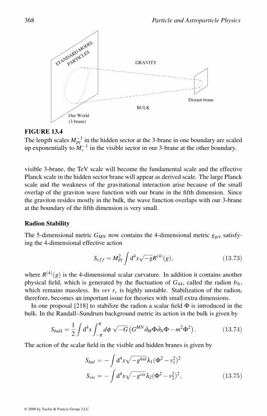
368 Particle and Astroparticle Physics
Our World
(3-brane)
GRAVITYPARTICLES
STANDARD MODEL
Distant brane
BULK
FIGURE 13.4The length scales M−1
Pl in the hidden sector at the 3-brane in one boundary are scaled
up exponentially to M−1∗ in the visible sector in our 3-brane at the other boundary.
visible 3-brane, the TeV scale will become the fundamental scale and the effective
Planck scale in the hidden sector brane will appear as derived scale. The large Planck
scale and the weakness of the gravitational interaction arise because of the small
overlap of the graviton wave function with our brane in the fifth dimension. Since
the graviton resides mostly in the bulk, the wave function overlaps with our 3-brane
at the boundary of the fifth dimension is very small.
Radion Stability
The 5-dimensional metric GMN now contains the 4-dimensional metric gµν satisfy-
ing the 4-dimensional effective action
Se f f = M2Pl
∫d4x
√−gR(4)(g), (13.73)
where R(4)(g) is the 4-dimensional scalar curvature. In addition it contains another
physical field, which is generated by the fluctuation of G44, called the radion bN ,
which remains massless. Its vev rc is highly unstable. Stabilization of the radion,
therefore, becomes an important issue for theories with small extra dimensions.
In one proposal [218] to stabilize the radion a scalar field Φ is introduced in the
bulk. In the Randall–Sundrum background metric its action in the bulk is given by
Sbulk =1
2
∫d4x
∫ π
−πdφ
√−G(GMN∂MΦ∂NΦ−m2Φ2) . (13.74)
The action of the scalar field in the visible and hidden branes is given by
Shid = −∫
d4x√
−ghidλ1(Φ2 − v21)
2
Svis = −∫
d4x√
−gvisλ2(Φ2 − v22)
2, (13.75)
© 2008 by Taylor & Francis Group, LLC
Extra Dimensions and Low-Scale Gravity 369
where vi and λi are parameters with nonzero mass dimensions.
We then make an ansatz that Φ depends only on the coordinates of the extra di-
mension and assume that the λi are large enough to give the vev of the scalar fields
at the two branes
Φ(0) = v1 and Φ(π) = v2. (13.76)
With another assumption ε = m2/4k 1, we can write the potential for the distance
of the two branes as
V (rc) = kεv21 +4kexp−4krcπ
(v2 − v1exp−εkrcπ
)2(1+
ε4
)−kεv1exp−(4+ε)krcπ
(2v2 − v1exp−εkrcπ
), (13.77)
which has a minimum at
krc =4k2
πm2 log
(v1
v2
). (13.78)
The expression for the stable distance rc between the branes in the presence of the
bulk scalar field Φ shows that there is no necessity for any fine tuning to get krc ∼ 10,
which gives the fundamental scale to be around TeV to get an effective Planck scale
in 4 dimensions.
One very important feature of the Randall–Sundrum model comes from the dual-
ity conjecture between warped AdS5 geometries with boundary branes and strongly
coupled (broken) conformal field theories coupled to dynamical gravity. For every
conformal field theory (CFT) operator there is a corresponding bulk field. Given any
boundary condition on these bulk fields at the four-dimensional boundary of the AdSslice, there is a unique solution of the string effective action (which includes grav-
ity). Introduction of the Planck brane allows a nice holographic interpretation of this
duality, which allows us to study the phenomenology of this scenario in a consistent
manner.
Although the hierarchy problem is solved and it gives us very rich phenomenol-
ogy, several new problems emerge in these models of extra dimensions. For exam-
ple, the question of proton decay becomes very important. Grand unification could
be achieved in these models below the fundamental scale of TeV, which makes the
proton lifetime too small. Several mechanisms have been suggested to solve this
problem. Two other problems need special attention in theories with extra dimen-
sions. Since the smallness of the neutrino mass and the axion coupling is attributed
to a large scale and there is no large scale in these theories, solutions to these prob-
lems require new approaches.
The theories with large and small extra dimensions are just two special cases of
a large class of theories, which bring us promise of new physics. There are other
constructions of brane worlds which can trap gravity in a very large number of ex-
tra dimensions. But the important point that these models of extra dimensions are
making is that the gravity can propagate in some dimensions, which are not accessi-
ble to the standard model particles. This will mean that the strength of gravitational
interaction can become strong at fairly low scale, which is the fundamental scale in
© 2008 by Taylor & Francis Group, LLC
370 Particle and Astroparticle Physics
the theory. The new low Planck scale depends on various unknown parameters and
cannot be determined by any theory. The Planck scale could be as low as TeV or this
could be as high as the effective Planck scale of 1019 GeV. We hope this new scale
to be in the TeV range, so all the new physics will become accessible to the next
generation experiments. This will allow us to probe all the new exciting physics of
models of extra dimensions and even study quantum gravity in the next few years.
However, if the scale is much higher, we may not observe any new signatures. In any
case, the possibility of observing new phenomenology in the TeV range is highly
welcome, since the next generation detectors have to be designed keeping these new
signatures in mind. The future experiments can only discriminate among the several
possible theories at the TeV scale and lead us to the next stage.
© 2008 by Taylor & Francis Group, LLC
14Novelties with Extra Dimensions
The possibility of new physics coming from extra space dimensions opened up many
new directions in this field. Most of the higher dimensional theories consider only
four noncompact space–time dimensions and the remaining compact space dimen-
sions. However, it has been demonstrated that the extra space dimensions could also
be noncompact in some cases. For example, the extra dimensions can be noncom-
pact if the geometry is warped and the radius of curvature of the extra dimensions are
small enough. It is also possible to construct models with extra dimensions, where
the extra dimensions do not play any crucial role with respect to gravity. The extra
dimensions are constructed in an interval, and the boundary points in this interval
provide new physics. If the end points are singular, one may construct grand unified
theories in such orbifolds with several interesting features. The boundary conditions
at the end-points can also be used to break gauge symmetries spontaneously. This
could be an alternative to the Higgs mechanism of spontaneous symmetry breaking.
The boundary conditions may also break supersymmetry giving rise to interesting
supersymmetric particle spectrum. If the ordinary particles are allowed to propagate
along the interval, it can lead to newer phenomenological implications.
14.1 Noncompact Warped DimensionsThere are evidences that we live in four noncompact dimensions. Newton’s law has
been established to a very high degree of accuracy, which is valid for four dimen-
sions. Although there are only four noncompact dimensions, it is possible to have
several compact extra dimensions. Even for compact higher dimensions the radius
of curvature should be very small. Otherwise, since gravity propagates along all
the dimensions, at short distances deviation from Newton’s 1/r2 law should be ob-
served. If the usual particles can also propagate in the extra dimensions, then there
will be even stronger constraints. For n extra compact dimensions, the Planck scale
in higher dimensions M∗ will be reduced compared with the Planck scale in four
dimensions MPl by the volume Vn of the extra dimensions M2n∗ = M2Pl/Vn. However,
these general comments would change in case of warped geometry.
If the metric of our four space–time dimensions depends on its position in the
extra dimensions, then the metric is called warped. The general comments about the
extra dimensions are based on the fact that the metric is factorizable and the space
371
© 2008 by Taylor & Francis Group, LLC
372 Particle and Astroparticle Physics
of extra dimensions can be written as a direct product of the usual noncompact four
space–time dimensions. If the space–time geometry is warped, then it is possible to
construct a consistent noncompact 4+n-dimensional theory of gravity [232]. In this
case the Planck scale in higher dimensions will be related to the four-dimensional
Planck scale by the curvature of the extra dimensions. Due to the warped geometry,
the extra dimensions can have a localized bound state of the higher-dimensional
graviton. Consider the wave equation for small gravitational fluctuations (see section
11.1) in the presence of a nontrivial potential V due to the curvature, which acts like
a source term, given by
[∂µ ∂ µ −d jd j +V (z j)] h(xµ ,z j) = 0. (14.1)
Here the coordinates are xµ for the four dimensions and z j for the extra dimensions.
The higher-dimensional gravitational fluctuations h(xµ ,z j) can be written in terms of
the four-dimensional Kaluza–Klein states ψ(z) with fixed wave function in the extra
dimensions
h(xµ ,z j) = expip·xψ(z).
The masses m of the four-dimensional Kaluza–Klein states is given by the eigenval-
ues of
[−d jd j +V (z)] ψ(z) = −m2 ψ(z) , (14.2)
where p2 = m2. If the background preserves Poincare invariance, then there is a nor-
malizable zero mode state representing the four-dimensional graviton, in addition to
all its Kaluza–Klein excited modes. In case of factorizable geometry, there is a gap
in the spectrum of the excited modes, which determines the scale at which deviation
from usual four-dimensional gravity is expected. In the present case although the
excited states have a continuum with no gap, the nontrivial potential V (z) implies
a single bound state corresponding to a massless four-dimensional graviton, whose
wave function is centered around the 3-brane containing the standard model parti-
cles. This reproduces four-dimensional gravity predictions at low energy and long
distances, in spite of the presence of the continuum of excited gravitons.
We present here the original model [232] which is a five-dimensional space–time
containing a single 3-brane with a positive tension. The standard model particles
are confined in the 3-brane. A regulator brane (denoted by brane′) at a distance of
y0 = πrc from the 3-brane of interest is introduced for checking consistency, which
will ultimately be taken to infinity (taking the limit y0 → ∞) and be removed from
the physical setup. The two branes, the standard model 3-brane and the regulator
brane, constitute the boundaries of a finite fifth dimension. The action is given by
S = Sgrav +Sbrane +Sbrane′ ,
Sgrav =∫
d4x∫
dy√−G(2M3
∗R−Λ)
Sbrane =∫
d4x√−gbrane(Vbrane +Lbrane), (14.3)
© 2008 by Taylor & Francis Group, LLC
Novelties with Extra Dimensions 373
where GMN (M,N = µ,4; µ = 0,1,2,3) is the five-dimensional metric, R is the
five-dimensional Ricci scalar, and M∗ is the fundamental scale for gravity in five
dimensions.
A solution to the Einstein’s equations which respects four-dimensional Poinare
invariance may be obtained when the boundary and bulk cosmological terms are
related by
Vbrane = −Vbrane′ = 24M3k, and Λ = −24M3k2,
with k to be the curvature parameter that would define the effective Planck scale in
four dimensions. The solution is a slice of the symmetric space, AdS5, and is given
by
ds2 = exp−2k|y| ηµν dxµ dxν +dy2, (14.4)
where 0 ≤ y ≤ y0 is the coordinate of the fifth dimension.
The four-dimensional graviton zero mode follows from this equation and is de-
scribed by an effective action
Se f f ⊂∫
d4x∫ πrc
0dy 2M3
∗rcexp−2k|y|R, (14.5)
where R denotes the four-dimensional Ricci scalar made of the four-dimensional
metric gµν(x). From this the effective Planck scale in four dimensions can be related
to the fundamental scale through the relation
M2Pl =
M3∗k
[1− exp−2ky0
], (14.6)
so there is a well-defined effective Planck scale even in the limit y0 → ∞. This allows
the removal of the regulator brane from the setup.
The next step is to study the spectrum of general linearized fluctuations
GMN = exp−2k|y| ηµν +hµν(x,y)
and check for consistency with four-dimensional gravity. This can be done by a
Kaluza–Klein reduction through separation of variable h(x,y) = expip·xψ(y) (where
p2 = m2) and obtaining a solution to the linearized equation of motion expanded
about the warped metric[−m2
2exp2k|y|− 1
2∂ 2
y −2kδ (y)+2k2]
ψ(y) = 0. (14.7)
Only the even functions of y are relevant for the boundary condition with the regu-
lator brane taken to infinity. The µν indices are eliminated by working in the gauge
∂ µ hµν = hµµ = 0, where µν indices are the same for all the terms.
To understand the concept without going into details, we make a change of vari-
ables
z =sgn(y)
k
(expk|y|−1
); ψ(z) = ψ(y)expk|y|/2; h(x,z) = h(x,y)expk|y|/2
© 2008 by Taylor & Francis Group, LLC
374 Particle and Astroparticle Physics
to obtain [−1
2∂ 2
z +V (z)]
ψ(z) = m2 ψ(z), (14.8)
where
V (z) =15 k2
8(k|z|+1)2 − 3k2
δ (z). (14.9)
The general shape of this potential tells us that the delta function supports a single
normalizable bound state mode, which is the massless graviton reproducing gravity
in four dimensions. The remaining eigenstates correspond to a continuum of the
excited Kaluza–Klein states. Since the potential falls off to zero for z0 → ∞, there
is no gap and the continuum of excited states has all possible m2 > 0. Tuning of the
cosmological terms ensure that the bound state mode corresponds to the massless
graviton. Taking only even functions of z and the limit z0 → ∞, only a semi-infinite
extra dimension is achieved. This can be extended to an infinite extra dimension by
allowing both the even and odd functions of z.
In the infinite extra dimension limit the effective nonrelativistic gravitational po-
tential between two particles with mass m1 and m2 on the standard model brane at
z = 0 is the static potential generated by exchange of the zero-mode and continuum
excited mode propagators. It is given by
V (r) ∼ GNm1m2
r+
∫ ∞
0
dmk
GNm1m2exp−mr
rmk
∼ GNm1m2
r
(1+
1
r2k2
). (14.10)
The leading term produces an effective four-dimensional gravity with usual Newto-
nian potential, which is due to the massless graviton or the bound state zero-mode.
The sum over excited continuum states adds an correction, extremely suppressed by
Planck scale squared (k is of the order of Planck scale). The production of the contin-
uum modes from the brane at z = 0 will also be suppressed due to the wave function
suppression there.
In this model the tension in the standard model brane is fine tuned, which is equiv-
alent to the fine tuning of the cosmological constant problem, since the bound state
graviton mode is determined by the brane tension and the bulk cosmological con-
stant. Planck scale is the same as the fundamental scale of the higher-dimensional
theory. The excited continuum of states thus decouples from the low-energy physics,
but is required for the consistency of the theory. At this stage this theory is not
complete and may not have significant phenomenological implications, but the basic
idea of noncompact extra dimensions with warped space–time geometry opens up
new possibilities.
© 2008 by Taylor & Francis Group, LLC
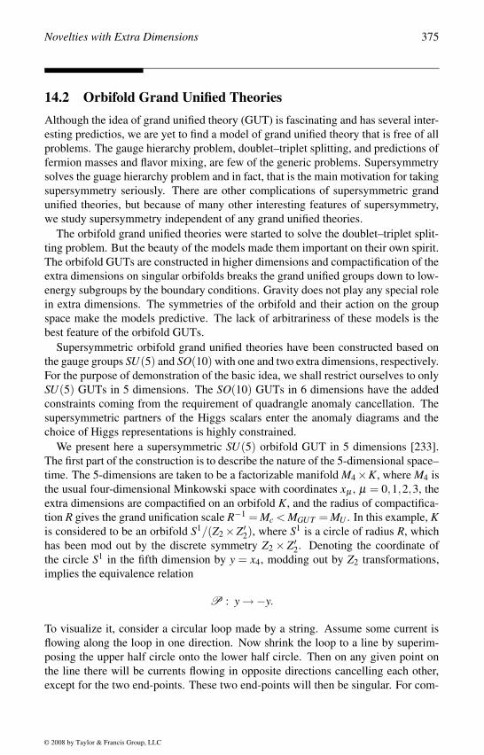
Novelties with Extra Dimensions 375
14.2 Orbifold Grand Unified TheoriesAlthough the idea of grand unified theory (GUT) is fascinating and has several inter-
esting predictios, we are yet to find a model of grand unified theory that is free of all
problems. The gauge hierarchy problem, doublet–triplet splitting, and predictions of
fermion masses and flavor mixing, are few of the generic problems. Supersymmetry
solves the guage hierarchy problem and in fact, that is the main motivation for taking
supersymmetry seriously. There are other complications of supersymmetric grand
unified theories, but because of many other interesting features of supersymmetry,
we study supersymmetry independent of any grand unified theories.
The orbifold grand unified theories were started to solve the doublet–triplet split-
ting problem. But the beauty of the models made them important on their own spirit.
The orbifold GUTs are constructed in higher dimensions and compactification of the
extra dimensions on singular orbifolds breaks the grand unified groups down to low-
energy subgroups by the boundary conditions. Gravity does not play any special role
in extra dimensions. The symmetries of the orbifold and their action on the group
space make the models predictive. The lack of arbitrariness of these models is the
best feature of the orbifold GUTs.
Supersymmetric orbifold grand unified theories have been constructed based on
the gauge groups SU(5) and SO(10) with one and two extra dimensions, respectively.
For the purpose of demonstration of the basic idea, we shall restrict ourselves to only
SU(5) GUTs in 5 dimensions. The SO(10) GUTs in 6 dimensions have the added
constraints coming from the requirement of quadrangle anomaly cancellation. The
supersymmetric partners of the Higgs scalars enter the anomaly diagrams and the
choice of Higgs representations is highly constrained.
We present here a supersymmetric SU(5) orbifold GUT in 5 dimensions [233].
The first part of the construction is to describe the nature of the 5-dimensional space–
time. The 5-dimensions are taken to be a factorizable manifold M4 ×K, where M4 is
the usual four-dimensional Minkowski space with coordinates xµ , µ = 0,1,2,3, the
extra dimensions are compactified on an orbifold K, and the radius of compactifica-
tion R gives the grand unification scale R−1 = Mc < MGUT = MU . In this example, Kis considered to be an orbifold S1/(Z2 ×Z′
2), where S1 is a circle of radius R, which
has been mod out by the discrete symmetry Z2 × Z′2. Denoting the coordinate of
the circle S1 in the fifth dimension by y = x4, modding out by Z2 transformations,
implies the equivalence relation
P : y →−y.
To visualize it, consider a circular loop made by a string. Assume some current is
flowing along the loop in one direction. Now shrink the loop to a line by superim-
posing the upper half circle onto the lower half circle. Then on any given point on
the line there will be currents flowing in opposite directions cancelling each other,
except for the two end-points. These two end-points will then be singular. For com-
© 2008 by Taylor & Francis Group, LLC
376 Particle and Astroparticle Physics
pleteness, we further mod this out by the second Z ′2 which acts as
P ′ : y′ →−y′,
with y′ = y+πR/2. With this we complete the construction of the orbifold in the fifth
dimension, which is essentially a line interval y ∈ [0,πR/2] with two fixed points at
the boundaries at y = 0 and y = πR/2 ≡ . The fixed points at the boundaries will
have 4-dimensional 3 branes O and O ′, respectively.
The basic assumption of the orbifold GUTs is that the fields propagating along
the fifth dimension or the bulk should also possess the two discrete symmetries Z2and Z′
2. In other words, corresponding to the action of the discrete groups Z2 ×Z′2
on the circle S1, there will be equivalent Z2 ×Z′2 parity transformations on the fields
propagating in the bulk. Any generic field in the bulk, Φ(xµ ,y), will then be acted
upon by the action of the two Z2 and Z′2 parities P and P ′ as
P : Φ(xµ ,y) → Φ(xµ ,−y) = PΦ Φ(xµ ,y)P ′ : Φ(xµ ,y′) → Φ(xµ ,−y′) = P′
Φ Φ(xµ ,y′). (14.11)
The parities P and P ′ give eigenvalues ±1. In general, there is no definite rule
to decide the parities of any field. Depending on the requirement of the model, one
needs to assign the parities of any field. However, once the parities of any field are
assigned, the interactions and the profile of the field will be determined.
To get the profile of the various fields, we write the mode expansions of the fields
Φ±±(xµ ,y) with eigenvalues P,P ′ ≡ ±,±:
Φ++(xµ ,y) =
√2
πR
∞
∑n=0
Φ(2n)++ (xµ)cos
2nyR
,
Φ+−(xµ ,y) =
√2
πR
∞
∑n=0
Φ(2n+1)+− (xµ)cos
(2n+1)yR
,
Φ−+(xµ ,y) =
√2
πR
∞
∑n=0
Φ(2n+1)−+ (xµ)cos
(2n+1)yR
,
Φ−−(xµ ,y) =
√2
πR
∞
∑n=0
Φ(2n+2)−− (xµ)cos
(2n+2)yR
. (14.12)
Only the 4D Kaluza–Klein field with eigenvalues ++ can have a massless zero
mode. The fields Φ++ and Φ+− can be nonvanishing at the brane O at y = 0, while
the fields Φ++ and Φ−+ can be nonvanishing at the brane O ′ at y = .
In 5D the local Lorentz group is O(5). The Weyl projection operator γ5 is part of
O(5) and hence both the left-chiral and right-chiral fields of 4D belong to the same
representation of any 5D field. The N = 1 supersymmetry in 5D will thus contain 8
real supercharges, which in 4D will imply an N = 2 supersymmetry. For any realis-
tic orbifold grand unified theory, the parity assignment corresponding to the discrete
symmetries P and P ′ should reduce N = 2 supersymmetry to N = 1 supersymme-
try in 4D and also break the SU(5) symmetry to the standard model gauge group
© 2008 by Taylor & Francis Group, LLC
Novelties with Extra Dimensions 377
SU(3)c ×SU(2)L ×U(1)Y . This can be achieved by the parity assignments
P = diag +1,+1,+1,+1,+1and P ′ = diag −1,−1,−1,+1,+1, (14.13)
where these matrix representations of P and P ′ act on the fundamental repre-
sentation of SU(5). Thus, all SU(5) components of any multiplet will have the
same parity under P , while the components of the SU(5) multiplets that are in-
variant under the standard model SU(3)c × SU(2)L ×U(1)Y (denoted by the index
a) will have opposite parity compared with the fields belonging to the coset space
SU(5)/SU(3)c×SU(2)L ×U(1)Y (denoted by the index a) under P ′. A coset space
G/H means the elements of the group space G, which are not elements of H.
The vector multiplet of N = 2 supersymmetry contains a vector supermultiplet
Va and a scalar supermultiplet Σa of N = 1 supersymmetry. The parity assignments
are inputs in orbifold GUTs, which determine the matter contents. One convenient
choice for the parity operator P is even for the vector multiplets and odd for the
scalar multiplets. The (P,P ′) assignments for the vector and scalar multiplets are
then given by
V a ≡ (+,+), V a ≡ (+,−), Σa ≡ (−,+), Σa ≡ (−,−).
Thus, only V a will have massless zero modes, and hence, at low energies only the
minimal supersymmetric standard model gauge bosons are present in the theory.
Although the 4-dimensional theory has only the standard model gauge symme-
try, the 5-dimensional theory has a larger position-dependent gauge symmetry. The
gauge transformation parameters ξa and ξa now have the Kaluza–Klein expansion
ξa(xµ ,y) =∞
∑n=0
ξ na (xµ)cos
2nyR
ξa(xµ ,y) =∞
∑n=0
ξ na (xµ)cos
(2n+1)yR
. (14.14)
At y = πR/2, all the modes of the gauge transformation parameter ξ na vanish. Thus,
in the brane O ′ at y = , only the standard model symmetry is present, whereas in
all other points in the fifth dimension all the gauge parameters are nonvanishing and
possess the SU(5) symmetry. For the gauge kinetic terms this implies
S =∫
d4xdy[
1
g25
F2 +δ (y)1
g2 F2 +δ (y− )1
g2a
F2a
], (14.15)
where Fa correspond to the field strengths for the standard model gauge groups (a =1,2,3) and F represents the field strengh for the entire SU(5) gauge symmetry. The
first and second terms are SU(5) invariant bulk and O brane gauge kinetic energies,
while the third term represents standard model gauge kinetic energy localized at
y = . The standard model gauge couplings ga are obtained by integrating over the
extra dimensions1
g2a
=
g25
+1
g2a, (14.16)
© 2008 by Taylor & Francis Group, LLC
378 Particle and Astroparticle Physics
where the contribution of g has been absorbed into a shift of ga. The standard model
gauge couplings ga now depend on the localized kinetic operators ga, making them
nonuniversal at the large cut-off scale. However, this problem can be removed by
making the extra dimensions large so that the nonuniversal contribution is suppressed
by the volume factor.
Next we introduce the Higgs scalars in the model. The usual Higgs doublet which
breaks the electroweak symmetry belongs to a 5 of SU(5). Supersymmetry then
requires both 5 and 5 representations of the SU(5) Higgs fields. The Higgs fields
could be introduced in the bulk and then impose parity P ′ to ensure that only the
standard model doublets have the zero modes and can remain massless, while the
triplet components become heavy naturally and there is no doublet–triplet splitting
problem. This was the main motivation to consider orbifold GUTs initially. One may
also introduce the Higgs fields in the standard model brane at y = . Then only the
standard model representations will appear in the theory and one may consider only
the Higgs doublets in the theory. There are no Higgs triplets in this model, which
also solves the doublet–triplet splitting problem.
The fermions can now be introduced in the bulk or in the SU(5) invariant brane at
y = 0 to preserve the SU(5) understanding of matter quantum numbers. If they are
in the brane, then they appear as supermultiplets in 10 + 5 representations. But, if
they are in the bulk, they appear in N = 2 hypermultiplets. However, the parities will
allow only one N = 1 supermultiplet to be the massless zero mode. Gauge coupling
unification in these theories requires the compactification scale Mc ∼ 1015 GeV to be
slightly less than the grand unification scale MU ∼ 2×10¹⁶ GeV. The Kaluza–Klein
states contribute to the evolution of the gauge coupling between these two scales.
14.3 Split SupersymmetrySupersymmetry, a symmetry between fermions and bosons, is a beautiful symmetry
to exist in nature. For constructing a consistent theory of gravity, the superstring
theory, supersymmetry plays a crucial role. However, a more popular reason for in-
troducing supersymmetry is to solve the gauge hierarchy problem. This implies that
the supersymmetry breaking scale should not be higher than TeV. Supersymmetry
also provides solution to the gauge coupling unification.
Recently it has been argued that the naturalness may not be a problem, rather we
must get used to it. We have noticed a strong naturalness problem with the cosmo-
logical constant. The observed value of the cosmological constant requires new dy-
namics at the scale of 10−3 eV, which should not be affected by any physics at much
higher energies, for example, the electroweak symmetry breaking scale or even the
Planck scale.
If we now extrapolate our lack of understanding of this naturalness question to the
Higgs sector, we may not require supersymmetry near the TeV scale. There could
© 2008 by Taylor & Francis Group, LLC
Novelties with Extra Dimensions 379
be supersymmetry at much higher scale so all the scalar superpartners are heavy.
However, the gauginos and Higgsinos remain light so the gauge coupling unification
is not disturbed. The model also predicts a dark matter candidate. This new class
of models with supersymmetry breaking scale to be very large is called the split
supersymmetry [234, 235].
Split supersymmetric models may not be as appealing as the regular supersymmet-
ric models, but they are a new possibility with distinct phenomenological predictions,
which could be verified in the next generation accelerator experiments. The essen-
tial features of any split supersymmetric models include predictions for a dark matter
candidate, which is usually a gravitino LSP. The standard model gauge coupling con-
stants evolve to a single unified gauge coupling at the grand unification scale. It is
assumed that grand unification into a simple group occurs without any intermediate
symmetry breaking scale and the gauginos and the Higgsinos have masses of the or-
der of 100 GeV. In split supersymmetric models all scalar fermions have masses of
the order of some intermediate symmetry breaking scale. The flavor changing neutral
current problem of the low-energy supersymmetry and the proton decay problems are
absent in all split supersymmetric models. Observable electron dipole moments are
one of the generic predictions of these models, which could be tested in the next gen-
eration of experiments. The particle spectrum required for split supersymmetry can
be obtained in some models originating from extra dimensions. We shall illustrate
the basic structure of these models with one example of an orbifold grand unified
theory [236]. However, the mechanism is generic in nature and could be applicable
to any 5-dimensional space with one of the dimensions an interval, and the effective
Planck scale around the grand unification scale [234].
Consider a supersymmetric SU(5) orbifold GUT in 5 dimensions with N = 1 su-
persymmetry, the same as the one discussed in the previous section. The standard
model particles are localized at the O ′ brane at y = , where SU(5) is broken to the
standard model. The quarks and the leptons remain massless in this brane. Super-
symmetry is broken by Scherk–Schwarz mechanism in extra dimensions [237]. The
scalar radius moduli T acquire kinetic terms only through gravity couplings. The F-
component of this radion chiral superfield T = r+θ 2 in the SU(5) invariant brane at
O then breaks supersymmetry [238] in the background making the minimum of the
potential negative. Fine tuning the F-component of the chiral superfield X in the O ′brane, the vacuum energy is made to vanish. The coupling of this field X makes all
scalar superpartners heavy, while the gauginos and the Higgsinos receive only 100
GeV order anomaly mediated masses.
We add a constant superpotential
W = cM35 ,
localized in the SU(5) invariant brane at O and write the tree-level effective La-
grangian with T and the conformal compensator field φ = 1+θ 2Fφ
L =∫
d4θφ †φK +∫
d2θφ 3W +H.c. , (14.17)
© 2008 by Taylor & Francis Group, LLC
380 Particle and Astroparticle Physics
where the Kahler potential K = M35(T +T †). The resulting scalar potential
V = M35(r|Fφ |2 +F∗
T Fφ +3cFφ +h.c)
(14.18)
leads to supersymmetry breaking minimum with vanishing potential
Fφ = 0 and FT = −3c.
The gravitino then receives a mass m3/2 = 1/r (assuming c = 1) by combining with
the fermionic partner of T .
The one-loop corrections make Fφ nonvanishing
Fφ ∼ 1
16π21
M35 r4
m3/2
with a negative potential at the minima. As discussed earlier, we now add a chiral
superfield X at the standard model brane O ′ and write the R-parity invariant super-
potential at O ′ as
W = m2X =1
4πr2 X . (14.19)
We assigned an R-symmetry charge 2 to the superfield X . The Kahler potential at O ′is then given by
K = X†X − (X†X)2
M25
+ · · ·. (14.20)
The minimum of the potential then breaks supersymmetry with
|Fφ |2 = m4 =1
16π2r4 (14.21)
and a vanishing cosmological constant.
The Kahler potential and the superpotential then gives the mass spectrum of all
the fields. This leads to masses of
scalar component o f X m2X ∼ m4/M2
5
f ermionic component o f X mψX ∼ m4/M35
vev f or X 〈X〉 ∼ m2/M5
(14.22)
and FX ∼ m2, where m = M35/M2
Pl . Contact interactions on the standard model brane
or anomaly or gravitationally induced effective operators
∫d4θ
1
M25
X†XQ†Q,∫
d2θm2XM2
5WW and
∫d4θ
X†XM2
5WW,
leads to the mass spectrum:
scalar superpartners o f f ermions mS ∼ |FX |M5
∼ M55
M4Pl
gaugino masses Mi ∼ |FX |2M3
5∼ M9
5M8
Pl
(14.23)
© 2008 by Taylor & Francis Group, LLC
Novelties with Extra Dimensions 381
We then assign a vanishing R-charge to Hu and Hd to prevent terms such as
M5HuHd . The leading order terms contributing to µB and µ are
∫d4θ
m2X†
M35
HuHd ,∫
d2θm2XM2
5HuHd and
∫d4θ
X†XM2
5HuHd ,
This gives us Higgsino masses similar to those of the gauginos with
µB ∼ |FX |2M2
5∼ m2
S and µ ∼ Mi. (14.24)
In the present model, the natural scale is the grand unification scale, which is of the
order of M5 ∼MG ∼ 3×10¹³ GeV. Assuming usual flat space relationship rm35 = M2
Pl ,
we get the different mass scales:
Gravitino mass m3/2 ∼ 1013GeV
Supersymmetry breaking scale mS ∼ 109GeV
Masses o f superpartners o f f ermions m f ∼ mS ∼ 109GeV
Gaugino and Higgsino masses Mi ∼ 100 GeV
(14.25)
The split supersymmetry spectrum comes out of this orbifold GUT model. Gauge
coupling unification is verified and the model predicts an LSP dark matter candidate.
Since the standard model fermions are now localized to the O ′ brane, where the
SU(5)/SU(3)c × SU(2)L ×U(1)Y multiplets are absent, there are no SU(3)c triplet
Higgs scalars, which could cause fast proton decay. Proton decay is naturally sup-
pressed, and fermion masses come from the usual standard model Yukawa couplings.
Split supersymmetric model is a phenomenological model with distinct predic-
tions that the superpartners of the quarks and leptons are heavy, but the gauginos and
Higgsinos are light. The gauge coupling unification is assured and LSP dark matter
is there. However, there exist some models of extra dimensions, including the mod-
els of orbifold grand unified theories, which can predict this spectrum consistently.
If superpartners of the fermions are not detected in the next generation accelerators,
then this possibility will become more attractive.
14.4 Higgsless ModelsThe standard model of electroweak interactions is based on the Higgs mechanism,
but we have yet to find the Higgs scalar. In fact, we have yet to find any fundamental
scalar particle until now. So, the discovery of the Higgs particle will establish that
spin-0 scalar particles exist in nature and the Higgs mechanism of spontaneous sym-
metry breaking will be established, which makes the discovery of the Higgs particle
© 2008 by Taylor & Francis Group, LLC
382 Particle and Astroparticle Physics
so important. The precision measurements of the parameters of the standard model
provided bounds on the mass of the Higgs particle. There is a stronger bound on
the Higgs mass in the supersymmetric theories. If the Higgs particle is heavier than
about 135 GeV, then that may rule out the minimal supersymmetric standard model.
But in case we do not find the Higgs particle at all within the allowed mass range, it
will pose a serious problem.
With a view to overcoming this problem several alternatives have been attempted.
The technicolor theory appeared promising in the beginning, but the precision mea-
surements of the electroweak parameters ruled out this possibility. In another pos-
sibility one adds a second Higgs scalar, which does not acquire any vev. For some
choice of parameters this scenario pushes up the mass of the Higgs scalar. Another
interesting possibility is the little Higgs model. These are essentially extensions of
the composite Higgs models, in which a new strong force binds the more funda-
mental constituents of the Higgs field. Inconsistency with the precision electroweak
measurements is avoided by making the Higgs scalars pseudo-Nambu–Goldstone
bosons and then incorporating collective symmetry breaking mechanism, which en-
forces the cancellation of the quadratic divergent contributions to the Higgs mass by
introducing new particles. These new particles may have phenomenological predic-
tions. However, at present the most promising alternative to the Higgs mechanism
seems to be the Higgsless model, which is a new scenario that may emerge in models
with extra dimensions.
The basic idea behind the Higgsless model is to break the gauge symmetry spon-
taneously and give masses to the fermions by applying specific boundary conditions
on an extra dimension in an interval [239, 240, 241]. We start with a model with one
extra dimension in an interval, which means that the extra dimension is neither ex-
tended to infinity nor compact. Consider a circle and identify all points of the circle
on the left with a corresponding point in the right. This straight line with singular-
ity at the end-points represents an extra dimensions in an interval. The boundary
conditions on the singular end-points can then break any gauge symmetry in this
interval.
This is an interesting idea, but there is no completely consistent theory based on
this idea. There is also an argument that these theories may not satisfy the unitarity
constraint [242]. But considering the importance of an alternative for the Higgs
mechanism, we expect that the problems of the Higgsless model can eventually be
removed.
Let us consider a 5-dimensional theory, where the fifth dimension is an interval
starting at 0 and ending at πR [239]. The end-points have singularity like the orbifold
models. We start with a scalar field φ in the bulk and write its action
S =∫
d4x∫ πR
0dy(
1
2∂ Nφ∂Nφ −V (φ)
+1
2δ (y)M2
1 φ 2 +1
2δ (y−πR)M2
2 φ 2)
. (14.26)
The two end-points have the masses for the scalar field. We now impose that the
© 2008 by Taylor & Francis Group, LLC
Novelties with Extra Dimensions 383
variation of the equation vanishes to get a consistent set of boundary conditions.
The bulk equation of motion is obtained by the variation of this equation and then
integrating by parts
∂ N∂Nφ +∂V∂φ
= 0. (14.27)
For the boundary conditions there will be contributions from the boundary pieces
δφ(∂5φ +M21 φ)∣∣y=0 = 0
δφ(∂5φ −M22 φ)∣∣y=πR = 0. (14.28)
These two equations are then solved using the consistent set of boundary conditions
that respects 4-dimensional Lorentz invariance at y = 0,πR:
(i) (∂5φ ±M2i φ)∣∣y=0,πR = 0 (14.29)
(ii) φ |y=0,πR = const. (14.30)
The former is a mixed boundary condition, and for Mi = 0, it reduces to the Neumann
boundary condition. The latter boundary condition becomes the Dirichlet boundary
condition for const. = 0 (see section 12.5 for discussions on these boundary condi-
tions). Depending on the problem under consideration, the different boundary con-
ditions may be used.
Let us now include the gauge bosons in the problem. We denote the 5-dimensional
gauge bosons as AaM, M = 0,1,2,3,4, where a is the index for the internal gauge
group in the adjoint representation. This field will decompose to a 4-dimensional
gauge boson Aaµ and a scalar Aa
5. In the Rξ gauge, the mixing between these fields
Aaµ with Aa
5 is eliminated by gauge fixing and the action becomes
S =∫
d4x∫ πR
0dy(−1
4Fa
µν Faµν − 1
2Fa
5ν Fa5ν
− 1
2ξ(∂µ Aaµ −ξ ∂5 Aa
5)2)
. (14.31)
ξ → ∞ will take it to unitary gauge, making all Aa5 mode massive. Since the Kaluza–
Klein modes of Aa5 become unphysical, we eliminate them. They become the longi-
tudinal modes of the gauge bosons.
Similar to the scalar field, we can write the usual bulk equations of motion by
integrating by parts and taking the variation of this action
∂MFaMν −g5 f abcFbMν AcM +
1
ξ∂ ν ∂ σ Aa
σ −∂ ν ∂5Aa5 = 0,
∂ σ Faσ5 −g5 f abcFb
σ5Acσ +∂5∂σ Aaσ −ξ ∂ 25 Aa
5 = 0. (14.32)
The boundary conditions are now given by
Faν5 δAaν |y=0,πR = 0
(∂σ Aaσ −ξ ∂5Aa5) δAa
5|y=0,πR = 0 , (14.33)
© 2008 by Taylor & Francis Group, LLC
384 Particle and Astroparticle Physics
where f abc is the structure function for the gauge group and g5 is the 5-dimensional
gauge coupling constant.
Maintaining the Lorentz invariance in 4-dimensions, the different choices of the
boundary conditions can be written as
(i) Aaµ∣∣y=0,πR
= 0; Aa5|y=0,πR = const. (14.34)
(ii) Aaµ∣∣y=0,πR
= 0; ∂5Aa5|y=0,πR = 0 (14.35)
(iii) ∂5Aaµ∣∣y=0,πR
= 0; Aa5|y=0,πR = const. (14.36)
There can be varieties of boundary conditions, which would depend on the problem
under consideration. If there are localized scalars on the boundary, the boundary con-
ditions on the gauge bosons can also be mixed, Neumann or Dirichlet. The boundary
conditions for different gauge directions could also be different.
We shall now demonstrate how some combinations of the boundary conditions
could be used to break the gauge symmetry. We shall consider a variant of the stan-
dard model without the Higgs scalar. Our main goal is to achieve the electroweak
symmetry breaking SU(3)c ×SU(2)L ×U(1)Y → SU(3)c ×U(1)Q and give masses
to the fermions from the suitable boundary conditions in the fifth dimension without
giving a vev to the Higgs scalar.
We start with a 5-dimensional space, in which the fifth dimension is compacti-
fied in an interval in a warped Randall–Sundrum background [232]. We shall con-
sider a left–right symmetric group in the bulk SU(3)c×O(4)×U(1)B−L ≡ SU(3)c×SU(2)L ×SU(2)R ×U(1)B−L and assume that the metric is conformally flat
ds2 =(
Rz
)2
(ηµν dxµ dxν −dz2). (14.37)
The coordinate of the fifth dimension extends over the interval corresponding to
range of mass scales TeV→ MPl , which is the interval [R,R′], where R ∼ 1/MPl and
R′ ∼ TeV−1.
We now apply the following boundary conditions in the branes at z = R and z = R′
at z = R′ :
∂zA+a
µ = 0, A−aµ = 0, ∂zBµ = 0,
A+a5 = 0, ∂zA−a
5 = 0, B5 = 0,(14.38)
at z = R :
∂z(g5Bµ + g5AR3
µ ) = 0, AR1,2µ = 0, ∂zALa
µ = 0,
g5Bµ −g5AR3µ = 0, AL,Ra
5 = 0, B5 = 0,
(14.39)
where we defined A±aM = (ALa
M ± ARaM )/
√2. These boundary conditions break the
group O(4) → SU(2)D in the brane at z = R′, while in the brane at z = R the group
breaks down to SU(2)R ×U(1)B−L →U(1)Y .
In the brane at z = R′, the symmetry breaking O(4) → SU(2)D could equivalently
be achieved by giving a large vev to a Higgs field in the boundary. These scalars
© 2008 by Taylor & Francis Group, LLC
Novelties with Extra Dimensions 385
would then decouple from the gauge boson scattering. The Higgs scalar transform-
ing as (2,2,0) under the group SU(2)L × SU(2)R ×U(1)B−L could be used for this
symmetry breaking. This will imply that a combination of the SU(2)L and SU(2)Rgauge bosons will become massive in this brane. In the similar way, in the brane at
z = R, the symmetry breaking SU(2)R×U(1)B−L →U(1)Y could be achieved by the
vev of the Higgs scalar (1,2,1/2) in the boundary. This will mean that the charged
gauge bosons and one combination of the neutral gauge boson will become heavy in
this brane.
When we match both the boundary conditions at z = R and z = R′, all the four
charged gauge bosons and the two combinations of the neutral gauge bosons of
the group SU(2)L ×SU(2)R ×U(1)B−L will become massive, leaving only the pho-
ton to be massless in the bulk. The matter fields in the bulk will then experi-
ence gauge interaction mediated only by the photon. Thus, the symmetry breakings
O(4)×U(1)B−L → SU(2)D×U(1)B−L at z = R′ and SU(2)L×SU(2)R×U(1)B−L →SU(2)L ×U(1)Y at z = R will leave only the U(1)Q symmetry unbroken in the bulk
so the matter field in the bulk experiences the electromagnetic interaction only.
These boundary conditions will then give the Kaluza–Klein mode expansions
Bµ = g5a0γµ(x)+∞
∑k=1
ψ(B)k (z)Z(k)
µ (x), (14.40)
AL,R3µ = g5a0γµ(x)+
∞
∑k=1
ψ(L,R3)k (z)Z(k)
µ (x), (14.41)
AL,R±µ =
∞
∑k=1
ψ(L,R±)k (z)W (k)±
µ (x). (14.42)
From this expansion it is clear that only the 4-dimensional photon field γµ(x) has a
flat wave function and could remain massless. All other fields become massive. The
lowest states in the Kaluza–Klein towers are the fields W (k)±µ and Z(k)
µ with masses
M2W =
1
R′2 log(R′/R)(14.43)
M2Z =
g25 +2g2
5
g25 + g2
5
1
R′2 log(R′/R). (14.44)
These fields correspond to the usual W± and Z bosons of the electroweak symmetry.
For R−1 = 1019 GeV we require R′−1 = 500 GeV for the correct masses of the W±and Z gauge bosons. This will then imply that the first Kaluza–Klein excitations of
these bosons will have masses of around 1.2 TeV and the next ones will have masses
of around 1.9 TeV.
The gauge coupling constants of the standard model are now given in terms of the
5-dimensional gauge coupling constants and the extensions of the extra dimension
by the relations
g2 =g2
5R log(R′/R)
,
© 2008 by Taylor & Francis Group, LLC
386 Particle and Astroparticle Physics
e2 =g2
5g25
(g25 +2g2
5)R log(R′/R), (14.45)
and the ρ parameter remains consistent with experiments
ρ =M2
W
M2Z cos2 θw
≈ 1.
The other parameters of the standard model are also found to be consistent. The
chiral fermions will only have zero modes in the warped space in an interval, but
for the fermion masses suitable boundary conditions for the different fermions have
to be introduced. Although none of these parameters come out as predictions of
the model, it is possible to find a consistent choice of the boundary conditions that
can explain the quark and lepton masses and predict the masses of their resonances
[241]. If this mechanism is realized in nature, the Kaluza–Klein excitations of the
gauge bosons should be observed in the next generation accelerators.
© 2008 by Taylor & Francis Group, LLC
Part V
Astroparticle Physics
© 2008 by Taylor & Francis Group, LLC
15Introduction to Cosmology
In cosmology we study the evolution of the universe starting with some simple prin-
ciples, known as the cosmological principles. We try to relate astrophysical obser-
vations with the cosmological models that are developed based on the cosmological
principles and the earlier observations and improve the model to explain newer phe-
nomena. With many new inputs from satellite based observations and also highly
sophisticated ground based experiments, the cosmological parameters have been de-
termined with much higher accuracy, and we have a much better understanding of
the evolution of our universe.
Out of the many possible cosmological models we have now converged to the
standard model of cosmology. Although the standard model does not explain all the
phenomena and we need to extend the model, it remains the starting point for our
understanding of the evolution of the universe. Most of the alternate cosmological
models have been ruled out by experiments.
To understand some aspects of cosmology, we need inputs from particle physics.
In the standard model of cosmology the universe started from a big-bang and contin-
ued to expand. If we extrapolate backwards, the universe was very dense in the past
and the average energy per particle was much higher. To understand the evolution of
the universe in that epoch, an understanding of the particle interactions at that energy
is required. Our present observations could have some information imprinted in them
about the particle interactions when the universe was hotter and the average energy
of the particles were much higher than the reach of our present day accelerators.
In this chapter we shall present a brief introduction to cosmology keeping in mind
the interplay between particle physics and cosmology, which we shall discuss in the
subsequent chapters. Most of the materials in this chapter are taken from one of the
books or reviews we consulted. Since this is a separate subject on its own, we tried to
include only the materials that are needed for the completeness of the present book.
We shall use the following units for length in this chapter:
Light year, the distance travelled by light in one year;
Parsec (pc), a distance of around 3.26 light years, at which a star would have a
parallax of one second of arc, where parallax is the apparent change in position of a
nearby star due to orbital motion of Earth around the sun;
Megaparsec (Mpc), 106 pc ∼ 3.09×1024 cm;
Astronomical Unit (AU), the average distance between Earth and the sun (∼ 1.5×10⁸ km).
389
© 2008 by Taylor & Francis Group, LLC
390 Particle and Astroparticle Physics
15.1 The Standard Model of CosmologyIf we want to make a precise statement about the universe, we can only state what we
see around us at present. But we want to know much more than that by generalizing
our present observations in a model and then extrapolating it to earlier times and
larger distances. Finally we want to test the predictions of the model from further
observations. Our knowledge of the universe is so limited that the simplest models
may fail to explain many phenomena, and we may have to extend the model in many
ways. So, the first task is to have a base structure, which can then be improved
continuously with newer observations.
From the several alternative cosmological models proposed in the beginning to
explain our universe, the hot big-bang cosmology has become the most successful
model and is now called the standard model of cosmology. As expected, this model
is extended continuously with newer ingredients, but it gives the base structure for
our understanding of the universe.
The big-bang cosmology should not be interpreted as a model of the universe
that started from a point with a big-bang, as if everything was created from some
singularity. It only means that if we extrapolate our present understanding of the
universe backward in time without any change, then the universe would have started
from a singularity at some point of time, which we denote as the beginning of the
universe and refer to any event in the universe with respect to this time. For example
the age of our present universe refers to this time in the past. However, it should
be kept in mind that the universe could have gone through different phases and the
evolution of the universe could have a different history than what we think at present.
Particularly at very early time when the universe was too dense and the average
energy was close to the Planck mass, the evolution of the universe was governed
by quantum gravity. Without any knowledge of quantum gravity, we cannot talk
about the evolution of the universe before that time. So, we can at most start our
discussions from that point of time.
Given the success of the standard model of cosmology and its extensions, we
shall not discuss the alternate cosmological models. The essential ingredients for the
standard model of cosmology are the following:
Cosmological Principle: It is a postulate that the universe is homogeneous and
isotropic. The basic idea originates from Mach’s principle that there is no
preferred frame of reference in the universe. Any object in the universe is
moving under the influence of all other objects in the universe. Theoretically
this may sound quite logical, but from an observational point of view this
is a bold step. At the scale of our galaxy, it would appear that our Milky
Way galaxy is an isolated island in the universe and there is inhomogeneity
all around. Only at a very large scale of, say, Hubble length ∼ 4000 Mpc,
does the universe appear to be homogeneous. The small inhomogeneity may
be attributed to some kind of perturbation.
© 2008 by Taylor & Francis Group, LLC
Introduction to Cosmology 391
Expanding Universe: It has been established from observations that the universe is
expanding in all directions at present. Every galaxy is moving away from any
other galaxies. The velocity of recession of any two objects is proportional to
the mean distance () between the two objects
d
dt= H0. (15.1)
This is known as Hubble’s law, and the constant of proportionality H0 is known
as Hubble constant, which gives the present expansion rate. The Hubble con-
stant is time dependent, and its variation with time tells us if the universe is
accelerating or decelerating. We shall denote any cosmological parameters at
present time with a subscript 0.
General Theory of Relativity: The evolution of the universe is governed by the
general theory of relativity. All observed phenomena are found to be consistent
with the explanations of the general theory of relativity. So, we extrapolate the
theory to all times, with a word of caution that the theory will fail to explain
the evolution of the universe in the quantum regime, when gravity was too
strong.
Cosmic Background Radiation: As we go back in time the universe shrunk to
smaller size and become denser and hotter. At some very early time the uni-
verse would have been dominated mostly by thermal blackbody radiation.
When matter decoupled from radiation, this thermal radiation remained as
cosmic background radiation with the information about thermal history im-
printed on them.
With these assumption we try to get a global picture of the evolution of the uni-
verse and then understand the small deviations and fluctuations as some additional
effects, which may contain more information about the early universe. If we do not
consider the small scale inhomogeneity and anisotropy of our universe, then the dy-
namics of our universe may be understood by the symmetric solution of the general
theory of relativity.
The expansion of the universe may be assumed to be uniform as a first order
approximation. This will give a simple picture of the universe–that it started from
a singular point and evolved continuously. We already know that this picture is not
correct, but with this picture we can extrapolate our knowledge to earlier times and
try to find out which relic signals may contain some information that can lead us
to a better understanding of our past. The most significant result it points to is the
existence of cosmic microwave background radiation.
If we assume that the simplest picture of the universe we are talking about was
almost the exact picture of the universe except for some small deviations, then we
can smoothly extrapolate our knowledge to earlier times. This extrapolation of our
simple notion of an expanding universe will lead us to a singular point from which
the universe started. This is referred to as the origin of our universe, the so-called
big-bang. We refer to this time as the origin of time and refer to any event in the
© 2008 by Taylor & Francis Group, LLC
392 Particle and Astroparticle Physics
universe with respect to this time. This will also allow us to define the age of our
universe.
Immediately after the big-bang the universe was extremely hot and the average
energy per particle was very high. Slowly the universe cooled down and the aver-
age energy came down continuously. After the atoms were formed matter decoupled
from radiation and the universe became matter-dominated. The thermal blackbody
radiation then constituted the cosmic background radiation. As the universe con-
tinued to expand, the wavelength of this background radiation also got stretched by
the same scale factor. So, the thermal background blackbody gamma-radiation with
very high energy of the early universe would become the 3 K microwave radiation at
present. Existence of this microwave background radiation confirmed this simplistic
picture as the backbone of our cosmological model.
When we include the effect of matter in this discussion the uniform expansion
can lead to three different possible fates of the universe. If the total density of the
universe is below a certain density, called the critical density, then the universe will
continue to expand forever. If the total density of the universe is above the critical
density, then the universe will eventually stop expanding and start collapsing again.
However, several considerations suggest that the most desirable value of the density
of the universe is the same as the critical density, in which case the expansion will
slow down but will never start collapsing again. In the presence of cosmological
constant these dynamics will get modified. If there is positive cosmological constant,
which has been observed, the universe will accelerate even when the density of the
universe is equal to the critical density.
With this simple picture of the universe we can write a brief history of the uni-
verse. However, we have already evidenced many deviations from this picture, some
of which can be considered as small fluctuations to this basic structure, while other
deviations require drastic extensions and modifications of the model. For complete-
ness we shall note some of the major deviations during this narration of the history
of the universe.
Brief History
The universe started with the big-bang at all points in space, not a single singular
point, and every point started moving away from each other uniformly. It was like
the surface of a balloon; as one blows a balloon, every point moves away from each
other. We can define a temperature of the universe, which corresponds to the average
energy per particle at any given time. We can also represent a particular time of the
universe by the available energy per particle at that time. When the universe cooled
down to a temperature corresponding to the Planck scale of MPl ∼ 1019 GeV, gravity
started becoming weak. Before this time the evolution of the universe was governed
by quantum gravity. Due to our lack of knowledge of quantum gravity, we cannot
extrapolate our results to any time earlier than this. This would mean that there might
not have been any big-bang to start with and the universe could have been evolving
in a completely different manner. So, we begin all our discussions from the Planck
scale.
© 2008 by Taylor & Francis Group, LLC
Introduction to Cosmology 393
TABLE 15.1Some of the possible important events during the evolution of the universe
Events Energy time tempin GeV in secs/yr in K
BIG-BANG ∞ 0 ∞
Planck scale: 1019 10−44s 1032
End of quantum gravity era
Grand unification 1015 10−37s 1028
LR symmetry, PQ symmetry, L-
violation, Supersymmetry, Extra di-
mensions, Baryogenesis, Inflation
Electroweak symmetry breaking 102 10−10s 1015
QCD chiral symmetry breaking and
color confinement
10−1 10−5s 1012
Nucleosynthesis 10−4 100s 109
Matter dominates over radiation 2×10⁻¹⁰ 3×10⁵y 3000Formation of atomsDecoupling of matter and radiation
Formation of large scale structures 10−12 109y 15
PRESENT UNIVERSE 2.3×10⁻¹³ 13.7×10⁹y 2.73
As the universe continued expanding it went through many phase transitions cor-
responding to the gauge symmetry breaking in particle physics. The first one was
immediately after the Planck scale, the phase transition corresponding to the grand
unification. The exotic particles giving rise to proton decay and other new phenom-
ena decoupled below this temperature of grand unification phase transition. This
means that these particles decayed into lighter particles, but the energy available to
the lighter particles was not large enough to recreate these particles again. So, the
number density of these particles reduced drastically. The next important landmark
in the history of the universe was the temperature corresponding to around 1010 GeV.
It is likely that lepton number violation took place around this energy, which in turn
generated a small asymmetry in the number density of matter and antimatter. Around
© 2008 by Taylor & Francis Group, LLC
394 Particle and Astroparticle Physics
this time several other important transitions might have taken place, such as the
left–right symmetry breaking, spontaneous parity violation, Peccei–Quinn symme-
try breaking, supersymmetry breaking in the hidden sector, or split supersymmetric
partners of matter decoupled. If there are dimensions higher than four, the extra di-
mensions should have decoupled from our four-dimensional world around this time.
Another very important event, which took place around this time, is inflation. We
now believe that the universe went through a phase of very rapid expansion, known
as the inflation, when all prehistory would have been erased. The scale of inflation
is expected to be as high as the GUT scale, but the reheating temperature is much
lower. In most supersymmetric models the scale is expected to have been as low as
106 GeV to avoid the overproduction of gravitinos.
After the electroweak phase transition at around 100 GeV, the massive gauge
bosons W±,Z decoupled because the inverse decay rates became very small. The
strength of weak interaction also started decreasing rapidly and became inversely
proportional to the square of the W±,Z gauge boson masses. This made the neu-
trinos very weakly interacting. At energies around 1 MeV, the neutrino interaction
rate became smaller than the expansion rate of the universe, so the neutrino could no
longer remain in equilibrium with the thermal bath and, hence, decoupled.
The next major event in the history of the universe was nucleosynthesis. After the
QCD chiral symmetry breaking at around 100 to 300 GeV, baryons and mesons were
formed. The primordial light nuclei formed after this at around 1 MeV. The most
attractive feature of nucleosynthesis is that the prediction of primordial light nuclei
fits very well with observations. So, any modifications of the present picture of our
cosmos should retain the predictions of nucleosynthesis.
After 3×10⁵ yrs, the universe became matter-dominated and atoms started form-
ing. As the electron density reduced due to formation of atoms, interactions of pho-
tons became much less and radiation decoupled from matter. This radiation became
the cosmic microwave background radiation that we see today. The radiation is uni-
formly distributed in all directions, but contains small fluctuations. This anisotropy
of the cosmic microwave provides us much important information about our early
universe and also about structure formation.
One of the most important modifications of the simple model of our cosmos is the
addition of the cosmological constant or dark energy. All the observations including
the anisotropy of the cosmic microwave background radiation now requires that our
universe is dominated by some background energy which acts like matter with neg-
ative pressure, so although the matter density of our universe is same as the critical
density, the universe is accelerating and will expand forever. Explanation of this dark
energy is very difficult. A large fraction of the matter is again in the form of dark
matter. Some of the suggestions to solve these problems require drastic modifica-
tions of the model of cosmology which can change the fate of our universe at a later
time. Therefore, although we have a simple structure of our universe that is beautiful
and can explain many things, it is far from complete.
© 2008 by Taylor & Francis Group, LLC
Introduction to Cosmology 395
15.2 Evolution of the UniverseWe shall develop our understanding of the standard cosmological model in steps, be-
ginning with the cosmological principle. The isotropy and homogeneity of space and
time refer only to very large scale. But theoretically we assume that at any scale the
universe is isotropic and homogeneous and the small anisotropy and inhomogeneity
are due to some perturbation, and we try to find the cause of this perturbation. In
slightly technical language this means that the effect of the rest of the universe on
any particular object is the same, which is denoted by the almost flat background
metric. Since the gravitational interaction of all objects in the universe on any par-
ticular test body can be described by the curvature of space in the neighbourhood of
the test body, we include the effect of gravitational interactions of all the objects in
the universe in the background metric. The cosmological principle then states that
the background metric is isotropic and homogeneous. In this chapter we shall refer
to section 11.1 for our concept of space–time and the gravitational interaction.
Geometry
We shall now develop the background metric satisfying the cosmological principle
starting from our geometrical understanding of space–time. Let us consider an in-
variant line element between two space–time points
ds2 = gµν dxµ dxν .
This line element tells us how two space–time points are connected when the ge-
ometry of space connecting the two points is described by the metric tensor gµν . In
the general theory of relativity the coordinates have no absolute significance, only
the line elements between two points are a relevant quantity of interest. This en-
sures Mach’s principle that there is no preferred coordinate system. The geometry
of space at any space–time point, represented by the metric tensor gµν , determines
the effect of gravitational interactions on a test object at the given space–time point.
The cosmological principle thus implies a background metric that is isotropic and
homogeneous.
For any comoving observer, there is no spatial separation. Hence, the proper time
interval (dx0 = dt corresponding to dxi = 0, i = 1,2,3) will be the invariant interval
connecting two neighbouring events ds2 = g00dt2 for the comoving observer imply-
ing g00 = 1. In a homogeneous and isotropic universe, synchronization of clocks
should be possible irrespective of the position of the clock, which implies g0i = 0.
The line element can then be written as
ds2 = dt2 +gi jdxidx j = dt2 −dl2, (15.2)
where dl2 is the proper distance between two points, which is the distance between
the two points at any instant of time t.
© 2008 by Taylor & Francis Group, LLC
396 Particle and Astroparticle Physics
We discussed the example of a balloon while explaining the expansion of the uni-
verse uniformly, in which all points are moving away from each other. A circle is
a one-dimensional space, embedded in a two-dimensional space with the constraint
that the distance from the origin to any point is fixed. This satisfies the condition that
as the radius of the circle increases, all points on the circle move away from each
other. A two-dimensional extension of this picture is a sphere, which can be con-
structed by taking all points in a 3-dimensional surface which are at a fixed distance
away from the origin. We generalize this to a 3-sphere, which can be constructed in
a 4-dimensional space with coordinates (x,y,z,w). All points on the sphere will be
at a fixed distance away from the origin, satisfying the condition
R2 = x2 + y2 + z2 +w2,
where R is a constant radius. This constraint equation will allow us to express the
fourth coordinate as
w2 = R2 − (x2 + y2 + z2). (15.3)
If we now express the coordinates (x,y,z) to a polar coordinate system (r,θ ,φ), so
x = r sinθ cosφ ; y = r sinθ sinφ ; y = r cosθ ,
we can express
dw =r drw
=r dr
(R2 − r2)1/2 .
This will allow us to write the spatial line element on the surface of this three-sphere
as
dl2 = dx2 +dy2 +dz2 +dw2
=dr2
1− r2/R2 + r2dθ 2 + r2 sin2 θdφ 2. (15.4)
It is sometimes convenient to write the spatial line element in a different form as
dl2 = R2[dχ2 + sin2 χdΩ], (15.5)
where we change the coordinates to
r = Rsin χ
and write the angular part as
dΩ = dθ 2 + sin2 θdφ 2.
This form of the equation shows explicit dependence of the line element on the radius
of the sphere.
© 2008 by Taylor & Francis Group, LLC
Introduction to Cosmology 397
Scale Factor
The next important ingredient for the understanding of the evolution of the universe
is the scale factor. We now demand the proper physical distance dl between two
comoving points on the 3-sphere scales with time. From our earlier discussions we
noticed that as the balloon inflates the distance between any two points increases.
For any sphere, the distance between any two points on its surface increases as the
radius of the sphere increases. From the last expression we can thus conclude that
homogeneity and isotropy of space allows the scaling of the line element only in the
form
dl2 = a(t)2 g0i jdxidx j.
The invariant 4-dimensional line element representing a homogeneous and isotropic
universe, in which the distance between any two comoving points is scaling as l(t) =a(t), can then be written as
ds2 = dt2 −a(t)2dl2
= dt2 −a2(t)
dr2
1− kr2 + r2dθ 2 + r2 sin2 θdφ 2
, (15.6)
where k = 1/R2 is a constant. This is the maximally symmetric Robertson–Walker
metric for a homogeneous and isotropic spatial section [243].
In our expanding universe the scale factor a(t) may be related to an observable,
the red-shift of any receding object, which is the change in wavelengths of spectral
lines. If light comes from a distant source (S) at (r, t), then the light started from the
source at an earlier time (t) corresponding to a scale factor a(t), which is different
from the scale factor a(t0) corresponding to the time (t0) when the light reaches the
observer O at (0, t0). Thus, measurement of the red-shift of the distant object can
give us the scale factor of an earlier time.
Let the wavelength of the light emitted by S be λ , so the time difference between
the emission of two crests is δ t = λ . Let us assume that the first crest reached us at
t0 and the second crest reached us at t0 +δ t0, so the wavelength we shall measure for
this light is λ0 = δ t0. For the light traveling along the geodesics ds2 = 0, assuming
dφ = dθ = 0, we can write from equation (15.6)
∫ t
t0
dta(t)
=∫ t+δ t
t0+δ t0
dta(t)
=∫ r
0
dr′
(1− kr′2)1/2.
If we now assume that the scale factor has not changed within the short period δ t0 or
δ t, we can get the relation
δ ta(t)
=δ t0
a(t0)=⇒ λ
λ0=
a(t)a(t0)
.
This allows us to define the red-shift z as
1+ z =λ0
λ=
a(t0)a(t)
, (15.7)
© 2008 by Taylor & Francis Group, LLC
398 Particle and Astroparticle Physics
which is related to the change in wavelength of any light which has travelled a long
distance from a time when the universe was smaller in size with scale factor a(t) to
our present time when the scale factor is a(t0).The rate of expansion of the universe is given by the Hubble parameter H (see
equation (15.1)). The proper distance between two points d(t), which is the distance
corresponding to dt = 0, given by
d(t) = a(t)∫ r
0
dr′
(1− kr′2)1/2,
and the velocity at which these two points are receding from each other, given by
v(t) = a(t)∫ r
0
dr′
(1− kr′2)1/2,
will give us the expression for the Hubble constant at any given time
H =v(t)d(t)
=a(t)a(t)
. (15.8)
The present value of the Hubble constant is denoted by H0 = a(t0)/a(t0). Usually
the Hubble constant is expressed as a dimensionless quantity by defining
h =H0
100 km s−1 Mpc−1 , (15.9)
and the present best fit value of the parameter is [44]
h = 0.73+0.3−0.4. (15.10)
Another related parameter of importance is the deceleration parameter, which gives
the rate of change of the Hubble constant, defined as
q = − a(t)a(t)2 a(t) = − 1
H2a(t)a(t)
. (15.11)
The present value of the deceleration parameter is denoted by q0. We follow the
convention that the present values of any parameters will have a subscript 0.
The curvature parameter k has important physical significance and gives the topo-
logical nature of space. When k is positive, the space is similar to a sphere with pos-
itive curvature. Since it is related to the radius of the sphere in the four-dimensional
space in which our 3-sphere is embedded, and is a constant parameter, we can always
normalize it to k = 1. The spatial line element is given by
dl2 = dχ2 + sin2 χdΩ . (15.12)
This corresponds to a closed universe. The spatial metric corresponds to a three-
sphere.
© 2008 by Taylor & Francis Group, LLC
Introduction to Cosmology 399
In the case of negative curvature, i.e., k is negative, we can make the substitution
R → iR, χ → iχ
and normalize to k = −1 and write the line element as
dl2 = dχ2 + sinh2 χdΩ . (15.13)
The hyperbolic plane is unbounded with infinite volume implying that the universe
is open.
The other topologically interesting case is the flat universe corresponding to zero
curvature k = 0. At any instant of time the metric is equal to the Minkowski space:
dl2 = dr2 − r2dΩ . (15.14)
Any line element is the same as that of a Minkowski space times the scale factor. We
shall now see how the universe evolved for the different values of k = ±1,0.
To understand how the scale factor evolves with time, we start with Einstein’s
equation (equation (11.28)) [173]
Rµν − 1
2gµνR +Λgµν = −8πGTµν . (15.15)
We include the cosmological constant Λ in the equation, which can have only cos-
mological consequences but no consequence on gravitational interactions between
two objects. Initially this term was introduced by Einstein to construct a static model
of the universe, but later he removed the term because expansion of the universe was
established. However, a most general form of the equation should include the cos-
mological constant. At present, observations require a nonvanishing cosmological
constant, so we shall include its effect in our discussions.
Equation of State
In addition to the geometry of space–time we need to know the form of matter dis-
tribution, given by the stress–energy tensor Tµν , to understand the development of
the metric with time. The homogeneity and isotropy of space simplifies this prob-
lem tremendously. Consistency with the symmetries of the metric dictates that the
stress–energy tensor must be diagonal, and isotropy implies the space-components
are equal. A simple form of the stress–energy tensor, consistent with these require-
ments can be taken to be of the form
T µν = diag[ρ,−p,−p,−p], (15.16)
where both the energy density ρ(t) and the pressure p(t) of this perfect fluid is time-
dependent. The time component of the conservation of stress–energy (T µν;ν = 0)
gives
d(ρa3) = −pd(a3), (15.17)
© 2008 by Taylor & Francis Group, LLC
400 Particle and Astroparticle Physics
which states that the change in energy in a comoving volume is given by the negative
of pressure times the change in volume.
The equation of state can be written as
p = ωρ. (15.18)
We consider a simple form where ω is independent of time. The energy density will
then evolve as
ρ ∝ a−3(1+ω). (15.19)
Different values of ω correspond to
(i) Matter dominated universe : p = 0 ρ ∝ a−3
(ii) Radiation dominated universe : p = ρ/3 ρ ∝ a−4
(iii) Vacuum energy dominated universe : p = −ρ ρ ∝ const.
In general, for ordinary matter ω lies in the Zeldovich interval of 0 ≤ ω ≤ 1. How-
ever, in some models it could be as low as −1/3 for matter and lower than −1 for
vacuum energy. We shall come back to this discussion again in the context of cos-
mological constant.
Evolution of the Scale Factor
To find out the evolution of the scale factor, we start with the nonvanishing compo-
nents of the Ricci tensor (Ri j) and the Ricci scalar (R) for the Robertson–Walker
metric
R00 = −3aa
Ri j = −(
aa
+2a2
a2 +2ka2
)gi j
R = −6
(aa
+a2
a2 +ka2
). (15.20)
The field equations governing the evolution of the scale factor a(t) are then given by
a2
a2 +ka2 =
8πG3
ρ +Λ3
=8πG
3(ρ +ρv) (15.21)
2aa
+a2
a2 +ka2 = −8πG p+Λ = 8πG (−p+ρv). (15.22)
These two equations are called the Einstein–Friedmann–Lemaitre equations [244].
Here we defined ρv = Λ/(8πG), which could be nonvanishing when any field ac-
quires a nonvanishing vacuum expectation value T vacµν = ρvgµν or if there is a nonva-
nishing cosmological constant Λ in Einstein’s equation.
© 2008 by Taylor & Francis Group, LLC
Introduction to Cosmology 401
We may rewrite equation (15.21) in terms of the Hubble parameter, defined in
equation (15.8), ask
H2a2 =8πG3H2 (ρ +ρv)−1 = Ω−1, (15.23)
where Ω = Ωm +ΩΛ; Ωm = ρ/ρc; ΩΛ = ρv/ρc and we define the critical density ρcas
ρc =3H2
8πG. (15.24)
Since H2a2 ≥ 0, we can infer
k = +1 ⇒ Ω > 1
k = 0 ⇒ Ω = 1
k = −1 ⇒ Ω < 1.
Thus, the universe is closed if the density of the universe is greater than the critical
density of the universe, flat if the density if same as the critical density, and open if
the density is less than the critical density.
Although it is difficult to get an explicit form of the scale factor, we can express
a(t) in some special cases in terms of some parameter related to time t. For this
discussion we shall assume a vanishing cosmological constant. For k = +1 (and
hence Ω0 > 1) and a matter-dominated universe, we can express a(t) in terms of a
parameter θ related to time as
a(t) = a0(1− cosθ)Ω0
2(Ω0 −1). (15.25)
This gives the evolution of a(t) for a closed universe. At t ≡ θ = 0, the universe starts
from a(0) = 0 and expands to a maximum value at θ = π and then collapse, back
to a point (a(tcol) = 0) again at a later time tcol ≡ θ = 2π . However, for the same
matter-dominated universe with k = −1 (and hence Ω < 1) the time development is
given in terms of ψ = −iθ as
a(t) = a0(coshψ −1)Ω0
2(1−Ω0)3/2 . (15.26)
The universe expands forever with increasing scale factor. k = 0 is the limiting case
when the universe expands forever without any acceleration. The same result will
also be valid for a radiation-dominated universe. However, if we include contribu-
tions from cosmological constant, this conclusion will change which we shall discuss
later. The best fit for the present density of the universe is [44]
Ω0 = 1.003+0.013−0.017. (15.27)
Thus, the total density (including contributions from cosmological constant) is al-
most same as the critical density
ρc0 = 6.8×10⁻²⁷ kg m−3.
© 2008 by Taylor & Francis Group, LLC
402 Particle and Astroparticle Physics
If the universe is open or closed Ω0 = 1, then from equation (15.23) it is implied
that near the Planck scale the universe started with |Ω−1| 10−50. Then, a natural
choice would be a flat universe Ω = 1 and k = 0, so it was flat at all times.
Combining the two Einstein–Friedmann–Lemaitre equations (15.21) and (15.22)
we can write an expression for the acceleration
aa
= −4πG3
(ρ +3p)+Λ3
. (15.28)
In the absence of the cosmological constant, this equation states that the present ex-
pansion (a > 0) of the universe must have started from a = 0, unless the sign of
(ρ + 3p) changed sometime in the past. This simple extrapolation leads to the con-
cept of the singular big-bang corresponding to a = 0. We denote the corresponding
time as t = 0 and mark any event in the history of the universe with reference to this
time. In other words we normalize the model with a(t = 0) = 0. If Λ contributes, the
origin of time may shift depending on the dynamics.
With reference to this origin of time, the present time defines the age of the uni-verse t0. The age of the universe depends directly on the Hubble constant, the decel-
eration parameter and other parameters of the model. For the simple cases of flat uni-
verse, it can be expressed as t0 ∼CH−10 where C = 2/3,1/2,1 for matter-dominated,
radiation-dominated or vacuum energy-dominated universes, respectively. For Ω =Ωm +ΩΛ = 1, it is possible to get an analytical expression for the age of the universe:
H0t0 =2
3√
ΩΛln
(1+
√ΩΛ√
1−ΩΛ
). (15.29)
The present best fit value of the age of the universe is [44]
t0 = 13.7+0.1−0.2 Gyr. (15.30)
The improved accuracy of this value assumes a cold dark matter model.
Cosmological Constant
One of the most important findings in cosmology is the nonvanishing cosmological
constant. The first clue for the nonvanishing cosmological constant came from super-
nova 1a observations and subsequently it was confirmed with results from studies of
rich clusters of galaxies and cosmic microwave background power spectrum, which
measured temperature anisotropy as a function of angular scale. A best fit for the
cosmological constant and matter density is
ΩΛ = 0.62±0.16 and Ωm = 0.24±0.10. (15.31)
The different components of the total matter density are [44]
Matter Density Ωmh2 = 0.127+0.007−0.009
Baryon Density Ωbh2 = 0.0223+0.0007−0.0009
Radiation Density Ωrh2 = 2.47×10⁻⁵.
© 2008 by Taylor & Francis Group, LLC
Introduction to Cosmology 403
Thus, the cosmological constant constitutes about 70% of the total density of the
universe, another 25% of the density is in the form of dark matter, and only about
5% is the baryonic matter.
The positive and nonvanishing cosmological constant is difficult to explain from
any theory. Writing in a different unit the value for the cosmological constant is
Λ ∼ 0.6×10−56 cm−2.
This is too small when we look at it from a different point of view. Consider the
electroweak phase transition, in which we start with a scalar potential
V (φ) = −1
2µ2φ †φ +
λ4
(φ †φ)2.
For µ2,λ > 0, the field φ gets a vacuum expectation value 〈φ〉 =√
µ2/λ and the
cosmological constant then corresponds to the minimum of the energy
Λφ = −4πG µ2|〈φ〉|2 ∼−2×10⁻⁴ cm−2.
This is too large compared with the present value of the cosmological constant. If
we consider the grand unified theory phase transition or the Planck scale, the situ-
ation will be much worse. However, if there is supersymmetry in nature, then the
cosmological constant will remain vanishing as long as supersymmetry is unbro-
ken. Supersymmetry breaking scale will be the relevant scale for the cosmological
constant, which is also much higher. Several solutions to the cosmological constant
problem has been discussed in the literature, which we shall discuss again in chapter
17. Some of these solutions require a different equation of state (p = ωρ) for the
dark energy. Present observations give the best fit value for the equation of state
parameter to be
ω = −0.98±0.12. (15.32)
This value is consistent with the dark energy solution of the cosmological constant,
which requires ω = −1.
The presence of the cosmological constant changes the evolution of the universe.
From equation (15.21) it is clear that the cosmological constant adds up to the total
density of the universe as far as expansion of the universe is concerned. Equation
15.22 shows the difference between the ordinary matter and cosmological constant
for the evolution of the universe. A positive cosmological constant or the dark energy
produces negative pressure for the expansion of the universe. This can be understood
better by writing the Poisson equation for the Newtonian potential φ :
∇2φ = 4πGρ −Λ. (15.33)
Solving for φ for a spherical mass distribution M, one can write the force on a test
body with mass m at a distance r as
F = −GMmr3 r +
1
3Λmr.
© 2008 by Taylor & Francis Group, LLC
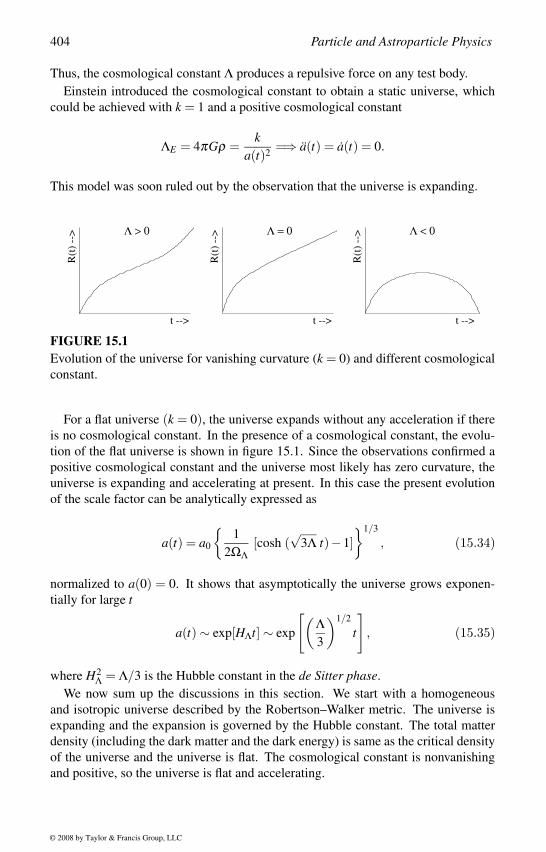
404 Particle and Astroparticle Physics
Thus, the cosmological constant Λ produces a repulsive force on any test body.
Einstein introduced the cosmological constant to obtain a static universe, which
could be achieved with k = 1 and a positive cosmological constant
ΛE = 4πGρ =k
a(t)2 =⇒ a(t) = a(t) = 0.
This model was soon ruled out by the observation that the universe is expanding.
R(t
) --
>
R(t
) --
> Λ < 0
t --> t -->t -->
R(t
) --
> Λ > 0 Λ = 0
FIGURE 15.1Evolution of the universe for vanishing curvature (k = 0) and different cosmological
constant.
For a flat universe (k = 0), the universe expands without any acceleration if there
is no cosmological constant. In the presence of a cosmological constant, the evolu-
tion of the flat universe is shown in figure 15.1. Since the observations confirmed a
positive cosmological constant and the universe most likely has zero curvature, the
universe is expanding and accelerating at present. In this case the present evolution
of the scale factor can be analytically expressed as
a(t) = a0
1
2ΩΛ[cosh (
√3Λ t)−1]
1/3
, (15.34)
normalized to a(0) = 0. It shows that asymptotically the universe grows exponen-
tially for large t
a(t) ∼ exp[HΛt] ∼ exp
[(Λ3
)1/2
t
], (15.35)
where H2Λ = Λ/3 is the Hubble constant in the de Sitter phase.
We now sum up the discussions in this section. We start with a homogeneous
and isotropic universe described by the Robertson–Walker metric. The universe is
expanding and the expansion is governed by the Hubble constant. The total matter
density (including the dark matter and the dark energy) is same as the critical density
of the universe and the universe is flat. The cosmological constant is nonvanishing
and positive, so the universe is flat and accelerating.
© 2008 by Taylor & Francis Group, LLC
Introduction to Cosmology 405
15.3 Primordial NucleosynthesisIn the early universe, we try to extrapolate our particle physics models to get some
information. But we could not verify most of these results. The earliest time from
which we could get some experimental inputs is the time of formation of nuclei,
when the average energy per particle was around 1 MeV. From our knowledge of the
present abundances of elements we could extrapolate them to the time of primordial
nucleosynthesis, when these elements had synthesized. This allows us to verify the
theoretical predictions for the elements, which is one of the major triumphs of the
standard model of cosmology.
Equilibrium Thermodynamics
We shall first introduce some thermodynamic quantities. Although in the early uni-
verse the expansion rate of the universe was too high for any reaction to come into
equilibrium, at the time of nucleosynthesis the universe may be described by equi-
librium thermodynamics. In equilibrium, the number density (n), energy density (ρ),
and pressure (p) of a dilute, weakly interacting gas of g internal degrees of freedom
is given by
n =g
(2π)3
∫f (p) d3 p
ρ =g
(2π)3
∫E(p) f (p) d3 p
p =g
(2π)3
∫ |p|23E
f (p) d3 p, (15.36)
where E2 = |p|2 +m2 and f (p) is the phase space distribution function,
[ f (p)] f ermion =1
exp(E−µ)/T +1and [ f (p)]boson =
1
exp(E−µ)/T −1, (15.37)
and µ is the chemical potential. In a reaction i+ j ↔ k + l in chemical equilibrium,
the chemical potentials of these particles satisfy
µi + µ j = µk + µl . (15.38)
In our convention, the Boltzmann constant kB = 1, so 1K = 0.86×10⁻¹³GeV.
The number densities of relativistic particles (with mass m T ) and nonrelativis-
tic particles (with mass m T ) are
nR = Cζ (3)π2 gT 3
nNR = g(
mT2π
)3/2
exp−(m−µ)/T , (15.39)
© 2008 by Taylor & Francis Group, LLC
406 Particle and Astroparticle Physics
where C = 1 for bosons, C = 3/4 for fermions, and the zeta function of 3 is ζ (3) =1.202... Thus, in equilibrium the total energy density and pressure will have con-
tributions mostly from the relativistic species, since the number density of the non-
relativistic species is exponentially suppressed. Neglecting the contributions of the
nonrelativistic species, we can then write a simplified expression for the energy den-
sity and pressure of all the particles as
ρR =π2
30g∗T 4
pR =ρR
3=
π2
90g∗T 4, (15.40)
where the effective number of massless degrees of freedom is given by the contribu-
tions from both fermions and bosons
g∗ = ∑i
1+C2
giT 4
iT 4 , (15.41)
where the summation extends over all the species, including both fermions and
bosons. We assume that gi numbers of species are at a temperature Ti. Here T is
the photon temperature and all the species with masses mi T contribute. Around
100 GeV, the effective number of degrees of freedom is g∗ ∼ 100, while at tempera-
tures less than 1 MeV, it is g∗ ∼ 3.36.
Another important quantity is the entropy of the universe S per comoving volume,
given by
S =a3(ρ + p)
T= a3 s, (15.42)
where the entropy density s is dominated by the relativistic particles and is given by
s =2π2
45g∗sT 3, (15.43)
where
g∗s = ∑i
1+C2
giT 3
iT 3 ,
and the photon number density is related to entropy as s = 1.8g∗snγ . For the present
value we can write s/nγ = 1.8g∗s(today) = 7.04. Conservation of energy implies
that the entropy per comoving volume remains constant in thermal equilibrium,
S = sa3 =2π2
45g∗a3T 3 = constant =⇒ a ∼ T−1 . (15.44)
Thus, during adiabatic expansion, the universe cools down.
With this definition of entropy we can now define the number density per co-
moving volume N ≡ n/s, which remains constant in equilibrium. For example, the
baryon number density per comoving volume
nB
s=
nb −nbs
(15.45)
© 2008 by Taylor & Francis Group, LLC
Introduction to Cosmology 407
remains unchanged if there is no baryon-number violating interactions. If there is
baryon-number violating interaction in equilibrium, the baryon number density van-
ishes. Any reaction can reach equilibrium, when the reaction rate Γ(T ) at any tem-
perature T is faster than the expansion rate of the universe
Γ(T ) > H(T ) = 1.66√
g∗T 2
MPl, (15.46)
where MPl is the Planck mass. Although this out-of-equilibrium condition can give
us a rough estimate, in actual problem the departure from equilibrium can be under-
stood by solving the Boltzmann equations.
Synthesis of Elements
At around 1 sec after the big-bang or about 1 sec after gravity started becoming
weak, synthesis of light elements, such as H, D, 3He, 4He and 7Li, started, when
the temperature was about 1010 K and the average kinetic energy was about 1 MeV
[245]. Although proton, neutron and light elements had formed at that time, they
were nonrelativistic. The number density of such nonrelativistic particles in thermal
equilibrium with mass number A is given by
nA = gA
(mAT2π
)3/2
exp(µA−mA)/T , (15.47)
where gA is the statistical factor. The chemical potential µA of the light elements
A with charge Z is related to that of the proton µp and the neutron µn in chemical
equilibrium by
µA = Zµp +(A−Z)µn. (15.48)
With the knowledge of the chemical potential of the species A, we can now write
the chemical potential and hence the number density of the species A in terms of the
number densities of the proton and neutron as
nA = gAA3/22−A(
2πmNT
)3(A−1)/2
nZpnA−Z
n expBA/T , (15.49)
where BA is the binding energy of the species A and is defined as
BA = Zmp +(A−Z)mn −mA. (15.50)
Binding energies (BA in MeV) and statistical factors (gA) of some of the light nucleiAZ are 2H [2.22,3], 3H [6.92,2], 3He [7.72,2], 4He [28.3,1], 12C [92.2,1], written asAZ [BA,gA].
Light Element Abundances
The primordial abundances of any nuclei are difficult to estimate. It is convenient to
define the relative mass fraction of the different species of nuclei A as
XA =AnA
nB=
nAAnn +np +∑i(AnA)i
, (15.51)
© 2008 by Taylor & Francis Group, LLC
408 Particle and Astroparticle Physics
with ∑i Xi = 1. Using the expression for the number density of the particles, the mass
fraction for a species A(Z) can then be written as
XA =1
2gA
[ηζ (3)√
π
(2TmN
)3/2]A−1
A5/2XZp XA−Z
n expBA/T , (15.52)
where the ratio of number of baryons to number of photons η = nb/nγ is an unknown
parameter in the model. This is a measure of the excess of baryons over antibaryons
in the universe and plays a crucial role in the evolution of the universe.
Theoretical estimates of the light element abundances are possible for the time
of primordial nucleosynthesis at a time t ∼ 180 s. However, actual measurements
are possible from a much later epoch, which introduce some uncertainty due to the
steller nucleosynthesis when some light elements are ejected and some heavy el-
ements are formed. High resolution spectra in astrophysical sites with low metal
contents are extrapolated to zero-metallicity to reduce errors. Taking care of theoret-
ical uncertainties and statistical and systematic errors, the relative mass fraction of4He, denoted by Y = 2nn/(nn +np), comes out to be [44]
Y = 0.249±0.009. (15.53)
The main source of error in 4He abundance is its steller production. On the other
hand, for deuterium abundance, the main error comes from its depletion at temper-
atures above 6× 10⁵ K through the reaction p+D→ 3He+γ . The present limit on
deuterium abundance is [44]
DH
= (2.78±0.29)105. (15.54)
It is difficult to measure 3He abundance with any reasonable accuracy. The produc-
tion of 3He from deuterium makes it more uncertain, and hence, this data is not used
to extract any information from nucleosynthesis. The 7Li abundance is even more
difficult to determine and its average value is [44]
7Li
H= (1.7±0.02+1.1
−0.0)×10−10. (15.55)
We shall now compare these light element abundances with the theoretical predic-
tions.
Nucleosynthesis Predictions
The observational evidences for the abundances of light elements spread over 10 or-
ders of magnitude with very little uncertainty. One of the major successes of the big-
bang cosmology is to predict this large hierarchy in the element abundances. There-
fore, any modification of the standard model of cosmology has to ensure that this
prediction is not jeopardized. For example, if there are more than four dimensions,
the extra dimensions should decouple from our present four-dimensional world be-
fore the time of nucleosynthesis.
© 2008 by Taylor & Francis Group, LLC
Introduction to Cosmology 409
The weak interaction processes
p+ e− ↔ n+νe, p+ νe ↔ n+ e+, n ↔ p+ e− + νe
keep the protons and neutrons in thermal equilibrium at around 10 MeV (10−2 s).
Any interaction continues to be in thermal equilibrium at any time t, if the interaction
at that time Γ(t) takes place at a faster rate than the expansion rate of the universe,
which is given by the Hubble parameter
H(T ) = 1.66√
g∗T 2
MPl. (15.56)
T is the temperature at time t, and g∗ is the number of relativistic degrees of freedom
available at that time. As the temperature comes down with time, the interaction rate
slows down faster than the Hubble parameter. When the interaction rate becomes
slower than the expansion rate of the universe, the particles move apart from each
other before they can interact with each other, and hence, the interaction goes out-
of-equilibrium. For the weak interaction, the departure from equilibrium starts at
around a temperature that satisfies
ΓH
≈(
T0.8 MeV
)3
< 1, (15.57)
which is about 0.8 MeV. Below this temperature the universe expands faster than the
weak interaction rate.
When the neutrons and the protons are in equilibrium, their relative abundance is
given by (neglecting chemical potentials)
nn
np= exp−∆m/kT , (15.58)
where ∆m = mn −mp. This abundance continues until they reach the temperature
0.8 MeV, when their interaction rate goes out-of-equilibrium and the neutron to pro-
ton ratio becomesnn
np= exp−∆m/kTf 1
6. (15.59)
At this time since the weak interaction rate becomes slower than the expansion rate of
the universe, the neutron to proton conversion freezes out and the neutron to proton
ratio becomes almost constant. Since neutrinos interact only through weak interac-
tion, the neutrinos decouple around the same time and the electrons and the positrons
annihilate. At a little lower temperature of 0.3−0.1 MeV, corresponding to about 1
to 3 minutes after the big-bang, formation of helium starts via the reactions
n+ p ↔ D+ γD+D ↔ 4He+ γD+ p ↔ 3He+ γD+n ↔ 3H+ γ,
© 2008 by Taylor & Francis Group, LLC
410 Particle and Astroparticle Physics
which give an amount of helium abundance of
Y =2nn
nn +np. (15.60)
The parameters involved in the prediction for the helium abundance are the fraction
of baryons to photons
η =nb
nγ, (15.61)
the number of relativistic degrees of freedom g∗, and the weak interaction rates for
the neutron, which depend on the nuclear matrix element
|M|2 ∼ G2F(1+3g2
A). (15.62)
Hence, the main source of error in the prediction for Y is the lifetime of the neutron
τn
τn = 885.3±2.0 s, (15.63)
since the axial vector coupling constant gA is obtained from the neutron lifetime [44]
τ−1n =
1.636 G2F
2π3 (1+3g2A) m5
e . (15.64)
At around 0.1 MeV, the equilibrium distribution of the neutron to proton ratio should
have been nn/np = 1/74, but since their interaction rate went out-of-equilibrium,
their actual distribution remains much higher, almost nn/np = 1/7. The formation of
heavier elements is prevented strongly because of the nonexistence of stable atomic
masses 5 and 8 nuclei and the Coulomb barriers. This explains why the abundance of7Li is suppressed by 10 orders of magnitude compared with the helium abundance.
Abundance of any heavier elements is also strongly suppressed for the same reason.
Nucleosynthesis Results
The abundance of a nucleus A(Z) depends on ηA−1 as shown in the defining equation
(15.52) for the relative mass fraction. The experimental values of the abundances of
elements could be used to estimate the value of the baryon-to-photon ratio η , which
comes out to be [44]
4.7 < η10 < 6.5 98% c.l., (15.65)
where η10 = η ×1010. A highly refined value of η10 is possible from an analysis of
the cosmic microwave background anisotropy data, which will be discussed in the
next section.
To estimate the amount of baryonic matter in the universe, we use the relation
η = 2.73×10⁻⁸ Ωbh2 for the present temperature, where
h =H0
100 km s−1 Mpc−1 . (15.66)
© 2008 by Taylor & Francis Group, LLC
Introduction to Cosmology 411
The range of η , as obtained from nucleosynthesis, then gives [44]
0.017 ≤ Ωb h2 ≤ 0.024. (15.67)
For a value of the Hubble constant (h ∼ 0.7) this implies 0.035 ≤ Ωb ≤ 0.049, i.e.,
the amount of baryonic matter constitutes only about 3 to 5% of the critical density of
the universe. On the other hand, the density of optically luminous matter is Ωlum ∼0.0024 h−1, which is only 0.35% of the critical density of the universe.
The temperature fluctuations measured in cosmic microwave background radia-
tion experiments (this will be discussed in the next section) on angular scales smaller
than the horizon at last scattering, can also provide an independent value for the
baryon-to-photon ratio η . This comes from the amplitudes of the acoustic peaks in
the cosmic microwave background (CMB) angular power spectrum. If photons are
created or destroyed between the nucleosynthesis era and the CMB decoupling, that
would distort the CMB angular power spectrum. The CMB anisotropies indepen-
dently test the nucleosynthesis predictions for Ωbh2.
One of the most interesting predictions of the primordial nucleosynthesis is the
number of neutrino species that were active at the time of nucleosynthesis, which
is Nν = 3 [44]. This bound results from the constraint on the parameter involved
in nucleosynthesis, the number of effective degrees of freedom g∗. However, this
bound is not too strong and a fourth generation neutrino is not ruled out completely
as yet. If this result is combined with the present LEP constraint that the number of
neutrinos with mass less than mZ/2 is 3, it allows one sterile neutrino (a singlet under
the standard model), which can mix with the ordinary neutrinos and contribute to the
nucleosynthesis bound. However, there is no constraint on the number of sterile
neutrinos that do not mix with the ordinary neutrinos.
15.4 Cosmic Microwave Background RadiationOne of the most crucial predictions of the standard big-bang cosmological model
is the CMB radiation [246]. Another otherwise successful cosmological model, the
steady state theory [247], could be discriminated from the observation of the CMB
radiation. Only the standard cosmological model predicts remnant isotropic and
homogeneous background radiations, which have been observed.
The universe was radiation dominated in the early stage. When the universe cooled
down and the average energy per particle came down below 1 eV, electrons began
combining with nuclei to form neutral atoms. Until this recombination era, photons
were interacting strongly with the charged electrons, protons and other nuclei, and
the mean free path of radiation was small. Once neutral atoms were formed, radiation
decoupled from matter and they could travel long distances almost unperturbed until
the present day. The cosmic microwave background is the radiation coming from this
surface of last scatter, which is the radiation from the time when radiation decoupled
© 2008 by Taylor & Francis Group, LLC
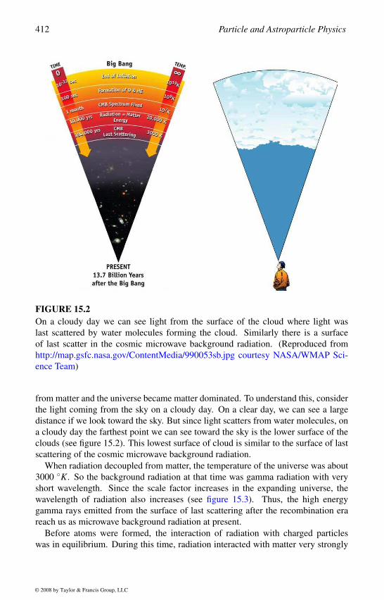
412 Particle and Astroparticle Physics
FIGURE 15.2On a cloudy day we can see light from the surface of the cloud where light was
last scattered by water molecules forming the cloud. Similarly there is a surface
of last scatter in the cosmic microwave background radiation. (Reproduced from
http://map.gsfc.nasa.gov/ContentMedia/990053sb.jpg courtesy NASA/WMAP Sci-
ence Team)
from matter and the universe became matter dominated. To understand this, consider
the light coming from the sky on a cloudy day. On a clear day, we can see a large
distance if we look toward the sky. But since light scatters from water molecules, on
a cloudy day the farthest point we can see toward the sky is the lower surface of the
clouds (see figure 15.2). This lowest surface of cloud is similar to the surface of last
scattering of the cosmic microwave background radiation.
When radiation decoupled from matter, the temperature of the universe was about
3000 K. So the background radiation at that time was gamma radiation with very
short wavelength. Since the scale factor increases in the expanding universe, the
wavelength of radiation also increases (see figure 15.3). Thus, the high energy
gamma rays emitted from the surface of last scattering after the recombination era
reach us as microwave background radiation at present.
Before atoms were formed, the interaction of radiation with charged particles
was in equilibrium. During this time, radiation interacted with matter very strongly
© 2008 by Taylor & Francis Group, LLC
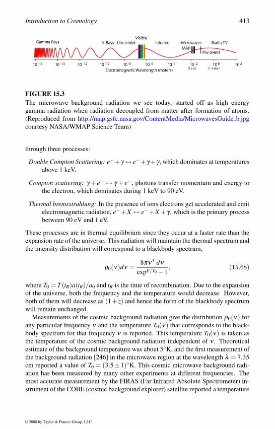
Introduction to Cosmology 413
FIGURE 15.3The microwave background radiation we see today, started off as high energy
gamma radiation when radiation decoupled from matter after formation of atoms.
(Reproduced from http://map.gsfc.nasa.gov/ContentMedia/MicrowavesGuide b.jpg
through three processes:
Double Compton Scattering: e−+γ ↔ e−+γ +γ , which dominates at temperatures
above 1 keV.
Compton scattering: γ + e− ↔ γ + e−, photons transfer momentum and energy to
the electron, which dominates during 1 keV to 90 eV.
Thermal bremsstrahlung: In the presence of ions electrons get accelerated and emit
electromagnetic radiation, e−+X ↔ e−+X +γ , which is the primary process
between 90 eV and 1 eV.
These processes are in thermal equilibrium since they occur at a faster rate than the
expansion rate of the universe. This radiation will maintain the thermal spectrum and
the intensity distribution will correspond to a blackbody spectrum,
ρ0(ν)dν =8πν3 dν
expE/T0 −1, (15.68)
where T0 = T (tR)a(tR)/a0 and tR is the time of recombination. Due to the expansion
of the universe, both the frequency and the temperature would decrease. However,
both of them will decrease as (1+ z) and hence the form of the blackbody spectrum
will remain unchanged.
Measurements of the cosmic background radiation give the distribution ρ0(ν) for
any particular frequency ν and the temperature T0(ν) that corresponds to the black-
body spectrum for that frequency ν is reported. This temperature T0(ν) is taken as
the temperature of the cosmic background radiation independent of ν . Theoretical
estimate of the background temperature was about 5K, and the first measurement of
the background radiation [246] in the microwave region at the wavelength λ = 7.35
cm reported a value of T0 = (3.5± 1)K. This cosmic microwave background radi-
ation has been measured by many other experiments at different frequencies. The
most accurate measurement by the FIRAS (Far Infrared Absolute Spectrometer) in-
strument of the COBE (cosmic background explorer) satellite reported a temperature
© 2008 by Taylor & Francis Group, LLC
courtesy NASA/WMAP Science Team)
414 Particle and Astroparticle Physics
of [248]
T0 = 2.726±0.01 K. (15.69)
The COBE data also confirmed the perfect blackbody spectrum of the cosmic mi-
crowave background radiation and gave a photon number density of
nγ = 412±2 cm−3. (15.70)
This background radiation came from the time of recombination.
To estimate the time of recombination or when the radiation decoupled from mat-
ter, we start with the scattering rate of e− with γ ,
Γγ = neσ , (15.71)
where the scattering cross-section σ can be approximated by the Thomson scattering
σ = 6.65× 10⁻²⁵ cm2 and the equilibrium number density of electrons ne can be
obtained from
ni = gi
(miT2π
)3/2
exp(µi−mi)/T . (15.72)
Here ni is the equilibrium number density of the particle i = e, p,H with mass mi,
chemical potential µi and statistical weight gi. We shall now consider the chemical
equilibrium of p + e → H + γ , which gives the relation µp + µe = µH , to write the
hydrogen equilibrium number density as
nH = npne
(meT2π
)−3/2
expB/T , (15.73)
where we used gH = 2gp = 2ge = 4. The binding energy B of hydrogen is defined as
B ≈ mp + me −mH = 13.6 eV. We can simplify it further by considering the charge
neutrality condition, ne = np.
We shall next define the ionization fraction Xe, in terms of the total baryon number
density nB = np +nH = ηnγ , as Xe = np/nB. Using the hydrogen equilibrium number
density, the Saha ionization formula for the equilibrium ionization fraction then gives
1−Xeqe
(Xeqe )2 =
4
3ηne
(meT2π
)−3/2
expB/T =4
3η
nH
np. (15.74)
Solving this equation it is possible to estimate the time of recombination, when 90%
of the electrons combined with protons to form hydrogen atoms during a red-shift of
zrec = 1200 to 1400.
Around the time of recombination, the radiation-dominated universe had also
changed over to a matter-dominated universe. The scale factor varies with time as
a ∼ t1/2 in the radiation-dominated universe and as a ∼ t2/3 in the matter-dominated
universe. The change over in the evolution of the scale factor took place when the
matter density and the radiation density were equal. This took place at around a
red-shift of zeq = 1500. It is, therefore, usually assumed that the recombination had
already taken place in a matter-dominated universe.
© 2008 by Taylor & Francis Group, LLC
Introduction to Cosmology 415
Soon after the formation of hydrogen atoms, since the number density of charged
particles was reduced drastically, the mean free paths of photons increased and the
universe became optically transparent. This decoupling of radiation from matter took
place during the red-shift of zdec = 1100 to 1200. After decoupling, this radiation
remained as background radiation, which reached us as the cosmic microwave back-
ground radiation.
15.5 Formation of Large Scale StructuresThe cosmic microwave background radiation is almost isotropic and homogeneous
and shows very little anisotropy, which means that the universe was very smooth at
the time of decoupling. But if the universe was so smooth, it would have been dif-
ficult to have structures as we observe. We see stars around us, which are grouped
in galaxies. These galaxies are again grouped in clusters of galaxies and clusters
arrange themselves in superclusters. In between the galaxies, clusters, or even super-
clusters, there are vast voids, which seems to be inconsistent with the homogeneous
and isotropic universe as indicated by the cosmic microwave background radiation.
It is thus expected that as the universe expands, small quantum fluctuations that went
out of the horizon size before the inflation enter our horizon and the gravitational
amplification of these small fluctuations create the large scale structures.
We start with a discussion of Jeans or gravitational instability [249], which could
amplify any small fluctuations that were present after the recombination. This would
give an indication of how such small density perturbations at the time of decoupling
could be amplified by gravitational instability to form the large scale structure we
observe today (see figure 15.4).
Let us consider a perfect fluid with density ρ , velocityv and pressure p, which is
described by the Euler equation and the equation of continuity as
∂v∂ t
+(v ·∇)v+1
ρ∇p+∇φ = 0
∂ρ∂ t
+∇ · (ρv) = 0. (15.75)
The Newtonian gravitational force g will satisfy the equations
∇ ·g = −4πGρ∇×g = 0. (15.76)
The last equation gives g = −∇φ , where φ is the Newtonian gravitational potential.
We shall now consider adiabtic perturbations and expand X ≡ ρ, p,v,φ as
X = X0 +X1, (15.77)
© 2008 by Taylor & Francis Group, LLC
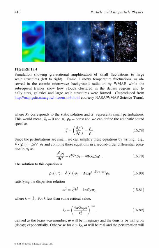
416 Particle and Astroparticle Physics
FIGURE 15.4Simulation showing gravitational amplification of small fluctuations to large
scale structures (left to right). Frame 1 shows temperature fluctuations, as ob-
served in the cosmic microwave background radiation by WMAP, while the
subsequent frames show how clouds clustered in the denser regions and fi-
nally stars, galaxies and large scale structures were formed. (Reproduced from
http://map.gsfc.nasa.gov/m or/m or3.html courtesy NASA/WMAP Science Team).
where X0 corresponds to the static solution and X1 represents small perturbations.
This would mean, v0 = 0 and p0,ρ0 = const and we can define the adiabatic sound
speed as
v2s =(
∂ p∂ρ
)=
p1
ρ1. (15.78)
Since the perturbations are small, we can simplify these equations by writing, e.g.,∇ · (ρv) = ρ0∇ ·v1 and combine these equations in a second-order differential equa-
tion in ρ1 as
∂ 2ρ1
∂ t2 − v2s∇2ρ1 = 4πGNρ0ρ1. (15.79)
The solution to this equation is
ρ1(r, t) = δ (r, t)ρ0 = Aexp(−ik·r+iωt)ρ0 (15.80)
satisfying the dispersion relation
ω2 = v2s k2 −4πGNρ0, (15.81)
where k = |k|. For k less than some critical value,
kJ =(
4πGNρ0
v2s
)1/2
, (15.82)
defined as the Jeans wavenumber, ω will be imaginary and the density ρ1 will grow
(decay) exponentially. Otherwise for k > kJ , ω will be real and the perturbation will
© 2008 by Taylor & Francis Group, LLC
Introduction to Cosmology 417
oscillate as sound waves. The mass contained within a sphere of radius λJ/2 = π/kJis called the Jeans mass
MJ =4π3
(πkJ
)3
ρ0 =π5/2
6
v3s
G3/2N ρ1/2
0
. (15.83)
Any structures with M > MJ are unstable against gravitational collapse.
It is convenient to study the density fluctuations in terms of the Fourier transform
of the density contrast δ (r, t) = ρ1/ρ0 = δρ/ρ , given by
δ (r, t) =V
(2π)3
∫δk(t)exp−ik·rd3k. (15.84)
|δk|2 is known as the power spectrum and it enters into statistical quantities such as
the correlation function, where
δk(t) = V−1∫
δ (r, t)expik·rd3x. (15.85)
V is the normalization factor.
We shall now include the effect of expansion of the universe by considering the
scale factor in these equations. The first order perturbations now satisfy the equations
∂v1
∂ t+
aav1 +
aa(r ·∇)v1 +
v2s
ρ0∇ρ1 +∇φ1 = 0
∂ρ1
∂ t+3
aa
ρ1 +aa(r ·∇)ρ1 +ρ0∇ ·v1 = 0
∇2φ1 = 4πGNρ1. (15.86)
We can express the density contrast δ (r, t) = ρ1/ρ0 in Fourier transform including
the scale factor as
δ (r, t) =1
(2π)3
∫δk(t)exp−i(k·r)/a(t)d3k. (15.87)
Similarly we expand the velocity v1 and the potential φ1 to solve these equations.
The first order equation for the density perturbation becomes
∂ 2δk
∂ t2 +2aa
∂δk
∂ t= δk
(4πGNρ0 − v2
s k2
a2
). (15.88)
This result is similar to static universe (a = 0) with physical wavenumber k/a. The
Jeans wavenumber now becomes k2J = 4πGρ0a2/v2
s , so for k kJ the perturbation
oscillates.
The solution is unstable for k kJ . For a spatially flat (k = 0) matter-dominated
universe, the universe is curvature dominated a ∼ t, and we can write
4πGNρ =2
3t2 andaa
=2
3t. (15.89)
© 2008 by Taylor & Francis Group, LLC
418 Particle and Astroparticle Physics
The density contrast then satisfies the equation
δk +4
3tδk − 2
3t2 δk = 0, (15.90)
which has two solutions, one growing and the other decaying. Since we are looking
for solutions that can amplify the small density fluctuations, we ignore the decaying
solution. The growing solution is given by
δk ∼ t2/3 ∼ a = (1+ z)−1. (15.91)
Thus, compared with the static case, with the inclusion of the scale factor the growth
is no longer exponential. The expansion of the universe slows down the growth from
an exponential behavior to a power law growth. In the relativistic case the power law
becomes δk ∼ t ∼ a2 = (1+ z)−2.
We now consider the Jeans mass as a function of time. In the radiation-dominated
phase, assuming that the universe consists of baryons and photons (ρ = ρB +ργ ), the
pressure is provided by the photons since the baryons are interacting strongly with
photons. Then the Jeans mass grows like a3. The Jeans mass grows from about a
solar mass to about M = 1016M by the time the universe grows from a red-shift of
1010 until the time of recombination.
After recombination, radiation decouples from matter and only the nonrelativistic
hydrogen atoms maintain the pressure, for which v2s = (5/3)(T/mH). This decrease
in the velocity of sound causes a sudden reduction of the Jeans mass to
MJ = 1.3×10⁵( z
1100
)3/2(Ωbh2)−1/2 M. (15.92)
During decoupling the Jeans mass drops from 1016M to 106M, the typical mass of
the globular clusters, the oldest objects in the universe. All heavier masses become
gravitationally unstable; δk grows proportional to a. This tells us that density fluctua-
tions have grown since the time of recombination by a factor (t0/ta)2/3 = 1+z≈ 103.
In this simple discussion we have not included some factors. Before the Jeans
instability becomes effective, the weakly interacting particles such as the neutrinos
could escape from the dense regions without interaction, smearing out some of the
perturbations. In actual calculations this factor of free streaming of neutrinos and
other weakly interacting particles has to be included in the Boltzmann equations.
This free streaming will not allow any structure formation at very small scales, but it
will not affect the large scale structure formation. Another damping is the collisional
damping or Silk damping [250]. At the time of recombination, the photon mean free
path increases and there can be damping due to collisions. Here also small scales are
washed out, i.e., inhomogeneities in the photon–baryon plasma are washed out.
© 2008 by Taylor & Francis Group, LLC
Introduction to Cosmology 419
15.6 Cosmic Microwave Background AnisotropyThe universe was initially radiation dominated, but they were interacting strongly
with charged electrons and protons and heavier nuclei. At around the red-shift of
z = 1500, the radiation and matter density became equal and then the formation of
atoms began. During the period z = 1200 to 1400 most of the charged particles
combined to form atoms. Since the number of charged particles reduced drasti-
cally, radiation decoupled from matter after this recombination at around a red-shift
of z = 1100. The light coming from this decoupling time, which is the surface of
last scattering, reaches us now from all directions evenly as the cosmic microwave
background radiation.
Although the cosmic microwave backgrond (CMB) radiation is almost isotropic
and homogeneous, a small anisotropy has been observed, which can explain the for-
mation of large scale structures in the universe. The gravitational amplification of the
small fluctuations in the CMB radiation of the order of ∆T/T ∼ 10−6 could explain
the formation of even the largest objects. In addition to explaining the formation of
large scale structures, the CMB anisotropy data could be probed to obtain precision
values for several cosmological parameters.
The CMB anisotropy comes from a measurement of the temperature anisotropy
with very high precision. A differential measurement of the full sky with a complex
sky scan pattern allows the data to limit systematic measurement errors. The most
precise data on the anisotropy of the temperature of the cosmic microwave back-
ground radiation have been provided by WMAP, as shown in figure 15.5. The CMB
temperature at two different points separated by an angle θ is measured and then by
taking the map average of ∆T/T , the correlation function C(θ) is calculated, which
contains most of the required information.
We can then define a statistical correlation function C(θ) in terms of the tempera-
tures T (n) and T (n′) measured in the two directions n and n′ separated by an angle
θ as
C(θ) = 〈∆T (n)∆T (n′)〉, (15.93)
where cosθ = n ·n′. Since we are interested in measuring a deviation from spherical
symmetry, it is convenient to expand the anisotropy parameter in terms of spherical
harmonics,
T (n) = T0 ∑l,m
aml Y m
l (θ ,φ), (15.94)
so the correlation function can be expressed in terms of the Legendre polynomials
Pl(cosθ) as
C(θ) =1
4π ∑l(2l +1)ClPl(cosθ). (15.95)
The monopole term (l = 0) corresponds to the spherically symmetric case and gives
the mean CMB radiation temperature
T0 = 2.725±0.001 K. (15.96)
© 2008 by Taylor & Francis Group, LLC
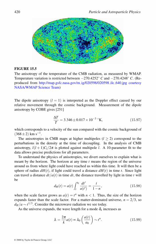
420 Particle and Astroparticle Physics
FIGURE 15.5The anisotropy of the temperature of the CMB radiation, as measured by WMAP.
Temperature variation is restricted between −270.4252 C and −270.4248 C. (Re-
produced from http://map.gsfc.nasa.gov/m ig/020598/020598 ilc 640.jpg courtesy
NASA/WMAP Science Team)
The dipole anisotropy (l = 1) is interpreted as the Doppler effect caused by our
relative movement through the cosmic background. Measurement of the dipole
anisotropy by COBE gives [251]
∆TT
= 3.346±0.017×10⁻³ K, (15.97)
which corresponds to a velocity of the sun compared with the cosmic background of
(368±2) km s−1.
The anisotropies in CMB maps at higher multipoles (l ≥ 2) correspond to the
perturbations in the density at the time of decoupling. In the analysis of CMB
anisotropy, l(l + 1)Cl/2π is plotted against multipole l. A 10-parameter fit to the
data allows precise predictions for all parameters.
To understand the physics of anisotropies, we divert ourselves to explain what is
meant by the horizon. The horizon at any time t means the region of the universe
around us from where light could have reached us within this time. It will then be a
sphere of radius dH(t), if light could travel a distance dH(t) in time t. Since light
can travel a distance dt/a(t) in time dt, the distance travelled by light in time t will
be
dH(t) = a(t)∫ t0
t
dt ′
a(t ′)=
t1−n
, (15.98)
when the scale factor grows as a(t) = tn with n < 1. Thus, the size of the horizon
expands faster than the scale factor. For a matter-dominated universe, n = 2/3, so
dH/a ∼ t1/3. Consider the microwave radiation we see today.
As the universe expands, the wave length for a mode δk increases as
λ =2πk
a(t) ∝ λ0
(a(t)a0
)∼ tn. (15.99)
© 2008 by Taylor & Francis Group, LLC
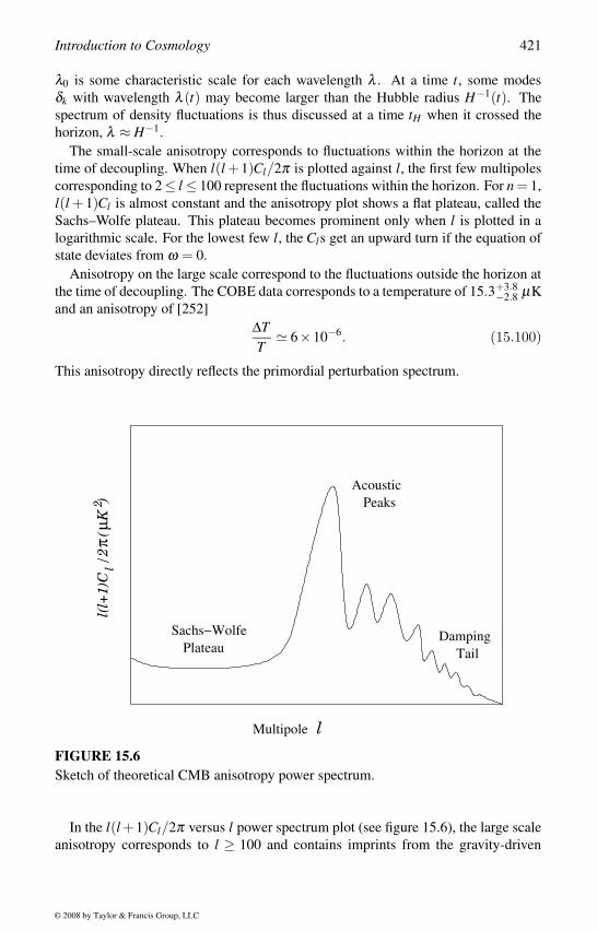
Introduction to Cosmology 421
λ0 is some characteristic scale for each wavelength λ . At a time t, some modes
δk with wavelength λ (t) may become larger than the Hubble radius H−1(t). The
spectrum of density fluctuations is thus discussed at a time tH when it crossed the
horizon, λ ≈ H−1.
The small-scale anisotropy corresponds to fluctuations within the horizon at the
time of decoupling. When l(l +1)Cl/2π is plotted against l, the first few multipoles
corresponding to 2≤ l ≤ 100 represent the fluctuations within the horizon. For n = 1,
l(l + 1)Cl is almost constant and the anisotropy plot shows a flat plateau, called the
Sachs–Wolfe plateau. This plateau becomes prominent only when l is plotted in a
logarithmic scale. For the lowest few l, the Cls get an upward turn if the equation of
state deviates from ω = 0.
Anisotropy on the large scale correspond to the fluctuations outside the horizon at
the time of decoupling. The COBE data corresponds to a temperature of 15.3+3.8−2.8 µK
and an anisotropy of [252]
∆TT
6×10⁻⁶. (15.100)
This anisotropy directly reflects the primordial perturbation spectrum.
l(l+
1)C
/2
(
K )
µπ
l2
Sachs−Wolfe
Plateau
Acoustic
Damping
Tail
Peaks
lMultipole
FIGURE 15.6Sketch of theoretical CMB anisotropy power spectrum.
In the l(l +1)Cl/2π versus l power spectrum plot (see figure 15.6), the large scale
anisotropy corresponds to l ≥ 100 and contains imprints from the gravity-driven
© 2008 by Taylor & Francis Group, LLC
422 Particle and Astroparticle Physics
acoustic oscillations. Before the formation of atoms, the universe was filled with
charged particles and the radiation was interacting strongly with matter. The gravita-
tional potential dominated by the dark matter and dark energy components allowed
the small perturbations ∼ (10−5) to evolve linearly. Each of the Fourier modes now
oscillates with the characteristic frequency determined by the adiabatic sound speed
in the fluid. The Fourier modes that were inside the horizon at the time of decou-
pling would smear out these perturbations. But the Fourier modes that were outside
the horizon at the time of decoupling would retain these phases when they entered
our horizon. This gives the acoustic peaks in the power spectrum plot for z ≥ 100.
However, since the surface of last scattering has a finite thickness, the oscillations of
the anisotropies will be damped for large l. This acoustic peak has been observed
in the power spectrum and the analysis of the anisotropy data could give us precise
values for the various parameters in the standard model [73].
To understand the evolution of the different modes, we have to specify the spec-
trum. We have to specify the amplitude of a given mode when it enters the horizon.
Since it is not possible to predict the spectrum without knowing how the fluctuations
came into existence, some simple forms are considered. One popular spectrum is a
power law spectrum (δρρ
)hor
k3/2|δk|√2 π
= AM−α , (15.101)
where |δk|2 ∝ k3(2α−1). The inflationary models predict the Harrison–Zeldovich
spectrum [253] of constant curvature perturbation, α = 0, which corresponds to the
Harrison–Zeldovich parameter n = 1. The COBE data yield a value for the Harrison–
Zeldovich parameter [254]
n = 1.2±0.3. (15.102)
Since inflation predicts n = 1, this may be an indication that the universe went
through an inflationary phase in the early universe. Formation of galaxies and the
measured CMB anisotropy gives a bound α > −0.1, while the overproduction of
black holes, and hence excess radiation that has not been observed, gives the con-
straint α < 0.2.
Specifying the amplitude of different modes at the time they cross the horizon
amounts to specifying time-dependent amplitudes. To avoid that one uses a spectrum
at a given time, which may then be related as(δρρ
)t=(
MMhor(t)
)−2/3(δρρ
)hor
, (15.103)
where Mhor is the mass of the nonrelativistic particles within the horizon.
The time considered for specifying the spectrum is when the structure formation
begins, t = teq. This depends on the type of dark matter of the universe. In the case of
hot dark matter (like neutrinos) the washing out of the fluctuations takes a long time
and structures form when the particles become nonrelativistic. On the other hand, the
cold dark matter (weakly interacting massive particles such as the neutralino LSP)
became nonrelativistic at a very early stage and introduced a gravitational potential
© 2008 by Taylor & Francis Group, LLC
Introduction to Cosmology 423
for the baryonic matter since the time of matter dominance. In these models baryonic
matter fell into the gravitational potential created by the cold dark matter soon after
recombination and formed the large scale structures.
The anisotropy in the cosmic microwave background radiation temperature probes
the density fluctuations in the early universe on comoving scales greater than ∼ 100
Mpc. There are several models of structure formation, which represent the range of
cosmological parameters. Each model predicts how a power spectrum of infinites-
imal density perturbations in the early universe develops into cosmic microwave
background radiation anisotropies and inhomogeneities in the galaxy [255]. Most
of the models are consistent with the constraints on baryon density from the big-
bang nucleosynthesis. Although earlier observations were consistent with both hot
and cold dark matter, for the present observations the best fit corresponds to the cold
dark matter with a cosmological constant.
15.7 InflationIn spite of all the successes of the standard model of cosmology, to solve some of
its problems it was proposed that the universe went through an inflationary phase in
the early universe. The CMB anisotropy data now indicates that the universe had
indeed gone through an inflationary phase. We shall now briefly mention how an
inflationary model works, after mentioning the problems of the standard model of
cosmology that required an inflation.
Flatness Problem
The curvature of our universe is a topological property of the metric. So, if the uni-
verse started with a positive, negative, or vanishing curvature (k = ±1,0), it should
have been maintaining it at all times. As we discussed earlier, the mass density (Ω),
which is directly related to the curvature (k) is given by
Ω−1 =ρ +ρv −ρc
ρc=
kH2R2 . (15.104)
A positive curvature (k = +1) implies Ω > 1, a negative curvature (k = −1) implies
Ω < 1, and a vanishing curvature (k = 0) implies Ω = 1.
During the radiation- or matter-dominated era the density of the universe grew as
ρ ∼ R−4 or ρ ∼ R−3, respectively. If the universe started with a matter density of
Ω < 1, around the Planck time (t ∼ M−1Pl ), the curvature of the universe would have
been
|Ω−1| 10−50. (15.105)
However, if the universe would have started with Ω = 1, then it would have been
the same all the time, which is the most natural solution. Present observations also
indicate that Ωtot ∼ 1 (see equation (17.13)).
© 2008 by Taylor & Francis Group, LLC
424 Particle and Astroparticle Physics
Horizon Problem
The second question is concerned with the event horizon, the distance from which
light could reach us today starting from the beginning of the universe. This distance
is given by
dH(t) = R(t)∫ t
0
dt ′
R(t ′). (15.106)
Since the scale factor grows as R ∼ tn with n < 1, the event horizon expands as
dH =t
1−n, (15.107)
which is faster than the increase in the scale factor. For a matter-dominated universe,
n = 2/3, so dH/R ∼ t1/3. Consider the microwave radiation we see today. This
radiation was emitted at the time of decoupling tdec ≈ 0.37× 10⁶ y. At that time
the universe was much smaller than its present size. The most distant microwave
radiation we could observe today corresponds to the present age of the universe of
t0 = 13.7×10⁹ y. Then the radiation we observe today was not causally connected at
the time of its emission. In fact, from the time of decoupling until now the universe
has grown by a factor of (t0/tdec)1/3 ∼ 35, and hence, the radiation we see today was
about 35 horizon lengths apart at the time of decoupling when it was emitted. Then
the isotropy of the background radiation cannot be explained. If we assume it was
isotropic at all lengths at all times, then the formation of large scale structures could
not be explained.
Monopole Problem
Another problem of the standard cosmological model is the monopole problem. Dur-
ing the phase transition of the grand unified theories, the symmetry breaking will
form regions with < φ >= v and < φ >= 0. Then after the phase transition is
over, with each causally connected region of space, there will be at least one re-
gion with < φ >= 0, which are the t’Hooft–Polyakov monopoles [256] with color
and magnetic properties and mass ∼ O(MX/α). This gives a number density of the
monopoles to be [257]
nM ∼ d−3H ∼ M6
X
M3Pl
. (15.108)
Taking the scale of grand unification to be around 1015 GeV, this gives a mass density
of the monopoles to be around
ρmonopoles ≈ 109 ρc, (15.109)
which is far beyond any permissible value. Similarly other topological objects such
as domain walls or cosmic strings could also be present with unacceptably high con-
tribution to the mass density of the universe.
© 2008 by Taylor & Francis Group, LLC
Introduction to Cosmology 425
Models of Inflation
The models of inflation [258] were proposed to solve these problems of horizon,
flatness, and monopole, but these models can have several other interesting features.
Present experiments also support the idea of inflation. During inflation the universe
goes through a phase of extremely fast expansion when the universe is dominated by
the vacuum energy density ρv. The scale factor evolves exponentially fast in this de
Sitter phase [259] (equation (15.35))
a(t) ∼ a(0)expHt and H2 =8πGN
3ρv. (15.110)
During this phase a small smooth causally coherent region of space of size less than
H−1 can grow to an enormous comoving volume, which becomes all of our observ-
able space at present. Then the horizon problem does not appear any more since at
present we see only a small part of the much larger causally connected space. So,
the smoothness of the small region before the inflation now appears as the isotropic
part of our entire observable space. The flatness problem is solved since the fast
expansion during the inflationary phase could flatten the universe to the extent that
it would appear almost flat at all times. Moreover, most inflationary models give the
density of the universe to be the same as that of the critical density. Since only one
monopole is expected in one causally connected region in space and in the inflation-
ary models much larger regions of space are causally connected, the number density
of monopoles and other topological defects becomes much less and consistent with
observations.
The main ingredient for the inflation is a scalar field φ with a particular potential,
so after the field acquires a vev the inflationary dynamics follows. The singlet scalar
field φ that drives inflation is called the inflaton. Consider a Higgs scalar φ , whose
vev < φ >= v = 0 breaks a symmetry at the scale v ∼ M. This will then produce a
vacuum energy of ρv = V (φ = 0) ∼ M4, and at a temperature below the critical tem-
perature, the vacuum energy will dominate. In the early universe the phase transition
took place in a sequence. At a temperature much higher than the critical temperature
(Tc), the potential has only one minimum corresponding to < φ >= 0. As the tem-
perature approaches the critical temperature, the potential starts developing a second
minimum at < φ >= v. However, since the two minima are separated by a barrier,
the universe still remains in the minimum corresponding to restored symmetry. At
the critical temperature the free energy of both minima becomes equal and allows
the universe to stay in any one of the minima. So, while most of the universe re-
mains in the old minimum, some bubbles start developing where inside the bubble
the minimum corresponds to the new minimum at < φ >= v.
As the universe cools down below the critical temperature, the new minimum
becomes the lowest energy minimum and, hence, the true vacuum, while the origin
becomes the false vacuum. At this time more and more particles start penetrating
the barrier and the bubbles start growing. Finally after a while the barrier height
vanishes, the false vacuum decays completely to the true vacuum, and the bubbles
grow at the speed of light. During this time the inflaton field rolls down slowly to the
© 2008 by Taylor & Francis Group, LLC
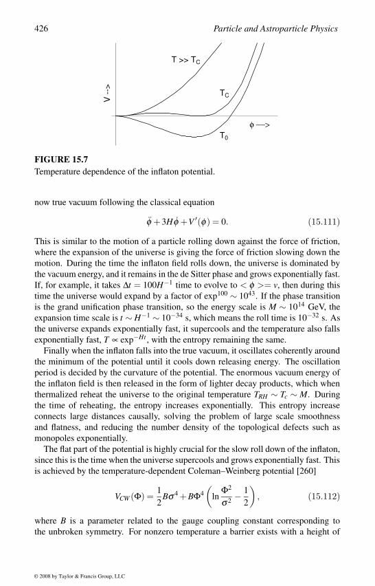
426 Particle and Astroparticle Physics
φ −−>T0
TC
T >> TC
V -
->
FIGURE 15.7Temperature dependence of the inflaton potential.
now true vacuum following the classical equation
φ +3Hφ +V ′(φ) = 0. (15.111)
This is similar to the motion of a particle rolling down against the force of friction,
where the expansion of the universe is giving the force of friction slowing down the
motion. During the time the inflaton field rolls down, the universe is dominated by
the vacuum energy, and it remains in the de Sitter phase and grows exponentially fast.
If, for example, it takes ∆t = 100H−1 time to evolve to < φ >= v, then during this
time the universe would expand by a factor of exp100 ∼ 1043. If the phase transition
is the grand unification phase transition, so the energy scale is M ∼ 1014 GeV, the
expansion time scale is t ∼ H−1 ∼ 10−34 s, which means the roll time is 10−32 s. As
the universe expands exponentially fast, it supercools and the temperature also falls
exponentially fast, T ∝ exp−Ht , with the entropy remaining the same.
Finally when the inflaton falls into the true vacuum, it oscillates coherently around
the minimum of the potential until it cools down releasing energy. The oscillation
period is decided by the curvature of the potential. The enormous vacuum energy of
the inflaton field is then released in the form of lighter decay products, which when
thermalized reheat the universe to the original temperature TRH ∼ Tc ∼ M. During
the time of reheating, the entropy increases exponentially. This entropy increase
connects large distances causally, solving the problem of large scale smoothness
and flatness, and reducing the number density of the topological defects such as
monopoles exponentially.
The flat part of the potential is highly crucial for the slow roll down of the inflaton,
since this is the time when the universe supercools and grows exponentially fast. This
is achieved by the temperature-dependent Coleman–Weinberg potential [260]
VCW (Φ) =1
2Bσ4 +BΦ4
(ln
Φ2
σ2 − 1
2
), (15.112)
where B is a parameter related to the gauge coupling constant corresponding to
the unbroken symmetry. For nonzero temperature a barrier exists with a height of
© 2008 by Taylor & Francis Group, LLC
Introduction to Cosmology 427
Φ∼ T 4. If the phase transition temperature is M ∼ 1014 GeV, the barrier becomes un-
stable only at a temperature of about T ∼ 109 GeV. However, the original Coleman–
Weinberg scenario has problems, because it assumes a massless Higgs scalar. There
are other scenarios such as the chaotic inflationary models, where a potential of the
form [261]
V (Φ) = λΦ4 (15.113)
is considered. The initial values Φi of the field Φ are distributed chaotically around
space and the minimum lies at < Φ >= 0. There is no symmetry breaking involved
and the field is introduced just to drive the inflation.
In the de Sitter phase, the inflatons roll over a fairly flat potential. During this time
the scalar is essentially massless. A massless, minimally coupled scalar field in the
de Sitter space can be decomposed into its Fourier components, which characterize
the spectrum of its quantum mechanical fluctuations [262]
(∆Φ)2k ≡
k3 |δφk|22π2V
=(
H2π
)2
, (15.114)
where δφk =∫
d3xexpik·xΦ(x). The size of quantum fluctuations in Φ is set by H/2π .
As each mode k crosses outside the horizon, it decouples from microphysics and
freezes as classical fluctuations. Since the potential energy density depends upon
the scalar field Φ, fluctuations in Φ produce perturbations in the energy density.
The power spectrum does not depend on the mode k and corresponds to Harrison–
Zeldovich spectrum with constant-curvature fluctuations, i.e., α = 0. This is a generic
feature of all inflationary models, which relies on the fact that the potential is almost
flat.
All massless or very light particles are also excited similarly to the inflaton in the
de Sitter space. When these excited modes re-enter the horizon, they propagate as
particles. In other words, all de Sitter space excitations ultimately result in particle
production after reheating. In supersymmetric models, in the de Sitter phase grav-
itinos are produced with an abundance proportional to the reheating temperature.
These gravitinos can dissociate the light elements produced during nucleosynthesis
and alter the light element abundances causing a problem, known as the gravitino
problem. A solution to this requires the reheat temperature TRH <∼ 109 GeV [263].
In the case of stable gravitinos, a limit on TRH can be derived from the closure limit
of the universe [264], which could be as large as 108 to 1011 GeV depending on
the mass of the gravitino. For unstable gravitinos, the upper bound on TRH from
primordial nucleosynthesis becomes [265]
TRH ≤ 109 GeV m3/2 < 1 TeV
TRH ≤ 1012 GeV 1 TeV < m3/2 < 5 TeV. (15.115)
Although the inflationary models solve several problems of the standard cosmo-
logical model, at present there is no standard model of inflation. However, with more
© 2008 by Taylor & Francis Group, LLC
428 Particle and Astroparticle Physics
and more data from different observations, we now understand the problem better.
At present there is no explanation for the origin of the inflaton. It could be scalar
giving rise to some symmetry breaking, or it could be some other fields introduced
just to drive the inflation. It is also not clear what determines the initial values in
the inflationary models. The dynamics of the inflationary model are yet to be under-
stood. The gravitino problem prefers a lower reheating scale, although it depends on
the model. All these drawbacks are mostly due to our lack of knowledge of the very
early universe and also of the possible extensions of the standard model of particle
physics. If a better understanding of the particle physics models beyond the standard
model can come from the next generation accelerators, then with the improvements
in our understanding of the early universe with all the new experiments that are com-
ing up due to advancements of technology, we hope to resolve these issues in future.
© 2008 by Taylor & Francis Group, LLC
16Baryon Asymmetry of the Universe
The interplay between particle physics and cosmology is opening up newer areas
of research, which are some of the topics in astroparticle physics. The motivations
behind these studies are to explain some problems of cosmology by particle physics
models and constrain models of particle physics using the astrophysical observations.
The baryon asymmetry of the universe is one of these issues in cosmology.
There are many models of baryogenesis, which can explain the present baryon
asymmetry of the universe. However, some interactions are severely constrained by
the requirement of the baryon asymmetry of the universe. The most popular model
of baryogenesis is through lepton number violation, which is called leptogenesis.
In leptogenesis, the lepton number violation required to explain the small neutrino
masses generates a lepton asymmetry of the universe, which gets converted to a
baryon asymmetry of the universe before the electroweak phase transition. If any
fast baryon or lepton-number violating interactions had been present in the early
universe, their existence could have erased the existing baryon asymmetry of the
universe. This constrains the strengths of any baryon or lepton-number violating
interactions. The constraints on the lepton number violation is directly related to
the neutrino masses, which makes these models verifiable. In this chapter we shall
highlight some of the activities in this field.
16.1 Baryogenesis
All astrophysical observations indicate that our visible universe is dominated by
matter and there is very little antimatter. This matter-dominance in our universe
is most crucial for our existence, but an understanding of why there is more mat-
ter than antimatter is difficult. A natural assumption is that the universe was neu-
tral with respect to all conserved charges, including baryon number. Then a locally
baryon-symmetric universe would imply that the number density of baryons and an-
tibaryons in a comoving volume around the time of nucleosynthesis would be around
nb/s ≈ nb/s ≈ 10−20.
The primordial abundances of light elements depend crucially on the amount of
baryonic matter (η) present at the time of nucleosynthesis, which requires a value
of the matter density higher than the antimatter density. The present value for the
429
© 2008 by Taylor & Francis Group, LLC
430 Particle and Astroparticle Physics
matter density per comoving volume is
nb
s(t = present) = η
nγ
s= (6.1+0.3
−0.2)×10−10 nγ
s, (16.1)
where s/nγ = 1.8g∗s(present) = 7.04, while the antibaryon density is around nb/s ∼10−20. At an early time before nucleosynthesis t < 10−6 sec, the number densities
of baryons and antibaryons would have been much higher nb/nγ ≈ nb/nγ ≈ 1 due to
quark–antiquark pair production and annihilations. However, the net baryon number
density per comoving volume would have been the same as the present value
nB
s(t < 10−6s) =
(nb −nb)s
= (6.1+0.3−0.2)×10−10 nγ
s.
This implies that at that time a very small amount of baryon asymmetry in the uni-
verse was present
nb −nbnb
(t < 10−6s) ∼ nB
nγ∼ nB
s· s
nγ∼ 10−8 , (16.2)
taking g∗s(t < 10−6s) ∼ 100. This tiny baryon asymmetry at an early time produced
the large difference between the baryon density (nb/s ∼ 10−10) and the antibaryon
density (nb/s ∼ 10−20) at the time of nucleosynthesis at around 1 sec.
In other words, before nucleosynthesis both the baryon-to-photon ratio and anti-
baryon-to-photon ratio were of the order of 1, but they should have cancelled each
other to 8 decimal points so their difference was about 10−8. This small primordial
baryon asymmetry is not natural. Since it is expected that the universe started with
an equal amount of baryons and antibaryons, some interactions of particle physics
should have generated this small baryon asymmetry of the universe before nucle-
osynthesis. Starting from a baryon-symmetric universe, the process of generating
this small amount of baryon asymmetry is called baryogenesis. In 1967 Sakharov
proposed a mechanism for generating such small baryon asymmetry starting from a
baryon-symmetric universe [266]. This proposal requires some elementary interac-
tions to satisfy three criteria to generate a baryon asymmetry of the universe starting
from a baryon-symmetric universe, which are
(i) baryon number violation,
(ii) C and CP violation and
(iii) departure from thermal equilibrium.
We shall now discuss these criteria in some details.
Baryon Number Violation
If baryon number B is conserved, then any interactions that generate a baryon from
a B = 0 state will also generate an antibaryon so the net baryon number will always
be zero. The starting assumption, that the universe is neutral with respect to any
© 2008 by Taylor & Francis Group, LLC
Baryon Asymmetry of the Universe 431
conserved charge, will imply that in equilibrium the number density of particles with
nonzero baryon number B would be the same as the antiparticle number density. This
follows from the fact that the expectation value of the conserved charge B vanishes.
The expectation value of any conserved baryon number B can be written as
< B >=Tr[B exp−βH
]Tr[exp−βH
] . (16.3)
Since particles and antiparticles have opposite baryon number, B has odd eigenvalues
under C operation, but even eigenvalues under P and T operations. Thus, any
conserved baryon number B is odd while H is even under CPT transformation. Thus,
CPT conservation implies vanishing of this expectation value. This implies the first
condition that baryon number should be violated for the generation of the baryon
asymmetry of the universe.
C and CP Violation
Let us consider an interaction in which the initial state i goes to the final state fwhere baryon number B is violated. In general, CP invariance implies
M(i → j) = M(i → j) = M( j → i). (16.4)
The condition that the amount of violation of baryon number in process i → j should
not be compensated by the equal amount of violation in the interactions of the an-
tiparticle i → j requires CP violation. In other word, the number of left-handed
particles generated in any process will be different from the number of right-handed
antiparticles (which are the conjugates of the left-handed particles) only when CPis violated. In addition, C violation is also required, since the generation of the
left-handed particles should not compensate the generation of the left-handed an-
tiparticles (which are the conjugates of the right-handed particles).
Departure from Thermal Equilibrium
Equation (16.3) and CPT conservation tell us that in equilibrium the total baryon
number of the universe vanishes since B is odd and H is even under CPT , unless
there is a nonvanishing chemical potential. Assuming chemical equilibrium then
means that the only way one can have a nonvanishing baryon number density is by
going away from the equilibrium distribution when equation (16.3) is no longer valid.
This is achieved when the interaction rate is very slow compared with the expansion
rate of the universe.
The out-of-equilibrium condition can be justified by considering the equilibrium
number densities of particles and antiparticles. CPT theorem tells us that the masses
of particles and their antiparticles are the same. If we assume that the chemical
potential associated with B is zero and CPT is conserved, then in thermal equi-
librium the phase space densities of baryons and antibaryons, given by nb ∼ nb ∼[exp(
√p2 +m2/T ) + 1]−1, are identical (we assume that there are no scalar fields
© 2008 by Taylor & Francis Group, LLC
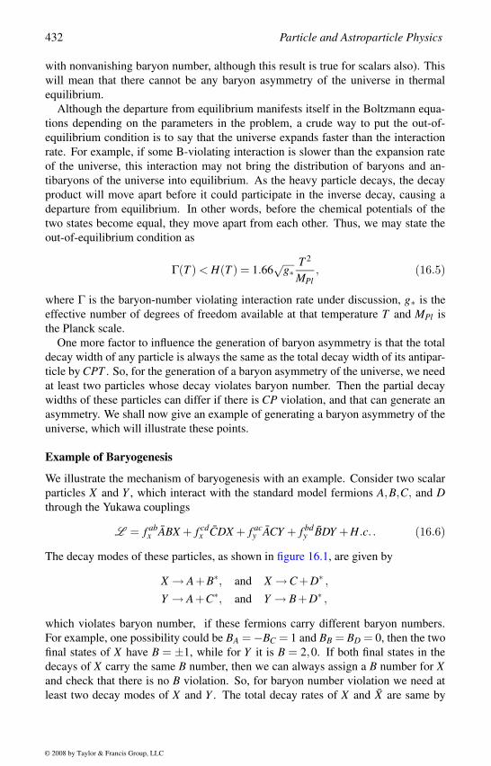
432 Particle and Astroparticle Physics
with nonvanishing baryon number, although this result is true for scalars also). This
will mean that there cannot be any baryon asymmetry of the universe in thermal
equilibrium.
Although the departure from equilibrium manifests itself in the Boltzmann equa-
tions depending on the parameters in the problem, a crude way to put the out-of-
equilibrium condition is to say that the universe expands faster than the interaction
rate. For example, if some B-violating interaction is slower than the expansion rate
of the universe, this interaction may not bring the distribution of baryons and an-
tibaryons of the universe into equilibrium. As the heavy particle decays, the decay
product will move apart before it could participate in the inverse decay, causing a
departure from equilibrium. In other words, before the chemical potentials of the
two states become equal, they move apart from each other. Thus, we may state the
out-of-equilibrium condition as
Γ(T ) < H(T ) = 1.66√
g∗T 2
MPl, (16.5)
where Γ is the baryon-number violating interaction rate under discussion, g∗ is the
effective number of degrees of freedom available at that temperature T and MPl is
the Planck scale.
One more factor to influence the generation of baryon asymmetry is that the total
decay width of any particle is always the same as the total decay width of its antipar-
ticle by CPT . So, for the generation of a baryon asymmetry of the universe, we need
at least two particles whose decay violates baryon number. Then the partial decay
widths of these particles can differ if there is CP violation, and that can generate an
asymmetry. We shall now give an example of generating a baryon asymmetry of the
universe, which will illustrate these points.
Example of Baryogenesis
We illustrate the mechanism of baryogenesis with an example. Consider two scalar
particles X and Y , which interact with the standard model fermions A,B,C, and Dthrough the Yukawa couplings
L = f abx ABX + f cd
x CDX + f acy ACY + f bd
y BDY +H.c. . (16.6)
The decay modes of these particles, as shown in figure 16.1, are given by
X → A+B∗, and X →C +D∗ ,
Y → A+C∗, and Y → B+D∗ ,
which violates baryon number, if these fermions carry different baryon numbers.
For example, one possibility could be BA =−BC = 1 and BB = BD = 0, then the two
final states of X have B = ±1, while for Y it is B = 2,0. If both final states in the
decays of X carry the same B number, then we can always assign a B number for Xand check that there is no B violation. So, for baryon number violation we need at
least two decay modes of X and Y . The total decay rates of X and X are same by
© 2008 by Taylor & Francis Group, LLC
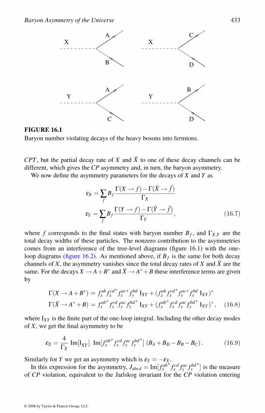
Baryon Asymmetry of the Universe 433
D
XX
Y Y
A
B
C
D
C
A B
FIGURE 16.1Baryon number violating decays of the heavy bosons into fermions.
CPT , but the partial decay rate of X and X to one of these decay channels can be
different, which gives the CP asymmetry and, in turn, the baryon asymmetry.
We now define the asymmetry parameters for the decays of X and Y as
εX = ∑f
B fΓ(X → f )−Γ(X → f )
ΓX
εY = ∑f
B fΓ(Y → f )−Γ(Y → f )
ΓY, (16.7)
where f corresponds to the final states with baryon number B f , and ΓX ,Y are the
total decay widths of these particles. The nonzero contribution to the asymmetries
comes from an interference of the tree-level diagrams (figure 16.1) with the one-
loop diagrams (figure 16.2). As mentioned above, if B f is the same for both decay
channels of X , the asymmetry vanishes since the total decay rates of X and X are the
same. For the decays X → A+B∗ and X → A∗+B these interference terms are given
by
Γ(X → A+B∗) = f abx f cd
x∗
f acy
∗ f bdy IXY +( f ab
x f cdx
∗f acy
∗ f bdy IXY )∗
Γ(X → A∗ +B) = f abx
∗f cdx f ac
y f bdy
∗IXY +( f ab
x∗
f cdx f ac
y f bdy
∗IXY )∗ , (16.8)
where IXY is the finite part of the one-loop integral. Including the other decay modes
of X , we get the final asymmetry to be
εX =4
ΓXIm[IXY ] Im[ f ab
x∗
f cdx f ac
y f bdy
∗] (BA +BD −BB −BC) . (16.9)
Similarly for Y we get an asymmetry which is εY = −εX .
In this expression for the asymmetry, Jabcd = Im[ f abx
∗ f cdx f ac
y f bdy
∗] is the measure
of CP violation, equivalent to the Jarlskog invariant for the CP violation entering
© 2008 by Taylor & Francis Group, LLC
434 Particle and Astroparticle Physics
YX X
Y Y
B
AC
C
A
A
B
B
A
D BD
C
D C
D
X X
Y
FIGURE 16.2One-loop diagrams contributing to CP violation in heavy boson decays.
in the quark mass matrices. If the theory has CP violation, this quantity will be
nonzero. Rephasing of the light fields will not affect this quantity. Under rephasing
of the fields
ψi → expiφiψi,
where i = A,B,C,D and ψA represents the particle A, the Yukawa couplings trans-
form as
f i jx,y → expi(φ j−φi) f i j
x,y,
and some of the Yukawa couplings can be made real. However, [ f abx
∗ f cdx f ac
y f bdy
∗]transforms to itself and Jabcd remains invariant under this rephasing. So, if there is
CP violation in the theory, this quantity will be nonvanishing for any allowed phase
transformations of the light fields.
Since the imaginary part Im[IXY ], i.e., the absorptive part of the integral, enters
the calculation of the asymmetry parameter, this integral is nonvanishing when the
fermions in the loop are lighter than the scalars, In this case the fermions could be
on mass shell and we could cut the diagram along the fermion lines. Both the scalars
should have baryon-number violating interactions, otherwise one of the ε’s will van-
ish implying vanishing of the other. If X and Y are degenerate then there are two
problems, both of which give a vanishing asymmetry. First the loop integral van-
ishes when these masses are degenerate. Second, the contribution to the asymmetry
generated by one of them will be erased by that of the other, since εX =−εY . If their
masses are different, say, MY > MX , then at a temperature MY > T > MX , the number
density of particles Y will be less than the photon number density, while the number
density of X will be the same as the photon number density. Then the contribution to
the asymmetry in the decay of Y will have a Boltzmann suppression factor compared
with the decay of X . This will make the sum of the two contributions nonvanishing.
© 2008 by Taylor & Francis Group, LLC
Baryon Asymmetry of the Universe 435
Boltzmann Equation
The amount of asymmetry that can be generated will depend on the various interac-
tion rates, the asymmetry parameter, and can be obtained by solving the Boltzmann
equations [267]. Since we are writing the interaction at a temperature T < MY , the
inverse decay rate of Y is very small, Y has already decayed and the number density
of Y has exponentially fallen off. Then we have to consider the interactions of only
the particles X , which are the decay rate ΓD, inverse decay rate ΓID and the 2 ↔ 2
scattering A+ B ↔C + D mediated by X and X scalar exchange ΓS. There will also
be scattering processes mediated by Y and Y , but they will be suppressed compared
with the X , X scalar exchange. These rates are given by
ΓD = αmX
mXT T ≥ mX1 T ≤ mX
ΓID = ΓD
1 T ≥ mX(mX
T
)3/2exp−mX /T T ≤ mX
ΓS = nσ = T 3α2 T 2
(T 2 +m2X )2 , (16.10)
where α = f 2/4π is the coupling strength of the X-bosons.
We now assume that A and B∗ are quarks, so X decays into two light quarks qqwith baryon number Bqq = +2/3 and X decays into two antibaryons qq carrying
baryon number Bqq = −2/3. The decays of Y also violate B, but the details are not
important for this discussion. In grand unified theories, C could be a quark and Dcould be a lepton, but this detail is not required for this analysis. We also assume
that the Yukawa coupling constants are complex so there is CP violation, which
should show up in the interference of the tree-level and one-loop diagrams. Then the
amplitudes for the X and X decays can be written as
|M(X → bb)|2 = |M(bb → X)|2 =1
2(1+ εX )|M0|2
|M(X → bb)|2 = |M(bb → X)|2 =1
2(1− εX )|M0|2.
We further assume that Y is heavier than X and at around mX , the inverse decay of
Y is not allowed, and hence, the number density of Y is negligible, but the number
density of X and X is controlled by the decays and the inverse decays of X and X and
is given by their equilibrium distribution. With this consideration we can now write
the Boltzmann equation of these scalars as
nX +3HnX = −ΓD(nX −neqX ), (16.11)
where the second term comes due to the expansion of the universe and neqX is the
equilibrium number density of X and is given by
neqX =
s g−1∗ T mX
sg∗(π
2
)1/2 (mXT
)3/2exp−mX /T T mX .
(16.12)
© 2008 by Taylor & Francis Group, LLC
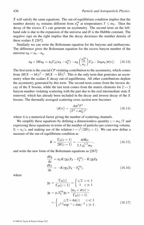
436 Particle and Astroparticle Physics
X will satisfy the same equations. The out-of-equilibrium condition implies that the
number density nX remains different from neqX at temperatures T ≤ mX . Then the
decay of the excess X’s can generate an asymmetry. The second term on the left-
hand side is due to the expansion of the universe and H is the Hubble constant. The
negative sign on the right implies that the decay decreases the number density of
these scalars X [267].
Similarly we can write the Boltzmann equation for the baryons and antibaryons.
The difference gives the Boltzmann equation for the excess baryon number of the
universe nB = nb −nb,
nB +3HnB = εX ΓD(nX −neqX )−nB
(neq
Xnγ
)ΓD −2nBnb〈σ |v|〉. (16.13)
The first term is the crucial CP violating contribution to the asymmetry, which comes
from |M(X → bb)|2 −|M(X → bb)|2. This is the only term that generates an asym-
metry when the scalars X decay out-of-equilibrium. All other contributions deplete
the asymmetry generated by this term. The second term comes from the inverse de-
cay of the X bosons, while the last term comes from the matrix elements for 2 ↔ 2
baryon-number violating scattering with the part due to the real intermediate state Xremoved, which has already been included in the decay and inverse decay of the Xbosons. The thermally averaged scattering cross section now becomes
〈σ |v|〉 ∼ Aα2T 2
(T 2 +m2X )2 , (16.14)
where A is a numerical factor giving the number of scattering channels.
We simplify these equations by defining a dimensionless quantity z = mX/T and
expressing these equations in terms of the number of particles per comoving volume,
Yi = ni/s, and making use of the relation t = z2/2H(z = 1). We can now define a
measure of the out-of-equilibrium condition as
K =ΓD(z = 1)2H(z = 1)
=αMPl
3.3 g1/2∗ mX
, (16.15)
and write the new form of the Boltzmann equations as [267]
dYB
dz= εX KzγD(YX −Y eq
X )−KzγBYB
dYX
dz= −KzγD(YX −Y eq
X ), (16.16)
where
γD =ΓD(z)
ΓD(z = 1)=
z/2 z 1
1 z 1
γB = g∗YeqX γD +
2nγ < σ |v| >ΓD(z = 1)
=
z/2+Aα/z z 1
z3/2exp−z +Aαz−5 z 1 .(16.17)
© 2008 by Taylor & Francis Group, LLC
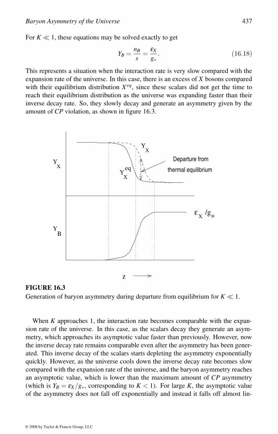
Baryon Asymmetry of the Universe 437
For K 1, these equations may be solved exactly to get
YB =nB
s=
εX
g∗. (16.18)
This represents a situation when the interaction rate is very slow compared with the
expansion rate of the universe. In this case, there is an excess of X bosons compared
with their equilibrium distribution X eq, since these scalars did not get the time to
reach their equilibrium distribution as the universe was expanding faster than their
inverse decay rate. So, they slowly decay and generate an asymmetry given by the
amount of CP violation, as shown in figure 16.3.
z
Departure from
thermal equilibrium
Xε /g
*
YX
YB
YX
eq
YX
FIGURE 16.3Generation of baryon asymmetry during departure from equilibrium for K 1.
When K approaches 1, the interaction rate becomes comparable with the expan-
sion rate of the universe. In this case, as the scalars decay they generate an asym-
metry, which approaches its asymptotic value faster than previously. However, now
the inverse decay rate remains comparable even after the asymmetry has been gener-
ated. This inverse decay of the scalars starts depleting the asymmetry exponentially
quickly. However, as the universe cools down the inverse decay rate becomes slow
compared with the expansion rate of the universe, and the baryon asymmetry reaches
an asymptotic value, which is lower than the maximum amount of CP asymmetry
(which is YB = εX/g∗, corresponding to K < 1). For large K, the asymptotic value
of the asymmetry does not fall off exponentially and instead it falls off almost lin-
© 2008 by Taylor & Francis Group, LLC
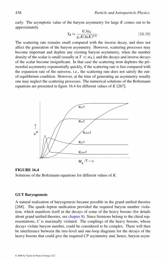
438 Particle and Astroparticle Physics
early. The asymptotic value of the baryon asymmetry for large K comes out to be
approximately
YB ≈ 0.3εX
g∗K(lnK)0.6 . (16.19)
The scattering rate remains small compared with the inverse decay, and does not
affect the generation of the baryon asymmetry. However, scattering processes may
become important and deplete any existing baryon asymmetry, when the number
density of the scalar is small (usually at T mX ), and the decays and inverse decays
of the scalar become insignificant. In that case the scattering term depletes the pri-
mordial asymmetry exponentially quickly, if the scattering rate is fast compared with
the expansion rate of the universe, i.e., the scattering rate does not satisfy the out-
of-equilibrium condition. However, at the time of generating an asymmetry usually
one may neglect the scattering processes. The numerical solutions of the Boltzmann
equations are presented in figure 16.4 for different values of K [267].
MX
/T --->
K>>1
K>1
K<<1
K=1
K<1
YB
--->
FIGURE 16.4Solutions of the Boltzmann equations for different values of K.
GUT Baryogenesis
A natural realization of baryogenesis became possible in the grand unified theories
[268]. The quark–lepton unification provided the required baryon number viola-
tion, which manifests itself in the decays of some of the heavy bosons (for details
about grand unified theories, see chapter 8). Since fermions belong to the chiral rep-
resentations, C is maximally violated. The couplings of the heavy bosons, whose
decays violate baryon number, could be considered to be complex. There will then
be interference between the tree-level and one-loop diagrams for the decays of the
heavy bosons that could give the required CP asymmetry and, hence, baryon asym-
© 2008 by Taylor & Francis Group, LLC
Baryon Asymmetry of the Universe 439
metry. Departure from thermal equilibrium is also naturally satisfied in these models
since the scale of unification is sufficiently high and the universe was expanding
very rapidly in that epoch. So, a coupling of α ∼ .01 would mean that for the uni-
fication scale mU ≤ 1016 GeV, the heavy bosons could decay satisfying the out-of-
equilibrium condition [268].
Although baryogenesis was considered to be a major success of the grand unified
theories, later it was realized that there are problems in these scenarios. In SU(5)grand unified theory, both the baryon number (B) and the lepton number (L) are
violated, but a combination (B− L) remains conserved globally. In SO(10) grand
unified theories, B−L number is a local symmetry of the theory, which is broken
at some intermediate scale. So the baryon number violation at the scale of grand
unification in both the SU(5) and SO(10) grand unified theories conserves (B−L).
This can also be seen from the operator analysis for proton decay, which says that to
the lowest order all baryon number violations in grand unified theories conserve B−L. It was later pointed out that any primordial baryon asymmetry, which conserves
B−L, will be washed out by fast baryon number violation due to the chiral anomaly
before the electroweak phase transition [269].
In the standard model the global baryon (B) and lepton (L) number symmetries
have anomalies [100] (see section 4.4). A global B anomaly comes from a triangle
loops with the fermions in the loop, the two SU(2)L gauge bosons at the two external
vertices, and a global B current at the third vertex. The sum over all the fermions
gives the total SU(2)L global B anomaly. A nonvanishing global B anomaly in the
standard model means that although the baryon number B is classically a global
symmetry in the standard model, quantum effects violate this global symmetry. Thus,
quantum–mechanical tunneling will allow transitions from one vacuum to another
with differing baryon numbers, which will violate baryon number.
In the standard model, both baryon and lepton numbers are global symmetries,
which are violated due to anomalies, but the anomaly corresponding to a com-
bination B − L vanishes. So, the anomaly induced vacuum transitions will con-
serve the combination B−L. In fact, the amount of baryon number violation (∆B)
and lepton number violation (∆L) are the same, and hence, ∆(B−L) = 0 although
∆(B + L) = 2∆B = 2∆L = 0. This B + L violating process is highly suppressed by
the quantum tunnelling probability at zero temperature [100]. But at high tempera-
ture this process was very fast due to an enhancement by the Boltzmann factor in the
presence of an instanton-like solution, the sphaleron [269]. In a typical sphaleron-
induced process, a vacuum with B + L = 6 and B− L = 0 can decay into another
vacuum with B+L = 0 and B−L = 0 releasing uude−ccsµ−ttbτ−. This sphaleron-
induced B + L violating process was in equilibrium for a long time before the elec-
troweak phase transition, which would have washed out any baryon asymmetry that
conserves B−L. Thus, the baryon asymmetry generated at the scale of grand unifica-
tion is erased leaving a baryon symmetric universe in the presence of the sphalerons
before the electroweak phase transition.
© 2008 by Taylor & Francis Group, LLC
440 Particle and Astroparticle Physics
Electroweak Baryogenesis
Since the baryon asymmetry created at the time of grand unification phase transition
was washed out by the sphaleron-induced transitions, attempts were made to gen-
erate a baryon asymmetry of the universe making use of the sphaleron transitions
[270]. In this mechanism there was no need to introduce any new physics beyond
the standard model. There is CP violation coming from the quark mixing matrix in
the standard model. The only hurdle was the out-of-equilibrium condition, which is
difficult to satisfy. A new mechanism was then suggested by considering the elec-
troweak phase transition to be of first order. In a first order phase transition, when
the temperature reaches the critical point, the free energies corresponding to the true
vacuum and the false vacuum become equal. At this point, both the vacua coexist
and bubbles start forming all over the place, where inside the bubble the electroweak
symmetry is broken and sphaleron transitions are not allowed. Since there is no
baryon number violation inside the bubbles, any baryon number violation along the
bubble wall can generate a B + L asymmetry inside the bubbles, which will not be
affected by the fast sphaleron transitions outside the bubbles. This makes it possible
to satisfy the out-of-equilibrium condition. CP violation takes place along the wall of
the bubble only, which can generate the required baryon asymmetry of the universe.
This model is highly attractive since it includes parameters entering in the standard
model.
Although the models of electroweak baryogenesis were predictive and calcula-
ble, the simplest models did not work. The amount of CP violation coming from the
quark mass mixing alone in the standard model is not enough and one requires exten-
sions of the standard model with new sources of CP violation to explain the required
baryon asymmetry of the universe. There is a more serious problem with these mod-
els, which comes from the fact that after the phase transition is over, the generated
baryon asymmetry is not washed out by the remaining fast baryon number violation.
After the phase transition is over, the false vacuum decays into the true vacuum and
all the bubble walls expand at a speed of light and finally cover the entire space. If
the baryon-number violating interactions have not ceased to exist by this time, they
will make the universe baryon symmetric again. This depends on the dynamics of the
model and gives a very strong constraint on the mass of the Higgs scalar [271]. With
the present experimental limit on the Higgs mass most of the models of electroweak
baryogenesis have been ruled out. In the supersymmetric models, the uncertainties
in the parameters allow electroweak baryogenesis for a slightly higher Higgs mass.
But the predictability of the electroweak baryogenesis is lost in these models.
There are many other mechanisms of baryogenesis [272], but the most popular of
these mechanisms is the leptogenesis. In this mechanism the lepton number violation
due to the Majorana masses of the neutrinos generate a lepton asymmetry of the
universe, which then gets converted to a baryon asymmetry before the electroweak
phase transition in the presence of the sphalerons [273].
© 2008 by Taylor & Francis Group, LLC
Baryon Asymmetry of the Universe 441
16.2 LeptogenesisLeptogenesis is the mechanism of generating a lepton asymmetry of the universe
before the electroweak phase transition, which can then be converted to the re-
quired baryon asymmetry of the universe in the presence of the sphalerons. The
fast sphaleron-induced B + L violating transitions converts any L asymmetry and,
hence, B− L asymmetry into a baryon asymmetry of the universe. We shall now
discuss how the sphaleron-induced transitions due to global B and L anomaly relate
the L asymmetry to the B asymmetry before the electroweak symmetry breaking.
Let us consider a global symmetry U(1)X in the standard model. The global
SU(2)L anomaly of this U(1)X symmetry will then mean that in a triangle-loop dia-
gram there are SU(2)L gauge bosons at the two vertices and at the third vertex there
is a global current corresponding to the U(1)X symmetry. So, the group theoretical
factor for a fermion in the loop transforming as doublet under SU(2)L and carrying
U(1)X quantum number x will be TrT aT a·x. For a doublet of SU(2), the quadratic
invariant may be normalized to TrT aT a= 1/2, thus the X anomaly will be propor-
tional to x/2. Fermions, which transform as singlets under SU(2)L, do not contribute
to the anomaly. The total X anomaly will be sum over all the fermions in the theory.
The quarks carry baryon number 1/3 and only the left-handed quarks transform as
doublets under SU(2)L. Thus, the SU(2)L B anomaly gets contribution only from the
left-handed doublet quarks and the corresponding group theoretical factor is AB =3× 1/2× 1/3 = 1/2 (the factor 3 comes because there are three colored doublets).
On the other hand the L anomaly comes from the left-handed leptons carrying L = 1,
which is AL = 1/2 ⇒ AB = AL ⇒ AB−L = 0 and AB+L = 1.
In the standard model both B and L are global symmetries, but due to the SU(2)Lglobal anomaly, the B + L symmetry is broken. The chiral nature of the weak inter-
action makes the B+L symmetry anomalous and the sum over all the fermions gives
a nonvanishing axial current [100]
δµ jµ5(B+L) = 6[
α2
8πW µν
a Waµν +α1
8πY µνYµν ], (16.20)
which breaks the B + L symmetry. There is no anomaly corresponding to the B−Lcharge. Because of this anomaly, baryon and lepton numbers are broken during the
electroweak phase transition,
∆(B+L) = 2Ngα2
8π
∫d4xW µν
a Waµν = 2Ngν , (16.21)
but their rate is very small at zero temperature, since they are suppressed by the
quantum tunnelling probability, exp[− 2πα2
ν ], where ν is a topological quantum num-
ber called the Chern–Simmons number. At finite temperature, this interaction rate
becomes strong in the presence of an instanton-like solution, the sphalerons [269],
and the quantum tunnelling factor is replaced by the Boltzmann factor exp[−V0T ν ],
© 2008 by Taylor & Francis Group, LLC
442 Particle and Astroparticle Physics
where the potential or the free energy V0 is related to the mass of the sphaleron field,
which is about TeV. As a result, at temperatures between
1012GeV > T > 102GeV, (16.22)
the sphaleron mediated B+L violating interactions will be very strong.
For the simplest scenario of ν = 1, the sphaleron-induced processes are ∆B =∆L = 3, given by
|vac >−→ [uLuLdLe−L + cLcLsLµ−L + tLtLbLτ−L ]. (16.23)
These baryon and lepton-number violating fast processes will exponentially deplete
any primordial B + L asymmetry of the universe. As a result, the number density
of both particles and antiparticles with B + L number will become the same as their
equilibrium distribution. On the other hand, if there is any B−L asymmetry of the
universe, that will be converted to a baryon asymmetry of the universe before the
electroweak phase transition. This can be seen from an analysis of the chemical
potential [274].
We shall now analyze the chemical potential assuming all particles are ultra-
relativistic, which is the case above the electroweak symmetry breaking. The particle
asymmetry, i.e., the difference between the number of particles (n+) and the number
of antiparticles (n−), can be given in terms of the chemical potential of the particle
species µ (for antiparticles the chemical potential is −µ) as
n+ −n− = ndgT 3
6
(µT
), (16.24)
where nd = 2 for bosons and nd = 1 for fermions.
Before the electroweak phase transition during the period (16.22), the sphaleron-
induced B+L violating interactions will be in equilibrium along with the other in-
teractions. In table 16.1, we present all other interactions and the corresponding
relations between the chemical potentials. Using these relations we eliminate some
of the chemical potentials to relate the baryon and lepton numbers with the B−Lquantum number during this interaction. In the third column we give the chemical
potential which we eliminate using the given relation. We start with chemical poten-
tials of all the quarks (µuL,µdL,µuR,µdR); leptons (µaL,µνaL,µaR, where a = e,µ,τ);
gauge bosons (µW for W−, and 0 for all others); and the Higgs scalars (µφ−,µφ
0 ).
The chemical potentials of the neutrinos always enter as a sum and for that rea-
son we can consider them as one parameter. We can then express all the chemical
potentials in terms of the following independent chemical potentials,
µ0 = µφ0 ; µW ; µu = µuL; µ = ∑
iµi = ∑
iµν iL. (16.25)
We can further eliminate one of these four potentials by making use of the relation
given by the sphaleron processes (16.23). Since the sphaleron interactions are in
© 2008 by Taylor & Francis Group, LLC
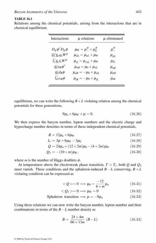
Baryon Asymmetry of the Universe 443
TABLE 16.1Relations among the chemical potentials, arising from the interactions that are in
chemical equilibrium.
Interactions µ relations µ eliminated
Dµ φ †Dµ φ µW = µφ− + µφ
0 µφ−
qLγµ qLW µ µdL = µuL + µW µdL
lLγµ lLW µ µiL = µν iL + µW µiL
qLuRφ † µuR = µ0 + µuL µuR
qLdRφ µdR = −µ0 + µdL µdR
liLeiRφ µiR = −µ0 + µiL µiR
equilibrium, we can write the following B+L violating relation among the chemical
potentials for three generations,
9µu +6µW + µ = 0. (16.26)
We then express the baryon number, lepton numbers and the electric charge and
hypercharge number densities in terms of these independent chemical potentials,
B = 12µu +6µW (16.27)Li = 3µ +6µW −3µ0 (16.28)Q = 24µu +(12+2m)µ0 − (4+2m)µW (16.29)
Q3 = −(10+m)µW , (16.30)
where m is the number of Higgs doublets φ .
At temperatures above the electroweak phase transition, T > Tc, both Q and Q3must vanish. These conditions and the sphaleron-induced B−L conserving, B + Lviolating condition can be expressed as
< Q >= 0 =⇒ µ0 =−12
6+mµu (16.31)
< Q3 >= 0 =⇒ µW = 0 (16.32)Sphaleron transition =⇒ µ = −9µu (16.33)
Using these relations we can now write the baryon number, lepton number and their
combinations in terms of the B−L number density as
B =24+4m
66+13m(B−L) (16.34)
© 2008 by Taylor & Francis Group, LLC
444 Particle and Astroparticle Physics
L =−42−9m66+13m
(B−L) (16.35)
B+L =−18−5m66+13m
(B−L). (16.36)
Below the critical temperature, the SU(2)L and the U(1)Y groups are broken leav-
ing the U(1)Q symmetry. Thus, Q should vanish since the universe is neutral with
respect to all conserved charges. However, since SU(2)L is broken below the critical
temperature, we can consider µφ0 = 0 and Q3 = 0. This gives us
< Q >= 0 =⇒ µW =12
2+mµu (16.37)
〈φ〉 = 0 =⇒ µ0 = 0 (16.38)
sphaleron transition =⇒ µ =−90−9m
2+mµu, (16.39)
which then allows us to write the baryon and lepton numbers as some combinations
of B−L as
B =32+4m
98+13m(B−L) (16.40)
L =−66−9m98+13m
(B−L) (16.41)
B+L =−34−5m98+13m
(B−L) . (16.42)
Thus, before the electroweak phase transition, any B−L asymmetry will be related
to the baryon asymmetry of the universe, while any B+L asymmetry will be wiped
off.
Any lepton number violation at some intermediate scale within the period 1012 −102 GeV, can thus affect the baryon asymmetry of the universe in the two cases:
If there is L violation at a faster rate than the expansion rate of the universe, any
L asymmetry will be washed out. Since B + L asymmetry is also washed out
by the sphaleron transition, together they will wash out any baryon asymmetry
[B = (B+L)−L] of the universe before the electroweak phase transition [274,
275].
If there is L violation satisfying the out-of-equilibrium condition and if there
is enough CP violation, an L asymmetry can be generated. In there is no
primordial B asymmetry, the L asymmetry will give us an equal amount of
B−L asymmetry. This B−L asymmetry will then give us a baryon asymmetry
of the universe
B =24+4m
66+13m(B−L) .
The generation of the baryon asymmetry of the universe originating from a
lepton number violation is known as leptogenesis [273, 274].
© 2008 by Taylor & Francis Group, LLC
Baryon Asymmetry of the Universe 445
In the rest of this chapter we shall consider these two cases and study the interplay
between the baryon asymmetry of the universe and the lepton-number violating Ma-
jorana masses of the neutrinos.
16.3 Models of LeptogenesisAmong the several generic mechanisms of neutrino mass, only the see-saw mech-
anism and the triplet Higgs mechanisms can generate a lepton asymmetry of the
universe naturally in the simplest models. In the radiative models, there are some
versions where it may be possible to generate a lepton asymmetry of the universe,
but most of the simple versions of these models are inconsistent with leptogenesis.
Some other mechanisms have to be invoked to explain the baryon asymmetry of the
universe in these models. We shall now demonstrate how, in the minimal version of
the see-saw and the triplet Higgs models, it is possible to generate a lepton asymme-
try of the universe.
See-Saw Leptogenesis
In the see-saw mechanism [55] for neutrino masses, the standard model is extended
to include right-handed neutrinos (NRi, i = e,µ,τ). The interaction Lagrangian for
the right-handed neutrinos is given by
Lint = hαi Lα φ NRi +Mi (NRi)c NRi, (16.43)
where Lα are the light leptons with α = 1,2,3 as the generation index and hαi are
the Yukawa couplings, which could be complex. Without loss of generality we work
in a basis in which the Majorana mass matrix of the right-handed neutrinos is real
and diagonal with eigenvalues Mi and assume a hierarchy M3 > M2 > M1.
The Majorana nature of the right-handed neutrinos will imply lepton number vio-
lation and hence the right-handed neutrinos can decay into a lepton and an antilepton
violating lepton number. The lepton-number violating decays of the right-handed
neutrinos
NRi → jL + φ ,
→ jLc +φ (16.44)
can then generate a lepton asymmetry of the universe if there is enough CP violation
and these interactions satisfy the out-of-equilibrium condition [273]. This L asym-
metry will be same as the B− L asymmetry, which will then become the baryon
asymmetry of the universe in the presence of the sphalerons.
There are now two independent sources of CP violation. In the original proposal
for baryogenesis and all subsequent articles, only the decay type CP violation was
considered, which comes from interference of tree-level and vertex diagrams [266].
© 2008 by Taylor & Francis Group, LLC
446 Particle and Astroparticle Physics
In the language of K-physics, it is the CP violation coming from the penguin dia-
gram in K-decays which is denoted by ε ′. Leptogenesis was first proposed with only
this contribution [273]. The tree-level decays of the right-handed neutrinos interfere
with the one-loop vertex diagrams of figure 16.5. In the decay of the right-handed
neutrinos, the one-loop diagram involves a right-handed neutrino of another gener-
ation. Since both right-handed neutrinos violate lepton number in their decays and
they have different masses, they can give the required CP violation [273, 276]. This
is similar to the example we discussed and the asymmetry parameter now comes out
to be
ε ′ =Γ(N → φ †)−Γ(N → cφ)Γ(N → φ †)+Γ(N → cφ)
= − 1
8πM1
M2
Im[∑α(h∗α1hα2)∑β (h∗β1hβ2)]
∑α |hα1|2 , (16.45)
in the limit of large mass difference between M2 and M1. This result is for two
generations. When they are degenerate, the asymmetry parameter vanishes.
NR
φ
NR
φ
νL
c
νL
NR
νL
φ
FIGURE 16.5Tree-level and one-loop vertex diagrams contributing to CP asymmetry in models
with right-handed neutrinos
There is another source of CP violation in the case of right-handed neutrino de-
cays, which is more interesting. In the language of K-physics, this is the CP vio-
lation entering into the mass matrix denoted by ε and comes from the box diagram
giving the K − K mixing. This type of CP violation coming from the mixing ma-
trix was not considered in earlier baryogenesis models. In the case of right-handed
neutrino decay, this type of CP violation comes from the Majorana mass matrix of
the heavy right-handed neutrinos [277] through a self-energy diagram [278, 279].
The interference of the tree-level diagrams for the right-handed neutrino decays with
the self-energy diagram of figure 16.6, in which the two heavy neutrinos belong to
two different generations, gives rise to this new oscillation type CP violation. In
this case unitarity implies that the decay of one of the heavy neutrinos may cancel
the asymmetry from the decay of the other neutrino entering into the self-energy
diagram. But when the heavy neutrinos decay satisfies the out-of-equilibrium condi-
© 2008 by Taylor & Francis Group, LLC
Baryon Asymmetry of the Universe 447
tion, the number densities of the two neutrinos differ during their decay, and hence,
this cancellation does not take place. This is the first example of an oscillation type
CP violation entering in the mass matrix of the heavy particles, which is used for
generating a baryon asymmetry of the universe [277].
NR
φN
Rc
φlL
c
νL
c
NR
νL
c
φ
FIGURE 16.6Tree-level and one-loop self-energy diagrams contributing to the generation of lepton
asymmetry in models with right-handed neutrinos
The oscillation type CP violation, which comes from the self-energy diagram,
makes the study of leptogenesis more fascinating. It may be interpreted as the right-
handed neutrinos oscillating into antineutrinos of different generations and since the
rates Γ[particle → antiparticle] = Γ[antiparticle → particle], an asymmetry in the
right-handed neutrinos is generated before they decay.
We shall now explain how the CP violation enters in the Majorana mass matrix,
which can then generate a lepton asymmetry. A Majorana particle is its own an-
tiparticle, but when CP is violated, it is convenient to consider the particle and the
antiparticle independently. The Hermitian conjugate terms give the interactions of
the CP conjugate states, which now have different couplings since there is CP viola-
tion. So, we shall denote the right-handed neutrinos as Ni, i = 1,2 (we shall restrict
our present discussion to two generation only) and their CP conjugate antiparticles
as Nci , i = 1,2. The Yukawa couplings of these fields can be written as
Lint = ∑i
Mi[(NRi)cNRi +NRi(NRi)c]
+∑α,i
h∗αi NRi φ † Lα +∑α,i
hαi Lα φ NRi
+∑α,i
h∗αi (Lα)c φ † (NRi)c +∑α,i
hαi(NRi)c φ (Lα)c (16.46)
where Mi are the diagonal Majorana masses and real. CP violation comes from
the complex phases in hαi. We have also written the Hermitian conjugate terms
explicitly.
The states |Ni〉 and |Nci 〉 are states with definite CP, but due to the complex phases
in the Yukawa couplings hαi, the physical states will be different from these states.
Since the physical states will evolve with time, their decays can violate CP. For
example, |Ni〉 can decay into leptons, while |Nci 〉 can decay into antileptons. But
© 2008 by Taylor & Francis Group, LLC
448 Particle and Astroparticle Physics
the physical states will be admixtures of |Ni〉 and |Nci 〉, and hence, both the physical
states could decay into both leptons and antileptons, violating CP.
We can write the effective mass matrix in the basis ( |Nc1〉 |Nc
2〉 |N1〉 |N2〉) as
M (0) =
0 0 M1 0
0 0 0 M2M1 0 0 0
0 M2 0 0
. (16.47)
The one-loop self-energy diagram will introduce small perturbation to this effective
mass matrix, given by
M (1) =
0 0 M(1)
11 M(1)12
0 0 M(1)12 M(1)
22
M(1)11 M(1)
12 0 0
M(1)12 M(1)
22 0 0
, (16.48)
with
M(1)i j = M(1)
ji =[
Mi ∑α
h∗αihα j +M j ∑α
hαih∗α j
](gdis
αi j −i2
gabsαi j) (16.49)
M(1)i j = M(1)
ji =[
Mi ∑α
hαih∗α j +M j ∑α
h∗αihα j
](gdis
αi j −i2
gabsαi j) (16.50)
and
M(1)ii = M(1)
ii =[
2Mi ∑α
hαih∗αi
](gdis
αi j −i2
gabsαi j). (16.51)
The dispersive part of the integral gdisαi j is absorbed in the renormalization of bare
parameters, while the absorbtive part gabαi j enters in the asymmetry parameter, which
is given by
gabsαi j =
1
16π, (16.52)
neglecting terms of order O(m2
α/p2), O(
m2φ /p2
)with p2 ≥ M2
i .
In general, all the physical states ψi, i = 1,2,3,4 are now combinations of all the
four states |Nc1〉, |Nc
2〉, |N1〉 and |N2〉, and decays of the physical states |Ψi > generate
the lepton asymmetry. The asymmetry parameter can, thus, be defined as
∆ =2
∑i=1
ΓΨi→l −ΓΨi→lc
ΓΨi→l +ΓΨi→lc. (16.53)
In the limit |M2 −M1| |M(1)i j | or |M(1)
i j |, we get
δ =1
8πM1M2
M22 −M2
1
Im[∑α(h∗α1hα2)∑β (h∗β1hβ2)
]∑α |hα1|2 . (16.54)
© 2008 by Taylor & Francis Group, LLC
Baryon Asymmetry of the Universe 449
For three generations there is a factor of 3/2. When the mass difference is large com-
pared with the width, the CP asymmetries generated through the mixing δ (through
the self-energy diagram) of the heavy neutrinos and the decays ε ′ (through the vertex
diagram) are comparable. However, for small mass difference δ becomes very large
compared with ε ′ by orders of magnitude [277] (as shown in figure 16.7).
1.0 1.2 1.4 1.6 1.8 2.0r −−>
0.0
0.5
1.0
1.5
2.0
2.5
Lept
on a
sym
met
ry
−−
>
δ
ε’
FIGURE 16.7Comparison of the two CP-violating contributions to the lepton asymmetry, where
r = M22/M2
1 . The vertex contribution to CP violation is denoted by ε ′ and the self-
energy contribution is denoted by δ (from [277]).
The self-energy contribution to the CP violation δ becomes very large when the
two right-handed neutrinos are almost degenerate, i.e., when the mass difference
is comparable with their width and there is a resonance effect [277] (as shown in
figure 16.8). As a result the amount of lepton asymmetry generated through this
mechanism could be orders of magnitude larger than the asymmetry generated by
the usual vertex-type CP violation. This phenomenon is called resonant leptogenesis
[277, 279].
The lightest right-handed neutrino N1 decays generate the asymmetry, so it should
satisfy the out-of-equilibrium condition
|hα1|216π
M1 < 1.66√
g∗T 2
MPat T = M1, (16.55)
which gives a bound on the mass of the lightest right-handed neutrino to be mN1 >
© 2008 by Taylor & Francis Group, LLC
450 Particle and Astroparticle Physics
1.0000 1.0005 1.0010r −−>
100
200
400
800
1600
Lept
on a
sym
met
ry −
−>
P = .001
P = .01
FIGURE 16.8Lepton asymmetry generated for a small mass difference between two heavy neutri-
nos, where P = ∑α h∗α1hα1 and r = M22/M2
1 . The resonant leptogenesis occurs when
the masses M1 and M2 are almost degenerate (from [277]).
108GeV [280]. Although this out-of-equilibrium condition can give us some esti-
mate, for actual calculation of the asymmetry one needs to solve the Boltzmann equa-
tion, taking into consideration both lepton-number conserving and lepton-number
violating processes mediated by the heavy neutrinos [276, 277, 278, 279].
In the present case we define the lepton number asymmetry as nL = nl − nlc and
write its time evolution equation
dnL
dt+3HnL = (ε ′ +δ )Γψ1 [nψ1 −neq
ψ1 ]−(
nL
nγ
)neq
ψ1 Γψ1 −2nγ nL〈σ |v|〉 . (16.56)
Here, Γψ1 is the decay rate of the physical state |ψ1〉, and 〈σ |v|〉 describes the ther-
mally averaged cross-section of l +φ † ←→ lc +φ scattering. The number density of
ψ1 satisfiesdnψ1
dt+3Hnψ1 = −Γψ1(nψ1 −neq
ψ1). (16.57)
We now define the parameter K = Γψ1(T = Mψ1)/H(T = Mψ1) as a measure of the
deviation from equilibrium. For K 1 we can find an approximate solution
nL
s=
1
g∗(ε ′ +δ ), (16.58)
where g∗ denotes the total number of massless degrees of freedom.
© 2008 by Taylor & Francis Group, LLC
Baryon Asymmetry of the Universe 451
The bound on the lightest right-handed neutrino mass comes from the out-of-
equilibrium condition and the constraint on the Yukawa couplings from the required
amount of lepton asymmetry. In the case of resonant leptogenesis, since there is
large enhancement of asymmetry, the constraints on the Yukawa couplings is relaxed.
Thus, the Boltzmann suppression will be compensated by the resonant enhancement
and the scale of leptogenesis could be lowered to as low as TeV [279].
The lepton asymmetry generated is the same as the B−L asymmetry of the uni-
verse (nB−L), since there is no primordial baryon asymmetry at this time
nB−L
s= −(ε ′ +δ ) η
neqψ1(T mN1)
s, (16.59)
where, neqψ1(T mN1)/s = 135ζ (3)/(4π4g∗), with g∗ = 106.75 for the standard
model and η is a measure of a departure from thermal equilibrium. When we lower
the scale, η becomes very small, but the increase in δ due to resonant oscillation
could compensate and the required amount of B−L asymmetry may be generated.
The sphaleron interactions now convert this B−L asymmetry to a baryon asymmetry
of the universenB
s=
24+4nH
66+13nH
nB−L
s, (16.60)
where nH is the number of Higgs doublets in the standard model. It is then possible
to explain the baryon asymmetry of the universe, as required by the big-bang nu-
cleosynthesis and measured by the WMAP, assuming the standard cold dark matter
cosmological model including a nonvanishing cosmological constant,
nB
nγ= (6.15±0.25)×10−10 with s = 7.04nγ . (16.61)
In some cases it is possible to relate the neutrino masses with the amount of generated
baryon asymmetry. This would then allow us to predict the absolute neutrino mass
from the observed value of the baryon asymmetry.
Triplet Higgs Leptogenesis
We now discuss leptogenesis in the triplet Higgs mechanism of neutrino masses [57].
In this scenario one adds two complex SU(2)L triplet Higgs scalars, which carry a
U(1)Y charge −1 (ξa ≡ [1,3,−1];a = 1,2). The interactions of these Higgs scalars
that break lepton number explicitly and are relevant for leptogenesis are given by
Lint = f ai jξai j + µaξ †
a φφ . (16.62)
These give the lepton-number violating decays of the triplet Higgs ξa,
ξ ++a →
l+i l+j (L = −2)φ+φ+ (L = 0)
(16.63)
These interactions can generate a lepton asymmetry of the universe if they are slow
enough and there is enough CP violation. In this case there are no vertex corrections
© 2008 by Taylor & Francis Group, LLC
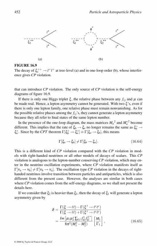
452 Particle and Astroparticle Physics
ξ1++
φ+
φ+
ξ2++
e+
e+
(b)
ξ1++
e+
e+
(a)
FIGURE 16.9The decay of ξ ++
1 → l+l+ at tree-level (a) and in one-loop order (b), whose interfer-
ence gives CP violation.
that can introduce CP violation. The only source of CP violation is the self-energy
diagrams of figure 16.9.
If there is only one Higgs triplet ξ , the relative phase between any fi j and µ can
be made real. Hence, a lepton asymmetry cannot be generated. With two ξ ’s, even if
there is only one lepton family, one relative phase must remain nonvanishing. As for
the possible relative phases among the fi j’s, they cannot generate a lepton asymmetry
because they all refer to final states of the same lepton number.
In the presence of the one-loop diagram, the mass matrices Ma2 and M∗
a2 become
different. This implies that the rate of ξb → ξa no longer remains the same as ξ ∗b →
ξ ∗a . Since by the CPT theorem Γ[ξ ∗
b → ξ ∗a ] ≡ Γ[ξa → ξb], this means
Γ[ξa → ξb] = Γ[ξb → ξa]. (16.64)
This is a different kind of CP violation compared with the CP violation in mod-
els with right-handed neutrinos or all other models of decays of scalars. This CPviolation is analogous to the lepton-number conserving CP violation, which may en-
ter in the neutrino oscillation experiments, where CP violation manifests itself as
Γ[νa → νb] = Γ[νb → νa]. The oscillation type CP violation in the decays of right-
handed neutrinos involve transition between particles and antiparticles, which is also
different from the present case. However, the analyses are similar in both cases
where CP violation comes from the self-energy diagrams, so we shall not present the
details here.
If we consider that ξ2 is heavier than ξ1, then the decay of ξ1 will generate a lepton
asymmetry given by
δ =Γ(ξ → )−Γ(ξ † → cc)Γ(ξ → )+Γ(ξ † → cc)
=Im[µ1µ∗
2 ∑k,l f 1kl f 2
kl∗]
8π2(M21 −M2
2)
[M1
Γ1
], (16.65)
© 2008 by Taylor & Francis Group, LLC
Baryon Asymmetry of the Universe 453
where
ΓabMb =1
8π
(µaµ∗
b +MaMb ∑k,l
f akl∗ f b
kl
)and Γa = Γaa. In this model the out-of-equilibrium condition is satisfied when the
masses of the triplet Higgs scalars are of the order of 1013 GeV.
The decay of the Higgs triplet will generate a lepton asymmetry, which becomes
the B − L asymmetry. This B − L asymmetry would convert itself to the baryon
asymmetry of the universe before the electroweak phase transition in the presence
of sphalerons. A neutrino mass in the range of 0.001− 1 eV can allow a baryon
asymmetry of the universe of nB/s ∼ 10−10 as desired [57].
The see-saw mechanism and the triplet Higgs mechanism of neutrino masses can
solve the problem of smallness of the Majorana neutrino masses and the baryon
asymmetry of the universe simultaneously. This makes these two scenarios popular
compared with the other models of neutrino masses. In the left–right symmetric
models, both right-handed neutrinos and the triplet Higgs scalars are present. So,
both these mechanisms can compete with each other for the generation of neutrino
masses and the baryon asymmetry of the universe.
16.4 Leptogenesis and Neutrino MassesWe shall now consider the constraints on the neutrino masses coming from leptogen-
esis. The first assumption is that the neutrino masses are Majorana masses, so lepton
number violation is associated with the neutrino masses. Any natural extensions of
the standard model thus imply a large lepton-number violating scale required for the
small neutrino masses. Depending on the strength of the lepton number violation,
this can either generate a baryon asymmetry of the universe through leptogenesis or
wash out any existing baryon asymmetry of the universe.
The sphaleron-mediated B+L violating transitions are in equilibrium during the
period 1012 − 102 GeV. If the lepton number violation satisfies the out-of-equilib-
rium condition and there is CP violation, this can generate a lepton asymmetry of the
universe. This lepton asymmetry will be the same as the B−L asymmetry, which
can then generate the required baryon asymmetry in the presence of the sphalerons.
On the other hand, if there is fast lepton number violation at any time before the
electroweak phase transition, that will erase any lepton asymmetry of the universe.
Erasure of the lepton asymmetry, together with the sphaleron-induced erasure of the
B + L asymmetry will leave us with a baryon symmetric universe. The requirement
of the baryon asymmetry at the time of nucleosynthesis thus constrains any lepton
number violation. The lepton number violation should not be too fast so it washes
out any baryon asymmetry. This can then constrain the mass of the neutrinos and
put stronger constraints on some specific models of neutrino masses [275, 281, 282].
In fact, it will constrain any lepton-number violating processes taking place before
© 2008 by Taylor & Francis Group, LLC
454 Particle and Astroparticle Physics
the electroweak phase transition. In this section we shall discuss some general con-
straints on lepton-number violating interactions.
The lepton number violation associated with any neutrino mass can be described
by the interaction [275]
L =2
MLLφφ , (16.66)
where L are lepton doublets, φ is the Higgs doublet, and M is the lepton-number
violating scale in the theory. Without specifying the origin of this scale, we can
estimate a neutrino mass from this operator to be mν ∼< φ >2 /M. We are not
including the couplings involved, which can change the details of the predictions.
But to show how it works, let us write the lepton-number violating scattering process
allowed by this interaction:
σ(νL +φ † → νL +φ) ∼ 1
π1
M2 . (16.67)
This process should not be faster than the expansion rate of the universe before the
electroweak phase transition, so as not to erase the baryon asymmetry of the universe,
which means
Γ∆L =0 ∼ 0.12
πT 3
M2 < H = 1.66√
g∗T 2
MPlat T ∼ 100 GeV, (16.68)
where H is the Hubble constant at that time, characterizing the expansion rate of the
universe. This gives a constraint on the lepton-number violating mass scale,
M > 109(
Tc
100 GeV
)1/2
GeV, (16.69)
where Tc is the critical temperature of the electroweak phase transition. This in turn
can give a bound on the mass of the neutrinos to be
mν < 50 keV. (16.70)
Although this is not a stringent limit, it gives an indication of how survival of the
baryon asymmetry of the universe can constrain the neutrino masses. This bound
can be improved slightly considering the scattering processes
W± +W± → e±α + e±α , (16.71)
where α = e,µ,τ . Soon after the electroweak phase transition starts, this process will
become operational and should be slow enough, which gives a constraint of mν < 20
keV [283].
There exist strong general constraints on any B−L number violating interactions
and, hence, lepton-number violating processes [281]. These constraints originate
from the fact that any fast B− L number violating interactions will make the uni-
verse B−L symmetric which in turn will make the universe baryon symmetric in the
© 2008 by Taylor & Francis Group, LLC
Baryon Asymmetry of the Universe 455
presence of the sphalerons. However, these constraints can be evaded in several ways
[282]. One common solution is that in the electroweak anomaly mediated processes,
B−3Li is conserved [282]. To see this, consider the sphaleron-mediated process,
|vac >→ [uude− + ccsµ− + ttbτ−], (16.72)
where the vacuum can decay into any one of these states. So, if any one of the three
combinations B−3Li (i = e,µ,τ) is conserved after the electroweak phase transition,
then the baryon asymmetry will not be erased even if the other two interactions are
fast. However, in practice it is difficult to make such models phenomenologically
consistent and to get the proper neutrino mixing.
Let us now consider the constraints on the R-parity violating models of neutrino
masses. There are lepton-number violating interactions
Li +Q j → (dck)
∗ → H1 +Ql , (16.73)
which should not be too fast and should satisfy
λ ′2T8π
<∼ 1.7√
g∗T 2
MPlat T = MSUSY . (16.74)
Assuming that the supersymmetry breaking scale MSUSY is 103 GeV, we find [284]
λ ′ <∼ 2×10⁻⁷, (16.75)
which is very much below the typical minimum value of 10−4 needed for radiative
neutrino masses [166]. The bound of equation (16.75) cannot be evaded even if one
uses the bilinear terms for neutrino masses. So, in all R-parity violating models one
needs to find some way to generate a baryon asymmetry of the universe.
The radiative Zee-type models also suffer from a similar problem [284]. In these
models one requires a charged singlet Higgs scalar, whose couplings break lepton
number explicitly. Consider a Zee-type radiative model, where the charged scalar
η− violates lepton number explicitly through its couplings
L = ∑i< j
fi j(νie j − eiν j)η+ + µ(φ+1 φ 0
2 −φ 01 φ+
2 )η−. (16.76)
Lepton-number is violated in the above by two units, and a neutrino mass is generated
radiatively. If these lepton number violating interactions are too fast, they will make
the universe lepton-symmetric before the electroweak phase transition, which will
then erase any baryon asymmetry of the universe in the presence of the sphalerons.
This requires η− to be heavy [285],
Mη
f 2i j
>∼ 1015GeV orMη
µ2>∼ 1015GeV and
Mη
µ2 f 2i j
>∼ 1016GeV. (16.77)
In this model the required neutrino mass cannot satisfy these out-of-equilibrium con-
ditions and generate a baryon asymmetry of the universe.
© 2008 by Taylor & Francis Group, LLC
456 Particle and Astroparticle Physics
These radiative models through R-parity violation or by the introduction of new
scalars can be made to work by introducing new physics, but the simplest models
cannot generate a lepton asymmetry of the universe. Only the see-saw mechanism
and the triplet Higgs models are mechanisms for neutrino masses which can generate
a lepton asymmetry of the universe without any extra input.
The condition that the lepton number violation should not be too fast implies a
strong bound on the lepton-number violating couplings in several other models. The
doubly charged leptons L−− will also have similar lepton-number violating interac-
tions, h1L++lRlR +h2MLL++χ−χ−, which will also be constrained by baryogenesis.
All the bounds coming from the survival of the baryon asymmetry of the universe
may be avoided to some extent, if a baryon asymmetry of the universe is generated
after the heavy scalars (whose interactions violate baryon number) have all decayed
away. However, in this case, there will still be a bound on the masses of these
heavy scalars, which is the scale of baryogenesis. If these scalars are lighter than the
scale at which baryon asymmetry of the universe is generated, then their interactions
will erase the asymmetry thus generated. Hence the bounds from the constraints of
baryogenesis can at most be made milder by generating a baryon asymmetry of the
universe at a lower energy scale.
In the see-saw mechanism of neutrino masses, leptogenesis takes place through
decays of the right-handed neutrinos. Without loss of generality, it is possible to
work in the basis where the right-handed neutrino Majorana mass matrix M is real
and diagonal with the hierarchy M3 > M2 > M1. Then at a temperature T ∼ M1, the
number densities of N2,3 will be much less, and only the decays of N1 (with mass M1)
will contribute to leptogenesis. It can be shown that the amount of lepton asymmetry
generated in these models can be related to the low-energy neutrino masses [286,
287].
We parameterize the light neutrino masses in terms of the measured quantities,
the atmospheric neutrino mass-squared difference ∆m2atm, the solar neutrino mass-
squared difference ∆m2sol , and the total mass squared
m2 = m21 +m2
2 +m23,
where m1,2,3 are the mass-eigenvalues of the light neutrinos. All neutrino masses
can then be expressed in terms of these three mass parameters. We also define an
effective mass m1, which enters the process of leptogenesis through decays of N1,
m1 =(m†
DmD)11
M1,
where mD = hv is the Dirac mass matrix of the neutrinos, h ≡ hαi are the Yukawa
couplings, and v is the vev of the electroweak symmetry breaking Higgs doublet.
It has been shown that the amount of CP violation in the decays of N1 can be
expressed in terms of these low-energy parameters and M1 [286] as
ε1 = − 3
16πM1
(h†h)11Im
[(h†h)
1
M(hT h∗)
]11
. (16.78)
© 2008 by Taylor & Francis Group, LLC
Baryon Asymmetry of the Universe 457
Corrections of order ∼ O(M1/M2,3) have been neglected. This CP asymmetry satis-
fies an upper bound [280] ε1 ≤ ε(M1, m), where
ε(M1, m) =3
16πM1
v2∆m2
atm +∆m2sol
m3(16.79)
and the maximum baryon asymmetry produced by N1 decay is given by [287, 288]
ηmaxB0 (m1,M1, m) = 1.38×10⁻³ε(M1, m)κ0(m1,M1, m), (16.80)
where κ0 is the efficiency factor that measures the number density of N1 with re-
spect to the equilibrium value, the out-of-equilibrium condition at decay and the
thermal corrections to ε1. m3 may be expressed in terms of m, ∆m2atm and ∆m2
solfor the different scenarios of neutrino mass hierarchy. For the normal hierarchy,
it is m3 = (m2 + 2∆m2atm + ∆m2
sol)/3, while for the inverted hierarchy, it is m3 =(m2 + ∆m2
atm + 2∆m2sol)/3. These relations can then be used to obtain bounds on
the mass of M1 and the light neutrinos considering thermal productions of right-
handed neutrinos. Taking into account all the interactions, one solves the Boltzmann
equations numerically to obtain bounds on the neutrino masses for which successful
leptogenesis is possible.
The see-saw models of neutrino masses allow leptogenesis through decays of
heavy right-handed neutrinos only for a small range of light neutrino masses [287].
The upper bound on the neutrino mass comes out to be mν < 0.20 eV, which trans-
lates into individual neutrino masses for the normal hierarchical neutrinos to be
m1,2 < 0.11 eV and m3 < 0.12 eV.
In the case of inverted hierarchy the bounds remain similar with mν < 0.21 eV and
for individual neutrinos
m1 < 0.11 eV and m2,3 < 0.12 eV.
Above these values, leptogenesis is not possible. There is also a lower bound on the
neutrino mass below which leptogenesis will not be possible in these models, but
those bounds are model dependent and weak.
The lower bound on the neutrino mass comes from the fact that at the time when
the right-handed neutrinos decay, their number density should not be too small to
generate the required lepton asymmetry; however, it should not be too fast so after the
asymmetry is generated it is washed out. In models of thermal leptogenesis, the right-
handed neutrinos are produced through scattering in the thermal bath. Including all
their interactions at temperatures above T = M1, it can be shown that leptogenesis is
possible for neutrino masses above mν > 10−3 eV [287]. The range of mass-squared
difference suggested by the atmospheric neutrinos√
∆m2atm ∼ 0.046 eV and solar
neutrinos√
∆m2sol ∼ 9× 10⁻³ eV is well suited to explain thermal leptogenesis in
the see-saw mechanism of neutrino masses. These considerations also give a lower
bound on the lightest right-handed neutrino mass of M1 ≥ 108 GeV [280].
© 2008 by Taylor & Francis Group, LLC
458 Particle and Astroparticle Physics
The upper bounds on the light neutrino masses are consistent with the bound com-
ing from the WMAP result of ∑mν < 0.69 eV, and this result implies that for the
values of the neutrino Majorana mass, as obtained in the neutrinoless double beta
decay, thermal leptogenesis is only marginally possible in the see-saw model. How-
ever, a more general analysis [289] including the precise computation of the ther-
mal leptogenesis [288] relaxed these bounds substantially. Although the bound for
the hierarchical heavy neutrinos remains similar, when the two heavy right-handed
neutrinos become almost degenerate the enhancement due to resonant leptogenesis
relaxes the upper bound on the neutrino masses to as high as 1 eV, thus making the
neutrinoless double beta decay observations consistent with resonant thermal lepto-
genesis [277]. For the thermal leptogenesis with triplet Higgs scalars [57], or when
the triplet Higgs in left–right symmetric models contribute mostly to the neutrino
masses, there is no constraint on the neutrino mass [290].
16.5 Generic Constraints
If there is fast baryon or lepton number violation before the electroweak phase tran-
sition, that will wash out any baryon asymmetry of the universe in the presence of
the sphaleron-induced fast B + L violation. This can, in turn, constrain the rate of
baryon and lepton-number violating interactions. Let us now consider the possible
effective operators, which can contribute to the baryon and lepton number violation
in the standard model [54]. The lowest-dimensional B violating operators are all of
the form QQQL. This operator QQQL has B−L = 0 and B + L = 2, and hence, all
processes allowed by this operator conserve B− L but violate B + L. The baryon
number violation arising from this operator could generate a baryon asymmetry of
the universe in grand unified theories but will be washed out by the fast sphaleron-
induced B+L violating transitions.
The lowest-dimensional B−L violating operator, which violates baryon number,
is QQQLφ , where φ is the usual Higgs doublet in the standard model. However,
compared with the B−L conserving processes, this process will be suppressed by
(< φ > /MU )2 ∼ 10−25. In some grand unified theories, the scale of B− L vio-
lation (MB−L) could be much lower than the scale of grand unification. In these
theories it is possible to have B−L violating baryon and lepton number violations.
The lowest-dimensional B−L violating operator is of the form LLφφ , which con-
tributes to the neutrino mass. There are also higher-dimensional B − L violating
effective operators, which are QQQQQQ and QQQLLL. These operators give rise
to neutron–antineutron oscillation and a three-lepton decay mode of the proton. Ex-
plicit realization of all these processes would require new Higgs scalars as well as
new gauge bosons. Some of these new particles could be very light and may have
other low-energy consequences.
© 2008 by Taylor & Francis Group, LLC
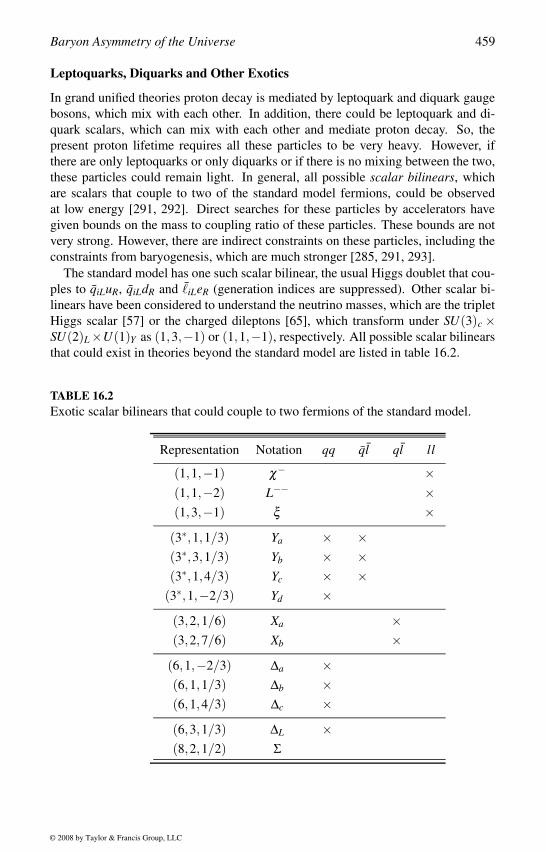
Baryon Asymmetry of the Universe 459
Leptoquarks, Diquarks and Other Exotics
In grand unified theories proton decay is mediated by leptoquark and diquark gauge
bosons, which mix with each other. In addition, there could be leptoquark and di-
quark scalars, which can mix with each other and mediate proton decay. So, the
present proton lifetime requires all these particles to be very heavy. However, if
there are only leptoquarks or only diquarks or if there is no mixing between the two,
these particles could remain light. In general, all possible scalar bilinears, which
are scalars that couple to two of the standard model fermions, could be observed
at low energy [291, 292]. Direct searches for these particles by accelerators have
given bounds on the mass to coupling ratio of these particles. These bounds are not
very strong. However, there are indirect constraints on these particles, including the
constraints from baryogenesis, which are much stronger [285, 291, 293].
The standard model has one such scalar bilinear, the usual Higgs doublet that cou-
ples to qiLuR, qiLdR and iLeR (generation indices are suppressed). Other scalar bi-
linears have been considered to understand the neutrino masses, which are the triplet
Higgs scalar [57] or the charged dileptons [65], which transform under SU(3)c ×SU(2)L×U(1)Y as (1,3,−1) or (1,1,−1), respectively. All possible scalar bilinears
that could exist in theories beyond the standard model are listed in table 16.2.
TABLE 16.2Exotic scalar bilinears that could couple to two fermions of the standard model.
Representation Notation qq ql ql ll
(1,1,−1) χ− ×(1,1,−2) L−− ×(1,3,−1) ξ ×(3∗,1,1/3) Ya × ×(3∗,3,1/3) Yb × ×(3∗,1,4/3) Yc × ×
(3∗,1,−2/3) Yd ×(3,2,1/6) Xa ×(3,2,7/6) Xb ×
(6,1,−2/3) ∆a ×(6,1,1/3) ∆b ×(6,1,4/3) ∆c ×(6,3,1/3) ∆L ×(8,2,1/2) Σ
© 2008 by Taylor & Francis Group, LLC
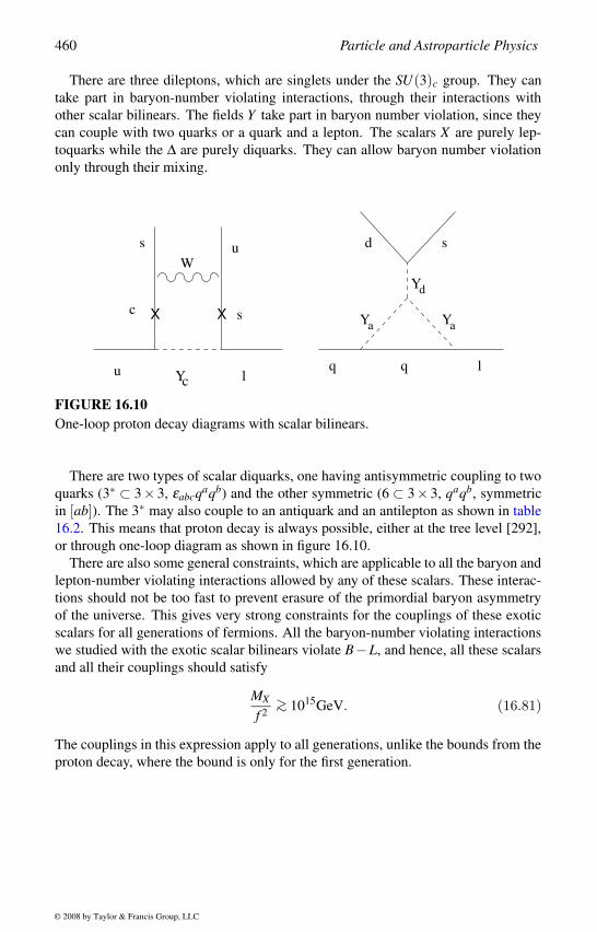
460 Particle and Astroparticle Physics
There are three dileptons, which are singlets under the SU(3)c group. They can
take part in baryon-number violating interactions, through their interactions with
other scalar bilinears. The fields Y take part in baryon number violation, since they
can couple with two quarks or a quark and a lepton. The scalars X are purely lep-
toquarks while the ∆ are purely diquarks. They can allow baryon number violation
only through their mixing.
XX
u lYq
c
W
s u
c s
q
d s
Y
YY
d
aa
l
FIGURE 16.10One-loop proton decay diagrams with scalar bilinears.
There are two types of scalar diquarks, one having antisymmetric coupling to two
quarks (3∗ ⊂ 3× 3, εabcqaqb) and the other symmetric (6 ⊂ 3× 3, qaqb, symmetric
in [ab]). The 3∗ may also couple to an antiquark and an antilepton as shown in table
16.2. This means that proton decay is always possible, either at the tree level [292],
or through one-loop diagram as shown in figure 16.10.
There are also some general constraints, which are applicable to all the baryon and
lepton-number violating interactions allowed by any of these scalars. These interac-
tions should not be too fast to prevent erasure of the primordial baryon asymmetry
of the universe. This gives very strong constraints for the couplings of these exotic
scalars for all generations of fermions. All the baryon-number violating interactions
we studied with the exotic scalar bilinears violate B−L, and hence, all these scalars
and all their couplings should satisfy
MX
f 2>∼ 1015GeV. (16.81)
The couplings in this expression apply to all generations, unlike the bounds from the
proton decay, where the bound is only for the first generation.
© 2008 by Taylor & Francis Group, LLC
17Dark Matter and Dark Energy
The evolution of the universe depends crucially on the total matter density of the
universe. Combined fit to all cosmological measurements now implies that the total
matter density equals the critical density of the universe, so the universe is flat. Out
of this, a contribution of about 70% comes from the vacuum energy (also called the
dark energy) or the cosmological constant
Λ ∼ 0.75×10−56 cm−2. (17.1)
Baryonic and nonbaryonic matter in the universe amount to only about 30% of the
critical density, out of which only about 5% is baryonic matter (see section 15.2).
The amount of nonbaryonic dark matter is then about 1/4 of the critical density of
the universe, i.e.,
ρDM = 1.7×10⁻³⁰ g cm−3. (17.2)
Neutrinos could be a hot (relativistic) dark matter candidate, but the present limits
on the neutrino masses imply that they cannot contribute to more than 1% of the
dark matter. Moreover, the large scale structure formation and the cosmic microwave
background anisotropy together require that most of the dark matter is nonrelativistic
(cold dark matter). Thus, the ΛCDM (nonvanishing cosmological constant and cold
dark matter) model is the most favored cosmological model at present, and the matter
content implies that the universe is flat and accelerating.
Although it is established that the universe is dominated by dark matter and dark
energy or cosmological constant, we have yet to find satisfactory solutions to these
two problems. The dark matter problem requires new particles, which would depend
on the model of particle physics beyond the standard model. So, detection and iden-
tification of the dark matter candidates may provide us new inputs to physics beyond
the standard model. The dark matter events reported by DAMA and the indirect ev-
idence for dark matter reported by EGRET could be the first indication. However,
the cosmological constant problem poses a new challenge for any theory. One now
expects to get a solution to this problem from a theory which includes gravity. Two
very promising solutions come from the string theory and the brane world scenar-
ios, although neither of these solutions was complete until now. Another interesting
observation that the scale of the cosmological constant and the neutrino masses are
of the same order of magnitude motivated a neutrino dark energy solution. After
discussing the present status of dark matter candidates and searches, we shall men-
tion some of these solutions of the cosmological constant problem and mention their
drawbacks.
461
© 2008 by Taylor & Francis Group, LLC
462 Particle and Astroparticle Physics
17.1 Dark Matter and Supersymmetry
The existence of dark matter in the universe has been established from many ob-
servations. The main criterion for any particle to be dark matter is that it should
not interact too fast and it must give us the observed dark matter relic density of
Ωd h2 ∼ 0.12. There are many possible candidates of dark matter, originating from
different particle physics models. These dark matter candidates may be classified
into two categories: hot and cold dark matter. If the dark matter candidate is a very
light particle that can remain relativistic and freeze out at about 1 MeV, we call it
a hot dark matter. The most probable candidates for hot dark matter are the neutri-
nos, but the present experimental upper bound on the neutrino mass implies that they
can at most contribute to 0.3% of the critical density, whereas the latest observations
in cosmology require a contribution of dark matter amounting to about 25% of the
critical density.
Heavier particles with mass of GeV and higher can be considered as cold dark
matter candidates, provided they interact weakly so they are present until now and
they are highly nonrelativistic. Since the abundance of these particles is inversely
proportional to their annihilation cross-section, their survival until today requires
them to be very weakly interacting. That is why these particles are also called the
weakly interacting massive particles (WIMP). A popular explanation is that WIMPs
are supersymmetric particles [294].
Any interaction in supersymmetric models with conserved R-parity contains at
least two superpartners of ordinary particles. As a result, whenever any superpart-
ners decay, the decay product contains at least one supersymmetric particle. As a
result, the lightest supersymmetric particle (LSP) cannot decay into any other par-
ticles. One of the neutralinos could be the LSP and its interaction rate is also very
small and hence there could be relic neutralinos which contribute to the dark mat-
ter of the universe. At an early time when the temperature was much higher than
the supersymmetry breaking scale, neutralinos were in thermal equilibrium with the
primordial cosmic soup of particles and radiation. As the universe cooled down to
a temperature below the mass of the neutralino, neutralinos could no longer be pro-
duced, but they could still annihilate away. Finally, the relic density of neutralinos is
fixed when the expansion rate of the universe exceeds the annihilation rate. This relic
density has been estimated for different supersymmetric models. Their abundance
depends on their annihilation cross-section, which should be comparable to the weak
interactions for them to contribute to the dark matter. This will also allow us to detect
the neutralinos directly in scattering experiments.
The relic density
Ωχ h2 =ρχ
ρch2
of the neutralino (χ) is calculated [295, 296] by first determining the particle density
© 2008 by Taylor & Francis Group, LLC
Dark Matter and Dark Energy 463
n using the Boltzmann equation
dndt
+3Hn = −(σv)ann(n2 −n2eq), (17.3)
where H is the Hubble parameter, neq is the equilibrium abundance and (σv)ann is
the thermally averaged product of the annihilation cross-section and velocity, taking
all channels of the χ −χ annihilation. Since the neutralinos are mixtures of gauginos
and Higgsinos, the annihilation can occur both via s-channel exchange of the Z0 and
Higgs bosons and via t-channel exchange of a scalar particle.
The present observations require a neutralino relic density Ωχ in the range of
0.1 < Ωχ h20 < 0.3, taking into account that the universe is flat and accelerating and
about 2/3 of the total matter in the universe is in the form of dark energy. If there
are other cold dark matter candidates contributing partly to the matter density in
the universe, then the neutralino relic density could be Ωχ < 0.1. This decrease in
Ωχ will imply a larger elastic scattering cross-section and the detection rate will be
reduced due to the reduced density of LSP in the galactic halo. However, for all
neutralino cold dark matter calculations, it is assumed that there are no other sources
of cold dark matter, so Ωχ ≥ 0.1 [297].
The neutralino dark matter candidates are highly model dependent and the details
depend on the supersymmetry breaking mechanism. A typical neutralino mass is
considered in the range of 50 GeV and a few TeV. The direct dark matter search ex-
periments concentrate on the LSP. In the minimal supersymmetric standard model,
the lightest neutralino is a probable candidate for the LSP with a mass in the range of
50 GeV to a TeV. The main uncertainty in the theoretical estimate of supersymmet-
ric dark matter comes from the neutralino–nucleon cross-section and usually large
tanβ solutions are preferred. However, it is not possible to make any more definite
comments at this stage. Only in the supergravity-inspired models and some other
choice of a constrained parameter space, the dark matter search might promise the
possibility of detection of supersymmetric particles even before the direct search ex-
periments in colliders [297]. In all other supersymmetric models the uncertainties in
the parameters and the supersymmetry breaking mechanism is too large to make any
predictions.
In the absence of a complete theory one makes certain assumptions about the grand
unification scale physics and extrapolates them to low-energy. The minimal super-
symmetric standard model is assumed to be valid at all energies from the electroweak
symmetry breaking scale to the grand unification scale. This is motivated by the orig-
inal N = 1 supergravity model, where N = 1 supersymmetry is broken in the hidden
sector using a Polonyi potential at an intermediate scale of MI ∼ 1010 GeV, which is
then communicated to the observable sector via gravitational coupling at the Planck
scale MPl [158]. This gives the low-energy soft supersymmetry breaking terms in
addition to the minimal supersymmetric standard model. In the observable sector all
supersymmetry breaking terms are soft terms and of the order of Msusy ∼ M2I /MPl ,
which is in the range of a few TeV. This scale of supersymmetry breaking is also in
the favored range for a cold dark matter particle of 50 GeV to a TeV. At the GUT
© 2008 by Taylor & Francis Group, LLC
464 Particle and Astroparticle Physics
scale this requires a common mass for all scalars m0 and a common trilinear coupling
A0 [155, 157].
In addition to the gauge coupling unification, the gaugino coupling unification to a
value m1/2 at the GUT scale MU is assumed in these theories. The weak scale spec-
trum of the supersymmetric particles is derived from renormalization group evolution
of the soft terms. Radiative breaking of the electroweak symmetry imposes further
constraints. In this model a minimal set of parameters [155, 157],
m0, m1/2, A0, tanβ , and sign(µ),
determines the sparticle masses and couplings.
In one mSUGRA analysis [298], the lightest neutralino χ ≡ χ01 is the LSP in
the model. It is mainly a Bino (the U(1)Y gaugino) for the choice of parameters
considered, taking into account the present laboratory constraints on the minimal su-
persymmetric standard model parameter space. This follows from the large Yukawa
coupling of the top quark, which drives the radiative electroweak symmetry break-
ing. In case of Bino LSP, the relic density of the neutralino LSP depends inversely
on the cross-section of χ annihilation process χχ → +− ( = e,µ,τ) through the
exchange of sleptons in the t- or u- channel. Since the charged leptons carry the
largest hypercharge among all the fermions and since they are the lightest in most
models, this is the dominant process in the χ annihilation. The final relic density is
given by [296]
Ωχ h2 =
(m2
χ +m2lR
)4
106 GeV2 m2χ
(m4
χ +m4lR
) .
The condition Ωχ h2 < 0.3 then requires mχ ,mlR ≤ 200 GeV. This is a welcome
result since this few hundred GeV supersymmetry breaking scale is independently
preferred to solve the gauge hierarchy problem.
The lightest neutralino in the minimal supersymmetric standard model, which is
the LSP, is a mixture of four superpartners of gauge and Higgs bosons (Bino, Wino
and two Higgsinos):
χ = N11B0 +N12W 0 +N13H01 +N14H0
2 . (17.4)
For different choice of the parameters, the LSP could be different combinations of
the neutralinos. For P ≡ N211 +N2
12 > 0.9, the LSP χ is gaugino-like, which is mostly
a combination of different gauginos. For P < 0.1, the LSP χ is Higgsino-like, oth-
erwise the LSP χ is mixed-type. In general, the parameters Ni j depend on the soft
supersymmetry breaking terms m1, m2 and µ given in equation (10.7). However,
in the mSUGRA model these parameters are not independent and the gaugino mass
unification relates them. In some interesting limiting cases, the LSP becomes a pure
state:
When µ → 0, the state S0 = H1 sinβ + H2 cosβ is the LSP with mass mS =µ sin2β ;
© 2008 by Taylor & Francis Group, LLC
Dark Matter and Dark Energy 465
When M2 → 0, the photino is the LSP with mass mγ =8
3
g21
g21 +g2
2M2;
When M2 is large and M2 µ , the Bino is the LSP with mass mB = M1;
When µ is large and µ M2, the Higgsino is the LSP with mass µ (modulo
the sign).
In the different cases, the neutralino–nucleon cross-sections could be different
leading to differing predictions. For a Bino LSP to be the relic neutralino, the
neutralino–nucleon cross-sections are very small in the mSUGRA allowed space so
direct and indirect searches for dark matter may not probe this mSUGRA parameter
space. When |µ| decreases, the Higgsino components N13 and N14 of χ increase,
and hence, P decreases. In this case the spin-independent cross-section increases,
resulting in good prospects for the detection of such a neutralino as a dark matter
(see section 10.1). So, the composition of the neutralino LSP becomes a deciding
factor for its detection as a dark matter candidate. There are other variants of the
CMSSM (see section 10.2), which can also lead to an enhanced neutralino–nucleon
cross-section by making the soft terms nonuniversal [159]. The large tanβ regime
was also considered as a source of higher cross-sections and is usually preferred.
There are other approaches, in which multiTeV scalars were considered satisfying
the naturalness criterion.
The neutralino–nucleon cross-sections can improve in the mSUGRA models, if we
assume that the scale of universality of the soft terms is MI , which is different from
the GUT scale MU . Now the universality of the scalar masses mi(MI) ≡ m0 and the
universality of the trilinear scalar couplings Al,u,d(MI) ≡ A0, are at some intermedi-
ate scale MI , which may have its origin in the string theory and can have a wide range
of choice [159]. The universality scale MI then changes the size of the neutralino–
nucleon cross-section. This class of models has the main drawback that the new uni-
versality scale is not determined by any theory. One more phenomenological variant
of this model was then considered, where the universality criterion is further relaxed
and the parameters are determined at the electroweak scale [294, 299]. This effective
low-energy phenomenological supersymmetric model is referred to as effMSSM. In
this approach it has been found that most of the MSSM parameter space allows a
gaugino-like neutralino with a small admixture of the Higgsino component, which
could be detected with the present level of sensitivity of the ongoing and planned
experiments. It is important that experimental observations are analyzed in a joint
spin-independent–spin-dependent approach [299, 300].
Soft terms arising from M-theory models also accommodate an LSP dark mat-
ter candidate [301]. However, in gauge-mediated supersymmetry breaking models,
there is no scope of dark matter candidate. The LSP is the gravitino and is very light
and the next-to-lightest supersymmetric particle (NLSP) is no longer stable. NLSP
is now heavier than the gravitino but lighter than any other sypersymmetric particles
and cannot be stable. It now decays into the gravitino and ordinary particles and
cannot remain as relics. Similarly, in the R-parity violating models, there is no stable
LSP that can become the dark matter candidate. The R-parity breaking trilinear inter-
© 2008 by Taylor & Francis Group, LLC
466 Particle and Astroparticle Physics
actions would allow a superparticle to decay into two ordinary nonsupersymmetric
particles. As a result the LSP can also decay into ordinary particles and is not stable.
So there is no dark matter candidate in R-parity violating supersymmetric models.
17.2 Models of Dark MatterThere are many possible candidates for the cold dark matter. The most popular one
is the R-parity conserving supersymmetric models, which seems to provide a can-
didate for cold dark matter naturally. However, we have not evidenced any signal
of supersymmetry and this prompted us to consider other extensions of the standard
model that can provide dark matter candidates naturally. Since the only evidence we
have for physics beyond the standard model is the neutrino masses, there are now
attempts to look for dark matter candidates originating from the models of neutrino
masses. At one time neutrinos were considered to be the strongest dark matter can-
didate, but the present upper limit on the neutrino masses ruled out this possibility.
In recent times it has been noticed that some radiative models of neutrino masses re-
quire Higgs scalars that do not acquire any vev and can be candidates for dark matter
of the universe. There are also some exotic dark matter candidates, which appear in
some models of particle physics, including the models with extra dimensions.
Dark Matter and Neutrinos
The right-handed sterile neutrinos could be a dark matter candidate depending on
their mass and mixing with active neutrinos [302]. However, the usual see-saw
mechanism for neutrino masses requires the mass of the right-handed neutrinos to
be very high with extremely small mixing with the active neutrinos, making their
contribution to the matter density of the universe to be negligible. In general, it is
difficult to satisfy all the low-energy constraints on the neutrino masses and mixing
and consistently explain the cold dark matter by the right-handed neutrinos alone.
Recently an interesting possibility of radiative neutrino masses has been proposed,
in which the generation of neutrino masses requires an additional Higgs doublet.
There is an extra Z2 symmetry, under which the right-handed neutrinos (Ni, i = 1,2,3)
and the new Higgs doublet η are odd, while all other particles are even. In this model
the neutral component of the new Higgs scalar, η , could account for the required cold
dark matter of the universe [303]. The new Higgs scalar with this exact Z2 discrete
symmetry does not interact with other fermions, and hence, it can modify the bound
on the standard model Higgs doublet φ mass coming from the naturalness and the
electroweak precision test observables.
The scalar potential for the fields φ and η is given by
V = µ21 |φ |2 + µ2
2 |η |2 +λ1|φ |4 +λ2|η |4 +λ3|φη |2 +λ4|φ †η |2 +λ5
2[(φ †η)2 +H.c.].
(17.5)
© 2008 by Taylor & Francis Group, LLC
Dark Matter and Dark Energy 467
We now assume that only the standard model Higgs φ acquires a vev,
〈φ〉 ≡(
0
v
)and 〈η〉 ≡
(0
0
), (17.6)
so the components of the scalar fields can be expressed as
φ =(
φ+
v+(φ R + iφ
I )/√
2
)and η =
(η+
(ηR +η
I )/√
2
). (17.7)
The fields η+ and ηI will become the longitudinal modes of the gauge bosons mak-
ing them massive and the usual physical Higgs scalar φ R can now become as heavy
as 400 to 600 GeV. The scalars η+, ηR and η
I do not interact with the light fermions
and remain inert. It is now possible to choose the coupling constants of the scalar po-
tential, which will make one of the neutral components of η the lightest inert particle
(LIP). The Z2 symmetry will make the LIP a stable particle and, hence, a candidate
for the dark matter of the universe.
The parameters of the scalar potential can be constrained by the present limits on
the dark matter. Direct detection of halo dark matter requires λ5 = 0, so ηR and η
Ido not become degenerate. The electroweak precision test parameters are modified
by the LIP, which allows a heavier physical Higgs scalar φ R . For the required dark
matter density, the LIP should have a mass of around 50 to 70 GeV with a splitting
between the mass of ηR (mR) and the mass of η
I (mI) around 8 to 9 GeV, which is
consistent with λ5 = 0.
The interaction (φ †η)2 and, hence, λ5 = 0 are also required for the neutrino
masses. The Z2 symmetry allows the coupling
LY = hαi (να η− α η+)Ni +H.c.+MiNiNi , (17.8)
but the Higgs φ does not couple to the right-handed neutrinos Ni and hence there is no
Dirac mass term for the neutrinos as in the canonical see-saw mechanism. Without
loss of generality we assume that the right-handed neutrino mass matrix is real and
diagonal. The neutrino mass matrix is then given by
Mναβ = ∑i
hαihβ iMi
16π2
[m2
R
m2R −M2
iln
m2R
M2i− m2
I
m2I −M2
iln
m2I
M2i
]. (17.9)
In principle, the lightest of the right-handed neutrinos could also be a dark matter
candidate. But from phenomenological constraints this possibility is not favored.
The main constraint comes from the branching fraction of µ → eγ . This leaves the
LIP to be a natural candidate for the dark matter.
Exotic Dark Matter
Several other extensions of the standard model predict new dark matter candidates.
The main constraint on any weakly interacting massive particles (WIMP) is that the
WIMPs should not overclose the universe, that is, their contribution to the matter
© 2008 by Taylor & Francis Group, LLC
468 Particle and Astroparticle Physics
density of the universe should not be more than the critical density of the universe.
This gives an upper limit on the mass of any stable particle to be 340 TeV [304].
The same consideration also gives bounds on the mass of the stable neutrinos to
be greater than 2 GeV [305] or the sum of masses of all the neutrinos to be less
than 94 eV [306]. When neutrinos were considered as dark matter candidates, these
constraints were important. However, the present upper bound on the absolute mass
of the neutrinos rules out any possibility of neutrino dark matter. Another dark matter
candidate, the axion, was also constrained by the consideration of overclosure of the
universe. These considerations work in an inverted manner for the axions. While
for neutrinos the intermediate range is forbidden, for axions only an intermediate
window is allowed. From cosmological and astrophysical considerations axions can
have a mass in the range of 10−2 to 10−5 eV with a very weak coupling (see section
7.3). If the axion could interact strongly, it would have come into thermal equilibrium
before the QCD phase transition leading to a background sea of invisible axions in
analogy to the neutrinos. Their interaction is required to be so weak that they could
never come into thermal equilibrium. But still coherent oscillations of the axions
could be excited and this could contribute to the mass density. For the axion mass to
be in the range of a few µeV to about an meV, the axion could contribute substantially
to the mass density of the universe [307].
Another class of dark matter candidates is very weakly interacting superheavy
particles. These particles were so weakly interacting that they were never in thermal
equilibrium in the early universe. Their abundance is also not determined by their
annihilation cross-section. They were produced during reheating after the inflation
with very little abundance. This would allow a superheavy dark matter candidate
with mass in the range of 1012 to 1016 GeV, which has to be stable or have a life-
time greater than the age of the universe, known as the WIMPZILLAs [308]. Their
annihilation cross-section should be weaker than the expansion rate of the universe
at the end of the inflation. Another stable dark matter candidate is the baryonic Q-
balls [309]. However, they cannot account for the entire dark matter since the total
baryon density is constrained by the limit from nucleosynthesis to be around 5% of
the critical density. Electrically charged Q-balls will lose their energy in atomic col-
lisions and could be detected in gravitational lensing experiments. Nonobservation
of such events gives a lower limit on the baryon number of the Q-balls to be 1021.
For electrically neutral Q-balls the lower limit on the baryonic charge is about 1023.
There is one more interesting dark matter candidate, the primordial black holes. The
string theory and M theory allow superheavy particles, the cryptons, which are stable
or metastable bound states of matter in the hidden sector and do not have any direct
couplings to ordinary matter; hence they are weakly interacting. Kaluza–Klein ex-
cited states associated with extra dimensions could also be dark matter candidates.
States with mass of around 1012 GeV were considered as possible superheavy dark
matter candidates [310].
The new developments with large extra dimensions and low scale strong grav-
ity promises new dark matter candidates. The higher-dimensional gravitons will
have several Kaluza–Klein modes in four dimensions, when the extra dimensions
are compactified. Although these Kaluza–Klein states can decay in our brane, it is
© 2008 by Taylor & Francis Group, LLC
Dark Matter and Dark Energy 469
possible that they are created in our brane but then are captured on a different brane
where gravity propagates. It can then become a natural dark matter candidate [311].
Although this dark matter is dark in our brane, it interacts very strongly in its own
brane. In some models the Kaluza–Klein excited states of the axions can also be dark
matter candidates, particularly if they are trapped in extra dimensions. Another pos-
sible candidate of dark matter in models of extra dimensions is a gas of fundamental
strings of submillimeter length, which could have been produced at a temperature
around MeV but could be as heavy as 1010 GeV or larger. These are the strings,
which connect two branes that sit on each other at higher temperature. There is no
analogous object in ordinary theories. Only at low temperature do the branes move
apart leaving the heavy strings as dark matter.
17.3 Dark Matter SearchesAlthough several experiments are going on to detect dark matter, so far only a very
small range of the parameter space could be covered by all the experiments. These
experiments can be classified as direct or indirect searches. In the direct detection
experiments, the elastic scattering of a WIMP off nuclei would be detected by detect-
ing the energy loss of the recoil nuclei through ionization and thermal processes. The
indirect detections plan to find events that could be due to the presence of WIMPs
trapped in the sun or Earth or contributing to the galactic density. If WIMPs populate
the halo of our galaxy, they could be detected directly by low-background experi-
ments or indirectly through their annihilation products in the halo, the center of the
sun or Earth.
The direct dark matter search experiments are very difficult. They look for a very
few events with a fairly large background. For neutralinos (χ) with masses between
10 GeV and 1 TeV, the deposited energy is below 100 keV. The event rate for such
experiments is approximately
Rdirect =1
mNφχ σχN =
1.4
mχ/GeVkg−1 yr−1, (17.10)
where σχN is the neutralino–nucleon interaction and φχ is the neutralino flux with
mass mχ . The requirement of a large detector mass, a low-energy threshold, a low
background, and an effective background discrimination technique make these ex-
periments extremely difficult.
The direct detection experiments are based mostly on the spin-independent in-
teractions of the WIMP because the cross-section of the spin-independent inter-
action with heavier nuclei is proportional to the atomic number of the target nu-
cleus and, hence, large. However, experiments based on the spin-dependent inter-
actions of the WIMP have higher sensitivity. As a result, both the spin-dependent
and spin-independent detectors span the same parameter space of supersymmetric
© 2008 by Taylor & Francis Group, LLC
470 Particle and Astroparticle Physics
models[299], even though the spin-dependent interaction cross-section of the WIMP
is small.
When the scattering does not depend on other factors such as isospin of the nu-
cleons in the spin-independent case, the interaction rate for all the A numbers of
nucleons will add up coherently. In this case the total cross-section will be propor-
tional to ISI = A2. Then one may compare different target elements by dividing the
total cross-section in any nuclei by ISI to get the rate (R0) corresponding to a single
nucleon. In a more realistic situation, this factor ISI will have a form
ISI = [(A−Z)+ εZ]2,
where ε = (1− 4sin2 θW ) ∼ 0.08 with the weak mixing angle sin2 θW . However, a
reasonable method of comparing results is to renormalize by a factor A2 or (A−Z)2.
In the spin-dependent case this interaction factor becomes
ISD = C2λ 2J(J +1),
where C depends on the quark spin content of the nucleon.
The DAMA experiment in Gran Sasso detected a variation of the event rate due
to the movement of the sun in the galactic halo and the Earth rotation around the
sun using NaI detectors [300]. From the analysis of about 295 kg y in terms of a
WIMP annual modulation signature, a positive signal has been reported. This result
should be confirmed by an independent experiment looking for annual modulation.
Ongoing experiments [312, 313] do not have the required sensitivity to look for the
modulation effect (see [300]).
The indirect search experiments for dark matter considers two important factors:
the gravitational capture rate of the WIMPs and their annihilation rate to neutrinos,
which can be detected on Earth. The solar gravitational capture cross-section is given
by [314]
σsun = f(1.2×1057) σXN ,
where an order of magnitude estimate of the WIMP-nucleon interaction cross-section
σXN is given by
σXN ≈ G2F
m4N
m2W
≈ 6×10−42 cm2
and the focusing factor f (∼ 10) is the ratio of kinetic to potential energy of the WIMP
near the sun. Then the flux of WIMP annihilation products (generally neutrinos)
from the sun is given by
φsun =1
4πd2 φX σsun,
where d is the Earth–sun distance and φX is the WIMP flux. Assuming that the
WIMPs constitute the major part of the measured dark matter halo density, the re-
sulting neutrino flux at Earth is then [314]
φν = 0.1 φsun =3×10⁻⁵
mX/GeVcm−2s−1. (17.11)
© 2008 by Taylor & Francis Group, LLC
Dark Matter and Dark Energy 471
The event rate for the indirect WIMP search is then given by
Rindirect = φν P = 1.8 (mX/GeV)yr−1 km−2, (17.12)
where P ∼ 2×10⁻¹³ (mX/GeV)2 is the probability to detect a neutrino with a neu-
trino telescope. For this purpose one looks for muons produced by neutrinos, e.g.,
in the Antarctic muon and neutrino detector array (AMANDA) experiment, which is
located in the ice of the Antarctics [315].
Recently an indirect evidence of dark matter signal from galactic high-energy
gamma ray has been reported. Using the Energetic Gamma Ray Experiment Tele-
scope (EGRET) aboard the Compton gamma ray observatory scientists have carried
out all-sky survey in high-energy gamma rays (E > 30 MeV) [316]. The observed
diffuse emission has a galactic component and a uniformly distributed extragalactic
component. A recent analysis of the excess in the diffuse galactic gamma ray data
above 1 GeV claims that this excess is consistent with a signal from dark matter an-
nihilation [317]. It is claimed that the excess shows all features expected from dark
matter WIMP annihilation and the WIMP mass expected is in the range 50 to 100
GeV compatible with supersymmetry.
17.4 Dark Energy and QuintessenceAt present all astrophysical observations indicate that the total density of the universe
is close to its critical density [44] Ωtot = 1.003+0.0130.017 and about 70% of the total
density is in the form of cosmological constant or dark energy. This implies that the
universe is flat and accelerating.
The present value of the cosmological constant corresponds to a very small mass
scale, comparable with the neutrino mass scale. In a different form it can be written
as
|Λ| ∼ [10−2 eV]4
.
While the contribution of the cosmological constant to the total density of matter is
almost one order of magnitude larger than that of the visible matter of the universe,
compared with the mass scales in particle physics this is too small. Compared with
the electroweak symmetry breaking scale, this is 13 orders of magnitude smaller:
|Λ|1/4
〈φ〉 ∼ 10−13.
Thus, the electroweak phase transition would induce a cosmological constant, which
is 52 orders of magnitude larger than the present observations.
An explanation of this cosmological constant problem can assume that the uni-
verse started with a small cosmological constant and the effects of the different phase
transitions are tuned to zero. But this requires most severe fine tuning in particle
© 2008 by Taylor & Francis Group, LLC
472 Particle and Astroparticle Physics
physics to all orders of perturbation. Even after the contributions from the elec-
troweak phase transition is cancelled by fine tuning of parameters, radiative correc-
tions will again generate similar contributions. Now the fine tuning has to be more
severe. In every order of perturbation theory this fine tuning will get worse and is
highly unnatural. A more popular solution to the cosmological constant problem is
the quintessence solution [318]. Although a fully consistent quintessence solution
has yet to be found, this appears to be the most likely solution to the cosmological
constant problem.
Varieties of models have been considered as a solution to this problem and differ
by their predictions for the equation of state of the dark energy, ω = p/ρ , where pand ρ are the pressure and the density of the dark energy. When ω is included in
the ΛCDM model to interpret some observations, degeneracy in some parameters
appears and it becomes difficult to interpret the data. However, a combined fit of all
the data sets gives [73]
ω = −0.98±0.12, (17.13)
which supports the simplest model that the equation of state for the dark energy is
ω = −1. It could then be either a cosmological constant or dark energy. The cos-
mological constant is a constant term in the Einstein equation, which remains the
same during the entire evolution of the universe. On the other hand a dark energy
comes from the nonvanishing of the trace of the energy–momentum tensor in vac-
uum, which could vary with time from its large value in the early universe to its
present value.
When the cosmological constant or the dark energy is constant in time, the fine
tuning can be neglected if some symmetry can protect the vanishing of the cosmolog-
ical constant to all orders in perturbation. The symmetry breaking can then induce a
small cosmological constant as required. Supersymmetry became the obvious choice
for this purpose, since supersymmetry implies vanishing of the vacuum energy. Let
us consider a global N = 1 supersymmetry generated by the Majorana fermion QM .
The anticommutation relation with QM is given by
QM, QM = 2γµ Pµ . (17.14)
The condition that the vacuum is supersymmetric QM |0〉 = 0 then implies that the
vacuum energy should vanish
〈0|H|0〉 = 〈0|P0|0〉 = 0. (17.15)
This ensures that as long as the global supersymmetry is exact, the vacuum energy
and the cosmological constant vanish. However, this solution could protect the cos-
mological constant only up to the scale of supersymmetry breaking. When super-
symmetry is broken, a cosmological constant proportional to the fourth power of the
supersymmetry breaking scale will again be generated.
A time varying dark energy starts with a very high value in the early universe
depending on the natural scale in the theory. The scale for the dark energy in the early
universe could be the QCD phase transition scale, electroweak symmetry breaking
© 2008 by Taylor & Francis Group, LLC
Dark Matter and Dark Energy 473
scale, or scale of inflation. In supersymmetric theories the largest scale would be
the supersymmetry breaking scale. This dark energy would vary with time and at
present it is given by the small observed value depending on the dynamics.
The quintessence solutions [318] of the cosmological constant problem assumes
that the mass density of a scalar field φ gives the dark energy. If this field has certain
typical potential that allows slow variation of the field, the dark energy decreases
with time. If the dark energy density were dominating over the matter density in the
nucleosynthesis era, it could have spoiled the nucleosynthesis predictions. So, the
decrease of the dark energy is slower than the mass densities of matter and radiation,
so the universe was dominated by matter and radiation for most of the time. Only
recently has the cosmological constant become more than the mass density in the
universe. Moreover, although the initial mass density of the scalar field was much
higher, given by the vacuum expectation value or a condensate of the scalar field,
and could be as high as the scale of inflation or the electroweak symmetry breaking
scale, in recent times the value of the dark energy has become comparable to the
matter density. The present value of the dark energy is twice as much as the matter
density of the universe.
There are varieties of quintessence models, each of which has some interesting
features and differing predictions for the evolution of the universe. Similar to the
different models of inflation, different models of quintessence can imply a substan-
tially different cosmological model. In all of these models a scalar singlet field φis introduced. It should not transform nontrivially under any gauge groups or the
Lorentz group, so it does not have any strong coupling with any matter. The scalar
field could be the inflaton field that drives the inflation or the cosmon field associ-
ated with the dilatation symmetry [318], or pseudo-Nambu–Goldstone bosons, that is
presently relaxing in its vacuum state [319], or some other scalar field depending on
the model. The potential of the scalar field determines its evolution and, hence, the
dynamics of the quintessence field. The direct coupling of this scalar quintessence
field to ordinary matter should be further suppressed to make it phenomenologically
consistent, since no such particles have been observed. This can lead to a new long
range force, weaker than gravity, which may have some observable effect.
A typical Lagrangian for the quintessence field can be of the form
Lq = V (φ)+1
2k(φ)∂µ φ∂ µ φ (17.16)
in units of reduced Planck mass MPl = 1. The potential for the quintessence field
φ should be slowly varying. Usually an exponential potential V (φ) = exp−φ or a
power-law potential V (φ) = φ−α for large φ can allow the decrease of the mass
density ρφ to be slower than the mass densities of matter and radiation. The kinetic
function k(φ) parameterizes a class of models such as the cosmon models, while
it is taken to be unity in other models. In the cosmon models, for small almost
constant k the dark energy density is small and varies very slowly, while for large
k the universe is dominated by the scalar field. In a realistic model k changes from
small to large values after structure formation. A few generic features of all the
quintessence models include a tiny time varying mass of the scalar quintessence field,
© 2008 by Taylor & Francis Group, LLC
474 Particle and Astroparticle Physics
which interacts with ordinary matter very weakly giving rise to a new long-range
interaction. Some exotic features of some specific models include negative kinetic
energy terms (ω < −1, phantom cosmology) or higher derivative kinetic terms (K-
essence), but none of these models explains why the cosmological constant becomes
important in the present epoch.
Since the cosmological constant originates in the Einstein equation as a constant
term or in the energy-momentum tensor, any theory of gravity attempts to solve the
cosmological constant problem by identifying some existing field with the scalar
quintessence field. String theory also attempts to solve the cosmological constant
problem with the fields already present in the theory. In string theory dimensional
quantities can be expressed by two parameters, the string tension and the vevs of
scalar fields. Thus, to explain the cosmological constant any mechanism involving
dynamics of some scalar fields is most natural. One considers a scalar field φ slowly
evolving in a runaway potential which decreases monotonically to zero as φ → ∞.
Runaway potential is also very common in dynamical supersymmetry breaking
scenarios. In any higher-dimensional theories the dilaton field is always present,
which comes as a scaling factor in the higher-dimensional metric, when expressed in
terms of the four-dimensional metric. This field can have the correct property of the
quintessence field in some models. A small value of the dilaton field s = 〈φ〉/MPlprovides a strong coupling, which in turn breaks supersymmetry dynamically. The
coupling effectively goes to zero together with the supersymmetry breaking effects
for φ → ∞ and the potential decreases monotonically. Such dynamical symmetry
breaking with runaway potential is considered to explain the smallness of the elec-
troweak symmetry breaking coming from superstring theory.
When supersymmetry is broken by gaugino condensation in an effective super-
string theory, the gauge coupling constant g20 ∼ 1/s at the superstring scale Ms be-
comes strong at a scale
Λ ∼ Msexp−1/2bg20 = Msexp−s/2b, (17.17)
where b is the one-loop beta function. Gauginos condensate at this scale with a value
〈λλ 〉 ∼ Λ3, which in turn, produces an effective potential for the dilaton field
V ∼ ∣∣< λλ >∣∣2 ∝ exp−3s/b. (17.18)
This potential has the required behavior for a quintessence solution and could explain
the smallness of the cosmological constant [318]. Moduli fields in superstring theo-
ries, whose vevs describe the radius of compactification, could also provide similar
solutions.
We shall now discuss this problem in a little more detail and point out the problems
with these solutions. Let us consider an example of a real scalar field φ , minimally
coupled to gravity and described by a potential
V (φ) = V0exp−λφ/mP , (17.19)
© 2008 by Taylor & Francis Group, LLC
Dark Matter and Dark Energy 475
where V0 is a positive constant. The energy density and pressure due to the scalar
field are now
ρφ =1
2φ 2 +V (φ) and pφ =
1
2φ 2 −V (φ). (17.20)
Neglecting the spatial curvature (k ∼ 0), the equation of motion becomes
φ +3Hφ = −dVdφ
, (17.21)
with
H2 =1
3m2P(ρB +ρφ ). (17.22)
A solution with the behavior ρφ ∝ a−nφ or ρφ /ρφ = −nφ H is of particular impor-
tance, which gives φ as a logarithmic function of time
φ = φ0 +2
λln(t/t0). (17.23)
The equation of state now reads
pφ = ωφ ρφ , (17.24)
with ωφ = (λ 2/3)− 1. For sufficiently small λ , the field φ can play the role of
quintessence. However, in a realistic situation we have to include the effect of the
background matter and radiation.
Let us now include the background matter and radiation energy density ρB with
pressure pB satisfying a standard equation of state
pB = ωBρB, (17.25)
where ωB is positive and lies between 0 and 1/3. We also have to consider λ 2 >3(1+ωB) and then the solution satisfies the condition
Ωφ ≡ ρφ
ρφ +ρB=
3
λ 2 (1+ωB)
ωφ = ωB. (17.26)
This is certainly not the required quintessence solution, which requires ωφ ∼ −1.
Thus, in realistic scenarios, consistent with observations that ρφ should be subdom-
inant during nucleosynthesis, a quintessence solution solving the cosmological con-
stant problem is difficult in these theories [320, 321].
A few solutions to this problem have been suggested [322], but none of them is
completely satisfactory. In one case a tracker field is introduced with the potential
V (φ) = λΛ4+α
φ α , (17.27)
© 2008 by Taylor & Francis Group, LLC
476 Particle and Astroparticle Physics
with α > 0. This provides a solution to a good approximation. But in this case,
the fact that the present value of φ is of order MPl becomes a source of problem.
In another solution the quintessence component comes out of the background en-
ergy density, where the potential has a local minimum (a bump). When the field
approaches the bump, it slows down and then allows for the background energy den-
sity. There are also models, known as quintessential inflation or deflation, where one
tries to use the same field for quintessence as well as to drive inflation. There exists
another class of models where the scalar field has not yet reached its stable ground
state and is still evolving in its potential [323]. The idea is very close to quintessence.
Although the quintessence solutions appear to be a solution of the cosmological
constant problem, there are problems in implementing them into realistic theories
[321]. The main problem comes from the weak coupling of the quintessence with
ordinary matter. The coupling of matter with the quintessence field would gener-
ate higher-order corrections such as λdφ d , which can destabilize the slow roll over,
unless we impose very stringent conditions on the coupling λd . The quintessence
fields are also supposed to be very light. Supersymmetric corrections will make
them heavy, unless the coupling is extremely weak. Another problem is the vev of
φ of the order of MPl . This would jeopardize the positive definiteness of the scalar
potential and hence the quintessence solution. Supersymmetric corrections may also
cause problems in this case. Thus, the quintessence problems have shifted the prob-
lem of small cosmological constant to why the quintessence fields couple to matter
so weakly. Another problem is why the dark energy dominates over the dark matter
only in the recent times.
17.5 Neutrino Dark Energy
It is interesting to note that the scale of dark energy is almost the same as the neu-
trino masses. This observation leads us to consider whether there is any connection
between the two phenomena. In an attempt to utilize this coincidence a neutrino
mass varying solution to the dark energy problem has been suggested [324]. In this
scenario the neutrino mass becomes a function of a scalar field, the acceleron, which
drives the universe to a late time accelerating phase. Although the proposal is not
complete, it has several interesting features.
The basic idea behind the neutrino dark energy (νDE) models is that the neutrino
mass varies as a function of a light scalar field A (the acceleron) [324]. In the
nonrelativistic limit, the thermal background of the neutrinos and antineutrinos nνgives a contribution to the potential amounting to mν nν . This neutrino source term
for A should not significantly vary spatially, at least over a distance of the inter-
neutrino spacing. For thermal relic neutrinos at the present time this implies that the
mass of the acceleron should be less than ∼ (10−4 eV).In addition there is a vacuum energy V0(mν) attributed to the acceleron, which
© 2008 by Taylor & Francis Group, LLC
Dark Matter and Dark Energy 477
also depends on the varying neutrino mass. Thus, the effective potential
V (mµ) = mν nν +V0(mν) (17.28)
tell us that the first term will drive mν to a lower value, while the second term will
force mν to large value. The minima of this potential
V ′(mµ) = nν +V ′0(mν) = 0 (17.29)
would then correspond to a point with intermediate mν and nonvanishing vacuum
energy V0(mν). The relationship of ω(t) with the scalar potential is given by
ω +1 = −mν V ′0(mν)V
=Ων
Ων +ΩDE(17.30)
for a simple equation of state p(t) = ω(t) ρ(t). The observed value of ω ≈ −1
implies that the energy density in neutrinos is much smaller than the total energy
density, which corresponds to mν V ′0 V (mν) and, hence, a flat potential. This
could be satisfied with a flat potential for A or if the dependence of mν on A is
rather steep. The flat potential could be taken to be
V0(mν) = Λ4 log
(1+∣∣∣∣M1(A )
µ
∣∣∣∣) . (17.31)
The form of M1(A ) determines the dynamics of the model. Two extreme possible
forms have been discussed, which are a linear form M1(A ) ∼ λA and an exponen-
tial form M1(A ) ∼ expA 2/ f 2. In the former case the potential is flat, while for the
second case the potential is quadratic.
The origin of the acceleron field was not specified in the original model. Subse-
quently it was pointed out that a pseudo-Nambu–Goldstone boson (pNGB), originat-
ing from lepton flavor violation, could be the acceleron field [325]. We demonstrate
with a two-generation example.
We start with the Yukawa couplings of the right-handed neutrinos Ni, i = 1,2 with
some scalar singlet fields Φi, i = 1,2, given by
LN =1
2α1N1Nc
1Φ1 +1
2α2N2Nc
2Φ2. (17.32)
This model has a U(1)1 ×U(1)2 symmetry, under which these fields transform as
N1 ≡ (1,0), N2 ≡ (0,1), Φ1 ≡ (2,0) and Φ2 ≡ (0,2), respectively. When the fields
Φi acquire vev, both these symmetries are broken and there will be two Nambu–
Goldstone bosons.
We also assume that the left-handed doublets TαL ≡ (να α ) ,α = e,µ transform
under U(1)1×U(1)2 as (1,0) and (0,1), respectively. To maintain the U(1)1×U(1)2symmetry, by all the renormalizable dimension-4 terms, we introduce three Higgs
doublet fields Ha,a = 0,1,2, all of which transforming as (1,2,1/2) under the standard
model. Under the U(1)1 ×U(1)2 symmetry, these fields transform as (0,0),(1,−1)
© 2008 by Taylor & Francis Group, LLC

478 Particle and Astroparticle Physics
and (−1,1), respectively. Then the U(1)1 ×U(1)2 invariant Yukawa interactions are
given by
Lmass = f11N11H0 + f12N12H1 + f21N21H2 + f22N22H0. (17.33)
After the electroweak symmetry breaking, these interactions will allow all the Dirac
mass terms for the neutrinos,
Lmass = mi jNiν j.
These mass terms are soft terms, which break the U(1)1 ×U(1)2 symmetry explic-
itly. This soft symmetry breaking will give a small mass to one of the Nambu–
Goldstone bosons (which now becomes the acceleron field A ), while the other
Nambu–Goldstone boson corresponding to the total lepton number will still remain
massless leading to a singlet-Majoron.
The mass of the acceleron A can be computed by evaluating the one-loop
Coleman–Weinberg potential, which gives a small finite mass of the acceleron of
the order of mA ∼ m2/M, which is of the order of the neutrino mass. After replac-
ing the fields Φi by their vevs and absorbing all the phases, it can be shown that the
Majorana masses of the right-handed neutrinos become dependent on the acceleron
Mi ≡ Mi(A ). We can then write the complete mass term as
Lµ =1
2Mi(A )Nc
i Ni +mi jNiν j +H.c. (17.34)
It is interesting to note that Mi(A ) is specified and the effective neutrino mass also
varies mν(A ) = mT M−1(A )m. We, thus, arrive at an effective potential
−Le f f = mTi j[Mi(A )]−1mi j νiν j +H.c.+Λ4 log(1+ |M1(A )/µ|), (17.35)
whose minima implies ω = −1.
This model has some problems [326], but some of them have been taken care of in
certain variants of this model [327, 328]. This scenario can be embedded in models
with triplet Higgs scalars [327], in which the naturalness problem of the present
model can be removed. For example, naturalness requires Mi to be of the order of
eV, but in the triplet Higgs models the heavy scale could be of the order of TeV,
which provides interesting phenomenology. Although the models of mass varying
neutrinos are not yet fully consistent in their present form, they provide interesting
phenomenology that could be tested in the near future.
© 2008 by Taylor & Francis Group, LLC
18Cosmology and Extra Dimensions
The extra dimensions were introduced to unify gravity with other gauge interactions.
Since we do not experience any new dimensions beyond our four space–time dimen-
sions, these extra dimensions were assumed to be compact. This would make these
extra dimensions invisible at our present energies. Any probe having energy of the
order of the compactification scale, which is the inverse of the radius of compacti-
fication, can only see these extra dimensions. Usually the compactification scale is
considered to be about the Planck scale, so all new excited states become heavy and
decouple from low-energy physics.
In a new class of theories with extra dimensions, gravitons are assumed to prop-
agate along the extra dimensions and all other interactions become blind to these
extra dimensions. This allows the construction of these theories with extra dimen-
sions with a very low compactification scale, as low as a few TeV. Since gravitational
interaction can see all the dimensions, in our four space–time dimensions the effect
of gravity is suppressed by the volume of the extra dimensions. Although gravity
is weak in our world, it is very strong in extra dimensions even at our present en-
ergies. Around the scale of compactification, the effects of quantum gravity may
not be neglected. These studies have opened up new interesting phenomenological
possibilities as well as cosmological consequences.
In these theories with TeV scale extra dimensions there is no large scale beyond
the scale of compactification. Moreover, since quantum gravity effects cannot be
ignored around the compactification scale, we cannot extend our theory of early uni-
verse much beyond the scale of compactification. There can be new physics appear-
ing around this scale. For example, one can use the holography principle to construct
a universe [329] which is a dense gas of black holes. Only at a later time did they
decay through Hawking radiation to a radiation dominated era. In this scenario in-
flation becomes redundant. There is also the standard brane cosmology, where it is
expected that the universe starts as a higher-dimensional theory and then all matter
gets concentrated to the branes and the bulk becomes almost empty [330]. Since the
subject is still developing, many of these concepts may change drastically. For exam-
ple, the fine tuning problem for the cosmological constant was first solved [331, 332],
but then another problem was noticed [333]. We shall, thus, restrict ourselves to the
basic concepts, which should not change. For example, in any brane cosmologies
the predictions of the standard big-bang cosmology should remain valid. We shall
first discuss the constraints on the models of extra dimensions arising from cosmol-
ogy and astrophysics. Keeping these constraints in mind we then proceed to discuss
some generic features of the brane cosmology.
479
© 2008 by Taylor & Francis Group, LLC
480 Particle and Astroparticle Physics
18.1 Bounds on Extra Dimensions
The models with large extra dimensions have one common feature that there are in-
finite towers of Kaluza–Klein excitations of the graviton, all moving in the bulk. At
present energies only the zero mode of the graviton can be present, and hence, the
interaction of gravity with ordinary matter is weak in our four space–time dimen-
sion. In addition, if there are other bulk particles such as the axion, then there will
be another tower of axion excitations, all interacting weakly with matter. We shall
restrict ourselves to gravitons only, which are inevitable.
Consider an n-dimensional space–time, in which d = n− 4 dimensions are com-
pact. The gravitons propagate in all the dimensions, so after compactification of the
extra dimensions, in our four dimensional space–time the graviton will have all the
Kaluza–Klein excited states. All these modes of graviton will interact with matter
with the same strength
L = −κ2
∑n
∫d4xhn
µν T µν , (18.1)
where κ =√
16πGN , T µν is the energy-momentum tensor of the standard model
and hnµν represents the n-th excited mode of the Kaluza–Klein graviton state Gn,
with mass mn = n/R. Although at our present energy most of these states cannot
be produced, in the early universe at high temperature all these states could have
been produced. For an order-of-magnitude estimate, we assume that the interaction
strength is approximated by 1/M2Pl .
We shall now try to check the consistency of these models of large extra dimen-
sions in terms of our present knowledge of the universe without restricting ourselves
to any particular model or going into the details of the evolution of the universe
[311]. At present we can predict the light element abundances from the big-bang
nucleosynthesis. Our first concern will be to prevent any new physics that destroys
the predictions of nucleosynthesis. At high temperatures if the Kaluza–Klein excited
graviton states Gn are produced in large number in the early universe, that would
destroy the prediction for the big-bang nucleosynthesis. As we shall see next, such
destructions can be prevented if the maximum temperature of the universe in these
models of large extra dimensions can be constrained.
Due to the lack of any fully consistent theory of quantum gravity, we start our
discussions on the early universe from the time of the Planck scale, when gravity
starts becoming weak. Similarly, in models of large extra dimensions we start from
temperatures below the Planck scale in our brane, when quantum gravity effects
start smearing out. This is the fundamental scale in the theory of extra dimensions
T < M∗. For preserving the nucleosynthesis predictions of the standard cosmological
model, we assume that the extra dimensions do not influence the expansion of the
3-brane at the time of nucleosynthesis. Below a certain temperature T∗, our universe
© 2008 by Taylor & Francis Group, LLC
Cosmology and Extra Dimensions 481
expands in the standard way with the Hubble parameter given by
H = 1.66√
g∗T 2
MPl, (18.2)
where g∗ is the effective number of degrees of freedom. The evolution of the extra
dimensions becomes independent of the evolution of our 4-dimensional universe.
This dictates the concept of a new maximum temperature T∗ in these theories [311].
At this maximum temperature T∗ the universe starts evolving in the standard way, the
bulk becomes virtually empty and the radii of the extra dimensions get stabilized to
their present value.
In these models of extra dimensions, the history of the early universe before the
maximum temperature T∗ becomes drastically different from the standard model
of cosmology. The maximum temperature T∗ is usually taken to be the reheating
temperature after inflation TRH and this is constrained mainly by the effects of the
Kaluza–Klein gravitons Gn. Production of these Kaluza–Klein gravitons Gn cools
the universe at very high temperature. Given the production rate for a species Gn
with mass mn < T to be
Γ ∼ T 7
M2Pl
, (18.3)
the rate of decrease of radiation energy density is given by the rate of creation of Gn
dndt
∼−dρdt
∼ T 7
M2Pl
(T R)d ∼ T d+7
Md+2∗. (18.4)
We use the relation MPl = M∗ (M∗R)d/2. This cooling rate should be less than the
cooling of the universe due to expansion, which dictates the condition,
T∗ < M(
M∗MPl
) 1d+1
. (18.5)
For d = 2 and M∗ = 1 TeV, the bound is T∗ < 10 TeV, which is a weak bound since
T∗ > 0.7 MeV is acceptable within the nucleosynthesis scenario.
Another bound comes from the overclosure of the universe by the Kaluza–Klein
gravitons. Even with very low production rate, the total number of Kaluza–Klein
gravitons created in the Hubble time H−1 is fairly large,
n(T ) ∼ T 2 MPl
(TM
)d+2
. (18.6)
If all of these states survive, they can modify the evolution of the universe and give
a very strong bound on these models. The lifetime of the n-th mode is
τn ∼ 1
Γn∼ M2
Plm3
n∼ 1031 yr
(1 eV
mn
)3
, (18.7)
© 2008 by Taylor & Francis Group, LLC
482 Particle and Astroparticle Physics
which is greater than the age of the universe, and hence, the Kaluza–Klein gravitons
can overclose the universe.
At the maximum temperature T∗, Kaluza–Klein gravitons with mass of order T∗ are
created. They become nonrelativistic (n ∼ T 3) below the maximum temperature T∗.
Consistency with the big-bang nucleosynthesis then requires that the mass density at
the nucleosynthesis epoch
ρgrav(TNS) ∼(
TNS
T∗
)3
T∗ n(T ) ∼ T 3NS MPl
(T∗M
)d+2
(18.8)
should be less than the energy density of one massless species. This constrains the
maximum temperature T∗ to be
T∗ < M(
TNS
MPl
) 1d+2
. (18.9)
For d = 2 and M = 1 TeV, the bound is T∗ < 10 MeV. If one requires that ρgrav should
be less than the critical density of the universe, a stronger bound of T∗ < 0.2 MeV is
obtained for d = 2 and M = 1 TeV. To avoid conflict with nucleosynthesis, we get a
bound on the fundamental scale of M∗ > 10 TeV.
The maximum temperature T∗ can be in the range of 1 MeV to 1 GeV without con-
flicting with the nucleosynthesis, but in this case generating a baryon asymmetry of
the universe and models for inflation becomes extremely difficult. One suggestion to
avoid this is to raise the maximum temperature T∗ without affecting nucleosynthesis
predictions. This can be done by allowing faster decay of the gravitons in the bulk
to something massless in the bulk or in another brane. This would allow the energy
density to scale as T 4, although the maximum temperature T∗ is still required to be
fairly low.
We shall now discuss the astrophysical bounds coming from stellar evolution, par-
ticularly from the sun and supernovae [334]. Light gravitons Gn produced in the stars
through
(a) γ γ → Gn, photon–photon annihilation,
(b) e+ e− → Gn, electron–positron annihilation,
(c) e− γ → e− Gn, gravi-Compton Primakoff scattering,
(d) e− (Ze) → e− (Ze) Gn, gravi-bremsstrahlung in a static electric field, and
(e) N N → N N Gn, nucleon–nucleon bremsstrahlung
can carry away energy from the interior of stars. If they are the main source of
cooling, then they can change the stellar evolution making it inconsistent with obser-
vation.
The nonobservation of shortening of the neutrino emission from the supernovae
SN1987a gives the strongest bound on the fundamental scale M∗ [311, 334, 335]. In
© 2008 by Taylor & Francis Group, LLC
Cosmology and Extra Dimensions 483
a supernovae explosion the neutrinos have a very short mean free path and cannot
escape. Slowly they thermalize and the mean free path increases and eventually
they may escape. But in models of extra dimensions gravitons can allow very fast
cooling, since they would efficiently transport energy out of the explosion. This
would reduce the spread in the arrival time of the neutrinos, so from the observation
of the supernovae SN1987a neutrinos, we get a bound of M∗ > 30 TeV.
18.2 Brane CosmologyThe standard model of cosmology has to be modified in theories with large or small
extra dimensions and TeV scale quantum gravity. In these classes of theories with
extra dimensions, we live in a 3-brane or in a world of four space–time dimensions
attached to a wall of the larger dimensions. Only gravity propagates in the bulk and
hence all the dimensions. In these theories the universe should evolve in a different
way than in ordinary models of particle physics where the Planck scale is at MPl . Due
to the dynamics in these theories of extra dimensions, inflation should also take place
at very low temperature. So new mechanisms for inflation have to be considered.
There are many new open questions in this scenario, which are yet to be answered.
So, developments in this field of research may change our present knowledge very
rapidly. We shall thus try to mention only a few generic issues of the present state of
brane cosmology.
The earliest epoch we can explore in the early universe is at the end of the quantum
gravity era, which is the Planck scale in the standard model of cosmology. In models
of extra dimensions, this becomes the fundamental scale of about a TeV
t0 ∼ M−1∗ . (18.10)
Another major difference between the standard model of cosmology and the brane
cosmology is the introduction of the maximum temperature T∗. We understand
the abundance of elements starting from nucleosynthesis fairly well in the standard
model of cosmology. But the Kaluza–Klein excited graviton Gn production can de-
stroy this prediction in any theories with extra dimensions. To preserve the predic-
tions of nucleosynthesis the universe should be allowed to evolve as in the ordinary
theory after a maximum temperature T∗, which depends on the model [311]. De-
pending on the number of extra dimensions, this maximum temperature T∗ could be
between MeV and a few GeV. For any number of dimensions, the highest value for
the maximum temperature T∗ could be the fundamental scale T = M∗. Below the
maximum temperature T∗ the extra dimensions should not affect our 4-dimensional
universe and hence the brane cosmology becomes identical to the ordinary standard
model of cosmology.
In any brane cosmology scenario the Kaluza–Klein gravitons should not be pro-
duced in too many numbers, and the contributions to the energy density due to the
© 2008 by Taylor & Francis Group, LLC
484 Particle and Astroparticle Physics
Kaluza–Klein gravitons should satisfy
ρKK M4∗ . (18.11)
This allows an estimate of the Hubble parameter at the earliest epoch t0 (equation
(18.10))
H ∼(
8πV (φ)3M2
Pl
)1/2
<M2∗MPl
M∗. (18.12)
The inflation should now occur within the period of T = M∗ and the maximum tem-
perature T∗ at a time scale ti ∼ H−1 M−1∗ .
We should impose one more severe constraint, that the bulk matter should not
influence the expansion of our universe [330]. The total energy in the bulk should be
much less than the total energy in our brane
ρbulk Md+4∗
(M∗MPl
)2
. (18.13)
In the ideal situation one assumes that the bulk is empty after the inflation and all
matter is concentrated in our brane. Before the temperature corresponding to the fun-
damental scale, all dimensions were equal and there was equal distribution of matter
in all directions in the higher-dimensional world. So, some specific mechamism
must have decoupled all matter from all extra dimensions leaving a multidimen-
sional empty space at some time in the past. After this time all matter in the universe
concentrated in our brane.
It is difficult to make the bulk essentially empty. In the early evolution of the
universe we have to take into consideration some new higher-dimensional phenom-
ena. One suggestion is based on the spontaneous creation of our brane in a higher-
dimensional space, where there were no branes or excitation at the beginning [336].
Let us consider a 5-dimensional example with a four-form B (which is a four index
antisymmetric tensor field) and branes with nonzero and zero charges with respect
to B. The coupling of the branes with the 4-form is
Sint = e∫
BABCDdΩABCD. (18.14)
The B field with nonvanishing constant field strength at the initial state of the 5-
dimensional universe will decay spontaneously into pairs of charged branes. A neu-
tral brane could also be associated with the creation of the charged branes, which
will then become our universe. After the spontaneous creation, the three volumes
of the branes increase and the junction between the charged and neutral ones moves
away leaving our universe as a homogeneous 3-dimensional space in an empty bulk.
Another important question we need to understand in these theories is the brane
inflation. We shall discuss one interesting possibility where the inflation originates
from the interaction of two parallel branes [337]. Consider the inflationary models
in ordinary theories, where the scalar field, whose vev drives the inflation, requires
© 2008 by Taylor & Francis Group, LLC
Cosmology and Extra Dimensions 485
an extremely flat potential. In general, the quantum gravity corrections may desta-
bilize the solution. If the Hubble parameter at that epoch is H, the quantum gravity
correction could be ∼ H2, and this can destabilize the scalar potential and prevent
slow roll over of the scalar field to its minimum, required for inflation. If V (φ) is the
scalar potential of the inflaton field φ , the curvature of the potential should be less
than the Hubble parameter
H2 ∼V (φ)/3M2Pl
at some region. Then quantum gravity corrections would allow low-energy terms
such as φφV (φ)/3M2Pl , which will spoil the condition for inflation.
This problem of conventional theories of inflation has a natural solution in the
brane inflation scenario with two interacting parallel branes. In this scenario the
inflaton φ parameterizes the distance r between two parallel brane worlds, one of
which is our brane. This scale of about r ∼ µm is too large compared with the quan-
tum gravity scale of TeV−1 ∼ 10−16 mm, and all the quantum effects are negligible
at this distance scale r. The potential is now given in terms of the distance between
the branes r as
V (r) = Md(
a+birlexp−mir − 1
(M∗r)d−2
), (18.15)
where a and bi are constants and mi are masses of heavy modes of φ . At large
distances this potential has a power-law behavior and this translates to a flat potential
for the inflaton field φ = M2∗r naturally.
In the brane world scenarios, the question of the baryon asymmetry of the universe
could be addressed in different ways [338]. While it is possible to generate a baryon
asymmetry of the universe with higher-dimensional bulk fields or using the Affleck–
Dine mechanism, a higher-dimensional mechanism originating from the brane world
scenario may also be invoked. In another possibility the collision of two parallel
branes in the early universe could also produce a matter–antimatter asymmetry of
the universe. If there was CP violation during the collision of the parallel branes,
some of the antimatter from our world could have moved to the other parallel brane.
If the collision took place after the inflation, then there would be excess matter in our
brane and equal amount of excess of antimatter in the other brane. It is also possible
that after the inflation when our brane is freely expanding, baby branes containing all
the antimatter would have formed due to deformations of the world volume, which
then moves apart from our brane making our brane baryon asymmetric.
There are also new sources of dark matter in the universe coming from the models
of extra dimensions [339]. In some cases the Kaluza–Klein gravitons and Kaluza–
Klein axions could be the dark matter candidates. One interesting possible candidate
is a gas of fundamental strings of submillimeter length. They could have been pro-
duced after the inflation at a temperature around MeV, but could be as heavy as 1010
GeV or larger. In ordinary cosmology production of such objects at low temperature
is not allowed, but in brane cosmology they can come from new brane physics. The
strings could connect two branes, which sit on each other at higher temperature. Only
at low temperature do the branes move apart leaving the heavy strings as dark matter.
© 2008 by Taylor & Francis Group, LLC
486 Particle and Astroparticle Physics
If such strings break down at some point of time, they will release their energy in the
form of very high energy particles.
Brane cosmologies have several other features, which are not present in the ordi-
nary standard model of cosmology. For example, inflation could take place in the
bulk and in our brane at different times leading to new consequences. The maximum
temperature T∗ is fairly low which may lead to inflation after the electroweak sym-
metry breaking. In that case it may not be possible to extract much information about
the physics beyond the standard model from cosmology, since all such information
would have been wiped off during inflation. The main disadvantage of the brane
cosmologies is that the predictions may not be tested for a long time, although these
models may provide us with many interesting possibilities.
18.3 Dark Energy in a Brane World
Astrophysical observations confirmed that about 2/3 of the total matter density of the
universe is in the form of dark energy or cosmological constant. Explanation of this
dark energy is one of the most serious problems for any theories of particle physics.
It is the most severe naturalness problem in particle physics that is yet to be solved.
While the present observations require the amount of dark energy to be nonvanishing
and extremely small, the vevs of the scalar fields breaking gauge symmetries always
act as vacuum energy contributing a large amount to the dark energy. Supersymme-
try appeared to solve this problem, but then supersymmetry breaking was found to
generate a larger cosmological constant. Superstring theory provided a consistent
theory of the dark energy as a quintessence solution, which, however, led to the fine
tuning problem of the coupling constant of the quintessence field. In models with
extra dimensions there are new problems. The first solution appeared to be highly
successful, but later it was found that the solution had only shifted the problem from
one place to another. There are now new solutions to the dark energy problem in
models with extra dimensions, but they are yet to be established.
The problem of dark energy can be stated in a different way. The vacuum ex-
pectation value corresponding to the electroweak symmetry breaking scale implies
a large energy density of the vacuum, which would pose a high curvature to all the
dimensions, which has not been observed. The observed value of the dark energy
or the cosmological constant corresponds to an order of magnitude smaller curva-
ture. In models of extra dimensions one solution suggests that it is possible that the
strong curvature would be a feature of only the extra dimensions, keeping our brane
flat. The cosmological constant problem in the brane cosmology then gets reformu-
lated to a problem of why the vacuum energy density has no effect on the curvature
induced on our brane.
In the brane world scenario it is possible to have a scalar living in the bulk with
coupling to our brane, which can then imply that the vacuum energy density affecting
© 2008 by Taylor & Francis Group, LLC
Cosmology and Extra Dimensions 487
all the dimensions occurs in a way that the metric induced in our brane is almost flat.
It will then be possible to make the cosmological constant vanishing by adjusting the
zero modes of the scalar [332]. In the case of nonfactorizable geometry it may be
possible to maintain the 4-dimensional Poincare invariance even when the vacuum
energy density induces a nontrivial warp factor.
Let us consider a bulk scalar field φ in 5 dimensions, which has couplings in our
brane. The total action has two parts
Stot = Sbulk +Sbrane,
which are given by
Sbulk =∫
dyd4x√−G
(− 1
2κ5R(5) +
b2
GMN∂Mφ∂Nφ)
Sbrane =∫
d4x√−g exp4κ5φ(0)L (ψ, gµν expκ5φ(0)), (18.16)
where L is the Lagrangian in the brane, ψ represents all matter, gµν is the induced
4-dimensional metric, and φ(0) = φ(x,y = 0) is the induced scalar field. Repre-
senting all the vacuum energy by εvac, including quantum effects, we can write the
interaction of εvac with gravity and the scalar field φ as
Sbrane = εvac
∫d4x
√−g exp4κ5φ(0). (18.17)
In this case there exist solutions preserving Poincare invariance in 4 dimensions.
This solution would be valid for any value of εvac with the same sign.
Let us now consider an explicit example of a metric, which is restricted by the
4-dimensional Poincare invariance
ds2 = a2(y)ηµν dxµ dxν −dy2. (18.18)
The warp factor a(y) then comes out to be
a(y) =
(1− 2
3κ2/35
exp2κ5φ0 |y|)1/4
, (18.19)
where φ0 comes out as a constant of integration in the solution with the 4-dimensional
Poincare invariance and is related to φ(x,y = 0) by
φ0 = φ(0)+1
2κ5ln(εvac κ8/3
5 ). (18.20)
Thus, we get a solution to the problem, which is highly promising, and the cosmo-
logical constant problem seems to have been solved [332].
When we look into the problem more carefully, we find that near the branes these
models have a singularity. In the above example, the singularity lies at
|ysing| = 3
2κ2/3
5 exp−2κ5 . (18.21)
© 2008 by Taylor & Francis Group, LLC
488 Particle and Astroparticle Physics
This singularity can be given a physical interpretation in the presence of an addi-
tional source term. The curvature singularity shows no finite extensions of the branes
into the transverse directions, like the black holes for point-like source. With these
sources the vanishing of the cosmological constant requires a consistency condition
for the brane world setup. This imposes an additional fine tuning of parameters of
the model, which is of the same order as the fine tuning of the cosmological constant.
Let us consider a parallel brane scenario as an example, where the second brane is
situated at |y| < |ysing| and we impose a orbifold symmetry. Between the two branes
there is no singularity in this case, which is the entire orbifold. However, in this case
the consistency condition requires that the metric should be a solution to the Einstein
equations. This will then imply that the tension of the second brane should be fine
tuned, which is not better than the fine tuning of the cosmological constant.
The brane cosmology appeared to provide a solution to the dark energy problem,
but it led to a new problem which requires similar amount of fine tuning as the cos-
mological constant problem. There is another suggestion to the cosmological con-
stant problem in the context of brane world making use of the anthropic principle.
Compared with the usual scenario with anthropic principle, now the smallness of the
parameters is protected by some discrete symmetry. Another interesting idea being
studied now is the possibility of a brane world with infinite volume extra dimension
[340]. In these theories gravity is modified at large distances and the universe is ac-
celerating due to gravity leaking into the extra dimensions. The dark energy problem
has yet to be solved completely, but the models of extra dimensions have at least
provided us with some new possibilities with interesting consequences.
© 2008 by Taylor & Francis Group, LLC
Epilogue
The standard model of particle physics has met with all success so far. Although
there are indirect indications, except for the neutrino masses, we have not evidenced
any signals for physics beyond the standard model. On the other hand, from theoreti-
cal considerations there are many reasons to believe that there is new physics beyond
the standard model.
The gauge coupling constants for the strong, the weak and the electromagnetic
interactions are free parameters and are widely different. So, an extremely attractive
proposition would be to consider a theory in which all three forces get unified into
a grand unified theory, so a single coupling constant can explain all three forces at
some very high energy. One major problem associated with any grand unified theory
is the gauge hierarchy problem. The electroweak phase transition takes place at a
much lower scale compared with the scale of grand unification. So the quadratic
divergences originating from the heavy particles in the theory tend to make the light
particles as heavy as the grand unification scale. This problem could be solved by
making the theory supersymmetric.
Supersymmetry is a fascinating theory, a symmetry between a fermion and a bo-
son, which promises unification of space–time symmetry with internal symmetries
and, in addition, provides a natural solution to the gauge hierarchy problem. Since
every supermultiplet contains both fermions and bosons, every supermultiplet corre-
sponding to the known particles (quarks, leptons, gauge bosons and Higgs scalars)
also contain their corresponding superpartners (squarks, sleptons, gauginos and
Higgsinos). Moreover, every interaction will be associated with new interactions,
in which the particles are replaced by their corresponding superpartners. Supersym-
metric theories promise very rich phenomenology. Since supersymmetry eliminates
the quadratic divergences, to solve the gauge hierarchy problem supersymmetry must
survive until low energy, making it verifiable in the next generation accelerators, such
as LHC or ILC.
On the theoretical side the superstring theory is emerging as the most consistent
theory of quantum gravity. Several new ideas have evolved in this direction following
the second string revolution with the advent of duality conjectures. A new class of
phenomenological models is emerging, in which the Planck scale could be lowered
and gravity could become strong at very low scale. The most interesting features
of this class of models is that the next generation accelerators may find signals for
the extra dimensions, grand unification, or even quantum gravity. In these models
there are new extra dimensions, in which only gravity could propagate and we are
confined at one end point in these extra dimensions. Then, at energies accessible at
489
© 2008 by Taylor & Francis Group, LLC
490 Particle and Astroparticle Physics
LHC or ILC, the Kaluza–Klein excitations of the usual particles will show up. There
are other signals of these models, such as the missing energy. Since gravitons can
take away energy from ordinary particles and vanish in the extra dimensions, there
will be events with missing energy. All this rich phenomenology makes these models
with extra dimensions highly attractive.
Another approach to test these attractive models of particle physics at high energy
is to look for cosmological consequences. We try to find if some information of these
high energy theories is imprinted in the astrophysical observations coming from the
early universe, when the universe was hot and average energy per particle was much
higher than our next generation accelerators can reach. We now have a satisfactory
understanding of all four fundamental interactions and the underlying fundamental
principles. With this knowledge we can explain the evolution of the universe in the
framework of the standard big-bang cosmological model. The predictions of the nu-
cleosynthesis and the cosmic microwave background radiation have established the
big-bang model as the standard model of cosmology. The parameters of the stan-
dard model of cosmology have been measured with fairly good accuracy. Different
types of measurements are leading to the same values of the cosmological parame-
ters, establishing the reliability of the results. Already we have evidenced a major
breakthrough result that the cosmological constant is required to be nonvanishing by
most of the precision observations, implying that the universe is flat and accelerating.
The total matter density of the universe is equal to the critical density, 2/3 of which
is cosmological constant in the form of dark energy and almost 1/3 is in the form of
dark matter. About 5% of the total matter is baryonic matter, and only a fraction of
it is visible. Although a large fraction of total matter is in the form of dark energy,
in particle physics scale this amount is too small to be explained naturally from any
models of particle physics.
There are also nonaccelerator particle physics experiments, such as the proton
decay, neutron–antineutron oscillation, dark matter searches, axion searches, and
neutrino physics experiments, which could also provide some information about the
nature of new physics we should expect at higher energies. Another clue for physics
beyond the standard model may come from the Higgs sector. If the Higgs scalar is
lighter than 138 GeV, then it would mean that either there are more Higgs or the
standard model breaks down at around 1 TeV. On the other hand, if the Higgs scalar
is found to be heavier than 130 GeV, then it will mean that probably there is no
supersymmetry in nature. If we cannot find any Higgs scalars at LHC or ILC, then
we have to study the Higgsless models more seriously.
Thus, we have now reached a very exciting juncture in physics. A new era is about
to begin. Although supersymmetry and extra dimensions are the two most interesting
possibilities, the reality could be something different. We have to wait and watch;
nature may surprise us with some drastically new observations. We are about to start
our new journey. Although we have no idea about this new epoch, one thing we have
realized from our experience is that particle and astroparticle physics have to work
hand in hand to reveal the beauty of nature in this new era.
© 2008 by Taylor & Francis Group, LLC
Bibliography
While preparing this manuscript I extensively followed some of the books and re-
views, which are listed in this bibliography. I am sure there are many other books,
which were not accessible to me, but which are very good books. The first few books
were used for several chapters, so they have been listed separately under the head-
ing “Particle Physics and Cosmology.” The remaining books and reviews are listed
subject-wise.
Particle Physics and Cosmology
T.-P. Cheng and L.-F. Li, Gauge Theory of Elementary Particle Physics, Oxford
University Press, Oxford, UK, 1984.
P.D.B. Collins, A.D. Martin and E.J. Squires, Particle Physics and Cosmology, John
Wiley and Sons, New York, 1989.
H.V. Klapdor-Kleingrothaus and U. Sarkar, Contemporary Particle Physics andCosmology, incomplete and unpublished.
H.V. Klapdor-Kleingrothaus and K. Zuber, Particle Astrophysics, Institute of
Physics, Bristol, 1997.
R.N. Mohapatra, Unification and Supersymmetry, Springer Verlag, Heidelberg,
1992.
Field Theory
J.D. Bjorken and S.D. Drell, Relativistic Quantum Mechanics, McGraw-Hill, New
York, 1964.
J.D. Bjorken and S.D. Drell, Relativistic Quantum Fields, McGraw-Hill, New York,
1965.
491
© 2008 by Taylor & Francis Group, LLC
492 Particle and Astroparticle Physics
M. Chaichian, Introduction to Gauge Field Theories, Springer, Heidelberg, 1984.
M. Kaku, Quantum Field Theory, A Modern Introduction, Oxford University Press,
New York, 1993.
M.E. Peskin and D.V. Schroeder, An Introduction to Quantum Field Theory, Perseus
Books, Reading, MA, 1995.
Group Theory
H. Georgi, Lie Algebras in Particle Physics, Benjamin/Cummings Publishing Co.,
Reading, MA, 1982.
R. Slansky, Group Theory for Unified Model Building, Phys. Rep. 79, 1 (1981).
B.G. Wybourne, Classical Groups for Physicists, John Wiley & Sons, New York,
1974.
Standard Model
E.S. Abers and B.W. Lee, Gauge theories, Phys. Rep. 9, 1 (1973).
G. Altarelli, Partons in quantum chromodynamics, Phys. Rep. 81, 1 (1982).
E.D. Commins and P.H. Bucksham, Weak Interaction of Leptons and Quarks, Cam-
bridge University Press, Cambridge, 1983.
H. Georgi, Weak Interactions and Modern Particle Physics, Benjamin-Cummings,
Reading, MA, 1984.
E.A. Paschos, Electroweak Theory, Cambridge University Press, Cambridge, 2006.
S. Weinberg, The Quantum Theory of Fields, Modern Applications vols I and II,
Cambridge Univrsity Press, Cambridge, 1996.
Neutrino Physics
J.N. Bahcall, Neutrino Astrophysics, Cambridge University Press, Cambridge, 1989.
S.M. Bilenky and S.T. Petcov, Massive neutrinos and neutrino oscillations, Rev.Mod. Phys. 59, 671 (1987).
© 2008 by Taylor & Francis Group, LLC
Bibliography 493
F. Boehm and P. Vogel, Physics of Massive Neutrinos, Cambridge University Press,
Cambridge, 1987.
M. Fukugita and A. Suzuki, (eds.), Physics and Astrophysics of Neutrinos, Springer
Verlag, Heidelberg, 1994.
B. Kayser, F. Gibrat-Debu and F. Perrier, The Physics of Massive Neutrinos, World
Scientific, Singapore, 1989.
R.N. Mohapatra and P. Pal, Massive Neutrinos in Physics and Astrophysics, World
Scientific, Singapore, 1991.
CP Violation
A. Ali, CKM phenomenology and B meson physics: present status and current
issues, hep-ph/0312303 (2003).
I.I. Bigi and A.I. Sanda, CP Violation, Cambridge University Press, Cambridge,
1999.
C. Jarlskog, (ed.), CP Violation, World Scientific, Singapore, 1989.
Y. Nir and H.R. Quinn, CP violation in B physics, Nucl. Sci. 42, 211 (1992).
E.A. Paschos and U. Turke, Quark mixing and CP violation, Phys. Rep. 178, 145
(1989).
G.G. Raffelt, Astrophysical methods to constrain axions and other novel particle
phenomenon, Phys. Rep. 198, 1 (1990).
G.G. Raffelt, Stars as Laboratories for Fundamental Physics, Univ. of Chicago
Press, Chicago, 1996.
L.J. Rosenberg and K.A. van Bibber, Searches for invisible axions, Phys. Rep. 325,
1 (2000).
M.S. Turner, Windows on the axion, Phys. Rep. 197, 67 (1990).
Grand Unified Theory
C. Kounnas, A. Masiero, D.V. Nanopoulos and K.A. Olive, Grand Unification withand without Supersymmetry and Cosmological Implications, World Scientific,
Singapore, 1993.
P. Langacker, Grand unified theories and proton decay, Phys. Rep. 72, 185 (1981).
G.G. Ross, Grand Unified Theories, Addison-Wesley, Reading, MA, 1984.
© 2008 by Taylor & Francis Group, LLC
494 Particle and Astroparticle Physics
Supersymmetry and Supergravity
R. Arnowitt, A. Chamseddine and P. Nath, Applied N=1 Supergravity, World Sci-
entific, Singapore, 1984.
S.P. Misra, Introduction to Supersymmetry and Supergravity, Wiley Eastern, New
Delhi, 1992.
A. Salam and J. Strathdee, Supersymmetry and superfields, Fortschr. Phys. 26, 57
(1978).
P. Van Nieuwenhuizen, Supergravity, Phys. Rep. 68, 189 (1981).
J. Wess and J. Bagger, Supersymmetry and Supergravity, Princeton University Press,
Princeton, NJ, 1983.
P. West, 1986 Introduction to Supersymmetry and Supergravity, World Scientific,
Singapore, 1986.
J. Gunion, H. Haber, G. Kane, and S. Dawson, The Higgs Hunter’s Guide, Addison
Wesley, Menlo Park, CA, 1990.
S. Dawson, Supersymmetry, Supergravity and Supercolliders, TASI97, (ed. J. Bag-
ger) World Scientific, Singapore, 1998.
K.A. Olive, Introduction to supersymmetry: astrophysical and phenomenological
constraints, hep-ph/9911307 (1999).
String Theory
D. Bailin and A. Love, Supersymmetric Gauge Field Theory and String Theory,
Institute of Physics, Bristol, 1994.
D. Bailin and A. Love, Orbifold compactification of string theory, Phys. Rep. 315,
285 (1999).
M. Green, Connection between M theory and superstrings, Nucl. Phys. Proc.Suppl. 68, 242 (1998).
M. Green, J.H. Schwarz and E. Witten, Superstring Theories vols I and II, Cam-
bridge University Press, Cambridge, 1986.
M. Kaku, Introduction to Superstrings, Springer-Verlag, New York, 1998.
J.H. Schwarz, From superstring to M theory, Phys. Rep. 315, 107 (1999).
© 2008 by Taylor & Francis Group, LLC
Bibliography 495
J.H. Schwarz, Introduction to M(atrix) theory and noncommutative geometry, Phys.Rep. 360, 353 (2002).
A. Sen, An introduction to nonperturbative string theory, hep-th/9802051 (1998).
Extra Dimensions
T. Appelquist, A. Chodos and P. Freund, Modern Kaluza-Klein Theories, Benjamin-
Cummings, New York, 1988.
M. Besancon, Experimental introduction to extra dimensions, hep-ph/0106165(2001).
S. Forste, Strings, branes and extra dimensions, Fortsch. Phys. 50, 221 (2001).
Y.A. Kubyshin, Models with extra dimensions and their phenomenology,
hep-ph/0111027 (2001).
D. Langlois, Cosmology with an extra-dimension, astro-ph/0301021 (2003).
A. Perez-Lorenzana, Theories in more than four-dimensions, AIP Conf. Proc. 562,
53 (2001).
A. Perez-Lorenzana, An introduction to the brane world, hep-ph/0406279 (2004).
V.A. Rubakov, Large and infinite extra dimensions: an introduction, Phys. Usp. 44,
871 (2001); Usp. Fiz. Nauk, 171, 913 (2001).
Cosmology
P. Coles and F. Lucchin, Cosmology: The Origin and Evolution of Cosmic Struc-ture, John Wiley and Sons, New York, 1998.
J.R. Ellis, Particle physics and cosmology, astro-ph/0305038 (2003).
A. Guth, The Inflationary Universe, The Quest for a New Theory of Cosmic Origin,
Helix Books, Addison-Wesley, Reading, MA, 1997.
E.W. Kolb and M.S. Turner, The Early Universe, Addison-Wesley, Reading, MA,
1989.
A. Lin, Particle Physics and Inflationary Cosmology, Harvard University Press,
Boston, MA, (1990).
© 2008 by Taylor & Francis Group, LLC
496 Particle and Astroparticle Physics
K. Olive, Inflation, Phys. Rep. 190, 307 (1990).
P.J.E. Peebles, The Large Scale Structure of the Universe, Princeton University
Press, Princeton, NJ, 1980.
D.N. Schramm and M.S. Turner, Big bang nucleosynthesis enters the precision era,
Rev. Mod. Phys. 70, 303 (1998).
S. Weinberg, Gravitation and Cosmology, Principles and Applications of the Gen-eral Theory of Relativity, John Wiley and Sons, New York, 1972.
Astroparticle Physics
V. Barger and C. Kao, Neutralino relic density in the minimal supergravity model,
Phys. Rep. 307, 207 (1998).
P. Binetruy, Cosmological constant versus quintessence, Int. J. Theor. Phys. 39,
1859 (2000).
W. Buchmuller and M. Plumacher, Matter antimatter asymmetry and neutrino prop-
erties, Phys. Rep. 320, 329 (1999).
G. Dvali, Submillimeter extra dimensions and TeV-scale quantum gravity, Int. J.Theor. Phys. 39, 1717 (2000).
H.B. Kim, Cosmology of Randall-Sundrum models, hep-ph/0102182 (2001).
H.V. Klapdor-Kleingrothaus, ed., Dark Matter in Astrophysics and Particle Physics,
Institute of Physics, Bristol, 1998.
D. Langlois, Brane cosmology: An Introduction, Prog. Theor. Phys. Suppl. 148,
181 (2003).
© 2008 by Taylor & Francis Group, LLC
References
[1] P.A.M. Dirac, Proc. Roy. Soc. Loc. A 114, 243 (1927).
[2] S. Tomonaga, Prog. Theor. Phys. 1, 27 (1946); Phys. Rev. 74, 224 (1948);
J. Schwinger, Phys. Rev. 75, 651 (1949); Phys. Rev. 76, 790 (1949);
R. Feynman, Phys. Rev. 76, 749 (1949); Phys. Rev. 76, 769 (1949).
[3] F.J. Dyson, Phys. Rev. 75, 486 (1949); Phys. Rev. 75, 1736 (1949).
[4] W. Gordon, Z. Phys. 40, 117 (1926);
O. Klein, Z. Phys. 41, 407 (1927).
[5] P.A.M. Dirac, Proc. Roy. Soc. Loc. A 117, 610 (1928); Proc. Roy. Soc. Loc. A126, 360 (1930).
[6] E. Noether, Kgl. Ges. Wiss. Nachrichten. Math. Phys. Klasse, Gottingen p 235
(1918).
[7] W. Pauli and V. Weisskopf, Helv. Phys. Act. 7, 709 (1934).
[8] W. Pauli, Phys. Rev. 58, 716 (1940).
[9] S.N. Gupta, Proc. Roy. Soc. Loc. A 63, 681 (1950)
K. Bleuler, Halv. Phys. Acta. 23, 567 (1950).
[10] G.C. Wick, Phys. Rev. 80, 268 (1950).
[11] H. Lehmann, K. Symanzik and W. Zimmerman, Nuovo Cim. 1, 1425 (1955).
[12] R.E. Cutkowsky, J. Math. Phys. 1, 429 (1960).
[13] C. Møller, Ann. Phys. 14, 531 (1932).
[14] H.J. Bhabha, Proc. Roy. Soc. Loc. A 154, 195 (1935).
[15] S. Mandelstam, Phys. Rev. B 94, 266 (1968).
[16] F. Bloch and A. Nordseick, Phys. Rev. 52, 54 (1937).
[17] W. Pauli and F. Villars, Rev. Mod. Phys. 21, 433 (1949).
[18] J.C. Ward, Phys. Rev. 78, 182 (1950);
Y. Takahashi, Nuovo Cim. 6, 371 (1957).
[19] J. Schwinger, Phys. Rev. 73, 416L (1948).
497
© 2008 by Taylor & Francis Group, LLC
498 Particle and Astroparticle Physics
[20] N.N. Bogoliubov, and O. Parasiuk, Acta. Math. 97, 227 (1957);
K. Hepp, Comm. Math. 2, 301 (1966);
W. Zimmerman, Comm. Math. 11, 1 (1968); Comm. Math. 15, 208 (1969).
[21] S. Weinberg, Phys. Rev. 118, 838 (1960).
[22] J.H. Christenson et al., Phys. Rev. Lett. 13, 138 (1964).
[23] G. Luders, Kgl. Dansk. Vidensk. Selsk. Mat. Fiz. Medd. 28, 5 (1954); Annalsof Physics 2, 1 (1957);
W. Pauli, Niels Bohr and the Development of Physics, McGraw-Hill, New
York, 1955.
[24] J. Goldstone, Nuovo Cim. 9, 154 (1961);
Y. Nambu, Phys. Rev. Lett. 4, 380 (1960);
J. Goldstone, A. Salam and S. Weinberg, Phys. Rev. 127, 965 (1962).
[25] Y. Chikashige, R.N. Mohapatra and R.D. Peccei, Phys. Rev. Lett. 45, 1926
(1980); Phys. Lett. B 98, 265 (1981);
H. Georgi, S. Glashow and S. Nussinov, Nucl. Phys. B193, 297 (1981);
G. Gelmini, S. Nussinov and T. Yanagida, Nucl. Phys. B219, 31 (1983);
J. Moody and F. Wilczek, Phys. Rev. D 30, 130 (1984).
[26] G. ’t Hooft, Nucl. Phys. B 33, 173 (1971); Nucl. Phys. B 35, 167 (1971);
B.W. Lee, Phys. Rev. D 5, 823 (1972).
[27] P.W. Higgs, Phys. Lett. 12, 132 (1964); Phys. Rev. Lett. 13, 508 (1964); Phys.Rev. 145, 1156 (1966);
F. Englert and R. Brout, Phys. Rev. Lett. 13, 321 (1964);
G.S. Guralnik, C.R. Hagen and T.W.B. Kibble, Phys. Rev. Lett. 13, 585
(1964);
T.W.B. Kibble, Phys. Rev. 155, 1554 (1967);
S. Weinberg, Phys. Rev. Lett. 18, 507 (1967).
[28] S. Adler, Phys. Rev. 177, 2426 (1969);
J. Bell and R. Jackiw, Nuovo Cim. 51A, 47 (1969);
W. Bardeen, Phys. Rev. 184, 1848 (1969).
[29] U. Sarkar, Int. J. Mod. Phys. A 22, 931 (2007).
[30] C.N. Yang and R.L. Mills, Phys. Rev. 96, 191 (1954);
R. Shaw, Problem of particle types and other contributions to the theory ofelementary particles, Ph.D. Thesis, Cambridge University Press, Cambridge,
1955.
[31] M. Gell-Mann, Phys. Lett. 8, 214 (1964).
G. Zweig, CERN preprint 8182/Th.401 (1964), reprinted in S.P. Rosen and D.
Lichtenberg, (ed.) Developments in Quark Theory of Hadrons, vol I, Hadronic
Press, MA, 1980.
© 2008 by Taylor & Francis Group, LLC
References 499
[32] C.G. Callan, Phys. Rev. D 2, 1541 (1970);
K. Symanzik, Comm. Math. Phys. 18, 227 (1970);
D. Gross and F. Wilczek, Phys. Rev. Lett. 30, 1343 (1973); Phys. Rev. D 8,
3497 (1973);
H.D. Politzer, Phys. Rev. Lett. 30, 1346 (1973).
[33] K. Wilson, Phys. Rev. D3, 1818 (1971).
[34] R.P. Feynman, Photon-Hadron Interactions, Benjamin, Reading, MA, 1972;
J.D. Bjorken and E.A. Paschos, Phys. Rev. 185, 1975 (1969).
[35] E. Fermi, Z. Phys. 88, 161 (1934).
[36] T.D. Lee and C.N. Yang, Phys. Rev. 104, 254 (1956).
[37] C.S. Wu, E. Ambler, R.W. Hayward, D.D. Hoppes and R.P. Hudson, Phys.Rev. 105, 1413 (1957).
[38] E.C.G. Sudarshan and R.E. Marshak, in Proc. Padua-Venice Conference onMesons and Newly Discovered Particles 1957;
R.P. Feynman and M. Gell-Mann, Phys. Rev. 109, 193 (1958);
E.C.G. Sudarshan and R.E. Marshak, Phys. Rev. 109, 1860(L) (1958).
[39] S. Glashow, Nucl. Phys. 22, 579 (1961);
A. Salam, in Elementary Particle Theory, ed. N. Svartholm, Almquist and
Forlag, Stockholm, 1968;
S. Weinberg, Phys. Rev. Lett. 19, 1264 (1967).
[40] UA1 Collaboration : G. Arinson et al., Phys. Lett. B 122, 103 (1983);
UA1 Collaboration : G. Banner et al., Phys. Lett. B 122, 476 (1983).
[41] N. Cabibbo, Phys. Rev. Lett. 10, 531 (1963);
M. Kobayashi and T. Maskawa, Prog. Theor. Phys. 49, 652 (1973).
[42] S. Glashow, J. Illiopoulos and L. Maiani, Phys. Rev. D 2, 1285 (1970).
[43] L. Wolfenstein, Phys. Rev. Lett. 51, 1945 (1983).
[44] W.-M. Yao et al. (Particle Data Group), J. Phys. G 33, 1 (2006); Latest update
[45] F. Parodi, in Proc. of XXIXth Int. Conf. on High Energy Physics, Vancouver,
BC 1998.
[46] A. Ali, in Proc. 13th Topical Conf. on Hadron Collider Physics, TIFR, Bom-
bay, India 1999; Report no. hep-ph/9904427 (1999).
[47] C. Jarlskog, Phys. Rev. Lett. 55, 1039 (1985); Z. Phys. C 29, 491 (1985);
I. Dunietz, O.W. Greenberg and D. Wu, Phys. Rev. Lett. 55, 2935 (1985);
O.W. Greenberg, Phys. Rev. D 32, 1841 (1985);
D. Wu, Phys. Rev. D 33, 860 (1986).
© 2008 by Taylor & Francis Group, LLC
available at: http://pdg.lbl.gov/.
500 Particle and Astroparticle Physics
[48] W. Pauli, (open letter to the participants of the conference in Tubingen), 1930;
Recorded in W. Pauli, Wissenschaftlicher Briefwechsel, Band II, Springer,
Berlin, 1985; the first publication was given in W. Pauli, Septieme Conseil
de Physique Solvay: Noyaux Atomiques, Paris 1934, p.324f (1933).
[49] E. Majorana, Nuovo Cim. 14, 171 (1937).
[50] H. Weyl, Z. Phys. 56, 330 (1929).
[51] S.M. Bilenky and B. Pontecorvo, Lett. Nuovo Cim. 17, 569 (1976);
V. Barger, P. Langacker, J.P. Leveille and S. Pakvasa, Phys. Rev. Lett. 45, 692
(1980);
J. Schechter and J.W.F. Valle, Phys. Rev. D 22, 2227 (1980).
[52] J. Schechter and J.W.F. Valle, Phys. Rev. D 23, 1666 (1981); Phys. Rev. D 25,
774 (1982);
L. Wolfenstein, Nucl. Phys. B 186, 147 (1981);
D. Wyler and L. Wolfenstein, Nucl. Phys. B 218, 205 (1983);
C.N. Leung and S.T. Petcov, Phys. Lett. B 125, 461 (1983); Phys. Lett. B 145,
416 (1984).
[53] L. Wolfenstein, Phys. Lett. B 107, 77 (1981);
J. Schechter and J.W.F. Valle, Phys. Rev. D 24, 1883 (1981); Phys. Rev. D 25,
2951 (1982);
J. Nieves, Phys. Rev. D 26, 3152 (1982); Phys. Lett. B 147, 375 (1984);
B. Kayser, Phys. Rev. D 30, 1023 (1984).
[54] S. Weinberg, Phys. Rev. Lett. 43, 1566 (1979); Phys. Rev. D 22, 1694 (1980);
F. Wilczek and A. Zee, Phys. Rev. Lett. 43, 1571 (1979);
F. Weldon and A. Zee, Nucl. Phys. B 173, 269 (1980).
[55] P. Minkowski, Phys. Lett. B 67, 421 (1977);
M. Gell-Mann, P. Ramond and R. Slansky, in Supergravity, Proc of the Work-shop, Stony Brook, New York, ed. P. van Nieuwenhuizen and D. Freedman,
North-Holland, Amsterdam, 1979;
T. Yanagida, in Proc of the Workshop on Unified Theories and Baryon Num-ber in the Universe, Tsukuba, Japan, ed. A. Sawada and A. Sugamoto, (KEK
Report No. 79-18, Tsukuba) 1979.
[56] J. Schechter and J.W.F. Valle, Phys. Rev. D 22, 2227 (1980);
R. N. Mohapatra and R. E. Marshak, in Proc of the Orbis Scientiae Conf.,Coral Gables, Fl., ed. A. Perlmutter and L.F. Scott, Plenum Press, NY, 1980;
T. P. Cheng and L. F. Li, Phys. Rev. D 22, 2860 (1980);
G.B. Gelmini and M. Roncadelli, Phys. Lett. B 99, 411 (1981);
C. Wetterich, Nucl. Phys. B 187, 343 (1981);
G. Lazarides, Q. Shafi and C. Wetterich, Nucl. Phys. B 181, 287 (1981);
[57] E. Ma and U. Sarkar, Phys. Rev. Lett. 80, 5716 (1998).
© 2008 by Taylor & Francis Group, LLC
References 501
[58] G. Lazarides and Q. Shafi, Phys. Rev. D 58, 071702 (1998);
W. Grimus, R. Pfeiffer and T. Schwetz, Eur. Phys. J. C 13, 125 (2000);
T. Hambye, E. Ma and U. Sarkar, Nucl. Phys. B 602, 23 (2001).
[59] J.C. Pati and A. Salam, Phys. Rev. Lett. 31, 661 (1973); Phys. Rev. D 8, 1240
(1973); ibid. D 10, 275 (1974).
[60] R.N. Mohapatra and J.C. Pati, Phys. Rev. D 11, 566, 2558 (1975);
R.N. Mohapatra and G. Senjanovic, Phys. Rev. D 12, 1502 (1975).
[61] R.E. Marshak and R.N. Mohapatra, Phys. Rev. Lett. 44, 1316 (1980).
[62] R.N. Mohapatra and G. Senjanovic, Phys. Rev. Lett. 44, 912 (1980); Phys.Rev. D 23, 165 (1981).
[63] G. Senjanovic, Nucl. Phys. B 153, 334 (1979);
G. Dvali, Q. Shafi and Z. Lazarides, Phys. Lett. B 424, 259 (1998);
K.S. Babu, J.C. Pati and F. Wilczek, Nucl. Phys. B 566, 33 (2000);
B. Brahmachari, E. Ma and U. Sarkar, Phys. Rev. Lett. 91, 011801 (2004);
U. Sarkar, Phys. Lett. B 594, 308 (2004).
[64] S.M. Barr, Phys. Rev. Lett. 92, 101601 (2004);
S.M. Barr and C.H. Albright, Phys. Rev. D 69, 073010 (2004); Phys. Rev. D70, 033013 (2004);
B.R. Desai, G. Rajasekaran and U. Sarkar, Phys. Lett. B 626, 167 (2005);
U. Sarkar, Phys. Lett. B 622, 118 (2005).
[65] A. Zee, Phys. Lett. B 93, 389 (1980);
L. Wolfenstein, Nucl. Phys. B 175, 93 (1980).
[66] B. Pontecorvo, Zh. Eksp. Teor. Fiz. 33, 549 (1957); [Sov. Phys. JETP 6, 429
(1958)]; Zh. Eksp. Teor. Fiz. 34, 247 (1957); [Sov. Phys. JETP 7, 172 (1958)].
[67] Z. Maki, M. Nakagawa and S. Sakata, Prog. Theor. Phys. 28, 870 (1962);
S. Eliezer and D.A. Ross, Phys. Rev. D 10, 3088 (1974);
S.M. Bilenky and B. Pontecorvo, Phys. Lett. B 61, 248 (1976);
H. Fritzsch and P. Minkowski, Phys. Lett. B 62, 72 (1976).
[68] CHOOZ Collaboration: M. Apollonio et al., Phys. Lett. B 466, 415 (1999).
[69] L. Wolfenstein, Phys. Rev. D 17, 2369 (1978);
S.P. Mikheyev and A. Smirnov, Yad. Fiz. 42, 1441 (1985) [Sov. J. Nucl. Phys.42, 913 (1986)].
[70] V. Barger, S. Pakvasa, R.J.N. Phillips and K. Whisnant, Phys. Rev. D 22, 2718
(1980);
P. Langacker, Nucl. Phys. B 282, 589 (1987).
[71] Super-Kamiokande Collaboration: Y. Fukuda et al., Phys. Lett. B 433, 9
(1998); Phys. Rev. Lett. 81, 1562 (1998); ibid. 93, 101801 (2004).
© 2008 by Taylor & Francis Group, LLC
502 Particle and Astroparticle Physics
[72] KamLAND Collaboration: K. Eguchi et al., Phys. Rev. Lett. 90, 021802
(2003);
T. Araki et al., Phys. Rev. Lett. 94, 081801 (2005).
[73] D.N. Spergel et al., Astrophys. J. Suppl. 148, 175 (2003).
[74] H.V. Klapdor-Kleingrothaus, A. Dietz, H. Harney and I. Krivosheina, Mod.Phys. Lett. A 16, 2409 (2001).
[75] LSND Collaboration: A. Athanassopoulos et al., Phys. Rev. Lett. 77, 3082
(1996); Phys. Rev. C 58, 2489 (1998); Phys. Rev. Lett. 81, 1774 (1998).
[76] MiniBOONE Collaboration: A.A. Aguilar-Arevalo et al., Phys. Rev. Lett. 98,
231801 (2007).
[77] K2K Collaboration: S.H. Ahn et al., Phys. Lett. B 511, 178 (2001); Phys. Rev.Lett. 90, 041801 (2003).
[78] J.N. Bahcall and M.H. Pinsonneault, Rev. Mod. Phys. 67, 781 (1995); Phys.Rev. Lett. 92, 121301 (2004);
J.N. Bahcall, S. Basu and M.H. Pinsonneault, Phys. Lett. B 433, 1 (1998).
[79] R. Davis, Jr., Phys. Rev. Lett. 12, 303 (1964).
[80] B.T. Cleveland et al., Nucl. Phys. Proc. Suppl.B 38, 47 (1995).
[81] Kamiokande Collaboration: Y. Fukuda et al. Phys. Rev. Lett. 77, 1683 (1996);
Super-Kamiokande Collaboration: Y. Fukuda et al., Phys. Rev. Lett. 81, 1158
(1998); ibid. 82, 1810 (1999); ibid. 86, 5656 (2001); Phys. Rev. D 69, 011104
(2004).
[82] SNO Collaboration: Q.R. Ahmad et al. Phys. Rev. Lett. 87, 071301 (2001);
ibid. 89, 011301 (2002); ibid. 89, 011302 (2002); ibid. 92, 181301 (2004).
[83] A. Halprin, S.T. Petcov and S.P. Rosen, Phys. Lett. B 125, 335 (1983);
C.W. Kim and H. Nishiura, Phys. Rev. D 30, 1123 (1984);
W.C. Haxton, Prog. Part. Nucl. Phys. 12, 409 (1984).
[84] H.V. Klapdor-Kleingrothaus and U. Sarkar, Proc. Ind. Nat. Sc. Acad., 70, 251
(2004).
[85] A. Pierce and H. Murayama, Phys. Lett. B 581, 218 (2004).
[86] W. Hu, D.J. Eisenstein and M. Tegmark, Phys. Rev. Lett. 80, 5255 (1998).
[87] O. Elgaroy et al., Phys. Rev. Lett. 89, 061301 (2002).
[88] S. Hannestad, JCAP 0305, 004 (2003).
[89] A. Burrows and J. Lattimer, Astrophys. J. 307, 178 (1986); Astrophys. J. 318,
L63 (1986);
R. Mayle, J.R. Wilson and D. Schramm, Astrophys. J. 318, 288 (1987).
© 2008 by Taylor & Francis Group, LLC
References 503
[90] M. Aglietta et al., Europhys. Lett. 3, 1321 (1987);
E.N. Alekseev et al., Phys. Lett. B 205, 209 (1988); JETP Lett. 45, 589 (1987);
K. Hirata et al., Phys. Rev. Lett. 58, 1490 (1987);
R. Bionta et al., Phys. Rev. Lett. 58, 1494 (1987).
[91] R. Barbieri, L.J. Hall and A. Strumia, Phys. Lett. B 445, 407 (1999);
E. Ma, U. Sarkar and D.P. Roy, Phys. Lett. B 444, 391 (1998);
E. Ma and D.P. Roy, Phys. Rev. D 59, 097702 (1999);
E. Akhmedov, Phys. Lett. B 467, 95 (1999); Nucl. Phys. Proc. Suppl.87, 321
(2000);
S.F. King, Rep. Prog. Phys. 67, 107 (2004).
[92] H.V. Klapdor-Kleingrothaus, H. Pas and A.Yu. Smirnov, Phys. Rev. D 63,
073005 (2001);
H.V. Klapdor-Kleingrothaus and U. Sarkar, Mod. Phys. Lett. A 16, 2469
(2001).
[93] A. Alavi-Harati. et al., Phys. Rev. Lett. 83, 22 (1999);
V. Fanti et al., Phys. Lett. B 465, 335 (1999).
[94] BELLE Collaboration: K. Abe et al., Phys. Rev. Lett. 87, 091802 (2001).
[95] T.T. Wu and C.N. Yang, Phys. Rev. Lett. 13, 380 (1964).
[96] L. Wolfenstein, Phys. Rev. Lett. 13, 562 (1964);
T.D. Lee, Phys. Rep. 9, 145 (1974);
S. Weinberg, Phys. Rev. Lett. 34, 657 (1976).
[97] ARGUS Collaboration: H. Albrecht et al. 1987 Phys. Lett. B 192, 245 (1987).
[98] A.B. Carter and A.I. Sanda, Phys. Rev. Lett. 45, 952 (1980); Phys. Rev. D 23,
1567 (1981);
I.I. Bigi and A.I. Sanda, Nucl. Phys. B 193, 85 (1981).
[99] S. Weinberg, Phys. Rev. D 11, 3583 (1975).
[100] G. ’t Hooft, Phys. Rev. Lett. 37, 8 (1976); Phys. Rev. D 14, 3432 (1976).
[101] C.G. Callan, R. Dashen and D. Gross, Phys. Lett. B 63, 334 (1976);
R. Jackiw and C. Rebbi, Phys. Rev. Lett. 37, 172 (1976).
[102] R.D. Peccei and H.R. Quinn, Phys. Rev. Lett. 38, 1440 (1977); Phys. Rev. D16, 1791 (1977).
[103] V. Baluni, Phys. Rev. D 19, 2227 (1979);
R. Crewther, P. DiVecchia, G. Veneziano and E. Witten, Phys. Lett. B 88, 123
(1979).
[104] K. Choi, C.W. Kim and W.K. Sze, John Hopkins report, JHU-TIPAC 8804
(1988).
[105] S. Weinberg, Phys. Rev. Lett. 40, 223 (1978);
F. Wilczek, Phys. Rev. Lett. 40, 271 (1978).
© 2008 by Taylor & Francis Group, LLC
504 Particle and Astroparticle Physics
[106] Y. Asano et al. Phys. Lett. B 107, 159 (1981).
[107] F. Wilczek, Phys. Rev. Lett. 39, 1304 (1977).
[108] S. Yamada, in Proc. Int. Symp. on Lepton and Photon Interactions at HighEnergy, (ed. Cassel D G and Kreinick), Cornell University, 1983.
[109] M. Dine, W. Fishler and M. Sredniki, Phys. Lett. B 104, 199 (1981);
A.P. Zhitnitskii, Sov. J. Nucl. Phys. 31, 260 (1980).
[110] J.E. Kim, Phys. Rev. Lett. 43, 103 (1979);
M.A. Shifman, A.I. Vainshtein and V.I. Yakharov, Nucl. Phys. B 166, 493
(1980).
[111] D. Demir and E. Ma, Phys. Rev. D 62, 111901 (R) (2000); J. Phys. G: Nucl.Part. Phys. 27, L87 (2001);
D. Demir, E. Ma and U. Sarkar, J.Phys. G: Nucl. Part. Phys. 26, L117 (2000).
[112] A. Akhoury, I. Bigi and H. Haber, Phys. Lett. B 135, 113 (1984).
[113] K. Choi and J.E. Kim, Phys. Lett. B 154, 393 (1985).
[114] J. Frieman, S. Dimopoulos and M. Turner, Phys. Rev. D 36, 2201 (1987).
[115] G.G. Raffelt and D.S.P. Dearborn, Phys. Rev. D 36, 2211 (1987);
D.S.P. Dearborn, D.N. Schramm and G. Steigman, Phys. Rev. Lett. 56, 26
(1986).
[116] R. Brinkmann and M. Turner, Phys. Rev. D 38, 2338 (1988);
G. Raffelt and D. Seckel, Phys. Rev. Lett. 60, 1793 (1988);
M.S. Turner, Phys. Rev. Lett. 60, 1797 (1988);
K. Choi, K. Kang and J.E. Kim, Phys. Rev. Lett. 62, 849 (1989).
[117] J. Preskill, M. Wise and F. Wilczek, Phys. Lett. B 120, 127 (1983);
L.F. Abbott and P. Sikivie, Phys. Lett. B 120, 133 (1983);
M. Dine and W. Fishler, Phys. Lett. B 120, 137 (1983);
J.E. Kim, Phys. Rep. 150, 1 (1987);
M.S. Turner, Phys. Rev. D 33, 819 (1986).
[118] P. Sikivie, Phys. Rev. Lett. 51, 1415 (1983); Phys. Rev. D 32, 2988 (1985).
[119] G.G. Raffelt and L. Stodolsky, Phys. Rev. D 37, 1237 (1988).
[120] J. Nieves and P. Pal, Phys. Rev. D 36, 315 (1987).
[121] A. Kusenko and R. Shrock, Phys. Lett. B 323, 18 (1994);
G.C. Branco, T. Morozumi, B.M. Nobre and M.N. Rebelo, Nucl. Phys. B 617,
475 (2001);
G.C. Branco, R. GonzalezFelipe, F.R. Joaquim, I. Masina, M.N. Rebelo and
C.A. Savoy, Phys. Rev. D 67, 073025 (2003);
S. Singh and U. Sarkar, Nucl. Phys. B 771, 28 (2007).
© 2008 by Taylor & Francis Group, LLC
References 505
[122] P. Pal and J. Nieves, Phys. Rev. D 64, 076005 (2001); Phys. Rev. D 67, 036005
(2003).
[123] V. Barger, R.J.N. Phillips and K. Whisnant, Phys. Rev. Lett. 45, 2084 (1980).
[124] H. Georgi and S. Glashow, Phys. Rev. Lett. 32, 438 (1974).
[125] H. Georgi, H. Quinn and S. Weinberg, Phys. Rev. Lett. 33, 451 (1974).
[126] H. Georgi and C. Jarlskog, Phys. Lett. B 86, 297 (1979).
[127] Super-Kamiokande Collaboration: Y. Hayato et al., Phys. Rev. Lett. 83, 1529
(1999);
K.S. Hirata et al., Phys. Lett. B 220, 308 (1989);
IMB Collaboration: W. Gajewski et al., Nucl. Phys. Proc. Suppl.A 28,
1610164 (1992);
FREJUS Collaboration: C. Berger et al., Phys. Lett. B 245, 305 (1991).
[128] J.C. Pati, A. Salam and U. Sarkar, Phys. Lett. B 133, 330 (1983).
[129] R.N. Mohapatra and R.E. Marshak, Phys. Lett. B 91, 222 (1980);
A. Davidson, Phys. Rev. D 20, 776 (1979).
[130] U. Amaldi, W. de Boer and H. Furstenau, Phys. Lett. B 260, 447 (1991).
[131] C.T. Hill, Phys. Lett. B 135, 47 (1984);
C. Wetterich and Q. Shafi, Phys. Rev. Lett. 52, 875 (1984);
C. Panagiotakopoulos and Q. Shafi, Phys. Rev. Lett. 52, 2336 (1984);
M.K. Parida, P.K. Patra and A.K. Mohanty, Phys. Rev. D 39, 316 (1989).
[132] B. Brahmachari, P.K. Patra, U. Sarkar and K. Sridhar, Mod. Phys. Lett. A 8,
1487 (1993).
[133] J. Ellis and M.K. Gaillard, Phys. Lett. B 88, 315 (1979).
[134] H. Georgi, in Particles and Fields, ed. C.E. Carlson, AIP, NY, (1975);
H. Fritzsch and P. Minkowski, Ann. Phys. 93, 193 (1975).
[135] D. Chang, R.N. Mohapatra and M.K. Parida, Phys. Rev. Lett. 52, 1072 (1984);
Phys. Rev. D 30, 1052 (1984);
D. Chang, R.N. Mohapatra, J. Gipson, R.E. Marshak and M.K. Parida, Phys.Rev. D 31, 1718 (1985).
[136] Riazuddin, R.E. Marshak and R.N. Mohapatra, Phys. Rev. D 24, 1310 (1981).
[137] W. Caswell, J. Milutinovic and G. Senjanovic, Phys. Rev. D 26, 161 (1982).
[138] S. Rao and R. Schrock, Phys. Lett. B 116, 238 (1982).
[139] S.P. Misra and U. Sarkar, Phys. Rev. D 28, 249 (1983);
J. Pashupathy, Phys. Lett. B 114, 172 (1982).
[140] Chetyrkin et al., Phys. Lett. B99, 358 (1981);
P.G. Sandars, J. Phys. G 6, L161 (1980);
© 2008 by Taylor & Francis Group, LLC
506 Particle and Astroparticle Physics
Riazuddin, Phys. Rev. D 25, 885 (1982);
C. Dover, M. Gal and J. Richards, Phys. Rev. D 27, 1090 (1983).
[141] M. Baldo-Ceolin et al., Z. Phys. C 63, 409 (1994).
[142] D. Volkov and V.P. Akulov, JETP Lett. 16, 438 (1972); Phys. Lett. B 46, 109
(1973);
J. Wess and B. Zumino, Nucl. Phys. B 70, 39 (1974); Phys. Lett. B 49, 52;
A. Salam and J. Strathdee, Nucl. Phys. B 76, 477 (1974); Phys. Lett. B 51,
353 (1974); Nucl. Phys. 80, 317 (1974).
[143] E. Witten, Nucl. Phys. B185, 513 (1981);
M. Dine, W. Fischler, and M. Srednicki, Nucl. Phys. B 189, 575 (1981);
S. Dimopoulos and S. Raby, Nucl. Phys. B 192, 353 (1981);
L.E. Ibanez and G. Ross, Phys. Lett. B 105, 439 (1981);
R. Kaul, Phys. Lett. B 109, 19 (1982);
R. Kaul and Majumdar P, Nucl. Phys. B 199, 36 (1982);
J. Polchinski and L. Susskind, Phys. Rev. D26, 3661 (1982).
[144] S. Coleman and J. Mandula, Phys. Rev. 159, 1251 (1967).
[145] R. Haag, J.T. Lopuszanski and M.F. Sohnius, Nucl. Phys. B 88, 257 (1975).
[146] L. O’Raifeartaigh, Nucl. Phys. B 96, 331 (1975).
[147] P. Fayet and J. Illiopoulos, Phys. Lett. B 51, 461 (1974).
[148] S. Dimopoulos and H. Georgi, Nucl. Phys. B193, 150 (1981);
S. Dimopoulos, S. Raby and F. Wilczek, Phys. Rev. D 24, 1681 (1981);
N. Sakai, Z. Phys. C 11, 153 (1981);
L.E. Ibanez and G. Ross, Phys. Lett. B 105, 439 (1981);
P. Fayet, Phys. Lett. B 69, 489 (1977); Phys. Lett. B 84, 416 (1979);
Kuroda M, Report no. hep-ph/9902340 (1999).
[149] S. Weinberg, Phys. Rev. D 26, 287 (1982);
N. Sakai and T. Yanagida, Nucl. Phys. B 197, 533 (1982);
C.S. Aulakh and R.N. Mohapatra, Phys. Lett. B 119, 136 (1982);
S. Dimopoulos, S. Raby and F. Wilczek, Phys. Lett. B 112, 133 (1982);
J. Ellis, D. Nanopoulos and S. Rudaz, Nucl. Phys. B 202, 43 (1982).
[150] L. Hall and M. Suzuki, Nucl. Phys. B231, 419 (1984);
T. Banks, Y. Grossman, E. Nardi and Y. Nir, Phys. Rev. D 52, 5319 (1995);
B. de Carlos and P. White, Phys. Rev. D54, 3427 (1996);
E. Nardi, Phys. Rev. D 55, 5772 (1997).
[151] G. Farrar and P. Fayet, Phys. Lett. B76, 575 (1978);
F. Zwirner, Phys. Lett. 132B, 103 (1983);
J. Ellis, G. Gelmini, C. Jarlskog, G. Ross and J.W.F. Valle, Phys. Lett. B150,
142 (1985);
G. Ross and J.W.F. Valle, Phys. Lett. B 151, 375 (1985);
© 2008 by Taylor & Francis Group, LLC
References 507
S. Dawson, Nucl. Phys. B261, 297 (1985);
R. Barbieri and A. Masiero, Nucl. Phys. B 267, 679 (1986);
S. Dimopoulos and L. Hall, Phys. Lett. B 207, 210 (1988).
[152] J.A. Casas et al., Nucl. Phys. B 436, 3 (1995); (E) B 439, 466 (1995);
M. Carena and C.E.M. Wagner, Nucl. Phys. B 452, 45 (1995).
M. Carena, J.R. Espinosa, M. Quiros and C.E.M. Wagner, Phys. Lett. B 335,
209 (1995);
M. Carena, M. Quiros and C.E.M. Wagner, Nucl. Phys. B 461, 407 (1996);
H.E. Haber, R. Hempfling and A.H. Hoang, Z. Phys. C 75, 539 (1997).
[153] A. Sopczak, in Proc. of the First International Workshop on Non-AcceleratorPhysics, Dubna, Phys. Atom. Nucl. 61, 938 (1998).
[154] H. Baer, C. Kao and X. Tata, Phys. Rev. D48, 2978 (1993);
H. Baer, J. Ellis, G. Gelmini, D. Nanopoulos and X. Tata, Phys. Lett. B 155,
175 (1985);
H. Baer, V. Barger, D. Karatas and X. Tata, Phys. Rev. D36, 96 (1987);
R. Barnett, J. Gunion and H. Haber, Phys. Rev. D37, 1892 (1988); Phys. Lett.B315, 349 (1993).
[155] H. Baer, C. Chen, F. Paige and X. Tata, Phys. Rev. D52, 1565; 2746 (1995);
Phys. Rev. D54, 5866 (1996); Phys. Rev. D53, 6241 (1996).
[156] S. Dimopoulos and D. Sutter, Nucl. Phys. B 452, 496 (1995);
D.W. Sutter, The Supersymmetric flavor problem and µ → e+γ Ph.D. thesis,
Stanford Univ., Report no. hep-ph/9704390 (1997).
[157] L. Hall, J. Lykken and S. Weinberg, Phys. Rev. D 27, 2359 (1983).
[158] A. Chamseddine, R. Arnowitt and P. Nath, Phys. Rev. Lett. 49, 970 (1982);
S. Weinberg, Phys. Rev. Lett. 50, 387 (1983).
[159] L.E. Ibanez and D. Lust, Nucl. Phys. B 382, 305 (1992);
B. de Carlos, J.A. Casas and C. Munoz, Phys. Lett. B 299, 234 (1993);
V. Kaplunovsky and J. Louis, Phys. Lett. B 306, 269 (1993).
[160] M. Dine and A. Nelson, Phys. Rev. D 48, 1277 (1993);
M. Dine, A. Nelson and Y. Shirman, Phys. Rev. D51, 1362 (1995);
M. Dine, A. Nelson, Y. Nir and Y. Shirman, Phys. Rev. D53, 2658 (1996);
C. Kolda, Nucl. Phys. Proc. Suppl.62, 266 (1997).
[161] S. Ambrosanio, S. Heinemeyer, B. Mele, S. Petrarca, G. Polesello, A. Rimoldi
and G. Weiglein, CERN yellow report CERN-TH-2000-054 Report no. hep-ph/0002191 (2000).
[162] M. Dine, N. Seiberg and E. Witten, Nucl. Phys. B289, 585 (1987);
J. Attick, L. Dixon and A. Sen, Nucl. Phys. B 292, 109 (1987).
[163] L. Randall and R. Sundrum, Nucl. Phys. B 557, 79 (1998);
G.F. Guidice, M. Luty, H. Murayama and R. Rattazi, JHEP 9812, 27 (1998).
© 2008 by Taylor & Francis Group, LLC
508 Particle and Astroparticle Physics
[164] I. Jack and D.R.T. Jones, Phys. Lett. B 482, 167 (2000).
[165] E. Ma and P. Roy, Phys. Rev. D 41, 988 (1990);
A. Joshipura and M. Nowakowski, Phys. Rev. D 51, 2421 (1995);
R. Hempfling, Nucl. Phys. B 478, 3 (1996);
F.M. Borzumati, Y. Grossman, E. Nardi and Y. Nir, Phys. Lett. B 384, 123
(1996);
B. Mukhopadhyay and S. Roy, Phys. Rev. D 55, 7020 (1997);
A. Diaz, J.C. Romao and J.W.F. Valle, Nucl. Phys. B 524, 23 (1998);
B. Mukhopadhyaya, S. Roy and F. Vissani, Phys. Lett. B 443, 191 (1998).
[166] M. Drees, S. Pakvasa, X. Tata and T. ter Veldhuis, Phys. Rev. D 57, R5335
(1998).
[167] R.N. Mohapatra, Phys. Rev. D 34, 3457 (1986);
V. Barger, G.F. Guidice and T. Han, Phys. Rev. D 40, 2987 (1989);
I. Hinchliffe and T. Kaeding, Phys. Rev. D 47, 279 (1993);
R.M. Godbole, P. Roy and X. Tata, Nucl. Phys. B 401, 67 (1993);
M. Hirsch, H.V. Klapdor-Kleingrothaus and S.G. Kovalenko, Phys. Rev. Lett.75, 17 (1995); Phys. Rev. D 53, 1329 (1996);
K.S. Babu and R.N. Mohapatra, Phys. Rev. Lett. 75, 2276 (1995);
G. Bhattacharyya, J. Ellis and K. Sridhar, Mod. Phys. Lett. A 10, 1583 (1995);
G. Bhattacharyya, D. Choudhury and K. Sridhar, Phys. Lett. B 355, 193
(1995);
J.L. Goity and M. Sher, Phys. Lett. B 346, 69 (1995).
[168] Y. Grossman and H.E. Haber, Phys. Rev. Lett. 78, 3438 (1997);
M. Hirsch, H.V. Klapdor-Kleingrothaus and S.G. Kovalenko, Phys. Lett. B398, 311 (1997); Phys. Rev. D 57, 1947 (1998);
L.J. Hall, T. Moroi and H. Murayama, Phys. Lett. B 424, 305 (1998).
[169] R.N. Mohapatra, Phys. Rev. D 34, 3457 (1986);
G. Bhattacharyya, H.V. Klapdor-Kleingrothaus and H. Pas, Phys. Lett. B463,
77 (1999).
[170] G. Bhattacharyya, H. Pas, L. Song and T.J. Weiler, Phys. Lett. B 564, 175
(2003);
H.V. Klapdor-Kleingrothaus and U. Sarkar, Mod. Phys. Lett. A 18, 2243
(2003).
[171] S. Dimopoulos, S. Raby and F. Wilczek, Phys. Rev. D24, 1681 (1981);
U. Amaldi et al., Phys. Rev. D36, 1385 (1987);
J. Ellis, S. Kelley and D. Nanopoulos, Phys. Lett. B260, 447 (1991);
M. Carena, S. Pokorski and C. Wagner, Nucl. Phys. B406, 59 (1993);
P. Langacker and N. Polonsky, Phys. Rev. D47, 4028 (1993).
[172] L.E. Ibanez, Phys. Lett. B118, 73 (1982); Nucl. Phys. B218, 514 (1983);
L.E. Ibanez and G. Ross, Phys. Lett. B110, 215 (1982);
J. Ellis, D. Nanopoulos and K. Tamvakis, Phys. Lett. B121, 123 (1983);
© 2008 by Taylor & Francis Group, LLC
References 509
L. Alvarez-Gaume, J. Polchinski and M. Wise, Nucl. Phys. B221, 495 (1983);
B. Ananthanarayan, G. Lazarides and Q. Shafi, Phys. Rev. D 44, 1613 (1991);
V. Barger, M. Berger and P. Ohmann, Phys. Rev. D49, 4908 (1994).
[173] A. Einstein, Zur allgemeinen Relativitatstheorie, Sitzungsber, Preuss. Akad.Wiss., Berlin, 778 (1915);
A. Einstein, Zur allgemeinen Relativitatstheorie (Nachtrag), Sitzungsber,Preuss. Akad. Wiss., Berlin, 799 (1915);
A. Einstein, Die Feldgleichungen der Gravitation, Sitzungsber, Preuss. Akad.Wiss., Berlin, 844 (1915).
[174] D. Hilbert, Die Grundlagen der Physik, Konigl. Gesell d. Wiss. Gotingen,Natr. Math. Phys. Kl., 395 (1915).
[175] K. Schwarzschild, Uber das Gravitationsfeld eines Masspunktes nach der
Einsteinschen Theorie, Sitzber. Deutsch. Akad. Wiss. Berlin, Kl. Math. Phys.Tech., 189 (1916).
[176] F.W. Dyson, A.S. Eddington and C. Davidson, Phil. Trans. Roy. Soc. A 220,
291 (1919).
[177] C.C. Counselman III et al., Phys. Rev. Lett. 33, 1621 (1974);
E.B. Fomalont and R.A. Sramek, Ap. J. 199, 749 (1975).
[178] A. Einstein, Sitzungsber, Preuss. Akad. Wiss., Berlin, 831 (1915);
G.M. Clemance, Rev. Mod. Phys. 19, 361 (1947);
C.W. Will, Ap. J. 196, L3 (1975);
J.H. Taylor, L.A. Fowler and R.M. McCullach, Nature 277, 437 (1979).
[179] D.Z. Freedman, P. van Nieuwenhuizen and S. Ferrara, Phys. Rev. D 13, 335
(1976);
S. Desser and B. Zumino, Phys. Lett. B 62, 335 (1976).
[180] E. Mach, The Science of Mechanics, Chicago, Open Court (1893).
[181] Th. Kaluza, Sitzungsber. Akad. Wiss. Berlin Math. Phys. Kl. 966 (1921);
O. Klein, Z. Phys. 37, 895 (1926).
[182] J. Scherk and J.H. Schwarz, Phys. Lett. B 57, 463 (1975);
E. Cremmer and J. Scherk, Nucl. Phys. B 103, 393 (1976); Nucl. Phys. B 108,
409 (1976);
Z. Horvath, L. Palla, E. Cremmer and J. Scherk, Nucl. Phys. B 127, 57 (1977);
Z. Horvath and L. Palla, Nucl. Phys. B 142, 327 (1978);
A. Salam and A. Strathdee, Phys. Rev. 184, 1750 (1969); Phys. Rev. 184, 1760
(1969).
[183] E. Witten, Nucl. Phys. B 186, 412 (1981).
[184] W. Rarita and J. Schwinger, Phys. Rev. 60, 61 (1941).
[185] K.S. Stelle and P. West, Nucl. Phys. B 145, 175 (1978);
P. van Nieuwenhuizen and S. Ferrara, Phys. Lett. B 76, 404 (1978);
© 2008 by Taylor & Francis Group, LLC
510 Particle and Astroparticle Physics
E. Cremmer, B. Julia, J. Scherk, S. Ferrara, L. Girardello and A. van Proeyen,
Nucl. Phys. B 147, 105 (1979);
K. Inoue et al., Prog. Theor. Phys. 68, 927 (1982);
L.E. Ibanez and G. Ross, Phys. Lett. B110, 227 (1982);
E. Cremmer, S. Ferrara, L. Girardello and A. van Proeyen, Phys. Lett. B 116,
231 (1982); Nucl. Phys. B 212, 413 (1983);
J. Bagger, Nucl. Phys. B211, 302 (1983);
L. Alvarez-gaume, M. Polchinski and M. Wise, Nucl. Phys. B250, 495 (1983).
[186] J.Polonyi, Budapest preprint no. KFKI-1977-93 (1977).
[187] P.G.O. Freund and M. Rubin, Phys. Lett. B 97, 233 (1980);
M. Duff and C.N. Pope, Supersymmetry and Supergravity ’82 ed. S. Ferrara
et al. (World Scientific, Singapore), 1983.
[188] M. Green and J.H. Schwarz, Phys. Lett. B 149, 117 (1984).
[189] P. Candelas, G.T. Horowitz, A. Strominger and E. Witten, Nucl. Phys. B 258,
46 (1985);
E. Witten, Nucl. Phys. B 258, 75 (1985).
[190] M. Dine, V. Kaplunovsky, M. Mangano, C. Nappi and N. Seiberg, Nucl. Phys.B 259, 519 (1985);
del Aguila F, G. Blair, M. Daniel and G.G. Ross, Nucl. Phys. B 272, 413
(1986);
J.P. Deredings, L.E. Ibanez and H.P. Niles, Phys. Lett. B 155, 65 (1985);
V. Kaplunovsky, Phys. Rev. Lett. 55, 1036 (1985);
S. Nandi and U. Sarkar, Phys. Rev. Lett. 56, 564 (1986);
R.N. Mohapatra, Phys. Rev. Lett. 56, 561 (1986);
A. Joshipura and U. Sarkar, Phys. Rev. Lett. 57, 33 (1986);
E. Ma, Phys. Rev. Lett. 58, 969 (1987).
[191] D. Gepner, Phys. Lett. B 199, 380 (1987); Phys. Lett. B 311, 191 (1988);
Nucl. Phys. B 296, 757 (1988);
B. Greene, C. Vafa and N.P. Warner, Nucl. Phys. B 324, 371 (1989);
B. Greene, C. Lutken and G. Ross, Nucl. Phys. B 325, 101 (1989);
A.N. Shellekens and Yankeilowicz, Phys. Lett. B 242, 45 (1990);
A.B. Zamolodchikov and V.A. Fateev, Sov. J. Nucl. Phys. 43, 657 (1986).
[192] P. Ramond, Phys. Rev. D 3, 2415 (1971).
[193] A. Neveu and J.H. Schwarz, Nucl. Phys. B 31, 86 (1971).
[194] F. Gliozzi, J.H. Scherk and D. Olive, Phys. Lett. B 65, 282 (1976); Nucl. Phys.B 122, 253 (1977).
[195] D.J. Gross, J.A. Harvey, E. Martinec and R. Rohm, Phys. Rev. Lett. 54, 502
(1985); Nucl. Phys. B 256, 253 (1985).
[196] G. Tian and S.T. Yau, in Proc. Argonne Symp. on Anomalies, Geometry andTopology, (World Scientific, Singapore), 1985.
© 2008 by Taylor & Francis Group, LLC
References 511
[197] B.R. Greene, K.H. Kirklin, P.J. Miron and G.G. Ross, Nucl. Phys. B 278, 667
(1986).
[198] F. Gursey, P. Ramond and P. Sikivie, Phys. Lett. B 60, 117 (1976);
Y. Achiman and B. Stech, Phys. Lett. B 77, 389 (1987);
F. Gursey and M. Serdaroglue, Nuovo Cim. A 65, 337 (1981).
[199] Y. Hosotani, Phys. Lett. B 126, 309 (1983); Phys. Lett. B 129, 193 (1983);
E. Witten, Phys. Lett. B 126, 351 (1984).
[200] K.R. Dienes, Phys. Rep. 287, 447 (1997);
L.E. Ibanez, Class. Quan. Grav. 17, 1117 (2000);
J. Ellis, Report no. hep-ph/9804440 (1998).
[201] A. Sen, Nucl. Phys. B 475, 562 (1996);
C. Vafa, Nucl. Phys. B 469, 403 (1996);
K. Dasgupta and S. Mukhi, Phys. Lett. B 385, 125 (1996).
[202] A. Sen, Report no. hep-ph/9810356 (1998).
[203] L. Susskind and J. Uglam, Phys. Rev. D 50, 2700 (1994);
J. Russo and L. Susskind, Nucl. Phys. B 437, 611 (1995);
A. Sen, Mod. Phys. Lett. A 10, 2081 (1995);
A. Strominger and C. Vafa, Phys. Lett. B 379, 99 (1996);
C. Callan and J. Maldacena, Nucl. Phys. B 472, 591 (1996);
A. Dhar, G. Mandal and S. Wadia, Phys. Lett. B 375, 51 (1996);
S. Das and S. Mathur, Phys. Lett. B 375, 103 (1996);
J. Maldacena and A. Strominger, Phys. Rev. D 55, 861 (1997).
[204] S. Hawking, Nature 248, 30 (1974); Comm. Math. Phys. 43, 199 (1975);
J. Bekenstein, Nuovo Cim. 4, 737 (1972); Phys. Rev. D 7, 2333 (1973); Phys.Rev. D 9, 3192 (1974).
[205] E. Witten, Nucl. Phys. B 443, 85 (1995);
J. Polchinski and E. Witten, Nucl. Phys. B 460, 335 (1996);
C. Hull and P. Townsend, Nucl. Phys. B 451, 525 (1995);
A. Font, L.E. Ibanez, D. Lust and F. Quevedo, Phys. Lett. B 249, 35 (1990);
S. Rey, Phys. Rev. D 43, 35 (1991);
A. Sen, Int. J. Mod. Phys. A 9, 3707 (1994).
[206] M. Rocek and E. Verlinde, Phys. Lett. B 373, 630 (1992).
[207] J. Maldacena, Adv. Theor. Math. Phys. 2, 231 (1998).
[208] S.S. Gubser, I.R. Klebanov and A.M. Polyakov, Phys. Lett. B 428, 105 (1998);
E. Witten, Adv. Theor. Math. Phys. 2, 505 (1998).
[209] G. ’t Hooft, gr-qc/9310026.
L. Susskind, J. Math. Phys. 36, 6377 (1995).
© 2008 by Taylor & Francis Group, LLC
512 Particle and Astroparticle Physics
[210] A. Sen, Nucl. Phys. B 475, 562 (1996);
T. Banks, M. Douglas and N. Seiberg, Phys. Lett. B 387, 278 (1996);
A. Hanany and E. Witten, Nucl. Phys. B 492, 152 (1997).
[211] N. Arkani-Hamed, S. Dimopoulos and G. Dvali, Phys. Lett. B429, 263 (1998);
I. Antoniadis, S. Dimopoulos and G. Dvali, Nucl. Phys. B 516, 70 (1998).
[212] I. Antoniadis, Phys. Lett. B 246, 377 (1990);
J.D. Lykken, Phys. Rev. D 54, 3693 (1996);
P. Horava and E. Witten, Nucl. Phys. B 460, 506 (1996).
[213] J. Polchinski, Phys. Rev. Lett. 75, 4724 (1995);
E. Witten, Nucl. Phys. B 460, 335 (1996);
A. Strominger, Phys. Lett. B 383, 44 (1996);
A.A. Tseytlin, Nucl. Phys. B 469, 51 (1996).
[214] K.R. Dienes, E. Dudas and T. Gherghetta, Phys. Lett. B436, 55 (1998); Nucl.Phys. B537, 47 (1999).
[215] C.D. Hoyle et al., Phys. Rev. Lett. 86, 1418 (2001).
[216] V.A. Rubakov and M. Shaposhnikov, Phys. Lett. B 125, 136 (1983).
[217] G. Dvali and M. Shifman, Phys. Lett. B 396, 64 (1997).
[218] W.D. Goldberger and M.B. Wise, Phys. Rev. Lett. 83, 4922 (1999).
[219] G.F. Giudice, R. Rattazzi and J.D. Wells, Nucl. Phys. B 544, 3 (1999); Nucl.Phys. B 595, 250 (2001);
T. Han, J.D. Lykken and R.-J. Zhang, Phys. Rev. D 59, 105006 (1998).
E. Mirabelli, M. Perelstein and M. Peskin, Phys. Rev. Lett. 82, 2236 (1999);
P. Mathews, S. Raychaudhuri and K. Sridhar, Phys. Lett. 450, 343 (1999);
J.L. Hewett, Phys. Rev. Lett. 82, 4765 (1999);
T. Rizzo, Phys. Rev. D 59, 115010 (1999).
[220] N. Arkani-Hamed and S. Dimopoulos, Phys. Rev. D 65, 052003 (2002);
N. Arkani-Hamed, H.-C. Cheng, B.A. Dobrescu and S. Dimopoulos, Phys.Rev. D 62, 096006 (2000);
N. Arkani-Hamed, L.J. Hall, D. Smith and N. Weiner, Phys. Rev. D 61,
116003 (2000).
[221] N. Arkani-Hamed and M. Schmaltz, Phys. Rev. D 61 (2000), 033005;
E.A. Mirabeli and M. Schmaltz, Phys. Rev. D 61, 113011 (2000);
G. Dvali and M. Shifman, Phys. Lett. B 475, 295 (2000).
[222] N. Arkani-Hamed, S. Dimopoulos, G. Dvali and J. March-Russell, Phys. Rev.D 65, 024032 (2002);
K.R. Dienes, E. Dudas and T. Gherghetta, Nucl. Phys. B537, 25 (1999).
[223] G. Dvali and A.Yu. Smirnov, Nucl. Phys. B 563, 63 (1999);
R. Barbieri, P. Creminelli and A. Strumia, Nucl. Phys. B 585, 28 (2000);
© 2008 by Taylor & Francis Group, LLC
References 513
A. Ionnisian and A. Pilaftsis, Phys. Rev. D 62, 066001 (2000);
A. de Gouvea, G.F. Giudice, A. Strumia and K. Tobe, Nucl. Phys. B 623, 395
(2002).
[224] E. Ma, M. Raidal and U. Sarkar, Phys. Rev. Lett. 85, 3769 (2000); Nucl. Phys.B 615, 313 (2001).
[225] R.N. Mohapatra, A. Perez-Lorenzana and C.A. de S Pires, Phys. Lett. B 491,
143 (2000);
R.N. Mohapatra, S. Nandi and A. Perez-Lorenzana, Phys. Lett. B 466, 115
(1999);
E. Ma, Phys. Rev. Lett. 86, 2502 (2000).
[226] Y. Grossman and M. Neubert, Phys. Lett. B 474, 361 (2000).
[227] S. Chang, S. Tazawa and M. Yamaguchi, Phys. Rev. D 61, 084005 (2000);
K.R. Dienes, E. Dudas and T. Gherghetta, Phys. Rev. D 62, 105023 (2000).
[228] L. Di Lella, A. Pilaftsis, G. Raffelt and K. Zioutas, Phys. Rev. D 62, 125011
(2000).
[229] E. Ma, M. Raidal and U. Sarkar, Phys. Lett. B 504, 296 (2001).
[230] M. Chaichian and A.B. Kobakhidze, Phys. Rev. Lett. 87, 171601 (2001).
[231] L. Randall and R. Sundrum, Phys. Rev. Lett. 83, 3370 (1999).
[232] L. Randall and R. Sundrum, Phys. Rev. Lett. 83, 4690 (1999).
[233] Y. Kawamura, Prog. Theor. Phys. 103, 613 (2000); 2001 ibid. 105, 999
(2001);
L.J. Hall and Y. Nomura, Phys. Rev. D 64, 055003 (2001);
A.B. Kobakhidze, Phys. Lett. B 514, 131 (2001);
G. Altarelli and F. Feruglio, Phys. Lett. B 511, 257 (2001);
A. Hebecker and J. March-Russell, Nucl. Phys. B 613, 3 (2001);
Y. Nomura, D.R. Smith and N. Weiner, Nucl. Phys. B 613, 147 (2001);
[234] N. Arkani-Hamed and S. Dimopoulos, JHEP 0506, 073 (2005);
N. Arkani-Hamed, S. Dimopoulos, G.F. Giudice and A. Romanino, Nucl.Phys. B 709, 3 (2005);
G.F. Giudice and A. Romanino, Nucl. Phys. B 699, 65 (2004); (Err) ibid. B706, 65 (2005).
[235] L. Anchordoqui, H. Goldberg and C. Nunez, Phys. Rev. D 71, 065014 (2005);
B. Mukhopadhyay and S. Sengupta, Phys. Rev. D 71, 035004 (2005);
J.L. Hewitt, B. Lillie, M. Masip and T.G. Rizzo, JHEP 0409, 070 (2004);
A. Arvanitaki, C. Davis, P.W. Graham and J. G. Wacker, Phys. Rev. D 70,
117703 (2004);
A. Pierce, Phys. Rev. D 70, 075006 (2004);
W. Kilan, T. Plehn, P. Richardson and E. Schmidt, Eur. Phys. J. C 39, 229
(2005).
© 2008 by Taylor & Francis Group, LLC
514 Particle and Astroparticle Physics
[236] U. Sarkar, Phys. Rev. D 72, 035002 (2005).
[237] J. Scherk and J. Schwarz, Nucl. Phys. B 153, 61 (1979).
[238] D.E. Kaplan and N. Weiner, Report no. hep-ph/0108001 (2001).
[239] C. Csaki, C. Grojean, H. Murayama, L. Pilo and J. Terning, Phys. Rev. D 69,
055006 (2004).
[240] C. Csaki, C. Grojean, L. Pilo and J. Terning, Phys. Rev. Lett. 92, 101802
(2004).
[241] Y. Nomura, JHEP 0311, 050 (2003);
C. Csaki, C. Grojean, J. Hubisz, Y. Shirman and J. Terning, Phys. Rev. D 70,
015012 (2004);
R. Barbieri, A. Pomarol and Rattazzi R, Phys. Lett. B 591, 141 (2004);
S. Gabriel, S. Nandi and G. Seidl, Phys. Lett. B 603, 74 (2004);
T. Nagasawa and M. Sakamoto, Prog. Theor. Phys. 112, 629 (2004).
[242] H. Georgi, Phys. Rev. D 71, 015016 (2005).
[243] H.P. Robertson, Astrophys. J.82, 284 (1935); Astrophys. J.83, 257 (1936);
A.G. Walker, Proc. Lond. Math. Soc. (2) 42, 90 (1936).
[244] A. Friedmann, Z. Phys. 10, 377 (1922); Z. Phys. 21, 326 (1924);
A.G. Lemaitre, Mon. Not. Roy. Astron. Soc. 91, 483 (1931). (Translated from
the original paper Annales de la Societe Scientifique de Bruxelles, XLVII A,
49 (1927)).
[245] G. Gamow, Phys. Rev. 70, 527 (1946);
R.A. Alpher, H. Bethe and G. Gamow, Phys. Rev. 73, 803 (1948);
F. Hoyle and R.J. Taylor, Nature 203, 1108 (1964);
P.J.E. Peebles, Astrophys. J. 146, 542 (1966);
L. Kawano, D.N. Schramm and G. Steigman, Astrophys. J. 327, 750 (1988).
[246] A.A. Penzias and R.W. Wilson, Astrophys. J. 142, 419 (1965).
[247] H. Bondi and T. Gold, Mon. Not. R. Astron. Soc. 108, 252 (1948);
F. Hoyle, Mon. Not. R. Astron. Soc. 108, 371 (1948);
F. Hoyle and J.V. Narlikar, Proc. Roy. Soc. A282, 191 (1964); A294, 138
(1966).
[248] J.C. Mather et al., Astrophys. J. 420, 439 (1994).
[249] J.H. Jeans, Phil. Trans. Roy. Soc. A 199, 49 (1902).
[250] G. Efstathiou and J. Silk, Fund. Cosmic Phys. 9, 1 (1983).
[251] A. Kogut et al., Astrophys. J. 464, L5 (1996);
D.J. Fixsen et al., Astrophys. J. 508, 123 (1998).
[252] G.F. Smoot et al., Astrophys. J. 396, L1 (1992);
E.L. Wright et al., Astrophys. J. 396, L13 (1992);
C.L. Bennett, Nucl. Phys. Proc. Suppl.B 38, 415 (1995).
© 2008 by Taylor & Francis Group, LLC
References 515
[253] E.R. Harrison, Phys. Rev. D 1, 2726 (1970);
Y. Zeldovich, Mon. Not. Roy. Astron. Soc. 160, 1 (1972).
[254] K.M. Gorski et al., Astrophys. J. 464, L11 (1996).
[255] E. Gawiser and J. Silk, Science 280, 1405 (1998);
J. Primack, astro-ph/9707285.
[256] G. t’Hooft, Nucl. Phys. B 79, 276 (1974);
A. Polyakov, Pis’ma Zh. Eksp. Teor. Fiz. 20, 430 (1974); Sov. Phys. JETPLett. 20, 194 (1974).
[257] T.W.B. Kibble, J. Phys. A : Math. Gen. 9, 1387 (1976).
[258] A.H. Guth, Phys. Rev. D 23, 347 (1981);
A.D. Linde, Phys. Lett. B 108, 389 (1982); Rep. Prog. Phys. 47, 925 (1984);
Prog. Theor. Phys. 85, 279 (1985);
A. Albrecht and P.J. Steinhardt, Phys. Rev. Lett. 48, 1220 (1982);
S.-Y. Pi, Phys. Rev. Lett. 52, 1725 (1984);
Q. Shafi and A. Vilenkin, Phys. Rev. Lett. 52, 691 (1984);
R. Holman, P. Ramond and G.G. Ross, Phys. Lett. B 137, 343 (1984).
[259] W. de Sitter, Proc. Akad. Weteusch. Amsterdam 19, 1217 (1917).
[260] S. Coleman and E. Weinberg, Phys. Rev. D 7, 1988 (1973);
S. Weinberg, Phys. Rev. D 9, 3357 (1974).
[261] S. Dimopoulos and L. Hall, Phys. Lett. B 196, 135 (1987).
[262] T. Bunch and P.C.W. Davies, Proc. Roy. Soc. Lond. A 360, 117 (1978).
[263] J. Ellis, J.E. Kim and D. Nanopoulos, Phys. Lett. B 145, 181 (1984);
M.Yu. Khlopov and A.D. Linde, Phys. Lett. B 138, 265 (1984);
J. Ellis, G.B. Gelmini, J.L. Lopez, D.V. Nanopoulos and S. Sarkar, Nucl. Phys.B 373, 399 (1992);
M. Kawasaki and T. Moroi, Progr. Theor. Phys. 93, 879 (1995);
T. Moroi, Ph.D. Thesis, Effects of the gravitino on the inflationary universe,
Report no. hep-ph/9503210 (1995);
[264] M. Bolz, W. Buchmuller and M. Plumacher, Phys. Lett. B 443, 209 (1998).
[265] E. Holtmann, M. Kawasaki, K. Kohri and T. Moroi, Phys. Rev. D 60, 023506
(1999).
[266] A.D. Sakharov, Pis’ma Zh. Eksp. Teor. Fiz. 5, 32 (1967).
[267] J.N. Fry, K.A. Olive and M.S. Turner, Phys. Rev. Lett. 45, 2074 (1980); Phys.Rev. D 22, 2953; 2977;
E.W. Kolb and S. Wolfram, Nucl. Phys. B 172, 224 (1980).
[268] M. Yoshimura, Phys. Rev. Lett. 41, 281 (1978); (E) Phys. Rev. Lett. 42, 7461
(1979);
© 2008 by Taylor & Francis Group, LLC
516 Particle and Astroparticle Physics
[269] V. Kuzmin, V.A. Rubakov and M.E. Shaposhnikov, Phys. Lett. B 155, 36
(1985).
[270] M.E. Shaposhnikov, Nucl. Phys. B 287, 757 (1987);
M.E. Shaposhnikov, Nucl. Phys. B 299, 797 (1988);
N. Turok and J. Zadrozny, Phys. Rev. Lett. 65, 2331 (1990);
L. McLerran, M.E. Shaposhnikov, N. Turok and M. Voloshin, Phys. Lett. B256, 451 (1991);
A.D. Dolgov, Phys. Rep. 222, 309 (1992);
V.A. Rubakov and M.E. Shaposhnikov, Usp. Fiz. Nauk 166, 493 (1996); Phys.Usp. 39, 461 (1996);
A. Kazarian, S. Kuzmin and M.E. Shaposhnikov, Phys. Lett. B 276, 131
(1992).
[271] A.I. Bochkarev, S.V. Kuzmin and M.E. Shaposhnikov, Phys. Lett. B 244, 275
(1990);
M. Dine, P. Huet and R. Singleton, Jr., Nucl. Phys. B 375, 625 (1992);
M.E. Shaposhnikov, Phys. Lett. B 316, 112 (1993).
[272] M.S. Turner, Phys. Lett. B 89, 155 (1979);
D. Lindley, Mon. Not. Roy. Astron. Soc. 196, 317 (1981);
L.L. Krauss, Phys. Rev. Lett. 49, 1459 (1982);
I. Affleck and M. Dine, Nucl. Phys. B 249, 361 (1985).
[273] M. Fukugita and T. Yanagida, Phys. Lett. B 174, 45 (1986).
[274] S.Yu. Khlebnikov and M.E. Shaposhnikov, Nucl. Phys. B 308, 885 (1988);
J.A. Harvey and M.S. Turner, Phys. Rev. D 42, 3344 (1990).
[275] M. Fukugita and T. Yanagida, Phys. Rev. D 42, 1285 (1990);
S.M. Barr and A. Nelson, Phys. Lett. B 246, 141 (1991).
[276] P. Langacker, R.D. Peccei and T. Yanagida, Mod. Phys. Lett. A 1, 541 (1986);
M. Luty, Phys. Rev. D 45, 445 (1992);
H. Murayama, H. Suzuki, T. Yanagida and J. Yokoyama, Phys. Rev. Lett. 70,
1912 (1993);
A. Acker, H. Kikuchi, E. Ma and U. Sarkar, Phys. Rev. D 48, 5006 (1993);
W. Buchmuller and M. Plumacher, Phys. Lett. B 389, 73 (1996).
[277] M. Flanz, E.A. Paschos, and U. Sarkar, Phys. Lett. B 345, 248 (1995);
M. Flanz, E.A. Paschos, U. Sarkar and J. Weiss, Phys. Lett. B 389, 693 (1996).
[278] A. Ignatev, V. Kuzmin and M.E. Shaposhnikov, JETP Lett. 30, 688 (1979);
F.J. Botella and J. Roldan, Phys. Rev. D 44, 966 (1991).
J. Liu and G. Segre, Phys. Rev. D 48, 4609 (1993);
L. Covi, E. Roulet and F. Vissani, Phys. Lett. B 384, 169 (1996).
[279] A. Pilaftsis, Phys. Rev. D 56, 5431 (1997);
L. Covi, E. Roulet and F. Vissani, Phys. Lett. B 424, 101 (1998);
W. Buchmuller and M. Plumacher, Phys. Lett. B 431, 354 (1998);
© 2008 by Taylor & Francis Group, LLC
References 517
M. Flanz and E.A. Paschos, Phys. Rev. D 58, 113009 (1998);
T. Hambye, J. March-Russell and S.M. West, JHEP 0407, 070 (2004);
A. Pilaftsis and T.E.J. Underwood, Nucl. Phys. B 692, 303 (2004).
[280] S. Davidson and A. Ibarra, Phys. Lett. B 535, 25 (2002).
[281] W. Fischler, G.F. Giudice, R. Leigh and S. Paban, Phys. Lett. B 258, 45
(1991);
W. Buchmuller and T. Yanagida, Phys. Lett. B 302, 240 (1993);
B. Campbell, S. Davidson, J. Ellis and K. Olive, Phys. Lett. B 256, 457 (1991).
[282] H. Dreiner and G.G. Ross, Nucl. Phys. B 410, 188 (1993);
J.M. Cline, K. Kainulainen and K.A. Olive, Phys. Rev. D 49, 6394 (1994);
A. Ilakovac and A. Pilaftsis, Nucl. Phys. B 437, 491 (1995).
[283] U. Sarkar, Phys. Lett. B 390, 97 (1997).
[284] E. Ma, M. Raidal and U. Sarkar, Phys. Lett. B 460, 359 (1999).
[285] E. Ma, M. Raidal and U. Sarkar, Eur. Phys. J. C 8, 301 (1999).
[286] W. Buchmuller, P. Di Bari and M. Plumacher Nucl. Phys. B 643, 367 (2002).
[287] W. Buchmuller, P. Di Bari and M. Plumacher, Phys. Lett. B 547, 128 (2002);
W. Buchmuller, P. Di Bari and M. Plumacher, Nucl. Phys. B 665, 445 (2003).
[288] G.F. Giudice, A. Notari, M. Raidal, A. Riotto and A. Strumia, Nucl. Phys. B685, 89 (2003).
[289] T. Hambye, Y. Lin, A. Notari, M. Papucci and A. Strumia, Nucl. Phys. B 695,
169 (2003).
[290] T. Hambye and G. Senjanovic, Phys. Lett. B582, 73 (2004).
[291] F. Cuypers and S. Davidson, Eur. Phys. J. C 2, 503 (1998).
[292] J.P. Bowes, R. Foot and R.R. Volkas, Phys. Rev. D 54, 6936 (1996).
[293] M. Leurer, Phys. Rev. D 49, 333 (1994);
S. Davidson, D. Bailey and B.A. Campbell, Zeit. Phys. C 61, 613 (1994).
[294] J. Ellis, J. Hagelin, D. Nanopoulos, K. Olive and M. Srednicki, Nucl. Phys. B238, 453 (1984);
K. Griest, Phys. Rev. D 38, 2357 (1988);
J. Ellis and R. Flores, Phys. Lett. B 300, 175 (1993);
A. Bottino et al., Astroparticle Phys. 2, 67; (1994)
T. Falk, K. Olive and M. Srednicki, Phys. Lett. B 339, 248 (1994);
V. Bednyakov, H.V. Klapdor-Kleingrothaus and S.G. Kovalenko, Phys. Lett.329, 5 (1994); Phys. Rev. D 55, 503 (1997).
[295] H. Goldberg, Phys. Rev. Lett. 50, 1419 (1983);
J. Ellis, J. Hagelin, D.V. Nanopoulos and M. Srednicki, Phys. Lett. B 127, 233
(1983);
© 2008 by Taylor & Francis Group, LLC
518 Particle and Astroparticle Physics
K. Griest, M. Kamionkowski and M. Turner, Phys. Rev. D 41, 3565 (1990);
J. Ellis, and L. Roszkowski, Phys. Lett. B 283, 252 (1992);
P. Nath and R. Arnowitt, Phys. Rev. Lett. 70, 3696 (1993);
V. Barger, C. Kao, P. Langacker and H.-S. Lee, Phys. Lett. B 600, 104 (2004);
H. Baer and M. Brihlik, Phys. Rev. D 53, 597 (1996).
[296] M. Drees and M.M. Nojiri, Phys. Rev. D 47,376 (1993);
M. Drees, Report no. hep-ph/9703260 (1997); Pramana 51, 87 (1998).
[297] J. Ellis, A. Ferstl and K.A. Olive, Phys. Lett. B 481, 304 (2000).
[298] J. Ellis et al., Phys. Lett. B 388, 97 (1996); ibid. B 413, 355 (1997); Phys. Rev.D 58, 095002 (1998).
[299] V.A. Bednyakov and H.V. Klapdor-Kleingrothaus, Phys. Rev. D 62, 043524
(2000); ibid. D 66, 115005 (2002); ibid. D 70, 096006 (2004).
[300] R. Bernabei et al., Phys. Lett. B 389, 757 (1996); 408, 439 (1996); 424, 195
(1996); AIP Conf. Proc. 698, 328 (2003); astro-ph/0405282; Neutrinolessdouble beta decay, ed. V.K.B. Kota and U. Sarkar, Narosa, Delhi, 121 (2007);
A. Incicchitti et al., Proc. TAUP 2005, Zaragoza, Spain (2005).
[301] D. Bailin, G.V. Kraniotis and A. Love, Phys. Lett. 432, 90 (1998); Nucl. Phys.B 556, 23 (1999).
[302] K. Abazajian, G.M. Fuller and M. Patel, astro-ph/0101524.
[303] R. Barbieri, L.J. Hall and V.S. Rychkov, Phys. Rev. D 74, 015007 (2006);
E. Ma, Mod. Phys. Lett. A 21, 1777 (2006).
[304] K. Griest and M. Kaminowski, Phys. Rev. Lett. 64, 615 (1990).
[305] B.W. Lee and S. Weinberg, Phys. Rev. Lett. 39, 165 (1977);
P. Hut, Phys. Lett. B 69, 85 (1977);
K. Sato and H. Kobayashi, Prog. Theor. Phys. 58, 1775 (1977);
M.I. Vysotski, A.I. Dolgov and Ya.B. Zel’dovich, JETP Lett. 26, 188 (1977).
[306] R. Cowsik and J. McClelland, Phys. Rev. Lett. 29, 669 (1972);
G. Gerstein and Ya.B. Zel’dovich, Zh. Eksp. Teor. Fiz. Pis’ma Red. 4, 174
(1966).
[307] G.G. Raffelt, Dark Matter in Astro- and Particle Physics, ed. H.V. Klapdor-
Kleingrothaus, Springer-Verlag, Heidelberg, 60 (2001).
[308] D. J. H. Chung, E. W. Kolb and A. Riotto, Phys. Rev. D 59, 023501 (1999).
[309] A. Kusenko, Dark Matter in Astro- and Particle Physics, ed. H.V. Klapdor-
Kleingrothaus, Springer-Verlag, Heidelberg, 306 (2001).
[310] K. Benakli, J. Ellis and D.V. Nanopoulos, Phys. Rev. D 59, 047301 (1999).
[311] N. Arkani-Hamed, S. Dimopoulos, G. Dvali, Phys. Rev. D 59, 086004 (1998).
© 2008 by Taylor & Francis Group, LLC
References 519
[312] H.V. Klapdor-Kleingrothaus, Nucl. Phys. Proc. Suppl.110, 58 (2002); Eur.Phys. J. C 33, S962 (2004).
[313] CDMS Collaboration: R. Abusaidi et al., Phys. Rev. Lett. 84, 5699 (2000);
D.S. Akerib et al., Nucl. Instrum. Meth. A 20, 105 (2004).
Edelweiss Collaboration: L. Chabert et al., Eur. Phys. J. C 33, S965 (2004).
[314] D. Hooper, Nucl. Phys. Proc. Suppl.B 101, 347 (2001);
V. Barger, F. Halzen, D. Hooper and C. Kao, Phys. Rev. D 65, 075022 (2002).
[315] AMANDA Collaboration: J. Ahrens et al., Eur. Phys. J. C 33, S953 (2004);
Nucl. Phys. A 721, 545 (2003); Phys. Rev. D 66, 032006 (2002).
[316] EGRET Collaboration: P. Sreekumar et al., Astrophys. J. 494, 523 (1998);
R.C. Hartman et al., Astrophys. J. 123, 79 (1999).
[317] W. de Boer, astro-ph/0506447.
[318] C. Wetterich, Nucl. Phys. B 302, 668 (1988);
B. Ratra and P.J.E. Peebles, Astrophys. J. 325, L17 (1988).
[319] C.T. Hill, D.N. Schramm and J.N. Fry, Nucl. Part. Phys. 19, 25 (1989);
J.A. Freeman, C.T. Hill and R. Watkins, Phys. Rev. D 46, 1226 (1992);
A.K. Gupta, C.T. Hill, R. Holman and E.W. Kolb, Phys. Rev. D 45, 441
(1992);
J.A. Freeman, C.T. Hill, A. Stebbins and I. Waga, Phys. Rev. Lett. 75, 2077
(1995).
[320] R.D. Peccei, J. Sola and C. Wetterich, Phys. Lett. B 195, 183 (1987);
P. Ferreira and M. Joyce, Phys. Rev. Lett. 79, 4740 (1997); Phys. Rev. D 58,
023503 (1997).
[321] S.M. Caroll, Phys. Rev. Lett. 81, 3067 (1998);
C. Kolda and D. Lyth, Phys. Lett. B 458, 197 (1999).
[322] I. Zlatev, L. Wang and P.J. Steinhardt, Phys. Rev. Lett. 82, 896 (1999);
A.R. Liddle and R.J. Scherrer, Phys. Rev. D 59, 023509 (1998).
[323] J. Frieman, C. Hill, A. Sebbins and I. Waga, Phys. Rev. Lett. 75, 2077 (1995).
[324] R. Fardon, A.E. Nelson and N. Weiner, JCAP 10, 005 (2004).
[325] R. Barbieri, L.J. Hall, S.J. Oliver and A. Strumia, Phys. Lett. B 625, 189
(2005);
C. Hill, I. Mocioiu, E.A. Paschos and U. Sarkar, Phys. Lett. B 651, 188 (2007).
[326] R. D. Peccei, Phys. Rev. D71, 023527 (2005);
N. Afshordi, M. Zaldarriaga, K. Kohri, Phys. Rev. D72, 065024 (2005);
X.-J. Bi, B. Feng, H. Li, and X. Zhang, Phys. Rev. D72, 123523 (2005);
A. W. Brookfield, C. van de Bruck, D. F. Mota, and D. Tocchini-Valentini,
Phys. Rev. Lett. 96, 061301 (2006), Phys. Rev. D 73, 083515 (2006);
H. Li, B. Feng, J.-Q. Xia, and X. Zhang, Phys. Rev. D 73, 103503 (2006).
© 2008 by Taylor & Francis Group, LLC
520 Particle and Astroparticle Physics
[327] E. Ma and U. Sarkar, Phys. Lett. B 638, 358 (2006);
P. Gu, H. He and U. Sarkar, arXiv:0704.2020 [hep-ph] (2007).
[328] R. Takahashi and M. Tanimoto, Phys. Lett. B633, 675 (2006);
R. Fardon, A. E. Nelson, and N. Weiner, JHEP 0603, 042 (2006).
[329] T. Banks and W. Fischler, An Holographic cosmology, Report no. hep-th/0111142 (2001).
[330] N. Kaloper and A. Linde, Phys. Rev. D 59, 101303 (1999).
[331] V.A. Rubakov and M.E. Shaposhnikov, Phys. Lett. B 125, 139 (1983).
[332] N. Arkani-Hamed, S. Dimopoulos, N. Kaloper and R. Sundrum, Phys. Lett.B 480, 193 (2000);
S. Kachru, M. Schulz and E. Silverstein, Phys. Rev. D 62, 085003 (2000).
[333] S. Forste, Z. Lalak, S. Lavignac and H.P. Niles, Phys. Lett. B 461, 360 (2000).
[334] V. Barger, T. Han, C. Kao and R.-J. Zhang, Phys. Lett. B 461, 34 (1999).
[335] S. Cullen and M. Perelstein, Phys. Rev. Lett. 83, 268 (1999).
[336] A. Gorsky and K. Selivanov, Phys. Lett. B 485, 271 (2000).
[337] G. Dvali and Tye S-H, Phys. Lett. B 450, 72 (1999).
[338] A. Pilaftsis, Phys. Rev. D 60, 105023 (1999);
G. Dvali and G. Gabadadze, Phys. Lett. B 460, 47 (1999);
A. Mazumdar and A. Perez-Lorenzana, Phys. Rev. D 65, 107301 (2002);
Z. Berezhiani, A. Mazumdar and A. Perez-Lorenzana, Phys. Lett. B 518, 282
(2001);
R. Allahverdi, Enqvist K, A. Mazumdar and A. Perez-Lorenzana, Nucl. Phys.B 618, 277 (2001).
[339] G. Dvali, Phys. Lett. B 459, 489 (1999).
[340] C. Deffayet, G. Dvali and G. Gabadadze, Phys. Rev. D 65, 044023 (2002);
G. Dvali, G. Gabadadze and M. Porrati, Phys. Lett. B 485, 208 (2000);
G. Dvali and G. Gabadadze, Phys. Rev. D 63, 065007 (2001).
© 2008 by Taylor & Francis Group, LLC