Embed Size (px)
Citation preview
Part VIII:Part VIII:•Aggregate SupplyAggregate Supply•Demand-Pull InflationDemand-Pull Inflation•Cost-Push InflationCost-Push Inflation
ECONOMICSECONOMICSWhat does it mean to me?

READ
Krugman Ch 27, 28
Mankiw Ch
Morton Unit 3

AGGREGATE SUPPLY
A schedule or a curve showing the level of real domestic output which
will be produced at each price level.
Higher price levels create an incentive for enterprises to produce and sell more output, while lower
price levels reduce output.
One can divide the supply curve into two parts: the short-term supply curve and the long-term supply
curve.

PRICE
LEVELS Real Gross Domestic
Product
RGDP0 RGDP1
PL1
PL0
A
B
PRICE
LEVELS Real Gross Domestic
Product
RGDPFE
The short-run relationship refers to a period when output can change in response to supply and demand, but input prices have not yet been able to adjust. Higher prices give incentive for enterprises to
produce and sell more output, while lower prices
reduce output.
SRAS
LRAS
The long-run supply curve reflect the relationship between RGDP produced and price level, once input prices have been able to
respond to changes in output prices. The vertical curve reflects the fact that producers are willing to supply is not affected by
changes in price.

The Short-Run Aggregate Supply Curve
*Krugman

Another way of viewing Aggregate
Supply is to divide the curve into three
segments:
PRICE
LEVELS Real Gross Domestic
Product
QU
Horizontal range
Vertical range (long-run)
Intermediate range (Short-run)
QF
QC
a b
c
d
•Horizontal Range (ab)
•Intermediate Range (bc)
•Vertical Range (cd)

PRICE
LEVELS Real Gross Domestic
Product
QU
Horizontal range
Vertical range (long-run)
Intermediate range (Short-run)
QF
QC
a b
c
dHORIZONTAL RANGE: (ab) includes only real levels of output which are substantially less than the full-employment output (QF). This country:
•is in a severe recession or depression
• large amounts of unused machinery , equipment, unemployed workers .

PRICE
LEVELS Real Gross Domestic
Product
QU
Horizontal range
Vertical range (long-run)
Intermediate range (Short-run)
QF
QC
a b
c
d
VERTICAL RANGE: (cd) the economy reaches its full-capacity real output at QC. This economy is:
•operating at its full capacity.
*Individual firms may try to expand production by bidding resources away from other firms.
*This bidding will raise resource prices and costs and ultimately product prices, but real output will remain unchanged. This is an INFLATIONARY period.

PRICE
LEVELS Real Gross Domestic
Product
QU
Horizontal range
Vertical range (long-run)
Intermediate range (Short-run)
QF
QC
a b
c
dINTERMEDIATE RANGE: (bc) between QU and QC , an expansion of real output is accompanied by a rising price level.
The aggregate economy is made up of innumerable product and resource markets, and full employment is not reached evenly or simultaneously in the various sectors or industries.
In the intermediate range of aggregate supply, per-unit production costs rise and firms must receive
higher product prices for their output to be profitable. In this
range, rising real output is accompanied by an
increasing price level.

PRICE
LEVELS Real Gross Domestic
Product
When discussing the shape of the aggregate supply curve, it is revealed that real
output increases as the economy moves from left to right through the horizontal ranges of aggregate supply.
These changes result from movements ALONG the aggregate supply
curve
An existing aggregate supply curve identifies the relationship between the price level and real output, other things being
equal.
and must be distinguished from shifts of the curve
itself.

What causes the aggregate supply curves to What causes the aggregate supply curves to shift?shift?
1. Changes in input prices
a) Domestic resource availability
a1 Land
a2 Labor
a3 Capital
a4 Entrepreneurial ability
b) Prices of imported resources
c) Market power
2. Change in Productivity
3. Change in legal-institutional environment
a) Business taxes and subsidies
b) Government regulations
DETERMINANTSDETERMINANTS
OfOf
AGGREGATE AGGREGATE
SUPPLYSUPPLY

1. Changes in input prices1. Changes in input prices
Input prices or resource prices are a major
determinant of aggregate supply.
Ceteris paribus, higher input prices increase per-unit production costs and reduce
aggregate supply.
Lower input prices do just the opposite.

a) Domestic resource availabilitya) Domestic resource availability
aa11 Land Land
Land resources might expand through discoveries of mineral deposits, irrigation of land, or
technical innovations.
An increaseincrease in the supply of land resources lowers the pricelowers the price of land inputs, lowering per-
unit costs.
Two examples of reductionsreductions in land-resource availability may also be cited:
1) the widespread depletion of the nation’s underground water reserves through irrigation,
2) the nation’s loss of topsoil through intensive farming.
Eventually, these problems may increase water and land prices and shift the aggregate supply shift the aggregate supply
curve leftwardcurve leftward.

a) Domestic resource availability) Domestic resource availability
aa22 Labor Labor
About 75 percent of all business costs are wages or salaries. An increaseincrease in the availability of labor resource reduces the price of laborreduces the price of labor and increases aggregate supply.
(i.e.) Aftr World War II, the influx of women into the labor force placed a downward
pressure on wages and
expanded U.S. aggregate supply.
(i.e.) Immigration of employable workers from abroad has historically increased the availability of labor in the
U.S. and reduced wages.

a) Domestic resource a) Domestic resource availabilityavailability
aa33 Capital CapitalAggregate supply usually increases when society adds to its stock of capital. Such an addition would happen if society saved more of its income and used the savings to purchase capital goods.
On the other hand, aggregate supply declines when the quantity and quality of the nation’s stock of capital diminishes.
For example, during the Great Depression of the 1930s, the U.S. capital stock deteriorated because new purchases were insufficient to offset the normal wearing out and obsolescence of plant and equipment. Aggregate supply declined.

a) Domestic resource availabilitya) Domestic resource availability
aa44 Entrepreneurial ability & Entrepreneurial ability & TechnologyTechnology
Ceteris paribus, the amount of entrepreneurial ability available to the economy may change, shifting the aggregate supply curve.If entrepreneurial activities or technology lowers the costs lowers the costs of productionof production and expands what might be produced in the economy, then the aggregate aggregate supply curves supply curves bothboth shift to shift to the rightthe right.

b) Prices of imported resourcesb) Prices of imported resources
A decreasedecrease in the prices of imported resources expands a nation’s aggregate expands a nation’s aggregate
supplysupply; an increase in the prices reduces aggregate supply.
Exchange rate fluctuations are one factor that alters the price of imported resources. If the dollar price of a foreign currency falls--the dollar appreciates--this enables U.S. firms to obtain more foreign currency with their dollar. Under these conditions, U.S. firms would expand their imports of
foreign resources and realize reductions in per-unit production costs at each level of output. Falling per-unit production costs of this type shift the U.S. aggregate supply
curve to the right.
An increase in the dollar price of foreign currency--dollar depreciation-- raises the
prices of imported resources.

c) Market powerc) Market power
Market power is the ability to set a price above the price that would occur in a competitive situation.
The rise and fall of market power held cut the Organization of Petroleum Exporting Countries (OPEC) during the past three decades is a good illustration. The tenfold increase in the price of oil that OPEC achieved during the 1970s permeated the economy, drove up per-unit production costs, and jolted the U.S. aggregate supply curve.

2. Change in Productivity2. Change in Productivity
Productivity relates a nation’s level of real output to the quantity of input used to produce that output. In other words, PRODUCTIVITY is a PRODUCTIVITY is a measure of average real output, or of real measure of average real output, or of real output per unit of inputoutput per unit of input:
total output
total inputProductivity =
An increase in productivity means the economy can obtain more real out put from its limited resources--its inputs.

How does an increase in productivity How does an increase in productivity affect the aggregate supply curve?affect the aggregate supply curve?
We first need to see how a change in productivity alters the per-unit production
cost.
Suppose real output is 10 units, 5 units of input are needed to produce that quantity, and the price of each input unit is $2.
Then total output
10
total input 5
Productivity =
= 2=
and
Per-unit Production = cost
Total input costs $2 x 5
Total output 10
= $1=

3. Change in legal-institutional environment3. Change in legal-institutional environment
a) Business taxes and subsidiesa) Business taxes and subsidies
Higher business taxes, such as sales, excise, Higher business taxes, such as sales, excise, and payroll taxes, increase per-unit costs and payroll taxes, increase per-unit costs
and reduce aggregate supply in much the same and reduce aggregate supply in much the same way as a wage increase.way as a wage increase.
Similarly, a business subsidy--as payment or Similarly, a business subsidy--as payment or tax break by government to firms--reduces tax break by government to firms--reduces production costs and increases aggregate production costs and increases aggregate
supply.supply.

3. Change in legal-institutional environment3. Change in legal-institutional environment
b) Government regulationsb) Government regulations
It is usually costly for businesses to comply with government regulations. Therefore, regulation increases per-unit
production costs and shifts the aggregate supply curve
leftward.
“Supply-side” proponents of deregulation of the economy have argued forcefully that, by increasing efficiency and
reducing the paperwork associated with complex
regulations, deregulation will reduce per-unit costs,
and shift the aggregate supply curve rightward.
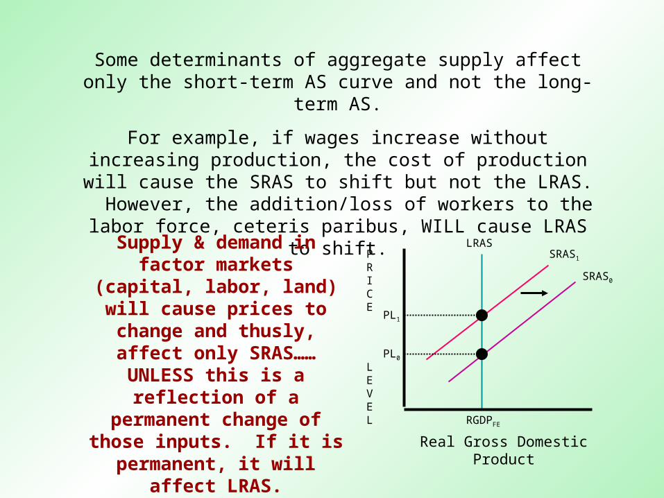
Some determinants of aggregate supply affect only the short-term AS curve and not the long-
term AS.
For example, if wages increase without increasing production, the cost of production will cause the SRAS to shift but not the LRAS. However, the addition/loss of workers to the labor force, ceteris paribus, WILL cause LRAS
to shift.PRICE
LEVEL
Real Gross Domestic Product
LRAS
SRAS0
SRAS1
RGDPFE
PL1
PL0
Supply & demand in factor markets
(capital, labor, land) will cause prices to change and thusly, affect only SRAS……UNLESS this is a reflection of a
permanent change of those inputs. If it is
permanent, it will affect LRAS.

Another influence that can cause the increase in the cost of production are natural disasters. Hurricanes, tornados, flooding, earthquakes and droughts could cause the short-run AS to shift to the left, ceretis paribus.

EQUILIBRIUM: REAL OUTPUT AND EQUILIBRIUM: REAL OUTPUT AND THE PRICE LEVELTHE PRICE LEVEL
PRICE
LEVEL
Real Gross Domestic Product
LRAS
SRAS
RGDPFE
PL0
AD
The intersection of the Aggregate Demand Curve
and the Short-Run Aggregate Supply Curve
determines the equilibrium level of real output and price
level. When equilibrium occurs at the potential output level (on the LRAS), the economy is operating at full-
employment.

Shifts of the Short-Run Aggregate Supply Curve
*Krugman

Shifts of the Short-Run Aggregate Supply Curve
*Krugman
Changes in
Commodity prices
Nominal wages
Productivity

Long-Run Aggregate Supply Curve
*Krugman
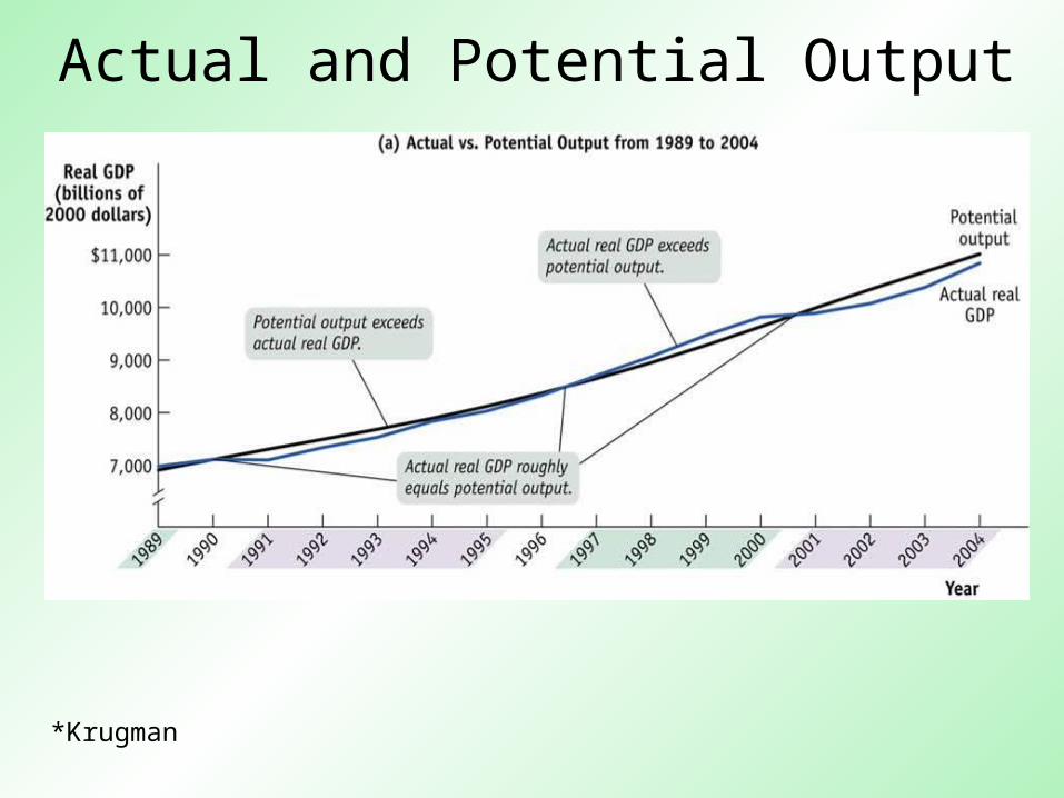
Actual and Potential Output
*Krugman
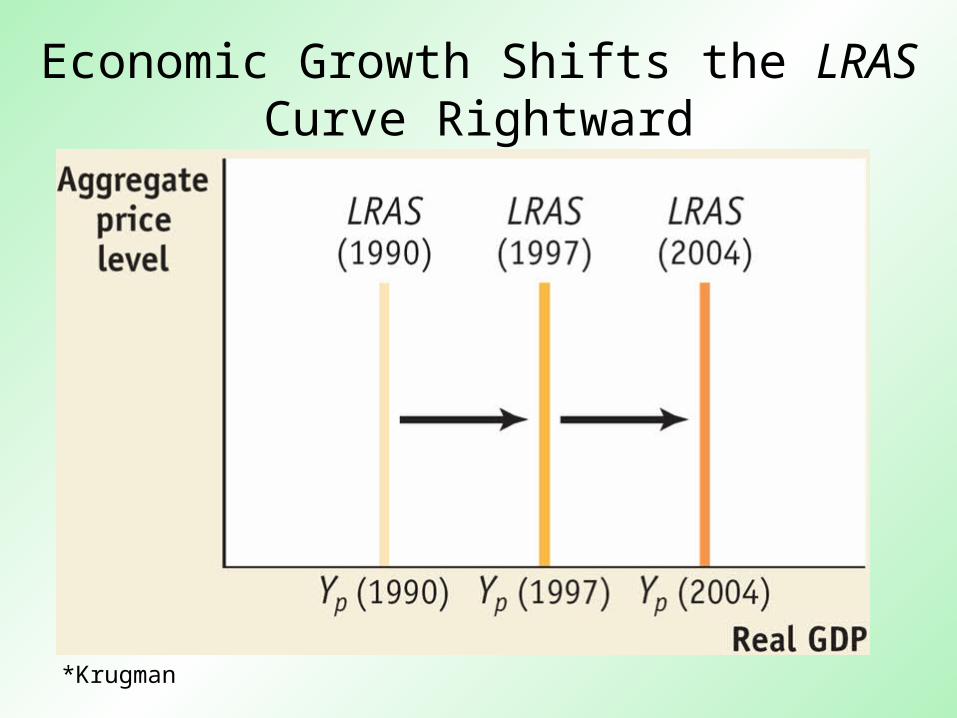
Economic Growth Shifts the LRAS Curve Rightward
*Krugman

From the Short Run to the Long Run
*Krugman

PRICE
LEVEL
Real Gross Domestic Product
LRAS
SRAS
RGDPFE
PL0
AD
Short-run equilibrium can change when the SRAS or AD shifts rightward or leftward.
However, long-run equilibrium of LRAS only changes when the LRAS curve shifts.
Economists anticipate many of
the supply and demand changes.
Whenever the changes are not
expected, economists call them SHOCKS.
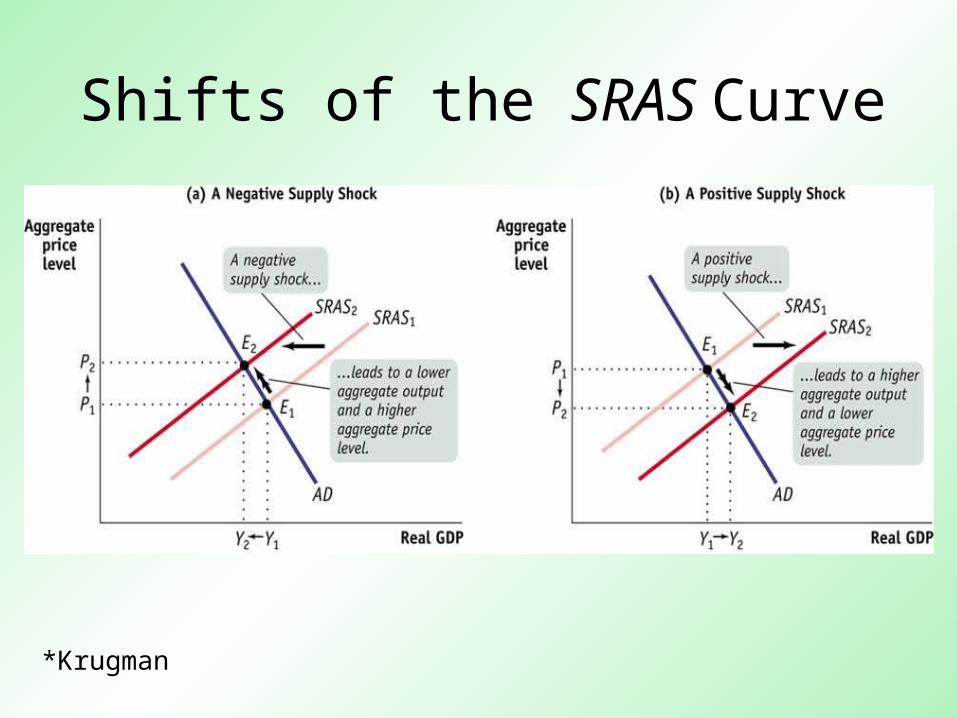
Shifts of the SRAS Curve
*Krugman

Short-Run Versus Long-Run Effects of a Negative Demand Shock
*Krugman

Short-Run Versus Long-Run Effects of a Positive Demand Shock
*Krugman
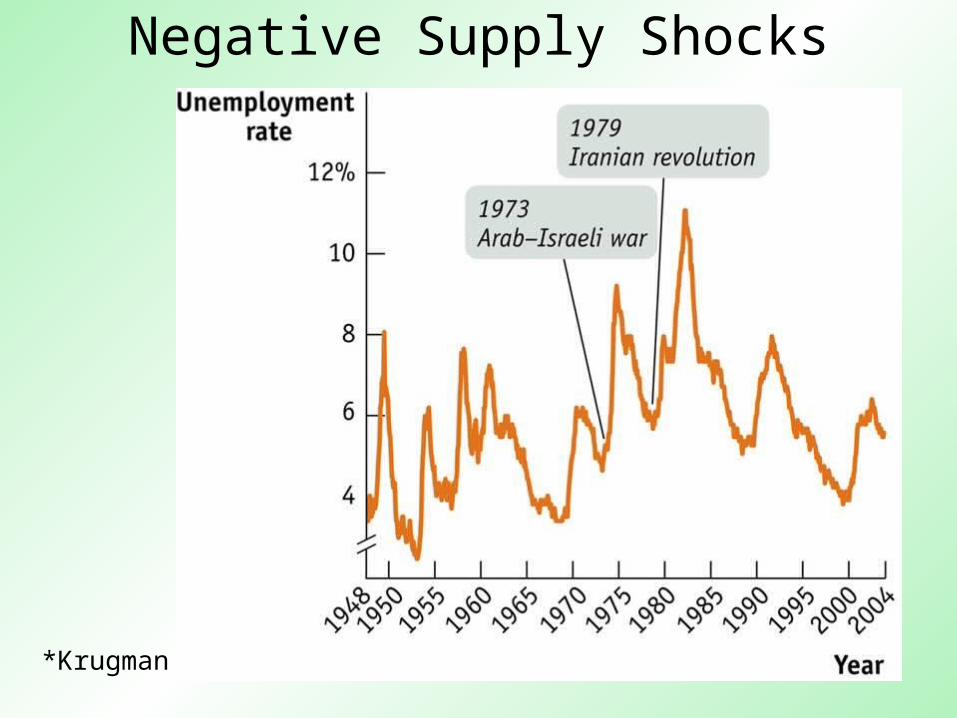
Negative Supply Shocks
*Krugman

Another way of looking at Macroeconomic Equilibrium:
As in the case of the intersection of a product’s demand curve and a product’s supply
curve, we can see that the intersection of the aggregate supply curve and the aggregate demand curve determines the economy’s EQUILIBRIUM EQUILIBRIUM
PRICE LEVELPRICE LEVEL and EQUILIBRIUM REAL DOMESTIC EQUILIBRIUM REAL DOMESTIC OUTPUTOUTPUT.
AD AD
AS ASPRICE
LEVEL
Real Domestic Output, GDP
PRICE
LEVEL
Real Domestic Output, GDP
Equilibrium in the intermediate range of aggregate supply.
Equilibrium in the horizontal
range of aggregate supply.

AD AD
AS ASPRICE
LEVEL
Real Domestic Output, GDP
PRICE
LEVEL
Real Domestic Output, GDP
Where equilibriumequilibrium occurs in the
intermediate range of aggregate supply, the
price level will change to eliminate underproduction or overproduction of
output.
PPee
PPeePP11
QQ22QQ22QQ11 QQee QQ11 QQee
Where equilibriumequilibrium occurs in the
horizontal range of aggregate supply, no change in the price level accompanies the
move toward equilibrium real
output.

AD1
ASPRICE
LEVEL
Real Domestic Output, GDP
PP11
QQ22QQ11
AD2
AD5
ASPRICE
LEVEL
Real Domestic Output, GDP
PP55
QQcc
AD6
PP66
The effect of an increase in aggregate demand depends upon the range of the aggregate supply
curve in which it occurs.
An increase in aggregate demand during the horizontal range increases the real output but leaves price
unaffected.
An increase in aggregate demand during the vertical range increases the price
level but production cannot exceed capacity.

AD3
ASPRICE
LEVEL
Real Domestic Output, GDP
PP33
QQ44QQ33
AD4
PP44
An increase in aggregate demand during the
intermediate range increases both real output and price.

AD1
ASPRICE
LEVEL
Real Domestic Output, GDP
PP11
QQ22QQ11
AD2
In comparing the figures below, one can see that GDP increase more in figure A than in figure C, even though the
shifts in AD are of equal magnitudes.
INFLATION AND THE MULTIPLIERINFLATION AND THE MULTIPLIER
AD3
ASPRICE
LEVEL
Real Domestic Output, GDP
PP33
QQ44QQ33
AD4
PP44
When we combine the two figures we will get……..

AD2
ASPRICE
LEVEL
Real Domestic Output, GDP
PP11
GDPGDP11
AD3
PP22
An increase in aggregate demand during the horizontal range (AD1 to AD2) means that the economy is in
recession…..excess production capacity and a high unemployment rate. Businesses are willing to produce more
output at existing prices.
AD1
GDPGDP22 GDPGDP33
An initial change in spending and resulting change in aggregate demand transmits fully into a change in real GDP and
employment. The price level remains constant.
In the horizontal range of aggregate supply a “full-
strength” multiplier is at
work.
FULL MULTIPLIER EFFECT

AD2
ASPRICE
LEVEL
Real Domestic Output, GDP
PP11
GDPGDP11
AD3
PP22
If the economy is in either the intermediate or vertical range of the aggregate supply curve, part or all of any
initial increase in aggregate demand will be dissipated in inflation and therefore NOT be reflected in increased real
output and employment.
AD1
GDPGDP22 GDPGDP33
Below, the shift from AD2 to AD3 is of the same magnitude as AD1 to AD2. Because we are in the intermediate range of the
aggregate supply curve, a portion of the increase in aggregate demand is absorbed as inflation as the price level rises from
P1 to P2. Real GDP rises only to
GDP’.
If the aggregate supply curve had been
horizontal, then the shift would have
increased real GDP to GDP3.
FULL MULTIPLIER EFFECT
REDUCED MULTIPLIER EFFECT
GDP’GDP’

THE RATCHET EFFECTTHE RATCHET EFFECT
What happens when aggregate demand decreases??
Horizontal Range:Horizontal Range: Real GDP falls and price level
remains unchanged.
Intermediate Range:Intermediate Range: Both real output and
price level diminishes.
Vertical Range:Vertical Range: Prices fall and real output remains at the full-
capacity level.
Our model suggests the following:

AD5
ASPRICE
LEVEL
Real Domestic Output, GDP
PP55
QQcc
AD6
PP66
AD3
PRICE
LEVEL
Real Domestic Output, GDP
PP33
QQ44QQ33
AD4
PP44
The complication is that many prices (of both products and resources) rise quickly
but are “sticky” or inflexible in a downward direction. Some economists call this the “ratchet effect’“ratchet effect’ because a ratchet is a
mechanism that cranks a wheel forward but not backward.

AD1
ASPRICE
LEVEL
Real Domestic Output, GDP
PP11
QQccQQ11
AD2
PP22
QQ22
c
a
b
If AD increases from AD1 to AD2 the economy moves from P1Q1 equilibrium (point a) on the horizontal range to
P2Qc equilibrium (point b) on the vertical range.
This increase in aggregate demand has increased the price level.
The higher product prices in turn result in increases in wages and increased input prices,
raising per-unit production costs at each level of available GDP.
These prices, however, do not come down very easily. Instead of the economy returning to
equilibrium at point a, the higher per-unit costs remain and the
aggregate supply curve will stay in place at
P2cAS (point c).

1) Wage Contracts:Wage Contracts: Unions prohibit wage cuts for duration of the contract.
2) Morale, Effort, and Productivity:Morale, Effort, and Productivity: Lower wages may reduce worker morale and work effort, lowering productivity.
3) Training Investments:Training Investments: Lowering wages may cause skilled workers to quit and costs would be incurred to train the new workers.
4) Minimum Wage:Minimum Wage: Legal floor for wages for lesser skilled workers.
5) Menu Costs:Menu Costs: The cost of changing prices (reprinting of menus & catalogs, advertising, etc.)
6) Fear of Price Wars:Fear of Price Wars: Concern that if one business lowers their prices, rivals will cut with deeper and deeper rounds of price cuts.
REASONS for DOWNWARD PRICE-LEVEL INFLEXIBILITY

DEMAND-PULL INFLATIONDEMAND-PULL INFLATION
…..is when the price level rises as a result of an increase in aggregate demand.
PRICE
LEVELS Real Gross Domestic
Product
SRASSRAS11
a
PL1
PL2
LRAS
RGDPFE
ADAD00
PL0
SRASSRAS00
ADAD11
An increase in consumer optimism could spur an increase in aggregate demand. This would cause an increase in the price level and an increase in
real output.
c
b
Remember, businesses have an incentive to produce more when the prices of their goods are rising faster than the costs of
inputs.Is it possible for Is it possible for production to exceed production to exceed
its potential?its potential?Yes….for a short time. As workers are encouraged to work overtime and part-time workers become full-time.

COST-PUSH INFLATIONCOST-PUSH INFLATION
What would happen if OPEC were to impose steep price increases on oil like they did
in 1973-74???The domestic per-unit price of producing
goods would increase and drive prices up. This is what is called COST-PUSH
INFLATION.PRICE
LEVELS Real Gross Domestic
Product
SRAS1
SRAS0
AD
a
b
P1
P2
A shift from SRAS0 to SRAS1 would cause the economy to move from point a to b. Cost-push inflation increases from P1 to P2 and real output
from RGDPFE to RGDP1.
LRAS
RGDPFERGDP1

When OPEC imposed steep price increases on oil in 1973-74, it caused a phenomenon known as STAGFLATION through the 1970s and 80s. This is where lower growth and higher prices occur together and shown below by a leftward
shift in the Aggregate Supply Curve.
When the Aggregate Demand Curve does
not change and price level increases, then inflation is caused by supply-side forces, not
demand.
PRICE
LEVELS Real Gross Domestic
Product
SRAS1
SRAS0
AD
a
b
P1
P2
LRAS
RGDPFERGDP1
KRUGMAN’S
Chapter 28
Income and Expenditure Approach

What you will learn in this chapter:The meaning of the consumption function, which shows how disposable income affects consumer spending
How expected future income and aggregate wealth affect consumer spending
The determinants of investment spending, and the distinction between planned investment and unplanned inventory investment
How the inventory adjustment process moves the economy to a new equilibrium after a demand shock
Why investment spending is considered a leading indicator of the future state of the economy

Disposable Income and Consumer Spending for American Households in 2003
*Krugman

The Consumption Function

The Aggregate Consumption Function
*Krugman

An Upwards Shift of the Aggregate Consumption Function
*Krugman
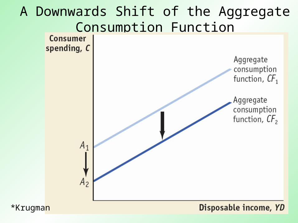
A Downwards Shift of the Aggregate Consumption Function
*Krugman

Fluctuations in InvestmentSpending and Consumer Spending

Planned Aggregate Spending and GDP
GDP = C + I
YD = GDP
C = A + MPC – YD
AEPlanned = C + IPlanned
Planned aggregate spending is the total amount of planned spending in the economy.

Planned Aggregate Spending and GDP
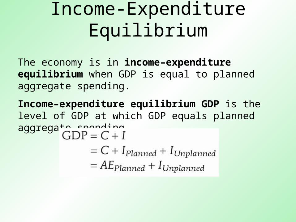
Income-Expenditure Equilibrium
The economy is in income–expenditure equilibrium when GDP is equal to planned aggregate spending.
Income–expenditure equilibrium GDP is the level of GDP at which GDP equals planned aggregate spending.

Income-Expenditure Equilibrium
*Krugman

The Multiplier Process and Inventory Adjustment
*Krugman

The Multiplier Process and Inventory Adjustment
*Krugman

The Paradox of Thrift
In the Paradox of Thrift, households and producers cut their spending in anticipation of future tough economic times.
It is called a paradox because what’s usually “good” (saving to provide for your family in hard times) is “bad” (because it can make everyone worse off).

Real Domestic Output, GDP
Aggregate
GDP2 GDP1 GDP3
Expendi tures 450
2
1
3 (Ca + Ig + Xn + G)1 at P1
Aggregate expenditures schedule will rise when the price level declines and fall when the price level
increases.
(Ca + Ig + Xn + G)3 at P3
(Ca + Ig + Xn + G)2 at P2
*McConnell, Brue

Real Domestic Output, GDP
Price
Level
1
3
GDP2 GDP1 GDP3
P1
P3
P2
AD
Real Domestic Output, GDP
Aggregate
GDP2 GDP1 GDP3
Expendi tures 450
2
2
1
3
P2
P1
P3
Compare the GDP at each level.
*McConnell, Brue

Compiled by:Compiled by:Virginia H. Meachum, Economics TeacherVirginia H. Meachum, Economics Teacher
Coral Springs High SchoolCoral Springs High School
Sources:Sources:Principles, Problems, and PoliciesPrinciples, Problems, and Policies, by Campbell McConnell & , by Campbell McConnell &
Stanley BrueStanley Brue
EconomicsEconomics, by Krugman, Wells, by Krugman, Wells
Principles of EconomicsPrinciples of Economics, by N. Gregory Mankiw, by N. Gregory Mankiw
Notes by Florida Council on Economic Education and FAU Notes by Florida Council on Economic Education and FAU Center for Economic EducationCenter for Economic Education
Notes by Foundation for Teaching EconomicsNotes by Foundation for Teaching Economics