Part 2C. Part 2C. Individual Demand FunctionsIndividual Demand Functions

3.3.Slutsky EquationsSlutsky EquationsSlutsky EquationsSlutsky EquationsSlutsky Slutsky 方程式方程式

OwnOwn--Price EffectsPrice Effects

yy

OwnOwn Price EffectsPrice Effects A A SlutskySlutsky DecompositionDecomposition CrossCross--Price EffectsPrice Effects CrossCross--Price EffectsPrice Effects Duality and the Demand Concepts Duality and the Demand Concepts

12014.11.20

OwnOwn Price EffectsPrice EffectsOwnOwn--Price EffectsPrice Effects

QQ Wh t h t h f d h hQ: Q: What happens to purchases of good x change when px changes?

x/px

Differentiation of the F O Cs from utilityDifferentiation of the F.O.Cs from utility maximization could be used.H thi h i b dHowever, this approach is cumbersome and provides little economic insight.

2

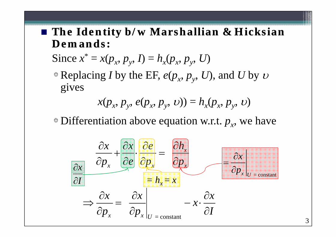
The Identity b/w The Identity b/w MarshallianMarshallian & Hicksian & Hicksian Demands:Demands:Since x* = x(px, py, I) = hx(px, py, U) y y

Replacing I by the EF, e(px, py, U), and U by givesg

x(px, py, e(px, py, )) = hx(px, py, )

Diff ti ti b ti t h

hx x e

Differentiation above equation w.r.t. px, we have

x

x x x

hx x ep e p p

xp

x

= constantx Up

= hx = x

x x x I

= constantx x U

xp p I

3

x x x

= constantx x U

xp p I

S.E.( – )

I.E.( ?)

The S E is always negative h

Th L f D d Th L f D d h ld

The S.E. is always negative as long as MRS is diminishing.

0x

x

hp

The Law of Demand The Law of Demand holds as long as x is a normal goodnormal good. 0 0

x

x xI p

If x is a GiffenGiffen goodgood, hen x must be an inferiorinferior goodgood

0 0x xp I

hen x must be an inferiorinferior goodgood. xp I

E/px = hx = xA $1 i i i ditA $1 increase in px raises necessary expenditures by x dollars. 4

Compensated Demand ElasticitiesCompensated Demand ElasticitiesCompensated Demand ElasticitiesCompensated Demand ElasticitiesThe compensated demand function: h (p , p , U)The compensated demand function: hx(px, py, U)

dh Compensated OwnCompensated Own--Price Elasticity of DemandPrice Elasticity of Demand

x

x x xh p

dhh h pe d h

,x xh px x x

x

dp p hp

Compensated CrossCompensated Cross--Price Elasticity of DemandPrice Elasticity of Demand

xdh

,x y

x

yx xh p

ph he dp p h

y y x

x

dp p hp

5

OwnOwn--Price Elasticity form of the Price Elasticity form of the SlutskySlutsky EquationEquationyy yy qq

xhx xxI

x xp p I

x x x xp h p px x Ix

x x

xp x p x I x I

h Ie e s e , , ,x x xx p h p x x Ie e s e

where Expenditure share on x.xx

p xsI

I

The Slutsky equation shows that the t d d t d icompensated and uncompensated price

elasticities will be similar ifthe share of income devoted to x is small

6

the share of income devoted to x is small.the income elasticity of x is small.

A Slutsky DecompositionA Slutsky DecompositionA Slutsky DecompositionA Slutsky Decomposition

Example: Example: CobbCobb Douglas utility functionDouglas utility function Example: Example: CobbCobb--Douglas utility functionDouglas utility functionU(x,y) = x0.5y0.5

1 I 1 IThe Marshallian Demands: 12 x

Ixp

0 5 0 5

12 y

Iyp

The IUF: 0.5 0.5

0.5 0.5

1 1( , , )2 2 2x y

x x x y

I I Ip p Ip p p p

x x x yp p p p

The EF: 0.5 0.5( , , ) 2x y x ye p p p p

The Hicksian Demands:0.5pe 0.5pe0.5y

xx x

pehp p

0.5

xy

y y

pehp p

7

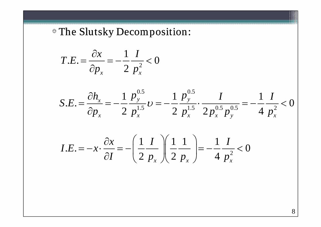
The Slutsky Decomposition: The Slutsky Decomposition: y py p

1 0x IT E 2. . 0

2x x

T Ep p

0.5 0.5

1.5 1.5 0.5 0.5 2

1 1 1. . 02 2 2 4

y yx p ph I IS Ep p p p p p

2 2 2 4x x x x y xp p p p p p

1 1 1 1I I 2

1 1 1 1. . 02 2 4x x x

x I II E xI p p p

8

Numerical Example: Numerical Example: CobbCobb--Douglas utility functionDouglas utility functionpp g yg yU(x,y) = x0.5y0.5

Let $1 $4 I $8

The Marshallian Demands:

Let px = $1, py = $4, I = $8

1 4Ix 1 1Iy The Marshallian Demands: 4

2 x

xp

The IUF: 0.5 0.5( ) 4 1 2p p I

12 y

yp

The IUF: ( , , ) 4 1 2x yp p I

The EF: ( , , ) 8x ye p p I x y

The Hicksian Demand for x:0.5 0.5

0.5 0.5

4 2 41

yx

ph

p

0.5 0.5

0.5 0.5

1 2 14

xy

php

1xp 4yp

9

Suppose that px : $1 $4pp px

The Marshallian Demands:1 8' 12 4

x 1 8' 12 4

y 2 4

The IUF: 0.5 0.5( , , ) 1 1 1x yp p I

h l i 0 5 0 5The real income: 0.5 0.5' ( , , ') 2 4 1 2 16x ye e p p

The Hicksian Demand for x:The Hicksian Demand for x:0.5

0.5

4 2 24xh

0.5

0.5

4 2 24yh

4 0.54y

The Slutsky Decomposition: . . : 1 4 3T E x

. . : 2 4 2xS E h x

. . . . . . ( 3) ( 2) 1I E T E S E 10

Figure: Figure: The Slutsky Decomposition The Slutsky Decomposition

px : $1 $4

y

px

. . : 1 4 3T E x

2 4 2S E h4

. . : 2 4 2xS E h . . . . . . ( 3) ( 2) 1I E T E S E

I

2

I I = –2y

IC1

1IC0

xS.E.I.E.

1 42 8

11

Figure: Figure: The Slutsky Decomposition The Slutsky Decomposition

px : $1 $4

px

px

. . : 1 4 3T E x

2 4 2S E h4

. . : 2 4 2xS E h

. . . . . . ( 3) ( 2) 1I E T E S E . . . . . . ( 3) ( 2) 1I E T E S E

xhx

1

xS.E.I.E.

1 42

12

CC P i Eff tP i Eff tCrossCross--Price EffectsPrice Effects The identity b/w The identity b/w MarshallianMarshallian & & HicksianHicksian The identity b/w The identity b/w MarshallianMarshallian & & HicksianHicksian

Demands:Demands:x(p p e(p p )) = h (p p )x(px, py, e(px, py, )) = hx(px, py, )

Diff ti ti b ti t h

hx x e

Differentiation above equation w.r.t. py, we have

x

y y y

hx x ep e p p

xp

x

= constanty Up

= hy = y

x x x I

= constanty y U

yp p I

13

CrossCross--Price Elasticity form of the Price Elasticity form of the SlutskySlutskyyy yyEquationEquation

hx x x

y y

hx xyp p I

y y yx

y y

p p phx x Iyp x p x I x I

y yp p

, , ,y x yx p h p y x Ie e s e

where Expenditure share on y.yy

p ys

I

I

14

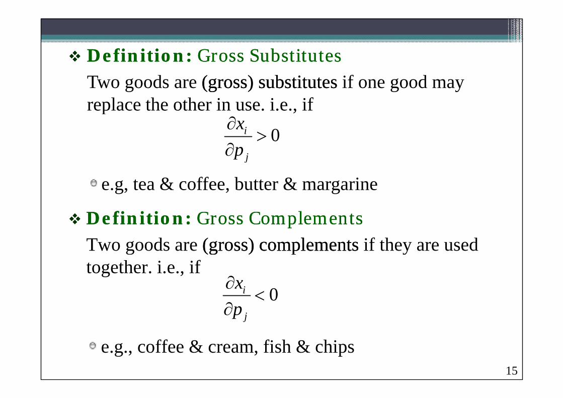
Definition: Definition: Gross SubstitutesGross SubstitutesTwo goods are (gross) substitutes(gross) substitutes if one good may replace the other in use. i.e., ifreplace the other in use. i.e., if

0i

j

xp

e.g, tea & coffee, butter & margarinejp

Definition: Definition: Gross ComplementsGross ComplementsTwo goods are (gross) complements(gross) complements if they are usedTwo goods are (gross) complements (gross) complements if they are used together. i.e., if

0ix 0i

jp

e.g., coffee & cream, fish & chips15

FigureFigure: : Gross Substitutes Gross Substitutes

When the price of y falls the

y

When the price of y falls, the substitution effect may be so large that the consumer purchases less xy

In this case we call x and y gross gross

and more y.

In this case, we call x and y gross gross substitutes.substitutes.y1

y0 U1x/py > 0

x x

U0

xx1 x0

16

FigureFigure: : Gross ComplementsGross Complements

When the price of y falls the

y

When the price of y falls, the substitution effect may be so small that the consumer purchases more x and y pmore y.

In this case we call x and y gross gross

y1

In this case, we call x and y gross gross complements.complements.

y0

U1Ux/py < 0

xx

U0

xx1x0

17

Definition: Definition: Net SubstitutesNet SubstitutesTwo goods are net substitutesnet substitutes if

h

constant

or 0i

j U

xp

0i

j

hp

Definition: Definition: Net ComplementsNet Complements

constantj U

ppTwo goods are net complements net complements if

xh

constant

or 0i

j U

xp

0i

j

hp

Note: The concepts of net substitutes and net substitutes and ll tt f l l b tit ti ff tb tit ti ff tcomplemencomplements ts focuses solely on substitution effectssubstitution effects.

18

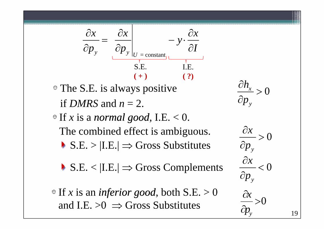
x x x

= constanty y U

yp p I

S.E.( + )

I.E.( ?)

The S E is always positive 0xh

If i l dl d I E 0

The S.E. is always positive if DMRS and n = 2.

0x

yp

If x is a normal goodnormal good, I.E. < 0. The combined effect is ambiguous. 0x

S.E. > |I.E.| Gross Substitutes

S E < |I E | Gross Complements

yp

0xS.E. < |I.E.| Gross Complements 0

yp

If x is an inferiorinferior goodgood both S E > 0 If x is an inferiorinferior goodgood, both S.E. > 0 and I.E. >0 Gross Substitutes 0

y

xp

19

Case of Many Goods (Case of Many Goods (nn > > 22))y (y ( ))The Generalized Slutsky Equation is:

x x x

=constant

i i ij

j j U

x x xxp p I

When n > 2, hi/pj can be negative.i.e., xi and xj can be net complementsnet complements.If the utility function is quasi-concave, then the the crosscross--netnet--substitution effectssubstitution effects are symmetricsymmetric. i.e., yy ,

ji

j i

hhp p

j ip p Proof:Proof:

2j jii

e p he ph e j jii

j j i j i i

pp ep p p p p p

20

Asymmetry of the Gross CrossAsymmetry of the Gross Cross--Price Effects Price Effects y yy yThe gross definitions of substitutes and complements are not symmetric.complements are not symmetric. It is possible for xi to be a substitute for xj and at the same time for x to be a complement of xthe same time for xj to be a complement of xi.

21

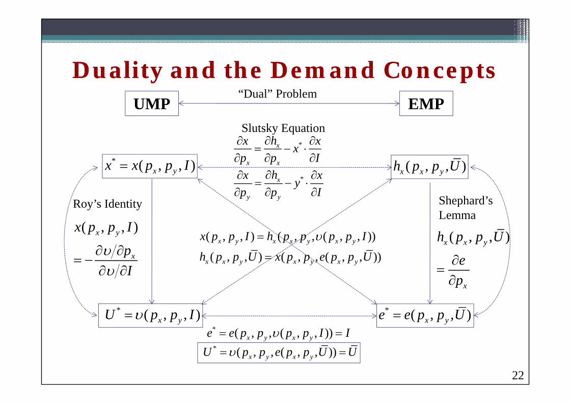
D lit d th D d C t D lit d th D d C t UMP EMP

“Dual” ProblemDuality and the Demand Concepts Duality and the Demand Concepts

Slutsky Equation*

xhx xxI* ( , , ) x yx x p p I

R ’ Id tit Shephard’s

( , , )x x yh p p U x xp p I*

x

y y

hx xyp p I

( , , )x x yh p p U

Roy’s Identity Shephard sLemma

( , , )

x yx p p I

( , , ) ( , , ( , , ))x y x x y x yx p p I h p p p p I

x

ep

xp

I( , , ) ( , , ( , , ))x x y x y x yh p p U x p p e p p U

* ( , , ) x yU p p I * ( , , ) x ye e p p U* ( , , ( , , )) x y x ye e p p p p I I( ( ))x y x yp p p p* ( , , ( , , )) x y x yU p p e p p U U

22