Terence D. Brown, Extension forest productsmanufacturing specialist, Oregon State University.

Part 2: Size Analysis ConsiderationsT.D. Brown

EM 8731 • June 2000$3.00

Lumber size control is one of the more complex parts of any lumberquality control program. When properly carried out, lumber size controlidentifies problems in sawing-machine centers, sawing systems, or setworkssystems. It is a key component of all good lumber quality control programs.In processing both large and small logs, lumber size control is an essentialelement in maximizing recovery.

Size control has two aspects: measurement andanalysis. Measurement is discussed in OSU Extensionpublication EM 8730, Lumber Size Control: Measure-ment Methods. Lumber size is one part of the manu-facturing process that can be quantified very well.Even though it requires time to take the measurements,given current technology, the benefits of size controlfar outweigh the cost of the time required.

Information obtained from a size control program isa powerful management and production control tool. As the mechanicalcondition of a sawing-machine center or sequential flow pattern becomesapparent in detail, maintenance priorities can be determined more easily. It iseasier to attach dollar values to proposed machine improvements if sizecontrol information is the basis for decision making. Results of lumber sizeanalysis are valuable for justifying new equipment and for setting specifica-tions for that equipment when it is installed.

The goal of a size control program is to minimize the sum of kerf, sawingvariation, and roughness. Also, the effect of minor changes in saw kerf orfeed speed can be determined immediately. Developing an effective sizecontrol program requires hard work, understanding, and patience, but thepayoffs are considerable. A mill manager who minimizes the amount ofwood cut per saw line without losing grade recovery will maximize thedollar return. Companies that have implemented size control programs, andhave reduced rough green sizes and kerfs as a result, have realized from$300,000 to $1,000,000 per year in additional lumber value depending onthe amount of improvement and the mill’s production level.

PERFORMANCE EXCELLENCEIN THE WOOD PRODUCTS INDUSTRY

Size control programshave realized…

from $300,000 to$1,000,000 per year inadditional lumber value.

2

LUMBER SIZE CONTROL

Most sawmills spend a great deal of time collecting size controldata. Looking at raw data can help make immediate corrections toobvious problems. Beyond that, it is the analysis of raw data thatcreates the greatest benefit of a lumber size control program.

There is some benefit just in collecting the data because thatprocess keeps maintenance personnel and machine operators “ontheir toes.” However, there are times when size data are collectedbut allowed to sit for days without being processed into meaningfulinformation. It is true that data analyzed in this way are still impor-tant as historical perspective, but they lose their immediate benefitof evaluating current processing capabilities.

Uses of size control informationSize control information has two primary benefits. The first and

most important is the ability to use the sawing variation informa-tion to troubleshoot machine center problems. Because of thesawmill’s dynamic nature, it is difficult to maintain control ofsawing-machine centers over a long period. Sawing variationinformation obtained from the data analysis can be used to isolateproblems and to identify the most likely places to look for solu-tions. This diagnostic application is by far the greatest value of anysize control program.

The second benefit is being able to estimate the appropriaterough green target size for the machine center. It is important tounderstand that no current mathematical model can estimate therough green target size of a particular machine center with anydegree of certainty. Most attempts involved highly complex model-ing that did not prove useful. Shrinkage variation due to drying andplaner variation can be as much as the sawing variation. Toaccount for all those sources of variation in a meaningful waycurrently is not practical.

Components of target sizeWhenever we discuss lumber size control, many people think

only about reducing sawing variation. There always will be somevariation. Therefore, attaining the least amount of sawing variationis only one part of cutting lumber to the smallest rough green sizepossible. We must look at all the factors that affect rough greentarget size.

The best way to visualize target size components is to workbackward from final product size. If the lumber has been surfaced

3

SIZE ANALYSIS

to establish its final size, the first component of target size isplaning allowance. The next component is shrinkage allowance (ifthe lumber is dried), and the last component is sawing variation.Figure 1 illustrates how each of these components builds upon theother to establish the rough green target size.

The largest size in Figure 1 is oversize lumber—which shouldnever occur in a mill with a well-run size control program. Thedays of throwing in a “fudge factor” to protect against undersizelumber have long passed. In today’s world, timber is expensive.

In Figure 1, each component of rough green target size appearsas a layer added to the previous one. By minimizing the thicknessof each layer, the rough green target size will be as small as pos-sible. Let’s look at these components and discuss howeach can be minimized.

Figure 1.—Target size components.

Oversize

Rough green target size

Planer allowance

Shrinkage allowance

Sawing variation

Planer allowanceThe amount of wood removed by both top and bottom heads

combines as total planer allowance. To fully understand how totalplaner allowance affects green target size, we need to know how aplaner works. The amount of lumber removed by the top andbottom planer heads is seldom the same, even though we assumethat it is roughly the same. (Although this discussion focuses onboard thickness, the same principles hold true for board width; it’sjust that different planer heads are involved.)

Final size

4

LUMBER SIZE CONTROL

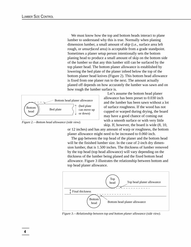
We must know how the top and bottom heads interact to planelumber to understand why this is true. Normally when planingdimension lumber, a small amount of skip (i.e., surface area leftrough, or unsurfaced area) is acceptable from a grade standpoint.Sometimes a planer setup person intentionally sets the bottomplaning head to produce a small amount of skip on the bottom sideof the lumber so that any thin lumber still can be surfaced by thetop planer head. The bottom planer allowance is established bylowering the bed plate of the planer infeed below the top of thebottom planer head knives (Figure 2). This bottom head allowanceis fixed from one planer run to the next. The amount actuallyplaned off depends on how accurately the lumber was sawn and onhow rough the lumber surface is.

Figure 3.—Relationship between top and bottom planer allowance (side view).

Let’s assume the bottom head planerallowance has been preset to 0.030 inchand the lumber has been sawn without a lotof surface roughness. If the wood has notcupped or warped during drying, the boardmay have a good chance of coming outwith a smooth surface or with very littleskip. If, however, the board is wide (8, 10,

Bottomhead

Bed plate

or 12 inches) and has any amount of warp or roughness, the bottomplaner allowance might need to be increased to 0.060 inch.

The gap between the top head of the planer and the bottom headwill be the finished lumber size. In the case of 2-inch dry dimen-sion lumber, that is 1.500 inches. The thickness of lumber removedby the top head (top head allowance) will vary depending on thethickness of the lumber being planed and the fixed bottom headallowance. Figure 3 illustrates the relationship between bottom andtop head planer allowance.

Figure 2.—Bottom head allowance (side view).

Bottom head planer allowance

(bed platecan move upor down)

Bottomhead

Tophead Top head planer allowance

Bottom head planer allowance

Final thickness

5

SIZE ANALYSIS

For example, the desired final size out of the planer is1.500 inches. If a board 1.580 inches thick enters the planer, andthe bottom planer allowance is 0.030 inch, then the top head willremove 0.050 inch. If the lumber is 1.560 inches entering theplaner, then the top planer will remove 0.030 inch.

It is vital that the total planer allowance used in calculatingrough green size be the actual settings used at the planer. Let’s takethe above example of a 1.560-inch board entering the planer with a0.030-inch bottom allowance. In this case, an equal thickness oflumber will be removed by the top and bottom heads. The board, infact, could be 1.540 inches in thickness and still have a tinyamount of wood—approximately 0.010 inch—removed by the tophead. In reality because of sawing variation, lumber is not going tohave a uniform thickness coming into the planer, and this pieceprobably would leave the planer with unsurfaced areas.

Suppose the planer setup person had a bad day and set up thebottom head so that the bottom planer allowance was 0.070 inch.In this case, the board that was 1.560 inches thick entering theplaner would never be touched by the top head and would comeout of the planer totally unsurfaced on the top face. The lumber hadplenty of wood to surface cleanly if the bottom head allowance hadbeen set correctly.

If a quality control (QC) person hears from the planer mill thatthe lumber is being cut too thin, the first thing to do is check howmuch wood the bottom planer head is removing. If, after planing,the lumber is surfaced cleanly on the bottom and shows all the skipon the top, then the problem is planer setup, not green target size inthe sawmill or shrinkage due to overdrying the lumber.

The goal is to minimize the amount of lumber the planer removeswhile still maintaining grade. This can be done only by presentingflat, smoothly sawn lumber to a planer that has been set up cor-rectly. Total planer allowances range from 0.120 inch for drysouthern pine to 0.010 inch for green Douglas-fir. This does notimply that southern pine manufacturers are doing a poorer job; it ismore a reflection of species differences and drying characteristics.In either case, more surface smoothness and greater sawing accu-racy tend to enable smaller planer allowances.

Shrinkage allowanceThe next “layer” that needs to be minimized is shrinkage. The

more the wood shrinks during drying, the thicker it must be sawninitially in the sawmill. Any quality control program should

The goal is…

to minimize theamount of lumber theplaner removes whilestill maintaining grade.

6

LUMBER SIZE CONTROL

minimize shrinkage during drying. It is absolutely pointless tospend time, energy, and money to make the machine centers in thesawmill saw accurately, then pay little attention to the dryingprocess. For a sawmill to gain the most benefit from its size controlprogram, it must do high-quality drying.

Wood does not shrink until moisture content reaches approxi-mately 30 percent. This is called the fiber saturation point. At thefiber saturation point, all water has been removed from the woodfibers’ cell cavities (lumens), but the wood fibers’ cell walls stillare fully saturated. When the wood’s surface reaches the fibersaturation point, it begins to shrink and continues shrinking in analmost linear fashion until the wood is completely dry (i.e., con-tains no water at all). Most dimension lumber can be gradedofficially as dry if its moisture content is below 19 percent, orbelow 15 percent if graded (KD15).

Some mills have a problem with drying variability. In trying todry all lumber below 19 (or 15) percent, some lumber might benear 5 percent. Lumber at 5 percent moisture content shrinks morethan lumber at 15 percent. The excessive shrinkage causes themill’s QC department to set target sizes in the mill thicker or widerthan would otherwise be necessary.

A wide range in moisture content may be due to natural causesbut, if excessive, more likely it is because drying kilns are notunder good control. The bottom line is that poor drying practicescan result in larger-than-necessary green target sizes just as poorsawing can.

Sawing variationSawing variation is the last target-size component. Sawing

variation information is useful not only for estimating target sizebut, more important, in troubleshooting machine center problems.

Sawing variation is an indicator of how accurately a sawing-machine center cuts lumber. Total sawing variation, S

T, has two

components: within-board sawing variation and between-boardsawing variation. Being able to distinguish between the two allowsquality-control personnel to troubleshoot machine center problems.

Within-board variationWithin-board variation, S

W, is a measure of how the thickness or

width varies along the length of a board. The three types of within-board variation are snake, wedging, and taper. Snake is the varia-tion along one face of the board relative to the opposite face(Figure 4).

7

SIZE ANALYSIS

One of the primary causes of saw snake is overfeeding a sawduring cutting. Even when snake does not result but within-boardvariation is above acceptable limits, overfeeding can be the cause.

Edge-to-edge wedging is a tapering of thickness from one edgeof the board to the other; it may not extend the entire length of theboard. Alignment and feeding problems in the machine centertypically also cause wedging.

End-to-end taper is a progressive decrease or increase in thick-ness from one end of the board to the other. Typical causes arefeeding and alignment problems in the machine center.

When these types of variation occur, quality-control personnelshould look to these potential sources of the problem. Not allwithin-board variation can be attributed to these causes, but theyare good places to start.

Between-board variationBetween-board variation, S

B, measures how the average thick-

ness or width of a board varies from one board to the next comingfrom the same saw line or machine center.

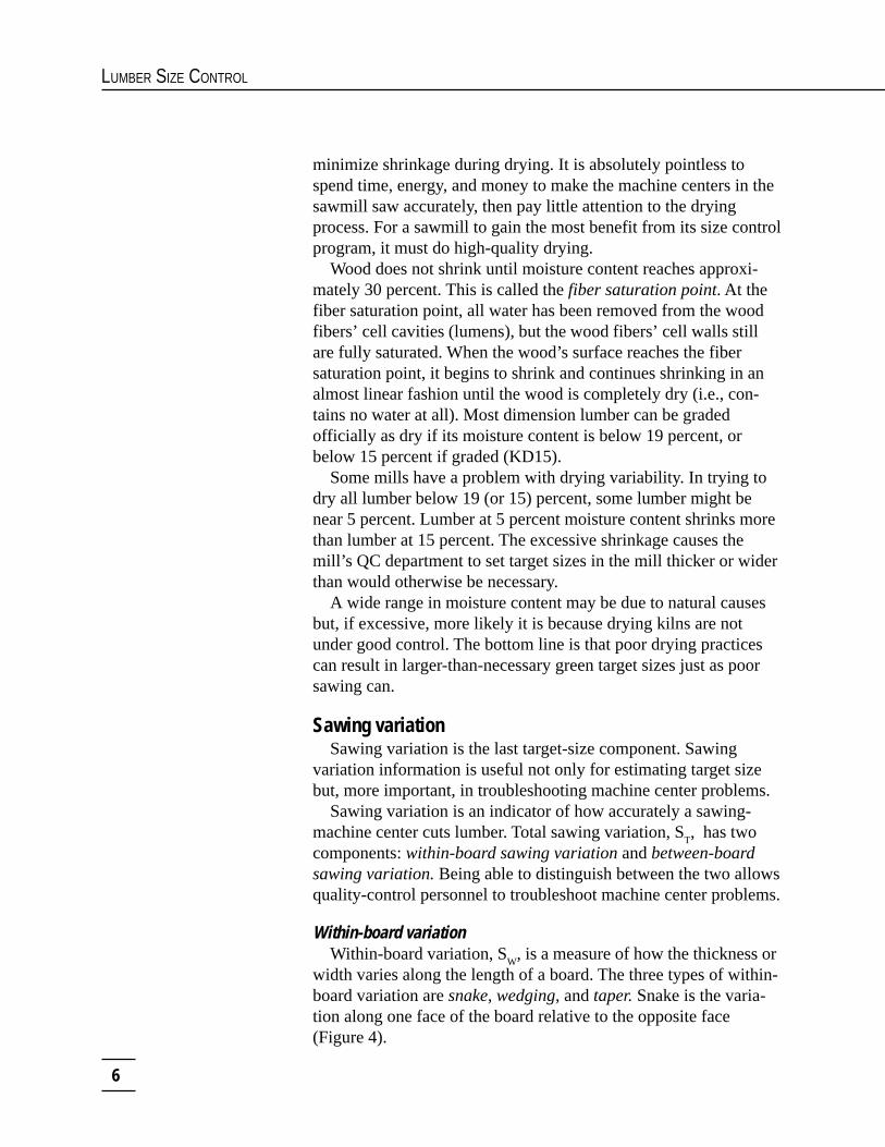
If lumber with excessive between-board variation comes fromthe same saw line (Figure 5, page 8), then setworks or set repeat-ability should be examined. If the variation is coming from

Figure 4.—Extreme within-board variation (“snake”).

8

LUMBER SIZE CONTROL

different saw lines, then saw spacing—either fixed or setworks-based—and individual saw kerf should be evaluated as potentialcauses.

It is important to realize that what may appear to be a between-board variation problem in a particular machine center may, in fact,be unrelated to that machine center. The reason instead may be thata cant that had been processed by a machine center earlier in thework flow was processed through the edger or resaw. The outsideboard may be a different size because the entire cant was badlymanufactured earlier by the other machine center.

Total sawing variationTotal sawing variation, S

T, is the mathematical relationship of

within-board and between-board variation. With planer allowanceand shrinkage allowance, it is used in the equation to estimaterough green target size.

Figure 5.—Excessive between-board variation.

9

SIZE ANALYSIS

Statistical linkagesSawing variation is a much easier concept to grasp for most

sawmill personnel than the statistical term standard deviation.However, all size-control software uses the term standard devia-tion. We typically talk about within-board, between-board, andtotal sawing variation, but in fact we really are talking aboutwithin-board, between-board, and total sawing standard deviation.

Standard deviationStandard deviation is a term that statisticians use to express the

amount of variability in a process. The greater the variability inthickness or width of lumber coming from a machine center, thegreater the standard deviation, be it within-board, between-board,or total sawing. The formulas to calculate standard deviation arediscussed on pages 21–22.

Usually, data on the sizes of lumber produced by a given sawing-machine center will, when plotted on a graph, form a bell-shapedcurve (Figure 6). This type of curve, or distribution of data, isconsidered a normal distribution; in other words, in most casesmost machine centers produce lumber with these size variations.

A normal distribution can be used to make some predictions ofhow all lumber cut on a machine center is being cut, based onsmaller sample sizes. Not all pieces sawn on a machine center willbe normally distributed, but they will be close enough to be treatedthat way. In Figure 6, the curve on the left has a larger total stan-dard deviation, S

T, than the distribution on the right. That is, the

range of thicknesses of boards from the machine center on the leftis greater than the range from the machine center on the right.(Note that average thickness is the same for both machine centers.)

Standard deviation…

is a statistical termthat expresses theamount of variabilityin a process.

Figure 6.—Two size distributions with different standard deviations.

Large standard deviation(S

T approx. 0.040 inch)

Small standard deviation(S

T approx. 0.015 inch)

1.600 1.680 1.760 1.650 1.680 1.710Thicknesses (inches)

10

LUMBER SIZE CONTROL

Estimating standard deviation given the thickest and thinnest boardsIf you know the thickest, thinnest, and average thickness in a

sample of boards—and you assume these data are part of a normaldistribution—it is possible to estimate the total standard deviationof the distribution. A handy statistical shortcut states that thethicknesses of 95 percent of all boards cut on a machine center willbe between two standard deviations above and two standard devia-tions below the average size. Stated another way, the total standarddeviation will be one-fourth of the range between the thinnest andthickest pieces of lumber measured.

Figure 7 shows a distribution with a range of 0.120 inch betweenthe thickest and thinnest measurements. Estimated total standarddeviation is one-fourth the total range, or 0.120 ÷ 4 = 0.030 inch.It’s that simple to calculate, and it gives mill personnel a muchbetter understanding of the relationship of standard deviation to thethickest and thinnest boards from that particular machine center.

For those who use true statistical control charts in quality-control programs, the upper and lower control limits on the controlcharts are calculated as three standard deviations above and threestandard deviations below the average of the pieces being mea-sured. The total of six standard deviations from the thickest to thethinnest boards covers 99.9 percent of all boards cut on a machinecenter, not the 95 percent used in the preceding example.

Because we typically use small samples, however, the statisticalshortcut of 95 percent is more appropriate. In the example below,the thickest and thinnest measurements in a sample of, say,10 boards would not in all likelihood be the smallest and largestsizes cut on that machine center. In the example above, if we were

Figure 7.—Estimating standard deviation from distribution end points.

Thinnest size = 1.620 inchesThickest size = 1.740 inchesTarget size = 1.680 inchesRange = 0.120 inchS

T = 0.120 ÷ 4 = 0.030 inch

1.620 1.680 1.7400.120 inch

11

SIZE ANALYSIS

to use control chart upper and lower controllimits, which assumes 99.9 percent coverage,we would have divided the 0.120 range inthickness by six, not four. This would haveresulted in an estimated total standard devia-tion of 0.020 inch, not 0.030 inch. In myopinion, because samples tend to be small,this would leave the impression that thestandard deviation was smaller than it in fact probably was. Ulti-mately, this could lead to reducing a target size by more than itshould be.

Estimating thickest and thinnest boards given the standard deviationTo estimate the thickest and thinnest boards in a sample, we

calculate in the opposite direction from the example above.Figure 8 shows a distribution with an average size of 1.680 inchesand a total standard deviation of 0.040 inch. The upper value (i.e.,thickest board) is calculated:

1.680 + (2 x 0.040) = 1.680 + 0.080 = 1.760 inches.Likewise, the lower value (thinnest board) is calculated:

1.680 – (2 x 0.040) = 1.680 – 0.080 = 1.600 inches.

Critical sizeFigure 6 (page 9) illustrates two different thickness distributions.

Both distributions have an average thickness of 1.680 inches, butthe difference in their standard deviations indicates very differentthickness ranges. Does either distribution mean that undersizeboards will come out of the planer? It is impossible to tell withoutadditional information. To see whether undersizing is predicted byany distribution, we need to use another tool: critical size.

Table 1. Sawing-accuracy benchmarks for softwoods.

Machine center Total standard deviation (ST)

Headrig/carriages 0.030–0.050 inch

Band resaws 0.020–0.030 inch

Board edgers 0.020–0.040 inch

Rotary gangs 0.005–0.015 inch

Figure 8.—Estimating thickest and thinnest boards from the standard deviation.

Average size = 1.680 inchesS

T = 0.040 inch

Thickest size = 1.680 + (2 x 0.040) = 1.760 inchesThinnest size = 1.680 – (2 x 0.040) = 1.600 inches

1.600 1.680 1.760

12

LUMBER SIZE CONTROL

Simply put, critical size is the minimum size that lumber couldconceivably be cut and still stay within grade size by the end of theprocess. The concept of critical size assumes no sawing variationin thickness or width—which is impossible, of course, in the realsawmill. Critical size is represented graphically by the three small-est “steps” in Figure 1 (page 3). Only when sawing variation isadded to critical size do we get the rough green target size.

For surfaced-green 2-inch (nominal dimension) lumber such asDouglas-fir, the critical size is the final size, 1.560 inches, plus theplaning allowance of, say, 0.030 inch bottom head and 0.030 inchtop head. Thus, the critical size is 1.560 + 0.060, or 1.620 inches.In other words, even if there were no sawing variation, the lumberwould need to be cut to at least 1.620 inches. Notice that in thisexample there is no shrinkage allowance factored into the criticalsize because Douglas-fir dimension lumber often is sold surfaced-green to a final size of 1.560 inches.

Under some circumstances, the critical size might not be1.620 inches. For lumber to be cleanly surfaced, the top headplaning allowance does not have to be a full 0.030 inch if thelumber is straight, flat, and not overly rough. Recall that in thisexample, the bottom head allowance is 0.030 inch, and so theplaner will take off that much. The top head takes off what is left inexcess of the desired final size. Thus, a person might argue that thetrue critical size is 1.560 + 0.030 + “some very small amount” toallow for the top head to plane the top surface.

The problem is that “some very small amount” could end upbeing an amount as large as the bottom head allowance dependingon warp, roughness, and other features of the lumber being planed.As a result, I always define critical size as containing just as muchtop head allowance as bottom head allowance—perhaps not strictlynecessary but warranted from a practical standpoint. If the allow-ance for top head removal exceeds “some very small amount,” thissafety margin helps compensate for variations in shrinkage andplaning.

The critical size for surfaced-green lumber, then, is defined as:CS = F + P

Where CS = Critical size F = Final size P = Total planer allowance (both top and bottom heads)

Using values from the example above, the critical size is:CS = 1.560 + 0.060 = 1.620 inches

Critical size…

is the minimum sizethat lumber can be cutand still stay withingrade size by the endof the process.

13

SIZE ANALYSIS

When setting critical size for surfaced-dry lumber such assouthern pine or SPF, shrinkage must be considered. The criticalsize for surfaced-dry lumber is:

CS = (F + P) x (1 + %Sh/100)Where %Sh = Percent shrinkage

Given a final size of 1.500 inches, a total planer allowance of0.080 inch, and shrinkage of 3 percent, the total calculation forsurfaced-dry lumber critical size is:

CS = (1.500 + 0.080) x (1 + 3/100)CS = 1.580 x 1.03 = 1.627 inches

Rough green target sizeRough green target size should be determined for each sawing

machine center so that the amount of undersize lumber comingfrom that machine center is minimal. As seen in Figure 1 (page 3),rough green target size includes critical size (final size + planingallowance + shrinkage allowance, if the lumber is dried) and anadded amount of sawing variation. We assume that the target sizein all the figures showing a size distribution is the same as theaverage size of the distribution. In fact, this is not normally thecase in the mill. Target size is a desired result, sometimes aplanned-for result. Average size, however, is an actual result andmay or may not be the target size. Actually, many times a machinecenter may be set to a target size of, let’s say, 1.680 inches, but theaverage size of the lumber cut is 1.700 inches. In that case,1.700 inches is the center of the size distribution.

The key point in establishing rough green target size is to mini-mize undersizing. Let’s look at this point, using the critical size of1.620 inches which we calculated for surfaced-green Douglas-firand the two size distributions in Figure 6 (page 9). Remember, wecannot tell whether either distribution in Figure 6 predicts thelumber will be undersize because we don’t yet know the criticalsize in either distribution.

A balanced distributionIn this example, the target size is 1.680 inches, total standard

deviation (ST) is 0.030 inch, and we assume that 95 percent of the

lumber is between 1.740 and 1.620 inches thick. We calculatedcritical size to be 1.620 inches. Because the size of the thinnestboard, 1.620 inches, is the same as the critical size, we say that thisdistribution is balanced (Figure 9, page 14).

14

LUMBER SIZE CONTROL

All lumber thinner than1.620 inches (critical size)will be undersize after finalcut. So, given the distribu-tion in Figure 9, how muchlumber is undersize? Recallthe rule of thumb: thick-nesses of 95 percent of thelumber will be within in arange equal to two standarddeviations on either side ofthe average size. Therefore,

of the lumber remaining, 2.5 percent will be thicker than 1.740 inchesand 2.5 percent will be thinner than 1.620 inches—that is, under-size. In the example illustrated in Figure 9, our target size could bethe same as the average size, 1.680 inches. Because the thin end ofthe range (the lower thickness value) and the critical size are thesame, we are undersizing only about 2.5 percent of the lumberbeing cut.

This situation would be considered ideal and balanced for a finalsize of 1.560 inches, a planer allowance of 0.060 inch, a totalstandard deviation of 0.030 inch, and a target size of 1.680 inches.Unfortunately, this is not always the case in lumber manufacturing.

Neglecting a size control programresults in a too-small target

Let’s first look at the case of a mill that once had an effectivelumber size control program and a target size of 1.680 inches.Now, because they have not done a good job of either monitoringor maintaining the machine center, their total standard deviation,S

T, has grown to 0.040 inch. Figure 10 shows this distribution as

the bell-shaped curve on theleft. Because the S

T is 0.040,

the thickest and thinnest sizesare 1.760 and 1.600 inchesrespectively. Note that criti-cal size is 1.620 inches. Anunacceptable amount oflumber is being producedbelow 1.620 inches—farmore than 2.5 percent. Thiswill result in excessive skip.Figure 10.—Target too small.

Criticalsize

1.600 1.620 1.680 1.700 1.760

ST = 0.040 inch

Target size = 1.680 inchesCritical size = 1.620 inches

Raise targetfrom 1.680 to 1.700 inches

Criticalsize

1.620 1.680 1.740

Figure 9.—Balanced size distribution.

ST = 0.030 inch

Critical size = 1.620 inchesSmallest size = 1.620 inchesTarget size = 1.680 inches

15

SIZE ANALYSIS

The only way the mill can prevent undersizing is to raise targetsize. But by how much? By 0.020 inch, to 1.700 inches. This shiftsthe distribution to the right, as represented by the heavier-line bellcurve. The lower end point rises from 1.600 to 1.620 inches, whichcoincides with critical size and an undersize rate of 2.5 percent.Figure 10 illustrates what most lumber manufacturers know intu-itively: if your sawing variation (thick and thin) increases, youhave to raise the target size to keep from undersizing lumber.

An excellent size control programenables a target-size reduction

A company that dedicates itself to creating an excellent sizecontrol program can reduce target sizes without increasing thepercentage of undersize lumber. For example, a particular machinecenter in this mill once produced lumber with an average size of1.680 inches, a critical size of 1.620 inches, and a total standarddeviation, S

T, of 0.030 inch. The “before” data in Figure 11 create a

distribution in balance; that is, the lower limit of thickness and thecritical size are the same.

Now, after many monthsof diligent effort, this millhas reduced total standarddeviation to 0.015 inch. The“after” data result in themore compressed bell curvein Figure 11. After reducingS

T to 0.015 inch, the smallest

size has been raised to1.650 inches. The criticalsize is 1.620 inches, so it isclear that there is no undersizingat all. As a result, the mill canreduce its target size. Figure 12shows that the original target sizecan be reduced from 1.680 to1.650 inches with no increase inundersizing.

What is this worth to the mill?That depends on the amount oflumber this machine producesand on lumber prices. For arotary gang in a small-log

Figure 12.—Reduction in ST enables a reduction in target size.

BeforeS

T = 0.030 inch

Target size = 1.680 inchesCritical size = 1.620 inches

AfterS

T = 0.015 inch

Target size = 1.650 inchesCritical size = 1.620 inches

Criticalsize

1.620 1.650 1.680 1.740

Figure 11.—Reduction in ST.

BeforeS

T = 0.030 inch

Target size = 1.680 inchesCritical size = 1.620 inches

AfterS

T = 0.015 inch

Target size = 1.680 inchesCritical size = 1.620 inches

Criticalsize

1.620 1.650 1.680 1.710 1.740

16

LUMBER SIZE CONTROL

sawmill cutting 80 MMBF per year, it could amount to $300,000or more in increased revenues.

About undersizingUndersize has been defined many ways. I define undersize

lumber as any lumber that, after planing, has some part of its wideor narrow faces that are not smoothly surfaced, that show skip.Lumber sold in the rough green state is undersize if any part of it issmaller than the final graded size.

It is important to note that some products, such as lam-stock andshop, cannot be at all undersize. On the other hand, dimension orstructural lumber graded “2 & better” can be up to 1⁄16-inch(0.063 inch) scant, as spelled out in grade rules, and still makegrade. Therefore, lam-stock usually is produced to a thicker targetsize than dimension lumber.

Even though undersize is a relative term depending on theproducts, it is possible to establish a target size based on a certainamount of allowable undersize. In each of the previous examples,the amount of undersize allowed was approximately 2.5 percent.Because a normal, or bell-shaped, curve is symmetrical on bothsides of the average-size point, a corresponding 2.5 percent of thelumber is oversize. This leaves 95 percent of the lumber betweenthese two points because, as previously stated, statistical theory isthat 95 percent of all lumber will fall between + 2 S

T and – 2 S

T of

the average. That is how we determined the thickest and thinnestsizes in Figure 8 (page 11).

What if we wanted to establish a target size based on someundersize rate besides 2.5 percent? We would multiply S

T by a

value called the standard normal deviation, which is referred to asZ. Table 2 lists several values of Z for various rates of undersize.

These values are statisticallydetermined and are based onthe characteristics of a normaldistribution.

Figure 13 illustrates that thetarget size is Z x S

T above the

lower thickness value (thinnestsize), 1.620 inches. In thisexample, Z = 2. (The lowerthickness value and critical sizeare the same in this example.)

Undersizeboards (%) Z

0 3.09

1 2.34

2 2.05

2.5 1.97*

3 1.88

4 1.75

5 1.65

10 1.28

15 1.04

*2 approximates this value in examples

Table 2. Z values.

Figure 13.—Relationship of Z x ST to target size.

ST = 0.030 inch

Critical size = 1.620 inchesZ = 2Target size = 1.680 inchesCritical

size

1.620 1.680 1.740

Z x ST = 0.060 inch

17

SIZE ANALYSIS

Estimating target sizeAll components of the target-size equation have been described.

Now they can be put together to estimate target size for surfaced-green lumber:

T = [(F + P) x (1 + %Sh/100)] + (Z x ST)

Where T = Target size F = Final size P = Total planer allowance %Sh = Percent of shrinkage (zero, in this case) Z = Standard normal variation S

T= Total sawing deviation

Thus: T = [(1.560 + 0.060) x (1 + 0)] + (2 x 0.030)

= (1.620 x 1) + 0.060 = 1.620 + 0.060

T = 1.680 inches

Notice in Figure 12 (page 15) that in both “before” and “after”cases critical size is 1.620 inches and target size is calculated byadding (Z x S

T) to critical size. In both instances, Z = 2.

The target-size equation above gives only an estimate of whattarget size actually should be. I cannot state this strongly enough: itis only an estimate, but probably a reasonable start. Recall that thedefinition of undersize is somewhat a moving target depending onthe product being manufactured. Another factor that affects target-size calculation is that we in effect add wood fiber to account forplaner allowance, and we add more wood fiber to account forsawing variation. One of the components of sawing variation iswithin-board variation (S

W). The greater the within-board variation,

the larger ST will be, but the relationship between the two isn’t as

simple as adding or subtracting. That’s because part of within-board variation is removed during planing, and there is no way tosay just how much will be removed because within-board variationis different from board to board.

Another component of the target-size equation that also variesfrom board to board—and even within a board—is shrinkage. Thetarget-size equation treats shrinkage as a constant, Sh. However,some boards may be cut a little thin in the sawmill and do notshrink as much in drying as another board cut to the correct size. Inboth cases, these boards could be planed with no undersize.

If we wanted to get very heavily involved in mathematics, wewould have to view shrinkage as a bell-shaped distribution just as

18

LUMBER SIZE CONTROL

sawing variation is, then try to develop a relationship that canaccount for each possible combination of thickness and shrinkage.To make it more complex, then we would have to recognize thatthe planer does not surface each board to the exact same thicknessor width, and that final size also is a bell-shaped distribution,which would have to be considered in the target-size equation.Finally, we would have to realize that some boards have surfacesthat are cut on two different machine centers, and we would needto account for the variation in each machine center as part of thetarget-size equation. It is just not practical to try to accommodateall this in calculating target size. As a result, we assume that planerallowance and shrinkage are constants. This causes the target-sizecalculation to be only an estimate of true target size. Some readersmight think that, because of these factors, estimating target size hasno value. To the contrary, an estimate is valuable in establishingwhether or not an existing target size is realistic.

It bears repeating that the true value of size control is not intrying to estimate a target size. It is in using the values of S

W and

SB to troubleshoot machine centers, with the goal of reducing both

components of variation over time and thus reducing total sawingvariation, S

T. Only then can mills begin the process of reducing

target sizes.

When and how to reduce target sizesTarget-size reduction should be started only after quality control

personnel are certain they can maintain a reduced total sawingvariation on a machine center over a month’s time. There havebeen instances in which a mill’s QC supervisor measured thesawing variation on a machine center, and it just happened that,due to a particular combination of saws and feed speed that day,the sawing variation was much lower than usual. Management thendecided to reduce target size based on that measurement. A fewdays later, after additional lumber had been manufactured, dried,and planed, that lumber was found to be undersize.

Once the machine center has been kept under control for amonth or so, it is appropriate to consider reducing the rough greentarget size. Now the question becomes, by how much? Begincalculating by plugging in the old and new values for S

T in the

target-size equation. This will tell you the relative magnitude of thechange. Next, if the mill is evaluating a machine center that hassettable sizes, reduce the target size by half the amount first esti-mated, and saw several hundred boards at several different times

Estimating target size …

is valuable in establish-ing whether or not anexisting target size isrealistic.

19

SIZE ANALYSIS

during the day. Track those boards until they are planed, thenevaluate the results. If everything is still OK, reduce the target therest of the way and reevaluate as before.

Reducing target sizes on rotary gangsDeciding to reduce a target size on a rotary gang is not easy;

usually it involves a major change in the guides and spacers, thuscreating a major expense to the mill. It is much better to simulatewhat that size reduction would look like after planing the lumber.This is easily done by making a test run. Recall that if the mill isnot going to reduce the bottom head planer allowance, the changein target size will affect only how much wood the top headremoves. Let’s say a reduction of 0.030 inch is being considered.For the test run, set the final size out of the planer to 0.030 inchthicker by raising the top head 0.030 inch. This simulates whatwould be removed by the top head if the target were reduced by0.030 inch and if final size were the same as before. This approachis much less costly than a rotary gang retrofit and yet accomplishesthe same thing.

Small target reductions and their impact on recoverySome people mistakenly believe that a reduction in target size of

0.030 inch, for example, cannot translate into added recoverybecause they believe it is not possible to get another board from sosmall a change. Granted, it is not very often that another board isgained by a change this small. The added recovery comes fromlonger boards and wider boards being created in either cants orside boards. The easiest way to see the effect of target-sizechanges—and, for that matter, kerf changes—on recovery is to rundata on a series of logs through the mill’s headrig computer pro-gram, if one is installed, using current mill settings and the new(reduced) kerf or target-size settings. It should be possible to see,log by log, the board-foot recovery before and after. If such asoftware program is not installed, commercial programs exist thatallow QC personnel to simulate sawing various log mixes accord-ing to different mill parameters.

Not every log is affected by a small target-size change. Certainincreases in log diameters will yield significant increases in boardlengths and widths; others will not. Look at a large number of logswith a complete log-diameter distribution for your mill to see atrue picture of the potential that small changes in target size havefor increased recovery. In addition, these programs can be used to

Look at a large numberof logs…

with a complete log-diameter distributionfor your mill to seehow small changes intarget size can increaserecovery.

20

LUMBER SIZE CONTROL

determine the impact of wane allowance changes as compared to aresulting change in market price for the lumber.

Calculating SW, SB, and STCalculating within-board, between-board, and total sawing

standard deviation is a necessary part of any size control program.Originally size control methods were developed so that peoplecould use calculators to determine these values (Brown 1982,1986). Today, dedicated lumber-size-control programs and com-puter spreadsheets are widespread. Calculator methods are nolonger time-efficient.

Readers not interested in the background mathematics of sizecontrol should skip this next section; those interested in the deriva-tion of within-board, between-board, and total sawing standarddeviation should read on.

New statistical methodologyThe methodology used previously (Brown 1982, 1986) is based

on original work by Warren (1973). This Analysis of VarianceApproach (ANOVA) is slightly more accurate than the new meth-odology presented here. However, there was a problem with theolder methodology. If within-board standard deviation was large,the value for between-board standard deviation would compute aszero. Statistically, this was like saying that all the variation in sizewas due to within-board standard deviation. From an ANOVAstandpoint, between-board standard deviation encompasses awithin-board standard deviation component. The within-boarddeviation component divided by the number of measurements perboard was subtracted from the between-board component in theolder method; the remainder was pure between-board deviationwhen S

B was calculated (Brown 1982, page 133). If that within-

board component (SW ÷ the number of measurements) was larger

than the between-board component, SB was assumed to be zero.

This outcome, though uncommon, did not lend itself well to thepractical matter of using within- and between-board standarddeviation to troubleshoot machine centers. As a result, the newmethod of calculating S

B does not subtract the within-board devia-

tion divided by the number of measurements per board, eliminatingthe S

B = 0 result. Obviously, values calculated for S

B by this new

method will be slightly larger than by the old method. However, iffour to six measurements per board are taken, the difference in S

B

values is minimal, only a few thousandths of an inch.

21

SIZE ANALYSIS

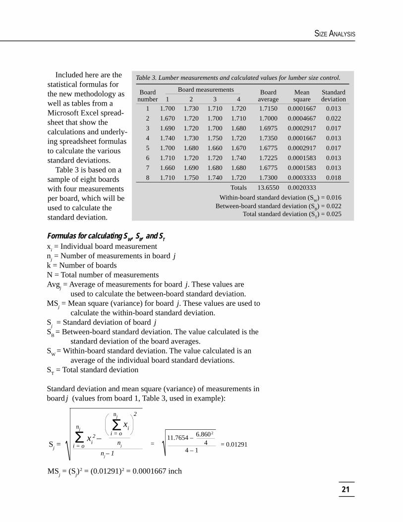
Table 3. Lumber measurements and calculated values for lumber size control.

Board Board Mean Standardnumber 1 2 3 4 average square deviation

1 1.700 1.730 1.710 1.720 1.7150 0.0001667 0.013

2 1.670 1.720 1.700 1.710 1.7000 0.0004667 0.022

3 1.690 1.720 1.700 1.680 1.6975 0.0002917 0.017

4 1.740 1.730 1.750 1.720 1.7350 0.0001667 0.013

5 1.700 1.680 1.660 1.670 1.6775 0.0002917 0.017

6 1.710 1.720 1.720 1.740 1.7225 0.0001583 0.013

7 1.660 1.690 1.680 1.680 1.6775 0.0001583 0.013

8 1.710 1.750 1.740 1.720 1.7300 0.0003333 0.018

Totals 13.6550 0.0020333

Within-board standard deviation (SW) = 0.016

Between-board standard deviation (SB) = 0.022

Total standard deviation (ST) = 0.025

Board measurements

Included here are thestatistical formulas forthe new methodology aswell as tables from aMicrosoft Excel spread-sheet that show thecalculations and underly-ing spreadsheet formulasto calculate the variousstandard deviations.

Table 3 is based on asample of eight boardswith four measurementsper board, which will beused to calculate thestandard deviation.

Formulas for calculating SW, SB, and ST

xi = Individual board measurement

nj = Number of measurements in board

j

k = Number of boardsN = Total number of measurementsAvg

j = Average of measurements for board

j. These values are

used to calculate the between-board standard deviation.MS

j = Mean square (variance) for board

j. These values are used to

calculate the within-board standard deviation.S

j = Standard deviation of board

j

SB = Between-board standard deviation. The value calculated is the

standard deviation of the board averages.S

W = Within-board standard deviation. The value calculated is an

average of the individual board standard deviations.S

T = Total standard deviation

Standard deviation and mean square (variance) of measurements inboard

j (values from board 1, Table 3, used in example):

MSj = (S

j)2 = (0.01291)2 = 0.0001667 inch

Sj =

nj – 1

xi2 –Σ

nj

i = o = 0.012914=11.7654 –6.8602

4 – 1

2

nj

Σnj

i = o

xi

22

LUMBER SIZE CONTROL

These are the equations that Microsoft Excel uses to calculatestandard deviation. Table 4 shows the same eight-board samplewith the underlying Excel equations for the calculations above andin Table 3.

Within-board standard deviation:

Between-board standard deviation:

Total standard deviation:

Boardnumber 1 2 3 4 Board average Mean square Standard deviation

1 1.700 1.730 1.710 1.720 = AVERAGE (B4:E4) = Std Dev 2 = STDEV (B4:E4)

2 1.670 1.720 1.700 1.710 = AVERAGE (B5:E5) = Std Dev 2 = STDEV (B5:E5)

3 1.690 1.720 1.700 1.680 = AVERAGE (B6:E6) = Std Dev 2 = STDEV (B6:E6)

4 1.740 1.730 1.750 1.720 = AVERAGE (B7:E7) = Std Dev 2 = STDEV (B7:E7)

5 1.700 1.680 1.660 1.670 = AVERAGE (B8:E8) = Std Dev 2 = STDEV (B8:E8)

6 1.710 1.720 1.720 1.740 = AVERAGE (B9:E9) = Std Dev 2 = STDEV (B9:E9)

7 1.660 1.690 1.680 1.680 = AVERAGE (B10:E10) = Std Dev 2 = STDEV (B10:E10)

8 1.710 1.750 1.740 1.720 = AVERAGE (B11:E11) = Std Dev 2 = STDEV (B11:E11)

Totals = SUM (Board avg.) = SUM (Mean sq.)

Within-board (SW) = SQRT (Sum_Mean_Sq/8)

Between-board (SB) = STDEV (Board avg.)

Total standard deviation (ST) = STDEV (Board_Measurements)

Board measurements

Table 4. Excel formulas for statistical calculations.

ST =

Σi = o

Nx

i2 – Σ

i = o

Nx

i

N

2

N – 1

93.2496 –

32 – 132

54.6202

= 0.02546=

SB =

Σj = o

kAvg

j2

k – 1

Σj = o

kAvg

j

2

k–

=23.310875 –

8 – 1

13.6552

8 = 0.02235

SW =

MSj

k0.0020333

8= 0.01594=

Σj = o

k

23

SIZE ANALYSIS

Typically most mills never calculate the equations in this sectionmanually. Most mills serious about size control buy lumber sizecontrol software to run on a personal computer.

Lumber size control softwareThere are two ways to analyze size measurement data. The first

and least expensive is to use a spreadsheet to calculate SW, S

B, and

ST. The big disadvantage is that a mill does not get much additional

information, nor can managers archive the information and com-bine it over time with other measurements.

From a time and information standpoint, the best way to analyzesize measurement data is with a dedicated, full-feature computer-ized size control program. In addition to calculating sawing varia-tions, such programs provide multiple ways to display results andanalyze size information. They act as databases in which size datacan be stored for later retrieval or combined with measurementstaken at later times. In addition, there are data collection systemsthat connect to digital calipers. These systems greatly increase thespeed and efficiency of taking measurements. They have someonboard data analysis capabilities and, most important, can down-load measurements directly into their PC-based size controlprograms. Check trade publications and the Internet to learn moreabout what specific software programs have to offer.

Sawing accuracy benchmarks for softwoodsTable 1 (page 11) lists some sawing-accuracy benchmarks that

represent the current abilities of sawing-machine centers to cutsoftwoods accurately. In general, rotary gangs saw lumber mostaccurately, bandmill carriage systems the least accurately. In asmall-log sawmill, all rotary gangs should be cutting with an S

T of

0.015 inch or less, and all resaws at 0.025 inch or less. Shiftingedgers tend to be the least accurate.

24

LUMBER SIZE CONTROL

The future of size controlAs long as sawmills exist, they will need to evaluate individual

machine centers. Currently, using manually operated caliperdevices is the most common way to collect size information. But in5 to 10 years, manually collecting size information will be doneonly in special troubleshooting cases. By then, most lumber sizemeasurements will be made by extremely accurate automatedsystems.

Currently there are two technological reasons that automatedsize control methods have not been successful commercially. Firstis that lasers and other noncontact measuring methods cannotmeasure lumber to a 0.005- to 0.010-inch precision in the mill—the precision necessary to equal dial caliper measurements.Second, current systems cannot identify which machine centerproduced which board. Both these limitations will be overcome inthe next few years. When that happens, sawmill size controlprograms will evolve into an even more effective tool. No longerwill quality control personnel have to spend so much time measur-ing lumber. They finally will be free to focus their efforts onanalyzing what the numbers are telling them. They also will havemore time to conduct recovery and other types of studies that helpdetermine where to focus QC efforts for the greatest benefit.Indeed, lumber size control will become even more meaningful toa mill’s overall QC program because the data collected by auto-mated systems will provide a more complete view of a machinecenter’s sawing capability.

Keeping target sizes smallis not just a sawing variation issue

A mill’s size control program focus must extend beyond thesawmill if it is to be successful. What good does it do to put a greatamount of effort into a size control program but ignore how wellthe kilns dry the lumber? Overdried lumber shrinks and warpsmore and can create the illusion that undersize at the planer is dueto sawing too thinly in the mill. Likewise, if the planer’s bottomhead is set to take off too much, the result can be undersize lumber.In either case, the “solution” probably will be to saw thicker andwider lumber in the mill—even though the problem was not at themill but at the kilns or planer.

The solution is to view quality control as much more than sizecontrol, and to view size control as much more than just whathappens in the sawmill. It takes everyone’s concentrated efforts to

Size control programs…

must extend beyondthe sawmill if they areto be successful.

25

SIZE ANALYSIS

maintain excellence in all phases of manufacturing. The definitionI like for quality control is “maximizing the value of the log andlumber product through all phases of manufacturing while main-taining or increasing production and meeting the needs of internaland external customers.”

The attitude of size controlThe true value of size control is the management philosophy that

accompanies the arithmetic. The philosophy seeks to systemati-cally identify opportunities, then respond to make improvements.The process described here is only the arithmetic to estimate areasonable target size. The philosophy goes beyond this. The day isapproaching when boards will be measured automatically in theprocess flow and all calculations will be by computer. But thephilosophy of size control will continue. Quality-control personnelmust continue to identify opportunities systematically and thenrespond by making improvements.

26

LUMBER SIZE CONTROL

ReferencesBrown, T.D., ed. 1982. Quality Control in Lumber Manufacturing

(San Francisco: Miller Freeman). 288 pp.Brown, T.D. 1982. Evaluating size control data. In: T.D. Brown,

ed. Quality Control in Lumber Manufacturing (San Francisco:Miller Freeman).

Brown, T.D. 1986. Lumber size control. Special Publication No.14, Forest Research Laboratory, Oregon State University,Corvallis, OR. 16 pp.

Warren, W.G. 1973. How to measure target thickness for greenlumber. Information Report VP-X-112, Western Forest ProductsLaboratory, Canadian Forest Service, Vancouver, BC. 11 pp.

27

SIZE ANALYSIS

Ordering informationTo order additional copies of this publication, send the complete

title and series number, along with a check or money order madepayable to OSU, to:

Publication OrdersExtension & Station CommunicationsOregon State University422 Kerr AdministrationCorvallis, OR 97331-2119Fax: 541-737-0817

We offer a 25-percent discount on orders of 100 or more copiesof a single title.

You can view our Publications and Videos catalog and manyExtension publications on the Web at http://eesc.orst.edu

This publication is part of a series, PerformanceExcellence in the Wood Products Industry. The variouspublications address topics under the headings of woodtechnology, marketing and business management,production management, quality and process control,and operations research.

For a complete list of titles in print, contact OSUExtension & Station Communications (address below) orvisit the OSU Wood Products Extension Web site athttp://www.orst.edu/dept/kcoext/wood.htm

PERFORMANCE EXCELLENCEIN THE WOOD PRODUCTS INDUSTRY

ABOUT THIS SERIES

28

LUMBER SIZE CONTROL

© 2000 Oregon State University

This publication was produced and distributed in furtherance of the Acts ofCongress of May 8 and June 30, 1914. Extension work is a cooperative programof Oregon State University, the U.S. Department of Agriculture, and Oregoncounties.

Oregon State University Extension Service offers educational programs,activities, and materials—without discrimination based on race, color, religion,sex, sexual orientation, national origin, age, marital status, disability, ordisabled veteran or Vietnam-era veteran status. Oregon State UniversityExtension Service is an Equal Opportunity Employer.

Published June 2000.