PARKER'S DYNAMO AND GEOMAGNETIC REVERSALS

M. RESHETNYAK1, D. SOKOLOFF2

1Institute of the Physics of the Earth, Russian Acad. Sci., 123995, Moscow, Russiae-mail adress: m.reshetnyak@gmail.com

2Department of Physics, Moscow State University, 119899, Moscow, Russiae-mail adress: sokoloff@dds.srcc.msu.su

In accordance with basics of the dynamo theory the observable large-scale magnetic

fields in the various astrophysical bodies associate with the break of the mirror symmetry of theflow. Usually, this break is caused by rotation of the body [1]. It appears, that existence of

rotation and density gradient is enough for correlation of the turbulent velocity v and its vorticity

w=rot v, what leads to the non-zero kinematic helicity: c=<v×w>, where <...> denotes averaging.

In the simplest case one assumes, that helicity has negative sign (for the self-gravitating bodies)

in the northern hemisphere and positive sign in the southern one, e.g. in the form c=-cos (J),

where J is an angle from the axis of rotation. Existence of the non-zero c makes easier

generation of the large-scale magnetic field.

However there are many reasons why c in the realistic physical applications can havemore complicated form. Some models, where together with equations for the magnetic field B

differential equation for c is solved [2]. Even for the geodynamo problems with prescribed c one

can expect that the non-uniform heat-flux at the core-mantle boundary can produce some

fluctuations of c. Similar situation can arise for the binary connected objects. Moreover, these

fluctuations can arise as a result of the limited number of statistics when c is computed for the

particular velocity field v [3]. These ideas motivated us to study how already for the kinematic

regime the small fluctuations of helicty c (and related with it a-effect) can change the final form

of the linear solution. For this aim we considered the eigen value problem for the well-knownParker's dynamo equations. The obtained results are relevant for the geodynamo and solar

dynamo applications. We also consider important point what sign of the dynamo number in theParker's dynamo is more suitable for the geodynamo applications and its relation with reversals

of the geomagnetic field.

One of the simplest dynamo models is a one-dimensional Pakrers's model of the form

[1,4]:

¶A/¶t=aB+A'', ¶B/¶t=-Dsin(J)A'+B'',

where A and B are azimuthal components of the vector potential and magnetic field, D is a

dynamo number, which is a product of the amplitudes of the a- and w-effects and primes denote

derivatives with respect to J. Equations are solved in the interval 0£J<£p with the boundary

conditions A=B=0 at J=0, p. Generation of the magnetic field (Br, B), where Br=A' - is a radial

component of the magnetic field, is a threshold phenomenon. It starts, when D is larger than

some critical value Dc. Here we consider the eigen value problem for these equations with a=cos

(J), see Fig.1a,b, where the complex growth rate g for the first three modes is presented. The

positive values of the real part Âg correspond to the growing solutions. These modes are sorted

in such a way, that the maximal growth rate is denoted with circles, then follow squares, and the

minimal growth rate corresponds to triangles. With increase of D (D>0) the first stationary (S)

mode (which imaginary part Ág is zero) appears. This mode is a quadrupole (Q). Increase of D

leads to the bifurcation of the second oscillatory dipole mode (OD). Ág characterizes frequency

of oscillations. Symmetry of Ág in respect to D-axis is connected with existence of the conjugate

solution. It appears that with increase of D Âg2 becomes larger than Âg1. The oscillatory solution

is a wave, which propagates from the equator to the poles.

Figure 1. Dependence of Âg (a) and Ág (b) on D for C=0 (a, b) and C=0.1 (c, d) for the first three modes in

the order of decaying Âg (circles, squares and triangles). The insets correspond to the scaled-up regions.

Figure 2. The butterfly diagrams of Br (left column) and B (right column) of the oscillatorydipole (a, b) and stationary quadrupole solutions (c, d) for D=200 and C=0. Similar plots e, f, g,h for C=0.1. The dipole solution corresponds to the circles, quadrupole solution - to the squares,

see Fig.1. The typical blurring for the oscillatory solution is observed. The stationary(quadrupole) solution has a weak dependence on C.

Figure 3. The butterfly diagrams of Br (left column) and B (right column) of the oscillatory quadrupole (a, b),oscillatory dipole (c, d) and stationary dipole (e, f) solutions for D=-1000 and C=0. Similar plots g, h, i, j, k, l

for C=0.1. The quadrupole solution corresponds to the circles, and two dipole solution - to the squares andtriangles, see Fig.1. Non-zero C leads to i) penetration of Br-quadrupole wave from the northern hemisphereto the southern one and damping of the quadrupole B-wave in the southern hemisphere; ii) damping of theoscillatory dipole Br - and B-waves in the northern hemisphere. The stationary solution is still unchanged.

The further increase of D leads the change of SQ-mode to OQ-mode, also propagating to thepoles.

For D<0 the first mode is SD. Then OQ-mode, which is a wave, propagating from thepoles to the equator, appears. For the large negative D there are already three modes: OD, OQ

and SD.

To introduce fluctuation of the a-effect we consider change of the mean (zero) value of

a

up to some small value C: a®a+C. The first glance at the behavior of g does not reveal any

significant changes in the spectrum, see Fig.1. However it does not mean, that nothing changed

in the system. It appears, that the form of the eigen solution is more sensitive to fluctuation C. To plot

the complex eigen functions we introduce the butterfly diagrams Â((Br, B) exp(iÁg)), see

Fig.2,3. Comparison of oscillatory modes with C=0 and C=0.1 gives that already small

fluctuation of a leads to the significant change of the eigen solution: the form of solution

becomes blurred Fig.2a,e and what is more important - asymmetry of the hemispheres becomes

apparent. It is well observed for OD-mode for B component, see Fig.2b,f, 3d,j where themagnetic field in the southern hemisphere is smaller then in the northern one. The other

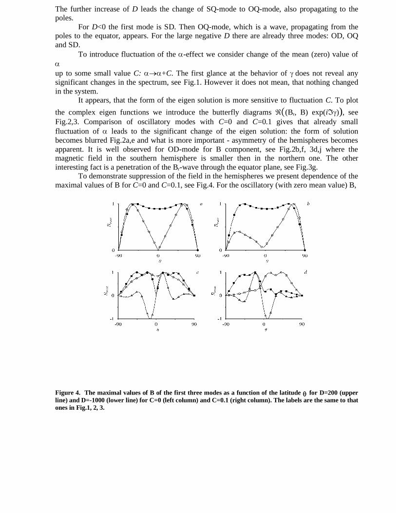
interesting fact is a penetration of the Br-wave through the equator plane, see Fig.3g. To demonstrate suppression of the field in the hemispheres we present dependence of the

maximal values of B for C=0 and C=0.1, see Fig.4. For the oscillatory (with zero mean value) B,

Figure 4. The maximal values of B of the first three modes as a function of the latitude q for D=200 (upperline) and D=-1000 (lower line) for C=0 (left column) and C=0.1 (right column). The labels are the same to thatones in Fig.1, 2, 3.

Figure 5. Distribution of the averaged on azimuthal direction kinematic helicity c (a), differential rotation W

(b) and their product cW (c) in the 3D-model of the thermal convection in the spherical shell for the modifiedRayleigh number Ra=102, Prandtl number Pr=1 and Ekman number E=10-4. The maximal values correspondto the white color, the dotted isolines - to the negative values.

Bmax(q) for C=0 is a positive symmetrical in respect to equator plane function. The non-zero C

leads to suppression of B in the southern hemisphere. As we already noted, fluctuation C doesnot change stationary solution. For D<0 the non-zero C leads to damping of OQ-mode in the

southern hemisphere and of OD-mode in the northern hemisphere. The exact answer why the small value of C leads to suppression of generation in one

hemisphere is addressed to the future linear analysis. Now we only can propose somesuggestions on this problem. So as this phenomenon appears when solution is oscillatory, then

we suppose, that it is concerned with the interference of the original wave and a new one causedwith bifurcation C. It is worthy to note, that C has the quadrupole symmetry in respect to the

equator plane. It means, that the new mode produced by C has opposite symmetry to the originalwave. Superposition of these modes can lead to suppression of the field generation in one

hemisphere.To apply our results to the geodynamo we need to fix a sign of the dynamo number D,

which is responsible for the direction of the wave propagation. For the solar dynamo situation isclear: the wave propagates from the poles to the equator and D is negative. For the geodynamo

situation is more difficult. May be the first estimate of sign of D in the Earth's core belongs toOlson, who, based on the structure of the flows in the liquid core of the Earth supposed, that D is

positive [5]. The more certain information on sign of D can be obtained from 3D numerical

simulations [6]. Here we present the typical distribution of the averaged helicity c, differential

rotation W=¶Vj/¶r based on the radial gradient of the azimuthal velocity and their product, which

give the sign of D (in the northern hemisphere), see Fig.4. It should be mentioned, that generallyused in geodynamo Boussinesq models of convection have limited sources of helicty generation.

So as liquid metal supposed to be incompressible, helicty can be generated in Ekman layes andby the cyclone convection. Increase of Rayleigh number can destroy vertical columns and move

helicty to the boundary layers. Presented results in Fig.4 correspond to the Rayleigh a few timeslarger than its critical value. Finally, we are close to conclude, that D is positive in the Earth's

core.Consider the first possibility, D>0. Following linear analysis presented above we have

transitions with increase of D of the form: SQ ® OD+SQ ® OD+OQ. Here and below modes in

sum are ordered in decreasing order of Âg. To describe change of regime with rapid to seldomreversals we need to find such a D, that OD changes either to SD or to OD+SD. The latter one

corresponds to the regime in vascillation. We do not observe such kind of transitions for D>0.

Case D<0, with SD ® SD+OQ ® OQ+OD+SD, which is more attractable for the solar

dynamo, appears to be more useful for the geodynamo also. It means, that for D near to the

threshold of generation reversals are absent. Increase of D leads to the bifurcation of OQ-mode,which can be associated with excursions of the geomagnetic field: the so-called failed reversals,

when the virtual dipole comes to the equator plane and then returns back. The further increase ofD gives us a new bifurcation with a dipole solution in vascillations. These oscillations

accompanied with a OQ-mode which introduce asymmetry in the hemispheres. References[1] Parker, E.N. Astrophys. J. 1955. 122. 293-314. [2] Kleeorin, N., Rogachevskii, I., Ruzmaikin, A. Astron. Astrophys. 1995. 297. 159-167.[3] Hoyng, P. Astron. Astrophys. 1993. 272. 321-339.[4] Ruzmaikin, A.A., Sokoloff, D.D., Shukurov, A.M. Magnetic Fields of Galaxies. Dordrecht : Kluwer. 1988.

279p.[5] Olson, P., Coe, R.S., Driscoll, P.E., Glatzmaier, G.A., Roberts, P.H. Phys. Earth Planet. Int. 2010. 180. 66-79.[6] Hejda, P., Reshetnyak, M. Stud.Geophys.Geod. 2004. 48. 741-746.