California State University, San Bernardino California State University, San Bernardino

CSUSB ScholarWorks CSUSB ScholarWorks

Theses Digitization Project John M. Pfau Library

2006

Parallel programming on General Block Min Max Criterion Parallel programming on General Block Min Max Criterion

ChuanChe Lee

Follow this and additional works at: https://scholarworks.lib.csusb.edu/etd-project

Part of the Software Engineering Commons

Recommended Citation Recommended Citation Lee, ChuanChe, "Parallel programming on General Block Min Max Criterion" (2006). Theses Digitization Project. 3065. https://scholarworks.lib.csusb.edu/etd-project/3065

This Thesis is brought to you for free and open access by the John M. Pfau Library at CSUSB ScholarWorks. It has been accepted for inclusion in Theses Digitization Project by an authorized administrator of CSUSB ScholarWorks. For more information, please contact scholarworks@csusb.edu.

PARALLEL PROGRAMMING ON GENERAL

BLOCK MIN MAX CRITERION

A Thesis

Presented to the

Faculty ofCalifornia State University,

San Bernardino

In Partial Fulfillment

of the Requirements for the DegreeMaster of Science

in

Computer Science

byChuanChe Lee

September 2006

PARALLEL PROGRAMMING ON GENERAL

BLOCK MIN MAX CRITERION

A ThesisPresented to the

Faculty of

California State University,

San Bernardino

byChuanChe LeeSeptember 2006

Approved by:

Dr. Richard Botting

© 2006 ChuanChe Lee

ABSTRACT

General Block Min Max Criterion (GBMM) is a

pre-2D-chopped robust estimation method designed by Dr.

Schubert. It may be applied on image clarification,

pollution detection ... etc. This thesis tries to

parallelize GBMM method not only to speedup it, but also

to see whether a pre-chopped algorithm is suitable to be

implemented in checker-board method or not.

iii

ACKNOWLEDGMENTS

The support of God is gratefully acknowledged. Trust

in the LORD with all your heart, and lean not on your own

understanding; In all your ways acknowledge Him, And He

shall direct your paths. Do not be wise in your own eyes; Fear the LORD and depart from evil. (Proverbs 3:5-7, NRSV)

I would first thank Dr. Keith Schubert, my advisor,

who has encouraged me through my studies at California

State University, San Bernardino. He explained to me in

detail his dissertation so that I could start my master's

thesis. He has also helped me to solve problems involving

the machines I have used to run my thesis program. He has

given me insights about how to design my thesis. I am

grateful to Dr. Schubert for all these and many other helps that I have received from him.

Thanks also go to Dr. Ernesto Gomez, who has taught

me C++ so that I could resume coding in that language

after more than ten years' suspension. Dr. Gomez has also helped me with hardware, interface and software problems.

I would thank Dr. Richard Botting, who has taught me

concepts of programming languages and shown kind concern

for my health.

Thanks also go to Dr. Owen Murphy, who was one of my

committee members. He taught me computation theory and

iv

algorithm. He explained to me in detail the structure of a

thesis proposal so that I could start writing my thesis.

I would thank Yenru Tzeng, my wife, who has taken

care of me and my two kids during my studies at California State University, San Bernardino.

I would also thank Mr. Brian Finch, who has helped me

with English language problems for almost three years.

I am grateful to Dr. Raymond Klefstad, a Professor of Electrical Engineering & Computer Science at University of

California, Irvine. Dr. Klefstad provided me with a chance

to use the Emulab as a backup cluster system.

DEDICATION

To my dear parents who have supported me both

mentally and financially.

TABLE OF CONTENTS

ABSTRACT........................................ iiiACKNOWLEDGMENTS ...................................... ivLIST OF TABLES....................................... ixLIST OF FIGURES...................................... xCHAPTER ONE: BACKGROUND

1.1 Introduction ................................ 11.2 Purpose of the Thesis....................... 11.3 Context of the Problem...................... 21.4 Significance of the Thesis.................. 21.5 Assumptions ................................. 31.6 Limitations ................................. 31.7 Definition of Terms ......................... 41.8 Organization of the Thesis.................. 4

CHAPTER TWO: LITERATURE REVIEW2.1 Introduction ................................ 62.2 The General Block Min Max Criterion.......... 62.3 Cannon's Algorithm .......................... 82.4 The Householder QR Decomposition............ 112.5 Parallel QR................................. 132.6 Summary..................................... 13

CHAPTER THREE: METHODOLOGY3.1 Introduction................................ 143.2 Reduce Parallel Overhead .................... 14

vi

3.2.1 Reduce Redundant CalculationParallel Overhead ..................... 15

3.2.2 Reduce Communication ParallelOverhead............................. 15

3.3 General Methods............................. 163.3.1 Delete Unnecessary If................ 163.3.2 Loop Unrolling for Parallel

Overhead............................. 173.4 About Cannon's Algorithm.............. 183.5 Multiplication.............................. 20

3.5.1 Row-Vector Matrix Multiplication ..... 203.5.2 Diagonal-Matrix Multiplication ....... 21

3.6 The Transpose............................... 233.6.1 The Vector Transpose................. 233.6.2 The Matrix Transpose................. 24

3.7 The Householder QR Decomposition............ 253.8 The Solving for x by QR..................... 273.9 The General Block Min Max................... 293.10 The Main Test Program...................... 32

CHAPTER FOUR: RESULTS4.1 Introduction................................ 334.2 Machine Used................................ 334.3 Numerical Result ............................ 34

4.3.1 Standard Matrix Multiplication ........ 344.3.2 Strassen's Algorithm .................. 38

4.4 Result Analysis............................. 42

vii

4.4.1 Small Image Clarification ............. 424.4.2 Speedup.............................. 434.4.3 Pre Block-Chopped Algorithm ........... 43

4.5 Summary...................................... 4 6CHAPTER FIVE: CONCLUSION

5.1 Introduction................................ 475.2 Known Problems That Hinder the Parallel

Speedup..................................... 475.2.1 Problems about Implement QR .......... 475.2.2 The Memory Allocation................ 485.2.3 Using Better MPI Functions ........... 485.2.4 Adjust the Threshold................. 49

5.3 Further Study............................... 50REFERENCES.................................. ......... 52

viii

LIST OF TABLES

Table 1. Time Needed for Ten GBMM Iterations forVector Size from 180 through 1380 for1, 4, 9 and 16 Processors................... 35

Table 2. Speedup on 4, 9, 16 Processors forVector Size from 180 through 1380 ........... 37

Table 3. Time Needed for ten GBMM Iterations forVector Size from 180 through 1380 for1, 4, 9 and 16 Processors................... 39

Table 4. Speedup on 4, 9, 16 Processors forVector Size from 180 through 1380 ...........

Table 5. Simply Test the Time Spend on WholeGBMM (Time W) and on the Last Step of Equation (9) (Time 9) on 1, 4, 9, and 16 Processes. The Ratio of the Time W to the Time 9 is Calculated and Listed Right to the Elements Recording thatTest........................................

41

45

ix

LIST OF FIGURES

Figure 1. Initial Distribution of Blocks among 16 = 42 Processes. . . . :..................... 9

Figure 2. Initial Shift of Cannon's Algorithm so that Each Process Contains Ai,k and Bk,j which are what Matrix Multiplication Requires ................... 10

Figure 3. The Way Cannon's Matrix Multiplication Algorithm Shifts. In C = A * B, Sub-Matrix A needs a Left Shift While Sub-Matrix B Needs an Up Shift................................. 11

Figure 4. The Portion that Each Process Contains to Perform the MatrixDiagonal-Matrix Multiplication ............ 22

Figure 5. The Portion that Each Process Contains to Perform the Diagonal-Matrix Matrix Multiplication ............................ 22

Figure 6. Time needed for ten GBMM Iterations for Vector Size from 180 through 1380 for 1, 4, 9 and 16 Processors.......... 36

Figure 7. Speedup on 4, 9, 16 Processors for Vector Size from 180 through 1380 ......... 38

Figure 8. Time Needed for Ten GBMM Iterations for Vector Size from 180 through 1380 for 1, 4, 9 and 16 Processors........... 40

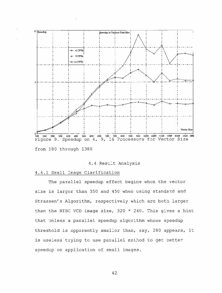
Figure 9. Speedup on 4, 9, 16 Processors for Vector Size from 180 through 1380 ......... 42

Figure 10. A Strange Phenomenon about the Megaflops Drop on Matrix Multiplication. The Unit on x Axis is the Size of Matrix, on y is the Megaflops. No Matter the Code is Compiled with Linux gcc -03 Option or Not, It Drops............................. 51

x

CHAPTER ONEBACKGROUND

1.1 IntroductionThe content of Chapter One presents an overview of

the thesis. The contexts of the problem are discussed followed by the purpose, significance of the thesis, and assumptions. Next, the limitations that apply to the

thesis are reviewed. Finally, definitions of terms are

presented.

1.2 Purpose of the ThesisThe purpose of the thesis is to develop a parallel

implementation of the General Block Min Max Criterion (GBMM) which is designed by Dr. Keith Schubert. [7] GBMM

is a robust estimation1 method which tries to solve Ax = b

where A is a matrix, b and x are vectors, especially when

A is ill-conditioned2. This thesis not only tries to

parallelize GBMM so that it will be performed more

1 Robust estimation is "an estimation technique which is insensitive to small departures from the idealized assumptions which have been used to optimize the algorithm." [11]

2 A matrix is ill-conditioned if the condition number ( k(A) = ||^4 'I'llxlll)

is large. The condition number is a measurement of whether a problem is good to digital computation. The condition number "gives a bound on how inaccurate the solution x will be after approximate solution. Note that this is before the effects of round-off error are taken into account."

1

rapidly, but also tries to see whether a pre block-chopped algorithm may better fit the checker board decomposition3

method or not.

3 Checker board decomposition is a widely used method in parallel implication to get better speedup.

1.3 Context of the ProblemThe context of the problem is to address whether the

block decomposed structure can match the checker board decomposition which is a widely used parallel method. Matrix multiplication is notoriously time consuming, but

is widely used in many fields both in research and

industry, such as physics, chemistry, pollution detection,

image clarification.

1.4 Significance of the ThesisThe significance of the thesis is, at least, twofold.

First of all, robust estimation and identification is

important in many ways as listed in previous sections. But

it usually takes time to calculate. The speedup is an endless desire and a necessity, especially in scientific usage. If we wish to clarify a video instantly for driving

in fog, the speed is definitely important in that

situation. Parallel computing is a good method to speedup.

2

Secondly, whether the structure of an algorithm is an

important issue to parallel or not? As a pre-block-chopped

algorithm, GBMM is a good example to examine.

1.5 AssumptionsAlthough GBMM does not have the following

assumptions, this thesis adds some assumptions listed

below:

1. The matrix A is chopped into equal size.

2. The number of processes used is a perfect square

number, say, 1, 4, 9, 16 ... n etc.

3. All the number of :partitions, q and p, and

matrix size, h and w, are multiple of n, the

square root of the number of processes ; used.

4 . Assume none of the in equation (6) listed

section 2.2 is zero.

1.6 LimitationsDuring the development of the thesis, a number of

limitations were noted. These limitations are presented

here.

This parallel implementation is based on Cannon's

Algorithm which will be briefly introduced in 2.2;

therefore, the number of processes should be a perfect

3

square number. This is the reason why this thesis must

have that assumption.

1.7 Definition of TermsThe following terms are defined as they apply to the

thesis.CPO - Communication Parallel Overhead.

DM - Diagonal Matrix.

Focused process - The process which is doing more work

than the other processes. Usually, process 0 is the

focused process, but not always so.GBMM - General Block Min Max. GBMM is a robust method

proposed by Dr. Schubert.MPI - The Massage Passing Interface. MPI is a library

specification for message-passing, proposed as a standard by a broadly based committee of vendors, implementers, and users.

RCPO - Redundant Calculations Parallel Overhead.

1.8 Organization of the ThesisThis thesis is divided into five chapters. Chapter

One provides an introduction to the context of the

problem, purpose of the thesis, significance of the

thesis, limitations, and definitions of terms. Chapter Two is a review of relevant literature. Chapter Three

4

documents the methodology used in this thesis. Chapter

Four presents the results from the research. Chapter Five

gives the conclusion of the thesis. Finally, the

references for the thesis are listed.

5

CHAPTER TWO

LITERATURE REVIEW

2.1 IntroductionChapter Two presents discussion of the relevant

literature. Section 2.2 describes the GBMM method. Section2.3 illustrates Cannon's Algorithm. Section 2.4 gives an

introduction to the Householder QR decomposition. Section

2.5 mentions parallel QR decomposition. And a brief

summary is presented in section 2.6.

2.2 The General Block Min Max CriterionGeneral Block Min Max Criterion (GBMM) is a robust

method provided by Dr. Schubert. This section describes

general ideas and equations that are used in this thesis.

The general (block) perturbation min max problem is

stated as

4,i+Ei,i

4,1 + ^<7,1

+ Eb,i

bq+Eb^..... (1)

where

A is the coefficient of Ax = b, where A belongs to

3m*n and b belongs to 3m.

q and p are block partition numbers of A on column

and row, respectively.

6

E is the errors in A.

Eb is the errors in b

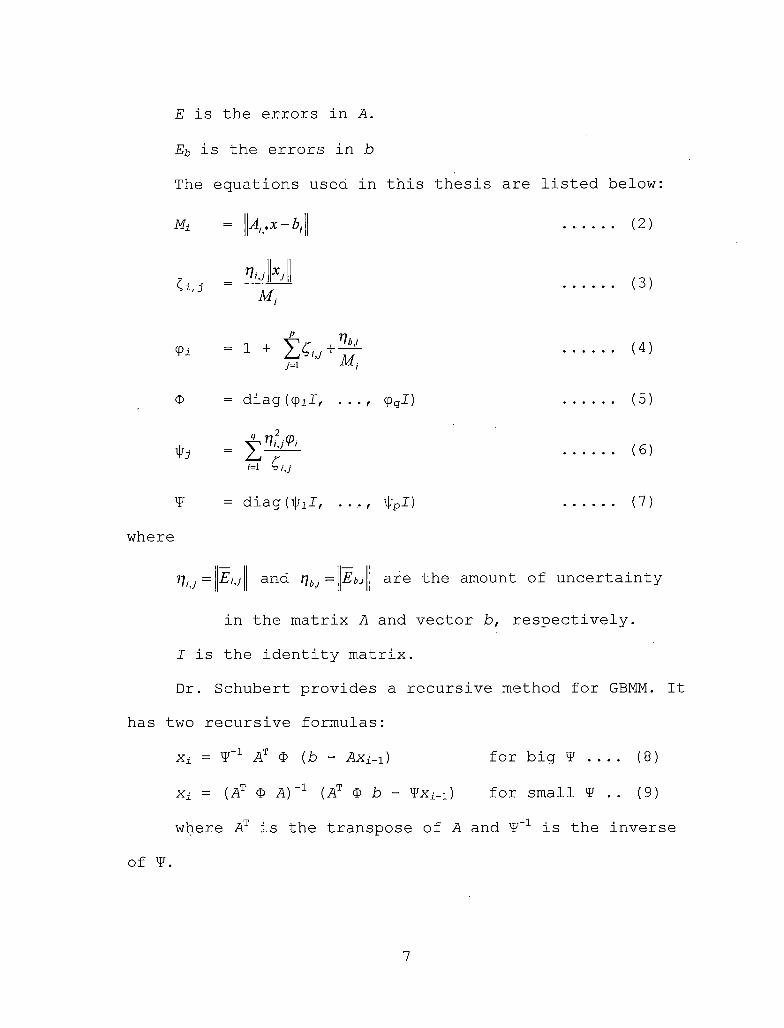
The equations used in this thesis are listed below:

Mi

Ci,J M

<Pi = 1 +>1

+LlM,

<D = diag (<pil, • • • f

W = diag (i|ql, • • • r

----- (2)

..... (3)

..... (4)

<PqI) (5)

..... (6)

typl) ..... (7) where

rhj = and rjbJ = \\E'b,i are the amount of uncertainty

in the matrix A and vector b, respectively.

I is the identity matrix.Dr. Schubert provides a recursive method for GBMM. It

has two recursive formulas:

Xi = T”1 At (b - Axi-i) for big 'P .... (8)

x± = (AT <t> A)-1 (At h? b - WXi-i) for small T .. (9)

where AT is the transpose of A and W_1 is the inverse

of T.

7

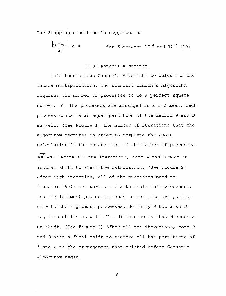
The Stopping condition is suggested as

ip1!' 5 for 5 between 10”4 and 10”8 (10)

2.3 Cannon's AlgorithmThis thesis uses Cannon's Algorithm to calculate the

matrix multiplication. The standard Cannon's Algorithm

requires the number of processes to be a perfect square

number, n2. The processes are arranged in a 2-D mesh. Each

process contains an equal partition of the matrix A and B

as well. (See Figure 1) The number of iterations that the

algorithm requires in order to complete the whole

calculation is the square root of the number of processes,

=n. Before all the iterations, both A and B need an

initial shift to start the calculation. (See Figure 2) After each iteration, all of the processes need to transfer their own portion of A to their left processes,

and the leftmost processes needs to send its own portion

of A to the rightmost processes. Not only A but also B

requires shifts as well. The difference is that B needs an

up shift. (See Figure 3) After all the iterations, both A

and B need a final shift to restore all the partitions of

A and B to the arrangement that existed before Cannon's

Algorithm began.

8

In each iteration, each process does a serial matrix ■

multiplication on the sub matrix the process has now. The

sum of all the iterations in a process, is the answer of the sub matrix that each .process is responsible for.

Ao,o Ao,i Ao,2 Ao,3

Bo.O Bo,i Bo,2 Bo,3

Ai,o Ai(1 Al,2 Al,3

Bi)o Bu Bl,2 Bi,3

A2,0 A24 A2,2 A23

B2,0 B24 B2.2 B2,3

A3,o Au A3,2 a3>3

B3,o B3,i B3,2 b3,3■■■ —Figure 1. Initial Distribution of Blocks among 16 = 4

Processes

9

Ao,o Ao,i Ao,2 Ao,3

Bo,o B1.1 B27 B3,3

Ai,i Ai,2 Al,3 Ai,o

Bi.o B2.1 B3,2 Bo,3

A2,2 A23 A2,0 A2,i

B2,0 B3J Bo,2 Bl,3

A3,3 A3,0 A3,i A3,2

B3.0 Bo,i Bl,2 B2,3Figure 2. Initial Shift of Cannon's Algorithm so that EachProcess Contains Ai,k and Bk,j which are what MatrixMultiplication Requires

10

1___________________ £Ao,o - Ao.i Ao,2 - Ao,3

Bo.o Bi.i B2,2 B3,3t t t f

Am Ai,2 - Al,3 *- Ai.o

Bi,o B2,l B3,2 Bo,3f t f

A2,2 A2,3 - A2,0 - A24

B2,0 B3J Bo,2 Bi,3t f

A3,3 - A3,0 - A3,l A3,2

B3,0 Bo,i Bl,2 B2,3r l— | '—f —oFigure 3. The Way Cannon's Matrix Multiplication Algorithm

Shifts. In C = A * B, Sub-Matrix A needs a Left ShiftWhile Sub-Matrix B Neecls an Up Shift

2..4 The Householder QR DecompositionThis thesis uses QR Decomposition instead of matrix

inversion to calculate the matrix inverse4 in equation . (9)5. The result obtained through the use of QR

4 Dr. Schubert uses Singular Value Decomposition (SVD) to compute the matrix inverse. SVD is more stable than QR but, of course, more complicated than QR.

5 In the case of the diagonal matrix, W, the inverse matrix of W, V"1,

can easily be calculated by inverting all the diagonal cells. Therefore, equation (8) needs neither inverse nor QR.

11

factorization is more stable than the one obtained from

the inverse.QR decomposition forms an orthogonal projector of A

on Q, so that A = QR where Q is an orthogonal matrix and R

is an upper triangular matrix (UTM).

The idea to use QR instead of the inverse is due to

the fact that if

A = QR,

then

Ax = b,

which becomes

QRx = b.

From the above, we can easily obtain

Rx = Q~rb.

Because the only operator of x is the UTM R, it is very

easy to solve for x.

This thesis use Householder QR Factorization to compute the QR decomposition. The implementation of the Householder QR Factorization Algorithm in this thesis can

be written as the following formulas, which closely

resemble those used by Math Lab:

for k = 1 to n

x = Ak-.m,k ..... dD

12

vk = szgw(x1)||x||2e1+x ..... (12)

n = MWL ....... (13)4:m,*:n = ^k-.m,k'.n ~2vk^Vk^k.m,k:n) ...................... (14)

And the Q_1jb is obtained by the following formulas:

for k = 1 to nbk-.m = h-.m-2vk<llbk-.m) ...................... <15)

2.5 Parallel QRThere are some parallel QR algorithms like [2], [4]

[5] or [9]. This thesis applies none of them. Nor does

this thesis use Givens rotation which is more easily

parallelized than Householder transformation. It just

parallelize Householder QR algorithm according to equation

(11) through (14) naively.

2.6 SummaryThe literature important to the thesis was presented

in this chapter. For a full version, please refer to the

bibliography.

13

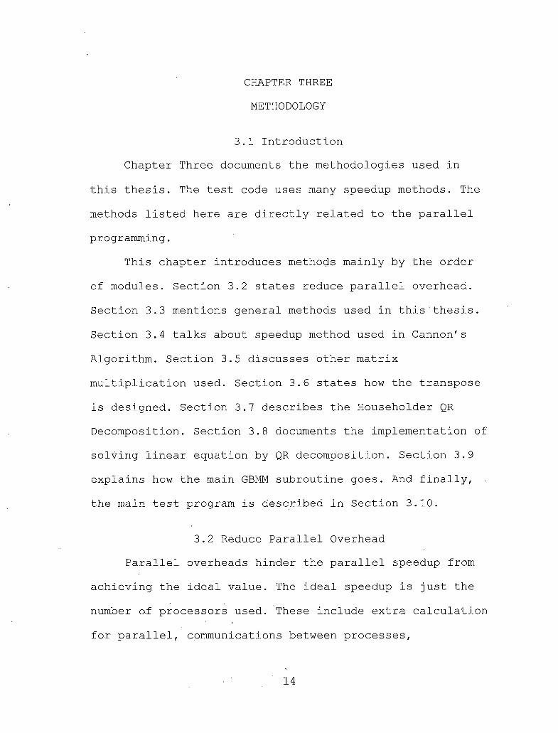
CHAPTER THREEMETHODOLOGY

3.1 IntroductionChapter Three documents the methodologies used in

this thesis. The test code uses many speedup methods. The

methods listed here are directly related to the parallel

programming.This chapter introduces methods mainly by the order

of modules. Section 3.2 states reduce parallel overhead. Section 3.3 mentions general methods used in this thesis.

Section 3.4 talks about speedup method used in Cannon's

Algorithm. Section 3.5 discusses other matrix multiplication used. Section 3.6 states how the transpose

is designed. Section 3.7 describes the Householder QR Decomposition. Section 3.8 documents the implementation of solving linear equation by QR decomposition. Section 3.9

explains how the main GBMM subroutine goes. And finally, the main test program is described in Section 3.10.

3.2 Reduce Parallel OverheadParallel overheads hinder the parallel speedup from

achieving the ideal value. The ideal speedup is just the

number of processors used. These include extra calculation

for parallel, communications between processes,

14

synchronizing the processes, etc. This thesis deals with

two kinds of parallel overheads only: redundant

calculations parallel overhead (RCPO) and communication

parallel overhead (CPO).3.2.1 Reduce Redundant Calculation ParallelOverhead

Redundant calculations parallel overhead are some

calculations required in parallel program but not needed in serial programs. For example, getting the number of

process used, knowing the ranking of this process,

calculation of which portion of data this process is

using, etc.In this thesis, some of these calculations include

the calculation of a process's 2-D coordinates and

ranking, vertical ranking, horizontal ranking and local block size. It uses global variables so that they are

calculated one time only in most cases.3.2.2 Reduce Communication Parallel Overhead

Communication parallel overhead refers to the time

spent on communications between processes which are totally unnecessary in serial programs.

There are many ways to reduce the CPO. In addition to

the checker-board decomposition, this thesis groups

15

information that need to communicate together to reduce

the latency.Another method used in this thesis to reduce CPO is

the application of Cannon's algorithm. See section 3.4 for

details.

3.3 General MethodsSome RCPO is not "calculations." It maybe a simple

if-statement, especially if the if-statement is in a loop,

it may cause detectable timing. This section states how

this thesis deals with this kind of problem.

3.3.1 Delete Unnecessary IfSometimes only the focused process has the correct

answer. For example, at the end of a subroutine, we may

need to write something like

if (id==y) return a;6

6 Unless explained, the programs or partial codes listed in this document are C style.

else return 0;

Because only the id==y has the correct answer, a, letting

all processes return a saves an if-statement on the

process whose rank is y which is. the focused process so

that the parallel overhead will be reduced a tiny bit.

16

For example, when calculating the 2-norm in a

subroutine, each process calculates the sum of the square

of each cell of the sub matrix it owns, and then does a

sum reduction to the focused process. The focused process

does a square root of the total sum, and then returns the answer, which is the 2-norm. The standard way to code on

the last return should be

return id==y ? garbage : sqrt(norm);

The focused process can not start calculating the

square root until the last partial squared sum has been

received which is a short time later than the last message

had been sent. Therefore, though this will cause all

unfocused processes in the same communication group an extra square root calculation, but will save the focused process an if-statement. Hence reduce the parallel

overhead on focused process a tiny bit.3.3.2 Loop Unrolling for Parallel Overhead

Loop unrolling is frequently used to speedup serial

program. It expands loops in some ways to allow instruction rescheduling, better register usage, or reduce

overhead instructions so that the speedup is achieved.

[12]Usually, when a program is parallelized, some extra

if-statement will be used which is a parallel overhead. If

17

this happened in a loop, it usually can be reduced by loop

unrolling. An example used in this research will be stated in 3.4.

3.4 About Cannon's AlgorithmAs briefly noted in 2.3, Cannon's Algorithm needs to

shift both A and.B on each iteration. The B in GBMM is a

const matrix, see equation (9). Keeping all the square

root of the number of process, n, portions of B7 required

for each process in each process will reduce the time

needed for communication, hence save n times of the

communication of one over n2 portion of B. Though it

wastes a little bit more than n times of RAM in each

process, it speedups dramatically.

7 This will reduce the scalability of this algorithm.

The way this thesis uses the advantage of constant matrix B in Cannon's Algorithm is as follows. The whole

matrix B is cut into n columns and scattered to all

processes from process 0. A three dimensional array, ***A,

is used to hold the n portions the process requires. Not

only the content of the ***A is all the value it needs,

but also the order of the content is prearranged to what

it will be used in Cannon's Algorithm. That is, the A[0]

18

in each process contains the portion for the first iteration of Cannon's multiplication this process

requires, A[l] the second, ... A[n-1] contains the last one

required in Cannon's Algorithm.

The preorder treatment for the initial shift in

Cannon's algorithm is done by exchanging the pointer *A,

not by switch the content of ***A so that the parallel

overhead will be reduced. The preordered treatment helps each process to use just the A[i] to compute in the ith

iteration of Cannon's Algorithm. The processes need not to

consider which sub 2-D array to use in this iteration. Not

only no communication is performed for B, but also no

tedious computation is executed.

The way the memory is allocated in ***A is the same as C arranged 3-D array to get better locality in each sub

2-D array, **a, which is what really used in our

algorithm.

About the serial multiplication part of Cannon's

Algorithm,- this thesis use both naively O(n3) standardmatrix multiplication method and O(nlog27) « O(n2’80735)

Strassen's Algorithm to implement it. [10]

19

3.5 MultiplicationMany kinds of matrix multiplication are used in this

thesis, not just the matrix multiplication mentioned in

the previous section. Matrix diagonal-matrix (DM) multiplication, DM matrix multiplication, row-vector

matrix multiplication row-vector column-vector

multiplication and matrix column-vector multiplication are

also used.Among them, only the matrix column-vector

multiplication, DM matrix multiplication and matrix DM

multiplication are implemented in ways that parallel

speedup may easily be detected.

During calculations, sub-matrices and sub-vectors are

distributed among processes. We do not need to gather them to a focused process and redistributed them. This is especially the case when, if we are lucky, the distributed answers are distributed in the way the following calculation needs -- there will be no CPO in this case.

3.5.1 Row-Vector Matrix MultiplicationLet whole 2-D mesh processes contain corresponding

sub matrix. Let each row of processes contain a full set of the row vector as figure 4 for matrix DM

multiplication. After calculation, each row of processes

has a set of the answer.

20

3.5.2 Diagonal-Matrix MultiplicationA DM is a matrix with the property that the values of

the entries that are not on the diagonal are zero.

Therefore, we can use an one-Dimensional array to store

the value of whole DM.The sequence .the DM matrix and matrix DM

multiplication is implemented as follows. Let whole 2-D

mesh processes contain corresponding sub matrix. Let each

row of processes contain a full set of the diagonal of the DM as figure 4 for matrix DM multiplication. Let each

column of processes contain a full set of the diagonal of

the DM as figure 5 for DM matrix multiplication. Thus,

each process contains all the values it needs to calculate

the matrix DM or DM matrix multiplication of its own portion.

21

Mo,o Mo,i Mo,2 Mo,3

Do Di d2 D3

Mi,o Mu Ml,2 Mi,3

Do Di D2 D3

M2,0 M2,i M2,2 M2,3

Do D. d2 d3

M3,0 M34 M3,2 M3,3

Do Di D2 d3Figure 4. The Portion that Each Process Contains toPerform the Matrix Diagonal-Matrix Multiplication

Do Do

Mo,o Mo,i

Do Do

Mo,2 Mo,3

Di Di

M.,o M,j

D2

M2,o

D2

M2,i

0co .

£Q Q

Di Di

Mi,2 M1.3

D2 d2

M2,2 M2,3

d3 d3

M3,2 M3,3Figure 5. The Portion that Each Process Contains toPerform the Diagonal-Matrix Matrix Multiplication

22

Thus, there will be no CPO if the DM was stored as

the multiplication demanded before the multiplication

begins.

3.6 The TransposeBoth the vector and matrix may need to be transposed.

The vector or matrix may be in focused process before the

transpose is required or the vector or matrix has been scattered in processes already. Though this will have four

different situations, the thesis used only two of them:

vector transpose when the vector has been scattered and matrix transpose when the matrix is in the focused process

only.

3.6.1 The Vector TransposeIn this thesis, all vectors are stored as

one-dimensional array. It depends on the function to interpret whether it is a column vector, row vector, or, even the diagonal of a DM.

Before entering the subroutine, all vectors had been row wise or column wise scattered among processes already.

In the subroutine, calculate local size first, and then

allocate memory for transposed vector. If the process is

on the diagonal of the process 2-D mesh, copy the original

values to the memory prepared for transposed vector.

23

Otherwise, calculate the rank of the destination process,

send to and receive from the destination process the

vector. Return the pointer points to the transposed

vector.3.6.2 The Matrix Transpose

The only one transpose happens in this thesis is at

the beginning of the GBMM subroutine where the deblur

matrix is stored in the focused process before been

scattered and transposed.In the matrix transpose subroutine, calculate local

size first, and then allocate memories for both communication buffer and transposed sub matrix. The

focused process calculates the rank of each process,

gather corresponding sub matrix to a continuous RAM, scatters the corresponding part of the sub matrix to correct processes.

Note that only the content of the sub matrix, **A,

are transferred. The index of the **A, *A, are calculated

at the time the memory is allocated because both the sent

and the received sub matrices are of the same arrangement

and the same size. Thus, eliminate the unnecessary communication which is a redundant CPO.

The order to scatter the matrix is from the largest

rank to the smallest rank,- the focused one. This will save

24

a memory block on the focused process and save the time to

copy from transfer buffer to the working buffer.Each process begins transposing its own sub matrix

after it has received the values it required. Then, free

up the transfer buffer.

3.7 The Householder QR DecompositionIn the Householder QR decomposition subroutine, it

calculates local size first, and then allocates memories for r, R, v, and V, where V is the matrix that collects the reflection vectors (RV), v. The final step of the

initial work is copy A into R. Because x is useless after

equation (12) and is almost the same as v except for the

first element, there is no x exist in RAM. The v totally

handles all the functions x need.In implementing the loop of the Householder QR

decomposition, it calculates the local size of k:m and k:n

(see equation (11)), gets the rank, id_now, of the process

which contains the current k, place the if-statement which

judges the process coordinates outside the loop of

partial-squared-sum calculations to reduce the RCPO in

loop, send the answer to the focused process, and sums the

answer up to get the squared sum, n2, of the vector. The

process whose rank is id_now calculates the square-root of

25

n.2 to get the 2-norm of x. Change the value of the first

element of v according to the equation (12).

About the equation (13) , calculate the 2-norm of v

through change of n.2, broadcast the 2-norm of v to those

who are in the same column of the focused process, the one

whose rank is id_now, in the process 2-D mesh. Then the

processes that contain the useful part of v normalize v.{Now start dealing with the equation (14). Broadcast

the useful part of v horizontally so that the distribution

of v matches the condition that the row-vector matrix

multiplication needs. If the process contains useful part

of v, make a pointer array, *s, in which each element

points to a special address of A so that **s is just the

sub matrix that equation (14) requires. Multiply row

vector v and the sub matrix, **s. Otherwise, make an array that all the elements value are zero which represent the answer of zero vector times a sub matrix. Do a

sum-reduction in the processes that are in the same column

of the focused process. Broadcast the result, v', to

processes that are in the same column of the focused

process. Separate this column of processes into four groups according to the position that the process relates to the focused one so that there is no RCPO in the loop

26

when doing the final part of equation (14),

= Ak.mk.n -2vjt(v') . Copy the answer to the V matrix which

consists of the v. Free up memories, set the return

pointer points to V.

3.8 The Solving for x by QRConsider the linear equation Ax = b, where A is a

matrix and b and x are vectors. The solution can be found

by QR factorization of' A, if A is not singular, as

following:

A x = b

,QR x = b

R x = Q~1b

Then, solve for x through the last equation by

back-substitution because R is a UTM (see section 2.4).

And the <2_1b can be obtained by the equation (15) listed in section 2.4.

The parallel implementation of the equation (15) is

preceded by calculation of local matrix size. Then, copy

vector b to a temporary vector, qb, call QR decomposition

function to get V and R, where V is the matrix that

collects the reflection vectors (RV), v.

In the main part of the equation (15), starts a loop

from zero to number of processes used -1, n-1, as the

27

index for columns of 2-D process mesh. Then, if the

processes contain' the value of the RVs, send the whole sub

V matrix to the processes in the first column in

corresponding row. Start a loop from zero to the width of the local matrix minus one. Separate the processes in the

first column into three groups according to what it

contains about v: no valid v, partial v, or full v to

calculate the partial 2(v*kbk.m) . Call MPI_Allreduce to get

the sum of the partial 2(y*kbk.m') , the true 2(v*kbk.m) . Calculate

the bk.m = bk.m-vk(2vkbk.m) . Broadcast the qb horizontally to

match the parallel back-substitution requires.The sequence of the back-substitution is listed

below. The pretreatment includes calculating the local

matrix size, allocating memories, making a copy of vector b so that the b will remain unchanged after this calculation and calculating the last equation am,n xn = bm.

For the loop part, the outer loop runs from n-1 down to zero while the inner loop runs from local width minus

one, wl, down to one. The two nested loops form the whole

range of the width of the original matrix. Vertically

broadcast the xm which has been pre-calculated in the

pretreatment or previous iteration. Let all the processes

on the same column of focused process calculate their own

28

part ofxn_i = [ (bm) - a*,nxn] / a*,n-i. After the inner loop,

broadcast the xlowest_one vertically as the pre-calculated xn of the next iteration of the outer loop. If the focused

process is not in the first column of process 2-D mesh,

send the x to the process left to itself.At the end of this function, free up the memory which

stores the copy of vector b, return the calculated x.

3.9 The General Block Min MaxThe main GBMM routine implements the equations (2) to

(10) listed in section 2.2 to get the answer. It sets all the local global variables8 first to reduce.the RCPL.

8 The global variables are set in the same gbmm.c file only to preserve some data security.

Then, it distributes the deblur matrix, A, to each process

as Cannon Algorithm's matrix B and shift it as mentioned

in section 3.4. The routine transpose it to each process,

then, scatters the vector b, r]b, and the matrix r/ in

checker-board style. Set all xi to 1 as the seed of the first iteration. Set the pointer to b transpose points to b by the fact that b transpose equals to b in process 0,

the focused one. In other process, allocate memory for

transposed vector of b for processes in the first column.

29

Calculate the transposed coordinate and rank. Except for the focused one, all the processes in the first row send its own b to the corresponding processes in the first

column.

In the iteration part, the routine broadcasts x

vertically if this is not the first iteration. Then it

calculates Ax, calculates the equation (2), (3), <I> and Y.

It frees up the memories used by equations (3) and (2). It

transposes 0 to be horizontally distributed so that the

distribution fits the requirement that the matrix DM

multiplication requires. It frees up the memory used by £.

It calculate the AT4>. It frees up the memory used by the

horizontal version of $. Then it calculates the norm of W. It broadcasts the value horizontally so that each process has the norm of T. The threshold to determine to use

equation (8) or (9) is set to be 100.

In the implementation of equation (8), the big W version, the code starts with calculating the inverse of the i|i9. Transpose the distribution of ¥ among processes from horizontally to vertically10. Then calculate the W_1

At<I>. Transpose Ax from the first column to the first row.

9 See footnote e on section 2.4.

10 There is no need to transpose if the processes are on the diagonal, of course.

30

Let the processes in the first row calculate b - Ax and

store it in Ax. Broadcast it vertically. Finally, use the

matrix column-vector multiplication subroutine to

calculate the new x, W"1 (b - Ax) .

In the implementation of equation (9), the small ¥

version, the code begins with calculating the Ar$ b

through matrix column-vector multiplication subroutine.

Then the processes in first row calculate Tx. Transpose

the value of Wx from stored in the first row of processes

to the first column ones. Let the first column processes

calculate the AT<I>b - Yx and store them in the same address

of those who store ATOb. Let all processes calculate AT<I>

A. Use QR subroutine to solve for x in equation (9),

x = (AT<I>jb - Wxi-i) . Free up AT4>b.No matter the norm o.f T is big or small, now start

dealing with the final parts: free up memories used in all

processes. The processes in the first row copy new x,

[lx,. - II calculate equation (10), the -—n—n—- 5, and free up theINI

unused memories and set pointer of x to new one. The

process 0 broadcasts the 5 to all processes, increases the

iteration counter. Finally, all processes check the

condition of whether the next iteration is needed by check

the 5 and iteration counter.

31

After all iterations, free up all the memories used.

Perform a gather action. Finally, free up the memory used

by x.

3.10 The Main Test ProgramThe main test program is written as follows. It reads

in the 27 and the files. The 2-D numbers of partitions

are written in the 17 file. The program generates a random

matrix as an original "image" / vectors sources. Then, generates a random square matrix as the blur matrix. Blur

the "image" by the blur matrix. The uncertainty bound of

the blur matrix is bound by 20% of the maximum of each

partition. Transpose the "image" so that the original

column vectors are continuously stored in memory, that is, it is now row vectors which, in C, is stored continuously.Finally, it starts to deblur the vectors one by one andsets the time stamp just before and after the calling of

the GBMM subroutine.

32

CHAPTER FOUR

RESULTS

4.1 IntroductionIncluded in Chapter Four was a presentation of the

results of the thesis. Section 4.2 states the hardware and

software used. Section 4.3 lists the numerical result.

Section 4.4 analysis the result. Finally, the summary of

the research is stated.

4.2 Machine UsedRaven is the machine that this thesis has used to run

the programs. It is a cluster computer composed of

thirteen Compaq ProLiant DL360 G2 computers. The ProLiant

DL360 G2 has dual Intel® Pentium© III 1.40GHz on board, Ll cache is 128KB, L2 cache is 512KB on-die. Each computer has 512 MB of 133MHz SDRAM 2:1 interleaved. Two Compaq NC

7780 Gigabit Ethernet NICs Embedded 10/100/1000 which are

optimized for best latency, but only one of them is

connected to the router. [14] The router used is D-Link

DGS-3224TG, which is a 20-port managed layer 2 Gigabit

Ethernet switching hub. The operation system used is Red

Hat Linux 3.4.20-8smp with gcc version 3.2.2-5. MPI 1.2 is

used as the interface.

33

4.3 Numerical ResultThis thesis is tested on Raven uses one, four, nine,

and sixteen processors. The 2-D partition number, q and p,

are always the same, namely, twelve and twelve, throughout the test listed in this document. The heights of the

"image" used to test are multiple of 60 from 180 through

1380. The widths of the "image" used to test are all the

same, namely, twelve. The 5- in equation (10) in section

2.2 is set to be IO”30 to cause a virtual infinite loop so that the number of iteration can be controlled. The serial

part of the Cannon's Algorithm is implemented in two

different ways: the standard matrix multiplication and

Strassen's Algorithm.

4.3.1 Standard Matrix MultiplicationThe number of "images" used is ten if the image

height, h, is smaller than 660. It is six if h is 660, 720

or 780. It is five if h is 840, 900, 960 or 1080. It is

four if h is 1020 or 1200. It is three if h is 1140 or

1260. It is two if h is 1320 or 1380. The result of the

time needed and the corresponding graph are listed below.

34

Table 1. Time Needed for Ten GBMM Iterations for Vector

Size from 180 through 1380 for 1, 4, 9 and 16 Processors

7~^._Proc.Size 1 4 9 16

180 0.532 4.760 4.095 6.015240 2.153 7.242 6.431 6.812300 5.658 9.483 8.172 8.526360 12.374 11.220 10.425 10.325420 22.357 14.229 12.602 •12.271480 37.283 17.794 14.773 14.149540 56.412 29.470 17.133 16.280600 77.887 36.044 ■ 19.777 18.303660 105.033 55.879 22.973 21.012720 137.464 66.949 28.255 24.308780 177.919 93.987 35.999 29.239840 223.167 110.904 48.308 34.469900 277.959 145.708 62.328 41.158960 571.489 178.777 83.245 45.703

1020 409.968 214.258 97.979 61.0061080 489.306 257.634 119.555 73.9321140 573.724 297.162 142.294 92.6001200 682.590 351.683 173.309 97.4411260 785.533 398.219 198.378 132.0421320 893.648 463.022 230.760 147.9631380 1020.838 520.903 267.046 173.182

35

Size from .180 through 1380 for 1, 4, 9 and 16 Processors

According to the time recorded, the speedup, which is the ratio between the sequential execution time and the

parallel execution time is calculated, listed and plotted

below.

36

Table 2. Speedup on 4, 9, 16 Processors for Vector Size from 180 through 1380

,'^~\Proc. Size 4 9 16

180 0.112 0.130 0.088240 0.297 0.335 0.316300 0.597 0.692 0.664360 1.103 1.187 1.199420 1.571 1.774 1.822480 2.095 2.524 2.635540 1.914 3.293 3.465600 2.161 3.938 4.255660 1.880 4.572 4.999720 2.053 4.865 5.655780 1.893 4.942 6.085840 2.012 4.620 6.474900 1.908 4.460 6.753960 3.197 6.865 12.504

1020 1.913 4.184 6.7201080 1.899 4.093 6.6181140 1.931 4.032 6.1961200 1.941 3.939 7.0051260 1.973 3.960 5.9491320 1.930 3.873 6.0401380 1.960 3.823 5.895

37

from 180 through 1380'.'

4.3.2 Strassen's AlgorithmThe number of "images" used is all the same, namely,

two, in testing the speedup if the serial part of Cannon's Algorithm is implemented in Strassen's Algorithm. The result of the time needed and the corresponding graph are

listed below.

38

Table 3. Time Needed for ten GBMM Iterations for Vector

Size from 180 through 1380 for 1, 4, 9 and 16 Processors

'^7~~-~^Proc Size 1 ' 4 9 16180 0.532 4.606 4.000 5.959240 1.358 7.298 6.440 6.776300 3.267 9.394 8.257 8.444360 6.722 10.993 10.376 10.306420 11.834 13.047 12.712 12.260480 19.712 15.305 16.838 14.142540 28.973 20.062 16.876 16.373600 42.901 26.185 18.956 18.303660 57.960 36.535 21.293 20.717720 76.145 45.340 24.477 24.114780 97.243 60.519 29.637 27.665840 122.503 73.044 38.079 31.230900 167.043 93.323 47.200 35.660960 229.045 124.835 61.374 39.901

1020 242.863 137.547 71.824 49.5901080 266.533 161.112 88.637 57.7171140 362.473 193.199 102.805 70.7931200 391.721 226.431 127.123 96.3251260 449.664 258.130 141.275 97.7041320 506.156 297.431 163.541 108.8621380 582.519 335.688 187.471 128.020

39

Size from 180 through 1380 for 1, 4, 9 and 16 Processors

According to' the time recorded, the speedup iscalculated, listed and plotted below.

40

Table 4. Speedup on 4, 9, 16 Processors for Vector Size

from 180 through 1380

'\Jroc.Size 4 9 16

180 0.115 0.133 0.089240 0.186 0.211 0.200300 0.348 0.396 0.387360 0.611 0.648 0.652420 0.907 0.931 0.965480 1.288 1.171 1.394540 1.444 1.717 1.770600 1.638 2.263 2.344660 1.586 2.722 2.798720 1.679 3.111 3.158780 1.607 3.281 3.515840 1.677 3.217 3.923900 1.790 3.539 4.684960 1.835 3.732 5.740

1020 1.766 3.381 4.8971080 1.654 3.007 4.6181140 1.876 3.526 5.1201200 1.730 3.081 4.0671260 1.742 3.183 4.6021320 1.702 3.095 4.6501380 1.735 3.107 4.550

41

from 180 through 1380

4.4 Result Analysis4.4.1 Small Image Clarification

The parallel speedup effect begins when the vector size is larger than 350 and 450 when using standard and

Strassen's Algorithm, respectively which are both larger

than the NTSC VCD image size, 320 * 240. This gives a hint

that unless a parallel speedup algorithm whose speedup

threshold is apparently smaller than, say, 280 appears, it is useless trying to use parallel method to get better

speedup on application of small images.

42

4.4.2 SpeedupThe speedup "looks" good on both algorithms when

vector size is smaller than, say, 750. According to Amdahl

effect which says that "for a fixed number of processors,

speedup is usually an increasing function of the problem

size," the curve should not bend down or stay around 2.0,

4.5 and 6.5 on 4, 9 and 16 processors respectively for a

standard algorithm and around 1.7, 3.2 and 4.2 for

Strassen's Algorithm on 4, 9 and 16 processors

respectively. The reason for that may be that the Ethernet

cards on the Raven are optimized for latency but the

algorithms used in this thesis are all designed for

optimized on bandwidth.4.4.3 Pre Block-Chopped Algorithm

The implementation of equations (5) and (7) does not

use the fact that the value in 0> and T are not totally

different. Instead of having different values of the number of the height and width of the deblur matrix, they

have only the number of the partitions, q and p, different

values, respectively. Making use of that fact to implement

the equations (5) and (7), especially the equations (8) and (9) where DM multiplication is dealt with, in parallel

may get a little bit speedup.

43

But by simply benchmark each step of GBMM, the ratio

of the time spent on the final step of equation (9), the

solving x = LT1 ft, to the time spent on the whole GBMM is

huge. It ranges from 0.29 to 0.46 on serial version. It

ranges from 0.58 to 0.96 (the average is 0.664) on four processes test. On nine and sixteen processes test, it

ranges from 0.64 to 0.91 (average 0.732) and 0.65 to 0.91

(average 0.781), respectively. (See Table 5) This shows

that the final step of equation (9) is the bottle neck of

the speedup in this implementation of GBMM, especially the

more processes is used, the more the average of the ratio

is.The fact that more than half of the time is spent on

solving x = fl-1 [3, especially the more processes is used,

the more the average of the ratio is, tells us that unless

there exist an parallel algorithm which can make good use of the pre-chopped characteristic to solve x = LT1 f3, or

there exist an parallel algorithm that can fast and accurate to solve x = 12”1 (3, the pre-chopped nature in

GBMM does not lead to easily parallel speedup through

checker-broad decomposition method.

44

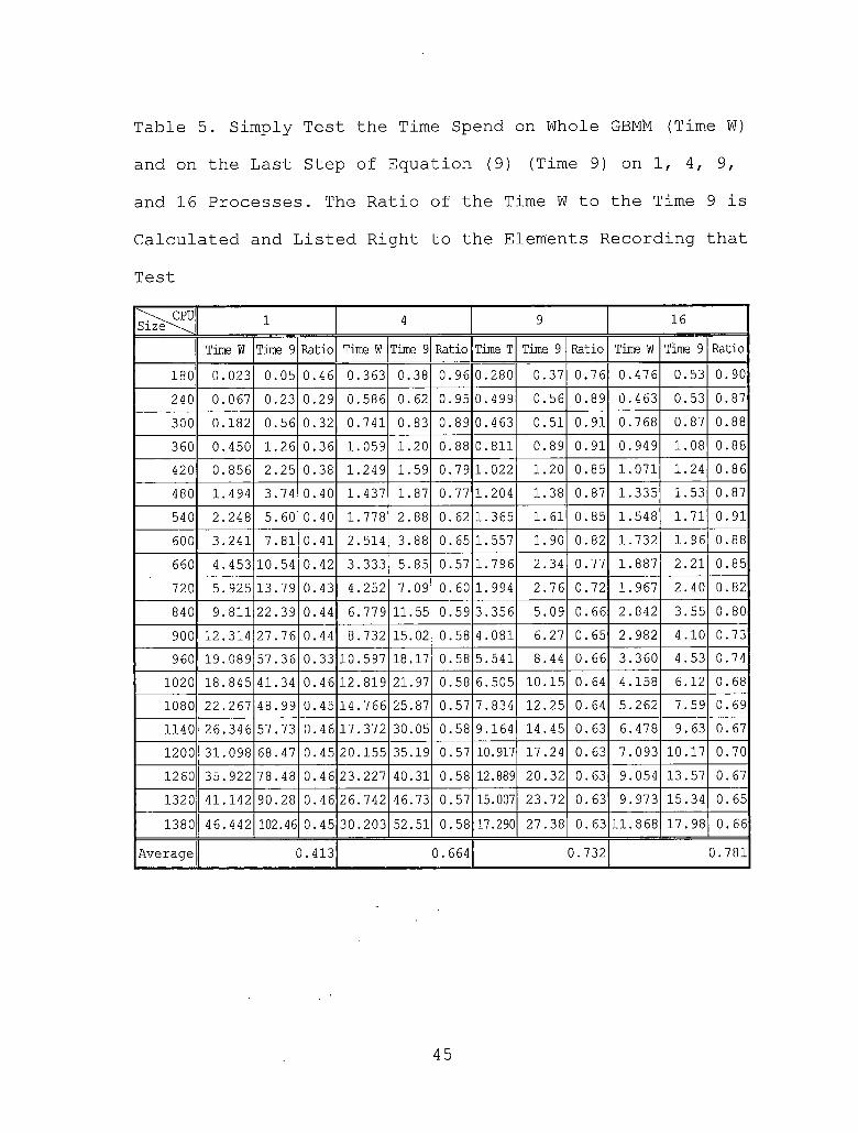
Table 5. Simply Test the Time Spend on Whole GBMM (Time W) and on the Last Step of Equation (9) (Time 9) on 1, 4, 9,

and 16 Processes. The Ratio of the Time W to the Time 9 isCalculated and Listed Right to the Elements Recording that

TestCPUSize'\ 1 4 9 16

Time W Time 9 Ratio Time W Time 9 Ratio Time T Time 9 Ratio Time W Time 9 Ratio180 0.023 0.05 0.46 0.363 0.38 0.96 0.280 0.37 0.76 0.476 0.53 0.90240 0.067 0.23 0.29 0.586 0.62 0.95 0.499 0.56 0.89 0.4 63 0.53 0.87300 0.182 0.56 0.32 0.741 0.83 0.89 0.463 0.51 0.91 0.768 0.87 0.88360 0.450 1.26 0.36 1.059 1.20 0.88 0.811 0.89 0.91 0.949 1.08 0.88420 0.856 2.25 0.38 1.249 1.59 0.79 1.022 1.20 0.85 1.071 1.24 0.86480 1.494 3.74 0.40 1.437 1.87 0.77 1.204 1.38 0.87 1.335 1.53 0.87540 2.248 5.60 0.40 1.778 2.88 0.62 1.365 1.61 0.85 1.548 1.71 0.91600 3.241 7.81 0.41 2.514 3.88 0.65 1.557 1.90 0.82 1.732 1.96 0.88660 4.453 10.54 0.42 3.333 5.85 0.57 1.796 2.34 0.77 1.887 2.21 0.85720 5.925 13.79 0.43 4.252 7.09 0.60 1.994 2.76 0.72 1.967 2.40 0.82840 9.811 22.39 0.44 6.779 11.55 0.59 3.356 5.09 0.66 2.842 3.55 0.80900 12.314 27.76 0.44 8.732 15.02 0.58 4.081 6.27 0.65 2.982 4.10 0.73960 19.089 57.36 0.33 10.597 18.17 0.58 5.541 8.44 0.66 3.360 4.53 0.74

1020 18.845 41.34 0.46 12.819 21.97 0.58 6.505 10.15 0.64 4.158 6.12 0.681080 22.267 48.99 0.45 14.766 25.87 0.57 7.834 12.25 0.64 5.262 7.59 0.691140 26.346 57.73 0.46 17.372 30.05 0.58 9.164 14.45 0.63 6.478 9.63 0.671200 31.098 68.47 0.45 20.155 35.19 0.57 10.917 17.24 0.63 7.093 10.17 0.701260 35.922 78.48 0.46 23.227 40.31 0.58 12.889 20.32 0.63 9.054 13.57 0.671320 41.142 90.28 0.46 26.742 46.73 0.57 15.007 23.72 0.63 9.973 15.34 0.651380 46.442 102.46 0.45 30.203 52.51 0.58 17.290 27.38 0.63 11.868 17.98 0.66

Average 0.413 0.664 0.732 0.781

45

4.5 SummaryNeither deblur small images nor the advantage of the

pre-chopped structure of GBMM can be achieved by the

parallel methods used in this research.

46

CHAPTER FIVE

CONCLUSION

5.1 IntroductionChapter Five presents the conclusion of the thesis.

Lastly, the Chapter concludes with a summary

5.2 Known Problems That Hinderthe Parallel Speedup

There are some known problems that hinder the

parallel speedup. Section 5.2.1 describes problems in the

implementation of QR decomposition. Section 5.2.2 states

the memory allocation problem. Section 5.2.3 suggests

using better MPI functions.5.2.1 Problems about Implement QR

As described in section 4.4.3, the final step of the

equation (9), the solving x = G”1 (3, is the bottle neck of

the parallel speedup in this implementation of GBMM. Therefore, if we want to improve instead of re-design the algorithms used in this research, it is the QR and solve-through-QR that one should first put the effort to.

In the implementation of QR decomposition, there are

many chances that only part of the processes in the same

column as the focused process need to have the value from

the focused one. For example, the upper part of the

47

process may not need to be involved in the communication when k is larger than the height of the matrix over the

square root of the number of process, n. The program

broadcasts the value to all processes in the same column by using standard broadcast function, MPI_Bcast, in stead

of designing a suitable and fast algorithm to send

messages only to the ones that need the value in all the implementation similar to that.

Of course, one may re-design these two algorithms, QR

and solve through QR, through better parallel QR algorithm such as Given's rotation. This should get better parallel

speedup.5.2.2 The Memory Allocation

There are too many memory allocations and frees used in this implementation. Calculate the total memory needed in the beginning of GBMM subroutine and allocate it one time at the beginning of the GBMM main subroutine, calculate all the pointers point to different and suitable address should both speedup the serial version and reduce

some parallel overhead. Hence, the parallel speedup should

be a little bit more than this version.5.2.3 Using Better MPI Functions

MPI has more than four sets of send / receive functions: standard (MPI_Send), nonblocking (MPI_Isend),

48

synchronous (MPI_Issend) and user-specified buffer (MPI_Bsend). For most of the algorithms used in this

research are suitable to use specified send / receive

functions such as user-specified function or synchronous

function. The MPI send / receive functions used in this

research are all basic ones: MPI_Send and MPI_Recv. For example, using user-specified buffering may reduce time

for copying the content.

5.2.4 Adjust the Threshold

Though equation (8), the big W version, is rarely

used in practice, the test code sets threshold to be 100,

which is found to be somewhat too large. The result is that none of the more than 8000 test samples11 run on

equation (8). They all run on equation (9).

11 About 3000 of the test samples are done during the program test. They are not listed in chapter 4.

Equation (8) is faster than Equation (9). It does not need to calculate QR decomposition. The inversion of the

diagonal cells can be fully parallelized so that its parallel speedup is more than Equation (9). Therefore, the average parallel speedup of GBMM should be a little bit

higher.

49

5.3 Further StudyThere are many ways to do further studies. For

accuracy, use singular value decomposition (SVD) instead

of QR to solve the problem. For speed, try to use even find faster parallel speedup method to solve x = A-1 b.

For matching the design, use parallel computer whose

Ethernet cards are tuned for bandwidth and retest this

algorithm.The reason for the outlying point on the one process

version at size 960 is still unknown. It had been run many times during more than two months on three different

Pentium-based computers. It seems to be something related to the problem about matrix multiplication. It was found

that the more the matrix size is related to power of two, the slower it seems to be. The experiments show that the

average Megaflops is around 180 on the test machine, but it drops to around 40 when size is 256, 384, 448, 512, 576, 640, 704, 768, 832, 896, 960, 1024 or 1088. It drops

to around. 120 when size is 320, 448, 544, or 608. It drops

down to around 90 when size is 800, 864. (See Figure 10)

960 is the only test size of GBMM in this research

that hits on one of'the slow point. So it shows a big

outlying point there.

50

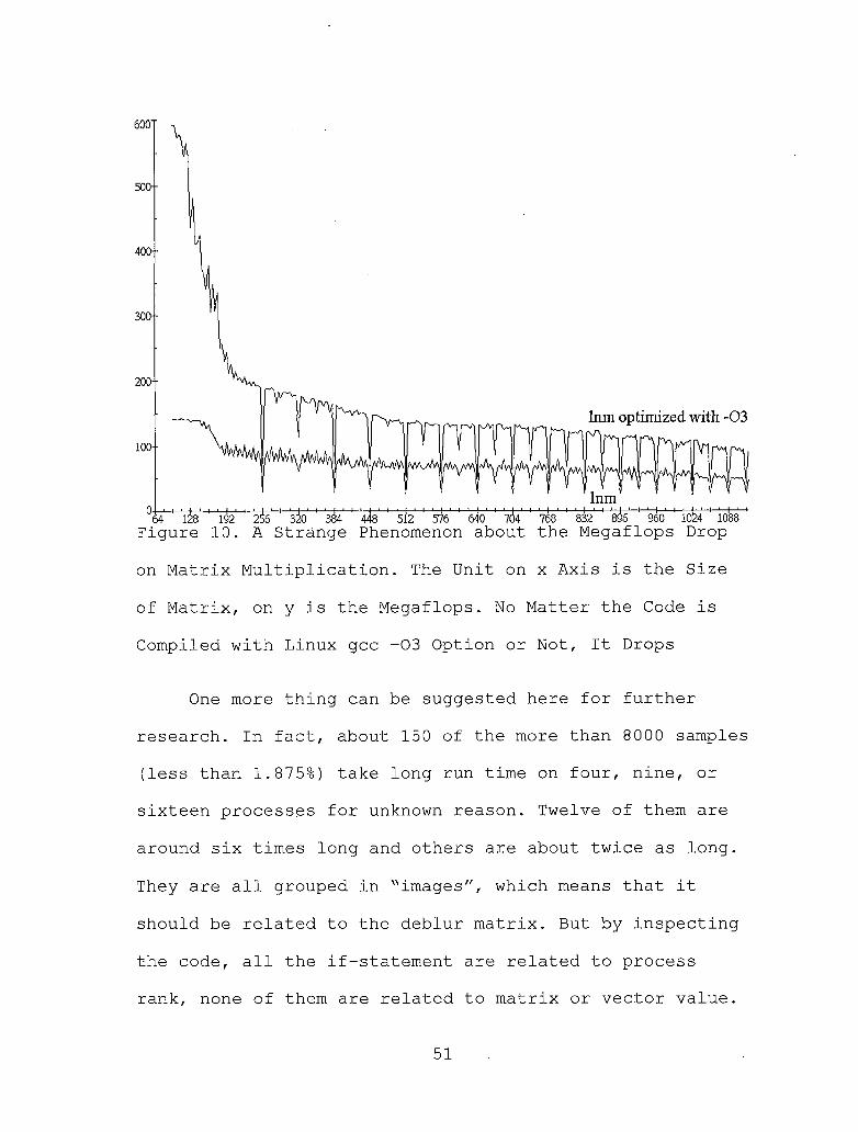
on Matrix Multiplication. The Unit on x Axis is the Size

of Matrix, on y is the Megaflops. No Matter the Code is

Compiled with Linux gcc -03 Option or Not, It Drops

One more thing can be suggested here for further

research. In fact, about 150 of the more than 8000 samples (less than 1.875%) take long run time on four, nine, or sixteen processes for unknown reason. Twelve of them are

around six times long and others are about twice as long.

They are all grouped in "images", which means that it

should be related to the deblur matrix. But by inspecting

the code, all the if-statement are related to process rank, none of them are related to matrix or vector value.

51

REFERENCES

[1] L. E. Cannon, "A Cellular Computer to Implement the Kalman Filter Algorithm", Ph.D. thesis. Montana State University, 1969.

[2] Rotella F., Zambettakis I., "Block Householder Transformation for Parallel QR Factorization", Applied Mathematics Letters, May 1999, vol. 12, no. 4, pp. 29-34(6), Ingenta.

[3] H. F. Jordan and G. Alaghband, "Fundamentals of Parallel Processing", Prentice Hall, Upper Saddle River, NJ, 2003.

[4] Lu, Mi; Liu, Kunlin, "Parallel algorithm for Householder Transformation with applications to ill-conditioned problems", International Journal of Computer Mathematics, v 64, n 1-2, 1997, p 89-101, Compendex.

[5] Shietung Peng; Stanislav Sedukhin; Igor Sedukhin, "Householder bidiagonalization on parallel computers with dynamic ring architecture", Parallel Algorithms / Architecture Synthesis, 1997. Proceedings. Second Aizu International Symposium , 17-21 March 1997, pp. 182 - 191, IEEE Explore.

[6] M. J. Quinn, "Parallel Programming in C with MPI and OpenMP", McGraw-Hill, New York, NY, 2003.

[7] K. E. Schubert, "A New Look at Robust Estimation and Identification", UCSB, 2003.

[8] J. C. Cabaleiro; F. F. Rivera; 0. G. Plata; E. L. Zapata, "Parallel algorithm for Householder's tridiagonalization of a symmetric matrix", Cybernetics and Systems, v 23, n 3-4, May-Aug, 1992, p 345-357, Compendex.

[9] E. Elmroth and F. G. Gustavson. "Applying recursion to serial and parallel QR factorization leads to better performance", IBM Journal of Research and Development, Emerging analytical techniques, vol. 44, No. 4, p. 605-624, 2000.http://www.research.ibm.com/journal/rd/444/elmroth.ht ml

52

[10] V. Strassen, "Gaussian Elimination Is Not Optimal", Numerical Mathematics, V. 13 1969, pp. 354-356

[11] Eric W. Weisstein, "Robust Estimation." From MathWorld--A Wolfram Web Resource.http://mathworld.wolfram.com/RobustEstimation.html

[12] http://en.wikipedia.org/wiki/Loop_unrolling[13] http://www.dlink.com[14] http://www.hp.com

53