Parallel Multigrid Solver for 3D Unstructured Finite ElementProblems

Mark Adams � James W. Demmel yAbstract

Multigrid is a popular solution method for the system of linear algebraic equations that arise from PDEs discretizedwith the finite element method. The application of multigrid to unstructured grid problems, however, is not well de-veloped. We discuss a method, that uses many of the same techniques as the finite element method itself, to applystandard multigrid algorithms to unstructured finite element problems. We use maximal independent sets (MISs) as amechanism to automatically coarsen unstructured grids; the inherent flexibility in the selection of an MIS allows forthe use of heuristics to improve their effectiveness for a multigrid solver. We present parallel algorithms, based on ge-ometric heuristics, to optimize the quality of MISs and the meshes constructed from them, for use in multigrid solversfor 3D unstructured problems. We conduct scalability studies that demonstrate the effectiveness of our methods on aproblem in large deformation elasticity and plasticity of up to 40 million degrees of freedom on 960 processor IBMPowerPC 4-way SMP cluster with about 60% parallel efficiency.

Key words: unstructured multigrid, parallel sparse solvers, parallel maximal independent sets

1 Introduction

This work is motivated by the success of the finite element method in effectively simulating complex physical systemsin science and engineering, coupled with the wide spread availability of ever more powerful parallel computers, whichhas lead to the need for efficient equation solvers for implicit finite element applications. Finite element matrices areoften poorly conditioned - this fact has made the use of direct solvers popular as their solve time is unaffected by thecondition number of the matrix. However, direct methods possess sub-optimal time and space complexity, as the scaleof the problems increase, when compared to iterative methods. Thus, as larger and faster computers become morewidely available, the use of iterative methods is becoming increasingly attractive.

Multigrid is one of a family of optimal multilevel domain decomposition methods [23], and is known to be an effec-tive method to solve finite element matrices [12, 15, 25, 5, 8, 18]. The general application of multigrid to unstructuredmeshes, which are the hallmark of the finite element method, has not been well developed and is currently an activearea of research. In particular, the development of scalable algorithms for unstructured finite element problems thatcan be easily integrated with existing finite element codes (ie, requiring only data that is easily available in most finiteelement applications), is an open problem. This paper discusses one promising approach to the development of scal-able and modular linear equation solvers for unstructured finite element problems; a more detailed presentation can befound in [1].

This paper proceeds as follows: Section x2 briefly introduces multigrid; section x3 introduces our basic algorithm;and section x4 describes our parallel methods to optimize the algorithm for finite element problems. Parallel finiteelement and multigridalgorithmic issues are discussed in section x5 and performance measures are discussed in sectionx6; numerical results on 3D problems in large deformation elasticity and plasticity, with incompressible materials andlarge jumps in material coefficients, are presented in section x7 with almost 40 million degrees of freedom on 240 4-waySMP IBM PowerPC nodes (with about 60% parallel efficiency). We conclude in section x8 with potential directionsfor future work.�Department of Computer Science, University of California Berkeley, Berkeley CA 94720 (madams@cs.berkeley.edu). This work is supportedby DOE grant No. W-7405-ENG-48yDepartment of Computer Science, University of California Berkeley, Berkeley CA 94720

1

2 Multigrid

Multigrid is known to be the asymptoticly optimal solution method for the discrete Poisson equation in serial. TheFFT is competitive with multigrid in parallel [7], however, unlike the FFT multigrid has been applied to unstructuredsecond order finite element problems in elasticity [20, 6] and plasticity [12, 15, 18], as well as fourth order finite elementproblems [11, 25].

Simple (and inexpensive) iterative methods like Gauss-Seidel, Jacobi, and block Jacobi [7] are effective at reduc-ing the high frequency error, but are ineffectual in reducing the low frequency error. These simple solvers are calledsmoothers as they “smooth” the error (actually they reduce high energy components, leaving the low energy compo-nents, which are “smooth” in, for example, Poisson’s equation with constant coefficients). The ineffectiveness of simpleiterative methods can be ameliorated by projecting the solution onto a smaller (coarse) space, that can resolve the lowfrequency content of the solution, in exactly the same manner as the finite element method projects the continuous so-lution onto a finite dimensional subspace to compute an approximate solution. This coarse grid correction is then addedto the current solution. Thus, the goal of a multigrid method is to construct, and compose, a series of function spacesin which iterative solvers and small direct solves can work together to economically reduce the entire spectrum of theerror.

Figure 1 shows the multigrid V-cycle, using a smoother S(A; b), restriction operator Ri+1 that maps residuals fromthe fine grid i to the next coarse grid i+ 1, and prolongation operator RTi+1 to map corrections from coarse grid i + 1to fine grid i.function MGV (Ai; ri)

if there is a coarser gridxi S(Ai; ri) // pre-smoothri ri � Axi // compute residualri+1 Ri+1(ri) // restrict residual to coarse gridxi+1 MGV (Ri+1AiRTi+1; ri+1) // compute coarse grid correctionxi xi + RTi+1(xi+1) // prolongate coarse grid correctionri ri � Aixi // compute residualxi xi + S(Ai; ri) // post-smoothelse xi A�1i ri // solve coarsest problem directlyreturn xi

Figure 1: Multigrid V-cycle Algorithm

Multigrid algorithms compute an approximate coarse grid correction, and then smooth the remaining error; the V-cycle adds a pre-smoothing step to symmetrize the operator. Many multigrid algorithms have been developed. Figure1 shows one iteration of “multiplicative” multigrid; we use the “full” multigrid algorithm (FMG) [4], in our numericalexperiments. One full multigrid cycle applies the V-cycle to each grid, starting with the coarsest grid, then adds theresult to the current solution, projects the new solution to the next finer grid, computes the residual, applies the V-cycleto this finer grid, and so on until the finest grid is reached.

3 Our method

Given a smoother, the only operators required by multigrid (Figure 1) are the restriction operators, the rows of whichdefine the coarse grid spaces. These coarse grid spaces can be constructed algebraically [25] or geometrically - weemploy a geometric approach. Traditionally geometric approaches have required that the user provide the coarse grids[12, 15, 18]; requiring coarse meshes may be an onerous responsibility for the solver to place on the user, and thus wewish to do this automatically within the solver. We build on a 2D serial algorithm first proposed by Guillard [13] andindependently by Chan and Smith [6]. The purpose of this algorithm is to automatically construct a coarse grid from afiner grid for use in standard multigrid algorithms. A high level view of the algorithm, at each level, is as follows:� The vertex set at the current level (the “fine” mesh) is evenly coarsened, using a maximal independent set (MIS)

algorithm (x4.1) to produce a much smaller subset of vertices.

2

� The new vertex set is automatically remeshed with tetrahedra.� Standard linear finite element shape functions for tetrahedra are used to produce the restriction operator (R). Thetranspose of the restriction operator is used as the prolongation operator.� The restriction operator is then used to construct the (Galerkin) coarse grid operator from the fine grid operator:Acoarse RAfineRT .

This method is applied recursively to produce a series of coarse grids, and their attendant operators, from a “fine” (ap-plication provided) grid.

The coarse grid operators can be formed in one of two ways - either algebraically to form a Galerkin coarse grid(Acoarse RAfineRT ), or by creating a new finite element problem on each coarse grid and letting the finite ele-ment implementation construct the matrices. The algebraic method has the advantage that it places less demand onusers by not requiring that they construct the coarse grid operators, thus allowing for modular software design. Thealgebraic approach also has the advantage that strain localizations, in nonlinear material problems, influence the coarsegrid operators, thereby potentially providing better operators.

An additional reason for constructing the coarse grid operators algebraically is that mesh generators, be they auto-matic or semi-automatic, are not accustomed to approximating the domain automatically (ie, not strictly maintainingthe topology of the domain) which is often required for efficiency - especially on the coarsest grids of large problemswith complex geometry. Thus, standard mesh generators may not be optimal on the coarsest grids of large complexproblems as they may not be able to reduce the complexity of the problems (as they are constrained to fully represent-ing the geometry of the problem) to the degree that the coarse grid can be solved efficiently with a direct solver. Becauseof the difficulty in generating the coarse grids, the quality of the coarse grids - as a finite element mesh - may be poorespecially on the coarsest grids (as can be seen from our coarse grids, x7) which can lead to robustness problems if thefinite element application is required to operate on these coarse grids.

We have opted for the algebraic approach - this requires that we construct only the restriction matrices; all of the op-erators that multigrid requires can be transparently constructed from these restriction operators. Our work thus centerson the construction of good quality restriction operators.

4 Automatic coarse grid creation with unstructured meshes

The goal of the coarse grid function spaces is to approximate the low frequency part of the spectrum of the current gridwell. Each successive grid’s function space should (with a drastically reduced vertex set) approximate, as best as itcan, the lowest frequencies (or eigenfunctions) of the previous grid. Our algorithms, introduced above and describedbelow, can be viewed as attempting to approximate the geometry of the problem, to a uniform degree, on each coarsegrid so as to approximate the eigenvectors efficiently in a general purpose (non-operator specific) way.

4.1 Maximal independent set algorithms

An independent set is a set of vertices I � V in a graph G = (V;E), in which no two members of I are adjacent (ie,8v; w 2 I; (v; w) =2 E); a maximal independent set (MIS) is an independent set for which no proper superset is alsoan independent set. Maximal independent sets are a popular device in selecting the “points” for unstructured multigridmethods. The simple greedy MIS algorithm [17, 14], is show in Figure 2, in which we provide vertices with a statevariable which is initialized to the “undone” state.

forall v 2 Vif v:state = undone thenv:state selected

forall v1 2 v:adjac // v:adjac is a list of vertices adjacent of v in Gv1:state deletedI fv 2 V j v:state = selectedgFigure 2: Greedy MIS algorithm for the serial construction of an MIS

3

4.2 Parallel maximal independent set algorithms

We use a partition based parallel MIS algorithm which requires that vertices v be given an data member v:proc, theunique processor number that each vertex is assigned to, and a list of adjacent vertices v:adjac [2]. The order in whicheach processor traverses the local vertex list can be governed by our heuristics although the global application of aheuristic requires an alteration to the MIS algorithm. We add an immutable data member to each vertex v: v:rank.In the parallel MIS algorithm, processor p can select a vertex v only if all v1 2 v:adjac are deleted (ie, v1:state =deleted) or v:rank > v1:rank or (v:rank = v1:rank and v:proc � v1:proc):This test is added to the test in the second line of Figure 2, and results in a correct global implementation of any heuristicthat is based on vertex ranking. To complete the parallel algorithm we simply embed the modified greedy algorithmin Figure 2 in an outer loop and send appropriate data to other processors on distributed memory machines (see [2] fordetails). We use “topological classification” to compute vertex ranks in our algorithm as described below.

4.3 Topological classification of vertices in finite element meshes

Our methods are motivated by the intuition that the coarse grids of multigrid methods should represent the geometryof the domains well in order to approximate the lower eigenvectors well, and hence be effective in multigrid solvers.We define a domain as a contiguous region of the finite element problem with a particular material property. We rankvertices with classifications derived from geometric features.

The first type of classification of vertices is to find the exterior vertices - if continuum elements are used then thisclassification is trivial. For non-continuum elements like plates, shells and beams, heuristics such as minimum degreecould be used to find an approximation to the “exterior” vertices, or a combination of mesh partitioners and convex hullalgorithms could be used. For the rest of this section we assume that continuum elements are used and so a boundaryof the domain represented by a list of facets can be defined and easily constructed. The exterior vertices give us ourfirst vertex classification from the last section: interior vertices are vertices that are not exterior vertices. We furtherclassify exterior vertices, but first we need a method to automatically identify faces in our finite element problems, fromwhich we can construct features, and then define vertex classifications.

4.4 A simple face identification algorithm

We want to identify faces, or “flat” regions, of the boundaries in the mesh; features can then be naturally constructedfrom these faces. Assume that a list of facets facet list has been created from all of the element facets that are on aboundary of the problem (these include boundaries between material types). Assume that each facet f 2 facet listhas calculated its unit normal vector f:norm, and that each facet f has a list of facets f:adjac that are adjacent to it.With these data structures, and a list with AddTail and RemoveHead functions with the obvious meaning, we cancalculate a face ID for each facet with the algorithm shown in Figure 3. All facets with the same face ID define oneface.

This algorithm simply repeats a breadth first search of trees rooted at an arbitrary “undone” facet, which is termi-nated by the requirement that a minimum angle (arccos TOL) be maintained by all facets in the tree with the root andwith its neighbors. This is a simple algorithm to partition the boundaries of the mesh into faces (or manifolds that aresomewhat “flat”). These faces are used in two ways:

1. Topological categories for vertices, used in the heuristics of section x4.2, can be inferred from these faces:� A vertex attached to exactly one face is a surface vertex.� A vertex attached to exactly two faces is an edge vertex.� A vertex attached to more than two faces is a corner vertex.

2. Feature sets of vertices can be constructed from these faces, eg, an edge is the set of all vertices that touch thesame two, and only two, faces. These feature sets are used to modify the graph that is used in the MIS algorithmso as to insure that vertices of the same feature class, though not in the same feature, do not interact with eachother in the MIS algorithm; section x4.6 discusses the reasons for this criteria.

4

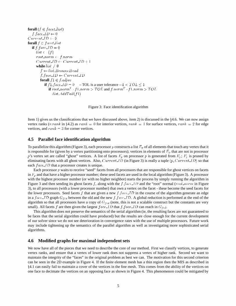
forall (f 2 facet list)f:face ID 0Current ID 0forall f 2 facet list

if f:face ID = 0list ffgroot norm f:normCurrent ID Current ID + 1while list 6= ;f list:RemoveHeadf:face ID Current ID

forall f1 2 f:adjacif f1:face ID = 0 – TOL is a user tolerance�1 < TOL � 1

if root normT � f1:norm > TOL and f:normT � f1:norm > TOLlist:AddTail(f1)Figure 3: Face identification algorithm

Item 1) gives us the classifications that we have discussed above, item 2) is discussed in the x4.6. We can now assignvertex ranks (v:rank in x4.2) as rank = 0 for interior vertices, rank = 1 for surface vertices, rank = 2 for edgevertices, and rank = 3 for corner vertices.

4.5 Parallel face identification algorithm

To parallelize this algorithm (Figure 3), each processor p constructs a listEp of all elements that touch any vertex that itis responsible for (given by a vertex partitioning onto processors); vertices in elements of Ep that are not in processorp’s vertex set are called “ghost” vertices. A list of facets Fp on processor p is generated from Ep; Fp is pruned byeliminating facets with all ghost vertices. Also, Current ID (in Figure 3) is really a tuple hp; Current IDi so thateach face ID that a processor creates is unique.

Each processor p waits to receive “seed” facets from all processors that are responsible for ghost vertices on facetsin Fp and that have a higher processor number; these seed facets are used in the local algorithm (Figure 3). A processorwith the highest processor number (or with no higher neighbor) starts the process by simply running the algorithm inFigure 3 and then sending its ghost facets f , along with the f:face ID and the “root” normal (root norm in Figure3), to all processors (with a lower processor number) that own a vertex on the facet - these become the seed facets forthe lower processors. Seed facets f that are given a new f:face ID in the course of the algorithm generate an edgein a face ID graph Gfid between the old and the new f:face ID. A global reduction is performed at the end of thealgorithm so that all processors have a copy of Gfid (note, this is not a scalable construct but the constants are verysmall). All facets f are then given the largest face ID that f:face ID can reach in Gfid.

This algorithm does not preserve the semantics of the serial algorithm (ie, the resulting faces are not guaranteed tobe faces that the serial algorithm could have produced) but the results are close enough for the current developmentof our solver since we do not see deterioration in convergence rates with the use of multiple processors. Future workmay include tightening up the semantics of the parallel algorithm as well as investigating more sophisticated serialalgorithms.

4.6 Modified graphs for maximal independent sets

We now have all of the pieces that we need to describe the core of our method. First we classify vertices, to generatevertex ranks, and ensure that a vertex of lower rank does not suppress a vertex of higher rank. Second we want tomaintain the integrity of the “faces” in the original problem as best we can. The motivation for this second criterioncan be seen in the 2D example in Figure 4. If the finite element mesh has a thin region then the MIS as described inx4.1 can easily fail to maintain a cover of the vertices in the fine mesh. This comes from the ability of the vertices onone face to decimate the vertices on an opposing face as shown in Figure 4. This phenomenon could be mitigated by

5

Deleted Vertex

Fine Grid

Coarse Grid

Selected Vertex

Figure 4: Poor MIS for multigrid of a “thin” body

randomizing the order that the vertices are added to the MIS, but thin regions tend to lower the convergence rate ofiterative solvers, and so we want to pay special attention to them.

The problem (in Figure 4) is that vertices are allowed to suppress vertices in the same feature class (eg, edges) - butin a different feature. This problem does not occur on logically square domains because when the grid is coarse enoughfor elements to “punch through” the domain the coarsening stops. On general domains, however, one must continuecoarsening, even when one dimension of some parts of the problem has coarsened “all the way through”, because theproblem may still be too large to solve cheaply with a direct solver.

Our simple modification (once we have identified faces) is to delete edges connecting nodes that do not share aface; this prevents a corner vertex from deleting an edge vertex with which it does not share a face and surface verticesfrom deleting surface vertices on different surfaces. Also, we do not allow corners to be deleted at all; this can beproblematic on meshes that have many initial “corners” (as defined by our algorithm); we mitigate this problem byreclassifying vertices on the coarser grids. We generally reclassify the third and subsequent grids (ie, we let the secondgrid vertices retain the type of the fine grid vertex from which it was derived). Note, this heuristic is problem dependentand should be a user defined parameter.

Figure 5 shows the problem in Figure 4 and the modified graph with edges removed as described above.

Surface vertices

Corner vertices

Figure 5: Original and modified graph

Figure 6 shows a possible MIS and coarse grid for this problem.

6

Coarse Grid

Fine Grid

Figure 6: MIS and coarse mesh

4.7 Vertex ordering in MIS

An additional degree of freedom in the MIS algorithm is the order of the vertices within each category. Thus far wehave implicitly ordered the vertices by topological category (or rank) - the ordering within each category can also bespecified. Two simple heuristics can be used to order the vertices: a “natural” order and a random order. Meshes may beinitiallyordered in a block regular order (ie, an assemblage of logically regular blocks), or ordered in a cache optimizingorder like Cuthill-McKee [24]; both of these ordering types are what we call natural orders. The MISs produced fromnatural orderings tend to be rather dense, random ordering on the other hand tend to be more sparse. That is, the MISswith natural orderings tend to be larger than those produced with random orders. For a uniform 3D hexahedral mesh,the asymptotics of the ratio of the MIS size to the vertex set size is bounded by 1=23 and 1=33, as the largest MIS picksevery second vertex and the smallest MIS selects every third vertex, in each dimension. Natural and random orderingsare simple heuristics to approach these bounds.

Small MISs are preferable as there is less work in the solver on the coarser mesh, and fewer levels are requiredbefore the coarsest grid is small enough to solve directly, but care must be taken not to degrade the convergence rateof the solver. In particular, as the boundaries are important to the coarse grid representation it may be advisable to usenatural ordering for the exterior vertices and a random ordering for the interior vertices.

4.8 Meshing of the vertex set on the coarse grid

The vertex set for the coarse grid remains to be meshed - this is necessary in order to construct the finite element coarsegrid space of our method. We use a standard Delaunay meshing algorithm to give us these meshes [10]. This is doneby placing a bounding box around the coarse grid vertices (on each processor) then meshing this to produce a meshthat covers all fine grid vertices. The tetrahedra attached to the bounding box vertices are removed and the fine gridvertices within these deleted tetrahedra are added to a list of “lost” vertices (lost list).

We continue to remove tetrahedra that connect vertices that were not “near” each other on the fine mesh and thatdo not have any fine grid vertices that lie “uniquely” within the tetrahedron. Define a vertex v to lie uniquely in atetrahedron if there is no tetrahedron that can provide the fine grid vertex with interpolates that are all above -� (forsome small number �). Finally, for each vertex v in lost list, we find a nearby element to use for the interpolants for v.Figure 7 shows an example of our methods applied to a problem in 3D elasticity. The fine (input) mesh is shown withthree coarse grids used in the solution.

7

Figure 7: Fine (input) grid and coarse grids for problem in 3D elasticity

5 Parallel architecture

We have developed a highly scalable implementation of our algorithms and a parallel finite element application for solidmechanics problems to effectively test our solver. Our parallel finite element system is composed of two basic parts:Athena, a parallel finite element program built on a serial finite element code (FEAP [9]) and a parallel mesh partitioner(ParMetis [16]), and our solver Prometheus. Prometheus can be further decomposed into two parts: Epimetheus, gen-eral unstructured multigrid support (built on PETSc [3]); and our particular multigrid algorithm Prometheus (whosesole responsibility is to construct the restriction operators between each grid). Prometheus and Epimetheus are notimplemented separately and constitute the publicly available library [19].

Athena reads a large “flat” finite element mesh input file in parallel (ie, each processor seeks and reads only the partof the input file that it, and it alone, is responsible for), uses ParMetis to partition the finite element graph, and thenconstructs a complete finite element problem on each processor. These processor sub-domains are constructed so thateach processor can compute all rows of the stiffness matrix, and entries of the residual vector, associated with verticesthat have been partitioned to the processor. This negates the need for communication in the finite element elementevaluation at the expense of some redundant work.

We use explicit message passing (MPI) for performance and portability, parallelize all parts of the algorithm forscalability. All components of multigrid can scale reasonably well (except for the coarsest grids, whose size remainsconstant as the problem size increases and is thus not a hindrance to scalability).

We target clusters of symmetric multi-processors (SMPs), which we call CLUMPs, as this seems to be the architec-ture of choice for the next generation of large machines. We accommodate CLUMPs by first partitioning the problemonto the SMPs and then the local problem is partitioned on to each processor. This approach implicitly takes advantageof any increase in communication performance within each SMP, though the numerical kernels (in PETSc) are “flat”MPI codes. Figure 8 shows the a diagram of the overall system architecture.

8

solution script

.

.

.

.

x (=b/A)

(memory resident) (memory resident)FEAP fileFEAP file

FEAP input file

FEAP FEAP FEAP

METIS

FEAP

ParMetis

ParMetisAthena Athena

Athena

PETSc

EpimetheusFE/AMG solver interface

Mat. Products (RAR’)

PrometheusMax. Ind. Sets

DelaunayFE shape func. (R)

materials file

file file file file

Partition to SMPs

Partition within each SMP

(p) (p) (p) (p)

FEAP(s)

Figure 8: Athena/Prometheus Architecture

9

6 Performance measures

The section defines the methods, goals, and terminology of our numerical experiments. The goal of our numericalexperiments is to measure the degree of scalability of our algorithms and implementations. We use efficiency as theprimary metric in the analysis of our experimental data. Perfect efficiency is defined as 1:0 and of course the higherthe efficiency the better. Time efficiencies are of the form: “optimal” / “measured” (ie, T (c;1)T (c�P;P ) where T (n; P ) is thetime to solve a problem with n equations on P processors) and flop rate efficiencies are of the form: “measured” /“optimal”. Orthogonal sources of (in)efficiencies (eg, iteration counts and flop rates) can be multiplied together to givethe total efficiency, which is often the most easily measured term - other efficiencies can be back calculated from thetotal efficiency with a model of the computation.

Efficiencies are useful as 1) they provide a uniform metric for measuring the many sources of slowdown in a code,2) they provide a bound on the benefit that can be gained by optimizinga particular aspect of a code, 3) they help identifyscalability bottlenecks in the application. We decompose efficiency into uniprocessor efficiency and parallel efficiency- the total efficiency being the product of the two. Uniprocessor efficiency is defined below; parallel efficiency e isdefined as the time to solve a problem of size n1 on one processor divided by the time to solve a refined discretizationof the problem, with nP = P � n1 equations on P processors.

The remainder of this section discusses the decomposition of efficiency, can be used as a reference for the numericalresults sections that follow, and can be skipped in the first reading. In general efficiency, or sources of inefficiency, canbe decompose into the following components:� uniprocessor efficiency or uniprocessor efficiency eu: the fraction of some “peak” megaflop rate (Mflop/sec)eu = f(1)=secf(1)PEAK=sec of the uniprocessor implementation, where f(1)=sec is the uniprocessor flop rate. Peak can

be defined as:

– Theoretical peak (ie, clock rate times flop issues per cycle).

– Dense matrix matrix-multiply - the fastest megaflop rate that any numerical code is likely to be able tosustain.

– Sparse matrix-vector multiply (withA inAx = b) - the source of most of the flops in most iterative methods- the fastest megaflop rate that any iterative solver is likely to be able to sustain in the solve phase.� Parallel efficiency is the product of the four efficiencies described below:

– work efficiency ew: the fraction of flops in the parallel implementation that are not redundant, ie, the num-ber of flops to solve the problem on one processor divided by the number of flops to solve the same problemwith P processors. Thus, ew = fP (1)f(P ) where fP (1) is the number of flops used to solve the nP unknownproblem on one processor and f(P ) is the number of flops used to solve the nP unknown problem with Pprocessors.

– scale efficiency es: this is the scalability of the algorithm with respect to non-redundant flops per unknown(ie, the non-redundant flops per unknown to solve the problem as the problem size increases). For iterativesolvers, it is convenient to further decompose scale efficiency.� iteration scale efficiency eIs: the efficiency in the number of iterations required; eIs = Iterations(1)Iterations(P ) ,

where Iterations(P ) is the number of iterations for the problem of size nP on P processors.� flop scale efficiency eFs : the efficiency in the non-redundant flops per unknown (or processor) per it-eration. We define the flops per iteration of thenP unknown problem by fI (P ) and the non-redundant

flops as f̂ (P ), and eFs = P �fI (1)f̂I (P ) . Recall, f(P ) is the toatl flops and so f̂ (P ) = ew � f(P ). Work ef-

ficiency ew is similar to es in that it relates to flop efficiency, though distinct from es as: ew is relatedonly to the number of processors used P ; scale efficiency es is related only to the size of the problem.

– load balance l: the ratio of the average to the maximum amount of work (flops) that a processor does inan operation, el = faveragefmaximum . This is easily measured (and defined) as we do not use any non-uniformalgorithmic constructs (ie, all processors are doing the same operation on the same mathematical object allof the time). Our load balance can be seen graphically in Figure 11.

10

– communication efficiency ec: the highest percentage of time that a processor is not waiting, processing,packing data, or any other form of work associated with interprocess communication. Communication ef-ficiency ec can be measured with flop rate efficiency, ec = f(P )=secP �f(1)=sec , as in Figure 11 (right), if there is noload imbalance induced blocking.

Our solver has perfect work efficiency ew, though we have some redundant work in the construction of the fine gridmatrixA0 in Athena (x5) as can be seen in Figure 12 (right) - we do not discuss work efficiency further and can assumethat f̂(P ) = f(P ). Our load balance is very good (see Figure 11) and we do not discuss load balance further.

We focus on communication efficiency ec and scale efficiency es; communication efficiency ec can be representedwith the flop rate efficiency. Scale efficiency es = eIs �eFs (flops per unknown) is the product of the number of iterationsrequired to converge and the number of flops per unknown per iteration. Thus, the efficiency e(P ) onP processors (andnP unknowns as defined above) can be effectively represented ase(P ) � Iterations(1)Iterations(P ) � P � f(1)f(P ) � f(P )=secP � f(1)=sec = eIs � eFs � ecwith the number of iterations Iterations(P ), flops iteration f(P ), and flop rate f(P )=sec. Iterations(P ) is tabulatedin Table 2, P �f(1)=secf(P )=sec is shown if Figure 11 (left), and f(P )=secP �f(1)=sec shown if Figure 11 (right).

This paper focuses on parallel efficiency but a few words about uniprocessor efficiency eu are warranted. Unipro-cessor efficiency can be measured against the theoretical peak megaflop rate of the processors; this is simple to definethough it is more effective for measuring the performance of the processor in question rather than the algorithm andimplementation. The megaflop rate of dense matrix-matrix multiply is more useful than peak speed as this invariablybounds the performance of numerical applications. Sparse matrix-vector multiply, with the fine grid matrix, is mostuseful as it is the source of most of the flops in most scalable solvers. We report data for the first and third uniprocessorefficiency (ie, theoretical peak and fine grid sparse matrix-vector multiply) in the following sections.

Good scalability can be defined as good parallel efficiency (e � 1:0 or e � C � 0 for some constantC independentof the number of processors) for the time to compute the solution x̂ that reduces the 2-norm of the residual by a fixedconstant rtol (ie,kAx̂�bkkbk � rtol ). We could alternatively define scalability by solving the linear system to the finiteelement discretization error; this is more attractive as it insures that perfect parallel efficiency is bounded from aboveby 1:0 and reflects the rational use of a solver. Discretization error is not used as the convergence tolerance because itis difficult to define (compute). Note, the PRAM complexities of all iterative solver algorithms are, to our knowledge,bounded by O (log(n)), thus optimal parallel efficiency will include a log(n) term.

An additional note, there are three main phases in the solution of a linear system: setup for the mesh (non-zerostructure of the fine grid), setup for each matrix (more than one for nonlinear problems), and the solve for x with aprovided right hand side (RHS) b. For direct solvers these three phases correspond to symbolic factorization, numericalfactorization, and the front solve and back substitution. The first phase is amortized in nonlinear and transient problemsand is thus not as important as the latter stages, unless the application solves just one linear system of equations foreach mesh configuration. The second phase, setup for each matrix, includes the coarse grid operator construction andsmoother setup in our solver, and is important for fully nonlinear problems as it is required for each RHS and thus itscost is not amortized by multiple solves. The final stage, the time in the actual multigrid iterations, is the most importantas this is always done in the solve of a system of linear equations. We focus on the solve phase (the last phase), thoughwe have fully scalable implementations of all three phases and we report times for all stages (Figure 10).

11

7 Numerical results

We use a model problem in solid mechanics to conduct scalability studies of our solver. Our problem is a sphere em-bedded in a cube; the sphere is constructed of seventeen alternating “hard” and “soft” layers and the cube is a “soft”material. Think of a spherical steel-belted radial inside a rubber cube. Symmetry can be used to model only one octant.The loading and boundary conditions are an imposed uniform displacement (crushing), on the top surface and symmet-ric boundary conditions on the three cut faces. The hard material is a J2 plasticity material with a mixed formulationand kinematic hardening [22]. The soft material is a large deformation (Neo-Hookean) hyperelastic material with amixed formulation [26]. Table 1 shows a summary of the constitution of our two material types.

Material Elastic mod. (E) Poisson ratio deformation type yield stress hardening mod.soft 10�4 0:49 large 1 NAhard 1 0:3 large 0:001 E 0:002

Table 1: Nonlinear materials

The hexahedral discretization is parameterized so that we can perform scalability experiments. Figure 9 shows thesmallest (base) version of the problem with 80 K (K=1000) degrees of freedom. Each successive problem has one morelayer of elements through each of the seventeen shell layers, with an appropriate (ie, similar) refinement in the othertwo directions and in the outer soft domain - resulting in problems of size: 80 K, 621 K, 2,086 K, 4,924 K, 9,595 K,16,554 K, 26,257 K, and 39,161 K degrees of freedom. We run this problem with about 40 K degrees of freedom perprocessor, on 2 to 960 processors.

Figure 9: 79,679 dof concentric spheres problem and final configuration

These experiments are performed on an IBM PowerPC cluster with 240 4-way SMP nodes at Lawrence LivermoreNational Laboratory. Each node has four 332 MHz PowerPC 604e processors, with 1.5 Gbytes of memory, and a the-oretical peak Mflop rate of 664 Mflop/sec per processor.

Single processor (PETSc) sparse matrix-vector products (on the fine grid of our problems) run at 36 Mflop/sec, andthe multigrid solves run at 34 Mflop/sec; two processor (the base case for these experiments) matrix-vector productsrun at 66 Mflop/sec, and the multigrid solves run at 63 Mflop/sec; the 960 processor case runs at 26.5 Gflop/sec in thematrix-vector products and 19.3 Gflop/sec in the solves. Thus, we have 59% (= 19;300960�34) parallel efficiency in the solvein these experiments. We have also run these experiments (up to the 24 million degrees of freedom problem) on a 640processor Cray T3E with 57% parallel efficiency as well, and about twice the total Mflop rate as the corresponding IBMexperiment.

12

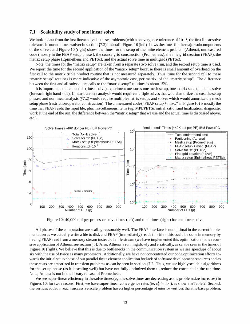
7.1 Scalability study of one linear solve

We look at data from the first linear solve in these problems (with a convergence tolerance of 10�4, the first linear solvetolerance in our nonlinear solver in section x7.2) in detail. Figure 10 (left) shows the times for the major subcomponentsof the solver, and Figure 10 (right) shows the times for the setup of the finite element problem (Athena), unmeasuredcode (mostly in the FEAP setup phase ), the coarse grid construction (Prometheus), the fine grid creation (FEAP), thematrix setup phase (Epimetheus and PETSc), and the actual solve time in multigrid (PETSc).

Note, the times for the “matrix setup” are taken from a separate (two solve) run, and the second setup time is used.We report the time for the second application of the “matrix setup” because there is small amount of overhead on thefirst call to the matrix triple product routine that is not measured separately. Thus, time for the second call to these“matrix setup” routines is more indicative of the asymptotic cost, per matrix, of the “matrix setup”. The differencebetween the first and all subsequent calls to the “matrix setup” routines is about 15%.

It is important to note that this (linear solve) experiment measures one mesh setup, one matrix setup, and one solve(for each right hand side). Linear transient analysis would require multiple solves that would amortize the cost the setupphases, and nonlinear analysis (x7.2) would require multiple matrix setups and solves which would amortize the meshsetup phase (restrictionoperator construction). The unmeasured code (“FEAP setup + misc.” in Figure 10) is mostly thetime that FEAP reads the input file, plus miscellaneous items (eg, MPI/PETSc initialization and finalization, diagnosticwork at the end of the run, the difference between the “matrix setup” that we use and the actual time as discussed above,etc.).

100 200 300 400 500 600 700 800 9000

20

40

60

80

100

120

Number of PEs (p)

Tim

e (s

ec)

Solve Times (~40K dof per PE) IBM PowerPC

number of iterations

Total Ax=b solve Solve for "x" (PETSc) Matrix setup (Epimetheus,PETSc)Iterations,tol=10−4

100 200 300 400 500 600 700 800 90010

1

102

103

104

105

Number of PEs (p)

Tim

e (s

ec)

"end to end" Times (~40K dof per PE) IBM PowerPC

Total end−to−end time Partitioning (Athena) Mesh setup (Prometheus) FEAP setup + misc. (FEAP) Solve for "x" (PETSc) Fine grid creation (FEAP) Matrix setup (Epimetheus,PETSc)

Figure 10: 40,000 dof per processor solve times (left) and total times (right) for one linear solve

All phases of the computation are scaling reasonably well. The FEAP interface is not optimal in the current imple-mentation as we actually write a file to disk and FEAP (immediately) reads this file - this could be done in memory byhaving FEAP read from a memory stream instead of a file stream (we have implemented this optimization in the recur-sive application of Athena, see section x5). Also, Athena is running slowly and erratically, as can be seen in the times ofFigure 10 (right). We believe that this is due to bottlenecks in the communication system as we see speedups of aboutsix with the use of twice as many processors. Additionally, we have not concentrated our code optimization efforts to-wards the initial setup phase of our parallel finite element application for lack of software development resources and asthese costs are amortized in transient problems as can be seen in section x7.2. Thus, we use highly scalable algorithmsfor the set up phase (as it is scaling well) but have not fully optimized them to reduce the constants in the run time.Note, Athena is not in the library release of Prometheus.

We see super-linear efficiency in the solve times (eg, the solve times are decreasing as the problem size increases) inFigures 10, for two reasons. First, we have super-linear convergence rates (ie, eIs > 1:0), as shown in Table 2. Second,the vertices added in each successive scale problem have a higher percentage of interior vertices than the base problem,

13

leading to higher rates of vertex reduction in the coarse grids. This is because as the number of unknowns n increasesthe “surface area” increases by O(n 23 ) whereas the interior increases by O(n). Thus, the ratio of interior vertices tosurface vertices increases as the scale of discretization decreases (n increases). Our coarse grid heuristics in section x4articulate the surfaces well (boundary and material interfaces), resulting in a higher ratio of surface vertices promotedto the coarse grid. Thus, the rate of vertex reduction is higher on the larger problems as they have proportionally moreinterior vertices, leading to less work per fine grid vertex (ie, eFs > 1:0), as can be seen in Figure 11 (left).

Equations 79,679 622,815 2,085,599 4,924,223 9,594,879 16,553,759 26,257,055 39,160,959Processors 2 15 50 120 240 400 640 960

MG preconditioned 29 27 22 20 20 20 20 21PCG Iterations in1st linear solve

Total PCG iterations 3108 4121 3117 3355 3060 3008 2978 3215in nonlinear solve

Total Newton 62 63 62 65 68 69 68 70iterations

Ave. PCG iterations 50 65 50 52 45 44 44 46per linear solveTotal Mflop/sec 63 421 1194 2901 5112 8524 13218 19253in MG iterations

Table 2: Number of iterations for first linear solve and total nonlinear solve

Figure 11 (left) shows the scaled efficiency of the number of flops per iteration per unknown in the solver eFs , aswell as the scaled efficiency of the time for each iteration. The efficiency of the time per iteration, the lower line inFigure 11 (left), shows the combined effect of the super-linear flop efficiency eFs and the parallel (in)efficiency of theflop rate (flop/sec/processor) ec. Communication efficiency ec is shown in Figure 11 (right). The total “solve for x”efficiency e (ie, the solve efficiency without the matrix setup or the grid setup phases) is shown in Figure 12 and isapproximately e = eIs � eFs � ec.

101

102

0

0.2

0.4

0.6

0.8

1

1.2

1.4

Number of PEs (p)

p / 2

* f(

2) /

f(p)

* N

(p)

/ N(2

)

flop/iteration/processor Efficiency (~40K dof per PE) IBM PowerPC

communication

load imbalance

esF * e

c

maximum flop/iteration/processoraverage flop/iteration/processortime per iteration

101

102

0

0.2

0.4

0.6

0.8

1

1.2

Number of PEs (p)

2 / p

* m

flop(

p)/s

ec /

mflo

p(2)

/sec

flop/sec/processor Efficiency (~40K dof per PE) IBM PowerPC

communication

load imbalance

maximum flop/sec/processoraverage flop/sec/processor

Figure 11: Flop/iteration/proc. (flop scale efficiency eFs ); flop rate (communication efficiency ec)

Figure 11 (right), the scaled efficiency of the maximum and average processor flop rate in the solve phase, showsthat we have 62% parallel efficiency in the flop rate (from the two processor case). We do not have a one processorversion of this problem but, using the flop rate of 34 Mflop/sec in the solve from a similar 40 K degree of freedom

14

problem on one processor, we have 59% parallel efficiency in the solve phase. Figure 11 also shows two views of twosources of inefficiency: communication ec and load imbalance l as discussed in section x6.

Note, Figure 11 (left) is scaled by a factor 2P � N(P )N(2) to account for the non-constant number of unknowns perprocessor (N (P )=P ); this factor is shown in Figure 12 (left) and the efficiencies of all of the major steps the linearsolve in Figure 12 (right).

101

102

0

0.5

1

1.5

Number of PEs (p)

2 / p

* T

ime(

2) /

Tim

e(p)

* N

(p)

/ N(2

)

Solve Efficiency (~40K dof per PE) IBM PowerPC

N(p) / N(2) * 2 / p

2 / p * mflop(p)/sec / mflop(2)/sec

Subdomain factorizationsSolve for "x" (PETSc) Total N(p) / N(2) * 2 / p R * A * P (Epimetheus) Solve Mflops/sec

101

102

0

0.5

1

1.5

2

2.5

Number of PEs (p)

2 / p

* T

ime(

2) /

Tim

e(p)

* N

(p)

/ N(2

)

Prometheus and Solve Efficiency (~40K dof per PE) IBM PowerPC

Solve for "x" (PETSc) Matrix setup (Epimetheus,PETSc)Fine grid creation (FEAP) Total Mesh setup (Prometheus)

Figure 12: efficiency e for all major components of one linear solve with about 40,000 dof per processor

7.2 Nonlinear scalability study

We use a full Newton nonlinear solution method; convergence is declared when the energy norm of the correction is10�20 times that of the first correction. This means that in Newton iteration m convergence is declared when��xTm � (b� Axm)�� < 10�20 � ��xT0 � (b� Ax0)��. The linear solver, within each Newton iteration, is preconditioned conjugate gradient (PCG), preconditioned with one“full” multigrid cycle. We use one pre-smoothing and one post-smoothing step within multigrid, preconditioned withblock Jacobi with 6 blocks for every 1,000 unknowns (these block Jacobi sub-domains are constructed with METIS).

The slightly modified version of FEAP (FEAPp [9]) calls our linear solver in each Newton iteration, with thecurrent residual rm = b � Axm, thus the linear solve is for the increment �x � A�1rm. We use a dynamic conver-gence tolerance (rtol) for the linear solve in each Newton iteration of rtol1 = 10�4 in the first iteration and rtolm =min(10�3; krmkkrm�1k � 10�1) on all subsequent iterations (m > 1). This heuristic is intended to minimize the number oftotal iterations required in the Newton solve by only solving each set of linear equations to the degree that it “deserves”.That is, if the true (nonlinear) residual is not converging quickly then solving the linear system to an accuracy far inexcess of the reduction in the residual is not likely to be economical.

The full nonlinear problem is run with ten “time” steps with a particular displacement increment in each step thatresults in a total vertical displacement of 3.6 inches down (the octant is 12.5 inches on a side and the top “soft” section is5 inches thick at the central vertical axis). Figure 13 (left) shows the percentage of the integration points, in the “hard”shells, whose stress state have reached the yield surface [22]; this gives an indication of the damage to the systemand results in material constitution that is very similar to that of highly incompressible materials. Over 24% of theintegration points, in the hard shells, are in the yield state at the final configuration.

Figure 13 (right), and Table 2, show the number of multigrid iterations in each linear solve of each of the ten Newtonsolves, stacked on top of each other and color coded for each Newton iteration. From this data we can see that the totalnumber of iterations is staying about constant as the scale of the problem increases. This data suggests that the nonlinearproblem is gettingharder to solve as the discretization is refined, because the number of iterations in the first linear solve

15

1 2 3 4 5 6 7 8 9 100

10

20

30

40

50

60

70

80

90

100Percentage of "hard" shell integration points in plastic state

"time" step

perc

ent p

last

ic in

tegr

atio

n po

ints

70K dof623K dof2,086K dof4,925K dof9,595K dof16,554K dof26,554K dof39,161K dof

21648 120 240 400 640 9600

500

1000

1500

2000

2500

3000

3500

4000

4500Solver iterations in 10 Newton nonlinear solves

Number of PEs

linea

r so

lver

iter

atio

ns

Figure 13: Percent of integration points in “hard” material that are in plastic state in each “time” step; Number ofiterations for all solves in nonlinear problem (see Table 2)

of the first step decreases as the problem size increases, as is shown in Table 2. That is, we are seeing a slight growthin the number of Newton iterations required, and the average number of iterations in the linear solver is not decreasingas dramatically as in the first linear solve. Table 2 shows the detailed iteration count data from these experiments.

8 Conclusion

We have developed a promising method for solving the linear set of equations arising from implicit finite element ap-plications. Our approach, a 3D parallel extension to a serial 2D algorithm, is to our knowledge unique in that it is a fullyautomatic (ie, the user need only provide the fine grid, which is easily available in most finite element codes) standardgeometric multigrid method for unstructured finite element problems. We have solved 40 million degree of freedomproblems on an IBM PowerPC cluster with 240 4-way SMP nodes with about 60% parallel efficiency. Prometheus isthe only fully parallelized scalable public domain solver that we are aware of and can be obtained from the Prometheushome page [19].

We have also developed a highly parallel finite element implementation, built on an existing state-of-the-art se-rial research finite element implementation. The implementation of our system (Athena/Prometheus) required about30,000 lines of our own C++ code, plus several large packages: PETSc (160,000 lines of C), FEAP (105,000 lines ofFORTRAN), METIS/ParMetis (20,000 lines of C), and geometric predicates (4,000 lines of C) [21].

Future work will include the continuing hardening of the algorithms and implementation with the application ofPrometheus to a wider variety of problems, as well as expanding the domain of applications which we support (eg,higher order elements, non-continuum elements). As we also plan to explore alternative (effective) unstructured multi-grid algorithms such as smoothed aggregation [25], to evaluate (and make publicly available) competitive algorithms.

Acknowledgments. We would like to thank the many people that have contributed libraries to this work: Robert L.Taylor for providing FEAP, The PETSc team for providing PETSc, George Karypis for providing ParMetis. We wouldlike to thank the reviewers for their helpful comments, Lawrence Livermore National Laboratory for providing accessto its IBM cluster computing systems and to the staff of Livermore Computing for their support services, LawrenceBerkeley National Laboratory for the use of their Cray T3E, and their support staff (this research used resources ofthe National Energy Research Scientific Computing Center, which is supported by the Office of Energy Research ofthe U.S. Department of Energy under Contract No. DE-AC03-76SF00098). This research was supported in part bythe Department of Energy under DOE Contract No. W-7405-ENG-48 and DOE Grant Nos. DE-FG03-94ER25219,DE-FG03-94ER25206.

16

References

[1] M. F. Adams. Multigrid Equation Solvers for Large Scale Nonlinear Finite Element Simulations. Ph.D. disser-tation, University of California, Berkeley, 1998. Tech. report UCB//CSD-99-1033.

[2] M. F. Adams. A parallel maximal independent set algorithm. In Proceedings 5th copper mountain conference oniterative methods, 1998. Best student paper award winner.

[3] S. Balay, W.D. Gropp, L. C. McInnes, and B.F. Smith. PETSc 2.0 users manual. Technical report, ArgonneNational Laboratory, 1996.

[4] W. Briggs. A Multigrid Tutorial. SIAM, 1987.

[5] V.E. Bulgakov and G. Kuhn. High-performance multilevel iterative aggregation solver for large finite-elementstructural analysis problems. International Journal for Numerical Methods in Engineering, 38, 1995.

[6] T. F. Chan and B. F. Smith. Multigrid and domain decomposition on unstructured grids. In David F. Keyes andJinchao Xu, editors, Seventh Annual International Conference on Domain Decomposition Methods in Scientificand Engineering Computing. AMS, 1995. A revised version of this paper has appeared in ETNA, 2:171-182,December 1994.

[7] J. Demmel. Applied Numerical Linear Algebra. SIAM, 1997.

[8] M.C. Dracopoulos and M.A Crisfield. Coarse/fine mesh preconditioners for the iterative solution of finite elementproblems. International Journal for Numerical Methods in Engineering, 38:3297–3313, 1995.

[9] FEAP. http://www.ce.berkeley.edu/� rlt.

[10] D. A. Field. Implementing Watson’s algorithm in three dimensions. In Proc. Second Ann. ACM Symp. Comp.Geom., 1986.

[11] J. Fish, V. Belsky, and S. Gomma. Unstructured multigrid method for shells. International Journal for NumericalMethods in Engineering, 39:1181–1197, 1996.

[12] J. Fish, M. Pandheeradi, and V. Belsky. An efficient multilevel solution scheme for large scale non-linear systems.International Journal for Numerical Methods in Engineering, 38:1597–1610, 1995.

[13] H. Guillard. Node-nested multi-grid with Delaunay coarsening. Technical Report 1898, Institute National deRecherche en Informatique et en Automatique, 1993.

[14] M. T. Jones and P. E. Plassman. A parallel graph coloring heuristic. SIAM J. Sci. Comput., 14(3):654–669, 1993.

[15] S. Kacau and I. D. Parsons. A parallel multigrid method for history-dependent elastoplacticity computations.Computer methods in applied mechanics and engineering, 108, 1993.

[16] George Karypis and Kumar Vipin. Parallel multilevel k-way partitioning scheme for irregular graphs. Supercom-puting, 1996.

[17] M. Luby. A simple parallel algorithm for the maximal independent set problem. SIAM J. Comput., 4:1036–1053,1986.

[18] D.R.J. Owen, Y.T. Feng, and D Peric. A multi-grid enhanced GMRES algorithm for elasto-plastic problems.International Journal for Numerical Methods in Engineering, 42:1441–1462, 1998.

[19] Prometheus. http://www.cs.berkeley.edu/�madams/Prometheus-1.1.

[20] J. Ruge. AMG for problems of elasticity. Applied Mathematics and Computation, 23:293–309, 1986.

[21] J. R. Shewchuk. Adaptive Precision Floating-Point Arithmetic and Fast Robust Geometric Predicates. Discrete& Computational Geometry, 18(3):305–363, October 1997.

17

[22] J.C. Simo and T.J.R. Hughes. Computational Inelasticity. Springer-Verlag, 1998.

[23] B. Smith, P. Bjorstad, and W. Gropp. Domain Decomposition. Cambridge University Press, 1996.

[24] S. Toledo. Improving memory-system performance of sparse matrix-vector multiplication. In Proceedings of the8th SIAM Conference on Parallel Processing for Scientific Computing, March 1997.

[25] P. Vanek, J. Mandel, and M. Brezina. Algebraic multigrid by smoothed aggregation for second and fourth orderelliptic problems. In 7th Copper Mountain Conference on Multigrid Methods, 1995.

[26] O.C. Zienkiewicz and R.L. Taylor. The Finite Element Method, volume 1. McGraw-Hill, London, Fourth edition,1989.

18