Parallel Algorithms - Introduction

Advanced Algorithms & Data StructuresLecture Theme 11

Prof. Dr. Th. OttmannSummer Semester 2006

2

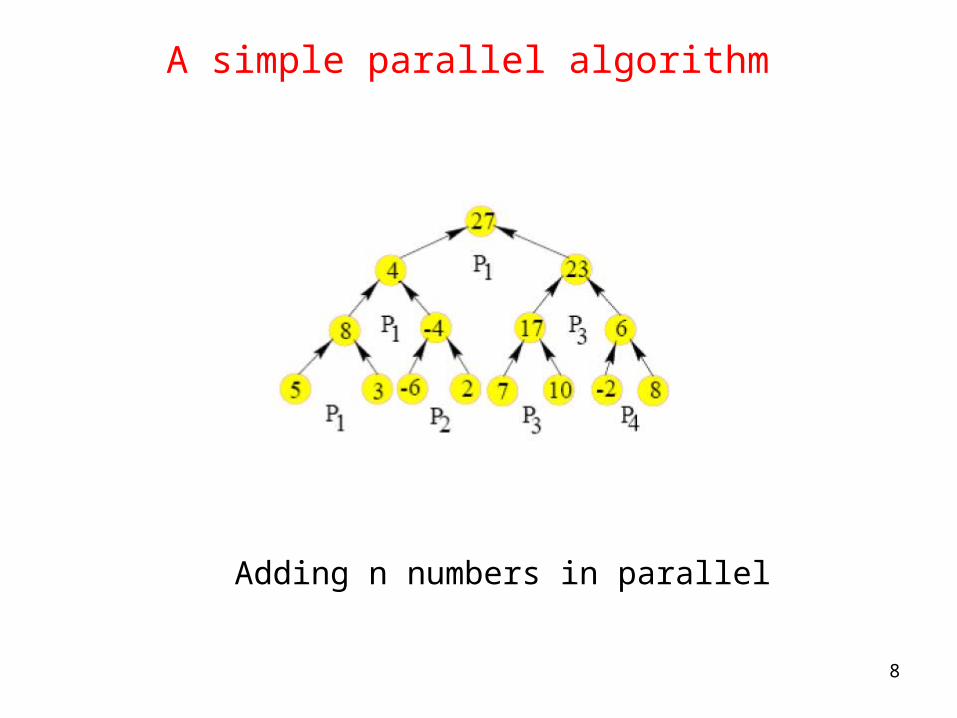
A simple parallel algorithm

Adding n numbers in parallel

3

A simple parallel algorithm

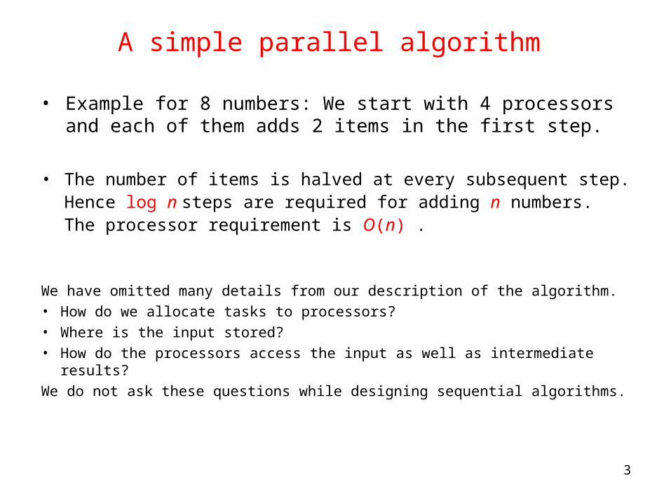
• Example for 8 numbers: We start with 4 processors and each of them adds 2 items in the first step.

• The number of items is halved at every subsequent step. Hence log n steps are required for adding n numbers. The processor requirement is O(n) .

We have omitted many details from our description of the algorithm.• How do we allocate tasks to processors?• Where is the input stored?• How do the processors access the input as well as intermediate results?

We do not ask these questions while designing sequential algorithms.

4

How do we analyze a parallel algorithm?

A parallel algorithms is analyzed mainly in terms of its time, processor and work complexities.

• Time complexity T(n) : How many time steps are needed?• Processor complexity P(n) : How many processors are used?• Work complexity W(n) : What is the total work done by all the

processors? Hence,

For our example: T(n) = O(log n) P(n) = O(n) W(n) = O(n log n)

5

How do we judge efficiency?

• We say A1 is more efficient than A2 if W1(n) = o(W2(n))

regardless of their time complexities.

For example, W1(n) = O(n) and W2(n) = O(n log n)

• Consider two parallel algorithms A1and A2 for the same problem.

A1: W1(n) work in T1(n) time.

A2: W2(n) work in T2(n) time.

If W1(n) and W2(n) are asymptotically the same then A1 is more efficient than A2 if T1(n) = o(T2(n)).

For example, W1(n) = W2(n) = O(n), but

T1(n) = O(log n), T2(n) = O(log2 n)

6

How do we judge efficiency?

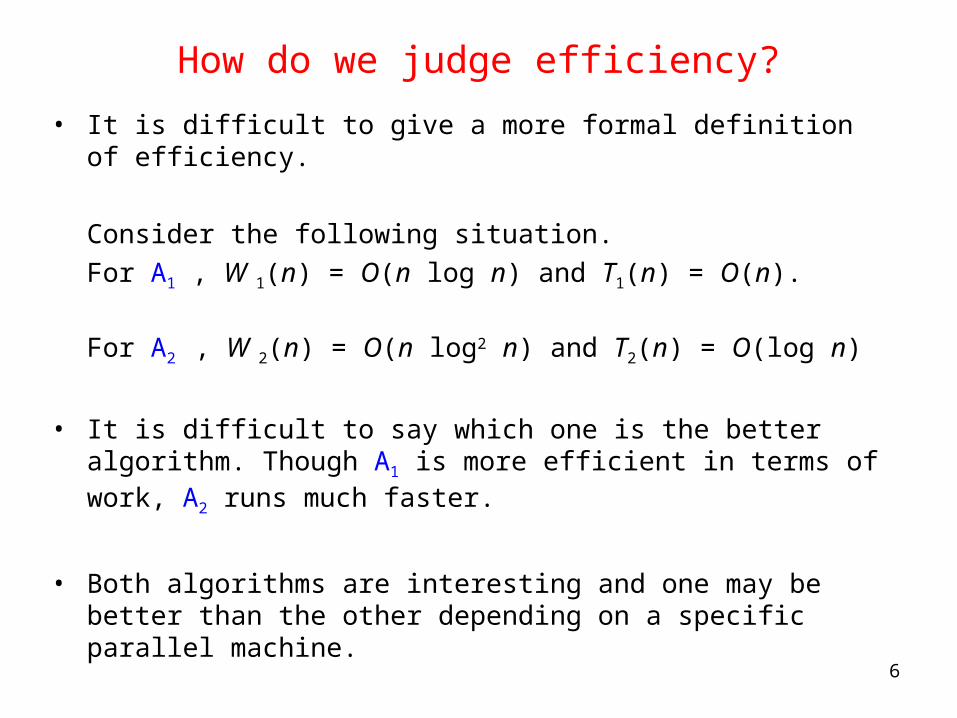
• It is difficult to give a more formal definition of efficiency.

Consider the following situation.

For A1 , W 1(n) = O(n log n) and T1(n) = O(n).

For A2 , W 2(n) = O(n log2 n) and T2(n) = O(log n)

• It is difficult to say which one is the better algorithm. Though A1 is more efficient in terms of work, A2 runs much faster.

• Both algorithms are interesting and one may be better than the other depending on a specific parallel machine.

7

Optimal parallel algorithms

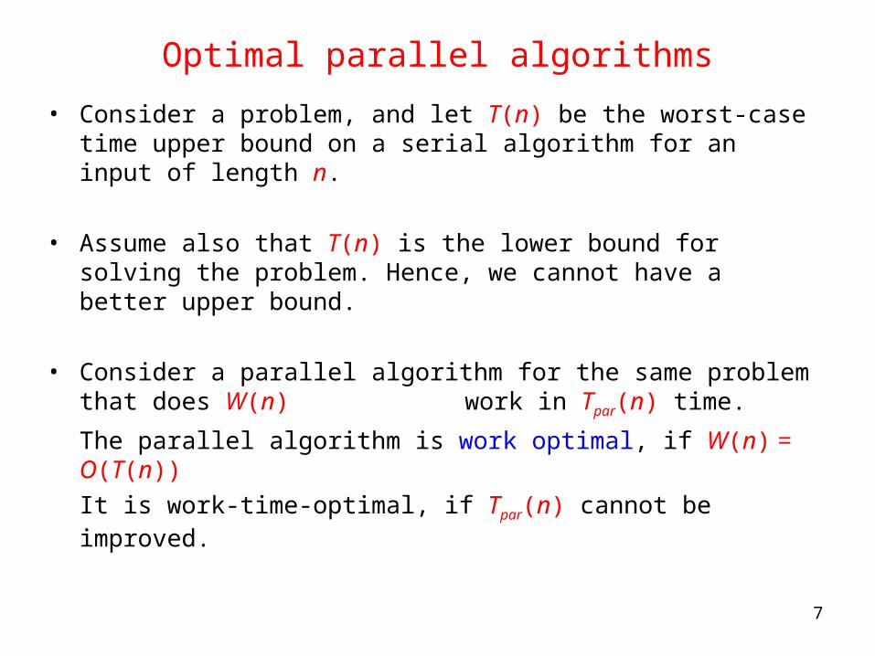
• Consider a problem, and let T(n) be the worst-case time upper bound on a serial algorithm for an input of length n.

• Assume also that T(n) is the lower bound for solving the problem. Hence, we cannot have a better upper bound.

• Consider a parallel algorithm for the same problem that does W(n) work in Tpar(n) time.

The parallel algorithm is work optimal, if W(n) = O(T(n))

It is work-time-optimal, if Tpar(n) cannot be improved.

8

A simple parallel algorithm

Adding n numbers in parallel

9

A work-optimal algorithm for adding n numbers

Step 1.• Use only n/log n processors and assign log n numbers to each

processor.• Each processor adds log n numbers sequentially in O(log n) time.

Step 2.• We have only n/log n numbers left. We now execute our original

algorithm on these n/log n numbers.

• Now T(n) = O(log n)

W(n) = O(n/log n x log n) = O(n)

10

Why is parallel computing important?

• We can justify the importance of parallel computing for two reasons.

Very large application domains, and

Physical limitations of VLSI circuits

• Though computers are getting faster and faster, user demands for solving very large problems is growing at a still faster rate.

• Some examples include weather forecasting, simulation of protein folding, computational physics etc.

11

Physical limitations of VLSI circuits

• The Pentium III processor uses 180 nano meter (nm) technology, i.e., a circuit element like a transistor can be etched within

180 x 10-9 m.

• Pentium IV processor uses 160nm technology.

• Intel has recently trialed processors made by using 65nm technology.

12

13

How many transistors can we pack?

• Pentium III has about 42 million transistors and Pentium IV about 55 million transistors.

• The number of transistors on a chip is approximately doubling every 18 months (Moore’s Law).

• There are now 100 transistors for every ant on Earth (Moore said so in a recent lecture).

14

Physical limitations of VLSI circuits

• All semiconductor devices are Si based. It is fairly safe to assume that a circuit element will take at least a single Si atom.

• The covalent bonding in Si has a bond length approximately 20nm.• Hence, we will reach the limit of miniaturization very soon.• The upper bound on the speed of electronic signals is 3 x 108m/sec,

the speed of light.• Hence, communication between two adjacent transistors will take

approximately 10-18sec.• If we assume that a floating point operation involves switching of at

least a few thousand transistors, such an operation will take about 10-15sec in the limit.

• Hence, we are looking at 1000 teraflop machines at the peak of this technology. (TFLOPS, 1012 FLOPS)

1 flop = a floating point operationThis is a very optimistic scenario.

15

Other Problems

• The most difficult problem is to control power dissipation.

• 75 watts is considered a maximum power output of a processor.

• As we pack more transistors, the power output goes up and better cooling is necessary.

• Intel cooled its 8 GHz demo processor using liquid Nitrogen !

16

The advantages of parallel computing

• Parallel computing offers the possibility of overcoming such physical limits by solving problems in parallel.

• In principle, thousands, even millions of processors can be used to solve a problem in parallel and today’s fastest parallel computers have already reached teraflop speeds.

• Today’s microprocessors are already using several parallel processing techniques like instruction level parallelism, pipelined instruction fetching etc.

• Intel uses hyper threading in Pentium IV mainly because the processor is clocked at 3 GHz, but the memory bus operates only at about 400-800 MHz.

17

18

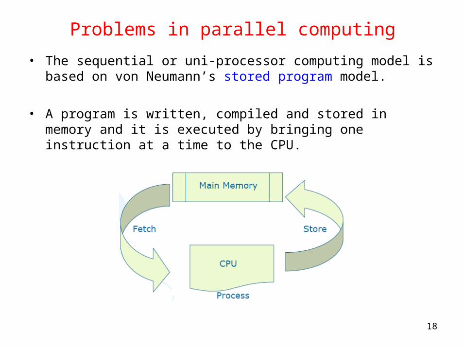
Problems in parallel computing

• The sequential or uni-processor computing model is based on von Neumann’s stored program model.

• A program is written, compiled and stored in memory and it is executed by bringing one instruction at a time to the CPU.

19

Problems in parallel computing

• Programs are written keeping this model in mind. Hence, there is a close match between the software and the hardware on which it runs.

• The theoretical RAM model captures these concepts nicely.• There are many different models of parallel computing and each

model is programmed in a different way.• Hence an algorithm designer has to keep in mind a specific model

for designing an algorithm.• Most parallel machines are suitable for solving specific types of

problems.• Designing operating systems is also a major issue.

20

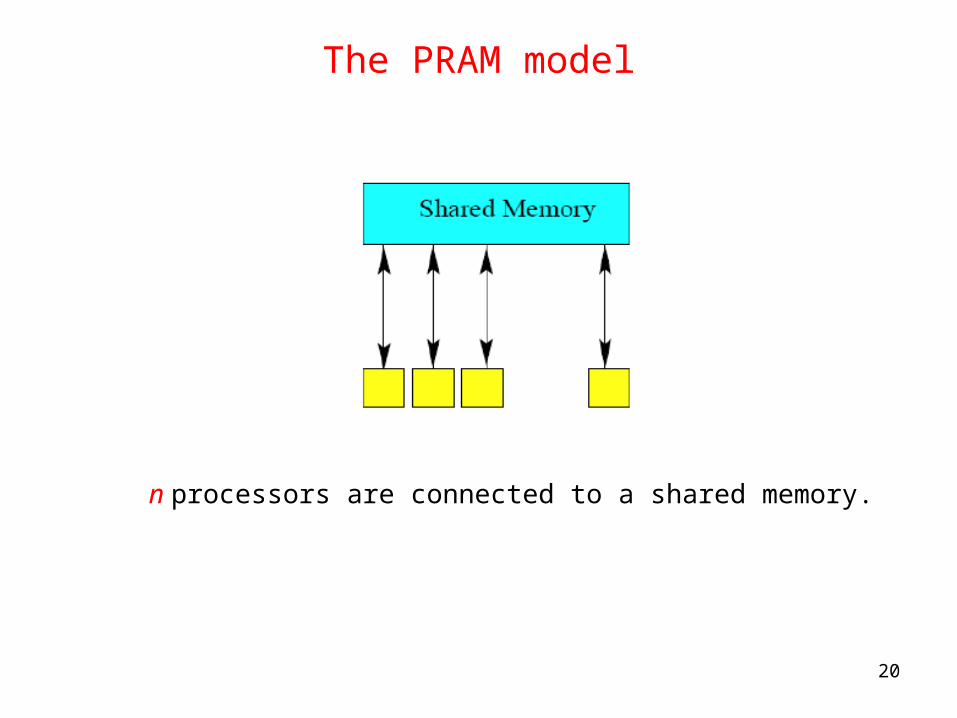
The PRAM model

n processors are connected to a shared memory.

21

The PRAM model

• Each processor should be able to access any memory location in each clock cycle.

• Hence, there may be conflicts in memory access. Also, memory management hardware needs to be very complex.

• We need some kind of hardware to connect the processors to individual locations in the shared memory.

• The SB-PRAM developed at University of Saarlandes by Prof. Wolfgang Paul’s group is one such model.

http://www-wjp.cs.uni-sb.de/projects/sbpram/

22

The PRAM model

A more realistic PRAM model