P rocess Mining Based Process Mining Based Inﬂuence

ot

he

L u

me

eT s

esse

cor

P ss

enis

uB

gniv

orp

mI

dna

gniz

ylan

A r

of s

isyl

anA

ecne

ufln

I de

saB

gnin

iM

ssec

orP

yti

srev

in

U otl

aA

0202

ecneicS retupmoC

desaB gniniM ssecorP rof sisylanA ecneuflnI

gnivorpmI dna gnizylanA sessecorP ssenisuB

otheL umeeT

LAROTCOD SNOITATRESSID

ot

he

L u

me

eT s

esse

cor

P ss

enis

uB

gniv

orp

mI

dna

gniz

ylan

A r

of s

isyl

anA

ecne

ufln

I de

saB

gnin

iM

ssec

orP

yti

srev

in

U otl

aA

0202

ecneicS retupmoC



otheL umeeT


ot

he

L u

me

eT s

esse

cor

P ss

enis

uB

gniv

orp

mI

dna

gniz

ylan

A r

of s

isyl

anA

ecne

ufln

I de

saB

gnin

iM

ssec

orP

yti

srev

in

U otl

aA

0202

ecneicS retupmoC



otheL umeeT


seires noitacilbup ytisrevinU otlaASNOITATRESSID LAROTCOD 781 / 0202

ecneuflnI desaB gniniM ssecorP gnivorpmI dna gnizylanA rof sisylanA

sessecorP ssenisuB

otheL umeeT

fo rotcoD fo eerged eht rof detelpmoc noitatressid larotcod A eht fo noissimrep eht htiw ,dednefed eb ot )ygolonhceT( ecneicS

no ,mooZ aiv noitcennoc etomeR ,ecneicS fo loohcS ytisrevinU otlaA .mp00.2 ta 0202 rebmevoN 62

ytisrevinU otlaA ecneicS fo loohcS ecneicS retupmoC

Printed matter4041-0619

NO

RDIC

SWAN ECOLABE

L

Printed matter1234 5678

rosseforp gnisivrepuS dnalniF ,ytisrevinU otlaA ,gnuJ xelA rosseforP tnatsissA

rosivda sisehT

dnalniF ,ytisrevinU otlaA ,némlloH okkaaJ .rD

srenimaxe yranimilerP ynamreG ,ytisrevinU nehcaA HTWR ,tslaA red nav liW .ri.rd.forP

sdnalrehteN ehT ,ygolonhceT fo ytisrevinU nevohdniE ,tdrahnnaM xileF ,rosseforP tnatsissA

tnenoppO ynamreG ,ytisrevinU nehcaA HTWR ,tslaA red nav liW .ri.rd.forP

seires noitacilbup ytisrevinU otlaASNOITATRESSID LAROTCOD 781 / 0202

© 0202 otheL umeeT

NBSI 9-7310-46-259-879 )detnirp( NBSI 6-8310-46-259-879 )fdp( NSSI 4394-9971 )detnirp( NSSI 2494-9971 )fdp(

:NBSI:NRU/if.nru//:ptth 6-8310-46-259-879

segamI : clP erawtfoS RPQ :egamI revoC

yO aifarginU iknisleH 0202

dnalniF

:)koob detnirp( sredro noitacilbuP

[email protected]

tcartsbA otlaA 67000-IF ,00011 xoB .O.P ,ytisrevinU otlaA if.otlaa.www

rohtuA otheL umeeT

noitatressid larotcod eht fo emaN sessecorP ssenisuB gnivorpmI dna gnizylanA rof sisylanA ecneuflnI desaB gniniM ssecorP

rehsilbuP ecneicS fo loohcS

tinU ecneicS retupmoC fo tnemtrapeD

seireS seires noitacilbup ytisrevinU otlaA SNOITATRESSID LAROTCOD 781 / 0202

hcraeser fo dleiF ecneicS retupmoC

dettimbus tpircsunaM 0202 lirpA 7 ecnefed eht fo etaD 0202 rebmevoN 62

)etad( detnarg ecnefed cilbup rof noissimreP 0202 rebotcO 32 egaugnaL hsilgnE

hpargonoM noitatressid elcitrA noitatressid yassE

tcartsbAa sedivorp gninim ssecorP .noitazinagro yreve rof laitnesse si sessecorp evorpmi ot ytiliba ehT

,smargaid ssecorp derevocsid fo mrof eht ni sessecorp lautca fo gnidnatsrednu desab-tcaf tuo yrrac ot deen snoitazinagrO .smelborp lanoitarepo rehto dna ,seussi ecnailpmoc ,skcenelttob

ecuder dna ssecorp eht evorpmi ot noitacolla ecruoser tneicfife dna sisylana esuac toor etarucca .smelborp

tnempoleved fo noitacolla eht evorpmi ot dohtem sisylana ecneuflni levon a stneserp krow sihT .wofl ssecorp tceffa yltnacfiingis taht saera ssenisub revocsid dna ,segnahc ssecorp tceted ,secruoser

evitcejbo desab-ytilibaborp htiw sisylana gninim ssecorp fo egasu eht senibmoc dohtem ehT ,stsylana ssenisub rof dengised yllaiceps si dohtem ehT .snoitaived fo sisylana dna serusaem

evitcaretni fo tes a sa desu eb ot ,snoitazinagro egral ni srotidua dna ,sreganam enil ,srenwo ssecorp gnizylana rof detneserp era smhtirogla dna sdohteM .stroper kramhcneb dna sesylana esuac toor

suounitnoc dna ,lufsseccus-non ro lufsseccus rehtie si esac hcae erehw smelborp yranib htob ot sthgiew cfiiceps-esac gnisu rof dohtem A .stsoc dna semit dael ssecorp gnidulcni ,selbairav

sedulcni osla krow sihT .detneserp osla si esac hcae fo ecnatropmi ssenisub evitaler eht redisnoc eht ni atad snoitarepo ssenisub tnaveler gniriuqca rof secitcarp tseb dna sdohtem noitaraperp atad

.tamrof gol tnevesegnahc ssecorp ssenisub seiduts taht aera hcraeser a si gninim ssecorp ni tfird tpecnoC ni segnahc yfitnedi ot desu eb nac gninim ssecorp woh swohs noitatressid sihT .emit revo

ssecorp ssenisub yfitnedi ot dohtem sisylana ecneuflni eht gnisu yb snoitarepo ssenisub yek gnirotinom fo tsisnoc sweiver ssenisub lacipyT .txetnoc weiver ssenisub eht ni segnahc level ytivitca fo noitceted eht elihw ,stegrat tsniaga serusaem )IPK( rotacidni ecnamrofrep

tnaveler ynaM .enola snoitavresbo launam evitcejbus no desab netfo si segnahc ssecorp .segnahc ot tpada ot wols snoitazinagro gnikam ,yltpmorp detceted ton era segnahc

gninim ssecorp fo egarevoc eht dnetxe gniretsulc sa hcus seuqinhcet gninrael enihcaM gnisu dna scitsiretcarahc wofl ssecorp no desab sesac gniretsulc rof dohtem A .sesylana

dohtem ehT .detneserp si setubirtta ssenisub htiw stluser eht nialpxe ot sisylana ecneuflni fo tser eht morf yltnacfiingis sreffid noitucexe ssecorp eht erehw saera ssenisub sefiitnedi

.noitazinagro eht,stesatad lairtsudni elbaliava ylcilbup htiw sdohtem ruo gnisu fo stluser eht ,yllaniF

hctuD a morf atad ssecorp snoitacilppa naol ,knabobaR morf atad ksed ecivres gnidulcni .detneserp era atad ssecorp yap ot esahcrup elbaliava ylcilbup dna ,etutitsnI laicnaniF

sdrowyeK atad ,sisylana ssecorp ,tnemevorpmi ssecorp ,sisylana esuac toor ,gninim ssecorp semit dael ,gniretsulc ,gninrael enihcam ,sisylana ecneuflni ,gninim

)detnirp( NBSI 9-7310-46-259-879 )fdp( NBSI 6-8310-46-259-879

)detnirp( NSSI 4394-9971 )fdp( NSSI 2494-9971

rehsilbup fo noitacoL iknisleH gnitnirp fo noitacoL iknisleH raeY 0202

segaP 162 nru :NBSI:NRU/fi.nru//:ptth 6-8310-46-259-879

ämletsiviiT otlaA 67000 ,00011 LP ,otsipoily-otlaA if.otlaa.www

äjikeT otheL umeeT

imin najriksötiäV .neesimättihek neissesorpatnimiotekiil isyylanasutukiav avutsurep naatnihuolissesorP

ajisiakluJ uluokaekrok nedieteitsureP

ökkiskY sotial nakiinketoteiT

ajraS seires noitacilbup ytisrevinU otlaA SNOITATRESSID LAROTCOD 781 / 0202

alasumiktuT akkiinketoteiT

mvp neskutiojrikisäK 0202.40.70 äviäpsötiäV 0202.11.62

äviäpsimätnöym navulylettiäV 0202.01.32 ileiK itnalgnE

aifargonoM ajriksötiävilekkitrA ajriksötiäveessE

ämletsiviiTatnihuolissesorP .elloitaasinagro ellesiakoj ätnötämättläv no nenimatnarap avuktaj neissesorP

atsannimiotekiil atsesiviitarepo neskytisäk nakrat navutsurep nihioisaisot aattout )gninim ssecorp( nedium aj neimlegnosuusiakumnetsumitaav ,nejoluaknollup nejuttetsinnut ,nedioivaakissesorp

iskesimätnehäv neimlegno aj iskesimättihek neissesorP .assodoum nejotniavahissesorp äimletenem aj ätsiysiruuj neimlegno nejuttiavah äisyylana aakkrat tavestivrat toitaasinagro

.niekio neesimaatnuus neissrusersytihekecneuflni( nämletenemisyylanasutukiav navutsurep naatnihuolissesorp eelettise öyt ämäT

aj iskesimestiavah netsotuumissesorp ,iskesimatnarap ninniokolla neissrusersytihek )sisylana äätsidhy ämleteneM .iskesimatsinnut nedieula-atnimiotekiil neivattukiav nuukluk nissesorp

no ämleteneM .niitniosylana neimaekkiop aj naatneksalsyysiökännedot äöttyäk nannihuolissesorp ,ellijatsimo neissesorp ,elliokityylanaissesorp nedioitaasinagro netruus uttannuus itsesiajisisne

tesiviitkaretni tavo ajopatöttyäk äisiekseK .elleskutsakrat ellesiäsis aj ellodhoj ellesiviitarepo ellisiräänib äkes timtirogla aj tämletenem emmätisE .titroparuliatrev aj tisyylana-yysiruuj

,ellijuttuum ellivuktaj ätte ,tunutsinnoäpe iat tunutsinno okoj no suapat neniakoj assioj ,ellimlegno netsutoniap netsiathoksuapat söym emmelettisE .teskunnatsuk aj tajaonemipäl neissesorp netuk

iskesimioimouh neskytikrematnimiotekiil nesilleethus neskuapat niknuk äöttyäk nejoteitöthäl neivattivrat aiskumekok aj äimletenem emmelettise iskäsiL .ässiesyylanasutukiav

.nyylettisäkise aj neesimäärekävyttiil naatnihuolissesorp no )tfird tpecnoc( itniosylana aj atnarues netsotuum neissesorP

netim emmätyäN .iskesimiktut netsotuum netsillaja neissesorpatnimiotekiil eulasumiktut iskesimatsinnut netsotuum neissesorpatnimiotekiil äätnydöyh iov äämletenemisyylanasutukiav

tavutsook teskuastakatnimiotekiil tesillipyyT .ässedyethy netsuastakatnimiotekiil itsesiytire nosatitteetivitka nuk allamas niisiettiovat asseethus atsannarues nedierattimykyksutirous nisoääp

.ellosat nejotniavah netsiviitkejbus näätsäklep niesu ääj nenimestiavah netsotuumissesorp äkim ,auttuluk naja näktip atsav niesu naatiavah teskotuumissesorp tävenete itsaatih niknisraV

.niiskotuum naamutuakum atiatih atsioitaasinagro eeket naatlaso.attuuvattak neisyylana-atnihuolissesorp tavatnejaal ,itnioretsulk netuk ,takiinketsimippoenoK

aj alleetsurep nulopitteetivitka iskesimioretsulk netsuapatissesorp nämletenem emmätisE nämleteneM .alluva nediettisäkatnimiotekiil neesimättiles netsolut äisyylanasutukiav emmätyäk

aaekkiop ukluk nissesorp assioj ,teeula-atnimiotekiil tesialles atiavah itsopleh naadiov alluva .atsoitaasinagro atsuum

netsilloet neivelo allivataas itsesikluj ätsötyäk neimletenem aiskolut emmelettise iskupoL .nihiessesorpotso aj -ylettisäk netsumekahanial ,-ulevlap TI neyttiil assnak nejotsieniaoteit

tanasniavA ,atnihuolnodeit ,isyylanaissesorp ,sytihekissesorp ,isyylanayysiruuj ,atnihuolissesorp tajaonemipäl ,itnioretsulk ,nenimippoenok ,isyylanasutukiav

)utteniap( NBSI 9-7310-46-259-879 )fdp( NBSI 6-8310-46-259-879

)utteniap( NSSI 4394-9971 )fdp( NSSI 2494-9971

akkiapusiakluJ iknisleH akkiaponiaP iknisleH isouV 0202

äräämuviS 162 nru :NBSI:NRU/fi.nru//:ptth 6-8310-46-259-879

Preface

I have been fascinated by artificial intelligence and decision support sys-tems since 1989 when I started to work in the Knowledge Engineeringdepartment of Software Technology Laboratory at the Nokia ResearchCenter. Those early-day symbolic artificial intelligence methods were farfrom perfect. Still, we managed to develop computer programs to analyzedata and support decision making. I received my M.Sc with honours in1995 from the Department of Information Technology at Aalto University,at that time known as Helsinki University of Technology. My M.Sc the-sis was titled Design and implementation of a functional object-orientedapplication development system. It was related to a commercial decisionsupport system software MUST Modeller which was used for strategicplanning and scenario analysis in many large organizations during 1990 -2010. After a series of acquisitions and management buy-outs, we mergedour company Planway Oy, where I was the Managing Director, to QPRSoftware Plc in 1999. Since that, I have been focusing on Business ProcessManagement. First ten years in QPR were full of customer projects aroundBusiness Process Analysis, Performance Management, Balanced Scorecard,and Strategy Execution. During a QPR innovation workshop meeting on16th April 2009, we documented our new innovation of using event log datafor drawing the flowcharts, and I started to lead the product developmentproject with a code name QPR Automated Process Bottleneck Remover. Sixmonths later, we started our first customer pilot projects, and the officialQPR ProcessAnalyzer 2.0 product launch for international markets tookplace on 15th February 2011. Two days later, on 17th February 2011, wemet with Professor Olli Simula in Otaniemi at Aalto University premises,signed my Ph.D. student application, and started my academic journey.

This dissertation is a result of four main activity areas. First, deliver-ing value to the actual end customer organizations by selling them theidea of using process mining, and then providing the value using pro-cess mining methods. During these years, QPR has conducted around400 process mining projects, and I have personally been involved in morethan 200 customer projects. Second, connecting with the active process

1

Preface

mining academia by reading articles, following presentations, and havingopen discussions in meetings, conferences, and other events. I have metand talked with around 100 fantastic researchers from process miningacademia, which has given me a lot of ideas and different perspectivesto process mining. Third, the studies in Aalto University related to datamining, machine learning, graph theories, information visualization, andcreative problem solving have all allowed me to learn many exciting anduseful skills. Fourth, the software product development activities in QPRhave engaged me in decisions regarding the product vision, features, func-tionalities and prioritization as well as product briefings with externalresearch companies.

My first words of thanks are to Markku Hinkka, my coauthor, a col-league since 1996, and a great friend for these last 24 years. Your softwaredevelopment skills are incredible, covering all aspects related to being asoftware product architect, scrum master, user interface designer, BIGData framework expert, and machine learning guru. You master all possi-ble programming languages such as C, C++, C#, Java, Python, SQL Server,Hadoop, Assembly, and Angular, as well as those numerous programminglanguages we have designed and implemented together during these years.During our Ph.D. journeys, you always had time to discuss process miningand algorithms, share ideas about our joint research papers, revise papers,formalize definitions, evaluate results and plan the next steps. You are theperson I have always been able to count on.

To my Ph.D. supervisor, Professor Alexander Jung: thank you for your al-ways encouraging words, your presence, and your trust. You have excellentskills and motivation to drive clarity, and you fully deserve your selectionas the teacher of the year 2018 at Aalto University. It was an honor to con-duct a joint presentation together in QPR Conference for process mining. Iam very grateful that you accepted to become my Ph.D. supervisor.

To my thesis advisor Doctor Jaakko Hollmén: big thank you for guidingme through these years, pointing out exciting research articles and encour-aging me to develop my own ideas. You were always positive and managedto find the time when it was needed.

To my coauthor Professor Keijo Heljanko: it was an honor to work withyou. I am deeply impressed by your integrity and dedication to research.I was lucky to join the meetings to discuss, formalize, and evaluate theresults of machine learning algorithms with you.

To my initial Ph.D. supervisor, Professor Emeritus Olli Simula: thankyou for welcoming me to the academic world when I started my Ph.D.journey in 2011 and needed a professor. I am delighted and grateful forthat invitation.

To Professor Wil van der Aalst, Distinguished Humboldt Professor atRWTH Aachen University: thank you for being the Godfather of ProcessMining and a great source of inspiration to my studies! As I started to do

2

Preface

process mining in 2009, you already had 10+ years of experience in thefield. I met you for the first time in the process mining camp in June 2012.You immediately made a huge positive impression on me; the passionyou have for process mining is inspiring and always strives to look formore opportunities and benefits. I am deeply honored for the invitation tothe Dagstuhl-Seminar 13481 Unleashing operational Process Mining inNovember 2013. During those five intense days, I had a chance to learnand share my thoughts directly with the best process mining experts, theleading professors, and researchers in the field. You made everyone feelcomfortable and facilitated great discussions. You are the most importantdriver behind the success of process mining and an excellent figureheadfor us all.

To my academic process mining friends Professor Massimiliano de Leoni,Professor Marlon Dumas, Professor Felix Mannhardt, Professor BoudewijnVan Dongen, Professor Josep Carmona Vargas, Professor Paolo Ceravolo,Professor Marcello La Rosa, Professor Hajo Reijers, Professor PaulusTorkki, and Doctor Johan Himberg: thank you for the important guidanceand motivation you have all given to me by listening to my presentationsabout influence analysis and sharing your comments and ideas with me.

To my commercial process mining friends, Doctor Anne Rozinat, DoctorChristian W. Günther, Tobias Rother, Doctor Rafael Accorsi, Aurora Sunna,Stewart Wallace, and Doctor Jan Machac: thank you for your feedbackrelated to influence analysis methodology and implemented process miningtool functionalities. Your open communication, sharing of ideas, and hardwork to succeed has given me a lot of energy.

To my colleagues in QPR Software Plc, Jari Jaakkola, Matti Erkheikki,Olli Komulainen, Miika Nurminen, Jaakko Riihinen, Olli Vihervuori,Jaakko Niemi, Tuomas Aalto, Jari Luomala, Vesa Kivistö, Polina Hietanenand Antti Manninen: You all have had an essential role in motivating andsupporting me to carry on with my work. It has been awesome to see thesuccess we have made together by implementing the functionalities intoour QPR ProcessAnalyzer tool and helping customers to use those methodsfor improving their business processes.

To Peter Selberg, the CEO of Agilon Analytics, Sweden: thank youfor the great discussion we had regarding the influence analysis. I hadbeen developing the idea of a continuous version of the method, and youimmediately saw the benefits. It was awesome to have you as our first pilotcustomer for the functionality implemented into our product.

To Rob Van Agteren, Managing Partner at Ackinas, Belgium: thank youfor highlighting the importance of working capital management. Yourinsight supported us in productizing a process mining solution for workingcapital maangement based on influence analysis.

To Jari Vuori, Matti Ketonen and Outi Aho, Vice Presidents and Directorsfrom Metsä Board, Finland: it was an honor to work with you very actively

3

Preface

during 2014-2015 for deploying process mining and influence analysis, andto take continuous analysis and monitoring into use for supporting yourLeanSCM project. I am grateful for your positive attitude, eagerness toreach business results, and willingness to share visionary thoughts aboutthe process mining possibilities.

To Marc Kerremans, Senior Research Director at Gartner Research:thank you for being the open, honest, and energetic person always ready toshare thoughts and ideas related to process mining and digital twin of anorganization (DTO) technologies. You have been a great companion in myquest for mastering process mining - both from the top-down perspective,including other DTO components, as well as to the practical strategiesfor boosting commercial process mining business. I am also super proudto have you as my friend with the same hairstyle - as documented in thepicture taken during the ICPM 2019 conference after party!

To Henriikka Maikku and Doctor Yrjänä Hynninen: thank you for beingthe Happy Writers! There are always moments in my life when I questionmy decisions, objectives, and goals. Regarding the goal of completing mydissertation, I have always had one extra motivator, and that has been youtwo! From the very moment when we found each other in the excellentcourse of Carol Kiriakos related to academic writing, I knew that I wantto complete this project. It felt so good to be able to send you those draftversions of my articles - big thanks!

To Professor Esa Saarinen: thank you, Esa, for the applied philosophyand creative problem-solving guidance you have given me during my stud-ies at Aalto University. You are the best philosopher I know. Your ideasfacilitate my thinking and somehow result in so many positive outcomesthat I can only wonder how it is possible. I was so happy to join all thelectures this spring 2020 in the famous Aalto lecture hall A. Good job Esa.

I want to thank Professor Wil van der Aalst, Distinguished HumboldtProfessor at RWTH Aachen University and Professor Felix Mannhardt,Norwegian University of Science and Technology (NTNU) for agreeing toact as pre-examiners for this dissertation and Professor Wil van der Aalstalso for agreeing to act as an opponent in defense of this dissertation.

To my family: Kirsi, Joonas, Juhani, Jaakko, Mia, Liisa, Jukka, Liina,and Jenni: thank you for your love and support, and thank you for contin-uously bringing joy, love, smile, positive energy, interesting ideas, excitingdiscussions and happiness to my life.

Espoo, November 2, 2020,

Teemu Lehto

4

Contents

Preface 1

Contents 5

List of Publications 7

Author’s Contribution 9

List of Figures 13

List of Tables 15

Abbreviations 17

1. Introduction 191.1 Objectives and scope . . . . . . . . . . . . . . . . . . . . . . . . 201.2 Related work . . . . . . . . . . . . . . . . . . . . . . . . . . . . . 251.3 Contributions of this Dissertation . . . . . . . . . . . . . . . . 30

2. Problem Setup 332.1 Process mining concepts . . . . . . . . . . . . . . . . . . . . . . 332.2 RQ1: How can process mining be used for resource alloca-

tion to maximize business improvement? . . . . . . . . . . . 362.3 RQ2: How can process mining be used to identify changes

in business operations? . . . . . . . . . . . . . . . . . . . . . . 392.4 RQ3: How can business areas that have a significant effect

on process flow behavior be discovered using clustering? . 40

3. Methods 433.1 Influence analysis methodology . . . . . . . . . . . . . . . . . 433.2 Analysis types for influence analysis . . . . . . . . . . . . . . 543.3 Analyzing business process changes . . . . . . . . . . . . . . 603.4 Discovering business area effects . . . . . . . . . . . . . . . . 673.5 Distributed computing . . . . . . . . . . . . . . . . . . . . . . . 73

5

Contents

4. Results 754.1 RQ1: How can process mining be used for resource alloca-



on process flow behavior be discovered using clustering? . 88

5. Conclusions 955.1 RQ1: How can process mining be used for resource alloca-



on process flow behavior be discovered using clustering? . 965.4 Future Work . . . . . . . . . . . . . . . . . . . . . . . . . . . . . 97

Appendices 98

A. Customer Case Studies 99

B. QPR ProcessAnalyzer 109

Bibliography 117

Errata 125

Publications 127

6

List of Publications

This thesis consists of an overview and of the following publications whichare referred to in the text by their Roman numerals.

I Teemu Lehto, Markku Hinkka, Jaakko Hollmén. Focusing BusinessImprovements Using Process Mining Based Influence Analysis. InBusiness Process Management Forum. BPM 2016., Rio de Janeiro,Brazil, pages 177-192, 9 2016.

II Teemu Lehto, Markku Hinkka, Jaakko Hollmén. Focusing Busi-ness Process Lead Time Improvements Using Influence Analysis. In7th International Symposium on Data-Driven Process Discovery andAnalysis (SIMPDA 2017), Neuchatel, Switzerland, pages 54-67, 122017.

III Teemu Lehto, Markku Hinkka, Jaakko Hollmén. Analyzing BusinessProcess Changes Using Influence Analysis. In 8th InternationalSymposium on Data-Driven Process Discovery and Analysis (SIMPDA2018), Seville, Spain, 12 2018.

IV Teemu Lehto, Markku Hinkka. Discovering Business Area EffectsTo Process Mining Analysis Using Clustering and Influence Analysis.In 23rd International Conference on Business Information Systems(BIS 2020), Colorado Springs, USA, 6 2020.

V Markku Hinkka, Teemu Lehto, Keijo Heljanko. Assessing Big DataSQL Frameworks for Analyzing Event Logs. In 24th EuromicroInternational Conference on Parallel, Distributed, and Network-BasedProcessing, Heraklion, Crete, Greece, 101-108, 2 2016.

VI Markku Hinkka, Teemu Lehto, Keijo Heljanko, Alex Jung. StructuralFeature Selection for Event Logs. In Business Process ManagementWorkshops - BPM 2017 International Workshops, Barcelona, Spain,Revised Papers, volume 308 of Lecture Notes in Business InformationProcessing, pages 20-35, 9 2017.

7

List of Publications

VII Markku Hinkka, Teemu Lehto, Keijo Heljanko, Alex Jung. Classify-ing Process Instances Using Recurrent Neural Networks. In BusinessProcess Management Workshops - BPM 2018 International Workshops,Sydney, NSW, Australia, September 9-14, 2018, Revised Papers, vol-ume 342 of Lecture Notes in Business Information Processing, pages313-324, 9 2018.

VIII Markku Hinkka, Teemu Lehto, Keijo Heljanko. Exploiting Event LogData-Attributes in RNN Based Prediction. Lecture Notes in BusinessInformation Processing, Volume 379, Data-Driven Process Discoveryand Analysis 8th and 9th IFIP WG 2.6 International Symposium,SIMPDA 2018 - 2019, Revised Selected Papers, 2020.

8

Author’s Contribution

Publication I: “Focusing Business Improvements Using ProcessMining Based Influence Analysis”

The author of this dissertation is the main contributor and responsible forthe contents of this publication. The original ideas related to influenceanalysis methodology, including usage of interestingness measures and dif-ferent change types, came from the author, who also designed the methods.The experiments and the case study were designed, executed, and reportedby the author. Research topic selection and evaluation of results weredone together with Markku Hinkka, who also contributed to the designof the change types. Jaakko Hollmén provided guidance, supervision, andcomments to the manuscript. The paper was written by the author of thisdissertation.

Publication II: “Focusing Business Process Lead TimeImprovements Using Influence Analysis”

The author of this dissertation is the main contributor and responsiblefor the contents of this publication. The original ideas related to usingthe influence analysis for analyzing lead times to including the usage ofcontinuous variables and case-specific weights, came from the author, whoalso designed the methods. The experiments and the case study weredesigned, executed and reported by the author. Research topic selectionand evaluation of results were done together with Markku Hinkka, whoalso contributed to the design of the weighted contribution analysis. JaakkoHollmén provided guidance, supervision, and comments to the manuscript.The paper was written by the author of this dissertation.

9


Publication III: “Analyzing Business Process Changes UsingInfluence Analysis”

The author of this dissertation is the main contributor and responsible forthe contents of this publication. The original ideas related to using theinfluence analysis for analyzing business process changes, including theusage of event-level data instead of case-level data, came from the author,who also designed the methods. The experiments and the case study weredesigned, executed, and reported by the author. Research topic selectionand evaluation of results were done together with Markku Hinkka, whoalso contributed to the design of the event level influence analysis. JaakkoHollmén provided guidance, supervision, and comments to the manuscript.The paper was written by the author of this dissertation.

Publication IV: “Discovering Business Area Effects To ProcessMining Analysis Using Clustering and Influence Analysis”

The author of this dissertation is the main contributor and responsiblefor the contents of this publication. The original ideas related to usingclustering and influence analysis techniques for analyzing differences inbusiness areas and consolidation of results from multiple clusterings aswell as the consolidation of individual business areas to case attribute level,came from the author, who also designed the methods. The experimentsand the case study were designed, executed, and reported by the author.Research topic selection and evaluation of results were done together withMarkku Hinkka, who also contributed to the design and implementationsof the clustering and influence analysis algorithms used in this paper. Thepaper was written by the author of this dissertation.

Publication V: “Assessing Big Data SQL Frameworks for AnalyzingEvent Logs”

Markku Hinkka is the main author of this publication. Markku Hinkka,the author of this dissertation and Keijo Heljanko contributed in researchtopic selection and evaluation of results. The author of this dissertationalso contributed to the design of the process mining based Flow and Traceanalysis methods.

Publication VI: “Structural Feature Selection for Event Logs”

Markku Hinkka is the main author of this publication. Markku Hinkka,

10


the author of this dissertation, Keijo Heljanko and Alex Jung contributedin research topic selection and evaluation of results. The author of thisdissertation also contributed to the design of the process mining basedstructural features.

Publication VII: “Classifying Process Instances Using RecurrentNeural Networks”

Markku Hinkka is the main author of this publication. Markku Hinkka,the author of this dissertation, Keijo Heljanko and Alex Jung contributedin research topic selection and evaluation of results. The author of thisdissertation also contributed to additional optimizations to shorten inputvector lengths and further speed up RNN training times.

Publication VIII: “Exploiting Event Log Data-Attributes in RNNBased Prediction”

Markku Hinkka is the main author of this publication. Markku Hinkka,the author of this dissertation and Keijo Heljanko contributed in researchtopic selection and evaluation of results. The author of this dissertationalso contributed in the design of process mining based activity type specificclustering for event attributes.

11

List of Figures

1.1 Illustrative groupings of cases for detecting problematicbusiness areas. . . . . . . . . . . . . . . . . . . . . . . . . . . . . 22

1.2 Illustrative traces for identifying changes in business oper-ations. . . . . . . . . . . . . . . . . . . . . . . . . . . . . . . . . . 23

1.3 Illustrative groupings of cases for discovering business ar-eas with a significant effect on process flow. . . . . . . . . . . 24

1.4 Hierarchy of Research Questions . . . . . . . . . . . . . . . . 25

2.1 Process mining concepts . . . . . . . . . . . . . . . . . . . . . . 362.2 Example process flowchart . . . . . . . . . . . . . . . . . . . . 36

3.1 Business review periods using fixed periods . . . . . . . . . 643.2 Business review periods using continuous periods . . . . . 653.3 Clustering accuracy based on selected features . . . . . . . 693.4 Distributed Computing Framework assessment results . . 74

4.1 Changes for BPI Challenge 2017 Applications. Changes forNovember 2016 compared to the previous six months . . . 85

4.2 Changes in Event Types for BPI Challenge 2017 Applica-tions. Changes for November 2016 compared to the previ-ous six months . . . . . . . . . . . . . . . . . . . . . . . . . . . . 86

4.3 Changes in Predecessors for BPI Challenge 2017 Applica-tions. Changes for November 2016 compared to the previ-ous six months . . . . . . . . . . . . . . . . . . . . . . . . . . . . 86

4.4 Changes for BPI Challenge 2017 Applications. Changes forNovember 2016 compared to the previous six months usingcontinuous comparison approach . . . . . . . . . . . . . . . . 87

A1 QPR ProcessAnalyzer - Webpage . . . . . . . . . . . . . . . . 109A2 Screenshot . . . . . . . . . . . . . . . . . . . . . . . . . . . . . . 110A3 Influence Analysis with details . . . . . . . . . . . . . . . . . 111A4 Influence Analysis with flowchart . . . . . . . . . . . . . . . . 111

13

List of Figures

A5 Influence Analysis with tooltips . . . . . . . . . . . . . . . . . 112A6 Influence Analysis in MS Excel . . . . . . . . . . . . . . . . . 113A7 Influence Analysis with Weights . . . . . . . . . . . . . . . . . 113A8 Duration Influence Analysis . . . . . . . . . . . . . . . . . . . 114A9 Weighted Duration Influence Analysis . . . . . . . . . . . . . 114A10 Clustering . . . . . . . . . . . . . . . . . . . . . . . . . . . . . . . 115

14

List of Tables

1.1 Benefit vs. effort matrix for a business improvement . . . . 201.2 Relationship between research questions and publications 251.3 2 x 2 Contingency table for rule A → B . . . . . . . . . . . . . 271.4 Contingency table for rule product = hats → duration ≥ 20d 27

2.1 Case Data . . . . . . . . . . . . . . . . . . . . . . . . . . . . . . . 352.2 Event log data . . . . . . . . . . . . . . . . . . . . . . . . . . . . 35

3.1 Illustrative category dimensions for cases . . . . . . . . . . . 453.2 Illustrative discovered business problems with correspond-

ing binary classifications expressions . . . . . . . . . . . . . . 473.3 Change types . . . . . . . . . . . . . . . . . . . . . . . . . . . . . 483.4 Change types by requirements . . . . . . . . . . . . . . . . . . 493.5 Example derived case data . . . . . . . . . . . . . . . . . . . . 523.6 Contribution values for problem ′durationdays ≥ 20′ . . . . 533.7 Analysis types . . . . . . . . . . . . . . . . . . . . . . . . . . . . 543.8 Problem size and example lead time for analysis types . . 553.9 Problem size, average function and contribution% definitions 563.10 Strengths and weaknesses of analysis types . . . . . . . . . 593.11 Strengths and weaknesses for using weights . . . . . . . . . 603.12 Illustrative categorization dimensions for events . . . . . . 62

4.1 Top positive contributors . . . . . . . . . . . . . . . . . . . . . 764.2 Contribution analysis on attribute value level – top nega-

tive contributors . . . . . . . . . . . . . . . . . . . . . . . . . . . 764.3 Benchmark of distinct values of ServiceComp WBS (CBy) 774.4 Comparison of root causes for all analysis types . . . . . . . 794.5 Comparison of root causes based on activity profiles for

binary analysis . . . . . . . . . . . . . . . . . . . . . . . . . . . 804.6 Comparison of root causes based on activity profiles for

continuous analysis . . . . . . . . . . . . . . . . . . . . . . . . . 814.7 Case Attribute analysis results for all analysis types . . . . 81

15

List of Tables

4.8 Activity profile: Top 20 activities ordered by unique occur-rence count . . . . . . . . . . . . . . . . . . . . . . . . . . . . . . 89

4.9 Clustering results based on Contribution . . . . . . . . . . . 914.10 Top 20 Business areas with major effect to process flow . . 924.11 Case Attributes ordered by the effect on process flow . . . . 93

16

Abbreviations

ABPD Automated Business Process Discovery

BPA Business Process Analysis

BPM Business Process Management

BPMN Business Process Model and Notation

DBMS Database Management System

DDBMS Distributed Database Management System

ERP Enterprise Resource Planning

GBM Gradient Boosting Machine

GRU Gated Recurrent Unit

KPI Key Performance Indicator

LSTM Long Short-Term Memory

ML Machine Learning

RDBMS Relational Database Management System

RNN Recurrent Neural Network

ROI Return On Investment

SQL Structured Query Language

XES eXtensible Event Stream

17

1. Introduction

Organizations face a variety of problems related to their business pro-cesses, including long lead times, many process variants, delayed customerdeliveries, bad product quality, and unnecessary rework. The problemscause reduced customer satisfaction, loss of business to competitors, highoperational costs, and failures to comply with regulations.

The inability to identify root causes for business problems means thatbusiness improvements do not target the right issues. This leads to:

1. Increased costs when inefficient operations are not improved andresources are spent on improving things that provide minimal benefit

2. Decreased sales when the constraints for making more sales are notremoved

3. Continuing regulatory problems when issues keep repeating.

This dissertation addresses the problem of supporting operational devel-opment initiatives in large organizations using process mining. Processmining is a method for discovering and analyzing business processes basedon event data. This event data is typically extracted directly from thedatabase tables in enterprise resource planning (ERP) systems or logs inworkflow management systems. Based on this data, the as-is version of theprocess is discovered and presented using flowcharts and other analysisdiagrams. Process mining is a fact-based, easy-to-repeat, and accuratemethod compared to the traditional subjective method of documentingprocesses based on interviews, discussions, and human interpretation.

One problem when using process mining to support operational develop-ment is that business analysts and managers often consider the event type(activity name) information extracted from ERP systems as very technical,too detailed, and unrelated to the everyday business problems. In thisdissertation, we show methods for overcoming this problem by using thecase and event attribute values that are often better understood by thebusiness people. The usage of attribute values requires advanced methods

19

Introduction

for finding the most significant values since, many organizations havethousands of customers, employees, and products.

Another problem is the lack of understanding of root causes for identifiedproblems. Many potential problems can be identified just by looking atthe discovered as-is flowchart. However, a detailed root cause analysis isneeded to confirm the real reason for the problem in order for the companyto succeed in its operative development initiatives. Finding these rootcauses is the other major topic of this dissertation.

1.1 Objectives and scope

This dissertation provides answers and methods for the following threeresearch questions:

1.1.1 Research Question 1 (RQ1) - How can process mining beused for resource allocation to maximize businessimprovement?

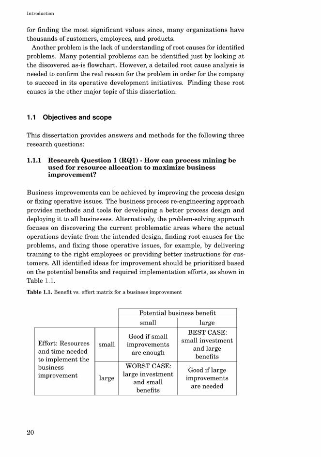
Business improvements can be achieved by improving the process designor fixing operative issues. The business process re-engineering approachprovides methods and tools for developing a better process design anddeploying it to all businesses. Alternatively, the problem-solving approachfocuses on discovering the current problematic areas where the actualoperations deviate from the intended design, finding root causes for theproblems, and fixing those operative issues, for example, by deliveringtraining to the right employees or providing better instructions for cus-tomers. All identified ideas for improvement should be prioritized basedon the potential benefits and required implementation efforts, as shown inTable 1.1.

Table 1.1. Benefit vs. effort matrix for a business improvement

Potential business benefitsmall large

Effort: Resourcesand time neededto implement thebusinessimprovement

smallGood if smallimprovements

are enough

BEST CASE:small investment

and largebenefits

large

WORST CASE:large investment

and smallbenefits

Good if largeimprovements

are needed

20

Introduction

In order to maximize business improvements, the available developmentresources must be allocated to those development projects that give thelargest benefits with the available resources, as shown in Table 1.1. Thisdissertation addresses the following aspects:

1. How to use process mining data preparation methods to acquirerelevant data of business operations in case and event log format,

2. How to define a binary business problem by categorizing each indi-vidual case as problematic or successful. Alternatively, how to definea business problem using a continuous variable like lead-time suchthat the degree of problems within each individual case is presentedas a value in the continuous variable.

3. How to define a variety of potential development projects by settinga scope for each project based on case attribute values.

4. How to combine potential benefits and resource needs into one mea-sure such that development projects can be ordered based on thismeasure, which is then used to allocate development resources tothose projects that maximize business improvement.

Figure 1.1 illustrates the main problem of RQ1 and the key solutionfor resource allocation. Black circles represent problematic cases, andwhite circles represent successful cases. The total area represents thewhole organization, and the division of the are into smaller different sizedrectangles represents the business areas based on distinct values of onecase attribute. The figure contains three layers, which represent threedifferent case attributes such as region, product group, and customer group.Our objective now is to find those business areas, in any of the layers,that contain a large amount of problematic cases. More specifically, wesearch for areas that have a high enough density and high enough absoluteamount of problematic cases by ordering all groupings of cases based on allcase attributes and their distinct values. Development resources need tobe allocated to those identified areas to maximize business improvementbenefits. In Figure 1.1, where business areas are represented as differentsized rectangles, the upper right corner business area is a good candidatefor resource allocation since it meets the two main criteria: 1. The densityof problematic cases is high (75%); and 2. The number of problematic casesis sufficiently high, as six out of a total of 60 problems are in this area. Theproblem setup for RQ1 is presented in Section 2.2.

1.1.2 Research Question 2 (RQ2) - How can process mining beused to identify changes in business operations?

Here our objective is to show what has changed in the process. Changesneed to be shown in the order of business significance. An important use

21

Introduction

Each layer corresponds to one grouping of cases, for example based on onecase attribute.��

�

��

Each rectangle in a layer represents cases that have the same valuefor the particular case attribute.

�

�

�

�

�

�

�

�

�

�

�

�

�

�

�

�

�

�

�

�

�

�

�

�

�

�

�

�

�

�

�

�

�

�

�

�

�

�

�

�

�

�

�

�

�

�

�

�

�

�

� �

�

�

�

�

�

�

�

�

�

�

�

�

�

�

�

�

�

�

�

��

�

�

�

�

�

� ��

�

�

�

�

�

�

�

�

�

�

�

�

�

�

�

�

�

�

�

�

�

�

�

�

�

�

�

�

�

�

�

�

�

�

�

�

�

�

�

�

�

�

�

�

�

�

�

�

�

�

�

�

�

�

�

�

�

�

�

�

�

�

�

�

�

�

�

�

�

�

�

�

�

�

�

�

�

�

�

�

�

�

�

�

�

�

�

�

�

�

��

�

�

��

�

�

�

�

��

�

�

�

�

�

�

�

� �

�

�

�

�

�

�

� � Development resourcesshould be first allocatedto this business areabecause:

1. Density of problemsis high (75%) and

2. Number of problem-atic cases is high enough(6 problems out of total60 are in this area)

Figure 1.1. Illustrative groupings of cases for detecting problematic business areas.

for this analysis is a periodical business review, for example, a monthlybusiness review, where our analysis is needed to show the most significantchanges by comparing the review period against previous historical periods.Another use is called concept drift analysis, where the properties of theprocess change over time.

Considering RQ2, the analyst person is not initially aware of a businessproblem in the process. The objective of RQ2 is to detect changes inbusiness operations comparing the review period with the history period.Changes are ordered by their significance. Example: We compare thecustomer order data from January 2020 against the customer order datafrom the full year 2019. We find out that in January 2020, a larger amountof Route Changed events are taking place compared to historical datafrom 2019. This change can be considered as a business problem, and theanalysis is then continued using the approach described in RQ1 to identifya development project for improving the process.

Figure 1.2 shows a timeline containing process cases, each consistingof individual events related to those cases. Position on the y-axis is usedfor presenting events belonging to the same case in a horizontal sequence.Each event has a label specifying the activity that took place and theevents and connected with arrows to show the transition from one event tothe next within the same case. Timeline is divided into a history periodand a review period. Detecting changes reveals that during the historyperiod the process typically contained events a, b and c, compared to the

22

Introduction

situation in review period when the process more often contains the eventsa, x and c. Other changes that should be detected include events occurringin a different order, skipping of events, extra events, repeating events,change in the event attribute value of any activity, and change of caseattribute value. The problem setup for RQ2 is presented in Section 2.3.

time �

a� b � d

a� x � c

a� b� ca� b� c� c

a� b� c

a � b� c a� b� c a� ba � x � c

a� x� c

a� x� ca � b � c

History period Review period

Process change: re-view period containsmore often the traces[a,x,c] compared tohistorical [a,b,c].

Figure 1.2. Illustrative traces for identifying changes in business operations.

1.1.3 Research Question 3 (RQ3) - How can business areas thathave a significant effect on process flow behavior bediscovered using clustering?

Our objective is to use clustering on historical data in order to groupsimilar kinds of process instances into the same clusters and then findingthe business areas that correlate most with these identified clusters.

Considering RQ3, the business analyst wants to understand what iscausing differences in process flow executions. Our approach finds outthose business areas that are causing the process flow to be different fromother business areas. Example: We want to understand better the order-to-cash process flow starting from end customer placing an order up tothe point of the cash being collected, including production, logistics, andother activities. Using our clustering-based method, we find out that RouteType and Delivery Country have a big effect on the process flow. Especiallywe find out that the process flow for cases having Route Type = Train issignificantly different from cases belonging to the other Route Types. Withthis information, we can now use our Influence Analysis method to discoveractual differences in the process flow of Route Type = Train cases comparedto the other Route Types cases in order to find potential business problems.If the Route Type = Train cases are entirely different from the other cases,then it may even make sense to analyze those cases separately from eachother.

Figure 1.3 shows the results of clustering 129 cases using the processflow information into five clusters. Each case is represented with a markercorresponding to one of the five clusters. The total area represents the

23

Introduction

whole organization, and the division of the area into smaller differentsized rectangles represents the business areas based on distinct values ofone case attribute. The main focus of RQ3 is to discover those businessareas that correlate with the clustering results. Figure 1.3 highlightsone business area containing six cases, out of which five share the samedistinct process flow behavior characterized by a particular cluster. Theproblem setup for RQ3 is presented in Section 2.4.

Each layer corresponds to one grouping of cases, for example based on onecase attribute.��

�

��

Each rectangle in a layer represents cases that have the same valuefor the particular case attribute.

�

+

�

�

+

�

�

x�

x

x

�

+

x

x

+�

�

+

+x

+

x

�

�

�

+

x

+

�

�

x

�

�

x

+

+

+

�

x

x+

+�

�

�

+

�

�

+

�

x

�

�

��

x+

+

�

�

�

+�

x++

�

+

�

+

+

�

+

�

�

x�

+

++

�

+

+

x

�x

x

+

�

�

�

�

+

x

+

+x

�Each symbol representsa case belonging to aparticular cluster basedon the process flow be-havior.

�Interesting businessarea containing mostlycases from cluster �

Figure 1.3. Illustrative groupings of cases for discovering business areas with a significanteffect on process flow.

Figure 1.4 depicts the dependencies between research questions andcorresponding solutions. RQ1 is the main research question introducing theInfluence Analysis methodology. RQ2 and RQ3 can be used as standalonequestions providing new analysis information, or the results from theseresearch questions can further be investigated using RQ1 to find the bestway to focus improvement resources for fixing the identified challenges.Table 1.2 summarizes the Publications related to each research question.

24

Introduction

RQ1: How can processmining be used for resource

allocation to maximizebusiness improvement?

RQ2: How can processmining be used to identify

changes in businessoperations?

RQ3: How can businessareas that have a significant

effect on process flowbehavior be discovered

using clustering?

Use RQ1 tofix identified

changes

Use RQ1 toanalyze and fix

problembusiness areas

Problemsidentified

using othermethods

�

��

��

��

�

Figure 1.4. Hierarchy of Research Questions

Table 1.2. Relationship between research questions and publications

Pub.I

Pub.II

Pub.III

Pub.IV

Pub.V

Pub.VI

Pub.VII

Pub.VIII

RQ1: How canprocess mining beused for resourceallocation to max-imize business im-provement?

X X X

RQ2: How canprocess mining beused to identifychanges in busi-ness operations?

X X X X

RQ3: How canbusiness areasthat have a sig-nificant effecton process flowbehavior be dis-covered usingclustering?

X X X X X X X

1.2 Related work

RQ1: How can process mining be used for resource allocation tomaximize business improvement?With current methodologies, it is difficult, expensive, and time-consumingfor organizations to identify the causes of their operational business prob-

25

Introduction

lems. One reason for the difficulty is that causality itself is a difficultconcept in dynamic business systems [48]. In addition, the theory of con-straints highlights the importance of finding the most relevant constraintsthat limit any system in achieving its goals [29].

The idea of root cause analysis has been widely studied. It includessteps such as problem understanding, problem cause brainstorming, datacollection, analysis, cause identification, cause elimination, and solutionimplementation [6].

Practically all large organizations use business data warehouse andbusiness intelligence systems to store the operational data created duringbusiness operations [20], [35]. In 2012 the amount of available data hadgrown to such an extent that the term Big Data was introduced to highlightnew possibilities of data analysis [44]. There are many data mining andstatistical analysis techniques that can be used to turn this data intoknowledge [49] [51]. There has also been more work carried out in thedetection of differences between groups [61] and finding contrast sets [8].

Studies in the field of process mining have highlighted the usage ofprocess mining for business process analysis [2]. Decision tree learninghas been used to explain why a certain activity path is chosen within theprocess, discovering decisions made during the process flow [52]. Decisiontrees generated from different process variants have also been used tofind relevant differences between those process variants [11]. A context-aware framework for analyzing performance characteristics from multipleperspectives has been presented in [33]. Causal nets have been furtherstudied as a tool and notation for process discovery [1]. The approach fordetecting cause-effect relations between process characteristics and processperformance indicators based on Granger causality is presented in [34].Our work is partly based on enriching and transforming process-based logsfor the purpose of root cause analysis [56]. We also adopt ideas from theframework for correlating business process characteristics [38]. Our workextends the current process mining framework by allowing business usersto identify root causes for business problems interactively. Our method isalso an example of abductive reasoning that starts with observation andtries to find a hypothesis that accounts for the observation [36].

Probability-based interestingness measures are functions of a 2 x 2contingency table [49]. Table 1.3 shows the generic representation of acontingency table for a rule A → B, where n(AB) denotes the amount ofcases satisfying both A and B, and N denotes total amount of cases. Anexample contingency table for a rule product = hats → durationdays ≥ 20in a database that contains a total of 10 cases such that 3 cases take longtime, 4 cases belong to category hats, and one case meets both conditions ie.the product delivered is hats and it took a long time is shown in Table 1.4.Summary of 37 different measures with a clear theoretical background andcharacteristics has been documented in [28]. However, a typical business

26

Introduction

person may not be familiar with the measures and may have difficultiesunderstanding the business meaning for each measure. In this dissertation,we will present three probability-based objective measures derived fromthree business process improvement levels. Business people will be able todecide the level of improvement they are planning to achieve and select ameasure based on that level.

Table 1.3. 2 x 2 Contingency tablefor rule A → B

B B

A n(AB) n(AB) n(A)

A n(AB) n(AB) n(A)

n(B) n(B) N

Table 1.4. Contingency table for ruleproduct = hats → duration ≥ 20d

B B

A 1 3 4

A 2 4 6

3 7 10

Example questions such as "Which customer characteristics are linkedto the occurrence of reclamations?" have been presented in a practicalframework for process mining analysis uses cases paper [39]. The diagramspresented in the paper show the limitation of the decision tree diagramsas these only show the positive root causes for the given question. Onebenefit of our method is that it provides the analysis results in the form ofcomparative benchmarking, showing both the most influential root causesfor the long process lead times as well as the most influential best practicesfor achieving short lead times. The ability to show the root causes forbad and good behavior simultaneously makes it possible to quickly seewhether the problem cases have a clear root cause or whether there is acommon root cause for cases of good behavior. Our methodology is based ondeviations management [50] by discovering significant root causes usingprocess mining data.

Existing studies on root cause analysis and decision tree analysis inthe process mining domain are related to binary conditions where eachindividual case is regarded as good or bad—for example, the decision treeapproach presented in [52]. Wetzstein et al. present a framework formonitoring and analyzing influential factors of business process perfor-mance [64]. However, their method also requires the usage of a binarycontribution measure. Gröger et al. also demonstrate relevant data miningapproaches for manufacturing process optimization [30] using binary anddecision tree approach. Advantages of using our method include the abilityto analyze root causes for continuous variables such as lead times, andthe use of case-specific weights for conducting a more business-orientedanalysis.

27

Introduction

RQ2: How can process mining be used to identify changes in businessoperations?Handling concept drift in process mining has been discussed in detail in[12], [13], [17] and [66]. These papers suggest three main problems tobe studied: detection of change points, characterization of change, andinsight into process evolution. Although these papers are excellent forimparting an understanding of how the process has changed, they sharethe challenge that they need completed cases and can each be categorizedas an offline analysis of change. If cases take six months to complete,the analysis results based on complete cases are at least six months old.However, as part of a business review, the management is reviewing a fixedperiod and trying to identify relevant change signals as early as possible,hinting how the processes might be changing at this very moment. Usingour method, the change point can be set to the beginning of the reviewperiod, and our method then shows the most relevant changes that haveoccurred. Our method can be categorized as online analysis of changes. Asomewhat similar approach has been presented in [47] where the completeevent log is divided into pre-drift and post-drift logs, and correspondingprocess models, which are compared to find the minimum set of changeoperations needed to explain the change behind a drift.

Concept drift in relation to machine learning has been studied extensivelyin [65], [43], and [62]. The objective of those studies is to increase theaccuracy of predictions by utilizing machine learning algorithms thatdiscover the changes in the process. Instead of making accurate predictions,our method is tailored to discover and explain changes as part of thesystematic periodical business review.

A novel Trace Clustering algorithm [32] presents an approach to analyzeattribute data from events and cases in addition to the traditional busi-ness process data. The approach is based on the Markov cluster (MCL)algorithm [25] for finding similar cases. Although the results look promis-ing, the challenge of this approach is that it uses complete cases and isthus more useful for offline process analysis than for periodical businessanalysis.

An approach more targeted for online business process drift detection ispresented in [42]. It uses the concept of partial order runs to run statisticaltests in order to find the exact point in time for the change. A somewhatsimilar method for concept-drift detection in event log streams has beenstudied in [7], which presents a method for detecting actual concept-drifttime and individual anomalies using histograms and clustering. However,these methods do not take into account the attribute data and are notaimed at providing insight into the business review question of whathas changed during the current business review period in comparison toprevious operations.

Since it is difficult to detect the changes by using only traditional statis-

28

Introduction

tical measures, a set of visual analytic tools enabling interactive processanalysis and process mining is presented in [16]. The paper presents avisualization for detecting concept drift and changes in business processand case attribute data by plotting all events to a stacked area graph withcalendar time on the horizontal axis. Even though the presented toolsare useful, they do not provide insight into what has changed during thepast review period in the event attribute level. Presented visualizationtechniques also have challenges when the amount of case attributes is solarge that case attributes cannot all be included in the visualizations atthe same time.

An alarm-based prescriptive process monitoring for making business peo-ple aware of changes that require active intervention is presented in [58].The method uses a sophisticated cost model to optimize the generationof alerts for business people. One challenge with their method is that itrequires a lot of settings and detailed level knowledge of the importanceof various process issues. These settings must be fixed beforehand so thatthe algorithm can then suggest active intervention when needed. Our ex-perience regarding actual business operations is that this kind of detailedinformation is not typically available, or is challenging to maintain overtime. However, our experience is that all large organizations conduct regu-lar business reviews, which makes it beneficial to present the discoveriesas part of the business review meetings.

RQ3: How can business areas that have a significant effect on processflow behavior be discovered using clustering?One key challenge in process mining is that a single event log may oftencontain many different process variants, in which case trying to discovera single process diagram for the whole log file is not a working solution.In the process mining context, clustering has been widely studied, withexcellent results [45], [54], [39], and [59]. This previous work covers theusage of several distance measures like Euclid, Hamming, Jaccard, cosine,Markov chain, edit distance, and several cluster approaches including par-titioning, hierarchical, density-based, and neural networks. However, mostof the previous research related to clustering within the process miningfield has been directly focused on the process flowchart discovery with theprime objectives categorized as process, variant or outlier identification,understandability of complexity, decomposition, or hierarchization. Inpractice, this means that clustering has been used as a tool for helpingthe other process mining methods such as control flow discovery to workbetter—that is, clustering has divided the event log into smaller sub-logsthat have been directly used for further analysis. Our approach enablesanalysts to use clustering for discovering those business areas that have asignificant effect on process behavior.

Research has started to address the challenge of how to explain the

29

Introduction

clustering results to business analysts [37]. The role of case attributesis important when explaining the characteristics of clusters to businessanalysts [53]. Our method provides an easy to understand representationof cluster characteristics based on the difference of densities and caseattribute information.

Considerable time has also been spent in the process mining communityto discover branching conditions from business process execution logs[40]. This has also led to the introduction of decision models and decisionmining [9], and to the use of the standard Decision Model and Notation(DMN) for automating operational decision-making [10]. As the objective ofdecision modeling is to provide additional details into individual branchingconditions, the objective of our approach is to analyze the effect of anybusiness area on the whole process flow, not just one decision branch at atime.

Extensive work has been carried out in the area of applying machinelearning techniques in process mining. A total of 55 academic papersare listed in a summary paper [26] about predicting the outcome of anongoing process instance. Discriminating features have been studied asone possible method for feature selection [18]. Discovering signaturepatterns from event logs has also been studied for predicting desired orundesired behavior [14]. Using event and case attributes to enhancecase-level predictions has been studied in [27] and [41]. Specific machinelearning algorithms have been studied for predicting the outcome of anongoing process instance using long-short-term memory (LSTM) [57], gatedrecurrent unit (GRU) [46], and recurrent neural networks (RNN) [63]. Ourwork uses these machine learning algorithms to deliver accurate predictionresults in shorter execution times, specifically with a high number of caseand event attributes.

1.3 Contributions of this Dissertation

This dissertation presents novel methodologies for analyzing businessprocesses using process mining. Its contributions consist of answering thethree research questions, which are briefly summarized below.

RQ1: How can process mining be used for resource allocation tomaximize business improvement?Our novel influence analysis methodology is first presented in PublicationI as a root cause analysis for business users, helping them to allocatebusiness improvements resources more effectively. Our contributionsinclude methods for collecting event and case attribute information to formnew categorization dimensions; methods for forming a binary classificationof cases such that each case is either problematic or successful; selection

30

Introduction

of a corresponding interestingness measure based on the desired levelof business process improvement effect; and the definitions of presentedinterestingness measures.

One essential element related to the calculation of our contribution mea-sure is the usage of both the density of analyzed problems and the totalsize of the business area compared to the whole dataset. Our contributionmeasure is a combination of both these aspects. As the method presentedin Publication I is only applicable for binary variables, the Publication IIfurther extends the influence analysis methodology for continuous vari-ables, as well as case-specific weighting. Continuous variables are particu-larly useful for analyzing business process lead times. Our contributionsregarding lead times also include the idea of analyzing the lead time vari-ance—that is, finding the root causes for durations that are too long or tooshort. We also show how the case-specific weights can be used to create abusiness-oriented analysis where each case is given a weight based on mea-sures such as monetary value, priority, business importance, profitability,or work effort.

As a special contribution related to working capital optimization, weshow how case-specific weights and continuous process lead times can beused to identify those business areas where the largest amounts of extraworking capital are tied-up.

Another contribution of our work is that its analysis can be used forbenchmarking. Since our contribution measure has a symmetrical behavior,all the business areas included in the root cause analysis get a positive ornegative contribution indicator, showing both the problem areas and thebest practice areas at the same time. For example, a discovery related tosales orders in a large organization can be used to benchmark the distinctvalues of the case attribute Regional Office. Each regional office gets apositive or negative contribution value such that the sum of all contributionvalues is always zero.

RQ2: How can process mining be used to identify changes in businessoperations?Publication III shows how to use the influence analysis methodology ina novel way to analyze process mining events instead of cases and useevent timestamps for identifying changes in the business process over time.Unlike most process mining change detection algorithms, which operate onthe case-level, our method analyzes changes in the individual event level.We show how case-level data can be used to construct features for the eventlevel. Our method detects changes in a timely manner, since there is noneed to wait for the cases to be completed. We present two alternativemethods—a binary approach and a continuous event-age approach—fordividing events into comparison data and review data for business reviewpurposes. Our contributions are related both to preparing the source data

31

Introduction

for the analysis, and to calculating the results and presenting to businessusers.

RQ3: How can business areas that have a significant effect on processflow behavior be discovered using clustering?Publication IV introduces a novel method of using clustering analysisto discover business areas that have a significant effect on process flowbehavior. Our contributions include a method for using process flow dataas features for clustering; parameters for the clustering algorithm; theidea of running the clustering several times with different parameters;usage of influence analysis measures for identifying significant businessareas; and a method of consolidating results for finding the most significantcase attributes. We show how the contribution measure works in practicefor explaining clustering results, discovering individual business areas,and finding the case attributes that correlate most with differences in theprocess flow.

Contributions applicable to all research questionsOne generic contribution of this dissertation is the problem setup docu-mented in Chapter 2, which aims to specify common issues and use casesrelated to analyzing and improving processes. As an additional contribu-tion, we provide case study analyses using real-life industrial data for allresearch questions in Chapter 4. These analyses show example resultsand an intended usage scenario for our methods.

Finally, we include a discussion section related to each research questionin Chapter 4 to provide our best practices and experiences of using thesemethods in our process mining projects.

Formal definition of Influence AnalysisSince the Influence Analysis is the main contribution of this dissertation,we present an overall definition of the algorithm already here in theIntroduction Section as follows:

Definition 1. Influence analysis is an algorithm that takes an event logL and its subset Lp as parameters. The result of the algorithm is a set of<feature, feature_value, contribution> tuples, where feature is any propertyof the cases in L, feature_value is any existing value for the particularfeature in the dataset, and contribution is the outcome of the algorithmthat measures the significance of the particular feature and feature_valuecombination for belonging, or not belonging to the subset of cases Lp.

32

2. Problem Setup

2.1 Process mining concepts

All research questions addressed in this dissertation use the process miningdata as the source data for the methods. We first give definitions for theseprocess mining concepts:

Definition 2. Let E = {e1, . . . , en}, be a set of events in the process analysis.

Definition 3. Let ET = {et1, . . . , etN } be a set of event types that representthe activity labels for events in the process analysis. Each event is of oneevent type such that #EventT ype(ei) ∈ ET, for all ei ∈ E.

Definition 4. Let #TimeStamp(ei) be the timestamp of the occurrence ofevent ei. Timestamp typically represents the date and time when the actualreal-life activity took place. Timestamps are required for ordering theevents within cases. They are also for calculating lead times and other KPImeasures

Definition 5. Let C = {c1, . . . , cm}, be a set of cases in the process analysis.Each individual case represents a single business process execution instanceand it has a unique case identifier. Each event belongs to exactly one casesuch that #Case(ei) ∈ C, for all ei ∈ E. Each case ci ∈ C has a trace which is anordered sequence of events #Trace(ci)= ⟨e1, e2, ..., el⟩, where ∀1≤ j ≤ l : e j ∈ Eand ∀2≤ j ≤ l : #TimeStamp(e j)≥ #TimeStamp(e j−1).

We will now define the case attributes that contain relevant businessdata for cases:

Definition 6. Let ATC = {atc1, . . . ,atcN } be a set of case attributes in theprocess analysis. Each case ci ∈ C has a value #atc j (ci) for each case attributeatc j ∈ ATC.

Definition 7. Let Vatc j = {v1atc j

, . . . ,vNatc j

} be a set of distinct values that thecase attribute atc j has in the process analysis.

33

Problem Setup

Definition 8. Let CaseAttributeSubgrouping(atc j) = {Cv1 , . . . ,CvN } be asubgrouping of all cases ci ∈ C so that ∀ci ∈ Cvn : #atc j (ci)= vn

atc j.

CaseAttributeSubgrouping for case attribute atc j allocates all the casesin process analysis into subgroups based on the value of atc j for eachcase. The number of subgroups for each case attribute is the number ofdistinct values for each case attributes. For example, subgroups for thecase attribute Region could contain America, Europe, Asia, Africa, Other,and Unknown.

We define the event attributes that contain relevant business data forevents similarly:

Definition 9. Let ATE = {ate1, . . . ,ateN } be a set of event attributes in theprocess analysis. Each event ei ∈ E has a value #ate j (ei) for each eventattribute ate j ∈ ATE.

Definition 10. Let Vate j = {v1ate j

, . . . ,vNate j

} be a set of distinct values that theevent attribute ate j has in the process analysis.

Definition 11. Let EventAttributeSubgrouping(ate j)= {Ev1 , . . . ,EvN } be asubgrouping of all events ei ∈ E so that ∀ei ∈ Evn : #ate j (ei)= vn

ate j.

The summary of these process mining concepts is presented in Figure2.1. Each concept is linked to the corresponding definition, as presentedin this section. Further introduction to process mining can be found inthe books "Process Mining - Discovery, Conformance and Enhancement ofBusiness Processes" [4] and "Process Mining - Data Science in Action" [3]

2.1.1 Example data

In this Section, we present a small example process mining data. Thechosen business process is the order-to-delivery process, and the caserepresents one individual order line.

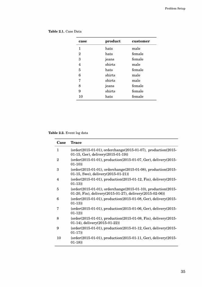
Table 2.1 shows example data containing ten process mining cases andthe case attributes product and customer with values for each case. Table2.2 contains an event log for each case specifying the activity name anddate of the activity. Event production also has the name of the countrywhere production was conducted as an event attribute.

Figure 2.2 shows a process model discovered from the example data usinga process mining algorithm where:

• The four rectangles order, orderchange, production and delivery rep-resent the discovered Event Types (activities) in the Event Log.

• The percentage value inside each rectangle shows the number ofcases visiting the particular Event Type.

• The flows between Event Types represent the transitions of a casemoving from one event type to another. Each presented flow shows

34

Problem Setup

Table 2.1. Case Data

case product customer

1 hats male2 hats female3 jeans female4 shirts male5 hats female6 shirts male7 shirts male8 jeans female9 shirts female10 hats female

Table 2.2. Event log data

Case Trace

1 {order(2015-01-01), orderchange(2015-01-07), production(2015-01-15, Ger), delivery(2015-01-19)}

2 {order(2015-01-01), production(2015-01-07, Ger), delivery(2015-01-10)}

3 {order(2015-01-01), orderchange(2015-01-08), production(2015-01-15, Swe), delivery(2015-01-21)}

4 {order(2015-01-01), production(2015-01-12, Fin), delivery(2015-01-13)}

5 {order(2015-01-01), orderchange(2015-01-10), production(2015-01-20, Fin), delivery(2015-01-27), delivery(2015-02-06)}



8 {order(2015-01-01), production(2015-01-08, Fin), delivery(2015-01-14), delivery(2015-01-22)}



35

Problem Setup

EventsCases 1 1..n

Event AttributesCase Attributes

Case AttributeValues

Event AttributeValues

1

1

n(case attributes)

n(cases)

1

1

n(event attributes)

n(events)

Event Types11..n

Def 1. Def 2.Def 4.

Def 5.

Def 5.

Def 8.

~Def 6. ~Def 9.

Figure 2.1. Process mining concepts

the volume information (i.e., how many cases contain the transitionfrom source event type to the destination event type) and the aver-age/median duration calculated as the median of the difference of thetimestamps.

• Specific start and end symbols represent the beginning and end ofthe trace.

Figure 2.2. Example process flowchart

2.2 RQ1: How can process mining be used for resource allocationto maximize business improvement?

RQ1 is about helping organizations to improve their business operations byproviding relevant root causes for discovered process problems. Important

36

Problem Setup

concepts related to RQ1 include:

• Business Problems. If the organization/process/system has no prob-lems, then the improvement potential is zero. Process mining oper-ates on the individual process instance level, meaning a system isanalyzed based on the individual process instances that have beenexecuted. The analysis uses the event log information containing allrecorded process steps with the timestamp information and otherevent attributes for each event. In this context, the existing pro-cess mining algorithms and methods are very efficient in detectingbusiness problems. We want to minimize these problems.

• Problem Types. There are two kinds of business problems relatedto process mining analysis: binary problems, where each case is clas-sified either as problematic or successful; and continuous problems,where each case has a specific numeric value representing the size ofthe problem. The continuous approach can be used for analyzing leadtimes where, for example, the actual length of the lead time in min-utes, hours, or days can be considered as the size of the problem—thelonger the lead time, the bigger the problem.

• Problem Weighting. The core idea of Business Process Manage-ment (BPM) is to improve business processes by analyzing equallyimportant individual process cases, for example, individual salesorders in the order-to-delivery process. The BPM approach typicallytries to find the reason why the process fails to deliver some customerorders on time, using equal importance for each sales order. However,from a business point of view, there are situations when it is bene-ficial to give specific weighting for individual cases. For example, itwould be more important to deliver high-value sales orders in time,making the order size in currency a good candidate for case-specificweighting.

• Development Projects. Improving real business operations re-quires development activities to be performed. A development projectconsists of those activities, aims to reduce problems, and has theseproperties:

– Scope determines the part of the business that is affected bythe development project. The scope for a development project isexpressed as a sub-group of cases based on a particular valueof a particular case attribute. The characteristics specifyingthe scope must be known before or, at the latest, during theexecution of the case.

– Improvement potential tells how many problems will be fixed byexecuting the development project.

37

Problem Setup

– Investment cost is an estimate of the amount of resources neededto get the results.

Finding the best scope for a development project is often tricky sinceit affects both the improvement potential and investment costs.

• Amount of resources. Organizations have an annual minimumamount of development resources available for operational improve-ment. Additional resources including extra personnel, allocation oftime from business operations, purchase of external services, andinvestments are available when the management accepts an improve-ment plan with a high return on investment (ROI).

• Objective. The aim is to identify those development projects thatfix the largest number of problems with the smallest amount ofresources.

Here are the formal definitions to these needed concepts:

Definition 12. Let P0 be the initial volume of problems in business op-erations before any development project. If P0 is zero, then there are noproblems in the business operations, and it would be impossible to find anydevelopment project that could improve the situation.

Definition 13. Let D = {d1, . . . ,dN } be a set of Development Projects.

Definition 14. Let Pdi be the total volume of problems in business opera-tions after the execution of development project di ∈ D. Pdi may be smalleror bigger than the initial volume of problems P0.

Definition 15. Let potential(di)= P0−Pdi be the improvement potential ofthe development project di.

Definition 16. Let cost(di) ∈ R≥0 be the cost of the development projectdi. According to the assumption that cost of a development project isproportional to scope of the development project, the cost of a developmentproject di affecting a subset of cases C j ∈ C would be cost(di)∝ n(C j).

Return on Investment (ROI) is often used to compare the efficiencies ofseveral different investments such as development projects. Using thepotential− costs as the benefit (or return) of the development project, thegeneric definition for RQ1 is formulated as finding the development projectwith highest ROI as:

Definition 17. Let RQ1= argmaxdi∈D ROI(di)= argmaxdi∈Dpotential(di)−cost(di)

cost(di)be the generic formalization for the question "Identify the developmentprojects with the highest development potential and lowest costs."

38

Problem Setup

2.3 RQ2: How can process mining be used to identify changes inbusiness operations?

The ability to detect changes is crucial for developing and improving agilebusiness operations. Unwanted changes need to be mitigated quickly, anddesired changes need to be reinforced and shared as best practices. Duringa business review, managers typically review the performance of businessoperations using Key Performance Indicators (KPIs). One problem is thatmanagers typically do not have an accurate fact-based understanding andanalysis of what has changed during the review period. They often rely onsubjective comments, views, and suggestions influenced by acute businesschallenges and crises. There are various details for business managersand analysts to consider:

• Setting the review period. Business managers should easily seewhat has changed during the review period by comparing the newprocess mining data against data from previous business reviewperiods. For example, a manager or internal auditor who has beenaway from business operations for a week, month, or year can easilyfind out what has been changed during that period compared to theprevious historical data. During an acute crisis like the coronaviruspandemic [68], process owners and line managers would benefit froman analysis showing how the process execution has changed on adaily level by comparing yesterday’s process execution data againstthe previous month.

• Fast and slow changes. Both the fast changes occurring suddenly,as well as the more gradual changes that occur in several years,should be detected to give managers accurate insight into the currentsituation, changes, and trends.

• Relevancy. Identified business process changes should be prioritizedbased on the combination of the relative amount of the changed casesas well as the absolute scope of the change in relation to the wholeprocess execution. A relatively small change in the context of anactivity that occurs in all cases is more important than a majorchange related to an activity that occurs only once per year.

• Root causes. In addition to identifying the relevant changes, itshould be possible to find possible root causes for the identifiedchanges. Also it should be possible to show or predict the effect andoutcome of each change in relation to a particular business outcomeor KPI measure.

• Data quality detection. Process mining and KPI reporting rely oncontinuously updating data, typically the ERP systems. The mini-mum requirement for the change detection system is that it should

39

Problem Setup

automatically detect major problems in these data integrations. Forexample, if the incremental loading of a database table containingcustomer delivery timestamps fails for one import, the magnitude ofchange should be so high that this issue is reporting very high in thelist of process changes. The change detection method should alwaysbe automatically used as a quality assurance feature for automatedperiodical data loads.

Here are the formal definitions to clarify the problem setup:

Definition 18. Let A = {α1, . . . ,αN } be a set of process mining event charac-teristics. The characteristic αi may be any particular event attribute value,a combination of several event attribute values, or any other property thatcan be defined for an event.

As an example, if all events have an event attribute PerformedBy andone possible value for this attribute is User1234, then the events havingthe characteristic αi have PerformedBy=User1234.

Definition 19. Let Eαi = {e1αi

, . . . , eNαi

} be a set of events sharing the samecharacteristic αi. Eαi ⊆ E.

Following the example above, the set of events Eαi where αi is Per-formedBy=User1234 would include all the events that have been Per-formedBy the User User1234. The key idea in detecting changes is toanalyze the distribution of events Eαi in relation to the whole set of events.Since our goal is to identify changes over time, we define a review periodas:

Definition 20. Let Er = {e1r, . . . , eN

r } be a set of events belonging to the ReviewPeriod r. Er ⊆ E.

As a measure for the business significance of any change, we are inter-ested in the difference in the density of the particular characteristic in thereview period compared to the whole dataset. Here is the generic definitionfor RQ2:

Definition 21. Let RQ2= argmaxαi∈A abs(

∣∣∣Er∩Eαi

∣∣∣

|Er| −∣∣∣Eαi

∣∣∣

|E| ) be the generic for-malization to the question "Identify those process mining event characteris-tics that are most significantly unevenly distributed over time."

2.4 RQ3: How can business areas that have a significant effect onprocess flow behavior be discovered using clustering?

It is often challenging to communicate the detailed process mining findingsto business people. While line managers may not be familiar with process

40

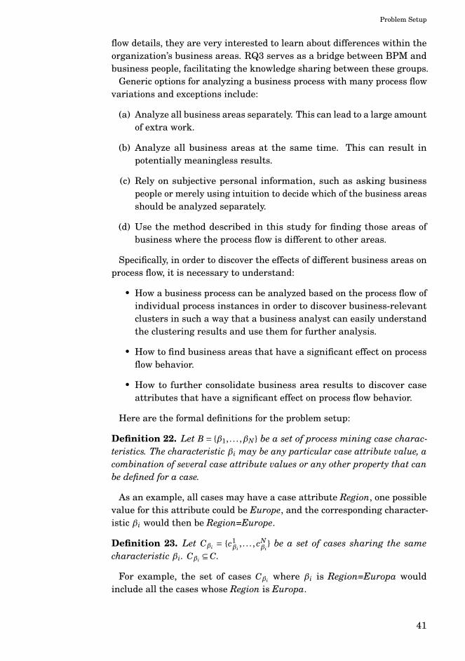
Problem Setup

flow details, they are very interested to learn about differences within theorganization’s business areas. RQ3 serves as a bridge between BPM andbusiness people, facilitating the knowledge sharing between these groups.

Generic options for analyzing a business process with many process flowvariations and exceptions include:

(a) Analyze all business areas separately. This can lead to a large amountof extra work.

(b) Analyze all business areas at the same time. This can result inpotentially meaningless results.

(c) Rely on subjective personal information, such as asking businesspeople or merely using intuition to decide which of the business areasshould be analyzed separately.

(d) Use the method described in this study for finding those areas ofbusiness where the process flow is different to other areas.

Specifically, in order to discover the effects of different business areas onprocess flow, it is necessary to understand:

• How a business process can be analyzed based on the process flow ofindividual process instances in order to discover business-relevantclusters in such a way that a business analyst can easily understandthe clustering results and use them for further analysis.

• How to find business areas that have a significant effect on processflow behavior.

• How to further consolidate business area results to discover caseattributes that have a significant effect on process flow behavior.

Here are the formal definitions for the problem setup:

Definition 22. Let B = {β1, . . . ,βN } be a set of process mining case charac-teristics. The characteristic βi may be any particular case attribute value, acombination of several case attribute values or any other property that canbe defined for a case.

As an example, all cases may have a case attribute Region, one possiblevalue for this attribute could be Europe, and the corresponding character-istic βi would then be Region=Europe.

Definition 23. Let Cβi = {c1βi

, . . . , cNβi

} be a set of cases sharing the samecharacteristic βi. Cβi ⊆ C.

For example, the set of cases Cβi where βi is Region=Europa wouldinclude all the cases whose Region is Europa.

41

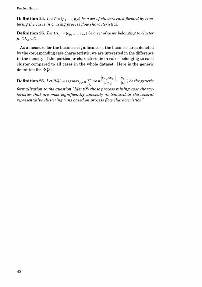
Problem Setup

Definition 24. Let P = {p1, . . . , pN } be a set of clusters each formed by clus-tering the cases in C using process flow characteristics.

Definition 25. Let CLp = {cp1 , . . . , cpN } be a set of cases belonging to clusterp. CLp ⊆ C.

As a measure for the business significance of the business area denotedby the corresponding case characteristic, we are interested in the differencein the density of the particular characteristic in cases belonging to eachcluster compared to all cases in the whole dataset. Here is the genericdefinition for RQ3:

Definition 26. Let RQ3= argmaxβi∈B∑p∈P

abs(

∣∣∣CLp∩Cβi

∣∣∣

∣∣CLp

∣∣ −

∣∣∣Cβi

∣∣∣

|C| ) be the generic

formalization to the question "Identify those process mining case charac-teristics that are most significantly unevenly distributed in the severalrepresentative clustering runs based on process flow characteristics."

42

3. Methods

This Chapter describes the approach and methods for solving the problemspresented in the previous Chapter 2. Section 3.1 describes the influenceanalysis methodology, which is used for calculating the interestingnessmeasures needed for root cause analysis, analyzing process changes, anddiscovering business area effects. Influence analysis serves as the corefoundation for this dissertation. It is first presented as a binary versionfor process mining cases only in Publication I. Section 3.2 extends theinfluence analysis method to continuous problem functions needed, forexample, in process lead time analysis. The section also shows how case-specific weights can be used to take into account the business importanceof each individual case as presented in Publication II. Section 3.3 showshow the influence analysis method can be used on the process event levelto analyze process changes as presented in Publication III. Finally, Section3.4 presents our method for discovering business area effects to processmining analysis using clustering based on influence analysis publishedin Publication IV utilizing the findings in Publication VI, Publication VII,and Publication VIII. Section 3.5 contains our study of the Big Data SQLFrameworks for using distributed computing techniques and frameworksto execute process mining tasks as published in Publication V.

3.1 Influence analysis methodology

3.1.1 Identifying the relevant business process

The first task is to identify a high-level problem in the operations. Afteridentifying the problem, we pinpoint the business process where caseswill be classified as successful or problematic based on whether they ex-perienced the problem or not. This is a non-trivial task, and making awrong decision leads to inaccurate results. For example, when analyzingroot causes for failures to deliver customer orders on time, the case can

43

Methods

be selected several ways, such as complete customer order in ERP, indi-vidual customer order line in ERP, or individual delivery order in ERP.A complex customer order may include several order lines with variousdifferent products and services, each of which may be delivered on severaldelivery orders according to the agreed schedules. To analyze the businessrelevant KPI (Key Performance Indicator) OnTimeDelivery, it is possibleto be interested in:

• the whole customer order to be completely delivered on time,

• each individual item within the order being delivered on time, or

• each agreed delivery of each order item being completed on time.

It is the job of the analyst to select the correct granularity level for theanalysis based on the actual business problem that is investigated.

3.1.2 Collecting event and case attribute information

The accuracy of our analysis depends on the amount of data available inevent and case logs. Since our goal is to create new insight for businesspeople, we encourage the use of all event and case attribute data available,even though that typically introduces a lot of noise and data that is notalways relevant to the problems being analyzed. The generation of suitablelog files with extended attributes is a well-studied area [38]. Methods alsoexist for enriching and aggregating event logs to case logs [56]. These arethe key steps for constructing event and case logs:

• Identifying the relational database table whose rows correspond tocases C. In object-oriented systems, this corresponds to identifyingthe object class whose instances correspond to cases C.

• Finding for each case ci in C, a set of objects Oi such that every objectoi j in Oi is linked to ci directly. Then add recursively all objects linkedto oi j as long as the objects seem to be relevant concerning the anal-ysis objectives. Note that since every table in a relational databaseis typically linked to all the other tables in the same database recur-sively, this leads to potentially thousands of relevant linked objectsfor each case.

• Forming the event log for ci by including one event for every times-tamp attribute of the case ci and any linked object oi j.

• Forming the case log for ci by aggregating all attribute values of ci

and every object oi j in Oi, thus creating potentially thousands of caseattributes for each case. Suitable aggregation functions include count,sum, max, min, average, median, concatenate, first, and last.

44

Methods

• Augmenting every case ci by adding external events that have oc-curred during the lifetime of the case, for example, machinebreak-started, machinebreak-completed, weekend, strike, queuetoolong, andbadweather.

3.1.3 Categorization dimensions for cases

The purpose of this step is to create new categorization dimensions forall cases. These dimensions will then be used when identifying the bestimprovement focus areas, so the more dimensions we have, the larger thecoverage of our analysis will be. Table 3.1 shows examples of dimensionsthat can be created for every event log based on the log itself.

Table 3.1. Illustrative category dimensions for cases

Category dimension Usage for analyses

The number of events per case Cases with many events may be complex andcontain much rework. Cases with only a fewevents may be incomplete.

The number of distinct activi-ties per case

Cases containing a large number of differentactivities have a greater variety of processingthan the straightforward cases.

Start and end timestamps ofthe whole case

Exact calendar date, month, week, and yearcan be used to detect process changes overthe time. Day of the week and month of theyear are useful for discovering periodic andseasonal behavior.

Start and end time of an indi-vidual event type

Same rationale as the case-level attributeabove. Usage of these measures will createat least one new dimension for each analyzedevent type.

Activity profile. The numberof event occurrences per eachevent type

Often the fact that a particular event is exe-cuted several times for a case is a root causefor business problems.

Transition profile. The numberof flow occurrences per eachtransition from one event typeto the next.

Usage of the transition profile makes it possi-ble to identify root causes caused by perform-ing the activities in a certain order.

Our method is used to analyze and compare individual cases against eachother in order to find subsets of cases that can be used as a scope for processimprovement activities. A generic framework for correlating differentprocess characteristics has been presented in [24] where individual eventlog characteristics like decision points, events, and resources correlatewith identified process problems. One important aspect of our method is tocommunicate the results to business analysts and decision-makers who arenot familiar with process execution details but instead are very familiar

45

Methods

with business entities like organization units, product groups, customers,and suppliers. For this reason, we use feature selection for creating newdimensions to the case level.

Structural feature selectionPublication Publication VI includes a more detailed analysis of selectingstructural process mining features as categorization dimensions for pre-diction purposes. The objective is to extract and condense the processflow information into case level features. Challenge is that the number ofstructural features easily grows high, making the analysis difficult. This isa real risk for the prediction purpose, since the resulting machine learningmodel may become overfitting and thus fails to generalize the predictions.For the root cause analysis, this is not such a big problem, since we areindeed trying to find causes for something that has already happened.Many of the structural features correlate with each other, such as missingan activity always results in missing all transitions where the currentactivity would be present, resulting in multiple root cause items for thesame process issues.

3.1.4 Forming a binary classification of cases such that eachcase is either problematic or successful

The purpose of this step is to find a binary classification expression thatspecifies whether a particular case is problematic or successful. In practice,a wide range of process mining methods can be used to make processdiscoveries as described in the process mining manifesto [2]. Typicalbusiness problems discovered using process mining methods include

• problems in the process execution, such as missing activities, extraprocessing steps, processing in the wrong order.

• performance issues, such as long lead-times for certain transitions,service-level agreement breaches

• quality issues, such as end customers returning the products, repeti-tions and rework

• compliance issues, such as breaches in the 4-eye principle where thesame person approves the purchase requisition and the purchaseorder

Table 3.2 shows some example business problems that have been dis-covered using process mining methods and the corresponding illustrativebinary classification expressions.

46

Methods

Table 3.2. Illustrative discovered business problems with corresponding binary classifica-tions expressions

Business problem Binary classification expression

Problematic cases are not com-pleted within the agreed servicelevel agreement 7 days

c.totalduration()> 7days

Problematic cases should not in-clude multiple ‘AddressChanged’activities

c.activitycount(′AddressChange′)> 1

March 2015 was a problematicmonth

c.startmonth()=′ 2015−03′

First AddressChanged eventshould not be recorded by John

c.getActivity(′AddressChanged′).f irst().recordedBy()=′ John′

In problematic cases the StartPro-duction is done directly after Re-ceiveOrderSize, there should beCreditCheck first

c. f lowcount(′ReceiveOrder′,′StartProduction′)> 0

3.1.5 Selecting a corresponding interestingness measure basedon the desired level of business process improvementeffect

In this step, we select which interestingness measure will be used to findthe best business improvement areas. Requirements for the interesting-ness measure include the following:

1. Easy to understand by business people. Business people make actualdecisions based on the analysis results, so they must understandthe results. It is essential to minimize the magic and maximize theclarity of analysis.

2. Big benefits. The selected interestingness measure should identifyareas that include many problematic cases. This requirement corre-sponds to the benefit dimension in Table 1.1.

3. Small effort. Implementing the change should require only a smallamount of resources. This requirement corresponds to the effortdimension in Table 1.1.

Regarding the first requirement of being easy to understand by businesspeople, we have identified three corresponding target levels for operationalbusiness improvements that business people are familiar with:

1. Ideal. The improvement project will be ideal, all problems of theidentified type will be removed, and all future cases will be completedwithout any of these problems.

2. Other average. The focus area can be improved so that it reaches thecurrent average performance of other areas. After the improvement

47

Methods

project, the share of problematic cases in the focus area will be equalto the average share of problematic cases in the other business areasbefore the improvements.

3. As-is average. The focus area can be improved so that it reaches thecurrent average performance of all areas. After the improvementproject, the share of problematic cases in the focus area will be equalto the average share of problematic cases in the whole business beforethe improvements.

Regarding the second requirement, big benefits, we calculate the overalldensity of problematic cases after the improvement. Table 3.3 showsthese overall density measures calculated for the three identified changetypes when A is the set of cases selected as a target for business processimprovement, B is the set of problematic cases before improvement, andB′ is the set of problematic cases after improvement.

Table 3.3. Change types

Changetype

To-be density ofproblematic cases

for the selectedsegment A after

the change P(B′|A)

Overall to-be den-sity of problem-atic cases after

the change P(B′) =P(B′|A)P(A) +

P(B|A)P(A)

Change inoverall den-sity of prob-

lematic casesP(B′)− P(B)

ideal Zero density = P( ) P( )P(A) +P(B|A)P(A) =P(B) − P(AB)

−P(AB)

otheraverage

Average of currentcases excluding this

segment = P(B|A)

P(B|A)P(A) +P(B|A)P(A) = P(B|A)

P(B|A)−P(B)

as-isaverage

Average of currentcases including this

segment = P(B)

P(B)P(A) +P(B|A)P(A) =

P(A)P(B) +P(B) − P(AB)

P(A)P(B)−P(AB)

Regarding the third requirement, small effort, we say that the effortneeded to improve a segment is relational to the size of the segmentP(A))—that is, the larger the segment, the more effort is needed to makeimprovement.

Table 3.4 summarizes the identified change types according to the threerequirements. Change type ideal sorts the results by the number of prob-lematic cases, thus maximizing benefits. Since it does not take into accountthe size of the segment, it performs poorly against the small effort require-ment. Change type other average performs well regarding the benefits, but

48

Methods

it fails to make a difference between different sized segments, includingall problematic cases. It is also difficult for business people to understandsince the benefit potential of each segment is related to the average per-formance of all other segments, which needs to be realized separately foreach segment. Change type as-is average performs well regarding thebenefits, is easy enough to understand for business people, and takes intoaccount the cost needed to implement the change. As shown in Table 3.4,we have given equal evaluation for the benefits for change types otheraverage and as-is average for the volume of benefits since both approachesprovide moderately high benefits for the development projects even as theother average yields slightly higher benefits than as-is average.

Table 3.4. Change types by requirements

Change type Easy to under-stand

Big benefits Small effort toachieve

Ideal + + + + + + -Other average + + + + +As-is average + + + + + + +

Based on Table 3.4, we propose to use the change type as-is average asthe target level for operational business improvements. We thus selectthe corresponding interestingness measure from Table 3.3 as P(AB)−P(A)P(B), which is also known as Leverage(A → B). Business meaning ofthis measure is that if the segment specified covered by the antecedent ofa rule is improved so that it reaches average performance, then the changein the total density of problematic cases is reduced by P(AB)−P(A)P(B).

Let B be a set of problematic cases and A be a set of cases that will beimproved in order to reach an as-is-average density of problematic cases.For influence analysis we define the following measures.

Definition 27. Let Contribution(A → B) = n(AB)− n(A)n(B)N , where n(AB) is

the number of problematic cases in segment A before improvement, n(A) isthe number of cases in segment A, n(B) is original amount of problematiccases, and N is total number of cases. This measure tells how many caseswill be improved when business improvement is focused on segment A.

Definition 28. Let Contribution%(A → B) = Contribution(A → B)/n(B),where n(B) is the amount of problematic cases before business improve-ment. This measure tells how big share of the total business problem isimproved when business improvement is focused on segment A.

Contribution is an interestingness measure that can now be used toanswer our research question 1 as formally defined in Definition 17 as:

RQ1 = argmaxdi∈D ROI(di) = argmaxA,B Contribution(A → B), where A isthe scope of the development project specified as any addressable subset of

49

Methods

cases, and B is the set of problematic cases before improvement. Other mea-sures typically used in associative rule mining include support: supp(X )=P(X ) to be used as frequency constraint, confidence: conf (X →Y )= P(Y |X )to be used for measuring probability and lift: l i f t(X → Y ) = P(X∩Y )

P(X )P(Y ) tomeasure dependency [15]. The Contribution measure can be seen as acombination of support, lift, and confidence such that a high contributioncan only be achieved when segment A is large enough, and the density ofproblems in that segment A is higher than on average.

Definition 29. Let AttributeContribution%(At → B) =12∑

Ai∈AttributeV alues(At) Abs(Contribution%(Ai → B)), whereAttributeV alues(At) is the set of all the sets of cases such that each indi-vidual set of cases contains all the cases having one specific attribute valuefor At. AttributeV alues(At) has thus one set of cases for every separatevalue for At. The AttributeContribution% measure shows the correlationbetween the set of problematic cases B and the particular case attributeAt on a scale of 0 to 1. A strong correlation indicates a high potentialfor business process improvement, while a low correlation closer to zeroindicates lower improvement potential. The division by 2 is used to ensurethat AttributeContribution% is always between 0 and 100%.

Attribute contribution is used to identify case attributes that contributemost to the finding. If there are large differences in the distributionof problematic cases for the different values of At, then the attributecontribution for At is high. If attribute contribution is low for attribute At,then we know that At does not include relevant causes for the problematiccases.

3.1.6 Finding the best categorization rules and attributes

The analysis is performed by running a rule learning algorithm for a set ofrules A → B where B is the binary classification value using the informationdefined in previous steps. The results show how much the overall densityof problematic cases changes when a selected business change is targetedto the segment covered by the antecedent A of the rule.

Based on the author’s empirical evaluation, we have used very straight-forward rules where the antecedent A consists of only one-dimensionalattribute (=Case Attribute) and one exact category value (=Value for theparticular case attribute). Usage of a simple antecedent makes the analy-sis easy to understand for business analysts and allows them to furthercontinue the analysis by limiting the analysis scope to the cases included inantecedent A and discovering the next antecedent A′ using other availablecase attributes as dimensions. This dissertation uses a brute force rulemining algorithm that simply calculates the selected interestingness mea-sure contribution% separately for all possible antecedents. This approach

50

Methods

provides complete benchmarking results for all individual case attributes.If the dataset is huge and performance becomes an issue, the authorsrecommend conducting the analysis first with a random sample to getapproximate results fast.

It would also be possible to construct antecedents based on multipleconditional attributes and use available association rule learning algo-rithms, such as Apriori [5] and Eclat [67], to find combinations with a highcontribution. However, when antecedents may contain multiple attributes,the amount of possible rules grows in a very high combinatorial growthrate. Holte [31] has also presented the idea that simple rules perform verywell on most business datasets.

3.1.7 Presenting the results

A full influence analysis report shows all discovered rules sorted by theselected interestingness measure. The top of the list contains the problem-atic cases (=best improvement areas), and the bottom of the list containsthe best practice examples.

Large dimensionality is typically a big problem when finding causes fromseveral thousand or more features. Our methodology solves this during thepresentation step by only showing a fixed amount of top and bottom rules.For example, an analysis may contain 1 000 dimensions with a total of 100million distinct single dimension antecedents. Our suggestion is to onlyshow, for example, the top 100 and bottom 100 antecedents. In this way,the interesting dimensions are likely to have at least some values in thetop or bottom ranges, and the user can continue checking that attribute inmore detail.

Another possibility is to show the report first only for the dimensions.In the previous example, where we have 1 000 dimensions, we first showthem ordered by the AttributeContribution%, and the user then selectsone attribute for more details.

The influence analysis report for one attribute shows the antecedents forone case attribute at a time. Based on the author’s empirical evaluation,this kind of view is beneficial for business people allowing them to bench-mark the problem and best practice areas for the selected case attributeand validate results.

3.1.8 Example analysis

We show a quick example of influence analysis results with the exampledata defined in Section 2.1.1. Comprehensive analyses with real-life dataare shown in Chapter 4. Table 3.5 shows new categorization dimensionsthat have been derived from source data. Duration days is the totalduration of the case in days. #Del represents the number of events of type

51

Methods

delivery occurring during the case. The Region is the value of productioncountry taken from the events of type production. Weekday represents theday of the week when the production event was conducted. #Order changesrepresents the number of events of type order change occurring in the caseand Trace is the full event type sequence of the whole case

Table 3.5. Example derived case data

case durat.days

#del region week-day

#orderchanges

trace

1 18 1 Ger Fri 1 order-orderchange-production-delivery

2 9 1 Ger Thu 0 order-production-delivery

3 20 1 Swe Fri 1 order-orderchange-production-delivery

4 12 1 Fin Tue 0 order-production-delivery

5 36 2 Fin Wed 1 order-orderchange-production-delivery-delivery

6 12 1 Ger Fri 0 order-production-delivery

7 11 1 Ger Wed 0 order-production-delivery

8 21 2 Fin Fri 0 order-production-delivery-delivery

9 16 1 Ger Tue 0 order-production-delivery

10 17 1 Ger Mon 0 order-production-delivery

Problematic cases are identified with a binary classification B such thatB = true if durationdays ≥ 20 else false. With this classification the cases3, 5, and 8 have B = true, so the original density of problematic cases isP(B)= 3/10= 0.3 Table 3.6 shows the rule mining algorithm results for eachof the presented three change types: as-is average, other average and ideal.Results are sorted by the change type as-is average effects. n(A) is the totalnumber of cases meeting the Antecedent criteria in the first column, andn(AB) is the number of those problematic cases that also meet the problemrule criteria ′durationdays ≥ 20′. Δn shows the change in the number ofproblematic cases for each change type and ΔP(B) shows the change inthe density of problematic cases. According to these results, the businessimprovement efforts should be targeted to segments # deliveries = 2 andproduct = jeans, since in both of these segments the number of problematiccases will drop by 1.4 as shown in the column Δ3n.

52

Methods

Table 3.6. Contribution values for problem ′durationdays ≥ 20′

ideal average as-is avgAntecedent n(A) n(AB) Δn ΔP(B) Δn ΔP(B) Δn ΔP(B)

# deliveries = 2 2 2 -2 -0.2 -1.75 -0.18 -1.4 -0.14product = jeans 2 2 -2 -0.2 -1.75 -0.18 -1.4 -0.14customer =female

6 3 -3 -0.3 -3 -0.3 -1.2 -0.12

# order changes =1

3 2 -2 -0.2 -1.57 -0.16 -1.1 -0.11

Region = Finland 3 2 -2 -0.2 -1.57 -0.16 -1.1 -0.11ProdDay = Fri 4 2 -2 -0.2 -1.33 -0.13 -0.8 -0.08Region = Sweden 1 1 -1 -0.1 -0.78 -0.08 -0.7 -0.07trace = order-orderchange-production-delivery-delivery

1 1 -1 -0.1 -0.78 -0.08 -0.7 -0.07

trace = order-production-delivery-delivery

1 1 -1 -0.1 -0.78 -0.08 -0.7 -0.07

ProdDay = Wed 2 1 -1 -0.1 -0.5 -0.05 -0.4 -0.04trace = order-orderchange-production-delivery

2 1 -1 -0.1 -0.5 -0.05 -0.4 -0.04

product = hats 4 1 -1 -0.1 0.33 0.03 0.2 0.02ProdDay = Mon 1 0 0 0 0.33 0.03 0.3 0.03ProdDay = Thu 1 0 0 0 0.33 0.03 0.3 0.03ProdDay = Tue 2 0 0 0 0.75 0.08 0.6 0.06# order changes =0

7 1 -1 -0.1 3.67 0.37 1.1 0.11

customer = male 4 0 0 0 2 0.2 1.2 0.12product = shirts 4 0 0 0 2 0.2 1.2 0.12# deliveries = 1 8 1 -1 -0.1 7 0.7 1.4 0.14Region = Ger-many

6 0 0 0 4.5 0.45 1.8 0.18

trace = order-production-delivery

6 0 0 0 4.5 0.45 1.8 0.18

53

Methods

3.2 Analysis types for influence analysis

As pointed out in the problem setup for RQ1 in Section 2.2, business prob-lems can be categorized as binary or continuous. It is also possible to usecase-specific weights. In this section, we extend our influence analysismethod to accommodate these problem types by introducing the four dif-ferent analysis types binary contribution (BiCo), continuous contribution(CoCo), weighted binary contribution (wBiCo) and weighted continuouscontribution (wCoCo) shown in Table 3.7. Depending on the problem type,the contribution formula can be either binary or continuous. Depending onthe relative importance of cases, the contribution formula can be weightedor not. In many business process analysis situations, the actual businessproblem can often be formulated with any of these four formulas. Sincethe formulas give potentially different results, it is essential to understandthat seemingly small differences in formulating the problem may lead tosubstantial differences in the analysis results. Thus it is often beneficialto use multiple contribution formulas for double-checking that suggestedbusiness process improvement areas are correct.

Table 3.7. Analysis types

Problem typeBinary Continuous

Caseweights

Equalweights

Binary contribution(BiCo)

Continuouscontribution (CoCo)

Differentweights

Weighted binarycontribution

(wBiCo)

Weightedcontinuous

contribution(wCoCo)

Business problem sizeThe calculating of the problem size before and after the development projectis not trivial. Using the given data, we have identified four different kindsof problem sizes, as summarized in Table 3.8. Development resourcesshould be allocated to improving issues where the problem size is large,and the size of the required investment is small. Problem size and anexample lead time process for each contribution formula are shown in Table3.8. When considering business process lead times, we typically want tomake the process generally faster (continuous variable), or want to ensurethat the lead time of each instance is shorter than a given target (binaryvariable). The continuous approach is useful when faster performance isdesirable without any lower bound. The binary approach is appropriate

54

Methods

when, for example, each process instance is categorized as successful ifit meets a service level agreement (SLA) and unsuccessful if it exceedsSLA. Following the principles of power-law distributions in empirical data[19], we can use the binary approach by selecting around 20% of the worstperforming cases to find explanations for bad performance.

Table 3.8. Problem size and example lead time for analysis types

Analysistype

Problem size Example lead time

BiCo Number of problem-atic cases

In the service desk process, a leadtime longer than seven days maybe considered as a problem case.

wBiCo Sum of the value ofproblematic cases

Free-of-charge pizza if deliverytakes more than 45 minutes. Prob-lem size is equal to the monetaryvalue of late pizza deliveries.

CoCo Sum of positive over-time compared toaverage lead time

Lead time from the customer call-ing helpdesk to the moment thecall is answered. The shorter thelead time, the better.

wCoCo Sum of overtime foreach case comparedto the weightedaverage lead timemultiplied by theweight separatelyfor each case

Lead time from sending an invoiceto the moment the payment ar-rives. When this lead time is mul-tiplied by the value of the invoice,we get the working capital, i.e., us-ing the value of the invoice as theweight for each case.

Common DefinitionsHere we present the common definitions used in all contribution formulasbased on previous definitions.

Definition 30. Let Cp = {cp1 , . . . , cpN } be a set of problematic cases. Cp ⊆ C.

Definition 31. Let Ca = {ca1 , . . . , caN } be a set of cases belonging to businessprocess improvement segment A. Ca ⊆ C.

Definition 32. Let dc j be the duration of the case c j.

Definition 33. Let wc j be the weight of the case c j. We consider linearweights so that double weight always means double importance. If wc j = 0then case c j will have no effect in the analysis when calculating weightedresults.

55

Methods

Definition 34. Let pr be the problem size in the original situation beforeany business process improvement: BiCo: the number of problem cases,wBiCo: the sum of weights of problem cases, CoCo: the sum of overtime com-pared to average duration, wCoCo: the sum of overtime per case multipliedwith the weight of the case compared to the weighted average duration.

The summary of contribution formula definitions is presented in Table3.9. Formulas are explained in more detail after the table.

Table 3.9. Problem size, average function and contribution% definitions

Type Total Problem size Average function Average functionfor subset Ca

Contribution%

BiCoprBiCo =

∑

c j∈Cp

1 (3.1)

Average Problemdensity:

ρ =

∑c j∈Cp

1

∑c j∈C

1(3.2)

ρa =

∑c j∈(Cp∩Ca)

1

∑c j∈Ca

1

(3.3)

(ρa −ρ)∑

c j∈Ca

1

prBiCo(3.4)

wBiCoprwBiCo =

∑

c j∈Cp

wc j (3.5)

Weighted AverageProblem density:

ρw =

∑c j∈Cp

wc j

∑c j∈C

wc j

(3.6)

ρwa =

∑c j∈(Cp∩Ca)

wc j

∑c j∈Ca

wc j

(3.7)

(ρwa −ρw)∑

c j∈Ca

wc j

prwBiCo(3.8)

CoCoprCoCo =

12

∑

c j∈C

∣∣∣dc j − d∣∣∣

(3.9)

Average leadtime:

d =

∑c j∈C

dc j

∑c j∈C

1

(3.10)

da =

∑c j∈Ca

dc j

∑c j∈Ca

1

(3.11)

(da − d)∑

c j∈Ca

1

prCoCo(3.12)

wCoCo

prwCoCo =

12

∑

c j∈C

wc j

∣∣∣dc j − dw

∣∣∣

(3.13)

Weighted Averagelead time:

dw =

∑c j∈C

wc j dc j

∑c j∈C

wc j

(3.14)

dwa =

∑c j∈Ca

wc j dc j

∑c j∈Ca

wc j

(3.15)

(dwa − dw)∑

c j∈Ca

wc j

prwCoCo(3.16)

56

Methods

Binary contribution - BiCoFor binary contribution, the problem size is the number of problematiccases. Every case needs to be classified as problematic or successful.Definitions for BiCo have already been presented in Section 3.1. However,we now present a new style for the definitions to be used for all analysistypes.

The total problem size for BiCo is the number of problematic casesprBiCo =

∣∣Cp∣∣= ∑

c j∈Cp

1 as shown in equation 3.1 in Table 3.9. Average func-

tion for BiCo is the average problem density ρ =∣∣Cp

∣∣

|C| =∑

c j∈Cp1

∑

c j∈C1 as shown in

equation 3.2. Similarly, the average problem density for BiCo of subset Ca

is ρa =∣∣Cp∩Ca

∣∣

|Ca| =∑

c j∈(Cp∩Ca )1

∑

c j∈Ca1 as shown in equation 3.3. Finally theContribution%

for BiCo of subset Ca is conBiCo =(ρa−ρ)

∑

c j∈Ca1

prBiCo=

∣∣Cp∩Ca

∣∣

∣∣Cp

∣∣ − |Ca|

|C| =∑

c j∈(Cp∩Ca )1

∑

c j∈Cp1 −

∑

c j∈Ca1

∑

c j∈C1

as shown in equation 3.4

Weighted binary contribution - wBiCowBiCo extends the previous sigma-based formulas by replacing the staticequal weight with case-specific weights wc j . Problem size as defined inequation 3.5 in Table 3.9 is the sum of weights of all problem cases. Averageproblem density as defined in equation 3.6 in Table 3.9 is the sum ofweights of all problem cases divided by the sum of weights of all cases, andcorrespondingly the average problem density in equation 3.6 in Table 3.9is the sum of weights of all problem cases in subset Ca divided by the sumof weights of all cases in subset Ca.

Continuous contribution - CoCoCoCo allows analyzing the root causes of continuous problems withoutthe need to have a binary value for each case. When analyzing the leadtime as a continuous problem, the cases are no longer separated into twobinary categories of just long and short cases. For continuous analysis,each case is considered problematic if the value of the continuous targetvariable is bigger than the average for all cases, as shown in equation 3.9in Table 3.9. The bigger the positive difference is, the worse the behavior.Conversely, if the continuous target value is less than average, then thecase is better than average. Using this approach, the sum of positivedeviations is always the same as the absolute value of the sum of negativedeviations, meaning that the problem size for the whole population C isalways zero. The problem size of any subset Ca may be nonzero, meaningthat the cases in subset Ca either have higher or lower values for thetarget variable than the whole population. For analyzing lead times, the

57

Methods

continuous target variable is any lead time variable of the business processcases—for example, the total end-to-end lead time or any partial lead timefrom one activity to another. The average function for continuous analysistypes is the average lead time, which is defined for the whole populationwith equation 3.10 and subset using equation 3.11 in Table 3.9.

The contribution measure for each possible subset Ca for CoCo is calcu-lated as follows: subtract the average lead time of whole population C fromthe average lead time of the subset Ca, and multiply this by the numberof cases in subset Ca. This gives an absolute value of how much more orless time is spent on the cases in subset Ca as a total compared to theaverage. The final step is to divide this figure by the problem size—that is,by the total sum of positive (or negative) cases in the population, givingthe definition for equation 3.12 in Table 3.9.

Weighted continuous contribution - wCoCoIn this Section, we extend the previously defined continuous contributionformulas to support case-specific weights. Using lead time as an examplethe the average weighted lead time using case-specific weights is calcu-lated with equation 3.14 in Table 3.9, where the lead time of each caseis multiplied by the case-specific weight, and the result is divided by thetotal sum of weights. This weighted lead time is then used to calculate thetotal problem size according to equation 3.13 in Table 3.9 so that the abso-lute difference of lead time for each case is multiplied by the case-specificweight and then summed up.

The calculations for wCoCo analysis are similar to those for non-weightedanalysis: subtract the weighted average duration of the subset Ca from thetotal weighted average and multiply this by the sum of weights in subsetCa. Dividing this by the total problem size gives the amount of weightedtime that would be saved if the lead times for cases Ca could be reducedto the average weighted lead time in the whole population C as shown inequation 3.16 in Table 3.9.

It is notable that wCoCo corresponds to the working capital needed ina business process when the weight used for each case is the amount ofcapital tied-up to each case during the transition representing the lead time.As an example, let us consider the process of building houses where eachcase is one house. Working capital needed is proportional to the total costof each house and the lead time from starting the construction to sellingthe house. wCoCo gives this measure when the cost of the house is usedas the case-specific weight, and the building time is used as the lead time.The business improvement activity for reducing working capital for thisconstruction company then corresponds to conducting influence analysisusing weighted continuous contribution analysis type to identify thosesubsets that should be the focus for process improvements. In businessterms, this corresponds to calculating the extra working capital (positive)

58

Methods

or unneeded working capital (negative) for each case and then summingthem together. According to our approach, if the lead time for every case isequally long, then the problem size is zero, and there is no extra workingcapital in the process.

Strengths and weaknesses of analysis typesDeciding which analysis type should be used in a particular businessprocess analysis situation is not a trivial decision. Table 3.10 shows thestrengths and weaknesses for binary and continuous analysis types andTable 3.11 respectively for weights. It is often desirable to select oneanalysis type as the baseline for each specific business analysis and thenuse the other analyses types for reviewing, double-checking, and confirmingresults from different perspectives.

Table 3.10. Strengths and weaknesses of analysis types

Type Strengths Weaknesses

Binary• Can be applied to every lead

time problem by separatingcases into good cases andbad cases based on a selectedcut-off threshold.

• Can be controlled by settingthe cut-of threshold for dura-tion.

• Manages outliers very wellbecause every case is justconsidered good or bad andthe amount of extra leadtime is not considered at all.

• Requires decision for the cut-off threshold. If a customerof the process would like theresult in ten days and aver-age duration currently is sixdays, should we consider allcases taking more than tendays as bad, or should the cut-off threshold be nine days inorder to improve cases thatare close to being missed;or should the threshold be20 days to allow identifica-tion of areas that have severeproblems? Influence anal-ysis gives potentially differ-ent results with every cut-offthreshold.

Continuous• Does not need any separate

cut-off threshold. Continu-ous variables such as leadtime are used directly by thealgorithm and overtime iscalculated from the averageduration.

• Is sensitive for outliers. Ifone case takes a milliontimes longer than the othercases, then the whole anal-ysis is likely to suggest im-provement in all the subsetsCa containing that particularcase.

59

Methods

Table 3.11. Strengths and weaknesses for using weights

Type Strengths Weaknesses

Equalweights • No need to define and

calculate weights.• Every case simply has

equal weight.• Not sensitive to outliers

regarding weights.

• It is often a major problem tolose a large customer, fail theservice level agreement of animportant customer request,or have quality issues with ex-pensive products. Using equalweights takes customer impor-tance and order size into ac-count.

Differentweights • Using the sales value,

profit, importance orsimilar as weightsmakes results morealigned with businessvalue and importance.

• It is not easy or straightfor-ward to define the weight foreach case. Some cases mayhave small or even zero value,but they could be part of animportant project for a majorcustomer.

• Using weights makes the anal-ysis sensitive to outliers.

3.3 Analyzing business process changes

In this Section, we provide a method for answering RQ2. We explain how toanalyze the variance and deviations in business processes on the individualtransaction level to discover and explain changes that have taken place.Our objective is to find areas that have more variance compared to averageareas. If there are no changes in the business operations, then the data inthe ERP system for the review period is similar to the data for the previousperiods. Conversely, if there are changes, then the data will be differentfrom the past data. Our method for analyzing business process changes isbased on the influence analysis methodology presented in Sections 3.1 and3.2 with two major exceptions: 1. The analysis is done on the event level,meaning that feature selection and creation of new categorial dimensionsare made for events. 2. Instead of problematic vs. non-problematic cases,the analysis is done over time comparing new and old events. The followingsections illustrate the main steps in our method.

3.3.1 Identifying the relevant business process

Our approach detects changes from one business process at a time. A largeorganization with multiple processes needs to run the analysis separatelyfor each business process to detect the changes in all business operations.

60

Methods

Typically, business reviews are based on consolidated data. For example,a dashboard report can contain several KPIs. The ERP systems in largeorganizations can easily contain 1 billion new database-level transactions(i.e., database rows) per month. A traditional business review could contain10 KPIs with 100 consolidated drill-down measures each. Only 0.0001%of the available data, i.e., 1 000 consolidated data elements derived from1 billion transaction-level data elements, would be available for makingfindings in business review. Using our method to set up ten process miningmodels containing an average of 1 million transaction-level events perbusiness review period of 1 month would make 1% of the data availablefor analysis, i.e., 10 million events from 1 billion transactions. In thisexample, our approach would give 10 000 times more data available inbusiness review as potential root cause elements than the approach basedon consolidated KPI data. We recommend organizations to analyze asmany processes as possible and include as many events as possible inorder to get a comprehensive view of the changes in business operations.We also suggest that the data to be prepared so that it covers as much ofthe end-to-end processes as possible in order to facilitate identifying rootcauses for the discovered process changes.

3.3.2 Collecting event and case attribute information

Typical process mining analysis consolidates data from the event level tothe case level. In our method, we further copy the consolidated case-leveldata into each event occurring in the case, which gives the analysis anaugmented set of attributes for each event. After collecting the data byidentifying cases, events, and their attributes according to Section 3.1.2,conduct the following steps to prepare the data for analysis done on theevent level:

• Use the properties of each event ei in E as event attributes.

• Identify for each event ei a corresponding case ci and copy all caseattributes as additional event attributes.

• Form an event path for each event ei by concatenating the eventtype names of events linked to the same case, sorted from oldestto newest. The event path can be expressed in many ways—forexample, as a single event attribute containing the full path, asseveral attributes containing single predecessor values or as the fullactivity and transition profiles copied from the case level to eachevent up to the point of the event occurrence time stamp.

• Identify for each event ei in E a set of objects Oi such that everyobject oi j in Oi is linked to ei. Use the properties of objects oi j asadditional event attributes for events ei.

61

Methods

• Augment every event ei by adding external events that have occurredat the same time. Examples of external events include machine-break,weekend, strike, queue-too-long, and bad-weather. Adding externalevents makes it possible to use this same approach for detectingchanges in external circumstances as well.

3.3.3 Categorization dimensions for events

The purpose of this step is to create new categorization dimensions for theevents. This method is otherwise similar to the Categorization dimensionsfor cases in Section 3.1.3, except that the dimensions are formed on theevent level. All these dimensions can then be used for detecting thechanges, so the more dimensions there are, the more extensive the coverageof the analysis will be. Table 3.12 shows examples of dimensions that canbe created for every event log based on the log itself.

Table 3.12. Illustrative categorization dimensions for events

Dimension Amount Dimension identi-fier

Value

Event types One "Event type name" Event type nameCase attributes One for each case

attribute"CA1:" + Case at-tribute name

Case attribute value

Case attributes byevent type

One for each com-bination of eventtype and case at-tribute

"CA2:" + Event typename + Case attributename

Case attribute value

Event attributes One for each eventattribute

"EA1:" + Event at-tribute name

Event attribute value

Event attributesby event type

One for each com-bination of eventtype and event at-tribute

"EA2:" + Event typename + Event at-tribute name

Event attribute value +Event type name

Predecessor name One "Predecessor1" Predecessor event typename

Predecessor nameby event type

One for each eventtype

"Predecessor2:" +Event type name

Predecessor event typename

Process path One "Path1" Full event type path in-cluding the event itself

Process path byevent type

One for each eventtype

"Path2:" + Event typename

Full predecessor eventtype path without theevent itself

Categorization dimensions form the bases for influence analysis whendiscovering the business process changes. Categorization dimensions areneeded to discover any root causes for changes. Having the event typesdimension enables us to detect changes in the amounts of particular eventtypes. For example, we could find out that there were more ontime deliveryevents and fewer customer complaint events during the review period ascompared to the comparison period. The case attributes dimension in Table3.12 is often very useful since it allows the detection of changes in thebackground data of active cases. For example, in November, there could

62

Methods

have been more events from Region with value Finland compared to theprevious six months. Case attribute changes may be analyzed as specificto particular event types using the event type name in the dimensionidentifier or as global case attributes without the event type name, or both.Similarly, all the dimensions in Table 3.12 can be added to the analysis.The total number of dimensions—that is, feature vectors for analysis—caneasily grow large if all the dimensions are to be used in the analysis. Forexample, with 30 event types, 50 case attributes, and 10 event attributes,the total amount of dimensions from Table 3.12 would be 1 + 50 + 1500 +10 + 300 + 1 + 30 + 1 + 30 = 1 923. Our influence analysis method workswell with this high dimensional data since it only shows those dimensionswhere the changes are most significant. If the performance becomes anissue, it is possible to select only those dimensions that seem to be essentialfor review purposes. The benefit of this is that business people are notoverloaded with data that they cannot understand, and the risk is thatsome relevant root causes are not reported. Advanced feature selectionalgorithms provide possibilities for limiting the number of features. Wehave studied this in Publication VI.

3.3.4 Defining data for review and comparison periods

In Sections 3.1 and 3.2, we discovered root causes for already known busi-ness problems. In order to identify changes, we will now define the businessproblem component of influence analysis in a different way specifying foreach event, whether it belongs to the historical period or the review period.

The change window divides the time into different parts: the reviewperiod and the comparison period. The review period is the new data corre-sponding to the new events in the business operations. The comparisonperiod is the old data containing old events. To identify changes, we needto identify the differences in the events in the review period versus thecomparison period.

Binary approachFigure 3.1 shows how the analysis data is divided into four different periodsin order to identify process changes.

• Review period (c). All events occurring in this period are takeninto consideration when discovering changes. If these events, theirquantities, and event attributes are similar to the comparison periodevents, then there are no significant changes. In real life, somethingis always changing, so our target is to detect the most importantchanges. An example review period could be one calendar month.

• Comparison period (b). All events occurring in this period arealso taken into consideration when discovering changes. A typical

63

Methods

Figure 3.1. Business review periods using fixed periods

setup would be to use the six months prior to the review period as acomparison period and one month as the review period. If a businessis very seasonal, then one option is to use a year-to-year comparisonperiod so that the comparison period can be compared to the samemonth in the previous year.

• History period (a). The events that occurred during the history pe-riod are not used as separate events in the review or comparison sets.However, these events should be used for constructing the businessprocess path (trace) for each event in both review and comparison pe-riods. For example, the review and comparison periods both containevents OntimeDeliveryFailed. In order to understand the root causesof these failures, we want to include a full process path for eachOntimeDeliveryFailed event so that we can analyze the difference inthe activities leading to the OntimeDeliveryFailed process step. Forthis reason, the predecessor events from the history period need to beused when constructing this path for review and comparison periodevents.

• Most recent data period (d). All events occurring after the reviewperiod are excluded from the analysis. As an example, the typicalbusiness review for November is done in early December when thedata from November is complete. We do not want to use the recentdata from December as it becomes available because that data will beanalyzed in next month’s business review. It is also possible to setup a review period such as the last 30 days, so that the review datacontains all recent data from the last 30 days, while the most recentdata period would then be empty.

The benefit of using a binary approach is that it is typically easy touse for business people who have prior knowledge of the operations forboth review period and comparison period. The binary approach also

64

Methods

guarantees that all discovered changes have indeed taken place duringthe well-defined review period, since the history and the most recent dataperiods are excluded from the analysis results.

Continuous approachAnother approach for defining the review and comparison periods is to usea continuous measure to determine to which period any particular eventbelongs. For example, an ad-hoc analysis can be performed by a processanalyst using the continuous approach, in order to see how the process hasgenerally changed over time.

Figure 3.2 shows an example of how the analysis data can be dividedinto four different periods using the continuous approach:

Figure 3.2. Business review periods using continuous periods

• Use half of the available data for the history period (a). This ensuresthat all analyzed events have a proper history and consistent set ofpredecessor events. To be exact, one can limit the history of eachanalyzed event in comparison period (b) and review period (c) to beexactly the length of the history period (a), starting from the actualtimestamp of the occurrence of the analyzed event.

• The other half of the data can then be used as a 50% comparisonperiod (b) and 50% review (c) period. This approach gives a neat 50%ratio, so that for each dimension, event type, and analysis finding,there should be an equal number of events in both the comparisonand review periods.

• To detect changes that have occurred in the long run, the oldestand newest events can be given higher weight than the events thattook place when the comparison period ended and the review periodstarted. One way to achieve this is to calculate an age attribute foreach event. Age would be equal to the elapsed time between theactual time of the event and the time of the most recent data refresh

65

Methods

to our analysis. The age attribute can then be used as the weightingmeasure for continuous contribution formulas, as defined in Table3.9. In practice, the continuous approach using age gives the mostsignificant weight for the events that take place at the beginning ofthe comparison period and at the end of the review period. Eventsthat take place in the middle have only a small weight, so this is aparticularly good approach for analyzing small gradual changes thatoccur over a long time.

3.3.5 Detecting changes

Definition 35. Let Ea = {ea1 , . . . , eaN } be a set of events sharing the samecharacteristics as defined in segment A. Ea ⊆ E. These characteristics arederived from different values for the Categorization Dimensions.

Definition 36. Let Ep = {ep1 , . . . , epN } be a set of Review Period events. Ep ⊆E to be used in the Binary Approach.

Definition 37. Let de j be the age of the event e j. Age is calculated as thedifference between a reference timestamp t0 and #TimeStamp(e j). Referencetimestamp can be any fixed timestamp as long as it is used for all events.Typical reference timestamp values include the runtime timestamp of theinfluence analysis algorithm and the latest data extraction timestamp. Ageis used in the Continuous Contribution approach by comparing each events’Age to the average Age.

Business problem sizeBusiness Problem Size is an important parameter for the Influence Anal-ysis, and it has been explained in Section 3.2 and defined in Definition34. Table 3.8 contains typical examples of problem size. However, thedefinition and usage of problem size is slightly different when detectingprocess changes. For process change detection using Binary Contribution,the problem size is the total amount of events in the Review Period, and ouranalysis identifies root causes for the changes in the density of certain kindof events in Review Period compared to the Comparison Period. Similarly,for the Continuous Contribution, the problem size is calculated using theAge - see Definition 37 - of each event occurrence as described below.

Binary change windowIn Binary Change Window analysis, each event is either included in the setof Review Period events or the set of Comparison period events. Note thatevents belonging to the History period and the Most Recent Data periodhave already been excluded from the analysis.

Converting the formulas from Table 3.9 from cases to events, the to-tal problem size for BiCo is the number of events in the review period

66

Methods

prBinaryChange =∣∣Ep

∣∣= ∑e j∈Ep

1 derived from Equation 3.1. Average function

for BiCo is the density of events with property a, i.e., the events thatbelong to the set Ea compared to the total amount of events in E as fol-

lows: ρ = |Ea||E| =

∑

e j∈Ea1

∑

e j∈E1 derived from Equation 3.2. Similarly, the problem

density for BiCo of subset Ea is the density of events belonging to the

set Ea within the review period events Ep as ρa =∣∣Ep∩Ea

∣∣

∣∣Ep

∣∣ =

∑

e j∈(Ep∩Ea )1

∑

e j∈Ep1 de-

rived from Equation 3.3. Finally theContribution% for BiCo of subset Ea

is conBiCo =∣∣Ep∩Ea

∣∣

∣∣Ep

∣∣ − |Ea|

|E| =∑

e j∈(Ep∩Ea )1

∑

e j∈Ep1 −

∑

e j∈Ea1

∑

e j∈E1 derived from Equation 3.4 in

Table 3.9.

Continuous change windowFor Continuous Change Window analysis, the formulas from Table 3.9are written as: Total problem size for CoCo is the sum of the distancebetween Age and average Age for each event separately prContinuousChange =12∑

e j∈E

∣∣∣de j − d∣∣∣ derived from Equation 3.9. The average function for CoCo is

the average age ρ = d =∑

e j∈Ede j

∑

e j∈E1 derived from Equation 3.10. Similarly the

average problem density for CoCo of subset Ea is ρa = da =∑

e j∈Eade j

∑

e j∈Ea1 derived

from Equation 3.11. Finally theContribution% for CoCo of subset Ea is

conCoCo =(da−d)

∑

e j∈Ea1

prCoCoderived from Equation 3.12 in Table 3.9.

Both binary and continuous methods give the possibility of using weightsfor individual events. For example, events occurring during the past 12months may have standard weights, and events occurring 13-24 monthsago may have slightly lower weights. Alternatively, event types may beprioritized to give the most important events higher weights.

3.4 Discovering business area effects

In this section, we present our methodology for discovering business areaeffects to process mining analysis using clustering and influence analysis aspublished in Publication IV. Our approach is to first cluster the cases usingavailable process flow features, and then conduct influence analysis usingcase attribute data to identify those business areas that have the highestcontribution with clustering results. If all values for any particular caseattribute are distributed randomly to all clusters, the contribution measure

67

Methods

for each corresponding business area is very small, and the informationfor the analyst is that the particular case attribute does not correlate withprocess flow variations. According to our methodology, this means that theparticular case attribute has no influence on the process flow behavior. Insummary, our method uncovers those business areas and case attributesthat have the highest contribution to the process flow behavior.

3.4.1 Clustering cases

Clustering is an unsupervised machine learning method used to groupsimilar objects into same clusters. Clustering can be done by using avariety of data, and different clustering algorithms with their specificparameters.

To identify those business areas that have the most substantial effect onthe process execution, we first perform clustering using relevant featuresrepresenting the process execution characteristics. These features havebeen widely studied in trace clustering papers [54] and [59]. We discussfeature selection in more detail in Publication VI and Publication VII.Clustering is a trade-off between quality and performance. As the amountof features increases, the quality of the results potentially improves to acertain degree while clustering takes more time.

Feature selectionThe methods presented in Section 3.4 rely on clustering as the unsuper-vised learning method. We have studied the usage of process miningresults as features for machine learning algorithms in Publication VI. Theaim of the methods presented in Publication VI is to find a set of featuresthat should be used as the baseline data for machine learning algorithmswhen making predictions regarding the outcome of individual cases. Bycomparing the seven different feature selection algorithms - Random, Blan-ket, Cluster, ClusterImp, LASSO1se, mRMREns5, and Rec2S, with fivedifferent structural feature types (activity, transition, starter, finisher, andordering) we come into the conclusion that the Cluster algorithm used withactivity occurrence counts within a process mining case yielded the bestresults for classification.

Feature selection results are shown in Figure 3.3. Best accuracy wasachieved by using activity profile (act) together with sequential ordering ofevent types (order). The feature selection study presented in Publication VIis also linked to the influence analysis experiments we have conducted withmethods presented in Sections 3.1 and 3.2. We used the structural featuretypes activity profile, transition profile, ordering, starter, and finisher asnew categorization dimensions, and found out that they often providemeaningful root causes for identified real-life process mining problems.The influence analysis results motivated us to use the machine learning

68

Methods

Figure 3.3. Clustering accuracy based on selected features

framework for a more detailed study about the significance of structuralfeatures.

A comparative analysis of process instance cluster techniques is pre-sented in [59] and shows how various clustering techniques have beenused to separate different process variants from a large set of cases aswell as reducing the complexity by grouping similar cases into same clus-ters. With our method, the main functional requirement for the clusteringalgorithm is that it needs to put cases with similar process flow behav-ior into the same clusters, and all 20 approaches listed in [59] meet thisrequirement.

Encoding of event dataThe amount of event data available from our analyses with real-life dataurged us to find more efficient ways of selecting the features for cluster-ing. Publication VII and Publication VIII present our findings for usingRecurrent Neural Networks (RNN) for learning the relevant features au-tomatically from the large datasets. Publication VII presents a methodfor encoding event activity sequences into input vectors. Publication VIIIimproves the analysis even further by presenting a methodology for us-ing event attribute values for classification. This is particularly usefulfor business-oriented analysis where attributes like customer, employee,product, or weekday may have a large impact on business outcomes.

Proposed feature selectionUsing our findings in Publication VI and Publication VII and based on theauthor’s empirical evaluation, we propose the following structural featuresto be used for clustering:

• Activity profile. This profile contains one feature for each event typelabel in the data. The value of this feature is related to the number

69

Methods

of occurrences of that particular event type within the case. If thenumber of occurrences is used as an exact value, then the cluster-ing algorithm somehow needs to take into account the continuousvalues—that is, repeating any activity seven times is more similarto repeating it six or eight times than repeating it only twice. Oneapproach is to use value zero if the event log contains no occurrencesof the event type for the given case and one if the log contains oneor more occurrences. Based on the author’s empirical evaluation,this approach provides good clustering results with a majority of theevent logs. However, if it is essential to distinguish cases where aparticular activity has occurred several times, it is recommended touse value zero for no occurrences of the event type, one for only oneoccurrence and two for two or more occurrences.

• Transition profile. This profile captures all process flows from eachactivity to the next activity. In effect, it contains the process controlflow information. Transition profile potentially provides a largenumber of features up to the square of the number of event typesplus one for start and end transitions. For example, in the sampleanalysis presented in Section 4.3.1, there are 42 distinct event types,giving potentially 432 = 1849 distinct transitions. Fortunately, thecontrol flow for 251 734 cases only contains 676 distinct transitions.Because the potential number of transition features is high, it ispractical to use the coding zero if the transition does not occur in thecase and one if it occurs once or more frequently.

Proposed clustering algorithmIf a particular clustering algorithm produces meaningful results and ifthere indeed is a correlation with a particular business area, then ourmethod gives very high contribution values for that business area. Theessential non-functional requirement for the clustering algorithm is per-formance—that is, the ability to produce results fast with a small amountof memory. Using our findings in Publication VI and Publication VIIand based on the author’s empirical evaluation, we propose the followingalgorithms and parameters for clustering:

• One-hot encoding. Since our activity and transition feature profilesonly include categorical values zero, one, and two, it is possible to usean efficient one-hot encoding. The total number of feature vectors isthe number of transitions plus twice the sum of activities.

• Hamming distance is the best choice for the distance function withbinary data such as one-hot encoded features, because it completelyavoids the floating-point distance calculations needed for the commonEuclidian distance measure.

70

Methods

• The k-modes clustering algorithm is suitable for categorical data. Inour tests, k-modes produced well-balanced clusters and was fast toexecute. The result of k-modes depends on the initial cluster centerinitialization. Agglomerative clustering algorithms took more time toexecute and produced highly unbalanced clusters. As the InfluenceAnalysis method can be used with any clustering algorithm, thechoice of algorithm, its parameter values and the actual input datamay have a major effect on the discovered business areas.

• Number of clusters has a significant effect on clustering results. Whenthe number of clusters is less than five, the large business areas corre-late more with the clustering. While clustering to 10 or more clusters,the smaller business areas like Vendor, Customer, Product havingmore distinct values correlate more with the clusters. Running theclustering several times is also an easy way to mitigate the randombehavior of k-modes coming from initialization.

• Number of clustering runs Clustering should be done several timeswith different number of clusters to discover significant business ar-eas within a potentially large number of case attributes. We found outthat clustering four times with cluster sizes 2, 3, 5, and 10 clustersgave enough variation in the results providing meaningful resultsabout the business areas. For example, if the clustered cases origi-nated from three distinct ProductGroups and five distinct Locations,then clustering runs of three and five are likely to discover differencessignificant differences in those dimensions if such differences exist.

3.4.2 Influence Analysis

Business AreasAll the case attributes that are relevant to business can be used as businessarea dimensions—for example, product code, company code, product line,sales unit, delivery team, geographical location, customer group, productgroup, branch offices, request category, and diagnosis code. However, alarge organization may have thousands of low-level product codes in theirERP system, so it is beneficial to have access to product hierarchy and useeach level as a separate business area dimension. Another example of aderived business area dimension is when a case attribute such as logisticsmanager can be used to identify the delivery team. We suggest having boththe logistics manager and delivery team as business area dimensions; if anyparticular logistics manager has a major effect on process flow behaviorand enough cases, then our method will show that person as the mostsignificant business area in the logistics manager dimension. The thirdexample of derived business areas is to utilize the event attributes. For

71

Methods

example, the logistics manager may be stored as an attribute value for thedelivery planning activity. If there is always a maximum of one deliveryplanning activity, then the attribute value can be used as such in the caselevel. If there are multiple delivery planning activities, then typical optionsinclude using the first occurrence, using the last occurrence, or using alist of all distinct values from activities as the value on the case level.The outcome of forming business area dimensions is a list of case-levelattributes that contain a specific (possibly empty) business area value foreach case. To continue our formal methodology, we now consider thesebusiness area dimensions as case attributes and the case attribute valuesas the corresponding business areas.

Interestingness MeasuresWe now present the definitions for interestingness measures used forfinding the business areas that correlate with the clustering results. LetC = {c1, . . . , cN } be the set of cases in the process analysis. Each case repre-sents a single business process execution instance. Let P = {p1, . . . , pN } be aset of clusters each formed by clustering the cases in C. Cp = {cp1 , . . . , cpN } isthe set of cases belonging to cluster p. Cp ⊆ C. Similarly, Ca = {ca1 , . . . , caN }is the set of cases belonging to the same business area a, ie. they have thesame value for the case attribute a.

Definition 38. Let Density ρ(a,C)= n(Ca)n(C) where n(Ca) is the total amount

of cases belonging to the business area a and n(C) is the total amount of allcases in the whole process analysis. Similarly, the density ρ(a,Cp)= n(Cp∩Ca)

n(Cp)is the density of cases belonging to the business area a within the cluster P.

Definition 39. Let Contribution%(a → p)= ρ(a,Cp)−ρ(a,C)=n(Cp∩Ca)

n(Cp) − n(Ca)n(C) is the extra density of cases belonging to the business area a

in the cluster p compared to average density.

If business area a is equally distributed to all clusters, then theContribution%(a → p) is close to zero in each cluster. If the businessarea a is a typical property in a particular cluster pi and rare propertyin other clusters, then the Contribution%(a → pi) is positive and otherContribution%(a → p j,where j <> i) values are negative. Calculating thesum of all Contribution values for all clusters is always zero, so the extradensity in some clusters is always balanced by the smaller than averagedensity in other clusters.

We now want to find the business areas that have a high contribution inmany clustering. We define:

Definition 40. Let BusinessAreaContribution(a)=∑pi∈P

n(Cpi )n(C) (max{Contribution%(a → pi),0})2.

Here we sum the weighted squares of all positive contributions the businessarea a has with any clustering pi. Positive values of Contribution%(a → pi)

72

Methods

indicate a positive correlation with the business area a and the particularcluster i, while negative values indicate that the business area a has smallerthan the average density in the cluster i. We found out that using only thepositive correlations gives more meaningful results when consolidating tothe business area level. Since a few high contributions are relatively moreimportant than many small contributions, we use the Variance of the densitydifferences, i.e., taking the square of the Contribution%(a → pi). Since acontribution within a small cluster is less important than contribution in alarge cluster, we also use the cluster size based weight n(Cp)

n(C) .

Any particular business area a may have a substantial contribution insome clusters and small contribution in other, so the sum of all theseclusterings is giving the overall correlation between business area a andall clusters pi ⊆ P

We use the term Business area for any combination of a process min-ing case attribute and a distinct value for that particular case attribute.BusinessAreaContribution thus identifies the individual case attributeand value combinations that have the highest effect on clustering results.It is then also possible to continue and consolidate the results further toCase Attribute level:

Definition 41. Let AT = {at1, . . . ,atN } be a set of case attributes in theprocess analysis. Each case ci ∈ C has a value at j ci

for each case attributeat j ∈ AT. at j ci

is the value of case attribute at j for case ci and Vat j ={vat j1

, . . . ,vat j N} is the set of distinct values that the case attribute at j has in

the process analysis.

Definition 42. Let CaseAttributeContribution(at) be a sum of all Busi-nessAreaContributions from all the business areas corresponding to thegiven case attribute at as

∑vat j i

∈Vat j

BusinessAreaContribution(at jvat j i)

3.5 Distributed computing

The methods presented in Sections 3.1, 3.2, and 3.3 have originally been im-plemented in QPR ProcessAnalyzer product using SQL language queries.In order to facilitate the analysis of large process mining datasets, weresearched the benefits of using distributed computing to meet the compu-tational challenges. As business data is typically stored in SQL databases,we performed a comparative study for evaluating the feasibility of BigData Processing frameworks. We present a method for assessing the capa-bility and performance of distributed computing frameworks Hive, Presto,and Spark compared to traditional relational databases in PublicationV using several test environments. The flow analysis and trace analy-

73

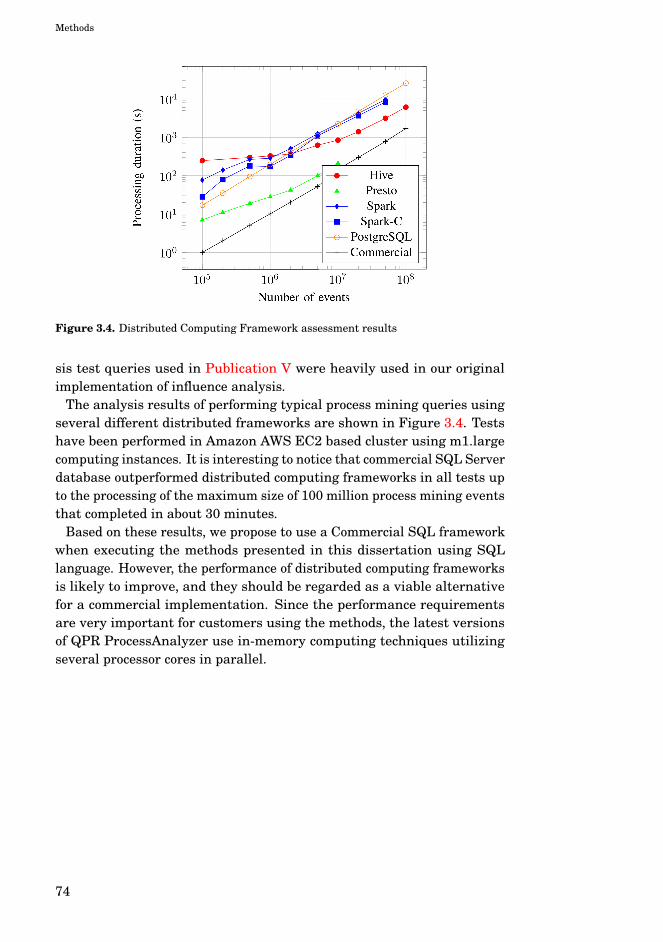
Methods

Figure 3.4. Distributed Computing Framework assessment results

sis test queries used in Publication V were heavily used in our originalimplementation of influence analysis.

The analysis results of performing typical process mining queries usingseveral different distributed frameworks are shown in Figure 3.4. Testshave been performed in Amazon AWS EC2 based cluster using m1.largecomputing instances. It is interesting to notice that commercial SQL Serverdatabase outperformed distributed computing frameworks in all tests upto the processing of the maximum size of 100 million process mining eventsthat completed in about 30 minutes.

Based on these results, we propose to use a Commercial SQL frameworkwhen executing the methods presented in this dissertation using SQLlanguage. However, the performance of distributed computing frameworksis likely to improve, and they should be regarded as a viable alternativefor a commercial implementation. Since the performance requirementsare very important for customers using the methods, the latest versionsof QPR ProcessAnalyzer use in-memory computing techniques utilizingseveral processor cores in parallel.

74

4. Results

This Chapter contains the results of applying our methods in publiclyavailable real-life data and provides a discussion summary of using themethods in industrial projects. Further insight and case studies aboutusing the merhod is found in Appendix A A. Supplementary details aboutthe implmentation of these methods with the QPR ProcessAnalyzer tool isshown in Appendix B B.


4.1.1 Case Study: Rabobank Group ICT

We evaluated the influence analysis with publicly available data fromRabobank Group ICT used in BPI Challenge 2014 [21]. The data consistsof 46.616 cases and a total of 466 737 events. Using a process mininganalysis, we discovered that the average duration for cases is five days,and the median duration is 18 hours. We decided to consider all cases thattook more than one week to complete as problematic, resulting in a totalof 7.400 (16%) cases. Table 4.1 shows that the biggest contributor to thisfinding is Impact=5. There is a total of 16.741 cases with Impact=5, out ofwhich 3.535 (21%) are problematic. As a contribution% this corresponds to12% of the total amount of problematic cases. For the process performancepoint of view, this is intuitive since it is probably acceptable to have low(5=lowest on scale 1..5) impact cases taking a long time compared to higherimpact cases. Table 4.1 shows that 29% of cases having ServiceCompWBS (CBy) = WBS000091 are completed in more than one week, whichmakes WBS000091 a candidate for business process improvements. IfWBS000091 would reach the average level of performance, then therewould 4% less problematic cases.

Table 4.2 shows rules that have the biggest negative contribution. These

75

Results

Table 4.1. Top positive contributors

Business Area n(A) n(AB) Δn ΔP(B)

Impact = 5 16741 3535 877 0,12Urgency = 5 16779 3538 874 0,12Priority = 5 16486 3473 856 0,12# Related Interactions = 2 2736 1108 674 0,09# Update from customer = 1 1692 793 524 0,07Closure Code = Other 16470 3137 522 0,07# Reassignments = 2 5378 1340 486 0,07# Reassignments = 3 2191 814 466 0,06# Reassignments = 4 1606 701 446 0,06Category = request for information 8846 1810 406 0,05CI Type (CBy) = computer 3404 865 325 0,04ServiceComp WBS (CBy) = WBS000091 2453 700 311 0,04CI Type (CBy) = application 29456 4979 303 0,04

can be regarded as the reasons why cases are completed within one weekmore often than average. If #Reassignments = 0, then only 6% of caseswill take more than one week. If these cases would take the same time asaverage cases, then there would be 37% more problematic cases. Anotherobservation from Table 4.2 is that only 11% of cases having ServiceCompWBS (CBy) = WBS000073 are completed late, which makes WBS000073 apositive benchmark.

Table 4.2. Contribution analysis on attribute value level – top negative contributors

Busines Area n(A) n(AB) Δn ΔP(B)

CI Name (aff) = SUB000456 3050 138 -346 -0,05CI Type (aff) = subapplication 7782 841 -394 -0,05Category = incident 37748 5582 -410 -0,06Closure Code = User error 3554 152 -412 -0,06CI Type (CBy) = subapplication 7711 800 -424 -0,06Urgency = 3 6536 607 -431 -0,06Priority = 3 6703 620 -444 -0,06Impact = 3 6591 602 -444 -0,06Service Component WBS (aff) =WBS000073

13342 1437 -681 -0,09

ServiceComp WBS (CBy) = WBS000073 13173 1401 -690 -0,09Reopen Time = (blank) 44332 6285 -752 -0,1# Related Interactions = 1 43058 5907 -928 -0,13# Reassignments = 0 27468 1628 -2732 -0,37

76

Results

ServiceComp WBS (CBy) was identified both as having a high positiveand negative contribution. Based on the author’s empirical evaluation, itis often beneficial to continue the analysis by showing the contributionof all distinct values of this case attribute in one list ordered by contribu-tion, as shown in Table 4.3. If the amount of distinct values is large, wepropose presenting only the top-10 most significant positive and negativecontributions.

Table 4.3. Benchmark of distinct values of ServiceComp WBS (CBy)

ServiceComp WBS (CBy) Contribution

WBS000091 4%WBS000072 3%WBS000088 2%WBS000162 2%WBS000263 1%WBS000296 1%WBS000271 1%WBS000092 1%WBS000187 1%WBS000089 0%WBS000318 0%WBS000219 0%WBS000172 0%WBS000096 0%WBS000223 0%WBS000125 0%WBS000292 0%WBS000146 0%WBS000128 -1%WBS000094 -1%WBS000307 -1%WBS000152 -1%WBS000016 -1%WBS000228 -1%WBS000095 -2%#N/B -2%WBS000073 -9%

In this Section, we used contribution analysis with real case data. Wewere able to identify causes for cases lasting more than one week. We ob-served a benchmark for a particular case attribute that seems to contributea lot to the finding. All the results have been shown in easy-to-understandlists ordered by the contribution metric. Showing these results to the peo-ple working in the process gives them more fact-based insight and enablesthem to combined this information with their tacit knowledge to discovereven deeper underlying cause-effect relationships.

Analyzing process lead times and using weightsWe now continue our case study using the Rabobank Group ICT data [21].As the lead time measure for each case, we used the total case duration

77

Results

from the first event to the last event within the case. Typical processmining analysis discovers that the average duration for cases is 5.07 days,and the median duration is 18 hours. If the duration was longer than sevendays, the case is categorized as problematic, which results in a total of 7400 (15.9%) problematic cases for the Binary Analysis.

As the weighting for cases, we use a formula wc j = (6− Impactc j )(6−Urgencyc j )(6− Priorityc j ) where Impact, Urgency and Priority all havevalues in (1,2,3,4,5) where 1 means highest importance and 6 is the lowestimportance. With this formula, the highest possible weight maxw = (6−1)(6−1)(6−1)= 125, lowest possible weight minw = (6−5)(6−5)(6−5)= 1, andthe weighted average lead time drops to 3.97 days. Since the weightedaverage lead time is shorter than the equal weight lead time, we concludethat the average lead time is shorter for more important cases than for lessimportant cases. The same finding can also be made from the binary resultssince the average problem density is 15.9% compared to the weightedaverage problem density of 11.1%.

Contribution results for individual case attribute valuesThe most significant positive and negative root causes according to differentAnalysis Types are shown in Table 4.4. The analysis is limited to thedistinct values of case attribute ServiceComp WBS(CBy), and the firstcolumn shows the case attribute value. Two columns are shown for eachanalysis type. Column Cont is the contribution% measure calculated usingour methods, which shows how a large portion of the problematic cases canbe explained with this case attribute value. Positive numbers mean thereare more than average problems in these cases, and negative numbersrepresent best practice areas with a smaller amount of problems. Thesecond column for each analysis type is the rank of the case attribute valuewithin the full results for that analysis type. The rank +1 means the mostsignificant root cause, and the rank -1 means the most significant bestpractice area.

For BiCo the highest contribution% is 4.2% for case attribute valueWBS000091 and lowest contribution% is -9.3% for case attribute valueWBS000073. When considering the most beneficial focus area for processimprovement reducing the lead time most we see that BiCo results inWBS000091 and all other Contribution Formulas result in WBS000088.According to the Table 4.4 the best performing ServiceComp WBS(CBy)regarding the lead time is WBS000073 in all analysis types except that inWeighted Binary Contribution the best performing area is #N/B.

Some interesting results include the behavior of cases whose attributeServiceComp WBS(CBy) has the value WBS000091 which contributes to4.2% (Top 1) of the total problem in BiCo, 3.4% (Top 2) in wBiCo, but only1.7% (Top 8) in CoCo and only 1.2% (Top 7) for wCoCo. The reason forthe higher contribution in BiCo and lower in CoCo is that average lead

78

Results

Table 4.4. Comparison of root causes for all analysis types

ServiceCompWBS(CBy)

BiCo wBiCo CoCo wCoCoCont R Cont R Cont R Cont R

WBS000091 +4,2% +1 +3,4% +2 +1,7% +8 +1,2% +7WBS000072 +2,8% +2 +0,8% +10 +3,4% +4 +0,6% +12WBS000088 +2,4% +3 +3,7% +1 +10,4% +1 +12,7% +1WBS000162 +2,2% +4 +2,9% +3 +8,6% +2 +10,0% +2WBS000055 +0,7% +9 +1,2% +7 +3,5% +3 +4,2% +4WBS000043 +0,2% +21 +1,2% +8 +1,3% +10 +4,8% +3.....WBS000228 -1,0% -4 +0,1% +50 -1,7% -3 -0,2% -39WBS000146 -0,5% -9 -2,2% -3 -0,7% -11 -2,8% -4WBS000095 -1,7% -3 -0,6% -8 -2,5% -2 -0,9% -8#N/B -1,7% -2 -8,3% -1 +2,6% +5 -5,9% -2WBS000073 -9,3% -1 -4,1% -2 -17,4% -1 -10,9% -1

time for area WBS000091 is only 6.14, which is only a little longer thanthe average for the whole process 5.07. This means that there are manyWBS000091 -cases that have lead time a little bit longer than 7 days. Onthe other hand, the behavior of area WBS000088 is the opposite, sinceit only contributes 2.4% (Top 3 value) of the total problem in BiCo, 3.7%(Top 1) in wBiCo, much more 10.4% (Top 1) in CoCo and even more 12.7%(Top 7) in wCoCo. Reason for this behavior is that the average lead timefor cases in area WBS000088 is 39.2 days, which is much longer than theaverage lead time 5.07

Exciting results include the behavior of area #N/B, which is listed as abest practice area with negative contribution -1.7% in BiCo (Top -2), -8.3%in wBiCo (Top -1) and -5.9% in wCoCo (Top -2). However, it is listed as aproblem area with a positive contribution 2.6% in CoCo as the 5th mostimportant problem area. There are at least two reasons for this result:first, the high weight cases in #N/B perform much better than the lowweight cases, i.e., BiCo contribution gets 6.6 percentage points better withweighting than without and CoCo contribution gets 8.5 percentage pointsbetter. The second reason is that area #N/B performs consistently worse inContinuous Analysis compared to the Binary Analysis, which is caused bythe higher than average lead time of 6.2% in CoCo, which again is causedby some specific long-duration cases in #N/B which may also be regardedas outliers in the data.

Contribution results for activity occurrencesIn this Section, we present the Rabobank root cause analysis for long-lasting cases using activity occurrence data. As a preprocessing step, weadd a new case attribute for each different activity name and use the

79

Results

number of activity occurrences as the value for that case attribute in eachcase. For example, if activity Status Change occurs twice for a certain case,then the value of case attribute Status Change is 2 for that particular case.

Table 4.5 shows the top-5 positive and negative root causes for binaryanalysis types and Table 4.6 the same for the continuous analysis typesleading us to the following observations:

• Lack of reassignments is the most important negative root cause for acase to exceed the seven day SLA (BiCo analyses) or generally take along time (CoCo analysis). In other words, having zero reassignmentsmakes a case very fast.

• Contribution values for activity occurrence numbers are much higherthan they are for the case attribute ServiceComp WBS(CBy), whichmeans that these activity amounts correlate more with the totalduration than the case attribute ServiceComp WBS(CBy).

• Update from customer(1) is the most important positive root causefor long case duration, as can be seen in continuous contributions inTable 4.6. However, for binary contributions in Table 4.5, the StatusChange(2) is the most important positive root cause, which meansthat having two occurrences of Status Change causes a bigger riskthan getting an update from a customer for failing SLA.

Table 4.5. Comparison of root causes based on activity profiles for binary analysis

BiCo wBiCoActivity occurrences Contrib. Activity occurrences Contrib.

n(Closed)=2 9.7% n(Status Changes)=2 10.3%n(Status Changes)=2 8.9% n(Comm. with customer)=1 10.1%n(Comm. with customer)=1 8.8% n(Closed)=2 9.9%n(Reopen)=1 7.8% n(Update from customer)=1 9.5%n(Update from customer)=1 7.1% n(Assignment)=3 9.3%... . ... .n(Status Change)=0 -20.8% n(Status Change)=0 -22.0%n(Assignment)=1 -26.4% n(Assignment)=1 -26.8%n(Update)=0 -29.6% n(Update)=0 -32.0%n(Operator Update)=0 -35.8% n(Operator Update)=0 -41.5%n(Reassignment)=0 -37.9% n(Reassignment)=0 -43.2%

Contribution results for case attributesIn this Section, we will show the results of calculating the summarycontribution values for case attributes. We use both the original caseattributes provided in the source data as well as the activity occurrencesfeatures as case attributes.

Table 4.7 shows that the count of Reassignments is the most influentialcase attribute for explaining the root causes for long durations for all

80

Results

Table 4.6. Comparison of root causes based on activity profiles for continuous analysis

CoCo wCoCoActivity occurrences Contrib. Activity occurrences Contrib.

n(Update from customer)=1 14.9% n(Update from customer)=1 15.6%n(Closed)=2 13.1% n(Status Change)=2 12.8%n(Status Change)=2 12.2% n(Update from customer)=2 12.5%n(Reopen)=1 11.8% n(Update)=2 12.1%n(Description Update)=1 11.1% n(Description Update)=1 12.0%... ...n(Update from customer)=0 -38.6% n(Assignment)=1 -43.0%n(Assignment)=1 -45.8% n(Update from customer)=0 -46.3%n(Update)=0 -51.3% n(Update)=0 -50.1%n(Operator Update)=0 -53.2% n(Operator Update)=0 -55.8%n(Reassignment)=0 -62.0% n(Reassignment)=0 -65.0%

Table 4.7. Case Attribute analysis results for all analysis types

Case Attribute BiCo wBiCo CoCo wCoCoCont R Cont R Cont R Cont R

n(Reassignment) 15.9% 1 20.8% 1 42.0% 1 46.5% 1n(Operator Update) 14.5% 2 19.4% 2 31.0% 2 34.1% 2n(Assignment) 10.2% 3 12.5% 3 27.5% 4 27.9% 4n(Update) 9.8% 4 11.8% 4 29.3% 3 28.9% 3n(Status Change) 6.8% 5 8.1% 5 12.5% 6 11.8% 6n(Update from customer) 2.4% 9 5.0% 6 18.4% 5 26.2% 5n(Comm. with customer) 3.5% 6 5.0% 7 5.9% 8 5.7% 13Closure Code 1.3% 18 2.3% 12 4.9% 12 7.7% 9Service Component WBS(aff)

1.5% 16 1.4% 20 7.4% 7 8.8% 8

# Related Interactions 2.5% 8 2.3% 13 5.3% 10 2.9% 21Impact 2.0% 10 3.3% 8 1.2% 25 5.9% 12n(Closed) 2.6% 7 2.1% 14 5.3% 11 2.7% 23ServiceComp WBS (CBy) 1.4% 17 1.5% 18 5.6% 9 5.0% 17Priority 1.9% 13 3.2% 9 1.1% 26 5.6% 14Cost 1.9% 12 3.0% 10 1.1% 27 5.5% 15Urgency 2.0% 11 3.0% 11 1.1% 28 5.4% 16n(Reopen) 1.6% 15 1.7% 16 4.1% 14 2.7% 22CI Name (aff) 0.7% 22 0.9% 25 4.8% 13 6.9% 11n(Description Update) 1.0% 19 1.9% 15 3.2% 20 3.9% 20Related Interaction 1.6% 14 1.5% 17 3.6% 16 2.1% 27KM number 0.4% 28 1.2% 21 3.8% 15 7.3% 10

81

Results

analysis types. We see that the number of occurrences of Operator Update,Assignment, Update, Status Change, Update from customer, and Commu-nication with customer all appear as very influential case attributes. Thismeans that the activity occurrence amounts have a high correlation withlong lead times. The first original case attributes in the list are ServiceComponent WBS (aff) and Closure Code. They both are more relevant inthe Continuous Contribution analyses compared to binary analyses. Someinteresting findings from these results include:

• Several activity occurrence counts have a much stronger influence onlong lead times than the original case attributes. This means thatwhat happens during the process instance execution is often morerelevant than original case attributes.

• Service Component WBS (aff) is the most important original caseattribute that could be used to predict long lead times. However,the contribution for Service Component WBS (aff) is clearly higherfor Continuous Contribution analysis types (Rank for CoCo is 7 andRank for wCoCo is 8) compared to the Binary Contribution analysis(Rank for BiCo is 16 and rank for wBiCo is 20). This means that asa whole, the individual Service Component WBS (aff) values are notsuch important root causes for determining if a case takes more thanone week. However, some individual Service Component WBS (aff)values are significant root causes for those cases that have a verylong duration, since CoCo analysis gives high weight for very longcases.

• Impact, Priority, and Urgency are all more relevant root causes forweighted analysis than for non-weighted analysis. The reason forthis is because the case-specific weights were calculated based onthese three case attributes.

4.1.2 Discussion

This section is based on the author’s empirical evaluation of using ourmethod in industrial process mining projects. Influence Analysis was firstintroduced in the commercial product QPR ProcessAnalyzer 1 version 3.7on 27th April 2012, showing both the change type ideal and change typeas-is average results 2.

Influence analysis has been successfully used in more than 200 customerprocess mining projects. Vanjoki presents a summary of analyzing auto-mated purchase to pay process value modeling and comparative process

1https://www.qpr.com/products/qpr-processanalyzer2https://devnet.onqpr.com/pawiki/index.php/QPR_ProcessAnalyzer_Release_Archive

82

Results

speeds using influence analysis [60]. In practice, problem areas and bestpractice areas have been accurately identified using influence analysis.

Interactive usage in workshop meetings has proven to be very valuable,and it motivates business people in the same meeting to share their tacitknowledge to deepen the influence analysis findings. A typical scenariois that participants first try to guess the most influencing factors, andwhen they then see the results their own hypotheses are strengthened orweakened. This process further facilitates participants’ thinking and col-laboration with each other. Based on the discussion, the organization thenselects the focus areas for business process improvements and starts moni-toring the performance on monthly intervals using the same contributionmeasures.

Our method is able to identify root causes for problems ranging fromvery rare to very common. However, a certain number of successful casesare necessary in order to discover root causes with our method. In practice,the Pareto principle percentages of 20% problematic cases versus 80%successful cases seem to be the ideal ratio, and anything between 0.1%and 50% problematic cases still works well. If noticeably more than 90%of cases are problematic, then the discovered best practice areas are oftenmore insightful than the discovered root cause areas.

Influence analysis also has an important application in deciding whetherthe organization should improve the whole process design or improvecertain problem areas. If the contribution values for all rules are relativelylow, then there is no clear root cause that should be fixed. Thus, if nofocus area is found and business still needs to be improved, there is a needto improve the whole process design. Also, the method can be used toevaluate potential risks in any given segment by checking those areas thathave a low density of problematic cases in the current as-is situation, sincethe number of problems will increase if those areas become like others, onaverage.

Actual root cause analysis is an iterative method for identifying theunderlying root causes of problems [6]. Depending on the problem and thecase attribute data available, the influence analysis method may return asignificant root cause already in the first query. However, the first querymay return a higher-level finding like Region=Europe. To further discoverthe root cause for the original problem in Europe, we suggest creatinga process mining filter so that our method can be run for all Europecases. This second influence analysis could now return a significant factorProductLine=Hats, which now suggests that the ProductLine=Hats inEurope is a particularly significant root cause for the original problem.Further multi-level queries of this kind can pinpoint very specific rootcauses for the problems, since while every round reduces the numberof cases, it is possible to increase the number of case attributes whileproviding fast response times for the business analyst.

83

Results

Summary of our results:

1. The influence analysis methodology is able to find root causes for longlead times.

2. Root causes for long lead times may be substantially different whenusing a predefined lead time limit for problematic/successful cases(binary) compared to when using continuous lead time values.

3. Case-specific weighting can be easily used when analyzing both bi-nary and continuous contributions.

4. When weighting is used in the continuous contribution analysis, theresults can be directly used for discovering opportunities for reducingworking capital.

5. Contribution values can be summarized to the case attribute levelby calculating the sum of squares of individual contribution% values.This gives a quick overview of interesting case attributes for anygiven lead time finding.


4.2.1 Case Study: BPI Challenge 2017 Dataset

In this Section, we show a real-life example of using the presented method-ology on the loan applications process data from a Dutch Financial Insti-tute. The data is publicly available as BPI Challenge 2017 Dataset [22]and contains 31 509 cases and a total of 1 202 267 events. The originaldataset has been prepared in a way that it contained full cases. Sincethe purpose of our analysis is to show business process changes withina continuous monitoring situation, we have taken the following steps inpreparing a setup for business review analysis.

• November 2016 is selected as the business review month. The datacontains 104 946 events whose timestamp belongs to November sothat the Review period will consist of these events.

• All events occurring later than November belong to the Most RecentData period and are excluded from analysis, consisting of 120 568events. These events would naturally be included in later businessreview periods.

84

Results

• The comparison period has been chosen to include the six months be-fore the review period, i.e., from May 2016 to October 2016 containing647 406 events.

• History period contains 329 347 events occurring before May 2016.These events are used for constructing the process path and pre-decessor dimensions for History and Review events, but they arenot included in the analysis as actual events belonging to eitherComparison or Review sets.

• The total number of events in the analysis is 752 352 consisting of104 946 events for the Review period (13.95% of all events) and 647406 events for the Comparison period (86.05% of all events).

Figure 4.1. Changes for BPI Challenge 2017 Applications. Changes for November 2016compared to the previous six months

Results using Binary Change WindowFigure 4.1 shows the top-10 most important changes in the business pro-cess and related data for the review period. We see that there are manyuser changes in event attribute org:resource, so it seems like employeesare changing a lot. User_133 has conducted 3 728 events during the reviewperiod and only 4 267 in the comparison period, so 47% of his events havetaken place during the review period, which makes him as the biggestprocess change, taking into account the size of his total activity (7 995events) and the difference 33% from the average 13.95%.

Figure 4.2 shows the changes in only the event type dimension. Theevent types W_Call incomplete files - suspend and W_Call after offers -ate_abort occur more often during the Review period, whereas the eventtypes W_Validate application - resume and W_Call after offers - suspendoccur less often during the Review period than in Comparison period.

Considering the business process related changes where the order of ac-tivities is changing, we limit the analysis to only the predecessor changeswhere a specific event takes place immediately after another event, as

85

Results

Figure 4.2. Changes in Event Types for BPI Challenge 2017 Applications. Changes forNovember 2016 compared to the previous six months

Figure 4.3. Changes in Predecessors for BPI Challenge 2017 Applications. Changes forNovember 2016 compared to the previous six months

shown in Figure 4.3. During the review period, the control flow transitionfrom event W_Call after offers - ate_abort to W_Call after offers - scheduleoccurs more often and the transition from event type W_Validate applica-tion - suspend to W_Validate application - resume less often than duringthe comparison period.

Results using Continuous Change WindowFigure 4.4 shows the continuous approach versions of the same overallanalysis as the previous binary approach Figure 4.1. The continuousanalysis is configured to discover differences in events from mid-August toNovember with events from May to mid-August. The results of Continuousanalysis are the result of giving each event a weight based on the Ageof the event. The bigger the distance from average Age, the bigger theweight of that particular event. Using the case study data, the averageAge of events is 103.97 days. An event occurring 100 days before or afterthe average data have 100 times the weight compared to an event takingplace one day after or before the average date. Similarly, an event that

86

Results

Figure 4.4. Changes for BPI Challenge 2017 Applications. Changes for November 2016compared to the previous six months using continuous comparison approach

takes place exactly in the average Age has zero weight as it does not belongeither to the old period or new period.

As shown in Figure 4.4, the most significant positive change over timehas been the number of events with User_133 as the org:resource. Theaverage Age of these events is 70.09 days shorter than the average (103.97days - 33.88 days). The Age is defined as relative to a fixed timestamp inthe analysis, and the absolute zero point for the Age is not relevant. Thetotal problem size for the analysis is the total sum of positive differencesfrom the average Age calculated from each event, which in this case studymodel gives a total of 19382661.6 days. The contribution of User_133 isthus calculated as −70.09days∗7995events/19382661days =−2.89%

Continuous analysis results are well in line with the binary approachresults, and differences are based on the different setup of Review andComparison periods and a different weighting approach as described. Forexample, User_133 as the new value for org:resource is still the biggestchange, and both org:resources User_67 and User_65 are included in top-10changes for both Binary and Continuous approaches as is visible in Figures4.1 and 4.4.

In this dissertation we have presented a method for detecting businessprocess changes. The method is based on previously published InfluenceAnalysis and it uses the conformance measure to scale different typesof changes in order to present various kind of changes sorted by theirsignificance. We have shown how to use Influence Analysis on the eventlevel instead of business process case level. Operating on the event levelmakes it possible to use all available data from the review period fordetecting changes instead of having to wait until a business process case iscompleted. Summary of our key experiences when using the analysis withreal-life cases include:

87

Results

4.2.2 Discussion

The following observations can be made based on the previous case studyresults and the author’s empirical evaluation of using the method in indus-trial process mining projects:

• Changes in business operations can be analyzed by comparing reviewperiod events to comparison period events using influence analysis.

• Operating on the event level makes it possible to use all availabledata from the review period for detecting changes instead of havingto wait until a business process case is completed.

• Business people quickly learn to read the influence analysis resultson a monthly basis. Detecting the top 10 or top 50 changes givesan excellent starting point for a more detailed periodical analysis ofbusiness process changes.

• Detected changes may also be a result of incorrect data integrationbetween the process mining system and the actual ERP system(s).Our method serves as an easy to use quality assurance tool for eval-uating the correctness of periodical data loads and integration. Forexample, after each monthly, weekly, or daily data import, the systemcan notify business analyst of the top 10 changes so that a potentialtechnical integration problem is detected and corrected before otherbusiness users waste time analyzing incorrect data.


4.3.1 Case Study: Purchase Order process

In this Section, we apply our method to the real-life purchase order processdata from a large Netherlands multinational company operating in thearea of coatings and paints. The data is publicly available as the BPIChallenge 2019 [23] dataset. We made the following choices:

• Source data We imported the data from the XES file as such with-out any modifications. To keep the execution times short, we exper-imented with the effect of running the analysis with a sample ofthe full dataset. Our experiments showed that the results remainedconsistent for sample size 10 000 cases and more. With a sample sizeof 1 000 cases, the K-modes clustering results were changing a lot ofdue to a large number of features and a small number of cases.

88

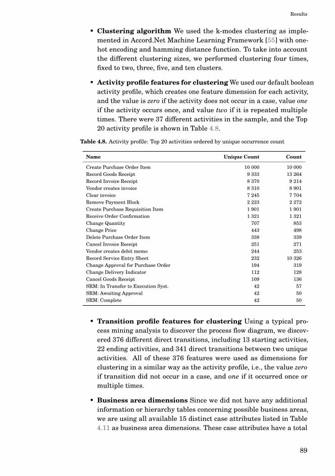
Results

• Clustering algorithm We used the k-modes clustering as imple-mented in Accord.Net Machine Learning Framework [55] with one-hot encoding and hamming distance function. To take into accountthe different clustering sizes, we performed clustering four times,fixed to two, three, five, and ten clusters.

• Activity profile features for clustering We used our default booleanactivity profile, which creates one feature dimension for each activity,and the value is zero if the activity does not occur in a case, value oneif the activity occurs once, and value two if it is repeated multipletimes. There were 37 different activities in the sample, and the Top20 activity profile is shown in Table 4.8.

Table 4.8. Activity profile: Top 20 activities ordered by unique occurrence count

Name Unique Count Count

Create Purchase Order Item 10 000 10 000Record Goods Receipt 9 333 13 264Record Invoice Receipt 8 370 9 214Vendor creates invoice 8 310 8 901Clear invoice 7 245 7 704Remove Payment Block 2 223 2 272Create Purchase Requisition Item 1 901 1 901Receive Order Confirmation 1 321 1 321Change Quantity 707 853Change Price 443 498Delete Purchase Order Item 338 339Cancel Invoice Receipt 251 271Vendor creates debit memo 244 253Record Service Entry Sheet 232 10 326Change Approval for Purchase Order 194 319Change Delivery Indicator 112 128Cancel Goods Receipt 109 136SRM: In Transfer to Execution Syst. 42 57SRM: Awaiting Approval 42 50SRM: Complete 42 50

• Transition profile features for clustering Using a typical pro-cess mining analysis to discover the process flow diagram, we discov-ered 376 different direct transitions, including 13 starting activities,22 ending activities, and 341 direct transitions between two uniqueactivities. All of these 376 features were used as dimensions forclustering in a similar way as the activity profile, i.e., the value zeroif transition did not occur in a case, and one if it occurred once ormultiple times.

• Business area dimensions Since we did not have any additionalinformation or hierarchy tables concerning possible business areas,we are using all available 15 distinct case attributes listed in Table4.11 as business area dimensions. These case attributes have a total

89

Results

of 9901 distinct values, giving us 9901 business areas to considerwhen finding those business areas that have the most significanteffect on process flow.

Clustering Results for Individual ClusteringTable 4.9 shows the results of clustering to fixed five clusters. We see thatthe first cluster contains 48% of cases, the second cluster 33%, third 17%,and both fourth and fifth one percent each. Here we show the five mostimportant business areas based on the contribution%, which is calculatedas the difference between Cluster specific density of that business areaand Total Density. These results already give hints about the meaningfulcharacteristics in the whole dataset, i.e., the first cluster contains manyStandard cases from spend areas related to Sales, Products for Resale,and NPR. On the other hand, the second cluster contains more than theaverage amount of cases from spend area Packaging, related to Labels andPR. VendorID_0120 seems to be highly associated with the process flowcharacteristics of the second cluster. The third cluster is dominated byConsignment cases. The fourth cluster contains many Metal Containers& Lids cases as well as cases from VendorIDs 0404 and 0104. Furtheranalysis of the top five business areas listed as characteristics for eachcluster confirms that these business areas indeed give a good overall ideaof the cases allocated into each cluster.

Discovering Business AreasWe clustered four times for fixed cluster amounts of 2,3,5 and 10 - yieldinga total of 20 clusters, and then consolidating the results into businessarea level using Definition 40. The top 20 of all these 9901 businessareas ordered by their respective Business Area Contribution is shown inTable 4.10. Clearly, the business areas Item Category = Consignment andItem Type = Consignment have the most significant effect on the processflow. Looking at the actual process model, we see that Consignment casescompletely avoid three of the five most common activities in the process,namely Record Invoice Receipt, Vendor creates invoice, and Clear Invoice.Similarly, the business area Spend area text = Packaging also has a highcorrelation with process flow characteristics. Analysis of the process modelshows that, for example, 23% of Packaging cases contain activity ReceiveOrder Confirmation compared to only 5% of the other cases. Furtheranalysis of all the business areas listed in Table 4.10 shows that eachof these areas has some distinctive process flow behavior that is morecommon in that area compared to the other business areas.

Clustering Summary for Case AttributesFinally, Table 4.11 consolidates individual business areas into the CaseAttribute level. Item Type having six distinct values and Item Category

90

Results

Table 4.9. Clustering results based on Contribution

Cluster Business Area a ClusterDensity

TotalDensity

Contri-bution

Spend area text = Sales 0.36 0.26 0.11Cluster1 Sub spend area text = Products for Re-

sale0.34 0.24 0.11

48% cases Spend classification text = NPR 0.41 0.32 0.10Item Type = Standard 0.96 0.87 0.09Item Category = 3-way match, invoicebefore GR

0.95 0.88 0.07

Spend area text = Packaging 0.65 0.44 0.21Cluster2 Sub spend area text = Labels 0.39 0.24 0.1633% cases Spend classification text = PR 0.79 0.66 0.13

Name = vendor_0119 0.14 0.05 0.08Vendor = vendorID_0120 0.14 0.05 0.08Item Category = Consignment 0.33 0.06 0.27

Cluster3 Item Type = Consignment 0.33 0.06 0.2717% cases Name = vendor_0185 0.09 0.02 0.08

Vendor = vendorID_0188 0.09 0.02 0.08Item = 10 0.33 0.26 0.07Sub spend area text = Metal Contain-ers & Lids

0.19 0.08 0.11

Cluster4 Name = vendor_0393 0.09 0.01 0.081% cases Vendor = vendorID_0404 0.09 0.01 0.08

Name = vendor_0104 0.11 0.04 0.07Vendor = vendorID_0104 0.11 0.04 0.07Spend classification text = NPR 0.59 0.32 0.27

Cluster5 Spend area text = Sales 0.41 0.26 0.151% cases GR-Based Inv. Verif. = TRUE 0.21 0.06 0.15

Item Category = 3-way match, invoiceafter GR

0.21 0.06 0.15

Sub spend area text = Products for Re-sale

0.38 0.24 0.14

91

Results

Table 4.10. Top 20 Business areas with major effect to process flow

Business Area a Contribution nCases n(Ca)

Item Category = Consignment 0.051 576Item Type = Consignment 0.051 576Spend area text = Packaging 0.040 4382Spend classification text = NPR 0.024 3175Sub spend area text = Labels 0.022 2351Spend area text = Sales 0.021 2574Item Type = Standard 0.021 8740Sub spend area text = Products for Resale 0.021 2390Spend classification text = PR 0.019 6574Item Category = 3-way match, invoice before GR 0.017 8760Spend area text = Logistics 0.013 210Item Type = Service 0.013 244Item = 1 0.012 342GR-Based Inv. Verif. = TRUE 0.012 623Item Category = 3-way match, invoice after GR 0.012 625Name = vendor_0119 0.007 549Vendor = vendorID_0120 0.007 549Sub spend area text = Road Packed 0.006 145Name = vendor_0185 0.004 163Vendor = vendorID_0188 0.004 163

with four distinct values, have the most significant effects on process flowcharacteristics. To confirm the validity of these results, we further anal-ysed the materials provided in the BPI Challenge 2019 website, includingthe background information and submission reports [23]. It is clear thatthe Item Type and Item Category indeed can be regarded as the most im-portant factors explaining the process flow behavior as they are specificallymentioned to roughly divide the cases into four types of flows in the data. Itis also interesting to see that both the Spend area text and Sub spend areatext have a significant effect on the process flow even though they have amuch higher number of distinct values (19 and 115) compared to Spendclassification text, which only has four distinct values.

4.3.2 Discussion

Summary of findings based on the previous case study results and theauthor’s empirical evaluation of using our method in industrial processmining projects:

• Our method is capable of discovering those business areas that havethe most significant effect on process execution. It provides valuableinformation to business people who are familiar with case attributesand attribute values, but not so familiar with the often technicalevent type names extracted from transactional system log files.

• Our method supports any available trace clustering method. Ourcase study shows that using the k-modes clustering algorithm with

92

Results

Table 4.11. Case Attributes ordered by the effect on process flow

Case Attribute at Contribution Distinct Values n(Vat)

Item Type 0.086 6Item Category 0.080 4Spend area text 0.077 19Sub spend area text 0.056 115Spend classification text 0.043 4Name 0.025 798Vendor 0.025 840Item 0.016 167GR-Based Inv. Verif. 0.012 2Purchasing Document 0.002 7937Document Type 0.000 3Goods Receipt 0.000 2Company 0.000 2Source 0.000 1Purch. Doc. Category name 0.000 1

activity and transition profiles provides good results.

• Clustering makes analysts aware that not all the cases in the processmodel are similar. Using the Contribution% measure to explainclustering results works well for explaining the clustering results tobusiness people.

• The presented case study confirms that the identified business ar-eas do indeed have distinctive process flow behavior—for example,missing activities, higher than average amounts of some particularactivities, or a distinctive activity execution sequence. Using ourmethod, the business analyst is able to divide the process model intosmaller subsets and analyze them separately. The analysis of anyprocess subset can be started by running the clustering to see if thecases are similar enough from process flow point of view.

• Clustering reduces the need for external subject matter businessexperts. It would ideal if there was someone on hand to explaineverything, but in reality the subject matter experts are very busy,and some essential details are always likely to be forgotten by busybusiness people.

93

5. Conclusions

This dissertation studies business-related process analysis methods basedon process mining data, with a focus on resource allocation, root cause anal-ysis, change identification, and analysis of business area effects on processflow. The dissertation consists of eight publications and this introduction.

The methods presented in this dissertation can be used to:

1. Allocate business improvement resources

2. Identify process-related changes in business operations

3. Discover business areas that have a significant effect on process flowbehavior


This dissertation presents an influence analysis method that can be usedfor effective resource allocation to maximize business improvement. Pub-lication I presents the original influence analysis method as a root causeanalysis method for focusing business improvements. Publication II ex-tends the method to cover continuous problem variables and case-specificweighting, specifically aiming at reducing lead times and working capitalanalysis. The objective of this first research question is to determine theoptimal scope for an improvement project to reduce the number of prob-lems already discovered by other means, as presented in Section 1.1.1. Therelated problem setup is formalized with concepts business problem, prob-lem type, problem weighting, development project, and amount of resourcesin Section 2.2.

The basic influence analysis method containing data preparation steps,options for the desired level of business improvement, and the calculationof corresponding interestingness measures is presented in Section 3.1 forbinary problems, and further extended to cover continuous problems and

95

Conclusions

case-specific weights in Section 3.2. Publication V presents results froma distributed computing framework assessment aimed at finding optionsfor using our method with massive amounts of data, briefly summarizedin Section 3.5. Section 4.1 presents a case study with real-life data andsummarizes our experiences in using the method.


As presented in Publication III, the influence analysis presented in Publi-cation I and Publication II can be extended to identify changes in businessoperations. Our objective is to discover various process changes and sortthem in order of business significance, as shown in 1.1.2. The problemsetup is formalized with concepts for setting the review period, fast andslow changes, relevancy, root causes, and data quality detection in Section2.3.

Although the method for analyzing business process changes is basedon influence analysis, it has two fundamental differences compared tothe original influence analysis used in RQ1. As presented in Section 3.3,these extensions are the analysis of event-level data instead of processmining cases, and the discovery of changes related to time instead of thediscovery of root causes related to a previously detected business problem.Section 4.2 presents a case study with real-life data and summarizes ourexperiences in using the method.


Publication IV presents a novel approach for discovering business areasthat have a significant effect on process flow. The goal is to use clusteringon historical data in order to group similar kinds of process instances intothe same clusters, and then finding the business areas that correlate mostwith these identified clusters, as presented in 1.1.3. The problem setupis formalized with concepts communicating clustering results to businessanalysts, finding the business areas that have a significant effect on processflow behavior, and further consolidating business area results to discovermost significant case attributes in Section 2.4.

Our method is based on clustering analysis for grouping the cases fol-lowed by influence analysis for discovering the business areas, as presentedin Section 3.4. In Publication VI we present results for effective featureselection related to clustering and in Publication VII and Publication VIIIwe examine the idea of learning the relevant features using recurrent neu-

96

Conclusions

ral networks, briefly summarized in Sections 3.4.1 and 3.4.1. Section 4.3presents a case study with real-life data and summarizes our experiencesin using the method.

5.4 Future Work

To further increase the usability and applicability of our influence analy-sis method, several research ideas could be explored. Current influenceanalysis uses discrete variables for discovering root causes and businessareas, and testing different techniques for discretization and grouping ofindividual values into subsets would provide new insights. This wouldbe specifically beneficial for using the lead times of transitions betweenany particular event types as potential root causes. It would also providefurther insight if decision mining techniques that form multiple compo-nent rules based on several attributes were combined with our influenceanalysis measures.

Individual business analysts often consider some of the discoveries gener-ated by our methods very interesting, and some not so important. It wouldoffer further insight if our method was combined with a machine learningbased system that would learn which findings are considered relevant andwhich are ignored by the analyst. This kind of learning could take place inmany levels, including: 1. Individual user using a specific process miningmodel; 2. Anybody using the same model; 3. One user using any processmining model; 4. All users within one organization using any models; 5.All users from hundreds of organizations internationally using the samecloud-based process mining environment.

Performance optimization is continuously needed to meet the growing cus-tomer requirements for big data analytics. In-memory computing shouldbe explored in more detail to find methods for analyzing large datasetssuch as 100TB with considerably smaller RAM sizes such as 1TB.

As presented in this dissertation, the influence analysis reports corre-lations between various aspects. The user of the method is responsiblefor understanding whether the correlation is indeed a proper root-causedependency based on the causality of the cause and effect or whether bothaspects are just effects of a third cause. Causality in process mining hasbeen studied utilizing the timestamps of the events to see how a change inoriginal aspects at one time may have caused effects on other aspects atlater times [34]. It would be interesting to include the causality in morerobustly into the Contribution measure.

From the economic point of view, one important future work is to take themethods presented in this dissertation into active use in process mininganalyst community for making processes more efficient, ensuring compli-ance, supporting robotic process automation, and driving successful digital

97

Conclusions

transformation. A survey exploring benefits and challenges related to theusage of our influence analysis based methods would provide useful insightand best practices.

Appendices

98

A. Customer Case Studies

This Appendix contains supplementary material from three industrialcustomer cases where the influence analysis has been in extensive use.

Metsä Board1. "The process analysis delivered the needed visibility for Metsä Board

to focus their improvement activities to the right areas."

2. "The overall goal of the development work was to improve customersatisfactionthrough better delivery accuracy, production efficiency,optimised stock rotationand reduced number of changes."

3. "The process insight and facts delivered by QPR ProcessAnalyzerwere priceless. We were immediately able to focus our process im-provement activities to the right things to reach the results ourbusiness needed. And not wasting time on trial and error." - JariVuori, Vice President Supply Chain, Metsä Board

4. Reaching optimal process performance requires continuous work andprocess owners now at Metsä Board regularly monitor their processeswith QPR ProcessAnalyzer. They base their developmnent activitieson facts, not on hunches. ... With the knowledge of where to targetdevelopment efforts, Metsä Board can now concentrate on customerneeds and deliver improved service experience.

EY1. Using QPR ProcessAnalyzer we also get a comprehensive understand-

ing of root causes and how to take corrective actions for improvingoperations.

2. "Root Cause analysis really works well in QPR ProcessAnalyzer",Stewart Wallace, Director, Risk Analytics, EY UK.

3. QPR ProcessAnalyzer’s latest machine learning and artificial intel-ligence (AI) based advancements such as clustering analysis and

99

Customer Case Studies

case level prediction lets business understand transaction-based datamuch faster.

4. "My favourite feature is conformance analysis, and business processmodelling and then correlate it with the root cause analysis", RickyVachhani, Manager, Risk & Data Analytics, EY UK.

KBC1. "With Root Cause Analysis, we found out why certain tasks are often

done incorrectly." - Sander Van Lombeek, Team Lead, CommercialCredits, KBC Group

2. “QPR ProcessAnalyzer allows us to keep track of SLA situation inevery subtask and find the root cause of inefficiency. To illustrate,we discovered a bottleneck caused by deficiency of the e-form system,doubling the promised processing time.” - Christof De Groote, ServiceManager Life Insurance, KBC Insurance

3. By using the holistic process mining view including bottlenecks androot causes, KBC is able to reduce throughput times

4. “I really really love the influence analysis. I think that’s one of themajor key benefits for me from the QPR ProcessAnalyzer tool.” -Sander Van Lombeek, Team Lead, Commercial Credits, KBC Group

5. "I am also experimenting with clustering and predictive models.” -Maaike Roekens, Credit Risk Model Manager, KBC Bank

100

Challenge BenefitsIncreasing pressure from regulators to use analytics for testing controlsReactive approach to errorsUnaware of weaknesses and bottlenecksRisk management landscape changesHow to know if controls are relevantLack of precise internal controlSlow process analytics

Obtain efficient view on internal processAssess quality of KPIsGive stakeholders greater confidence to make right business decisionsPredict errors in preventive controlsPrioritize actions based on risksReal-time monitoring of dataAutomated Root Cause analysisIdentification of corrective actions

EY is using Process Mining for Risk Management and Internal Audit

powered by QPR ProcessAnalyzer

One of the biggest professional services firms in the world, headquartered in UK, providing

assurance, tax, consulting and advisory services to businesses from their 700 offices in

over 150 countries.

Employees: 270,000+Revenue: 36 billion USD

www.ey.com

Risk Management Landscape

Stewart Wallace, Director, Risk Analytics, EY UK

“Process mining allows you to look at every transaction, 100 percent coverage.”

The risk management landscape is changingrapidly. The enormous growth of datademands internal control and audit team to beable to give strategic advice (on riskmanagement and control) for stakeholders tomake right business decisions and takeadvantage of opportunities. On the otherhand, financial regulators and other industrybodies urge business to disclose its internalcontrol process.In order to stay one step ahead, businessesneed to adapt fast. “That is why understandingyour processes is absolutely critical, and that’swhere process mining steps in.” – says StewartWallace, Director, Risk Analytics, EY UK.

Compared to traditional risk and controlmethodology, process mining proves to be anexceptional technological breakthrough.“Before, you looked at the processdocumentation and talked to the people inorder to form an opinion about what washappening. And we all know that would giveyou maybe 40 percent of the truth,” saysStewart, “but process mining is using data totell you what’s actually happening, 100 percentcoverage. Process mining gives you a holisticview of all business processes showing what isgoing right or wrong. Using QPRProcessAnalyzer we also get a comprehensiveunderstanding of root causes and how to takecorrective actions for improving operations.”

Give stakeholder confidence in making business decisions “We are able to identify areas

where themes within the audit reports did not match with what was recorded in the audit tracking system.”Ricky Vachhani, Manager,Risk & Data Analytics, EY UK

Obtain efficient view on internalcontrolAs the business shifts to become more agile,resulting in constant changes in processes andoperations, only the dynamism of processmining can keep up with these rapid changes.“Traditional analytics is static and hard-coded.If we now have a new event in the middle of ourprocess, process mining picks that up, buttraditional analytics won’t.” – says Stewart.

Analysis in less than one weekUsing QPR ProcessAnalyzer, the EY UK RiskAnalytics team has been able to complete anend-customer process mining analysis in lessthan one week. This includes time from initialdata acquisition to model building, creatingdashboards and presenting results to thecustomer. Complex end-to-end processesnaturally take longer but typically one to twoweeks is enough for any well-defined processmining analysis or iteration.“QPR ProcessaAnalyzer helps us design datamodels and dashboards the fastest so that timeto insight is the shortest.” – says Stewart.

“QPR is the one that I always turn to for ease of use and fastest time to insight. Root Cause analysis really works well in QPR ProcessAnalyzer”

Favourite QPR ProcessAnalyzer feature

Stewart Wallace, Director,Risk Analytics, EY UK

QPR Software PlcQPR Software Plc (Nasdaq Helsinki) provides process mining, performance management and enterprise architecture solutions for digital transformation, strategy execution and business process improvement in over 50 countries. QPR software allows customers to gain valuable insights for informed decisions that make a difference.Dare to improve.

Read more at www.qpr.com

QPR ProcessAnalyzer solutionRisk Management and internal audit solutions built based on QPR ProcessAnalyzer dashboardsLicenses covering EY UK employees and end customersQPR ProcessAnalyzer hosted in high security Azure datacenterEvent log data from multiple systems including SAP, Oracle and audit tracking systems

“My favorite feature is conformance analysis, and business process modelling and then correlate it with the root cause analysis”

Ricky Vachhani, Manager,Risk & Data Analytics, EY UK


Real-time data monitoringQPR ProcessAnalyzer’s latest machine learningand artificial intelligence (AI) basedadvancements such as clustering analysis andcase level prediction lets business understandtransaction-based data much faster. This helpsbusiness to identify almost instantly whentransactions are going down a suboptimal pathand alert to the process owner to takeimmediate corrective actions. From the internalcontrol and audit perspectives, this approachbrings much more practical and monumentalbenefits, compared to traditional way ofworking.“With QPR ProcessAnalyzer we now embedprocess mining in real time, identify bottleneckinstantly, and take actions much earlier, so thebusiness gets more benefit, more actionableinsights on a continuous basis” – says Stewart.

Internal Audit ProcessProcess mining can detect inefficiencies andbottlenecks also in the internal audit processitself. “A large banking customer of EY asked ourteam to perform mining based analysis of theirinternal audit process. We were able to detectissues like audit reports showing no issues whilstevent logs data showed multiple rounds oftesting and approval” says Ricky Vachhani,Manager , Risk & Data Analytics, EY UK.

Challenge BenefitsUnknown reasons for process failuresToo much manual workUnidentified costs in the back officeHigh number of process variations Long process lead timesFailing Service Level Agreements

Reduce operational risksIdentify RPA opportunitiesRemoved bottlenecks to meet SLAsMaximize efficiency front and back officeFaster credit acceptance processHarmonized process for home loans

KBC Group is reducing risks, automating processes, and

improving customer satisfactionwith QPR ProcessAnalyzer

A multi-channel bank-insurer, focusing on private clients and small and medium-sized enterprises headquartered in Belgium and

operating in some 30 countries

Employees: 42,000+Revenue: 8 billion EURAssests: 290+ billion EURClients: > 11.000.000

www.kbc.com

Reduce operational risksMany risk management operations in KBC arecentralized, making it quite difficult to findreasons for process failures occurring in localoffices in 30 countries. “QPR ProcessAnalyzerallows us to follow up worldwide execution ofprocesses from the headquarter office. With RootCause Analysis, we found out why certain tasksare often done incorrectly. These insightssubstantiate our decisions to automate said tasksand implement a four-eye principle.” - saysSander Van Lombeek, Team Lead, CommercialCredits, KBC Group.

Sander Van Lombeek, Team Lead, Commercial Credits, KBC Group

“Process Mining is the technology that helps us to make data powerful.”

Identify RPA opportunitiesQPR ProcessAnalyzer is helping KBC to detectunnecessary manual steps in credit acceptanceprocess. “Based on process mining analysis, wehave started to automate the credit applicationchecking process, so that a software robotcollects more information to speed up creditapproval decision.” - says Maaike Roekens,Credit Risk Model Manager at KBC Bank.

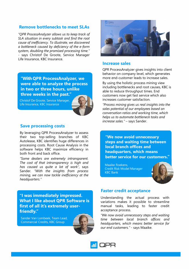
Increase salesQPR ProcessAnalyzer gives insights into client behavior on company level, which generates more end-customer leads to increase sales. By using the holistic process mining view including bottlenecks and root causes, KBC is able to reduce throughput times. End customers now get fast service which also increases customer satisfaction. “Process mining gives us real insights into the sales potential of our employees based on conversation ratios and working time, which helps us to automate bottleneck tasks and increase sales.” – says Sander.

“I was immediately impressed. What I like about QPR Software is first of all it’s extremely user-friendly.”Sander Van Lombeek, Team Lead, Commercial Credits, KBC Group

Save processing costsBy leveraging QPR ProcessAnalyzer to assesstheir two top-selling branches of KBCAutolease, KBC identifies huge differences inprocessing costs. Root Cause Analysis in thesoftware helps KBC maximize efficiency inboth front and back office.“Some dealers are extremely intransparent.The cost of that intransparency is high andhas caused us quite a lot of work”, saysSander. ”With the insights from processmining, we can now tackle inefficiency at theheadquarters.”

Faster credit acceptanceUnderstanding the actual process withvariations makes it possible to streamlinemanual tasks, leading to faster creditacceptance process.“We now avoid unnecessary steps and waitingtime between local branch offices andheadquarters, which means better service forour end customers.” - says Maaike.

“With QPR ProcessAnalyzer, wewere able to analyze the processin two or three hours, unlikethree weeks in the past.”

Christof De Groote, Service Manager,Life Insurance, KBC Insurance

“We now avoid unnecessary steps and waiting time between local branch offices and headquarters, which means better service for our customers.”Maaike Roekens,Credit Risk Model ManagerKBC Bank

“QPR ProcessAnalyzer allows us to keep track ofSLA situation in every subtask and find the rootcause of inefficiency. To illustrate, we discovereda bottleneck caused by deficiency of the e-formsystem, doubling the promised processing time.”- says Christof De Groote, Service ManagerLife Insurance, KBC Insurance.

Remove bottlenecks to meet SLAs

Easy to collect dataQPR ProcessAnalyzer eases the process ofcollecting the required data from our in-house built banking systems. By dividingcredit acceptance process activities into fivephases, local branch activities are efficientlybenchmarked with similar activities in thehead office.“QPR’s process mining tool is a great way toget your facts together and ensure we all aretalking on the same level” - says Maaike.

“Process discovery, Chart View and Dashboards are my favorite features. I am also experimenting with clustering and predictive models.”

Maaike Roekens,Credit Risk Model Manager, KBC Bank

QPR Software PlcQPR Software Plc (Nasdaq Helsinki) provides process mining, performance management and enterprise architecture solutions for digital transformation, strategy execution and business process improvement in over 50 countries. QPR software allows customers to gain valuable insights for informed decisions that make a difference.Dare to improve.

Read more at www.qpr.com



QPR ProcessAnalyzer solutionUsed in KBC Bank and KBC Insurance20+ process mining models including main processes such as credit acceptance and customer terminationEvent log data loaded from main banking and insurance systems

”QPR ProcessAnalyzer is very intuitive - after 2-3 hours I was able to do experiments of myown. It’s a very user-friendlyproduct.”

Christof De Groote, Service Manager,Life Insurance, KBC Insurance


“I really really love the influence analysis. I think that’s one of the major key benefits for me from the QPR ProcessAnalyzer tool.”Sander Van Lombeek, Team Lead, Commercial Credits, KBC Group

Better employee performanceIn the past, KBC measured employeeperformance based on only the number ofsigned contracts. With QPR ProcessAnalyzer,they now can integrate time factor on individualprocess mining task level into performancemeasurement.“We evaluated the performance of 1000 KBCemployees with QPR ProcessAnalyzer to find outwhat are the time-consuming activities in thewhole process.” – says Sander.

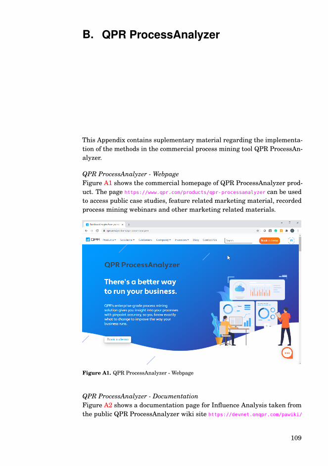
B. QPR ProcessAnalyzer

This Appendix contains suplementary material regarding the implementa-tion of the methods in the commercial process mining tool QPR ProcessAn-alyzer.

QPR ProcessAnalyzer - WebpageFigure A1 shows the commercial homepage of QPR ProcessAnalyzer prod-uct. The page https://www.qpr.com/products/qpr-processanalyzer can be usedto access public case studies, feature related marketing material, recordedprocess mining webinars and other marketing related materials.

Figure A1. QPR ProcessAnalyzer - Webpage

QPR ProcessAnalyzer - DocumentationFigure A2 shows a documentation page for Influence Analysis taken fromthe public QPR ProcessAnalyzer wiki site https://devnet.onqpr.com/pawiki/

109

QPR ProcessAnalyzer

index.php/Root_Causes.

Figure A2. Screenshot

Influence Analysis - with detailsFigure A3 shows the QPR ProcessAnalyzer user interface with one exampleof influence analysis feature. The user has selected a particular eventtype Returned with Notification as the criteria for root causes, ie. Casesgoing through the Event Type Returned with Notification are consideredas problematic cases. The Red and Blue coloring conditional coloring isused for the Contribution values which are presented in the table. Redcolor correlates with the problem cases, ie. the problem cases are likely tohave this property. Blue color correlates with the opposite, ie blue casesare NOT likely to belong to the set of problem cases.

110

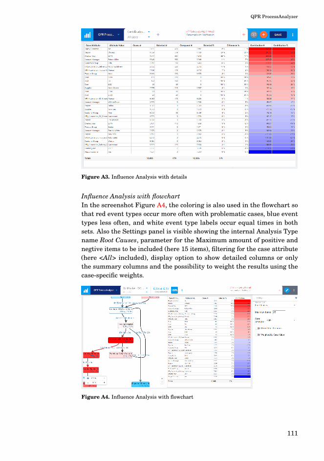
QPR ProcessAnalyzer

Figure A3. Influence Analysis with details

Influence Analysis with flowchartIn the screenshot Figure A4, the coloring is also used in the flowchart sothat red event types occur more often with problematic cases, blue eventtypes less often, and white event type labels occur equal times in bothsets. Also the Settings panel is visible showing the internal Analysis Typename Root Causes, parameter for the Maximum amount of positive andnegtive items to be included (here 15 items), filtering for the case attribute(here <All> included), display option to show detailed columns or onlythe summary columns and the possibility to weight the results using thecase-specific weights.

Figure A4. Influence Analysis with flowchart

111

QPR ProcessAnalyzer

Influence Analysis with tooltipsFigure A5 shows the Influence Analysis using a multiple line format withpop-up explanation texts. Here the user is analyzing cases where ConfrmedDelivery Date is before Delivery Completed, as shown in the red root causesanalysis rule in the top ribbon. Root causes are being shown for boththe top negative and positive root causes based on the absolute valueof contribution. As the user has clicked the property Customer Group= Women, a pop-up text is explaining the finding as: "Customer GroupWomen has the analyzed feature in 23% of the cases which is 8.0% more(184 cases) than on average. This root cause explains 15% (184 of 1,197cases) of the occurrence of the analyzed feature, provideds that there is acausal relationship.".

Figure A5. Influence Analysis with tooltips

Influence Analysis in MS ExcelFigure A6 shows the Influence Analysis in Microsoft Excel user inter-face. The original implementation released on 27.4.2012 executed analysisqueries using Microsoft SQL Server computing engine and Microsoft Exceluser interface clients.

112

QPR ProcessAnalyzer

Figure A6. Influence Analysis in MS Excel

Influence Analysis with WeightsFigure A7 shows the Influence Analysis results similar to the previousfigure. Results contain an additional column Case Value after the caseamounts. Contribution measures now explain how much each businessarea contributes to the total value of the problematic cases, instead of justthe total amount of problematic cases..

Figure A7. Influence Analysis with Weights

Duration Influence AnalysisFigure A8 shows the Influence Analysis conducted for the total duration ofthe case. One benefit of this kind of analysis is that it can be completed forevery process mining model without any user selected parameter values.Analysis shows the average duration (here 45,58 days) as points out theRegion = Dallas where average duration is 79,57 days for 1393 cases. Ifall cases in Dallas would have been completed in 45,58days, the total timesaving would have been (79,57 - 45,58) x 1393, i.e., 47 353,22 days. Thisin turn is 44,04% of the total 143 335,58 days of overtime in the wholepopulation. Business analysts can easily focus on the top and bottom rowsto identify potential causes for long (or short) durations and lead times.

113

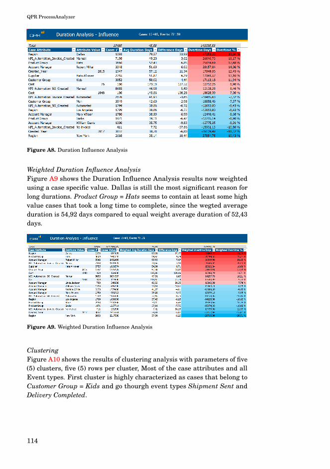
QPR ProcessAnalyzer

Figure A8. Duration Influence Analysis

Weighted Duration Influence AnalysisFigure A9 shows the Duration Influence Analysis results now weightedusing a case specific value. Dallas is still the most significant reason forlong durations. Product Group = Hats seems to contain at least some highvalue cases that took a long time to complete, since the wegted averageduration is 54,92 days compared to equal weight average duration of 52,43days.

Figure A9. Weighted Duration Influence Analysis

ClusteringFigure A10 shows the results of clustering analysis with parameters of five(5) clusters, five (5) rows per cluster, Most of the case attributes and allEvent types. First cluster is highly characterized as cases that belong toCustomer Group = Kids and go thourgh event types Shipment Sent andDelivery Completed.

114

QPR ProcessAnalyzer

Figure A10. Clustering

115

Bibliography

[1] Van Der Aalst, W., Adriansyah, A., & Van Dongen, B. (2011, Septem-ber). Causal nets: a modeling language tailored towards process dis-covery. In International conference on concurrency theory (pp. 28-42).Springer, Berlin, Heidelberg.

[2] Van Der Aalst, W., Adriansyah, A., De Medeiros, A. K. A., Arcieri,F., Baier, T., Blickle, T., ... & Burattin, A. (2011, August). Processmining manifesto. In International Conference on Business ProcessManagement (pp. 169-194). Springer, Berlin, Heidelberg.

[3] Van Der Aalst, Wil. (2016). Process Mining - Data Science in Action,Second Edition. Springer-Verlag Berlin Heidelberg, ISBN 978-3-662-49850-7.

[4] Van Der Aalst, W. (2011). Process mining: discovery, conformanceand enhancement of business processes (Vol. 2). Heidelberg: Springer.ISBN 978-3-642-19344-6

[5] Agarwal, R., & Srikant, R. (1994, September). Fast algorithms formining association rules. In Proc. of the 20th VLDB Conference (pp.487-499).

[6] Andersen, B. and Fagerhaug, T. (2006). Root cause analysis: simplifiedtools and techniques. ASQ Quality Press, 2006.

[7] Barbon Junior, S., Tavares, G. M., da Costa, V. G. T., Ceravolo, P.,& Damiani, E. (2018, April). A Framework for Human-in-the-loopMonitoring of Concept-drift Detection in Event Log Stream. The WebConference 2018 (pp. 319-326).

[8] Bay, S. D. and Pazzani, M. L. (2001). Detecting group differences:Mining contrast sets. Data Mining and Knowledge Discovery 5 (3),213–246.

117

Bibliography

[9] Bazhenova, E., & Weske, M. (2016, September). Deriving decisionmodels from process models by enhanced decision mining. In Inter-national conference on business process management (pp. 444-457).Springer, Cham.

[10] Biard, T., Le Mauff, A., Bigand, M., & Bourey, J. P. (2015, October).Separation of decision modeling from business process modeling usingnew “Decision Model and Notation”(DMN) for automating operationaldecision-making. In Working Conference on Virtual Enterprises (pp.489-496). Springer, Cham.

[11] Bolt, A., de Leoni, M., & van der Aalst, W. M. (2018). Process variantcomparison: using event logs to detect differences in behavior andbusiness rules. Information Systems, 74, 53-66.

[12] Bose, R. J. C., van der Aalst, W. M., Žliobaite, I., & Pechenizkiy, M.(2011). Handling concept drift in process mining. In InternationalConference on Advanced Information Systems Engineering (pp. 391-405). Springer, Berlin, Heidelberg.

[13] Bose, R. J. C., Van Der Aalst, W. M., Zliobaite, I., & Pechenizkiy, M.(2014). Dealing with concept drifts in process mining. IEEE transac-tions on neural networks and learning systems, 25(1), 154-171.

[14] Bose, R. J. C., & van der Aalst, W. M. (2013, April). Discoveringsignature patterns from event logs. In 2013 IEEE Symposium onComputational Intelligence and Data Mining (CIDM) (pp. 111-118).IEEE.

[15] Brin, S., Motwani, R., Ullman, J. D., & Tsur, S. (1997, June). Dynamicitemset counting and implication rules for market basket data. InProceedings of the 1997 ACM SIGMOD international conference onManagement of data (pp. 255-264).

[16] Buijs, J. C. A. M., & van der Aalst, W. M. P. (2017). Enabling in-teractive process analysis with process mining and visual analytics.BIOSTEC 2017, 573.

[17] Carmona, J., & Gavalda, R. (2012). Online techniques for dealingwith concept drift in process mining. In International Symposium onIntelligent Data Analysis (pp. 90-102). Springer, Berlin, Heidelberg.

[18] Cheng, H., Yan, X., Han, J., & Hsu, C. W. (2007, April). Discriminativefrequent pattern analysis for effective classification. In 2007 IEEE23rd International Conference on Data Engineering (pp. 716-725).IEEE.

[19] Clauset, A., Shalizi, C. R., & Newman, M. E. (2009). Power-law distri-butions in empirical data. SIAM review, 51(4), 661-703.

118

Bibliography

[20] Devlin, B. A., & Murphy, P. T. (1988). An architecture for a businessand information system. IBM systems Journal, 27(1), 60-80.

[21] Van Dongen, B.F. (2014). BPI Challenge 2014. Rabobank Ned-erland. Dataset. http://dx.doi.org/10.4121/uuid:c3e5d162-0cfd-4bb0-bd82-af5268819c35, 2014

[22] van Dongen, B.F. (2017). BPI Challenge 2017. Eindhoven University ofTechnology. Dataset. https://doi.org/10.4121/uuid:5f3067df-f10b-45da-b98b-86ae4c7a310b

[23] Van Dongen, B.F. (2019), Dataset BPI Challenge 2019. 4TU.Centrefor Research Data. https://doi.org/10.4121/uuid:d06aff4b-79f0-45e6-8ec8-e19730c248f1

[24] De Leoni, M., van der Aalst, W. M., & Dees, M. (2016). A generalprocess mining framework for correlating, predicting and clusteringdynamic behavior based on event logs. Information Systems, 56, 235-257.

[25] Van Dongen, S. (2000). A Cluster Algorithm for Graphs. Technicalreport, National Research Institute for Mathematics and ComputerScience in the Netherlands.

[26] Di Francescomarino, C., Ghidini, C., Maggi, F. M., & Milani, F. (2018,September). Predictive process monitoring methods: Which one suitsme best?. In International Conference on Business Process Manage-ment (pp. 462-479). Springer, Cham.

[27] Di Francescomarino, C., Dumas, M., Maggi, F. M., & Teinemaa, I.(2017). Clustering-based predictive process monitoring. IEEE trans-actions on services computing, 12(6), 896-909.

[28] Lqiang, G., & Hamilton, H. J. (2006). Interestingness Measures forData Mining: A Survey [J]. ACM Computing Surveys (CSUR), (3),61-93.

[29] Goldratt, E. M. (1990). Theory of constraints. Croton-on-Hudson:North River.

[30] Gröger, C., Niedermann, F., & Mitschang, B. (2012, July). Data mining-driven manufacturing process optimization. In Proceedings of theworld congress on engineering (Vol. 3, pp. 4-6).

[31] Holte, R. C. (1993). Very simple classification rules perform well onmost commonly used datasets. Machine learning, 11(1), 63-90.

[32] Hompes, B., Buijs, J. C., van der Aalst, W. M., Dixit, P., & Buurman,H. (2015). Detecting Change in Processes Using Comparative TraceClustering. In SIMPDA (pp. 95-108).

119

Bibliography

[33] Hompes, B. F., Buijs, J. C., & van der Aalst, W. M. (2016, October). Ageneric framework for context-aware process performance analysis.In OTM Confederated International Conferences" On the Move toMeaningful Internet Systems" (pp. 300-317). Springer, Cham.

[34] Hompes, B. F. A., Maaradji, A., La Rosa, M., Dumas, M., Buijs, J. C.A. M., & van der Aalst, W. M. P. (2017). Discovering causal factorsexplaining business process performance.

[35] Inmon, William H. (2005). Building the Data Warehouse. John Wiley& Sons. ISBN: 978-0-764-59944-6.

[36] Kakas, A. C., Kowalski, R. A., & Toni, F. (1992). Abductive logicprogramming. Journal of logic and computation, 2(6), 719-770.

[37] De Koninck, P., De Weerdt, J., & vanden Broucke, S. K. (2017). Ex-plaining clusterings of process instances. Data mining and knowledgediscovery, 31(3), 774-808.

[38] De Leoni, M., Van der Aalst, W. M., & Dees, M. (2014, September). Ageneral framework for correlating business process characteristics.In International Conference on Business Process Management (pp.250-266). Springer, Cham.

[39] De Leoni, M., van der Aalst, W. M., & Dees, M. (2016). A generalprocess mining framework for correlating, predicting and clusteringdynamic behavior based on event logs. Information Systems, 56, 235-257.

[40] De Leoni, M., Dumas, M., & García-Bañuelos, L. (2013, March). Dis-covering branching conditions from business process execution logs.In International Conference on Fundamental Approaches to SoftwareEngineering (pp. 114-129). Springer, Berlin, Heidelberg.

[41] Leontjeva, A., Conforti, R., Di Francescomarino, C., Dumas, M., &Maggi, F. M. (2016, September). Complex symbolic sequence encod-ings for predictive monitoring of business processes. In InternationalConference on Business Process Management (pp. 297-313). Springer,Cham.

[42] Maaradji, A., Dumas, M., La Rosa, M., & Ostovar, A. (2015). Fast andaccurate business process drift detection. In International Conferenceon Business Process Management (pp. 406-422). Springer, Cham.

[43] Maisenbacher, M., & Weidlich, M. (2017, June). Handling conceptdrift in predictive process monitoring. In Services Computing (SCC),2017 IEEE International Conference on (pp. 1-8). IEEE.

120

Bibliography

[44] Mayer-Schönberger, V., & Cukier, K. (2013). Big data: A revolutionthat will transform how we live, work, and think. Houghton MifflinHarcourt.

[45] De Medeiros, A. K. A., Guzzo, A., Greco, G., Van Der Aalst, W. M.,Weijters, A. J. M. M., Van Dongen, B. F., & Saccà, D. (2007). Processmining based on clustering: A quest for precision. In InternationalConference on Business Process Management (pp. 17-29). Springer,Berlin, Heidelberg.

[46] Nolle, T., Seeliger, A., & Mühlhäuser, M. (2018, September). Binet:Multivariate business process anomaly detection using deep learning.In International Conference on Business Process Management (pp.271-287). Springer, Cham.

[47] Ostovar, A., Leemans, S. J., & Rosa, M. L. (2020). Robust drift charac-terization from event streams of business processes. ACM Transac-tions on Knowledge Discovery from Data (TKDD), 14(3), 1-57.

[48] Pearl, J. (2009). Causality. Cambridge university press.

[49] Piatetsky-Shapiro, G. (1991). Discovery, analysis, and presentation ofstrong rules. Knowledge discovery in databases, 229-238.

[50] Piatetsky-Shapiro, G., & Matheus, C. J. (1994, July). The interest-ingness of deviations. In Proceedings of the AAAI-94 workshop onKnowledge Discovery in Databases (Vol. 1, pp. 25-36).

[51] Quinlan, J. R. (1986). Induction of decision trees. Machine learning,1(1), 81-106.

[52] Rozinat, A., & van der Aalst, W. M. (2006, September). Decisionmining in ProM. In International Conference on Business ProcessManagement (pp. 420-425). Springer, Berlin, Heidelberg.

[53] Seeliger, A., Nolle, T., & Mühlhäuser, M. (2018, September). FindingStructure in the Unstructured: Hybrid Feature Set Clustering forProcess Discovery. In International Conference on Business ProcessManagement (pp. 288-304). Springer, Cham.

[54] Song, M., Günther, C. W., & Van der Aalst, W. M. (2008). Traceclustering in process mining. In International Conference on BusinessProcess Management (pp. 109-120). Springer, Berlin, Heidelberg.

[55] Souza, C. R. (2014). The accord .NET framework. São Carlos, Brazil.http://accord-framework.net

[56] Suriadi, Suriadi, Ouyang, Chun, van der Aalst, Wil M.P., & ter Hof-stede, Arthur (2013) Root cause analysis with enriched process logs.

121

Bibliography

Lecture Notes in Business Information Processing [Business Pro-cess Management Workshops: BPM 2012 International Work-shopsRevised Papers], 132, pp. 174-186.

[57] Tax, N., Verenich, I., La Rosa, M., & Dumas, M. (2017, June). Pre-dictive business process monitoring with LSTM neural networks. InInternational Conference on Advanced Information Systems Engi-neering (pp. 477-492). Springer, Cham.

[58] Teinemaa, I., Tax, N., de Leoni, M., Dumas, M., & Maggi, F. M.(2018, September). Alarm-based prescriptive process monitoring. InInternational Conference on Business Process Management (pp. 91-107). Springer, Cham.

[59] Thaler, T., Ternis, S. F., Fettke, P., & Loos, P. (2015). A ComparativeAnalysis of Process Instance Cluster Techniques. Wirtschaftsinfor-matik, 2015, 423-437.

[60] Vanjoki, V. (2013). Automated Purchase to Pay Process Value Mod-eling and Comparative Process Speeds. Lappeenranta University ofTechnology, 2013.

[61] Webb, G. I., Butler, S., & Newlands, D. (2003, August). On detect-ing differences between groups. In Proceedings of the ninth ACMSIGKDD international conference on Knowledge discovery and datamining (pp. 256-265).

[62] Webb, G. I., Hyde, R., Cao, H., Nguyen, H. L., & Petitjean, F. (2016).Characterizing concept drift. Data Mining and Knowledge Discovery,30(4), 964-994.

[63] Verenich, I., Dumas, M., La Rosa, M., Maggi, F. M., Chasovskyi, D.,& Rozumnyi, A. (2016). Tell me what’s ahead? Predicting remainingactivity sequences of business process instances.

[64] Wetzstein, B., Leitner, P., Rosenberg, F., Brandic, I., Dustdar, S., &Leymann, F. (2009, September). Monitoring and analyzing influentialfactors of business process performance. In 2009 IEEE InternationalEnterprise Distributed Object Computing Conference (pp. 141-150).IEEE.

[65] Žliobaite, I., Pechenizkiy, M., & Gama, J. (2016). An overview ofconcept drift applications. In Big data analysis: new algorithms for anew society (pp. 91-114). Springer, Cham.

[66] Yeshchenko, A., Di Ciccio, C., Mendling, J., & Polyvyanyy, A. (2019,November). Comprehensive process drift detection with visual analyt-ics. In International Conference on Conceptual Modeling (pp. 119-135).Springer, Cham.

122

Bibliography

[67] Zaki, M. J. (2000). Scalable algorithms for association mining. IEEEtransactions on knowledge and data engineering, 12(3), 372-390.

[68] Zhu, N., Zhang, D., Wang, W., Li, X., Yang, B., Song, J., ... & Niu, P.(2020). A novel coronavirus from patients with pneumonia in China,2019. New England Journal of Medicine.

123

Errata

Publication IV

Corrected text in page 10. Should use the subscript Ep instead of incorrectsubscript Ea.

Correct version:Similarly, the problem density for BiCo of subset Ea is the density of

events belonging to the set Ea within the review period events Ep as

ρa =∣∣Ep∩Ea

∣∣

∣∣Ep

∣∣ =

∑

e j∈(Ep∩Ea )1

∑

e j∈Ep1 derived from Equation 3.3.

Incorrect version in the publication:Similarly, the average problem density for BiCo of subset Ea is ρa =

∣∣Ep∩Ea

∣∣

|Ea| =∑

e j∈(Ep∩Ea )1

∑

e j∈Ea1 derived from Equation 3.3.

125

.noitazinagro yreve rof laitnesse si sessecorp evorpmi ot ytiliba ehT

sessecorp lautca fo gnidnatsrednu desab-tcaf a sedivorp gninim ssecorP

ecnailpmoc ,skcenelttob ,smargaid ssecorp derevocsid fo mrof eht ni

tuo yrrac ot deen snoitazinagrO .smelborp lanoitarepo rehto dna ,seussi

tnempoleved fo noitacolla tneicfife dna sisylana esuac toor etarucca

.smelborp ecuder dna ssecorp eht evorpmi ot secruoser

eht evorpmi ot dohtem sisylana ecneuflni levon a stneserp krow sihT

dna ,segnahc ssecorp tceted ,secruoser tnempoleved fo noitacolla

.wofl ssecorp no tceffe tnacfiingis a evah taht saera ssenisub revocsid

htiw sisylana gninim ssecorp fo egasu eht senibmoc dohtem ehT

ehT .snoitaived fo sisylana dna serusaem evitcejbo desab-ytilibaborp

enil ,srenwo ssecorp ,stsylana ssenisub rof dengised yllaiceps si dohtem

fo tes a sa desu eb ot ,snoitazinagro egral ni srotidua dna ,sreganam

dna sdohteM .stroper kramhcneb dna sesylana esuac toor evitcaretni

erehw smelborp yranib htob gnizylana rof detneserp era smhtirogla

suounitnoc dna ,lufsseccus-non ro lufsseccus rehtie si esac hcae

gnisu rof dohtem A .stsoc dna semit dael ssecorp gnidulcni ,selbairav

ssenisub evitaler eht noitaredisnoc otni ekat ot sthgiew cfiiceps-esac

atad sedulcni osla krow sihT .detneserp osla si esac hcae fo ecnatropmi

fo atad tnaveler gniriuqca rof secitcarp tseb dna sdohtem noitaraperp

.tamrof gol tneve eht ni snoitarepo ssenisub

-otl

aA

DD

78

1/

02

02

+jhdba

e*GMFTSH

9

NBSI 9-7310-46-259-879 )detnirp(

NBSI 6-8310-46-259-879 )fdp(

NSSI 4394-9971 )detnirp(

NSSI 2494-9971 )fdp(

ytisrevinU otlaA

ecneicS fo loohcS

ecneicS retupmoC

fi.otlaa.www

+ SSENISUB YMONOCE

+ TRA

+ NGISED ERUTCETIHCRA

+ ECNEICS

YGOLONHCET

REVOSSORC























-otl

aA

DD

78

1/

02

02

+jhdba

e*GMFTSH

9

NBSI 9-7310-46-259-879 )detnirp(

NBSI 6-8310-46-259-879 )fdp(


NSSI 2494-9971 )fdp(

ytisrevinU otlaA

ecneicS fo loohcS

ecneicS retupmoC

fi.otlaa.www

+ SSENISUB YMONOCE

+ TRA


+ ECNEICS

YGOLONHCET

REVOSSORC























-otl

aA

DD

78

1/

02

02

+jhdba

e*GMFTSH

9

NBSI 9-7310-46-259-879 )detnirp(

NBSI 6-8310-46-259-879 )fdp(


NSSI 2494-9971 )fdp(

ytisrevinU otlaA

ecneicS fo loohcS

ecneicS retupmoC

fi.otlaa.www

+ SSENISUB YMONOCE

+ TRA


+ ECNEICS

YGOLONHCET

REVOSSORC


Documents

P rocess Mining Based Process Mining Based Inﬂuence