Embed Size (px)
Citation preview

Ovidius University
SEMINAR SERIES INMATHEMATICS AND COMPUTER
SCIENCE
CONSTANTZA – ROMANIA
2013

CONTENTS
I. Preface . . . . . . . . . . . . . . . . . . . . . . . . . . . . . . . . . . . . . . . . . . . . . . . . . . . . . . . . . . . . . 1
II. Initial blow-up solutions of a semilinear heat equation(Barbu Luminita) . . . . . . . . . . . . . . . . . . . . . . . . . . . . . . . . . . . . . . . . . . . . . . . . . . . 2
III. About Weitzenock’s inequality(Mihaly BENCZE) . . . . . . . . . . . . . . . . . . . . . . . . . . . . . . . . . . . . . . . . . . . . . . . . 22
IV. ODBDetective: a meta-data mining tool for detecting breaches of someOracle database design, implementation, querying, and manipulatingbest practice rules(Christian Mancas and Alina Iuliana Dicu) . . . . . . . . . . . . . . . . . . . . . . . . 26
V. A diabetes mortality study using generalized linear models(Ileana Gheorghiu and Raluca Vernic) . . . . . . . . . . . . . . . . . . . . . . . . . . . . . 45
Seminar Series in Mathematics and Computer Science:2013, 2–19
Initial blow-up solutions of a semilinear heatequation ∗
Abstract
We study the existence and uniqueness of a maximal solution ofequation ut −∆u + f(u) = 0 in Ω × (0,∞), where Ω is a domain witha non-empty compact boundary, which satisfy u = g on ∂Ω× (0,∞),assuming that g and f are continuous given functions and f is also con-vex, nondecreasing, f(0) = 0 and verifies Keller-Osserman condition.We show that if the boundary of Ω satisfies the parabolic Wiener cri-terion then the maximal solution is the unique large solution, i. e., itblows up at t = 0.
1 Introduction
We consider the following semilinear parabolic equation:
ut −∆u + f(u) = 0 in Q∞Ω := Ω× (0,∞), (1)
with the boundary condition
u = g on ∂lQ∞Ω = ∂Ω× (0,∞), (2)
where Ω ⊂ RN , N ≥ 2, is a domain (bounded or possibly unbounded) witha non-empty compact boundary. Concerning the nonlinear functions f and gwe assume that
f : [0,∞) → [0,∞) is a continuous and non-decreasing function,
f(0) = 0, f > 0 on (0,∞), (f1)
∗Luminita BarbuOvidius University, Department of Mathematics and Informatics, Blvd. Mamaia124,900527, Constanta, Romaniae-mail: [email protected]
2
Initial blow-up solutions of a semilinear heat equation 3
which satisfies the Keller-Osserman condition (see [6], [9]):
∫ ∞
1
[2F (s)]−1/2ds <∞ where F (s) =
∫ s
0
f(τ)dτ, (f2)
and g : ∂lQ∞Ω → [0,∞) is a continuous given function.
The main purpose of this paper is to study the existence and uniqueness of alarge initial solution of equation (1), subject to the boundary condition (2),that is a positive function u which satisfies (1), (2) and
limt→0
u(·, t) = ∞, uniformly on any compact subset of Ω. (3)
The existence of large solutions for the corresponding elliptic equation
−∆u+ f(u) = 0 in Ω, (4)
have been originally studied by Keller [6] and Osserman [9] in 1957. In theseworks they provided a condition on f (more precisely, condition (f2)) whichis necessary and sufficient in order that the set of solutions of (4) should belocally bounded from above. The result of Keller and Osserman states:
Theorem 1. Let f be a function satisfying assumptions (f1) and (f2). Thereexists a continuous and nonincreasing function h defined on R+ with the limits
limρ→0
h(ρ) = ∞, limρ→∞
h(ρ) = 0,
such that, for any domain Ω RN and any function u ∈ C(Ω) satisfying∆u ≥ f(u) in D′(Ω), u(x) ≤ h(dist(x, ∂Ω)) ∀x ∈ Ω.
As a consequence of the above Theorem, it is known that if f satisfiesconditions (f1) and (f2) then a large solution u (i. e. a function u ∈ C1(Ω)which verifies equation (4) in Ω and u(x) → ∞ as dist(x, ∂Ω) → 0, x ∈ K, forevery bounded set K ⊂ Ω) exists in every bounded domain which possesses aLipschitz boundary. Labutin [5] showed that the Lipschitz condition on ∂Ω canbe replaced by a Wiener type condition which is necessary and sufficient for theexistence of a large solution. Uniqueness in smooth domains was establishedunder some additional assumptions on f (see [2]). Other results concerningexistence and uniqueness for large solutions of (4) in non-smooth domains Ωhave been obtained by Marcus and Veron in [7].
The aim of this article is to extend these questions to the parabolic equation(1). We note that the special case f(u) =| u |q−1 u, q > 1, has been studiedby Waad Al Sayed and Veron in [1]. It is worth pointing out that the existenceand the uniqueness of the solution of problem (1) which satisfies u = ∞ on
4 Initial blow-up solutions of a semilinear heat equation
the parabolic boundary Ω × 0⋃∂Ω × (0,∞) when Ω is a domain in RN
with a compact boundary and f is a continuous increasing function satisfyingsuperlinear growth condition have been studied by Marcus and Veron in arecent article [8].
In Section 2 we consider the following problem, denoted by PΩ,0:
ut −∆u + f(u) = 0 in Q∞
Ω ,
u = 0 on ∂lQ∞Ω .
PΩ,0
The first result we obtain in this paper is an existence theorem for maximalsolutions of problems PΩ,0 under appropriate assumptions on function f , whenΩ is an arbitrary subdomain of RN with compact boundary (see Theorem 8below). Next, we prove that a such solution is also a minimal solution of ourproblem which satisfies (3) (Proposition 9). In the next part of this Sectionwe suppose that ∂Ω verifies the parabolic Wiener criterion. In this case thesolution constructed in Theorem 8 is more regular, as we shall prove in The-orem 11 (see also Proposition 12). The last purpose of the paper is to obtaina result concerning the existence and uniqueness for the solutions of prob-lem consisting of equation (1), lateral boundary condition (2) and (3). Theassumptions we should require to achieve our goal are given in Theorem 13,the main result of Section 3. We point out that the existence and uniquenessof such a solution u is associated to the existence of a large solution to thestationary equation (4) and solution of the ODE (see Remark 6)
ϕ′ + f(ϕ) = 0 in (0,∞), limtց0
ϕ(t) = ∞.
2 Maximal solutions of problem PΩ,0
We will be concerned with problem PΩ,0 formulated above under assumptions(f1), (f2), where Ω is a domain of RN , N ≥ 2, with a non-empty compactboundary.
In order to investigate this problem, we choose as our framework the Hilbertspace H := L2(Ω), endowed with the usual scalar product, denoted 〈·, ·〉, andthe corresponding induced norm, denoted ‖ · ‖. It is not difficult to see thatPΩ,0 can be represented as an equation in the Hilbert space H , associated toa maximal monotone operator:
du
dt(t) +AΩ(u(t)) = 0, t ∈ (0,∞), (5)
Initial blow-up solutions of a semilinear heat equation 5
where u(t) := u(·, t), f : D(f) ⊂ H → H ,
D(f) = u ∈ H ; x→ f(u(x)) belongs to H,f(u)(x) = f(u(x)) for a. a. x ∈ Ω, ∀ u ∈ D(f),
(f is the canonical extension of f to H), AΩ : D(AΩ) ⊂ H → H,
D(AΩ) = u ∈ H10 (Ω); ∆u ∈ H
⋂D(f), AΩu = −∆u+ f(u) ∀ u ∈ D(AΩ).
It is well known that under assumption (f1), operator AΩ is maximal mono-tone. In fact, AΩ is even cyclically monotone. More precisely, since f is thederivative of the convex function j(x) =
∫ x
0 f(y)dy, we have AΩ = ∂ψΩ, whereψΩ : H → (−∞,∞],
ψΩ(u) =
12
∫Ω |∇u|2dx+
∫Ω j(u)dx, if u ∈ H1
0 (Ω), j(u) ∈ L1(Ω),
+∞, otherwise,
where | · | denotes the euclidian norm of RN (see, e.g., [10], p. 197). Therefore,according to well known Brezis’ result (see [3])), we have:
Theorem 2. Assume that (f1) is satisfied and u0 ∈ H is a given function.Then, there exists a unique strong solution u of equation (5) which satisfiesthe initial condition u(0) = u0, such that u(t) ∈ D(AΩ) ∀ t > 0,
u ∈ C([0,∞);L2(Ω))⋂L2loc(0,∞;H1
0 (Ω))⋂H1
loc(0,∞;L2(Ω)).
In addition,
‖ (du/dt)(t) ‖≤ 1/t ‖ u0 ‖ ∀ t ∈ (0,∞). (6)
In the following we consider solutions of equation(5) with the above regu-larity.
Definition 3. Let Ω be a bounded subdomain of RN . We denote by S0(Q∞Ω )
the set of positive functions u ∈ C(0,∞;L2(Ω))⋂L2loc(0,∞;H1
0 (Ω)) such thatut, ∆u ∈ L2
loc(0,∞;L2(Ω)), u(·, t) ∈ D(AΩ) ∀ t > 0, which verify (5) for allt > 0.
More generally, we denote by S(Q∞Ω ) the set of all positive functions u ∈
L2loc(0,∞;H1(Ω))
⋂H1
loc(0,∞;L2(Ω)), f(u) ∈ L2loc(0,∞;L2(Ω)), such that
∫
Ω
[(∂u/∂t)ζ +∇u · ∇ζ + f(u)ζ](·, t)dx = 0 ∀ t > 0, ζ ∈ H10 (Ω). (7)
6 Initial blow-up solutions of a semilinear heat equation
We define in a similar way a subsolution (resp. supersolution) of (1) byimposing the same regularity conditions on u and f(u) and
∫
Ω
[(∂u/∂t)ζ +∇u · ∇ζ + f(u)ζ](·, t)dx ≤ 0 ∀ t > 0, ζ ∈ H10 (Ω), (8)
respectively,
∫
Ω
[(∂u/∂t)ζ +∇u · ∇ζ + f(u)ζ](·, t)dx ≥ 0 ∀ t > 0, ζ ∈ H10 (Ω). (9)
Now we consider the case when Ω is unbounded and we assume that Ωc ⊂BR0 , denote by ΩR = Ω
⋂BR, R ≥ R0, and by H1
0 (ΩR) the closer in H1(ΩR)of the space of C∞(ΩR)− functions which vanish in a neighborhood of ∂Ω.
Definition 4. If Ω is not bounded and Ωc ⊂ BR0 , we denote by S0(Q∞Ω ) the
set of positive functions u such that, for any R ≥ R0, u ∈ C(0,∞;L2(ΩR))⋂L2loc(0,∞; H1
0 (ΩR)), ut,∆u ∈ L2loc(0,∞;L2(ΩR)), u(·, t) ∈ H1
0 (ΩR) ∀ t > 0,which verify (5) for all t > 0. Also, we denote by S(Q∞
Ω ) the set of all positivefunctions
u ∈ L2loc(0,∞;H1(ΩR))
⋂H1
loc(0,∞;L2(ΩR)), f(u) ∈ L2loc(0,∞;L2(ΩR)),
such that∫
ΩR
[(∂u/∂t)ζ +∇u · ∇ζ + f(u)ζ](·, t)dx = 0 ∀ t > 0, ζ ∈ H10 (ΩR), (10)
for all R ≥ R0.
Remark 5.
Suppose that Ω is a bounded subdomain of RN , f verifies assumption (f1),and
f is a convex function. (f3)
Obviously, if u1, u2 ∈ S(Q∞Ω ), then u1 + u2 is a supersolution of (1).
On the other hand, if u ∈ S(Q∞Ω ) and v is a supersolution of (1), such that
supp [u−v]+(·, t) is a compact subset of Ω ∀ t > 0 and limtց0 ‖ [u−v]+(·, t) ‖=0, then u(x, t) ≤ v(x, t) ∀ t > 0, for a.a. x ∈ Ω.
Indeed, starting with the obvious inequality
∫
Ω
(∂(u− v)
∂tζ +∇(u − v) · ∇ζ
)(·, t)dx ≤
∫
Ω
(f(v)− f(u))(·, t)ζdx,
Initial blow-up solutions of a semilinear heat equation 7
∀ t > 0, ζ ∈ H10 (Ω), and taking in the above inequality ζ = [u − v]+(·, t) ∈
H10 (Ω) ∀ t > 0, we can see that
∫
Ω
(∂h∂th+ | ∇h |2
)(·, t)dx ≤
∫
Ω
((f(v) − f(u))h
)(·, t)dx
≤ −∫
Ω
(f(h)h
)(·, t)dx ≤ 0 ∀ t > 0,
(11)
where h := [u − v]+ (we have used that f is a convex function, f(0) = 0,therefore f(a+ b) ≥ f(a) + f(b) ∀ a, b ≥ 0).
Clearly, inequality (11) implies
d
dt‖ h(·, t) ‖2≤ 0 ∀ t > 0 ⇒ t→‖ h(·, t) ‖ is non-increasing on (0,∞).
Therefore, ‖ h(·, t) ‖≤ limsց0 ‖ h(·, s) ‖= 0, which implies h(x, t) = 0 ⇔u(x, t) ≤ v(x, t) ∀ t > 0, for a.a. x ∈ Ω.
Remark 6.
If assumptions (f1)− (f3) are satisfied, then there exists a unique solutionϕ : (0,∞) → (0,∞), of the following problem:
ϕ′ + f(ϕ) = 0 in (0,∞),limtց0
ϕ(t) = ∞. (12)
Indeed, it is known that under assumptions (f1)−(f3), F (t) := −∫∞t
1f(s)ds <
∞ ∀ t > 0. On the other hand, since f is a convex function, s → f(s)/s isnon-decreasing on (0,∞), therefore f(s)/s ≤ f(1) ∀ 0 < s ≤ 1. Thus for everys ∈ (0, 1) we have
∫ 1
s
dt
f(t)≥ 1
f(1)
∫ 1
s
dt
t= − 1
f(1)ln s.
It follows that limsց0
∫ 1
sdtf(t) = ∞, which implies lim
tց0F (t) = −∞. Therefore,
F : (0,∞) → (−∞, 0) is a C1 increasing bijective function and the general
solution of equation (11)1 is F (ϕ(t)) = −t +K, K ≤ 0. Taking into account(12)2, we obtain K = 0, therefore the unique solution of problem (12) is
ϕ(t) = F−1(−t) ∀ t > 0.
Lemma 7. Suppose that assumptions (f1)− (f3) are satisfied. If u ∈ S(Q∞Ω )
the following estimate holds:
u(x, t) ≤ ϕ(t) + UΩ(x) ∀ (x, t) ∈ Q∞Ω , (13)

8 Initial blow-up solutions of a semilinear heat equation
where UΩ ∈ C1(Ω) is a maximal solution of the equation
−∆u+ f(u) = 0 in Ω (14)
(for the existence of a such solution, see [7], p. 642).If, in addition, Ω is bounded and u ∈ S0(Q
∞Ω ), then:
u(x, t) ≤ ϕ(t) ∀ (x, t) ∈ Q∞Ω . (15)
Proof. Let Ωnn∈N be a sequence of bounded subsets of Ω with smoothboundary such that Ω
n ⊂ Ωn+1, Ω =⋃
n∈N Ωn. For every n ∈ N, denote by Un
the maximal solution of (14) in Ωn (in fact, as Ωn is bounded and possessessmooth boundary, Un is a large solution). Let u ∈ S(Q∞
Ω ).Clearly, ϕ,Un ∈ S(Q∞
Ωn), therefore ϕ+Un is a supersolution of (1) in Q∞Ωn .
For τ > 0 and n ∈ N, we denote by vn,τ the function defined as follows
vn,τ (x, t) := u(x, t+ τ) − (Un(x) + ϕ(t)) ∀ (x, t) ∈ Q∞Ωn .
Obviously, supp [vn,τ ]+(·, t) is a compact subset of Ωn ∀ t > 0. In addition,by Lebesgue’s theorem, limtց0 ‖ [vn,τ ]+(·, t) ‖L2(Ωn)= 0. Thus, making use ofRemark 5, we find u(x, t+ τ) ≤ Un(x) +ϕ(t) ∀ t > 0, for a.a. x ∈ Ωn. Lettingτ ց 0 and using the continuity we find
u(x, t) ≤ Un(x) + ϕ(t) ∀ t > 0, x ∈ Ωn. (16)
Finally, we can pass to the limit as n→ ∞ in inequality (16) to obtain (13).The proof of the last part of the Lemma goes similarly, with slight modifi-
cations. More exactly, if Ω is bounded and u ∈ S0(Q∞Ω ), we denote vτ (x, t) :=
u(x, t+ τ) − ϕ(t) ∀ (x, t) ∈ Q∞Ω . Since supp [vτ ]+(·, t) is a compact subset of
Ω ∀ t > 0 and, on account of Lebesgue’s theorem, limtց0 ‖ [vτ ]+(·, t) ‖= 0, byRemark 5 we find that u(x, t + τ) ≤ ϕ(t) ∀ t > 0, for a.a. x ∈ Ω. Inequality(15) follows by letting τ ց 0.
Next, we continue with a result about the existence of a maximal solutionof problem PΩ,0 :
Theorem 8. Assume that (f1)− (f3) are satisfied. Then problem PΩ,0 has amaximal solution uΩ ∈ S0(Q
∞Ω ), more precisely:
uΩ ≥ u in Q∞Ω , ∀ u ∈ S0(Q
∞Ω ). (17)
Proof.
Step 1. Construction of uΩ in the case that Ω is bounded.
Initial blow-up solutions of a semilinear heat equation 9
Let k ∈ N∗. By Theorem 2, the following Cauchy problem in H :
duk
dt (t) +AΩ(uk(t)) = 0, t ∈ (0,∞),uk(0) = k in Ω,
(18)
has a unique strong solution, denoted by uk ∈ S0(Q∞Ω ). Since f is non-
decreasing, it follows by the maximum principle that the corresponding se-quence of these solutions ukk increases with k and in view of Lemma 7 (see(15)) is locally uniformly bounded in Q∞
Ω by ϕ. Thus, for every (x, t) ∈ Q∞Ω
we can define uΩ(x, t) := limk→∞ uk(x, t).Next, we check that uΩ ∈ S0(Q
∞Ω ) is a maximal solution of problem PΩ,0.
Let K be a compact subset of (0,∞). Now, making use of inequalities (6),(15), assumption (f1) and equation (18)1 we find
‖ (duk/dt)(·, t) ‖ =‖ AΩ(uk)(·, t) ‖≤ (1/t0)√meas(Ω)ϕ(t0),
‖ uk(·, t) ‖ ≤ √meas(Ω)ϕ(t0), f(uk(·, t)) ≤ f(ϕ(t0)) ∀ k ∈ N, t ∈ K,
where t0 := inft; t ∈ K. Therefore, according to Lebesgue’s theorem anddemi-closedness of maximal monotone operators we obtain that
uk → uΩ in H1loc(0,∞;L2(Ω)), f(uk) → f(uΩ) in L2
loc(0,∞;L2(Ω)),
uΩ ∈ H1loc(0,∞;L2(Ω)), f(uΩ) ∈ L2
loc(0,∞;L2(Ω)), uΩ(·, t) ∈ D(AΩ),
AΩ(uk(·, t)) A(uΩ(·, t)) in L2(Ω) ∀ t > 0.
We let k → ∞ in (18)1 and derive that uΩ verify (5) for all t > 0. Now, let usverify that uΩ ∈ C(0,∞;L2(Ω)). By a standard computation, we find
‖ (uk − ul)(·, t) ‖2 +2
∫ t
s
‖ ∇(uk − ul)(·, θ) ‖2(L2(Ω))N dθ ≤‖ (uk − ul)(·, s) ‖2,
∀ 0 < s < t. Since ‖ (uk − ul)(·, s) ‖→ 0 as k, l → ∞, we obtain uk → uΩ inC([s, t];L2(Ω)) ∀ 0 < s < t which implies uΩ ∈ C(0,∞;L2(Ω)).
It remains to show that uΩ is a maximal solution of problem PΩ,0. To thisend, let τ > 0, u ∈ S0(Q
∞Ω ), kτ ∈ N, such that ukτ (x, 0) = kτ > ϕ(τ) and
define the function
vτ (x, t) := u(x, t+ τ) − ukτ (x, t) ∀(x, t) ∈ Q∞Ω .
It is easy to see that vτ (·, t) ∈ H10 (Ω) ∀ t > 0. In addition, limtց0 ‖
[vτ ]+(·, t) ‖= 0, and thus, using a similar reasoning as in Remark 5, vτ (·, t) =0 ∀ t > 0, a.e. in Ω. Finally, making use of the continuity and letting τ → 0(which implies kτ → ∞) it follows that u ≤ uΩ in Q∞
Ω .
10 Initial blow-up solutions of a semilinear heat equation
Step 2. Construction of uΩ when Ω is unbounded.
Let R0 > 0 be large enough such that ∂Ω ⊂ BR0 and for n > R0, we denoteby Ωn = Ω
⋂Bn and uΩn the solution obtained in Step 1 with Ω replaced
by Ωn. More precisely, for n, k ∈ N∗, uΩn = limk→∞ un,k, where un,k is thestrong solution of the Cauchy problem:
dun,k
dt (t) +AΩn(un,k(t)) = 0, t ∈ (0,∞),un,k(0) = k in Ωn.
(19)
It is clear that un,k ≤ un+1,k, therefore uΩn ≤ uΩn+1 in Ωn × (0,∞). On theother hand, for every x0 ∈ Ω there exists n0 ∈ N such that x0 ∈ Ωn for alln ≥ n0. In view of the monotonicity of the sequence uΩn(x0, t)n≥n0 and (15)we can define uΩ(x0, t) = limn→∞ uΩn(x0, t) ∀ t > 0.
Now, we are going to prove that uΩ belongs to the space S0(Q∞Ω ) and is
a maximal solution of problem PΩ,0. As we have been proved in Step 1, uΩn
satisfiesduΩn
dt(t) + AΩn(uΩn(t)) = 0, t ∈ (0,∞). (20)
Taking the scalar product in L2(Ωn) of (20) and ξ2uΩn where ξ ∈ C∞0 (Ωn),
we get
1
2
d
dt
∫
Ωn
ξ2uΩn(·, t)2dx+
∫
Ωn
(| ∇uΩn |2 +f(uΩn)uΩn
)(·, t)ξ2dx
+ 2
∫
Ωn
(∇uΩn(·, t) · ∇ξ)ξuΩn(·, t)dx = 0 ∀ t > 0,
from which we derive
1
2
d
dt
∫
Ωn
ξ2uΩn(·, t)2dx+
∫
Ωn
(2−1 | ∇uΩn |2 +f(uΩn)uΩn
)(·, t)ξ2dx
≤ 2
∫
Ωn
ξ2 | ∇ξ |2 uΩn(·, t)2dx.
Let us consider R > R0, τ > 0. In what follows we denote by Ck(k = 1, · · · , 4)different positive constants which depend on R and N , but are independentof n, t, τ. Taking ξ such that 0 ≤ ξ ≤ 1, supp ξ ⊂ Bc
2R, ξ ≡ 1 on BR, in theabove inequality and integrating over [τ, t], we obtain:
1
2
∫
ΩR
uΩn(·, t)2dx+
∫ t
τ
∫
ΩR
(2−1 | ∇uΩn |2 +f(uΩn)
)uΩndxds
≤ 2
∫ t
τ
∫
Ω2R
u2Ωn| ∇ξ |2 dxds+ 1
2
∫
Ω2R
uΩn(·, τ)2dx ≤ C1(t+ 1)ϕ(τ)2,
(21)
Initial blow-up solutions of a semilinear heat equation 11
∀ n > 2R, t > τ > 0 (we have used inequality (15)). Letting n → ∞ in (21)and using Fatou’s lemma we find∫
ΩR
uΩ(·, t)2dx+∫ t
τ
∫
ΩR
(| ∇uΩ |2 +2f(uΩ)uΩ
)dxds ≤ 2C1(t+1)ϕ(τ)2, (22)
for all t > τ.Next, if we take the scalar product in L2(Ωn) of (20) with (t−τ)ξ2duΩn/dt,
we get
(t− τ)
∫
Ωn
duΩn
dt(·, t)2ξ2dx
+d
dt
(t− τ)
∫
Ωn
(2−1 | ∇uΩn |2 +j(uΩn)
)(·, t)ξ2dx
−∫
Ωn
(2−1 | ∇uΩn |2 +j(uΩn)
)(·, t)ξ2dx
= −2(t− τ)
∫
Ωn
duΩn
dt(·, t)(∇uΩn(·, t) · ∇ξ)ξdx
≤ t− τ
2
∫
Ωn
duΩn
dt(·, t)2ξ2dx+ 2(t− τ)
∫
Ωn
| ∇uΩn(·, t) |2| ∇ξ |2 dx,
for every t > τ, where j(x) =∫ x
0 f(y)dy (see [3], Proposition 2, p. 517).Integrating this inequality over [τ, t] and taking ξ as before, we infer
1
2
∫ t
τ
∫
ΩR
(s− τ)du2Ωn
dtdxds
+ (t− τ)
∫
ΩR
(2−1 | ∇uΩn |2 +j(uΩn)
)(·, t)dx
≤C2
∫ t
τ
(s− τ + 1)
∫
Ω2R
| ∇uΩn |2 dxds
+ C3
∫ t
τ
∫
Ω2R
j(uΩn)dxds,
(23)
∀ n > 2R, t > τ > 0. On account of inequalities (15) and (22), the right handside of (23) remains bounded by C4(t + 1)2(ϕ(τ)2 + j(ϕ(τ))). Passing to thelet as n→ ∞ in (23) we derive by Fatou’s lemma:
1
2
∫ t
τ
∫
ΩR
(s− τ)du2Ωdt
dxds
+ (t− τ)
∫
ΩR
(2−1 | ∇uΩ(·, t) |2 +j(uΩ(·, t))
)dx
≤C4(t− τ + 1)2(ϕ(τ)2 + j(ϕ(τ))) ∀ t > τ > 0.
(24)
12 Initial blow-up solutions of a semilinear heat equation
Obviously, (23) is an estimate in L2(τ, t; H10 (ΩR)), which is a closed subspace of
L2(τ, t;H1(ΩR)), therefore uΩ ∈ L2loc(τ, t; H
10 (ΩR)). Note also that inequalities
(21), (23) imply uΩ ∈ S0(Q∞Ω ).
Finally, our next goal is to show that uΩ is a maximal solution of problemPΩ,0. Let us consider u ∈ S0(Q
∞Ω ). For every τ > 0 and R ≥ R0 we set
vR,τ (x, t) := u(x, t + τ) − uΩ(x, t) − UR(x) ∀ (x, t) ∈ ΩR × (0,∞), whereUR is the large positive solution of equation (14) with Ω = BR. Obviously,supp [vR,τ ]+(·, t) is a compact subset of ΩR ∀ t > 0. Also, by Lebesgue’stheorem, limsց0 ‖ [vR,τ ]+(·, s) ‖L2(ΩR)= 0, therefore making use of Remark 5,we get
u(x, t+ τ) ≤ UR(x) + uΩ(x, t),
∀ t > 0, for a.a. x ∈ ΩR. Letting R → ∞, τ ց 0, and using the continuitywe find u(x, t) ≤ uΩ(x, t) ∀ t > 0, x ∈ Ω (we have used that limR→∞ UR(x) =0 ∀ x ∈ Ω, which is a consequence of Theorem 1). This concludes the proof.
Proposition 9. Under assumptions of Theorem 8, the maximal solution uΩ ∈S0(Q
∞Ω ) is a minimal solution with initial blow-up, more exactly:
limtց0
uΩ(x, t) = ∞ locally uniformly on Ω, (25)
and ∀ u ∈ S(Q∞Ω ) such that limtց0 u(x, t) = ∞ locally uniformly on Ω we
haveuΩ ≤ u in Q∞
Ω . (26)
In addition,
limtց0
uΩ(x, t)
ϕ(t)= 1 locally uniformly on Ω. (27)
Proof. We will use the same notations as in the proof of Theorem 8. LetK be a compact subset of Ω. For y ∈ K, let Q∞
Br(y):= Br(y)× (0,∞) ⊂ Q∞
Ω
and denote by Ur,y the unique positive large solution of the problem
−∆Ur,y + f(Ur,y) = 0 in Br(y),lim
|x−y|→rUr,y(x) = ∞.
For τ > 0, there exists kτ ∈ N, such that ukτ (x, 0) = kτ > ϕ(τ). We denoteby vτ,r the function defined as follows
vτ,r := ϕ(t+ τ) − uΩ(x, t)− Ur,y(x) ∀(x, t) ∈ Q∞Br(y)
.
Obviously,
uΩ(x, t)+Ur,y(x) ≥ ukτ (x, t)+Ur,y(x) > ϕ(t+τ) ∀ t > 0, for a.a. x ∈ ∂Br(y),
Initial blow-up solutions of a semilinear heat equation 13
therefore, for all t > 0, supp [vr,τ ]+(·, t) is a compact subset of Br(y). Inaddition, limtց0 ‖ [vτ,r]+(·, t) ‖= 0 ∀ t > 0 which implies (see Remark 5)uΩ(x, t) + Ur,y(x) ≥ ϕ(t+ τ) ∀ t > 0 for a.a. x ∈ Br(y). Therefore, using thecontinuity and letting τ → 0 in the previous inequality we infer
uΩ(x, t) + Ur,y(x) ≥ ϕ(t) ∀ (x, t) ∈ Q∞Br(y)
. (28)
On the other hand, for any 0 < r′ < r there exists a positive constant Cy,r′
such that Ur,y(x) ≤ Cy,r′ ∀ x ∈ Br′(y). This inequality together with (28)implies lim
tց0uΩ(x, t) = ∞ uniformly on Br′(y). As K can be covered by a finite
number of such balls we obtain (25).Next we are going to prove (27). Making use of inequalities (15) and (28)
(with Ω replaced by Br(y)) we obtain
uBr(y)(x, t) + Ur,y(x) ≥ ϕ(t) ≥ uBr(y)(x, t) ∀ (x, t) ∈ Q∞Br(y)
,
and hence
limtց0
uBr(y)(x, t)
ϕ(t)= 1 locally uniformly on Br′(y) ∀ r′ < r. (29)
Since
uBr(y)(x, t) + Ur,y(x) ≥ uΩ(x, t) ≥ uBr(y)(x, t) ∀ (x, t) ∈ Q∞Br(y)
,
the last equality (29) leads us to (27).Finally, if u ∈ S(Q∞
Ω ) is a solution of (1) which satisfies initial blow-upcondition locally uniformly on Ω, and Ω is a bounded subdomain of RN wehave uk ≤ u in Q∞
Ω and letting k → ∞ we derive (26). On the other hand,when Ω is unbounded we have uΩn ≤ u in Q∞
Ωn, where Ωn = Ω
⋂Bn. Letting
n→ ∞ in the previous inequality, (26) follows. The proof is complete. In fact, (27) remains true if we replaced uΩ by any solution u ∈ S(Q∞
Ω )which verifies the initial blow-up condition on Ω. The proof follows ideassimilar to those we have already used in the proof of Proposition 9.
If ∂Ω has the minimal regularity which allows the Dirichlet problem to besolved by any continuous function g given on ∂lQ
∞Ω , we can consider another
construction of the maximal solution of problem PΩ,0. The needed assumptionon ∂Ω is known as the parabolic Wiener criterion (PWC) (see [11]).
Definition 10. If ∂Ω is compact and satisfies PWC, we denote by S0(Q∞Ω ) the
set of all positive solutions of problem PΩ,0 which belong to the space C2,1(Q∞Ω )⋂
C(Ω× (0,∞)).
Theorem 11. Assume that (f1) − (f3) are satisfied, ∂Ω is compact and sat-isfies PWC. Then problem PΩ,0 has a maximal solution uΩ ∈ S0(Q
∞Ω ).
14 Initial blow-up solutions of a semilinear heat equation
Proof. We first assume that Ω is bounded. In the same manner as in theproof of Theorem 8 we can construct the maximal solution uΩ as being thelimit in Ω× (0,∞) of the increasing sequence ukk≥1, where uk is the uniquesolution (on account of the maximum principle) of the problem PΩ,0, whichsatisfies the initial condition uk(·, 0) = k in Ω for all k ≥ 1. Clearly, such asolution uk exists and belongs to S0(Q
∞Ω ) on account of PWC assumption.
Furthermore, inequality (14) is still valid for uk in Ω× (0,∞). In view of thisestimate, the sequence ukk≥1, is locally uniformly bounded in Ω × (0,∞)and therefore (by standard parabolic equations estimates) it is compact inC2,1(Q∞
Ω ).Consequently, uΩ := limk→∞ uk belongs to C2,1(Q∞
Ω )⋂C(Ω× (0,∞)) and
verifies (1) in Q∞Ω . In addition, taking into account the construction of uΩ we
get uΩ = 0 on ∂Ω× (0,∞), therefore u ∈ S0(Q∞Ω ).
On the other hand, if Ω is unbounded we consider R0 > 0 such that∂Ω ⊂ BR0 and for n > R0, n ∈ N we denote by uΩn the solution obtainedabove with Ω replaced by Ωn = Ω
⋂Bn. From the construction of uΩn we
derive that uΩn ≤ uΩn+1 in Q∞Ωn. Since uΩn ≤ ϕ in Ωn × (τ,∞) ∀ τ > 0 we
can see that there exists uΩ := limn→∞ uΩn in Q∞Ω . By applying a bootstrap
regularity argument we obtain uΩ ∈ S0(Q∞Ω ).
In order to establish the maximality of uΩ in S0(Q∞Ω ) we can use similar
reasonings to those we have already used in the last part of the proof ofTheorem 8, so we will just sketch its. For example, let us suppose that Ω isunbounded. We will use the same notation as in the proof of the previousTheorem. If u ∈ S0(Q
∞Ω ), for R > R0, τ > 0 we set
vR,τ := u(·, ·+ τ)− uΩ − UR in ΩR × (0,∞).
Clearly, [vR,τ ]+ is a subsolution of (1) in ΩR× (0,∞) which is zero on (∂ΩR×(0,∞))
⋃(ΩR×0.) As a consequence of the maximum principle we get vR,τ ≤
0 in ΩR × (0,∞). Letting R → ∞, τ → 0 in the last inequality we obtainu ≤ uΩ in Q∞
Ω .
Proposition 12. Under assumptions of Theorem 11
uΩ ∈ S0(Q∞Ω ), uΩ = uΩ. (30)
Proof. Let us suppose that Ω is bounded. As ∂Ω verifies PWC, thereexists a sequence Ωnn of smooth domains such that
Ωn ⊂ Ωn ⊂ Ωn+1 ⊂ Ω,
⋃
n
Ωn = Ω, supdist (x,Ωc) ;x ∈ ∂Ωn < 1/n.
For τ > 0, n ∈ N, we consider the solutions un,τ ∈ C2,1(Ωn×(τ,∞))⋂C(Ω
n×
Initial blow-up solutions of a semilinear heat equation 15
(τ,∞)) of the following problems:
∂tun,τ −∆un,τ + f(un,τ) = 0 in Ωn × (τ,∞),un,τ = 0 on ∂Ωn × [τ,∞),un,τ (·, τ) = uΩ(·, τ) in Ωn.
(31)
By the maximum principle, ∀ t > τ we have
0 ≤ uΩ(·, t)− un,τ (·, t) ≤ maxuΩ(x, s) ; (x, s) ∈ ∂Ωn × [τ, t] → 0 as n→ ∞.
This implies that
limn→∞
un,τ = uΩ uniformly on Ω× [τ, t] ∀ t > τ > 0, (32)
where un,τ is the extension by 0 outside Ωn × [τ,∞). As ∂Ωn is smooth weobtain un,τ (·, t) ∈ H1
0 (Ωn) therefore un,τ (·, t) ∈ H1
0 (Ω) ∀ t > τ. A standardcomputation involving Green’s formulae and inequality (15) leads us to theestimates
1
2
∫
Ω
un,τ(·, t)2dx+
∫ t
τ
∫
Ω
(| ∇un,τ |2 +f(un,τ)un,τ
)dxds ≤ C1ϕ(τ)
2, (33)
∫ t
τ
∫
Ω
(s− τ)dun,τds
2
dxds+ (t− τ)
∫
Ω
(2−1 | ∇un,τ |2 +j(un,τ )
)(·, t)dx
≤C2(t− τ + 1)2(ϕ2(τ) + j(ϕ(τ))) ∀ t > τ > 0,
(34)
where C1, C2 are positive constants depending on Ω. We let n → ∞ andderive by Fatou’s lemma and (32) that estimates (33) and (34) still hold withuΩ instead of un,τ . Obviously these inequalities imply uΩ ∈ S0(Q
∞Ω ).
If Ω is unbounded we can consider smooth internal approximations ofbounded domains, Ωm
n m of Ωn := Ω⋂Bn ∀ n > R0, as above. There-
fore⋃
m,nΩmn = Ω. For τ > 0, we denote by um,n,τ the solutions of problems
(31) with Ωn replaced by Ωmn . Using the same arguments as in the case when
Ω is bounded we derive
limm,n→∞
um,n,τ = uΩ uniformly on Ω× [τ, t] ∀ t > τ > 0.
Next, reasoning as in the proof of Theorem 11 we can see that inequalities(22) and (24) hold with u replaced by uΩ, therefore uΩ ∈ S0(Q
∞Ω ).
Finally, by the construction, uΩ is a solution which satisfies initial blow-upcondition locally uniformly on Ω and belongs to S0(Q
∞Ω ). In conclusion, taking
into account Theorem 8 and Proposition 9 we obtain uΩ = uΩ. The proof iscomplete.
16 Initial blow-up solutions of a semilinear heat equation
3 Uniqueness of initial blow-up solutions
As a consequence of the results obtained in Section 2 we are able to state andprove the main Theorem of this paper concerning the existence and uniquenessfor the solution of problem PΩ,g, consisting of equation (1) and boundarycondition (2), which verifies initial blow-up condition:
Theorem 13. Let Ω be a domain in RN with a compact boundary satisfy-ing PWC. Assume that f verifies assumptions (f1) − (f3). Then for any g ∈C(∂lQ
∞Ω ), g ≥ 0 there exists a unique positive solution uΩ,g ∈ C2,1(Q∞
Ω )⋂C(Ω×
(0,∞)) of the following problem
ut −∆u+ f(u) = 0 in Q∞Ω ,
u = g on ∂lQ∞Ω ,
limtց0
uΩ,g(x, t) = ∞ locally uniformly on Ω.(35)
Proof.
Step 1. Existence.
The construction of a solution verifying (34) is similar to that we have alreadyused in the proof of Theorem 11. Thus, we are not going into many detailsbut we will just describe the basic steps to be followed when, for example, Ωis bounded. More exactly, for τ > 0, k ∈ N, we denote by uk,τ,g the uniquepositive solution belongs to C2,1(Qτ,∞
Ω )⋂C(Ω× (0,∞)), Qτ,∞
Ω := Ω× (τ,∞),of the problem
ut −∆u+ f(u) = 0 in Qτ,∞Ω ,
u = g on ∂Ω× (τ,∞),u(·, τ) = k in Ω.
In view of the following estimate
uk,τ,g(x, t) ≤ uΩ(x, t− τ) + u0,τ,g(x, t) ∀ (x, t) ∈ Qτ,∞Ω
:= Ω× (τ,∞) ∀ k ∈ N,
the increasing sequence uk,τ,gk is locally uniformly bounded in Qτ,∞Ω
. There-
fore, there exists limk→∞ uk,τ,g(x, t) := u∞,τ,g(x, t) for all (x, t) ∈ Qτ,∞Ω
. Ob-
viously, u∞,τ,g ∈ C(Qτ,∞Ω
), u∞,τ,g = g on ∂Ω × (τ,∞) and by the parabolic
regularity theory we obtain that u∞,τ,g belongs to C2,1(Qτ,∞Ω ) and verifies (1)
in Qτ,∞Ω . Clearly, limtցτ u∞,τ,g(x, t) = ∞ locally uniformly on Ω.
Since, u∞,τ,g ≥ u∞,τ ′,g in QτΩ
for all 0 < τ ′ < τ there exists uΩ,g(x, t) =
limtցτ u∞,τ,g(x, t) for all (x, t) ∈ Ω × (0,∞). Obviously, uΩ,g is a solution ofproblem (35).
If Ω is unbounded we define uΩ,g(x, t) = limn→∞ uΩn,g(x, t) for all (x, t) ∈Ω × (0,∞), where uΩn,g is the solution of problem (35) with Ω replaced byΩn = Ω
⋂Bn.
Initial blow-up solutions of a semilinear heat equation 17
Step 2. Uniqueness.
Assume that there exists another positive solution ug ∈ C(Ω×(0,∞))⋂C2,1(Q∞
Ω )of problem (35) and we will verify that ug = uΩ,g.
As u∞,τ,g dominates in Ω×(τ,∞) the restriction to this set of any solutionu ∈ C2,1(Q∞
Ω )⋂C(Ω× (0,∞)) of problem PΩ,g, we have u∞,τ,g ≥ ug in Qτ,∞
Ω
and letting τ ց 0 we getug ≤ uΩ,g in Q∞
Ω . (36)
Now, for every τ > 0 we denote by uτ the solution of the problem
ut −∆u+ f(u) = 0 in Qτ,∞Ω ,
u = 0 on ∂Ω× (τ,∞),u(·, τ) = ug(·, τ) in Ω.
(37)
Similarly, we denote by uτ the unique positive solution of the problem (37)1,2with initial condition at t = τ, u(·, τ) = uΩ,g(·, τ) in Ω.We have uτ ≤ ug, uτ ≤uτ ≤ uΩ,g in Qτ,∞
Ω . Put
Wg := uΩ,g−ug, λ := p(uΩ,g, ug) inQ∞Ω , Wτ,g := uτ−uτ , λτ := p(uτ , uτ ) inQ
τΩ,
where
p(r, s) :=
f(r)−f(s)
r−s if r 6= s,
0 if r = s.
Observe that the convexity of function f implies p(r2, s2) ≥ p(r1, s1) ∀ r1 ≥s1, r2 ≥ s2, r2 ≥ r1, s2 ≥ s1. Therefore λ ≥ λτ in Qτ
Ω and a straightforwardcalculation yields
∂t(Wg −Wτ,g)−(Wg −Wτ,g) + λ(Wg −Wτ,g) ≤ 0 in Qτ,∞Ω . (38)
Furthermore, Wg −Wτ,g = 0 on(∂Ω× [τ,∞)
)⋃(Ω× τ
). Thus, according
to the maximum principle we obtain that
Wg ≤Wτ,g in Qτ,∞Ω . (39)
On the other hand,
uτ (x, τ) = ug(x, τ) ≥ uτ ′(x, τ), uτ (x, τ) = uΩ,g(x, τ) ≥ uτ ′(x, τ),
for all x ∈ Ω, 0 < τ ′ < τ , therefore there exist the limits limτց0 uτ (x, t) :=u0(x, t) and limτց0 uτ (x, t) := u0(x, t) for all (x, t) ∈ Q∞
Ω . In addition, bystandard arguments we have already used it follows that u0 and u0 are solu-tions of problem (35) with g = 0 which belong to C2,1(Q∞
Ω )⋂C(Ω× (0,∞)).
If we take into account (39) and let τ ց 0, we infer
uΩ,g − ug ≤ u0 − u0 in Q∞Ω . (40)

18 Initial blow-up solutions of a semilinear heat equation
Since uΩ,g ≥ uΩ we can derive from maximum principle that u0 ≥ uΩ, whichimplies u0 = uΩ (we have used the maximality of uΩ). On the other hand,on account of Proposition 9 and Theorem 11, u0 ≥ uΩ = uΩ. Therefore, theright-hand side of inequality (40) is negative. This together with (36) leads touΩ,g = ug in Q∞
Ω . The proof is complete.
References
[1] W. Al Sayed, L. Veron, Solutions of some nonlinear parabolic equations with initialblow-up, arXiv:0809.1805 (September 2008).
[2] C. Bandle, M. Marcus, Asymptotic behavior of solutions and their derivative for somesemilinear elliptic problems with blow-up on the boundary, Ann. I. H. P., Analyse NonLineaire 12 (1995), 155-171.
[3] H. Brezis, Proprietes regularisantes de certains semi-groupes non lineaires de con-tractions dans les espaces de Hilbert, Israel J. Math., 9 (1971), 513-534.
[4] F. C. Carstea, V. D. Radulescu, Blow-up boundary solutions of semilinear ellipticproblems, Nonlinear Analysis 48 (2002), 521-534.
[5] D. Labutin, Wiener regularity for large solutions of nonlinear equations, Arkiv forMatematik (41) no.2 (2003), 307-339.
[6] J. B. Keller, On solution of ∆u = f(u), Comm. Pure Appl. Math. 10 (1957), 503-510.
[7] M. Marcus, L. Veron, Existence and uniqueness results for large solutions of generalnonlinear elliptic equations, J. Evol. Equ. 3 (2003), 637-652.
[8] M. Marcus, L. Veron, Initial trace of positive solutions of some nonlinear parabolicequations, arXiv:0906.0669 (June 2009).
[9] R. Osserman, On the inequality ∆u ≥ f(u), Pacific J. Math. 7 (1957), 1641-1647.
[10] R.E. Showalter, Monotone Operators in Banach Spaces and Nonlinear Partial Differ-ential Equations,American Mathematical Society, 1997.
[11] W. Ziemer, Behavior at the boundary of solutions of quasilinear parabolic equations,J. Diff. Equations 35 (1980), 291-305.

Initial blow-up solutions of a semilinear heat equation 19
Seminar Series in Mathematics and Computer Science:2013, 22–25
About Weitzenbock’s inequality ∗
Abstract
In this article we present a refinement of Weitzenock’s inequality.
1 Introduction
Roland Weitzenock (Austria, 26.05.1885 - Netherlands, 07.24.1995) had re-markable results in differential geometry. On 24.03.1919 the professor at theDepartment of mathematics of University of Prague Carolina sent a paper tothe journal Zeitschrift Matematiche (5 (1919), pp. 137-146) entitled ”Ubereine Ungleichung in der Dreieck geometrie” which was published immediately.In this article he develops the following theorem:
Theorem 1.1.(R. Weitzenock) Let a, b, c be the sides of the triangle ABCand A [ABC] the area of the triangle ABC. Then
a2 + b2 + c2 ≥ 4√3A [ABC] .
Proof. Using Heron’s formula, we obtain
A [ABC] =√s(s− a)(s− b)(s− c),
where s = a+b+c2 . Inequality from the statement becomes
∑a2 ≥
√3(a+ b+ c)
∏(−a+ b+ c)
which after squaring becomes∑
(a− b)2 ≥ 0. We have equality if and only ifa = b = c.
∗Mihaly BENCZEstr. Harmanului nr 6, 505600 Sacele-Negyfalu BRASOV, ROMANIAe-mail: [email protected]
22
About Weitzenbock’s inequality 23
In the article mentioned Weitzenock give three proofs, an extension for poly-gon and an extension for tetrahedron.
2. Results
We give a refinement of Weitzenock’s inequality.
Theorem 2.1. In any triangle ABC we have the inequalities :(i) ∑ a√
s− a≥ 2
√3s;
(ii)∑ a√
s− a+ 2
√3s ≥
√2∑ a+ b√
c.
Proof.(i) The function f : (0, 1) → R, f(t) = 1−t√
tis convex, and applying Jensen’s
inequality we obtain
f(x) + f(y) + f(z) ≥ 3f(x+ y + z
3), ∀x, y, z ∈ (0, 1).
For x = 1− as , y = 1− b
s , z = 1− cs we obtain the stated inequality.
(ii) Applying Popoviciu’s inequality for the function f from (i), we have:
f(x) + f(y) + f(z) + 3f(x+ y + z
3) ≥
≥ 2f(x+ y
2) + 2f(
y + z
2) + 2f(
z + x
2), ∀x, y, z ∈ (0, 1).
For x = 1− as , y = 1− b
s , z = 1− cs we obtain the second inequality.
Corollary 2.1. In any triangle ABC we have the inequalities :(i) ∑
a√(s− b)(s− c) ≥ 2
√3A [ABC] ;
(ii)∑
a√(s− b)(s− c) + 2
√3A [ABC] ≥ r
√2s
∑ a+ b√c
;
24 About Weitzenock’s inequality
(iii)∑ ab√
(s− a)(s− b)≥ 2s
(4− R
r
).
Proof. We obtain the inequalities (i) and (ii), using Theorem 1.1 and the theinequalities (i) and (ii) from Theorem 2.1.Inequality 3 is obtained from squaring the inequality (1) of Theorem 2.1.
Corollary 2.2. In any triangle ABC we have the inequalities :(i) ∑
a2 ≥∑
a√(s− b)(s− c) ≥ 4
√3A [ABC] ,
which is a refinement of Weitzenock ′s inequality.(ii)
∑a2 + 4
√3A [ABC] ≥ 2
∑a√(s− b)(s− c) + 4
√3A [ABC] ≥
≥ 2r√2s
∑ a+ b√c.
Proof. We apply the inequality
√(s− b)(s− c) ≤ s− b+ s− c
2=
a
2
in Corollary 2.1.
References
[1] O. Bottema, Geometric inequalities, Wolters-Noordh of Publishing, Groeningen, 1969.
[2] Octogon Mathematical Magazine (1993-2012).

About Weitzenbock’s inequality 25
Seminar Series in Mathematics and Computer Science:2013, 26–44
ODBDetective: a metadata mining tool fordetecting breaches in some Oracle database
design, implementation, querying, and
manipulating best practice rules ∗†
Abstract
ODBDetective is a tool for detecting violations of Oracle databasedesign, implementation, querying, and manipulating best practice rules,by mining Oracle’s metadata catalogues. Presented here are the set ofconsidered rules, as well as ODBDetective’s architecture design princi-ples, and usage.
1 Introduction
Too often, databases (dbs) are very poorly designed, implemented, queried,and manipulated. As a consequence, they allow storing implausible data,sometimes even do not accept plausible data, are very slow when dataaccumulates, and need too much unneeded disk and memory space. Basedon a subset of some important best practice rules in this field (see a morecomprehensive set in [1] and the complete one in [2]) introduced in the secondsection of this paper, a metadata mining tool for detecting breaches of theserules, called ODBDetective was designed and developed in and for Oracle dbsand by using Oracle’s PL/SQL. Section 3 presents its architecture and design,
∗Christian MancasOvidius University, Department of Mathematics and Informatics, Blvd. Mamaia124,900527, Constanta, Romaniae-mail: [email protected]
†Alina Iuliana DicuComputer Science in English Department, Polytechnic University, Bucharest, Romaniae-mail: alina iuliana [email protected]
26
ODBDetective: a metadata mining tool 27
a summary of its user guide, as well as results of its use for a production db.The paper ends with conclusion and further work, acknowledgements, andreferences.
1.1 Related work
Even some medium complex relational db management systems (RDBMS),like, for example, MS Access, offer tools for assessing db schemes quality. Itis true that since its 10th version, Oracle provides advisor data and in thecurrent 11g version even a couple of partially automated tools for exploitingthem (see [3]; unfortunately, they are available only in its Enterprise edition,not also in its Standard one): the Automatic SQL Tuning (ASQLT), the SQLAccess Advisor (SQLAA), and the Real-time SQL Monitoring (RTSQLM).ASQLT offers better SQL profiling (by fixing potential regression after updateand verifying benefit through test execution), sensible defaults with flexibleconfiguration, and making the easy decisions, but under complete DBA con-trol; obviously, it is only easing DBAs tasks of improving SQL statementsexecution performances. RTSQLM is mainly an extension of ASQLT for par-allel transactions: it guides tuning efforts by monitoring and reporting anySQL execution that consumes more than 5 sec. of CPU or I/O time andruns in parallel (PQ, PDML, PDDL), by monitoring each execution indepen-dently, with no performance impact, and by exposing statistics at multiplelevels (global and parallel execution, as well as plan operation). SQLAA helpsby suggesting best indexes types PA is the only one of great help from the dbphysical implementation point of view: it detects when a table, materializedview, or index should or should not be partitioned (including hash and newinterval on date and number partition types) and, if partitioned, recommendswhen to add partition-wise joining too. Moreover, Oracle made public a bestpractice rules guide (see [4]), which also includes three of the ones consideredby ODBDetective too: reduce data contention, choose indexing techniquesthat are best for your application, and use static SQL whenever possible (seesection 3 below, violation types 1, 19, 20, and 27). Obviously, many of the dbimplementation, fine-tuning, querying, and manipulating best practice rulesfrom [1] and [2] are derived not only from their author’s experience, but alsofrom other Oracle documentation (e.g. [5]).
Other similar, third party tools exist; for example, DB Optimizer, a mem-ber of Embarcadero Technologies’ DB PowerStudio for Oracle [6], which,compared to Oracle’s ones, only adds graphical tools and analyze SQL andPL/SQL complex statements, also including bind variables, for pinpointingindexes that are used, not used, or needed but missing. The most interestingrecent theoretical paper on conceptual db schema optimization [7] offers animpressive list of 54 references and a mathematical background for
28 ODBDetective: a meta-data mining tool
characterizing and detecting two classes of equivalence (one based on the math-ematical semantics of the conceptual schemas and the other one on conceptualpreference by humans) between schemas before and after each optimizationstep, based on rules, but no actual language for constraint and derivationrule specifications is presented: it only announces that a tool for performingschema optimization in a semi-automated way was currently being designed.
The latest paper in this field [8], presents (unfortunately using poor En-glish) an optimization method of relational schemas based on the standardnormalization theory (but only up to 3NF, not 5NF, as theory is from longtime ago established), by eliminating partial and transitive functional depen-dencies; obviously, its major drawback is that, in order to apply this method,you first need the set of corresponding functional dependencies. Moreover, ithas been proven since decades (see, e.g., [2]) that relational db design is notenough powerful, as the relational data model is purely syntactic type one,and that db design has to be done by using higher conceptual level, semanticdata models.
It is worth noting that db scheme optimization is of paramount importance:all major RDBMS competitors are striving to invent, patent, and apply newsuch methods in order to gain as many pleased customers as possible. Forexample, [9] presents a U.S. patent obtained for SAP: for answering queriesmore quickly and efficiently on tables storing directed graphs (and especiallytrees), path information is also stored for connecting each node to all thosewith which it is connected. [10] and [11] present two U.S. related patents(the first one still pending approval) for IBM: a db optimizer collects statisticson which type of applications access dbs and possibly makes changes to theirschemes based on them; specifically, new redundant columns of a better suiteddata type might be automatically added, filled with corresponding converseddata, and maintained synchronized forever with the duplicated column basedata; as a further refinement, the optimizer also detects when one type ofapplication accesses a column a percentage of time that exceeds a predefinedthreshold level and is less than other such level and creates a new column inthe db such that data is present in both formats.
[12] internationally presented a mathematical data model (introduced andpresented in Romania some two decades earlier and fully presented in [2]). [13],[14], and [15] present the most important details of it relevant to this papersubject, as they are founding the semantic normal relational form into whichthis model is translating its mathematic schemes (see [2] and [16]); db designbest practice rules of [1] and [2], which are obviously applicable no matterwhat the targeted RDBMS, are derived from this semantic normal form. Notethat a vast majority of the rest of the rules are also applicable on any otherRDBMS as well.

ODBDetective: a metadata mining tool 29
2 Some important db design, implementation, querying,and manipulating best practice rules
2.1 Design
BP1 (Surrogate primary keys). Each fundamental (not temporary, not derivedtable) should have an associated primary surrogate key: an one-to-one integerproperty (range restricted according to the maximum possible correspondinginstances cardinality - see BP2 below), whose sole meaning should be uniqueidentification of the corresponding lines (this being the reason to refer to themas surrogate or syntactic keys too).
Note that very rarely, by exception, such a surrogate key might also have asemantic meaning: for example, rabbit cages may be labeled physically too bythe corresponding surrogate key values (and, obviously, no supplementary at-tribute should then be added for unique identification, as it would redundantlyduplicate the corresponding surrogate key). Also note that the surrogateprimary key #T of a table T can be thought of as the x for all other columnsof T (e.g. let T = COUNTRIES, with Country(1) = ‘U.S.A.’, Country(2) =‘China’, Country(3) = ‘Germany’, IntlTelPrefix(1) = ‘01’, IntlTelPrefix(2) =‘02’, IntlTelPrefix(3) = ‘49’, etc.).
Such minimal primary keys favor optimal foreign keys (see BP5 below),with least possible time for computing joins. If storage space is a drasticconcern, you might not add them to tables that are not referenced; otherwise,it is better to always add them both for avoiding tedious supplementary DBAtasks when they will become referenced too, as well as for homogeneity reasons.Obviously, derived/computed tables, be them temporary or not, may have noprimary keys. Note that, not only in the RDM, but also in all RDBMS, any keymay be freely chosen as the primary one and that, actually, as a consequence,unfortunately, the vast majority of existing dbs are using concatenated and/ornot only numeric primary keys.
BP2 (Instances cardinalities). Surrogate keys should always take valuesin integer sets whose cardinalities should reflect maximum possible number ofelements of the corresponding sets.
For example, #Cities values should be between 0 and 999 forstates/regions/departments/ lands/ etc. (e.g. in Oracle, NUMBER(3)), or99,999 (e.g. NUMBER(5)) for countries, or 99,999,999 (e.g. NUMBER(9))worldwide, whereas #Countries values should be between 0 and 250 (e.g.NUMBER(3)). Note that, for example, not specifying cardinality in Oracle(e.g. using only NUMBER), means that the system is using its correspondingmaximum (i.e. NUMBER(38), which needs 22 bytes that not only wastesspace, but is much slower as it cannot be processed, e.g. for joins, by CPUarithmetic/logic units, the fastest ones).
30 ODBDetective: a meta-data mining tool
BP3 (Semantic keys). Any fundamental (not temporary, not derived)table corresponding to an object set that is not a subset (of another object set)should have associated all of its corresponding semantic (candidate, ordinary)keys: either one-to-one columns or minimally one-to-one column products.With extremely rare exceptions (see the rabbit cages example in BP1 above),any such non-subset table should consequently have at least one semantic key:any of its lines should differ in at least one non-primary key column (notethat there is not only one NULL value, as, for example, Oracle and MS SQLServer erroneously assume in this context, but an infinite number of NULLs,all of them distinct!). Only sub-sets and derived/ computed ones might nothave semantic keys. Note that any table may have more than one key (and,according to a theorem from [13] and [14], a maximum number of keys equalto the combination of n taken [n/2] times, where n is the total number ofsemantic, non-primary key columns of the table and [x ] is the integer partof x ). Obviously, in order to reject implausible instances, all of them (justlike all of the other existing constraints) should always be included in thecorresponding conceptual models, schemes, and implementations.
For example, COUNTRIES has the following two keys: CountryName(there may not be two countries having same name) and Code (no two coun-tries may have the same code, used from vehicle plates to the U.N.); STATEShas three keys: State · Country (there may not be two states of a same countryhaving same name), Code · Country (there may not be two states of a samecountry having same code), and TelPrefix · Country (there may not be twostates of a same country having same telephone prefix). Derived set ExtStates,computed from STATES and COUNTRIES above (e.g. with an inner join be-tween them on the object identifier #Country and Country, implemented asa foreign key in STATES referencing #Country, be it in a temporary table orin an persistent one), extending STATES with, say, CountryName, should nothave any key (and no other constraint either!). Subset IPS of EMPLOYEES,storing only those employees having a retention bonus together with theircorresponding periods and amounts, should not have any key either.
Note that, for all subsets tables, all of their lines may always be uniquelyidentified semantically too (through the subset surrogate primary key, seeBP1 above) by all of the keys of the corresponding superset table (in theabove example, any important people in IPS, by all keys of EMPLOYEES ).Also note that, obviously, subset tables too may have other keys (than theirprimary ones).
BP4 (No superkeys). We should never consider superkeys (i.e. one-to-onecolumn products that are not minimal, that is for which there is at least onecolumn that can be dropped and the remaining sub-product is also one-to-one; equivalently, superkeys are those products that properly include keys, i.e.

ODBDetective: a metadata mining tool 31
they include at least one key without being equal to it), either conceptually,or, especially, for implementations. We should always stick to keys (i.e. eitherone-to-one columns or minimally one-to-one column products).
For example, obviously, within the U.S., both StateCode and StateNameare and will always be unique (one-to-one, hence keys); trivially, these two con-straints should be added to any dbs including the STATES table (obviously,only when the sub-universe is limited to the U.S. or to any other particularcountry; worldwide, these two columns are not one-to-one anymore – see BP3above). Even if not that trivial, you should never also add either a productsuperkey with any of them (e.g. StateCode · StatePopulation) or, worse, ofboth of them (StateCode · StateName): the result will not only be anunjustified bigger db, but especially a slower one, as it will have to enforce thissuperfluous constraint too for any insert or update concerning at least one ofthe corresponding values. Obviously, it would be even worse to replace sucha key with, in fact, one of its superkeys: for example, if you do not add thetwo single unique constraints above, but, instead, you add the constraint thattheir product (StateCode · StateName) is unique, then you allow forimplausible instances (e.g. that there may be several states having samename, but different codes, and/or several ones having same codes, but dif-ferent names). Note that, unfortunately, not only MS Access, SQL Server,Oracle, or MySQL do not reject superkeys!
BP5 (Foreign keys). Any foreign key should always reference the primarykey of the corresponding table. Hence, it should be a sole integer column:we should never use concatenated columns, neither non-integer columns asforeign keys. Moreover, their definitions should match exactly the ones of thecorresponding referenced primary keys (see BP2 above).
This rule is not only about minimum db space, but mainly for processingspeed: numbers are processed by the fastest CPU sub-processors, the arith-metic ones (and the smaller the number, the fastest the speed: for not hugenumbers, only one simple CPU instruction is needed, for example, in compar-ing two such numbers for, let’s say, a join), whereas character strings need theslowest sub-processors (and a loop whose number of steps is directly propor-tional to the strings length); moreover, nearly a thousand natural numbers,each of them between 0 and nearly 4.3 billion, are read from the hard disk(the slowest common storage device) with only one read operation (e.g. froma typical index file), while reading a thousand strings of, let’s say, 200 ASCIIcharacters needs 6 such read operations.
Please note that, again, unfortunately, not only RDM, but all RDBMSs tooallow foreign keys, be them concatenated or not, to reference not only primarykeys (see BP1 above), but anything else, including non-keys (provided thatall of the corresponding columns belong to a same table). Please also note
32 ODBDetective: a meta-data mining tool
that, most unfortunately, it is a widespread practice to declare concatenatedprimary keys containing concatenated foreign keys for chains of referencingtables; consequently, even if the root of such a chain has only a column asits primary key, the next table in the chain should have a primary key witharity of at least two, the third one’s arity should be of at least three, etc.For example, in very many dbs COUNTRIES’ primary key is CountryName,STATES’ one is Country · SName, where Country is a foreign key referencingCountryName, and CITIES’ one is Country · State · City, where Country ·State is a foreign key referencing Country · SName.BP6 (At least one not null non primary key column per table). Any tableshould have at least one not accepting nulls column, other than its primarykey: what would a line having only nulls (except for its syntactic surrogatekey value) stand for?
2.2 Implementation
BP7 (Multiple tablespaces). Critical tables, (almost) static ones, core ones (tothe enterprise, being used by several applications), very large ones, temporaryones, all of the others, and indexes of any db should be placed in distincttablespaces (and all of them also distinct from the system ones) for optimalfine-tuning (e.g. caching all frequently used small static tables in memory –seeBP8 below–, setting adequate block sizes, etc.), and thus performance.
Whenever several hard disks are available, tablespaces should cleverly ex-ploit them all (e.g. storing critical tables tablespace on the fastest one). Cre-ate associated datafiles with autoextension enabled, rather than creating manysmall ones. Separate user data from system dictionary data to reduce I/O con-tention. BP8 (Caching tables). Always cache small, especially lookup static(but not only) tables.
BP9 (Not adding indexes). Indexes should not be added either for smallinstances tables or for columns containing mostly NULLs in which you do notsearch for NOT NULL values. Obviously, there should not be more than oneindex on same columns (although all there are RDBMSs allowing it!).
BP10 (Concatenated indexes). For concatenated indexes, the order of theircolumns should be given by the cardinality of their corresponding duplicatevalues: the first one should have the fewest duplicates, whereas any other oneshould have more duplicates than its predecessor and fewer than its successor;columns having very many duplicates or NULLs should then be either placedlast, or even omitted from indexes. For example, as in a CITIES table thereare much more distinct ZipCode values (rare duplicates being possible onlybetween countries) than Country ones (as, generally, there are very many citiesin a country), the corresponding unique index should be defined in the order<ZipCode, Country>.

ODBDetective: a metadata mining tool 33
BP11 (Indexes types). Normal (B-Trees) indexes should be used exceptfor small range of values, when bitmap ones should be used instead. Note,however, that bitmap indexes are greatly improving queries, but are signifi-cantly slowing down updates and that they are available only for EnterpriseOracle editions, and not for the standard ones too.
BP12 (Indexes effectiveness). For improving indexes effectiveness, DBAsshould regularly gather statistics on them. (Note that on some RDBMS -e.g.Oracle starting with 10g- this can be scheduled and performed automatically.)
BP13 (Avoid row chaining). If pctfree setting is too low, updates mayforce Oracle to move rows (row-migration). In some cases (e.g. when rowlength is greater than db block size) row chaining is inevitable. When rowchaining and migration occur, each access of a row will require accessing mul-tiple blocks, impacting the number of logical reads/writes required for eachcommand. Hence, never decrease pctfree and always use largest block sizespossible.
2.3 Querying and manipulating
BP14 (Use parallelism). Whenever possible, be it for querying and/or manip-ulating, use parallel programming!
1. Process several queries in parallel by declaring and opening multipleexplicit cursors, especially when corresponding data is stored on differentdisks and the usage environment is a low-concurrency one.
2. Create and rebuild indexes in parallel.
3. Use the PARALLEL ENABLED option of functions (including pipelinedtable ones), which allows them to be used safely in slave sessions ofparallel DML evaluations.
BP15 (Avoid dynamic SQL). Whenever possible, avoid dynamic SQL and useviews and/or parameterized stored procedures instead; when it is absolutelyneeded, keep dynamicity to the minimum possible (i.e. keep dynamic onlywhat cannot be programmed otherwise and for the rest use static SQL) andprefer the native one, introduced as an improvement on the DBMS SQL API,as it is easier to write and execute faster. Note that DBMS is still main-tained because of the inability of native dynamic SQL to perform so-called”Method 4 Dynamic SQL”, where the name/number of SELECT columns orthe name/number of bind variables is dynamic. Also note that native dy-namic SQL cannot be used for operations performed on a remote db. Viewsand stored procedures have obvious advantages: not only they are already

34 ODBDetective: a meta-data mining tool
parsed, but they also have associated optimized execution plans stored andready to execute.BP16 (Avoid subqueries). Subqueries allow for much more elegant and closeto mathematical logic queries, but are generally less efficient than correspond-ing equivalent join queries without subqueries (except for cases when DBMSsoptimizers replace them with equivalent subqueryless queries).BP17 (Use result cache queries). For significant performance improvement offrequently run queries with same parameter values, always use result cachequeries and query fragments: as their results are cached in memory (moreprecisely, in the result cache, part of the shared pool), there is no more needto re-evaluate them (trivially, except for the first time and then only for eachtime when underlying data is updated).BP18 (Compound triggers). Always use compound triggers instead ofordinary ones, not only for new code, but also by replacing existing ordinaryones, whenever possible: they improve not only codding efficiency, but alsoprocessing speed for bulk operations.BP19 (Setting firing sequences). Always use, whenever necessary, setting thetriggers firing sequence.BP20 (Use function result cache). Whenever appropriate, use function resultcache functions, which enhances corresponding code performance (e.g. withat least 40% and up to 100% for most of pure Oracle PL/SQL code).
3 ODBDetective: a tool for best practice rules violationsdetection
Based on the above best practice rules, this first version of ODBDetectiveprovides detection of the following 32 types of violations:
1. User tables and/or indexes in system tablespaces.
2. Tables having no not null columns (except for the primary key).
3. Empty non-temporary tables, their associated indexes and constraints.
4. Tables on which no other interesting (i.e. not trigger only referring tothe corresponding table) object (e.g. view, stored procedure/function,etc.) depends upon.
5. Small (under x lines) non-cached tables.
6. Temporary tables constraints.
7. Tables having migrated rows.

ODBDetective: a metadata mining tool 35
8. Tables to shrink.
9. Empty columns (and especially non-VARCHAR ones) in non-empty ta-bles, their associated indexes, and constraints.
10. Keyless non-empty fundamental tables.
11. Fundamental tables not corresponding to subsets that don’t have seman-tic keys.
12. Oversized surrogate primary keys.
13. Tables having concatenated primary keys.
14. Tables having non-numeric primary key columns.
15. Tables having superkeys.
16. Concatenated foreign keys.
17. Foreign keys having non-numeric columns.
18. Over and under-sized foreign keys.
19. Improperly typed foreign keys.
20. Normal (B-tree) indexes that should be of bitmap type (as their columnshave less than y% distinct values or more than z% null ones).
21. Bitmap indexes that should be of normal (B-tree) type (as their columnshave more than y% distinct values and less than z% null ones).
22. Indexes to be compressed (on tables having less than w lines).
23. Concatenated indexes with wrong columns order.
24. Indexes without recent statistics gathered on them.
25. More than one index on same columns.
26. Total number of sub-queries and each ones position in source code.
27. Total number of dynamic SQL executions and each ones position insource code.
28. Not parallel enabled functions and each ones position in source code.
29. Not result cache queries and each ones position in source code.
36 ODBDetective: a meta-data mining tool
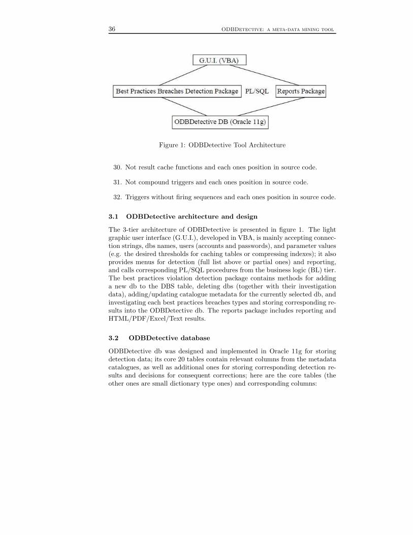
Figure 1: ODBDetective Tool Architecture
30. Not result cache functions and each ones position in source code.
31. Not compound triggers and each ones position in source code.
32. Triggers without firing sequences and each ones position in source code.
3.1 ODBDetective architecture and design
The 3-tier architecture of ODBDetective is presented in figure 1. The lightgraphic user interface (G.U.I.), developed in VBA, is mainly accepting connec-tion strings, dbs names, users (accounts and passwords), and parameter values(e.g. the desired thresholds for caching tables or compressing indexes); it alsoprovides menus for detection (full list above or partial ones) and reporting,and calls corresponding PL/SQL procedures from the business logic (BL) tier.The best practices violation detection package contains methods for addinga new db to the DBS table, deleting dbs (together with their investigationdata), adding/updating catalogue metadata for the currently selected db, andinvestigating each best practices breaches types and storing corresponding re-sults into the ODBDetective db. The reports package includes reporting andHTML/PDF/Excel/Text results.
3.2 ODBDetective database
ODBDetective db was designed and implemented in Oracle 11g for storingdetection data; its core 20 tables contain relevant columns from the metadatacatalogues, as well as additional ones for storing corresponding detection re-sults and decisions for consequent corrections; here are the core tables (theother ones are small dictionary type ones) and corresponding columns:

ODBDetective: a metadata mining tool 37
1. DBS(x, DB, ConnString), for storing investigated dbs names and theirconnection strings;
2. OBJS(x, DB, Owner, Object Name, SubObject Name, Object ID, Data Object ID,Object Type, Status, Temporary, Generated, Secondary, NameSpaceEdition Name), for storing data on dbs’ objects;
3. DEPENDENCIES(x, Object, Referenced Object, Referenced Link Name,Dependency Type), for storing dependencies between dbs’ objects;
4. TABLES(x, Object, Tablespace, Cluster, IOT Name, Status, PCT Free,PCT Used, Ini Trans, Max Trans, Initial Extent, Next Extent, MinExtents, Max Extents, PCT Increase, FreeLists, FreeList Groups, Car-dinal, Blocks, Empty Blocks, Avg Space, Chain Cnt, Avg Row Len,Avg Space Freelist Blocks, Num FreeList Blocks, Degree, Instances, Cache,Table Lock, Sample Size, Partioned, IOT Type, Temporary, Secondary,Nested, Buffer Pool, Flash Cache, Cell Flash Cache, Row Movement,Global Stats, User Stats, Duration, Skip Corrupt, Monitoring, Clus-ter Owner, Dependencies, Compression, Compress For, Dropped, Read Only,Segment Created, Result Cache, Static, Fundamental, Used in SP), forstoring data on tables;
5. TBL COLUMNS(x, Object, Data Type, Data Length, Data Precison,Data Scale, Nullable, Default Length, Num Distinct, Low Value, High Value,Num Nulls, Num Buckets, Char Col Decl Length, Avg Col Len, Char Length,Char Used, Data Type Owner, Column ID, Density, Sample Size, Char-acter Set Name, Global Stats, User Stats, V80 FMT Image, Data Upgraded,Histogram, Computed, Needs Index, Index Type, Join Index), for stor-ing data on tables’ columns;
6. CONSTRAINTS(x, Object, Table, Constraint Type, Index, R Con-straint, Status, Validated, Delete Rule, Bad, View Related, Invalid, Rely,Generated, Deferred, Deferrable), for storing data on dbs’ constraints;
7. CONSTR COLS(x, Constraint, Column, Position), for storing data onconstraints’ columns;
8. INDEXES(x, Object, Index Type, Table, Uniqueness, Compression, Pre-fix Length, Tablespace, Ini Trans, Max Trans, Initial Extent, Next Extent,Min Extents, Max Extents, PCT Increase, PCT Threshold, FreeLists,FreeList Groups, Include Column, PCT Free, BLevel, Leaf Blocks, Dis-tinct Keys, Avg Data Blocks Per Key, Avg Leaf Blocks Per Key, Clus-tering Factor, Status, Num Rows, Sample Size, Degree, Instances, Par-titioned, Temporary, Generated, Secondary, Buffer Pool, Flash Cache,

38 ODBDetective: a meta-data mining tool
Cell Flash Cache, User Stats, Global Stats, Duration, PCT Direct Access,Parameter, DomIdx Status, DomIdx OpStatus, FuncIdx Status, Join Index,IOT Redundant PKey Elim, Dropped, Visibility, DomIdx Management,ToBeAdded, Used, BitMap, ToReorder), for storing data on tables’ in-dexes;
9. INDEXES COLS(x, Index, Column, Column Position, Descend, Cor-rect Column Position), for storing data on indexes’ columns;
10. SEQS(x, Object, Min Value, Max Value, Increment By, Cycle Flag, Or-der Flag, Cache Size, Last Number), for storing data on dbs’ sequences;
11. TRIGGERS(x, Object, Trigger Type, Triggering Event, Triggering Object,Column, Referencing Names, When Clause, Status, Description, Ac-tion Type, CrossEdition, Before Statement, Before Row, After Row, Af-ter Statement, Instead of Row, Fire Once, Apply Server Only), for stor-ing data on dbs’ triggers;
12. VIEWS(x, Object, Text Length, Type Text, OID Text Length, OID Text,View Type Owner, View Type, Superview, Editioning View, Read Only,Edition Name), for storing data on dbs’ views;
13. SOURCE CODE LINES(x, Name, Type, Line, Text), for storing dbs’packages, procedures, and functions PL/SQL source code lines;
14. TBLSPACES(x, Object, Block Size, Initial Extent, Next Extent, MinExtents, Max Extents, Max Size, PCT Increase, Min ExtLen, Status,Contents, Extent Management, Allocation Type, Segment Space Management,Def Tab Compression, Retention, BigFile, Predicate Evaluation, Encrypted,Compress For), for storing data on tablespaces;
15. CLUSTERS(x, Object, Tablespace, PCT Free, PCT Used, Key Size,Ini Trans, Max Trans, Initial Extent, Next Extent, Min Extents, Max Extents,PCT Increase, FreeLists, FreeList Groups, Avg Leaf Blocks Per Key, Clus-ter Type, Functions, HashKey, Degree, Instances, Cache, Buffer Pool,Flash Cache, Cell Flash Cache, Single Table, Dependencies), for stor-ing data on table clusters;
16. PARTITIONS(x, Table, Partitioning Type, SubPartitioning Type, Par-tition Count, Def SubPartition Count, Partitioning Key Count, Sub-Partitioning Key Count, Status, Def Tablespace, Ref PTN Constraint,Interval, Is Nested), for storing data on tables’ partitions;
17. SEGMENTS(x, Partition, Segment Name, Segment Type, Segment SubType,Bytes, Blocks, Extents, Initial Extent, Next Extent, Min Extents, Max Extents,

ODBDetective: a metadata mining tool 39
Max Size, Retention, MinRetention, PCT Increase, FreeLists, FreeL-ist Groups, Buffer Pool, Flash Cache, Cell Flash Cache), for storingdata on partitions’ segments;
18. ADVISOR LOG(x, Owner, Task ID, Task Name, Execution Start, Exe-cution End, Status, Status Message, PCT Completion Time, Progress Metric,Metric Units, Activity Counter, Reccomendation Count, Error Message),for storing data extracted from the dbs’ advisors logs;
19. ADVISOR RECS(x, Owner, RecType), for storing data extracted fromthe dbs’ advisors recommendations.
As it can be seen, except for DBS, all other above tables and most of theircolumns are duplicating part of Oracle metadata catalogue. First reason for itis not adding unneeded overload to investigated db instances; second, investi-gation reports are much more substantial; thirdly, some numeric smaller andfaster foreign keys between these tables are replacing the original Oracle ones(e.g. columns Object from DEPENDENCIES, TABLES, TBL COLUMNS,CONSTRAINTS, INDEXES, SEQS, TRIGGERS, VIEWS, TBLSPACES, andCLUSTERS, as well as DEPENDENCIES.Referenced Object, TABLES.Tablespace,TABLES.Cluster, CONSTR COLS.Constraint, INDEXES COLS.Index, IN-DEXES COLS.Column, TRIGGERS.Triggering Object, TRIGGERS.Column,CLUSTERS.Tablespace, PARTITIONS.Table, SEGMENTS.Partition, etc.);finally, investigation results may be added, without tampering with the Ora-cle metadata catalogue.
For example, added columns Static, Fundamental, and Used in SP of TA-BLES are storing whether or not tables are (quasi-)static (i.e. they are veryrarely updated, if any), actually storing fundamental or derived data, andused in PL/SQL dynamic code respectively. Similarly, columns Computed,Needs Index, Index Type, and Join Index of TBL COLUMNS are storingwhether or not columns are storing fundamental or computed data, an in-dex on them should be added, and if yes, of what type (normal B-tree orbitmap), and, if bitmap, of what subtype (join or not), respectively. Then,columns ToBeAdded, Used, BitMap, and ToReorder of INDEXES are storingwhether or not new indexes should be added or existing ones are actually usedor should be dropped because they are too expensive, or their type should bechanged, or their columns should be re-ordered.
3.3 ODBDetective usage
ODBDetective was already used on several U.S. customers’ dbs with greatresults. For example, such a db has a total of 3,860 user objects (and 5,649

40 ODBDetective: a meta-data mining tool
dependencies between them) –with only 116 being temporary and 191 au-tomatically generated indexes ones–, out of which 586 tables (totaling 8,621columns and 129,956,314 rows) interconnected by 415 foreign keys, with 66temporary ones, and 2,842 indexes (out of which 2,651 are explicitly defined);their instances’ plausibility is enforced by 3,860 constraints, out of which 278are unique ones, with 229 primary and 49 semantic keys, 3,167 are check con-straints, the remaining 415 being referential integrities; there are also one view,151 sequences, 19 triggers, 127 packages (containing 1,647 procedures and 467functions) totaling 129,730 PL/SQL lines.
Running all of the 32 ODBDetective options discovered were the following:
• 180 empty non-temporary tables, on which there were defined 211 in-dexes and 243 constraints;
• 165 fundamental tables on which no interesting object depended on;
• 268 constraints on temporary tables (257 check, 10 primary, and onesemantic keys);
• no cached table, although there were 168 such candidates for x = 1,000and 58 for x = 100;
• 2 tables having migrated rows; 311 empty columns, out of which 161were not VARCHAR (1 BLOB, 2 CLOB, 3 CHAR, 49 DATE, and 106NUMBER), and on which were defined 24 constraints (1 check, 1 unique,and 22 foreign keys) and 21 indexes; 292 keyless non-empty fundamentaltables; 40 tables having concatenated primary keys (3 quaternary, 8ternary, and 29 double);
• 15 not numeric primary keys (11 VARCHAR2, 1 CHAR, and 3 DATE);all 239 tables having surrogate primary keys were oversized (and what isworse, to the maximum possible NUMBER(38) value, needing 22 byteseach!); 8 concatenated foreign keys (4 ternary and 4 double);
• 63 foreign keys having non-numeric columns;
• all 415 foreign keys were oversized (again at the maximum NUMBER(38)possible!);
• 273 improperly typed foreign keys; 576 normal indexes that should havebeen bitmap instead (for y = 10 and z = 90);
• 56 indexes to be compressed for w = 100 and other 37 for w = 1,000;
ODBDetective: a metadata mining tool 41
• 24 concatenated indexes (out of which 14 were unique ones, with 6 forprimary keys!) totalizing 80 columns on non-empty tables having wrongcolumns order;
• 740 subqueries; and 317,542 SQL statements dynamically built and ex-ecuted.
• Unfortunately too, there were no statistics gathered on indexes, no par-allel enabled functions, no result cache queries, no result cache functions,no compound triggers, and no triggers with firing sequences either.
• Fortunately, there were no tables or indexes in system tablespaces, notable having no not null columns, no table to shrink, no superkeys, nobitmap indexes that should be normal (as there were no bitmap indexesat all), and no more than one index on same columns.
According to this data, customer decided corresponding changes in its dbscheme; once done, the performance of its application was better by morethan 2.5 times.
4 Conclusion and further work
ODBDetective architecture, design principles, and usage are presented. ODB-Detective is a tool for detecting violations of some very important Oracle dbdesign, implementation, querying, and manipulating, greatly simplifying thetask to correct corresponding anomalies. A few of the ODBDetective featuresare also provided by Oracle tools, but only available for the very expensiveEnterprise Editions. ODBDetective is somewhat similar, for example, to DBOptimizer [6], but has very many powerful additional features. Running ODB-Detective on several production dbs was very successful, as proved by theexample presented above.
Automatic violations detection can obviously be based only on syntacticcriteria. In order to make correct decisions for db schemes enhancements,users should analyze ODBDetective output and, based on semantic knowl-edge, decide whether or not to correct each of the syntactically discoveredpossible violations (e.g. analyzed current instance may be a non-typical one,empty tables may be legitimately be empty as they are, in fact, temporaryones, some tables instances might grow much larger in certain contexts, etc.).ODBDetective db is already prepared to store such decisions.
Further work will include adding supplementary best practice rules (see [1]and [2]), automatically generate SQL scripts for correcting user confirmed vio-lations, enhancing the graphic user interface for both presenting investigation
42 ODBDetective: a meta-data mining tool
data and managing updates to decision data, as well as extensions to otherRDBMSs than Oracle.
Acknowledgements
This work was partly sponsored by Asentinel Intl. srl, Bucharest, Romania,a subsi-diary of Asentinel, Memphis, TN, U.S.A. (http://www.asentinel.com/).
References
[1] Mancas C. Best practice rules (2012). Technical Report TR0-2012, Asentinel Intl. srl,Bucharest, Romania.
[2] Mancas C. Databases for the wise. A completely algorithmic approach to conceptualdata modeling, database design, implementation, and optimization. (2013). To bepublished by Apple Academic Press, NJ, U.S.A.
[3] Oracle Corp. DBA’s New Best Friend: AdvancedSQL Tuning Features of Oracle Database 11g (2007).http://www.oracle.com/technetwork/database/manageability/sqltune-presentation-ow07-130395.pdf.
[4] Oracle Corp. Guide for Developing High-PerformanceDatabase Applications (2010). An Oracle White Paper,http://www.oracle.com/technetwork/database/performance/perf-guide-wp-final-133229.pdf.
[5] Oracle Corp. Oracle§Database Performance Tuning Guide 11g Release 1 (2008).
[6] Embarcadero Technologies, Inc. DB PowerStudio§for Oracle (2012).http://www.embarcadero.com/products/db-powerstudio-for-oracle.
[7] Proper H.A. and Halpin T.A. Conceptual Schema Optimisation – Database Optimi-sation before sliding down the Waterfall (2004). Technical Report 341, June 23, 2004version, Dept. Comp. Sci., Univ. of Queensland, Brisbane, Australia.
[8] Dong Yu-Jie and Li Fu-Guo. Research on Optimization Strategy of Relational Schemabased on Normalization Theory (2010). Proc. of 3rd Intl. Symp. On Comp. Sci. andComputational Techn. ISCSCT’10, Jiaozuo, P.R.China, 41-43.
[9] Kaiser M. et al. Data organization for database op-timization (2005). U.S. Patent application 0010606 A1,http://www.google.ro/patents/US20050010606?dq=database+optimization.
[10] Arnold J.A. et al. Database optimization apparatus and method (2007). U.S. Patentapplication 0073644 A1, http://www.google.com/patents/US20070073644.
[11] Arnold J.A. et al. Database optimization apparatus and method (2006). U.S. Patentnumber 7089260, http://www.google.com/patents/US7089260.
[12] Mancas C. On Knowledge Representation Using an Elementary Mathematical DataModel (2002). Proc. of the 1st IASTED Int. Conf. on Information and KnowledgeSharing IKS 2002, Univ. of the U.S. Virgin Islands, St. Thomas, USVI, USA, 206-211.

ODBDetective: a metadata mining tool 43
[13] Mancas C. and Dragomir S. On the Equivalence between Entity-Relationship andFunctional Data Modeling (2003). Proc. of the 7th IASTED Int. Conf. on Softw. Eng.and Appl. SEA 2003, Marina del Rey, CA, USA, 335-340.
[14] Mancas C. and Dragomir S. An Optimal Algorithm for Structural Keys Design (2003).Proc. of the 7th IASTED Int. Conf. on Softw. Eng. and Appl. SEA 2003, Marina delRey, CA, USA, 328-334.
[15] Mancas C. and Crasovschi L. An Optimal Algorithm for Computer-Aided Design ofKey Type Constraints (2003). Proc. of the 1st Balkan Conf. in Informatics BCI 2003,Aristotle Macedonian Univ., Thessaloniki, Greece, 574-584.
[16] Mancas C. and Mancas S. MatBase Relational Import Subsystem (2006). Proc. ofIASTED Datab. And Appl., DBA 2006, Innsbruck, Austria, 123-128.

44 ODBDetective: a meta-data mining tool
Seminar Series in Mathematics and Computer Science:2013, 45–57
A diabetes mortality study using generalizedlinear models ∗†
Abstract
Modeling mortality due to different factors is very important in manyfields like, e.g., medicine and insurance. In particular, being one of themajor causes of illness and death, special attention is paid to diabetes.In this paper, we used several generalized linear models to study themortality due to diabetes in Romania during 2009. Easy to estimatewith the existing software like R, such models can provide a powerfultool in mortality studies, and even improve the existing techniques.
1 Introduction
A statistical model describes in the form of mathematical equations how one ormore random variables are related to one or more other variables. One of themost common techniques for estimating the relationships among variables isregression analysis. Regression modeling deals with explaining the movementsin one variable (called dependent or response) by the movements in one or moreother variables (called independent or predictors or explanatory). The simplestform of regression is the linear one, in which case the model specification is thatthe dependent variable is a linear combination of the independent ones; this isappropriate when the response variable has a normal distribution. However,such an assumption is inappropriate for many types of response variables.
∗Ileana GheorghiuOvidius University, Department of Mathematics and Informatics, Blvd. Mamaia124,900527, Constanta, Romaniae-mail: [email protected]
†Raluca VernicOvidius University, Department of Mathematics and Informatics, Blvd. Mamaia124,900527, Constanta, Romaniae-mail: [email protected]
45
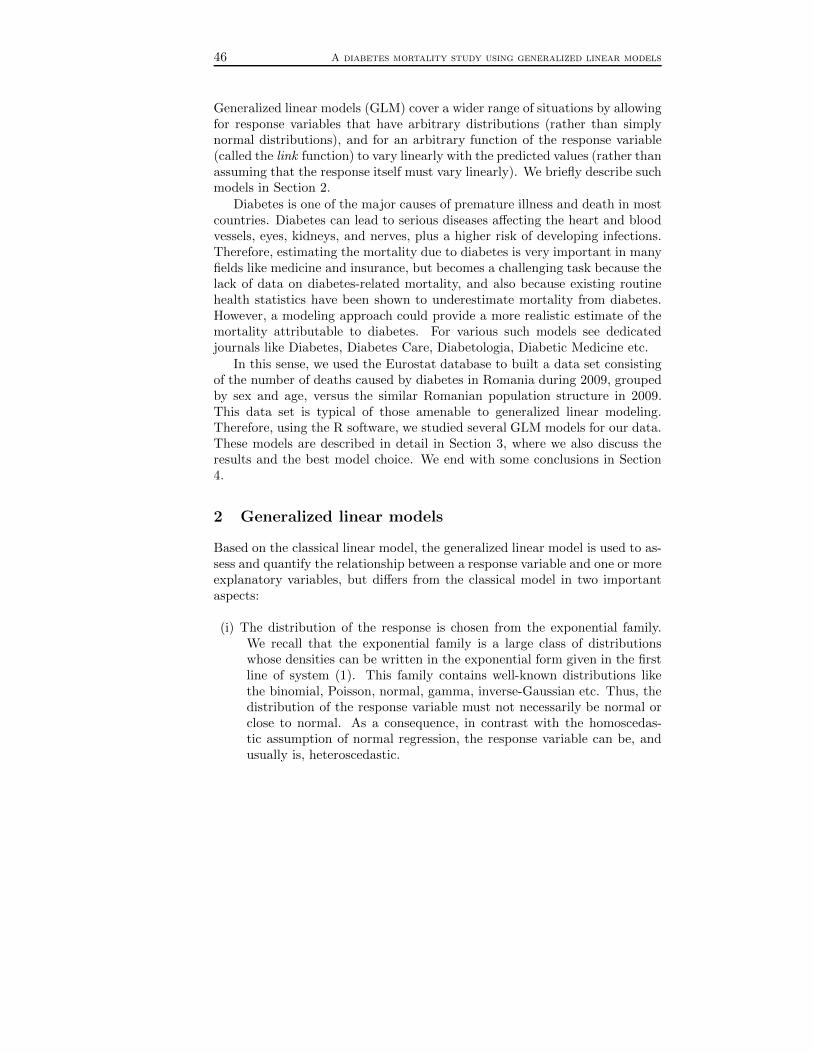
46 A diabetes mortality study using generalized linear models
Generalized linear models (GLM) cover a wider range of situations by allowingfor response variables that have arbitrary distributions (rather than simplynormal distributions), and for an arbitrary function of the response variable(called the link function) to vary linearly with the predicted values (rather thanassuming that the response itself must vary linearly). We briefly describe suchmodels in Section 2.
Diabetes is one of the major causes of premature illness and death in mostcountries. Diabetes can lead to serious diseases affecting the heart and bloodvessels, eyes, kidneys, and nerves, plus a higher risk of developing infections.Therefore, estimating the mortality due to diabetes is very important in manyfields like medicine and insurance, but becomes a challenging task because thelack of data on diabetes-related mortality, and also because existing routinehealth statistics have been shown to underestimate mortality from diabetes.However, a modeling approach could provide a more realistic estimate of themortality attributable to diabetes. For various such models see dedicatedjournals like Diabetes, Diabetes Care, Diabetologia, Diabetic Medicine etc.
In this sense, we used the Eurostat database to built a data set consistingof the number of deaths caused by diabetes in Romania during 2009, groupedby sex and age, versus the similar Romanian population structure in 2009.This data set is typical of those amenable to generalized linear modeling.Therefore, using the R software, we studied several GLM models for our data.These models are described in detail in Section 3, where we also discuss theresults and the best model choice. We end with some conclusions in Section4.
2 Generalized linear models
Based on the classical linear model, the generalized linear model is used to as-sess and quantify the relationship between a response variable and one or moreexplanatory variables, but differs from the classical model in two importantaspects:
(i) The distribution of the response is chosen from the exponential family.We recall that the exponential family is a large class of distributionswhose densities can be written in the exponential form given in the firstline of system (1). This family contains well-known distributions likethe binomial, Poisson, normal, gamma, inverse-Gaussian etc. Thus, thedistribution of the response variable must not necessarily be normal orclose to normal. As a consequence, in contrast with the homoscedas-tic assumption of normal regression, the response variable can be, andusually is, heteroscedastic.

A diabetes mortality study using generalized linear models 47
(ii) A transformation of the mean of the response variable is linearly relatedto the explanatory variables.
More precisely, given a response y, the generalized linear model (GLM) is
f (y) = c (y, φ) exp
yθ − a (θ)
φ
g (µ) = x′β, (1)
where the first equation specifies that the distribution of the response is in theexponential family, while the second equation specifies that a transformationg (µ) of the mean µ is linearly related to the explanatory variables contained inx =(x1, ..., xp)
′ by means of the coefficients β =(β1, ..., βp)′ . In other words,
model (1) states that, given the explanatory variables x, the mean µ is deter-mined through g(µ) (called the link); then, given µ, θ is determined througha (θ) = µ (here a is the first derivative of a); finally, given θ, y is determinedas a draw from the exponential density specified in a(θ). Observations on yare assumed to be independent.
Note that the choice of the link g determines how the mean µ is related tothe explanatory variables x. In the normal linear model, this relationship isµ = x′β. In the GLM, the relationship is generalized to g (µ) = x′β, where gis a monotonic, differentiable function (such as log or square root). For detailson GLMs and their applications in different fields, see e.g., De Jong and Heller(2008), Hardin and Hilbe (2001), Myers et al. (2010).
There are several well-studied particular GLM cases, as the Poisson, logis-tic, gamma or invers-Gaussian ones. We briefly present the first two that willbe useful for our numerical study.
Poisson model. The Poisson regression model is
Y ∼ Poisson(µ), g(µ) = x′β.
Popular choices for g(µ) are the identity link µ = x′β and the log link lnµ =x′β, in which case µ = exp(x′β) is always positive.
Logistic model. In logistic regression, the response variable is of categori-cal type, therefore this regression can be binomial or multinomial. Binomial orbinary logistic regression refers to the situation in which the observed outcomecan have only two possible types (e.g., dead/alive, male/female, success/failureor yes/no), hence the outcome can be coded as ”0” and ”1”, and the responsevariable becomes an indicator one (also called dichotomous variable). Multi-nomial logistic regression refers to cases where the outcome can have three ormore possible types.
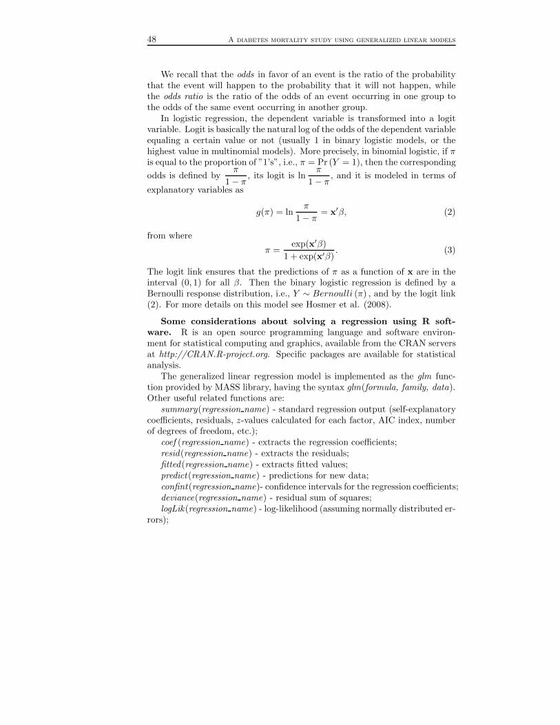
48 A diabetes mortality study using generalized linear models
We recall that the odds in favor of an event is the ratio of the probabilitythat the event will happen to the probability that it will not happen, whilethe odds ratio is the ratio of the odds of an event occurring in one group tothe odds of the same event occurring in another group.
In logistic regression, the dependent variable is transformed into a logitvariable. Logit is basically the natural log of the odds of the dependent variableequaling a certain value or not (usually 1 in binary logistic models, or thehighest value in multinomial models). More precisely, in binomial logistic, if πis equal to the proportion of ”1’s”, i.e., π = Pr (Y = 1), then the corresponding
odds is defined byπ
1− π, its logit is ln
π
1− π, and it is modeled in terms of
explanatory variables as
g(π) = lnπ
1− π= x′β, (2)
from where
π =exp(x′β)
1 + exp(x′β). (3)
The logit link ensures that the predictions of π as a function of x are in theinterval (0, 1) for all β. Then the binary logistic regression is defined by aBernoulli response distribution, i.e., Y ∼ Bernoulli (π) , and by the logit link(2). For more details on this model see Hosmer et al. (2008).
Some considerations about solving a regression using R soft-ware. R is an open source programming language and software environ-ment for statistical computing and graphics, available from the CRAN serversat http://CRAN.R-project.org. Specific packages are available for statisticalanalysis.
The generalized linear regression model is implemented as the glm func-tion provided by MASS library, having the syntax glm(formula, family, data).Other useful related functions are:
summary(regression name) - standard regression output (self-explanatorycoefficients, residuals, z-values calculated for each factor, AIC index, numberof degrees of freedom, etc.);
coef (regression name) - extracts the regression coefficients;resid(regression name) - extracts the residuals;fitted(regression name) - extracts fitted values;predict(regression name) - predictions for new data;confint(regression name)- confidence intervals for the regression coefficients;deviance(regression name) - residual sum of squares;logLik(regression name) - log-likelihood (assuming normally distributed er-
rors);

A diabetes mortality study using generalized linear models 49
AIC (regression name) - information criteria including AIC, BIC/SBC in-dexes (assuming normally distributed errors).
Moreover, several diagnostic plots can be obtained by the command plot(regression name),e.g., residuals versus fitted values, normal Q-Q plot, etc. For more details onusing R see, e.g., Kleiber and Zeileis (2008).
3 Diabetes mortality study
The data set consists of the number of deaths caused by diabetes in Ro-mania during 2009. The deaths are grouped by sex and age, see Table 1;columns 4 and 6 in this table also contain the total number of persons inthe corresponding age and sex class, i.e., the Romanian population structureby age and sex in 2009. The data are taken from the Eurostat database(epp.eurostat.ec.europa.eu ¿ European Commission ¿ Eurostat).
Male FemaleAge
class
Class
middle
Deaths
numberPopulation
Deaths
numberPopulation
¡5 2 0 554518 0 5241055-9 7 0 550009 0 52066410-14 12 2 570898 0 54367815-19 17 1 700697 0 67154520-24 22 1 875528 1 83863225-29 27 1 846071 2 80635130-34 32 8 909596 3 86432135-39 37 9 861367 3 83497240-44 42 15 774940 7 76564945-49 47 33 638182 14 65120750-54 52 69 745326 38 79714455-59 57 113 670679 70 74820960-64 62 114 476065 89 55990565-69 67 144 407641 153 52637870-74 72 190 383576 257 54403275-79 77 180 279052 243 42354780-84 82 131 158723 200 26681785+ 90 53 69944 117 138648
Table 1. Diabetes deaths in Romania during 2009 and population structure
We are interested in finding a model that expresses the average number ofdeaths µ (or, equivalently, the mortality rate ν = µ/n) as a function of sex,

50 A diabetes mortality study using generalized linear models
age and population size, n. Denoting by Y the random variable number ofdeaths per year, we consider the following Poisson GLM for it
Y ∼ Poisson(µ), g(µ) = lnµ = lnn+ x′β ⇐⇒ µ = nex′β , (4)
where x =(1, x1, x2, ..., xp)′with x1 =
0,man1,woman
models the sex, and the
variables x2, ..., xp are related to the age. The age can be modeled usingcategorical or quantitative variables. We considered models for both situationsand we used the glm function provided by R software to evaluate all modelscoefficients.
I. Categorical age variables. The age effect can be modelled using indi-
cator variables for each age class, i.e., xi+1 =
0, the age is not in class i1, the age is in class i
, i =
1, ..., 18. In this case, we shall consider one age class as base level, more pre-cisely, the 9th class 40-44. Therefore, model (4) becomes
lnµ = lnn+ β0 + β1x1 +∑
i=2,...,19i6=10
βixi. (5)
The coefficients values are given in Table 2; from columns 3 and 6 in this tablewe can see the multiplicative effect of each age class compared with the baseclass 40-44. The estimated mortality rate results as
ν =µ
n=
e−10.119−21.273, for men in first age classe−10.119−2.879, for men in 5-9 age class...e−10.119−21.266, for men in last age classe−10.334−21.273, for women in first age classe−10.334−2.879, for women in 5-9 age class...e−10.334−21.266, for women in last age class
.

A diabetes mortality study using generalized linear models 51
Variable Coeff. βi eβi Variable Coeff. βi eβi
Intercept -10.119 4×10⁻⁵ Age class 40-44 0 1Sex: male 0 1 Age class 45-49 0.647 1.90980Sex: female -0.215 0.80654 Age class 50-54 1.267 3.55018Age class < 5 -21.273 5.77×10⁻¹⁰ Age class 55-59 1.690 5.41948Age class 5-9 -2.879 0.56191 Age class 60-64 2.179 8.83746Age class 10-14 -4.268 0.01401 Age class 65-69 2.603 13.50419Age class 15-19 -3.596 0.02743 Age class 70-74 2.827 16.89470Age class 20-24 -3.199 0.04080 Age class 75-79 3.088 21.93317Age class 25-29 -1.792 0.16663 Age class 80-84 3.149 23.30505Age class 30-34 -1.574 0.20723 Age class 85+ -21.266 5.81×10⁻¹⁰
Age class 35-39 -0.918 0.39908Table 2. Model’s (5) coefficients
Based on the corresponding R output for our data, we concluded that:
1. The sex and age variables are significant for model (5), as shown by the ztest. Moreover, analyzing the deviation of several models, we concludedthat including the age class in a model that already contains the sexsignificantly improves the model.
2. For the base age level 40-44, we have an estimated mortality rate dueto diabetes equal to e−10.119 = 4.03064× 10⁻⁵ for men and e−10.334 =3.25088× 10⁻⁵ for women. More precisely, we can obtain women’s mor-tality rate by multiplying men’s mortality rate with 0.8065, i.e., women’smortality rate is 80.65% of men’s mortality rate, or, equivalently, about19.35% smaller than men’s rate for all age levels.
3. To compare the mortality rate of different age classes, we must look atcolumns 3 and 6 in Table 2. For example, the effect of the age class35-39 compared with the base class 40-44 results by multiplying themortality of the base class with e−0.9185 = 0.399, i.e., for the age class35-39 we have a decrease of the mortality rate of about 60.1% for bothsexes compared to the base level.
II. Quantitative age variables. To get a better idea of the age effect, inFigure 1 we plotted the deaths number as a function of the middle of the ageclass for each sex. The obtained shapes suggest using a polynomial to modellnµ as a function of the middle of the age class seen as a quantitative variablethat will now be represented by x2. The degree of the polynomial should bedetermined by trials. We tried three different models involving polynomials
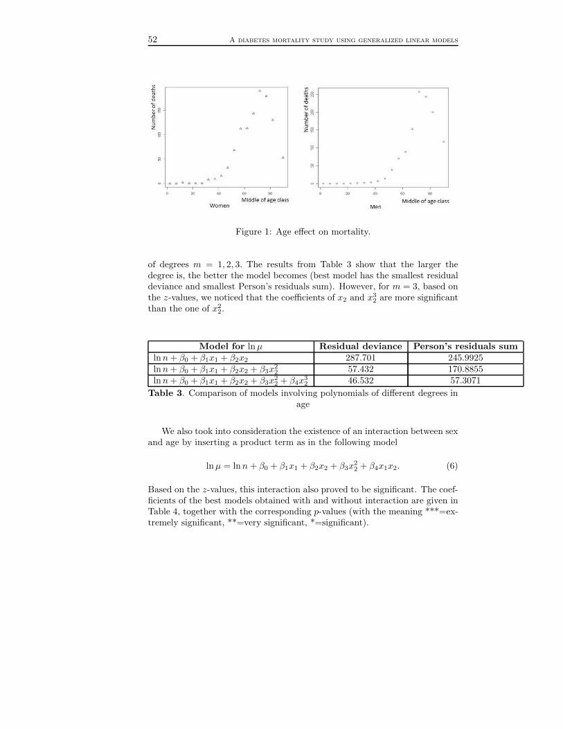
52 A diabetes mortality study using generalized linear models
Figure 1: Age effect on mortality.
of degrees m = 1, 2, 3. The results from Table 3 show that the larger thedegree is, the better the model becomes (best model has the smallest residualdeviance and smallest Person’s residuals sum). However, for m = 3, based onthe z-values, we noticed that the coefficients of x2 and x3
2 are more significantthan the one of x2
2.
Model for lnµ Residual deviance Person’s residuals sumlnn+ β0 + β1x1 + β2x2 287.701 245.9925lnn+ β0 + β1x1 + β2x2 + β3x
22 57.432 170.8855
lnn+ β0 + β1x1 + β2x2 + β3x22 + β4x
32 46.532 57.3071
Table 3. Comparison of models involving polynomials of different degrees inage
We also took into consideration the existence of an interaction between sexand age by inserting a product term as in the following model
lnµ = lnn+ β0 + β1x1 + β2x2 + β3x22 + β4x1x2. (6)
Based on the z-values, this interaction also proved to be significant. The coef-ficients of the best models obtained with and without interaction are given inTable 4, together with the corresponding p-values (with the meaning ***=ex-tremely significant, **=very significant, *=significant).
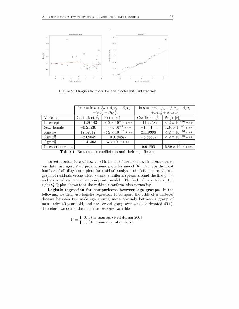
A diabetes mortality study using generalized linear models 53
Figure 2: Diagnostic plots for the model with interaction
lnµ = lnn+ β0 + β1x1 + β2x2
+β3x22 + β4x
32
lnµ = lnn+ β0 + β1x1 + β2x2
+β3x22 + β4x1x2
Variable Coefficient βi Pr (> |z|) Coefficient βi Pr (> |z|)Intercept −10.80143 < 2× 10⁻¹⁶ ∗ ∗∗ −11.22582 < 2× 10⁻¹⁶ ∗ ∗∗Sex: female −0.21530 3.6× 10⁻⁷ ∗ ∗∗ −1.55165 1.04× 10⁻⁸ ∗ ∗∗Age x2 17.52617 < 2× 10⁻¹⁶ ∗ ∗∗ 21.19998 < 2× 10⁻¹⁶ ∗ ∗∗Age x2
2 −2.09049 0.019487∗ −5.65502 < 2× 10⁻¹⁶ ∗ ∗∗Age x3
2 −1.41563 3× 10⁻⁴ ∗ ∗∗ − -Interaction x1x2 − − 0.01895 5.89× 10⁻⁷ ∗ ∗∗
Table 4. Best models coefficients and their significance
To get a better idea of how good is the fit of the model with interaction toour data, in Figure 2 we present some plots for model (6). Perhaps the mostfamiliar of all diagnostic plots for residual analysis, the left plot provides agraph of residuals versus fitted values; a uniform spread around the line y = 0and no trend indicates an appropriate model. The lack of curvature in theright Q-Q plot shows that the residuals conform with normality.
Logistic regression for comparisons between age groups. In thefollowing, we shall use logistic regression to compare the odds of a diabetesdecease between two male age groups, more precisely between a group ofmen under 40 years old, and the second group over 40 (also denoted 40+).Therefore, we define the indicator response variable
Y =
0, if the man survived during 20091, if the man died of diabetes

54 A diabetes mortality study using generalized linear models
and one explanatory variable for the age group, i.e.,
X1 =
0, if the man age is < 401, if the man age is ≥ 40
.
Hence we have x =(1, x1)′and β =(β0, β1)
′. The results of cross-classifying
the number of men by age group and death/survival are presented in Table 5.
Age group (X1 variable)age< 40 (X1 = 0) age≥ 40 (X1 = 1)
No. of diabetes deaths (Y = 1) 22 1042No. of survivors (Y = 0) 5868662 4603086Total 5868684 4604128
Table 5. Number of male deaths and survivors by age group (under andover 40)
We denote π (0) = Pr (Y = 1 |X1 = 0) and π (1) = Pr (Y = 1 |X1 = 1).
Then the odds of a diabetes decease in the age group under 40 isπ (0)
1− π (0),
while in the age group 40+ it isπ (1)
1− π (1); in this case, we define the odds
ratio as
OR =
π(1)1−π(1)
π(0)1−π(0)
=π (1)
π (0)
1− π (0)
1− π (1). (7)
Using now the logistic model given by (2)-(3), we obtained the following table(containing formulas for the conditional probabilities):
Age group (explanatory) variableResponse variable X1 = 0 (< 40) X1 = 1 (40+)
Y = 1 (diabetes decease) π (0) =eβ0
1 + eβ0π (1) =
eβ0+β1
1 + eβ0+β1
Y = 0 (survivor) 1− π (0) =1
1 + eβ01− π (1) =
1
1 + eβ0+β1
Total 1 1
Table 6. Deaths and survivors proportions by age group (under and over 40)
Inserting the corresponding formulas into (7), the odds ratio simplifies to
OR =eβ0+β1
eβ0= eβ1 .
A diabetes mortality study using generalized linear models 55
The simplicity of this relation transformed the logistic regression into a pow-
erful analytic tool. Moreover, if the ratio1− π (0)
1− π (1)≃ 1, then we can use the
approximationπ (1)
π (0)≃ OR.
In our case, from Table 5, we have OR =1042
460308622
5868662
= 60.367, from where we
obtained the estimations
β0 = −12.495, β1 = lnOR = 4.100.
We conclude that, according to the 2009 data, a man aged over 40 living inRomania has a risk of diabetes death 60.32 times higher than the correspondingrisk of a man under 40. Confidence intervals can also be built, and similarconclusions can be drawn for other age groups, as well as for women.
4 Conclusions
In this study, we have shown how to estimate, using generalized linear models,the risk of death caused by a disease (in our case, diabetes) in different agegroups, based on historical data previously recorded. As an alternative to theexisting methods that often underestimate mortality, such models can provideextremely useful information on health for medical studies and, also, for lifeinsurance. For example, considering the fact that the aging population createsserious imbalances in insurances systems, various products of current interestcould be developed using actuarial mathematics.
Moreover, our approach is meant to highlight the easiness of generalizedlinear models in general, and of the logistic regression model in particular,recommending it in various fields (not necessarily related to mathematics)and promoting it as a powerful research tool.
References
[1] De Jong, P. and Heller, G. Z. (2008). Generalized Linear Models forInsurance Data. Cambridge University Press.
[2] Hardin, J. and Hilbe, J. (2001). Generalized Linear Models and Exten-sions. STATA Press.
[3] Hosmer, D., Lemeshow, S. and Rodney, X. (2008). Applied Logistic Re-gression. John Wiley & Sons.

56 A diabetes mortality study using generalized linear models
[4] Kleiber, C. and Zeileis, A. (2008). Applied Econometrics with R. Springer.
[5] Myers, R., Montgomery, D., Vining ,G. and Robinson, T. (2010). Gener-alised Linear Models with Applications in Engineering and Sciences. JohnWiley & Sons.

A diabetes mortality study using generalized linear models 57