Embed Size (px)
Citation preview

Overview of LISST data
Quantities of interest: Cn,z, wf,n
Program: Vertical profiler data with LISST-100 Bottom boundary layer size distribution w LISST-100 Settling velocity spectrum with LISST-ST and by the way..New Observations reveal differences
in scattering by spheres vs random shaped particles

Principles of the LISST
0 5 10 15 20 25 30 350
0.01
0.02
0.03
0.04
0.05
0.06
73 micron
10 micron
Detector Ring No.
Sca
tter
ing LISST-100
Signature of size is in location of peak.
Observed multi-angle scattering is inverted >> size distribution.
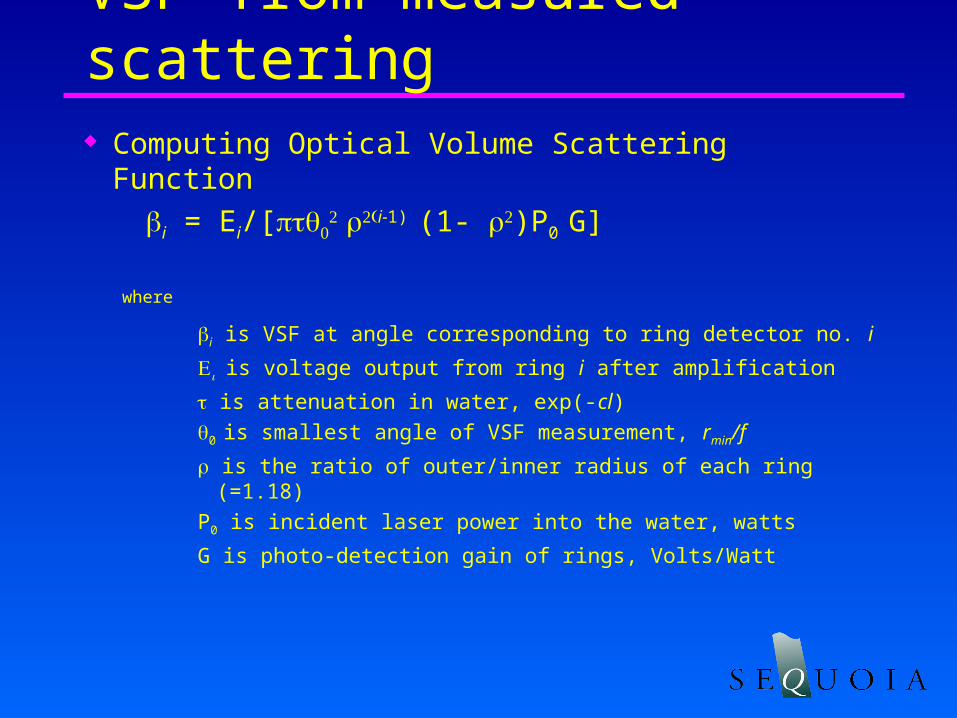
VSF from measured scattering Computing Optical Volume Scattering Function
i = Ei/[i-1) (1- )P0 G]
where
i is VSF at angle corresponding to ring detector no. i
is voltage output from ring i after amplification
is attenuation in water, exp(-cl)
0 is smallest angle of VSF measurement, rmin/f
is the ratio of outer/inner radius of each ring (=1.18)
P0 is incident laser power into the water, watts
G is photo-detection gain of rings, Volts/Watt

Field measurement of VSF
10-3
10-2
10-1
100
102
103
104
105
106
107
File WHOI316; VSF from top to bottom on a calm day
Scattering angle, radians
Data from HYCODE, LISST on a profiler.

Estimating settling velocity with the -ST
Method is to trap water in settling column, sample over quasi-log time scale, invert for 8 size-classes;– Fit expected history curve for concentration history of
each size-class by adjusting settling time.
100
105
0
500
1000
1500
100
105
0
500
1000
1500
100
105
0
500
1000
1500
100
105
0
500
1000
1500
100
105
0
500
1000
1500
100
105
0
200
400
600
800
100
105
0
100
200
300
400
100
105
0
50
100
150
200

Settling velocity vs Stokes/Gibbs Large particles show departure from Gibbs law (or
modified Stokes law) due to flocculation;

Mean settling velocity ‘law’
A simple power-law wf ~ dq
is not suitable.
Fractal more suitable.
Gibb’s law

4 Questions and a new study
1. Why do fine particles appear to settle at ‘super-stokes’ velocities?
2. Why the systematic offset in the calibration for spheres vs natural particles?
3. Why do natural particles ~8 micron appear as ~3 micron (literature, Milligan, pers. Comm.)?
4. Why does laser diffraction method always produce a peak at the fine particle end from field data, but not with lab spheres?

Ongoing research- Natural Particles
settling column techniques used to isolate narrow sizes with 0.1 resolution.
0 5 10 15 20 25 300
0.2
0.4
0.6
0.8
1
1.2Normalized scattering
Detector Ring No.
Sca
tter
ing
0 5 10 15 20 25 30 350
0.01
0.02
0.03
0.04
0.05
0.06
73 micron
10 micron
Detector Ring No.
Sca
tter
ing

Ongoing research- Natural Particles
Some key points:– Jones(1988) presented pure diffraction solution, his
results depend only on ka; observations on ka and .
– Volten(2000) presents the most recent work with natural particles, but only for >5o
– new insights into size-specific counterpart to Mie theory
– This research will produce empirical matrix for use with LISST data when observing natural sediments
– The data qualitatively explain the ‘super-stokes’ settling rates produced by the -ST for finest particles

in conclusion The analysis task is to integrate size and
settling velocity data with Trowbridge’s on velocity structure
Integrate natural particle scattering data in interpretation of multi-angle scattering to tighten estimates of size distribution, settling velocity distribution etc.

Mie Calculation vs Pure Diffraction
Mie and diffraction
0 0.05 0.1 0.15 0.2 0.2510
-8
10-6
10-4
10-2
100
Angle
Nor
mal
ized
sca
tter
ing
Mie, index 1.5
Mie, index 1.5+0.1 i
Diffraction through aperture
ka = 100

A new family of possibilities In October 2001, we found new comets,
blobs, stars, to:– Measure concentration in a size-range– Measure concentration > or < a cut-off– Measure concentration for specified fractal
dimension of particles. These family of comets are found by
replacing the unit vector U of previous slide This development was prompted by a
question by Dr Ted Melis, USGS, Flagstaff.

New focal plane detectors (‘other comets’)