Overview of Enhancing Database Performance and I/O Techniques

Overview of Enhancing Database Performance and I/O Techniques

By: Craig Borysowich [email protected] Enterprise Architect

Imagination Edge Inc.

Database Performance and I/O Overview

Database Performance Components

In addition to the disk subsystem there are various components affecting the performance of any database application. In most cases, a good part of the performance improvement can be achieved from database design, physical layout of tables and indexes, appropriate indexes and query optimization techniques.

Detailed descriptions of these areas are beyond the scope of this document. Please refer to the respective vendor’s performance tuning guide for more information.

Database I/O Overview

To correctly configure the disk subsystem of a database server a basic understanding of database access patterns and methods is required. This section provides a high level overview of the database I/O process and typical patterns of common application types. This information will be referenced throughout the remainder of this paper.

Database I/O Schemes

Database systems store data in a logical collection of disk files or disk partitions. The physically atomic unit of a database file is referred to as a database page or database block. The typical size of a database page is 2K-16K. Most databases don't allow the user to change this size. However, some databases allow the administrator to define the page size at database creation time.

In general, smaller database page sizes are desired for OLTP applications, and larger page sizes are good for DSS applications. More about these application types will be discussed later in this section.

Physical reads and writes of the data are done at the database page level. Therefore, most disk requests are performed using the 2K database page size. There are some exceptions to this on large table scans. If the database system detects that a long scan will be done it will often read in larger blocks, but this feature doesn't usually change the tuning process.

The process of executing I/O routines is similar across most database systems. Reads of database pages are done by database process(es) or thread(s) servicing the application. Many read operations can usually be conducted in parallel and each is independent of the other. Writes of data pages, on the other hand, are not initiated by a user application. When an application updates or inserts new data, the change is actually put into the database cache by the application's database process. Some time later an independent database function will clean the dirty data pages from memory. These writes will usually occur as a large batch of asynchronous

writes. Hence write operations are not usually a steady stream of single page writes, but periodic, heavy bursts of write activities. In contrast to the data pages, writes of transaction log pages are a very steady stream of single page writes. These occur during insert, update and delete operations and again are controlled by background database processes, such as checkpoint or lazy write process.

Database Application Types

By examining different database applications and database functions, the fundamental I/O profile used to access the disk can be determined. This determines whether a particular data set will be accessed either sequentially or randomly. The key high-level application types include transaction processing, decision support and batch processing systems. In this section we will examine the various access patterns on the database files and later apply these patterns to how the drives should be configured. The distinct file types to be examined are data and index files, transaction logs, and import/export files.

Online Transaction Processing (OLTP)

Online transaction processing (OLTP) applications are high-throughput, insert/update intensive systems. These systems are usually characterized by constantly growing large volumes of data that large number of users access concurrently. Examples of typical OLTP applications are order processing applications, banking applications and reservation systems. The key goals of an OLTP system are availability, speed, concurrency, and recoverability.

The I/O profile resulting from this load is heavy random reads and writes across the data and index files. The transaction logs, however, are hit with a heavy stream of sequential write operations of 2K-16K in size.

Decision Support System (DSS)

Decision support or data warehousing applications perform queries on the large amount of data, usually gathered from OLTP applications, and provide competitive information to the decision-makers in an organization. Decision support systems must handle complex queries on data that is less frequently updated than OLTP systems.

DSS is characteristic of multiple users executing complicated joins and aggregations on large sets of data. Even though many of the operations could use some sequential processing, contention with other users and join and indexing operations result in a fairly random access pattern to the data and index files.

Usually, if the database is dedicated to DSS, no updates will be done to the database during heavy query load. In this case, no I/O will occur on the transaction logs. If online updates are applied to the database, it must be remembered when configuring the drive subsystem that log file response time may still be important to the overall performance of the system.

Characteristics of OLTP and DSS are compared in the Table 1.

OLTP DSS OLTP DSS

Transaction Regular business transactions Heavy on retrievals and updates Short and quick queries

Ad hoc queries on historical data Heavy on retrievals, light on updates Complex and long running queries

Locking Many locks of short duration Lock contention can be high

Few locks of long duration

Performance User response time critical Complex queries

User response not critical

Number of rows accessed

Few Many

Concurrent Users Many Few

Disk I/O Frequent disk writes New records are continually added and existing records are updated or deleted

Relatively few disk writes Pages are moved in and out of cache

Table 1: Characteristics of OLTP and DSS

Batch Processing Batch processing is the most likely application to produce significant sequential I/O on the data files. The types of activities referred to here often occur after hours and usually in isolation of other activities. Batch processing involves database dumps, database loads, detail report processing, and index creation.

Overview of Database Vendor’s I/O features The following are I/O features of the Oracle database. Both Oracle7 and Oracle8 server information is referenced. For further information regarding these features, please refer to the Oracle documentation set for your version of Oracle.

Partitioning Partitioned tables and indexes provide the ability to divide large tables and indexes into smaller and more manageable pieces (partitions). The ability to partition tables and indexes allows for a more granular table/index layout, better management of table and disk storage and increased I/O performance. The partitioning feature is particularly beneficial for DSS systems.

• Table Partitioning – Oracle8 allows range partitioning, which uses a range of column values (partitioning key) to map rows or index entries to partitions. The partitioning key consists of an ordered list of up to sixteen columns and is based on the partitioning column values. The most common range partitioning is by date. A table cannot be partitioned if it is a cluster; contains LOBs, LONG or LONG RAW datatypes or objects; or is an index-organized table.

• Index Partitioning – Is similar to table partitioning. There are two types of index partitioning: Local and Global. In a local partitioned index, all keys in a particular index partition refer only to rows stored in a single underlying table partition (i.e. All keys in a particular index partition map to all rows in a single underlying table partition). In a global partitioned index, the keys in a particular index partition may refer to rows stored in more than one underlying table partition (i.e. All indexes in one partition may map to rows in three different partitions.) An index cannot be partitioned if it is a cluster index, defined on a clustered table, or a bitmap index on a partitioned table. Oracle8 supports prefixed and non-prefixed local indexes and prefixed global indexes. A prefixed index is partitioned on a left prefix of the index columns, while a non-prefixed index is partitioned on something other than a left prefix of the index columns.

• SQL*Loader Partitioned Object Support – Supports loading partitioned objects into the database. The direct path has been changed to accommodate mapping rows to partitions of tables and to support local and global indexes. Parallel direct-path includes concurrent loading of an individual partition as well as support for concurrent loading of a partitioned table.

Parallelism The parallelism feature in Oracle allows multiple processes, called parallel query processes or parallel server processes, to work together simultaneously to execute a single SQL statement. When Oracle is not parallelizing the execution of SQL statements, each SQL statement is done sequentially by a single process. The number of parallel server processes associated with a single operation is known as the degree of parallelism. The degree of parallelism depends upon the number of disks in your system and optimizes the use of partitioning.

Asynchronous I/O Oracle7 Server for Windows NT uses the asynchronous I/O capabilities of Windows NT. Asynchronous I/O allows the DBWR and/or the LGWR thread to avoid blocking on I/O. Using the asynchronous I/O capabilities of the operating system and Oracle, only one DBWR thread is necessary in the system. This cuts down on system idle time that might occur when the DBWR is blocked on I/O.

RAID Technology Overview

Redundant Array of Independent Disks A drive array is simply a collection of disk drives which are grouped together to create an array of physical drives. Drive array technology distributes data across a series of disk drives to unite these physical drives into one or more, higher performance logical drives. Distributing the data makes it possible to access data concurrently from multiple drives in the array, yielding I/O rates

faster than non-arrayed drives. This approach that makes a collection of disks appear to the host as a single virtual disk or logical volume is called disk striping. The storage capacity of a striped array will be equal to the sum of the individual capacities of the drives of which it is composed. The drawback to disk striping is its negative impact on array reliability. The failure of any drive in the array means you have lost the entire volume.

The best way to protect against the possibility of disk drive failure is known as Redundant Array of Independent Disks (RAID). The RAID concept uses redundant information stored on different disks to ensure that the subsystem can survive the loss of any one in the array without affecting the availability of data to users.

RAID storage technology was developed at University of California in Berkeley, is a decade old and expanding in acceptance. To define generally accepted RAID levels, as well as to educate users, a group of vendors and other interested parties formed the RAID Advisory Board (RAB, St. Peter, MN) in 1992. Compaq was among the first vendors to bring RAID technology to the world of Intel based servers.

RAID provides many fault tolerance options to protect your data. However, each RAID level offers a different mix of performance, reliability, and cost to your environment. Out of the several RAID methods RAID 0, RAID 1 and RAID 5 are of interest in this White Paper.

The RAID configuration you choose affects the amount of available disk storage capacity and performance of your drive array. The following section lists the supported RAID levels and illustrates how the RAID configuration you select affects the performance and capacity of the database server.

RAID Levels RAID 0 (No Fault Tolerance): This RAID level is not a true fault tolerance method because it does not provide data redundancy; therefore, provides no fault protection against data loss. RAID 0 is known as “stripe sets” because data is simply striped across all of the drives in the array. This configuration provides high performance at a low cost. However, you incur a risk of possible data loss. You may consider assigning RAID level 0 to drives that require large capacity (some cases full capacity of the disks) and high speed, and can afford the loss of data in the event of a disk failure.

RAID 1 (Disk Mirroring): This configuration of mirrored sets of data uses 50 percent of drive storage capacity to provide greater data reliability by storing a duplicate of all user data on a separate disk drive. Therefore, half of the drives in the array are duplicated or “mirrored” by the other half. This RAID level provides high level of fault tolerance, but your drive cost doubles because this level requires twice as many disk drives to store the same amount of data and therefore might not be cost-effective for your environment.

RAID4 (Data Guarding): In RAID 4 one of the disks in the stripe set is used for drive parity. To calculate the parity, data from all the data drives in the stripe set are read. RAID 4 is not commonly used for database applications.

RAID 5 (Distributed Data Guarding) RAID 5 is also called “Stripe Sets with Parity”. This level of RAID actually breaks data up into blocks, calculates parity, then writes the data blocks in “stripes” to the disk drives, saving one stripe on each drive for the parity data. This method is cost effective. The total amount of disk space used for redundancy is equivalent to the capacity of a single drive; therefore, the overall cost for this method of fault tolerance is lower than Disk Mirroring. In RAID 5 configuration, if a drive fails, the controller uses the data on the parity drive and the data on the remaining drives to reconstruct data from the failed drive. This allows the system to continue operating with slightly reduced performance until you replace the failed drive.

Calculation of physical I/O operations for RAID 5 is given below. Although a read operation generates only one I/O, a write operation generates two physical reads and two physical writes.

Read1: Read the old data

Read2: Read the old parity

Write1: Write the new data

Write2: Write the new parity

For example, if you have a RAID 5 volume of five physical disk drives Disk1, Disk2, Disk3, Disk4 and Disk5. If you need to perform one physical write to Data0, the RAID controller reads the old data from Disk1 and reads the old parity from Disk5 (the data and parity are stored on different drives). The new data is written back to Disk1 and new parity if written back to Disk5.

Table 2: A RAID5 volume of 5 disks

Disk1 Disk2 Disk3 Disk4 Disk5 Disk1 Disk2 Disk3 Disk4 Disk5

Data0 Data1 Data2 Data3 Parity0

Data4 Data5 Data6 Parity1 Data7

Data8 Data9 Parity2 Data10 Data11

Data12 Parity3 Data13 Data14 Data15

Parity4 Data16 Data17 Data18 Data19

RAID 5 is suitable for read intensive volumes. Read operations can occur in parallel and independent write operations are possible because of the interleaved parity.

For example, suppose the measured application I/O profile is 3 reads for every 1 write, and the average number of I/Os per seconds per drive in the RAID 0 configuration is between 30 and 35 I/Os.

RAID 0 – 24 reads 8 writes = 32 I/Os per second per drive

RAID 1 – 24 reads and 16 writes = 40 I/Os per second per drive

RAID 5 – 40 reads and 16 writes = 56 I/Os per second per drive

Empirical testing has shown that the 4.3GB drives support 55-60 random I/Os per second without incurring latency delays, which means in all 3 configurations the drives are operating within specifications.

Characteristics of RAID Levels are given in Table 3.

Table 3: Characteristics of RAID levels

RAID 0 RAID 1 RAID 5 RAID 0 RAID 1 RAID 5

Usable disk space 100% 50% 67% to 93 %

Parity and Redundancy

None Duplicate data Parity distributed over each drive

Minimum number of disks

2 2 3

I/Os per Read 1 Read 1 Read 1 Read

I/Os per Write 1 Write 2 Writes 2 Reads + 2 Writes

Performance Best Good Worst for Writes

Fault Tolerance Worst Best Good

Cost Best Worst Good

Characteristics Best over all performance, but data is lost if any drive in the logical drive fails. Uses no storage space for fault tolerance

Tolerant of multiple, simultaneous drive failures. Higher write performance than RAID 5. Uses the most storage capacity for fault tolerance. Requires an even number of drives, Good for split reads

Tolerant of single drive failures. Uses the least amount of storage capacity for fault tolerance

Stripe Size on Compaq SMART controllers.

256 Sectors (128K) 256 Sectors (128K) 32 Sectors (16K)

Fault-Tolerance Evaluation There are several fault-tolerance options to a System Administrator depending upon the integrity requirements, the availability requirements, and the recovery issues of the application being deployed. The Compaq SMART Array Controller RAID levels relevant to this discussion include 0, 1 and 5. RAID 0 simply refers to data striping multiple disks into a single logical volume and has no fault-tolerance. RAID 1 and RAID 5 are both fault-tolerant, but require a different amount of drives to accomplish the fault-tolerance. RAID 1 or drive mirroring uses 50% of the drives in a volume for the fault-tolerance. RAID 5 requires only a single drive worth of the volume's total capacity for the fault-tolerance. For example, if a RAID 5 volume is configured with 6 1GB drives, the usable capacity of the volume is 5GB. With RAID 1 this same 5GB's of usable space requires 10 1GB drives. Which level of RAID to use is completely dependent on the individual situation. No one alternative is best for every application. Some applications may need complete redundancy and the System Administrator is willing to pay for it; while others may be willing to risk some down time for a more cost-effective implementation. In addition, the I/O loads generated by a particular application may fit very well in the performance constraints of RAID 5, while other applications will suffer serious performance penalties with RAID 5. This section explains some of the trade-offs associated with each alternative and possible performance implications, but it is up to the implementers to evaluate each alternative's applicability to their environment.

Data Protection Levels Data protection here refers to the degree the database integrity is protected from a physical disk failure. Which scheme is chosen is determined by the degree to which the organization can afford down time and/or data loss. Obviously the higher the degree of protection, the higher the cost of the system. However, the cost of a few thousand dollars of redundant disks may be much less than the cost of a system being down. This comparison does not compare fault-tolerant mode RAID 1 with RAID 5, only the trade-offs of using fault-tolerance or not. The next section discusses the issues around the choice of RAID level.

The most secure option is to configure the entire drive subsystem to run in a fault-tolerant mode. In this case, no single disk failure will stop the system or risk any loss of data. If the drive subsystem supports hot-swap drives, such as the SMART Controller with a ProLiant system, the

system will not need to be brought down for repairs. If the system doesn't support this feature, down time will need to be scheduled. Most business critical applications, particularly OLTP systems, use this level of fault-tolerance.

The second option uses fault-tolerance on some volumes, but leaves others unprotected from a single disk failure. This involves putting all database transaction logs, critical database system tables, the operating system, and boot partition on a volume with some form of fault-tolerance. The remainder of the system is configured with volumes using no fault-tolerance. These volumes contain general data tables, index structures, and other non-critical database objects such as temporary space. If a protected drive fails the system continues to run in the same manner as described in the previous configuration. If an unprotected drive fails, the system will eventually error and the current instance of the database will be lost. At this point the system is brought down and repaired, the database is restored from a previous backup, and the database restored to the instant of failure by rolling forward committed transactions from the protected transaction logs. The reason for protecting the operating system and system tables of the database is to ease and speed the recovery process. If the operating system or system catalogs are lost, the database can still be recovered. However, the process is more complicated and takes much longer.

The final configuration option is to run with the disk subsystem completely unprotected. In this situation, any disk failure will usually result in the requirement to restore the full database from a previous backup or reload the database if loaded from an ASCII dump of another system. All updates done since the backup or original load are lost and are NOT recoverable. This may be acceptable for many types of operations, such as static weekly loads of a decision support system.

RAID Level Considerations In order to protect a database from a drive failure, a SMART Array Controller volume may be configured with either RAID 1 or RAID 5. Compaq array controllers even allow RAID levels to be mixed on a single controller when system requirements need varying level of performance and protection. As is usually the case, no single configuration fits all application scenarios. This discussion gives a system administrator and DBA the information needed to make an educated decision regarding the appropriate choice of RAID configurations depending on an application's specific characteristics.

Cost/Performance Trade-offs In general RAID 5 provides a more cost-effective solution compared to RAID 1, particularly when I/O performance requirements are well below the performance capabilities of the configured drives. The larger the capacity requirement the more pronounced the cost advantage becomes. For example, in a configuration which needs only 1GB a RAID 5 solution could be 3 550MB drives and the RAID 1 solution would be 2 1GB drives. There is very little difference between these two configurations' prices. However, if looking at a 14 GB system, RAID 5 could be done with 8 2GB drives as opposed to 14 2GB drives for the RAID 1 configuration.

Even though RAID 5 often has a cost advantage, RAID 1 has its own advantages for price/performance and increased fault-tolerance. If the application(s) using a database server have high I/O requirements, RAID 1 will provide significantly better performance at the same user capacity due to the increased number of drives. To increase the performance of the RAID 5 volume requires increasing the number of drives on the volume and therefore the capacity over what the application really needs. As will become evident from the examples in the next section, RAID 1 and RAID 5 may have the same price/performance costs on high I/O systems.

Another advantage of RAID 1 over RAID 5 is its ability to tolerate more than a single drive failure. This can occur and the server continues running as long as the multiple failed drives are not the pair mirroring each other. For example, if a RAID 1 volume consists of 4 drives mirrored to 4 drives, the first drive of the first set of drives could fail and before that drive is replaced any other drive, except for the first drive in the second set, could also fail and the system will continue to operate. In contrast, on a RAID 5 volume only a single drive can fail. If a second drive fails, before the failed drive has been replaced and recovered, the data will be lost.

Failed State Considerations Obviously, the only configuration where this is relevant is RAID 1 and RAID 5. The performance degradation for RAID 1 should be negligible since the only difference is that one less drive is available for read operations. However, under RAID 5 a more significant penalty may be incurred. The reason for the degradation is, that for every read or write request to the failed drive, an I/O operation against all other drives in the volume is required. In most database systems the sustainable load will drop until the drive is replaced and the rebuild process is complete.

Recovery Time The failed drive recovery time is highly influenced by the following factors:

• Type and size of the drive

• RAID level

• Workload on the system

• Controller type

• Compaq SMART Array Accelerator setting

• Compaq SMART Array drive recovery priority level

On an OLTP system configured with RAID 1 array of 9.1 GB disk drives on a SMART-2DH controller, Array Accelerator set for 100% write and drive recovery set for low priority; when the system was idle the approximate drive recovery time to recover a 9.1GB failed drive was 45 minutes.

During OLTP processing the recovery time is approximately 20 to 30 minutes per GB. If the system is in use during the drive rebuild, recovery time may be very dependent on the level of activity. Most systems should recover in nearly the same time with moderate activity as with no load, particularly RAID 1. RAID 5 is much more sensitive to system load during the recovery period due to the considerably heavier I/O requirements of the failed system as described previously. Take this recovery time and failed-state performance into account when deciding between RAID 1 and RAID 5.

Online Spare Drives If you are running a mission critical application that cannot tolerate any outages due to disk failures, consider using online spare disks supported by Compaq SMART Array controllers. This will further improve your system’s fault tolerance. An online spare (sometimes called a hot-spare) is a drive the controller uses when a drive failure occurs. If a drive fails, the controller rebuilds the data that was on the failed drive onto the online spare. The controller also sends data that it

would normally store on the failed drive directly to the online spare. You can assign an online spare to an array containing a RAID 1 and RAID 5 logical drive.

Database Transaction Log devices As the database transaction log files are used to recover from data loss, it is very important to fully protect these files. Testing done in our lab shows that dedicating a RAID1 volume is most suitable for log devices.

You should isolate the transaction log device from any other database and system I/O activities during heavy update activity. In most of the insert/update intensive OLTP applications the ability of the log device to support the number of physical I/O often limits the overall throughput. Dedicating separate devices for data and log files will eliminate potential I/O device contention. Usually, if the database is dedicated to DSS no updates will be done to the database during heavy query load. In this case, very little I/O will occur on the transaction logs.

However, a typical log file's space requirement may not need the space of an entire physical disk. You can usually share a single large disk between the log file and other files on the system, which are not active during heavy update activities. Examples of items which coexist well with the log file include the operating system, database executables, database dump files, etc.

If you have multiple databases under the same database server, it may not be practical to have dedicated physical devices to each transaction log files. In such case, have dedicated log devices for insert/update intensive and performance critical databases.

Compaq Array Controller Technology Overview

SMART Array Controller Family The SMART Controller provides drive array technology, which distributes data across a series of hard drives, and links physical drives to unite the physical drives into a single, higher performance logical drive. Distributing the data makes it possible to access data concurrently from multiple drives in the array, yielding I/O rates many times faster than individual drives. With the increased I/O rate, the computer system can better meet the needs of file server and multi-user host environments.

The SMART Controller offers the following fault management and data reliability features:

• Auto reliability monitoring

• Dynamic sector repairing

• Drive parameter tracking

• Drive failure features

• Interim data recovery

• Automatic data recovery

• Hot-pluggable drives

• Controller duplexing

• Online spares

The Array Accelerator Cache on the SMART Controller dramatically improves I/O performance. Depending on the model of the SMART Controller this cache varies from 4MB-16MB and can be configured for Read Cache, Write Cache or both. The ECC Memory mirroring along with rechargeable batteries located on the SMART Controller protect the cache.

The Compaq SMART-2 Array Controller features advanced intelligent I/O subsystems. This advanced controller was designed specifically to meet today’s network data storage requirements and deliver the power to respond to future needs.

• Hot-Pluggable Capacity Expansion - Server storage capacity can be expanded on-line without shutting the server down. This feature is a breakthrough in data storage management. It is quite useful for administrators expanding storage capacity and implementing fault tolerant array configurations.

• Data Availability - On-line administration of storage is now available thus reducing planned down time. Unplanned downtime is also reduced with fault tolerance features that guard against disk drive and controller component failures.

• Manageability - The new GUI (Graphic User Interface) based Compaq Array Configuration Utility simplifies array configuration and provides an intuitive, easy-to-use method for making changes and initiating capacity expansion.

• High Performance - High levels of I/O throughput and data bandwidth are provided to support demanding workloads. The controller provides an advanced intelligent I/O architecture consists of specialized modules that significantly enhance performance. These include an enhanced Array Accelerator for write-back and read-ahead caching, a hardware-based RAID engine, and an optimized local processor. The Array Accelerator is quite useful for increasing performance in database and fault tolerance configurations. This will be discussed in details in the following section.

Fault Management Features of SMART-2 Controllers 1. Auto reliability monitoring (ARM): is a background process that scans hard drives for bad sectors in fault tolerant logical drives. ARM also verifies the consistency of parity data in drives with data guarding or distributed data guarding. This process assures that you can recover all data successfully if a drive failure occurs in the future. ARM operates only when you select RAID 1, RAID 4, or RAID 5. ARM is only run when drives are not being accessed.

2. Dynamic sector remapping: Using the dynamic sector repairing process, the controller automatically remaps any sectors with media faults it detects either during normal operation or during auto reliability monitoring.

3. Drive parameter tracking: Drive parameters tracking monitors more than 15 drive operational parameters and functional tests. This includes parameters such as read, write, and seek errors, spin-up time, cable off, and functional tests such as track-to-track seek time, one-third stroke, and full stroke seek time. Drive parameter tracking allows the SMART-2 Controller to detect drive problems and predict drive failure before they actually occur. It also makes pre-failure warranty possible on Compaq disk drives.

4. Drive Failure notification: Drive failure features produce various drive alerts or error messages depending on the Compaq server model. Refer to the documentation included with your server to determine what drive failure features are included on your server model. Other Compaq options such as Compaq Insight Manager and Compaq Server Manager/R provide additional drive failure features. See your Authorized Compaq Reseller for more information on these products.

5. Controller level RAID support: In RAID 5, RAID 4, or RAID 1 fault tolerant configurations, if a drive fails, the system continues to operate in an interim data recovery mode. For example, if you

had selected RAID 5 for a logical drive with four physical drives and one of the drives fails, the system continues to process I/O requests, but at a reduced performance level. Replace the failed drive as soon as possible to restore performance and full fault tolerance for that logical drive.

6. On-line Spare capability: On-line spare capability allows users to allocate up to four disk drives as on-line spares. These drive remain up and running, but are not active. If an active drive fails during system operation, the controller automatically begins to rebuild the data from the failed drive onto a spare. Once the rebuild is complete, the system is again fully fault tolerant.

7. Automatic data recovery: After you replace a failed drive, automatic data recovery reconstructs the data and places it on the replaced drive. This allows a rapid recovery to full operating performance without interrupting normal system operations. You must specify RAID 5, RAID 4, or RAID 1 through the Array Configuration Utility to make the recovery feature available. The drive failure alert system and automatic data recovery are functions of the SMART-2 Controller; they operate independently of the operating system

8. Hot-pluggable drive support: The SMART-2 Controller, used with a Compaq ProLiant Storage System (such as the U1, U2, F1, F2, SCSI and Fast-Wide SCSI-2 Storage Systems), and a Compaq ProLiant Server or Rack-Mountable Compaq ProLiant Server, supports hot-pluggable drives. You can install or remove these drives without turning off the system power. This feature is a function of the Compaq ProLiant Storage System and the Compaq ProLiant Server and operates independently of the operating system.

9. OS level fault tolerance features: Some operating systems support controller duplexing, a fault tolerance feature that requires two SMART-2 Controllers, and software level RAID support. With duplexing, the two controllers each have their own drives that contain identical data. In the unlikely event of a SMART-2 Controller failure, the remaining drives and SMART-2 Controller service all requests. Controller duplexing is a function of the operating system and takes the place of other fault tolerance methods. Refer to the documentation included with your operating system for implementation.

Array Accelerator The Array Accelerator Cache on the SMART Controller dramatically improves I/O performance. Depending on the model of the SMART Controller this cache varies from 4MB-16MB and can be configured for Read Cache, Write Cache or both. The ECC Memory mirroring along with rechargeable batteries located on the SMART Controller protect the cache. Fully charged batteries will preserve data in the cache for up to 96 hours. This will ensure that the data temporarily stored is safe even with equipment failure or power outage. The battery cells used are Lithium Magnesium Dioxide and are recharged via a “trickle” charge applied while system power is present. Key features of the Compaq Array Accelerator are discussed below.

Read-Ahead Caching The Array Accelerator uses an intelligent read-ahead algorithm that can anticipate data needs and reduce wait time. It can detect sequential read activity on single or multiple I/O threads and predict what sequential read requests will follow. It will then “read-ahead”, or pre-fetch data, from the disk drives before the data is actually requested. When the read request does occur, it can then be sent out of high-speed cache memory at microsecond speeds rather than from the disk drive at millisecond speed.

This read-ahead algorithm provides excellent performance for sequential small block read requests. At the same time it avoids being penalized by random read patterns, because read-ahead is disabled when non-sequential read activity is detected. Thus, it overcomes the problem

with some array controllers in the industry today that use fixed read-ahead schemes that increase sequential read performance but degrade random read performance.

Write-Back Caching The Array Accelerator also uses a write-back caching algorithm that allows applications to continue without waiting for write operations to complete. This technique is also referred to in the industry as a posted-write caching scheme. Without this type of caching, the controller would be forced to wait until the write data is actually written to disk before returning completion status to the operating system. With write-back caching, the controller can “post” write data to high-speed cache memory and immediately return “back” completion status to the operating system. The write operation is completed in microseconds rather than milliseconds.

Data in the write cache is written to disk later, at the optimal time for the controller. The system then combines or “coalesces” the blocks of data into larger blocks and writes them to the hard disk. This results in fewer and larger sequential I/Os, thus improves performance. While the data is in cache, it is protected against memory chip failure by Error Checking and Correcting (ECC) and against system power loss by the integrated battery backup mechanism. Other array controllers on the market today do not have any type of backup; therefore, they run the risk of data loss during write-back caching if power to the controller should be disrupted or lost.

Balanced Cache Size The enhanced Array Accelerator on the SMART-2/E Controller (the EISA version) has 4MB of usable cache for excellent performance with optimal cost effectiveness. The enhanced Array Accelerator on the SMART-2/DH Controller (the PCI version) has 16MB of usable cache. With the streamlined architecture of the SMART-2 Controller, these cache sizes provide excellent performance enhancements for sequential, small-size read requests and small-to-medium-size write requests.

ECC Protection The Array Accelerator uses ECC technology to protect data in cache DRAM. This provides greater protection than mirroring and is much more cost effective. The ECC scheme generates 16 bits of check data for every 64 bits of user data. This check data can be used not only to detect errors but also to correct them. ECC can be used to detect and correct DRAM bit errors, DRAM chip failures, and memory bus errors on the Array Accelerator connector.

Battery Backup The Array Accelerator has rechargeable batteries as one of its components. They provide backup power to the cache DRAM should the system power be interrupted or lost. When power is restored to the system, an initialization feature writes the preserved data to the disk drives. The controller recharges the batteries automatically under normal operating conditions. If the controller fails, you can move the Array Accelerator to another controller.

The batteries can preserve data in the Array Accelerator for up to 4 days. Note that this depends on the present condition of the Array Accelerator batteries. If you feel that this risk is too great, you can disable the Array Accelerator.

Disk-Related Performance Characteristics The following terms are often used in the industry to describe the performance characteristics of disk performance. These general terms describe characteristics that can affect system performance, so it is important to understand how each term could impact your system.

• Seek Time - The time it takes for the disk head to move across the disk to find a particular track on a disk.

• Average Seek Time - The average time required for the disk head to move to the track that holds the data you want. This average time will generally be the time it takes to seek half way across the disk

• Latency - The time required for the disk to spin one complete revolution.

• Average Latency - The time required for the disk to spin half a revolution.

• Average Access time - The average length of time it takes the disk to seek to the required track plus the amount of time it takes for the disk to spin the data under the head. The average access time equals to the average seek time plus latency.

• Disk Transfer Rate - The speed at which the bits are being transferred to and from the disk media (actual disk platter) and is a function of the recording frequency. Typical units are bits per second (BPS) or bytes per second.

• RPM (Revolutions Per Minute) - The measurement of the rotational speed of a disk drive on a per minute basis. The slower the RPM, the higher the mechanical latencies. Disk RPM is a critical component of hard drive performance because it directly affects the rotational latency and the disk transfer rate.

Transfer Rates A disk subsystem is made up of multiple hardware components such as hard disks, SCSI channel, disk controller, I/O bus, file system and disk controller cache. These subsystems communicate with each other using hardware interfaces such as SCSI channels and PCI buses. These communication highways, called channels and/or buses, communicate at different speeds known as transfer rates. Therefore, by knowing the transfer rate of each subsystem device, potential bottlenecks can be identified and corrected.

The key to enhance system performance is focusing on how to maximize data throughput by minimizing the amount of time the disk subsystem has to wait to receive or send data. Remember that the slowest disk subsystem component determines the overall throughput of the system.

• Disk Transfer Rates - Normally, the disk transfer rate is lower than the bus speed. By adding more drives, the system can process more I/O requests, up to the saturation of the bus speed. Thus increasing overall all speed, which improves system performance.

• SCSI Channel Transfer Rates - The disk controllers being used today can transfer data up to 40MB/s to and from the hard disk controller by way of the SCSI bus. If the disk drive can transfer at only 5MB/s, then the disk drive is the bottleneck.

• Disk Controller Transfer Rates - Disk controllers are continuously improved to support wider data paths and faster transfer rates. Currently, Compaq supports three industry standard SCSI interfaces on their disk controllers, namely Fast-SCSI-2,

Fast-Wide SCSI-2, and Wide-Ultra SCSI with the transfer rate 10, 20 and 40 MB/s respectively.

• I/O Bus Transfer Rates - The PCI Bus has a transfer rate of 133 MB/s. Due to its fast transfer rate, it is the second least (file system cache being first) likely of all of the disk subsystem components to be performance bottleneck.

• File System and Disk Controller Caching Transfer Rates - File system and disk controller caching have significant impact on the system performance. Accessing data in memory, also know as Random Access Memory (RAM), is quite fast, while accessing data on disk is a slower process. Thus in order to improve system performance we should try to avoid disk accessing whenever possible and prefer to fetch data from memory.

• Concurrency - Concurrency is the process of eliminating the wait time involved to retrieve and return requested data. It occurs when multiple slow devices, e.g. disk drives, place I/O requests on a single faster device , e.g. SCSI bus. It allows multiple requests to be processed at the same time thus reducing idle time of the SCSI bus and utilize the fast transfer rate of the bus and improve performance.

Compaq SMART Array Controllers for Database Servers The features offered by Compaq SMART Array Controllers are well suited for database servers where data availability and performance are of the utmost importance. The data stored on database servers is usually mission critical and must be available 24 hours a day and 7 days a week. Interruptions in the availability of that data can mean lost revenue. Compaq understands this type of scenario and has developed the Compaq SMART Array Controller for just such an environment.

Compaq has loaded the SMART Array Controller with capabilities such as RAID (levels 1,4,5), online spares, automatic data recovery, and auto reliability monitoring to handle drive failures. However, Compaq also recognizes that early detection is also extremely critical. Drive parameter tracking allows the controller to identify problems early on before they cause drive failures. This early warning can be valuable to system administrators in preparing for drive replacement.

Performance is also key for database servers, and Compaq SMART Array Controllers are optimized for database performance. Because the controller has a 32-bit RISC processor on it and RAID algorithms are handled by hardware based engines, the SMART Array Controller can offload processing cycles from the main server CPU’s. This means high RAID5 performance and more server CPU cycles are available for the database software, which usually means better performance.

A key part of database server performance is data access time. The read-ahead cache combined with intelligent read-ahead algorithms mean that database software can see microsecond read access times to data on disk when doing large sequential data access. These read-ahead capabilities can greatly speed up large decision support style queries. The write-back cache can allow microsecond write access times which allow system administrators to tune database page cleaning algorithms for optimal performance. The write-back cache can dramatically reduce the amount of time it takes to do a database checkpoint since that operation requires many write operations to be done in a limited amount of time.

So the Compaq SMART Array Controllers offer a wide variety of features that enhance data availability and performance. This combination makes it a great choice for database server environments of all sizes.

Array Configuration Guidelines

Disk Subsystem Monitoring on NT It is necessary to determine the I/O rates of your system to size your disk subsystem. This section provides information on tools to monitor your disk subsystem.

Diskperf

The diskperf option allows you to monitor the disk subsystem activity. It is very useful when monitoring performance of the drive subsystem. If this option is disabled, performance monitor will not be able to monitor low level disk-related activity, such as LogicalDisk and PhysicalDisk counters.

Having this option enabled slightly degrades performance. Enable diskperf only when needed, then disable it to get maximum performance.

You can enable or disable diskperf using Control Panel/Devices or by issuing the diskperf -y|n command from the system prompt. When using the Control Panel, set diskperf to automatically start at boot time to enable. You must restart your system for the diskperf option to become effective.

The diskperf option is described in a greater detail in the Microsoft Windows NT Resource Kit.

Disk Performance Monitor Objects and their Meaning You can monitor LogicalDisk- and PhysicalDisk-related objects, such as Avg. Disk sec/Transfer or Disk Transfers/sec. Monitoring LogicalDisk and PhysicalDisk-related objects requires you to have the diskperf option enabled.

Object: Logical Disk

Counter: Avg. Disk sec/Read, Avg. Disk sec/Write

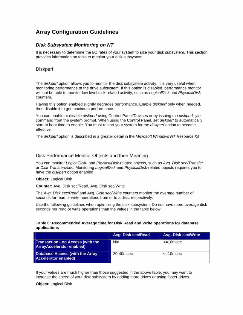
The Avg. Disk sec/Read and Avg. Disk sec/Write counters monitor the average number of seconds for read or write operations from or to a disk, respectively.

Use the following guidelines when optimizing the disk subsystem. Do not have more average disk seconds per read or write operations than the values in the table below.

Table 6: Recommended Average time for Disk Read and Write operations for database applications

Avg. Disk sec/Read Avg. Disk sec/Write

Transaction Log Access (with the ArrayAccelerator enabled)

N/a <=10msec

Database Access (with the Array Accelerator enabled)

20-40msec <=10msec

If your values are much higher than those suggested in the above table, you may want to increase the speed of your disk subsystem by adding more drives or using faster drives.

Object: Logical Disk

Counter: Disk Transfers/sec

The Disk Transfers/sec counter monitors the rates of read and write operations on the disk. It is important to realize that if you have a Compaq SMART or SMART-2 Array controller and several drives allocated to a logical volume, this counter monitors the total number of disk transfers per logical volume. To calculate number of disk transfers per second per drive, you must divide the Disk Transfers/sec value by the number of drives in the logical volume.

Volume Configuration The most confusing decision when configuring a system is how an array of physical drives should be partitioned into logical volumes. In reality this is a very easy step in the configuration process, once the methodology is understood. The key is to let an array do what it is intended to do, that is, distribute I/O requests among all available drives.

Configuration and tuning of a disk subsystem for database applications should be focused on getting the most out of each drive and having an appropriate number of drives on a system. By carefully studying the applications accessing the database, the data can be distributed in such a manner that each drive receives an approximately equal number of requests.

There are basic principles that are used in planning your disk layout, regardless of the type of database that you have.

• Spread randomly accessed data over as many disks drives as possible. Placing randomly accessed data on a single logical volume of many physical disk drives will help to balance the I/O load.

• Isolate purely sequential I/O to its own array. This will avoid excessive drive head movement. There are three basic database operations that are characteristically sequential: database transaction logging, bulk loading and unloading of the database, and batch reporting or updating requiring table scans.

Group randomly accessed data Looking back at the environment definitions covered earlier, most data access on database servers is basically random. When the goal is to optimize these application classes, database data and index files should be grouped onto a single array volume for each disk array controller in a machine. For example, if an OLTP database contains a number of large tables and their associated indexes totaling 5GB, these should all be put on a single volume of six 1GB drives. This guarantees that all drives will have approximately equal I/O load during normal operation of the system. This load balancing is done by the disk controller, due to the low-level striping of files across all disks in the volume, with no additional effort required by the System Administrator or DBA.

In contrast, techniques that have been carried over from traditional, non-array systems include the separation of data and index files to separate physical drives and separation of large data tables to their own dedicated drives. The reason for this was to allow simultaneous access to multiple drives. The problem with these techniques is that it puts the burden of load balancing upon the System Administrator. By carefully studying the applications accessing the database, the data can be distributed in such a manner so that each drive receives an approximately equal number of disk requests. Unfortunately, two assumptions are made that are difficult to achieve. Those are that the System Administrator and DBA can determine the actual I/O profile of an application and, that once determined, the I/O profile will remain constant throughout a day's processing and over the life of the application. For example, an application will often use different tables at different times of the day. Table A may have heavy access in the morning as a business gets started for the day. As the day wears on, most access may move over to Table B. If these

tables were separated on different physical disks, the application would overload the disk with Table A in the morning and overload the disk with Table B later. However, with an array controller these two tables would be put on the same logical volume spread across multiple drives allowing all drives to share equally in the I/O load throughout the day. Another example to further demonstrate this concept is data growth. Again using Table A and Table B, when the database is initially deployed Table A and B are approximately the same size and receive the same number of I/O requests. At that time, it makes sense for each table to be on its own drive. Over time, Table B grows by 10 percent per month in both size and I/O requests. After just 9 months Table B has doubled in access frequency and is now a bottleneck to system performance. If both these tables are put on a single array volume this table growth is shared among all drives on the volume, thus avoiding the disk bottleneck.

The case covered thus far applies when all the disks are attached to a single controller. Obviously when the amount of data and indexes exceeds the capacity of a single controller you will have multiple volumes in the system. At this point you have three options for distributing the data across the controllers.

1. Use an operating system facility to stripe the volume across controllers.

2. Use the database facilities to stripe the data across the controllers.

3. Segment different data to each controller.

There is no best solution to this situation. It is a matter of preference to the Administrator. General trade-offs of each are listed below to help you make your own decision. The degree of each of these may vary depending upon operating system and database software chosen. The pros and cons of each option are shown in Table 9.

Table 9: Multiple Controller Options

Use an operating system facility to stripe the volume across controllers.

Pros Cons

Ease of space management as database grows

More difficult volume management

Ease of backup with everything on one file system

Very long tape recovery times of volume

Performance penalty associated with file system striping

Use the database facilities to stripe the data across the controllers.

Pros Cons

Little to no negative performance impact Most complicated database configuration process

Ease of space management as database grows

More complicated backup/recovery process

Segment different data to each controller.

Pros Cons

Best performance when balanced properly Requirement of administrator to understand access patterns

Fastest, easiest tape recovery of volume

Fastest tape backup, allows multiple tape usage

Isolate sequentially accessed data Even though most data in a database server is read and/or written randomly, there are several cases of sequential access. During a long sequential read or write process, if the drive head can stay on the same physical disk track, performance will be dramatically better than if the head must continually seek between tracks. This principle is the same for traditional, non-array controllers and array controllers.

Actually, the largest single time component in reading or writing a block of data on a disk is the time required to move the drive head between tracks. The best drives on the market today range from 8 to 10 milliseconds average seek time and many drives you may be using from just a few of years ago could be as high as 16 or 19 ms for an average seek time. The remaining activities in an I/O routine include: the database makes a request from the operating system, the operating system requests the data from the controller, the controller processes the request and makes the request from the drive, the block rotates under the drive head, the data is transferred to the controller, back to the operating system, and finally the application. All of this takes only 10 to 15 ms, depending upon the particular controller, operating system, and database. Obviously, minimizing seek time, where able, has a significant benefit.

So much for low-level numbers, what does this mean to your application and how do you take advantage of it. There are three basic database operations that are characteristically sequential: transaction logging, bulk loading and unloading of the database, and batch reporting or updating requiring table scans. In many cases involving sequential I/O, the operations associated with it will not be the primary function of the system, but may be the most important aspect for your tuning due to nightly batch windows or backup time constraints. If the typical random access to the data will be relatively light or done by few users, you may want to give priority to tuning sequential operations over random I/O distribution.

The transaction log is the most obvious sequential I/O routine. In any update environment the transaction log is sequentially written from beginning to end. You should isolate the log file from any other system I/O activities during heavy update activity. However, a typical log file's space requirement may not need the space of an entire physical disk. You can usually share a single large disk between the log file and other files on the system which are not active during heavy update activities. Examples of items which coexist well with the log file include the operating system, database executables, database dump files, etc.

Bulk loads and batch updates are often associated with decision support systems. The typical scenario involves extracting large volumes of data from production transaction processing systems on a pre-defined schedule, such as daily or weekly. The data is then moved to the DSS server and loaded into a database. Performance of this load operation can be very critical due to nightly time constraints. Optimization of this process is very different from the typical system. In contrast to the random nature of most multi-user systems, a batch load or update can have up to four concurrent sequential operations. These operations include reading the input file, writing the database data file, writing the database index file, and writing the transaction log. To optimize the load time of the data each of these file types should be isolated to their own logical volumes. In contrast, pure optimization for daily multi-user decision support would put ALL of the above files on a single, large volume to allow concurrent access of all drives on the server by all read operations. The performance impact on daily access of optimization for load times should be less than 20%. However, the gain in load time can be over 200% which is often well worth the small random access penalty.

The final general application classes, which rely on sequential I/O performance include batch reporting and database dumps. These are fairly simple operations to optimize and there are only a couple of concepts to keep in mind. The profile of reporting and unloading is sequential table scans with some resulting output being written to a non-database file. In the case of a detailed analysis report, a report file of several megabytes may be spooled to a large disk file. The database dump sequentially reads tables writing the results to either a tape device or disk file. When the output is written to a disk file on the server, the target disk should be a different physical volume from the source of the data. If this is the only activity at the time the volume used for the log file is a good target; otherwise, another volume should be added to the system of sufficient size to accommodate the output file.

Physical Disk Requirements Once you understand the target environment, the volume configuration guidelines, and the fault-tolerance requirements the next step is to determine how many disks to distribute the data across and which type of disks are required. The goal is to use the lowest cost/megabyte drives, usually the largest drives available, while having enough drives to satisfy the physical I/O rate required by the application. The information presented here will help in meeting this goal.

The number and type of disk drives required by a disk subsystem volume is dependent upon the throughput requirements of the environment and the total amount of data on the server. Throughput requirements are composed of two characteristics, the degree of concurrency among user requests and the request rate from the application. Concurrency and request rate are distinct, but related concepts. Concurrency refers to the number of physical requests that are in the process of being executed by the disk controller(s). The degree of concurrency is primarily influenced by the number of users on the system and the frequency of requests from those users. Request rate is the absolute number of reads and writes per unit of time, usually expressed as I/Os per second. Usually, the higher the concurrency level, the higher the request rate. Yet, fairly high request rates can be generated by a single batch process with no concurrent requests. Of course, the number of physical disk requests that actually occur will depend upon the size of the database relative to the amount of disk cache and the resulting cache hit rate. The worst case scenario would result in as many concurrent disk requests as simultaneous user requests.

The reason for understanding the application I/O request rate is that multiple I/O requests can typically be processed in parallel if the data is distributed across multiple disk drives. Therefore, even though large drives are usually "faster" than smaller drives, this performance difference cannot offset the advantage of two drives’ ability to respond to multiple requests in parallel. The target number of drives in a server should be approximately equal to the sustained or average number of simultaneous I/O requests, with three drives being a typical minimum for the data and index files.

The following evaluation process determines the number of drives required by a volume containing data accessed randomly by multiple users. Repeat this process for each volume to be used on a database server. In the case of high transaction rate systems, this process may yield too many drives to fit on a single controller, at which point the drives can be split into multiple, equal volumes across controllers. For systems or volumes using purely sequential I/O or having no concurrent disk requests, i.e. only one or two users on the system at a time, strict calculations for the number of drives is not required. For this case, use the fastest drives available and as many as required to meet the space requirements of the system.

The steps used to determine the optimal number of drives are summarized here followed by a detailed explanation of each step and several case studies:

1. Determine typical I/O request rate by analyzing transaction I/O requirements and typical transaction rates of the target application(s).

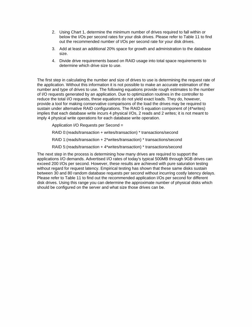
2. Using Chart 1, determine the minimum number of drives required to fall within or below the I/Os per second rates for your disk drives. Please refer to Table 11 to find out the recommended number of I/Os per second rate for your disk drives.

3. Add at least an additional 20% space for growth and administration to the database size.

4. Divide drive requirements based on RAID usage into total space requirements to determine which drive size to use.

The first step in calculating the number and size of drives to use is determining the request rate of the application. Without this information it is not possible to make an accurate estimation of the number and type of drives to use. The following equations provide rough estimates to the number of I/O requests generated by an application. Due to optimization routines in the controller to reduce the total I/O requests, these equations do not yield exact loads. They do, however, provide a tool for making conservative comparisons of the load the drives may be required to sustain under alternative RAID configurations. The RAID 5 equation component of (4*writes) implies that each database write incurs 4 physical I/Os, 2 reads and 2 writes; it is not meant to imply 4 physical write operations for each database write operation.

Application I/O Requests per Second =

RAID 0:(reads/transaction + writes/transaction) * transactions/second

RAID 1:(reads/transaction + 2*writes/transaction) * transactions/second

RAID 5:(reads/transaction + 4*writes/transaction) * transactions/second

The next step in the process is determining how many drives are required to support the applications I/O demands. Advertised I/O rates of today's typical 500MB through 9GB drives can exceed 200 I/Os per second. However, these results are achieved with pure saturation testing without regard for request latency. Empirical testing has shown that these same disks sustain between 30 and 80 random database requests per second without incurring costly latency delays. Please refer to Table 11 to find out the recommended application I/Os per second for different disk drives. Using this range you can determine the approximate number of physical disks which should be configured on the server and what size those drives can be.

Chart 1: Smart Array Drive I/O Rate Capacities.

Chart 1 is used in conjunction with the previously discussed equations to determine the number of physical disks required by an application. Locate on the Y-axis the number of I/Os per second required by the application. Move across the graph locating the intersection of the application I/O rate and the recommended application I/O per second for drives area. The number of drives is then determined by locating the drive count on the horizontal axis. The more conservative the implementation desired, the lower the I/O rates per drive that will be required. Also, if using RAID 1 an even number of drives is required. If the result is an odd number of drives, round up to the next even number. When throughput requirements are more than the chart indicates; continue adding controllers and drives until the required throughput is achieved.

Chart 2 can be used for I/O subsystem capacity planning. If you know your application I/Os per second rates, you can determine the minimum number of SMART controllers needed. If your application I/O rate demands multiple controllers, you will have to distribute the disk drives evenly across the controllers for balancing the I/O load.

Finally, the total space requirements for the database and support files, combined with the throughput requirements and fault-tolerance, determine the size of disks, which will provide an optimal solution. When calculating total space requirements, add an additional 20% free space above the actual data requirements for growth and miscellaneous overhead. Again, a set of equations provides the answer to the appropriate size drive.

Drive size requirements based on total space needs and fault-tolerance:

RAID 0: [total space / number of drives] Rounded up to next drive size

RAID 1: [total space / (number of drives / 2)] Rounded up to next drive size

RAID 5: [total space / (number of drives - number of controller volumes)] Rounded up to next drive size

Chart 2: Smart Array Controller I/O Capacities.

Several examples are presented which illustrate the use of this process. All RAID levels are presented for each case. Some cases still require a judgment call by the implementers to choose the number of drives or drive sizes, but the alternatives are drastically narrowed. The alternatives chosen are conservative configurations and the reason for the choice, if not a single alternative, is explained.

Case 1: Complex transaction processing system requiring multiple queries per update.

Reads: 100/transaction

Writes: 5/transaction

Transaction rate: 2/second

Space Requirements: 3GB Database + 20% Free space = 3.6GB

RAID 0: (100 + 5) * 2 = 205 I/Os / Second

205 I/Os / Second => 5 or 6 Drives of 35 to 45 I/Os per second

3.6 / 6 = .6 => Round up to next drive size => 1GB Drives

A conservative implementation yields 6 1GB drives for the data volume.

RAID 1: (100 + (2*5)) * 2 = 220 I/Os / Second


3.6 / (8 / 2) = .9 => Round up to next drive size => 1GB Drives

A conservative implementation yields 8 1GB drives for the data volume. The alternative of using 6 drives was not chosen due to possibly lower performance and 2GB drives would be required to meet space requirements. Using 2GB drives would yield a higher cost system in addition to lower performance.

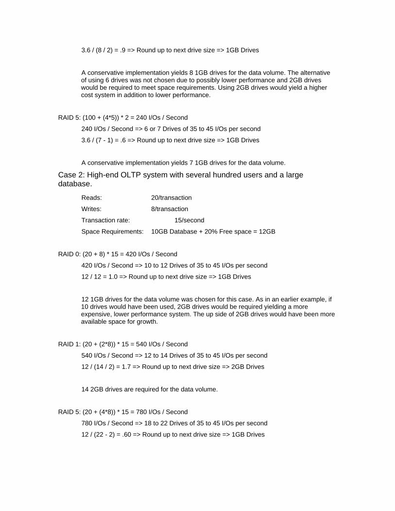
RAID 5: (100 + (4*5)) * 2 = 240 I/Os / Second


3.6 / (7 - 1) = .6 => Round up to next drive size => 1GB Drives

A conservative implementation yields 7 1GB drives for the data volume.

Case 2: High-end OLTP system with several hundred users and a large database.


Writes: 8/transaction

Transaction rate: 15/second

Space Requirements: 10GB Database + 20% Free space = 12GB

RAID 0: (20 + 8) * 15 = 420 I/Os / Second

420 I/Os / Second => 10 to 12 Drives of 35 to 45 I/Os per second

12 / 12 = 1.0 => Round up to next drive size => 1GB Drives

12 1GB drives for the data volume was chosen for this case. As in an earlier example, if 10 drives would have been used, 2GB drives would be required yielding a more expensive, lower performance system. The up side of 2GB drives would have been more available space for growth.

RAID 1: (20 + (2*8)) * 15 = 540 I/Os / Second


12 / (14 / 2) = 1.7 => Round up to next drive size => 2GB Drives

14 2GB drives are required for the data volume.

RAID 5: (20 + (4*8)) * 15 = 780 I/Os / Second


12 / (22 - 2) = .60 => Round up to next drive size => 1GB Drives

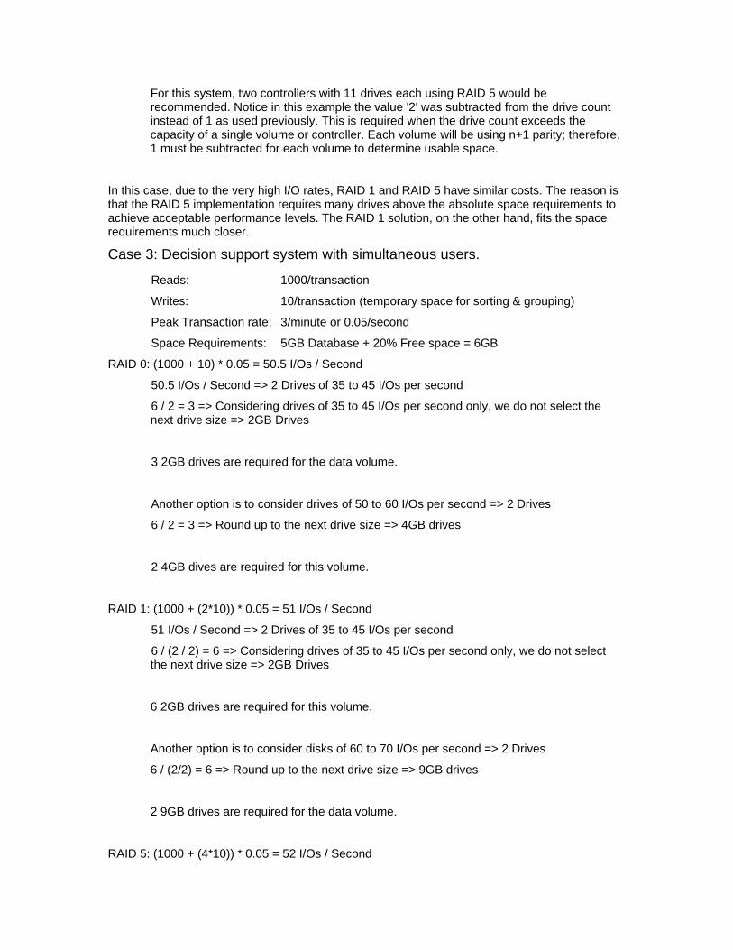
For this system, two controllers with 11 drives each using RAID 5 would be recommended. Notice in this example the value '2' was subtracted from the drive count instead of 1 as used previously. This is required when the drive count exceeds the capacity of a single volume or controller. Each volume will be using n+1 parity; therefore, 1 must be subtracted for each volume to determine usable space.

In this case, due to the very high I/O rates, RAID 1 and RAID 5 have similar costs. The reason is that the RAID 5 implementation requires many drives above the absolute space requirements to achieve acceptable performance levels. The RAID 1 solution, on the other hand, fits the space requirements much closer.

Case 3: Decision support system with simultaneous users.


Writes: 10/transaction (temporary space for sorting & grouping)

Peak Transaction rate: 3/minute or 0.05/second


RAID 0: (1000 + 10) * 0.05 = 50.5 I/Os / Second

50.5 I/Os / Second => 2 Drives of 35 to 45 I/Os per second

6 / 2 = 3 => Considering drives of 35 to 45 I/Os per second only, we do not select the next drive size => 2GB Drives


Another option is to consider drives of 50 to 60 I/Os per second => 2 Drives

6 / 2 = 3 => Round up to the next drive size => 4GB drives

2 4GB dives are required for this volume.

RAID 1: (1000 + (2*10)) * 0.05 = 51 I/Os / Second

51 I/Os / Second => 2 Drives of 35 to 45 I/Os per second

6 / (2 / 2) = 6 => Considering drives of 35 to 45 I/Os per second only, we do not select the next drive size => 2GB Drives

6 2GB drives are required for this volume.

Another option is to consider disks of 60 to 70 I/Os per second => 2 Drives

6 / (2/2) = 6 => Round up to the next drive size => 9GB drives


RAID 5: (1000 + (4*10)) * 0.05 = 52 I/Os / Second

52 I/Os / Second => 2 Drives

6 / (2 - 1) = 6 => Considering drives of 35 to 45 I/Os per second only, we do not select the next drive size => 2GB Drives

4 2GB Drives are required for the data volume.

Case 4: Complex decision support with several simultaneous users.


Writes: 20/transaction (temporary space for sorting & grouping)

Peak Transaction rate: 6/minute or 0.1/second


RAID 0: (2000 + 20) * 0.1 = 202 I/Os / Second


12 / 4 = 3 => Rounded up to next drive size => 4GB Drives


RAID 1: (2000 + (2*20)) * 0.1 = 204 I/Os / Second


12 / (4 / 2) = 6 =>Considering drives of 50 to 60 I/Os per second only, we do not select the next drive size => 4 GB Drives


Another option is to consider disks of 60 to 70 I/Os per second

12 / (4 / 2) = 6 => Round up to next drive size => 9 GB Drives


RAID 5: (2000 + (4*20)) * 0.05 = 208 I/Os / Second

208 I/Os / Second => 4 Drives

12 / (4 - 1) = 4 => 4 GB Drives

4 4GB Drives are required for the data volume.

The general conclusion from this discussion is that more, smaller disks are best for high user, high I/O, high concurrency systems and fewer, larger disks work best for environments with one/few users, high I/O, low concurrency requirements.

General Guidelines for Array Configuration for UDB2 Oracle8 – OLTP Configuration

A typical Oracle OLTP environment has the following characteristics:

• Database Tables and Indexes are accessed by a large number of small block random I/Os

• Typical Read/Write ratio is 3 to 1

• Temporary Tablespace is usually small and not very heavily used.

• Redo log I/O is characterized by a large number of sequential writes.

To properly configure this system, a minimum of two arrays is needed. The first array is for the Oracle REDO logs. The second array is for the data/index/temp data files. If unable to configure enough disks in an array to support either the space requirements or the I/O load of the database, configure additional arrays on separate controllers until the I/O subsystem meets the requirements of the database.

RAID protection is necessary on the transaction logs for recoverability of the database. With so many changes to the data, the transaction log becomes a very important tool should a database destructive event occur during the operation of the database. Due to the I/O nature of the log drives, RAID 1 (mirroring) is the best performing way to protect this data. Because recovery is possible from a backup and rolling forward of the transaction REDO logs, RAID protection on the data is less important than on the transaction logs, however depending upon availability requirements of the data, it may be necessary to put some RAID protection on these data arrays. When this is done, factor in the additional I/O overhead that the RAID protection causes for calculating the number of disk drives necessary to support the total I/O throughput.

Controller cache on an OLTP system is usually best when set to 100% write cache. This is because no sequential reading is being done on the database in the normal environment. This is true for all of the Oracle data files.

Oracle8 – DSS Configuration

A typical Oracle DSS environment has the following characteristics:

• Database Tables and Indexes are accessed by a large number of large block sequential I/Os

• Typical Read/Write ratio is 5 to 1. However, reads are about 4 or 5 times larger than writes.

• Temporary Tablespace is usually large and accessed with a combination of random/sequential reads/writes depending upon what operation is happening at the time.

• Redo log I/O is minimal during queries, may be heavy during batch updates, but is in small sequential writes in either case.

• Single queries are broken up into pieces that can be run in parallel. Thus, one user can cause multiple I/O streams to be generated.

I/O planning in DSS is more complicated than in OLTP because of the large number of different sequential scans. The thing to remember is to create an array for every sequential I/O stream. When a query gets split up by the parallel query engine, a single operation gets split into multiple parts. The work is divided by partitions if the query is on a partitioned table; otherwise, it is divided up by Oracle ROWID (which really splits up the work by files, unless you have more parallel query servers than files for a given operation). Therefore, at minimum have an array for each partition of your table. This way the sequential accessibility of the database is maximized.

The different methods of loading, maintaining, and running in a DSS environment along with availability needs and maximum recovery times will dictate how much RAID protection you need on your database. If the data remains relatively static and a restore from a backup media can be done in the amount of allowable downtime requirements, then no RAID protection would be necessary at all not even on the log drives. If this is not the case, depending upon the needs of the database, some portions of it, i.e. transaction logs, data files, index files, or temporary files, or possibly all of the database will need to be RAID protected. The best RAID protection will be RAID 1 (mirroring). This is because it has less overhead than RAID 5 protection does, and it also provides the benefits of split reads. A split read is when a process is reading from one half of the mirrored set and another I/O request comes in the second half of the mirrored set can service the new request and not interrupt the other I/O request stream. In this manner, an array could handle two sequential I/O streams at the same time. Thus reducing the number of arrays required by your system.

Setting the controller cache in a DSS environment is a little trickier. The write cache needs to be sufficient for handling the data throughput required on the Temporary Tablespaces. If there is RAID protection on the drives, the write cache is even more important. However, don’t make the write cache so large that there is nothing left for the read ahead buffers. In the worst case this should be 50%/50% read/write cache. Temporarily, during the database build and tablespace create phase and during the data loading phase, setting the cache to 100% write will make these function go much more quickly.

Flat Files for Loading the Database

If loading the database is being done by SQL*Loader, the flat files should be stored on separate disks than the database. If these files are stored on another array controller, then the cache setting for that controller should be set to 100% write cache while creating the flat file, and then switched to 100% read cache when actually running the SQL*Loader thread. Each SQL*Loader thread should have a dedicated array from which it reads data and it should write to a separate array which contains the Oracle data file. This means that in an ideal situation there will be at least twice as many arrays of disks as there are SQL*Loader threads performing the load operation.

Documents

Overview of Enhancing Database Performance and I/O Techniques