Embed Size (px)
Citation preview

Enhancing state space reduction techniques for modelcheckingBosnacki, D.
DOI:10.6100/IR549628
Published: 01/01/2001
Document VersionPublisher’s PDF, also known as Version of Record (includes final page, issue and volume numbers)
Please check the document version of this publication:
• A submitted manuscript is the author's version of the article upon submission and before peer-review. There can be important differencesbetween the submitted version and the official published version of record. People interested in the research are advised to contact theauthor for the final version of the publication, or visit the DOI to the publisher's website.• The final author version and the galley proof are versions of the publication after peer review.• The final published version features the final layout of the paper including the volume, issue and page numbers.
Link to publication
Citation for published version (APA):Bosnacki, D. (2001). Enhancing state space reduction techniques for model checking Eindhoven: TechnischeUniversiteit Eindhoven DOI: 10.6100/IR549628
General rightsCopyright and moral rights for the publications made accessible in the public portal are retained by the authors and/or other copyright ownersand it is a condition of accessing publications that users recognise and abide by the legal requirements associated with these rights.
• Users may download and print one copy of any publication from the public portal for the purpose of private study or research. • You may not further distribute the material or use it for any profit-making activity or commercial gain • You may freely distribute the URL identifying the publication in the public portal ?
Take down policyIf you believe that this document breaches copyright please contact us providing details, and we will remove access to the work immediatelyand investigate your claim.
Download date: 25. Jun. 2018

Enhancing State Space ReductionTechniques for Model Checking
Dragan Bosnacki

CIP-DATA LIBRARY TECHNISCHE UNIVERSITEIT EINDHOVEN
Bosnacki, Dragan
Enhancing state space reduction techniques for model checking /by Dragan Bosnacki. - Eindhoven : Technische Universiteit Eindhoven, 2001.Proefschrift. - ISBN 90-386-0951-5NUGI 855Subject headings : model checking / programming; formal methods /software; specifications / software verificationCR Subject Classification (1998) : D.2.4.
The work in this thesis has been carried out under the auspices of the researchschool IPA (Institute for Programming research and Algorithmics).
IPA dissertation series 2001-14
Printed by University Press Facilities, Eindhoven

Enhancing State Space Reduction Techniques
for Model Checking
Proefschrift
ter verkrijging van de graad van doctor aan de Technische UniversiteitEindhoven, op gezag van de Rector Magnificus, prof.dr. R.A. van Santen, vooreen commissie aangewezen door het College voor Promoties in het openbaar te
verdedigen op woensdag 7 november 2001 om 16.00 uur
door
Dragan Bosnacki
geboren te Berovo, Macedonie

Dit proefschrift is goedgekeurd door de promotoren:
prof.dr. J.C.M. Baeten
enprof.ir. M.P.J. Stevens
Copromotor:
dr. D.R. Dams

Acknowledgments
There are many people and institutions who helped me in various ways duringthe writing of this thesis. Aware of the inevitable risk of forgetting someone, Iwill try to list them with some words of gratitude that unfortunately often willbe only a pale shadow of what they should have been. For those that I haveforgotten to mention – a proverb from my homeland: ”May the evil also forgetyou”.
First of all, I would like to thank my copromotor Dennis Dams. I considermyself extremely fortunate that I had during all these years his valuable guidanceand friendship. His was always able to help with all my technical questions, aswell as to give me the right advise at the right time. Dennis is also a coauthorof several papers whose modified versions became chapters of this thesis.
No less gratitude is reserved for my promotor Jos Baeten. He opened for methe doors of the Western European science by inviting me to a short stay atthe Eindhoven University of Technology in the fall of 1996. Since then he hasbeen offering me continuously technical and moral support. He also deserves thecredit for creating a nice working atmosphere in the Formal Methods group. Josis the only boss that I know that regularly goes from door to door in order togather his group for lunch.
Gerard Holzmann provided for me the opportunity to spend an unforgettablesummer 1998 in Bell Laboratories. The experience of walking in the corridorwith probably the greatest concentration of computer science celebrities in theworld is something I always talk about with pleasure. Thanks go to Gerard alsofor patiently answering numerous technical questions regarding Spin and modelchecking in general.
Most of the work on this thesis was done under the auspices of the EuropeanCommunity’s Fourth Framework project Verifying Industrial REactive Systems(VIRES) (Esprit LTR 23498) which I gratefully acknowledge. I would like toalso thank all the participants in the project with whom I had the opportunityto discuss my research.
During the Ph.D. studies in Eindhoven I was on leave from the Instituteof Informatics, Faculty of Natural Sciences and Mathematics of the St. Cyriland Methodius University in Skopje, Macedonia. I am immensely grateful to mycolleagues from the Institute for their understanding and support.
On this occasion I should not forget the technical and financial support bythe IPA postgraduate school. The events organized by the school offered anexcellent opportunities for learning and enjoyment.
I am grateful to Leszek Holenderski for coauthoring the papers who becamebasis for two of the chapters in this thesis. We spent a lot of time on interestingdiscussions, often outside our research. We had different opinions about manyissues, but at the end I think that I learned many interesting things from him.
iii

Tanks go to Twan Basten for coauthoring of Chapter 2, numerous discussionson the topic of partial order reduction, and helping me with the Samenvattingin Dutch.
Natalia Sidorova is a coauthor of the paper who is a basis of Chapter 5 ofthe thesis. I am also grateful to her for the numerous discussions regarding theverification of timed systems.
I would like to thank Mario Stevens for accepting to be my second promotor.Doron Peled and Hans Toetenel kindly accepted to be members of the reading
committee and gave valuable insightful comments on the first version of thisdocument, for which I am indebted to them.
I am mostly grateful to Smile Markovski for his support during the yearsI spent at the Institute of Informatics in Skopje, Macedonia. Many things intheoretical computer science I learned from him. I am also honored that heaccepted to be a member of the defense committee for my thesis.
Jan-Friso Groote and Antti Valmari also kindly accepted to be members ofthe defense committee, for which I honor them.
Many thanks to Tijn Borghuis and Tim Willemse for their helpful remarkson parts of the manuscript and their friendship.
I am grateful to Peter Hilbers for believing in my potentials as a researcherand his understanding during the finishing of the last chapter of the thesis.
Rob Gerth and Bart Knaack drew my attention to Spin, for which I wouldlike to thank them. Rob also played a significant role in my decision to come toEindhoven.
Many people from the University helped indirectly with my thesis, for whichI give them my warmest thanks: Suzana Andova for her moral support, con-structive criticism and helping me not to forget the taste of the Macedoniancuisine; Marcella de Rooij, Victor Bos, Georgi Jojgov and Martijn Oostdijk forbeing with me during my ups and downs and letting me winning couple ofRisk games; Sjouke Mauw for his friendship, valuable advises and always sup-portive smile; Ana Sokolova, Anne-Meta Overstegen, Ruurd Kuiper, Rob Ned-erpelt, Nicu Goga, Peter Peters, Roel Bloo, Michael Franssen, Andre Engels,Erik de Vink, Kees Middelburg, Loe Feijs, Francois Monin, Francien Dechesne,Dmitri Chkliaev, Elize Russell, Michel Reniers, Sergey Tourine, Nino Mushku-diani, Olga Caprotti, Oana Balan, Marcin Grodek, Martin Hill, Desiree Mijers,Jolande Mathijsse, Trees Klaver, and Monique Bechtold for making my days atthe University more enjoyable.
The successful finishing of this thesis would not be possible without the goodeducation I received at the St. Cyril and Methodius University in Skopje, Mace-donia, during the postgraduate studies at the Institute of Informatics, Faculty ofNatural Sciences and Mathematics, and the undergraduate studies at the Facultyof Electrical Engineering.
The last, but by far the greatest gratitude goes to my parents for their endlesslove, all kinds of unconditional support, and for always believing in me muchmore than I believed in myself.
Eindhoven, September 2001.
iv

Contents
Acknowledgments . . . . . . . . . . . . . . . . . . . . . . . . . . . . . . . . . . . . . . . . . . . . . . . iii
Contents . . . . . . . . . . . . . . . . . . . . . . . . . . . . . . . . . . . . . . . . . . . . . . . . . . . . . . . . . v
1 Introduction . . . . . . . . . . . . . . . . . . . . . . . . . . . . . . . . . . . . . . . . . . . . . . . . . . . 1
2 Enhancing Partial-Order Reduction via Process Clustering . . . . 13
3 Partial Order Reduction in Presence of Rendez-vousCommunications with Unless Constructs and Weak Fairness . . . . 31
4 Integrating Real Time into Spin: A Prototype Implementation 55
5 Model Checking SDL with Spin . . . . . . . . . . . . . . . . . . . . . . . . . . . . . . . 77
6 A Heuristic for Symmetry Reductions with Scalarsets . . . . . . . . . 93
7 Nested Depth First Search Algorithms for Symmetry Reductionin Model Checking . . . . . . . . . . . . . . . . . . . . . . . . . . . . . . . . . . . . . . . . . . . . 123
8 Conclusions . . . . . . . . . . . . . . . . . . . . . . . . . . . . . . . . . . . . . . . . . . . . . . . . . . 169
9 Samenvatting . . . . . . . . . . . . . . . . . . . . . . . . . . . . . . . . . . . . . . . . . . . . . . . 173
v


1. Introduction

Introduction
1 Motivation and Background
1.1 The Need for Formal Methods
One can often hear the expression “with computer precision” which is usuallyused to describe a flawless impeccable execution of some task. Unfortunately,computers do not always work correctly. Moreover, the errors of software andhardware systems applied in safety-critical systems like nuclear power plants,medical equipments, highway and air traffic control, railways, electronic com-merce, can be potentially disastrous. Such grim predictions are supported byfamous failures, like the Ariane 5 space rocket disaster or the Pentium bug, cost-ing billions of dollars [3]. But as information technology penetrates in our dailylife, there will be even more prosaic reasons why the errors will not be toler-ated. Just imagine a football aficionado whose TV crashes during the penaltyshootouts because of the embedded software, or you being cut by your intelli-gent shaver. There are predictions that in the future the main problem for theapplication of information technology will not be the lack of raw computationalpower, but our inability to develop complex systems with sufficient confidencein their correctness.
The traditional engineering techniques for validation, like peer review, sim-ulation, and testing, have often proved inadequate and too expensive to avoiderrors in information processing artifacts. One reason for this is that they exploreonly a part of the possible behavior of the system. As a result some erroneousbehavior often escapes undetected.
In the last two decades, alternative, formal approaches for validation haveemerged. They are based on formal methods, i.e., on methods that are moresystematic and that have solid mathematical foundations. One of the main ad-vantages of formal methods is that they perform exhaustive exploration of allpossible behaviors. In this thesis we concentrate on model checking as a formalapproach for debugging and verification of hardware and software.
1.2 Model Checking
Roughly speaking, model checking [3] is an automated technique that, given amodel of the system and some property, checks whether the model satisfies theproperty. Originally suggested in the beginning of the eighties independentlyby Emerson and Clarke, and Quelle and Sifakis, nowadays the technique gainspopularity, with several major companies developing in-house model-checkingtools. Compared to the other (semi)automated formal techniques (for instance,deductive methods, like theorem provers) model checking is relatively easy touse. The specification of the model is very similar to programming and as such

Introduction 3
it does not require much additional expertise from the user. The verificationprocedure is completely automated and often takes only several minutes. Anotherimportant advantage of the method is that, if the verification fails, the possibleerroneous behavior of the system can be reproduced. This significantly facilitatesthe location and correction of the errors.
The Characteristics of the Analyzed Systems. In this document we dealwith concurrent systems, i.e., systems composed of components that can operateconcurrently and communicate with each other. It is assumed that the (compo-nents of the) systems are reactive, i.e. continuously interact with their environ-ment. Typical representatives of reactive systems are communication protocols,operating systems, process control software, and aircraft control. This is in con-trast with traditional sequential programs which can be seen as data transform-ers with single input and single output, i.e., interacting with the environmentonly at their beginning and end. Concurrency is modeled by interleaving, i.e.,it is assumed that only one component executes an action at a time and theconcurrent actions are arbitrarily ordered. Considering the reactive nature ofthe concurrent systems that are analyzed, we are interested in the verification ofcontrol (interaction) properties, rather than properties that are related to data.
The Formal Framework and the Scope. As outlined in [16], each frameworkfor formal analysis consists of four components:
– formal semantics in which the system and the property are interpreted;– formal language for describing the system;– formal language for describing the property;– formal, preferably automated, techniques with which it can be checked whether
the system satisfies the property;
We use variants of (labeled) transition systems to give the semantics of thesystems and properties. In other words, the semantics of the system is its statespace, i.e., the set of all possible states that the system can reach and the tran-sitions between them. The state transition systems are represented in a naturalway as labeled graphs. Model checking by definition is applied on systems withfinite state space.
Although some of the presented research is adaptable to the branching-timeframework, we mainly work with trace semantics, i.e., we specify the propertieseither directly in the model, or in linear temporal logic (LTL) [6] and, moregeneral, Buchi automata [19].
The results presented in the thesis are derived using directly the semanticmodel, i.e., the labeled transition systems, and as such are independent of thelanguage in which the (model of the) system is specified. Having said this, wealso emphasize that most of the work presented in this document was instigatedby and implemented in the model checker Spin with its input language Promela,developed by Gerard Holzmann at Bell Laboratories [11].

4
Further, we consider model checking algorithms based on explicit enumera-tion of the state space, as opposed to the symbolic algorithms based on binarydecision diagrams (c.f. [3]), for instance.
Although it is safe to conjecture that at least some of our results can be usedfor hardware verification, a tacit assumption throughout the thesis is that weare targeting debugging and verification of software systems.
The State Space Explosion Problem. Model checking requires search ofthe state space of the system, which may increase exponentially with the size ofthe system description. As a consequence, one of the major bottlenecks in modelchecking is the so called state space explosion [22]. The state space explosionis simply the combinatorial explosion caused by the interaction (interleaving)of the components and/or by the usage of data structures ranging over manydifferent values. There exist numerous techniques to combat this problem, likesymbolic verification, on-the-fly verification, abstraction, partial order reduction,symmetry reduction, etc. In our research we put emphasis on the last two: partialorder reduction and reduction based on symmetry.
2 Contributions of This Thesis
The main contributions of this thesis are several improvements of the techniquesfor state space reduction. As stressed above, we focus on partial order reductionand reduction based on symmetries. The basic idea behind both techniques isto restrict the part of the state space which is explored for the verification insuch a way that the properties of interest are preserved. However, in generalthey exploit different features of the concurrent systems and as a consequencethey use different algorithms. In the first two parts of this section we briefly givethe intuition behind each of the techniques and summarize the correspondingresults.
The practical component of our contribution is reflected in the implementa-tion of almost all of the obtained theoretical results. In this context we developedseveral upgrades of the model checker Spin and wrote accompanying programs.The prototype implementations were successfully tested on case studies from theacademic literature and on protocols originating from industry. The last part ofthe section gives a brief overview of these practical aspects.
2.1 Partial Order Reduction
Partial order reduction [9, 18, 21] exploits the independence of the checked prop-erty from the execution order of the statements in the program (model de-scription). More specifically, two statements a, b are allowed to be permutedprecisely when, if for all sequences v, w of statements: if vabw (where juxtapo-sition denotes concatenation) is an accepted behavior, then vbaw is an acceptedbehavior as well. In a sense, instead of checking all the execution sequences, thedesired property is checked only on representative sequences, which results in

Introduction 5
significant savings in space and time. Finding the optimal relation for indepen-dence (permutability) of statements can be as difficult as the original verificationproblem [3]. Consequently, in practice only sufficient conditions for such a per-mutability are used that can be checked locally and preferably using only syn-tactic criteria, i.e., directly from the system specification. The actual reductionof the state space is realized during the state space exploration by limiting thesearch from a given state s to only a subset of the statements that are executablein s.
Among the results that we obtained regarding partial order reduction, weemphasize the following:
Partial order reduction for discrete time. We present an adaptation fortimed systems of the untimed algorithm for partial order reduction by Peled andHolzmann [18, 12], under the assumption that time is modeled with integers. Onecan consider that partial order reduction techniques consist of two parts. Thefirst part is related with the determining the independence relation betweenstatements. As we mentioned above, this part is usually done before the statespace exploration starts. The second part is the actual exploration algorithmwhich, based on the independence relation and the structure of the state space,has to chose the subset of transitions which have to be explored from each state.Our main idea regarding the discrete-time extension is related to the criteriafor independence of the statements (actions) which are applied on timers. Asa consequence, the adaptation is independent of the rest of the engine of thepartial order algorithms, which means that the proposed extension can be easilyadapted to other approaches to partial order reduction, like for instance [9] or[21]. The implementation of the algorithm in the extension of Spin with discretetime, DT Spin, showed encouraging results (see also the discussion about DTSpin in the Tools section below).
Compatibility of partial order reduction for systems in which syn-chronizing (rendez-vous) communications are combined with prioritychoice and/or weak fairness. When synchronizing (rendez-vous) commu-nications are used in Promela models, the priority choice construct unless ingeneral is not compatible with partial order reduction algorithms. Also the weakfairness algorithm in Spin is not compatible with partial order reduction in pres-ence of rendez-vous statements. Interestingly enough, it turns out that the sameerroneous reduction pattern causes the incompatibility in both cases. After iden-tifying this pattern we propose several solutions such that the power of partialorder reduction can be retained in the presence of unless and weak fairness.
It can be expected that the importance of the above mentioned compatibili-ties will grow in the future, especially for the priority choice (unless). Namely,the unless statement in Promela is a natural way to model exceptions. Withthe popularity of the latter as a concept in modern programming languages(like Java), the compatibility of the priority choice with the other features ofverification tools iis an important advantage.

6
Exploiting system hierarchy for partial order reduction. Most of themodel checking techniques treat the model as a flat composition of processes.Our approach of partial order reduction via process clustering shows how onecan profit from the model structure for better state space reduction. Usually,the heuristics for independence of statements in partial order reduction regarda statement as either global or local, depending on the scope of the objects thatare accessed by the statement. Our main idea is to introduce instead of thistwo-level view, several levels of globality of statements based on the structuralhierarchy of the system. Most of the time this hierarchy is obtained for free, i.e.,it is already contained in the specification (for instance, imposed by the syntax ofthe specification or modeling language). We show that employing a more refinednotion of globality results in significant reductions (sometimes several orders ofmagnitude) of the state space, compared to the case when the standard two-level approach is used. Moreover, the gain in state space is without significantpenalties in the verification time.
2.2 Symmetry Reduction
Symmetry based state space reductions [14, 15] exploit the inherent symmetry ofthe analyzed system. The main idea behind the technique can be illustrated onvariants of the mutual exclusion problem. Assume that we have two processes,A and B. Then, for the verification of the mutual exclusion property, the statein which process A is in the critical section, while process B can enter thecritical section (and violate the mutual exclusion property) is equivalent to thesymmetric state where the roles of A and B are swapped. More formally we saythat the states are equivalent under permutation (in this case a simple swap)of the process IDs. The symmetric states are grouped in equivalence classes.Whenever during the exploration of the state space a state is generated which isthe same up to a permutation of process IDs (i.e., belongs to the same equivalenceclass) as an already visited state, the search can be pruned. Formally speaking,we can consider that instead of exploring the original (concrete) state space, wecheck an abstract state space whose states are (representatives of the) symmetryequivalence classes of states from the original state space.
Below we give our main contributions related to symmetry based reductions.
Developing efficient heuristics for finding representatives of equiva-lence classes. The problem of finding (canonical) representatives of the equiv-alence classes under symmetry is equivalent to the graph isomorphism problemfor which no polynomial solution is known. As a result the gain in state spacecan be diminished by unacceptably long verification times. We propose four ver-sions of a new heuristic for finding representatives. The implementation in Spinshowed that the heuristics work well and can potentially significantly improvethe performance of verification tools.
Model checking under weak fairness using symmetry reductions. Wepresent an algorithm for model checking that combines weak fairness with sym-

Introduction 7
metry reduction. The algorithm is based on the nested depth first search al-gorithm (NDFS) by Courcoubetis, Vardi, Wolper and Yannakakis [4]. This isin contrast with similar algorithms that exist in the literature which requirefinding maximal strongly connected components (MSCC) in a graph. As a con-sequence, our algorithm has all the advantages that NDFS has over the MSCCapproach. It is compatible with the approximative verification techniques of [11,24], which is not the case with the MSCC based algorithms. Also, we argue thatin practice our algorithm has better time and space complexity. Finally, withour algorithm it is easier to reconstruct a diagnostic execution sequence whichleads to a possible error.
As intermediate results we give an NDFS based algorithm for state spacereduction techniques that preserve bisimulation [7]. (Symmetry reduction is aspecial case of the latter.) Also we discuss a modification of Spin’s weak fairnessalgorithm (without symmetry). To this end we introduce the notion of weaklyfair extension of transition system which facilitates the correctness proof of thealgorithm.
2.3 Tools and Case Studies
One of the main advantages of the model checking techniques is that they arereadily implementable in tools. A significant part of the work of this thesis wasspent on the various extensions and improvements of model checking tools andaccompanying programs. Almost all theoretical results listed above have beenimplemented and the prototype implementations have been evaluated on casestudies. As mentioned already, most of the practical work is related to the modelchecker Spin, which is one of the most popular model checking tools, successfullyused in academia and industry. Below we give a short summary of the developedor upgraded software.
DT Spin. Standard Spin does not feature the possibility to express time quan-titatively. For instance, given two consecutive statements a and b, we know thatb will be executed after a, but we cannot specify, for instance, that b will hap-pen five time units after a. This can be a handicap when dealing with systemsthat critically depend on timing. DT Spin is an extension of Spin with dis-crete time which allows the specification of such quantitative timing relationsbetween statements. DT Spin is fully compatible with Spin and allows verifica-tion of all the properties that can be verified with standard Spin. Moreover, theabove mentioned discrete-time partial order reduction algorithm is implementedin DT Spin, which resulted in significant savings in the state space in the casestudies.
if2pml is a translator from the language IF into Promela, the input languageof Spin. IF [2] is an emerging language designed at VERIMAG Grenoble thataims at providing a common intermediate format for connecting various for-mal languages and tools. The translator if2pml was written as a second part of a

8
translator from the language SDL to Promela. It was successfully used in the val-idation of MASCARA, a communication protocol developed by industry, whoseoriginal specification was written in SDL. During the development of if2pml wecame across several non-trivial problems that had to be resolved, most of themrelated to the timing features of IF and SDL.
SymSpin is an extension of Spin for exploiting symmetry based reductiontechniques. More particularly, we have implemented on top of Spin the abovementioned heuristics for finding representatives of the equivalence classes. Inmost of the case studies the obtained reduction approached the theoretical limitof N !, where N is the number of processes in the system.
3 Related Work
Related work is discussed in more detail in each chapter. Here we briefly outlinethe most important related references grouped according to the subject.
Partial order reduction Our work on partial order reduction is mostly basedon the partial order algorithm by Doron Peled [18] and on its variant (a jointwork with Gerard Holzmann) which is implemented in Spin [12].
Although there exist several attempts to extend the partial order reductiontechniques to timed systems (e.g. [5]) with dense time (i.e., time is modeled withreal numbers), to the best of our knowledge there is no successful implementationof any of them. We are not aware of any work on partial order reduction fordiscrete time (time modeled as integers).
It was already mentioned that partial order reduction algorithms during thestate space search explore only a subset of the transitions which originate in agiven state. The algorithm of [18, 12] requires that all transitions in this subsetbelong to the same process. Our improvement based on process clustering re-moves this constraint. We only require that the transitions that are in the subsetbelong to a same group (cluster) of processes. There are several references in theliterature that deal with grouping actions of several processes together for theexplored subset. (Actually, one of the very first references in partial order reduc-tion [17] is based on this kind of idea.) However, to the best of our knowledgethere are no papers which do this grouping by exploiting the hierarchical struc-ture of the system. Our paper was inspired by the NEXT reduction heuristicfrom [1]. As shown in [1], the NEXT heuristic in general capitalizes on differentaspects of concurrency in order to reduce the state space, and as such differsfrom partial order reduction.
To the best of our knowledge, the compatibility of partial order reductionwith fairness and priority choice in presence of synchronizing communication hasnot been treated in the literature before.

Introduction 9
Symmetry reduction Probably the most referenced work regarding symmetryreductions is that of Ip and Dill [14]. We also rely mainly on this work, partic-ularly in our paper about the heuristics for finding representatives. In a sense,one can consider our work as complementary to [14], where the main attention isdevoted to the question how to efficiently detect the symmetries in the system,i.e., how to ensure that the obtained state space is symmetric. On the otherhand, we deal with the question how to detect the symmetry between the states,i.e., how to detect during state space exploration that two states are equivalent,provided that the sate space is symmetric.
The problem of finding representatives is (most of the time in very generalterms) discussed in [14, 8, 15]. In our opinion the heuristics we propose haveadvantage in their simplicity and efficiency.
The only algorithms for reconciling symmetry reduction and weak fairnessthat we could find in the literature were the ones from [8] and [10]. As mentionedabove, our algorithm has some advantages over these two algorithms because it iscompatible with approximative verification techniques, in practice requires lesstime and memory, and has better diagnostic output in case an error is detected.
Verification of SDL models with Spin We are aware of at least two otherattempts to verify SDL with Spin [13, 20]. In our opinion they tackle successfullyonly the untimed part of the SDL specification. The main advantage of our ap-proach is that it also correctly captures the quantitative aspects of the behaviorrelated to SDL timers.
4 Organization of the Thesis
This document is mostly a collection of articles whose original versions alreadyhave been published or submitted for publication. Consequently, they are meantto be self contained and are independent of each other. Therefore, some overlapand repetition of the basic concepts is unavoidable.
The thesis can be roughly divided into three parts. The first part containsthe papers which describe the contributions related to partial order reductiontechniques. The second part is the paper on verification of SDL specificationswith Spin, containing the main case study, the MASCARA protocol. The lastpart comprises two papers related to the symmetry based reductions.
The first part consists of Chapters 2, 3 and 4. Chapter 2 discusses the ex-ploitation of the system hierarchy for more efficient partial order reduction. InChapter 3 we give a solution for the compatibility of partial order reductionin models that contain synchronizing (rendez-vous) communication statements,with priority choice and/or weak fairness. The main subject of Chapter 4 is theextension of Spin with discrete time and an adaptation of the untimed algorithmfor partial order reduction.
Chapter 5 describes the verification of SDL specifications with the modelchecker Spin. In that context the developed methodology and tools, among whichthe translator if2pml, are described.

10
The third part consists of Chapters 6 and 7. Chapter 6 deals with theheuristics for efficiently finding representatives of equivalence classes. Chapter 7presents the algorithm for model checking under weak fairness using symmetryreduction.
The last Chapter 8 concludes the thesis with a summary of the results anda discussion of the directions for future work.
4.1 The Origin of the Chapters
Almost all the work on this thesis was done under the auspices of the EuropeanCommunity’s Fourth Framework project Verifying Industrial REactive Systems(VIRES) (Esprit LTR 23498) [23]. Most of the material that is presented in thisdocument has been published or submitted for publication. We give below theorigin of each of the chapters.
Chapter 2 is the paper
T. Basten, D. Bosnacki, Enhancing Partial-Order Reduction via ProcessClustering, 16th IEEE Conference on Automated Software EngineeringASE 2001, IEEE Computer Society Press, 2001.
A previous version of the paper appeared as
T. Basten, D. Bosnacki, Enhancing Partial-Order Reduction via ProcessClustering, Technical report, Eindhoven University of Technology CSR00-11, 2000.
Chapter 3 is a revised version of the paper
D. Bosnacki, Partial Order Reduction in Presence of Rendez-vous Com-munications with Unless Constructs and Weak Fairness, Theoretical andPractical Aspects of SPIN Model Checking, 5th and 6th InternationalSPIN Workshops, Lecture Notes in Computer Science 1680, pp. 40–56,Springer-Verlag, 1999.
Chapter 4 is a combination of revised versions of the papers
D. Bosnacki, D. Dams, Integrating Real Time into Spin: A PrototypeImplementation, Proceedings of the FORTE/PSTV XVIII Conference,pp. 423-439, Kluwer, 1998.
and
D. Bosnacki, D. Dams, Discrete-Time Promela and Spin Proc. of For-mal Techniques in Real-Time and Fault-Tolerant Systems FTRTFT ’98,Lecture Notes in Computer Science 1486, pp. 307–310, Springer-Verlag,1998.
Chapter 5 is the paper

Introduction 11
D. Bosnacki, D. Dams, L. Holenderski, N. Sidorova, Model Checking SDLwith Spin, Tools and Algorithms for the Construction and Analysis ofSystems, TACAS 2000, Lecture Notes in Computer Science 1785, pp.363–377, Springer-Verlag, 2000.
Chapter 6 is a combination of revised versions of the papers:
D. Bosnacki, D. Dams, L. Holenderski, Symmetric Spin, The 7th Int.SPIN Workshop on Model Checking of Software, SPIN 2000, LectureNotes in Computer Science 1885, pp. 1–19, Springer, 2000.
and
D. Bosnacki, D. Dams, L. Holenderski, A Heuristic for Symmetry Reduc-tions with Scalarsets, Formal Methods for Increasing Software Produc-tivity, FME 2001, Lecture Notes in Computer Science 2021, pp. 518–533,Springer, 2001.
Chapter 7 is unpublished so far.
References
1. R. Alur, B.-Y. Wang, ”Next” heuristic for on-the-fly model checking, ConcurrencyTheory, CONCUR ’99, LNCS 1664, pp. 98-113, Springer, 1999.
2. M. Bozga, J-C. Fernandez, L. Ghirvu, S. Graf, J.P. Karimm, L. Mounier, J. Sifakis,If: An Intermediate Representation for SDL and its Applications, In Proc. of SDL-FORUM’99, Montreal, Canada, 1999.
3. E.M. Clarke, Jr., O. Grumberg, D.A. Peled, Model Checking, The MIT Press, 2000.4. C. Courcoubetis, M. Vardi, P. Wolper, M. Yannakakis, Memory Efficient Algo-
rithms for the Verification of Temporal Properties, Formal Methods in SystemDesign I, pp. 275-288, 1992.
5. D. Dams, R. Gerth, B. Knaack, R. Kuiper, Partial-order Reduction Techniques forReal-time Model Checking, Formal Aspects of Computing, (10):469–482, 1998.
6. E.A. Emerson, Temporal and Modal Logic, in J. van Leeuwen (ed.), Formal Modelsand Semantics, Elsevier, pp. 995-1072, 1990.
7. E.A. Emerson, S. Jha, D. Peled, Combining partial order and symmetry reduc-tions, in Ed Brinksma (ed.), Proc. of TACAS’97 (Tools and Algorithms for theConstruction and Analysis of Systems), LNCS 1217, Springer, pp. 19–34, 1997.
8. E.A. Emerson, A.P. Sistla, Utilizing Symmetry when Model Checking under Fair-ness Assumptions: An Automata Theoretic Approach, Proc. of CAV’95 (ComputerAided Verification), LNCS 697, Springer, pp. 309–324, 1995.
9. P. Godefroid, Partial Order Methods for the Verification of Concurrent Systems:An Approach to the State Space Explosion, LNCS 1032, Springer, 1996.
10. V. Gyuris, A.P. Sistla, On-the fly model checking under fairness that exploits sym-metry, in O. Grumberg (ed.), Proc. of CAV’97 (Computer Aided Verification),LNCS 1254, Springer, pp. 232–243, 1997.
11. G.J. Holzmann, Design and Validation of Communication Protocols, Prentice Hall,1991. Also: http://netlib.bell-labs.com/netlib/spin/whatispin.html

12
12. G. Holzmann, D. Peled, An Improvement in Formal Verification, FORTE 1994,Bern, Switzerland, 1994.
13. G.J. Holzmann, J. Patti, Validating SDL Specification: an Experiment, In E.Brinksma, G. Scollo, Ch.A. Vissers, editors, Protocol Specification, Testing andVerification, Enschede, The Netherlands, 6-9 June 1989, Amsterdam, North-Holland, pp. 317-326, 1990.
14. C.N. Ip, D.L. Dill, Better verification through symmetry. Formal Methods inSystem Design, Vol. 9, pp. 41–75, 1996.
15. C.N. Ip, State Reduction Methods for Automatic Formal Verification, PhD thesis,Department of Computer Science of Stanford University, 1996.
16. Z. Manna, A. Pnueli, Temporal Verification of Reactive Systems: Safety, Springer-Verlag, 1995.
17. W.T. Overman, Verification of Concurrent Systems: Function and Timing, Ph.D.Thesis, UCLA, Los Angeles, California, 1981.
18. D. Peled, Combining Partial Order Reductions with On-the-Fly Model Checking,Computer Aided Verification ’94, LCNS 818, pp. 377-390, Springer, 1994.
19. W. Thomas, Automata on Infinite Objects, in J. van Leeuwen (ed.), Formal Modelsand Semantics, pp. 995-1072, Elsevier, 1990.
20. H. Tuominen, Embedding a Dialect of SDL in PROMELA, 6th Int. SPIN Work-shop, LNCS 1680, pp. 245-260, Springer, 1999.
21. A. Valmari, Stubborn sets for reduced state space generation, Advances in PetriNets 1990, LNCS 483, pp. 491–515, Springer, 1991.
22. A. Valmari, The State Explosion Problem. Lectures on Petri Nets I: Basic Models,LNCS 1491, pp. 429-528, Springer, 1998.
23. VIRES Home Page, http://radon.ics.ele.tue.nl/ vires/
24. P.Wolper, D. Leroy, Reliable Hashing without Collision Detection, Proc. of CAV’93(Computer Aided Verification), LNCS 697, pp. 59–70, Springer, 1993.

2. Enhancing Partial-Order Reductionvia Process Clustering
This chapter is an extended version of the paper
T. Basten, D. Bosnacki,Enhancing Partial-Order Reduction via Process Clustering,16th IEEE Conference on Automated Software Engineering ASE 2001,IEEE Computer Society Press, 2001.
A previous version of the same paper also appeared as
T. Basten, D. Bosnacki,Enhancing Partial-Order Reduction via Process Clustering,Technical report, Eindhoven University of Technology CSR 00-11, 2000.

Enhancing Partial-Order Reductionvia Process Clustering
Twan Basten1 and Dragan Bosnacki2
1 Dept. of Electrical Eng., Eindhoven University of Technology,PO Box 513, NL-5600 MB Eindhoven, The Netherlands
e-mail: [email protected] Dept. of Computing Science, Eindhoven University of Technology
PO Box 513, NL-5600 MB Eindhoven, The Netherlandse-mail: [email protected]
Abstract. Partial-order reduction is a well-known technique to copewith the state-space-explosion problem in the verification of concur-rent systems. Using the hierarchical structure of concurrent systems, wepresent an enhancement of the partial-order-reduction scheme of [12, 19].A prototype of the new algorithm has been implemented on top of theverification tool SPIN. The first experimental results are encouraging.
1 Introduction
Over the last decades, the complexity of computer systems has been increasingrapidly, with a tendency towards distribution and concurrency. The correct func-tioning of these complex concurrent systems is becoming an ever larger problem.Many verification and proof techniques have been invented to solve this problem.An important class of techniques are those based on a fully automatic, exhaustivetraversal of the state space of a concurrent system. Well-known representativesare the various model-checking techniques.
An infamous problem complicating an exhaustive traversal of the state spaceof a concurrent system is the state explosion, caused by the arbitrary interleavingof independent actions of the various components of the system. Several tech-niques have been developed to cope with this problem. Partial-order reductionis a very prominent one (see, for example, [1, 7, 8, 11, 12, 18–22]). It exploits theindependence of actions to reduce the state space of a system while preserv-ing properties of interest. During the generation of a state space, in each state,a subset of the enabled actions satisfying certain criteria is chosen for furtherexploration. Following [12, 19], we call these sets ample sets.
The traditional approach to partial-order reduction (see, for example, [12,19]) deals with systems seen as an unstructured collection of sequential processesrunning in parallel. However, many systems have inherent hierarchical structure,imposed either explicitly by the language used for the system specification thatgroups processes in blocks or similar constructs (e.g., SDL, UML), or implicitlyby the interconnections among processes. In this paper, we present a partial-order-reduction algorithm that exploits the hierarchical structure of a system.

Enhancing Partial-Order Reduction via Process Clustering 15
As our starting point, we take the partial-order algorithm of Holzmann andPeled [12, 19]. This algorithm is implemented in the verification tool SPIN [9]and has proven to be successful in coping with the state-space explosion. It is alsosufficiently flexible to allow extensions (see for instance the extensions for timedsystems in [4, 17]). The algorithm uses a notion of safety to select ample sets.The safety requirement is imposed via syntactical criteria to avoid expensivecomputations during the state-space traversal. These criteria yield ample setsconsisting of either all enabled actions of a single process or all enabled actionsof all processes. Our idea is to introduce a gradation of the safety requirementbased on the hierarchical structure of a system. To this end, we introduce theconcept of a clustering hierarchy to capture the system hierarchy and the induced(in)dependencies among processes. This generalization allows ample sets consist-ing of actions from different, but not necessarily all, processes. Our cluster-basedalgorithm is a true generalization of the partial-order-reduction algorithm of [12,19]. It can also be seen as a version of the algorithm of Overman [18], adapted forclustering hierarchies and LTL model checking. We implemented our algorithmon top of the verification tool SPIN. The results obtained with the prototypeare encouraging, in particular, considering that a visual language is being de-veloped for SPIN [15] that combines naturally with our cluster-based reductionalgorithm.
The remainder of this paper is organized as follows. Section 2 explains thestate-space-explosion problem and the basic concepts that play a role in thispaper. Section 3 presents some known theoretical results on partial-order re-duction as well as the reduction algorithm of [12, 19]. In Section 4, we presentour cluster-based partial-order-reduction algorithm. Section 5 gives experimentalresults. Finally, Section 6 contains concluding remarks.
Acknowledgments. Our work is inspired by the Next heuristic of Rajeev Alurand Bow-Yaw Wang presented in [2]. We thank Dennis Dams and Jeroen Ruttenfor their contributions.
2 Preliminaries
State spaces of concurrent systems. Concurrent systems typically consist ofa number of processes running in parallel. To exchange information, these pro-cesses communicate via messages and/or shared memory. The left part of Figure1 shows the very simple concurrent system example. It consists of three pro-cesses, P0, P1, and P2, each one executing a sequence of two actions. Assumingthat there is no communication and, thus, all actions can be executed indepen-dently, the right part of Figure 1 shows the state space of system example.
The numbers 00 through 08, 10 through 18, and 20 through 28 representstates of system example. The states encode all relevant information of examplesuch as, for example, the values of variables and local program counters. Theinitial state of the system is state 00 (marked with a small arrow). The labeledarrows in Figure 1 correspond to state changes or transitions of the system. Thelabels link transitions to actions of the system. For example, action labels a0

16 Twan Basten and Dragan Bosnacki
System example
P0: a0; a1;
P1: b0; b1;
P2: c0; c1;
a1
00
01 02
03 04 05
06 07
08
10
11 12
13 14 15
16 17
18
20
22
25
27
21
2423
26
28
c0
c1
b1
b0a0
Fig. 1. A concurrent system and its state space.
and b1 correspond to actions a0 and b1 of system example. Note that parallelarrows in Figure 1 are assumed to have identical action labels.
The example of Figure 1 illustrates a well-known problem complicating theverification of concurrent systems. Clearly, each of the processes in example canonly be in three different states. However, Figure 1 shows that the completestate space of example consists of 27 (=33) states. The state space of a systemwith a fourth process (executing two actions) already consist of 81 (=34) states,whereas the state space of a system consisting of two processes consists of only 9(=32) states. This example illustrates that the state space of a concurrent systemgrows (in the worst case) exponentially if the number of processes in the systemincreases. This phenomenon is known as the state-space explosion. Obviously,the state-space explosion complicates verification techniques that are based onan exhaustive traversal of the entire state space of a concurrent system.
Labeled transition systems. The notion of a state space is the most importantconcept in this paper. To formally reason about state spaces, we introduce thenotion of a labeled transition system.
Definition 1 (Labeled transition system). A labeled transition system, orsimply an LTS, is a 6-tuple (S, s, A, τ,Π,L), where
– S is a finite set of states;– s ∈ S is the initial state;– A is a finite set of actions;– τ : S × A → S is a (partial) transition function;– Π is a finite set of boolean propositions;– L : S → 2Π is a state labeling function.
Consider again the example of the previous paragraph. The states, the initialstate, the actions, and the transition function of an LTS for example are eas-ily derived from the right-hand side of Figure 1. However, the figure does notcontain any labeling of states with propositions. Propositions and state labelingare included in the definition of an LTS because they play a role when one is
Enhancing Partial-Order Reduction via Process Clustering 17
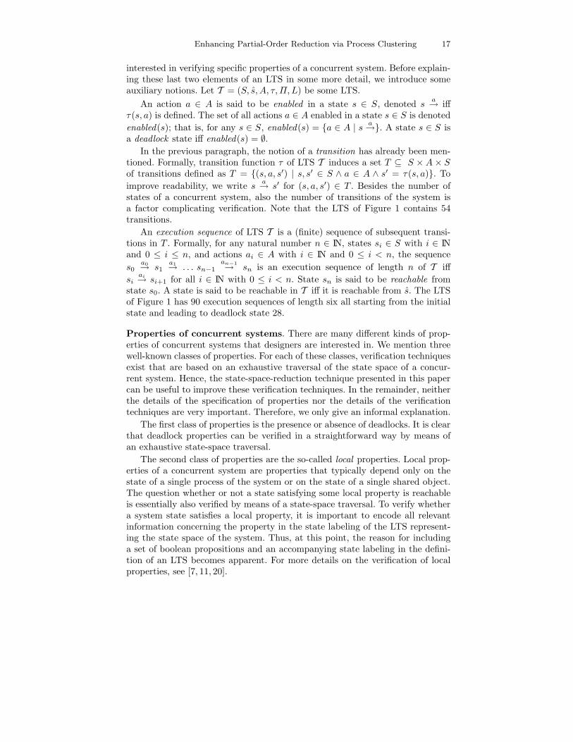
interested in verifying specific properties of a concurrent system. Before explain-ing these last two elements of an LTS in some more detail, we introduce someauxiliary notions. Let T = (S, s, A, τ,Π,L) be some LTS.
An action a ∈ A is said to be enabled in a state s ∈ S, denoted sa→ iff
τ(s, a) is defined. The set of all actions a ∈ A enabled in a state s ∈ S is denotedenabled(s); that is, for any s ∈ S, enabled(s) = {a ∈ A | s
a→}. A state s ∈ S isa deadlock state iff enabled(s) = ∅.
In the previous paragraph, the notion of a transition has already been men-tioned. Formally, transition function τ of LTS T induces a set T ⊆ S × A × Sof transitions defined as T = {(s, a, s′) | s, s′ ∈ S ∧ a ∈ A ∧ s′ = τ(s, a)}. Toimprove readability, we write s
a→ s′ for (s, a, s′) ∈ T . Besides the number ofstates of a concurrent system, also the number of transitions of the system isa factor complicating verification. Note that the LTS of Figure 1 contains 54transitions.
An execution sequence of LTS T is a (finite) sequence of subsequent transi-tions in T . Formally, for any natural number n ∈ IN, states si ∈ S with i ∈ INand 0 ≤ i ≤ n, and actions ai ∈ A with i ∈ IN and 0 ≤ i < n, the sequences0
a0→ s1a1→ . . . sn−1
an−1→ sn is an execution sequence of length n of T iffsi
ai→ si+1 for all i ∈ IN with 0 ≤ i < n. State sn is said to be reachable fromstate s0. A state is said to be reachable in T iff it is reachable from s. The LTSof Figure 1 has 90 execution sequences of length six all starting from the initialstate and leading to deadlock state 28.
Properties of concurrent systems. There are many different kinds of prop-erties of concurrent systems that designers are interested in. We mention threewell-known classes of properties. For each of these classes, verification techniquesexist that are based on an exhaustive traversal of the state space of a concur-rent system. Hence, the state-space-reduction technique presented in this papercan be useful to improve these verification techniques. In the remainder, neitherthe details of the specification of properties nor the details of the verificationtechniques are very important. Therefore, we only give an informal explanation.
The first class of properties is the presence or absence of deadlocks. It is clearthat deadlock properties can be verified in a straightforward way by means ofan exhaustive state-space traversal.
The second class of properties are the so-called local properties. Local prop-erties of a concurrent system are properties that typically depend only on thestate of a single process of the system or on the state of a single shared object.The question whether or not a state satisfying some local property is reachableis essentially also verified by means of a state-space traversal. To verify whethera system state satisfies a local property, it is important to encode all relevantinformation concerning the property in the state labeling of the LTS represent-ing the state space of the system. Thus, at this point, the reason for includinga set of boolean propositions and an accompanying state labeling in the defini-tion of an LTS becomes apparent. For more details on the verification of localproperties, see [7, 11, 20].

18 Twan Basten and Dragan Bosnacki
The third class of properties are those expressible in (next-time-free) Linear-time Temporal Logic (LTL). Also LTL properties are formulated in terms of thepropositions in an LTS. It is beyond the scope of this paper to give a formaldefinition of LTL; the interested reader is referred to [16]. The technique forverifying LTL formulae is referred to as (LTL) model checking. Again, the detailsare not important. For more information, see, for example, [12].
3 Partial-Order Reduction
Section 3.1 gives results, known from the literature on partial-order reduction(see, for example, [1, 7, 8, 11, 12, 18–22]), that are needed to prove that our reduc-tion technique preserves deadlocks, local properties, and next-time-free LTL. Sec-tion 3.2 presents the partial-order-reduction algorithm of Holzmann and Peled[12, 19]. In Section 3.3, we briefly discuss implementation issues.
3.1 Basic theoretical framework
The basic idea of state-space-reduction techniques for enhancing verification isto restrict the part of the state space of a concurrent system that is exploredduring verification in such a way that properties of interest are preserved. Thereare several types of reduction techniques. In this paper, we focus on partial-order reduction. This technique exploits the independence of properties from thepossible interleavings of the actions of the concurrent system. It uses the factthat the state-space explosion is often caused by the interleaving of independentactions of concurrently executing processes of the system (see Figure 1).
To be practically useful, a reduction of the state space of a concurrent systemmust be achieved during the traversal of the state space. This means that it mustbe decided per state which transitions, and hence which subsequent states, mustbe considered. Let T = (S, s, A, τ,Π,L) be some LTS.
Definition 2 (Reduction). For any so-called reduction function r : S → 2A,we define the (partial-order) reduction of T with respect to r as the smallest LTSTr = (Sr, sr, A, τr,Π, Lr) satisfying the following conditions:
– Sr ⊆ S, sr = s, τr ⊆ τ , and Lr = L ∩ (Sr × Π);– for every s ∈ Sr and a ∈ r(s) such that τ(s, a) is defined, τr(s, a) is defined.
Note that these two requirements imply that, for every s ∈ Sr and a ∈ A, ifτr(s, a) is defined, then also τ(s, a) is defined and τr(s, a) = τ(s, a).
It may be clear that not all reductions preserve all properties of interest. Thus,depending on the properties that a reduction must preserve, we have to defineadditional restrictions on r. To this end, we need to formally capture the notionof independence introduced earlier. Actions occurring in different processes maystill influence each other, for example, when they access global variables. Thefollowing notion of independence defines the absence of such mutual influence.

Enhancing Partial-Order Reduction via Process Clustering 19
Intuitively, two actions are independent iff, in every state where they are bothenabled, (1) the execution of one action cannot disable the other and (2) theresult of executing both actions is always the same.
Definition 3 (Independence). Actions a, b ∈ A with a �= b are independentiff, for all states s ∈ S such that s
a→ and sb→,
– τ(s, a) b→ and τ(s, b) a→, and– τ(τ(s, a), b) = τ(τ(s, b), a).
An example of independent actions are two assignments to or readings from localvariables in distinct processes. Note that two actions are trivially independentif there is no state in which they are both enabled. It is straightforward to seethat, in our running example of Figure 1, all actions are mutually independent.
The first class of properties we are interested in is the presence or absence ofdeadlocks. In order to preserve deadlock states of an LTS in a reduced LTS, thereduction function r must satisfy the following two conditions (called provisos):
– C0: r(s) = ∅ iff enabled(s) = ∅.– C1 (persistency): For any s ∈ S and execution sequence s = s0
a0→ s1a1→
. . .an−1→ sn of length n ∈ IN \ {0} such that, for all i ∈ IN with 0 ≤ i < n,
ai �∈ r(s), action an−1 is independent of all actions in r(s).
The basic idea behind the persistency proviso is that, during the state-spacetraversal, transitions caused by actions that are independent of all the actionschosen by the reduction function can be ignored.
Theorem 1 (Deadlock preservation [7, Theorem 4.3]). Let r be a reduc-tion function for LTS T that satisfies provisos C0 and C1. Any deadlock statereachable in T is also reachable in the reduced LTS Tr and vice versa.
A few remarks are in order. First, Theorem 4.3 in [7] does not state that anydeadlock reachable in a reduced LTS is also reachable in the original LTS. How-ever, this result follows immediately from proviso C0. Second, [7] uses a slightlystronger definition of independence. However, the proof of Theorem 4.3 in [7]carries over to our setting without change. Finally, observe that several authorspresented state-space-reduction algorithms that preserve deadlocks [8, 18, 20].
Consider again Figure 1. It is not difficult to define a reduction functionsatisfying provisos C0 and C1 that reduces the LTS of Figure 1 to an LTSconsisting of a single execution sequence from state 00 to state 28. Clearly, thisreduction preserves deadlock state 28.
The second class of properties we discuss is the class of local properties. Alocal property is a boolean combination of propositions in Π whose truth valuecannot be changed by two independent actions. That is, a property φ is local iff,for all states s ∈ S and independent actions a, b ∈ A such that s
a→, sb→, and φ
has different truth values in states s and τ(s, a), the truth values of φ in s and inτ(s, b) are the same. An LTS satisfies a local property φ iff there is a reachable

20 Twan Basten and Dragan Bosnacki
state that satisfies φ. Typical examples of local properties are properties thatdepend only on the state of a single process or shared object. To guarantee that areduction of a state space preserves local properties, it suffices that the reductionfunction r satisfies the following requirement (in addition to C0 and C1).
– C2 (cycle proviso): For any cycle s0a0→ s1
a1→ . . .an−1→ sn = s0 of length
n ∈ IN \ {0}, there is an i ∈ IN with 0 ≤ i < n such that r(si) = enabled(si).
Theorem 2 (Local-property preservation). Let r be a reduction functionfor LTS T satisfying provisos C0, C1, and C2. Let φ be a local property. LTS Tsatisfies φ iff the reduced LTS Tr satisfies φ.
Proviso C2 prevents the so-called “ignoring problem” identified in [20]. Infor-mally, the ignoring problem occurs when a reduction of a state space ignores theactions of an entire process. Proofs of (variants of) Theorem 2 can be found in[7, 11, 20]. In fact, these references show that proviso C2 can be weakened if oneis only interested in the preservation of local properties. The stronger provisogiven above is needed for the preservation of next-time-free LTL properties.
The third class of properties we are interested in is the class of propertiesexpressible in next-time-free LTL. For any LTL formula φ, prop(φ) is the set ofpropositions occurring in φ.
Definition 4 (Invisibility). An action a ∈ A is φ-invisible in state s ∈ S iffτ(s, a) is undefined or, for all π ∈ prop(φ), π ∈ L(s) ⇔ π ∈ L(τ(s, a)). Action ais globally φ-invisible iff it is φ-invisible for all s ∈ S.
Informally, an action is globally φ-invisible iff it cannot change the truth valueof formula φ.
Given a next-time-free LTL formula φ and assuming that a reduction functionr satisfies the following proviso in addition to C0, C1, and C2, it can be shownthat the reduced LTS satisfies φ iff the original LTS satisfies φ. For a precisedefinition of the satisfaction of an LTL formula by some LTS, see [16].
– C3 (invisibility): For any state s ∈ S, all actions in r(s) are globally φ-invisible or r(s) = enabled(s).
Theorem 3 (Next-time-free LTL preservation [19, 21]). Let r be a reduc-tion function for LTS T satisfying C0, C1, C2, and C3. Let φ be a next-time-freeLTL formula. LTS T satisfies φ iff the reduced LTS Tr satisfies φ.
3.2 The partial-order-reduction algorithm of Holzmann and Peled
Given the three theorems of the previous subsection, the challenge is to findinteresting reduction functions and efficient algorithms implementing the corre-sponding reductions. A well-known partial-order-reduction algorithm is the onedescribed in [12, 19]. The most important aspects of the algorithm are the follow-ing: (1) It is based on a depth-first search (DFS) of the state space of a concurrent

Enhancing Partial-Order Reduction via Process Clustering 21
system and (2) it uses a reduction function based on the process structure of thesystem. For the full details of the algorithm, the reader is referred to the originalreferences [12, 19]. In this paper, we concentrate on the reduction function. Tothis end, we introduce a notion of processes in our framework of LTSs.
Let T = (S, s, A, τ,Π,L) be some LTS. We assume that a given set of pro-cesses P is associated with T as follows. Each process P ∈ P is a set of actions,i.e., P ⊆ A. We require that A = ∪P∈PP and that, for all P,Q ∈ P with P �= Q,P ∩ Q = ∅. That is, the set of processes partitions the set of actions. FunctionPid : A → P yields for each action the process it is contained in. Not every par-titioning of actions yields a meaningful process structure. Concurrency withinprocesses is not allowed. Therefore, we require the following. Let a, b ∈ A witha �= b be a pair of distinct actions belonging to the same process in P. For anystate s ∈ S such that a, b ∈ enabled(s), b �∈ enabled(τ(s, a)). That is, each twoactions from a single process that are simultaneously enabled in a given statemust disable each other. Clearly, this restriction disallows concurrency withinprocesses, whereas it does allow choices.
The following definition is crucial in the formulation of the abovementionedreduction function. It depends on the class of properties one is interested in.
Definition 5 (safety). An action a ∈ A is said to be safe iff it is independentfrom any (other) action b ∈ A with Pid(b) �= Pid(a). An action a ∈ A is said tobe safe for a given next-time-free LTL formula φ iff it is independent from anyaction b ∈ A with Pid(b) �= Pid(a) and globally φ-invisible.
As mentioned, the algorithm of [12, 19] performs the reduction of the state spaceduring a DFS. A DFS uses a stack to store partially investigated states. Thereduction is obtained by defining for each state a so-called ample set. Note thatthe definition uses safety and, hence, depends on the particular class of propertiesto be verified.
Definition 6 (Reduction function ample). Let s ∈ S. Consider the set SPof processes P ∈ P such that:
– enabled(s) ∩ P �= ∅,– for all a ∈ enabled(s) ∩ P , a is safe (for some next-time-free LTL formula
φ),– and τ(s, a) is not on the DFS stack.
If SP is empty, then define ample(s) = enabled(s); otherwise, choose an arbi-trary element P of SP and define ample(s) = enabled(s) ∩ P . Set ample(s) issaid to be the ample set for s.
It is not difficult to verify that reduction function ample satisfies provisos C0through C3 given in the previous subsection. C0 follows easily from Definition6. C1 and C3 follow from the safety requirement in Definition 6. Finally, C2follows from the requirement in Definition 6 that the state resulting from theexecution of an action in the ample set cannot be on the DFS stack unless theample set consists of the entire set of enabled actions. As a result, the reductionvia ample preserves deadlocks (Theorem 1), local properties (Theorem 2), andnext-time-free LTL (Theorem 3). For more details, see [12, 19].

22 Twan Basten and Dragan Bosnacki
3.3 Implementation in SPIN
SPIN [9] is a tool supporting the automatic verification of deadlock, local, andnext-time-free LTL properties. Specifications of concurrent system are writtenin the language PROMELA. The partial-order-reduction algorithm of [12, 19]has been implemented in SPIN. To allow for the efficient computation of amplesets during a DFS, sufficient conditions for the safety of actions are derived fromthe PROMELA specification before starting the DFS (see [12]). For instance,a sufficient condition for the safety of an action that can be derived from aPROMELA specification is that it does not touch any global objects such asvariables or communication channels. Another good reference for readers inter-ested in implementation issues concerning partial-order reduction is [7].
4 Cluster-based Partial-Order Reduction
We motivate our improvement of partial-order reduction by means of two differ-ent specifications of the same concurrent system given in Figure 2. Specificationexample1 has two global variables and four processes, each of them executinga single action assigning a value to one of these variables. Clearly, none of theactions is independent of all the other actions, which by Definition 5 means thatnone of the actions is safe. Thus, reduction function ample of Definition 6 yieldsno reduction. The interested reader could verify that the LTS corresponding tothe concurrent system has 25 states and 40 transitions.
System example1
int u, v;
P0: a(u:=0);
P1: b(u:=1);
P2: c(v:=0);
P3: d(v:=1);
System example2
C0: int u;
P0: a(u:=0);
P1: b(u:=1);
C1: int v;
P2: c(v:=0);
P3: d(v:=1);
⊥⊥a b
0⊥
1⊥ 0⊥
10
1⊥
11 00 01
1011 0001
b
d
c
a
d
c
c
dc
d
Fig. 2. Two specifications of a concurrent system and a reduced state space.
Specification example2 in Figure 2 is a variant of example1 with the pro-cesses clustered in pairs. The two clusters encapsulate the dependencies betweenprocesses. As a result, all actions within one cluster are independent of all ac-tions within the other one. Our idea is to augment an LTS with a hierarchy ofclusters and to generalize Definitions 5 and 6 to clusters. Thus, it is possibleto reduce the state space of the system of Figure 2 to an LTS that includes allinterleavings of actions within clusters C0 and C1 but only a single interleavingof actions from different clusters (see Figure 2), while preserving all propertiesof interest. Let T = (S, s, A, τ,Π,L) be an LTS with processes P.

Enhancing Partial-Order Reduction via Process Clustering 23
Definition 7 (Clustering). A cluster of processes in P is simply a set ofprocesses. A clustering C ⊆ 2P of P is a set of clusters partitioning P, i.e.,P = ∪C∈CC and, for all C,D ∈ C with C �= D, C ∩ D = ∅. A clustering hier-archy H for P is a finite ordered set {C0, C1, . . . , Cn−1}, where n ∈ IN \ {0}, ofclusterings of P such that, for all i ∈ IN with 0 < i < n,
– |Ci| < |Ci−1| and– for each C ∈ Ci−1, there exists a D ∈ Ci such that C ⊆ D.
For any i ∈ IN with 0 ≤ i < n, clustering Ci is called level i of the hierarchy.Level Ci is above level Cj iff i > j; it is below Cj iff i < j.
Clearly, Definition 7 implies that each level in a clustering hierarchy is a coarsen-ing of all lower levels. Also note that the maximum number of levels in a cluster-ing hierarchy is limited by the number of processes in P. A clustering hierarchyfor example2 consisting of three levels (numbered 0, 1, and 2) is the following:{{{P0}, {P1}, {P2}, {P3}}, {C0 = {P0, P1}, C1 = {P2, P3}}, {{P0, P1, P2, P3}}}.
Let H = {C0, . . . , Cn−1}, with n ∈ IN \ {0}, be a clustering hierarchy for P.For all i ∈ IN with 0 ≤ i < n, function Cid(i) : P → Ci yields for a given processthe level-i cluster it belongs to; that is, given a process P ∈ P and level i ∈ INwith 0 ≤ i < n, Cid(i)(P ) = C with C ∈ Ci the unique cluster such that P ∈ C.
Definition 8 (Level-i safety). Let i ∈ IN with 0 ≤ i < n. Action a ∈ A islevel-i safe (for a given next-time-free LTL formula φ) iff it is independent of anyaction b ∈ A with Cid(i)(Pid(b)) �= Cid(i)(Pid(a)) (and globally φ-invisible).
In the above clustering hierarchy for example2, all actions are level-1 and (triv-ially) level-2 safe, but not level-0 safe.
Given a cluster C ⊆ P, let actions(C) = ∪P∈CP . Furthermore, for any states ∈ S, let enabled(s, C) = actions(C) ∩ enabled(s).
Definition 9 (Reduction function cample). Let s ∈ S. Let, for each levelCi ∈ H, SC i be the set of clusters C ∈ Ci such that enabled(s, C) �= ∅, forall a ∈ enabled(s, C), a is level-i safe (for some next-time-free LTL formulaφ), and τ(s, a) is not on the DFS stack. If the set SC i is empty for all levelsCi, then define cample(s) = enabled(s); otherwise, choose a level Ci such thatthe set SC i is non-empty, select an arbitrary element C of SC i, and definecample(s) = enabled(s, C).
It is interesting to observe that function ample of Definition 6 is a special caseof function cample of Definition 9 with a trivial hierarchy of only one level thatconsists of trivial clusters each containing only one process.
Theorem 4. The reduction of an LTS obtained via reduction function campleof Definition 9 preserves deadlock-, local-, and next-time-free LTL properties.
Proof. It is straightforward to prove that cample satisfies provisos C0, C1, C2,and C3 of Section 3.1. The arguments are the same as in Section 3.2, where it isargued that function ample of Definition 6 satisfies these provisos. The desiredresult follows immediately from Theorems 1, 2, and 3.

24 Twan Basten and Dragan Bosnacki
Consider again the concurrent system of Figure 2. The figure shows a reducedstate space of this system. In each state, the values of variables u and v aregiven with ⊥ meaning that a value is undefined. The sets of actions chosen ineach state are ample sets as defined by function cample of Definition 9. Thereduced state space has 13 states and 12 transitions. This means reductionsof the complete state space, consisting of 25 states and 40 transitions, of 48%in states and 70% in transitions. (Recall that standard partial-order reductionyields no reductions.)
In practice, the largest state-space reductions are obtained by choosing theample sets as small as possible. A simple way to obtain small ample sets is tosearch the levels in a clustering hierarchy for suitable clusters in increasing order.
Another practical issue is how to obtain useful clustering hierarchies. Sucha clustering should maximize the dependencies between processes within a clus-ter and minimize the dependencies between clusters. It is our aim to obtainsuch hierarchies statically, derived from the concurrent-system specification. Inthat way, we avoid the overhead of forming a hierarchy on-the-fly by inspectingdependencies between processes during the DFS. One possibility to derive a hi-erarchy in a static way is to preprocess the system specification and to clusterprocesses based on shared objects. Another option is to use the existing hierar-chical or modular structure of a specification; many contemporary specificationand modeling languages such as UML and SDL include standard hierarchicalstructuring mechanisms. A final option could be the use of advanced statisticalclustering techniques (based on run-time information) as described in [14].
5 Experiments
To validate our cluster-based reduction algorithm, we implemented a prototypeon top of the verification tool SPIN, version 3.2.4. We applied our prototypeimplementation to several examples. Since PROMELA, the input language ofSPIN, does not support modular design, we provided the clustering hierarchiesourselves (based on a straightforward informal analysis of the examples). Our fo-cus is on the generation of state spaces; we did not verify any properties. The goalof the experiments is to compare reductions in states and transitions obtained viaour algorithm with reductions obtained via SPIN’s standard partial-order reduc-tion. As may be expected, similar to standard partial-order reduction, our algo-rithm performs best for systems with a large amount of concurrency. In all cases,we observe significantly larger reductions than the ones obtained with standardpartial-order reduction. Moreover, in all cases, our algorithm reduces verificationtimes. The overhead of upgrading the standard partial-order-reduction engine ismarginalized by the gain in time because of the smaller number of generatedstates and transitions.
In the remainder, we show the results of three case studies. The experimentswere performed on a Sun Ultra-10 machine, with a 299 MHz UltraSPARC-IIiprocessor and 128 MB of main memory, running the SunOS 5.6 operating system.All the verification times are given in seconds.

Enhancing Partial-Order Reduction via Process Clustering 25
Best-case example. Our first case study consists of variants of system example2of Figure 2. The systems we verified consist of N pairs of processes and N vari-ables, each pair sharing one of these variables. The system with N=2 correspondsto system example2. Table 1 shows the obtained results, including the reduc-tions in states and transitions in percentages compared to SPIN with standardpartial-order reduction. The numbers deviate from the theoretical results givenin Section 4 due to implementation details of SPIN. SPIN adds to each processa special end transition that is independent of all other transitions. The stan-dard SPIN partial-order reduction captures the independence of these specialend transitions. Our prototype implementation takes, in addition, advantage ofthe independence of some transitions involving shared variables, as explained inSection 4. We used a hierarchy of two layers, with the nontrivial layer consistingof clusters that coincided with process pairs.
without POR standard POR cluster-based POR
N states trans time states trans time states % trans % time
2 65 108 0.1 60 76 <0.1 30 50 30 61 <0.1
3 329 784 0.1 304 480 <0.1 66 78 66 86 <0.1
4 1657 5216 0.1 1532 2908 0.1 138 91 138 95 <0.1
5 8313 32680 0.9 7688 17064 0.7 282 96 282 98 <0.1Table 1. Results for the best-case example.
Parity Computer. The second example, taken from [2], models a Parity Com-puter with a tree structure. The system consists of a root module, N clientmodules as leaves, and join modules as intermediate nodes. The system withN=4 is shown in Figure 3. The figure also shows a clustering hierarchy that isimmediately derived from the modular structure of the Parity Computer.
Client00 Client01 Client11Client10
Root
Join req1req0
Join0
ack00req00 req01
ack01
ack0Join1
ack11
ack1
req10ack10
req11
req acklevel clusters
2 {C00, C01, C10, C11,J0, J1, J}, {R}
1 {C00, C01, J0},{C10, C11, J1},{J}, {R}
0 {C00}, {C01},{C10}, {C11},{J0}, {J1}, {J}, {R}
Fig. 3. The Parity Computer

26 Twan Basten and Dragan Bosnacki
A client process starts with nondeterministically generating a bit value thatit puts into the request variable that it shares with its parent join module.Subsequently, it continuously waits for an acknowledgment from its parent. Eachtime it receives an acknowledgment, it again sends an arbitrary bit value to itsparent. A join process computes the parity (XOR) of its two inputs and transmitsit upwards to its parent, while, simultaneously, sending an acknowledgment toits children. Eventually, parity bits are delivered to the root process.
Consider again the example in Figure 3. Our cluster-based partial-order-reduction algorithm takes advantage of the fact that a join process communicateswith its parent and its children in alternating order. Because the cluster with rootJoin0 is independent of the cluster with root Join1, we can reduce the state spaceby basically serializing the transitions internal to one of these clusters with thoseinternal to the other one. SPIN’s standard reduction algorithm does not give anyreduction because all transitions involve global variables. As Table 2 shows, thereduction with cluster-based partial-order reduction is quite impressive.
standard POR cluster-based POR
N states trans time states % trans % time
4 1749 4798 0.1 1294 26 2352 51 0.1
5 7933 27012 0.8 3938 50 6775 75 0.3
6 69615 288678 10.0 21620 69 38372 86 0.6
7 320095 1213520 47.3 25228 92 44730 98 1.6
8a 2782640 15381300 621.2 30377 99 55828 >99 2.1
a Because of the large memory requirements, this experiment was performed on a SunUltra-Enterprise machine with three 248 MHz UltraSPARC-II processors and 2304MB of main memory, running the SunOS 5.5.1 operating system.
Table 2. Results for the Parity Computer.
The reduction with cluster-based partial-order reduction is slightly worse(though of the same order of magnitude) than the reduction reported in [2] forthe same examples, obtained with the Next heuristic. However, it is difficult todraw any final conclusions about the comparative efficiency of the two techniquesbased only on this one example. First, the input languages in which the modelsare specified are different, which inevitably leads to differences in the model.Second, the Parity-Computer example is one of the best cases for the Nextheuristic and, as the authors note themselves in [2], there are many examplesfor which partial-order reduction gives better results than the Next heuristic.
Concurrent Alternating-Bit Protocol. Finally, we consider the ConcurrentAlternating-Bit Protocol (CABP) of [13]. The CABP consists of six components,as depicted in Figure 4. Each component is modeled as a separate process.
The CABP uses the standard alternating-bit scheme to avoid communicationerrors. Component A fetches data from its environment and transmits this datarepeatedly through channel K until an acknowledgment is received from D.

Enhancing Partial-Order Reduction via Process Clustering 27
A K B
D L C
standard POR cluster-based POR
states trans time states % trans % time
16384 67073 3.6 12897 21 44460 34 1.1
Fig. 4. Concurrent Alternating-Bit Protocol
A does not wait for a negative response before retransmitting. Channel K isunreliable in the sense that it can corrupt or lose data. The role of B is toforward successfully received data to the environment; each correct receptionis acknowledged to C. C transmits acknowledgments repeatedly via unreliablechannel L. D receives acknowledgments from L and passes them to A.
As for the Parity Computer, also for the CABP the standard reduction al-gorithm does not produce any reduction; all transitions involve communicationsthrough global synchronous (rendez-vous) channels. The cluster-based reductionalgorithm, however, capitalizes on part of the concurrency between the systemmodules, as the results in Figure 4 show. The hierarchy consists of two levels,with nontrivial level {A}, {K,B}, {C}, and {L,D}. The implementation of Aand C is such that each action in these processes depends on both its neighbors.Thus, any other process clustering does not improve the results.
6 Conclusion
The main contribution of this paper is an enhancement of the partial-order-reduction scheme of [12, 19]. Using the inherent structure of concurrent systems,we improve the way the safety (i.e., independence and invisibility) of actionsis determined syntactically during the compilation of the system specification.The resulting ample sets may contain actions from more than one process. Al-though ample sets with actions from several processes have been considered ear-lier (e.g., [1]), to the best of our knowledge, the idea of exploiting hierarchical sys-tem structure is not present in the literature. We implemented our algorithm ontop of SPIN, by upgrading SPIN’s standard partial-order-reduction engine. Theprototype implementation has been tested on several examples known from theliterature and the obtained results are encouraging: Compared to SPIN’s stan-dard partial-order-reduction algorithm, significantly larger reductions of statespaces are obtained and verification times are decreased.
It will be interesting to see how our approach works in combination withother state-space-reduction heuristics. Following [6], it is easy to show that ourtechnique is fully compatible with symmetry reduction. The two techniques areorthogonal because they exploit different features of concurrent systems. Weagree with the conjecture in [2] that partial-order reduction (and also our en-hancement) is compatible with the Next heuristic. It seems though that cluster-based partial-order reduction and the Next heuristic are not fully orthogonal,because they capture to some extent the same redundancies in state spaces. It

28 Twan Basten and Dragan Bosnacki
is interesting to study the relation between the Next heuristic and cluster-basedpartial-order reduction in more detail.
The main task in the near future is to fully automate our implementation.In the current prototype, the clustering hierarchy and safety levels must beincluded manually. A fully automatic implementation will allow us to test theimplementation on larger, real-world examples. We also plan to take advantageof the improved partial-order reduction [10] introduced in the latest releases ofSPIN, as well as the introduction of V-Promela [15]. Another interesting topicis the study of clustering heuristics (see, e.g., [14]). Good clustering heuristicsmight actually yield better clustering hierarchies than the ones obtained from thehierarchical structure specified by a system designer. Finally, our cluster-basedalgorithm is compatible with the upgrade of SPIN’s engine for timed systemsfrom [4]. It is very likely that it can be combined with recent attempts of partial-order reduction for timed automata [3, 5, 17].
References
1. R. Alur, R.K. Brayton, T.A. Henzinger, S. Qadeer, and S.K. Rajamani. Partial-Order Reduction in Symbolic State-Space Exploration. In O. Grumberg, editor,Computer Aided Verification, CAV ’97, LNCS 1254, pages 340–351. Springer, 1997.
2. R. Alur and B.-Y. Wang. “Next” Heuristic for On-the-fly Model Checking,. InJ.C.M. Baeten and S. Mauw, editors, Concurrency Theory, CONCUR ’99, LNCS1664, pages 98–113. Springer, 1999.
3. J. Bengtsson, B. Jonsson, B. Lilius, and W. Yi. Partial Order Reductions forTimed Systems. In D. Sangiorgi and R. de Simone, editors, Concurrency Theory,CONCUR ’98, LNCS 1466, pages 485–501. Springer, 1998.
4. D. Bosnacki and D. Dams. Integrating Real Time into Spin: A Prototype Imple-mentation. In S. Budkowski, A. Cavalli, and E. Najm, editors, Formal DescriptionTechniques and Protocol Specification, Testing and Verification, FORTE/PSTV,pages 423–439. Kluwer, 1998.
5. D. Dams, R. Gerth, B. Knaack, and R. Kuiper. Partial-order Reduction Techniquesfor Real-time Model Checking. Formal Aspects of Computing, 10(5–6):469–482,1998.
6. E.A. Emerson, S. Jha, and D. Peled. Combining Partial Order and SymmtetryReductions. In E. Brinksma, editor, Tools and Algorithms for the Constructionand Analysis of Systems, TACAS ’97, LNCS 1217, pages 19–34. Springer, 1997.
7. P. Godefroid. Partial-Order Methods for the Verification of Concurrent Systems:An Approach to the State-Explosion Problem. LNCS 1032. Springer, 1996.
8. P. Godefroid and P. Wolper. Using Partial Orders for the Efficient Verification ofDeadlock Freedom and Safety Properties. In K.G. Larsen and A. Skou, editors,Computer Aided Verification, CAV ’91, LNCS 575, pages 332–342. Springer, 1991.
9. G.J. Holzmann. Design and Validation of Computer Protocols. Prentice-Hall, 1991.10. G.J. Holzmann. The Engineering of a Model Checker: The Gnu i-Protocol Case
Study Revisited. In D. Dams, R. Gerth, S. Leue, and M. Massink, editors, Theo-retical and Practical Aspects of SPIN Model Checking, LNCS 818. Springer, 1999.
11. G.J. Holzmann, P. Godefroid, and D Pirottin. Coverage Preserving ReductionStrategies for Reachability Analysis. In R.J. Linn, Jr. and M.U. Uyar, editors,Protocol Specification, Testing and Verification, XII, pages 349–363. Elsevier, 1992.

Enhancing Partial-Order Reduction via Process Clustering 29
12. G.J. Holzmann and D. Peled. An Improvement in Formal Verification. InD. Hogrefe and S. Leue, editors, Formal Descriptions Techniques VII, FORTE’94, pages 197–211. Chapman & Hall, 1995.
13. C.P.J. Koymans and J.C. Mulder. A Modular Approach to Protocol VerificationUsing Process Algebra. In J.C.M. Baeten, editor, Applications of Process Algebra,Cambridge Tracts in Theoretical Computer Science 17, pages 261–306. CambridgeUniversity Press, 1990.
14. T. Kunz and J.P. Black. Using Automatic Process Clustering for Design Re-covery and Distributed Debugging. IEEE Transactions on Software Engineering,21(6):515–527, 1995.
15. S. Leue and G.J. Holzmann. V-Promela: A Visual, Object-Oriented Languagefor Spin. In Object-Oriented Real-Time Distributed Computing, ISORC ’99, pages14–23. IEEE Computer Society Press, 1999.
16. Z. Manna and A. Pnueli. The Temporal Logic of Reactive and Concurrent Systems:Specification. Springer, 1991.
17. M. Minea. Partial Order reduction for Model Checking of Timed Automata. InJ.C.M. Baeten and S. Mauw, editors, Concurrency Theory, CONCUR ’99, LNCS1664, pages 431–446. Springer, 1999.
18. W.T. Overman. Verification of Concurrent Systems: Function and Timing. PhDthesis, UCLA, Los Angeles, California, 1981.
19. D. Peled. Combining Partial Order Reductions with On-the-fly Model Checking.In D.L. Dill, editor, Computer Aided Verification, CAV ’94, LNCS 818, pages 377–390. Springer, 1994.
20. A. Valmari. Stubborn Sets for Reduced State Space Generation. In G. Rozenberg,editor, Advances in Petri Nets 1990, LNCS 483, pages 491–515. Springer, 1991.
21. A. Valmari. A Stubborn Attack on State Explosion. Formal Methods in SystemDesign, 1:297–322, 1992.
22. B. Willems and P. Wolper. Partial-Order Methods for Model Checking: FromLinear Time to Branching Time. In Logic in Computer Science, LICS ’96, pages294–303. IEEE Computer Society Press, 1996.


3. Partial-Order Reduction in Presence ofRendez-vous Communications with Priority
Choice and Weak Fairness
This chapter is a revised version of:
D. Bosnacki, Partial-Order Reduction in Presence of Rendez-vous Com-munications with Unless Constructs and Weak Fairness, Theoretical andPractical Aspects of SPIN Model Checking, 5th and 6th InternationalSPIN Workshops, Lecture Notes in Computer Science 1680, Springer-Verlag, 1999, pp. 40–56

Partial Order Reduction in Presence ofRendez-vous Communications with Priority
Choice and Weak Fairness
Dragan Bosnacki �
Dept. of Computing Science, Eindhoven University of TechnologyPO Box 513, 5600 MB Eindhoven, The Netherlandsfax: +31 40 246 3992, e-mail: [email protected]
Abstract. If synchronizing (rendez-vous) communications are used inPromela models, the priority choice feature (unless construct) and theweak fairness algorithm are not compatible with the partial order reduc-tion algorithm used in Spin’s verifier. After identifying the wrong partialorder reduction pattern that causes both incompatibilities, we give so-lutions to these two problems. To this end we propose corrections inthe identification of the safe statements for partial order reduction and,as an alternative, we discuss corrections of the partial order reductionalgorithm.
1 Introduction
The issue of fairness is an inherent and important one in the study of concur-rency and nondeterminism, in particular in the area of verification of concurrentsystems. Since fairness is used as generic notion there is a broad taxonomyof fairness concepts. In this chapter we confine our attention to the notion ofweak fairness on the level of processes which is implemented in the Spin verifier.This means that we require that for every execution sequence of the concurrentprogram which is a composition of several processes, if some process becomescontinuously enabled at some point of time (i.e. can always execute some ofits statements), then at least one statement from that process will eventuallybe executed. This kind of fairness is most often associated with mutual exclu-sion algorithms, busy waiting, simple queue-implementations of scheduling, andresource allocation. Weak fairness will guarantee the correctness of statementslike eventually entering the critical region for every process which is continuouslytrying to do that (in the mutual exclusions) or eventually leaving the waitingqueue for each process that has entered it (in the scheduling) [10].
Partial order reduction is one of the main techniques that are used to allevi-ate the problem of state space explosion in the verification of concurrent systems
� On leave from the Institute of Informatics, Faculty of Natural Sciences and Math-ematics, University “Sts. Cyril and Methodius”, Skopje, Macedonia. Supported byEC ESPRIT LTR Project No. 23498 (VIRES).

POR in Presence of Rendez-vous 33
[20, 11, 14, 16] and it is indeed one of Spin’s main strengths. The idea is, insteadof exploring all the execution sequences of a given program, to group them inequivalence classes which consist of interleavings of independent program state-ments. Then only representatives for each equivalence class are considered. Inpractice this is realized such that from each state only a subset of the executablestatements are taken.
Combining the algorithms for model-checking under weak fairness with par-tial order reduction is a prerequisite for the verification of many interestingproperties to be feasible in practice. However, it was discovered [7] that the twoalgorithms are not compatible when rendez-vous communications occur in thePromela models. As a result, in the present implementation of Spin (version 3.3and later) the combination of weak fairness with partial order reduction whenrendez-vous are used in the models is not allowed.
Another problem with Spin’s partial order reduction in presence of rendez-vous occurs when the unless construct is used in the Promela models. Thecombination of these three Spin features is also currently forbidden. As unlessis a natural way to represent exceptions, and the latter gains more and morepopularity in modern programming languages (e.g. Java), this incompatibilitycan be a serious drawback.
Interestingly, it turns out that both incompatibilities are caused by exactlythe same pattern of wrong partial order reduction. After pointing out this incor-rect reduction pattern we propose solutions to the problems with fairness andunless. For both cases we discuss two kinds of solutions, classified according tothe two different phases of the verification in which they are implemented. Thefirst kind corrects the identifications of so called safe statements for the partialorder reduction algorithm. The marking of statements as safe is done during thecompilation of the Promela model, so we call these solutions static. The secondkind are the dynamic solutions which are applied during the exploration of thestate space and are in fact corrections of the partial order reduction algorithm.
In the next section we give the necessary preliminaries for the rest of thechapter. Section 3 is devoted to partial order reduction and the concrete al-gorithm that is used in Spin. In Section 4 we discuss the problem with theunless construct and give some solutions to overcome it. Section 5 deals withthe Spin’s weak fairness algorithm. We first present the algorithm and show itscorrectness. After locating the problem and comparing it to the priority choice(unless) case, we again propose both static and dynamic solutions. The lastsection is a summary with some considerations concerning future work.
2 Preliminaries
In this section, following [14] and [6], we give the semantics of Promela programs(models) and their verification in terms of finite labeled transition systems.
We represent the programs as collections of processes. The semantics of theprocess Pi can be represented as a labeled transition system (LTS). An LTS

34 Dragan Bosnacki
is a quadruple (Si, si, τi, Li), where Si is a finite set of states, si ∈ Si is adistinguished initial state, Li is a finite set of program statements (labels), andτi : Si × Li → 2Si is a transition function. The transition function induces theset Ri ⊆ Si × Li × Si of transitions. Every transition in Ri is the result of anexecution of a statement from the process, and (si, a, s′i) ∈ Ri iff s′i ∈ τi(si, a).We introduce a function Label that maps each transition to the correspondingstatement. For a statement a, with Pid(a) we denote the process to which abelongs. (If two syntactically identical statements belong to different processeswe consider them as different.) A statement a is enabled in some state s ∈ Si
iff there exists s′ ∈ Si such that s′ ∈ τ(s, a). In this case we also say that thetransition s
a→ s′ is enabled in s. (The enabledness (executability) of a givenstatement is obtained from the process specification according to rules that wedo not consider here.) En(a) denotes the set of states in which a is enabled.Given a state s and process p we say that p is enabled in s (we write s ∈ En(p))if there is a statement a such that Pid(a) = p and s ∈ En(a).
Now we can define the semantics of the program P that corresponds to theconcurrent execution of the processes Pi(1 ≤ i ≤ N) as an LTS which is aproduct of the labeled transition systems corresponding to the component pro-cesses. In the definition we pay a special attention to the transitions generated byrendez-vous communications. We model each such communication as an atomicsequence of a rendez-vous send statement a and a corresponding rendez-vous re-ceive statement a′. The statements a and a′ generate the consecutive transitionst and t′, respectively, such that Label(t) = a and Label(t′) = a′. To preserve theatomicity of the execution, it is required that t′ is the only outgoing tranistionfrom the intermediate global state obtained after the execution of t. The productLTS (S, s, τ, L) consists of:
– state space S =∏
1≤i≤N Si, i.e., the Cartesian product of the state spacesSi,
– initial state s = (s1, . . . , sN ),– L =
⋃1≤i≤N Li, i.e., the set of statements is the union of the statement sets
of the components,– and the transition function defined as:
1. if a is not a rendez-vous statement, then (s1, . . . , s′k, . . . , sN ) ∈
τ(s1, . . . , sk, . . . , sN , a) iff s′k ∈ τk(sk, a)2. if a is a rendez-vous send, and there is a rendez-vous receive statement
a′, such that Pid(a′) �= Pid(a), s′k ∈ τk(sk, a) and s′l ∈ τl(sl, a′), then
(a) (s1, . . . , s′k, . . . , sl, . . . , sN ) ∈ τ(s1, . . . , sk, . . . , sl, . . . , sN , a)
(b) (s1, . . . , s′k, . . . , s′l, . . . , sN ) ∈ τ(s1, . . . , s
′k, . . . , sl, . . . , sN , a′)
(c) There is no action a′′ �= a′ such that (s1, . . . , s′k, . . . , sl, . . . , sN ) ∈
En(a′′), i.e., no other statement can be interleaved with the execu-tion of receive;
A popular way to represent requirements on the program is by a linear tempo-ral logic (LTL) formula [9]. In Spin, next-time-free LTL is used, which means thatformulae may contain only boolean propositions on system states, the boolean

POR in Presence of Rendez-vous 35
operators ∧, ∨, ! (negation), and the temporal operators � (always), � (even-tually) and U (until). For verification purposes the LTL formulae are translatedinto Buchi automata.
A Buchi automaton is a tuple B = (Σ,S, ρ, s, F ), where:
– Σ is an alphabet,– S is a set of states,– ρ : S × Σ → 2S is a transition function,– s ∈ S is the initial state,– and F ⊆ S is a set of designated states called acceptance states.
A run of B over an infinite word w = a1a2 . . ., is an infinite sequence s0s1 . . . ofstates, where s0 is the initial state s and si ∈ ρ(si−1, ai), for all i ≥ 1. A runs0s1 . . . is accepting if for some s ∈ F there are infinitely many i’s such thatsi = s. The word w is accepted by B if there is an accepting run of B over w.
The transitions of the Buchi automaton that is obtained from the formulaare labeled with boolean propositions over the global system states of the LTScorresponding to the program. i.e., the alphabet Σ is a set of boolean proposi-tions.
In order to prove the satisfaction of the LTL formula by the program P , wefurther define the synchronous product of the LTS (SP , sP , τP , LP ) correspond-ing to P and the Buchi automaton A = (Σ,SA, ρ, sA, FA) obtained from thenegation of the LTL formula, to be an LTS extended with acceptance states,i.e., extended LTS (XLTS) (S, s, τ, L, F ),1 with:
– state set S = SP × SA,– initial state s = (sP , sA),– transition function τ : S × L → 2S defined as (s2P , s2A) ∈ τ(s1P , s1A, a) iff
s2P ∈ τP (s1P , a) and there is a proposition p ∈ Σ such that s2A ∈ ρ(s1A, p)and p is true in s1P ,
– set of statements L = LP ;– and a set of designated acceptance states F = {(sP , sA) | sA ∈ FA}, i.e. we
declare as acceptance states the states with second component belonging tothe acceptance set of the Buchi automaton A.
Unless stated differently, for the rest of the chapter we fix the XLTS T to bethe tuple (S, s, τ, L, F ) as defined above. With R we denote the set of transitionsof T .
An execution sequence or path is a finite or infinite sequence of subsequenttransitions, i.e., for si ∈ S, ai ∈ L, the sequence s0
a0→ s1a1→ s2 . . . is an execution
sequence in T iff siai→ si+1 ∈ R for all i ≥ 0. An infinite execution sequence is
said to be accepting iff it starts in the inital state s and there is an acceptance1 Although the proliferation of different formal models (LTS, Buchi automata, ex-
tended LTS) that are used to represent the semantics and the state space mightseem unnecessary, we use three different formal concepts in order to follow moreclosely [14] and [6], so that we will be able to reuse most of the results from thesepapers in a seamless way.

36 Dragan Bosnacki
state s ∈ F that occurs infinitely many times in the sequence. A finite executionsequence c = s0
a0→ s1a1→ . . .
an−1→ sn(n ≥ 1) is a cycle iff the start and end statescoincide, i.e. s0 = sn. Given a finite or infinite execution sequence σ = s0
a0→s1
a1→ s2 . . ., a process Pi, 1 ≤ i ≤ N , and a state sj from the execution sequence,we say that Pi is executed in σ in sj iff Pid(aj) = i. A state s is reachable iffthere exists a finite execution sequence that starts at s and ends in s. A cyclec is reachable iff there exists a state in c which is reachable. A cycle c is anacceptance cycle if it contains at least one acceptance state.
The satisfaction of the formula by the program P can now be proven byshowing that there are no accepting execution sequences of the extended LTS T .On the other hand, the existence of accepting execution sequences means thatthe formula is not satisfied. From the definition of Buchi automata and extendedLTS and following the reasoning from [6], for instance, it is straightforward toconclude that the extended LTS has an accepting execution sequence iff it hassome state s ∈ F that is reachable from the initial state and reachable fromitself (in one or more steps) [6]. Thus, we have to look for reachable acceptancecycles in the XLTS T . In the sequel we call an XLTS also a state space.
3 Partial Order Reduction
In this section we give a brief overview of the partial order reduction (POR)algorithm by Holzmann and Peled [14], that is considered throughout the chap-ter. This algorithm is also implemented in Spin. We start by rephrasing somedefinitions from [14].
The basic idea of the reduction is to restrict the part of the state space that isexplored by the DFS, in such a way that the properties of interest are preserved.To this purpose, the independence of the checked property from the possibleinterleaving of statements is exploited. More specifically, two statements a,b areallowed to be permuted precisely then, if for all sequences v,w of statements:if vabw (where juxtaposition denotes concatenation) is an accepted behavior,then vbaw is an accepted behavior as well. In practice, sufficient conditionsfor such permutability are used that can be checked locally, i.e., in a state. Forthis, a notion of “concurrency” of statements is used that captures the idea thattransitions are contributed by different, concurrently executing processes of thesystem.
We first introduce some additional terminology. Without loss of generalitywe assume that the transition function τ of the LTS representing the programis deterministic, i.e., the set τ(s, a) consits of at most one element, for any states ∈ S and any statement a ∈ L. For q ∈ En(a), let a(q) be the state which isreached by executing a in state q. Concurrent statements (i.e. statements withdifferent Pids) may still influence each other’s enabledness, whence it may not becorrect to only consider one particular order of execution from some state. Thefollowing notion of independence defines the absence of such mutual influence.Intuitively, two statements are independent if in every state where they are both

POR in Presence of Rendez-vous 37
enabled, they cannot disable each other, and are commutative, i.e., the order oftheir execution makes no difference to the resulting state.
Definition 1. The statements a and b are independent iff for all states q suchthat q ∈ En(a) and q ∈ En(b),
– a(q) ∈ En(b) and b(q) ∈ En(a), and– a(b(q)) = b(a(q)).
Statements that are not independent are called dependent.
Note that a and b are trivially independent if En(a) ∩ En(b) = ∅. An exampleof independent statements are assignments to or readings from local variables,executed by two distinct processes.
Also note that the statements a and b are considered to be independent evenif a can enable b (and vice versa). The main requirement is that the statementsdo not disable each other. This is unusual in a sense, because in the literature amore strict definition prevails that does not allow that a statement can enableanother statement (e.g. [20, 11]). The advantage of the subtlety in Definition 1is that it ensures a greater set of independent statements than the “classical”definition and consequently a better reduction of the state space. However, wemust be careful with this, because as we will see later, this feature is closelyconnected with the incompatibilities that we are discussing in this chapter.
Another reason why it may not be correct to only consider only one particularorder of execution from state s of two concurrent statements a and b is that thedifference between the intermediate states a(s) and b(s) may be observable inthe sense that it influences the property to be checked. For a given propositionp that occurs in the property (an LTL formula), and a state s, let p(s) denotethe boolean value of the proposition p in the state s. Then, a is nonobservableiff for all propositions p in the property and all states s ∈ En(a), we havep(s) = p(a(s)). The statement a is said to be safe if it is nonobservable andindependent from any other statement b for which Pid(b) �= Pid(a).
In the rest of this section we describe in a rather informal way the partialorder algorithm from [14]. For the full details about the algorithm we recommendthe original references [14, 16].
The reduction of the search space is effected during the DFS, by limiting thesearch from a state s to a subset of the transitions that are enabled in s, theso-called ample set. Such an ample set is formed in the following way: If there isa process Pi who can potentially execute2 only safe statements in s, and for alltransitions s
a→ s′ that are labeled with statements from Pi (i.e. Pid(a) = i) thestate s′ is not on the DFS stack, then the ample set consists of all the transitionsfrom this process only, i.e. all transitions t from s such that Pid(Label(t)) = i.Otherwise, the ample set consists of all enabled transitions in s.
If we now introduce the notion of ample process set, consisting of the processesthat have a transition in the ample set, then the reduced DFS algorithm isobtained by replacing in the standard DFS exploration algorithm (Fig. 1) line 4by the line2 See for more details [14].

38 Dragan Bosnacki
4 for each process i in ample process set do
Obviously the ample process set consists of either only one or all the processesin the system. In the latter case there is no reduction and the reduced searchalgorithm behaves as the standard DFS, for this particular invocation.
1 proc dfs(s)
2 add s to Statespace
3 /* for each successor s’ of s do */
4 for each process i = 1 to N do
5 nxt = all transitions enabled in s with Pid(t)=i
6 for all t in nxt do
7 s’ = successor of s via t
8 if s’ not in Statespace then
9 dfs(s’)
10 fi
11 od
12 od
13 end
Fig. 1. Standard depth first search algorithm.
It can be proven [14, 16] that one can use the reduced state space (XLTS)R(T ), obtained as discribed above, instead of the original XLTS T to check anyprogram property which is stated as an LTL formula. In [14, 16] it is shown that
Theorem 1 ( [14, 16]). There exists a reachable acceptance cycle in T iff thereexists a reachable acceptance cycle in R(T ).
The acceptance cycle in the reduced state space is detected by the cycle-checkalgorithm in Spin that we consider in more detail in Section 5.1.
The condition that all transitions from the ample set must end out of the DFSstack, the so-called “cycle proviso”, ensures that a statement that is constantlyenabled, cannot be “forgotten” by leaving it outside the ample set in a cycle oftransitions.
While the cycle proviso is clearly locally checkable during a DFS, the condi-tion that an enabled statement is safe is not, as the definition of safety requiresindependence from any concurrent statement. A sufficient condition for safetyof a statement a that can be checked locally is that a does not touch any globalvariables or channels. Indeed, it is this condition that is implemented in Spin.
However, it will turn out that one solution for our incompatibility problemswill be to refine this safety criterion.
4 The unless Construct
The unless construct is a mean for modeling exception handling routines andpriority choices. Its syntax is stmnt unless stmnt. The first (left-hand) statement

POR in Presence of Rendez-vous 39
is called normal or main, while the second (right-hand) is the escape statement.3
Semantically, the executability of the normal statement depends on the exe-cutability of the escape sequence. The escape sequence has higher priority thanthe normal statement, which means that the normal statement will be executedonly if the escape statement is not executable. Otherwise the escape statementis executed and the normal statement is ignored (skipped). This dependencebetween the two statements of unless causes problems when the partial orderreduction is used and the escape statement is a rendez-vous communication.
chan c = [0] of {bit}
active proctype A()
{
skip; c?1;
}
acive proctype B()
{
assert(false) unless c!1;
}
Fig. 2. Motivating example for unless statement.
Let us consider the motivating Promela example given in Figure 2.4 (Inthe sequel we assume that the reader is familiar with Promela.) Suppose thatboth A and B are in their starting points, i.e. A is trying to execute its skipstatement, while B is attempting to do its unless statement. Obviously thehigher priority rendez-vous send offer c!1 issued by B cannot find a matchingreceive, so the verifier should detect the assertion violation assert(false).5
However, in the reduced search this is not detected, because of the incorrectpartial order reduction. The problem with the reduction occurs because the skipstatement is not safe anymore. Namely, the criterion that a statement is safe ifit does not affect any global objects is no longer true. Because the executability
3 In general, both statements can be sequences of Promela statements. Also the unlessconstruct can be nested. The results from this chapter can be extended in a straight-forward way for this general case.
4 The example is distilled from a model made in the discrete time extension of SpinDTSpin [2]. The model was written by Victor Bos, who first drew our attention tothe possible problems with the unless statement.
5 Strictly speaking in this example we are considering a safety property that is notexpressed as an LTL formula. The equivalent formulation of the property in LTL canbe done in a straightforward way and the partial order reduction will fail because ofthe same reason as in the present case. We use this version of the example for thesake of simplicity.

40 Dragan Bosnacki
of the rendez-vous statement c?1 can be changed only because of the change ofthe location in process A (program counter), no statements are unconditionallyglobally independent according to the Definition 1.
assert(false)
assert(false)
s
s’
c!1 | c?1
c!1 | c?1skip
Fig. 3. Interdependence between the unless construct and a statement which is safein absence of unless.
The reason is depicted in Fig. 3. In the starting state described above therendez-vous send c!1 is disabled, but with the execution of skip it becomes en-abled. This means that skip has indirectly disabled assert(false) which wasenabled in the starting state. In that way skip and assert(false) are not in-dependent according to the Definition 1, because skip disables assert(false).
The problem can be solved both statically in compile time or dynamicallyduring the exploration of the state space. The dynamic solution consists of check-ing whether in a given state there is a disabled rendez-vous statement (more pre-cisely, rendez-vous send) which is part of an escape statement and in that casethe partial order reduction is not performed in the given state. The drawback ofthis solution is that it can be time consuming.
The static solution is to simply declare each statement which is followedin the process specification (proctype) by a rendez-vous communication (moreprecisely, by a rendez-vous receive) as unsafe. We use the term followed takinginto account all the cycles and jumps in the Promela specification. For example,the last statement of the body of an iteration is followed by the first statementof the body. Whether a given statement is followed by a rendez-vous can bechecked by inspecting Spin’s internal representation of the Promela program(abstract syntax tree). This can be done during the generation of the C source(pan.c) of the special purpose verifier for the program. Thus, the solution doesnot cause any time overhead during the verification. Its drawback with regardto the dynamic solution is that the reduction can be less effective because ofan unnecessary strictness. It can happen that the reduction is unnecessarilyprevented even when in the state that is considered by the DFS there is no

POR in Presence of Rendez-vous 41
disabled rendez-vous send in an unless construct or even there is no statementwith an unless construct at all.
5 Fairness
A pattern very similar to the one from the previous section that causes the partialorder reduction algorithm to fail in presence of rendez-vous communications,occurs when the weak fairness option is used in the verification. The weak fairnessalgorithm is also a very instructive example how things can become complicatedbecause of the feature interaction.
5.1 The Standard Nested Depth-First Search (NDFS) Algorithm
The weak fairness algorithm we are going to deal with is an extension of thenested depth first search (NDFS) algorithm by Courcoubetis, Vardi, Wolperand Yannakakis [6] for memory efficient verification of LTL properties. The al-gorithm is a more efficient alternative to the usual computation of the stronglyconnected components of the underlying graph for the XLTS. It is also com-patible with Spin’s bit-state hashing, which is not the case with the stronglyconnected components algorithm. We start with a brief overview of the NDFSalgorithm given in Figure 4.
The core idea of the algorithm is to extend the standard DFS of the statespace in Fig. 1 with a procedure that checks for an acceptance cycle. Thus,whenever the standard DFS is about to retract from an acceptance state, it isinterrupted and the cycle-check procedure is called. The procedure is again aDFS which is started with an acceptance state as a root (seed). If the root stateis matched within the cycle-check procedure, an acceptance cycle is reported andthe algorithm is stopped. Otherwise, the standard DFS is resumed from the pointit has been interrupted. If no cycle is found, than the property is successfullyverified.
We need to work with two copies of the state space in order to ensure thatthe second DFS does not fail to detect a cycle by cutting the search because ithas encountered a state visited already by the first DFS. To distinguish betweenstates belonging to different copes we extend the state with one bit denoting thestate space copy.
The following theorem from [6] establishes the correctness of the algorithm.
Theorem 2 ( [6]). Given an XLTS T , when started in the initial state s, thealgorithm in Fig. 4 reports a cycle iff there is a reachable acceptance cycle in T .
Note 1. An important feature of the NDFS algorithm is that any state in thesecond copy of the state space is visited in at most one of the calls to dfs2. Thisis due to the characteristic position of the call of the cycle-check procedure dfs2,namely, immediately before the recursion retracts from an acceptance state. Asshown in [6], this ensures that the part of the second copy of the state space thathas been explored by the previous calls of dfs2 can be reused in the current callof the cycle-check procedure.

42 Dragan Bosnacki
1 proc dfs1(s)
2 add {s,0} to Statespace
3 /* for each successor s’ of s do */
4 for each process i = 1 to N do
5 nxt = all transitions enabled in s with Pid(t)=i
6 for all t in nxt do
7 s’ = successor of s via t
8 if {s’,0} not in Statespace then
9 dfs1(s’)
10 fi
11 od
12 od
13 if acceptance(s) then
14 seed:={s,1};
15 dfs2(s)
16 fi
17 end
18 proc dfs2(s) /* the nested search */
19 add {s,1} to Statespace
20 /* for each successor s’ of s do */
21 for each process i = 1 to N do
22 nxt = all transitions enabled in s with Pid(t)=i
23 for all t in nxt do
24 s’ = successor of s via t
25 if {s’,1} not in Statespace then
26 dfs2(s’)
27 else
28 if {s’,1}==seed then
29 report cycle
30 fi
31 fi
32 od
33 od
34 end
Fig. 4. Nested depth first search algorithm.

POR in Presence of Rendez-vous 43
5.2 Description of the Weak Fairness Algorithm
We consider weak fairness with regard to processes, i.e. we say that a givenexecution sequence is fair if for each process that becomes continuously enabledstarting at some point in the execution sequence, a transition belonging to thisprocess is eventually executed. Formally
Definition 2. An infinite execution sequence s0a0→ s1
a1→ s2 . . . is fair iff foreach process Pl, 1 ≤ l ≤ N , the following holds: If there exists i ≥ 0 such that Pl
is enabled in sj for all j ≥ i, then there are infinitely many k ≥ i such that Pl
is executed in sk.A cycle c = s0
a0→ s1a1→ . . . sn−1
an−1→ s0 is fair iff whenever a process P isenabled in all states si, 0 ≤ i < n, then P is executed in some state sj, 0 ≤ j < n.
When model checking under fairness, we are interested only in fair acceptanceruns (sequences). This means that we require the detected cycles to be fair,i.e. each continuously enabled process along the cycle contributes at least onetransition to it.
The weak fairness (WF) algorithm we are considering here is by GerardHolzmann and it is a variant of Choueka’s flag algorithm [13]. The weak fairnessalgorithm is also implemented in Spin.
The basic idea behind the weak fairness algorithm is to apply the NDFS toan extended state space instead of the original one. The extended state space isdesigned such that to each fair acceptance cycle from the original state space,there is a corresponding acceptance cycle, which need not be fair, in the extendedstate space, and vice versa. As a consequence, the model checking can be doneon the extended state space instead on the original one.
The extended state space consists of N +2 copies of the original state space,where N is the number of processes. To distinguish between the different copiesof a same state s, we extend each state with a counter component whose valuedenotes the copy of the state space the state s belongs to. Intuitively, when thealgorithm operates in a particular copy, this means that it has reached a certainphase. Our goal is to detect a cycle that:
1. contains at least one state which is an acceptance state in the original statespace, and
2. along which each process either executes a transition or becomes disabled.
In order to treat the two cases of condition 2 uniformly, we consider that whenprocess i is disabled, it executes a special εi-transition, where 1 ≤ i ≤ N , whichdoes not change the state. The εi-transitions are labeled with the special state-ment εi. This statement differs from all other statements and only changes thestate counter component to i + 1.
We check the fulfillment of the two conditions above in a sequential manner.To this end the algorithm passes cyclically through all the copies, from 0 throughN + 1 and back to 0.6
6 As we will see shortly, the NDFS algorithm applied on the extended state spacestarts in copy 0, while the cycle checks with dfs2 begin in copy N + 1. See also thecode of the algorithm in Fig. 7.

44 Dragan Bosnacki
Schematically, the extended state space is depicted in Fig. 5. The algorithm
Pid(t) = 1
T1 TN
T
F (T )
T0TN+1
Pid(t) = N
ε0ε0
F
F
Pid(t) �= 1 Pid(t) �= N
Pid(t) =N − 1
Fig. 5. The extended state space for the weak fairness algorithm.
resides in copy 0 until an acceptance state is encountered, i.e., condition 1 isachieved. When this happens it immediately passes to copy 1. To this end weintroduce another type of special transitions, labeled with the special statementε0. Like εi-transitions, an ε0-transition too does not change the state, but onlythe counter (in this case from 0 to 1). The ε0-transitions (statements), however,do not belong to any process.
Copies 1 to N correspond to each of the processes. Intuitively, when thealgorithm operates in copy i, 1 ≤ i ≤ N , it is waiting for process i to executea transition (ordinary or ε). When in copy i process i executes a transitionthe algorithm passes to copy i + 1. Otherwise, if some other process executes atransition, the algorithm stays in copy i.
The cycle check always starts in copy N + 1. All the states in this copyare considered as acceptance states in the new extended state space. The mostimportant characteristic of the copy N+1 is that, unlike in the other copies, thereare no transitions from itself leading back to it. More precisely, each transitionthat generates a state in copy N + 1 is immediately followed by an ε0-transitionto copy 0. This is to avoid detection of acceptance cycles which might be closedby staying inside copy N + 1 and which might not satisfy conditions 1 and 2.

POR in Presence of Rendez-vous 45
From the state space structure one can see that each cycle passing throughcopy N + 1 must also pass through all the other copies. Therefore, such a cyclesatisfies conditions 1 and 2 and corresponds to a fair acceptance cycle in theoriginal state space.
In the sequel we give more formal treatment of the intuitive picture givenabove. We begin by defining the extended state space:
Definition 3. Given an XLTS T = (S, s, τ, L, F ) and processes P1, . . . , PN ,N ≥ 2, we define its (weakly) fair extension F (T ) to be the smallest XLTS(Sf , sf , τf , L ∪ {ε0, ε1 . . . εN}, Ff ), where L ∩ {ε0, ε1 . . . εN} = ∅, satisfying:
– (s, 0) ∈ Sf
– 1. if (s, 0) ∈ Sf , s �∈ F , and s′ ∈ τ(s, a) for some a ∈ L, then (s′, 0) ∈τf ((s, 0), a),
2. if (s, 0) ∈ Sf , s ∈ F , then (s, 1) ∈ τf ((s, 0), ε0),3. if (s, C) ∈ Sf , 1 ≤ C ≤ N , s′ ∈ τ(s, a), and Pid(a) �= C, than (s′, C) ∈
τf ((s, C), a),4. if (s, C) ∈ Sf , 1 ≤ C ≤ N , s′ ∈ τ(s, a), and Pid(a) = C, then (s′, C +
1) ∈ τf ((s, C), a),5. if (s, C) ∈ Sf , 1 ≤ C ≤ N , and PC is not enabled in s, then (s, C + 1) ∈
τf ((s, C), εC),6. if (s,N + 1) ∈ Sf , then (s, 0) ∈ τf ((s,N + 1), ε0).
– sf = (s, 0)– Ff = {(s,N + 1) | s ∈ S} ∩ Sf .
Pid(ε0) = 0 and Pid(εi) = i, for all 1 ≤ i ≤ N .
The algorithm which generates and explores the fair extension F (T ) is givenin Fig. 6. The pseudo-code is an extension of the standard DFS (Fig. 1) that im-plements Def. 3. Lines 2 and 3 implement case 2 of the definition (ε0-transitionsfrom copy 0 to copy 1). The recursive call of dfs changes only the counter com-ponent. Similarly, lines 5 and 6 implement case 6 (ε0-transitions from copy N +1to copy 0). cases 3, 4 and 5 are implemented in the main part of the algorithm(lines 7–19). The counter increment required in cases 4 and 5 is captured by line9. If the value of the counter C does not match the process ID i then there isno increment, which is in accord with case 3. Further, case 5 (εi-transitions) isimplemented with lines 11 and 12. The check for C == i in line 12 is to ensurethat an εi-transition is created only if the ID of the disabled process matchesthe counter component. Finally, case 0 is also implicitly captured. Namely, if thecounter component C is 0, but s is not an acceptance state in the original statespace, then lines 2 and 3 do not apply, and also there is no increment of thecounter component in line 9, because C is 0 and i ranges from 1 to N.
An obvious way to check the system under weak fairness is to first gener-ate F (T ) from T , using the algorithm from Fig. 6 and then apply the NDFSalgorithm to F (T ). Because of the efficiency reasons we will do these two stepssimultaneously, i.e., combine them in the on-the-fly algorithm given in Fig. 7.
The new version of the algorithm is obtained in an obvious way by insertingthe lines for cycle check, i.e., applying the standard NDFS scheme from Fig. 4

46 Dragan Bosnacki
1 proc dfs(s,C)
2 add {s,C} to Statespace
3 if C == 0 and acceptance(s) then
4 dfs(s,1) /* epsilon_0 move to copy 1 */
5 else if C == N+1 then
6 dfs(s,0) /* epsilon_0 move to copy 0 */
7 else
8 for each process i = 1 to N do
9 if C == i then C’ = C+1 else C’ = C fi
10 nxt = all transitions t enabled in s with Pid(t)=i
11 if nxt = empty then /* epsilon_i move */
12 if {s,C’} not in Statespace and C == i then dfs(s,C’) fi
13 else
14 for all t in nxt do
15 s’ = successor of s via t
16 if {s’,C’} not in Statespace then dfs(s’,C’) fi
17 od
18 fi
19 od
20 fi
21 end
Fig. 6. An algorithm for generating the weakly fair extension F(T).
to the exploration of F (T ) from Fig. 6. For the correctness of the algorithm wehave to show the following cycle correspondence between the original and theextended state space:
Lemma 1. There exists a reachable fair acceptance cycle in T iff there exists areachable acceptance cycle in F (T ).
Proof. Let us denote the sets of transitions of T and F (T ) with R and Rf ,respectively. Let c = s0
a0→ s1a1→ ...sn−1
an−1→ sn be a reachable fair acceptancecycle in T . We first prove by induction that for each state s in T , if s is reachable,then (s, C) in F (T ), for some C ≥ 0, is also reachable. The induction is on thelength of the shortest path(s) between the initial state s and s. For length 0the claim trivially holds, because s is the only state which is reachable via apath with length 0 and by Def. 3 the state (s, 0) is in F (T ). Assume that s isreachable from s via path of length n + 1, n ≥ 0. Then there exists a state s′
reachable through a path of length n, such that s′ a→ s ∈ R, for some a ∈ L.By the induction hypothesis there exists (s′, C ′) in F (T ) which is reachable. Wewill prove that there exists an execution sequence leading from (s′, C ′) to (s, C),C ≥ 0. We have to consider several cases, taking into account Def. 3:
(i) If 1 ≤ C ′ ≤ N , then the execution sequence consists of only one transitionwhich is implied by cases 3 and 4 (and because of the transition s′ a→ s ∈ R).
(ii) If C ′ = 0 and s′ is not an acceptance state in T , then the desired executionsequence (transition) exists because of case 1.

POR in Presence of Rendez-vous 47
1 proc dfs1(s,C)
2 add {s,C,1} to Statespace
3 if C == 0 and acceptance(s) then
4 dfs1(s,1) /* epsilon0 move to copy 1 */
5 else if C == N+1 then
6 dfs1(s,0) /* epsilon0 move to copy 0 */
7 else
8 for each process i = 1 to N do
9 if C == i then C’ = C+1 else C’ = C fi
10 nxt = all transitions t enabled in s with Pid(t)=i
11 if nxt = empty then /* epsilon move */
12 if {s,C’,1} not in Statespace and C == i then dfs1(s,C’) fi
13 else
14 for all t in nxt do
15 s’ = successor of s via t
16 if {s’,C’,1} not in Statespace then dfs1(s’,C’) fi
17 od
18 fi
19 od
20 fi
21 if acceptance((s,C)) then seed:={s,C,1}; dfs2(s,C) fi
22 end
23 proc dfs2(s,C) /* the nested search */
24 add {s,C,1} to Statespace
25 if C == 0 and acceptance(s) then
26 dfs2(s,1) /* epsilon0 move to copy 1 */
27 else if C == N+1 then
28 dfs2(s,0) /* epsilon0 move to copy 0 */
29 else
30 for each process i = 1 to N do
31 if C == i then C’ = C+1 else C’ = C fi
32 nxt = all transitions enabled in s with Pid(t)=i
33 if nxt = empty then /* epsilon move */
34 if {s,C’,1} == seed then report cycle
35 else if {s,C’,1} not in Statespace and C == i then dfs2(s,C’) fi
36 else
37 for all t in nxt do
38 s’ = successor of s via t
39 if {s’,C’,1} = seed then report cycle
40 else if {s’,C’,1} not in Statespace then dfs2(s’,C’) fi
41 od
42 fi
43 od
44 fi
45 end
Fig. 7. Weak fairness (WF) algorithm.

48 Dragan Bosnacki
(iii) If C ′ = 0 and s′ is an acceptance state in T , then, by case 2, there existsthe transition (s′, 0) ε0→ (s′, 1) and this case reduces to case (ii).
(iv) If C ′ = N + 1, by case 6 there exists the transition (s′, N + 1) ε0→ (s′, 0)and the proof boils down to case (ii) or case (iii).
We construct an acceptance cycle in F (T ) that corresponds to c, by unfoldingc according to the definition of τf (Def. 3). Without loss of generality supposethat we start at s0 by mapping it to (s0, C) ∈ F (T ) for some C ≥ 0, whoseexistence we just proved. We continue traversing c and mapping its transitions totransitions in F (T ) according to to the definition of τf . The only ambiguity thatmight occur is resolved such that case 5 from the definition of τf has priorityover case 3. More precisely, suppose we have to extend the obtained path inF (T ) from some state (s, C ′) ∈ Sf by mapping a transition s
a→ s′ ∈ R and theprocess C ′ is disabled (so, Pid(a) �= C ′). In this case we first extend the path inF (T ) with (s, C ′) εC→ (s, C ′ + 1) ∈ Rf and after that we continue the mappingof s
a→ s′. As c is fair, after several steps (bounded by N(n + 1)) we will arriveat some acceptance state (sa1 , N + 1) ∈ F (T ). According to case 6 of Def. 3,from this state we pass via an ε0-transition to (sa1 , 0). After several steps wewill encounter an acceptance state from which we pass via a ε0-transition to astate with counter value 1. The counter is increased until again some acceptancestate (sa2 , N + 1) is hit. If sa1 = sa2 , then we are done because we have closedthe desired acceptance cycle. Otherwise, we repeat the whole procedure from(sa2 , N +1). As the number of states in c is finite, we will inevitably revisit someacceptance state (sak
, N + 1) and in that way generate the corresponding cyclein F (T ).
For the other direction, observe that each acceptance cycle in F (T ) mustcontain some state (s, 0), such that s ∈ F is an acceptance state in T . Thisis because in F (T ) from an acceptance state we always pass to a state withcounter component 0 (Def. 3, case 6). From Def. 3 it is clear that the onlytransition from copy 0 is via a ε0-transition (case 2), from some state (s′, 0) suchthat s′ ∈ F . Further, it is obvious that in order to get back to the acceptancestate in copy N + 1, one has to pass through all copies from 1 to N , i.e., eachprocess contributes a transition to the cycle, or is disabled in some state. So,each acceptance cycle in F (T ) can be mapped into a fair acceptance cycle inT by simply removing the ε0- and εi-transitions and merging accordingly thestates that are connected via these. In the same way we can map any path fromthe initial state (s, 0) to some state (s, C) on the acceptance cycle in F (T ), intoa path from s to s in T , which gives the reachability of the obtained cycle inT . �
As the WF algorithm is in fact the NDFS algorithm applied to F (T ), thecorrectness of the algorithm is implied by Lemma 1 and Theorem 2, which implythe following theorem
Theorem 3. Given an XLTS T , when started in the initial state (s, 0) of F (T ),the algorithm in Fig. 7 reports a cycle iff there is a reachable fair acceptance cyclein T .

POR in Presence of Rendez-vous 49
Note 2. The WF algorithm can be optimized by eliminating ε0 and εi-transitions.In Spin there are no ε0-transitions. Also part of the εi-transitions are eliminatedand all intermediate states that are produced by the εi-transitions. However,these optimizations can be regarded as an implementational detail which is notrelevant for the discussions in this chapter.
5.3 (In)compatibility with the Partial Order Reduction Algorithm
The Motivating Counter Example. One can regard F (T ) as an ordinaryLTS by abstracting from the state structure. Thus, it is straightforward to showthat F (T ) is compatible with the partial order reduction techniques in general([16, 14, 11, 20, 18]), provided that the original set of independent statements inT is adjusted in an appropriate way. More precisely, one has to reduce the set ofindependent statements because of the εi-transitions (1 ≤ i ≤ N). Notice thatε0-transitions are not a problem because they are trivially independent of anyother action in the system. This is because a ε0-statement is always the onlyaction (transition) from a given state, i.e., it is never simultaneously enabledwith any other action (from the Def. 3, cases 2 and 6). The εi-statements canbe dependent with some of the statements that are independent in T . In whatfollows we explain the dependence and show how the compatibility of the WFalgorithm with POR in Spin can be repaired by restricting the set of independentstatements.
The incompatibility of the weak fairness algorithm with POR (because ofrendez-vous communications) was first observed by Dennis Dams on the examplein Fig. 8:
In the model from Fig. 8 the LTL formula �p, where p is defined as b == true,is not valid even under fairness. The crucial role in the incompatibility is playedby the statement x = 0 in process C. Namely, because of this statement, therendez-vous send c!1 from process B is no longer continuously enabled. Since,now there exists a fair cycle formed just by the statements from A and C, i. e.c!0; c?x; x = 0; c!0 ... along which the process B can be safely ignoredbecause it is not continuously enabled.
However, when partial order reduction was used the verifier incorrectly re-ported that the formula was valid.7 So, the aforementioned fair cycle formedby the processes A and C was not discovered. The reason for the failure is verysimilar to the one for the unless statements. Again the same pattern occurs ofa wrong partial order reduction because of the incorrect independence relation.But this time the problem is related to the εi-transitions. Recall that those tran-sitions only change the counter component C when all statements of the processP , such that Pid(P ) = C, are disabled. As illustrated in Fig. 9 the problem isagain caused by the rendez-vous statements.
With s we denote the state in the original state space in which process Cis about to execute the statement x = 0, the processes A and B are hanging on7 Note that if one tries to run the example with the recent releases of Spin an error
will be issued because of the incompatibility of fairness and partial-order reductionin models with rendez-vous operations.

50 Dragan Bosnacki
chan c =[0] of {bit};
bool b = false;
active proctype A()
{
starta:
c!0;
goto starta
}
active proctype B()
{
startb:
c!1; b = true;
goto startb
}
active proctype C()
{ bit x;
startc:
c?x; x = 0;
goto startc
}
Fig. 8. Motivating example for the fairness algorithm.
their rendez-vous sending statements, and the counter C from the WF algorithmequals the Pid of process B. Then, the statement x = 0 is no longer safe, becauseit is dependent with the statement εPid(B) (i.e. εC). Namely, because c!1 isdisabled, according to the WF algorithm the εPid(B)-statement is enabled. Afterthe execution of x = 0 the system passes to the state s′ in which c!1 becomesenabled, and consequently the εPid(B)-statement is not possible anymore. Onthe other hand in s′, after x = 0, c!1 becomes enabled and must be included inthe fair cycles. Since Spin assumes that x = 0 is safe, in the reduced search theverifier never considers the fair cycle in which process B does not contribute atransition, which is, of course, wrong.
Solution to the Compatibility Problem. There is an apparent analogywith the pattern from the unless case. By enabling a rendez-vous statement(transition) (c!1 in combination with c?x) we are preventing another transition(in this case the εPid(B) transition) which is in discord with the independencedefinition.
As in the case of the unless construct two kinds of solutions are possible. Thefirst solution is static and it is actually the same with the one for the problem
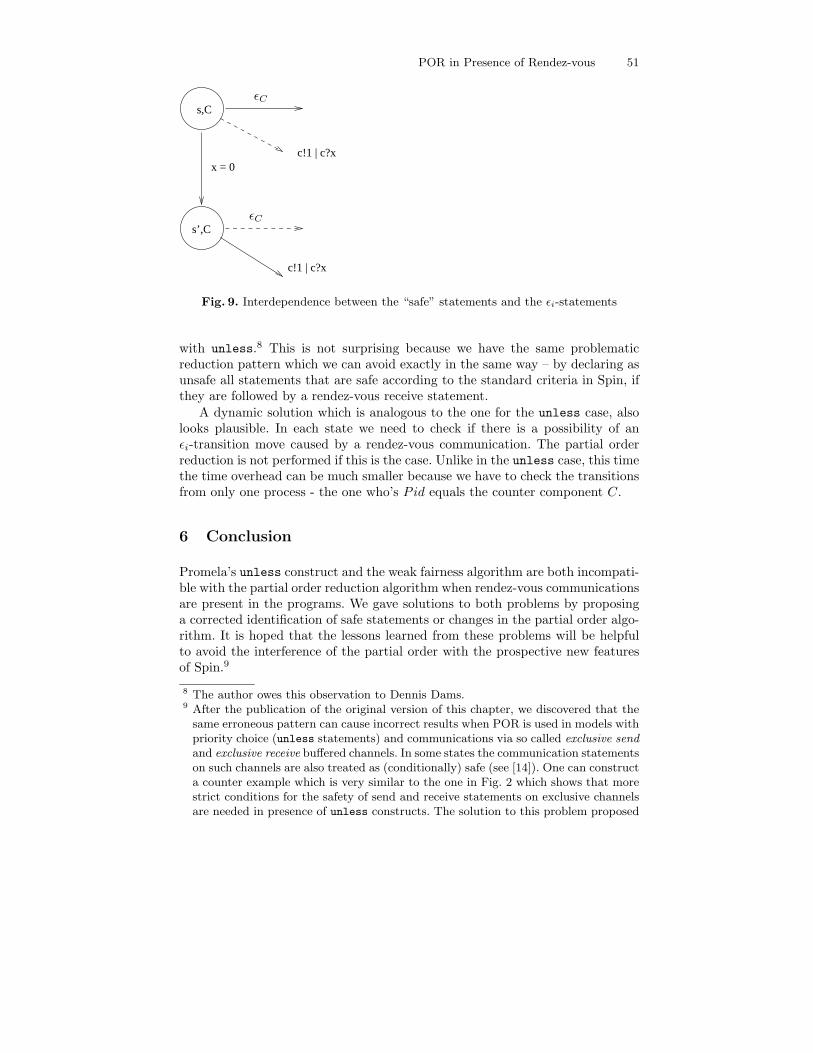
POR in Presence of Rendez-vous 51
s’,C
s,C
c!1 | c?x
c!1 | c?xx = 0
εC
εC
Fig. 9. Interdependence between the “safe” statements and the εi-statements
with unless.8 This is not surprising because we have the same problematicreduction pattern which we can avoid exactly in the same way – by declaring asunsafe all statements that are safe according to the standard criteria in Spin, ifthey are followed by a rendez-vous receive statement.
A dynamic solution which is analogous to the one for the unless case, alsolooks plausible. In each state we need to check if there is a possibility of anεi-transition move caused by a rendez-vous communication. The partial orderreduction is not performed if this is the case. Unlike in the unless case, this timethe time overhead can be much smaller because we have to check the transitionsfrom only one process - the one who’s Pid equals the counter component C.
6 Conclusion
Promela’s unless construct and the weak fairness algorithm are both incompati-ble with the partial order reduction algorithm when rendez-vous communicationsare present in the programs. We gave solutions to both problems by proposinga corrected identification of safe statements or changes in the partial order algo-rithm. It is hoped that the lessons learned from these problems will be helpfulto avoid the interference of the partial order with the prospective new featuresof Spin.9
8 The author owes this observation to Dennis Dams.9 After the publication of the original version of this chapter, we discovered that the
same erroneous pattern can cause incorrect results when POR is used in models withpriority choice (unless statements) and communications via so called exclusive sendand exclusive receive buffered channels. In some states the communication statementson such channels are also treated as (conditionally) safe (see [14]). One can constructa counter example which is very similar to the one in Fig. 2 which shows that morestrict conditions for the safety of send and receive statements on exclusive channelsare needed in presence of unless constructs. The solution to this problem proposed

52 Dragan Bosnacki
A natural task for the future work would be the implementation of the solu-tions in Spin. As a first step towards the static solution we tested successfully aprototype implementation done by modifying the Spin mechanism for labelingthe safe statements [3]. The first main problem was to find the successor of agiven statement. The major difficulty in this context was the handling of thevarious Promela jump constructs (break, goto, etc.). The second more seriousproblem was the detection whether some channel is a synchronous (rendez-vous)one. We circumvented this by treating all the channels as rendez-vous, i.e., eachstatement which is followed by a receiving statement on any channel was treatedas unsafe. Also the implementation of the first dynamic solution for the fairnessshould not be too involved.
As a final remark, the compatibility with the weak fairness algorithm can beimportant for the existing [17, 2] and future extensions of Spin with real time,especially having in mind the work of [4] about Zeno cycles in the real-timesystems.
Acknowledgments The author is grateful to Dennis Dams, Gerard Holzmann,Victor Bos and Leszek Holenderski for their valuable information and comments.
References
1. J. Bengtsson, B. Jonsson, J. Lilius, W. Yi, Partial Order Reductions for TimedSystems, CONCUR’98, LNCS 1466, pp. 485-501, 1998.
2. D. Bosnacki, D. Dams, Integrating Real Time in Spin: a Prototype Implementation,FORTE/PSTV’98, Kluwer, pp. 423-439, 1998.
3. D. Bosnacki, D. Dams, J. Orzechowski, unpublished work, 1999.4. A. Bouajjani, S. Tripakis, S. Yovine, On-the-Fly Symbolic Model-Checking for Real-
Time Systems, In Proc. of the 18th IEEE Real-Time Systems Symposium, pp.232-243, IEEE, 1997.
5. E. Clarke, E. Emerson, A. Sistla, Automatic Verification of Finite-state ConcurrentSystems Using Temporal Logic Specifications, ACM Transactions on ProgrammingLanguages and Systems, 8(2), pp. 244-263, 1986.
6. C. Courcoubetis, M. Vardi, P. Wolper, M. Yannakakis, Memory Efficient Algo-rithms for the Verification of Temporal Properties, Formal Methods in SystemDesign I, pp. 275-288, 1992.
7. D. Dams, private communication8. D. Dams, R. Gerth, B. Knaack, R. Kuiper, Partial-order Reduction Techniques for
Real-time Model Checking, FMICS’98, CWI, pp.157-170, 1998.9. E.A. Emerson, Temporal and Modal Logic, in J. van Leeuwen (ed.), Formal Models
and Semantics, Elsevier, pp. 995-1072, 1990.10. N. Francez, Fairness, Springer, 1986.11. P. Godefroid, Partial Order Methods for the Verification of Concurrents Systems:
An Approach to the State Space Explosion, LNCS 1032, Springer, 1996.12. G.J. Holzmann, Design and Validation of Communication Protocols, Prentice Hall,
1991. Also: http://netlib.bell-labs.com/netlib/spin/whatispin.html
by the author was implemented by Gerard Holzmann in the standard distributionof Spin (versions 3.3. and later).

POR in Presence of Rendez-vous 53
13. G. J. Holzmann, Personal communication, 1999.14. G. Holzmann, D. Peled, An Improvement in Formal Verification, FORTE 1994,
Bern, Switzerland, 1994.15. G. Holzmann, D. Peled, M. Yannakakis, On Nested Depth First Search, Proc. of
the 2nd Spin Workshop, Rutgers University, New Jersay, USA, 1996.16. D. Peled, Combining Partial Order Reductions with On-the-Fly Model Checking,
Computer Aided Verification 1994, LCNS 818, pp. 377-390, 1994.17. S. Tripakis, C. Courcoubetis, Extending Promela and Spin for Real Time, TACAS
’96, LCNS 1055, Springer Verlag, 1996.18. A. Valmari, Stubborn sets for reduced state space generation, Advances in Petri
Nets 1990, LNCS 483, Springer, pp. 491–515, 1991.19. M. Vardi, P. Wolper, Automata Theoretic Techniques for Modal Logics of Programs,
Journal of Computer and System Science, 32(2), pp. 182-221, 1986.20. B. Willems, P. Wolper, Partial Order Models for Model Checking: From Linear to
Branching Time, Proc. of 11 Symposium of Logics in Computer Science, LICS 96,New Brunswick, pp. 294-303, 1996.


4. Integrating Real Time into Spin: A PrototypeImplementation
This chapter is a combination of the updated versions of:
D. Bosnacki, D. Dams, Integrating Real Time into Spin: A PrototypeImplementation, Proceedings of the FORTE/PSTV XVIII Conference,Kluwer, 1998, pp. 423-439
and
D. Bosnacki, D. Dams, Discrete-Time Promela and Spin Proc. of For-mal Techniques in Real-Time and Fault-Tolerant Systems FTRTFT ’98,Lecture Notes in Computer Science 1486, Springer-Verlag, 1998, pp. 307–310

Integrating Real Time into Spin:A Prototype Implementation
Dragan Bosnacki � and Dennis Dams
Department of Mathematics and Computing Science,Eindhoven University of Technology,PO Box 513, 5600 MB Eindhoven,
The Netherlands,{dragan, wsindd}@win.tue.nl
Abstract. We present a discrete-time extension of Promela, a high levelmodelling language for the specification of concurrent systems, and theassociated Spin model checker. Our implementation is fully compatiblewith Spin’s partial order reduction algorithm, which is indeed one of itsmain strengths. The real time package is for most part orthogonal tothe other features of the tool, resulting in a modular extension. We haveevaluated it by several experiments, with encouraging results.
1 Introduction
Promela is a high level modelling language for specification of concurrent sys-tems. The models written in Promela serve as input to the Spin software packagefor their automated verification.
The time ordering of actions in a Promela program is implicit and dependson the (fixed) sequential composition of statements within each one of the com-ponent processes, as well as on the (unspecified) interleaving of statements fromdifferent processes. This time relation is only qualitative, meaning that we do notknow the exact time interval that will elapse between two events. This can be ashortcoming when systems are to be verified whose correct functioning dependson timing parameters. Many such examples can be found among communicationprotocols that have to deal with unreliable transport media, where the durationof timeout intervals is important.
In this chapter, we introduce an extension to Promela that allows to quantifythe time elapse between events, by specifying the time slice in which they occur.We describe a prototype implementation that integrates this extension into theSpin tool. Of particular concern is the compatibility of such an extension withthe partial order reduction algorithm, which is an approach to alleviate thestate-space explosion inherent in model checking, and indeed one of Spin’s mainstrengths. We prove that Spin’s partial order algorithm remains correct under the
� On leave from the Institute of Informatics, Faculty of Natural Sciences and Mathe-matics, University “Sts. Cyril and Methodius”, Skopje, Macedonia

Integrating Real Time into Spin: A Prototype Implementation 57
new timing constructs, and conduct a number of experiments that demonstrateits effectiveness.
The prototype implementation described in this chapter grew out of an earlierimplementation of discrete time in Promela and Spin [4] instigated by process al-gebra ACP [3] and clocked transition systems [18]. There, the timing constructsfrom the process algebra ACPdrt were modelled by macro definitions entirelyon the level of Promela. An advantage of such an approach is that the real-timepackage thus obtained is orthogonal to Spin: when needed, it can be incorporatedas a simple header-file inclusion, for the current and future versions of Spin. Fur-thermore, the resulting real-time extension is easily moderated, allowing to gainexperience with several alternative syntactical constructs and semantic mod-els of time, and also to study the interaction with Spin’s other features, mostnotably its partial order reduction algorithm. An obvious drawback of such a“high-level” solution is its inefficiency, which is to be avoided particularly in thecase of a model checker. The real-time extension of Promela described in thecurrent chapter still uses macro definitions for certain constructs. However, theoperation that occurs most frequently, namely the advance of time (“tick”), hasbeen implemented on a lower level, in the source code of the Spin tool.
Eventually, we envisage a more complete integration of the real-time packageinto Spin, not only regarding the level of implementation, but the integration ofreal time and partial order reduction as well. Also, the underlying mathematicalmodel will be changed from discrete to dense time. While this complicates theimplementation, it is commonly accepted (c.f. [1]) that the resulting model-checking algorithms for dense time have comparable computational complexity.Having said this, we do stress that also discrete-time models are sufficient for abroad range of practical applications [14].
A closely related development is the RT-Spin package of [25]. Although thatextension of Spin is more general in that it can model Timed Automata ([1]),with real-valued clocks, it has a number of drawbacks. The most important one isthat it is not compatible with the partial order reduction algorithm. Furthermore,Timed Automata lack a notion of urgency; instead, the fact that a transitionwith a deadline must be taken on time, has to be modelled explicitly in RT-Spin. Also, the package has not been kept up-to-date with Spin versions laterthan Version 2.0.
The extension of partial order reduction techniques to apply to real-time sys-tems has recently been studied in [21] and [20]. Other model checkers that covertimed behaviour are, e.g., UPPAAL [17], COSPAN [2], PMC [23], HyTech [13].The latter indeed is able to handle the more general class of linear hybrid sys-tems.
2 The Spin Model Checker
Promela and Spin have been developed for the analysis and verification of com-munication protocols. The language syntax is derived from C, but also uses thedenotations for communications from Hoare’s CSP and control flow statements

58 Dragan Bosnacki and Dennis Dams
based on Dijkstra’s guarded commands. The full presentation of Promela andSpin is beyond the scope of this chapter. We suggest [15] as a reference to theinterested reader; here, we only give a brief overview of Spin’s verification capa-bilities.
In Promela, system components are modeled as processes that can commu-nicate via channels either by buffered message exchanges or rendez-vous oper-ations, and also through shared memory represented as global variables. Theexecution of statements is asynchronous and interleaved, which means that inevery step only one enabled action is performed, without any assumptions of therelative speed of process executions.
Given as input a Promela model, Spin generates a C program that performsa verification of the system by scanning the state space using a depth-first search(DFS) algorithm. This way, both safety properties such as absence of deadlock,unspecified message receptions, invalid end states and assertions can be checked,as well as liveness properties such as non-progress cycles and eventual receptionof messages. The so-called never claims, which are best seen as monitoring pro-cesses that run in lock step with the rest of the system, are the most general wayto express properties in Spin. Being Buchi Automata, they can express arbitraryomega-regular properties. Spin provides an automatic translator from formulaein linear-time temporal logic (LTL) to never claims. When errors are reported,the trace of actions leading to an invalid state or cycle is saved, so that theerroneous sequence can be replayed as a guided simulation.
For large state spaces methods, Spin features state-vector compressing, partial-order reduction and bit-state hashing.
2.1 Partial Order Reduction
Partial order reduction (POR) is a technique to cope with the state explosionproblem in model-checking. We give a brief introduction to the POR algorithmthat is used in Spin, rephrasing some definitions from [16].
The basic idea of the reduction is to restrict the part of the state space that isexplored by the DFS, in such a way that the properties of interest are preserved.To this purpose, the independence of the checked property from the possibleinterleavings of statements is exploited. More specifically, two statements a,b areallowed to be permuted precisely when, if for all sequences v,w of statements:if vabw (where juxtaposition denotes concatenation) is an accepted behaviour,then vbaw is an accepted behaviour as well. In practice, sufficient conditionsfor such permutability are used that can be checked locally, i.e., in a state. Forthis, a notion of “concurrency” of statements is used that captures the idea thattransitions are contributed by different, concurrently executing processes of thesystem.
The semantics of a Promela program can be represented as a labeled transitionsystem (LTS). An LTS is a triple (S, s0, T ), where S is a finite set of states, s0
is a distinguished initial state, and T ⊆ S × S is a set of transitions. Everytransition in T is the result of executing a statement in some process of thePromela program. We introduce a function Label that maps each transition to

Integrating Real Time into Spin: A Prototype Implementation 59
the corresponding statement. For a statement a, Pid(a) denotes the processto which a belongs and En(a) denotes the set of (global) states in which a isenabled. For q ∈ En(a), a(q) is the state which is reached by executing a in stateq.
Concurrent statements (i.e. statements with different Pids) may still influ-ence each other’s enabledness, whence it may not be correct to only consider oneparticular order of execution from some state. The following notion of indepen-dence defines the absence of such mutual influence. Intuitively, two statementsare independent if in every state where they are both enabled, they cannot dis-able each other, and are commutative, i.e., the order of their execution makesno difference to the resulting state.
Definition 1. The statements a and b are independent iff for all states q suchthat q ∈ En(a) and q ∈ En(b),
– a(q) ∈ En(b) and b(q) ∈ En(a), and– a(b(q)) = b(a(q)).
Statements that are not independent are called dependent.
Note that a and b are trivially independent if En(a) ∩ En(b) = ∅. An exampleof independent statements are assignments to or readings from local variables,executed by two distinct processes.
Another reason why it may not be correct to only consider only one particularorder of execution from state s of two concurrent statements a and b is that thedifference between the intermediate states a(s) and b(s) may be observable inthe sense that it influences the property to be checked. For a given proposition pthat occurs in the property (an LTL formula), and a state s, let p(s) denote theboolean value of the proposition p in the state s. Then, a is invisible iff for allpropositions p in the property and all states s ∈ En(a), we have p(s) = p(a(s)).a is said to be safe if it is invisible and independent from any other statement bfor which Pid(b) �= Pid(a).
The reduction of the search space is now effected during the DFS, by limitingthe search from a state s to a subset of the statements that are enabled in s, theso-called ample set. Such an ample set is formed in the following way: If thereis a process which has only safe statements enabled and all those transitionslead to a state which is not on the DFS stack, then the ample set consists ofall the statements from this process only. Otherwise, the ample set consists ofall enabled statements in s. It can be proven [16, 22] that the reduced graphobtained in this way preserves the properties of the original LTS, stated as anLTL formula. The condition that all transitions from the ample set must end outof the DFS stack, the so-called “cycle proviso”, ensures that a statement that itis constantly enabled, cannot be “forgotten” by leaving it outside the ample setin a cycle of transitions.
While the cycle proviso is clearly locally checkable during a DFS, the condi-tion that an enabled statement is safe is not, as the definition of safety requiresindependence from any concurrent statement. A sufficient condition for safety

60 Dragan Bosnacki and Dennis Dams
of a statement a that can be checked locally is that a does not touch any globalvariables or channels. Indeed, it is this condition that is implemented in Spin.
3 Introducing Discrete Time in Promela and Spin
3.1 Real Time in Promela
In the discrete-time model, time is divided into slices of equal length, indexedby natural numbers. The actions are then framed into those slices, obtaining inthat way a measure for the elapsed time between events belonging to differentslices. The elapsed time between events is measured in ticks of a global digitalclock that is increased by one with every such tick. Within a slice however, weonly know the relative ordering between events, as in the time free case. Thepassage of time has the lowest priority – time can only progress if all the otherprocesses of the system have finished the execution of their actions scheduled forthe current time slice.
The example in Fig. 1 illustrates the time model. The elapsed time between
0 i i+1 i+2 i+3 i+41
A B C D
Fig. 1. Illustration of the discrete-time model.
the events A and B which happen in the i-th time slice and the events C andD which belong to i + 3rd time slice is three ticks. However we cannot measurethe time distance between A and B, or between C and D – we only know thatA precedes B and that C is before D.
In state space enumeration methods like the one used in Spin, verificationcan be regarded as checking all possible simulations of the system. In that sensethe simulation can be considered as a primitive for the validation, so we startwith the description of the discrete time implementation for simulation purposes.The basic idea is to execute the system time slice by time slice. Recalling thatthe execution of statements in Spin is asynchronous and interleaved, the basicproblem is how to avoid interleaving of actions belonging to different time slices.One way to solve this is by forcing each process to stop the execution afterit has executed all the actions for the current time slice, waiting to receive asignal that the system has passed to a new time slice. This synchronization isdone by a special “daemon” process that is not a part of the modelled systemand waits in the background to become active only when all the other processesfrom the system are blocked. This daemon process is a pacemaker that transfersthe system to the next time slice, by sending unblocking signals to the otherprocesses.
We implement this synchronization scheme by extending Promela with a newvariable type timer corresponding to discrete time countdown timers, three new

Integrating Real Time into Spin: A Prototype Implementation 61
statements set, expire and tick that operate on the new type, and a specialtiming process Timers which is the daemon process that uses ticks to decreasethe timer values. The implementation can be done entirely on user level, withoutany additional changes in the Spin source code, for example, with the followingPromela macro definitions and timer process:
#define timer int
#define set(tmr,val) (tmr=val)
#define expire(tmr) (tmr==0) /*timeout*/
#define tick(tmr) if :: tmr>=0 -> tmr=tmr-1 :: else fi
proctype Timers()
{ do :: timeout -> atomic{ tick(tmr1); tick(tmr2) } od }
The first macro defines timer as a synonym for the integer type. The setmacro sets the value of the timer tmr to val. The expire macro is a test whichbecomes true when tmr becomes 0. The tick macro is used only in the Timersprocess and it decreases the value of tmr provided that it is active, i.e., itsvalue is non-negative. Timers with negative values are considered as deactivated.Timers consists of an endless do iteration that realizes the passage of time. Itis run concurrently with the other processes of the system. The key idea of theconcept is the usage of timeout - a predefined Promela statement that becomestrue when no other statement within the system is executable. By guardingticks with timeout, we ensure that no process will proceed with an action fromthe next time slice until the other processes have executed all actions from thecurrent time slice1.
Within a process, statements are divided into time slices by putting set andexpire at the beginning and end, respectively, of each time slice. For instance,assuming that we have declared timer tmr, and that A, B and C are nonblockingPromela statements, the sequence
set(tmr,1); A; B; expire(tmr); C
means that A and B will be executed in same time slice, while C belongs tothe next time slice. The expire statement is a synchronization point where theprocess waits for tmr to become zero. This can be done only by Timers, i.e.,only when all active timers are decreased. Thus, it is guaranteed that C will beexecuted in the next time slice. In fact, set is only a labelling of the time slice(some sort of reading of the global digital clock we assumed in our time model)and it can be permuted with the statements from the time slice that it labels(in our case A and B).
Also, in cases where we have empty time slices, we optimize sequences of theform
set(tmr,1);expire(tmr);set(tmr,1);expire(tmr);...;set(tmr,1);expire(tmr);
1 There is one tick for each timer in the system, In the example above we assumedthat there are only two timers, tmr1 and tmr2. The ticks are wrapped in atomic
statement in order to avoid unwanted unblocking of some of the system processesbefore all timers are decreased.

62 Dragan Bosnacki and Dennis Dams
by set(tmr,val); expire(tmr); , where val is the number of set-expirepairs.
It is often convenient to use derived macros for modeling various delays. Forinstance, one tick delay and unbounded nondeterministic delay are implemented,by the following macros
#define delay(tmr,val) set(tmr,val); expire(tmr)
#define udelay(tmr) do :: delay(tmr,1) :: break od
In the unbounded nondeterministic delay, at each iteration a nondeterminis-tic choice is made whether the loop will be broken and the process will proceedwith the execution of a new statement, or the decision will be delayed for thenext time slice. In a similar way a nondeterministic bounded delay up to a cer-tain number of ticks, or a nondeterministic delay within lower and upper boundscan be modeled.
The expressiveness of our extended Promela is the same as the one of timedautomata interpreted in integral time (fictitious clocks, using the terminology of[1]). It is straightforward to show that using the aforementioned derived timingconstructs one can model timed automata interpreted in integral time. Con-versely, following the approach of [25], the semantics of the extended Promelacan be given via timed automata.
It is noteworthy that, because of the independence of the timing implemen-tation from the other parts of the Spin’s source code, the expressivity of thetiming framework is in fact augmented with the introduction of new features inSpin. For instance, a scheduler for several processes running on a single processorcan be modeled in a natural way like an additional master process that synchro-nizes the other processes by giving them execution permission via Promela’sprovided declarator mechanism, which was recently introduced into Spin (fromversion 3.0).
3.2 Example
In this section we show how the discrete time can be used for the specificationand verification of the Parallel Acknowledgment with Retransmission (PAR)protocol [24]. The choice of PAR was motivated by the fact that it is a relativelysimple protocol, yet it is complex enough that its correct functioning depends onthe duration of time intervals in a nontrivial way. PAR has been used in similarstudies as this one, cf. [26, 19].
PAR is one-way (simplex) data-link level protocol intended to be used overunreliable transmission channels which may corrupt or lose data. There are fourcomponents in our implementation: a sender, a receiver, data channel K andacknowledgment channel L (Fig. 2). The sender receives data from the upperlevel and sends them labeled with a sequence number that alternates between0 and 1 over the channel K. After that it waits for an acknowledgment via thechannel L. If this does not occur after some period of time, the sender times outand resends the old data. If the data are received undamaged and labelled with
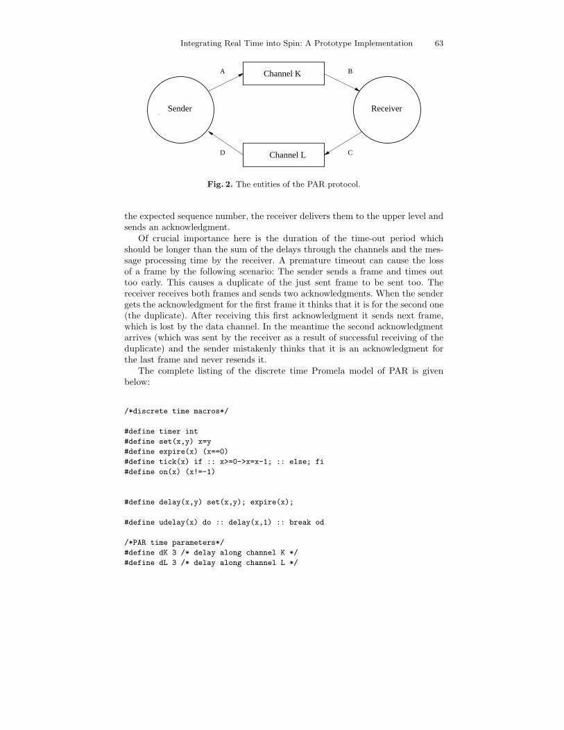
Integrating Real Time into Spin: A Prototype Implementation 63
A
D
B
CChannel L
Sender Receiver
Channel K
Fig. 2. The entities of the PAR protocol.
the expected sequence number, the receiver delivers them to the upper level andsends an acknowledgment.
Of crucial importance here is the duration of the time-out period whichshould be longer than the sum of the delays through the channels and the mes-sage processing time by the receiver. A premature timeout can cause the lossof a frame by the following scenario: The sender sends a frame and times outtoo early. This causes a duplicate of the just sent frame to be sent too. Thereceiver receives both frames and sends two acknowledgments. When the sendergets the acknowledgment for the first frame it thinks that it is for the second one(the duplicate). After receiving this first acknowledgment it sends next frame,which is lost by the data channel. In the meantime the second acknowledgmentarrives (which was sent by the receiver as a result of successful receiving of theduplicate) and the sender mistakenly thinks that it is an acknowledgment forthe last frame and never resends it.
The complete listing of the discrete time Promela model of PAR is givenbelow:
/*discrete time macros*/
#define timer int
#define set(x,y) x=y
#define expire(x) (x==0)
#define tick(x) if :: x>=0->x=x-1; :: else; fi
#define on(x) (x!=-1)
#define delay(x,y) set(x,y); expire(x);
#define udelay(x) do :: delay(x,1) :: break od
/*PAR time parameters*/
#define dK 3 /* delay along channel K */
#define dL 3 /* delay along channel L */

64 Dragan Bosnacki and Dennis Dams
#define dR 1 /* receiver’s message processing time */
#define To 9 /* sender’s timeout value */
#define MAX 8 /*max number of different message contents*/
/*timers*/
timer sc, rc, xk, xl;
proctype Timers()
{
do
:: timeout ->
atomic{tick(sc); tick(xk);
tick(rc); tick(xl);}
od;
}
/*channels*/
chan A = [0] of {byte, bit};
chan B = [0] of {byte, bit};
chan C = [0] of {bit};
chan D = [0] of {bit};
/*protocol entities*/
proctype Sender()
{
byte mt; /* message data */
bit sn=0; /* sequence number*/
R_h:
/*message can be sent in any time slice*/
udelay(sc);
mt = (mt+1)%MAX;
S_f:
A!mt,sn; /*sand through channel K*/
set(sc,To);
W_s:
do
:: D?_ ->
if
:: atomic{skip; delay(sc, 1); sn=1-sn; goto R_h;};
:: atomic{printf("MSC: ACKerr\n"); goto S_f};
fi;
:: expire(sc) -> goto S_f; /*timeout*/
od;
}
proctype Receiver()
{

Integrating Real Time into Spin: A Prototype Implementation 65
byte mr, me=1; /* received and expexted message*/
bit rsn, esn=0; /*received and expected sequence number*/
W_f:
B?mr,rsn;
if
:: rsn == esn -> goto S_h; /*correct message and seq. num */
:: rsn == 1-esn -> goto S_a; /*correct message, wrong seq. num */
:: atomic{printf("MSC: MSGerr\n");
goto W_f;};
fi;
S_h:
/*Out!mr*/
assert(mr == me);
atomic{delay(rc,dR);
/*message processing delay*/
esn = 1-esn; me = (me+1)%MAX};
S_a:
C!1; /*send ack through channel L*/
atomic{delay(rc, 1); goto W_f;};
}
/*channel processes*/
proctype K()
{
byte rd; /*received chunk*/
bit rab; /*received and expected bits*/
do
:: A?rd,rab;
delay(xk, dK);
if
:: skip; B!rd,rab;
:: skip;
fi;
od;
}
proctype L()
{
do
:: C?_;
delay(xl,dL);
if
:: skip; D!1;
:: skip;
fi;
od;
}

66 Dragan Bosnacki and Dennis Dams
init
{ atomic{set(sc,-1); set(rc,-1);
set(xk,-1); set(xl,-1);
run Timers();
run Sender();
run K();
run L();
run Receiver();}
}
The Promela model starts with the already described preamble of macros fordiscrete time.
Then, after the definition of protocol specific parameters, the timers are de-clared. There is one timer per protocol entity, i.e., for sender (sc), receiver (rc),channel K (xk) and channel L (xl). Although used locally in this model, thetimers are declared on global level in order to be accessible for Timers. The fourdefined Promela channels A, B, C and D have capacity 0 meaning that they aresynchronous rendez-vous channels. A, B, C and D are used only as auxiliary chan-nels, because the “real” unreliable channels are modeled as proctypes, i.e. as aseparate processes. The channels A and B are the input and output, respectively,to the channel K.
They deal with messages consisting of two fields — one of type byte andone of type bit, corresponding to the message contents and the alternating bit.Similarly, C and D are the input and output for L and they can carry messagescontaining just one bit — the acknowledgment.
After the declarations of local variables, the Sender process begins with anunbounded start delay of the first operation which fetches a message from theupper level (user). In our model this is simplified by allowing Sender to generatethe message itself by the statement mt = (mt+1)%MAX. The message followed bya sequence number is sent through the channel K. This event is “labeled” byan activation of the timer sc which is needed for the usual timeout mechanism(not to be confused with the timeout Promela statement) for unblocking theprotocol in case of message or acknowledgment loss. After sending the messagethe Sender blocks waiting for the arrival of an acknowledgment or the expirationof the timeout timer. In the first case a nondeterministic choice 2 is made betweensignalling an error because of a corrupted acknowledgment and accepting theacknowledgment as correct.
Receiver starts by waiting for a message. This is achieved by the statementB?mr,sn, which denotes the reception of a message through the channel B. Thereceiving statements in our implementation are treated as executable as soon aspossible, i.e. in the same slice when the corresponding sender is ready to send.After the label S h an assert is used to ensure that the received message alwaysmatches the expected one. (Note that this statement is added to the model only
2 The if statement is similar by its semantics to the do statement - a random choiceis made between the alternatives and if none of them is enabled, then the statementis blocked.

Integrating Real Time into Spin: A Prototype Implementation 67
because of validation reasons.) The message processing latency is modeled by adelay on the Receiver’s timer. Also the expected message and sequence numberare updated. Successful reception is confirmed by sending a message through L(via Promela channel C) and after a latency delay the Receiver starts waitingagain for a new message.
Channel processes model the lossy channels K and L. Both processes havethe same structure — after a delay they nondeterministically chose betweendelivering or losing the message. The skip is always executable. It is used hereto give equal precedence for both choices.
All processes are started from a special process called init via run state-ments. By enclosing the run statements within an atomic it is ensured that theystart simultaneously.
Verification of the model can be done like in the standard Spin. Among theother properties, the validator is able to find out and display the scenario oflosing a message, in case of an erroneous combination of the timing parameters.
3.3 Low Level Implementation
In order to achieve more efficiency we get down from the high-level implementa-tion to a lower level, by realizing the tick construct in the Spin’s source code.Also, the new semantics of tick is adopted so as to decrease all the timers in thesystem together. The implementation of the new statement in Spin is completelymodular and does not interfere with other features.
The timing procedure now becomes much simpler:
proctype Timers
{ do :: timeout -> tick od }
As it is universal for all models, it can be made part of the standard headerfile that contains the basic macros. Another advantage of the new tick is thatthe timers can be declared locally. Like ordinary local variables, local timerscan be dynamically created and deleted together with the processes they belongto. To the best of our knowledge this possibility is not present in any tool forvalidation of timed systems. A variable number of timers automatically meansa smaller state space, due to Spin’s variable size state representation.
The most important benefit of the local usage of timers is the partial orderreduction which is, as already emphasized, one of the main strengths of enumer-ative methods. The integration of partial order reduction with the discrete timemodel is one of the main results of this chapter and it is the topic of the nextsubsection.
3.4 Compatibility with Partial Order Reduction
In this section we prove that the partial order reduction algorithm of (standard,untimed) Spin is correct for the timed extension as well. This algorithm is basedon selecting, during the DFS exploration of the state space, only statementsfrom the ample set. The construction of an ample set is based on the notion

68 Dragan Bosnacki and Dennis Dams
of safety of statements: given a criterion to determine which statements aresafe, the underlying theory, that was presented in Section 2.1, guarantees thatthe reduction strategy is correct, i.e. that (LTL) properties are preserved. Foruntimed Spin, this criterion is that a statement does not read or write any globalvariables or channels. We will now show that this criterion is still sufficient inthe presence of timed statements.
Lemma 1. Any statement that is safe in standard, untimed Promela, remainssafe in the presence of the new timed statements set, expire, and tick. Fur-thermore, when applied to local3 timers, the statements set and expire are safe,and tick is independent from any other statement.
Proof. In order to show that a statement is safe, we have to show that it isinvisible, and independent from any concurrent statement (i.e. any statementwith a different Pid).
Let a be a statement in untimed Promela that is safe. Then it is clearly stillinvisible in timed Promela. Also, a is obviously still independent from any con-current untimed statement. a’s independence from any (“new”) timed statementthat is concurrent follows from the fact that the set of timer variables, that arethe only variables which can be read or written by timed statements, is disjointfrom the set of ordinary variables which can be affected by a.
Next, we let a be one of the statements set and expire, applied to a localtimer. a is invisible because the local timer variable may not occur in the propertyto be checked. Let b be a concurrent statement different from tick. Then ais obviously independent from b because of the disjoint sets of variables theyoperate on. Independence between tick and a, and indeed independence betweentick and any timed or untimed statement, follows from the fact that tick cannever be enabled simultaneously with another statement. This is because of theway tick is implemented: it is only enabled in the case of a timeout condition.
As tick is implemented in the Spin source code, it is not subject to reduction bythe partial order algorithm. However, this does not have any repercussions: anytick statement, regardless whether it is acting on a local or on a global timer,is the only statement that is enabled, when it is enabled at all. So, no reductionwould have been possible anyway.
3.5 Zero Cycles
In the semantics of time that we use the flow of time can be stopped if thesystem enters a so called zero cycle. A zero cycle is a cycle in the state spacethat consists of a sequence of events which does not contain the tick statement.As all the other statements in the system have priority over timeout, i.e. tick,
3 Recall that a local timer is a timer variable that is declared local to a Promelaprocess. In timed Spin, it can be manipulated by the declaring process or by thetick operation.

Integrating Real Time into Spin: A Prototype Implementation 69
the effect of such a cycle is that the Timers procedure is never activated andtime does not pass.
If one is not careful, it is quite easy to introduce zero cycles in the specifi-cations. Our experience with the SDL specification of the MASCARA protocol(which we revisit below) confirms that.
Naturally, we would like to avoid these artificial situations when the passageof time is blocked. To this end we have to be able to check for existence of zerocycles before we start the verification. We can do this by checking the systemfor the LTL formula �� timeout. The latter is a formal equivalent of the claimthat along each infinite execution sequence of the system the predicate timeoutholds infinitely often, i.e., infinitely often the tick statement is executed, whichimplies that time progresses.
4 Experimental Results
We have tested the implementation on various models known in the literature(e.g. Train Gate Controller, Seitz Circuit, Leader Election Protocol). We focusour attention on three of them that illustrate the effectiveness of the implemen-tation and in particular the partial order reduction: Fischer’s mutual exclusionprotocol, the already presented PAR protocol and the Bounded RetransmissionProtocol (BRP). We also applied the discrete-time extension to the MASCARAprotocol – a telecommunication protocol developed by the WAND (WirelessATM Network Demonstrator) consortium [9]. Besides partial order reductionwe used as an additional option minimized automata, a technique for reduc-tion of the state space recently included in the standard Spin distribution. Inthe options column of the tables below, “n”, “r” and “ma” denote verificationswithout POR, with POR, and with POR together with minimized automata,respectively.
The version of the Fischer’s protocol that was verified is a translation of thesame model written in Promela with real (dense) time of [25], with virtually thesame timing parameters. The obtained results for the verification of the mutualexclusion property are shown in Table 1 (N is the number of processes).
As expected, the state space growth is exponential and we were able tovalidate the model without using POR up to 4 processes. For 6 processes evenPOR was not enough and it had to be strengthened with minimized automata.Nevertheless, the profit from POR is obvious and even becomes more evidentas the number of processes grows. While for N = 2 the number of states isreduced to 72% compared to the case without POR, and the transitions arereduced to 56%, for N = 4 the reduction increases to 27% and 12% for statesand transitions, respectively.
It is difficult to compare our implementation with the one from [25], becausethey are based on different time models. Nevertheless, having in mind that theproperty that was checked was a qualitative one, for which discrete time suf-fices [14], one can safely say that after N = 4 our implementation has betterperformance. In fact, for N = 5 the validator from [25] runs out of memory. Ob-

70 Dragan Bosnacki and Dennis Dams
Table 1. Results for Fischer’s protocol.
N option states transitions memory [MB] time [s]
n 528 876 1.453 0.12 r 378 490 1.453 0.1
ma 378 490 0.342 0.2
n 8425 10536 1.761 0.83 r 3813 4951 1.596 0.4
ma 3813 4951 0.445 0.3
n 128286 373968 7.085 15.54 r 34157 44406 3.132 2.8
ma 34157 44406 0.650 33.7
5 r 288313 377032 17.570 36.2ma 288313 377032 1.059 332.5
6 ma 2.35e6 3.09e6 2.118 6246.1
viously, POR is the decisive factor, because without POR our implementationis also incapable to handle cases for N > 4.
In the case of the PAR protocol the reduction is very small and even dimin-ishes with the increase of parameters (Table 2).
Table 2. Results for the PAR protocol.
time parametersdK dL dR To option states transit. mem. [MB] time [s]
3 3 1 9 n 1318 1822 1.453 0.2r 1116 1533 1.493 0.3
30 30 10 90 n 7447 9994 1.761 0.5r 7295 9705 1.801 0.6
300 300 100 900 n 68737 91714 5.135 4.9r 68585 91425 5.420 4.9
ma 68585 91425 2.221 143.7
The insensitivity of PAR model to reduction can be explained by observ-ing that PAR is in fact a sequential algorithm. The protocol entities take turnsduring the execution of the protocol, most of the time only one of them beingactive while the others are waiting passively for some trigger-event. Very littleconcurrent activity results in a bad behaviour of the POR algorithm which dealswith concurrent actions from different processes. It is an opposite situation com-pared to Fischer’s protocol where the higher degree of concurrency led to animprovement of the effects of POR.
Note the sensitivity of the state space to the increase of parameter values.This sensitivity to parameters is analogous to the same effect observed in the

Integrating Real Time into Spin: A Prototype Implementation 71
region automaton implementation of the dense time system based on timed au-tomata [1, 2]. At least for the type of protocols like PAR, when the sequentialcomponent of the system is predominant, this problem can be solved by groupingtogether consecutive ticks into one tick to avoid generation of spurious interme-diate states.
The BRP protocol is a simplified version of an industry protocol used byPhilips in remote control devices. Our implementation of the protocol is basedon [8], where the protocol was treated using a combination of Uppaal (for timingaspects) and Spin (for consistency of the specification). We give the results forsafety properties (absence of deadlock and assertions). Using the same param-eters as in [8], all the properties verified there can be checked with a memoryconsumption of at most 5 Mbytes and less than a minute of CPU time. This is amuch better result than the one in [8]. In addition, our model has the advantagethat the validation is done completely within Spin.
Table 3. Results for the timed version of BRP.
option states transitions memory [MB] time [s]
n 32967 71444 4.116 6.7
r 12742 14105 2.517 3.2
ma 12742 14105 1.571 26.4
Table 4. Results for the untimed version of BRP.
option states transitions memory [MB] time [s]
n 199454 658852 7.515 37.6
r 113566 294546 5.547 19.0
The benefit of POR reduction is obvious — the number of states is reduced to39%, while the transitions are reduced to 20%. In order to get an indication howwell the partial order reduction combines with our time extension in Spin, wehave compared the above reductions for the BRP to the partial order reductionthat is achieved on a slightly different version of the protocol that does notinvolve timers (see e.g. [11] or [10]). The result is given in Table 4. The effectfor the timed version turns out to be even better: 39% and 20% versus 57% and45%. It has to be said though that in order to model the effect of timeouts inthe untimed case, we need an additional global variable, which may influencethe effects of the reduction.
The MASCARA protocol is an extension of the ATM (Asynchronous TransferMode) networking protocol to wireless networks. Our model of the protocolconsists of one static access point (AP) which communicates with several mobileterminals (MT). A more detailed description of the protocol can be found in

72 Dragan Bosnacki and Dennis Dams
Chapter 5 of this thesis. Tables 5 and 6 contain the results of deadlock check forthe case of one and two MTs, repspectively.
Table 5. Results for MASCARA with one mobile terminal.
option states transitions memory [MB] time [s]
n 17421 61151 4.712 4.6
r 8586 18293 3.106 1.5
For the case with one mobile terminal the the reduction in the number ofstates is to 50% and in the number of transitions to 30% of the correspondingfigures produced without POR. Similar remarks hold for the verification time.
Table 6. Results for MASCARA with two mobile terminals.
option states transitions memory [MB] time [s]
n > 4.99 × 10⁸ > 2.67 × 10⁹ > 20550 > 300000
r 7.24418 × 10⁷ 2.67684 × 10⁸ 3525.314 67354.172
Without POR option for the case with two MTs the machine ran out ofmemory. The reduction both in the number of states and transitions is at leastone order of magnitude.
5 Conclusions and Future Work
We presented an extension of Promela and Spin with discrete time, using in-teger variables as timers to stamp the time slices. The core idea was to use aspecial background daemon process to implement the passage of time. For thispurpose we used the Promela timeout predefined statement as a mechanism forprocess (i.e. timer) synchronization. We first showed how the concepts can beimplemented using only the existing features of Promela and Spin, by extendingthe language with new time statements as Promela macro definitions. The usageof timing features was demonstrated on the specification and validation of thePAR protocol.
As one step further toward a more efficient integration of the timing frame-work into Spin, we implemented timing on the level of the validator’s sourcecode. With this low level implementation, we gain the possibility to use thetimers locally. This allows for dynamic change of the number of timers in thesystem — a feature which to the best of the authors’ knowledge does not existin any implementation of verification of real-time systems. This is in accord withthe possibility of dynamic creation of processes already present in Spin. But, themost important benefit of the local usage of timers, and one of the main results

Integrating Real Time into Spin: A Prototype Implementation 73
of this chapter, was the adaptation of the existing partial order reduction algo-rithm to the discrete time setting. The urgency that is a necessary feature in themodeling of a broad class of interesting timing dependent systems is achievedin a natural way, without usage of invariants. The low level implementation isa seamless and completely compatible extension of the standard Spin validatorwhich allows one to use all the existing features of the untimed validator in astandard way. We showed the efficiency of the partial order reduction and theimplementation in general on several examples, of which we emphasize the veri-fication of the Bounded Retransmission Protocol and the MASCARA protocol,both originating from industry. The main future tasks will certainly be to testthe approach and accumulate experience by doing new verifications on systemsknown in the literature or some new real-world (industry) cases which are timedependent.
Besides the improvement of the existing prototype, the main direction forthe future work will be the extension of Promela and Spin with dense time,which will provide the possibility to express and verify a more general class ofproperties. The full description of the implementation will be presented in aforthcoming paper. Here we give an outline of the basic idea, assuming that thereader is familiar with the theory of timed automata (see for instance [1]). Inthe dense-time extension we consider each Promela process in the system as atimed automaton, thus, the system as a whole is then represented as a parallelcomposition of timed automata. For this purpose we have to extend Promelawith a new variable type clock whose value can be tested (compared) and/orset to zero. We are going to implement the discretizations of the timed automata,called region automata. Once we have these discretizations we can reuse the samebasic concepts from the discrete-time implementation presented in this chapter.The key idea is that to represent the time passage for the dense time one canagain use a discrete global clock which ranges over clock regions (instead overinteger valued vectors, as it was for the discrete time). The number of regions isalways finite [1] which guarantees termination of the validation procedure. Thus,the whole concept of a special procedure that implements the time passage canbe applied, like for the discrete-time case. Although there are many technicaldetails that we omit because of the space limitations, it is obvious that the sameconcept of timeout as a clock tick can be also reused to obtain an extensionwhich can be easily integrated with the other features of Spin. With regard tothe efficiency it is promising that the partial order reduction algorithm can beadapted in the same way as for discrete time [6].
It would be very interesting to incorporate the ideas about data and timeabstraction of [7] both in the existing discrete time prototype, as well as inthe future dense time implementation, in order to obtain verifications that areindependent of the concrete parameter values, and to see how general is theirapplicability.
Another promising idea is to extend the concept of a time managing pro-cess to a class of hybrid systems called discrete time rectangular automata [12].This can be done by introducing, besides timers (clocks), new time dependent

74 Dragan Bosnacki and Dennis Dams
variables and allowing the timing process to change their value also with stepsgreater than one [5].
Acknowledgments. The authors would like to thank Stavros Tripakis, Bart Knaack,and the anonymous referees for their helpful comments.
References
1. R. Alur, D.L. Dill, A Theory of Timed Automata, Theoretical Computer Science,126, pp.183-235, 1994.
2. R. Alur, R.P. Kurshan, Timing Analysis in Cospan, Hybrid Systems III, LNCS1066, pp.220-231, Springer, 1996.
3. J.C.M. Baeten, J.A. Bergstra, Discrete Time Process Algebra, Formal Aspects ofComputing 8 (2), pp. 142-148, 1991.
4. D. Bosnacki, Implementing Discrete Time in Promela and Spin, International Con-ference on Logic in Computer Science, LIRA ’97, University of Novi Sad, Yu-goslavia, 1997. (Copy also available from the author)
5. D. Bosnacki, Toward Modeling of Hybrid Systems in Promela and Spin, Proceed-ings of the 3rd International Workshop on Formal Methods for Industrial CriticalSystems FMICS’98, pp. 75-96, Amsterdam, The Netherlands, 1998.
6. D. Bosnacki, Partial Order Reduction for Region Automata (abstract), Proceed-ings of the 11th Nordic Workshop on Programming Theory NWPT’99, Uppsala,Sweden, October 1999
7. D. Dams, R. Gerth, Bounded Retransmission Protocol Revisited, Verification ofInfinite Systems, Infinity, Bologna, Italy, 1997.
8. P.R. D’Argenio, J.-P. Katoen, T. Ruys, J. Tretmans, The Bounded RetransmissionProtocol Must Be on Time!, TACAS’97, 1997.
9. T. Dravapoulos, N. Pronios, S. Denazis, et al, The Magic WAND, Deliverable 3D2,Wireless ATM MAC, 1997.
10. S. Graf, H. Saidi, Construction of Abstract State Graphs with PVS, ComputerAided Verification ’97, LCNS 1254, pp. 72-83, Springer, 1997.
11. J.F. Groote, J. van de Pol, A Bounded Retransmission Protocol for Large DataPackets, in Wirsing, M., Nivat, M., ed., Algebraic Methodology and Software Tech-nology, LCNS 1101, pp. 536-550, Springer-Verlag, 1996.
12. T.A. Henzinger, P.W. Kopke, Discrete-Time Control for Rectangular Automata, In-ternational Colloquium on Automata, Languages and Programming (ICALP 1997),LNCS 1256, pp. 582-593, Springer-Verlag, 1997.
13. T.A. Henzinger, P.-H. Ho, H. Wong-Toi, A Model Checker for Hybrid Systems,Computer Aided Verification 97, LNCS 1254, pp.460-463, Springer-Verlag,1992.
14. T.A. Henzinger, Z. Manna, A. Pnueli, What good are digital clocks?, Proceedingsof the ICALP’92, LNCS 623, pp.545-558, Springer-Verlag, 1992.
15. G.J. Holzmann, Design and Validation of Communication Protocols, Prentice Hall,1991. Also: http://netlib.bell-labs.com/netlib/spin/whatispin.html
16. G. Holzmann, D. Peled, An Improvement in Formal Verification, FORTE 1994,Bern, Switzerland, 1994.
17. K.G. Larsen, P. Pettersson, W. Yi, UPPAAL: Status & Developments, ComputerAided Verification CAV 97, LNCS 1254, pp.456-459, Springer-Verlag, 1992.
18. Y. Kesten, Z. Manna, A. Pnueli, Verifying Clocked Transition Systems, Handoutsof School on Embedded Systems, Veldhoven, The Netherlands, 1996.

Integrating Real Time into Spin: A Prototype Implementation 75
19. A.S. Klusener, Models and Axioms for a Fragment of Real Time Process Algebra,Ph.D. Thesis, Eindhoven University of Technology, 1993.
20. B. Knaack, Real-time extension of SPIN - Ongoing Research, Abstracts fromSPIN’97, Third SPIN Workshop, Twente University, Enschede, The Netherlands,1997. Also: http://netlib.bell-labs.com/netlib/spin/ws97/papers.html
21. F. Pagani, Partial Orders and Verification of Real Time Systems, Formal Tech-niques in Real Time and Fault Tolerant Systems FTRTFT 96, LNCS, Springer,1996.
22. D. Peled, Combining Partial Order Reductions with On-the-Fly Model Checking,Computer Aided Verification 1994, LCNS 818, pp. 377-390, 1994.
23. R.L. Spelberg, H. Toetenel, M. Ammerlaan, Partition Refinement in Real-TimeModel Checking Proc. of Formal Techniques in Real-Time and Fault-TolerantSystems FTRTFT ’98, LNCS 1486, pp. 143–157, Springer-Verlag, 1998.
24. A. Tanenbaum, Computer Networks, Prentice Hall, 1989.25. S. Tripakis, C. Courcoubetis, Extending Promela and Spin for Real Time, TACAS
’96, LCNS 1055, Springer Verlag, 1996.26. F. Vaandrager, Two Simple Communication Protocols, in Baeten, J.C.M., ed., Ap-
plications of Process Algebra, pp.23-44,Cambridge University Press, 1990.


5. Model Checking SDL with Spin
This chapter was priviously published as:
D. Bosnacki, D. Dams, L. Holenderski, N. Sidorova, Model CheckingSDL with Spin, Tools and Algorithms for the Construction and Analy-sis of Systems, TACAS 2000, Lecture Notes in Computer Science 1785,Springer-Verlag, 2000, pp. 363–377.
Model Checking SDL with Spin�
Dragan Bosnacki1, Dennis Dams2, Leszek Holenderski1, and Natalia Sidorova2
1 Dept. of Computing Sci., Eindhoven University of TechnologyPO Box 513, 5600 MB Eindhoven, The Netherlands
{D.Bosnacki,L.Holenderski}@tue.nl2 Dept. of Electrical Eng., Eindhoven University of Technology
PO Box 513, 5600 MB Eindhoven, The Netherlands{D.Dams,N.Sidorova}@tue.nl
Abstract. We present an attempt to use the model checker Spin as averification engine for SDL, with special emphasis put on the verifica-tion of timing properties of SDL models. We have extended Spin with afront-end that allows to translate SDL to Promela (the input languageof Spin), and a back-end that allows to analyse timing properties. Com-pared with the previous attempts, our approach allows to verify not onlyqualitative but also quantitative aspects of SDL timers, and our trans-lation of SDL to Promela handles the SDL timers in a correct way. Weapplied the toolset to the verification of a substantial part of a complexindustrial protocol. This allowed to expose several non-trivial errors inthe protocol’s design.
1 Introduction
We present an approach to automating the formal verification of SDL, by modelchecking SDL specifications with Spin. SDL [8] is a visual specification language,especially well suited for communication protocols, and quite popular in industry.Spin [5] is one of the most successful enumerative model checkers.
In order to connect the Spin verification engine to SDL, we had to extendSpin in two ways. First, we had to implement a front-end which would allow toautomatically translate SDL to Promela (the input language of Spin). Second,we had to extend Spin with the notion of discrete time, to be able to model SDLtimers. The extended version is called DT Spin and its input language is calledDT Promela (where DT stands for discrete time).
The translation of SDL to Promela is split into two steps. In the first stepwe use the sdl2if tool, implemented in Verimag, Grenoble, which transformsSDL programs to the intermediate format IF [3] that was designed for the repre-sentation of timed asynchronous systems. This first step flattens the hierarchicstructure of SDL blocks to bare processes which can then be directly transformedto Promela processes, in the second step, by our tool if2pml.
� This research has been supported by the VIRES project (Verifying Industrial Reac-tive Systems, Esprit Long Term Research Project #23498).

Model Checking SDL with Spin 79
We applied our method to the verification of a substantial part of MAS-CARA which is a complex telecommunication protocol developed by the WAND(Wireless ATM Network Demonstrator) consortium [13]. As a result, we exposedseveral non-trivial errors in the design of MASCARA.
In order to resolve the usual problems caused by the lack of the formalsemantics of SDL, we decided to rely on the semantics of SDL as determinedby the ObjectGEODE tool [11]. In particular, we assume that transitions areatomic and instantaneous, and timeout signals are not necessarily sent at thebeginning of a time slice (in other words, the timer messages are treated like othermessages, without any special priority). More details are given in Section 3.2.
We are aware of two other attempts to use Spin as a verification enginefor SDL [6, 10]. In our opinion, they were not fully successful. First, both ap-proaches tackle the qualitative aspects of SDL timers only, in the sense that theyabstract out the concrete values of timers. Our approach allows to analyze thequantitative aspects of SDL timers as well. Second, the previous approaches areincorrect, as far as the timing issues are concerned. More precisely, instead ofjust introducing more behaviours, which is unavoidable when the concrete valuesof timers are abstracted out, they simultaneously remove some of the behavioursthat are allowed by SDL, which may lead to unsound results (so called “falsepositives”). Some concrete examples are given in Section 3.3. The incorrectnessof the previous attempts also shows that taking the timing issues of SDL intoaccount, when using Spin to model check SDL, is not trivial.
We do not claim that our approach is correct, in the formal sense. Ideally,one should prove that the approach is sound (no “false positives” are possible)and complete (no “false negatives” are possible). In principle, such a correctnessresult cannot be established, due to the lack of formal semantics, both for SDLand Promela, which would be simple enough to carry such correctness proofs.However, we give some informal justification of the correctness of our approach.
We clearly separate the qualitative and quantitative aspects of SDL timers.This allows to analyze the SDL models that use timers, both in the abstractand concrete way. The two methods have their own benefits and drawbacks.In the abstract case, if DT Spin decides that some safety property holds thenthe property is true for all values of timers, and is thus time independent. Thismay be a desired feature of a model. On the other hand, proving the timeindependence may come at a price: “false negatives” are possible, in the case aproperty does depend on time. The analysis with the concrete values of timersdoes not lead to “false negatives”, but the price may be a bigger state space thatmust be enumerated by DT Spin.
We put some effort in making DT Spin a “conservative” extension of Spin:DT Promela is designed in such a way that standard Spin can be used to modelcheck DT Promela programs obtained from the SDL models with abstractedtimers. This may be useful for those who prefer to use a proven technology,instead of our experimental DT Spin.
The paper is organized as follows. In Section 2, we give an overview of Spinand DT Spin. Section 3 is devoted to the translation of SDL to DT Promela. The

80 Dragan Bosnacki, Dennis Dams, Leszek Holenderski, and Natalia Sidorova
verification method and its application to the MASCARA protocol is presentedin Sections 4 and 5. Finally, we conclude with Section 6.
2 Spin and DT Spin
2.1 Spin and Promela
Spin [5] is a software tool that supports the analysis and verification of concurrentsystems. The system descriptions are modelled in a high-level language, calledPromela. Its syntax is derived from C, and extended with Dijkstra’s guardedcommands and communication primitives from Hoare’s CSP.
In Promela, system components are specified as processes that can interacteither by message passing, via channels, or memory sharing, via global variables.The message passing can either be buffered or unbuffered (as in Hoare’s CSP).Concurrency is asynchronous (no assumptions are made on the relative speed ofprocess executions) and modelled by interleaving (in every step only one enabledaction is performed).
Given a Promela model as input, Spin generates a C program that performsa verification of the system by enumerating its state space, using a depth-firstsearch algorithm. This way, both safety properties (such as absence of deadlock,unspecified message receptions, invalid end states, and assertions) and livenessproperties (such as non-progress cycles and eventual reception of messages) canbe checked. The most general way of expressing properties in Spin is via so-callednever claims, which are best seen as monitoring processes that run in lock stepwith the rest of the system. The never claims are, in fact, Buchi Automata, andthus can express arbitrary omega-regular properties. Spin provides an automatictranslator from formulae in linear-time temporal logic (LTL) to never claims, so itcan be used as a full LTL model checker. In case the system violates a property,the trace of actions leading to an invalid state, or a cycle, is reported. Theerroneous trace can be replayed, on the Promela source, by a guided simulation.
To cope with the problem of state space explosion, Spin employs severaltechniques, such as partial-order reduction, state-vector compression, and bit-state hashing.
2.2 DT Spin and DT Promela
DT Spin [2] is an extension of Spin with discrete time. In the time model used inDT Spin, time is divided into slices indexed by natural numbers that can be seenas readings of a fictitious global digital clock that ticks at the end of each slice.The events happening in the same slice are assigned the same clock value, sothe elapsed time between events is measured in ticks. In our model, time passesonly if no other action in the system is possible.
Since concurrency is modelled by interleaving, all the events happening in onerun of a system are totally ordered and thus two events happening in the sameslice are not considered necessarily simultaneous. Instead, they are considered

Model Checking SDL with Spin 81
to be ordered, and their ordering inside one slice is determined by the orderingof the run. The properties that depend only on the ordering of events are calledqualitative while those depending on the elapsed time between events are calledquantitative.
In order to capture timing features, standard Promela is extended to DTPromela. A new data type, called timer, is introduced. It is used to declarevariables that represent discrete-time countdown timers. Three new statementsthat operate on timers are added: set(tmr,val) activates the timer tmr, byassigning the integer value val to tmr, reset(tmr) deactivates tmr, by settingit to −1, and expire(tmr) tests whether the value of tmr is 0. Initially, a timerhas value −1.
In fact, the new statements are defined as Promela macros, in a special headerfile included at the beginning of every DT Promela model:
#define timer short /* a short integer */#define set(tmr,val) tmr = val#define reset(tmr) tmr = -1#define expire(tmr) tmr == 0
The new statements allow to model a broad class of timing constraints, andother timed statements can easily be defined as Promela macros, by combiningset, reset and expire with the control flow statements offered by Promela.There is yet another operation on timers: the tick statement decreases thevalue of all active timers by 1. It is used internally by DT Spin, at the end ofevery time slice, and is not available to the user.
DT Spin is fully compatible with Spin, and all features of Spin can be usedto analyse discrete-time models. In particular, the partial order reduction algo-rithm of Spin [7, 9] had to be adapted for timed systems [2]. Besides qualitativeproperties, a broad range of quantitative properties can be verified using booleanexpressions on timer values, in the assertions and LTL formulae.
3 Translating SDL to DT Promela
The process of model checking an SDL specification is depicted in Figure 1. AnSDL specification is pushed through the pipe of translators sdl2if and if2pml,to obtain a DT Promela program that serves as input to DT Spin or Spin. Theresult of a negative verification experiment (e.g., an erroneous trace) has to bechecked manually against the SDL specification.
sdl2if translates SDL to the language IF (Intermediate Format, [3]) whichis a specification language for timed concurrent systems consisting of a fixednumber of communicating automata. IF was designed as an intermediate for-malism for connecting several industrial formal description techniques, such asLOTOS and SDL, to a number of verification tools developed in the researchcommunity.
sdl2if is implemented with the help of the SDL/API Interface provided bythe ObjectGEODE tool [11]. The current implementation of sdl2if is able to

82 Dragan Bosnacki, Dennis Dams, Leszek Holenderski, and Natalia Sidorova
sdl2if
spin
dtspin
translation translationIF
specificationSDL DT Promela
if2pml
Fig. 1. The tools used in the verification.
translate a substantial subset of SDL. The only essential omissions are dynami-cally created processes and abstract data types.
In the overall SDL to DT Promela translation, sdl2if resolves the hier-archical aspects of SDL by “flattening” the hierarchy of blocks down to bareprocesses and resolving appropriately the sources, destinations and priorities ofthe signals exchanged between the processes. On the way, the SDL proceduresare eliminated by inlining (when possible), and the syntactic sugar of SDL (en-abling conditions, continuous signals, the special input none) is transformed tomore primitive constructs. Moreover, some implicit constructs are made explicit(sender, offspring, parent, discarded signals). Details are given in [3].
On the other hand, if2pml performs the translation of the SDL core lan-guage, coping with issues that have more semantical flavor (like preserving theatomicity of the transitions or implementing the discard mechanism). Since IF isintended to be an intermediate language for a variety of high-level specificationformalisms, it is quite expressive. As not all of its constructs are needed for rep-resenting SDL models, if2pml only translates the subset of IF that is relevantto SDL.
IF and sdl2if were developed at Verimag, Grenoble, while if2pml and DTSpin were developed by the authors at the Eindhoven University of Technology.All the tools were developed in the framework of the VIRES project [12].
In what follows we describe the translation from IF to DT Promela in moredetail. The presentation is divided into three parts. In Section 3.1 we describehow the SDL processes (i.e., IF automata) are represented in Promela. In Sec-tion 3.2, the DT Promela representation of the SDL/IF timers is given. Finally,in Section 3.3, the abstraction from the concrete values of timers is described.
3.1 IF to Promela: Translating Automata
As in Promela, the IF models are sets of processes that communicate via buffers.This provides an almost one-to-one translation of these concepts. Also, the IFdata types can directly be translated to their Promela counterparts (with someminor restrictions on the range types).

Model Checking SDL with Spin 83
The way the SDL/IF automata are represented in Promela is fairly standard,and can be grasped by comparing the IF source given in Fig. 2 with its Promelatranslation in Fig. 3. A state is represented by a Promela label. All the outgoingtransitions are translated to the branches of the choice statement associatedwith the label. The discard mechanism is implemented via self-looping to thesame state, after reading a signal that has to be discarded in the state. Theatomicity of SDL/IF transitions is preserved by putting the if statement insidethe atomic statement.1
process proc: buffer buf;
state
state1 discard sig3, sig4 in buf
state2
...
transition
from state1 input sig1 from buf do body1 to state2;
from state1 input sig2 from buf do body2 to state3;
...
Fig. 2. A skeleton of an IF program.
proctype proc() {
state1: atomic {
if
:: buf?sig1 -> translated_body1; goto state2;
:: buf?sig2 -> translated_body2; goto state3;
...
:: buf?sig3 -> goto state1; /* discard */
:: buf?sig4 -> goto state1; /* discard */
fi
}
state2: atomic{
...
}
...
}
Fig. 3. Promela translation of the structure from Fig. 2
The implementation of if2pml is still in a prototype stage and some SDLfeatures are not supported yet. The most notable omissions are the mechanism of1 A special care is taken to correctly handle the stable and non-stable states in IF.

84 Dragan Bosnacki, Dennis Dams, Leszek Holenderski, and Natalia Sidorova
saving a signal, the dynamic creation of processes, and the abstract data types.The implementation of the save mechanism in Promela is possible, but ratherinvolved. It may lead to a substantial growth of the state space during modelchecking, and for this reason we have chosen to omit it. The dynamic processcreation is a basic feature of Promela, so it can easily be implemented oncesdl2if supports it. Finding a satisfactory solution for the abstract data typesremains a future work for both sdl2if and if2pml.
3.2 IF to DT Promela: Translating Timers
The crucial issue about time in SDL is the detection of timer expirations (time-outs). In SDL, a timer expiration results in sending a timeout pseudo-signalto the input queue of the process the timer belongs to. The timeout signal isthen handled as an ordinary signal: it is either consumed, by a transition that isguarded by the timeout signal, or discarded, in a state with no such transitions.In both cases, the corresponding timer is deactivated.
Our implementation of timers does not use such timeout signals. Instead,we associate with each SDL timer a DT Promela timer variable, and detect theexpiration of the timer by testing whether the timer variable has value 0, andthe timer is deactivated by setting the timer variable’s value to −1.
More precisely, for each timer tmr declared in an SDL process, we add a newbranch to all the choice statements associated with states (see figure 3). Assumea state, say state1, with an outgoing transition guarded by tmr. For such astate we add the branch
:: expire(tmr) -> reset(tmr); translated body1; goto state2;
If state1 has no outgoing transitions guarded by tmr, we add the branch
:: expire(tmr) -> reset(tmr); goto state1; /* discard */
It turns out that under the time semantics given below (as determined bythe ObjectGEODE tool [11]), these two approaches to timers are equivalent.However, the “variable” approach has an advantage over the “signal” approach,from the verification point of view, since it generates smaller state spaces. Inthe “signal” approach, an additional Promela process (or even several processes)would be needed, in order to generate the timeout signals in a right way. This,together with the overhead of exchanging timeout signals, increases the statespace.
In what follows, we give an informal justification of the above mentionedequivalence.
The semantics of time in SDL. Transitions are instantaneous. Time canonly progress if at least one timer is active and all SDL processes are waitingfor further input signals (i.e., all input queues are empty, except for saved sig-nals). Time progression amounts to performing a special transition that makes

Model Checking SDL with Spin 85
time increment until an active timer expires. In the sequel, we refer to the seg-ments of time separated by the special transition as time slices. (Note that timeprogression is discretized.)
With each timer there is associated a pseudo-signal and an implicit transition,called a timeout transition. When a timer expires, in some time slice, its timeouttransition becomes enabled and can be executed at any point of the time slice.The execution of this transition adds the associated pseudo-signal to the processqueue. The timeout transitions of the timers that expire simultaneously can beexecuted in any order.
If the set or reset operation is performed on a timer after its timeouttransition becomes enabled, the timeout transition is disabled. If the timer isset or reset after adding its associated pseudo-signal to the process queue, thepseudo-signal is removed from the queue.
Model equivalence. In order to justify the equivalence of the two models weneed to show that any execution sequence in the signal model can be simulatedby an execution sequence in the variable model, and vice versa. In what follows,we assume that SDL timers are never set to the special value now (i.e., our timervariables are never set to 0, explicitly), and we only concentrate on the simulationof the transitions which relate to timers, since the two models coincide on theuntimed features. There are two issues which have to be considered: the set andreset operations on timers, and the expiration of timers.
The set and reset operations coincide in the two models, so this issue doesnot cause problems. As far as the expiration of timers is concerned, it should beobvious that the time slice in which a timer expires is recognized in the sameway, in both models.
The only problematic issue is whether consuming/discarding the timeoutsignals, in the signal model, is properly simulated with our count-down timers,and vice versa. Our claim that, in fact, this is the case is based on the assumptionthat the following, more direct, translation of SDL/IF to Promela would becorrect.
Assume ts T denotes the timeout signal corresponding to timer T , in thesignal model. In order to handle the consumption of ts T like the consumptionof an ordinary signal, by an SDL/IF transition guarded by ts T, the followingbranch
:: buf?ts_T -> translated_body1; goto state2;
could be added to the Promela translation in figure 3.Similarly, in order to handle the discarding of ts T as an ordinary signal, the
following branch
:: buf?ts_T -> goto state1; /* discard */
could be added to the choice statements that corresponds to the states with nooutgoing transitions guarded by ts T.
Observe that the

86 Dragan Bosnacki, Dennis Dams, Leszek Holenderski, and Natalia Sidorova
:: expire(tmr) -> reset(tmr); ...
branches, in our real Promela code, correspond directly to the above branches.More precisely, expire(tmr) -> reset(tmr) corresponds directly to buf?ts T.Namely, expire(tmr) corresponds to the check whether ts T is in the inputqueue, and reset(tmr) corresponds to the removal of ts T from the queue.
3.3 Timer Abstraction
It turns out that standard Spin can also be used to model check a DT Promelamodel, for a property that does not depend on time. The advantage of usingSpin instead of DT Spin is that Spin usually consumes less resources than DTSpin. In order to convert a DT Promela model into a Promela model, it sufficesto change the special header file included at the beginning of every DT Promelamodel (see Section 2.2):
#define timer bool#define set(tmr,val) tmr = true#define reset(tmr) tmr = false#define expire(tmr) tmr == true
The new definitions abstract out the concrete values of active timers, byconsistently mapping them to true. The concrete value −1, which is used tomark an inactive timer, is consistently mapped to false (under the assumptionthat each timer is initialised to false). Obviously, such an abstraction is soundsince no behaviours are lost. More precisely, any behaviour with concrete timerscan be simulated with abstract timers, since the active timers are allowed toexpire nondeterministically, at any time.
This is not the case in the related approaches [6, 10], where some heuristicapproximations of the timer behaviour are used rather than a proper abstraction.The approximations do not only add some behaviours, but also lose some ofthem, as shown in the following examples.
In [6] the authors try to minimize the number of timer expirations, in theabstract system, that do not correspond to expirations in the concrete system.They take advantage of the observation that, in practice, the transitions guardedby a timer expiration are supposed to resolve the kind of deadlocks when no othertransitions except the ones triggered by timeout signals would be enabled. Thetimers are represented by processes that send the corresponding timeout signalswhen the special Promela statement timeout becomes enabled. The timeoutstatement becomes enabled when no other transition is enabled, in the system.
However, there are situations when a behaviour of the concrete system cannotbe simulated by the approximate one. Let us consider two concurrent processes,say P1 and P2, specified by the following transition systems:
P1 : • T1/A−−−→ • B/−−−→ •
P2 : • T2/B−−−→ • A/−−−→ •

Model Checking SDL with Spin 87
where T1 and T2 are timer signals, A and B are normal signals, and X/Y denotes“receive X and send Y to the other process”.
If both T1 and T2 expire simultaneously then, in the concrete system, P1 andP2 may exchange signals A and B, and both reach their final states. However,in the abstract system, one of the processes will not be able to reach its finalstate. Initially, the first transitions of both processes are enabled. If P1 performsits first transition (and thus sends A to P2), the first transition of P2 becomesdisabled. P2 must discard A, before its first transition becomes enabled again,and thus it will not be able to pass the A/ guard. Similarly, if P2 performs itsfirst transition, P1 will not be able to pass the B/ guard.
In the approximation used in [10], one pseudo-process is used to handle alltimer expirations. After each set operation this pseudo-process immediatelysends the corresponding timeout signal to the input queue of the process thatsets the timer. As a result, if an SDL process uses two timers, they can only expirein the order they are set, no matter what values they are set to. Obviously, thebehaviour in which an SDL process sets the timers T1 and T2 (in that order)to such values that T2 expires before T1 cannot be simulated by the abstractsystem.
4 Verification Methodology
The aim of this section is to present the way the real verification process isperformed. Industrial-size SDL models normally cannot be verified with existingmodel-checking tools as a whole, so the first natural task is to split a protocol intosome relatively autonomous parts of a reasonable size and apply to them compo-sitional verification. Fortunately, due to their block-structure, SDL-systems canbe usually split in a natural way without much effort.
The obtained sub-models are not self-contained, i.e. the behaviour of theirenvironment is not specified. Since Spin can only model-check closed systemswe need to close our model first. We achieve this by adding an “environment”process specified in SDL at the same hierarchy level as the extracted model itself.
The simplest possible approach is to construct an environment producing allthe “possible” behaviours but practice shows that this is not of much use inreal life. Such an environment leads to adding to the model too many erroneousbehaviours and thus one gets too many “false negatives” during model-checking.Local livelocks, cycles with non-progressing time, and non-existing deadlocksare the typical examples of those false-errors. Moreover, since many redundantbehaviours are added, this may also lead to a state explosion. Another possibilityis to construct an environment being able to send/receive a signal whenever themodelled system is ready to get/send it. Applying such an approach reduces theadded behaviours but it still adds some unwanted behaviours caused by sendingnon-realistic signal sequences.
Both these approaches are not safe: in case of adding non-progressing timecycles, we loose some behaviour of the system. So they can be considered as

88 Dragan Bosnacki, Dennis Dams, Leszek Holenderski, and Natalia Sidorova
a kind of heuristics only, that may be of some use at the first stage of systemdebugging.
A different approach is to provide an SDL-specification of the “right” envi-ronment, i.e. the one, which faithfully models the assumptions under which thecomponent was designed, giving an abstraction of a real environment. Althoughit makes the soundness of verification results dependent on the quality of theenvironment model, it usually turns out to be a practical method.
The closed SDL-model can be automatically translated into DT Promelathrough the translators sdl2if and if2pml. Then one should choose betweenverification of the concrete model with DT Spin and verification of the modelwith abstracted time in the standard Spin. First, the built-in Spin features (find-ing deadlocks and livelocks, unreachable code) are used. After correcting discov-ered structural errors, functional properties defined by a designer or drawn fromthe informal specification of the system can be verified.
It would seem obvious to verify all non-timed properties with an abstracted-time model and all timed properties with a concrete model. However, sometimesit is more convenient to verify non-timed properties with a concrete model aswell. If some functional property was proved with the abstracted-time model,it is proved for all possible values of timers. However if it was disproved, or adeadlock in the model was found, the next step is to check whether the erroneoustrace given by Spin is a real error in the system or it is a false error causedby adding erroneous behaviour either with abstracting from time or with tooabstract specification of the environment. It can happen that the property doesnot hold for the concrete model, however the erroneous trace given by Spin isone of the added behaviours. This behaviour cannot be reproduced for the SDLmodel with SDL-simulation tools and we cannot conclude whether the propertyholds or not.
One can not force Spin to give the trace from the non-added behaviours. DTSpin allows to reduce the set of added behaviours guaranteeing that timers areexpiring in the correct order. In our verification experiments we had a numberof cases when application of DT Spin, instead of Spin, gave a chance to get areal erroneous trace and disprove the property (see the next section).
5 Case Study: Verifying the MASCARA Protocol
We have applied our tools to the verification of an industrial-size communica-tion protocol called MASCARA (Mobile Access Scheme based on Contentionand Reservation for ATM), developed by the WAND (Wireless ATM NetworkDemonstrator) consortium [13]. The protocol is an extension of the ATM (Asyn-chronous Transfer Mode) networking protocol to wireless networks.
A wireless ATM network comprises of a fixed wire-based ATM network thatlinks a number of geographically distributed access points, which transparentlyextend ATM services to mobile users, via radio links operating in the 5.2 GHzfrequency band and achieving data rates of 23.5 MBits/s. The task of MAS-CARA is to mediate between the mobile users and the access points, to offer

Model Checking SDL with Spin 89
the mobile users the advantages of the standard wire-based ATM protocol: highreliability, capacity-on-demand, and service-independent transport. The trans-parent extension of ATM over radio links is a challenge, as standard ATM has notbeen designed to work in a wireless environment. The radio medium is charac-terised by a high bit error rate, the transmission mode is typically broadcast (orat least multicast) and the scarcity of available radio bandwidth calls for a timedivision duplex (i.e. half duplex) mode. All this leads to the necessity of extrafunctionality allowing to cope with these dissimilar environmental properties.
A crucial feature of MASCARA is the support of mobility. A mobile terminal(MT) can reliably communicate with an access point (AP) only within some areacalled the AP’s cell. Whenever an MT moves outside the cell of its current APit has to perform a so-called handover to an AP whose cell the MT has movedinto. A handover must be managed transparently with respect to the ATMlayer, maintaining the agreed quality of service for the current connections. Sothe protocol has to detect the need for a handover, select a candidate AP toswitch to and redirect the traffic with minimal interruption.
The protocol is too large to be automatically verified as a whole so we haveconcentrated our efforts on the verification of a substantial part called MCL(MASCARA Control). The main purpose of MCL is to support the mobilityissues. It contains 9 processes, each with up to 10 states (6 on average). Its mainfunction is to monitor the current radio link quality, gather information aboutradio link qualities of its neighbouring APs (to make a quick handover, in thecase of deterioration of the current link quality), and switch from one AP toanother (during the handover procedure).
During the first phase of the verification, several deadlocks were found.Most of them were related to improper synchronisation between various re-quest/confirm subprotocols (a component requests a service from another com-ponent and waits until the confirmation arrives that the request is either rejectedor served). The second source of deadlocks was the potential race conditions be-tween various components of MCL, due to the fully asynchronous communicationin SDL (non-blocking sending of messages). The following example describes oneof the race conditions we have found.
Most MASCARA components must be initialised before they are preparedto serve requests from other components. The components are grouped intovarious tree-like hierarchies, and the initialisation phase for a group is triggeredby sending the INIT signal to the group’s root. Each node that receives theINIT signal resends the signal to all its children. However, in such a cascadeof INIT signals there is a possible race condition: Spin found a trace in MCLwhere an already initialised component tried to immediately request a servicefrom a component that had not been initialised yet. Such a request was simplydiscarded and thus its confirmation was never sent back, leading to a deadlockin MCL.
After correcting these errors, we continued the verification, by exploitinganother useful Spin feature—unreachable code diagnosis. The analysis of theunreachable code reported by Spin revealed that some code for serving one par-

90 Dragan Bosnacki, Dennis Dams, Leszek Holenderski, and Natalia Sidorova
ticular request is never reached and thus the request for that particular servicewas never confirmed. Further analysis showed that there was a local deadlockpossible. (This local deadlock could not be discovered by Spin, in previous ex-periments, since Spin can only discover global deadlocks.)
Finally, we verified some functional properties that we derived from the in-formal specification. An example of such a property is given below.
One of the tasks of MCL is to periodically update a list that contains informa-tion about the quality of radio links with the neighbouring APs. This updatingphase is called the TI procedure. In order to judge the quality of a radio link witha particular AP, MCL must connect to that particular AP, so the connectionwith the current AP is suspended during the whole TI procedure. Therefore, an-other procedure, checking the quality of the current connection and making thedecision on the necessity of a handover, should not interfere with TI procedure.
This requirement was encoded as a simple observer for the following safetyproperty: a handover request never comes in between the two messages thatmark the beginning and the end of the TI procedure. The verification experimentwith Spin, which was supposed to confirm this property, showed instead a traceviolating it. Unfortunately, the erroneous trace could not be simulated by theSDL model of MCL (so we got a so-called “false negative”). However, whenexactly the same experiment was repeated with DT Spin we got a differenterroneous trace which could then be simulated by the SDL model. Thus, theproperty was indeed violated, DT Spin allowed us to find yet another error inMASCARA protocol.
The explanation of the different results obtained with Spin and DT Spin isobvious. The TI procedure is triggered by a timer, so the behaviour of the TIprotocol could indeed depend on proper timing. In the model with abstractedtime, as used in Spin, timers can expire at any time, so Spin can produce awrongly timed trace that is not accepted by an SDL simulator (which allowsonly properly timed traces, of course). After finding a way to re-design thecomponents, some other functional properties were proved.
When we planned the first series of verification experiments we expectedto reach the limits of Spin and DT Spin quickly. We were proved wrong. Inthe experiment that consumed the most resources, Spin reported the followingstatistics:
State-vector 416 byte, depth reached 3450, errors: 055959 states, stored23.727 memory usage for states (in MB)25.582 total memory usage (in MB)14.2 total time (in seconds)
which should be read in the following way:
State-vector 416 byte is the memory needed to represent one state.55959 states, stored is the number of different states found in the model (all
the states must be kept during the state space enumeration, so 23.727MBmemory was needed for states).

Model Checking SDL with Spin 91
depth reached 3450 is the greatest depth reached during the depth-first search(since Spin must keep a state stack of at least this depth, about 1.7MB wasneeded in addition to the state memory).
It is quite likely that with our 2048MB memory we will be able to handleeven more complex case studies.
6 Conclusions and future work
We have developed a tool, if2pml, that enables the translation from SDL toPromela. It can be used, together with the accompanying tool sdl2if, to modelcheck SDL specifications with Spin.
Our approach preserves the timing aspects of SDL. This is in contrast toother translators that we know, which only approximate timing aspects. SDLtimers, which expire by sending signals, are in our approach translated into thetimer variables provided by DT Promela. We have argued the correctness of thistranslation.
The approach has been successfully used on an industrial case study. Moreinformation is available from http://radon.ics.ele.tue.nl/~vires/public/results.
As a future work, we consider to extend the tool by implementing the trans-lation of dynamic process creation in SDL and the save construct. SDL supportsvarious styles of specifying data types. It needs to be investigated how the spec-ification of data aspects can be combined with the translation from SDL toPromela.
Acknowledgments
We gratefully acknowledge VERILOG for giving us free access to their Object-GEODE tool. We would also like to thank Marius Bozga, Lucian Ghirvu, Su-sanne Graf (Verimag, Grenoble) and Gerard Holzmann (Bell Labs) for fruitfuldiscussions during the implementation of the if2pml tool.
References
1. R. Alur, D.L. Dill, A Theory of Timed Automata, Theoretical Computer Science,126, pp.183-235, 1994.
2. D. Bosnacki, D. Dams, Integrating Real Time into Spin: A Prototype Implementa-tion, S. Budkowski, A. Cavalli, E. Najm, editors, Formal Description Techniquesand Protocol Specification, Testing and Verification (FORTE/PSTV’98), Kluwer,1998.
3. M. Bozga, J-C. Fernandez, L. Ghirvu, S. Graf, J.P. Karimm, L. Mounier, J. Sifakis,If: An Intermediate Representation for SDL and its Applications, In Proc. of SDL-FORUM’99, Montreal, Canada, 1999.
4. I. Dravapoulos, N. Pronios, S. Denazis et al., The Magic WAND, Deliverable 3D2,Wireless ATM MAC, September 1997.

92 Dragan Bosnacki, Dennis Dams, Leszek Holenderski, and Natalia Sidorova
5. G. J. Holzmann, Design and Validation of Communication Protocols, Prentice Hall,1991. Also: http://netlib.bell-labs.com/netlib/spin/whatispin.html
6. G.J. Holzmann, J. Patti, Validating SDL Specification: an Experiment, In E.Brinksma, G. Scollo, Ch.A. Vissers, editors, Protocol Specification, Testing andVerification, Enchede, The Netherlands, 6-9 June 1989, pp. 317-326, Amsterdam,1990. North-Holland.
7. G.J. Holzmann, D. Peled, An Improvement of Formal Verification, PSTV 1994Conference, Bern, Switzerland, 1994.
8. A. Olsen et al., System Engineering Using SDL-92, Elsevier Science, North-Holland, 1997.
9. D. Peled, Combining Partial Order Reductions with On-the-Fly Model Checking,Computer Aided Verification CAV 94, LCNS 818, pp. 377-390, 1994.
10. H. Tuominen, Embedding a Dialect of SDL in PROMELA, 6th Int. SPIN Work-shop, LNCS 1680, pp. 245-260, 1999.
11. Verilog, ObjectGEODE tutorial, Version 1.2, Verilog SA, Toulouse, France, 1996.12. VIRES, Verifying Industrially Relevant Systems, Esprit Long Term Research
Project #23498, http://radon.ics.ele.tue.nl/~vires, 1996.13. WAND consortium, Magic WAND - Wireless ATM Network Demonstrator,
http://www.tik.ee.ethz.ch/~wand, 1996.

6. A Heuristic for Symmetry Reductions withScalarsets
Chapter 6 is a combination of revised versions of the papers:
D. Bosnacki, D. Dams, L. Holenderski, Symmetric Spin, The 7th Int.SPIN Workshop on Model Checking of Software, SPIN 2000, LectureNotes in Computer Science 1885, pp. 1–19, Springer, 2000.
and
D. Bosnacki, D. Dams, L. Holenderski, A Heuristic for Symmetry Reduc-tions with Scalarsets, Formal Methods for Increasing Software Produc-tivity, FME 2001, Lecture Notes in Computer Science 2021, pp. 518–533,Springer, 2001.

A Heuristic for Symmetry Reductions withScalarsets�
Dragan Bosnacki1, Dennis Dams2, and Leszek Holenderski1
1 Dept. of Computing Sci., Eindhoven University of TechnologyPO Box 513, 5600 MB Eindhoven, The Netherlands
2 Dept. of Electrical Eng., Eindhoven University of TechnologyPO Box 513, 5600 MB Eindhoven, The Netherlands
{D.Bosnacki,D.Dams,L.Holenderski}@tue.nl
Abstract. We present four versions of a new heuristic for coping withthe problem of finding (canonical) representatives of symmetry equiva-lence classes (the so-called orbit problem), in symmetry techniques formodel checking. The practical implementation of such techniques hingeson appropriate workarounds of this hard problem, which is equivalentto graph isomorphism. We implemented the four strategies on top ofthe Spin model checker as a symmetry-reduction package called Symm-Spin. Using SymmSpin we compared the performance of the strategieson several examples, with encouraging results.
1 Introduction
One way to combat the state explosion problem in model checking [5, 8] is toexploit symmetries in a system description. In order to grasp the idea of sym-metry reduction, consider a mutual exclusion protocol based on semaphores.The (im)possibility for processes to enter their critical sections will be similarregardless of their identities, since process identities (pids) play no role in thesemaphore mechanism. More formally, the system state remains behaviorallyequivalent under permutations of pids. During state-space exploration, when astate is visited that is the same, up to a permutation of pids, as some state thathas already been visited, the search can be pruned. The notion of behavioralequivalence used (bisimilarity, trace equivalence, sensitivity to deadlock, fair-ness, etc.) and the class of permutations allowed (full, rotational, mirror, etc.)may vary, leading to a spectrum of symmetry techniques.
The two main questions in practical applications of symmetry techniques arehow to find symmetries in a system description, and how to detect, during state-space exploration, that two states are equivalent. To start with the first issue: asin any other state-space reduction method based on behavioral equivalences, theproblem of deciding equivalence of states requires, in general, the construction
� This research has been supported by the VIRES project (Verifying Industrial Reac-tive Systems, Esprit Long Term Research Project #23498).

A Heuristic for Symmetry Reductions with Scalarsets 95
of the full state space. Doing this would obviously invalidate the approach, asit is precisely what we are trying to avoid. Therefore, most approaches proceedby listing sufficient conditions that can be statically checked on the system de-scription. The second problem, of detecting equivalence of states, involves thesearch for a canonical state by permuting the values of certain, symmetric, datastructures. In [4] it was shown that this orbit problem is at least as hard as test-ing for graph isomorphism, for which currently no polynomial algorithms areknown. Furthermore, this operation must be performed for every state encoun-tered during the exploration. For these reasons, it is of great practical importanceto work around the orbit problem. In practice, heuristics for the graph isomor-phism problem can be reused to obtain significant speedups. In case these do notwork, one can revert to a suboptimal approach in which (not necessarily unique)normalized states are stored and compared.
The use of symmetry has been studied in the context of various automatedverification techniques. We mention here only a few papers that are most closelyrelated to our work, which is in the context of asynchronous systems. For a morecomplete overview we refer to the bibliography of [20]. Emerson and Sistla haveapplied the idea to CTL model checking in [10], with extensions to fairness in[13] and [16]. In [11], Emerson and Trefler extended the concepts to real-timelogics, while in [12] they considered systems that are almost symmetric. Clarke,Enders, Filkorn, and Jha used symmetries in the context of symbolic modelchecking in [4]. Emerson, Jha, and Peled, and more recently Godefroid, havestudied the combination of partial order and symmetry reductions, see [9, 15].Our work draws upon the ideas of Dill and Ip [18–20]. They introduce, in theprotocol description language Murϕ, a new data type called scalarset by whichthe user can point out (full) symmetries to the verification tool. The values ofscalarsets are finite in number, unordered, and allow only a restricted numberof operations, that do not break symmetry; any violations can be detected atcompile time.
We take the approach of Ip and Dill as the starting point. In order to workaround the orbit problem, we follow their idea of splitting the state vector —the following is adapted from [18]:
We separate the state into two parts. The leftmost (most significant)part is canonicalized (by picking the lexicographically smallest equiva-lent as a representative). Because the same lexicographical value may beobtained from different permutations, we may have a few canonicaliz-ing permutations for this part of the state. The second, rightmost partis normalized by one of the permutations used to canonicalize the firstpart. The result is a normalized state of a small lexicographical value.
In this paper, we improve on this idea by exploiting another degree of freedom,namely the freedom to choose the ordering of variables in the state vector, onwhich the lexicographical ordering is based. Viewed differently, we reshuffle thepositions of variables in the state vector — but only conceptually so! — beforesplitting it. In doing so, the goal is to move certain variables to the left soas to reduce the number of permutations that is determined by canonicalizing

96 Dragan Bosnacki, Dennis Dams, and Leszek Holenderski
the leftmost part. Reshuffling of the state vector is done by searching for anarray that is indexed by a scalarset type. This main array is then conceptuallypositioned at the leftmost end of the state vector. This results in a new heuristicfor normalization, called the sorted strategy. A second improvement ensues bynot using one of the permutations obtained from canonicalizing the leftmost partof the state vector, but using all of them in order to canonicalize the second part.This segmented strategy induces the same reduction as canonicalization of thestate vector without splitting—which we have also implemented for referencepurposes (full strategy)—but involves a much smaller overhead in time, as isdemonstrated by our experiments.
We have also implemented a variation on this, which is particularly usefulwhen no main array occurs in the system description. Namely, in the case that theprocess identities are of type scalarset, a main array can be coined by putting theprogram counters of the individual processes together in an array. The resultingstrategies are called pc-sorted and pc-segmented.
In order to compare these 5 strategies, we have implemented them on topof the Spin model checker [17]. The implementation resulted in a symmetry-reduction package called SymmSpin. An overview of SymmSpin is given in Sec-tion 4.
Building upon results reported in [9], our extension is compatible with Spin’spartial order reduction algorithm, which is another, orthogonal approach to re-duce the state space, and indeed one of the major strengths of the Spin tool.
We are aware of only one other attempt to extend Spin with symmetryreductions [23]. With their implementation the user himself (herself) has towrite a function that computes the normalized state. As a consequence, it ishard to see how this approach can be generalized. Moreover, it might requirequite a deep knowledge of Spin’s internal workings.
Our current implementation preserves all safety properties. A large numberof experiments have been conducted that show good results (Section 5).
2 Preliminaries
A transition system is a tuple T = (S, s0,→) where S is a set of states, s0 ∈ Sis an initial state, and → ⊆ S × S is a transition relation. We assume that Scontains an error state e �= s0 which is a sink state (whenever e → s then s = e).
An equivalence relation on S, say ∼, is called a congruence on T iff for alls1, s2, s
′1 ∈ S such that s1 ∼ s2 and s1 → s′1, there exists s′2 ∈ S such that
s′1 ∼ s′2 and s2 → s′2. Any congruence on T induces a quotient transition systemT/∼ = (S/∼, [s0],⇒) such that [s] ⇒ [s′] iff there exists a transition q → q′,such that q ∈ [s], q′ ∈ [s′].
A bijection h : S → S is said to be a symmetry of T iff h(s0) = s0, h(e) = e,and for any s, s′ ∈ S, s → s′ iff h(s) → h(s′). The set of all symmetries of Tforms a group (with function composition).

A Heuristic for Symmetry Reductions with Scalarsets 97
Any set A of symmetries generates a subgroup G(A) called a symmetry group(induced by A). G(A) induces an equivalence relation ∼A on states, defined as
s ∼A s′ iff h(s) = s′, for some h ∈ G(A)
Such an equivalence relation is called a symmetry relation of T (induced by A).The equivalence class of s is called the orbit of s, and is denoted by [s]A.
Any symmetry relation of T is a congruence on T (Theorem 1 in [19]), andthus induces the quotient transition system T/∼A. Moreover, s is reachable froms0 if and only if [s]A is reachable from [s0]A (Theorem 2 in [19]). This allows toreduce the verification of safety properties of T to the reachability of the errorstate [e] in T/∼A (via observers, for example).
In principle, it is not difficult to extend an enumerative model checker tohandle symmetries, i.e., to explore T/∼A instead of T . Provided with a set Aof symmetries and a function rep : S → S which for a given state s picks upa representative state from [s]A, one can explore T/∼A by simply exploring apart of T , using rep(s) instead of s. A generic algorithm of this type is given inSection 4. In the sequel, by a reduction strategy we mean any concrete rep.
When choosing a reduction strategy one has to deal with two contradictoryrequirements: rep should both lead to a substantial reduction of the exploredstate space and be computationally inexpensive. Obviously, the best reductionof the state space is obtained if rep is canonical (i.e., rep(s) = rep(s′) whenevers ∼A s′) since then the explored part of T is isomorphic with T/∼A. On theother hand, a canonical rep may be computationally costly and the time overheadcaused by using it can substantially exceed the time savings gained by exploringa smaller state space.
In Section 3 we formally define several reduction strategies and then, inSection 5, compare their performance on several examples.
3 Reduction Strategies
Assume a model is specified by a program in a programming language based onshared variables. The variables are typed, and the types are of two kinds only:simple types (say, finite ranges of integers) and array types. An array type canbe represented by a pair I �→ E of types where I is the type of indices and E isthe type of elements. I must be simple while E can be any type that does notdepend on I �→ E. Let DT denote the set of all values of type T then a value ofan array type I �→ E is a function a : DI → DE . We write a[i] instead of a(i).
We assume that a program specifies a set of processes run in parallel, andthat the processes use only global variables. (The latter assumption is not es-sential. We use it only to simplify the presentation.) Let V denote the set ofvariables used in the program and D denote the union of DT , for all types Tused in the program. A program P induces a transition system TP , via a formalsemantics of the programming language. We assume that in the semantics statesare pairs (sV , sPC ) where sV : V → D is the valuation of program variables

98 Dragan Bosnacki, Dennis Dams, and Leszek Holenderski
and sPC represents the values of program counters, for each process in P . Fors = (sV , sPC ) and v ∈ V, s(v) means sV(v).
In order to simplify the detection of symmetries in TP , we assume a specialsimple type called Pid which is a scalarset (i.e., an unordered subrange of integersfrom 0 to n − 1, for some fixed n). Its elements are called pids (for processidentifiers). We assume that all programs are of the form B||C0|| · · · ||Cn−1 whereB is a base process and C0, . . . , Cn−1 are instances of a parameterized familyC = λ i : Pid . Ci of processes. Notice that Pid can be used as any other simpletype, for example, to index arrays.
For such a class of programs, it is convenient to treat the program counters ofthe family C as an array indexed by pids, and to consider it as a global variable.Thus, in s = (sV , sPC ), the program counters of the family C are in fact “stored”in the component sV , and sPC represents only the program counter of B.
Let P denote the set (in fact, the group) of all pid permutations. A pid permu-tation p : Pid → Pid can be lifted to states, via p∗ : S → S. Intuitively, p∗ appliesp to all values of type Pid that occur in a state, including the pids used as arrayindices. Formally, for s = (sV , sPC ), we have p∗(s) = (λ v.ptype(v)(sV(v)), sPC )where pT : DT → DT is defined as
pT (d) = d if T is a simple type other than PidpPid(d) = p(d)
pI �→E(a) = λ i ∈ DI . pE(a[pI(i)])
In fact, p∗ is a symmetry of TP (Theorem 3 in [19]). Moreover, P∗ = {p∗ : p ∈ P}is a symmetry group of TP (since (·)∗ preserves the group operations of P). Infact, P and P∗ are isomorphic (with (·)∗ as an isomorphism).
All the reduction strategies considered in this paper have the same pattern.For a given state, a set of pid permutations is generated, and each permutationis applied to the given state. All the states obtained in this way are equivalentw.r.t. the symmetry relation, and we choose one of them as a representative.Formally, this process is specified by a function rep : S → S defined as
rep(s) = µ({p∗(s) : p ∈ π(s)})where µ : 2S → S is a choice function (i.e., µ(X) ∈ X, for any nonempty X ⊆ S)and π : S → 2P generates a set of pid permutations for a given state.
We call such rep a general reduction strategy since it is parameterized by πand µ. A concrete reduction strategy is obtained from rep by fixing some π, andis denoted by repπ. In the sequel, we consider several concrete strategies whichwe call full, sorted, segmented, pc-sorted and pc-segmented. The names denotethe respective π functions in repπ, and whenever we say “strategy π” we reallymean “strategy repπ”.
In the full strategy, all pid permutations are taken into account, thus full(s) =P. Since this strategy is canonical, for any choice function µ, it leads to the bestreduction of the state space. However, it is computationally intensive.
In order to improve the full strategy we make two assumptions. In fact, theassumptions are needed only for presentation purposes (we want to derive the

A Heuristic for Symmetry Reductions with Scalarsets 99
improvements to full, and not just state them). As it will turn out later, theycan be dropped.
First, we assume a choice function of a particular kind, namely the one whichpicks up the lexicographically smallest state, under some lexicographical order-ing of states. Formally, let us assume that each simple type used in a programis totally ordered, and that the order of pids is just the natural order of the set{0, . . . , n − 1}.1 As usual, such a total order can be lifted to the lexicograph-ical order on arrays (by considering them as vectors), and then to states (byconsidering them as vectors).
Second, we assume that program P uses a variable M : Pid �→ E which is anarray indexed by pids and whose elements do not involve pids. M is called a mainarray. Most real protocols specified in a language based on shared variables, andof the form B||C0|| · · · ||Cn−1, use such an array, either directly or indirectly.(Notice that each local variable declared in the parametric program C = λ i :Pid . Ci, and whose type does not involve Pid , can be considered an elementof an array indexed by Pid , when lifted to the global level.) We further assumethat M dominates in the total order used by our particular choice function µ,in the sense that the main array is located at the beginning of the state vector.(If it is not the case, the state vector can be reshuffled.)
Let us consider a state s. Notice that if repfull(s) = s′ then s′(M) must besorted, w.r.t. the ordering of E, due to our particular choice of µ. So instead ofconsidering all pid permutations in full it is enough to consider only those whichsort s(M). (Notice that there may be more than one sorting permutation, if s(M)contains repeated values.) Let �s(M) denote the set of all sorting permutations.
In the sorted strategy we consider just one pid permutation �p ∈ �s(M) ob-tained by applying a particular sorting algorithm to s(M). (Formally, sorted(s) ={�p}.) Obviously, the repsorted strategy is faster then repfull. Unfortunately, it isnot canonical since �p minimizes only s(M) and not necessarily the whole s. (Ifs(M) contains repeated values then there may be another sorting permutationp such that p∗(s) is smaller than �p∗(s).)
In the segmented strategy we consider all the permutations in �s(M).2 (For-mally, segmented(s) = �s(M).) Obviously, repsegmented is canonical, for the partic-ular choice function we have assumed. Moreover, repsegmented(s) = repfull(s), forany s.
As an example, consider the following picture showing a state vector beforeand after sorting its main array M .
1 This is not inconsistent with the assumption that Pid is a scalarset, and thus un-ordered. In fact, a scalarset can be ordered but a program that uses such a scalarsetmust not depend on the order (all the models of the program obtained under differentorderings must be isomorphic).
2 The name “segmented” comes from the way we have implemented the computationof segmented(s). We first sort s(M), locate all the segments of equal values in thesorted array, and permute these segments independently.

100 Dragan Bosnacki, Dennis Dams, and Leszek Holenderski
M [0]
2
8
2 7
2
7
7
8
sorting M
2
induces apid permu-tation p
M [1] M [2] M [3] M [4]
rest of the state vector
“p(rest of the state vector)”
7
M is indexed by pids, which in this case range from 0 to 4. M ’s elements arethe numbers 2, 7, and 8, taken from some type that differs from Pid . Supposethat the particular sorting algorithm being used sorts M as indicated by thedashed arrows. This particular sorting induces the pid permutation p = {0 �→0, 1 �→ 4, 2 �→ 2, 3 �→ 1, 4 �→ 3}, which is then applied to the rest of the statevector in order to obtain the representative under the sorted strategy. If weapplied all pid permutations to the upper state vector in the picture, then thelexicographical minimum among the results, call it smin, would start with thesame values as the lower state vector, namely 2, 2, 7, 7, 8. However, the restof smin need not coincide with the rest of the lower state vector. The reasonis that there are other pid permutations that yield the same initial values, forexample p′ = {0 �→ 1, 1 �→ 4, 2 �→ 3, 3 �→ 0, 4 �→ 2}, but may give smaller resultsthan p. The segmented strategy applies all the permutations that sort M (inthis example there are four of them) on the whole state vector, and selects thesmallest among the results, which is then guaranteed to be smin.
The requirement that program P uses an explicit main array can be dropped,by observing that in every program of the form B||C0|| · · · ||Cn−1 there is, in fact,an implicit array indexed by pids, namely the array of program counters for pro-cesses C0,. . . ,Cn−1. Thus, we can consider the variants of sorted and segmentedin which we use the array of program counters instead of M . The variants arecalled pc-sorted and pc-segmented, respectively. If P contains a main array aswell then both sorted/segmented and pc-sorted/pc-segmented are applicable to P ,so the question arises which of the combinations is better. We cannot say muchabout sorted versus pc-sorted, in general. However, segmented and pc-segmentedare both canonical, so they are equally good, as far as the reduction of a statespace is considered.
The following result allows us to drop the assumption about our particularµ function.
Theorem 1. For any choice function µ, repsegmented is canonical.
Proof. Let P (s) = {p∗(s) : p ∈ segmented(s)}. We have to show that if s ∼ s′,i.e., there exists a pid permutation p such that p∗(s) = s′, then µ(P (s)) =µ(P (s′)). In order to show it for any choice function µ, it is enough to show thatP (s) = P (s′). Assume s1 ∈ P (s) then s1 = p∗1(s) for some pid permutation p1,where p∗1 sorts the array M in s. Observe that s = (p−1)∗(s′) where p−1 is theinverse of p. Hence, s1 = p∗1((p
−1)∗(s′)). Since p∗1 ◦ (p−1)∗ sorts the array M ins′, s1 ∈ P (s′). Similarly, if s1 ∈ P (s′) then s1 ∈ P (s).

A Heuristic for Symmetry Reductions with Scalarsets 101
Remark 1. In the proof, the only step specific to the segmented strategy is theobservation that if p establishes the equivalence of states s and s′, and p∗1 sortsthe array M , then also p∗1 ◦ (p−1)∗ sorts the array M . Thus, the theorem can begeneralized to any strategy π that preserves pid permutations in the followingsense: if p establishes the equivalence of states s and s′ then for any p1 ∈ π(s),p∗1◦(p−1)∗ ∈ π(s′). For example, this condition holds for the full and pc-segmentedstrategy as well.
The theorem has an important practical consequence. Suppose we want toextend an existing enumerative model checker with symmetry reductions. Usu-ally, a model checker stores a state in a continuous chunk of memory. A veryefficient way of implementing µ is to choose the lexicographically smallest chunkby simply comparing such memory chunks byte by byte (for example, in C, thebuilt-in function memcmp could be used for this purpose). By Theorem 1, suchµ is a choice function, no matter where the main array resides in the memorychunk. Thus, the requirement that the main array dominates in the total orderused by µ is not needed. Also, the array of program counters, used in pc-sortedand pc-segmented, need not even be be contiguous. As a consequence, we do notneed to reshuffle a state vector in order to use the presented strategies.
Finally, the assumption that programs are of the form B||C0|| · · · ||Cn−1withprocess indices in the scalarset Pid is only needed to formalize the pc-sorted andpc-segmented strategies. For segmented and sorted, the only essential assumptionabout Pid is that it is a distinguished scalarset.
In Section 5 we compare, on several examples, the performance of all theconcrete strategies introduced above.
4 Extending Spin with Symmetry Reductions
In order to compare the performance of the various reduction strategies in prac-tice, we have embedded them into the enumerative model checker Spin [17]. Theresult of our extension of Spin with a symmetry package is called SymmSpin.
When extending an existing enumerative model checker, in the spirit of [19],two essential problems have to be solved. First, the input language must beextended, to allow the usage of scalarsets in a program that specifies a model.Second, a symmetry reduction strategy must be added to the state space ex-ploration algorithm. Both problems are non-trivial. As far as the extension ofthe input language is concerned, a compiler should be able to check whetherthe scalarsets really induce a symmetry relation (i.e., whether a program doesnot rely on the order of the range of integers that represents a scalarset). As faras adding a reduction strategy is concerned, the rep function should be imple-mentable in an efficient way.
In order for a model checker to be a successful tool for the verification ofsymmetric systems, good solutions are needed for both problems. However, theredoes not seem to be much sense in putting an effort into solving the languageextension problem without having an efficient reduction strategy. That is whyin SymmSpin we have mainly concentrated on the second problem.

102 Dragan Bosnacki, Dennis Dams, and Leszek Holenderski
As far as the first problem is concerned, it could be solved just by lifting thesyntactical extensions of Murϕ [19] to Spin. Although not entirely straightfor-ward, it should not pose fundamental difficulties. Unfortunately, to do it in theright way, one would need to extensively modify the existing Promela parser. InSymmSpin, we have tried to avoid this effort, as explained in Section 4.3.
4.1 A Modified State Space Exploration Algorithm
In principle, extending an existing enumerative model checker to handle sym-metries is not difficult, once the rep function is implemented. Instead of using astandard algorithm for exploring T = (S, s0,→), as depicted in Fig. 1, one ex-plores the quotient T/∼ using a simple modification of the algorithm, as depictedin Fig. 2. (This modification is borrowed from [19].)
1 reached := unexpanded := {s0};2 while unexpanded �= Ø do3 remove a state s from unexpanded;4 for each transition s → s′ do5 if s′ = error then6 stop and report error;7 if s′ �∈ reached then8 add s′ to reached and unexpanded;
Fig. 1. A standard exploration algorithm
1 reached := unexpanded := {rep(s0)};2 while unexpanded �= Ø do3 remove a state s from unexpanded;4 for each transition s → s′ do5 if s′ = error then6 stop and report error;7 if rep(s′) �∈ reached then8 add rep(s′) to reached and unexpanded;
Fig. 2. A standard exploration algorithm with symmetry reductions
In practice, we had to overcome several problems, due to idiosyncrasies ofSpin. For example, it turned out that the operation “add rep(s′) to unexpanded ”is difficult to implement reliably, due to a peculiar way Spin represents the setunexpanded as a set of “differences” between states rather than states themselves.For this reason, we had to change the exploration algorithm given in Fig. 2. Inour3 algorithm, the original states, and not their representatives, are used to3 We acknowledge a remark from Gerard Holzmann which led us to this algorithm.

A Heuristic for Symmetry Reductions with Scalarsets 103
generate the state space to be explored, as depicted in Fig. 3. (The algorithmsdiffer only in lines 1 and 8.)
1 reached := {rep(s0)}; unexpanded := {s0};2 while unexpanded �= Ø do3 remove a state s from unexpanded;4 for each transition s → s′ do5 if s′ = error then6 stop and report error;7 if rep(s′) �∈ reached then8 add rep(s′) to reached and s′ to unexpanded;
Fig. 3. Our exploration algorithm with symmetry reductions
Using the notation of Section 2, consider a state transition system T =(S, s0,→) and some group G(A) of symmetries. Since the symmetry relation ∼A
is a congruence, obviously the algorithm in Fig. 3 visits at least one representa-tive of each equivalence class (orbit) induced by ∼A. In other words, after thealgorithm ends, provided that no error is reported, for each state s ∈ S, there isat least one s′ ∈ reached such that s′ ∈ [s]A. Using the results of [19], this impliesdirectly the correctness of the algorithm in Fig. 3, i.e., the algorithm reports anerror iff there exists an error state e ∈ S.
If the rep function is canonical, the algorithms from Fig. 2 and 3 explore thesame number of states, provided that no error is reported. This follows from thefollowing reasoning. The total number of visited states is bounded by the numberof representatives, i.e., the number of different states s such that s = rep(s′), forsome s′ ∈ S. This is because the number of visited states is equal to the numberof states which are removed from unexpanded in line 3. Since a state s is added tounexpanded only if its representative is not already in reached (lines 7 and 8), thetotal number of states which are added to unexpanded cannot exceed the numberof representatives. On the other hand, as we already mentioned, the algorithm isguaranteed to visit at least one representative of each equivalence class. Thus, ifrep is canonical, the upper and lower bounds of visited states are the same andthey are equal to the number of equivalence classes. Moreover, the number ofexplored transitions is also the same in both algorithms. This follows from thefact that for each state s for which our algorithm computes its successors withthe statement “for each transition s → s′ do” (line 4), the algorithm in Fig. 2computes the successors of rep(s). Since s and rep(s) are related by a symmetry,they must have the same number of successors (recall that any symmetry is abijection).
Under some quite natural constraints on the nondeterministic parts of thealgorithms (and provided that rep is canonical), one can show that both of themvisit the same number of states and explore the same number of transitions, evenif an error is reported:

104 Dragan Bosnacki, Dennis Dams, and Leszek Holenderski
Proposition 1. Given a transition system T , let rep be canonical and supposethe following holds for the algorithms in Figures 2 and 3:
1. The order in which a state s is chosen from unexpanded in line 3 (remove astate s from unexpanded;) in the algorithm in Fig. 3 is such that: For eachtwo states s1, s2, it is the case that s1 is chosen before s2 iff in the same linein the algorithm in Fig. 2 rep(s1) is chosen before rep(s2).
2. The order in which transitions are explored in line 4 (for each transitions → s′ do) in the algorithm in Fig. 3 is such that: For each two transitionss → s′, s → s′′, it is the case that s → s′ is chosen before s → s′′ iffin the same line in in the algorithm in Fig. 2 the transition rep(s) → s1,where rep(s1) = rep(s′), is chosen before the transition rep(s) → s2, whererep(s2) = rep(s′′).
Then, when applied on T , for both algorithms the total number of states that areremoved from unexpanded in line 3 is the same, as well as the total number oftransitions that are explored in line 4.
Proof. For brevity, we denote the algorithms in Fig. 2 and 3 with A3 and A4,respectively. In order to prove the property we show that each execution step ofA3 can be mimicked by an execution step of A4. To this end we prove that ateach point the following invariants hold:
1. the set of reached states is the same in both executions,2. there is a bijection between the sets unexpanded such that each state s from
unexpanded of A4 is mapped into the state rep(s) in unexpanded of A3.
Obviously the invariants are preserved after the initialization of reached andunexpanded in line 1. Constraint (1) and invariant (2) imply that, if a state sis chosen in line 3 of A3, then a state s′ is chosen in the same line of A4 suchthat rep(s′) = s. Similarly, because of constraint (2), if a transition s → s1 ischosen in line 4 of A3, then the transition s′ → s′1 is chosen in the same line ofA4 such that s = rep(s′) and s1 = rep(s′1). (As any symmetry is bijection, thesame number of transitions are chosen in both executions in line 4.) Thus, fromthe discussion above it follows that, if an error is reported (line 5) by A3, thenit is reported also by A4. Further, having in mind invariant (1) we can concludethat the boolean expression “rep(s′) �∈ reached” (line 7) has the same value inboth executions. This in combination with constraint (2) also implies that theinvariants are preserved by the statements in line 8 that update reached andunexpanded.
If rep is not canonical, then the number of explored states and transitionsdiffers between the two algorithms and depends on the choice of rep. The algo-rithms are incomparable in this case, because it can happen that our algorithmexplores fewer states and/or transitions than the algorithm in Fig. 2, or viceversa.
However an advantage of our algorithm is that it allows (regardless whetherrep is canonical or not) to easily regenerate an erroneous trace from the set

A Heuristic for Symmetry Reductions with Scalarsets 105
unexpanded, in case an error is encountered. Since Spin explores the state spacein a depth first manner, the set unexpanded is in fact structured as a stack.When an error is encountered the stack contains the sequence of states that leadto the error, and its contents can directly be dumped as the erroneous trace.In the algorithm from Fig. 2, the stack would contain the representatives ofthe original states, and since the representatives are not necessarily related bythe transition relation in the original model, the stack would not necessarilyrepresent an existing trace in the original model.
We put an effort into efficiently implementing the 5 variants of the rep func-tion. For example, it turns out that all the sets of pid permutations used in ourreduction strategies can always be enumerated starting with an initial permu-tation and then composing it with transpositions (permutations that swap twoelements). As a consequence, the most costly operation p∗ (that applies a givenpid permutation to a given state) can be optimized by using two versions of p∗.In addition to the general version that is applicable to any pid permutation,we also use a restricted (and more efficient) version that is only applicable totranspositions. Our implementation is described in more details below.
In the verification experiments described in Section 5, we used Spin in twoways: with and without its partial order reduction (POR) algorithm. AllowingSpin to use its POR algorithm together with our symmetry reductions is sounddue to Theorem 19 in [9] which guarantees that the class of POR algorithms towhich the Spin’s POR algorithm belongs, is compatible with the generic sym-metry reduction algorithm. With a straightforward modification, the theorem’sproof is valid for our algorithm as well.
It can be shown (see next chapter) that the nested depth-first search algo-rithm of [6], which is used in Spin for cycle detection, remains correct with thesymmetry reduction. This implies that we can go beyond safety properties, ormore precisely, the full class of ω-regular correctness properties can be handledby Spin.4
4.2 An Overview of SymmSpin
Our goal was first to experiment with various reduction strategies, to checkwhether they perform well enough to undertake the effort of fully extendingSpin with a symmetry package (such as modifying the Promela parser). So theproblem was how to extend Spin in a minimal way that would be sufficient toperform various verification experiments with some symmetric protocols. In fact,we have managed to find a way which does not require any change to the Spintool itself, but only to the C program generated by Spin.
The C program generated by Spin is kept in several files. Two of them areof particular interest to us: pan.c that implements a state exploration algo-rithm, and pan.h that contains the declarations of various data structures used
4 In fact, as pointed out in [4, 10], the property which is being checked should also besymmetric. More precisely, the property should be invariant under any permutationof of the scalarsets (Pids).

106 Dragan Bosnacki, Dennis Dams, and Leszek Holenderski
in pan.c, including a C structure called State that represents a state of thetransition system being verified. Our current extension of Spin with symmetryreductions simply adds a particular reduction strategy to pan.c. This is done intwo steps.
First, we locate in pan.c all calls to the procedures that add a newly vis-ited state to the set of already visited states. The calls have the generic formstore(now) where now is a global variable that keeps the current state. All thecalls are changed to store(rep(now)) where rep is the name of a C functionthat implements the reduction strategy. In this way, the representatives, and notthe states themselves, are stored in the set of already visited states. The pan.ccode that computes the successor states of now is left unchanged. As a conse-quence, the original states, and not their representatives, are used to generatethe state space to be explored. This agrees with the exploration algorithm inFig. 3.
Second, the C code for rep is generated and added to pan.c. This step is notstraightforward since we have to scan pan.h for various pieces of informationneeded for the implementation of rep.
The two steps are performed by a Tcl script called AdjustPan. The currentversion of the script is about 1800 lines, not counting comments.
4.3 The AdjustPan Script
Conceptually, the symmetry relation is deduced from a Promela program, sayfoo.pml, that uses special types called scalarsets which are unordered ranges ofintegers (in SymmSpin, always of the form 0..n− 1, for some constant n < 256).
Actually, in order to avoid modifications to the Promela parser, there is nospecial declaration for scalarsets. Instead, the standard Promela type byte isused for this purpose. Also, the symmetry relation is not deduced from foo.pmlitself. Instead, it is deduced from an additional file, say foo.sym, that mustaccompany the Promela program. The additional file (later called a system de-scription file) must be prepared by a user, and must contain all informationrelevant to the usage of scalarsets in the original Promela program that specifiesa symmetric concurrent system.
The precise description of the syntax of the system description file, and itsmeaning, is beyond the scope of this paper. In short, it resembles the declarationpart of Promela, and allows to describe all the data structures and processes,appearing in the original Promela program, that depend on scalarsets. Thisdescription is then used by the rep function to locate all fragments of the Spinstate vector that depend on a particular scalarset, and lift a permutation of thescalarset to the state.
The only important restriction in the current version of SymmSpin is thatthe concurrent system specified by a symmetric Promela program must bestatic, in the sense that all the processes must be started simultaneously, bythe init{atomic{...}} statement.
The AdjustPan script is called with two parameters: the name of one ofthe 5 reduction strategies described in Section 3, and the name of a system
A Heuristic for Symmetry Reductions with Scalarsets 107
description file. The script reads three files: pan.h, pan.c (both generated bySpin from foo.pml), and foo.sym. The information in foo.sym and pan.h isused to modify pan.c. The modified version of pan.c is stored under the namepan-sym.c, and is used to model check the symmetric Promela program.
In summary, SymmSpin is used in the following way:
– Write a symmetric Promela program, say foo.pml, and its system descrip-tion file, say foo.sym.
– Run Spin (with the -a option) on foo.pml (this will generate pan.h andpan.c files).
– Run AdjustPan on foo.sym with a particular reduction strategy (this willgenerate pan-sym.c file).
– Compile pan-sym.c with the same options you would use for pan.c, and runthe generated binaries to model check the symmetric Promela program.
4.4 The Implementation of Strategies
In this section we highlight some implementation details of SymmSpin, to give anidea of how the rep function is implemented in an efficient way. To simplify thepresentation, we assume that only one scalarset is used in a Promela program.
The canonical strategies full, segmented and pc-segmented are implementedby a C function of the following shape:
State tmp_now, min_now;
State *rep(State *orig_now) {
/* initialize */
memcpy(&tmp_now, orig_now, vsize);
/* find the representative */
memcpy(&min_now, &tmp_now, vsize);
...
return &min_now;
}
The parameter orig now is used to pass the current state now. In order toavoid any interference with the original code in pan.c that uses now for its ownpurposes (for example, to generate the successor states of the current state), wemust assure that rep does not modify now. For this reason, we copy orig nowto the auxiliary state tmp now.
The representative is found by enumerating permutations of a scalarset, andapplying them to (the copy of) the current state. The lexicographically smallestresult is kept in min now. After each permutation, it is updated by the followingstatement
if (memcmp(&tmp_now, &min_now, vsize) < 0)
memcpy(&min_now, &tmp_now, vsize);
In strategies sorted and pc-sorted, only one permutation is considered, so theauxiliary state min now is not needed. Hence, the strategies are implemented bya function of the following shape:

108 Dragan Bosnacki, Dennis Dams, and Leszek Holenderski
State tmp_now;
State *rep(State *orig_now) {
/* initialize */
memcpy(&tmp_now, orig_now, vsize);
/* find the representative */
...
return &tmp_now;
}
In the rest of this section, we present the rep functions for the full, sortedand segmented strategies. The pc-sorted and pc-segmented strategies are similarto the sorted and segmented strategies.
Strategy full
State tmp_now, min_now;
State *rep_full(State *orig_now) {
memcpy(&tmp_now, orig_now, vsize);
/* find the representative */
memcpy(&min_now, &tmp_now, vsize);
permute_scalar(SIZE_OF_SCALAR);
return &min_now;
}
The representative is found by the permute scalar procedure that takes thesize of a scalarset, say size, and generates all permutations of numbers from 0 tosize − 1, excluding the identity permutation. Each permutation is then appliedto the current state. Applying a permutation may be quite expensive. It can beimplemented more efficiently if a permutation is a transposition (i.e, a swap oftwo numbers). For this reason, the permutations are generated incrementally, bycomposing successive transpositions (starting from the identity permutation). Atricky algorithm (borrowed from [21], and presented in Fig. 4) is used for thispurpose.
It happens that the transpositions generated by the algorithm always swaptwo succesive elements p and p + 1, but we do not rely on this feature. When-ever a new transposition is computed, permute scalar calls apply swap. Theapply swap procedure has the following header:
void apply_swap(State *state, int v1, int v2)
It lifts the transposition of scalar values v1 and v2 to a given state. The liftingis performed in situ, by modifying the given state. The body of apply swap isgenerated by AdjustPan, using the information given in a system description file.The generated C code is straightforward. It consists of a sequence of guardedassignments that swap v1 with v2, for each variable that depends on a scalarset.
For example, if x is a global variable of a scalarset type then the followingcode fragment is generated:
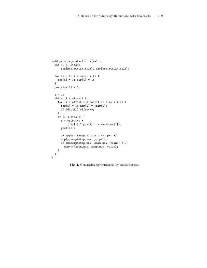
A Heuristic for Symmetry Reductions with Scalarsets 109
void permute_scalar(int size) {
int i, p, offset,
pos[MAX_SCALAR_SIZE], dir[MAX_SCALAR_SIZE];
for (i = 0; i < size; i++) {
pos[i] = 1; dir[i] = 1;
}
pos[size-1] = 0;
i = 0;
while (i < size-1) {
for (i = offset = 0;pos[i] == size-i;i++) {
pos[i] = 1; dir[i] = !dir[i];
if (dir[i]) offset++;
}
if (i < size-1) {
p = offset-1 +
(dir[i] ? pos[i] : size-i-pos[i]);
pos[i]++;
/* apply transposition p <-> p+1 */
apply_swap(&tmp_now, p, p+1);
if (memcmp(&tmp_now, &min_now, vsize) < 0)
memcpy(&min_now, &tmp_now, vsize);
}
}
}
Fig. 4. Generating permutations by transpositions
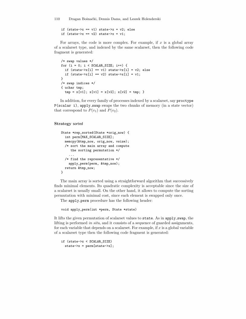
110 Dragan Bosnacki, Dennis Dams, and Leszek Holenderski
if (state->x == v1) state->x = v2; else
if (state->x == v2) state->x = v1;
For arrays, the code is more complex. For example, if x is a global arrayof a scalarset type, and indexed by the same scalarset, then the following codefragment is generated:
/* swap values */
for (i = 0; i < SCALAR_SIZE; i++) {
if (state->x[i] == v1) state->x[i] = v2; else
if (state->x[i] == v2) state->x[i] = v1;
}
/* swap indices */
{ uchar tmp;
tmp = x[v1]; x[v1] = x[v2]; x[v2] = tmp; }
In addition, for every family of processes indexed by a scalarset, say proctypeP(scalar i), apply swap swaps the two chunks of memory (in a state vector)that correspond to P (v1) and P (v2).
Strategy sorted
State *rep_sorted(State *orig_now) {
int perm[MAX_SCALAR_SIZE];
memcpy(&tmp_now, orig_now, vsize);
/* sort the main array and compute
the sorting permutation */
...
/* find the representative */
apply_perm(perm, &tmp_now);
return &tmp_now;
}
The main array is sorted using a straightforward algorithm that successivelyfinds minimal elements. Its quadratic complexity is acceptable since the size ofa scalarset is usually small. On the other hand, it allows to compute the sortingpermutation with minimal cost, since each element is swapped only once.
The apply perm procedure has the following header:
void apply_perm(int *perm, State *state)
It lifts the given permutation of scalarset values to state. As in apply swap, thelifting is performed in situ, and it consists of a sequence of guarded assignments,for each variable that depends on a scalarset. For example, if x is a global variableof a scalarset type then the following code fragment is generated:
if (state->x < SCALAR_SIZE)
state->x = perm[state->x];

A Heuristic for Symmetry Reductions with Scalarsets 111
The guard is needed to solve a subtle problem with the initialization ofscalarset variables. Since all variables used in a standard Promela program areautomatically initialized with 0, it is common to use 0 to represent an undefinedvalue. Unfortunately, this convention cannot be used for scalarsets. The reasonis that in our implementation, a scalarset of size n is a range of integers from0 to n − 1, so 0 must be treated as other well-defined values (otherwise, thesymmetry would be broken). Thus, a value outside of the range must be usedfor an undefined value. By convention, we use n for this purpose, and the guardguarantees that the undefined value is treated in a symmetric way (i.e., it isnever permuted, as required in [19]). In fact, any value not less than n can beused to represent the undefined value.
For arrays, the code is more complex. For example, if x is a global arrayof a scalarset type, and indexed by the same scalarset, then the following codefragment is generated:
/* permute values */
for (i = 0; i < SCALAR_SIZE; i++) {
if (state->x[i] < SCALAR_SIZE)
state->x[i] = perm[state->x[i]];
}
/* permute indices */
{ uchar buf[SCALAR_SIZE];
memcpy(buf, state->x, sizeof(state->x));
for (i = 0; i < SCALAR_SIZE; i++)
state->x[perm[i]] = buf[i];
}
Notice that when permuting indices we have to use a buffer.
Strategy segmented
State *rep_segmented(State *orig_now) {
int perm[MAX_SCALAR_SIZE];
memcpy(&tmp_now, orig_now, vsize);
/* sort the main array and compute
the sorting permutation */
...
/* locate blocks */
...
/* find the representative */
apply_perm(perm, &tmp_now);
memcpy(&min_now, &tmp_now, vsize);
if (num_of_blocks > 0)
permute_blocks(0, block_start[0],
block_size[0]);
return &min_now;
}
First, the main array is sorted as in the sorted strategy. Second, the segmentsof equal values are located, in the sorted main array, by a straightforward linear

112 Dragan Bosnacki, Dennis Dams, and Leszek Holenderski
algorithm. The information about the segments (called blocks henceforth) isstored in the following global data structures:
int num_of_blocks;
int block_start[MAX_SCALAR_SIZE],
block_size[MAX_SCALAR_SIZE];
Finally, the canonical representative is found by procedure permute blocksthat generates all permutations of indices in successive blocks, excluding theidentity permutation. Its code is given in Fig. 5. Each permutation is then appliedto the current state, and the lexicographically smallest result is chosen.
void permute_blocks(int block, int start,
int size) {
int i, p, offset,
pos[MAX_SCALAR_SIZE], dir[MAX_SCALAR_SIZE];
/* go to the last block */
if (++block < num_of_blocks)
permute_blocks(block, block_start[block],
block_size[block]);
block--;
/* the same as permute_scalar, but apply
transposition is changed to */
...
swap_in_block(block, p, p+1);
...
}
void swap_in_block(int block, int p1, int p2) {
/* apply transposition p1 <-> p2 */
apply_swap(&tmp_now, p1, p2);
if (memcmp(&tmp_now, &min_now, vsize) < 0)
memcpy(&min_now, &tmp_now, vsize);
/* permute the next block */
if (++block < num_of_blocks)
permute_blocks(block, block_start[block],
block_size[block]);
}
Fig. 5. Permuting blocks
The procedure uses double recursion, to assure that the number of calls toapply swap and comparisons between tmp now and min now is minimal. It is ageneralization of permute scalar used in rep full. Conceptually, the indicesof separate blocks, when considered relative to the start of a respective block,

A Heuristic for Symmetry Reductions with Scalarsets 113
can be perceived as separate scalarsets. Inside one block, all transpositions ofthe block’s indices are generated as in permute scalar. The double recursion isused to properly compose the permutations of separate blocks, by chaining theinvocations of permute blocks.
5 Experimental Results
We tried our prototype implementation on several examples. The obtained re-ductions were often very close to the theoretical limits, thus, we were able toobtain reductions of several orders of magnitude in the number of states. Also,due to the significantly smaller number of states that had to be explored, inall the cases the verification with symmetry reduction was faster than the onewithout it. The experiments showed that there is no favorite among the reduc-tion strategies regarding the space/time ratio. This suggests that it makes senseto have all strategies (maybe except full) as separate options of the extendedmodel-checker.
In the verification experiments we used Spin and SymmSpin both with andwithout the partial order reduction (POR) option. In most of the cases therewas a synergy between the symmetry and the partial order reductions. The tworeduction techniques are orthogonal because they exploit different features ofthe concurrent systems, therefore, their cumulative effect can be used to obtainmore efficient verification.
In the sequel, we present the results for three of the examples. All experimentswere performed on a Sun Ultra-Enterprise machine, with three 248 MHz UltraSPARC-II processors and 2304MB of main memory, running the SunOS 5.5.1operating system. Verification times (in the rows labeled with “t”) are given inseconds (s.x), minutes (m:s), or hours (h:m:s); the number of states (in the rowslabeled with “s”) is given directly or in millions (say, 9.1M); o.m. stands for outof memory, and o.t. denotes out of time (more than 10 hours); +POR and -PORmean with and without POR, respectively.
5.1 Peterson’s Mutual Exclusion algorithm [22].
For this well known example5 we verified the mutual exclusion property. Theresults for different numbers N of processes are shown in Table 1.
The gain due to the symmetry reduction is obvious. The obtained reductions,ranging from 49% (for N = 2) to 99% and more (for N ≥ 5) are close to thetheoretical maxima, which can be explained with the high degree of symmetry inthe protocol. The verification times are also better, even with the straightforwardfull strategy, due to the smaller number of states that are generated during thesearch. We used both symmetry and partial order reduction (which is default5 In our implementation the global predicate that guards the entry in the critical sec-
tion is checked atomically. As this guard ranges over all process indices, the atomicitywas necessary due to the restrictions on statements that can be used such that thestate space symmetry is preserved.

114 Dragan Bosnacki, Dennis Dams, and Leszek Holenderski
Table 1. Results for Peterson’s mutual exclusion algorithm.
N 2 3 4 5 6 7
+POR -POR +POR -POR +POR -POR +POR -POR +POR -POR +POR -POR
s 154 263 4992 11318 202673 542921 9.1M o.m. o.m. o.m. o.m. o.m.
no sym. t 6.5 5.6 6.8 6.3 25.0 1:09 19:04 — — — — —
s 89 134 980 1976 9634 24383 86112 262749 700543 2.5Ma 5.3Ma o.m.
full t 6.5 5.6 6.7 5.9 10.4 19.3 2:35 12:02 2:04:03 o.t. o.t. —
seg. t 6.7 5.6 6.6 5.8 8.5 12.4 38.0 2:31 7:36 44:40 1:56:00 —
pc-seg. t 6.5 5.6 6.6 5.8 8.4 11.3 37.4 1:59 10:01 40:46 4:26:32 —
s 113 160 1877 3967 35644 88489 595843 1.8M 8.8M o.m. o.m. o.m.
sorted t 6.5 5.6 6.6 6.1 11.0 21.6 1:42 8:13 28:37 — — —
s 92 137 1149 2396 20339 46804 401423 942786 9.6M o.m. o.m. o.m.
pc-sort. t 6.5 5.6 6.6 5.8 10.2 15.0 1:36 4:53 54:53 — — —
a The number of states is obtained with segmented and pc-segmented.
in standard Spin), separately and in combination. Standard Spin with partialorder reduction could not handle more than 5 processes. However, the segmentedversions of the symmetry heuristics alone were sufficient for N = 6. For N = 7we had to use a combination of both reduction techniques in order to stay insidethe available memory.
The sorted strategies are comparable with their segmented counterparts onlyfor small values of N . For greater values they deteriorate and even the possi-ble gain in time over the segmented versions disappears because of the greaternumber of states that have to be explored.
One can also expect that as N increases pc-segmented and pc-sorted will loosethe advantage they have over segmented and sorted, for smaller values of N . Thereason is that the number of different elements in the main array of segmentedand sorted increases as N increases, while the number of values of the pc counterstays the same. (We use as a main array the array of flags. Whenever process ienters the competition for the critical section, it sets flag i to a value between 1and N − 1. The default value is 0. Notice that the values of the flag array arenot of the scalarset type Pid , although their range is the same as the range ofPid .) Intuitively, the greater versatility of the values in the main array, the fewerpermutations have to be generated on average, in order to canonicalize the state.This tendency is already visible for N = 6 (for which sorted is winning over pc-sorted) as well as for N = 7 (for which segmented is better than pc-segmented).
5.2 Data Base Manager [24].
The system that we consider consists of N ≥ 2 data base managers, which modifya data base and exchange messages to ensure the consistency of the data base

A Heuristic for Symmetry Reductions with Scalarsets 115
contents. Our model deals with the procedural part of the protocol, i.e., withthe message exchange, by abstracting from the actual modification of the database. Initially all managers are in inactive state until one of them modifies thedata base. This manager in one atomic step reserves the data base for itself andsends a message to every other manager. After that it waits for acknowledgmentsfrom the other managers. All other managers concurrently perform a two stepsequence: reception of the message, and sending of an acknowledgment. Whenall acknowledgments are available, the manager who initially modified the database and started the whole procedure, reads them. At the same moment it alsoreleases the data base so that it can be modified by the other managers, afterwhich it returns to inactive state. We checked the model for absence of deadlock.
Table 2. Results for the Data Base Manager example.
N 7 8 9 10 11 12
+POR -POR +POR -POR +POR -POR +POR -POR +POR -POR +POR -POR
s 100 5112 130 17506 164 59060 202 196842 244 649552 290 2.1M
no sym. t 0.0 0.5 0.0 1.9 0.0 8.2 0.0 32.1 0.0 2:11 0.0 8:27
s 16 31 18 39 20 48 22 58 24 69 — —
full t 0.5 2.0 4.6 24.5 48.0 6:16 9:08 1:27:40 1:55:09 22:07:36 o.t. o.t.
seg. t 0.3 0.4 2.8 3.8 28.3 39.1 5:22 7:20 1:06:32 1:30:53 o.t. o.t.
pc-seg. t 0.1 0.1 0.8 1.0 7.3 9.1 1:16 1:33 15:16 17:14 o.t. o.t.
s 27 250 31 505 35 1016 39 2039 43 4086 47 8181
sorted t 0.0 0.0 0.0 0.1 0.0 0.2 0.0 0.6 0.0 1.3 0.0 3.1
s 16 58 18 91 20 155 22 245 24 415 26 659
pc-sort. t 0.0 0.0 0.0 0.0 0.0 0.0 0.0 0.1 0.0 0.1 0.0 0.3
Our experiments are in accord with the theoretically predicted results from [24]:both symmetry and POR applied separately reduce the exponential growth ofthe state space to quadratic, and in combination they give linear growth. Unlikein the previous example, this time pc-segmented strategy is a clear winner oversegmented. The explanation is again in the diversity of the elements occurring inthe sorted array – the only possible values of the main array for segmented are0 and 1, while the pc counter has 7 different values. (The main array consistsof boolean flags which are set to 1 when a manager reserves the data base andsends a message to all the other processes.) It is interesting that pc-sorted incombination with POR is by far the most successful strategy. It achieves thesame reduction as the canonical strategies, but within much shorter time. Itremains to be seen whether this is just a peculiarity of this model, or it occursfor a wider class of examples.

116 Dragan Bosnacki, Dennis Dams, and Leszek Holenderski
5.3 The Initialization Protocol [14].
Assume that we are given a system of n processes each consisting of an initialpart and a main part. The data structures can have arbitrary initial values.The role of the Initialization Protocol from [14] is to synchronize the processessuch that none of them can enter its main part before all the others have finishedtheir initial parts.6 Process synchronization is done via shared boolean variables.Each process has so called co-component process whose task is to manage thesynchronization of the boolean variables. We refer the reader to [14] for moredetails.
The protocol is an example of a system with one scalar variable and twoprocess families indexed by this scalar – the family of processes that are syn-chronized and the family of their co-components. In such a case one can expectthe same maximal amount of reduction of n! (where n is the family size) as withone family.
Table 3. Results for the Initialization Protocol example.
n 2 3 4 5
+POR -POR +POR -POR +POR -POR +POR -POR
s 2578 2578 131484 131484 7.0M 7.0M o.m. o.m.
no sym. t 6.4 1.1 19.3 12.2 18:50 16:31 — —
s 1520 1521 26389 26399 386457 386536 5.3M o.m.
full t 6.2 1.0 11.4 6.0 4:53 4:46 5:38:05 —
seg. t 6.3 1.0 11.1 5.4 3:19 3:04 2:28:20 —
pc-seg. t 6.3 0.9 10.1 4.4 1:54 1:39 47:03 —
s 2344 2344 98602 98602 4.2M 4.2M o.m. o.m.
sorted t 6.3 1.0 17.9 11.0 12:13 12:22 — —
s 1607 1607 40395 40395 987830 987830 o.m. o.m.
pc-sort. t 6.3 0.1 11.8 5.7 3:55 3:17 — —
We verified the correctness of the algorithm for several values of n by placingbefore the main part of each process an assertion which checks that all the otherprocesses have terminated their initial parts.
Because of the intensive use of global variables, partial order reduction hadalmost no effect in this example. Thus, the state space reduction was mostly dueto the symmetry. The canonical heuristic segmented and pc-segmented prevailedover the non-canonical ones regarding both space and time. Compared to full,they were significantly faster for larger values of n. Better performance of pc-segmented and pc-sorted over segmented and sorted respectively, can be explained6 Note that this would be trivial if we could assume that the variables’ initial values
were known.

A Heuristic for Symmetry Reductions with Scalarsets 117
by the fact that the main array that was used in the latter strategies is of booleantype. This means that the elements of the main array can have only two values,in contrast with the program counter which ranges over at least 15 differentvalues. Intuitively, the greater versatility of values in the pc array means thatfewer permutations have to be generated on average in order to canonicalize thestate.
5.4 Base Station.
This example is a simplified version of MASCARA – a telecommunication proto-col developed by the WAND (Wireless ATM Network Demonstrator) consortium[7]. The protocol is an extension of the ATM (Asynchronous Transfer Mode) net-working protocol to wireless networks. We present the results for two models ofthe protocol.
Our first model represents a wireless network connecting N ≥ 2 mobile sta-tions (MS) that may communicate with each other, using a limited number(M ≥ 1) of radio channels provided by one base station BS. More specifically,when MS A wants to send a message to MS B it must request a channel fromBS. Provided there are channels available, A is granted one, call it c. If B wantsto receive messages, it queries BS. As there is a pending communication for Bthrough c, BS assigns c to B. After the communication has taken place, both Aand B return the channel to BS. The results given in Table 4 are for checkingfor unreachable code, with M = 2.
Table 4. Results for the Base Station example (first model).
N 2 3
+POR -POR +POR -POR
s 15613 15621 o.m. o.m.
no sym. t 7.6 6.4 — —
s 7808 7812 3.4M 3.4M
full t 7.5 6.3 17:39 13:00
seg. t 5.8 6.3 12:10 9:46
pc-seg. t 5.9 6.4 13:24 10:18
s 7856 7860 3.9M 3.9M
sorted t 7.2 6.3 12:58 9:48
s 8282 8286 5.1M 5.1M
pc-sort. t 7.5 6.3 16:48 12:57
For N = 2 the symmetry reduction approaches the theoretical limit of 50%.For N = 3 standard Spin ran out of memory, while with symmetry reduction itwas possible to verify the model. In this example POR did not play a significant

118 Dragan Bosnacki, Dennis Dams, and Leszek Holenderski
role. Also, there was no clear preference between segmented, pc-segmented andsorted.
In the second model, instead of having N stations which can both receive andsend messages, we consider a network connecting ns ≥ 1 sending mobile stationsand nr ≥ 1 receiving mobile stations. Another important difference is that thecommunication is modeled with Promela channels, instead of global variables.For the rest the description of the protocol given for the first model applies alsoto the second one.
Table 5. Results for the Base Station example (second model).
ns = 2 ns = 3 ns = 2
nr = 2 nr = 2 nr = 3
+POR -POR +POR -POR +POR -POR
s 4.6M 9.0M o.m. o.m. o.m. o.m.
no sym. t 5:02 13:48 — — — —
s 1.2M 2.3M 9.0M o.m. 9.4M o.m.
full t 1:41 5:03 28:57 — 30:32 —
pc-seg. t 1:32 4:54 19:29 — 20:36 —
s 1.7M 3.5M o.m. o.m. o.m. o.m.
pc-sort. t 1:58 6:03 39:02 — — —
Thus, there are two families of symmetric processes in the second model:The family of sending stations and the family of receiving stations. Unlike inthe Initialization Protocol, the two families are independent, and, consequently,indexed with two different scalar sets.
On this example we could apply only pc-segmented and pc-sorted becausethere was no main array that could be used for sorted and segmented. Onecan see that for the canonical strategies the reduction indeed approaches thetheoretical limit ns! · nr!. (In general, for a system with k independent processfamilies indexed by k scalar sets, the reduction due to symmetry is limited byn1! · n2! · . . . · nk!, where ni, 1 ≤ i ≤ k, is the number of processes in the i-thfamily.)
With the usage of Promela channels instead of global variables, the contribu-tion of the partial order reduction became significant (Table 5), which was notat all the case in the first model. One can also notice the orthogonality of thetwo heuristics – namely, the factor of reduction due to symmetry was almost thesame with or without POR.

A Heuristic for Symmetry Reductions with Scalarsets 119
6 Conclusions and Future Work
We have presented four variants of a new heuristic for coping with the orbit prob-lem in symmetry reduction. Their strength is based on the observation that thelexicographical ordering on state vectors may be tuned to optimize the splittingheuristic of [18]. Of the resulting strategies, the segmented/pc-segmented ver-sions indeed produce canonical representatives of orbits, while sorted/pc-sortedare only normalizing. The sorted and segmented strategies presuppose the pres-ence of a main array in the program. Their pc variants exploit the array ofprogram counters in programs containing a family of similar processes.
Based on these strategies, we developed SymmSpin, an extension of Spinwith a symmetry-reduction package. We compared the effects of the strategies,as well as the reference fullstrategy, on several examples. The experimental resultsshow that there is no uniform winner: It depends on the program which of thestrategies performs best. In some cases, this was in fact predicted by the formof the program. Thus, it make sense to have all strategies (maybe except full) asseparate options of the extended model-checker.
The resulting package has been described at a detailed level. For maximalmodularity, the implementation is in the form of a Tcl script that operates onthe verification engine produced by Spin. We point the interested reader to theweb site accompanying this paper, [1], for the full source code.
The results obtained with this experimental implementation are sufficientlyencouraging in order to integrate the symmetry strategies more completely intothe Spin tool. One concern here is to ensure the compatibility of the symmetryreduction with Spin’s other features. So far, we have focussed on the partialorder reduction. In the next chapter we show that the correctness of Spin’s cycledetection algorithm, which lies at the heart of its capability to handle the fullclass of ω-regular correctness properties, is preserved. Furthermore, the symme-try is compatible with the recent extension to timed systems, DTSpin ([2]). Itshould be added that the present implementation is able to deal with multiplescalar sets and multiple process families. Also, almost all Promela features arehandled, including queues. For the latter there is still the restriction though thatthe queue elements have to be simple, non-structured types.
Also, the restrictions on the scalarset variables are as yet not automaticallychecked. The most natural solution to this problem would be to extend thePromela syntax to allow specifications of scalarsets directly instead of via anaccompanying file. This will facilitate the automatic verification of the syntacticconditions along the lines of [19], that are needed to ensure the soundness ofthe analysis. With the present implementation this is still a task for the user. Amore ambitious attempt would be the automatic detection of scalarsets directlyfrom the Promela sources.

120 Dragan Bosnacki, Dennis Dams, and Leszek Holenderski
Next, we plan to extend the symmetry algorithm itself with other systemtopologies, like rings7. An interesting question is whether the choice of an ap-propriate strategy can be automated, based on syntactic clues.
References
1. AdjustPan Script, http://www.win.tue.nl/~lhol/SymmSpin, April 2000.2. D. Bosnacki, D. Dams, Integrating Real Time into Spin: a Prototype Implemen-
tation, in S. Budkowski, A. Cavalli, E. Najm (eds), Proc. of FORTE/PSTV’98(Formal Description Techniques and Protocol Specification, Testing and Verifica-tion), 423–438, Paris, France, 1998.
3. D. Bosnacki, D. Dams, L. Holenderski, Symmetric Spin, SPIN’2000 (The 7thInternational SPIN Workshop on Model Checking of Software), pp. 1–19, LNCS1885, 2000.
4. E.M. Clarke, R. Enders, T. Filkorn, S. Jha, Exploiting Symmetry in TemporalLogic Model Checking, Formal Methods in System Design, Vol. 19, 77–104, 1996.
5. E.M. Clarke, O. Grumberg, D.A. Peled, Model Checking, The MIT Press, 2000.6. C. Courcoubetis, M. Vardi, P. Wolper, M. Yannakakis, Memory Efficient Algorithm
for the Verification of Temporal Properties, Formal Methods in System Design I,pp. 275-288, 1992.
7. I. Dravapoulos, N. Pronios, S. Denazis et al, The Magic WAND, Deliverable 3D2,Wireless ATM MAC, Sep 1997.
8. E.A. Emerson, Temporal and Modal Logic, in Jan van Leeuwen (ed.), Formal Mod-els and Semantic, Vol. B of Handbook of Theoretical Computer Science, Chap. 16,995–1072, Elsevier/The MIT Press, 1990.
9. E.A. Emerson, S. Jha, D. Peled, Combining Partial Order and Symmetry Reduc-tions, in Ed Brinksma (ed.), Proc. of TACAS’97 (Tools and Algorithms for theConstruction and Analysis of Systems), LNCS 1217, 19–34, Springer, 1997.
10. E.A. Emerson, A.P. Sistla, Symmetry and Model Checking, in C. Courcou-betis (ed.), Proc. of CAV’93 (Computer Aided Verification), LNCS 697, 463–478,Springer, 1993.
11. E.A. Emerson, R.J. Trefler, Model Checking Real-time Properties of SymmetricSystems, Proc. of the 23rd International Symposium on Mathematical Foundationsof Computer Science (MFCS), 427–436, Aug. 1998.
12. E.A. Emerson, R.J. Trefler, From Asymmetry to Full Symmetry: New Techniquesfor Symmetry Reduction in Model Checking, Proc. of CHARME’99 (The 10th IFIPWG10.5 Advanced Research Working Conference on Correct Hardware Design andVerification Methods), Bad Herrenalb, Germany, Sep. 1999.
13. E.A. Emerson, A.P. Sistla, Utilizing Symmetry when Model-checking under Fair-ness Assumptions: an Automata-theoretic Approach, ACM Transactions on Pro-gramming Languages and Systems, 19(4):617–638, July 1997.
14. W.H.J.Feijen, A.J.M. van Gasteren, On a Method of Multiprogramming, Springer-Verlag, 1999.
15. P. Godefroid, Exploiting Symmetry when Model-checking Software, Proc. ofFORTE/PSTV’99 (Formal Methods for Protocol Engineering and Distributed Sys-tems), 257–275, Beijing, Oct. 1999.
7 The group of shift permutations can be handled by a simplification of our approach,where instead of sorting the main array, it is cyclically shifted until it starts with aminimal element.

A Heuristic for Symmetry Reductions with Scalarsets 121
16. V. Gyuris, A.P. Sistla, On-the-fly Model Checking under Fairness that ExploitsSymmetry, in O. Grumberg (ed.), Proc. of CAV’97 (Computer Aided Verification),LNCS 1254, 232–243, Springer, 1997.
17. G.J. Holzmann, Design and Validation of Communication Protocols, Prentice Hall,1991. Also: http://netlib.bell-labs.com/netlib/spin/whatispin.html
18. C.N. Ip, D.L. Dill, Better Verification Through Symmetry, in D. Agnew, L. Clae-sen, R. Camposano (eds), Proc. of the 1993 Conference on Computer HardwareDescription Languages and their Applications, Apr. 1993.
19. C.N. Ip, D.L. Dill, Better Verification Through Symmetry. Formal Methods inSystem Design, Vol. 9, 41–75, 1996.
20. C.N. Ip, State Reduction Methods for Automatic Formal Verification, Ph.D. thesis,Department of Computer Science of Stanford University, Dec 1996.
21. V. Lipskiy, Kombinatorika dlya Programmistov, Mir, Moscow, 1988. (In Russian)22. N.A. Lynch, Distributed Algorithms, Morgan Kaufmann Publishers, 1996.23. R. Nalumasu, G. Gopalakrishnan, Explicit-enumeration Based Verification Made
Memory-efficient, Proc. of CHDL’95 (Computer Hardware Description Languages),617-622, Chiba, Japan, Aug. 1995.
24. A. Valmari, Stubborn Sets for Reduced State Space Generation, Advances in PetriNets 1990, LNCS 483, 491–515, Springer, 1991.


7. Nested Depth First Search Algorithms forSymmetry Reduction in Model Checking

Nested Depth First Search Algorithms forSymmetry Reduction in Model Checking
Dragan Bosnacki
Dept. of Computing Science, Eindhoven University of TechnologyPO Box 513, 5600 MB Eindhoven, The Netherlands
e-mail: [email protected]
Abstract. We propose an algorithm for model checking under weakfairness that exploits symmetry for state space reduction. As interme-diate results we also discuss two other algorithms which deal separatelywith weak fairness and symmetry reduction. The algorithms presentedin this chapter are based on the Nested Depth First Search (NDFS) al-gorithm by Courcoubetis, Vardi, Wolper and Yannakakis. We argue thatthe worst case time complexity of our algorithm for model checking underweak fairness with symmetry is of the same order of magnitude as thetime complexity of the algorithms known in the literature. Moreover,as these algorithms require finding all strongly connected components(SCC) in the state space graph, our algorithm preserves the advantagesof the NDFS over the SCC approach.
1 Introduction
Model checking [6, 22] is a widespread technique for the automated verificationof concurrent systems. The technique lends itself to implementation and as suchit is successfully used in the construction of verification tools [23]. However,model-checking tools are often limited by memory requirements because of theproblem of state space explosion. One of the important techniques to alleviatethis problem is symmetry reduction.
Symmetry is present in many systems, like mutual exclusion algorithms,cache coherence protocols, bus communication protocols, etc. In order to graspthe idea behind symmetry reduction, consider a typical mutual exclusion proto-col. The (im)possibility for processes to enter their critical sections simultane-ously will stay the same if the process identities are permuted. As a consequence,when during state-space exploration a state is visited that is the same, up toa permutation of pids, as some state that has already been visited, the searchcan be pruned. More formally, the symmetry of the system is represented bya given group G of permutations that act on the global states of the system.It turns out that two states s and s′ are behaviorly equivalent if there existsa permutation π ∈ G such that s′ can be obtained by applying π on s. Thus,the system state space T is partitioned into equivalence classes. We define aselection function h which selects a unique representative from each equivalenceclass. Next, the quotient state space h(T ) is constructed that contains only these

NDFS for Symmetry Reduction 125
representatives and the property is checked using h(T ) instead of T . As h(T ) isin general much smaller than T , the gain in memory and time needed for theverification algorithms can be significant.
The issue of fairness is an inherent and important one in the study of con-currency and nondeterminism, in particular in the area of the verification ofconcurrent systems. Since fairness is used as generic notion there is a broadtaxonomy of fairness concepts. In this chapter we confine our attention to thenotion of weak fairness on the level of processes. This means that we requirethat for every execution sequence of the concurrent program which is a composi-tion of several processes, if some process becomes continuously enabled at somepoint of time (i.e. can always execute some of its statements), then at least onestatement from that process will eventually be executed. This kind of fairnessis most often associated with mutual exclusion algorithms, busy waiting, sim-ple queue-implementations of scheduling, and resource allocation. Weak fairnesswill guarantee the correctness of statements like eventually entering the criticalregion for every process which is continuously trying to do this (in the mutualexclusions) or eventually leaving the waiting queue for each process that hasentered it (in the scheduling) [13].
Thus, combining the algorithms for model-checking under weak fairness withreduction techniques, and in particular symmetry, is a prerequisite for the veri-fication of many interesting properties in practice. However, when coupling thetwo concepts special care should be taken, because of the possible incompatibil-ities between the particular algorithms.
The main contribution of the chapter is an algorithm for model checkingunder weak fairness (in the sense described above) that exploits symmetry re-duction. As intermediate results we also discuss two other algorithms which dealseparately with weak fairness and symmetry reduction.
We assume that the properties that are checked are specified as Buchi au-tomata [21]. As a consequence the problem of checking whether some givenproperty holds for the system under consideration can be reduced to the prob-lem of finding acceptance cycles (i.e., cycles that contain acceptance states) inthe graph representing the product of the system model state space with theproperty automaton (c.f. [7, 5]).
All the algorithms that are presented in the chapter are based on the so-callednested depth first search (NDFS) algorithm by Courcoubetis, Vardi, Wolper andYannakakis [7] for detecting acceptance cycles in the state space. In the NDFSalgorithm from each acceptance state which is visited during the standard DFSexploration of the state space a check procedure is called in order to detect apossible acceptance cycle through the state. This nested cycle check is itself aDFS, which explains the name “nested DFS”.
In order to capture weak fairness, one has to modify the standard NDFSalgorithm. This is because the latter only guarantees that it will find some ac-ceptance cycle, if there exists one, but not all of them. Thus, one cannot use thestraightforward idea to just ignore the detected cycles which are not fair untilone finds a fair one, or there are no more cycles. In the chapter we present an

126 Dragan Bosnacki
algorithm for model checking under weak fairness which is a minor modificationof the weak fairness algorithm by Gerard Holzmann implemented in the modelchecker Spin. The idea of the upgrade for weak fairness is to do the acceptancecycle search in an extended state space in which it is guaranteed that each cyclethat is detected is a fair one. In fact, we need a more general result that claimsthat there exists a fair acceptance cycle in the original state space if and onlyif there exists an acceptance cycle in the extended state space. We show thecorrectness of our modified fairness algorithm by arguing that it is equivalent tothe standard NDFS algorithm applied to the extended state space.
Our second stepping stone towards the main algorithm is presented in amore general framework of state space reductions that preserve bisimulation,introduced by Emerson, Jha and Peled [12]. The symmetry based reductionsare only a special case of such reductions. The algorithm that we consider is astraightforward generalization of the symmetry reduction algorithms from [19,10, 12, 3]. After presenting an NDFS version of this generalization, we prove itscorrectness.
Finally, we present the main algorithm that reconciles the issues of fairnessand symmetry. We begin by discussing why a straightforward combination of theNDFS versions of the fairness and bisimulation preserving reduction algorithmsfails. After that we briefly introduce symmetry reduction as a special case of abisimulation preserving reduction. The algorithm for fairness and symmetry isbased on the theory developed by Emerson and Sistla [11]. In this chapter wedo the necessary adjustments of the theory so that we can fit it into the NDFSconcept. The main idea (borrowed from [11]) is to work with a reduced statespace hG(T ) which, unlike for the ordinary symmetry reduction algorithm, hastransitions annotated with permutations. In this way the process identities fromthe original state space T , which are scrambled during the reduction, can berestored and the corresponding fair acceptance cycles detected. In order to facil-itate the implementation of the cycle detection we further unfold the annotatedreduced state space into a threaded state space h∗
G(T ). Besides using the NDFSconcept, the main novelty of our approach is to reduce the search for a fair ac-ceptance cycle in the annotated state space hG(T ) to a search of N acceptancecycles in the threaded state space h∗
G(T ), where N is the number of processes inthe system. There is one to one correspondence between these acceptance cyclesand the processes. Moreover, each of the cycles is weakly fair with regard toits corresponding process, meaning that the process either executes a statementalong the cycle or it is disabled in some state of the cycle. The main benefit ofsuch an approach is that one can avoid that the annotating permutations arekept as part of the representation of the state or on the DFS stack. The formeris necessary in order to keep the advantages of the NDFS algorithm.
The unfolding into a threaded structure augments the size of the annotatedstate space roughly by a factor of N . The search for fair cycles contributesan additional factor of N , which gives in total N2 times bigger structure thanthe reduced annotated state space. However, the gain in memory is substantialbecause the annotated state space is often a factor N ! smaller than the original
NDFS for Symmetry Reduction 127
one. In fact, using efficient storage techniques [16] one can show that in practicethe factor N2 can be avoided, i.e., often the threaded structure also can be storedin virtually the same memory size as the annotated state space.
In the literature we could find two algorithms for exploiting symmetry underweak fairness. The first one is from the already mentioned paper of Emersonand Sistla [11], while the second one is by Gyuris and Sistla [14] and it is animprovement of the first algorithm. We show that the time complexity of ouralgorithm is the same as for the above mentioned algorithms. However, as thealgorithms in [11, 14] require finding all strongly connected components (SCC) inthe state space graph, our algorithm capitalizes on the advantages that the NDFSapproach has over the SCC based algorithms. Probably the most important oneamong these advantages is that, unlike the two existing algorithms, our algorithmis compatible with the memory efficient approximative verification techniqueslike bit-state hashing [15] and hash-compact [24]. In practice, when the propertywhich is being verified does not hold, the NDFS based algorithms are faster andrequire less memory to find an error. Also, with the NDFS based algorithmsit is much easier to reconstruct the counter example execution which witnessesthe error, by simply dumping the contents of the stack. Our algorithm is alsoeasier to implement because it does not require complex structures to keep theannotating permutations.1
Chapter layout. In the next section we give the basic notions used throughoutthe chapter, as well as the standard NDFS algorithm. In Section 3 we describethe weak fairness algorithm and prove its correctness using the notion of weaklyfair extension of labeled transition system. Section 4 introduces bisimulation pre-serving reduction. In this section we give the NDFS algorithm for model checkingby exploiting these kind of reductions, without fairness. In the next section wefirst recall the basics of symmetry reduction and the theory of [11]. After pre-senting the extensions of the theory we give the main algorithm that combinessymmetry reduction with weak fairness, and show its correctness. Finally wediscuss its space and time complexity. The last section summarizes the chapterand provides some guidelines for future work.
2 Preliminaries
2.1 Model-checking Problem, Labeled Transition systems andBisimulations
In the sequel we adopt the automata-theoretic approach to model checking. Inparticular, we assume that the properties are given as Buchi automata [21]. Thisallows us to reduce the model checking problem to the problem of finding a cycle
1 For the algorithm from [14] the authors claim that it is not necessary to keep thepermutations as a part of the state. However, it is hard to see how this can beachieved without a significant time overhead.

128 Dragan Bosnacki
in the finite graph representing the combination between the state space of themodel and the property.
There are several ways to get this graph which depend on the languages inwhich the model and the property are specified, as well as on the formalismsused to represent their semantics. One typical way is the following:
Assume that we are given the model M and the property f , representedin some modeling language and temporal logic, respectively. We want tocheck if all execution sequences (computations) of M satisfy f . From thedescription of M , usually given as a parallel composition of processesPi, we can obtain the global behavior of M semantically representedby a graph T whose nodes are the global states of M and the edgesare the transitions between them. The negation of f , ¬f , is translatedinto the Buchi automaton A¬f , which can be also regarded as a statespace graph with a special set of designated states. In order to checkthe property we need the state space graph G which is obtained as aproduct of T and A¬f . The intuition is that A¬f monitors T by guessingnondeterministically the infinite execution sequences in T . A¬f inducesdesignated states also in G. In order for property f to hold for M , theset of infinite execution sequences in G that pass through infinitely manysuch designated states should be empty. Otherwise, there is an executionwhich is in accord with the negation of f , and therefore it is a counterexample that the property does not hold. As G is finite, finding an infiniteexecution which is a counter example boils down to detecting cyclescontaining designated states.
The state space graph T usually grows exponentially with the size of thedescription of M , which causes also an exponential growth of G. Building thewhole T can be avoided using on-the-fly techniques. In this approach we buildonly A¬f before starting the construction of G. A¬f is used to reduce the size ofG by generating only the part of T which is needed for the product, i.e., whichis in accord with A¬f . The property is checked simultaneously while building G.This increases the efficiency of the model-checking procedure because often inpractice we can come up with a counterexample in an early phase of the statespace graph exploration, which means that the complete graph G does not haveto be stored in the memory.
We refer the interested reader, for instance, to [7], for a formal descriptionof the scheme given above. In the sequel we work directly with the final statespace graph G representing the product of the semantics of the model and the(negation of the) property, abstracting from the way it is obtained. From themodel description or the property, we keep only the information which mightbe needed in the verification (e.g., process IDs). For a more detailed descriptionhow the composition can be done on-the-fly see for example [5, 20, 17].
For our purposes, we represent the final state space graph as a labeled tran-sition system formally defined as follows:

NDFS for Symmetry Reduction 129
Definition 1. Let Prop be a set of atomic propositions. A labeled transitionsystem (LTS) is a 6-tuple T = (S,R,L,A, s, F ), where
– S is a finite set of states,– R ⊆ S×A×S is a transition relation (we write s
a→ s′ ∈ R for (s, a, s′) ∈ R),– L : S → 2Prop is a labeling function which associates with each state a set
of atomic propositions that are true in the state,– A is a finite set of actions,– s is the initial state,– F ⊆ S is the set of acceptance states.
Unless stated differently, we fix T to be (S,R,L,A, s, F ) for the rest of thechapter.
As mentioned above, we specify a model as a collection of processes. Tocapture this in the semantics we assume that a finite sequence of processesP1, P2, . . . , PN , N ≥ 1, is associated with the LTS. We introduce the mappingPid : R → {1, . . . , N}, which assigns to each transition a process index. Intu-itively, Pid(s a→ s′) = i means that the transition s
a→ s′ is generated by somestatement executed by the process Pi. An action a is enabled in a state s ∈ Siff s
a→ s′ ∈ R for some s′ ∈ S. We say that the process Pi is enabled in s ∈ Siff there exists s′, such that s
a→ s′ ∈ R and Pid(s a→ s′) = i. An executionsequence or path is a finite or infinite sequence of subsequent transitions, i.e.,for si ∈ S, ai ∈ A, the sequence s0
a0→ s1a1→ s2 . . . is an execution sequence in
T iff siai→ si+1 ∈ R for all i ≥ 0. An infinite execution sequence is said to be
accepting iff there is an acceptance state s ∈ F that occurs infinitely many timesin the sequence. A finite execution sequence c = s0
a0→ s1a1→ . . .
an−1→ sn,n ≥ 1is a cycle iff the start and end states coincide, i.e. s0 = sn. Given a finite orinfinite execution sequence σ = s0
a0→ s1a1→ s2 . . ., a process Pi, 1 ≤ i ≤ N , and
a state sj from the execution sequence, we say that Pi is executed in σ in sj
iff Pid(sja→ sj+1) = i. A state s is reachable iff there exists a finite execution
sequence that starts at s and ends in s. A cycle c is reachable iff there exists astate in c which is reachable. A cycle c is an acceptance cycle if it contains atleast one acceptance state.
Next, we define bisimulation between to LTSs:
Definition 2. Given two LTSs T1 = (S1, R1, L1, A, s1, F1) andT2 = (S2, R2, L2, A, s2, F2), an equivalence relation B ⊆ S1 × S2 is called abisimulation between T1 and T2 iff the following conditions hold:
– s1Bs2;– If sBs′, then:
• L1(s) = L2(s′);• s ∈ F1 iff s′ ∈ F2;• Given an arbitrary transition s
a→ s1 ∈ R1, there exists s2 ∈ S2 suchthat s′ a→ s2 ∈ R2 and s1Bs2;
• The symmetric condition holds: Given an arbitrary transition s′ a→ s2 ∈R2, there exists s1 ∈ S1 such that s
a→ s1 ∈ R1 and s1Bs2;

130 Dragan Bosnacki
We say that T1 and T2 are bisimilar iff there exists a bisimulation betweenT1 and T2.
2.2 The Standard Nested Depth-First Search Algorithm
The algorithms presented in this chapter are based on the algorithm of [7]for memory efficient verification of LTL [9] properties, called nested depth-firstsearch (NDFS) algorithm. The algorithm is implemented in the model-checkerSpin [15]. In the rest of this section we give a brief overview of the NDFS algo-rithm.
We begin by considering the basic depth-first search algorithm in Fig. 1.When it is started in the initial state s of a given LTS T , the basic depth-first search algorithm generates and explores the reachable part of T , i.e., allreachable states and all transitions between them.
1 proc dfs1(s)
2 add s to Stack
3 add s to States
4 for each transition (s,a,s’) do
5 add {s,a,s’} to Transitions
6 if s’ not in States then dfs1(s’) fi
7 od
8 delete s from Stack
9 end
Fig. 1. Basic DFS algorithm.
Note that in the algorithm in Fig. 1, as well as in all other algorithms in thischapter, we need to represent only the states of the LTS; the representation of thetransitions is not needed. Another remark is that also no explicit representationof the depth-first search stack is needed. Thus, the variables Transitions, Stack,and the statements from lines 2, 5, and 8 are only used in the presentation andin some of the proofs of the algorithms.
The basic DFS cannot detect cycles. Therefore, in order to do model checkingwe extend it with a call to a procedure that checks for a cycle, as soon as anacceptance state is encountered. The new algorithm is given in Fig. 2.
The cycle check procedure is again a DFS which reports a cycle and stopsthe algorithm if the seed acceptance state is matched. If a cycle through theacceptance state does not exist, then the basic DFS is resumed at the point inwhich it was interrupted by the nested cycle check. In the sequel we also call thebasic DFS first DFS, while the nested cycle checks all together are called secondDFS. We need to work with two distinct copies of the state space in order toensure that the second DFS does not fail to detect a cycle by cutting the searchbecause it has hit a state already visited by the first DFS.

NDFS for Symmetry Reduction 131
1 proc dfs1(s)
2 add s to Stack1
3 add s to States1
4 if accepting(s) then States2:=empty; seed:=s; dfs2(s) fi
5 for each transition (s,a,s’) do
6 add {s,a,s’} to Transitions
7 if s’ not in States1 then dfs1(s’) fi
8 od
9 delete s from Stack1
10 end
11 proc dfs2(s) /* the nested search */
12 add s to Stack2
13 add s to States2
14 for each transition (s,a,s’) do
15 add {s,a,s’} to Transitions2
16 if s’ == seed then report cycle
17 else if s’ not in States2 then dfs2(s’) fi
18 od
19 delete s from Stack2
20 end
Fig. 2. Nested depth first search (NDFS) algorithm, version 1 (“preorder”).
An important feature of the algorithm in Fig. 2 is that before the cyclecheck is called its copy of the state space is reset in line 4 with the statementStates2:=empty. Hence, the cycle check is always started from scratch. As aconsequence, some states can be visited several times (by different cycle checks),which increases the time complexity of the algorithm. The reinitialization ofStates2 is needed, because otherwise some acceptance cycles can be missed. Anexample of an LTS for which the algorithm without reinitialization fails is shownin Fig. 3. The states s and s1 are acceptance states. All the states are visited and
a0s s2s1
a2
a1
Fig. 3. A counterexample LTS for the NDFS with state space preservation.
put in States2 during the first cycle check which is started from s. Thus, whenthe second cycle check is called from s1, it is stopped at s2 which was entered in

132 Dragan Bosnacki
States2 by the previous cycle check. As a result, the cycle s1a1→ s2
a2→ s1 is notreported.
In order to be able to preserve the States2 between cycle checks and reusethe previous calls of dfs2, we need a small modification of the algorithm – thecycle check should start only after all the successors of an acceptance state areexplored, i.e., when the recursion retracts from an acceptance state [7]. This isachieved by moving line 4 to the end of the procedure dfs1, i.e., after line 8,and removing the statement States2 := empty which is not needed anymore.
Also, in the new version of the algorithm we use only one States (andTransitions) variable and extend the state representation with an additionalbit to distinguish between the two different copies of the state space, belongingto the first and second DFS, respectively. The variable States is preserved be-tween the calls of dfs1 and dfs2 and, as a result, each state is visited only oncealso during the second DFS. The resulting algorithm is shown in Fig. 4.
1 proc dfs1(s)
2 add s to Stack1
3 add {s,0} to States
4 for each transition (s,a,s’) do
5 add {{s,0},a,{s’,0}} to Transitions
6 if {s’,0} not in States then dfs1(s’) fi
7 od
8 if accepting(s) then seed:={s,1}; dfs2(s) fi
9 delete s from Stack1
10 end
11 proc dfs2(s) /* the nested search */
12 add s to Stack2
13 add {s,1} to States
14 for each transition (s,a,s’) do
15 add {{s,1},a,{s’,1}} to Transitions
16 if {s’,1} == seed then report cycle
17 else if {s’,1} not in States then dfs2(s’) fi
18 od
19 delete s from Stack2
20 end
Fig. 4. Nested depth first search (NDFS) algorithm.
The following claim (Theorem 1 from [7]) establishes the correctness of thealgorithm
Theorem 1 ( [7]). Given an LTS T , the NDFS algorithm in Fig. 4, when calledon s, reports a cycle iff there is a reachable acceptance cycle in T .

NDFS for Symmetry Reduction 133
The cycle which is reported is contained in Stack2, while Stack1 contains thepath from the initial state that leads to it. Thus, the counterexample executioncan be reproduced by concatenating the contents of the stacks.
The fact that for each state s the copies in the first and second DFS differonly in the second (bit) component can be used to save memory space [18]. Thestates (s, 0) and (s, 1) can be stored together as (s, b1, b2), where b1 (respectivelyb2) is a bit which is set to 1 iff (s, 0) (resp. (s, 1)) has been already visited duringthe first (resp. second) DFS.
The NDFS algorithm can be optimized by reporting a cycle when a stateis visited which is already on the stack of the first DFS [18]. Unfortunately,this optimization does not work when NDFS is combined with partial orderreduction [18].
3 Weak Fairness
We consider weak fairness with regard to processes, i.e. we say that a givenexecution sequence is fair if for each process that becomes continuously enabledstarting at some point in the execution sequence, a transition belonging to thisprocess is executed infinitely many times. Formally:
Definition 3. An infinite execution sequence s0a0→ s1
a1→ s2 . . . is fair iff foreach process Pl, 1 ≤ l ≤ N the following holds: If there exists i ≥ 0 such that Pl
is enabled in sj for all j ≥ i, then there are infinitely many k ≥ 0 such that Pl
is executed in sk.A cycle c = s0
a0→ s1a1→ . . . sn−1
an−1→ s0 is fair iff whenever a process P isenabled in all states si, 0 ≤ i < n, then P is executed in some state sj, 0 ≤ j < n.
When solving the model-checking problem under the (weak) fairness assump-tion we are interested only in fair accepting execution sequences. As we workwith finite LTSs, it is obvious that translated in terms of acceptance cycles thefairness assumption means that we require that the acceptance cycles we detectin the state space are fair.
3.1 Description of the Weak Fairness Algorithm
The weak fairness (WF) algorithm presented in the sequel is a modification ofthe algorithm implemented in the model checker Spin by Gerard Holzmann. Itis a variant of Choueka’s flag algorithm [16].
Consider the following straightforward adaptation of the standard NDFS:
Each time the second DFS is resumed from a seed (acceptance) state,keep track which processes have contributed a transition or have beendisabled so far, starting from the seed state. Whenever the seed state ismatched, i.e., an acceptance cycle is detected, check if all the processeshave contributed a transition or have been disabled in some state. If thisis not true, then the cycle is not fair and simply ignore it, backtrack and

134 Dragan Bosnacki
continue the search until a fair cycle is found or all acceptance states arechecked without detecting a cycle.
This approach does not work because the NDFS algorithm guarantees to reportat least one acceptance cycle (if there are any), but not all of them. Consequently,fair acceptance cycles could remain undetected.
To bypass the above described limitations of the NDFS, we apply it not to theoriginal state space, but to an extended state space. The latter is constructedsuch that the existence of a fair acceptance cycle in the original state spaceimplies that there exists an acceptance cycle in the extended state space, andvice versa.
We first give the intuition behind the extended state space and the modifiedNDFS algorithm. The set of states of the extended state space consists of Ncopies of the original state set, where N is the number of processes. The intuitionbehind the copies is that when the algorithm works in the i-th copy of the statespace, this means that it waits for process i to contribute a transition or tobecome disabled. (In order to treat these two cases uniformly, we will assume thatwhen process i is disabled in the original state space, in the extended state spaceit executes a default transition, labeled with εi.) When the algorithm is in copy iand process i executes a transition, then the algorithm passes to copy i+1. Fromcopy N it goes back to copy 1. Let us suppose that the acceptance states of theextended system are the acceptance states of the original system which reside incopy 1, and that the cycle check always starts in copy 1. Obviously, if a cycle goesthrough all N copies and arrives back to copy 1, then it is fair. Unfortunately,cycles through the acceptance states can be closed without leaving copy 1. Aremedy for this problem is to ensure that from an acceptance state we canonly go to a state which is in the next copy. Apparently, copy 1 (or any othercopy) cannot in general satisfy this requirement because it is in conflict with therequirement that we pass to copy i + 1 only by taking transitions of process i.
Therefore, we introduce a new special copy 0, which does not correspond toany process and to which we move the acceptance states. Copy 0 is insertedbetween copy N and copy 1, i.e., now we pass from copy N to copy 0, insteadof copy 1. Whenever we are in an acceptance state in copy 0 we go via a specialτ -transition to copy 1. The τ -transitions do not belong to any process and donot correspond to any transition from the original system. Note that the onlypossible transitions from an acceptance state of the extended state space areτ -transitions. We stay inside copy 0 as long as transitions originating from anon-acceptance state are explored. The extended state space with copy 0 andits relation to the original state space is shown in Figure 5.
T and F denote the original state space and its acceptance states, respec-tively. The extended state space is denoted with F(T ), the set of its acceptancestates with Ff , while Ti, 1 ≤ i ≤ N are the copies of the original state space T .With T0−Ff we denote copy 0 of the original state space without the acceptancestates Ff . The label Pid(t) = i (Pid(t) �= i) on the arrows between the copiesexpress the fact that we can pass between the copies i and i+1 (resp. stay insidecopy i) by executing a transition belonging to process i. One can see that in the

NDFS for Symmetry Reduction 135
Pid(t) = 1
Pid(t) �= 1
Pid(t) = N − 1
T0
T1 TN
Pid(t) �= N
Pid(t) = N
Ff
T
F
F (T )
T0 − Ff
τ
Fig. 5. The extended state space for the weak fairness algorithm.
new setting all the cycles that pass through an acceptance state must also passthrough all the copies and, consequently, they are all fair.
For representing the extended state space, we extend each original state withan integer counter that denotes the current copy of the state set. Formally, theextended state space is defined as follows:
Definition 4. Given an LTS T = (S,R,L,A, s, F ) and processes P1, . . . , PN ,N ≥ 2, we define its (weakly) fair extension to be the LTS F(T ) = (Sf , Rf , Lf , A∪{τ, ε1, . . . εN}, sf , Ff ) as
– Sf = S × {0, 1, . . . , N}– Rf is defined with the following cases:
1. (s, 0) a→ (s′, 0) ∈ Rf iff s �∈ F and sa→ s′ ∈ R;
2. (s, 0) τ→ (s, 1) ∈ Rf iff s ∈ F ;3. (s, C) a→ (s′, C) ∈ Rf iff C > 0 and s
a→ s′ ∈ R and Pid(s a→ s′) �= C;4. (s, C) a→ (s′, (C + 1) mod (N + 1)) ∈ Rf iff C > 0 and s
a→ s′ ∈ R andPid(s a→ s′) = C;
5. (s, C) εC→ (s, (C + 1) mod (N + 1)) ∈ Rf iff C > 0 and PC is disabled ins;
– for all (s, C) ∈ Sf , Lf ((s, C)) = L(s).– sf = (s, 0)– Ff = {(s, 0) | s ∈ F}.

136 Dragan Bosnacki
Pid((s, C) τ→ (s′, C ′)) = 0, Pid((s, C) εi→ (s′, C ′)) = i, and Pid((s, C) a→(s′, C ′)) = Pid(s a→ s′), for all 1 ≤ i ≤ N , (s, C), (s′, C ′) ∈ Sf and a ∈ A.
The most direct way to do the model checking under weak fairness is to firstunfold the original state space T into its weakly fair extension F(T ) and then toapply the NDFS algorithm on F(T ). Instead, for efficiency reasons, we do theunfolding of the state space and the NDFS simultaneously. In this way we keepthe advantage of the on-the-fly approach that, if there exists a fair acceptancecycle, usually we do not have to generate the whole F(T ).
The merge of the two stages is straightforward. The pseudo-code of the al-gorithm is given in Figure 6. The code is basically the standard NDFS model-checking algorithm modified for manipulation of the new counter component inorder to generate the extended state space according to Definition 4.
We represent the states of the extended state space as triples of the form(s, C, b). They are obtained in a straightforward way by extending each state s,apart from the bit b discriminating between the first and second DFS, also withthe integer counter C that keeps track of the current copy of the original statespace.
The line
for each transition (s,a,s’) do
that occurs in the standard NDFS algorithm in Fig. 4 in the WF algorithm inFig. 6 is expanded into
for each process i = 1 to N do...nxt = all transitions enabled in s with Pid(t)=i...for all (s,a,s’) in nxt do
This refinement is necessary because in the WF algorithm the process identitiesplay a significant role.
The other modifications that are added to the standard NFDS scheme arebecause of Definition 4, more precisely, to capture the transition relation Rf .The τ -transitions (case 2 of the definition) are generated with the true branch ofthe outermost if (lines 4-6 and 28-30). The increment of the counter componentby 0 or 1 in the cases 3 to 5 is reflected in the line 9 and 33. The ε-transitions(case 5) are implemented with the true branch of the if statement (line 11-13and 35-38). Finally, case 0 is also implicitly implemented through line 9 and 33.As variable i is never 0, if C is 0, then the assignment C’ = C is executed, whichleaves the counter component unchanged.
3.2 Correctness of the Weak Fairness Algorithm
We first show that the WF algorithm is in fact the NDFS algorithm appliedto the fair extension F(T ). The main idea is to execute in lock-step the twoalgorithms and show that they produce the same state space.

NDFS for Symmetry Reduction 137
1 proc dfs1(s,C)
2 add {s,C} to Stack1
3 add {s,C,0} to States
4 if C == 0 and accepting(s) then
5 add {{s,0,0},tau,{s,1,0}} to Transitions
6 if {s,1,0} not in States then dfs1(s,1) fi /* tau move */
7 else
8 for each process i := 1 to N do
9 if C == i then C’ := (C+1) mod (N+1) else C’ := C fi
10 nxt := all transitions t enabled in s with Pid(t) == i
11 if nxt == empty then /* epsilon move */
12 if C == i then add {{s,C,0},epsilon,{s,C’,0}} to Transitions fi
13 if {s,C’,0} not in States and C == i then dfs1(s,C’) fi
14 else
15 for all (s,a,s’) in nxt do
16 add {{s,C,0},a,{s’,C’,0}} to Transitions
17 if {s’,C’,0} not in States then dfs1(s’,C’) fi
18 od
19 fi
20 od
21 fi
22 if C == 0 and accepting(s) then seed := {s,C,1}; dfs2(s,C) fi
23 delete {s,C} from Stack1
24 end
25 proc dfs2(s,C) /* the nested search */
26 add {s,C} to Stack2
27 add {s,C,1} to States
28 if C == 0 and accepting(s) then
29 add {{s,0,1},tau,{s,1,1}} to Transitions
30 if {s,1,1} not in States then dfs2(s,1) fi /* tau move */
31 else
32 for each process i := 1 to N do
33 if C == i then C’ := (C+1) mod (N+1) else C’ := C fi
34 nxt := all transitions t enabled in s with Pid(t) == i
35 if nxt == empty then /* epsilon move */
36 if C == i then add {{s,C,1},epsilon,{s,C’,1}} to Transitions fi
37 if {s,C’,1} == seed then report cycle
38 else if {s,C’,1} not in States and C == i then dfs2(s,C’) fi
39 else
40 for all (s,a,s’) in nxt do
41 add {{s,C,1},a,{s’,C’,1}} to Transitions
42 if {s’,C’,1} == seed then report cycle
43 else if {s’,C’,1} not in States then dfs2(s’,C’) fi
44 od
45 fi
46 od
47 fi
48 delete {s,C} from Stack2
49 end
Fig. 6. Weak fairness (WF) algorithm.

138 Dragan Bosnacki
Lemma 1. Given an LTS T , for every execution E of the NDFS algorithmfrom Fig. 4, started in (s, 0) ∈ F(T ), there exists an execution E′ of the WFalgorithm, started in s ∈ T , such that the parts of F(T ) which are generated andexplored by E and E′ are the same.
Proof. We will construct an execution E′ of the WF algorithm applied to Twhile tracing the execution E applied to F(T ). We denote the j-th elementfrom the bottom of the Stacki, i = 1, 2, with Stacki(j), i.e., Stacki(0) is thebottom element. The function length(Stacki) returns the number of elements inStacki. Thus Stacki(length(Stacki) − 1) is the top element. The superscript ofa variable denotes the execution, i.e., algorithm, it belongs to.
We will show that at each point the following invariants hold:
– length(StackEi ) = length(StackE′
i ),i = 1, 2, and StackEi (j) = StackE′
i (j)),i =1, 2, 0 ≤ j ≤ length(StackE′
i − 1), and– StatesE
i = StatesE′i and TransitionsE
i = TransitionsE′i .
Initially, the invariants hold because both E and E′ begin by adding (s, 0) toStates and Stack. Now, we advance E and show how it can be mimicked by E′,while preserving the invariants. Suppose that at some point in E a τ -transitionis generated and added to the state space. From the Def. 4 it follows that thestate which is on the top of the StackE
i and which is currently visited in bythe NDFS, i.e., in the execution E, is an acceptance state. By the invariant, thesame state is also on the top of the StackE′
i . Thus, as the counter component ofthis state is 0, because of the lines 4-6 and 28-30 in dfs1 and dfs2, respectively,the same τ -transition is added to the StatesE′ . This is because the state whichis generated by the τ -transition is the same in both executions. Also, as theStates variables contain the same states, the search is continued via a recursivecall to dfs1 (dfs2) in NDFS (E) if and only if the same is done in WF (E′).Moreover, in both algorithms the same state is passed as an argument to thecalled procedure, which implies that the same state will be pushed in their Stackvariables by both algorithms.
In a similar way one can show using Def. 4 that one can mimic in E′ theε- (lines 10–12 and 35–37), as well as the ordinary transitions (lines 14–16 and39–42). We assume that in the for each statements of NDFS the transitionsfrom s are taken in the same order as in the nested loops (for each and forall) in the WF algorithm. In other words, the processes are checked for enabledtransitions in increasing order, starting at process 1, and the transitions of eachprocess are chosen in the same order as in the statement
for all (s,a,s’) in nxt do
in lines 14 and 39 of WF. �It is worth noting that C = k, for some 1 ≤ k ≤ N , implies that the processes
with indices less then k have been executed or been disabled in some state afterthe last “restarting” of the counting via a τ -transition from some acceptancestate.

NDFS for Symmetry Reduction 139
The next step is to prove the correspondence between the fair acceptancecycles in the original state space and the acceptance cycles in its weakly fairextension.
Lemma 2. There exists a reachable fair acceptance cycle in T iff there exists areachable acceptance cycle in F(T ).
Proof. Let c = s0a0→ s1
a1→ ...an−1→ sn be a reachable fair acceptance cycle in T .
Let us suppose without loss of generality that there is a path p from the initialstate s to s0. By applying the definition of Rf (Def. 4) p can be mapped in F(T )into a path p′ from (s, 0) to (s0, C), for some C.
We can continue extending p′ by mapping c, starting from s0 and according tothe definition of Rf . (Note that we might have to pass the cycle c several times.)The only ambiguity that can occur during the mapping is resolved such that theε-transitions (i.e. Case 5 in Def. 4) have priority over the ordinary transitions(i.e. Case 3 in Def. 4). More precisely, when we are extending from some state(s, C) and the corresponding transition in c is s
a→ s′, then if PC is disabledin s, the path in F(T ) is extended with (s, C) ε→ (s, (C + 1) mod (N + 1)),otherwise the extension is (s, C) a→ (s′, C). As c is fair and contains acceptancestates we will arrive eventually in F(T ) in some acceptance state (sa0 , 0). (Thenumber of steps can be zero, if (s0, C) is already an acceptance state.) If we keepcycling and mapping along c, again because of the fact that c is a fair acceptancecycle, we will come again across an acceptance state (sa1 , 0). If sa0 = sa1 we aredone because we have found the desired acceptance cycle in F(T ). Otherwise,we repeat the same procedure starting from (sa1 , 0). Because the number ofacceptance states along c is finite we will eventually end up in F(T ) in someacceptance state (sak
, 0) that we have already visited. It is obvious from theabove construction that the obtained acceptance cycle passing through (sak
, 0)is reachable from the initial state (s, 0).
For the reverse direction, we show that each acceptance cycle c from F(T )is projected into a fair acceptance cycle c′ in T . The last property follows di-rectly from the definition of F(T ). Each acceptance cycle in F(T ) contains aτ -transition from some acceptance state (s, 0) to the state (s, 1). This transi-tion is the only one from (s, 0) and the counter component along the cycle canbe changed only by increasing it modulo N + 1. Thus, in order to get back to(s, 0) each process must execute a transition along the cycle (ordinary or ε). Thedesired fair acceptance cycle in T is obtained by simply omitting the countercomponent of the states in c and eliminating the ε- and τ -transitions by mergingthe states which are connected via these. As c is reachable in F(T ), some (s, C)on c is also reachable via some path p in F(T ) which starts at the initial state(s, 0). The path p too can be projected by omitting the counter components andthe ε-transitions into a path p′ in T that leads to the state s which is on c′. �
Finally, Lemma 1, Lemma 2 and Theorem 1 put together give the correctnessof the WF algorithm:

140 Dragan Bosnacki
Theorem 2. Given an LTS T , the weak fairness algorithm (WF) from Figure 6,when called on (s, 0), reports a cycle if and only if there exists a reachable fairacceptance cycle in T .
4 Combining Symmetry Reduction and Weak Fairness
In this section we combine the ideas of the weak fairness algorithm from theprevious section with reduction techniques that exploit symmetry. We first treatthe simpler case of a NDFS algorithm for symmetry reduction without fairness.Using the approach of [12] we present this algorithm in the framework of bisimu-lation preserving reduction, which is a generalization of the symmetry reduction.
It should be emphasized once again that we assume that we work on a statespace which is the product of the system model and the property, i.e., a Buchiautomaton. In order to ensure bisimulation preservation, both the model andthe property (Buchi automaton) have to satisfy certain conditions. Most of thetime these conditions are just sufficient conditions which are efficiently checkablein practice, preferably on syntactic level [19, 10, 11]. In what follows we abstractfrom them and assume that they are captured in the selection function whichwe define below.
4.1 Bisimulation Preserving Reduction without Fairness
We begin by recalling some definitions and results from [12].The main idea is to perform the model checking on an abstract state space,
which is usually much smaller than the original one. To this end, the originalstate set S is partitioned into equivalence classes, by means of some functionh : S → S, such that two states s1 and s2 are in the same class iff h(s1) = h(s2).The abstract state space consists of the representatives of these classes withtransitions between them as defined below.
Definition 5. Given a function h : S → S on LTS T = (S,R,L,A, s, F ), wedefine the corresponding abstract LTS h(T ) to be (Sh, Rh, Lh, A, h(s), Fh), where
– Sh = h(S), the set of representatives,– r1
a→ r2 ∈ Rh with Pid(r1a→ r2) = i iff there exists s ∈ S such that
r1a→ s ∈ R with Pid(r1
a→ s) = i and h(s) = r2.– for all r ∈ Sh, Lh(r) = L(r), and– Fh = h(F ).
Usually, several different transitions from T are represented by the sametransition in h(T ). As a result, only the pids of the representative transitions arepreserved, while those of the other transitions are lost by the reduction.
In order to obtain a correspondence between the acceptance cycles in T andh(T ) we need to impose some additional constraints on the function h.
Definition 6. For a given LTS T , a function h : S → S is a selection functioniff there exists a bisimulation B ⊆ S × S between T and T such that
NDFS for Symmetry Reduction 141
1. for all s ∈ S, sBh(s),2. sBs′ implies that h(s) = h(s′).
In the sequel we assume that h is a selection function. We say that h preservesthe bisimulation relation B. Intuitively, the function h picks a representative foreach equivalence class of S induced by B.
The following result (Lemma 8 from [12]) is implied directly by the definitionsgiven above:
Lemma 3 ([12]). Given an LTS T = (S,R,L,A, s, F ) and a selection functionh, T and h(T ) are bisimilar.
As a consequence we can do the model checking in the reduced state space. Inthe sequel we show how this can be done with a variation of the NDFS algorithmapplied to the reduced state space h(T ). We begin with the following claim:
Lemma 4. Given an LTS T and a selection function h : S → S for T
1. for each path p = s0a0→ s1
a1→ ...sn−1an−1→ sn in T , there exists a corre-
sponding path q = r0a0→ r1
a1→ ...rn−1an−1→ rn in h(T ), such that ri = h(si),
0 ≤ i ≤ n.2. if h is a selection function, then for each path p = r0
a0→ r1a1→ ...rn−1
an−1→ rn
in h(T ) and every state s0 such that h(s0) = r0, there exists a correspondingpath q = s0
a0→ s1a1→ ...sn−1
an−1→ sn in T , such that ri = h(si), 0 ≤ i ≤ n.
Proof. 1. From r0 = h(s0) by point 1 of Def. 6 we conclude that s0Br0. Thus,there exists s′1 ∈ S such that r0
a0→ s′1 ∈ R in T and s′1Bs1. By point 2of Def. 6 h(s′1) = h(s1). Thus, by Def. 5 there exists in h(T ) a transitionr0
a0→ r1, where r1 = h(s1). Using analogous arguments we can show byinduction on i that for each transition si
ai→ si+1 ∈ R from p there exists acorresponding transition ri
ai→ ri+1 ∈ Rh from q, 1 ≤ i ≤ n−1, which provesthe existence of q.
2. By point 1 of Def. 6 h(s0) = r0 implies r0Bs0. Since r0a0→ r1, there exists
s1 such that s0a0→ s1 and r1Bs1. Applying point 2 of Def. 6 we obtain
that h(s1) = h(r1). Thus, we need to show that h(r1) = r1. By point 1of Def. 6 we have that r1Bh(r1). Now we use the fact that r1 is a uniquerepresentative in h(T ) of its equivalence class (under B). More precisely, fromthe definition of h(T ) (Def. 5) it follows that there exists a state s in T suchthat h(s) = r1. By point 1 of Def. 6 sBr1. Using again point 2 of Def. 6 oneobtains h(s) = h(r1), and consequently, h(r1) = r1. Continuing in this way,we construct the path q by finding for each transition ri
ai→ ri+1 ∈ Rh fromp, a corresponding transition si
ai→ si+1 ∈ R, 1 ≤ i ≤ n − 1.�
Lemma 5. There exists a reachable acceptance cycle in the LTS T iff thereexists a reachable acceptance cycle in h(T ).

142 Dragan Bosnacki
Proof. Let c = s0a0→ s1
a1→ . . . sn−1an−1→ s0 be a reachable acceptance cycle in
T and let us suppose without loss of generality that s0 is an acceptance state.Because c is reachable, also any state on c, and therefore s0, is reachable in T .
Thus, there exists in T a path p = sb0→ q1
b1→ . . . qn−1bm−1→ s0. By point 1 of
Lemma 4 there exists a path from h(s) to h(s0), and therefore h(s0) is reachablein h(T ).
Similarly, point 1 of Lemma 4 implies that c′ = h(s0)a0→ h(s1)
a1→ . . . h(sn−1)an−1→
h(s0) is a cycle in h(T ). As by Def. 5 h(s0) is an acceptance state, it follows thatc′ is an acceptance cycle in h(T ).
For the reverse direction, let c = r0a0→ r1
a1→ . . . rn−1an−1→ rn, where r0 = rn,
be a reachable acceptance cycle in h(T ). Like in the previous cases, without lossof generality let us assume that r0 is an acceptance state.
By point 2 of Lemma 4 c can be mapped into a path p = s0a0→ s1
a1→. . . sn−1
an−1→ sn in T , such that ri = h(si), 1 ≤ i ≤ n. If s0 �= sn, i.e., the pathp is not a cycle, we repeat the mapping of c, starting this time from sn. Wecontinue this unfolding of c in T until we close a cycle c′ in T . Obviously, thiswill eventually happen, because the number of times we repeat the mapping ofc is limited by the number of states in the equivalence class of s0 (which is finitebecause there are only finitely many states in an LTS). Moreover, c′ contains s0
or some other state from its equivalence class, therefore, an acceptance state.It remains to prove that c′ is reachable in T . By point 2 of Lemma 4 the above
described construction of c′ can be started in any state s0, such that r0 = h(s0).We show that at least one such a state (and therefore c′ which is constructedstarting from it) is reachable in T . Because c is reachable, there exists a pathin h(T ) from the initial state h(s) to r0. By point 2 of Lemma 4 there exists acorresponding path in T from s to some state s0 such that r0 = h(s0). Thus, s0
is reachable in T . �We generate and search the reduced abstract state space for acceptance cycles
with a straightforward modification of the standard (postorder) NDFS fromFigure 4, which we call reduced NDFS (RNDFS). To this end the searched statespace is made to comply with Def. 5. More precisely, RNDFS is obtained fromthe standard NDFS algorithm by replacing all the occurrences (except in lines4 and 14) of the newly generated state s’ with its representative h(s’). TheRNDFS algorithm is given in Fig. 7.
As the RNFDS algorithm is in fact NDFS applied to the reduced state space,its correctness follows directly from the correctness of the NDFS algorithm (The-orem 1) and the bidirectional cycle correspondence Lemma 5. Thus, we have thefollowing claim:
Theorem 3. Given an LTS T and a selection function h, the nested depth firstsearch algorithm with bisimulation preserving reduction (RNDFS) in Figure 7,when called on (the initial state) h(s), reports a cycle if and only if there is areachable acceptance cycle in T .
An important advantage of the standard NDFS algorithm is that the erro-neous execution can be recreated by dumping the contents of the stack (Stack1

NDFS for Symmetry Reduction 143
1 proc dfs1(s)
2 add s to Stack1
3 add {s,0} to States
4 for each transition (s,a,s’) do
5 add {s,0},a,{h(s’),0}} to Transitions
6 if {h(s’),0} not in States then dfs1(h(s’)) fi
7 od
8 if accepting(s) then seed := {s,1}; dfs2(h(s0,1) fi
9 delete s from Stack1
10 end
11 proc dfs2(s) /* the nested search */
12 add s to Stack2
13 add {s,1} to States
14 for each transition (s,a,s’) do
15 add {{s,1},a,{h(s’),1}} to Transitions
16 if {h(s’),1} == seed then report cycle
17 else if {h(s’),1} not in States then dfs2(h(s’)) fi
18 delete s from Stack2
19 od
20 end
Fig. 7. Nested depth first search algorithm with bisimulation preserving reduction(RNDFS).
and Stack2. Unfortunately, this is no longer true with RNDFS. The reason isthat in RNDFS dfs1 and dfs2 are not called with the newly generated states asarguments, but instead from their representatives (lines 6 and 16). Consequently,the stacks might contain a sequence of states which corresponds to an executionsequence that do not exist in the original LTS T . (This effect of introducing tran-sitions between representative states in h(T ) is obvious from Def. 5.) In order tosolve this problem, we modify the RNDFS algorithm such that dfs1 and dfs2are called on the newly generated states and also the original states are savedon the stack instead of their representatives. However, in order to still benefitfrom the reduction only the representatives are saved in States, Transitionsand the seed. The modified RNDFS (MRNDFS) is given in Fig. 8.
Notice that in fact the MRNDFS algorithm explores part of the original statespace T , i.e., part of the original execution sequences, while building the abstractstate space. As argued above, this is because always the original state is unfoldedin the line
for each transition (s,a,s’) do
and also the procedures dfs1 and dfs2 are called with the original state asargument, i.e. the original state is stored in Stack1 or Stack2. The explorationof the original state space is pruned whenever an equivalent state has alreadybeen explored.

144 Dragan Bosnacki
1 proc dfs1(s)
2 add s to Stack1
3 add {h(s),0} to States
4 for each transition (s,a,s’) do
5 add {{h(s),0},a,{h(s’),0}} to Transitions
6 if {h(s’),0} not in States then dfs1(s’) fi
7 od
8 if accepting(h(s)) then seed := {h(s),1}; dfs2(s,1) fi
9 delete s from Stack1
10 end
11 proc dfs2(s) /* the nested search */
12 add s to Stack2
13 add {h(s),1} to States
14 for each transition (s,a,s’) do
15 add {{h(s),1},a,{h(s’),1}} to Transitions
16 if {h(s’),1} == seed then report cycle
17 else if {h(s’),1} not in States then dfs2(s’) fi
18 delete s from Stack2
19 od
20 end
Fig. 8. Modified nested depth first search algorithm with bisimulation preserving re-duction (MRNDFS).
Next, we show that the algorithms MRNDFS and RNDFS are equivalent inthe sense that they produce (part of) the same LTS h(T ).
Lemma 6. Given an LTS T and a selection function h, for every execution Eof the RNDFS algorithm on h(T ), started in h(s), there exists an execution E′
of the MRNDFS algorithm on T , started in s, such that the parts of h(T ) whichare saved in the variables States and Transitions in both algorithms are thesame.
Proof. The proof is similar to the proof of Lemma 1. We construct an executionE′ of the MRNDFS algorithm applied to T while tracing the execution E ofRNDFS applied to h(T ). Using the same denotations as in the proof of Lemma 1,we define analogous invariants, i.e., we show that at each point the followingholds:
1. length(StackEi ) = length(StackE′
i ), i = 1, 2, and StackEi (j) = h(StackE′
(j)),i = 1, 2, 0 ≤ j ≤ length(StackE − 1), and
2. StatesE = StatesE′and TransitionsE = TransitionsE′
.
Initially, the invariants hold. This is because the execution E begins by addingboth (h(s), 0) to States and Stack. The execution E′ in the very beginning alsoadds h(s) to its States after pushing s in its Stack. We show that the lockstepexecution of E and E′ preserves the invariants. Let sE and sE′ be the states
NDFS for Symmetry Reduction 145
which are currently visited by E and E′, respectively. The states are the topelements of the corresponding Stack variables, both in E and E′. Thus, it followsby the first invariant that sE = h(sE′). This implies by Def. 6 that there existsa bisimulation B such that sEBsE′ . Thus, there exists a transition which canbe taken in the MRNDFS (i.e. E′), and which corresponds to the transitionwhich is taken in the RNDFS (i.e. E). When the RNDFS algorithm choosessuccessor states in line 4, this can be done in any order. We assume that thetransitions in the for all statements are chosen such that the following holds:if s
a1→ s1 is selected by MRNDFS before sa2→ s2, the transition h(s) a1→ h(s1) is
selected by RNDFS before the transition h(s) a2→ h(s2). The existence of the lasttwo transitions is implied by the bisimilarity between s and h(s). Because therepresentatives of each equivalence class are unique, the same transition is addedto Transitions in both algorithms. Note that in general MRNDFS can explorea different number of transitions in its for all statement than RNDFS in thesame statement. This is because, in general, two bisimilar states do not have thesame number of outgoing transitions labeled with the same action and leadingto corresponding bisimilar states.2 However, this is not a problem because theextra transitions do not cause additional states and transitions to be saved inTransitions and States. Thus, they can be executed in the for all iteration,for instance, after all the other transitions are explored, without any effect toStack, States and Transitions. The obtained successor states are bisimilar tooand consequently dfs1 and dfs2 are called in the RNDFS iff they are calledin MRNDFS. Moreover the argument states are bisimilar which preserves theelementwise bisimilarity of the Stacks and implies that the same states are addedto States when the recursive call is entered. �
As by Lemma 6 the MRNDFS algorithm boils down to the RNDFS algorithm(which is applied to the abstract state space h(T )), its correctness is a corollaryof Theorem 3:
Theorem 4. Given an LTS T , the modified nested depth first search algorithmwith bisimulation preserving reduction (MRNDFS) in Figure 8, when called ons, reports a cycle if and only if there is a reachable acceptance cycle in T .
4.2 Bisimulation Preserving Reduction with Weak Fairness
Unlike for the ordinary acceptance cycles, there does not exist a correspondencebetween the fair acceptance cycles in T and h(T ). This can be seen on thefollowing example 3:
Example 1. Consider the LTS in Fig. 9. State s0 = s is the initial state andF = {s1, s4}. For simplicity, the edges of T are labeled only with the transitionPids. Obviously, the acceptance cycle s1 − s2 − s3 − s2 − s1 in T is fair, while2 However, for symmetry reduction, that we introduce later, this number is always the
same, because of the specific way the selection function h is chosen.3 We owe this example to Dennis Dams

146 Dragan Bosnacki
1s5 1
2
1
s62
1
1
s2 s3
s0
s1 s4
21
2
2
1
2
2
2
1
Fig. 9. Original LTS T .
the reduced LTS h(T ), where h(s0) = s0, h(s1) = s1, h(s2) = s2, h(s3) = s2,h(s4) = s1, h(s5) = s5, and h(s6) = s5, given in Fig. 10, does not contain a fairacceptance cycle.
1
1
2
2
1
2
1s0
s1
s5
s2
2
1
Fig. 10. Reduced LTS h(T ) corresponding to the LTS T in Fig. 9.
From the discussion above it is obvious that the straightforward approach ofapplying the (weak) fairness algorithm from Section 3 to h(T ) is not going towork.
Another straightforward way to model check under weak fairness utilizingthe bisimulation preserving reduction is to incorporate the weak fairness re-quirement into the formula (automaton) that expresses the property. In thatway the RNDFS algorithm can be used in its original form from Fig. 7. How-ever, due to the additional conditions imposed on h by the property component

NDFS for Symmetry Reduction 147
of the states of T 4, this approach can be quite ineffective. For instance, it isknown that for the case when the bisimulation is symmetry reduction (that weconsider in a moment), such an approach does not give any reduction [11].
However, one can find satisfactory solutions for special cases of bisimulationpreserving reductions. In the next section we present one such algorithm forsymmetry reduction.
4.3 Symmetry Reduction with Weak Fairness
The algorithm for combining symmetry reduction with weak fairness that wepresent below is based on the theory developed in [11]. Here we do the necessaryadjustments in order to integrate it with the NDFS cycle detection algorithmfrom Section 2.2.
Given a LTS T = (S,R,L,A, s, F ) let Perm(I) and Perm(S) be the groupsof permutations of the sets I = {1, . . . , N} of pids and S of states, respectively.Both Perm(I) and Perm(S) are groups under the functional composition ◦defined as: For any two permutations π1, π2, (π1◦π2)(x)
def= π1(π2(x)). We denote
with e the identity permutation and π−1 is the inverse of π. Further, we assumethat each permutation π ∈ Perm(I) can be lifted into the permutation π∗ onthe state set S. This assumption is quite natural regarding the way symmetryreduction is handled in practice (see for instance [19, 10, 3]). Formally, we requirethat there exists a mapping ()∗ : Perm(I) → Perm(S) which maps each π ∈Perm(I) into π∗ ∈ Perm(S).
Definition 7. Given a LTS T = (S,R,L,A, s, F ) and a mapping ()∗ : Perm(I) →Perm(S), a subgroup G of Perm(I) is called a symmetry group of T iff for allπ ∈ G
– sa→ s′ ∈ R iff π∗(s) a→ π∗(s′) ∈ R and Pid(π∗(s) a→ π∗(s′)) = π(Pid(s a→
s′)).– For all s ∈ S π∗(s) = s iff s = s– For all s ∈ S L(s) = L(π∗(s)).– s ∈ F iff π∗(s) ∈ F .
We say that the states s1, s2 ∈ S are in the same orbit iff there exists π ∈G such that π∗(s1) = s2. The symmetry group G induces the orbit relationΘG ⊆ S × S defined as ΘG = {(s1, s2) | s1 and s2 are in the same orbit}. Fromthe definition of symmetry it is trivial to show that ΘG is a bisimulation onT . Thus, it follows that each function h : S → S which has the following twoproperties
– (s, h(s)) ∈ Θ.– If (s, s′) ∈ Θ, then h(s) = h(s′)
is a bisimulation preserving selection function on T . In what follows we assumethat h denotes a bisimulation selection function which satisfies the aforemen-tioned two properties.4 Roughly speaking, each atomic proposition in the property formula (Buchi automa-
ton) should be invariant under h, in order for L(s) = L(h(s)) to hold.

148 Dragan Bosnacki
4.4 Annotated LTS
As has been discussed above, the abstract LTS obtained according to Def. 5cannot be used to detect fair acceptance cycles in the original LTS. The obviousreason for that is that in general a transition in h(T ) represents several transi-tions from T , which has as a consequence that the Pids of the original transitionsare lost. For instance, in Fig. 10 transition s2
1→ s2 of h(T ) represents the transi-tions s2
1→ s3 and s32→ s2 of T given in Fig. 9. In order to solve this problem, we
define along the lines of [11] a less compressed version of the reduced LTS fromDef. 5. Using some additional information about the transitions it is possible torecover the paths in the original LTS T . More precisely, it is possible by passingalong an acceptance cycle in h(T ) to recover a corresponding fair acceptancecycle in T .
To this end first notice that for any two states s, s′ ∈ S belonging to thesame orbit there can exist several permutations π ∈ G such that π∗(s) = s′.5
Given a state s and its (orbit) representative h(s), from the permutations π suchthat π∗(s) = h(s) we choose according to some criterion a (unique) canonicalpermutation πs. For brevity, in the sequel, given a state s and a permutation π,we write π(s) instead of π∗(s). One can say that πs is the encoding permuta-tion which encodes state s from T into its representative h(s) in hG(T ), whileπ−1
s is the decoding permutation which recovers s when applied to h(s). In thenew version of the abstract LTS we annotate the transitions with the decodingcanonical permutation which we use later in order to regenerate paths of theoriginal LTS T .
Definition 8. Given a LTS T = (S,R,L,A, s, F ) with a symmetry group G anda selection function h : S → S we define the corresponding annotated quotientLTS hG(T ) to be (Sh, Rh, Lh, Ah, h(s), Fh), where
– Sh = h(S),– Ah = A × G,
– r1a,π−1
s→ r2 ∈ Rh ⊆ Sh × Ah × Sh iff r1a→ s ∈ R and h(s) = r2, with
Pid(r1a,π−1
s→ r2) = Pid(r1a→ s). (Intuitively, the transition r1
a→ s ∈ R is
represented by r1a,π−1
s→ r2 ∈ Rh.)– for all r ∈ Sh, Lh(r) = L(r), and– Fh = h(F ).
Example 2. The annotated quotient LTS for the LTS T in Fig. 9 is given inFig. 11. (Recall that we label the transitions with their pids instead of actions.)There are only two processes in the system. The set G = {e, f}, where e is the5 For instance, consider the following situation. Let processes i, j and k be instances of
the same program text and let all these processes have access only to local variables.Further, let in some state s the program counters and the local variables of theseprocesses have the same value, This means that except for the pids, the parts of theprocesses in the state description are the same. Obviously, the permutation whichonly swaps processes i and j will produce the same state as the permutation whichonly swaps i and k.

NDFS for Symmetry Reduction 149
1, e
1, f
1, e
2, e
2, f
1, e
s0
s1
s2
1, e
2, e
2, e
s5
Fig. 11. Annotated LTS hG(T ).
identity permutation, and f is the “flip” permutation which maps 1 to 2 andvice versa. (Notice that e−1 = e and f−1 = f .)
Using the permutations we are able to “unwind” the paths from hG(T )transition by transition into paths in T . Given a path p = r0
a0,π1→ r1a1,π2→
. . . rn−1an−1,πn→ rn we define the “cumulative” permutation along p up to the
state ri
Πp,i ={
π1 ◦ π2 ◦ . . . ◦ πi , 1 ≤ i ≤ ne , i = 0
The following lemma from [11] establishes a more precise correspondence be-tween the paths in T and hG(T ):
Lemma 7 ([11]).
1. If p = r0a0,π1→ r1
a1,π2→ . . . rn−1an−1,πn→ rn is a path in hG(T ), then the path
obtained by unwinding p,
unwind(p)def= r0
a0→ Πp,1(r1)a1→ . . . Πp,n−1(rn−1)
an−1→ Πp,n(rn)
where Pid(Πp,i−1(ri−1)ai−1→ Πp,i(ri)) = Πp,i−1(Pid(ri−1
ai−1,πi→ ri)), 1 ≤i ≤ n, is a path in T . (Notice that r0 = Πp,0(r0).)
2. If p = r0a0→ s1
a1→ . . . sn−1an−1→ sn is a path in T starting at a representative
state r0, then there exists a path in hG(T )
q = r0a0,π1→ r1
a1,π2→ . . . rn−1an−1,πn→ rn
such that p = unwind(q).
Intuitively, an edge permutation πi can be seen as a “relative” decoding whichapplied to the representative state ri recovers the original state si, under the as-sumption that the processes are not permuted in the state ri−1. In contrast, Πp,i

150 Dragan Bosnacki
is an “absolute” decoding which restores si taking into account the cumulativeeffect of all permutations from the start state r0.
Having the permutation on the edges, one can recover fair acceptance cyclesin T :
Example 3. The acceptance cycle s11,e→ s2
1,f→ s21,f→ s2
1,e→ s1, which is not fairin hG(T ) (Fig. 11), is unwound into the fair acceptance cycle s1
1→ s21→ s3
2→s2
1→ s1 in T (Fig. 9).
Given a cycle c and some integer n ≥ 1, then cn denotes the cycle obtainedby concatenating n copies of c. Given a path p and a cycle c we say that p isalong c iff there exists an integer n ≥ 1, and paths (possibly with length 0) q, q′
such that cn = qpq′. If p is a cycle, then we say that p is a subcycle of c.In order to establish a correspondence with the fair cycles in T , we need a
new kind of fair cycles in hG(T ) called subtly fair cycles [11]. We would like toconsider as fair those cycles in hG(T ) that can be unwound into fair cycles in Tas implied by the following definition:
Definition 9. Cycle c in hG(T ) is subtly (weakly) fair iff for each state r in c
and for each i ∈ I there exists a path p = r0a0,π1→ r1 . . .
an−1,πn→ rnan,πn+1→ rn+1
along c, such that
– r = r0,– process j, where j = Π−1
p,n(i), is disabled or executed in rn (i.e., Pid(rnan+1,πn+1→
rn+1) = j).
In order to grasp the intuition behind the above definition first notice that,because the pids are scrambled in hG(T ), the process with pid i in r0 appears“disguised” in each state rk (0 ≤ k ≤ n + 1) of p as process with pid l, wherel = Π−1
p,k(i). In other words, process l is the encoding in rk of process i. Thus, if wetake the pids in r0 as a reference point, when we detect that process j = Π−1
p,n(i)is executed or disabled in rn, this actually means that process i (which we aretracing along p) is the one which is executed or disabled.
Another useful observation is that j = Π−1p,n(i) is the same as Πp,n(j) = i, i.e.,
the decoding of pid j is i. By Lemma 7, the path p in hG(T ) from the definitionabove mimics a path p′ in the original LTS T , such that both p and p′ begin inthe same state r0. Thus, it is really process i which is executed or disabled in p′,but in the annotated LTS the same process occurs encoded as process j (whichis executed or disabled in the corresponding abstract path p).
Note 1. The requirement from Def. 9 is satisfied for each state in c iff it issatisfied for some state in c. Suppose that the requirement is satisfied for some
state r, and let p′ = r′0a′0,π′
1→ r′1 . . .a′
k−1,π′k→ r′k be a path along c from some
arbitrary state r′ = r′0 to r = r′k. Let m = Π−1p′,k(i), for a given i ∈ I. As
r satisfies the requirement of the definition, there is some path p = r0a0,π1→
r1 . . .an−1,πn→ rn
an,πn+1→ rn+1 along c, where r0 = r, such that j = Π−1p,n(m)

NDFS for Symmetry Reduction 151
is disabled or executed in rn. Obviously the path obtained by concatenating p′
and p satisfies the requirements of the definition for process i with regard tor′ because process j = Π−1
p,n(Π−1p′,k(i)) = (Πp′,k ◦ Πp,n)−1(i) = Π−1
p′p,k+n(i) isdisabled or executed in rn.
The next two Lemmata follow directly from Def. 9 and Lemma 7:
Lemma 8. If a given cycle c = r0a0→ s1
a1→ . . . sn−1an−1→ r0 in T is fair and
r0 = h(r0), i.e., r0 is a representative state, then there exists in hG(T ) a subtlyfair cycle c′, such that c = unwind(c′).
Proof. Let c = r0a0→ s1
a1→ . . . sn−1an−1→ r0 be a fair cycle in T beginning at the
representative state r0. By point 2 of Lemma 7 there exist a corresponding cyclein hG(T )
c′ = r0a0,π1→ r1
a1,π2→ . . . rn−1an−1,πn→ r0
such that c = unwind(c′). Because c is fair, for any i ∈ I there exist some0 ≤ k < n such that process i is disabled or executed in the state sk in c. Ifprocess i is executed, then the definition of unwind (Lemma 7, item 1) impliesthat process j = Π−1
c,k (i) is executed in rk = Π−1c,k (sk). If process i is disabled
in sk, then from the definition of symmetry (Def. 7) it follows that also processj = Π−1
p,k(i) is disabled in rk. Thus, we can conclude that that for the state r0 in c′
for each i ∈ I there exists a path p along c′ which satisfies the requirements of thedefinition of subtly fair cycle (Def. 9). By Note 1 it follws that the requirementsof the Def. 9 are also satisfied for all states of c′. �Lemma 9. If cycle c in hG(T ) is subtly fair, then there exists l ≥ 1 such thatthe cycle unwind(cl) is fair in T .
Proof. Consider an arbitrary process i ∈ I. It is clear that l can be chosen suchthat the path p from Def. 9 is a prefix of cl. From Def. 9 we have that processj = Π−1
p,n(i) is disabled or executed in the state rn in p. If j is executed inrn, then the definition of unwind implies that i = Πp,n(j) is executed in thestate sn = Πp,n(rn) from unwind(cl). If j is disabled, then by the definition ofsymmetry, i = Πp,n(j) is disabled in sn. �
Lemma 9 and 8 imply the following theorem:
Theorem 5. There exists in T a reachable fair acceptance cycle iff there existsin hG(T ) a reachable subtly fair acceptance cycle.
Proof. Let c = s0a0→ s1
a1→ . . . sn−1an−1→ s0 be a reachable fair acceptance
cycle in T , such that s0 is not necessarily a representative state. Consider thecycle obtained by applying the canonical permutation πs0 to each transition ofc: πs0(c) = πs0(s0)
a0→ πs0(s1)a1→ . . . πs0(sn−1)
an−1→ πs0(s0), with Pid(πs0(sk) ak→πs0(sk+1)) = πs0(Pid(sk
ak→ sk+1))(1 ≤ k < n). The cycle πs0(c) is in T by thedefinition of symmetry (Def. 7). By the fairness of c for each i ∈ I the processπs0(i) is enabled or executed in πs0(c), which implies that πs0(c) is also fair. As

152 Dragan Bosnacki
πs0(s0) = h(s0) is a representative state the existence of a corresponding subtlyfair cycle c′ in hG(T ) (such that πs0(c) = unwind(c′)) follows from Lemma 8.Obviously, both πs0(c) and c′ contain acceptance states, thus c′ is an acceptancecycle. Because c is reachable there exists a path in T from the initial state sto s0. By the definition of symmetry (Def. 7), s = h(s). Thus, the second partof Lemma 7 implies that there exists a corresponding path in hG(T ) from theinitial state h(s) to h(s0), i.e., that c′ is reachable.
For the reverse direction, let c be an acceptance cycle in hG(T ). The existenceof the corresponding cycle c′ in T is given by Lemma 9. From the definition ofthe annotated LTS it easy to see that c′ must contain acceptance states. In orderto prove the reachability of c′ in T consider the representative state r in whichwe begin the unwinding of c according to Lemma 9. As c is reachable there existsa path p in hG(T ) from h(s) to r. Because h(s) = s, by the first part of Lemma 7there exists the path unwind(p) in T from s to some state s such that r = π(s)for some π ∈ G. By the definition of symmetry, πs(p), defined analogously asπs0(c) above, is a path in T from πs(s) = s to πs(s) = r. Thus, r, and thereforec′, is reachable in T . �
4.5 Threaded LTS
Thanks to the preserved permutations we are able to establish a correspondencebetween the fair cycles. However, extracting the fair acceptance cycles directlyfrom hG(T ) can still be difficult. This is mainly because during the state spacesearch in hG(T ) we might have to pass several times through the same (repre-sentative) state. In order to get the intuition behind the problem consider thepath p from Def. 9 which we construct for detecting some subtly fair cycle c.Recall that because the pids are scrambled in hG(T ), process i (from the stater0) which we are tracing along the path p, in the state rk (0 ≤ k ≤ n + 1)appears “disguised” as process l = Π−1
p,k(i). As in general Π−1k1,p(i) �= Π−1
k2,p(i)(0 ≤ k1 < k2 ≤ n + 1), it can happen that two states rk1 and rk2 of p arethe same, but process i has different encodings in each of them. Obviously, thedifferent occurrences in p of the same state r from the cycle c are distinguishedby the pid l of the process which is the encoding in r of process i. In order toovercome this problem we define another, less compressed, version of hG(T ).
The new kind of LTS is a straightforward adaptation of the notion of threadedgraph from [11]. The new threaded LTS physically implements the annotatingpermutations. To this end, the states are extended with a component whichtakes values from the set I. In this way one can distinguish between the abovementioned different appearances of the same state along some path. In the newLTS there exists a transition between two states (r1, i), (r2, j) iff there is a tran-sition between r1 and r2 in hG(T ) annotated with π and j = π−1(i). As π−1
is the “relative” encoding permutation, this makes it easier to keep track of aparticular process i in the reduced state space. Because the original states fromT are scrambled in hG(T ), process i in r1 appears in r2 encoded as process j.The second components of the states in h∗
G(T ) reflect this transformation.

NDFS for Symmetry Reduction 153
Definition 10. The threaded LTS associated with hG(T ) is the LTS h∗G(T ) =
(S∗h, R∗
h, L∗h, A∗
h, s∗, F ∗h ), where
– S∗h = (Sh × I) ∪ {s∗},
– A∗h = A ∪ {τ} (Note that, unlike Ah, the actions of A∗
h do not containpermutations from G as a second component),
– • for all i ∈ I, s∗ τ→ (h(s), i) ∈ R∗h ⊆ S∗
h × A∗h × S∗
h and Pid(s∗ τ→(h(s), i)) = 0,
• (r1, i)a→ (r2, j) ∈ R∗
h ⊆ S∗h × A∗
h × S∗h iff r1
a,π→ r2 ∈ Rh, j = π−1(i),and Pid((r1, i)
a→ (r2, j)) = Pid(r1a,π→ r2) (Note that the transition pids
are preserved),– for all (r, i) ∈ S∗
h, L∗h((r, i)) = Lh(r), and L∗
h(s∗) = Lh(h(s)).– F ∗
h = {(r, i) | r ∈ Fh}Note 2. The initial state s∗ is only used to represent that the search in h∗
G(T )can start nondeterministically in any copy (h(s), i) of the initial state of hG(T ),and it does not play any role in the sequel. There are only transitions from butnot to the initial state s∗. Also the Pids of the transitions from the initial statecould have been assigned arbitrarily.
Example 4. The threaded graph h∗G(T ) corresponding to hG(T ) from Fig. 11
is given in Fig. 12. Notice that h∗G(T ) is not symmetric in its pid labeling as
11
2
1
0
1
2
11 1
0
1
2
2
2
1 12 2
s0, 2
s1, 1 s1, 2
s5, 2s5, 1
s2, 1 s2, 2
s∗
s0, 1
Fig. 12. Threaded graph example.
the original LTS T is. This is because the pids of the transitions from hG(T )are preserved in h∗
G(T ). In other words, the pids of the image transitions inh∗
G(T ) are not affected by the annotating hG(T ). On the other hand, the secondcomponents of the states in h∗
G(T ) do depend on the annotating permutations,

154 Dragan Bosnacki
which causes the asymmetry. (Although in this particular case, for N = 2, thethreaded LTS has greater size than the original LTS T , in practice, for greatervalues of N , the LTS h∗
G(T ) is much smaller than T . We revisit this issue laterwhen we discuss the complexity of the algorithm which combines symmetry withfairness.)
Given a process i and a path p in hG(T ), we define in h∗G(T ) a corresponding
“thread” q, which is actually the path p whose states are extended such that theirsecond components reflect the encodings of process i along p. More precisely, ifp begins in the state r0, then q begins in (r0, i). In each state (rk, ik) of q thesecond component ik is the pid of the process which is the encoding in rk of theprocess i from r0.
The following lemma, analogous to Lemma 3.7 from [11], follows directlyfrom Def. 10. It establishes the correspondence between the paths in hG(T ) andtheir threads in h∗
G(T ):
Lemma 10. 1. if p = r0a0,π1→ r1
a1,π2→ . . . rn−1an−1,πn→ rn is a path in hG(T )
and i ∈ I, then the path
thread(p, i)def= (r0, i)
a0→ (r1,Π−1p,1(i)) a1→ . . . (rn−1,Π
−1p,n−1(i))
an−1→ (rn,Π−1p,n(i))
with Pid((rk,Π−1p,k(i)) ak→ (rk+1,Π
−1p,k+1(i))) = Pid(rk
ak,πk+1→ rk+1), 0 ≤ k <n, is the corresponding thread of p in h∗
G(T ) with respect to process i.2. If p = (r0, i0)
a0→ (r1, i1)a1→ . . . (rn−1, in−1)
an−1→ (rn, in) is a path in h∗G(T ),
then there exists a corresponding path in hG(T )
q = r0a0,π1→ r1
a1,π2→ . . . rn−1an−1,πn→ rn
such that p = thread(q, i0).
Proof. 1. Let p and i be as defined in the lemma. We prove the existence ofthread(p, i) by induction on the length of p. The base case, when p consists ofonly one transition, i.e., n = 1, follows directly by Def. 10, by observing thatΠ−1
p,1(i) = π−11 . Suppose that there exists a thread with respect to i for each
n = k and let p = r0a0,π1→ r1
a1,π2→ . . . rkak,πk+1→ rk+1 be a path in hG(T ). By
the induction hypothesis to the path p′ = r0a0,π1→ r1
a1,π2→ . . . rk−1ak−1,πk→ rk
there corresponds the thread thread(p′, i) in h∗G(T ) which terminates in the
state (rk,Π−1p,k(i)). By Def. 10 to the transition rk
ak,πk+1→ rk+1 in hG(T ) therecorresponds in h∗
G(T ) the transition (rk,Π−1p,k(i)) ak→ (rk+1, π
−1k+1(Π
−1p,k(i)). It
is easy to check that π−1k+1(Π
−1p,k(i)) = Π−1
p,k+1(i), which implies that indeedthread(p′, i) can be extended into thread(p, i).
2. Using very similar arguments as for point 1 above, we show by induction onthe length of p that for each state (rk, ik) (0 ≤ k ≤ n) in p there exists a pathq in hG(T ) such that ik = Π−1
q,k(i0). For n = 1 Def. 10 implies immediately
that to (r0, i0)a0→ (r1, i1) there corresponds the transition r0
a0,π1→ r1 in hG(T )

NDFS for Symmetry Reduction 155
such that i1 = π−11 (i0) = Π−1
q,1 (i0). Assume that the claim holds for n = k.The induction hypothesis implies that there exists a path q′ in hG(T ) thatterminates in the state rk. By Def. 10 to the transition (rk, ik) ak→ (rk+1, ik+1)there corresponds the transition rk
ak,πk+1→ rk+1 in hG(T ) such that ik+1 =π−1
k+1(ik). Thus, with this last transition q′ can be extended into the path q.The induction hypothesis implies ik = Π−1
q,k(i0). Thus, taking into accountthat π−1
k+1(Π−1q,k(i0)) = Π−1
q,k+1(i0), it is obvious that q is the wanted path.�
Intuitively, given a path p in hG(T ) and a pid i, along thread(p, i) one canfollow the evolution of i under the cumulative permutation starting at the initialstate r0 of the path p. Notice that Π−1
p,j (i) is exactly the encoding of the processi in the state rj on p.
The next step is to establish a correspondence between the subtly fair accep-tance cycles from hG(T ) and the acceptance cycles in h∗
G(T ). We first describeinformally the basic idea. Each subtly fair cycle in hG(T ) contains N subcyclesci (i ∈ I) such that (1) ci corresponds to process i and (2) ci is subtly fair withrespect to process i in the sense that there exists a state r on ci such that theprocess which is encoding of process i in r is executed or disabled in r. Now,showing that the cycle c is subtly fair boils down to showing for each processi ∈ I that its corresponding subcycle ci is subtly fair with respect to it. In orderto be sure that in our check we cover all the processes from I, i.e., that no twosubcycles correspond to the same process, we require that the subcycles share acommon (acceptance) state r′. (One can consider this state as a reference pointfrom which we start the paths p from the definition Def. 9.) As each subcycle ci
has a corresponding image (thread) c∗i in hG(T ), we check the subtle fairness ofci by checking that c∗i is fair in the sense which is defined later.
Thus, from the discussion above it follows that we need new kinds of fairness.We begin with the following definition of a cycle which is fair with respect toone particular process:
Definition 11. Cycle c in hG(T ) is subtly (weakly) fair with respect to processi, i ∈ I, iff there exists a state r of c and a path along c starting at r = r0,p = r0
a0,π1→ r1 . . .an−1,πn→ rn
an,πn+1→ rn+1, such that process j = Π−1p,n(i) is
disabled in rn or it is executed in c in rn, i.e., Pid(rnan,πn+1→ rn+1) = j.
The following obvious result is essentially an alternative definition of a fairacceptance cycle in hG(T ):
Lemma 11. Cycle c in hG(T ) is subtly fair iff for each process i, i ∈ I thereexists a subcycle of c, ci, such that ci is subtly fair with respect to process i.
Proof. Let c be a subtly fair cycle and let r be an arbitrary state in r. By Def. 9there exists a path p along c, which begins in r, as defined in Def. 9. Consideran arbitrary process i. From the definition of subtly fair cycle with respect to agiven process (Def. 11) it is clear that one can use the same state r and path p

156 Dragan Bosnacki
in order to satisfy Def. 11 for c. Thus, c is also subtly fair with respect to processi. Since c is subcycle of itself by taking ci = c we obtain the the desired subcyclefor each i ∈ I.
For the reverse direction, given a cycle c in hG(T ), let us assume that thereexist subcycles ci (i ∈ I) of c such that ci is subtly fair with respect to processi. Consider the cycle ci for an arbitrary i. By the definition of a subtly fair cyclewith respect to a single process (Def. 11) there exists a state r of c and a path palong c which have the properties required in that definition. As ci is a part ofc the path p is also along c. Taking into account Note 1, if such a path p existsfrom the state r on c, then there is a path with the same properties for all statesin c. Therefore, Def. 9 is satisfied for process i. As i was arbitrary chosen, thesame argument can be repeated for all i ∈ I, which implies that c is a subtlyfair cycle. �Note 3. Obviously cycle c in hG(T ) is subtly fair iff it is subtly fair with respectto each process i ∈ I. Also, given a state s on c one can always choose thesubcycles ci such that s belongs to all of them.
In a similar way like for hG(T ), we need to adapt the definition of fairnessto h∗
G(T ):
Definition 12. Cycle c in h∗G(T ) is plainly fair with respect to process i iff there
exist in c a state (r, i) and a state (r′, j) in which process j is disabled or it isexecuted in c.
The intuition is that the cycle c corresponds to the cycle c′ in hG(T ) obtainedby omitting the second components of the states in c. In terms of Def. 9, we canconstruct the path p along the cycle c (i.e., c′), with r0 = r (i.e, (r, i)) andrn = r′, (i.e., (r′, j)). Obviously, j = Π−1
p,n(i), as required by Def. 9.It is easy to derive from Lemma 10 the following correspondence between
cycles of hG(T ) and h∗G(T ) which are fair with respect to a particular process:
Lemma 12. For all i ∈ I, cycle c in hG(T ) is a subtly fair with respect toprocess i iff there exists in h∗
G(T ) a cycle which is plainly fair with respect toprocess i.
Proof. Let c = r0a0,π1→ r1
a1,π2→ . . . rn−1an−1,πn→ r0 be a subtly fair with respect
to process i cycle in hG(T ). The path in h∗G(T )
thread(c, i) = (r0, i)a0→ (r1,Π
−1p,1(i)) a1→ . . . (rn−1,Π
−1p,n−1(i))
an−1→ (rn,Π−1p,n(i))
need not be a cycle because in general Π−1p,n(i) �= i. However, for every permuta-
tion π ∈ G there exists l ≥ 1 such that πl = e. Consequently, for some l it holds(Π−1
p,n)l(i) = i. This implies that thread(cl, i) (which begins at (r0, i)) is a cyclein h∗
G(T ). Because c is subtly fair with respect to process i, there exists somek such that process j = Π−1
cl,k(i) will be executed or disabled in some state rk
in cl. If process j is executed in rk, then by item 1 of the path correspondence

NDFS for Symmetry Reduction 157
Lemma 10 it is clear that also process j is executed in the state (rk, j) of thethread of cl. By the definition of the threaded LTS (Def. 10) process j is disabledin rk iff it is disabled in (rk, j). Thus, the thread of cl is plainly fair with respectto process i.
Conversely, let us assume that c = (r0, i0)a0→ (r1, i1)
a1→ . . . (rn−1, in−1)an−1→
(r0, i0), for an arbitrary i = i0, is a plainly fair cycle in h∗G(T ). By Lemma 10
there exist a cycle c′ such that c = thread(c′, i). Because c is plainly fair withrespect to i there exists k such that process ik is executed or disabled in (rk, ik).By repeating the reasoning from the proof of the path correspondence Lemma 10one can show that ik = Π−1
c′,k(i0), and consequently ik will play the role of j fromthe definition of subtly fair cycle (Def. 9). By the definition of thread it followsthat if process ik is executed in (rk, ik), then ik is executed in the state rk of c′.By the definition of threaded LTS we have that process ik is disabled in rk iff itis disabled in (rk, ik). Thus, c′ is subtly fair with respect to process i. �
Example 5. Consider the cycle c = s1 − s2 − s2 − s2 − s1 of hG(T ) in Fig. 11.Its subcycle c1 = s1 − s2 − s1 is fair with respect to process 1, while c itself issubtly fair with respect to process 2. In the threaded LTS h∗
G(T ) (Fig. 12) thecycle (s1, 1)− (s2, 1)− (s1, 1), which is plainly fair with respect to process 1, andthe cycle (s1, 2) − (s2, 2) − (s2, 1) − (s2, 2) − (s1, 2), which is plainly fair withrespect to process 2, correspond to c1 and c, respectively.
Finally, combining the previous results one can establish the following the-orem which is the basis of our algorithm. It states the cycle correspondencebetween the original LTS T and the corresponding threaded LTS h∗
G(T ).
Theorem 6. There exists a reachable fair acceptance cycle in T iff for somereachable acceptance state s in T there exists in h∗
G(T ) for each i ∈ I an ac-ceptance cycle ci which is plainly fair with respect to process i and contains the(acceptance) state (h(s), i).
Proof. Assume that there exist a reachable fair acceptance cycle in T . By The-orem 5 there exists a reachable subtly fair acceptance cycle c in hG(T ). ByLemma 11 this is equivalent with the existence in hG(T ) of N subcycles of thisacceptance cycle, each corresponding to a particular process. (Note that in thisdirection we did not need explicitly the acceptance state s.) By Lemma 12 toeach subcycle ci, which is subtly fair with respect to process i (i ∈ I), therecorresponds a thread in h∗
G(T ) which is plainly fair with respect to i.For the reverse direction assume that there exists in h∗
G(T ) a set of N cyclesci, such that ci is plainly fair with respect to process i (i ∈ I) and each of themcontains the acceptance state (h(s), i). According to Lemma 12 for each ci thereexists a subtly fair cycle c′i in hG(T ). From Lemma 10 it follows that h(s) is in c′i.Now Lemma 11 implies that c′i can be combined into one subtly fair acceptancecycle in hG(T ). As s is reachable in T , it follows by Lemma 7 (point 2) thath(s) is also reachable in hG(T ), i.e., c′ is reachable in hG(T ). Finally, Theorem 5implies the existence of a reachable fair acceptance cycle in T . �

158 Dragan Bosnacki
4.6 An Algorithm for Symmetry Reduction with Weak Fairness
From the previous theorem it is clear that we need an algorithm for finding foreach process i ∈ I an acceptance cycle in h∗
G(T ) which is plainly fair with respectto it. This can be done by modifying the cycle check in the NDFS algorithm.Thus, starting in each acceptance state s, instead of checking for one (plainlyfair) acceptance cycle, we need to check for N acceptance cycles passing throughs.
Finding a Cycle which is Plainly Fair with with Respect to one Pro-cess. We first present an algorithm which can be used for checking for a cyclewhich is plainly fair with respect to one particular process. Such a cycle checkboils down to a relatively simple graph algorithm, given in Fig. 13, which is avariant of (preorder) nested depth first search. Started at the root node (in our
/* seed == r, where r is the root node */
1 proc dfs2(s)
2 add s to Stack1
3 add {s,0} to Nodes
4 for each transition (s,a,s’) do
5 add {{s,0},a,{s’,0}} to Edges
6 if special(s’) then
7 if {s’,1} not in Nodes then dfs3(s’) fi
8 else
9 if {s’,0} not in Nodes then dfs2(s’) fi
10 fi
11 od
12 delete s from Stack1
13 end
14 proc dfs3(s)
15 add s to Stack2
16 add {s,1} to Nodes
17 for each transition (s,a,s’) do
18 add {{s,1},a,{s’,1}} to Edges
19 if s’ == seed then report cycle
20 else if {s’,1} not in Nodes then dfs3(s’,1) fi
21 od
22 delete s from Stack2
23 end
Fig. 13. Finding a cycle passing through the initial state and a special node.
case: an acceptance state) r, the algorithm finds a cycle which passes throughr and which contains at least one special node (in our case: a state in whichprocess i is disabled or a state which is generated via a transition by process i).

NDFS for Symmetry Reduction 159
The procedures dfs2 and dfs3 work in separate state spaces. The cycle checkis started by calling dfs2 at the root node r. If a special node s is encountered,then dfs3 is called. The search continues in the second state space until (thecopy of) r is matched (which means that the desired cycle is detected), or allstates reachable from s are generated, without detecting a cycle, in which casethe control is returned back to dfs2. Unlike in the standard NDFS algorithm,in the algorithm in Fig. 13 seed is a constant equal to r. The following theoremstates formally the correctness of the algorithm:
Lemma 13. Given a graph G, a node r of G, and a set of special nodes S (whichis a subset of the nodes of G), the algorithm in Fig. 13, when called on r, reportsa cycle iff there exists a cycle in G which contains r and at least one special nodes ∈ S.
Proof. It is clear that if the algorithm reports a cycle, then it has found a pathback to the root r. As the cycle is reported only by dfs3, and as dfs3 is calledonly when a special node is generated, it follows that the detected cycle containsat least one node s ∈ S.
For the opposite direction, let us suppose that there exists a cycle whichcontains r and some state s ∈ S. Let Q ⊆ S be the set of special nodes whichare in some cycle passing through r. First notice that for each node which isgenerated in dfs2 all its successors are explored either by calling dfs2 or dfs3(lines 6-10). This and the correctness of the DFS algorithm, guarantees that,unless the algorithm is stopped by reporting a cycle, each state reachable fromr will be generated at least once (by dfs2 or dfs3, or by both). Therefore, alsoall states in S will be generated. Moreover, at least one node from Q will begenerated by dfs2. Suppose that this is not true, i.e., suppose that the nodesin Q are only generated by dfs3. For each such a node s ∈ Q there exists apath back to r. On the other hand, dfs3 is called on some special node s′ ∈ Sgenerated by dfs2. As there is a path from r to s′ and from s′ to s, obviouslys′ also must be in Q, which is a contradiction.
Now, let s be the node in Q which is the first (in preorder) generated bydfs2. We show that a cycle through s will be reported. Suppose, this is not true,i.e., that dfs3 is wrongly truncated on some node s′ from which there exists apath back to r. This is only possible if s′ has been generated by some previouscycle check from another state s′′ ∈ S. This implies that there exists a cyclepassing through s′′, s′, and r, i.e., s′′ ∈ Q. As s′′ must have been generated bydfs2 before s, this is a contradiction. �
A NDFS Algorithm for Symmetry Reduction with Weak Fairness.Now that we have the cycle check algorithm we are ready to proceed with thealgorithm for symmetry reduction under weak fairness (RWF), given in Fig. 14.In analogy with the weak fairness (WF) algorithm, we do the search for theplainly fair cycles sequentially, starting from process 1. If a cycle for process iis found, then we continue by starting the search for a cycle corresponding to

160 Dragan Bosnacki
process i+1. In accord with Theorem 6, the algorithm reports a fair acceptancecycle in T if it finds for each i a corresponding cycle ci.
The algorithm is a version of the standard NDFS algorithm – a kind ofdouble nested depth first search. The first DFS is performed by calling dfs1 inthe initial state of hG(T ). The cycle check is implemented by a straightforwardadaptation of the algorithm from Fig. 13. The procedures dfs2 and dfs3 inFig. 13 correspond to dfs2 and dfs3, respectively in RWF. Nodes and Edges arerenamed into States and Transitions, respectively. Like in the weak fairnessalgorithm, as the process identity plays a crucial role, the for statement fromline 4 of the algorithm in Fig. 6 is expanded into two nested for iterations(lines 14 and 20 in the RWF algorithm). The function special from line 6in Fig. 6 is refined into a check if the process is disabled or executed (lines17 and 21, respectively). Function perm(s’,C1) returns the value πs′(C1) =(π−1)−1
s′ (C1) (in accord with Def. 10). The cycle check is started in postorderfor each acceptance state by calling dfs2.
The cycle check for a particular process i is launched by calling dfs2 in theacceptance state (s, i). Procedure dfs2 works in a copy of h∗
G(T ) correspondingto process i. Analogously to the WF algorithm, each state is extended with acounter that denotes the process to which the copy corresponds. If a state isgenerated in which process i is disabled or executed (lines 17,18 and 21,22),then dfs3 is called. The latter operates in a copy of hG(T ) (instead of h∗
G(T ))corresponding to process i, which is also denoted by a counter added to thestate. This small optimization is trivially justified by the following result, whichis proved along the same lines as Lemma 1 from [14]:
Lemma 14. Let there exist a path from (s, j) to (s′, j′) in h∗G(T ). Then there
exists a path in h∗G(T ) from (s′, j′) to (s, j) iff there exists a path from s′ to s in
hG(T ).
Proof. The second part of the path correspondence lemma Lemma 10 impliesthat if there exists a path from (s′, j′) to (s, j) in h∗
G(T ), then there is also apath from s′ to s in hG(T ).
For the opposite direction, first notice that existence of a path from (s, j) to(s′, j′) in h∗
G(T ) implies by the path correspondence Lemma 10 (point 2) thatthere is a path from s to s′ in hG(T ) as well. Combined with the assumptionthat there exists a path from s′ to s, this gives us a cycle c in hG(T ) from sback to itself via s′. In the same way as in the proof of the cycle correspondenceLemma 12 one can show that there exists l ≥ 1 such that the thread(cl, j) (whichbegins in (s, j)) is a cycle in h∗
G(T ). This cycle has as a prefix the thread of thepath from s to s′, which means that it contains both (s, j) and (s′, j′). Thus,there exists a path from (s′, j′) to (s, j). �
The search continues in hG(T ) until (a copy of) the acceptance state s ismatched (which means that the desired cycle is detected), or all states reachablefrom s are generated, without detecting a cycle. (In the latter case the control isreturned back to dfs2.) If a cycle plainly fair with respect to process i is foundthe algorithm reports a success only if i = N (line 39), otherwise the cycle check

NDFS for Symmetry Reduction 161
continues with the next process by calling dfs2 with process i + 1 and statespace copy i + 1 as arguments (line 40).
The correctness of the RWF algorithm is given by the following claim:
Theorem 7. Given a LTS T the algorithm for reduction under weak fairness(RWF) in Fig. 14 when called in h(s) reports a cycle iff there exists a reachablefair acceptance cycle in T .
Proof. Suppose that the algorithm reports a cycle. From the correctness of thegeneral DFS algorithm (c.f. [1]) and the structure of the RWF algorithm, it isclear that in that case the algorithm has found in each pair of copies of hG andh∗
G, i.e., for each i ∈ I, a plainly fair cycle ci which contains (r, i), where r issome acceptance state in hG(T ). By Theorem 6 this implies the existence of afair acceptance cycle in T .
Assume that there exists a fair acceptance cycle in T . Theorem 5 guaranteesthat there exists a corresponding subtly fair acceptance cycle in hG(T ), whileTheorem 6 implies the existence of the desired cycles ci in h∗
G(T ) for all i ∈ I.We show that one set of such cycles will be detected by the RWF algorithm.Let r be the acceptance state which is the first in postorder in hG(T ) (i.e., thefirst one deleted from Stack1 in the RWF algorithm) such that there exists asubtly fair acceptance cycle c in hG(T ) which contains it. We show that whenthe RWF algorithm starts the cycle set check from r, in each pair of state spacecopies corresponding to process i none of the states from the plainly fair cycle ci
(corresponding to c) is already entered in the state space. As a consequence, thealgorithm will detect ci by generating these states. The proof is by contradictionand it is similar to the proof [7, 5] of the standard NDFS algorithm. Assume thatthe claim is not true, i.e., that that the cycle check for some process i is wronglytruncated because a state (r′′, C1, C2) or (r′′, C2) has been found which alreadywas in States. Lemma 13 ensures that such a state could not be generated bythe current cycle check. Thus the problematic state must have been generatedby some previous cycle check, i.e., a previous call of dfs2 or dfs3, from someacceptance state r′ in hG(T ). From the path correspondence results one can seethat this is true if and only if there exists a path p1 from r′ to r′′ in hG(T ). Onthe other hand, as there is a path p2 between r′′ and r (which is a part of thecycle c), this also means that there exists a path from r′ to r (the concatenationof p1 and p2). Combining this with the fact that r′ is deleted from Stack1 beforer, we conclude from the properties of the DFS that r must have been generatedby dfs1 before r′. (This means that r has been on Stack1 when r′′ was visitedby the nested search from r′.) In graph-theoretic terminology we say that r is anancestor of r′. This implies that there exists a path p3 between r and r′ (see, forinstance, Lemma 1 of [7]) (This path was contained in Stack1 at the momentwhen r′′ has been visited from r′.) Because c is subtly fair, the concatenation ofthe paths p1, c (starting at r′′ via r and back to r′′), p2 and p3 is also a subtlyfair acceptance cycle containing r′ (see Fig. 15). This is in contradiction withour choice of r to be the first acceptance state removed from Stack1 that is ina subtly fair acceptance cycle. �

162 Dragan Bosnacki
1 proc dfs1(s)
2 add s to Stack1
3 add {s,0} to States
4 for each transition (s,a,s’) do
5 add {{s,0},a,{h(s’),0}} to Transitions
6 if {h(s’),0} not in States then dfs1(h(s’)) fi
7 od
8 if accepting(s) then seed := s; dfs2(s,1,1) fi
9 delete s from Stack1
10 end
11 proc dfs2(s,C1,C2) /* the nested search */
12 add {s,C1,C2} to Stack2
13 add {s,C1,C2} to States
14 for each process i := 1 to N do
16 nxt := all transitions t enabled in s with Pid(t) == i
17 if nxt == empty then /* process i is disabled */
18 if C1 == i and {h(s),C2} not in States then dfs3(h(s),C2) fi
19 else
20 for all (s,a,s’) in nxt do
21 if C1 == i then /* process i is executed */
22 if {h(s’),C2} not in States then dfs3(h(s’),C2)
23 else
24 C1’ := perm(s’,C1)
25 add {{s,C1,C2},a,pi_s,{h(s’),C1’,C2}} to Transitions
26 if {h(s’),C1’,C2} not in States then dfs2(h(s’),C1’,C2)
27 fi
28 od
29 fi
30 od
31 delete {s,C1,C2,fl} from Stack2
32 end
33 proc dfs3(s,C2)
34 add s to Stack3
35 add {s,C2} to States
36 for each transition (s,a,s’) do
37 add {{s,C2},a,{h(s’),C2}} to Transitions
38 if h(s’) == seed then
39 if C2 == N then report cycle
40 else dfs2(seed,C2+1,C2+1)
41 else if {h(s’),C2} not in States then dfs3(h(s’),C2) fi
42 od
43 delete s from Stack3
44 end
Fig. 14. Reduction under weak fairness (RWF) algorithm.

NDFS for Symmetry Reduction 163
r
r′′
r′c
p2
p3
p1
Fig. 15. Paths and cycles from the proof of the RWF Algorithm.
4.7 Complexity of the RWF Algorithm
We compare the complexity of the RWF algorithm with the complexity of thealgorithms of Emerson and Sistla (ES95) [11] and Gyuris and Sistla (GS97) [14].As we already mentioned, these were the only algorithms for combining weakfairness and symmetry that we could find in the literature. GS97 is an improvedversion of ES95, so we will mainly refer to the former for comparison. The GS97algorithm is on-the-fly and it is based on the algorithm for finding all maximalstrongly connected components from [1].
It was already mentioned that in our algorithms we need to store only states,while transitions are used only in the proofs. Therefore in the sequel we willconsider the number of states as the size, denoted as |T |, of a given LTS T . Inour space complexity calculations we assume that the memory needed for theDFS stack is much smaller than the memory which is used for the States. Inpractice, this is often a reasonable assumption.
A straightforward analysis of the RWF algorithm shows that we need Ncopies of the threaded LTS h∗
G(T ) (in the dfs2 part of the cycle check for eachof the N processes) and N+1 copies of the annotated reduction hG(T ) – one copyfor the first depth first search with dfs1 and N copies for the dfs3 part of thecycle check. From Def. 10 one can see that the size of h∗
G(T ) is O(N · |hG(T )|).This gives us O((N2 + N + 1) · |hG(T )|), i.e., O(N2 · |hG(T )| for the spacecomplexity of RWF. As hG(T ) is usually much smaller (by a factor close toN !) than the original LTS T the gain in reduction with the RWF algorithm isobvious.
Moreover, in practice the real memory requirements are much smaller, be-cause there is an efficient way of storing the states of the copies of h∗
G(T ) andhG(T ). (Recall that we do not have to store transitions.) The storage techniqueis due to Gerard Holzmann and it is used in the implementation of the weak fair-ness algorithm used by the model checker Spin. The technique is a generalizationof the trick with the two bits described in Section 2.2 for the original NDFS algo-

164 Dragan Bosnacki
rithm. It uses the fact that the copies of each state s in hG(T ), (s, 0), . . . , (s,N)differ only in their counter components. This means that we can represent allN +1 copies by keeping the description that corresponds to s plus an additionalarray flag of N bits to differentiate the copies of s. The bit flag[C] is set iff thestate (s, C) is in the state space. In this way, instead of (N + 1) · |s| bits, where|s| is the size of the description of s, we need only |s|+N +1 bits for all copies ofs. Because in practice |s| � N + 1, the memory complexity is virtually reducedto O(|h(T )|). With a similar reasoning we can show that we need |s| + N2 bitsto represent all copies of a given state in h∗
G(T ), instead of N2 · |s| with thestraightforward approach.
GS97 uses several extra data structures of which two integers are essen-tial. For computing of the maximal strongly connected components, the GS97algorithm has to keep two special unique numbers for each state. Therefore2 · log|hG(T )| extra bits are needed in the state space description. The abovedescribed efficient storage technique is not used, but even if it had been used,in general 2Nlog|hG(T )| extra bits would have been needed for the two uniquenumbers for each of the N copies of the state. Thus, even with this minimalassumed overhead, for systems where 2 · log|hG(T )|) > N our algorithm willhave shorter description of the state vector. For instance, for log|hG(T )|) = 20,i.e. around 106 states even with 39 processes the overhead in the RWF algorithmwill be smaller. In practice most of the time we have a much smaller number ofprocesses, while state spaces of 106 are often encountered.
Regarding the time complexity it is assumed that finding a representativecan be done in an efficient way, more precisely, in our calculations we assume aconstant time. Unfortunately, this is the case only for some special systems andsymmetries. In general, no polynomial algorithm is known to compute a canon-ical representative. There are however efficient heuristics that work reasonablywell in practice(c.f. [19, 3]). A constant time for finding a representative is alsoassumed in the complexity calculations for the GS97 algorithm, therefore, thisfeature does not have any impact on the comparison.
The time complexity of the algorithm is also dictated by the sizes of hG(T )and h∗
G(T ), except that we have to take into account also the transitions. FromDef. 10 it is clear that each transition r1
a,π→ r2 from hG(T ) induces at mostN transitions in h∗
G(T ) (one transition from each copy (r1, i)). Thus, also withthe transitions included in the size of the state space |h∗
G(T )| is O(N · |hG(T )|).By repeating the reasoning for the space complexity we obtain that the timecomplexity of the RWF algorithm is O(N2 · |hG(T )|). (Recall that we assumethat the canonical representatives are computed in constant time.) This is thesame complexity as for the GS97 algorithm.
As the GS97 algorithm requires finding maximal strongly connected compo-nents, RWF has all the advantages that NDFS has over the maximal stronglyconnected components. Probably the most important among those is that, un-like GS97, RWF is compatible with the approximative verification techniqueslike bit-state hashing [15] or hash-compact [24].

NDFS for Symmetry Reduction 165
Another advantage of the RWF algorithm is more efficient error detection.Intuitively, it is much easier (faster and within less memory) to find an accep-tance cycle than to identify a whole maximal strongly connected componentwhich contains an acceptance state. Also with RWF it is easier to reconstructan execution which leads to the error.
The annotating permutations in the RWF algorithm are generated as abyproduct of the algorithm for finding representatives. For instance, with vir-tually no time penalty the algorithm from [3] can be extended to also producethe permutation πs for a given state s. In GS97 the permutations (as well asseveral other extra data structures) are saved as a part of the state description.Although it is mentioned in [14] that keeping the permutations is not necessary,because they can be always recalculated, it is unclear if this can be done withouta significant time overhead.
5 Conclusion and Future Work
We presented an efficient algorithm for model checking under weak fairness usingreduction based on symmetry and proved its correctness. To this end we firstdiscussed an algorithm for model checking under weak fairness. As the secondintermediate step we gave an algorithm for model checking with bisimulationpreserving reduction without fairness. The correctness of these two algorithmswas also proved. Finally, we presented an extension of the theory developed byEmerson and Sistla [11] in order to fit the concept of the nested depth firstsearch.
An important future task is to prove compatibility of our algorithm withother state space reduction techniques. In that way we can use the combinationto obtain better state space reduction. The compatibility of partial order withthe bisimulation preserving reduction can be shown along the lines of [12]. It willbe more challenging to reconcile symmetry reduction and partial order reductionunder weak fairness.
Recently we have been extending the model checker Spin with symmetryreduction with encouraging results [3]. As part of this extension, we intend totry both the bisimulation preserving reduction algorithm (MRNDFS) and thereduction under weak fairness (RWF) algorithm in practice.
It is straightforward to show that the algorithm for bisimulation preservingreduction is compatible with the discrete-time extension of Spin from [2]. Weconjecture that this is the case also with the RWF algorithm. The RWF algo-rithm might also be of interest for dense-time systems regarding the problem ofsolving non-zenoness from [4] that relies on weak fairness.
Acknowledgments. The author would like to thank Dennis Dams for his detailedproofreading, the numerous examples, and the invaluable suggestions, Jos Baetenfor the proofreading and the idea for a more elegant proof of Lemma 4, as wellas Leszek Holenderski, Gerard Holzmann, and Doron Peled for their helpfulcomments regarding the questions treated in this chapter.

166 Dragan Bosnacki
References
1. A.V. Aho, J.E. Hopcroft, J.D. Ulmann, The Design and Analysis of ComputerAlgorithms, Addison Wesley, 1974.
2. D. Bosnacki, D. Dams, Integrating Real Time in Spin: a Prototype Implementation,FORTE/PSTV’98, Kluwer, pp. 423-439, 1998.
3. D. Bosnacki, D. Dams, L. Holenderski, Symmetric Spin, 7th Int. SPIN Workshopon Model Checking of Software SPIN 2000, pp. 1-19, LNCS 1885, Springer, 2000.
4. A. Bouajjani, S. Tripakis, S. Yovine, On-the-Fly Symbolic Model-Checking for Real-Time Systems, In Proc. of the 18th IEEE Real-Time Systems Symposium, pp.232-243, IEEE, 1997.
5. E.M. Clarke, Jr., O. Grumberg, D.A. Peled, Model Checking, The MIT Press, 2000.6. E. Clarke, E. Emerson, A. Sistla, Automatic Verification of Finite-state Concurrent
Systems Using Temporal Logic Specifications, ACM Transactions on ProgrammingLanguages and Systems, 8(2), pp. 244-263, 1986.
7. C. Courcoubetis, M. Vardi, P. Wolper, M. Yannakakis, Memory Efficient Algo-rithms for the Verification of Temporal Properties, Formal Methods in SystemDesign I, pp. 275-288, 1992.
8. D.R. Dams, Abstract Interpretation and Partition Refinement for Model Checking,PhD thesis, Eindhoven University of Technology, Eindhoven, The Netherlands,1996.
9. E.A. Emerson, Temporal and Modal Logic, in J. van Leeuwen (ed.), Formal Modelsand Semantics, pp. 995–1072, Elsevier, 1990.
10. E.A. Emerson, A.P. Sistla, Symmetry and model checking, Proc. of CAV’93 (Com-puter Aided Verification), LNCS 697, pp. 463–478, Springer, 1993.
11. E.A. Emerson, A.P. Sistla, Utilizing Symmetry when Model Checking under Fair-ness Assumptions: An Automata Theoretic Approach, Proc. of CAV’95 (ComputerAided Verification), LNCS 697, pp. 309–324, Springer, 1995.
12. E.A. Emerson, S. Jha, D. Peled, Combining partial order and symmetry reduc-tions, in Ed Brinksma (ed.), Proc. of TACAS’97 (Tools and Algorithms for theConstruction and Analysis of Systems), LNCS 1217, pp. 19–34, Springer, 1997.
13. N. Francez, Fairness, Springer, 1986.14. V. Gyuris, A.P. Sistla, On-the fly model checking under fairness that exploits sym-
metry, in O. Grumberg (ed.), Proc. of CAV’97 (Computer Aided Verification),LNCS 1254, pp. 232–243, Springer, 1997.
15. G. J Holzmann, Design and Validation of Communication Protocols, Prentice Hall,1991. Also: http://netlib.bell-labs.com/netlib/spin/whatispin.html.
16. G. J. Holzmann, Personal communication.17. G. Holzmann, D. Peled, An Improvement in Formal Verification, FORTE 1994,
Bern, Switzerland, 1994.18. G. Holzmann, D. Peled, M. Yannakakis, On Nested Depth First Search, Proc. of
the 2nd Spin Workshop, Rutgers University, New Jersey, USA, 1996.19. C.N. Ip, D.L. Dill, Better verification through symmetry. Formal Methods in
System Design, Vol. 9, pp. 41–75, 1996.20. D. Peled, Combining Partial Order Reductions with On-the-Fly Model Checking,
Computer Aided Verification 1994, LCNS 818, pp. 377–390, 1994.21. W. Thomas, Automata on Infinite Objects, in J. van Leeuwen (ed.), Formal Models
and Semantics, pp. 995–1072 Elsevier, 1990.22. M. Vardi, P. Wolper, Automata Theoretic Techniques for Modal Logics of Programs,
Journal of Computer and System Science, 32(2), pp. 182–221, 1986.

NDFS for Symmetry Reduction 167
23. B. Willems, P. Wolper, Partial Order Models for Model Checking: From Linear toBranching Time, Proc. of 11 Symposium of Logics in Computer Science, LICS 96,New Brunswick, pp. 294–303, 1996.
24. P.Wolper, D. Leroy, Reliable Hashing without Collision Detection, Proc. of CAV’93(Computer Aided Verification), LNCS 697, pp. 59–70, Springer, 1993.


8. Conclusions

Conclusions
In this chapter we briefly summarize the results of the thesis and give somegeneral directions for future work. For more detailed comments we refer thereader to the concluding sections of each of the chapters.
1 Summary
In the thesis we have addressed the problem of state-space explosion which isoften the main obstacle in many practical applications of model-checking. To thisend we have presented improvements of several existing state-space reductiontechniques for model checking which are based on explicit enumeration of thestate space. We focused on enhancing several practical and efficient algorithmsfor exploring a part of the state space, while still preserving the property whichis to be verified. In particular, our research was concentrated on reductions thatexploit the independence of the checked property from the execution order ofthe actions in the system (partial order reduction), and on reductions that takebenefit from the system symmetry.
The main contributions of the thesis related to partial order reduction arethe following:
– Exploiting system hierarchy for more efficient partial order reduction via pro-cess clustering – we showed how one can profit from more refined treatmentof the notion of independence between actions (Chapter 2).
– Solving the compatibility of partial order reduction with priority choice andweak fairness in models with rendez-vous communication (Chapter 3).
– Adapting partial order reduction for untimed systems to discrete-time sys-tems, i.e., for the case when time is modeled with integers (Chapter 4).
The contributions related to symmetry based reductions can be summarizedas follows:
– Efficient heuristics for finding representatives of equivalence classes for sym-metry based reduction (Chapter 6).
– An efficient algorithm for model checking under weak fairness using symme-try reduction based on nested depth first search (Chapter 7).
The success of model checking is mainly due to the fact that it is relativelyeasily implementable in tools. Almost all obtained theoretical results listed aboveare practically implemented and the developed prototype implementations areevaluated on case studies. The implementation work is closely related to themodel checker Spin. From the practical contributions we mention:
– DT Spin – an extension of Spin with discrete time which features the discrete-time partial order reduction algorithm presented in the thesis (Chapter 4).

Conclusions 171
– if2pml – a translator from the modeling language IF to Spin’s input languagePromela, meant to be the second part of a translator from SDL to Promela(Chapter 5).
– SymmSpin – a symmetry-reduction package for Spin based on the heuristicpresented in the thesis (Chapter 6).
The implementations were tested on examples from the literature and indus-try with promising results. In particular we mention MASCARA – an industrialprotocol that combines wireless communication with ATM (Chapter 5).
Apart from being an indicator for the quality of the results and the imple-mentation, the experiments were often an inspiration for new theoretical work.A typical example is the compatibility of partial order reduction with prioritychoice and fairness in models with rendez-vous communications. The correctionof the partial-order reduction algorithm and the proposed enhancements weredirectly instigated by experimenting with Spin and its discrete-time extensionDT Spin, developed in this thesis.
2 Perspectives
There are indeed many directions in which the research of this thesis can beextended. We discuss some of them in general terms.
Beyond Safety Properties and LTL. In the thesis we focused mainly on theverification of safety properties and LTL. It will be interesting to see if theresults can be extended to some other types of properties, for instance the onesexpressed in CTL and CTL∗. It seems that some of the results, like the processclustering concept and the compatibility with priority choice, can be adapted inan obvious way for the latter. For most of the results however, the adaptationwill not be trivial. For instance, it is an open question if the weak fairnessalgorithm (in the context of symmetry reduction) can be upgraded beyond thenested depth-first search cycle detection (Chapters 3 and 7), which will probablybe needed to cover CTL and CTL∗.
Adding Time. In this thesis we treated partial order reduction for timed systems,in the case where time is modeled by integers. It will be interesting to see towhat extent our approach can be adapted to the case where reals are the timemodel, and, even further, to hybrid systems. Similar questions that naturallyarise involve the application of symmetry reduction to timed systems. Althoughwe have done some initial steps in that direction – mainly in the context of theinteger model of time – many problems are still open.
Beyond Model-checking. Since the state-space explosion problem occurs in otherareas of computer science (like controller synthesis, optimizations, etc.), the en-hancement of the state space reduction techniques presented in this thesis maybe applicable beyond model checking and verification. In fact, any problem which

172
relies on state-space exploration and at the same time features some form of in-dependence of the execution order of the transitions and/or symmetry in thesystem is a good candidate to benefit from the results in the thesis.
Tools and Case Studies. We are planning several improvements of the softwarewritten in the framework of this thesis, as well as practical realizations of theresults that were not already implemented. Therefore an obvious task will be toapply the implementations to case studies, mostly on real-world examples. Asmentioned above, our experience shows that this is a potential source of newresearch, driven by practical problems.

Samenvatting
Model-checking is een techniek voor het automatisch opsporen van fouten inen de verificatie van hardware en software. De techniek is gebaseerd op het door-zoeken van de globale toestandsruimte van het systeem. Deze toestandsruimtegroeit vaak exponentieel met de grootte van de systeembeschrijving. Als gevolghiervan is een van de voornaamste knelpunten in model-checking de zogenaamdetoestandsexplosie. Er bestaan veel aanpakken om met dit probleem om te gaan.We presenteren verbeteringen van sommige bestaande technieken voor reduc-tie van de toestandsruimte die gebaseerd zijn op expliciete enumeratie van dieruimte. We schenken vooral aandacht aan het verbeteren van verscheidene algo-ritmen die, hoewel ze slechts een deel van de toestandsruimte onderzoeken, nogsteeds gegeven een eigenschap kunnen bewijzen of weerleggen. In het bijzonderis ons onderzoek toegespitst op twee typen reducties. Het eerste type, partiele-ordening (PO) reductie, buit de onafhankelijkheid van acties in het systeem uit.Het tweede type is een klasse van reducties die voordeel halen uit symmetrieenvan het systeem.
De voornaamste bijdragen van dit proefschrift in verband met de partieleordening reductie zijn de volgende:
– Het gebruik van systeemhierarchie voor efficientere partiele-ordening reduc-tie door klustering van processen – De meeste model-checking techniekenbeschouwen het model als een platte compositie van processen. We latenzien hoe de reductie kan profiteren van de systeemstructuur door uitbuitingvan de hierarchie in het systeem (Hoofdstuk 2).
– Correcte syntactische criteria om onafhankelijke acties te vinden voor partieleordening reductie voor systemen met synchronizerende communicaties diegecombineerd zijn met prioriteit-keuze en/of zwakke fairness (Hoofdstuk 3).
– Partiele-ordening reductie voor discrete tijd – We laten zien hoe het algo-ritme voor partiele ordening reductie zonder tijd aangepast kan worden, inhet geval tijd gerepresenteerd wordt middels gehele getallen (Hoofdstuk 4).
De bijdragen betreffende symmetrie-gebaseerde reducties kunnen als volgtsamengevat worden:
– Efficiente heuristieken voor het vinden van representanten van equivalentie-klassen voor symmetrie-gebaseerde reductie (Hoofdstuk 6).
– Een efficient algoritme voor model-checking onder zwakke fairness met toe-standsruimte reductietechnieken die gebaseerd zijn op symmetrie (Hoofdstuk7).
Het succes van model-checking is voornamelijk gebaseerd op de relatief gemakke-lijke implementatie in software gereedschappen. Bijna alle bovengenoemde theo-retische resultaten zijn geımplementeerd in de praktijk en de ontwikkelde proto-type implementaties zijn geevalueerd in praktijkstudies. Het meeste implemen-tatie werk is gerelateerd aan de model checker Spin. Van de praktische bijdragenin dit document noemen we:

174
– DT Spin – een uitbreiding van Spin met discrete tijd die het in het proef-schrift gepresenteerd discrete-tijd PO reductie algoritme bevat (Hoofdstuk4).
– if2pml – een vertaler van de modelleertaal IF naar Spins invoertaal Promela,die als het tweede deel van een vertaler van SDL naar Promela bedoeld is(Hoofdstuk 5).
– SymmSpin – een symmetrie-reductie pakket voor Spin, gebaseerd op deheuristiek beschreven in dit proefschrift (Hoofdstuk 6).
De implementaties zijn getest op voorbeelden uit de literatuur en het bed-rijfsleven met bemoedigende resultaten. In het bijzonder noemen we MASCARA– een industrieel protocol dat draadloze communicatie met ATM combineert(Hoofdstuk 5).
De experimenten zijn niet alleen een aanwijzing voor de kwaliteit van de re-sultaten en de implementatie, maar ze waren en zijn ook een inspiratie voor nieuwtheoretisch werk. Een typerend voorbeeld is de verenigbaarheid van partiele or-dening reductie met prioriteit-keuze en fairness in modellen met rendez-vouscommunicatie. De verbetering van het partiele-ordening algoritme was recht-streeks geınspireerd door experimenten met Spin en zijn discrete-tijd uitbreidingDT Spin, ontwikkeld in dit proefschrift.
Titles in the IPA Dissertation Series
J.O. Blanco. The State Operator inProcess Algebra. Faculty of Mathematicsand Computing Science, TUE. 1996-1
A.M. Geerling. Transformational De-velopment of Data-Parallel Algorithms.Faculty of Mathematics and ComputerScience, KUN. 1996-2
P.M. Achten. Interactive FunctionalPrograms: Models, Methods, and Imple-mentation. Faculty of Mathematics andComputer Science, KUN. 1996-3
M.G.A. Verhoeven. Parallel LocalSearch. Faculty of Mathematics andComputing Science, TUE. 1996-4
M.H.G.K. Kesseler. The Implementa-tion of Functional Languages on ParallelMachines with Distrib. Memory. Facultyof Mathematics and Computer Science,KUN. 1996-5
D. Alstein. Distributed Algorithms forHard Real-Time Systems. Faculty ofMathematics and Computing Science,TUE. 1996-6
J.H. Hoepman. Communication, Syn-chronization, and Fault-Tolerance. Fac-ulty of Mathematics and Computer Sci-ence, UvA. 1996-7
H. Doornbos. Reductivity Argumentsand Program Construction. Faculty ofMathematics and Computing Science,TUE. 1996-8
D. Turi. Functorial Operational Seman-tics and its Denotational Dual. Facultyof Mathematics and Computer Science,VUA. 1996-9
A.M.G. Peeters. Single-Rail Hand-shake Circuits. Faculty of Mathematicsand Computing Science, TUE. 1996-10
N.W.A. Arends. A Systems Engineer-ing Specification Formalism. Faculty ofMechanical Engineering, TUE. 1996-11
P. Severi de Santiago. Normalisationin Lambda Calculus and its Relation to
Type Inference. Faculty of Mathematicsand Computing Science, TUE. 1996-12
D.R. Dams. Abstract Interpretation andPartition Refinement for Model Check-ing. Faculty of Mathematics and Com-puting Science, TUE. 1996-13
M.M. Bonsangue. Topological Duali-ties in Semantics. Faculty of Mathemat-ics and Computer Science, VUA. 1996-14
B.L.E. de Fluiter. Algorithms forGraphs of Small Treewidth. Faculty ofMathematics and Computer Science, UU.1997-01
W.T.M. Kars. Process-algebraic Trans-formations in Context. Faculty of Com-puter Science, UT. 1997-02
P.F. Hoogendijk. A Generic Theory ofData Types. Faculty of Mathematics andComputing Science, TUE. 1997-03
T.D.L. Laan. The Evolution of TypeTheory in Logic and Mathematics. Fac-ulty of Mathematics and Computing Sci-ence, TUE. 1997-04
C.J. Bloo. Preservation of Termina-tion for Explicit Substitution. Facultyof Mathematics and Computing Science,TUE. 1997-05
J.J. Vereijken. Discrete-Time ProcessAlgebra. Faculty of Mathematics andComputing Science, TUE. 1997-06
F.A.M. van den Beuken. A Func-tional Approach to Syntax and Typing.Faculty of Mathematics and Informatics,KUN. 1997-07
A.W. Heerink. Ins and Outs in Re-fusal Testing. Faculty of Computer Sci-ence, UT. 1998-01
G. Naumoski and W. Alberts. ADiscrete-Event Simulator for SystemsEngineering. Faculty of Mechanical En-gineering, TUE. 1998-02

J. Verriet. Scheduling with Communi-cation for Multiprocessor Computation.Faculty of Mathematics and ComputerScience, UU. 1998-03
J.S.H. van Gageldonk. An Asyn-chronous Low-Power 80C51 Microcon-troller. Faculty of Mathematics and Com-puting Science, TUE. 1998-04
A.A. Basten. In Terms of Nets: SystemDesign with Petri Nets and Process Al-gebra. Faculty of Mathematics and Com-puting Science, TUE. 1998-05
E. Voermans. Inductive Datatypes withLaws and Subtyping – A RelationalModel. Faculty of Mathematics and Com-puting Science, TUE. 1999-01
H. ter Doest. Towards Probabilis-tic Unification-based Parsing. Faculty ofComputer Science, UT. 1999-02
J.P.L. Segers. Algorithms for the Sim-ulation of Surface Processes. Faculty ofMathematics and Computing Science,TUE. 1999-03
C.H.M. van Kemenade. Recombi-native Evolutionary Search. Faculty ofMathematics and Natural Sciences, Univ.Leiden. 1999-04
E.I. Barakova. Learning Reliability: aStudy on Indecisiveness in Sample Selec-tion. Faculty of Mathematics and NaturalSciences, RUG. 1999-05
M.P. Bodlaender. Schedulere Op-timization in Real-Time DistributedDatabases. Faculty of Mathematics andComputing Science, TUE. 1999-06
M.A. Reniers. Message SequenceChart: Syntax and Semantics. Facultyof Mathematics and Computing Science,TUE. 1999-07
J.P. Warners. Nonlinear approaches tosatisfiability problems. Faculty of Math-ematics and Computing Science, TUE.1999-08
J.M.T. Romijn. Analysing IndustrialProtocols with Formal Methods. Facultyof Computer Science, UT. 1999-09
P.R. D’Argenio. Algebras and Au-tomata for Timed and Stochastic Sys-tems. Faculty of Computer Science, UT.1999-10
G. Fabian. A Language and Simulatorfor Hybrid Systems. Faculty of Mechani-cal Engineering, TUE. 1999-11
J. Zwanenburg. Object-Oriented Con-cepts and Proof Rules. Faculty of Math-ematics and Computing Science, TUE.1999-12
R.S. Venema. Aspects of an Inte-grated Neural Prediction System. Facultyof Mathematics and Natural Sciences,RUG. 1999-13
J. Saraiva. A Purely Functional Imple-mentation of Attribute Grammars. Fac-ulty of Mathematics and Computer Sci-ence, UU. 1999-14
R. Schiefer. Viper, A Visualisation Toolfor Parallel Progam Construction. Fac-ulty of Mathematics and Computing Sci-ence, TUE. 1999-15
K.M.M. de Leeuw. Cryptology andStatecraft in the Dutch Republic. Facultyof Mathematics and Computer Science,UvA. 2000-01
T.E.J. Vos. UNITY in Diversity. Astratified approach to the verification ofdistributed algorithms. Faculty of Mathe-matics and Computer Science, UU. 2000-02
W. Mallon. Theories and Tools for theDesign of Delay-Insensitive Communi-cating Processes. Faculty of Mathematicsand Natural Sciences, RUG. 2000-03
W.O.D. Griffioen. Studies in Com-puter Aided Verification of Protocols.Faculty of Science, KUN. 2000-04
P.H.F.M. Verhoeven. The Design ofthe MathSpad Editor. Faculty of Math-ematics and Computing Science, TUE.2000-05

J. Fey. Design of a Fruit Juice Blendingand Packaging Plant. Faculty of Mechan-ical Engineering, TUE. 2000-06
M. Franssen. Cocktail: A Tool forDeriving Correct Programs. Faculty ofMathematics and Computing Science,TUE. 2000-07
P.A. Olivier. A Framework for Debug-ging Heterogeneous Applications. Facultyof Natural Sciences, Mathematics andComputer Science, UvA. 2000-08
E. Saaman. Another Formal Specifica-tion Language. Faculty of Mathematicsand Natural Sciences, RUG. 2000-10
M. Jelasity. The Shape of Evolution-ary Search Discovering and RepresentingSearch Space Structure. Faculty of Math-ematics and Natural Sciences, UL. 2001-01
R. Ahn. Agents, Objects and Eventsa computational approach to knowledge,observation and communication. Facultyof Mathematics and Computing Science,TU/e. 2001-02
M. Huisman. Reasoning about Javaprograms in higher order logic using PVSand Isabelle. Faculty of Science, KUN.2001-03
I.M.M.J. Reymen. Improving DesignProcesses through Structured Reflection.Faculty of Mathematics and ComputingScience, TU/e. 2001-04
S.C.C. Blom. Term Graph Rewriting:syntax and semantics. Faculty of Sci-ences, Division of Mathematics and Com-puter Science, VUA. 2001-05
R. van Liere. Studies in InteractiveVisualization. Faculty of Natural Sci-ences, Mathematics and Computer Sci-ence, UvA. 2001-06
A.G. Engels. Languages for Analysisand Testing of Event Sequences. Facultyof Mathematics and Computing Science,TU/e. 2001-07
J. Hage. Structural Aspects of Switch-ing Classes. Faculty of Mathematics andNatural Sciences, UL. 2001-08
M.H. Lamers. Neural Networks forAnalysis of Data in Environmental Epi-demiology: A Case-study into Acute Ef-fects of Air Pollution Episodes. Faculty ofMathematics and Natural Sciences, UL.2001-09
T.C. Ruys. Towards Effective ModelChecking. Faculty of Computer Science,UT. 2001-10
D. Chkliaev. Mechanical verification ofconcurrency control and recovery proto-cols. Faculty of Mathematics and Com-puting Science, TU/e. 2001-11
M.D. Oostdijk. Generation and pre-sentation of formal mathematical docu-ments. Faculty of Mathematics and Com-puting Science, TU/e. 2001-12
A.T. Hofkamp. Reactive machine con-trol: A simulation approach using χ. Fac-ulty of Mechanical Engineering, TU/e.2001-13
D. Bosnacki. Enhancing state space re-duction techniques for model checking.Faculty of Mathematics and ComputingScience, TU/e. 2001-14