Overcoming Data Scarcity in Earth Science

Overcoming Data Scarcity in Earth Science

Printed Edition of the Special Issue Published in Data

www.mdpi.com/journal/data

Angela Gorgoglione, Alberto Castro Casales, Christian Chreties Ceriani and Lorena Etcheverry Venturini

Edited by



Special Issue Editors

Angela Gorgoglione

Alberto Castro Casales

Christian Chreties Ceriani

Lorena Etcheverry Venturini

MDPI • Basel • Beijing • Wuhan • Barcelona • Belgrade

Alberto Castro Casales Universidad de la Rep ublica Uruguay

Special Issue Editors

Angela Gorgoglione Universidad de la Rep ublica

Uruguay

Christian Chreties CerianiUniversidad de la Rep ublica Uruguay

Editorial Office

MDPISt. Alban-Anlage 66

4052 Basel, Switzerland

This is a reprint of articles from the Special Issue published online in the open access journal

Data (ISSN 2306-5729) from 2018 to 2020 (available at: https://www.mdpi.com/journal/data/

special issues/Data Scarcity)

For citation purposes, cite each article independently as indicated on the article page online and as

indicated below:

LastName, A.A.; LastName, B.B.; LastName, C.C. Article Title. Journal Name Year, Article Number,

Page Range.

ISBN 978-3-03928-210-4 (Pbk)

ISBN 978-3-03928-211-1 (PDF)

Cover image courtesy of Chait Goli.

c© 2020 by the authors. Articles in this book are Open Access and distributed under the Creative

Commons Attribution (CC BY) license, which allows users to download, copy and build upon

published articles, as long as the author and publisher are properly credited, which ensures maximum

dissemination and a wider impact of our publications.

The book as a whole is distributed by MDPI under the terms and conditions of the Creative Commons

license CC BY-NC-ND.

Lorena Etcheverry Venturini Universidad de la Rep ublica Uruguay

Contents

About the Special Issue Editors . . . . . . . . . . . . . . . . . . . . . . . . . . . . . . . . . . . . . vii

Angela Gorgoglione, Alberto Castro, Christian Chreties and Lorena Etcheverry

Overcoming Data Scarcity in Earth ScienceReprinted from: Data 2020, 5, 5, doi:10.3390/data5010005 . . . . . . . . . . . . . . . . . . . . . . . 1

Shiny Abraham, Chau Huynh and Huy Vu

Classification of Soils into Hydrologic Groups Using Machine LearningReprinted from: Data 2020, 5, 2, doi:10.3390/data5010002 . . . . . . . . . . . . . . . . . . . . . . . 6

Maryam Zavareh and Viviana Maggioni

Application of Rough Set Theory to Water Quality Analysis: A Case StudyReprinted from: Data 2018, 3, 50, doi:10.3390/data3040050 . . . . . . . . . . . . . . . . . . . . . . 20

Gabriel Cazes Boezio and Sofıa Ortelli

Use of the WRF-DA 3D-Var Data Assimilation System to Obtain Wind Speed Estimates inRegular Grids from Measurements at Wind Farms in UruguayReprinted from: Data 2019, 4, 142, doi:10.3390/data4040142 . . . . . . . . . . . . . . . . . . . . . . 35

Malcolm N. Mistry

A High-Resolution Global Gridded Historical Dataset of Climate Extreme IndicesReprinted from: Data 2019, 4, 41, doi:10.3390/data4010041 . . . . . . . . . . . . . . . . . . . . . . 51

Emily L. Pascoe, Sajid Pareeth, Duccio Rocchini and Matteo Marcantonio

A Lack of “Environmental Earth Data” at the Microhabitat Scale Impacts Efforts to ControlInvasive Arthropods That Vector PathogensReprinted from: Data 2019, 4, 133, doi:10.3390/data4040133 . . . . . . . . . . . . . . . . . . . . . 62

Elena Bataleva, Anatoly Rybin and Vitalii Matiukov

System for Collecting, Processing, Visualization, and Storage of the MT-Monitoring DataReprinted from: Data 2019, 4, 99, doi:10.3390/data4030099 . . . . . . . . . . . . . . . . . . . . . . 76

v

About the Special Issue Editors

Angela Gorgoglione received her Ph.D. in Civil and Environmental Engineering from Politecnico

di Bari (Interpolytechnic Doctoral School—Politecnico di Bari, Milano, Torino) in 2016. She is

currently an Assistant Professor at Universidad de la Republica, Uruguay. Her research applies

hydraulic/hydrologic principles to improve the understanding of natural and urban systems

and to contribute to solving significant environmental problems. Her research interests include

water-quality modeling, hydrologic modeling, urban hydrology, and stormwater pollution.

Alberto Castro received his Ph.D. in Computer Architecture, major in Computer Networks at

Universitat Politecnica de Catalunya, Spain, in 2014. He is currently an Assistant Professor at

Universidad de la Republica, Uruguay. His research interests include communication networks,

cognitive networks, and machine learning.

Christian Chreties received his Ph.D. in Engineering—Applied Fluid Mechanics at the School of

Engineering, Universidad de la Republica, Uruguay. He is currently the Head of the Department of

Fluid Mechanics and Environmental Engineering at the Universidad de la Republica, Uruguay, and

has been an Associate Professor since 2004. His research work includes applied surface hydrology,

fluvial hydraulics and sediment transport, and water resources management.

Lorena Etcheverry received her BE in Computer Engineering (2003), M.Sc. degree in Computer

Science (2010), and Ph.D. in Computer Science (2016) from Universidad de la Republica, Uruguay.

During her Ph.D., she worked at the Laboratory for Web & Information Technologies at Universite

Libre de Bruxelles (ULB), Belgium, and also at Instituto Tecnologico de Buenos Aires, Argentina.

Since 2003, she has been with Universidad de la Republica, where she is currently an Assistant

Professor. Her research interests are in the field of data management, in particular big data

management, graph databases, data anonymization, and Semantic Web.

vii

data

Editorial


Angela Gorgoglione 1,*, Alberto Castro 2, Christian Chreties 1 and Lorena Etcheverry 2

1 Department of Fluid Mechanics and Environmental Engineering (IMFIA), School of Engineering,Universidad de la República, Montevideo 11300, Uruguay; [email protected]

2 Department of Computer Science (InCo), School of Engineering, Universidad de la República,Montevideo 11300, Uruguay; [email protected] (A.C.); [email protected] (L.E.)

* Correspondence: [email protected]

Received: 26 December 2019; Accepted: 30 December 2019; Published: 1 January 2020

Abstract: The Data Scarcity problem is repeatedly encountered in environmental research. This mayinduce an inadequate representation of the response’s complexity in any environmental system toany input/change (natural and human-induced). In such a case, before getting engaged with newexpensive studies to gather and analyze additional data, it is reasonable first to understand whatenhancement in estimates of system performance would result if all the available data could be wellexploited. The purpose of this Special Issue, “Overcoming Data Scarcity in Earth Science” in theData journal, is to draw attention to the body of knowledge that leads at improving the capacity ofexploiting the available data to better represent, understand, predict, and manage the behavior ofenvironmental systems at meaningful space-time scales. This Special Issue contains six publications(three research articles, one review, and two data descriptors) covering a wide range of environmentalfields: geophysics, meteorology/climatology, ecology, water quality, and hydrology.

Keywords: earth-science data; data scarcity; missing data; data quality; data imputation; statisticalmethods; machine learning; environmental modeling; environmental observations

1. Introduction

Environmental modeling deals with the representation of processes that occur in the real world inspace and time. Based on differential equations, dynamic models mostly describe the processes thattransform the environment through time. The spatial interactions and topological rules are mostlymanaged by geographic information systems (GIS) [1]. These mathematical models heavily rely onthe data collected by direct field observations. However, a functional and complete dataset of anyenvironmental variable is difficult to collect because of two main reasons: (i) the low reliability inthe measurements (e.g., due to issues related to the equipment location or occurrences of equipmentmalfunctions); and (ii) the high cost of the monitoring campaigns [2,3]. The lack of an adequate amountof Earth-science data may induce an unsatisfactory and not reliable representation of the response’scomplexity of an environmental system to any input/change, both natural and human-induced. In thiscase, before undertaking expensive studies to collect and analyze additional environmental data, it isreasonable to first understand what improvement in estimates of system performance would result ifall the available data could be well exploited [4].

Missing data imputation is a crucial task in cases where it is fundamental to use all available dataand not neglect records with missing values [5]. Since the 1980s, many techniques to impute missingdata have been proposed [6,7]. Generally speaking, the methods for filling in an incomplete datasetcan be divided into two main categories: single imputation and multiple imputations [6]. Singleimputation, i.e., filling in precisely one value for each missing one, intuitively has many appealingfeatures, e.g., standard complete-data methods can be applied directly, and the substantial effortrequired to create imputations needs to be carried out only once. Multiple-imputation is a method of

Data 2020, 5, 5; doi:10.3390/data5010005 www.mdpi.com/journal/data1

Data 2020, 5, 5

generating multiple simulated values for each missing item to reflect appropriately the uncertaintyrelated to missing data [8].

A well-known and computationally simple method for the imputation of missing data is themean substitution. However, it can disrupt the inherent structure of the data considerably, leading tosignificant errors in the covariance/correlation matrix and thereby degrading the performance of themodel based on this data set [9]. A slightly better approach is to impute the missing elements from anANOVA model [8]. More advanced imputation methods have been developed, and several methodsand algorithms are now available.

The purpose of this Editorial is twofold: (i) combine and address the contributions of this SpecialIssue to use them as a basis in this area of science; (ii) encourage communication among the variousdisciplines by identifying and grouping complementary research solutions.

2. Summary

The main goal of the Special Issue “Overcoming Data Scarcity in Earth Science” in the Data journal,was to emphasize the body of knowledge that aims at enhancing the capacity of exploiting the availabledata to better characterize, understand, predict, and manage the behavior of environmental systemsat all practical scales. This Special Issue contains six publications (three research articles, one review,and two data descriptors) covering a wide range of environmental disciplines: hydrology [10], waterquality [11], meteorology/climatology [12,13], ecology [14], and geophysics [15].

2.1. Hydrology

In their article, Abraham et al. presented an application of machine learning for classifying soil intohydrologic groups [10]. Based on several soil characteristics such as the value of saturated hydraulicconductivity, and percentages of sand, silt, and clay, the authors trained machine learning models toclassify soil into four hydrologic groups (Group A: soils with high infiltration rate and low runoff;Group B: soils with a moderate infiltration rate; Group C: soils with a slow infiltration rate; Group D:a very slow infiltration rate and high runoff potential). Afterward, they compared the results of theclassification obtained using four different algorithms, (i) k-Nearest Neighbors (kNN), (ii) SupportVector Machine (SVM) with Gaussian Kernel, (iii) Decision Trees, (iv) Classification Bagged Ensemblesand TreeBagger (Random Forest), with those obtained using estimation based on soil texture. Overall,kNN, Decision Tree, and TreeBagger performed better then SVM-Gaussian Kernel and ClassificationBagged Ensemble. Among the four hydrologic groups, the authors noticed that group B had thehighest rate of false positives.

2.2. Water Quality

Zavareh and Maggioni proposed an approach to analyzing water quality data based on rough settheory (RST) [11]. They collected six water quality indicators (temperature, pH, dissolved oxygen,turbidity, specific conductivity, and nitrate concentration) at the outlet of the catchment that containsthe George Mason University campus in Fairfax (VA, United States) over three years (October2015–December 2017). They evaluated the efficiency of using RST to estimate one water qualityindicator based on other given (known) indicators. The authors stated that RST does not requireany prior information on the dataset and represents a powerful tool able to deal with uncertaintyand vagueness in the sample. Overall, RST was proven capable of finding primary indicators anddiscovering decision-making rules. RST-based decision-making rules can be a remarkable aid foranalysts and planners for their decision-making process.

2.3. Meteorology/Climatology

In their work, Cazes Boezio and Ortelli evaluated the use of data-assimilation techniques from fieldmeasurements into initial conditions of atmospheric numerical simulations to obtain wind estimates inUruguay (South America), at heights of 100 m above the ground and lower [12]. The wind was assessed

2

Data 2020, 5, 5

with hourly frequency in a regular grid that covers the entire country. The field data to be assimilatedwas measured with anemometers placed 100 m above the ground in local wind farms. The data wasassimilated into initial conditions for the Weather Research and Forecast regional model (WRF) of theNational Center of Atmospheric Research (NCAR) using the module for data assimilation included inthis model, the WRF-DA module. The authors stated that in addition to its direct use in the numericalprediction process, the results of data assimilation can be considered as “pseudo-observations” ofatmospheric variables in regular grids.

In his data-descriptor publication, Mistry introduced a new high-resolution global gridded datasetof climate-extreme indices (CEIs) based on sub-daily precipitation and temperature data from theGlobal Land Data Assimilation System (GLDAS) [13]. This dataset, called “CEI_0p25_1970_2016”,includes 71 annual (monthly in some cases) CEIs at 0.25◦ × 0.25◦ gridded resolution, covering 47years over the period 1970–2016. The author stated that CEI_0p25_1970_2016 fills gaps in existingCEI datasets by encompassing more indices and by being the only comprehensive global griddedCEI data available at high spatial resolution. The data of individual indices are freely downloadablein the commonly used Network Common Data Form 4 (NetCDF4) format. Potential applications ofCEI_0p25_1970_2016 include the evaluation of sectoral impacts (e.g., hydrology, agriculture, energy,health), as well as the identification of spatial and temporal patterns that show similar historical ofhigh/low temperature and precipitation extremes.

2.4. Ecology

In their thorough review, Pascoe et al. identified and discussed how the currently availableenvironmental Earth data are lacking concerning their applications in species distribution modeling,mainly when predicting the potential distribution of invasive arthropods that vector pathogens (IAVPs)at significant space-time scales [14]. The authors examined the issues related to the interpolationof weather-station data, and the lack of microclimatic data, which is significant to the environmentexperienced by IAVPs. Furthermore, they provided some suggestions for filling these data gaps.The optimal resolution of environmental data relevant to IAVP ecology will likely vary according tothe species under consideration, but they assumed that this resolution would typically be less than 1 mand hourly. The authors encourage modelers and ecologists to take a proactive approach in collectingsmall resolution data using data loggers, crowdsourcing, unmanned aerial vehicles or controlledenvironmental studies. They proposed that these proximally-sensed data, as well as remotely-senseddata, be made open access in a user-friendly database.

2.5. Geophysics

In their work, Bataleva et al. developed a sophisticated geophysical station that collects, processes,and store geophysical information, in particular, electrical and magnetic components of the naturalelectromagnetic field, useful for the study of geodynamic processes occurring in the Earth’s crustand upper mantle [15]. This station is located in the territory of the Bishkek Geodynamic ProvingGround, located in the active seismic zone of the Northern Tien Shan (on the border between Chinaand Kyrgyzstan, Central Asia).

3. Statistics

The following tables (from Tables 1–4) represent some statistics about the publications belongingto the Special Issue “Overcoming Data Scarcity in Earth Science” in the Data journal.

3

Data 2020, 5, 5

Table 1. Brief report of the Special Issue.

Submission Quantity

Received 9Published after review 6Rejected 3Acceptance rate 66.67%Median publication time 57 days

Table 2. Type of publications belonging to the Special Issue.

Type of Publication Quantity Percentage

Article 3 50Review 1 17Data descriptor 2 33Total 6 100

Table 3. Disciplines covered by the publications of the Special Issue.

Discipline Quantity Percentage

Hydrology 1 17Water quality 1 17Meteorology/climatology 2 33Ecology 1 17Geodynamics 1 17Total 6 100

Table 4. Countries of the authors.

Country Quantity Percentage

Czech Republic 1 5Italy 5 26Kyrgyzstan 3 16Netherland 1 5United States 7 37Uruguay 2 11Total 18 100

Author Contributions: Conceptualization, A.G.; writing—original draft preparation, A.G.; writing—review andediting, A.C., C.C., and L.E. All authors have read and agreed to the published version of the manuscript.

Funding: This research received no external funding.

Acknowledgments: We gratefully acknowledge the technical and administrative support of the Data journal team.We also want to thank the Authors who contributed towards this Special Issue on “Overcoming Data Scarcity inEarth Science”, as well as the Reviewers who provided the authors with suggestions and constructive feedback.

Conflicts of Interest: The authors declare no conflict of interest.

References

1. Chaulya, S.K.; Prasad, G.M. Chapter 7—Application of cloud computing technology in mining industry.In Sensing and Monitoring Technologies for Mines and Hazardous Areas; Elsevier: Amsterdam, The Netherlands,2016; pp. 351–396.

2. Gorgoglione, A.; Bombardelli, F.A.; Pitton, B.J.L.; Oki, L.R.; Haver, D.L.; Young, T.M. Uncertainty in theparameterization of sediment build-up and wash-off processes in the simulation of water quality in urbanareas. Environ. Model. Softw. 2019, 111, 170–181. [CrossRef]

4

Data 2020, 5, 5

3. Gorgoglione, A.; Gioia, A.; Iacobellis, V.; Piccinni, A.F.; Ranieri, E. A rationale for pollutograph evaluation inungauged areas, using daily rainfall patterns: Case studies of the Apulian region in Southern Italy. Appl.Environ. Soil Sci. 2016, 2016, 9327614. [CrossRef]

4. Gorgoglione, A.; Gioia, A.; Iacobellis, V. A Framework for assessing modeling performance and effectsof rainfall-catchment-drainage characteristics on nutrient urban runoff in poorly gauged watersheds.Sustainability 2019, 11, 4933. [CrossRef]

5. Jerez, J.M.; Molina, I.; García-Laencina, P.J.; Alba, E.; Ribelles, N.; Martín, M.; Franco, L. Missing dataimputation using statistical and machine learning methods in a realbreast cancer problem. Artif. Intell. Med.2010, 50, 105–115. [CrossRef] [PubMed]

6. Little, R.J.; Rubin, D.B. Statistical Analysis with Missing Data; John Wiley & Sons: Hoboken, NJ, USA, 2002.7. Schafer, J.L. Analysis of Incomplete Multivariate Data; CRC Press: Boca Raton, FL, USA, 2010.8. Junninen, H.; Niska, H.; Tuppurainen, K.; Ruuskanen, J.; Kolehmainen, M. Methods for imputation of

missing values in air quality data sets. Atmosph. Environ. 2004, 38, 2895–2907. [CrossRef]9. Tutz, G.; Ramzan, S. Improved methods for the imputation of missing data by nearest neighbor methods.

Comput. Stat. Data Anal. 2015, 90, 84–99. [CrossRef]10. Abraham, S.; Huynh, C.; Vu, H. Classification of soils into hydrologic groups using machine learning. Data

2020, 5, 2. [CrossRef]11. Zavareh, M.; Maggioni, V. Application of rough set theory to water quality analysis: A case study. Data 2018,

3, 50. [CrossRef]12. Cazes Boezio, G.; Ortelli, S. Use of the WRF-DA 3D-Var data assimilation system to obtain wind speed

estimates in regular grids from measurements at wind farms in Uruguay. Data 2019, 4, 142. [CrossRef]13. Mistry, M.N. A high-resolution global gridded historical dataset of climate extreme indices. Data 2019, 4, 41.

[CrossRef]14. Pascoe, E.L.; Pareeth, S.; Rocchini, D.; Marcantonio, M. A Lack of “environmental earth data” at the

microhabitat scale impacts efforts to control invasive arthropods that vector pathogens. Data 2019, 4, 133.[CrossRef]

15. Bataleva, E.; Rybin, A.; Matiukov, V. System for collecting, processing, visualization, and storage of theMT-Monitoring data. Data 2019, 4, 99. [CrossRef]

© 2020 by the authors. Licensee MDPI, Basel, Switzerland. This article is an open accessarticle distributed under the terms and conditions of the Creative Commons Attribution(CC BY) license (http://creativecommons.org/licenses/by/4.0/).

5

data

Article

Classification of Soils into Hydrologic Groups UsingMachine Learning

Shiny Abraham *, Chau Huynh and Huy Vu

Department of Electrical and Computer Engineering, Seattle University, Seattle, WA 98122, USA;[email protected] (C.H.); [email protected] (H.V.)* Correspondence: [email protected]

Received: 1 October 2019; Accepted: 15 December 2019; Published: 19 December 2019

Abstract: Hydrologic soil groups play an important role in the determination of surface runoff,which, in turn, is crucial for soil and water conservation efforts. Traditionally, placement of soilinto appropriate hydrologic groups is based on the judgement of soil scientists, primarily relying ontheir interpretation of guidelines published by regional or national agencies. As a result, large-scalemapping of hydrologic soil groups results in widespread inconsistencies and inaccuracies. This paperpresents an application of machine learning for classification of soil into hydrologic groups. Based onfeatures such as percentages of sand, silt and clay, and the value of saturated hydraulic conductivity,machine learning models were trained to classify soil into four hydrologic groups. The results of theclassification obtained using algorithms such as k-Nearest Neighbors, Support Vector Machine withGaussian Kernel, Decision Trees, Classification Bagged Ensembles and TreeBagger (Random Forest)were compared to those obtained using estimation based on soil texture. The performance of thesemodels was compared and evaluated using per-class metrics and micro- and macro-averages. Overall,performance metrics related to kNN, Decision Tree and TreeBagger exceeded those for SVM-GaussianKernel and Classification Bagged Ensemble. Among the four hydrologic groups, it was noticed thatgroup B had the highest rate of false positives.

Keywords: multi-class classification; soil texture calculator; k-Nearest Neighbors; support vectormachines; decision trees; ensemble learning

1. Introduction

Soils play a crucial role in the global hydrologic cycle by governing the rates of infiltration andtransmission of rainfall, and surface runoff, i.e., precipitation that does not infiltrate into the soiland runs across the land surface into water bodies, such as streams, rivers and lakes. Runoff occurswhen rainfall exceeds the infiltration capacity of soils, and it is based on the physical nature of soils,land cover, hillslope, vegetation and storm properties such as rainfall duration, amount and intensity.The rainfall-runoff process serves as a catalyst for the transport of sediments and contaminants, suchas fertilizers, pesticides, chemicals and organic matter, negatively impacting the morphology andbiodiversity of receiving water bodies [1,2]. Flooding and erosion caused by uncontrolled runoff,particularly downstream, results in damage to agricultural lands and manmade structures [1]. Hence,modeling surface runoff is an essential part of soil and water conservation efforts, including but notlimited to, forecasting floods and soil erosion and monitoring water and soil quality.

The U.S. Department of Agriculture’s (USDA) agency for Natural Resources Conservation Service(NRCS), formerly known as the Soil Conservation Service (SCS), developed a parameter called CurveNumber (CN) to estimate the amount of surface runoff. Furthermore, soils are classified into HydrologicSoil Groups (HSGs) based on surface conditions (infiltration rate) and soil profiles (transmission rate).Combinations of HSGs and land use and treatment classes form hydrologic soil-cover complexes,each of which is assigned a CN [3]. A higher CN indicates a higher runoff potential. Consequently,


Data 2020, 5, 2

accurate classification of HSGs is critical for the calculation of CNs that provide a meaningful predictionof runoff.

In the United States, more than 19,000 soil series have been identified and aggregated into mapunit components with similar physical and runoff characteristics, and assigned to one of four HSGs:A, B, C or D. The original assignments were based on measured rainfall, runoff and infiltrometerdata [4]. Since then, assignments have been based on the judgement of soil scientists, primarily relyingon their interpretation of criteria published in the National Engineering Handbook (NEH) Part 630,Hydrology [5]. As with any subjective interpretation, the placement of soils into appropriate hydrologicgroups have been non-uniform and inconsistent over time and across geographical locations. Soils withsimilar runoff characteristics were placed in the same hydrologic group, under the assumptionthat soils found within a climatic region with similar depth, permeability and texture will havesimilar runoff responses. Conventional soil mapping techniques extrapolate these classifications andgeo-reference them with GPS (Global Positioning Systems) and digital elevation models visualized in aGIS (Geographic Information Systems) [6,7]. However, in addition to the inconsistent classificationof soil profiles, the varying definition of mapping units introduces a certain degree of subjectivity.Over the past two decades, Pedology research has witnessed an evolution from traditional soilmapping techniques to methods for ‘the creation and population of spatial soil information systems bynumerical models inferring the spatial and temporal variations or soil types and soil properties fromsoil observation and knowledge and from related environmental variables’ [8], also known as DigitalSoil Mapping (DSM) [9–11].

Considering the advances in modern computing and the vastly expanding soil databases, NRCSand the Agricultural Research Service (ARS) formed a joint working group in 1990 to addressshortcomings attributed to guidelines stated in NEH reference documents [12]. Two among the severalgoals identified by the group were to standardize the procedure for the calculation of CNs fromrainfall-runoff data and to reconsider the HSG classifications. A fuzzy model that was developedusing the National Soil Information System (NASIS) soil interpretation subsystem was applied to1828 unique soils using data from Kansas, South Dakota, Missouri, Iowa, Wyoming and Colorado.Correlation between the soil’s assigned and modeled HSG was analyzed, and the overall HSG frequencycoincidence exceeded 54 percent [13]. It was observed that the correlation frequencies for soils fromgroups A and D were higher than those for groups B and C. These correlation inconsistencies wereattributed to: (1) boundary conditions that occur when soils exhibit properties that do not fit entirelyinto a single hydrologic group. The effects of this are more profound for groups B and C considering thatthey are each bounded by two groups (2) fuzzy modeling of the subjective HSG criteria. To address theinconsistencies due to boundary conditions, an improved method that developed an automated systembased on detailed soil attribute data was proposed by Li, R et al. [14]. This work aimed to mitigatethe aggregation effect of HSGs on soil information, and eventually the CNs, due to the assignment ofsimilar soils into different HSGs (exaggerating small differences between them) or different soils tothe same HSG (omitting differences between them). Furthermore, this work successfully identifiedimproper placement of HSGs. However, this work used a significantly smaller sample size of 67 soiltypes in the Lake Fork watershed in Texas.

Machine learning, a branch of Artificial Intelligence, is an inherently interdisciplinary field that isbuilt on concepts such as probability and statistics, information theory, game theory and optimization,among many others. In 1959, Arthur Samuel, one of the pioneers of machine learning, definedmachine learning as a “field of study that gives computers the ability to learn without being explicitlyprogrammed” [15]. A more recent and widely accepted definition can be attributed to Tom Mitchell:“A computer program is said to learn from experience E with respect to some class of tasks T andperformance measure P, if its performance at tasks in T, as measured by P, improves with experienceE” [16]. Based on the approach used, type of input and output data, and nature of the problem beingaddressed, machine learning techniques can be classified into four main categories: (1) supervisedlearning; (2) unsupervised learning; (3) semi-supervised learning; and (4) reinforcement learning.

7

Data 2020, 5, 2

In supervised learning, the goal is to infer a function or mapping from training data that is labeled.The training data consist of an input vector X and an output vector Y that is labeled based on availableprior experience. Regression and classification are two categories of algorithms that are based onsupervised learning. Unsupervised learning, on the other hand, deals with unlabeled data, with thegoal of finding a hidden structure or pattern in this data. Clustering is one of the most widely usedunsupervised learning methods. In semi-supervised learning, a combination of labeled and unlabeleddata is used to generate an appropriate model for the classification of data. The reinforcement learningmethod uses observations gathered from the interaction with the environment to make a sequenceof decisions that would maximize the reward or minimize the risk. Q-learning is an example of areinforcement learning algorithm.

The application of machine learning techniques in soil sciences ranges from the prediction ofsoil classes using DSM [17,18] to the classification of sub-soil layers using segmentation and featureextraction [19]. The predictive ability of machine learning models has been leveraged for agriculturalplanning and mass crop yield, the prediction of natural hazards, including, but not limited to, landslides,floods, drought and forest fires and monitoring the effects of climate change on the physical andchemical properties of soil [20,21]. Based on high spatial resolution satellite data, terrain/climatic data,and laboratory soil samples, the spatial distribution of six soil properties including sand, silt, andclay were mapped in an agricultural watershed in West Africa [22]. Of the four statistical predictionmodels tested and compared, i.e., Multiple Linear Regression (MLR), Random Forest Regression (RFR),Support Vector Machine (SVM) and Stochastic Gradient Boosting (SGB), machine learning algorithmsperformed generally better than MLR for the prediction of soil properties at unsampled locations.In a similar study for a steep-slope watershed in southeastern Brazil [23], the performance of threealgorithms: Multinomial Logistic Regression (MLR), C5-decision tree (C5-DT) and Random Forest (RF)was evaluated and compared based on performance metrices of overall accuracy, standard error, andkappa index. It was observed that the RF model consistently outperformed the other models, whilethe MLR model had the lowest overall accuracy and kappa index. In the context of DSM applications,complex models such as RF are found to be better classifiers than generalized linear models such asMLR. While machine learning offers the added advantage of identifying trends and patterns withcontinuous improvement over time, these models are only as good as the quality of the data collected.An unbiased and inclusive dataset, along with the right choice of model, parameters, cross-validationmethod, and performance metrices is necessary to achieve meaningful results.

In this work, we investigated the application of four machine learning methods: kNN,SVM-Gaussian Kernel, Decision Trees and Ensemble Learning towards the classification of soil intohydrologic groups. The results of these algorithms are compared to those obtained using estimationbased on soil texture.

2. Background

Soils are composed of mineral solids derived from geologic weathering, organic matter solidsconsisting of plant or animal residue in various stages of decomposition, and air and water that fillthe pore space when soil is dry and wet, respectively. The mineral solid fraction of soil is composedof sand, silt and clay, relative percentages of which determine the soil texture in accordance with theUSDA system of particle-size classification. Sand, being the larger of the three, feels gritty, and rangesin size from 0.05 to 2.00 mm. Sandy soils have poor water-holding capacity that can result in leachingloss of nutrients. Silt, being moderate in size, has a smooth or floury texture, and ranges from 0.002to 0.05 mm. Clay, being the smallest of the three, feels sticky, and is made up of particles smallerthan 0.002 mm in diameter. In general, the higher the percentage of silt and clay particles in soil, thehigher is its water-holding capacity. Particles larger than 2.0 mm are referred to as rock fragmentsand are not considered in determining soil texture, although they can influence both soil structureand soil–water relationships. The ease with which pores in a saturated soil transmit water is knownas saturated hydraulic conductivity (Ksat), and it is expressed in terms of micrometers per second

8

Data 2020, 5, 2

(or inches per hour). Pedotransfer functions (PTFs) are commonly used to estimate Ksat in terms ofreadily available soil properties such as particle size distribution, bulk density, and organic mattercontent [24,25]. Machine Learning-based PTFs have been developed to understand the relationshipbetween soil hydraulic properties and soil physical variables [26].

Hydrologic Soil Groups

Soils are classified into HSGs based on the minimum rate of infiltration obtained for bare soil afterprolonged wetting [5]. The four hydrologic soil groups (HSGs) are described as follows:

Group A—Soils in this group are characterized by low runoff potential and high infiltration rates whenthoroughly wet. They typically have less than 10 percent clay and more than 90 percent sand or gravel.The saturated hydraulic conductivity of all soil layers exceeds 40.0 micrometers per second.Group B—Soils in this group have moderately low runoff potential and moderate infiltration rateswhen thoroughly wet. They typically have between 10 and 20 percent clay and 50 to 90 percent sand.The saturated hydraulic conductivity ranges from 10.0 to 40.0 micrometers per second.Group C—Soils in this group have moderately high runoff potential and low infiltration rates whenthoroughly wet. They typically have between 20 and 40 percent clay and less than 50 percent sand.The saturated hydraulic conductivity ranges from 1.0 to 10.0 micrometers per second.Group D—Soils in this group are characterized by high runoff potential and very low infiltration rateswhen thoroughly wet. They typically have greater than 40 percent clay and less than 50 percent sand.The saturated hydraulic conductivity is less than or equal to 1.0 micrometers per second.Dual hydrologic soil groups—Certain wet soils are placed in group D based solely on the presence of ahigh water table. Once adequately drained, they are assigned to dual hydrologic soil groups (A/D,B/D and C/D) based on their saturated hydraulic conductivity. The first letter applies to the drainedcondition and the second to the undrained condition.

3. Methods

3.1. Soil Survey Data

The dataset used for this work was obtained from USDA’s NRCS Web Soil Survey (WSS), thelargest public-facing natural resource database in the world [27]. The Soil Survey Geographic Database(SSURGO) developed by the National Cooperative Soil Survey was used to identify Areas of Interests(AOI) in the State of Washington the Idaho Panhandle National Forest. Tabular data corresponding toPhysical Soil Properties and Revised Universal Soil Loss Equation, Version 2 (RUSLE2) related attributesfor various AOIs were retrieved from the Microsoft Access database and compiled into MicrosoftExcel spreadsheets. Features of interest include the map symbol and soil name, its correspondinghydrologic group, percentages of sand, silt and clay, depth in inches and Ksat in micrometers persecond. The initial dataset comprised of 4468 unique soil types.

As with most survey-based datasets, there were incomplete or missing data, inconsistencies informatting and undesired data entries. The compiled dataset was preprocessed to remove samplescorresponding to: missing data points, dual hydrologic groups (A/D, B/D and C/D), and soil layersbeyond a water impermeable depth range of 20 to 40 inches. This reduced the dataset to 2107 uniquesoil types. MATLAB® programming environment was used for all data preparation and processing.

3.2. Estimation Based on Soil Texture

Based on the percentages of sand, silt, and clay, soils can be grouped into one of the four majortextural classes: (1) sands; (2) silts; (3) loams; and (4) clays. The soil textural triangle shown inFigure 1 illustrates twelve textural classes as defined by the USDA [28]: sand, loamy sand, sandyloam, loam, silt loam, silt, sandy clay loam, clay loam, silty clay loam, sandy clay, silty clay, andclay. These classifications are typically named after the primary constituent particle size, e.g., “sand”,

9

Data 2020, 5, 2

or a combination of the most abundant particles sizes, e.g., “sandy clay”. One side of the trianglerepresents percent sand, the second side represents percent clay, and the third side represents percentsilt. Given the percentages of sand, silt and clay in the soil sample, the corresponding textural class canbe read from the triangle. Alternately, the NRCS soil texture calculator [28] can be used to determinetextural class based on specific relationships between sand, silt and clay percentages as shown inTable 1. In this work, the method used to assign HSGs based on soil texture was adopted from Hongand Adler (2008) [29], which was modified from the USDA handbook [30] and National EngineeringHandbook Section 4 [5]. MATLAB® was used to assign HSGs based on soil texture calculations.

Figure 1. The soil textural triangle is used to determine soil textural class from the percentages of sand,silt and clay in the soil [28].

Table 1. Soil texture calculations and mapping to hydrologic soil groups [28,29].

Relationship between Sand, Silt and Clay Percentages Textural Class Hydrologic Soil Group

((silt + 1.5 * clay) < 15) SAND A

((silt + 1.5 * clay ≥ 15) AND (silt + 2 * clay < 30)) LOAMY SAND A

((clay ≥ 7 && clay < 20) AND (sand > 52) AND ((silt + 2 * clay) ≥ 30) OR(clay < 7 && silt < 50 AND (silt + 2 * clay) ≥ 30)) SANDY LOAM A

((clay ≥ 7 AND clay < 27) AND (silt ≥ 28 AND silt < 50) AND (sand ≤ 52)) LOAM B

((silt ≥ 50 AND (clay ≥ 12 AND clay < 27)) OR ((silt ≥ 50 AND silt < 80)AND clay < 12)) SILT LOAM B

(silt ≥ 80 AND clay < 12) SILT B

((clay ≥ 20 AND clay < 35) AND (silt < 28) AND (sand > 45)) SANDY CLAYLOAM C

((clay ≥ 27 AND clay < 40) AND (sand > 20 AND sand ≤ 45)) CLAY LOAM D

((clay ≥ 27 AND clay < 40) AND (sand ≤ 20)) SILTY CLAY LOAM D

(clay ≥ 35 AND sand > 45) SANDY CLAY D

(clay ≥ 40 AND silt ≥ 40) SILTY CLAY D

clay ≥40 AND sand ≤ 45 AND silt < 40 CLAY D

3.3. Machine Learning Algorithms

A common problem encountered in machine learning and data science is that of overfitting, wherethe model does not generalize well from training data to unseen data. Cross validation techniques aregenerally used to assess the generalization ability of a predictive model, thus avoiding the problem

10

Data 2020, 5, 2

of overfitting. In this work, a Monte Carlo Cross-Validation (MCCV) method [31] was used byrandomly splitting the dataset into equal-sized training and test subsets, training the model, predictingclassification and repeating the process 100 times. The overall prediction accuracy (or other performancemetrics) is the average over all iterations.

A machine learning algorithm can be classified as either parametric or non-parametric. Parametricmethods assume a finite and fixed set of parameters, independent of the number of training examples.In non-parametric methods, also called instance-based or memory-based learning, the number ofparameters is determined in part by the data, i.e., the number of parameters grows with the sizeof the training set. Due to the availability of a large dataset with labeled data, in this work, weconsidered four non-parametric supervised learning algorithms: (1) kNN (2) SVM Gaussian Kernel (3)Decision Trees (4) Random Forest. A qualitative introduction to these algorithms is presented in thefollowing subsections.

3.3.1. k-Nearest Neighbors (kNN) Algorithm

kNN algorithm, an instance-based method of learning, is based on the principle that instanceswithin a dataset will generally exist in close proximity to other instances that have similar properties.If the instances are tagged with a classification label, then the value of the label of an unclassifiedinstance can be predicted based on the labels of its nearest neighbors.

The Statistics and Machine Learning Toolbox from MATLAB® was used to create a ClassificationkNN model using function ‘fitcknn’, followed by the function ‘predict’ to predict classification fortest data.

knn_model = fitcknn (features, labels, ‘NumNeighbors’, k)predict_HSG = predict (knn_model, features_test)

where features is a numeric matrix that contains percent sand, percent silt, percent clay and Ksat;label is a cell array of character vectors that contain the corresponding HSGs; and k represents thenumber of neighbors.

3.3.2. Support Vector Machines (SVMs) with Gaussian Kernel

Support Vector Machines are non-parametric, supervised learning models that are motivated by ageometric idea of what makes a classifier “good” [32]. For linearly separable data points, the objectiveof the SVM algorithm is to find an optimal hyperplane (or a decision boundary) in an N-dimensionalspace (where N is the number of features) that distinctly classifies data points. Support vectors are thedata points that lie closest to the hyperplane. The SVM algorithm aims to maximize the margin aroundthe separating hyperplane, essentially making it a constrained optimization problem.

For data points that are not linearly separable, which is true of most real-world data, the featurescan be mapped into a higher-dimensional space in such a way that the classes become more easilyseparated than in the original feature space. A technique commonly referred to as the ‘kernel trick’,uses a kernel function that defines the inner product of the mapping functions in the transformedspace. One of the most popular kernels are the Radial Basis Functions (RBFs), of which, the Gaussiankernel is a special case.

The Statistics and Machine Learning Toolbox from MATLAB® was used to create a template forSVM binary classification based on a Gaussian kernel function using function ‘templateSVM’, followedby the function ‘fitcecoc’ that trains an Error-Correcting Output Codes (ECOC) model based on thefeatures and labels provided. t is specified as a binary learner for an ECOC multiclass model. Finally,the function ‘predict’ is used to predict classification for test data.

t = templateSVM (‘KernelFunction’, ‘gaussian’)SVM_gaussian_model = fitcecoc (features, labels, ‘Learners’, t);predict_HSG = predict (SVM_gaussian_model, features_test)

11

Data 2020, 5, 2

3.3.3. Decision Trees

Decision Trees are hierarchical models for supervised learning in which the learned function isrepresented by a decision tree [16,33]. The model classifies instances by querying them down the treefrom the root to a leaf node, where each node represents a test over an attribute, each branch denotes itsoutcomes and each leaf node represents one class. Based on the measure used to select input variablesand the type of splits at each node, decision trees can be implemented using statistical algorithms suchas CART (Classification And Regression Tree), ID3 (Iterative Dichotomiser 3) and C4.5 (successor ofID3), among many others.

The Statistics and Machine Learning Toolbox from MATLAB® was used to grow a fitted binaryclassification decision tree based on the features and labels using function ‘fitctree’, followed by thefunction ‘predict’ to predict classification for test data. Function ‘fitctree’ uses the standard CARTalgorithm to grow decision trees.

decisiontree_model = fitctree (features, labels);predict_HSG = predict (decisiontree_model, features_test)

3.3.4. Ensemble Learning

While decision trees are a popular choice for predictive modeling due to their inherent simplicityand intuitiveness, they are often characterized by high variance. Consequently, decision trees can beunstable because small variations in the data might result in a completely different tree and hence, adifferent prediction. Ensemble learning methods that combine and average over multiple decisiontrees have been used to improve predictive performance [32]. Bagging (or bootstrap aggregation) is atechnique that is used to generate new datasets with approximately the same (unknown) samplingdistribution as any given dataset. Random forests, an extension of the bagging method, also selectsa random subset of features. In other words, random forests can be considered as a combination of‘bootstrapping’ and ‘feature bagging’.

The Statistics and Machine Learning Toolbox from MATLAB® was used to grow an ensembleof learners for classification using function ‘fitcensemble’’, followed by the function ‘predict’ to predictclassification for test data.

ensemble_model = fitcensemble (features, labels);predict_HSG = predict (ensemble_model, features_test);

The function ‘TreeBagger’ bags an ensemble of decision trees for classification using the RandomForest algorithm, followed by the function ‘predict’ to predict classification for test data. Decision treesin the ensemble are grown using bootstrap samples of the data, with a random subset of features touse at each decision split.

treebagger_model = TreeBagger (50, features, labels, ‘OOBPrediction’, ‘On’, ‘OOBPredictorImportance’, ‘On’);predicted_HSG = predict (treebagger_model, features_test);

‘OOBPrediction’ and ‘OOBPredictorImportance’ are set to ‘on’ to store information on whatobservations are out of bag for each tree and to store out-of-bag estimates of feature importance in theensemble, respectively.

12

Data 2020, 5, 2

4. Performance Metrics

A Confusion matrix is commonly used to visualize the performance of a classification algorithm.Figure 2 illustrates the confusion matrix for a multi-class model with N classes [34]. Observations oncorrect and incorrect classifications are collected into the confusion matrix C

(cij), where cij represents

the frequency of class i being identified as class j. In general, the confusion matrix provides four typesof classification results with respect to one classification target k:

• True Positive (TP)—correct prediction of the positive class (ck,k)• True Negative (TN)—correct prediction of the negative class (

∑i, j∈N\{k}

cij)

• False Positive (FP)—incorrect prediction of the positive class (∑

i∈N\{k}cik)

• False Negative (FN)—incorrect prediction of the negative class (∑

i∈N\{k}cki)

Figure 2. Confusion matrix for a multi-class model with N classes [34].

Several performance metrics can be derived from these four outcomes. The ones of interest to usare listed below, for per-class classifications:

• Accuracy: This metric simply measures how often the classifier makes a correct prediction.

Overall Accuracy =

∑Ni=1 ci,i∑N

i=1∑N

j=1 ci, j(1)

• Recall (Sensitivity or True Positive Rate): This metric denotes the classifier’s ability to predict acorrect class

Recallclass =TPclass

TPclass + FNclass(2)

• Precision: This metric represents the classifier’s certainty of correctly predicting a given class

Precisionclass =TPclass

TPclass + FPclass(3)

• False Positive Rate (FPR): This metric represents the number of incorrect positive predictions outof the total true negatives

FPRclass =FPclass

FPclass + TNclass(4)

13

Data 2020, 5, 2

• True Negative Rate (TNR or Specificity): This metric represents the number of correct negativepredictions out of the total true negatives

TNRclass =TNclass

FPclass + TNclass(5)

• F1-Score: This metric is a harmonic mean of precision and recall. Although the F1-score is not asintuitive as accuracy, it is useful in measuring how precise and robust the classifier is.

F1− Scoreclass =2 ∗ TPclass

2 ∗ TPclass + FNclass + FPclass(6)

• Matthews Correlation Coefficient (MCC): For binary classification, MCC summarizes into a singlevalue the confusion matrix. This is easily generalizable to multi-class problems as well.

MCCclass =TPclass ∗ TNclass − FPclass ∗ FNclass√

(TPclass + FPclass) ∗ (TPclass + FNclass) ∗ (FPclass + TNclass) ∗ (FNclass + TNclass)(7)

• Cohen’s Kappa (κ): This metric compares an Observed Accuracy with an Expected Accuracy(random chance)

κclass =po − pe

1− pe(8)

where po represents the accuracy and pe represents a factor that is based on normalizedmarginal probabilities.

For multi-class classification problems, averaging per-class metric results can provide an overallmeasure of the model’s performance. There are two widely used averaging techniques: macro-averagingand micro-averaging.

• Macro-average: Macro-averaging reduces the multi-class predictions down to multiple sets ofbinary predictions. The desired metric for each of the binary cases are calculated and then averagedresulting in the macro-average for the metric over all classes. For example, the macro-average forRecall is calculated as shown below:

Recallmacro =

∑Ni=1 Recalli

N(9)

• Micro-average: Micro-averaging uses individual true positives, true negatives, false positives andfalse negatives from all classes to calculate the micro-average. For example, the micro-average forRecall is calculated as shown below:

Recallmicro =

∑Ni=1 TPclass∑N

i=1 TPclass +∑N

i=1 FNclass(10)

Macro-averaging assigns equal weight to each class, whereas micro-averaging assigns equalweight to each observation. Micro-averages provide a measure of effectiveness on classes withlarge observations, whereas macro-averages provide a measure of effectiveness on classes withsmall observations.

5. Results and Discussions

Following data preparation and pre-processing in MATLAB®, soil data samples were classifiedinto one of the four hydrologic groups using soil texture calculations, followed by classifications usingthe following algorithms: (a) k-Nearest Neighbor (kNN), (b) SVM Gaussian Kernel, (c) Decision Tree,

14

Data 2020, 5, 2

(d) Classification Bagged Ensemble, and (e) TreeBagger. A Monte Carlo Cross-Validation (MCCV)method was used to avoid the problem of overfitting [31]. A measure of overall accuracy was firstcomputed to compare all five algorithms with the soil texture-based classification. Table 2 showsthat overall accuracy for the latter is significantly lower than those for the machine learning-basedclassification algorithms. In fact, none of the HSG C occurrences were correctly classified using soiltexture calculations. The TreeBagger (Random Forest) algorithm has the highest overall accuracyof 84.70 percent, closely followed by the Decision Tree and kNN algorithms with 83.12 percent and80.66 percent, respectively. Although applied for an entirely different dataset, the fuzzy systemhydrologic grouping model [13] results in an overall correlation frequency of 60.5 percent for HSGs A,B, C and D, with higher correlation between assigned and modeled results for HSGs A and D.

Table 2. Comparison of overall accuracy.

Method Overall Accuracy

Soil Texture Calculator 0.54k-Nearest Neighbor (kNN) 0.81

SVM Gaussian Kernel 0.72Decision Tree 0.83

Classification Bagged Ensemble 0.79TreeBagger 0.85

For datasets in which the classes are not represented equally (also known as imbalanced classes),accuracy is typically not a good measure of performance. Out of the 2107 unique soil samples in theobserved group, 337 belong to HSG A, 1142 to HSG B, 511 to HSG C and 117 to HSG D. Given thatour dataset is relatively imbalanced, we further evaluate the performance of all five algorithms basedon metrics of Recall, Precision, FPR, TNR, F1-Score, MCC and Kappa. It is important to account forchance agreement when dealing with highly imbalanced classes since a high classification accuracycould result from classifying all observations as the largest class [35,36]. Table 3 lists per-class resultsand macro- and micro-averages of these metrics for classification using kNN, SVM and Decision Trees.Table 4 presents the same for two Ensemble Learning algorithms. A graphical comparison of individualclasses (HSGs) for each metric is shown in Figure 3.

Table 3. Comparison of performance metrics for classification using k-Nearest Neighbors (kNN),Support Vector Machine (SVM) and decision trees.

k-Nearest Neighbor (kNN); k = 4

Recall Precision FPR TNR F1 Score MCC Kappa

HSG A 0.84 0.86 0.03 0.97 0.84 0.82 0.69HSG B 0.85 0.84 0.20 0.80 0.84 0.65 0.08HSG C 0.72 0.73 0.09 0.91 0.72 0.63 0.56HSG D 0.73 0.83 0.01 0.99 0.77 0.76 0.89

Macro Average 0.78 0.81 0.08 0.92 0.79 0.72 0.56

Micro Average 0.80 0.80 0.07 0.93 0.80 0.73 0.73

Support Vector Machines (SVM) Gaussian Kernel


Macro Average 0.66 0.78 0.13 0.87 0.69 0.59 0.58

Micro Average 0.74 0.74 0.09 0.91 0.74 0.65 0.65

Decision Tree


Macro Average 0.78 0.84 0.08 0.92 0.80 0.73 0.55

Micro Average 0.79 0.79 0.07 0.93 0.79 0.72 0.72

15

Data 2020, 5, 2

Table 4. Comparison of performance metrics for classification using ensemble learning algorithms.

Classification Bagged Ensemble

Recall Precision FPR TNR F1 Score MCC Kappa


Macro Average 0.72 0.83 0.10 0.90 0.75 0.68 0.57

Micro Average 0.79 0.79 0.07 0.93 0.79 0.73 0.73

TreeBagger; N = 50


Macro Average 0.79 0.86 0.07 0.93 0.81 0.76 0.55

Micro Average 0.78 0.78 0.08 0.92 0.78 0.70 0.70

It should be noted that micro-averages for Recall, Precision and F1-Sscore are equal, as expectedin multi-class classification problems. Moreover, micro-averages for MCC and Kappa are equal. It canbe observed that for all five algorithms, the ability of the classifiers to correctly predict (Recall) HSGs Aand B are relatively higher when compared to HSGs C and D. This is in line with results obtained forthree-class and seven-class classification of soil types using Decision Trees and SVM in [19], whereinsandy soils had higher classification accuracy. On the other hand, the certainty with which theclassifiers predict correct classes (Precision) is relatively higher for HSG D in our work. A comparisonof macro- and micro-averages of F1-Scores among the five classifiers shows that kNN, Decision Tree andTreeBagger have scores close to 0.8, while SVM-Gaussian Kernel lags with a score close to 0.7. Amongthe four soil groups, HSG B has the highest rate of False Positives, with the highest being 57.8 percentfor SVM-Gaussian Kernel and lowest being 19.83 percent for kNN. The fact that HSG B is the largestclass in the dataset, and bordered by two other groups, explains the high FPR. A comparison of macro-and micro-averages of MCCs among the five classifiers shows comparable results (~0.72) for kNN,Decision Tree and TreeBagger. Yet again, SVM-Gaussian kernel has the lowest score (~0.6). The resultsof Cohen’s Kappa coefficient for HSG B shows some discrepancy that is consistent across all fiveclassifiers. This may be related to the corresponding high FPRs. Regardless, the micro-average Kappavalue is consistent with that of MCC, possibly accounting for any class imbalance. An interestingobservation is that the micro- and macro-averages of Kappa coefficients for all five classifiers are similarin value. The macro-averages range from 0.55 (RF and DT) to 0.58 (SVM) and micro-averages rangefrom 0.65 (SVM) to 0.73 (kNN and CBE), all within the moderate to substantial agreement range [37].This similarity is observed in studies related to machine learning techniques for DSM, suggestingthat the quality and robustness of datasets is of greater importance than the classifier itself [38,39].In the context of predicting soil map units on tropical hillslopes in Brazil, an RF model yielded anoverall accuracy of 78.8 percent and a Kappa index of 0.76, while a Decision Tree model had an overallaccuracy of 70.2 percent and a Kappa value of 0.66 [39]. In contrast, for classification based on soiltaxonomic units in British Columbia, Canada, kNN and SVM resulted in the highest accuracy of72 percent; however, models such as CART with bagging and RF were preferred due to the speed ofparameterization and the interpretability of the results, while resulting in similar accuracies rangingfrom 65 to 70 percent [40].

16

Data 2020, 5, 2

Figure 3. A graphical representation of per-class performance metrics for kNN, SVM-Gaussian Kernel,Decision Trees and Ensemble Learning Algorithms (CBE and TB).

6. Conclusions

This work presents the application of machine learning towards classification of soil into hydrologicgroups. The machine learning models tested were kNN, SVM-Gaussian Kernel, Decision Trees andEnsemble Learning (Classification Bagged Ensemble and Random Forest). It was observed that for allfive classifiers, Recall for HSGs A and B were relatively higher when compared to HSGs C and D, butprecision was relatively higher for HSG D. Overall, performance metrics related to kNN, Decision Treeand TreeBagger exceeded those for SVM-Gaussian Kernel and Classification Bagged Ensemble.

As part of future work, the effects of class imbalance will be investigated by comparing datasetswith varying degrees of imbalance and using various cross-validation techniques with proportional

17

Data 2020, 5, 2

stratified random sampling. Deep learning methods that address this classification problem will alsobe explored.

Author Contributions: Conceptualization, S.A.; methodology, S.A.; software, S.A., C.H. and H.V.; validation,S.A., C.H. and H.V.; formal analysis, S.A., C.H. and H.V.; investigation, S.A., C.H. and H.V.; resources, S.A.; datacuration, S.A., C.H. and H.V.; writing—original draft preparation, S.A.; writing—review and editing, S.A., C.H.and H.V.; visualization, S.A., C.H. and H.V.; supervision, S.A.; project administration, S.A.; funding acquisition,S.A. All authors have read and agreed to the published version of the manuscript.

Funding: This research was funded by W.M. Keck Foundation through the Undergraduate EducationGrant Program.


References

1. Huffman, R.L.; Fangmeier, D.D.; Elliot, W.J.; Workman, S.R. Infiltration and Runoff. In Soil and WaterConservation Engineering, 7th ed.; American Society of Agricultural Engineers: St. Joseph, MI, USA, 2013;pp. 81–113.

2. Kokkonen, T.; Koivusalo, H.; Karvonen, T. A Semi-Distributed Approach to Rainfall-RunoffModelling—ACase Study in a Snow Affected Catchment. Environ. Model. Softw. 2001, 16, 481–493. [CrossRef]

3. Hydrology Training Series: Module 104-RunoffCurve Number Computations. Available online: https://www.wcc.nrcs.usda.gov/ftpref/wntsc/H&H/training/runoff-curve-numbers1.pdf (accessed on 12 December 2018).

4. Musgrave, G.W. How Much of the Rain Enters the Soil? In Water: U.S. Department of Agriculture Yearbook;United States Government Publishing Office (GPO): Washington, DC, USA, 1995; pp. 151–159.

5. United States Department of Agriculture. Chapter 7: Hydrologic Soil Groups. In Part 630 Hydrology, NationalEngineering Handbook; 2009. Available online: https://directives.sc.egov.usda.gov/viewerFS.aspx?id=2572(accessed on 10 December 2018).

6. Morris, D.K.; Stienhardt, G.C.; Nielsen, R.L.; Hostetter, W.; Haley, S.; Struben, G.R. Using GPS, GIS, andRemote Sensing as a Soil Mapping Tool. In Proceedings of the 5th International Conference on PrecisionAgriculture, Bloomington, IN, USA, 16–19 July 2000.

7. Usery, E.L.; Pocknee, S.; Boydell, B. Precision farming data management using geographic informationsystems. Photogramm. Eng. Remote. Sens. 1995, 61, 1383–1391.

8. Lagacherie, P.; McBratney, A.B.; Voltz, M. (Eds.) Digital Soil Mapping: An Introductory Perspective; Elsevier:Amsterdam, The Netherlands, 2007; Volume 31, pp. 3–24.

9. McBratney, A.B.; Mendonça-Santos, M.L.; Minasny, B. On digital soil mapping. Geoderma 2003, 117, 3–52.[CrossRef]

10. Carré, F.; McBratney, A.B.; Mayr, T.; Montanarella, L. Digital soil assessments: Beyond DSM. Geoderma 2007,142, 69–79. [CrossRef]

11. Arrouyas, D.; McKenzie, N.; Hempel, J.; de Forges, A.R.; McBratney, A.B. GlobalSoilMap: Basis of the GlobalSpatial Soil Information System; Taylor and Francis: London, UK, 2014.

12. Runoff Curve Number Method: Beyond the Handbook. Available online: https://www.wcc.nrcs.usda.gov/ftpref/wntsc/H&H/CNarchive/CNbeyond.doc (accessed on 15 June 2019).

13. Neilsen, R.D.; Hjelmfelt, A.T. Hydrologic Soil-Group Assignment. In Proceedings of the International WaterResources Engineering Conference, Reston, VA, USA, 3–7 August 1998.

14. Li, R.; Rui, X.; Zhu, A.-X.; Liu, J.; Band, L.E.; Song, X. Increasing Detail of Distributed RunoffModeling UsingFuzzy Logic in Curve Number. Environ. Earth Sci. 2015, 73, 3197–3205. [CrossRef]

15. Samuel, A.L. Some studies in machine learning using the game of checkers. IBM J. research dev. 1959, 3,210–229. [CrossRef]

16. Mitchell, T.M. Machine Learning, 1st ed.; McGraw-Hill, Inc.: New York, NY, USA, 1997; p. 2.17. Illés, G.; Kovács, G.; Heil, B. Comparing and Evaluating Digital Soil Mapping Methods in a Hungarian Forest

Reserve. Can. J. Soil Sci. 2011, 91, 615–626. [CrossRef]18. Behrens, T.; Schmidt, K.; MacMillan, R.A. Multi-Scale Digital Soil Mapping with Deep Learning. Sci. Rep.

2018, 8, 15244. [CrossRef]19. Bhattacharya, B.; Solomatine, D. Machine learning in soil classification. Neural Netw. 2006, 19, 186–195.

[CrossRef]

18

Data 2020, 5, 2

20. Tayfur, G.; Singh, V.P.; Moramarco, T.; Barbetta, S. Flood Hydrograph Prediction Using Machine LearningMethods. Water 2018, 10, 968. [CrossRef]

21. Yang, M.; Xu, D.; Chen, S.; Li, H.; Shi, Z. Evaluation of Machine Learning Approaches to Predict Soil OrganicMatter and pH Using vis-NIR Spectra. Sensors 2019, 19, 263. [CrossRef] [PubMed]

22. Forkuor, G.; Hounkpatin, O.K.; Welp, G.; Thiel, M. High Resolution Mapping of Soil Properties Using RemoteSensing Variables in South-Western Burkina Faso: A Comparison of Machine Learning and Multiple LinearRegression Models. PLoS ONE 2017, 12, e0170478. [CrossRef] [PubMed]

23. Silva, B.P.C.; Silva, M.L.N.; Avalos, F.A.P.; Menezes, M.D.d.; Curi, N. Digital soil mapping includingadditional point sampling in Posses ecosystem services pilot watershed, southeastern Brazil. Sci. Rep. Nat.2019, 9, 13763.

24. Wösten, J.H.M.; Pachepsky, Y.A.; Rawls, W.J. Pedotransfer functions: Bridging the gap between availablebasic soil data and missing soil hydraulic characteristics. J. Hydrol. 2001, 251, 123–150. [CrossRef]

25. Abdelbaki, A.M.; Youssef, M.A.; Naguib, E.M.F.; Kiwan, M.E.; El-giddawy, E.I. Evaluation of PedotransferFunctions for Predicting Saturated Hydraulic Conductivity for U.S. Soils. In Proceedings of theAmerican Society of Agricultural and Biological Engineers Annual International Meeting, Reno, NV, USA,21–24 June 2009.

26. Araya, S.N.; Ghezzehei, T.A. Using machine learning for prediction of saturated hydraulic conductivity andits sensitivity to soil structural perturbations. Water Resour. Res. 2019, 55, 5715–5737. [CrossRef]

27. Natural Resources Conservation Service Web Soil Survey. Available online: https://websoilsurvey.sc.egov.usda.gov/App/HomePage.htm (accessed on 10 November 2018).

28. Natural Resources Conservation Service Soil Texture Calculator. Available online: https://www.nrcs.usda.gov/wps/portal/nrcs/detail/soils/survey/?cid=nrcs142p2_054167 (accessed on 10 November 2018).

29. Hong, Y.; Adler, R.F. Estimation of global SCS curve numbers using satellite remote sensing and geospatialdata. Int. J. Remote. Sens. 2008, 29, 471–477. [CrossRef]

30. Urban Hydrology for Small Watersheds, Technical Release 55. Available online: www.nrcs.usda.gov/downloads/hydrology_hydraulics/tr55/tr55.pdf (accessed on 15 June 2019).

31. Xu, Q.S.; Liang, Y.Z. Monte Carlo cross validation. Chemom. Intell. Lab. Syst. 2001, 56, 1–11. [CrossRef]32. Knox, S.W. Machine Learning: A Concise Introduction; John Wiley & Sons Inc.: Hoboken, NJ, USA, 2018.33. Bell, J. Machine Learning: Hands-On for Developers and Technical Professionals; John Wiley & Sons Inc.:

Hoboken, NJ, USA, 2014.34. Kruger, F. Activity, Context, and Plan Recognition with Computational Causal Behavior Models. Ph.D. Thesis,

University of Rostock, Mecklenburg, Germany, 2016. Available online: https://pdfs.semanticscholar.org/bebf/183d2f57f79b5b3e85014a9e1d6392ad0e5c.pdf (accessed on 10 June 2019).

35. Brungard, C.W.; Boettinger, J.L.; Duniway, M.C.; Wills, S.A.; Edwards, T.C., Jr. Machine learning for predictingsoil classes in three semi-arid landscapes. Geoderma 2015, 239, 68–83. [CrossRef]

36. Congalton, R.G.; Green, K. Assessing the Accuracy of Remotely Sensed Data: Principles and Practices; CRC/Taylor& Francis: Boca Raton, FL, USA, 1998.

37. Landis, J.R.; Koch, G.G. The measurement of observer agreement for categorical data. Biometrics 1977, 33,159–174. [CrossRef]

38. Meier, M.; de Souza, E.; Francelino, M.; Filho, E.I.F.; Schaefer, C.E.G.R. Digital Soil Mapping Using MachineLearning Algorithms in a Tropical Mountainous Area. Revista Brasileira de Ciência do Solo 2018, 42, 1–22.[CrossRef]

39. Chagas, C.S.; Pinheiro, H.; Carvalho, W.; Anjos, L.H.C.; Pereira, N.R.; Bhering, S.B. Data mining methodsapplied to map soil units on tropical hillslopes in Rio de Janeiro, Brazil. Geoderma Reg. 2016, 9, 47–55.[CrossRef]

40. Heung, B.; Ho, H.C.; Zhang, J.; Knudby, A.; Bulmer, C.; Schmidt, M. An overview and comparison ofmachine-learning techniques for classification purposes in digital soil mapping. Geoderma 2016, 265, 62–77.[CrossRef]


19

data

Article

Application of Rough Set Theory to Water QualityAnalysis: A Case Study

Maryam Zavareh * and Viviana Maggioni

Department of Civil, Environmental and Infrastructure Engineering, George Mason University, Fairfax,VA 22030, USA; [email protected]* Correspondence: [email protected]; Tel.: +1-703-993-5117

Received: 27 September 2018; Accepted: 3 November 2018; Published: 7 November 2018

Abstract: This work proposes an approach to analyze water quality data that is based on rough settheory. Six major water quality indicators (temperature, pH, dissolved oxygen, turbidity, specificconductivity, and nitrate concentration) were collected at the outlet of the watershed that containsthe George Mason University campus in Fairfax, VA during three years (October 2015–December2017). Rough set theory is applied to monthly averages of the collected data to estimate one indicator(decision attribute) based on the remainder indicators and to determine what indicators (conditionalattributes) are essential (core) to predict the missing indicator. The redundant attributes are identified,the importance degree of each attribute is quantified, and the certainty and coverage of any detectedrule(s) is evaluated. Possible decision making rules are also assessed and the certainty coveragefactor is calculated. Results show that the core water quality indicators for the Mason watershedduring the study period are turbidity and specific conductivity. Particularly, if pH is chosen as adecision attribute, the importance degree of turbidity is higher than the one of conductivity. If thedecision attribute is turbidity, the only indispensable attribute is specific conductivity and if specificconductivity is the decision attribute, the indispensable attribute beside turbidity is temperature.

Keywords: rough set theory; water quality; attribute reduction; core attribute; rule extraction

1. Introduction

Since water quality is affected by complex factors like animal/human activities and weatherevents, its continuous sampling and monitoring is of paramount importance for human health [1].The United States Geological Survey (USGS) has been continuously monitoring the quality of surfacewater across the U.S. over the past decades [2]. The most common water quality indicators suggestedby the USGS are temperature, specific conductance, dissolved oxygen concentration (DO), pH, andturbidity. Collecting and analyzing water quality data is a challenging task. First off, water qualitymonitoring techniques are different in different water bodies like streams, lakes, bays, and estuaries,characterized not only by different microscopic and macroscopic organisms, but also by differentecosystems, flow rate, and accessibility. Additional common challenges include uncertainty in waterquality observations and instrument failure. In the instance of instrument malfunctioning or stoprecording, one or more values in the time series may be missing. Popular methods to recover gapsin time series are divided into two major groups: deterministic and stochastic [3]. Examples ofdeterministic approaches are nearest-neighbor interpolation, polynomial interpolation, and methodsbased on distance weighting. Regression methods, auto regressive methods, and machine learningmethods fall under the stochastic category [3].

Sampling water quality is further complicated by the development of an effective method toanalyze and evaluate the collected data. Water quality data are usually characterized by non-Gaussiandistributions. Also, the presence of outliers and missing values are very common [4]. As a result,


Data 2018, 3, 50

finding an appropriate analytical method is key. Some popular classical methods are graphicalanalysis (e.g., boxplots, scatter plots, and Q-Q plots), probability distribution analysis, and trendanalysis. However, when dealing with excessive amount of data, it is easy to miss hidden patternsand information. In the past two decades, several studies have proposed novel approaches to analyzewater quality data, including fuzzy theory [5], maximum likelihood methods [6], principal componentanalysis [7], cascade correlation artificial neural network [8], interactive fuzzy multi-objective linearprogramming [9], linear regression [10], inexact chance-constrained quadratic programming [11], andDempster-Shafer methods [12]. All these methods have the ability to deal with large datasets andinvestigate relationships among water quality indicators. However, to take advantage of the abovetools, prior and/or additional information about the data is needed. For example, the fuzzy set theoryrequires a grade of membership (that defines how each data point is mapped to a membership value)or a value of possibility (e.g., possible, quite possible, slightly possible, impossible). Similarly, theDempster-Shafer theory necessitates basic probability analysis [13].

Rough Set Theory (RST), introduced by Pawlak in 1982 [13], represents a valid alternative toovercome these issues. RST is a powerful tool to deal with large amounts of information, does notrequire preliminary or additional information about the data, and considers vagueness and uncertaintyin the dataset [14]. RST is commonly used in classification, ranking, multi-criteria decision analysis,and decision rules [15]. One of the applications of RST is pattern recognition by attribute reduction.By reducing unnecessary features, RST is capable of discovering hidden patterns in high dimensionaldatasets [16]. The philosophy of rough set is based on the assumption that some information isassociated to every object in the universe. Objects sharing the same information are called indiscernibleand the indiscernibility relation is the mathematical basis of rough set theory [17]. This tool has beensuccessfully applied to areas like healthcare, banking, medicine, engineering, environmental science,among others [17].

In this work, we investigate the potential of applying RST to water quality analysis. RST isuseful when dealing with complexity and vagueness in a dataset, which is always the case whenanalyzing water quality field data. Although a few attempts exist in the field of environmental andwater resources engineering [18,19], the application of RST for assessing water quality indicators hasnot been widely explored. For example, Shen and Chouchoulas [20] proposed a hybrid system calledfuzzy-rough estimator to assess the size of algae population based on water characteristics. Althoughtheir attribute reduction method (going from eleven original attributes to seven) was demonstratedto be successful, their approach was not capable of extracting high accuracy sets of rules. Anotherapplication of RST in water resources engineering is the one investigated by Barbagallo et al. [21]who studied reservoir operating rules. This study employed the integrated RST and Rose application,a software developed by the University of Poznan in Poland [22], to provide the minimal conditionattributes and reveal the relevance of each attribute. Dong et al. [18] proposed a model to forecastannual runoff from a reservoir using RST. Their results showed that the larger the samples was, themore accurate the model. In a study performed by Ip et al. [23], RST was employed to identify thesignificant water quality indicators in a decision-making system. Specifically, RST was able to reducethe number water quality indicators and quantify the importance degree of each core indicator.

Other studies combined RTS with other approaches, such as the one by Pai and Lee [19] thatintroduced the Multinomial Logistics Regression (MLR) model. MLR was used to investigate therelationship between different degrees of water pollution and environmental factors, like the onebetween the concentration of SO2 emitted by car and motorcycle exhausts and ozone density in theatmosphere. This framework was shown to be capable of predicting water quality using environmentalfactors rather than monitoring the processes of chemical elements. Another example is the work byKarimi et al. [24] who employed the variable consistency dominance-based rough set approach toexplore the complex relationship between water quality and environmental indicators. They exploredthe relationship between total dissolved solids (TDS) and environmental indicators used as explanatoryvariables, such as precipitation, river water temperature, runoff, normalized difference vegetation

21

Data 2018, 3, 50

index (NVDI), land surface temperature, river water temperature. Using a moving average filter inthe TDS data, they decreased the noise and reduced the width of the boundary region between thelower approximation (all elements in a subset belong to the set) and upper approximation (all elementspossibly belong to the set).

The main goal of this work is to assess the efficiency of using RST to estimate one water qualityindicator based on given (known) indicators. Evaluating the overall quality of the stream water isoutside the scope of this work. What we consider here is a comprehensive approach that looks atseveral water quality indicators rather than providing a generic assessment of the stream healthiness.Our hypothesis is that, when observations in a time series are missing, RST is capable of providinginformation regarding the missing indicator based on the other recorded indicators. RST also identifiesthe dispensable indicators. By eliminating the dispensable (redundant) indicator or indicators, thecomplexity of the dataset is reduced. The strength of each indicator in finding an unknown indicator isassessed and dispensable attributes are identified to discover hidden patterns. Section 2 introduces thebasics of rough set theory and its application to a water quality dataset collected in Fairfax, VA during2015 to 2017. Section 3 presents the results, whereas Section 4 discusses the results and summarizesthe main conclusions.

2. Materials and Methods

2.1. Rough Set Theory

In RST, data are represented by an information system or information table consisting ofnon-empty sets of finite objects (rows) and non-empty finite set of attribute (columns). More formally:

S = (U, A) (1)

where S is the decision system, U is the universe, and A is an attribute.The central concept in RST is the indiscernibility relation, a relationship between two (or more)

objects where all the values are identical (equivalent) with respect to a subset of consideredattributes [25]. The indiscernibility relation is defined as any subset B of A with a binary relation I(B) on U. For every a ∈ A: (x, y) ∈ I(B) if and only if a(x) = a(y), where the value of attribute a is forelement x (or y).

Approximation is another fundamental concept in RST. On one hand, lower approximation refersto the domain of objects that are known with certainty to belong to the subset of interest. The lowerapproximation is also called B-positive region, posB(X). On the other hand, upper approximation refersto objects that possibly belong to the subset of interest [26].

Suppose X ⊂ U, and B ⊂ A, the Blower and Bupper approximation of X, respectively, are:

Blower (X) = ∪ {B(x):B(x) ⊂ X} (2)

Bupper (X) = ∪ {B(x):B(x) ∩ X �= ∅}. (3)

Therefore, the B-boundary region of X is defined as:

BNB(X) = Bupper (X) − Blower (X). (4)

If the boundary region is empty, then X is exact (or crisp). Otherwise, X is inexact and is classifiedas rough. The approximation method is a valuable method to express data topological properties [14].The decision-making (DM) rule is another helpful tool to discover hidden patterns in a dataset and isdefined as follows:

S = (U, C, D) (5)

22

Data 2018, 3, 50

where C is a disjoint set of condition attributes and D is the decision attribute. For every x ⊂ U, thereexist C1(x), . . . , Cn(x), d1(x), . . . , dm(x). The decision rule induced by x in S is:

C1(x), . . . , Cn(x) → d1(x), . . . , dm(x) or C →D. (6)

where the arrow implies the decision D is based on condition C. The importance degree of attributesrelative to the decision is calculated as:

γcd (c) = {|posc(D)|/|U|} − {|pos(c − {c})(D)|/|U|}. (7)

This way the most important attributes are selected and if the importance degree equals zero, theattribute is unimportant. The larger γcd (c), the higher the attribute degree of importance is. Pleasenote that the importance degree is not a percentage and has no units. If |x| is the number of elementin a set (i.e., cardinality of x), then the support of decision is defined as:

suppx(C,D) = |A(x)| = |C(x) ∩ D(x)| (8)

and the strength of the decision is quantified as:

σx(C,D) = suppx(C,D)/|U|. (9)

In other words, the support of the decision corresponds to the number of times that a certain ruleis observed within the dataset and the strength of the decision is the support of the decision dividedby the total number of decision rules. So, if the support of a decision is high, it means that the numberof times that the specific decision rule is repeated is high and consequently, this decision rule is strong.

Also, the certainty of the decision rule is calculated as:

cerx(C,D) = [|C(x) ∩ D(x)|]/|C(x)| = suppx(C,D)/|C(x)| = σx(C,D)/π|C(x)| (10)

where π|C(x)| = |C(x)|/|U|. When cerx equals to one, then C→xD is a certain decision rule.Another useful factor in the DM rule concept is the coverage of decision rule defined as:

covx(C,D) = [|C(x) ∩ D(x)|]/|D(x)| = suppx(C,D)/|D(x)| = σx(C,D)/π|D(x)| (11)

where π|C(x)| = |D(x)|/|U|. The coverage coefficient is the conditional probability of reasons for agiven decision.

When C→xD is a decision rule, then D→xC is called the inverse decision rule and can be used togive explanations (reasons) for a decision. Please note that the certainty factors for inverse decisionrules are coverage factors for the original decision rule [14].

2.2. Study Area and Dataset

In this study, we evaluate the chemical and physical quality of water at the outlet of thewatershed that contains the George Mason University campus in Fairfax, VA. Figure 1 shows thewatershed boundaries and the location where water quality indicators were sampled. This urbanizedwatershed contains two small creeks and one retention pond and is located within the larger PohickCreek Watershed. Moreover, it consists of generally flat to sloping topography with most drainage(approximately 90%) flowing towards the south central portion of the campus and Pohick Creek.

A water quality monitoring instrument (the Eureka Manta2 Waterprobe) with six sensorsautomatically records six water quality indicators (listed in Table 1): dissolved oxygen concentration(DO), nitrate concentration, pH, specific conductivity, temperature, and turbidity. These water qualityindicators were chosen for several reasons. First off, they are listed by the Environmental ProtectionAgency (EPA) to define water quality standards for surface water [27]. Secondly, since George

23

Data 2018, 3, 50

Mason University complies with the Clean Water Act and EPA storm water regulations, its FacilitiesDepartment monitors these indicators across the campus every year [28]. The water quality proberecorded each indicator every hour from October 2015 to December 2017. However, the probe was outfor calibration and repairs occasionally and there have been some frequent network issues with thedata logger. As a result, only 14 months of data are used in this work.

Figure 1. Location of study site.

Most data have been collected during 2016 and 2017. Both years are characterized by monthlymean temperature and precipitation that are similar to the 30-year mean values for the region [29].Specifically, the average temperature during the past 30-year in Fairfax, VA is 13 ◦C and the yearlyaverage temperature both in 2016 and 2017 is 14 ◦C. The average 30-year cumulative precipitation is107 cm and the average precipitation for 2016 and 2017 is 90 cm and 104 cm, respectively. This indicatesthat 2016 and 2017 are not anomalous years in terms of regional climatology [29]. The collected data,summarized in Table 1, show that water temperature fluctuates from about 5 ◦C in winter to almost30 ◦C in summer. The average pH is 6.75 and it falls in the range identified by EPA water qualitystandards for the Commonwealth of Virginia [27]. The average DO is 6.14 mg/L and it is also withinthe EPA water quality standards. The level of nitrate (average of 136.11 mg/L-N) shows that therunoff water possibly traveled through lands with fertilizers. Another possible source of nitrate is theatmosphere containing nitrogen compounds derived from automobiles [30]. According to EPA, thenatural level of nitrate from wastewater effluent can range up to 30 mg/L. Finally, the high standarddeviations in conductivity and turbidity are also common because of the frequent storms in this region.

The collected data are then discretized into three categories (low, medium and high): (i) any valuelower than the 25th quartile is classified as low (L); (ii) any value between the 25th and 75th quartilesis classified as medium (M); and (iii) any value higher than the 75th quartile is classified as high (H).

24

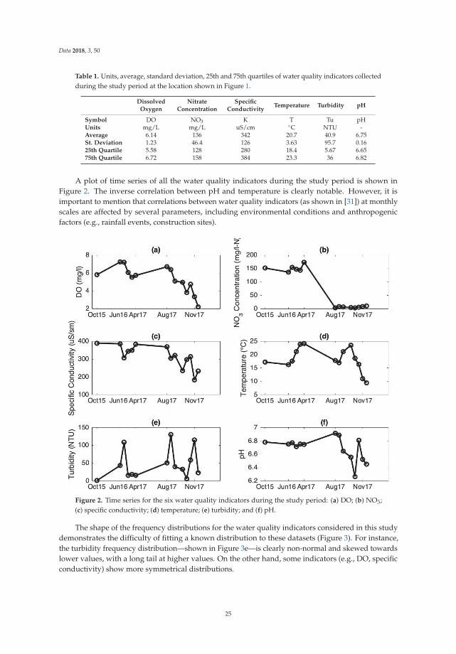
Data 2018, 3, 50

Table 1. Units, average, standard deviation, 25th and 75th quartiles of water quality indicators collectedduring the study period at the location shown in Figure 1.

DissolvedOxygen

NitrateConcentration

SpecificConductivity

Temperature Turbidity pH

Symbol DO NO3 K T Tu pHUnits mg/L mg/L uS/cm ◦C NTU -Average 6.14 136 342 20.7 40.9 6.75St. Deviation 1.23 46.4 126 3.63 95.7 0.1625th Quartile 5.58 128 280 18.4 5.67 6.6575th Quartile 6.72 158 384 23.3 36 6.82

A plot of time series of all the water quality indicators during the study period is shown inFigure 2. The inverse correlation between pH and temperature is clearly notable. However, it isimportant to mention that correlations between water quality indicators (as shown in [31]) at monthlyscales are affected by several parameters, including environmental conditions and anthropogenicfactors (e.g., rainfall events, construction sites).

Figure 2. Time series for the six water quality indicators during the study period: (a) DO; (b) NO3;(c) specific conductivity; (d) temperature; (e) turbidity; and (f) pH.

The shape of the frequency distributions for the water quality indicators considered in this studydemonstrates the difficulty of fitting a known distribution to these datasets (Figure 3). For instance,the turbidity frequency distribution—shown in Figure 3e—is clearly non-normal and skewed towardslower values, with a long tail at higher values. On the other hand, some indicators (e.g., DO, specificconductivity) show more symmetrical distributions.

25

Data 2018, 3, 50

Figure 3. Frequency distribution histograms for: (a) DO; (b) NO3; (c) specific conductivity;(d) temperature; (e) turbidity; and (f) pH during the study period.

3. Results

The information table is set up to apply RST to the data collected at the Mason watershed outlet.Specifically, five water quality indicators are chosen as the conditional attributes and the sixth oneas the decision attribute. The water quality probe reads each water quality indicator every hour.However, in order to introduce rough set theory to water quality analysis, coarse resolution (monthlyaverage) data are examined. This not only helps with showing a limited amount of condition anddecision attributes in the following tables, but also helps to reduce the random noise in the datasample. Numerical values are assigned to each of the 14 months and presented as time codes in Table 2.The following analysis is based on the scenario in which pH is chosen as the decision attribute (D) andthe rest of the indicators as condition attributes (C). In set theory formalism, this corresponds to U = {1,2, 3, 4, 5, 6, 7, 8, 9, 10, 11, 12, 13, 14}, C = {DO, NO3, K, T, Tu}, and D = {pH}, where C and D can beeither L, or M, or H.

The first step is to identify redundant (or identical) time codes. After analyzing each time code, {7}and {8} are the only ones found identical, not only in terms of attributes, but also in terms of decision.This means that every single conditional and decision attribute is the same for time codes {7} and {8}.The fact that they are identical not only in terms of condition attributes but also in terms of decisionattributes shows that if DO and K are medium, NO3 and T are low, and Tu is high, pH is certainlyhigh. This is the first certain decision rule concluded from Table 2. No other time codes are found to beidentical in terms of condition and/or decision attributes. Thus, since all the other codes are unique interms of both condition and decision attributes, each one of them represents a unique rule. As a result,13 unique rules are identified in Table 2.

26

Data 2018, 3, 50

Table 2. Attributes and decision values where pH is the decision attributes and the other indicators arecondition attributes.

Time Code Date (M-Y) DO NO3 K T Tu pH

1 October-15 M M H L L M2 April-16 H M H L H M3 May-16 H M M L H M4 June-16 M M M M M M5 July-16 L M M H M M6 August-16 M H M H M M7 April-17 M L M L H H8 May-17 M L M L H H9 June-17 L L M M H L10 August-17 L L L H M L11 September-17 L L M M M L12 October-17 L L M L H M13 November-17 L L L L H L14 December-17 L L L L M L

The second step explores the discernibility relation by eliminating one condition attribute at thetime. There are 6 tables in Table 3 and each table except the first one is missing one attribute. Firstly,as discussed above, time codes {7} and {8} are identical and they are highlighted. Secondly, if DO,NO3, and T were removed, discernibility would be the same, as shown in Table 3(b),(c),(e). As a result,these three attributes are deemed dispensable. Thirdly, if K and Tu were removed, new decision ruleswould appear. These new rules are highlighted in Table 3(d),(f) as well. In Table 3(d), time codes {2}and {3} are identical both in terms of condition and decision attributes, however, time codes {12} and{13} are just identical in terms of condition attribute. In Table 3(f), time codes {9} and {11} and timecodes {13} and {14} are alike in terms of condition and decision attributes. Hence, there is a change indiscernibility making both K and Tu indispensable.

The formal process of identifying dispensable attributes is further investigated in Table 4. The firstcolumn represents the attribute that is removed, whilst the second column represents the uniquecondition attribute combination in the absence of the corresponding attribute. When K and Tu areremoved, the unique condition attribute combinations are different than when other indicators areremoved in the other cases. In the third column, the unique decision making rules are displayed.If column 3 is not identical to the rules found in the presence of all attributes (conditional and decision),then the removed attribute is deemed dispensable (column 5). More specifically, the posc(D) isequal to {(1), (2), (3), (4), (5), (6), (7,8), (9), (10), (11), (12), (13), (14)}. If column 3 does not matchposc(D), the removed attribute is indispensable. As a result of the analyses shown in Tables 3 and 4,the indispensable attributes are specific conductivity and turbidity. Clearly, in the absence of K,decision rules {2} and {3} are identical, in the absence of Tu, decision rules {9} and {11} are identical,and decision rules {13} and {14} are also identical. These attributes are defined as the core attributes.

27

Data 2018, 3, 50

Table 3. Analysis of the discernibility relation with identical time code highlighted for the followingcases: (a) all attributes; (b) DO eliminated; (c) NO3 concentration eliminated; (d) specific conductivityeliminated; (e) temperature eliminated; (f) turbidity eliminated.

(a) (b)

Time Code DO NO3 K T Tu pH Time Code DO NO3 K T Tu pH

1 M M H L L M 1 M H L L M2 H M H L H M 2 M H L H M3 H M M L H M 3 M M L H M4 M M M M M M 4 M M M M M5 L M M H M M 5 M M H M M6 M H M H M M 6 H M H M M7 M L M L H H 7 L M L H H8 M L M L H H 8 L M L H H9 L L M M H L 9 L M M H L

10 L L L H M L 10 L L H M L11 L L M M M L 11 L M M M L12 L L M L H M 12 L M L H M13 L L L L H L 13 L L L H L14 L L L L M L 14 L L L M L(c) (d)


1 M H L L M 1 M M L L M2 H H L H M 2 H M L H M3 H M L H M 3 H M L H M4 M M M M M 4 M M M M M5 L M H M M 5 L M H M M6 M M H M M 6 M H H M M7 M M L H H 7 M L L H H8 M M L H H 8 M L L H H9 L M M H L 9 L L M H L

10 L L H M L 10 L L H M L11 L M M M L 11 L L M M L12 L M L H M 12 L L L H M13 L L L H L 13 L L L H L14 L L L M L 14 L L L M L(e) (f)


1 M M H L M 1 M M H L M2 H M H H M 2 H M H L M3 H M M H M 3 H M M L M4 M M M M M 4 M M M M M5 L M M M M 5 L M M H M6 M H M M M 6 M H M H M7 M L M H H 7 M L M L H8 M L M H H 8 M L M L H9 L L M H L 9 L L M M L

10 L L L M L 10 L L L H L11 L L M M L 11 L L M M L12 L L M H M 12 L L M L M13 L L L H L 13 L L L L L14 L L L M L 14 L L L L L

28

Data 2018, 3, 50

Table 4. Calculating the discernibility and dispensability.

Attribute C U/Ind(C-{c}) Pos(c-{c})(D) Pos(c-{c})(D) = Posc(D)? Indispensability

DO(1), (2), (3), (4), (5),(6), (7,8), (9), (10),

(11), (12), (13), (14)

(1), (2), (3), (4), (5),(6), (7,8), (9), (10),

(11), (12), (13), (14)Y N

NO3

(1), (2), (3), (4), (5),(6), (7,8), (9), (10),

(11), (12), (13), (14)

(1), (2), (3), (4), (5),(6), (7,8), (9), (10),

(11), (12), (13), (14)Y N

K(1), (2,3), (4), (5), (6),(7,8), (9), (10), (11),

(12,13), (14)

(1), (2,3), (4), (5), (6),(7,8), (9), (10), (11),

(12), (13), (14)N Y

T(1), (2), (3), (4), (5),(6), (7,8), (9), (10),

(11), (12), (13), (14)

(1), (2), (3), (4), (5),(6), (7,8), (9), (10),

(11), (12), (13), (14)Y N

Tu(1), (2), (3), (4), (5),

(6), (7,8), (9,11),(10), (12), (13,14)

(1), (2), (3), (4), (5),(6), (7,8), (9,11),

(10), (12), (13,14)N Y

The application of RST to the water quality data sampled at the Mason campus that wasdiscussed above identified the fundamental and redundant water quality indicators. Their importancedegree as conditional attributes in determining the other indicators (decision) is then quantifiedusing Equation (7). Table 5 shows the indispensable attributes for each decision attribute and theircorresponding importance degree. There are only two indispensable attributes identified for eachdecision attribute. Specifically, two indispensable attributes are identified for pH, DO, T, and K,whereas only one indispensable attribute is identified for Tu (i.e., specific conductivity). This alsomeans that several attributes are redundant and not necessary to fill in possible gaps in time series.This kind of conclusion is extremely useful when obtaining ground observations is complicated byimpervious terrain, financing constraints, and/or extreme atmospheric conditions.

Results in Table 5 demonstrate that turbidity is equally important in every scenario considered inthe study with an importance degree of 0.14. Specific conductivity is the next important factor withan importance degree of 0.07. If the decision attribute is turbidity, the only indispensable attribute isspecific conductivity and if the specific conductivity is the decision attribute, the indispensable attributebeside turbidity is temperature. According to the foregoing analysis, if any of the six water qualityindicator needs to be retrieved because of a missed measurement, turbidity and specific conductivityare the core values that would provide useful information about the missing information. Moreover,the decision in every scenario is weighted towards turbidity since the importance degree of turbidityis higher than the importance degree of conductivity.

Table 5. Importance degree of C attributes relative to the decision attribute D.

Decision AttributeIndispensable Attribute 1

(Importance Degree)Indispensable Attribute 2

(Importance Degree)

pH Tu (0.14) K (0.07)DO Tu (0.14) K (0.07)

NO3 Tu (0.14) K (0.07)T Tu (0.14) K (0.07)

Tu K (0.07) -K Tu (0.14) T (0.07)

There is a direct relationship between temperature and all the other water quality indicators.Furthermore, conductivity has an effect on turbidity and turbidity influences dissolved oxygenconcentration, which also affects nitrate concentration. However, there is no direct relation between pH

29

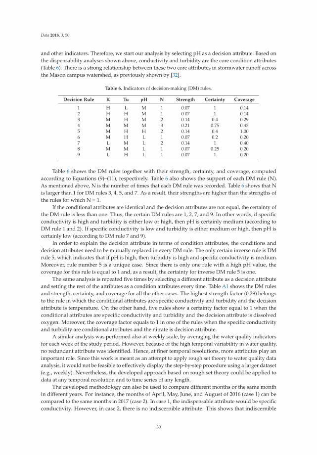
Data 2018, 3, 50

and other indicators. Therefore, we start our analysis by selecting pH as a decision attribute. Based onthe dispensability analyses shown above, conductivity and turbidity are the core condition attributes(Table 6). There is a strong relationship between these two core attributes in stormwater runoff acrossthe Mason campus watershed, as previously shown by [32].

Table 6. Indicators of decision-making (DM) rules.

Decision Rule K Tu pH N Strength Certainty Coverage

1 H L M 1 0.07 1 0.142 H H M 1 0.07 1 0.143 M H M 2 0.14 0.4 0.294 M M M 3 0.21 0.75 0.435 M H H 2 0.14 0.4 1.006 M H L 1 0.07 0.2 0.207 L M L 2 0.14 1 0.408 M M L 1 0.07 0.25 0.209 L H L 1 0.07 1 0.20

Table 6 shows the DM rules together with their strength, certainty, and coverage, computedaccording to Equations (9)–(11), respectively. Table 6 also shows the support of each DM rule (N).As mentioned above, N is the number of times that each DM rule was recorded. Table 6 shows that Nis larger than 1 for DM rules 3, 4, 5, and 7. As a result, their strengths are higher than the strengths ofthe rules for which N = 1.

If the conditional attributes are identical and the decision attributes are not equal, the certainty ofthe DM rule is less than one. Thus, the certain DM rules are 1, 2, 7, and 9. In other words, if specificconductivity is high and turbidity is either low or high, then pH is certainly medium (according toDM rule 1 and 2). If specific conductivity is low and turbidity is either medium or high, then pH iscertainly low (according to DM rule 7 and 9).

In order to explain the decision attribute in terms of condition attributes, the conditions anddecision attributes need to be mutually replaced in every DM rule. The only certain inverse rule is DMrule 5, which indicates that if pH is high, then turbidity is high and specific conductivity is medium.Moreover, rule number 5 is a unique case. Since there is only one rule with a high pH value, thecoverage for this rule is equal to 1 and, as a result, the certainty for inverse DM rule 5 is one.

The same analysis is repeated five times by selecting a different attribute as a decision attributeand setting the rest of the attributes as a condition attributes every time. Table A1 shows the DM rulesand strength, certainty, and coverage for all the other cases. The highest strength factor (0.29) belongsto the rule in which the conditional attributes are specific conductivity and turbidity and the decisionattribute is temperature. On the other hand, five rules show a certainty factor equal to 1 when theconditional attributes are specific conductivity and turbidity and the decision attribute is dissolvedoxygen. Moreover, the coverage factor equals to 1 in one of the rules when the specific conductivityand turbidity are conditional attributes and the nitrate is decision attribute.

A similar analysis was performed also at weekly scale, by averaging the water quality indicatorsfor each week of the study period. However, because of the high temporal variability in water quality,no redundant attribute was identified. Hence, at finer temporal resolutions, more attributes play animportant role. Since this work is meant as an attempt to apply rough set theory to water quality dataanalysis, it would not be feasible to effectively display the step-by-step procedure using a larger dataset(e.g., weekly). Nevertheless, the developed approach based on rough set theory could be applied todata at any temporal resolution and to time series of any length.

The developed methodology can also be used to compare different months or the same monthin different years. For instance, the months of April, May, June, and August of 2016 (case 1) can becompared to the same months in 2017 (case 2). In case 1, the indispensable attribute would be specificconductivity. However, in case 2, there is no indiscernible attribute. This shows that indiscernible

30

Data 2018, 3, 50

attributes may vary depending on environmental and/or anthropogenic conditions. This kind ofcomparison highlights possible changes in the stream water quality conditions, whose sources can bepotentially investigated by the analyst.

4. Discussion

This study investigates the application of RST to water quality analysis. RST does not requireany prior information on the dataset and represents a powerful tool to deal with uncertainty andvagueness in the sample. Moreover, RST is capable of finding indiscernible attributes and extractingrules based on core attributes. This work presents the basic concepts of rough set theory and itsapplication to six water quality indicators collected during a 3-year-long study period at the GeorgeMason University campus in Fairfax, VA. More specifically, monthly averages for each water qualityindicator are calculated and 14 months are considered.

It is important to mention that the streamflow velocity at the watershed outlet where data werecollected is particularly high during and after rainfall events. As a result, the common relationshipsamong water quality attributes are not observed in this case study that focuses on the monthly scale.For example, when water temperature is low, DO concentration is commonly high [33]. However, wecannot observe this rule at the monthly resolution. When a storm happens, even during summer whentemperatures are high, the rapidly moving water contains more DO than stagnant water in winterdays (when the temperature is lower).

Coarse temporal resolution (i.e., monthly) data are selected here in order to present a novelmethodology in the field of water quality analysis. The coarse resolution helps with showing alimited number of attributes and decision values. Six different scenarios are studied here and in eachscenario one attribute is assigned to be a decision attribute and the rest are reflected as conditionalattributes. In most cases, specific conductivity (with an importance degree of 0.07) and turbidity (withan importance degree of 0.14) are the core conditional attributes. In addition, we generate DM rulesfor each scenario and calculate the strength, certainty, and coverage of each rule. The certain rulesshow that if specific conductivity is high and turbidity is either low or high, then pH is medium.Also, if specific conductivity is low and turbidity is either medium or high, then pH is certainly low.However, the coverage of these DM rules is the lowest among all DM rules. Five other possible DMrules with certainty lower than one are identified as well. There is one DM rule with coverage factor ofone (DM 5), which means that there is only one DM rule with a unique pH value (high). As a result,the certainty for the inverse DM rule 5 is one.

Overall, RST was proven capable of finding core indicators and discovering DM rules.Considering more attributes and more data entries could increase the certainty of the identifiedDM rules and possibly identify additional DM rules. RST-based DM rules can be of tremendous helpto planners and analysts in their decision making process. For instance, results from this study can beuseful for university facility managers that monitor water quality across campus. If applied to a largerscale, the proposed methodology has the potential of providing timely, relevant, and essential waterquality information.

Future work should look at the raw data at their native resolution (one hour). Although nodifference in the DM rules was observed in the weekly analysis with respect to the monthly one,increasing the resolution to one hour may result in higher certainty in the DM rules. Moreover, otherlocations should be investigated to verify the efficiency of the proposed methodology and possiblysampling additional indicators (i.e., conditional attributes). Further conditional attributes can berelated to atmospheric conditions, like the amount and duration of precipitation events and landcover/land use.

Author Contributions: Conceptualization, M.Z. and V.M.; Data, M.Z.; Formal analysis, M.Z.; Methodology, M.Z.and V.M.; Project administration, M.Z. and V.M.; Resources, V.M.; Supervision, V.M.; Writing—original draft, M.Z.;Writing—review & editing, V.M.

Funding: This research received no external funding.

31

Data 2018, 3, 50


Appendix A

Table A1. DM rules for various scenarios, with different decision attributes: (a) DO; (b) Tu; (c) NO3;(d) T; and (e) k.

(a) (b)

K Tu DO N Strength Certainty Coverage DO K Tu N Strength Certainty Coverage

H L M 1 0.07 1.00 0.20 H H H 1 0.07 1.00 0.14H H H 1 0.07 1.00 0.50 H M H 1 0.07 1.00 0.14M H H 1 0.07 1.00 0.50 L M H 2 0.14 0.50 0.29M M M 2 0.14 0.50 0.40 L L H 1 0.07 0.33 0.14M M L 2 0.14 0.50 0.29 M M H 2 0.14 0.50 0.29M H M 2 0.14 0.40 0.40 M H L 1 0.07 1.00 1.00M H L 2 0.14 0.40 0.40 L M M 2 0.14 0.50 0.33L M L 2 0.14 1.00 0.40 L L M 2 0.14 0.67 0.33L H L 1 0.07 1.00 0.20 M M M 2 0.14 0.50 0.33(c) (d)

K Tu NO3 N Strength Certainty Coverage K Tu T N Strength Certainty Coverage

M M H 1 0.07 0.25 1.00 L M H 1 0.07 0.50 0.33M H L 2 0.14 0.40 0.25 M M H 2 0.14 0.50 0.67L M L 2 0.14 1.00 0.25 H L L 1 0.07 1.00 0.13M H L 1 0.07 0.20 0.13 H H L 1 0.07 1.00 0.13L H L 1 0.07 1.00 0.13 L H L 1 0.07 1.00 0.13M H L 1 0.07 0.20 0.13 L M L 1 0.07 0.50 0.13M M L 1 0.07 0.25 0.13 M H L 4 0.29 0.80 0.50H L M 1 0.07 1.00 0.20 M M M 2 0.14 0.50 0.67H H M 1 0.07 1.00 0.20 M H M 1 0.07 0.20 0.33M H M 1 0.07 0.20 0.20M M M 2 0.14 0.50 0.40(e)

T Tu K N Strength Certainty Coverage

L L H 1 0.07 1.00 0.50L H H 1 0.07 0.17 0.50H M L 1 0.07 0.33 0.33L H L 1 0.07 0.17 0.33L M L 1 0.07 1.00 0.33M M M 2 0.14 1.00 0.22H M M 2 0.14 0.67 0.22L H M 3 0.21 0.50 0.33M H M 1 0.07 1.00 0.11L H M 1 0.07 0.17 0.11

References

1. Pai, P.-F.; Li, L.-L.; Hung, W.-Z.; Lin, K.-P. Using ADABOOST and Rough Set Theory for Predicting DebrisFlow Disaster. Water Resour. Manag. 2014, 28, 1143–1155. [CrossRef]

2. Wagner, R.J.; Boulger, R.W., Jr.; Oblinger, C.J.; Smith, B.A. Guidelines and Standard Procedures for ContinuousWater-Quality Monitors: Station Operation, Record Computation, and Data Reporting [Internet]. 2006 [Cited1 June 2018]. (Techniques and Methods). Report No.: 1-D3. Available online: http://pubs.er.usgs.gov/publication/tm1D3 (accessed on 5 November 2018).

3. Lepot, M.; Aubin, J.-B.; Clemens, F.H.L.R. Interpolation in Time Series: An Introductive Overview of ExistingMethods, Their Performance Criteria and Uncertainty Assessment. Water 2017, 9, 796. [CrossRef]

4. Fu, L.; Wang, Y.-G. Statistical Tools for Analyzing Water Quality Data|IntechOpen [Internet]. 2012 [Cited3 July 2018]. Available online: /books/water-quality-monitoring-and-assessment/statistical-tools-for-analyzing-water-quality-data (accessed on 5 November 2018).

5. Liou, S.M.; Lo, S.L.; Hu, C.Y. Application of two-stage fuzzy set theory to river quality evaluation in Taiwan.Water Res. 2003, 37, 1406–1416. [CrossRef]

6. Chen, X.; Li, Y.S.; Liu, Z.; Yin, K.; Li, Z.; Wai, O.W.; King, B. Integration of multi-source data for water qualityclassification in the Pearl River estuary and its adjacent coastal waters of Hong Kong. Cont. Shelf Res. 2004,24, 1827–1843. [CrossRef]

32

Data 2018, 3, 50

7. Shrestha, S.; Kazama, F. Assessment of surface water quality using multivariate statistical techniques: A casestudy of the Fuji river basin, Japan. Environ. Model. Softw. 2007, 22, 464–475. [CrossRef]

8. Diamantopoulou, M.J.; Antonopoulos, V.Z.; Papamichail, D.M. Cascade Correlation Artificial NeuralNetworks for Estimating Missing Monthly Values of Water Quality Parameters in Rivers. Water ResourManag. 2007, 21, 649–662. [CrossRef]

9. Singh, A.P.; Ghosh, S.K.; Sharma, P. Water quality management of a stretch of river Yamuna: An interactivefuzzy multi-objective approach. Water Resour. Manag. 2007, 21, 515–532. [CrossRef]

10. Manache, G.; Melching, C.S. Identification of reliable regression- and correlation-based sensitivity measuresfor importance ranking of water-quality model parameters. Environ. Model. Softw. 2008, 23, 549–562.[CrossRef]

11. Qin, X.S.; Huang, G.H. An Inexact Chance-constrained Quadratic Programming Model for Stream WaterQuality Management. Water Resour Manag. 2009, 23, 661. [CrossRef]

12. Hou, D.; He, H.; Huang, P.; Zhang, G.; Loaiciga, H. Detection of water-quality contamination events basedon multi-sensor fusion using an extended Dempster–Shafer method. Meas. Sci. Technol. 2013, 24, 055801.[CrossRef]

13. Pawlak, Z. Rough sets. Int. J. Comput. Inf. Sci. 1982, 11, 341–356. [CrossRef]14. Polkowski, L. Rough Sets: Mathematical Foundations [Internet]. Physica-Verlag Heidelberg. 2002 [Cited

27 April 2018]. (Advances in Intelligent and Soft Computing). Available online: //www.springer.com/us/book/9783790815108 (accessed on 5 November 2018).

15. Skowron, A.; Suraj, Z. Rough Sets and Intelligent Systems—Professor Zdzisław Pawlak in Memoriam; SpringerScience & Business Media: Berlin, Germany, 2012; p. 682.

16. Nguyen, T.-T.; Nguyen, P.-K. Reducing Attributes in Rough Set Theory with the Viewpoint of MiningFrequent Patterns. Int. J. Adv. Comput. Sci. Appl. 2013, 4. [CrossRef]

17. Pawlak, Z. Rough set theory and its applications. J. Telecommun. Technol. 2002, 3, 7–10.18. Dong, S.-H.; Zhou, H.-C.; Xu, H.-J. A Forecast Model of Hydrologic Single Element Medium and Long-Period

Based on Rough Set Theory. Water Resour. Manag. 2004, 18, 483–495. [CrossRef]19. Pai, P.-F.; Lee, F.-C. A Rough Set Based Model in Water Quality Analysis. Water Resour. Manag. 2010, 24,

2405–2418. [CrossRef]20. Shen, Q.; Chouchoulas, A. FuREAP: A Fuzzy–Rough Estimator of Algae Populations. Artif. Intell. Eng. 2001,

15, 13–24. [CrossRef]21. Barbagallo, S.; Consoli, S.; Pappalardo, N.; Greco, S.; Zimbone, S.M. Discovering Reservoir Operating Rules

by a Rough Set Approach. Water Resour. Manag. 2006, 20, 19–36. [CrossRef]22. Predki, B.; Słowinski, R.; Stefanowski, J.; Susmaga, R.; Wilk, S. ROSE—Software Implementation of the

Rough Set Theory. In Rough Sets and Current Trends in Computing [Internet]; Lecture Notes in ComputerScience; Springer: Berlin/Heidelberg, Germany, 1998; pp. 605–608.

23. Ip, W.C.; Hu, B.Q.; Wong, H.; Xia, J. Applications of rough set theory to river environment quality evaluationin China. Water Resour. 2007, 34, 459–570. [CrossRef]

24. Karami, J.; Alimohammadi, A.; Seifouri, T. Water quality analysis using a variable consistencydominance-based rough set approach. Comput. Environ. Urban Syst. 2014, 43, 25–33. [CrossRef]

25. Pawlak, Z.; Grzymala-Busse, J.; Slowinski, R.; Ziarko, W. Rough Sets. Commun. ACM 1995, 38, 88–95.[CrossRef]

26. Rissino, S.; Lambert-Torres, G. Rough Set Theory—Fundamental Concepts, Principals, Data Extraction, andApplications. In Data Mining and Knowledge Discovery in Real Life Applications; Ponce, J., Karahoca, A., Eds.;IN-TECH: Hong Kong, China, 2009; pp. 35–58.

27. Department, V.; Quality, E. Virginia Administrative Code, Title 9. Environment, Agency 25. State WaterControl Board, Chapter 260. Water Quality Standards. Available online: https://www.epa.gov/sites/production/files/2014-12/documents/vawqs.pdf (accessed on 5 November 2018).

28. Mason MS4 Program|Facilities|George Mason University [Internet]. [Cited 24 October 2018]. Availableonline: https://facilities.gmu.edu/resources/land-development/ms4/ (accessed on 5 November 2018).

29. NWSCIW. National Weather Service Sterling [Internet]. [Cited 27 October 2018]. Available online:https://w2.weather.gov/climate/local_data.php?wfo=lwx (accessed on 5 November 2018).

30. Nitrogen and Water: USGS Water Science School [Internet]. [Cited 27 July 2018]. Available online:https://water.usgs.gov/edu/nitrogen.html (accessed on 5 November 2018).

33

Data 2018, 3, 50

31. Copetti, D.; Marziali, L.; Viviano, G.; Valsecchi, L.; Guzzella, L.; Capodaglio, A.G.; Tartari, G.; Polesello, S.;Valsecchi, S.; Mezzanotte, V.; et al. Intensive monitoring of conventional and surrogate quality parameters ina highly urbanized river affected by multiple combined sewer overflows. Water Sci. Technol. Water Suppl.2018. [CrossRef]

32. Gholoom, A. Studying the Impact of Different Green Rooftop Designs on Stormwater [Internet] [Thesis].2018 [Cited 17 July 2018]. Available online: http://mars.gmu.edu/handle/1920/10916 (accessed on5 November 2018).

33. Dissolved Oxygen, from the USGS Water Science School: All about Water. [Internet]. [Cited 26 July 2018].Available online: https://water.usgs.gov/edu/dissolvedoxygen.html (accessed on 5 November 2018).


34

data

Article

Use of the WRF-DA 3D-Var Data Assimilation Systemto Obtain Wind Speed Estimates in Regular Gridsfrom Measurements at Wind Farms in Uruguay

Gabriel Cazes Boezio 1,* and Sofía Ortelli 1,2

1 School of Engineeering, Universidad de la República, Montevideo 11300, Uruguay; [email protected] Usinas y Trasmisiones del Estado (UTE), Montevideo 11200, Uruguay* Correspondence: [email protected]; Tel.: +598-27115279

Received: 31 August 2019; Accepted: 24 October 2019; Published: 29 October 2019

Abstract: This work assessed the quality of wind speed estimates in Uruguay. These estimates wereobtained using the Weather Research and Forecast Model Data Assimilation System (WRF-DA) toassimilate wind speed measurements from 100 m above the ground at two wind farms. The qualityof the estimates was assessed with an anemometric station placed between the wind farms. Thewind speed estimates showed low systematic errors at heights of 87 and 36 m above the ground. Atboth levels, the standard deviation of the total errors was approximately 25% of the mean observedspeed. These results suggested that the estimates obtained could be of sufficient quality to be usefulin various applications. The assimilation process proved to be effective, spreading the observationalgain obtained at the wind farms to lower elevations than those at which the assimilated measurementswere taken. The smooth topography of Uruguay might have contributed to the relatively good qualityof the obtained wind estimates, although the data of only two stations were assimilated, and theresolution of the regional atmospheric simulations employed was relatively low.

Keywords: data assimilation; 3D-Var

1. Summary

This work evaluated the use of techniques for assimilation of data from field measurements intoinitial conditions of atmospheric numerical simulations in order to obtain wind estimates in Uruguay,at heights of 100 m above the ground and lower. The wind was estimated with hourly frequency ina regular grid that covers the country. The field data to be assimilated was operatively measured inwind farms installed in Uruguay, using anemometers placed 100 m above the ground. The data wasassimilated into initial conditions for the Weather Research and Forecast regional model (WRF) of theNational Center of Atmospheric Research (NCAR), [1] using the module for data assimilation includedin this model, the WRF-DA module [2].

The data assimilation process, also called analysis, is an essential component of numericalatmospheric forecasts, and its main purpose is to generate initial conditions for the predictions. Thevariables that compose an initial condition are called prognostic variables because the model usestheir values at a given instant to compute their values at a later time. To generate an initial conditionfor a specific numerical model at a given time, a first approximation is generally used. This firstapproximation, called “background condition”, usually consists of a prediction for the same instant,obtained with the same model, from previous initial conditions. The data assimilation system mustcombine the information from the background condition with the information from measurementsof atmospheric variables (or variables of systems related to it; for example, the ocean, the soil, or thecryosphere). This combination of information is done in a way that optimizes the quality of the result instatistical terms, either minimizing the expected value of the sum of its quadratic errors or maximizing


Data 2019, 4, 142

its likelihood. Note that the short-term predictions used as background values are, in turn, affected byfield measurements that were assimilated during previous times. This allows considering informationfrom regions or atmospheric levels in which few measurements are available since measurements,done earlier in other regions or at other levels, can propagate their influence through atmosphericdynamical processes into the zones that have relatively fewer observations.

Kalnay [3] described the main techniques for data assimilation that are currently used, such asoptimal interpolation, 3D-Var, Kalman filters, ensemble Kalman filters, and 4D-Var. The WRF-DAsystem implements the 3D-Var [4] and 4D-Var techniques [5], and a technique that combines theensemble Kalman filter with 3D-Var [6,7]. Harlim [8] pointed that the referred techniques assume thatthe errors from the background conditions and the field measurements are unbiased and normallydistributed, although numerical models inevitably have systematic errors. These assumptions canprovide reasonable estimates of the first-order statistics while being practical to implement. However,these methodologies require caution for interpreting their higher-order statistical estimates, and animportant challenge in data assimilation is to use existing methods in the presence of model systematicerrors. The author proposed methodologies to mitigate the effects of model systematic errors onthe results of the assimilation process. Rao and Sandu [9] proposed an a-posteriori error estimationmethodology that quantifies the impact of model and data errors on the inference results of inverseproblems, including the 4D-Var assimilation process. The model and data errors considered includeboth unbiased noise and systematic biases. The authors found that the proposed methodology couldbe useful to reduce and quantify uncertainties in a real-time system with feedback. Besides, the errorestimates can be used to locate faulty sensors and to determine areas of maximum sensitivity, whereimprovements in the stations network or an increase in model resolution may be required.

In addition to its direct use in the numerical prediction process, the results of data assimilationcan be considered “pseudo-observations” of atmospheric variables in regular grids. Note that these donot consist purely of interpolations of field measurements in a regular grid since they also consider theinformation from short-term predictions. The uses of the pseudo-observations obtained from a dataassimilation process can be very broad, but they require an evaluation of their quality by comparisonwith field measurements not used in the assimilation process.

The current work used the rather conventional 3D-Var assimilation technique. In Section 2,we described the data used, both from field measurements and from numerical predictions used asbackground conditions, and we referred to the quality control method used for the field data from thewind farms. In Section 3, we described the main aspects of the 3D-Var assimilation technique and itsimplementation in this work using the WRF DA system. In Section 4, we described the main results,and in Section 5, we presented the conclusions.

2. Data Description

The wind data used in the data assimilation process was obtained from two anemometers installedin the “Rosendo Mendoza” (WF1) and “Valentines” (WF2) wind farms. The geographic locations ofthese wind farms are shown in Figure 1. The anemometers were placed 100 m above the ground,and they recorded mean velocities for successive periods of 15 min, which were transmitted to theNational Dispatch of Electric Charges of Uruguay, operated by the Electricity Market Administration(Administración del Mercado Eléctrico; ADME) and the National Administration of Electric PowerPlants and Transmissions (Usinas y Trasmisiones del Estado; UTE), and Uruguayan National PublicElectricity Utility Organizations. In addition to the wind measurements, the mean electric powergenerated in the same 15-min periods and the corresponding quantity of aerogenerators that wereeffectively active were also transmitted by each wind farm. These additional data allowed for a qualitycontrol analysis of the measurements, as described by Orteli and Cazes Boezio [10]. With the historicalinformation of wind velocity and electric power generated, the authors built an empirical wind-powercurve for each wind farm. In those cases in which not all the aerogenerators of the wind farm wereactive, the power generation that would correspond to a condition of full availability was estimated by

36

Data 2019, 4, 142

linear extrapolation. The authors considered that those combinations of wind and generated powerthat depart from the empirical curve beyond certain thresholds were suspicious of being affected bymalfunctioning of the measurement or recording systems, or by occasional interference of the wake ofan aerogenerator with the anemometer. The data from WF1 and WF2 available for this study werefrom the months from January to May and from November to December of 2017 (seven months).

Figure 1. The geographic location of anemometers used for data assimilation (WF1 and WF2) andvalidation (Vst).

To evaluate the quality of the pseudo-observations obtained through the implemented dataassimilation process, an independent station was used (“validation station”, VSt), which is located atColonia Arias, Uruguay. The station location is also shown in Figure 1. The station measures windspeed and direction at heights of 87 and 36 m above the ground and is part of a network of stations thatmeasures wind velocity and solar radiation that has been operated by UTE since 2009. This network isdescribed by Cornalino and Draper [11], and its measurements (that include wind velocities averagedevery 10 min) are made available online by UTE. In recent years, many of the anemometric stationsoperated by UTE have become affected by wind farms. The VSt of Colonia Arias has been active since2011, and during the period studied in this work, it was not affected by any wind farm. Figure 2shows the wind speed at the WF1, WF2, and Vst sensors averaged for each local hour during the sevenmonths considered.

The assimilation process uses regional simulations computed with the WRF model from NCAR,as shown by Cazes Boezio and Orteli [12]. The regional simulations take their initial and boundaryconditions from global predictions made by the Global Forecast System (GFS) of the National Oceanand Atmosphere Administration (NOAA) of the Unites States. The horizontal grid of the regionalsimulations has a resolution of 30 km in the zonal and meridional directions, as shown in Figure 3. Thevertical direction is discretized in 54 levels, 7 of which are within the first 100 m of height above theground. In Appendix A, we indicated the parameterizations of physical processes employed, and wedefined in detail the vertical discretization. The regional simulations have two purposes: first, theygenerate the background conditions into which the data measured in WF1 and WF2 are assimilated;and second, they allow for the estimation of the matrix of covariances of the errors of these backgroundconditions. In Section 3, the hours of initialization and the simulated periods used for each one ofthese purposes were specified.

37

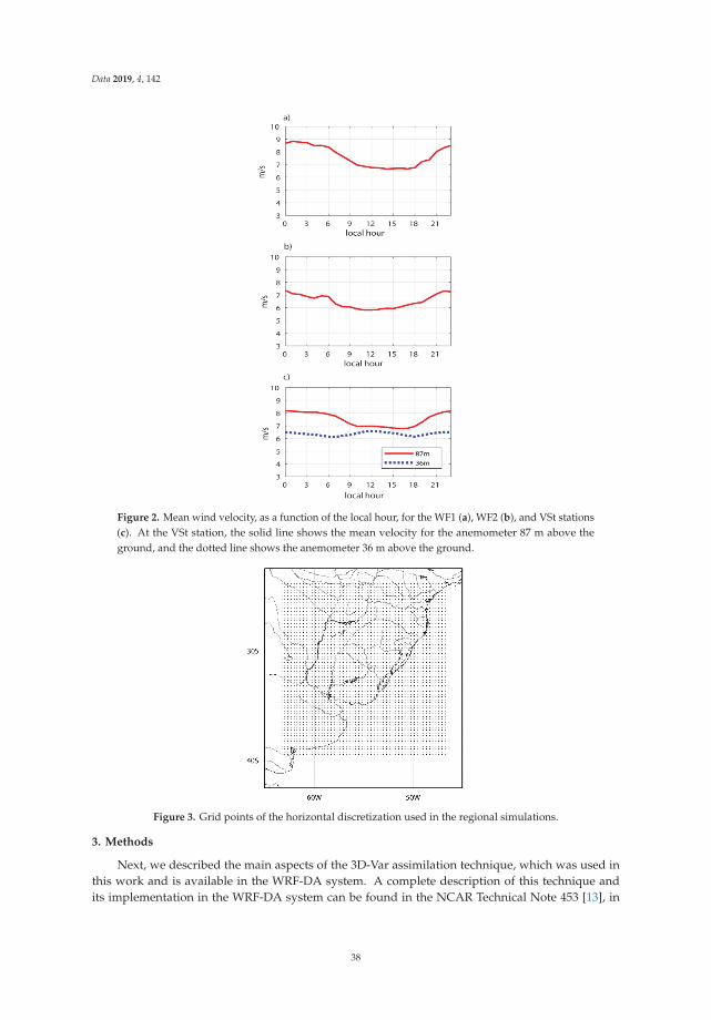
Data 2019, 4, 142

Figure 2. Mean wind velocity, as a function of the local hour, for the WF1 (a), WF2 (b), and VSt stations(c). At the VSt station, the solid line shows the mean velocity for the anemometer 87 m above theground, and the dotted line shows the anemometer 36 m above the ground.

Figure 3. Grid points of the horizontal discretization used in the regional simulations.

3. Methods

Next, we described the main aspects of the 3D-Var assimilation technique, which was used inthis work and is available in the WRF-DA system. A complete description of this technique andits implementation in the WRF-DA system can be found in the NCAR Technical Note 453 [13], in

38

Data 2019, 4, 142

Barker et al. [4] and Barker et al. [2], while the corresponding operational details are given in theWRF-DA User Guide [14].

The background condition information is displayed as a vector called xb, which contains thevalues of all the different prognostic variables that compose the background condition in a certainconventional order. This information is displayed for each variable and each point of the grid. Thefield measurements that are to be assimilated, obtained at the same instant that corresponds to xb,are displayed as a vector called y, also in a conventional order. The initial condition determined bythe assimilation system is expressed as a vector called xa, with a structure analogous to that of xb. xa

combines the information from the background condition xb and the field measurements containedin y, as expressed in Section 1. The 3D-Var technique determines the vector xa as that of maximumlikelihood, conditioned to the information of the background condition and the field measurements,and is the vector x that minimizes the following expression [3]:

J(x) =12(x− xb)

TB−1(x− xb) +12(y−H(x))TR−1(y−H(x)) (1)

that is, J(xa) must be minim. In this formula, B and R are the matrices of error covariances of thebackground condition xb and the field measurements y, respectively. It is assumed that these errorsare normal variables and are unbiased. The B matrix is thus related to the accidental errors of xb, whilethe model systematic errors or biases are assumed to be zero, as pointed out in [8]. Matrix B is definedas follows:

B ≡ E((xb − xt)·(xb − xt)

T)

(2)

where E represents the expected value of the elements of the matrix (xb − xt)·(xb − xt)T, and xt is the

vector of the true values of the variables contained in xb. Note the actual values of xt are unknown, soit becomes necessary to define a technique to estimate the values of B from available information.

H(x) is an operator that yields results analogous to the variables y from the model prognosticvariables included in x. As an example, if an element of y represents the measurement of the meridionalwind at a certain geographical location and a certain height, H(x) interpolates the values of themeridional wind field obtained from the numerical model at the geographical location and the heightof this measurement. The H operator is generally non-linear, but it is possible to linearize it with thefollowing approximation:

H(x) = H(xb + x− xb) ≈ H(x) + ∇H(x− xb), (3)

where ∇H is the gradient of H(x). If the linearized expression for H(x) is used, J(x) assumes aquadratic form.

It is assumed that the errors of the field measurements contained in vector y are statisticallyindependent of each other, so R is a diagonal matrix; its diagonal contains the variances of the errors ofeach field measurement.

The matrix B is essential to this assimilation system. First, its non-diagonal terms contain thecovariances of xb errors at different grid points and also the covariances of errors of different variables.These covariances are necessary to propagate the information related to any field measurement throughthe horizontal and vertical directions and allow measurement of a specific variable to affect the analysisof others. In addition to this, the matrices B−1 and R−1 together determine the relative importance ofthe background conditions xb and the field measurements y to determine the analysis xa.

The WRF-DA system offers two methods to estimate B: the National Meteorological Centermethod (NMC), described by Parrish and Derber [15], and a method based on ensembles of predictions([1], Chapter 9). Due to the availability of computer resources, we used the NMC method, which isrelatively more economic. This method requires a database of pairs of xb; each pair has two short-termpredictions for the same hour obtained with different forecast horizons (for example, 12 and 24 h), andconsequently with different initial conditions. The pairs of predictions correspond to certain hours of

39

Data 2019, 4, 142

the day (for example, 0:00 and 12:00 GMT), and cover a certain period (for example, one year). It isassumed that the differences between the forecasts of each pair have statistical properties analogous tothose of the background condition errors, and in particular, to estimate B, the following approximationcan be used:

B = E((xb − xt)

T·(xb − xt))≈ E((

x12hsb − x24hs

b

)T·(x12hsb − x24hs

b

))(4)

where x12hsb and x24hs

b are a generic pair of predictions with 12 and 24 h time horizons, respectively. Thevalidation of this technique to estimate B is empirical.

Note that, if n is the length of the xa, and xb vectors, the size of B is nxn. This implies a matrixof very large dimensions that would cause important technical difficulties to operate with B or B−1,and even to store them in the computer memory. The 3D-Var technique implemented in the WRF-DAsystem solves this problem by factoring B as a product of certain matrices that have clear physicalinterpretations, allowing certain assumptions about their structures to be made and making themcomputationally tractable [2,4].

As a final remark in this subsection, we noted that both for the simulations of the backgroundconditions and the estimation of the B matrix, a specific configuration of the WRF model was used,which here is the one described in Section 2.

WRF-DA Implementation for This Work

To apply the NMC method to estimate the matrix B, we used WRF-GFS simulations extended for24 h and initialized at 0:00 GMT and 12:00 GMT during the entire year of 2016. The results obtainedfor 12 and 24 h after the initial conditions were used to estimate the matrix B, as indicated in theprevious section. In order to gain insight into the spatial structure of the covariances contained in B,Decombes et al., [16] and Rivi [17] proposed “pseudo-single observation tests”. Such tests consist ofchoosing a particular variable of xb in a particular grid point and suppose a hypothetical observationthat increments in a fixed amount the background value of this variable at the selected grid point. Thedata assimilation process is carried on considering this single pseudo observation and prescribing ahypothetical value of the standard deviation of its error. Rivi [17] showed that the xa − xb differencewas proportional to the covariance between the errors of the background variable in question at thechosen grid point and the errors of the rest of the background variables at all the grid points. The plotsof the xa − xb differences for selected variables illustrate how the B matrix spreads the information offield measurements. In Appendix B, we summarized the fundamentals of the pseudo observationtests, and we showed some selected results for the B matrix estimated here.

The background conditions xb were obtained from WRF-GFS simulations initiated at 0:00, 6:00,12:00, and 18:00 GMT, during those months of 2017 for which information from the WF1 and WF2stations was available. We used the hourly results of these simulations from 4 to 9 h since theinitialization of each simulation. In this way, four consecutive simulations could cover the 24 h of eachday. The selected forecast horizon was the earliest for which the GFS prediction results were availablein real-time, with some time left to carry out the processes described in this work. In this way, it ispossible to implement these processes in an operative mode. For each local hour in Uruguay, Table 1shows which WRF-GFS initialization cycle was used, and which hour within its forecast horizoncorresponded to the background condition for that local hour.

40

Data 2019, 4, 142

Table 1. Hours within the WRF simulations used to define the background conditions as a function ofthe initialization cycle and local time in Uruguay. Each row corresponds to an initialization cycle, andeach column corresponds to a local hour in Uruguay. The hours used within each cycle are indicated,considering the hours elapsed since its initialization.

Local UY Hour

InitializationCycle

0* 1 2 3 4 5 6 7 8 9 10 11 12 13 14 15 16 17 18 19 20 21 22 23

0:00 4 5 6 7 8 96:00 4 5 6 7 8 9

12:00 4 5 6 7 8 918:00 9* 4 5 6 7 8

*: Local time 0 uses the results at the ninth hour of the simulation started at 18:00 GMT on the previous day as abackground condition.

In the present study, the assimilation made for each hour was independent of the previousassimilations; the corresponding background condition only incorporated information from the GFSglobal simulation. This is called a “cold start”. Alternatively, the background conditions could alsohave considered the field measurements made in previous hours. This alternative is called a warmstart. The warm start method was tested in the context of the present work and obtained results ofequivalent quality to those obtained with the cold start, so here we showed only the latter results. Thesimilarity of the results from both methods might be because the assimilated information was verylocal; the assimilation of data in a wider region could influence the simulations in the area of interestover more hours and thus increase the relevance of assimilation from previous hours. The verificationof this hypothesis requires a database of field measurements more complete than the one that wasavailable for this work.

Each field measurement is specified to the WRF-DA system in a file that contains the day and timeof the measurement, the geographic coordinates, and ground elevation of the corresponding station,the height of the measurement sensor, and the records of wind speed and direction. This informationis used to generate the vector of field observations, y. Considering that the topography of the regionalmodel has some degree of smoothing, the elevation of the specified terrain is not the actual elevation,but the elevation corresponding to the topography of the model interpolated to the station’s locationcoordinates. The height specified for the sensors is the elevation of the station plus 100 m. The specifiedmodule of wind speed is the average of the anemometer record for two consecutive 15-min periodscentered on the hour for which the assimilation will be performed.

The specified wind direction is deduced from the background condition, interpolating eachcomponent of the wind vector to the geographical position and elevation of the anemometer. Althoughvanes are available at the stations, it was found that using their records produces results that are not assatisfactory as those obtained by deducing the wind direction from the background condition. Thissuggests that the quality of data obtained from these weathervanes is relatively poor, while regionalshort-term predictions are reasonably good with regard to this variable. It may be of interest to evaluatethe effect of the assimilation of atmospheric pressure measurements on the wind direction obtained inthe analysis, but no such observations were available to complete this analysis.

In addition, to estimate the R matrix, the WRF-DA system uses a file that specifies the standarddeviations of the errors of the different kinds of field observations (obserr.txt). In the present work,we adjusted the errors specified in this file, proposing a value of 0.1 m/s for wind speed, which isreasonable for the type of sensors installed in the stations considered here [18]. For wind direction,we kept the default value proposed in the obserr.txt file, 5◦. We also pointed out that the WRF-DAsystem uses two “namelist” files to prescribe parameters to be set for the B matrix estimation and thecomputation of the resultant analysis (xa vector). In this work, we used the default values for theseparameters, which are indicated in the WRF-DA user guide [14].

41

Data 2019, 4, 142

4. Results

To evaluate the quality of the obtained pseudo-observations, we interpolated each component ofthe wind vector to the geographic location of VSt and the levels of 87 and 36 m above the ground, andthen we computed the wind speed at these levels. Figure 4a shows the systematic error or bias of thetwo levels for each hour of the day. The bias is defined as the average of the wind estimate at a givenlevel and hour minus the corresponding observed value over all the studied days:

b ≡ sa − sobs (5)

where sa is the wind speed interpolated from the analysis to the location and level of each Vst sensor,and sobs is the correspondent measured wind speed. The overline represents the average over all thestudied days. Figure 4b shows the relative bias, defined as the bias divided by the observed meanwind speed at the corresponding hour:

brel ≡ sa − sobs

sobs(6)

Figure 4. (a) Bias and (b) relative bias of wind estimates, which are 87 m above ground (red solid line)and 36 m above ground (blue dotted line), at VSt as a function of the local hour.

At 87 m, the bias was moderate, generally smaller than 0.5 m/s, while relative bias was generallysmaller than 5%. At 36 m, the bias and the relative bias were similarly moderate: the bias was generallysmaller than 0.5 m/s, while the relative bias during some hours was slightly larger than that found at87 m. Note that 87 m above the ground was similar to the elevation of the assimilated observations,while the 36-m elevation was significantly closer to the ground. The moderate systematic errors foundat both elevations indicated that the data assimilation technique effectively combined the informationfrom short-term WRF predictions and wind measurements. The wind measurements from the windfarms lacked information about elevations relatively close to the ground, e.g., at 36 m, while the WRFsimulations did include this information since they considered several elevations within the first 100 mabove the ground but had errors of their own. The assimilation process corrected these errors at thelocations and elevations of the anemometers in the wind farms and also transmitted the effects of

42

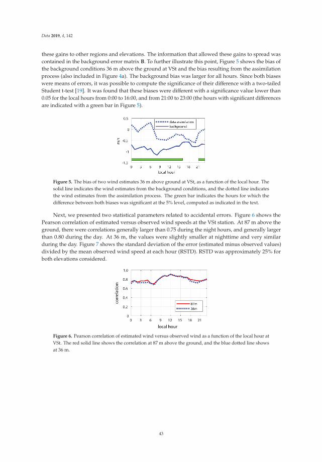
Data 2019, 4, 142

these gains to other regions and elevations. The information that allowed these gains to spread wascontained in the background error matrix B. To further illustrate this point, Figure 5 shows the bias ofthe background conditions 36 m above the ground at VSt and the bias resulting from the assimilationprocess (also included in Figure 4a). The background bias was larger for all hours. Since both biaseswere means of errors, it was possible to compute the significance of their difference with a two-tailedStudent t-test [19]. It was found that these biases were different with a significance value lower than0.05 for the local hours from 0:00 to 16:00, and from 21:00 to 23:00 (the hours with significant differencesare indicated with a green bar in Figure 5).

Figure 5. The bias of two wind estimates 36 m above ground at VSt, as a function of the local hour. Thesolid line indicates the wind estimates from the background conditions, and the dotted line indicatesthe wind estimates from the assimilation process. The green bar indicates the hours for which thedifference between both biases was significant at the 5% level, computed as indicated in the text.

Next, we presented two statistical parameters related to accidental errors. Figure 6 shows thePearson correlation of estimated versus observed wind speeds at the VSt station. At 87 m above theground, there were correlations generally larger than 0.75 during the night hours, and generally largerthan 0.80 during the day. At 36 m, the values were slightly smaller at nighttime and very similarduring the day. Figure 7 shows the standard deviation of the error (estimated minus observed values)divided by the mean observed wind speed at each hour (RSTD). RSTD was approximately 25% forboth elevations considered.

Figure 6. Pearson correlation of estimated wind versus observed wind as a function of the local hour atVSt. The red solid line shows the correlation at 87 m above the ground, and the blue dotted line showsat 36 m.

43

Data 2019, 4, 142

Figure 7. The relative standard deviation of wind estimate error as a function of the local hour at VSt.The red solid line shows the correlation at 87 m above the ground, and the blue dotted line shows at36 m.

Figure 8 shows scatter plots of estimated versus observed wind speeds at 7:00 and 12:00 and 87and 36 m above the ground. These hours were chosen because they represent the periods of the daywith the relatively worst and best adjustments, as assessed in Figures 6 and 7. Samples of assimilatedvalues and the corresponding observed wind speed values, including those shown in Figure 8, made itpossible to estimate probability distributions of the errors, such as empirical percentiles, from whichconfidence intervals for the wind speed estimates could be calculated.

Figure 8. Estimated wind versus observed wind 100 m above the ground at VSt at (a) 7:00 and (b) 12:00.Estimated wind versus observed wind 30 m above ground at VSt at (c) 7:00 and (d) 12:00.

5. Summary and Conclusions

This work assessed the quality of wind speed estimates in Uruguay obtained with the WRF-DAsystem, which was used to assimilate wind speed measurements 100 m above the ground at two windfarms. The quality of the estimates was assessed with an anemometric station placed between the wind

44

Data 2019, 4, 142

farms, that measured wind speed at 87 and 36 m above the ground. The information to be assimilatedfrom field measurements was minimal, not only because it included only two stations but also becauseit lacked records of other atmospheric variables that are related to wind, such as atmospheric pressure.It was interesting to assess the extent to which these minimum field measurements could generateuseful interpolations and evaluate the quality of the wind estimates at elevations both similar anddifferent to those of the assimilated records. The measurement station used to validate the wind speedassessments was placed between those used for the assimilation process, so the conclusions of theassessment are applicable only to regions between the two main stations.

Wind speed estimates showed a low systematic error at the verification station, generally below0.5 m/s at both 87 and 36 m above the ground. A relative systematic error was generally less than 5%of the average speed. This result indicated that the data assimilation technique effectively combinedinformation from field measurements and background conditions. The assimilated measurementsdid not include information from elevations as low as 36 m. The background conditions did containinformation from these low elevations, but with systematic errors of their own. The assimilationtechnique managed to propagate the gain from the observations at 100 m above the ground in the windfarms to other regions and to lower elevations. The covariance matrix of the background conditionerror was essential to the propagation of these observational gains.

As for the total error, the correlation values between observed and estimated wind speed and thestandard deviation of the total error of each estimate, generally about 1 m/s to 1.5 m/s, suggested thatthe obtained estimates could be of sufficient quality to be useful in various applications. Some examplesof applications in which such estimates are valuable are the estimation of wind climatology within therange of the considered height levels, retrospective simulations of transport processes and dispersion ofair pollutants, or real-time estimation of environmental conditions in which systems whose operationcan be affected by the wind are being used. In any case, the effective use of pseudo-observations ina specific application requires the estimation of their confidence intervals, which are necessary bothto assess whether the accuracy of pseudo-observations is acceptable for the application in questionand to take into account the effects of the uncertainty of these data if they are used. The generation ofdatabases of pseudo-retrospective observations, such as the one presented in this work, allows for theestimation of these confidence intervals.

For future studies, we are interested in quantifying the effects of including atmospheric pressureobservations on the quality of the results. We are also interested in evaluating the effect of expandingthe region in which observations are collected for the assimilation of data on the results of the hotstart option.

Finally, we pointed out that the topography of the studied region is not completely flat butis relatively smooth. This can contribute to the quality of results obtained by assimilating a fewobservations in numerical simulations with relatively low resolution. In the case of regions withrelatively complex topography, the numerical simulation may require finer spatial resolution toproperly take into account the effects of topography on the wind field. The proper quantity andlocation of measurement stations should also be evaluated in each case.

Author Contributions: Conceptualization, G.C.B., S.O.; methodology, G.C.B., S.O.; software, G.C.B., S.O.;validation, G.C.B., S.O.; formal analysis, G.C.B., S.O.; investigation, G.C.B., S.O.; resources, G.C.B.; data curation,G.C.B. and S.O.; writing—original draft G.C.B.; visualization, G.C.B.; supervision, G.C.B.; project administration,G.C.B.; funding acquisition, G.C.B.

Funding: This research was funded by UTE and the Comisión Sectorial de Investigación Científica (CSIC) of theUniversidad de la República, Uruguay, grant number CSIC-UTE-2017-33. The Agencia Nacional de InvestigaciònCientífica, ANII, Uruguay, founded earlier stages of this work, grant FSE-2011-6562.

Acknowledgments: UTE provided the data to do this study. The reviewers of this work made valuable commentsand indications that contributed to its improvement.

Conflicts of Interest: The authors declare no conflicts of interest.

45

Data 2019, 4, 142

Appendix A

The setting of the WRF model used in this work is analogous to that of the work by Cazes Boezioand Ortelli [12] which evaluates short-term forecasts of wind power generated in Uruguay. Thehorizontal resolution was 30 km in the zonal and meridional direction. Figure 3 shows the grid pointsused to compute air temperature, pressure, density, and vertical velocity. The grid points used tocompute the zonal and meridional velocities (not shown) were staggered one half of the horizontalresolution in the zonal and the meridional directions, respectively, according to the Arakawa C-gridarrange [1].

The model setting employed considered 54 layers in the vertical direction. The model verticalcoordinate is η [1], defined as

η =pd − pT

pS − pT(A1)

where pd is the hydrostatic component of dry air pressure at a particular atmosphere level, and pS andpT are the analogous pressures at the Earth’s surface and the atmosphere conventional top, respectively.In this work, the atmosphere top was set to 50 hPa. Table A1 gives the values of h at each layer interface.

Table A1. η values at the top of each layer of the vertical discretization.

LayerNumber

h Value atLayer Top

LayerNumber

h Value atLayer Top

LayerNumber

h Value atLayer Top

1 0.9880 19 0.9240 37 0.7135

2 0.9969 20 0.9165 38 0.6911

3 0.9950 21 0.9088 29 0.6668

4 0.9935 22 0.9008 40 0.6406

5 0.9935 23 0.8925 41 0.6123

6 09910 24 0.8840 42 0.5806

7 0.9899 25 0.8752 43 0.5452

8 0.9861 26 0.8661 44 0.5060

9 0.9821 27 0.8567 45 0.4630

10 0.9777 28 0.8471 46 0.4161

11 0.9731 29 0.8371 47 0.3656

12 0.9682 30 0.8261 48 0.3119

13 0.9629 31 0.8141 49 0.2558

14 0.9573 32 0.8008 50 0.1982

15 0.9513 33 0.7863 51 0.1339

16 0.9450 34 0.7704 52 0.0804

17 0.9382 35 0.7531 53 0.0362

18 0.9312 36 0.7341 54 0.0000

The horizontal velocities and the air temperature were computed inside each layer, whilethe vertical velocity was computed at the layer interfaces, according to the Lorenz vertical gridarrangement [1].

The WRF model allowed us to choose several parameterizations of physical processes, especiallyfor atmospheric boundary layer processes, surface layer processes, short and long wave radiativeheat transfers, convective precipitation, clouds microphysics, and drag associated with gravity waves.Table A2 shows the parameterizations chosen in the current work and indicates references for them.

46

Data 2019, 4, 142

Table A2. Parameterization of physical processes used.

Physical Process Scheme Used

Short Wave Radiation Dudhia scheme [20]

Long Wave Radiation RRTM schene [21]

Surface Layer Revised MM5 surface layer scheme [22]

Atmospheric Boundary Layer Yonsei University scheme [23]

Microphysics Hong et al. scheme [24]

Cumulus Precipitation Simplified Arakawa Schubert scheme [25]

Gravity Wave Drag Kim Arakawa scheme [26]

Land Processes Noah land surface model [27]

Appendix B

Kalnay [3] showed the result of the optimization indicated in Equation (A1), that yields the 3D-Varanalysis xa and is equivalent to the result of the optimal interpolation procedure,

xa − xb = B(∇H)T·[∇H·B·(∇H)T + R]−1·[y− (∇H)(xb)] (A2)

We chose a particular variable and a particular grid point that corresponds to the kth element ofxb or xa, according to the conventional order of these vectors. We defined the synthetic observation y

at the chosen grid point as the kth value of xb plus a conventional increment Δ,

y = xb(k) + Δ (A3)

Since the ∇H operator produces analogous variables to those of the vector of observations y

from xb, and the analogous to the synthetic observation y in the background condition is xb(k), thecorrespondent ∇H is a vector with all its terms equal to 0, except the kth element, which is equal to 1, so

H(xb) = xb(k), and y−H(xb) = Δ (A4)

The matrix R of covariance of observation errors has a single element, which is the covariance ofthe synthetic observation y. We chose a conventional value s2 for this covariance. Rizvi [17] showedthat with these choices, Equation (A2) yields

xa − xb =Bk

bkk + σ2 (A5)

where Bk is the k column of B. Equation A5 indicates that the xa − xb difference is proportional to avector that gives all the covariances of the error of xb(k) with the errors of all the other variables of xb.Note that the xa − xb difference is independent of the xb condition chosen. Plots of xa − xb fields for aselected variable at a selected level of the numerical domain can help to understand the geographicalstructure of the error covariances of that variable at that level.

Here, we chose to increase in 1 m/s the zonal (”test A”) and the meridional (“test B”) wind of aparticular xb condition at the grid point and level closest to the location of the Vst station and the levelof 87 m above ground. s was chosen as 1 m/s. Figure A1a shows the xa − xb field for zonal velocityresulting from test A, at the same model level of the selected grid point (level 7 from the ground).Figure A1b shows the xa − xb field for the meridional velocity at the same level, for “test B”. Theseresults indicated that WF1 and WF2 were located in regions, where the zonal and meridional windsare well correlated with those of the Vst, and, therefore, wind estimates at this location benefit from

47

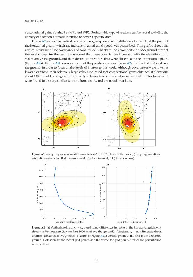
Data 2019, 4, 142

observational gains obtained at WF1 and WF2. Besides, this type of analysis can be useful to define thedensity of a station network intended to cover a specific area.

Figure A2 shows the vertical profile of the xa − xb zonal wind difference for test A, at the point ofthe horizontal grid in which the increase of zonal wind speed was prescribed. This profile shows thevertical structure of the covariances of zonal velocity background errors with the background error atthe level chosen for the test. It was found that these covariances increased with the elevation up to500 m above the ground, and then decreased to values that were close to 0 in the upper atmosphere(Figure A2a). Figure A2b shows a zoom of the profile shown in Figure A2a for the first 150 m abovethe ground, in order to focus on the levels of interest to this work. Although covariances were lower atlower elevations, their relatively large values indicated that observational gains obtained at elevationsabout 100 m could propagate quite directly to lower levels. The analogous vertical profiles from test Bwere found to be very similar to those from test A, and are not shown here.

Figure A1. (a) xa − xb zonal wind difference in test A at the 7th layer of the model; (b) xa − xb meridionalwind difference in test B at the same level. Contour interval, 0.1 (dimensionless).

Figure A2. (a) Vertical profile of xa − xb zonal wind differences in test A at the horizontal grid pointclosest to Vst location (for the first 8000 m above the ground). Abscissa, xa − xb (dimensionless),ordinate, elevation above ground; (b) zoom of Figure A2, a vertical profile at the first 150 m above theground. Dots indicate the model grid points, and the arrow, the grid point at which the perturbationis prescribed.

48

Data 2019, 4, 142

References

1. Skamarock, W.C.; Klemp, J.B.; Dudhia, J.; Gill, D.O.; Barker, D.M.; Wang, W.; Powers, J.G. A Descriptionof the Advanced Research WRF Version 3. NCAR Tech Note NCAR/TN-475+STR. Available online:http://citeseerx.ist.psu.edu/viewdoc/summary?doi=10.1.1.484.3656 (accessed on 25 October 2019).

2. Barker, D.; Huang, X.Y.; Liu, Z.; Auligné, T.; Zhang, X.; Rugg, S.; Ajjaji, R.; Bourgeois, A.; Bray, J.; Chen, Y.; et al.The Weather Research and Forecasting Model’s Community Variational/Ensemble Data Assimilation System,WRFDA. Available online: https://journals.ametsoc.org/doi/pdf/10.1175/BAMS-D-11-00167.1 (accessed on 25October 2019).

3. Kalnay, E. Atmospheric Modelling, Data Assimilation and Predictability; Cambridge University Press: Cambridge,UK, 2003; p. 345.

4. Barker, D.; Huang, X.Y.; Guo, Y.-R.; Xiao, Q.N. A three dimensional (3Dvar) data assimilation system for usewith MM5. Implementation and Initial Results. Mon. Weather Rev. 2004, 132, 897–914. [CrossRef]

5. Huang, X.Y.; Xiao, Q.; Barker, D.M.; Zhang, X.; Michalakes, J.; Huang, W.; Henderson, T.; Bray, J.; Chen, Y.;Ma, Z. Four-dimensional variational data assimilation for WRF: Formulation and preliminary results. Mon.Weather Rev. 2009, 137, 299–314. [CrossRef]

6. Wang, X.; Barker, D.M.; Snyder, C.; Hamill, T.M. A hybrid ETKF-3DVAR data assimilation scheme for theWRF model. Part I: Observing system simulation experiment. Mon. Weather Rev. 2008, 136, 5116–5131.[CrossRef]

7. Wang, X.; Barker, D.M.; Snyder, C.; Hamill, T.M. A hybrid ETKF-3DVAR data assimilation scheme for theWRF model. Part II: Real observation experiments. Mon. Weather Rev. 2008, 136, 5132–5147. [CrossRef]

8. Harlim, J. Model Error in Data Assimilation. In Nonlinear and Stochastic Climate Dynamics; Franzke, C.,O’Kane, T., Eds.; Cambridge University Press: Cambridge, UK, 2017; pp. 276–317. [CrossRef]

9. Rao, V.; Sandu, S. A-posteriori error estimates for inverse problems. Procedia Comput. Sci. J. 2018, 20,1256–1265.

10. Orteli, S.; Boezio, G.C. Construction of Empirical Speed-Power Curves in Wind FarmsInstalled in Uruguay. Application to Real-Time Data Quality Control and Estimationof Potential Generation in Case of Restrictions. X Brazilian Micrometeorology Workshop.Available online: https://www.even3.com.br/anais/micrometeorologia2017/64488-construcao-de-curvas-de-velocidade-potencia-empiricas-em-parques-eolicos-instalados-no-uruguai-aplicacao-ao-contr/ (accessedon 25 October 2019).

11. Cornalino, E.; Draper, M. Planning the Distribution of Wind Farms in Uruguay in Order to Optimize theOperability of Large Amounts of Wind Power. Available online: www.fing.edu.uy/cluster/eolica/publi/Cornalino_Draper_EWEC2012_FINAL.pdf (accessed on 29 October 2019).

12. Cazes Boezio, G.; Orteli, S. Minimum-cost numerical prediction system for wind power in Uruguay, with anassessment of the diurnal and seasonal cycles of its quality. Sci. Nat. 2018, 40, 206–210.

13. Barker, D.; Huang, W.; Guo, Y.-R.; Bourgeois, A. A Three-Demiensional Variational (3DVAR) Data AssimilationSystem for Use with MM5 (No. NCAR/TN-453+STR). Available online: https://opensky.ucar.edu/islandora/object/technotes%3A309 (accessed on 25 October 2019).

14. User’s Guide for the Advanced Research WRF (ARW) Modeling System Version 3.9 WRF-ARW, Chapter6. Available online: http://www2.mmm.ucar.edu/wrf/users/wpsv3.9/known-prob-3.9.html (accessed on 25October 2019).

15. Parrish, D.F.; Derber, J.C. The National Meteorological Center’s spectral statistical interpolation analysissystem. Mon. Weather Rev. 1992, 120, 1747–1763. [CrossRef]

16. Descombes, G.; Auligné, T.; Vandenberghe, F.; Barker, D.; Barré, J. Generalized background error covariancematrix model (GEN_BE v2.0). Geosci. Model Dev. 2015, 8, 669–696. [CrossRef]

17. Rizvi, S. WRF-DA Background Error (Modeling and Estimation), WREF-DA Tutorial Presentation Slides,Chapter 4. University Corporation for Atmospheric Research, 2016. Available online: www2.mmm.ucar.edu/wrf/users/wrfda/Tutorials/2016_Aug/docs/WRFDA_BE.pdf (accessed on 29 October 2019).

18. Cataldo, J.; Universidad de la República, Montevideo, Uruguay. Personal communication, 2019.19. Press, W.H.; Taukolsky, S.A.; Vettering, W.T.; Flannery, B.P. Numerical Recipes in Fortran 77: The Art of Scientific

Computing; Cambridge University Press: Cambridge, UK, 1996; p. 1010.

49

Data 2019, 4, 142

20. Dudhia, J. Numerical study of convection observed during the winter monsoon experiment using a mesoscaletwo-dimensional model. J. Atmos. Sci. 1989, 46, 307–310. [CrossRef]

21. Iacono, M.J.; Delamere, J.S.; Mlawer, E.J.; Shephard, M.W.; Clough, S.A.; Collins, W.D. Radiative forcing bylong-lived greenhouse gases: Calculations with the AER radiative transfer models. J. Geophys. Res. 2008, 113,D13103. [CrossRef]

22. Jimenez, P.; Dudhia, J.; Gonzalez-Ruoco, J.F.; Navarro, J.; Montavez, J.P.; Garcia-Bustamente, F. A revisedscheme for the WRF surface layer formulation. Mon. Weather Rev. 2012, 140, 898–918. [CrossRef]

23. Hong, S.-Y.; Noh, Y.; Dudhia, J. A new vertical diffusion package with an explicit treatment of entrainmentprocesses. Mon. Weather Rev. 2006, 134, 2318–2341. [CrossRef]

24. Hong, S.Y.; Dudhia, J.; Chen, S.H. A Revised Approach to Ice Microphysical Processes for the BulkParameterization of Clouds and Precipitation. Mon. Weather Rev. 2004, 132, 103–120. [CrossRef]

25. Grell, G.A. Prognostic evaluation of assumptions used by cumulus parameterizations. Mon. Weather Rev.1993, 121, 764–787. [CrossRef]

26. Kim, Y.J.; Arakawa, A. Improvement of Orographic Gravity Wave Parameterization Using a MesoscaleGravity Wave Model. J. Atmos. Sci. 1995, 52, 1875–1902. [CrossRef]

27. Niu, G.-Y.; Yang, Z.L.; Mitchel, K.E.; Chen, F.; Ek, M.B.; Barlage, M.; Kumar, A.; Manning, K.; Niogi, D.;Rosero, E. The community Noah land surface model with multiparameterization options (Noah-MP): 1.Model description and evaluation with local-scale measurements. J. Geophys. Res. 2011, 116, D12. [CrossRef]


50

data

Data Descriptor

A High-Resolution Global Gridded HistoricalDataset of Climate Extreme Indices

Malcolm N. Mistry 1,2

1 Department of Economics, Ca’ Foscari University of Venice, 30121 Venice, Italy; [email protected] Centro Euro-Mediterraneo sui Cambiamenti Climatici (CMCC), 30175 Venice, Italy

Received: 18 February 2019; Accepted: 9 March 2019; Published: 13 March 2019

Abstract: Climate extreme indices (CEIs) are important metrics that not only assist in theanalysis of regional and global extremes in meteorological events, but also aid climate modellers andpolicymakers in the assessment of sectoral impacts. Global high-spatial-resolution CEI datasetsderived from quality-controlled historical observations, or reanalysis data products are scarce.This study introduces a new high-resolution global gridded dataset of CEIs based on sub-dailytemperature and precipitation data from the Global Land Data Assimilation System (GLDAS).The dataset called “CEI_0p25_1970_2016” includes 71 annual (and in some cases monthly) CEIsat 0.25◦ × 0.25◦ gridded resolution, covering 47 years over the period 1970–2016. The data ofindividual indices are publicly available for download in the commonly used Network CommonData Form 4 (NetCDF4) format. Potential applications of CEI_0p25_1970_2016 presented here includethe assessment of sectoral impacts (e.g., Agriculture, Health, Energy, and Hydrology), as well asthe identification of hot spots (clusters) showing similar historical spatial patterns of high/lowtemperature and precipitation extremes. CEI_0p25_1970_2016 fills gaps in existing CEI datasets byencompassing not only more indices, but also by being the only comprehensive global gridded CEIdata available at high spatial resolution.

Dataset: https://doi.org/10.1594/PANGAEA.898014

Dataset License: CC-BY: Creative Commons Attribution 4.0 International

Keywords: climate extreme indices (CEIs); ClimPACT; GLDAS; Expert Team on Climate ChangeDetection and Indices (ETCCDI); Expert Team on Sector-specific Climate Indices (ET-SCI)

1. Introduction

Extremes in climate such as floods, droughts, and cold and heat-waves can have significantsocietal, ecological, and economic impacts globally [1]. Since the publication of the third assessmentreport of the Intergovernmental Panel on Climate Change (IPCC) in 2000, characterizing extremesunder past and projected future climate has generated rapid interest [2]. The climate modellingcommunity, for instance, has spent increasing effort to capture high-frequency extreme events intheir simulations of historical and future projected climate. The underlying aim for both regionaland global climate modelling exercises (e.g., CORDEX and PRIMAVERA)1 has been to develop abetter understanding of the evolution of extreme weather events under long-term climate changeand variability.

The impetus to better understand extreme weather events is further driven by the impactmodellers who assess sectoral damages at varying spatial scales. The two vital characteristics of

1 CORDEX: http://www.cordex.org/; PRIMAVERA: https://www.primavera-h2020.eu/.


Data 2019, 4, 41

climate that are at the core of impact models are (i) mean climate and (ii) the occurrence andfrequency of extreme events [3]. An increasing notion shared within the climate research communityis that even a relatively small change in the frequency or severity of extreme weather events(i.e., in the tails of the probability distribution function) would have profound impacts on life andassets [4], thus making it further imperative to analyze extremes at higher temporal and spatialresolutions. For the scientific community focusing on impacts of climate change and variability,historical observations of extreme indicators can facilitate a better understanding of the role of extremeevents and sectoral implications [5].

Largely driven by the requirement for a robust definition of climate extreme indicators, the ExpertTeam on Climate Change Detection and Indices (ETCCDI)2 in 1999 led the first efforts in defining a set ofclimate extreme indices (CEIs) that provide a comprehensive overview of temperature and precipitationstatistics [4,6–8]. The ETCCDI has developed an internationally coordinated set of core climate indicesconsisting of 27 descriptive indices for moderate weather extremes3 [9–11]. The preliminary set of these27 core indices were drawn up keeping the detection and attribution needs of the research communityin mind [10,11]. Noting the limitations of the ETCCDI indices with regard to restricted scope/usage inassessing sectoral impacts, additional sector-relevant indices were recommended and developed bythe Expert Team on Sector-specific Climate Indices (ET-SCI) [9].

This study introduces a new open-access high-resolution global gridded (0.25◦ × 0.25◦)4 dataset of71 CEIs (including the original 27 ETCCDI indices), covering the period 1970–2016. The dataset(hereafter referred to as “CEI_0p25_1970_2016”) aims to contribute to the existing CEI databases bymaking available the first comprehensive CEI dataset currently unavailable for the climate communityat a high resolution with worldwide coverage. Moreover, a consistent global CEI dataset covering along historical time period can lay a framework for not only analyzing observed changes in extremes,but also potentially improving information services on extremes at regional scales [10].

The CEI_0p25_1970_2016 are a set of core (Table S1 in Supplementary Materials) and non-core(Table S2 in Supplementary Materials) indices5 as defined and developed by the ETCCDI/ET-SCI,and adopted by the World Meteorological Organization (WMO). The set of “core indices” refers toindices that were developed by ETCCDI targeting the research community focusing on “detection andattribution” in climate science (details in Section 4).

The rest of the paper is organized as follows. Section 2 describes the CEI_0p25_1970_2016 in detail.Section 3 discusses the underlying meteorological dataset and the tools/methodology used in thepreparation of the CEI_0p25_1970_2016. Section 4 outlines the novelty, potential scope, application, andlimitations of the CEI_0p25_1970_2016. Dataset availability, ongoing work, and some recommendationsfor future research are summarized in Section 5.

2. Dataset Description

2.1. Spatial and Temporal coverage of CEI_0p25_1970_2016

The CEIs included in this study encompass all but two indices6 that are part of the completelist of 73 ETCCDI/ET-SCI core and non-core indices [9]. The CEI_0p25_1970_2016 is derivedusing meteorological variables from the reanalysis data product Global Land Data Assimilation

2 Formed by the World Meteorological Organization (WMO) Commission for Climatology (CCl).3 Extreme events that by definition typically occur a few times annually rather than severe impact, decadal weather events.

The indices for moderate weather extremes use absolute or percentile thresholds generally set at moderate values (e.g., 25 ◦C,90th percentile).

4 ~27 km × 27 km at the equator.5 https://www.wcrp-climate.org/data-etccdi.6 The two indices Cooling and Heating Degree Days (CDD and HDD) are computed separately as part of another dataset of

additional indices relevant for health and energy sectors, currently under preparation [12]. Further details are provided inSection 5.2.

52

Data 2019, 4, 41

System (GLDAS) [13]. GLDAS is a new generation of reanalysis developed jointly by the NationalAeronautics and Space Administration (NASA) Goddard Space Flight Center (GSFC) and NationalCenters for Environmental Prediction (NCEP) [14]. Because the spatial extent of GLDAS covers allland north of 60◦ S, the indices in CEI_0p25_1970_2016 are also computed over the corresponding1440 (longitude) × 600 (latitude) grid cells. Further description of GLDAS as well as the reasons forusing it as a data source in this study are discussed in Section 3.

2.2. Other Existing Datasets Incorporating CEIs

While other similar historical gridded CEI datasets do exist, they are either (i) regional in coverage,(ii) at coarser resolution, or (iii) limited in the number of indices available for research purpose.Examples include (i) the 30 CEIs made available by E-OBS at 0.10◦ gridded resolution for Europehttp://surfobs.climate.copernicus.eu/dataaccess/access_eobs_indices.php, (ii) the global 0.50◦

gridded resolution S-14 indices dataset of 27 core ETCDDI indices available at http://h08.nies.go.jp/s14/ [15], and (iii) the global 3.75◦ × 2.5◦ resolution HadEX2 and GHCNDex datasets of 27 coreETCDDI indices available at https://www.climdex.org/learn/datasets/ [6,7]. To the best of theauthor’s knowledge, the present database CEI_0p25_1970_2016 is currently the only comprehensivehigh-resolution global-gridded historical dataset of ETCCDI/ET-SCI core and non-core indices.

3. Materials and Methods

3.1. Data Acquisition and Processing

The CEIs used in this study were computed utilizing the WMO ET-SCI recommended anddeveloped R-software package “ClimPACT2”7 [9]. R [16] is an open-source language and softwareenvironment, developed primarily (but not solely) for statistical computing, and is applied widely inclimate research. Moreover, ClimPACT2 also makes use of several R subroutines, such as SPEI [17],and is designed for operating on parallel computing infrastructure.

For the computation of CEI, ClimPACT2 requires the following meteorological variables(i) maximum near-surface air temperature (TX), (ii) minimum near-surface air temperature (TN), and(iii) near-surface total precipitation (PR), all at daily timesteps. These variables in the native NetworkCommon Data Form 4 (NetCDF4)8 format were obtained from the GLDAS-version 29 [13,18,19],available at 3-hourly timesteps and a fine spatial resolution of 0.25◦ × 0.25◦. GLDAS is a globalhigh-resolution reanalysis dataset that incorporates satellite and ground-based observations, producingoptimal fields of land surface states and fluxes in near-real-time [13].

For the purpose of computing the CEI, the 3-hourly gridded variables (TX, TN, and PR) werefirst temporally aggregated to construct daily mean TX and TN, and daily total PR, using a suite ofcommand line operators from NetCDF Command Operators (NCO ver 4.3.4)10 and Climate DataOperators (CDO ver 1.9.0)11. Indices based on percentile thresholds (e.g., WSDI and CSDI in Table S1)were computed using years 1970–2000 as the baseline period. For details on classification of CEIs(namely “percentiles”, “absolute”, “threshold”, “duration”, and “others”), readers are guided forfurther reading in [6–9].

7 R version 3.5.0 (“Joy in Playing”) x86_64 on Linux Centos 6.6 software architecture. ClimPACT2 was accessed on23 September 2018 from https://github.com/ARCCSS-extremes/climpact2.

8 NetCDF is a set of scientific software libraries, with self-describing and machine-independent data format. https://www.unidata.ucar.edu/software/netcdf/docs/.

9 Data accessed from https://disc.gsfc.nasa.gov/ on 12 July 2018.10 NCO [20]: accessed on 14 July 2018 from http://nco.sourceforge.net/.11 CDO [21] accessed on 14 July 2018 from http://www.mpimet.mpg.de/cdo.

53

Data 2019, 4, 41

3.2. Choice of GLDAS as a Reanalysis Dataset for the Computation of CEIs

Vis-à-vis other global gridded reanalysis datasets, GLDAS offers several advantages. First,GLDAS provides a consistent quality-controlled long global gridded time-series of the requiredvariables (i.e., TX, TN, and PR) at a high spatial resolution. Other reanalysis data products availablewere found to have either a coarser spatial resolution (e.g., ECMWF-ERA40 and JRA-55, both availablefrom the mid-1950s but at 1.125◦), or a shorter time series (e.g., newly released ECMWF-ERA5 at 0.281◦

from 1979–present day, and NCEP-CFSv2 at 0.205◦ from 2011–present day). Second, GLDAS runs innear-real-time, offering the potential to regularly update the database presented here.

The choice of GLDAS for computing the current set of indices was further motivated by its largenumber of additional meteorological (e.g., specific humidity, surface pressure), land surface state(e.g., soil moisture, surface temperature), and flux (e.g., evaporation, sensible heat flux) variables,not commonly available in other reanalysis data products for a long time-series and at a highspatial resolution12. While none of these additional variables are required for computing the currentset of indices, another dataset [12] of sectoral indices that are not presently implemented in theETCCDI/ET-SCI indices requires a subset of these variables (details in Section 5.2). The two datasets ofindices (current and [12] under prep.) will together comprise a large (~85) number of indices bothbased on the same underlying GLDAS data, thus enabling the climate impacts community to access“ready-to-use” multi-sectoral indices.

GLDAS has been comprehensively evaluated using different regional/global reference datasetsin earlier studies (e.g., see [14] who compare the GLDAS daily surface air temperature at 0.25◦ griddedresolution with two reference datasets): (a) Daymet data (2002 and 2010) for the conterminous UnitedStates at 1-km gridded resolution, and (b) global meteorological observations (2000) from the GlobalHistorical Climatology Network (GHCN).

Equally well-documented are certain known limitations of the temperature and precipitationestimates in GLDAS. Whereas spatial details in high mountainous areas are not sufficiently estimatedby the GLDAS data, the surface air temperature estimates are generally accurate, with some cautionrecommended for mountainous areas [14]. Previous studies that have incorporated GLDAS datainclude (i) [22] for impact assessment studies in energy sector, and (ii) [23,24] for the analysis ofregional environmental conditions and changes. For a comprehensive list of GLDAS-related references,readers are referred to https://ldas.gsfc.nasa.gov/gldas/GLDASpublications.php.

4. Key Features, Scope of Application, and Limitations of CEI_0p25_1970_2016

4.1. Novelty of CEI_0p25_1970_2016

The CEI_0p25_1970_2016 is currently the only dataset providing researchers and policymakerswith an exhaustive list of ETCCDI/ET-SCI recommended indices, dating back to the precedingfour decades, covering nearly all global land grid-cells, and assembled using a quality-controlledreanalysis data product at a high spatial resolution. Considering the computational time and resourcesrequired for assembling a comprehensive dataset of CEIs at a global scale, the biggest asset ofCEI_0p25_1970_2016 from the users’ perspective is the open access to a pre-compiled ready-to-useset of indices in its native data format, along with a web interface allowing robust statistical analysisand mapping of the results in a few easy steps (details in Section 5.1).

12 At the time of assembling the current dataset, the newly released ECMWF-ERA5 that also includes a large set of variableswas not publicly available prior to the year 2000.

54

Data 2019, 4, 41

4.2. Scope of Application

The CEIs included in this study are not only suited as assessment tools in multiple sectors such asAgriculture, Health, Energy, Water resource, etc., but also as metrics capable of being aggregated ascomposite indicators for risk assessment and vulnerability studies (e.g., as demonstrated and appliedrecently by [25] over Italy in the form of a “Climate Risk Index”). A number of earlier studies havedemonstrated the efficacy of the CEIs, both in detection and attribution studies, as well in the impactsassessment of climate change and variability in key sectors. Examples include (i) [26] who use “Rx1day”(Table S2) to examine the changes in model-simulated extreme precipitation by decomposing the dailyregional-scale extreme precipitation as contributions from atmospheric thermodynamics and dynamics;and (ii) [27] who consider a broad range of CEIs (from Tables S1 and S2), for assessing future climatechange impacts on agriculture, human health, ecological ecosystems and utility (energy demand)in Canada.

Moreover, it is widely known and established in sectoral impact studies employing empiricalmethods that a large proportion of variation in the outcome variable is better explained by theclimatic variables accounting for moderate or severe extremes (e.g., the relationship (i) betweencrop productivity and a variant of the index “GDDgrown” in Table S1, known as killing degreedays (KDDs) [28], (ii) between electricity consumption and degree-day indices namely “CDD” and“HDD” [29]). CEI_0p25_1970_2016 for instance provides an instant resource platform for empiricalmodellers to download and investigate a number of potential predictor variables that are robustmoderate/severe extreme indicators.

The robust characteristics and climatological attributes captured by ETCCDI/ET-SCI indicescan facilitate consistent comparison of results across different climatic zones, different time periods,and the identification of regions (clusters) with similar characteristics in extremes (e.g., grid cellswith similar trends in annual days when daily maximum temperature is at least 30 ◦C (“TXge30”,Table S1). The identification of common hot spots can be of potential interest to policymakers, insurancecompanies, and country planners for the assessment of the risk and vulnerability of regions to extremeweather disasters (e.g., flooding, drought, heat waves).

While the mean climatology of a location is invariably well-captured by the state-of-the-artreanalysis data products and Earth System Models (ESMs), extremes (particularly in precipitation) atfine spatial scales have been difficult to replicate [30]. CEIs provide the modelling community with adetailed set of indicators enabling the comparison of different input data sources in their ability tomodel extremes [8,9].

Finally, with the planned inclusion of additional indices to the current inventory ofETCCDI/ET-SCI indices in the near future [9], the development of larger CEI datasets for historicaland future time periods could make valuable instruments available to researchers, policymakers, andadaptation planners focusing on occurrences and return periods of rarer extreme meteorological events(e.g., using extreme value theory).

4.3. Limitations of Indices Included in CEI_0p25_1970_2016

While the CEIs included in this study (Tables S1 and S2) were developed by the WMO expertteams to largely address the growing demands of sectoral impact modellers, certain limitations ofthe existing ETCCDI/ET-SCI indices have been recognized, and efforts are ongoing to develop otherrobust indices meeting multi-sectoral requirements [9]. For instance, under the current framework ofET-SCI definitions, the Heat Wave Magnitude (HWM) indices (Table S2 are based on the methodologydeveloped by either [31] or [32]. The more recently developed HWM Index daily (HWMId) defined

55

Data 2019, 4, 41

by [33] and implemented in various sectoral studies (e.g., [34] for river discharge and [35] for assessingimpacts on wheat yields13) is yet to be included in the inventory of ETCCDI/ET-SCI indices.

Moreover, the ETCCDI/ET-SCI indices are defined largely at annual timescales, and some aredefined at monthly timescales as well. For certain sectoral applications (e.g., in Agriculture andEnergy), the current set of monthly/annual indices may prove less useful, as climate anomalies needto be computed over different timescales. For instance, the “GSL” index (Table S1) in its current formdefined at annual timescales does not account for heterogeneity in the length of crop-specific growingseason (further details in [35]). In such cases, using indices computed at annual timescales can lead tomisleading results. Some further shortcomings of the existing ETCCDI/ET-SCI indices are discussedand recommended for future work (details in Section 5.2).

Lastly, it must be emphasized that because CEI_0p25_1970_2016 utilizes temperature andprecipitation data from GLDAS, when using the current set of indices users should keep in mind theknown uncertainties and limitations of the GLDAS data (as discussed in Section 3.2).

5. Dataset Availability and Plans for Future Work

5.1. Data Access, File Naming Convention, and Size

CEI_0p25_1970_2016 can be accessed as individual netCDF4 files fromhttps://doi.org/10.1594/PANGAEA.89801414. The files follow the naming conventionCEI_timescale_GLDAS_0p25_deg_hist_1970_2016.nc (Figure 1), wherein “CEI” is the abbreviation ofthe index (as described in Tables S1 and S2) and “timescale” is either “ANN”, “MON”, or “DAY”,relating to annual, monthly, or daily timescales15 over which the corresponding CEI is computed.

The size of the individual NetCDF files vary between 156 megabytes (Mb) and 1.9 gigabytes(Gb), depending on the CEI and time-scales at which it is computed. One exception is the file“hw_ANN_GLDAS_0p25_deg_hist_1970_2016.nc” which is 3.1 Gb as it includes twenty individualindices in a single netCDF4 file. GLDAS does not include data over (or near) water bodies. Such gridcells where the required GLDAS TX, TN, and PR data are not available for computing the CEIsare identified by missing values “1.e+20f”. Further details of the variables/dimensions in theindividual netCDF4 files can be examined using either NCO or CDO commands, such as “ncdump-h netcdf_file_name” or “cdo sinfo netcdf_file_name”, respectively. For creating quick plots andexploratory data analysis of individual netCDF files, open-access data tools such as Panoply (https://www.giss.nasa.gov/tools/panoply/) or NCview (http://meteora.ucsd.edu/~pierce/ncview_home_page.html) are recommended. Sample plots using Panoply for the four indices (“TXx”, “HWM_Tx90”,“CSDI”, and “PRCPTOT”) are shown in Appendix A (Figures A1–A4).

13 The authors use a slightly modified version of HWDId in their study, which they refer to as Heat Magnitude Day (HMD)in agriculture.

14 The dataset will also be mirrored on KNMI Climate Explorer (http://climexp.knmi.nl/about.cgi?id=someone@somewhere),a web application interface that can facilitate not only rapid aggregation and robust statistical analysis of the CEI, but alsodownloading of spatio-temporal subsets and quick plotting.

15 The dataset includes a total of 89 netCDF4 files (49 on annual, 39 on monthly and 1 on daily timescales). Some indices havedata both on monthly and annual timescales.

56

Data 2019, 4, 41

Figure 1. Snapshot of the data repository web interface showing individual files in CEI_0p25_1970_2016that are available for download at https://doi.org/10.1594/PANGAEA.898014.

5.2. Ongoing Work and Recommendations for Work in Future

The indices in CEI_0p25_1970_2016 are intended to be updated post-2016 years, subject to theavailability of the required GLDAS raw meteorological variables in the coming years. The updatedlonger time-series of CEIs of more recent years should prove beneficial to the research communityfocusing on recent extreme events (e.g., the droughts of 2017 and 2018 in south-east Australia, the heatwaves of 2018 in California, United States of America, the more recent January–February 2019 extremecold wave in North America). Additionally, upon the formal inclusion of any new indices (such as the“HWMId” and the “Crop-specific GSL” as discussed in Section 4.3) by the WMO expert teams to theirlist of ET-SCI indices, the same will be formally included in the existing dataset presented in this study.

While the ETCCDI/ET-SCI core and non-core indices employed in this study encompass a verylarge spectrum of sectoral and non-sectoral indices, the list is by no means exhaustive. Motivated bythe suggestions of the R ClimPACT2 [9] package creators, another dataset of indices largely relevantfor health and energy sectors (called “HEI_0p25_1970_2016”) is currently under preparation [12].

Some features of HEI_0p25_1970_2016 will for instance be the inclusion of the two ETCCDI indices(i.e., CDD and HDD [36]) that are not included in this study16. Moreover, HEI_0p25_1970_2016 will alsoaccount for additional meteorological variables (e.g., near-surface relative humidity and wind speed)for computing non ETCCDI/ET-SCI indices, such as the Humidex [37,38], the Heat Index (HI) [39,40],and the Discomfort Index (DI) [41,42]. Together, both CEI_0p25_1970_2016 and HEI_0p25_1970_2016are aimed to address the growing needs of the climate impact community, by overcoming the currentdata scarcity of high-resolution global gridded CEIs in earth science.

16 The R ClimPACT2 used in the present study for computing CEI_0p25_1970_2016 is hard-coded to compute the degree-days(CDD, HDD) on annual time scales. Degree-days at monthly and seasonal timescales are equally important in the energysector. These are developed at various base (threshold) temperatures at the same gridded resolution in HEI_0p25_1970_2016.

57

Data 2019, 4, 41

Supplementary Materials: The following are available online at http://www.mdpi.com/2306-5729/4/1/41/s1,Table S1: 32 Core ET-SCI indices. Bold indicates index is also an ETCCDI index. (TX: daily maximum near-surfaceair temperature, TN: daily minimum near-surface air temperature, PR: daily near-surface total precipitation,H: Health, AFS: Agriculture and Food Security, WRH: Water Resources and Hydrology); Table S2: 39 non-coreET-SCI indices. Bold indicates index is also an ETCCDI index. Sectoral abbreviations same as in Table S1.

Funding: This work was supported by research funding from the European Research Council (ERC) underthe European Union’s Horizon 2020 research and innovation programme under grant agreement No. 756194(ENERGYA).

Acknowledgments: The author is grateful to Nicholas Herold in assisting with the R software packageClimPACT2; Lisa Alexander and Enrico Scoccimarro for constructive discussion on sectoral extreme indices;Enrica De Cian for feedback on the draft version of the paper; the high-performance computing resources of theBoston University Shared Computing Cluster (SCC) on which the CEIs were computed; and NASA GoddardEarth Sciences Data and Information Services Center (GES DISC) for making GLDAS data publicly available.Developers of R SPEI package, CDO, and NCO are also acknowledged for providing open-access tools that wereused for data preparation in this study. The constructive feedback received from three anonymous reviewershelped to improve the manuscript further.

Conflicts of Interest: The author declares no conflict of interest.

Appendix A. Sample Plots of Selective Indices from Tables S1 and S2 Using Panoply

Figure A1. Annual Warmest Day “TXx” (◦C) in 2003.

Figure A2. Warmest Day “HWM_Tx90” (◦C) in 2003 (Average temperature across allindividual heatwaves).

58

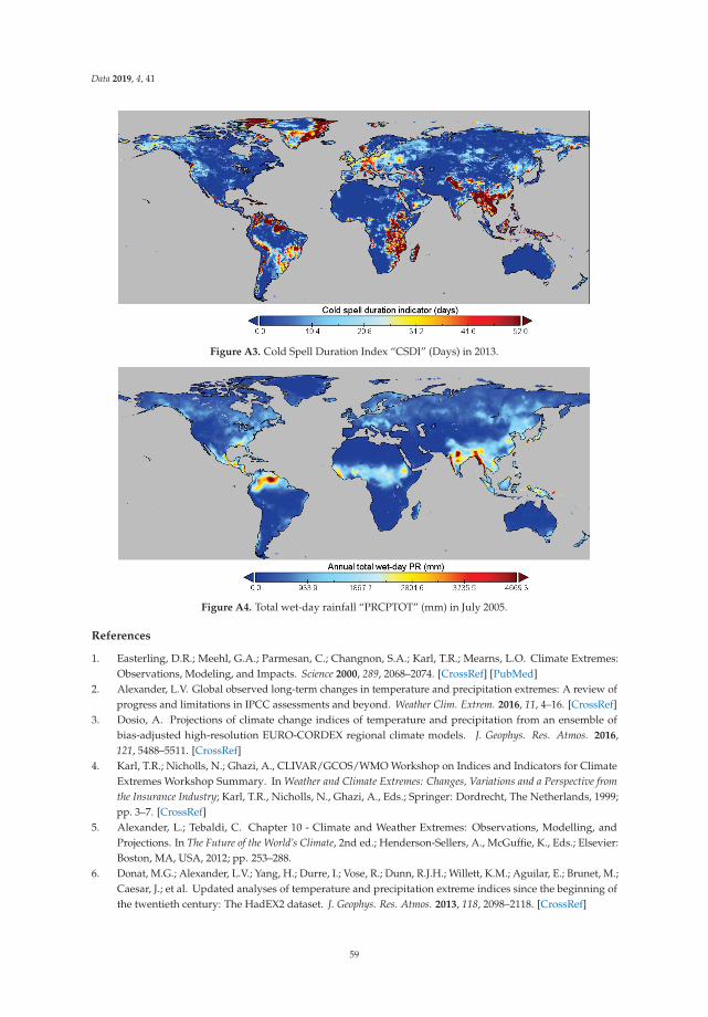
Data 2019, 4, 41

Figure A3. Cold Spell Duration Index “CSDI” (Days) in 2013.

Figure A4. Total wet-day rainfall “PRCPTOT” (mm) in July 2005.

References

1. Easterling, D.R.; Meehl, G.A.; Parmesan, C.; Changnon, S.A.; Karl, T.R.; Mearns, L.O. Climate Extremes:Observations, Modeling, and Impacts. Science 2000, 289, 2068–2074. [CrossRef] [PubMed]

2. Alexander, L.V. Global observed long-term changes in temperature and precipitation extremes: A review ofprogress and limitations in IPCC assessments and beyond. Weather Clim. Extrem. 2016, 11, 4–16. [CrossRef]

3. Dosio, A. Projections of climate change indices of temperature and precipitation from an ensemble ofbias-adjusted high-resolution EURO-CORDEX regional climate models. J. Geophys. Res. Atmos. 2016,121, 5488–5511. [CrossRef]

4. Karl, T.R.; Nicholls, N.; Ghazi, A., CLIVAR/GCOS/WMO Workshop on Indices and Indicators for ClimateExtremes Workshop Summary. In Weather and Climate Extremes: Changes, Variations and a Perspective fromthe Insurance Industry; Karl, T.R., Nicholls, N., Ghazi, A., Eds.; Springer: Dordrecht, The Netherlands, 1999;pp. 3–7. [CrossRef]

5. Alexander, L.; Tebaldi, C. Chapter 10 - Climate and Weather Extremes: Observations, Modelling, andProjections. In The Future of the World’s Climate, 2nd ed.; Henderson-Sellers, A., McGuffie, K., Eds.; Elsevier:Boston, MA, USA, 2012; pp. 253–288.

6. Donat, M.G.; Alexander, L.V.; Yang, H.; Durre, I.; Vose, R.; Dunn, R.J.H.; Willett, K.M.; Aguilar, E.; Brunet, M.;Caesar, J.; et al. Updated analyses of temperature and precipitation extreme indices since the beginning ofthe twentieth century: The HadEX2 dataset. J. Geophys. Res. Atmos. 2013, 118, 2098–2118. [CrossRef]

59

Data 2019, 4, 41

7. Donat, M.G.; Alexander, L.V.; Yang, H.; Durre, I.; Vose, R.; Caesar, J. Global Land-Based Datasets forMonitoring Climatic Extremes. Bull. Am. Meteorol. Soc. 2013, 94, 997–1006. [CrossRef]

8. Sillmann, J.; Kharin, V.V.; Zhang, X.; Zwiers, F.W.; Bronaugh, D. Climate extremes indices in the CMIP5multimodel ensemble: Part 1. Model evaluation in the present climate. J. Geophys. Res. Atmos. 2013,118, 1716–1733. [CrossRef]

9. Alexander, L.; Herold, N. ClimPACT2 Indices and Software (R Software Package). Available online:https://htmlpreview.github.io/?https://raw.githubusercontent.com/ARCCSS-extremes/climpact2/master/user_guide/ClimPACT2_user_guide.htm (accessed on 12 March 2019).

10. Alexander, L.V.; Zhang, X.; Peterson, T.C.; Caesar, J.; Gleason, B.; Klein Tank, A.M.G.; Haylock, M.; Collins, D.;Trewin, B.; Rahimzadeh, F.; et al. Global observed changes in daily climate extremes of temperature andprecipitation. J. Geophys. Res. Atmos. 2006, 111. [CrossRef]

11. Zhang, X.; Alexander, L.; Hegerl, G.C.; Jones, P.; Tank, A.K.; Peterson, T.C.; Trewin, B.; Zwiers, F.W. Indicesfor monitoring changes in extremes based on daily temperature and precipitation data. Wiley Interdiscip. Rev.Clim. Chang. 2011, 2, 851–870. [CrossRef]

12. Mistry, M. A High-Resolution Global Gridded Dataset of Climate Indices Relevant for Health and EnergySector. 2019, under prep.

13. Rodell, M.; Houser, P.R.; Jambor, U.; Gottschalck, J.; Mitchell, K.; Meng, C.J.; Arsenault, K.; Cosgrove, B.;Radakovich, J.; Bosilovich, M.; et al. The Global Land Data Assimilation System. Bull. Am. Meteorol. Soc.2004, 85, 381–394. [CrossRef]

14. Ji, L.; Senay, G.B.; Verdin, J.P. Evaluation of the Global Land Data Assimilation System (GLDAS) AirTemperature Data Products. J. Hydrometeorol. 2015, 16, 2463–2480. [CrossRef]

15. Iizumi, T.; Takikawa, H.; Hirabayashi, Y.; Hanasaki, N.; Nishimori, M. Contributions of different bias-correctionmethods and reference meteorological forcing data sets to uncertainty in projected temperature and precipitationextremes. J. Geophys. Res. Atmos. 2017, 122, 7800–7819. [CrossRef]

16. R Core Team. R: A Language and Environment for Statistical Computing; R Core Team: Vienna, Austria, 2018.17. Begueria, S.; Vicente-Serrano, S.M. SPEI: Calculation of the Standardised Precipitation-Evapotranspiration

Index. R Package Version 1.6. 2013. Available online: http://CRAN.R-project.org/package=SPEI(accessed on 11 August 2018).

18. Kumar, S.V.; Peters-Lidard, C.D.; Tian, Y.; Houser, P.R.; Geiger, J.; Olden, S.; Lighty, L.; Eastman, J.L.; Doty, B.;Dirmeyer, P.; et al. Land information system: An interoperable framework for high resolution land surfacemodeling. Environ. Model. Softw. 2006, 21, 1402–1415. [CrossRef]

19. Peters-Lidard, C.D.; Houser, P.R.; Tian, Y.; Kumar, S.V.; Geiger, J.; Olden, S.; Lighty, L.; Doty, B.;Dirmeyer, P.; Adams, J.; Mitchell, K.; Wood, E.F.; Sheffield, J. High-performance Earth system modeling withNASA/GSFC’s Land Information System. Innov. Syst. Softw. Eng. 2007, 3, 157–165. [CrossRef]

20. Zender, C.S. Analysis of self-describing gridded geoscience data with netCDF Operators (NCO).Environ. Model. Softw. 2008, 23, 1338–1342. [CrossRef]

21. Schulzweida, U. Climate Data Operators (CDO) User Guide, Version 1.9.0; Max-Planck-Institute for Meteorology:Hamburg, Germany, 2018.

22. De Cian, E.; Sue Wing, I. Global Energy Consumption in a Warming Climate. Environ. Resour. Econ. 2019,72, 365–410. [CrossRef]

23. Zhong, L.; Su, Z.; Ma, Y.; Salama, M.S.; Sobrino, J.A. Accelerated Changes of Environmental Conditions onthe Tibetan Plateau Caused by Climate Change. J. Clim. 2011, 24, 6540–6550. [CrossRef]

24. Gao, Y.; Cuo, L.; Zhang, Y. Changes in Moisture Flux over the Tibetan Plateau during 1979–2011 and PossibleMechanisms. J. Clim. 2014, 27, 1876–1893. [CrossRef]

25. Mysiak, J.; Torresan, S.; Bosello, F.; Mistry, M.; Amadio, M.; Marzi, S.; Furlan, E.; Sperotto, A. Climate riskindex for Italy. Philos. Trans. Ser. A Math. Phys. Eng. Sci. 2018, 376, 20170305. [CrossRef] [PubMed]

26. Pfahl, S.; O’Gorman, P.A.; Fischer, E.M. Understanding the regional pattern of projected future changes inextreme precipitation. Nat. Clim. Chang. 2017, 7, 423. [CrossRef]

27. Li, G.; Zhang, X.; Cannon, A.J.; Murdock, T.; Sobie, S.; Zwiers, F.; Anderson, K.; Qian, B. Indices of Canada’sfuture climate for general and agricultural adaptation applications. Clim. Chang. 2018, 148, 249–263.[CrossRef]

28. Schlenker, W.; Roberts, M.J. Nonlinear temperature effects indicate severe damages to U.S. crop yields underclimate change. Proc. Natl. Acad. Sci. USA 2009, 106, 15594–15598. [CrossRef]

60

Data 2019, 4, 41

29. Guan, H.; Beecham, S.; Xu, H.; Ingleton, G. Incorporating residual temperature and specific humidity inpredicting weather-dependent warm-season electricity consumption. Environ. Res. Lett. 2017, 12, 024021.[CrossRef]

30. Sillmann, J.; Thorarinsdottir, T.; Keenlyside, N.; Schaller, N.; Alexander, L.V.; Hegerl, G.; Seneviratne, S.I.;Vautard, R.; Zhang, X.; Zwiers, F.W. Understanding, modeling and predicting weather and climate extremes:Challenges and opportunities. Weather Clim. Extrem. 2017, 18, 65–74. [CrossRef]

31. Perkins, S.E.; Alexander, L.V. On the Measurement of Heat Waves. J. Clim. 2013, 26, 4500–4517. [CrossRef]32. Nairn, J.R.; Fawcett, R.J.B. The Excess Heat Factor: A Metric for Heatwave Intensity and Its Use in Classifying

Heatwave Severity. Int. J. Environ. Res. Public Health 2015, 12, 227–253. [CrossRef] [PubMed]33. Russo, S.; Sillmann, J.; Fischer, E.M. Top ten European heatwaves since 1950 and their occurrence in the

coming decades. Environ. Res. Lett. 2015, 10, 124003. [CrossRef]34. Zampieri, M.; Russo, S.; di Sabatino, S.; Michetti, M.; Scoccimarro, E.; Gualdi, S. Global assessment of heat

wave magnitudes from 1901 to 2010 and implications for the river discharge of the Alps. Sci. Total Environ.2016, 571, 1330–1339. [CrossRef] [PubMed]

35. Zampieri, M.; Ceglar, A.; Dentener, F.; Toreti, A. Wheat yield loss attributable to heat waves, drought andwater excess at the global, national and subnational scales. Environ. Res. Lett. 2017, 12, 064008. [CrossRef]

36. ASHRAE Handbook; American Society of Heating, Refrigerating and Air-Conditioning Engineers: Atlanta,GA, USA, 2001; Chapter 31.

37. Masterton, J.M.; De l’environnement atmosphérique, C.S.; Richardson, F.A. Humidex: A Method of QuantifyingHuman Discomfort Due to Excessive Heat and Humidity; Environment Canada, Atmospheric Environment:Downsview, ON, Canada, 1979.

38. Buzan, J.R.; Oleson, K.; Huber, M. Implementation and comparison of a suite of heat stress metrics withinthe Community Land Model version 4.5. Geosci. Model Dev. 2015, 8, 151–170. [CrossRef]

39. Steadman, R.G. The Assessment of Sultriness. Part I: A Temperature-Humidity Index Based on Human Physiologyand Clothing Science. J. Appl. Meteorol. 1979, 18, 861–873. [CrossRef]

40. Rothfusz, L. The Heat Index “Equation” (or, More Than You Ever Wanted to Know About Heat Index);Natl. Weather. Serv. Tech. Attach. 1990. Available online: https://www.weather.gov/media/bgm/ta_htindx.PDF (accessed on 12 March 2019).

41. Thom, E.C. The Discomfort Index. Weatherwise 1959, 12, 57–61. [CrossRef]42. Epstein, Y.; Moran, D.S. Thermal Comfort and the Heat Stress Indices. Ind. Health 2006, 44, 388–398.

[CrossRef] [PubMed]

c© 2019 by the author. Licensee MDPI, Basel, Switzerland. This article is an open accessarticle distributed under the terms and conditions of the Creative Commons Attribution(CC BY) license (http://creativecommons.org/licenses/by/4.0/).

61

data

Review

A Lack of “Environmental Earth Data” at theMicrohabitat Scale Impacts Efforts to Control InvasiveArthropods That Vector Pathogens

Emily L. Pascoe 1,*, Sajid Pareeth 2, Duccio Rocchini 3,4,5,6 and Matteo Marcantonio 7,*

1 Department of Medicine and Epidemiology, School of Veterinary Medicine, University of California,Davis, CA 95616, USA

2 Water Science and Engineering Department, IHE Delft Institute for Water Education,2611AX Delft, The Netherlands; [email protected]

3 Center Agriculture Food Environment (C3A), University of Trento, Via E. Mach 1,38010 S. Michele all’Adige, TN, Italy; [email protected]

4 Department of Cellular, Computational and Integrative Biology (CIBIO), University of Trento,Via Sommarive, 14, 38123 Povo, TN, Italy

5 Department of Biodiversity and Molecular Ecology, Fondazione Edmund Mach,Research and Innovation Centre, Via E. Mach 1, 38010 S. Michele all’Adige, TN, Italy

6 Department of Applied Geoinformatics and Spatial Planning, Faculty of Environmental Sciences,Czech University of Life Sciences Prague, Kamýcka 129, Praha—Suchdol 16500, Czech Republic

7 Department of Pathology, Microbiology, and Immunology, School of Veterinary Medicine,University of California, Davis, CA 95616, USA

* Correspondence: [email protected] (E.L.P.); [email protected] (M.M.)

Received: 27 May 2019; Accepted: 19 September 2019; Published: 29 September 2019

Abstract: We currently live in an era of major global change that has led to the introduction andrange expansion of numerous invasive species worldwide. In addition to the ecological and economicconsequences associated with most invasive species, invasive arthropods that vector pathogens(IAVPs) to humans and animals pose substantial health risks. Species distribution models that areinformed using environmental Earth data are frequently employed to predict the distribution ofinvasive species, and to advise targeted mitigation strategies. However, there are currently substantialmismatches in the temporal and spatial resolution of these data and the environmental contextswhich affect IAVPs. Consequently, targeted actions to control invasive species or to prepare thepopulation for possible disease outbreaks may lack efficacy. Here, we identify and discuss how thecurrently available environmental Earth data are lacking with respect to their applications in speciesdistribution modeling, particularly when predicting the potential distribution of IAVPs at meaningfulspace-time scales. For example, we examine the issues related to interpolation of weather station dataand the lack of microclimatic data relevant to the environment experienced by IAVPs. In addition,we suggest how these data gaps can be filled, including through the possible development of adedicated open access database, where data from both remotely- and proximally-sensed sources canbe stored, shared, and accessed.

Keywords: arthropod vector; invasive species; microhabitat; species distribution modeling;remote sensing

1. Introduction

In an era of major global change (i.e., in climate, land use, habitat fragmentation, and movementsof humans and other species) the introduction of invasive species and the geographic expansionof endemic species to novel ranges are occurring at unprecedented rates [1,2]. Invasive species


Data 2019, 4, 133

have extensive negative impacts on the ecosystems they invade, such as losses in both taxonomicand functional diversity [3], resulting in severe economic consequences. For example, in the USAinvasive insects cost the agricultural sector USD 13 billion per year due to crop loss and damage [4],routine activities to control Aedes mosquitoes in Cuba cost USD 16.80 per household [5], and GreatBritain spends USD 34.6 million per year on the control of invasive fresh-water species [6]. The stakesare even higher when invasive species can vector pathogens that cause disease in humans, animals,or plants. Some arthropod species that are highly invasive are among the most effective vectors ofhuman pathogens. Mosquitoes, such as Aedes aegypti [Linneaus, 1762] and Aedes albopictus [Skuse,1895], are invasive arthropods able to vector pathogens (henceforth referred to as IAVPs) and transmitthree globally important viruses to humans: chikungunya, dengue, and Zika [7]. Likewise, theAsian longhorned tick Haemaphysalis longicornis [Neumann, 1901], which is rapidly expanding acrossthe east coast of the USA [8], can vector the severe fever and thrombocytopenia syndrome virus,which has human fatality rates exceeding 30% in Asia [9]. Of veterinary importance, the biting midgeCulicoides imicola [Kieffer, 1913] is currently expanding in range throughout Europe and can transmitthe bluetongue and African horse sickness viruses [10]. Plants are also affected, cotton whiteflies(Bemisia species, including Bemisia tabaci [Gennadius, 1889]), now present in every continent exceptAntarctica, can transmit over 100 different plant viruses [10].

In order to prevent the potentially catastrophic ecological, economical, and health consequencesassociated with IAVPs, mitigation methods must be rapidly employed following species introductionor expansion into a new geographical range [11]. Mitigation methods may include IAVP controland eradication, or communication of the risks to policy makers, physicians and the public,and environmental data are often used to inform these different processes. Here, we describethe benefits and limitations associated with using i) remotely sensed data, which we define as dataacquired by sensors mounted on satellite, airborne, or other distant means, and ii) proximally senseddata, which we define as having been collected by a ground-based, or other platform, in close proximityto the variable being measured, in order to inform IAVP mitigation.

2. Linking Environmental Earth Data and IAVPs

As observed by Malanson and Walsh; “detection and eradication [of invasive species] are essentiallyspatial problems. They primarily require learning where the invasives are and getting there” [12]. This is asimplification of a more complex issue, which may also involve a lack of personnel or funding toefficiently implement detection and eradication, insufficient communication or perception of the IAVPrisk, and even IAVP resistance to control measures. However, environmental data can be used toaddress the “spatial problems” by informing predictions on where invasive species may be introducedand become established.

In some instances, using environmental data in the mitigation of an invasive species can be asstraightforward as directly detecting the species. For example, thanks to the reflectance properties ofvegetation, invasive plants can be mapped using indices such as NDVI (the Normalized DifferenceVegetation Index) or EVI (the Enhanced Vegetation Index) that are derived from remotely sensed datathat measures infrared reflectance (e.g., in [13], and also see [14] for a review on this method). A similarconcept can be applied to invasive arthropods which cause damage to vegetation, and NDVI data hasbeen used to track the dispersal of invasive insects by monitoring defoliation [15,16]. Although weatherradars have detected mass migrations of invasive insects [17], as yet remotely sensed data cannotdirectly characterize IAVP geographical distributions. There are promising proximal sensing methodsthat use reflectance data from cameras that can detect and differentiate between multiple fruit flyspecies, including those that vector crop pathogens [18] (see also [19] for an interesting application ofproximal sensing of an invasive pathogenic plant bacterium). However, mapping IAVP distribution inreal-time is often less desirable than preempting the potential geographic distribution, as surveillanceand control are more efficient if implemented prior to the establishment of a species [11,12,20].

63

Data 2019, 4, 133

Species distribution models (SDMs) are frequently used to predict the current and future geographicdistribution of IAVPs [11,12,20] due to their ability to be applied to species that cannot be directlydetected because they are small, elusive or inhabit remote locations. Typically, correlative SDMs apply analgorithm, such as maximum entropy, boosted regression trees or random forest, that combines empiricaloccurrence data on the species with relevant environmental data (e.g., average temperature andprecipitation) to predict the spatial and temporal distributions of a species [21,22]. Mechanistic models,such as compartmental or agent-based models have also been developed, alone or in combinationwith correlative models, to characterize potential species distributions [23,24]. Here, we adopt a broaddefinition of SDMs to include any modeling approach that aims to predict the distribution of a species,from logistic regression to multi-criteria decision analyses. In the last few decades there has beena sharp increase in the number of publications on SDMs, with hundreds published each year [25].This dramatic rise in interest in SDMs is in part due to advances in remote sensing technology, includingnew satellites and sensors that have hugely increased the quantity and quality of environmental datathat can be used [26].

3. Gathering Environmental Data for SDMs

The accuracy of SDM predictions is highly dependent on how closely the data used in the modelmatch conditions relevant to the species and, despite considerable increases in both spatial and temporalresolution of available environmental data, there is often still a substantial mismatch in the conditionsrepresented by the available data and those experienced by IAVP species. Environmental data used inSDMs can be classified as bio-physical or climatic, both of which can be measured by proximal sensing,but data used in SDMs is typically derived from remote sensing.

3.1. Bio-Physical Variables

Bio-physical variables generally include land-use, land cover, primary productivity, and vegetationphenology and fragmentation. Bio-physical variables are almost exclusively derived from Earthobservation satellites which measure either reflectance at various wavelengths in the electromagneticspectrum, or emitted radiances in the thermal spectrum. These reflectance data can be used to calculateNDVI and NDWI (Normalized Difference Water Index), which are applied instead of, or alongside,other satellite imagery/reflectance data to ascertain variables such as land-use and land cover (Table 1).Satellite data are available in a wide range of spatial (<1 m to >5 km) and temporal (hourly to yearly)resolutions, and allow for some user flexibility based on the scale at which the model is applied(e.g., eco-region, county, national, global). Given technological limitations due to on-board storagemedia or limited opportunity for data transmission, spatial and temporal resolution of remote sensingtools are inversely correlated [27]. As the majority of bio-physical variables remain static or exhibit verygradual changes over time, spatial resolution is often prioritized over temporal resolution. For example,since 1972 the NASA-USGS Landsat series has provided uninterrupted data on the Earth’s surface at arelatively high resolution of 30 m, but measurements are only taken once every 16 days, although thiswill increase to every eight days starting from 2020. NOAA VIIRS provides a series of environmentaldata, as well as monthly cloud-free composites of visible infrared emittance for the entire Earth duringnight at a resolution of 15 arcsec (<500 m at the equator) [28], which can be used as a proxy for humansettlements to inform the possible human contact risk associated with IAVP presence [29,30]. Since the1980’s, satellite remote sensors such as AVHRR and, many years later, MODIS, have allowed thederivation of more spatially and temporally continuous vegetation and surface temperature data at amoderate spatial resolution (250–1000 m), but with more frequent (daily) observations, thus greatlyenriching the available datasets [31]. In addition, the more recent Sentinel missions (2A, 2B, 3) from theEuropean Space Agency (ESA) have offered optical data at 10–300 m spatial resolution every 3–7 dayssince 2016.

64

Data 2019, 4, 133

Ta

ble

1.

Asu

mm

ary

ofth

em

ain

sou

rces

ofen

viro

nmen

tal

dat

ath

atca

nbe

use

din

spec

ies

dis

trib

uti

onm

odel

ing

ofin

vasi

vesp

ecie

sth

atve

ctor

pat

hoge

ns,

incl

udin

gin

form

atio

non

the

envi

ronm

enta

lvar

iabl

esth

atca

nbe

deri

ved

from

the

data

,spa

tiala

ndte

mpo

ralr

esol

utio

n,an

dth

ege

ogra

phic

exte

ntth

atth

eda

taar

eab

leto

cove

r. Mis

sio

n/S

en

sor

Ty

pe

of

Sen

sin

gE

nv

iro

nm

en

tal

Vari

ab

les

for

IAV

Ps

Sp

ati

al

Reso

luti

on

Tem

po

ral

Gra

inan

dE

xte

nt

Exte

nt

NA

SA-M

OD

ISM

ulti

-sat

ellit

eN

DV

I,N

DW

I,LS

T,La

ndco

ver

0.25

–1km

4-ti

mes/d

ay[2

001–

pres

ent]

Glo

bal

NA

SA-U

SGS

Land

sats

erie

sM

ulti

-sat

ellit

eN

DV

I,N

DW

I,im

ager

y30

m16

d[1

972–

pres

ent]

Glo

bal

ESA

SEN

TIN

ELm

issi

ons

Mul

ti-s

atel

lite

ND

VI,

ND

WI,

LST,

imag

ery

10–3

00m

3–10

d[2

015–

pres

ent]

Glo

bal

NO

AA

VII

RS

Mul

ti-s

atel

lite

ND

VI,

ND

WI,

LST,

imag

ery,

hum

anse

ttle

men

ts37

5–75

0m

1d–

mon

thly

[201

5–pr

esen

t]G

loba

l

Glo

balP

reci

pita

tion

Mea

sure

men

tM

issi

on(G

PMM

)M

ulti

-sat

ellit

ePr

ecip

itat

ion

11km

*2–

3h

[201

5–pr

esen

t]G

loba

l(65

S-65

N)

Trop

ical

Rai

nfal

lMea

suri

ngM

issi

on(T

RM

M)

Mul

ti-s

atel

lite

Rai

nfal

l28

km*

3h–

7d

[199

8–20

15)

Trop

ical

and

sub-

trop

ical

regi

ons

USD

A-N

AIP

Air

born

eN

DV

I,im

ager

y60

cm–

1m

“Sna

psho

t”ev

ery

3ye

ars

[200

3–pr

esen

t]M

ainl

and

USA

(var

iabl

eco

vera

ge)

Data

set

Nam

eA

nci

llary

Data

En

vir

on

men

tal

Vari

ab

les

for

IAV

Ps

Sp

ati

al

Reso

luti

on

Tem

po

ral

Gra

inan

dE

xte

nt

Exte

nt

Wor

dClim

Wea

ther

stat

ion

2m

air

tem

pera

ture

and

prec

ipit

atio

n1

km*

LTA

1950

–200

0G

loba

l

MO

DIS

Land

Cov

erTy

pe/D

ynam

ics

Sate

llite

Land

cove

r0.

5–1

kmYe

arly/t

wic

ea

year

[200

1–pr

esen

t)G

loba

l

Cop

erni

cus

Land

Cov

erM

ulti

-sat

ellit

e(S

POT,

PRO

BA-V

,Sen

tine

l-2)

Land

cove

r10

0m

Mul

ti-y

ear

[201

5–pr

esen

t)G

loba

l

USG

SLa

ndC

over

map

sSa

telli

te(L

ands

at)a

ndge

ospa

tial

anci

llary

data

sets

Land

cove

r/im

perv

ious

surf

ace

30m

Mul

ti-y

ear

[200

1–pr

esen

t]C

onti

nent

alU

S

CO

RIN

ELa

ndC

over

map

sM

ulti

-sat

ellit

e(L

ands

at,

SPO

T,IR

S,R

apid

Eye,

Sent

inel

-2)

Land

cove

r10

0m

Mul

ti-y

ear

[199

0–pr

esen

t]Ex

tend

edEU

PRIS

MC

limat

eda

taW

eath

erst

atio

nA

irte

mpe

ratu

re,p

reci

pita

tion

,va

por

pres

sure

,day

leng

th0.

8–4

kmD

aily

[189

5–**

)C

onti

nent

alU

S

Dai

lySu

rfac

ew

eath

eran

dcl

imat

olog

ical

sum

mar

ies

(DA

YM

ET)

Wea

ther

stat

ion

Air

tem

pera

ture

,pre

cipi

tati

on,

vapo

rpr

essu

re,d

ayle

ngth

1km

Dai

ly[1

980–

pres

entc

alen

dar

year

]N

orth

Am

eric

a,Pu

erto

Ric

oan

dH

awai

i

*A

ppro

xim

ate

spat

ialr

esol

utio

nin

met

ric

unit

ofle

ngth

son

the

equa

tor,

**6

mon

ths

from

curr

entd

ate.

65

Data 2019, 4, 133

The accuracy of satellite data is generally strongly linked to the method of derivation, geographicalregion, climatic condition, and availability of in-situ data for calibration, which in turn affect SDMresults. For example, cloud cover often hinders satellite optical data, especially in inter-tropicalregions, but there are multiple statistical approaches that can fill these gaps over space or time [32].Remotely sensed data on bio-physical Earth observations can be combined with ground-based (in-situ)data to provide crucial information on habitat structure, and are therefore commonly used in SDMs.Large extent datasets for bio-physical variables, such as the Global Copernicus Land Cover maps(spatial resolution = 100 m) [33], the pan-European Corine Land Cover (100 m) [34], the USA NationalLand Cover Datasets (30 m) [35] and the global MODIS Land Cover Type/Dynamics (500 m–1 km) [36],are derived using a combination of satellite and ground (in-situ) sensors [35]. However, these data aretypically presented as a single multi-annual “snapshot” using a composite of several observations overtime, and thus, provide very limited information on temporal variation.

3.2. Climatic Variables

Climatic data, which is often fundamental in the physiology of arthropods, includes variablessuch as land surface temperature (LST) or air temperature and precipitation. Such data are commonlyderived from remote sensing and are frequently used in SDMs. Precipitation can be measured byactive satellite sensors in the micro-wave region and offer high temporal (hourly) but coarse spatialresolution data (e.g., GPM and TRMM; Table 1). As for bio-physical variables, the spatial andtemporal resolution of satellite data for climatic variables are also inversely related, which resultsin a lack of high spatial resolution data at higher temporal frequencies of measurement. In the caseof climatic variables, which can vary minute-by-minute, temporal resolution is highly important.This trade-off often plays a significant role in attaining high accuracy results from SDMs. To fillthese temporal gaps, recent satellite missions that measure radiance in the thermal spectrum bands(i.e., which measure temperature) are focused on providing higher spatial resolution climatic datawith frequent measurements (e.g., Sentinel 2A/B data at 10 m with weekly acquisitions).

In addition to satellite-derived Earth data, data collected by ground-based weather stations, or acombination of both, such as the WorldClim, PRISM, Daymet and ECA&D datasets, are perhaps themost widely used climatic data in SDMs due to the user friendly format that requires comparativelylittle pre-processing compared with satellite data (e.g., [37–42]). As weather stations measure variablesat discrete geographic locations these data must be interpolated to create a continuous spatial layerbefore being used in SDMs. There are multiple methods by which weather station data can beinterpolated, but all are limited by the density of weather stations in the study area, and are confoundedby topographical features and spatial gradients, although satellite or other remotely sensed data canhelp to remedy some of these shortcomings [37,43,44].

For regional SDM applications high resolution datasets are required, but the availability of suchdata remains a challenge also for current satellite missions, despite considerable improvements duringthe last few years with the advent of the new Landsat and Sentinel missions.

4. Issues Faced When Using Environmental Data in IAVP Models

As described, there are many environmental datasets available that can inform SDMs.However, these datasets are often of limited relevance in the context of IAVP modeling, not least due tosubstantial mismatches between the spatial resolution at which predictions are made and the resolutionat which the predictions are interpreted, communicated or applied. The spatial resolution of modelpredictions are constrained by the resolution of the environmental data used, which is typically in theorder of kilometers. However, the subsequent predictions are often used to inform actions applied atspatial scales in the order of meters, such as informing which neighborhoods should be targeted forsurveillance and control, where to install deer fences to control tick abundances, or communicatingIAVP presence. Although some inaccuracies in SDM outputs may seem trivial in the context ofa scientific paper, they can pose a serious issue when accurate predictions are required for use in

66

Data 2019, 4, 133

“real world” scenarios. For example, SDMs and model-derived data are used by the Centers for DiseaseControl and Prevention (CDC) in the USA to inform administrative regions on the likelihood of Aedesmosquito invasion, in order to distribute vector control resources (e.g., intensive surveillance andinsecticide application) [45,46]. Consequently, disparities between the spatial resolution of the dataused to inform the model and that at which model outputs are applied will result in model outputsthat are inaccurate for their intended applications. At best, IAVP distributions may be over-estimated,leading to unnecessary use of resources, and at worst, distributions can be underestimated such thatno, or insufficient, actions are employed to control IAVPs in an area that is actually at risk. Indeed, aneconomic evaluation of biological invasions states that “uncertainty prevails concerning what ecosystemswill be invaded and what impacts an invasion will have within these ecosystems”, highlighting that accurateecological and economic analyses are crucial in the allocation of finite resources to control invasivespecies [47].

There is also a mismatch in spatial resolution between environmental data used in SDMs, and thatat which the IAVP is affected. Indeed, many arthropods, such as mosquitoes and ticks are smalland poikilothermic, and are therefore heavily affected by microclimatic conditions, which vary atfine spatial scales (in the order of centimeters to meters) and differ to the surrounding macroclimaticconditions [48–50]. For example, potentially invasive ticks, especially nidicolous (nest-dwelling)species, spend almost their entire life-cycle within a limited spatial radius; following a bloodmealthey detach from the host and remain within the host’s nest or a nearby sheltered area, such as acave or crevice, in order to metamorphose [51]. Within these isolated and sheltered microhabitatsenvironmental conditions can be very different to those in the surrounding environment. In thesame way, IAVPs can be sensitive to extreme environmental conditions, for example the lone startick (Amblyomma americanum [Linnaeus, 1758]), which is invasive across much of the north east of theUSA, dies within just 2 h of exposure to temperatures of ≤−3 ◦C in the laboratory [52] and rapidlydesiccates when exposed for several hours to temperatures exceeding 30 ◦C [53]. Likewise, mortalityof Culicoides brevitarsis [Kieffer, 1917] (Diptera: Ceratopogonidae), a vector of the bluetongue virus,is high in the laboratory when temperatures are greater than 35 ◦C, even if just for a few days [54].Consequently, high temporal resolution of data is required to accurately capture the variance andrange in environmental variables [44], but at present the most accessible remotely sensed data are onlyavailable for 1–6 day interval measurements, thus do not capture data at the same hourly temporalresolution that can affect IAVP survival. There is a wealth of literature demonstrating that if specieswere theoretically subjected to the macroclimate as measured by remote sensing, rather than themicroclimate which they truly experience, their behavior, reproduction, growth, survival, and bothphenotypic and genotypic adaptations would all be profoundly impacted [55].

In addition to issues of resolution in environmental data, some factors that impact IAVP distributioncannot be directly measured, and instead other measurements are used as a proxy, or are interpolated,for the variable of interest. Due to its importance in the IAVP life cycle, temperature is among the mostbroadly applied variables in IAVP species distribution modeling. However, land surface temperatureis generally used as a proxy for ambient temperature [27,56,57], whilst relative humidity, which is vitalto arthropod survival, is often calculated from temperature and dew point measurements, or minimumday-time air temperature [58]. SDMs are made further complex when the species of interest has multiplelife stages, each of which may exploit a different microhabitat. Mosquitoes have an “amphibious” lifehistory, throughout which they experience air, below-water, and water-surface temperatures, by havingterrestrially fixed or floating eggs, aquatic immature larvae and flying adults [59]. Researchers havemeasured air temperature, water temperature, and precipitation to understand whether air temperature,usually used to determine mosquito distribution or life cycle, provides an appropriate direct measure fordetermining Anopheles [Diptera: Culicidae] larval development in water [48]. The authors of one suchstudy concluded that their results “suggest that although widely used, air temperature alone does not providean appropriate variable for estimating immature mosquito development or for setting threshold temperatures”.Another study that measured temperature in microhabitats suitable for Aedes mosquitoes found that

67

Data 2019, 4, 133

when utilizing temperature from remote sensors or weather stations instead of from proximal dataloggers, model outputs predicted that Ae. albopictus developmental rates were delayed and populationgrowth rates were under-estimated (Figure 1) [60]. Thus, the environmental characteristics importantto the survival of an IAVP vary considerably compared to those that can be measured or interpolated bycurrently available data [59,61], and the obliged use of sub-optimal proxy data may result in erroneousmodel outputs [48,61].

Figure 1. Temperature time series in an area invaded by Aedes albopictus mosquitoes in Italy (11.13◦N,46.2◦E). Grey points and smoothed trends represent temperature measured at the microhabitatscale (i.e., an artificial, hard plastic, water filled container typically used for egg laying by thisspecies) in different environmental settings: full-shadow, half-shadow, and full sun conditions.Temperatures were recorded inside (mosquito larvae habitat) and outside water (mosquito adultand egg habitat) using iButton® (Maxim Integrated, US) DS1923 data loggers at one hour intervals.Blue points and smoothed trends depict four-daily Land Surface Temperature (LST; MOD11A1 andMYD11A1 MODIS data) values, derived from the Moderate Resolution Imaging Sensor (MODIS)instruments, on-board the Terra and Aqua satellites. MODIS data were downloaded from a NASAserver (https://lpdaac.usgs.gov/data_access), imported into GRASS GIS, and temperature values wereextracted for each pixel (1 km resolution) where iButton sensors were placed (this figure was producedusing data reported in [60]).

Strictly related to the low spatial resolution at which remotely sensed data are acquired, ecotones,i.e., where two macrohabitats intersect, for instance at the edge of a river, between mountains andvalleys, green areas in a city or in catch-basins, are not currently well-captured by environmentaldata. However, ecotones can create microhabitat refugia in a macrohabitat that would otherwise beunsuitable. For example, Hoogstraal demonstrated that in the Nile Valley which is otherwise too dryfor ticks, the soft tick Ornithodoros sonrai [Sautet and Witkowski, 1943] was able to colonize rodentburrows close to a permanent river, which provided adequate water and humidity [62]. Research hasidentified general patterns and mathematical relationships in the “buffering effect” of the physicalstructure of a microhabitat and has determined that, in general, within the microhabitat experienced by

68

Data 2019, 4, 133

the tick, temperature and relative humidity are lower than that of the external environment typicallymeasured for environmental data [63]. However, these patterns are influenced by a variety of factors,including the structure of the microhabitat and surrounding hydrography [63].

5. Attempting to Overcome the Lack of Microhabitat Data

Methods to capture, interpret, and produce remotely-sensed data that can be applied to SDMs arecontinually improving. In March 2019, Planet announced that they can provide satellite imagery fromwhich NDVI can be derived at a resolution of 3–5 m, every 3 days (https://www.planet.com/pulse/developing-the-worlds-first-indicator-of-forest-carbon-stocks-emissions/). Additionally the projectcan gain NDVI at 0.8 m using Light Detecting and Ranging (LiDAR) sensors mounted on aircraft,but for only a single time point due to the costliness of this data collection process. Despite theseimprovements, there may be a considerable lag time between such data being available and being usedin SDMs, which typically require time series data spanning multiple years to truly capture adequateinformation on the climate. In addition, high resolution data at such a large scale require intensecomputational power and expertise for use in SDMs, as high resolution satellite data brings with itchallenges related to differentiating details between variables within the imagery, as well as new sourcesof noise [64]. For instance, a project attempted to use NDWI calculated from QuickBird satellite imageryat 2.44 m spatial resolution to locate potential habitat for invasive mosquitoes (e.g., swimming pools).However, ground truthing of the data showed that shadows cast upon swimming pools by surroundingtrees or structures resulted in decreased NDWI values and reduced the ability to detect water bodies [65].

We understand that improving the quality of the remotely sensed data processing chain,including geometric and radiometric corrections, is a complex discipline in itself and takes timeand an organized effort. However, we can take better ownership of the data that are currentlyavailable to us, and can follow the lead of other disciplines in doing this. A set of EssentialBiodiversity Variables (EBV) have been identified to support biodiversity monitoring under theframework of the Group on Earth Observations Biodiversity Observation Network (GEO BON). Out of21 candidate EBVs suggested by GEO BON, 14 EBVs have been identified as directly or indirectlymeasurable by remote sensing (https://geobon.org/ebvs/what-are-ebvs/) [66–68]. Two subsets of EBVs,focusing on Species Abundance (SA EBV) and Species Distribution (SD EBV), have been introducedand defined as a space-time-species-gram (cube), which can address species distribution or abundanceirrespective of the taxonomy or scale [69]. This classification is facilitated by the availability of global,high-resolution, remotely-sensed data on environmental conditions and ecological species attributes.The framework has been optimized for biodiversity monitoring, but an equivalent product couldbe developed for relevant data pertaining to invasive species monitoring. Similarly, other areasof research have identified the need for environmental data that better meet the requirements ofmodelers, and have built high resolution and user friendly databases. For example, Bio-ORACLE(Ocean Rasters for Analysis of Climate and Environment) is a global dataset of environmentaldata which has been tailored for, and successfully implemented in, the distribution modeling ofmarine species [70–73]. Creating similar datasets that include environmental (both remotely andproximally sensed) data relevant to IAVP species at a fine spatial scale and a user friendly formatcould greatly improve the way in which currently available environmental data are used in IAVPSDMs. In addition, online data repositories, that include microhabitat data are available, such asDataONE (Data Observation Network for Earth, https://www.dataone.org/), JaLTER (Japan Long-TermEcological Research Network; http://db.cger.nies.go.jp/JaLTER/metacat/style/skins/jalter-en/index.jsp)and the VLIZ: IMIS (The Flanders Marine Institute: Integrated Marine Information System,http://www.vliz.be/en/imis for example see [74]). Whilst these databases represent a great resource,people must be made aware that microclimatic data do exist, and centralization of microhabitatdata in a well-structured repository could greatly facilitate data dissemination and utilization by thescientific community.

69

Data 2019, 4, 133

On a smaller scale, unmanned aerial vehicles (UAVs) and drones can be equipped with visiblelight, near-infrared, and/or thermal sensors to measure environmental variables, producing NDVIand surface temperature data at high resolution and at the desired scale [75,76]. UAVs have also beenused to survey for bird and primate nesting and resting sites to estimate population numbers [77,78],and although this method is not currently suitable for the direct detection of IAVPs, host nesting sites,e.g., woodrat middens, or water bodies suitable for mosquito egg laying, could be surveyed usingthese techniques and used as a parameter for host availability in SDMs.

Environmental data at the microhabitat level can also be measured using data loggers; small sensorsable to measure a range of variables paralleling those that can be remotely sensed, such as temperature,light, air velocity, barometric pressure, and relative humidity (e.g., see HOBO® U30 USB Station(U30-NRC) data logger; Bourne, MA). Many data loggers are small enough to be placed in almost anymicrohabitat, and can be programmed to record measurements at multiple intervals throughout a 24 hperiod. Data derived from such data loggers has been successfully used to model the extirpation andpersistence of mammals (American pika, Ochotona princeps [Richardson, 1828]) [79,80] and thermalecology potentially related to butterfly distribution (Aglais urticae Lepidoptera: Nymphalidae [Linnaeus,1758], Inachis io Lepidoptera: Nymphalidae [Linnaeus, 1758] and Polygonia c-album, Lepidoptera:Nymphalidae [Linnaeus, 1758]) [81], and could no doubt also be applied to IAVP distributions.While a large number of data loggers need to be employed to collect sufficient data for speciesdistribution modeling, requiring considerable resources to deploy and manage, these data could besupplemented by crowd-sourced means. Environmental data can now be collected from sensors withinsmart phones that can measure multiple variables, including temperature, pressure, and light, as wellas from privately owned amateur weather stations and apps that ask citizens to report climatic data,such as amount of precipitation [82].

Despite the generalized application of coarse resolution data for modeling the distribution ofIAVPs, overcoming the lack of data at a microhabitat scale has been attempted, although not necessarilyfor SDMs. An alternative and empirical strategy to improve our understanding of microhabitat thermalproperties can be in the implementation of controlled experiments, that allow us to characterizemicrohabitat properties [83,84]. For example, studies have directly measured temperature withinaquatic mosquito egg laying sites [48], and have recorded environmental variables in catch basinsknown to be egg laying sites for Ae. albopictus in Italy [58]. Both studies found that modeling mosquitopopulation dynamics using these variables, rather than air temperature which is typically used,changes, and likely improves, the estimated development of the mosquito. An increasing number ofscientific studies call for a better estimation of the thermal characteristics of mosquito microhabitats,specifically in order to achieve more reliable SDMs [48,58,85].

The strategies to overcome the lack of microhabitat data proposed above require intense use ofresources, and we propose that microhabitat data collected by data loggers, crowd-sourcing, unmannedaerial vehicles, and/or controlled environmental studies are maintained in a database which can befreely contributed to, and be used by all those studying IAVP ecology. An open access database ofmicrohabitat data could greatly facilitate the propagation of both collection and use of this type ofenvironmental data.

6. Conclusions

Currently, environmental data that is used to inform ecological niche models largely relieson remotely sensed data, which is at a relatively course temporal and spatial resolution and doesnot accurately represent the microhabitat experienced by the species of interest, nor that at whichactivities informed by the prediction are executed. The predicted distribution of invasive arthropodsresulting from models are therefore likely to be insufficient for direct application. The subsequentover- and/or under-estimations in IAVP distribution can have considerable consequences on controlefforts, which may be informed by such predictions. We posit that consequently, efficiency and efficacyin the allocation of resources to control IAVPs are sub-optimal. The optimal resolution of environmental

70

Data 2019, 4, 133

data relevant to IAVP ecology will likely vary according to the species under consideration, but weassume that this resolution will typically be <1 m and hourly. The scientific community may be farfrom having, for example, remotely-sensed measured temperature data at a 1 m spatial resolution orhourly temporal resolution for large extensions. However, we argue that any effort to improve theavailability of data at a finer resolution than currently available will be of great benefit for modelingthe distribution, abundance, or demographic rates of IAVP species. In the meantime we encouragemodelers and ecologists to take a proactive approach in collecting fine resolution data using data loggers,crowd-sourcing, unmanned aerial vehicles and/or controlled environmental studies. We propose thatthese proximally-sensed data, as well as remotely-sensed data, be made open access in a user friendlydatabase. We also hope that the suggestions made here for overcoming issues in environmental datafor modeling IAVP distributions can be adapted and applied to species distribution modeling in otherareas of research.

Author Contributions: Conceptualization, E.L.P. and M.M.; investigation, E.L.P., S.P., and M.M.; resources, E.L.P.,S.P., D.R., and M.M.; formal analysis, M.M.; data curation, M.M.; Writing—Original Draft preparation, E.L.P., S.P.,D.R., and M.M.; Writing—Review and Editing, E.L.P., S.P., and M.M.; visualization, E.L.P. and M.M.; supervision,M.M.; project administration, E.L.P.

Funding: E.L.P. and M.M. acknowledge funding support from the Pacific Southwest Regional Center of Excellencefor Vector-Borne Diseases funded by the U.S. Centers for Disease Control and Prevention (Cooperative AgreementU01CK000516). M.M. also acknowledges funding from the National Aeronautics and Space Administration’sApplied Sciences Program in Health and Air Quality (Grant NNX15AF36G).


References

1. Dukes, J.S.; Mooney, H.A. Does global change increase the success of biological invaders? Trends Ecol. Evol.1999, 14, 135–139. [CrossRef]

2. Pyšek, P.; Richardson, D.M. Invasive species, environmental change and management, and health. Annu. Rev.Environ. Resour. 2010, 35, 25–55. [CrossRef]

3. Charles, H.; Dukes, J.S. Impacts of Invasive Species on Ecosystem Services. In Biological Invasions;Ecological Studies, Nentwig, W., Eds.; Springer: Berlin/Heidelberg, Germany, 2007; pp. 217–237,ISBN 978-3-540-36920-2.

4. U.S. Fish and Wildlife Services. The Cost of Invasive Species. 2012. Available online: https://www.fws.gov/verobeach/pythonpdf/costofinvasivesfactsheet.pdf (accessed on 20 February 2019).

5. Baly, A.; Toledo, M.E.; Lambert, I.; Benítez, E.; Rodriguez, K.; Rodriguez, E.; Vanlerberghe, V.; der Stuyft, P.V.;Baly, A.; Toledo, M.E.; et al. Cost of intensive routine control and incremental cost of insecticide-treatedcurtain deployment in a setting with low Aedes aegypti infestation. Rev. Soc. Bras. Med. Trop. 2016, 49, 418–424.[CrossRef]

6. Oreska, M.P.J.; Aldridge, D.C. Estimating the financial costs of freshwater invasive species in Great Britain:A standardized approach to invasive species costing. Biol. Invasions 2011, 13, 305–319. [CrossRef]

7. Grard, G.; Caron, M.; Mombo, I.M.; Nkoghe, D.; Mboui Ondo, S.; Jiolle, D.; Fontenille, D.; Paupy, C.;Leroy, E.M. Zika virus in Gabon (central Africa)—2007: A new threat from Aedes albopictus? PLoS Negl. Trop.Dis. 2014, 8, e2681. [CrossRef]

8. Rainey, T.; Occi, J.L.; Robbins, R.G.; Egizi, A. Discovery of Haemaphysalis longicornis (Ixodida: Ixodidae)parasitizing a sheep in New Jersey, United States. J. Med. Entomol. 2018, 55, 757–759. [CrossRef]

9. Robles, N.J.C.; Han, H.J.; Park, S.-J.; Choi, Y.K. Epidemiology of severe fever and thrombocytopenia syndromevirus infection and the need for therapeutics for the prevention. Clin. Exp. Vaccine Res. 2018, 7, 43–50.[CrossRef]

10. Sanders, C.J.; Mellor, P.S.; Wilson, A.J. Invasive arthropods. Rev. Sci. Tech. 2010, 29, 273–286. [CrossRef]11. Simberloff, D. How much information on population biology is needed to manage introduced species?

Conserv. Biol. 2003, 17, 83–92. [CrossRef]12. Malanson, G.P.; Walsh, S.J. A Geographical Approach to Optimization of Response to Invasive Species.

In Science and Conservation in the Galapagos Islands: Frameworks & Perspectives; Social and Ecological Interactions

71

Data 2019, 4, 133

in the Galapagos Islands, Walsh, S.J., Mena, C.F., Eds.; Springer: New York, NY, USA, 2013; pp. 199–215,ISBN 978-1-4614-5794-7.

13. Carter, G.A.; Lucas, K.L.; Blossom, G.A.; Lassitter, C.L.; Holiday, D.M.; Mooneyhan, D.S.; Fastring, D.R.;Holcombe, T.R.; Griffith, J.A. Remote sensing and mapping of tamarisk along the Colorado River, USA:A comparative use of summer-acquired hyperion, Thematic Mapper and QuickBird Data. Remote Sens. 2009,1, 318–329. [CrossRef]

14. Rocchini, D.; Boyd, D.S.; Féret, J.-B.; Foody, G.M.; He, K.S.; Lausch, A.; Nagendra, H.; Wegmann, M.;Pettorelli, N. Satellite remote sensing to monitor species diversity: Potential and pitfalls. Remote Sens. Ecol.Conserv. 2015, 2, 25–36. [CrossRef]

15. Eklundh, L.; Johansson, T.; Solberg, S. Mapping insect defoliation in Scots pine with MODIS time-series data.Remote Sens. Environ. 2009, 113, 1566–1573. [CrossRef]

16. Jepsen, J.U.; Hagen, S.B.; Høgda, K.A.; Ims, R.A.; Karlsen, S.R.; Tømmervik, H.; Yoccoz, N.G. Monitoring thespatio-temporal dynamics of geometrid moth outbreaks in birch forest using MODIS-NDVI data.Remote Sens. Environ. 2009, 113, 1939–1947. [CrossRef]

17. GrrlScientist. Massive Swarm of Ladybugs Detected by California Weather Radar. Forbes. 2019.Available online: https://www.forbes.com/sites/grrlscientist/2019/06/10/160-square-mile-swarm-of-ladybugs-detected-by-california-weather-radar/#54ac52054d64 (accessed on 7 August 2019).

18. Nansen, C. The potential and prospects of proximal remote sensing of arthropod pests. Pest Manag. Sci.2016, 72, 653–659. [CrossRef]

19. Rey, B.; Aleixos, N.; Cubero, S.; Blasco, J. Xf-Rovim. A field robot to detect olive trees infected byXylella fastidiosa using proximal sensing. Remote Sens. 2019, 11, 221. [CrossRef]

20. Dunn, A.M.; Hatcher, M.J. Parasites and biological invasions: Parallels, interactions, and control.Trends Parasitol. 2015, 31, 189–199. [CrossRef]

21. Elith, J.; Graham, C.H. Do they? How do they? WHY do they differ? On finding reasons for differingperformances of species distribution models. Ecography 2009, 32, 66–77. [CrossRef]

22. Shabani, F.; Kumar, L. Should species distribution models use only native or exotic records of existence orboth? Ecol. Inform. 2015, 29, 57–65. [CrossRef]

23. Gutierrez, A.P.; Ponti, L.; Dalton, D.T. Analysis of the invasiveness of spotted wing Drosophila(Drosophila suzukii) in North America, Europe, and the Mediterranean Basin. Biol. Invasions 2016, 18, 3647–3663.[CrossRef]

24. Proestos, Y.; Christophides, G.K.; Ergüler, K.; Tanarhte, M.; Waldock, J.; Lelieveld, J. Present and futureprojections of habitat suitability of the Asian tiger mosquito, a vector of viral pathogens, from global climatesimulation. Philos. Trans. R. Soc. B 2015, 370, 20130554. [CrossRef]

25. Lobo, J.M.; Jiménez-Valverde, A.; Hortal, J. The uncertain nature of absences and their importance in speciesdistribution modelling. Ecography 2010, 33, 103–114. [CrossRef]

26. Cord, A.F.; Meentemeyer, R.K.; Leitão, P.J.; Václavík, T. Modelling species distributions with remote sensingdata: Bridging disciplinary perspectives. J. Biogeogr. 2013, 40, 2226–2227. [CrossRef]

27. Hay, S.I. An overview of remote sensing and geodesy for epidemiology and public health application.Adv. Parasitol. 2000, 47, 1–35.

28. Kyba, C.C.M.; Garz, S.; Kuechly, H.; De Miguel, A.S.; Zamorano, J.; Fischer, J.; Hölker, F. High-resolutionimagery of Earth at night: New sources, opportunities and challenges. Remote Sens. 2015, 7, 1–23. [CrossRef]

29. Elvidge, C.; Baugh, K.; Hobson, V.; Kihn, E.; Kroehl, H.; Davis, E.; Cocero, D. Satellite inventory of humansettlements using nocturnal radiation emissions: A contribution for the global toolchest. Glob. Chang. Biol.1997, 3, 387–395. [CrossRef]

30. Marcantonio, M.; Rizzoli, A.; Metz, M.; Rosà, R.; Marini, G.; Chadwick, E.; Neteler, M. Identifying theenvironmental conditions favouring West Nile virus outbreaks in Europe. PLoS ONE 2015, 10, e0121158.[CrossRef]

31. Pareeth, S.; Salmaso, N.; Adrian, R.; Neteler, M. Homogenised daily lake surface water temperature datagenerated from multiple satellite sensors: A long-term case study of a large sub-Alpine lake. Sci. Rep. 2016,6, 31251. [CrossRef]

32. Metz, M.; Andreo, V.; Neteler, M. A new fully gap-free time series of land surface temperature from MODISLST data. Remote Sens. 2017, 9, 1333. [CrossRef]

72

Data 2019, 4, 133

33. European Environment Agency Copernicus Land Monitoring Service—Corine Land Cover. Available online:https://www.eea.europa.eu/data-and-maps/data/copernicus-land-monitoring-service-corine (accessed on20 August 2019).

34. Land Monitoring Service CORINE Land Cover—Copernicus Land Monitoring Service. Available online:https://land.copernicus.eu/pan-european/corine-land-cover (accessed on 20 August 2019).

35. Yang, L.; Jin, S.; Danielson, P.; Homer, C.; Gass, L.; Bender, S.M.; Case, A.; Costello, C.; Dewitz, J.; Fry, J.; et al.A new generation of the United States National Land Cover Database: Requirements, research priorities,design, and implementation strategies. ISPRS J. Photogramm. Remote Sens. 2018, 146, 108–123. [CrossRef]

36. Friedl, M.A.; Sulla-Menashe, D.; Tan, B.; Schneider, A.; Ramankutty, N.; Sibley, A.; Huang, X.MODIS Collection 5 global land cover: Algorithm refinements and characterization of new datasets.Remote Sens. Environ. 2010, 114, 168–182. [CrossRef]

37. Fick, S.E.; Hijmans, R.J. WorldClim 2: New 1-km spatial resolution climate surfaces for global land areas.Int. J. Climatol. 2017, 37, 4302–4315. [CrossRef]

38. Hijmans, R.J.; Cameron, S.E.; Parra, J.L.; Jones, P.G.; Jarvis, A. Very high resolution interpolated climatesurfaces for global land areas. Int. J. Climatol. 2005, 25, 1965–1978. [CrossRef]

39. Jarnevich, C.S.; Reynolds, L.V. Challenges of predicting the potential distribution of a slow-spreading invader:A habitat suitability map for an invasive riparian tree. Biol. Invasions 2011, 13, 153–163. [CrossRef]

40. Kreakie, B.J.; Fan, Y.; Keitt, T.H. Enhanced migratory waterfowl distribution modeling by inclusion of depthto water table data. PLoS ONE 2012, 7, e30142. [CrossRef]

41. Pascoe, E.L.; Marcantonio, M.; Caminade, C.; Foley, J.E. Modeling potential habitat for Amblyomma tickspecies in California. Insects 2019, 10, 201. [CrossRef]

42. Cornes, R.C.; van der Schrier, G.; van den Besselaar, E.J.M.; Jones, P.D. An ensemble version of the E-OBStemperature and precipitation data sets. J. Geophys. Res. Atmos. 2018, 123, 9391–9409. [CrossRef]

43. Bedia, J.; Herrera, S.; Gutiérrez, J.M. Dangers of using global bioclimatic datasets for ecological nichemodeling. Limitations for future climate projections. Glob. Planet. Chang. 2013, 107, 1–12. [CrossRef]

44. Hofstra, N.; Haylock, M.; New, M.; Jones, P.; Frei, C. Comparison of six methods for the interpolation ofdaily, European climate data. J. Geophys. Res. Atmos. 2008, 113, D21. [CrossRef]

45. Center for Diseases Control and Prevention (CDC). ESTIMATED Potential Range of Aedes aegypti and Aedesalbopictus in the United States, 2017; CDC: Atlanta, GA, USA, 2018.

46. Rose, R.I. Pesticides and public health: Integrated methods of mosquito management. Emerg. Infect. Dis.2001, 7, 17–23. [CrossRef] [PubMed]

47. Born, W.; Rauschmayer, F.; Bräuer, I. Economic evaluation of biological invasions—A survey. Ecol. Econ.2005, 55, 321–336. [CrossRef]

48. Paaijmans, K.P.; Imbahale, S.S.; Thomas, M.B.; Takken, W. Relevant microclimate for determining thedevelopment rate of malaria mosquitoes and possible implications of climate change. Malar. J. 2010, 9, 196.[CrossRef] [PubMed]

49. Schulze, T.L.; Jordan, R.A.; Hung, R.W. Effects of microscale habitat physiognomy on the focal distribution ofIxodes scapularis and Amblyomma americanum (Acari: Ixodidae) nymphs. Environ. Entomol. 2002, 31, 1085–1090.[CrossRef]

50. Beck-Johnson, L.M.; Nelson, W.A.; Paaijmans, K.P.; Read, A.F.; Thomas, M.B.; Bjørnstad, O.N. The importanceof temperature fluctuations in understanding mosquito population dynamics and malaria risk. R. Soc. OpenSci. 2017, 4, 160969. [CrossRef] [PubMed]

51. Gray, J.S.; Estrada-Peña, A.; Vial, L. Ecology of nidicolous ticks. In Biology of Ticks; Oxford University Press:Oxford, UK, 2014; Volume 2, pp. 39–60.

52. Burks, C.S.; Stewart, R.L.; Needham, G.R.; Lee, R.E. The role of direct chilling injury and inoculative freezingin cold tolerance of Amblyomma americanum, Dermacentor variabilis and Ixodes scapularis. Physiol. Entomol.1996, 21, 44–50. [CrossRef]

53. Yoder, J.A.; Tank, J.L. Similarity in critical transition temperature for ticks adapted for different environments:Studies on the water balance of unfed ixodid larvae. Int. J. Acarol. 2006, 32, 323–329. [CrossRef]

54. Allingham, P.G. Effect of temperature on late immature stages of Culicoides brevitarsis (Diptera:Ceratopogonidae). J. Med. Entomol. 1991, 28, 878–881. [CrossRef] [PubMed]

55. Zellweger, F.; De Frenne, P.; Lenoir, J.; Rocchini, D.; Coomes, D. Advances in microclimate ecology arisingfrom remote sensing. Trends Ecol. Evol. 2019, 34, 327–341. [CrossRef] [PubMed]

73

Data 2019, 4, 133

56. Chabot-Couture, G.; Nigmatulina, K.; Eckhoff, P. An environmental data set for vector-borne diseasemodeling and epidemiology. PLoS ONE 2014, 9, e94741. [CrossRef] [PubMed]

57. Vancutsem, C.; Ceccato, P.; Dinku, T.; Connor, S.J. Evaluation of MODIS land surface temperature datato estimate air temperature in different ecosystems over Africa. Remote Sens. Environ. 2010, 114, 449–465.[CrossRef]

58. Vallorani, R.; Angelini, P.; Bellini, R.; Carrieri, M.; Crisci, A.; Zeo, S.M.; Messeri, G.; Venturelli, C.Temperature characterization of different urban microhabitats of Aedes albopictus (Diptera Culicidae) inCentral–Northern Italy. Environ. Entomol. 2015, 44, 1182–1192. [CrossRef]

59. Becker, N. Mosquitoes and Their Control; Springer: Berlin/Heidelberg, Germany; London, UK, 2010;ISBN 978-3-540-92874-4.

60. Marcantonio, M. Environmental Modelling and Spatial Ecology with Focus on Invasive Aedes Mosquitoes andEmergent Mosquito-Borne Pathogens. Ph.D. Thesis, Technische Universität Berlin, Berlin, Germany, 2017.

61. Yee, D.A. Thirty years of Aedes albopictus (Diptera: Culicidae) in America: An introduction to currentperspectives and future challenges. J. Med. Entomol. 2016, 53, 989–991. [CrossRef]

62. Hoogstraal, H. A Preliminary, Annotated list of ticks (Ixodoidea) of the Anglo-Egyptian Sudan. J. Parasitol.1954, 40, 304. [CrossRef]

63. Vial, L. Biological and ecological characteristics of soft ticks (Ixodida: Argasidae) and their impact forpredicting tick and associated disease distribution. Parasite 2009, 16, 191–202. [CrossRef] [PubMed]

64. Nagendra, H.; Rocchini, D. High resolution satellite imagery for tropical biodiversity studies: The devil is inthe detail. Biodivers. Conserv. 2008, 17, 3431. [CrossRef]

65. McFeeters, S.K. Using the normalized difference water index (NDWI) within a geographic information systemto detect swimming pools for mosquito abatement: A practical approach. Remote Sens. 2013, 5, 3544–3561.[CrossRef]

66. O’Connor, B.; Secades, C.; Penner, J.; Sonnenschein, R.; Skidmore, A.; Burgess, N.D.; Hutton, J.M.Earth observation as a tool for tracking progress towards the Aichi Biodiversity Targets. Remote Sens.Ecol. Conserv. 2015, 1, 19–28. [CrossRef]

67. Schmeller, D.S.; Weatherdon, L.V.; Loyau, A.; Bondeau, A.; Brotons, L.; Brummitt, N.; Geijzendorffer, I.R.;Haase, P.; Kuemmerlen, M.; Martin, C.S.; et al. A suite of essential biodiversity variables for detecting criticalbiodiversity change. Biol. Rev. 2018, 93, 55–71. [CrossRef] [PubMed]

68. Vihervaara, P.; Auvinen, A.-P.; Mononen, L.; Törmä, M.; Ahlroth, P.; Anttila, S.; Böttcher, K.; Forsius, M.;Heino, J.; Heliölä, J.; et al. How Essential Biodiversity Variables and remote sensing can help nationalbiodiversity monitoring. Glob. Ecol. Conserv. 2017, 10, 43–59. [CrossRef]

69. Jetz, W.; McGeoch, M.A.; Guralnick, R.; Ferrier, S.; Beck, J.; Costello, M.J.; Fernandez, M.; Geller, G.N.; Keil, P.;Merow, C.; et al. Essential biodiversity variables for mapping and monitoring species populations. Nat. Ecol.Evol. 2019, 3, 539. [CrossRef] [PubMed]

70. Bridge, T.; Beaman, R.; Done, T.; Webster, J. Predicting the location and spatial extent of submerged coralreef habitat in the Great Barrier Reef World Heritage Area, Australia. PLoS ONE 2012, 7, e48203. [CrossRef][PubMed]

71. Jueterbock, A.; Tyberghein, L.; Verbruggen, H.; Coyer, J.A.; Olsen, J.L.; Hoarau, G. Climate change impacton seaweed meadow distribution in the North Atlantic rocky intertidal. Ecol. Evol. 2013, 3, 1356–1373.[CrossRef] [PubMed]

72. Quillfeldt, P.; Masello, J.F.; Navarro, J.; Phillips, R.A. Year-round distribution suggests spatial segregation oftwo small petrel species in the South Atlantic. J. Biogeogr. 2013, 40, 430–441. [CrossRef]

73. Tyberghein, L.; Verbruggen, H.; Pauly, K.; Troupin, C.; Mineur, F.; De Clerck, O. Bio-ORACLE: A globalenvironmental dataset for marine species distribution modelling: Bio-ORACLE marine environmental datarasters. Glob. Ecol. Biogeogr. 2012, 21, 272–281. [CrossRef]

74. Guden, R.M.E.; Vafeiadou, A.M.; De Meester, N.; Derycke, S.; Moens, T. Relative Abundance Data of 4 CrypticLineages of the Nematode Litoditis Marina in a Saltmarsh Habitat in the Western-Scheldt Estuary; The FlandersMarine Institute: Integrated Marine Information System: London, UK, 2018.

75. Díaz-Delgado, R.; Ónodi, G.; Kröel-Dulay, G.; Kertész, M. Enhancement of ecological field experimentalresearch by means of UAV multispectral sensing. Drones 2019, 3, 7. [CrossRef]

74

Data 2019, 4, 133

76. Harvey, M.C.; Rowland, J.V.; Luketina, K.M. Drone with thermal infrared camera provides high resolutiongeoreferenced imagery of the Waikite geothermal area, New Zealand. J. Volcanol. Geotherm. Res. 2016,325, 61–69. [CrossRef]

77. Afán, I.; Máñez, M.; Díaz-Delgado, R. Drone monitoring of breeding waterbird populations: The case of theGlossy ibis. Drones 2018, 2, 42. [CrossRef]

78. Bonnin, N.; Van Andel, A.C.; Kerby, J.T.; Piel, A.K.; Pintea, L.; Wich, S.A. Assessment of chimpanzee nestdetectability in drone-acquired images. Drones 2018, 2, 17. [CrossRef]

79. Wilkening, J.L.; Ray, C.; Beever, E.A.; Brussard, P.F. Modeling contemporary range retraction in Great Basinpikas (Ochotona princeps) using data on microclimate and microhabitat. Quat. Int. 2011, 235, 77–88. [CrossRef]

80. Beever, E.A.; Ray, C.; Mote, P.W.; Wilkening, J.L. Testing alternative models of climate-mediated extirpations.Ecol. Appl. 2010, 20, 164–178. [CrossRef]

81. Bryant, S.R.; Thomas, C.D.; Bale, J.S. The influence of thermal ecology on the distribution of three nymphalidbutterflies. J. Appl. Ecol. 2002, 39, 43–55. [CrossRef]

82. Muller, C.L.; Chapman, L.; Johnston, S.; Kidd, C.; Illingworth, S.; Foody, G.; Overeem, A.; Leigh, R.R.Crowdsourcing for climate and atmospheric sciences: Current status and future potential. Int. J. Climatol.2015, 35, 3185–3203. [CrossRef]

83. Thomas, S.M.; Obermayr, U.; Fischer, D.; Kreyling, J.; Beierkuhnlein, C. Low-temperature threshold for eggsurvival of a post-diapause and non-diapause European aedine strain, Aedes albopictus (Diptera: Culicidae).Parasites Vectors 2012, 5, 100. [CrossRef] [PubMed]

84. Watt, J.H.; van den Berg, S. Chapter 15. Semi-Controlled Environments: Field Research. In Research Methodsfor Communication Science; Allyn & Bacon: Boston, MA, USA, 2002; pp. 227–241.

85. Asare, E.O.; Tompkins, A.M.; Amekudzi, L.K.; Ermert, V. A breeding site model for regional, dynamicalmalaria simulations evaluated using in situ temporary ponds observations. Geospat. Health 2016, 11, 390.[CrossRef] [PubMed]


75

data

Data Descriptor

System for Collecting, Processing, Visualization,and Storage of the MT-Monitoring Data

Elena Bataleva, Anatoly Rybin and Vitalii Matiukov *

Research Station of the Russian Academy of Sciences in Bishkek, Bishkek 720049, Kyrgyzstan* Correspondence: [email protected]

Received: 20 May 2019; Accepted: 12 July 2019; Published: 14 July 2019

Abstract: On the basis of the Research Station of the Russian Academy of Sciences in Bishkek,a unique scientific infrastructure—a complex geophysical station—is successfully functioning,realizing a monitoring of geodynamic processes, which includes research on the network of points ofseismological, geodesic, and electromagnetic observations on the territory of the Bishkek GeodynamicProving Ground located in the seismically active zone of the Northern Tien Shan. The scientific andpractical importance of monitoring the geodynamical activity of the Earth’s crust takes place not onlyin seismically active regions, but also in the areas of the location of particularly important objects,mining, and hazardous industries. Therefore, it seems highly relevant to create new software andhardware to study geodynamic processes in the earth’s crust of seismically active zones, based onintegrated monitoring of the geological environment in the widest possible depth range. The use ofmodern information technology in such studies provides an effective data management tool. Theconsidering system for collecting, processing, and storing monitoring electromagnetic data of theBishkek geodynamic proving ground can help overcome the scarcity of experimental data in the fieldof Earth sciences.

Dataset: For general use, a center for collective use of scientific equipment “Integrated geodynamicresearch” (CCU IGR) was created, on the basis of the Research Station of the Russian Academy ofSciences in Bishkek (RS RAS) (http://ckp-rf.ru/auth/). Through it, you can register and get access todata that is laid out for general use. In open access on the Internet, EDI-files on the MANAS profileare posted at http://ds.iris.edu/spud/emtf.

Dataset License: CC-BY

Keywords: database; geophysical monitoring; magnetotelluric monitoring; processing

1. Summary

The complex of regional geophysical works, including magnetotelluric studies, is carried out inalmost all major tectonic provinces worldwide. One of the tasks of such a complex is to study thegeodynamic state of the regions and assess the development and distribution of hazardous geologicalprocesses. Tien Shan region is one of the most tectonically active. This paper discusses the informationaspects of the developed technology of multidisciplinary geophysical monitoring of geodynamicprocesses in the Earth’s crust seismically active regions. The approach to the created technology isbased on the integrated use of structural-functional and object-oriented information models. Thedeveloped structural-functional information model describes the processes of obtaining, storing andconverting raw electromagnetic data, measured by magnetotelluric soundings method (MTS), and theobject-oriented model used for describing the data itself (initial, intermediate, and final) and therelationships between them. The models are built using CASE tools All Fusion (Business ProcessModeler—BPwin) and Power Designer, to define the boundaries and hierarchical structure of the


Data 2019, 4, 99

developed system. The created technology provides an effective information system for integratedgeophysical monitoring of geodynamic processes originating in the earth’s crust of the seismicallyactive zone of the Northern Tien Shan (the territory of the Bishkek geodynamic polygon) [1–3]. Themain element of the complex geophysical monitoring is electromagnetic observations with a naturalsource of electromagnetic fields, which include magnetotelluric (MT) continuous observations ofchanges in the electrical parameters of the geoelectric cross-section at stationary points, continuousgeomagnetic observations of the full vector T of the geomagnetic field at stationary points of thenetwork and periodic observations at controlled points served by mobile stations. MT observations areused to determine variations of electromagnetic parameters in the Tien Shan lithosphere to a depths of100 km and to study their relationship with geodynamic processes, occurring at these depths.

This work represents the results of research related to the development of azimuthalmagnetotelluric monitoring techniques, which consists of analyzing the obtained time series ofelectromagnetic parameters in order to determine the contribution of each of the components of theimpedance tensor to the informativeness of monitoring studies [3]. On the basis of the correlationanalysis of gravitational tidal effects and the results of magnetotelluric monitoring, an additional test iscarried out, the previously identified azimuthal dependence of the environmental stress sensitivity.When performing modern monitoring studies, scientists have to face an unprecedented amount of datathat is subject to orderly storage, processing, graphical visualization and analysis [4]. Both stationsare located on the territory of the Bishkek geodynamic proving ground, which in turn is part of theNorthern Tien Shan seismic zone (Figure 1), and data is recorded around the clock in the periodof 0.01–1000 s. Over the years of research, a catalog of geoelectrical data based on magnetotelluricsoundings (MTS) and magnetovariational soundings (MVS) made in a series of regional and localprofiles in the range of periods from 0.06 to 1800 s, created in the Tien Shan region, has been constantlyupdated. The catalog also includes the results of deep magnetotelluric soundings (periods up to10,000 s). Information characterizing the parameters of the network of magnetotelluric observations(observation points and their coordinates) is contained in the catalog of the regional network ofMTS, MVS cost center. To date, the established regional network of MTS and MVS for stationaryobservation points and profiles covers almost the entire territory of Tien Shan, within Kyrgyzstan andthe surrounding areas.

77

Data 2019, 4, 99

Figure 1. Location map of points of the geophysical monitoring, performed on the territory of the CentralTien Shan: 1—modern alluvial boulder-pebble deposits; 2—alluvial boulder-pebble deposits of the firstabove-flood terrace; 3—blocky-pebble glacial deposits; 4—Early and Middle Ordovician granodiorite;5—Miocene pebble-crumbly-sandy strata; 6—Riphean complexes (undivided); 7—Pliocene–Pleistocenealluvial boulder deposits of the Sharpyldak series; 8—Shamsi fault; 9—activated faults and fracturezones of the basement: a—main; b—secondary; 10—activated faults assumed under the cover ofmodern sediments: a—main; b—secondary; 11—points of regime magnetotelluric soundings (MTS);12—points of stationary and profile magnetotelluric observations; 13—settlements; 14—main faultstructures; 15—the border of Kyrgyzstan; 16—points of regime deep MTS; 17—points of regime deepMTS of 2018; 18—points of electromagnetic monitoring; 19—points of the network of GPS observations;20—KNET teleseismic network sites.

The data acquisition and information processing system of magnetotelluric monitoring allowscollecting and accumulating data from a variety of monitoring observation points—stationary, regime,and profile (Figure 1). Monitoring was performed to study geodynamic processes in the Earth’s crustand upper mantle based on the calculation of the transfer functions between the components of themagnetotelluric field with high temporal resolution in order to study their temporal dynamics. The finalresult of such monitoring, from a formal point of view, is a set of time series of various data [5,6]. In thepractice of monitoring geodynamical processes, statistical methods of data analysis are widely used.In particular, a correlation analysis is used to determine the degree of the interrelation of the observeddata series. Time series are formed, which are used to study changes in the recorded parameters overtime and to isolate anomalies associated with the preparation of strong earthquakes [7,8]. Programsare designed for visualization, processing, and analysis of time series. They have a convenient userinterface. They implemented arithmetic, statistical, and other functions for working with time series.It is possible to edit drawings (graphs) on the screen, save, and print them.

2. Data Description

According to the results of continuous monitoring of electromagnetic, geomagnetic, GPS,gravimetric, and seismic observations, banks of primary data of the territory of the Bishkek geodynamicproving ground are formed and a catalog of earthquakes is compiled. As an example, consider theprocedure for collecting data from magnetotelluric monitoring.

2.1. Data Collection Procedure

The monitoring network continuously records the MT field on the embedded flash memory ofthe Phoenix MTU-5D instrumentation. The duration of the recording depends on the amount of flashmemory and registration parameters. The registration parameters indicate the polling frequency and

78

Data 2019, 4, 99

the duration of the recording. At the maximum polling frequency, the recording time is about 20 days,after which data is copied from the flash memory to a laptop, and the equipment is serviced andrestarted. When working on the MTS profile, the measurement mode depends on the objectives ofthe study and is seasonal. In an ordinary observation point on a profile, the duration of an MT-fieldrecording is a time interval from several hours to several days, which is determined by the depth ofsoundings. To check the performance of the station, a test recording of about an hour is made. Themost informative is the night registration.

2.2. Structure and Data Processing of the Magnetotelluric Sounding (MTS) Method

The primary time series files of magnetotelluric data are stored in two binary files one of whichsaves the data of high and middle-frequency band (2400 and 150 Hz) at intervals of a few seconds fromthe beginning of the minute, while the second file continuously saves low-frequency data (24 Hz).

Time series are accompanied by a small binary file which saves registration parameters. To processtime series data, use the SSMT 2000 program from the standard set of Phoenix software. As a resultof this processing, average daily MT monitoring records are obtained stored as binary files. Workwith these files is performed using the GSPlot (General Spectra Plot) program from the standard set ofPhoenix software. The GSPlot program allows to visually view the transformants of the MT data andalso presents them in a table form.

The data storage scheme of magnetotelluric soundings processing is based on the data storagescheme in the international data exchange standard MT. In this standard, sensing data at a point iswritten to a file with the extension EDI (Electrical Data Interchange). EDI files are obtained using theMT-Correct processing application program developed by the North-West geophysical company andsaved in ASCII format, in contrast to the primary binary files.

2.3. Structure and Storage of Magnetotelluric (MT) Data

All MT sounding material, both source material and processing results, are placed in archives onworking computers, in a database and in an external archive on CDs. In the MT database, the materialis classified by year of observation, by profiles and measurement points.

The data of the MT-monitoring are located in the directories corresponding to the names of theitems—Aksu-mon and Chon-mon, in which folders with the number of years of monitoring are created.

The data on the MT-profiles are in the directories with the name of the profile and year of work.

3. Methods

The geophysical monitoring database (DB) of the RS RAS includes an electromagnetic observationdatabase with an artificial source of electromagnetic field, electromagnetic observations with a naturalsource of electromagnetic field, geodetic GPS observations on a local network and geomagneticobservations and can be considered as a single distributed database (Distributed DataBase—DDB) [9]of geophysical monitoring. These databases play the role of local databases located in different nodesof the corporate and/or global computer network. DDB, as defined by Data [10], can be considered as aloosely coupled network structure whose nodes are local databases.

Local databases are autonomous, independent, and self-defined; access to them is providedthrough the DBMS. Connections between nodes are replicated data streams. DDB topology is astar structure.

For organizing the collection, storage of data, and processing of the results of MT monitoring,the As IS model was developed. The model was developed in the BPWin [11] environment in the formof data flow diagrams (DFD-diagrams) and is presented in Figure 2.

79

Data 2019, 4, 99

Figure 2. Data streams in magnetotelluric (MT)-monitoring (Model As IS).

For on-line access to the results of MT monitoring, a model of a distributed interactive system ofaccess to the results of magnetotelluric monitoring in the form of a data flow diagram (DFD diagrams)was developed. This model is essentially an As To Be model and is presented in Figure 3.

Figure 3. Model of a distributed interactive system of access to the result of magnetotelluric(MT)-monitoring (Model As To Be).

On the system model, the main process is allocated: distributed interactive system of access tothe results of monitoring MT and two external entities: User and Storage. The repository is a storagemedium on the external medium with respect to the system, on which the primary Phoenix stationfiles, the average daily (processed) files, and EDI files are stored. Figure 4 shows an example of the MTdata outputs that was obtained from the database.

80

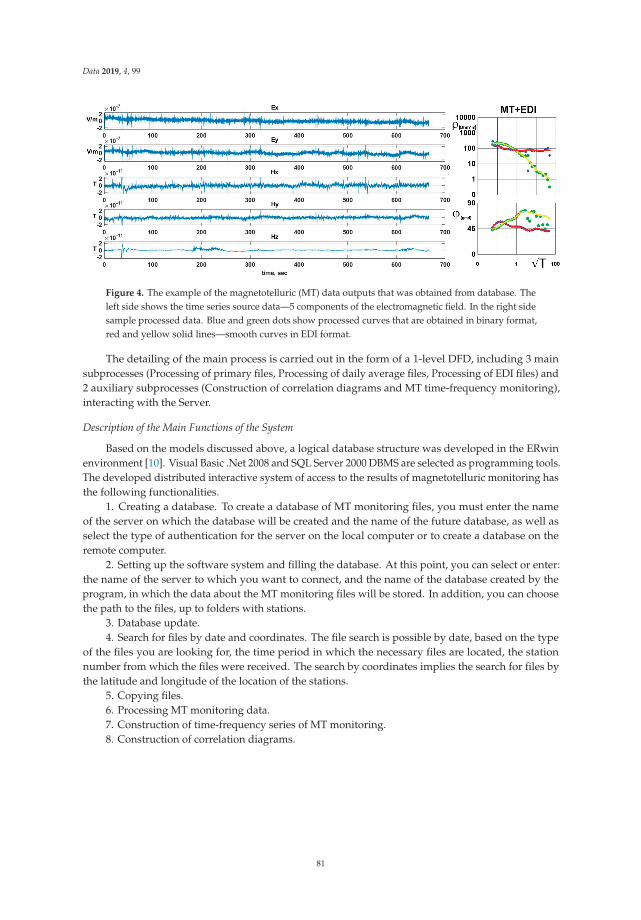
Data 2019, 4, 99

Figure 4. The example of the magnetotelluric (MT) data outputs that was obtained from database. Theleft side shows the time series source data—5 components of the electromagnetic field. In the right sidesample processed data. Blue and green dots show processed curves that are obtained in binary format,red and yellow solid lines—smooth curves in EDI format.

The detailing of the main process is carried out in the form of a 1-level DFD, including 3 mainsubprocesses (Processing of primary files, Processing of daily average files, Processing of EDI files) and2 auxiliary subprocesses (Construction of correlation diagrams and MT time-frequency monitoring),interacting with the Server.

Description of the Main Functions of the System

Based on the models discussed above, a logical database structure was developed in the ERwinenvironment [10]. Visual Basic .Net 2008 and SQL Server 2000 DBMS are selected as programming tools.The developed distributed interactive system of access to the results of magnetotelluric monitoring hasthe following functionalities.

1. Creating a database. To create a database of MT monitoring files, you must enter the nameof the server on which the database will be created and the name of the future database, as well asselect the type of authentication for the server on the local computer or to create a database on theremote computer.

2. Setting up the software system and filling the database. At this point, you can select or enter:the name of the server to which you want to connect, and the name of the database created by theprogram, in which the data about the MT monitoring files will be stored. In addition, you can choosethe path to the files, up to folders with stations.

3. Database update.4. Search for files by date and coordinates. The file search is possible by date, based on the type

of the files you are looking for, the time period in which the necessary files are located, the stationnumber from which the files were received. The search by coordinates implies the search for files bythe latitude and longitude of the location of the stations.

5. Copying files.6. Processing MT monitoring data.7. Construction of time-frequency series of MT monitoring.8. Construction of correlation diagrams.

81

Data 2019, 4, 99

4. User Notes

Usage: for collecting and processing geophysical information, in particular for measuring,recording, and processing the electrical and magnetic components of the natural electromagnetic field,in the study of geodynamic processes occurring in the Earth’s crust and upper mantle using electricalsurvey methods. Thus, the developed software system makes it possible to increase the efficiency ofprocessing MT monitoring data by significantly reducing the time spent searching for the necessaryinformation, the ability to quickly view the newly received data, and create a distributed databaseof monitoring MT observations over a period of about 15 years. Currently, the system is in the trialoperation of the Research Station of the Russian Academy of Sciences.

5. Patents

As part of these studies, the database “Local database of magnetotelluric data in the system ofgeophysical monitoring of geodynamic processes in the Earth’s crust of seismically active regions”was registered. Certificate No. 2012621291, issued on 07.12.2012. Copyright holder FGBUN ResearchStation of the Russian Academy of Sciences in Bishkek. Authors: Rybin A.K., Matiukov V.E., DesyatkovG.A., Lychenko N.M., Manzhikova S.T. At the present, this database is actively used and developed.

Author Contributions: Conceptualization, E.B.; Data curation, A.R.; Investigation, A.R.; Methodology, E.B.;Project administration, A.R.; Software, V.M.; Visualization, V.M.; Writing—original draft, E.B.; Writing—review &editing, V.M.

Funding: The presented researches are carried out within the fulfilment of the State Assignment by the ResearchStation of the Russian Academy of Sciences (subject AAAA-A19-119020190063-2 (0155-2019-0001)) and with thefinancial support of the Russian Foundation for Basic Research (Project 17-05-00654).


References

1. Rybin, A.; Fox, L.; Ingerov, O.; Schelochkov, G.; Safronov, I.; Batalev, V.; Bataleva, E. MT monitoringexperiment in the Northern Tien Shan seismogenic zone/CD ROM: Abstracts. In Proceedings of the 10-thScientific Assembly of the International Association of Geomagnetism and Aeronomy, Toulouse, France,18–25 July 2005.

2. Rybin, A.K.; Batalev, V.Y.; Bataleva, E.A.; Matiukov, V.E.; Desyatkov, G.A.; Lychenko, N.M.; Manzhikova, S.T.;Ten, V. Development of a distributed interactive system of access to the results of magnetotelluric monitoring.In Proceedings of the Problems of geodynamics and geoecology of intracontinental orogens VII InternationalSymposium, Bishkek city, Kyrgyz Republic, 19–24 June 2011; pp. 179–187.

3. Bataleva, E.A.; Batalev, V.Y.; Rybin, A.K. On the question of the interrelation between variations in crustalelectrical conductivity and geodynamical processes. Izvestiya Phys. Solid Earth 2013, 49, 402–410. [CrossRef]

4. Lyubushin, A.A. Multidimensional analysis of the time series of geophysical monitoring systems.Izvestiya Phys. Solid Earth 1993, 3, 103–108.

5. Bataleva, E.A.; Batalev, V.Y. Development of Programs to Analyze the Data on Azimuthal MagnetotelluricMonitoring Part 1. Analysis of magnetotelluric monitoring data. Vestnik Kyrgyz-Slavic University 2014, 14,3–7.

6. Bataleva, E.A.; Batalev, V.Y. Development of Programs to Analyze the Data on AzimuthalMagnetotelluric Monitoring Part 2. Development of software for analysis of MT monitoring data.Vestnik Kyrgyz-Slavic University 2014, 14, 8–12.

7. Bataleva, E.A.; Zabinyakova, O.B.; Batalev, V.Y. Software Development for Monitoring ElectromagneticParameters of the Bishkek Geodynamic Providing Group. Vestnik Kyrgyz-Slavic University 2017, 17, 144–149.

8. Bataleva, E.A.; Zabinyakova, O.B.; Batalev, V.Y. Development for Magnetotelluric Profile Monitoring Cantor’sMinipoligon. Vestnik Kyrgyz-Slavic University 2017, 17, 150–153.

9. Date, C.J. What is distributed database? Available online: ftp://sohoftp.nascom.nasa.gov/pub/www/publications/chapter10.pdf (accessed on 3 March 2019).

82

Data 2019, 4, 99

10. Infological modeling. Available online: http://www.rus-lib.ru/book/28/ps/01/027-044.html (accessed on15 April 2019).

11. Maklakov, S.V. BPwin and ERwin—CASE-development tools for information systems. M.: Dialog-MEPI.1999. Available online: https://studfiles.net/preview/942930/page:10/ (accessed on 10 May 2019).


83

MDPISt. Alban-Anlage 66

4052 BaselSwitzerland

Tel. +41 61 683 77 34Fax +41 61 302 89 18

www.mdpi.com

Data Editorial OfficeE-mail: [email protected]

www.mdpi.com/journal/data

MDPI St. Alban-Anlage 66 4052 Basel Switzerland

Tel: +41 61 683 77 34 Fax: +41 61 302 89 18 ISBN 978-3-03928-211-1

Documents

Overcoming Data Scarcity in Earth Science