OUTSIDE IN: EXPLORATIONS IN THE POLITICAL ECONOMY OF …ses.wsu.edu/.../2019/11/Ethan-Spangler-Final-Dissertation-Dec.-2017.… · The Middle East, Central Asia, and South-East Asia

OUTSIDE IN: EXPLORATIONS IN THE POLITICAL ECONOMY OF NATIONAL

SECURITY

By

ETHAN SPANGLER

A dissertation submitted in partial fulfillment of

the requirements for the degree of

DOCTOR OF PHILOSOPHY

WASHINGTON STATE UNIVERSITY

School of Economic Sciences

December 2017

c Copyright by ETHAN SPANGLER, 2017

All Rights Reserved

c Copyright by ETHAN SPANGLER, 2017

All Rights Reserved

To the Faculty of Washington State University:

The members of the Committee appointed to examine the dissertation of

ETHAN SPANGLER find it satisfactory and recommend that it be accepted.

Philip Wandschneider, Ph.D., Chair

Ben Smith, Ph.D.

Michael Brady, Ph.D.

Thomas L. Marsh, Ph.D.

ii

ACKNOWLEDGMENT

I would like to thank my adviser, Philip Wandschneider, for helping me discover my

academic path. His support and guidance have made me the economist that I am. Working

with Phil made me realize my combined passion for research and teaching. I would also like

to thank the other members of my dissertation committee; Ben Smith, Thomas L. Marsh,

and Michael Brady, for their comments, questions, and assistance that helped me improve

and progress my research.

Most importantly, I would like to thank my fiancee, Morgan Conklin, and my parents,

Catherine Zublin and Edward Spangler, for their support, endless encouragement, and tol-

erance of my incessant kvetching. Without them this would not have been possible.

iii

OUTSIDE IN: EXPLORATIONS IN THE POLITICAL ECONOMY OF NATIONAL

SECURITY

Abstract

by Ethan Spangler, Ph.D.

Washington State University

December 2017

Chair: Philip Wandschneider

In this dissertation, I examine how countries respond to external and internal national

security issues in the 21stCentury. The first chapter analyzes European military expenditures

with an emphasis on how European countries respond to US expenditures at the global

and regional levels. Using a dynamic panel model, I find that European countries respond

significantly and negatively to US global military expenditures but there is statistical impact

at the regional level.

The second chapter presents a theoretical model of dissent and political stability, focusing

on the interactions of a non-altruistic government and its citizenry. Simulations show how

exogenous shocks at the government and individual levels can affect political stability. Find-

ings suggest that countries can be stable in their political instability and that counties with

a preference for using government services over suppression are more likely to be politically

stable.

The third chapter develops a method of estimating a countrys public dissent and political

stability using data from social media site Twitter. Tweets voicing dissatisfaction with the

government were collected, scored, and aggregated; forming the basis of the measure of public

dissent. Combining these estimates of dissent with macroeconomic data creates an overall

estimation of a country’s political stability.

iv

TABLE OF CONTENTS

Page

ACKNOWLEDGMENT . . . . . . . . . . . . . . . . . . . . . . . . . . . . . . . . iii

ABSTRACT . . . . . . . . . . . . . . . . . . . . . . . . . . . . . . . . . . . . . . iv

LIST OF TABLES . . . . . . . . . . . . . . . . . . . . . . . . . . . . . . . . . . . viii

LIST OF FIGURES . . . . . . . . . . . . . . . . . . . . . . . . . . . . . . . . . . ix

CHAPTER ONE . . . . . . . . . . . . . . . . . . . . . . . . . . . . . . . . . . . . 1

1 Introduction . . . . . . . . . . . . . . . . . . . . . . . . . . . . . . . . . . . . 1

2 Related Literature . . . . . . . . . . . . . . . . . . . . . . . . . . . . . . . . 4

3 Theory . . . . . . . . . . . . . . . . . . . . . . . . . . . . . . . . . . . . . . . 6

4 Data . . . . . . . . . . . . . . . . . . . . . . . . . . . . . . . . . . . . . . . . 12

5 Empirical Analysis . . . . . . . . . . . . . . . . . . . . . . . . . . . . . . . . 18

5.1 Static Fixed Effects Model . . . . . . . . . . . . . . . . . . . . . . . . . . . . 19

5.2 Dynamic Model . . . . . . . . . . . . . . . . . . . . . . . . . . . . . . . . . . 23

6 Conclusion . . . . . . . . . . . . . . . . . . . . . . . . . . . . . . . . . . . . . 26

7 References . . . . . . . . . . . . . . . . . . . . . . . . . . . . . . . . . . . . . 28

CHAPTER TWO . . . . . . . . . . . . . . . . . . . . . . . . . . . . . . . . . . . . 30

1 Introduction . . . . . . . . . . . . . . . . . . . . . . . . . . . . . . . . . . . . 30


3 Theoretical Model . . . . . . . . . . . . . . . . . . . . . . . . . . . . . . . . . 33

3.1 Individual’s Problem . . . . . . . . . . . . . . . . . . . . . . . . . . . . . . . 34

3.2 Government’s Problem . . . . . . . . . . . . . . . . . . . . . . . . . . . . . . 38

v

4 Solving the Model . . . . . . . . . . . . . . . . . . . . . . . . . . . . . . . . . 41

4.1 Individual’s solution . . . . . . . . . . . . . . . . . . . . . . . . . . . . . . . 41

4.2 Total Dissent . . . . . . . . . . . . . . . . . . . . . . . . . . . . . . . . . . . 43

4.3 Government Solution . . . . . . . . . . . . . . . . . . . . . . . . . . . . . . . 44

5 Simulations . . . . . . . . . . . . . . . . . . . . . . . . . . . . . . . . . . . . 45

5.1 Initial Dissent . . . . . . . . . . . . . . . . . . . . . . . . . . . . . . . . . . . 48

5.2 Shocks . . . . . . . . . . . . . . . . . . . . . . . . . . . . . . . . . . . . . . . 51

5.2.1 Resource Shocks . . . . . . . . . . . . . . . . . . . . . . . . . . . . . 51

5.2.2 Φ and Ω Shocks . . . . . . . . . . . . . . . . . . . . . . . . . . . . . . 53

5.2.3 Environment Shock . . . . . . . . . . . . . . . . . . . . . . . . . . . . 55

5.2.4 Enforcement Shock . . . . . . . . . . . . . . . . . . . . . . . . . . . . 57

6 Conclusion . . . . . . . . . . . . . . . . . . . . . . . . . . . . . . . . . . . . . 58

7 References . . . . . . . . . . . . . . . . . . . . . . . . . . . . . . . . . . . . . 60

CHAPTER THREE . . . . . . . . . . . . . . . . . . . . . . . . . . . . . . . . . . 62

1 Introduction . . . . . . . . . . . . . . . . . . . . . . . . . . . . . . . . . . . . 62


2.1 Twitter Literature . . . . . . . . . . . . . . . . . . . . . . . . . . . . . . . . 66

3 Theory . . . . . . . . . . . . . . . . . . . . . . . . . . . . . . . . . . . . . . . 68

4 Methods . . . . . . . . . . . . . . . . . . . . . . . . . . . . . . . . . . . . . . 71

4.1 Scoring Tweets . . . . . . . . . . . . . . . . . . . . . . . . . . . . . . . . . . 73

4.2 Case Studies: Canada and Kenya . . . . . . . . . . . . . . . . . . . . . . . . 75

5 Data and Estimation . . . . . . . . . . . . . . . . . . . . . . . . . . . . . . . 76

5.1 Estimating Political Stability . . . . . . . . . . . . . . . . . . . . . . . . . . 80

vi

6 Conclusion . . . . . . . . . . . . . . . . . . . . . . . . . . . . . . . . . . . . . 81

7 References . . . . . . . . . . . . . . . . . . . . . . . . . . . . . . . . . . . . . 84

vii

LIST OF TABLES

Page

CHAPTER ONE . . . . . . . . . . . . . . . . . . . . . . . . . . . . . . . . . . . . 1

1 Sample Countries, 2000-2014 . . . . . . . . . . . . . . . . . . . . . . . . . . . 13

2 Data Description, European Variables . . . . . . . . . . . . . . . . . . . . . . 16

3 Data Description, US Military Variables . . . . . . . . . . . . . . . . . . . . 17

4 Summary Statistics . . . . . . . . . . . . . . . . . . . . . . . . . . . . . . . . 17

5 Static Fixed Effect Models with GR . . . . . . . . . . . . . . . . . . . . . . . 21

6 Static Fixed Effects with GDP . . . . . . . . . . . . . . . . . . . . . . . . . . 22

7 Initial Dynamic Models . . . . . . . . . . . . . . . . . . . . . . . . . . . . . . 23

8 Final Dynamic Model . . . . . . . . . . . . . . . . . . . . . . . . . . . . . . . 24

CHAPTER TWO . . . . . . . . . . . . . . . . . . . . . . . . . . . . . . . . . . . . 30

9 Parameter Basis . . . . . . . . . . . . . . . . . . . . . . . . . . . . . . . . . . 45

10 Parameter Values . . . . . . . . . . . . . . . . . . . . . . . . . . . . . . . . . 48

CHAPTER THREE . . . . . . . . . . . . . . . . . . . . . . . . . . . . . . . . . . 62

11 Twitter Data Summary Statistics . . . . . . . . . . . . . . . . . . . . . . . . 77

12 Statistical Tests . . . . . . . . . . . . . . . . . . . . . . . . . . . . . . . . . . 78

13 Estimation Values . . . . . . . . . . . . . . . . . . . . . . . . . . . . . . . . . 80

viii

LIST OF FIGURES

Page

CHAPTER ONE . . . . . . . . . . . . . . . . . . . . . . . . . . . . . . . . . . . . 1

Figure 1 Comparative Military Expenditures 2001-2012 . . . . . . . . . . . . . 2

Figure 2 US Military Presence in Europe 2001-2012 . . . . . . . . . . . . . . . 3

Figure 3 European Military Expenditures 2000-2014 . . . . . . . . . . . . . . . 3

Figure 4 Andrews Plot of Sample Countries . . . . . . . . . . . . . . . . . . . 13

CHAPTER TWO . . . . . . . . . . . . . . . . . . . . . . . . . . . . . . . . . . . . 30

Figure 1 Activism Preference Distribution Plot, xi ∼ logN(0, 1) . . . . . . . . 36

Figure 2 Low Initial Dissent, D0 = 1 . . . . . . . . . . . . . . . . . . . . . . . 49

Figure 3 High Initial Dissent, D0 = 100 . . . . . . . . . . . . . . . . . . . . . . 50

Figure 4 Resource Shock . . . . . . . . . . . . . . . . . . . . . . . . . . . . . . 52

Figure 5 Φ Shock . . . . . . . . . . . . . . . . . . . . . . . . . . . . . . . . . . 53

Figure 6 Ω Shock . . . . . . . . . . . . . . . . . . . . . . . . . . . . . . . . . . 54

Figure 7 Environment Shock . . . . . . . . . . . . . . . . . . . . . . . . . . . . 55

Figure 8 Enforcement Shock . . . . . . . . . . . . . . . . . . . . . . . . . . . . 56

CHAPTER THREE . . . . . . . . . . . . . . . . . . . . . . . . . . . . . . . . . . 62

Figure 1 Tweet distribution and densities in Canada and Kenya . . . . . . . . 76

Figure 2 Weekly Dissent levels in Canada and Kenya . . . . . . . . . . . . . . 77

Figure 3 Weekly Total Dissent levels in Canada and Kenya . . . . . . . . . . . 78

Figure 4 Monotonic Transformations of Total Dissent . . . . . . . . . . . . . . 79

Figure 5 Daily Internet Searches for ‘Brexit’ in Canada and Kenya . . . . . . . 79

ix

Figure 6 Weekly Nominal Estimated Political Stability in Canada and Kenya . 81

Figure 7 Weekly Scaled Estimated Political Stability in Canada and Kenya . . 81

x

CHAPTER ONE

ALLIES WITH BENEFITS: US EFFECT ON EUROPEAN DEMAND FOR MILITARY

EXPENDITURES

1 Introduction

The US-European relations have been an international security staple since the establish-

ment of the North Atlantic Treaty Organization (NATO) in 1949. NATO’s first Secretary

General, Lord Ismay, stated that a primary goal of the organization was to “keep the Amer-

icans in, the Russians out” (Reynolds, 1994 p 13). For over 40 years, that is exactly what

NATO did, protecting Europe from Soviet aggression and reinforcing cross Atlantic rela-

tions. However, after several decades of cooperation, US-European relations may be facing

new challenges.

Over the course of the 21stCentury US interests and attention have been drawn elsewhere.

The Middle East, Central Asia, and South-East Asia have all become an increasing concern of

US foreign policy. Furthermore, many within the US feel that European states have become

too reliant upon the US for their security. As stated by former US Secretary of Defense

Robert Gates “the blunt reality is that there will be dwindling appetite and patience in the

U.S. Congress and in the American body politic writ large to expend increasingly precious

funds on behalf of nations that are apparently unwilling to devote the necessary resources

or make the necessary changes to be serious and capable partners in their own defense.”

(Schultz, 2011).

To understand what consequences this shift in attention may have or the implications of

security dependency for US-European relations, it is first important to establish what kind

of security relationship the US and the European community have. Do European states see

1

US military expenditures as a complement to their own efforts or as a substitute, or neither?

While intentions are beyond this study, empirical analysis can provide some insight. The

primary goal of this paper is to estimate the potential effect US military expenditures may

have on European demand for military expenditures.

Compounding the analysis is the complexity and scale of the US military. The US cur-

rently occupies a dominant position in terms of international power. Following the collapse

of the Soviet Union in the early 1990s the world began a period of US hegemony. Figure

1, using data from the Stockholm International Peace Research Institute (SIPRI), plots US

military expenditures alongside the aggregated military expenditures of all European NATO

members1, Russia, China, and Iran in real terms. China, Russia, and Iran are included be-

cause they are considered potential rivals. By 2011 the US was spending more than double

all other NATO countries combined. This considerable expenditure of resources by the US

is only 4.7% of US GDP (SIPRI), whereas the average military expenditure by European

states is 1.4% of GDP for 2011.

2000 2002 2004 2006 2008 2010 2012Year

0

100

200

300

400

500

600

700

Mili

tary

Ex

pe

nd

itu

res

(bill

ion

s U

S 2

00

5 $

)

USEuro-NATOChinaRussianIran

Figure 1: Comparative Military Expenditures 2001-2012

During this period of increasing US total military expenditures, the US’s physical pres-

1For the sake of brevity, all mentions of NATO past this point will be in reference to its European membersexclusively

2

ence in Europe decreased. Figure 2 shows the number of active US bases and military

personnel deployed in Europe, based on data obtained from the US Defense Department’s

Base Structure Reports. Active US bases and military personnel essentially co-move with

one another, peaking around 2004/2005 and then declining thereafter. So there are poten-

tially two contrary forces potentially influencing European military spending with respect

to the US: global military expenditures and regional military expenditures.

2000 2002 2004 2006 2008 2010 2012Year

70000

80000

90000

100000

110000

120000

US M

ilitary Personnel

Military Personnel (BSR)

100

120

140

160

180

200

220

240

260

US Bases

Bases

Figure 2: US Military Presence in Europe 2001-2012

2000 2002 2004 2006 2008 2010 2012 2014Year

0

10

20

30

40

50

60

70

Military Expenditures (billions US 2005 $)

France

Germany

Italy

Netherlands

Spain

UK

2000 2002 2004 2006 2008 2010 2012 2014Year

0

1

2

3

4

5

6

7

8

9

Military Expenditures (billions US 2005 $)

Austria

Belgium

Croatia

Czech Rep.

Denmark

Estonia

Finland

Greece

Hungary

Ireland

Latvia

Lithuania

Luxembourg

Norway

Poland

Portugal

Romania

Slovak Rep.

Slovenia

Sweden

Switzerland

Figure 3: European Military Expenditures 2000-2014

A secondary goal of this paper is to examine whether European states respond to the US

3

global military expenditures, US regional expenditures, both, or neither; and if European

states respond differently to US global and regional military expenditures. While aggregate

European military expenditures display very little variation, there is individual fluctuation

as shown in Figure 3, adding validity to this analysis. This study’s findings suggest that

US regional factors show minimal importance while US global military expenditures have a

statistically significant and negative effect on European military expenditures. The structure

of this paper is as follows: a review of relevant literature, theory, data, empirical analysis,

and conclusion.

2 Related Literature

A rich literature exists on the factors shaping military expenditures. A traditional in-

terpretation of military expenditures is to take the neoclassical approach and view military

expenditures as a pure public good, wherein the state balances security and opportunity

costs (Smith, 1989; Sandler, 1993). Complicating the demand for military expenditures are

other internal and external factors. Internal factors include economic variables, bureaucracy,

politics, and ideology (Albalate et al., 2012; Bove and Brauner, 2016; Tongur et al., 2015).

External factors, which are the primary concern of this study, include the military spending

of potential allies and enemies.

Understanding the causes and effects of military expenditures is important because mil-

itary expenditures can have a negative impact on economic growth. A survey by Dunne

and Tian (2013) finds that, in most cases, increases in military expenditures do not induce

economic growth; Dunne and Nikolaidou (2012) find this to be the case among the EU15. A

possible reason behind this is that military expenditures often have an inverse relationship

with other forms of government spending (Nikolaidou, 2008), because military expenditures

4

divert resources that could be used for other government services or development. Hence

factors that increase military expenditures could result in welfare loss for a state, as resources

transfer to defense and away from pursuits that are potentially more beneficial to economic

growth, resulting in generally reduced growth for the state.

The opportunity costs of military expenditures are a potential reason why many empir-

ical studies suggest that when state have reliable allies, security free-riding is more likely

(De La Fe and Montolio, 2001; Nikolaidou, 2008; Ringsmose, 2010; Beeres et al., 2012).

Conversely, other studies give evidence that some states are security followers and their mili-

tary expenditures co-move with allies (Smith 1989; Solomon 2005; Nikolaidou, 20082; Douch

and Solomon, 2012). A common element among these studies is that they use a time series

dominated by Cold War politics and predominantly focus on the security relations within a

formal alliance, specifically NATO.

This paper extends existing work in several important ways. First, a distinction is made

between the US’s global and regional military expenditures. Using information obtained

through the US Department of Defense I am able to proxy for US regional military expen-

ditures in Europe. The ability to make the distinction between the US’s total and regional

military expenditures is relevant because previous studies (Rosh, 1988; Dunne and Perlo-

Freeman, 2003; Nordhaus et al., 2012, Skogstad, 2016) find that the strategic environment a

state faces significantly impact its demand for military expenditures. By making the distinc-

tion between global and regional security, a more nuanced analysis can be done regarding

the factors influencing European military expenditures.

Second, I test pan-European security relations outside a formal alliance structure through

the inclusion of non-NATO European states in the analysis. This is important because the

high degree of European integration, especially in regards to security arrangements, means

2Nikolaidou (2008) is cited on contrary points because they do individual time series analyses for variousEuropean countries. In some cases Nikolaidou found cooperation and in other cases substitution.

5

that focusing on members of a single alliance is inappropriate and it is better to look at

Europe as a whole. Third, this paper uses government revenue, opposed to GDP, as a better

empirical representation of European income constraints and as well as counters endogeneity.

Finally, I use a more recent post-Cold War data set. The separation of Cold War and

post-Cold War periods is important because parameter relationships have likely changed

between the two periods (Dunne and Perlo-Freeman, 2003). The time period of interest here

also covers several important strategic shifts: the transition of NATO to smaller scale crisis

response, initiation of the Global War on Terrorism, and the Great Recession. A period

encompassing these substantial shifts warrants independent analysis in order to make more

effective policy recommendations.

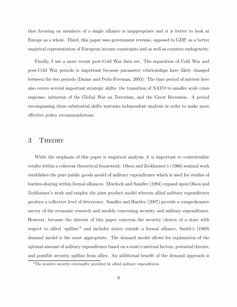
3 Theory

While the emphasis of this paper is empirical analysis, it is important to contextualize

results within a coherent theoretical framework. Olson and Zeckhauser’s (1966) seminal work

establishes the pure public goods model of military expenditures which is used for studies of

burden-sharing within formal alliances. Murdoch and Sandler (1984) expand upon Olson and

Zeckhauser’s work and employ the joint product model wherein allied military expenditures

produce a collective level of deterrence. Sandler and Hartley (2007) provide a comprehensive

survey of the economic research and models concerning security and military expenditures.

However, because the interest of this paper concerns the security choices of a state with

respect to allied ‘spillins’3 and includes states outside a formal alliance, Smith’s (1989)

demand model is the most appropriate. The demand model allows for explanation of the

optimal amount of military expenditures based on a state’s internal factors, potential threats,

and possible security spillins from allies. An additional benefit of the demand approach is

3The positive security externality provided by allied military expenditures.

6

relatively easy empirical translation.

The theoretical model of this paper is based on Smith’s (1989) neoclassical approach to

deriving a state’s demand for military expenditures. In Smith’s approach state i functions as

a rational actor seeking to maximize its welfare function, W , which is a function of security,

S, consumption, C, and a vector of parameterizing internal domestic variables, Z:

W = f(S, C, Z) (1)

Maximization of state i’s welfare function is subject to a budget constraint:

Y = ME + CE (2)

Where ME is military expenditures, CE is non-military consumption expenditures, and

Y is total state income. ME = PMM and CE = PCC, M and C being military and

consumption goods with PM and PC their respective prices. PC is normalized, leaving the

ratio, PM/PC . Usually it is assumed that military and civilian prices behave the same,

dropping from analysis. Solomon (2005) notes that military prices can move separately from

civilian prices. Unfortunately, few countries separately track their military price deflator so

this data cannot be included in the estimation.

Security is a function of a state i’s own military expenditures, ME, the aggregate spillin

of allied military expenditures, Q, potential threats, Th, and other security factors, X :

S = f(ME,Q, Th,X) (3)

RegardingQ, assuming a Nash-Cournot specification wherein all n countries in the system

have made their best-response equilibrium choices, state i takes a function of the military

7

expenditures of all others as given:

Q = f

(n∑

j=1

MEj

)

(4)

where j 6= i. The exact nature of the function is dictated by the specifics of the spillin.

Collective defense organizations such as NATO are predicated upon Q being essentially a

linear combination, whereas other alliance structures may only see a portion of allied spillin.

The Nash-Cournot specification is appropriate since this study includes states outside a

formal alliance structure, but there is still some degree of expected security cooperation. The

military expenditures of other states induce a different response from state i depending on if

one is an ally or rival. Allied expenditures, Q, could be viewed as either complements, sub-

stitutes, or neither. The military expenditures of rivals, Th, usually has a positive effect on

state i’s military expenditures. An empirical implication of the Nash-Cournot specification

is using lags of the Q and Th variables during estimation.

Maximization of the state’s welfare functions subject to the budget and security yields

the ME demand:

ME = f(Y, PM/PC, Q, Th, Z,X) (5)

The above is the standard general form of state i’s demand for military expenditures. For

the purposes of this study the general form expands to the specific setting, leading to the

following:

ME = f(MEt−1, Y, GE, Trade, PopDen,NATO−i, USG, USR, Russia, Iraq) (6)

8

Thus European demand for military expenditures becomes a function of demand for other

government expenditures, national income, US global and regional military expenditures,

neighboring NATO expenditures, Russian military expenditures, and participation in the

Iraq War:

• MEt−1 is a one period lag of military expenditures. A one period lag of military

expenditures is used to account for bureaucratic inertia of a state. The use of lagged

military expenditures, though theoretically relevant, creates estimations issues which

will be discussed later.

• Y is total government income. Military expenditures are assumed to be a normal good

and therefore should have a positive relationship with respect to government income.

• GE is other government expenditures, excluding military. Government expenditures

represents the opportunity cost of military expenditures. Since military expenditures

often crowd out other government expenditures (e.g. guns verse butter) the coefficient

is expected to be negative.

• Trade is the country’s summed value of exports and imports of both goods and services.

• PopDen is population density. Population density is included to capture any scale

public good effect military expenditures may have (Dunne and Perlo-Freeman 2003;

Nikolaidou 2008) and to capture the defensive burden of protecting the country’s land-

mass. A large sparsely populated country is harder to defend than one that is highly

concentrated.

• NATO−i is the aggregated military expenditures of all European NATO members

excluding the military expenditures of country i if they are a member.

• USG and USR are US military expenditures at the global and regional levels.

9

• Russia is Russian military expenditures, the threat variable.

• Iraq is an indicator variable for participation in the Iraq War. If a state participated

in the conflict one would expect their military expenditures to increase as a result.

The NATO, USG and USR are used to assess the individual spillins that might be

affecting European demand for military expenditures. NATO, USG and USR could each

have a different effect on European demand for military expenditures: either complementary,

substitutive, or neither. Empirical analysis should give evidence as to what the potential

relationship is. If the coefficient for either is negative and significant, it would indicate

that US and NATO military expenditures are seen as substitutes for a state’s own military

expenditures (free-riding). If the coefficients are positive and significant, that would indicate

that US and NATO military expenditures are seen as complementary (following). Lack of

significance or significant coefficients of zero for either would suggest European states are

autarkic in their security choices. A core assumption of this paper is that the relationship is

one way, i.e. European military expenditures do not influence US military expenditures.

NATO was used because while other pan European security organizations have formed

(e.g. the EU’s Common Security and Defence Policy), NATO remains the most prominent

and active of the international defense organizations in Europe. Any large scale security

crisis affecting Europe would likely involve NATO. So how European states respond to the

aggregated military expenditures of the European members of NATO allows one to assess

the degree of security coordination across the continent.

As stated earlier, a secondary goal of this paper is to distinguish the effects of US global

and regional military expenditures. The separation of the two is important because countries

face different issues at the regional and global levels. At the regional level a country is more

aware of the issues, risks, and actors at play; known unknowns. However, at the global level,

issues become more complicated and harder to identify; unknown unknowns. Additionally,

10

the difficulties of security increase dramatically the further a country tries to project itself

beyond its borders. US actions outside of Europe: nation building, combating terrorism,

anti-piracy, are ‘out-of-area’ spilling (Sandler and Shimizu 2014). Thus, at the regional level

the presence of a powerful outside allied actor may be viewed as beneficial but not critical.

However, at the global level, a powerful interest-aligned ally could be viewed as more valuable

to smaller states.

Rosh (1988) and Dunne and Perlo-Freeman (2003) include trade, imports plus exports, to

account for the potential ease a country might have in purchasing arms abroad, potentially

increasing military expenditures. In this analysis, trade is included for slightly different

reasons. Here trade is used to represent how vulnerable a country is to potential international

instability and conflict. If a conflict were to disrupt trade, a country highly dependent upon

trade would suffer more than an a more insular country. The more a country is engaged in

trade, the more it will need to spend on defense to protect its trade. Additionally, a small

country that is highly dependent on trade is more likely to value the presence of an outside

stabilizing force, such as the US. Given that many European countries have export intensive

economies, this is an important variable to include.

Russian is used as the threat variable because Russia still represents the most pressing

existential security concern to European states, and as such should have a positive effect on

European demand for military expenditures. Although there has been cooperation between

Russian and the West in the form of the NATO-Russia Council, recent events diminish its

relevancy. Russian transgressions in Ukraine and posturing along Baltic States suggests

that the tenure of the NATO-Russia Council was little more than an unsteady detente

than genuine peace building. Furthermore, incidences such as the 2007 cyberattack on the

Estonian government and the 2008 invasion of Georgia (which was considering joining NATO

prior to the invasion) further emphasize the continued tensions between East and West.

11

4 Data

To assess the potential effects of US military expenditures on European demand for

military expenditures, this study uses a panel series of 28 countries for years 2000 to 2014.4

The time period, 2000-2014, was chosen for the previously stated policy reasons as well as

practical limitations. Some variables used in the empirical analysis, most significantly those

used to proxy US regional military expenditures, are only available for the given time period.

European nations were chosen because of the relative homogeneity between states (devel-

oped, democratic, pro-West, etc.), lack of significant interstate and intrastate conflict, and

minimal regional tension. Some European states were excluded from the analysis due to

practical and theoretical reasons. The various European microstates were excluded as they

are inconsequential to the analysis and their security is guaranteed by other states in the

sample. Many of the Balkan states and Turkey were excluded due to data availability issues.

Moreover, it is felt that the idiosyncratic properties of these states are likely to make them

outliers, distorting results.

Previous research into the factors influencing military expenditures generally used mul-

tiple time series case studies (Nikolaidou, 2008; Douch and Solomon, 2012). Using multiple

time series works when each country faces a unique security environment. However, when

several countries face a similar security environment and are relatively similar in character-

istics, as is the case with Europe, panel analysis becomes feasible allowing for a far more

robust sample size. To illustrate this point, the sample domestic data for each country has

been put into an Andrews Plot5 in Figure 4. Each color represents a sample country and

each line an observation. While the axes values are relatively unimportant, the relevant

detail is that overall the data flows in roughly the same manner and there are no extreme

4see Table 1 for a full list of countries used.5An Andrews Plot puts data through a finite Fourier Series that preserves the mean and variance. For

more information see Garcıa-Osorio and Fyfe (2005)

12

outliers, validating the use of panel data.

Austria* Finland* Latvia RomaniaBelgium France Lithuania SlovakiaBulgaria Germany Luxembourg SloveniaCroatia Greece Netherlands Spain

Czech Republic Hungary Norway Sweden*Denmark Ireland* Poland Switzerland*Estonia Italy Portugal UK

*=Non-NATO

Table 1: Sample Countries, 2000-2014

−3 −2 −1 0 1 2 3−6

−4

−2

0

2

4

6 1e12

AustriaBelgiumCroatiaCzech RepublicDenmarkEstoniaFinlandFranceGermanyGreeceHungaryIrelandItalyLatviaLithuaniaLuxembourgNetherlandsNorwayPolandPortugalRomaniaSlovakiaSloveniaSpainSwedenSwitzerlandUK

Figure 4: Andrews Plot of Sample Countries

Country level data were obtained through Stockholm International Peace Research Insti-

tute (SIPRI), the World Bank, and Eurostat, as noted in Table 2. Governmental financial

figures were converted from percent GDP to level and normalized to US$ 2005 figures. Past

studies have used GDP for government income in the demand function; however, this study

uses government revenue instead. Whereas GDP encompasses all economic activity in the

state, of which the government only partially controls, government revenue is a better reflec-

tion of the resources available to policymakers. Since the period of analysis does not contain

large scale Clauswitzian style total warfare, this is a reasonable decision to make. Sandler

(1993) proposes using government revenue as the income variable, but few empirical papers

follow this suggestion probably due to data availability. The issue of data availability per-

13

sists somewhat and unbalances the panel slightly in this study. Using government revenue

also avoids endogeneity issues because military expenditures are included in GDP, which

range between 1-4% of GDP for European states (SPIRI). As a robustness check, alternative

specifications were run using GDP in place of government revenue.

Table 3 lists all variables used for global and regional US military expenditures. In

translating the theoretical variables for US global and regional military expenditures, US

global military expenditures are easily obtained and empirically represented through US total

military expenditures. However, only US total military expenditures are available, regional

expenditures are not. To get around this gap in the data, I use US military personnel and

base information from the US Department of Defense as proxies for US regional military

expenditures. Recall from Figure 2 that US active bases and military personnel in Europe

roughly follow one another, so it is reasonable to believe that they can be used as proxies for

US regional military expenditures. For the purposes of this paper, an active base is any US

installation that has military personnel. Civilian or deactivated facilities are not included in

the analysis. As with US total military expenditures, the interpretation of the coefficients

is the same. In the empirical analysis the US regional expenditures are analyzed using the

proxies in multiple ways: the regional total, country specific, and interaction terms between

US military personnel and bases at both the regional and country levels.

Information for US military personnel and bases in Europe was obtained through the

US Department of Defense Base Structure Report (BSR) and the Defense Manpower Data

Center (DMDC). The BSR is a yearly report that details all US bases and base person-

nel deployments worldwide, while the DMDC tracks all US military personnel deployments

worldwide. While DMDC releases quarterly reports of deployments, older records only in-

clude the September reports, thus these were the reports used for all years.

The distinction between the BSR and DMDC is that the DMDC includes deployments

14

to countries where the US does not possess its own facilities and the deployments can be for

much shorter periods. Including the BSR and DMDC data enables testing of the importance

of global vs. regional US military expenditures to the European community. A short coming

of the BSR is that reports only goes back to 2001 and stops including military personnel

at bases in 2012, thus limiting the time span this data can be used. As shown in Table

3, different specifications of the BSR and DMDC data were used, the first being regional

aggregation of US bases and military personnel and the second country specific. For the

regional total DMDC figures, US military personnel in countries outside of the sample but

in the regional sphere, such as the Balkans and Turkey, were included. Country invariant

variables are denoted in Table 4.

It should be noted that data for US total military expenditures includes those incurred

for the Iraq War. There are several reasons why the costs of the Iraq War were not removed

from the analysis. First, many European countries participated in the conflict, most notably

the UK, so US spending in Iraq would be strategically relevant to them. Second, while many

countries sampled did not participate in the conflict or voiced opposition to the conflict,

it could be argued that after the initial invasion it was within the strategic interests of

European states that the US remain in Iraq to maintain stability. Had the US pulled out

prematurely, it likely would have further destabilized the region and resulted in a massive

diaspora from Iraq, similar to the current refugee crisis emanating from Syria. Third, there

is no good way to disentangle the costs of the Operation Iraqi Freedom from US total

military expenditures. There are some estimates available, but these generally only include

the costs that explicitly took place within the conflict; they do not include the extended

support, training, and logistical costs that were also involved in the conflict. Finally, previous

literature that analyzed potential spillin of US military expenditures did not control for other

US excursions, such as the Vietnam War (Smith, 1989; Solomon, 2005; Nikolaidou, 2008;

Douch and Solomon, 2012).

15

Label Variable Source Period Interval Units

ME Military Expenditures SIPRI 2000-2014 Annual 2005 US$ (Millions)GR Government Revenue Eurostat 2000-2014 Annual 2005 US$ (Millions)GDP Gross Domestic Product World Bank 2000-2014 Annual 2005 US$ (Millions)GE Government Expenditures World Bank 2000-2014 Annual 2005 US$ (Millions)Trade Summed Exports and Imports World Bank 2000-2014 Annual 2005 US$ (Millions)

Popden Population Density World Bank 2000-2014 Annual Popluation per km2

Iraq Involved in the Iraq War SIPRI 2000-2014 Annual Indicator

∆Russia% Change in RussianMilitary Expenditures

SIPRI 2000-2014 Annual Percentage

NATOAggregate NATOMilitary Expenditures

SIPRI 2000-2014 Annual 2005 US$ (Millions)

Table 2: Data Description, European Variables

The NATO figure is the aggregation of all the military expenditures of European NATO

members excluding Iceland6. Over the period of analysis NATO expanded its membership

(2004 and 2009). For the relevant years, the military expenditures for the new NATO

members were added to the aggregation. In this form, the NATO variable used here is very

similar to the “Security Web” variable Rosh (1988) and Dunne and Perlo-Freeman (2003)

employ but instead of a measure of potential enemies, it accounts for potential regional allies

exclusively. Because an individual NATO member’s military expenditures are removed from

the aggregation, there is little concern for endogeneity.

Instead of using the level of Russian military expenditures, yearly percentage change in

Russian military expenditures is used. While Russia does remain a threat to Europe, reliable

data for military expenditures remains difficult to acquire. For much for the time period of

interest, only estimated values are available. Additionally, it is believed that Russian military

expenditures are highly correlated with the US’s (Solomon 2005). Using the percent change

smooths out the noise of using the estimated data as well as the issue of correlation with the

US.6Iceland was excluded due to data availability issues. However, Icelands military expenditures are tiny

relative to the rest of NATO, averaging only $21 million over the years available, so there should be no lossin statistical validity

16

Label Variable Source Period Interval Units

US US total military expenditures SIPRI 2000-2014 Annual 2005 US$

US milper BSRtotal

US military personnel,regional total

BSR 2001-2012 Annual Individual

US bases BSRtotal

US military bases,regional total


US milper BSRcountry

US military personnel,country specific


US bases BSRcountry

US military bases,country specific


US milper DMDCtotal

US military personnel,country specific

DMDC 2000-2013 Annual Individual

US miulper DMDCcountry

US military personnel,regional total

DMDC 2000-2013 Annual Individual

Table 3: Data Description, US Military Variables

Mean Std. Dev. Min Max T n N

ME 12,224.83 20,693.73 101 103,232 15 28 420GE 126,424.05 186,439.43 1,764 828,867 15 28 420GR 504,756.76 513,500.47 139,556 1,569,831 14.89 28 417GDP 545,215.18 797,645.58 9,944 3,226,807 15 28 420Trade 561,935.36 929,505.33 9,322.80 6,185,422.0 15 28 420Popden 128.52 103.26 12.30 500.89 15 28 420Iraq 0.15 0.35 0 1 15 28 420NATO* 232,533.93 17,256.55 176,069 255,935 15 28 420∆Russia* 0.10 0.08 0.02 0.35 15 28 420US* 510,456.52 97,920.73 338,909 634,489 15 28 420US milper BSRtotal*

94,338.17 14,196.70 74,663 119,687 12 28 336

US bases BSRtotal

158.75 43.02 112 260 12 28 336

US milper BSRcountry

3,332.69 12,641.52 0 86,060 12 28 336

US bases BSRcountry

5.56 21.83 0 209 12 28 336

US milper DMDCtotal*

107,627.00 57,128.06 67,255 296,834 14 28 392

US milper DMDCcountry

3,566.26 14,975.28 0 199,950 14 28 392

*=Country invariant

Table 4: Summary Statistics

17

5 Empirical Analysis

The empirical testing used in this paper is an extension of that utilized by Dunne and

Perlo-Freeman (2003) but expanded upon to fulfill the stated goals. Initial specification

testing is done using a static fixed effects (FE) model while final analysis is done using the

Arellano-Bond dynamic panel estimator.

Results from a Box-Cox specification test suggest the use of the double-log form.7 How-

ever, because some countries do not have either a US base or military personnel, in models

using country specific US military base and personnel deployments these variables remain

in their original linear form. Additionally, Russian military expenditures have already been

transformed into yearly percentage change so there is no need to log. An added benefit of

using the double-log specification is that coefficients are now elasticities.

A fixed effects model is employed because it helps account for the unique properties

of each state in the sample that might affect their security choices but are not explicitly

accounted for by the other variables, such geography and other time invariant characteristics.

Results from a Hausman test support the use of of country specific fixed effects. Corrections

for heteroskedasticity were implemented using clustered robust standard errors. Interaction

terms for US military personnel and bases at the regional level and for trade and US total

military expenditures were initially included but dropped due to collinearity. As per the

Nash-Cournot specification external spillin security variables, US variables and NATO, have

been lagged 1 period. ∆Russia is not lagged because as a percentage change, the time

dimension is already accounted for. Lagging these variables also helps mitigate potential

issues of simultaneity.

7The Box-Cox test suggested a transformation of .047 and .136 on the dependent and independent vari-ables respectively. Since a transformation with these values would lack clear interpretability, the double-logis applied.

18

5.1 Static Fixed Effects Model

The static FE model was used for specification testing across the eight models because

there are more tools available to test the strength of fit. The primary objective of the static

model is to ascertain what empirical form of US regional variables affects European military

expenditures: regional totals, country specific, and BSR vs. DMDC. The secondary objective

is to test if government revenue or GDP is a better empirical representation of state income.

Tables 5 and 6 contain the results from eight specifications of the static FE models

tested, each column representing a different econometric model. Table 5 contains models

using government revenue, GR, while Table 6 uses GDP . Findings suggest that model 4,

judged by the overall R2, variable significance, and the AIC and BIC values; seem to be

the most robust. The benefits of using GR seem to more than make up for unbalancing the

panel. While model 4 seems to be the best model, model 3 presents interesting properties

with only being slightly inferior to model 4. Thus, the variables used in models 3 and 4 will

each be evaluated in a dynamic model in the next section.

Across models it is quite clear that US military expenditures are important to European

policymakers, but it is US total military expenditures that matters most. At no point across

specifications does the number of US military personnel seem to matter: neither regional

total, country specific deployments, nor differentiating between the BSR and DMDC data.

Given that the US uses its European bases as staging grounds for operations elsewhere8, it

is possible that these troops are not seen as a permanent force to be relied upon.

Contrasting the results for US military personnel, the variables for US bases are more

interesting. The number of US bases in a country seems to be unimportant while the

regional total of US bases is significant. A possible reason being that opening a new base

or reactivating an old facility is a considerable investment of resources on the part of the

8For example, the US African Command headquarters is actually in Stuttgart, Germany

19

US and not something done brashly. The opening and closing of US bases overseas could

also coincide with strategic shifts of the US. Thus if the US is opening bases in a region

it could be a sign of increasing regional tension, provoking increased military expenditures

throughout the area.

20

Model 1 Model 2 Model 3 Model 4

ME CoefficientRobust

Std. Err.Coefficient

Robust


Robust


Robust

Std. Err.

GR 0.107 (0.250) 0.185 (0.249) 0.118 (0.249) 0.180 (0.250)GE 0.721 (0.243)*** 0.707 (0.236)*** 0.735 (0.239)*** 0.697 (0.234)***Trade 0.014 (0.123) 0.016 (0.123) 0.015 (0.122) 0.015 (0.123)PopDen 0.161 (0.586) 0.169 (0.599) 0.18 (0.586) 0.175 (0.606)∆Russia 0.152 (0.123) 0.318 (0.095)*** 0.18 (0.094)* 0.303 (0.093)***Iraq 0.082 (0.032)** 0.093 (0.032)** 0.077 (0.032)** 0.094 (0.032)***Constant -14.064 (11.490) -25.580 (13.494)* -17.011 (13.086) -25.998 (13.737)*

Lagged VariablesNATO 1.035 (0.417)** 1.554 (0.505)*** 1.096 (0.451)** 1.573 (0.514)***US -0.469 (0.158)*** -0.608 (0.156)*** -0.467 (0.153)*** -0.598 (0.154)***US milper BSR total -0.011 (0.088)US base BSR total 0.082 (0.030)** 0.074 (0.030)*US milper BSR country (linear) 0.000 (0.000)US base BSR country (linear) 0.000 (0.005) -0.001 (0.002)BSR milper-base interact country 0.000 (0.000)US milper DMDC total 0.019 (0.013)US milper DMDC country (linear) 0.000 (0.000)BSR-DMDC interact country 0.000 (0.000)

N 335 335 335 335

Overall R2 0.919 0.911 0.917 0.913AIC -661 -656 -662 -655BIC -623 -614 -624 -613***=1% significant, **=5% significant, *=10% significant

Table 5: Static Fixed Effect Models with GR

21

Model 5 Model 6 Model 7 Model 8



Robust


Robust


Robust

Std. Err.

GDP 0.438 (0.345) 0.554 (0.343) 0.428 (0.342) 0.542 (0.346)GE 0.551 (0.231)** 0.517 (0.227)** 0.573 (0.229)** 0.509 (0.226)**Trade -0.106 (0.172) -0.125 (0.173) -0.101 (0.173) -0.125 (0.175)PopDen 0.242 (0.596) 0.250 (0.606) 0.251 (0.594) 0.256 (0.611)∆Russia 0.175 (0.122) 0.310 (0.087)*** 0.186 (0.089)** 0.288 (0.084)***Iraq 0.082 (0.031)** 0.090 (0.029)*** 0.077 (0.077)** 0.091 (0.029)***Constant -13.312 (10.541) -22.726 (11.809)* -16.101 (11.787) -23.042 (12.074)*

Lagged VariablesNATO 0.881 (0.435)* 1.286 (0.496)** 0.951 (0.462)** 1.304 (0.507)**US -0.418 (0.161)** -0.522 (0.160)*** -0.414 (0.158)** -0.511 (0.160)***US milper BSR total -0.022 (0.089)US base BSR total 0.072 (0.028)** 0.063 (0.063)**US milper BSR country (linear) 0.000 (0.000)US base BSR country (linear) -0.002 (0.005) -0.002 (0.002)BSR milper-base interact country 0.000 (0.000)US milper DMDC total 0.016 (0.014)US milper DMDC country (linear) 0.000 (0.000)BSR-DMDC interact country 0.000 (0.000)

N 336 336 336 336

Overall R2 0.927 0.922 0.925 0.924AIC -671 -669 -671 -669BIC -632 -627 -633 -630***=1% significant, **=5% significant, *=10% significant

Table 6: Static Fixed Effects with GDP

22

Model A Model B



Robust

Std. Err.

GR 0.418 (0.155)*** 0.421 (0.148)***PopDen 0.971 (0.445)** 0.947 (0.448)**∆Russia 0.176 (0.071)** 0.198 (0.070)***Iraq 0.063 (0.023)*** 0.070 (0.023)***Constant -25.571 (8.381)*** -26.799 (8.600)***

Lagged VariablesMEt-1 0.458 (0.075)*** 0.459 (0.076)***NATO 1.238 (0.249)*** 1.321 (1.321)***US -0.378 (0.083)*** -0.406 (0.089)***US base BSR total 0.013 (0.018)US milper DMDC total 0.010 (0.011)US base BSR country (linear) 0.000 (0.001)US milper DMDC country (linear) 0.000 (0.000)BSR-DMDC interact country 0.000 (0.000)

N 307 307

Arellano-Bond Test z (P-value) z (P-value)AR(1) -3.646 (0.000) -3.639 (0.000)AR(2) -0.974 (0.327) -0.929 (0.349)***=1% significant, **=5% significant, *=10% significant

Table 7: Initial Dynamic Models

5.2 Dynamic Model

Since inclusion of a lagged dependent variable with fixed effects results in biased and

inconsistent estimates (Nickell, 1981), the use of dynamic panel methods is justified. Judson

and Owen (1999) suggest that models matching the conditions of this dataset (T ≈ 10, un-

balanced), should employ estimation using the Arellano and Bond method (1991) to achieve

consistent and efficient results. As with the static models, corrections for heteroskedasticity

were implemented using clustered robust standard errors.

Table 7 shows the results of static models 3 and 4 transformed into a dynamic models

A and B respectively. Results from an Arellano-Bond test in Table 7 show that inclusion

of a one period lag of the dependent variable is appropriate and that the requirements of

the Arellano and Bond dynamic panel estimation are met. The dynamic model uses the

same basic specification as the previous static model but incorporates a one period lag of a

state’s own military expenditures, resulting in more coherent results. Prior to the dynamic

transition, GE and Trade were each found to be highly correlated9 with GR, making it

impossible to separate their individual effects, so GE and Trade were removed from analysis.

9Correlation coefficients of .995 and .957 respectively

23


Std. Err.

GR 0.390 (0.145)***PopDen 0.645 (0.360)*∆Russia 0.175 (0.07)**Iraq 0.070 (0.024)***Constant -20.830 (8.039)***

Lagged VariablesMEt-1 0.486 (0.079)***NATO 1.106 (0.257)***US -0.361 (0.085)***

N 362

Arellano-Bond Test z (P-value)AR(1) -3.490 (0.001)AR(2) -0.913 (0.355)***=1% significant, **=5% significant,*=10% significant

Table 8: Final Dynamic Model

A Wald test of overall significance suggested that these variables did not contribute to the

analysis, and leading to the results in Table 7.

As with the static models, US regional variables again show no statistical significance. It

appears that no feasible combination of the data available representing US regional military

expenditures has a statistically measurable impact on European states. Either these are not

the regional US variables European states respond to or European states do not factor in US

regional variables into their security choices. Again, a Wald test on both models confirmed

that the analysis was likely better off without these US regional variables, leading to the

final dynamic model.

From Table 8, we observe that the coefficients for own lagged military expenditures, GR,

Population density, change in Russian military expenditures, US total military expenditures,

NATO military expenditures, and the Iraq War indicator are all significant.

As before, we see that the military expenditures of the US and NATO are highly sig-

nificant and have inverse effects from one another. The coefficient for US total military

expenditures is -.361, indicating that US total military expenditures likely negatively affect

European military expenditures. This means that on average among European states some

degree of strategic substitution off the US is possibly taking place. Additionally since this

24

was estimated using a double-log form, the -.361 represents an elasticity of substitution be-

tween US and European military expenditures. Thus a 10% increase in total US military

expenditures would on average likely result in a 3.6% decrease in military expenditures in

Europe, all else equal. Conversely, the coefficient for NATO is 1.106, implying a substantial

level of co-movement with and within the alliance.

The near unit elasticity with NATO military expenditures denotes a high degree of secu-

rity coordination across the continent. It is hard to imagine a scenario in which a European

state is attacked, even one outside of NATO, and it not provoking a collective response from

the rest of the continent. European handling of the conflicts of the Balkans in the 1990s ex-

emplifies this tacit cohesion. The significance and positive effect of collective NATO military

expenditures is unsurprising given the substantial level of community development Euro-

pean states have sought post WWII. Since nearly all European states face the same security

threats and have entrenched defensive relationship, co-movement and strategic coordination

is natural.

European states also appear to be acutely aware of their regional security concerns, specif-

ically the threat Russia poses. While there is still a substantial gap in military expenditures

between the two parties as shown in Figure 1, it appears that European states respond pos-

itively to increases in Russian military expenditures. Given the events in Ukraine, which

began in 2013, this effect may be even stronger in the future.

Combining the results for US regional variables, US total military expenditures, NATO

military expenditures, and the change in Russian military expenditures; a potentially inter-

esting story emerges. European states do not seem to rely on the US for regional security,

they either believe their defensive structures and organizations are sufficient for the task

or US intervention is expected should the worst happen. However, at the global level the

US’s willingness to endure the costs of operating as a hegemon seems to be tolerated. Since

25

the US and Europe share many of the same international norms, the US is less likely to be

viewed as a threat. Also many European states have export based economies, and though

trade was insignificant in the analysis, the need to keep trade open may explain a greater

concern for overall global stability rather than regional.

6 Conclusion

The dynamic panel analysis of this paper gives evidence that US military expenditures

negatively affect European demand for military expenditures. However, a distinction is

made between US total and regional military expenditures; with regional expenditures, as

proxied by US military personnel and base deployments across Europe, having no statistically

significant impact on European states. This finding suggests that there is probably some

degree of free-riding behavior among European states but only through US total military

expenditures. Additionally, this paper has added to the defense economics literature on

demand for military expenditures by demonstrating that government revenue can be used

to represent government income empirically. While historical data for government revenue

may not be as prevalent as GDP information, for contemporary analysis it is better in that

it is more representative of government income constraints and mitigates endogeneity.

Going back to the statements by Gates at the beginning of this paper, it would appear

that Gates was correct in his assertion that European states see US military expenditures as

a substitute for their own, but it is at the global rather than at the regional level. However,

to claim that Europe is free-riding off the US, would be an oversimplification.

It appears that European states are merely capitalizing on what they perceive as a

security surplus provided by the US. No one has forced the US to expend so many resources

on security, it has done so under its own volition. With this in mind, the question to ask then

26

is not “Why do European states free-ride?”, but instead “Why does the US spend so much

more on security that other states are able to free-ride?” What is clear is that the current

status quo is infeasible in the long run: it is economically infeasible for the US, strains

relations between longtime allies, and leaves Europe ill prepared for sudden crisis. However,

there is too much that binds the US and Europe together for the relations developed over

last half century to be dismissed entirely. A better course of action is for both parties to

reevaluate their respective security policies and find a more optimal arrangement for all.

A possible solution is the institution of a payment structure similar to the one employed

during the Gulf War; wherein the US military engaged Iraqi forces but the operation was

partially financed by European states. This solution builds off the potential returns to scale

in security provided by a global hegemon, but is more economically sustainable. A quasi-

protectorate system may seem incompatible with the notion of sovereignty, but so long as

interests are aligned there could very well be efficiency gains from a single hegemon, one

subsidized by allies, pursuing global stability.

27

7 References

Albalate, D., G. Bel, and F. Elias (2012). Institutional determinants of military spending.Journal of Comparative Economics 40 (2), 279-290.

Arellano, M. and S. Bond (1991). Some tests of specification for panel data: Monte carloevidence and an application to employment equations. Review of Economic Studies 58(2), 277-297.

Beeres, R., E. J. D. Bakker, M. Bollen, and E. Westerink (2012). Country Survey: AnEconomic Analysis of Military Expenditures In The Netherlands, 1990-2009. Defenceand Peace Economics 23 (4), 365-387.

Bove, V. and J. Brauner (2016). The demand for military expenditure in authoritarianregimes. Defence and peace economics 27 (5), 609-625.

De La Fe, P. G. and D. Montolio (2001). Has Spain Been Free-Riding in NATO? AnEconometric Approach. Defence and Peace Economics 12 (5), 465-485.

Douch, M. and B. Solomon (2014). Middle powers and the demand for military expenditures.Defence and Peace Economics 25 (6), 605-618.

Dunne, J. P. and E. Nikolaidou (2012). Defence spending and economic growth in the eu15.Defence and Peace Economics 23 (6), 537-548.

Dunne, J. P. and S. Perlo-Freeman (2003). The demand for military spending in developingcountries: A dynamic panel analysis. Defence and Peace Economics 14 (6), 461-474.

Dunne, J. P. and N. Tian (2013). Military Expenditure and Economic Growth: A Survey.Economics of Peace and Security Journal 8 (1), 5-11.

Garcia-Osorio, C. and C. Fyfe (2005). Visualization of high-dimensional data via orthogonalcurves. Journal of Universal Computer Science 11 (11), 1806-1819.

Judson, R. A. and A. L. Owen (1999). Estimating dynamic panel data models: a guide formacroeconomists. Economics letters 65 (1), 9-15.

Murdoch, J. C. and T. Sandler (1984). Complementarity, free riding, and the militaryexpenditures of NATO allies. Journal of public economics 25 (1-2), 83-101.

Nickell, S. (1981). Biases in dynamic models with fixed effects. Econometrica: Journal ofthe Econometric Society 49 (6), 1417-1426.

Nikolaidou, E. (2008). The Demand for Military Expenditure: Evidence from the EU15(1961-2005). Defence and Peace Economics 19 (4), 273-292.

Nordhaus, W., J. R. Oneal, and B. Russett (2012). The effects of the international security

28

environment on national military expenditures: A multicountry study. InternationalOrganization 66 (03), 491-513.

Olson, M. and R. Zeckhauser (1966). An economic theory of alliances. The review ofeconomics and statistics 48 (3), 266-279.

Reynolds, D. (1994). The Origins of the Cold War in Europe: International Perspectives.Yale University Press.

Ringsmose, J. (2010). NATO burden-sharing redux: continuity and change after the coldwar. Contemporary Security Policy 31 (2), 319-338.

Rosh, R. M. (1988). Third world militarization: Security webs and the states they ensnare.The Journal of Conflict Resolution 32 (4), pp. 671-698.

Sandler, T. (1993). The Economic Theory of Alliances A Survey. Journal of Conflict Reso-lution 37 (3), 446-483.

Sandler, T. and K. Hartley (2007). Handbook of Defense Economics: Defense in a globalizedworld, Volume 2. Elsevier.

Sandler, T. and H. Shimizu (2014). NATO burden sharing 1999-2010: an altered alliance.Foreign Policy Analysis 10 (1), 43-60.

Schultz, T. (2011). Robert Gates blasts NATO members in final speech. Public RadioInternational (PRI).

SIPRI (Various Years). SIPRI Year Book. Stockholm International Peace Research Insti-tute/Oxford University Press.

Skogstad, K. (2016). Defence budgets in the post-cold war era: a spatial econometricsapproach. Defence and Peace Economics 27 (3), 323-352.

Smith, R. P. (1989). Models of Military Expenditure. Journal of Applied Econometrics 4(4), 345-359.

Solomon, B. (2005). The Demand for Canadian Defense Expenditures. Defense and PeaceEconomics 16 (3), 171-189.

Tongur, U., S. Hsu, and A. Y. Elveren (2015). Military expenditures and political regimes:Evidence from global data, 1963-2000. Economic Modelling 44, 68-79.

29

CHAPTER TWO

A DYNAMIC MODEL OF DISSENT AND POLITICAL STABILITY

1 Introduction

The past decade has seen dramatic political shifts in both the developing and developed

worlds. In December 2010 mass protests and demonstrations erupted across Tunisia, de-

manding an end to the autocratic regime of Ben-Ali. For years Tunisia had been plagued by

corruption, high unemployment, inflation, and many other systemic problems that the gov-

ernment failed to address. The Tunisian protests quickly turned into a full scale revolution

and Ben-Ali was forced to flee the country a mere two months after protests began. Spurred

by the success in Tunisia and facing the same governmental failures, long suppressed public

outrage unleashed itself and cascaded through the rest of North Africa and the Middle East,

resulting in what is now referred to as the Arab Spring. While the events of the Arab Spring

are still unfolding, thus far it has resulted in complete regime changes in Tunisia, Libya,

and Egypt, ongoing civil wars in Syria and Yemen, and political concessions in many other

countries (The Economist, 2016).

While less explosive, the developed world has seen its own manifestations of political in-

stability. A UK referendum rejected continued membership in the EU, a move that surprised

much of the world. In the US, Donald Trump, a man that has never held public office, rode

a wave of populist rhetoric into the White House; beating a candidate considered to be a

political insider. Other Western countries have seen formerly fringe parties either be elected

into office or make substantial legislative gains. In each case, populist policies and politicians

were carried into office by a public that felt the previous governments had failed to address

their concerns adequately (Judis, 2016).

30

Surface analysis of the Arab Spring and Western populism may find few parallels between

them, but at a deeper level the two are quite similar. In both cases, the governments of each

failed to address the concerns of large sections of the public. The only difference between

the two is that with the Arab Spring, there were no nonviolent means to enact change to

the government whereas in the West there are non-violent means to change the government,

i.e. voting. So while the means may have differed, riots vs. ballots, the effect was often the

same, a change in government.

Part of why these events were so surprising may be the lack of a model on how the

interactions of a government and its citizens affects a country’s political stability. It is com-

mon in economics to view the government as a benevolent social planner, a fictitious but

theoretically convenient entity, seeking to maximize social welfare. Some theoretical develop-

ments have stepped away from absolute benevolence and introduce a measure of corruption

(Acemoglu and Robinson, 2001), but the overall set up remains. A better understanding of

political stability is important because it can significantly impact economic growth (Alesina

and Perotti, 1996; Jong-A-Pin, 2009; Aisen and Veiga, 2013).

This paper steps away from the social planner model and seeks to construct a model of

governance more nuanced than the social planner and robust enough to account for both

authoritarian and democratic countries. The purpose of this paper is to develop a dynamic

theoretical model concerning the interactions between a non-altruistic government and its

public and how that relationship affects political stability. Using simulations we are able to

show that countries can display a consistent pattern of political instability but not succumb

to governmental failure. Additionally, we find that governments that favor soft power tend

to be more stable, regardless of total government resources. Overall we feel this is a model

that can provide significant basis to new studies of political stability.

The structure of this paper is as follows: a review of the literature concerning political

31

stability, our theory on the structure of political stability, simulations and analysis, and

finally conclusion.


The bulk of the literature concerning political stability focuses on the factors motivating

revolt and revolution. Grossman (1991), Acemoglu and Robinson (2001), MacCulloch (2001

and 2005), Apolte (2012a) explore the role of income inequality in fomenting revolution.

Other approaches concentrate on the role of regime types (Guttman and Reuveny, 2014) or

government institutions (Goldstone et al., 2010; Acemoglu et al, 2012; Fukuyama 2014). The

general findings of these works is that the more unequal a society is and the less effective its

institutions, the more unstable the country will likely be.

Diverging from the top down macroeconomic approach, literature from the Public Choice

field applies an individual agent approach. Tullock’s (1971 and 1974) seminal works con-

cerning the economics of rebellion focus on the paradoxical observation that while it seems

inherently irrational for an individual to join a rebellion, objective evidence is to the contrary

since revolutions have occurred and will continue to. In essence, the problem is how do people

cooperate enough to form a functional rebellion. Tullock answers this problem by focusing on

the potential material gains that could come from a successful rebellion. Kurrild-Klitgaard

(1997), Apolte (2012a and 2012b), and Bueno de Mesquita (2010) all build from the foun-

dation established by Tullock and offer their own solutions to the ‘paradox of rebellion’ but

remain within the game theoretic structure established by Tullock.

The authors of this paper believe that the focus on revolution, though valuable, does not

capture the entirety of the situation. Revolution is the end point of a long process. A nation

can exist for a long time in a state of low political stability but not descend into revolt;

32

i.e. be stable in its instability. Thus, in a departure from the literature, we will be focusing

on the decisions and dynamics that precipitate a revolution. By focusing on the dynamics

preceding a revolution, we avoid the theoretical difficulties that have hampered the collective

action problem explored by the literature on the paradox of rebellion.

The model presented here has its roots in Buchanan and Tullock (1962) but extends it to

incorporate Acemoglu and Robinson’s (2001) self interested government. Our focus is on the

dynamic interactions of a non-altruistic government and its citizenry. This paper bridges the

institutional and public choice approaches to include both the effectiveness of government

institutions and an individual’s choice to dissent. The goal of this paper is not to predict

the spark that ignites a revolution, but instead to examine the environment that allows a

spark to turn into a revolution. Through simulation we explore how different countries with

differing parameter values react and handle various exogenous shocks.

3 Theoretical Model

‘In perpetrating a revolution, there are two requirements: someone or something to revolt

against and someone to actually show up and do the revolting.’ (Allen 1975, p. 107). In

this paper we adopt a similar mentality as Allen by incorporating the actions of both the

government and the people. The model begins in period 0, the catalyst being the initial

amount of total dissent, D0. This D0 can be thought of as either anarchists or remnants of

the previous regime, their origin doesn’t really matter just that it exists. The notion that

some subsection of the population will always be dissatisfied with the government is in line

with the ‘median voter theorem’ (Congleton, 2003). A government then forms to manage and

organize affairs, setting initial policy choices. The government maximizes political stability

by choosing its level of public and security allocations, subject to a resource constraint and

33

the level of discontent from the citizenry. In turn, each member of the public chooses their

level of dissent based on their own preferences and the probability of punishment. This

dynamic repeats until state failure, which we will explicitly define later.

3.1 Individual’s Problem

Initial framing of the individual’s problem begins in the general sense as a household

problem,

U(c, l) s.t. M |E (1)

where utility, U(c, l), is a function of consumption, c and leisure, l, subject to an income

constraint, M , and environmental/societal constraints, E. This represents the aspects of an

individual’s life that they have control over. However, there are some things an individual

cannot control.

The story is that in their daily lives, individuals face societal problems. It could be

as mundane as a long line at the DMV1. Perhaps they encountered a corrupt police officer.

Another scenario could involve members of a different group harassing the individual. Maybe

they saw a story about a wealthy, well-connected elite dodging criminal charges. Whatever

the particular issue, it is a problem that the individual cannot solve themselves, but it

has negatively affected their life. These are societal issues that only a government could

properly address. However, the government is unable and/or unwilling to address these

problems completely to the satisfaction of the individual. Without any direct power to alter

their situation the individual does what people usually do in such situations, they dissent.

Our origin for dissent is very similar to Gurr’s (2015) concept of ‘relative deprivation’

1In the US, the Department of Motor Vehicles (DMV) is a notoriously inefficient government office.

34

wherein the perceived difference between a person’s value expectation and their value capa-

bilities insights political violence. However, here we are emphasizing the relationship between

the individual and their government. The incongruity between an individual’s expectations

of what a government should do and the reality of what a government does do is the origin

of dissent.

Having already solved their household problem, the individual then uses a portion of

what would be their leisure and instead uses it to dissent, which provides a cathartic release.

Dissenting gives the individual some level of utility, with how much extra utility dictated

by individual preferences and external parameters. Tullock (1971 and 1974) had a similar

notion that there could be potential non-material benefits of rebellion to the individual, but

Tullock views it more as entertainment whereas we view dissent as therapeutic, a subtle but

nuanced difference. In our model the individual optimizes across a single variable, so we

can use a simple functional form wherein the individual maximizes utility from dissenting

based on costs and benefits. Additionally, because the individual is using resources that

would otherwise be used for leisure, this places an upper limit on the amount of dissent an

individual can do.

Individual’s Problem:

maxdi,t

Ui,t =di,t

xi

gt ∗ Ei,t

− Pt

(

dt−1

∣∣∣∣∣

Dt−1

St

, σ

)

dAi,t (2)

di,t is the amount individual i dissents in period t and is treated as a level variable wherein

each period an individual chooses their level of dissent based on the situation they find

themselves in and their own preferences. We assume that dissent takes only non-negative

values, di,t ≥ 0. Different levels of di,t have different interpretations. An individual with

di,t = 0 is interpreted as not dissenting, this person is either content with the government or

35

too scared to dissent. Alternatively a positive value of di,t can be interpreted as being more

active. On the low end, di,t > 0, could be contacting government representatives, attending

open forums, voting for opposition parties, or kvetching about politics with colleagues. At

the extreme end, di,t >> 0, dissent takes on a more active or revolutionary bent: protests,

riots, molotovs. Since individuals dissent during time they would otherwise be using for

leisure there is a maximum amount a single individual can dissent for a given period, di,tmax.

xi is the exponent that represents an individual’s activism preference with respect to

dissenting. We assume xi ∼ logN(0, 1), the Log-Normal PDF. Different values of xi have

different interpretations. As show in Figure 1, an individual with a xi on the left of the

distribution (the darker shades) could be seen an individual with high anxiety when it

comes to dissenting. However, as we move to the right of the distribution (lighter shades),

the individual becomes more amenable to dissent. Near the peak, these individuals might be

comfortable discussing their frustrations among close peers (‘dinner party dissenters’) but

more active actions is unlikely. As we move to the far right, each higher value of xi represents

a more overt activist role the individual would be willing to undertake. Since we have made

an assumption on the distribution of activism, this allows us to model how much dissent

there will be in a country each period for given government policy choices.

Figure 1: Activism Preference Distribution Plot, xi ∼ logN(0, 1)

Ei,t and gt reduce the amount of utility an individual gets from dissenting. Ei,t is an

36

exogenous parameter assessing an individual’s environment each period and 0 < E < 1.

By environment we mean an individual’s living situation within a country: unemployment,

healthcare, safety, equality, etc. Ei,t allows us to weigh the validity of dissent for comparisons

across countries. Dissent in a country where conditions are good (‘first world problems’) are

far less meaningful than in countries with more difficult situations. By weighing dissent

based on the circumstances of a country, we are better able to establish a framework of

political stability that works for both developed and developing countries. gt is per capita

public resources from the government (gt =Gt

Ntwhere Nt is the population) and is treated as

given in the individual’s problem. gt represents how much government goods and services are

given to each citizen and is a transfer of resources or provision of services. The government

cannot restrict who receives this, regardless of their level of dissent.

Pt

(

dt−1

∣∣∣∣∣

Dt−1

St, σ

)

is a the probability of being caught dissenting against the government

and it follows the Log-Normal PDF. St is government resources spent on quelling dissent and

is treated as given in the individual’s problem. Dt−1 is the preexisting total dissent. dt−1 is

the average individual dissent from the previous period. σ represents policing effectiveness.

For low σ the police are extremely prompt at arresting those that dissent beyond acceptable

limits. For higher σ the probability of being arrested becomes more spread out. For practical

empirical purposes σ can be proxied by the ratio of Total Reported Crime

Crimes Cleared. While not perfect, it

does provide some insight into police effectiveness. A is the punishment parameter for

dissenting and is structured such that A > 1. In our model, severity of punishment is scaled

according to an individual’s level of dissent.

An assumption with Pt

(

dt−1

∣∣∣∣∣

Dt−1

St, σ

)

is that the amount an individual dissents does

not affect their probability of being caught for dissenting. The reasoning is that the amount

of dissent a single individual could produce is insignificant within an entire nation (d << D).

That said, if an individual is caught they will be punished based on the amount they have

dissented. The benefit of structuring Pt in this way is that even though it is exogenous to an

37

individual, it is still endogenous to the system. This allows the probability of being caught

to alter as conditions change, both endogenously and exogenously.

3.2 Government’s Problem

In our view there is no reason to think a government solely seeks to maximize social

welfare. Evidence abounds with leaders less than sympathetic towards the plights of their

constituents: North Korea, Syria, and unfortunately many others. The idea of a self inter-

ested government has been addressed previously, covering areas of budgetary maximization

(Blais and Dion, 1990) and lobbying (Grossman and Helpman, 1994). However, here we

take a different approach and follow a similar path as Bueno de Mesquita and Smith (2011)

in that there are really only parameter differences between dictatorships and democracies.

In our view, it seems that the primary goal of leaders is retaining power, obtaining some

benefit contingent upon sustained stability. Thus it becomes the goal of the government to

maximize political stability.

The government’s problems begins with the with the leader’s problem. As stated pre-

viously stated, leader receive some benefit from holding power. The leader could be taking

funds from the treasury, receiving a portion of resource export profits, have firms they

are heavily invested in receive lucrative no-bid government contracts, or a simple salary.

Whatever the case, the leader only gets this benefit if they are in power and this benefit is

exogenous from the rest of the system. So the leader seeks to maximize their own utility

subject to political stability (Λt) remaining positive.

Leaders’ Problem:

max Ut(Bt)

> 0 if Λt > 0

= 0 otherwise

(3)

38

where Bt is the benefit the leader receives from holding power. The leader only obtains

this benefit when political stability is positive, thus reframing the government’s objective to

maximize stability rather than social welfare. In this framework, social welfare is more a

means to an end rather than the goal in and of itself.

Government’s Problem:

maxGt,St

T ∗

∑

t=1

βtΛt =

T ∗

∑

t=1

βt

(Gt

Dt−1

− Φ

)α(St

Dt−1

− Ω

)γ

s.t. PGGt + PSSt = Rt (4)

It is the goal of the government to maximize stability over time. The stability function

uses a Stone-Geary functional form. Gt is government resources used for government services.

Basically Gt provides all the civil resources we expect a functioning government to provide

(schools, hospitals, DMVs, etc). St is security resources, used to suppress the population. If

Gt is the carrot, St is the stick. Gt and St are the two tools the government uses to either

placate/suppress the public and maintain order, with PG and PS their mutual prices . Rt

is government income available to the decision makers each period and is exogenous. This

makes PGGt + PSSt = Rt the government budget constraint. No government can spend

unlimited amounts of resources, so they face a constraint.

Φ and Ω, are the anarchy conditions, representing the minimum amount of public services

and security resources needed in order for the government to function at even a basic level.

If either of these minimum conditions are not met for whatever reason, such as an exogenous

shock, stability goes to zero and there is a revolution. This is why the problem is maximized

to T ∗ not ∞, since all governments eventually fail. Should Λt ≤ 0, that would signify the

state has broken down and a revolution has taken place, resetting the system. βt is the

government’s discount factor for stability.

α and γ are parameters representing how much a government favors using Gt and St

39

respectively. It is assumed that α + γ = 1. One would expect a democracy to favor G over

S (α > γ) but the opposite would hold for a totalitarian regime (α < γ). No country can

forgo either completely; even the most kleptocratic and despotic regimes provide some form

of service to citizens and utopian societies still have a police force.

Dt−1 is total dissent from the previous period. Dissent reduces the effectiveness of gov-

ernment policy and in turn makes it difficult for the government to retain power. Ruling

those that do not wish to be controlled will always be more difficult than a placid popula-

tion. Thus, the more dissent that exists in the system, the more difficult it will be for the

government to maintain stability.

As shown, the government reacts to the previous period of dissent whereas the individual

reacts to the current period. The result is that the government cannot keep up with the

situation on the ground. This bureaucratic delay is the source of instability. WhenDt ≈ Dt−1

the instability is small and manageable, but when Dt 6≈ Dt−1 the state may misallocate

resources and the possibility of state failure increases. Continued incongruences could result

in the situation spiraling out of control.

Absent from the model are taxes. These were primarily left out to reduce unnecessary

complexity, but there are theoretical and practical justifications as well. One could argue

that this is fatal omission of the model. After all one of the primary motivators of the US

Revolution was taxes. However, over the course of 200 years the role of government and

cultural norms concerning taxation have changed. Researchers have suggested that there

is a ‘tax morale’ wherein people do not seem to resent paying taxes (Djanali and Sheehan-

Connor, 2012). This result is likely contingent upon the perceived quality of the government

(Fox, 2001; Cummings et al., 2009). So the issue isn’t taxation as a concept, it’s paying taxes

to a potentially corrupt government that is. This is something the model already accounts

for and to include taxes would be a redundant.

40

4 Solving the Model

This is a two stage dynamic interaction between the government and the public. In the

initial period the government sets initial policy G1 and S1 based on some starting value of

D0, initial total dissent. D0 can be interpreted a handful of ways: they could be from a group

of anarchists (they hate all government) or maybe the losers in the contest that established

the current government. Whatever their origins, we just need an initial level of dissent to

be greater than 0. Since no government has ever formed without some degree of acrimony,

this is not an unreasonable assumption. We can solve for an equilibrium through backwards

induction, the goal being to determine dynamics of Dt. We will begin with the individual’s

problem.

4.1 Individual’s solution

Determining individual demand for dissent starts first by discussing the scenarios which

do and do not facilitate individual dissent. This requires examining the first order and second

order conditions.

Differentiating the individual problem with respect to di,t we obtain the FOC:

dU

ddi,t= xi

di,txi−1

Ei,tgt− Pt

(

dt−1

∣∣∣Dt−1

St

, σ

)

AdA−1i,t (5)

Differentiating again with respect to di,t we obtain the SOC:

d2U

dd2i,t= (xi − 1)xi

di,txi−1

Ei,tgt− Pt

(

dt−1

∣∣∣Dt−1

St

, σ

)

(A− 1)AdA−2i,t (6)

For the dUddi,t

and d2Udd2i,t

Let:

41

xi

di,txi−1

Ei,tgt︸︷︷︸

H

−Pt

(

dt−1

∣∣∣Dt−1

St

, σ

)

AdA−1i,t

︸︷︷︸

I

and:

(xi − 1)xi

di,txi−2

Ei,tgt︸︷︷︸

J

−Pt

(

dt−1

∣∣∣Dt−1

St

, σ

)

(A− 1)AdA−2i,t

︸︷︷︸

K

Then the various scenarios are:

1. If xi < 0, then dUddi,t

< 0 and di,t = 0.

2. If xi > 0 and H < I, then dUddi,t

< 0 and di,t = 0.

3. If 1 > xi > 0 and H > I; then utility is maximized when dUddi,t

> 0, d2Udd2i,t

< 0, and

di,t > 0.

4. If xi > 1, H > I, and J < K; then utility is maximized when dUddi,t

> 0, d2Udd2i,t

< 0, and

di,t > 0.

5. If xi > 1, H > I, and J > K, then dUddi,t

> 0, d2Udd2i,t

> 0, and di,t = di,tmax.

Scenarios 1 through 4 pose very little to be concerned about, providing a nice distribution

of dissenters and non-dissenters amongst the populace. The 5th, however, requires a bit more

explanation. Given the previously stated individual resource constraint, M , by extension

there exists a maximum possible amount of dissent, di,tmax. During situations in which dU

ddi,t

and d2Udd2i,t

are positive the individual would only be able to dissent the maximum amount

possible, di,tmax.

With our various scenarios outlined we can now move on to the process of deriving

individual demand for dissent, which is a simple algebraic process.

42

Begin with the first order condition:

dU

ddi,t=0

xi

di,txi−1

gtEi,t

− PtAdA−1i,t =0

xi

di,txi−1

gtEi,t

=PtAdA−1i,t

di,t =

(gtEi,tPtA

xi

) 1xi−A

(7)

We shall call this solutions di,t∗ and use it to determine the expected total dissent, Dt.

4.2 Total Dissent

To find the expected total dissent, we integrate di,t∗ times the PDF of xi, which is

LogN(0, 1), across the relevant range of xi, 0 to xmax, will give the average amount of

dissent per capita in a country. Multiplying this by the population, Nt, gives the expected

total dissent, Dt.

Dt =Nt

∫ xmax

0

di,t∗

1

x√2π

exp

(

−(lnx)2

2σ2

)

dx (8)

A solution for total dissent cannot be analytically determined so we turn to numerical

simulation, which will be discussed in Section 5. While an analytic solution was explored,

the necessary additions and assumptions to make that possible would have been onerous as

well as substantially reduce the parsimony of the model.

43

4.3 Government Solution

To solve the government’s problem the first step is to normalize prices with respect to

PG and take a Lagrangian. Let ρ = PS

PG.

L =

(Gt

Dt−1

− Φ

)α(St

Dt−1

− Ω

)γ

+ λ[Rt −Gt − ρSt] (9)

Take the FOCs with respect to Gt and St, then simplify:

Gt: α

(Gt

Dt−1

− Φ

)α−11

Dt−1

(St

Dt−1

− Ω

)γ

− λ = 0

St: γ

(Gt

Dt−1

− Φ

)α1

Dt−1

(St

Dt−1

− Ω

)γ−1

− λρ = 0

ρα

(Gt

Dt−1

− Φ

)α−11

Dt−1

(St

Dt−1

− Ω

)γ

= γ

(Gt

Dt−1

− Φ

)α1

Dt−1

(St

Dt−1

− Ω

)γ−1

ρα

(St

Dt−1

− Ω

)

= γ

(Gt

Dt−1

− Φ

)

Gt = Dt−1

[

ρα

γ

(St

Dt−1

− Ω

)

+ Φ

]

(10)

Insert this into the government resource constraint.

ρSt +Gt = Rt

ρSt +Dt−1

[

ρα

γ

(St

Dt−1

− Ω

)

+ Φ

]

= R

ρSt +ραSt

γ− ραDt−1Ω

γ+Dt−1Φ = Rt

St

(

ρ+ ρα

γ

)

= Rt +ραDt−1Ω

γ−Dt−1Φ

St

(ρ(γ + α)

γ

)

= Rt −Dt−1

(

Φ− ρα

γΩ

)

(11)

44

Label Variable Basis Source

α preference for G specifiedγ preference for S specified

ρ price ratio,PSPG

specified

R Government resources GDP World BankΦ S fixed costs estimated World BankΩ G fixed costs estimated World Bank

σ Security effectivenessTotal Reported Crime

Cleared CrimesUS FBI Crime Statistics

A Dissent punishment Political Freedom Score Freedom HouseEi,t Quality of life Human Development Index UN

Table 9: Parameter Basis

Solve for St and we get

St =γ

ρ(γ + α)

[

Rt −Dt−1

(

Φ− ρα

γΩ

)]

(12)

This is the government’s security equation. We repeat the same steps to find Gt.

Gt =α

γ + α

[

Rt −Dt−1

(

ρΩ− γ

αΦ)]

(13)

5 Simulations

Given that a complete analytic solution for the theoretical model is not possible, numer-

ical simulation must be employed. To do this we developed eight country archetypes to test.

While there are endless possible combination of the parameters, these eight were chosen be-

cause they represent a broad range of characteristics and provide the most theoretical insight

as to how differing parameter values affect stability. The values used in the simulations are

based on extrapolations of real world data but are stylized to fit within the confines of the

simulation. The explanation of each simulated country includes a list of which real world

countries were used as a basis for forming the parameters values.

Table 1 details the origin of the values used for the parameters in the simulations.

Preference(α and γ) values were specified by the authors to provide theoretical contrast

between countries, but were influenced in part by estimates taken from the same analysis

45

used for the anarchy conditions (Ω and Φ) based on data from sample countries estimated

from nonlinear least squares. ρ is specified as 1 since military and civilian prices are often

equivalent and co-move, allowing unity to be assumed ((SIPRI, 1983; Sandler and Hartley,

2007). Government resources, R, are based on GDP figures. σ represents the effectiveness

of security forces in suppressing dissent.

The value of σ was based on the ratio of total reported crime over total cleared crime. In

2014 there were over 9.4 million violent (murder, assault, rape) and property (theft, larceny,

vandalism) crimes in the US. Of these crimes, 2.2 million were cleared. The ratio of these

provides an approximate σ value of 4 which is what was used as a starting value in the

simulations. Due to data limitations regarding crime rates around the world, this initial

value of σ was applied to the other simulation parameters with minor changes to create

theoretical variation.

A is based on the Political Rights scores from Freedom House on a scale of 1 being

the most free and 7 being the least.2 Ei,t is based on the the UN’s Human Development

Index. Population is held constant between all simulated countries, with N = 10, 000.

Computational limitations prevent using a larger population. Since we are dealing with a

smaller population than most countries, GDP values have been scaled accordingly, but the

same relative GDP per captia remains. Simulations were conducted using Mathematica and

exact values used in the simulations can be seen in Table 2. For all simulations only 100

periods were analyzed. This was done because the authors are more concerned with the

short-term fluctuations in stability than asymptotics. The following is a brief synopsis of

each simulated country:

• Freedonia: meant to represent the developed, socialist, and soft-power focused West-

ern states. As such the parameters features a wealthy and efficient government, a

2For computational reasons explained earlier a minimum value of 1.1 is used for simulation.

46

preference for using government services to quell dissent, low punishment for those

that are caught dissenting, and a high quality of life for citizens. Countries used for

parameter basis: Canada, Japan, Western Europe, and Scandinavia.

• ‘Merika: very similar to Freedonia in terms of preferences but slightly more disposed

to using force to suppress dissent and slightly reduced quality of life. Countries used

for parameter basis: Australia, South Korea, UK, and US.

• Kleptopia: the antithesis of Freedonia. Kleptopia is a wealthy developed state but

instead prefers brute force methods to maintain stability. Kleptopia also has a lower

quality of life for its citizens. Country used for parameter basis: Russia.

• Cathay: more balanced in preferences but with a slight list towards suppression. Is

representative of states on the cusp of political and economic development. Punish-

ment for dissenting is still quite high but quality of life is decent. Countries used for

parameter basis: Brazil, China, India.

• Rentistan: typical wealthy rentier state. Has equal preferences for both government

services and suppression but also has low quality of life for it’s citizens and is prone to

corruption and inefficiency. Countries used for parameter estimates: Nigeria, Qatar.3

• Develpolus: the prototypical developing nation. Has equal preferences in regards to

methods of maintaining order but is poor, has a low quality of life, and the government

is either inefficient, corrupt, or both; leading to higher fixed costs. Countries used for

parameter basis: Jordan, Kenya, Nepal.

• Bellicostia: similar to Kleptopia but lacks both the resources and skills. Resources

are limited but are used primarily on suppression. Indicative of autocratic states.

Countries used for parameter estimates: Iran, Pakistan, Syria.

3There was insufficient data available from other resource rich states, such as the Gulf States.

47

Freedonia ‘Merika Kleptopia Cathay Rentistan Develpolus Bellicostia Hippieberg

α 0.9 0.8 0.1 0.4 0.5 0.5 0.1 0.9γ 0.1 0.2 0.9 0.6 0.5 0.5 0.9 0.1ρ 1 1 1 1 1 1 1 1R 350,000,000 350,000,000 350,000,000 150,000,000 300,000,000 100,000,000 50,000,000 50,000,000Φ 17,500,000 17,500,000 52,500,000 1,500,000 105,000,000 35,000,000 500,000 14,500,000Ω 17,500,000 17,500,000 17,500,000 6,000,000 105,000,000 35,000.00 14,500,000 500,000σ 3 3 3 6 9 9 5 5A 1.1 1.1 6 6 5 5 6 1.1E 0.9 0.85 0.7 0.7 0.7 0.5 0.6 0.6N 10,000 10,000 10,000 10,000 10,000 10,000 10,000 10,000

Table 10: Parameter Values

• Hippieberg: similar to Freedonia but lacks both the resources and skills. There is

a preference for using government services over suppression but has few resources.

Countries used for parameter basis: Bhutan, Uruguay, Baltic states.

5.1 Initial Dissent

The first set of simulations focus on how states adapt to different levels of initial dissent,

D0. Many new countries face high levels of initial dissent, which often affects their stability.

After WWII, decolonizations resulted in the creation of many new countries. However,

many of the governments of these young countries fell shortly after because they could never

overcome the initial enmity of their creation.

The first simulations contrasts when countries form under low and high initial dissent.

Figure 2, depicts a near perfect scenario wherein there is almost no initial dissent (D0 = 1)

while Figure 3 shows our countries starting with a high level of initial dissent (D0 = 100).

It should be noted that while it may seem that these are flat lines, there is period to period

variation.

In both Figures 2 and 3 we see that countries that rely more heavily on suppression

experienced substantial variation in their stability levels regardless of the resources available

to the state. Cathay and Bellicostia saw their stability levels oscillate throughout the entire

48

duration of the simulation without ever achieving a level of consistency on par with their

neighbors. In striking contrast to the rest, Kleptopia immediately plunged into negative

values. This is despite the fact that Kleptopia has considerably more resources than either

Cathay or Bellicostia.

20 40 60 80 100Time

2×107

4×107

6×107

8×107

Stability

Freedonia

Merika

20 40 60 80 100Time

1×108

2×108

3×108

4×108

5×108

6×108

Stability

C

2 40 60 80 100Time

5.0×107

1.0×108

1.5×108

Stability

R

D

H

20 40 60 80 100Time

1×108

2×108

3×108

4×108

5×108

6×108

7×108

Stability

B

20 40 60 80 100Time

-×1010

-1.5×1010

-1.0×1010

-5.0×109

Stability

K !" #$

Figure 2: Low Initial Dissent, D0 = 1

Generally each country behaves very similarly in both the low and high initial dissent

scenarios. The only difference being the lower average stability level in the high initial dissent.

This can be seen most prevalently with Freedonia, ‘Merkia, and Bellicostia. Freedonia and

‘Merika see substantial drops on their level of stability but remain consistent. Bellicostia

no longer has the initial spike in stability, but instead goes immediately into its oscillating

pattern. Whether there is low or high initial dissent, it seems that the overall pattern for

each country remains the same. The only difference is the high initial dissent scenario settles

49

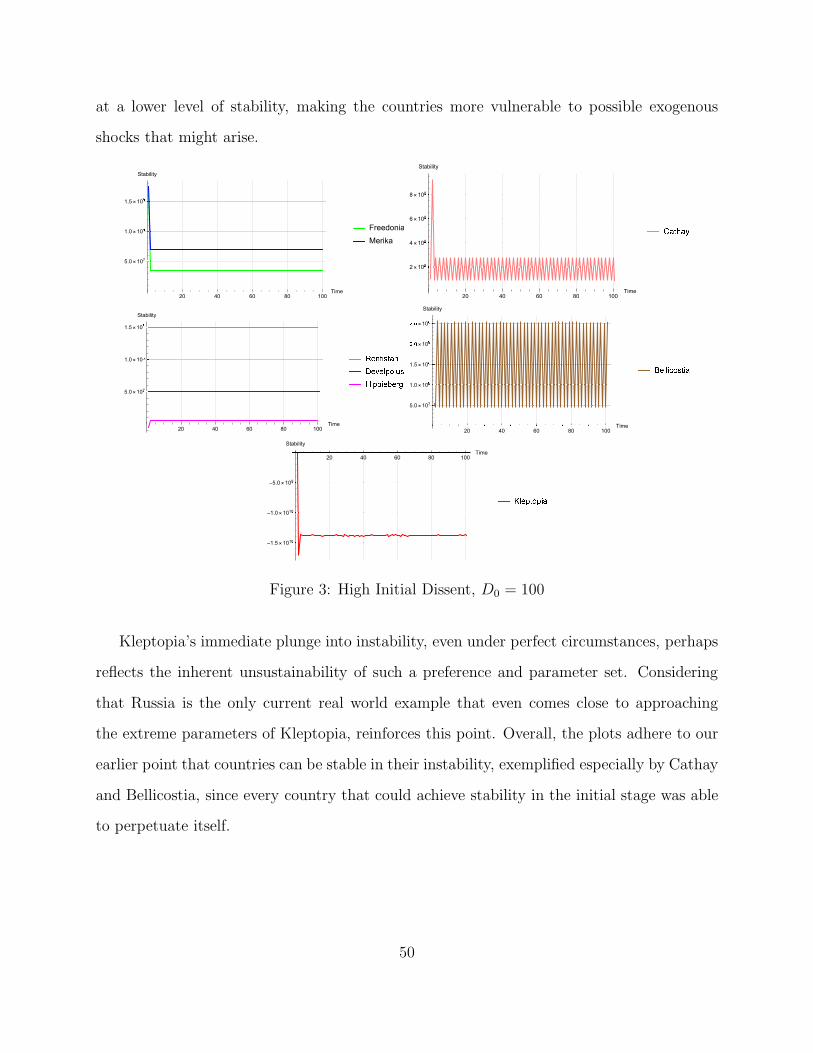
at a lower level of stability, making the countries more vulnerable to possible exogenous

shocks that might arise.

20 40 60 80 100Time

5.0×107

1.0×10%

1.5×10%

Stability

Freedonia

Merika

20 40 60 80 100Time

2×108

4×108

6×108

8×108

Stability

&'()'*

20 40 60 80 100Time

5.0×107

1.0×10+

1.5×10+

Stability

,-./01/3.

4-5-69:6;1

<0990-=->?

20 40 60 80 100Time

5.0×107

1.0×10@

1.5×10@

AEF×10@

AEG×10@

Stability

IJLLMNOPQMS

20 40 60 80 100Time

-1.5×1010

-1.0×1010

-5.0×109

Stability

TUVWXYWZ[

Figure 3: High Initial Dissent, D0 = 100

Kleptopia’s immediate plunge into instability, even under perfect circumstances, perhaps

reflects the inherent unsustainability of such a preference and parameter set. Considering

that Russia is the only current real world example that even comes close to approaching

the extreme parameters of Kleptopia, reinforces this point. Overall, the plots adhere to our

earlier point that countries can be stable in their instability, exemplified especially by Cathay

and Bellicostia, since every country that could achieve stability in the initial stage was able

to perpetuate itself.

50

5.2 Shocks

Next we consider how robust various countries types are to various exogenous shocks.

All shocks are simulated under the same conditions with low initial dissent (D0 = 1), but

then at period 50 a shock occurs in one of the parameters listed below and the effects of the

shock are observed for the remainder of the run. The magnitude of the shocks are either a

25% increase or decrease in the parameter, whichever would negatively affect the stability

of a state.

• R: the government resources are severely cut. Examples include the president emp-

tying the treasury and fleeing to a non-extraditing country, currency devaluation, or

massive recession/depression. Whatever the reason, the state now has fewer resources

available to it.

• Ω,Φ: the government is hit with new levels of corruption/incompetence and more

resources must be spent on the anarchy parameters.

• E: the quality of life suddenly drops. Mass joblessness, public health crisis, environ-

mental degradation.

• σ: the government is less effective at catching people that dissent. Propagation of

social media eases coordination of protesters, the police strike, pressure from human

rights groups.

5.2.1 Resource Shocks

Figure 4 shows our countries reacting to a resource shock. Most of our countries show a

substantial drop in stability after the hit to resources. Freedonia, ‘Merika, and Hippieberg

each see substantial drops in stability levels, but Freedonia and ‘Merkia still maintain rela-

51

20 40 60 80 100Time

2×107

4×107

6×107

8×107

Stability

Freedonia

\]^_`ab

20 40 60 80 100Time

1×108

2×108

3×108

4×108

5×108

6×108

Stability

cdefdg

20 40 60 80 100Time

5.0×107

1.0×10h

1.5×10h

Stability

Rentistan

Develpolus

Hippieberg

20 40 60 80 100Time

1×108

2×108

3×108

4×108

5×108

6×108

7×108

Stability

Bellicostia

20 40 60 80 100Time

-ijk×1010

-1.5×1010

-1.0×1010

-5.0×109

Stability

Kleptopia

Figure 4: Resource Shock

tively high stability levels while Hippieberg sees its lowest level of stability. Bellicostia sees

a slight increase in the oscillation range of stability. Kleptopia shows the least amount of

change due to the shock, likely due to its high resources and authoritarian nature, though it

remains at a negative level of stability.

The most interesting case is Rentistan, which suffers a high relative drop in stability.

The fact that Rentistan seems the most vulnerable to a drop in resources makes sense given

that the legitimacy of such regimes is often predicated upon their ability to provide for

their citizens. When such a state is unable to provide the expected goods and services (or

intimidate its citizens sufficiently) its stability will likely deteriorate.

52

5.2.2 Φ and Ω Shocks

20 40 60 80 100Time

2×107

4×107

6×107

8×107

Stability

Freedonia

Merika

20 40 60 80 100Time

1×108

2×108

3×108

4×108

5×108

6×108

Stability

lmnomp

20 40 60 80 100Time

-6×109

-4×109

-2×109

Stability

Rentistan

Develpolus

Hippieberg

20 40 60 80 100Time

1×108

2×108

3×108

4×108

5×108

6×108

7×108

Stability

Bellicostia

20 40 60 80 100Time

-qrs×1010

-1.5×1010

-1.0×1010

-5.0×109

Stability

Kleptopia

Figure 5: Φ Shock

Figures 5 and 6 depicts shocks to the anarchy parameters, Φ and Ω, respectively. When

there is a shock to minimum necessary government services, Φ, there is a varied and counter-

intuitive results across countries. Most curious, countries that place a preference on govern-

ment services seem to suffer the least from the shock. Freedonia, ‘Merika, and Hippieberg

show almost no change from the shock. Cathay and Bellicostia maintain their extreme oscil-

lation, but after the shock each sees a decrease in the amplitude. Interestingly countries that

take a more balanced or forceful stance; Rentistan, Develpolus, and Kleptopia, see extreme

drops in stability.

A possible reason why we get this result is that countries which take a balanced approach

or favor suppression, provide a limited amount of government services to the public to

53

20 40 60 80 100Time

2×107

4×107

6×107

8×107

Stability

Freedonia

Merika

20 40 60 80 100Time

1×108

2×108

3×108

4×108

5×108

6×108

Stability

tuvwux

20 40 60 80 100Time

2×109

4×109

6×109

8×109Stability

Rentistan

Develpolus

20 40 60 80 100Time

1×108

2×108

3×108

4×108

5×108

6×108

7×108

Stability

Bellicostia

Hippieberg

20 40 60 80 100Time

-yz×1010

-1.5×1010

-1.0×1010

-5.0×109

Stability

Kleptopia

Figure 6: Ω Shock

begin with. Thus, if those limited services are further reduced, the effects of the shock

are more dramatic than they would be for others. Conversely, Freedonia, ‘Merika, and

Hippieberg have an extreme preference for government services. This high level of investment

in government services mutes the effect of the shock because they were already experiencing

diminish marginal effects on stability.

The effects of a shock to security fixed costs, Ω, has similar results as the shock to

government services but differs in several interesting way. As with the Φ shock, Freedonia,

‘Merika, and Hippieberg show no substantial variation. Their structures are able to absorb

the shock without much disruption to overall stability. Kleptopia is also able to weather the

shock without fluctuating. Cathay and Bellicostia here have the opposite reaction as in the

Φ shock, their amplitude increasing after the shock. The most interesting response is from

54

20 40 60 80 100Time

2×107

4×107

6×107

8×107

Stability

Freedonia

|~

20 40 60 80 100Time

1×108

2×108

3×108

4×108

5×108

6×108

Stability

20 40 60 80 100Time

5.0×107

1.0×10

1.5×10

Stability

Rentistan

Develpolus

Hippieberg

20 40 60 80 100Time

1×108

2×108

3×108

4×108

5×108

6×108

7×108

Stability

Bellicostia

20 40 60 80 100Time

-×1010

-1.5×1010

-1.0×1010

-5.0×109

Stability

Kleptopia

Figure 7: Environment Shock

Rentistan and Develpolus. The shock initially results in a massive spike in stability but then

falls backdown into an oscillating pattern like Cathay and Bellicostia.

5.2.3 Environment Shock

Figure 7 shows a shock to the citizen’s environment/quality of life, E. Freedonia, ‘Merika,

Rentisan, Develpolus, and Hippieberg show no visible change after the shock. Cathay and

Bellicostia see a minor increase in amplitude, but one that is smaller than in other shocks.

Kleptopia has the strongest reaction, seeing a substantial drop in its already negative sta-

bility. Of all the shocks, a change in the average citizen’s environment seems to have the

least dramatic effect. A possible reason why we see this minimal change with respect to an

55

20 40 60 80 100Time

2×107

4×107

6×107

8×107

Stability

Freedonia

Merika

20 40 60 80 100Time

1×108

2×108

3×108

4×108

5×108

6×108

Stability

20 40 60 80 100Time

5.0×107

1.0×10

1.5×10

Stability

Rentistan

Develpolus

Hippieberg

20 40 60 80 100Time

1×108

2×108

3×108

4×108

5×108

6×108

7×108

Stability

Bellicostia

20 40 60 80 100Time

-×1010

-1.5×1010

-1.0×1010

-5.0×109

Stability

Kleptopia

Figure 8: Enforcement Shock

environmental shock is that a change in average citizen environmental wellbeing does not

happen in isolation. Often it’s precipitated by some other shock throughout the country,

such as a resource shock, and the two compound one another.

Additionally, the minute results from the E shock may be revealing a limitation in our

model. Currently our citizens have no memory, and thus would not experience loss aversion

from the decreases in living conditions. So there is no way for us to account for the more

realistic public anger that would likely arise from a dramatic drop in quality of life.

56

5.2.4 Enforcement Shock

Figure 8 shows a shock to policing effectiveness, σ. Bucking the results from the other

simulations, here the most interesting result comes from Freedonia and ‘Merika. The initial

enforcement shock causes a spike in stability for Freedonia and ‘Merika but then drops

into a oscillating pattern that dampens back to pre-shock levels. Rentistan, Develpolus,

Hippieberg, and Kleptopia show no change from the enforcement shock. Whereas, Cathay

and Bellicostia see a substantial increase in the amplitude of their stability oscillations after

the shock.

While these simulations represent only a handful of all possible combinations, they are

still highly informative as to the parameter relationships governing a country’s political

stability. Overall, it seems that the most important factor affecting stability is government

resources. Throughout the simulations, countries with the most resources displayed the

most consistency in their political stability. However, how one allocates those resources is

the critical detail. Kleptoia, which has just as many resources as Freedonia and ‘Merika,

was never able to achieve a positive level of stability. It would seem that a country cannot

simply beat people into submission, they must provide some benefit to the populace as well.

Another interesting result is extreme oscillation of Cathay and Bellicostia. Each was

surprisingly robust to all the shocks, even though neither was able to reach a steady level of

stability. In fact, averaging across time, Cathay and Bellicostia were the most stable states.

However, the period to period change in stability, was also the greatest with the two. So in

a short-run perspective these two would seem very unstable, but if one expands to see the

whole picture we can see that they are stable in their instability. Situations like this might

be why there are many seemingly politically unstable countries in the world, but large scale

political revolutions are relatively rare.

57

6 Conclusion

Through this paper we believe we have formed a coherent theoretical narrative on how

the interactions of a government and its citizenry determine a country’s level of political sta-

bility. The importance of this work is that it establishes a framework for examining political

stability, one that bridges the gap between the top and bottom viewpoints. Advanced nu-

merical simulation have allowed us to overcome the limitations and restrictions an analytic

solution would impose, while still allowing significant insight to be gained on the factors

affecting political stability.

Our simulations show that a multitude of factors, at both the individual and the macro

levels, can influence a states political stability. While it seems that the resources of the state

is the most impactful in maintaining stability, merely being wealthy is not sufficient. How

a state allocates resources between government services and security is what really seems to

dictate overall stability, a preference for government services being the most stabilizing.

A shortcoming of this paper is that the model only applies to cases of internal strife

and does not take into account the role of outside influences. Additionally, this model

presents a relatively homogenous state, but could easily be expanded to a state where there

is factionalization or high inequality within the state. However, it must be stated that this

is a preliminary model with significant room for expansion in future research endeavors.

Generally findings suggests that there are sets of parameter values that form loose Nash

equilibria of stability, with some equilibria appearing to be more robust to shocks than others.

States, both rich and poor, with preferences for government services as a means to maintain

stability are the most consistently stable. States that rely more heavily on suppression

and security, conversely, are more unstable. Additionally we have shown that a state can be

stable in its instability, oscillating dramatically between periods but maintaining a consistent

pattern over time. This finding aligns with the notion that there are many supposedly

58

unstable countries, but large scale political upheavals remain relatively rare events.

59

7 References

Acemoglu, D. and J. A. Robinson (2001). A Theory of Political Transitions. AmericanEconomic Review 91 (4), 938-963.

Acemoglu, D., J. A. Robinson, and D. Woren (2012). Why nations fail: the origins of power,prosperity and poverty, Volume 4. SciELO Chile.

Aisen, A. and F. J. Veiga (2013). How does political instability affect economic growth?European Journal of Political Economy 29, 151-167.

Alesina, A. and R. Perotti (1996). Income distribution, political instability, and investment.European economic review 40 (6), 1203-1228.

Allen, W. (1972). Without feathers. Random House.

Apolte, T. (2012a). Toward a more general approach to political stability in comparativepolitical systems. Technical report, Diskussionspapier, Centrum fur InterdisziplinareWirtschaftsforschung.

Apolte, T. (2012b). Why is there no revolution in north korea? the political economy ofrevolutions revisited. Public Choice 150, 17.

Blais, A. and S. Dion (1990). Are bureaucrats budget maximizers? the niskanen model itscritics. Polity 22 (4), 655-674.

Buchanan, J. M. and G. Tullock (1962). The calculus of consent, Volume 3. University ofMichigan Press Ann Arbor.

Bueno de Mesquita, B. and A. Smith (2011). The Dictators Handbook: Why Bad Behavioris Almost Always Good Politics. Public Affairs.

Congleton, R. D. (2003). The median voter model. The encyclopedia of public choice,707-712.

Cummings, R. G., J.Martinez-Vazquez, M. McKee, and B. Torgler (2009). Tax morale affectstax compliance: Evidence from surveys and an artefactual field experiment. Journal ofEconomic Behavior Organization 70 (3), 447-457.

De Mesquita, E. B. (2010). Regime change and revolutionary entrepreneurs. AmericanPolitical Science Review 104 (03), 446-466.

Djanali, I. and D. Sheehan-Connor (2012). Tax affinity hypothesis: Do we really hate payingtaxes? Journal of Economic Psychology 33 (4), 758-775.

Fox, J. O. (2001). If Americans really understand the income tax.

Fukuyama, F. (2014). Political order and political decay: From the industrial revolution to

60

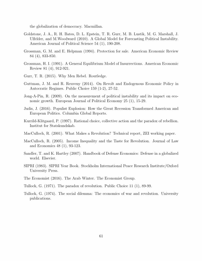
the globalization of democracy. Macmillan.

Goldstone, J. A., R. H. Bates, D. L. Epstein, T. R. Gurr, M. B. Lustik, M. G. Marshall, J.Ulfelder, and M.Woodward (2010). A Global Model for Forecasting Political Instability.American Journal of Political Science 54 (1), 190-208.

Grossman, G. M. and E. Helpman (1994). Protection for sale. American Economic Review84 (4), 833-850.

Grossman, H. I. (1991). A General Equilibrium Model of Insurrections. American EconomicReview 81 (4), 912-921.

Gurr, T. R. (2015). Why Men Rebel. Routledge.

Guttman, J. M. and R. Reuveny (2014). On Revolt and Endogenous Economic Policy inAutocratic Regimes. Public Choice 159 (1-2), 27-52.

Jong-A-Pin, R. (2009). On the measurement of political instability and its impact on eco-nomic growth. European Journal of Political Economy 25 (1), 15-29.

Judis, J. (2016). Populist Explosion: How the Great Recession Transformed American andEuropean Politics. Columbia Global Reports.

Kurrild-Klitgaard, P. (1997). Rational choice, collective action and the paradox of rebellion.Institut for Statskundskab.

MacCulloch, R. (2001). What Makes a Revolution? Technical report, ZEI working paper.

MacCulloch, R. (2005). Income Inequality and the Taste for Revolution. Journal of Lawand Economics 48 (1), 93-123.

Sandler, T. and K. Hartley (2007). Handbook of Defense Economics: Defense in a globalizedworld. Elsevier.

SIPRI (1983). SIPRI Year Book. Stockholm International Peace Research Institute/OxfordUniversity Press.

The Economist (2016). The Arab Winter. The Economist Group.

Tullock, G. (1971). The paradox of revolution. Public Choice 11 (1), 89-99.

Tullock, G. (1974). The social dilemma: The economics of war and revolution. Universitypublications.

61

CHAPTER THREE

LET THEM TWEET CAKE: ESTIMATING PUBLIC DISSENT AND POLITICAL

STABILITY USING TWITTER

1 Introduction

The importance of political stability is well established and can affect all aspects of an

economy (Kaufmann et al. 1999b) and substantially impede economic growth (Alesina and

Perotti, 1996; Jong-A-Pin, 2009; Aisen and Veiga, 2013). Additionally, there is a propen-

sity for a country’s political stability issues to leak beyond its borders, negatively affecting

neighboring nations’ stability and creating large scale welfare implications. However, despite

its significance, measurement of political stability has remained underdeveloped.

As demonstrated by the recent uprisings in the Middle East, Thailand, and Ukraine; large

scale political changes are difficult to predict. The three commonly used measures of political

stability are Political Risk Services (PRS), the Business Environment Risk Intelligence Index

(BERI), and the Economist Intelligence Unit (EIU). Each of these indexes combine political,

financial, and economic factors to assess a nation’s political stability (Howell, 1998). The

financial and economic portions are predominately based on quantitative data (foreign debt,

inflation, GDP per capita, etc) while political factors are more qualitative.

Political factors for each index are determined and scored by panels of experts (Howell,

1998). These experts are usually former diplomats, scholars, and other suitably qualified

individuals. While these teams of experts can be quite large and knowledgeable, it is still a

relatively small group of people trying to assess an entire nation. Additionally these experts

lack a clear theoretical foundation for their decisions.

Since political factors compose 33-66% of each index (Howell, 1998), if these experts

62

are somehow misinformed the validity of the index could be greatly affected. In turn this

potential bias would affect all research based on these indexes. Additionally, over a twenty

year study Tetlock (2005) was able to show that political forecasts based on expert opinion

were only marginally better than random chance. It becomes quite apparent that a new

method of assessing political stability is needed.

To highlight the issue of why a more robust measure of political stability is needed let

us examine some contemporary examples and their related political stability analysis. The

October 2005 PRS report on Thailand said “unrest is not expected to threaten general sta-

bility, nor intensify to the point of endangering the [Thai Rak Thai Party’s (TRT)] dominant

political position...the chances of the TRT being forced from power at any point during the

five year forecast period are slim...” (PRS 2006, p. 40). Less than a year later a military

coup ousted the Prime Minister Shinawatra and outlawed his TRT party, and began a period

of political strife that continues to plague Thailand. The PRS report on Ukraine published

October 2012, stated that “a repeat of the Orange Revolution...is unlikely.” and “Ukrainians

are disillusioned but in general they possess little appetite for protest.” (PRS 2013, p. 11).

Mass protests began in November 2013 and by February 2014 the Yanukovych regime had

fallen. The PRS report on Tunisia, published October 2010, called Tunisia an “oasis of

stability” (PRS 2011, p. 3) and postulated a 85% probability that Tunisian dictator Ben

Ali would retain power for the next 18 months. By January 2011, mass protests and revolt

resulted in the dissolution of the ruling RCD party, the exile of Ben Ali to Saudi Arabia, and

the establishment of an interim government. While it may be easy to critique these forecasts

with the benefit of hindsight, these examples highlight the inherent difficulty in predicting

something as opaque and complex as political stability.1

A shared limitation of previous political stability measurements was a lack of both a

1It should be noted that PRS publishes monthly reports on its surveyed countries but those are onlyavailable to its subscribers.

63

theoretical framework and quality data. Thankfully, advancements in both areas have arisen

that substantially mitigate these issues. Spangler and Smith (2017) establish a theoretical

framework for understanding political stability. They base their theory on the dynamic

interactions of a government and its citizens. Regarding data, the spread of social media

platforms such as Twitter and development of text analysis techniques means that researchers

can tap into the zeitgeist of a population.

In this paper we use online public dissent against a government as a basis for examining

a country’s political stability. Whereas previous measures of political stability relied on

expert opinion, polling, or other traditional methodology; this paper develops a measure

of political stability based on data collected from Twitter. The following sections of this

paper will review literature concerning measuring political stability and other relevant topics,

theoretical model, explanation of the methodology employed in this paper, proof of concept

case studies using Canada and Kenya, and finally conclusion.


We have already discussed the predominant methods for measuring political stability

(Howell 1998) and their potential flaws, but there are other methods that need to be ad-

dressed. Kaufmann et al. (1999a) proposes using ‘aggregate governance indicators’ which

combines hundreds of different variables and indicators (including those built by PRS, BERI,

and EUI) together to evaluate several factors of governmental quality to get the most out

of available data. Jong-A-Pin (2009) uses a similar multi-dimensional approach to evaluate

the economic impact of political stability. This approach does work to smooth out some of

the issues of a single indicator but ultimately Kaufmann et al. concludes that contempo-

rary methods “point to the inadequacy of existing governance measures.” (Kaufmann et al.,

64

1999a p. 31). Other methods of evaluating government effectiveness rely on crowd sourcing,

polling, and surveying; but all have their own limitations.

Ungar et al. (2012) relies on expert opinion, but instead of just a few experts Ungar et al.

employ thousands, using a mixture of crowd sourcing and simplification of complex issues.

Ungar et al.’s approach works by having their army (over 2000 individuals) of forecasters

assign probability estimates to specific events happening within a given time (Q:“Will Julius

Caesar cease power before March 15th?”, A: Yes, 42% probability.), updating their predictions

as needed before the deadline. Finally, all predictions are combined to form a single aggregate

forecast of the event.

Ungar et al.’s method, and prediction markets in general, are extremely effective in

harnessing the wisdom of crowds, but at the same time they are hamstrung by the simpli-

fications needed in order to harness that wisdom. They work best when asking the crowd

simple questions, which may not capture all the nuances and complexities necessary to un-

derstand an issue, especially when attempting to gauge a country’s overall political stability.

Additionally, in dealing with esoteric issues, there might only be a few experts with area

knowledge, which leaves this method vulnerable to the same problems as described earlier

(Tetlock, 2005). Finally, maintaining and incentivizing a vast number of forecasters is likely

very costly and time intensive, as one must wait for forecasters to make and adjust their

judgements.

Polling and surveying provide flexible formats for assessment. Paired with demographic

information, they can also be quite focused. Unfortunately effective polling and surveying is

costly and time consuming. There are also unique issue that are difficult for researchers to

overcome. The biggest hurdle is one of honesty since respondents often have little incentive to

be honest, to varying degrees of malevolence. For instance, poles and surveys are susceptible

to the ‘social desirability bias’, wherein respondents have a tendency to provide what they

65

perceive to be the socially acceptable answer to questions (Setphens-Davidowitz, 2017). This

especially could be a problem if someone is being asked about popular government entities

or policies they are in the opposition to.

The issue is further intensified by the fact that many places where accurate measurement

of political stability is most needed, might also be places where honest public speech is not

safe. According to Freedom House (2017), of the 195 countries evaluated, only 44% were

regarded as ‘free’ in regards to political rights. This means that in most countries a person

might be unwilling to provide their honest thoughts to a stranger asking about their govern-

ment. On the other extreme, respondents may provide strategic answers with the intent of

influencing potential policy that may be based on poll results, biasing results (Morgan and

Stocken, 2008). Finally, results could be biased because respondents provide false informa-

tion purely for their own trollish amusement (Setphens-Davidowitz, 2017). Fortunately, the

rise of the internet and associated social media platforms has provided a wealth of new data

that helps overcome the problems of previous methods.

2.1 Twitter Literature

One social media platform that has proven to be especially useful to researchers is Twitter.

Twitter is a micro-blogging website that allows users to post short messages (tweets) that

can be viewed and shared by other users. These posts can also include tags that allow users

to link posts with a common theme. All of this creates a vast network of information that can

be freely and publicly observed. With a current active monthly user base of over 300 million

people (Twitter, 2016) spread across the world, all sharing their opinions and thoughts on a

myriad of topics, there is vast potential for this data source.

Twitter data has already shown to be useful in several areas, often performing better

than traditional data sources. Asur and Huberman (2010) were able to use Twitter chatter

66

to predict film box office returns better than the industry standard. Bollen et al. (2011)

show that Twitter data can be used to forecast stock market fluctuations. Smith and Wooten

(2013) shows that people use Twitter as a source of information and were able to estimate

demand for this information. In terms of politics, O’Conner et al. (2010) and Lampos et

al. (2013) use Twitter as a more accurate source for political forecasting than traditional

polling.

There is also interesting research concerning issues of political stability using Twitter

data. Carly et al. (2013) find that Twitter chatter increases as large scale political events

unfold. Carly et al.’s findings demonstrate that there is a very real connection between real

world and online behavior; people are tweeting in response to things that are happening

in life. This point is further reinforced by research suggesting that Twitter can be used

in protest recruitment (Gonzalez-Bailon et al. 2011) and predicting protest participation

(Kallus, 2014). This line of research has been deemed so promising that the US Department

of Defense has funded several ongoing projects in this area (Minerva Initiative, 2014).

This paper adds to the work on political stability by building an empirical measure of

political stability. The core of this measure is based on Twitter data but also supported by

macroeconomic data. By examining Twitter data directly, we mitigate many of the issues

of other measures of political stability that rely heavily on expert opinion, polls, or surveys.

Also, by combining our measure with macroeconomic data, we can get a much broader

picture of a country’s political stability than previous street level Twitter studies and allow

for cross country analysis using the same methodology. Overall we argue that this approach

could greatly aid in assessing which countries are at risk of governmental failure, before

reaching headlines.

67

3 Theory

The central premise of this paper is that people use online platforms, specifically Twitter,

to kvetch about politics and express dissent against their government. Previous methods

of evaluating governmental quality generally have tried to find some quantifiable way to

evaluate government institutions. Instead, we are interested in the public’s perceptions of

these institutions. A well functioning government should be like air, if it’s working well,

no one will talk about it. The idea is that the more dysfunctional a government and its

institutions are, the more demand there will be for dissent against the government.

The theoretical foundation for demand for dissent is from Spangler and Smith (2017). In

this model a non-altruistic government and its citizens dynamically interact. The government

maximizes its own stability, Λt, by choosing its level of public services, Gt, and security, St,

allotments subject to a resource constraint, Rt, and total dissent from the citizenry in the

previous period, Dt−1. For stability purpose Gt is the carrot and St the stick. Equation (1)

shows the general form, but for estimation purposes the functional form shown in Equation

(2) is used.

Government’s problem general form:

maxGt,St

T ∗

∑

t=1

βtΛt =T ∗

∑

t=1

βt (Gt, α, St, γ,Dt−1, Rt,Φ,Ω) (1)

Government’s problem functional form:

maxGt,St

T ∗

∑

t=1

βtΛt =

T ∗

∑

t=1

βt

(Gt

Dt−1

− Φ

)α(St

Dt−1

− Ω

)γ

s.t. Gt + St = Rt (2)

The government optimizes its stability across time to T ∗, the inevitable point of eventual

68

state failure, and discounted at rate . The government chooses its allocations of Gt and St

based on its preferences for each, α and γ respectively. A minimum amount of resources must

be allocated to Gt and St to operate at minimum capacity and avoid anarchy, denoted by Φ

and Ω. An issue with Φ and Ω is that, while theoretically relevant, data limitations prevent

coherent estimation. So Φ and Ω are not included in empirics. For practical estimation Gt

and St can be represented by yearly government civil and military expenditures.

The source of instability is the bureaucratic lag between periods, since the government

responds to the total dissent from the previous period Dt1 while citizens react to the current

period. When, Dt ≈ Dt−1, there is minimal instability. However, when Dt 6≈ Dt−1 the

government misallocates its resources and the situation can spiral out of control, possibly

resulting in governmental failure.

Individual’s Problem:

maxdi,t

Ui,t = (di,t, xi, gt, Ei,t, Pt, A) (3)

In response to the government, the members of the public maximizes their utility by

choosing their level of dissent, di,t, based on their own preferences and the risk of punishment.

Equation (3) shows the general form of an individual’s utility from dissent, Ui,t. An important

component of this function is an individual’s activism preference, xi, which is assumed to be

distributed LogN(0, 1) across the population. For some values of xi an individual will would

receive disutility from dissent, so they will elect not to, di,t = 0. Whereas higher values of

xi means that the individual receives utility from dissenting, di,t > 0. This heterogeneity

amongst the population means that each period for given policy choices (Gt,St) there is a

spread of people that do not dissent and variation in the level of dissent among those that

do.

69

Maximization of individual utility w.r.t. to di,t yields d∗

i,t, individual demand for dissent.

d∗i,t = (xi, gt, Ei,t, Pt, A) (4)

The benefits and services the individual receives from the government is gt, with gt =Gt

Nt

andNt is total population, their quality of life, Ei,t, the probability of being caught dissenting,

Pt, and the severity of punishment for dissenting, A. Pt is a function of individual dissent

from the previous period, dt−1, the ratio of previous total dissent to security allocations,

Dt−1

St, and policing effectiveness, σ.

Individual’s demand for dissent is a reflection of perceived governmental quality. Every

day, individuals face societal issues they themselves cannot overcome, but these issues nega-

tively affect their life. These are issues such as crime, corruption, and other societal problem

(usually with public goods characteristics) that are difficult for individuals to provide for

themselves and are usually provided by governments. However, for whatever reason the

government is unable to address the issues sufficiently for the individual. The simultaneous

frustration with governmental expectations and the inability to do anything, leads the indi-

vidual to do the only thing they can do, dissent. Dissenting provides a cathartic release for

the individual, making them feel slightly better.

From the individual, finding total dissent is just a matter of consolidating dissent across

the populations

Dt = f

(Nt∑

i=1

di,t

)

(5)

where Dt is a function of the combine dissent of the population. In this paper a linear

combination is used.

70

This theoretical model allows for better understanding of how shocks at the governmental

and individual level may affect a countrys overall level of political stability. Also, by vary-

ing the governmental and individual parameters, cross country comparisons can be done.

However, while many of these shocks are difficult to detect as they happen, we are able to

observe the increase in Twitter chatter that would likely accompany such a shock. Thus, by

examining how the public expresses anger online, we get a window into a country’s political

stability.

4 Methods

An issue in transitioning from the theoretical model to the empirical model, is how

does one acquire an estimate for Dt, total dissent. Most other variables and parameters

can be obtained through existing data or internal estimation. The spread of social media,

specifically Twitter, allows us to capture dissent. A central premise of this project is that

digital behavior is representative of real world behavior. This paper follows a similar method

as Smith and Wooten (2013) and Carly et al. (2013), but expanded to capture the more

open ended nature of political stability.

Our process began by first forming a list of words expected to be consistent with the

language one would use to express dissent against the government. The list included words

and phrases such as: ‘police’, ‘rule of law’, ‘corruption’, ‘molotov’, as well as the names

of important political figures and institutions in our sample countries, Canada and Kenya.

We then collect any tweet containing at least one of our words. Technical limitations bar

collection of more than 1% of all incoming Twitter traffic, constraining the amount of target

words we would be able to collect.

While by no means exhaustive, the goal was to collect as many tweets as possible that

71

might express dissent against the government. The authors of this paper do not claim to

be experts on either Canada or Kenya, but extensive research and care was taken to ensure

that the collection list reflected the contemporary political landscape of each country. Initial

data collection of tweets containing words from our list began June 13, 2016 and ran to

September 11, 2016.

The next step is to run our collected tweets through regular expressions, which allows us

to go beyond a simple word count but instead account for the context of the tweet. Con-

trolling for context using regular expressions is important for several reasons. First, location

information is only known if the user voluntarily provides it on their Twitter profile, which

relatively few do. Explicitly coding regular expressions to focus on Canadian or Kenyan

issues ensures that we analyze the right tweets. Even if these are tweets are coming from

people outside the country, they are still discussing things unique to our sample countries.

They could be reporters, scholars, tourists, or expatriates; and more than likely they are

discussing something relevant.

Second, some words have different cultural meanings that might create bias if only a

simple word count was employed. For example, one of our code words is ‘anarchy’ and in

Kenya it is used in the very traditional style of discussing issues involving lack of government

and lawlessness. However, in Canada the vast majority of tweets containing ‘anarchy’ were

discussing the TV show Sons of Anarchy. Though this is quite the endorsement of that TV

program, it is not relevant to our purposes.

The potential for misidentification is why single word counts were used sparingly in this

paper. Single word counts were only used when collecting tweets in languages other than

English (Swahili and French) or with very specific terms used only in a negative context (e.g.

‘nairobbery’). The issue of translation should be minimal since in both Canada (Poblete et

al., 2011) and Kenya (The Economist, 2014) the predominant language of choice on Twitter

72

is English.

A potential criticism of this analysis is that even with our regular expressions we are not

able to fully control and quantify the tone of a tweet. For example, how do we deal with

sarcasm. To answer this potential criticism, we feel that any tweet containing a political

message, even one clearly satirical in nature, does not happen in a vacuum. The tweet

authors have encountered something in their life that causes them to respond. The fact that

they’ve responded sarcastically is just a choice of phrasing and is inconsequential for our

purposes. It only matters that they posted the tweet. The same logic can also be applied to

people tweeting in defense of their government and institutions. Again, this is not happening

in a vacuum; these people are reacting to something and we are capturing that in their tweet.

4.1 Scoring Tweets

Each regular expression is scored on a scale of 1 to 5, with 1 being low dissent and 5

being high dissent. A single Tweet can be scored multiple times depending on its contents.

The more expressive a tweet, the more an individual is dissenting. Take this example tweet

admonishing some unspecified political leader:

A regular expression meant to capture the sentiment of this tweet would look like:

([.?!]⋆)(\b(Leader)\b)([.?!]⋆)(corrupt)

This regular expression would capture any tweet that mentions the Leader and ‘corrupt’ in

73

the same tweet. Since this is a fairly standard political critique, it would be scored as 2. The

regular expression could also be expanded to included words that might convey a similar

sentiment.

([.?!]∗)(\b(Leader)\b)([.?!]∗)((corrupt)|(crook(ed)?)|(criminal)) -Score 2

This tweet also contains other inflammatory statements we would want to capture and score

with the following regular expressions:

([.?!]∗)(\b(Leader)\b)([.?!]∗)(tyrant) -Score 2

([.?!]∗)(\b(Leader)\b)([.?!]∗)((idiot(ic)?)|(stupid(ity)?)|(incompetent)) -Score 1

([.?!]∗)(\b(Leader)\b)([.?!]∗)(impeach(ed)?) -Score 4

Based on how we’ve scored the regular expressions, the final score of this tweet would be

9. the final score represents an individual’s estimated di,t. In this example, di,t = 9. This

tweet is used as an example of a single tweet containing multiple points of interest, but this

is likely to be the minority of cases. Twitter has a 140 character limit, so in all likelihood

most tweets will only contain a single regular expression.

Individual scores are aggregated weekly across the Twitter population, NTwitter, to form

estimates of total dissent in a country, Dt.

Dt =

NTwitter∑

i=1

di,t (6)

The end result is a estimate of public dissent that lets us know what people are angry about

and to what degree.

74

While previous work used various measures and proxies to assess government institutional

quality, many of those measures have the same subjectivity problem as the political stability

measures discussed earlier or can only be used ex-post. By focusing on dissent and weighting

it by quantitative macroeconomic data we can get a more accurate view of institutional

quality by looking at how frustrated people are with these institutions.

It should be noted that each individual regular expression score is ordinal in nature

(i.e.1st, 2nd, 3rd). Calling for a political leader to be impeached expresses more dissent than

merely calling them an idiot. There is a somewhat clear hierarchy but no fixed distance.

However, by combining the scores of a tweet to get di,t, the data is reshaped to cardinal

in nature (i.e. 1,2,3). This is an admitted weakness, but a necessary one. As a robustness

check, the regular expressions scores will be monotonically transformed to ensure that results

are consistent and not merely the product of weighting.

4.2 Case Studies: Canada and Kenya

Two sample countries were selected as case studies to provide proof of concept: Canada

and Kenya. Each country was selected for their similarities and differences. First, En-

glish is the major language of politics, education, government, and most importantly the

internet in both countries. Having a shared language significantly reduces the potential for

misidentification translation would entail. Second, there are different a priori expectations

of eachs political stability. Canada is a developed country that often ranks amongst the

top of nations in terms of development, citizen happiness, and governmental transparency.

Conversely, Kenya is a developing country with a history of political instability, corruption,

and ethnic tension. Most notably, there was substantial post election violence in 2007 after

the election of Mwai Kibaki as president. This unrest resulted in the deaths of 1,200 people

and displaced hundreds of thousands (Blair, 2016). A measure of political stability should

75

be robust enough to account for the substantial differences between the two.

Figure 1: Tweet distribution and densities in Canada and Kenya

Finally and most importantly, the populations of each country are prolific users of Twit-

ter. In Canada there are over 7 million monthly active users on Twitter (Statista, 2017). In

Kenya, there are an estimated 700 thousand monthly active users (Kemibaro, 2014). This

means that Twitter provides an easy way of surveying the political moods of large sections

of the Canadian and Kenyan populations. Figure 1 shows the distribution and concentration

of the analyzed tweets, which follow the major population centers of each country.

5 Data and Estimation

Summary statistics from the regular expression analysis are presented in Table 1. These

are tweets that are explicitly about political issues of Canada or Kenya. During the period of

analysis we observed 73,511 unique tweets from Canada and 37,603 from Kenya. As expected

most tweets contained only a single regular expression.

In nominal terms, there were more Canadian tweets expressing dissent than Kenyan.

This result is likely because Canada has monthly active user population roughly ten times

76

Canada Kenya

N 73,511 37,603

Mean di,t 1.48 4.74

Std. dev. di,t 0.86 0.76

Mode di,t 1 5

Max di,t 12 10

Mean Dt 12,123.78 19,816.89

Std. dev. Dt 10,494.53 30,713.60

Table 11: Twitter Data Summary Statistics

greater than Kenya. However, the interesting result is that even though there were more

Canadian tweets, on average each individual Canadian tweet expressed less dissent than in

Kenya. Average individual dissent in Canada was 1.48 compared to 4.74 in Kenya.

Figure 2 shows the summed weekly estimated dissent levels for low(1-2), medium(3-

5), and high(6+) dissent tweets and Figure 3 shows the combined total Dt for each country.

Figures 2 and 3 show that even though there were less tweets from Kenya, on average there is

a higher level of dissent in Kenya than Canada. Table 2 shows results from a Mann-Whitney

U test and a Kolmogorov-Smirnov test that further indicate the presence of fundamental

differences in dissent levels between the two countries. Given Kenya’s previously stated

issues with respect to corruption and political violence this makes sense.

0

5000

10000

15000

000

000

Canada

Low

Medium

High

Jul Aug Sep

0

20000

40000

60000

80000

100000

Kenya

Low

Medium

High

Figure 2: Weekly Dissent levels in Canada and Kenya

Note that these results only accounts for those that expressed some form of dissent

online (di,t > 0. Recall that Canada has 7 million active users on Twitter and Kenya 700

77

Jul Aug Sep

0

20000

40000

60000

80000

100000

Total Dissent

Canada

Kenya

Figure 3: Weekly Total Dissent levels in Canada and Kenya

Mann-Whitney U TestU=2494300000***

Kolmogoro-Smirnov TestD=0.788***

***= significant at 1%

Table 12: Statistical Tests

thousand. We did not detect dissent from most users in each country (di,t = 0). Roughly

1% of Canadian Twitter users expressed some level of dissent during this period, while 5%

of Kenyan Twitter users did. The take away is that relative to their user populations, more

Kenyans expressed dissent and at higher levels than Canadians.

As a robustness check and to ensure that the results in Figure 3 are not a product of the

linear weighting of the regular expression scores, monotonic transformations were applied

to the regular expression scores. Figure 4 again shows total dissent in Canada and Kenya

but the results transformed through logarithmic, squared, and exponential functions. The

previous results hold in all three cases, there is consistently more dissent in Kenya than

Canada.

Another interesting result of our analysis can be seen in Figures 2 and 3. Towards the

end of June, there is a massive spike in dissent for both countries. Examination of news

articles in each country during this period reveals no significant events that would explain

the spike. However, broadening the scope to the world level does uncover an explanatory

event: Brexit.

78

Jul Aug Sep

0

5000

10000

15000

20000

¡000

30000

Logarithmic

Canada

Kenya

Jul Aug Sep

0

100000

200000

300000

400000

500000

Squared

Canada

Kenya

Jul Aug Sep

0

500000

1.0×106

1.5×106

¢£¤×106

¢£¥×106

¦£¤×106Exponential

Canada

Kenya

Figure 4: Monotonic Transformations of Total Dissent

Jul Aug Sep

0

20

40

60

80

100

Searches

Canada

Kenya

Figure 5: Daily Internet Searches for ‘Brexit’ in Canada and Kenya

The UK referendum on whether or not to continue membership in the European Union,

colloquially known as ‘Brexit’, occurred on June 23, 2016. The slight skew towards the

beginning of July on the time line is a result of scaling the original time series from daily to

weekly. Search history for ‘Brexit’ from Google Trends (Figure 5) for each country, confirms

that citizens from each country were interested in the events of Brexit. Given that Canada

and Kenya were UK colonies and each maintains friendly relationships with the UK, it’s

logical that UK politics would be of interest to citizens of each. However, that relationship

alone does not explain why we see a spike in dissent in each after Brexit.

79

Canada Kenya

2016 Civil Expenditures(2010 US$)

368,837,027,606 6,823,643,525

2016 Military Expenditures(2010 US$)

18,068,962,843 732,694,153

α .414 .759γ .586 .241Source: World Bank

Table 13: Estimation Values

A possible explanation is that the events of Brexit may have encouraged people to discuss

their own country’s issues. Since people use Twitter as a news source (Smith and Wooten,

2013; Twitter, 2016), it is entirely plausible that they logged on to Twitter to see/discuss

what was going on with Brexit and then stayed to discuss political events relevant to their

own country. This reveals an unexpected sensitivity to outside large scale events this type

of analysis might have. However, as we know from the Arab Spring (The Economist, 2016),

events in one country can often inspire events in another. This is especially true when it

comes to issues of political stability.

5.1 Estimating Political Stability

Table 3 shows the 2016 values of government civil and military expenditures from each

country along with their estimated preferences for each. Using the functional form provided

by Equation (2), we can obtain a weighted weekly estimates of political stability.

Figure 6 shows our nominal estimates of political stability for Canada and Kenya. To

get estimates of political stability each country relative to one another, dissent estimates

are rescaled based on active monthly user population. Government expenditures are also

rescaled to control for population differences. The normalized scaled estimates of political

stability are shown in Figure 7.

80

Jul Aug Sep

0

5.0×106

1.0×107

1.5×107

§¨©×107

§¨ª×107

Stability

Canada

Kenya

Figure 6: Weekly Nominal Estimated Political Stability in Canada and Kenya

Jul Aug Sep

0

5.0×106

1.0×107

1.5×107

«¬×107

«¬®×107

Canada

Kenya

Figure 7: Weekly Scaled Estimated Political Stability in Canada and Kenya

Again, the results adhere to a priori expectations. Controlling for population differences

only magnifies the findings. Canada appears to be more politically stable than Kenya. This

means that Canada is likely more resilient to potential exogenous shocks (recession, terrorist

attacks, natural disaster, health crisis, etc) than Kenya would be to the same shock. Canada’s

developed economy, efficient government, and strong civil society likely factor heavily in this

result. While showing that Canada is more politically stable than Kenya may seem like an

obvious result, it is nonetheless important. The disparity between the estimates of the two

signifies that this is a valid method of cross country analysis.

6 Conclusion

This paper has presented a new method of estimating public dissent and political sta-

bility. By collecting tweets expressing dissent against the government and weighting with

81

government and military expenditures, we were able to obtain estimates of political stability

for Canada and Kenya. Our estimates show that Canada is likely more politically stable

than Kenya. Our results are in line with other methods, highlighting the verifiability of this

process. While this paper used data from Twitter as its basis, the methodology could easily

be employed to other similarly structured social media platform one has access too.

Knowing what countries are potentially in crisis is important for several reasons. First,

being able to intervene before a country falls apart is far easier than trying to reassemble the

broken pieces. Second, these failed states often become havens for criminals, terrorists, and

other misanthropes. Third, instability in one country has a nasty habit of leaking beyond

its borders. The failed state of Somalia is an unfortunate testament to all three. As the

whole world becomes more integrated knowing where crisis may emerge becomes ever more

critical.

As important as this research is, it is not impervious to criticism. A primary issue with

this method of estimating political stability is that it is highly dependent upon the social

media population. The smaller the population using Twitter in a country, the less useful

this estimate will be. However, growing the user base, especially in developing countries, is

a strategic goal of Twitter Inc (Twitter, 2016). The steady rise in smart phone usage across

the world (Poushter, 2016) should aid Twitter’s market penetration.

Another issue is that some governments are manipulating social media for their own

benefit (King, 2016). This is a concern but one that is likely overstated. Only a few countries

in the world have both the desire and the means to negatively affect social media platforms.

Furthermore, a social media company’s entire business is predicated upon its ability to

maintain users. If consumers do not feel that they are getting an honest experience on a

platform, they will go elsewhere. Thus it becomes the goal of multibillion dollar firms to

counter the machinations of rogue states.

82

The final critique of using social media data is that we have selection bias because these

platforms tend to have a younger user base. This is certainly the case with Twitter users

in Canada (Insights West, 2016) and Kenya (Simon et al., 2014), where the average Twitter

user is in their twenties. However, Rothchild (2015) shows that a properly statistically

weighted non-representative sample can still be effective for poll forecasting. Additionally,

this potential bias may even be an asset that enhances our measure. The demographic group

most likely to use social media, the young, are also the most likely to advocate for large scale

political change. Thus by forming the basis of our measure on dissent on social media, we’re

actually able to account for the group most likely to take to the streets.

The goal of this paper is not to replacement for traditional means of measuring political

stability. Instead, it is meant as an enhancement that incorporates societal and technological

changes to mitigate potential biases. Knowing what expressions people use for expressing

dissent and how to properly judge the validity of those statements still requires an expert’s

knowledge and opinion. However, using this framework would help reduce the subjective

nature of interpreting political stability.

83

7 References

Aisen, A. and F. J. Veiga (2013). How does political instability affect economic growth?European Journal of Political Economy 29, 151-167.

Alesina, A. and R. Perotti (1996). Income distribution, political instability, and investment.European economic review 40 (6), 1203-1228.

Asur, S. and B. A. Huberman (2010). Predicting the future with social media. In Web Intel-ligence and Intelligent Agent Technology (WI-IAT), 2010 IEEE/WIC/ACM InternationalConference on, Volume 1, pp. 492-499.

Blair, E. (2016). Kenyan political unrest raises fears of new flare-up in 2017 vote. Reuters.

Bollen, J., H. Mao, and X. Zeng (2011). Twitter mood predicts the stock market. Journalof computational science 2 (1), 1-8.

Carley, K. M., J. Pfeffer, H. Liu, F. Morstatter, and R. Goolsby (2013). Near real timeassessment of social media using geo-temporal network analytics. In Advances in SocialNetworks Analysis and Mining (ASONAM), 2013 IEEE/ACM International Conference,pp. 517-524.

Freedom House (2017). Freedom in the World 2017. Rowman Littlefield.

Gonzalez-Bailon, S., J. Borge-Holthoefer, A. Rivero, and Y. Moreno (2011). The dynamicsof protest recruitment through an online network. Scientific reports 1.

Howell, L. D. (1998). The Handbook of Country and Political Risk Analysis. the PRSGroup.

Insights West (2016). 2016 canadian social media monitor. Technical report, Insights West.

Jong-A-Pin, R. (2009). On the measurement of political instability and its impact on eco-nomic growth. European Journal of Political Economy 25 (1), 1529.

Kallus, N. (2014). Predicting crowd behavior with big public data. In Proceedings of the23rd International Conference on World Wide Web, pp. 625630. ACM.

Kaufmann, D., A. Kraay, and P. Zoido-Lobaton (1999a). Aggregating governance indicators.World Bank Policy Research Working Paper 2195.

Kaufmann, D., A. Kraay, and P. Zoido-Lobaton (1999b). Governance matters. World BankPolicy Research Working Paper 2196.

King, G., J. Pan, and M. E. Roberts. How the chinese government fabricates social mediaposts for strategic distraction, not engaged argument. American Political Science Review2.

84

Lampos, V., D. Preotiuc-Pietro, and T. Cohn (2013). A user-centric model of voting inten-tion from social media. In ACL (1), pp. 9931003.

Minerva Initiative (2014). Minerva Research Summaries Resources Fall 2014. Technicalreport, US Department of Defense.

Morgan, J. and P. C. Stocken (2008). Information aggregation in polls. The AmericanEconomic Review 98 (3), 864896.

OConnor, B., R. Balasubramanyan, B. R. Routledge, and N. A. Smith (2010). From tweetsto polls: Linking text sentiment to public opinion time series. ICWSM 11 (122-129), 12.

Poblete, B., R. Garcia, M. Mendoza, and A. Jaimes (2011). Do all birds tweet the same?:characterizing twitter around the world. In Proceedings of the 20th ACM internationalconference on Information and knowledge management, pp. 10251030. ACM.

Poushter, J. (2016). Smartphone ownership and internet usage continues to climb in emerg-ing economies. Pew Research Center 22.

PRS Group. The 2006 Political Risk Yearbook: East Asia the Pacific, Volume 5.

PRS Group. The 2011 Political Risk Yearbook: Middle East North Africa, Volume 2.

PRS Group. The 2013 Political Risk Yearbook: East Europe, Volume 7.

Simon, T., A. Goldberg, L. Aharonson-Daniel, D. Leykin, and B. Adini (2014). Twitter inthe cross firethe use of social media in the westgate mall terror attack in Kenya. PloSone9 (8), e104136.

Smith, B. and J. Wooten (2013). Pundits: The confidence trick: Better confident than right?Significance 10 (4), 1518.

Spangler, E. and B. Smith (2017). A dynamic model of political stability and dissent.Working Paper.

Statista (2017). Number of twitter users in canada from 2012 to 2020 (in millions). Technicalreport, Statista.

Stephens-Davidowitz, S. (2013). Who will vote? Ask Google. Manuscript, https://goo.gl/hDbE9H.

Tetlock, P. (2005). Expert Political Judgment: How good is it? How can we know? PrincetonUniversity Press.

The Economist (2014). A million conversations now: Twitter in Kenya. The EconomistGroup.

The Economist (2016). The Arab Winter. The Economist Group.

Twitter (2016). Twitter annual report 2016. http://bit.ly/2yPxFDd.

85

Ungar, L., B. Mellors, V. Satop a a, J. Baron, P. Tetlock, J. Ramos, and S. Swift (2012).The good judgment project: A large scale test of different methods of combining expertpredictions. Technical report, AAAI Technical Report.

86

Documents

OUTSIDE IN: EXPLORATIONS IN THE POLITICAL ECONOMY OF …ses.wsu.edu/.../2019/11/Ethan-Spangler-Final-Dissertation-Dec.-2017.… · The Middle East, Central Asia, and South-East Asia