Orthorectification Using Rational Polynomials - · PDF filepage 2 Orthorectification Using Rational Polynomials Before Getting Started You can print or read this booklet from MicroImages’

page 1

Orthorectification Using Rational PolynomialsTutorial

OrthorectificationUsing

Rational Polynomials

with

TNTmips®

RPC

ORTHO

page 2

Orthorectification Using Rational Polynomials

Before Getting Started

You can print or read this booklet from MicroImages’ Web site. The Web siteis also your source for the newest Tutorial booklets on other topics. You candownload an installation guide, sample data, and the latest version of TNTmips.

http://www.microimages.com

You can orthorectify images that have a mathematical model of the image geom-etry in the form of a set of rational polynomial coefficients supplied by the imagevendor or computed in the Georeference process. This procedure also requires adigital elevation model. You can often improve the fit of a vendor’s rationalpolynomial model to a particular image by regeoreferencing the image using accu-rate 3D ground control points. This booklet introduces the concepts andprocedures involved in rational polynomial orthorectification in TNTmips, in-cluding the use of the rational polynomial model in georeferencing the image priorto rectification.

Prerequisite Skills This booklet assumes that you have completed the exercisesin the Getting Started and Introduction to the Display Interface tutorial book-lets. Those exercises introduce essential skills and basic techniques that are notcovered again here. You should also be familiar with the topics covered in theGeoreferencing and Rectifying Images tutorial booklets. Please consult thosebooklets for any review you need.

Sample Data The exercises in this booklet use sample data that is distributedwith the TNT products. If you do not have access to a TNT products DVD, youcan download the data from MicroImages’ web site. In particular, this bookletuses sample files in the RECTIFY directory.

More Documentation This booklet is intended only as an introduction toorthorectifying satellite images. Details of the process can be found in a varietyof tutorial booklets, color plates, and Quick Guides, which are all available fromMicroImages’ web site.

TNTmips® License Levels TNTmips (the Map and Image Processing System)comes in three versions: the professional version of TNTmips (TNTmips Pro), thelow-cost TNTmips Basic version, and the TNTmips Free version. All versionsrun exactly the same code from the TNT products DVD and have nearly the samefeatures. If you did not purchase the professional version (which requires asoftware license key) or TNTmips Basic, then TNTmips operates in TNTmipsFree mode. All the exercises can be completed in TNTmips Free using the samplegeodata provided.

Randall B. Smith, Ph.D., 24 February 2015©MicroImages, Inc., 2004-2015

page 3


STEPSstart TNTmipsselect Image / Resampleand Reproject /Automatic... from theTNTmips menu

Aerial and satellite images of land surfaces commonlycontain spatial distortions due to terrain relief andoff-vertical imaging geometry. Orthorectification isa procedure that removes these distortions, creat-ing an orthoimage with features positioned as theywould be in a planimetric map. Because anorthoimage has map-like geometry, map-derived the-matic data layers register more accurately with anorthoimage than with an unrectified image, and thespatial information you extract from an orthoimageis more accurate.

You can orthorectifyimages in the TNTmipsAutomatic Resamplingprocess using theRational Polynomialresampling model andan accurate elevationraster (DEM). Ortho-ready images from theQuickBird, WorldView,IKONOS, ALOS, andPleiades satellites,among others, aresupplied with auxiliaryfiles containing theorthorectification model in the form of rationalpolynomial coefficients (RPC). These images arealso acquired from a high viewing angle to minimizeterrain distortion.

You can also use the Georeference process tocompute a Rational Polynomial orthorectificationmodel for any aerial or satellite image for which youcan provide a set of accurate 3D control points. Seethe Technical Guide entitled Compute RationalPolynomial Model for Orthorectification for moreinformation.

Welcome to RPC Orthorectification

In the research literature theacronym RPC is derivedeither from “RationalPolynomial Coefficients” or“Rational Polynomial Cameramodel”. Other authors usethe term Rational FunctionModel (RFM) to refer to thesame mathematical model.

Planimetric street vector (orange, traced from aerialorthophoto) overlaid on panchromatic IKONOS satelliteimage (1-meter cell size) of part of La Jolla, California.Left, georeferenced but unrectified image. Right, imageafter RPC orthorectification, resulting in excellent matchwith street vector. Area has about 60 meters of relief.

page 4


In a conventional aerial photograph made with a fram-ing camera, each location in the image is captured atthe same time from a single camera position. Be-cause of this simple image geometry, the coordinatetransformation from two-dimensional image coordi-nates to three-dimensional Earth-surface coordinatescan be expressed mathematically using relativelysimple expressions.

Most remote sensing satellite images, on the otherhand, are built up of groups of scan lines acquiredas the satellite moves forward in its orbit. As a re-sult, different parts of the same image are acquiredfrom different sensor positions. In order to rigor-ously describe the transformation from imagecoordinates to Earth surface coordinates, a math-ematical sensor model that incorporates all of thephysical elements of the imaging system can be ex-ceedingly long and complex. For example, theIKONOS rigorous sensor model is 183 pages long!

Rational Polynomial satellite sensor models are sim-pler empirical mathematical models relating imagecoordinates (row and column position) to latitudeand longitude using the terrain surface elevation.The name Rational Polynomial derives from the factthat the model is expressed as the ratio of two cubicpolynomial expressions. Actually, a single imageinvolves two such rational polynomial expressions,one for computing row position and one for the col-umn position. The coefficients of these two rationalpolynomials are computed by the satellite companyfrom the satellite’s orbital position and orientationand the rigorous physical sensor model. Using thegeoreferenced satellite image, its rational polyno-mial coefficients, and a DEM to supply the elevationvalues, the TNTmips Automatic Resampling Processcomputes the proper geographic position for eachimage cell, producing an orthorectified image.

About Rational Polynomial Models

Orthorectified Image

Rational PolynomialCoefficients for Image

Image(Unrectified)

DEM Raster

+

+

Rational PolynomialOrthorectification

A cross-track scanningimager such as IKONOSbuilds up an image fromgroups of scan linesacquired from differentpositions in space (circles)as the satellite movesforward in orbit (arrow).

ground

space

page 5


Acquiring a Digital Elevation ModelThe digital elevation model you use to orthorectifyan image need not match the image area or cell size(the common area of the two is orthorectified). Toachieve the best results, however, the cell size ofthe DEM should be as close as possible to that ofthe image you are rectifying. DEMs with 30-meterresolution produced by the United States Geologi-cal Survey (USGS) are available for free downloadfor any area in the United States, and 10-meter USGSDEMs are available in most areas. For other coun-tries elevation data with similar resolution may beavailable for purchase from the relevant govern-ment agency. A global 90-m DEM produced fromNASA’s Shuttle Radar Topography Mission(SRTM V3) is also available for all of Earth’s landareas from MicroImages. An enhanced 30-m SRTMDEM is also available from the USGS EROS DataCenter for many areas.

If you cannot locate a DEM with sufficient spatialresolution for your image area, you may be able tocreate your own. Topographic contour data is avail-able for some areas in digital form, or it can beproduced from a scanned topographic map of thearea. The resulting vector contour data can besurface-fit in the TNTmips Surface Modeling pro-cess to create a DEM. (See the tutorial bookletentitled Surface Modeling for more information.)For example, MicroImages wished to rectifiy a 1-mpanchromatic IKONOS image of La Jolla, Califor-nia, but a 30-m DEM was the best resolutionavailable from the USGS. Instead we purchasedlow-cost vector contour data with 5-foot contourinterval from the County of San Diego. After edit-ing to remove contouring artifacts, we surface-fitthe contours to create a DEM with 1-meter cell sizeand elevation values in decimal meters (floating-point raster), a resolution more appropriate to ourimage data.

Portion of DEM with 1-metercell size created by surface-fitting vector contour lineswith a 5-foot contour interval(black lines).

Portion of a 30-m DEM(displayed with color palette)for the La Jolla, Californiaarea, the best resolutionavailable from the USGS.

page 6


Elevation Units and Reference Surfaces

The rational polynomial coefficients for a particular satellite image are computedusing data on the orbital position and orientation of the satellite sensor. Thesatellite position includes a height (elevation) component, but that raises thequestion, height above what? The physical surface of the Earth is irregular andits elevation is not known precisely everywhere, so it cannot be used as a referencesurface. Satellite heights instead are referenced to an ideal, mathematically-defined

geometric shape, an earth-centered ellipsoid, thatprovides a global best fit to the overall shape ofthe earth. This ellipsoid is most commonly theWorld Geodetic System (WGS) 1984 ellipsoid thatforms the basis for the WGS 1984 geodetic datum.Both remote sensing satellites (such as QuickBirdand IKONOS) and the constellation of GlobalPositioning System (GPS) satellites referenceelevations to this hypothetical ellipsoidal surface.Thus the elevation values built into the RPC modelfor an image are ellipsoidal elevations, as are theelevation values computed by GPS receivers fromthe GPS satellite information.

Edit Object Information window for aDEM in feet, with Cell Value Scale set torescale DEM values to meters.

Topographic contour maps and digital elevation models may express elevationvalues in a variety of units. For example, DEMs available for the United Statesmay have elevations in meters, decimeters, or feet, depending on the data sourceand the local relief. Before using a DEM for RPC orthorectification, check themetadata or other text information that accompanied the original data to verify theelevation units. The RPC orthorectification procedure requires elevations in meters.If your DEM uses other elevation units, don’t panic. The simplest remedy is to

open the TNTmips File Manager (Tools/ File Manager), navigate to the DEM ras-ter, and press the Edit icon button, whichopens the Edit Object Information win-dow. The Scale panel on this windowincludes a Cell Value Scale field in whichyou can enter the conversion factor torescale the raster cell values to meters(for example, 0.1 to rescale decimeters tometers and 0.3048 to convert feet tometers). Most TNTmips processes willthen automatically use the rescaled value.

The global best-fit ellipsoid isnearly spherical, with a polarradius that is shorter than theequatorial radius by a factorof 1 / 298.257.

page 7


0-50-100 +50

Since rational polynomial image models use ellipsoidal elevations, georeferenceand rectification procedures that use this model must convert orthometric DEMelevations to ellipsoidal heights by adding the local geoid height. Therefore,when you select a DEM in the Georeference or Automatic Resampling processes,you are prompted to enter a geoid height. (Because of the regional scale of geoidheight variations, a single geoid height value can suffice for an entire IKONOS orQuickBird scene.) You can find the appropriate geoid height for your image areaby entering the latitude and longitude of the image center in one of several freegeoid height calculators available on the World Wide Web:

http://earth-info.nga.mil/GandG/wgs84/gravitymod/egm96/intpt.html

http://sps.unavco.org/geoid/

http://www.ngs.noaa.gov/cgi-bin/GEOID_STUFF/geoid03_prompt1.prl

On the other hand, the elevation values in most DEMs give the height of theground surface relative to local mean sea level. This value is sometimes calledorthometric height. Mean sea level on a global scale is a broadly undulatingsurface called the geoid,whose shape has been determined from studies of theEarth’s gravity field supplemented by GPS survey data. The vertical separationbetween the geoid and el-lipsoid at any location iscalled the geoid height,which may be either posi-tive (geoid above ellipsoid)or negative (geoid belowellipsoid). Geoid heightsvary gradually on a re-gional to continental scalewithin the range -100 to+100 meters.

Obtaining the Geoid Height

meters

0

30 S

60 S

30 N

60 N

0 90 E 18090 W180

Global Geoid Height Relative to the WGS84 Ellipsoid

A Windows 9x/NT software program to compute geoid heights is also available(with supporting files) for free download at:

http://earth-info.nga.mil/GandG/wgs84/gravitymod/egm96/egm96.htm

EllipsoidGeoid Geoid height

(negative)

Geoid height(positive)

Geoid height in vertical section (exaggerated)

Land Surface

Land Surface

Orthometric heightOrthometric height

page 8


Run the RPC OrthorectificationOrthorectification using the Rational Polynomialmodel provided by an image vendor is carried out inthe Automatic Resampling process using the Ratio-nal Polynomial selection on the Model menu. Youcan set the model before or after selecting the rasterobject (or set of raster objects) you wish to rectify.When you complete the second of these two ac-tions, you are presented with a series of dialogsprompting you to select the elevation raster and toselect the text file containing the rational polynomialcoefficients. You must also provide a value for thelocal geoid height.

In this exercise you orthorectify a color image cre-ated from the red, green, and blue bands of a sampleIKONOS multispectral image covering part of LaJolla, California. The image has a cell size of 4 metersand covers about 4 square kilometers. Topographi-cally, the area is a plateau sloping southwest, cut bynarrow canyons, and has a local relief of 200 meters.The image and associated elevation model are shownon the next page.

You can use the Display process to overlay the originaland orthorectified images to see the geometricchanges produced by the rectification.

STEPSin the RasterResampling window,press [Select Rasters...]navigate into the LJMESA

Project File in the RECTIFY

sample data directoryand select IKONLJM4on the Settings tabbedpanel, set the Modelmenu to RationalPolynomial

when prompted toselect the RationalPolynomial model file,select RECTIFY /IKONLJM4_RPC.TXT

when prompted toselect the DEM raster,select DEM_4M from theLJMESA Project Fileset the Method menu toNearest Neighbor andthe Cell Size menu toManualset the Orient menu toProjective North and theExtents menu to EntireInputenter -35.0 in the Geoidheight fieldpress [Run]use the standard SelectObject window to selector create a destinationProject File and to namethe output raster object

page 9


Regeoreferencing the ImageThe image you rectified in the previous exercise has georeference informationobtained from the image provider. The satellite company determines thegeographic “footprint” of the image using data on the position of the imagingsatellite in its orbit, the direction the sensor was pointing, and an average elevationfor the scene. These parameters are used to compute map coordinates for thefour image corners. But small errors in the satellite parameters can translate intolarge errors in the image georeferencing. These errors can cause misregistrationwith the DEM you use for rectification, which in turn leads to errors in the positionand internal geometry of the orthorectified image you produce.

You can improve the orthorectification results for most images by regeoreferencingthe image (using the TNTmips Georeference process) with accurate, well-distrib-uted ground control points (GCPs). This will ensure that accurate geographicextents are computed for the image and that it registers correctly with the DEMduring orthorectification. (For best results, delete the corner control points pro-vided with the image.) The new control points should be distributed relativelyuniformly over the entire extent of the image, including the edges and corners.

A well-distributed set of ground control points for the IKONOS multispectral image of LaJolla Mesa (left) covers the image extents and also includes a range of elevations, asshown in the view of the DEM (right).

The georeference process can also use your control points to refine the rationalpolynomial orthorectification model provided with the image (see the followingpages). As few as 4 to 6 accurate, well-distributed points may significantly im-prove the fit of the model and thus improve the registration and internal geometryof the orthorectified image you produce with it. A larger number of control pointsmay improve the fit in some cases, in part by diluting or averaging out positionalerrors introduced by any less accurate control points. Placing additional controlpoints in topographically significant locations (such as hill tops and valley bot-toms) may further improve the fit of the RPC model.

page 10


STEPSchoose Main/Georeference from theTNTmips menuin the Georeferencewindow, pressthe Open iconbuttonuse the standard SelectObjects dialog to selectraster object IKONLJM4G

from the LJMESA ProjectFilechoose RationalPolynomial from theModel menuin the Select RationalPolynomial Model Filewindow that appears,choose RECTIFY /IKONLJM4_RPC.TXT

Georeference with RPC ModelThe version of the sample IKONOS image that youopen in this exercise has been provided with 8 con-trol points in a UTM coordinate system using theAffine model. To evaluate these and any addedpoints in the context of RPC orthorectification wechoose the Rational Polynomial option from theModel menu. You are then prompted to select theRPC text file to provide the rectification coefficients.

When you use the Rational Polynomial model inGeoreference, control point residuals are computedby first projecting all control point positions throughthe rational polynomial transformation to remove ter-rain displacements, so that the residuals indicatedepartures from the rectification model. The pro-cess also makes adjustments to the transformationbetween image and geographic coordinates to mini-mize these residuals. This adjustment requires anaccurate elevation value for each control point inaddition to its horizontal coordinates. You can enterelevation values manually in the Elevation columnin the control point list, or assign the elevation valuefrom the corresponding cell in the DEM as shown in

a later exercise.

Choose Options / Columnsto open a window that letsyou choose which columnsof data to show in thecontrol point list. Make surethat the Elevations column istoggled on.

The bottom part of the Georeference window shows summarystatistics for the current set of control points. The RMS (Root Mean Square) Residualand Mean Absolute Residual values provide measures of the fit of the entire set ofcontrol points to the adjusted rational polynomial model. These values are updatedimmediately with any change in the control points.

page 11


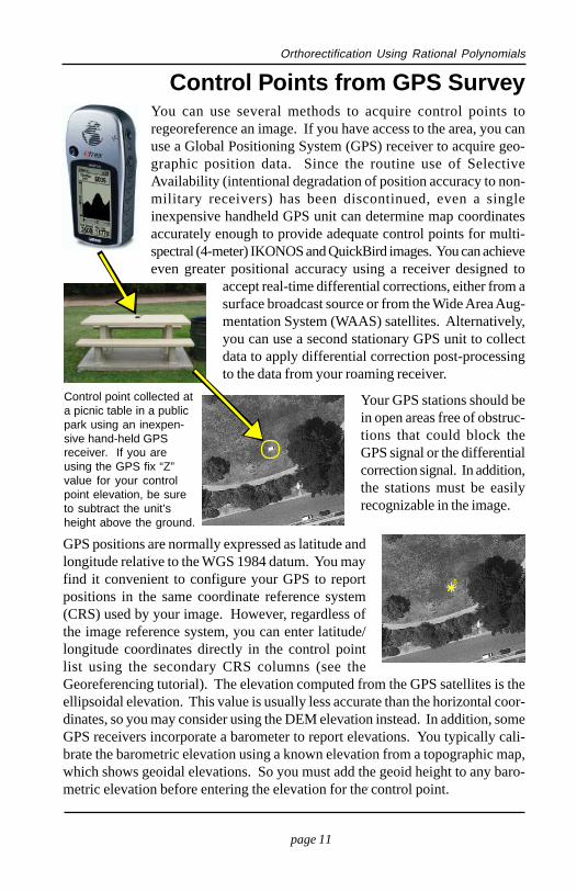
Control Points from GPS Survey

Control point collected ata picnic table in a publicpark using an inexpen-sive hand-held GPSreceiver. If you areusing the GPS fix “Z”value for your controlpoint elevation, be sureto subtract the unit’sheight above the ground.

You can use several methods to acquire control points toregeoreference an image. If you have access to the area, you canuse a Global Positioning System (GPS) receiver to acquire geo-graphic position data. Since the routine use of SelectiveAvailability (intentional degradation of position accuracy to non-military receivers) has been discontinued, even a singleinexpensive handheld GPS unit can determine map coordinatesaccurately enough to provide adequate control points for multi-spectral (4-meter) IKONOS and QuickBird images. You can achieveeven greater positional accuracy using a receiver designed to

accept real-time differential corrections, either from asurface broadcast source or from the Wide Area Aug-mentation System (WAAS) satellites. Alternatively,you can use a second stationary GPS unit to collectdata to apply differential correction post-processingto the data from your roaming receiver.

Your GPS stations should bein open areas free of obstruc-tions that could block theGPS signal or the differentialcorrection signal. In addition,the stations must be easilyrecognizable in the image.

GPS positions are normally expressed as latitude andlongitude relative to the WGS 1984 datum. You mayfind it convenient to configure your GPS to reportpositions in the same coordinate reference system(CRS) used by your image. However, regardless ofthe image reference system, you can enter latitude/longitude coordinates directly in the control pointlist using the secondary CRS columns (see theGeoreferencing tutorial). The elevation computed from the GPS satellites is theellipsoidal elevation. This value is usually less accurate than the horizontal coor-dinates, so you may consider using the DEM elevation instead. In addition, someGPS receivers incorporate a barometer to report elevations. You typically cali-brate the barometric elevation using a known elevation from a topographic map,which shows geoidal elevations. So you must add the geoid height to any baro-metric elevation before entering the elevation for the control point.

page 12


Control from Maps or OrthoimagesIf you cannot travel to the image area or don’thave access to a GPS, you can use a digitalversion of a topographic map, other planimet-ric map, or orthoimage of the area to providecontrol point locations. In the United Statesand some other developed countries,georeferenced bitmap (raster) images of topo-graphic maps at various scales are availablefrom government agencies. If only paper mapsare available to you, you can have themscanned and then georeference the resultingmap rasters. Digital orthoimages may be avail-able from federal, state/provincial, or localgovernment agencies.

When using a scanned map as a reference forgeoreferencing, you will need to find featuresthat are readily recognizable in both the mapand your image, such as road intersections andstream confluences. The accuracy of your con-trol point positions on the reference map is more dependent on the spatial accuracystandard of the original map than on the cell size of the scanned version. Areference orthoimage typically provides more mutually-recognizable features aswell as more detail and better spatial accuracy.

To use a reference object in theGeoreference process, choose Show 2DReference View from the Options menu.Then add the desired raster object to theReference View. See theGeoreferencing tutorial booklet for moreinformation.

A topographic map has the advantage of including elevation information in theform of contour lines. You can compute the elevation for a control point byinterpolating between adjacent contours. Remember that control point eleva-tions must be ellipsoidal elevations in meters; before assigning your interpolatedelevation to the point in the Georeference process, convert it to meters (if neces-sary) and add the local geoid height. If your DEM of the image area is sufficientlydetailed, you may want to assign control point elevations from the DEM instead.If you are using an orthoimage to georeference your image, you will need toacquire control point elevations from the DEM or other source.

page 13


Control Point Elevations from DEMSeveral tools in the Georeference process make iteasy to assign control point elevations from a DEM.If you add a DEM as a terrain layer in theGeoreference Input View, the process automaticallyturns on the Default Z from Surface icon button inthe Georeference window’s toolbar (see illustrationbelow). This button sets a program mode in whicheach new control point you add is automaticallysupplied with an elevation value from the DEM cellcorresponding to that location. (You can also turnthis mode on and off manually, of course.)

In addition, when you select one or more existingcontrol points in the list, the Set Z from Surface iconbutton becomes active. Pushing this button assignsan elevation value to each selected control pointfrom the corresponding cells in the surface layerDEM. (If no surface layer has been added yet, as inthis exercise, you are automatically prompted to se-lect one and set the geoid height). You can thus usethe Set Z from Surface procedure to deal with exist-ing control points and the Default Z from Surfacemode to handle any new control points you add.

Default Z from Surface Set Z from Surface

STEPSleft-click on any field inthe listing for controlpoint 1 to select thispointhold down the shift keyand click on the listingfor control point 8 toselect all of the pointspress the Set Zfrom Surface iconbuttonwhen prompted, selectraster object DEM_4M

from the LJMESA ProjectFile as the terrain layerenter -35 in the Promptdialog for the local geoidheight and press [OK]note that elevationshave been assigned toeach point from the DEMsave the modifiedgeoreference

When you save thegeoreferenceinformation using theRational Polynomialmodel, the RPCcoefficients areautomatically savedwith the georeferencesubobject. When youopen such an image inthe AutomaticResampling process,the RPC model is readautomatically and youare prompted to selectthe DEM to use. Youcan keep the defaultoption of FromGeoreference on theModel menu, and setthe appropriate geoidheight.

page 14


Evaluating Control PointsYou can use the individual control point residuals and the RMS error statisticsshown in the Georeference window to help judge the accuracy of your controlpoints. However, this is a subjective procedure, and there are no rigid guidelines.Ideally, you would like the point residuals to be less than the cell size of the image,but you may only be able to approximate this level of accuracy. A large errorresidual for a particular point may indicate that you made a blunder of some sort.You may have incorrectly recorded a GPS map coordinate in the field, mistyped avalue when entering point coordinates, or placed the point in the wrong locationin the Input or Reference view. If you can’t identify an obvious source of error ordon’t have the information to correct it, you can toggle off the checkbox to the leftof the point’s entry in the list to make the anomalous point Inactive. The residualsfor the remaining active points (and the overall RMS error for the active points)are automatically recalculated. If you find there is dramatic improvement, youmay want to delete the anomalous point.

To inactivate a controlpoint, left-click on thecheckbox to the leftof its entry in the listto uncheck it. The listvalues for an inactivecontrol point aredimmed (shown ingray).

However, remember that residuals are computed from a global best fit to the entireset of active points. All points contribute equally to this procedure, so the resultis influenced by the distribution of points. A control point may have a highresidual error because it is isolated from other points that are more clusteredtogether, and you usually need to retain such isolated points to provide adequatecoverage of the image. Don’t assume that the point with the highest residual isnecessarily the “worst point” in the set. And residuals do not reveal systematicerror that may affect all points equally, such as choosing the wrong datum.

page 15


Using Test Points

In this example, GPScontrol points for the 1-meter image below(yellow) are supplement-ed with inactive testpoints (green) placedfrom orthophotos with0.15 meter resolution.The overall XY RMS errorfor the test points iscomparable to (even lessthan) the error for thecontrol points, indicatingan accurate set ofcontrol points.

If you have a sufficient number of control points that you believe are accurate,you can reserve some of them to use as test points to check the quality of yourcontrol point set. First enter just the control points, check the residuals, and editor delete any problem points. Then enter the test points and set each of them tobe inactive. Residuals and overall RMS errors are computed separately for theactive and inactive points, so they represent independent applications of thecurrent RPC model. Since your “test” points were not used to develop the activepoint model, they represent an independent test of the accuracy of your controlpoints. If the RMS error and individual point residuals for your test points aresmall (comparable in size to those for the active points), then you probably havea suitably accurate set of control points to perform the RPC orthorectification.

To see the effects of regeoreferencing, runthe RPC orthorectification again (steps onpage 8) using the regeoreferenced sampleimage (IKONLJM4G) and the 3D control pointsprovided. You can used the Display processto overlay the two orthoimages you producedto see the geometric changes that result.

The status of control points (active or inactive) issaved when you save the georeferenceinformation for an object.

page 16

Orthorectification Using Rational PolynomialsAdvanced Software for Geospatial Analysis

MicroImages, Inc.

MicroImages, Inc. publishes a complete line of professional software for advanced geospatialdata visualization, analysis, and publishing. Contact us or visit our web site for detailed prod-uct information.

TNTmips Pro TNTmips Pro is a professional system for fully integrated GIS, imageanalysis, CAD, TIN, desktop cartography, and geospatial database management.

TNTmips Basic TNTmips Basic is a low-cost version of TNTmips for small projects.

TNTmips Free TNTmips Free is a free version of TNTmips for students and profession-als with small projects. You can download TNTmips Free from MicroImages’ web site.

TNTedit TNTedit provides interactive tools to create, georeference, and edit vector, image,CAD, TIN, and relational database project materials in a wide variety of formats.

TNTview TNTview has the same powerful display features as TNTmips and is perfect forthose who do not need the technical processing and preparation features of TNTmips.

TNTatlas TNTatlas lets you publish and distribute your spatial project materials on CD orDVD at low cost. TNTatlas CDs/DVDs can be used on any popular computing platform.

Index

RPC

ORTHO

barometric elevation...............................11contours..............................................5,12Default Z from Surface............................13digital elevation model (DEM)............3-13ellipsoid...................................................6ellipsoidal elevation...........................6,7,12geoid........................................................7geoid height................................7,8,10-12georeference........................................9-15Global Positioning System (GPS)...............7

IKONOS.....................................3,4,5,8,11orthometric height...................................7orthorectification.................3,4,5,8,9,10,13,15QuickBird............................................3,11rational polynomial.................3,4,7-10,13residuals.......................................10,13-15Root Mean Square (RMS) error.........13-15Set Z from Surface.................................13topographic map...................................12Wide Area Augmentation System.............11

Documents

Orthorectification Using Rational Polynomials - · PDF filepage 2 Orthorectification Using Rational Polynomials Before Getting Started You can print or read this booklet from MicroImages’