Embed Size (px)
Citation preview
Math. Ann. 261, 515-534 (1982) Imam �9 Springer-Verlag 1982
Factoring Polynomials with Rational Coefficients
A. K. Lenstra 1, H. W. Lenstra, Jr. 2, and L. Lovfi~z 3 I
1 Mathematisch Centrum, Kruislaan 413, NL-1098 SJ Amsterdam, The Netherlands 2 Mathematisch Instituut, Universiteit van Amsterdam, Roetersstraat 15, NL-1018 WB Amsterdam, The Netherlands 3 Bolyai Institute, A. J6zsef University, Aradi v6rtan6k tere 1, H-6720 Szeged, Hungary
In this paper we present a polynomial-time algorithm to solve the following problem: given a non-zero polynomial f e Q[X] in one variable with rational coefficients, find the decomposition of f into irreducible factors in Q[X]. It is well known that this is equivalent to factoring primitive polynomials feZ[X] into irreducible factors in Z[X]. Here we call f ~ Z[X] primitive if the greatest common divisor of its coefficients (the content of f ) is 1.
Our algorithm performs well in practice, cf. [8]. Its running time, measured in bit operations, is O(nl2+n9(log[fD3). Here f~Tl[X] is the polynomial to be factored, n = deg(f) is the degree of f, and
for a polynomial ~ a ~ i with real coefficients a i. i
An outline of the algorithm is as follows. First we find, for a suitable small prime number p, a p-adic irreducible factor h of f, to a certain precision. This is done with Berlekamp's algorithm for factoring polynomials over small finite fields, combined with Hensel's lemma. Next we look for the irreducible factor h o of f in Z[X] that is divisible by h. The condition that h o is divisible by h means that h o belongs to a certain lattice, and the condition that h o divides f implies that the coefficients of h o are relatively small. It follows that we must look for a "small" element in that lattice, and this is done by means of a basis reduction algorithm. It turns out that this enables us to determine h 0. The algorithm is repeated until all irreducible factors of f have been found.
The basis reduction algorithm that we employ is new, and it is described and analysed in Sect. 1. It improves the algorithm given in a preliminary version of [9, Sect. 3]. At the end of Sect. 1 we briefly mention two applications of the new algorithm to diophantine approximation.
The connection between factors of f and reduced bases of a lattice is treated in detail in Sect. 2. The theory presented here extends a result appearing in [8, Theorem 2]. It should be remarked that the latter result, which is simpler to prove, would in principle have sufficed for our purpose.
0025-5831/82/026 l/0S 15/$04.00

516 A.K. Lenstra et al.
Section 3, finally, contains the description and the analysis of our algorithm for factoring polynomials.
It may be expected that other irreducibility tests and factoring methods that depend on diophantine approximation (Cantor [3], Ferguson and Forcade [5], Brentjes [2, Sect. 4A], and Zassenhaus [16]) can also be made into polynomial- time algorithms with the help of the basis reduction algorithm presented in Sect. 1.
Splitting an arbitrary non-zero polynomial f e Z [ X ] into its content and its primitive part, we deduce from our main result that the problem of factoring such a polynomial is polynomial-time reducible to the problem of factoring positive integers. The same fact was proved by Adleman and Odlyzko [1] under the assumption of several deep and unproved hypotheses from number theory.
The generalization of our result to algebraic number fields and to polynomials in several variables is the subject of future publications.
1. Reduced Bases for Lattices
Let n be a positive integer. A subset L of the n-dimensional real vector space IR" is called a lattice if there exists a basis b 1, b 2 ..... b, of ~," such that
n
t In this situation we say that bl, b 2 .. . . . b n form a basis for L, or that they span L. We call n the rank of L. The determinant d(L) of L is defined by
(1.1) d(L) = tdet(b 1, b 2 . . . . , b,)l,
the b i being written as column vectors. This is a positive real number that does not depend on the choice of the basis [4, Sect. 1.2].
Let b~,b 2 .. . . . b, elR" be linearly independent. We recall the Gram-Schmidt orthogonalization process. The vectors b* (1 _-__iN n) and the real numbers #ij (1 __<j < i N n) are inductively defined by
i - -1
(1.2) b * = b i - • I~,ib*, j = l
(1.3) -" * * * # i i - (bi, b1 )/(bi, bj ),
where (,) denotes the ordinary inner product on Ill". Notice that b* is the i - 1 i - 1
projection of b~ on the orthogonal complement of }-" lRbj, and that ~, IRb i i-1 1=I 1=I
= ~ lRb*, for 1 <_i<n. It follows that b*, b* . . . . ,b* is an orthogonal basis of IR". j = l
In this paper, we call a basis bl, b2, ...,b n for a lattice L reduced if
(1.4) I/~,i1<1/2 for l<=j<i<n
and
b* 2 > z m , 12 for l< i__n , (1.5) [b*+#i~-i i-1 = 4 v i - 1 -
Polynomials with Rational Coefficients 517
where I I denotes the ordinary Euclidean length. Notice that the vectors b* +#i i-1 b*- 1 and b*_ 1 appearing in (1.5) are the projections of b t and b i_ 1 on the
i - 2
orthogonal complement of ~. ~,b r The constant �88 in (1.5) is arbitrarily chosen, j = l
and may be replaced by any fixed real number y with �88 < y < 1.
(1.6) Proposition. Let b 1, b 2 . . . . , b, be a reduced basis for a lattice L in g~", and let b~, b 2 ... . . b, be defined as above. Then we have
(1.7) [bjl2<2i-l.lb*l 2 for l < j < i - < n ,
(1.8) d(L) < f i Ibil < 2 "("- 1)/,,. d(L), i = 1
(1.9) ibll < 2(, - 1)/4. d(t) l / , .
Remark. If �88 in (1.5) is replaced by y, with �88 < y < 1, then the powers of 2 appearing in (1.7), (1.8) and (1.9) must be replaced by the same powers of 4 / (4y- 1).
Remark. From (1.8) we see that a reduced basis is also reduced in the sense of [9, (7)-I.
Proof of (1.6). From (1.5) and (1.4) we see that
b. 2>t_3 ,2 ~- b* l l 2 > � 8 9 2 i - . ~ - ~ , 4 - - ~ i i - - l ! i -
for 1 < i < n, so by induction
Ib*lE<2'-J.lb*[2 for l < j < i < n .
From (1.2) and (1.4) we now obtain i - 1
Ibi[ 2-- [b*l 2 + ~/~,jlbj 1 2 , 2 j = l
i - 1
<lb*l 2 + E �88 j = l
=(1 -t-�88 2)). Ib*l 2
=< 2 i- 1.1b.12
It follows that
[bj[2__<2 ~- 1.1b.i 2 N2 i- 1.1b.i 2
for 1 -< j< i<n . This proves (1.7). From (1.1), (1.2) it follows that
d(L) = Idet(b*, b* .. . . . b*)l
and therefore, since the b* are pairwise orthogonal
d(L)= f i Ib*l. i = l
From Ib*[ ~ Ibil and Ibtl < 2 (i- 1)/2. Ib*l we now obtain (1.8). Putting j = 1 in (1.7) and taking the product over i= 1, 2 ... . . n we find (1.9). This proves (1.6).
518 A.K. Lenstra et al.
Remark. Notice that the proof of the inequality
(1.10) d ( t ) < fi Ibfl i=1
did not require the basis to be reduced. This is Hadamard's inequality.
(1.11) Proposition. Let L CF," be a lattice with reduced basis b 1, b 2 ..... b,. Then
Ibll 2 < 2"- 1. ixl 2
for every x e L , x~eO.
Proof. Write x = ~ ribi= ~, r;b* with r, eT/, r;elR (1 <i<n). I f / i s the largest i=1 i=1
index with r i . 0 then r' i = ri, so
Ixl 2 _>_ r'i 2 . Ib*l 2 >__ Ib*l 2 .
By (1.7), we have Ib 1 [z < 2 i- 1. jb.12 < 2"- 1. ib.12. This proves (1.11).
(1.12) Proposition. Let L CN" be a lattice with reduced basis b 1, b2,..., b,. Let x 1, x 2 ..... x~eL be linearly independent. Then we have
Ibjl 2 < 2"- 1 .max{Lxl[ 2, Ix2[ 2 . . . . . Ixt[ 2 }
for j = l , 2 .... ,t.
Proof. Write x j= ~ rljb ~ with rlj~Z ( l < i < n ) for l < j < t . For fixed j, let i(j) i=1
denote the largest i for which r i j . 0 . Then we have, by the proof of (1.i1)
(1.13) Ix j[ 2 ~ Ibm(j)[ 2
for 1 =<j =< t. Renumber the xj such that i(1)_-< i(2)=<... _<_ i(t). We claim that j____ i(j) for 1 =< j-_< t. If not, then x 1, x2, ..., xj would all belong to P,b i + Rb2 +. . . + IRbj_ 1, a contradiction with the linear independence of x 1, x2 . . . . . x r From j__< i(j) and (1.7) we obtain, using (1.13):
[bjl2<~2i(J) -1. h* 2 < 2 " - 1 ~'03 - "Ib~(J) 12 -<- 2 " - 1. ixjl2
for j = 1, 2 . . . . , t. This proves (1.12).
Remark. Let ,tl, 2 2 . . . . . 2. denote the successive minima of 112 on L, see I-4, Chap. VIII], and let b, ,b 2 . . . . ,b. be a reduced basis for L. Then (1.7) and (1.12) easily imply that
21 -%<lb i12<2" - l ; q for l<_i<n,
so [b~l 2 is a reasonable approximation of 2 v
(1.14) Remark. Notice that the number 2 "-1 may in (1.11) be replaced by max{[bll2/lb*12: l < iNn} and in (1.12) by max{[bjl2/lb*12: l <j<__i<n}.
(1.15) We shall now describe an algori thm that transforms a given basis b , b 2 . . . . ,b, for a lattice L into a reduced one. The algorithm improves the
Polynomials with Rational Coefficients 519
algorithm given in a preliminary version of [9, Sect. 3]. Our description incorporates an additional improvement due to J. J. M. Cuppen, reducing our running time estimates by a factor n.
To initialize the algorithm we compute b* (1 < i < n) and #i~ (1 < j <i_<_ n) using (1.2) and (1.3). In the course of the algorithm the vectors bl, b 2 . . . . . b, will be changed several times, but always in such a way that they form a basis for L. After every change of the b~ we shall update the b* and #ij in such a way that (1.2) and (1.3) remain valid.
At each step of the algorithm we shall have a current subscript k~{1,2 .. . . . n+ 1}. We begin with k=2.
We shall now iterate a sequence of steps that starts from, and returns to, a situation in which the following conditions are satisfied:
(1.16) I~jl__<�89 for l < j < i < k ,
(1.17) [b*+/~ i h* 2>_alh. 2 for l < i < k . i - l ~ i - - 1 = 4 Vi- l !
These conditions are trivially satisfied if k = 2. In the above situation one proceeds as follows. If k-- n + 1 then the basis is
reduced, and the algorithm terminates. Suppose now that k__<n. Then we first achieve that
(1.18) [#kk_l[<�89 if k > l .
If this does not hold, let r be the integer nearest to #k k-~, and replace b k by b k - r b k - 1 . The numbers #kj with j < k - 1 are then replaced by #ki--rPk-1 j, and #k k- 1 by #k k- 1 -- r. The other Po and all b* are unchanged. After this change (1.18) holds.
Next we distinguish two cases.
Case 1. Suppose that k > 2 and
2<3_ h* 2 (1.19) Ib'~ + ~ k k - l b * - i 4 ~k-1 �9
Then we interchange b k_ 1 and b k, and we leave the other b i unchanged. The vectors b*_ t and b~' and the numbers/~kk- 1, #k- l j, #ki' Pik- 1, #ik, for j < k - 1 and for i > k, have now to be replaced. This is done by formulae that we give below. The most important one of these changes is that b~'_ 1 is replaced by b* + #k k- lbk - 1 ; SO the new value of tb~'_ 1[ 2 is less than ] times the old one. These changes being made, we replace k by k - 1. Then we are in the situation described by (1.16) and (1.17), and we proceed with the algorithm from there.
Case 2. Suppose that k = 1 or
(1.20) [b~+lakk_lb~ - 2 3 * 2 11 >~lbk- l l .
In this case we first achieve that
(1.21) I~k~l<�89 for l < - j ~ k - 1 .
[For j = k - 1 this is already true, by (1.18).] If (1.21) does not hold, let l be the largest index < k with I~1 >�89 let r be the integer nearest to #kZ, and replace b k by
520 A.K. Lenstra et al.
b k - rb~. The numbers #kj with j < l are then replaced by #k j - - rib j, and gkl by #kt- r ; the other Po and all b* are unchanged. This is repeated until (1.21) holds.
Next we replace k by k + 1. Then we are in the situation described by (1.16) and (1.17), and we proceed with the algorithm from there.
Notice that in the case k = 1 we have done no more than replacing k by 2. This finishes the description of the algorithm. Below we shall prove that the
algorithm terminates.
(1.22) For the sake of completeness we now give the formulae that are needed in case 1. Let bl, b 2 . . . . , b, be the current basis and b*, #ij as in (1.2) and (1.3). Let k be the current subscript for which (1.16), (1.17), (1.18), and (1.19) hold. By % c*, and v~j we denote the vectors and numbers that will replace bi, b*, and #q, respectively. The new basis c 1, c 2 . . . . , c, is given by
Ck_l=bk, ck=bk_l, c i = b i for i ~ - k - l , k . k - 2
Since c*_ 1 is the projection of b k on the orthogonal complement of ~ lRbj we j = l
have, as announced:
c*_ 1 = b * + # k k _ l b ~ _ l
[cf. the remark after (1.5)]. To obtain c* we must project b*_ 1 on the orthogonal complement of lRc~'_ r That leads to
W ( C * C * V R R - I = ( b ~ - I , C * - I , , , k - l , k - l )
- b* 2 * 2 - - ~ k k - x l k - l l / I c k - l l ,
c * - b * - * - - k - - 1 P k k - l C k - 1 "
For i # k - 1, k we have c * = b * . Let now i > k . To find V~k_ ~ and Vik we substitute
b * _ - * +c* 1 - - V k k - l C k - 1
b* =(1 - - # k k - Irk k- 1)Ck - 1 -- # k k - Z Ck
- b* 2 * 2 * , -(I ~1/Ic~-~l ) ' c ~ _ l - ~ _ ~ c ~
i - 1
in b~ = b* + ~. &~b*. That yields j = l
v i ~ - ~ = ~i k - l v k k - 1 + /al~lb *12 / I c L 1t ~
Finally, we have
Vlk = #i k- 1 -- lhk#k k- 1"
Vk - 1 j -~- ~'lkj ' Pk j -~- ~'Lk - 1 j
for l < j < k - 1, and v~j=~j if 1 <-_j<i<=n, { i , j } • ( k - 1, k ) = ~ .
We remark that after the initialization stage of the algorithm it is not necessary to keep track of the vectors b*. It suffices to keep track of the numbers Ib*l 2, in
C* 2 _ b* 2 , 2 , 2 addition to/~ij and the vectors b i. Notice that I kl --I k-ll "lbkl /]CR-11 in the above, and that the left hand side of (1.19), (1.20) equals [ktb* 2 +l lkk_ l lbk_ l l .2 * 2
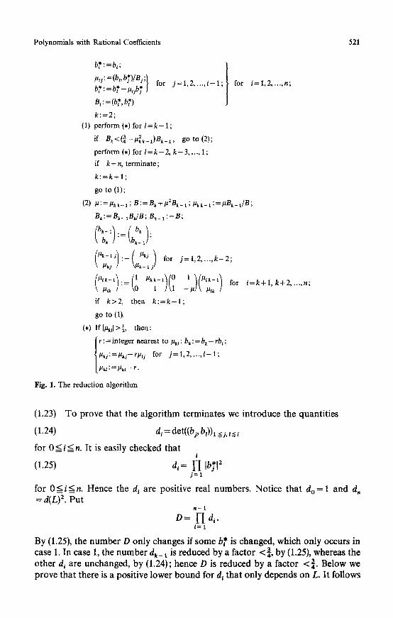
The entire algorithm is represented in Fig. 1, in which B l = Ib~l 2.
Polynomia l s with Ra t iona l Coefficients 521
(1)
(2)
(,)
b * : = b l ;
#ij (b,, b*)/Bi ;~ for j = l , 2 . . . . . i - l ;
be . - b e /~ljbi )
B, : = (b*, b*)
k : = 2 ;
per form (.) for I = k - 1 ;
if Bk<(�88 go to (2);
pe r form (.) for l = k - 2, k - 3 . . . . . 1 ;
if k = n, t e rmina te ;
k : = k + l ;
go to (1);
# : = P k k - 1 ; B:=Bk +#ZBk-~ ; Igkk-l :=#Bk-1/B;
Bk:=Bk_aBk/B; Bk_ 1 : = B ;
#~k / 1 ] \ 1 - - # / \ #~k /
if k > 2 , then k : = k - 1 ;
go to (1). If I~1>~, then :
r: = integer neares t to #kt ; bk: = bk-- rbt ;
#~ : = / ~ j - - r/~lj for j = 1, 2 . . . . . l - 1 ;
/zta: = ~tkS -- r.
Fig. 1. The reduct ion a lgor i thm
for i = 1 ,2 , . . . , n ;
i = k + l , k + 2 , . . . , n ;
(1.23) To prove that the algorithm terminates we introduce the quantities
(1.24) di = det((bi, bz)) 1 _< j, l__<
for 0 < i < n. It is easily checked that i
(1.25) d ,= I-I [b*l 2 j = l
for 0 < i < n. Hence the d i are positive real numbers. Notice that d o = 1 and d, =d(L) 2. Put
n- -1
D = 1-I di. i=1
By (1.25), the number D only changes if some b* is changed, which only occurs in case 1. In case 1, the number d k_ 1 is reduced by a factor <�88 by (1.25), whereas the other d~ are unchanged, by (1.24); hence D is reduced by a factor <�88 Below we prove that there is a positive lower bound for d t that only depends on L. It follows
522 A.K. Lenstra et al.
that there is also a positive lower bound for D, and hence an upper bound for the number of times that we pass through case 1.
In case 1, the value of k is decreased by 1, and in case 2 it is increased by 1. Initially we have k=2, and k < n + 1 throughout the algorithm. Therefore the number of times that we pass through case 2 is at most n - 1 more than the number of times that we pass through case 1, and consequently it is bounded. This implies that the algorithm terminates.
To prove that d i has a lower bound we put
m(L) = min{Ix[ 2 :xE L, x ~: 0}.
This is a positive real number. For i > 0, we can interpret d i as the square of the determinant of the lattice of rank i spanned by b 1, b 2 ..... bi in the vector space
P, bj. By I-4, Chap. I, Lemma 4 and Chap. II, Theorem I], this lattice contains a ./=1 non-zero vector x with Ixl 2<(4/3) ti- l)/2d~/i. Therefore di>(3/4) i"-l)/2m(L)~, as required.
We shall now analyse the running time of the algorithm under the added hypothesis that b~eZ n for l < i < n . By an arithmetic operation we mean an addition, subtraction, multiplication or division of two integers. Let the binary length of an integer a be the number of binary digits of lal.
(1.26) Proposition. Let LC7Z ~ be a lattice with basis bl,b 2 ..... b,, and let Beff(, B > 2, be such that [bil2 <= B for 1 < i < n. Then the number of arithmetic operations needed by the basis reduction algorithm described in (1.15) is O(n41ogB), and the integers on which these operations are performed each have binary length O(n log B).
Remark. Using the classical algorithms for the arithmetic operations we find that the number of bit operations needed by the basis reduction algorithm is O(nr(logB)3). This can be reduced to O(n 5 + ~(logB) 2 + ~), for every e > 0, if we employ fast multiplication techniques.
Proof of (1.26). We first estimate the number of times that we pass through cases 1 and 2. In the beginning of the algorithm we have d i < B i, by (1.25), so D ~ B ~t"- 1)/2 Throughout the algorithm we have D ~ 1, since die 7Z by (1.24) and d i > 0 by (1.25). So by the argument in (1.23) the number of times that we pass through case 1 is O(n 2 logB), and the same applies to case 2.
The initialization of the algorithm takes O(n 3) arithmetic operations with rational numbers; below we shall see how they can be replaced by operations with integers.
For (1.18) we need O(n) arithmetic operations, and this is also true for case 1. In case 2 we have to deal with O(n) values of l, that each require O(n) arithmetic operations. Since we pass through these cases O(n 2 logB) times we arrive at a total of O(n 4 logB) arithmetic operations.
In order to represent all numbers that appear in the course of the algorithm by means of integers we also keep track of the numbers d~ defined by (1.24). In the initialization stage these can be calculated by (1.25). After that, they are only changed in case 1. In that case, dk_ 1 is replaced by d k_ 1.lc~_ll2/Ib*_ll2=dk_2 'lc*_ t[ 2 [in the notation of (1.22)] whereas the other d i are unchanged. By (1.24),

Polynomials with Rational Coefficients 523
the d~ are integers, and we shall now see that they can be used as denominators for all numbers that appear:
(1.27) [b*12=dJd~_l ( l < i < n ) ,
(1.28) d~_ ib*eLC7Z," (1 <i<n) ,
(1.29) djldij~7Z (1 < j < i < n ) .
i - 1
The first of these follows from (1.25). For the second, we write b* = b i - )-" ;t~rb j r = l with 2~jel~ Solving 2i~ ... . . 2ii_ ~ from the system
i - 1
(b~,bz)= ~ 2,j(br, b~) ( 1 < / < i - 1 ) j = l
and using (1.24) we find that d~_12ireZ, whence (1.28). Notice that the same argument yields
di-1 bk-- #kjb eZ" for i < k ; J
this is useful for the calculation of b~ at the beginning of the algorithm. To prove (1.29) we use (1.3), (1.27), and (1.28):
dj~ii = d flb~, b*)/(b*, b*) = d r_ ~(b~, b*) = (b~, d r_ ~b*)e 7z.
To finish the proof of (1.26) we estimate all integers that appear. Since no d~ is ever increased we have d~<B ~ throughout the algorithm. This estimates the denominators. To estimate the numerators it suffices to find upper bounds for Ib~'l 2, Ib,I 2, and [/~l.
At the beginning we have Ib*12<lb~12<B, and max{Ib*12:l<i<n} is non- increasing; to see this, use that * 2 3 , c * 2 < b * 2 ICk-ll <~lb~-l l 2 and k = k-1 in (1.22), the
�9 is a projection of b~'_ r Hence we have tb*t2<B latter inequality because c k throughout the algorithm.
To deal with [b~l 2 and /~j we first prove that every time we arrive at the situation described by (1.16) and (1.17) the following inequalities are satisfied:
(1.30) Ib~12<=nB for i ~ k ,
(1.31) Ibkl 2 < n2(4B)" if k 4: n + 1,
(1.32) I~irl<�89 for l<=j<i, i<k ,
(1.33) [I, tij[ < (nBJ) 1/2 for 1 < j < i, i > k,
(1.34) I#krl<2"-k(nB"-l) 1/2 for l ~ j < k , if k # : n + l .
Here (1.30), for i < k, is trivial from (1.32), and (1.31) follows from (1.34). Using that
(1.35) #~ < Ib,I 2/1b*12 = dj_ 11b,I 2td~ < n r- 11b,12
we see that (1.33) follows from (1.30), and (1.32) is the same as (t.16). It remains to prove (1.30) for i> k and to prove (1.34). At the beginning of the algorithm we even have Ib~12 < B and #2~Br, by (1.35), so it suffices to consider the situation at the
524 A .K . Lenstra et al.
end of cases 1 and 2. Taking into account that k changes in these cases, we see that in case 1 the set of vectors {b i : i ~ k} is unchanged, and that in case 2 the set {bi:i>k } is replaced by a subset. Hence the inequalities (1.30) are preserved. At the end of case 2, the new values for #kj (if k + n + 1) are the old values of #k § 1 ~, SO here (1.34) follows from the inequality (1.33) at the previous stage. To prove (1.34) at the end of case 1 we assume that it is valid at the previous stage, and we follow what happens to gkj" To achieve (1.18) it is, for j < k - 1, replaced by #kS--r#k-1 j,
<2-1 with Ir[<2[#kk_ll and I/~k-1 jl=2, so
(1.36) I/~k~-- r /~_ 1 jl----< I~h~l + I ~ ~- 11 <2"-k+l(nB"-l) 1/2 by (1.34).
In the notation of (1.22) we therefore have
]Vk_lj[<2"-tk-l)(nB"-l) 1/2 for j < k - 1
and since k - 1 is the new value for k this is exactly the inequality (1.34) to be proved.
Finally, we have to estimate Ibi[ 2 and #~j at the other points in the algorithm. For this it suffices to remark that the maximum of I~kll, I~kzl . . . . . I~k k- 11 is at most doubled when (1.18) is achieved, by (1.36), and that the same thing happens in case 2 for at most k - 2 values of I. Combining this with (1.34) and (1.33) we conclude that throughout the course of the algorithm we have
I#i~l<2"-l(nB"-l) 1/2 for l <j<i<n and therefore
Ib~l 2 < n2(4B)" for 1 < i < n.
This finishes the proof of (1.26).
(1.37) Remark. Let 1 < n' < n. If k, in the situation described by (1.16) and (1.17), is for the first time equal to n' + 1, then the first n' vectors b~, b2,..., b,, form a reduced basis for the lattice of rank n' spanned by the first n' vectors of the initially given basis. This will be useful in Sect. 3.
(1.38) Remark. It is easily verified that, apart from some minor changes, the analysis of our algorithm remains valid if the condition L C 77" is replaced by the condition that (x, y)e 77 for all x, y ~ L; or, equivalently, that (b i, b j)e 77 for 1 < i, j ~ n. The weaker condition that (b~,bj)~ll~, for 1 <i, j<n, is also sufficient, but in this case we should clear denominators before applying (1.26).
We close this section with two applications of our reduction algorithm. The first is to simultaneous diophantine approximation. Let n be a positive integer, cq, at 2 .. . . . ~, real numbers, and eEIR, 0 < e < 1. It is a classical theorem [4, Sect.V. 10] that there exist integers Pl, P2 .. . . . p,, q satisfying
IPl-q~l <e for l < i ~ n ,
l <=q<e-".
We show that there exists a polynomial-time algorithm to find integers that satisfy a slightly weaker condition.

P o l y n o m i a l s wi th R a t i o n a l Coeff ic ients 525
(1.39) Proposition. There exists a polynomial-time algorithm that, given a positive integer n and rational numbers cq, ~t 2 . . . . , ~,, ~ satisfying 0 < e < 1, finds integers Pl, P2 .. . . . p,, q for which
[Pi-q~i] <e for l < i < n ,
1 < q < 2 "("+ 1)/4e-".
Proof. Let L be the lattice (n + 1) x (n + 1)-matrix
1 0
0 1
0 0
0 0
of rank n + l spanned by
... 0 - ~ 1 \
... 0 - a ~
" . .
. . . 1 - - 0~.
. . . 0 2-n(n+ l)/4~ n+ l
the columns of the
The inner p roduc t of any two columns is rat ional, so by (1.38) there is a po lynomia l - t ime a lgor i thm to find a reduced basis bl, b 2 . . . . . b,+ 1 for L. By (1.9) we then have
ibll <2. /4 .d(L)l/(,+ 1)=a.
Since b~eL, we can write
b x = (P 1 - qct 1, P2 - qCta . . . . , p , - qct,, q. 2 - "t" + 1)/4~, + 1)m
with Pl, P2 . . . . ,p., qe7L It follows that
[Pi- qcql < e for 1 --% i < n,
Iql < 2"~"+ 1)/%-.,
F r o m e < 1 and b 1 # 0 we see that q ~= 0. Replacing b 1 by - b 1, if necessary, we can achieve tha t q > 0.
This proves (1.39). Another appl icat ion of our reduct ion a lgor i thm is to the p rob lem of finding
Q-l inear relat ions a m o n g given real numbers al , a2 . . . . ,0t,. Fo r this we take the lattice L to be 77", embedded in IR "+ 1 by
( ( m l , m2,. . . ,mn)P--~ m l , m 2 , . . . , m n , C m i~ i , i = 1
here c is a large cons tant and g', is a good ra t ional app rox ima t ion to cq. The first basis vector of a reduced basis of L will give rise to integers ml, m 2 . . . . . m. tha t are
not too large such that s mi~ i is very small. P I
i = 1
Applying this to gi = ~d- x we see tha t our a lgor i thm can be used to test a given real n u m b e r 0t for algebraicity, and to determine its irreducible polynomial . Tak ing for a a zero of a po lynomia l f e Z [ X ] , f~eO, and generalizing the a lgor i thm to complex ct, one finds in this way an irreducible factor of f in 7Z[X]. I t is likely tha t this yields actually a po lynomia l - t ime a lgor i thm to factor f in Q[X] , an a lgor i thm tha t is different f rom the p-adic me thod described in Sect. 3.
In a similar way we can test given real numbers a, fl, ~ . . . . for algebraic dependence, taking the ~ti to be the monomia l s in g, fl, V . . . . up to a given degree.
5 2 6 A . K . L e n s t r a e t al .
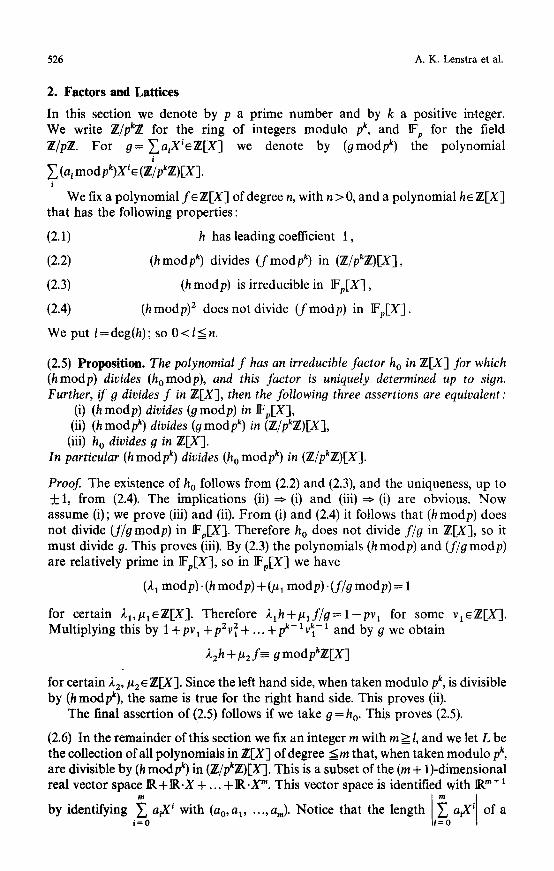
2. Factors and Lattices
In this section we denote by p a prime number and by k a positive irrteger. We write Z/pkTZ for the ring of integers modulo pk, and IFp for the field 7//pTZ. For g=~aiXiET~[X] we denote by (gmodp k) the polynomial
i ~. (ai modpk)Xie (2Upk7Z)[X].
i
We fix a polynomial f ~ Z[X] of degree n, with n > 0, and a polynomial he Z[X] that has the following properties:
(2.1) h has leading coefficient 1,
(2.2) (hmodp k) divides ( f modp k) in (7Z/pk?Z)[X],
(2.3) (h modp) is irreducible in lFp[X],
(2.4) (hmodp) 2 does not divide ( fmodp) in IFp[X].
We put l-- deg(h) ; so 0 < l < n.
(2.5) Proposition. The polynomial f has an irreducible factor h o in 7ZIX] for which (hmodp) divides (homodp) , and this factor is uniquely determined up to sign. Further, if g divides f in 7Z[X], then the following three assertions are equivalent:
(i) (h modp) divides (g modp) in IFp[X], (ii) (h modp k) divides (g modp k) in (7l/pk2~)[X],
(iii) h o divides g in 7ZI-X-I. In particular (h modp k) divides (h o modp k) in (77/pk7Z)[X].
Proof. The existence of h o follows from (2.2) and (2.3), and the uniqueness, up to _+1, from (2.4). The implications (ii)=~ (i) and (iii)=~ (i) are obvious. Now assume (i); we prove (iii) and (ii). From (i) and (2.4) it follows that (h modp) does not divide (fig modp) in Fp[X]. Therefore h o does not divide f ig in 7ZI-X], so it must divide g. This proves (iii). By (2.3) the polynomials (h modp) and (fig modp) are relatively prime in IFp[X], so in IFp[X] we have
(21 modp). (h modp) + (#1 modp). (fig modp) = 1
for certain 2a,/alETZ[X ]. Therefore 2 1 h + l ~ l f / g = l - p v l for some v l~Z[X ]. Multiplying this by 1 +pv 1 +p2v2 + ... +pk- lv]-1 and by O we obtain
22h + #2 f = g modpkZ[x]
for certain 22, #2EZ[X]. Since the left hand side, when taken modulo pk, is divisible by (h modpk), the same is true for the right hand side. This proves (ii).
The final assertion of (2.5) follows if we take g = h o. This proves (2.5).
(2.6) In the remainder of this section we fix an integer m with m ~ l, and we let L be the collection of all polynomials in ~.[X] of degree =m that, when taken modulo pk, are divisible by (h modp k) in (TZ/pkTZ)[X]. This is a subset of the (m + 1)-dimensional real vector space IR + R . X + . . . + R .X m. This vector space is identified with IR m + 1
by identifying a~f i with (ao, a 1 . . . . . a,,,). Notice that the length a~X i of a i = O t
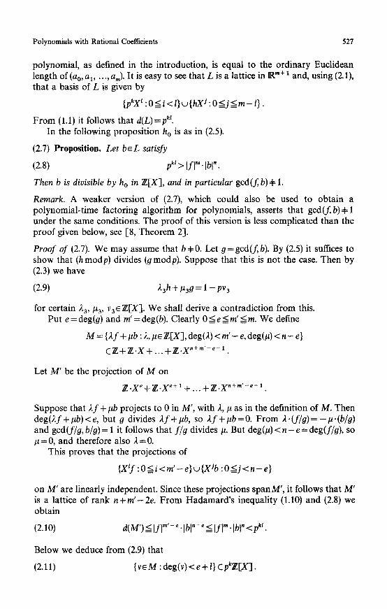
Polynomials with Rational Coefficients 527
polynomial, as defined in the introduction, is equal to the ordinary Euclidean length of (a 0, a 1 . . . . . am). It is easy to see that L is a lattice in Rm+ 1 and, using (2.1), that a basis of L is given by
{pkX~ :O<<_i <l}w{hXJ : O < j < m - l } .
From (1.1) it follows that d(L)=p kt. In the following proposition h o is as in (2.5).
(2.7) Proposition. Let b~ L satisfy
(2.8) pkt > lflm.lb{".
Then b is divisible by h o in 7Z[X], and in particular gcd( f b )# 1.
Remark. A weaker version of (2.7), which could also be used to obtain a polynomial-time factoring algorithm for polynomials, asserts that gcd (f, b) 4: l under the same conditions. The proof of this version is less complicated than the proof given below, see [8, Theorem 2].
Proof of (2.7). We may assume that b#:0. Let g=gcd(f ,b) . By (2.5) it suffices to show that (h modp) divides (g modp). Suppose that this is not the case. Then by (2.3) we have
(2.9) ~-3 h + #3g = 1 - pv 3
for certain 2 3, #3, v3E 7/IX]. We shall derive a contradiction from this. Put e = deg(9) and m' = deg(b). Clearly 0 < e < m' < m. We define
M = {).f + #b : 2, #~ 7/IX], deg(2) < m' - e, deg(#) < n - e}
C Z + 7 / ' X + . . . +7/ .X "+" ' - ~- 1.
Let M' be the projection of M on
2g .X~+ 7/.X e+ 1 + . . . + Z .X "+" ' - e - 1.
Suppose that 2 f + #b projects to 0 in M', with ;t, # as in the definition of M. Then deg(2f+#b)<e, but O divides 2f+l~b, so 2 f + # b = 0 . From 2 . ( f / 9 ) = - # ' ( b / o ) and gcd(f/9, b/9)= 1 it follows that f /o divides #. But deg(#)< n - e = deg(f/9), so # = 0, and therefore also ;t = 0.
This proves that the projections of
{x i f : O < i < m ' - e } ~ { X J b :O<=j<n-e}
on M' are linearly independent. Since these projections spanM', it follows that M' is a lattice of rank n + m ' - 2 e . From Hadamard's inequality (1.10) and (2.8) we obtain
(2.10) d(M') < Ifl m'- ~ . I bl "-e < Ifl"" Ibl" < pk, .
Below we deduce from (2.9) that
(2.11) {v~M : deg (v )<e+ l} cpkTZ[X].

528 A.K. Lenstra et al.
Hence, if we choose a basis b,,,be+ 1 . . . . ,b,+m,-e-1 of M' with deg(bj)=j, see [4, Chap. I, Theorem I.A], then the leading coefficients of be, be+l, ...,b~+z_ 1 are divisible by pk. [Notice that e + l - l < n + m ' - e - 1 because g divides b and (h modp) divides (fig modp).] Since d(M') equals the absolute value of the product of the leading coefficients of be, be+ 1, ...,b,,+,n,e_ 1 we find that d(M')>p kl. Combined with (2.10) this is the desired contradiction.
To prove (2.11), let v~M, deg(v)< e + I. Then g divides v. Multiplying (2.9) by v/g and by 1 + pv 3 + p272 q- _k- 1. k- 1 ... +p v 3 we obtain
(2.12) 24h + #4 v - v/g mod pkT][X]
with 24,/~4~Z[X]. From v e M and be_L it follows that (vmodp k) is divisible by (hmodpk). So by (2.12) also (v/gmodp k) is divisible by (hmodpk). But (hmodp k) is of degree l with leading coefficient 1, while (v/gmodp k) has degree < e + l - e = I. Therefore v/9 - 0 modpkZ[X], so also v -- 0 modpkT/[X]. This proves (2.11).
This concludes the proof of (2.7).
(2.13) Proposition. Let p, k, f, n, h, l be as at the beginning of this section, h o as in (2.5), and m, L as in (2.6). Suppose that bx, b 2 . . . . . br,+ l is a reduced basis for L (see (1.4) and (t.5)), and that
(2.14) pkZ> 2,,.,,,/2 (2mm )"/2lflr,,+,.
Then we have deg(ho)<m/f and only if
(2.15) Ibll <(pkZ/lflm) 1/" .
Proof The "if'-part is immediate from (2.7), since deg(bl)~ m. To prove the "only
if'-part, assume that deg(ho)<m. Then hoeL by (2.5), and Ihol< "lfl by a
result of Mignotte [10; cf. 7, Exercise 4.6.2.20]. Applying (1.11) to x =h o we find
that Ib11<2"/2.1hol<__2"/2. "lfl. By (2.14) this implies (2.15). This proves
(2.13).
(2.16) Proposition. Let the notation and the hypotheses be the same as in (2.13), and assume in addition that there exists an index je {1, 2 . . . . , m + 1} for which
(2.17) [b j] < (pkZ/lfl")1/,.
Let t be the largest such j. Then we have
deg(ho) = m + 1 - t,
h o = gcd(b x, b 2 . . . . , bt),
and (2.17) holds for all j with 1 ~ j < t .
Proof Let J={ je{1 ,2 ... . . m + l } : (2.17) holds}. From (2.7) we know that h o divides bj for every j~J. Hence if we put
hi = gcd({bj :j~ J})
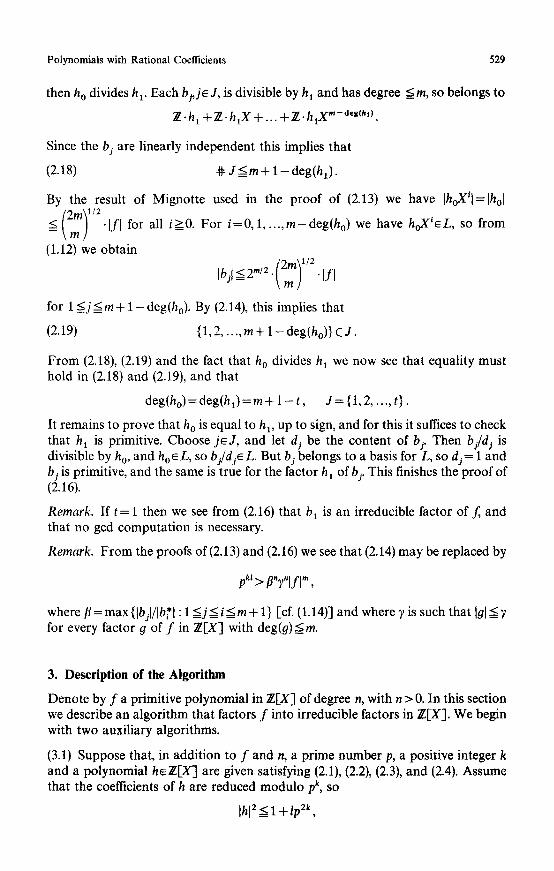
Polynomials with Rational Coefficients 529
then h o divides h t. Each bj, j~ J, is divisible by h 1 and has degree < m, so belongs to
2~-h~ + Z .h lX + ... + Z . h l X m-a'*th~ .
Since the bj are linearly independent this implies that
(2.18) ~ J < m + 1 - deg(hl).
By the result of Mignotte used in the proof of (2.13) we have IhoXil=}hol
< "If[ for all i>0. For i=0 ,1 . . . . . m-deg(ho) we have hoXieL, so from
(1.12) we obtain
Ib~l < 2 m/2" "Ifl
for 1 < j < m + 1 -deg(ho). By (2.14), this implies that
(2.19) { 1, 2 .. . . . m + 1 - deg(ho) } C J .
From (2.18), (2.19) and the fact that h o divides h 1 we now see that equality must hold in (2.18) and (2.19), and that
deg(ho)=deg(hx )=m+l- t , J = { 1 , 2 .. . . . t}.
It remains to prove that h o is equal to hx, up to sign, and for this it suffices to check that hi is primitive. Choose j eJ , and let dj be the content of bj. Then bj/dj is divisible by h o, and howL, so b /d i lL . But bj belongs to a basis for L, so dr= 1 and b 2 is primitive, and the same is true for the factor h i of bj. This finishes the proof of (2.16).
Remark. If t = 1 then we see from (2.16) that b~ is an irreducible factor of f, and that no god computation is necessary.
Remark. From the proofs of (2.13) and (2.16) we see that (2.14) may be replaced by
pkZ > fl"7"lflm ,
where fl = max {Ibjl/Ib*,l : 1 < j < i ~ m + 1 } [cf. (1.14)] and where 7 is such that 101 < y for every factor # of f in Z[X] with deg(g)<m.
3. Description of the Algorithm
Denote by f a primitive polynomial in Z[X] of degree n, with n > 0. In this section we describe an algorithm that factors f into irreducible factors in Z[X]. We begin with two auxiliary algorithms.
(3.1) Suppose that, in addition to f and n, a prime number p, a positive integer k and a polynomial heT/[X] are given satisfying (2.1), (2.2), (2.3), and (2.4). Assume that the coefficients of h are reduced modulo pk, SO
[hi 2 ~< 1 + l p 2k ,
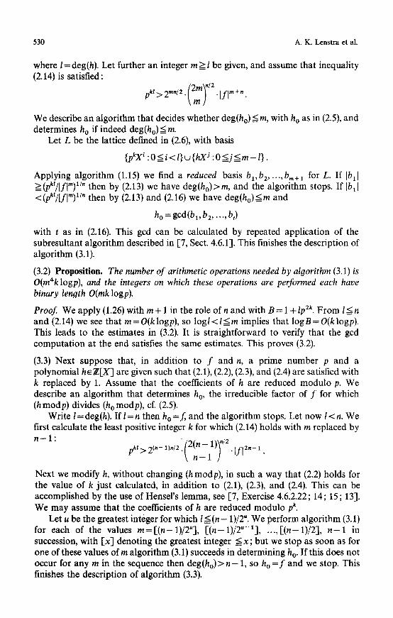
530 A.K. Lenstra et al.
where l= deg(h). Let further an integer m > l be given, and assume that inequality (2.14) is satisfied:
pk, > 2r,,/2 . (2mm)"/2 . ,flm+, .
We describe an algorithm that decides whether deg(ho)<m, with h o as in (2.5), and determines h o if indeed deg(ho) < m.
Let L be the lattice defined in (2.6), with basis
{pkXi :0 < i < l}u{hX j : O < j < m - l } .
Applying algorithm (1.15) we find a reduced basis bl,b 2 .... ,b,,+l for L. If Ibll >(pkZ/Iflm)l/" then by (2.13) we have deg(ho)>m, and the algorithm stops. If tbll < (pkl/lflr')l/" then by (2.13) and (2.16) we have deg(ho)< m and
h o = gcd(bl, b2 ... . . bt)
with t as in (2.16). This gcd can be calculated by repeated application of the subresultant algorithm described in [7, Sect. 4.6.1]. This finishes the description of algorithm (3.1).
(3.2) Proposition. The number of arithmetic operations needed by algorithm (3.1) is O(m4k logp), and the integers on which these operations are performed each have binary length O(mk logp).
Proof. We apply (1.26) with m + 1 in the role of n and with B = 1 + Ip 2k. From 1 < n and (2.14) we see that m = O(k logp), so log /< l < m implies that log B = O(k logp). This leads to the estimates in (3.2). It is straightforward to verify that the gcd computation at the end satisfies the same estimates. This proves (3.2).
(3.3) Next suppose that, in addition to f and n, a prime number p and a polynomial heZ[X] are given such that (2.1), (2.2), (2.3), and (2.4) are satisfied with k replaced by 1. Assume that the coefficients of h are reduced modulo p. We describe an algorithm that determines h o, the irreducible factor of f for which (h modp) divides (h 0 modp), cf. (2.5).
Write/=deg(h). If l= n then h o =f , and the algorithm stops. Let now l< n. We first calculate the least positive integer k for which (2.14) holds with m replaced by n - l :
1),/2 ( 2 ( n - 1)/"/2 . ifl2,_ 1 pU>2(,- "\ n - 1 ]
Next we modify h, without changing (h modp), in such a way that (2.2) holds for the value of k just calculated, in addition to (2.1), (2.3), and (2.4). This can be accomplished by the use of Hensers lemma, see I'7, Exercise 4.6.2.22; 14; 15; 13]. We may assume that the coefficients of h are reduced modulo pk.
Let u be the greatest integer for which l~ ( n - 1)/2 u. We perform algorithm (3.1) for each of the values m = 1'(n- 1)/2"1 [ ( n - 1)/2 ~- 1] . . . . . I-(n- 1)/2], n - 1 in succession, with 1-x] denoting the greatest integer < x ; but we stop as soon as for one of these values of m algorithm (3.1) succeeds in determining h o. If this does not occur for any m in the sequence then deg(ho)> n - 1 , so h o = f and we stop. This finishes the description of algorithm (3.3).
Polynomials with Rational Coefficients 531
(3.4) Proposition. Denote by m o =deg(ho) the degree of the irreducible factor h o of f that is found by algorithm (3.3). Then the number of arithmetic operations needed by algorithm (3.3) is O(mo(nS +n41oglfl+nalogp)), and the integers on which these operations are performed each have binary length O(n3 +n21oglfl + n logp).
Proof From
it follows that
(2(n- 1)] "/2 [f12,_ 1 Pk-l<P<k-1)t<2t"-l)"/2\ n--1 ]
k logp = ( k - 1) logp + logp = O(n 2 q- n loglfl + logp).
Let m I be the largest value of m for which algorithm (3.1) is performed. From the choice of values for m it follows that ml <2rag, and that every other value for m that is tried is of the form [ml/2i], with i_>_1. Therefore we have ~'m4=O(m~). Using (3.2) we conclude that the total number of arithmetic operations needed by the applications of algorithm (3.1) is O(m4k logp), which is
O(m4(n 2 + n loglfl + logp)),
and that the integers involved each have binary length O(mlklogp), which is
O(mo(n 2 + n log Ifl + logp)).
With some care it can be shown that the same estimates are valid for a suitable version of Hensel's lemma. But it is simpler, and sufficient for our purpose, to replace the above estimates by the estimates stated in (3.4), using that m o < n; then a very crude estimate for Hensel's lemma will do. The straightforward verification is left to the reader. This proves (3.4).
(3.5) We now describe an algorithm that factors a given primitive polynomial f ~ Z[X] of degree n > 0 into irreducible factors in 7Z[X].
The first step is to calculate the resultant R(f, f ') of f and its derivative f ' , using the subresultant algorithm [7, Sect. 4.6.1]. If R(f,f ')=O then f and f ' have a greatest common divisor g in 7/IX] of positive degree, and g is also calculated by the subresultant algorithm. This case will be discussed at the end of the algorithm. Assume now that R(f f') +- O.
In the second step we determine the smallest prime number p not dividing R(f, f'), and we decompose ( f modp) into irreducible factors in IFp[X] by means of Berlekamp's algorithm [7, Sect. 4.6.2]. Notice that R(f, f') is, up to sign, equal to the product of the leading coefficient of f and the discriminant of f So R( f f ' ) ~Omodp implies that ( fmo d p ) still has degree n, and that it has no multiple factors in IFp[X]. Therefore (2.4) is valid for every irreducible factor (hmodp) of ( f m o d p ) i n •p[X].
In the third step we assume that we know a decomposition f = f l f 2 in Z[X] such that the complete factorizations of f l in ~.[X] and (f2 modp) in IF~[X] are known. At the start we can take fa = 1, f2 = f In this situation we proceed as follows. If f2 = + 1 then f = + f l is completely factored in Z[X], and the algorithm stops. Suppose now that f2 has positive degree, and choose an irreducible factor
532 A . K . L e n s t r a e t al.
(h modp) of (f2 modp) in IFp[X]. We may assume that the coefficients of h are reduced modulo p and that h has leading coefficient 1. Then we are in the situation described at the start of algorithm (3.3), with f2 in the role of f, and we use that algorithm to find the irreducible factor ho of fz in Z[X] for which (h modp) divides (h o modp). We now replace f l and fz by flho and fz/ho, respectively, and from the list of irreducible factors of (f2 modp) we delete those that divide (h o modp). After this we return to the beginning of the third step.
This finishes the description of the algorithm in the case that R(f, f ' )~0. Suppose now that R(f, f ' ) = 0, let g be the gcd of f and f ' in Z[X], and put fo = fig. Then f0 has no multiple factors in 7Z[X], so R(fo, f~) 4: O, and we can factor fo using the main part of the algorithm. Since each irreducible factor of g in 2~[X] divides fo we can now complete the factorization of f = fog by a few trial divisions. This finishes the description of algorithm (3.5).
(3.6) Theorem. The above algorithm factors any primitive polynomial f~ TZ[X] of positive degree n into irreducible factors in 7/IX[. The number of arithmetic operations needed by the algorithm is O(n 6-F n 5 log[fl), and the integers on which these operations are performed each have binary length O(n a + n 2 log[f[). Here If1 is as defined in the introduction.
Using the classical algorithms for the arithmetic operations we now arrive at the bound O(n12 + n9(log[f[) 3) for the number of bit operations that was announ- ced in the introduction. This can be reduced to O(n9+~+ n 7 + ~(log[f[) 2+ ~), for every e > 0, if we employ fast multiplication techniques.
Proof of (3.6). The correctness of the algorithm is clear from its description. To prove the estimates we first assume that R(f, f ' ) ~ 0. We begin by deriving an upper bound for p. Since p is the least prime not dividing R(f, f ' ) we have
(3.7) I-I q < [R(f f')[. q < p, q prime
It is not difficult to prove that there is a positive constant A such that
(3.8) I-I q >eAp q< p, qprimc
for all p>2 , see [6, Sect. 22.2]; by [12] we can take A=0.84 for p>101. From Hadamard's inequality (1.10) we easily obtain
[R(f, f')[ < nnlf[ 2n-1 .
Combining this with (3.7) and (3.8) we conclude that
(3.9) p < (n log n + (2n- 1) log Ifl)/A
or p = 2. Therefore the terms involving logp in proposition (3.4) are absorbed by the other terms.
The call of algorithm (3.3) in the third step requires O(mo.(n 5 +n41oglf2[)) arithmetic operations, by (3.4), where m 0 is the degree of the factor h 0 that is found. Since f2 divides f, Mignotte's theorem [10; cf. 7, Exercise 4.6.2.20] that was used in the proof of (2.13) implies that loglf21 = O(n + loglfl). Further the sum ~mo of the

Polynomials with Rational Coefficients 533
degrees of the irreducible factors of f is clearly equal to n. We conclude that the total number of arithmetic operations needed by the applications of (3.3) is O(n 6
+ n 5 loglf[). By (3.4), the integers involved in (3.3) each have binary length O(n 3 + n 2 loglfl).
We must now show that the other parts of the algorithm satisfy the same estimates. For the subresultant algorithm in the first step and the remainder of the third step this is entirely straightforward and left to the reader. We consider the second step.
Write P for the right hand side of (3.9). Then p can be found with O(P) arithmetic operations on integers of binary length O(P); here one can apply [11] to generate a table of prime numbers < P, or alternatively use a table ofsquarefree numbers, which is easier to generate. From p < P it also follows that Berlekamp's algorithm satisfies the estimates stated in the theorem, see [7, Sect. 4.6.2].
Finally, let R(f, f') = 0, and fo = f/gcd(f, f ' ) as in the algorithm. Since fo divides f, Mignotte's theorem again implies that loglfol = O(n+ loglfl). The theorem now follows easily by applying the preceding case to fo.
This finishes the proof of (3.6).
(3.10) For the algorithms described in this section the precise choice of the basis reduction algorithm is irrelevant, as long as it satisfies the estimates of proposition (1.26). A few simplifications are possible if the algorithm explained in Sect. 1 is used. Specifically, the gcd computation at the end of algorithm (3.1) can be avoided. To see this, assume that m o =deg(ho) is indeed <m. We claim that h o occurs as b 1 in the course of the basis reduction algorithm. Namely, by (1.37) it will happen at a certain moment that bl, b 2 . . . . . bmo+l form a reduced basis for the lattice of rank m o + l spanned by {p~Xi:O<i<l}u{hXJ:O<j<mo-l}. At that moment, we have ho=bl, by (2.13) and (2.16), applied with m o in the role ofm. A similar argument shows that in algorithm (3.3) one can simply try the values m = l, l+ 1, . . . , n - 1 in succession, until hois found.
Acknowledgements are due to J. J. M. Cuppen for permission to include his improvement of our basis reduction algorithm in Sect. 1.
References
1. Adleman, L.M., Odlyzko, A.M. : Irreducibility testing and factorization of polynomials, to appear. Extended abstract: Proc. 22nd Annual IEEE Symp. Found. Comp. Sci., pp. 409-418 (1981)
2. Brentjes, A.J. : Multi-dimensional continued fraction algorithms. Mathematical Centre Tracts 145. Amsterdam: Mathematisch Centrum 1981
3. Cantor, D.G.: Irreducible polynomials with integral coefficients have succinct certificates. J. Algorithms 2, 385-392 (1981)
4. Cassels, J.W.S.: An introduction to the geometry of numbers. Berlin, Heidelberg, New York: Springer 1971
5. Ferguson, H.R.P., Forcade, R.W. : Generalization of the Euclidean algorithm for real numbers to all dimensions higher than two. Bull. Am. Math. Soc. 1, 912-914 (1979)
6. Hardy, G.H., Wright, E.M. : An introduction to the theory of numbers. Oxford: Oxford University Press 1979
7. Knuth, D.E. : The art of computer programming, Vol. 2, Seminumerical algorithms. Reading: Addison-Wesley 1981
534 A.K. Lenstra et al.
8. Lenstra, A.K.: Lattices and factorization of polynomials, Report IW 190/81. Amsterdam: Mathematisch Centrum 1981
9. Lenstra, H.W., Jr. : Integer programming with a fixed number of variables. Math. Oper. Res. (to appear)
10. Mignotte, M. : An inequality about factors of polynomials. Math. Comp. 28, 1153-1157 (1974) 11. Pritchard, P. : A sublinear additive sieve for finding prime numbers. Comm. ACM 24, 18-23 (1981) 12. Barkley Rosser, J., Schoenfeld, L. : Approximate formulas for some functions of prime numbers. I11.
J. Math. 6, 64-94 (1962) 13. Yun, D.Y.Y. : The Hensel lemma in algebraic manipulation. Cambridge : MIT 1974; reprint : New
York: Garland 1980 14. Zassenhaus, H. :On Hensel factorization. I. J. Number Theory 1, 291-311 (1969) 15. Zassenhaus, H. : A remark on the Hensel factorization method. Math. Comp. 32, 287-292 (1978) 16. Zassenhaus, H. : A new polynomial factorization algorithm (unpublished manuscript, 1981)
Received July 11, 1982