®MATLAB : Introductory Tutorial Originally prepared by Mark S Goldman, UC Davis (used with permission)

Modified, extended, and edited by Daniel Zysman, MIT

This tutorial is intended to get you acquainted with the MATLAB programming environment. It is not intended as a thorough introduction to the language, but rather as a practical guide to the most useful functions and operations to be used in this course. For additional resources see the Getting help section at the end of this document, or do a search on the web for “MATLAB tutorials.”

I. Getting to know MATLAB

MATLAB is a programming environment for working mostly with numerical data, and symbolic equations to a certain extent. MATLAB is an interpreted language, thus the code is compiled (translated from what you type into machine-readable code) and run as you type it in. For this reason, it is an easy environment in which to perform a few manipulations on some data and plot the output. In MATLAB you can also write and run scripts and functions, which are covered in this tutorial. In addition, MATLAB contains a vast array of built-in functions for performing manipulations on data so that you do not need to code the most powerful and commonly used numerical methods from scratch.

When you open MATLAB on your computer, the following screen or something very similar (depending on your OS and version) should appear:

1

Courtesy of The MathWorks, Inc. Used with permission. MATLAB and Simulink are registered trademarksof The MathWorks, Inc. See www.mathworks.com/ trademarks for a list of additional trademarks. Otherproduct or brand names may be trademarks or registered trademarks of their respective holders.

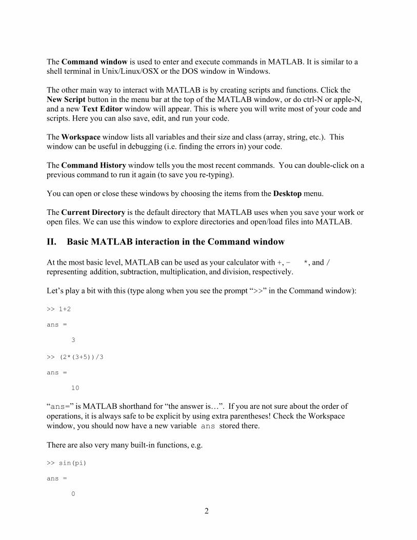
The Command window is used to enter and execute commands in MATLAB. It is similar to a shell terminal in Unix/Linux/OSX or the DOS window in Windows.

The other main way to interact with MATLAB is by creating scripts and functions. Click the New Script button in the menu bar at the top of the MATLAB window, or do ctrl-N or apple-N, and a new Text Editor window will appear. This is where you will write most of your code and scripts. Here you can also save, edit, and run your code.

The Workspace window lists all variables and their size and class (array, string, etc.). This window can be useful in debugging (i.e. finding the errors in) your code.

The Command History window tells you the most recent commands. You can double-click on a previous command to run it again (to save you re-typing).

You can open or close these windows by choosing the items from the Desktop menu.

The Current Directory is the default directory that MATLAB uses when you save your work or open files. We can use this window to explore directories and open/load files into MATLAB.

II. Basic MATLAB interaction in the Command window

At the most basic level, MATLAB can be used as your calculator with +, −��*, and / representing addition, subtraction, multiplication, and division, respectively.

Let’s play a bit with this (type along when you see the prompt “>>” in the Command window):

>> 1+2

ans =

3

>> (2*(3+5))/3

ans =

10

“ans=” is MATLAB shorthand for “the answer is…”. If you are not sure about the order of operations, it is always safe to be explicit by using extra parentheses! Check the Workspace window, you should now have a new variable ans stored there.

There are also very many built-in functions, e.g.

>> sin(pi)

ans =

0

2

Note that “pi=3.14159…” is known by MATLAB and that MATLAB is case-sensitive (try typing Sin(pi/2) and see what happens). The variables i and j are reserved for the

imaginary unit 1 . Therefore assignments of the type “i=…, j=…” should be avoided. Other useful functions are exp (the exponential function), log (the natural logarithm), and log10 (logarithm in base 10). You can explore the help file associated with a given built-in MATLAB function by typing, for example:

>> help exp

MATLAB also has a very extensive and useful documentation browser. Type this command to access it:

>> doc

Creating variables:

A variable is a storage space in a computer for numbers or characters. The equal sign “=” is used to assign a value to a variable.

At the command prompt, type:

>> a = 8

You just created a variable named a and assigned it a value of 8. If you now type

>> a*5

you get the answer 40.

Now type

>> b = a*5;

You just made a new variable b, and assigned it a value equal to the product of the value of a and 5. By adding a semicolon, you suppressed the output from being printed. Suppressing the output will be important later. To retrieve the value of b, just type

>> b

without a semicolon. Now try typing:

>> a = a + 10

This re-assigns to the variable a,the sum of the previous value of a (which was 8), plus 10, resulting in the new value of the variable a being 18. Note: this illustrates that ‘=’ means ‘assign’ in MATLAB. It is not a declaration that the expressions on the two sides of the ‘=’ sign are ‘equal’ (because certainly a cannot equal itself plus 10!).

3

To test for equality we use the “==” operator, to distinguish it from a variable assignment:

>> a==10

ans =

0

The output in this case is a logical variable, type:

>> whos

and you will see that ans belongs to the logical class. Logical variables are either false (value of 0) or true (value of 1). whos gives you information about the variables currently held in memory.

Try the following expressions to familiarize yourself with logical expressions that capture the properties greater than, less than, and not equal to:

>> a>10

>> a<5

>> a~=10

The operators “<=” and “>=” are for less than or equal to, and greater than or equal to, respectively.

Vectors and matrices:

In MATLAB, most numerical variables are real-valued matrices, or arrays (of type "double" for the programmers). This makes it easy to perform manipulations on groups of related numbers at the same time. You did not realize it, but the variables you created above are 1 row by 1 column (or “1x1” for short) matrices. Sort the elements in the workspace by size to verify this.

Let's see more about how arrays work. Type

>> a = [1 2 3 4 5]

a =

1 2 3 4 5

You just created an array containing the numbers 1 through 5. Notice that we use square brackets to list elements of an array. This array can be thought of as a matrix that is 1 row deep and 5 columns wide (often called a row vector). To confirm this, use the size command, which tells you the number of rows (first element returned) and number of columns (second element returned) in an array:

>> size(a)

4

ans =

1 5

To obtain the number of elements in a vector, use the numel command:

>> numel(a)

ans =

5

You can also add or multiply arrays by a constant, or add arrays. Try:

>> b = 2*a

b =

2 4 6 8 10

>> b+a

ans =

3 6 9 12 15

You can access the value of a given element of a or b by using parentheses. Type

>> a(3)>> b(4)

and you see the values of the 3rd element of the a array and the 4th element of the b array, respectively. You can also use b(end) or a(end) to see the last element.

Finally, you can append one vector onto another to make a longer vector. For example, try typing:

>> a = [a 8 9 10]

a = 1 2 3 4 5 8 9 10

This re-assigns the variable a to a new row vector containing the elements of the previous vector a, followed by the new elements [8 9 10].

If you prefer to arrange your array into a column (i.e. a 5 row x 1 column matrix, or column vector), you can do this by separating the elements by semicolons:

>> a = [1; 2; 3; 4; 5]

a =

1

5

2 3 4 5

>> size(a)

ans =

5 1

Now suppose we decide that we really would have liked to organize the elements of a into a row vector. There are two ways to get back to our original assignment:

Method 1: use the uparrow key (↑) to scroll back through your previous commands until you reach the a = [1 2 3 4 5] command and then press return (equivalently, you can also use the Command History window). The downarrow key (↓) scrolls forward through previous commands (in case you scroll back too far).

For practice, undo this by double-clicking on a = [1; 2; 3; 4; 5] in the Command History window so that a is again a column vector.

Method 2: Another way to change from a row to a column vector is to do the transpose operation, denoted by a single quotation mark ′. The transpose of a matrix exchanges the rows and columns of a matrix. Let’s try this:

>> a = a'

a =

1 2 3 4 5

The above line re-assigns to the variable a the values of the row vector a'.

So far we have dealt with row and column vectors. Now let’s construct (i.e. create and assign values to) a matrix that we will name “M”:

>> M = [1 2; 3 4]

M =

1 2 3 4

Note the syntax: elements in the same row are separated by spaces. The semicolon designates a new row. Try running the commands size and numel for matrix M and interpret their output.

To find out the value of the element in the 1st row, 2nd column of M, type:

>> M(1,2)

ans =

6

2

Similarly, if we would like to re-assign this element to equal 7 instead of 3 we would type:

>> M(1,2) = 7

M =

1 7 3 4

Note that typing:

>> M(2)

ans =

7

generates a different answer than M(1,2). This is because we use a linear index rather than the matrix subscript. MATLAB maps the linear indices of a matrix (here we use a 3 by 3 example) to subscripts in the following way:

So the linear indices go column-wise. MATLAB functions ind2sub and sub2ind are very helpful for converting linear indices to subscripts and vice versa.

The transpose of matrix M is found by typing:

>> M'

ans =

1 3 7 4

Notice that the previous 1st row is now the first column and the previous 2nd row is now the second column.

Next, let’s do some arithmetic on matrices. Let’s begin by clearing the memory of all the

7

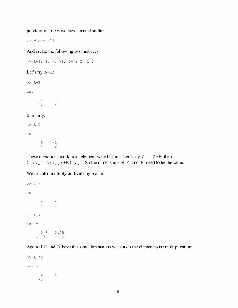
previous matrices we have created so far:

>> clear all

And create the following two matrices:

>> A=[2 1; -3 7]; B=[2 2; 1 1];

Let’s try A+B:

>> A+B

ans =

4 3 -2 8

Similarly:

>> A-B

ans =

0 -1 -4 6

These operations work in an element-wise fashion. Let’s say C = A+B, then C(i,j)=A(i,j)+B(i,j). So the dimensions of A and B need to be the same.

We can also multiply or divide by scalars:

>> 2*B

ans =

4 4 2 2

>> A/4

ans =

0.5 0.25 -0.75 1.75

Again if A and B have the same dimensions we can do the element-wise multiplication:

>> A.*B

ans =

4 2 -3 7

8

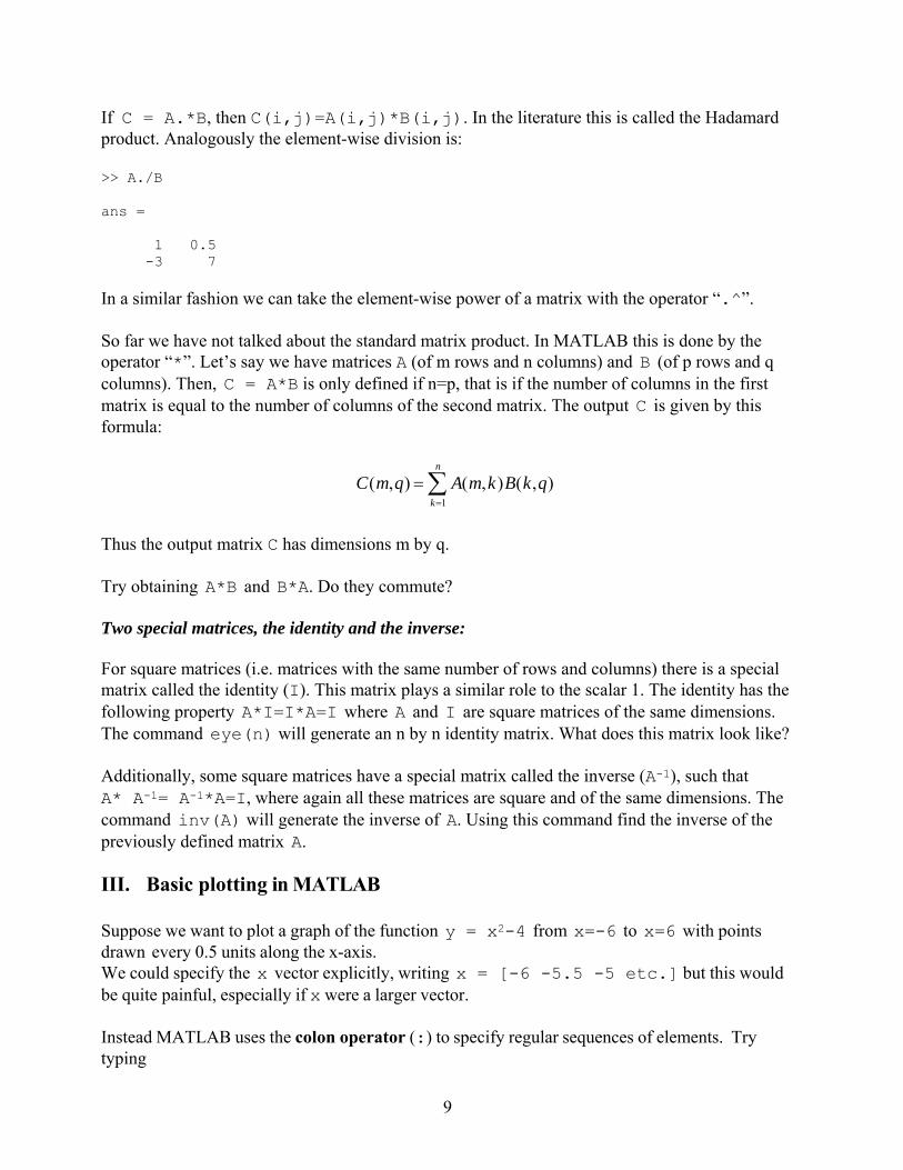
If C = A.*B, then C(i,j)=A(i,j)*B(i,j). In the literature this is called the Hadamard product. Analogously the element-wise division is:

>> A./B

ans =

1 0.5 -3 7

In a similar fashion we can take the element-wise power of a matrix with the operator “.^”.

So far we have not talked about the standard matrix product. In MATLAB this is done by the operator “*”. Let’s say we have matrices A (of m rows and n columns) and B (of p rows and q columns). Then, C = A*B is only defined if n=p, that is if the number of columns in the first matrix is equal to the number of columns of the second matrix. The output C is given by this formula:

n

C(m,q) A(m,k)B(k,q) k1

Thus the output matrix C has dimensions m by q.

Try obtaining A*B and B*A. Do they commute?

Two special matrices, the identity and the inverse:

For square matrices (i.e. matrices with the same number of rows and columns) there is a special matrix called the identity (I). This matrix plays a similar role to the scalar 1. The identity has the following property A*I=I*A=I where A and I are square matrices of the same dimensions. The command eye(n) will generate an n by n identity matrix. What does this matrix look like?

Additionally, some square matrices have a special matrix called the inverse (A-1), such that A* A-1= A-1*A=I, where again all these matrices are square and of the same dimensions. The command inv(A) will generate the inverse of A. Using this command find the inverse of the previously defined matrix A.

III. Basic plotting in MATLAB

Suppose we want to plot a graph of the function y = x2-4 from x=-6 to x=6 with points drawn every 0.5 units along the x-axis. We could specify the x vector explicitly, writing x = [-6 -5.5 -5 etc.] but this would be quite painful, especially if x were a larger vector.

Instead MATLAB uses the colon operator (:) to specify regular sequences of elements. Try typing

9

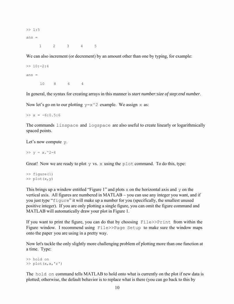
>> 1:5

ans =

1 2 3 4 5

We can also increment (or decrement) by an amount other than one by typing, for example:

>> 10:-2:4

ans =

10 8 6 4

In general, the syntax for creating arrays in this manner is start number:size of step:end number.

Now let’s go on to our plotting y=x^2 example. We assign x as:

>> x = -6:0.5:6

The commands linspace and logspace are also useful to create linearly or logarithmically spaced points.

Let’s now compute y.

>> y = x.^2-4

Great! Now we are ready to plot y vs. x using the plot command. To do this, type:

>> figure(1) >> plot(x,y)

This brings up a window entitled “Figure 1” and plots x on the horizontal axis and y on the vertical axis. All figures are numbered in MATLAB – you can use any integer you want, and if you just type “figure” it will make up a number for you (specifically, the smallest unused positive integer). If you are only plotting a single figure, you can omit the figure command and MATLAB will automatically draw your plot in Figure 1.

If you want to print the figure, you can do that by choosing File>>Print from within the Figure window. I recommend using File>>Page Setup to make sure the window maps onto the paper you are using in a pretty way.

Now let's tackle the only slightly more challenging problem of plotting more than one function at a time. Type:

>> hold on >> plot(x,x,'r')

The hold on command tells MATLAB to hold onto what is currently on the plot if new data is plotted; otherwise, the default behavior is to replace what is there (you can go back to this by

10

typing hold off). The second function simply plots x versus itself in red. The last argument (i.e. item you specify, in this case 'r') to the plot function is a string (i.e. array of characters) where you can pass some parameters to the plotting function. The single quotes is the syntax for telling MATLAB that the r is the character r and not a variable you may have created and named r. In this case, the character r is an optional argument to the plot function that tells MATLAB to draw the plot in the color red (the default color is blue). To really get into all of the various options is complicated (type help plot if you want to see), but if you follow the pattern of the examples here you may not need to get into all of the details.

Now we have two plots in the same window. These plots are lines through the points we have given MATLAB. Now, suppose that we want to show the data points. We can do this by adding two new plots. First, close the previous figure window by using close(#), where # is the figure number, or by clicking the close box on the window itself. Then type:

>> plot(x,y,'o')>> plot(x,x,'ro')

This adds two new plots. The first plots y vs. x using o's at each point. The second plots x vs. x using o's at each point and the color red.

Now let's add some labels to the graph and practice changing the axis limits using the title, xlabel, ylabel, legend, and axis commands. Type:

>> title('First two powers of the integers and half integers') >> xlabel('Integers and half integers')>> ylabel('First two powers')

>> legend('second power','first power')>> axis([-6 6 -10 50])

If you would like more help on the syntax of any of these commands, type help commandname.

In this course, you will often be interested in putting more than one plot in a window for clarity and to save paper. This is where the subplot command comes in. Close the window you have been working in and now type:

>> figure(1) >> subplot(2,1,1) >> plot(x,y,'o') >> title('Integers and half integers squared') >> subplot(2,1,2) >> plot(x,x,'o') >> title('Integers and half integers')

subplot allows you to define an MxN matrix of plotting panels within a figure, where M=the number of rows of plotting panels within the figure (first argument of the function), N=the number of columns of plotting panels (second argument), and the third argument describes which plotting panel to draw in presently. Above, we have defined a 2x1 matrix of plotting panels, and plotted x vs. y in the 1st one and x vs. x in the 2nd one. For subplotting MATLAB indexes linearly by row. Note that we specify the title after calling the subplot and plot

11

commands.

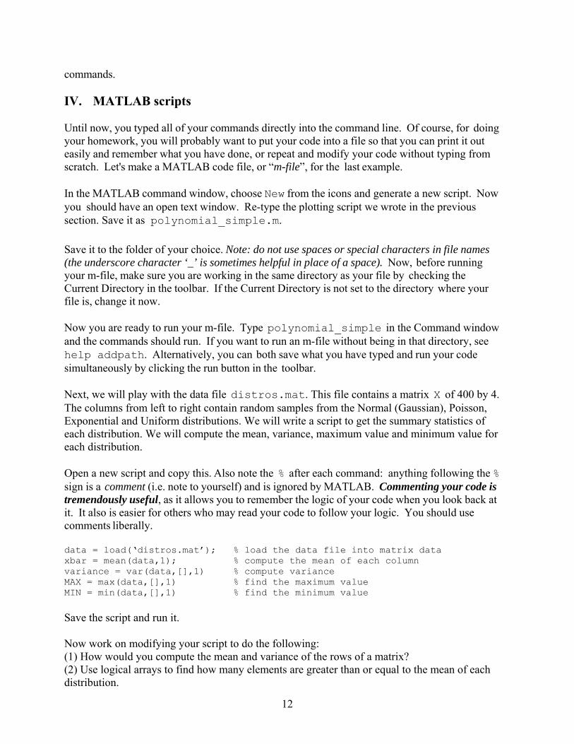
IV. MATLAB scripts

Until now, you typed all of your commands directly into the command line. Of course, for doing your homework, you will probably want to put your code into a file so that you can print it out easily and remember what you have done, or repeat and modify your code without typing from scratch. Let's make a MATLAB code file, or “m-file”, for the last example.

In the MATLAB command window, choose New from the icons and generate a new script. Now you should have an open text window. Re-type the plotting script we wrote in the previous section. Save it as polynomial_simple.m.

Save it to the folder of your choice. Note: do not use spaces or special characters in file names (the underscore character ‘_’ is sometimes helpful in place of a space). Now, before running your m-file, make sure you are working in the same directory as your file by checking the Current Directory in the toolbar. If the Current Directory is not set to the directory where your file is, change it now.

Now you are ready to run your m-file. Type polynomial_simple in the Command window and the commands should run. If you want to run an m-file without being in that directory, see help addpath. Alternatively, you can both save what you have typed and run your code simultaneously by clicking the run button in the toolbar.

Next, we will play with the data file distros.mat. This file contains a matrix X of 400 by 4. The columns from left to right contain random samples from the Normal (Gaussian), Poisson, Exponential and Uniform distributions. We will write a script to get the summary statistics of each distribution. We will compute the mean, variance, maximum value and minimum value for each distribution.

Open a new script and copy this. Also note the % after each command: anything following the % sign is a comment (i.e. note to yourself) and is ignored by MATLAB. Commenting your code is tremendously useful, as it allows you to remember the logic of your code when you look back at it. It also is easier for others who may read your code to follow your logic. You should use comments liberally.

data = load(‘distros.mat’); % load the data file into matrix data xbar = mean(data,1); % compute the mean of each columnvariance = var(data,[],1) % compute varianceMAX = max(data,[],1) % find the maximum value MIN = min(data,[],1) % find the minimum value

Save the script and run it.

Now work on modifying your script to do the following: (1) How would you compute the mean and variance of the rows of a matrix? (2) Use logical arrays to find how many elements are greater than or equal to the mean of each distribution.

12

(3) Compute the median and mode of each distribution.

Aside on manipulating matrices:

Next, suppose that we want to manipulate just one column (i.e. one of the distributions) of the supplied data. We can type in the command window:

>> distro1 = data(:,1);

The colon is MATLAB shorthand notation for 1:1:end. The column vector distro1 will have all the elements of the first column of data.

Similarly we might want to work with a single sample from all distributions:

>> sample4 = data(4,:);

will retrieve the 4th sample of each distribution.

Now, try:

>> S = data(:);

This will generate a long column vector (1600 x 1 in this case) where the columns of data are appended to each other. Thus, here the colon is MATLAB shorthand notation for all elements concatenated column wise.

Next, I want to introduce you to two very useful MATLAB commands: repmat and reshape. The first one allows us to make copies of a vector or a matrix:

>> Z = repmat(sample4,4,1);

This will create a 4 by 4 matrix where each row is a copy of the vector sample4.

The second command allows us to change the shape of a given matrix. Take into account that MATLAB picks the elements from the original matrix column wise. Let’s see an example:

>> Z = reshape(data,100,16);

The output matrix will have the same number of elements as the original matrix being reshaped.

Let’s go back to our script. Sometimes we want to subtract the mean of the distribution from each sample. This will generate data with zero mean (this is sometimes referred as centering the variables).

Use repmat in your code to center (by mean subtraction) the supplied data, add the required lines to your script and save the centered data to matrix DataCentered. Check that DataCentered has a mean of roughly 0.

13

V. Functions, how to generalize scripts

MATLAB has many built-in functions that allow many operations to be carried out in a single line. You just learned a few (e.g. size(matrix) and plot(vector1, vector2, formatting)). The general format is [output1, output2, .., outputn] = function_name(arguments) with the appropriate function name and arguments. For example, in this course we will often create an array t of time points:

>> t=1:0.25:6;

Then

>> x=sin(t)

creates a vector of the same size as t, with values of the sine of t at each point. (Try plotting x=sin(t) vs. t to check this out.)

Here is another useful one:

>> y=zeros(1,5)

The zeros function assigns to the variable y a 1 x 5 array of zeros. A similar useful function is ones.

This is all very interesting, but sometimes we need to write functions to perform tasks that MATLAB does not provide functions for. An example of this is data centering (mean subtraction) discussed in the previous section.

In this section we will show you how to write a function. The proposed function looks like this:

function centeredData = centering (Data)% centers the data contained in the input matrix so that% it has a mean value of 0

[r,c]=size(Data);xbar = mean(Data,1);Z = repmat(xbar,r,1);centeredData = Data - Z;end

The first line defines the function centering which has a single input (Data) and a single output (centeredData). Then there are comments and the body of commands for the function. The function always closes with an end. It is convenient to save the function as an m-file with the same name as the function (in this case centering.m). The calculations inside a function are private to that function. Only the defined outputs can be transferred to other scripts or functions.

Run this function on the distribution data. You should see that after running your function your workspace does not have the variables, r, c, xbar and Z. This is the meaning of private.

14

Exercise: Write a new function that subtracts the mean and divides each element by the corresponding group standard deviation. MATLAB has a built in function for this called zscore. Check if your function provides the same results on the given data set.

VI. More data visualization with MATLAB

Making histograms and fitting data:

Let’s continue with the distributions data set. We will select the column that follows a normal distribution and make a histogram to visualize the shape of the distribution. To make the histogram we will create 30 contiguous bins:

data = load (‘distros.mat’); X = data(:,1); m = floor(min(X)); % round to lower integer close to minimum M = ceil(max(X)); % round to larger integer close to maximum numBins = 20; bins = m:(M-m)/(numBins-1):M; % 20 linearly spaced bins

Next we will use the function histc to count the number of events falling in each bin and plot the histogram using bar: counts = histc(X, bins); % produce the counts for each binbar(bins, counts./sum(counts), 'histc'); % plot bar graph % Notice that we have normalized it, so that the sum of the counts is 1

Next, let’s use MATLAB curve fitting capabilities to estimate a normal distribution to the data we have. This is done with the command fitdist: pd=fitdist(X,'Normal'); Go to the workspace and double click on the object pd. The variable editor will pop up and you will have access to the fitted parameters, in this case the mean and standard deviation of the Normal distribution. With the fitted parameters we need to construct a Normal curve, to do so we use the command pdf: Ncurve = pdf(pd,bins);plot(bins, Ncurve);

Now make a figure that overlays the histogram with the fitted curve.

Exercise: Make histograms of the other distributions.

MATLAB has many more plotting capabilities that you will experiment with in the course.

15

VII. Logical structures: loops, the if statement, and logical operators

for loops:

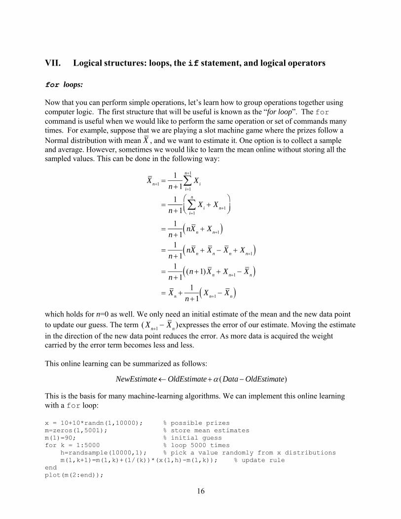
Now that you can perform simple operations, let’s learn how to group operations together using computer logic. The first structure that will be useful is known as the “for loop”. The for command is useful when we would like to perform the same operation or set of commands many times. For example, suppose that we are playing a slot machine game where the prizes follow a Normal distribution with mean X , and we want to estimate it. One option is to collect a sample and average. However, sometimes we would like to learn the mean online without storing all the sampled values. This can be done in the following way:

1 n1

X n1 n 1 Xi i1

n1 Xi

X n 1 i1

n1

1 nX X n n1n 1

n

1

1nX X X X n n n n1

1 (n 1) X X X n n1 nn 1

X X X n n1 nn

1

1

which holds for n=0 as well. We only need an initial estimate of the mean and the new data point to update our guess. The term ( X X )expresses the error of our estimate. Moving the estimate

n1 n

in the direction of the new data point reduces the error. As more data is acquired the weight carried by the error term becomes less and less.

This online learning can be summarized as follows:

NewEstimate OldEstimate (Data OldEstimate)

This is the basis for many machine-learning algorithms. We can implement this online learning with a for loop:

x = 10+10*randn(1,10000); % possible prizesm=zeros(1,5001); % store mean estimates m(1)=90; % initial guess for k = 1:5000 % loop 5000 times

h=randsample(10000,1); % pick a value randomly from x distributionsm(1,k+1)=m(1,k)+(1/(k))*(x(1,h)-m(1,k)); % update rule

end plot(m(2:end));

16

In this case I stored the estimates for plotting but this is not necessary. Run the script and check the results.

The above example also illustrates the syntax of a for loop, namely the first line of a for loop is “for variable = vector”, the last line is “end”, and the in-between lines are the commands to be executed over and over again, once for each element of the vector.

Specifically, what the for loop does is:

1. Assign the variable (e.g. k) to equal the first element of vector (e.g. 1 if the vector is [1 2 … 5000]).

2. Execute all lines following the “for variable = vector” line and before the “end” line.

3. “Loop” back to the beginning, now assigning variable (e.g. k) to equal the 2nd element of vector (e.g. 2 in the example above), and again execute all lines before the “end” line.

4. Keep looping through the elements of vector until all values have been used. When the last element of vector (e.g. 5 in the example above) has been assigned to variable and the lines before the “end” line have been executed, the loop is finished executing.

Another example of using for-loops is when computing derivatives numerically. Let’s consider the function f (t) cos(2t) . Then the derivative can be calculated as follows:

df f (t t) f (t)f (t) lim

dt t0 t

If t is sufficiently small we can numerically approximate the derivative in this way:

dt = 0.01; % approximation for Delta tt = -1:dt:1; % time vector m = numel(t); % number of elements time vector f = cos(2*pi*t); % function to be numerically differentiateddfdt = zeros(m-1,1); % vector for storing derivativesfor k = 1 : m-1

dfdt(k,1)=(f(k+1)-f(k))/dt; % update formulaend

Next plot the results and compare to the analytical solution.

Note: Sometimes you may find that you have made a mistake where the computer appears to freeze because it is looping through a near-infinite number of iterations of a for loop (or appears to freeze for some other reason you cannot figure out!). If this happens, you can interrupt your simulation and return to the prompt in the Command window by typing CTRL-C.

if statement:

The other most useful logical operation is the “if” statement. Try:

17

for A=1:5 if (A > 3)

A end % end of if statement

end

% end of for loop

This program steps through the values in the array 1:5 and, if the value of A during the current step is greater than 3, prints this value of A. Note that for loops and if statements always need to be concluded with an end statement.

Boolean (true or false) logic:

Often we simply want to know if something is true or false. MATLAB denotes true by the integer 1 and false by the integer 0. For example, try:

>> a = 1:6; >> b = (a>2)

The above line assigns to b a vector of the same size as a with 0’s (false’s) and 1’s (true’s) designating whether that element of a is greater than 2. Remember that you can also do < (less than), <= (less than or equal to), >= (greater than or equal to), == (equal to) and ~= (not equal).

Next try:

>> a(b) = -1

a =

1 2 -1 -1 -1 -1

Now, let’s add a bit more logic to our loop. Revise your m-file to read:

clear s; % clears the variable s out of memory for A=1:5 if (A > 3)

A % print out the value of A elseif (A==3) % note syntax: “A equals 3” is denoted by a double equal sign!

% The single “=” is used for assigning values to variables. % Confusing these is one of the easiest ways to have an error

% in your code! s = ‘hello’ % to print and/or assign a text string, put it inside single

% quotation markselse % A equals 1 or 2

-A % print out negative of the value of A end % end of if statement

end % end of for loop

Can you predict what this will output? Try it out by saving this file (always remember to save before running your code – this is a common error!) and running it. The if… elseif… else structure is useful for going through logic. The elseif or else can be omitted if not needed. Type help if for more information.

18

The clear s statement at the beginning of this script removes any information that might have been in the variable s from the computer’s memory (e.g. if you had previously assigned a variable s earlier in your MATLAB session). You should always clear all variables from the computer’s memory before starting a new program. Usually, it is simplest to just type clear all, which removes all variables from memory, at the top of your m-file. To close all open windows (so that you do not end up with plots from old runs appearing in your new figures), type close all – to be safe, I recommend putting clear all and close all at the top of all m-files you write.

while loop:

Another type of loop, similar to the for loop, is called the while loop. If you are interested, you can get more information about this by typing help while at the command prompt.

VIII. Getting help

Learning to use MATLAB help is an essential part of programming in MATLAB, as MATLAB has far more commands than can be contained in any single book. There are many places to get help for MATLAB. Some of them are:

1. Typing help commandname where commandname designates the command you want to know the syntax for. Alternatively (I prefer this one), type doc commandname which brings up the much prettier MATLAB help window.

2. You can also bring up MATLAB’s help/search engine by typing doc at the command line or by clicking on “Help>>MATLAB (or Product) Help” in the main MATLAB window. Type words you are looking for into the “Search” box (in the left pane of this window) or you can try to look through “Contents”. In my experience, “Search” is much better than the lookfor command.

3. Lots of resources can be found by browsing the web, including the Mathworks website.

19

MIT OpenCourseWarehttps://ocw.mit.edu

Resource: Brains, Minds and Machines Summer CourseTomaso Poggio and Gabriel Kreiman

The following may not correspond to a particular course on MIT OpenCourseWare, but has beenprovided by the author as an individual learning resource.

For information about citing these materials or our Terms of Use, visit: https://ocw.mit.edu/terms.