Organizational Structure and Pricing: Evidence from a

Organizational Structure and Pricing:

Evidence from a Large U.S. AirlineAli Hortaçsu, University of Chicago and NBER

Olivia R. Natan , University of California, Berkeley

Hayden Parsley, University of Texas, Austin

Timothy Schwieg, University of Chicago, Booth

Kevin R. Williams, Yale School of Management and NBER*

November 2021

Abstract

We study how organizational boundaries affect pricing decisions using compre-hensive data provided by a large U.S. airline. We show that contrary to prevailingtheories of the firm, advanced pricing algorithms have multiple biases. To quantifythe impacts of these biases, we estimate a structural demand model using sales andsearch data. We recover the demand curves the firm believes it faces using forecastingdata. In counterfactuals, we show that correcting biases introduced by organizationalteams individually have little impact on market outcomes, but addressing all biasessimultaneously leads to higher prices and increased dead-weight loss in the marketsstudied.

JEL Classification: C11, C53, D22, D42, L10, L93Keywords: Pricing Frictions, Organizational Inertia, Dynamic Pricing, Revenue Man-agement, Behavioral IO

*The views expressed herein are those of the authors and do not necessarily reflect the views of theNational Bureau of Economic Research. We thank the anonymous airline for giving us access to the dataused in this study. Under the agreement with the authors, the airline had "the right to delete any trade se-cret, proprietary, or Confidential Information" supplied by the airline. We agreed to take comments in goodfaith regarding statements that would lead a reader to identify the airline and damage the airline’s repu-tation. All authors have no material financial relationships with entities related to this research. We alsothank the seminar participants at Yale University, University of Virginia, Federal Reserve Bank of Minneapo-lis, University of Chicago, University of California-Berkeley, the NBER 2021 Summer Institute, and theVirtual Quantitative Marketing Seminar for comments. We gratefully acknowledge financial support fromthe NET Institute, www.NETinst.org. Emails: [email protected], [email protected], [email protected], [email protected], [email protected]

1 Introduction

Dramatic decreases in the cost of computation and data storage, along with algorithmic

innovations, have increasingly allowed firms to develop data-driven decision optimization

systems. Data and algorithms now play a key role in driving firm decisions across indus-

tries. This is especially relevant in the airline context where firms must match fixed flight

capacity with dynamically evolving demand. To solve this difficult allocation problem,

airlines have developed sophisticated pricing systems over the last several decades. These

systems depend on inputs from multiple organizational teams. How airlines allocate deci-

sion rights across teams within the firm is not unique to the industry. Hotels, cruises, car

rentals, entertainment venues, and retailers have all adopted features of the airline pricing

model. Given the investments firms have made into these decision machines and their wide

use across industries, we may expect that prices are close to optimal.

In this paper, we study how organizational boundaries affect pricing decisions by lever-

aging a data partnership with a large international air carrier based in the United States.1

The granularity of the data allow us to understand the firm’s incentives to adjust prices

without needing to assume prices are optimally set. We show that contrary to prevalent

theories of the firm, the pricing at a sophisticated firm—one that employs advanced opti-

mization techniques and has a heavy reliance on automation—does not appear to react to

some important market fundamentals. This includes not internalizing consumer substitu-

tion to other products, using persistently biased forecasts, and not responding to changes in

opportunity costs driven by scarcity. We show that these biases are introduced by separate

teams within the firm. What happens to prices and allocative efficiency if organizational

teams address the pricing frictions that we document? Using a new technique to estimate

demand and detailed forecasting data to infer the firm’s beliefs about the demand it faces,

we find that correcting pricing frictions introduced by teams individually does little to af-

fect market outcomes. However, we also show that addressing biased introduced across

organizational teams simultaneously can result in increased price targeting and higher rev-

1The airline has elected to remain anonymous.

1

enues, but also higher dead-weight loss for the routes studied. Our results highlight how

non-coordinating teams with complementary functions can have significant consequences

on firm performance.

We begin by providing an empirical glimpse under the hood of dynamic pricing so-

lutions used by airlines. In addition to observing prices and quantities, we also observe

granular demand forecasts, output of the pricing and allocation algorithms, the optimiza-

tion code itself, and clickstream data that detail all consumer interactions on the airline’s

website. The core data cover hundreds of thousands of flights spanning hundreds of domes-

tic origin-destination pairs. We document the main organizational details of how pricing

decisions are made within the firm and provide insights on the incentives to adjust prices

over time in Section 2 and Section 3, respectively. We show that all major airlines have

similar organizational structures. Therefore, we believe our discussion and subsequent em-

pirical findings likely hold for the airline industry broadly and perhaps for other industries

that have adopted similar pricing technologies and organizational structures.

In Section 4, we discuss data patterns that suggest the airline could be doing more with

its data. We show that prices do not necessarily adjust when the value of remaining capacity

changes. This is caused by coarse pricing, or the use of “fare buckets." However, the fact

opportunity costs may adjust by hundreds of dollars without triggering a price adjustment

suggests a mismatch between the fares chosen by one organizational team and demand

fundamentals. We establish that the forecasts maintained by a separate team respond to

demand “surprises” too little and too late. These demand forecasts are biased upward in

two years of data. We establish that the pricing algorithm itself is biased by showing that

cross-price elasticities are not considered when setting prices. Finally, we show that the

firm chooses prices on the inelastic side of the demand curve—according to their own

estimates of demand—in more than half of the data sample.

In the second stage of our analysis, we quantify the impacts of these observed pricing

frictions on welfare. To do this, we estimate a structural model of consumer demand using a

recently proposed demand methodology (Hortaçsu, Natan, Parsley, Schwieg, and Williams,

2021). In Section 5, we consider a model in which “leisure” and “business” travelers

2

arrive according to independent and time-varying Poisson distributions in discrete time.

Consumers know their preferences and solve discrete choice maximization problems. Each

consumer chooses among the available flight options or an outside option. We provide

evidence to motivate some of our demand assumptions, including that consumers do not

appear to be betting on price and consumer arrivals are not endogenous to price.

We estimate the model using consumer search and bookings data. Aggregate search

counts calculated from the clickstream data inform the overall arrival process, and we

identify the price coefficient using instrumental variables (see Section 6). The estimates

presented in Section 7 reveal meaningful variation in demand, with a general increase in

search for travel as the departure date approaches and substantial changes in the overall

price sensitivity of consumers over time. We discuss similarities and differences in model

estimates across routes.

Given the demand estimates, we then ask: what does the firm believe its demand curves

look like? We call these “firm beliefs” and we recover them in Section 8 using detailed

forecasting data and output from an algorithm that classifies search and bookings as coming

from a “leisure” or “business” traveler. Relative to our baseline demand estimates, we find

that the firm’s beliefs about their demand has more compressed demand elasticities both

within and across routes, more elastic demand near departure, and consumer types that

are “closer together" in terms of preferences. Using these recovered demand curves, we

confirm our descriptive finding that prices are often too low: nearly 30% of observed prices

are below the optimal price if capacity costs were zero.

In Section 9, we perform counterfactual exercises using a pricing model that closely fol-

lows the heuristic the firm uses. First, we isolate pricing frictions individually—removing

forecast bias and mismatched fare choices to the forecast, separately. We show that out-

comes are largely unchanged because the pricing heuristic commonly defaults to the lowest

filed fare because it expects that future demand can be satisfied with remaining capacity.

However, we also show internalizing complementarities across teams—correcting the fore-

cast and inputting fares into the algorithm tailored to this forecast—yields very different

outcomes. Coordination guarantees that fares never drop below the optimal price if capac-

3

ity costs were zero. This raises the distribution of fares offered and allows the firm to target

business travelers with higher fares. Revenues increase substantially—upward of 17% for

some markets. Dead-weight loss also increases by over 10%. The fact that that the firm

could extract additional surplus but has chosen not to do so is puzzling. We argue that this is

possible due to under-experimentation across organizational teams that we quantify in the

data. We also hypothesize the firm may consider the implicit cost of regulatory oversight

or long-term competitive responses as alternative explanations.

1.1 Related Literature

This paper contributes to a growing literature in behavioral industrial organization that ex-

amines pricing frictions, including DellaVigna and Gentzkow (2019) and Hitsch, Hortaçsu,

and Lin (2021) in retailing, Huang (2021) in peer-to-peer markets, Ellison, Snyder, and

Zhang (2018) in online retailing, and Cho and Rust (2010) in rental cars. We confirm pric-

ing frictions also impact firms that have pioneered advanced pricing algorithms. Our work

also contributes to research on miscalibrated firm expectations, as forecasts are persistently

biased (Massey and Thaler, 2013; Akepanidtaworn, Di Mascio, Imas, and Schmidt, 2019;

Ma, Ropele, Sraer, and Thesmar, 2020). Dubé and Misra (2021) provide an example where

a firm has not priced optimally and pricing to the correct demand curve greatly increases

revenue. In our setting, pricing to the correct demand curves is insufficient to greatly impact

revenues if other pricing frictions are not addressed.

Our work also contributes to the literature in organizational economics. The adoption

of information technology (IT) can increase productivity when complementary organiza-

tional and management practices are implemented alongside these investments (Bresnahan,

Brynjolfsson, and Hitt, 2002; Bloom, Sadun, and Van Reenen, 2012).2 Although Athey

and Stern (2002) do not find strong complementarities in one IT setting, we find substantial

complementarities in the context of pricing algorithms. Our work complements empirical

research on the impacts of decentralized-decision making on firm performance (Aguirre-

gabiria and Guiton, 2020; Filippas, Jagabathula, and Sundararajan, 2021) and theoretical2Brynjolfsson and Milgrom (2012) provide an overview of this and related work.

4

work on the inputs to organizational teams, including Che and Yoo (2001), Siemsen, Bala-

subramanian, and Roth (2007), Alonso, Dessein, and Matouschek (2008, 2015).

Finally, this paper quantifies the effectiveness of pricing heuristics proposed in op-

erations research using airline data (Littlewood, 1972; Belobaba, 1987, 1989; Brumelle,

McGill, Oum, Sawaki, and Tretheway, 1990; Belobaba, 1992; Wollmer, 1992). Additional

work on the welfare consequences of dynamic pricing include Sweeting (2012); Cho, Lee,

Rust, and Yu (2018); Hendel and Nevo (2013); D’Haultfœuille, Février, Wang, and Wilner

(2020); Castillo (2019); Aryal, Murry, and Williams (2021); and Williams (forthcoming).

2 Organizational Structure and Division Responsibilities

We study the US airline industry, an industry that directly supports over two million jobs

and contributes over $700 billion to the US economy.3 In 2019 alone, 811 million passen-

gers flew within the United States.4. In addition to being an important industry in its own

right, airlines have influenced the development of pricing technologies that are now used in

other sectors—for example, in hospitality, retailing, and entertainment and sports events.

Although the sophistication of these technologies has improved, many of the original yield

management ideas described in McGill and Van Ryzin (1999) and Talluri and Van Ryzin

(2004) remain in place today.

Fares at our air carrier depend on the actions of managers in several distinct depart-

ments, and these departments do not explicitly coordinate their actions. Generally, deci-

sions become increasingly granular, taking all previous departments’ decisions as given.

First, network planning decides the network, flight frequencies, and capacity choices. Sec-

ond, the pricing department sets a menu of fares and fare restrictions for all possible

itineraries. Finally, the revenue management (RM) department decides the number of seats

to sell for every fare-itinerary combination.

The RM group maintains the demand forecasting model and pricing algorithm, but does

3See https://www.iata.org/en/iata-repository/publications/economic-reports/the-united-states–value-of-aviation/. July 1, 2021.4See https://www.bts.gov/newsroom/2019-traffic-data-us-airlines-and-foreign-airlines-us-flights-final-full-year. July 1, 2021.

5

not have control over the fares inputted into these algorithms. The pricing department sets

fares, but does not use the forecasting information.5 The forecasting model incorporates

historical information and current bookings information to predict flight-level sales. The

pricing algorithm allocates remaining inventory given the fare menu. A commonly used

pricing heuristic in the industry is Expected Marginal Seat Revenue (EMSR-b), which

closely approximates the algorithm used by the firm. We provide additional details of

the EMSR-b in Online Appendix A and outline the algorithm here. EMSR-b belongs to a

class of static optimization solutions. Dynamics are removed because it assumes all future

demand will arrive tomorrow. The key trade-off, therefore, is to offer seats today versus

reserve them for tomorrow. Given all pricing inputs, it calculates the opportunity cost of

a seat and then assigns the number of seats it is willing to sell at all price levels. Lowest

priced units are assumed to sell first. If expected future demand is high (low), it will restrict

(not restrict) inventory at lower prices today.

Figure 1: Fare Bucket Availability and Lowest Available Fare

020406080100120Days Before Departure

Bucket1Bucket2Bucket3Bucket4Bucket5Bucket6Bucket7Bucket8Bucket9

Bucket10Bucket11Bucket12

Fare

Buc

ket

Lowest Available Price

Note: Image plot of fare availability over time as well as the active lowest available fare. Bucket1 is the least expensive; Bucket12 isthe most expensive fare class. The color depicts the magnitude of prices—blue are lower fares, red are more expensive. White spacedenotes no fare availability. The white line depicts the lowest available fare.

We demonstrate how inputs impact prices for an example flight at our airline in Fig-

ure 1. On the vertical axis, we show the anonymized fare buckets decided by the pricing

5Each filed fare contains an origin, destination, filing date, class of service, routing requirements, andother ticket restrictions. A common fare restriction decided by the pricing department is an advance purchasediscount, which specifies an expiration date for a discounted fare to be purchased by. These discounts arecommonly observed seven, 14, and 21 days before departure.

6

department, with bucket one being the least expensive and bucket twelve being the most

expensive. The bottom right of the graph shows that the pricing department restricts the

availability of the lowest fares close to the departure date. There is relatively little variation

in prices for a given bucket over time. Given fares and the forecast (not shown), the white

line marks to lowest available price (LAP) offered to consumers. This is an output of the

algorithm maintained by the RM group. All flights, regardless of market structure, flight

frequencies, etc., are priced using the same algorithm.

2.1 Potential Pricing Bias with Uncoordinated Inputs

Pricing heuristics can be sensitive to algorithm inputs. To see this, consider a firm selling

15 units over two sequential markets. Demand in the first period is equal to Q1(p1) =

10− 10p1, and demand in the second period is Q2(p2) = 10− p2. If the firm maximizes

total revenues subject to the capacity constraint, the capacity constraint will not bind, and

optimal prices are equal to (p1, p2) = (0.5, 5). This outcome can be also obtained using the

pricing and revenue management roles and the pricing algorithm EMSR-b described above

if the pricing department assigns prices to be {0.5, 5} and {5}, and the RM group “forecasts”

demand to be the functions above.

EMSR-b decides the number of seats that can be sold at each input price to ensure

that future demand can be satisfied. Lower prices are restricted only in situations where

future demand cannot be satisfied. In this case, five seats are needed for period two, and

the algorithm will appropriately allocate all seats to 0.5 in the first period. Suppose instead

that the pricing department did not coordinate with the RM group and set prices equal to

{.2, .5, 5} and {5}. Note that all first-period prices leave sufficient capacity available for

the second period, which means EMSR-b will allocate all seats at the lowest price, 0.2.

Consequently, the heuristic will choose a suboptimal price even though the optimal price,

0.5, is included in the choice set.

7

2.2 All US Airlines have the same Organizational Structure

Our description of airline pricing is not unique to our airline—all airlines have the same

organizational structure and use similar pricing techniques. We show this by collecting job

postings information for all the major carriers in the U.S.6 We confirm that Alaska, Ameri-

can, Delta, JetBlue, Southwest, and United have a network planning, pricing, and revenue

management department. As an example, JetBlue Airlines job postings show that the firm

has three teams related to pricing: Future Schedules, Revenue Management-Pricing, and

Revenue Management-Inventory. Job details delineate team responsibilities. The Rev-

enue Management department at JetBlue has two separate teams, Pricing and Inventory.

The Pricing team has ownership over fares by “monitoring industry pricing changes filed

through a clearinghouse throughout the day, and determining and executing JetBlues re-

sponse.”7 The Inventory team uses “inventory controls to determine the optimal fare to sell

at any given moment in time to maximize each flights revenue.”8 American Airlines man-

agers describe how inventory controls are implemented in Smith, Leimkuhler, and Darrow

(1992)—they outline EMSR-b. Because all carriers have the same organizational structure

and use similar algorithms, we believe our analysis characterizes the entire industry, rather

than the perspective from a single firm.

3 Data and Summary Analysis

We use data provided by a large international air carrier based in the United States. To

maintain anonymity, we exclude some data details. In Online Appendix B, we describe our

route selection criteria.6Screenshots of the job postings are available on request.7See https://careers.jetblue.com/job/Long-Island-City-Analyst-Revenue-Management-NY-11101/737962800/. July 1, 2021.8See https://careers.jetblue.com/job/Long-Island-City-Analyst-Revenue-Management-NY-11101/737962800/. July 1, 2021.

8

3.1 Data Tables

We combine several data sources, which we commonly refer to as: (1) bookings, (2) inven-

tory, (3) search, (4) fares, and (5) forecasting data.

(1) Bookings data: The bookings data contain details for each purchased ticket, re-

gardless of booking channel, e.g., the airline’s website, travel agency, etc. Key variables

included in these data are the fare paid, the number of passengers involved, the particular

flights included in the itinerary, the booking channel, and the purchase date.9 Our analysis

concentrates on nonstop bookings and economy class tickets.

(2) Inventory data: The inventory data contain the decisions made by the RM group.

Inventory allocation is conducted daily. The data include the number of seats the airline is

willing to sell for each fare class in economy and aircraft capacity. We also observe output

from the pricing algorithm, including the opportunity cost of a seat.

(3) Search data: We observe all consumer interactions on the airline’s website for two

years. The clickstream data include search actions, bookings, and referrals from other

websites. Tracking occurs regardless as to whether an individual has a consumer loyalty

account or is logged in.

(4) Filed fares data: The filed fares data contain the decisions made by the airline’s

pricing department. A filed fare contains the price, fare class, and all ticket restrictions,

including any advance purchase discount requirements.

(5) Forecasting data: The air carrier forecasts future demand at granular levels. We

observe these predictions down to the flight-passenger type-price level. In addition to the

baseline forecast, we also observe all managerial adjustments to the forecasts.

3.2 Data Summary

Table 1 provides a basic summary of the nearly 300,000 flights in our cleaned sample. We

focus on the last 120 days before departure due to the overwhelming sparsity of search and

sales observations earlier in the booking horizon.

9We document facts using nonstop bookings, however, our measure of remaining capacity adjusts for alltickets sold, e.g., connections, reward tickets, and consumers altering tickets, etc..

9

Table 1: Summary Statistics

Data Series Variable Mean Std. Dev. Median 5th pctile 95th pctile

FaresOne-Way Fare ($) 201.3 139.4 163.3 88.0 411.1Num. Fare Changes 9.3 4.2 9.0 3.0 17.0Fare Changes | Inc. 50.4 73.0 31.2 2.2 164.5Fare Changes | Dec. -53.0 75.5 -32.2 -175.2 -4.3

BookingsBooking Rate-OD 0.2 0.7 0.0 0.0 1.0Booking Rate-All 0.6 1.4 0.0 0.0 3.0Load Factor (%) 82.2 21.4 90.0 36.0 102.0

SearchesSearch Rate 1.9 4.8 0.0 0.0 9.0

Summary statistics for the data sample. Fares are for nonstop flights only. The initial load factor is the percentage of the number of seatsoccupied 120 days before departure. The booking rates are for non-award, direct travel on nonstop flights and for all traffic on nonstopflights, respectively . The number of passengers denotes the number of passengers per booking. The ending load factor includes allbookings, including award and connecting itineraries. The search rate is for origin-destination queries at the daily level. The number ofpassengers is the number of passengers per request.

Average flight fares in our sample are $201, with large dispersion across routes and

over time. Typically, prices for a particular flight adjust nine times and double in 120 days.

Many adjustments occur at specified times, such as after expiration of advance purchase

discount opportunities. However, over 60% of price adjustments occur before the first AP

fares expires. This is because inventory (and therefore, prices) is re-optimized daily.

In our sample, the average load factor is 82.2%.Although overselling is possible, we

abstract from this possibility because we do not observe denied boarding/no show infor-

mation. Our notion of capacity will be actual plane capacity plus the number of seats the

airline is willing to sell over capacity (if any)—the observed “authorized” capacity.

3.3 Empirical Facts that Motivate Demand Assumptions

We summarize search and purchase patterns to motivate some of our demand assumptions.

The bookings data suggest that unit demand is a reasonable assumption. The average

passengers per booking is 1.3. In addition, the bookings data confirm that overwhelmingly,

consumers purchase the lowest available fare even though several fares may be offered at

any point in time. We find that 91% of consumers purchase the lowest available fare. Using

10

a separate data base that contains an indicator for corporate bookings under special fares,

we find that corporate discounts are not a concern for the routes studied.

Bookings and searches are sparse, which motivates using a model model that accounts

for low daily demand. 60-80% of observations involve zero observed searches. The fraction

of zero sales is even higher (80% zeros). Zeros are not just present because we focus on

nonstop demand. The fraction of zero sales for any itinerary involving a particular flight

ranges between 40-80%.

We adopt a two-type consumer model, corresponding to “leisure” and “business” travel-

ers, because that is how the firm considers demand. The airline maintains separate forecasts

for these consumer types, and an algorithm classifies every search and booking into these

two categories.10 We explore the predictions of this algorithm in Section 8.

Figure 2: Search and Booking Facts to Motivate Demand Model(a) CDF of Same Itin. Searches

0 2 4 6 8 10Number Re-Searching Same Itnerary

0.0

0.2

0.4

0.6

0.8

1.0

CD

F

(b) CDF of Similar Itin. Searches

0 2 4 6 8 10Number DDs Searched for a Given OD

0.0

0.2

0.4

0.6

0.8

1.0

CD

F

(c) Channel Booking Distributions

020406080100120Days From Departure

0.00.51.01.52.02.53.03.54.0

Perc

enta

ge o

f Boo

king

s DirectOTAsAgency

(a) Empirical CDF of the number of days from departure searchers appear for a given itinerary. (b) Empirical CDF of the number ofdeparture dates a given searcher looks for. (c) Percentage of Bookings, across days from departure, for each Channel. Direct refersto bookings that occur on the air carrier’s website, OTAs is purchases made on online travel agencies, and Agency are bookings madethrough travel agencies.

Figure 2-(a) and (b) motivate our assumption that consumers solve static optimization

problems. We investigate the tendency for consumers to return to search for tickets for con-

sumers who were not referred to the airline from other websites. Panel (a) shows the CDF

of number of times that consumers search for the same itinerary across days. 90% of con-

sumers search for an itinerary (OD-DD pair) once. Panel (b) shows the CDF for the number

of different departure dates (for the same OD) that consumers search for within a cookie.

10The airline does consider additional types of passengers, but these categorizations are very small relativeto the two we consider. If we observe any searches or sales from other categories, we reassign them to beleisure travelers.

11

82% of customers search a single departure date. The average time lag between searches

for different departure dates is 45 days, which may suggest entirely different purchasing

opportunities (different trips).

Figure 2-(c) motivates adjusting our model for non-observed searches differently over

time. The figure shows the distributions of bookings across booking channels over time.

OTAs, or online travel agencies, closely follows the distribution of bookings via the di-

rect channel. However, the agency curve—which includes corporate travel bookings—is

more concentrated closer to departure. We discuss this adjustment in Section 6.1. Note

that Figure 2-(c) shows some bunching in bookings immediately before advance purchase

opportunities expire. Although this may suggest consumers strategically time their pur-

chasing decisions—they are forward looking—we find evidence that supports certain days

before departure simply have higher demands. Using the search data, we split the sample

into two groups, one that includes routes that never have 7-day AP requirements, and one

that includes these requirements. We find that that search activity (and purchases) bunch at

the 7-day AP requirement, regardless of their existence. Because arrivals increase regard-

less of price changes, we maintain the commonly used assumption that the market size is

not endogenous to price. Instead, we flexibly estimate arrivals as a function of time and the

departure date that allows for this bunching.

4 Pricing Frictions Across Organizational Teams

In this section, we document several pricing frictions that suggests that the firm does not

price optimally.

4.1 Coarse Pricing and Not Responding to All Available Information

Figure 3 demonstrates that the firm has access to, and indeed generates, payoff relevant

information that its pricing algorithms do not respond to. In panel (a), we plot the frac-

tion of flights that experience changes in price or marginal costs (the shadow value on the

capacity constraint as reported by the pricing algorithm) over time. The figure shows that

12

costs change at a much higher frequency than do prices. This occurs because of the in-

dustry practice of using a discrete set of fares (fare buckets). That is, it is possible that

marginal costs change by $1 but the next fare is $20 more expensive. Our analysis suggests

this friction is significantly more important. In panel (b), we run a flexible regression of

the change in costs on an indicator function of a price adjustment occurring. As the figure

shows, changes in marginal costs exceeding $150 only lead to price adjustments with 50%

probability. This may suggest alternative fares could lead to higher revenues.

Figure 3: Fare Adjustments in Response to Opportunity Cost Changes(a) Fare vs. Shadow Price Changes

020406080100120Day From Departure

0

20

40

60

80

100

Perc

enta

ge o

f Flig

hts Changes in Fares

Changes in Shadow Values

(b) Probability of Fare Change

300 200 100 0 100 200 300Change in Shadow Value

0.0

0.2

0.4

0.6

0.8

1.0

Prob

abili

ty

Pr(Fare Change)

Note: (a) The fraction of flights that experience changes in the fare or the opportunity cost of capacity over time. (b) The probability ofa fare change, conditional on the magnitude in the change in the shadow value.

Prices are coarse both within a day and across days. At any point in time, each route

sees roughly a dozen different fare classes (such as the example flight in Figure 1). Over

time, the median number of unique prices used for a particular fare is two (mean is three).

4.2 Reacting to Surprises with Delay

The spikes in Figure 3-(a) occur at seven day intervals because firm reforecasts demand for

future flights on a weekly interval. Outside of these periods, the firm reoptimizes inventory

given the forecast. The firm’s decision not to update their forecasts continuously may

be another source of pricing friction. We demonstrate via an example that information

exists which could improve/tune forecasting models. With the current system, reactions to

“surprises” occur too little and too late. In particular, demand forecasts maintained by RM

13

respond to demand surprises with delay, leading to missed opportunities both for the flight

in question, but also for future flights which are mistakenly thought to be over-(or under-)

demanded.

Figure 4: Reacting to Surprises: A Conference Example(a) Average Load Factor


0

20

40

60

80

100

Load

Fac

tor

t-14t-7Conference Date (t)t+7

(b) Fares


100150200250300350400450

Fare

s

(c) Forecasted Demand


0

50

100

150

200

250

Fore

cast

ed D

eman

d

Note: All plots contain data series for flights departing the date of a large conference (which moves both location and dates each year)and the corresponding flights in the surrounding weeks of the conference. (a) Shows the average load factor across flights (b) Containsthe average lowest available fares across flights (c) Has the average total expected seats to sell at a given point in time unconstrained bythe remaining capacity.

In Figure 4, we show average load factors, fares, and forecasted demand for a particular

route-departure date. This departure date is special because it involves a conference which

alternates both date and location each year. In addition to flights on the conference date, we

include information for flights on this route one week before and after the conference date

for comparison. As shown in panel (a), as soon as the location and date of the conference

is announced, around 200 days from departure, there is a sudden jump in load factor. The

firm’s revenue management software responds with delay (over a month) to the sudden

jump in bookings. Prices eventually increase dramatically as seen in panel (b). Panel (c)

shows that the forecasting algorithm, having observed the conference shock, then inflates

the forecast for the following week—to higher levels than the conference date. That is, the

algorithm incorrectly believes the next week will now also involve a conference. However,

in panel (a) we see that the flights a week later contain no surprises—bookings follow a

similar pattern as other dates. Consequently, fares are too high for the non-conference

flights and too low for a conference flights.

14

4.3 Using Persistently Biased Forecasts

The forecasting model maintained by RM systematically not only reacts to surprises with

delay, it also persistently overstates future demand. We observe biased forecasts over two

years of data. In Figure 5, we plot the firms’ forecast against realized future sales. On av-

erage, the firm’s forecasts are biased upwards from the true distribution of future sales for

nearly the entire booking horizon. For the median observed forecast, the forecast is 10%

higher than the actual future demand, which is equivalent to predicting an extra 2.5 seats

will be sold. The forecast becomes more accurate toward departure because total remain-

ing demand declines. Although the average forecast is biased upward, suggesting prices

may be too high, the forecasts appear misaligned with observed demand at different prices

(panel b). Low-fare transactions are underforecasted by 20%, and high-fare transactions

are overforecasted by 10%. This suggests the forecasting model may not accurately reflect

the actual composition of demand.

Figure 5: Firm Forecasting and Realized Sales(a) Forecasting Bias Time Series


020406080

100120140160

Dem

and

Rem

aini

ng (%

)

Raw Demand ForecastManager Adjusted Demand ForecastRealized Demand

(b) Forecasting Bias over Fare Levels

Low Medium HighFare Levels

20

10

0

10

Fore

cast

Bia

s (%

)

Note: Forecasts and future sales are normalized by the aircraft’s total coach capacity. Plots show 7-day moving average to smooth acrossstrong day of week effects in the forecast sample. (a) Business traveler forecasts and realized sales. (b) Leisure traveler forecasts andrealized sales.

We also observe all managerial adjustments to the forecasts, which is also plotted in

Figure 5-(a). We find that user adjustments improve forecast accuracy, but the improvement

is small in magnitude relative to the total bias.

Forecasts are biased for all routes in the sample. Biases are slightly larger, both in per-

centage terms and in levels, for markets with competition. This may reflect the additional

15

complexity the firm faces when predicting residual demand.

4.4 Not Accounting for Cross-Price Elasticities

Dynamic pricing is computationally and theoretically complicated. Research in operations

research have offered heuristics (including EMSR-b) to solve such models, but this typi-

cally comes at the cost of abstracting from key market features. We show one important

market feature not captured by the pricing algorithm are cross-price elasticities.

Figure 6: Shadow Value and Price Response to Bookings with Multiple Flights(a) Shadow Value

0 2 4 6 8 10 12 14 16 18 20Number Booked for Flight With Bookings

0255075

100125150

Cha

nge

in S

hado

w V

alue Flight with bookings (and 95% CI)

Flight without bookings (and 95% CI)

(b) Prices

0 2 4 6 8 10 12 14 16 18 20Number Booked for Flight With Bookings

0255075

100125150

Cha

nge

in P

rice

Flight with bookings (and 95% CI)Flight without bookings (and 95% CI)

Note: (a) The orange line denotes the average change in shadow value for a flight when a sale at a given intensity occurs. The blue lineis the average change to shadow value when a sale occurs to another flight at a given intensity. (b) This panel depicts the same as panela, but instead of changes in shadow value it depicts changes in price.

To show that pricing does not internalize substitutes, we subsample our data. We extract

observations that satisfy the following conditions: (i) the firm offers two flights a day; (ii)

we include periods where demand is not being reforecasted (the observed as spikes in

Figure 3); (iii) the total daily booking rate is low (less than 0.5); and (iv) one flight receives

bookings and the other flight does not. By considering markets where the total booking rate

is low, the following intuition uses theoretical results in continuous time. In Figure 6-(a),

we plot the average change in shadow values for the flights that receive bookings and for

the flights that do not receive bookings (the substitute option) using flexible regressions.

In standard continuous time dynamic pricing models, every time a unit of capacity is sold,

prices jump, e.g., in Gallego and Van Ryzin (1994). This is also true in environments with

multiple products—any sale causes all prices to increase. Figure 6-(a) confirms substitute

16

opportunity costs are unaffected by bookings. Panel (b) shows there is no price response.

This necessarily means that prices are not directly affected by competitor pricing decisions

in markets with competition.

4.5 Pricing on the Inelastic Side of the Demand Curve

We provide model-free evidence that the firm may be systematically underpricing ac-

cording to its own expectations about demand. This bias is the result of incompatibili-

ties in pricing inputs and the pricing algorithm. We use granular forecasting data (E Q )

that report the expected sales at the level of flight ( j ), departure date (d ), days from de-

parture (t ), forecasting period (s ), and price (p ). The difference between s and t de-

fines how far in advance the forecast is constructed. For this exercise, we select obser-

vations such that s = t . Because we observe the forecast for multiple prices, we calcu-

late the elasticity of demand, [(Q1 −Q2)/Q2]/[(P1 −P2)/P2], using the observed flight price

as the base price along with the next highest price. We also compute the arc elasticity,

[(Q1−Q2)/(Q1+Q2)/2]/[(P1−P2)/(P1+P2)/2].

We find that 34% to 52% of flight observations are priced on the inelastic side of the de-

mand curve using the firm’s forecasting data, depending on how elasticities are computed.

We consider whether differences in managerial ability influence outcomes (Goldfarb

and Xiao, 2011, 2016; Hortaçsu, Luco, Puller, and Zhu, 2019) by comparing the incidence

of pricing on the inelastic side of the demand curve across teams. We observe the identity

of the revenue and pricing analysts involved in managing pricing inputs, and estimate re-

gressions of the form I(elasticity >−1)r,i = X r,iβ +ur,i , where X contains team identifiers

as well as route characteristics. We find statistically significant differences across teams,

however, even the best teams are associated with setting “inelastic prices” 30% of the time.

Higher traffic markets (in terms of nonstop passengers) have a larger percentage of inelas-

tic prices, and single-carrier markets see roughly 5% more frequent inelastic prices than

competitor markets, holding passenger count constant.

17

5 Empirical Model of Air Travel Demand

In order to quantify the impacts of the pricing biases just discussed, we need to estimate

a model of air travel demand. We utilize both the demand model and estimation approach

of Hortaçsu, Natan, Parsley, Schwieg, and Williams (2021). We consider the demand for

nonstop flights for a particular origin-destination pair departing on a particular departure

date. The definition of a market is an origin-destination (r ), departure date (d ), and day

before departure (t ) tuple. The booking horizon for each flight j leaving on date d is

t ∈ {0, ..., T }. The first period of sale is t = 0, and the flight departs at T . In each of the

sequential markets t , arriving consumers choose flights from the choice set J (r, t , d ) that

maximize their individual utilities, or select the outside option, j = 0.

5.1 Utility Specification

Arriving consumers are one of two types, corresponding to leisure (L) travelers and busi-

ness (B ) travelers. An individual consumer is denoted as i and her consumer type is denoted

by ℓ ∈ {B , L}. The probability that an arriving consumer is a business traveler is equal to γt .

We incorporate two assumptions to greatly simplify the demand system. First, we assume

that consumers are not forward looking and do not strategically choose flights based on

remaining capacity, C j ,t ,d . This avoids the complication that consumers may choose a less

preferred option in order to increase the chances of securing a seat. Second, we assume that

when demand exceeds remaining capacity for a particular flight, random rationing ensures

the capacity constraint is not violated.

We assume that the indirect utilities are linear in product characteristics and given by

(suppressing the r subscript)

ui , j ,t ,d =

X j ,t ,dβ −pj ,t ,dαℓ(i )+ξ j ,t ,d + ϵi , j ,t ,d , j ∈ J (t , d )

ϵi ,0,t ,d , j = 0.

In the specification, X j ,t ,d denote product characteristics other than price pj ,t ,d . Consumer

18

preferences over product characteristics and price are denoted by�β ,αℓ�ℓ∈{B ,L}. For nota-

tional parsimony, we commonly refer to the collection {αB ,αL} as α. The term ϵi , j ,t ,d is an

unobserved random component of utility and is assumed to be distributed according to a

type-1 extreme value distribution. All consumers solve a straightforward utility maximiza-

tion problem; consumer i chooses flight j if, and only if,

ui , j ,t ,d ≥ ui , j ′,d ,t , ∀ j ′ ∈ J ∪{0}.

The distributional assumption on the idiosyncratic error term leads to analytical ex-

pressions for the individual choice probabilities of consumers (Berry, Carnall, and Spiller,

2006). In particular, the probability that consumer i wants to purchase a ticket on flight j

is equal to

s ij ,t ,d =

exp�X j ,t ,dβ −pj ,t ,dαℓ(i )+ξ j ,t ,d

�1+∑

k∈J (t ,d ) exp�Xk ,t ,dβ −pk ,t ,dαℓ(i )+ξk ,t ,d

� .Since consumers are one of two types, we define s L

j ,t ,d be the conditional choice probability

for a leisure consumer (and s Bj ,t ,d for a business consumer). Integrating over consumer

types, we have

s j ,t ,d = γt s Bj ,t ,d + (1−γt )s

Lj ,t ,d .

5.2 Arrival Processes and Integer-Valued Demand

We assume both consumer types arrive according to time-varying Poisson distributions. By

explicitly modeling consumer arrivals, we can rationalize low or even zero sale observa-

tions. Specifically, we assume: (i) arrivals are distributed Poisson with rate λt ,d , (ii) arrivals

are independent of price (as argued in Section 3.3); (iii) consumers have no knowledge of

remaining capacity; (iv) consumers solve the above utility maximization problems. With

these assumptions, conditional on prices and product characteristics, demand for flight j is

equal to

q̃ j ,t ,d ∼ Poisson�λt ,d · s j ,t ,d

�.

19

With a random rationing assumption, demand may be censored, i.e., q j ,t ,d =min¦

q̃ j ,t ,d , C j ,t ,d

©.

6 Estimation

6.1 Empirical Specification

Because consumer arrivals are observed at the t , d level, we cannot estimate the arrival

process at the same granularity. Instead, we estimate the arrival process assuming a multi-

plicative relationship between day before departure and departure dates using the following

specification,

λt ,d = exp(λt +λd ).

We pursue this parameterization because searches tend to increase over time (λt ) but there

are also strong departure-date effects (λd ). These parameters are route-specific.

In an ideal world, we observe all searches and estimate arrival rates using the sum of all

leisure and business searches, i.e., ALt ,d +AB

t ,d . However, we do not observe all searches—

for example, a consumer who searches and purchases through a travel agency will result

in an observed purchase without an observed search. Figure 2-(a) suggests that we should

adjust for unobserved searches differently over time. We use the distributions of book-

ings and searches by passenger type as determined by the passenger-type classifier. Using

properties of the Poisson distribution, we assign

ALt ,d ∼ Poisson(λt ,d (1− γ̃t )ζ

Lt )

ABt ,d ∼ Poisson(λt ,d γ̃t ζ

Bt ),

where γ̃t is the firm’s beliefs over the probability of business (see Section 8 for more details)

and ζℓt is the fraction of bookings that do not occur on the direct channel for each consumer

type.11 That is, we use the relative fraction of L (B ) sales and searches across channels to

11We use time intervals early on because of sparsity in searches and sales. The largest time windowis composed of 14 days. Closer to the departure date, the intervals become length one. We smooth thecalculated fractions using a fifth order polynomial approximation.

20

scale up L (B ) arrivals. This logic follows the simpler case with a single consumer type:

if searches account for 20% of total sales, and we assume unobserved searches follow the

same underlying demand distributions, we can scale up estimated arrival rates by 5×. As

we are concerned about the accuracy of this assignment algorithm, We conduct robustness

to this specification in Section 7.

We assume consumer utility is given by

ui , j ,t ,d =β0−αℓ(i )pj ,t ,d +FE(Time of Day j )+FE(Week)+FE(DoW)+ξ j ,t ,d + ϵi , j ,t ,d ,

where "FE" denotes fixed effects for the variable in parentheses. This flexibility in the

utility and arrivals allows for rich substitution patterns, including seasonality effects, day-

of-week effects, etc.

We parameterize the probability an arrival is of the business type as

γt =exp�

f (t )�

1+exp�

f (t )� ,

where f (t ) is an orthogonal polynomial basis of degree five with respect to days from de-

parture. This specification allows for non-monotonicites while producing values bounded

between zero and one.

Finally, we allow for the relationship between the unobserved demand shock ξ and

prices to change over the booking horizon using four blocks of time. For each block,

we assume the two unobservables are jointly normal. This captures varying managerial

intervention in pricing over time that we observe in the data.

6.2 Estimation Procedure

We use a hybrid-Gibbs sampler to estimate route-specific parameters. With Poisson ar-

rivals, we can rationalize zero sale observations while maintaining a Bayesian IV corre-

lation structure between price and ξ. Our approach builds upon the estimation procedure

developed by Jiang, Manchanda, and Rossi (2009) by incorporating search, Poisson de-

21

mand, and censored demand. Additional details on the estimation procedure can be found

in Online Appendix C. A complete treatment can be found in Hortaçsu, Natan, Parsley,

Schwieg, and Williams (2021).

6.3 Identification and Instruments

One difficulty in estimating a model with aggregate demand uncertainty is separably iden-

tifying shocks to arrivals from shocks to preferences. We address this complication by

using search data. Conditional on market size, preference parameters are identified using

the same variation commonly cited in the literature on estimating demand for differentiated

products using market level data. The flight-level characteristic parameters are identified

from the variation of flights offered across markets, and the price coefficients are identified

from exogenous variation introduced by instruments.

We use the carrier’s shadow price of capacity as reported by the revenue management

software, advance purchase indicators, and total number of inbound or outbound bookings

from a route’s hub airport as our demand instruments.12 The shadow price informs the

opportunity cost of capacity. The advance purchase indicators account for that fact that

prices typically adjust in situations where the opportunity cost is not observed to change

(see Figure 3). The total number of inbound or outbound bookings to a route’s hub airport

captures the change in opportunity cost for flights that are driven by demand shocks in

other markets. For example, for a flight from A to B , where B potentially provides service

elsewhere and is a hub, we use all traffic from B onward to other destinations C or D . We

assume demand shocks are independent across markets, so shocks to B → C and B → D

are unrelated to demand for A→ B . Thus, a positive shock to onward traffic, out of hub B ,

will raise the opportunity cost of serving A→ B → C or A→ B → D . This propagates to

price set on the A→ B leg.

12For a route with origin O and destination D , where D is a hub, the total number of outbound bookingsfrom the route’s hub airport is defined as the following;

∑Ki=1 QD ,D ′ . Where QD ,D ′ is the the total number of

bookings in period t , across all flights, for all K routes where the origin is the original route’s destination.If the route’s origin is the hub, we calculate the total number of inward bound bookings, which would be;∑K

i=1 QO ′,O . Where QO ′,O is the total bookings from all K routes where the original routes origin is thedestination.

22

7 Demand Estimates

We select a subset of routes for estimation (39 ODs) where our air carrier is the only airline

providing nonstop service. Our estimation sample includes routes with varying market

characteristics, including flight frequency, importance of seasonality, and percentage of

nonstop and non-connecting traffic. See Online Appendix B for additional information.

Figure 7: Model Estimates for Example Route(a) Model vs. Data Search


0.5

1.0

1.5

2.0

2.5

3.0

3.5

Arr

ival

s

Model ArrivalsSearch Data

(b) Model vs. Empirical Sales


0.0

0.2

0.4

0.6

0.8

1.0

1.2

Purc

hase

s

Model PurchasesData Purchases

(c) Pr(Business) over Time


0.0

0.2

0.4

0.6

0.8

1.0

Prob

abili

ty o

f Bus

ines

s Model Data , zeros removed

(d) Demand Elasticities over Time


2.5

2.0

1.5

1.0

0.5

Dem

and

Elas

ticiti

es

Mean Elasticity× p

Note: The horizontal axis of all plots denotes the negative time index, e.g. zero corresponds to the last day before departure. (a)Normalized model fit of searches with data searches. (b) Model fit of product shares with empirical shares. (c) Fitted values of γt overtime, along with the probability a consumer is business conditional on purchase. (d) Mean product elasticities over time, along with theleast and most elastic flights.

We first present key findings for a single route and then summarize our results across

routes. For our example route, 88% percent of observations have zero product sales. It is

not unusual to have so many zeros. The number of nonstop flights varies over the calendar

year; typically, A single flight is offered. In Figure 7-(a), we show that our arrival rates

closely match the scaled up arrival data. The fit is very good because our specification

23

includes d - and t -specific parameters. Arrival rates are increasing toward the deadline.

Panel (b) shows model and data bookings over time. Model bookings closed follow the

data and show a common pattern that purchases increase when prices rise. This suggests

demand becomes more inelastic, which we confirm in the bottom panels. Panel (c) reports

our estimates of the probability of a business-type consumer. We commonly find a signif-

icant change in the composition of arriving consumers over time, starting with a very low

probability of business and ending close to one. This pattern is consistent with the demand

estimates in Williams (forthcoming). Recall that consumer types describe preferences, but

not necessarily the reason for travel. In panel (d), we plot average flight elasticities. Elas-

ticities start at -2.1 and increase past -1.0 closer to the departure date.

Table 2: Demand Estimates Summary across Markets

Parameter Mean Std. Dev. Median 25th Pctile. 75th Pctile.

Monday Arrivals 3.653 2.882 2.645 1.484 5.432Tuesday Arrivals 3.001 2.260 2.030 1.352 4.827Wednesday Arrivals 3.274 2.433 2.075 1.472 5.127Thursday Arrivals 3.785 2.760 2.650 1.685 5.685Friday Arrivals 4.395 3.432 2.995 2.007 6.119Saturday Arrivals 3.085 2.412 2.175 1.285 4.490Sunday Arrivals 4.286 3.393 3.426 1.764 6.466

Day of Week Spread 32.53 19.61 28.19 17.55 39.81Flight Time Spread 74.99 59.29 45.45 34.70 95.95Week Spread 52.35 61.90 35.12 21.98 56.62

Intercept -1.095 1.274 -0.777 -1.405 -0.509αB 0.286 0.167 0.277 0.165 0.376αL 1.764 0.736 1.834 1.169 2.199

Note: Spread refers to the dollar amount a leisure consumer would pay to move from the least preferred time or day offered to the mostpreferred time or day of week. Arrival parameters refer to the variation in search across flight departure day of week.

In Table 2, we report variation in demand estimates across routes. The top panel shows

average arrival rates for different days of the week. The interquaratile ranges across routes

confirm that average arrivals tend to be low. Friday and Sunday tend to be the busiest

travel days for the markets in our estimation sample. The next panel describes the spread in

willingness to pay (in dollars) for a leisure consumer to switch between the most and least-

24

preferred option (day of the week, time of day, week of year). Time of day preferences tend

to be stronger than day of the week preferences. Consumers generally prefer morning and

late afternoon departure times. We estimate that some weeks have systematically higher

demands than other weeks. This is not true for all routes, and it does not always reflect

seasonal variation in demand.

In Figure 8-(a), we plot arrival rates for the mean route as well as the interquartile

range over routes over time. Although levels of arrivals vary (the interquartile range spans

more than a doubling of arrivals), overall more consumers search as the departure date

approaches. In addition, demand tends to become significantly more inelastic over time,

even though prices tend to price. This is shown in panel (b), which shows average own-

price elasticities for the mean, median, and interquartile range of markets. The drop off in

elasticities close to the departure date mostly reflect very significant price increases after

crossing advance purchase discount opportunities.

Figure 8: Aggregate Arrivals and Elasticities(a) Arrivals


0

2

4

6

8

Arr

ival

s

Mean ArrivalsInterquartile RangeMedian Arrivals

(b) Elasticity


1.6

1.4

1.2

1.0

0.8

0.6

0.4

Elas

ticity

Mean ArrivalsInterquartile RangeMedian Arrivals

(a) Estimated Arrivals aggregated over all 39 routes. (b) Estimated Own Price Elasticity of demand aggregated over all 39 routes

Over all markets observed, we estimate a mean elasticity of -1.05. We find that 56%

of markets have inelastic demand. We further decompose these elasticities by route. We

find that 82% of our estimated routes feature at least 10% of markets (departure date, days

before departure) with inelastic demand. Just above half of the routes have inelastic demand

on average. Inelastic demand tends to occur close to the departure date. We find that 85% of

routes have inelastic demand in the final ten days before departure. We find no correlation

25

between elasticity and number of searches for the route; in fact, although many of the

inelastic routes tend to be routes from a large city to smaller regional cities, we find that the

smallest and largest routes by search volume have elastic demand. We find a correlation

(26%) between estimated elasticities and the probability of business, as calculated from the

firm’s passenger assignment algorithm. That is, routes that tend to have a greater fraction

of business arrivals have less elastic demand than other routes.

7.1 The Impact of the Scaling Factor on Demand Estimates

We consider alternative specifications on our scaling factor ζ in order to understand how

changes in imputed market size affect our demand estimates. Our biggest concern is that

our scaling factor may understate the presence of price-sensitive consumers who primarily

shop with online travel agencies. For each route, we adjust our leisure scaling factor by

multiplying the original scaling factor by 1.5, 2, 3, 5 and 10. We find that between 1.5 to

3 times the original scaling factor, our demand estimates are largely unchanged. For larger

scaling factors—between 5 and 10—we find that demand becomes less price sensitive far

from departure and more price sensitive close to departure. The parameters most affected

by this scaling are the parameters governing the probability of business, γ. As we scale

up the leisure arrival process, our estimated probability of business falls. The change in

consumer types over time is reduced, however, we still estimate average elasticities to be

similar to the baseline model.

8 Firm Beliefs about Demand

We ask, What does the firm believe demand looks like? To answer this question, we use

detailed forecasting data and our demand model to infer the firm’s beliefs about demand.

We proceed in two steps. First, we recover firm beliefs on the arrival processes. We

assume the firm uses same model of consumer arrivals and that the total intensity of demand

is the same as our estimates, i.e., λt ,d = λtλd . However, we allow the composition of

26

arriving customers to vary. For every route, we calibrate γt as

γbeliefst =

∑ArrivalsB

t∑ArrivalsB

t +∑

ArrivalsBt

,

where ArrivalsBt is the total number of arrivals classified as business for route r (L is sim-

ilarly defined) using the passenger classification algorithm. With these estimates, firm be-

liefs on the arrival process are λtλdγbeliefst for business passengers, and λtλd (1−γbeliefs

t ) for

leisure traffic. We label these Poisson distribution rates λ̃Bt ,d and λ̃L

t ,d .

Second, we recover firm beliefs on preferences using the forecasting data, E Q . Recall

that we observe the forecast for period t , s days before departure. As an example, we

observe the forecast for a flight three days before departure, forecasted 100 days before

departure. Therefore, the forecast was constructed (100− 3) periods in advance. Define ∆

to be all combinations of differences between s and t , i.e.,

∆= {(s − t ) |∀t ≤ s ≤ T and 0≤ t ≤ T } ∈N.

Whereas our previous analysis used the aggregate forecast (see Section 4.5), here we use

the forecasts at the consumer-type level, ℓ ∈ {L , B }.We assume the firm also uses a Poisson demand model, with the same specification

as ours. Because the firm considers single-product demand, we consider a single-product

setting when recovering beliefs. We transform the forecasting data to a cumulative forecast

that provides a direct analogue to our model,

Q̃ ℓj ,k ,t ,d :=∑k ′≥k

E Q ℓj ,k ′,t ,d .

This is the forecast at fare buckets greater than or equal to k for consumer type ℓ. In

addition, we assume the forecasting model assigns λ̃ℓt ,d as the arrival process for each flight

j ∈ Jd .13 Our assumptions imply that the unconstrained forecast is simply the Poisson

13Instead, we could assume arrivals are λ̃ℓt ,d /J , so that each flight receives 1/J of arrivals. This increasesproduct shares and results in consumers estimated to be more price insensitive.

27

demand rate for the given index, i.e.,

Q̃ ℓj ,k ,t ,d = λ̃

ℓt ,d s ℓj ,k ,t ,d (·).

If we take logs of the equation above and subtract the log of the outside good, we can use

the inversion of Berry (1994) to obtain the following estimation equation

log

�Q̃ ℓ

j ,k ,t ,d

λ̃t ,d

�− log(s ℓ0,t ,d ) = log(s ℓj ,k ,t ,d )− log(s ℓ0,t ,d ) = δ̃

ℓj ,k ,t ,d . (1)

This is only possible because the forecasting data is at the consumer-type level, which

allows us to avoid using the contraction mapping in Berry, Levinsohn, and Pakes (1995) and

Berry, Carnall, and Spiller (2006). The inversion allows us to impose similar restrictions

imposed in our model, i.e., the only difference in mean utility across consumer types is on

the price coefficient.14

Defining the left-hand side of Equation 1 above as δ̃, we obtain a linear estimating

equation of the form

δ̃= X β̃ − α̃p +ξ+u ,

14We must also confront a data limitation in that our forecasting data is not necessarily at the t level, butrather, at a grouping of t s the firm uses for decision making. The number of days in a grouping varies.We address this data feature in the following way. Note that our demand model does not have t -specificparameters—preferences do not vary by day before departure. Therefore, if Q̃ ℓ is the forecast for consumertype i for multiple periods, the model analogue to this is

Q̃ ℓ·,t ∗ =∑t ∈t ∗λ̃ℓ·,t s ℓ·,t (·) =�∑

t ∈t ∗λ̃ℓ·,t�

s i· (·).

We can simply sum over the relevant time indices for arrival rates because the time-index does not enterwithin-consumer type shares, and the forecasting data assumes a constant price within a grouping of time.This is important because we can then define consumer-type product shares as

Q̃ ℓ·,t ∗∑t ∈t ∗ λ̃

ℓ·,t= s ℓ(·).

Thus, we obtain the following inversion,

log

�Q̃ ℓ·,t ∗∑t ∈t ∗ λ̃

ℓ·,t

�− log(s ℓ0 ) = log(s ℓ)− log(s ℓ0 ) = δ̃

ℓ. (2)

28

where β̃ , α̃B , α̃L are recovered firm beliefs about demand. We include our estimated ξ

in the model, which is the mean of the posterior for that observation taken from our es-

timates. Thus, this approach also estimates a firm "ξ" that also differs across consumer

types through u . We set these residuals equal to zero after recovering firm beliefs. These

assumptions do not greatly impact our findings.

Figure 9: Firm Beliefs on Demand(a) Market Shares


0.02

0.04

0.06

0.08

0.10

Prob

abili

ty o

f Pur

chas

e

BusinessBusiness (Beliefs)LeisureLeisure (Beliefs)

(b) Probability of Business


0.0

0.2

0.4

0.6

0.8

1.0

Gam

ma

EstimatesBeliefs

(c) Expected demand


0.0

0.1

0.2

0.3

0.4

Expe

cted

Sal

es

BusinessBusiness (Beliefs)LeisureLeisure (Beliefs)

(d) Flight Elasticities


2.5

2.0

1.5

1.0

0.5

Ow

n-Pr

ice

Elas

ticity

EstimatesBeliefs

Note: (a) Comparison of product shares across consumer types, over time. (b) Estimates of γt versus those calculated using the passengerassignment algorithm. (c) Forecasted demand across consumer types, over time. (d) Comparison of own-price elasticities over time. (b)and (d) contain the 25th and 75th percentiles. Results are reported averaging over all observations in the data.

In Figure 9, we provide a visual summary comparing the model predictions using our

demand estimates (Model E) from those recovered from the forecasting data (Model B).

In panel (a), we plot product shares for both passenger types over time. Both Models

B and E produce similar preferences for business travelers, however, Model B results in

consumer types being "closer together" than under Model E, with leisure travelers being

more price inelastic than under our estimates. In panel (b), we plot the probability that an

29

arriving customer is a business traveler. Model E places more mass on business travelers

and produces larger changes in the types of consumers arriving over the booking horizon.

Model B produces a small drop in business consumer arrivals very close to departure.

Panel (c) depicts expected demand. The significant differences in γt creates a sizeable

gap in business passenger demand close to departure. Model E results in more purchases

close to departure. Finally, in panel (d), we plot own-price elasticities over time. Model

E produces elasticities that are increasing (toward zero) as γt increases, whereas Model B

results in mostly constant elasticities that then drop close to departure. This is due to the

probability of business being relatively flat and consumer types being closer together in

terms of preferences.

Overall, the two models are quite different. Model B yields more compressed demand

elasticities where aggregate demand is slightly more inelastic well in advance of the de-

parture date than compared to Model E. This is driven by the upward bias in the forecast-

ing data along with reduced variance in the forecasts across flights (relative to bookings).

Model E suggests there is more heterogeneity in demand across both flights and routes,

with a more pronounced change in arriving consumer preferences over time.

We also estimate more flexible specifications to examine whether the firm is learning

about future demand via their forecast, but we find that learning does not play a large role

in shaping the firm’s beliefs. We allow for the firm’s beliefs (β̃ , α̃) to be specific to ∆ or

to ∆×T . We do not find evidence of learning about consumer preferences, as deviations

between between the belief estimates and model estimates do not converge across ∆ or

∆× T . These findings are consistent with Section 4.2, which suggests that the firm may

be updating beliefs about demand incorrectly based on realized sales. This is likely due to

oversmoothing in the demand forecast methodology. We will abstract from both the firm’s

exact forecast methodology and from any learning about demand in our counterfactual

simulations. Instead, we will use the baseline firm belief estimates discussed above.

30

8.1 How compatible are fares with the firm’s beliefs about demand?

Using Model B demand estimates, we assess the compatibility of prices with the firm’s

beliefs about willingness to pay. To do so, we consider a simple scenario: Suppose capacity

were sufficiently large so that capacity costs are zero. In this scenario, the firm can solve a

static pricing problem. What would be the revenue maximizing price? The optimal price

sets marginal revenue equal to zero, or M R Model B(p ) = 0. This price identifies the lowest

price the firm should ever charge under Model B demand. We perform this calculation for

every flight-day before departure combination.

We find a significant mismatch between prices and Model B demand. Only 49.6%

of observations involve fare menus, filed by the pricing department, where the minimum

menu price exceeds the price that solves M R Model B(p ) = 0. Although we find that 85.1% of

filed fares are higher than the lowest price that should ever be charged (higher fare classes

are more expensive), 29.8% of observed prices are below the optimal price if capacity

were unconstrained. This implies that the pricing algorithm frequently selects prices that

are incompatible with the demand estimates recovered using the forecasting data. As the

simple example in Section 2.1 demonstrates, the pricing heuristic can be sensitive to inputs,

and our results suggest fare menus often contain prices that are too low, consistent with our

descriptive analysis in Section 4.5.

9 Counterfactual Analysis of Pricing Frictions

9.1 Counterfactual Models

We quantify the impacts of pricing frictions on welfare through several counterfactuals.

Our baseline model approximates the firm’s current practices. We use the demand esti-

mates calibrated from the biased forecasts managed by the RM department (Model B), the

ESRMb pricing heuristic, and the observed fares filed by the pricing department.

Next, we correct a single pricing bias and leave others uncorrected. We substitute the

Model B demand estimates for the Model E demand estimates. This corrects for persis-

31

tently biased forecasts. We leave the set of fares used in the heuristic fixed.

In the third counterfactual, we use the biased forecasts (Model B) but alter the fares

inputted to the algorithm. We adjust the pricing menus so that they are tailored to the

demand forecast. Using the insights from Section 8.1, we set the minimum price of the

menu to be the price that solves M R = 0. We then increase fares by scaling prices from 1×to 2.5× the minimum price spanning the number of observed buckets for each route. This

counterfactual simulates coordination between the fares filed by the pricing departure—a

group that does not forecast demand, with the revenue management department—a group

that forecasts demand but does not select fares.

Finally, we address frictions introduced by both the RM and pricing departments. We

use the unbiased forecasts (Model E) along with fares coordinated with Model E demands

using the procedure just outlined.

EMSR-b is a heuristic and is itself biased (Wollmer, 1992) because it does not consider

substitute products. To account for substitutes, we also consider counterfactuals where

prices are determined by solving a dynamic pricing problem. We follow the dynamic pric-

ing (DP) problem in Williams (forthcoming), where a firm selects a price for each flight

from a discrete set of prices that maximizes its current and expected future profits. We

assume that the firm solves

Vt (Ct , pt ) =maxp∈Pt

�Re

t (Ct , pt )+EVt+1(Ct+1, pt+1 |Ct , pt )�

,

where Ct is the vector of remaining capacity for each flight offered in that time period, pt

is the vector of prices the firm selects, and R et (Ct , pt ) is the firm’s expected flow revenue.

These value functions are specific to a route and departure date.

We consider two versions of the DP. We first simulate pricing for each flight indepen-

dently, assuming other flights will be priced at the lowest priced fare. This is analogous to

how we proceed with EMSR-b. We then consider a multi-product DP and limit ourselves

to |J |= 2 due to the dimensionality of the more complicated environments. Our DP results

are thus based on a selected set of routes (and departure dates). We use the coordinated

32

fare menus derived under Model B and Model E as inputs. As before, these fares may not

be optimal, especially when the firm prices substitute products.

9.2 Counterfactual Implementation

For each counterfactual, we simulate flights based on the empirical distribution of observed

remaining capacity 120 days before departure. For each vector of initial remaining capaci-

ties, we then draw preferences and arrival rates given our demand estimates (Model E). We

simulate 10,000 flights for each initial capacity, demand combination. Like our demand

model, we do not endogenize connecting (or flow) bookings. Therefore, we handle con-

necting bookings through exogenous decreases in remaining capacity, based on Poisson

rates estimated using changes in observed remaining capacity not due to nonstop book-

ings.15 Consumers are assumed to arrive in a random order within a period. If demand

exceeds remaining capacity, consumers are offered seats in the order they arrive. That is,

if the lowest-priced fare has a single seat and is sold immediately, the next arriving con-

sumer within a period is offered the next least-expensive fare. Note that this differs from

our demand model where all consumers are assumed to pay the same price within a period.

However, because arrival rates are low, consumers very rarely pay different prices in our

simulations. This is consistent with the data as well.16

9.3 Welfare Comparison and Addressing Organizational Frictions

We report our main counterfactual results in Table 3. Our baseline model—used to ap-

proximate present day airline pricing practices—is shown in the first row. We normalize

this baseline to 100% for all welfare measures (consumer surplus leisure and business, rev-

enues, and welfare). Rows two through four present counterfactuals in which a single or

multiple pricing biases are corrected. Results are reported in percentage differences.

15Alternatively, we could subtract off observed connecting bookings from the initial capacity condition.However, this constrains initial capacity and results in higher prices than what we observe in the data.

16We remove seven markets from our analysis that are estimated to have inelastic demand throughout time.These markets feature very low arrival rates and a very high percentage of zeros (over 95%). Our results arerobust to including these routes, though the averages are over 5% higher with the inelastic routes included.

33

Table 3: Counterfactual Estimates and a Comparison to Present Practices

Counterfactual C SL C SB R e v W

1) Observed Fares and Biased Forecasts 100.0 100.0 100.0 100.0

2) Coordinated Fares Given Biased Forecast 72.5 103.4 94.1 98.3

3) Unbiased Forecasts Given Observed Fares 99.8 99.9 101.6 100.5

4) Coordinated Fares and Unbiased Forecasts 118.0 65.6 117.2 87.1Note: In counterfactual (1), we approximate current pricing practices. Counterfactual (2) and (3) address a single organizational teambias, but leave others in place. Finally, in counterfactual (4), we consider a scenario in which RM and pricing department decisions arecoordinated.

We find that correcting a single pricing friction but not others leaves outcomes largely

unchanged. As the table shows, in rows two and three, all numbers are close to 100% (ex-

cept scenario 2, C SL ). Consider using the unbiased forecasts with observed fares (scenario

3). Although Model E demands differ greatly from Model B, the reason that the counterfac-

tuals produce similar outcomes is because EMSR-b generally expects that future demand

can be accommodated with remaining capacity and both data generating processes. Be-

cause the opportunity cost of capacity is estimated by the algorithm to be low, EMSR-b

typically allocates units to the lowest filed fare. This is also observed in the data. The low-

est filed fare in scenarios (1) and (3) coincide, hence, outcomes are very similar. Scenario

(2) produces similar results because the coordinates fares based on the incorrect forecast

assign the lowest filed fare to be reasonably close to observed fares. In particular, because

firm beliefs place consumer types closer together and the optimal static price early on is

higher than observed fares. This lowers leisure consumer surplus. On the other hand, the

fare grid closer to departure contains fares slightly lower than observed, causing business

surplus to increase slightly. The combined effects of pricing according to the incorrect

demand curves results in revenues that are lower than baseline.

When the unbiased forecast is used with price menus coordinated to that unbiased fore-

cast, outcomes are very different. This is shown in row (4). Recall that passenger types are

farther apparent in terms of preferences according to Model E estimates. Because capac-

ity is often not constrained, coordinates fares early on tend to be lower, and coordinated

34

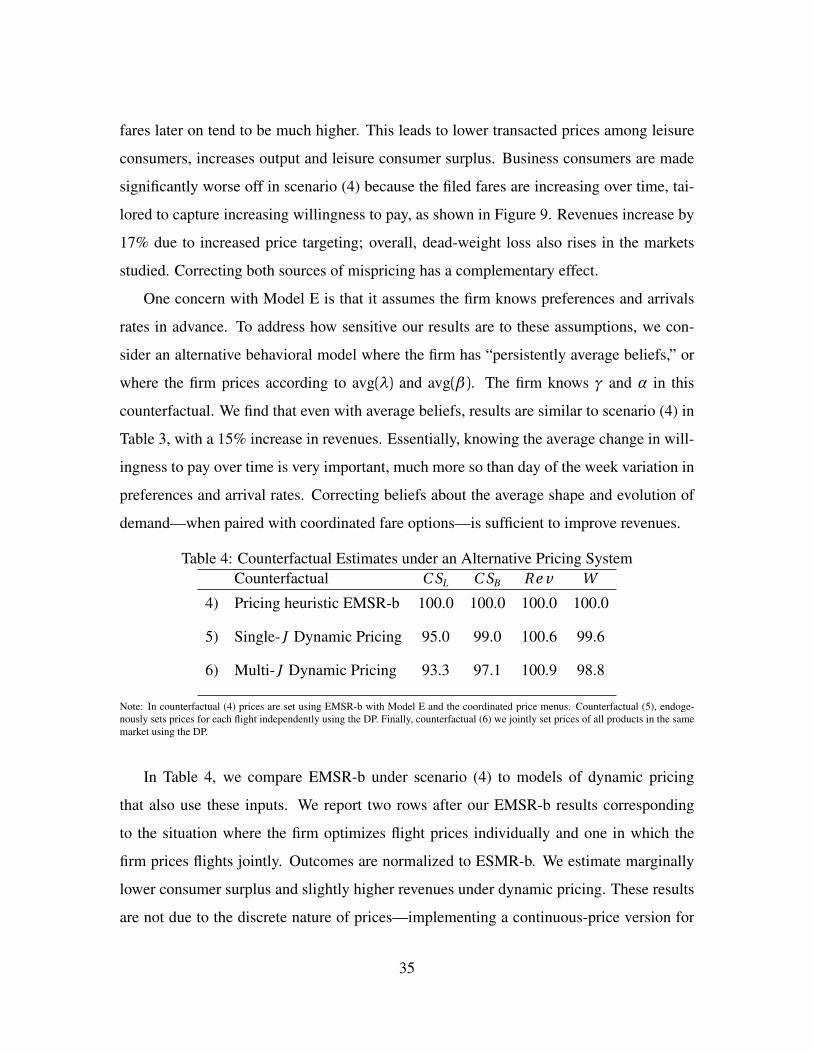
fares later on tend to be much higher. This leads to lower transacted prices among leisure

consumers, increases output and leisure consumer surplus. Business consumers are made

significantly worse off in scenario (4) because the filed fares are increasing over time, tai-

lored to capture increasing willingness to pay, as shown in Figure 9. Revenues increase by

17% due to increased price targeting; overall, dead-weight loss also rises in the markets

studied. Correcting both sources of mispricing has a complementary effect.

One concern with Model E is that it assumes the firm knows preferences and arrivals

rates in advance. To address how sensitive our results are to these assumptions, we con-

sider an alternative behavioral model where the firm has “persistently average beliefs,” or

where the firm prices according to avg(λ) and avg(β ). The firm knows γ and α in this

counterfactual. We find that even with average beliefs, results are similar to scenario (4) in

Table 3, with a 15% increase in revenues. Essentially, knowing the average change in will-

ingness to pay over time is very important, much more so than day of the week variation in

preferences and arrival rates. Correcting beliefs about the average shape and evolution of

demand—when paired with coordinated fare options—is sufficient to improve revenues.

Table 4: Counterfactual Estimates under an Alternative Pricing SystemCounterfactual C SL C SB R e v W

4) Pricing heuristic EMSR-b 100.0 100.0 100.0 100.0

5) Single-J Dynamic Pricing 95.0 99.0 100.6 99.6

6) Multi-J Dynamic Pricing 93.3 97.1 100.9 98.8

Note: In counterfactual (4) prices are set using EMSR-b with Model E and the coordinated price menus. Counterfactual (5), endoge-nously sets prices for each flight independently using the DP. Finally, counterfactual (6) we jointly set prices of all products in the samemarket using the DP.

In Table 4, we compare EMSR-b under scenario (4) to models of dynamic pricing

that also use these inputs. We report two rows after our EMSR-b results corresponding

to the situation where the firm optimizes flight prices individually and one in which the

firm prices flights jointly. Outcomes are normalized to ESMR-b. We estimate marginally

lower consumer surplus and slightly higher revenues under dynamic pricing. These results

are not due to the discrete nature of prices—implementing a continuous-price version for

35

single flight markets yields quantitatively similar results.

9.4 Discussion

Our descriptive evidence and counterfactual results suggest the firm has the ability to ex-

tract additional surplus by raising prices but has chosen not to do so. Note that the firm’s

current prices practices are rational if the costs of adjusting the pricing inputs are suffi-

ciently high, and our estimates of the revenue gains provide a lower bound. Our analysis

suggests coordinating fares to an unbiased forecast results in the largest revenue gains—

more so than changing the pricing technology or moving to continuous prices. Implement-

ing these changes would require revising demand estimates firm-wide and addressing span

of control to allow coordination in fares chosen by the pricing department.

On the other hand, our results may provide evidence of “behavioral firms." The fact that

optimal prices are significantly higher than current ones may suggest experiments could fail

to reveal consumers’ willingness to pay, or the firm may be experimenting too little. We

find some support for the latter possibility. Our search data allow us to see experiments

run on the airline’s website. We can confirm there has been very limited experimentation

during the sample period.

Recall that our analysis focuses on routes where the air carrier is the only airline pro-

viding nonstop service. It may be the case that the firm is choosing to offer lower prices

in these markets as a strategic response to the threat of an additional entrant (Goolsbee and

Syverson, 2008). We have abstracted away from such dynamic considerations. The fact

that our documented biases also occur in markets with direct competitors may suggest this

hypothesis is not correct.

Finally, the firm may be concerned about potential regulatory oversight with optimal

prices. Our demand estimates suggest more pronounced change in demand elasticity across

the booking period, so optimal prices lead to increased segmentation across consumers. It

may be that the firm is concerned about backlash of “price gouging” as observed in other

contexts, including in ride share and retailing.

36

10 Conclusion

In this paper, we document several ways in which sophisticated pricing systems do not

respond to some key market features. These pricing frictions arise due to different orga-

nizational teams being responsible for separate inputs into the pricing system. We find

that not coordinating on algorithm inputs curtails the ability of a large U.S. airline from

optimizing price. This has important implications for welfare due to the complications of

allocating seats in a dynamically evolving market environment.

We show that the current pricing algorithm is effective at filling seats, but could extract

more revenue. If pricing frictions are addressed individually, outcomes are unchanged.

This is because other biases are sufficiently strong that the pricing algorithm does not re-

act to a single optimized input. We also show that if all pricing frictions are addressed

simultaneously, this helps the firm optimize prices, but may increase dead-weight loss.

Beyond airlines, our results highlight the difficulty firms may have in designing organi-

zational structures around data and algorithms. When algorithms are complex and require

numerous inputs, it may be infeasible for a single organizational team to monitor and man-

age all inputs. When firms delegate tasks to teams, and teams have distinct boundaries, this

may prohibit potential complementarities in data-driven decision making.

ReferencesAguirregabiria, V., and F. Guiton (2020): “Heterogeneous Decision-Making in a Retail

Chain:Evidence from Store Managers at LCBO,” Working Paper.

Akepanidtaworn, K., R. Di Mascio, A. Imas, and L. Schmidt (2019): “Selling fast andbuying slow: Heuristics and trading performance of institutional investors,” WorkingPaper.

Alonso, R., W. Dessein, and N. Matouschek (2008): “When does coordination requirecentralization?,” American Economic Review, 98(1), 145–79.

(2015): “Organizing to adapt and compete,” American Economic Journal: Mi-croeconomics, 7(2), 158–87.

Aryal, G., C. Murry, and J. W. Williams (2021): “Price Discrimination in InternationalAirline Markets,” Working Paper.

37

Athey, S., and S. Stern (2002): “The Impact of Information Technology on EmergencyHealth Care Outcomes,” RAND Journal of Economics, pp. 399–432.

Belobaba, P. (1987): “Air Travel Demand and Airline Seat Inventory Management,” Ph.D.thesis, Massachusetts Institute of Technology.

Belobaba, P. P. (1989): “OR practice-application of a probabilistic decision model to airlineseat inventory control,” Operations Research, 37(2), 183–197.

(1992): “Optimal vs. heuristic methods for nested seat allocation,” in Presentationat ORSA/TIMS Joint National Meeting.

Berry, S., M. Carnall, and P. Spiller (2006): “Airline hubs: costs, markups and the implica-tions of customer heterogeneity,” Advances in airline economics, 1, 183–214.

Berry, S. T. (1994): “Estimating Discrete-Choice Models of Product Differentiation,” TheRAND Journal of Economics, pp. 242–262.

Berry, S. T., J. Levinsohn, and A. Pakes (1995): “Automobile Prices in Market Equilib-rium,” Econometrica, pp. 841–890.

Bloom, N., R. Sadun, and J. Van Reenen (2012): “The organization of firms across coun-tries,” The quarterly journal of economics, 127(4), 1663–1705.

Bresnahan, T. F., E. Brynjolfsson, and L. M. Hitt (2002): “Information technology, work-place organization, and the demand for skilled labor: Firm-level evidence,” The quarterlyjournal of economics, 117(1), 339–376.

Brumelle, S. L., J. I. McGill, T. H. Oum, K. Sawaki, and M. Tretheway (1990): “Alloca-tion of airline seats between stochastically dependent demands,” Transportation Science,24(3), 183–192.

Brynjolfsson, E., and P. Milgrom (2012): “1. Complementarity in Organizations,” in Thehandbook of organizational economics, pp. 11–55. Princeton University Press.

Castillo, J. C. (2019): “Who Benefits from Surge Pricing?,” Available at SSRN 3245533.

Che, Y.-K., and S.-W. Yoo (2001): “Optimal incentives for teams,” American EconomicReview, 91(3), 525–541.

Cho, S., G. Lee, J. Rust, and M. Yu (2018): “Optimal Dynamic Hotel Pricing,” WorkingPaper.

Cho, S., and J. Rust (2010): “The flat rental puzzle,” The Review of Economic Studies,77(2), 560–594.

DellaVigna, S., and M. Gentzkow (2019): “Uniform pricing in us retail chains,” The Quar-terly Journal of Economics, 134(4), 2011–2084.

38

D’Haultfœuille, X., P. Février, A. Wang, and L. Wilner (2020): “Estimating the Gains (andLosses) of Revenue Management,” Working Paper.

Dubé, J.-P., and S. Misra (2021): “Personalized Pricing and Consumer Welfare,” WorkingPaper.

Ellison, S. F., C. Snyder, and H. Zhang (2018): “Costs of managerial attention and activityas a source of sticky prices: Structural estimates from an online market,” Discussionpaper, National Bureau of Economic Research, Working Paper.

Filippas, A., S. Jagabathula, and A. Sundararajan (2021): “The Limits of Centralized Pric-ing in Online Marketplaces and the Value of User Control,” Working Paper.

Gallego, G., and G. Van Ryzin (1994): “Optimal Dynamic Pricing of Inventories withStochastic Demand Over Finite Horizons,” Management science, 40(8), 999–1020.

Goldfarb, A., and M. Xiao (2011): “Who thinks about the competition? Managerial abilityand strategic entry in US local telephone markets,” American Economic Review, 101(7),3130–61.

(2016): “Transitory shocks, limited attention, and a firms decision to exit,” Dis-cussion paper, Working paper.

Goolsbee, A., and C. Syverson (2008): “How do incumbents respond to the threat of entry?Evidence from the major airlines,” The Quarterly Journal of Economics, 123(4), 1611–1633.

Hendel, I., and A. Nevo (2013): “Intertemporal price discrimination in storable goods mar-kets,” American Economic Review, 103(7), 2722–51.

Hitsch, G. J., A. Hortaçsu, and X. Lin (2021): “Prices and Promotions in US Retail Markets:Evidence from Big Data,” Quantitative Marketing & Economics.

Hortaçsu, A., O. Natan, H. Parsley, T. Schwieg, and K. Williams (2021): “IncorporatingSearch and Sales Information in Demand Estimation,” Working Paper.

Hortaçsu, A., F. Luco, S. L. Puller, and D. Zhu (2019): “Does strategic ability affect ef-ficiency? Evidence from electricity markets,” American Economic Review, 109(12),4302–42.

Huang, Y. (2021): “Seller-Pricing Frictions and Platform Remedies: The Case of Airbnb,”Working Paper.

Jiang, R., P. Manchanda, and P. E. Rossi (2009): “Bayesian Analysis of Random CoefficientLogit Models using Aggregate Data,” Journal of Econometrics, 149(2), 136–148.

39

Littlewood, K. (1972): “Forecasting and control of passenger bookings,” Airline GroupInternational Federation of Operational Research Societies Proceedings, 1972, 12, 95–117.

Ma, Y., T. Ropele, D. Sraer, and D. Thesmar (2020): “A quantitative analysis of distortionsin managerial forecasts,” Working Paper.

Massey, C., and R. H. Thaler (2013): “The loser’s curse: Decision making and marketefficiency in the National Football League draft,” Management Science, 59(7), 1479–1495.

McGill, J. I., and G. J. Van Ryzin (1999): “Revenue management: Research overview andprospects,” Transportation science, 33(2), 233–256.

Siemsen, E., S. Balasubramanian, and A. V. Roth (2007): “Incentives that induce task-related effort, helping, and knowledge sharing in workgroups,” Management science,53(10), 1533–1550.

Smith, B. C., J. F. Leimkuhler, and R. M. Darrow (1992): “Yield management at Americanairlines,” Interfaces, 22(1), 8–31.

Sweeting, A. (2012): “Dynamic Pricing Behavior in Perishable Goods Markets: Evidencefrom Secondary Markets for Major League Baseball Tickets,” Journal of Political Econ-omy, 120(6), 1133 – 1172.

Talluri, K., and G. Van Ryzin (2004): The Theory and Practice of Revenue Management,vol. 68. Springer Science & Business Media.

Williams, K. R. (forthcoming): “Dynamic Airline Pricing and Seat Availability,” Econo-metrica.

Wollmer, R. D. (1992): “An airline seat management model for a single leg route whenlower fare classes book first,” Operations research, 40(1), 26–37.

40

Online AppendixOrganizational Structure and Pricing: Evidence from a Large U.S. Airline

by Hortaçsu, Natan, Parsley, Schwieg, and Williams

Table of ContentsA Details on the Pricing Heuristic, EMSR-b 2

A.1 Littlewood’s Rule . . . . . . . . . . . . . . . . . . . . . . . . . . . . . . . . . . . . . . . 2

A.2 EMSR-b Algorithm . . . . . . . . . . . . . . . . . . . . . . . . . . . . . . . . . . . . . . 3

B Route Selection 6

B.1 Estimation Sample Comparison . . . . . . . . . . . . . . . . . . . . . . . . . . . . . 9

C Demand Estimation Procedure 10

1

A Details on the Pricing Heuristic, EMSR-b

We approximate the solution to a dynamic pricing (DP) problem using a well-known

heuristic in operations research, Expected Marginal Seat Revenue-b or EMSR-b (Belob-

aba, 1987). The heuristic was developed in order to avoid solving highly complex dynamic

pricing problems. The heuristic simplifies the firm’s decision in each period by aggregating

all future sales before the deadline into a single future period. It also simplifies the demand

system to be for only a single product, so competitive effects cannot be considered. We

describe this process below and show how to incorporate Poisson demand in EMSR-b. It is

important to note that EMSR-b provides an allocation over a given finite set of prices, in-

stead of providing the optimal price itself given any state of the world. EMSR-b associates

each price with a fare-class then chooses a maximal number of sales that can be made to

each fare-class. This means that consumers may face different prices within a single pricing

period when one class is closed and a higher priced class opens.

A.1 Littlewood’s Rule

EMSR-b is a generalization of Littlewood’s rule, which is a simple case where a firm prices

two time periods uses two fare classes. A firm with a fixed capacity of goods (seats) wants

to maximize revenue across two periods, where leisure (more elastic) consumers arrive

in the first period and business (less elastic) consumers arrive in the second period. The

firm sets a cap on the number of seats b it is willing to sell in the first period to leisure

passengers. This rule returns a maximum number of seats for leisure when the price to

both leisure and business customers has already been decided; it does not determine optimal

pricing.

The solution equates the price of a seat sold in the first period (to leisure travelers) to

the opportunity cost of lowering capacity for sales in the second period (business travelers).

Given prices pL , pB , capacity C , and the arrival CDF of business travelers FB , Littlewood’s

rule equates the fare ratio to the probability that business class sells out. The fare ratio is

2

the marginal cost of selling the seat to leisure (the lower revenue pL ) which is set equal to

the marginal benefit—the probability that the seat would not have sold if left for business

customers only. Littlewood’s rule is given by

1− FB (C − b ) =pL

pB.

This equation can then be solved for b , the maximum number of seats to sell to leisure

customers in period one. This solution is exact if consumers arrive in two separate groups

and there are only two time periods and two consumer types.

A.2 EMSR-b Algorithm

The EMSR-b algorithm (Belobaba, 1987) extends Littlewood’s rule to multiple fare levels

or classes. For each fare class, all fare classes with higher fares are aggregated into a single

fare-class called the “super-bucket.” Once this bucket is formed, Littlewood’s rule applies,

and can be done for each fare class iteratively. Rather than just comparing leisure and

business classes, the algorithm now weights the choice of selling a lower fare-class ticket

against an average of all higher fare classes.

We apply the algorithm for K sorted fare-classes such that p1 > p2 > ...> pK . Each fare

class has independent demand with a distribution Fk . Under our specification, the demand

for each fare class is distributed Poisson with mean µk that is given by future arrivals times

the share of the market exclusive to that bucket.

The super-bucket is a single-bucket placeholder for a weighted average of all higher

fare-class buckets. Independent Poisson demand simplifies this calculation, as the sum of

independent Poisson distributions is itself Poisson. The mean of the super-bucket is the sum

of the mean of each higher fare-class bucket. The price of the super-bucket is a weighted

average of the price of each higher-fare class, using the means as the weight.

For each fare class, Littlewood’s Rule is then applied with the fare-class taking the

place of leisure travel, and the super-bucket in place of business travel. It is assumed that

3

all future arrivals appear in a single day. The algorithm then describes a set of fare-class

limits bk that define the maximum number of sales for each class before closing that fare

class. We denote the remaining capacity of the plane at any time by C . The algorithm uses

the following pseudo-code:

for t > 2 do

for k ← K to 1 by −1 doi) Compute un-allocated capacity Ck ,t =C −∑K

i=k bi ,

ii) Construct the super-bucket

µs b =k−1∑i=1

µi , ps b =1

µs b

k−1∑i=1

piµi , Fs b ∼ Poisson(µs b ),

iii) Apply Littlewood’s Rule using the super-bucket distribution as the demand for

business

Ck ,t − bk =min§

Fs b−1�

1− pk

ps b

�, Ck ,t

ª.

end

endIn the case where t = 1, dynamics are no longer important, so there is no longer a need

to trade off based on the opportunity cost. As a result, we limit the fare of the highest

revenue class to all remaining capacity, and set limits of all other classes to zero.

A.2.1 Fare Class Demand

What remains is computing the mean µk for each fare class bucket. We detail the process

in this section. Demand in each market is an independent Poisson with arrival rate exp(λtt +

λdd )s j (p ). Note that this p is a vector of the prices of all flights in the market. We assume

that the firm believes other flights will be priced at their historic average over the departure

date and day before departure. This allows us to construct a residual demand function s j (pj )

that is a function of the price of the current flight only. We will treat this as the demand for

4

the flight at a given bucket’s price for the remainder of this section.

Each fare class has a set price pk , at any time t , departure date d we will see exp(λtt +

λdd ) arrivals, of which s (pk ) are willing to purchase a fare for bucket k . However, s (pk−1)

are willing to purchase a fare for bucket k−1 as well, since they will buy at the higher price

pk−1. Only exp(λtt +λ

dd )�st (pk )− st (pk−1)

�are added by the existence of this fare class with

price pk < pk−1. Note that this is a flow quantity—the amount of purchases in time t , but

EMSR-B requires stock quantities: How many will purchase over the remaining lifetime

of the sale?

What is the distribution of future purchases then? Each day t is an independent Poisson

process split by the share function. Independent split Poisson processes are still Poisson,

so we may compute the mean of purchases solely in a fare class by summing arrivals over

future time t , and taking the difference in shares between price pk and pk−1. For time t

and departure date d , the stock demand for fare-class k is given by

t∑i=1

exp(λti +λ

dd )�st (pk )− st (pk−1)

�,

where st (p0) = 0 for notational parsimony.

This demand distribution is only used to compute the super-bucket demand distribution.

Note that we only include future stock demand in the super bucket, and thus only sum

arrivals until time t −1. For fare-class k . The super bucket’s stock demand is given by

µs b =

�t−1∑i=1

exp(λti +λ

dd )si (pk−1)

�ps b =

1

µ

k−1∑j=1

pj

t−1∑i=1

exp(λti +λ

dd )�si (pj )− si (pj−1)�

.

The updated pseudo-code for the EMSR-b algorithm is:

5

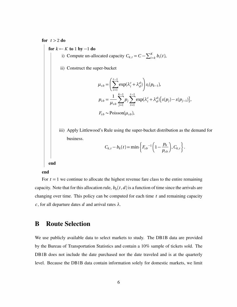
for t > 2 do

for k ← K to 1 by −1 doi) Compute un-allocated capacity Ck ,t =C −∑K

i=k bi (t ),

ii) Construct the super-bucket

µs b =

�t−1∑i=1

exp(λti +λ

dd )

�si (pk−1),

ps b =1

µs b

k−1∑j=1

pj

t−1∑i=1

exp(λti +λ

dd )�s (pj )− s (pj−1)�

,

Fs b ∼ Poisson(µs b ),

iii) Apply Littlewood’s Rule using the super-bucket distribution as the demand for

business.

Ck ,t − bk (t ) =min§

Fs b−1�

1− pk

ps b

�, Ck ,t

ª.

end

endFor t = 1 we continue to allocate the highest revenue fare class to the entire remaining

capacity. Note that for this allocation rule, bk (t , d ) is a function of time since the arrivals are

changing over time. This policy can be computed for each time t and remaining capacity

c , for all departure dates d and arrival rates λ.

B Route Selection

We use publicly available data to select markets to study. The DB1B data are provided

by the Bureau of Transportation Statistics and contain a 10% sample of tickets sold. The

DB1B does not include the date purchased nor the date traveled and is at the quarterly

level. Because the DB1B data contain information solely for domestic markets, we limit

6

our analysis to domestic markets as well. Furthermore, we use the air carrier’s definition

of markets to combine airports within some geographies.

Figure 10: Nonstop, One-stop and Connecting TrafficDestination

Origin One-stop

Connecting

Note: We use the term nonstop to denote the sold black line, or passengers solely traveling between�Origin, Destination

�. Unless

otherwise noted, we will use directional traffic, labeled O →D . Non-directional traffic is specified as O ↔D . The blue, dashed linesrepresent passengers flying on O ↔D , but traveling to or from a different origin or destination. Finally, one-stop traffic are passengersflying on O ↔D , but through a connecting airport.

We consider two measures of traffic flows when selecting markets: traffic flying nonstop

and traffic that is non-connecting. Both of these metrics are informative for measuring

the substitutability of other flight options (one-stop, for example) as well as the diversity

of tickets sold for the flights studied (connecting traffic). Figure 10 provides a graphical

depiction of traffic flows in airline networks that we use to construct the statistics. We

consider directional traffic flows from a potential origin and destination pair that is served

nonstop by our air carrier. The first metric we calculate is the fraction of traffic flying

from O → D nonstop versus one or more stops. This compares the solid black line to the

dashed orange line. Second, we calculate the fraction of traffic flying from O →D versus

O →D →C . This compares the solid black line to the dashed blue line.

Figure 11 presents summary distributions of the two metrics for the markets (ODs) we

select. In total, we select 407 ODs for departure dates between Q3:2018 and Q3:2019. The

top row measures the fraction of nonstop and connecting traffic for tickets sold by our our

carrier. The left plot shows that, conditional on the air carrier operating nonstop flights

between OD, an overwhelming fraction of consumers purchase nonstop tickets instead of

purchasing one-stop connecting flights. The right panel shows that fraction of consumers

who are not connecting to other cities either before or after flying on segment OD. There is

7

Figure 11: Route Selection Using Bureau of Transportation Statistics Data(a) Within Airline Fraction Nonstop

0.0 0.2 0.4 0.6 0.8 1.0Fraction

0.0

0.1

0.2

0.3

0.4

0.5

0.6

Den

sity

(b) Within Airline Fraction Non-Connecting

0.0 0.2 0.4 0.6 0.8 1.0Fraction

0.000.050.100.150.200.250.300.350.40

Den

sity

(c) All Airlines Fraction Nonstop

0.0 0.2 0.4 0.6 0.8 1.0Fraction

0.000.020.040.060.080.100.12

Den

sity

(d) All Airlines Fraction Non-Connecting

0.0 0.2 0.4 0.6 0.8 1.0Fraction

0.00

0.02

0.04

0.06

0.08

0.10

0.12

Den

sity

Note: Density plots over the fraction of nonstop traffic and the fraction of non-connecting traffic for the selected routes using DB1B data."Within" means passengers flying on our air carrier. "Total" means all air carriers on a given origin-destination pair. Within nonstop andtotal nonstop coincide if our carrier is the only carrier flying nonstop.

significant variation across markets, with the average being close to 50%.

Figure 12: DB1B Comparison(a) DB1B OD Traffic Comparison

0.3 0.4 0.5 0.6 0.7 0.8 0.9 1.0Nonstop Traffic Fraction

0.0

0.2

0.4

0.6

0.8

1.0

Non

-con

. Tra

ffic

Fra

ctio

n

Selected ODs MeanDB1B CarrierSelected ODs

(b) DB1B OD Fare Comparison

0 200 400 600 800 1000Fare

0.000

0.001

0.002

0.003

0.004

Den

sity

DB1B CarrierSelected ODs

Note: (a) A scatter plot of the fraction nonstop and fraction non-connecting for all origin-destination pairs served by our air carrier. Theblue dots show selected markets; the orange dots show non-selected markets. (b) Kernel density plots of all fares in the DB1B data forour air carrier; the blue line shows the density for our selected markets.

8

The bottom panel repeats the statistics but replaces the denominator of the fractions

with the sum of traffic flows across all air carriers in the DB1B. Both distributions shift to

the left because of existence of competitor connecting flights and sometimes direct com-

petitor flights. In nearly 75% of the markets we study, our air carrier is the only firm

providing nonstop service. Our structural analysis will only consider single carrier mar-

kets.

In Figure 12-(a), we show a scatter plot of the fraction of nonstop traffic and the fraction

of non-connecting traffic for all origin-destination pairs offers by our air carrier in the

DB1B. The orange dots depict routes non-selected markets and the blue dots show the

selected markets. We see some dispersion in selected markets, however this is primarily

on non-connecting traffic. An overwhelming fraction of the selected markets have high

nonstop traffic, although this is true in the sample broadly. Essentially, conditional on

the air carrier providing nonstop service, most passengers choose nonstop itineraries. In

Figure 12-(b) we show the distribution of purchased fares in the DB1B for our carrier along

with our selected markets. The distribution of prices for the selected sample are slightly

shifted to the right, which makes sense since we primarily select markets where the air

carrier is the only airline providing nonstop service.

B.1 Estimation Sample Comparison

Our estimation sample contains 39 markets. Compared to the overall sample, these routes

tend to be smaller in terms of total number of passengers, larger in terms of percentage

of nonstop and non-connecting passengers, and nonstop service is provided only by our

air carrier. We report percentage differences between our estimation routes and the entire

sample for key characteristics below in Table 5. Figure 13 shows a two-way plot of the

fraction of nonstop and non-connecting traffic for the routes selected for estimation relative

to the entire sample.

9

Table 5: Estimation Routes Comparison

Characteristic Percentage Difference from Mean

Number of Nonstop Passengers -38.8%Total Number of Passengers -33.4%Number of Local Passengers -37.7%Fraction of Traffic Nonstop 1.02%Fraction of Traffic Non-Connecting 5.91%

Note: Statistics calculated using the DB1B data for the years 2018-2019.

Figure 13: Route Estimation Selection using DB1B Data

0.2 0.4 0.6 0.8 1.0Nonstop Traffic Fraction

0.0

0.2

0.4

0.6

0.8

1.0

Non

-con

. Tra

ffic

Fra

ctio

n

Selected ODs MeanSample ODsSelected ODs

Note: A scatter plot of the fraction nonstop and fraction non-connecting for all origin-destination pairs served by our air carrier. Theblue dots show markets used for estimation; the orange dots show non-selected markets.

C Demand Estimation Procedure

We provide an overview on the implementation details of each stage the MCMC routine for

demand parameter estimation. Simultaneously drawing from the joint distribution of our

large parameter space is infeasible, therefore, we use a Hybrid Gibbs sampling algorithm.

The algorithm steps are shown below. At each step of the posterior sampler, we sequen-

tially draw from the marginal posterior distribution groups of parameters, conditional on

other parameter draws. Where conjugate prior distributions are unavailable, we use the

Metropolis-Hastings algorithm, a rejection sampling method that draws from an approx-

imating candidate distribution and keeps draws which have sufficiently high likelihood.

Additional detail can be found in Hortaçsu, Natan, Parsley, Schwieg, and Williams (2021).

10

1: for c = 1 to C do2: Update arrivals λ (Metropolis-Hastings)3: Update shares s (·) (Metropolis-Hastings)4: Update price coefficients α (Metropolis-Hastings)5: Update consumer distribution γ (Metropolis-Hastings)6: Update linear parameters β (Gibbs)7: Update pricing equation η (Gibbs)8: Update price endogeneity parameters Σ (Gibbs)9: end for

Algorithm 1: Hybrid Gibbs Sampler

Sampling Arrival Parameters

We start the sampling procedure by drawing from the posterior distribution of arrival pa-

rameters, λt ,d . The posterior is derived by defining the joint likelihood of arrivals for each

consumer type and quantities sold, conditional on product shares. Recall that arriving con-

sumers have likelihood based on their type:

ALt ,d ∼ Poisson(λt ,d (1− γ̃t )ζ

Lt ),

ABt ,d ∼ Poisson(λt ,d γ̃t ζ

Bt ),

where γ̃t is the probability a consumer is of the business type as derived from the pas-

senger assignment algorithm, and ζℓt is the fraction of bookings that do not occur on the

direct channel for each consumer type (leisure and business). The purchase likelihood is a

function of shares and arrivals and is equal to

q̃ j ,t ,d ∼ Poisson�λt ,d · s j ,t ,d

�,

q j ,t ,d =min¦

q̃ j ,t ,d , C j ,t ,d

©.

This directly accounts for censored demand due to finite capacity. Since arrivals are re-

stricted to be non-negative, we restrict the set of fixed effects by transforming the multi-

plicative fixed effects to be of the form λt ,d = exp�Wt ,dτ�. We select a log-Gamma prior

11

for τ. We sample from the posterior distribution by taking a Metropolis-Hastings draw

from a normal candidate distribution.

Sampling Shares and Utility Parameters

Updating shares. We treat product shares as unobserved, since the market size may

be very small and lead to irreducible measurement error. We use data augmentation to

treat shares as a latent parameter that we estimate. Conditional on all other parameters

(λ,α,γ,β ,η,Σ), product shares are an invertible function of the demand shock, ξ. If we

conditioned additionally on ξ, shares would be a deterministic function of data and other

parameter draws. Instead, we leverage the stochastic nature of ξ, which we explicitly pa-

rameterize. The distribution of unobserved ξ is the source of variation for constructing a

conditional likelihood for shares:

ξ j ,t ,d = f −1�s j ,t ,d |β ,α,γ, X�

υ j ,t ,d = pj ,t ,d −Z ′j ,t ,dη

��κ= k ∼N iid(0,Σk )

such that Σk =

σ2k ,11 ρk

ρk σ2k ,22

.Here, κ is a mapping from days to departure t to an interval (block) of time. That is,

the pricing error and the demand shock have a block-specific joint normal distribution.

Conditional on the pricing shock υ, the distribution of ξ, fξ j ,t ,d(·), is

ξ��υ,κ= k ∼N�ρkυ

σ2k ,11

,σ2k ,22−

ρ2k

σ2k ,11

�.

The density of shares is then given by the transformation fs j ,t ,d(x ) = fξ j ,t ,d

�f −1(x )�·��Jξ j ,t ,d→s j ,t ,d

��−1,

where Jξ j ,t ,d→s j ,t ,dis the Jacobian matrix of model shares with respect to ξ. To produce the

full joint conditional likelihood of shares, we also include the mass function for sales,

which are a product of shares and arrivals:

12

∏t

∏d

J (t ,d )∏j=1

ϕ f −1(s j ,t ,d )− ρkυ

σ2k ,11s

σ2k ,22− ρ2

k

σ2k ,11

(λt ,d s j ,t ,d )q j ,t ,d exp(−λt ,d s j ,t ,d )

q j ,t ,d !

· ��Jξ→s

��−1,

where ϕ(·) is the standard normal density function. We draw from the posterior based on a

uniform prior distribution and normal candidate Metropolis-Hastings draws.

Updating price coefficients, αB ,αL . We construct the conditional likelihood (and thus

the conditional posterior distribution) for α = (αB ,αL ) in a similar manner to the product

shares. For any candidate value of price sensitivity, we recover a residual ξ, invert the

demand system, and recover a likelihood. Conditional on λ, shares, η, β , and Σ, we

compute the distribution of ξ and determine the likelihood of a particular draw of α, given

by ∏t

∏d

J (t ,d )∏j=1

ϕ f −1(s j ,t ,d )− ρkυ

σ2k ,11s

σ2k ,22− ρ2

k

σ2k ,11

· ��Jξ→s

��−1,

where ϕ(·) is the standard Normal density function. We impose a log-Normal prior on α,

and impose αB < αL to avoid label-switching. To draw from the conditional posterior, we

take a Metropolis-Hasting step using a normal candidate distribution.

Updating the distribution of consumer types, γ. We allow for the mix of consumer

types to change over the booking horizon t . We define γ from a sieve estimator of the

booking horizon t , and we sample the sieve coefficients, ψ, according to

γt =Logit�G (t )′ψ�

,

where G (t ) is a vector of Bernstein polynomials. The logistic functional form ensures that

the image of γ in the interval (0,1). The inversion procedure used to construct the likelihood

13

is similar to α and shares. It yields a likelihood for sieve coefficients ψ of the form

∏t

∏d

J (t ,d )∏j=1

ϕ f −1(s j ,t ,d )− ρkυ

σ2k ,11s

σ2k ,22− ρ2

k

σ2k ,11

· ��Jξ→s

��−1.

We use a uniform prior onψ, and we sample from the posterior with a Metropolis-Hastings

step using a normal candidate draw.

Updating remaining preferences, β . To sample the remaining preferences that are

common across consumer types, we impose a normal prior on β , with mean β̄0 and vari-

ance V0. We adjust for price endogeneity to conduct a standard Bayesian regression. Define

δ j ,t ,d = X j ,t ,dβ + ξ j ,t ,d , which is evaluated at the ξ computed in the prior step. We nor-

malize each component of δ by subtracting the expected value of ξ and dividing by its

standard deviation. The normalized equations have unit variance and are thus conjugate to

the normal prior. Let σk ,2|1 =sσ2

k ,22− ρ2k

σ2k ,11

be the variance of ξ conditional on υ and Σ.

We center and scale δ:

δ j ,t ,d − ρκt

σ2κt ,11υ

σκt ,2|1=

1

σκt ,2|1X j ,t ,d β̄ +U β

j ,t ,d ,

where U β ∼N (0,1). Then, the posterior distribution of β isN (βN , VN ), where

βN = (X̂′X̂ +V0

−1)−1 �

V0−1β0+ X̂ ′δ̂�

,

VN = (V0−1+ X̂ ′X̂ )−1

,

X̂ j ,t ,d =X j ,t ,d

σκt ,2|1,

δ̂=δ j ,t ,d − ρκt

σ2κt ,11υ

σκt ,2|1.

Given this normalization, we can draw directly from the conditional posterior distribution

of β using a Gibbs step.

14

Sampling Price-Endogeneity Parameters

Updating pricing equation, η. We use a linear pricing equation of the form

pj ,t ,d = Z j ,t ,dη+υ j ,t ,d .

Conditional on shares, λ, γ, α, and β , ξ is known. Therefore, we use the conditional

distribution of υ given ξ to perform another Bayesian linear regression in a similar manner

to β . We impose a Normal prior and normalize prices. Define σκt ,1|2 =sσ2κt ,11− ρ2

κt

σ2κt ,22

. It

follows thatpj ,t ,d − ρκt

σκt ,22ξ j ,t ,d

σκt ,1|2=

1

σκt ,1|2X j ,t ,d η̄+U η

j ,t ,d ,

where U η ∼N (0,1). Just as we did for β , we can draw from the posterior of η from a linear

regression with unit variance. This step allows us to directly sample from the posterior of

η rather than using a Metropolis-Hastings step.

Updating the price endogeneity parameters, Σ. We flexibly model the joint distribution

of ξ and υ by allowing for a route-specific, time-varying correlation structure. We divide

the booking horizon into four equally sized 30-day periods, and each block is indexed k .

We restrict the price endogeneity parameters Σ, which determine the joint distribution of

ξ,υ, to be identical within these blocks. Within each block, the pricing and demand residual

follow the same joint distribution. We draw the variance of this normal distribution with a

typical Inverse-Wishart parameterization. Our prior for Σk is I W (ν, V ) where k refers to

the block. Define the vector Yk = (υ,ξ) to be the collection of residual pairs conditional on

block k , and Yk ∼N (0,Σk ). The posterior for the covariance matrix Σk is then

Σk ∼ I W (ν+nk , V +Y ′k Yk ).

Block k has nk observations. This Gibbs step is repeated for each block k , and we sample

directly from the conditional posteriors of Σ.

15

Documents

Organizational Structure and Pricing: Evidence from a